Detailed comparison of numerical methods for the perturbed

Rev

ised

Proo

f

J Eng MathDOI 10.1007/s10665-013-9678-x

Detailed comparison of numerical methods for the perturbedsine-Gordon equation with impulsive forcing

Danhua Wang · Jae-Hun Jung · Gino Biondini

Received: 5 September 2012 / Accepted: 25 October 2013© Springer Science+Business Media Dordrecht 2013

Abstract The properties of various numerical methods for the study of the perturbed sine-Gordon (sG) equation1

with impulsive forcing are investigated. In particular, finite difference and pseudo-spectral methods for discretizing2

the equation are considered. Different methods of discretizing the Dirac delta are discussed. Various combinations3

of these methods are then used to model the soliton–defect interaction. A comprehensive study of convergence4

of all these combinations is presented. Detailed explanations are provided of various numerical issues that should5

be carefully considered when the sG equation with impulsive forcing is solved numerically. The properties of6

each method depend heavily on the specific representation chosen for the Dirac delta—and vice versa. Useful7

comparisons are provided that can be used for the design of the numerical scheme to study the singularly perturbed8

sG equation. Some interesting results are found. For example, the Gaussian approximation yields the worst results,9

while the domain decomposition method yields the best results, for both finite difference and spectral methods.10

These findings are corroborated by extensive numerical simulations.11

Keywords Finite difference methods · Impulsive forcing · Sine-Gordon equation · Spectral methods12

1 Introduction13

The sine-Gordon (sG) equation is a ubiquitous physical model that describes nonlinear oscillations in various settings14

such as Josephson junctions, self-induced transparency, crystal dislocations, Bloch wall motion of magnetic crystals,15

and beyond (see [1] for references). The sG equation is also an important theoretical model as it is a completely16

integrable system [2]. Many nonintegrable, nonlinear models also bear solitary wave solutions. In the specific case17

of the sG equation, these traveling wave solutions take the form of “kinks.” Because various physical effects often18

result in the presence of localized defects or impurities, the interaction of such solutions with defects has been19

extensively studied in the literature [3–18]. In particular, the perturbed sG equation with the localized, nonlinear20

impulsive forcing, such as21

utt − uxx + sin u = εδ(x) sin u, u : R+ × R → R, ε ∈ R

+, (1)22

also has been considered [3,7,9,10]. Henceforth, subscripts x and t denote partial differentiation with respect to23

space and time, respectively, δ(x) is the Dirac delta distribution [19], and ε is the forcing strength. Specifically, the24

D. Wang · J.-H. Jung · G. Biondini (B)Department of Mathematics, State University of New York at Buffalo, Buffalo, NY 14260, USAe-mail: [email protected]

123

Journal: 10665-ENGI MS: 9678 � TYPESET DISK LE CP Disp.:2013/12/21 Pages: 20 Layout: Medium

Rev

ised

Proo

f

D. Wang et al.

Dirac delta forcing in (1) models the action of an attractive defect [5] for ε > 0. To the best of our knowledge,25

the numerical treatment of (1) has not been adequately discussed in the literature. The issue is relevant because the26

Dirac delta is, of course, a distribution, and it is well known that the product of distributions is not, in general, a27

well-defined quantity. Even when one can show that the equation admits a unique (weak) solution, the presence of28

the impulsive forcing seriously affects the convergence of any numerical method used.29

The purpose of this work is to address these issues by investigating and comparing the convergence properties of30

various numerical methods. Convergence is checked by determining the critical initial soliton velocity. Due to the31

singular property of the potential term of δ(x) and the critical solution behaviors of the sG equation, the convergence32

depends strongly on the representation of the Dirac delta. We provide in this paper a detailed explanation of33

various numerical issues that should be carefully considered when the sG equation with impulsive forcing is solved34

numerically.35

In particular, we consider (1) finite-difference methods, both in time and space, and (2) spectral collocation meth-36

ods (in space). In the nonlinear optics community, finite-difference methods have been most commonly used due to37

the simplicity and ease of handling the singular potential term. Spectral methods employ a global approximation,38

which may not be suitable for dealing with a singular term such as the Dirac delta. It is well known that, in the39

presence of such singularities, spectral methods yield oscillatory solutions. However, when appropriate regulariza-40

tion methods are adopted, spectral methods can be implemented efficiently and accurately, even for a singularly41

perturbed equation such as (1).42

We have found that no single discretization method for the sG equation is the best in all cases. Instead, the43

properties of each method depend heavily on the specific representation chosen for the Dirac delta—and vice versa.44

For all cases, high resolution is required to capture the proper behavior of the critical soliton behaviors due to the45

singular potential. Spectral methods yield slightly better results than finite-difference methods when the domain46

decomposition method is used, but the overall convergence seems close to algebraic rather than exponential. The47

specific advantages and disadvantages of each method will be discussed.48

Several different ways of representing the Dirac delta will be compared:49

(a) Gaussian delta representation:50

δσ (x) = 1/(σ√

2π) exp(−x2/(2σ 2)), (2)51

which is the most commonly used regularization method in the existing literature to solve (1) and the nonlinear52

Schrödinger equation with a singular potential [9]. The idea is simply that if one chooses σ → 0 and N → ∞53

(where N + 1 is the number of spatial grid points, as discussed in Sect. 3), δσ (x) converges to δ(x) in the54

distribution sense. This approach is popular because of its simplicity. However, due to the nonzero value of σ ,55

the potential term always has a nonzero width, which affects the soliton dynamics. This results in a rather slow56

convergence for both the finite-difference and spectral methods, as discussed later.57

(b) Point source:58

δps(x) ={

0 x �= 0,

δ0 x = 0,(3)59

with δ0 chosen appropriately. The main advantage of this approach is that it is the simplest to implement, and60

such a definition yields a delta function of zero width on a discrete grid. By choosing the value of δ0 for the given61

number of grid points properly, one can satisfy the normalization condition of the Dirac delta and mimic the62

local singularity on the grid. Due to these properties, our numerical results show that this crude regularization63

yields a good approximation, and even better results than the Gaussian regularization for both finite-difference64

and spectral methods. It is interesting to observe that spectral methods yield reasonable results with this point65

source approximation.66

(c) Self-consistent delta representation. This approach is based on the fact that δ(x) = d[H(x)]/dx in the distrib-67

ution sense, where H(x) is the Heaviside step function [i.e., H(x) = 0 for all x < 0, H(x) = 1/2 for x = 0,68

and H(x) = 1 for all x > 0].69

Numerically, this choice is realized by taking70

δσ (x) = D Hσ (x),71

123


Rev

ised

Proo

f

sine-Gordon with impulsive forcing

where D is the numerical differentiation operator consistent with the spatial discretization of (1), and Hσ (x)72

is a discrete representation of the Heaviside function. [For example, Hσ (x) = 0 for all x ≤ −σ , Hσ (x) =73

(1 + x/σ)/2 for all |x | < σ , and Hσ (x) = 1 for all x ≥ σ .] The discrete representation of δσ (x) based on this74

approach is oscillatory, but the resulting solution is without oscillations if the problem is linear. This approach is75

simple and consistent with the discretization method. Moreover, it is flexible enough that one can even choose76

a value of σ = 0. We will show that this approach yields better results than the Gaussian regularization.77

(d) Domain decomposition. Using the continuity of u(x, t) at x = 0 [namely, u(0+, t) = u(0−, t),∀t > 0], (1)78

yields the following jump condition at x = 0:79

ux (0+, t) − ux (0

−, t) = −ε sin[u(0, t)]. (4)80

One then splits the domain [−L , L] into two subdomains, [−L , 0) and (0, L], and solves numerically (1) with81

ε = 0 in each subdomain, together with the jump condition (4). Thus, the domain decomposition approach82

does not involve a regularization of the Dirac delta, and the solutions in each subdomain are continuous in their83

derivatives. Thus one can expect that spectral methods will yield the most accurate result. However, compared84

to the previous discretization methods, this approach requires one to solve the additional Eq. (4). Moreover,85

when the kink is located near or at the interface, correctly reproducing the sharp transition in the kink profile86

may require a high resolution in order to avoid Gibbs oscillations. When the kink is trapped (i.e., localized near87

the defect), these spurious oscillations also affect the soliton behavior. As a result, even though this method has88

better accuracy, its overall convergence is not superior to that of other methods.89

All of these representations are further discussed in Sect. 3. Note that (a) was used in [9] and (b) in [3], but neither90

discussed the numerical treatment of the partial differential equation (PDE). This paper will provide some useful91

guidelines on implementing numerically the singularly perturbed sG equation to study the critical behavior of its92

soliton solutions.93

The outline of this paper is as follows. In Sects. 2 and 3 we discuss some mathematical and numerical prelim-94

inaries. In Sect. 4 we discuss finite-difference methods with the Gaussian delta, self-consistent delta, and point95

source methods. In Sect. 5 we do the same for the spectral collocation method. In Sect. 6 we discuss the domain96

decomposition method. Finally, in Sect. 7 we compare the results and offer some final remarks.97

2 Mathematical preliminaries98

2.1 Well-posedness99

Equation (1) is posed with the boundary conditions (BCs) ux (±∞, t) = 0 for t > 0. Before attempting to solve100

it numerically, one must first address the issue of whether the problem is well-posed, namely, whether a unique101

solution exists that depends continuously on the initial condition (IC). A necessary requirement for well-posedness102

is to be able to assign an unambiguous meaning to the right-hand side of (1). This requires one to show that the103

product term of δ(x) sin[u(x, t)] is well defined, at least in the distribution sense. In turn, this requires one to104

show that the preceding product, when multiplied by a test function and integrated over x from −∞ to ∞, has105

a well-defined value. This last task is easily accomplished using any of the common representations of the Dirac106

delta, such as the box representation,107

δσ (x) ={

1/(2σ) |x | < σ,

0 |x | ≥ σ,(5)108

or the Gaussian delta representation (2). In both cases one has109

limσ→0+

∞∫−∞

δσ (x) f (x) dx = 12

[f (0+) + f (0−)

]110

123


Rev

ised

Proo

f

D. Wang et al.

for all functions f in a suitable functional class [19], where f (0±) = limx→0± f (x). Also, for all σ > 0,111

∞∫−∞

δσ (x) dx = 1. (6)112

Replacing δ(x) with δσ (x) in (1), one obtains a forced nonlinear PDE that is easily shown to be well-posed. Denote113

its solution by uσ (x, t), and let u(x, t) = limσ→0+ uσ (x, t). Next one shows that for t > 0114

limσ→0+

∞∫−∞

δσ (x) sin[uσ (x, t)] f (x) dx = 12

{sin[u(0+, t)] f (0+) + sin[u(0−, t)] f (0−)

},115

in the same functional class, and that u(x, t) solves the unperturbed sG equation116

utt − uxx + sin u = 0 (7)117

for all x �= 0, together with the continuity condition118

u+(0, t) = u−(0, t) =: u(0, t) (8)119

and the jump condition (4). That is, u(x, t) is continuous at x = 0, but ux (x, t) is discontinuous at x = 0, and (1)120

is well-posed in the sense that it admits a weak solution, albeit not a classical solution.121

In this work we will represent the Dirac delta using the Gaussian delta representation, a point source, the self-122

consistent representation, or the domain decomposition method (see Sect. 3.3 for further details). One could use123

other representations, such as the “sinc” function: δσ (x) = sin(x/σ)/(πx). This representation is not as convenient,124

however, because δσ (x) decays only weakly as x → ±∞ [i.e., δσ (x) = O(1/x) as x → ±∞], and limσ→0+ δσ (x)125

does not exist for all finite x �= 0. As a result, this representation applies in a much smaller functional class compared126

to the previous ones. For this reason we decided not to use it.127

2.2 Behavior of perturbed solutions128

The unperturbed sG equation [namely, (1) with ε = 0] admits the well-known kink solution129

uo(x, t) = 4arctan{exp[νmo(x − X (t))]}, (9)130

where X (t) = Vot + Xo is the kink position, Vo is its velocity, ν = ±1 is the kink polarity, Xo is the initial position131

of the kink, and mo = 1/√

1 − V 2o . Without loss of generality we take ν = 1.132

When ε �= 0, we take the IC to be the value of the kink solution (9) at t = 0, that is,133

u(x, 0) = uo(x, 0), (10)134

with uo(x, t) as previously. Since (1) is second-order in time, a second IC must be chosen. We then take135

ut (x, 0) = u1(x, 0), (11)136

where137

u1(x, 0) = (∂uo/∂t)(x, 0) = −4moVo arctan{exp[mo(x − Xo)]} exp[−2mo(x − Xo)]. (12)138

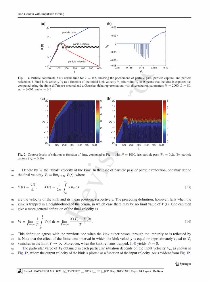
There are then three possible outcomes: (a) particle pass, (b) particle reflection, and (c) particle capture [3], as139

illustrated schematically in Fig. 1a. That is, respectively: (a) the kink may either go through the impurity at x = 0140

and continue to propagate, (b) it may bounce back – possibly after oscillating around the origin for a while – or (c) it141

may remain trapped forever in the region near the origin. Figure 2 shows the contour levels of the kink solution142

profiles as a function of time for a typical particle pass (a) and particle capture (b). The red region is the front of143

the kink solution [in which u(x, t) 2π ], whereas the blue is the back of the kink solution [where u(x, t) 0].144

123


Rev

ised

Proo

f


0 100 200 300 400 500 600−20

−10

0

10

20

t

X (

t)

particle pass

particle capture

particle reflection

0.15 0.155 0.16 0.165 0.17−0.08

−0.06

−0.03

0

0.03

0.06

Vo

Vf

(a) (b)

Fig. 1 a Particle coordinate X (t) versus time for ε = 0.5, showing the phenomena of particle pass, particle capture, and particlereflection. b Final kink velocity Vf as a function of the initial kink velocity Vo (the value Vf = 0 means that the kink is captured) ascomputed using the finite-difference method and a Gaussian delta representation, with discretization parameters N = 2000, L = 80,�t = 0.002, and σ = 0.1

t

X

0 100 200 300 400 500 600−20

−15

−10

−5

0

5

10

15

20(a) (b)

0

1

2

3

4

5

6

t

X

0 100 200 300 400 500 600−20

−15

−10

−5

0

5

10

15

20

0

1

2

3

4

5

6

Fig. 2 Contour levels of solution as function of time, computed as Fig. 1 with N = 1000. (a): particle pass (Vo = 0.2). (b): particlecapture (Vo = 0.16)

Denote by Vf the “final” velocity of the kink. In the case of particle pass or particle reflection, one may define145

the final velocity Vf = limt→∞ V (t), where146

V (t) = dX

dt, X (t) = 1

2π

∞∫−∞

x ux dx (13)147

are the velocity of the kink and its mean position, respectively. The preceding definition, however, fails when the148

kink is trapped in a neighborhood of the origin, in which case there may be no limit value of V (t). One can then149

give a more general definition of the final velocity as150

Vf = limT →∞

1

T

T∫0

V (t) dt = limT →∞

X (T ) − X (0)

T. (14)151

This definition agrees with the previous one when the kink either passes through the impurity or is reflected by152

it. Note that the effect of the finite time interval in which the kink velocity is equal or approximately equal to Vo153

vanishes in the limit T → ∞. Moreover, when the kink remains trapped, (14) yields Vf = 0.154

The particular value of Vf obtained in each particular situation depends on the input velocity Vo, as shown in155

Fig. 1b, where the output velocity of the kink is plotted as a function of the input velocity. As is evident from Fig. 1b,156

123


Rev

ised

Proo

f

D. Wang et al.

the forced PDE (1) is characterized by a critical velocity Vcr = Vcr(ε), which is the smallest value such that each157

IC with Vo > Vcr experiences particle pass.158

3 Numerical preliminaries159

3.1 Spatial and temporal discretizations160

For all the numerical methods considered in this work, the solution of (1) will be computed by appropriately161

choosing N + 1 spatial grid points x0, . . . , xN in [−L , L], with162

−L = x0 < x1 < · · · < xN−1 < xN = L .163

Letting �t be the temporal step size and tk = k�t , with K = T/�t and T = 600, we take ukn = u(num)(xn, tk) for164

n = 0, . . . , N and k = 0, . . . , K . The superscript “(num)” denotes the numerical solution. Explicitly, for the finite-165

difference method, xn = −L + n�x , with �x = 2L/N , while for the Chebyshev pseudo-spectral methods, xn are166

the Chebyshev Gauss–Lobatto nodes, xn = −L cos(nπ/N ) for n = 0, . . . , N . Note that in all the simulations we167

will use even values of N , resulting in an odd number of spatial grid points, so that the point x = 0 is always part of168

the spatial grid: xN/2 = 0. As will be clear in Sect. 3.3, this is essential in ensuring a good numerical representation169

of the Dirac delta.170

Since the goal is to compare the various methods with regard to the treatment of the space-dependent impulsive171

perturbation, the treatment of the spatial part is critically important [20]. Hence, for all the numerical methods we172

simply use finite differences to discretize the time derivative in (1). Specifically, we use the second-order centered173

difference stencil174

∂2un

∂t2

∣∣∣∣t=tk

= uk+1n − 2uk

n + uk−1n

(�t)2 + O(�t2). (15)175

The foregoing choice results in a leap-frog integration scheme, which is second-order with respect to time. After176

performing numerical tests, we verified that choosing �t ≤ 2 × 10−4 produced an error of less than 10−4 on the177

critical velocity in all cases (see below for details), except when required by stability requirements resulting from178

the value of spatial step size �x , in which case appropriately smaller values of �t were chosen (see Sects. 4 and 5179

for details).180

3.2 Initial and boundary conditions181

The aforementioned leap-frog method requires one to supply two starting values. Consistently with (10), for each182

numerical method we then impose183

u0n = uo(xn, 0), u1

n = uo(xn, 0) + �t u1(xn, 0) (16)184

for all n = 0, . . . , N . The value of Xo in (10) should be large enough to ensure that the results are not affected185

by the proximity of the kink to the origin at time t = 0. [Note that the value Xo = −6 used in [3] was not large186

enough to satisfy this criterion.] On the other hand, Xo = −16 (used in all the simulations presented in this work)187

was sufficiently large that the simulation results were unaffected by it. This was verified by checking that taking188

Xo = −26 did not change the results to a level of accuracy of 10−4. Similarly, as we show later in more detail, the189

value L = 80 ensured that no boundary effects affected the solution at the specified level of accuracy, 10−4, in any190

of the numerical methods used.191

Recall that the PDE (1) is posed with the BCs ux (±∞, t) = 0. Numerically, at the left boundary of the192

computational domain (i.e., at x = −L) we impose the exact incoming BC193

u(−L , t) = 4arctan{mo exp[(−L − Xo − Vot) ]}, 0 < t < T . (17)194

At the right boundary of the computational domain (i.e., at x = L) one has several choices. Here we impose the195

outflow BC196

ut (L , t) + ux (L , t) = 0, 0 < t < T, (18)197

123


Rev

ised

Proo

f


so that if the kink propagates up to the edge of the computational domain, it continues to propagate, leaving the198

domain. Note that (18) is not a perfect outflow BC [21] because the final velocity of the kink (which is unknown199

a priori) is always different from 1 [which is the value that would result in a perfect transmission according to (18)].200

As a result, if the kink reaches x = L , a small portion of it is reflected into the domain. This, however, does not201

affect the numerical results because in all the simulations described below, the output value of the kink is measured202

before the kink reaches the right edge of the computational domain.203

3.3 Dirac delta discretization204

As mentioned in Sect. 1, we consider several different ways to treat the Dirac delta numerically. We now provide205

further details for each method.206

(a) Gaussian representation In this case, numerically one replaces δ(x) with representation (2), evaluated at the207

spatial grid points. It is useful to define two special subcases, which we denote as the three-point Gaussian208

and the five-point Gaussian. These are obtained by choosing σ such that the values obtained from (2) are209

nonnegligible at only three or five grid points, respectively. For finite differences, one can do this by taking210

σ = �x/2 or σ = �x/√

2, respectively. In both cases, one has δσ (0) = 1/(√

2π σ). In the first case, however,211

one has δσ (±�x)/δσ (0) = e−2 0.14 and δσ (±2�x)/δσ (0) = e−8 3.4×10−4. In the second case, instead,212

one has δσ (±�x)/δσ (0) = e−1 0.37, δσ (±2�x)/δσ (0) = e−4 0.018 and δσ (±2�x)/δσ (0) = e−9 213

1.2 × 10−4. The choice of σ for pseudo-spectral methods follows similar considerations, except that one needs214

to take into account that in that case the grid spacing is nonuniform and is largest at the origin. Specifically,215

�xN/2 = xN/2+1 − xN/2 = xN/2 − xN/2−1 = L sin(π/N ) Lπ/N is the grid spacing on either side of the216

origin. Therefore, in this case we define the three- and five-point Gaussians as those obtained respectively with217

σ = π L/(2N ) and σ = π L/(√

2 N ).218

(b) Point source This is a special limit of the box representation (5) in which δσ (xn) �= 0 only at the central grid219

point, xN/2 = 0. Specifically, one uses (5), with σ = �xN/2/2, where again �xN/2 is the grid spacing to the220

left and the right of the origin. All the spatial discretizations used in this work result in spatial grids that are221

symmetric around the origin. In this way one has δσ (xn) = 0 for all n �= N/2 and δσ (xn) = δ0 for n = N/2.222

The value of δ0 is then chosen so that the perturbation is properly normalized, δ0 = 1/�xN/2, which ensures223

that (6) is satisfied.224

(c) Self-consistent representation Mathematically one writes δσ (x) = d[Hσ (x)]/dx , where Hσ (x) is a represen-225

tation of the Heaviside step function: H(x) = 0 for all x > 0, H(x) = 1/2 for x = 0, and H(x) = 1 for all226

x > 0. Numerically, this choice is realized by taking δσ (x) = D Hσ (x), where D is the numerical differentia-227

tion operator consistent with the spatial discretization and Hσ (x) is a discrete representation of the Heaviside228

function. Explicitly,229

δσ (xn) =N∑

m=0

Dn,m Hm, (19)230

where Hn = Hσ (xn) for n = 0, 1, . . . , N . We use the “tanh” representation for Hσ231

Hσ (x) = 12

(1 + tanh(x/σ)

). (20)232

As σ → 0, it is obvious that Hσ (x) → H(x).233

(d) Domain decomposition As explained earlier, (1) is equivalent to (7) for all x �= 0, together with the jump234

condition (4). Numerically, one solves (7) on the two spatial domains [−L , 0) and (0, L], and the jump con-235

dition (4) becomes a BC for each domain. The jump condition has two effects: (1) it couples the solutions in236

the two domains; (2) it provides an implicit equation for u(0, t), which allows one to update the value of the237

solution at the origin, ukN/2 = u(0, tk). The precise way in which this second step is realized will be discussed238

in Sect. 6.239

123


Rev

ised

Proo

f

D. Wang et al.

Note that the Gaussian delta representation and the self-consistent delta introduce the additional discretization240

parameter σ , while the point source model and the domain decomposition have no such free parameter.241

3.4 Critical velocity and validation242

Each numerical method will produce an estimate of the critical velocity that in general depends on the values of243

the discretization parameters. For example, if the finite difference method is used in conjunction with the Gaussian244

representation, one has V (num)cr = Vcr(ε; L , N ,�t, σ ). A similar situation arises for all other numerical methods.245

An obvious and important question is then whether, for each method, V (num)cr converges to Vcr as the discretization246

parameters 1/N ,�t, σ tend to 0, and, if so, how quickly. In this work we compare the various numerical methods247

with respect to this criterion.248

Let us discuss the algorithm used to numerically reconstruct the kink position X (t) as a function of time.249

Numerically, we define X (t) as the position of the half-value of the kink. In order to determine X (t) at time t , we250

consider the maximum value umax(t) = maxx∈[−L ,L]u(x, t) and the minimum value umin(t) = minx∈[−L ,L]u(x, t)251

of the solution. We calculate the average of these values, uavg = (umin + umax)/2. We then find the numerical252

solution value closest to the average value, and we take the corresponding x-coordinate of this closest value to be253

the kink position X (t). While one could obviously use much more sophisticated procedures, the above-described254

algorithm is very fast, and, in most cases, it captures the kink position quite well. The algorithm fails occasionally255

when large amounts of dispersive radiation are generated. However, this only happens when the kink is reflected,256

and therefore the failure of the algorithm does not affect the results about the value of the critical velocity. Other257

options were also tried, such as the numerical evaluation of (13), but the corresponding results had a comparable258

level of accuracy to those with the above method.259

Finally, from the kink position X (t) we obtain the output velocity Vf . Specifically, we define Vf as the average260

velocity for the last 50 measured values of X (t). We then repeat the simulations for many, finely spaced values of261

Vo, and we take the numerically determined Vcr to be the greatest lower bound of the set of the initial velocities such262

that X (T ) = 6. We use the value of V (num)cr obtained from the most accurate simulations—namely, those with the263

largest number of grid points—to be our estimate for Vcr. This results in the previously quoted value Vcr = 0.1657.264

The last issue that must be discussed is the uncertainty in the preceding value of Vcr. We should emphasize265

that the accuracy of Vcr is not affected by the uncertainty in the measurement of Vf because the critical velocity266

is an input velocity, not an output one. Here input velocity means the input velocity of the kink before the kink267

reaches the impurity, whereas output velocity means the velocity of the kink after the kink has interacted with the268

impurity. In other words, note from Fig. 1b that dVf/dVo → ∞ as Vo → Vcr from the right. Thus, the uncertainty269

in the value of Vcr is simply determined by how accurately one can measure input velocities. Accordingly, the270

uncertainty in the estimate of Vcr was taken to be the upper limit of the difference between the input velocity of271

a kink and its measured velocity when ε = 0. As discussed in more detail in the following sections, for each272

numerical method the parameters L , N , �t , and Xo were chosen such that this uncertainty was always less than273

10−4, implying that the simulations allow one to estimate the critical velocity with four significant digits after the274

decimal point. Correspondingly, the input velocities used in the simulations were chosen such that the difference275

between consecutive values of Vo was �Vo 10−4.276

4 Finite-difference methods277

4.1 Implementation278

As mentioned earlier, we use a spatial grid size �x = 2L/N , and we take the grid points to be xn = −L + n�x279

for n = 0, 1, . . . , N . Taking ukn = u(num)(xn, tk), discretizing (1), and utilizing the three-point, second-order280

centered stencil for the second spatial derivative, we obtain, for all k ≥ 1 and n = 1, 2, . . . , N − 1,281

123


Rev

ised

Proo

f


uk+1n − 2uk

n + uk−1n

(�t)2 − ukn+1 − 2uk

n + ukn−1

(�x)2 + [1 − εδσ (xn)] sin ukn = 0. (21)282

The IC and the left BC are specified by simply imposing (16) and (17), as discussed in Sect. 3. At the right283

boundary, we discretize (18) with the explicit scheme284

uk+1N − uk

N

�t+ uk

N − ukN−1

�x= 0. (22)285

The Courant-Friedrichs-Lewy stability criterion for the foregoing scheme is�t < �x = 2L/N . A more stringent286

requirement on the temporal step size, however, is provided by the need to preserve accuracy, as we discuss in the287

following sections. As mentioned earlier, one can obtain an upper bound for the error in the determination of288

the critical velocity by simply taking the difference between the numerically determined velocity of a kink in the289

case ε = 0 and that of the exact analytical solution. When applying the foregoing finite-difference scheme to the290

unperturbed sG equation, we find that the error in the numerically determined kink velocity is 10−4 or less when291

L = 80, �t = 2×10−4, and N ≥ 4,000. With these constraints, we then proceed to test the various representations292

of the Dirac delta.293

4.2 Perturbed kink behavior with finite differences294

We first test the finite-difference method with the Gaussian delta. As explained in Sect. 3.3, when using the Gaussian295

representation of the Dirac delta one simply replaces δ(x) with δσ (xn), as given by (2). Figure 4a shows the296

numerically determined critical velocity as a function of N and σ when all other discretization parameters are297

sufficiently small that the corresponding numerical errors are smaller than 10−4, which can therefore be neglected.298

Figure 4b shows the dependence of the absolute error E = |V (num)cr − Vcr| on N and σ . The continuum limit299

corresponds to the limit (1/N , σ ) → 0, which is the point at infinity in the direction of the lower left corner of300

either plot. The error should therefore vanish in this limit. Indeed, Fig. 4b shows that, if one takes the limit N → ∞301

while σ is fixed, then V (num)cr converges to a finite value, which in turn converges to Vcr as σ → 0. On the other302

hand, if one decreases σ while N is fixed, then V (num)cr increases, and no finite critical velocity emerges, in the303

sense that eventually V (num)cr → 1, and the system ceases to display any particle passes. This behavior can be easily304

explained by recalling that �x = 2L/N . Thus, when σ � L/N , the perturbing term in the numerical method305

becomes effectively a point source because the Gaussian has nonnegligible values only at the central grid point. In306

that case, however, the source term is not normalized correctly because when σ � �x , it is307

∞∫−∞

δσ (x) dx N−1∑n=0

δσ (xn)�x �x/(σ√

2π) �= 1.308

In fact, the right-hand side of the preceding equation tends to infinity as σ → 0, with �x fixed, meaning that in309

this limit the perturbation to the sG equation grows to an infinite strength.310

The foregoing discussion demonstrates that, as with the limit (�x,�t) → 0, one must be careful when taking the311

limit (1/N , σ ) → 0 to recover the correct PDE behavior. In particular, when using the Gaussian delta representation,312

we see that the three-point Gaussian is not convergent, and one needs to take at least the five-point Gaussian to313

recover the correct behavior in the limit N → ∞.314

Next we test the finite-difference method with the self-consistent delta. As discussed earlier, this choice is realized315

by replacing δ(x) in (21) with (19). In particular, the differentiation matrix obtained from the second-order centered316

difference stencil yields317

δσ (xn) =⎧⎨⎩

(Hσ (x1) − Hσ (x0))/�x n = 0,

(Hσ (xn+1) − Hσ (xn−1))/2�x n = 1, . . . , N − 1,

(Hσ (xN ) − Hσ (xN−1))/�x n = N .

318

123


Rev

ised

Proo

f

D. Wang et al.

Note that, even though the first and last values in the preceding equation are obtained from a one-sided stencil, these319

values are not used in (21) since the solution at the first and last grid points are updated using the BCs.320

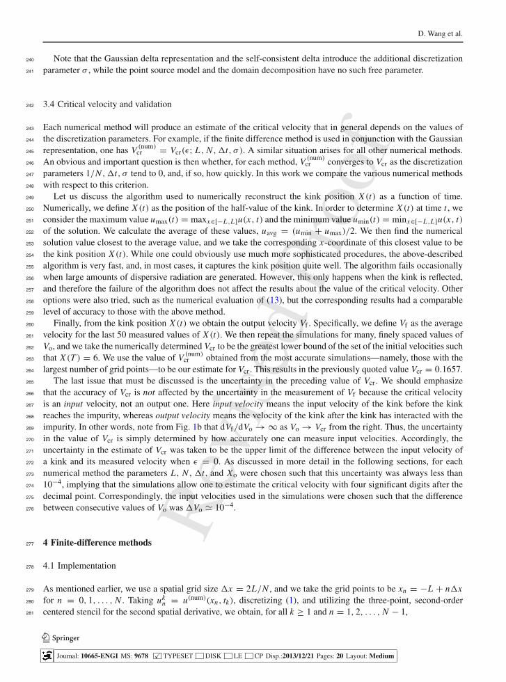
As before, Fig. 5 shows the dependence on N and σ of the numerical critical velocity and the absolute error.321

Again, if σ is fixed while N is increased, V (num)cr converges to a finite value, which in turn converges to Vcr as σ → 0.322

Contrary to the case of the Gaussian delta, however, if σ is decreased while N is fixed, V (num)cr still converges to a323

finite value. This is related to the fact that, unlike the Gaussian delta, even when σ = 0, the perturbation is not a324

point source, as can be seen in Fig. 3, and it is still normalized correctly. The error floor at the bottom left corner325

of Fig. 5b is due to the fact that we only keep four significant digits for the value of critical velocity.326

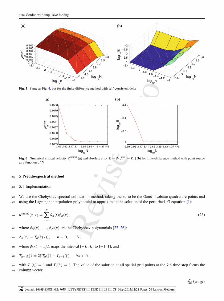
Finally, we use the point source representation of the Dirac delta, taking σ = �x/2 in (5). Recall from Sect. 3.3327

that in this case there is no extra Dirac delta discretization parameter. Hence, in this case Fig. 6 simply shows the328

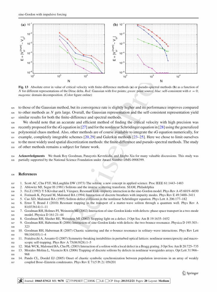
dependence on N of the numerical critical velocity V (num)cr and the absolute error E = |V (num)

cr − Vcr|. In this case329

we find that V (num)cr already converges to the correct value when N = 4,000. As in the case of the self-consistent330

delta, the error floor at 10−4 is a consequence of the fact that we only have four significant digits.331

As shown in Figs. 4–6, the point source and self-consistent approximation approaches yield better performance332

than the Gaussian approach. In particular, it is interesting that the point source works well. The overall order of333

convergence from Fig. 6 is approximately 2.3.334

−4 −2 0 2 4

0

0.2

0.4

0.6

0.8

1

1.2

1.4

1.6

x

δ (x

)

−4 −2 0 2 4

0

0.2

0.4

0.6

0.8

1

1.2

1.4

1.6

x

δ (x

)(a) (b)

Fig. 3 Numerical representations of Dirac delta on finite interval [−L , L] with L = 80 and N = 300 with an equally spaced grid(a) and on a grid of Gauss–Lobatto nodes xn = −L cos(nπ/N ) (b): five-point Gaussian (magenta), three-point Gaussian (red), pointsource (black), self-consistent with σ = 0 (blue) with second-order centered differences (a) or Chebyshev differentiation matrix (b).(Color figure online)

3.33.5

3.73.9

4.14.3

4.5

−2.55−2.35

−2.15−1.95

−1.75−1.55

−1.35−1.15

00.20.40.60.8

1

log10

Nlog

10σ

Vcr(n

um)

3.33.5

3.73.9

4.14.3

4.5

−2.55−2.35−2.15−1.95−1.75−1.55−1.35−1.15

−4−3.5

−3−2.5

−2−1.5

−1−0.5

0

log10

N

log10

σ

log

10E

(a) (b)

Fig. 4 Numerical critical velocity V (num)cr (a) and absolute error E = |V (num)

cr − Vcr| (b) for finite-difference method with Gaussiandelta as a function of N and σ

123


Rev

ised

Proo

f


3.33.5

3.73.9

4.14.3

4.5

−2.4−2.2

−2−1.8

−1.6−1.4

−1.2−1

0.160.1610.1620.1630.1640.1650.166

log10

Nlog

10σ

Vcr(n

um)

3.33.5

3.73.9

4.14.3

4.5

−2.4−2.2

−2−1.8

−1.6−1.4

−1.2−1

−4

−3.5

−3

−2.5

−2

(b)(a)

log10

Nlog

10σ

log

10E

Fig. 5 Same as Fig. 4, but for the finite-difference method with self-consistent delta

2.69 2.93 3.17 3.41 3.65 3.89 4.13 4.37 4.610.1655

0.1659

0.1663

0.1667

0.1671

0.1675

0.1679

0.1683

log10

N

Vcr(n

um)

2.69 2.93 3.17 3.41 3.65 3.89 4.13 4.37 4.61

−4

−3.6

−3.1

−2.6

log10

N

log 10

E

(a) (b)

Fig. 6 Numerical critical velocity V (num)cr (a) and absolute error E = |V (num)

cr − Vcr| (b) for finite-difference method with point sourceas a function of N

5 Pseudo-spectral method335

5.1 Implementation336

We use the Chebyshev spectral collocation method, taking the xn to be the Gauss–Lobatto quadrature points and337

using the Lagrange interpolation polynomial to approximate the solution of the perturbed sG equation (1):338

u(num)(x, t) =N∑

n=0

un(t)φn(x), (23)339

where φ0(x), . . . , φN (x) are the Chebyshev polynomials [22–26]:340

φn(x) = Tn(ξ(x)), n = 0, . . . , N ,341

where ξ(x) = x/L maps the interval [−L , L] to [−1, 1], and342

Tn+1(ξ) = 2ξTn(ξ) − Tn−1(ξ) ∀n ∈ N,343

with T0(ξ) = 1 and T1(ξ) = ξ . The value of the solution at all spatial grid points at the kth time step forms the344

column vector345

123


Rev

ised

Proo

f

D. Wang et al.

uk = (uk0, . . . , uk

N )T, (24)346

with ukn = u(num)(xn, tk).347

We then discretize (1) in both time and space using the Chebyshev differentiation matrix for the spatial derivative348

and central differences for the time discretization,349

uk+1 − 2uk + uk−1

(�t)2 − D2N uk + (

IN − ε δN)

sin uk = 0. (25)350

Here IN is the (N+1) × (N+1) identity matrix, δN = diag(δσ (x0), . . . , δσ (xN )), and D2N is the (N+1) × (N+1)351

second-order Chebyshev differentiation matrix, which allows one to express the values of uxx (x, t) at the spectral352

collocation points as a function of uk0, . . . , uk

N [22–26].353

As with the finite-difference method, the IC is specified by assigning u0n and u1

n according to (10), and the left BC354

is specified by assigning uk0 according to (17). Finally, for the right boundary, similarly to (22), we discretize (18)355

with the explicit scheme356

uk+1N − uk

N

�t+ uk

N − ukN−1

xN − xN−1= 0.357

To avoid blow-up, one needs �t < �x . The grid spacing is nonuniform, and one should take358

�x = minn=1,...,N

{xn − xn−1} = xN − xN−1 = x1 − x0 = L (1 − cos(π/N )) Lπ2/(2N 2). (26)359

Hence, in this case �t = O(1/N 2). Note that the coefficients u0(t), . . . , uN (t) of the Chebyshev polynomials360

in (23) are never used in practice in the numerical solution of the PDE.361

As before, we test the Chebyshev spectral collocation method on the unperturbed sG equation (7) to quantify the362

numerical error of the numerically measured velocity of the kink solution. We find that the error is less than 10−4363

when L = 80 and N = 500. As before, with these constraints we then proceed to test the various discretizations of364

the Dirac delta.365

Recall that the Chebyshev polynomials on the Gauss–Lobatto points, x j = − cos( jπ/N ) for j = 0, . . . , N , are366

basically cosine functions. That is,367

Tl(x j ) = cos(l cos−1(x)) = cos(l cos−1(cos( jπ/N ))) = cos(l jπ/N ).368

Thus the derivative of u(x, t) for any derivative order based on the matrix vector multiplication can be efficiently369

implemented via the fast Fourier transformation (FFT).370

Equivalently, one can also implement a spectral Galerkin method using a Galerkin projection. The difference is371

that the Galerkin projection can directly project the Dirac delta, which is computed easily using the definition of372

the δ-function for the one-domain approach. If the computational domain is split into two subdomains, the Galerkin373

procedure is applied in each domain, and the jump condition is incorporated into the Galerkin procedure. This will374

be explained in Sect. 6.375

5.2 Perturbed kink behavior with pseudo-spectral method376

We first test the Gaussian representation (2) of the Dirac delta. In (25), δN becomes the diagonal matrix377

δN = diag (δσ (x0), . . . , δσ (xN )) . (27)378

Figure 7 shows the numerically determined critical velocity V (num)cr and the absolute error E = |V (num)

cr − Vcr|379

as a function of N and σ . As in Fig. 4, the continuum limit corresponds to the limit (1/N , σ ) → 0 (the point at380

infinity in the lower left corner of the plots), and the error should therefore vanish in this limit. Indeed, as with381

finite differences, if one increases N while σ is fixed, V (num)cr converges to a finite value, which in turn converges382

to Vcr as σ → 0. As with finite differences, however, if one decreases σ while N is fixed, eventually one reaches a383

value at which the perturbing term becomes effectively a point source – again with the wrong normalization. If σ384

123


Rev

ised

Proo

f


2.52.6

2.72.8

2.93

3.13.2

3.3

−3−2.5

−2−1.5

−1−0.5

0

00.20.40.60.8

1

log10

Nlog

10σ

Vcr(n

um)

2.52.6

2.72.8

2.93

3.13.2

3.3

−3−2.5

−2−1.5

−1−0.5

0

−4−3.5

−3−2.5

−2−1.5

−1−0.5

0

log10

N

log10

σ

log 10

E

(a) (b)

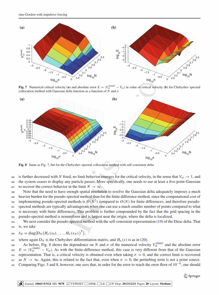
Fig. 7 Numerical critical velocity (a) and absolute error E = |V (num)cr − Vcr| in value of critical velocity (b) for Chebyshev spectral

collocation method with Gaussian delta function as a function of N and σ

2.52.6

2.72.8

2.93

3.13.2

3.33.4

−3−2.5

−2−1.5

−1−0.5

0

(a) (b)

0.020.040.060.080.1

0.120.140.160.18

log10

Nlog

10σ

Vcr(n

um)

2.52.6

2.72.8

2.93

3.13.2

3.33.4

−3−2.5

−2−1.5

−1−0.5

0

−4−3.5

−3−2.5

−2−1.5

−1

log10

N

log10

σ

log 10

E

Fig. 8 Same as Fig. 7, but for the Chebyshev spectral collocation method with self-consistent delta

is further decreased with N fixed, no limit behavior emerges for the critical velocity, in the sense that Vcr → 1, and385

the system ceases to display any particle passes. More specifically, one needs to use at least a five-point Gaussian386

to recover the correct behavior in the limit N → ∞.387

Note that the need to have enough spatial resolution to resolve the Gaussian delta adequately imposes a much388

heavier burden for the pseudo-spectral method than for the finite difference method, since the computational cost of389

implementing pseudo-spectral methods is O(N 2) compared to O(N ) for finite differences, and therefore pseudo-390

spectral methods are typically advantageous when one can use a much smaller number of points compared to what391

is necessary with finite differences. This problem is further compounded by the fact that the grid spacing in the392

pseudo-spectral method is nonuniform and is largest near the origin, where the delta is localized.393

We next consider the pseudo-spectral method with the self-consistent representation (19) of the Dirac delta. That394

is, we take395

δN = diag(DN

(Hσ (x0), . . . , Hσ (xN )

)T),396

where again DN is the Chebyshev differentiation matrix, and Hσ (x) is as in (20).397

As before, Fig. 8 shows the dependence on N and σ of the numerical velocity V (num)cr and the absolute error398

E = |V (num)cr − Vcr|. As with the finite-difference method, this case is very different from that of the Gaussian399

representation. That is, a critical velocity is obtained even when taking σ = 0, and the correct limit is recovered400

as N → ∞. Again, this is related to the fact that, even when σ = 0, the perturbing term is not a point source.401

Comparing Figs. 5 and 8, however, one sees that, in order for the error to reach the error floor of 10−4, one should402

123


Rev

ised

Proo

f

D. Wang et al.

2.46 2.69 2.92 3.15 3.38 3.610.1658

0.166

0.1665

0.167

0.1675

0.168

0.1685

0.169

0.1694

log10

N

Vcr(n

um)

2.46 2.69 2.92 3.15 3.38 3.61−4

−3.8

−3.6

−3.4

−3.2

−3

−2.8

−2.6

−2.4

log10

N

log 10

E

(a) (b)

Fig. 9 Numerical critical velocity (a) and absolute error (b) for Chebyshev spectral collocation method with point source as a functionof N

take comparable numbers of spatial grid points in the finite-difference and pseudo-spectral methods, again voiding403

the advantage of the latter over the former.404

Finally, we study perturbed behavior with pseudo-spectral methods when the Dirac delta is modeled by a point405

source using (5), with σ = �xN/2/2 = (xN/2+1−xN/2−1)/4. Figure 9 shows the dependence on N of the numerical406

critical velocity and absolute error. As N increases, V (num)cr converges to the correct value. Note, however, that the407

convergence rate is only linear with N , negating the spectral convergence of the method for the unperturbed408

equation.409

From Figs. 7–9 we see that the self-consistent approach and the point source approach are superior to the Gaussian410

approximation method. It is also interesting that the point source approach with the spectral method still yields411

stable and accurate results. Among these three approaches, the self-consistent approach yields the best performance.412

The overall order of convergence for the self-consistent method is approximately 2.78 when σ 10−3, and that413

for the point source approach is approximately 1.2.414

6 Domain decomposition methods415

As discussed earlier, when using domain decomposition methods one divides the original domain into two subdo-416

mains, [−L , 0] and [0, L], and solves the unperturbed sG equation in each domain. That is, the solutions in the left417

subdomain and the right subdomain, denoted respectively as u∓(x, t), satisfy418

u−t t − u−

xx + sin u− = 0, −L < x < 0, (28)419

u+t t − u+

xx + sin u+ = 0, 0 < x < L . (29)420

At the intersection of the two subdomains, one has the continuity condition (8) together with the jump condition (4).421

At the outer boundaries of the two subdomains, one has the right and left BCs (17) and (18), and the ICs in422

each subdomain are simply the restrictions of (10). In each subdomain, either the finite-difference method or the423

Chebyshev spectral collocation method can be used to solve (28) and (29).424

6.1 Domain decomposition with finite-difference method425

We use the same uniform spatial grid size �x = 2L/N in each interval [−L , 0] and [0, L], obtaining N/2 + 1 grid426

points in each subdomain. Explicitly, one has x−n = −L + n�x for n = 0, . . . , N/2 on [−L , 0] and x+

n = n�x427

for n = 0, . . . , N/2 on [0, L]. The corresponding representations for the solutions in the two subdomains are428

u±,kn = u(num)(x±

n , tk). Note that there are only N+1 spatial points (not N+2) since x−N/2 = x+

0 = 0.429

123


Rev

ised

Proo

f


Discretizing the equation at the kth time step and utilizing the three-point centered stencil for the second deriv-430

atives we obtain, for k ≥ 1 and n = 1, 2, . . . , N/2 − 1,431

u±,k+1n − 2u±,k

n + u±,k−1n

(�t)2 − u±,kn+1 − 2u±,k

n + u±,kn−1

(�x)2 + sin u±,kn = 0.432

The initial and left BCs are imposed in a straightforward way. For the right boundary we use the explicit scheme,433

similarly to what was done in Sect. 4:434

u+,k+1N/2 − u+,k

N/2

�t+ u+,k

N/2 − u+,kN/2−1

�x= 0. (30)435

From the continuity condition (8) we have436

u+,k0 = u−,k

N/2. (31)437

Moreover, the jump condition (4) needs to be discretized as well. For this purpose, we use a higher-order438

approximation for the derivative term using Lagrange interpolation polynomials. For example, for the solution near439

x = x−N/2 in the left domain, u−(x, t), the Lagrange interpolation based on p ≥ 1 points including u−(0−, t) is440

given by441

u−(x, t) =N/2∑

i=N/2−p

u−(xi , t)li (x) =N/2∑

i=N/2−p

u−(xi , t)∏

N/2−p≤m≤N/2, m �=i

x − xm

xi − xm.442

The derivative of u−(x, t) at x = x−N/2 is then given by443

du−(x, t)

dx

∣∣∣∣x=x−

N/2

=N/2∑

i=N/2−p

u−(xi , t)l ′i (x−N/2).444

For example, if we choose p = 2, which yields second-order accuracy, we get445

du−(x, t)

dx

∣∣∣∣x=x−

N/2

= 1

�x

[3

2u−,k

N/2 − 2u−,kN/2−1 + 1

2u−,k

N/2−2

].446

Similarly,447

du+(x, t)

dx

∣∣∣∣x=x+

0

= 1

�x

[−3

2u+,k

0 + 2u+,k1 − 1

2u+,k

2

].448

Using u−,kN/2 = u+,k

0 with the jump condition (4), we then have449

1

�x

[−3u+,k+1

0 + 4u+,k+11 − u+,k+1

2

]= −ε�x sin u+,k+1

0 = −ε�x sin u−,k+1N/2 . (32)450

The last condition provides a nonlinear equation for the unknown value u+,k+10 = u−,k+1

N/2 , which we solve using451

Newton’s method to obtain the updated value of the solution at x = 0, i.e., u(0, t).452

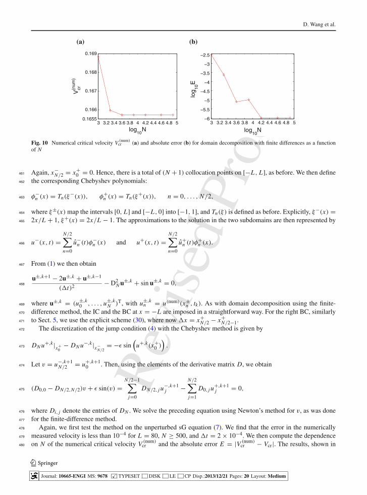
As before, we first test the domain decomposition method on the unperturbed sG equation (7). We find that453

the error in the numerically measured velocity of a kink is less than 10−4 when L = 80, �t = 2 × 10−4, and454

N ≥ 8,000. We then compute the numerical critical velocity V (num)cr and the absolute error E = |V (num)

cr − Vcr| as a455

function of N . The results are shown in Fig. 10. It appears that the numerical critical velocity converges to the PDE456

value with an overall convergence order of approximately 2.9, which is a better order than the single-domain case.457

6.2 Domain decomposition with Chebyshev spectral collocation method458

We introduce the spectral collocation points in each subdomain [−L , 0] and [0, L] as follows: for n = 0, . . . , N/2459

x−n = −(L/2)[1 + cos(2nπ/N )], x+

n = (L/2)[1 − cos(2nπ/N )].460

123


Rev

ised

Proo

f

D. Wang et al.

3 3.2 3.4 3.6 3.8 4 4.2 4.4 4.6 4.8 50.1655

0.166

0.167

0.168

0.169

log10

N

Vcr(n

um)

3 3.2 3.4 3.6 3.8 4 4.2 4.4 4.6 4.8 5−6

−5.5

−5

−4.5

−4

−3.5

−3

−2.5

log10

N

log 10

E

(a) (b)

Fig. 10 Numerical critical velocity V (num)cr (a) and absolute error (b) for domain decomposition with finite differences as a function

of N

Again, x−N/2 = x+

0 = 0. Hence, there is a total of (N + 1) collocation points on [−L , L], as before. We then define461

the corresponding Chebyshev polynomials:462

φ−n (x) = Tn(ξ−(x)), φ+

n (x) = Tn(ξ+(x)), n = 0, . . . , N/2,463

where ξ±(x) map the intervals [0, L] and [−L , 0] into [−1, 1], and Tn(ξ) is defined as before. Explicitly, ξ−(x) =464

2x/L + 1, ξ+(x) = 2x/L − 1. The approximations to the solution in the two subdomains are then represented by465

u−(x, t) =N/2∑n=0

u−n (t)φ−

n (x) and u+(x, t) =N/2∑n=0

u+n (t)φ+

n (x).466

From (1) we then obtain467

u±,k+1 − 2u±,k + u±,k−1

(�t)2 − D2N u±,k + sin u±,k = 0,468

where u±,k = (u±,k0 , . . . , u±,k

N )T, with u±,kn = u(num)(x±

n , tk). As with domain decomposition using the finite-469

difference method, the IC and the BC at x = −L are imposed in a straightforward way. For the right BC, similarly470

to Sect. 5, we use the explicit scheme (30), where now �x = x+N/2 − x+

N/2−1.471

The discretization of the jump condition (4) with the Chebyshev method is given by472

DN u+,k |x+0

− DN u−,k |x−N/2

= −ε sin(

u+,k(x+0 )

).473

Let v = u−,k+1N/2 = u+,k+1

0 . Then, using the elements of the derivative matrix D, we obtain474

(D0,0 − DN/2,N/2)v + ε sin(v) =N/2−1∑

j=0

DN/2, j u−,k+1j −

N/2∑j=1

D0, j u+,k+1j = 0,475

where Di, j denote the entries of DN . We solve the preceding equation using Newton’s method for v, as was done476

for the finite-difference method.477

Again, we first test the method on the unperturbed sG equation (7). We find that the error in the numerically478

measured velocity is less than 10−4 for L = 80, N ≥ 500, and �t = 2 × 10−4. We then compute the dependence479

on N of the numerical critical velocity V (num)cr and the absolute error E = |V (num)

cr − Vcr|. The results, shown in480

123


Rev

ised

Proo

f


2.46 2.63 2.8 2.97 3.14 3.31 3.480.1656

0.1657

0.1658

log10

N

Vcr(n

um)

2.46 2.63 2.8 2.97 3.14 3.31 3.48−6

−5.5

−5

−4.5

−4

(a) (b)

log10

N

log 10

E

(E =

|Vcr(n

um) −

Vcr(p

de) |)

Fig. 11 Same as Fig. 10, but for domain decomposition with Chebyshev pseudo-spectral method

Fig. 11, demonstrate that the numerical critical velocity converges to that of the PDE value with a convergence481

order of approximately 2.482

6.3 Domain decomposition with semi-implicit methods483

The domain decomposition method (as well as the one-domain approach with the Galerkin projection of the Dirac484

delta) can be more efficiently implemented using a semi-implicit scheme. For this purpose, consider the Legendre485

approximation of the solution, uN (x, t), as a polynomial of degree at most N such that486

u(x, t) =N∑

l=0

ul(t)Ll(ξ(x)),487

where Ll(ξ) is the Legendre polynomial of degree l and ξ is the linear mapping ξ : x → [−1, 1], i.e., x = Lξ .488

Using this expression in (1) yields489

N∑l=0

d2ul(t)

dt2 Ll(ξ(x)) = 1

L2

N∑l=0

ul(t)L ′′l (ξ(x)) − sin(u(x, t)),490

where the prime denotes derivative with respect to ξ , and where we used dξ/dx = 1/L . Using the Galerkin491

projection onto Ll ′(ξ) and the orthogonality of Ll(x) and Ll ′(x) for l �= l ′ we obtain492

d2ul(t)

dt2 = 1

L2

N∑l=0

ul(t)2l ′ + 1

2

1∫−1

L′′l (ξ)Ll ′(ξ)dξ − 2l ′ + 1

2

1∫−1

sin(u(x, t))Ll ′(ξ)dξ.493

Define the column vector u = (u0, . . . , uN )T, as well as the matrix A = (Al ′,l), and the column vector b = (bl ′) as494

Al ′,l = 2l ′ + 1

2

1∫−1

L′′l (ξ)Ll ′(ξ)dξ, bl ′ = −2l ′ + 1

2

1∫−1

sin(u(x, t))Ll ′(ξ)dξ.495

The semi-implicit scheme employs an implicit scheme for the linear part of the equation and an explicit scheme for496

the nonlinear part of the equation as follows:497

un+1 − 2un + un−1

�t2 = 1

L2 Aun+1 + bn .498

123


Rev

ised

Proo

f

D. Wang et al.

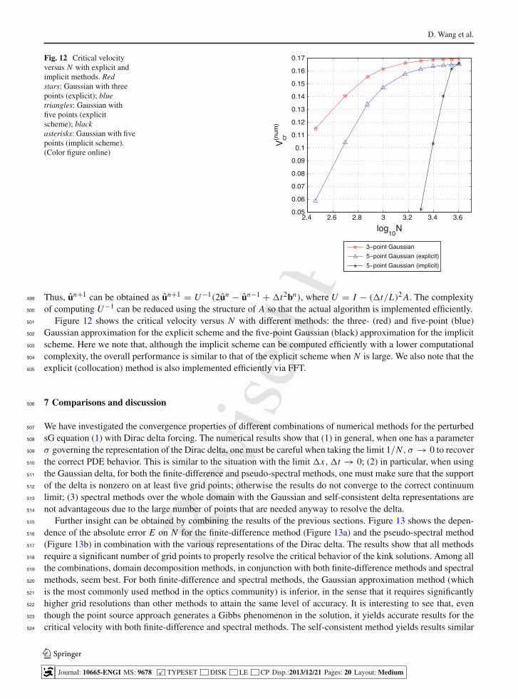
Fig. 12 Critical velocityversus N with explicit andimplicit methods. Redstars: Gaussian with threepoints (explicit); bluetriangles: Gaussian withfive points (explicitscheme); blackasterisks: Gaussian with fivepoints (implicit scheme).(Color figure online)

2.4 2.6 2.8 3 3.2 3.4 3.60.05

0.06

0.07

0.08

0.09

0.1

0.11

0.12

0.13

0.14

0.15

0.16

0.17

log10

N

Vcr(n

um)

3−point Gaussian

5−point Gaussian (explicit)

5−point Gaussian (implicit)

Thus, un+1 can be obtained as un+1 = U−1(2un − un−1 + �t2bn), where U = I − (�t/L)2 A. The complexity499

of computing U−1 can be reduced using the structure of A so that the actual algorithm is implemented efficiently.500

Figure 12 shows the critical velocity versus N with different methods: the three- (red) and five-point (blue)501

Gaussian approximation for the explicit scheme and the five-point Gaussian (black) approximation for the implicit502

scheme. Here we note that, although the implicit scheme can be computed efficiently with a lower computational503

complexity, the overall performance is similar to that of the explicit scheme when N is large. We also note that the504

explicit (collocation) method is also implemented efficiently via FFT.505

7 Comparisons and discussion506

We have investigated the convergence properties of different combinations of numerical methods for the perturbed507

sG equation (1) with Dirac delta forcing. The numerical results show that (1) in general, when one has a parameter508

σ governing the representation of the Dirac delta, one must be careful when taking the limit 1/N , σ → 0 to recover509

the correct PDE behavior. This is similar to the situation with the limit �x,�t → 0; (2) in particular, when using510

the Gaussian delta, for both the finite-difference and pseudo-spectral methods, one must make sure that the support511

of the delta is nonzero on at least five grid points; otherwise the results do not converge to the correct continuum512

limit; (3) spectral methods over the whole domain with the Gaussian and self-consistent delta representations are513

not advantageous due to the large number of points that are needed anyway to resolve the delta.514

Further insight can be obtained by combining the results of the previous sections. Figure 13 shows the depen-515

dence of the absolute error E on N for the finite-difference method (Figure 13a) and the pseudo-spectral method516

(Figure 13b) in combination with the various representations of the Dirac delta. The results show that all methods517

require a significant number of grid points to properly resolve the critical behavior of the kink solutions. Among all518

the combinations, domain decomposition methods, in conjunction with both finite-difference methods and spectral519

methods, seem best. For both finite-difference and spectral methods, the Gaussian approximation method (which520

is the most commonly used method in the optics community) is inferior, in the sense that it requires significantly521

higher grid resolutions than other methods to attain the same level of accuracy. It is interesting to see that, even522

though the point source approach generates a Gibbs phenomenon in the solution, it yields accurate results for the523

critical velocity with both finite-difference and spectral methods. The self-consistent method yields results similar524

123


Rev

ised

Proo

f


102 103 10410−6

10−5

10−4

10−3

10−2

10−1

N

E =

|Vcr(n

um) −

Vcr

|

102

103

104

10−6

10−5

10−4

10−3

10−2

10−1

N

E =

|Vcr(n

um) −

Vcr

|

(a) (b)

Fig. 13 Absolute error in value of critical velocity with finite-difference methods (a) or pseudo-spectral methods (b) as a function ofN for different representations of the Dirac delta. Red: Gaussian with five points; green: point source; blue: self-consistent with σ = 0;magenta: domain decomposition. (Color figure online)

to those of the Gaussian method, but its convergence rate is slightly higher and its performance improves compared525

to other methods as N gets large. Overall, the Gaussian representation and the self-consistent representation yield526

similar results for both the finite-difference and spectral methods.527

We should note that an accurate and efficient method of finding the critical velocity with high precision was528

recently proposed for the sG equation in [27] and for the nonlinear Schrödinger equation in [28] using the generalized529

polynomial chaos method. Also, other methods are of course available to integrate the sG equation numerically, for530

example, completely integrable schemes [20,29] and Galerkin methods [23–25]. Here we chose to limit ourselves531

to the most widely used spatial discretization methods: the finite-difference and pseudo-spectral methods. The study532

of other methods remains a subject for future work.533

Acknowledgments We thank Roy Goodman, Panayotis Kevrekidis, and Jingbo Xia for many valuable discussions. This study was534

partially supported by the National Science Foundation under Award Number DMS-0908399.535

References536

1. Scott AC, Chu FYF, McLaughlin DW (1973) The soliton: a new concept in applied science. Proc IEEE 61:1443–1483537

2. Ablowitz MJ, Segur H (1981) Solitons and the inverse scattering transform. SIAM, Philadelphia538

3. Fei Z (1992) Y S Kivshar and L Vázquez, Resonant kink–impurity interaction in the sine-Gordon model. Phys Rev A 45:6019–6030539

4. Forinash K, Peyrard M, Malomed BA (1994) Interaction of discrete breathers with impurity modes. Phys Rev E 49:3400–3411540

5. Cao XD, Malomed BA (1995) Soliton-defect collisions in the nonlinear Schrödinger equation. Phys Lett A 206:177–182541

6. Ernst T, Brand J (2010) Resonant trapping in the transport of a matter-wave soliton through a quantum well. Phys Rev A542

81(033614):1–11543

7. Goodman RH, Holmes PJ, Weinstein MI (2002) Interaction of sine-Gordon kinks with defects: phase space transport in a two-mode544

model. Physica D 161:21–44545

8. Goodman RH, Slusher RE, Weinstein MI (2002) Stopping light on a defect. J Opt Soc Am B 19:1635–1652546

9. Goodman RH, Haberman R (2004) Interaction of sine-Gordon kinks with defects: the two-bounce resonance. Physica D 195:303–547

323548

10. Goodman RH, Haberman R (2007) Chaotic scattering and the n-bounce resonance in solitary–wave interactions. Phys Rev Lett549

98(104103):1–4550

11. Fratalocchi A, Assanto G (2007) Symmetry-breaking instabilities in perturbed optical lattices: nonlinear nonreciprocity and macro-551

scopic self-trapping. Phys Rev A 75(063828):1–5552

12. Mak WCK, Malomed BA, Chu PL (2003) Interaction of a soliton with a local defect in a Bragg grating. J Opt Soc Am B 20:725–735553

13. Morales-Molina L, Vicencio RA (2006) Trapping of discrete solitons by defects in nonlinear waveguides arrays. Opt Lett 31:966–554

968555

14. Pando CL, Doedel EJ (2005) Onset of chaotic symbolic synchronization between population inversions in an array of weakly556

coupled Bose–Einstein condensates. Phys Rev E 71(5 Pt 2): 056201557

123


Rev

ised

Proo

f

D. Wang et al.

15. Peyrard M, Kruskal MD (1984) Kink dynamics in the highly discrete sine-Gordon system. Physica D 14:88–102558

16. Piette B, Zakrzewski WJ (2007) Scattering of sine-Gordon kinks on potential wells. J Phys A 40(5995):1–16559

17. Soffer A, Weinstein MI (2005) Theory of nonlinear dispersive waves and selection of the ground state. Phys Rev Lett 95(213905):1–4560

18. Trombettoni A (2003) Discrete nonlinear Schrödinger equation with defects. Phys Rev E 67(016607):1–11561

19. Friedlander FG, Joshi MS (1998) Introduction to the theory of distributions. Cambridge University Press, Cambridge562

20. Ablowitz MJ, Herbst BM, Schober CM (1995) Numerical simulation of quasi-periodic solutions of the sine-Gordon equation.563

Phycica D 87:37–47564

21. Jung J-H, Don WS (2009) Collocation methods for hyperbolic partial differential equations with singular sources. Adv Appl Math565

Mech 1:769–780566

22. Boyd JP (2001) Chebyshev and Fourier spectral methods. Dover, New York567

23. B Fornberg (1998) A practical guide to pseudospectral methods. Cambridge Universiy Press, Cambridge568

24. Gottlieb D (1977) Numerical analysis of spectral methods: theory and applications. SIAM, Philadelphia569

25. Hesthaven JS, Gottlieb S, Gottlieb D (2007) Spectral methods for time-dependent problems. Cambridge Universiy Press, Cambridge570

26. Trefethen LN (2000) Spectral methods in Matlab. SIAM, Philadelphia571

27. Chakraborty D, Jung J-H (2013) Efficient determination of the critical parameters and the statistical quantities for Klein–Gordon572

and sine-Gordon equations with a singular potential using generalized polynomial chaos methods. J Comput Sci 4:46–61573

28. Chakraborty D, Jung J-H, Lorin E (2013) Efficient determination of critical parameters of nonlinear Schrödinger equation with574

point-like potential using generalized polynomial chaos methods. App Numer Math 72:115–130575

29. Faddeev LD, Takhtajan LA (1987) Hamiltonian methods in the theory of solitons. Springer, New York576

123


Documents

Detailed comparison of numerical methods for the perturbed