1

Deteriorating cost efficiency in commercial banks signals increasing risk of failure Anca Podpiera and Jiří Podpiera* Abstract. In this paper we show, using estimated cost efficiency scores for the Czech banking sector that the cost inefficient management was the leading indicator of bank failures during years of banking sector’s consolidation and thus suggest its inclusion into early warning systems. JEL Classification: J21, J28, E58 Key words: bank failure, cost efficiency, stochastic frontier, hazard model 1. Introduction

The weak performance and failures of the commercial banks operating in the Czech Republic has repeatedly emerged as a conundrum during the course of economic transition started in the early 1990s. Out of 48 commercial banks in 1994 and six later licensed banks, 21 banks have failed until 2003 and except for 2001 and 2002, no other year passed without at least one bank failure. The development of the Czech banking sector did not represent an isolated case. It rather appeared as a general tendency of banking sector transformation in the Central and Eastern European countries.1 This development required significant financial participation of government authorities (in terms of billions of Euro). The majority of measures undertaken by the Czech authorities to prevent multiple failures aimed at the improvement of banks’ financial ratios. Indeed, financial ratios play dominant role in the systems developed for classification of banks into group of failures and non-failures – early warning systems (Barr and Siems, 1994). The early warning systems such as CAMELS, ORAP or PATROL2 contain on the top of standard financial indicators also the management quality assessment. However, this component appears underrepresented and in addition it is based on ad hoc information available to the supervision. The Czech supervisory authority bases its assessment on a CAMELS rating. Derviz and Podpiera (2004) tested the marginal importance of the management component on a peer group of Czech banks and find that the rating can be almost entirely explained by only few financial ratios. This confirms that the * Address: Czech National Bank, Na Příkopě 28, 115 03, Prague 1, Czech Republic. The authors would like to thank Randall K. Filer, Laurent Weill, Michael Taylor, Miroslav Singer, Alexis Derviz, Tomas Holub, Ales Capek and Michal Mejstrik for valuable comments and suggestions. All expressed views and opinions are of the authors and are not necessarily endorsed by the Czech National Bank. 1 Poland and Slovakia, for instance, recorded similar development. While in Poland at least one bank every year during 1993-2001 declared failure and from 87 commercial banks in 1993, by the end of 2001 23 banks were either in liquidation, bankruptcy or taken-over. In Slovakia the total number of banks in the system has decreased from 29 in 1997 to 20 in early 2002. 2 CAMELS’ rating stands for C-capital, A-asset quality, M-management, E-earnings, L-liquidity, and S-market risk. This rating system was implemented in the U.S.A. in the 1980s. Rating system ORAP stands for Organization and Reinforcement of Preventive Action and is in use in France since 1997. The five components of PATROL are: capital adequacy, profitability, credit duality, organization and liquidity and was implemented in Italy in 1993 (for an extended survey, see Sahajwala and Bergh, 2000).

2

banking supervision was relying on these ratios and assessment of the management quality played a minor role. However, the targeted standard financial ratios, such as ROA, ROE, capital adequacy, etc. mirror the mismanagement only shortly prior to an occurrence of bank failure. Moreover, they seem to contain little additional information compared to publicly available information. Hanousek and Roland (2001) tested a variety of predictors of failed banks in the Czech Republic in 1994-96 and concluded that the financial ratios did not outperform the simple deposit interest rates.3 Numerous studies, for instance Seballos and Thomson (1990), Looney et al. (1989) or Cates (1985), emphasize the management quality as the key determinant of banks’ success in a risky world. Given the weak performance of described early warning systems for timely diagnostics of adverse development in commercial banks in the Czech Republic during the period of sector’s transformation we aim to test the potential relevance of advanced measures of managerial performance, such as the cost efficiency scores. Barr and Siems (1994) used cost efficiency to proxy the management quality and found its significant explanatory power for explaining bankruptcy in the U.S. The cost efficiency is the most conventional concept of efficiency pursued in studies of bank performance. Especially the stochastic frontier techniques have recently gained on popularity because of their property to remove the effect of differences in prices or other exogenous market factors which could, if not accounted for, shade the correct assessment of managerial performance (Bauer et al., 1998). The cost efficiency analysis implies that banks are being ranked according to their relative performance to the best practice bank in terms of managing the operating costs of producing the same output under the same conditions, such as output quality, production function and market conditions, (see Berger and Humphrey, 1997, for a literature survey). Thus, deterioration of the bank’s relative cost efficiency might signal its increasing vulnerability. The existing cost efficiency studies on the Czech banking sector are conducted predominantly in cross-country framework, accounting for only a fraction of operating banks and focus on the identification of the cost efficiency and its determining factors (Stavárek, 2003; Grigorian and Manole, 2002; Weill, 2003a and Weill, 2003b). However, a study relating cost efficiency to bank failure is missing. In this study, we address the correlation between cost inefficient management and bank failure by carrying out a cost efficiency analysis and Cox proportional hazards model estimation. We use a quarterly panel of all operating banks in the Czech banking sector over its consolidation period 1994-2002. This enhances the statistical efficiency of the estimates in the relatively small Czech banking sector and gives the permission for the yearly evaluation of relative efficiency scores and thus for tracking banks’ relative efficiencies in time. In order to expose the results to a robustness check we employ three parametric methods: stochastic frontier analysis, yearly (four quarters) fixed effects model and random effects model. Subsequently, we use our estimated efficiency scores and test their relation to the probability of bank failures in a hazard model. The results of our analysis validate the high relevance of regular cost efficiency screening for early warning signals of managerial problems in commercial banks. Our results unambiguously 3 When a bank is in financial distress, it increases interest rates on deposits to collect liquidity and hereby signals its status.

3

show that the banks’ rank-order based on relative efficiency scores possess the ability to predict the risk of bank failure. A monitoring of the rank-order of the failed banks in the years preceding the occurrence of their failure shows, that two years prior to the failure, these banks are placed either the fourth or the third quartile of banks’ ranking. One year prior to failure, vast majority of the failed banks were among the worst performers. The results of Cox proportional hazards model (i.e., assessing the probability of failure conditional on the relative cost efficiency score) confirmed a negative and significant relation between cost efficiency and the risk of bank failure regardless the technique used for derivation of the efficiency scores. The rest of the paper is organized as follows. A brief description of the consolidation process in the Czech banking sector is outlined in Section 2. Section 3 presents the methodological approach to cost efficiency analysis and data description. Section 4 contains the results of estimating cost efficiency and Cox proportional hazards model. Section 5 concludes. 2. Consolidating the Czech banking sector The consolidation of the Czech banking sector started in 1994 by reduction in granted banking licenses. This was a precautionary response by the Czech National Bank (CNB) to a surge in the number of licensed banks in previous period, low level of capital in small and medium banks and high and growing share of non-performing loans in the portfolio of banks. The first six bank failures occurred during 1994-1996. To prevent a domino bankruptcy effect, the CNB carried out a quality control of bank portfolios and by setting the necessary volumes of provisions and reserves it prepared for more radical action towards banks with insufficient reserves. In 1996, a more realistic assessment of the risk positions was imposed, i.e., an obligatory transfer of potential loss from asset operations into real loss, CNB (1996). This step placed capital adequacy of many banks under the required threshold of 8%. As a consequence, shareholders of 15 banks were obliged to increase the capital with the aim of reaching the threshold until the end of 1996. Nevertheless, the low quality assets remaining in the portfolios of small banks still represented a potential for adverse development in these banks. A stabilization program for small banks was designed to provide with the opportunity of gradual creation of reserves. In particular, the poor-quality assets were temporarily purchased by Česká finanční a.s.4 i.e., replaced by liquidity, and only later (after sufficient reserves were created) purchased back by banks. Despite these measures, the cases of bank failures continued to occur. Within two subsequent years 1997-1998, eight banks failed. In 1998, the privatization plan of the remaining state-owned banks was on the way. The operations of Konsolidační banka contributed to cleaning the portfolios of these banks in the process of preparation for the strategic privatization. As a result of privatization, mergers and failures, from 29 Czech-owned commercial banks (out of which 5 were state-owned) in 1994, at the end of 2003 there remained only 4, which were competing with 15 foreign commercial banks and 9 branches of foreign banks. Between 1999-2003, the cases of bank failure diminished, however they did not disappear: seven banks declared bankruptcy. Notwithstanding substantial measures taken by the Czech 4 An institution hundred percent-owned by Konsolidační banka (Consolidation Bank). Konsolidační banka had the unique scope of managing non-performing loans. This bank was created in 1993 and starting 2001 transformed into Konsolidační Agentura (Consolidation Agency).

4

authorities, with the sole exception of 2001 and 2002 there was no single year without a bank failure since 1994. The development in the Czech banking sector left the Czech authorities with a financial consolidation bill for 3.3 bn Euro, IMF (2005). 3. The model 3.1 The choice of method The methods for evaluating frontier efficiency basically break into parametric and nonparametric methods. The former category is represented by the Data envelopment analysis and the Free disposable hull. The latter comprises the Stochastic frontier approach (SFA) in cross-section or panel data framework, cross-section or panel data Thick Frontier Approach, and panel data techniques of the Random effects model (REM) and the Distribution free approach (DFA). For a comprehensive survey and detail description of these methods, see Berger and Humphrey (1997). In the analysis, we favored parametric over nonparametric methods for the reason that parametric methods study economic efficiency, i.e., technological as well as allocative efficiency, whereas the nonparametric techniques focus on analyzing technological efficiency only.5 The core principle of parametric methods is based on introducing a composite error term and disentangling the inefficiency component from it. Following Kumbhakar and Lovell (2000), a stochastic cost frontier can be expressed as:

Ei }exp{*),,( iii wyc υβ≥ (1) where Ei= ni

nni xw∑ is the total expenditure incurred by the bank i facing the prices wni >0 for

the inputs xni and producing a vector of outputs yi ; β is a vector of parameters to be estimated. The right hand side of the inequality i.e., }exp{*),,( iii wyc υβ represents the stochastic cost frontier. It consists of two parts: a deterministic part c(yi, wi, β ) that is common to all banks and a bank-specific random part (error term), exp{ iυ }, representing the random shocks faced by each bank. The random shock is considered as a composite error term, iii u ευ += , consisting of the inefficiency factor ui which brings the costs above those of the best-performing bank and iε standing for the random error to account for measurement error or other exogenous factors which can temporarily either increase or decrease the costs. Making use of alternative estimation methods, differing in embedding distributional assumptions, is a compelling means to validate results and strengthen their policy impact. Therefore we employed three panel data parametric methods, namely SFA, REM and DFA (in the form of the Fixed effects model - FEM). The small number of banks in the Czech banking sector did not give permission for application of the cross-section analysis in SFA and TFA. At the same time, application of methods that necessitate long periods of constant relative efficiency performance deem inappropriate due to expected significant changes in the relative performance during the banking sector’s transformation. 5 By ignoring the prices, the technological efficiency (nonparametric methods) limits the consideration only to too few output or too much input.

5

The differences between particular parametric methods stem from the way of disentangling inefficiency from the random part of the stochastic cost frontier. The SFA assumes that the inefficiency term ui has an asymmetric distribution (either half-normal, truncated normal or exponential) whereas the random error iε has a symmetric distribution, usually normal. The inefficiency is then inferred indirectly from the estimated mean of the conditional distribution of u given u+ε , )/( ε+≡ uuEu

)) . Following Greene (1993), we assume that the inefficiency term has a truncated normal distribution – being a more general alternative. This implies that the point estimator of ui is:

E(ui|ui+ei)=

⎥⎥⎥⎥

⎦

⎤

⎢⎢⎢⎢

⎣

⎡

−+

−−

+−Φ

++

+ σλµ

σλε

σλµ

σλε

σλµ

σλε

φ

λσλ )(

))(

(

))(

(

)1( 2ii

ii

iiu

u

u

where v

u

σσλ = , 222

uv σσσ += . The cost efficiency for bank i is computed as: CEi=exp{-ui}.

The FEM framework assumes that bank cost (in)efficiency is time invariant implying that differences in efficiency among banks are constant within a year (four quarters). itε is a random error, i.i.d. (0, εσ ), and is uncorrelated with the regressors. No additional distributional assumptions are needed (see Fried et al., 1993). The assumption of FEM regarding the time invariant cost (in)efficiency could be a strong one since over a year the relative efficiency might shift due to some technical changes, interest rate changes, etc. Therefore, we employ the REM to relax this assumption. The use of REM implies that the measured inefficiency stems from the variability across banks while the variation within banks is exclusively due to the ordinary operating cost fluctuations for each bank. The ui are randomly distributed with constant mean and variance and uncorrelated with iε and with the regressors (see, Kumbhakar and Lovell, 2000). The calculation of the inefficiency in the case of the FEM and REM follows

{ }nju jjii ,...,1|min =−= αα ))) , where jα) is the j-th bank-specific constant derived by the respective method. Whereas in the case of FEM, the bank-specific constants are directly estimated through a bank dummy, in the case of REM, based on Fried et al. (1993) we compute for bank i

∑ −−=t

ititTi xbayi

)'*(1α) .6

Given the estimate of ui, the cost efficiency for bank i is computed: CEi=exp{-ui}. In order to compare the results of estimation methods, we follow the consistency criteria formulated by Bauer et al. (1998). In particular, we compare the distributional characteristics of the inefficiency scores, such as their means and standard deviations. More crucially, we assess whether the three techniques generate similar ranking of banks and compute the number of banks that are jointly identified by each pair of methods in the top ten and bottom ten banks.

6 As described by Fried et al. (1993), the inefficiency term ][ˆ

iii uEu −= α)). In order to obtain the estimate of

E[ui], the distribution of the inefficiency term would have to be assumed. However, using the suggested rescaling to the minimum inefficiency eliminates this term.

6

3.2 The cost efficiency frontier The specification of the cost frontier function takes the translog form. The translog function is the most commonly estimated one in the literature due to its sufficiently flexible functional form (Taylor expansion around the mean) that has proven as an effective tool for empirical assessment of the efficiency:7, 8 lnTCi= 0α +

mm n j m

jjmnmmn

l

j j k mmmkjjkjj wYwwwYYY ∑∑ ∑∑∑ ∑∑ ∑ ++++

3 3 2 32 2 3

lnlnln21lnln

21ln ργγββ + iυ

where iυ is the composite error term, TC denotes the total costs, which represents the sum of expenditures incurred for labor, physical capital and borrowed funds. The vector of input prices for labor, physical capital and borrowed funds is denoted by w. Y is the vector of outputs including demand deposits and total loans net of bad loans.9 Demand deposits are included as an output because significant costs are associated with their production and maintenance (see, Bauer et al. 1998). 10 The total loans in this study, besides the usual industrial and commercial loans, real estate loans and loans to individuals, comprise also the interbank market loans. This is motivated by the fact that the Czech banking sector interbank loans represent a significant share of total bank loans. Loans to other banks and to central bank account on average over 1994-2002 for 30% of total loans. Moreover, as Dinger and von Hagen (2003) claim, the Czech banking sector operates as a two-tier system in which the interbank market is an important source of financing for small banks. In these conditions, excluding the interbank market would imply that the cost efficiency would be systematically biased upwards for the small banks and would likely contaminate the relation between cost efficiency and risk of failure. The bad loans were excluded from the total loans since their inclusion would potentially overstate the performance of careless banks. Although the administration of bad loans might be costly and hence the exclusion of bad loans biases downwards the cost efficiency of banks with large portfolio of bad loans, it only helps to unveil banks' suspicious practices and as such helps to detect problematic management since in our view, the bad loans were to significant extent not simply due to “bad luck” but to excessive risk taking (see Berger and DeYoung, 1997). 7 While Cobb-Douglas function would be too simple, the Fourier transformation would be unnecessary complicated, see Bikker (2004). 8 Some studies include the factor share equations derived from Shepard's lemma (Mester, 1996; Weill, 2003a). However, following Berger (1993), we are aware of that including share equations would impose unnecessarily ex ante restriction of allocative efficiency of given input proportions. Nevertheless, Berger (1993) concludes that there are no significant differences among the results of estimates without share equations and with share equations (fully-restricted specification). 9 Some authors, e.g. Weill (2003a), include other earning assets than loans as an additional output. However, we carried out the estimation of efficiency scores both including and excluding other earning assets and found very negligible differences in the rank-order of banks. Therefore, we opt for the more parsimonious specification because the production of other earning assets is not a key financial intermediation function. They constitute an equal investment opportunity for all banks, in the sense that any bank can opt to invest in these assets and finally, they do not involve substantial costs unlike attracting deposits and granting loans. 10 Besides, the recent advances in classification of outputs and inputs using the opportunity cost approach, as employed by Guarda and Rouabah (2005), show that deposits are the only type of activity that is for some banks an output and for others an input. Therefore to allow for a more flexible specification, we introduced deposits both as outputs and inputs.

7

Moreover, a peculiarity of the Czech banking sector development was the accumulation of huge amounts of bad loans in the accounts of Czech banks and the creation of the Konsolidační banka, to which Czech banks have from time to time transferred their bad loans. Therefore, the inclusion of the bad loans would artificially make considerable differences among banks' outputs: those banks still having the bad loans in the accounts at some point in time would appear with higher output then those without bad loans or with already transferred bad loans. In addition, the inclusion of bad loans could hide the problems with bank's administration, as a bank that is not risk averse, having large share of bad loans and practically negligible cost of customer screening, would turn out to be very cost efficient, but in fact possess very high risk of failure. 3.3 Data description and construction of variables Quarterly real data,11 used in the analysis, cover all commercial banks operating in the Czech Republic during the period 1994-2002 (see the list of banks in the Appendix, Table A-1). The data is based on balance sheets and income statements of banks that were reported to the Banking Supervision of the Czech National Bank. Since the analyzed period was characterized by bank mergers, failures and entries it required a standardized treatment of these occurrences. The mergers of banks were treated as follows: within the year of occurrence of merger onwards, the bank resulting from the merger was considered as a single joint-bank (i.e., the data for banks in the merger was consolidated in the year of merger). The bank failures that occurred within a year were considered as not operating in the whole year. The periods, where some quarters of data for a bank were missing, the bank was excluded from the sample. The Table 1 provides an overview of entries, exits and mergers of banks and gives the number of the banks in the system and sample of banks used in the analysis. For more details on particular banks, see the Appendix A-1. Table 1: Development in the banking sector 1994 1995 1996 1997 1998 1999 2000 2001 2002 2003Entries* - 1 3 - 2 - - - - - Exits - official year of failure** 1 2 3 5 3 3 2 - - 2 Mergers - - - - 2 - 1 1 1 - Banks in the system at the beginning of the year 48 47 46 46 41 38 35 32 31 30 Excluded banks (incomplete year - missing data) 5 1 3 4 2 1 - 1 - 2

out of which due to exit or entry within a year - - 1 4 2 - - - - 2 Sample of banks for analysis 42 45 43 37 36 34 32 30 30 28 Note: *the entry of GE Capital Bank in 1998 took place via purchase a part of Agrobanka. **revocation of license, conservationship or liquidation; IP Banka and Agrobanka were treated as failures.

As for the construction of variables, demand deposits and total loans net of bad loans are accounted the outputs. The demand deposits represent quarterly average of the Czech Koruna real value of client demand deposits denominated in all currencies. The total loans net of bad loans comprises the quarterly average of the Czech Koruna real value of loans denominated in all currencies granted to both resident and non-resident clients, loans given to government, loans to and deposits with the Central Bank and loans to and deposits with the other financial institutions. From the total has been subtracted the amount of bad loans (loans past due 361 days). 11 Nominal data were deflated by the CPI with the base of average of 1994.

8

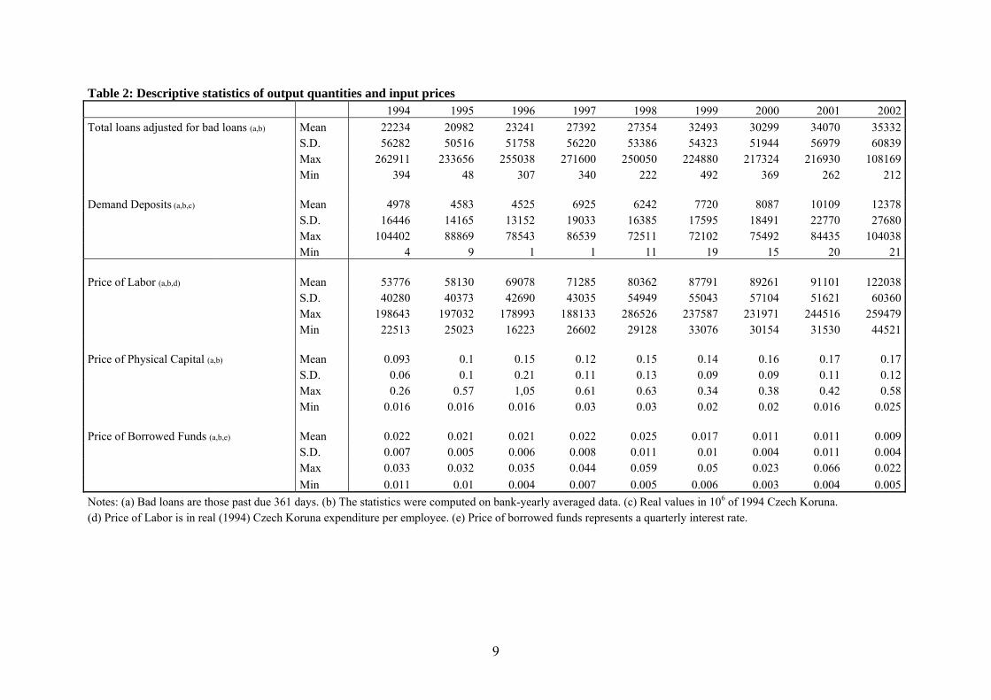
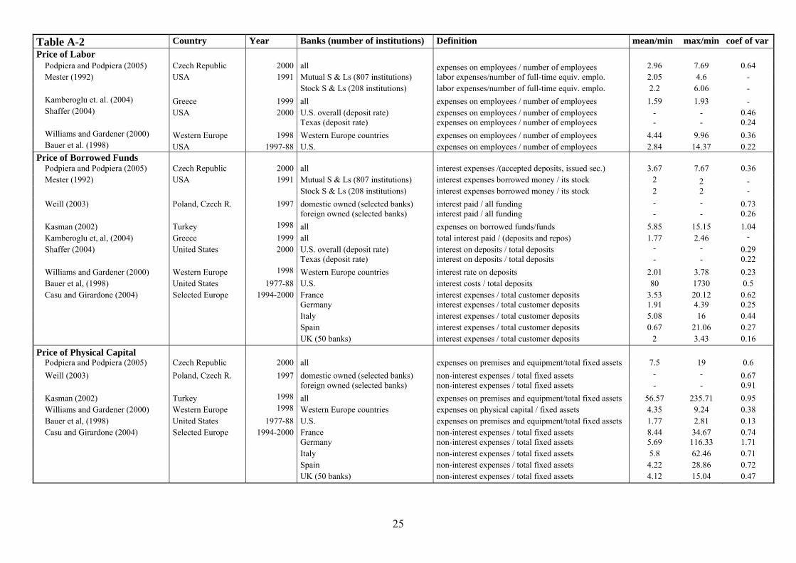
As the input prices were considered price of labor, price of physical capital and price of borrowed funds. The Price of labor represents the unit price of labor and is constructed as the quarterly average of total expenses for employees divided by the end-of-quarter number of employees. Further, the Price of physical capital represents the unit price of physical capital and is constructed as the quarterly average of expenses for rents, leasing, amortization and materials divided by the book value of fixed assets. And finally, the Price of borrowed funds is the quarterly average of expenses incurred for interest paid for borrowed funds from government, central bank, other banks, clients and for issued securities, divided by the amount of these funds. Table 2 provides the descriptive statistics of the variables used in this study. Table A-2 in the Appendix compares our data to similar data sets in selected studies in terms of the ratios max/min, mean/min and the coefficient of variation. As we can see, our data are closely comparable with those used in similar studies of banking efficiency (see for instance Mester, 1992; Bauer et al., 1998; Weill, 2003b; Kasman, 2002; Kamberoglu et al., 2004; Shaffer, 2004; Williams and Gardener, 2000; Casu and Girardone 2004). The highest similarity to the Czech data can be found in the Western European countries, such as France or the U.K.

9

Table 2: Descriptive statistics of output quantities and input prices 1994 1995 1996 1997 1998 1999 2000 2001 2002 Total loans adjusted for bad loans (a,b) Mean 22234 20982 23241 27392 27354 32493 30299 34070 35332 S.D. 56282 50516 51758 56220 53386 54323 51944 56979 60839 Max 262911 233656 255038 271600 250050 224880 217324 216930 108169 Min 394 48 307 340 222 492 369 262 212 Demand Deposits (a,b,c) Mean 4978 4583 4525 6925 6242 7720 8087 10109 12378 S.D. 16446 14165 13152 19033 16385 17595 18491 22770 27680 Max 104402 88869 78543 86539 72511 72102 75492 84435 104038 Min 4 9 1 1 11 19 15 20 21 Price of Labor (a,b,d) Mean 53776 58130 69078 71285 80362 87791 89261 91101 122038 S.D. 40280 40373 42690 43035 54949 55043 57104 51621 60360 Max 198643 197032 178993 188133 286526 237587 231971 244516 259479 Min 22513 25023 16223 26602 29128 33076 30154 31530 44521 Price of Physical Capital (a,b) Mean 0.093 0.1 0.15 0.12 0.15 0.14 0.16 0.17 0.17 S.D. 0.06 0.1 0.21 0.11 0.13 0.09 0.09 0.11 0.12 Max 0.26 0.57 1,05 0.61 0.63 0.34 0.38 0.42 0.58 Min 0.016 0.016 0.016 0.03 0.03 0.02 0.02 0.016 0.025 Price of Borrowed Funds (a,b,e) Mean 0.022 0.021 0.021 0.022 0.025 0.017 0.011 0.011 0.009 S.D. 0.007 0.005 0.006 0.008 0.011 0.01 0.004 0.011 0.004 Max 0.033 0.032 0.035 0.044 0.059 0.05 0.023 0.066 0.022 Min 0.011 0.01 0.004 0.007 0.005 0.006 0.003 0.004 0.005 Notes: (a) Bad loans are those past due 361 days. (b) The statistics were computed on bank-yearly averaged data. (c) Real values in 106 of 1994 Czech Koruna. (d) Price of Labor is in real (1994) Czech Koruna expenditure per employee. (e) Price of borrowed funds represents a quarterly interest rate.

10

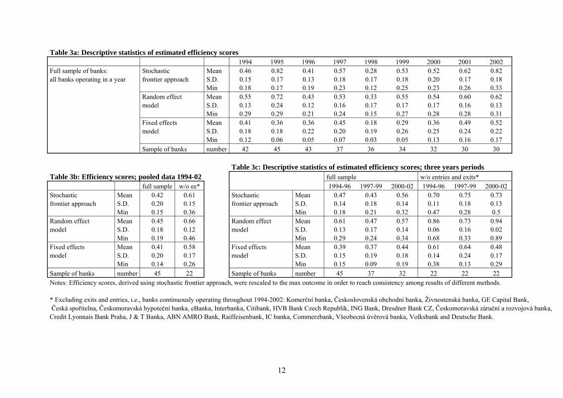
4. Results 4.1 Statistics on efficiency scores The cost efficiency frontier was estimated on nine yearly panels of four quarters for nine consecutive years 1994-2002. The descriptive statistics of the main results of the three parametric methods for each year are presented in Table 3a. The development of the mean cost efficiency, which is the percentage of resources of the average bank sufficient to produce the same output if it were on the efficiency frontier, exhibits a decline in 1995-1998 and an increase in 1999-2002. Taking for instance the SFA results, the score of 0.46 in 1994 indicates that the average bank was in that year wasting 54% of its resources relative to the best-practice bank, in 2002 however, it was already only 18%. Our findings of the stronger mean efficiency performance in the period following 1999 seem intuitive as many least efficient banks had already exited the market by that time and the restructuring and privatization had an efficiency enhancing effect (see Weill, 2003a for the evidence on impact of foreign ownership on efficiency in Czech and Polish banks during 1998-2002). Table 3b summarizes the results of estimating the cost efficiency on pooled data12 for different sample of banks – full sample and sample excluding entries and exists. The mean efficiency for the full sample appears to be 20 percentage points lower that for the alternative sample. This finding shows that the mean efficiency is crucially dependent on the choice of the sample of banks which complicates the comparison of efficiency development across studies that use different sample of banks. Even more crucially, estimating the efficiency scores on three sub-periods for the full sample and sample excluding entries and exists, the derived mean efficiencies for different samples differ even in their trend (see Table 3c). Whereas the results for the full sample show a decline in 1997-1999 and upswing in 2000-2002, the results for the alternative sample (two out of three techniques13) suggest an increase in 1997-1999 and a decline in 2000-2002. Given our findings, we stress the need to analyze the entire banking sector in order to derive more conclusive results regarding mean efficiency development of the whole banking sector. Referring to our findings, an exact comparison between mean efficiency results of different studies working with different samples of bank is not advisable. Despite the limited comparability of mean efficiency between studies, we found rough support in the existing literature for our results. Weill (2003a) analyzed a mixed sample of large Czech and Polish banks in 1997 using SFA and found a median efficiency of 0.73; this compares to our median in that year for the entire Czech banking sector of 0.61. Employing DEA for 17 transition countries over 1995-1998, Grigorian and Manole (2002) find the mean efficiency scores for the sample of large Czech banks between 0.55 and 0.8 with the lowest value during 1996-1997. Stavárek (2003) analyzed large set of Czech banks during 1999-2002 using DEA and derived mean efficiency between 0.7 and 0.85. 12 Assuming constant ranking of banks during the investigated period to analyze the difference in mean efficiency between different samples of banks. 13 The third technique, i.e., REM is less reliable method in small homogenous samples as the inefficiency is derived from the variation across banks, which is limited in small homogenous samples.

11

In the light of the cost efficiency findings for banking sectors internationally, the levels of mean efficiency in 2002 (0.52-0.82) suggest a convergence of the Czech banking sector in average efficiency level to those found for both the U.S. and the European banking sectors. According to the survey of Berger and Humphrey (1997), the efficiency scores from 50 U.S. bank efficiency studies displayed a mean of 0.72 for non-parametric techniques and a mean of 0.84 for parametric techniques. Bukh et al. (1995), in a DEA study of bank efficiency for Norway, Sweden, Finland and Denmark, find mean efficiency scores between 0.54 and 0.85. Fecher and Pestieau (1995) obtained mean efficiency scores in the range 0.71 and 0.98 when applying DFA for 11 OECD countries.

12

Table 3a: Descriptive statistics of estimated efficiency scores 1994 1995 1996 1997 1998 1999 2000 2001 2002 Full sample of banks: Stochastic Mean 0.46 0.82 0.41 0.57 0.28 0.53 0.52 0.62 0.82 all banks operating in a year frontier approach S.D. 0.15 0.17 0.13 0.18 0.17 0.18 0.20 0.17 0.18 Min 0.18 0.17 0.19 0.23 0.12 0.25 0.23 0.26 0.33 Random effect Mean 0.55 0.72 0.43 0.53 0.33 0.55 0.54 0.60 0.62 model S.D. 0.13 0.24 0.12 0.16 0.17 0.17 0.17 0.16 0.13 Min 0.29 0.29 0.21 0.24 0.15 0.27 0.28 0.28 0.31 Fixed effects Mean 0.41 0.36 0.36 0.45 0.18 0.29 0.36 0.49 0.52 model S.D. 0.18 0.18 0.22 0.20 0.19 0.26 0.25 0.24 0.22 Min 0.12 0.06 0.05 0.07 0.03 0.05 0.13 0.16 0.17 Sample of banks number 42 45 43 37 36 34 32 30 30 Table 3c: Descriptive statistics of estimated efficiency scores; three years periods Table 3b: Efficiency scores; pooled data 1994-02 full sample w/o entries and exits* full sample w/o ee* 1994-96 1997-99 2000-02 1994-96 1997-99 2000-02 Stochastic Mean 0.42 0.61 Stochastic Mean 0.47 0.43 0.56 0.70 0.75 0.73 frontier approach S.D. 0.20 0.15 frontier approach S.D. 0.14 0.18 0.14 0.11 0.18 0.13 Min 0.15 0.36 Min 0.18 0.21 0.32 0.47 0.28 0.5 Random effect Mean 0.45 0.66 Random effect Mean 0.61 0.47 0.57 0.86 0.73 0.94 model S.D. 0.18 0.12 model S.D. 0.13 0.17 0.14 0.06 0.16 0.02 Min 0.19 0.46 Min 0.29 0.24 0.34 0.68 0.33 0.89 Fixed effects Mean 0.41 0.58 Fixed effects Mean 0.39 0.37 0.44 0.61 0.64 0.48 model S.D. 0.20 0.17 model S.D. 0.15 0.19 0.18 0.14 0.24 0.17 Min 0.14 0.26 Min 0.15 0.09 0.19 0.38 0.13 0.29 Sample of banks number 45 22 Sample of banks number 45 37 32 22 22 22 Notes: Efficiency scores, derived using stochastic frontier approach, were rescaled to the max outcome in order to reach consistency among results of different methods. * Excluding exits and entries, i.e., banks continuously operating throughout 1994-2002: Komerční banka, Československá obchodní banka, Živnostenská banka, GE Capital Bank, Česká spořitelna, Českomoravská hypoteční banka, eBanka, Interbanka, Citibank, HVB Bank Czech Republik, ING Bank, Dresdner Bank CZ, Českomoravská záruční a rozvojová banka, Credit Lyonnais Bank Praha, J & T Banka, ABN AMRO Bank, Raiffeisenbank, IC banka, Commerzbank, Všeobecná úvěrová banka, Volksbank and Deutsche Bank.

13

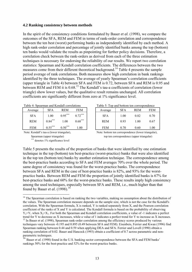
4.2 Ranking consistency between methods In the spirit of the consistency conditions formulated by Bauer et al. (1998), we compare the outcomes of the SFA, REM and FEM in terms of rank-order correlation and correspondence between the ten best (worst) performing banks as independently identified by each method. A high rank-order correlation and percentage of jointly identified banks among the top (bottom) ten banks would validate the results as pinpointing for further policy decisions. Therefore, a correlation check between the rank-orders as derived from each of the three estimation techniques is necessary for endorsing the reliability of our results. We report two correlation statistics: Spearman and Kendall correlation coefficients. The differences between the two measures come from their different theoretical background.14 Table 4 presents the sample period average of rank correlations. Both measures show high correlation in bank rankings identified by the three techniques. The average of yearly Spearman’s correlation coefficients (upper triangle in Table 4) between SFA and FEM is 0.72, between SFA and REM is 0.95 and between REM and FEM it is 0.68.15 The Kendall’s tau-a coefficients of correlation (lower triangle) show lower values, but the qualitative result remains unchanged. All correlation coefficients are significantly different from zero at 1% significance level. Table 4: Spearman and Kendall correlations Table 5: Top and bottom ten correspondence

Average SFA REM FEM Average SFA REM FEM

SFA 1.00 0.95*** 0.72*** SFA 1.00 0.82 0.70

REM 0.84*** 1.00 0.68*** REM 0.93 1.00 0.67

FEM 0.55*** 0.50*** 1.00 FEM 0.70 0.60 1.00 Note: Kendall’s tau-a (lower triangular), Note: bottom ten correspondence (lower triangular), Spearman (upper triangular) top ten correspondence (upper triangular) *** denotes 1% significance level Table 5 presents the results of the proportion of banks that were identified by one estimation technique in the top (bottom) ten best-practice (worst-practice) banks that were also identified in the top ten (bottom ten) banks by another estimation technique. The correspondence among the best-practice banks according to SFA and FEM averages 70% over the whole period. The same degree of consistency was found for the worst-practice banks. The correspondence between SFA and REM in the case of best-practice banks is 82%, and 93% for the worst-practice banks. Between REM and FEM the proportion of jointly identified banks is 67% for best-practice banks and 60% for the worst-practice banks. These results imply high consistency among the used techniques, especially between SFA and REM, i.e., much higher than that found by Bauer et al. (1998).16 14 The Spearman correlation is based on ranking the two variables, making no assumption about the distribution of the values. The Spearman correlation measure depends on the sample size, which is not the case for the Kendall's correlation. With the Spearman formula, X is ranked, Y is ranked separately from X, and the Pearson correlation coefficient of the ranks of X and Y is calculated. The Kendall formula is based on the probability of observing Y2>Y1 when X2>X1. For both the Spearman and Kendall correlation coefficients, a value of -1 indicates a perfect trend for Y to decrease as X increases, while a value of 1 indicates a perfect trend for Y to increase as X increases. 15 In Bauer et al. (1998), Spearman rank-order correlation among the efficiency scores produced by various techniques vary between -0.195 and 0.895 (0.49 between SFA and FEM). Eisenbeis, Ferrier and Kwan (1996) find Spearman ranking between 0.44 and 0.59 when applying DEA and SFA. Ferrier and Lovell (1990) obtain a ranking correlation of 0.02. Bauer and Hancock (1993) obtain a coefficient of 0.7 across parametric and non-parametric techniques. 16 Bauer et al. (1998) found in the U.S. banking sector correspondence between the SFA and FEM banks’ rankings 50% for the best-practice and 52% for the worst-practice banks.

14

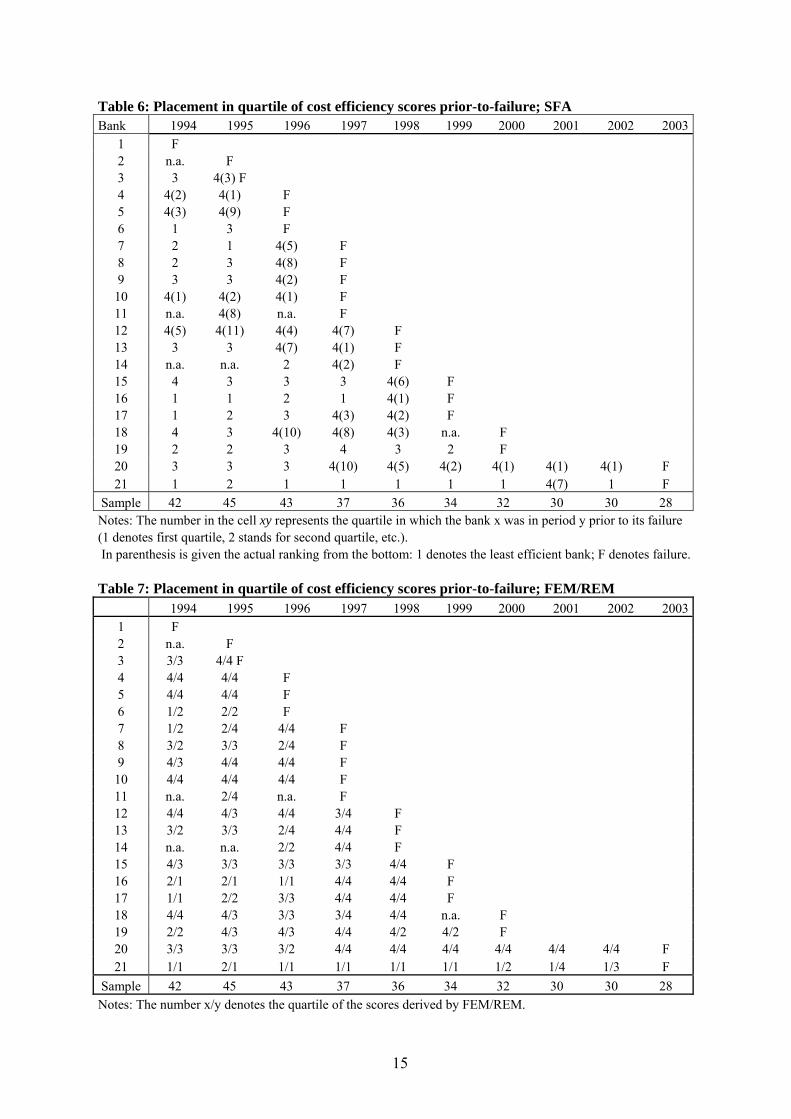
4.3 Rank-order and Cox proportional hazards model The analysis of the relationship between relative efficiency scores and the likelihood of bank failure uses two approaches: a simple assessment of the rank-order placement of failing banks prior to their failure and estimation of the Cox proportional hazards model. The former approach is based on year-by-year systematic recording the position of failed banks in the quartile of banks’ rank-order. We ordered the failed banks according to their survival length and labeled them accordingly (i.e., Bank 1 has the shortest survival length; Bank 21 has the longest survival length). For each year prior to the year of their failure we recorded their placement in the quartiles of rank-ordered banks. The results are presented in Table 6 for SFA and in Table 7 for FEM and REM. At the bottom of the tables is given number of banks in the sample. As appears in the Table 6, the failing banks five years prior to failure were found around the second quartile. Within three to four years prior to failure, the banks tended to descend towards the third quartile. Two years prior to failure, 56% of banks were in the bottom cost efficiency quartile and 23% of them were in the third quartile. One year prior to failure, 83% of banks were in the fourth quartile and 6% in the third quartile. Besides the tendency of failing banks to locate in the bottom quartile prior to their failure, banks tend to descend even to the lowest places within the bottom quartile. This can be seen from the numbers in the parenthesis in Table 6, which show the placement of banks within the fourth quartile (1 denotes the least efficient bank, 2 stands for the second least efficient bank, etc.). The placements of banks according to their efficiency scores into quartiles of FEM and REM (see Table 7) closely resemble to the SFA placement. With the exception of one or two banks, the results are practically identical across all three methods.

15

Table 6: Placement in quartile of cost efficiency scores prior-to-failure; SFA Bank 1994 1995 1996 1997 1998 1999 2000 2001 2002 2003

1 F 2 n.a. F 3 3 4(3) F 4 4(2) 4(1) F 5 4(3) 4(9) F 6 1 3 F 7 2 1 4(5) F 8 2 3 4(8) F 9 3 3 4(2) F 10 4(1) 4(2) 4(1) F 11 n.a. 4(8) n.a. F 12 4(5) 4(11) 4(4) 4(7) F 13 3 3 4(7) 4(1) F 14 n.a. n.a. 2 4(2) F 15 4 3 3 3 4(6) F 16 1 1 2 1 4(1) F 17 1 2 3 4(3) 4(2) F 18 4 3 4(10) 4(8) 4(3) n.a. F 19 2 2 3 4 3 2 F 20 3 3 3 4(10) 4(5) 4(2) 4(1) 4(1) 4(1) F 21 1 2 1 1 1 1 1 4(7) 1 F

Sample 42 45 43 37 36 34 32 30 30 28 Notes: The number in the cell xy represents the quartile in which the bank x was in period y prior to its failure (1 denotes first quartile, 2 stands for second quartile, etc.). In parenthesis is given the actual ranking from the bottom: 1 denotes the least efficient bank; F denotes failure. Table 7: Placement in quartile of cost efficiency scores prior-to-failure; FEM/REM 1994 1995 1996 1997 1998 1999 2000 2001 2002 2003

1 F 2 n.a. F 3 3/3 4/4 F 4 4/4 4/4 F 5 4/4 4/4 F 6 1/2 2/2 F 7 1/2 2/4 4/4 F 8 3/2 3/3 2/4 F 9 4/3 4/4 4/4 F 10 4/4 4/4 4/4 F 11 n.a. 2/4 n.a. F 12 4/4 4/3 4/4 3/4 F 13 3/2 3/3 2/4 4/4 F 14 n.a. n.a. 2/2 4/4 F 15 4/3 3/3 3/3 3/3 4/4 F 16 2/1 2/1 1/1 4/4 4/4 F 17 1/1 2/2 3/3 4/4 4/4 F 18 4/4 4/3 3/3 3/4 4/4 n.a. F 19 2/2 4/3 4/3 4/4 4/2 4/2 F 20 3/3 3/3 3/2 4/4 4/4 4/4 4/4 4/4 4/4 F 21 1/1 2/1 1/1 1/1 1/1 1/1 1/2 1/4 1/3 F

Sample 42 45 43 37 36 34 32 30 30 28 Notes: The number x/y denotes the quartile of the scores derived by FEM/REM.

16

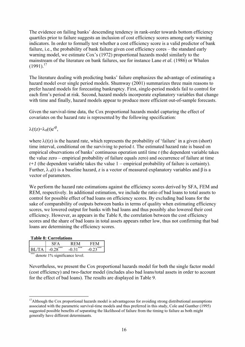
The evidence on failing banks’ descending tendency in rank-order towards bottom efficiency quartiles prior to failure suggests an inclusion of cost efficiency scores among early warning indicators. In order to formally test whether a cost efficiency score is a valid predictor of bank failure, i.e., the probability of bank failure given cost efficiency cores – the standard early warning model, we estimate Cox’s (1972) proportional hazards model similarly to the mainstream of the literature on bank failures, see for instance Lane et al. (1986) or Whalen (1991).17 The literature dealing with predicting banks’ failure emphasizes the advantage of estimating a hazard model over single period models. Shumway (2001) summarizes three main reasons to prefer hazard models for forecasting bankruptcy. First, single-period models fail to control for each firm’s period at risk. Second, hazard models incorporate explanatory variables that change with time and finally, hazard models appear to produce more efficient out-of-sample forecasts. Given the survival-time data, the Cox proportional hazards model capturing the effect of covariates on the hazard rate is represented by the following specification: λ(t|z)=λ0(t)ezβ, where λ(t|z) is the hazard rate, which represents the probability of ‘failure’ in a given (short) time interval, conditional on the surviving to period t. The estimated hazard rate is based on empirical observations of banks’ continuous operation until time t (the dependent variable takes the value zero – empirical probability of failure equals zero) and occurrence of failure at time t+1 (the dependent variable takes the value 1 – empirical probability of failure is certainty). Further, λ 0(t) is a baseline hazard, z is a vector of measured explanatory variables and β is a vector of parameters. We perform the hazard rate estimations against the efficiency scores derived by SFA, FEM and REM, respectively. In additional estimation, we include the ratio of bad loans to total assets to control for possible effect of bad loans on efficiency scores. By excluding bad loans for the sake of comparability of outputs between banks in terms of quality when estimating efficiency scores, we lowered output for banks with bad loans and thus possibly also lowered their cost efficiency. However, as appears in the Table 8, the correlation between the cost efficiency scores and the share of bad loans in total assets appears rather low, thus not confirming that bad loans are determining the efficiency scores. Table 8: Correlations SFA REM FEM BL/TA -0.28*** -0.31*** -0.23*** *** denote 1% significance level.

Nevertheless, we present the Cox proportional hazards model for both the single factor model (cost efficiency) and two-factor model (includes also bad loans/total assets in order to account for the effect of bad loans). The results are displayed in Table 9. 17Although the Cox proportional hazards model is advantageous for avoiding strong distributional assumptions associated with the parametric survival-time models and thus preferred in this study, Cole and Gunther (1995) suggested possible benefits of separating the likelihood of failure from the timing to failure as both might generally have different determinants.

17

Table 9: Cox proportional hazards model (reported are coefficients) BL/TA EFF Log-likelihood ps-R2 HR=f(SFA,BL/TA) 0.044(0.008)*** -3.34(1.51)** -69.02 0.20 HR=f(REM, BL/TA) 0.041(0.009)*** -5.43(2.04)*** -67.75 0.22 HR=f(FEM, BL/TA) 0.05(0.008)*** -3.46(1.78)** -69.35 0.20 HR=f(SFA) - -4.96(1.42)*** -78.79 0.10 HR=f(REM) - -7.71(1.88)*** -75.91 0.14 HR=f(FEM) - -3.97(1.58)** -82.27 0.06 Note: HR stands for hazard rate; BL/TA represents the ratio of bad loans over total assets; EFF stands for efficiency scores; standard errors are in parentheses; number of observations: 326; failures: 19; stars denote significance level *10%, **5%, and *** 1%.

Our results confirm that after controlling for the effect of bad loans (the coefficient on the ratio is positive and significant in all regressions, that is, the higher the ratio, the higher the risk of bank failure), the efficiency score significantly explains the risk of failure regardless the method used for efficiency evaluation, i.e., SFA, FEM or REM. The coefficients on the variable EFF (efficiency scores) are negative and significant (see the upper half of the Table 9), implying that a decrease in efficiency increases the risk of bank failure. This conclusion is confirmed from the hazard model estimation with the single factor (see the lower half of the Table 9) – negative and significant relation between efficiency and risk of bank failure. All in all, the relative efficiency scores derived by all three estimation methods proved to be valid predictors of risk of bank failure and placed the majority of failing banks among least efficient quartile one year prior their failure. Our results thus underline the findings concerning the relationship between cost efficiency and bank failure of Berger and Humphrey (1992), Barr and Siems (1994) and Wheelock and Wilson (1995), who conclude that failing banks tend to locate far from the efficiency frontier. In our case, the vast majority of failed banks were in the fourth quartile one year prior to failure. 4.4 Power functions and early warning model selection Although it has been shown that the rank-order based on SFA, REM and FEM, respectively exhibit strong correlation and very close correspondence in terms of top ten and bottom ten banks, it might be beneficial to discriminate among the methods in terms of their performance for an early warning model. A convenient criterion for selection of the best performing early warning model is based on evaluation of power functions (see Gilbert et al., 2000). Usually, the construction of the power function is done through the successive computation of type I (false negative) and type II errors18 (false positive) for different cut-off predicted probabilities of failure. Since we focus on the predictive performance of the cost efficiency scores, we employ this framework on the domain of efficiency scores instead of through the hazard model mapped probabilities of failure.19 In order to compute the power function, we set ten cut-off efficiency scores, i.e., 0, 18 The type I error stands for the probability of omitting to select a failed bank among potentially failing ones, whereas the type II error represents the probability of labeling a bank as likely failing that does not actually fail. 19 This is due to the fact that predicted probabilities from the estimated hazard model (given one factor model) are only mapping the efficiency domain into domain of probability of failure. Thus, using directly the efficiency scores simplifies the application of efficiency evaluation for power function computation. If the early warning model would consist of more indicators than efficiency scores, it would be necessary to perform the hazard model estimation and apply the power function to the results of the hazard model.

18

0.1, …, 1, and for each of them evaluate both the type I and type II errors. Thus for instance, if the cut-off point is efficiency score of 1 (all banks that have efficiency below 1 are labeled as failures, i.e., in this case all banks), the type I error is the zero percent (of missed next year banks failures), and type II error is hundred percent (of misidentified next year non-failures). The plot of the both types of errors represents a trade-off between excessive screening of banks that do not fail on one side and missing to identify failed banks on the other side. The errors constructed from the data over nine years (i.e., by number of next year failures weighted average of type I and type II errors) can be seen in the Figure 1.

0 0. 1 0. 2 0. 3 0. 4 0. 5 0. 6 0. 7 0. 8 0. 9 10

0. 1

0. 2

0. 3

0. 4

0. 5

0. 6

0. 7

0. 8

0. 9

1

Ty

pe

II

err

or

(pe

rce

nta

ge

of

mis

ide

nti

fie

d n

on

-fa

ilu

res

)

Ty pe I er ror (perc ent age of m is s ed f a i lures )

← [label as fail banks whose eff(SFA) <0.4]

SF A (area below c urv e = 0. 29)

R EM (area below c urv e = 0. 27)F EM (area below c urv e = 0. 36)

Figure 1: Plot of power functions The smallest area under the curves pertains to the most effective model of early warning, since such a model minimizes the error type II for all values of error type I. In other words, for any given share of missed next year bank failures, it minimizes cost of screening of healthy banks. The smallest area corresponds to the REM (0.27), closely followed by SFA (0.29). The FEM (0.36) seems to be outperformed by the pervious two estimation methods. Further, as pointed on the plot, the cut-off efficiency score of 0.4 for SFA is likely optimal since the higher cut-off score would add to error type II without lowering error type I and similarly a lower cut-off score would lower type II error by 10% but double type I error to 40%. Taking the 0.4 cut-off means that two out of every ten next year failed banks will remain unidentified and roughly 3 banks out of every ten non-failed banks will be screened.

19

5. Concluding remarks This paper studies the signaling effect of cost ineffective management for the risk of bank failure. Finding reliable early warning indicators of problematic management in banks becomes increasingly important issue given the low signaling performance of the commonly applied financial ratios. We show, using data for the complete set of commercial banks (including exits and entry) in the Czech banking sector during the period of its substantial transformation, that the risk of bank failure is closely correlated with cost inefficient management. Estimates of relative cost efficiency scores, using three alternative parametric methods proved to be significant predictors of the risk of bank failure. Besides, we observed that the banks that failed tends to gradually descend in the relative ranking of efficiency to the bottom quartiles and one year prior to failure, all failed banks were placed at least by one method in the least efficient quartile. Our findings thus validate the signaling effect of deteriorating efficiency for risk of bank failure. The constructed power functions for each estimation technique showed that the stochastic frontier approach and random effects model are preferred for early warning systems to fixed effects model. In addition we noted, by comparing the mean efficiency derived from the full sample of banks and that from a sample of banks excluding entries and exits, a substantial dependence of mean efficiency on the sample selection. It follows that the results of mean efficiency derived on different samples in different periods are rather difficult to compare.

20

References Bauer, P. and D. Hancock (1993). The Efficiency of the Federal Reserve in Providing Check Processing Services. Journal of Banking and Finance, 17, 287-311. Bauer P., Berger A., Ferrier G. and D. Humphrey (1998). Consistency Conditions for Regulatory Analysis of Financial Institutions: A Comparison of Frontier Efficiency Methods. Journal of Economics and Business, 50, 85-114. Barr, R. and T. Siems (1994). Predicting bank failure using DEA to quantify management Quality. Federal Reserve Bank of Dallas, Financial Industry Studies Working Paper No. 1-94. Berger, A. (1993). Distribution-free estimates of efficiency in the U.S. banking industry and test of the standard distributional assumptions. Journal of Productivity Analysis 4, 261-292. Berger, A. and R. DeYoung (1997). Problems loans and cost efficiency in commercial banks. Journal of Banking and Finance 21, 849-870. Berger, A. and D. Humphrey (1992). Measurement and Efficiency Issues in Commercial Banking. in Z.Griliches, ed. Measurement issues in the Service Sectors. National Bureau of Economic Research, University of Chicago Press, 245-79. Berger, A. and D. Humphrey (1997). Efficiency of financial institutions: International survey and directions for further research. European Journal of Operational Research, 98, 175-212. Bikker, J.A. (2005). Competition and Efficiency in a Unified European Banking Market. E.E. Publishing Inc. The U.K. Bukh, P., S. Berg and F. Forsund (1995). Banking Efficiency in the Nordic Countries: A Four-Countries Malmquist Index Analysis. WP University of Aahus, Denmark Casu, B., C. Girardone (2004). An Analysis of the Relevance of OBS Items in Explaining Productivity Change in European Banking. EFMA 2004 Basel Meetings Paper, http://ssrn.com/abstract=492863. Cates, D.C. (1985). Bank Risk and Predicting Bank Failure. Issues in Bank Regulation 9,16-20. CNB (1996). Banking Supervision in the Czech Republic. Czech National Bank, Prague. CNB (2001). Banking Supervision in the Czech Republic. Czech National Bank, Prague. CNB (2002). Banking Supervision in the Czech Republic. Czech National Bank, Prague. Cole R.A., J.W. Gunther (1995). Separating the Likelihood and Timing of Failure. Journal of Banking and Finance, vol. 19, 1073-1089. Cox, D. R. (1972). Regression Models And Life Tables. Journal of Roy. Statistics Society, 34 p. 187-220. Derviz A. and J. Podpiera (2004). Predicting Bank CAMELS and S&P Ratings: The Case of the Czech Republic. Czech National Bank WP No. 1.

21

Dinger, V. and J. von Hagen (2003). Bank Structure and Profitability in Central and Eastern European Countries. Paper prepared for IAES conference, Lisboa. Eisenbeis R., G. Ferrier and S. Kwan (1996). An Empirical Analysis of the Informativeness of Programming and SFA Efficiency Scores: Efficiency and Bank Performance. WP University of North Carolina, Chapel Hill Fecher, F. and P. Pestieau (1993). Efficiency and Competition in O.E.C.D. Financial Services. in H.O. Fried, C.A.K.Lovell, ans S.S. Schmidt, eds., The Measurement of Productive Efficiency: Techniques and Applications. Oxford University Press, U.K., 374-85. Ferrier, G. and C.A.K. Lovell (1990). Measuring Cost Efficiency in Banking: Econometric and Linear Programming Evidence. Journal of Econometrics, 46, 229-45. Fried, H., Lovell C.A.K. and S.Schmidt (1993). The Measurement of Productive Efficiency. Techniques and Applications. Oxford University Press, New York. Fries S., D. Neven and P. Seabright (2002). Bank Performance in Transition Economies. EBRD Working Paper 76, November. Gilbert, R.A., A.P. Meyer, M.D. Vaughan (2000). The Role of a CAMEL Downgrade Model in Bank Surveillance. WP21, Federal Reserve Bank of St. Louis. Greene, W. H. (1993). The Econometric Approach to Efficiency Analysis. in H.O.Fried, C.A.K.Lovell and S.S.Schmidt, eds., The Measurement of Productive Efficiency: Techniques and Applications. New York: Oxford University Press. Grigorian D.A. and V. Manole (2002). Determinants of Commercial Bank Performance in Transition: An Analysis of Data Envelope Analysis. IMF Working Papers, 2/146. Guarda P. and A. Rouabah (2005). Measuring Banking Output and Productivity: A User Cost Approach to Luxembourg Data. Banque Centrale du Luxemburg, Memo. Hanousek J. and G. Roland (2001). Banking Passivity and Regulatory Failure in Emerging Markets: Theory and Evidence from the Czech Republic. CERGE-EI Working Paper 192. International Monetary Fund (2005): Internal Documents for the Article IV Mission in the Czech Republic. Kamberoglou, N. C., E. Liapis, G. T. Simigiannis, P. Tzamourani (2004). Cost Efficiency in Greek Banking. Bank of Greece WP. Kasman, A. (2002). Cost Efficiency, Scale Economies, and Technological Progress in Turkish Banking. Central Bank Review, 1, 1-20. Kumbhakar, S. and Lovell, C.A. Knox (2000). Stochastic Frontier Analysis. Cambridge University Press. Mester, L. (1992). Efficiency in the savings and loan industry. Journal of Banking and Finance 17, 267-286.

22

Lane W.R., S.W. Looney, and J.W. Wansley (1986). An Application of the Cox Proportional Hazards Model to Bank Failure. Journal of Banking and Finance 10, 511-531. Looney, S.W., J.W. Wansley and W.R. Lane (1989). An Examination of Misclassifications with Bank Failure Prediction Models. Journal of Economics and Business 41, 327-336. Mester, L. (1996). A Study of bank efficiency taking into account risk preferences. Journal of Banking and Finance, 20, 1025-1045. Sahajwala R., P. van den Bergh, (2000). Supervisory risk assessment and early warning systems, BIS Working papers 4, Bank for International Settlements Seballos, L.D., J.B. Thomson (1990). Underlying Causes of Commercial Bank Failures in the 1980s. Economic Commentary, Federal Reserve Bank of Clevelend. Shaffer, S. (2004). External versus Internal Economies in Banking. Journal of Banking and Finance, forthcoming. Stavárek, D. (2003). Banking Efficiency in Visehrad Countries Before Joining the European Union. Paper prepared for the Workshop on Efficiency of Financial Institutions and European Integration, October 2003, Technical University Lisbon, Portugal. Shumway, T. (2001). Forecasting Bankruptcy More Accurately: A Simple Hazard Model. Journal of Business, 74(1), 101-24. Weill, L. (2003a). Banking efficiency in transition economies: The Role of foreign ownership. The Economics of Transition, 11(3), 569-592. Weill, L. (2003b). Is There a Lasting Gap in Bank Efficiency between Eastern and Western European Countries? mimeo. Weill, L.(2004). Measuring cost efficiency on European banking: A comparison of frontier techniques. Journal of Productivity Analysis, 21(2), 133-152. Whalen G. (1991). A Proportional Hazards Model of Bank Failure: An examination of its usefulness as an early warning tool. Federal Reserve Bank of Cleveland Economic Review, First Quarter, 21-31. Wheelock, D. and P. Wilson (1995a). Evaluating the Efficiency of Commercial Banks: Does Our View of What Banks Do Matter? Review of Federal Reserve Bank of St. Louis, July/August 1995. Wheelock, D. and P. Wilson (1995b). Explaining bank failures: Deposit insurance, regulation and efficiency. Review of Economics and Statistics, 77, 689-700. Williams J., E.P.M. Gardener (2003). The Efficiency of European Regional Banking. Regional Studies 37(4): 321-30.

23

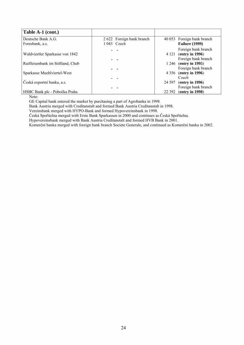
Appendix

Table A-1 1994 2002 Assets Assets Bank (order of CNB's register) (CZK mln) Ownership (CZK mln) Ownership / Status Komerční Banka, a.s. 316 815 Czech 473 703 Foreign Československá Obchodní Banka, a.s. 145 534 Czech 540 077 Foreign Živnostenská Banka, a.s. 25 627 Czech 51 801 Foreign Agrobanka, a.s. 61 399 Czech Failure (1997) GE Capital Bank, a.s. - - 53 084 Foreign (entry 1998) Česká Spořitelna, a.s. 344 837 Czech 467 299 Foreign Banka Bohemia, a.s. 13 408 Czech Failure (1994) Banka Baska, a.s. 5 442 Czech Failure (1997) Pragobanka, a.s. 14 545 Czech Failure (1998) Kreditní a průmyslová banka, a.s. 2 436 Czech Failure (1995) Ekoagrobanka, a.s. 15 482 Czech Failure (1997) SOCIETÉ GENERALE 7 393 Foreign Merger (2002) Kreditní Banka Plzeň, a.s. 14 654 Czech Failure (1996) Českomoravská hypoteční banka, a.s. 5 153 Czech 16 861 Czech Banka Haná, a.s. 13 312 Czech Failure (2000) AB BANKA, a.s. 13 903 Czech Failure (1995) eBanka, a.s. 5 558 Czech 14 793 Foreign Interbanka, a.s. 2 708 Foreign 9 598 Foreign Citibank, a.s. 12 444 Foreign 76 771 Foreign Creditanstalt, a.s. 8 921 Foreign Merger (1998) Bank Austria, a.s. 4 477 Foreign Merger (1998) Evrobanka, a.s. 6 115 Czech Failure (1997) HVB Bank Czech Republic, a.s. - - 124 806 Foreign (merger 2001) UNION Banka, a.s. 5 735 Czech 24 449 Czech (failure in 2003) ING Bank N.V. 6 507 Foreign bank branch 44 614 Foreign bank branch Realitbanka, a.s. 1 140 Czech Failure (1997) COOP Banka, a.s. 5 830 Czech Failure (1998) Vereinsbank CZ, a.s. 9 298 Foreign Merger (1998) HYPO-BANK CZ, a.s. 3 617 Foreign Merger (1998) Dresdner Bank CZ, a.s. 5 716 Foreign 18 812 Foreign Česká Banka Praha, a.s. 8 413 Czech Failure (1995) Českomoravská záruční a rozvojová banka, a.s. 5 562 Czech 70 645 Czech Erste Bank Sparkassen (ČR), a.s. 4 367 Foreign Merger (2000) Moravia Banka, a.s. 8 126 Czech Failure (1999) Plzeňská Banka, a.s. 1 007 Czech 1 263 Czech (failure in 2003) Credit Lyonnais Bank Praha, a.s. 7 127 Foreign 15 884 Foreign IP Banka, a.s. 147 940 Czech Failure (2000) První Slezská Banka, a.s. 1 135 Czech Failure (1996) ABN AMRO Bank N.V 1 427 Foreign bank branch 37 840 Foreign bank branch Raiffeisenbank, a.s. 2 720 Foreign 53 960 Foreign Vekomoravská Banka, a.s. 3 002 Czech Failure (1998) J & T Banka, a.s. 2 735 Foreign 4 537 Foreign První Městská Banka, a.s. 719 Czech 7 972 Czech IC banka, a.s. 545 Foreign 1 282 Foreign Commerzbank AG, a.s. 12 742 Foreign bank branch 85 326 Foreign bank branch Universal Banka, a.s. 2 780 Czech Failure (1999) Všeobecná Úvěrová Banka, a.s. 1 324 Foreign bank branch 2 428 Foreign bank branch Volksbank, a.s. 492 Foreign 14 462 Foreign

24

Table A-1 (cont.)

Deutsche Bank A.G. 2 622 Foreign bank branch 40 053 Foreign bank branch Foresbank, a.s. 1 043 Czech Failure (1999)

Waldviertler Sparkasse von 1842 - -

4 121 Foreign bank branch (entry in 1996)

Raiffeisenbank im Stiftland, Cheb

- - 1 246

Foreign bank branch (entry in 1995)

Sparkasse Muehlviertel-West

- - 4 356

Foreign bank branch (entry in 1996)

Česká exportní banka, a.s.

- - 24 597

Czech (entry in 1996)

HSBC Bank plc - Pobočka Praha

- - 22 392

Foreign bank branch (entry in 1998)

Note: GE Capital bank entered the market by purchasing a part of Agrobanka in 1998. Bank Austria merged with Creditanstalt and formed Bank Austria Creditanstalt in 1998. Vereinsbank merged with HYPO-Bank and formed Hypovereinsbank in 1998. Česká Spořitelna merged with Erste Bank Sparkassen in 2000 and continues as Česká Spořitelna. Hypovereinsbank merged with Bank Austria Creditanstalt and formed HVB Bank in 2001. Komerční banka merged with foreign bank branch Societe Generale, and continued as Komerční banka in 2002.

25

Table A-2 Country Year Banks (number of institutions) Definition mean/min max/min coef of var Price of Labor

Podpiera and Podpiera (2005) Czech Republic 2000 all expenses on employees / number of employees 2.96 7.69 0.64 Mester (1992) USA 1991 Mutual S & Ls (807 institutions) labor expenses/number of full-time equiv. emplo. 2.05 4.6 - Stock S & Ls (208 institutions) labor expenses/number of full-time equiv. emplo. 2.2 6.06 - Kamberoglu et. al. (2004) Greece 1999 all expenses on employees / number of employees 1.59 1.93 - Shaffer (2004) USA 2000 U.S. overall (deposit rate) expenses on employees / number of employees - - 0.46 Texas (deposit rate) expenses on employees / number of employees - - 0.24 Williams and Gardener (2000) Western Europe 1998 Western Europe countries expenses on employees / number of employees 4.44 9.96 0.36 Bauer et al. (1998) USA 1997-88 U.S. expenses on employees / number of employees 2.84 14.37 0.22

Price of Borrowed Funds Podpiera and Podpiera (2005) Czech Republic 2000 all interest expenses /(accepted deposits, issued sec.) 3.67 7.67 0.36 Mester (1992) USA 1991 Mutual S & Ls (807 institutions) interest expenses borrowed money / its stock 2 2 - Stock S & Ls (208 institutions) interest expenses borrowed money / its stock 2 2 - Weill (2003) Poland, Czech R. 1997 domestic owned (selected banks) interest paid / all funding - - 0.73 foreign owned (selected banks) interest paid / all funding - - 0.26 Kasman (2002) Turkey 1998 all expenses on borrowed funds/funds 5.85 15.15 1.04 Kamberoglu et, al, (2004) Greece 1999 all total interest paid / (deposits and repos) 1.77 2.46 - Shaffer (2004) United States 2000 U.S. overall (deposit rate) interest on deposits / total deposits - - 0.29 Texas (deposit rate) interest on deposits / total deposits - - 0.22 Williams and Gardener (2000) Western Europe 1998 Western Europe countries interest rate on deposits 2.01 3.78 0.23 Bauer et al, (1998) United States 1977-88 U.S. interest costs / total deposits 80 1730 0.5 Casu and Girardone (2004) Selected Europe 1994-2000 France interest expenses / total customer deposits 3.53 20.12 0.62 Germany interest expenses / total customer deposits 1.91 4.39 0.25

Italy interest expenses / total customer deposits 5.08 16 0.44 Spain interest expenses / total customer deposits 0.67 21.06 0.27 UK (50 banks) interest expenses / total customer deposits 2 3.43 0.16

Price of Physical Capital Podpiera and Podpiera (2005) Czech Republic 2000 all expenses on premises and equipment/total fixed assets 7.5 19 0.6 Weill (2003) Poland, Czech R. 1997 domestic owned (selected banks) non-interest expenses / total fixed assets - - 0.67

foreign owned (selected banks) non-interest expenses / total fixed assets - - 0.91 Kasman (2002) Turkey 1998 all expenses on premises and equipment/total fixed assets 56.57 235.71 0.95 Williams and Gardener (2000) Western Europe 1998 Western Europe countries expenses on physical capital / fixed assets 4.35 9.24 0.38 Bauer et al, (1998) United States 1977-88 U.S. expenses on premises and equipment/total fixed assets 1.77 2.81 0.13 Casu and Girardone (2004) Selected Europe 1994-2000 France non-interest expenses / total fixed assets 8.44 34.67 0.74

Germany non-interest expenses / total fixed assets 5.69 116.33 1.71 Italy non-interest expenses / total fixed assets 5.8 62.46 0.71 Spain non-interest expenses / total fixed assets 4.22 28.86 0.72 UK (50 banks) non-interest expenses / total fixed assets 4.12 15.04 0.47