Embed Size (px)
Citation preview
Journal of Industrial Engineering and ManagementJIEM, 2014 – 7(1): 42-71 – Online ISSN: 2014-0953 – Print ISSN: 2014-8423
http://dx.doi.org/10.3926/jiem.543
Determining supply chain safety stock level and location
Bahareh Amirjabbari, Nadia Bhuiyan
Concordia University (Canada)
[email protected], [email protected]
Received: September 2012Accepted: December 2013
Abstract:
Purpose: The lean methodology and its principles have widely been applied in supply chain
management in recent decades. Manufacturers are one of the most important contributors in a
supply chain and inventory plays a paramount role for them to become lean. Therefore, there
should be appropriate management of inventory and all of its drivers in accordance with a lean
strategy. Safety stock is one of the main drivers of inventory; it protects against increasing the
stretch in the breaking points of the supply chain, which in turn can result in possible reduction
of inventory. In this paper an optimization model and a simulation model are developed and
applied in a real case to optimize the safety stock level with the objective of logistics cost
minimization.
Design/methodology/approach: In order to optimize the safety stock level while minimizing logistics
costs, a nonlinear cost minimization safety stock model is developed in this paper and then it is
applied in a real world manufacturing case company. A safety stock simulation model based on
appropriate metrics in the case company’s supply chain performance is also provided.
Findings: These models result in not only the optimum levels but also locations of safety stock
within the supply chain.
Originality/value: In this research, two models of cost minimization and simulation have been
developed and also applied in a real case company to result in not only optimized levels but also
optimized locations of safety stock across the whole supply chain. In addition, the appropriate
-42-
Journal of Industrial Engineering and Management – http://dx.doi.org/10.3926/jiem.543
supply chain performance measurement metrics have been introduced in this paper and the
simulation model is developed based on those.
Keywords: safety stock, supply chain, lean, cost, optimization
1. Introduction
Applying the lean philosophy in a supply chain has received increasing attention from
researchers in the last few decades. Contributors of a supply chain, no matter to which
industry they belong, aim to follow the lean philosophy to make their business processes more
and more efficient in order to survive on the market. Lean thinking is essentially about
increasing efficiency, eliminating waste, and bringing new ideas by using empirical methods.
Taylor (1999), Adamides, Karacapilidis, Pylarinou and Koumanakos (2008), Kainuma and
Tawara (2006), Lamming (1996), Crino, McCarthy and Carier (2007), Wu and Wee (2009) did
research on applying lean to the supply chain. There are also invaluable researches on the
comparison of the lean paradigm with other methodologies in supply chain management such
as Naylor, Naim and Berry (1999), Qi, Xuejun and Zhiyong (2007), and Mason-Jones, Nalor
and Towill (2000).
Supply chain integration results in flow control which is essential in an operating system and
such flow control is associated with inventory control (Slack, Chambers, Harland, Harrison &
Johnston, 1995; Gunasekaran, Patel & Tirtiroglu, 2001; De Toni & Tonchia, 2011). In addition,
inventory is ones of the seven wastes introduced in lean philosophy that has to be tackled.
Inventory plays a paramount role in manufacturers efforts to become lean. Therefore, one of
the most important strategies to become lean for manufacturers is having efficient inventory
within their chain. Chun Wu (2003), Cagliano, Caniato and Spina (2004), Wu (2009), McCullen
and Towill (2001) studied on the application of lean in the manufacturing area.
Having an efficient level of inventory is a step towards increasing the inventory turnover in
companies. According to the definition of turnover, decreasing the level of inventory helps to
increase the turns. On the other hand, reducing inventory will lead to uncertainties and
consequently stockouts (Natarjan & Goyal, 1994). Therefore, safety stock is needed to protect
against these kinds of uncertainties. Indeed, proper management of safety stock, as one of the
most important drivers of inventory, has become critical objective towards leanness and having
efficient inventory. Therefore, a manufacturing case company, who attempts to manage its
inventory efficiently across the chain, has been selected in this paper and a safety stock
optimization model has been proposed in order to optimize the levels and locations of safety
stock within its chain.
-43-
Journal of Industrial Engineering and Management – http://dx.doi.org/10.3926/jiem.543
There are different objectives that an optimization safety stock can be built on such as
minimization of cost, maximization of service level, and aggregate considerations (Silver, Pyke
& Peterson, 1998). Optimal determination approaches based on cost and service level
objectives are more appropriate for practical applications (Inderfurth, 1991). Nowadays, firms
are taking important steps towards an agreement on reducing total cost and inventories and
increasing information sharing in order to improve the financial and operational performance of
each channel of the supply chain (Maloni & Benton, 1997). Logistics costs are more targeted in
this regard as reducing costs of equipment, materials, and labor is difficult at best in today’s
competitive market (Long, Liu, Meng & Chen, 2009). Therefore, minimization of logistics costs
is also selected as the basis of the determination of optimum safety stock in this paper.
Logistics costs are mainly related to procurement and supply, manufacturing process, and after
sales service. Thus, holding and shortage costs are selected as representations of logistics
costs in the optimization model.
Towards the goal of managing the supply chain properly, performance measurement and
metrics play an important role in setting objectives, evaluating performance, and determining
future actions (Gunasekaran, Patel & McGaughey, 2004). Therefore, besides developing an
optimization model, a safety stock simulation model is also provided in this paper to find the
most appropriate levels and locations of safety stock for the case company under study by
introducing its proper metrics for measuring supply chain performance.
A supply chain has different nodes such as different tiers of suppliers, producer, assembly,
distributors, and end customer. Product availability is a critical measure for the performance of
logistics and the supply chain (Coyle, Bardi & Langley, 2009). One of the areas that has to be
measured for the evaluation of suppliers in the context of the supply chain is the “flow”
(Gunasekaran et al., 2004). Indeed, flow or in another word, product availability is a critical
measure for the performance of logistics and the supply chain. There are different issues that
cause disruptions and unavailability of products in the supply chain, as for example variability,
whether in demand or lead time; quality issues; or internal and external issues such as low
delivery performances, improper scheduling, inadequate product capacity, poor maintenance,
among others. Therefore, safety stock is essential to compensate for the weakness of the
supply chain for part availability and this factor has been considered in the selected safety
stock optimization model of this study.
The challenge that we face in this paper is applying lean philosophy to the safety stock
management within the supply chain for the purpose of reducing logistics costs. Therefore, for
achieving the goal of having efficient safety stock across the supply chain and consequently
reducing logistics costs, a safety stock cost minimization model and a simulation model are
developed in this paper and then applied to a case company which is a manufacturer.
-44-
Journal of Industrial Engineering and Management – http://dx.doi.org/10.3926/jiem.543
In this paper, we apply a safety stock cost minimization model and also a simulation safety stock
model in a case company which is a manufacturer. In the next section, we provide a review of
the literature. In Section 3, we describe the case company. In Section 4, we introduce the
optimization model, followed by the model formulation in Section 5. Results of the optimization
model are then presented in the next section. In Section 7, the simulation model with
performance measurement metrics are provided. We then provide a discussion of the results and
their implications, and then conclude with some suggestions for avenues of future research.
2. Literature Review
There are many different methods and approaches in determining safety stock under different
situations according to the literature. Aleotti Maia and Qassim (1998) proposed an optimization
safety stock model with the objective of total inventory cost minimization. They also provided
an analytical solution for finding the preferable case by comparing the inventory holding cost
and opportunity cost. The conclusion was that holding inventory in the intermediate levels
which only reduce the frequency of stockout is not economical.
A linear programming formulation with the control variables of safety stock was presented by
Jung, Blau, Pekny, Reklaitis and Eversdyk (2008). This model aims to minimize the total supply
chain’s inventory and also meet the target of the service level. The interdependence between
the service level at upstream and downstream stages of the supply chain, the nonlinear
performance functions, and also the safety capacity constraint have been incorporated into this
model. Linearization of the nonlinear functions has also been provided. Constant production
capacity, zero lead time at the warehouse, and normally distributed demand are some of the
assumptions applied in this model. In addition, raw material and transportation means have
been assumed to be always available.
Li and Li (2009) presented a dynamic model of the safety stock in a Vendor Managed Inventory
(VMI) system. Only the variability sourced by demand is considered in this model as the
variability related to the suppliers disappear in the VMI system.
Zhao, Lai and Lee (2001) evaluated alternative methods in the determination of the safety
stock level in multilevel MRP systems by using a simulation approach. In addition, the results
of the evaluation of the relation between the safety stock multiplier and different system
performance measures such as service level, schedule instability, and total cost in different
methods has been provided.
Desmet, Aghezzaf and Vanmaele (2010) presented an approximation model for safety stock in
a two-echelon distribution system which incorporates the variance of the central warehouse
and the retailers in the replenishment lead time. In addition, the variance of the service time
-45-
Journal of Industrial Engineering and Management – http://dx.doi.org/10.3926/jiem.543
of the orders at the warehouse which has substantial effect on the system’s lead time variance
has been considered in this model.
Safety stock level and location determination in the supply chain with a stochastic environment
is a challenging task; therefore, there are many different assumptions in the models and
approaches provided in this area to make it simpler. For example, some of these approaches
exclude the suppliers’ variability, some of them have limitations in their applications, some of
them put limitation on the demand distribution, among others. A general safety stock
optimization model with the objective of logistics cost minimization by considering both
internal and external variabilities is presented in this paper. This model is also considering the
factor of part availability which is really critical in the chain.
Measurement of the supply chain performance is really critical for the success of any business
as it deals with strategic, tactical, and operational planning and control. Supply chain
performance determines the winner and measuring it facilitates the improvement of the overall
chain’s performance (Chen & Paulraj, 2004). Based on the Deloitte report, although 91 percent
of North American manufacturers recognized the supply chain management role as a critical
one for the organizational success, only 2 percent of them are in the world class range for their
supply chains (Thomas, 1999). Measuring the supply chain performance is challenging in
essence of integrating quantitative and qualitative measurements and also making linkage
between strategy and performance measurement (Shepherd & Gunter, 2006).
Gunasekaran et al. (2004) developed a framework for supply chain performance measurement
and metrics. They claimed the reason that many companies have not succeeded in maximizing
their supply chain’s potential is because of failing in developing the performance measures and
metrics for enhancing the efficiency of their supply chain. They categorized the performance
metrics into metrics for order planning, evaluation of supply link, metrics at production level,
evaluation of delivery link, measuring customer service, and logistics cost.
Xia, Ma and Lim (2007) proposed an analytic hierarchy process (AHP) based methodology for
supply chain performance measurement and highlighted some of the important metrics in this
regard. They introduced four supply chain strategies that companies applied in case of
competing in the market which are lean supply chain, agile supply chain, leagile supply chain,
and adaptive supply chain. Then, they introduced the commonly used supply chain attributes
that are reliability, responsiveness, flexibility, re-configurability, and cost. After that, they
weighted these different attributes in each different supply chain strategies. They also used a
fuzzy logic in case of measuring the qualitative measures and integrate them with the
quantitative ones.
There are different metrics for measuring and assessing supply chain performance. Integrating
them is a challenging task. In this study, the most appropriate metrics for this purpose have
-46-
Journal of Industrial Engineering and Management – http://dx.doi.org/10.3926/jiem.543
been introduced and a simulation safety stock model has been developed on their basis which
supports the results of the optimization model.
3. Case Study
Nowadays, companies are becoming more and more interested in being lean to maintain
competitiveness in the market. There are different areas within a company that could be
improved towards making the company and its whole chain lean and leveraging from its
benefits. One of the most important among these areas is the “inventory” of the company,
which must be efficient according to lean principles. There are a number of different inventory
drivers and safety stock is one of them. Indeed, the case company tries to manage the
inventory across its supply chain efficiently, and towards this goal, efficient levels and locations
of safety stock have become more and more highlighted as a prerequisite condition. Therefore,
doing research on efficient management of safety stock, its model, and also applying it to the
case company are the purposes of this paper. Cost minimization has been selected as the
objective of the safety stock efficient model according to the desire of the case company’s
logistics management.
The company under study, which we will hereinafter refer to as ABC for the purpose of
confidentiality, is a manufacturer and leader in the aerospace industry. The company is
characterized by high demand variability and long lead time, among others. ABC is a
multi-stage manufacturer. Tiers of suppliers, procurement, manufacturing, final assembly, and
customers (internal and external) are different nodes of the ABC’s supply chain. The
downstream nodes are the upstream nodes’ customers, and the replenishment lead time of
customer nodes is the order waiting time provided by their upstream nodes. In addition, ABC
has a generally structured multi-stage system and there is no restriction with respect to the
number of predecessors and successors of any node. Such multi-stage systems focus
considerable attention on setting and positioning safety stock.
ABC has two different manufacturing plants (MFs). The procurement department of the
company is responsible for procuring the raw materials or semi- finished parts through
suppliers to manufacturing plants or even supplying parts from one manufacturing plant to
another (inter plants transfers). Indeed, the word “supplier” in the model could be the
representative of the external supplier or internal manufacturing entity. It should be noted that
procurement’s location can be different from manufacturing ones. Finished parts from
manufacturing entities have two internal customers that pull their outputs; they are Assembly
(ASSY) and Aftermarket (AFM). These two latter entities are the last stages of the internal
chain of the company just before the end customer. There are also some external supplied
finished parts required for Assembly and Aftermarket that the procurement department is
again in charge of supplying them. The Assembly entity has different finished product families
-47-
Journal of Industrial Engineering and Management – http://dx.doi.org/10.3926/jiem.543
with their own specifications. Therefore, if availability of parts (right parts at right time) can be
assured for the internal customers, on-time delivery performance to the end customer will be
assured as well. This availability should be guaranteed through safety stock, but the optimum
safety stock level and location should also minimize logistics costs.
In order to apply the safety stock model to a real world case, preparing the most appropriate
input data is critical to obtain the desired results. Data was collected through many different
databases, company documentation and reports, company’s SAP system, project meetings,
and with the help of operational and strategic support personnel at ABC. Each set of
information and data was collected from the appropriate logistics departmental personnel in
the company. For example, logistics top managers provided the objective of the model and
high-level process. The databases and metrics used will be discussed in more detail in the next
sections.
This study provides considerable managerial experience, insights, and knowledge about how
business firms deal with challenges in applying lean philosophy to safety stock management in
supply chain towards minimizing logistics costs.
4. Optimization Model Description
The optimization model is presented through different possible value streams of each finished
product family of the company and developed using lingo optimization software to result in the
optimum level of safety stock with its optimum location in the stream. In order to limit the
number of stages and for simplification, only the last two stages of those value streams that
have more than two nodes before the internal customer stage are selected. Therefore, all the
previous stages and their connections are being excluded and their performances are being
captured only through the input of the latest second stage. The other reason for this limitation
is the difficulty in defining the shortage costs in upstream stages of the chain due to lack of
visibility and control. Furthermore, the objective of the model is cost minimization, and the
upstream stages’ contributions towards cost are significantly less than the downstream stages,
thus this simplifying assumption should have a negligible effect on overall results. Although,
there is a sample (Value Stream 4) presented in section 6 that goes beyond this limitation just
to show the applicability of the model for the whole chain from end to end point.
Shortage cost, overage cost, and delivery performances are the inputs of the model. Different
combinations of raw material (semi-finished part) and finished part are considered as indices in
the model based on the selected value streams.
-48-
Journal of Industrial Engineering and Management – http://dx.doi.org/10.3926/jiem.543
5. Optimization Model Formulation
For all value streams, the notations of the model are as follows:
a. Sets and Indices
i Raw material/ semi-finished part
p Finished part
u Customer (ASSY, AFM)
b. Variables
Ki Delivery performance of procurement to manufacturing
Kp Delivery performance of manufacturing or procurement to customers
c. Parameters
Pi Supplier delivery performance to procurement
(If supplier is a manufacturing plant, P i would be manufacturing performance for semi-
finished part)
Pp Manufacturing performance for finished part
(Ratio between on time manufactured and planned manufacture of finished part)
• It should be noted that index of “p” is used for only those finished parts that are
manufactured in ABC. Indeed, for those finished parts that are supplied through
suppliers, index of “i” is used.
CS Cost of shortage
CO Cost of overage
xi Raw material/semi-finished part safety stock
xp Finished part safety stock
qi Raw material/semi-finished part quantity ordered
qp Finished part quantity ordered
q* On-time delivered quantity of raw material/ semi-finished part or finished part
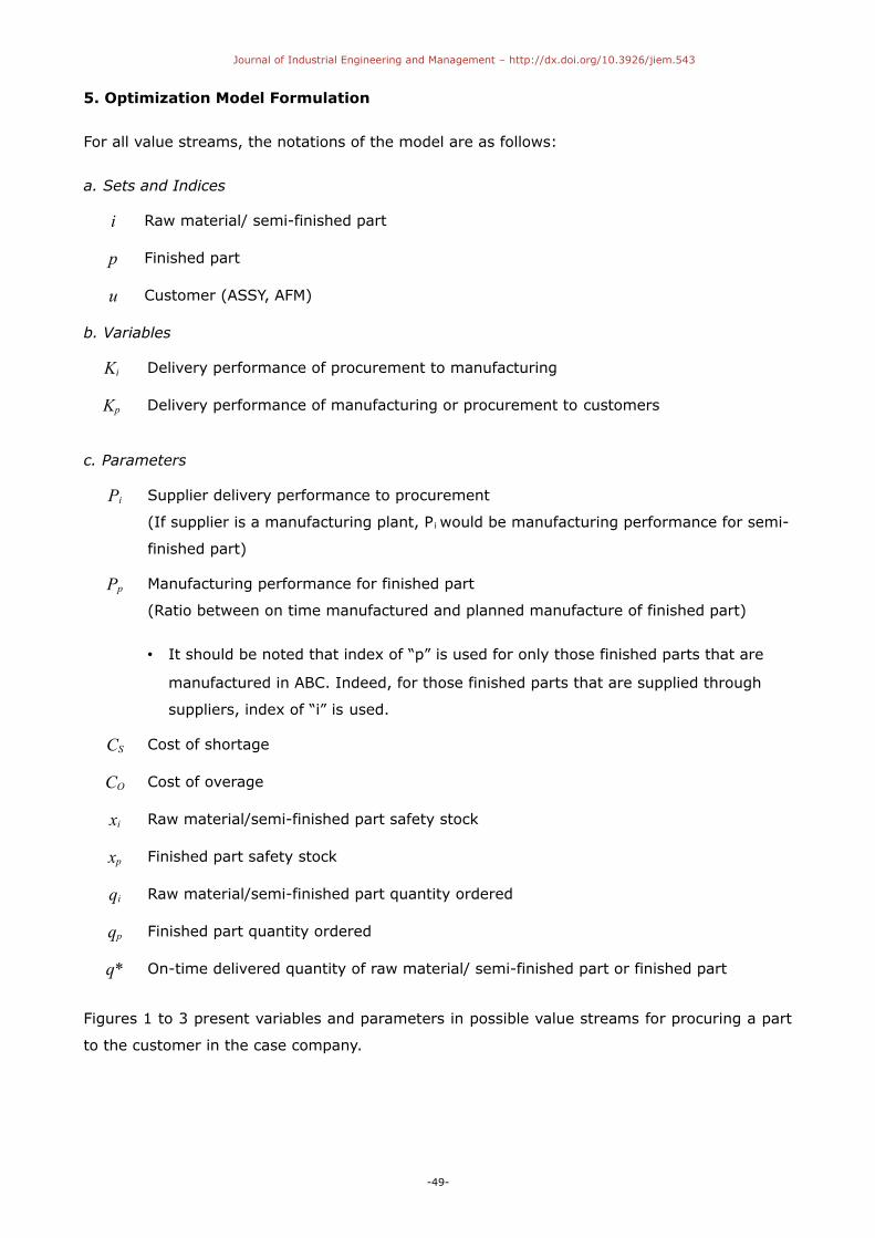
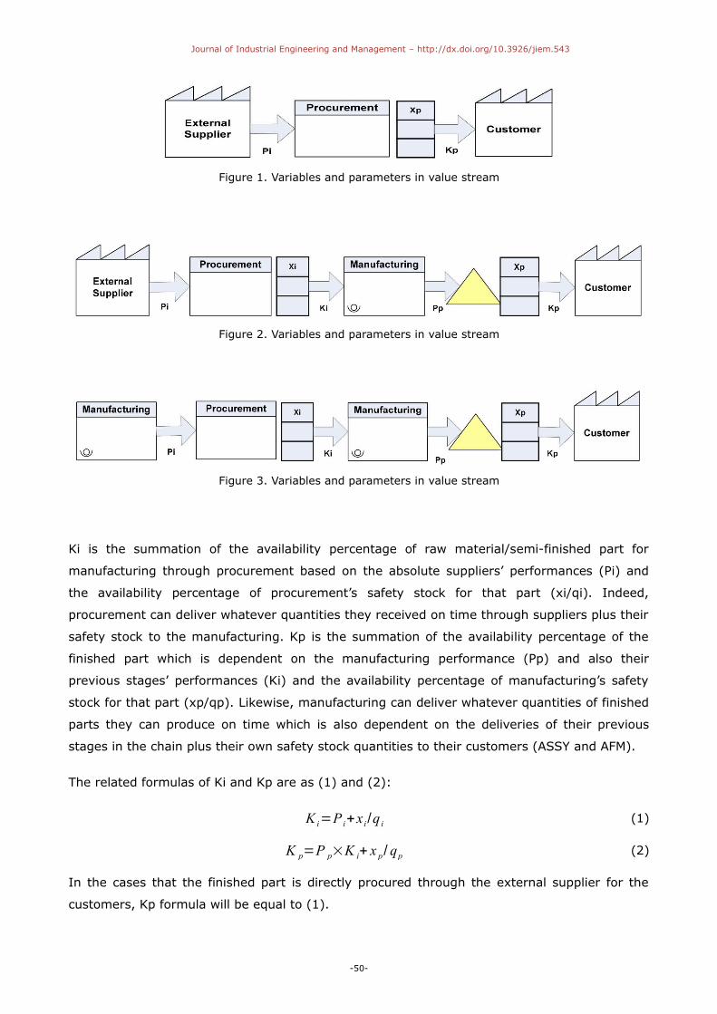
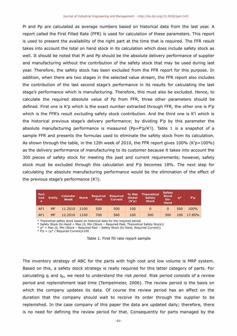
Figures 1 to 3 present variables and parameters in possible value streams for procuring a part
to the customer in the case company.
-49-
Journal of Industrial Engineering and Management – http://dx.doi.org/10.3926/jiem.543
Figure 1. Variables and parameters in value stream
Figure 2. Variables and parameters in value stream
Figure 3. Variables and parameters in value stream
Ki is the summation of the availability percentage of raw material/semi-finished part for
manufacturing through procurement based on the absolute suppliers’ performances (Pi) and
the availability percentage of procurement’s safety stock for that part (xi/qi). Indeed,
procurement can deliver whatever quantities they received on time through suppliers plus their
safety stock to the manufacturing. Kp is the summation of the availability percentage of the
finished part which is dependent on the manufacturing performance (Pp) and also their
previous stages’ performances (Ki) and the availability percentage of manufacturing’s safety
stock for that part (xp/qp). Likewise, manufacturing can deliver whatever quantities of finished
parts they can produce on time which is also dependent on the deliveries of their previous
stages in the chain plus their own safety stock quantities to their customers (ASSY and AFM).
The related formulas of Ki and Kp are as (1) and (2):
K i=P i+x i /q i (1)
K p=P p×K i+ x p/ qp (2)
In the cases that the finished part is directly procured through the external supplier for the
customers, Kp formula will be equal to (1).
-50-
Journal of Industrial Engineering and Management – http://dx.doi.org/10.3926/jiem.543
Pi and Pp are calculated as average numbers based on historical data from the last year. A
report called the First Filled Rate (FFR) is used for calculation of these parameters. This report
is used to present the availability of the right part at the time that is required. The FFR result
takes into account the total on hand stock in its calculation which does include safety stock as
well. It should be noted that Pi and Pp should be the absolute delivery performance of supplier
and manufacturing without the contribution of the safety stock that may be used during last
year. Therefore, the safety stock has been excluded from the FFR report for this purpose. In
addition, when there are two stages in the selected value stream, the FFR report also includes
the contribution of the last second stage’s performance in its results for calculating the last
stage’s performance which is manufacturing. Therefore, this must also be excluded. Hence, to
calculate the required absolute value of Pp from FFR, three other parameters should be
defined. First one is K’p which is the exact number extracted through FFR, the other one is P’p
which is the FFR’s result excluding safety stock contribution. And the third one is K’i which is
the historical previous stage’s delivery performance; by dividing P’p by this parameter the
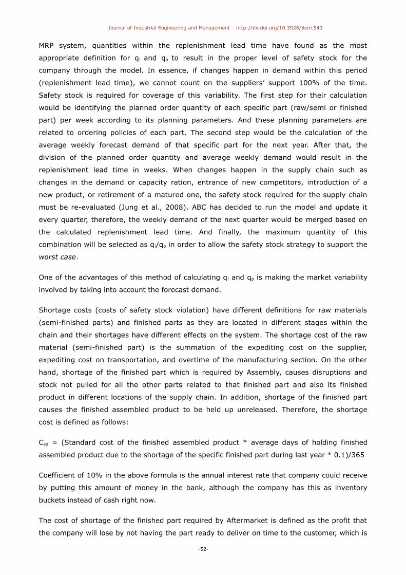
absolute manufacturing performance is measured (Pp=P’p/K’i). Table 1 is a snapshot of a
sample FFR and presents the formulas used to eliminate the safety stock from its calculation.
As shown through the table, in the 12th week of 2010, the FFR report gives 100% (K’p=100%)
as the delivery performance of manufacturing to its customer because it takes into account the
300 pieces of safety stock for meeting the past and current requirements; however, safety
stock must be excluded through this calculation and P’p becomes 18%. The next step for
calculating the absolute manufacturing performance would be the elimination of the effect of
the previous stage’s performance (K’i).
PartCod
eEntity
CalendarWeek Stock
RequiredPast
RequiredCurrent
% MetGlobal(K'p)
TheoreticalSafetyStock
SafetyStockOn-
Hand
q* P'p
AF1 MF 11.2010 2100 500 500 100 0 0 500 100%
AF1 MF 12.2010 1100 700 560 100 300 300 100 17.85%
* Theoretical safety stock based on historical data for the required period.* Safety Stock On-Hand = Max (0, Min (Stock – Required Past, Theoretical Safety Stock))* q* = Max (0, Min (Stock – Required Past – Safety Stock On Hand, Required Current))* P'p = (q* / Required Current)x100
Table 1. First fill rate report sample
The inventory strategy of ABC for the parts with high cost and low volume is MRP system.
Based on this, a safety stock strategy is really required for this latter category of parts. For
calculating qi and qp, we need to understand the risk period. Risk period consists of a review
period and replenishment lead time (Tempelmeier, 2006). The review period is the basis on
which the company updates its data. Of course the review period has an effect on the
duration that the company should wait to receive its order through the supplier to be
replenished. In the case company of this paper the data are updated daily; therefore, there
is no need for defining the review period for that. Consequently for parts managed by the
-51-
Journal of Industrial Engineering and Management – http://dx.doi.org/10.3926/jiem.543
MRP system, quantities within the replenishment lead time have found as the most
appropriate definition for qi and qp to result in the proper level of safety stock for the
company through the model. In essence, if changes happen in demand within this period
(replenishment lead time), we cannot count on the suppliers’ support 100% of the time.
Safety stock is required for coverage of this variability. The first step for their calculation
would be identifying the planned order quantity of each specific part (raw/semi or finished
part) per week according to its planning parameters. And these planning parameters are
related to ordering policies of each part. The second step would be the calculation of the
average weekly forecast demand of that specific part for the next year. After that, the
division of the planned order quantity and average weekly demand would result in the
replenishment lead time in weeks. When changes happen in the supply chain such as
changes in the demand or capacity ration, entrance of new competitors, introduction of a
new product, or retirement of a matured one, the safety stock required for the supply chain
must be re-evaluated (Jung et al., 2008). ABC has decided to run the model and update it
every quarter, therefore, the weekly demand of the next quarter would be merged based on
the calculated replenishment lead time. And finally, the maximum quantity of this
combination will be selected as q i/qp in order to allow the safety stock strategy to support the
worst case.
One of the advantages of this method of calculating q i and qp is making the market variability
involved by taking into account the forecast demand.
Shortage costs (costs of safety stock violation) have different definitions for raw materials
(semi-finished parts) and finished parts as they are located in different stages within the
chain and their shortages have different effects on the system. The shortage cost of the raw
material (semi-finished part) is the summation of the expediting cost on the supplier,
expediting cost on transportation, and overtime of the manufacturing section. On the other
hand, shortage of the finished part which is required by Assembly, causes disruptions and
stock not pulled for all the other parts related to that finished part and also its finished
product in different locations of the supply chain. In addition, shortage of the finished part
causes the finished assembled product to be held up unreleased. Therefore, the shortage
cost is defined as follows:
Csp = (Standard cost of the finished assembled product * average days of holding finished
assembled product due to the shortage of the specific finished part during last year * 0.1)/365
Coefficient of 10% in the above formula is the annual interest rate that company could receive
by putting this amount of money in the bank, although the company has this as inventory
buckets instead of cash right now.
The cost of shortage of the finished part required by Aftermarket is defined as the profit that
the company will lose by not having the part ready to deliver on time to the customer, which is
-52-
Journal of Industrial Engineering and Management – http://dx.doi.org/10.3926/jiem.543
the direct cost. Besides that, there are many intangible effects of this shortage that are called
indirect costs and are difficult to gauge accurately (Graves & Rinnooy Kan, 1993). One of them
is loss of customers’ goodwill that may turn them to other competitors in the future.
The cost of overage is defined as the interest that the company is losing by holding inventory
instead of having it in cash. Hence, it is the multiplication of standard cost of the part and the
annual interest rate (10%).
As can be seen through the formulas and definitions, a period of one year has been selected
for historical data collection. As the factors (such as shortage cost and delivery performances)
that are gathered within this time frame are critical to make an appropriate decision about the
level and location of safety stock, one year has been selected in order to have a sufficient
window view.
Some samples of value streams associated with their models’ formulas are presented below.
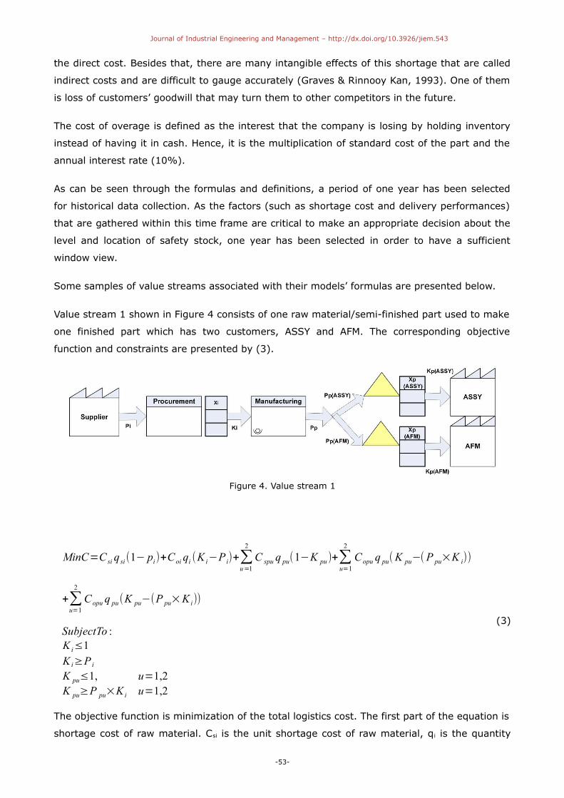
Value stream 1 shown in Figure 4 consists of one raw material/semi-finished part used to make
one finished part which has two customers, ASSY and AFM. The corresponding objective
function and constraints are presented by (3).
Figure 4. Value stream 1
MinC=C si qsi(1− pi)+Coi qi (K i−P i)+∑u=1
2
C spu q pu(1−K pu)+∑u=1
2
Copu q pu(K pu−(P pu×K i))
+∑u=1
2
Copu q pu(K pu−(P pu×K i))
SubjectTo :K i≤1K i≥P iK pu≤1, u=1,2K pu≥P pu×K i u=1,2
(3)
The objective function is minimization of the total logistics cost. The first part of the equation is
shortage cost of raw material. Csi is the unit shortage cost of raw material, qi is the quantity
-53-
Journal of Industrial Engineering and Management – http://dx.doi.org/10.3926/jiem.543
ordered for the raw material, and (1-Pi) is the shortage possibility. The second part of equation
is holding cost of raw material. Co is the unit overage cost of raw material, qi is the quantity
ordered, and (ki-pi) is the overage possibility. Likewise, the other two parts of the function are
related to the shortage cost and holding cost of the finished part for two customers.
The constraints of the model are about the boundaries for the delivery performances. The
upper bounds for both Ki and Kp are 100%. The lower bound for K i is equal to the supplier
delivery performance (Pi). Indeed, the lowest delivery performance of the raw material from
the procurement to the manufacturing is the availability of that part through the supplier
without safety stock. The lower bound for Kp is the multiplication of the previous stages’
performances which are Pp and Ki.
If for this case, there were two different kinds of finished parts but again in demand with both
customers, then there should be a summation on both indices of finished part (p) and
customer (u) in the objective function.
In value stream 2 which is shown in Figure 5, two raw materials/semi-finished parts are used
to make one finished part which has two customers, ASSY and AFM. The corresponding model
is also presented by (4).
Figure 5. Value stream 2
MinC=∑i=1
2
C si q i(1−P i)+∑i=1
2
Coi qi(K i−P i)
+∑u=1
2
C spuq pu(1−K pu)
+∑u=1
2
C opu q pu(K pu−(P pu∏i=1
2
K i))
(4)
-54-
Journal of Industrial Engineering and Management – http://dx.doi.org/10.3926/jiem.543
SubjectTo :K i≤1, i=1,2K i≥P i , i=1,2K pu≤1, u=1,2
K pu≥P pu∏i=1
2
K i , u=1,2
As before, if there were two different finished parts for the same situation, the model would be
changed.
As can be seen through the constraints of the model, the company’s objective is to have 100%
delivery performances. Therefore, the upper boundaries of both stages are assigned to 100%
in order to not to allow the model to impose a shortage to the system. Of course, these upper
bounds could be less than 1 based on the service level goals in different cases.
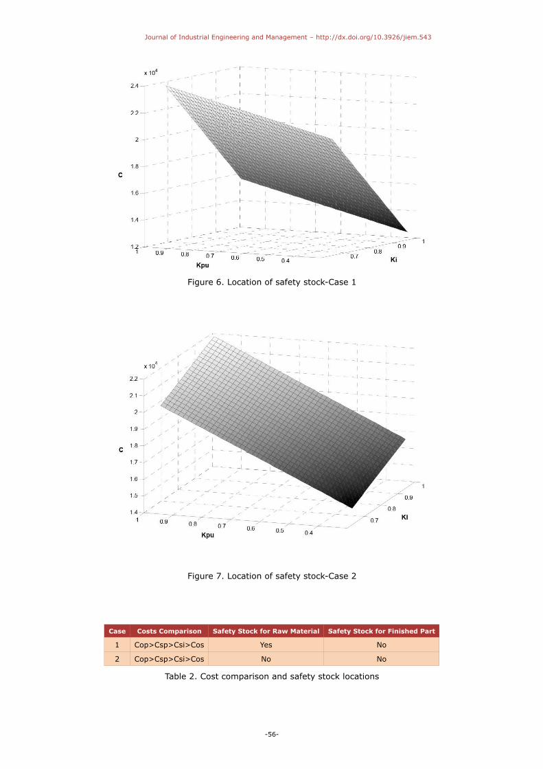
By this definition of the model, costs factors would be the indicators for the location of the
safety stock and its level would be identified based on the boundaries of the delivery
performances. Figures 6 and 7 are two sample feasible regions of the linear model to illustrate
the varying of the safety stock location based on the optimal point. In addition, Table 2
presents the comparison between the costs in each case and also the recommended location of
the model for the safety stock. The assumptions applied in the model in these cases are
linearity, having only one customer for finished part, and equality of q i and qp. The optimization
model will be linear if there is only one raw material/semi-finished part and optimum point with
minimum cost will happen only in one of the four boundaries; therefore, the linearity
assumption is used in this section. In addition, it would be easier to depict the feasible regions
by the assumption of having only one customer. The coefficients of the variables in the
optimization model are costs and order quantities; so, the equality assumption of the order
quantities is used for eliminating their contributions in the comparisons and highlighting the
role of costs in determining the optimal location of safety stock.
-55-
Journal of Industrial Engineering and Management – http://dx.doi.org/10.3926/jiem.543
Figure 6. Location of safety stock-Case 1
Figure 7. Location of safety stock-Case 2
Case Costs Comparison Safety Stock for Raw Material Safety Stock for Finished Part
1 Cop>Csp>Csi>Cos Yes No
2 Cop>Csp>Csi>Cos No No
Table 2. Cost comparison and safety stock locations
-56-
Journal of Industrial Engineering and Management – http://dx.doi.org/10.3926/jiem.543
In order to make the results of the model more effective for the company, one of the most
problematic finished product families of the Assembly was selected, and value streams of its
finished parts that are going to be assembled were reviewed with the model. As each of the
selected final product families could have 100 different value streams in the case company, it
was decided to apply the optimization model only to those value streams that end with finished
parts that were consistently in shortage report during last year in order to limit samples. Value
streams of these pacer parts vary. Some of them could have only the supplier stage before the
assembly and some others could be very long. As discussed before, these long value streams
were limited by taking into account only parts of level 1 and 2 of its finished product’s bill of
materials (BOM).
6. Optimization Model Computational Results
Results of the model applied to some value stream samples of one finished product family in
the company are presented in Table 3. This table includes input factors to the model such as
delivery performances (Pi, Pp), parts quantities (qi, qp), costs (Cs, Co) along with parameters
required to calculate them (K’i, P’p, K’p, standard cost) for each value stream. This table also
presents the old and new safety stock levels and total costs (for those cases that all required
data were available) to compare previous situation with new one. All historical data presented
in this table, as mentioned before in section 5, are based on last year records. Lingo 11.0 was
used to solve the non-linear optimization model. It should be mentioned that due to
confidentiality, masked data are used in this paper.
Table 3. Computational results
-57-
Journal of Industrial Engineering and Management – http://dx.doi.org/10.3926/jiem.543
Value stream 4 of Table 3 shows one of the class A finished parts (ALNS) required for Assembly
for the selected product family. This finished part has three semi-finished parts (level 2 in
finished product’s BOM which are L, N, and S in Table 3). “L” is an in-house part and is
manufactured in ABC. Furthermore, the manufacturing plant requires raw material (T) to
produce this part which is procured through the supplier. Part T is in level 3 in the BOM.
Therefore, this sample goes far beyond the limitation of levels 1 and 2, and shows that the
model is applicable for all stages of the value streams as long as the input data of the model
are provided.
Manufacturing, receives the two other semi-finished parts (N and S) required for producing the
finished part directly through suppliers. Figures 8 and 9 present the respective value stream
and BOM.
Figure 8. Value stream
Figure 9. BOM
This last value stream (value stream 4), can be a representative case to illustrate the error and
especially in this case, the overestimating of safety stock result in the analysis of parts in
isolation and not within the chain. If, ALNS was being considered separately and apart of its
chain, system may allocate some level of safety stock for that due to the K’ p which is 85%. But,
-58-
Journal of Industrial Engineering and Management – http://dx.doi.org/10.3926/jiem.543
when this part is analyzed within its chain, it is understood that the reason for no availability of
the finished part is not due to the last stage performance but it is due to the low delivery
performances of the semi-finished parts. Therefore, keeping safety stock in the last stage only
increases the holding cost of the system.
An analysis of the results shows that the weakness of the supply chain must be compensated
with safety stock, while it is optimized to meet the desired objective of the business. It has
been shown in this paper that in optimizing the safety stock based on a cost minimization
objective, not only its level but also its location in the supply chain is important. In fact, by
keeping safety stock in upstream stages, there will be savings in holding costs. On the other
hand, by keeping safety stock in downstream stages, there will be savings in lead time.
Therefore, these two options must be traded off towards optimizing safety stock location for
minimizing the total logistics costs. Through this procedure, any business can improve its
profitability and also become a superior competitor with its chain.
7. Simulation Model
Besides developing an optimization model, a simulation model is also provided by introducing
and assessing the relevant metrics of the case company’s supply chain for finding the most
appropriate level and also location of safety stock with the objective of total logistics cost
minimization. This safety stock simulation model sustains the results of the optimization
model. The simulation safety stock model consists of some matrices that allow us to assess the
performance of any stages of the supply chain in a matter of safety stock level and location. It
should be noted that all data that are presented in the tables of this section are the masked
data due to confidentiality.
As a first step, metrics used at the company for measuring the performances of its supply
chain were collected to help build the simulation model. The first one is called On-Time
Delivery (OTD) which shows the delivery performance of the supplier (internal or external) to
its customer(s) (internal or external). However, this metric is not the best one for three main
reasons. The first reason is that OTD is not capturing the expeditions of purchase orders. The
second reason is that the OTD does not consider quality problems. The last reason is related to
the incorporation of safety stock in OTD’s calculation for delivery performances that does not
result in the pure delivery performances.
Therefore, another metric called First Fill Rate (FFR) which has been already defined in the
optimization safety stock model will be used in our simulation model. It should be noted that
OTD and FFR are calculated based on the last six months' records. FFR would be the average
of this record, but OTD is calculated as the “weighted average” as it is being reported with the
percentage aligned with deliveries.
-59-
Journal of Industrial Engineering and Management – http://dx.doi.org/10.3926/jiem.543
The third metric is the length of Lateness which represents how many days a specific part is
delivered late to its customer within the supply chain. Length of Lateness is equal to Posting
Date minus Statistical Date.
The fourth metric is the Safety Stock Coverage (in weeks) which is calculated by dividing each
part’s safety stock’s quantity into its weekly requirements (demand).
And finally the last metric is the information extracted from the quality report which reports
the parts that have quality issues and creating the bucket called quality lot. This report
includes quality issue creation date, quality issue completion date, and quantity of parts with
quality issues.
In order to develop the desired simulation safety stock model, safety stock’s distribution within
the supply chain has to be found to determine if it is located properly with the support of the
defined metrics. Hence, as a first step, a matrix has been developed as shown in Table 4. This
table includes different finished products of the company in the row and the contributors of the
supply chain in the column and the value of the safety stock related to each combination of the
product and supply chain contributor. More specifically for the case under study, the pivot table
would be as of Table 5.
Table 4. Safety stock distribution pivot table template
Sum of SS Value Split
Supply Chain Contributors AB AE AF ACD AG
Procurement $107,170 $105,870 $726,680 $290,340 $125,780
Manufacturing $566,120 $348,420 $235,596 $65,072 $91,400
Assembly $42,170 $9,194 $7,800 $17,500 $14,012
Grand Total $715,460 $463,484 $970,076 $372,912 $213,192
Sales Volume ($M) $25 $40 $105 $27 $26
Table 5. Case company's safety stock distribution pivot table
-60-
Journal of Industrial Engineering and Management – http://dx.doi.org/10.3926/jiem.543
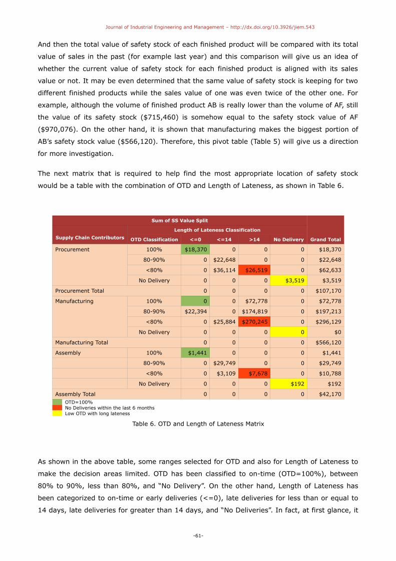
And then the total value of safety stock of each finished product will be compared with its total
value of sales in the past (for example last year) and this comparison will give us an idea of
whether the current value of safety stock for each finished product is aligned with its sales
value or not. It may be even determined that the same value of safety stock is keeping for two
different finished products while the sales value of one was even twice of the other one. For
example, although the volume of finished product AB is really lower than the volume of AF, still
the value of its safety stock ($715,460) is somehow equal to the safety stock value of AF
($970,076). On the other hand, it is shown that manufacturing makes the biggest portion of
AB’s safety stock value ($566,120). Therefore, this pivot table (Table 5) will give us a direction
for more investigation.
The next matrix that is required to help find the most appropriate location of safety stock
would be a table with the combination of OTD and Length of Lateness, as shown in Table 6.
Sum of SS Value Split
Grand TotalSupply Chain Contributors
Length of Lateness Classification
OTD Classification <=0 <=14 >14 No Delivery
Procurement 100% $18,370 0 0 0 $18,370
80-90% 0 $22,648 0 0 $22,648
<80% 0 $36,114 $26,519 0 $62,633
No Delivery 0 0 0 $3,519 $3,519
Procurement Total 0 0 0 0 $107,170
Manufacturing 100% 0 0 $72,778 0 $72,778
80-90% $22,394 0 $174,819 0 $197,213
<80% 0 $25,884 $270,245 0 $296,129
No Delivery 0 0 0 0 $0
Manufacturing Total 0 0 0 0 $566,120
Assembly 100% $1,441 0 0 0 $1,441
80-90% 0 $29,749 0 0 $29,749
<80% 0 $3,109 $7,678 0 $10,788
No Delivery 0 0 0 $192 $192
Assembly Total 0 0 0 0 $42,170OTD=100%No Deliveries within the last 6 monthsLow OTD with long lateness
Table 6. OTD and Length of Lateness Matrix
As shown in the above table, some ranges selected for OTD and also for Length of Lateness to
make the decision areas limited. OTD has been classified to on-time (OTD=100%), between
80% to 90%, less than 80%, and “No Delivery”. On the other hand, Length of Lateness has
been categorized to on-time or early deliveries (<=0), late deliveries for less than or equal to
14 days, late deliveries for greater than 14 days, and “No Deliveries”. In fact, at first glance, it
-61-
Journal of Industrial Engineering and Management – http://dx.doi.org/10.3926/jiem.543
may be concluded that parts located in the green area are good opportunities for safety stock
reduction. However, it is clear that there should be other indicators to make the final decision
in this regard. The required indicators are FFR, Safety Stock Coverage, and Quality Report. In
what follows, we discuss the table according to the colored areas.
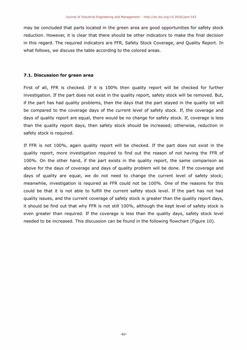
7.1. Discussion for green area
First of all, FFR is checked. If it is 100% then quality report will be checked for further
investigation. If the part does not exist in the quality report, safety stock will be removed. But,
if the part has had quality problems, then the days that the part stayed in the quality lot will
be compared to the coverage days of the current level of safety stock. If, the coverage and
days of quality report are equal, there would be no change for safety stock. If, coverage is less
than the quality report days, then safety stock should be increased; otherwise, reduction in
safety stock is required.
If FFR is not 100%, again quality report will be checked. If the part does not exist in the
quality report, more investigation required to find out the reason of not having the FFR of
100%. On the other hand, if the part exists in the quality report, the same comparison as
above for the days of coverage and days of quality problem will be done. If the coverage and
days of quality are equal, we do not need to change the current level of safety stock;
meanwhile, investigation is required as FFR could not be 100%. One of the reasons for this
could be that it is not able to fulfill the current safety stock level. If the part has not had
quality issues, and the current coverage of safety stock is greater than the quality report days,
it should be find out that why FFR is not still 100%, although the kept level of safety stock is
even greater than required. If the coverage is less than the quality days, safety stock level
needed to be increased. This discussion can be found in the following flowchart (Figure 10).
-62-
Journal of Industrial Engineering and Management – http://dx.doi.org/10.3926/jiem.543
Figure 10. Green area flowchart
7.2. Discussion for yellow area
This area could be related to the parts that delivered in low frequencies but in big batches.
Therefore, it cannot be concluded right away to remove the safety stock. Indeed, it is needed
to making sure that whenever these parts arrive they do not have quality issues. Then, their
safety stock can be removed; otherwise, removal of their safety stock will make the company
to be in shortage.
7.3. Discussion for red area
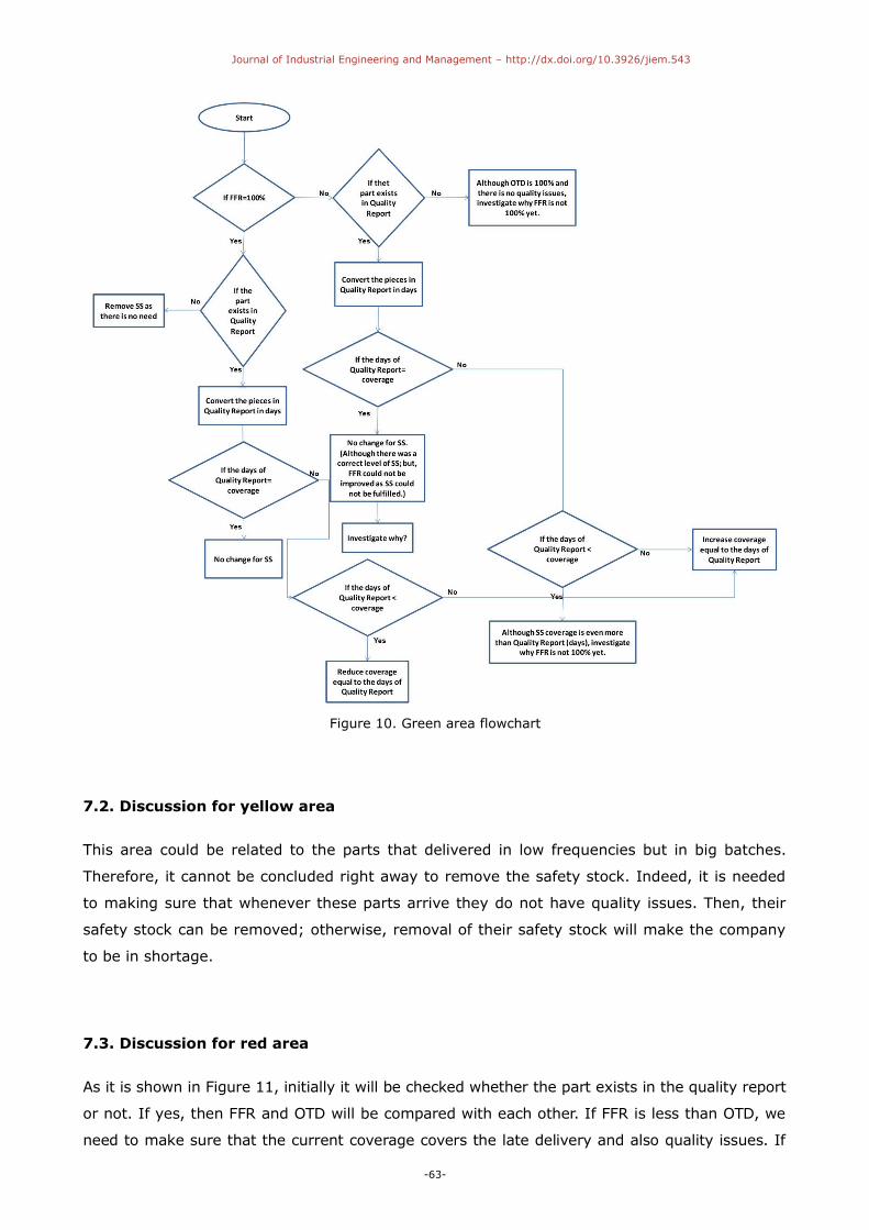
As it is shown in Figure 11, initially it will be checked whether the part exists in the quality report
or not. If yes, then FFR and OTD will be compared with each other. If FFR is less than OTD, we
need to make sure that the current coverage covers the late delivery and also quality issues. If
-63-
Journal of Industrial Engineering and Management – http://dx.doi.org/10.3926/jiem.543
FFR is greater than the OTD, then it should be checked if FFR is 100% or not, and after that
safety stock coverage should be compared with the quality report (days) plus lateness.
On the other hand, if the part does not exist in the quality report and FFR is less than OTD, we
need to investigate the reason as there is no variability due to quality issues in this case and
level of safety stock should be only equal to the lateness in the delivery. But, if FFR is greater
than OTD, it should be checked whether FFR is 100% or not, and then safety stock coverage
should be compared with lateness.
Figure 11. Red area flowchart
For calculating the days that the part was in the quality lot to compare it with the coverage of
safety stock, “Duration in Quality Lot (in days)” and “Frequency of appearing the part in
Quality Report” within last year for each part should be provided. Then, the days related to the
“Maximum” of the frequency would be the representative of the days of being in the quality
lot. If the maximum of the frequency is not unique, then the “Maximum” of their duration days
will be selected. Table 7 shows this information that was gathered at the company.
-64-
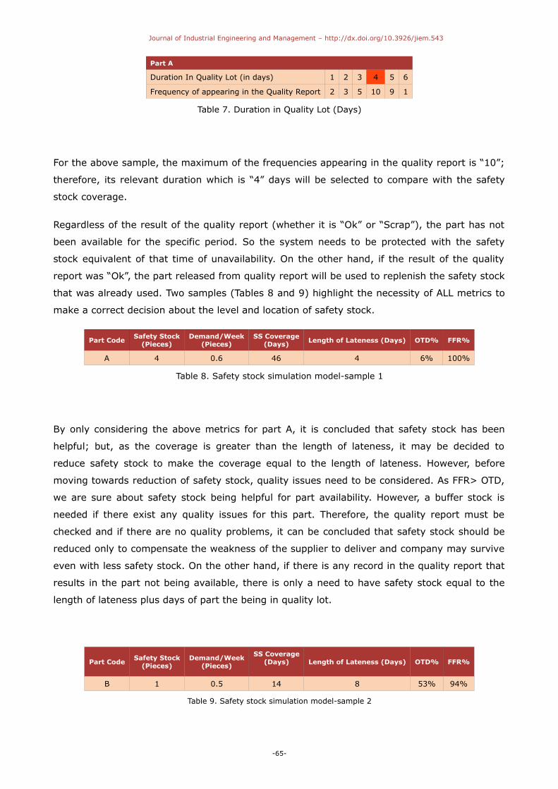
Journal of Industrial Engineering and Management – http://dx.doi.org/10.3926/jiem.543
Part A
Duration In Quality Lot (in days) 1 2 3 4 5 6
Frequency of appearing in the Quality Report 2 3 5 10 9 1
Table 7. Duration in Quality Lot (Days)
For the above sample, the maximum of the frequencies appearing in the quality report is “10”;
therefore, its relevant duration which is “4” days will be selected to compare with the safety
stock coverage.
Regardless of the result of the quality report (whether it is “Ok” or “Scrap”), the part has not
been available for the specific period. So the system needs to be protected with the safety
stock equivalent of that time of unavailability. On the other hand, if the result of the quality
report was “Ok”, the part released from quality report will be used to replenish the safety stock
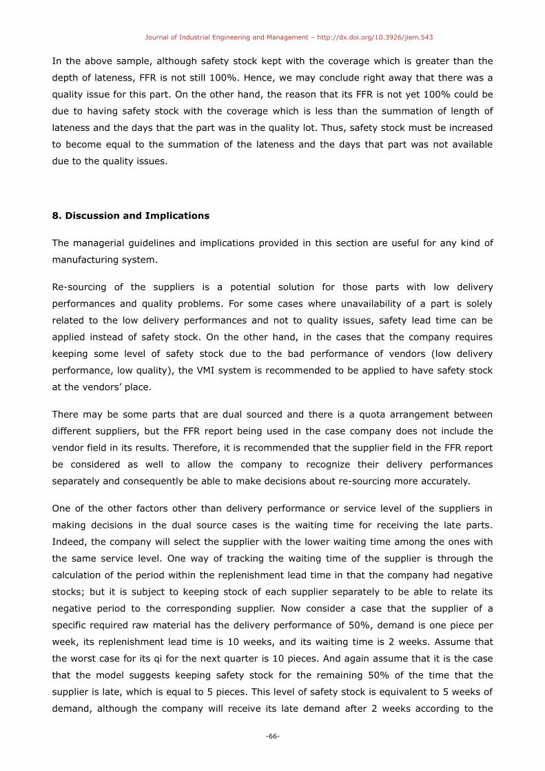
that was already used. Two samples (Tables 8 and 9) highlight the necessity of ALL metrics to
make a correct decision about the level and location of safety stock.
Part CodeSafety Stock
(Pieces)Demand/Week
(Pieces)SS Coverage
(Days) Length of Lateness (Days) OTD% FFR%
A 4 0.6 46 4 6% 100%
Table 8. Safety stock simulation model-sample 1
By only considering the above metrics for part A, it is concluded that safety stock has been
helpful; but, as the coverage is greater than the length of lateness, it may be decided to
reduce safety stock to make the coverage equal to the length of lateness. However, before
moving towards reduction of safety stock, quality issues need to be considered. As FFR> OTD,
we are sure about safety stock being helpful for part availability. However, a buffer stock is
needed if there exist any quality issues for this part. Therefore, the quality report must be
checked and if there are no quality problems, it can be concluded that safety stock should be
reduced only to compensate the weakness of the supplier to deliver and company may survive
even with less safety stock. On the other hand, if there is any record in the quality report that
results in the part not being available, there is only a need to have safety stock equal to the
length of lateness plus days of part the being in quality lot.
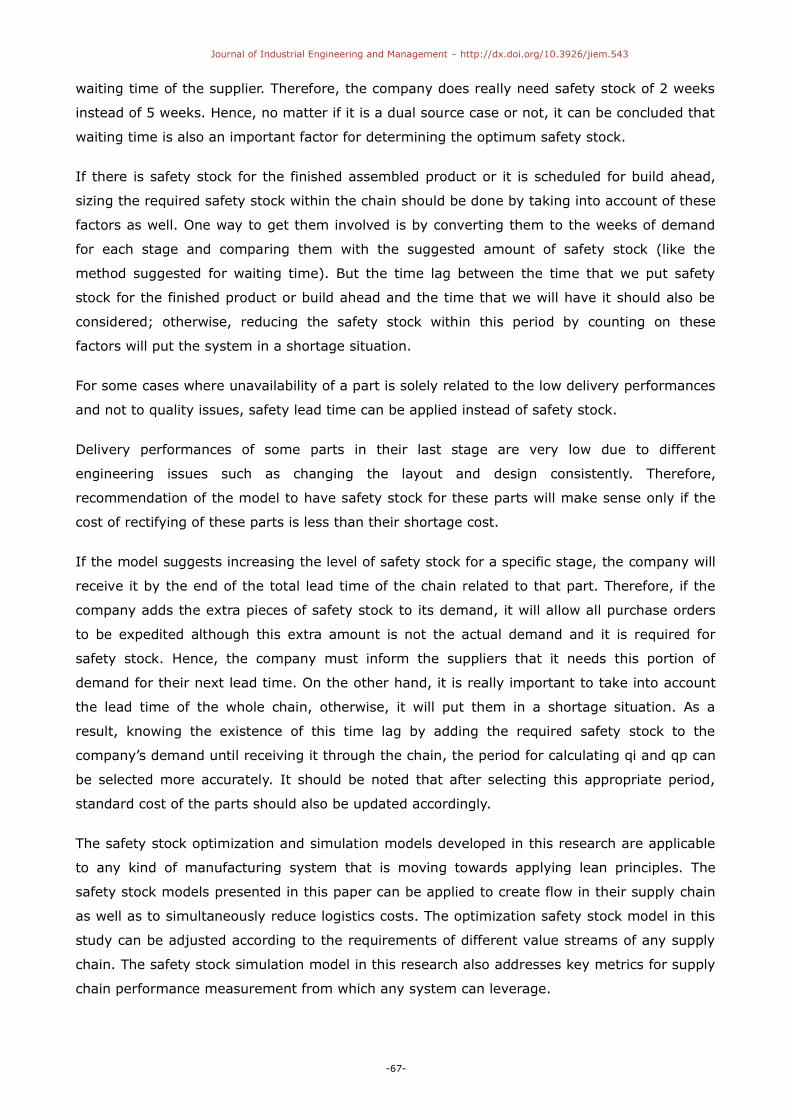
Part CodeSafety Stock
(Pieces)Demand/Week
(Pieces)
SS Coverage(Days) Length of Lateness (Days) OTD% FFR%
B 1 0.5 14 8 53% 94%
Table 9. Safety stock simulation model-sample 2
-65-
Journal of Industrial Engineering and Management – http://dx.doi.org/10.3926/jiem.543
In the above sample, although safety stock kept with the coverage which is greater than the
depth of lateness, FFR is not still 100%. Hence, we may conclude right away that there was a
quality issue for this part. On the other hand, the reason that its FFR is not yet 100% could be
due to having safety stock with the coverage which is less than the summation of length of
lateness and the days that the part was in the quality lot. Thus, safety stock must be increased
to become equal to the summation of the lateness and the days that part was not available
due to the quality issues.
8. Discussion and Implications
The managerial guidelines and implications provided in this section are useful for any kind of
manufacturing system.
Re-sourcing of the suppliers is a potential solution for those parts with low delivery
performances and quality problems. For some cases where unavailability of a part is solely
related to the low delivery performances and not to quality issues, safety lead time can be
applied instead of safety stock. On the other hand, in the cases that the company requires
keeping some level of safety stock due to the bad performance of vendors (low delivery
performance, low quality), the VMI system is recommended to be applied to have safety stock
at the vendors’ place.
There may be some parts that are dual sourced and there is a quota arrangement between
different suppliers, but the FFR report being used in the case company does not include the
vendor field in its results. Therefore, it is recommended that the supplier field in the FFR report
be considered as well to allow the company to recognize their delivery performances
separately and consequently be able to make decisions about re-sourcing more accurately.
One of the other factors other than delivery performance or service level of the suppliers in
making decisions in the dual source cases is the waiting time for receiving the late parts.
Indeed, the company will select the supplier with the lower waiting time among the ones with
the same service level. One way of tracking the waiting time of the supplier is through the
calculation of the period within the replenishment lead time in that the company had negative
stocks; but it is subject to keeping stock of each supplier separately to be able to relate its
negative period to the corresponding supplier. Now consider a case that the supplier of a
specific required raw material has the delivery performance of 50%, demand is one piece per
week, its replenishment lead time is 10 weeks, and its waiting time is 2 weeks. Assume that
the worst case for its qi for the next quarter is 10 pieces. And again assume that it is the case
that the model suggests keeping safety stock for the remaining 50% of the time that the
supplier is late, which is equal to 5 pieces. This level of safety stock is equivalent to 5 weeks of
demand, although the company will receive its late demand after 2 weeks according to the
-66-
Journal of Industrial Engineering and Management – http://dx.doi.org/10.3926/jiem.543
waiting time of the supplier. Therefore, the company does really need safety stock of 2 weeks
instead of 5 weeks. Hence, no matter if it is a dual source case or not, it can be concluded that
waiting time is also an important factor for determining the optimum safety stock.
If there is safety stock for the finished assembled product or it is scheduled for build ahead,
sizing the required safety stock within the chain should be done by taking into account of these
factors as well. One way to get them involved is by converting them to the weeks of demand
for each stage and comparing them with the suggested amount of safety stock (like the
method suggested for waiting time). But the time lag between the time that we put safety
stock for the finished product or build ahead and the time that we will have it should also be
considered; otherwise, reducing the safety stock within this period by counting on these
factors will put the system in a shortage situation.
For some cases where unavailability of a part is solely related to the low delivery performances
and not to quality issues, safety lead time can be applied instead of safety stock.
Delivery performances of some parts in their last stage are very low due to different
engineering issues such as changing the layout and design consistently. Therefore,
recommendation of the model to have safety stock for these parts will make sense only if the
cost of rectifying of these parts is less than their shortage cost.
If the model suggests increasing the level of safety stock for a specific stage, the company will
receive it by the end of the total lead time of the chain related to that part. Therefore, if the
company adds the extra pieces of safety stock to its demand, it will allow all purchase orders
to be expedited although this extra amount is not the actual demand and it is required for
safety stock. Hence, the company must inform the suppliers that it needs this portion of
demand for their next lead time. On the other hand, it is really important to take into account
the lead time of the whole chain, otherwise, it will put them in a shortage situation. As a
result, knowing the existence of this time lag by adding the required safety stock to the
company’s demand until receiving it through the chain, the period for calculating qi and qp can
be selected more accurately. It should be noted that after selecting this appropriate period,
standard cost of the parts should also be updated accordingly.
The safety stock optimization and simulation models developed in this research are applicable
to any kind of manufacturing system that is moving towards applying lean principles. The
safety stock models presented in this paper can be applied to create flow in their supply chain
as well as to simultaneously reduce logistics costs. The optimization safety stock model in this
study can be adjusted according to the requirements of different value streams of any supply
chain. The safety stock simulation model in this research also addresses key metrics for supply
chain performance measurement from which any system can leverage.
-67-
Journal of Industrial Engineering and Management – http://dx.doi.org/10.3926/jiem.543
The safety models developed in this research are applicable to any kind of manufacturing
system that is moving towards applying lean principles. The models presented in this research
can be applied to create flow in companies supply chain as well as to simultaneously reduce
logistics costs and they can be adjusted according to the requirements of different value
streams of any supply chain.
9. Conclusions
In this research, a safety stock optimization model is provided with the objective function of
total logistic costs minimization to result in not only the optimal level of safety stock but also
the optimal location of it across the supply chain. The constraints of the model provided for the
boundaries of the delivery performances of each stage of the supply chain. Then, it is applied
to a practical real-world problem with different possible value streams.
Providing supply chain performance measurement metrics that can be integrated is a
challenging task. This study introduced some of these metrics such as First Fill Rate, On Time
Delivery, safety stock coverage, among others. These metrics have been linked and a safety
stock simulation model has been developed based on them.This simulation model supports the
results of the optimization model for the optimal level and location of safety stock. c
If a part is procured through more than one supplier, the current optimization model tracks
their performance with only one average number representative of all of them. In future work,
the model may be extended simultaneously by increasing the accessibility of the other required
input data to decide on the level of safety stock for each of these suppliers separately.
Due to the inaccessibility of the required data, the optimization model is currently limited to
the last two stages before the customer in the chain. Again, by enhancing the visibility and
control of the upstream stages in the chain, the optimization model can be applied for each
specific part from its starting point until the end of the chain. Furthermore, by increasing the
accessibility of the data, the cost of shortage of raw material/semi-finished part can be more
accurate by adding the re-sequencing cost of manufacturing. The cost of shortage of the
finished part required by Assembly can also be more precise by making the average days of
shortage weighted based on the frequency of its occurrence (increasing or decreasing trend of
shortage).
One of the avenues for future work for this research would be taking into account the factors
of waiting time for receiving the late parts, safety stock for the finished assembled product,
and build ahead in making the decision for the safety stock.
-68-
Journal of Industrial Engineering and Management – http://dx.doi.org/10.3926/jiem.543
References
Adamides, E.D., Karacapilidis, N., Pylarinou, H., & Koumanakos, D. (2008). Supporting
collaboration in the development and management of lean supply networks. Production
Planning & Control, 19(1), 35-52. http://dx.doi.org/10.1080/09537280701773955
Aleotti Maia, L.O., & Qassim, R.Y. (1998). Minimum cost safety stocks for frequently delivery
manufacturing. International Journal of Production Economics, 233-236.
Cagliano, R., Caniato, F., & Spina, G. (2004). Lean, Agile and traditional supply: how do they
impact manufacturing performance? Journal of Purchasing & Supply Management, 10,
151-164. http://dx.doi.org/10.1016/j.pursup.2004.11.001
Chen, I.J., & Paulraj, A. (2004). Understanding supply cahin management: critical research
and theoretical framework. International Journal of Production Research, 42(1), 131-163.http://dx.doi.org/10.1080/00207540310001602865
Chun Wu, Y. (2003). Lean manufacturing: a perspective of lean suppliers. International Journal
of Operations & Production Management, 23(11), 1349-1376.http://dx.doi.org/10.1108/01443570310501880
Coyle, J.J., Bardi, E.J., & Langley, C.J. (2009). Supply chain management: a logistics
perspective.
Crino, S.T., McCarthy, D.J., & Carier, J.D. (2007). Lean Six Sigma for supply chain management
as applied to the Army Rapid Fielding Initiative. In 1st Annual IEEE Systems Conference.
Desmet, B., Aghezzaf, E.H., & Vanmaele, H. (2010). A normal approximation for safety stock
optimization in a two-echelon distribution system. Journal of the Operational Research
Society, 61(1), 156-163. http://dx.doi.org/10.1057/jors.2008.150
De Toni, A., & Tonchia, S. (2001). Performance measurement systems: Models, characteristics
and measures. International Journal of Operations & Production Management, 21, 46-70.http://dx.doi.org/10.1108/01443570110358459
Graves, S.C., & Rinnooy Kan, A.H.G. (1993). Logistics of production and inventory. Handbooks
in Operations Research and Management Science.
Gunasekaran, A., Patel, C., & McGaughey, R.E. (2004). A framework for supply chain
performance measurement. International Journal of Production Economics, 87, 333-347.http://dx.doi.org/10.1016/j.ijpe.2003.08.003
Gunasekaran, A., Patel, C., & Tirtiroglu, E. (2001). Performance measures and metrics in a
supply chain environment. International Journal of Operations & Production Management,
21(1/2), 71-87. http://dx.doi.org/10.1108/01443570110358468
-69-
Journal of Industrial Engineering and Management – http://dx.doi.org/10.3926/jiem.543
Inderfurth, K. (1991). Safety stock optimization in multi-stage inventory system. International
Journal of Production Economics, 24(1-2), 103-113. http://dx.doi.org/10.1016/0925-
5273(91)90157-O
Jung, J.Y., Blau, G., Pekny, J.F., Reklaitis, G.V., & Eversdyk, D. (2008). Integrated safety stock
management for multi-stage supply chains under production capacity constraints. Computers
and Chemical Engineering, 32, 2570-2581. http://dx.doi.org/10.1016/j.compchemeng.2008.04.003
Kainuma, Y., & Tawara, N. (2006). A multiple attribute utility theory approach to lean and
green supply chain management. International Journal of Production Economics, 101,
99-108. http://dx.doi.org/10.1016/j.ijpe.2005.05.010
Lamming, R. (1996). Squaring lean supply with supply chain management. International
Journal of Operations & Production Management, 16(2), 183-196.http://dx.doi.org/10.1108/01443579610109910
Li, Q.Y., & Li, S.J. (2009, July). A dynamic model of the safety stock under VMI. Proceedings of
the Eighth International Conference on Machine Learning and Cybernetics, 1304-1308.
Long, Q., Liu, L.F., Meng, L.Q., & Chen, W. (2009). Logistics cost optimized election in the
manufacturing process based on ELECTURE-II Algorithm. In Proceedings of the IEEE
International Conference on Automation and Logistics.
Maloni, M.J., & Benton, W.C. (1997). Supply chain partnerships: Opportunities for operations
research. European Journal of Operational Research, 101(3), 419-429.http://dx.doi.org/10.1016/S0377-2217(97)00118-5
Mason-Jones, R., Nalor, B., & Towill, D.R. (2000). Lean, agile or leagile? Matching your supply
chain to the marketplace. International Journal of Production Research, 38(17), 4061-4070.http://dx.doi.org/10.1080/00207540050204920
McCullen, P., & Towill, D. (2001). Achieving lean supply through agile manufacturing.
Integrated Manufacturing Systems, 524-533. http://dx.doi.org/10.1108/EUM0000000006232
Natarajan, R., & Goyal, S. (1994). Safety stocks in JIT environments. International Journal of
Operations & Production Management, 14(10), 64-71.http://dx.doi.org/10.1108/01443579410067261
Naylor, J.B., Naim, M.M., & Berry, D. (1999). Leagility: Integrating the lean and agile
manufacturing paradigms in the total supply chain. International Journal of Production
Economics, 62, 107-118. http://dx.doi.org/10.1016/S0925-5273(98)00223-0
Qi, F., Xuejun, X., & Zhiyong, G. (2007). Research on Lean, Agile and Leagile Supply Chain.
National Natural Foundation of China Grand and IOM European, 4902-4905.
-70-
Journal of Industrial Engineering and Management – http://dx.doi.org/10.3926/jiem.543
Silver, E.A., Pyke, D.F., & Peterson, R. (1998). Inventory management and production planning
and scheduling. 3rd ed.
Shepherd, C., &, Gunter, H. (2006). Measuring supply chain performance: current research and
future directions. International Journal of Productivity and Performance Management,
55(3/4), 242-258. http://dx.doi.org/10.1108/17410400610653219
Slack, N., Chambers, S., Harland, C., Harrison, A., & Johnston, R. (1995). Operations
Management. Pitman Publishing, London.
Taylor, D. (1999). Parallel Incremental Transformation Strategy: An Approach to the
Development of Lean Supply Chains. International Journal of Logistics Research and
Applications, 2(3), 305-323. http://dx.doi.org/10.1080/13675569908901587
Tempelmeier, H. (2006). Inventory management in supply networks. Problems, Models,
Solutions.
Thomas, J. (1999). Why your supply chain doesn't work. Logistics Management and
Distribution Report.
Wu, H. (2009). The Lean manufacture research in environment of the supply chain of modern
industry engineering. 16th Conference on Industrial Engineering and Engineering
Management, 297-300.
Wu, S., & Wee, H.M. (2009). How Lean supply chain effects product cost and quality- A case
study of the Ford Motor Company. In 6th International Conference on Service Systems and
Service Management.
Xia, L.X.X., Ma, B., & Lim, R. (2007). AHP Based Supply Chain Performance Measurement
System. In Emerging Technologies and Factory Automation.
Zhao, X., Lai, F., & Lee, T.S. (2001). Evaluation of safety stock methods in multilevel material
requirements planning (MRP) systems. Production Planning & Control, 12(8), 794-803.http://dx.doi.org/10.1080/095372800110052511
Journal of Industrial Engineering and Management, 2014 (www.jiem.org)
Article's contents are provided on a Attribution-Non Commercial 3.0 Creative commons license. Readers are allowed to copy, distribute
and communicate article's contents, provided the author's and Journal of Industrial Engineering and Management's names are included.
It must not be used for commercial purposes. To see the complete license contents, please visit
http://creativecommons.org/licenses/by-nc/3.0/.
-71-