Embed Size (px)
Citation preview
Technische Universitat Munchen
Fakultat fur Bauingenieur- und Vermessungswesen
Computation in Engineering
Prof. Dr. rer.nat. Ernst Rank
Development of An Earthwork Simulation Model
with Plant Simulation
Master Thesis
Hao Zhou
Superisor: Dipl.-Inf. Yang Ji
Submission date: January 15, 2010

Munich, January 15, 2010
I, Hao Zhou (master student of Computational Mechanics at the Technical University
Munich, student ID no. ), solemnly declare that I have written this thesis
independently, and that I did not make use of any aids other than those acknowledged
in this thesis. Neither this thesis, nor any similar work, have previously been submitted
to any examination board.
Hao Zhou
i

Acknowledgements
My heartfelt appreciation goes to Dipl.-Inf. Yang Ji from the chair of Computation in
Engineering. Your scientific attitude, cordial suggestions and encouragement help me
all the time during the research and writing of the thesis.
I also want to thank Dipl.-Ing. Yao Hu for reading and correcting the thesis literally.
Finally, I want to appreciate the support from my parents, girl friend and all my friends.
ii
Abstract
Simulation technique is widely used in many engineering subjects. However, it is less
applied in civil engineering, especially in road construction field. In this thesis, an
earthwork simulation model is developed with commerial discrete event simulation sys-
tem Plant Simulation to simulate earthwork processes in road construction.
The earthwork simulation model describes the earthwork processes. With its help, the
simulaiton system can analyze the utilization of the involved construction equipments
during road construction. Finally, in this thesis, statistical experiments are designed to
analyze the simulation results.
iii
Contents
1 Introduction 1
1.1 Scope and structure of this thesis . . . . . . . . . . . . . . . . . . . . . 1
1.2 State of the art of simulation technique . . . . . . . . . . . . . . . . . . 2
1.2.1 Application domains . . . . . . . . . . . . . . . . . . . . . . . . 3
1.2.2 Commercial simulation system Plant Simulation . . . . . . . . . 4
1.2.3 General architecture of simulation system . . . . . . . . . . . . 5
2 Road Construction Simulation Model 8
2.1 Construction site layout . . . . . . . . . . . . . . . . . . . . . . . . . . 8
2.2 Specification of simulation model components . . . . . . . . . . . . . . 10
2.2.1 Earthwork components . . . . . . . . . . . . . . . . . . . . . . . 10
2.2.1.1 Cut . . . . . . . . . . . . . . . . . . . . . . . . . . . . 10
2.2.1.2 Fill . . . . . . . . . . . . . . . . . . . . . . . . . . . . . 14
2.2.2 Earth transportation components . . . . . . . . . . . . . . . . . 15
2.2.2.1 Truck system . . . . . . . . . . . . . . . . . . . . . . . 16
2.2.2.2 Track system . . . . . . . . . . . . . . . . . . . . . . . 16
2.3 Integration with 3D earthwork assessment system . . . . . . . . . . . . 17
2.4 Simulation results analysis . . . . . . . . . . . . . . . . . . . . . . . . . 18
3 Earthwork simulation model in Plant Simulation 20
3.1 Introduction to Plant Simulation . . . . . . . . . . . . . . . . . . . . . 20
3.1.1 Characteristics of Plant Simulation . . . . . . . . . . . . . . . . 20
3.1.2 Graphical user interface overview . . . . . . . . . . . . . . . . . 22
3.1.3 Important objects used in construction site simulation . . . . . 23
iv
3.1.4 Introduction to SimTalk . . . . . . . . . . . . . . . . . . . . . . 26
3.1.5 Event management in Plant Simulation . . . . . . . . . . . . . . 26
3.2 A road construction simulation model . . . . . . . . . . . . . . . . . . . 27
3.2.1 Earthwork model . . . . . . . . . . . . . . . . . . . . . . . . . . 32
3.2.1.1 Cut model . . . . . . . . . . . . . . . . . . . . . . . . . 32
3.2.1.2 Fill model . . . . . . . . . . . . . . . . . . . . . . . . . 38
3.2.2 Earth transportation system model . . . . . . . . . . . . . . . . 42
3.2.2.1 Truck system model . . . . . . . . . . . . . . . . . . . 42
3.2.2.2 Track system model . . . . . . . . . . . . . . . . . . . 44
3.2.2.3 Event flow of the earth transportation system model . 44
3.2.3 Data transmission system . . . . . . . . . . . . . . . . . . . . . 48
3.2.4 Result analysis system . . . . . . . . . . . . . . . . . . . . . . . 50
3.2.4.1 Single simulation execution results analysis system . . 51
3.2.4.2 Multiple simulation execution results analysis system . 52
4 Simulation Results and Analysis 54
4.1 Results of a single simulation execution . . . . . . . . . . . . . . . . . . 54
4.2 Results of multiple simulation executions . . . . . . . . . . . . . . . . . 61
4.2.1 Case study 1 . . . . . . . . . . . . . . . . . . . . . . . . . . . . 61
4.2.2 Case study 2 . . . . . . . . . . . . . . . . . . . . . . . . . . . . 64
5 Summary 68
Bibliography 69
v
1. Introduction 1
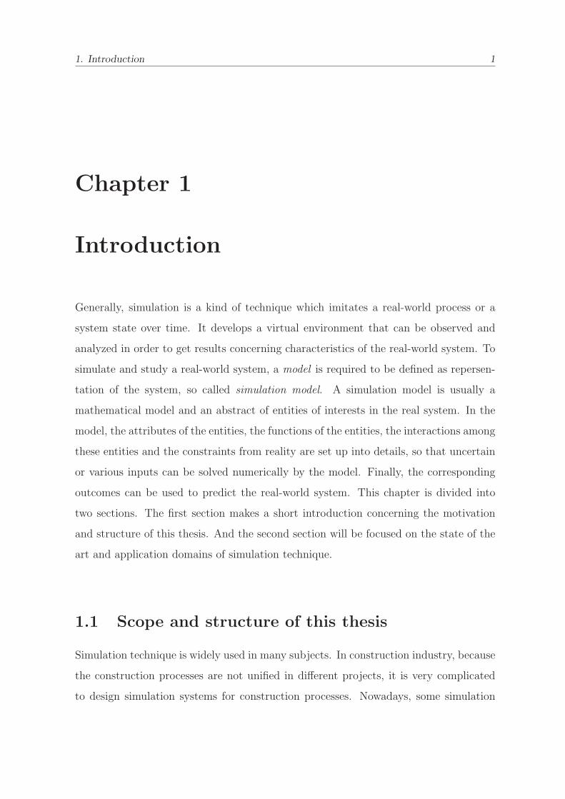
Chapter 1
Introduction
Generally, simulation is a kind of technique which imitates a real-world process or a
system state over time. It develops a virtual environment that can be observed and
analyzed in order to get results concerning characteristics of the real-world system. To
simulate and study a real-world system, a model is required to be defined as repersen-
tation of the system, so called simulation model. A simulation model is usually a
mathematical model and an abstract of entities of interests in the real system. In the
model, the attributes of the entities, the functions of the entities, the interactions among
these entities and the constraints from reality are set up into details, so that uncertain
or various inputs can be solved numerically by the model. Finally, the corresponding
outcomes can be used to predict the real-world system. This chapter is divided into
two sections. The first section makes a short introduction concerning the motivation
and structure of this thesis. And the second section will be focused on the state of the
art and application domains of simulation technique.
1.1 Scope and structure of this thesis
Simulation technique is widely used in many subjects. In construction industry, because
the construction processes are not unified in different projects, it is very complicated
to design simulation systems for construction processes. Nowadays, some simulation
1.2. State of the art of simulation technique 2
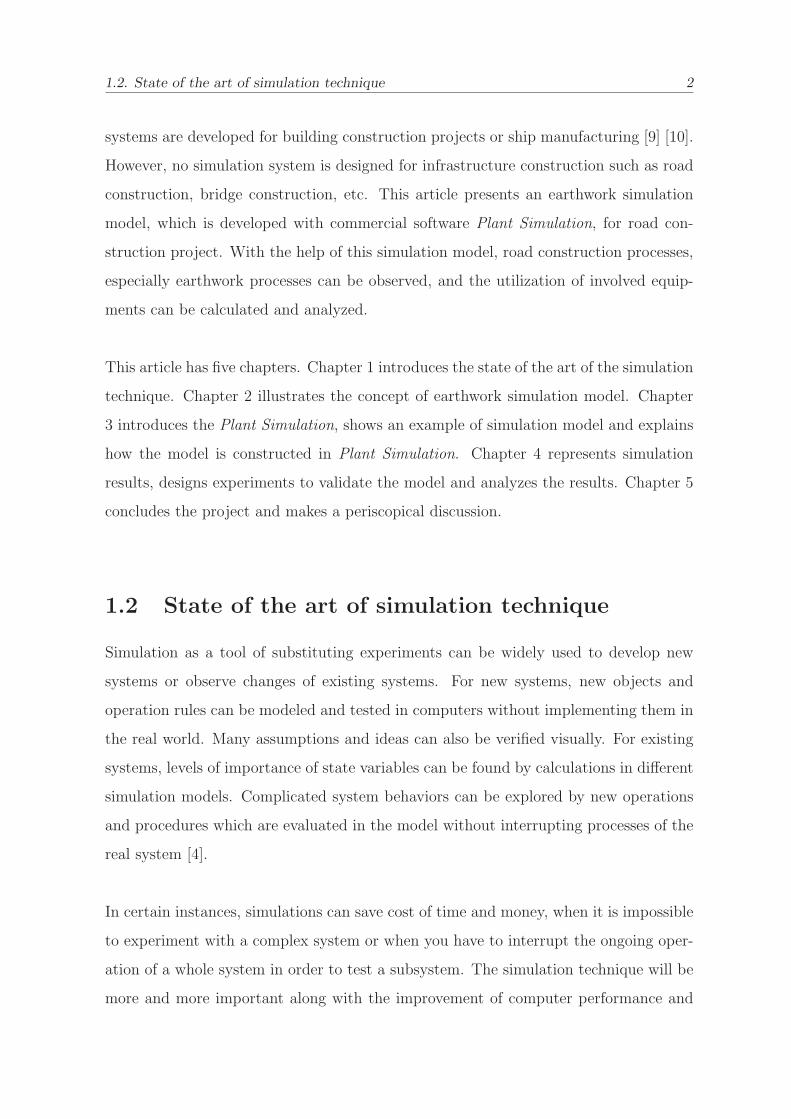
systems are developed for building construction projects or ship manufacturing [9] [10].
However, no simulation system is designed for infrastructure construction such as road
construction, bridge construction, etc. This article presents an earthwork simulation
model, which is developed with commercial software Plant Simulation, for road con-
struction project. With the help of this simulation model, road construction processes,
especially earthwork processes can be observed, and the utilization of involved equip-
ments can be calculated and analyzed.
This article has five chapters. Chapter 1 introduces the state of the art of the simulation
technique. Chapter 2 illustrates the concept of earthwork simulation model. Chapter
3 introduces the Plant Simulation, shows an example of simulation model and explains
how the model is constructed in Plant Simulation. Chapter 4 represents simulation
results, designs experiments to validate the model and analyzes the results. Chapter 5
concludes the project and makes a periscopical discussion.
1.2 State of the art of simulation technique
Simulation as a tool of substituting experiments can be widely used to develop new
systems or observe changes of existing systems. For new systems, new objects and
operation rules can be modeled and tested in computers without implementing them in
the real world. Many assumptions and ideas can also be verified visually. For existing
systems, levels of importance of state variables can be found by calculations in different
simulation models. Complicated system behaviors can be explored by new operations
and procedures which are evaluated in the model without interrupting processes of the
real system [4].
In certain instances, simulations can save cost of time and money, when it is impossible
to experiment with a complex system or when you have to interrupt the ongoing oper-
ation of a whole system in order to test a subsystem. The simulation technique will be
more and more important along with the improvement of computer performance and
1.2. State of the art of simulation technique 3
the development of simulation software.
1.2.1 Application domains
Historically, simulation is more physical. People always choose smaller or cheaper
physical objects to imitate and analyze real objects. However, as the development
of computer science, computer simulation becomes more and more popular. Modern
simulation technique can be used in many areas.
Engineering. Simulation techniques appear in a wide range of engineering application.
For example, a city traffic system can be simulated to observe when and where traffic
jam happens, and how the traffic jam interrupts normal vehicle flows [5]. A lifecycle
simulation of a machine can reduce the cost of prototype design and production, and
decrease the time-to-market. A mechanical simulation can check a structure’s safety
factors in different loading conditions in order to judge if the design of the structure is
reliable.
Health care. More and more medical simulators are developed. Some simulators pro-
vide data to help doctors decide diagnostic methods, or even convenience doctors during
surgeries. Some simulators construct human body models to observe human responses
in different situations. For example, in automobile industry, human body models al-
ways appear in the crash simulation in order to check whether the driver is safe or not
under the umbrella of the security system of a car [7].
Finance and business. Simulation techniques can be done to imitate a company’s op-
eration. For example, a queuing system can be simulated for a bank to analyze and
observe behavior of tellers and customers. The result can be used to improve service
quality and attract new customers. Some financial companies can also experiment with
the models of scenarios planning by computer simulation in order to increase their com-
petitive power.
1.2. State of the art of simulation technique 4
Military and aerospace applications. Simulation techniques occur in these fields be-
cause their real experiments are prohibitively expensive or extremely dangerous. These
simulations can provide safe circumstance and mistake-allowed policy for trainees. In
such situation, trainees can get psychological and skill preparation and effectively avoid
mistakes in real operations [3].
Entertainment. A strong branch of simulation technique is the entertainment simula-
tion. In films, a lot of astonishing footages are made by computer simulations instead
of video recorders. In computer games, especially sports games and shooting games,
players can be drawn into virtual realities to act as sports stars or assassins who can
attempt some specific tasks.
Construction. This is a new application field of simulation technique. The construction
simulation model can be used to observe construction processes [8]. This thesis is about
earthwork simulation in road construction application. We can also see the simulation
model in other applications such as building construction [9] and ship manufacturing
[10].
1.2.2 Commercial simulation system Plant Simulation
Plant Simulation is a discrete event based simulation tool of creating digital models of
logistic and production systems. In the running of a digital system model, the system’s
processes can be observed, its characteristics can be explored and its performance can
be optimized. Digital models constructed in Plant Simulation are allowed to run exper-
iments and what-if scenarios without interrupting the existing systems. These models
can also be used in planning processes, before the real factories or construction sites
are installed. Plant Simulation offers a number of objects (e.g., material flow objects,
movable units) to imitate system components in detail. It also offers a lot of tools (e.g.,
charts, interface) to display simulation results, evaluate different system scenarios and
1.2. State of the art of simulation technique 5
communicate with other softwares [2].
1.2.3 General architecture of simulation system
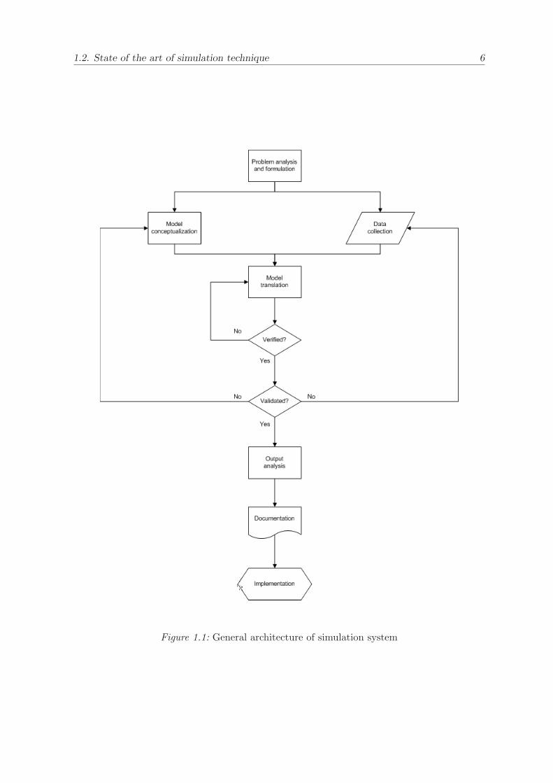
The general architecture of simulation system is showed in figure 1.1. The first step of
designing simulation system is problem analysis and formulation. Before a simulation
is implemented, a statement of the problem should be clearly understood by simulation
designers and users. They should be also clear about what they expect from using the
simulation system. It is necessary for simulation designers to identify the characteristics
of all the required objects and the interrelationships among these objects. Then the
simulation model can be fomulated by mathematical equations and physical laws.
The design of a simulation model is the most important step among all simulation steps.
The model design process can be divided into three parts: model conceptualization, data
collection, and model translation. Generally speaking, in the model conceptualization
stage, it is not necessary to create a model which is exactly the same as the real sys-
tem. The ability of abstracting the main features of the real system decides the art of
modeling. It is better to start with a simpler model, and make it more complex during
the validation of the model. In addition, the accuracy of selecting assumptions is also
important in model conceptualization. Data collection normally requires a great effort
in every simulation study. The objectives of a simulation determine what kind of and
how many data the simulation needs. The collected data can be used to construct or
even validate the model. Model translation means that abstracted features, selected
assumptions and collected data will be translated into computer-recognizable formats
using programming languages such as C, C++ and Java. After a model is translated
into a program, the program should be compiled and verified. In addition, the model
itself should also be validated to make sure if it works well and at same time find reme-
dies for errors.
The output analysis estimates the performance of a system design. According to output
1.2. State of the art of simulation technique 6
Figure 1.1: General architecture of simulation system
1.2. State of the art of simulation technique 7
analysis, model designers can check whether simulation results are consistent with what
they expect before the simulation model runs. In addition, the output analysis can also
check the stability of the simulation model. In documentation, two important things
will be explained clearly in a report. One is the progress that illustrates the history of a
simulation study. It can help policymakers to make decision and facilitate designers to
keep the project on. The other is the program which organizes computations in com-
puter. The program documentation is important when a user want to be familiar with
the program. The user with the help of the program can change variables of the model,
analyze the interplay of parameters, and make decisions according to the results. The
last step of a simulation study is implementation. How well the previous steps perform
decides the success of the implementation. The better a model designer understand the
nature of the problem and the model, or the more effort the model designer spends in
the model building process, the greater success the simulation will achieve.
2. Road Construction Simulation Model 8
Chapter 2
Road Construction Simulation
Model
As mentioned in the last chapter, simulation model is a representation of real-world sys-
tem. On one hand, simulation model should be as concise and efficient as possible. On
the other hand, the model should also be detailed enough to draw valid conclusions [4].
This chapter introduces how to design a road construction simulation model in a general
way. First, important components and submodels are specified. Second, the main at-
tributes and characteristics of each component are explained. Third, an abstract of data
interface and some essential mathematical calculations of result analysis are introduced.
2.1 Construction site layout
Earthwork is one of the most important tasks in the road construction. Earthworks
comprise excavation, transportation, filling and compaction of huge amount of earth
quantities, which normally cost a lot of time and money. So it is necessary for civil
engineer to maximize the efficiency of the involved resources and minimize the cost.
One way of decreasing cost is soil reuse, especially the excavated earth materials. Along
a designed road construction route, some areas need to be excavated and the others
2.1. Construction site layout 9
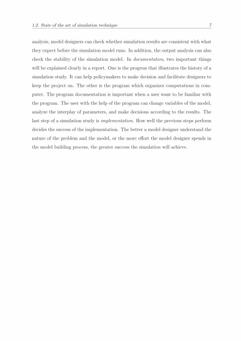
need to be filled. The areas are called cut and fill respectively. Figure 2.1 shows a
part of road verical alignment. This figure has two coordinates. One is stationing and
the other is high. The vertical alignment consists of two curves named road level and
terrain level. Many areas are shaped by the intersection of these two curves. The area
in which the terrain level is higher than the road level is called cut area (yellow), and
the one in which the terrain level is lower than the road level is called fill area (green).
The earthwork can be regarded as earth movement from cut to fill area.
Figure 2.1: Cut and fill
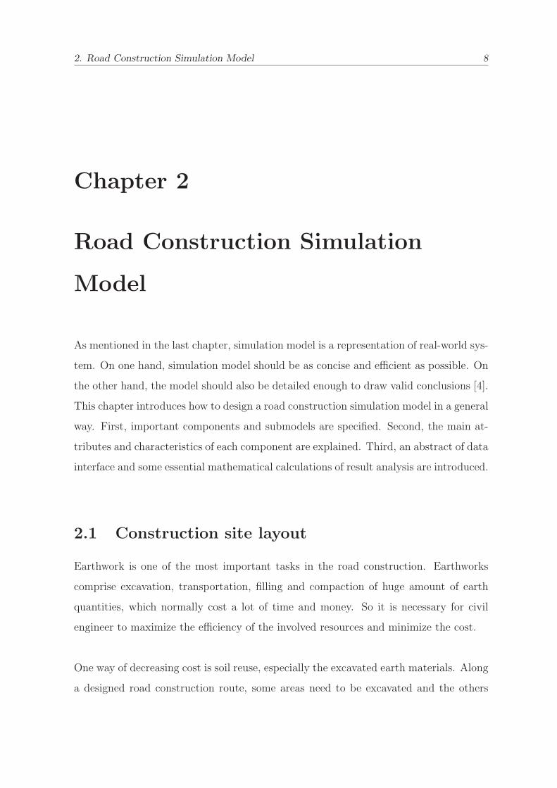
Another way of decreasing cost is to well organize the construction site resources. The
resources include excavators that remove earth, bulldozers that fill pits, trucks that
move earth, routes on which the trucks move and other construction equipments. All of
these resources should be included in the road construction simulation model. Figure
2.2 shows a simple construction site layout. It contains a cut, fill, dump area, tempo-
rary storage and a truck full of earth moving from the cut to the fill. Dump area stores
unrecyclable earth and temporary storage stores earth outside the system. Because the
functionality of temporary storage is the same as cut area, we regard the temporary
storage as cut. Analogically, we regard dump area as fill. The road construction site
can be divided into two parts: one is earthwork system, which includes cuts, fills and
correlative equipments; the other part is earth transportation system, which includes
tracks and trucks. The models of these two parts will be explained in detail in the
following sections.
2.2. Specification of simulation model components 10
Cut Fill
TransporterEarth
Track
Temporary StorageDump Area
Figure 2.2: Simple construction site layout
2.2 Specification of simulation model components
As mentioned above, a road construction model consists of earthwork model and earth
transportation model. The earthwork model is responsible for cutting and filling. The
earth transportation model is responsible for moving earth among those cuts and fills.
In this section, we will specify the components of these two models and the attributes
of all the components.
2.2.1 Earthwork components
Earthwork model that includes cut model and fill model has a lot of essential com-
ponents. In the following two sections, the cut and fill model are explained in an
object-oriented way. The cut model, fill model and their submodels are regarded as
objects.
2.2.1.1 Cut
Cut model is one of components of earthwork model in which earth is excavated and
loaded on trucks by excavators. Detailedly, a truck goes into a cut area. As soon as the
2.2. Specification of simulation model components 11
truck stops at a certain loading position of this cut area, one or more excavators start
working to excavate earth from this cut area and to load earth materials on the truck.
When the truck is fully loaded, it moves out of the cut area and the transportation
process begins. At the same time, the excavator(s) stop working and wait for the next
truck. The objects included in the cut model are excavation object, excavator and inner
track.
Excavation object
Excavation object can be regarded as a kind of earth storage. All the stored earth
materials will finally be removed out. The excavation process is realized by excavators.
An excavation object should include the following attributes:
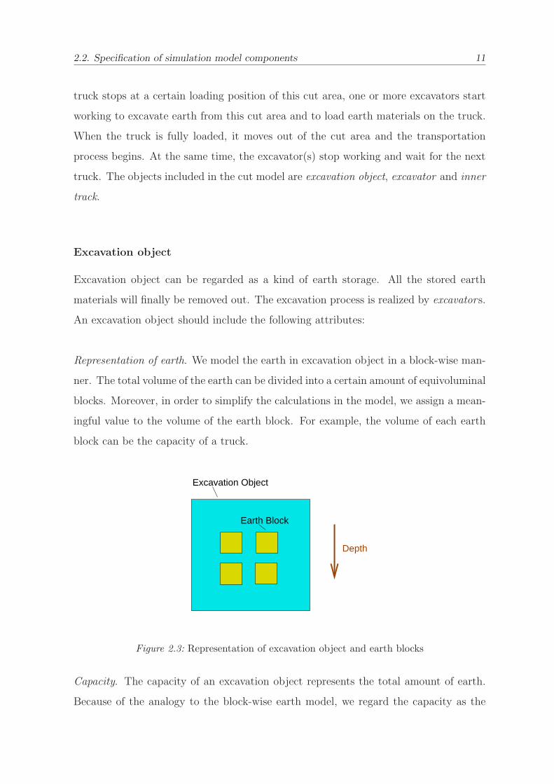
Representation of earth. We model the earth in excavation object in a block-wise man-
ner. The total volume of the earth can be divided into a certain amount of equivoluminal
blocks. Moreover, in order to simplify the calculations in the model, we assign a mean-
ingful value to the volume of the earth block. For example, the volume of each earth
block can be the capacity of a truck.
Earth Block
Excavation Object
Depth
Figure 2.3: Representation of excavation object and earth blocks
Capacity. The capacity of an excavation object represents the total amount of earth.
Because of the analogy to the block-wise earth model, we regard the capacity as the
2.2. Specification of simulation model components 12
total number of the earth blocks in an excavation object. For example, the capacity of
the excavation object show in figure 2.3 is 4.
Subsoil types and positions. The information includes the distribution of earth in an
excavation object and the material property of earth. The distribution illustrates how
high or how deep each earth block is. For example, the earth blocks in the figure 2.3
have different depth. The material property of earth decides the excavating manner.
These information affects the working time of the excavator and also the forwarding
simulation processes.
Excavator
Excavator moves earth blocks from an excavation object to trucks. To fill in a truck, an
excavator need many working cycles. An excavator model should include the following
attributes:
Capacity. The capacity means the amount of earth that can be moved by an excava-
tor per working cycle. It can also be considered as the capacity of an excavator’s bucket.
Processing time. This includes the time of articulated arm rotation, the time of bucket
lifting up and lowering down and the time of bucket grabbing. In addition, the pro-
cessing time changes according to earth blocks with different material properties or
positions.
Control methods. In the control methods, the excavator’s processing procedures such
as the articulated arm rotation, lifting up and lowering down earth, etc., can be pro-
grammed. The control method can also constrain the operation of the excavator. For
example, the excavator starts working until a truck reaches a proper position. The
excavator stop working until the truck leaves or the excavator object is empty.
2.2. Specification of simulation model components 13
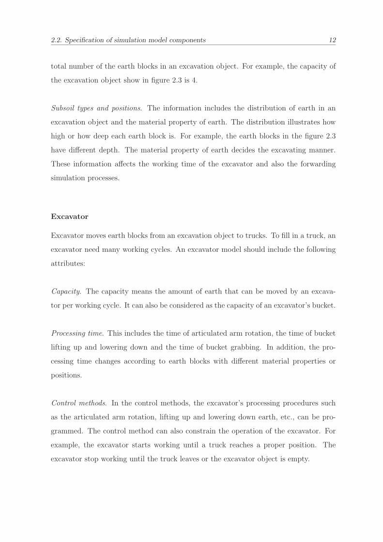
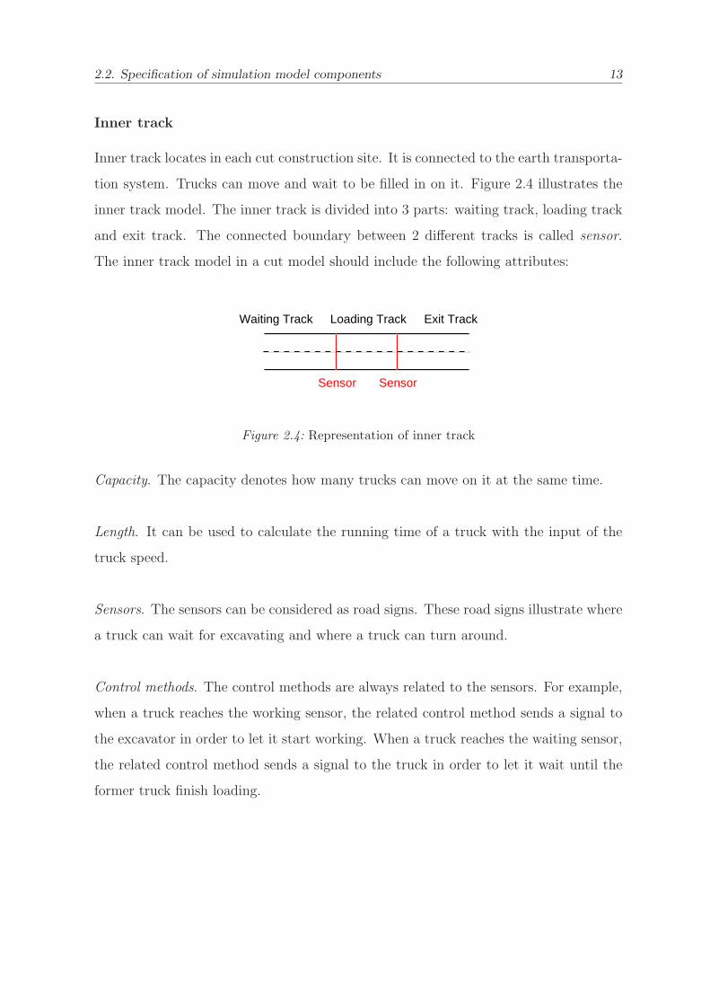
Inner track
Inner track locates in each cut construction site. It is connected to the earth transporta-
tion system. Trucks can move and wait to be filled in on it. Figure 2.4 illustrates the
inner track model. The inner track is divided into 3 parts: waiting track, loading track
and exit track. The connected boundary between 2 different tracks is called sensor.
The inner track model in a cut model should include the following attributes:
Waiting Track Loading Track Exit Track
SensorSensor
Figure 2.4: Representation of inner track
Capacity. The capacity denotes how many trucks can move on it at the same time.
Length. It can be used to calculate the running time of a truck with the input of the
truck speed.
Sensors. The sensors can be considered as road signs. These road signs illustrate where
a truck can wait for excavating and where a truck can turn around.
Control methods. The control methods are always related to the sensors. For example,
when a truck reaches the working sensor, the related control method sends a signal to
the excavator in order to let it start working. When a truck reaches the waiting sensor,
the related control method sends a signal to the truck in order to let it wait until the
former truck finish loading.
2.2. Specification of simulation model components 14
2.2.1.2 Fill
Fill model is one of components of earthwork model in which earth is transported and
unloaded by the truck to fill area. In this model, trucks coming from the earth trans-
portation system go into the inner track of the fill model. After the trucks are unloaded
in a certain position, one or more bulldozers move the earth to the pit. Similar to cut
model, following objects are included in the fill model: pit object, bulldozer and inner
track.
Pit object
Pit object can also be regarded as a kind of earth storage. In the beginning of a simula-
tion run, it is empty, but it will finally be filled in when the simulation ends. It cannot
move earth by itself but by bulldozers. An pit object should include the following at-
tributes:
Representation of earth. Refer to section 2.2.1.1.
Capacity. The capacity represents the quatity of earth a pit object can store. Because
of the analogy to the block-wise earth model, we regard the capacity as the total num-
ber of the earth blocks in an pit object.
Inventory of earth. The inventory records the information of the earth blocks a pit
object receives. The information contains the number of the earth blocks, original po-
sitions in excavation objects, etc.
Bulldozer
Bulldozer moves received earth blocks to a pit. Its blade can push large quantities of
soil, sand, rubble, etc. A bulldozer model should include the following attributes:
2.2. Specification of simulation model components 15
Capacity. The capacity means the amount of earth that the blade of a bulldozer can
push at a time.
Processing time. Because a bulldozer is normally a caterpillar tracked tractor that is
equipped with a large blade, the processing time is the moving time per working cycle.
Control methods. The methods control the bulldozer’s push behavior. The control
method can also constrain the operation of the bulldozer. For example, the bulldozer
starts working after unloading trucks. The bulldozer stop working until the pit object
is full.
Inner track
Inner track locates in each fill area. It is connected to the earth transportation system.
Trucks can move, turn around and be unloaded. The attributes and working manner
of the inner track in fill model is similar to the one in the cut model (refer to section
2.2.1.1).
2.2.2 Earth transportation components
Earth transportation system plays an important role in the earthwork processes. The
earth transportation plan determines the amount of earth that should be transported
from cuts to fills in certain duration. To carry out the plan, it is necessary to create an
earth transportation model that clarifies the distribution and capacity of tracks, sets the
number and destination of trucks, and organizes other transportation resources. The
earth transportation model includes two components: truck system and track system.
2.2. Specification of simulation model components 16
2.2.2.1 Truck system
Dump trucks are normally used in road construction sites. A dump truck is loaded by
excavator and unloaded by its hydraulic device. It is a proper tool to transport loose
materials. A dump truck model should include the following attributes:
Capacity. The capacity means the maximum amount of earth the truck is able to hold.
Speed. This means the average moving speed of the truck. It changes according to the
situation of the road.
Destination. The destination of a truck can be changed in the fill model, cut model
and track system. For example, a truck departs from an original place to a cut area.
After filled by an excavator, the truck should change its destination to a fill area. In
the next step, after unloaded, the truck returns to the cut area again, if there are still
earth materials that have to be transported.
2.2.2.2 Track system
The cuts and fills in a road construction simulation model are connected by track
system. Sensors and control methods in a track model control the truck running desti-
nations. A track model in the earth transportation system should include the following
attributes:
Capacity. The capacity means the maximum number of trucks that are able to move
on the track.
Length. It can be used to calculate the running time of the truck.
Direction control. It changes the destination of the truck at the crossroads.
2.3. Integration with 3D earthwork assessment system 17
2.3 Integration with 3D earthwork assessment sys-
tem
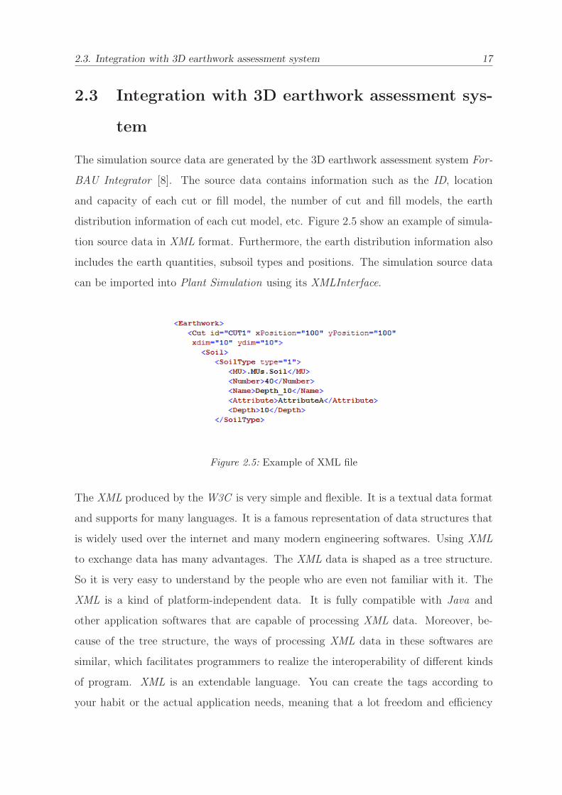
The simulation source data are generated by the 3D earthwork assessment system For-
BAU Integrator [8]. The source data contains information such as the ID, location
and capacity of each cut or fill model, the number of cut and fill models, the earth
distribution information of each cut model, etc. Figure 2.5 show an example of simula-
tion source data in XML format. Furthermore, the earth distribution information also
includes the earth quantities, subsoil types and positions. The simulation source data
can be imported into Plant Simulation using its XMLInterface.
Figure 2.5: Example of XML file
The XML produced by the W3C is very simple and flexible. It is a textual data format
and supports for many languages. It is a famous representation of data structures that
is widely used over the internet and many modern engineering softwares. Using XML
to exchange data has many advantages. The XML data is shaped as a tree structure.
So it is very easy to understand by the people who are even not familiar with it. The
XML is a kind of platform-independent data. It is fully compatible with Java and
other application softwares that are capable of processing XML data. Moreover, be-
cause of the tree structure, the ways of processing XML data in these softwares are
similar, which facilitates programmers to realize the interoperability of different kinds
of program. XML is an extendable language. You can create the tags according to
your habit or the actual application needs, meaning that a lot freedom and efficiency
2.4. Simulation results analysis 18
are acquired by users. All in all, from a programmer’s point of view, the XML is a
language of extreme simplicity, generality, flexibility and usability. It is a powerful and
appropriate tool to store and share data [6].
2.4 Simulation results analysis
The aim of the simulation system is to observe the behaviors of various components in
the real-world system. We want to use the simulation model to analyze earthwork pro-
ductivity. Moreover, we also need to calculate the utilization of involoved equipments
and observe whether the capacities or number of the road construction resources are
properly designed or not. All the above mentioned factors can influence the total cost
of the real-world system.
Because earth transportation that costs a huge amount of time and money is very
important in road construction. What we are interested in is the behavior of trans-
portation system. We fix other cost-related factors, e.g. the capacities of excavating
and filling machines, and only change the number and delivery path of trucks in order
to observe how the transportation behavior influences the whole system. Moreover,
during the simulation running, it is also necessary to calculate the effective utilization
of the truck. Such calculations are explained as follows:
Working portion. The working portion of a truck is the time portion during which the
truck runs on the road. As equation (2.1) illustrated, to calculation the factor, only the
total waiting time and the truck’s running time are need to be recorded.
WorkingPortion = 1 −
TotalWaitingTime
TotalRunningTime(2.1)
2.4. Simulation results analysis 19
Blocking portion. The blocking portion of a truck is the time portion during which the
truck is blocked on the road, e.g. in waiting zone of cut model. It does not include the
time portion during which the truck is loaded and unloaded. The calculation of the
blocking portion is according to equation (2.2) and equation (2.3):
TotalBlockingTime = TotalWaitingTime − LoadingAndUnloadingTime (2.2)
BlockingPortion =TotalBlockingTime
TotalRunningTime(2.3)
Average working portion. The average working portion is the arithmetic mean value of
the working portion values of all the involved trucks. It is calculated by equation (2.4):
AverageWorkingPortion =
∑WorkingPortion
TotalTruckNumber(2.4)
Average blocking portion. The average blocking portion is the arithmetic mean value
of the blocking portion values of the all involved trucks. It is calculated by equation
(2.5)[where is example].
AverageBlockingPortion =
∑BlockingPortion
TotalTruckNumber(2.5)
3. Earthwork simulation model in Plant Simulation 20
Chapter 3
Earthwork simulation model in
Plant Simulation
The last chapter introduces the idea of developing road construction simulation model.
This chapter will show how to realize the simulation concept in the commercial software
Plant Simulation [1]. This chapter can be divided into 2 parts. In the first part, we will
introduce the Plant Simulation and its programming language SimTalk. In the second
part, we will make an example of the road construction site scenario to explain working
principles and construction procedures.
3.1 Introduction to Plant Simulation
In section 1.2.2, we made a short introduction concerning Plant Simulation. This section
will explain the characteristics and working principle of Plant Simulation. In addition,
it is also necessary to introduce the Plant Simulation’s programming language SimTalk.
3.1.1 Characteristics of Plant Simulation
Plant Simulation is a discrete event simulation program, i.e., it only inspects those
points in time, at which events take place in the simulation model. For example, such
3.1. Introduction to Plant Simulation 21
events include an entity entering into or exiting out of a material flow object, or an
entity touches a sensor on a length-oriented material flow object. These events may
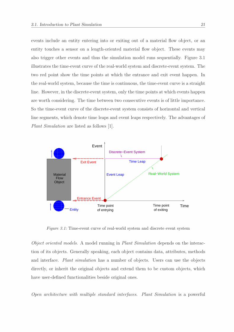
also trigger other events and thus the simulation model runs sequentially. Figure 3.1
illustrates the time-event curve of the real-world system and discrete-event system. The
two red point show the time points at which the entrance and exit event happen. In
the real-world system, because the time is continuous, the time-event curve is a straight
line. However, in the discrete-event system, only the time points at which events happen
are worth considering. The time between two consecutive events is of little importance.
So the time-event curve of the discrete-event system consists of horizontal and vertical
line segments, which denote time leaps and event leaps respectively. The advantages of
Plant Simulation are listed as follows [1].
MatrialFlow
Object
���������������������
���������������������
���������������������
���������������������
MaterialFlow
Object
Time pointTime pointof entrying of exitingEntity
Exit Event
Entrance Event
Event
Time
Discrete−Event System
Real−World SystemEvent Leap
Time Leap
Figure 3.1: Time-event curve of real-world system and discrete event system
Object oriented models. A model running in Plant Simulation depends on the interac-
tion of its objects. Generally speaking, each object contains data, attributes, methods
and interface. Plant simulation has a number of objects. Users can use the objects
directly, or inherit the original objects and extend them to be custom objects, which
have user-defined functionalities beside original ones.
Open architecture with multiple standard interfaces. Plant Simulation is a powerful
3.1. Introduction to Plant Simulation 22
platform to cooperate with other softwares because it has a variety of data interfaces.
It is able to import and export many types of file (e.g., Microsoft Excel file, XML file,
ODBC database). And these files often appear in modern engineering design softwares.
Library management. Plant Simulation has a variety of libraries (e.g., Kanban System,
Logistics, 3D Library). These libraries facilitate users from different simulation fields.
3.1.2 Graphical user interface overview
The following figure shows the graphical user interface of Plant Simulation. It includes
a menu bar, some tool bars, an Explorer, a Toolbox, a Console and a main panel. The
menu bar and tool bars, which collect all the operations and controlling functionalities,
are similar to most of common used softwares. The Console displays some system meth-
ods such as initialization, resetting, etc. It can not only displays errors when compiling
errors occur but also displays results when they are necessary to be output on screen.
The Toolbox has five tabs: Material Flow, Resources, Information Flow, User Interface
and Tools. Every tab has a number of built-in system objects which can be used to
construct scenarios.
The left side of the graphical user interface is the Explorer. Its Class Library tab lists
folders that store original system objects and custom objects. In the figure 3.2, the
first 6 folders have the same content as the Toolbox. The next few folders store custom
objects. For example, in the folder Components, we store the cut, fill, excavator, me-
chanical parts of excavator and track model. These models are the essential components
of a road construction site model. In addition, the Test folder stores testing cases of
single model, and the Task folder stores various construction site scenarios that imply
the development and improvement of the simulation model.
The center of the graphical user interface is the main panel. It shows simulation sce-
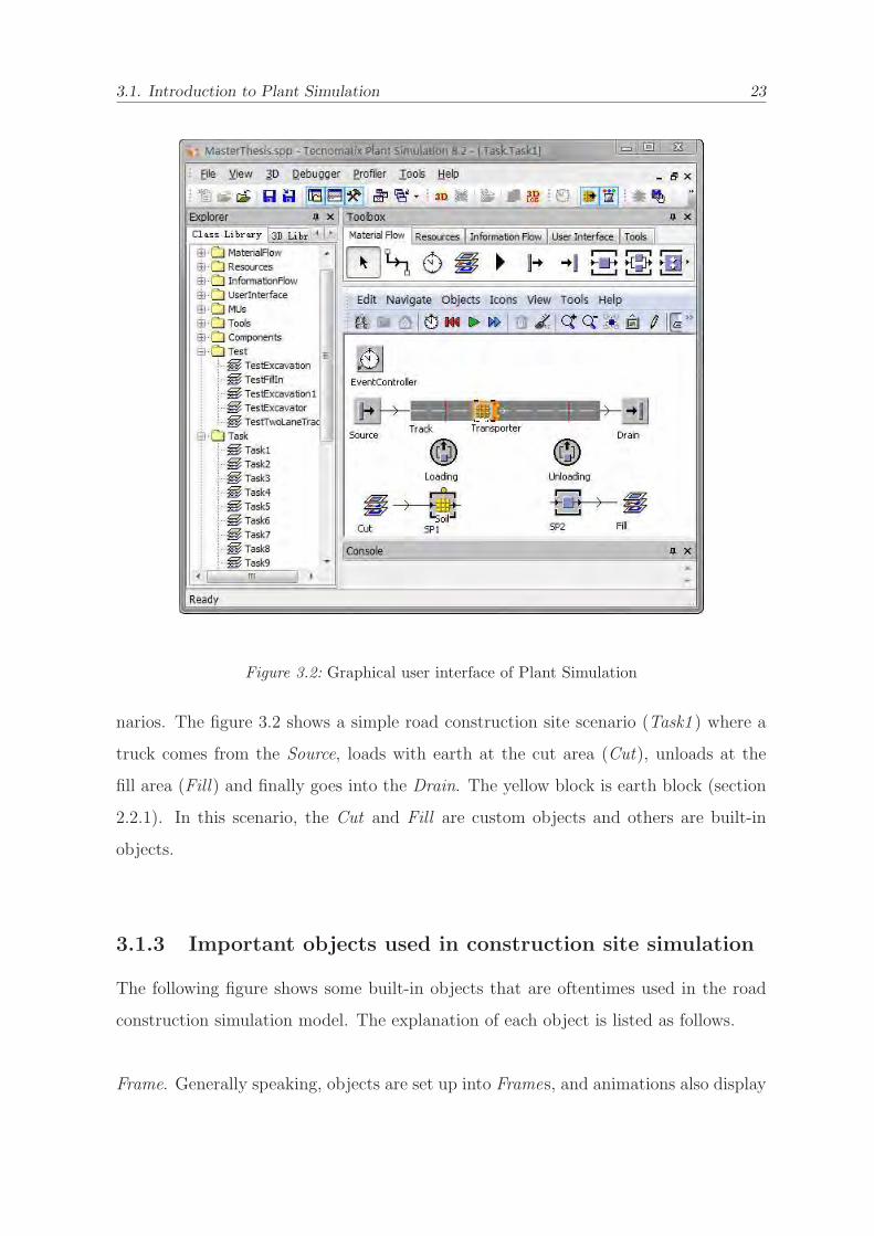
3.1. Introduction to Plant Simulation 23
Figure 3.2: Graphical user interface of Plant Simulation
narios. The figure 3.2 shows a simple road construction site scenario (Task1 ) where a
truck comes from the Source, loads with earth at the cut area (Cut), unloads at the
fill area (Fill) and finally goes into the Drain. The yellow block is earth block (section
2.2.1). In this scenario, the Cut and Fill are custom objects and others are built-in
objects.
3.1.3 Important objects used in construction site simulation
The following figure shows some built-in objects that are oftentimes used in the road
construction simulation model. The explanation of each object is listed as follows.
Frame. Generally speaking, objects are set up into Frames, and animations also display
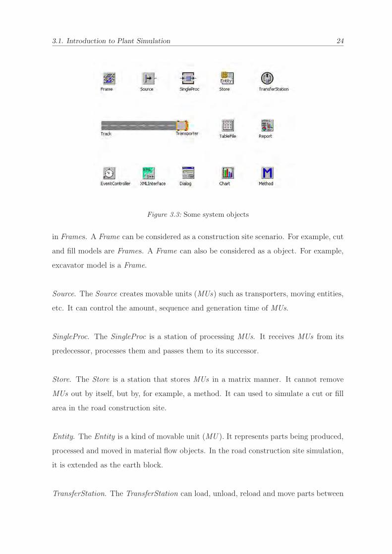
3.1. Introduction to Plant Simulation 24
Figure 3.3: Some system objects
in Frames. A Frame can be considered as a construction site scenario. For example, cut
and fill models are Frames. A Frame can also be considered as a object. For example,
excavator model is a Frame.
Source. The Source creates movable units (MUs) such as transporters, moving entities,
etc. It can control the amount, sequence and generation time of MUs.
SingleProc. The SingleProc is a station of processing MUs. It receives MUs from its
predecessor, processes them and passes them to its successor.
Store. The Store is a station that stores MUs in a matrix manner. It cannot remove
MUs out by itself, but by, for example, a method. It can used to simulate a cut or fill
area in the road construction site.
Entity. The Entity is a kind of movable unit (MU ). It represents parts being produced,
processed and moved in material flow objects. In the road construction site simulation,
it is extended as the earth block.
TransferStation. The TransferStation can load, unload, reload and move parts between
3.1. Introduction to Plant Simulation 25
two matrial flow objects.
Track and Transporter. They are basic components of earth transportation system.
Table. The Table can store data and interact with other objects. It is also an interface
to export and import XML files, EXCEL files, etc.
HTML report. The HTML report can store and show the results of simulation experi-
ments.
EventController. The EventController controls the running of a simulation. For exam-
ple, it can start, stop, initiate and reset a simulation. It can list the events that happen
in a simulation model.
XMLInterface. The XMLInterface is able to read and write XML file. It is a important
interface to communicate with other engineering softwares.
Dialog. The Dialog is a custom designed object. It facilitates users to manipulate com-
plicated models unnecessary to understand the model construction processes.
Chart. The Chart presents results of a simulation running. It makes user easier to view
the results and manage the model.
Method. The Method is written by the SimTalk language. It is a programming environ-
ment in Plant Simulation. It can be imported into many objects to control simulation
processes and achieve necessary calculations. The detail of the Method object and the
SimTalk language will be explained in the next section.
3.1. Introduction to Plant Simulation 26
3.1.4 Introduction to SimTalk
SimTalk based on the programming language Eiffel [11] is the programming language
provided by Plant Simulation. It extends the ways of controlling simulation model. In
Plant Simulation, each object has many built-in attributes. SimTalk can access and
change those attributes or even create new attributes for objects.
SimTalk language is written in the Method object. A Method is a small runnable pro-
gram on the Plant Simulation platform. The Method is always combined with other
objects in order to modify and extend their attributes. The Method is called by an
event or another Method.
SimTalk consists of two parts. One is the built-in methods in the material flow objects
and the information flow objects. The other is user defined methods, which realize user-
specified requirements. The user defined methods can extend the features of objects
and achieve some mathematical computation [2].
3.1.5 Event management in Plant Simulation
The simulation models in Plant Simulation are controlled by events. Most of events
happen when an entity is created or deleted, or when an entity enters or goes out of a
material flow object. For example, in the road construction simulation model, events
normally happen when a truck is created, a truck enters or goes out of a track, an earth
block is moved onto or removed out of a truck, an earth block passes through a material
flow object, etc.
Event always cooperates with control methods. In Plant Simulation, as soon as an
event happens, the corresponding method is called. Figure 3.4, which describes an en-
tity passing through a length-oriented material flow object, illustrates 4 kinds of event
control manner: front activated entrance control, rear activated entrance control, front
activated exit control and rear activated exit control. The front activated entrance con-
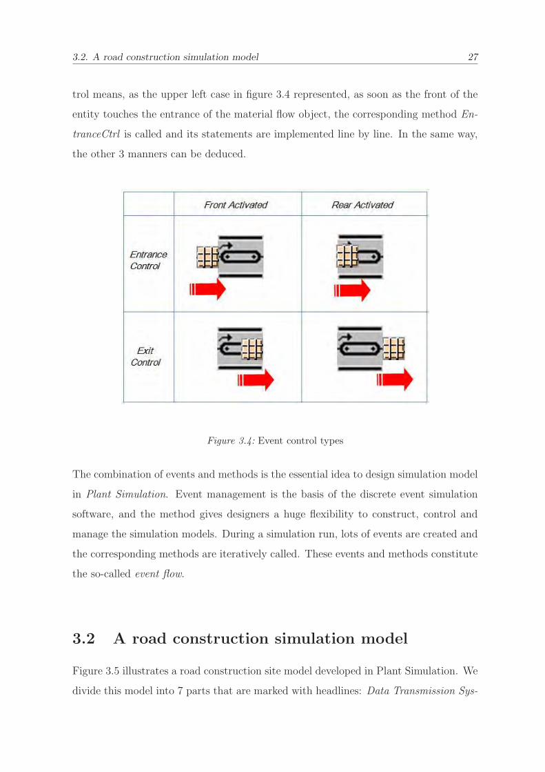
3.2. A road construction simulation model 27
trol means, as the upper left case in figure 3.4 represented, as soon as the front of the
entity touches the entrance of the material flow object, the corresponding method En-
tranceCtrl is called and its statements are implemented line by line. In the same way,
the other 3 manners can be deduced.
Figure 3.4: Event control types
The combination of events and methods is the essential idea to design simulation model
in Plant Simulation. Event management is the basis of the discrete event simulation
software, and the method gives designers a huge flexibility to construct, control and
manage the simulation models. During a simulation run, lots of events are created and
the corresponding methods are iteratively called. These events and methods constitute
the so-called event flow.
3.2 A road construction simulation model
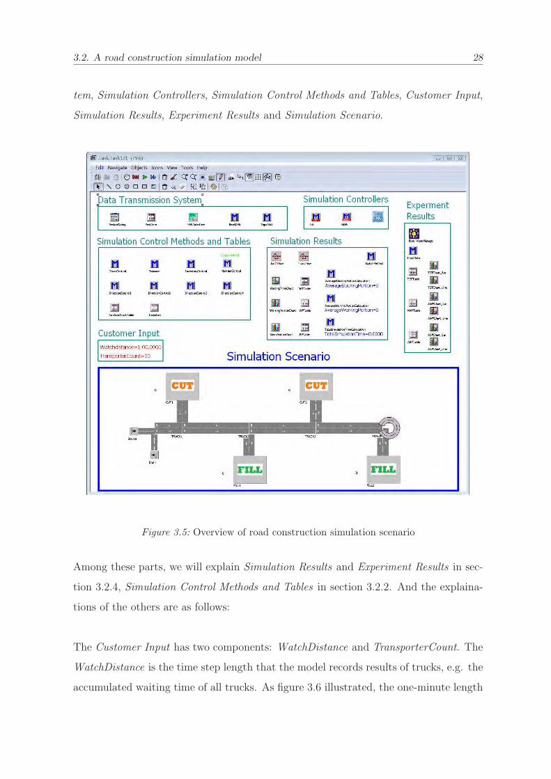
Figure 3.5 illustrates a road construction site model developed in Plant Simulation. We
divide this model into 7 parts that are marked with headlines: Data Transmission Sys-
3.2. A road construction simulation model 28
tem, Simulation Controllers, Simulation Control Methods and Tables, Customer Input,
Simulation Results, Experiment Results and Simulation Scenario.
Figure 3.5: Overview of road construction simulation scenario
Among these parts, we will explain Simulation Results and Experiment Results in sec-
tion 3.2.4, Simulation Control Methods and Tables in section 3.2.2. And the explaina-
tions of the others are as follows:
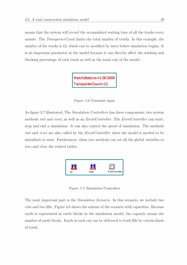
The Customer Input has two components: WatchDistance and TransporterCount. The
WatchDistance is the time step length that the model records results of trucks, e.g. the
accumulated waiting time of all trucks. As figure 3.6 illustrated, the one-minute length
3.2. A road construction simulation model 29
means that the system will record the accumulated waiting time of all the trucks every
minute. The TransporterCount limits the total number of trucks. In this example, the
number of the trucks is 12, which can be modified by users before simulation begins. It
is an important parameter in the model because it can directly affect the working and
blocking percentage of each truck as well as the total cost of the model.
Figure 3.6: Customer input
As figure 3.7 illustrated, The Simulation Controllers has three components, two system
methods init and reset, as well as an EventController. The EventController can start,
stop and end a simulation. It can also control the speed of simulation. The methods
init and reset are also called by the EventController when the model is needed to be
initialized or reset. Furthermore, these two methods can set all the global variables to
zero and clear the related tables.
Figure 3.7: Simulation Controllers
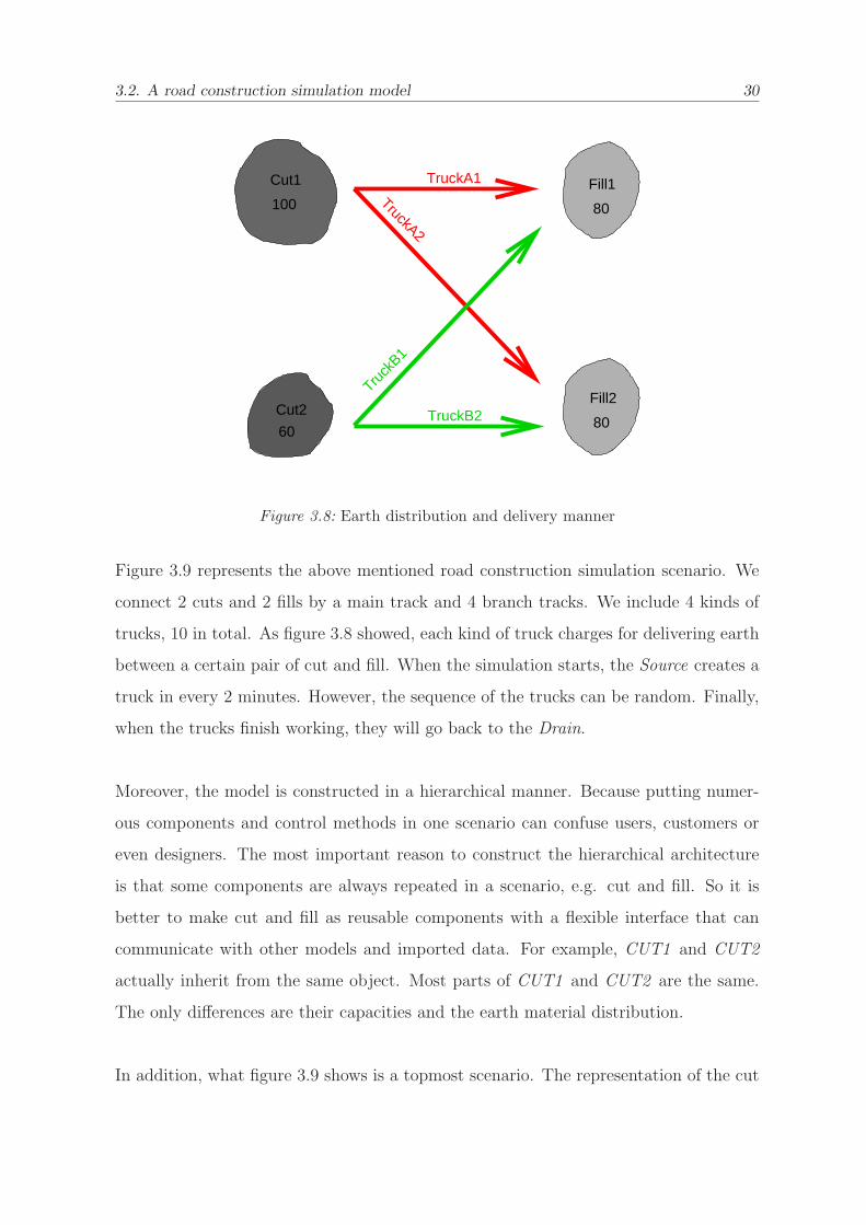
The most important part is the Simulation Scenario. In this scenario, we include two
cuts and two fills. Figure 3.8 shows the scheme of the scenario with capacities. Because
earth is represented as earth blocks in the simulation model, the capacity means the
number of earth blocks. Earth in each cut can be delivered to both fills by certain kinds
of truck.
3.2. A road construction simulation model 30
100
Cut1
60
Cut2
80
Fill1
Fill2
80
TruckA1
TruckB2
Truck
B1
TruckA2
Figure 3.8: Earth distribution and delivery manner
Figure 3.9 represents the above mentioned road construction simulation scenario. We
connect 2 cuts and 2 fills by a main track and 4 branch tracks. We include 4 kinds of
trucks, 10 in total. As figure 3.8 showed, each kind of truck charges for delivering earth
between a certain pair of cut and fill. When the simulation starts, the Source creates a
truck in every 2 minutes. However, the sequence of the trucks can be random. Finally,
when the trucks finish working, they will go back to the Drain.
Moreover, the model is constructed in a hierarchical manner. Because putting numer-
ous components and control methods in one scenario can confuse users, customers or
even designers. The most important reason to construct the hierarchical architecture
is that some components are always repeated in a scenario, e.g. cut and fill. So it is
better to make cut and fill as reusable components with a flexible interface that can
communicate with other models and imported data. For example, CUT1 and CUT2
actually inherit from the same object. Most parts of CUT1 and CUT2 are the same.
The only differences are their capacities and the earth material distribution.
In addition, what figure 3.9 shows is a topmost scenario. The representation of the cut
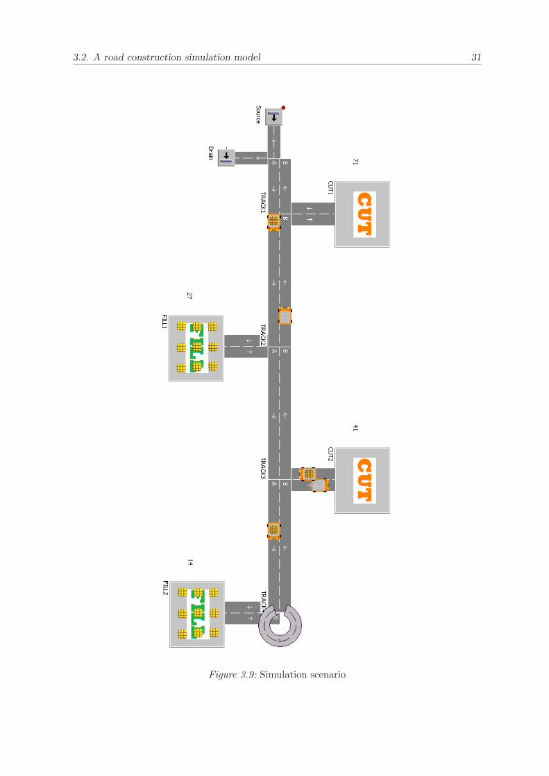
3.2. A road construction simulation model 31
Figure 3.9: Simulation scenario
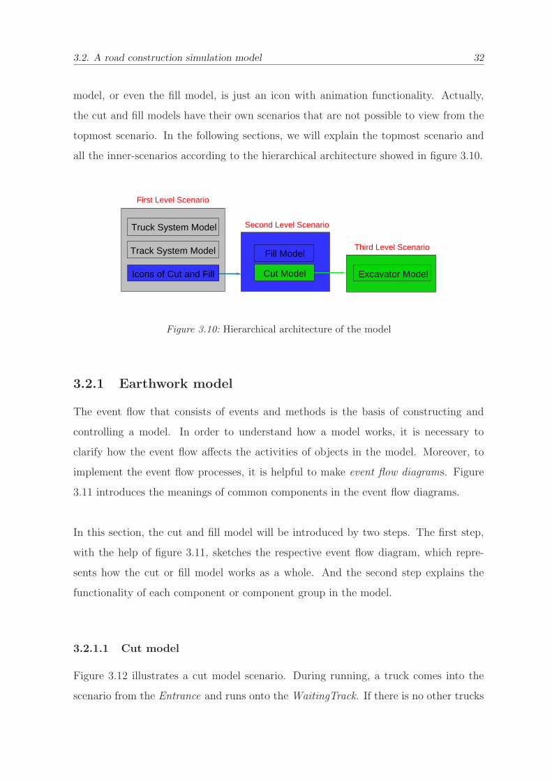
3.2. A road construction simulation model 32
model, or even the fill model, is just an icon with animation functionality. Actually,
the cut and fill models have their own scenarios that are not possible to view from the
topmost scenario. In the following sections, we will explain the topmost scenario and
all the inner-scenarios according to the hierarchical architecture showed in figure 3.10.
Truck System Model
Track System Model
Excavator Model
First Level Scenario
Second Level Scenario
Third Level Scenario
Cut Model
Fill Model
Icons of Cut and Fill
Figure 3.10: Hierarchical architecture of the model
3.2.1 Earthwork model
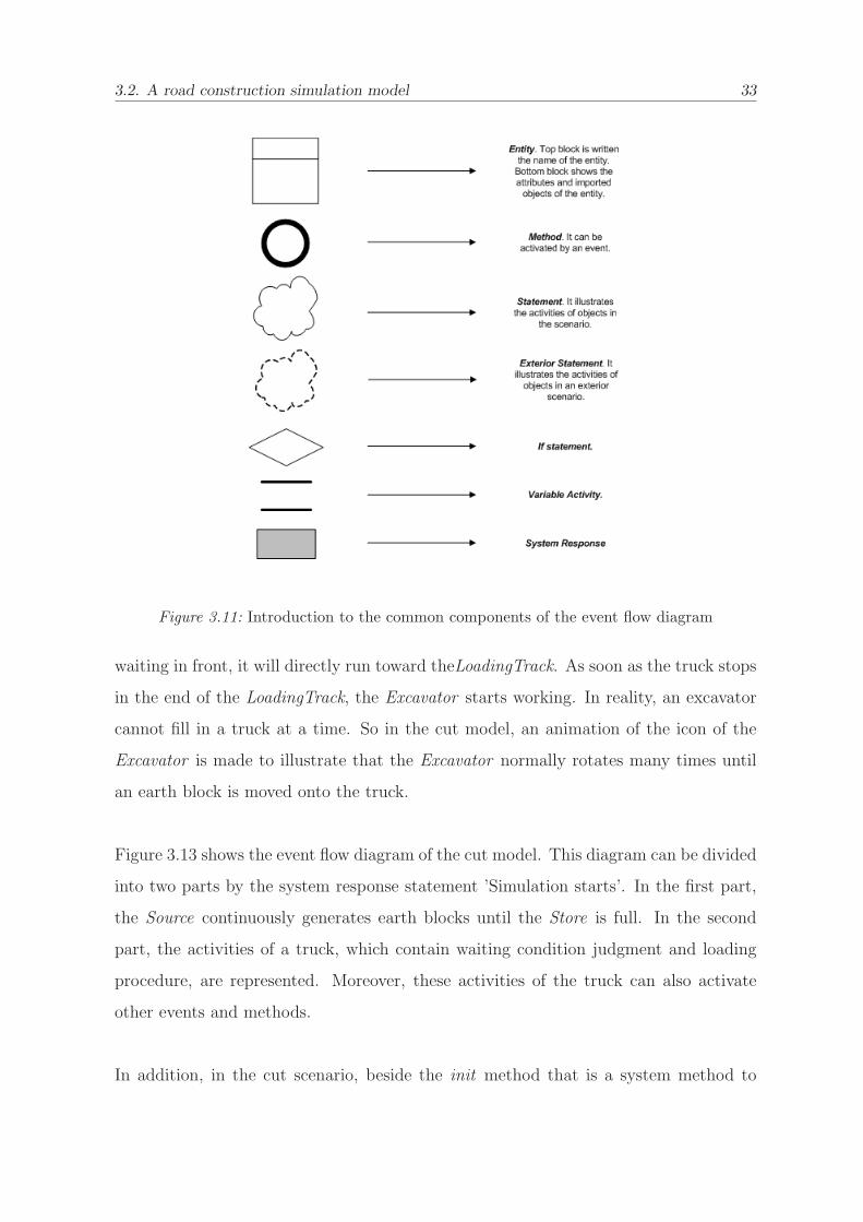
The event flow that consists of events and methods is the basis of constructing and
controlling a model. In order to understand how a model works, it is necessary to
clarify how the event flow affects the activities of objects in the model. Moreover, to
implement the event flow processes, it is helpful to make event flow diagrams. Figure
3.11 introduces the meanings of common components in the event flow diagrams.
In this section, the cut and fill model will be introduced by two steps. The first step,
with the help of figure 3.11, sketches the respective event flow diagram, which repre-
sents how the cut or fill model works as a whole. And the second step explains the
functionality of each component or component group in the model.
3.2.1.1 Cut model
Figure 3.12 illustrates a cut model scenario. During running, a truck comes into the
scenario from the Entrance and runs onto the WaitingTrack. If there is no other trucks
3.2. A road construction simulation model 33
Figure 3.11: Introduction to the common components of the event flow diagram
waiting in front, it will directly run toward theLoadingTrack. As soon as the truck stops
in the end of the LoadingTrack, the Excavator starts working. In reality, an excavator
cannot fill in a truck at a time. So in the cut model, an animation of the icon of the
Excavator is made to illustrate that the Excavator normally rotates many times until
an earth block is moved onto the truck.
Figure 3.13 shows the event flow diagram of the cut model. This diagram can be divided
into two parts by the system response statement ’Simulation starts’. In the first part,
the Source continuously generates earth blocks until the Store is full. In the second
part, the activities of a truck, which contain waiting condition judgment and loading
procedure, are represented. Moreover, these activities of the truck can also activate
other events and methods.
In addition, in the cut scenario, beside the init method that is a system method to
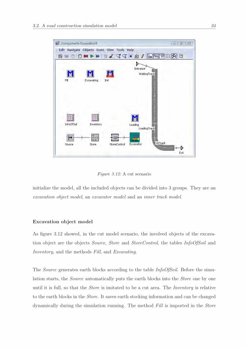
3.2. A road construction simulation model 34
Figure 3.12: A cut scenario
initialize the model, all the included objects can be divided into 3 groups. They are an
excavation object model, an excavator model and an inner track model.
Excavation object model
As figure 3.12 showed, in the cut model scenario, the involved objects of the excava-
tion object are the objects Source, Store and StoreControl, the tables InfoOfSoil and
Inventory, and the methods Fill, and Excavating.
The Source generates earth blocks according to the table InfoOfSoil. Before the simu-
lation starts, the Source automatically puts the earth blocks into the Store one by one
until it is full, so that the Store is imitated to be a cut area. The Inventory is relative
to the earth blocks in the Store. It saves earth stocking information and can be changed
dynamically during the simulation running. The method Fill is imported in the Store
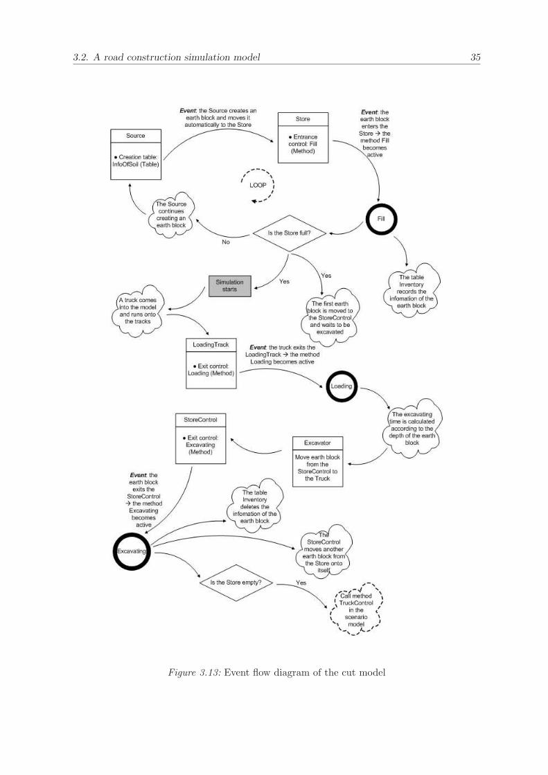
3.2. A road construction simulation model 35
Figure 3.13: Event flow diagram of the cut model
3.2. A road construction simulation model 36
as an entrance control method. As soon as an earth block goes into the Store, the Fill
changes the content of the Inventory. Furthermore, it also judges whether the Store is
full or not. If it is full, the simulation starts.
Because the Store object in Plant Simulation cannot remove its stock by its own, it is
necessary to set up an SingleProc object StoreControl to help the earth blocks move
out of the Store. The method Excavating is imported into the StoreControl as an exit
control. As soon as an earth block goes out of the StoreControl, the method moves
another earth block out of the Store and at the same time update the Inventory. Fur-
thermore, the method also judges whether the Store is empty or not. If it is empty, it
will call the method TruckControl in the topmost scenario (figure 3.5) which lets the
corresponding trucks stop working.
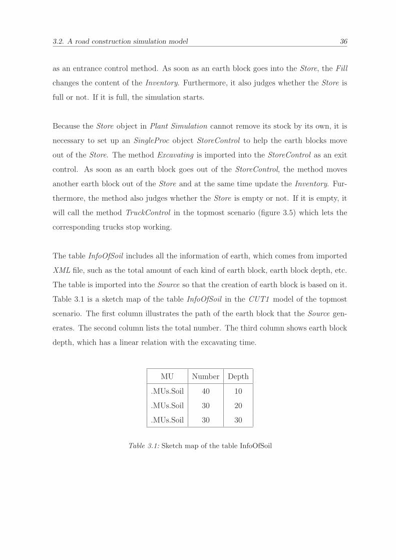
The table InfoOfSoil includes all the information of earth, which comes from imported
XML file, such as the total amount of each kind of earth block, earth block depth, etc.
The table is imported into the Source so that the creation of earth block is based on it.
Table 3.1 is a sketch map of the table InfoOfSoil in the CUT1 model of the topmost
scenario. The first column illustrates the path of the earth block that the Source gen-
erates. The second column lists the total number. The third column shows earth block
depth, which has a linear relation with the excavating time.
MU Number Depth
.MUs.Soil 40 10
.MUs.Soil 30 20
.MUs.Soil 30 30
Table 3.1: Sketch map of the table InfoOfSoil
3.2. A road construction simulation model 37
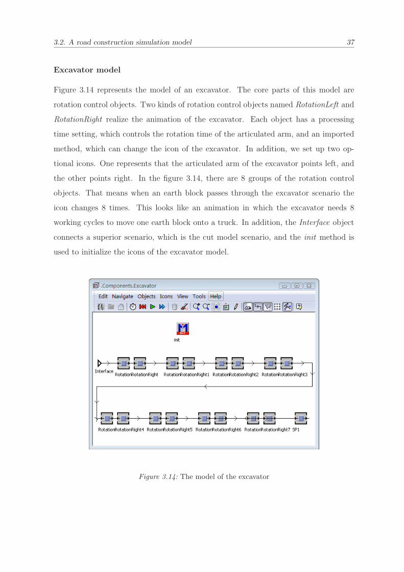
Excavator model
Figure 3.14 represents the model of an excavator. The core parts of this model are
rotation control objects. Two kinds of rotation control objects named RotationLeft and
RotationRight realize the animation of the excavator. Each object has a processing
time setting, which controls the rotation time of the articulated arm, and an imported
method, which can change the icon of the excavator. In addition, we set up two op-
tional icons. One represents that the articulated arm of the excavator points left, and
the other points right. In the figure 3.14, there are 8 groups of the rotation control
objects. That means when an earth block passes through the excavator scenario the
icon changes 8 times. This looks like an animation in which the excavator needs 8
working cycles to move one earth block onto a truck. In addition, the Interface object
connects a superior scenario, which is the cut model scenario, and the init method is
used to initialize the icons of the excavator model.
Figure 3.14: The model of the excavator
3.2. A road construction simulation model 38
Inner track model
Figure 3.12 shows the involved objects of the inner track model are the Track objects
WaitingTrack, LoadingTrack and ExitTrack, the Interface objects Entrance and Exit,
and the method Loading.
The Entrance and Exit connect to the external earth transportation system which is
located in the topmost scenario (figure 3.9). They are the entrance and exit of trucks
that come into the cut model. The truck queuing system is constructed by the capacity
of 3 tracks. The capacity of the LoadingTrack is 1 and the capacity of other tracks is
infinite. That means if there is a truck running on the LoadingTrack, other later-coming
trucks have to wait on the WaitingTrack. The Loading is the exit control method of the
LoadingTrack. The method has 4 functions. First, the method controls the behavior of
the earth block. It can move an earth block onto a truck. Second, the method controls
the behavior of the truck. In the beginning, it stops the truck, and later, it moves the
truck to the ExitTrack after it is loaded. Third, the method calculates the excavating
time of the Excavator. In this example model, the processing time has a linear relation
with the depth of the earth block. Fourth, the method controls the behavior of the
Excavator. The Excavator starts working when a truck reaches the end of the Loading-
Track and stops working when the truck is full.
3.2.1.2 Fill model
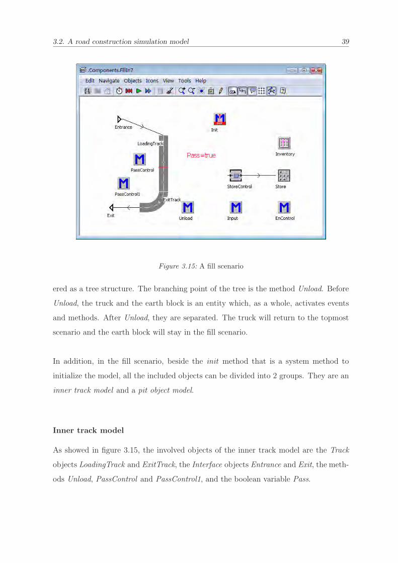
Figure 3.15 illustrates a fill model scenario. During running, a truck comes into the
scenario from the Entrance and runs onto the LoadingTrack. If there is a truck waiting
in front, it will stop before the red line that is a Sensor object. Otherwise, the truck
keeps moving. As soon as the truck stops in the end of the LoadingTrack, is will be
unloaded. Then, the earth block moves toward the Store automatically, and the truck
goes out of the scenario by the Exit.
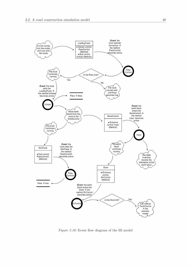
Figure 3.16 shows the event flow diagram of the fill model. This diagram can be consid-
3.2. A road construction simulation model 39
Figure 3.15: A fill scenario
ered as a tree structure. The branching point of the tree is the method Unload. Before
Unload, the truck and the earth block is an entity which, as a whole, activates events
and methods. After Unload, they are separated. The truck will return to the topmost
scenario and the earth block will stay in the fill scenario.
In addition, in the fill scenario, beside the init method that is a system method to
initialize the model, all the included objects can be divided into 2 groups. They are an
inner track model and a pit object model.
Inner track model
As showed in figure 3.15, the involved objects of the inner track model are the Track
objects LoadingTrack and ExitTrack, the Interface objects Entrance and Exit, the meth-
ods Unload, PassControl and PassControl1, and the boolean variable Pass.
3.2. A road construction simulation model 40
Figure 3.16: Event flow diagram of the fill model
3.2. A road construction simulation model 41
As the former section mentioned, the Entrance and Exit connect to the external earth
transportation system which is located in the topmost scenario. They are the entrance
and exit of trucks that come into the fill model. The truck queuing system is constructed
by the 2 tracks, 3 methods PassControl, PassControl1 and Unload, and the boolean
variable Pass. The PassControl is combined with the sensor (red line) on the Loading-
Track. The truck coming into the scenario can pass the sensor if the Pass is ’true’ or
should wait if it is ’false’. The Unload is the exit control method of the LoadingTrack.
As soon as a truck passes the sensor and touches the exit of the track, the Unload
method makes the Pass turn into ’false’ to prevent following trucks passing through
the red line. The PassControl1 is the exit control method of the ExitTrack. So when
the unloading finishes and the truck moves out of the track, the method PassControl1
makes the Pass turn into ’true’ again. This ensures that only one truck can run on
the track fragment which is from the sensor to the exit of the ExitTrack. By the way,
although the control manner of the queuing system is different from the one in the cut
model, the principles are the same. Furthermore, the Unload method still has 2 more
functions beside controlling Pass. First, the method controls the behavior of the earth
block. It can move an earth block out of a truck and put it onto the StoreControl.
Second, the method controls the behavior of the truck. In the beginning, it stops the
truck, and later, it moves the truck to the ExitTrack after it is unloaded.
Pit object model
As figure 3.15 showed, in the fill model scenario, the involved objects of the pit object
are the objects Store and StoreControl, the table Inventory, and the methods Input and
EnControl.
The Input is the entrance control method of the StoreControl. It updates the Inventory,
which records stock information of the Store, when an earth block is removed from a
truck. The StoreControl can be regarded as a simple bulldozer model whose capacity
is one earth block and processing time is one minute. The EnControl is the entrance
3.2. A road construction simulation model 42
control method of the Store. It judges whether the Store is full or not. If it is full,
it will call the method TruckControl in the topmost scenario which lets corresponding
trucks stop working.
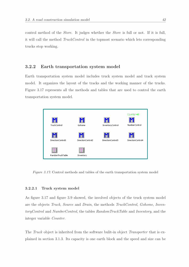
3.2.2 Earth transportation system model
Earth transportation system model includes truck system model and track system
model. It organizes the layout of the tracks and the working manner of the trucks.
Figure 3.17 represents all the methods and tables that are used to control the earth
transportation system model.
Figure 3.17: Control methods and tables of the earth transportation system model
3.2.2.1 Truck system model
As figure 3.17 and figure 3.9 showed, the involved objects of the truck system model
are the objects Truck, Source and Drain, the methods TruckControl, Gohome, Inven-
toryControl and NumberControl, the tables RandomTruckTable and Inventory, and the
integer variable Counter.
The Truck object is inherited from the software bulit-in object Transporter that is ex-
plained in section 3.1.3. Its capacity is one earth block and the speed and size can be
3.2. A road construction simulation model 43
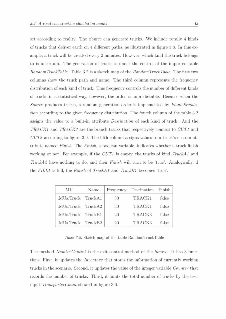
set according to reality. The Source can generate trucks. We include totally 4 kinds
of trucks that deliver earth on 4 different paths, as illustrated in figure 3.8. In this ex-
ample, a truck will be created every 2 minutes. However, which kind the truck belongs
to is uncertain. The generation of trucks is under the control of the imported table
RandomTruckTable. Table 3.2 is a sketch map of the RandomTruckTable. The first two
columns show the truck path and name. The third column represents the frequency
distribution of each kind of truck. This frequency controls the number of different kinds
of trucks in a statistical way, however, the order is unpredictable. Because when the
Source produces trucks, a random generation order is implemented by Plant Simula-
tion according to the given frequency distribution. The fourth column of the table 3.2
assigns the value to a built-in attribute Destination of each kind of truck. And the
TRACK1 and TRACK3 are the branch tracks that respectively connect to CUT1 and
CUT2 according to figure 3.9. The fifth column assigns values to a truck’s custom at-
tribute named Finish. The Finish, a boolean variable, indicates whether a truck finish
working or not. For example, if the CUT1 is empty, the trucks of kind TruckA1 and
TruckA2 have nothing to do, and their Finish will turn to be ’true’. Analogically, if
the FILL1 is full, the Finish of TruckA1 and TruckB1 becomes ’true’.
MU Name Frequency Destination Finish
.MUs.Truck TruckA1 30 TRACK1 false
.MUs.Truck TruckA2 30 TRACK1 false
.MUs.Truck TruckB1 20 TRACK3 false
.MUs.Truck TruckB2 20 TRACK3 false
Table 3.2: Sketch map of the table RandomTruckTable
The method NumberControl is the exit control method of the Source. It has 3 func-
tions. First, it updates the Inventory that stores the information of currently working
trucks in the scenario. Second, it updates the value of the integer variable Counter that
records the number of trucks. Third, it limits the total number of trucks by the user
input TransporterCount showed in figure 3.6.
3.2. A road construction simulation model 44
The method TruckControl controls the custom attribute Finish of all the currently
working trucks. When a truck finishes its task, the Finish attribute will be altered
from ’false’ to ’true’ by the TruckControl. The method is called if a cut is empty or
a fill is full. Meanwhile, it activates another method name Gohome that let the truck
whose Finish is ’true’ goes to the object Drain. All in all, the TruckControl, Gohome
and Finish can be considered as a control module that makes corresponding trucks
stop working according to the situation of the cuts and fills. In addition, the method
InventoryControl is the entrance control method of the Drain. It updates the Inventory
by deleting the information of the truck that comes into the Drain.
3.2.2.2 Track system model
As figure 3.17 and figure 3.9 showed, the involved objects of the track system model
are all the tracks and the 4 methods named DirectionControl1, DirectionControl2, Di-
rectionControl3 and DirectionControl4.
All the tracks are divided into two kinds: main track and branch tracks. There are
totally 4 branch tracks: TRACK1, TRACK2, TRACK3 and TRACK4. Each branch
track is imported a direction control method. The direction control method controls
the destination of the truck which reaches the crossroad. For example, when a truck
full of earth moves out of CUT1 and reaches the crossroad that is formed by TRACK1
and the main track, the method DirectionControl1 becomes working. The method let
the TruckA1 move toward FILL1 and the TruckA2 move toward FILL2.
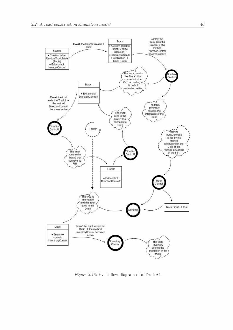
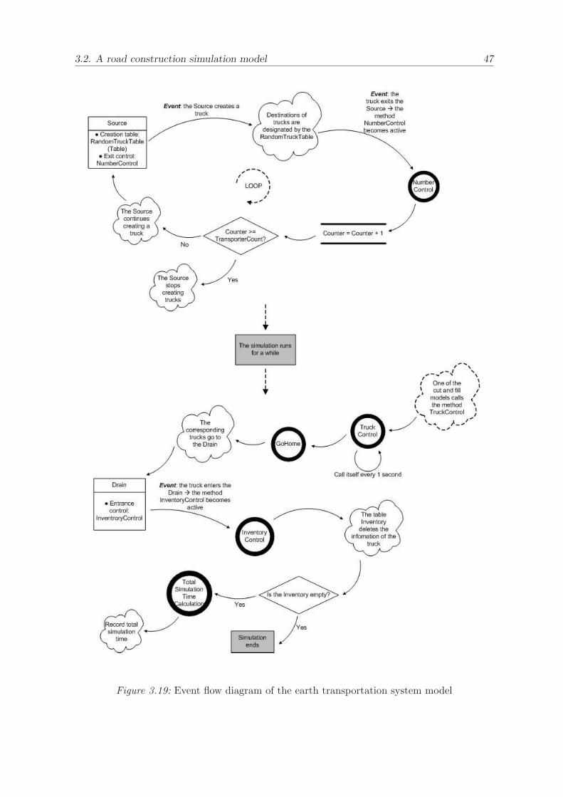
3.2.2.3 Event flow of the earth transportation system model
The following two figures are the event flow diagrams of the earth transportation system
model. Figure 3.18 represents how the event flow of a truck of the type TruckA1 looks
like during its whole life cycle. And figure 3.19 is the event flow diagram of the earth
3.2. A road construction simulation model 45
transportation system model.
Figure 3.18 can be divided into two parts. In the first part, a truck is produced and
carries earth between CUT1 and FILL1 time and time again. This procedure is de-
scribed by a ’LOOP’ sign. In the second part, the method TruckControl is called by
the CUT1 or FILL1. The truck gets a signal of stopping working and at the same time
the loop is interrupted. Then, the truck goes to the Drain and its lift cycle ends.
Figure 3.19 can also be divided into two parts. The first part illustrates how the system
controls the total number of trucks. In the second part, after all the trucks carry earth
for a while, the TruckControl is called by a cut or a fill model. Moreover, the method
calls itself every one second to check the status of the trucks so that the corresponding
trucks stop working. After all the trucks finish working and go into the Drain, the
simulation ends and the total simulation time should be recorded.
3.2. A road construction simulation model 46
Figure 3.18: Event flow diagram of a TruckA1
3.2. A road construction simulation model 47
Figure 3.19: Event flow diagram of the earth transportation system model
3.2. A road construction simulation model 48
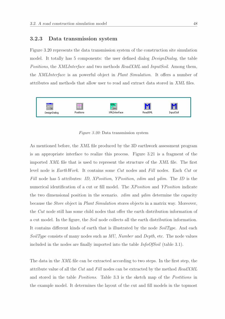
3.2.3 Data transmission system
Figure 3.20 represents the data transmission system of the construction site simulation
model. It totally has 5 components: the user defined dialog DesignDialog, the table
Positions, the XMLInterface and two methods ReadXML and InputSoil. Among them,
the XMLInterface is an powerful object in Plant Simulation. It offers a number of
attributes and methods that allow user to read and extract data stored in XML files.
Figure 3.20: Data transmission system
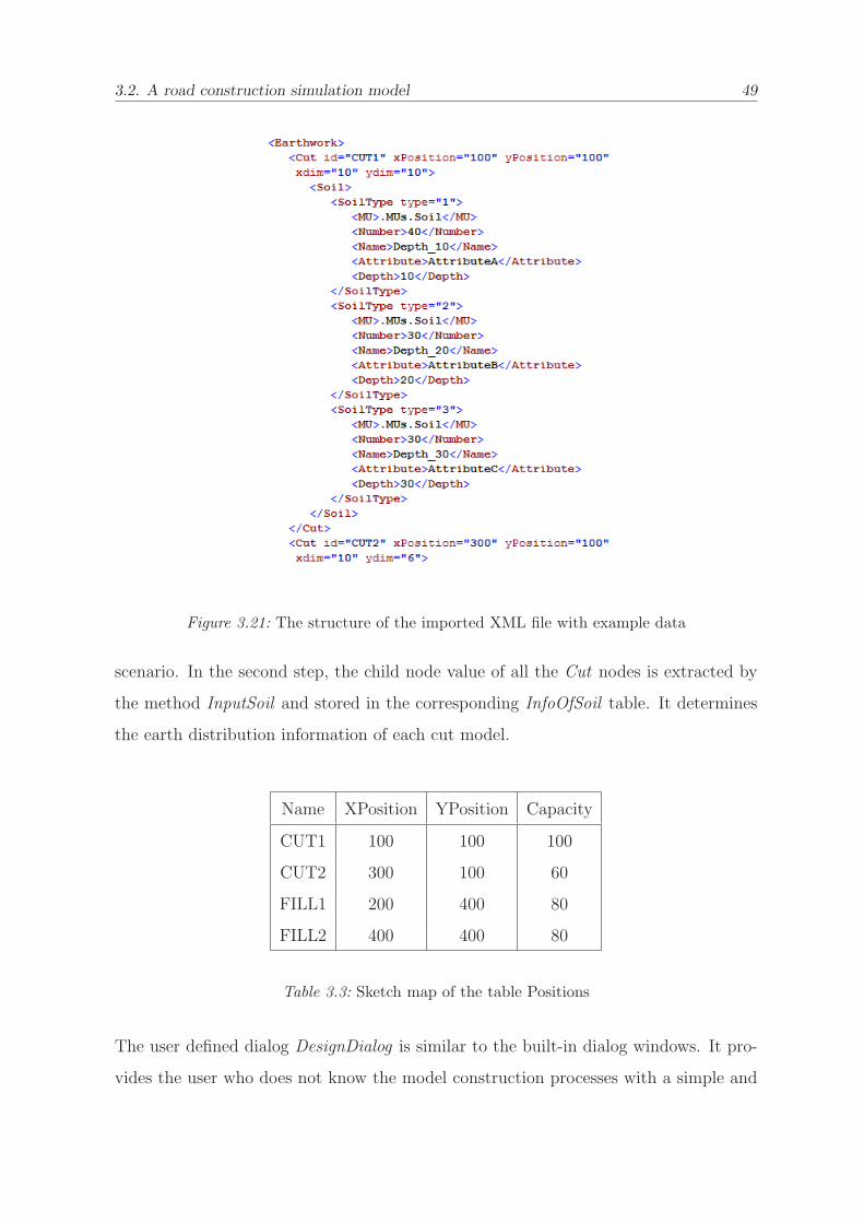
As mentioned before, the XML file produced by the 3D earthwork assessment program
is an appropriate interface to realize this process. Figure 3.21 is a fragment of the
imported XML file that is used to represent the structure of the XML file. The first
level node is EarthWork. It contains some Cut nodes and Fill nodes. Each Cut or
Fill node has 5 attributes: ID, XPosition, YPosition, xdim and ydim. The ID is the
numerical identification of a cut or fill model. The XPosition and YPosition indicate
the two dimensional position in the scenario. xdim and ydim determine the capacity
because the Store object in Plant Simulation stores objects in a matrix way. Moreover,
the Cut node still has some child nodes that offer the earth distribution information of
a cut model. In the figure, the Soil node collects all the earth distribution information.
It contains different kinds of earth that is illustrated by the node SoilType. And each
SoilType consists of many nodes such as MU, Number and Depth, etc. The node values
included in the nodes are finally imported into the table InfoOfSoil (table 3.1).
The data in the XML file can be extracted according to two steps. In the first step, the
attribute value of all the Cut and Fill nodes can be extracted by the method ReadXML
and stored in the table Positions. Table 3.3 is the sketch map of the Postitions in
the example model. It determines the layout of the cut and fill models in the topmost
3.2. A road construction simulation model 49
Figure 3.21: The structure of the imported XML file with example data
scenario. In the second step, the child node value of all the Cut nodes is extracted by
the method InputSoil and stored in the corresponding InfoOfSoil table. It determines
the earth distribution information of each cut model.
Name XPosition YPosition Capacity
CUT1 100 100 100
CUT2 300 100 60
FILL1 200 400 80
FILL2 400 400 80
Table 3.3: Sketch map of the table Positions
The user defined dialog DesignDialog is similar to the built-in dialog windows. It pro-
vides the user who does not know the model construction processes with a simple and
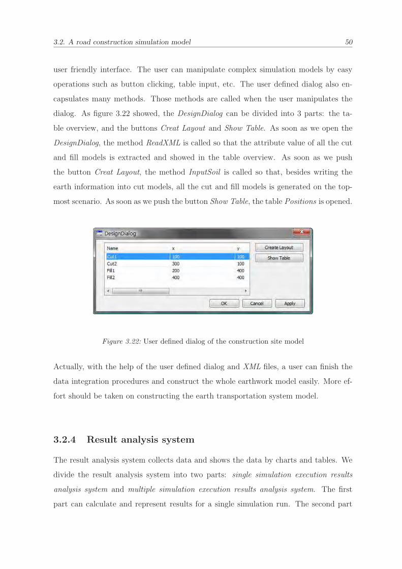
3.2. A road construction simulation model 50
user friendly interface. The user can manipulate complex simulation models by easy
operations such as button clicking, table input, etc. The user defined dialog also en-
capsulates many methods. Those methods are called when the user manipulates the
dialog. As figure 3.22 showed, the DesignDialog can be divided into 3 parts: the ta-
ble overview, and the buttons Creat Layout and Show Table. As soon as we open the
DesignDialog, the method ReadXML is called so that the attribute value of all the cut
and fill models is extracted and showed in the table overview. As soon as we push
the button Creat Layout, the method InputSoil is called so that, besides writing the
earth information into cut models, all the cut and fill models is generated on the top-
most scenario. As soon as we push the button Show Table, the table Positions is opened.
Figure 3.22: User defined dialog of the construction site model
Actually, with the help of the user defined dialog and XML files, a user can finish the
data integration procedures and construct the whole earthwork model easily. More ef-
fort should be taken on constructing the earth transportation system model.
3.2.4 Result analysis system
The result analysis system collects data and shows the data by charts and tables. We
divide the result analysis system into two parts: single simulation execution results
analysis system and multiple simulation execution results analysis system. The first
part can calculate and represent results for a single simulation run. The second part
3.2. A road construction simulation model 51
can get statistical results of multiply simulation executions.
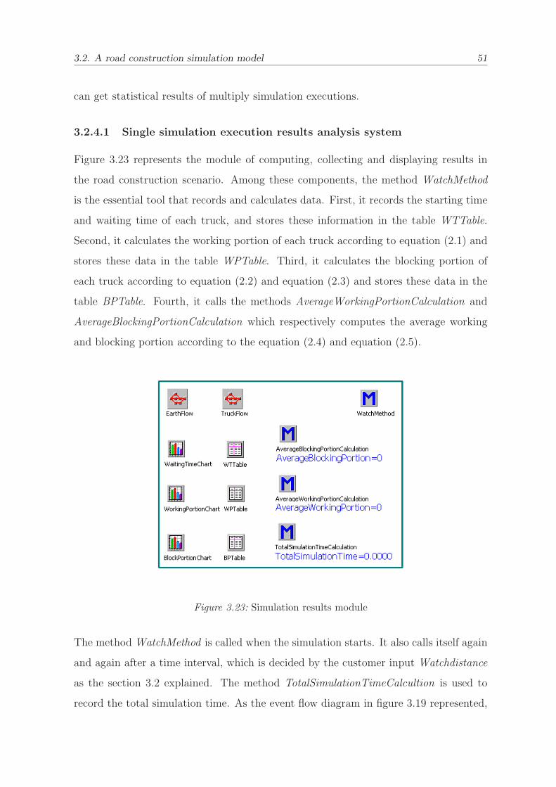
3.2.4.1 Single simulation execution results analysis system
Figure 3.23 represents the module of computing, collecting and displaying results in
the road construction scenario. Among these components, the method WatchMethod
is the essential tool that records and calculates data. First, it records the starting time
and waiting time of each truck, and stores these information in the table WTTable.
Second, it calculates the working portion of each truck according to equation (2.1) and
stores these data in the table WPTable. Third, it calculates the blocking portion of
each truck according to equation (2.2) and equation (2.3) and stores these data in the
table BPTable. Fourth, it calls the methods AverageWorkingPortionCalculation and
AverageBlockingPortionCalculation which respectively computes the average working
and blocking portion according to the equation (2.4) and equation (2.5).
Figure 3.23: Simulation results module
The method WatchMethod is called when the simulation starts. It also calls itself again
and again after a time interval, which is decided by the customer input Watchdistance
as the section 3.2 explained. The method TotalSimulationTimeCalcultion is used to
record the total simulation time. As the event flow diagram in figure 3.19 represented,
3.2. A road construction simulation model 52
it is called when all the trucks finish working and the table Inventory becomes empty.
The global variables AverageBlockPortion, AverageWorkingPortion and TotalSimula-
tionTime are used to display the simulation results. They are respectively controlled
by the corresponding methods over them. The charts WaitingTimeChart, WorkingPor-
tionChart and BlockingPortionChart can convert the data stored in WTTable, WPTable
and BPTable into diagrams. In addition, in figure 3.23, the EarthFlow and TruckFlow
are the SankeyDiagram objects in Plant Simulation. We use these two objects to show
the flow quantity of trucks and earth blocks.
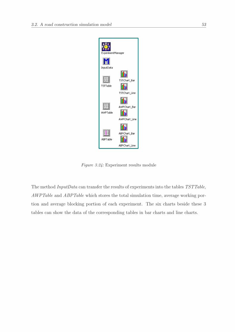
3.2.4.2 Multiple simulation execution results analysis system
Figure 3.24 represents the module of designing experiment, collecting data and dis-
playing results. The essential object in this module is the ExperimentManager. It is
a powerful tool of executing different case studies. Users can implement a case study,
which contains one or several experiments, in the ExperimentManager in order to ob-
serve different model parameters and analysis the statistical results. A case study
always investigates how a certain sets of system input values influence the correspond-
ing output values. Each experiment in the case study has a certain set of input values.
Normally, an experiment has one or several simulation runs which is named observation.
So all the observations in an experiment have the same set of input values.
Generally speaking, if a model has a random process, the simulation results become un-
predictable. For example, in this road construction simulation model, it is impossible
to predict the sequence of trucks and the number of each kind of truck. The objective of
such a stochastic case study is to calculate the statistical results such as the standard
deviation and the mean value, etc. In an experiment of such a stochastic problem,
several observations with unchanged input value are required to get an accurate sta-
tistical result. However, the seed values of generating random number stream in each
observation should be different. With the help of ExperimentManager, the experiments
and observations are automatically executed.
3.2. A road construction simulation model 53
Figure 3.24: Experiment results module
The method InputData can transfer the results of experiments into the tables TSTTable,
AWPTable and ABPTable which stores the total simulation time, average working por-
tion and average blocking portion of each experiment. The six charts beside these 3
tables can show the data of the corresponding tables in bar charts and line charts.
4. Simulation Results and Analysis 54
Chapter 4
Simulation Results and Analysis
How long can the earthwork finish? How is the utilization of involved construction
equipments? Is it possible that the transportation system is failed by traffic jam?
What should be the proper number of the trucks? After the simulation model is con-
structed and carried out in Plant Simulation, all of these questions can be answered.
In this chapter, the simulation results will be showed by tables and charts at first. Then
2 case studies are set up to illustrate statistical results. These simulation results can
validate the accuracy of the simulation model and at the same time can offer proposals
for designers to organize road construction resources.
4.1 Results of a single simulation execution
During the simulation running, 10 trucks are produced according to the RandomTruck-
Table as showed in table 3.2. That means the number of each kind of truck is random
and the sequence of the trucks is also random. Figure 4.1 is the table Inventory (sec-
tion 3.2.2.1) in the simulation scenario. The first two columns represent the numeration
and corresponding types of the trucks. The third column records the path and built-in
numeration of each truck, which is used to control the truck behavior by the SimTalk
programming language. Totally, there are 3 TruckA1 s, 3 TruckA2 s, 2 TruckB1 s and 2
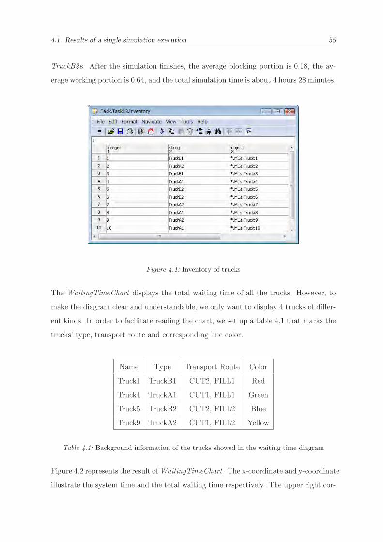
4.1. Results of a single simulation execution 55
TruckB2 s. After the simulation finishes, the average blocking portion is 0.18, the av-
erage working portion is 0.64, and the total simulation time is about 4 hours 28 minutes.
Figure 4.1: Inventory of trucks
The WaitingTimeChart displays the total waiting time of all the trucks. However, to
make the diagram clear and understandable, we only want to display 4 trucks of differ-
ent kinds. In order to facilitate reading the chart, we set up a table 4.1 that marks the
trucks’ type, transport route and corresponding line color.
Name Type Transport Route Color
Truck1 TruckB1 CUT2, FILL1 Red
Truck4 TruckA1 CUT1, FILL1 Green
Truck5 TruckB2 CUT2, FILL2 Blue
Truck9 TruckA2 CUT1, FILL2 Yellow
Table 4.1: Background information of the trucks showed in the waiting time diagram
Figure 4.2 represents the result of WaitingTimeChart. The x-coordinate and y-coordinate
illustrate the system time and the total waiting time respectively. The upper right cor-
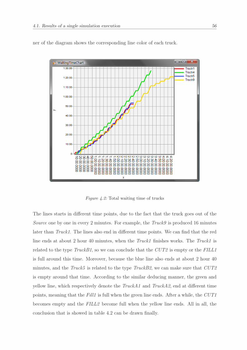
4.1. Results of a single simulation execution 56
ner of the diagram shows the corresponding line color of each truck.
Figure 4.2: Total waiting time of trucks
The lines starts in different time points, due to the fact that the truck goes out of the
Source one by one in every 2 minutes. For example, the Truck9 is produced 16 minutes
later than Truck1. The lines also end in different time points. We can find that the red
line ends at about 2 hour 40 minutes, when the Truck1 finishes works. The Truck1 is
related to the type TruckB1, so we can conclude that the CUT2 is empty or the FILL1
is full around this time. Moreover, because the blue line also ends at about 2 hour 40
minutes, and the Truck5 is related to the type TruckB2, we can make sure that CUT2
is empty around that time. According to the similar deducing manner, the green and
yellow line, which respectively denote the TruckA1 and TruckA2, end at different time
points, meaning that the Fill1 is full when the green line ends. After a while, the CUT1
becomes empty and the FILL2 become full when the yellow line ends. All in all, the
conclusion that is showed in table 4.2 can be drawn finally.
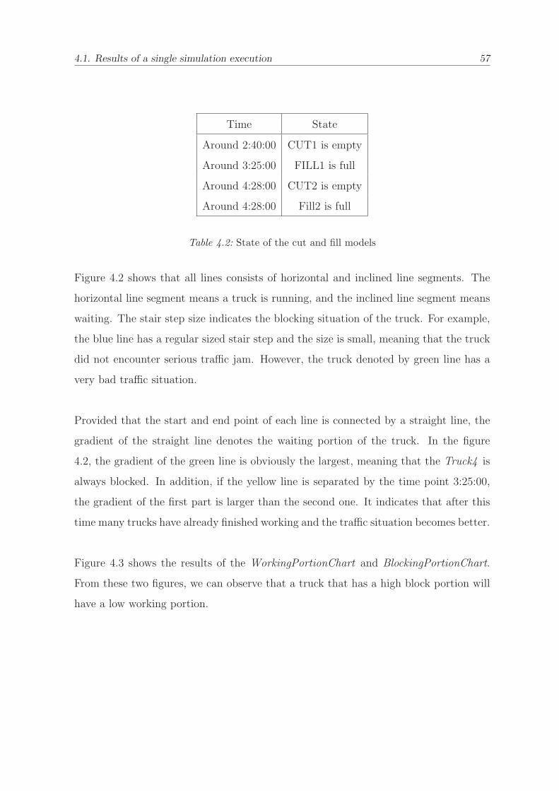
4.1. Results of a single simulation execution 57
Time State
Around 2:40:00 CUT1 is empty
Around 3:25:00 FILL1 is full
Around 4:28:00 CUT2 is empty
Around 4:28:00 Fill2 is full
Table 4.2: State of the cut and fill models
Figure 4.2 shows that all lines consists of horizontal and inclined line segments. The
horizontal line segment means a truck is running, and the inclined line segment means
waiting. The stair step size indicates the blocking situation of the truck. For example,
the blue line has a regular sized stair step and the size is small, meaning that the truck
did not encounter serious traffic jam. However, the truck denoted by green line has a
very bad traffic situation.
Provided that the start and end point of each line is connected by a straight line, the
gradient of the straight line denotes the waiting portion of the truck. In the figure
4.2, the gradient of the green line is obviously the largest, meaning that the Truck4 is
always blocked. In addition, if the yellow line is separated by the time point 3:25:00,
the gradient of the first part is larger than the second one. It indicates that after this
time many trucks have already finished working and the traffic situation becomes better.
Figure 4.3 shows the results of the WorkingPortionChart and BlockingPortionChart.
From these two figures, we can observe that a truck that has a high block portion will
have a low working portion.
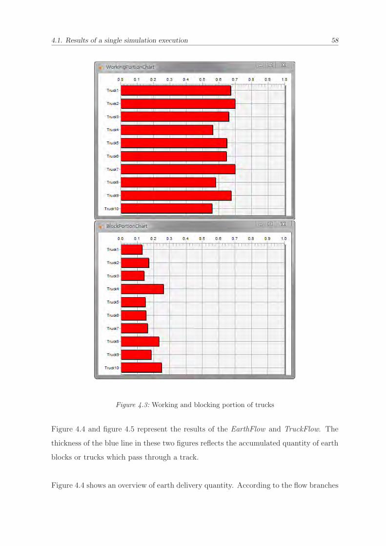
4.1. Results of a single simulation execution 58
Figure 4.3: Working and blocking portion of trucks
Figure 4.4 and figure 4.5 represent the results of the EarthFlow and TruckFlow. The
thickness of the blue line in these two figures reflects the accumulated quantity of earth
blocks or trucks which pass through a track.
Figure 4.4 shows an overview of earth delivery quantity. According to the flow branches
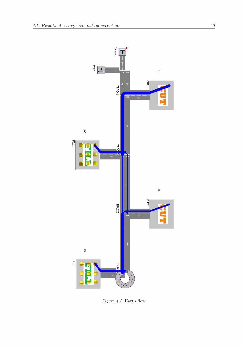
4.1. Results of a single simulation execution 59
Figure 4.4: Earth flow
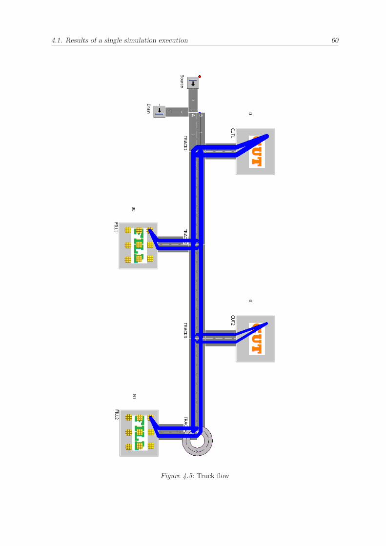
4.1. Results of a single simulation execution 60
Figure 4.5: Truck flow
4.2. Results of multiple simulation executions 61
between the TRACK2 and TRACK3, we can observe the earth delivery routes and
glance through the earth flow quantities that go to or come from different places. Fig-
ure 4.5 reflects the traffic situation. We can conclude that in this simulation the Track1
and the road fragment between the TRACK1 and TRACK2 are the busiest. It indi-
cates that the capacity of CUT1 is higher so that more delivery times are required.
4.2 Results of multiple simulation executions
In this section, we carry out some experiments to draw statistical conclusions which
are used to verify the simulation model. Moreover, the experiments give a number of
simulation results that come from different sets of inputs. These results can give users
proposals of selecting proper input values in order to get a relatively optimum results.
Figure 3.24 represents the module of designing experiment, collecting data and display-
ing results.
4.2.1 Case study 1
This case aims to investigate the influence of the number of trucks on the total simu-
lation time and blocking situation of trucks. We set up the input values as showed in
the table 4.3. In the table, we have totally 9 experiments. The frequency values are
the same. The only change is the number of trucks. The output values are the total
simulation time, average working portion and average blocking portion. In addition, for
each experiment, we set up 200 observations in a 75 percent confidence level. During
the simulation running, Plant Simulation converts each set of frequency values into the
value between 0 to 1 in the proportion of the input integer values.
Figure 4.6 represents the result of the total simulation time. From 8 trucks to 16 trucks,
the total simulation time decreases dramatically. However, when the number is contin-
uously increased, the curve becomes convergence. And the convergence value is about
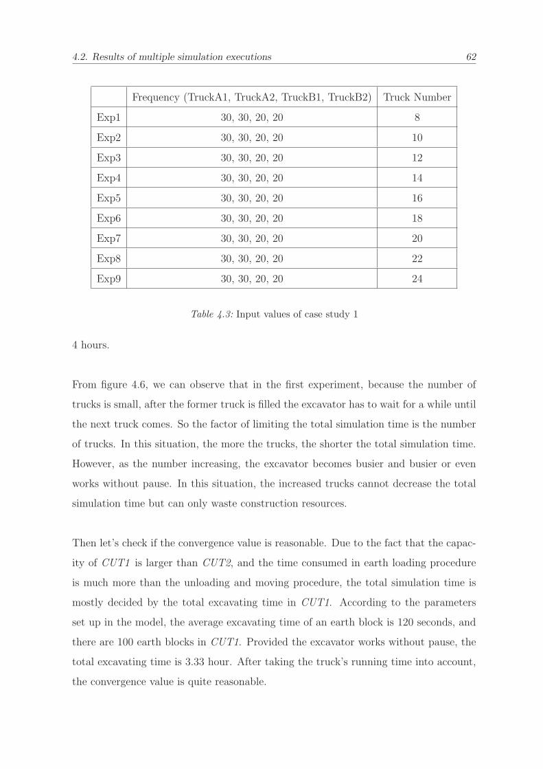
4.2. Results of multiple simulation executions 62
Frequency (TruckA1, TruckA2, TruckB1, TruckB2) Truck Number
Exp1 30, 30, 20, 20 8
Exp2 30, 30, 20, 20 10
Exp3 30, 30, 20, 20 12
Exp4 30, 30, 20, 20 14
Exp5 30, 30, 20, 20 16
Exp6 30, 30, 20, 20 18
Exp7 30, 30, 20, 20 20
Exp8 30, 30, 20, 20 22
Exp9 30, 30, 20, 20 24
Table 4.3: Input values of case study 1
4 hours.
From figure 4.6, we can observe that in the first experiment, because the number of
trucks is small, after the former truck is filled the excavator has to wait for a while until
the next truck comes. So the factor of limiting the total simulation time is the number
of trucks. In this situation, the more the trucks, the shorter the total simulation time.
However, as the number increasing, the excavator becomes busier and busier or even
works without pause. In this situation, the increased trucks cannot decrease the total
simulation time but can only waste construction resources.
Then let’s check if the convergence value is reasonable. Due to the fact that the capac-
ity of CUT1 is larger than CUT2, and the time consumed in earth loading procedure
is much more than the unloading and moving procedure, the total simulation time is
mostly decided by the total excavating time in CUT1. According to the parameters
set up in the model, the average excavating time of an earth block is 120 seconds, and
there are 100 earth blocks in CUT1. Provided the excavator works without pause, the
total excavating time is 3.33 hour. After taking the truck’s running time into account,
the convergence value is quite reasonable.
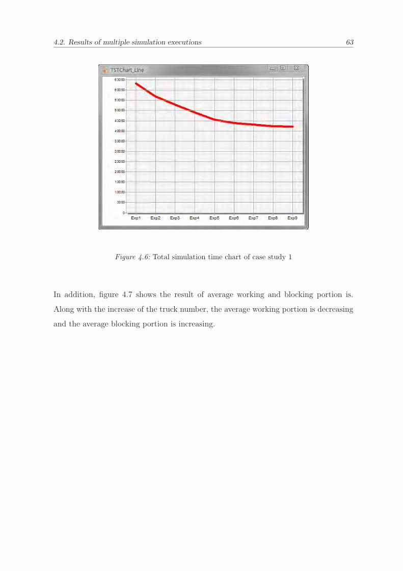
4.2. Results of multiple simulation executions 63
Figure 4.6: Total simulation time chart of case study 1
In addition, figure 4.7 shows the result of average working and blocking portion is.
Along with the increase of the truck number, the average working portion is decreasing
and the average blocking portion is increasing.
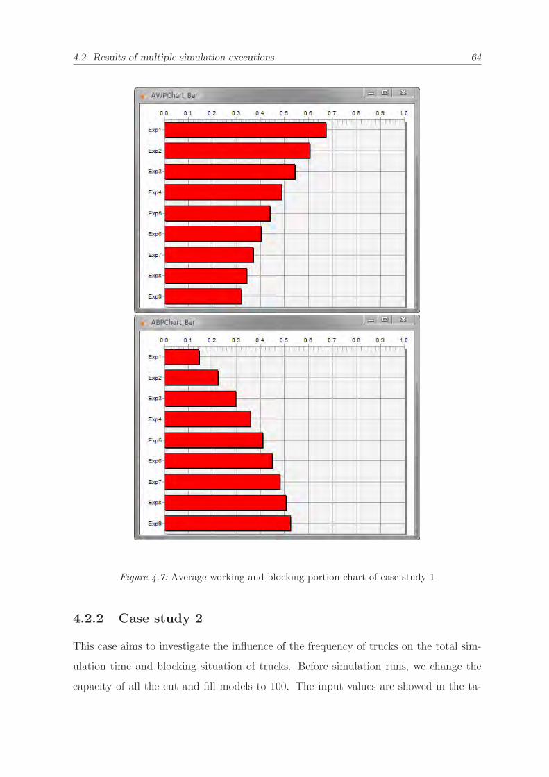
4.2. Results of multiple simulation executions 64
Figure 4.7: Average working and blocking portion chart of case study 1
4.2.2 Case study 2
This case aims to investigate the influence of the frequency of trucks on the total sim-
ulation time and blocking situation of trucks. Before simulation runs, we change the
capacity of all the cut and fill models to 100. The input values are showed in the ta-
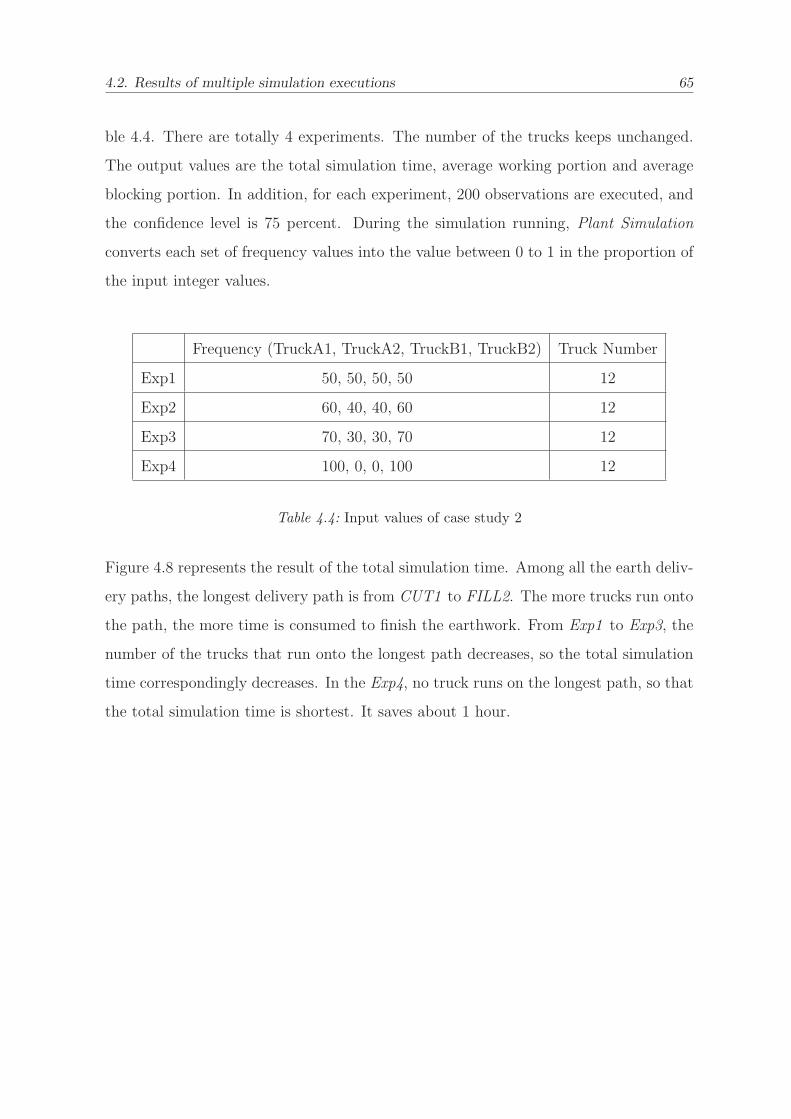
4.2. Results of multiple simulation executions 65
ble 4.4. There are totally 4 experiments. The number of the trucks keeps unchanged.
The output values are the total simulation time, average working portion and average
blocking portion. In addition, for each experiment, 200 observations are executed, and
the confidence level is 75 percent. During the simulation running, Plant Simulation
converts each set of frequency values into the value between 0 to 1 in the proportion of
the input integer values.
Frequency (TruckA1, TruckA2, TruckB1, TruckB2) Truck Number
Exp1 50, 50, 50, 50 12
Exp2 60, 40, 40, 60 12
Exp3 70, 30, 30, 70 12
Exp4 100, 0, 0, 100 12
Table 4.4: Input values of case study 2
Figure 4.8 represents the result of the total simulation time. Among all the earth deliv-
ery paths, the longest delivery path is from CUT1 to FILL2. The more trucks run onto
the path, the more time is consumed to finish the earthwork. From Exp1 to Exp3, the
number of the trucks that run onto the longest path decreases, so the total simulation
time correspondingly decreases. In the Exp4, no truck runs on the longest path, so that
the total simulation time is shortest. It saves about 1 hour.
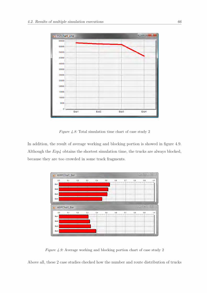
4.2. Results of multiple simulation executions 66
Figure 4.8: Total simulation time chart of case study 2
In addition, the result of average working and blocking portion is showed in figure 4.9.
Although the Exp4 obtains the shortest simulation time, the trucks are always blocked,
because they are too crowded in some track fragments.
Figure 4.9: Average working and blocking portion chart of case study 2
Above all, these 2 case studies checked how the number and route distribution of trucks

4.2. Results of multiple simulation executions 67
influence the simulation model. Due to the face that the model has a variety of pa-
rameters, we are able to set up other case studies for certain parameters to check their
influence on the system. Furthermore, beside validation of the model, the case studies
also contain lots of simulation runs among which relatively optimum results can be
selected and implemented in the real-world system.
5. Summary 68
Chapter 5
Summary
In this article, we developed an earthwork simulation model in Plant Simulation and
explained how the model was constructed. Then, we designed different use cases to
validate the model and to analyze the simulation results. The Plant Simulation has a
friendly graphic user interface that let users check the behavior and situation of each
component of the simulation model during the simulation run. The model can record
simulation results, e.g. utilization of trucks and total simulation time. The model can
also draw statistical conclusions that help the civil engineers to well organize construc-
tion resources. The model has a flexible interface that can be used to integrated with
the 3D earthwork assessment system. The 3D earthwork assessment system offers com-
pulsory simulation source data for the earthwork simulation model. The model can be
used before the real-world construction site is set up or even when the road construction
is progressing.
However, this earthwork simulation model also has some disadvantages. The cut and fill
can be created by the imported data from 3D earthwork assessment system. Although
the cut and fill model can also be reused into different road construction projects, the
3D earthwork assessment system cannot provide all the simulation source data. For
example, it cannot provide information concerning excavators, truck and transporta-
tion routes. So, for different road construction projects, a lot of effort on redesigning
excavator model, truck system and transportation routes must be spent. Furthermore,

Bibliography 69
the engineers who want to get familiar with, or even to extend, the model should have
experience of using Plant Simulation.
Concern for the outlook, an optimization module for the earthwork simulation model
could be developed in order to optimize the earthwork efficiency and the utilization of
the involved equipments.
Bibliography 70
Bibliography
[1] www.plm.automation.siemens.com.
[2] Tecnomatix Plant Simulation 8.2 Step-by-Step Help, 2006.
[3] J. B. Allen. War Games: Inside the Secret World of the Men who Play at Anni-
hilation. McGraw Hill, 1987.
[4] J. Banks, J. S. Carson, B. L. Nelson, and D. M. Nicol. Discrete-Event System
Simulation. Prentice Hall, 2005.
[5] M. Carey. Optimal time-varying flows on congested networks. Operations Research,
1987.
[6] E. R. Harold. Processing XML with Java: A Guide to SAX, DOM, JDOM, JAXP,
and TrAX. Addison Wesley, 2002.
[7] E. Haug. Engineering safety analysis via destructive numerical experiments. EU-
ROMECH 121, 1981.
[8] Y. Ji, A. Borrmann, and E. Rank. An integrated 3d simulation framework for
earthwork processes. 2005.
[9] M. Koenig, Beissert U., and H.-J. Bargstaedt. Visual simulation - an appropriate
approach to support execution planning in building engineering. Proc. of the 7th
International Conference on Construction Applications of Virtual Reality (ConVR
2007), 2007.

Bibliography 71
[10] D. Steinhauer. Planung komplexer montageablaeufe mit hilfe der constraint-
basierten simulation. Advances in Simulation for Production and Logistics Ap-
plications, 2008.
[11] www.wikipedia.org.