Development of an Electromagnetic Glottal Waveform Sensor

for Applications in High Acoustic Noise Environments by

Altin Pelteku

A Thesis

Submitted to the Faculty

of the

WORCESTER POLYTECHNIC INSTITUTE

in partial fulfillment of the

Degree of Master of Science

in

Electrical Engineering

by

_________________________________

Altin Pelteku

January 2004

APPROVED:

_________________________________ Prof. Reinhold Ludwig, ECE Dept., WPI

Advisor

_________________________________ Prof. Gene Bogdanov, ECE Dept., WPI

Committee Member

_________________________________ Prof. Hossein Hakim, ECE Dept., WPI

Committee Member

_________________________________ Prof. Donald R. Brown III,

Committee member

_________________________________ Prof. Fred J. Looft,

Head of ECE Dept., WPI

ii

Abstract

The challenges of measuring speech signals in the presence of a strong

background noise cannot be easily addressed with traditional acoustic technology. A

recent solution to the problem considers combining acoustic sensor measurements with

real-time, non-acoustic detection of an aspect of the speech production process. While

significant advancements have been made in that area using low-power radar-based

techniques, drawbacks inherent to the operation of such sensors are yet to be surmounted.

Therefore, one imperative scientific objective is to devise new, non-invasive non-acoustic

sensor topologies that offer improvements regarding sensitivity, robustness, and acoustic

bandwidth.

This project investigates a novel design that directly senses the glottal flow

waveform by measuring variations in the electromagnetic properties of neck tissues

during voiced segments of speech. The approach is to explore two distinct sensor

configurations, namely the “six-element” and the “parallel-plate” resonator. The research

focuses on the modeling aspect of the biological load and the resonator prototypes using

multi-transmission line (MTL) and finite element (FE) simulation tools. Finally, bench

tests performed with both prototypes on phantom loads as well as human subjects are

presented.

iii

Acknowledgements

This work was sponsored by the Defense Advanced Research Projects Agency

(DARPA). Their support and feedback were invaluable to the completion of this work. I

would like to extend many thanks my advisor, Prof. Reinhold Ludwig, for his optimism,

leadership and encouragement throughout the term of this project. I would also like to

thank the members of my committee: Prof. Brown for providing me with the opportunity

to work on this project and for being a driven project manager, Dr. Gene Bogdanov for

making the MTL tools available and carefully reviewing this document, and Prof. Hakim,

who is a great teacher and person. I would also like to thank professor Jill Ruffs for

dedicating time to construct the agarose neck model. Additional thanks go out to Todd

Billings for helping out with many practical issues and the faculty of the Electrical and

Computer Engineering department here at Worcester Polytechnic Institute. And finally,

my deepest gratitude goes towards my parents and family, whose support and

encouragement have helped me in all facets of life.

iv

Table of Contents

Abstract.............................................................................................................................. ii

Acknowledgements .......................................................................................................... iii

Table of Contents ............................................................................................................. iv

List of Figures................................................................................................................... vi

List of Tables .................................................................................................................. viii

1 Introduction............................................................................................................... 1 1.1 Objective ............................................................................................................. 2 1.2 Organization........................................................................................................ 3

2 Background ............................................................................................................... 4 2.1 Principle of operation.......................................................................................... 4 2.2 Overview of the human speech process.............................................................. 7

2.2.1 Anatomy of the vocal tract.......................................................................... 8 2.2.2 Sound generation ...................................................................................... 16 2.2.3 Other speech sounds ................................................................................. 19

2.3 Dielectric properties of human tissue ............................................................... 20 2.4 Overview of existing non-acoustical speech detection techniques................... 22

3 Theoretical Considerations .................................................................................... 24 3.1 Lumped resonator structures............................................................................. 24 3.2 Distributed resonator structures ........................................................................ 26

3.2.1 Parallel plate resonator.............................................................................. 26 Radiation currents ................................................................................................. 27 Tuning and matching ............................................................................................ 29

3.3 Six-element resonator ....................................................................................... 31 3.3.1 Coupled microstrip line resonators ........................................................... 33

3.4 A review of Maxwell’s equations ..................................................................... 35 3.5 Modeling efforts................................................................................................ 36

3.5.1 Multi-conductor transmission line model ................................................. 37 3.5.2 Finite Element Frequency Domain Model................................................ 40

3.6 Weighted residual formulation ......................................................................... 41 3.6.1 Domain discretization and matrix formulation ......................................... 44 3.6.2 Basis function selection ............................................................................ 45 3.6.3 Boundary Conditions ................................................................................ 46

3.7 Simulation procedure ........................................................................................ 48

4 Numerical Simulations and Field Predictions...................................................... 50

4.1 Six element resonator........................................................................................ 50 4.1.1 MTL simulation results............................................................................. 51 4.1.2 FEM simulation results ............................................................................. 54

v

4.2 Parallel plate resonator predictions................................................................... 61 4.2.1 FEM predictions........................................................................................ 63 4.2.2 Load and resonator refinements................................................................ 65 4.2.3 Pspice simulations..................................................................................... 67 4.2.4 FEM predictions........................................................................................ 70 4.2.5 Field distribution inside the load............................................................... 73

4.3 Field strength issues.......................................................................................... 74

5 Practical Implementation and Test Results.......................................................... 81 5.1 Six-element resonator ....................................................................................... 81

5.1.1 Construction procedure............................................................................. 81 5.1.2 Phantom load tests .................................................................................... 82

5.2 Parallel-plate resonator ..................................................................................... 87 5.2.1 Construction.............................................................................................. 87 5.2.2 Bench testing............................................................................................. 89

5.3 Interface electronics .......................................................................................... 95 5.3.1 Circulator .................................................................................................. 95

Construction and network analyzer tests .............................................................. 97

6 Conclusions............................................................................................................ 101 6.1 Recommendations........................................................................................... 102

References...................................................................................................................... 104

Appendix A. Resonator Components.......................................................................... 108

Appendix B. Circulator PCB layout and circuit components................................... 109

vi

List of Figures

Figure 2-1: Measurement of glottal state and change in relative permittivity. .................. 5 Figure 2-2: S11 change in a tuned resonator when driven near resonance. ....................... 7 Figure 2-3: Functional block diagram of the vocal tract structures................................... 8 Figure 2-4: Overview of the vocal tract [9]. ..................................................................... 10 Figure 2-5: Sagittal view of the laryngeal structures [10]. .............................................. 11 Figure 2-6: Posterior view of the laryngeal cartilages [11]............................................. 13 Figure 2-7: Coronal view of the vocal folds [12]. ............................................................ 15 Figure 2-8: The one-mass model of the vocal area [8]..................................................... 16 Figure 2-9: The vocal tract output spectrum via the source-filter theory......................... 18 Figure 2-10: Relative permittivity, conductivity and electric loss tangent for different

body tissues in the frequency range 20-300MHz. ..................................................... 22 Figure 3-1: The basic LC cell............................................................................................ 24 Figure 3-2: The parallel RLC resonator. .......................................................................... 25 Figure 3-3: The series RLC resonator. ............................................................................. 26 Figure 3-4: Topology of the parallel plate resonator. ...................................................... 27 Figure 3-5: Radiation currents due to unbalanced feed-point [20].................................. 28 Figure 3-6: Topology of the balanced, well-tuned parallel plate resonator..................... 30 Figure 3-7: Lumped representation of the balanced, well-tuned parallel plate resonator.

................................................................................................................................... 30 Figure 3-8: Topology of the six-element resonator........................................................... 31 Figure 3-9: Circuit representation of the six-element resonator [32]. ............................. 32 Figure 3-10: Single-port and two-port network representation........................................ 33 Figure 3-11: Cascading of different networks via the ABCD representation. .................. 34 Figure 4-1: Dimensions and materials of the MTL neck model. Note that all structures

shown in this figure are cylindrical with a height of 38.1mm. ................................. 51 Figure 4-2: Overall S11(f) response of closed vs. open from MTL tools. .......................... 52 Figure 4-3: Second mode of S11(f) response of closed vs. open from MTL tools. ............. 53 Figure 4-4: Third mode of S11(f) response of closed vs. open from MTL tools................. 53 Figure 4-5: Dimensions and materials of the FEM neck model. All structures shown

above are cylinders with a height of 38.1mm [28]. .................................................. 55 Figure 4-6: Overall S11(f) response of closed vs. open from FEM tools........................... 56 Figure 4-7: Second mode of S11(f) response of closed vs. open from FEM tools.............. 56 Figure 4-8: Third mode of S11(f) response of closed vs. open from FEM tools. ............... 57 Figure 4-9: Electric field plots for modes 1-6 in order are shown in a) through f).......... 60 Figure 4-10: Overall S11(f) response of closed vs. open for the PPRES from FEM tools,

using the biological load of Figure 4-5..................................................................... 63 Figure 4-11: Zoomed-in S11(f) response of closed vs. open for the PPRES from FEM

tools, using the biological load of Figure 4-5. .......................................................... 64 Figure 4-12: Modifications to the laryngeal structures. The vocal folds are replaced with

a 5mm tall cylinder. .................................................................................................. 65 Figure 4-13: Matching networks for the parallel plate resonator at 50MHz. .................. 66 Figure 4-14: Simulation model with Pspice. ..................................................................... 67

vii

Figure 4-15: Overall S11(f) response of closed vs. open for the PPRES from Pspice, using the matching circuit of Figure 4-13. ......................................................................... 68

Figure 4-16: Zoomed-in S11(f) response of closed vs. open for the PPRES from Pspice, using the matching circuit of Figure 4-13................................................................. 69

Figure 4-17: Snapshot of the resonator model in HFSS 8.5. ............................................ 70 Figure 4-18: Overall S11(f) response of closed vs. open for the balanced well-tuned

PPRES from FEM tools using the refinement of Figure 4-12................................... 71 Figure 4-19: Zoomed-in S11(f) response of closed vs. open for the balanced well-tuned

PPRES from FEM tools using the refinement of Figure 4-12................................... 72 Figure 4-20: Electric field plot for the balanced, well-matched PPRES. ......................... 74 Figure 4-21: Electric field and magnetic field strengths for the six-element resonator for

all resonant modes. ................................................................................................... 79 Figure 4-22: Electric and magnetic field strengths for the parallel-plate resonator. ...... 80 Figure 5-1. Photos of the assembled six-element resonator ............................................. 82 Figure 5-2: Non-biological load test setup. ...................................................................... 83 Figure 5-3: S11 (dB) of a) the unloaded resonator and b) the agarose-loaded resonator. 85 Figure 5-4: The s-parameters response of the six-element resonator in CW mode, while

driven at its third resonance a) 50Hz excitation b) 75Hz excitation. ....................... 86 Figure 5-5. Photographs of the PPRES sensor: (a) without fabric, (b) with fabric cover.

................................................................................................................................... 89 Figure 5-6: S11 for a female subject .................................................................................. 90 Figure 5-7: S11 for a male subject ..................................................................................... 91 Figure 5-8: Tests in CW mode for a male subject when humming at a) 85.7Hz, b)

142.86Hz, c) 214.3Hz and d) 342.86Hz.................................................................... 93 Figure 5-9: A three-port circulator schematic. ................................................................. 96 Figure 5-10: Photo of the assembled circulator. .............................................................. 97 Figure 5-11: Circulator S-parameter measurements with the HP 8714ES. ..................... 99 Figure 5-12: Topology of the interface circuitry and receiver using the parallel plate

resonator. ................................................................................................................ 100

viii

List of Tables

Table 2-1: Summary of anatomical terms........................................................................... 9 Table 4-1: Six-element resonator prototype design parameters. ...................................... 50 Table 4-2: Dielectric properties of relevant tissues at 200MHz [6].................................. 52 Table 4-3: Dielectric properties of relevant tissues at 50MHz [6].................................... 62 Table 4-4: Parallel-plate speech sensor prototype design parameters. ............................. 62 Table 4-5: FCC Limits for Maximum Permissible Exposure (MPE) [38]. ...................... 75 Table 4-6: Maximum safe power level. ............................................................................ 80

1

1 Introduction

Detection of speech signals with non-acoustic methods has been previously

attempted by different groups and organizations (see [1] [2] and [3], for instance). The

idea has lately received renewed attention, primarily for measuring speech signals in high

acoustic noise environments. The Defense Advanced Research Projects Agency

(DARPA) has recently sponsored the Advanced Speech Encoding program, the goal of

which, as stated by DARPA [4], is to “develop a voice communication concept that:

1. Requires very low bandwidth (~200 bps or less).

2. Provides excellent intelligibility (at least as good as the DoD 4800 bps std).

3. Suppresses external acoustic noise.

4. Can provide speaker authentication.”1

The difficulty of measuring speech signals in high acoustic noise environments

originates from the limitation of acoustic transducers: they are inept in differentiating

between noise and speech on a fundamental basis. Limitations of traditional acoustic

technology can be overcome by implementing multiple-sensor systems that combine

acoustic with non-acoustic measurements of the speech signal. While such systems have

proven to be effective in noise cancellation [5] and reconstruction of the original speech

signal [1], significant challenges relating to sensitivity and robustness still remain (see

Section 2.4). One important scientific goal is to develop new non-acoustic sensor ideas

that offer improvements regarding sensitivity, bandwidth and immunity to complicated

scattering environments. As a subset of the Advanced Speech Encoding program this

1 http://www.darpa.mil/ato/programs/vocorder.htm

2

project determines the feasibility of the glottal resonator (GRES), a novel non-acoustic

speech sensor.

1.1 Objective

The objective of this thesis is to determine the feasibility and quantify the

performance of the glottal resonator (GRES) for the purpose of non-evasive

measurements of the glottal waveform in high acoustic noise environments. The new

sensor exploits the capacitive sensing technique as described in Section 2.1. The project

goal is to design and built a prototype and evaluate its sensitivity to voiced speech.

The practical objectives for this project are to:

1. Develop a theoretical foundation that closely predicts the behavior of the sensor.

The approach is to conduct a computer simulation study of GRES sensors using

multi-transmission line and finite element analysis tools.

2. Construct prototypes of the GRES sensor and perform bench testing to determine

the sensitivity to voiced speech.

3. Provide technical support in the collection of the experimental datasets for the

GRES sensor prototype containing synchronized GRES sensor and acoustic

measurements of at least two human subjects in a variety of standardized noise

environments and noise levels.

4. Address practical implementation issues of the GRES sensors including

sensitivity, ergonomics, potential health effects, acoustic bandwidth,

electromagnetic field containment, and cost.

The approach is to explore two sensor designs: a coupled microstrip line resonator, and a

parallel plate resonator. Both sensor designs measure variations in electromagnetic

3

properties of human tissue near the region of the vocal folds during voiced segments of

speech.

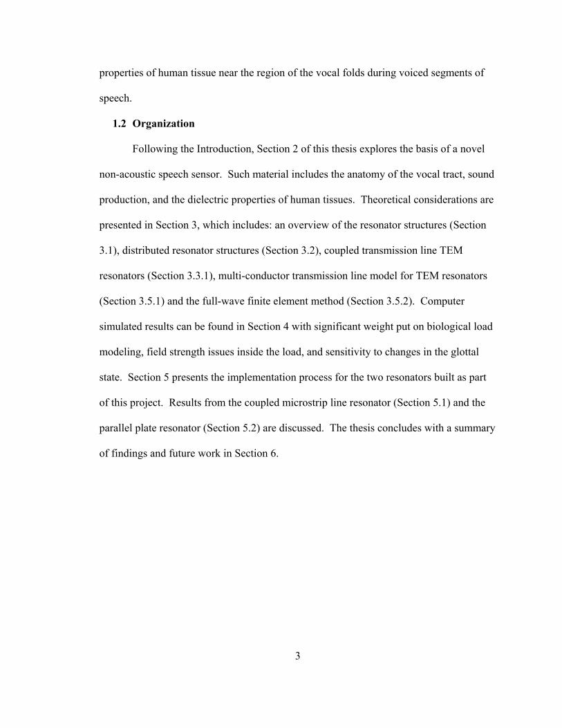
1.2 Organization

Following the Introduction, Section 2 of this thesis explores the basis of a novel

non-acoustic speech sensor. Such material includes the anatomy of the vocal tract, sound

production, and the dielectric properties of human tissues. Theoretical considerations are

presented in Section 3, which includes: an overview of the resonator structures (Section

3.1), distributed resonator structures (Section 3.2), coupled transmission line TEM

resonators (Section 3.3.1), multi-conductor transmission line model for TEM resonators

(Section 3.5.1) and the full-wave finite element method (Section 3.5.2). Computer

simulated results can be found in Section 4 with significant weight put on biological load

modeling, field strength issues inside the load, and sensitivity to changes in the glottal

state. Section 5 presents the implementation process for the two resonators built as part

of this project. Results from the coupled microstrip line resonator (Section 5.1) and the

parallel plate resonator (Section 5.2) are discussed. The thesis concludes with a summary

of findings and future work in Section 6.

4

2 Background

This section presents the principle of operation of the GRES sensor and speech

information relevant to the function of the sensor.

2.1 Principle of operation

The principle of operation of the glottal resonator sensor is based on two key

aspects of speech production. First, it is known that during voiced segments of speech

the vocal folds open and close at a rate equal to the fundamental frequency of the acoustic

waveform produced at the output of the vocal tract. Second, experimental research

shows that the relative permittivity of most body tissues near the position of the vocal

folds is on the order of 40-200 times that of air for frequencies in the range of 20MHz-

200MHz [6]. From these facts, it is presumed that during voiced segments of speech, the

compound relative permittivity of a cross-section of the neck near the vocal folds

experiences significant variations, while oscillating at the same fundamental frequency as

the acoustic waveform output. This suggests that the glottal state and part of the acoustic

waveform at the output of the vocal tract can be deduced from measurements of the

relative permittivity of the larynx during voiced segments of speech.

In this project we investigate two separate designs for measuring the change in

relative permittivity of the larynx. First, we discuss the “six-element” sensor that utilizes

a coupled microstrip line transverse electromagnetic structure, driven by a low power

(≤100 µW) radio frequency (RF) source operating around 200MHz. Second, a new

sensor is developed that utilizes a tuned parallel plate resonator (PPRES) with a lower

5

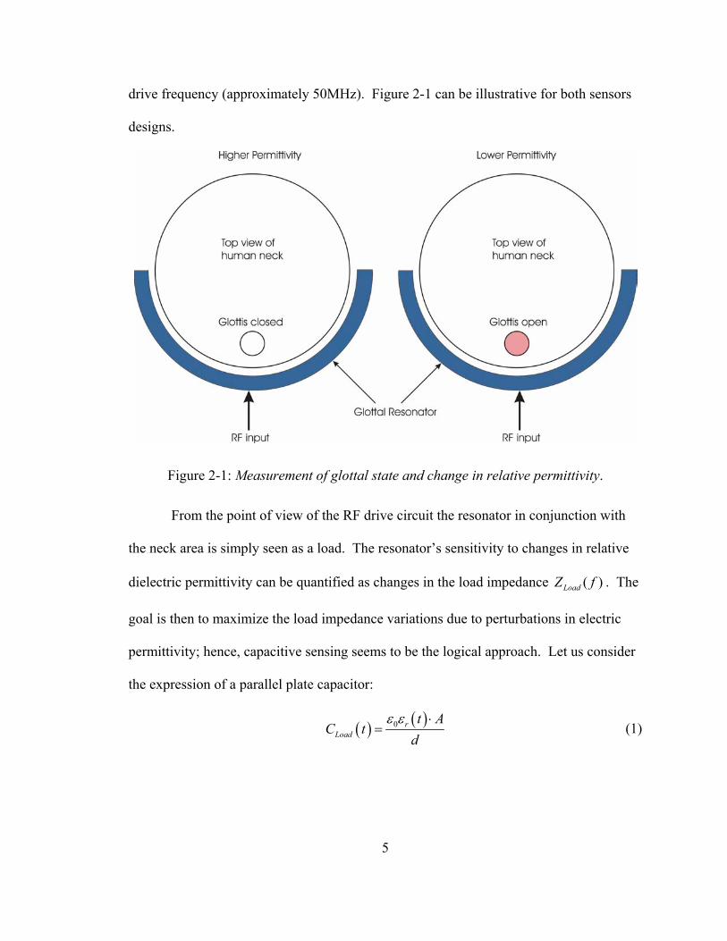
drive frequency (approximately 50MHz). Figure 2-1 can be illustrative for both sensors

designs.

Figure 2-1: Measurement of glottal state and change in relative permittivity.

From the point of view of the RF drive circuit the resonator in conjunction with

the neck area is simply seen as a load. The resonator’s sensitivity to changes in relative

dielectric permittivity can be quantified as changes in the load impedance ( )LoadZ f . The

goal is then to maximize the load impedance variations due to perturbations in electric

permittivity; hence, capacitive sensing seems to be the logical approach. Let us consider

the expression of a parallel plate capacitor:

( ) ( )0 rLoad

t AC t

dε ε ⋅

= (1)

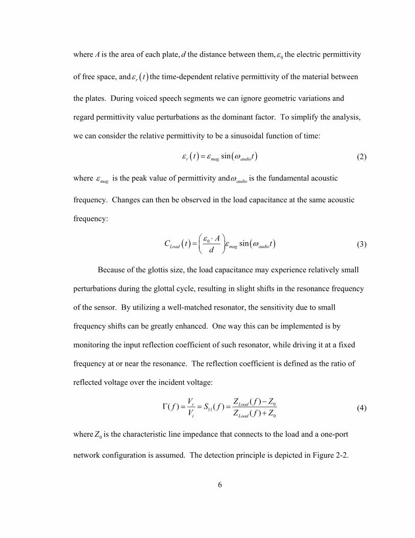
6

where A is the area of each plate, d the distance between them, 0ε the electric permittivity

of free space, and ( )r tε the time-dependent relative permittivity of the material between

the plates. During voiced speech segments we can ignore geometric variations and

regard permittivity value perturbations as the dominant factor. To simplify the analysis,

we can consider the relative permittivity to be a sinusoidal function of time:

( ) ( )sinr mag audiot tε ε ω= (2)

where magε is the peak value of permittivity and audioω is the fundamental acoustic

frequency. Changes can then be observed in the load capacitance at the same acoustic

frequency:

( ) ( )0 sinLoad mag audioAC t t

dε ε ω⋅ =

(3)

Because of the glottis size, the load capacitance may experience relatively small

perturbations during the glottal cycle, resulting in slight shifts in the resonance frequency

of the sensor. By utilizing a well-matched resonator, the sensitivity due to small

frequency shifts can be greatly enhanced. One way this can be implemented is by

monitoring the input reflection coefficient of such resonator, while driving it at a fixed

frequency at or near the resonance. The reflection coefficient is defined as the ratio of

reflected voltage over the incident voltage:

011

0

( )( ) ( )( )

Loadr

i Load

Z f ZVf S fV Z f Z

−Γ = = =

+ (4)

where 0Z is the characteristic line impedance that connects to the load and a one-port

network configuration is assumed. The detection principle is depicted in Figure 2-2.

7

S11 (f0, closed glottis)

S11 (f0, open glottis)

RF drive

Frequency (f0)

S11 (dB)

Frequency

Resonant frequency

during closed glottis

Resonant frequency

during open glottis

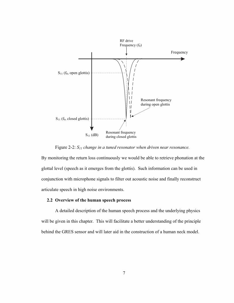
Figure 2-2: S11 change in a tuned resonator when driven near resonance.

By monitoring the return loss continuously we would be able to retrieve phonation at the

glottal level (speech as it emerges from the glottis). Such information can be used in

conjunction with microphone signals to filter out acoustic noise and finally reconstruct

articulate speech in high noise environments.

2.2 Overview of the human speech process

A detailed description of the human speech process and the underlying physics

will be given in this chapter. This will facilitate a better understanding of the principle

behind the GRES sensor and will later aid in the construction of a human neck model.

8

2.2.1 Anatomy of the vocal tract

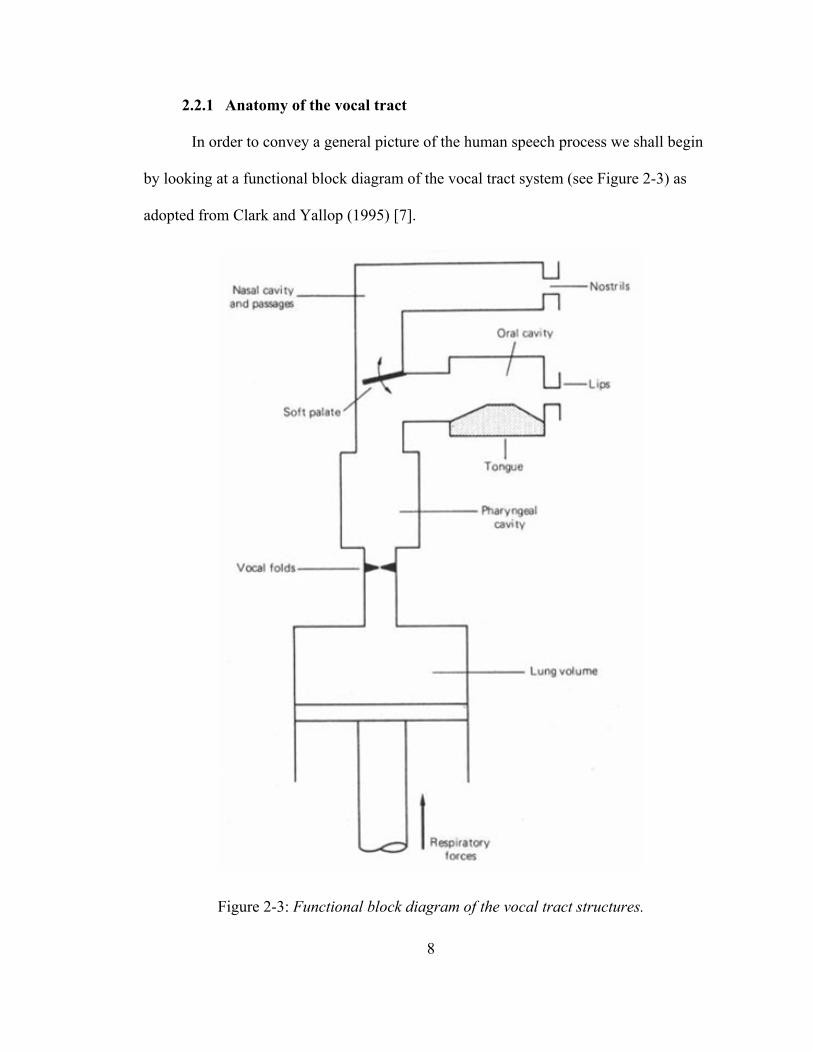
In order to convey a general picture of the human speech process we shall begin

by looking at a functional block diagram of the vocal tract system (see Figure 2-3) as

adopted from Clark and Yallop (1995) [7].

Figure 2-3: Functional block diagram of the vocal tract structures.

9

Let us next examine the vocal tract anatomy while entailing some of its important

structures. Prior to presenting such material, however, we need to introduce some

anatomical terms, summarized in Table 2-1.

Table 2-1: Summary of anatomical terms.

Anatomical term Meaning

Anterior Toward the front

Posterior Toward the back

Superior Above

Inferior Below

Longitudinal In the direction of

Transverse Perpendicular to

Coronal Frontal

Medial Towards a center axis or a midplane

Lateral Away from a center axis or a midplane

Sagittal Along a median plane

Glottis The air cavity between the vocal folds

Subglottal Below the glottis

Supraglottal Above the glottis

The vocal tract is part of the respiratory system; its main functional blocks are: the

lungs, the larynx, the pharynx, the oral apparatus and the nasal cavities (see Figure 2-4).

During voiced speech, flexure of the diaphragm causes the lung pressure to rise above

atmospheric: usually between 0.3kPa and 1.2kPa [8] (where 1.2kPa is associated with

10

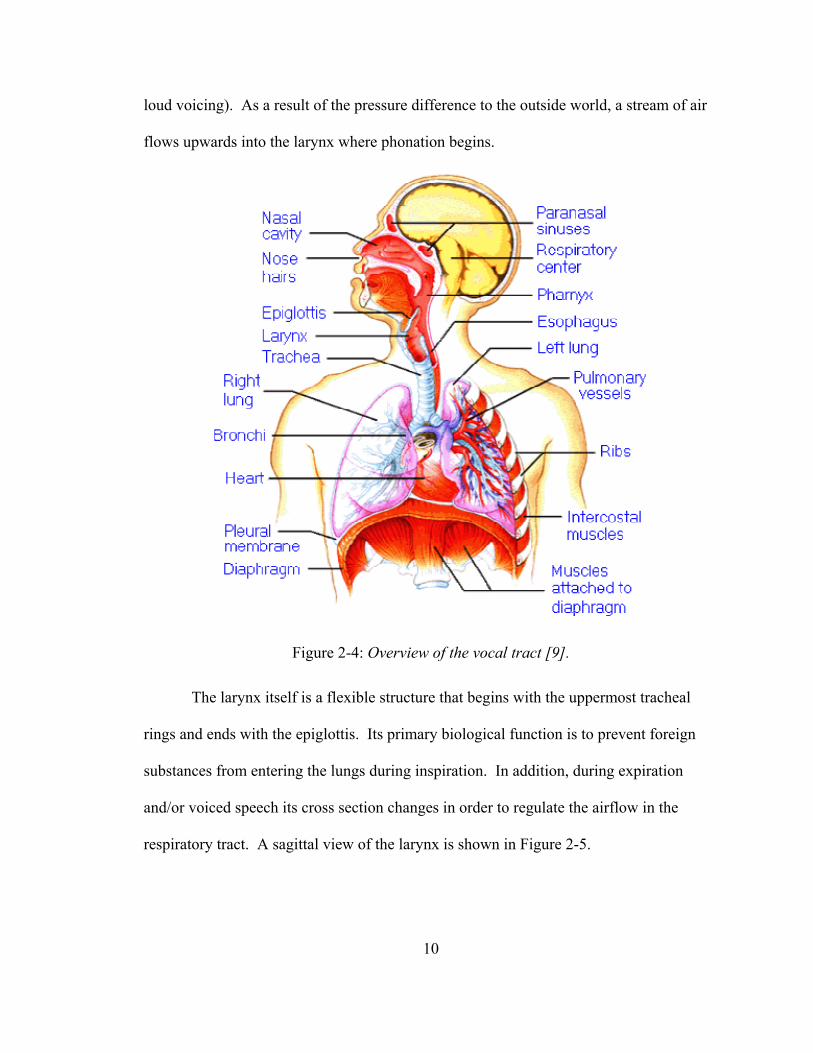
loud voicing). As a result of the pressure difference to the outside world, a stream of air

flows upwards into the larynx where phonation begins.

Figure 2-4: Overview of the vocal tract [9].

The larynx itself is a flexible structure that begins with the uppermost tracheal

rings and ends with the epiglottis. Its primary biological function is to prevent foreign

substances from entering the lungs during inspiration. In addition, during expiration

and/or voiced speech its cross section changes in order to regulate the airflow in the

respiratory tract. A sagittal view of the larynx is shown in Figure 2-5.

11

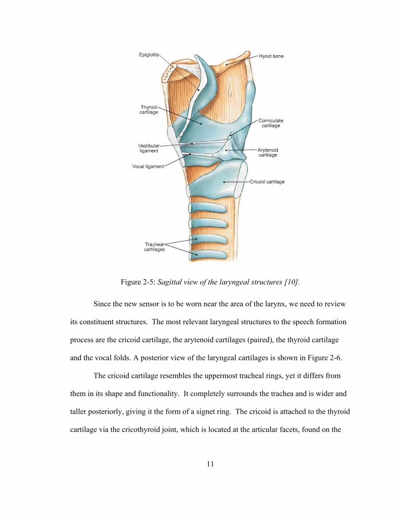
Figure 2-5: Sagittal view of the laryngeal structures [10].

Since the new sensor is to be worn near the area of the larynx, we need to review

its constituent structures. The most relevant laryngeal structures to the speech formation

process are the cricoid cartilage, the arytenoid cartilages (paired), the thyroid cartilage

and the vocal folds. A posterior view of the laryngeal cartilages is shown in Figure 2-6.

The cricoid cartilage resembles the uppermost tracheal rings, yet it differs from

them in its shape and functionality. It completely surrounds the trachea and is wider and

taller posteriorly, giving it the form of a signet ring. The cricoid is attached to the thyroid

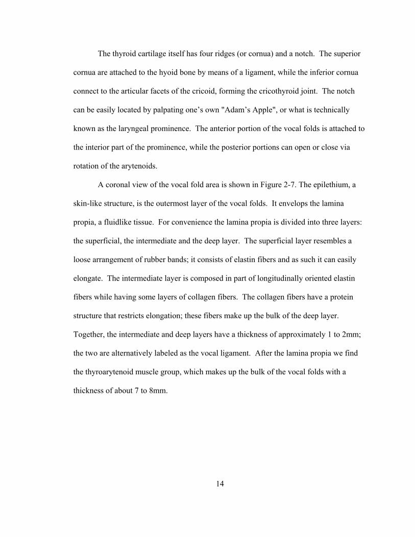
cartilage via the cricothyroid joint, which is located at the articular facets, found on the

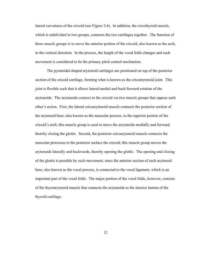
12

lateral curvatures of the cricoid (see Figure 2-6). In addition, the cricothyroid muscle,

which is subdivided in two groups, connects the two cartilages together. The function of

these muscle groups is to move the anterior portion of the cricoid, also known as the arch,

in the vertical direction. In the process, the length of the vocal folds changes and such

movement is considered to be the primary pitch control mechanism.

The pyramidal-shaped arytenoid cartilages are positioned on top of the posterior

section of the cricoid cartilage, forming what is known as the cricoarytenoid joint. This

joint is flexible such that it allows lateral/medial and back/forward rotation of the

arytenoids. The arytenoids connect to the cricoid via two muscle groups that oppose each

other’s action. First, the lateral cricoarytenoid muscle connects the posterior section of

the arytenoid base, also known as the muscular process, to the superior portion of the

cricoid’s arch; this muscle group is used to move the arytenoids medially and forward,

thereby closing the glottis. Second, the posterior cricoarytenoid muscle connects the

muscular processes to the posterior surface the cricoid; this muscle group moves the

arytenoids laterally and backwards, thereby opening the glottis. The opening and closing

of the glottis is possible by such movement, since the anterior section of each arytenoid

base, also known as the vocal process, is connected to the vocal ligament, which is an

important part of the vocal folds. The major portion of the vocal folds, however, consists

of the thyroarytenoid muscle that connects the arytenoids to the interior lamina of the

thyroid cartilage.

13

Figure 2-6: Posterior view of the laryngeal cartilages [11].

14

The thyroid cartilage itself has four ridges (or cornua) and a notch. The superior

cornua are attached to the hyoid bone by means of a ligament, while the inferior cornua

connect to the articular facets of the cricoid, forming the cricothyroid joint. The notch

can be easily located by palpating one’s own "Adam’s Apple", or what is technically

known as the laryngeal prominence. The anterior portion of the vocal folds is attached to

the interior part of the prominence, while the posterior portions can open or close via

rotation of the arytenoids.

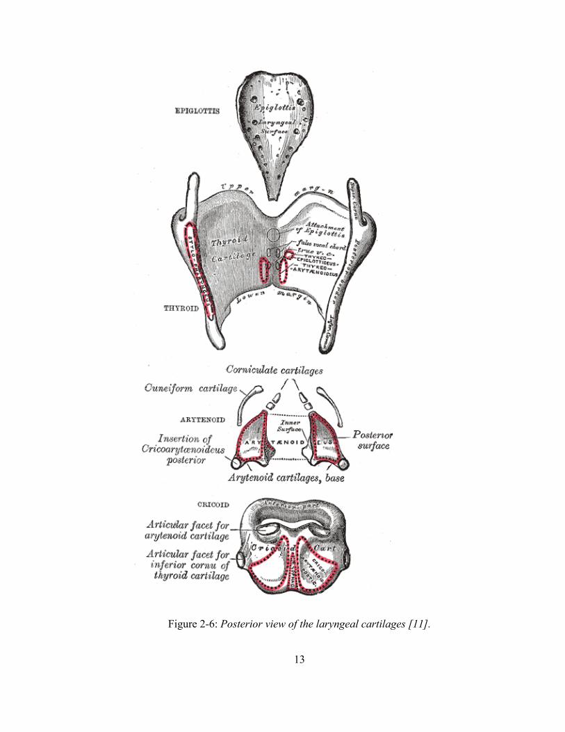
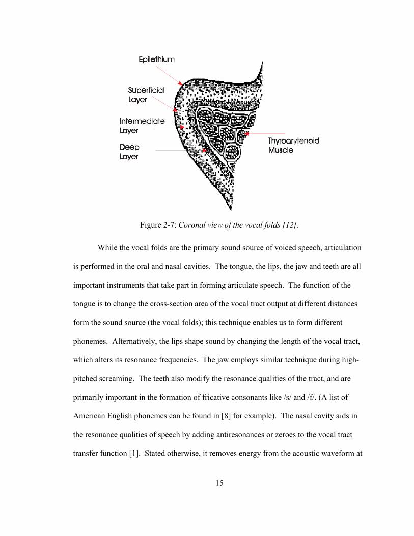
A coronal view of the vocal fold area is shown in Figure 2-7. The epilethium, a

skin-like structure, is the outermost layer of the vocal folds. It envelops the lamina

propia, a fluidlike tissue. For convenience the lamina propia is divided into three layers:

the superficial, the intermediate and the deep layer. The superficial layer resembles a

loose arrangement of rubber bands; it consists of elastin fibers and as such it can easily

elongate. The intermediate layer is composed in part of longitudinally oriented elastin

fibers while having some layers of collagen fibers. The collagen fibers have a protein

structure that restricts elongation; these fibers make up the bulk of the deep layer.

Together, the intermediate and deep layers have a thickness of approximately 1 to 2mm;

the two are alternatively labeled as the vocal ligament. After the lamina propia we find

the thyroarytenoid muscle group, which makes up the bulk of the vocal folds with a

thickness of about 7 to 8mm.

15

Epilethium

Superficial

Layer

Intermediate

Layer

Deep

Layer

Thyroarytenoid

Muscle

Figure 2-7: Coronal view of the vocal folds [12].

While the vocal folds are the primary sound source of voiced speech, articulation

is performed in the oral and nasal cavities. The tongue, the lips, the jaw and teeth are all

important instruments that take part in forming articulate speech. The function of the

tongue is to change the cross-section area of the vocal tract output at different distances

form the sound source (the vocal folds); this technique enables us to form different

phonemes. Alternatively, the lips shape sound by changing the length of the vocal tract,

which alters its resonance frequencies. The jaw employs similar technique during high-

pitched screaming. The teeth also modify the resonance qualities of the tract, and are

primarily important in the formation of fricative consonants like /s/ and /f/. (A list of

American English phonemes can be found in [8] for example). The nasal cavity aids in

the resonance qualities of speech by adding antiresonances or zeroes to the vocal tract

transfer function [1]. Stated otherwise, it removes energy from the acoustic waveform at

16

particular harmonics. The effect is more prominent during the production of nasal sounds

(phonemes such as /m/, /n/), when the nasal tract is open and the oral cavity is shut off.

Now that we have a basic understanding of the constituent structures of the vocal

tract we shall look at the sound production process. Sound propagation through the vocal

tract can be found in several references [1][8], and is not explored here.

2.2.2 Sound generation

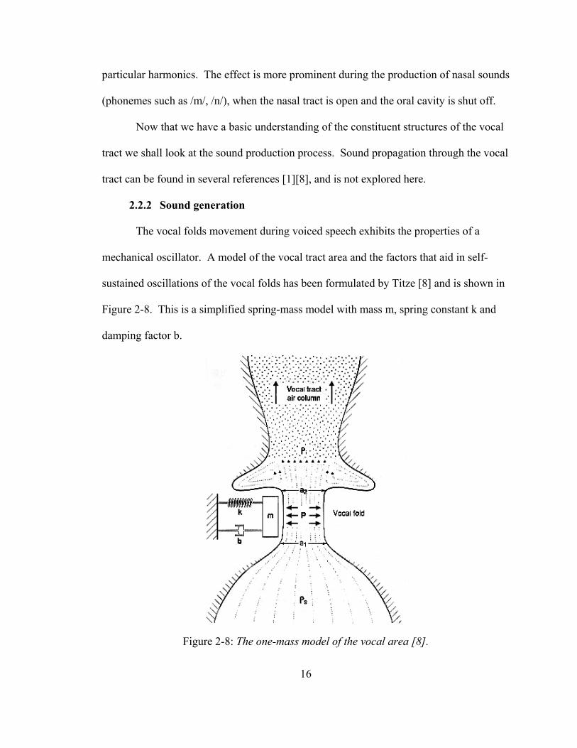
The vocal folds movement during voiced speech exhibits the properties of a

mechanical oscillator. A model of the vocal tract area and the factors that aid in self-

sustained oscillations of the vocal folds has been formulated by Titze [8] and is shown in

Figure 2-8. This is a simplified spring-mass model with mass m, spring constant k and

damping factor b.

Figure 2-8: The one-mass model of the vocal area [8].

17

A brief description of the voiced speech process via the vocal fold vibration

theory can be as follows: as phonation begins, an increase in relative lung pressure, Ps,

forces the folds to partially open and air to flow through the glottis into the supraglottal

region. This airflow causes the supraglottal and intraglottal pressures, Pi and P, to rise.

The folds continue to open until equilibrium is reached: the force caused by intraglottal

pressure balances internal forces acting the opposite way (the spring in Figure 2-8 is

recoiled). This will coincide with the maximum distance reached between the vocal folds

(or maximum glottal area). At this point the flow begins to decrease; however, the air

column in the supraglottal region has inertia associated with it. The air column continues

to move upwards causing a rarefaction (decrease in air density) above the vocal folds,

which forces them to close.

As with any type of oscillator a compensating mechanism must be in place to

neutralize any losses, such as friction forces that occur during the speech cycle. The

compensating mechanism ensures that vocal fold vibrations are self-sustained, otherwise

acoustical waves would “die-out” and speech would not be continuous. It has been

shown mathematically [8] that the inertia of the air column in the supraglottal region

during voiced speech serves such role. Based on such premise, vocal fold oscillations

transform the airflow generated from the lungs into pressure pulses at the glottis, which

propagate both in the subglottal and supraglottal directions.

The rate at which the folds vibration takes place is equal to the fundamental

frequency of the acoustic wave at the output of the vocal tract. Since the airflow is

modulated at the same rate during the glottal cycle, the glottal flow (airflow through the

18

glottis) must correspond to a periodic waveform; however, this waveform is not a

sinusoid (see [13] and [14] for example).

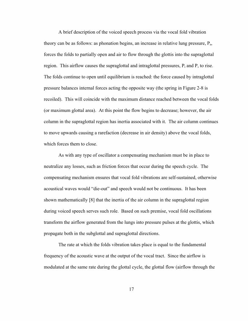
The harmonic content of the acoustic wave at the output of the vocal tract differs

from the frequency spectrum of the glottal flow. It can be derived from the spectrum of

the glottal flow by superimposing a particular frequency envelope (see [14] for example);

the shape of this envelope differs from one phoneme to the other. From a system level

point of view the speech process can then be described by the source-filter theory, which

considers the vocal folds to be the sound source and the rest of the vocal tract as a filter

with a certain transfer function (see Figure 2-9).

Figure 2-9: The vocal tract output spectrum via the source-filter theory.

FrequencyF0

Harmonics

Glottal Flow Spectrum

Frequency

Vocal Tract Transfer Function

FrequencyF0

Harmonics

Vocal Tract Output Spectrum

19

By detecting volumetric changes in the dielectric properties of neck tissues near

the position of the glottis, the GRES sensor is designed to provide “noise-free”

measurements of the glottal flow waveform during voiced segments of speech. Research

has shown that measurements of the glottal flow waveform (see Section 2.4) combined

with acoustic sensor measurements can effectively yield the vocal tract transfer function

and recover the speech signal in the presence of strong background noise.

2.2.3 Other speech sounds

There are additional speech sounds that are not produced during vibrations of the

glottal area. These include fricatives. The generation of fricative sounds can be

explained in terms of fluid dynamic quantities, where it is customary to study the flow of

fluid through a quantity called the Reynolds number:

Re vhµ

= (5)

where v is the particle velocity, h is the effective width of the orifice andµ is the

kinematic coefficient of viscosity. This quantity helps to describe the flow of a fluid

through a constriction; if a certain threshold value is exceeded, turbulence will be created

at exit. Otherwise, the flow will be smooth or laminar.

Turbulence is the cause for the production of fricatives. When the opening of the

glottis is small, its flow impedance increases. This causes a higher particle velocity,

which means that the Reynolds number increases. Turbulent flow creates nearly random

variations of air pressure in the glottis area, or otherwise stated an aperiodic acoustic

source. Fricatives are produced when this aperiodic source is sustained over a sufficient

20

amount of time [15]. In addition to fricatives there are speech sounds that may have

more than one source: for example the voiced fricative /z/.

Because of the nature of fricatives, i.e. turbulence instead of vocal tract

oscillations, we do not anticipate detecting them with the GRES sensor positioned around

the neck (the electric permittivity does not change).

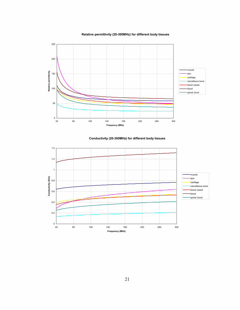
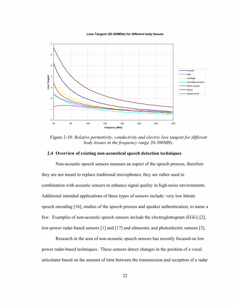
2.3 Dielectric properties of human tissue

In order for the sensor to be effective, we need to capitalize on the difference

between air and human tissue relative permittivity. There is an abundance of measured

data on the dielectric constant of different body tissues over a wide frequency range. In

addition, researchers have focused on how to interpolate the empirical data into a

function for the electric permittivity over a wide frequency range [6]. Such efforts enable

us to obtain relative permittivity data over a wide frequency range. It is worthy to note

two important things:

1. The value of the relative permittivity in the region of interest is on the order of 40-

200 for most body tissues

2. The relative permittivity of all tissues experiences minimal change over a narrow

band (even several MHz)

For example, the graphs in Figure 2-10 were produced from tabulated data retrieved

from the Italian Research Health Council’s website [6]:

21

Relative permittivity (20-300MHz) for different body tissues

0

50

100

150

200

250

20 60 100 140 180 220 260 300

Frequency (MHz)

Rel

ativ

e pe

rmitt

ivity

muscle

skin

cartilage

cancelleous bone

blood vessel

blood

spinal chord

Conductivity (20-300MHz) for different body tissues

0

0.2

0.4

0.6

0.8

1

1.2

1.4

20 60 100 140 180 220 260 300

Frequency (MHz)

Con

duct

ivity

(S/m

) muscle

skin

cartilage

cancelleous bone

blood vessel

blood

spinal chord

22

Loss Tangent (20-300MHz) for different body tissues

0

1

2

3

4

5

6

7

20 60 100 140 180 220 260 300

Frequency (MHz)

Loss

Tan

gent

muscle

skin

cartilage

cancelleous bone

blood vessel

blood

spinal chord

Figure 2-10: Relative permittivity, conductivity and electric loss tangent for different

body tissues in the frequency range 20-300MHz.

2.4 Overview of existing non-acoustical speech detection techniques

Non-acoustic speech sensors measure an aspect of the speech process, therefore

they are not meant to replace traditional microphones; they are rather used in

combination with acoustic sensors to enhance signal quality in high-noise environments.

Additional intended applications of these types of sensors include: very low bitrate

speech encoding [16], studies of the speech process and speaker authentication, to name a

few. Examples of non-acoustic speech sensors include the electroglottogram (EGG) [2],

low-power radar-based sensors [1] and [17] and ultrasonic and photoelectric sensors [3].

Research in the area of non-acoustic speech sensors has recently focused on low

power radar-based techniques. These sensors detect changes in the position of a vocal

articulator based on the amount of time between the transmission and reception of a radar

23

pulse. Radar-based sensors usually operate in the microwave region, i.e. 2GHz, and by

utilizing the scattering properties of the microwave signal can obtain a reflection from a

voice articulator’s surface, such as a tracheal wall. When worn near the vocal fold

region, radar-based sensors are able to obtain a signal related to subglottal pressure that is

used as a means for defining an excitation function for the human vocal tract during

voiced segments of speech [1]. The excitation function has been combined with acoustic

measurements to describe the human vocal tract transfer function [18], as well as to

provide a method for removing acoustic noise from speech signals [5].

One significant disadvantage of low-power radar vocal function sensors originates

from their inherent reliance on accurately measuring the roundtrip-time of an RF pulse.

Consequently, these types of sensors are sensitive to antenna alignment and positioning.

In addition, the human vocal tract has several soft and hard tissue layers and that allows

for multiple signal reflections. It has been observed that in the presence of complicated

scattering environments, radar based sensors can produce ambiguous results [19]. The

goal of this project is to overcome the aforementioned limitations of recently developed

non-acoustic sensor technologies. One evident advantage of the GRES sensor is that by

measuring an integrated effect of a cross section of the neck on a propagating

electromagnetic field, the sensor is unaffected by complicated scattering environments.

24

3 Theoretical Considerations

This section presents two different configurations of the GRES sensor along with

modeling methods used for predicting its behavior.

3.1 Lumped resonator structures

The basic building block of any resonator structure is LC-tank circuit (Figure

3-1), consisting of an inductor L and capacitor C. The resonance frequency of such

system is well known to be 01

2f

LCπ= . Clearly this is an idealized circuit that exhibits

no power loss and infinite quality factor, Q, which is defined as:

Q= Peak energy stored2Energy loss per cycle

π . In general, the Q of a resonator is indicative of how sharp

the impedance transition at resonance is. For the GRES sensor, a higher Q intuitively

results in a higher sensitivity to changes in the relative permittivity during voiced

segments of speech. However, Q is not the only factor that determines sensitivity of the

sensor. If the sensor is well-matched at resonance, small perturbations in the load

parameters cause large swings in the S11 magnitude response.

Figure 3-1: The basic LC cell.

25

To account for inherent losses in practical implementation of such structures, a

resistance is added to the initial LC circuit. There are two commonly discussed resonator

topologies, both of which will be summarized below:

1. The parallel RLC

2. The series RLC

The basic topology of the parallel RLC is shown in Figure 3-2. The resonance

frequency of such topology is again: 01

2f

LCπ= . The quality factor of the parallel

RLC is found to be: 00

R CQ RC RL L

ωω

= = = . In order for this circuit to have a high Q

the parallel resistance must be fairly high compared to the impedance of either the

inductor or capacitor.

Figure 3-2: The parallel RLC resonator.

The basis topology of the series RLC is shown in Figure 3-3. The resonance

frequency is the same as that of a basic LC cell: 01

2f

LCπ= . The quality factor is

found to be: 0

0

1 1L LQR RC R C

ωω

= = = .

26

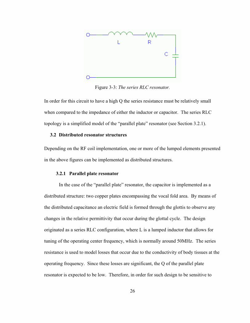
Figure 3-3: The series RLC resonator.

In order for this circuit to have a high Q the series resistance must be relatively small

when compared to the impedance of either the inductor or capacitor. The series RLC

topology is a simplified model of the “parallel plate” resonator (see Section 3.2.1).

3.2 Distributed resonator structures

Depending on the RF coil implementation, one or more of the lumped elements presented

in the above figures can be implemented as distributed structures.

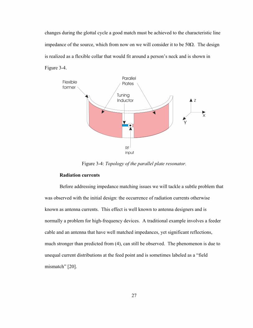
3.2.1 Parallel plate resonator

In the case of the “parallel plate” resonator, the capacitor is implemented as a

distributed structure: two copper plates encompassing the vocal fold area. By means of

the distributed capacitance an electric field is formed through the glottis to observe any

changes in the relative permittivity that occur during the glottal cycle. The design

originated as a series RLC configuration, where L is a lumped inductor that allows for

tuning of the operating center frequency, which is normally around 50MHz. The series

resistance is used to model losses that occur due to the conductivity of body tissues at the

operating frequency. Since these losses are significant, the Q of the parallel plate

resonator is expected to be low. Therefore, in order for such design to be sensitive to

27

changes during the glottal cycle a good match must be achieved to the characteristic line

impedance of the source, which from now on we will consider it to be 50Ω. The design

is realized as a flexible collar that would fit around a person’s neck and is shown in

Figure 3-4.

Z

Tuning

Inductor

X

Parallel

Plates

Y

Flexible

former

RF

input

Figure 3-4: Topology of the parallel plate resonator.

Radiation currents

Before addressing impedance matching issues we will tackle a subtle problem that

was observed with the initial design: the occurrence of radiation currents otherwise

known as antenna currents. This effect is well known to antenna designers and is

normally a problem for high-frequency devices. A traditional example involves a feeder

cable and an antenna that have well matched impedances, yet significant reflections,

much stronger than predicted from (4), can still be observed. The phenomenon is due to

unequal current distributions at the feed point and is sometimes labeled as a “field

mismatch” [20].

28

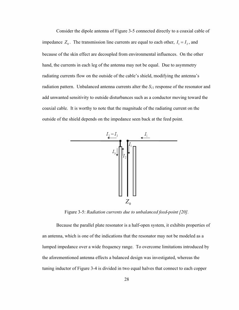
Consider the dipole antenna of Figure 3-5 connected directly to a coaxial cable of

impedance 0Z . The transmission line currents are equal to each other, 1 2I I= , and

because of the skin effect are decoupled from environmental influences. On the other

hand, the currents in each leg of the antenna may not be equal. Due to asymmetry

radiating currents flow on the outside of the cable’s shield, modifying the antenna’s

radiation pattern. Unbalanced antenna currents alter the S11 response of the resonator and

add unwanted sensitivity to outside disturbances such as a conductor moving toward the

coaxial cable. It is worthy to note that the magnitude of the radiating current on the

outside of the shield depends on the impedance seen back at the feed point.

0Z

Figure 3-5: Radiation currents due to unbalanced feed-point [20].

Because the parallel plate resonator is a half-open system, it exhibits properties of

an antenna, which is one of the indications that the resonator may not be modeled as a

lumped impedance over a wide frequency range. To overcome limitations introduced by

the aforementioned antenna effects a balanced design was investigated, whereas the

tuning inductor of Figure 3-4 is divided in two equal halves that connect to each copper

29

plate (see Figure 3-6); in this manner the resonance frequency stays the same as

previously.

Normally, a balun is employed to join an unbalanced feed to a balanced antenna

[21]. Baluns are usually divided into current baluns and voltage baluns [22] and [23].

Current baluns provide a high impedance to radiating currents at the feed point. Voltage

baluns, on the other hand, provide differential voltage at the feed point. Voltage baluns

may or may not suppress radiating currents locally, i.e. if the system is perfectly

symmetric radiating currents will be suppressed. When considering the balanced design

of Figure 3-6, the inductor connected to the shield of the cable acts as a current balun by

presenting a high local impedance to radiating currents that flow back from the copper

plate to the feed point.

Tuning and matching

It is well known that maximum power is transferred to a load, when the load

impedance is the complex conjugate of the source impedance. For the parallel plate

speech sensor a good impedance match means that the reflected voltage wave is small

(most of the power is delivered to the load). When looking at a return loss plot a good

match displays itself as a dip in the S11(f) response. Since it is unlikely that losses in the

neck will equal to the characteristic impedance of the source, a matching network must

be devised to transform the load impedance at resonance to 50Ω.

To resolve issues related to radiating currents flowing in the cable and to improve

matching at resonance a balanced, well-matched design is introduced in Figure 3-6.

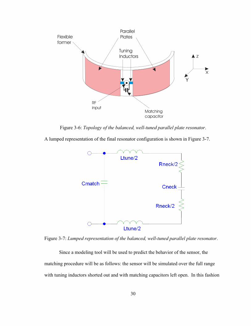
30

Z

Matching

capacitor

Tuning

Inductors

X

Parallel

Plates

Y

Flexible

former

RF

input

Figure 3-6: Topology of the balanced, well-tuned parallel plate resonator.

A lumped representation of the final resonator configuration is shown in Figure 3-7.

Figure 3-7: Lumped representation of the balanced, well-tuned parallel plate resonator.

Since a modeling tool will be used to predict the behavior of the sensor, the

matching procedure will be as follows: the sensor will be simulated over the full range

with tuning inductors shorted out and with matching capacitors left open. In this fashion

31

we can determine the impedance at the desired resonance frequency. A matching

program based on the well-known Smith Chart method (see [24], [25] and [26] for

example) will be utilized to transform the sensor’s impedance to the 50Ω characteristic

line impedance of the source.

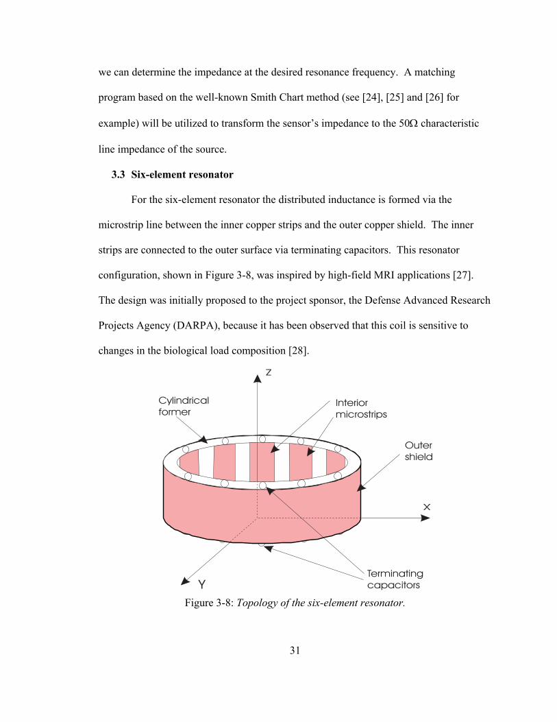
3.3 Six-element resonator

For the six-element resonator the distributed inductance is formed via the

microstrip line between the inner copper strips and the outer copper shield. The inner

strips are connected to the outer surface via terminating capacitors. This resonator

configuration, shown in Figure 3-8, was inspired by high-field MRI applications [27].

The design was initially proposed to the project sponsor, the Defense Advanced Research

Projects Agency (DARPA), because it has been observed that this coil is sensitive to

changes in the biological load composition [28]. Z

Terminating

capacitors

Interior

microstrips

X

Outer

shield

Y

Cylindrical

former

Figure 3-8: Topology of the six-element resonator.

32

Initially, the design was presented as a capacitive sensor (see [28]); however, its

detection technique is based on conductive and eddy-current losses that occur during the

glottal cycle. The simplest way to see this from a lumped element point of view is by

considering the coupling between the coil elements, which is primarily inductive in

nature (it resembles a transformer). In fact, the mutual inductance between the current-

carrying strips has been an important parameter in the modeling of traditional MRI coils

designs (see [29], [30] and [31]). Based on such premise and on the fact that the human

tissue is conductive at the operating frequency, the time-varying magnetic field induces

eddy-currents in the biological load; these losses modify the S11 response during voiced

segments of speech.

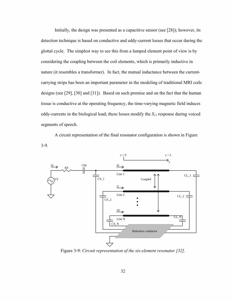
A circuit representation of the final resonator configuration is shown in Figure

3-9.

CS_2

CS_1

CS_N

CL_2

CL_1

CL_N

i0

i1

iN

Reference conductor

z = 0 z = L

zCM

RSiS

VS

Line 1

Line 2

Line N

Coupled

Figure 3-9: Circuit representation of the six-element resonator [32].

33

In order to make the sensor wearable, a half-open system will be utilized, i.e. the

dielectric former will not cover 360°, but only a fraction of the full circle. The name six-

element resonator is derived from the fact that only 6-inner strips are utilized.

3.3.1 Coupled microstrip line resonators

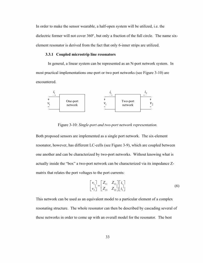
In general, a linear system can be represented as an N-port network system. In

most practical implementations one-port or two port networks (see Figure 3-10) are

encountered.

One-port

network

Two-port

network

1i 2i1i

1v 1v 2v

Figure 3-10: Single-port and two-port network representation.

Both proposed sensors are implemented as a single port network. The six-element

resonator, however, has different LC-cells (see Figure 3-9), which are coupled between

one another and can be characterized by two-port networks. Without knowing what is

actually inside the “box” a two-port network can be characterized via its impedance Z-

matrix that relates the port voltages to the port currents:

1 11 12 1

2 21 22 2

v Z Z iv Z Z i

=

(6)

This network can be used as an equivalent model to a particular element of a complex

resonating structure. The whole resonator can then be described by cascading several of

these networks in order to come up with an overall model for the resonator. The best

34

route to arrive at the overall model is by utilizing the ABCD or chain matrix. The Z-

matrix can be converted into its ABCD-equivalent by the following formula:

11

21 21

22

21 21

1

Z ZZ ZA B

C D ZZ Z

∆ =

(7)

where 11 22 12 21Z Z Z Z Z∆ = − . The overall ABCD-matrix would then be the product of the

individual matrices. This idea is illustrated below (Figure 3-11).

1i 2i

1v2v

1 1

1 1

A B

C D

2 2

2 2

A B

C D

1 1

1 1

A B

C D

2 2

2 2

A B

C D

2i

2v

1i

1v=

Figure 3-11: Cascading of different networks via the ABCD representation.

If we consider the mutual inductive coupling to be primarily influenced by the

adjacent strip, then the six-element resonator can be represented as a series of the LC

resonating cells. The entire structure can then be described by cascading the ABCD

networks of the individual cells as depicted in Figure 3-11. This technique is valuable

since the coupling between the resonating elements determines to a large extent the

sensitivity of the six-element resonator, and in general that of a multi transmission line

resonator. Since this method is only applicable for relatively low frequencies, a

mathematical solution based on Maxwell’s equations must be devised.

35

3.4 A review of Maxwell’s equations

Obtaining field solutions via analytical or numerical techniques requires solving

Maxwell’s equations. In the frequency domain Maxwell’s equations are presented in the

differential form as:

D ρ∇⋅ = (8)

0B∇⋅ = (9)

E j Hωµ∇× = − (10)

H J j Eωε∇× = + (11)

With the constitutive relationships:

D Eε=

B Hµ=

J Eσ=

The above quantities are defined as:

D : Electric flux density

E : Electric field intensity

B : Magnetic flux density

H : Magnetic field intensity

ε : Electric permittivity

µ : Magnetic permeability

ρ : Electric charge density

J : Impressed current density

36

In general, analytical solutions to Maxwell’s equations become cumbersome and

unfeasible even for distributed structures with modest complexities. So, in order to

predict the frequency response and field values in and around the proposed resonator

designs, a numerical modeling method is employed.

3.5 Modeling efforts

Several modeling methods exist, each offering certain advantages and

disadvantages. The simplest method treats all coil elements and the load as lumped

impedances, which is usually a good approximation at relatively low frequencies. As the

structure size becomes comparable to the wavelength, so-called full-wave solvers based

on Maxwell’s equations must be utilized. Full-wave solvers discretize the solution

domain and solve the governing partial differential equations (PDEs) by either explicit or

implicit means. The most common techniques include finite differences, the method of

moments and finite elements.

The finite difference time domain (FDTD) method solves the governing PDEs

explicitly by using a marching in time technique. The field values are updated at the end

of each time step and if the mesh size is chosen appropriately, field values converge to a

stable state. Although this technique is relatively fast its main disadvantage rests on the

fact that FDTD solvers cannot easily handle arbitrary geometrical shapes. The method of

moments (MoM) is based on the integral formulation of Maxwell’s equations. MoM

generates results very fast, however, it cannot easily handle a complex biological load

with different material properties and it scales worse than FDTD or the finite element

method (FEM) due to fully populated matrices. The finite element method, on the other

hand, can easily conform to arbitrary geometrically shaped objects with different material

37

properties. FEM discretizes the solution domain into contiguous non-overlapping

elements and interpolates the fields inside each element through so-called basis functions.

Typical solution times with a FEM solver last from several hours to days depending on

the desired accuracy and the availability of computational resources; hence, speed is the

biggest drawback to the FEM.

In addition to these well-known techniques, the multi-conductor transmission line

(MTL) theory has been recently implemented for predicting the behavior of MRI coils

[27] and [32]. This particular MTL solver employs a boundary element method (BEM)

in the transverse plane (xy-plane Figure 3-8), while considering transverse

electromagnetic (TEM) propagation in the longitudinal direction (z-direction Figure 3-8).

We discuss the MTL method and the FEM on the subsequent chapters.

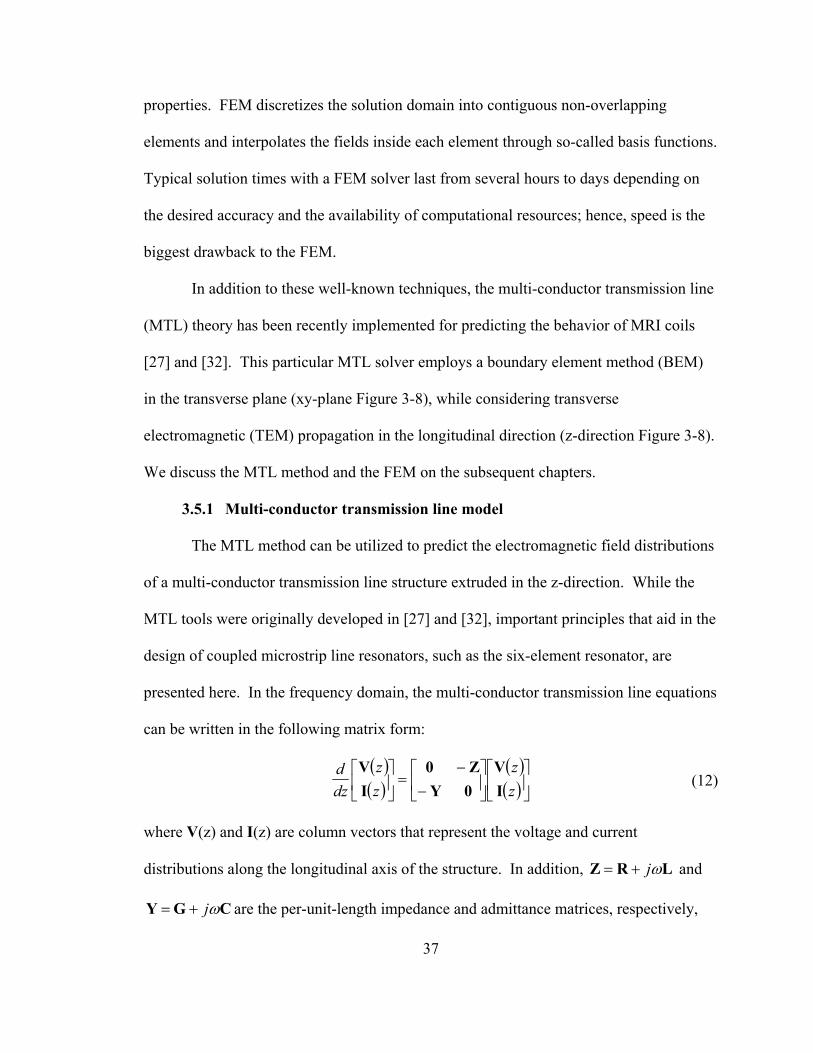
3.5.1 Multi-conductor transmission line model

The MTL method can be utilized to predict the electromagnetic field distributions

of a multi-conductor transmission line structure extruded in the z-direction. While the

MTL tools were originally developed in [27] and [32], important principles that aid in the

design of coupled microstrip line resonators, such as the six-element resonator, are

presented here. In the frequency domain, the multi-conductor transmission line equations

can be written in the following matrix form:

( )( )

( )( )

−

−=

zz

zz

dzd

IV

0YZ0

IV

(12)

where V(z) and I(z) are column vectors that represent the voltage and current

distributions along the longitudinal axis of the structure. In addition, LRZ ωj+= and

CGY ωj+= are the per-unit-length impedance and admittance matrices, respectively,

38

which characterize the multi-conductor transmission line structure as a function of

angular frequency fπω 2= . A boundary element numerical technique based on the

Laplace’s equation is employed to compute these matrices in the xy-plane [32].

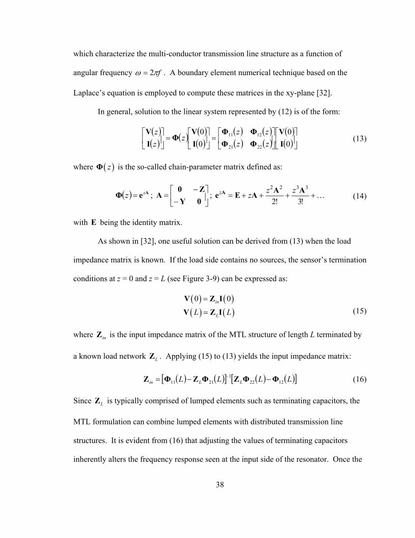
In general, solution to the linear system represented by (12) is of the form:

( )( ) ( ) ( )

( )( ) ( )( ) ( )

( )( )

=

=

00

00

2221

1211

IV

ΦΦΦΦ

IV

ΦIV

zzzz

zzz

(13)

where ( )zΦ is the so-called chain-parameter matrix defined as:

( ) AeΦ zz = ;

−

−=

0YZ0

A ; …++++=!3!2

3322 AAAEe A zzzz (14)

with E being the identity matrix.

As shown in [32], one useful solution can be derived from (13) when the load

impedance matrix is known. If the load side contains no sources, the sensor’s termination

conditions at z = 0 and z = L (see Figure 3-9) can be expressed as:

( ) ( )0 0in=V Z I

( ) ( )LL L=V Z I (15)

where inZ is the input impedance matrix of the MTL structure of length L terminated by

a known load network LZ . Applying (15) to (13) yields the input impedance matrix:

( ) ( )[ ] ( ) ( )[ ]LLLL LLin 12221

2111 ΦΦZΦZΦZ −−= − (16)

Since LZ is typically comprised of lumped elements such as terminating capacitors, the

MTL formulation can combine lumped elements with distributed transmission line

structures. It is evident from (16) that adjusting the values of terminating capacitors

inherently alters the frequency response seen at the input side of the resonator. Once the

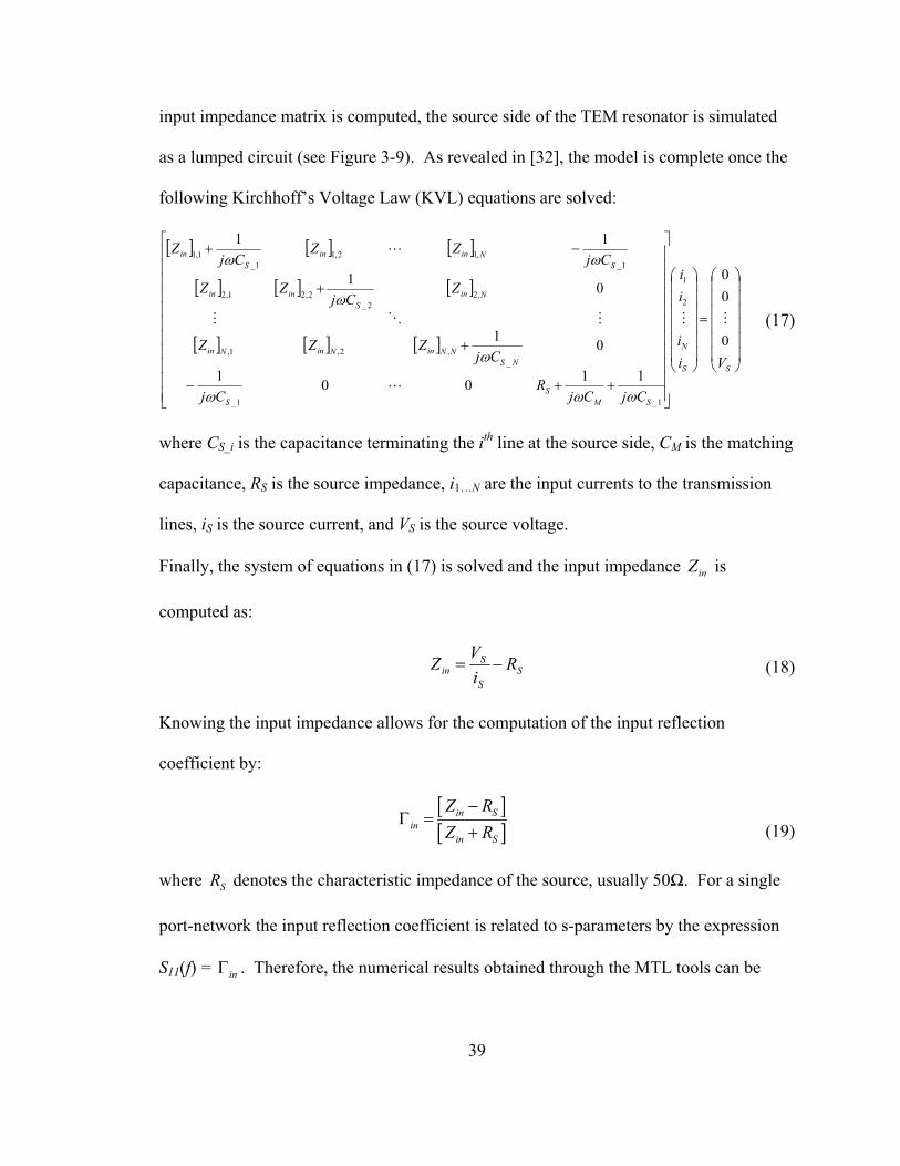
39

input impedance matrix is computed, the source side of the TEM resonator is simulated

as a lumped circuit (see Figure 3-9). As revealed in [32], the model is complete once the

following Kirchhoff’s Voltage Law (KVL) equations are solved:

[ ] [ ] [ ]

[ ] [ ] [ ]

[ ] [ ] [ ]

=

++−

+

+

−+

SS

N

SMS

S

NSNNinNinNin

NinS

inin

SNinin

Sin

Vii

ii

CjCjR

Cj

CjZZZ

ZCj

ZZ

CjZZ

CjZ

0

00

11001

01

01

11

2

1

1_1_

_,2,1,

,22_

2,21,2

1_,12,1

1_1,1

ωωω

ω

ω

ωω

(17)

where CS_i is the capacitance terminating the ith line at the source side, CM is the matching

capacitance, RS is the source impedance, i1…N are the input currents to the transmission

lines, iS is the source current, and VS is the source voltage.

Finally, the system of equations in (17) is solved and the input impedance inZ is

computed as:

SS

Sin R

iVZ −= (18)

Knowing the input impedance allows for the computation of the input reflection

coefficient by:

[ ][ ]

in Sin

in S

Z RZ R

−Γ =

+

(19)

where SR denotes the characteristic impedance of the source, usually 50Ω. For a single

port-network the input reflection coefficient is related to s-parameters by the expression

S11(f) = inΓ . Therefore, the numerical results obtained through the MTL tools can be

40

directly compared to s-parameter measurements obtained from a standard network

analyzer.

Typically, the MTL method can predict the S11(f) response of the six-element

resonator, including a biological load model inside it, within a matter of minutes on a

standard personal computer. This great benefit renders the MTL method as a primary

candidate for performing rapid design tasks.

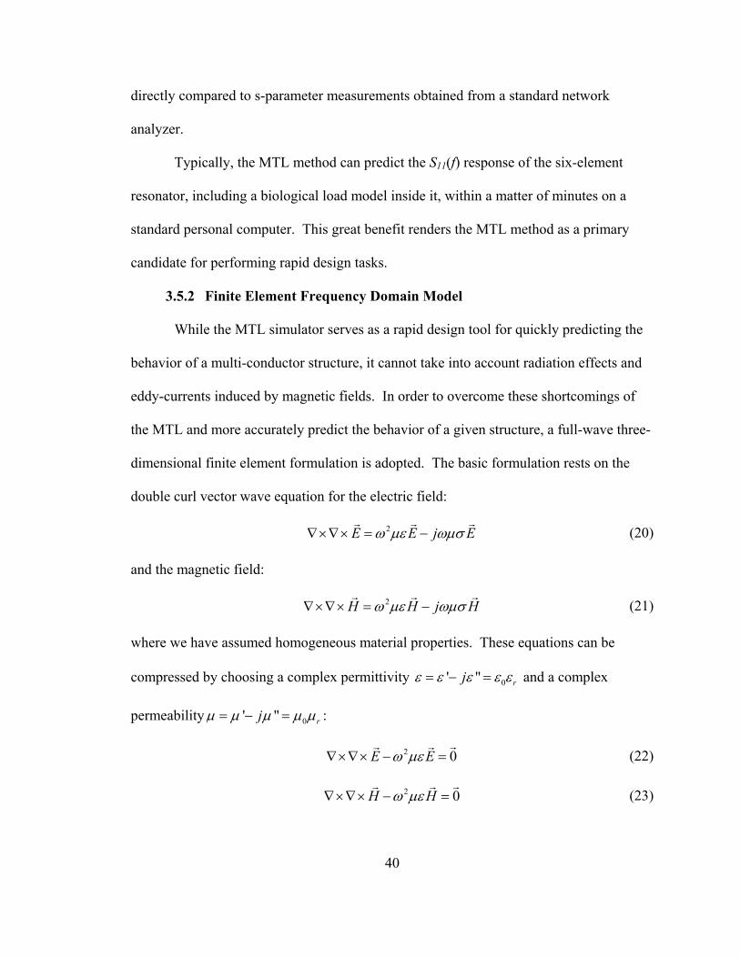
3.5.2 Finite Element Frequency Domain Model

While the MTL simulator serves as a rapid design tool for quickly predicting the

behavior of a multi-conductor structure, it cannot take into account radiation effects and

eddy-currents induced by magnetic fields. In order to overcome these shortcomings of

the MTL and more accurately predict the behavior of a given structure, a full-wave three-

dimensional finite element formulation is adopted. The basic formulation rests on the

double curl vector wave equation for the electric field:

2E E j Eω µε ωµσ∇×∇× = − (20)

and the magnetic field:

2H H j Hω µε ωµσ∇×∇× = − (21)

where we have assumed homogeneous material properties. These equations can be

compressed by choosing a complex permittivity 0' " rjε ε ε ε ε= − = and a complex

permeability 0' " rjµ µ µ µ µ= − = :

2 0E Eω µε∇×∇× − = (22)

2 0H Hω µε∇×∇× − = (23)

41

where rε and rµ are complex quantities.

There exist two standard FEM treatment techniques:

a) The variational method

b) The method of weighted residuals

In the following section we discuss the method of weighted residuals primarily because

of its wide use and ease of implementation.

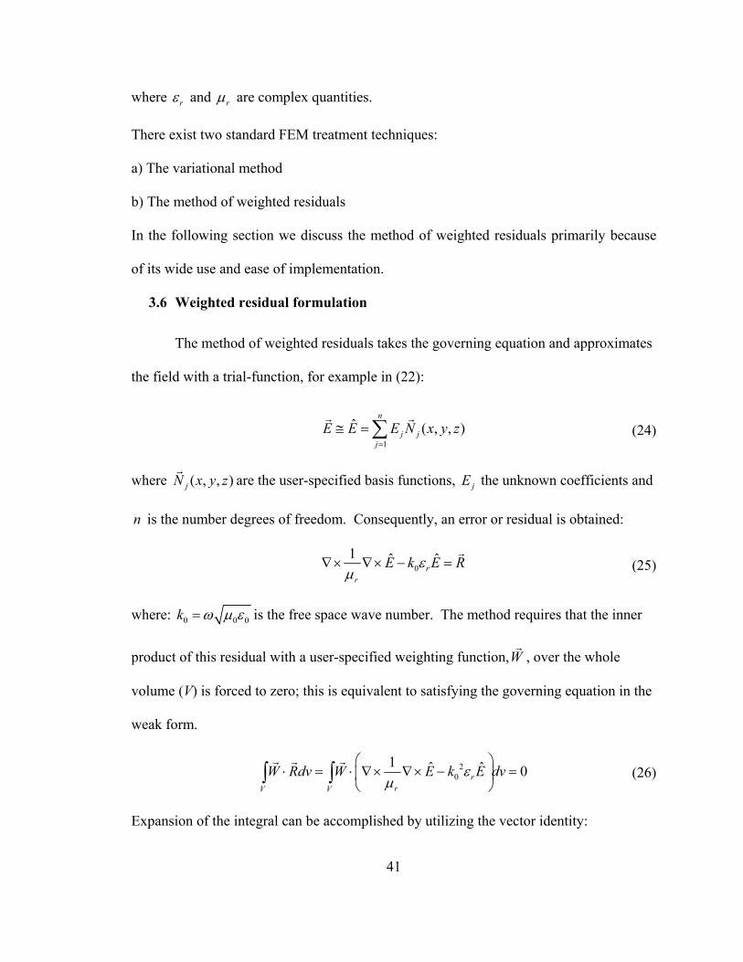
3.6 Weighted residual formulation

The method of weighted residuals takes the governing equation and approximates

the field with a trial-function, for example in (22):

1

ˆ ( , , )n

j jj

E E E N x y z=

≅ =∑ (24)

where ( , , )jN x y z are the user-specified basis functions, jE the unknown coefficients and

n is the number degrees of freedom. Consequently, an error or residual is obtained:

01 ˆ ˆ

rr

E k E Rεµ

∇× ∇× − = (25)

where: 0 0 0k ω µ ε= is the free space wave number. The method requires that the inner

product of this residual with a user-specified weighting function,W , over the whole

volume (V) is forced to zero; this is equivalent to satisfying the governing equation in the

weak form.

20

1 ˆ ˆ 0rrV V

W Rdv W E k E dvεµ

⋅ = ⋅ ∇× ∇× − =

∫ ∫ (26)

Expansion of the integral can be accomplished by utilizing the vector identity:

42

( )( ) ( ) ( ) ( )( )ˆ ˆ ˆW E E W W E⋅ ∇× ∇× = ∇× ⋅ ∇× −∇ ⋅ × ∇× (27)

and the divergence theorem:

( ) ( )ˆ ˆˆV S

E dv n E ds∇⋅ = ⋅∫ ∫ (28)

Application of (27) to (25) results in:

( ) ( ) ( )( )1 1 1ˆ ˆ ˆˆr r rV V S

W E dv E W dv n W E dsµ µ µ

⋅ ∇× ∇× = ∇× ⋅ ∇× − ⋅ × ∇×

∫ ∫ ∫ (29)

where S is the surface enclosing the solution domain, and the normal n points away from

the solution (integration) region. Using the clockwise property of the scalar triple-

product:

( ) ( ) ( )ˆ ˆ ˆˆ ˆ ˆn W E W E n W n E⋅ ×∇× = ⋅ ∇× × = − ⋅ ×∇× (30)

the electric field formulation (26) reduces to:

( ) ( ) ( )20

1 1ˆ ˆ ˆˆrr rV S

W E k W E dv W n E dsεµ µ

∇× ⋅ ∇× − ⋅ = − ⋅ ×∇×

∫ ∫ (31)

Proper choice of the basis functions enables us to implement the surface integral

as an explicit impedance boundary. Perfect E and perfect H boundaries do not contribute

to the surface integral while for radiation boundaries the region of interest has special

tensor properties; boundary conditions will be explored in depth in Section 3.6.3

In order to implement the impedance boundary, the ˆn E×∇× term must be

expanded. Since E represents the electric field, from equation (10) the wave equation

can be converted into the following form:

43

( ) ( ) ( )20 0 0

1 ˆ ˆ ˆˆrrV S

W E k W E dv jk W n H dsε ηµ

∇× ⋅ ∇× − ⋅ = ⋅ ×

∫ ∫ (32)

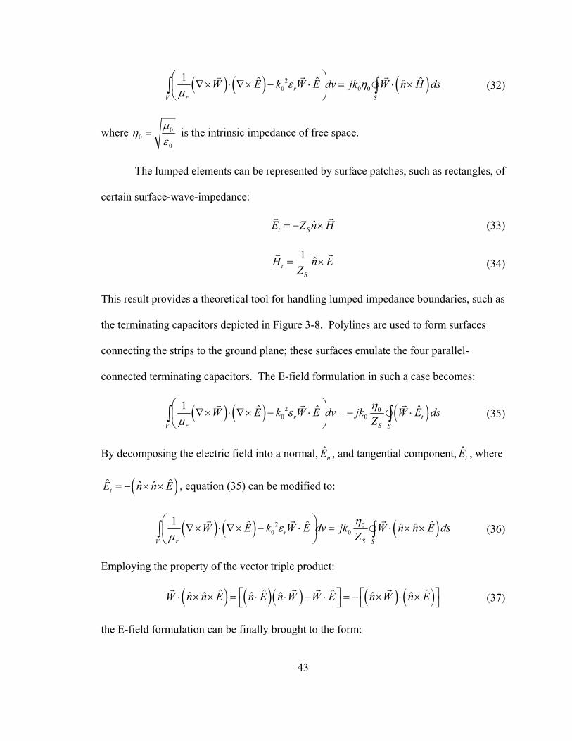
where 00

0

µηε

= is the intrinsic impedance of free space.

The lumped elements can be represented by surface patches, such as rectangles, of

certain surface-wave-impedance:

ˆt SE Z n H= − × (33)

1 ˆtS

H n EZ

= × (34)

This result provides a theoretical tool for handling lumped impedance boundaries, such as

the terminating capacitors depicted in Figure 3-8. Polylines are used to form surfaces

connecting the strips to the ground plane; these surfaces emulate the four parallel-

connected terminating capacitors. The E-field formulation in such a case becomes:

( ) ( ) ( )2 00 0

1 ˆ ˆ ˆr t

r SV S

W E k W E dv jk W E dsZηε

µ

∇× ⋅ ∇× − ⋅ = − ⋅ ∫ ∫ (35)

By decomposing the electric field into a normal, ˆnE , and tangential component, ˆ

tE , where

( )ˆ ˆˆ ˆtE n n E= − × × , equation (35) can be modified to:

( ) ( ) ( )2 00 0

1 ˆ ˆ ˆˆ ˆrr SV S

W E k W E dv jk W n n E dsZηε

µ

∇× ⋅ ∇× − ⋅ = ⋅ × × ∫ ∫ (36)

Employing the property of the vector triple product:

( ) ( )( ) ( ) ( )ˆ ˆ ˆ ˆˆ ˆ ˆ ˆ ˆ ˆW n n E n E n W W E n W n E ⋅ × × = ⋅ ⋅ − ⋅ = − × ⋅ × (37)

the E-field formulation can be finally brought to the form:

44

( ) ( ) ( ) ( )2 00 0

1 ˆ ˆ ˆˆ ˆ 0rr SV S

W E k W E dv jk n W n E dsZηε

µ

∇× ⋅ ∇× − ⋅ + × ⋅ × = ∫ ∫ (38)

Although rarely used, a similar statement can be obtained for the magnetic field:

( ) ( ) ( ) ( )20 0

0

1 ˆ ˆ ˆˆ ˆ 0Sr

rV S

ZW H k W H dv jk n W n H dsµε η

∇× ⋅ ∇× − ⋅ + × ⋅ × =

∫ ∫ (39)

3.6.1 Domain discretization and matrix formulation

The solution domain is partitioned by deploying a desired number of nodes

throughout the region of interest, while choosing the desired tessellation. Common

implementations utilize tetrahedrons as the basic cell in order to make good

approximations for arbitrary shaped objects. Consequently, basis functions are applied

inside each basic cell. Using (24) the discretized formulation takes the form:

( ) ( ) ( ) ( )2 00 0

1

1 ˆ ˆ 0N

i j r i j i j jj r SV S

W N k W N dv jk n W n N ds EZηε

µ=

∇× ⋅ ∇× − ⋅ + × ⋅ × =

∑ ∫ ∫ (40)

for i=1..N.

The different weighted residual formulations vary from each other in the way the

weighting functions are selected. A widely used technique, the Galerkin, uses the same

weighting functions as the basis functions:

k kW N= (41)

The Galerkin formulation for the electric field now becomes:

( ) ( ) ( ) ( )2 00 0

1

1 ˆ ˆ 0N

j r i j i j jij r SV S

W W k W W dv jk n W n W ds EZηε

µ=

∇× ⋅ ∇× − ⋅ + × ⋅ × =

∑ ∫ ∫ (42)

for i=1..N. This result can be represented in the matrix form:

45

0=AE (43)

where E denotes the vector of unknown E-field coefficients, and A is the matrix with

known elements:

( ) ( ) ( ) ( )2 00 0

1 ˆ ˆij j r i j i jir SV S

A W W k W W dv jk n W n W dsZηε

µ

= ∇× ⋅ ∇× − ⋅ + × ⋅ × ∫ ∫ (44)

Since the A matrix is known, then it’s a matter of choosing an efficient solver in order to

obtain the values of the unknown coefficients. Ongoing research in this area includes

devising more efficient banded matrix solvers and matrix preconditioning for faster

convergence of iterative solvers such as conjugate gradient [33].

3.6.2 Basis function selection

The choice of basis functions determines to a large extent the accuracy of the

FEM formulation. Generally speaking, the key ingredients in selecting a basis function

are:

a) Selection of an orthogonal series basis function

b) Selection of a computationally efficient series

In the frequency domain formulation, a fully orthogonal basis set ensures that both

conditions are satisfied:

0i jV

W W dv for i j⋅ = ≠∫

and 0e

i jV

W W dv for i j∇× ⋅∇× = ≠∫ (45)

If such basis set could be implemented in practice, the result would be a diagonal matrix

the inversion of which is trivial. Computational efficiency can still be improved by

46

properly choosing a nearly orthogonal basis set, the result of which is a sparse matrix

structure. For example, the Lagrange polynomials find many uses in the solution of heat

problems, where node-based interpolation is adequate for the divergence operators:

1

( )( )

ki

jj j i

x xNx x=

−=

−∏ (46)

where ;i j≠ k = number of nodes in element and 0jN = for all nodes not in element.

In the solution of electromagnetic problems node-based interpolation is not well

suited for the curl operator. Instead, edge or face basis functions are chosen. For

example, the Whitney 1-form vector shape function associated with the edge between

two adjacent nodes ( i and j ) takes the form:

ij i j j iW λ λ λ λ= ∇ − ∇ (47)

where iλ and jλ are the barycentric functions for the two nodes [34]. Higher order

functions are possible, however, stretching the limits of the scope of this project we refer

the interested reader to the appropriate literature [34].

3.6.3 Boundary Conditions

The finite element solution ensures that continuity of the electric and magnetic

field is maintained between interfaces of different material boundaries.

( )1 2ˆ 0n E E× − =

( )1 2ˆ sn H H J× − = (48)

Here the normal points from medium region 1 to region 2 and Js is an impressed surface

current density. Where the finite element mesh is terminated, additional boundary

conditions can be imposed that are either of electric type

47

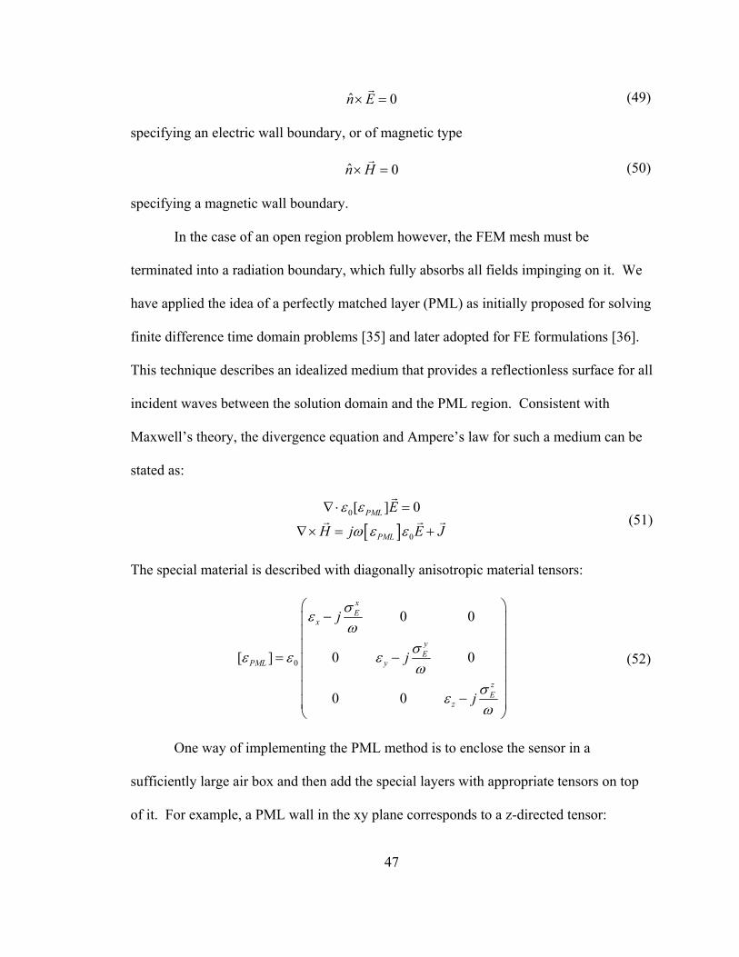
ˆ 0n E× = (49)

specifying an electric wall boundary, or of magnetic type

ˆ 0n H× = (50)

specifying a magnetic wall boundary.

In the case of an open region problem however, the FEM mesh must be

terminated into a radiation boundary, which fully absorbs all fields impinging on it. We

have applied the idea of a perfectly matched layer (PML) as initially proposed for solving

finite difference time domain problems [35] and later adopted for FE formulations [36].

This technique describes an idealized medium that provides a reflectionless surface for all

incident waves between the solution domain and the PML region. Consistent with

Maxwell’s theory, the divergence equation and Ampere’s law for such a medium can be

stated as:

0[ ] 0PML Eε ε∇ ⋅ =

[ ] 0PMLH j E Jω ε ε∇× = + (51)

The special material is described with diagonally anisotropic material tensors:

0

0 0

[ ] 0 0

0 0

xE

x

yE

PML y

zE

z

j

j

j

σεω

σε ε εω

σεω

−

= −

−

(52)

One way of implementing the PML method is to enclose the sensor in a

sufficiently large air box and then add the special layers with appropriate tensors on top

of it. For example, a PML wall in the xy plane corresponds to a z-directed tensor:

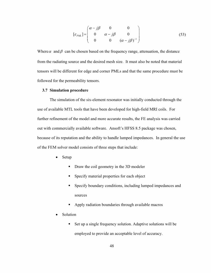
48

1

0 0[ ] 0 0

0 0 ( )PML

jj

j

α βε α β

α β −

− = − −

(53)

Whereα andβ can be chosen based on the frequency range, attenuation, the distance

from the radiating source and the desired mesh size. It must also be noted that material

tensors will be different for edge and corner PMLs and that the same procedure must be

followed for the permeability tensors.

3.7 Simulation procedure

The simulation of the six-element resonator was initially conducted through the

use of available MTL tools that have been developed for high-field MRI coils. For

further refinement of the model and more accurate results, the FE analysis was carried

out with commercially available software. Ansoft’s HFSS 8.5 package was chosen,

because of its reputation and the ability to handle lumped impedances. In general the use

of the FEM solver model consists of three steps that include:

• Setup

Draw the coil geometry in the 3D modeler

Specify material properties for each object

Specify boundary conditions, including lumped impedances and

sources

Apply radiation boundaries through available macros

• Solution

Set up a single frequency solution. Adaptive solutions will be

employed to provide an acceptable level of accuracy.

49

The generated mesh may be further refined in order to get higher

accuracy.

Based on the refined mesh, set up the desired sweep range, the

field accuracy, the number of frequency steps and solve.

Because of the finite number of steps allowed for frequency

sweeps, additional sweeps may be carried in order to zoom-in to a

particular mode.

• Post-processing

Plot the S11 response of the resonator and save the data file.

Import the data file into Matlab where better manipulation of the

plots can be carried through.

The electric field distribution at the mode of interest can be

captured as a screenshot.

We next examine the results of various frequency sweeps for both resonators.

50

4 Numerical Simulations and Field Predictions

This section applies the MTL and FE methods to specific examples of the six-element

and the parallel plate resonator. The behavior of each sensor is predicted in the context

of changes during the glottal cycle.

4.1 Six element resonator

The six-element resonator design was initially modeled with the basic

construction shown in Figure 3-8 and with specific parameters given in Table 4-1.

Table 4-1: Six-element resonator prototype design parameters.

Parameter Value

Plexiglass former inner radius 69.8mm

Plexiglass former outer radius 76.2mm

Plexiglass former height 38.1mm

Number of interior microstrip lines 6

Width of interior microstrip lines (same for all) 21.21mm

Spacing between interior microstrip lines (same for all) 3.175mm

Total angle spanned by shield 120 degrees

Value of terminating capacitance 108pF

In order for the sensor to be easily worn around the neck, the cylindrical former spans a

total angle of 120 degrees. As a result, there are only six copper-strips (hence the name

six-element resonator) in the interior of the sensor. The MTL method was used to select

values for the terminating capacitance for this design such that the first resonant mode

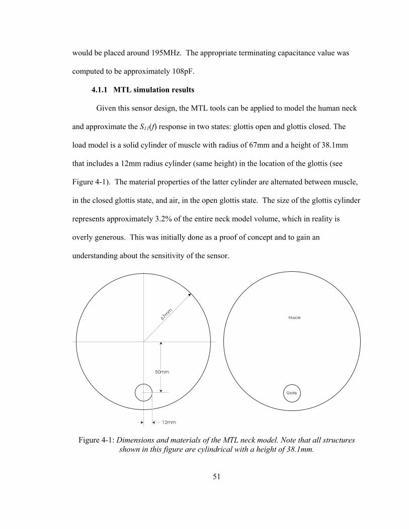
51

would be placed around 195MHz. The appropriate terminating capacitance value was

computed to be approximately 108pF.

4.1.1 MTL simulation results

Given this sensor design, the MTL tools can be applied to model the human neck

and approximate the S11(f) response in two states: glottis open and glottis closed. The

load model is a solid cylinder of muscle with radius of 67mm and a height of 38.1mm

that includes a 12mm radius cylinder (same height) in the location of the glottis (see

Figure 4-1). The material properties of the latter cylinder are alternated between muscle,

in the closed glottis state, and air, in the open glottis state. The size of the glottis cylinder

represents approximately 3.2% of the entire neck model volume, which in reality is

overly generous. This was initially done as a proof of concept and to gain an

understanding about the sensitivity of the sensor.

Figure 4-1: Dimensions and materials of the MTL neck model. Note that all structures shown in this figure are cylindrical with a height of 38.1mm.

Muscle

Glottis

67m

m

12mm

50mm

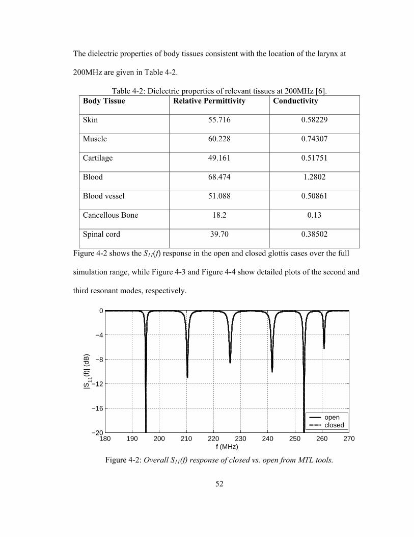
52

The dielectric properties of body tissues consistent with the location of the larynx at

200MHz are given in Table 4-2.

Table 4-2: Dielectric properties of relevant tissues at 200MHz [6]. Body Tissue Relative Permittivity Conductivity

Skin 55.716 0.58229

Muscle 60.228 0.74307

Cartilage 49.161 0.51751

Blood 68.474 1.2802

Blood vessel 51.088 0.50861

Cancellous Bone 18.2 0.13

Spinal cord 39.70 0.38502

Figure 4-2 shows the S11(f) response in the open and closed glottis cases over the full

simulation range, while Figure 4-3 and Figure 4-4 show detailed plots of the second and

third resonant modes, respectively.

180 190 200 210 220 230 240 250 260 270−20

−16

−12

−8

−4

0

f (MHz)

|S11

(f)|

(dB

)

openclosed

Figure 4-2: Overall S11(f) response of closed vs. open from MTL tools.

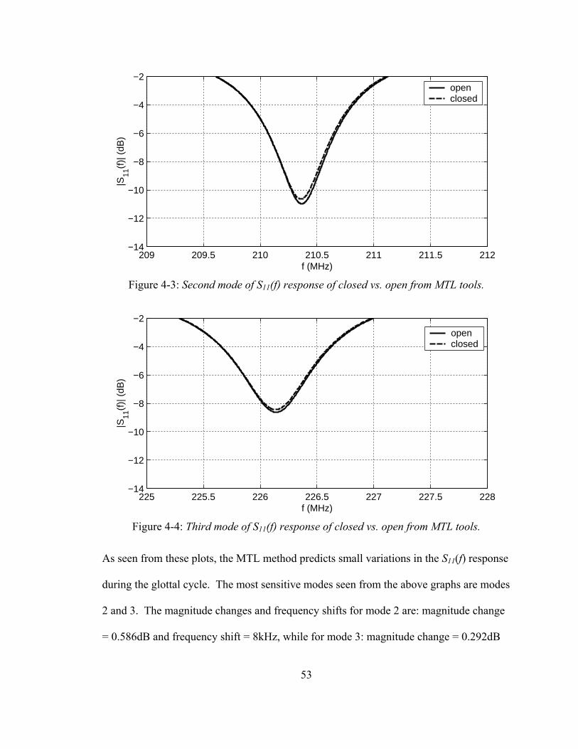
53

209 209.5 210 210.5 211 211.5 212−14

−12

−10

−8

−6

−4

−2

f (MHz)

|S11

(f)|

(dB

)

openclosed

Figure 4-3: Second mode of S11(f) response of closed vs. open from MTL tools.

225 225.5 226 226.5 227 227.5 228−14

−12

−10

−8

−6

−4

−2

f (MHz)

|S11

(f)|

(dB

)

openclosed

Figure 4-4: Third mode of S11(f) response of closed vs. open from MTL tools.

As seen from these plots, the MTL method predicts small variations in the S11(f) response

during the glottal cycle. The most sensitive modes seen from the above graphs are modes

2 and 3. The magnitude changes and frequency shifts for mode 2 are: magnitude change

= 0.586dB and frequency shift = 8kHz, while for mode 3: magnitude change = 0.292dB

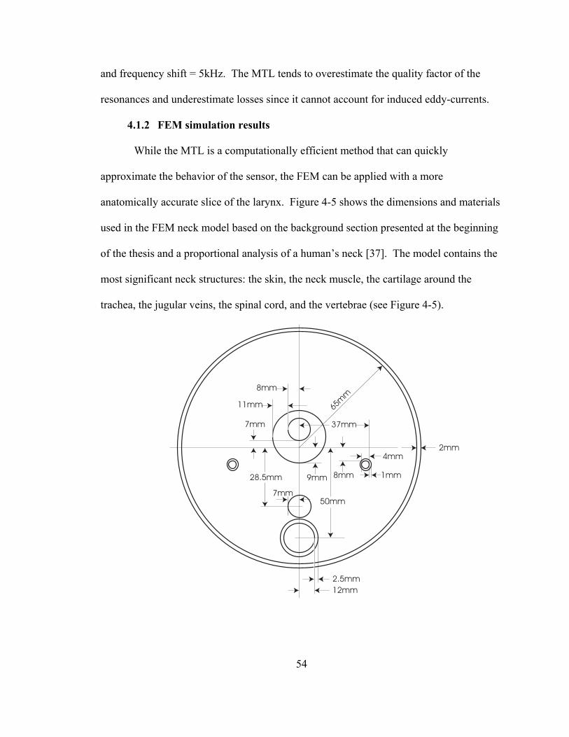
54

and frequency shift = 5kHz. The MTL tends to overestimate the quality factor of the

resonances and underestimate losses since it cannot account for induced eddy-currents.

4.1.2 FEM simulation results

While the MTL is a computationally efficient method that can quickly

approximate the behavior of the sensor, the FEM can be applied with a more

anatomically accurate slice of the larynx. Figure 4-5 shows the dimensions and materials

used in the FEM neck model based on the background section presented at the beginning

of the thesis and a proportional analysis of a human’s neck [37]. The model contains the

most significant neck structures: the skin, the neck muscle, the cartilage around the

trachea, the jugular veins, the spinal cord, and the vertebrae (see Figure 4-5).

2mm

65m

m

12mm

2.5mm

50mm

28.5mm

7mm

8mm

11mm

7mm

9mm 1mm

37mm

4mm

8mm

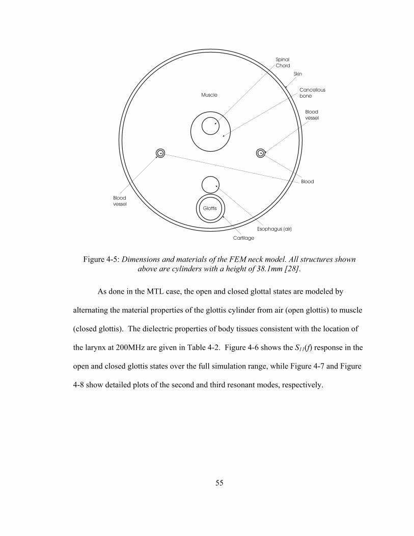
55

Cartilage

Skin

Spinal

Chord

MuscleCancellous

bone

Esophagus (air)

Blood

Blood

vessel

Blood

vessel

Glottis

Figure 4-5: Dimensions and materials of the FEM neck model. All structures shown above are cylinders with a height of 38.1mm [28].

As done in the MTL case, the open and closed glottal states are modeled by

alternating the material properties of the glottis cylinder from air (open glottis) to muscle

(closed glottis). The dielectric properties of body tissues consistent with the location of

the larynx at 200MHz are given in Table 4-2. Figure 4-6 shows the S11(f) response in the

open and closed glottis states over the full simulation range, while Figure 4-7 and Figure

4-8 show detailed plots of the second and third resonant modes, respectively.

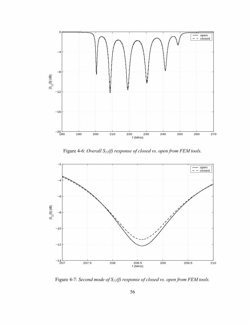
56

180 190 200 210 220 230 240 250 260 270−20

−16

−12

−8

−4

0

f (MHz)

|S11

(f)| (

dB)

openclosed

Figure 4-6: Overall S11(f) response of closed vs. open from FEM tools.

207 207.5 208 208.5 209 209.5 210−14

−12

−10

−8

−6

−4

−2

f (MHz)

|S11

(f)| (

dB)

openclosed

Figure 4-7: Second mode of S11(f) response of closed vs. open from FEM tools.

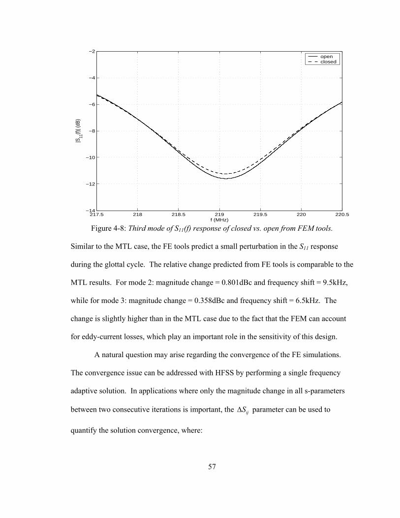
57

217.5 218 218.5 219 219.5 220 220.5−14

−12

−10

−8

−6

−4

−2

f (MHz)

|S11

(f)| (

dB)

openclosed

Figure 4-8: Third mode of S11(f) response of closed vs. open from FEM tools.

Similar to the MTL case, the FE tools predict a small perturbation in the S11 response

during the glottal cycle. The relative change predicted from FE tools is comparable to the

MTL results. For mode 2: magnitude change = 0.801dBc and frequency shift = 9.5kHz,

while for mode 3: magnitude change = 0.358dBc and frequency shift = 6.5kHz. The

change is slightly higher than in the MTL case due to the fact that the FEM can account

for eddy-current losses, which play an important role in the sensitivity of this design.

A natural question may arise regarding the convergence of the FE simulations.

The convergence issue can be addressed with HFSS by performing a single frequency

adaptive solution. In applications where only the magnitude change in all s-parameters

between two consecutive iterations is important, the ijS∆ parameter can be used to

quantify the solution convergence, where:

58

current previousij ij ijS S S∆ = − (54)

The iterative solver will continue to refine the mesh until either the number of iterations

or the ijS∆ value is met. In order to ensure conformance to the ijS∆ parameter, the

number of iterations can be set to a large value. On the other hand, ijS∆ should not be set

to a really small value, since such accuracy may not be achieved, and the solver will

eventually run out of memory. For the six-element resonator the solution converged

nicely after setting 0.02ijS∆ = . In general, the adaptive solution frequency is chosen at

the higher end of a full frequency sweep, since this allows for the mesh to capture enough

nodes per wavelength to ensure adequate coverage for the full frequency sweep.

Although the six-element resonator has six radically different modes, the adaptive

solution was conducted at the second resonant mode frequency.

The FE post-processing tools can also be utilized to generate detailed field plots

in a region of interest. More intuition about the sensitivity of the six-element resonator in

different modes can be gained by observing the electric field strength and the amount of

field penetration into the glottal region. Figure 4-9 shows the electric field magnitudes in

a cross-sectional plane of the neck for all resonant modes. The field magnitudes are

plotted for the “open glottis” state only. Since the six-element resonator is an eddy

current based sensor, the most sensitive modes will have greater electric field magnitudes

in the glottal region. From these plots it can be deduced that that mode 2, which has the

highest field strength in the glottal region, is the most sensitive mode. For mode 3, the

field penetrates well in the glottal region, but it is not as strong in magnitude as mode 2.

The E-field plots confirm the sensitivity results seen in the S11(f) plots, presented in the

59

previous section. The sensitivity of this design can be improved by increasing the

operating frequency, which increases ωε and in turn eddy-current losses. Also, by

decreasing the sensor size the fields can be more concentrated in the glottal area;

however, too small a sensor may not provide enough penetration into the region of

interest.

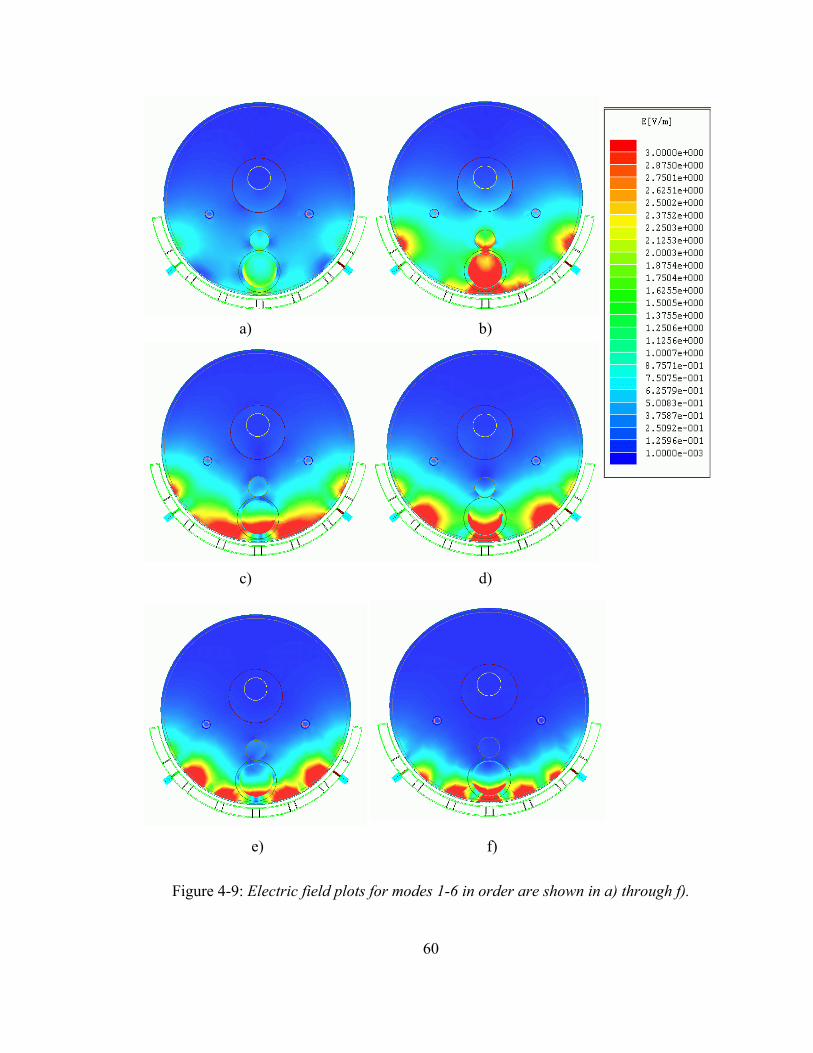
60

a) b)

a) b)

c) d)

c) d)

e) f)

Figure 4-9: Electric field plots for modes 1-6 in order are shown in a) through f).

61

From the S11(f) response obtained through FE simulations it is apparent that the

six-element resonator offers insignificant changes during the glottal cycle and cannot be

implemented as an effective non-acoustic speech sensor. This is reinforced by the fact

that the glottal cycle was captured by alternating an entire 38.1mm tall cylinder between

neck muscle and air, which in reality is a gross approximation. While this was done as an

initial proof-of-concept, a more elaborate vocal folds model must be used. A better

approximation of the glottis size would be a cylinder of diameter 12mm and height of

5mm. This problem will be addressed with the parallel plate resonator by introducing a

refinement to the biological model (Section 4.2.2).

As previously discussed, the six-element resonator is able to detect changes in

eddy-current and conductive losses that occur during the glottal cycle. However, the

aggregate effect of the small volumetric changes during the glottal cycle and the

relatively small conductivity value of tissue (on the order of 0.3 Sm

) prevents large

changes in the S11 response. Given the time constraint of the project, an alternate sensor

design, composed of two copper plates that encompass the glottal area, was investigated,

instead of trying to optimize the six-element sensor. FE simulations are presented next

for the parallel plate sensor.

4.2 Parallel plate resonator predictions

Initial FE simulations utilized the same biological load as shown in Figure 4-5. In

addition, since the new resonator operates at a lower frequency (around 50MHz) the

properties of all body tissues will be modified accordingly (see Table 4-3).

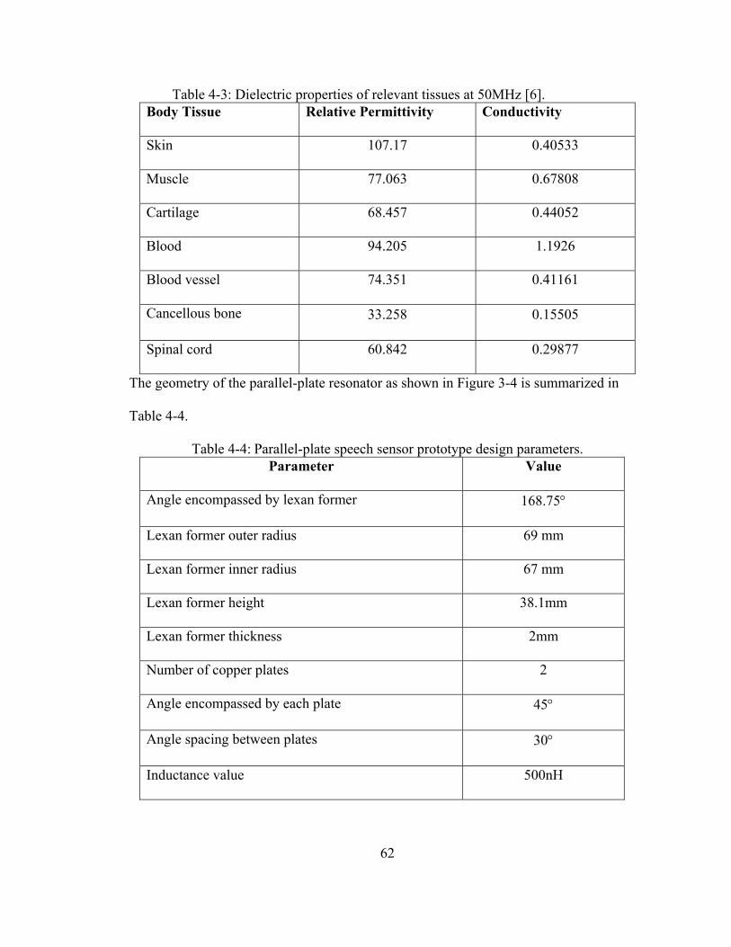
62

Table 4-3: Dielectric properties of relevant tissues at 50MHz [6]. Body Tissue Relative Permittivity Conductivity

Skin 107.17 0.40533

Muscle 77.063 0.67808

Cartilage 68.457 0.44052

Blood 94.205 1.1926

Blood vessel 74.351 0.41161

Cancellous bone 33.258 0.15505

Spinal cord 60.842 0.29877

The geometry of the parallel-plate resonator as shown in Figure 3-4 is summarized in

Table 4-4.

Table 4-4: Parallel-plate speech sensor prototype design parameters. Parameter Value

Angle encompassed by lexan former 168.75°

Lexan former outer radius 69 mm

Lexan former inner radius 67 mm

Lexan former height 38.1mm

Lexan former thickness 2mm

Number of copper plates 2

Angle encompassed by each plate 45°

Angle spacing between plates 30°

Inductance value 500nH

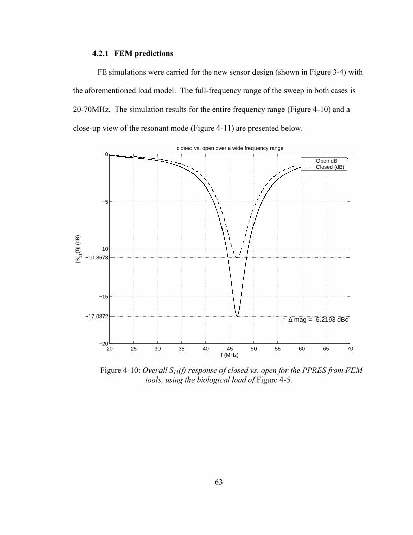
63

20 25 30 35 40 45 50 55 60 65 70−20

−17.0872

−15

−10.8678

−10

−5

0

↓

↑ ∆ mag = 6.2193 dBc

f (MHz)

|S11

(f)|

(dB

)

closed vs. open over a wide frequency range

Open dBClosed (dB)

4.2.1 FEM predictions

FE simulations were carried for the new sensor design (shown in Figure 3-4) with

the aforementioned load model. The full-frequency range of the sweep in both cases is

20-70MHz. The simulation results for the entire frequency range (Figure 4-10) and a

close-up view of the resonant mode (Figure 4-11) are presented below.

Figure 4-10: Overall S11(f) response of closed vs. open for the PPRES from FEM tools, using the biological load of Figure 4-5.

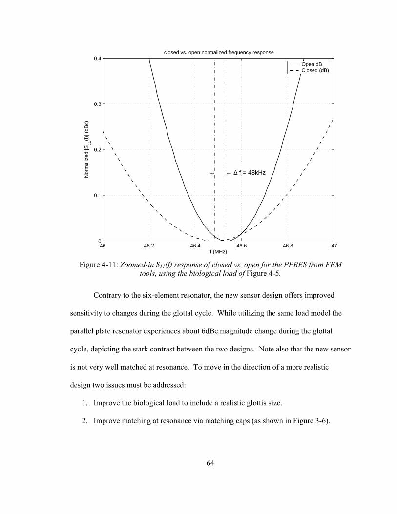
64

46 46.2 46.4 46.6 46.8 470

0.1

0.2

0.3

0.4

→ ← ∆ f = 48kHz

f (MHz)

Nor

mal

ized

|S11

(f)|

(dB

c)

closed vs. open normalized frequency response

Open dBClosed (dB)

Figure 4-11: Zoomed-in S11(f) response of closed vs. open for the PPRES from FEM

tools, using the biological load of Figure 4-5.

Contrary to the six-element resonator, the new sensor design offers improved

sensitivity to changes during the glottal cycle. While utilizing the same load model the

parallel plate resonator experiences about 6dBc magnitude change during the glottal

cycle, depicting the stark contrast between the two designs. Note also that the new sensor

is not very well matched at resonance. To move in the direction of a more realistic

design two issues must be addressed:

1. Improve the biological load to include a realistic glottis size.

2. Improve matching at resonance via matching caps (as shown in Figure 3-6).

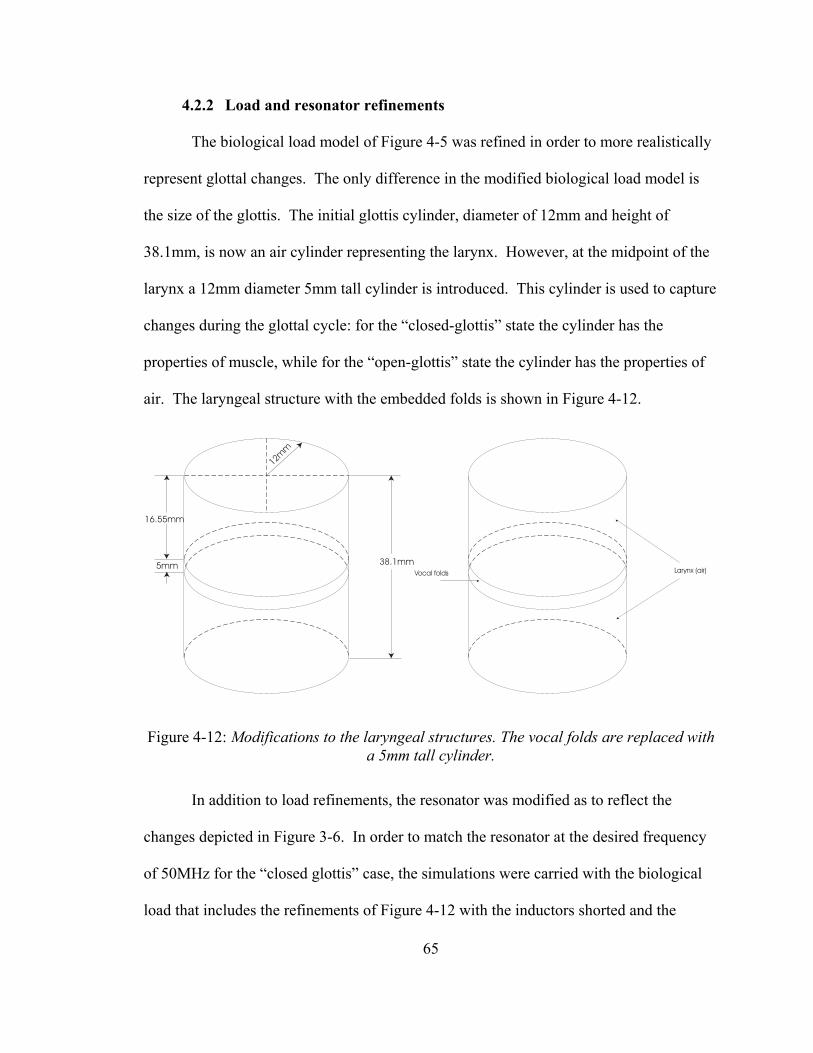
65

38.1mm5mm

12m

m

16.55mm

Larynx (air)Vocal folds

4.2.2 Load and resonator refinements

The biological load model of Figure 4-5 was refined in order to more realistically

represent glottal changes. The only difference in the modified biological load model is

the size of the glottis. The initial glottis cylinder, diameter of 12mm and height of

38.1mm, is now an air cylinder representing the larynx. However, at the midpoint of the

larynx a 12mm diameter 5mm tall cylinder is introduced. This cylinder is used to capture

changes during the glottal cycle: for the “closed-glottis” state the cylinder has the

properties of muscle, while for the “open-glottis” state the cylinder has the properties of

air. The laryngeal structure with the embedded folds is shown in Figure 4-12.

Figure 4-12: Modifications to the laryngeal structures. The vocal folds are replaced with a 5mm tall cylinder.

In addition to load refinements, the resonator was modified as to reflect the

changes depicted in Figure 3-6. In order to match the resonator at the desired frequency

of 50MHz for the “closed glottis” case, the simulations were carried with the biological

load that includes the refinements of Figure 4-12 with the inductors shorted and the

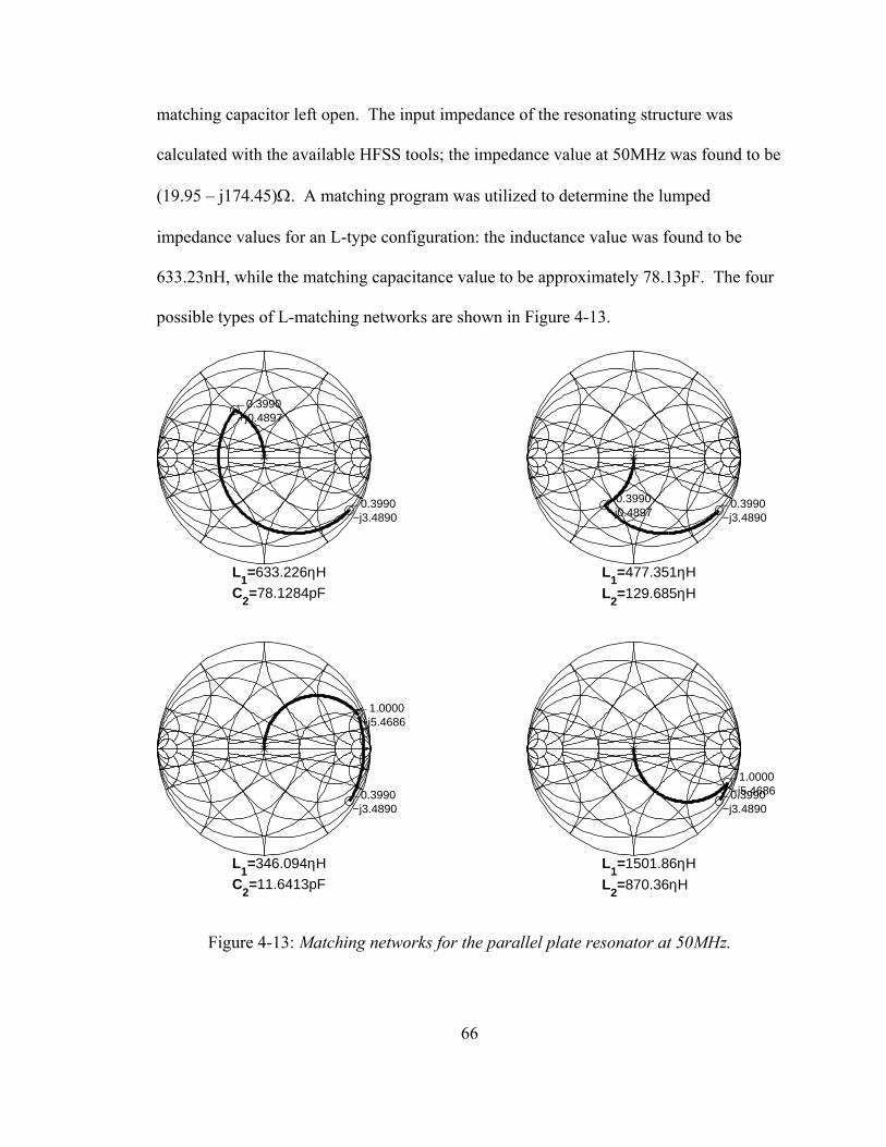
66

matching capacitor left open. The input impedance of the resonating structure was

calculated with the available HFSS tools; the impedance value at 50MHz was found to be

(19.95 – j174.45)Ω. A matching program was utilized to determine the lumped

impedance values for an L-type configuration: the inductance value was found to be

633.23nH, while the matching capacitance value to be approximately 78.13pF. The four

possible types of L-matching networks are shown in Figure 4-13.

←0.3990 −j3.4890

←0.3990 +j0.4897

L1=633.226ηH

C2=78.1284pF

←0.3990 −j3.4890

←0.3990 −j0.4897

L1=477.351ηH

L2=129.685ηH

←0.3990 −j3.4890

←1.0000 +j5.4686

L1=346.094ηH

C2=11.6413pF

←0.3990 −j3.4890

←1.0000 −j5.4686

L1=1501.86ηH

L2=870.36ηH

Figure 4-13: Matching networks for the parallel plate resonator at 50MHz.

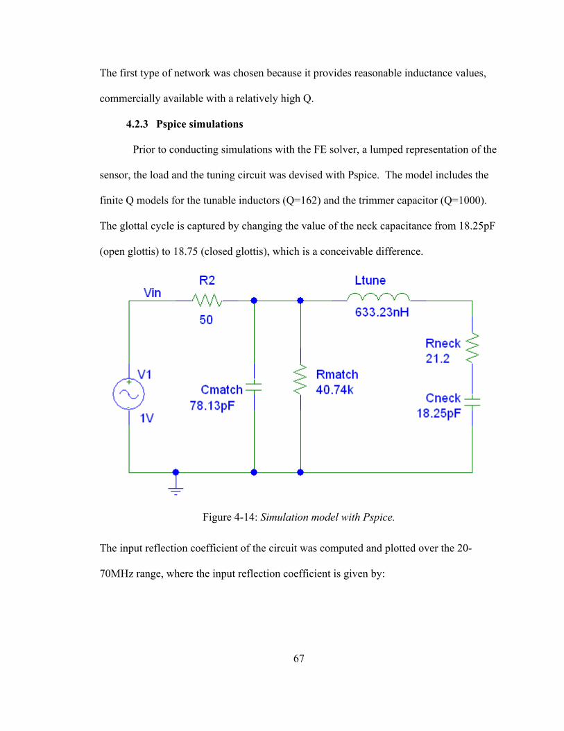
67

The first type of network was chosen because it provides reasonable inductance values,

commercially available with a relatively high Q.

4.2.3 Pspice simulations

Prior to conducting simulations with the FE solver, a lumped representation of the

sensor, the load and the tuning circuit was devised with Pspice. The model includes the

finite Q models for the tunable inductors (Q=162) and the trimmer capacitor (Q=1000).

The glottal cycle is captured by changing the value of the neck capacitance from 18.25pF

(open glottis) to 18.75 (closed glottis), which is a conceivable difference.

Figure 4-14: Simulation model with Pspice.

The input reflection coefficient of the circuit was computed and plotted over the 20-

70MHz range, where the input reflection coefficient is given by:

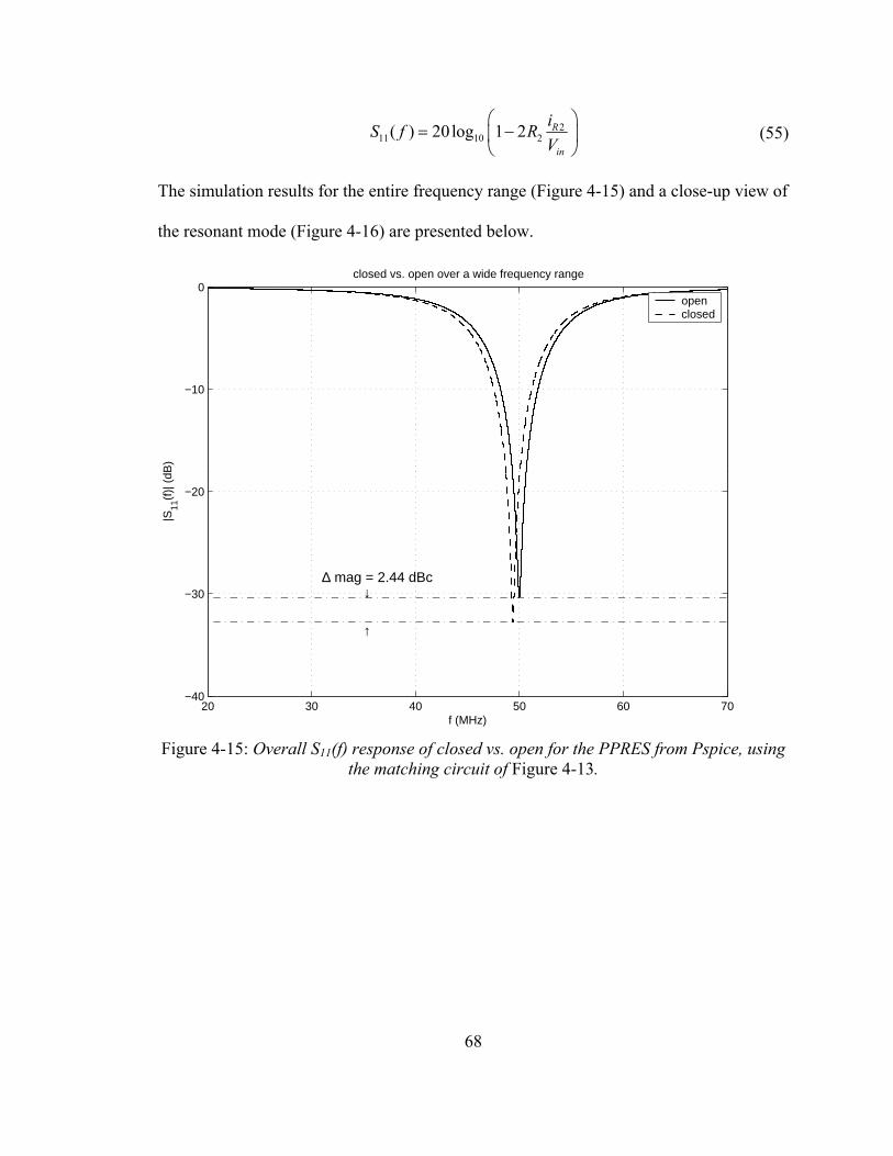
68

211 10 2( ) 20log 1 2 R

in

iS f RV

= −

(55)

The simulation results for the entire frequency range (Figure 4-15) and a close-up view of

the resonant mode (Figure 4-16) are presented below.

20 30 40 50 60 70−40

−30

−20

−10

0

↑

↓∆ mag = 2.44 dBc

f (MHz)

|S11

(f)|

(dB

)

closed vs. open over a wide frequency range

openclosed

Figure 4-15: Overall S11(f) response of closed vs. open for the PPRES from Pspice, using

the matching circuit of Figure 4-13.

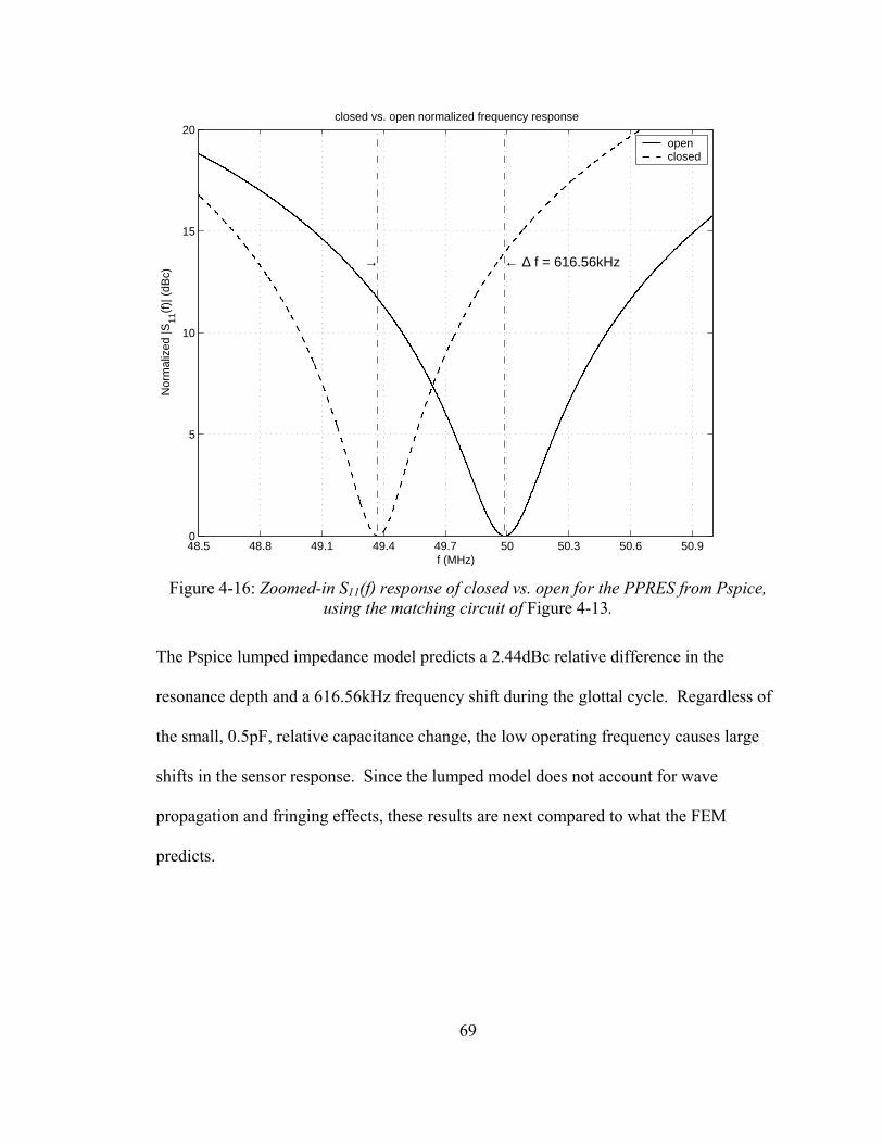
69

48.5 48.8 49.1 49.4 49.7 50 50.3 50.6 50.90

5

10

15

20

→ ← ∆ f = 616.56kHz

f (MHz)

Nor

mal

ized

|S11

(f)|

(dB

c)

closed vs. open normalized frequency response

openclosed

Figure 4-16: Zoomed-in S11(f) response of closed vs. open for the PPRES from Pspice,

using the matching circuit of Figure 4-13.

The Pspice lumped impedance model predicts a 2.44dBc relative difference in the

resonance depth and a 616.56kHz frequency shift during the glottal cycle. Regardless of

the small, 0.5pF, relative capacitance change, the low operating frequency causes large

shifts in the sensor response. Since the lumped model does not account for wave

propagation and fringing effects, these results are next compared to what the FEM

predicts.

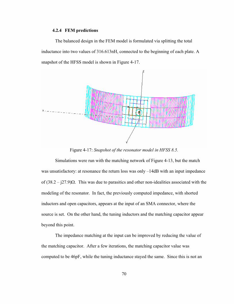
70

4.2.4 FEM predictions

The balanced design in the FEM model is formulated via splitting the total

inductance into two values of 316.613nH, connected to the beginning of each plate. A

snapshot of the HFSS model is shown in Figure 4-17.

Figure 4-17: Snapshot of the resonator model in HFSS 8.5.

Simulations were run with the matching network of Figure 4-13, but the match

was unsatisfactory: at resonance the return loss was only –14dB with an input impedance

of (38.2 – j27.9)Ω. This was due to parasitics and other non-idealities associated with the

modeling of the resonator. In fact, the previously computed impedance, with shorted

inductors and open capacitors, appears at the input of an SMA connector, where the

source is set. On the other hand, the tuning inductors and the matching capacitor appear

beyond this point.

The impedance matching at the input can be improved by reducing the value of

the matching capacitor. After a few iterations, the matching capacitor value was

computed to be 46pF, while the tuning inductance stayed the same. Since this is not an

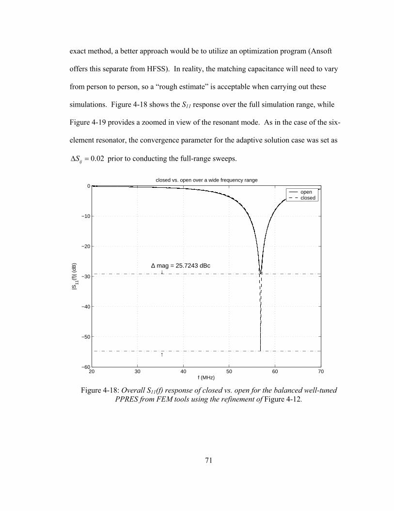
71

exact method, a better approach would be to utilize an optimization program (Ansoft

offers this separate from HFSS). In reality, the matching capacitance will need to vary

from person to person, so a “rough estimate” is acceptable when carrying out these

simulations. Figure 4-18 shows the S11 response over the full simulation range, while

Figure 4-19 provides a zoomed in view of the resonant mode. As in the case of the six-

element resonator, the convergence parameter for the adaptive solution case was set as

0.02ijS∆ = prior to conducting the full-range sweeps.

20 30 40 50 60 70−60

−50

−40

−30

−20

−10

0

↓

↑

∆ mag = 25.7243 dBc

f (MHz)

|S11

(f)|

(dB

)

closed vs. open over a wide frequency range

openclosed

Figure 4-18: Overall S11(f) response of closed vs. open for the balanced well-tuned

PPRES from FEM tools using the refinement of Figure 4-12.

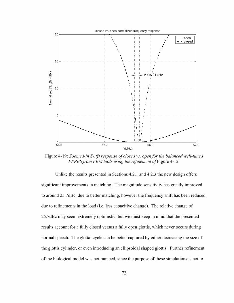
72

56.5 56.7 56.9 57.10

5

10

15

20

→ ← ∆ f = 21kHz

f (MHz)

Nor

mal

ized

|S11

(f)|

(dB

c)

closed vs. open normalized frequency response

openclosed

Figure 4-19: Zoomed-in S11(f) response of closed vs. open for the balanced well-tuned

PPRES from FEM tools using the refinement of Figure 4-12.

Unlike the results presented in Sections 4.2.1 and 4.2.3 the new design offers

significant improvements in matching. The magnitude sensitivity has greatly improved

to around 25.7dBc, due to better matching, however the frequency shift has been reduced

due to refinements in the load (i.e. less capacitive change). The relative change of

25.7dBc may seem extremely optimistic, but we must keep in mind that the presented

results account for a fully closed versus a fully open glottis, which never occurs during

normal speech. The glottal cycle can be better captured by either decreasing the size of

the glottis cylinder, or even introducing an ellipsoidal shaped glottis. Further refinement

of the biological model was not pursued, since the purpose of these simulations is not to

73

exactly predict the quantitative behavior of the sensor, but to gain a better understanding

of its qualitative behavior. In either case, the work had to progress in the direction of a

practical implementation, and both FEM and the Pspice results provided confidence that

the sensor would in fact provide a signal proportional to the glottal flow waveform during

voiced segments of speech.

4.2.5 Field distribution inside the load

As in the case of the six-element resonator, using the available FE post-processing

tools we can obtain detailed field plots that show the amount of electric-field penetration

into the glottal area and provide some intuition about the sensitivity of the parallel-plate

resonator. The magnitude of the electric field is shown for the single resonant mode of

the parallel plate sensor for the case when the load is in the “open glottis” state. As it can

be seen from the field plot the magnitude of the electric field in the glottal region is

comparable to the case of the six-element resonator, despite being driven at ten times less

the input RF power (-10dBm). More importantly the plot shows that there is a nonzero

electric field gradient through the glottal area in the x-direction, which is an indication of

capacitive coupling between the copper plates.

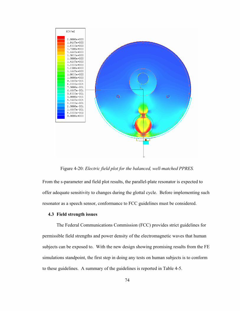
74

Figure 4-20: Electric field plot for the balanced, well-matched PPRES.

From the s-parameter and field plot results, the parallel-plate resonator is expected to

offer adequate sensitivity to changes during the glottal cycle. Before implementing such

resonator as a speech sensor, conformance to FCC guidelines must be considered.

4.3 Field strength issues

The Federal Communications Commission (FCC) provides strict guidelines for

permissible field strengths and power density of the electromagnetic waves that human

subjects can be exposed to. With the new design showing promising results from the FE

simulations standpoint, the first step in doing any tests on human subjects is to conform

to these guidelines. A summary of the guidelines is reported in Table 4-5.

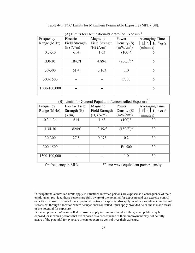
75

Table 4-5: FCC Limits for Maximum Permissible Exposure (MPE) [38].

(A) Limits for Occupational/Controlled Exposure2 Frequency Range (MHz)

Electric Field Strength (E) (V/m)

Magnetic Field Strength (H) (A/m)

Power Density (S) (mW/cm2)

Averaging Time E2, H2

or S (minutes)

0.3-3.0 614 1.63 (100)* 6

3.0-30 1842/f 4.89/f (900/f2)* 6

30-300 61.4 0.163 1.0 6

300-1500 -- -- f/300 6

1500-100,000 -- -- 5 6

(B) Limits for General Population/Uncontrolled Exposure3

Frequency Range (MHz)

Electric Field Strength (E) (V/m)

Magnetic Field Strength (H) (A/m)

Power Density (S) (mW/cm2)

Averaging Time E2, H2

or S (minutes)

0.3-1.34 614 1.63 (100)* 30

1.34-30 824/f 2.19/f (180/f2)* 30

30-300 27.5 0.073 0.2 30

300-1500 -- -- F/1500 30

1500-100,000 -- -- 1.0 30

f = frequency in MHz *Plane-wave equivalent power density

2 Occupational/controlled limits apply in situations in which persons are exposed as a consequence of their employment provided those persons are fully aware of the potential for exposure and can exercise control over their exposure. Limits for occupational/controlled exposure also apply in situations when an individual is transient through a location where occupational/controlled limits apply provided he or she is made aware of the potential for exposure. 3 General population/uncontrolled exposures apply in situations in which the general public may be exposed, or in which persons that are exposed as a consequence of their employment may not be fully aware of the potential for exposure or cannot exercise control over their exposure.

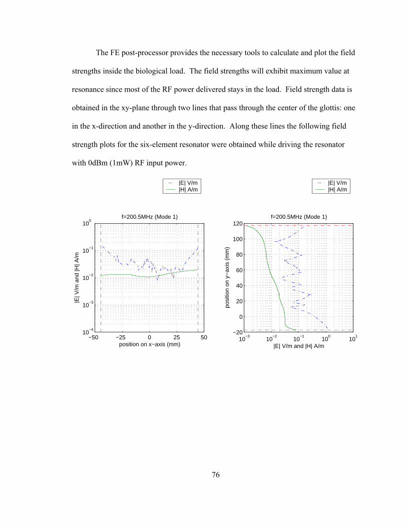
76

The FE post-processor provides the necessary tools to calculate and plot the field

strengths inside the biological load. The field strengths will exhibit maximum value at

resonance since most of the RF power delivered stays in the load. Field strength data is

obtained in the xy-plane through two lines that pass through the center of the glottis: one

in the x-direction and another in the y-direction. Along these lines the following field

strength plots for the six-element resonator were obtained while driving the resonator

with 0dBm (1mW) RF input power.

−50 −25 0 25 5010

−4

10−3

10−2

10−1

100

position on x−axis (mm)

|E| V

/m a

nd |H

| A/m

f=200.5MHz (Mode 1)

10−3

10−2

10−1

100

101

−20

0

20

40

60

80

100

120

|E| V/m and |H| A/m

posi

tion

on y

−ax

is (

mm

)

f=200.5MHz (Mode 1)

|E| V/m|H| A/m

|E| V/m|H| A/m

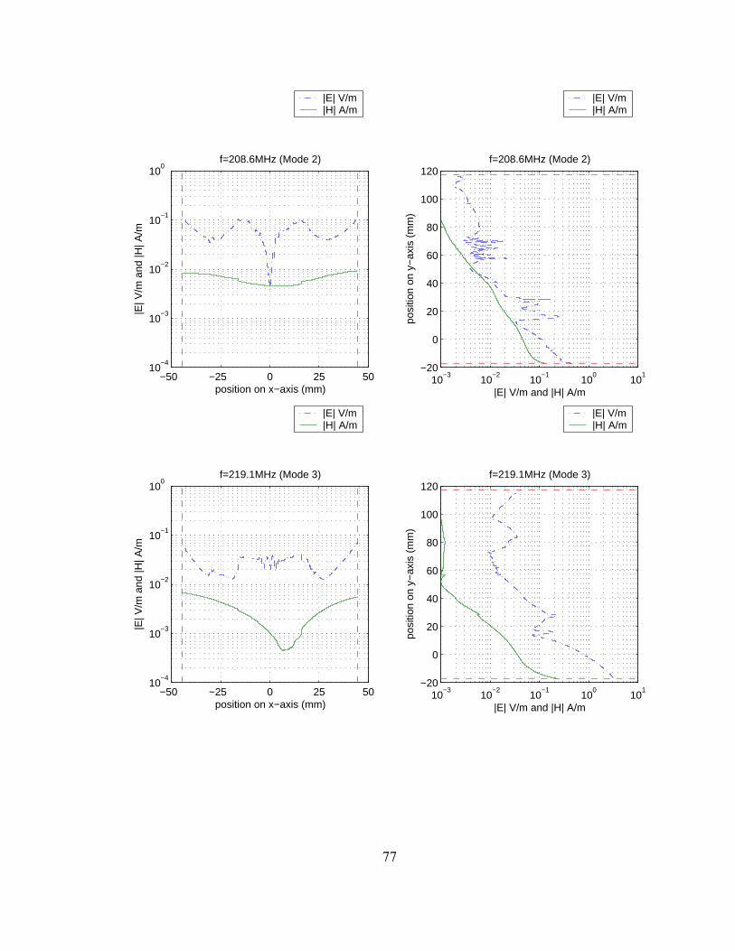
77

−50 −25 0 25 5010

−4

10−3

10−2

10−1

100

position on x−axis (mm)

|E| V

/m a

nd |H

| A/m

f=208.6MHz (Mode 2)

10−3

10−2

10−1

100

101

−20

0

20

40

60

80

100

120

|E| V/m and |H| A/m

posi

tion

on y

−ax

is (

mm

)

f=208.6MHz (Mode 2)

|E| V/m|H| A/m

|E| V/m|H| A/m

−50 −25 0 25 5010

−4

10−3

10−2

10−1

100

position on x−axis (mm)

|E| V

/m a

nd |H

| A/m

f=219.1MHz (Mode 3)

10−3

10−2

10−1

100

101

−20

0

20

40

60

80

100

120

|E| V/m and |H| A/m

posi

tion

on y

−ax

is (

mm

)

f=219.1MHz (Mode 3)

|E| V/m|H| A/m

|E| V/m|H| A/m

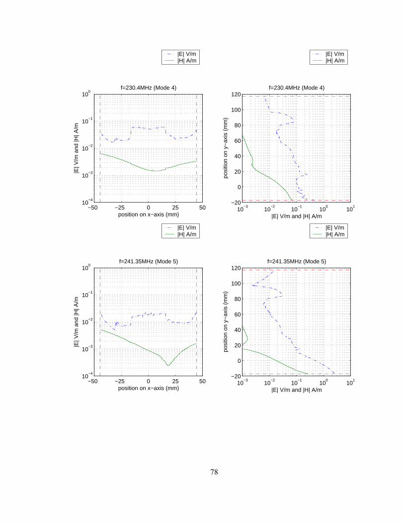
78

−50 −25 0 25 5010

−4

10−3

10−2

10−1

100

position on x−axis (mm)

|E| V

/m a

nd |H

| A/m

f=230.4MHz (Mode 4)

10−3

10−2

10−1

100

101

−20

0

20

40

60

80

100

120

|E| V/m and |H| A/m

posi

tion

on y

−ax

is (

mm

)

f=230.4MHz (Mode 4)

|E| V/m|H| A/m

|E| V/m|H| A/m

−50 −25 0 25 5010

−4

10−3

10−2

10−1

100

position on x−axis (mm)

|E| V

/m a

nd |H

| A/m

f=241.35MHz (Mode 5)

10−3

10−2

10−1

100

101

−20

0

20

40

60

80

100

120

|E| V/m and |H| A/m

posi

tion

on y

−ax

is (

mm

)

f=241.35MHz (Mode 5)

|E| V/m|H| A/m

|E| V/m|H| A/m

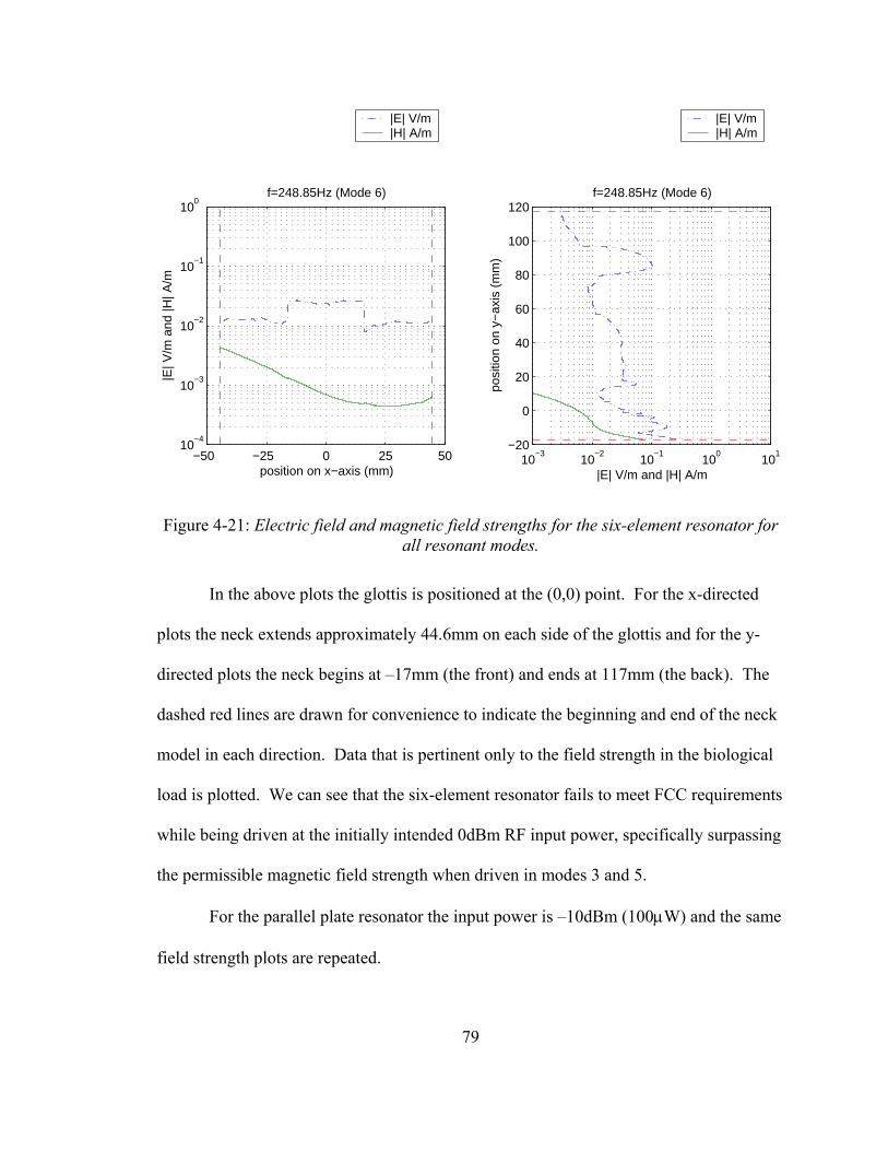
79

−50 −25 0 25 5010

−4

10−3

10−2

10−1

100

position on x−axis (mm)

|E| V

/m a

nd |H

| A/m

f=248.85Hz (Mode 6)

10−3

10−2

10−1

100

101

−20

0

20

40

60

80

100

120

|E| V/m and |H| A/m

posi

tion

on y

−ax

is (

mm

)

f=248.85Hz (Mode 6)

|E| V/m|H| A/m

|E| V/m|H| A/m

Figure 4-21: Electric field and magnetic field strengths for the six-element resonator for all resonant modes.

In the above plots the glottis is positioned at the (0,0) point. For the x-directed

plots the neck extends approximately 44.6mm on each side of the glottis and for the y-

directed plots the neck begins at –17mm (the front) and ends at 117mm (the back). The

dashed red lines are drawn for convenience to indicate the beginning and end of the neck

model in each direction. Data that is pertinent only to the field strength in the biological

load is plotted. We can see that the six-element resonator fails to meet FCC requirements

while being driven at the initially intended 0dBm RF input power, specifically surpassing

the permissible magnetic field strength when driven in modes 3 and 5.

For the parallel plate resonator the input power is –10dBm (100µW) and the same

field strength plots are repeated.

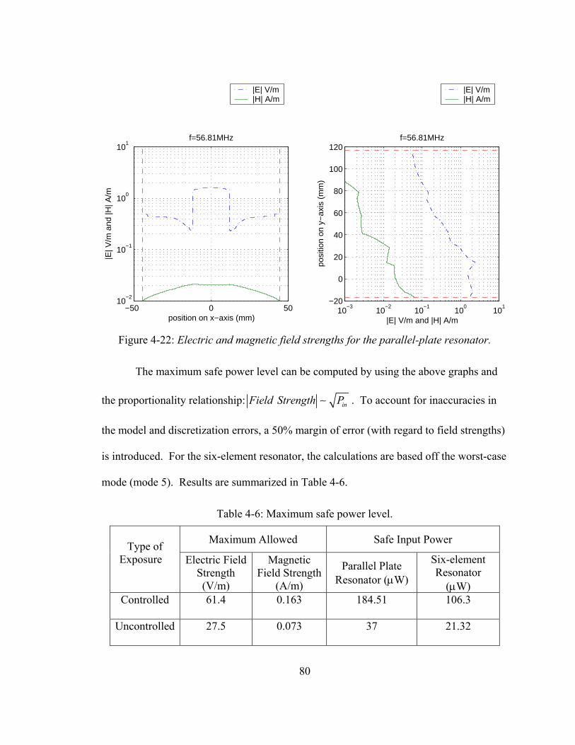
80

−50 0 5010

−2

10−1

100

101

position on x−axis (mm)

|E| V

/m a

nd |H

| A/m

f=56.81MHz

10−3

10−2

10−1

100

101

−20

0

20

40

60

80

100

120

|E| V/m and |H| A/mpo

sitio

n on

y−

axis

(m

m)

f=56.81MHz

|E| V/m|H| A/m

|E| V/m|H| A/m

Figure 4-22: Electric and magnetic field strengths for the parallel-plate resonator.

The maximum safe power level can be computed by using the above graphs and

the proportionality relationship: inField Strength P∼ . To account for inaccuracies in

the model and discretization errors, a 50% margin of error (with regard to field strengths)

is introduced. For the six-element resonator, the calculations are based off the worst-case

mode (mode 5). Results are summarized in Table 4-6.

Table 4-6: Maximum safe power level.

Maximum Allowed Safe Input Power Type of Exposure

Electric Field

Strength (V/m)

Magnetic Field Strength

(A/m)

Parallel Plate Resonator (µW)

Six-element Resonator

(µW) Controlled 61.4 0.163 184.51 106.3

Uncontrolled 27.5 0.073 37 21.32

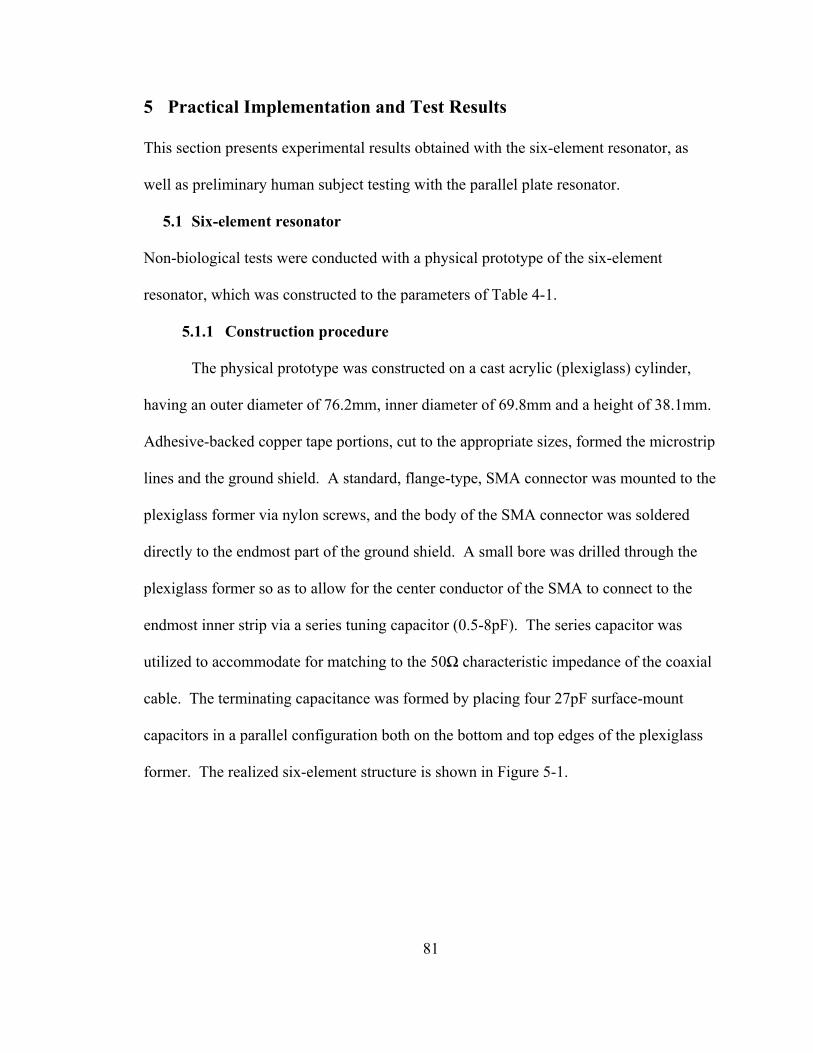
81

5 Practical Implementation and Test Results

This section presents experimental results obtained with the six-element resonator, as

well as preliminary human subject testing with the parallel plate resonator.

5.1 Six-element resonator

Non-biological tests were conducted with a physical prototype of the six-element

resonator, which was constructed to the parameters of Table 4-1.

5.1.1 Construction procedure

The physical prototype was constructed on a cast acrylic (plexiglass) cylinder,

having an outer diameter of 76.2mm, inner diameter of 69.8mm and a height of 38.1mm.

Adhesive-backed copper tape portions, cut to the appropriate sizes, formed the microstrip

lines and the ground shield. A standard, flange-type, SMA connector was mounted to the

plexiglass former via nylon screws, and the body of the SMA connector was soldered

directly to the endmost part of the ground shield. A small bore was drilled through the

plexiglass former so as to allow for the center conductor of the SMA to connect to the

endmost inner strip via a series tuning capacitor (0.5-8pF). The series capacitor was

utilized to accommodate for matching to the 50Ω characteristic impedance of the coaxial

cable. The terminating capacitance was formed by placing four 27pF surface-mount

capacitors in a parallel configuration both on the bottom and top edges of the plexiglass

former. The realized six-element structure is shown in Figure 5-1.

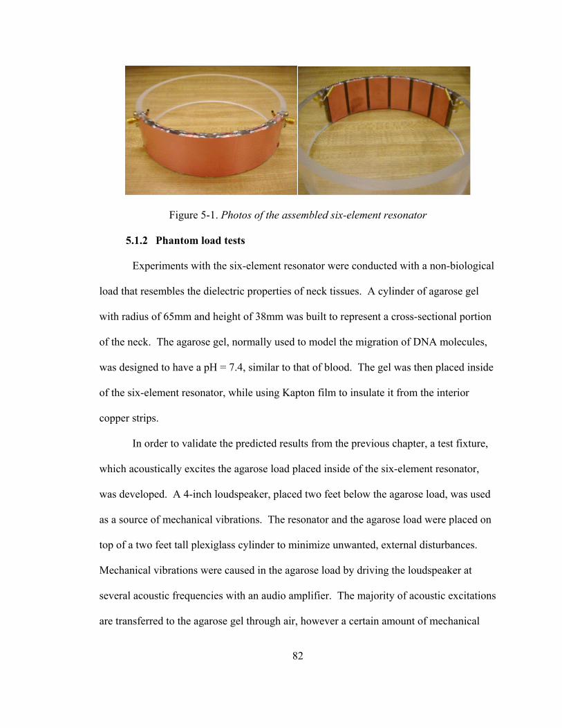
82

Figure 5-1. Photos of the assembled six-element resonator

5.1.2 Phantom load tests

Experiments with the six-element resonator were conducted with a non-biological

load that resembles the dielectric properties of neck tissues. A cylinder of agarose gel

with radius of 65mm and height of 38mm was built to represent a cross-sectional portion

of the neck. The agarose gel, normally used to model the migration of DNA molecules,

was designed to have a pH = 7.4, similar to that of blood. The gel was then placed inside

of the six-element resonator, while using Kapton film to insulate it from the interior

copper strips.

In order to validate the predicted results from the previous chapter, a test fixture,

which acoustically excites the agarose load placed inside of the six-element resonator,

was developed. A 4-inch loudspeaker, placed two feet below the agarose load, was used

as a source of mechanical vibrations. The resonator and the agarose load were placed on

top of a two feet tall plexiglass cylinder to minimize unwanted, external disturbances.

Mechanical vibrations were caused in the agarose load by driving the loudspeaker at

several acoustic frequencies with an audio amplifier. The majority of acoustic excitations

are transferred to the agarose gel through air, however a certain amount of mechanical

83

coupling occurs through the test fixture as well. The s-parameters of the resonator were

monitored via a Hewlett Packard 8714ES network analyzer. Figure 5-2 shows the test

setup used in this case.

Figure 5-2: Non-biological load test setup.

Plots of the return loss (S11 in dB) versus frequency for the unloaded and loaded resonator

are shown in Figure 5-3.

84

a)

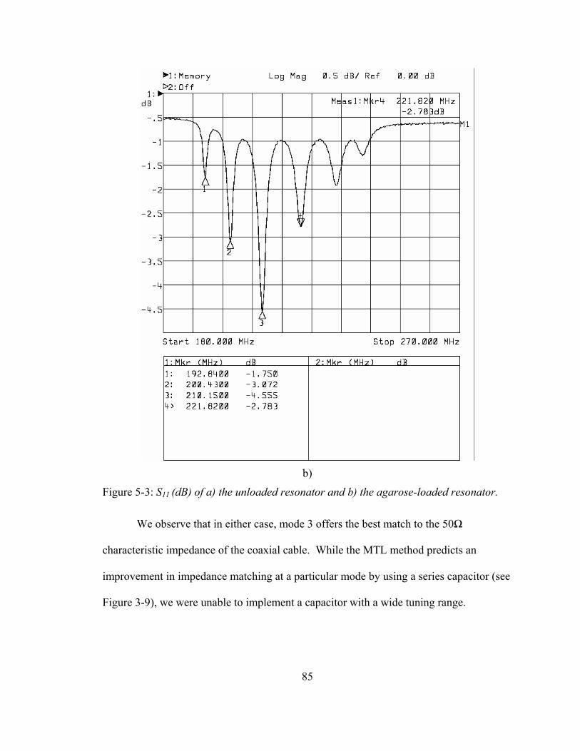
85

b)

Figure 5-3: S11 (dB) of a) the unloaded resonator and b) the agarose-loaded resonator.

We observe that in either case, mode 3 offers the best match to the 50Ω

characteristic impedance of the coaxial cable. While the MTL method predicts an

improvement in impedance matching at a particular mode by using a series capacitor (see

Figure 3-9), we were unable to implement a capacitor with a wide tuning range.

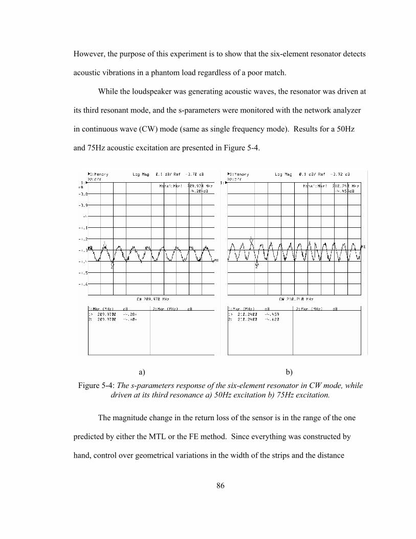
86

However, the purpose of this experiment is to show that the six-element resonator detects

acoustic vibrations in a phantom load regardless of a poor match.

While the loudspeaker was generating acoustic waves, the resonator was driven at

its third resonant mode, and the s-parameters were monitored with the network analyzer

in continuous wave (CW) mode (same as single frequency mode). Results for a 50Hz

and 75Hz acoustic excitation are presented in Figure 5-4.

a) b)

Figure 5-4: The s-parameters response of the six-element resonator in CW mode, while driven at its third resonance a) 50Hz excitation b) 75Hz excitation.

The magnitude change in the return loss of the sensor is in the range of the one

predicted by either the MTL or the FE method. Since everything was constructed by

hand, control over geometrical variations in the width of the strips and the distance

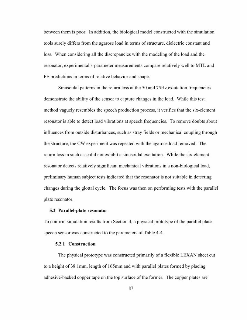
87

between them is poor. In addition, the biological model constructed with the simulation

tools surely differs from the agarose load in terms of structure, dielectric constant and

loss. When considering all the discrepancies with the modeling of the load and the

resonator, experimental s-parameter measurements compare relatively well to MTL and

FE predictions in terms of relative behavior and shape.

Sinusoidal patterns in the return loss at the 50 and 75Hz excitation frequencies

demonstrate the ability of the sensor to capture changes in the load. While this test

method vaguely resembles the speech production process, it verifies that the six-element

resonator is able to detect load vibrations at speech frequencies. To remove doubts about

influences from outside disturbances, such as stray fields or mechanical coupling through

the structure, the CW experiment was repeated with the agarose load removed. The

return loss in such case did not exhibit a sinusoidal excitation. While the six-element

resonator detects relatively significant mechanical vibrations in a non-biological load,

preliminary human subject tests indicated that the resonator is not suitable in detecting

changes during the glottal cycle. The focus was then on performing tests with the parallel

plate resonator.

5.2 Parallel-plate resonator

To confirm simulation results from Section 4, a physical prototype of the parallel plate

speech sensor was constructed to the parameters of Table 4-4.

5.2.1 Construction

The physical prototype was constructed primarily of a flexible LEXAN sheet cut

to a height of 38.1mm, length of 165mm and with parallel plates formed by placing

adhesive-backed copper tape on the top surface of the former. The copper plates are

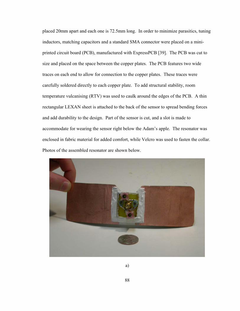
88

placed 20mm apart and each one is 72.5mm long. In order to minimize parasitics, tuning

inductors, matching capacitors and a standard SMA connector were placed on a mini-

printed circuit board (PCB), manufactured with ExpressPCB [39]. The PCB was cut to

size and placed on the space between the copper plates. The PCB features two wide

traces on each end to allow for connection to the copper plates. These traces were

carefully soldered directly to each copper plate. To add structural stability, room

temperature vulcanising (RTV) was used to caulk around the edges of the PCB. A thin

rectangular LEXAN sheet is attached to the back of the sensor to spread bending forces

and add durability to the design. Part of the sensor is cut, and a slot is made to

accommodate for wearing the sensor right below the Adam’s apple. The resonator was

enclosed in fabric material for added comfort, while Velcro was used to fasten the collar.

Photos of the assembled resonator are shown below.

a)

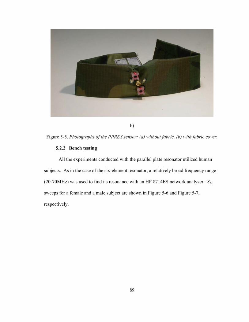
89

b)

Figure 5-5. Photographs of the PPRES sensor: (a) without fabric, (b) with fabric cover.

5.2.2 Bench testing

All the experiments conducted with the parallel plate resonator utilized human

subjects. As in the case of the six-element resonator, a relatively broad frequency range

(20-70MHz) was used to find its resonance with an HP 8714ES network analyzer. S11

sweeps for a female and a male subject are shown in Figure 5-6 and Figure 5-7,

respectively.

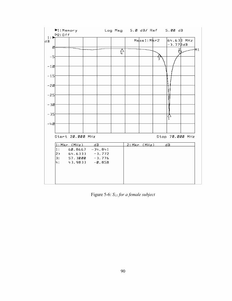
90

Figure 5-6: S11 for a female subject

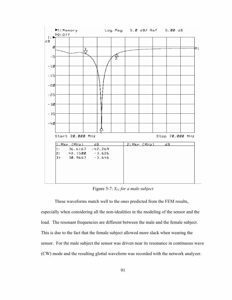
91

Figure 5-7: S11 for a male subject

These waveforms match well to the ones predicted from the FEM results,

especially when considering all the non-idealities in the modeling of the sensor and the

load. The resonant frequencies are different between the male and the female subject.

This is due to the fact that the female subject allowed more slack when wearing the

sensor. For the male subject the sensor was driven near its resonance in continuous wave

(CW) mode and the resulting glottal waveform was recorded with the network analyzer.

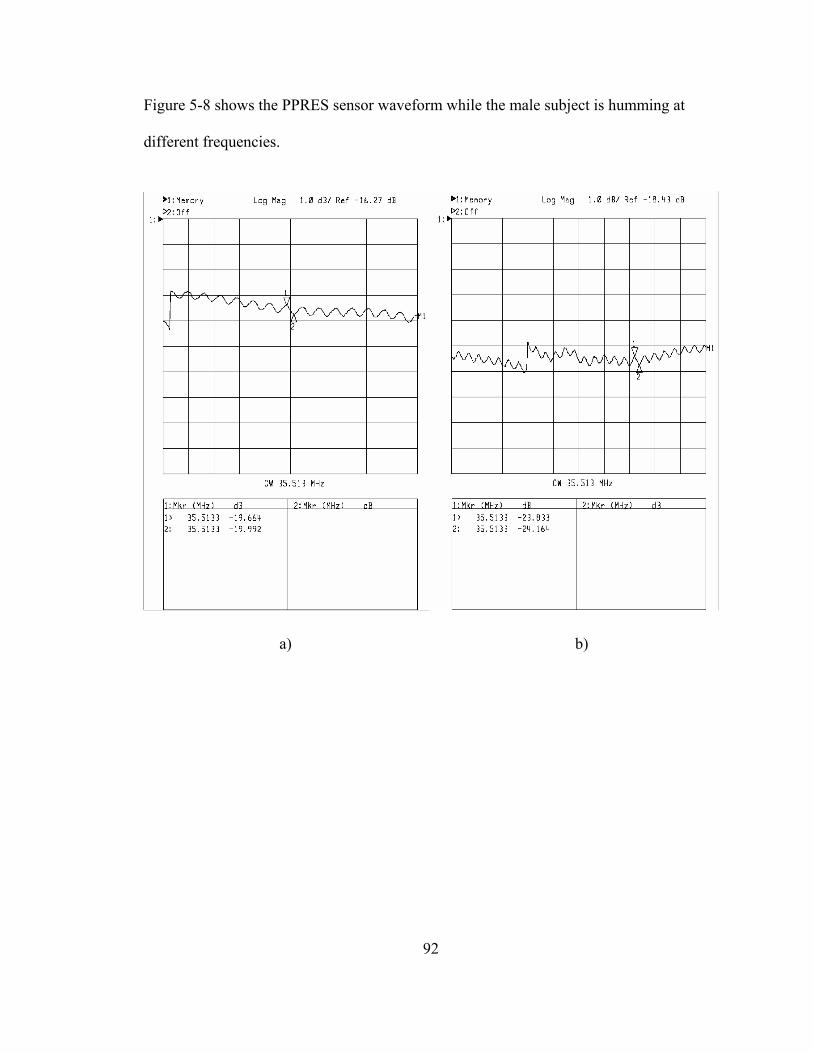
92

Figure 5-8 shows the PPRES sensor waveform while the male subject is humming at

different frequencies.

a) b)

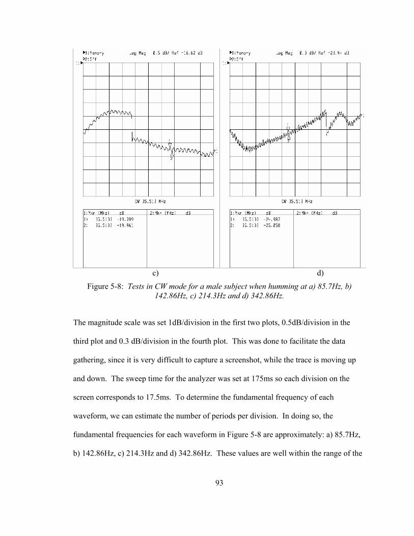
93

c) d)

Figure 5-8: Tests in CW mode for a male subject when humming at a) 85.7Hz, b) 142.86Hz, c) 214.3Hz and d) 342.86Hz.

The magnitude scale was set 1dB/division in the first two plots, 0.5dB/division in the

third plot and 0.3 dB/division in the fourth plot. This was done to facilitate the data

gathering, since it is very difficult to capture a screenshot, while the trace is moving up

and down. The sweep time for the analyzer was set at 175ms so each division on the

screen corresponds to 17.5ms. To determine the fundamental frequency of each

waveform, we can estimate the number of periods per division. In doing so, the

fundamental frequencies for each waveform in Figure 5-8 are approximately: a) 85.7Hz,

b) 142.86Hz, c) 214.3Hz and d) 342.86Hz. These values are well within the range of the

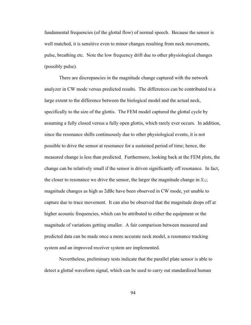
94

fundamental frequencies (of the glottal flow) of normal speech. Because the sensor is

well matched, it is sensitive even to minor changes resulting from neck movements,

pulse, breathing etc. Note the low frequency drift due to other physiological changes

(possibly pulse).

There are discrepancies in the magnitude change captured with the network

analyzer in CW mode versus predicted results. The differences can be contributed to a

large extent to the difference between the biological model and the actual neck,

specifically to the size of the glottis. The FEM model captured the glottal cycle by

assuming a fully closed versus a fully open glottis, which rarely ever occurs. In addition,

since the resonance shifts continuously due to other physiological events, it is not

possible to drive the sensor at resonance for a sustained period of time; hence, the

measured change is less than predicted. Furthermore, looking back at the FEM plots, the

change can be relatively small if the sensor is driven significantly off resonance. In fact,

the closer to resonance we drive the sensor, the larger the magnitude change in S11;

magnitude changes as high as 2dBc have been observed in CW mode, yet unable to

capture due to trace movement. It can also be observed that the magnitude drops off at

higher acoustic frequencies, which can be attributed to either the equipment or the

magnitude of variations getting smaller. A fair comparison between measured and

predicted data can be made once a more accurate neck model, a resonance tracking

system and an improved receiver system are implemented.

Nevertheless, preliminary tests indicate that the parallel plate sensor is able to

detect a glottal waveform signal, which can be used to carry out standardized human

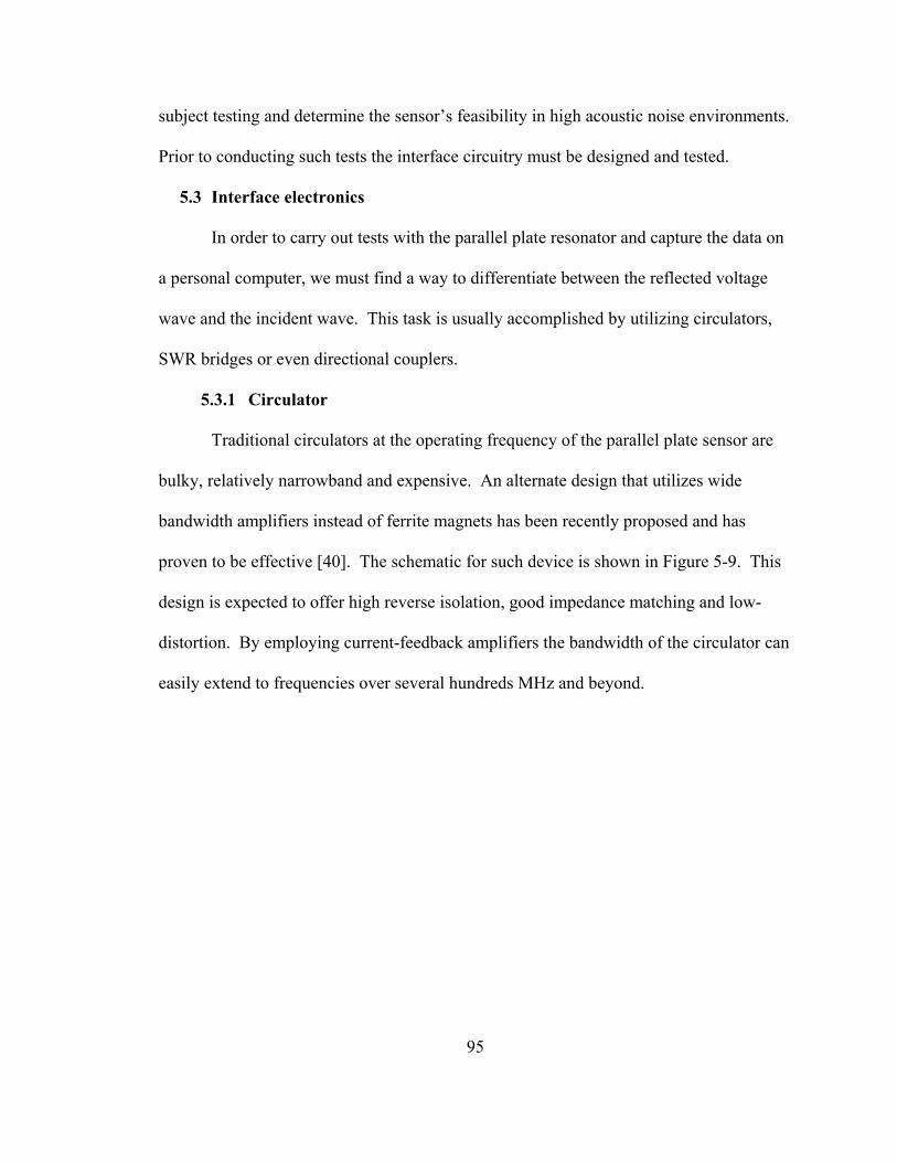
95

subject testing and determine the sensor’s feasibility in high acoustic noise environments.

Prior to conducting such tests the interface circuitry must be designed and tested.

5.3 Interface electronics

In order to carry out tests with the parallel plate resonator and capture the data on

a personal computer, we must find a way to differentiate between the reflected voltage

wave and the incident wave. This task is usually accomplished by utilizing circulators,

SWR bridges or even directional couplers.

5.3.1 Circulator

Traditional circulators at the operating frequency of the parallel plate sensor are

bulky, relatively narrowband and expensive. An alternate design that utilizes wide

bandwidth amplifiers instead of ferrite magnets has been recently proposed and has

proven to be effective [40]. The schematic for such device is shown in Figure 5-9. This

design is expected to offer high reverse isolation, good impedance matching and low-

distortion. By employing current-feedback amplifiers the bandwidth of the circulator can

easily extend to frequencies over several hundreds MHz and beyond.

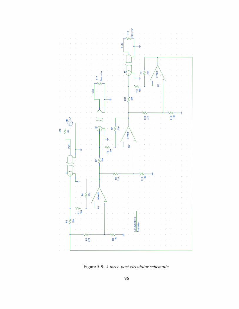
96

Figure 5-9: A three-port circulator schematic.

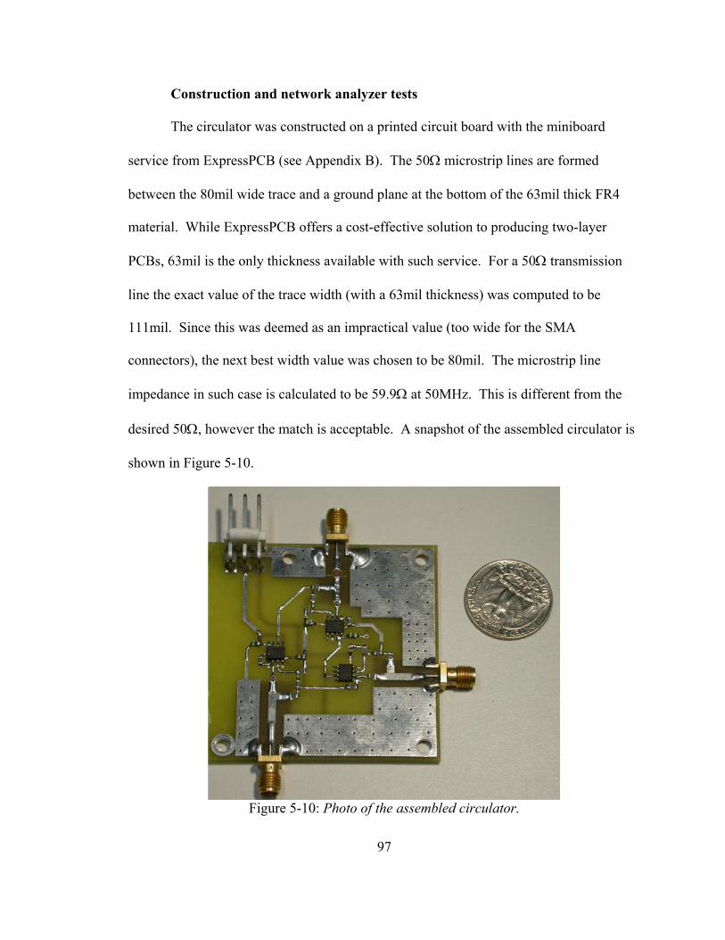
97

Construction and network analyzer tests

The circulator was constructed on a printed circuit board with the miniboard

service from ExpressPCB (see Appendix B). The 50Ω microstrip lines are formed

between the 80mil wide trace and a ground plane at the bottom of the 63mil thick FR4

material. While ExpressPCB offers a cost-effective solution to producing two-layer

PCBs, 63mil is the only thickness available with such service. For a 50Ω transmission

line the exact value of the trace width (with a 63mil thickness) was computed to be

111mil. Since this was deemed as an impractical value (too wide for the SMA

connectors), the next best width value was chosen to be 80mil. The microstrip line

impedance in such case is calculated to be 59.9Ω at 50MHz. This is different from the

desired 50Ω, however the match is acceptable. A snapshot of the assembled circulator is

shown in Figure 5-10.

Figure 5-10: Photo of the assembled circulator.

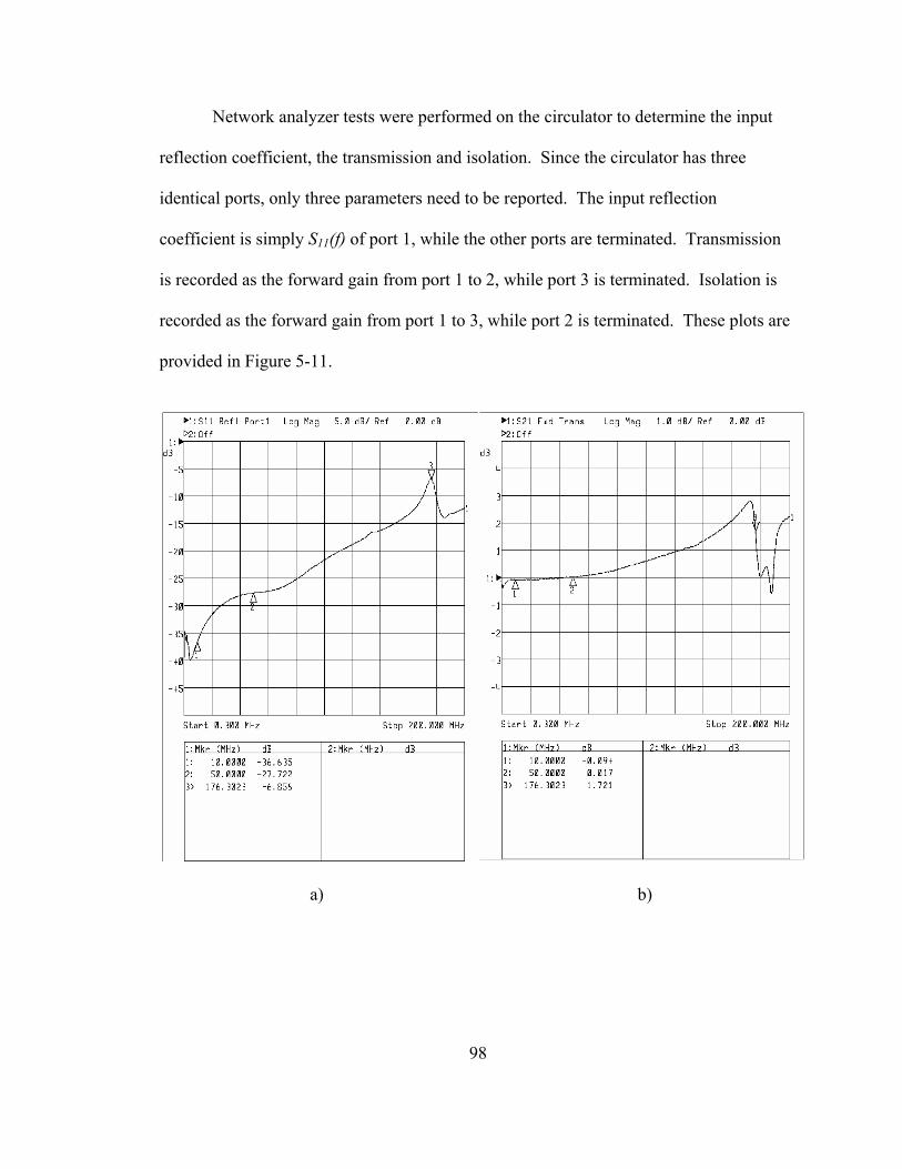
98

Network analyzer tests were performed on the circulator to determine the input

reflection coefficient, the transmission and isolation. Since the circulator has three

identical ports, only three parameters need to be reported. The input reflection

coefficient is simply S11(f) of port 1, while the other ports are terminated. Transmission

is recorded as the forward gain from port 1 to 2, while port 3 is terminated. Isolation is

recorded as the forward gain from port 1 to 3, while port 2 is terminated. These plots are

provided in Figure 5-11.

a) b)

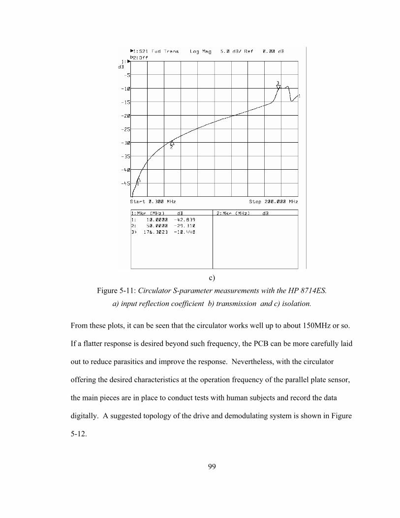
99

c)

Figure 5-11: Circulator S-parameter measurements with the HP 8714ES.

a) input reflection coefficient b) transmission and c) isolation.

From these plots, it can be seen that the circulator works well up to about 150MHz or so.

If a flatter response is desired beyond such frequency, the PCB can be more carefully laid

out to reduce parasitics and improve the response. Nevertheless, with the circulator

offering the desired characteristics at the operation frequency of the parallel plate sensor,

the main pieces are in place to conduct tests with human subjects and record the data

digitally. A suggested topology of the drive and demodulating system is shown in Figure

5-12.

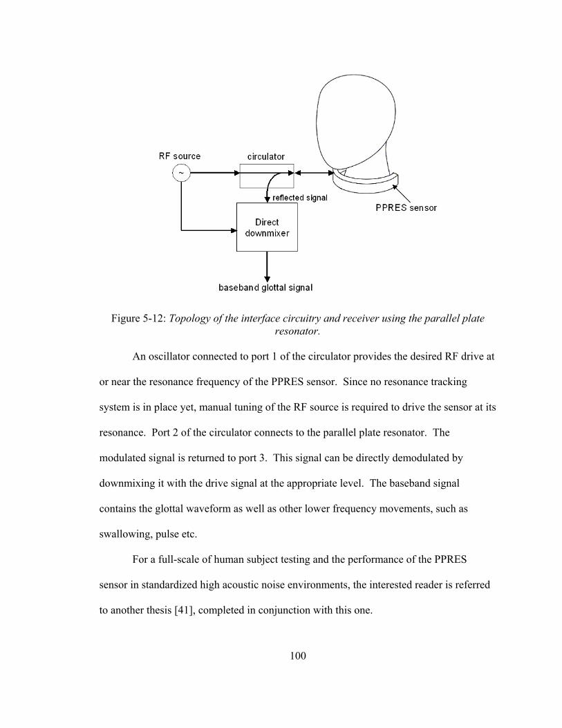
100

Figure 5-12: Topology of the interface circuitry and receiver using the parallel plate resonator.

An oscillator connected to port 1 of the circulator provides the desired RF drive at

or near the resonance frequency of the PPRES sensor. Since no resonance tracking

system is in place yet, manual tuning of the RF source is required to drive the sensor at its

resonance. Port 2 of the circulator connects to the parallel plate resonator. The

modulated signal is returned to port 3. This signal can be directly demodulated by

downmixing it with the drive signal at the appropriate level. The baseband signal

contains the glottal waveform as well as other lower frequency movements, such as

swallowing, pulse etc.

For a full-scale of human subject testing and the performance of the PPRES

sensor in standardized high acoustic noise environments, the interested reader is referred

to another thesis [41], completed in conjunction with this one.

101

6 Conclusions

This thesis determined the feasibility of the GRES sensor for the purpose of non-

acoustic voiced speech measurements. Two configurations were investigated: the six-

element resonator, inspired by high-field magnetic resonance imaging, and the parallel

plate resonator, a novel design. Both sensors were modeled with available software tools

that can predict their behavior during changes in the glottal state. These tools include the

MTL method, for rapid performance evaluation and optimization, and the FEM, when

further refinement of the model and more accurate results are desired. In addition, the

FEM is applicable to any three-dimensional electromagnetic structure, while the MTL is

not.

Experimental results conducted with the six-element resonator were presented to

confirm its sensitivity to acoustic vibrations in a non-biological phantom load. However,

the six-element resonator is unfeasible in detecting small changes that occur during the

glottal cycle. On the other hand, the parallel plate resonator is capable of directly

detecting the glottal flow waveform through a capacitive sensing technique. Bench

testing demonstrates the ability of the parallel plate sensor to offer more than adequate

sensitivity and sufficient acoustic bandwidth to cover at least normal speaking glottal

frequencies. The sensor is also unaffected by complicated scattering environments

because it responds to the composite relative permittivity of a cross-sectional portion of

the neck. The design is tunable, allowing for different people to use it, and it can be

manufactured at a very low cost. The sensor may additionally provide some information

about the articulation process, i.e. possibly some skin vibration due to acoustic coupling,

102

but such claims have not yet been established. Finally, conformance to FCC guidelines

regarding safe operating power levels was investigated. In addition to sensor results, an

efficient method was employed to distinguish between the reflected and incident voltage,

which allows for data recording and real time processing.

While the GRES sensor provides exceptional results, the project has a lot of new

challenges to meet in order to generate a final product someday.

6.1 Recommendations

Recommendations for future work address two major avenues of improvement:

1) Optimization of the parallel plate sensor

2) Practical implementation issues

The sensor can be designed to operate at a higher frequency, where wave

propagation plays a more prominent role. By operating at a higher frequency the size of

the sensor would be reduced and the fields can be concentrated near the front of the neck,

where the vocal folds are located. An optimization program can be used to investigate

the effect of varying different geometrical parameters. Without an optimization program

the FEM simulations would take too long, so in that case a faster modeling tool can be

employed or even developed. The biological load model can be further refined to more

accurately predict changes during the glottal state, although such step would probably

require more computational resources (or a different platform like Unix). But with the

new 64-bit computers maybe that will not be a problem in the future. The operation of

the sensor can be better understood once skin and other tissue vibrations are properly

modeled, and by having a longer neck model than the sensor structure (to account for

stray fields in the z-direction).

103

With regard to practical issues, the sensor’s comfort level can be improved by

implementing it on a flexible PCB. Structural stability must be kept in mind when

designing the flexible PCB, since the sensor could break or crack by repeated usage. In

terms of interface electronics, a driving circuit that is able to track changes from non-

speech related activities, such as neck movements, swallowing, pulse, must be designed

and implemented. In addition to tracking the resonance frequency, the driving circuit

must be able to maintain a proper impedance match. A resonance tracking system that

utilizes a phase locked loop (PLL) for relatively high Q (larger than 10) applications is

described in [42]. While the network analyzer provides measurements for quick

comparison to predicted results, a better receiver design is required for future

experiments. Due to the unavailability of tools, the noise figure of the circulator that was

implemented was not measured. This task can be accomplished by utilizing a noise

figure meter. Finally, once noise sources for the front-end and receive subsystem are

modeled, the drive input power can be optimized based on the SNR of the system.

104

References

[1] Burnett, G.C., “The Physiological Basis of Glottal Electromagnetic Micropower Sensors (GEMS) and Their Use in Defining an Excitation Function for the Human Vocal Tract.” Ph.D. dissertation, University of California, Davis, 1999.

[2] Boves, L., and Cranen. B., “Evaluation of glottal inverse filtering by means of physiological registrations,” in ‘Proceedings of the International Conference on Acoustics, Speech, and Signal Processing (ICASSP)’, Vol. 7, pp. 1988–1991.

[3] Hess, W., Pitch Determination of Speech Signals: Algorithm and devices, New York: Springer-Verlag, 1983.

[4] Defense Advanced Research Projects Agency, “Advanced Speech Encoding,” [Online document], [2002 November 15], Available at HTTP: http://www.darpa.mil/ato/programs/vocorder.htm

[5] Ng, L.C., Burnett, G.C., Holzrichter, J.F., Gable, T.J., “Denoising of human speech using combined acoustic and EM sensor signal processing,” in Proceedings of the International Conference on Acoustics, Speech, and Signal Processing (ICASSP), Istanbul, Turkey, June 2000, vol. 1, pp. 229-232.

[6] Italian National Research Council, Institute for Applied Physics, “Dielectric Properties of Body Tissues,” [Online document], [2003 February 17], Available at: http://niremf.iroe.fi.cnr.it/tissprop/

[7] Clark, J. and Yallop, C., An Introduction to Phonetics and Phonology, 2nd edition, Oxford, UK: Blackwell Publishers, 1995.

[8] Titze, I.R., Principles of Voice Production, Englewood Cliffs, NJ: Prentice-Hall, 1994.

[9] American Medical Association, “AMA (Atlas) Respiratory System -- Structure Detail,” [Online document], [2003 March 21], Available at HTTP: http://www.ama-assn.org/ama/pub/category/7166.html

[10] Prentice Hall Inc, “The Respiratory System,” [Online document], [2003 April 12], Available at HTTP: http://media.pearsoncmg.com/ph/esm/esm_martini_fundanaphy_5/bb/obj/23/CH23/html/ch23_5_1.html

[11] Gray, H., Anatomy of the Human Body, 20th edition, New York: Bartleby.com, 2000.

[12] Mahshie, J., “The Morphology of the Vocal Fold,” [Online document], [2003 June 3], Available at HTTP: http://aslp.gallaudet.edu/jmahshie/714/larynx/sld013.htm

[13] Flanagan, J.L., Speech Analysis Synthesis and Perception, New York: Springer-Verlag, 1972.

[14] Fry, D.B., Ed., Acoustic Phonetics, Cambridge, UK: Cambridge University Press, 1976.

105

[15] Minifie, F.D., Hixon, T.J., Williams, F., Eds., Normal Aspects of Speech, Hearing, and Language, Englewood Cliffs, NJ: Prentice-Hall, 1973.

[16] Campbell, W., Quatieri, T., Campbell, J., and Weinstein, C., 2003, Multimodal speaker authentication using nonacoustic sensors, in ‘Workshop on Multimodal User Authentication’, Santa Barbara, CA.

[17] Holzrichter, J.F., Burnett, G.C., Ng, L.C., and Lea, W.A., “Speech articulator measurements using low power EM-wave sensors,” Journal of the Acoustical Society of America, vol. 103, no. 1, pp. 622-625, Jan.1998.

[18] Burnett, G.C., Holzrichter, J.F., Gable, T.J., and Ng, L.C., “Direct and indirect measures of speech articulator motions using low power EM sensors,” in Proceedings of the 14th International Congress of Phonetic Sciences, San Francisco, CA, Aug. 1999, pp. 2247-2249.

[19] Burnett, G.C., Holzrichter, J.F., Gable, T.J., and Ng, L.C., “The use of glottal electromagnetic micropower sensors in determining a voiced excitation function,” in Proceedings of the 138th Meeting of the Acoustical Society of America, Columbus, OH, Nov. 1999.

[20] Nikolova, N.K., “Other Practical Dipole/Monopole Geometries Matching Techniques for Dipole/Monopole Feeds,” [Online document], [2003 May 5], Available at HTTP: http://www.ece.mcmaster.ca/faculty/georgieva/antenna_dload/Antennas_L10.pdf

[21] Balanis, C., Antenna Theory: Analysis and Design, 2nd edition, New York: John Wiley & Sons, 1996.

[22] Poynting Group, “Balun tutorial,” [Online document], [2003 May 10], Available at HTTP: http://www.poynting.co.za/tech_training/tut_balun.shtml

[23] The American Radio Relay League, The ARRL Handbook for Radio Amateurs, 78th edition, Newington, CT: ARRL-the national association for Amateur Radio, 2001.

[24] Bowick, C., RF Circuit Design, Indianapolis, IN: H.W. Sams, 1982.

[25] Ludwig, R., and Bretchko, P., RF Circuit Design: Theory and Applications, Upper Saddle River, NJ: Prentice Hall, 2000.

[26] Pozar, D., Microwave Engineering, 2nd edition, New York: John Wiley & Sons, 1998.

[27] Bogdanov, G. and Ludwig, R., “Coupled Microstrip Line Transverse Electromagnetic Resonator Model for High-Field Magnetic Resonance Imaging,” Magnetic Resonance in Medicine, vol. 47, no. 3, pp. 579-593, Mar. 2002.

[28] Brown, D.R., Ludwig, R., Pelteku, A., Bogdanov, G., and Keenaghan, K., “A Novel Non-Acoustic Speech Sensor,” Measurement Science and Technology, submitted December 2003.

[29] Harpen, M.D., “Equivalent circuit for birdcage resonators.” Magnetic Resonance in Medicine, vol. 29, pp. 263-268, 1993.

106

[30] Pascone, R., Vullo, T., Farrelly, J., and Cahill, P.T., “Explicit treatment of mutual inductance in eight-column birdcage resonators.” Magnetic Resonance Imaging, vol. 10, pp. 401-410, 1992.

[31] Tropp, J., “Mutual inductance in the birdcage resonator.” Journal of Magnetic Resonance, vol. 126, pp. 9-17, 1997.

[32] Bogdanov, G., “Radio-Frequency Coil Design for High Field Magnetic Resonance Imaging.” Ph.D. diss., Worcester Polytechnic Institute, Worcester, 2002.

[33] Van Der Vorst, H. A., Iterative Krylov methods for large linear systems, New York: Cambridge University Press, 2003.

[34] Bossavit, A., “Whitney forms: a class of finite elements for three dimensional computations in electromagnetism,” IEE Proc., Part A, Vol. 135, No. 8, 493–500, Nov. 1988.

[35] Berenger, J. P., "A perfectly matched layer for the absorption of electromagnetic waves", J. Comp. Phy., vol. 114, pp. 185-200, Oct. 1994.

[36] Sacks, Z. S., Kingsland, D. M., Lee, R., and Lee, J-F., "A perfectly matched anisotropic absorber for use as an absorbing boundary condition", IEEE Trans. Antennas and Propagation, vol. 43, pp. 1460-1463, Dec. 1995.

[37] Rohen, J. W., and Yokochi, C., Color Atlas of Anatomy: A Photographic Study of the Human Body, 3rd edition, New York, N.Y.: Igaku-Shoin Medical Publishers Inc., 1993.

[38] Federal Communications Commission, “Questions and Answers about Biological Effects and Potential Hazards of Radiofrequency Electromagnetic Fields,” [Online document], [2003 July 20], Available at HTTP: http://www.fcc.gov/Bureaus/Engineering_Technology/Documents/bulletins/oet56/oet56e4.pdf

[39] Engineering Express --- expresspcb.com, “PC board layout software and low cost board manufacturing service,” [Online software], [2003 January 20], Available at HTTP: http://www.expresspcb.com/ExpressPCBHtm/Download.htm

[40] Wenzel, C., “Low Frequency Circulator/Isolator Uses No Ferrite or Magnet,” [Online document], [2003 February 10], Available at HTTP: http://www.wenzel.com/pdffiles/RFDesign3.pdf

[41] Keenaghan, K. M., “A Novel Non-Acoustic Voiced Speech Sensor: Experimental Results and Characterization.” Master’s thesis, Worcester Polytechnic Institute, Worcester, 2004.

[42] Gokcek, C., “Tracking the resonance frequency of a series RLC circuit using a phase locked loop,” [Online document], [2003 August 4], Available at HTTP: http://www.egr.msu.edu/~gokcek/freqtrack.pdf

[43] Fabre P., “Un procede electrique percutane d’inscription de l’accolement glottique au cours de la phonation: glottographie de haute frequence,” Bull. Nat. Med., pp. 66–69, 1957.

107

[44] Farnsworth, D.W., “High speed motion pictures of the human vocal cords,” Bell Labs. Rec., vol. 18, pp. 203–208, 1940.

[45] Goldshen, A.J., Garcia, O., and Petajan, E., “Continuous optical speech recognition,” in Proceedings of the 28th IEEE Asilomar Conference on Signals Systems, and Computers, 1994.

[46] Jeffrey, A., Advanced Engineering Mathematics, Orlando, FL: Harcourt/Academic Press, 2002.

[47] Kinsler, L. and Frey, A., Fundamentals of Acoustics, 2nd edition, New York: Wiley, 1962.

[48] Krauss, H.L, and Bostian, C.W., Solid State Radio Engineering, 3rd edition, New York: John Wiley & Sons, 1980.

[49] Lapidus, L., Numerical solution of partial differential equations in science and engineering. New York: Wiley-Interscience, 1999.

[50] Ludwig, R., Bogdanov G., Sullivan, J.M., King, J.A., and Ferris, C., “A coupled microstrip line TEM resonator model for high-field magnetic resonance imaging”, at HiRes Imaging in Small Animals, Sept. 2001, p. 194.

[51] MacNeilage, P. F., Ed., The production of Speech, New York: Springer-Verlag, 1983.

[52] Story, B. H., “Physical modeling of voice and voice quality,” [Online document], [2003 June 21], Available at HTTP: http://www.u.arizona.edu/~bstory/voqual03_story.pdf

[53] Teager, H., and Teager, S., “Evidence for nonlinear sound production mechanisms in the vocal tract,” in Speech Production and Speech Modeling, (W. Hardcastle and A. Marchal, eds.), vol. D 55 of NATO ASI Series, Kluwer Academic Publishers, pp. 241-261.

[54] Tsuk, M.L., and Kong, J.A., “A hybrid method for the calculation of the resistance and inductance of transmission lines with arbitrary cross sections.” IEEE Transaction on Microwave Theory and Techniques, vol. 39, pp. 1338-1347, 1991.

[55] Wheeler, H.A., “Formulas for the skin effect.” Proceedings of the IRE, vol. 30, pp. 412-424, 1942.

108

Appendix A. Resonator Components

Component listing for the six-element resonator

Quantity Manufacturer Part number Description Supplier Supplier part

number

1 Plastics

Unlimited N/A

Cast Acrylic, 6”OD,

1/4” thick

Plastics

Unlimited N/A

13” N/A N/A Copper tape, 2” wide,

1.5mil thick McMaster-

Carr 76555A654

48 Kemet C1206C270J5G

ACTU

Ceramic 27pF cap,

1206, NPO Digikey

399-1198-1-

ND

2 Johnson

Components 142-0701-621

SMA, Jack, flange

mount Digikey J492-ND

2 Building

Fasteners

NY PMS 256

0025 PH 2-56 Nylon screw Digikey H530-ND

Component listing for the parallel plate resonator

Quantity Manufacturer Part number Description Supplier Supplier part

number

1 Plastics

Unlimited N/A

LEXAN sheet, 0.5mm

thick

Plastics

Unlimited N/A

6" N/A N/A Copper tape, 2” wide,

1.5mil thick McMaster-

Carr 76555A654

2 Coilcraft 144-08J12 Tunable inductor,

0.344 µH nominal Coilcraft 144-08J12

2 Sprague-

Goodman GCL40000

Trimmer cap, 1-40pF,

Blue Digikey SG1037-ND

1 Amp/Tyco

Electronics 221789-1

SMA, Jack, Vertical

PCB Digikey A24691-ND

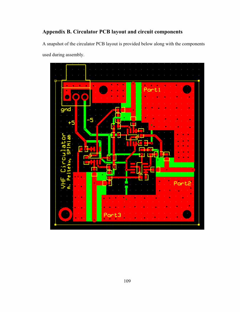
109

Appendix B. Circulator PCB layout and circuit components

A snapshot of the circulator PCB layout is provided below along with the components

used during assembly.

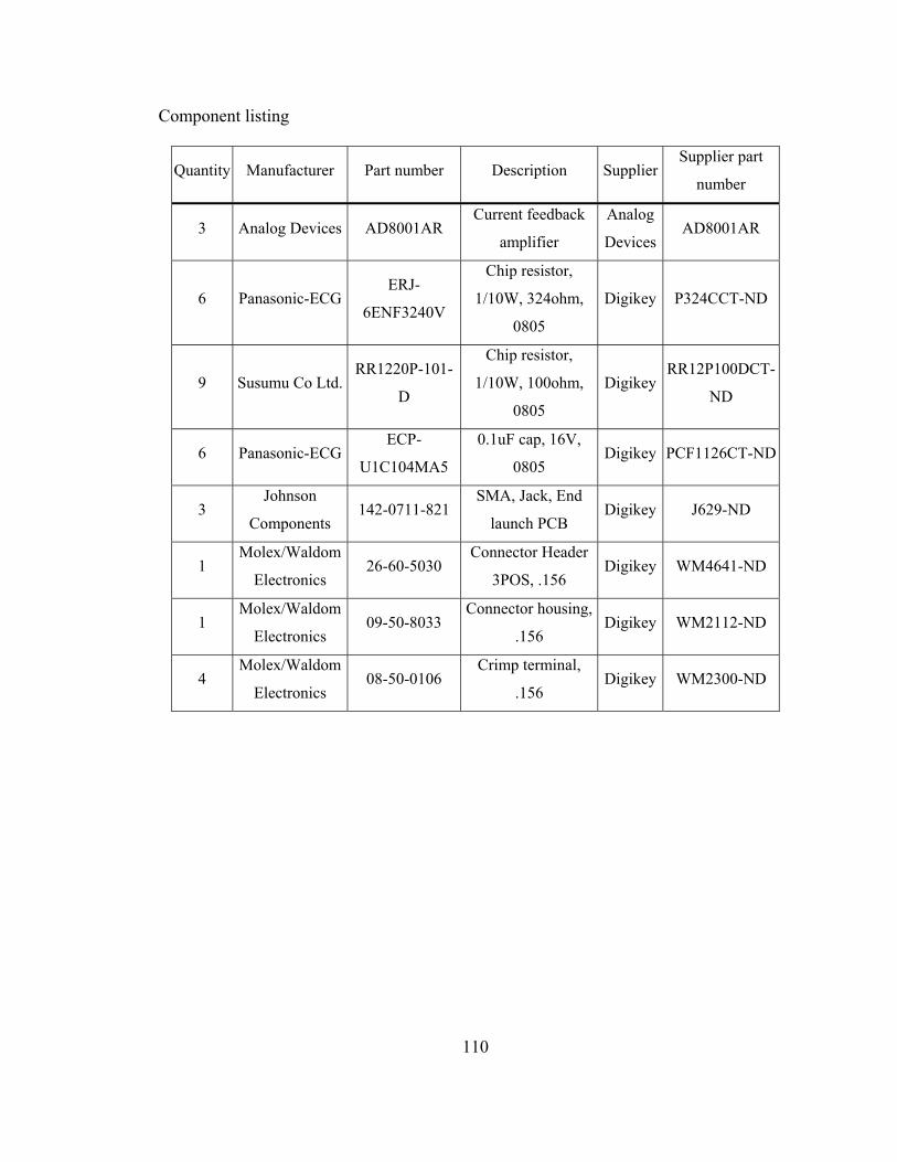
110

Component listing

Quantity Manufacturer Part number Description Supplier Supplier part

number

3 Analog Devices AD8001AR Current feedback

amplifier

Analog

Devices AD8001AR

6 Panasonic-ECG ERJ-

6ENF3240V

Chip resistor,

1/10W, 324ohm,

0805

Digikey P324CCT-ND

9 Susumu Co Ltd. RR1220P-101-

D

Chip resistor,

1/10W, 100ohm,

0805

Digikey RR12P100DCT-

ND

6 Panasonic-ECG ECP-

U1C104MA5

0.1uF cap, 16V,

0805 Digikey PCF1126CT-ND

3 Johnson

Components 142-0711-821

SMA, Jack, End

launch PCB Digikey J629-ND

1 Molex/Waldom

Electronics 26-60-5030

Connector Header

3POS, .156 Digikey WM4641-ND

1 Molex/Waldom

Electronics 09-50-8033

Connector housing,

.156 Digikey WM2112-ND

4 Molex/Waldom

Electronics 08-50-0106

Crimp terminal,

.156 Digikey WM2300-ND