Developments in Modelling Risk Aggregation - BIS

Basel Committee on Banking Supervision

Joint Forum

Developments in Modelling Risk Aggregation

October 2010

Copies of publications are available from:

Bank for International Settlements Communications CH-4002 Basel, Switzerland

E-mail: [email protected]

Fax: +41 61 280 9100 and +41 61 280 8100

This publication is available on the BIS website (www.bis.org).

© Bank for International Settlements 2010. All rights reserved. Brief excerpts may be reproduced or translated provided the source is cited.

ISBN 92-9131- 847-7 (print)

ISBN 92-9197- 847-7 (online)

http://www.bis.org/

THE JOINT FORUM

BASEL COMMITTEE ON BANKIN G SUPER VIS ION

INTERNATIO NAL ORGANIZAT ION OF SECURIT IES COMMISS IONS

INTERNATIO NAL ASSOCIATION OF INSURANCE SUPERVISORS

C / O B A N K F O R I N T E R N A T I O N A L S E T T L E M E N T S

C H - 4 0 0 2 B A S E L , S W I T Z E R L A N D


October 2010


Contents

Executive Summary..................................................................................................................1 1. Introduction......................................................................................................................3 2. Summary of key conclusions and observations ..............................................................4 3. Aggregation methods within regulatory frameworks........................................................7 4. Developments in firms' risk aggregation methods.........................................................12 5. Validation and management of model risks in risk aggregation ....................................19 6. Diversification effects in risk aggregation ......................................................................22 7. Supervisory reliance on firms’ risk aggregation results .................................................24 8. Potential improvements to risk aggregation ..................................................................26

Annex A: Risk aggregation in the Basel II Capital Framework ...............................................33 Annex B: Canadian Minimum Continuing Capital and Surplus Requirements (MCCSR).......40 Annex C: European Union Solvency II Directive ....................................................................43 Annex D: The Swiss Framework for Insurance Companies ...................................................49 Annex E: US Insurance Risk Based Capital (RBC) Solvency Framework .............................53 Annex F: Developments in firms' risk aggregation methods...................................................56 Annex G: Technical underpinnings of aggregation methods ..................................................72 Annex H: Approaches to managing model risks for risk aggregation processes....................93 Annex I: Diversification effects within risk aggregation...........................................................99

Developments in Modelling Risk Aggregation: Summary Report

Executive Summary

Why did the Joint Forum undertake this project?

This mandate sought to understand industry developments in modelling risk aggregation and developments in supervisory approaches, particularly in light of the Crisis.

Specifically, it aimed to

• Describe current modelling methods used by firms and regulators to aggregate risk;

• Describe how firms and regulators achieve confidence that the aggregation techniques can perform as anticipated under a wide range of conditions; and

• Suggest potential improvements to risk aggregation by firms and supervisors.

It built on earlier Joint Forum work in 2003, 2006 and 2008.

What did the Joint Forum do?

Between April and September 2009 the Joint Forum working group interviewed industry participants from North America, Europe and the Pacific, and supervisors from member countries.

These interviews discussed the following:

• How modelling has developed;

• How industry uses modelling;

• Strengths and weaknesses of current modelling techniques;

• Industry attitudes to improving current modelling techniques, and

• Supervisors' attitudes towards current modelling techniques.

What did the report find?

How firms use Risk Aggregation Models ('RAM's')

The Joint Forum found that Risk Aggregation Models ('RAM's) are used to provide information to support decisions which contribute to the resilience of complex firms.

RAM's are used, for instance, to support decisions about capital allocation and the capital adequacy and solvency. They are also used to support risk management functions (including risk identification, monitoring and mitigation).

The Joint Forum found that, despite recent advances, RAM's in current use have limitations. They have not adapted to support all the functions and decisions for which they are now used. Firms using them may not, as a result be seeing clearly or understanding fully the risks they face.

Developments in Modelling Risk Aggregation 1

For instance, RAM's – designed originally to assess the relative risks and relative merits of different capital projects for capital allocation purposes – are being used to support capital adequacy and solvency assessments. Yet these assessments require precision in measuring absolute, not relative, levels of risk and reliable ways of assessing 'tail events'. Relying on these RAM's may lead to underestimates of capital adequacy or solvency needs.

RAM's designed for capital allocation purposes also lack the granularity needed to provide a clear picture of the incidence, scope and depth of risks and the correlation between different risks. Risk management frameworks using these RAM's may not, therefore, be adequately safeguarding the firm.

There was, however, no evidence that models in current use had contributed to any failures during the recent Crisis.

Some firms are addressing these issues – particularly in addressing the treatment of tail events - others are not. Some firms are starting, for instance, to address issues related to assessing tail events. Some are moving away from using basic 'Value at Risk' (VaR) measures of the risk of independent extreme events to measures such as 'Expected Shortfall' (which is more sensitive to 'tail event' probabilities) and 'Tail VaR' (which accounts for both the probability and severity of an extreme event) measures. Use is also being made of scenario analysis and stress testing.

The Joint Forum also found that firms face a range of practical challenges in using RAM's with cost and quality implications. These include managing the volume and quality of data and communicating results in a meaningful way. Despite these issues, we found there was little or no appetite for fundamentally reassessing or reviewing how risk aggregation processes are managed.

Supervisors' attitudes to current modelling techniques

Generally, supervisors do not rely on RAMs currently used by firms. Modelling is generally seen as a 'work in progress' with best practices yet to be established. Substantial improvements and refinements in methods – particularly in aggregating across risk classes - would be needed before supervisors are likely to be comfortable relying on these models.

What does the report recommend?

The Joint Forum makes recommendations to both firms and to supervisors.

Recommendations to firms

To address the limitations noted in our research, firms should consider a number of improvements to the RAM's they currently use. Firms making these improvements will be able to see and understand the risks they face more clearly. This will require significant investment. The improvements firms should consider are the following:

• Firms should reassess risk aggregation processes and methods according to their purpose and function and, where appropriate, reorient them;

• Where RAMs are used for risk identification and monitoring purposes, firms should take steps to ensure they are more

o sensitive (so be able to identify change quickly);

2 Developments in Modelling Risk Aggregation

o granular (so be able to drill down to identify and analyse the risk positions which cause changes);

o flexible (so be flexible enough to reflect changes in portfolio characteristics and the external environment); and

o clear (so able to see and understand the sources of risk and their effect on the firm);

• Firms should consider changes to methodologies used for capital and solvency purposes to better reflect tail events. This includes attributing more appropriate probabilities to potential severe 'real life events', and conducting robust scenario analysis and stress testing;

• Firms should consider better integrating risk aggregation into business activities and management;

• Firms should consider improving the governance of the risk aggregation process, particularly the areas in which expert judgment enters the risk aggregation processes. This could be done by enhancing the transparency of these judgments and their potential impact on risk outcomes, and the controls that surround the use of judgment.

Recommendations to supervisors

Supervisors should recognise and communicate with firms the risks posed by continued use of RAM's. In doing so, they should highlight the benefits of appropriately calibrated and well-functioning RAM's for improved decision making and risk management within the firm.

Supervisors should work with firms to implement these improvements.

1. Introduction

Sound risk management in financial firms and risk-sensitive prudential supervision generally are each based on comprehensive assessments of the risks within financial firms. Risk aggregation – the process of combining less-comprehensive measures of the risks within a firm to obtain more comprehensive measures – is fundamental to many aspects of risk management as well as risk-sensitive supervision.1 However, new developments in financial markets, in financial management practices, in supervisory approaches, and in risk aggregation practices themselves, present an ongoing challenge. Rapid development of these markets and management practices may reduce the appropriateness of incumbent risk aggregation approaches. However, adoption of significant new approaches for risk aggregation creates the possibility that financial firms may rely on flawed methodological approaches to risk aggregation that could cause management to overlook material risks and affect the firm’s assessment of its solvency under different economic conditions. Further, inconsistencies in risk aggregation processes may develop between the various financial

1 Note that “risk aggregation” in this sense does not refer to the various management and information systems

challenges associated with ensuring that risk information is effectively and appropriately reported across the firm or group to the respective responsible management areas; although this is a necessary step for risk management generally.


sectors due to differences in the timing of adoption of new approaches or differences in the way new approaches are reflected in practices or regulations. In the area of solvency regulations, potential differences in approaches to risk aggregation have surfaced in conjunction with new or emerging regulatory frameworks. Basel II is being implemented currently in a number of jurisdictions, while other new approaches to solvency are being explored or developed in the insurance sector.

Most recently, the performance of various aspects of risk aggregation methodologies during times of significant financial turmoil raises fresh questions about the robustness of such approaches, and presents opportunities to improve practices. This report addresses current methods being used by firms and regulators to aggregate risk, the ways in which firms and regulators achieve confidence that aggregation methods perform as anticipated under a wide range of conditions, and suggests potential improvements for risk aggregation by firms and supervisors in the areas of solvency assessment and risk identification and monitoring. As such, a reorientation of risk aggregation methods to adquately address these functional areas may require a significant investment of effort and resources by firms.

The work for this report was carried out by interviewing and obtaining feedback from industry participants (from North America, Europe and the Pacific) as well as collecting information and views from supervisors that are members of the Joint Forum.

2. Summary of key conclusions and observations

Risk aggregation provides necessary information that enables effective group-wide or enterprise-wide risk management, as well as a wide variety of other key business decisions and business processes. However, the financial crisis that began in 2007 highlighted at least some degree of failure of risk aggregation methods. Many of the firms interviewed for this report now acknowledge that “model risk” in this area may be higher than previously recognised. Despite that recognition, there has been surprisingly little movement by most of these firms to reassess or revise risk aggregation practices in significant ways.

Overall, no single, commonly accepted approach for risk aggregation was evident across firms interviewed. This is consistent with the findings of previous studies. Risk aggregation frameworks used in practice appear to be determined to some extent by business strategy, business practices, risk characteristics, and management purposes.2 Financial firms develop and employ risk aggregation frameworks for particular functions; management functions identified include capital allocation, risk identification and monitoring, pricing, solvency assessment, and capital management, among others. But while each of these purposes involves aggregation of risk, they place different demands on risk aggregation methods, and alternative approaches have different strengths and weaknesses that vary in importance depending on the specific application. Because the validity of any method depends on its purpose and use, methods can be used with greater confidence if they are used for the specific purpose for which they were developed, and less confidence when they are pushed beyond their original design. It is unlikely that all of these purposes can be served effectively with a single approach to risk aggregation. Some of the firms interviewed do use different methods for different functions, although many attempt to address different functions using

2 Heterogeneous groups with a more diverse set of business activities, entities, or exposure types place greater

emphasis on aggregating risk into a single measure and extracting diversification benefits, even though their heterogeneity and complexity clearly makes risk aggregation more difficult.


the same method. A concern is that the chosen method often remains a mathematical structure, operating in a vacuum as it is not deeply engrained in the business and management of the firm. As such, risk aggregation cannot adequately fulfill its function of providing to management and business lines the information necessary to safeguard the firm.

Although the original purpose of risk aggregation varied to a certain extent from firm to firm, many commonly used methods – for example, many of those based on economic capital modelling – were developed for risk (or capital) allocation. But there are other important management functions that depend on effective risk aggregation. One that has become increasingly prominent is solvency assessment, which helps firms and supervisors determine the probability of financial distress and the absolute level of capital sufficient to keep the firm operating under relatively severe conditions. Another highly important function is risk identification and monitoring, which is one of the primary prerequisites for good risk management, and a precondition for progress in other areas; a firm must be able to identify the risks to which the firm is exposed so that, at a minimum, the firm can monitor those risks.

In general, a reorientation or refinement of risk aggregation methods, requiring significant additional investment of effort and resources by firms in methods and systems, likely would be needed to make them suitable for risk identification and monitoring on the one hand, and for assessing capital adequacy on the other. Most of the firms interviewed did not have aggregation processes or methods in place that were developed for the explicit purpose of risk identification and monitoring.3

Most firms also would need to enhance or modify existing risk aggregation methods for reliable solvency assessment. In particular, solvency assessment requires that outcomes in the tails of relevant distributions be assessed with reliability and accuracy in absolute terms. In contrast, the original purposes of many models (such as capital allocation) require relative measurement of risk, in contexts that place less emphasis on accuracy in the tails. For example, interviews revealed that, given the common assumptions underlying risk aggregation models, few users view the events that these models assess as having 0.1 percent probability to truly be 1-in-1000-year events. While such models may be appropriate for other purposes, such as allocation of risk and capital, they are much less suitable for assessing capital adequacy and solvency. At a minimum, firms need to recognise the shortcomings of these models if they use them for solvency assessment.

Financial institutions commonly seek recognition of diversification benefits as measured by their internal risk aggregation methods in capital adequacy discussions with regulators and supervisors. However, reliable measures of diversification benefits require reliable measurement of risk, particularly in the tails of distributions. As noted above, in general, commonly used methods are not well-suited for reliable assessment of tail risks. In addition, differences in methodology led to quite different results with regard to diversification benefits. Interviewed firms noted that many characteristics of risk aggregation methods (such as the specific compartmentalisation of risks, the granularity of the aggregation approach, and various elements of expert judgment) significantly affect measured diversification benefits, even though these characteristics have no bearing on the existence or extent of real economic diversification effects.

3 This observation is consistent with other recent work examining risk management practices, such as that of

the Senior Supervisors Group, which also found that a common attribute of some of the firms that best weathered the financial crisis that began in 2007 was the presence of risk identification processes that were able to identify emerging risks early.


Risk aggregation challenges identified through the interviews were both technical and practical. One common technical theme was a growing consensus that aggregation based on linear measures of correlation is a poor method for capturing tail dependence; classical correlation measures do not give an accurate indication and understanding of the real dependence between risk exposures.

Practical challenges relate to information management and data quality, appropriate internal communication of results, and overall process management. Firms also noted that judgment is necessary to appropriately aggregate risk information and to employ the risk information for business decisions, which makes expert judgment an integral and crucial part of most risk aggregation processes, but at the same time complicates the challenges of validation, governance, and control.

Some of the more advanced risk aggregation methodologies were observed at a few of the insurance firms interviewed. Some use methods that focus more directly on capturing tail risk or on introducing tail events into solvency calculations. They also tend to be less “silo-based” in their approaches to risk measurement, and were more inclined than bank-centric groups to use risk aggregation methods as a tool for consistent pricing of risk. In addition, some of these insurance firms appeared to price for systematic or catastrophic risks to a greater extent than was the case for banks, even though systematic risk clearly is present for banks as well. Although not all methods are readily transferable across firms or sectors, the differences in risk aggregation approaches suggest there may be potential benefits from a broader sharing of practices.

Current regulatory frameworks incorporate the results of firms’ risk aggregation methods in various ways; however, the extent to which diversification benefits are incorporated in regulatory calculations varies substantially across regulatory regimes, and depends on the specific context. Supervisors surveyed for this report understand that opportunities for diversification exist, but were skeptical that financial firms are able to measure diversification benefits reliably.

In general, most supervisors claimed not to rely to a great extent on capital calculations or the derived diversification benefits from firms’ internal models, particularly when assessing overall capital adequacy or determining solvency. Risk aggregation methods are viewed by many supervisors surveyed as potentially interesting “works in progress” for assessing diversification benefits and overall capital adequacy or solvency. To some extent this supervisory stance may be appropriate. As noted above, many current risk aggregation approaches were not developed specifically to assess capital adequacy. Basing regulatory or supervisory assessments of capital adequacy on traditional risk aggregation models may create incentives that distort the models and unintentionally subvert their suitability for other important internal uses. Specifically, linking capital requirements to internal model results likely strengthens the desire by firms to extract and recognise any possible diversification benefits, despite the limited reliability of the measured diversification effects provided by most currently used models.

Some solvency regimes, notably in the insurance sector, rely on internal risk aggregation results that incorporate diversification benefits. Given the challenges firms acknowledge in reliably assessing diversification, and the general scepticism of many regulators with respect to the performance of internal risk measurement methods, a deliberative and watchful approach is appropriate while more experience is gained with models-based approaches. Model results should be reviewed carefully and treated with caution, to determine whether claimed diversification benefits are reliable and robust.


3. Aggregation methods within regulatory frameworks

Risk-based regulatory capital frameworks must incorporate, explicitly or implicitly, some approach to adding up or aggregating measured risk. Work stream members studied regulatory regimes that either exist or are in development, to highlight the range of approaches taken to risk aggregation within regulatory frameworks.

Description of the aggregation methods

The Basel II Capital Framework

The first Pillar calculates a bank’s overall minimum capital requirement as the sum of capital requirements for the credit risk, operational risk, and market risk. Firms do not recognise any diversification benefits between the three risk types when computing the capital requirement.

For intra-risk aggregation within credit risk, both the Standardised Approach (SA) based on external ratings and the Internal Ratings-Based Approach (IRBA) in which banks estimate key risk parameters presume that capital charges are portfolio-invariant. The approach implicitly recognises a certain amount of diversification, through the construction and calibration of the risk-weight function. The underlying risk model assumes that idiosyncratic risk is effectively diversified away within the credit portfolios of large banks, with a single systematic “state variable” or measure of macroeconomic conditions affecting all exposure classes. However, diversification is not measured directly, and the approach does not take into account potential exposure concentrations in a portfolio containing large, single-name exposures, or in a portfolio that is relatively less diversified in other ways.

Basel II includes two methodologies for market risk, the standardised measurement method (SMM) and the internal models approach (IMA). Under the SMM, the minimum capital requirement for market risk is defined as the (arithmetic) sum of the capital charges calculated for each individual risk type (interest rate risk, equity risk, foreign exchange risk, commodities risk and price risk in options). In contrast, the IMA allows banks to use risk measures derived from their own internal risk management models, subject to a set of qualitative conditions and quantitative standards. In terms of risk aggregation within and across the individual market risk drivers and possible resulting diversification benefits, banks with supervisory permission to use the IMA are explicitly allowed to recognise empirical correlations within and across each of the broad market risk categories.

For operational risk, under the Standardised Approach gross income for each of eight business lines is multiplied by a fixed percentage specified in the Basel II framework. In general, total required capital is the three-year average of a simple summation of the capital charges for each business line. Under the Advanced Measurement Approach (AMA), a bank must have an internal operational risk measurement system, and banks are allowed considerable flexibility in the methodology used to quantify operational risk exposure.

As part of Pillar 2 of the Basel II framework, banks assess their own capital adequacy using an internal capital adequacy assessment process (ICAAP). Since these processes are by definition internal, they aggregate risk in various ways, using the types of methods described in Section 4 of this report. However, because Pillar 1 establishes the minimum capital requirement, ICAAP calculations cannot result in a reduction of required capital; instead, the ICAAP will either determine no additional capital is needed, or additional capital is required above Pillar 1 levels.


Canadian Minimum Continuing Capital and Surplus Requirements (MCCSR)

Life insurance companies in Canada are subject to the capital requirements contained in OSFI’s MCCSR guideline, and property and casualty insurers are subject to the requirements of the Minimum Capital Test (MCT) guideline. The MCT is a factor-based requirement that aggregates risks additively, and does not incorporate explicit measurements of or assumptions about diversification. However, the MCCSR employs more sophisticated approaches in some areas.

MCCSR imposes capital requirements for the following risk components: asset default risk, mortality risk, morbidity risk, lapse risk, disintermediation risk, and segregated fund guarantee risk. The requirements do allow some diversification benefits within the categories of mortality, morbidity and segregated funds risk. There is no diversification benefit given across these risk components. Therefore, the total MCCSR capital requirement is determined as the unadjusted sum of the capital requirements for each component risk.

MCCSR required capital is calculated on a consolidated basis by risk, not by legal entity. Consequently, insofar as diversification benefits are recognised in the requirement (such as for mortality volatility risk), these benefits will be recognised even when risk exposures span several entities within an insurance group.

European Union - Solvency II

The Solvency Capital Requirement (SCR) under Solvency II is defined as the Value-at-Risk (VaR) of the Basic Own Funds at 99.5% and a horizon of one year. Firms choose between a standard formula, a full internal model, or a partial internal model; the aggregation process varies depending on the choice made.

The standard formula is modular, meaning that the calculation is based on several risk modules, each of which is supposed to reflect the appropriate VaR and capital charge on a stand-alone basis. These capital charges then are aggregated through a correlation matrix (Var-Covar approach) to take into account dependencies. (Future implementing measures may prescribe further splitting of modules into sub-modules, this has not yet been formalised.) The Directive prescribes two different approaches to assess the group SCR: a method based on consolidated data, or a method called deduction aggregation. These two methods do not lead to the same diversification effects. This is why Article 220 of the Framework Directive clearly sets out that the consolidated data method is the default method, even though the group's supervisor is allowed to decide, where appropriate, to apply the alternative method instead of - or in combination with - the default method. Implementing measures will specify the criteria that will allow the group's supervisor to diverge from the default method.

Internal models used for the SCR are meant to be used by firms for risk management as well as for the determination of regulatory capital requirements. No particular method is prescribed, although the Directive defines a number of minimum requirements on the system for measuring diversification effects.

Firms are allowed to use partial internal models, provided that the model can be fully integrated into the standard formula. Within the scope of the partial internal model, diversification benefits are treated in the same way as in full internal models.

The Swiss Framework for Insurance Companies

The Swiss Solvency Test (SST) became mandatory for all Swiss insurers to compute as of 2008. The SST framework consists of a standard model, and principles for internal models.


The standard model, for use by Switzerland-based single insurance companies of standard size and complexity, is based on modules for the following risks: market risk, credit risk (counterparty default), non-life insurance risk, life insurance risk, and health insurance risk. Operational risks are not part of the current SST. Principles for internal modelling have to be followed when the standard model does not adequately capture the risks for larger and more complex companies, all re-insurance companies, and groups and conglomerates. The internal model can differ slightly (partial internal model) or substantially (full internal model) from the standard model. Diversification between risk categories is recognised in all cases.

For life companies, closed form Var-Covar aggregation (see Section 4) is used. For non-life business, the company determines details of the aggregation of the various distributions in its model. Then risk is calculated using an Expected Shortfall measure applied to the main resulting distribution. In addition, firms apply scenario analysis as specified by the Swiss insurance regulator and aggregate them to get the final capital requirement. Finally, an amount called market value margin is evaluated and added to the required capital. The market value margin reflects the cost of raising the capital necessary to insure the solvency through the end of the engagement according to the SST.

In the SST framework, a group is solvent when all legal entities would be judged solvent under the SST for single legal entities. In practice, a large insurance group is allowed to compute the SST at cluster levels (made of homogeneous sub-set of legal entities). In some cases the regulator authorises a consolidated computation. The internal transactions should be considered and modelled adequately in case they have a material effect on the firm’s capital. The degree of sophistication of the aggregation procedure for computing the solvency capital requirement should be commensurate with the complexity of the business, of the group structure, of the internal transactions and with the current financial situation of the group.

US Insurance Risk Based Capital (RBC) Solvency Framework

The risk-based capital (RBC) system was created to provide a capital adequacy standard that is related to risk, raises a safety net for insurers, is uniform among the US states, and provides regulatory authority for timely action. A separate RBC formula exists for each of the primary insurance types: life, property and casualty, and health. Each formula utilises a generic formula approach rather than a modelling approach, although the Life RBC Formula has recently incorporated some modelling related to interest rate risk. The formula focuses on the material risks that are common for a particular insurance type; the generic formula setup typically pulls data from each insurer as reported in the uniform statutory financial statement and assesses a factor to calculate an RBC risk charge. The calculation of an RBC risk charge is performed for every individual risk item included in the RBC formula.

Once all component RBC risk charges are calculated, a covariance calculation is performed. The result of this covariance calculation is less than the sum of the individual RBC risk charges; the covariance adjustment was incorporated to reflect the fact that all risks captured in the RBC formula would not occur at the same time. The construction of the covariance calculation may be considered to be a type of diversification factor, as it implicitly assumes less than perfect correlation between the component risk charges.


Differences in the treatment of risk aggregation4

Each regulatory regime may aggregate risk on one or more of several broad levels. Intra-risk aggregation is carried out across exposures within an individual risk type, such as credit risk or morbidity risk. Inter-risk aggregation refers to aggregation across the individual risk types, for example to combine measurements of credit risk and operational risk.5 Finally, within groups, risks may be aggregated into a consolidated measure across entities. As shown in the table, the regulatory frameworks described above differ in various ways across these three broad dimensions of risk aggregation.

As the first column of the table indicates, it is not uncommon for intra-risk diversification benefits to be recognised to some extent within regulatory solvency regimes. Diversification benefits generally are recognised within market risk, but the extent of recognition differs materially within credit risk. In many cases, the treatment of credit risk reflects an assumption that the underlying portfolios are well-diversified. Solvency regimes that permit internal models tend to be more open to recognising diversification benefits within all risk types, provided that the methodology for determining the benefit has been approved by the supervisor. The recognition of diversification benefits within insurance risk also strongly differs between the regulatory regimes.

4 See section 7 for a summary of supervisory views on risk aggregation methods used by supervised firms. 5 Risk categorisations and the distinction between intra-risk and inter-risk are introduced for practical reasons in

regulations, but are to a certain extent arbitrary, and can differ across regulatory regimes. Using these distinctions requires clear definitions of the risk categories, but no commonly accepted list of distinct risk categories exists at the international level. Moreover, note that some regulatory frameworks, such as the Swiss Solvency Test (SST), do not distinguish between intra-risk and inter-risk aggregation.


Recognition of diversification in selected solvency regimes

Solvency Regime Intra-Risk Inter-Risk Group or

Company Level

Basel II Pillar 1

No, for credit risk, although minimum capital calibration for IRB reflects an assumed degree of diversification, with assumptions most applicable under IRB. Yes for market risk under internal models approach, and to some extent under the standardised approach. No, for operational -- under standardised, Yes for AMA; not required but allowed if supported – with considerable latitude allowed in calculation of dependencies.

No, capital is additive between three risk categories.

No, but calculation is done at group level, which may involve netting of intra-group exposures.

Basel II Pillar 2 Possibly, through ICAAP, but subject to supervisory interpretation.

Canadian Insurance Minimum Continuing Capital and Surplus Requirements (MCCSR)

Yes, some diversification benefits within the risk components of mortality, morbidity and segregated fund guarantee risk. No diversification benefit is given for credit, lapse, or disintermediation risks.

No, capital is additive between risk categories.

Yes, to extent risks that can be diversified are consolidated across legal entities.

US Insurance Risk Based Capital (RBC)

Yes, asset concentration factors, number of issuers for bond holdings, formula for market risk; in addition, specific recognition of diversification across liabilities.

Yes, covariance calculation computed for component RBC risk charges, but restricted due to assumption of less-than-perfect correlation.

No, capital is determined at the legal entity level for each separate entity.

Swiss Solvency Test Standard Model

Yes, recognition of risk diversification for market and insurance risks, which are aggregated with a VarCovar method with appropriate distributions and scenarios; credit risk is treated as under Basel II.

(No standard model for groups)

Swiss Solvency Test Internal Model

Yes, recognition of risk diversification for all risk categories, with no difference between intra- and inter-risk aggregation; however, credit risk can be treated as under Basel II.

Yes, cluster model plus possibly a consolidated view. Also, modelling of internal group transactions.

Solvency II (EU) Standard Formula

Yes, recognition of risk diversification: sub risks are aggregated with Var/Covar methods.

Yes, recognition of some risk diversification: • Aggregation by Var/Covar

method. • Correlation between credit

and non-life risks is 0.5, most other correlations are 0.25

• No diversification between operational risk and other risks.

Solvency II (EU) Internal Model

Yes, diversification benefits recognised if methodology is approved by supervisor.

No, but group wide consolidation is possible for insurance groups • No cross-

sectoral diversification

See Annexes A-E for more details on specific regulatory regimes.


In general, solvency regimes less commonly recognise the potential for diversification across risk types. Under Pillar 1 of Basel II and the Canadian insurance regime, there is no diversification benefit with respect to inter-risk aggregation reflected in required capital, since capital is additive across the risk categories. The standard formula under Solvency II does permit diversification benefits to be reflected through inter-risk aggregation, with the exception of operational risk, which must be added to the other risks. Solvency regimes that are based on the use of internal risk aggregation models, such as the Swiss Solvency Test and Solvency II, are more open to recognition of diversification across risk types, under the condition that firms have sound processes to incorporate inter-risk diversification. Recognition of inter-risk diversification benefits would also be possible within Pillar 2 of Basel II, through the ICAAP and Supervisory Review and Evaluation Process (SREP) processes.

In general, the solvency regimes do not recognise diversification across entities at the group level; instead, capital requirements are additive across legal entities. Consolidation may reflect some implicit recognition of diversification benefits if the regime permits netting of intra-group exposures. Approaches based on firms’ internal modelling may provide for recognition of diversification benefits on a consolidated basis, generally subject to some type of supervisory approval of methodologies; examples include the ICAAP required under Pillar 2 of Basel II and the modelling of intra-group exposures for the Swiss Solvency Test.

4. Developments in firms' risk aggregation methods

Risk aggregation methods varied widely between the interview participants, an observation also made in previous Joint Forum reports. Nevertheless, some general modelling approaches and developments can be identified. This section relates these approaches to the nature of and to some characteristics of the firm or to the management functions that they have to support. The section also provides insight into the modifications made to the risk aggregation frameworks of some financial institutions in response to the crisis that started in 2007.

Risk aggregation frameworks and the nature of the organisation

An appropriate risk aggregation framework is fundamental for adequate firm-wide risk management. Its main objective is to provide appropriate risk information to the relevant management to steer the business. However, interviews with industry participants indicate that providing this information continues to prove to be a huge challenge.

In some respects the business strategy and business model of a firm appear to influence both the overall approach and certain details of the design of a firm’s risk aggregation framework and the respective risk choice of aggregation methods. Groups that have a clear strategy to conduct heterogeneous activities and thereby spread their exposures across different types of risks in general are more purposeful about identifying high-level diversification benefits through the aggregation process. This focus is reflected in the aggregation methods chosen and the parameter estimates used. These heterogeneous groups appear to have a stronger tendency to aggregate risks into a single figure; from the interviews, the heterogeneous complex groups seemed to emphasise aggregating into a single or limited number of total group-wide measures. In contrast, the more business-line focused firms are generally more sceptical towards aggregating different kinds and sources of risk into single risk figures and subsequently calculating diversification benefits (which seems to be reflected in more conservative aggregation approaches). They tend to use a greater number and variety of aggregation methods, and this appeared to afford them more flexibility in producing detailed risk analyses and aggregated risk measures on an ad hoc


basis. Where the heterogeneous groups generally put great effort into calculating a single risk measure, the homogeneous groups generally used aggregation to understand risk and changes in risks. However, very often the business model, activities, and management processes of a firm do not influence the risk aggregation framework to a sufficient extent. For instance, firms may calculate group-wide capital figures taking into account diversification effects across the different activities, even though these activities are not effectively managed on a group-wide basis.

On the practical side, risk aggregation imposes significant information systems challenges. Firms have to maintain the quality of exposure and risk information to be sufficiently consistent that it can be aggregated in a meaningful way ("matching apples to apples"), a challenge that can become particularly prominent when a firm is pursuing business combinations that are motivated by potential “diversification benefits”. The activities of these firms generate vast amounts of information that could be used in aggregation, often from multiple systems; risk aggregation also generally requires the management of vast volumes of external data (eg on the economy or a particular market) to calculate any meaningful risk measures. To manage this information challenge, firms often must make judgments concerning the materiality of (sources of) risks. The complexity of an organisation also can exacerbate the challenge of expressing risk as an aggregate measure. Ultimately the information has to be communicated coherently to the appropriate management areas having the responsibilities over the particular risks. IT systems are required to cope with the disparity and volume of data flows, to match different systems, to provide the necessary flexibility and to maintain sufficient computing capacity to meet the purposes of the risk aggregation and the requirements of management. As such, risk aggregation provides an important and positive incentive to the firm to deploy the infrastructure that they need to identify, measure and manage the risks. The effort and strategy for data collection underlying the risk aggregation methods provides a fundamental base for the risk analysis in itself.

In response to these challenges, firms "bundle" as much risk information as possible within a common risk expression. Mathematical assumptions and approximations are made to aggregate different risk exposures. The greater the differences in the inherent risk characteristics between lower-level risk sources, the less realistic or more stylised these assumptions may become. To control for the impact of these underlying assumptions on the aggregated risks, some firms apply clear internal policies and use different risk expressions in parallel to view some dimension of aggregated risk from multiple angles. However, in general, it can be expected that the larger the financial institution and the more dispersed the risk exposures across different risk types (or the more complex the group), the more challenging the risk aggregation.

The roles or functions of risk aggregation within the firm's management

The risk aggregation framework may consist of different methods, each having a distinct purpose or supporting a specific function within the firm's management. The roles or functions of risk aggregation identified are: risk identification and monitoring, solvency assessment and determination, capital allocation, consistent risk pricing, and assessing intermediate outcomes against longer-term strategic objectives. However, aggregation methods are designed and validated for specific purposes, not for all purposes or management functions. When methods are used for purposes other than those for which they were originally intended, problems may result. In addition, some firms were found to employ a single risk aggregation method to serve simultaneously more than one of the functions noted above. In such cases, conflicts easily arise, for instance stemming from conflicting needs for adaptability versus stability, for consideration of normal versus stressed conditions, and for differences in the time horizon.


1. Risk identification and risk monitoring

A fundamental role of risk aggregation in effective group-wide risk management is to support risk identification and monitoring, which enables the firm to understand and explain its risks and the changes in those risks. As discussed by the Senior Supervisors Group6 this identification and analysis function proved essential for early risk identification, and typically was missing or inadequate at firms that were severely affected by the crisis.

Only a limited number of firms were found to have a method developed for the purpose of risk identification and monitoring. A typical characteristic of methods suited for this purpose is that they focus on changes or trends in (aggregated) risk measures rather than on their point-in-time or absolute level, and express risk as a distance measure from certain self-imposed limits. In this role, methods are required to have a high level of sensitivity, granularity and clarity so that risk changes or new risks can be quickly identified and constantly monitored. Typically these methods are strongly adaptive to changes in the risk portfolio and in the external environment and are therefore more dynamic in their measurement approach. In terms of granularity, methods must allow "drilling down" into the details of the risks to enable identification of the risk positions that cause changes, to develop an understanding and explanation of these risk changes, and to identify underlying risk drivers that might cause these changes. In this setting, the focus is more on obtaining a view of potential interactions between risk exposures, rather than to make great efforts to "precisely" measure dependencies (for instance in terms of linear correlations) between risk exposures. To obtain the necessary level of clarity, these methods seem not to have as their ultimate objective the aggregation or combination of the risks into a single figure, as this may severely blur or obscure the view of the sources of these risks and their changes. Additionally, these aggregation methods frequently use different measures or approaches to obtain a view of risks from different angles or to obtain a more complete picture of risks.

Finally, methods used for this purpose require substantial flexibility in their application so that they can be used to aggregate the risk exposure to non-standard or ad-hoc categorisation of risk. In general, traditional economic capital models are felt not to properly meet these requirements.

2. Solvency assessment and determination

Most aggregation models now in use for capital adequacy assessment, such as traditional economic capital models, were initially developed for capital allocation decisions. Over time these traditional models have moved beyond their initial purpose and are now intensively applied for capital adequacy or solvency assessment. However, these traditional economic capital models generally do not appear to have the appropriate features to determine and assess required capital levels. Assessing and determining capital levels requires precision in the measurement of absolute risk levels, whereas in practice capital allocation uses require only relative measurement of risks. Additionally, to perform capital or solvency assessment and determination, methods are required to be reliable and accurate in the tails of the risk distribution. Tail accuracy requires that the models correctly incorporate potential severe events and attribute correct probabilities to these events, to meet the objective of keeping the firm operating under these extreme conditions. However, as will be discussed in more detail below, typical economic capital models generally are not able to capture "real-life" extreme events with the correct probability.

6 Observations on Risk Management Practices during the Recent Market Turbulence, March 2008, Senior

Supervisors Group.


In addition, there is a risk that tying capital requirements to these economic capital models may change the incentives associated with the use of these models; for instance, the desire to extract diversification benefits out of the methods may become much stronger.

3. Capital allocation and consistent risk pricing

As discussed above, traditional economic capital models were initially developed for capital allocation purposes, that is, to provide for the distribution of risks to the relevant businesses and entities, to confront them with costs that create appropriate incentives aligned with the true risks of those businesses or entities and to determine the most efficient use of available capital across competing alternatives in the firm. An economic capital model thus provides a certain rule to allocate relative shares of the total risk to the different businesses or entities – typically, under relatively normal conditions. The extent and granularity with which capital (and also measured diversification benefits) was allocated to different entities of the group differed significantly between the firms interviewed.

These allocation methods are also used for consistent pricing of risk, although this practice is more developed within the insurance sector than the banking sector. Pricing risks touches upon the core of the business or the activity. Although there is no uniform practice across the insurance firms, some insurance firms seem to focus more on systematic or tail risks when pricing risks. Other insurance firms and most of the banks that use risk aggregation results for this purpose generally price for risk under more “normal conditions”. These differences may be explained by differences in the risk characteristics of the portfolios. However, from the 2007-2009 financial events it has become clear that the bank portfolios are also subject to systematic risks. The degree to which systematic risks are priced (or the extent to which diversification benefits are recognised in the pricing) strongly determines the “cost” of the transaction. Consistent pricing of the risks (taking into account the external environment) may prevent firms from entering into deals that are not appropriately priced for the true level of risk.

4. Evaluating medium-term developments against strategic objectives

A limited number of firms have begun to make clear linkages between their aggregated medium-term risks or potential capital evolution (for instance, via economic capital models or stress test exercises), and the longer-term strategic objectives (possibly expressed in terms of risk appetite, ALM mismatches, or capital consumption). This exercise is done to assess whether the identified risk and any changes or developments in risk are in line with the targeted risk profile.

Experience during the financial crisis of 2007 - 2009

A key trigger of changes in risk aggregation methods, and particularly dependency modelling, appears to be prior loss experience on the part of the firms. For example, an insurance firm reported that the first WTC attack in 1994 led them to analyse and aggregate more fully their risk exposures across distinct risk underwriting businesses to a single counterparty within one building, a particular area, or a geographic region. Similarly, natural perils and manmade catastrophes have, over time, taught insurance firms that health and P&C underwriting risks are more strongly interrelated than previously imagined.

The interviewed firms described some general common lessons learned from the crisis, of which probably the most commonly mentioned was the necessity (but difficulty) of capturing tail risks and dependencies resulting from tail events. In this respect, interviewed firms generally observed that correlations between risk exposures appear to be notably different


during stress periods than in normal times. Some firms viewed the recent crisis as a confirmation of the deficiencies of aggregating risks using correlations, and the sensitivity of risk aggregation to computed correlation values. In particular, banks interviewed generally admitted that the interaction between market risk and credit risk was more important than had previously been recognised for some portfolios. Some firms reported that during the crisis they lacked necessary information to obtain a clear view of risks, that reporting was too infrequent, and that intensive manual work had to be performed to aggregate data. Some firms also reported that market disruptions had a severe impact within the liquidity risk sphere. One response has been to review the measurement horizons of VaR calculations to adjust for differences in asset liquidity. In general, though, interviewed firms reported that their risk aggregation methods performed adequately through the crisis and that only minor amendments are required, such as modest increases in certain correlation values or in volatility and spread parameters.

In contrast a limited number of interviewed firms are contemplating or making material changes to their risk aggregation framework or to particular aggregation methods. In addition to their experiences during the crisis, firms noted that regulatory and supervisory responses to the crisis (such as scenario stress test exercises) or other developments that have nothing to do with the crisis (such as Solvency II in the EU) can be important drivers of fundamental revisions of the aggregation framework and methods.

Var-Covar approach

The variance-covariance approach is a convenient and commonly used analytical technique that allows managers to combine marginal distributions of losses or distinct tail losses into a single aggregate loss distribution or tail loss estimate. The sole requirement is to characterise the level of interdependence of standalone losses, which is typically accomplished with a matrix of linear correlations. The lower the correlations on the non-diagonal elements of the matrix, the greater the level of diversification that can be realised with incremental (long) exposure to a risk component. For most multi-variable distributions, the correlation matrix (containing a single number for each distinct pair of variables) is not sufficient to adequately represent all the ways that two variables can interact. That appears to be the case only for members of the family of elliptical distributions, which includes the Gaussian. Strengths: The main advantages of Var-Covar are that it is simpler relative to other methods, can be evaluated formulaically and does not require fundamental information about the lower-level risks. Weaknesses: While Var-Covar is a simple and highly tractable approach to risk aggregation, the cost to the unwary user is that it effectively fills in unspecified details about the nature of the loss distributions, which may or may not be accurate or intended (eg assumption of elliptical distributions). Var-Covar thus imposes a simple dependency structure on what is believed to be a more complex web of dependencies. Almost all empirical dependencies involve a huge amount of information and are not readily reduced to a single number for each distinct pair of variables. In addition, Var-Covar (and other top-down aggregation tools such as copulas) also face difficulty in dealing with circumstances in which standalone risks are not actually exclusive but are believed to be integrated (eg market and credit risk).

Recent developments in risk aggregation methods

At the lowest level of the risk aggregation are the risk expressions that are aggregated. The traditional VaR measure was prevalent within many of the aggregation methods discussed. The VaR measure was generally praised for its ease of communication as it is "well understood by senior management" as well as among quantitative experts. However, a number of firms are replacing the classical VaR measure with an Expected Shortfall or tail VaR measure, or are evaluating several quantiles at once to obtain a more accurate view of the tail shape of loss distributions. This was particularly prevalent within insurance-based groups. Many industry participants noted that point measures of tails (such as the classical VaR measure) may miss important information on the tail shape of the distribution, and therefore lead to an incorrect appraisal and aggregation of the portfolio risks. Assessment and aggregation of different tail quantiles may thus be very necessary. Firms also were very sceptical that a 99.5% confidence level of VaR measures, under classical aggregation methods, actually reflected a 1-in-200 year scenario.


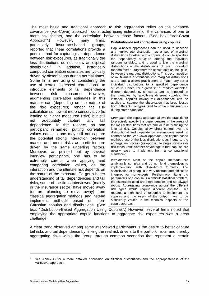
The most basic and traditional approach to risk aggregation relies on the variance-covariance (Var-Covar) approach, constructed using estimates of the variances of one or more risk factors, and the correlation between those factors. (See box: “Var-Covar Approach”.) However, many firms, particularly insurance-based groups, reported that linear correlations provide a poor method for capturing tail dependence between risk exposures, as traditionally the loss distributions do not follow an eliptical distribution.7 In addition, historically computed correlation estimates are typically driven by observations during normal times. Some firms are using or considering the use of certain "stressed correlations" to introduce elements of tail dependence between risk exposures. However, augmenting correlation estimates in this manner can (depending on the nature of the risk exposures) render the risk calculation somewhat more conservative (ie leading to higher measured risks) but still not adequately capture any tail dependence. In this respect, as one participant remarked, putting correlation values equal to one may still not capture the potential strong interaction between market and credit risks as portfolios are driven by the same underling factors. Moreover, as pointed out by several interview participants, one has to be extremely careful when applying and comparing correlation values, as the interaction and the ultimate risk depends on the nature of the exposure. To get a better understanding of tail dependencies and tail risks, some of the firms interviewed (mainly in the insurance sector) have moved away (or are planning to move away) from classical aggregation methods, and instead implement methods based on non-Gaussian copulas and distributions. (See box: “Distribution-Based Aggregation Using Copulas”.) However, several firms noted that employing the appropriate copula functions to aggregate risk exposures was a great challenge.

Distribution-based aggregation using copulas

Copula-based approaches can be used to describe any multivariate distribution as a set of marginal distributions together with a copula. A copula specifies the dependency structure among the individual random variables, and is used to join the marginal distributions – the distributions of each individual random factor – together; the copula acts as the "glue" between the marginal distributions. This decomposition of multivariate distributions into marginal distributions and a copula allows practitioners to match any set of individual distributions to a specified dependence structure. Hence, for a given set of random variables, different dependency structures can be imposed on the variables by specifying different copulas. For instance, copulas having tail dependence can be applied to capture the observation that large losses from different risk types tend to strike simultaneously during stress situations.

Strengths: The copula approach allows the practitioner to precisely specify the dependencies in the areas of the loss distributions that are crucial in determining the level of risk. Copulas allow direct control over the distributional and dependency assumptions used. In contrast to the Var-Covar approach, the copula-based methods use entire loss distributions as inputs to the aggregation process (as opposed to single statistics or risk measures). Another advantage is that copulas are usually easy to implement from a computational standpoint.

Weaknesses: Most of the copula methods are analytically complex and do not lend themselves to implementation with closed-form formulas. The specification of a copula is very abstract and difficult to interpret for non-experts. Furthermore, fitting the parameters of a copula is a difficult statistical problem, the estimators used are often complex and not always robust. Aggregating group-wide across the different risk types would require different copulas. This requires a high level of expertise to implement the copulas and the users of the output have to be sufficiently versed in the technical aspects of the copula approach.

A clear trend observed among some interviewed participants is the desire to better capture tail risks and tail dependence by linking the real risk drivers to the portfolio risks, and thereby aggregating risks within the group through common scenarios that represent a certain

7 See Annex G for a more detailed discussion on elliptical distributions and the appropriateness of the

VaRCovar approach.


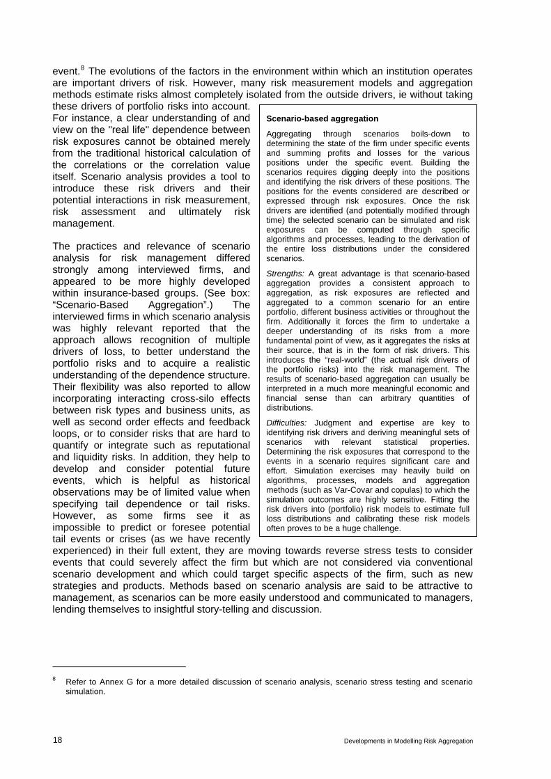
Scenario-based aggregation

Aggregating through scenarios boils-down to determining the state of the firm under specific events and summing profits and losses for the various positions under the specific event. Building the scenarios requires digging deeply into the positions and identifying the risk drivers of these positions. The positions for the events considered are described or expressed through risk exposures. Once the risk drivers are identified (and potentially modified through time) the selected scenario can be simulated and risk exposures can be computed through specific algorithms and processes, leading to the derivation of the entire loss distributions under the considered scenarios.

Strengths: A great advantage is that scenario-based aggregation provides a consistent approach to aggregation, as risk exposures are reflected and aggregated to a common scenario for an entire portfolio, different business activities or throughout the firm. Additionally it forces the firm to undertake a deeper understanding of its risks from a more fundamental point of view, as it aggregates the risks at their source, that is in the form of risk drivers. This introduces the “real-world” (the actual risk drivers of the portfolio risks) into the risk management. The results of scenario-based aggregation can usually be interpreted in a much more meaningful economic and financial sense than can arbitrary quantities of distributions.

Difficulties: Judgment and expertise are key to identifying risk drivers and deriving meaningful sets of scenarios with relevant statistical properties. Determining the risk exposures that correspond to the events in a scenario requires significant care and effort. Simulation exercises may heavily build on algorithms, processes, models and aggregation methods (such as Var-Covar and copulas) to which the simulation outcomes are highly sensitive. Fitting the risk drivers into (portfolio) risk models to estimate full loss distributions and calibrating these risk models often proves to be a huge challenge.

event.8 The evolutions of the factors in the environment within which an institution operates are important drivers of risk. However, many risk measurement models and aggregation methods estimate risks almost completely isolated from the outside drivers, ie without taking these drivers of portfolio risks into account. For instance, a clear understanding of and view on the "real life" dependence between risk exposures cannot be obtained merely from the traditional historical calculation of the correlations or the correlation value itself. Scenario analysis provides a tool to introduce these risk drivers and their potential interactions in risk measurement, risk assessment and ultimately risk management.

The practices and relevance of scenario analysis for risk management differed strongly among interviewed firms, and appeared to be more highly developed within insurance-based groups. (See box: “Scenario-Based Aggregation”.) The interviewed firms in which scenario analysis was highly relevant reported that the approach allows recognition of multiple drivers of loss, to better understand the portfolio risks and to acquire a realistic understanding of the dependence structure. Their flexibility was also reported to allow incorporating interacting cross-silo effects between risk types and business units, as well as second order effects and feedback loops, or to consider risks that are hard to quantify or integrate such as reputational and liquidity risks. In addition, they help to develop and consider potential future events, which is helpful as historical observations may be of limited value when specifying tail dependence or tail risks. However, as some firms see it as impossible to predict or foresee potential tail events or crises (as we have recently experienced) in their full extent, they are moving towards reverse stress tests to consider events that could severely affect the firm but which are not considered via conventional scenario development and which could target specific aspects of the firm, such as new strategies and products. Methods based on scenario analysis are said to be attractive to management, as scenarios can be more easily understood and communicated to managers, lending themselves to insightful story-telling and discussion.

8 Refer to Annex G for a more detailed discussion of scenario analysis, scenario stress testing and scenario

simulation.


A limited number of interviewed insurance firms perform a bottom-up aggregation of risk exposures by simulating a large number of scenarios (10,000 and more) that may be constructed from historical observations, forecasting models, and judgment. These scenario simulation approaches and their extent of development and application differed significantly across firms. A very limited number of insurance-based groups appeared to be moving toward aggregating the entire balance sheet of the group through common simulated scenarios.

Developing scenarios and understanding and having a view on the risk drivers, including

io-based aggregation may enforce active management based on the risk drivers and their evolutions, an approach that currently is rare

mbiguity, is an important part of an effective risk aggregation process. Appropriate judgment has been identified as crucial to steer firms

Finally, note that some of the trends discussed cannot be considered to be entirely "new". For instance, after the stock market crash of 1987, market participants started to talk about

risk ses.

gement of model risks in risk aggregation

n effects. Models are valuable tools, but models also may be incorrect or misleading. This “model risk” is prominent in the area of risk aggregation, and measures of

their potential evolution and interactions, will enhance the understanding of potential tail dependence and tail risks. It may enhance the active identification of potential interactions between exposures, as this remains quite limited among interviewed firms. In such a setting, an identification of dependencies can be more important than precise measurement, if concentrations are limited. In addition, scenar

among firms.

Scenario-based aggregation generally requires important judgmental input. However, for nearly all approaches, firms have suggested that a subjective overlay, or the use of judgment within the overall risk assessment to address a

through crisis episodes.

One perhaps surprising potential pitfall for firms when considering different aggregation approaches is popularity: techniques may develop some measure of authority mainly on the grounds of their widespread use and familiarity. For widely used approaches, many users may not sufficiently question their appropriateness for a given application, or may not thoroughly consider their limitations.

and consider the necessity of "non-Gaussian" distribution assumptions in their measurement, as the crash showed that market prices do not follow Gaussian procesHowever, the classical distribution assumptions (such as Gaussian, lognormal, or Pareto distributions) still seem to be the most commonly used distributional assumptions in many areas of risk management practice.

5. Validation and mana

Validation of risk aggregation methods can be a challenge as common outcomes-based methods, such as back-testing, are not likely to have sufficient observations from tail events to be a reliable tool. Still, validation is critical for assuring management that the model works as intended. This section outlines the importance of validation and addresses some approaches interviewed firms have taken. These include business use tests and setting model parameters conservatively, to reduce model risk and achieve comfort that methods are likely to perform as intended.

Most institutions acknowledge a wide margin of potential error in aggregation methods and measured diversificatio

diversification may be particularly affected by such risk. Ideally, model risk should be identified, assessed, and controlled by any user of models. Model users must have some means for achieving an adequate degree of comfort that models will work as intended and


generate results that are reliable. To develop a sufficient degree of comfort, institutions use a variety of tools to control the risk aggregation and estimation process. Foremost among these are validation, effective challenge by internal users of model results, and conservatism in calibration and use.

Control of model risk in the area of risk aggregation is particularly challenging because expert judgment plays such a major role in many approaches. Firms rely on expert judgment because modelling risk aggregation is a highly complex activity and data are scarce;

s precise than previously believed. Firms acknowledge that certain material risks are difficult to

methods of risk aggregation and aggregated risk measures, to highlight the potential range of results and to generate benchmarks. Some firms have emphasised the importance of not blindly accepting and applying model results.

ating fundamental changes in validation or other

g. However, many firms confirmed that the number of observations available is not sufficient to test extreme

benchmarks.

such precision may necessitate a different set of validation tools or a greater level of rigour.

complexity and the lack of data together create a strong and probably unavoidable need for the exercise of judgment by experts. For example, determining realistic or credible dependencies generally is a matter of informed judgment exercised outside of the models themselves. Effective control of model risk also is complicated by the focus on tail events rather than events that reflect more usual conditions. Since such events by definition are rarely experienced, conventional validation methods are least effective, and expert opinions are most difficult to assess.

The performance of risk aggregation methods during recent market turmoil highlighted a variety of potential shortcomings of those methods. Many firms now admit that model risk was higher than had previously been recognised or acknowledged, and models were les

capture, such as reputation and liquidity risks, and that certain material risks may have been masked by some of the methods used. Some emerging lessons are widely cited. For example, one common observation is the importance of regularly reassessing the dependencies that are the primary determinants of diversification effects. Another lesson cited is the importance of using multiple

However, in general firms are not contemplprocesses that they use to acquire comfort in model reliability. Firms generally indicate that they see the deficiencies that surfaced during the market turmoil as more closely related to the strength and completeness of model-risk control processes, rather than to the fundamental nature of those processes.

Validation methods for risk aggregation

Common validation approaches include back-testing and benchmarkin

outcomes, making back-testing a relatively weak validation tool. Firms also noted that benchmarking against results claimed by other firms may be of little value, because diversification benefits depend heavily on the nature of the underlying portfolio and portfolios differ from firm to firm in ways that may be important but not evident. External benchmarks can provide some sense of a range for what would be considered reasonable results, but these results may reflect assumptions that are not disclosed. Some firms indicated that outside consultants are one of the few sources for external

In some cases firms may be using validation tools that were developed when models served a different primary purpose; this may lead to less effective validation, as validation processes often are purpose-driven and designed to test the specific use of a model. For instance, a top-level capital estimate computed for capital allocation may not require great precision, since relative allocations are the primary focus, whereas for capital adequacy assessments a higher level of absolute precision is needed; ensuring


Some firms use scenario-based stress testing as a non-statistical supplement to other

to control model risk by ensuring that some competent party – one not

me that results in a

r

e many points at which conservatism can be incorporated, thus potentially leading to excessive conservatism, or to offsetting adjustments in different parts of the overall computation; in some cases, the direction of adjustment that leads to greater conservatism is not obvious or

t of conservatism, but if the underlying models are not reliable, it is difficult to assess how conservative any adjustments

validation tools. Stress tests may highlight features of models that are not addressed by other aspects of validation. Sensitivity analysis during model development is often used to identify variables or parameters to which results are particularly sensitive, and to alert management to potential market or environmental changes that could significantly affect estimates of diversification benefits or capital adequacy.

Business use as a control device

Firms also aim responsible for development of the methods under consideration – can provide “effective challenge” to the assumptions and decisions reflected in those methods, and to the outcomes of the methods or models. While some firms rely on internal and external audit functions for effective challenge, many firms claim that internal business use helps support effective challenge by creating an internal constituency with a strong interest in having models that reflect economic and business realities. Business managers affected by model outcomes should have an important stake in ensuring that risk aggregation models are not deeply flawed.

However, such “use” pressure may be asymmetric, since business managers are less likely to challenge an outcome that benefits the business, such as an outcolower allocation of capital than would be commensurate with the true level of risk. Perhaps understandably, firms reported that they hear from business managers when the results go against them, but not necessarily when the model results are in their favour. The challenge provided by business use also depends on the nature of that use; for example, unless the absolute level of risk and capital from aggregation methods plays some material role in business processes, use is unlikely to be a source of highly effective challenge to the method and results. In addition, business managers may not have the appropriate training oexpertise to judge whether models are working correctly or incorrectly.

Senior managers of firms recognise the potential conflicts of interest posed by a reliance on business use to challenge models, but it is unclear how in practice they adjust for or account for that asymmetry. The strongest evidence that users are in fact providing effective challenge would be evidence that users in practice have questioned aspects of models or other methods and that such questioning has led to process improvements; this type of tangible evidence seems to be relatively rare for risk aggregation processes at many firms.

Because model risk in risk aggregation may not be adequately controlled through the challenges provided by validation and business use, firms frequently opt to incorporate assumptions or adjustments they describe as conservative. Choices of parameters or other modelling assumptions are deemed conservative if they tend to overstate risks and understate the benefits of diversification. Conservatism in modelling can be a valuable way to mitigate model risk, but has limits to its effectiveness. In complex methods there ar

intuitive. Rigorous analysis is required to assess the impac

actually are. There is no common standard for the appropriate degree of conservatism in any given circumstances, leaving the adjustment as a matter of management judgment. Thus, a reliance on conservatism as the general solution to model risk may not be adequate.


6. Diversification effects in risk aggregation

The previous two sections discuss how difficult it can be for firms to correctly reflect tail events in aggregation methods and to validate risk aggregation methods. This section, tackles the diversification benefits which for many firms are an important by-product of their risk aggregation process. Firms increasingly urge financial regulators and supervisors to recognise these computed benefits in regulatory capital determinations. However, this

ditions. Other interviewed firms indicated that the level of risk reduction through diversification can be as high as 60 percent relative to regulatory calculations or to simple summations across the different

efits varied widely even

diversification stem from materially different sources. Systematic risk is determined by the

on risk drivers and the idiosyncratic factors).

section raises a large number of caveats related to the computed diversification benefits that are derived from traditional aggregation methods and raises questions that senior management and supervisors should ask about any estimated diversification benefit. In particular, questions should be directed at issues such as: are the diversification benefits backed by real economic rationale or mainly the result of modelling features and aggregation methods; how do the level of benefits change under varying business models; and will the benefits remain under severe events and stressful economic and financial market conditions.

The computed benefits typically reflect the calculation that the risk of unexpected losses at higher levels of aggregation may differ from a simple summation of standalone risks, given imperfect dependencies or relationships between exposures at any given point in time.9 Differences in firms’ methodologies seemed to drive some of the estimates, as the levels of diversification benefits computed differed markedly across the firms interviewed. Some firms reported that they do not even compute group-wide diversification benefits as they do not believe these benefits will be realised under more stressful con

risk types. Moreover, the magnitude of measured diversification benacross firms that were superficially similar, suggesting that differences in computed diversification may importantly stem from differences in conceptual approaches to diversification and measurement methodologies. Whether these computed diversification benefits actually can and will be realised depends on the real economic underpinnings and determinants of the potential diversification benefits across a firm.

Real economic determinants of potential diversification effects

The term "diversification" is often used quite generically; for instance, very often no distinction is made between diversification across idiosyncratic factors and common or systematic drivers of risk. However, making a distinction between the two types of diversification is actually necessary to understand the firm’s risks, as these two types of

common underlying drivers or sources of risk, and potentially can be reduced by diversifying exposures across those risk drivers; in contrast, idiosyncratic risk is the risk that remains – that is, not due to common underlying risk drivers – and can be reduced (to a certain extent) by increasing the number of names or counterparties in the firm’s portfolio. In this respect, diversification can be referred to as the potential risk reduction from spreading the firm’s exposures across different common risk drivers and idiosyncratic risk factors (assuming a different behaviour between the comm

The extent of risk diversification also depends on the prevailing market conditions, the state of the economy and other elements of the 'external' environment. The more two positions or

9 Opposite exposures to the same risk factor may also reduce risk, but are not encompassed in this description

of diversification benefits.


risk exposures differ in terms of their pattern of variation over time, the more likely their combination will generate diversification benefits. However, the pattern of variation often is not constant, but instead changes along with developments in the external environment, and

r augment or reduce the effect on risk that would otherwise be observed. Many firms either neglect or explicitly choose not to reflect the dynamic elements

ite firms’ attempts to mitigate some of the risks. Firms also often recognise risk reductions from diversification effects between risk activities or risk categories that are not managed through an integrated

effective realisation of these

ggregation of risk within financial institutions. However, when grouping risks into different categories, a crucial

ation techniques, recognising a larger number of risk factors within the portfolio risk measure results in greater "diversification

the impact of a risk driver on risk exposures may significantly vary thereby potentially reducing the levels of diversification.

Traditional portfolio theory and risk aggregation approaches commonly rely on the assumption that these patterns are constant over time. They typically also disregard crucial factors that have a significant influence on the actual realised portfolio risks. Many "qualitative" factors – such as knowledge of local habits, economies, markets, and products – also affect whether any "diversification" is realised.

The extent of any risk reduction attributable to diversification effects may also importantly be affected by management’s behaviour. Actions taken by the management of a firm as market conditions evolve, or actions taken by other market participants in reaction to changing conditions, may eithe

of their management actions in the risk aggregation process, even though these actions taken by firms in response to market developments and changes can materially influence the interactions between risks. This has important implications, since it is quite possible that some of the dependencies may be reinforced by firm actions, desp

approach, leading one to question whether there can bediversification effects.

Additionally, there may be structural or legal impediments to realisation of diversification benefits; examples of such impediments are restrictions on the transfer of capital and liquidity. In that case, even though the underlying economics might suggest potential for diversification, no diversification benefits could be realised in practice.

The impact of methodology on measured diversification

Computed diversification benefits are influenced by many factors of the aggregation process, which greatly complicates the understanding of (and discussion of) diversification benefits. For example, compartmentalising of risk exposures into different risk groups or risk types is a common approach to the management, measurement, and a

assumption made is that risks can be cleanly separated. In reality, risk exposures in these different buckets or compartments typically have some common underlying or potentially interacting risk drivers that evoke an interaction between risk exposures in different buckets. Therefore, conventional methods that compartmentalise risks into different buckets and aggregate through common distribution assumptions may lead to significant underestimation of risks or overestimation of diversification benefits. In addition, this compartmentalisation of risks may also hinder appropriate management of the risks, as the bucketing may lead management to ignore certain important risks or risk interactions.

The level of granularity within the risk aggregation approach is a crucial factor affecting the management and measurement of diversification benefits. With regard to risk measurement, the level of granularity of the aggregation method influences computed diversification benefits. Under traditional portfolio measurement and aggreg

benefits" computed. The same effect comes into play for traditional approaches that compartmentalise the risks according to the different risk types, business units, product


types, legal entities or geography. Typically, the more the aggregation approach differentiates portfolios or activities according to these categories, the greater the diversification benefit. A greater focus by the financial institution on risk management at the level of compartmentalised entities or sub-portfolios may lead to a stronger emphasis on diversification within the financial institution but might also hinder the recognition (and hence management) of concentrated exposures at the group level.

Methodological choices within the entire aggregation process are rife with decisions based at least somewhat, and often to a large extent, on the judgment of experts. For instance, expert judgment often is used to compensate for the now widely recognised non-linear

y be used to ation benefits

gregation results

A survey of supervisory authorities from a number of jurisdictions indicated that most banking

As part of ongoing supervisory activities, supervisors generally review and assess aggregation methods used by firms to evaluate capital adequacy and as part of the firms’

s process typically includes a e Internal Capital Adequacy

dependencies that are not captured by linear approaches. Expert judgment maincorporate or reflect real economic determinants of portfolio risks or diversificin risk aggregation methods. Clearly any such expert-based changes (to correlation values, other dependency measures, or the entire aggregation approach) may materially affect the computed diversification benefits and make the estimated diversification benefits sensitive to the methodological choices as opposed to the economics of the underlying activities.

7. Supervisory reliance on firms’ risk ag

Given the fact that some firms have sought recognition of diversification benefits in the determination of regulatory capital requirements and the relatively poor performance of risk aggregation methods in the crisis that started in 2007, financial supervisors in many countries have been considering the extent to which they should rely on the results of firms’ risk aggregation. This section summarises supervisors’ stated views on the level of confidence that they have in, and the extent of their reliance upon, firms’ risk aggregation results, their views on prospects for future efforts in risk aggregation, and the general adequacy of risk aggregation methods during the crisis.

and insurance supervisors do not rely significantly on inter-risk aggregation methods used by firms at this time.10 However, there are exceptions, as at least one supervisor noted that a few banks calculated inter-risk diversification benefits, reflecting the banks’ abilities in this particular area of modelling. One respondent offered very conditional acceptance, if the modelling was thoroughly validated and found to be acceptable for regulatory purposes. Many countries did allow for intra-risk aggregation in assessments of risk and capital, as supervisors felt such modelling was much more advanced and useful in determining an organisation’s risk profile.

overall risk control frameworks. For banking supervisors, thireview of firms’ internal risk aggregation methods under thAssessment Process (ICAAP) required for Pillar 2 of the Basel II framework. However, most of these modelling efforts remain “work in progress,” and best practices have yet to be established. Supervisors continue to meet with firms to discuss methodologies and assumptions, as well as to talk with firms about implementation and determine the degree of reliance on risk aggregation methods by the firm’s management.

10 As noted in Section 3, the distinction between inter- and intra-risk aggregation is to some extent arbitrary, and

no single, clear, internationally agreed set of definitions of risk categories currently exists.


Supervisory confidence in firms’ risk aggregation results

The primary reason given by bank supervisors for their lack of acceptance was that modelling in risk aggregation was not yet sufficiently well developed as to be proven reliable. As one supervisor put it “[t]he area of inter-risk diversification is the least well understood” within risk aggregation techniques such as economic capital modelling. Many added that there was not yet a well accepted standard in this area of risk quantification. Others noted that institutions either needed to do more work in this area, or were not yet sophisticated

is still underway in preparation for Solvency II, and thus supervisors see it as premature to be taking into account the methods used by firms to aggregate risks. However, one European supervisory

k aggregation.

focused on evaluation of risk aggregation modelling as part of Pillar 2 or as part of other supervisory activities related to evaluation of risk management. One respondent indicated that this evaluation had been built into the supervisory process, with a combination

ey would consider this area as

enough to model diversification benefits using more promising approaches, such as copulas.

Data was cited as a general problem. Some respondents felt there was insufficient data to calibrate and back-test such models. Others noted a tendency for historical data to underestimate periods of market stress unless it was adjusted in some manner, which is generally viewed as a difficult and subjective exercise.

Some banking supervisors noted that risk aggregation modelling was primarily developed for managing a bank under “normal” conditions, or periods of little or no financial stress. Because of this, models may not necessarily be reliable for purposes of capital adequacy assessment, which typically must consider extreme tail events. In addition, some banks have credit risk as the dominant risk, with other risks in a considerably more secondary role; as a result, potential diversification benefits (other than within credit risk) would likely be small.

Insurance supervisors indicated greater acceptance of firms’ modelling diversification benefit to some degree. But this acceptance was conditional, as most felt this area was still in development and required considerably more effort to develop and validate. For insurance firms in most European countries, development of risk aggregation practices

authority has encouraged insurance firms to calculate diversification benefits, as they believe this exercise is an important part of understanding and disclosing actual risk levels. One response indicated that insurance regulators are moving from a balance sheet approach to a risk-based framework, although this is in very early stages of development.

Supervisory views with respect to future efforts in risk aggregation

In terms of future efforts to achieve greater comfort with aggregation methods, supervisors again differ. Supervisors in some countries are only in the early stages of understanding how such modelling can be applied, discerning methods that appear more promising, and determining if institutions would benefit from enhanced focus on modelling risAt this time, these supervisors do not rely on risk aggregation approaches, and have no specific timeline for relying on such methods. One noted that neither they nor the major firms they supervise rely on such methods; both parties are only in very early stages of discussing this general area of risk quantification. Risk aggregation models could be accepted for use at some time in the future, but supervisors may ultimately reach a decision that such approaches are not sufficiently reliable or worth the significant effort required.

Other supervisors were more receptive to the use of risk aggregation approaches, often as part of ICAAP, but still believe this area requires further study. To obtain comfort, these supervisors

of off-site and on-site activities. Several supervisors noted thpart of their evaluation of validation processes. Supervisors also noted they would closely evaluate the levels of diversification claimed, applying some reasonableness test to the exercise.


Adequacy of risk aggregation methods during the crisis

The general view of supervisors was that firms’ aggregation methods were inadequate during the crisis and showed several areas of weakness. One supervisor observed that models may function well for specific purposes and for specific market conditions, but might fail to estimate the capital required to survive the losses under stress events. A notable weakness was reliance on assumptions that markets would be liquid; another area of weakness was inaccurate assumptions about risk transfer. One response noted the need to include exposures not captured by traditional measures, such as off-balance sheet exposures, exposures due to explicit or implicit support, linkages between direct and indirect sources of risk due to concerns about reputation, and the potential for risks to interact during times of stress. The recent turmoil emphasised to supervisors that correlations and risk interactions may change very rapidly under stress, more rapidly than risk management processes can be

uring the crisis, many existing platforms were challenged to aggregate risk

practices” needed to be established, which likely will require considerable effort. Accordingly, many expressed a desire to encourage further dialogue and development in this area. Several supervisors noted that better risk aggregation could foster

respondent noted that in general, stress tests did not seem to be sufficiently forward-looking or adequately firm-wide. To the extent that firms did not utilise stress tests as part of their decision making processes,

adjusted to incorporate such changes. Stress tests could not anticipate the evolution of interactions and the relationships between risks and second order effects, unless very severe scenarios were considered.

Supervisors noted several concerns regarding data and its application. In general, most supervisors concluded that the crisis surfaced notable data deficiencies, whether due to lack of historical data or lack of applicable data. One supervisor emphasised the need to mitigate potential modelling failures or data deficiencies by using stress testing processes of banks. One respondent noted that risk aggregation frameworks place high demands on information systems; dexposures with greater granularity and in various combinations. IT systems were not sufficiently dynamic or flexible, and information requests by supervisors resulted in ad hoc solutions.

Drawing from these experiences, supervisors generally did not foresee dramatic changes in their reliance on firms’ internal aggregation methods. The general view was that substantial improvements and refinements in methods would be needed before supervisors would be comfortable placing significantly greater reliance on risk aggregation results. Many supervisors suggested that “best

better overall risk management.

Stress testing as an alternative

Drawing from the experience from the crisis, many responses indicated that supervisors have enhanced or emphasised stress testing. However, supervisors are aware of the limitations of stress tests and noted a range of concerns. One

there was a concern with lack of involvement by top management.

8. Potential improvements to risk aggregation

Although financial institutions generally report that they are not fundamentally reassessing or reviewing their risk aggregation frameworks, the financial events of 2007–2009, as well as the many issues raised in this report, indicate a strong need for significant investment of effort and resources by financial institutions, and probably also financial supervisors, to make risk aggregation frameworks more appropriate for effective group- and enterprise-wide management. These investments will differ across firms, and should be commensurate with


the complexity of the financial firm and its operations, as complexity poses material challenges in creating a risk aggregation framework that enables effective management. The primary points of emphasis in this report should provide a valuable guide when making such

ncies in conventionally computed diversification benefits. Efforts to improve practices in general should also focus on the governance of the aggregation framework, and on enhanced use of scenario analysis and

approaches.

ents of currently used risk aggregation methods will be required to make them suitable for risk identification and monitoring. These investments will

Key conditions for an aggregation process or method to serve the purpose of risk

trends or levels in

investments; this section summarises several potential improvements that would make risk aggregation methods more effective.

A primary emphasis of such efforts should be a reassessment of risk aggregation processes and methods according to their purpose or function. The function of risk identification, monitoring and analysis should receive particular emphasis, given the generally observed neglect of this function within risk aggregation and the fact that it is a primary prerequisite for risk management. Second, solvency assessment and determination should also receive particular care, given the significance of an adequate solvency assessment for the firm and the material interest of supervisory authorities. The risk aggregation processes and methods supporting both of these functions may require fundamental review, and potentially profound changes if they are to be adequately addressed (for instance, in respect to the general conditions provided below).11 Making a clear distinction between these two functions helps to clarify some of the main conditions to fulfil these functions. Advances in capital adequacy assessment should also address the particular deficie

scenario stress testing as risk aggregation

Risk identification and risk monitoring

A fundamental requirement for effective risk management is to be able to identify the risks to which the firm is exposed so that the firm can, at least, monitor the risks more closely. But in general firms do not have aggregation processes or methods in place that have been developed for the purpose or function of risk identification and monitoring. Firms generally also do not tend to emphasise this use of processes or methods. Additional investments in terms of reorientation or refinem

require phased and continuous improvement, requiring firms to understand and recognise the limitations of their methods.

identification and monitoring is for it to have a high level of sensitivity, granularity, flexibility, and clarity with regard to changes in portfolio risks:

• Sensitivity: Aggregation methods that are suited for risk identification are typically designed to quickly surface changes or deviations from(aggregated) risk exposure. As a result, these methods are oriented more toward relative changes in (aggregated) risk measures (for example, relative to certain risk levels or self-imposed limits) rather than point-in-time levels.

• Granularity: These methods also require the ability to drill down to the lowest risk levels of business lines and exposures, to identify the risk positions that cause changes and to search for and analyse the underlying drivers of risk.

11 Other identified functions are also material for effective management of risk aggregation and also require

further study and discussion. For instance, an issue raised regarding consistent risk pricing is at what point in the tail should the risk be priced: extremes, or somewhat more normal conditions?


• Flexibility: Methods must be flexible enough to capture and adapt to changes in portfolio characteristics as well as to changes in the external environment. Additionally flexibility is required to enable aggregation of risk exposures to non-standard types of risk or ad-hoc categorisations of risk.

• Clarity: Clarity is achieved when sources of risk and their effects on the firm are readily evident and understood. This is in contrast to techniques that focus on aggregating all risks into a single figure or measure, as aggregating risks through certain methods may actually mask or obscure important sources of risk. A single risk measure or figure may also provide an excessively narrow view of different

ing of potential interactions between risk exposures, which requires a view of and understanding of the common underlying risk drivers or sources of risk, to identify potential interactions between risk exposures. This contrasts with the

, which does require more precision in the

der relatively severe

assessment therefore need to

have the required features to analyse tail events and the impact on portfolio risks. These

dimensions or the full extent of a certain risk or exposure.12 Clarity therefore may also require different risk measures of a single risk position or portfolio to obtain a clearer view of different risk dimensions or a more complete view of the loss distribution under different economic and financial market conditions.

It is clear that in this setting a precise measurement of dependencies is less important than the identification and understand

emphasis required for solvency purposesmeasurement of dependencies.

Solvency assessment and determination

For assessment of a firm's solvency, the risk aggregation process must determine if the absolute level of capital is sufficient to keep the firm operating unconditions. In addition, capital adequacy assessment requires the risk aggregation method to provide precision in the absolute level of risk or capital. Hence, an effective risk aggregation process for capital adequacy assessment imposes two conditions: an assessment of absolute risk (or capital) figures, and consideration of extreme events.

Risk aggregation methods used for the purpose of solvency correctly reflect tail events. Tail accuracy requires as a condition that these methods attribute correct probabilities to potential severe 'real-life' events. The consequences of inaccuracy can be significant, given the potential to severely underestimate the required capital. These required conditions, though, are difficult to satisfy in practice.

Identification of potential severe real-life events for portfolio risks requires a fundamental understanding of the characteristics and underlying drivers of portfolio risks and knowledge of the relevant developments in the business and external environment. Moreover, since both firms and the environment in which they operate change over time (that is, they are non-stationary), the nature of these harmful severe events change through time. Precise determination of the probabilities of severe events occuring, given their prospective and low-frequency nature is nearly impossible. However, as a first step firms should recognise the limitations of these practices when assessing required solvency levels on the basis of these methods. In addition, firms should improve on most aggregation practices now in use for solvency assessment, which were not developed for these purposes and generally do not

12 For instance, point measures of tail quantiles (such as the traditional VaR measure) may miss important

information on the tail shape of the distribution, and therefore may lead to an incorrect appraisal of and aggregation of portfolio risks. Assessment and consideration of multiple tail quantiles may help address this shortcoming.


improvements are likely to take time, and at each stage as improvements are made a firm should acknowledge the limitations of the current method in use. Robust practices and a thorough understanding of potential limitations will help the firm to internally develop its own

s and measure the influence of potential real-life extreme events on portfolio risks. In this kind of approach, the

calculations, for instance, through the use of copula techniques. However, although these

during real-life severe events the probability of a certain risk materialising is observed to increase when another risk has

alues; instead, correlations should depend on the underlying risk positions and portfolios and the potential interaction between these positions. Applying uniform stressed correlations across the firms can also hinder attempts to measure

recognition of diversification benefits. In this respect, given the extreme challenges to solvency assessment

solvency assessment, which may be distinct from those of other stakeholders (eg rating agencies or other financial market participants).

In terms of analysis, firms should identify potential severe events for their risk portfolio and assess the adequacy of capital in relation to these severe events. A limited number of interviewed firms appeared to perform exercises to identify, asses

probabilities of these tail events are of less importance; instead, the discussion centres on the events that the firm wants to or should survive and protect against.

In addition, more appropriate methods could be used that better capture and reflect severe events. For instance, a limited number of interviewed firms employed simulation techniques that give more prominence to particular tail events or introduced certain severe events in the simulations. Some interviewed firms also try to better reflect tail dependence in their risk

techniques could be more appropriate, in general they are in early stages of development, testing and application and their overall reliability is yet to be determined in practice.

To assess solvency under severe events, an appropriate dependence structure is crucial to correctly reflect the potential interactions between risk exposures for these tail events. However, the commonly used correlation coefficients are not adequate for this task. First, these coefficients do not by themselves provide an understanding or indication of the potential real dependence between risk exposures. Second, aggregating through correlations is also a poor method for capturing tail dependence;

materialised. Partly as a result, some firms have abandoned or no longer rely on aggregation techniques based on correlations for solvency purposes.

In practice correlations are often compared or benchmarked between and within portfolios, risk types or firms. However, comparing or benchmarking correlations requires extreme caution, as the appropriate correlation depends on the nature of the exposures being considered. A correlation that might represent a high dependence between certain risk positions in one portfolio or firm might reflect much less dependence when applied to risk positions in another portfolio or firm. Hence, firms and supervisors should be reluctant to apply certain "common" correlation v

risks when distributions are fat-tailed.

Diversification benefits within capital adequacy assessments

Quantification of diversification effects has emerged as an important element in risk aggregation for solvency purposes, and diversification benefits are a natural outcome or by-product of the risk quantification. Just as solvency assessment and determination should be performed against potential tail events, so should risk quantification and

(such as the necessity of precision in absolute risk measurement and tail accuracy), group-wide diversification benefits should be treated with great scepticism and care.

Many characteristics of traditional aggregation methods that significantly affect the measured diversification benefits do not fully reflect real economic determinants of diversification


effects. Examples include the compartmentalisation of risks, which is based on the assumption of a clear separation between risk buckets, and the level of granularity of the risk aggregation approach, with more granularity generally leading to greater computed diversification benefits. The computed diversification benefits from traditional aggregation methods may thus strongly differ from the real economic diversification within the firm's portfolios. Typically, these real economic determinants of diversification effects are neglected when firms are claiming or seeking recognition of diversification benefits. Firms should explore true dependencies and diversification under severe conditions by ensuring that the impact of these real economic determinants (composition and developments of the underlying portfolios, market conditions, external environment) under severe events are reflected in their risk quantification and analyses to a much greater extent than is currently the case. Additionally, diversification benefits derived from risk quantification should not be taken as certain. Whether any computed diversification benefits will be effectively realised depends to a significant extent on qualitative factors (such as local knowledge of products and markets) and behavioural factors (such as management actions under severe events). Moreover, structural and legal impediments (such as restrictions on the transfer of capital) also often limit the realisation of diversification benefits, and should be taken into account

oduce a more forward-looking risk management approach. Rigorous scenario analysis can provide a tool to enhance the understanding of portfolio risks

is try to capture potential real-life tail events in their risk calculations. Scenario stress testing can provide a

aches through which they try to identify scenarios that could lead to specific extreme loss outcomes, and which may not be

os requires the translation of the different risk positions into exposures to these scenarios. Therefore, aggregating risks through common underlying scenarios can be a

when assessing diversification benefits.

Scenario analysis, scenario stress testing and scenario simulation as risk aggregation tools

A limited number of interviewed firms employed the technique of scenario analysis to underpin the risk identification and monitoring function with a more fundamental risk analysis. More specifically, a few firms noted that scenario analysis helps them consider more carefully the real sources or drivers of risk and their potential evolution, and identify and develop an understanding of the dependence or the potential interaction between risk exposures. Rigorous scenario analysis requires the identification of risk drivers and the analysis of their behaviour, trends, changes and potential interactions. It also provides a tool to introduce the “real world" into risk aggregation and risk identification. In doing so, scenario analysis forces recognition of the constant changes in the portfolio and the external environment, and helps to intr

and it can challenge the mathematical constructs and outcomes of the more statistically oriented aggregation methods.

Scenario analysis is an important input for the scenario stress testing and/or scenario simulation that some firms employ to assess or determine the adequate level of capital. In this respect, scenario stress tests or simulations are employed to consider potential future events that are not adequately represented in historical data. Firms that do th

better view of the sensitivity of the firm to particular tail events, and can enhance the recognition of tail events within risk quantification and solvency assessment.

A few firms are also exploring "reverse" stress testing appro

recognised through traditional scenario development processes. Reverse stress testing may help in covering "blind spots" in the event space of the firm.

Some firms that aggregate different risk exposures on common underlying scenarios were somewhat less silo-based in their risk aggregation and management approach, and seemed to develop a stronger firm-wide view of risks. Additionally, working through common scenari


useful additional technique to enhance the understanding and management of the cross-firm risks.

Scenario analysis and scenario stress testing though should not be viewed as the ultimate panaceas, since these techniques have their deficiencies (eg typically they rely on a large range of assumptions, translating scenarios into relevant risk parameters proves to be difficult, and heavy reliance is placed on judgment and qualitative insights of management). However, these techniques should be regarded as valuable additional techniques for effective risk aggregation and management. Scenario analysis and scenario stress testing are essential tools to challenge the more traditional, statistically based aggregation methods and help identify the shortcomings of these methods. The framework for scenario analysis and stress testing has to be well established within the management of the firm, its function of challenging the mathematical constructs and outcomes of the statistically oriented aggregation methods have to be well defined, and a clear consistent link between both

e specifically, they should enhance the control of, and the transparency of, these judgments and their potential impact

t tool to validate and raise the confidence in the aggregation methods, as conventional validation techniques such as back-testing and

equire use beyond the purposes for which internal aggregation methods were initially developed, and similarly firms should not interpret

approaches should be set up.

Governance of the aggregation framework

Expert judgment plays a crucial role within the entire risk aggregation process, to determine appropriate modelling assumptions and calibration techniques, to determine relevant scenarios, to interpret calculation outcomes, and to make a large number of other decisions that fundamentally affect the process. Expert decisions materially affect risk quantification outcomes and diversification benefits. However, these judgments and their impact on the risk outcomes typically are not transparent within the overall aggregation process. Therefore, firms should improve the governance of expert judgment; mor

on risk outcomes. This can help clarify the assumptions underlying the aggregation methods and their limitations for end-users of the risk aggregation results.

Such transparency of the assumptions and decisions reflected in aggregation methods is crucial for ensuring effective challenge of the methods and their outcomes. Such challenge by business end-users proves to be an importan

benchmarking are difficult to execute as a result of the paucity of data for tail events and the difficulty of identifying appropriate benchmarks.

In recognition of the fact that effective use of aggregation methods within the business can provide an important challenge to the models and processes, supervisors often impose a use test requirement when assessing internal aggregation methods. However, while use tests are valuable, supervisors should be careful not to r

the common supervisory use test requirement as a requirement to apply aggregation methods beyond their initial purpose.

At some firms, significant emphasis is placed on conservatism in modelling and in the use of models; such conservatism can be a valuable way to mitigate model risk, but its effectiveness in risk aggregation is limited due to the complexity of many of the models used and the difficulty of determining the ultimate impact of many conservative assumptions. Moreover, although conservatism in the calibration and use of models may to some extent address certain limitations in modelling, conservatism should not render firms complacent, as it is an imperfect substitute for good risk assessment and modelling. For instance, some firms rely on conservatism in the calibration of certain risk parameters to address the failure of their methods to adequately capture tail risks. Such additional conservatism should not deter the firm from an enhanced focus on assessing tail risks. In addition, firms should not



owever, extensive reliance on methods in particular areas for which they have clear

limitations, or on methods that are corrected by addition of an inappropriate 'layer' of conservatism, is not prudent and may well lead to significant risk management deficiencies.

equate conservatism with prudence. Applying certain conservative assumptions to address model limitations may well increase measured risk and lead to higher capital calculations;h

Annex A

Risk aggregation in the Basel II Capital Framework

Overview

This annex discusses the risk aggregation methods required under the Basel II capital framework, and how risks are aggregated under the first and second Pillars.13 Under the first Pillar, firms do not recognise any diversification benefits between the three risk types (credit, market, and operational) when computing the capital requirement; however, firms may recognise certain diversification benefits within each risk type. For market risk, under the internal models approach supervisors can explicitly allow banks to recognise empirical correlations within and across each of the broad market risk categories. For operational risk, the Advanced Measurement Approach allows banks considerable flexibility in the methodology used to quantify operational risk exposure with the potential to recognise diversification benefits in the aggregation of operational risk. The Advanced Internal Ratings-Based Approach for credit risk implicitly incorporates an element of diversification. These areas, as well as the flexibility provided under Pillar 2 for banks’ Internal Capital Adequacy Assessment Processes, are discussed in more detail below.

Risk aggregation within Pillar 1 (Minimum Capital Requirements)

The first Pillar determines the calculation of the bank’s overall minimum capital requirement, on a worldwide consolidated basis, as the sum of the credit risk capital requirement,14 the capital charge for operational risk, and the capital charge for market risk. In terms of aggregation across risk types, under Pillar 1 the different risk types are summed and no (additional) diversification benefits between the three risk types are recognised. The following text thus focuses on the description of the regulatory requirements and other relevant issues regarding risk aggregation within each of the individual risk types.

Aggregation of credit risk within Pillar 1

Both the Standardised Approach (SA) and the Internal Ratings-Based Approach (IRBA) calculate minimum regulatory capital for credit risk by determining capital for credit exposures classified into product and risk categories. Under the SA, exposures are classified into 13 standardised asset classes. The risk weight applied to certain classes of exposures, such as sovereign and corporate exposures, depends on credit ratings assigned by external credit assessment institutions recognised as eligible for these purposes by national supervisors. Off-balance sheet exposures are transformed into credit exposure equivalents through the use of credit conversion factors, set for various classes of assets depending on the level of risk they pose.

13 Basel II: International Convergence of Capital Measurement and Capital Standards: A Revised Framework -

Comprehensive Version, June 2006: http://www.bis.org/publ/bcbs128.htm. The Basel Committee is currently in the process of amending the existing framework in several areas, which is not reflected in this paper.

14 Excluding debt and equity securities in the trading book and all positions in commodities, but including counterparty credit risk on all over-the-counter derivatives whether in the trading or the banking books.


http://www.bis.org/publ/bcbs128.htm

Under the IRBA, banking book exposures are categorised into broad product classes such as wholesale, retail, securitisation and equity. The wholesale and retail classes are further partitioned into obligor rating grades or risk segments, based on internal risk ratings which reflect borrower credit quality and loan or facility type. The bank is required to assign to each such risk rating or segment its own estimates of key risk parameters: PD, LGD, EAD, and Maturity (where applicable).15 The bank then calculates required capital for each exposure by entering the assigned risk parameters into the appropriate IRBA capital formula. These are summed to arrive at aggregate capital for credit risk.

In terms of aggregation of risk, both the SA and the IRBA presume that capital charges are portfolio-invariant, meaning that capital charges on a given exposure depend only on its own characteristics and not on the characteristics of the portfolio in which it is held.16 The theoretical foundation for portfolio invariance is the Asymptotic Single Risk Factor (ASRF) Model, which involves two fundamental assumptions. First, idiosyncratic risk is effectively diversified away, as would be the case in a large, granular portfolio where no single exposure (or group of exposures subject to the same specific sources of risk, such as loans to the same borrower) has more than a negligible share of the total. Second, there is one and only one “state variable” or measure of macroeconomic conditions that is relevant to all exposure classes. The degree to which an individual exposure’s probability of default depends on this risk factor is captured by a correlation parameter (“asset value correlation” or AVC) of the IRBA risk weight function.17

The ASRF model and IRBA recognise the diversification benefits accruing to a large, national or international banking organisation through the assumed averaging out of idiosyncratic risk, and by assuming imperfect correlation of credit losses with the aggregate risk factor.18 At the same time, the specification of a single systematic risk factor recognises that the “average” portfolio will exhibit some degree of concentration to particular sectors of the economy. This assumption requires only that the portfolio be reflective of the overall economy, and as such have a similarly diversified (or concentrated) mix of industry and geography, so that the sole source of systematic risk is the overall state of the economy.19 Thus, the assumptions of the model are a reasonable approximation to the portfolio characteristics of a large, diversified financial institution, and the model provides a useful representation for such institutions.

While this approach allows relative simplicity of use, it leaves certain aggregate portfolio risk characteristics unmeasured and so in some cases may not adequately represent an individual institution’s risk profile. In particular, it does not account for potential exposure concentrations that may cause the portfolio loss rate to depend on individual loans or groups of loans in addition to the macroeconomic risk factor common to all exposures. Such concentrations might reflect a portfolio containing large, single-name exposures, in which idiosyncratic risks are not entirely diversified away, or they may arise because the portfolio is

15 Both the foundation and the advanced IRBA rely on banks' PD estimates; however banks' internal estimates

of LGD, EAD, and Maturity can only be applied under the advanced IRBA. 16 A Risk-Factor Model Foundation for Ratings-Based Bank Capital Rules”, Michael B Gordy, 22 October, 2002,

p 2. 17 The AVC is specified in the Basel II rule and depends on the asset class and PD of the exposure. It is not

estimated by the firm. 18 Calibrated AVCs range from 12 to 24 percent for wholesale exposures and 15 percent or lower for retail

exposures. 19 In practice, the IRBA potentially ignores benefits arising from diversification across asset categories (eg

wholesale and retail), because the empirical calibration of AVCs was implemented sector by sector, rather than with reference to a single, consistent macroeconomic variable.


less diversified across sectors or geographies then the overall economy. Such concentrations increase portfolio credit risk by generating additional correlation among defaults and losses or by increasing the contribution of individual exposures.20

Aggregation of Market Risk within Pillar 1

The Basel II Capital Framework defines market risk as the risk of losses in both on- and off-balance sheet positions arising from movements in market prices. Typically, two distinct components of market risk are recognised: general market risk (changes in market prices resulting from general market behaviour) and specific risk (changes in market prices that are specific to an instrument and independent of general market movements). For a particular instrument, the market risk drivers that influence the market prices of that instrument must be identified. There are four generally recognised market risk drivers subject to the minimum capital requirement: the risks pertaining to interest rate related instruments, equities risk in the trading book, foreign exchange risk and commodities risk throughout the bank.21 In measuring market risk, the Basel II Capital Framework provides banks with a choice between two methodologies: the standardised measurement method (SMM) and the internal models approach (IMA). The total capital charge for market risk is determined as either (i) the capital charge for market risk under the SMM, or (ii) the measure of market risk derived within the IMA, or (iii) a mixture of (i) and (ii) summed arithmetically.22

Under the SMM, the minimum capital requirement for market risk is defined as the sum of the capital charges calculated for each individual risk type, summed arithmetically.23

• the capital requirement for interest rate and equity risk is the sum of two separately calculated capital charges: one for general market risk in the portfolio and another for specific risk of each instrument;

• the capital charge for general foreign exchange risk throughout the bank;

• the capital charge for general commodities risk throughout the bank; and

• the capital charge for price risk in options.

In contrast, the IMA allows banks to use risk measures derived from their own internal risk management models, subject to a set of stringent qualitative conditions and quantitative standards. As regards the former, this includes general criteria concerning the adequacy of the risk management system and guidelines for specifying an appropriate set of market risk factors. With respect to the quantitative standards, the Basel II Capital Framework24 requires

20 For a more comprehensive discussion of concentration risk in relation to the ASRF model, see Studies on

credit risk concentration, Basel Committee on Banking Supervision Working Paper No 15, November 2006. 21 The latter two are not subject to the specific risk as changes in foreign exchange rates and commodities prices

are dependent on general market movements. 22 In cases when banks are allowed to use both internal models and the standardised methodology. 23 In this process, the Basel II Capital Framework defines a variety of specific approaches for calculating the

capital charge for each risk driver (set out in paragraphs 709 to 718(lxix)). These specific approaches thus pose an additional layer of complexity in aggregating the individual capital charges (risks), reflecting the granularity and distinct features of the respective underlying positions (eg short vs. long etc).

24 This overview focuses on the currently implemented regulatory treatment set out in the Basel II framework. It should be noted that in July 2009 the Basel Committee adopted important revisions to the trading book rules. These new rules, to be implemented no later than the end of 2010, introduce higher capital requirements to capture the credit risk of complex trading activities. They also include a new stressed value-at-risk (Stress VaR) requirement, intended to help dampen the cyclicality of the minimum regulatory capital framework. More details: http://www.bis.org/publ/bcbs158.htm.


that banks compute Value-at-Risk on a daily basis, subject to a 99th one-tailed confidence interval, considering an instantaneous price shock equivalent to a 10 working day movement in prices. In this regard, banks are required to meet a market risk capital requirement on a daily basis that is the higher of (i) the previous day’s VAR and (ii) the average of the daily VAR of the preceding 60 business days, multiplied by the multiplication factor. Under the IMA, no particular type of model is prescribed. As long as the model used captures all the material risks by the bank, banks are free to use any type of model. Examples of models include those based on variance-covariance matrices and historical or Monte Carlo simulations.

In terms of risk aggregation within and across the individual market risk drivers and possible resulting diversification benefits, banks with supervisory permission to use the IMA are explicitly allowed to recognise empirical correlations within the broad market risk categories.25 In addition, the supervisory authority may also recognise empirical correlations across broad risk factor categories, provided that the supervisory authority is satisfied that the bank’s system for measuring correlations is sound and implemented with integrity. This is in sharp contrast to the SMM, where diversification benefits are recognised to a significantly lesser extent.

In the IMA context, all methods and models that allow recognising diversification benefits embed a certain dependence structure. The robustness of the assessment of risk and in particular of the resulting diversification effects critically depend on the "correctness” of that dependence structure. For example, the recognition of diversification benefits while applying certain types of models under the VarCovar or simulation approaches based on fixed correlation matrices inherently assumes a certain degree of stability in dependencies between risk factors that -considering that events fall within the 99th percentile confidence interval- ultimately allow reducing the overall level of risk. However, in case of events that fall in the tail of the distribution (particularly if the distribution is not normal), the dependencies between risk factors may feature radically different characteristics. This might materialise for instance in undesirable simultaneous increases in correlations between risk factors that instead of expected diversification benefits might ultimately result in a considerably higher amount of loss and higher probability than predicted under the respective VaR or simulation approach. For these reasons, it can be concluded that certain types of models used under the VaR or simulation approaches based on fixed correlation matrices have a tendency to underestimate the level of overall risk.

Aggregation of Operational Risk within Pillar 1

To calculate risk based capital for operational risk under The Standardised Approach (TSA), the first step banks must take is to divide their activities into eight business lines, and calculate gross income for each of the eight categories, which is used as a broad exposure indicator. For each business line, gross income is then multiplied by a fixed percentage (“Beta”) determined by Basel Committee for each of these business lines. In general, the total capital charge is the three year average of the simple summation of the capital charges for each business line. In terms of risk aggregation, this summation approach effectively makes the assumption of perfect correlation between each of these business lines.

To calculate risk based capital for operational risk under the Advanced Measurement Approach (AMA), a bank must have an internal operational risk measurement system that uses the following four elements; use of internal loss data, relevant external data, scenario

25 Per paragraph 718 (lxxvi) of the Basel II Capital Framework.


analysis, and factors relating to the bank’s business environment and internal control systems. Pillar I allows considerable flexibility in the methodology a bank uses to quantify its operational risk exposure. However, the bank must demonstrate it has optimally weighted these four elements, so as to most effectively quantify its exposure to operational risk. Specifically, the bank must demonstrate that its operational risk measurement approach meet standards similar to IRBA for credit risk (ie one year holding period and a 99.9th percentile confidence interval). The approach must be comprehensive, “sufficiently granular”, and it must capture potentially severe loss events. Risk mitigants, such as insurance, may be recognised (subject to various criteria), allowing a reduction of up to 20% of the bank’s risk-based capital requirement for operational risk.

The AMA does not prescribe a level of granularity for a bank’s operational risk exposure estimates. However, the bank’s measurement system must be sufficiently “granular” to capture the major drivers of operational risk affecting the shape of the tail of loss estimates. For a bank calculating multiple operational risk exposure estimates, the AMA requires the bank to sum the estimates. However, the bank may be allowed to use internally determined correlations in operational risk losses across individual operational risk estimates, provided the bank can demonstrate correlations are reasonably sound, even in periods of stress.

Risk Aggregation within Pillar 2 (Supervisory Review Process)

One of the main areas reserved for treatment under Pillar 2 is “risks considered under Pillar 1 that are not fully captured by the Pillar 1 process”, as well as “…those factors not taken into account by the Pillar 1 process.” (Basel II Capital Framework, paragraph 724). While credit concentrations, interest rate risk in the banking book, business and strategic risks are the only areas where additional considerations are explicitly required, the above language could allow or encourage consideration of many other risks. Principle 1 of Pillar 2 (the Supervisory Review Process) requires banks to “have a process for assessing their overall capital adequacy in relation to their risk profile and a strategy for maintaining their capital levels.” This is often referred to as the Internal Capital Adequacy Assessment Process (ICAAP). Pillar 2 also provides for more detailed work in terms of risk aggregation, as it allows supervisors to evaluate a bank’s internal capital adequacy assessments, to ensure that target levels of capital chosen are comprehensive and relevant to the current operating environment.

In this context, the ultimate aim of Pillar 2 supervisory activities is the establishment of a robust capital adequacy assessment process, in line with the principle of proportionality in particular for the largest and more sophisticated banking institutions. This process is expected to be a fully comprehensive and separate process from Pillar 1, with the ultimate goal of determining aggregate capital required for all material risks and their interactions. Regardless of the outcome of a Pillar 2 compliant comprehensive capital assessment, capital levels cannot go below certain regulatory minimum levels as determined within the Pillar 1 framework.

It has been a long-standing supervisory practice to require banks to conduct internal capital adequacy assessments, and for supervisors to consider a wide variety of information when assessing banks' capital adequacy, in addition to the minimum regulatory capital requirements.

In this respect, for banks using an economic capital model in their dialogue with supervisors in the context of the ICAAP, risk aggregation techniques and in particular their validation can


be considered as one of the most challenging aspects of developing an economic capital framework. In order to confront these challenges, the Basel Committee has developed several recommendations26 identifying issues that should be considered by supervisors in order to make effective use of internal measures of risk that are not designed for regulatory purposes.

Pillar 2 in the United States

In the United States, the ICAAP evaluation can be seen as a natural extension of Internal Capital Adequacy and Economic Capital expectations of some bank supervisors. ICAAP evaluation is part of Basel II qualification for mandatory banks, which is currently in process.

US Pillar 2 guidance considerably expands on the above Basel Committee Pillar 2 language in the area of risk aggregation, whereby banks must not only consider all risks not evaluated under Pillar 1, but the inter-relationships between and among those risks. Lessons learned from recent market events were incorporated into the guidance, including issues involving risk concentrations and diversifications, especially during stress conditions. Given it is applicable to the largest and more sophisticated banks in the US, risk aggregation as part of Pillar 2 is generally expected to be commensurately more sophisticated.

In terms of risk aggregation, supervisors direct the banks to include such considerations as part of the bank's ICAAP. Then supervisors evaluate the ICAAP to ensure aggregation of risk has been fully addressed as appropriate additions to capital, which includes interdependencies, both intra-risk and inter-risk. Per US Pillar 2 guidelines; “Each bank should have systems capable of aggregating across risk types.” (Pillar 2, paragraph 31). More specifically, “…a bank is encouraged to consider the various interdependencies among risk types, the different techniques used to identify such interdependencies, and the channels through which those interdependencies may arise – across risk types, within the same business lines, and across business lines.” The ICAAP would also include “possible effects of diversification”. But on the other hand, a bank must consider data quality and consistency of dependencies, especially when considering the effect of market stress. And “In general, a bank should consider a wide range of possible adverse outcomes that have the potential to affect multiple risks at the same time and to limit expected diversification benefits.” The focus of this guidance is on all dependencies and not just correlations, in order to broaden evaluation to include all possible dependencies including non-linear relationships. To the extent there are uncertainties in the estimate of these dependencies, this should result in holding higher levels of capital.

Pillar 2 in the European Union

In the EU, the Basel II Capital Framework has been transposed in the legislative framework of all EU Member States via the Capital Requirement Directive (CRD).27 Within the ICAAP

26 Basel Committee on Banking Supervision: Range of practices and issues in economic capital frameworks,

March 2009; http://www.bis.org/publ/bcbs152.pdf. The recommendations related to risk aggregation have been developed against the findings that ‘practices and techniques in risk aggregation are generally less sophisticated than the methodologies that are used in measuring individual risk components. They rely heavily on ad-hoc solutions and judgment without always being theoretically consistent with the measurement of the components. Moreover, since individual risk components are typically estimated without much regard to the interactions between risks, the aggregation methodologies used may underestimate overall risk even if no diversification assumptions are used’.

27 Comprising Directive 2006/48/EC and Directive 2006/49/EC.


http://www.bis.org/publ/bcbs152.pdf?noframes=1

and Supervisory Review Process, the CRD is not specific with respect to the way all the material risks considered under Pillar 2 should be aggregated. Nevertheless, Art 124 of the Directive 2006/48/EC requires that the review and evaluation of the ICAAP by competent authorities within Pillar 2 shall also include the impact of diversification effects and how such effects are factored into the risk measurement system.

In order to further promote convergence of supervisory practice and consistency of approach in the CRD implementation, the Committee of European Banking Supervisors (CEBS) has developed several guidelines, including on the application of the Supervisory Review Process under Pillar 2 ("Guidelines"). These Guidelines28 represent the collective views of EU supervisors on the standards that institutions subject to the CRD are expected to observe and the supervisory practices that competent authorities apply in the ICAAP-Supervisory Review Process dialogue.29

In terms of risk aggregation, the Guidelines require that the structure of this dialogue comprises four main components,30 consistent with the areas defined by paragraph 724 of the Basel II Capital Framework. According to the Guidelines, these components should not be interpreted as resulting in automatic capital add-ons, implied by a simple aggregation of the respective risks and the capital which may be attributed to them: "There may be good reasons why the total amount of capital allocated may be less than the sum of the individual risk elements; however these would need to be assessed within the context of an holistic approach which would have to be sufficiently robust".31

With respect to the requirement in Art 124 of the CRD regarding the modelling of diversification effects within banks’ ICAAP models, CEBS has developed a set of issues for consideration that should serve as the basis for the for the Supervisory Review Process dialogue with a view to better delineate the conditions under which a diversification framework could be considered as satisfactory. These considerations or issues – which constitute a technical annex to the Guidelines – highlight general qualitative and quantitative elements that supervisors should consider when assessing the processes surrounding the measurement of diversification and the distribution of diversification benefits. They cover several important areas such as the availability and quality of the data input, robustness, consistency and conservatism of the methodology, validation, governance, differences between results of ICAAP and Pillar 1 capital calculations, and group dimensions.

28 This includes additional technical guidance with respect to the management of interest rate risk arising from

non-trading activities, the management of concentration risk and stress testing under the Supervisory Review Process.

29 For example, the Guidelines require that the ICAAP is based on adequate measurement and assessment process, however at the same time stating that there is no single 'correct' process. Depending on proportionality considerations and the development of practices over time, institutions may therefore design their ICAAP in different ways.

30 Pillar 1 risks, risks not fully captured under Pillar 1, Pillar 2 risks and external factors (eg economic cycle). CEBS, Compendium of Guidelines, Electronic Guidebook, p.351 http://www.c-ebs.org/documents/Publications/Compendium-of-Guidelines/2008-09-03-EGB2.aspx

31 CEBS, Compendium of Guidelines, Electronic Guidebook, p.352


http://www.c-ebs.org/documents/Publications/Compendium-of-Guidelines/2008-09-03-EGB2.aspx

Annex B

Canadian Minimum Continuing Capital and Surplus Requirements (MCCSR)

Overview

Life insurance companies in Canada are subject to the capital requirements contained in OSFI’s MCCSR guideline, and property and casualty insurers are subject to the requirements of the Minimum Capital Test (MCT) guideline. The MCT is a factor-based requirement that aggregates risks additively, and does not incorporate explicit measurements of or assumptions about diversification. However, the MCCSR employs more sophisticated approaches in some areas, as discussed in more depth in this annex.

Individual risk component calculation

MCCSR imposes capital requirements for the following risk components: asset default (C-1) risk, mortality risk, morbidity risk, lapse risk, disintermediation (C-3) risk, and segregated fund guarantee risk.32 The following describes each of the risk components, along with any credit given for diversification within the component. The requirements do allow some diversification benefits within the categories of mortality, morbidity and segregated funds risk.

Asset default (C-1) risk: This component is designed to cover the risk of losses resulting from asset defaults, loss of market value of equities, and related reductions in income. It is calculated as the sum of factors applied to the balance sheet carrying amounts of all of a company’s assets. The factors were developed during the 1990s, and were not calibrated to any specific confidence level. Since the total requirement is the sum of the individual asset requirements, there is no explicit diversification credit given within this risk. On the other hand, the factors themselves are premised on the assumption that the asset portfolio is well diversified.

Mortality risk: The MCCSR mortality component is designed to cover identified mortality risks that are not covered in actuarial liabilities. These are volatility risk (also called Bernoulli risk, it is the risk that claims may be higher than expected due to random fluctuations about the mean), and catastrophe risk. The mortality component is the sum of the volatility and catastrophe components. The volatility component is calibrated to a level of confidence equivalent to an expected shortfall of 95% over the full term of a company’s liabilities, while the catastrophe component was derived from mortality during the 1918 Spanish influenza epidemic, and is not calibrated to any specific confidence level.

The volatility component is explicitly designed to give credit for diversification. The component is equal to a constant, multiplied by the square root of the variance of a company’s projected present value of death claims. This variance is calculated by summing the variances over all of the company’s policies or blocks of business, based on the assumption that volatility losses arising from different policies are independent. As a result, the volatility component grows approximately in proportion to the square root of the size of a

32 C-1 and C-3 refer to contingencies for which the Society of Actuaries stated that provisions should be made.

Record of Society of Actuaries, 1979, Vol. 5, No. 1.


company’s book of business rather than directly in proportion, and the relative (but not absolute) requirement approaches zero as the size of the book increases.

The catastrophe component is equal to the losses that would occur if mortality rates over the upcoming year were 10% higher than those assumed in the liability valuation. Since it is assumed that a catastrophe would strike many members of the population simultaneously, this component is additive, and does not take diversification into account.

Morbidity risk: The morbidity component, which applies to accident and sickness coverages, is designed to provide for risks arising from volatility in claims experience, and from events that would lead to increased claims. The gross requirement is calculated additively as the sum of factors applied to premiums and reserves, and is not calibrated to any specific confidence level.

In order to reflect the reduced claims volatility associated with large books of business, the gross requirement is multiplied by a statistical fluctuation factor to arrive at the net requirement. The formula for this factor is given by:

>+

≤=

000,000,9$ if,9007.0

000,000,9$ if , 1)(

MM

MMSFF

where M is the gross requirement. Companies may therefore receive a diversification reduction of up to 30% in the morbidity requirement. The fluctuation factor was calibrated to fit the total requirements for several sample portfolios of varying sizes.

Lapse risk: The lapse component is designed to provide for the risk that lapse experience may vary year to year from what has been assumed in the valuation of liabilities. It is calculated by revaluing all of a company’s actuarial liabilities using higher or lower lapse assumptions at each duration, depending on which adjustment produces the higher reserve. The component is not calibrated to any specific confidence level and is additive by policy, meaning that there is no explicit credit given for diversification.

Changes in interest rate environment (C-3) risk: This component is designed to cover the risk associated with asset depreciation arising from interest rate increases, and the corresponding potential for policyholders to cash in their policies in order to reinvest the proceeds at a higher rate (disintermediation risk). It is calculated by applying factors to policy reserve amounts, and is not calibrated to any specific confidence level. Since the component is meant to cover only systemic increases in interest rates, it is additive by policy, and does not give any explicit credit for diversification.

Segregated fund guarantee risk: This component is designed to cover risks relating to investment guarantees provided to policyholders. It may be calculated using either factors that have been prescribed by OSFI, or using a company’s approved internal model. The factor approach calculates the total requirement as the sum of the requirements for each guarantee, where the factors were derived from Monte Carlo simulations and were calibrated to a 95% expected shortfall level of confidence over the life of the guarantee. Although the total factor requirement is calculated using simple summation, there is an implicit credit given for portfolios that are diversified in either of two particular aspects. The inputs to the computer spreadsheet function that calculates the requirement for a single guarantee include arguments that depend on the diversification (by asset type) of the company’s entire guaranteed portfolio, as well as the dispersion of the times at which the guarantees embedded within the book of business become payable. Thus, a book of investment


guarantees that is well diversified with respect to asset mix and maturity dates will achieve a lower overall requirement than an otherwise similar book that is not.

Companies that use approved internal models to calculate their requirements for segregated fund guarantee risk run Monte Carlo simulations of the market variables and their effects on the company’s guarantee liabilities. The total requirement is calculated at an expected shortfall level of confidence between 90% and 98% over the life of the guaranteed book of business, with higher levels of confidence used for guarantees that will become payable sooner. It is possible for companies using models to achieve diversification benefits that are qualitatively similar to those present in trading book market risk models. The most notable characteristic of segregated fund models as compared to other market risk models is that they project market returns over a much longer time horizon (eg ten years rather than ten days).

Inter-risk aggregation

There is no diversification benefit given across these risk components. Therefore, the total MCCSR capital requirement is determined as the unadjusted sum of the capital requirements for each component risk.

Aggregation of insurance groups

MCCSR required capital is calculated on a consolidated basis by risk, not by legal entity. Consequently, insofar as diversification benefits are recognised in the requirement (such as for mortality volatility risk), these benefits will be recognised even when risk exposures span across several entities within an insurance group.


Annex C

European Union Solvency II Directive

Overview

One of the assumed goals of the Solvency II Directive is to establish a closer link between regulatory and economic capital. The Directive also aims at promoting good risk management. Therefore the Solvency Capital Requirement (SCR) is defined as the Value-at-Risk (VaR) of the Basic Own Funds with a quantile set at 99.5% and a time horizon of one year. The Directive also states that “that economic capital should be calculated on the basis of the true risk profile…”, taking account of the impact of possible risk mitigation techniques as well as diversification effects.

Solvency II is a 'Lamfalussy'-style Framework Directive. This means that the Framework Directive ('Level 1') focuses mainly on elaborating the basic enduring principles, or political choices, underpinning the solvency system. The Framework Directive has been published in the Official Journal on 17 December 2009. The more detailed, technical rules will then be put in place by the Commission in the form of implementing measures ('Level 2'), which will be subject to scrutiny by the European Parliament and the Council of Ministers. The Commission has requested and received technical advice from the 'Level 3' committee (Committee of European Insurance and Occupational Pensions Supervisors, CEIOPS) to assist the Commission in its task and to inform the technical content of the implementing measures. The Level 3 committee had prepared this advice in consultation with market participants, end-users and consumers, and submitted it to the Commission who is now engaged in a drafting phase of these legal provisions."

To estimate this SCR, firms have to choose between one of the following options: a standard formula, a full internal model, or a combination of previous items (called a partial internal model). The aggregation process may vary depending on the choice made by the firms. The following sections summarise each approach, and their respective aggregation methods.

Aggregation in the Standard Formula

The standard formula is based on a modular structure. This means that the calculation is based on several risk modules which are supposed to reflect the appropriate VaR on a stand-alone basis, and therefore the capital charge for a given module. These capital charges are afterwards aggregated through a correlation matrix (Var/CoVar approach) to take into account dependencies. The correlations are both based on statistical studies and on expert judgment.

The aggregation process is actually a two-step process, sub-modules being aggregated to produce the capital charge for a given risk module and the overall SCR being the output of the aggregation of these modules.

The different risk modules considered in the standard formula are the following:

• Non-life underwriting risk

• Life underwriting risk

• Health underwriting risk


• Market risk

• Counterparty default risk

• Operational risk

Three of these modules are further split into three sub-modules in the Directive:

• Non-life underwriting risk into premium and reserve risk on the one hand, and catastrophe risk on the other hand. According to CEIOPS advice on non-life underwriting risk, premium and reserve risk is calculated based on an assumed distribution for the aggregate claims of the different lines of business (taking therefore implicitly diversification effects), these numbers being aggregated through a correlation matrix, whereas catastrophe risk will probably be estimated with a scenario approach.

• Life underwriting risk into mortality, longevity, disability, expenses, revision, lapse and catastrophe risks.

• Market risk into interest rate, equity, property, spread, concentration, and currency risks. It is important to notice that there is in many cases no allowance for diversification benefits in an asset class. For example, the same capital charge will arise when the firm’s exposure to equity is diversified or when it only holds one type of equity. This factors in concentration risk: in this module, firms shall take into account a fall in the value of all assets linked to one group every time the global exposure to this group exceeds a given threshold.

The sub-risks in these modules are aggregated via correlation matrices.

Risk diversification

While future implementing measures may prescribe further splitting of modules into sub-modules, this has not yet been formalised.

One particular thing to notice is that there is no allowance for diversification between the operational risk and the other risks since the SCR is the sum of the Basic SCR (BSCR, the SCR for all the risks excluding operational risk), the SCR related to operational risk and the adjustment for the loss-absorbing capacity of technical provisions and deferred taxes.

The process to assess the BSCR (including the top-level aggregation matrix) is already defined in the directive as follows:

××=ji

jiji SCRSCRCorrSCRBasic,

,

j

i

Market Default Life Health Non-

life

Market 1 0.25 0.25 0.25 0.25

Default 0.25 1 0.25 0.25 0.5

Life 0.25 0.25 1 0.25 0

Health 0.25 0.25 0.25 1 0

Non-life 0.25 0.5 0 0 1


Aggregation in the Internal Model Approach

Solvency 2 explicitly allows insurance and reinsurance firms to build internal models themselves. These internal models are meant to be used by firms for risk management as well as for the determination of regulatory capital requirements. Internal models shall thus fit firms’ business models. As these business models vary widely, no particular method is prescribed to assess regulatory capital requirements with internal models.

The treatment of diversification effects in internal models is regulated in Article 121 “Statistical quality standards”, paragraph 5:

“Insurance and reinsurance undertakings may take account in their internal models of dependencies within risk categories, as well as across risk categories, provided that supervisory authorities are satisfied that the system used for measuring those diversification effects is adequate.”

To assist the Commission in the drafting of the corresponding provisions in the Level 2 implementing measures, CEIOPS has sent to the Commission advice on tests and standards for internal models (CEIOPS DOC - 48/09, former CP 56).33 The proposed Implementing Measures about diversification effects are developed in this CEIOPS advice. The advice reflects the European supervisors’ opinion on the Level 2 regulations. It follows the principle-based approach adopted for the internal models methodology. For instance, it is proposed that firms determine their own categorisation of risks which are subject to aggregation. Furthermore, minimum requirements for the firm’s system measuring diversification are proposed. A more detailed summary of the parts of the advice that deal with risk aggregation can be found in the box on the next page. The European Commission will develop Level 2 regulations based on this CEIOPS’ advice. However, the European Commission is not forced to follow the advice.

CEIOPS DOC - 48/09 (former CP 56)

The Level 2 regulations for the internal models are currently being worked out by the European commission. The latest document on this is the CEIOPS advice which represents a consensus found by the member states’ insurance supervisors. The EU Commission takes this advice as a possible starting point for the Level 2 measures.

The CEIOPS advice on risk aggregation is structured in a section containing the general remarks and the three key issues (namely concerning the risk categories, adequate system for measuring diversification effects, and aggregation of distributions). However, note that this is the CEIOPS advice on which the European Commission can clearly deviate.

33 See www.ceiops.eu/media/files/consultations/consultationpapers/CP56/CEIOPS-L2-Advice-on-Tests-and-

Standards-internal-model-approval.pdf


General Remarks

The general remarks point to the specific challenges in determining diversification through an aggregation process and its impact on the model outcome. To illustrate this, an example is given in which the simple sum of risks measured as value-at-risk is an underestimation of the combined risk. This is of particular interest for internal models in insurance firms as the distributions of the risks aggregated usually are more prone to result in such behaviour than those used in internal models in the banking sector. Due to these challenges the CEIOPS advice mentions a number of possible actions by the supervisor to confront these difficulties, such as requiring stress tests or imposing a different aggregation methodology.

Furthermore, a link to the use test is made by emphasising that “a strong link exists between the benefits realised in the internal model and the structure and practice of risk management reflected in the use test”.34

Categorisation of risks

On the risk categories in internal models the CEIOPS advice states that “undertakings shall determine their own risk categories while allowing for the homogeneity principle.”35 The homogeneity principle states that “similar risks should be treated in similar fashion and therefore be part of the same risk category.”36 This is done to reflect the principle that an internal model in Solvency 2 should be designed to fit the business model and therefore be in the undertaking’s responsibility.

Adequate System for Measuring Diversification Effects

The minimum requirements on the system for measuring diversification effects, are that “the undertaking:

• identifies the key variables driving dependencies;

• provides support for the existence of diversification effects;

• justifies the assumptions underlying the modelling of dependencies;

• takes into particular consideration extreme scenarios and tail dependencies;

• tests the robustness of this system on a regular basis[...]

• takes diversification effects actively into account in business decisions;”37

Group internal models shall, in addition to the above, demonstrate that risk that specifically arise from the group activity are quantified and taken into account as a reduction in the group diversification benefits.

34 CEIOPS DOC -48/09, paragraph 5.230 35 CEIOPS DOC -48/09, paragraph 5.252 36 CEIOPS DOC -48/09, paragraph 5.239 37 CEIOPS DOC -48/09, paragraph 5.253


Aggregation of distributions with only key points known

The CEIOPS advice points out that the aggregation of risks with distributions with only key points known is particularly challenging and therefore has to meet particularly high standards regarding validation and documentation. Furthermore, any increased model uncertainty due to this need to be met by additional measures of the undertaking to demonstrate the solvency capital requirement (SCR) equivalent to the 99.5% VaR is calculated.

Risk aggregation in a partial internal model

The Directive allows firms to use partial internal models, provided that (among other reasons) its design allows the model to be fully integrated into the standard formula. Within the internally modelled part of the partial internal model, the proposed regulation is that diversification benefits are treated in the same way as in full internal models.

Similar to the situation with internal models, the latest document on the Level 2 regulations is the CEIOPS advice (CEIOPS DOC – 61/10, former CP 65)38 reflects the European supervisors’ opinion on partial internal models. A summary of the parts of the advice that deal with risk aggregation can be found in the box below. The European Commission will develop Level 2 regulations based on this CEIOPS’ advice. As with the advice on internal models, the European Commission is not forced to follow the advice.

CEIOPS DOC – 61/10 (former CP 65)

In particular CEIOPS has advised the Commission to integrate the results of the partial model into the standard formula using:

• The standard formula correlation matrix if possible and relevant; else:

• One of the techniques being developed in a Level 3 Guidance if possible and relevant; else:

• A technique developed by the firm itself if possible and relevant; else:

• A technique chosen by the supervisor on a case-by-case basis.

Group-wide aggregation

When it comes to groups, the Directive prescribes two different approaches to assess the group SCR: a method based on consolidated data, or a method called deduction aggregation.

"These two methods do not lead to the same diversification effects, which is why Article 220 of the Framework Directive clearly sets out that the consolidated data method is the default method, even though the group's supervisor is allowed to decide, where appropriate, to apply the alternative method instead of - or in combination with - the default method. Implementing

38 http://www.ceiops.eu/media/files/consultations/consultationpapers/CP65/CEIOPS-L2-Advice-Partial-Internal-

Models.pdf


measures will specify the criteria the group's supervisor would be allowed to diverge from the default method. The method based on consolidated data is quite similar to the solo calculation, the main difference being that the risk exposures are the group consolidated exposures. The main remaining question is the definition of these consolidated exposures: will it be possible to use a look-through approach that enables the aggregation of the exposures for all the participations in entities where ownership is less than 100 percent or will some of these participations just be considered as common share investments? It is difficult to quantify what the diversification benefits will be prior to the calculation.

In the deduction-aggregation method, the group SCR is calculated as the sum of the SCRs for the solo firms. In this case, there is no allowance for diversification benefits between different entities in the same group.

Group level

Under Solvency II regulation, aggregation across different entities of an insurance group is possible for the calculation of the group capital requirements. However, from a solo perspective, firms are not allowed to take into account benefits arising because they belong to groups.


Annex D

The Swiss Framework for Insurance Companies

Overview

Switzerland adopted a directive39 in 2005 specifying for insurance companies, groups, and conglomerates the requirements to develop internal models to model their risks and aggregate them in order to derive a solvency capital requirement (called target capital). This process is called the Swiss Solvency Test (SST), and it became mandatory for all insurance companies and groups as of 2008.

The SST framework, with its standard model and the principles for internal model, offers a full spectrum of sophistication in the risk modelling methods and the associated aggregation techniques. By an adequate combination of usual probability distributions with interdependencies, the adjunction of special scenarios and the possible direct generation of numerous scenarios from advanced models, it is possible to adapt the sophistication grade of the risk modelling and the associated aggregation techniques to the level required by the complexity of the company.

The SST is principle-based and not rule-based. The Swiss supervisory authority has in this context developed the following:

1. A standard model which is meant to be used by a Swiss based single insurance company of standard size and complexity.

2. Principles for internal modelling when the standard model does not adequately capture the risks to be used by large size and more complex companies, all re-insurance companies, and is mandatory for groups and conglomerates. The internal model can differ slightly (partial internal model), or substantially (full internal model) from the standard model.

The main requirements for determination of target capital are the following:

1. There must be adequate description, modelling and calibration of the risks and their possible dependencies.

2. It should evaluate a series of scenarios fixed by the authority and/or developed by the company.

3. There are no fixed requirements for the aggregation method. However the aggregation method’s level of quality should match that of the risk modelling.

4. The determination of the risk levels is done using the Expected Shortfall (ES) at a 99% confidence level and a one year horizon.

39 Directive for the supervision of private insurance companies (Verordnung über die Beaufsichtigung von

privaten Versicherungsunternehmen), 9 Nov 2005, to be found on http://www.admin.ch. Circular for the Swiss Solvency Test SST (Rundschreiben Schweizer Solvenztest), FINMA-RS 08/44, to be found on http://www.finma.ch


http://www.admin.ch/

http://www.finma.ch/

5. Determination of the market value margin is required. This is an amount taking into account the cost of capital to borrow the regulatory capital until the full run-off of the company, in case the latter would be bought by another company.

6. The modelling of the risks should be embedded or at least consistent with the internal risk policies, risk management processes and corporate governance and is subject to regular revision.

Aggregation in the standard model

The standard model is based on modules40 associated the following risks: market risks, credit risks (counterparty default), non-life insurance risks, life insurance risks, health risks. Operational risks are not part of the current SST version.

The market risks are modelled for a total of 81 risks factors, including interest rate risk, which are modelled by Gaussian distributions, and assumed to be linearly correlated. The volatilities and the corresponding correlation matrix are determined on historical data and provided by the regulator. The dependencies of the risks owned by the company to these risk factors are computed on a linear basis (1st order). Note that the risk factors impact the asset and the liability sides, as insurance liabilities are highly sensitive to interest rates. The resulting main market volatility is derived using all these ingredients by the formula:

,,

i j i ji j

Vola Corr Vola Vola= × ×

The insurance risks are modelled on the basis of common or standard analytical distributions. In the life sector, stochastic risks are modelled on the basis of the Gaussian distribution and the parametric risks are also assessed using a Gaussian distribution. In the non-life sector a common distribution is the log-normal, as well as long-tailed distributions like Pareto distributions for natural catastrophe lines. In all cases appropriate correlation matrices are provided to take linear dependencies into account between various risk factors. Aggregation is accomplished using a variance-covariance method (also called moment aggregation), and overall volatility for the insurance risks is computed using the formula above.

Credit risk is modelled using the Basel II approach. The resulting required capital for credit risk is simply added to the required capital resulting from the models of market and insurance risks in order to form the final required capital. There is no explicit stochastic modelling of credit risk in the standard model.

Aggregation for various capital calculations

For life companies the aggregation consists in using the close formula for Var-Covar aggregation as all distributions are Gaussian. For non-life business the company should by itself proceed in the correct numerical convolution of the various distributions in its model. Then the main risk level is derived by applying the ES to the main resulting distribution. Expected Shortfalls for the partial risk categories are also computed but they do not enter the aggregation procedure.

40 Swiss Solvency Test, technical document and template, to be found on http://www.finma.ch


http://www.finma.ch/

Besides the risk modelling that relies on particular probability distribution assumptions, the Swiss regulator provides a series of special scenarios of various types (financial, insurance and mixture of both). The regulator also encourages the company to develop its own scenarios in addition in order to capture the specificities of the enterprise. Each scenario is given a probability of occurrence (usually below 1%). The scenarios are like stressed events occurring with small probabilities which are difficult to estimate; they are usually fixed by expert judgment.

The company should first evaluate the impact of these scenarios in terms of losses. These scenarios are then aggregated to the main loss probability distribution coming from the market, credit and insurance risks. The aggregation method consists of a weighted sum of the main distribution shifted by the loss attached to each scenario. The respective weights are the probabilities of occurrence for the scenarios (this technical procedure corresponds to a proper mathematical convolution which is the correct way of aggregating). The net effect of this procedure is to give more weights to the tails of the distributions and therefore to increase prudentially the solvency capital requirement.

The market value margin is derived from the estimate of the time series of the future regulatory capital needed to run the company in run-off mode assuming the company is sold after one year. Although its computation is in theory quite complex (needing a multi-year modelling) the market value margin corresponds in the standard model simply to the cost of capital of the discounted sum of these future required regulatory capitals. This amount is aggregated to the solvency capital requirement obtained above by a simple addition ignoring stochastic dependency effects.

Aggregation in case of non-standard modelling

In case the risk landscape cannot be adequately captured by the standard model, the company must develop a more sophisticated description of the three risk categories (market, insurance and credit risk). For risk modelling based on purely abstractive models without relevant concrete foundations, like financial risks, the simple distributions can be replaced by more elaborated ones where the dependencies are modelled (eg with copulas) with higher complexity. For the credit risks, the Basel II model can be replaced by a stochastic modelling of the default processes in connection with stock exchange prices and indices (eg Merton model). For risks which can be derived from a concrete modelling of the reality, like natural catastrophes (eg storms, flooding, earthquakes) or contagion effects (eg pandemics), it is more convenient to represent the risk landscape through a large set of scenarios generated by dedicated (possibly commercial) engines.

According to the sophistication of the risk modelling, various types of aggregation methods are used: one that is complex and scenario based, and a simpler Var-Covariance method.

In the most elaborate case, numerous scenarios (usually in the range of 10,000 to one million) are generated for the three risk categories. The difficulty of this exercise consists in generating scenarios reflecting the correct dependencies within each of the three categories, but also between the three categories themselves. Then the aggregation consists of adding these together on an event-to-event basis, and determining the ES of the resulting distribution. This method is the most adequate aggregation method in the context of risk modelling. Justification is not needed for this method, but it is more technically challenging and complex to build the model and generate adequate scenarios.

In case where the parts of the risk modelling rely on usual probability distributions (partial internal models), it is possible to aggregate some categories of risks using the Var-Covariance method. In this case the dependencies between correlations are provided in an


adequate correlation matrix. This method is usually easier to implement for the company. However the regulator requires justification for this choice which is often difficult to accomplish.

Within the internal model approach the company should also evaluate the impact of specific scenarios and integrate their effects as in the case of the standard model. For the second case above the aggregation procedure can proceed in a similar way as for the standard model. In the first case the integration of these specific scenarios is usually straightforward and simply consists of adding those with the appropriate probability occurrences to the core list of scenarios already built. Then the aggregation procedures remain similar. The difficulty lies in the estimation of the occurrence probability in order to make sure that the special scenarios are correctly represented in the main joint-distribution.


In the SST framework a group is solvent when all legal entities are solvent in the sense of the SST for single legal entities. In practice a large group may compute the various SST at cluster levels (made of homogeneous sub-set of legal entities) where the definition of these clusters is agreed to by the regulator.

As far as group aggregation is concerned, the SST methodology is very similar to that for single entities. For each individual cluster, the description of the risk categories and aggregation of these categories is handled in a similar way. The crucial difference in this case is modelling dependencies between legal entities in the group. Internal transactions between legal entities, such as re-insurance programs, loans, guarantees and others can have an important effect on the solvency of an insurance group.

Groups with a simple structure (eg a holding company and a few operating insurance companies below, with few internal transactions) can decide to simply add the solvency capital requirements of each legal entity. This approach is rather conservative and doesn’t consider diversification effects between clusters. This method is accepted by the regulator, provided that risks have been adequately modelled, although additional scenarios at the group level may be required.

Complex groups with significant intra group transactions, may wish to estimate diversification effects at the group level. In such cases the effect of these internal transactions should be modelled by the group. The usual technique consists of generating numerous scenarios and evaluating the impact of the internal transactions on an event-to-event basis. Then target capital can be derived for each cluster and finally group solvency can be established.


Annex E

US Insurance Risk Based Capital (RBC) Solvency Framework

Overview

Since the mid 1990s, the US state based system of insurance regulation has employed a uniform risk based capital solvency framework which was cooperatively developed by state insurance regulators through the National Association of Insurance Commissioners (NAIC). The NAIC risk-based capital (RBC) system was created to provide a capital adequacy standard that is related to risk, raises a safety net for insurers, is uniform among the states, and provides regulatory authority for timely action. The system consists of two components: the RBC formula and the RBC Model Act. It is important to note, that unlike other more recently developed systems, the goal of the NAIC RBC system is to identify poorly capitalised companies, not to distinguish between well capitalised and adequately capitalised entities as occurs in other sectors.

Capital calculation

A separate RBC formula exists for each of the primary insurance types: life, property and casualty, and health. Each formula utilises a generic formula approach rather than a modelling approach, although the Life RBC Formula has recently incorporated some modelling related to interest rate risk. As a generic formula, every single risk exposure of a company is not necessarily captured in the formula. The formula focuses on the material risks that are common for the particular insurance type. The generic formula setup typically pulls data from each insurer as reported in the uniform statutory financial statement and assesses a factor to calculate an RBC risk charge. The factors are based upon relevant statistics; for example bond default rates were used to establish the factors assessed against the six credit quality designations of bonds (1 being highest quality with a minimal factor, and 6 being lowest quality with the highest factor). The calculation of an RBC risk charge is performed for every individual risk item included in the specific RBC formula. For example, the carrying value of NAIC designation 3 bonds is pulled from the statutory annual statement and multiplied by a pre-tax factor of 4.5% in the Life RBC formula to generate the RBC risk charge for designation 3 bonds.

All of the RBC risk charges are separated into components based upon statistical correlation:

For the life RBC formula, one asset risk component includes certain affiliated investments, a second includes common stock and related unaffiliated and affiliated assets, and the third component includes all other assets. The remaining components of the Life RBC formula are Insurance Risk, Interest Rate Risk, Health Provider Credit Risk, Business Risk – Non-Health (guaranty fund and separate account related), and Business Risk – Health Administrative Expense.

The Property and Casualty RBC formula includes three asset risk components (Affiliated Insurance Company Assets, Fixed Income Investments, and Equity Investments), Credit-Related Assets, and two Underwriting Risk components (Reserves RBC, and Net Premiums Written).


The Health RBC formula includes two asset risk components (Affiliated Company Investments, and Other Invested Assets), Insurance/Underwriting Risk, Credit Risk, and Business Risk.

The individual risks included in each component go through the calculation to generate individual RBC Risk Charges, and these are aggregated in categories within the specific component. Once all component RBC risk charges are calculated, a covariance calculation is performed. The result of this covariance calculation is less than the sum of the individual RBC risk charges. This covariance adjustment was incorporated to reflect the fact that all risks captured in the RBC formula would not be manifested at the same time.

Implementation of the RBC results occurs through the use of RBC Laws, adopted in each accredited state and based on the NAIC RBC Model Act. The final covariance adjusted calculation of required Risk Based Capital is used to establish the four action and control levels defined in the NAIC RBC Model Act. Each action and control level defined in the Model requires progressively more extensive regulatory involvement and oversight for the affected insurer. The goal is to intervene when necessary early enough to correct solvency issues or, at worst, take a company into supervision or receivership while there is likely to still be some capital remaining.

Intra-Risk Diversification

The US Risk Based Capital (RBC) solvency framework for life and non-life companies described above does contain some mechanisms aimed at recognising diversification, or lack of diversification, across an insurer’s asset portfolio.

There is an RBC Asset Concentration Factor which assigns a factor to the ten largest exposures (across multiple investment types) to a single issuer. If an insurer is minimally exposed to a single issuer, then the dollar amount multiplied by the factor would be modest. However, if an insurer is significantly exposed to a specific issuer, then that calculation would become more significant.

There is also a “number of issuers” calculation for bond holdings (the predominant asset class for most US insurers), called the bond size factor. Factors start out higher for a low number of issuers, and decrease as the number of issuers increases to different tiers (first 50, next 50, next 300, and over 400). A total weighted average factor is utilised to assess the RBC capital requirement. If the number of issuers is over 1,300 issuers, the insurer will receive a discount.

In the Life RBC formula, for the Market Risk (C-3 Phase II) component of overall risk based capital, there is recognition of diversification benefits. Instructions are in "Correlation of Fund Returns”:

“In constructing the scenarios for the proxy funds, the company may require parameter estimates for a number of different market indices. When more than one index is projected, it is generally necessary to allow for correlations in the simulations. It is not necessary to assume that all markets are perfectly positively correlated, but an assumption of independence (zero correlation) between the equity markets would inappropriately exaggerate the benefits of diversification. An examination of the historic data suggests that correlations are not stationary and that they tend to increase during times of high volatility or negative returns. As such, the actuary should take care not to underestimate the correlations in those scenarios used for the capital calculations."


Inter-risk diversification

The construction of the RBC formulas' covariance calculation may actually be considered as a type of diversification factor, as it implicitly assumes less than perfect correlation between the component risk charges.


There is no specific recognition of diversification across US insurer liabilities within the RBC framework. The appropriate capital requirement is based upon an insurer’s spread of risk across different lines of insurance business, each with its own factor.


Annex F

Developments in firms' risk aggregation methods

A recurring observation is that risk aggregation methods between the interview participants varied widely. Indeed, this observation has been made in previous Joint Forum reports.41 However, underneath this variety, there were regularities about chosen aggregation methods and the ways in which they are used that can be summarised and evaluated. In addition, the general modelling approaches for aggregating risks have coalesced around definable set of methods, and have exposed a wide spectrum of institutions to very similar group-wide risk measurement implications, requirements, and limitations.

This annex is organised as follows. In the first section, we discuss the ways in which risk aggregation frameworks were found to be related to different characteristics of the firm (such as its business strategy, its activities, its risk profile, and the history of the firm). We also describe the numerous challenges faced in aggregating risk. In the second section, we enter in more detail on the different functions for risk aggregation and explain these in relation to the different roles of aggregation within the firm's management. In certain cases, these functions appear to determine to some extent the characteristics of the aggregation method. Next, we explore the latest trends and developments in risk aggregation at firms, including those which appear to have risen in response to the recent financial crisis.

Section 1. Risk aggregation frameworks and the nature of the organisation

There was a discernible association between the risk aggregation frameworks employed at a particular firm and the nature of the following:

• the firm’s business strategy,

• the business activity of the firm and its risk characteristics,

• the firm’s organisational structure,

• history of the firm, and

These determinants are non-exclusive and highly overlapping, and there are lines of cause and effect between them. In addition, some are proximate causes for the nature of risk aggregation while others appear more distant. The different items are discussed under the titles “nature of business” and “challenges to risk aggregation”.

Nature of business

Across the interviewed firms, a generally reported function of risk aggregation was to inform management of the “total risk” or “risk change” for a particular portfolio or sub-portfolio, or to inform management of the firm’s degree of exposure to a single specific risk factor or driver (or set of them). This process involves collecting summary risk information on pools of individual risky positions or exposures or on previously sub-totalled risk amounts.

41 Joint Forum, 2003, Trends in risk integration and aggregation.


Firms vary in the extent to which their lower level risk measures are combined to produce higher-level risk totals for management purposes and whether a single group-wide risk outcome is produced. Firms also differ in the extent of their “pursuit of diversification” across the business group. More specifically, firms are most likely to calculate diversification benefits out of the aggregation process if they have a clear business strategy of diversification along different sorts of businesses or activities and, as such, of spreading their exposures to different kinds and sources of risks. Drawing a clear distinction between firms along their "pursuit of diversification" may be difficult, since risk diversification is a common principle of risk management that is applied within each financial institution. Some firms are more purposeful in “extracting” high-level diversification benefits when computing aggregated risk measures for the group. This “benefit” is usually a second-level outcome of the risk aggregation calculation. It may be compared to a null alternative, such as a simple summation of the equivalent risk measure calculated at lower levels, and is sometimes determined through the use of linear correlation assumptions between risk exposures, risk types, portfolios, or legal or business entities. Even among these firms, there is a clear difference in the level of scepticism to computed diversification benefits. Business groups with a relatively clear strategy or strong preference for diversifying between different business and kinds or sources of risk will, in this annex, be referred to as “heterogeneous groups.”

In contrast to these heterogeneous groups, some business groups interviewed showed a relatively weaker tendency or interest in deriving diversification benefits from their aggregation results. Moreover, several of these firms also seemed rather sceptical towards an overall or broad aggregation of all risks within the group. We will refer to such entities as "homogeneous groups," since, among the interviewed firms, they typically have a more homogeneous set of businesses or business models within the group. As a result, risk itself may be less idiosyncratic across the groups, reducing potential diversification benefit and accordingly, the level of interest shown in extracting such benefits. However, the distinction in levels of homogeneity is relative, and the so-called homogeneous firms were certainly not ignorant about the potential existence of diversification effects. Diversification effects were often regarded when considering potential risk drivers and their evolutions (for instance, under stressed condition). These effects were in varying extent implicitly or explicitly considered when computing certain aggregated risks. Though top-of-the-house diversification benefits were not derived or did not receive much focus, due to the low desire to prove diversification benefits out of the aggregation process, the low level of confidence in computing diversification benefits and the different intended use or purpose of the risk aggregation methods. The issue of diversification benefits as "second-order outcome" of the aggregation process will be discussed in more detail in Annex I.

Besides the choice of having a diversified or a focused business, other elements of the business model impact the risk aggregation framework. For instance, it is a strategic decision of a firm which risks that they take and manage. A limited number of interviewed firms particularly noted that they are willing to accept and manage market risk and are much more reluctant about "long-term risks" (or risks that take a longer-term period to materialise, such as in the classical definition of credit risk). Those firms have their entire books on a marked-to-market basis and focus on identifying and explaining risk changes. One insurance firm's strategic decision is to limit risks on the asset side and manage in particular the underwriting risks. This decision translated into their having a number of tools to aggregate and explain the underwriting risks. The aggregation of investment risks was less elaborate, though asset and liability management side risks were aggregated through a stress testing framework.

Challenges (and responses) to risk aggregation at firms

Risk aggregation poses several significant challenges for the interviewed firms. As risk measurement and aggregation depend fundamentally on information, the quality of the


information to be aggregated needs to be managed. Such information needs to be defined such that it meets an appropriate standard of consistency and additivity (“matching apples to apples"). In one respondent’s parlance, a “common language” is needed among individual risk measures.

A separate challenge is that the interviewed firms, which consisted entirely of complex business groups or advisers and technologists to complex groups, must handle vast volumes of information from multiple systems simply to calculate risk measures. Top-level risk aggregation specialists at the firm cannot independently collect all information that may be relevant, and must instead cede control over the terms of data collection to lower levels. Additionally, there are limits to data storage and processing power available for risk aggregation.

In this respect, risk aggregation provides an important and positive incentive to the firm to deploy the necessary infrastructure to identify, measure and manage the risks. The resources and effort devoted to data collection underlying the risk aggregation methods provides a fundamental foundation for the risk analysis in itself.

A response to these challenges is to bundle as much risk information as possible within a common risk expression. This may in turn be supplemented by judgments concerning the materiality of the excluded (or potentially excluded) sources of risk (for example, based on their significance in the portfolio or in revenues). The mathematical assumptions underlying such expressions of risk inevitably rely on some simplification of reality. Furthermore, the greater the differences in the inherent risk characteristics between lower level risk sources, the less realistic or more stylised these assumptions may turn, particularly when combined with informational deficiencies or processing limitations.

Risk heterogeneity poses an issue within risk types – such as P&C and life instrument underwriting, securities trading, bank lending – as well as between them. One participating firm noted that aggregating market price and default risk between corporate bond and equity exposures is difficult. In addition, the firm noted that, to guard against the danger of simplification, “from the bottom to the top of the organisation, everyone needs to understand the sensitivities of the risk measures when combining data from different areas”.

The complexity of the organisation and diversity of activities within a firm can lead to problems of categorisation and assignment that exacerbate the challenge of expressing risk as an aggregate measure. If the group as a whole is to act on the aggregated risk measures, the measure must be designed so that it can be communicated coherently to areas bearing responsibility for the risks. As one participant mentioned, it is not sufficient simply to collect the aggregated risk information, as "the aggregated risks have to be managed". In practice, the division of responsibilities may reflect the historical composition of the groups as well as the true loci of risk creation, as risk management techniques do not necessarily evolve with or dictate the evolution of the business, legal or risk management structure.

The interviewed participants try to meet the challenges to an effective risk aggregation framework in multiple ways. Some firms use different aggregation methods and measures in parallel, to view some dimension of aggregated risk from multiple angles. As one participant explained, aggregation "makes you collapse different risk dimensions into one figure", and as a result, it may be prudent to have multiple perspectives on the aggregate risk. Moreover, some participants responded by abdicating the effort to aggregate all potentially quantifiable risks identified by the firm. For instance, one firm had a policy of aggregating only so-called "homogeneous risks," because "aggregating inhomogeneous risks may lead to hidden risks". The inhomogeneous risks were then reported separately to the higher management levels.


At the same time, perceived homogeneity does appear to relieve pressure to aggregate risk at some firms. One firm cited the homogeneity of its activities and risks to argue that aggregation of different risks stemming from different business lines redundant. This firm’s attitude towards aggregation was similar to that of an insurance-based group that maintained a clear policy not to aggregate the risks across its insurance and equity/mutual fund business lines.

Thus, a generalisation one may draw from these interviews, which is intuitive, is that the larger the financial institution and the more dispersed the risk exposures across risk types and sources (or the more complex the group), the more challenging the risk aggregation. Hence, given their tendency to disperse risks across different risk sources, heterogeneous complex firms generally face a relatively complex and challenging risk aggregation. Note though, that the adequacy of aggregation is not per se a perfect linear function of the heterogeneity of the firm, as many other elements play a role, such as the level of integration, the level of resources, and the care to develop data and models commensurate with the scope of the aggregation challenge.42 Less intuitively, the tendency to have risks dispersed across different risk sources may partly explain an impression from the interviews that more heterogeneous complex groups were more desirous of achieving coherency by way of a single or limited number of total group-wide risk measures. By contrast, homogenous groups tend to focus less on aggregating risk and more on explaining disaggregated risk measures in a variety of ways. They tended to use a greater number and variety of aggregation methods, and this appeared to afford them more flexibility in producing detailed risk analyses and aggregated risk measures on an ad hoc basis.

A secondary implication of these discussions is that certain kinds of growth may pose a (perhaps under-appreciated) challenge to risk aggregation. A firm’s size and heterogeneity can relate to historical mergers or acquisition involving companies with somewhat different business models. When considering such combinations, potential diversification benefits under the consolidated entity are sometimes a motivating factor. However, overcoming historical differences between combined firms such that the challenges posed for risk aggregation are relieved may take some time. A long integration process may involve tying together different IT platforms, and reconciling differences in data definitions and collection, risk languages, and risk measures practices.

Section 2 - The roles or functions of risk aggregation within the firm's management

The purposes of risk aggregation methods for the firm's management vary widely across firms and, in certain cases and to a certain extent, appear to be a determining factor in the design of the aggregation method. The different intended uses reflect the different roles of risk aggregation within risk management. The roles identified are: risk identification and monitoring, consistent risk pricing, capital allocation, capital adequacy or solvency assessment, and assessing intermediate outcomes against longer-term strategic objectives.

1. Risk identification and monitoring

A fundamental function for adequate and effective (group-wide) risk management and a precondition for progress in other areas is risk identification and monitoring.

42 Note though, that the stronger focus of the more homogeneous firms might give them the room to develop, for

instance, more complex products (with complex risk characteristics).


However, in general aggregation methods are not developed for this function. Only a limited number of firms were found to have a method developed for the purpose of risk identification and monitoring. Where this is the case, these methods seemed specifically designed to bring changes or trends in the (aggregated) risk exposures quickly to the surface and express risks as a distance measure from certain self-imposed limits. For example, these may be motivated by a desire on the part of management to quickly detect newly emerging risks or over-concentrations of exposures. Since change is of the essence, a precise measurement of the absolute risk level (as well as the potential error in the absolute measures) is less relevant, as is the need to identify. Although the potential risk interactions are highly important, the measurement of the dependencies between the risk exposures receives less attention as again the absolute levels are less crucial. This might be well expressed by the finding that some of these firms simply summed different risk exposures within their methods. The risk aggregation methods and the potential management actions taken in response to what these show tend to have a relative short time horizon.43

Typically the aggregation approaches to identify and monitor the risks of these firms don't have as "ultimate objective" to aggregate the risks into a single figure, since aggregating risks might obscure or hide changes in and sources of risks (see discussion above). These firms also reported that providing these monitoring and identification functions often required “drilling down” to the "lowest levels", for instance, to isolate the total exposure to one counterparty, one building, and so on. The ability to "dig deep" into the details of the aggregated risks, or to slice and dice these aggregated risks is required to explain and understand the changes in the portfolio risks and to identify the risk position(s) that cause the changes and to search for their underlying drivers. Moreover, for these methods the focus is more on obtaining a view on the potential interactions between risk exposures, due to common underlying risk drivers than to make great efforts to "precisely" measure, for instance, the linear correlations between risk exposures. Additionally, these aggregation methods use different measures or practices to obtain a view on risks from different angles or to obtain a more complete picture on risks. Furthermore, these methods required substantial flexibility in their applicability so that they could be used to aggregate the risk exposure to non-standard or ad-hoc categorisations of risk, for example, to respond quickly to an emergent management concern.

A specific class of these methods at some interviewed firms are employed to manage the market or traded credit risk. To enable management of marked-to-market (MtM) trading portfolios, changes in (aggregated) risk positions or exposures have to manifest immediately. This aggregation framework must have the ability to reflect changes at the bottom of the aggregation hierarchy up to the top at a given point in time. Additionally, these methods require sufficient granularity to explain and detect the potential drivers behind changing aggregated MtM amounts. A dynamic response to these risk measures calls for frequent calibration and adaptation to changing market conditions. This requires constant assessment of the methods and ad hoc adjustments “if the assumptions do not track with market changes”. To support management actions, the risk measures, their components, and evolution may be observed against the changes in the financial markets and the wider economy.

To identify and monitor risks and particularly to identify how different risk exposures could combine through time, several interviewed firms were found to specifically employ scenario stress test exercises or scenario-simulation (see below).

43 This time perspective or horizon of course tends to depend on the type of firms and the risk characteristics of

the managed risks. Typically, for securities firms and banks, it might range from one day to one week or month. For insurance firms, the time perspective might commonly be a couple of months or semester.


2. Capital allocation and consistent risk pricing

Several of the firms interviewed reported that they developed economic capital models, a commonly used framework for risk aggregation, to provide a consistent method of risk allocation or as a risk-adjustment to performance measurement. Economic capital is commonly a medium-term risk measurement framework (of several months to up to a year, when used for allocation) that focuses on the risks to the economic or financial-accounting balance sheet, specifically the potential for unanticipated reduction in net capital levels over the time horizon. The aggregation method for economic capital typically consists of unifying portfolio-level VaR or Expected Shortfall risk measures (defined in respect to a certain confidence level) as a single group-wide potential loss measure, based on linear correlation matrices in which the correlated elements are considered to be the loss distributions of the distinct portfolios (see the discussion in the third section of this chapter on the variance-covariance approach).

Economic capital models are commonly used in capital allocation decisions. Capital allocation has the function of providing appropriate incentives to lower level business units to use capital efficiently, to ensure accordingly that capital is employed efficiently at an aggregate level. The use of a common allocation framework across lower levels is meant to ensure that capital levels are adequate to the group’s risk tolerance level. Its effectiveness is contingent on the lower level units’ ability to manage risks to a level appropriate to their capital allocation.

To create the proper incentives for lower level entities some interviewed firms allocate the computed diversification benefits across the entities at the top of the house. However, there was certainly no consensus among the interviewed firms about whether or how to do so, and some revealed little confidence in the accuracy of any estimate of diversification benefit and subsequent re-allocation to lower levels. Others reported that these diversification benefits are realised at the top group-wide level and that they should remain there, as “the entire group creates the benefits”. Additionally, some reported a reluctance to have certain entities 'pay' for the activities in which other entities take part, and on which they have no power to influence.

The methods used to allocate the capital (and the diversification benefits) varied widely among the interviewed firms. Firms, however, often took steps driven by concerns about the stability of their estimates and a resultant desire to provide a cushion between allocated and group-wide economic capital. Some firms allocate capital using loss estimates at a lower confidence levels than the confidence levels at which they calculate their required economic capital. Several firms reported that they use a tail VaR or Expected Shortfall measure to allocate the risks, even if the economic capital measure is based on the VaR measure. One firm also reported that it uses a lower confidence level in calculating economic capital for lower level entities than it does for the group.

Groups with a heavier concentration of insurance businesses, in particular, reported that economic capital models also help them to price group-wide risks in a consistent manner. In this respect, the consistent risk pricing mechanism is traditionally based on the same economic capital model that is employed for capital allocation. That such use of these models are relatively more prevalent within insurance-based businesses may be explained by their earlier adoption of the technique compared to banks, and by the notion that, in the words of one participant, “the key function of insurance is about pricing diversification". However, the notion of pricing that takes into account diversification is also prevalent in groups focused more heavily on banking activities.


When pricing risk, some insurance-based groups appeared to focus more directly on tail risk.44 However, this was not a general approach within insurance sector and certainly was not an approach taken by banking firms. Hence this tendency was not ubiquitous, and the level of focus seemed to depend on the characteristics of the risks faced by the groups. The banking groups typically appeared to set prices to reflect the risk of losses from more moderate events rather than tail events if pricing was based at least partly on economic capital models.

The difference in business profiles between the groups probably play a role in this observation. Insurance positions are relatively longer in term, and for P&C insurers in particular catastrophic events are often the essence of the risk. At the same time, recent events pose a challenge to the latter argument. It has become clear that the banking business is also subject to catastrophe risk, that is the systematic risk in the banking system. In addition, the pricing of a risk is not just a function of risk level but also of the current cheapness or richness attached to each unit of risk. The more that firms want to charge for the “undiversified risk” of a portfolio the more expensive that risk will be calculated to be (and the lower diversification benefit that may be granted).

3. Capital adequacy or solvency assessment and determination

While firms reported that the primary purposes of the economic capital models, as risk aggregation methods, was to allocate and price the risks, they noted that these models only lately evolved and became used for capital adequacy assessments. This evolution was reported to be driven largely by regulators, rating agencies, and, in some cases, investors. For instance, one participant remarked that, "through ICAAP, supervisors created a new purpose for the economic capital models". An important implication is that tying capital requirements to the economic capital models may change the incentives and the original purposes of the models, as the desire for firms to extract and recognise any possible diversification benefits may become much stronger.

Some of these firms, along the same line of discussion, commented that because the initial purpose of economic capital models was capital allocation and pricing, the methods may not be appropriate for determining adequate capital levels for solvency purposes. Assessing and determining capital levels requires precision in the measurement of absolute risk levels, where these traditional purposes require more a relative measurement of risks. Additionally, to perform capital or solvency assessment and determination, methods are required reliability and accuracy in the tails of the risk distribution. Or in other words, tail accuracy requires that the models correctly incorporate the potential severe events and attribute correct probabilities to these events, and this with the objective to keep the firm operating under these extreme conditions. However, as will be discussed in more detail below, generally these common economic capital models are not able to capture the "real-life" extreme events. Multiple reasons by interviewed firms were given for most of the aggregation models now in use for capital adequacy assessment not to have the appropriate features: the standard correlation matrices to aggregate risks do not allow the capture of any tail risks; the distributional assumptions often made within the common economic capital models may only hold during normal conditions; and the VaR measure may not be the most adequate measure for capital adequacy determination. As mentioned, in the third section of this chapter, the report provides more detail on the general assumptions made within the firm’s top-level risk aggregation methods and their limitations.

44 The risk of very rare outcomes, as opposed to a general scale of potential fluctuation in outcomes, such as the

standard deviation.


Several firms using specific aggregation methods had as their sole purpose of the exercise the capital adequacy or solvency assessment. Some of these firms employed the regulatory framework while others used a version adjusted to include add-ons for inadequately or non-captured risks. These add-ons may be determined by certain (reverse) scenario stress test exercises. Others may use certain methods in which a number of purposefully conservative assumptions and parameters are introduced to capture particularly stressed conditions. Still others seemed to base their capital adequacy assessment more on scenario stress test exercises. In regard to the introduction of the more conservative assumptions and stressed conditions, one participant clearly stated that the firm very well understands that their method may "overstate capital needs during normal conditions but also that it may understate capital needs during stressed conditions". The capital needs would thus depend on the conditions considered.

Other stakeholders of the firm or interested parties, such as external rating agencies, particular financial market participants, and financial supervisors, may have different views and interests in the determination of the solvency level. Therefore, it is necessary that firms have robust aggregation methods for solvency purposes and understand the limitations of these methods to internally derive well-founded and solid solvency assessments and determination of the minimum absolute level of capital for maintaining solvency.

Risk aggregation methods for capital adequacy and the management actions based on such methods typically have a medium term perspective (ranging from one to three years).

4. Long-term business and strategic management

A number of interviewed firms reported that they used some risk aggregation method to serve a particular long-term strategic objective. The insurance-based groups often reported a specific aggregation system for their long-term asset-liability management (ALM) framework. Some groups also mentioned their use of particular risk aggregation methods specifically for the determination of their overall risk appetite. One firm was found to have a "risk appetite quantification process" that builds on long-term horizon scenarios to determine whether it is close to realising its long-term objectives and provides a check against excessive growth.

A limited number of firms have begun to make clear linkages between their aggregated medium-term risks or potential capital evolution (for instance, via economic capital models or stress test exercises); and the longer-term strategic objectives (possibly expressed in terms of risk appetite, ALM mismatches, or capital consumption). This exercise is done to assess whether the identified risk and risk changes or developments are in line with the targeted risk profile. Firms were able to point to historical management actions, such as adjustments to their investment portfolios, that were taken as a result of optimisation exercises involving medium-term risk and capital calculations taken in light of longer-term objectives.

The medium-term risk aggregation methods used for capital allocation or adequacy purposes were also used by some firms to provide information that could guide strategic decisions such as mergers or acquisitions. In particular, these firms reported an interest in the potential diversification benefits that these actions could bring about for the consolidated entity (as alluded to in the discussion earlier about challenges to risk aggregation). However, the question does arise whether these frameworks are adequate to capture post-combination changes in the risk profile of the consolidated firm. For example, it may be difficult to know exactly how the two entities will be integrated before the combination has taken place.


5. Conflicts in risk aggregation methods linked to their different roles within risk management

Some firms were found to employ a single risk aggregation method to serve simultaneously more than one of the purposes or roles of risk aggregation in risk management described above. This can quite clearly lead to conflict. One example of this is the need for an adaptable aggregation method for one purpose juxtaposed with a need for stability for another. For instance, monitoring and identifying sudden changes in the firm’s risk profile demands rapid adaptability and a high level of sensitivity on the part of the underlying measures and aggregation method. In contrast, making decisions about the allocation or pricing of risk requires a certain level of stability in the aggregation method so that decision-makers can set themselves on a target that does not change more quickly than they can react.

Another example of a conflict is that which occurs between capital allocation or pricing decision models and assessments of capital adequacy. Frameworks designed for capital allocation and pricing purposes may be based principally on an assumption of normal business conditions. This assumption is not reconcilable, however, with capital adequacy assessment, even perhaps if slight changes are made to the model parameters to incorporate additional conservativeness.

A final example of a source of conflict is that methods suitable for particular purposes will tend to reference a different time horizon from a method meeting a different purpose. A particular manifestation of this conflict is that the model parameters estimated for one (eg, asset return volatility or correlation) might be inappropriate for the other, due to changes in the behaviour of these variables over time and in respect to different intervals of time.

Section 3. Trends in developments in risk aggregation methods

While, as has been described, risk aggregation methods differ widely across the firms interviewed, the interviews also revealed that risk aggregation methods continue to evolve and practices are changing. A key trigger of changes in risk aggregation methods, and particularly dependency modelling, appears to be prior loss experience on the part of the firms. For example, an insurance firm reported that the first WTC attack in 1994 led them to analyse and aggregate more fully their risk exposures, across distinct risk underwriting businesses, to a single counterparty within one building, a particular area, or a geographic region. Similarly, natural perils and manmade catastrophes have, over time, taught insurance firms that health and P&C underwriting risks are more strongly interrelated than previously imagined. Finally, one lesson of the recent financial crisis is that the dependence between market price risk and operational risk may be higher than expected, for example, if a firm has to cut back the positions of a rogue trader in a downward-trending market.

Lessons learned from the crisis

In general interviewed firms reported that their risk aggregation methods performed adequately throughout the crisis and that only some minor amendments were required. As such, fundamental adjustments and changes made or being contemplated to the risk aggregation framework proved generally to be rather limited. Some of the minor amendments observed, for instance, involved modest increases in certain correlation values or particular volatility and spread parameters. These modest changes specifically lay within the market and credit risk spheres and the interactions between both risks. Given the nature of the crisis these adjustments were more prominent within the banking-based groups, though parameter updates were also made to the investment risk models of the insurance firms.


A general observation of the interviewed firms is that correlations between risk exposures appear to be notably different during stress period compared to normal times. The changes in correlations result from changes in the relationship between risk exposures, which are determined by the development and interactions of underlying risk drivers. Firms emphasised that entering a stress condition implies a certain stronger co-movement of risk exposures and as such many firms slightly increased particular correlation values (eg with 10-20%). However, firms were keen to emphasise that during a stress situation certainly not all correlations moved towards one; relations under normal conditions just seemed to “break-down.” For some firms this proved the very existence of diversification benefits within their firm. Additionally, some relationships were said to have changed beneficially for the firm, as in the case, for instance, of certain market movements driven by a flight to quality (eg Japanese Yen). Some firms reported that they specifically analysed the movements of the correlations measured within their aggregation methods in order to characterise their stability and behaviour during the crisis episode. However, such reasoning seemed to neglect that the behaviour and interactions of these variables are determined by how changes in the underlying drivers unfolded (ie the specific event). Being confronted with another specific event (or crisis) may well influence the relationship between risk exposures differently, as the underlying drivers and their interactions may by then change.

Other firms saw in the recent crisis events a confirmation of the deficiencies in aggregating risks using correlations and the sensitivity of the risk aggregation to computed correlation values. The dependence structure was said to be too rich to be described by a single parameter such as the linear correlation coefficient.45 In their view, dependency modelling has "to deal with the real world" and it is therefore necessary to search and incorporate the potential causal relations between risks (for instance through scenario-analysis, see below). This way, it might be possible to better understand that risk factors that are thought to be independent can collapse during a crisis event and behave in unison. The disruptions during the crisis were noted to impact interaction between market and credit risk in particular. Banks participating in the interviews generally admitted that the interaction between market risk and credit risk is more important than had previously been recognised for some portfolios (and quite a number increased their correlation assumptions between the two). However, a limited number of banking and insurance firms were of the opinion that simply setting the correlation value between market and credit risk equal even to one was too limiting to capture the risks (and their interactions), as these risks are driven by the same underlings.

Additionally, some firms pointed at the extreme caution required when employing and comparing correlation estimates for risk aggregation, as the dependency depends on the nature of the risk position (see Box A below). For instance, an insurance company noted that for certain entities the adverse scenario is a simultaneous fall in equity and interest rate risk, whereas in other entities it is a fall in equity risk and increase of interest rate risk. In this respect scenario analysis helps in understanding the potential dependencies and severe events. Some firms also pointed to the great difficulty of handling large correlation matrices (a correlation matrix of 400 by 400 was reported) and required modifications to the correlation matrices to make sure they obey the semi-definiteness condition (see Box C in Annex G). The correlation coefficients entered within these correlation matrices seemed to vary widely even for certain crucial relations. For instance, some firms seemed to be well aware of the potential impact of a catastrophic event on market risks, while others regarded these risks as independent (receiving zero correlation).

45 One firm also mentioned that the human-brain is too limited to express a complex dependency structure into a

single linear correlation coefficient.


Besides the impact of the disruptions during the crisis on the credit and market risk interactions, the disruptions also had a severe impact within the liquidity risk sphere. Several firms particularly noted that they reviewed their measurement horizons of their VaR calculations to adjust for differences in the asset liquidity or to alter haircuts. A limited number of firms have also made reference to faulty assumptions concerning the secured funding market, specifically their failure to anticipate that even for high-quality, liquid collateral, the secured funding market could effectively close. These firms took as a key lesson from the crisis the need to understand and model certain extreme liquidity risk events caused by market failures and crowded trades.

A clear trend among interviewed firms is the increased development and use of scenario analysis and stress testing to better understand potential interactions between risk exposures and to ameliorate deficiencies in the risk assessment. In particular, banking-based groups showed a strong interest to advance and to have a stronger reliance on scenario stress test exercises. Scenario stress testing was already at an older stage of development and more widely employed within the insurance firms prior to the crisis.46

A development observed more prominently within insurance-based groups is to employ scenario-simulation to identify, measure and aggregate risk exposures. However, this latter technique should not be viewed entirely as a reaction to the crisis as it has already been under development for some time within the insurance industry. In this respect, it can be noted that clearly some of the trends in the aggregation developments have been influenced in an important manner by regulatory and supervisory initiatives.

Tail probability measures

The risk expressions that are aggregated at lower levels and reported to top-level management range from net notional exposures to tail VaR measures. There generally was no great degree of uniformity of tail probability measures where used among the firms interviewed.

The traditional Value at Risk (VaR) measure was prevalent within many of the aggregation methods discussed. The VaR measure was generally praised for its ease of communication as it is "well understood by senior management" as well as among quantitative experts. The failure of the VaR measure to obey the essential properties of a coherent risk measure (see Box A in Annex G) was by some catalogued to be a rather technical issue of lesser practical consequence. A limited number of firms noted that the initial purpose of the measure was to provide a measure of risk for trading in liquid markets. As such, several firms were reported to adjust the calculation horizons of the "short-term" VaR measure to incorporate the differences in asset liquidity, thereby moving towards "longer-term" VaR measures. For instance, liquid instruments would be estimated on the basis of a 10 day observation window, while an illiquid credit may be estimated on the basis of one-to-six month windows, depending on the liquidity perception. In addition to adjustments to the asset liquidation horizon, some firms were adding particular elements to their frameworks such as jump processes, stressed volatilities, or the modelling of particular events via simulation, thereby moving towards what they call "stress or stressed VaR" measures (see below).

A number of firms are replacing the classical VaR measure with an Expected Shortfall or tail VaR measure or other (non-VaR) tail measures with the objective of having a better view on the tail of the loss distribution. The non-coherence property of the classical VaR measure

46 Joint Forum, 2008, Cross-sectoral review of group wide identification of risks.


was also mentioned by some interviewed firms as a reason to move to the latter measures. Still other firms go further than a change in risk measure and choose to evaluate several quantiles of the tail at once to obtain a more accurate view of tail shape, since the loss distributions may not have smoothly declining tails. However, others are sceptical about the value of revising measures of tail risk because of a general lack of confidence in what can be known about the shape of the loss distribution beyond a certain confidence level. It is clear to many participants that point tail-measures (such as the classical VaR measure) miss a lot of information on the shape of the tail and may lead to a strong misrepresentation of the risks within the tail.

The use of the Expected Shortfall or tail VaR measure and the assessment of different quantiles of the loss distribution were more prevalent within insurance-based groups than banking-based groups. However, some banking-based groups specifically introduced the tail-VaR measure for allocation purposes.

Capturing tail risks and tail dependencies

A limited number of firms saw, as clear outcome or lesson to be learn from the crisis, the need to better understand and assess the so-called "tail risks" and "tail dependencies". A classical definition of tail risks would be "extreme losses with a low probability".47 The extreme losses are caused by severe or tail events that affect many different risk exposures at the same time; tail dependencies refer to this observation of strong conditional probability of tail events among different risk exposures in these scenarios. Extreme events and their effects are seen as catalysts that can trigger further tail events. Given the low frequency of observations concerning these tail events, the risks were generally reported as extremely hard to capture within the aggregation framework.

Of great importance to the severe (or tail) losses observed during the crisis were risks that participants reported in the interviews as posing a significant challenge to quantify and relate to other risks. Of these risks, reputational risk was probably the most frequently mentioned, but also liquidity risk and political risk were frequently highlighted. Some interviewed firms for instance pointed at the unexpected number and amount of collateral calls experienced from the hitting of contractual triggers and at the interaction of reputation risk and liquidity manifest in the freeze of funding. For the most part, material, difficult-to-quantify risks continue not to be directly addressed, and for liquidity risk, it is not clear whether the risk simply became higher or required a fundamentally different frame of observation. Liquidity risk is generally not incorporated into the capital risk aggregation methods but is instead aggregated through separate systems. An exception to this rule is that some firms try to capture asset liquidity risk through modifications of assumed holding periods or introduction of market liquidity premiums.

Some firms reported that they employ or consider using "stressed correlations" to introduce elements of tail dependencies between risk exposures. For instance, one firm reported that it replaced the correlations within the Basel II IRB model with higher stressed correlations to account for the potential tail dependence. Different methods are used among these firms to derive these stressed correlations. As Annex G will more elaborately discuss, using higher correlations does not allow to capture the tail dependencies, though, depending on the underlying positions it may represent a relatively more conservative risk estimation.

47 Whereas, tail risks commonly are referred to have a low probability, it should be observed, though, that it often

takes time for these severe events to build-up, hence, the likelihood of the event taking place may increase over time.


To get a better view on and understanding of the tail dependencies and tail risks some interviewed firms are moving or moved away from the classical aggregation methods often based on Gaussian or log-normal distribution assumptions to aggregate their risks. For instance, interviewed firms are considering or implemented methods based on non-Gaussian copulas and distributions. These developments are considered also to be aided by the fact that there is now more tail data available. Though, this trend is clearly more observed among the insurance-based groups. The main motivation of firms to move away from Gaussian copula is its inability to quantify any tail dependence. A limited number of interviewed firms use copulas chosen from the more general class of elliptical copulas, which have the advantage that tail dependence can be explicitly incorporated into the aggregation to, for instance, capture the fact that during times when losses occur, more severe losses are observed in different risk categories simultaneously than during good times. Deriving and employing the appropriate copula was said to be a great challenge. Several interviewed firms also noted that "copulas have an image problem with senior management" as they are mathematically moderately complex and require expert judgment. We refer to Annex G for a more elaborate discussion of the use of copulas within risk aggregation.

In addition, to better express the severe events not only did some firms rely on more heavy tailed distributions, they for instance also adjusted statistical distributions or historically derived distributions by running specific simulation adjustments to obtain relatively more tail outcomes (or thus to give a relatively larger weight to tail outcomes).

The previously described developments are all within aggregation frameworks and methods that are mainly based on “non-explanatory” and latent variable models. A clear trend observed among interviewed firms is the desire to better capture tail risks and tail dependencies, by linking the real risk drivers to the portfolio risks, and thereby aggregating risks within the group through common scenarios that represent a certain event. This is done via two techniques scenario stress testing and scenario simulation. Underlying risk drivers may include events relating to macroeconomic developments (interest rates, credit spreads, inflation, growth, unemployment), atmospheric changes, or pandemic developments.

Aggregation based on risk drivers and scenario events

Scenario analysis

As a risk aggregation technique scenario analysis / stress testing is widely under development and increased use. Particularly among banks, the crisis (and the supervisory initiatives) led to an increased emphasis on scenario stress testing exercises, and a reconsideration, in its favour, of its relative level of importance compared to economic capital models. This increase in perceived importance and use was well described by one firm, which leverages their scenario stress testing “to provide a platform for dialogue among all levels of management, leading them to better understand their portfolios and actively manage the risks identified”. Practices among firms and the extent of the development and implementation strongly differ.

Notwithstanding, these developments within the banking based groups, scenario stress testing is still much more advanced among insurance firms. The advantages of scenario stress tests were said to be multiple. Considering different scenarios makes a firm recognise that there are multiple drivers of loss. They allow to incorporate interacting cross-silo effects between risk types and business units. They are more attractive because they are more easily understood by and communicated to managers, lending themselves to story-telling and discussion. The flexibility allows for the incorporation of second round effects, feed back loops, or consideration of risks that are hard to quantify or integrate such as reputational and liquidity risks or endogenous risks within the financial system. As such they allow developing forward-looking views and experiments about possible future world situations. These can


then provide input for the active risk management, limit concentrations and may act as model validation (alternative to the use of statistical models).

A key positive aspect of scenario stress testing is that it requires an analysis of the underlying risk drivers, their current state and their potential evolution and how they might interact to build scenarios. As such, a link is made between the risk drivers, their potential evolution and interplay (ie the scenario under consideration) and the portfolio or group-wide risks. These scenarios determine the extent that tail risks and the risk interactions or dependencies are considered within the stress calculations. Crucial to quantify these scenarios is the need to translate the risk drivers into risk factors and to determine the sensitivities of the risk exposures to the risk factors under the considered scenarios.

Though, one aspect of the crisis on which often interviewed firms remarked was the unexpectedness and severity of the tail events and outcomes. Therefore, as several firms see it as impossible to predict or foresee such kinds of events in their full extent (into their scenario-analysis), they are moving to reverse stress testing exercises to identify scenarios that could lead to severe firm losses. In this respect, reverse stress tests are seen as a tool to consider scenarios/events that could severely affect the firm and which are not considered via conventional scenario development. Reverse stress testing is thus used to help identify the events that would not necessarily be pre-conceived and one firm referred to it as to make sure “to cover the entire event space.” In most cases, reverse stress testing still relies on an element of imagination, perhaps with input at lower business levels. One participant noted that the effect of reverse stress testing on dependency is that it forces managers to think about second-order effects, ie the combination of events occurring at the same time.

The purposes of scenario analyses and their practices differed significantly among the interviewed firms. Purposes ranged from providing an alternative method to the statistical model (model validation), risk identification and quantification, risk explanation to senior management, limitation of concentrations, input for active risk management. Regarding the practices of the firms, there was first an important difference in the extent and the depth of the considered scenarios. This is expressed in the extent that firms search for the explanatory risk drivers of the portfolio risks, consider potential evolutions and interactions of these risk drivers and have this embedded in the management. Different scenarios on the same portfolios were run to assess, for instance, potential feedback effects or differences in behaviour (eg mean reversion, autoregressive volatility clustering), and as such to reflect more realistic behaviour. Some groups only considered at the group-wide level a limited number of scenarios (eg, three) while others a multitude, and these were said to be employed with frequencies ranging from as little as once per year to “each moment when deemed necessary”. Throughout the firm, some groups reported to have scenario stress tests for “each risk measured”.

The interplay of the stress test results with the other aggregated risk measures was often unclear, among them, the consolidation of scenario stress tests with the results of economic capital models. An exception to this was reported for one firm that was said to “compare the probability of the scenario given by the internal model to the expected frequency of such a scenario”. This comparison is used to assess whether the internal model is realistic and whether dependencies between risks are considered sufficiently severe. Also unclear was the extent that decisions and actual management actions are based on the stress test results.

Scenario simulation

A limited number of interviewed insurance firms perform a bottom-up aggregation of risk exposures through simulating a large number (10.000 to 100.000 or more) of scenarios that may be constructed from historical observations, forecasting models and judgment. This


scenario simulation spans in some firms only some particular risk types. An example would be natural catastrophe risks for which, for instance, 1000 storm event observations are enriched by certain sampling techniques, and uncertainty modelling and expert judgment is applied. Modelling the exposures to the events considered under the scenarios was reported to require significant effort. The scenario simulation was in certain cases also used to capture potential interactions between certain types of risk (eg P&C and health risk, P&C and investment risks or the interaction between market and credit risk). An example was the desire to generate different levels of excess mortality and to jointly simulate the potential effect on equity-wide prices, real estate, credit spreads etc. A very limited number of insurance-based groups were shown to move in the direction of aggregating the entire balance sheet of the group through simulated common underlying scenarios. These firms often use a kind of Economic Scenario Generator (ESG) that provide the common economic scenarios to jointly estimate and value the credit and market risks at the asset side and (based on the same common scenarios) and the insurance liabilities that are affected by economic evolutions through their discount rate. Box A below provides more information on Economic Scenario Generators (ESG).

Box A: Economic Scenario Generators

Economic Scenario Generators (ESGs) are a tool used by some financial institutions to simulate the effects of a range of economic conditions, as reflected by a number of macroeconomic and financial variables, on the firm’s asset and liabilities. For example, changes in the returns on bonds can be assessed through interest rate movements, which may be estimated from structural models and/or simulations based on past observations. Structural models try to capture (often in an imperfect/approximate manner) the interaction between different economic variables (such as economic growth (gdp), nominal and real interest rates, inflation rates, exchange rates, and credit spreads). The structural models applied could change depending on the external environment or the economic conditions that had to be considered.

Computer models, eg, Monte Carlo simulations, are used to perform thousands of simulations to provide a distribution for the respective variable(s) of interest. The different realisations for the variables modeled constitute “economic scenarios”. By jointly simulating the different economic variables, joint return distributions for multiple assets can be obtained. The respective distributions feed into the financial institution's asset-liability models, permitting an assessment of a potentially large number of different sources of risk to the firm.

Given these models are typically used by insurance firms, the time horizon considered is relatively long compared to banking firms so that the bands for paths of variables are set fairly wide. This has the benefit of capturing fairly extreme scenarios, from a statistical viewpoint, including co-movement in variables, but this also makes it more difficult for the model to be back-tested. Further, relying on strict scenario simulation that solely makes use of past data may not capture particular scenarios of interest to the firm. However, additional scenario analysis may be performed to introduce particular scenarios that the firm is interested in (also see the scenario-based aggregation section in Annex G for more details).

An important note is that the “economic scenarios” are only as good as the models underlying the ESGs, and that management needs to understand the basics of the ESG used (full macro model, simulations based on past observations, etc.) to generate the ultimate paths of the macroeconomic and financial variables that are being fed in to the firm’s risk aggregation models.


Only a limited number of insurance firms were shown to use the technique of scenario simulation to aggregate the risks. The much stronger presence of this technique at insurance firms than at banks, was reported by the interviewed insurance firms to have several reasons, such as a stronger focus on systematic risk and long-term tail risks, a more direct relation between the risk drivers and the underwriting risks and the different organisation structure. However, in reaction to the crisis a limited number of banks were shown to contemplate making changes that would introduce scenario simulation within their risk estimation and aggregation. Specifically, by developing their “stressed VaR” measures that would depend on simulated (real-life and hypothetical) stressed events, those banks could move towards risk estimation and aggregation based on risk drivers.


Annex G

Technical underpinnings of aggregation methods

This annex discusses the technical underpinnings of the most popular aggregation techniques used for the purposes of capital adequacy or solvency assessment, capital allocation and risk pricing. Aggregation methods have typically coalesced around a standard tool box. The popularity of these tools and techniques can be explained in part by their distinct advantages, which include, in different cases, computational convenience, flexibility, and ease of interpretation. Once they obtain a certain acceptance and use in financial practice, the popularity of these tools and techniques may be self-reinforcing and persistent.

A potential pitfall of popularity is that the techniques may develop some measure of authority mainly on the grounds of their widespread use and familiarity. Many users may question insufficiently their appropriateness for a given application, or may not thoroughly consider their limitations. This section will summarise the technical concepts involved in these methods and provide background into the implications, requirements, and limitations of using them. The three techniques discussed are the variance-covariance approach (and its simpler variants such as simple summation), copula-based simulation, and scenario-based simulation.

G.1 VarCovar approach

The variance-covariance (VarCovar) approach is a convenient and commonly used analytical technique that allows managers to combine marginal (ie, “standalone”) distributions of losses, or distinct tail losses48 directly (for capital requirements), into a single aggregate loss distribution or tail loss estimate. The sole requirement is to characterise the level of interdependence of standalone losses, which is typically accomplished with a matrix of linear correlations. Some organisations apply VarCovar at lower levels of risk aggregation, eg, to aggregate market price risk in the trading book. A common use, and one that will be the focus of this section, is to apply VarCovar at the top level of risk aggregation, where fundamental drivers used to model lower-level risks often cannot easily be combined. At a banking organisation, for example, VarCovar may be used to aggregate losses from “trading book market risk,” “banking book credit risk,” “operational risk,” and so on. The main advantages of VarCovar are that it uses a limited number of inputs, can be evaluated formulaically, and does not require fundamental information about lower-level risks.

Statistical foundation of VarCovar

Some of the simplest top-level risk aggregation practices observed are special cases of VarCovar, although their VarCovar foundations may not always be acknowledged. These include the practice of estimating total capital requirements as the sum of lower-level capital requirements, as well as the practice of taking the square root of the sum of squared lower-

48 In this discussion, “tail risk” is used as a generic term for any specific tail risk measure – eg, 99% VaR, 95%

VaR, expected shortfall at the 99% tail – that is assumed to be evaluated in a consistent way at a fixed confidence level for both the aggregate risk and individual lower-level risks. Most of this discussion does not depend on the specific measure used.


level capital requirements (implying an assumption of independent lower-level risks). Any use of VarCovar presumes certain characteristics about the underlying loss distributions. Whether these accurately describe the actual loss distribution in itself underpins the validity and implications of applying the approach. For a practical example, if these conditions do not hold, then calculating aggregate risk level as the sum of lower-level risks, commonly interpreted as a ceiling on aggregated risk, does not mean that one fully considers the potential interaction between the lower-level risks or that the aggregate risk is quantified at the chosen theoretical confidence level. While VarCovar is a simple and highly tractable approach to risk aggregation, the cost to the unwary user is that it effectively fills in unspecified details about the nature of the loss distributions, which may or may not be accurate or intended.49

An expression50 for aggregate risk under VarCovar is as follows:

2 2

1 1 1 1 1,cov( , ) 2 ( , )

N N N N N

i j i i i j i ji j i i j i j

R w w i j w r w w rr corr i jλ= = = = = ≠

= = +

where R is the aggregate risk or capital requirement, r are the lower-level risks which compose the aggregate risk (evaluated at a fixed confidence level), cov(i,j) is the covariance between variables i and j, corr(i,j) is their correlation, and w(i) are concentration weights for the lower-level risk sources (equal to 1 if lower-level risk is already scaled in the end units). The role of λ will be detailed below. The covariance between two variables is equivalent to the product of the correlation coefficient, the standard deviation of the first variable in the pair, and the standard deviation of the second. The variance of each variable (the square of the standard deviation) is found on the diagonal on the covariance matrix and is equivalent to the covariance of the variable with itself. Assuming the weights are 1, the formula for R is expressed in matrix notation as √(r’Cr), where r is the vector of lower-level risks and C is the correlation matrix. R can be any tail risk measure consistent with

. ( , ,..; ) ( . (..), . (..),..; )f g h C f g h Cα α α= , where f(..) is the aggregate tail risk corresponding to lower-level tail risks g(..), h(..), and so on; and correlation matrix C (this property corresponds to the Positive Homogeneity for a coherent risk measure (see Box A - Coherent Risk Measures)). An increase in all lower-level tail risks (eg, 99% VaR) by a fixed proportion must increase aggregate VaR by the same proportion. A canonical example of where this holds is where lower-level risks are assumed to be normally distributed. Empirical distributions of aggregate and lower-level losses may be strained to meet this requirement.

A statistical foundation of the variance-covariance approach is that the mean and variance of a real variable are known if the variable can be expressed as a linear combination of other variables whose means, variances, and covariances are defined and known. Direct substituting these relationships into the VarCovar formulation, R divided by λ can be assumed to represent the standard deviation of an aggregate loss distribution so long as each r(i)/λ represents the standard deviation of the “ith” lower-level loss distribution, the correlation matrix contains the true linear correlation coefficients (more formally, the Pearson product moment correlations) between any two lower-level losses, and (as customary in calculating capital requirements) the expected loss in each distribution is assumed to be zero. λ is the ratio of the tail risk value to the standard deviation; this is specific to the shape

49 J McNeil, R Frey, and P Embrechts, Quantitative Risk Management by A Princeton, 2005. 50 Rosenberg, Joshua V and Schuermann, Til, A General Approach to Integrated Risk Management with

Skewed, Fat-Tailed Risk. Journal of Financial Economics, FRB of New York Staff Report No. 185, SSRN - http://ssrn.com/abstract=880422.


http://ssrn.com/abstract=880422

of the loss distribution and the choice of risk measure (eg, 99% VaR), but must be jointly applicable to both lower-level and aggregate risks. This is again consistent with the scaling property described earlier, but has no guarantee of being an empirical reality.

Perfect linear dependence, independence and diversification

The assumed correlation matrix in effect controls the level of diversification recognised by the enterprise across the lower-level risks using VarCovar. The lower the correlations on the non-diagonal elements of the matrix (diagonal elements must be equal to 1), the greater the level of diversification that can be realised with incremental (long) exposure to a risk component. In addition, simply for VarCovar to be evaluated, the matrix must satisfy numerical constraints which are explained in Box C discussing the Positive Semi-Definiteness Assumption. The simple cases of VarCovar that were described earlier are a consequence of different assumptions for the correlation matrix: for example, assuming a matrix of 1s is identical to simply summing the lower-level risks to produce aggregate risk, while applying the identity matrix (1s on the diagonal, 0s elsewhere) is equivalent to calculating aggregate risk as the square root of the sum of squared lower-level risks; the former represents an assumption of perfect linear correlation and the latter an assumption of linear independence. In both cases, however, if the aggregation distribution does not scale as inherently assumed, neither will represent what is intended.

The correlations within the VarCovar

Practitioners usually interpret the elements of the correlation matrix used in VarCovar as the linear correlations between any given pair of variables, although strictly speaking, the factors applied in the VarCovar need not represent these as long as they follow the usual numerical constraints on correlations. In any case, for most multi-variable distributions, the correlation matrix (containing a single number for each distinct pair of variables) is not sufficient to determine all the ways that two variables can interact. That appears to be the case only for members of the family of so-called elliptical distributions, which includes the normal or Gaussian. Otherwise, it provides only partial information about dependence, and more information would be needed to describe the full dependence structure (see Box B – Correlations vs Dependencies). Since capital requirements are concerned with improbable outcomes, joint behaviour when losses are significant is more important than the correlation coefficient measured over the entire range of outcomes, good and bad, for those variables, which represents at best a sort of average of conditional linear dependencies.

Risk managers may try to overcome weaknesses in applying correlations by substituting a pseudo-correlation matrix, such as a “stressed” or “tail correlation” measure, which may be derived independently or as an adjustment on historical correlations, as well as by taking ad hoc adjustments to the risk measure under the previously mentioned simple-sum (“perfect correlation”) assumption. One drawback of using a subjective or judgment-based assessment is that it may be calibrated to match a desired overall outcome rather than receiving an appropriate level of independent justification. More mechanical means of estimating tail dependence between risk sources, including the use of local approximation for tail correlation matrices that can be justified under certain hypothetical circumstances, reduce the level of subjective judgment required.

An alternative to linear correlation matrices involves the use of rank correlation measures independently of assumed marginal distributions, possibly to accommodate a more conservative joint distribution or tail correlation matrix. A given rank correlation matrix can be applied to an unlimited choice of specific standalone distributions for the underlying variables. In particular, any system of “fat tailed” marginal distributions can be combined as a jointly fat-tailed multivariable distribution using their rank correlations, including those derived


from limited or thinner-tailed data. Such a distribution may be capable of producing more severe and realistic examples of joint behaviour under stress than one could produce by entering their linear correlations into VarCovar. Rank variables, which are used to calculate Spearman’s rank correlation, have much of the same properties as the real variables from which they are derived and can be manipulated similarly. However, since rank transformations do not preserve the assumptions required of VarCovar (such as uniform risk scaling), the calculation of an aggregate risk measure using rank information is better suited to simulation via copula functions, which will be discussed in the next section.

Still another possibility, particularly to overcome lack of data, is the use of factor decomposition of lower-level risks to determine the correlation between them51. Factor models estimate potential changes in the value of a risky asset based on its factor sensitivities to available risk factors and an idiosyncratic (residual) component. In a pure factor model, the risk factors are orthogonal, and the idiosyncratic component consists of independent, Gaussian draws. The covariance of returns across any two assets is determined by their individual sensitivities to the common factors and their common factor variances (their correlations are dependent on those things as well as the variances of their residuals). Factor structures can be estimated using regression or other numerical techniques, and adjusted in specific ways to engineer a suitable correlation matrix.

VarCovar and other top-down aggregation tools (including copulas) also face difficulty in dealing with circumstances in which “standalone” risks are not actually exclusive but are believed to be integrated. This is, for instance, the case for banking market risk and credit risk, which, while often calculated separately, may originate from the same portfolios, same underlying events, or the very same entities. Integrating such risks is still a frontier issue in risk aggregation, and involves interplay of continuous and somewhat discontinuous risk factors that may not lend themselves to the smooth assumptions of top-down approaches, particularly constant linear correlations.

Conclusions

It is important to note, in conclusion, that in nearly all cases where it is applied for risk management, the VarCovar is an imposition of simple dependency structure on what is believed to be a more complex web of dependencies. Almost all empirical dependencies involve a huge amount of information and are not readily reduced to a single number per distinct pair of variables. Copulas, by contrast, are capable of specifying a full dependence structure, with minimal requirements on what the distributions must actually look like. While copulas can be made as flexible as the user requires, the results of VarCovar are most akin to those of copulas simulations on the joint behaviour of known elliptical multivariable distributions such as the normal/Gaussian. Similarly, pure factor-models, whose correlations may feed VarCovar formulations, are Gaussian in foundation, though they can be extended. These limits of the VarCovar, which are inextricably linked to aforementioned VarCovar constraints on distributions of the standalone risks, can lead to deeply misleading results if those inherent assumptions do not coincide with the experience or intention of the risk manager.

51 Meucci, Attilio, Risk and Asset Allocation, 2007, Chapter 3.4.


G.2 Distribution-based aggregation

In contrast to the VarCovar approach, the copula-based methods described in this section use entire loss distributions as inputs to the aggregation process, as opposed to single statistics or risk measures. These allow direct control over the distributional and dependency assumptions used, and make it possible to impose a wide variety of dependency structures on the aggregated distributions. Most of the methods in this category are analytically complex, and do not lend themselves to implementation with closed-form formulas. As a consequence, these methods almost always involve simulation when used in applications.

Definition

A copula, in simplest terms, can be viewed as a random vector (ie a multivariate distribution) whose individual components (ie marginal distributions) are all random variables that are uniformly distributed on the interval [0,1]. The copula-based approach can be used to describe any multivariate distribution as a set of marginal distributions together with a copula. The copula specifies the dependency structure among the individual random variables, and is used to join the marginal distributions together. Sklar’s Theorem (1959) states that any multivariate distribution is uniquely determined by its marginal distributions and a copula, and that any combination of marginal distributions with a copula gives rise to a valid multivariate distribution.

This decomposition of multivariate distributions into marginal distributions and a copula allows practitioners to match any set of individual distributions to a specified dependence structure using a bottom-up approach. For a given set of random variables, different dependency structures can be imposed on the variables by specifying different copulas. Conversely, given a specific copula, random variables having various types of distributions can be joined together using the copula to produce multivariate distributions having different marginal distributions but similar dependency structures.

How copulas are used for risk aggregation

Copula techniques depend on the following property that relates a random variable to its distribution function: If X is any continuous random variable and FX is the distribution function of X, then FX(X) is distributed uniformly on the interval [0,1]. One consequence of this is that if U is a random variable that is uniformly distributed on the interval [0,1], the random

variable (this is simply the U-th percentile of the random variable X) has the same distribution as X. This property can be used to simulate X by drawing random samples from a uniform [0,1] distribution and then evaluating the corresponding percentiles of X, given by the

function , at the sampled points.

)(1 UFX−

1−XF

In practice, an entity will have several loss distributions, corresponding to different types of losses, that it wishes to aggregate. If we assume that are random variables (not

necessarily identically distributed) for n different loss types, whose distribution functions are respectively, then the procedure for sampling from the aggregate loss

distribution using a copula is as follows:

nXX ,,1

nq XX FF ,,

1. Draw a joint sample of uniform random variables )~,,~( 1 nuu from the distribution

specified by the copula.


2. Translate the sample from the copula distribution into a sample from the conjoined loss distribution by calculating the 1

~u -th percentile of X1, the 2~u -th percentile of X2,

etc. (in vector form, this is ( ))~(,),~( 11

1nXX uFuF

nq

−− )

3. Calculate the realised sample for the aggregate loss as the sum of the percentiles drawn from each distribution (ie )~()~( 1

11

nXX uFuFnq

−− ++).

4. Drawing many samples for the aggregate loss distribution will produce a simulated distribution. Any measure of risk (such as VaR or expected shortfall) can be computed from this simulated distribution.

Step 1) of the above process involves simulating a multivariate distribution, while step 2) only involves simulating single-variable distributions successively. Thus, step 1) is usually the hardest part of the process, although many copulas can be simulated without much difficulty.

Example: A company wishes to aggregate two loss distributions: a lognormal distribution that is the exponent of a normal distribution with mean 2 and standard deviation 1, and an exponential distribution having mean 12. The company uses a two-dimensional copula that generates the joint samples shown in columns 2 and 3 of the table below. The uniform sample in column 2 is translated as a percentile into a sample loss from the lognormal distribution in column 4, while the uniform sample in column 3 is translated into a sample loss from the exponential distribution in column 5. The corresponding samples from the aggregate loss distribution are shown in column 6.

Sample Number

(1)

Copula Sample

(first component)

(2)

Copula Sample (second

component)(3)

Lognormal Distribution

Sample (4)

Exponential Distribution

Sample (5)

Aggregate Loss Sample (6) = (5) + (4)

1 82.3% 40.6% -2.9 -10.8 -13.7 2 50.3% 79.8% -7.3 -2.7 -10.0 3 9.3% 18.5% -27.7 -20.3 -48.0 4 66.6% 25.5% -4.8 -16.4 -21.2 5 28.4% 61.7% -13.1 -5.8 -18.9 6 42.1% 44.4% -9.0 -9.7 -18.8 7 60.9% 98.6% -5.6 -0.2 -5.8 8 30.6% 10.2% -12.3 -27.3 -39.6 9 97.6% 56.5% -1.0 -6.9 -7.9 10 42.4% 54.0% -8.9 -7.4 -16.3 11 41.0% 2.9% -9.3 -42.3 -51.6 12 14.6% 22.8% -21.2 -17.8 -38.9 13 91.5% 40.1% -1.9 -11.0 -12.8 14 38.4% 93.6% -9.9 -0.8 -10.7 15 55.0% 70.4% -6.5 -4.2 -10.7 16 6.4% 27.2% -33.8 -15.6 -49.5 17 63.1% 70.7% -5.3 -4.2 -9.4 18 8.0% 72.9% -30.2 -3.8 -34.0 19 32.1% 20.6% -11.8 -18.9 -30.7 20 21.8% 55.1% -16.1 -7.2 -23.3


The next subsection gives a short overview of some of the copula functions used by the financial industry to aggregate risks.

Distribution functions of copulas

A copula, being a multivariate distribution, can be specified completely by its distribution function, and copulas are most often analysed in terms of their distribution functions. Since all of the components of a copula range over the interval [0,1], a copula can be described as a function C mapping the Euclidean cube [0,1]n to the interval [0,1]. This function must satisfy all of the conditions that a multivariate distribution function must satisfy (ie non-decreasing in each component, right continuity, limits of 0 and 1, rectangle inequality). In addition, since all of the marginal distributions must be uniform, C must satisfy the condition that, for all arguments of the function and all u in the interval [0,1]:

uuC =)1,,1,,1,,1(

Any function meeting all of these conditions corresponds to a unique copula52.

Copulas from known distributions

One simple way to generate copula distribution functions is from known multivariate distributions. Given any multivariate distribution function F having marginal distribution functions , the function: nFF ,,1

( ))(,),(),,( 11

111 nnn uFuFuuC −−= F

defines a copula. The widely-used Gaussian copula is defined in this manner: if Σ is a positive semi-definite correlation matrix and ΦΣ is the standardised multivariate normal distribution function having correlation matrix Σ, the distribution function for the Gaussian copula is given by:

( ))(,),(),,( 11

11 nn uuuuC −−

Σ ΦΦ= Φ

where Φ is the standardised (univariate) normal distribution function. This copula is easy to simulate because the underlying multivariate normal distribution with correlation matrix Σ is easy to simulate: if is a sample from the correlated multivariate normal

distribution, then is a sample from the corresponding Gaussian copula.

This technique is often used with more general multivariate distributions for which the correlation matrix is a key parameter, such as the class of elliptic distributions.

),,( 1 nxx

( )(,), nxΦ )

( 1xΦ

Archimedean copulas

Another technique for generating copulas is to directly construct functions that meet all of the requirements to be a distribution function for a multivariate random variable. One example of such a construction is the class of Archimedean copulas, defined by:

( ))()(),,( 11

1 nn uuuuC ϕϕϕ ++= −

52 We refer to Nelson, Roger, An introduction to Copulas, Springer, 2006 for a more detailed discussion on

distribution functions of copulas


),0(]1,0[: ∞→ϕwhere is a strictly decreasing, surjective, infinitely differentiable convex rchimedean copulas include the Gumbel copula, generated by the function. Examples of A

ϕ )ln()( xx −=function α for 1≥α , the Clayton copula, generated by the function

θϕ θ /)1()( −= −xx for 0>θ , and the Frank copula, generated by

))ln)( =ϕ x . In contrast to the Gaussian copula, the Archimedean copulas nctions that can be simply described in closed form. However, unlike the

en necessary to use advanced techniques (such as Laplace transforms) in order to simulate Archimedean copulas.

While it is possible to generate a large range of Archimedean copulas through various choices of generator φ, all of the Archimedean copulas

( /()1( −− αα ee x 1have distribution fuGaussian copula, it is oft

created using the above formula have

When aggregating risk exposures, the issue of dependence is extremely important. For have a model that reproduces the phenomenon

The magnitude of a copula distribution function, or alternatively, the rate at which it increases the level of dependence it imposes among the

This copula implies perfect negative dependence between the aggregated random variables, ie that one variable is a decreasing function of the other. Under perfect negative

ven by the Fréchet upper bound:

the disadvantage of being highly symmetric. Specifically, if one exchanges any two of the arguments in the distribution function, the function will remain unchanged. This symmetry limits the use of these copulas to aggregating risks that are uniform and interact in the same manner, such as credit portfolios of homogeneous risks. They cannot be used to model asymmetric behaviour, which is quite commonly observed within risks (in bad times, there are more adverse risk outcomes observed than there are beneficial outcomes observed during good times). By contrast, the Gaussian copula will not have this symmetry property unless all off-diagonal elements of the correlation matrix are the same. There have been many successful attempts in the research literature to generalise the class of Archimedean copulas to include copulas that are asymmetric.

Measures of dependence for copulas

example, a practitioner may wish to observed in the real world that, during stress periods, risks tend to materialise at the same time. This dependence is a crucial determinant of the shape of the distribution and the computed risks. Under the copula approach, the entire dependence structure between a set of random variables is encapsulated in the choice of copula. Thus, any desired dependence structure can be specified through the choice of copula, which can then be used to aggregate any set of marginal loss distributions.

Relation between size and dependence

from 0 to 1, serves as an indicator ofdistributions that it aggregates. For a copula in two variables, the lowest possible value of a distribution function is given by the Fréchet lower bound:

)1,0max(),( 2121 −+= uuuuC

dependence, when one of the aggregated variables is at a high percentile in its range, the other variable will be at a correspondingly low percentile.

The highest possible value of the distribution function is gi

),min(),( uuuuC = 2121


and implies perfect positive dependence, namely that one variable is an increasing function of the other. Under perfect positive dependence, when one of the aggregated variables is at a high percentile, the other variable will be at a similarly high percentile.

In between these lower and upper bounds lies the product copula given by:

2121 ),( uuuuC =

which implies that the two aggregated variables will be independent. Similar concepts of positive dependence and independence can be extended to copulas in dimensions higher than 2.

Correlations

When a set of distributions is joined by a copula, the standard (Pearson) correlation matrix of the resulting multivariate distribution will vary with the marginal distributions that are input to the copula. Consequently, it is difficult to use the standard correlation measure when working with copulas, as the effect of the marginal distributions will be confounded with the properties of the copula. If copula parameters are fit based on the standard correlations observed for a particular set of marginal distributions, the parameters are likely to lead to invalid results when the copula is used to aggregate a different set of marginal distributions. This type of error is often made in practice, and may severely reduce the reliability of the aggregation measure if not corrected.

In order to avoid having a model’s results rendered invalid by the effect of the marginal distributions on the standard correlation, it is necessary to use measures of correlation that depend only on the copula itself. This need is met by measures of rank correlation, specifically the Spearman rho and Kendall tau correlation coefficients [see Box B – Correlations vs Dependencies]. These have the property that they are invariant under increasing functions, because they depend only on the relative rank of an observation within a data set rather than the actual value of the observation. This implies that the measures will be the same for all multivariate distributions having the same copula, and that they can be calculated directly from the copula distribution function. As an example, the matrix of Spearman rho correlations for a copula is simply the Pearson correlation matrix of the copula’s uniform marginal distributions.

These measures find their greatest use in the calibration of copula parameters, because the rank correlation measures from observed data can be used to calibrate a copula directly, without having to make any a priori assumptions about the marginal distributions of the observations.

Tail dependence

It has been observed that large losses, either from different risk types or within the same risk type, tend to strike simultaneously during stress situations, and practitioners often wish to capture this phenomenon in their copula models. This concept can be formalised through the definition of tail dependence.

Given a copula C in two variables (or alternatively, a two-variable marginal copula taken from a higher-dimensional copula), a stress situation will correspond to one or both of the variables taking values close to zero; this will translate into large losses when the copula values are fed into the inverse distribution functions of the loss random variables. If we know that one of the copula variables has taken on a small value, this indicates that a stress scenario may be underway, and that the other copula variable is more likely to take on a


small value than it usually would be. Mathematically, this means that if U1 and U2 are the two uniform copula variables and ν is a value close to zero, the conditional probability:

( )νν ≤≤ 21Pr UU

will be higher than ν, which is the unconditional probability. Since this conditional probability can be expressed as:

( )( ) ν

ννν

νν ),(Pr

andPr

2

21 CU

UU=

≤≤≤

the coefficient of lower tail dependence for the copula is defined to be:

ννν

ν

),(lim0

C→

and the copula is said to exhibit lower tail dependence if this limit is greater than zero.

The Gaussian copula does not exhibit any tail dependence between pairs of its variables, even if the correlation matrix used in the copula is different from the identity matrix. This is considered to be a major drawback of the Gaussian copula that limits its use in applications. However, the more general class of elliptic copulas does contain copulas having tail dependence. In particular, copulas derived from the multivariate t distribution are often chosen in order to incorporate an explicit degree of tail dependence into the aggregate risk distribution.

Gaussian copula (correlation = 0)

0

0.02

0 0.02

T copula (3 degrees of freedom, correlation = 0)

0

0.02

0 0.02

The two charts represent the 98% tail regions for a Gaussian copula and for a t copula with 3 degrees of freedom. Both copulas were simulated assuming zero correlation between the two uniform marginal distributions, and both copulas had 100,000 points sampled. Because of tail dependence, the t copula has almost seven times as many observations falling within the tail region, and clusters noticeably at the lower left corner.

Conclusions

The following table summarises the properties of particular copulas that have been mentioned above:


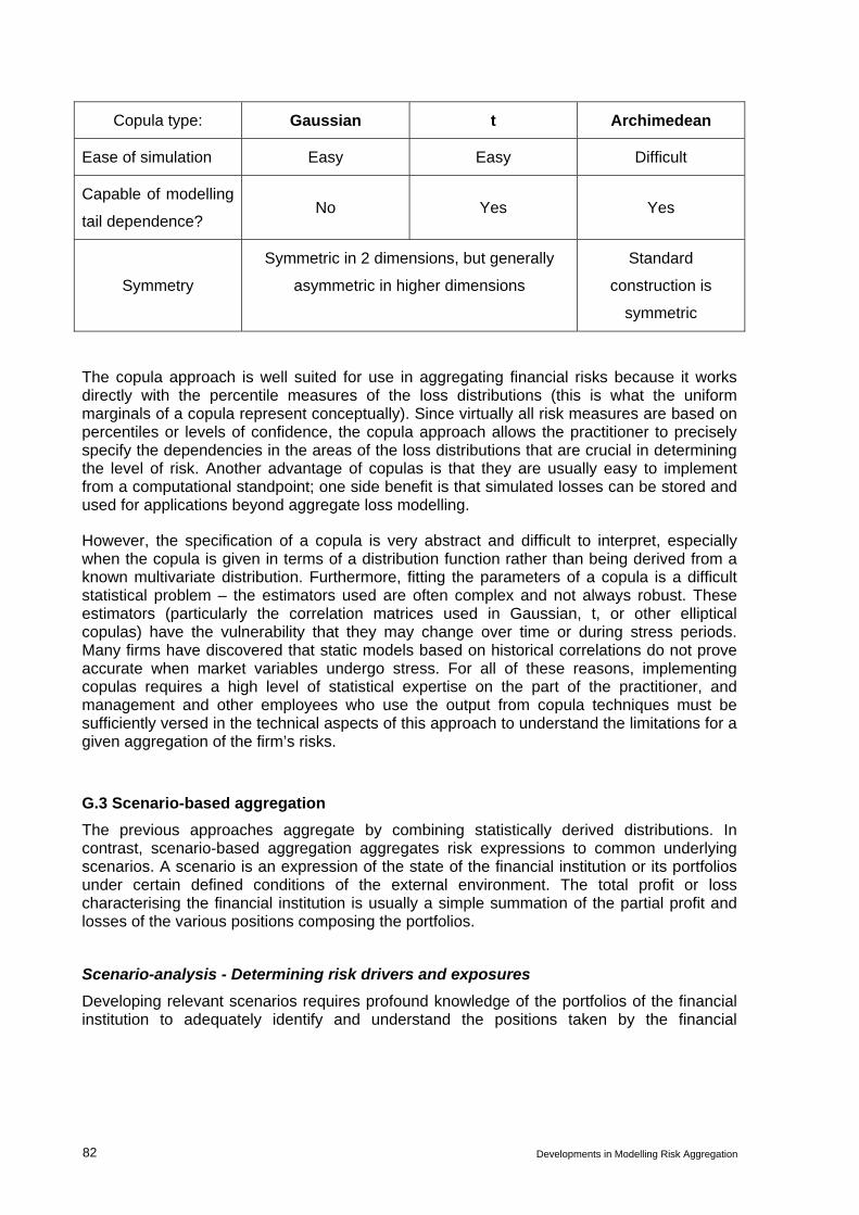
Copula type: Gaussian t Archimedean

Ease of simulation Easy Easy Difficult

Capable of modelling

tail dependence? No Yes Yes

Symmetry

Symmetric in 2 dimensions, but generally

asymmetric in higher dimensions

Standard

construction is

symmetric

The copula approach is well suited for use in aggregating financial risks because it works directly with the percentile measures of the loss distributions (this is what the uniform marginals of a copula represent conceptually). Since virtually all risk measures are based on percentiles or levels of confidence, the copula approach allows the practitioner to precisely specify the dependencies in the areas of the loss distributions that are crucial in determining the level of risk. Another advantage of copulas is that they are usually easy to implement from a computational standpoint; one side benefit is that simulated losses can be stored and used for applications beyond aggregate loss modelling.

However, the specification of a copula is very abstract and difficult to interpret, especially when the copula is given in terms of a distribution function rather than being derived from a known multivariate distribution. Furthermore, fitting the parameters of a copula is a difficult statistical problem – the estimators used are often complex and not always robust. These estimators (particularly the correlation matrices used in Gaussian, t, or other elliptical copulas) have the vulnerability that they may change over time or during stress periods. Many firms have discovered that static models based on historical correlations do not prove accurate when market variables undergo stress. For all of these reasons, implementing copulas requires a high level of statistical expertise on the part of the practitioner, and management and other employees who use the output from copula techniques must be sufficiently versed in the technical aspects of this approach to understand the limitations for a given aggregation of the firm’s risks.

G.3 Scenario-based aggregation

The previous approaches aggregate by combining statistically derived distributions. In contrast, scenario-based aggregation aggregates risk expressions to common underlying scenarios. A scenario is an expression of the state of the financial institution or its portfolios under certain defined conditions of the external environment. The total profit or loss characterising the financial institution is usually a simple summation of the partial profit and losses of the various positions composing the portfolios.

Scenario-analysis - Determining risk drivers and exposures

Developing relevant scenarios requires profound knowledge of the portfolios of the financial institution to adequately identify and understand the positions taken by the financial


institution.53 In addition, it requires an identification of the risk drivers of these positions; ie the stochastic variables that determine the performance of the respective position. Risk drivers are commonly external to the financial institution, eg financial and economic variables such as interest rates, GDP and unemployment, health conditions, or weather conditions determining the natural catastrophes, or social conditions determining material damages caused by humans (eg car accidents, fire). However, the risk drivers can also be internal or partly internal to the financial institution, for instance drivers of operational risk. In a next step, the risk positions are defined in terms of risk exposures relative to the risk drivers. Risk exposures are summary risk expressions characterising how the economic value of the risk position depends on the risk driver.

These relationships between the risk exposures and the risk drivers are typically linearised to preserve a certain level of simplicity. In this case the sensitivity of the risk position to a risk driver is described. However, practitioners should bear in mind that dependencies are not always linear (eg with interest rates, or in presence of optionalities).

A comprehensive analysis of the risk portfolios of the financial institution to well identify and understand the risk positions, and their drivers, and studying and describing the impact of the risk drivers and the changes in exposures comprise the building blocks of scenario analysis. These building blocks are necessary aspects to adequately perform scenario stress tests. In this respect scenario stress tests can be seen as a particular type of scenario analysis, that focuses on capturing and assessing potential "real-life" extreme events on the economic value of the financial institution.

Some interviewed firms go one step further and simulate a multitude of scenarios, these simulations are based on scenario generators.

Scenario simulation

Scenario simulation and scenario generation is made possible through the high computing power of modern computers. Large series of scenarios are generated by independently drawing large numbers of random variables and processing the random draws through models that describe particular processes or phenomena (eg a natural storm, a pandemic or an economic evolution).

Three types of models or algorithms are distinguished underlying these scenario generators:

1. A first category consists of models that tries to describe and proxy "real physical processes or natural laws". These processes usually rely on dynamic modelling that let risk factors develop through time. Examples are for instance pandemics, for which models describe how the virus can change, propagate between individuals and how it acts on the individual resulting in states of sickness of various severity or in death. Similar approaches are being used for wind storms and earthquakes.

2. A second category would be models that describe processes for which there is no real physical model. The models in this category may rely on a particular theory, which might (partially) fit certain historical observations. These models then underlie the scenarios simulated. Often certain ad-hoc distribution assumptions are used to

53 Positions on the asset side as well as on the liabilities side are considered by the financial institutions as well

as risk positions arising from internal processes of the enterprise (for instance, intra-group transactions, service agreements and commitments)


perform the simulations. This is, for instance, the case for most of the financial processes (eg interest rates, equities prices and indices, exchange rates).

3. Finally the third class of processes combines the first two categories and mixes physical with theoretical descriptive and empirical processes. Examples might for instance be processes that integrated natural catastrophe scenarios with economic and financial scenarios.

Firms may use several different and unrelated event generators to generate particular scenarios for different portfolios. These different types of scenarios may need to be integrated in order to obtain global scenarios that are applied on the different portfolios of the financial institution. When the scenarios are considered to be independent, scenarios can simply be randomly combined. However, when the scenarios are not independent mechanisms have to allow for interactions between the generators. These interactions are introduced through different methods. A simple technical method consists of using a covariance matrix (ie VarCovar approach as described above). Copulas are also often used to combine events from different event generators. In case the methods clearly show limitations and interactions between the scenarios are complex then the modelling of the different processes have to be performed simultaneously, leading to complicated event generators (eg pandemics and financial market risk factors).

As is typically the case when relying on simulation techniques, an issue to address is the number of simulation runs or events required to obtain an adequate level of precision in the estimate. Determining the required precision is not a difficult task but it is important to consider in the risk measurement process.

Conclusions

Scenario-based aggregation is conceptually and intellectually appealing as it eliminates ad-hoc methods of aggregation by aggregating exposures on the basis of common scenarios. As a result, the risk aggregation process avoids the common approach of inserting statistically derived distributions into risk management processes that may not reflect operational or legal business lines.

Proper scenario-based aggregation requires a profound understanding of the risks the firm is exposed to; it forces the firm to make extensive assessments of its portfolio risks and to identify risk drivers and assess the exposures to these risk drivers. Obtaining a clear view on the economic condition of the firm and deriving relevant economic scenarios proves hard and requires a strong reliance on the expert judgment and qualitative insights of the management. It requires experts and managers to develop solid representations of and views in various areas of the economic "reality" of their financial institution. Building this required knowledge and understanding takes time and it is not without its own risks as the potential to overlook exposures or have the profile change during the modelling period is an issue that the experts need to remain cognizant of.

In addition, scenario-based aggregation relies heavily on a range of assumptions (eg regarding the scenarios considered or developed, the scenarios being selected and the expression of risk positions in terms of exposures to the scenarios) which have to be well understood and considered when interpreting the results. In particular, it is not straightforward to reconcile the scenarios with the more traditional parametric descriptions of the risk.

The results of the scenario analysis and scenario simulation can be relatively easily and meaningfully interpreted in an economic and financial context. In addition, a firm can, for example, develop emergency or recovery plans from extreme scenarios. Consequently,


although the team performing the modelling usually needs to be relatively highly specialised, the results and interpretation of the results can be understood by a non expert executive manager.

Scenario simulation requires sufficient computing power and solid IT programs and platforms. The modern and well built simulation programmes commonly support changes to the dependencies and the distributions, allowing the user to make prospective studies, study sensitivities and stability of processes and thereby test the robustness of the methods. The programs can allow certain scenarios to be given specific weights and additional scenarios can be (artificially) added to focus on particular aspects of the risk. These methods demonstrate a great deal of flexibility that does not exist in the more simple aggregation methods.


Box A – Coherent risk measures

A reasonable description of a risk situation requires knowledge of a lot of information whereas a risk measure is a single number, leading to a significant reduction of information. On the other hand, a financial actor (eg investor, underwriter or regulator) takes a binary decision (to invest , to subscribe, to authorise). In this respect, a risk measure should as adequately as possible reflect the properties of the risk being considered.

Properties required by a coherent risk measure

At least 15 years of agitated discussions have resulted in the establishment of the essential properties that an adequate risk measure should obey([1], [2]):

• The choice of a reference instrument (usually a one year risk free state bond) is a vital ingredient and can be considered as a yardstick to which the risk will be compared.

• Positive homogeneity: implies that if a position has a risk, doubling the risk position leads to doubling the risk.

• Sub-additivity: means that the risk of the sum of two positions is always smaller or equal to the sum of the risks of the two positions.

• Translation invariance: adding to a portfolio an amount of cash invested in the reference instrument reduces the risk measurement of this portfolio by the same amount.

• Monotonicity: a position that always results in smaller losses than another position always has a smaller risk than the other position.

Examples of coherent and non-coherent risk measures:

Several risks measures are already widely used in practice. They have different properties:

• Total exposure: is a coherent risk measure, in fact the most severe one for a given reference instrument. In practice, the exposure is traditionally "weighted" to provide a more adequate risk measure.

• Standard deviation based risk measures: defined as the standard deviation relative to the expected value of the position. A certain refinement would be the use of the semi variance on the loss side of the distribution. It is not a coherent risk measure as it does not fulfill the monotonicity property.

• Value at Risk: simply reflects the quantile at a particular defined quantile level (α). This is a widely used and intuitive risk measure, however, it is not a coherent risk measure as it does not fulfill the sub-additivity property. This poses a severe draw-back to the use of the VaR measure.

• Expected Shortfall (or Tail-Value-at-Risk): has been mainly developed to cope with the non sub-additivity condition of the Value-at-Risk measure. It is defined as the average value of the losses at quantiles lower than the specified quantile (α).

Coherent measures of risk in practice

A crucial property for a coherent risk measure is the sub-additivity condition. As mentioned previously the VaR measure fails to satisfy this condition although the measure is widely used in practice. This can be explained by the fact that when distributions are normal or close to normal it can be shown that Value at Risk and Expected Shortfall are quite close and behave similarly. In this respect, normal distribution assumptions are quite common to


simplify the risk measurement. However, as soon as a risk position is characterised by a long tail behaviour, the similarity between VaR and ES does not hold anymore. Unwarily employing the VaR measure to risk positions characterised by long tail risk may lead to a strong underestimation of the risk. Furthermore mixing risk measures established with different reference instruments and with different currencies can also lead to unexpected behaviours.

Coherent risk measure and use of scenarios

A highly interesting property (known as the representation theorem, see [1]) allows establishing a comprehensive link between coherent risk measures and scenarios.

A scenario is stricto sensu a well precise possible realisation of the future (eg stock prices fall by 20% and interest rates rise by 100 bp). This concept can be generalised by considering a set of such scenarios weighted by some probabilities that are subjective and represent what practitioners (industry and regulators) consider as potential future realisations. This information represents nothing else but a probability density function called a generalised scenario.

The representation theorem states that a coherent risk measure is fully defined by a family of generalised scenarios and vice versa. This property emphasises and favours the use of scenarios by financial institutions to assess their risks as it allows more than the other methods to stay compatible with the coherence of the risk measure which has be shown to be a fundamental property.

References to articles:

• [1] Philippe Artzner, “Application of Coherent Risk Measures to Capital Requirements in Insurance”, North American Actuarial Journal, Volume 3, Number 2, April 1999

• [2] Glenn Myers, Coherent measures of risks, an exposition for the Lay actuaries, Casualty Actuarial Society, 2000.


Box B – Correlations vs dependencies

Linear correlations have been quite popular in finance and business applications. The calculation of the linear correlation coefficient (also called Pearson Product Moment Correlation) is straight-forward, and it is easily linked to linear models that are intuitive and readily explainable to a wide variety of users. A given correlation suffices, in a relatively straightforward fashion, to explain the joint or combined probability distribution for two or more normal random variables, thus preserving the general computational advantages and intuition (and real-world weakness) of modelling with the normal distribution. This is highly convenient both for underlying stochastic models involved in pricing and risk analysis as well as models that may be used for top-of-the-house risk aggregation. The following table explains correlation measures such as linear correlation in the context of the more general concept of statistical dependence, with which it may easily be confused.

Dependence Correlation Independence Event A: Credit-related losses on the consumer loan portfolio will exceed

USD 150 million. Event B: Insurance claims will exceed premiums by USD 20 million. In statistics, A and B are independent if Pr ( A | B ) = Pr ( A ) or, equivalently, Pr ( B | A ) = Pr ( B ) Verbally: “Probability of A given B is equal to the Probability of A.” “Probability of A is the same whether or not B occurs.”

Dependence versus correlation

Dependence means that the probability distribution of a variable is different depending on the state of the other variable. If the events are dependent, whether one of the events occurs should cause one to change his or her estimate of the probability that the other occurs.

Correlation is a commonly used label for specific measures of dependence between pairs of variables. In qualitative discussions, “correlation” is often not carefully distinguished from “dependence”.

Characterisation & scaling

Qualitatively, there are varying degrees of dependence. Variables that are highly dependent may have conditional distributions (eg, probability of A given B) that are very different from their unconditional distributions (probability of A assuming nothing about B). The degree of dependence may vary with the value of the conditioning (“given”) variable. If extreme values for that variable are associated with relatively high conditional probabilities for dependent variables, which may signify high tail dependence.

Correlation is a normalised measure of dependence. “Correlation coefficient” most often refers to Pearson Product Moment Correlation. This is a measure of linear relationship and is scaled from -1 to 1. Other correlation coefficients include Spearman’s Rank Correlation & Kendall’s Tau, also scaled from -1 to 1. Independent random variables have a correlation of zero. The closer to -1 or 1, the stronger the level of dependence.


Dependence is described in full only by knowing the entire joint probability distribution – ie, the function describing the probability of any possible combination of outcomes.

Correlation measures can be limited in how they represent dependence. A set of variables can have important dependencies (eg, at the tail) that are not represented clearly by a specific measure of correlation. Also, a given correlation might not distinguish between two very different joint distributions. Risk managers hope to capture important dependencies rather than measure correlation well, per se.

Limits

In business and financial time series, correlation measures often prove to be unstable. Particularly during stressful periods, correlation may appear, after the fact, to have increased significantly, leading to greater than anticipated losses. It can be difficult or impossible for risk managers to obtain reliable, time-independent measures of dependence due to potential changes in the overall dependence structure.


Box C - Positive semi-definiteness

Aggregating risk measures with correlation matrices is a commonly used approach. However, aggregation using correlation matrices involves making implicit assumptions that often turn out to be inconsistent: One condition that must be obeyed in order to ensure consistency is that the correlation matrix be positive semi-definite.

Definition and properties

An matrix A is said to be positive semi-definite if, for all vectors v: nn× 1×n

0≥AvvT

The term is what is placed under the square root using the VarCovar approach, where A is the linear correlation matrix and v is the vector of component capital requirements. It is important that this term not be negative, as the square root of a negative number is not defined. However, the condition for positive semi-definiteness is more restrictive than it first appears, as it must be satisfied for all vectors v, including those that contain negative numbers. It is not sufficient if the condition is satisfied only for vectors containing positive entries, which would normally be the case for a vector of capital requirements.

AvvT

The condition of being positive semi-definite is sufficient to ensure that a matrix satisfying all of the other conditions for a correlation matrix (ie symmetric, 1’s on the diagonal, all other entries between -1 and 1) is in fact the correlation matrix for some set of random variables. In other words, given any positive semi-definite matrix meeting all of the other conditions that a correlation matrix must satisfy, one can find a set of random variables having this matrix as its correlation matrix. Positive semi-definiteness is therefore a fundamental and defining property of correlation matrices. For this reason, it is considered essential (not just desirable) for any correlation matrix used in practice to have this property.

Examples

As mentioned at the start, one thing that can go wrong if an entity attempts to aggregate its economic capital requirements under the VarCovar approach using a matrix that is not positive semi-definite is that the total requirement may end up being the square root of a negative number. For example, if a company models three risks with respective requirements of 1000, 2000 and 3000, and uses the matrix:

−−−−−−

17.05.07.0115.011

as a correlation matrix for aggregation, its total requirement will end up being 1400000− , which is undefined. The positive semi-definiteness condition ensures that the amount under the square root sign in the VarCovar formula will never be negative.

Note however that the requirement for a correlation matrix to be positive semi-definite has nothing to do with whether the individual correlations are positive or negative. For example, the following matrix is positive semi-definite even though it contains negative entries:


−−−−−−

15.03.05.016.03.06.01

On the other hand, the matrix:

19.03.09.018.03.08.01

is not positive semi-definite. While this matrix will always produce a positive number under the square root in the VarCovar formula if all of the risk requirements aggregated are positive, it should not be used as a correlation matrix because it is impossible for three random variables to have these correlations simultaneously.

The problem with the last matrix can be understood intuitively. For three random variables, the matrix implies that the first and second random variables are highly correlated (0.8). It also implies that the second and third random variables are very highly correlated (0.9). However, a correlation of 0.3 implies that the first and third random variables are only weakly correlated, which cannot occur as both variables are correlated strongly with the second random variable. In fact, given that the first two correlations are 0.8 and 0.9, the third correlation must be at least 0.458. If the first two correlations are known with a high degree of certainty but the last correlation is not, using the above correlation matrix in the VarCovar approach is guaranteed to underestimate the total capital requirement, as the term under the square root will be too low by at least 2 times 0.158 times the product of the first and third capital requirements.

In summary, what these examples show is that the positive-definiteness condition imposes internal consistency on a set of correlations. While any particular (off-diagonal) element in a correlation matrix is free to range between -1 and 1, the correlations looked at together must not contradict one another. It is precisely the positive-definiteness condition that ensures this internal consistency.

Practical considerations

Correlations are frequently estimated using judgment, or using data series for which not all variables were observed simultaneously. When these correlations are combined into a single matrix, the resulting matrix is often not positive semi-definite. There will thus be a need to somehow convert the estimated matrix into one that is positive semi-definite.

Very often, the negative eigenvalues in an estimated correlation matrix are small in magnitude, and can be ascribed to noise in the collected data. If so, one simple technique is to diagonalise the estimated matrix, replace any negative eigenvalues on the diagonal with zero, and reconstitute the matrix with the new eigenvalues (as the final step, the matrix will have to be multiplied by diagonal matrices on the left and right to set the diagonal elements back to 1). More sophisticated techniques exist that can determine the positive semi-definite matrix that is closest to a given matrix, as measured by some specified matrix norm.54 These methods are fast and easy to apply, but if the resulting matrix differs significantly from the original matrix, this should call the accuracy of the correlation estimation process into question.

54 For example, see Nicholas Higham, Computing the Nearest Correlation Matrix, IMA J Numer. Anal,

22(3):329–343, 2002.


Some techniques for estimating correlations will always produce a matrix that is positive semi-definite. For example, factor models of correlation (such as those used in arbitrage pricing theory and KMV)55,56 model asset returns as linear combinations of systematic random variables. After these linear coefficients have been estimated, it is possible to calculate the correlation between any two asset returns. Since all correlations are based on the same underlying factors, they will be internally consistent, and any matrix that is formed from these correlations is guaranteed to be positive semi-definite.

55 We refer to Gur Huberman and Shenyu Wang, 2005, Arbitrage Pricing Theory, for a more elaborate

discussion on arbitrage pricing theory. 56 We refer to Michel Crouhy, Robert Mark and Dan Galai, Risk management, McGraw-Hill, 2001 for a more

elaborate discussion on the MKMV model.


Annex H

Approaches to managing model risks for risk aggregation processes

Most institutions recognise the wide margin for potential error in aggregation methods and potential diversification effects, as well as the need to develop an adequate degree of comfort that the methods will work as intended so that results can be used with confidence. To develop a sufficient degree of comfort, institutions use a variety of tools to control the risk aggregation and estimation process. Those tools generally can be divided into three major areas: (1) “effective challenge” to methods, assumptions, and results through validation and use, (2) process verification and governance practices, and (3) conservatism in calibration and use. Relative use of these tools, like the degree of rigor expected from aggregation methods, generally depends on portfolio composition, the materiality of risks, and specific management uses of model results. Firms reported that responsibility for oversight of the risk aggregation process ranged from the Chief Risk Officer to risk management committees to the CEO.

One of the key risks that must be assessed is model risk. In this context, a “model” should be understood as any system or method through which the management of a firm distils complex information into its essential elements to facilitate decisions, including those related to risk aggregation. Models are valuable tools for risk measurement and other aspects of financial or business management, whether for capital allocation or for determining required capital levels under adverse scenarios. But models also may be incorrect or misleading. This “model risk” must be identified, assessed, and controlled by any user of models.

Model risk in risk aggregation

Control of model risks should be an integral part of sound risk management of the aggregation process. Risks should be mitigated or controlled; model risks that remain unmitigated should be monitored, and the existence of those remaining risk should be acknowledged as the models are used in practice. Firms’ models produced a wide range of estimates for diversification benefits, even for firms with similar business models, and the risk that the models may produce an incorrect estimate for the diversification benefit was recognised by at least some of the firms.

Model risk is prominent in the area of risk aggregation, and measures of diversification may be particularly affected by such risk. Many of the risk aggregation methods are quite complex and it was clear from some of the firm interviews that senior managers did not have a complete understanding of the risk aggregation models. Thus, users of risk aggregation models must assess how much confidence can be placed in the results. Model users must have some means for achieving an adequate degree of comfort that models are “fit for purpose”, meaning that they will work as intended and generate results that are reliable. At the same time, model risk never can be eliminated entirely, so decision processes relying on model results must reflect an appropriate appreciation of the degree of imprecision that accompanies those results. Some of the firms indicated that it was easier to present meaningful information to risk committees that had more quantitatively inclined senior risk managers as opposed to trying to present models and results to management committees with broader representation.


Effective challenge through validation and use

Control of model risk begins with processes to ensure that some competent party – one that was not responsible for development of the methods under consideration – can provide an “effective challenge” to the assumptions and decisions reflected in those methods, and to the outcomes of the methods or models. Many firms stated that they rely on peer reviews or protests from business line managers. However, for challenge to be effective, challengers must have appropriate incentives; these incentives are often maintained through a degree of functional independence from the development process, although appropriate incentives can be created and supported in other ways, such as through compensation practices or organisational culture.

Importantly, the source of the challenge must be someone sufficiently competent to be effective; in some quantitative areas, the requisite knowledge, skills, and expertise may be substantial. Many of the firms interviewed stated that they rely on internal and external audit functions, and one also reported using an outside academic for validating risk aggregation models and processes. Finally, even a well-incented and competent challenge may fail to be effective if its source lacks the ability to actually effect needed change when problems are identified; this can be characterised as a matter of having inadequate influence or “stature” within the organisation to be taken seriously.

Ultimately, effective challenge to models in most organisations seems to come through the two primary channels of validation and use. Both channels are important for controlling model risk in the area of risk aggregation modelling.

Validation as a source of effective challenge

Validation refers to the application of various tools to assess whether models are likely to work as intended. Validation techniques used in common practice vary in sophistication, complexity, and intent. However, it can be misleading to focus excessively on the specific techniques used for validation, whether statistical or otherwise. For an effective validation process, validation tools are only part of a larger validation process, which as a process also must encompass features such as a clearly established schedule for validation activities, clear assignment of responsibilities for those activities, and commitment at high levels within the organisation to act on the validation results as appropriate.

Model validation tends to be most effective when it reflects consideration of the intended use of models; validation should be purpose-driven. However, as noted above many of the methods now used for risk aggregation to assess capital adequacy and measure diversification effects originally were developed for capital allocation. Thus firms may in some cases be using validation tools that were developed when models served a different primary purpose. This may lead to less effective validation, as a validation process designed with a capital allocation focus may not be appropriate for aggregation. For instance, a top-level capital estimate computed for purposes of capital allocation may not require great precision, since relative allocations are the primary focus. In contrast, for capital adequacy assessments a higher level of absolute precision is needed, and ensuring such precision may necessitate a different set of validation tools or a greater level of rigour.

Common validation approaches in the area of risk aggregation include back-testing, benchmarking, and stress testing.

Back-testing

A core aspect of the assessment of model-based methods is an evaluation based in part on how well the models have performed in the past. Past performance may be determined


through various statistical methods or tests, including back-testing. Back-testing is the comparison of model predictions to actual outcomes. In the context of risk aggregation and diversification, one challenge stems from the focus in risk aggregation on tail risk at very high quantiles. Many firms confirmed that the number of observations available were not sufficient to test such extreme outcomes, making back-testing a relatively weak validation tool. As a result, most model users find that economic capital models and similar risk aggregation methods are not well validated when the only validation method relied upon is back-testing.

Benchmarking

Benchmarking is the comparison of results from the firm’s risk aggregation processes with the results from one or more alternatives that have a similar purpose. However, even when other models and results can be identified as benchmark candidates, firms indicate that diversification benefits are difficult to compare because of a lack of transparency in the data and in the resulting correlations or dependencies. Moreover, alternatives may incorporate unknown and unobserved modelling decisions that make comparisons difficult, or may reflect different degrees of granularity in the underlying risk measures. One firm advocated the use of internal “test portfolios” that can be used to understand the sensitivity to parameters and to identify the implications of changes in the firm’s models.

External benchmarks can provide a range for what would be considered reasonable results, but these results may reflect assumptions that are not disclosed. Industry surveys can provide benchmark correlations, but are not likely to have a level of granularity comparable to the firm’s. One other avenue is independent academic reviews, but those are typically ad hoc, and are less likely to be successful in an area where methodology and practice is undergoing relatively rapid change. Some firms indicated that outside consultants are one of the few sources for external benchmarks.

Firms noted that it was difficult to assess levels of diversification benefits claimed by other firms, because diversification benefits depend heavily on the nature of the underlying portfolio. Portfolios differ from firm to firm in ways that may be important but not evident. Benchmarks are less meaningful if factors such as correlations, or the percentage risk reduction attributed to diversification, depend on too many other aspects of business composition and methodology.

Firms also note that risk aggregation processes focus on the identification of dependencies under stress conditions and during tail events, which makes it more difficult to identify appropriate indices or other market indicators against which to benchmark. A further complication is that risk aggregation models are often calibrated using a large number of alternative sources of data, since individual sources often are inadequate. As a result, it can be difficult to identify usable benchmarks if they only contain information that has already been incorporated during development or estimation processes.

Stress testing as a validation tool

Stress testing can provide a degree of independent assessment of the quality of risk aggregation methods. As a largely non-statistical method, scenario-based stress tests may usefully complement statistical methods by providing another tool to assess parameter estimates, and by providing a challenge to modelling assumptions that might not be highlighted by other methods.

Stress tests may reveal model shortcomings and help illustrate the reasonable range of outcomes and their sensitivity to assumptions, thereby helping provide management with a sense of the confidence that should be placed in model results. As noted above, some statistical tests may have low power due to the lack of data for tail event analyses, but


qualitative judgments based on economic and financial market analyses and scenarios may better highlight valid relationships under non-normal economic and financial market environments. During model development, sensitivity analysis can be used to identify variables or estimated parameters to which the results are particularly sensitive and focus additional attention on that part of the model, or at least alert management to the types of changes in the economic or financial market environment that could have a significant impact on resulting estimates of capital needs or computed diversification benefits.

Reverse stress testing can serve as an additional check on risk aggregation models, especially since a reverse stress test may identify business lines or risk types that are believed to be correlated even though statistical analysis may not reveal them as such under more “normal” economic and financial market conditions. One firm reported that through reverse stress testing exercises conducted every six months, the firm can bring analysts together to discuss possibilities, allowing for better analysis and judgment. A second firm reported that understanding correlations requires a realistic understanding of stress scenarios, which can then be used to inform the methodologies for risk aggregation, including assessments of correlations between different risks. The reverse stress-testing process makes it easier to discuss risk within the firm, although it requires a considerable amount of judgment.

Validation of Vendor Models

The processes used by firms to assess and aggregate risks rely to varying extents on proprietary models, data, and systems acquired from vendors. The reliability of correlation estimates, dependency relationships, and risk aggregation results more generally is even more questionable when the dependency modelling and calibration methods used are embedded in proprietary third-party vendor credit risk models. For enterprise-wide risk, one firm stated that it has no confidence in vendor models that are “black boxes”, and claimed to be very careful not to become wedded to black-box models.

Expert Judgment and Validation

Expert judgment plays a major role in many approaches to measuring diversification using risk aggregation models. Firms rely on expert judgment because modelling risk aggregation is a highly complex activity and data are scarce. There is nothing inherently wrong with the use of expert judgment, and in fact an element of judgment is almost certainly unavoidable. However, the application of judgment requires appropriate controls. Expert judgment is relied upon heavily in such fundamental elements as specifying the copula to be used, or setting conservative correlation coefficients in variance-covariance matrices, as well as for constructing good scenarios for stress tests and determining whether model results are reasonable. One firm pointed out that expert judgment is especially evident in the development of reverse stress tests, since a determination has to be made as to what combinations of risk drivers and exposures could cause a large loss of a given size. Another firm pointed to the use of expert judgment for determining liquidity horizons and for making assumptions about less liquid instruments.

Given the reliance on expert judgment, experts can actually introduce an additional element of risk that is a form of model risk, and which should be controlled like other aspects of risk in aggregation methods. Elements of expert judgment can and should be addressed within the model validation process in order to control the risk. Some key forms of control used by firms include clear approval processes for judgmental changes to models, identification of the relevant pool of qualified experts, steps to ensure that excessive control or influence is not concentrated in any one expert, and documentation of major decision points and the rationale behind the decisions made. Management within a firm needs to question expert judgment to determine that alternatives have been considered adequately, and explore the


ramifications of subjective decisions to understand how sensitive diversification benefits are to the decisions made by experts.

Model use as a source of effective challenge

Material internal usage can be a signal of perceived reliability. Firms recognise that use also helps support effective challenge by creating an internal constituency with a strong interest in having models that function well and that reflect economic and business realities. Thus, “use tests” are an important potential source of effective challenge for models, taking on additional importance when conventional forms of validation are less effective as in the case of risk aggregation models. However, the strongest evidence that use tests are in fact providing effective challenge would be evidence that users in practice have questioned aspects of models or other methods and that such questioning has led to process improvements; this type of tangible evidence seems to be relatively rare for risk aggregation processes at many firms. Only one firm reported that the use test is ingrained into the firm’s culture throughout the organisation.

Business managers affected by model outcomes will question the methods and assumptions underlying the models, particularly if business managers are significantly impacted by and do not agree with the outcome. Such challenges can be healthy if they are constructive and vigorous and force modellers to provide compelling explanations of aspects of the models. Aggregation processes are considered more “proven” if they have been accepted or deemed reasonable by the business managers – that is, if the modellers have “buy-in” from business units. However, modellers also must have sufficient senior management support to resist pressure from business units to modify models to create outcomes that are less accurate but more favourable to the business unit.

Business managers have an important stake in making sure risk aggregation models are correct if the evaluation of their performance depends upon the results of those models. This is most likely to be the case if the aggregation is ultimately used for capital allocation purposes. However, this pressure may be asymmetric since the business manager is less likely to challenge a favourable outcome that benefits the business, such as an outcome that results in a lower allocation of capital than would be commensurate with the true level of risk. Indeed, firms reported that they hear from business managers when the results go against them, but not necessarily when the model results are in their favour. Senior managers of firms seem to recognise the potential conflict of interest in reliance on use tests, but it is unclear how they adjust for or account for the asymmetry in practice. In addition, business managers may not have the appropriate training or expertise to judge whether the model is working correctly or incorrectly.

The nature of the challenge provided by business use also depends on the nature of the use. For example, business managers may have a greater interest in the trend in expected and unexpected losses and how changes in trends affect allocations of risk or capital, and less of a stake in the absolute level used to determine capital adequacy. Unless the absolute level of risk and capital from aggregation methods plays some material role in business processes, use is unlikely to be a source of highly effective challenge.

Process verification and governance

Risk aggregation is an internal process for financial institutions, and like other internal processes is potentially subject to the usual range of governance and internal controls. Firms using models implement aspects of governance such as requiring board-level approval for major elements of processes, regular verification of processes by internal audit, presentation


of results to senior management, approval requirements for changes to methods, adequate controls around the use of expert judgment, audit coverage, and so on.

Firms reported varying degrees of rigor in the governance process for validating and reporting the outcomes of risk aggregation efforts. For example, at one firm the Chief Risk Officer meets with the Chief Executive Officer (CEO) to discuss the models, methodologies, and results. Another firm claims to hold everyone accountable as a risk manager, and the risks are reported to senior management and the Board of Directors through various committees, each led by a direct report to the CEO; results of these efforts are verified by the firm’s audit function. For some firms, the Board of Directors is active and pays significant attention to the modelling underlying the risk aggregation, while for other firms the Board plays little or no role.

Conservatism

In recognition of model risk, and to compensate at least in part for the fact that the risk cannot be eliminated, firms and their experts frequently opt to incorporate assumptions or adjustments that are described as conservative, reasonable, or prudent into the aggregation process and ultimate estimation of diversification benefits. Choices of parameters or other modelling assumptions are deemed conservative if they tend to overstate risks and understate the benefits of diversification. Most of the firms interviewed stated that they were conservative in their assumptions, particularly when it came to adjusting variance-co-variance matrices to reflect stress scenarios.

However, with complex methods there are many points at which conservatism can be incorporated, thus potentially leading to excessive conservatism, or to offsetting adjustments in different parts of the overall computation. This may particularly happen in cases where, due to model complexity, the direction of adjustment that leads to greater conservatism is not obvious or intuitive. Moreover, if models are not precise or are not reliable, it is difficult to assess how conservative any adjustments actually are. There is no common standard for the appropriate degree of conservatism in any given circumstances, leaving the adjustment as a matter of management taste and judgment. Thus, a reliance on conservatism as the general solution to model risk may be inadequate.

Validating assumptions and adjustments made in the interest of conservatism is important, but it is a challenge for most firms. Ultimately, if an institution cannot develop adequate comfort and confidence through other means, the results or output of models should be used with great caution if they are used at all. In a sense, this conservatism in use is a final layer of defence applied by firms against losses due to model failure.


Annex I

Diversification effects within risk aggregation

Diversification benefits are for many firms an important by-product of their risk aggregation process. These firms over the years have been increasing their pressure on financial regulators and supervisors to recognise the benefits that roll out of this process. Therefore in this annex we first discuss the real economic determinants of the potential portfolio diversification effects. In the second section we describe the characteristics of the traditional aggregation methods that importantly determine the measured diversification benefits.

The level of computed diversification benefits differed markedly across the firms interviewed. Several firms interviewed showed a great scepticism toward common measures of diversification benefits through aggregating risks, such as methods that depend on linear correlations, and tended to devote little effort to deriving diversification benefits. By contrast other interviewed firms indicated that the level of risk reduction through diversification can be as high as 60 percent relative to simple summations across the different risk types, with similar reductions relative to regulatory calculations. These latter firms typically pursue a heterogeneous business mix.

The magnitude of measured diversification benefits also varies widely even across firms that are superficially similar, suggesting that differences in computed diversifications may importantly stem from differences in conceptual approaches to diversification and measurement methodologies rather than true differences in risk.57 One interviewed firm noted that its computed diversification benefit depended on whether the calculation was done by risk category (distinguishing between risk types and business units) or whether a more risk factor based approach was taken (in terms of credit spreads, exchange rates, ...). The measured diversification benefits also appeared to depend on the risk measures (eg VaR or expected shortfall) and the quantiles of the loss distribution (eg 99.5% or 99.75%) reflected in these measures.

From this, it is evident that the entire aggregation approach significantly determines the extent to which a firm incorporates diversification benefits in its risk calculation. However, whether these computed diversification benefits can and will actually be realised depends on the real economic underpinnings and determinants of the potential diversification benefits within a portfolio. Profound knowledge of these real economic underpinnings and determinants is essential to understand the potential for diversification within a portfolio and to assess the computed diversification benefits within the risk aggregation approach.

57 A survey conducted by the International Financial Risk Institute and Chief Risk Officer’s Forum in 2007 found

“[e]stimates of the impact of diversification on the capital estimate differ significantly – between 10-30% in banking and 21-59% in insurance…” Two reasons were pointed to: (1) differences in methodological approaches (eg, variance-covariance approach by banks and simulation by insurance groups) and (2) large differences in correlations estimates that cannot be attributed solely to differences in business mix.


Real economic determinants of potential diversification effects

1. Two types of diversification effects

In general two types of diversification effects can be distinguished: (1) diversification of name-specific or “idiosyncratic” risk factors and (2) diversification across systematic risk factors (non-diversifiable risk). The idiosyncratic risk refers to the risk that stems from isolated / independent events of a particular name or counterparty - for instance, the sources of idiosyncratic risk could be management decisions, market acceptance of new products, corporate governance aspects and so on that cause one counterparty to prosper or fall into disarray. General portfolio and risk management theory states that through spreading a portfolio across different names or counterparties the idiosyncratic risk can be diversified away. In other words, to the extent that the firm-specific influences on two asset returns differ - for instance, due to two firms differing in management capacities and internal governance arrangements - holding these two assets instead of one should reduce the idiosyncratic risk component within the portfolio risk. This can be referred to as diversification across idiosyncratic (or name-specific) risk.

If the portfolio includes a large number of names or counterparties, the portfolio risk attributable to name specific developments becomes very small, with minimal risk reductions from adding additional names. The portfolio risk that remains is determined by common underlying drivers or sources of risk, traditionally referred to as the systematic risk of the portfolio. These underlying drivers are multiple; they may range, for instance, from changes in short-term interest rates (perhaps due to monetary policy) to changes in the global weather conditions; from change in legislation to changes in the health conditions; etc. Portfolios differ in their exposure to and sensitivity to common underlying and potentially interacting risk drivers. Additionally, the materiality of risk drivers may change because of underlying conditions. For instance, particular legislative changes within a country may affect the risk related to that particular country. Diversifying the portfolio across two countries may decrease the impact of changes in one country on portfolio risk. From this perspective, the systematic risk within the portfolio may be decreased by spreading the portfolio across the two countries. Of course, legislative or policy changes may be coordinated among different countries, thereby in fact, severely reducing the diversification of the portfolio risk exposures across the two "local" legislative risk drivers within both countries. Other examples of the same kind are the traditional distribution of portfolio exposures across countries or regions and across industries to diversify monetary, budgetary, technology (and so on) drivers. However, as the credit crisis that started in mid-2007 has shown, financial and economic integration means that many different countries and industries may be affected at the same time. In general, portfolio risk therefore can be reduced to a certain extent by diversifying among different common drivers of risk — that is, by diversifying across systematic factors.

Making a distinction between the two types of diversification is actually very necessary to understand the portfolio risks, as these two types of diversification stem from materially different sources. Portfolio management may and likely does affect both dimensions of diversification, and therefore, both dimensions must be measured and managed at all times. Any portfolio decision with only one of the dimensions in mind could easily have unintended consequences for the other diversification dimension. For instance, the portfolio decision to diversify along different names (diversification of the idiosyncratic risk) can, for instance lead to a concentration to particular risk drivers (increase of the systematic risk) when not recognising or ignoring the risk drivers. A characterising example of the difficulties to understand the differences in diversification, are the securitisation products of which the high-grades of the more senior tranches were often explained by the exposure to a diversified portfolio, with this implying a diversification across names. However, the exposure


to the common drivers of risk (the systematic risk component) were in this discourse often neglected as, for instance, concentrations to mortgage regions or general underwriting practices were not recognised.58 Of the two types of diversification, the diversification across these common underlying risk drivers is typically the type that accounts for the largest computed diversification benefits within financial institutions; however, it is also the type of diversification that seems to be the most difficult to understand and manage.

The above traditional portfolio-theoretic approach to diversification disregards crucial factors that have a significant influence on the actual realised portfolio risks. Many "qualitative" factors – such as the level of knowledge of the "local habits, economies, markets, and products" – actually help determine whether any "diversification" is realised or whether the diversification strategy instead leads to an increase in portfolio risk. Firms often neglect these elements in the pursuit of diversification benefits, with the "diversification" that US CDOs and ABS was said to provide to local EU and Asian financial institutions being a notable recent example.

2. The dynamics of economic diversification

As the discussion above indicates, the extent of risk diversification across single names and common risk drivers that can be achieved in any situation within a portfolio at a particular time depends on the composition of the portfolio of exposures, but also on the prevailing market conditions, the state of the economy and other elements of the 'external' environment; as discussed above, the real economic determination of diversification benefits within a portfolio of exposures greatly depends on these external conditions that affect the risk drivers of the portfolio risks.

The more two positions or risk exposures differ in terms of their pattern of variation over time, the more likely their combination will generate diversification benefits. Traditional portfolio theory59 and risk aggregation approaches commonly rely on the assumption that these patterns are constant over time, which is translated into fixed correlations based on past observations.

However, the pattern of variation often is not constant, but changes along with the developments in the external environment, and the impact of a risk driver on risk exposures may significantly vary. For instance, a foreign exchange position such as a long position in the Pound Sterling might appreciate against the Euro because of interest rate hikes by the Bank of England. However, those interest rate hikes might instead depreciate the currency if financial market participants conclude that these rate hikes will affect the economy too severely. The interrelations among the risk drivers also may change. For example, traditionally oil and equity prices have moved in opposite directions, as higher oil prices dampen economic prospects and thereby negatively affect general equity prices; being long oil in the investment portfolio would provide a natural hedge to some extent against a general decline in equity prices. However, during the last two years oil prices and the general level of equity prices have more been moving more in tandem, thereby reducing the hedging potential of the long exposure to oil.

Risk drivers importantly interact, and movement in one may have important subsequent effects on other risk drivers. For instance, interest rate hikes may not only directly increase

58 A more elaborate discussion is provided in J Garcia and S Goossens, The Art of Credit Derivates, Chapter 22,

Wiley Finance. 59 H Markowitz, 1952 Portfolio Selection, Journal of Finance, Vol 7, No 1


the default probability on loans due to higher interest payments, but might also have a severe impact on the obligor through effects on equity prices and exchange rate fluctuations. Subsequent reactions or second order effect may potentially be quite material but are even more difficult to understand and capture within risk assessments. Moreover, the risk drivers, their impact, and their interactions may change quite suddenly or "jump to another state". Overall, these complex relationships require more than just an analysis of static linear effects of risk drivers on exposures.

In summary, the actual scope for diversification (across systematic factors) depends on the particular risk drivers to which a portfolio is exposed, the relative magnitudes of those exposures, and the evolving impact and relationships among the risk drivers, which likely are significantly affected by developments in the external environment. Therefore, potential real economic diversification likely varies over time as the external environment evolves, in ways that can only be understood through identification and assessment of the drivers of real economic diversification or the drivers of portfolio risks and their potential evolution.

3. Behavioural factors and legal impediments

The extent of any risk reduction that may be attributable to diversification effects may also importantly be affected by “behavioural” factors. Actions taken by the management of a firm as market conditions evolve, or actions taken by other market participants in reaction to changing conditions, may either augment or reduce the effect on risk that would otherwise be observed. For instance, the firm's own management actions might change the composition of the portfolio and thereby introduce risk interactions that previously were not there.

Additionally, there may also be structural or legal impediments to realisation of diversification benefits; examples of such impediments are restrictions on capital and liquidity transfer. That is, there may be difficulties in, or even outright prohibitions against, allowing gains in one area to offset losses in another. In that case, even though the underlying economics might suggest potential for diversification, no diversification benefits could be realised in practice. One interviewed firm specifically factored intragroup transactions into its simulation (eg, intragroup retrocessions, and not permitting the transfer of surplus capital from one subsidiary to another), thus accounting for the relationships between subsidiaries and with the parent. However, generally these kinds of restrictions are not taken into account when calculating diversification benefits.

The impact of methodology on measured diversification

It is clear that aggregation methodologies and their calibration determine the level of computed diversification benefits for a given portfolio. Given the constant changes in the external environment, the accuracy, precision, and reliability of aggregation methods and measured diversification benefits are likely to vary over time and across firms. The computed diversification benefits are influenced by many factors, including organisational structure, aggregation method, and granularity. These factors complicate the understanding of (and discussion of) diversification benefits. The balance of this section discusses characteristics of traditional aggregation methods that significantly affect measured diversification benefits, regardless of the potential for real economic diversification.

1. Compartmentalisation of risks (risk bucketing)

Bucketing of risk exposures into different risk groups or risk types is a common approach to the management, measurement, and aggregation of risk within financial institutions, although this compartmentalisation of risks is more prevalent within the banking-based groups than


the insurance-based groups. However, such risk bucketing can lead to underestimation of risk or overestimation of diversification benefits.

When compartmentalising risks, a crucial assumption made is that risks can clearly be separated. However, risk exposures in these different buckets typically have some common underlying or potentially interacting risk drivers that evoke an interaction between risk exposures in different buckets. The BCBS Working Paper "Findings on the Interaction of Market and Credit Risk" provides a striking example of the interaction between market and credit risk for a bank lending in foreign currency loans to domestic borrowers:

"When for example the domestic economy slows, ceteris paribus, the probability of domestic borrowers defaulting increases. When the domestic currency depreciates, ceteris paribus, the value of the loan in domestic currency increases as it is denominated in foreign currency. So, on the surface one could think that the two effects offset each other. But this reasoning would neglect the strong relationship between exchange rate changes and default risk in this type of contract. The ability of a domestic borrower to repay a loan in foreign currency depends in a non-linear way on fluctuations in the exchange rate (unless the domestic borrower has other revenues in the foreign currency in which the loan is denominated). A home currency depreciation has a particularly malign effect on the repayment amount and therefore repayment probability of a foreign currency loan by an unhedged domestic borrower, which tends to be stronger than the valuation effect mentioned above."

This example suggests that conventional aggregation methods that compartmentalise the risks into buckets may lead to severe underestimation of risks, particularly if linear methods are used to account for dependence between buckets. As more thoroughly discussed in Annex F, this example also shows that adding separate risk buckets together may not be a conservative approach as traditionally believed, since effects within the two clusters could reinforce each other. The BCBS paper calls these interactions "compounding effects", arising in their example "when losses from default on an instrument depend on movements in market risk factors, or conversely, when changes in the values of instruments due to movements of market risk factors depend on whether there is a default or rating migration."

Not only may this compartmentalisation of risks lead to incorrect estimation of portfolio risks it may also severely hinder an appropriate management of the risks, as the bucketing may lead management to ignore certain important risks or risk interactions. More integrated risk aggregation approaches that attribute gains and losses to common or interacting risk drivers in a consistent manner likely support better risk management. In general, the more that aggregation methods depart from or fail to consider the real economic determinants or the 'reality' that defines the potential diversification benefits within the portfolio of risk exposures, the larger the potential error in the estimation of the benefits and the greater the danger that the apparent level of computed diversification benefits is artificial.

2. The level of granularity

The level of granularity within the risk aggregation approach is a crucial factor affecting the management and measurement of diversification benefits.

With regard to risk measurement, the level of granularity of the aggregation method influences computed diversification benefits. Under traditional portfolio measurement and aggregation techniques, recognising a larger number of risk factors within the portfolio risk measure results in greater "diversification benefits" computed. Consider the following stylised example: A bank extending credits in different EU countries might be affected by the changes in budgetary policy in a single EU country. Assume that the firm employs a portfolio factor model that is sensitive to changes in the budgetary policies of the different EU


countries and is calibrated on this local EU country level. That portfolio model might show the effect in terms of risk of this change in budgetary policy for that one country and will show the diversification through its exposures to the different EU countries. Suppose now that a budgetary policy change is coordinated at the EU level that impacts each EU country's economy; because the model focuses on the local EU level and is calibrated taking into account this diversification at the local level, the risk estimation of the change in budgetary policy at the EU level will be underestimated (and diversification benefits will be overestimated).

The same line of reasoning holds with regard to traditional aggregation approaches that compartmentalise risks according to different risk types, business units, product types, legal entities or geography. Typically the more the aggregation approach differentiates portfolios or activities according to these categories, and thus the higher the focus on these compartmentalised entities or sub-portfolios, the higher the diversification benefits the aggregation approach will be able to show.

Additionally, some interviewed firms commented that a greater focus by the group on risk management at the level of compartmentalised entities of sub-portfolios places a stronger emphasis on diversification within the group but might also hinder the recognition (and hence management) of concentrated exposures at the group level.

Greater granularity in risk measurement may be seen as desirable in some cases, as it could lead to greater precision in measuring and understanding certain risks. However, it may also degrade the statistical reliability of, for instance, correlation matrices used during the aggregation process, or of the component marginal distributions that play a central role in copula-based approaches (for example, if the greater granularity leads to small sample sizes). Excessive granularity thus may raise questions about the reliability of the final risk estimates.

Ultimately, the final choice of degree of granularity or focus on "local entities" in the aggregation process is a matter of judgment, with no single, commonly accepted way to determine whether an appropriate level of granularity has been selected. Decisions regarding the level of granularity clearly interact with the measurement of the level of diversification benefits and the management of the group-wide risks.

3. Management actions

Although actions taken by firms in response to market developments and changes in risk influence dependencies, many firms explicitly choose not to reflect such dynamic elements in the risk aggregation process. This has important implications, since it is quite possible that some of the dependencies may be reinforced by firm actions, despite firms’ attempts to mitigate some of the risks. Of course, it is also possible that management actions might reduce the negative impact of dependencies; arguably this is one of the primary purposes of risk management. Some firms mentioned a desire to include that effect through assumptions about their ability to trade out of positions as conditions change over some horizon. But modelling that behaviour, validating its assumed impact, and determining whether it would materialise in actual practice are all important elements and open issues. It is clear that diversification effects depend on how firms respond to market developments and to changes in the external environment, but these responses are difficult to model, and few firms successfully do so.



4. Expert judgment

Methodological choices within the entire aggregation process are rife with decisions based at least somewhat, and often to a large extent, on the judgment of experts. For example, in some cases experts believe that economic and financial market proxies do not adequately represent the behavior of important variables, and so make corresponding adjustments to parameters in models. In many cases, experts have a substantial influence on correlations used in a variance-covariance approach when available data are not sufficient to estimate correlation coefficients with an acceptable degree of confidence; a number of firms indicated that experts often set or modify correlations based on their experience and analysis of data.

Expert judgment often is used to compensate for the now widely recognised non-linear dependencies that are not captured by linear approaches. For example, credit spreads in two countries may be uncorrelated in a normal economic environment, but experts may be confident that credit spreads in a stressed environment would become highly correlated because both countries’ economies depend on the same manufacturing sector; some firms indicated that in such a situation experts might increase correlations by some subjectively determined (but arguably well informed) amount such as 15 percent or 25 percent. Use of alternatives to the variance-covariance approach do not eliminate, or even necessarily reduce, the likely role expert judgment; similar issues arise with copula-based approaches, where certain parameters of the selected copula or the marginal distributions can significantly influence results, and data may be scarce or unreliable (and intuition perhaps less reliable as well). Risk measurement and diversification results are also very sensitive to decisions such as the choice of a specific copula. There is little in either theory or data (particularly for tail-risk applications) to definitively guide the choice, but alternative specifications materially affect the final assessment of diversification benefits. Expert judgment may be used to incorporate or reflect real economic determinants of portfolio risks or diversification benefits in risk aggregation methods. Clearly any such expert-based changes (to correlation values, other dependency measures, or the entire aggregation approach) may materially affect the computed diversification benefits. Given the material impact of expert judgment, strong governance should be in place to ensure that the effect of the expert judgments is transparent within the firm.

5. Purpose and design

A general finding of this work stream is that many risk aggregation methods used for capital adequacy assessment were originally not developed for that purpose. The initial focus of these techniques typically was on risk attribution or capital allocation, that is, on the attribution of aggregate, top-of-the house risk (and/or capital) to lower levels of aggregation (such as business units or risk types). The difference may seem subtle – conceptually the aggregation process is simply run in reverse – but in practice it shifts the degree of emphasis placed on assessment of absolute diversification benefits toward a focus on relative risk. In this respect, aggregation for capital purposes and for the assessment of diversification benefits requires precision in the absolute estimates of risk.

Documents

Developments in Modelling Risk Aggregation - BIS