1

Dictionary learning for sparse coding:Algorithms and convergence analysis

Chenglong Bao, Hui Ji, Yuhui Quan and Zuowei Shen

Abstract—In recent years, sparse coding has been widely used in many applications ranging from image processing to patternrecognition. Most existing sparse coding based applications require solving a class of challenging non-smooth and non-convexoptimization problems. Despite the fact that many numerical methods have been developed for solving these problems, it remainsan open problem to find a numerical method which is not only empirically fast, but also has mathematically guaranteed strongconvergence. In this paper, we propose an alternating iteration scheme for solving such problems. A rigorous convergenceanalysis shows that the proposed method satisfies the global convergence property: the whole sequence of iterates is convergentand converges to a critical point. Besides the theoretical soundness, the practical benefit of the proposed method is validated inapplications including image restoration and recognition. Experiments show that the proposed method achieves similar resultswith less computation when compared to widely used methods such as K-SVD.

Index Terms—dictionary learning, sparse coding, non-convex optimization, convergence analysis

F

1 INTRODUCTION

Sparse coding aims to construct succinct represen-tations of input data, i.e. a linear combination ofonly a few atoms of the dictionary learned fromthe data itself. Sparse coding techniques have beenwidely used in applications, e.g. image processing,audio processing, visual recognition, clustering andmachine learning [1]. Given a set of signals Y :=y1, y2, . . . , yp, sparse coding aims at finding a dictio-nary D := d1, d2, . . . , dm such that each signal y ∈ Ycan be well-approximated by a linear combinationof djmj=1, i.e., y =

∑m`=1 c`d`, and most coefficients

c`s are zero or close to zero. Sparse coding can betypically formulated as the following optimizationproblem:

minD,cipi=1

p∑i=1

1

2‖yi −Dci‖2 + λ‖ci‖0, (1)

subject to ‖di‖ = 1, 1 ≤ i ≤ m. The dictionary dimen-sion m is usually larger than the signal dimension n.

1.1 Overview of the problemThe problem (1) is a non-convex problem whosenon-convexity comes from two sources: the sparsity-promoting `0-norm, and the bi-linearity between thedictionary D and codes cipi=1 in the fidelity term.Most sparse coding based applications adopt an al-ternating iteration scheme: for k = 1, 2, . . . ,

(a) sparse approximation: update codes cipi=1 via solv-ing (1) with the dictionary fixed from the previousiteration, i.e. D := Dk.

• C. Bao, H. Ji, Y. Quan and Z. Shen are with the Department ofMathematics, National University of Singapore, Singapore, 119076.E-mail: matbc,matjh,matquan,matzuows@nus.edu.sg

(b) dictionary refinement: update the dictionary D viasolving (1) with codes fixed from the previousiteration, i.e. ci := ck+1

i for i = 1, . . . , p.

Thus, each iteration requires solving two non-convexsub-problems (a) and (b).

The sub-problem (a) is an NP-hard problem [2],and thus only a sub-optimal solution can be foundin polynomial time. Existing algorithms for solving(a) either use greedy strategies to obtain a local min-imizer (e.g. orthogonal matching pursuit (OMP) [3]),or replace the `0-norm by its convex relaxation, the`1-norm, to provide an approximate solution (e.g. [4],[5], [6], [7]).

The sub-problem (b) is also a non-convex problemdue to the existence of norm equality constraints onatoms dimi=1. Furthermore, some additional non-convex constraints on D are used for better per-formance in various applications, e.g. compressedsensing and visual recognition. One such constraintis an upper bound on the mutual coherence µ(D) =maxi6=j |〈di, dj〉| of the dictionary, which measures thecorrelation of atoms. A model often seen in visualrecognition (see e.g. [8], [9], [10]) is defined as follows,

minD,C‖Y −DC‖2 + λ‖C‖0 +

µ

2‖D>D − I‖2, (2)

subject to ‖di‖ = 1, 1 ≤ i ≤ m. Due to the additionalterm ‖D>D − I‖2, the problem (2) is harder than (1).

1.2 Motivations and our contributions

Despite the wide use of sparse coding techniques, thestudy of algorithms for solving (1) and its variantswith rigorous convergence analysis has been scantin the literature. The most popular algorithm forsolving the constrained version of (1) is the K-SVD

2

0 10 20 30 40 500

0.5

1

1.5

2x 10

4

Number of Iteration

||Ck+

1 −Ck || F

OursKSVD

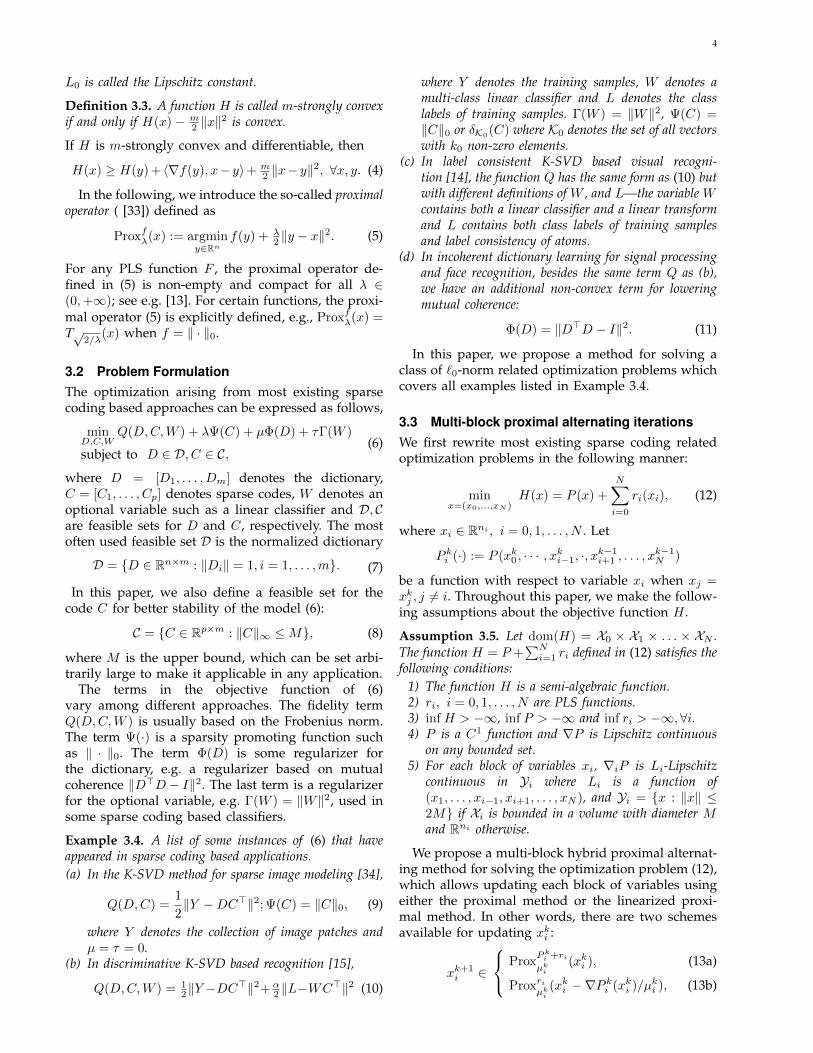
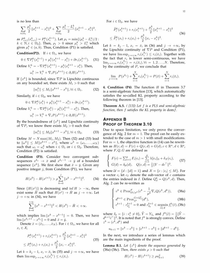
Fig. 1. Convergence behavior: the increments of the coeffi-cient sequence Ck generated by K-SVD and by the proposedmethod in image denoising.

method [11], which calls OMP for solving the sparseapproximation sub-problem. The OMP method is agreedy algorithm known for its high computationalcost. For problem (2), existing applications usuallycall some generic non-linear optimization solver. Al-though these alternating iteration schemes generallycan guarantee that the objective function value isdecreasing, the generated sequence of iterates maydiverge. Indeed, the sequence generated by K-SVD isnot always convergent; see Fig. 1 for the convergencebehavior of the sequence generated by K-SVD in atypical image denoising problem. Recently, the so-called proximal alternating method (PAM) [12] andthe proximal alternating linearized method (PALM)[13] were proposed to solve a class of non-convex op-timization problems, with strong convergence. How-ever, problems considered in [12] and [13] are rathergeneral—a direct call of these two methods is notoptimal when being applied to sparse coding.

There certainly is a need for developing new algo-rithms to solve (1) and its variants. The new algo-rithms should not only be computationally efficientin practice, but also have strong convergence guaran-teed by theoretical analysis, e.g. the global convergenceproperty: the whole sequence generated by the methodconverges to a critical point of the problem.

This paper proposes fast alternating iterationschemes satisfying the global convergence property,applicable to solving the non-convex problems aris-ing from sparse coding based applications, including(1), (2), and discriminative extensions of the K-SVDmethod [14], [15]. Motivated by recent work on multi-block coordinate descent [16], PAM [12] and PALM[13], we propose a multi-block hybrid proximal alter-nating iteration scheme, which is further combinedwith an acceleration technique from the implementa-tion of the K-SVD method. The proposed dictionarylearning methods have their advantages over existingdictionary learning algorithms. Unlike most existingsparse coding algorithms, e.g. K-SVD, the proposedmethod satisfies the global convergence property andis more computationally efficient with comparableresults. Compared to some recent generic methods,e.g. PALM [13]), for solving these specific non-convexproblems, the proposed dictionary learning methoddecreases the objective function value faster than

PALM and yields better results in certain applicationssuch as image denoising.

The preliminary version of this work appeared in[17], whereas this paper introduces several extensions.One is the extension of the two-block alternatingiteration scheme to the multi-block alternating iter-ation scheme, which has wider applicability. Anotherimprovement over the original is that the new schemeallows choosing either the proximal method or the lin-earized proximal method to update each block, whichmakes it easier to optimize the implementation whenapplied to solving specific problems. Furthermore,this paper adds more visual recognition experiments.

2 RELATED WORK

In this section, we briefly review the most relatedsparse coding methods and optimization techniques.

Based on the choice of sparsity-promoting function,existing sparse coding methods fall into one of the fol-lowing three categories: (a) `0-norm based methods,(b) `1-norm based methods, and (c) methods based onsome other non-convex sparsity-promoting function.One prominent existing algorithm for solving `0-normbased problems is the so-called K-SVD method [11].The K-SVD method considers the constrained versionof (1) and uses an alternating iteration scheme be-tween D and ci: with the dictionary fixed, it uses theOMP method [18] to find sparse coefficients ci, andthen with sparse coefficients fixed, atoms in the dic-tionary D are sequentially updated via the SVD. TheK-SVD method is widely used in many sparse codingbased applications with good performance. However,the computational burden of OMP is not trivial, andthus there exists plenty of room for improvement. Inaddition, there is no convergence analysis for K-SVD.

Anther approach to sparse coding is using the `1-norm as the sparsity-promoting function. Many `1-norm based sparse coding methods have been pro-posed for various applications; see e.g. [5], [6], [19],[20]. The variational model considered in these workscan be formulated as follows,

minD∈D,C∈C

p∑i=1

1

2‖yi −Dci‖2 + λ‖ci‖1, (3)

where D, C are predefined feasible sets of the dictio-nary D and coefficients C, respectively. It is evidentthat the sparse approximation sub-problem now onlyrequires solving a convex problem. Many efficientnumerical methods are available for `1-norm basedsparse approximation, e.g. the homotopy method [21]used in [5] and the fast iterative shrinkage threshold-ing algorithm [22] used in [6]. Methods for dictionaryrefinement either sequentially updates atoms (e.g. [5],[6]) or simultaneously updates all atoms using theprojected gradient method [7]. None of the methodsmentioned above has any convergence analysis. Re-cently, an algorithm with convergence analysis was

3

proposed in [23], based on the multi-block alternatingiteration scheme [16].

The `1-norm based approach has its drawbacks, e.g.it results in over-penalization on large elements of asparse vector [24], [25]. To correct such biases causedby the `1-norm, several non-convex relaxations of `0-norm were proposed for better accuracy in sparsecoding, e.g., the non-convex minimax concave in [26]and the smoothly clipped absolute deviation in [24].Proximal algorithms have been proposed in [27], [28],[29] to solve these problems containing non-convexrelaxations. Again, these methods can only guaran-tee that sub-problems during each iteration can besolved using some convergent method. The questionof global convergence of the whole iteration schemeremains open.

The block coordinate descent (BCD) method wasproposed in [30] for solving multi-convex problems,which are generally non-convex but convex in eachblock of variables. It is known that the BCD methodmay cycle and stagnate when being applied to solvenon-convex problems; see e.g. [31]. A multi-block co-ordinate descent method was proposed in [16] whichupdates each block via either the original method, theproximal method, or the linearized proximal method.Its global convergence property was established formulti-convex problems, which are not applicable tothe cases discussed in this paper. The recently pro-posed PAM [32] updates each block using the proxi-mal method. The sub-sequence convergence propertywas established in [32], and the global convergenceproperty was established in [12] for the case of two-block alternating iterations. In [13], PALM, whichsatisfies the global convergence property, was pro-posed to solve a class of non-convex and non-smoothoptimization problems; it updates each block usingthe linearized proximal method. PALM is applicableto problems in sparse coding.

The work presented in this paper is closely re-lated to these block coordinate descent methods. Theproposed scheme is also a multi-block alternatingiteration scheme, but it is different from these pre-vious methods in several aspects, owing to it be-ing tailored for sparse coding problems. It enablesblock-wise granularity in the choice of update scheme(i.e. between the proximal method and the linearizedproximal method). Such flexibility is helpful to de-velop efficient numerical methods that are optimizedfor the specific problems in practical applications.In addition, motivated by the practical performancegain of an acceleration technique used in the K-SVDmethod, we developed an accelerated plain dictionarylearning method. The proposed dictionary learningmethods show their advantages over existing ones invarious sparse coding based applications. The globalconvergence property is also established for all thealgorithms proposed in this paper.

3 NUMERICAL ALGORITHM

3.1 Preliminaries on non-convex analysis

In this section, we introduce some notation and pre-liminaries which will be used in the remainder of thispaper. Vectors and matrices are denoted by lower anduppercase letters, respectively. Sets are denoted bycalligraphic letters. Given a vector y ∈ Rn, yj denotesthe j-th entry. For a matrix Y ∈ Rm×n, Yj ∈ Rndenotes the j-th column and Yij denotes the i-thentry of Yj . Given a matrix Y ∈ Rm×n, its infinitynorm is defined as ‖Y ‖∞ = maxi,j |Yij |, and its `0norm, denoted by ‖Y ‖0, is defined as the number ofnonzero entries in Y . The `2 norm of vectors and theFrobenius norm of matrices are uniformly denoted as‖ · ‖. Given a positive constant λ > 0, the so-calledhard-thresholding operator Tλ(Y ) is defined as

Tλ(x) =

x, if |x| > λ;

0, λ, if |x| = λ;

0, otherwise,

when applied to scalar variables. When applied tomatrix Y , Tλ(Y ) applies Tλ on each entry of Y . For aset S, its associate indicator function δS is defined by

δS(Y ) =

0, if Y ∈ S;

+∞, if Y /∈ S.

For a proper and lower semi-continuous (PLS) func-tion, denoted as f : Rn → R ∪ +∞, the domain off is defined by domf = x ∈ Rn : f(x) < +∞. Next,we define the critical points of a PLS function.

Definition 3.1 ( [13]). Consider a PLS function f .• The Frechet subdifferential of f is defined as

∂f(x) =

u : lim inf

y→x,y 6=x

f(y)− f(x)− 〈u, y − x〉‖y − x‖

≥ 0

if x ∈ domf , and ∅ otherwise.

• The limiting subdifferential of f is defined as

∂f(x) = u : ∃ xk → x, f(xk)→ f(x)

and uk ∈ ∂f(xk)→ u.

• x is a critical point of f if 0 ∈ ∂f(x).

It can be seen that if x is a local minimizer of f ,then 0 ∈ ∂f(x). If f is convex, then

∂f(x) = ∂f(x) = u|f(y) ≥ f(x) + 〈u, y − x〉,∀y,

i.e., 0 ∈ ∂f(x) is the first order optimal condition. If(ci, D) is a critical point of (1), then it satisfies

(D>Dci)j = (D>yi)j , if (ci)j 6= 0.

Definition 3.2 (Lipschitz Continuity). A function f isa Lipschitz continuous function on the set Ω, if there existsa constant L0 > 0 such that

‖f(x1)− f(x2)‖ ≤ L0‖x1 − x2‖ ∀x1, x2 ∈ Ω.

4

L0 is called the Lipschitz constant.

Definition 3.3. A function H is called m-strongly convexif and only if H(x)− m

2 ‖x‖2 is convex.

If H is m-strongly convex and differentiable, then

H(x) ≥ H(y) + 〈∇f(y), x− y〉+ m2 ‖x− y‖

2, ∀x, y. (4)

In the following, we introduce the so-called proximaloperator ( [33]) defined as

Proxfλ(x) := argminy∈Rn

f(y) + λ2 ‖y − x‖

2. (5)

For any PLS function F , the proximal operator de-fined in (5) is non-empty and compact for all λ ∈(0,+∞); see e.g. [13]. For certain functions, the proxi-mal operator (5) is explicitly defined, e.g., Proxfλ(x) =T√

2/λ(x) when f = ‖ · ‖0.

3.2 Problem FormulationThe optimization arising from most existing sparsecoding based approaches can be expressed as follows,

minD,C,W

Q(D,C,W ) + λΨ(C) + µΦ(D) + τΓ(W )

subject to D ∈ D, C ∈ C,(6)

where D = [D1, . . . , Dm] denotes the dictionary,C = [C1, . . . , Cp] denotes sparse codes, W denotes anoptional variable such as a linear classifier and D, Care feasible sets for D and C, respectively. The mostoften used feasible set D is the normalized dictionary

D = D ∈ Rn×m : ‖Di‖ = 1, i = 1, . . . ,m. (7)

In this paper, we also define a feasible set for thecode C for better stability of the model (6):

C = C ∈ Rp×m : ‖C‖∞ ≤M, (8)

where M is the upper bound, which can be set arbi-trarily large to make it applicable in any application.

The terms in the objective function of (6)vary among different approaches. The fidelity termQ(D,C,W ) is usually based on the Frobenius norm.The term Ψ(·) is a sparsity promoting function suchas ‖ · ‖0. The term Φ(D) is some regularizer forthe dictionary, e.g. a regularizer based on mutualcoherence ‖D>D − I‖2. The last term is a regularizerfor the optional variable, e.g. Γ(W ) = ‖W‖2, used insome sparse coding based classifiers.

Example 3.4. A list of some instances of (6) that haveappeared in sparse coding based applications.(a) In the K-SVD method for sparse image modeling [34],

Q(D,C) =1

2‖Y −DC>‖2; Ψ(C) = ‖C‖0, (9)

where Y denotes the collection of image patches andµ = τ = 0.

(b) In discriminative K-SVD based recognition [15],

Q(D,C,W ) = 12‖Y −DC

>‖2+ α2 ‖L−WC>‖2 (10)

where Y denotes the training samples, W denotes amulti-class linear classifier and L denotes the classlabels of training samples. Γ(W ) = ‖W‖2, Ψ(C) =‖C‖0 or δK0

(C) where K0 denotes the set of all vectorswith k0 non-zero elements.

(c) In label consistent K-SVD based visual recogni-tion [14], the function Q has the same form as (10) butwith different definitions of W , and L—the variable Wcontains both a linear classifier and a linear transformand L contains both class labels of training samplesand label consistency of atoms.

(d) In incoherent dictionary learning for signal processingand face recognition, besides the same term Q as (b),we have an additional non-convex term for loweringmutual coherence:

Φ(D) = ‖D>D − I‖2. (11)

In this paper, we propose a method for solving aclass of `0-norm related optimization problems whichcovers all examples listed in Example 3.4.

3.3 Multi-block proximal alternating iterationsWe first rewrite most existing sparse coding relatedoptimization problems in the following manner:

minx=(x0,...,xN )

H(x) = P (x) +

N∑i=0

ri(xi), (12)

where xi ∈ Rni , i = 0, 1, . . . , N . Let

P ki (·) := P (xk0 , · · · , xki−1, ·, xk−1i+1 , . . . , x

k−1N )

be a function with respect to variable xi when xj =xkj , j 6= i. Throughout this paper, we make the follow-ing assumptions about the objective function H .

Assumption 3.5. Let dom(H) = X0 × X1 × . . . × XN .The function H = P +

∑Ni=1 ri defined in (12) satisfies the

following conditions:1) The function H is a semi-algebraic function.2) ri, i = 0, 1, . . . , N are PLS functions.3) inf H > −∞, inf P > −∞ and inf ri > −∞,∀i.4) P is a C1 function and ∇P is Lipschitz continuous

on any bounded set.5) For each block of variables xi, ∇iP is Li-Lipschitz

continuous in Yi where Li is a function of(x1, . . . , xi−1, xi+1, . . . , xN ), and Yi = x : ‖x‖ ≤2M if Xi is bounded in a volume with diameter Mand Rni otherwise.

We propose a multi-block hybrid proximal alternat-ing method for solving the optimization problem (12),which allows updating each block of variables usingeither the proximal method or the linearized proxi-mal method. In other words, there are two schemesavailable for updating xki :

xk+1i ∈

ProxPk

i +riµki

(xki ), (13a)

Proxriµki

(xki −∇P ki (xki )/µki ), (13b)

5

During each iteration, each block can be either up-dated via the proximal method (13a) or via the lin-earized proximal method (13b). Such flexibility fa-cilitates optimizing for performance when appliedto specific problems in practice, an advantage overmethods such as PALM, which updates each blockusing the linearized proximal method. The proposedalgorithm is outlined in Alg. 1.

Algorithm 1 Multi-block hybrid proximal alternatingmethod for solving (12)

1: Main Procedure:1. Initialization: x0

i and µ0i , i=0,. . . ,N.

2. For k = 0, . . . ,K,(a) For 0 = 1, . . . , N ,

xk+1i ∈ Prox

Pki +riµki

(xki )∪Proxriµki

(xki−∇P ki (xki )/µki )

End(b) Update µk+1

i .End

Remark 3.6 (Parameter Updating). Let Ω1 denote theset of variables using (13a) and let Ω2 denote the set ofvariables using (13b). Then, µki is updated according tothe following criteria:

1) For xi ∈ Ω1, µki ∈ (a, b) where a, b > 0.2) For xi ∈ Ω2, µki ∈ (a, b) and µki > Lki , where Lki

denotes the Lipschitz constant of ∇P ki .The details of updating µki will be discussed when applyingAlg. 1 to solving specific problems.

Theorem 3.7. [Global Convergence] The sequence xkgenerated by Alg. 1 converges to a critical point of (12), ifthe following two conditions are both satisfied:

1) the objective function H defined in (12) satisfiesAssumption 3.5.

2) the sequence xk is bounded.

Proof: see Appendix A.As we will show in the next section, Theorem 3.7

is applicable to all of the cases listed in Example 3.4.

3.4 Applications of Algorithm 1 in Sparse Coding

In this section, based on Alg. 1, we present twodictionary learning methods for sparse coding basedapplications. The main one is the accelerated plaindictionary learning method which covers case (a) inExample 3.4, as well as the cases (b) and (c) withvery minor modifications. It is not applicable to case(d) owing to the existence of the term ‖D>D − I‖2.The other is the discriminative dictionary learning methodwhich covers all four cases in Example 3.4, includingthe case (d). Under the same alternating iterationscheme, these two methods differ from each other inhow the blocks of variables are formed and how theyare updated.

3.4.1 Accelerated plain dictionary learning

Recall that the minimization problem for plain dictio-nary learning can be expressed as

minD∈Rn×m,C∈Rp×m

12‖Y −DC

>‖2 + λ‖C‖0, (14)

subject to ‖Di‖2 = 1, i = 1, . . . ,m and ‖C‖∞ ≤M . wesplit (C,D) into the following variable blocks:

(x0, x1, . . . , xN ) := (C;D1, D2, . . . , Dm).

Then, Alg. 1 can be applied to solve (14), in whichr0(C) = λ‖C‖0 + δC(C),

ri(Di) = δD(Di), i = 1, 2 . . . ,m,

P (C,D1, . . . , Dm) = 12‖Y − [D1, D2, . . . , Dm]C>‖2,

where D, C are defined in (7) and (8) respectively.During each iteration, we propose the following

update strategy: code C is updated via the linearizedproximal method and the dictionary atoms Dis areupdated via the proximal method. In other words, Ck+1 ∈ Proxr0

µk(Ck −∇P k0 (Ck)/µk), (15a)

Dk+1i ∈ Prox

Pki +riλki

(Dki ), i = 1, 2, . . . ,m. (15b)

Both sub-problems, (15a) and (15b), have closed-formsolutions. Define

Uk = Ck − 1µk∇P k0 (Ck),

Ck,i = (Ck+11 , . . . , Ck+1

i−1 , Cki+1, . . . , C

kp ),

Dk,i = (Dk+11 , . . . , Dk+1

i−1 , Dki+1, . . . , D

km),

Rk,i = Y −Dk,i(Ck,i)>,

pk,i = Rk,iCki + λkiDki .

(16)

Then we have

Proposition 3.8. Suppose M is chosen such that M >√2λ/µk. Then, both (15a) and (15b) have closed form

solutions which are given byCk+1 = sign(Uk)min(

∣∣∣T√2λ/µk(Uk)

∣∣∣ ,M),

Dk+1i = (‖pk,i‖2)−1pk,i, i = 1, , 2 . . . ,m,

(17)where denotes Hadamard product, and Uk, pk,i are givenby (16).

Proof: By direct computation, we know minimiza-tion problems (15a) and (15b) are equivalent to

Ck+1 ∈ argminC∈Cµk

2λ‖C − Uk‖2 + ‖C‖0,

Dk+1i ∈ argmin‖d‖2=1

c02 ‖d− p

k,i/c0‖2,(18)

where c0 = λkj + ‖Ckj ‖22. Then, it can be seen that thesolutions of two sub-problems are given by (17).

Remark 3.9 (Setting of step sizes µk, λki ). There arem+1 step sizes that need to be set: µk in (15a) and λki mi=1

in (15b). Let 0 < a < b be two constants; step size µk can

6

be chosen as µk = max(ρL(Dk), a), where ρ > 1 andL(Dk) satisfies

‖∇CP (C1, Dk)−∇CP (C2, Dk)‖ ≤ L(Dk)‖C1 − C2‖.

The step sizes λki are simply chosen as λki ∈ (a, b).Moreover, we can set L(Dk) to be the maximum eigenvalueof the matrix Dk>Dk. It can be seen that L(Dk) is abounded sequence as each column in D is of unit norm.

The iterative scheme (18) can be further improvedby adding an additional acceleration step in eachiteration. Such an acceleration technique was firstintroduced in the approximated K-SVD method [35].In the approximated K-SVD method, after updatingone atom during dictionary refinement, one imme-diately updates the associated coefficients to furtherdecrease the objective function value. Thus, we canalso incorporate such a technique into the iterativescheme (18) for faster convergence.

Let RI denote the sub-matrix of R whose columnsare indexed in the index set I . Then, we immedi-ately update Ci via solving the following optimizationproblem:

Ck+1i ∈ argmin

‖c‖∞≤M

1

2‖Rk,i −Dk+1

i c>‖2 (19)

subject to c` = 0, ` ∈ Ii, where Ii = ` ∈ ZN : Ck`,i = 0and Rk,i is defined in (16). The minimization problem(19) has a closed form solution given by

Ck+1`,i = sign(g`) min(|g`|,M), (20)

where g = (Rk,iIi )>Dk+1i if ` /∈ Ii and 0 otherwise.

A detailed description of the accelerated plain dic-tionary method for solving (14) is given in Alg. 2.Even with the additional acceleration step (b) (ii),Alg. 2 remains global convergent.

Theorem 3.10. The sequence, (Ck, Dk), generated byAlg. 2 is bounded and converges to a critical point of (14).

Proof: see Appendix B.

Remark 3.11. Alg. 2 can also be applied to solving cases(b)-(c) in Example 3.4 by including the update of block W .The update strategy is the same as that of the discriminativedictionary learning method discussed in the next section.However, Alg. 2 is not suitable for solving case (d) inExample 3.4. The existence of the term ‖D>D−I‖2 in theobjective function of the case (d) makes the iterative scheme(18) not efficient as the sub-problems no longer have closedform solutions.

3.4.2 Discriminative incoherent dictionary learningDiscriminative incoherent dictionary learning is basedon the following model:

minD,C,W

12‖Y −DC

>‖2 + α2 ‖L−WC>‖2

+µ2 ‖D

>D − I‖2 + λ‖C‖0 + τ2‖W‖

2,(21)

Algorithm 2 Accelerated plain dictionary learning1: INPUT: Training signals Y ;2: OUTPUT: Learned dictionary D;3: Main Procedure:

1. Initialization: D0, ρ > 1, K ∈ N and b > a > 0.2. For k = 0, 1, . . . ,K,(a) update sparse code C:µk = max(ρ‖Dk>Dk‖2, a),

Ck+1 = sign(Uk)min(|T√2λ/µk(Uk)|,M),

where Uk is defined by (16).(b) update dictionary D: for i = 1, . . . ,m,

(i). Update Di via

Dk+1i = (‖pk,i‖2)−1pk,i,

where pk,i is defined in (16) with λki ∈ (a, b).(ii). re-update the coefficients Ci

Ck+1i := Ck+1

i ,

where Ck+1i is given by (20).

where D ∈ D, C ∈ C and D, C are defined in (7) and(8) respectively. Clearly, all four cases in Example 3.4are covered by this model. We propose forming theblocks of variables by splitting (C,D,W ) into

(W,C1, C2, . . . , Cm, D1, D2, . . . , Dm).

Recall that the term ‖D>D − I‖2 in (21) is equal to2∑i 6=j(D

>i Dj)

2 since ‖Di‖ = 1,∀i = 1, . . . ,m. Thenwe have

P (· · · ) = 12‖Y−DC

>‖2+α2 ‖L−WC>‖2+µ

∑i 6=j

(D>i Dj)2

andr0(W ) = τ‖W‖2/2,ri(Ci) = λ‖Ci‖0 + δC(Ci), i = 1, 2 . . . ,m,

ri+m(Di) = δD(Di), i = 1, 2 . . . ,m,

(22)

where D, C are defined in (7) and (8) respectively.Based on Alg. 1, we propose the following update

strategy: both the linear classifier W and the sparsecode C are updated using the proximal method, andthe dictionary D is updated using the linearized prox-imal method. In other words,

W k+1 ∈ ProxPk

0 +r0γk (W k);

Ck+1i ∈ Prox

Pki +riµki

(Cki ), i = 1, 2, . . . ,m;

Dk+1i ∈ Prox

ri+m

λki

(dki ), i = 1, . . . ,m,

(23)

where dki = Dki −∇P ki (Dk

i )/λki . In (23), all three sub-problems have closed form solutions. Define

V k = αCk>Ck + (τ + γk)I,

qk,i = Rk,i>Dki + µkiC

ki + Sk,i>W k+1

i ,

Dk,i = (Dk+11 , . . . , Dk+1

i−1 , Dki , . . . , D

km),

(24)

7

where Rk,i is defined in (16) and

Sk,i = L−∑j<i

W k+1i Ck+1>

i −∑j>i

W k+1i Ck>i .

Then, we have

Proposition 3.12. Suppose M is chosen such that M >√2λ/aki , where aki = ‖Dk

i ‖2 +µki . Then, all sub-problemsin (23) have closed form solutions given by

W k+1 = (αLCk + γkW k)(V k)−1,

Ck+1i = sign(qk,i)min(

∣∣∣T√2λ/aki

(qk,i/aki )∣∣∣ ,M),

Dk+1i = (‖dk,i‖2)−1dk,i,

(25)

Proof: By direct computation, the minimizationproblems in (23) are equivalent to

minWα2 ‖L−WCk>‖2 + γk

2 ‖W −Wk‖2 + τ

2‖W‖2,

min‖c‖∞≤Maki2λ‖c− q

k,i/aki ‖2 + ‖c‖0, 1 ≤ i ≤ m,min‖d‖2=1 ‖d− dk,i‖2, 1 ≤ i ≤ m.

It can be seen that the solutions of the above mini-mization problems are given by (25).

Remark 3.13 (Updating step sizes γk, µki , λki ). There

are 2m+ 1 step sizes. Let a > b be two positive constants;we simply set γk, µki ∈ (a, b). Step sizes λki can be set asλki = max(ρLki , a), where Lki is the Lipschitz constant of∇P ki+m in X = d ∈ Rn : ‖d‖ ≤ 2. Although it is noteasy to compute Lki , ‖Cki ‖2 +2µ‖Dk,i>Dk,i‖ is no smallerthan the Lipschitz constant Lki .

A detailed description of the discriminative dic-tionary learning method for solving (21) is given inAlg. 3. The global convergence property of Alg. 3 canbe shown using similar analysis as that of Alg. 1.

Corollary 3.14. The sequence, (W k, Ck, Dk), generatedby Alg. 3 is bounded and converges to a critical point of(21).

Proof: see Appendix C.

Remark 3.15. The acceleration step used in Alg. 2 is nothelpful for further improving the performance of Alg. 3, asthe coefficients C are sequentially updated in Alg. 3, whilethey are updated in Alg. 2 as one block.

4 EXPERIMENTS

In this section, the two proposed dictionary learningmethods are evaluated in two applications: imagedenoising and visual recognition. Most existing sparsecoding based image denoising approaches are basedon model (9) of case (a) in Example 3.4. The threemodels in cases (b)–(d) in Example 3.4 have been usedin various visual recognition applications.

Algorithm 3 Discriminative incoherent dictionarylearning

1: INPUT: Training signals Y ;2: OUTPUT: Learned Incoherent Dictionary D;3: Main Procedure:

1. Initialization: D0, C0, ρ > 1, and b > a > 0.2. For k = 0, 1, . . . ,(a) Update W : γk ∈ (a, b) and

W k+1 = (αLCk + γkW k)(V k)−1,

where V k is defined in (24).(b) Update sparse code Ci: for i = 1, . . . ,m,

Ck+1i = sign(qk,i)min(|T√

2λ/aki(qk,i/aki )|,M),

where qk,i is defined in (24) with µki ∈ (a, b).(c) Estimate Di: for i = 1, . . . ,m,λki = max(ρ(‖Cki ‖22 + 2µ‖Dk,i>Dk,i‖2), a),

Dk+1i = dk,i/‖dk,i‖2,

where dk,i is defined in (24).

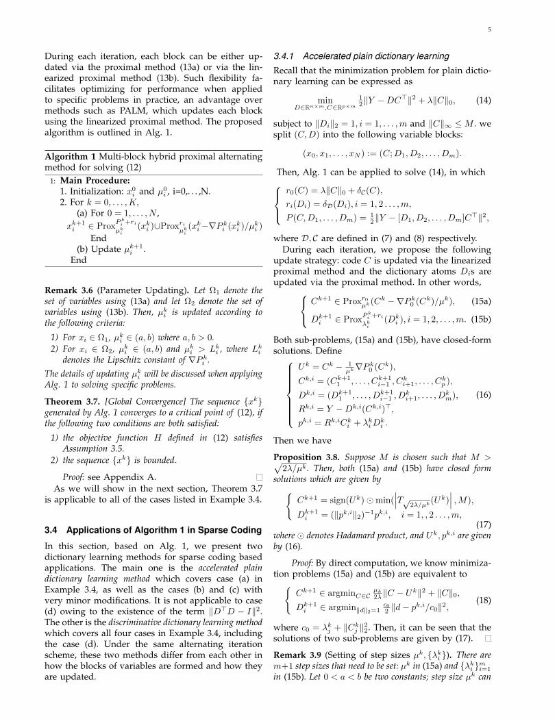
Iteration number0 5 10 15 20 25 30

Obj

ectiv

e va

lue

#108

3.58

3.59

3.6

3.61

3.62

3.63Noise level <=10

PALMAlg. 2Alg. 3

Iteration number0 5 10 15 20 25 30

Obj

ectiv

e va

lue

#108

6.61

6.62

6.63

6.64

6.65

6.66

6.67Noise level <=15

PALMAlg. 2Alg. 3

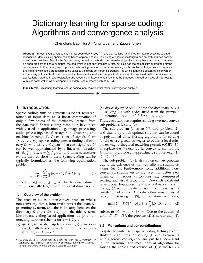
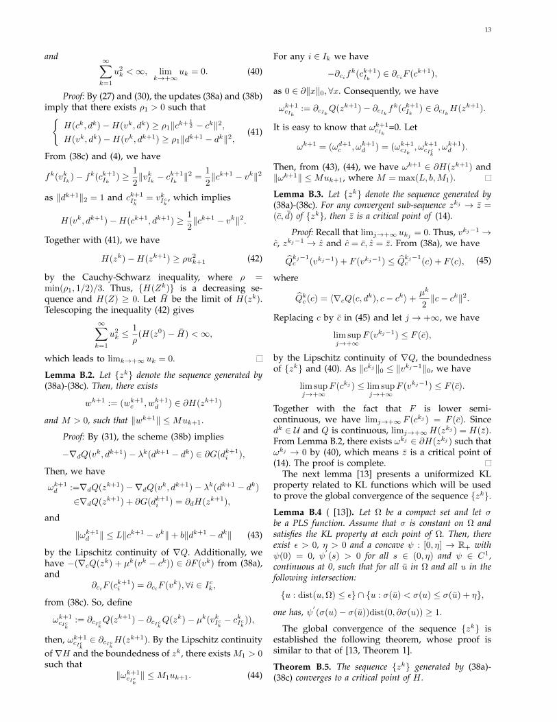
Fig. 2. Objective function value versus iteration number insparse coding based image de-noising.

1

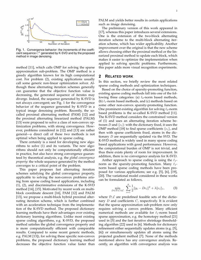
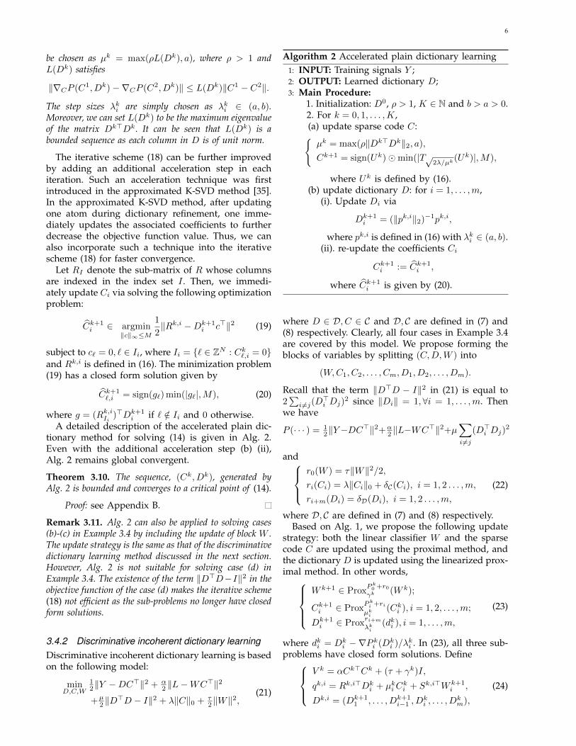
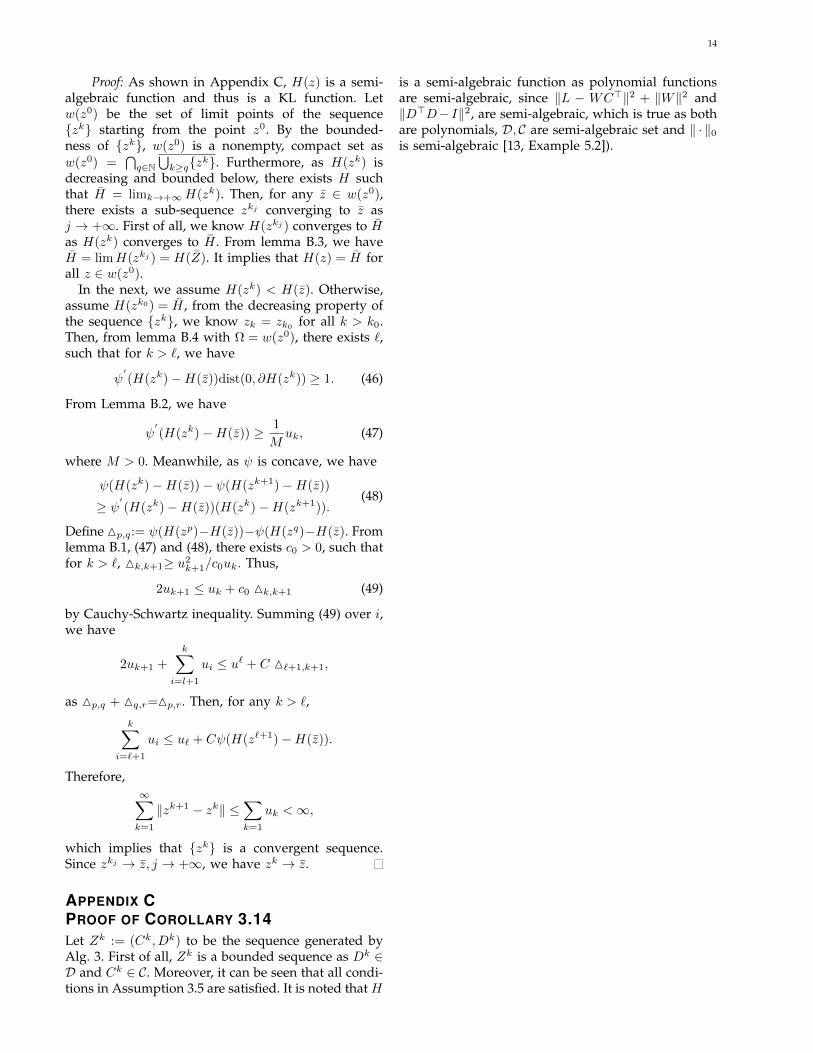
Boat512 Fingerprint512 Hill512

Lena512 Man512 Peppers512

Fig. 3. Six test images for image denoising.

8

4.1 Image DenoisingIn image denoising, we follow the same procedure in[11]. Through all the experiments in image denoising,the dimension of the dictionary is set to be the same asthe K-SVD method [34], i.e. m = 4n, The dictionary islearned from 4× 104 image patches randomly chosenfrom the input noisy image. The patch size is 8×8. Theparameter λ is set to 15σ2 for the dictionary learningprocess, where σ denotes noise standard deviation.level, the parameter ρ is set to 1 + 10−3. All methodsused in experiments were set to run for at most 30iterations. All experiments were preformed in theLinux version of MATLAB R2011b (64 bit) runningon a PC workstation with an INTEL CPU (2.4 GHZ)and 48 GB of RAM. The experiments are done on sixtest images (see Fig. 3) with different noise standarddeviations.

Four dictionary learning methods were tested inimage denoising: the K-SVD method [35]1, PALM[13], Alg. 2 and Alg. 3. Same as the K-SVD method,the dictionary is initialized using an over-completeDCT dictionary (see [11] for more details). Alg. 3 wasapplied to solving (1) by setting the weight of theincoherence term and the weight of discriminativeterm to zero and removing the corresponding compu-tational steps. The implementation of PALM is doneby splitting (C,D) into the blocks (C,D1, D2, . . . , Dm)and updating each block using the linearized proxi-mal method.

4.1.1 Computational efficiencyFig. 2 shows how fast the objective function valueis reduced by each of the three methods. The K-SVD method is not included as it considers an un-constrained model whose objective function is dif-ferent from the other three. It can be seen that bothAlg. 2 and Alg. 3 reduce the objective function valuenoticeably faster than PALM. The difference betweenAlg. 2 and Alg. 3 is rather minor.

A comparison of running time is shown in Tab. 1. Itcan be seen that Alg. 2 and PALM are the fastest one,while the K-SVD method and Alg. 3 are noticeablyslower. The speed of Alg. 2 and PALM on runningtime agrees with the theoretical computational com-plexity. Let K denote the average number of nonzeroentries in each column of C. By direct counting, thetotal number of the dominant operations per iterationin Alg. 2 is

TAlg. 2 = p(2nm+ 6Km+ 4Kn) + 6nm2.

When K n ∼ m p, it is about 2pnm, while it isabout 2pnm+ pK2m in the K-SVD method ( [35]).

Overall, Alg. 2 is the best performer as it is notice-ably faster at reducing the objective function valueper iteration while at the same time not requiringsignificantly more time per iteration.

1. http://www.cs.technion.ac.il/∼ronrubin/software.html

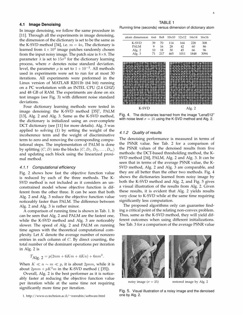
TABLE 1Running time (seconds) versus dimension of dictonary atom

atom dimension 6x6 8x8 10x10 12x12 14x14 16x16

K-SVD 39 70 114 164 228 308PALM 9 16 28 42 60 86Alg. 2 10 18 30 45 66 96Alg. 3 71 217 465 1011 1848 3094

K-SVD Alg. 2

Fig. 4. The dictionaries learned from the image ”Lena512”with noise level σ = 25 using the K-SVD method and Alg. 2.

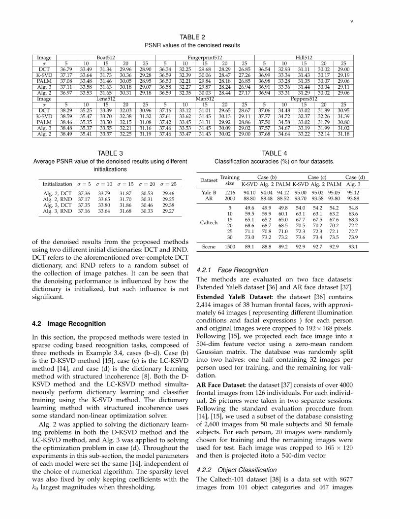
4.1.2 Quality of resultsThe denoising performance is measured in terms ofthe PSNR value. See Tab. 2 for a comparison ofthe PSNR values of the denoised results from fivemethods: the DCT-based thresholding method, the K-SVD method [34], PALM, Alg. 2 and Alg. 3. It can beseen that in terms of the average PSNR value, the K-SVD method, Alg. 2 and Alg. 3 are comparable, andthey are all better than the other two methods. Fig. 4shows the dictionaries learned from noisy image byboth the K-SVD method and Alg. 2, and Fig. 5 givesa visual illustration of the results from Alg. 2. Giventhese results, it is evident that Alg. 2 yields resultsvery close to K-SVD while at the same time requiringsignificantly less computation.

The proposed algorithms only can guarantee find-ing a critical point of the relating non-convex problem.Thus, same as the K-SVD method, they will yield dif-ferent outcomes when using different initializations.See Tab. 3 for a comparison of the average PSNR value

noisy image (σ = 25) restored image by Alg. 2

Fig. 5. Visual illustration of a noisy image and the denoisedone by Alg. 2.

9

TABLE 2PSNR values of the denoised results

Image Boat512 Fingerprint512 Hill512σ 5 10 15 20 25 5 10 15 20 25 5 10 15 20 25

DCT 36.79 33.49 31.34 29.96 28.90 36.34 32.25 29.68 28.29 26.85 36.54 32.93 31.11 30.02 29.00K-SVD 37.17 33.64 31.73 30.36 29.28 36.59 32.39 30.06 28.47 27.26 36.99 33.34 31.43 30.17 29.19PALM 37.08 33.48 31.46 30.05 28.95 36.50 32.21 29.84 28.18 26.85 36.98 33.28 31.35 30.07 29.06Alg. 3 37.11 33.58 31.63 30.18 29.07 36.58 32.27 29.87 28.24 26.94 36.91 33.36 31.44 30.04 29.11Alg. 2 36.97 33.53 31.65 30.31 29.18 36.59 32.35 30.03 28.44 27.17 36.94 33.31 31.29 30.02 29.06Image Lena512 Man512 Peppers512σ 5 10 15 20 25 5 10 15 20 25 5 10 15 20 25

DCT 38.29 35.25 33.39 32.03 30.96 37.16 33.12 31.01 29.65 28.67 37.06 34.48 33.02 31.89 30.95K-SVD 38.59 35.47 33.70 32.38 31.32 37.61 33.62 31.45 30.13 29.11 37.77 34.72 32.37 32.26 31.39PALM 38.46 35.35 33.50 32.15 31.08 37.42 33.45 31.31 29.92 28.86 37.50 34.58 33.02 31.79 30.80Alg. 3 38.48 35.37 33.55 32.21 31.16 37.46 33.53 31.45 30.09 29.02 37.57 34.67 33.19 31.99 31.02Alg. 2 38.49 35.41 33.57 32.25 31.19 37.46 33.47 31.43 30.02 29.00 37.68 34.64 33.22 32.14 31.18

TABLE 3Average PSNR value of the denoised results using different

initializations

Initialization σ = 5 σ = 10 σ = 15 σ = 20 σ = 25

Alg. 2, DCT 37.36 33.79 31.87 30.53 29.46Alg. 2, RND 37.17 33.65 31.70 30.31 29.25Alg. 3, DCT 37.35 33.80 31.86 30.46 29.38Alg. 3, RND 37.16 33.64 31.68 30.33 29.27

of the denoised results from the proposed methodsusing two different initial dictionaries: DCT and RND.DCT refers to the aforementioned over-complete DCTdictionary, and RND refers to a random subset ofthe collection of image patches. It can be seen thatthe denoising performance is influenced by how thedictionary is initialized, but such influence is notsignificant.

4.2 Image Recognition

In this section, the proposed methods were tested insparse coding based recognition tasks, composed ofthree methods in Example 3.4, cases (b–d). Case (b)is the D-KSVD method [15], case (c) is the LC-KSVDmethod [14], and case (d) is the dictionary learningmethod with structured incoherence [8]. Both the D-KSVD method and the LC-KSVD method simulta-neously perform dictionary learning and classifiertraining using the K-SVD method. The dictionarylearning method with structured incoherence usessome standard non-linear optimization solver.

Alg. 2 was applied to solving the dictionary learn-ing problems in both the D-KSVD method and theLC-KSVD method, and Alg. 3 was applied to solvingthe optimization problem in case (d). Throughout theexperiments in this sub-section, the model parametersof each model were set the same [14], independent ofthe choice of numerical algorithm. The sparsity levelwas also fixed by only keeping coefficients with thek0 largest magnitudes when thresholding.

TABLE 4Classification accuracies (%) on four datasets.

Dataset Training Case (b) Case (c) Case (d)size K-SVD Alg. 2 PALM K-SVD Alg. 2 PALM Alg. 3

Yale B 1216 94.10 94.04 94.12 95.00 95.02 95.05 95.12AR 2000 88.80 88.48 88.52 93.70 93.58 93.80 93.88

Caltech

5 49.6 49.9 49.8 54.0 54.2 54.2 54.810 59.5 59.9 60.1 63.1 63.1 63.2 63.615 65.1 65.2 65.0 67.7 67.5 67.6 68.320 68.6 68.7 68.5 70.5 70.2 70.2 72.225 71.1 70.8 71.0 72.3 72.3 72.1 72.730 73.0 73.2 73.2 73.6 73.4 73.5 73.9

Scene 1500 89.1 88.8 89.2 92.9 92.7 92.9 93.1

4.2.1 Face RecognitionThe methods are evaluated on two face datasets:Extended YaleB dataset [36] and AR face dataset [37].Extended YaleB Dataset: the dataset [36] contains2,414 images of 38 human frontal faces, with approxi-mately 64 images ( representing different illuminationconditions and facial expressions ) for each personand original images were cropped to 192×168 pixels.Following [15], we projected each face image into a504-dim feature vector using a zero-mean randomGaussian matrix. The database was randomly splitinto two halves: one half containing 32 images perperson used for training, and the remaining for vali-dation.AR Face Dataset: the dataset [37] consists of over 4000frontal images from 126 individuals. For each individ-ual, 26 pictures were taken in two separate sessions.Following the standard evaluation procedure from[14], [15], we used a subset of the database consistingof 2,600 images from 50 male subjects and 50 femalesubjects. For each person, 20 images were randomlychosen for training and the remaining images wereused for test. Each image was cropped to 165 × 120and then is projected itoto a 540-dim vector.

4.2.2 Object ClassificationThe Caltech-101 dataset [38] is a data set with 8677images from 101 object categories and 467 images

10

from an additional background category. Same as [39],for each image, the SIFT feature based spatial pyra-mid feature [40] was extracted and further reducedto 3000-dim via PCA. Following standard protocol,we randomly picked 5, 10, 15, 20, 25, 30 samples percategory for training and used the rest for test.

4.2.3 Scene classificationThe experiments were done on the Scene-15dataset [40], which contains both outdoor andindoor scenes. The number of images per categoryvaries from 210 to 410, and the resolution of eachimage is about 250 × 300. For each image, theSIFT feature based spatial pyramid feature [40]was extracted and further reduced to 3000-dim viaPCA. Following the experimental settings of [14],we randomly selected 100 images per category fortraining and used the rest for test.

4.2.4 Results and DiscussionThe results are listed in Tab. 4. It can be seen that theperformance of Alg. 2 is at least comparable to that ofthe K-SVD method or PALM in all scenarios. Overall,the classification performance using the sparse codingmodel in the case (d) of Example 3.4 is better than theother three models, and Alg. 3 can be used for solvingthe non-convex problem in case (d) of Example 3.4.

5 SUMMARY AND FUTURE WORK

In this paper, we proposed a multi-block alternatingproximal method with global convergence propertyfor solving a class of `0-norm related optimizationproblems arising from sparse coding. The proposedalgorithms are not only theoretically sound for non-convex problems arising from sparse coding basedapplications, but were also shown to be computation-ally efficient in practical sparse coding based applica-tions. In future, we will further investigate stochasticmethods for solving the optimization problems insparse coding with the aim of converging to globalminimizers.

REFERENCES[1] I. Tosic and P. Frossard, “Dictionary learning,” IEEE Signal

Process. Mag., vol. 28, no. 2, pp. 27–38, 2011.[2] A. L. Chistov and D. Y. Grigor’ev, “Complexity of quantifier

elimination in the theory of algebraically closed fields,” inMathematical Foundations of Computer Science. Springer, 1984,pp. 17–31.

[3] A. Tropp, “Greed is good: algorithmic results for sparse ap-proximation,” IEEE Trans. Inf. Theory, 2004.

[4] S. Chen, D. Donoho, and M. Saunders, “Atomic decompositionby basis pursuit,” SIAM J. Sci. Comput., 1999.

[5] J. Mairal, F. Bach, J. Ponce, and G. Sapiro, “Online learning formatrix factorization and sparse coding,” J. Mach. Learn. Res.,vol. 11, pp. 19–60, 2010.

[6] R. Jenatton, J. Mairal, F. R. Bach, and G. R. Obozinski, “Prox-imal methods for sparse hierarchical dictionary learning,” inICML, 2010.

[7] J. Mairal, F. Bach, J. Ponce, G. Sapiro, and A. Zisserman,“Supervised dictionary learning,” in NIPS, 2009.

[8] I. Ramirez, P. Sprechmann, and G. Sapiro, “Classification andclustering via dictionary learning with structured incoherenceand shared features,” in CVPR, 2010.

[9] B. Mailhe, D. Barchiesi, and M. D. Plumbley, “INK-SVD:Learning incoherent dictionaries for sparse representations,”in ICASSP, 2012.

[10] D. Barchiesi and M. D. Plumbley, “Learning incoherent dic-tionaries for sparse approximation using iterative projectionsand rotations,” IEEE Trans. Signal Process., 2013.

[11] M. Aharon, M. Elad, and A. Bruckstein, “K-SVD: An algorithmfor designing overcomplete dictionaries for sparse representa-tion,” IEEE Trans. Signal Process., vol. 54, no. 11, pp. 4311–4322,2006.

[12] H. Attouch, J. Bolte, P. Redont, and A. Soubeyran, “Proximalalternating minimization and projection methods for noncon-vex problems: An approach based on the kurdyka-lojasiewiczinequality,” Math. Oper. Res., vol. 35, no. 2, pp. 438–457, 2010.

[13] J. Bolte, S. Sabach, and M. Teboulle, “Proximal alternatinglinearized minimization for nonconvex and nonsmooth prob-lems,” Math. Program., pp. 1–36, 2013.

[14] Z. Jiang, Z. Lin, and L. Davis, “Learning a dicscriminativedictionary for sparse coding via label consistent K-SVD,” inCVPR, 2011.

[15] Q. Zhang and B. Li, “Discriminative K-SVD for dictionarylearning in face recognition,” in CVPR, 2010.

[16] Y. Xu and W. Yin, “A block coordinate descent method formulti-convex optimization with applications to nonnegativetensor factorization and completion,” SIAM J. Imaging. Sci.,vol. 6, no. 3, pp. 1758–1789, 2013.

[17] C. Bao, H. Ji, Y. Quan, and Z. Shen, “`0 norm based dictioanrylearning by proximal method with global convergence,” inCVPR, 2014.

[18] A. Tropp, “Greed is good: algorithmic results for sparse ap-proximation,” IEEE Trans. Inf. Theory, 2004.

[19] J. Mairal, F. Bach, J. Ponce, G. Sapiro, and A. Zisserman, “Non-local sparse models for image restoration,” in ICCV, 2009.

[20] J. Mairal, M. Elad, and G. Sapiro, “Sparse representation forcolor image restoration,” IEEE Trans. Image Process., vol. 17,no. 1, pp. 53–69, 2008.

[21] B. Efron, T. Hastie, I. Johnstone, and R. Tibshirani, “Least angleregression,” Ann. statist., vol. 32, no. 2, pp. 407–499, 2004.

[22] A. Beck and M. Teboulle, “A fast iterative shrinkage-thresholding algorithm for linear inverse problems,” SIAM J.Imaging. Sci., 2009.

[23] Y. Xu and W. Yin, “A fast patch-dictionary method for thewhole image recovery,” UCLA CAM report, 2013.

[24] J. Fan and R. Li, “Variable selection via nonconcave penalizedlikelihood and its oracle properties,” J. Am. Statist. Assoc., 2001.

[25] C.-H. Zhang, “Nearly unbiased variable selection under min-imax concave penalty,” Ann. Statist., 2010.

[26] J. Shi, X. Ren, G. Dai, J. Wang, and Z. Zhang, “A non-convexrelaxation approach to sparse dictionary learning,” in CVPR,2011.

[27] A.Rakotomamonjy, “Direct optimization of the dictionarylearning,” IEEE Trans. Signal Process., 2013.

[28] S. Sra, “Scalable nonconvex inexact proximal splitting,” inNIPS, 2012.

[29] P. Gong, C. Zhang, Z. Lu, J. Huang, and J. Ye, “A generaliterative shrinkage and thresholding algorithm for non-convexregularized optimization problems,” in ICML, 2013.

[30] J. M. Ortega and W. C. Rheinboldt, Iterative solution of nonlinearequations in several variables. Siam, 2000, vol. 30.

[31] M. J. Powell, “On search directions for minimization algo-rithms,” Math. Program., vol. 4, no. 1, pp. 193–201, 1973.

[32] L. Grippo and M. Sciandrone, “On the convergence of theblock nonlinear gauss–seidel method under convex con-straints,” Oper. Res. Lett., vol. 26, no. 3, pp. 127–136, 2000.

[33] R. T. Rockafellar and R. J.-B. Wets, Variational analysis:grundlehren der mathematischen wissenschaften. Springer, 1998,vol. 317.

[34] M. Elad and M. Aharon, “Image denoising via sparse andredundant representations over learned dictionaries,” IEEETrans. Image Process, 2006.

[35] R. Rubinstein, M. Zibulevsky, and M. Elad, “Efficient imple-mentation of the K-SVD algorithm using batch orthogonalmatching pursuit,” CS Technion, 2008.

11

[36] A. S. Georghiades, P. N. Belhumeur, and D. J. Kriegman, “Fromfew to many: Illumination cone models for face recognitionunder variable lighting and pose,” IEEE Trans. Pattern Anal.Mach. Intell., 2001.

[37] A. Martınez and R. Benavente, “The ar face database,” Com-puter Vision Center, Tech. Rep., 1998.

[38] L. Fei-Fei, R. Fergus, and P. Perona, “Learning generativevisual models from few training examples: An incrementalbayesian approach tested on 101 object categories,” in CVPRWGMBV, 2004.

[39] L. Zhang, W. Dong, D. Zhang, and G. Shi, “Two-stage imagedenoising by principle component analysis with local pixelgrouping,” Pattern Recogn., 2011.

[40] S. Lazebnik, C. Schmid, and J. Ponce, “Beyond bags of fea-tures: Spatial pyramid matching for recognizing natural scenecategories,” in CVPR, 2006.

[41] H. Attouch, J. Bolte, and B. F. Svaiter, “Convergence of descentmethods for semi-algebraic and tame problems: proximal al-gorithms, forward–backward splitting, and regularized gauss–seidel methods,” Math. Program., vol. 137, no. 1-2, pp. 91–129,2013.

APPENDIX APROOF OF THEOREM 3.7At first, we define KL functions and semi-algebraicfunctions used for the convergence analysis.

Definition A.1 (Kurdyka-Łojasiewicz property [13]).Let f : Rd → (−∞,+∞] be a PLS function. The functionis said to have the KL property at x ∈ dom∂f := x ∈Rd : ∂f 6= ∅ if there exist η > 0, a neighborhood X of xand a concave and continuous function ψ : [0, η) → R+

which satisfies ψ(0) = 0, ψ is C1 on (0, η) and continuousat 0 and ψ

′(s) > 0,∀s ∈ (0, η), such that for all

x ∈ X ∩ x : f(x) < f(x) < f(x) + η,

the following inequality holds:

ψ′(f(x)− f(x))dist(0, ∂f(x)) ≥ 1. (26)

If f satisfy the KL property at each point of dom∂f thenf is called a KL function.

Definition A.2. (Semi-algebraic sets and functions [12])A subset S of Rn is called the semi-algebraic set if thereexists a finite number of real polynomial functions gij , hijsuch that S =

⋃j

⋂ix ∈ Rn : gij(x) = 0, hij(x) < 0. A

function f is called the semi-algebraic function if its graph(x, t) ∈ Rn × R, t = f(x) is a semi-algebraic set.

The main tool for the proof is the following theorem.

Theorem A.3 ( [41]). Assume H(z) is a PLS functionwith inf H > −∞, the sequence zkk∈N is a Cauchysequence and converges to a critical point of H(z), if thefollowing four conditions hold:

(P1) Sufficiently decreasing: there exists some positiveconstant ρ1, such that

H(zk)−H(zk+1) ≥ ρ1‖zk+1 − zk‖2, ∀k.

(P2) Relative error: there exists some positive constantρ2 > 0, such that for any wk ∈ ∂H(zk),

‖wk+1‖F ≤ ρ2‖zk+1 − zk‖, ∀k.

(P3) Continuity: there exists a subsequence z(kj)j∈Nand z such that

z(kj) → z, H(zkj )→ H(z), as j → +∞.

(P4) KL property: H satisfies the KL property in itseffective domain.

By the theorem above, we only need to check thatthe sequence generated by Alg. 1 satisfies the condi-tions (P1)-(P4). Let Ω1,Ω2 denote the index sets of thevariables that use proximal update (13a), linearizedproximal update(13b) respectively, and define

P ki (·) := P (xk+10 , · · · , xk+1

i−1 , ·, xki+1, . . . , xkN ),

P ki (·) := P ki (xki ) + 〈∇P ki (xki ), · − xki 〉.

Condition (P1). Before proceeding, we first presenta lemma about continuous differentiable functionswhich can be derived from [13, Lemma 3.1].

Lemma A.4. Let h : Rn → R be a continuouslydifferentiable function and ∇h is Lh-Lipschitz continuousin Ω = x : ‖x‖ ≤M. Then, we have

h(u) ≤ h(v) + 〈u− v,∇h(v)〉+ Lh2‖u− v‖2F ,∀u, v ∈ Ω1,

where Ω = x : ‖x‖ ≤M/2.

Proof: For any x, y ∈ Ω, by the triangular inequal-ity, we know x + αy ∈ Ω where 0 ≤ α ≤ 1. Defineg(α) = h(x+ αy). Then, we have

h(x+ y)− h(x) = g(1)− g(0) =

∫ 1

0

dg

dα(α)dα

≤∫ 1

0

y>∇h(x)dα+ |∫ 1

0

y>(∇h(x+ αy)−∇h(x))dα|

≤y>∇h(x) + ‖y‖∫ 1

0

Lhα‖y‖dα = y>∇h(x) + Lh‖y‖2/2

which completes the proof.When i ∈ Ω1, the term P ki (xki ) + ri(x

ki ) is no less than

P ki (xk+1i ) + ri(x

k+1i ) +

µki2‖xk+1

i − xki ‖2. (27)

When i ∈ Ω2, the term P ki (xki ) + ri(xki ) is no less than

P ki (xki ) + ri(xk+1i ) +

µki2‖xk+1

i − xki ‖2. (28)

By the Lipschitz continuity of ∇iP and lemma A.4,

P ki (xk+1i ) ≤ P ki (xki ) +

Lki2‖xk+1

i − xki ‖2. (29)

The combination of (28) and (29) leads to the fact thatP ki (xki ) + ri(x

ki ) is no less than

P ki (xk+1i ) + ri(x

ki ) +

µki − Lki2

‖xk+1i − xki ‖2. (30)

Summing up (27) and (30) gives the term

H(xk)−H(xk+1) = P k0 (xk0)− P kN (xk+1N )

12

is no less than∑i∈Ω1

µki2‖xk+1

i − xki ‖2 +∑i∈Ω2

µki − Lki2

‖xk+1i − xki ‖2,

as P ki+1(xki+1) = P ki (xk+1i ). Let ρ1 = min(µki −Lki )/2 :

k ∈ N, i ∈ Ω2. Then, ρ1 > 0 since µki > Lki whichgives µki ∈ (a, b). Thus, Condition (P1) is satisfied.

Condition(P2). If i ∈ Ω1, we have

0 ∈ ∇P ki (xk+1i ) + µki (xk+1

i − xki ) + ∂ri(xk+1i ). (31)

Define V ki = −∇P ki (xk+1i )− µki (xk+1

i − xki ). Then,

ωki := V ki +∇iP (xk+1) ∈ ∂iH(xk+1).

If xk is bounded, since ∇P is Lipschitz continuouson any bounded set, there exists M1 > 0 such that

‖wki ‖ ≤M1‖xk+1 − xk‖,∀i ∈ Ω1. (32)

Similarly, if i ∈ Ω2, we have

0 ∈ ∇P ki (xki ) + µki (xk+1i − xki ) + ∂ri(x

k+1i ).

Define V ki = −∇P ki (xki )− µki (xk+1i − xki ). Then,

ωki := V ki +∇iP (xk+1) ∈ ∂iH(xk+1).

By the boundedness of xk and Lipschitz continuityof ∇P , we know there exists M2 > 0 such that

‖wki ‖ ≤M2‖xk+1 − xk‖,∀i ∈ Ω2. (33)

Define M = N max(M1,M2). Then (32) and (33) leadto ‖ωk‖ ≤ M‖xk+1 − xk‖, where ωk = (ω1, . . . , ωN )such that ωi = ωki when i ∈ Ω1 or i ∈ Ω2. Therefore,Condition (P2) is satisfied.

Condition (P3). Consider two convergent sub-sequences xkj → x and xkj−1 → y of a boundedsequence xk. We first show that x = y. Given anypositive integer j, from Condition (P1), we have

H(x0)−H(xj+1) > ρ

j∑k=0

‖xk − xk+1‖2. (34)

Since H(xj) is decreasing and inf H > −∞, thereexist some H such that H(xj) → H as j → +∞. Letj → +∞ in (34), we have

+∞∑k=0

‖xk − xk+1‖2 < H(x0)− H < +∞.

which implies lim ‖xk − xk−1‖ = 0. Then, we havelim ‖xkj+1 − xkj‖ = 0 and x = y.

Denote x = (x1, . . . , xN ). For i ∈ Ω1, we have for allxi ∈ Xi

P ki (xk+1i ) + ri(x

k+1i ) +

µki2‖xk+1

i − xki ‖2

≤ P ki (xi) + ri(xi) +µki2‖xi − xki ‖2.

(35)

Let k = kj − 1, xi = xi in (35) and j → +∞, we havethen lim supj→+∞ ri(x

kji ) ≤ ri(xi).

For i ∈ Ω2, we have

P ki (xk+1i ) + ri(x

k+1i ) +

µki2‖xk+1

i − xki ‖2

≤ P ki (xi) + ri(xi) +µki2‖xi − xki ‖2.

(36)

Let k = kj − 1, xi = xi in (36) and j → +∞, bythe Lipschitz continuity of ∇P and Condition (P1),we have lim supj→+∞ ri(x

kji ) ≤ ri(xi). Together with

the fact that ri is lower semi-continuous, we havelimj→+∞ ri(x

kji ) = ri(xi),∀i = 1, 2 . . . , N. Therefore,

by the continuity of P , we conclude that

limj→+∞

P (xkj ) +

N∑i=1

ri(xkji ) = P (x) +

N∑i=1

ri(xi).

4. Condition (P4). The function H in Theorem 3.7is a semi-algebraic function [13], which automaticallysatisfies the so-called KL property according to thefollowing theorem in [13].

Theorem A.5. ( [13]) Let f is a PLS and semi-algebraicfunction, then f satisfies the KL property in domf .

APPENDIX BPROOF OF THEOREM 3.10Due to space limitation, we only prove the conver-gence of Alg. 2 for m = 1. The proof can be easily ex-tended to the case of m > 1 with small modifications.For m = 1, the objective function in (14) can be rewrit-ten as H(c, d) = F (c) +Q(c, d) +G(d), c ∈ Rn, d ∈ Rp,where F,Q,G are defined as F (c) =

∑pi=1 Fi(ci) =

p∑i=1

λ‖ci‖0 + δX (ci),

G(d) = δU (d), Q(c, d) = 12‖Y − dc

>‖2.(37)

where U = d : ‖d‖ = 1 and X = c : |ci| ≤ M. Fora vector c, let cI denote the sub-vector of c containsthe entries indexed in I . Define Qkd = Q(vk, d). Then,Alg. 2 can be re-written as

vk ∈ ProxF2λ/µk(ck − 1

µk∇cQ(ck, dk)), (38a)

dk+1 ∈ ProxG+Qk

d

λk (dk), (38b)

ck+1 : ck+1Ick

= 0 and ck+1Ik∈ argmin

c∈Xfki (c), (38c)

where Ik = i : vki 6= 0, Y = YIk and fk(c) = 12‖Y −

dk+1c>‖2. It is noted that fk is strongly convex. Definezk = (ck, dk) and

uk+1 = ‖vk − ck‖+ ‖ck+1 − vk‖+ ‖dk+1 − dk‖.

In the next, we introduce a series of lemmas whichare the main ingredients of the proof.

Lemma B.1. Let zk denote the sequence generated by(38a)-(38c). Then, there exists ρ > 0 such that

H(zk)−H(zk+1) ≥ ρu2k+1 (39)

13

and ∞∑k=1

u2k <∞, lim

k→+∞uk = 0. (40)

Proof: By (27) and (30), the updates (38a) and (38b)imply that there exists ρ1 > 0 such that

H(ck, dk)−H(vk, dk) ≥ ρ1‖ck+ 12 − ck‖2,

H(vk, dk)−H(vk, dk+1) ≥ ρ1‖dk+1 − dk‖2,(41)

From (38c) and (4), we have

fk(vkIk)− fk(ck+1Ik

) ≥ 1

2‖vkIk − c

k+1Ik‖2 =

1

2‖ck+1 − vk‖2

as ‖dk+1‖2 = 1 and ck+1Ick

= vkIck, which implies

H(vk, dk+1)−H(ck+1, dk+1) ≥ 1

2‖ck+1 − vk‖2.

Together with (41), we have

H(zk)−H(zk+1) ≥ ρu2k+1 (42)

by the Cauchy-Schwarz inequality, where ρ =min(ρ1, 1/2)/3. Thus, H(Zk) is a decreasing se-quence and H(Z) ≥ 0. Let H be the limit of H(zk).Telescoping the inequality (42) gives

∞∑k=1

u2k ≤

1

ρ(H(z0)− H) <∞,

which leads to limk→+∞ uk = 0.

Lemma B.2. Let zk denote the sequence generated by(38a)-(38c). Then, there exists

wk+1 := (wk+1c , wk+1

d ) ∈ ∂H(zk+1)

and M > 0, such that ‖wk+1‖ ≤Muk+1.

Proof: By (31), the scheme (38b) implies

−∇dQ(vk, dk+1)− λk(dk+1 − dk) ∈ ∂G(dk+1i ),

Then, we have

ωk+1d :=∇dQ(zk+1)−∇dQ(vk, dk+1)− λk(dk+1 − dk)

∈∇dQ(zk+1) + ∂G(dk+1i ) = ∂dH(zk+1),

and

‖ωk+1d ‖ ≤ L‖ck+1 − vk‖+ b‖dk+1 − dk‖ (43)

by the Lipschitz continuity of ∇Q. Additionally, wehave −(∇cQ(zk) + µk(vk − ck)) ∈ ∂F (vk) from (38a),and

∂ciF (ck+1i ) = ∂ciF (vk),∀i ∈ Ick,

from (38c). So, define

ωk+1cIc

k

:= ∂cIckQ(zk+1)− ∂cIc

kQ(zk)− µk(vkIck − c

kIck

)),

then, ωk+1cIc

k

∈ ∂cIckH(zk+1). By the Lipschitz continuity

of ∇H and the boundedness of zk, there exists M1 > 0such that

‖ωk+1cIc

k

‖ ≤M1uk+1. (44)

For any i ∈ Ik we have

−∂cifk(ck+1Ik

) ∈ ∂ciF (ck+1),

as 0 ∈ ∂‖x‖0,∀x. Consequently, we have

ωk+1cIk

:= ∂cIkQ(zk+1)− ∂cIk fk(ck+1

Ik) ∈ ∂cIkH(zk+1).

It is easy to know that ωk+1cIk

=0. Let

ωk+1 = (ωd+1c , ωk+1

d ) = (ωk+1cIk

, ωk+1cIc

k

, ωk+1d ).

Then, from (43), (44), we have ωk+1 ∈ ∂H(zk+1) and‖ωk+1‖ ≤Muk+1, where M = max(L, b,M1).

Lemma B.3. Let zk denote the sequence generated by(38a)-(38c). For any convergent sub-sequence zkj → z =(c, d) of zk, then z is a critical point of (14).

Proof: Recall that limj→+∞ ukj = 0. Thus, vkj−1 →c, zkj−1 → z and c = c, z = z. From (38a), we have

Qkj−1c (vkj−1) + F (vkj−1) ≤ Qkj−1

c (c) + F (c), (45)

where

Qkc (c) = 〈∇cQ(c, dk), c− ck〉+µk

2‖c− ck‖2.

Replacing c by c in (45) and let j → +∞, we have

lim supj→+∞

F (vkj−1) ≤ F (c),

by the Lipschitz continuity of ∇Q, the boundednessof zk and (40). As ‖ckj‖0 ≤ ‖vkj−1‖0, we have

lim supj→+∞

F (ckj ) ≤ lim supj→+∞

F (vkj−1) ≤ F (c).

Together with the fact that F is lower semi-continuous, we have limj→+∞ F (ckj ) = F (c). Sincedk ∈ U and Q is continuous, limj→+∞H(zkj ) = H(z).From Lemma B.2, there exists ωkj ∈ ∂H(zkj ) such thatωkj → 0 by (40), which means z is a critical point of(14). The proof is complete.

The next lemma [13] presents a uniformized KLproperty related to KL functions which will be usedto prove the global convergence of the sequence zk.

Lemma B.4 ( [13]). Let Ω be a compact set and let σbe a PLS function. Assume that σ is constant on Ω andsatisfies the KL property at each point of Ω. Then, thereexist ε > 0, η > 0 and a concave ψ : [0, η] → R+ withψ(0) = 0, ψ

′(s) > 0 for all s ∈ (0, η) and ψ ∈ C1,

continuous at 0, such that for all u in Ω and all u in thefollowing intersection:

u : dist(u,Ω) ≤ ε ∩ u : σ(u) < σ(u) ≤ σ(u) + η,

one has, ψ′(σ(u)− σ(u))dist(0, ∂σ(u)) ≥ 1.

The global convergence of the sequence zk isestablished the following theorem, whose proof issimilar to that of [13, Theorem 1].

Theorem B.5. The sequence zk generated by (38a)-(38c) converges to a critical point of H .

14

Proof: As shown in Appendix C, H(z) is a semi-algebraic function and thus is a KL function. Letw(z0) be the set of limit points of the sequencezk starting from the point z0. By the bounded-ness of zk, w(z0) is a nonempty, compact set asw(z0) =

⋂q∈N

⋃k≥qzk. Furthermore, as H(zk) is

decreasing and bounded below, there exists H suchthat H = limk→+∞H(zk). Then, for any z ∈ w(z0),there exists a sub-sequence zkj converging to z asj → +∞. First of all, we know H(zkj ) converges to Has H(zk) converges to H . From lemma B.3, we haveH = limH(zkj ) = H(Z). It implies that H(z) = H forall z ∈ w(z0).

In the next, we assume H(zk) < H(z). Otherwise,assume H(zk0) = H , from the decreasing property ofthe sequence zk, we know zk = zk0 for all k > k0.Then, from lemma B.4 with Ω = w(z0), there exists `,such that for k > `, we have

ψ′(H(zk)−H(z))dist(0, ∂H(zk)) ≥ 1. (46)

From Lemma B.2, we have

ψ′(H(zk)−H(z)) ≥ 1

Muk, (47)

where M > 0. Meanwhile, as ψ is concave, we have

ψ(H(zk)−H(z))− ψ(H(zk+1)−H(z))

≥ ψ′(H(zk)−H(z))(H(zk)−H(zk+1)).

(48)

Define Mp,q:= ψ(H(zp)−H(z))−ψ(H(zq)−H(z). Fromlemma B.1, (47) and (48), there exists c0 > 0, such thatfor k > `, Mk,k+1≥ u2

k+1/c0uk. Thus,

2uk+1 ≤ uk + c0 Mk,k+1 (49)

by Cauchy-Schwartz inequality. Summing (49) over i,we have

2uk+1 +

k∑i=l+1

ui ≤ u` + C M`+1,k+1,

as Mp,q + Mq,r=Mp,r. Then, for any k > `,

k∑i=`+1

ui ≤ u` + Cψ(H(z`+1)−H(z)).

Therefore,∞∑k=1

‖zk+1 − zk‖ ≤∑k=1

uk <∞,

which implies that zk is a convergent sequence.Since zkj → z, j → +∞, we have zk → z.

APPENDIX CPROOF OF COROLLARY 3.14Let Zk := (Ck, Dk) to be the sequence generated byAlg. 3. First of all, Zk is a bounded sequence as Dk ∈D and Ck ∈ C. Moreover, it can be seen that all condi-tions in Assumption 3.5 are satisfied. It is noted that H

is a semi-algebraic function as polynomial functionsare semi-algebraic, since ‖L − WC>‖2 + ‖W‖2 and‖D>D− I‖2, are semi-algebraic, which is true as bothare polynomials, D, C are semi-algebraic set and ‖ · ‖0is semi-algebraic [13, Example 5.2]).