Did China Tire Safeguard Save U.S. Workers?∗

Sunghoon Chung† Joonhyung Lee‡ Thomas Osang§

June 2014

Abstract

It has been well documented that trade adjustment costs to workers due to global-

ization are significant and that temporary trade barriers have been progressively used in

many countries, especially during periods with high unemployment rates. Consequently,

temporary trade barriers are perceived as a feasible policy instrument for securing domes-

tic jobs in the presence of increased globalization and economic downturns. However, no

study has assessed whether such temporary barriers have actually saved domestic jobs. To

overcome this deficiency, we evaluate the China-specific safeguard case on consumer tires

petitioned by the United States. Contrary to claims made by the Obama administration,

we find that total employment and average wages in the tire industry were unaffected by

the safeguard using the ‘synthetic control’ approach proposed by Abadie et al. (2010). Fur-

ther analysis reveals that this result is not surprising as we find that imports from China

are completely diverted to other exporting countries partly due to the strong presence of

multinational corporations in the world tire market.

JEL Classification: F13, F14, F16

Keywords: China Tire Safeguard, Temporary Trade Barriers, Trade Diversion, Synthetic

Control Method.

∗We thank James Lake and Daniel Millimet for their constant feedback and discussions. We also thank Mered-ith Crowley, Maggie Chen, Thomas Prusa, Timothy Salmon, Romain Wacziarg, Leonard Wantchekon, as well asparticipants at the Midwest International Trade Conference, Spring 2013, and SMU seminar for helpful comments.All errors are ours.

†Corresponding author, Korea Development Institute, 15 Giljae-gil, Sejong 339-007, Korea, Tel: 82-44-550-4278,Fax: 82-44-550-4226, Email: sunghoon.chung@kdi.re.kr

‡Department of Economics, Fogelman College of Business and Economics, The University of Memphis, Email:jlee17@memphis.edu

§Department of Economics, Southern Methodist University, Email: tosang@smu.edu

1

“Over a thousand Americans are working today because we stopped a surge in Chinese

tires, but we need to do more.”

- President Barack Obama, State of the Union Address, Jan 24th, 2012.

“The tariffs didn’t have any material impact on our North American business.”

- Keith Price, a spokesman for Goodyear Tire & Rubber Co., Wall Street

Journal, Jan 20th, 2012.

1 Introduction

While trade barriers have reached historically low levels, a growing number of countries

are worried about job losses as a consequence of the trade liberalization. The concern is well

epitomized in the recent U.S. trade policy agenda. The Obama administration has filed trade

dispute cases with the World Trade Organization (WTO) at a pace twice as fast as that of the

previous administration. Moreover, the Interagency Trade Enforcement Center (ITEC) was

set up in February 2012 to monitor and investigate unfair trade practices.1 During the 2012

presidential election, both candidates pledged to take even stronger actions to protect U.S.

businesses and workers.2

The incentives to secure jobs by raising trade barriers are well explained in the literature.

Political economy of trade policy theory explains that higher risk of unemployment makes in-

dividuals more protectionist, which induces them to demand more protection through voting

or union lobbying activity. The politicians who seek re-election then protect industries with

high unemployment rates (Wallerstein, 1987; Bradford, 2006; Matschke and Sherlund, 2006;

Yotov, 2012). In addition to political economy considerations, there are other models that jus-

tify protectionism. Costinot (2009) derives a model where the aggregate welfare can improve

when highly unemployed industries are protected. Davidson et al. (2012) emphasize fairness

or altruistic concern toward displaced workers as another incentive for protection. Bagwell

and Staiger (2003) argue that trade policies are preferred to domestic redistributive policies

because they beggar thy neighbor: While domestic policies come at the expense of domestic

residents, trade policies cost foreigners.

Surprisingly, however, the literature so far has ignored to check whether such protective

trade policies can actually save domestic jobs. In fact, studies have only focused on the other

1See Rapoza (2012, January 25th) Forbes.2In fact, ever-increasing imports from China were discussed as one of the greatest future threats to the national

security of the U.S. in the debates for the 2012 presidential election.

2

direction, i.e., how trade liberalization affects employment or wages. Gaston and Trefler (1994)

and Trefler (2004), for example, find that import competition due to tariff declines have neg-

ative effects on wages in the U.S. and employment in Canada. In recent studies, Autor et

al. (2013a,b) estimate how much the import surge from China costs U.S. manufacturing em-

ployees, and find that the greater import competition causes higher unemployment, lower

wages, less labor market participation, and greater chance of switching jobs and receiving

government transfers. Roughly speaking, these costs account for one quarter of the aggregate

decline in U.S. manufacturing employment. McLaren and Hakobyan (2012) also find a signif-

icant adverse effect of import exposure to Mexico on U.S. wage growth for blue-color workers

after the implementation of the North American Free Trade Agreement (NAFTA).3

The evidences above seem to imply that re-imposing trade barriers would secure domestic

jobs. However, most recent protection policies are enacted in the form of antidumping, coun-

tervailing duties, or safeguards, which are systematically different in their nature from the

trade barriers such as Most-Favored-Nation (MFN) tariff rates and import quotas that have

been lowered in recent decades. These policies, often collectively called temporary trade bar-

riers (TTBs), are typically (i) contingent, (ii) temporary, and (iii) discriminatory in that duties

are imposed for a limited time to a small set of products from particular countries.4 Due to

these characteristics, there are at least two channels that may divert trade flows and weaken

the impact of a TTB on domestic markets. First, the temporary feature of TTBs leaves a room

for targeted exporting firms to adjust their sales timing to either before or after the tariff inter-

vention. Second, perhaps more importantly, the discriminatory feature can divert the import

of subject products from the targeted country to other exporting countries. Thus, whether –

and the degree to which – a TTB can secure domestic jobs remains an unanswered empirical

question.

Despite the lack of empirical evidence, many WTO member countries have already been

opting for TTBs, especially in domestic recession phases with high unemployment rates. Knet-

ter and Prusa (2003) link antidumping filings with domestic real GDP growth to find their

counter-cyclical relationship during 1980-1998 in the U.S., Canada, Australia, and the Euro-

pean Union. Irwin (2005) extends a similar analysis to the period covering 1947-2002 in the

U.S. case, and finds that the unemployment rate is an important determinant of antidump-

ing investigations. More recently, two companion studies by Bown and Crowley (2012, 2013)

investigate thirteen emerging and five industrialized economies, respectively, and report evi-

dence that a high unemployment rate is associated with more TTB incidents.

This paper aims to fill up the deficiency in the literature by evaluating a special safeguard

3Similar patterns are observed in developing countries, too. See Goldberg and Pavcnik (2005) for Columbia,Menezes-Filho and Muendler (2011) and Kovak (2013) for Brazil, Topalova (2010) for India.

4An exception to discriminatory feature is Global safeguard measure, since it is imposed to all countries.

3

case on Chinese tires (China Tire Safeguard or CTS, henceforth) that has received a great deal

of public attention among recent TTB cases.5 Under Section 421 China-specific safeguard,

the U.S. imposed higher tariffs on certain Chinese passenger vehicle and light-truck tires for

three years from the fourth quarter of 2009 to the third quarter of 2012. The safeguard duties

were 35% ad valorem in the first year, 30% in the second, and 25% in the third on top of the

MFN duty rates.6 The case has triggered not only Chinese retaliation on U.S. poultry and

automotive parts, but also a serious controversy on the actual effectiveness of the CTS for the

U.S. tire industry.7 Despite such controversy, the CTS has been cited as a paragon of successful

trade policy for job security during the 2012 U.S. presidential campaign by both candidates.

The CTS provides a uniquely advantageous setting for answering the question of this pa-

per. While the CTS is representative in that it bears all three TTB characteristics described

above, one important distinction of the CTS is that the safeguard duties are exogenously de-

termined. In antidumping cases, which are the most pervasive form of TTB, duties are en-

dogenously determined to offset the dumping margin. Even after the duties are in place, they

are recalculated over time to adjust the dumping behavior changes of exporting firms.8 These

endogenous tariff changes complicate the evaluation of a tariff imposition effect. Secondly,

the change in the total import of subject Chinese tires before and after the safeguard initiation

is considerably large in both levels and growth rates.9 If TTBs have labor market outcomes,

this dramatic change should allow us to observe it. Third, contrary to most trade disputes in

which the producers filed a claim, the petition for the CTS was filed by the union representing

employees. This implies that the petition is indeed intended for employees’ benefits and thus

labor market effects.10

Estimating the impact of the China Tire Safeguard brings some challenges that need to be

addressed. Above all, the estimates may be confounded by macroeconomic trends. Since the

U.S. economy has been in recovery after the great recession of 2008-09, one may capture a spu-

riously inflated labor market effects that would have occurred even without tariff changes. A

typical identification strategy in this case is to compare the tire industry with similar industries

who have not experienced tariff changes. However, there is no clear criterion for choosing ap-

propriate control industries in our case. To circumvent this problem, we exploit the synthetic

control method (SCM) designed by Abadie and Gardeazabal (2003) and Abadie et al. (2010).

5Prusa (2011, P. 55) describes the China Tire Safeguard as “one of the most widely publicized temporary tradebarriers during 2005–9, garnering significant press attention both in the USA and in China.”

6MFN duty rates are 4% for radial (or radial-ply) tires and 3.4% for other type (bias-ply) of tires.7See also Bussey (2012, January 20th) in Wall Street Journal.8This recalculation process is also called administrative review process. Many studies investigate the implica-

tion of the review process on exporting firm’s pricing behavior. See, for example, Blonigen and Haynes (2002) andBlonigen and Park (2004).

9Detail statistics are provided in Section 3.10Prusa (2011) argues that the last two features are the main reasons of receiving unusual public attention.

4

The core strategy of the SCM is to construct a “synthetic” industry by optimally weighting a

group of potential controls so that its outcome resembles the outcome of the tire industry as

close as possible during the pre-intervention period. Hence, the synthetic industry will mimic

the counterfactual tire industry for the post-intervention period as well in the absence of the

safeguard measuring.

The SCM estimates provide a striking result. Contrary to the Obama administration’s claim

that the safeguard measures had a positive effect on the labor market (see quote above), we

find that total employment and wages in the tire industry show no different time trends from

those in the synthetic industries. Our result is supported by another finding that the substan-

tial drop in Chinese tire imports is completely offset by the increase in imports from other

countries. This complete import diversion leaves little room for domestic producers to make

an adjustment in their production, which in turn induces no change in the labor market. Thus,

our study highlights that the discriminatory feature of TTB plays a crucial role for the negligi-

ble labor market effect.

To our best knowledge, there is no study that investigates the effect of a TTB on domestic

labor market outcomes. Some papers have looked at the exporting firms’ strategic responses

to a TTB through price adjustments (Blonigen and Haynes, 2002; Blonigen and Park, 2004),

quantity controls (Staiger and Wolak, 1992), or tariff-jumping investment (Blonigen, 2002;

Belderbos et al., 2004). These firm behaviors alter the aggregate trade patterns, and these

changes in trade patterns have been analyzed in the literature (Prusa, 1997; Brenton, 2001;

Bown and Crowley, 2007). Other studies have turned their attention to TTB effects on do-

mestic firms, with particular interests in output (Staiger and Wolak, 1994), markup (Konings

and Vandenbussche, 2005), profit (Kitano and Ohashi, 2009), and productivity (Konings and

Vandenbussche, 2008; Pierce, 2011).11 Although these studies may have some implications for

labor market outcomes, they are insufficient to draw definite conclusions on employment and

wage effects.

We begin our study with an overview of the China safeguard and the U.S. tire industry in

section 2. Section 3 describes data and time trends of Chinese tire imports and employment.

Section 4 provides the empirical model and discusses the results. Section 5 reports and dis-

cusses the results, and section 6 explores a potential mechanism that has driven our results.

Section 7 concludes with policy implications and the direction of future researches.

11These studies mostly deal only with antidumping cases. (Blonigen and Prusa, 2003) provide a comprehensivesurvey on the literature of antidumping.

5

2 Overview of China Safeguard and the U.S. Tire Industry

The U.S. Trade Act of 1974 describes conditions under which tariffs can be applied and

which groups can file a petition. Once the petition is filed, the International Trade Commis-

sion (USITC) makes a recommendation to the president. The president then makes a decision

whether to approve or veto the tariff. Two sections (Section 201 and 421) of the Trade Act

of 1974 deal with the use of safeguard tariffs. Under Section 201 (Global Safeguard), USITC

determines whether rising imports have been a substantial cause of “serious” injury, or threat

thereof, to a U.S. industry. On the other hand, Section 421 (China-specific Safeguard or China

Safeguard) applies only to China. China Safeguard was added by the U.S. as a condition to

China’s joining the WTO in 2001 and expired in 2013. Under Section 421, the USITC deter-

mines whether rising imports from China cause or threaten to cause a significant “material”

injury to the domestic industry. Total seven China Safeguard cases had been filed, of which

two were denied by the USITC and five were approved. Of these five approved cases, the

president ruled in favor of only one, which is the tire case.

There are a number of noteworthy differences regarding Global Safeguard vs. China Safe-

guard. First, the term “serious” vs. “material” implies a significant difference. Simply put,

China Safeguard can be applied under weaker conditions than Global Safeguard. For China

Safeguard to be applied, rising imports do not have to be the most important cause of injury to

the domestic industry, while this has to be the case for Global Safeguard. That is, the imports

from China need not be equal to or greater than any other cause. Second, China Safeguard is

discriminatory and allows MFN treatment to be violated.12

The U.S. tire industry has several characteristics to be considered for our analysis. First,

tire production is dominated by a few large multinational corporations (MNCs) in both the

U.S. and the world. As of 2008, ten firms produce the subject tires in the U.S., and eight of

them are MNCs.13 Production of the subject tires are so concentrated that five major MNCs

(Bridgestone, Continental, Cooper, Goodyear, and Michelin) control about 95% of domestic

production and 60% of worldwide production.14 Except Continental, Seven MNCs of the ten

domestic producers also have manufacturing facilities in China. Second, the subject tires are

known to feature three distinct classes, flagship (high quality), secondary (medium quality),

12There are three other primary areas under the WTO in which exceptions to MFN-treatment for import restric-tions are broadly permissible: (1) raising discriminatory trade barriers against unfairly traded goods under an-tidumping or countervailing duty laws; (2) lowering trade barriers in a discriminatory manner under a reciprocalpreferential trade agreement; and (3) lowering trade barriers in a discriminatory manner to developing countriesunilaterally, for example, under the Generalized System of Preferences (GSP). For an additional discussion of theChina safeguard, see Messerlin (2004) and Bown (2010).

13The ten U.S. subject tire producers are Bridgestone, Continental, Cooper, Denman, Goodyear, Michelin, Pirelli,Specialty Tires, Toyo, and Yokohama. Eight firms except Denman and Specialty Tires are MNCs.

14Data source: Modern tire dealer (http://www.moderntiredealer.com/stats/default.aspx).

6

and mass market (low quality). The domestic producers have largely shifted their focus to

higher-value tires since 1990s, leaving mass market tire productions to overseas manufactur-

ers.

These characteristics explain why the petition was not welcomed by the U.S. tire produc-

ers. The temporary tariff protection may actually hurt the MNCs’ global production strate-

gies. Moreover, the CTS would not have any positive influence to their domestic facilities that

mainly produce high and medium quality tires, given that those tires are not well substitutable

for low quality Chinese tires.15

3 Data and Descriptive Statistics

Our data on quarterly imports from 1998Q1 to 2012Q3 are taken from the U.S. International

Trade Commission. Import data are available up to Harmonized System (HS) 10-digit, and

each 10-digit code is defined as a “product”. Import value is measured by customs value

that is exclusive of U.S. import duties, freight, insurance, and other charges. We also define

an “industry” as the 6-digit industry in the North American Industry Classification System

(NAICS). According to the definition, the tire industry is 326211, “Tire Manufacturing (except

Retreading)”, which comprises “establishments primarily engaged in manufacturing tires and

inner tubes from natural and synthetic rubber”. This corresponds to 62 tire-related products in

the HS 10-digit level (with heading 4006, 4011, 4012, and 4013) among which 10 tire products

are subject to the safeguard measures.

Data on employment and wages in U.S. tire industry covering the same time period are

from the Bureau of Labor Statistics Quarterly Census of Employment and Wages (QCEW).16 In

fact, Bureau of Labor Statistics provides two different industry-level employment databases,

the QCEW and the Current Employment Statistics (CES). We use the QCEW in this paper,

because it provides total employment and wages statistics for all 6-digit industries, while the

CES contains only part of them.17 For industry-level characteristics, we use data taken from

the Annual Survey of Manufactures.

Figure 1 plots time trends of the aggregate import value of the ten tire products subject to

the CTS as well as total employment in the U.S. tire industry from 1998Q1 to 2012Q3. The

import of Chinese tires starts to surge in 2001, just before China’s accession to the WTO. It

continues to grow dramatically until the activation of the CTS, except for a slight drop in

15Because of these characteristics of the U.S. tire industry, Prusa (2009) predicted that the effect of the CTS wouldbe negligible.

16While wages are reported on a quarterly basis, employment data are produced monthly. We construct quar-terly employment data by simply averaging of the monthly data.

17Both databases have employment data in the tire industry. We checked the discrepancy between the two data,but there was no systematic or significant difference.

7

early 2009 due to the global financial crisis.18 Specifically, the import increases by 300 times

during ten years from $5.2 million dollars in 1999 to $1.56 billion dollars in 2008. In terms of

relative size, China alone accounts for a quarter of the U.S. total import of subject tires in 2008,

with tire imports from the rest of the world (ROW) at $4.80 billion dollars in the same year.

The value also amounts to 9.2% of gross value added of the U.S. tire industry in 2008, which

stood at $16.98 billion dollars.

The punitive tariffs substantially discourage the rising trend, reducing total imports from

China by 62% between 2009Q3 to 2009Q4. A sharp rise between Q2 and Q3 followed by the

sharp decline between Q3 and Q4 indicates that some importers in the U.S. bought the subject

Chinese tires in advance of the CTS to avoid the higher expected price after 2009Q3. After

2009Q4, tire imports from China are relatively flat, albeit at a much lower level compared to

pre-CTS levels.

Interestingly, the trend of employment in the U.S. tire industry stands in sharp contrast

to the trend of Chinese tire imports. It starts to fall when the Chinese tire imports start to

rise in 2001. In particular, the decline of employment in 2002Q1 coincides with China’s WTO

accession. Another falloff in 2006Q4 is caused by the strike in the U.S. tire industry and is not

relevant to the Chinese tire imports. In terms of growth, employment in the U.S. tire industry

falls by 30.5% from 2002Q1 to 2009Q3.19

The activation of the CTS seems to not only stop further decline in employment (with some

lags) but also prompt a slight recovery thereafter. As the Obama administration claims, total

employment increases from 45,855 in 2009Q3 to 46,812 in 2011Q4, an increase of about one

thousand workers. However, the employment trend around 2009 is obviously confounded by

the economic recovery from the global financial crisis, and thus the time-series data alone do

not allow us to identify the safeguard effect on employment in the U.S. tire industry.

4 Empirical Model

4.1 A Conceptual Framework

We conceptually sketch how domestic labor market can be affected by foreign competition

to propose an appropriate empirical model for identifying the safeguard effect. If the labor

market for an industry were competitive, domestic employment and wages would be simul-

18As Staiger and Wolak (1994) finds, subject tire imports may also fall because of the safeguard investigationstarted from April in 2009.

19Note that, however, there are many other industries that suffered from more severe employment losses thanthe tire industry over the same period. For example, we compare the employment growth rates of nine NAICS6-digit industries in Table 2. The table shows that three out of nine industries have lower employment growthrates than the tire industry has.

8

taneously determined by its supply and demand elasticities. A change in foreign competition

works as a product demand shifter in this model. For example, an increase in import com-

petition would shrink the demand for domestic product and thereby decrease labor demand

while wages adjust to soften the degree to which the demand decreases through labor supply

elasticities (Freeman and Katz, 1991; Revenga, 1992).

In reality, however, industries in the U.S. are likely to face non-competitive labor market

for a number of reasons. One important reason is the presence of labor union through which

its members bargain with employers over terms and working conditions of employment. We

indeed observe such behavior in the tire industry being expressed as a strike in 2006. In

this case, the negotiated wage rate tends to be higher than the competitive rate and, in turn,

reduces the demand for labor, although their magnitudes can be heterogeneous across indus-

tries depending on workers’ bargaining power (Abowd and Lemieux, 1993; Revenga, 1997).

Non-competitive wages and employment can also be driven by other factors including effi-

ciency wages or factor immobility, but in any case the adjustment would arguably be made

in the same direction (i.e., higher wages and lower employment than the competitive equilib-

rium). The non-competitive market structure would also induce some rigidities in wages and

employment over time, because the terms and conditions of employment may hold at least

for a few years.

That said, we benchmark the empirical model by Revenga (1997) where non-competitive

wages are first negotiated between labor union and employers in the presence of foreign com-

petition and then firms choose their employment level according to their own labor demand

curves. More arguments are added to the model as necessary to explain some important fea-

tures in our context. Consider the following wage equation:

wit = α1qit + α2kit + α3mit + α4rit + γwit Dit + µw

i λwt + εit (1)

where wit is log of average weekly wages in industry i at time t. Firms that minimize their

production cost for given factor prices (other than wages) and output level would set their

wages at which marginal cost of labor equals marginal revenue product of labor. Hence, wit is

basically a function of output (qit), cost of capital (kit), and cost of materials (mit) which are all

taken logarithm. The level of industry foreign competition, a product demand shifter in this

model, is proxied by (log of) import penetration ratio, rit, which is equal to the ratio of import

to market size (= output + import - export).20

When the government intervenes in product markets by imposing punitive tariffs to cer-

tain imported goods, its impact on industry wages is supposed to be captured by the coef-

20The lagged wage rate can be added to the equation to explain the rigidity in wages.

9

ficient γwit . Thus, Dit is a simple treatment assignment indicator that is one if industry i is

protected by the safeguard action at time t, and zero otherwise. Note that γwit varies fully over

time and across industries to give us a complete set of heterogeneous safeguard effects on

all industries in all post-intervention periods. The time-varying safeguard effect reflects the

declining schedule of the CTS by 5% annually, but it could also mean that the responses of

industries may come with some lags or simply be transitory.

Eq. (1) contains the term for unobservables (µwi λw

t ) as well as the error term (εit). The unob-

servables are made up of a vector of interactive fixed effects of which dimension is unknown,

and the whole term captures the effects of an unknown number of common factors (λwt ) with

heterogeneous factor loadings (µwi ) that may be jointly correlated with observables. This term

is more flexible to control for unobserved heterogeneity than the conventional configuration

of fixed effects.21 Indeed, we observe several economy-wide shocks in the sample period that

seems to have heterogeneous impacts on industry-level employment and wages across U.S.

industries. As an example, we have no rationale to assume that the financial crisis in 2008

would affect all industries by an equal magnitude. Similarly, not all industries would receive

an equal impact by the China’s accession to WTO in 2001 or its currency manipulation over

recent years. Perhaps, more relevantly, if wage bargaining is negotiated based on the “out-

side” or “alternative” wages available throughout the economy and different industries have

different bargaining powers, then the negotiated wages will also be different across industries.

All of these common factors and industry-specific factor loadings with their interactions may

cause the petitions for protection and subsequent government interventions, in which case

failing to control for such interactive effects would lead to biased estimates for γwit . We assume

that the error term is a white noise.

Once wages are set, firms now are assumed to choose employment level as much as they

demand for the given factor prices (including wages) and output level. The conditional labor

demand function can be estimated from the following equation:

nit = β1qit + β2kit + β3mit + β4rit + β5wit + γnitDit + µn

i λnt + υit . (2)

Log of employment, nit, in industry i at time t is conditional on wages as well as other

factor prices, output level, import penetration ratio, and the treatment assignment in a similar

fashion to Eq. (1).22 However, the structure of unobservables (µni λn

t ) in Eq. (2) can be different

from the one in Eq. (1) in terms of its dimension, since there might be some common factors

that affect employment but not wages and vice versa. The error term vit follows a white noise

21By letting µwi =

[µw

1i 1]

and λwt =

[1

λw1t

], the vector of interactive fixed effects reduces to the conventional two

factors panel model with industry-specific effect and time effect.22Again, the lagged employment can be added to the equation to explain the rigidity in employment.

10

process.

4.2 Estimation Strategy

A common approach to identify the treatment effect is the Difference-In-Differences (DID)

design. In a conventional DID model, the treatment (tire) industry is compared with some

control industries that have not experienced any trade policy change under the assumption

that the treatment industry would have followed the same trend as control industries had the

policy not changed. Therefore, the DID model requires a proper selection of a control group

to satisfy the common trend assumption.

In our case study, however, there is no clear criterion which industries should be chosen

as the control group. One choice may be a group of all manufacturing industries that filed

no petition (hence no protection) during the sample period, but those industries may be too

heterogeneous in their characteristics to have the same time trend in outcome variables. Alter-

natively, a group of manufacturing industries that did file petitions but failed to be accepted

can be considered in the sense that the group would face more or less similar circumstances to

the tire industry. Another possible control group consists of all industries (other than the tire

industry) under the same NAICS 3-digit code, i.e., 326 Plastics and Rubber Product Manufac-

turing since they are classified within the same 3-digit code based on the similarity of industry

characteristics. However, neither of these groups are convincing to satisfy the common trend

assumption.23

The Synthetic Control Method (SCM), designed by Abadie and Gardeazabal (2003) and

Abadie et al. (2010), is appealing to deal with the present problem. They provide a method

to generate a synthetic industry as the optimally weighted average over the outcomes of po-

tential control industries such that the average provides the best fit with the treatment in-

dustry’s outcome for the pre-intervention period. In other words, the SCM chooses the best

combination of any given control industries in the pre-intervention period to generate the

missing counterfactual of the treatment industry, so called synthetic industry, in the post-

intervention period, and thereby increases the likelihood of satisfying the common trend as-

sumption. Thus, the method is less demanding when it comes to choosing the "proper" set of

control industries.

There are two more big advantages to use the synthetic control method in our analysis.

First, the SCM can estimate the time-varying heterogeneous effect of the CTS, while a conven-

23Another problem in the conventional DID method occurs if the number of controls are small, since it leadsto an over-rejection of the null hypotheses of zero effect. Indeed, the suggested control groups above, except thegroup of manufacturing industries that filed no petition, have less than twenty industries. According to Bertrandet al. (2004), we need at least about 40 control industries (with one treatment industry) in order to avoid the over-rejection problem.

11

tional DID or panel fixed effect estimation can only provide an estimate for the time-invariant

average treatment effect. Second, it allows that the dimension of the vector of interactive

fixed effects is arbitrarily unknown. Given that unobservable (time-varying) macroeconomic

or (time-invariant) industry-specific factors have differential effects on each industry and they

are potentially related with the industry selection mechanism for trade remedies, this advan-

tage is important to obtain consistent estimates for the safeguard effect.

However, the SCM has a notable caveat. In order for the SCM to work, we need all ob-

servables to be time-invariant in the model, i.e., the estimation equations should look like the

following:

wit = Xwi α + γw

it Dit + µwi λw

t + εit (3)

nit = Xni β + γn

itDit + µni λn

t + υit . (4)

where Xwi and Xn

i are the vectors of all observables in Eq. (1) and (2) that are restricted to be

constant over time. Thus, Xi’s should be interpreted as the pre-intervention industry charac-

teristics to predict the post-intervention values of outcome variables. Although this require-

ment may appear restrictive, the SCM can instead have any (or combination of) available pre-

intervention outcome variables in Xi, that is, Xi can include all values of dependent variables

in the pre-intervention period as predictors. These lagged values obviously explain the time

trend of dependent variables. Hence, they can account for rigidities in wages and employ-

ment in the pre-intervention period. Moreover, the problem of time-constant restriction on

predictors would be minimized to the extent which each lagged values represent the industry

characteristics at that period.

4.3 Implementation

Without loss of generality, let the tire industry be industry 1 among observable industries.

For all I− 1 potential control industries, a vector of weights, ω = [ω2, ω3, · · · , ωI ], is assigned

such thatI

∑i=2

ω?i yit = y1t, ∀t ≤ 2009Q3 and

I

∑i=2

ω?i Xi = X1 . (5)

Here, the outcome and the vector of predictors, (yit, Xi), is either (wit, Xwi ) or (nit, Xn

i ) for

all i ∈ I. The Eq. (5) implies that we can obtain the exact solution for ω? only if ({y1t}t≤2009Q3, X1)

belongs to the convex hull of [({y2t}t≤2009Q3, X2), · · · , ({yIt}t≤2009Q3, XI)]. If it is not the case,

some weights have to be set negative to minimize the differences between variables in the left-

and right-hand sides in Eq. (5), but the fit may be poor. To avoid such extrapolation problem,

we choose all NAICS 6-digit manufacturing industries that filed no petition during the sample

12

period as our potential control industries in the baseline analysis. This selection gives us 146

control industries.

Note that the optimal weight is obtained for the whole pre-intervention period. Abadie

et al. (2010) show that, for a sufficiently long pre-intervention period, the outcome of the

synthetic industry, ∑Ii=2 ω?

i yit, provides an unbiased estimator of the counterfactual y1t for all

t.24 The estimated treatment effect on the tire industry is obtained by

γ1t = y1t −I

∑i=2

ω?i yit, ∀t ≥ 2009Q4 (6)

where γ1t is for either wages or employment. Finally, we include the 2008 values of total

value of domestic shipments, cost of capital, cost of materials, and import penetration ratio

(additionally, wages for the employment equation) and each variable’s three year growth rate

from 2005 to 2008 as time-invariant pre-intervention characteristics. The sample period in

the baseline analysis ranges from 2001Q1 to 2012Q3, and all values of outcome variables in

this pre-intervention period could also be added in Xi’s as predictors. However, with only

a few selective values in the pre-intervention period, we can provide almost the same but

more efficient estimate for the treatment effect. Therefore, we choose eight lagged values of

employment and wages in 2001Q1, 2002Q2, 2003Q3, 2005Q1, 2006Q1, 2007Q3, 2008Q3, and

2009Q3 that are included in the estimation equations as additional predictors.

5 Estimation Results

5.1 Main Finding

After the synthetic industries for employment and wages are constructed, their industry

characteristics and growth rates are compared to those of the tire industry as well as those of

simple averages of all control industries in Table 1. All numbers indicate that the two synthetic

industries are closer to the tire industry than the averages of all controls in both industry char-

acteristics and growth rates. In particular, the change in employment/wages from 2001Q1

to 2009Q3 are almost identical between tire and synthetic industry giving strong support for

the common trend assumption. At the same time, other industry characteristics of synthetic

industry are much more similar to tire industry than the simple average. Thus, if tire indus-

try had experienced the fundamental change in production structure such that technology or

capital replaced labor and labor-intensive products were offshored, our synthetic industry is

also likely to have such experiences. On the other hand, a conventional DID method would

24For more detail descriptions on estimation procedure and proofs, see Abadie et al. (2010).

13

use the simple average of controls as the counterfactual tire industry, and the common trend

assumption is more likely to be violated.

Table 2 reports the list of control industries with strictly positive weights that construct the

two synthetic industries. Since employment and wages do not exhibit the same time trend,

we expect the optimal weights for each synthetic industry to differ, which turns out to be

true. This again supports the superiority of the synthetic industry approach over the equally

weighted average of 146 controls for both employment and wages.

Figure 2 compares the trends of employment and wages in the U.S. tire industry with those

of the synthetic industries. In general, the synthetic industries mimic employment and wage

trends of the tire industry quite well in the pre-intervention period. An exception is around

2006Q4 due to the strike in the U.S. tire industry. The Root Mean Squared Prediction Error

(RMSPE) shown at the bottom of each figure measures the sum of discrepancies between out-

comes in tire and in synthetic industries for the pre-intervention period. It will be used later as

a criterion for whether a synthetic industry is constructed well enough to mimic the treatment

industry. For the post-intervention period, we see no significant differences between the tire

industry and the synthetic industries for both employment and wages.

To infer the significance of the treatment effects formally, the SCM suggests a set of placebo

tests. A placebo test can be performed by choosing one of the control industries as the treated

industry and the other 145 industries as untreated industries. Specifically, we drop the tire

industry from the sample, and treat industry 2 as the treatment industry. Then, we follow the

same SCM procedure described above to obtain estimates of γ2t for t ≥ 2009Q4 using the rest

of industries 3 through 146 as control industries. This procedure is repeated for i = 3, · · · , 146.

Since all control industries are not protected during the sample period, their treatment effects,

γit for j = 2, · · · , 146, are expected to be zero. Hence, if the tire industry was affected by the

safeguard measures, we should be able to observe significantly different γ1t’s from all other

γit’s.

The results of two sets of placebo tests for employment and wages are displayed in Fig-

ure 3. Because some industries have poor synthetic industries with high RMSPEs, we show

the estimated treatment effects for industries whose RMSPE is less than 0.01 for employment

and 0.02 for wages. The vertical axis shows the estimated treatment effects of the tire and

placebo industries over the sample period. All of them are close to zero before the activation

of CTS, with exception of 2006Q4 in the case of the tire industry. In particular, the treatment

effects in the tire industry after the CTS are well bounded by other placebo treatment effects.

This confirms that neither employment nor wages in the tire industry are significantly affected

by the safeguard measures.

14

5.2 Robustness

We first conduct a couple of robustness checks for our findings with the same SCM esti-

mation method. First of all, the results do not change when we drop the period of the tire

industry strike (i.e., 2006Q4) from our sample period. Secondly, we use alternative control

groups: (i) a group of 35 industries that filed a form of TTB at least once during the sample

period, but failed to be protected at all, and (ii) a group of 14 industries under NAICS 326

Rubber and Plastic Product Manufacturing that are free of any TTB case during the sample

period. The results do not change for both control groups. Finally, our findings still hold when

employment and wages are measured in levels instead of log transforms.25

Next step is to employ alternative estimation methods to check whether our SCM results

are robust to such different methods. First, we estimate the treatment effect using a traditional

DID method. Specifically, we run the following regression equation:

yit = δi + λt + Xitβ + τDit + εit (7)

where yit is either employment or wages in log term and Xit is the vector of corresponding

covariates as in Eq. (1) and Eq. (2). δi and λt are industry and time fixed effects, respectively.

This model is a typical difference-in-differences specification that assigns an equal weight to

all control industries. The first column in Table 3 presents the estimation results. The sample

period ranges from 2007Q3 to 2011Q4 so that we have nine quarters before and after the CTS

activation in the sample.26 Thus, the sample size is 18 quarters times 147 industries including

the tire industry, which equals 2,646. The safeguard effect is shown to be negatively significant

for employment at the 1% level, while it has no significant effect on wages.

Eq. (7) is often called as a random growth model if we add the industry-specific linear

time trend of the dependent variable, ρit, in the equation. This specification is particularly

advantageous when the petition and the subsequent decision for the safeguard protection are

made because of the overall time trend of employment or wages. Technically speaking, it

allows industry-specific growth rates to be correlated with the treatment assignment, Dit, so

that we can avoid the selection bias problem as long as the selection is based on the growth

rates of the dependent variable. Estimation results are presented in the second column in

Table 3. Again, the CTS effect on domestic employment is negatively significant. On the other

hand, its impact on wages is now positive and significant even at the 1% significance level.

25We do not report results for the robustness checks to keep focusing on the main results. The results areavailable upon request.

26The truncation in the pre-intervention period excludes the impact of the strike in the U.S. tire industry. Thetruncation in the post-intervention period is simply due to the lack of data on industry characteristics in 2012. Theestimation results are qualitatively same when we extend the pre-intervention periods.

15

The two estimations above are relying on the common trend assumption between the tire

industry and the rest of 146 control industries. Obviously, this assumption is too restrictive

for given heterogeneity across industries. To deal with the issue, we employ the Propensity

Score Matching method to select control industries comparable to the tire industry in the third

robustness check. Just like we matched industry characteristics in 2008 between the treatment

and control groups for the SCM case, here we match observables in 2008 (i.e., from 2008Q1 to

2008Q4) and choose 10 nearest neighbors to the tire industry with replacement, based on the

propensity scores.27 Then, we run the weighted regression on the controls with unobserved

heterogeneity and industry-specific linear time trend. Consequently, our sample size is as

large as 4,680. Column (3) in Table 3 indicates that the treatment effect is neither significant on

employment nor on wages.28

Fourth, we try to account for the cross-sectional dependence through common factors us-

ing the model developed by Pesaran (2006). The model specification is as follows:

yit = Xitβi + τiDit + µiλt + εit . (8)

Eq. (8) is closer to the original equations for wages and employment than Eq. (7), since it

allows the unknown vectors of industry- and time-specific unobserved effects to interact with

each other (µiλt). It also has an advantage that observable covariates can be time-varying,

compared to the SCM specification in Eq. (3) and Eq. (4) where the observables are time-

invariant. On the other hand, this model is less suitable than the SCM specification in the

sense that the coefficient τ should be time-constant to provide an average treatment effect

over the whole post-intervention period.

The intuition behind the estimation strategy in Pesaran (2006) is straightforward: To ac-

count for all biasing effects of the unobservable common factors (λt), the model includes the

cross-sectional averages of dependent and independent variables (i.e., yt and Xt) as regressors

in a similar spirit to a panel correlated random effect model. Estimation then is separately per-

formed for each panel unit (i.e., each industry) so that the industry-specific unobserved effect

(µi) as well as the treatment effect (τi) can also be estimated by construction.29 We leave more

discussions on the estimation procedure to Pesaran (2006) and present the results in the fourth

column in Table 3. Clearly, we can see that there is no significant CTS effect, both statistically

and economically, on domestic employment and wages in the tire industry.

27The selected control industries in terms of NAICS code are 311611, 312130, 321219, 334210, and 336111 for theemployment equation and 322110, 324110, 327310, and 336111 for the wage equation.

28As mentioned earlier, small number of treatment and control industries may cause the over-rejection problem.In our case, the null hypothesis is already rejected, but we still provide Wild bootstrap P-values suggested byCameron et al. (2008) to accurately test the statistical significance of estimates.

29Pesaran and Tosetti (2011) show that this estimated treatment effect is robust to the serial correlation in theerror term which is a desired feature in our case.

16

As a final note, the industry that we analyzed (NAICS 326211) experienced more than one

policy change. While Passenger Car and Light Truck Tires under NAICS 326211 were subject

to China Safeguard from the 3rd quarter of 2009 for 3 years, Off-the-road Tires imported from

China were subject to anti-dumping (AD) duties from the 3rd quarter of 2008 that are still ef-

fective. Since our treatment group (NAICS 326211) is contaminated by the AD duties, ignoring

it might cast doubts on our empirical results. However, the domestic production of off-the-

road tires is less than 5% whereas that of passenger car and light truck tires is about 80% out

of the total production in the tire industry.30 Hence, even if AD duties might have affected

the employment and wages of the U.S. tire industry, its impacts would not be economically

significant. Moreover, if one looks at the employment and wages trend around 2008 in Figure

2, the AD duties do not seem to matter for the domestic employment and wages.31

6 Potential Mechanism

Our evidence regarding the CTS raises the question of why there is no effect. In this section,

we provide a potential mechanism through which the CTS had only a negligible impact on

employment and wages in the U.S. tire industry. Specifically, we focus on the discriminatory

nature of TTB as the key driving factor: Since the punitive tariff is imposed on a certain set

of products made in only one or few countries, imports may be diverted to other non-tariffed

countries who produce the same products. As Prusa (1997) argues, if this import diversion is

complete in the sense that the import decline from the target countries is offset by the import

increase from non-target countries, domestic producers have little room for any adjustment.32

In our case, we indeed find a complete import diversion in terms of import value as well

as volume (i.e., quantity). Obviously, however, not every TTB would produce the complete

diversion as in our case, and we need to understand what determines the degree to which

import is diverted. Although answering this question is beyond the scope of our study, we

provide some theoretical and anecdotal evidence that MNCs play an important role for the

30Authors calculate the ratio using disaggregated production data from 2008 Annual Survey of Manufacturers.This ratio is similar to the report of Modern Tire Dealer in 2008. In terms of imports proportion, off-the-road tireswere only 9% out of total Chinese new tire imports in 2008, while passenger car and light truck tires are about75%.

31In fact, we attempt to investigate passenger car tires only. While the employment and wages data on passengercar tires are not available, the annual shipment data are available from Annual Survey of Manufacturers. Wecalculate the annual ratio of passenger car tire production out of total tire production and multiply this ratio tothe employment data, assuming that the shipment ratio is proportional to the employment ratio. If there had beena change in employment of passenger car tires manufacturing, the shipment must have been reflected. The SCMresults and traditional DID results using this weighted data produce the exactly same message: no impact of CTSon domestic labor market. Estimation results are available upon request.

32Konings and Vandenbussche (2005) empirically support this argument by showing that domestic firms donot change their mark-up when they experience a strong import diversion after their industry is protected byantidumping action.

17

complete diversion at the end of this section.

6.1 Trade Diversion

To formally assess how the total imports of subject tires from China and the RoW change

before and after the CTS, we again exploit a random growth model used in the previous sec-

tion. Subject tire imports were more rapidly increasing than the control tire imports both

in level and percentage change terms, and the safeguard measures are selectively applied to

some tire products based on the import growth rates. The random growth model deals with

this selection bias.

In our DID design for the tariff effect on subject tire imports, a natural control group would

comprise the other 52 tire-related products not subject to a tariff change. However, 13 tire

products out of 52 are subject to anti-dumping duties as noted in section 5.2. Also, some tire

products are either not imported for many years or highly volatile in their import volumes.

After dropping such products out of the control group, we have 33 control units versus 10

treatment units.33 Given these 43 tire-related products in our sample, clustering standard

errors at the product level is reasonably safe to avoid the over-rejection problem as discussed

in Bertrand et al. (2004) and Angrist and Pischke (2009). We also confine our sample period

from 2006Q4 to 2012Q3 so that three years before and after the treatment can be compared,

though extending the sample period does not change our results qualitatively.

In the model, the treatment effect, τj, is assumed heterogeneous across products but con-

stant over time. Let the import value (or volume) of product j at time t (from either China or

RoW), yjt, be given by

yjt = exp(δj + λt + ρjt + τjDjt)εjt (9)

where δj and λt are product and time fixed effects, respectively, ρjt captures the product-

specific (linear) growth rate, and εjt is the idiosyncratic shock with zero mean. A typical

estimation approach is to transform Eq. (9) into log-linear form to obtain the fixed effect (FE)

estimator. However, Santos Silva and Tenreyro (2006) argue that the log-linear transformation

can cause a bias due to heteroskedasticity or zero trade values, and suggest a Poisson pseudo-

maximum likelihood (PPML) estimator with the dependent variable in levels. Hence, we

follow the PPML estimation method, although the FE estimates are not qualitatively different.

Estimation results are provided in the first two columns in Table 4. Since we have some zero

trade values, the sample size is less than 1,032 (= 43×24). Panel A shows the average treatment

effect (ATE) on the subject Chinese tire imports, which is also called the trade destruction

effect by Bown and Crowley (2007). Trade destruction is both statistically and economically33As emphasized in the main analysis, there is no clear criterion for selecting control unit. Our finding in this

section is at least robust to the extent which it include the volatile products in the control group.

18

significant: The estimates show that safeguard measures reduced subject tire imports from

China by around 62% more than non-subject Chinese tire product imports in total value and

52% in quantity.

Panel B shows trade diversion effect by estimating the ATE on the subject tire import from

RoW. Trade diversion is also significant, with around a 17% increase in total value and a

38% increase in quantity. These increases are substantial, given that the total import value

of subject tires from the RoW in the pre-intervention period are, on average, three-times that

from China. To examine whether the trade diversion was actually complete, we estimate the

ATE on the total U.S. import (including China) of subject tires (see Panel C). Statistically and

economically insignificant estimates in Panel C imply that the total U.S. tire imports, whether

they are measured by value or volume, are not affected by the CTS. Thus, we find that trade

destruction is completely offset by trade diversion.

We look at how import unit values from China and the RoW change with the tariff in the

last column. As Trefler (2004) notes, changes in unit values within an HS 10 digit is likely

to reflect changes in prices. We use the same setup as Eq. (9) with import unit values as the

dependent variable instead. The unit value is defined as the ratio of customs value to total

quantity imported. Hence, it is the value prior to the import duty. The unit value of a tire

product from RoW is the weighted average of each country’s product unit value with its im-

port share being used as the weight. Panel A of the table estimates the ATE in unit values of

the subject Chinese tire products. The estimated effect is statistically insignificant. This im-

plies that the safeguard measures are mostly passed through which in turn is consistent with

the notion that the import destruction effect was substantial. Moreover, the estimation results

for the RoW case in Panel B are equally insignificant. These results together imply that the

reduction in tire imports from China is completely offset by a rise in RoW tire imports at the

pre-TTB unit price.

6.2 The Role of MNCs

The potential mechanism described above implies that the labor market effect of a TTB

would crucially depend on the degree to which an import diversion occurs. Although the

existing literature has not provided a rigorous explanation for the degree of diversion, we

can expect that factors such as the level of protection, industry structure, and substitutability

between foreign and domestic goods would affect the magnitude of import diversion. In the

CTS case, low substitutability between Chinese and domestic tires might stimulate the import

diversion from China to other countries who produce similar quality tires. Also, as Konings

et al. (2001) argue, high concentration of the subject tire market might increase the strategic

19

rivalry which in turn offsets the effects of the safeguard measures.34

In our view, however, a more crucial reason for the ‘complete’ diversion is that the world

market for subject tire productions is dominated by MNCs. If there were no MNCs and the

tires were produced entirely by local exporters, trade diversion would induce the U.S. im-

porters to look for new exporters from other countries. Certainly, the frictions in replacing

trade partners make trade diversion costly. Not only that, even if trade partners are replaced,

the (new) local exporters might not be able to fully meet the domestic demand because of their

physical capacity constraints (Ahn and McQuoid, 2013; Blum et al., 2013) or credit constraints

(Chaney, 2013; Manova, 2013). On the other hand, MNCs who have multiple production facil-

ities across countries can substantially reduce such frictions, since they can not only reallocate

tire productions along their horizontal production chains to circumvent capacity constraint,

but also use internal capital markets linked with their parent firms to mobilize additional

funds in case of liquidity constraint. In fact, recent studies by Alfaro and Chen (2012) and

Manova et al. (2014) consistently find evidence that MNCs are more flexible to external shocks

and react better than local exporters by exploiting their production and financial linkages.

Due to the lack of adequate data, we cannot formally test the hypothesis that trade diver-

sion tends to be stronger in prevalence of MNCs. However, anecdotal evidence combined

with the U.S. import data corroborates our argument. Table 5 lists the top 10 subject tire ex-

porting countries to the U.S. in order of export percentage growth. All of these countries have

manufacturing facilities of the world’s major tire MNCs. For example, Thailand, the high-

est ranked country in the table, has production facilities of large MNCs such as Bridgestone,

Goodyear, Michelin, Sumitomo, and Yokohama. The Japanese business magazine, Nikkei, re-

ports that Thailand has become a key export base for these MNCs after the CTS activation.35

Indonesia has the subject tire plants of Bridgestone, Goodyear, and Sumitomo. Particularly,

Bridgestone in Indonesia has expanded its production capacity to meet increased demands in

2010.36

In terms of the dollar value of the net increase, it is South Korea who has benefited the most.

There are two major MNCs headquartered in South Korea (Hankook and Kumho) which also

have plants in China. These two MNCs shifted large shares of their productions from China

to South Korea and other countries to circumvent the safeguard measures. Especially, Han-

kook Tire Co., the biggest foreign tire producers in China and the world’s fastest-growing tire

company, clearly reports that “the [America] regional headquarters diversified production

34Konings et al. (2001, p. 294-5) discuss a couple of possible reasons why the import diversions in the EuropeanUnion are generally weaker than in the U.S. The reasons include lower duty level, lower market concentration,higher uncertainty in decision making process, and more tariff-jumping FDI.

35Article source: http://www.thetruthaboutcars.com/2010/07/trade-war-watch-15-thai-tires-trump-chinese/.The original article is available at http://www.nikkei.com/article/DGXNASDD210AG_R20C10A7MM8000/

36Article source: http://www.bridgestone.com/corporate/news/2010051401.html

20

sources to circumvent the additional 35 percent safeguard tariff on Chinese-made tires that

was imposed from the fourth quarter of 2009.” (Hankook Tire Annual Report 2010, p. 44).

In the case of Taiwan, Asia Times (2011, September 10th) reports that Bridgestone Taiwan,

which in the past did not export tires to the U.S., began to export one million tires to the U.S.

in 2009 in response to the tariff imposed on China. Furthermore, Cooper, headquartered in

Ohio, did not start sourcing tires from its U.S. plants to replace the Chinese imports. Instead,

the company switched to its partners in Taiwan and South Korea to supply the U.S. market.

These pieces of evidence altogether support that the discriminatory tariff induced MNCs to

switch productions from China to other countries.

Finally, it is noteworthy to compare our findings to another safeguard protection case, the

tariff on imports of heavyweight motorcycles from Japan between 1983 and 1987. This case

is often heralded as a great success of safeguard protection.37 While the nature of the Japan

safeguard is similar to the CTS in that it was temporary and discriminatory as well, there is a

major difference between them: The major motorcycle companies at the time were not MNCs.

Had Japanese or American (i.e., Harley-Davidson) firms been MNCs in the 80s with plants

outside the U.S. and Japan, our analysis suggests that the impact of the safeguard would have

been much weaker.

7 Concluding Remarks

Two branches in the trade literature independently document that trade adjustment costs

to workers due to the globalization are significant and that TTBs have been progressively used

across countries during periods of high unemployment rates. Our interpretation of these two

phenomena is that temporary trade barriers are perceived as a feasible policy instrument for

securing domestic jobs in the presence of increased globalization. Recent U.S. foreign trade

policies are also in line with our interpretation. Particularly, during the recent presidential

election in 2012, both candidates pledged stronger protection policies against China to save

domestic jobs while citing the China-specific safeguard case on consumer tires as a successful

example. This paper formally asks whether the CTS actually saved domestic jobs. Using the

synthetic control method to estimate the impact of the CTS, we find that the U.S. tire industry

experienced no gains in both employment and wages.

The negligible labor market effects are not surprising as further analysis reveals that im-

ports from China were completely diverted to other exporting countries leaving the U.S. pro-

duction unchanged. We also provide a potential reason for the complete import diversion.

37There is some controversy on whether the safeguard protection actually saved Harley-Davidson, the onlyheavyweight motorcycles maker in the U.S. at the time, but the safeguard surely gave some breathing room toHarley-Davidson on the brink of bankruptcy. See Feenstra (2004, Chapter 7) and Kitano and Ohashi (2009).

21

Since the world tire industry is dominated by a small number of multinational corporations

with their own production and financial networks, the reallocation of production across coun-

tries is relatively frictionless. Since MNCs would diversify subject tire production to countries

who have a comparative advantage in producing similar quality tires, countries such as Thai-

land, Indonesia, South Korea, Mexico, and Taiwan became the predominant beneficiaries of

the discriminatory tariff policy, but not the U.S. Although we provide anecdotal evidence for

the crucial role that MNCs played in making the complete trade diversion possible, a more

systematic analysis with adequate data is left for future work.

Our study predicts that other TTBs that bear similar characteristics to the CTS should have

little impact on domestic labor markets in industries where MNCs are major players. This

prediction is particularly important given the remarkable trend in recent years toward the

proliferation of massively networked MNCs. Hence, negligible TTB effect should be more

pronounced in the future. Accordingly, an optimal trade policy design must take the presence

of MNCs into account.

References

Abadie, Alberto, Alexis Diamond, and Jens Hainmueller (2010) ‘Synthetic control methods for com-

parative case studies: Estimating the effect of california’s tobacco control program.’ Journal of the

American Statistical Association 105(490), 493–505

Abadie, Alberto, and Javier Gardeazabal (2003) ‘The economic costs of conflict: A case study of the

basque country.’ American Economic Review 93(1), 113–132

Abowd, John A., and Thomas Lemieux (1993) ‘The effects of product market competition on collective

bargaining agreements: The case of foreign competition in canada.’ The Quarterly Journal of Economics

108(4), 983–1014

Ahn, JaeBin, and Alexander F. McQuoid (2013) ‘Capacity constrained exporters: Micro evidence and

macro implications’

Alfaro, Laura, and Maggie Xiaoyang Chen (2012) ‘Surviving the global financial crisis: Foreign owner-

ship and establishment performance.’ American Economic Journal: Economic Policy 4(3), 30–55

Angrist, Joshua D., and Jorn-Steffen Pischke (2009) Mostly Harmless Econometrics: An Empiricist’s Com-

panion (Princeton University Press)

Asia Times (2011, September 10th) ‘US drivers pay steep price for china tire tariff.’ Retrieved from

http://www.atimes.com/atimes/China_Business/MI10Cb01.html

Autor, David H., David Dorn, and Gordon H. Hanson (2013a) ‘The china syndrome: Local labor market

effects of import competition in the united states.’ American Economic Review 103(6), 2121–2168

22

Autor, David H., David Dorn, Gordon H. Hanson, and Jae Song (2013b) ‘Trade adjustment: Worker

level evidence.’ NBER Working Paper 19226, July

Bagwell, Kyle, and Robert W. Staiger (2003) ‘Protection and the business cycle.’ Advances in Economic

Analysis & Policy

Belderbos, R., H. Vandenbussche, and R. Veugelers (2004) ‘Antidumping duties, undertakings, and

foreign direct investment in the EU.’ European Economic Review 48(2), 429–453

Bertrand, Marianne, Esther Duflo, and Sendhil Mullainathan (2004) ‘How much should we trust

differences-in-differences estimates?’ The Quarterly Journal of Economics 119(1), 249–275

Blonigen, Bruce A (2002) ‘Tariff-jumping antidumping duties.’ Journal of International Economics

57(1), 31–49

Blonigen, Bruce A., and Jee-Hyeong Park (2004) ‘Dynamic pricing in the presence of antidumping

policy: Theory and evidence.’ The American Economic Review 94(1), 134–154

Blonigen, Bruce A., and Stephen E Haynes (2002) ‘Antidumping investigations and the pass-through

of antidumping duties and exchange rates.’ American Economic Review 92(4), 1044–1061

Blonigen, Bruce A., and Thomas J. Prusa (2003) ‘Antidumping.’ In Handbook of International Trade, ed.

E. Kwan Choi and James Harrigan (Blackwell Publishing Ltd) p. 251–284

Blum, Bernardo S., Sebastian Claro, and Ignatius J. Horstmann (2013) ‘Occasional and perennial ex-

porters.’ Journal of International Economics 90(1), 65–74

Bown, Chad P. (2010) ‘China’s WTO entry: Antidumping, safeguards, and dispute settlement.’ In

China’s Growing Role in World Trade, ed. Robert C. Feenstra and Shang-Jin Wei (University of Chicago

Press) pp. 281–337

Bown, Chad P., and Meredith A. Crowley (2007) ‘Trade deflection and trade depression.’ Journal of

International Economics 72(1), 176–201

Bown, Chad P., and Meredith A Crowley (2012) ‘Emerging economies, trade policy, and macroeco-

nomic shocks.’ Federal Reserve Bank of Chicago Working Paper 2012-18

Bown, Chad P., and Meredith A. Crowley (2013) ‘Import protection, business cycles, and exchange

rates: Evidence from the great recession.’ Journal of International Economics 90(1), 50–64

Bradford, Scott (2006) ‘Protection and unemployment.’ Journal of International Economics 69(2), 257–271

Brenton, Paul (2001) ‘Anti-dumping policies in the EU and trade diversion.’ European Journal of Political

Economy 17(3), 593–607

Bussey, John (2012, January 20th) ‘Get-tough policy on chinese tires falls flat.’ Wall Street Journal. Re-

trieved from http://online.wsj.com/article/SB10001424052970204301404577171130489514146.html

23

Cameron, A. Colin, Jonah B. Gelbach, and Douglas L. Miller (2008) ‘Bootstrap-based improvements for

inference with clustered errors.’ Review of Economics and Statistics 90(3), 414–427

Chaney, Thomas (2013) ‘Liquidity constrained exporters.’ NBER Working Paper 19170

Costinot, Arnaud (2009) ‘Jobs, jobs, jobs: A "New" perspective on protectionism.’ Journal of the European

Economic Association 7(5), 1011–1041

Davidson, Carl, Steven J. Matusz, and Douglas Nelson (2012) ‘A behavioral model of unemployment,

sociotropic concerns, and the political economy of trade policy.’ Economics & Politics 24(1), 72–94

Feenstra, Robert C. (2004) Advanced International Trade: Theory and Evidence (MIT Press)

Freeman, Richard B., and Lawrence F. Katz (1991) ‘Industrial wage and employment determination in

an open economy.’ In Immigration, Trade and the Labor Market, ed. John M. Abowd and Richard B.

Freeman (University of Chicago Press) pp. 235–259

Gaston, Noel, and Daniel Trefler (1994) ‘Protection, trade, and wages: Evidence from U.S. manufactur-

ing.’ Industrial and Labor Relations Review 47(4), 574–593

Goldberg, Pinelopi Koujianou, and Nina Pavcnik (2005) ‘Trade, wages, and the political economy

of trade protection: evidence from the colombian trade reforms.’ Journal of International Economics

66(1), 75–105

Hankook Tire (2010) ‘Hankook tire annual report 2010.’ Hankook Tire Corporation

Irwin, Douglas A. (2005) ‘The rise of US anti-dumping activity in historical perspective.’ World Economy

28(5), 651–668

Kennedy, Peter E. (1981) ‘Estimation with correctly interpreted dummy variables in semilogarithmic

equations.’ American Economic Review 71(4), 801

Kitano, Taiju, and Hiroshi Ohashi (2009) ‘Did US safeguards resuscitate harley-davidson in the 1980s?’

Journal of International Economics 79(2), 186–197

Knetter, Michael M., and Thomas J. Prusa (2003) ‘Macroeconomic factors and antidumping filings:

evidence from four countries.’ Journal of International Economics 61(1), 1–17

Konings, Jozef, and Hylke Vandenbussche (2005) ‘Antidumping protection and markups of domestic

firms.’ Journal of International Economics 65(1), 151–165

(2008) ‘Heterogeneous responses of firms to trade protection.’ Journal of International Economics

76(2), 371–383

Konings, Jozef, Hylke Vandenbussche, and Linda Springael (2001) ‘Import diversion under european

antidumping policy.’ Journal of Industry, Competition and Trade 1(3), 283–299

24

Kovak, Brian K (2013) ‘Regional effects of trade reform: What is the correct measure of liberalization?’

American Economic Review 103(5), 1960–1976

Manova, Kalina (2013) ‘Credit constraints, heterogeneous firms, and international trade.’ The Review of

Economic Studies 80(2), 711–744

Manova, Kalina, Shang-Jin Wei, and Zhiwei Zhang (2014) ‘Firm exports and multinational activity

under credit constraints’

Matschke, Xenia, and Shane M. Sherlund (2006) ‘Do labor issues matter in the determination of U.S.

trade policy? an empirical reevaluation.’ American Economic Review 96(1), 405–421

McLaren, John, and Shushanik Hakobyan (2012) ‘Looking for local labor market effects of NAFTA.’

Working paper

Menezes-Filho, Naércio Aquino, and Marc-Andreas Muendler (2011) ‘Labor reallocation in response

to trade reform.’ NBER Working Paper 17372

Messerlin, Patrick A. (2004) ‘China in the world trade organization: Antidumping and safeguards.’ The

World Bank Economic Review 18(1), 105–130

Pesaran, M. Hashem (2006) ‘Estimation and inference in large heterogeneous panels with a multifactor

error structure.’ Econometrica 74(4), 967–1012

Pesaran, M. Hashem, and Elisa Tosetti (2011) ‘Large panels with common factors and spatial correla-

tion.’ Journal of Econometrics 161(2), 182–202

Pierce, Justin R. (2011) ‘Plant-level responses to antidumping duties: Evidence from U.S. manufactur-

ers.’ Journal of International Economics 85(2), 222–233

Prusa, Thomas J. (1997) ‘The trade effects of U.S. antidumping actions.’ In The Effects of U.S. Trade

Protection and Promotion Policies, ed. Robert C. Feenstra (University of Chicago Press) pp. 191–214

(2009) ‘Estimated economic effects of the proposed import tariff on passen-

ger vehicle and light truck tires from china.’ Technical Report. Retrieved from

http://www.cbe.csueastbay.edu/~alima/courses/4700/Articles/PrusaTireTariffAnalysis.pdf

(2011) ‘USA: evolving trends in temporary trade barriers.’ In The Great Recession and Import Protection:

The Role of Temporary Trade Barriers, ed. Chad P. Bown (London: Centre for Economic Policy Research)

pp. 53–83

Rapoza, Kenneth (2012, January 25th) ‘Obama’s half-truth on china tire tariffs.’ Forbes. Retrieved from

http://www.forbes.com/sites/kenrapoza/2012/01/25/obamas-half-truth-on-china-tire-tariffs/

Revenga, Ana L. (1992) ‘Exporting jobs?: The impact of import competition on employment and wages

in U.S. manufacturing.’ The Quarterly Journal of Economics 107(1), 255–284

25

(1997) ‘Employment and wage effects of trade liberalization: The case of mexican manufacturing.’

Journal of Labor Economics 15(S3), S20–S43

Santos Silva, J. M. C., and Silvana Tenreyro (2006) ‘The log of gravity.’ Review of Economics and Statistics

88(4), 641–658

Staiger, Robert W., and Frank A. Wolak (1992) ‘The effect of domestic antidumping law in the presence

of foreign monopoly.’ Journal of International Economics 32(3–4), 265–287

(1994) ‘Measuring industry-specific protection: Antidumping in the united states.’ Brookings Papers

on Economic Activity. Microeconomics 1994, 51–118

Topalova, Petia (2010) ‘Factor immobility and regional impacts of trade liberalization: Evidence on

poverty from india.’ American Economic Journal: Applied Economics 2(4), 1–41

Trefler, Daniel (2004) ‘The long and short of the canada-U.S. free trade agreement.’ American Economic

Review 94(4), 870–895

Wallerstein, Michael (1987) ‘Unemployment, collective bargaining, and the demand for protection.’

American Journal of Political Science 31(4), 729–752

Yotov, Yoto V. (2012) ‘Trade adjustment, political pressure, and trade protection patterns.’ Economic

Inquiry pp. 1–19

26

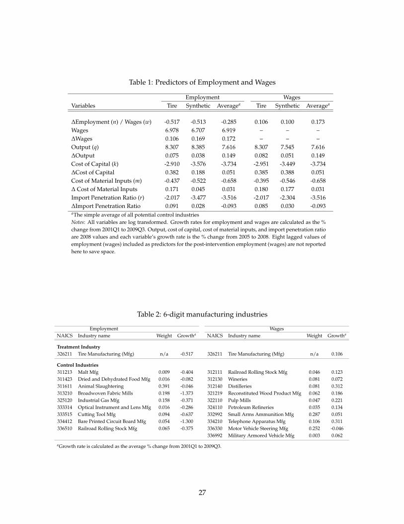
Table 1: Predictors of Employment and Wages

Employment WagesVariables Tire Synthetic Averagea Tire Synthetic Averagea

∆Employment (n) / Wages (w) -0.517 -0.513 -0.285 0.106 0.100 0.173Wages 6.978 6.707 6.919 – – –∆Wages 0.106 0.169 0.172 – – –Output (q) 8.307 8.385 7.616 8.307 7.545 7.616∆Output 0.075 0.038 0.149 0.082 0.051 0.149Cost of Capital (k) -2.910 -3.576 -3.734 -2.951 -3.449 -3.734∆Cost of Capital 0.382 0.188 0.051 0.385 0.388 0.051Cost of Material Inputs (m) -0.437 -0.522 -0.658 -0.395 -0.546 -0.658∆ Cost of Material Inputs 0.171 0.045 0.031 0.180 0.177 0.031Import Penetration Ratio (r) -2.017 -3.477 -3.516 -2.017 -2.304 -3.516∆Import Penetration Ratio 0.091 0.028 -0.093 0.085 0.030 -0.093aThe simple average of all potential control industriesNotes: All variables are log transformed. Growth rates for employment and wages are calculated as the %change from 2001Q1 to 2009Q3. Output, cost of capital, cost of material inputs, and import penetration ratioare 2008 values and each variable’s growth rate is the % change from 2005 to 2008. Eight lagged values ofemployment (wages) included as predictors for the post-intervention employment (wages) are not reportedhere to save space.

Table 2: 6-digit manufacturing industries

Employment WagesNAICS Industry name Weight Growtha NAICS Industry name Weight Growtha

Treatment Industry326211 Tire Manufacturing (Mfg) n/a -0.517 326211 Tire Manufacturing (Mfg) n/a 0.106

Control Industries311213 Malt Mfg 0.009 -0.404 312111 Railroad Rolling Stock Mfg 0.046 0.123311423 Dried and Dehydrated Food Mfg 0.016 -0.082 312130 Wineries 0.081 0.072311611 Animal Slaughtering 0.391 -0.046 312140 Distilleries 0.081 0.312313210 Broadwoven Fabric Mills 0.198 -1.373 321219 Reconstituted Wood Product Mfg 0.062 0.186325120 Industrial Gas Mfg 0.158 -0.371 322110 Pulp Mills 0.047 0.221333314 Optical Instrument and Lens Mfg 0.016 -0.286 324110 Petroleum Refineries 0.035 0.134333515 Cutting Tool Mfg 0.094 -0.637 332992 Small Arms Ammunition Mfg 0.287 0.051334412 Bare Printed Circuit Board Mfg 0.054 -1.300 334210 Telephone Apparatus Mfg 0.106 0.311336510 Railroad Rolling Stock Mfg 0.065 -0.375 336330 Motor Vehicle Steering Mfg 0.252 -0.046

336992 Military Armored Vehicle Mfg 0.003 0.062

aGrowth rate is calculated as the average % change from 2001Q1 to 2009Q3.

27

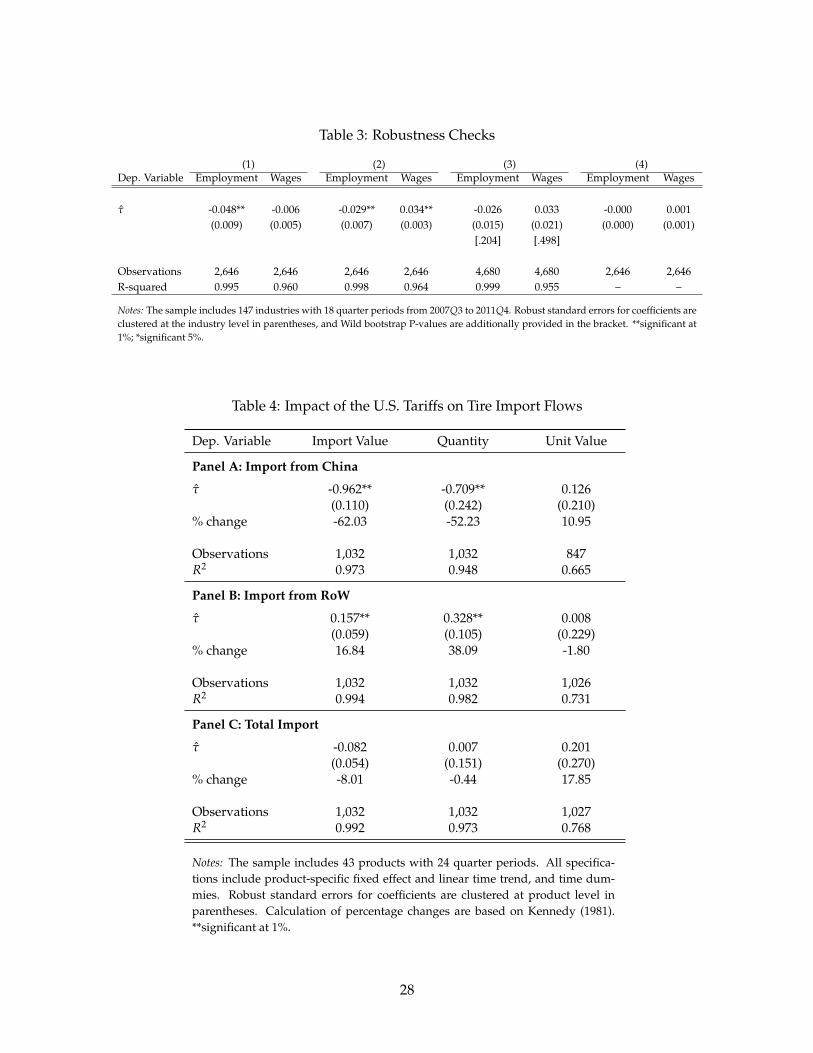
Table 3: Robustness Checks

(1) (2) (3) (4)Dep. Variable Employment Wages Employment Wages Employment Wages Employment Wages

τ -0.048** -0.006 -0.029** 0.034** -0.026 0.033 -0.000 0.001(0.009) (0.005) (0.007) (0.003) (0.015) (0.021) (0.000) (0.001)

[.204] [.498]

Observations 2,646 2,646 2,646 2,646 4,680 4,680 2,646 2,646R-squared 0.995 0.960 0.998 0.964 0.999 0.955 – –

Notes: The sample includes 147 industries with 18 quarter periods from 2007Q3 to 2011Q4. Robust standard errors for coefficients areclustered at the industry level in parentheses, and Wild bootstrap P-values are additionally provided in the bracket. **significant at1%; *significant 5%.

Table 4: Impact of the U.S. Tariffs on Tire Import Flows

Dep. Variable Import Value Quantity Unit Value

Panel A: Import from China

τ -0.962** -0.709** 0.126(0.110) (0.242) (0.210)

% change -62.03 -52.23 10.95

Observations 1,032 1,032 847R2 0.973 0.948 0.665

Panel B: Import from RoW

τ 0.157** 0.328** 0.008(0.059) (0.105) (0.229)

% change 16.84 38.09 -1.80

Observations 1,032 1,032 1,026R2 0.994 0.982 0.731

Panel C: Total Import

τ -0.082 0.007 0.201(0.054) (0.151) (0.270)

% change -8.01 -0.44 17.85

Observations 1,032 1,032 1,027R2 0.992 0.973 0.768

Notes: The sample includes 43 products with 24 quarter periods. All specifica-tions include product-specific fixed effect and linear time trend, and time dum-mies. Robust standard errors for coefficients are clustered at product level inparentheses. Calculation of percentage changes are based on Kennedy (1981).**significant at 1%.

28

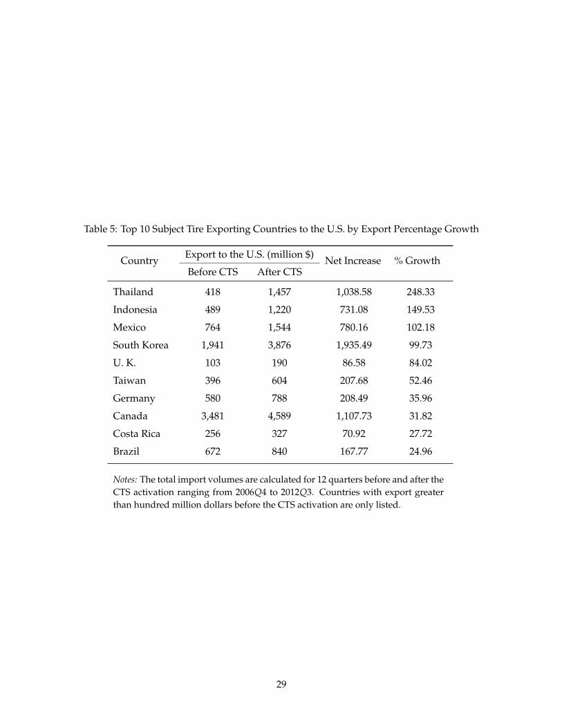
Table 5: Top 10 Subject Tire Exporting Countries to the U.S. by Export Percentage Growth

CountryExport to the U.S. (million $)

Net Increase % GrowthBefore CTS After CTS

Thailand 418 1,457 1,038.58 248.33

Indonesia 489 1,220 731.08 149.53

Mexico 764 1,544 780.16 102.18

South Korea 1,941 3,876 1,935.49 99.73

U. K. 103 190 86.58 84.02

Taiwan 396 604 207.68 52.46

Germany 580 788 208.49 35.96

Canada 3,481 4,589 1,107.73 31.82

Costa Rica 256 327 70.92 27.72

Brazil 672 840 167.77 24.96

Notes: The total import volumes are calculated for 12 quarters before and after theCTS activation ranging from 2006Q4 to 2012Q3. Countries with export greaterthan hundred million dollars before the CTS activation are only listed.

29

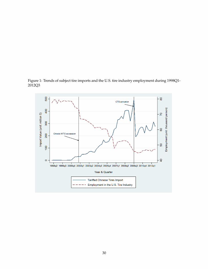
Figure 1: Trends of subject tire imports and the U.S. tire industry employment during 1998Q1-2012Q3

30

Figure 2: Trends in the U.S. Tire vs. Synthetic Industry during 2001Q1–2012Q3

(a) Total Employment

(b) Average Wage

31

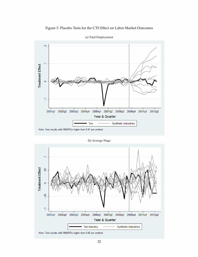
Figure 3: Placebo Tests for the CTS Effect on Labor Market Outcomes

(a) Total Employment

(b) Average Wage

32

Figure 4: Trend in the U.S. Tire Import during 2001Q1-2012Q3

33