Digging for Development:Mining Booms and Local Economic Development in

India ∗

Sam Asher†

Paul Novosad‡

Abstract

How does natural resource extraction affect local economic activity in poor coun-tries? Does this industry crowd out other sectors by raising the price of fixed factors,or does it has positive externalities and make other industries more productive? Usinginternational prices and geological deposit locations to instrument for the value of sub-surface natural resources, we examine the impact of mineral resource wealth on localeconomic structure in India. Because Indian policy directs all taxes and royalties frommining to the state and federal governments, we are able to isolate the direct effect ofnatural resource wealth, and exclude any effect of increased government spending. Inthe cross-section, towns in resource rich areas are smaller, with larger mining sectorsand smaller manufacturing and retail sectors. The causal time series results, however,suggest that these effects may be due to unobserved aspects of natural advantage.Booms in the value of subsurface natural resources result in broad-based growth intowns up to 50km from the nearest mineral deposit. Rural areas are affected at asmaller radius, with growth in agroprocessing, but a decline in service sectors, sug-gesting a reallocation of labor toward mineral extraction and upstream industries. Wefurther document how the increasing capital intensity of the mining sector affects thereturns to the largely unskilled local labor force.

∗We are thankful for useful discussions with Alberto Alesina, Josh Angrist, Lorenzo Casaburi, ShawnCole, Ed Glaeser, Ricardo Hausmann, Richard Hornbeck, Lakshmi Iyer, Asim Khwaja, Michael Kremer,Sendhil Mullainathan, Rohini Pande, Andrei Shleifer and David Yanagizawa. We are grateful to SandeshDhungana for excellent research assistance. Mr. PC Mohanan of the Indian Ministry of Statistics has beeninvaluable in helping us use the Economic Census. This project received financial support from the Centerfor International Development and the Warburg Fund (Harvard University). All errors are our own.†Oxford University‡Dartmouth College. paul.novosad@dartmouth.edu

1 Introduction

Does natural resource wealth put regions or nations on an adverse development path? Em-

pirical work beginning with Sachs and Warner (1995) has led to the idea that the particular

characteristics of wealth from natural resources could be a detriment to long-run growth,

especially in countries with poor institutions.1

Most of the empirical evidence supporting a negative effect of natural resource wealth on

economic development has been based on cross-country comparisons.2 Recognizing the many

confounding variables inherent to cross-country work, researchers have turned to within-

country studies, and have focused on changes in resource extraction over time.3

This literature has found mixed results on the effect of natural resources on economic

development. The interpretation of these mixed results is challenging, as there are many

mechanisms by which natural resource wealth can affect local development, which include: (i)

changes in local factor prices (Corden, 2012); (ii) local agglomeration spillovers (Ellison and

Glaeser, 1997); (iii) increased public spending from mineral royalties; and (iv) deterioration

in political outcomes (Robinson et al., 2006). This paper focuses on the first and second

categories: the direct local economic consequences of mining booms. The context is India, a

nation which as a whole is not highly dependent on point-source natural resources, but has

many regions which produce coal, iron, gold and a range of other valuable minerals.

By using subnational and subregional variation, we are able to compare outcomes across

regions that share basic political and economic institutions. We identify exogenous variation

from changes in global prices of mineral resources found in India. We are also able to rule

1See van der Ploeg (2011) for a survey of the literature.2Sachs and Warner (1995) begins this literature. Mehlum et al. (2006) is a recent example, finding that

natural resources a detrimental in the presence of bad institutions, but beneficial otherwise. Alexeev andConrad (2009) is a dissenting voice in the cross-country literature, arguing that natural resources do not haveadverse effects, but rather raise income without raising other indicators of development normally correlatedwith income.

3Some recent examples include Carrington (1996), Aragon and Rud (2013), Caselli and Michaels (2013),and Domenech (2008).

2

out the channel of fiscal surplus, because royalties are collected and spend at the state level

in India, and we rely on within state variation.4

The cross sectional relationship between mineral deposits and economic structure are

consistent with views that natural resource wealth can inhibit economic development, or set it

onto a suboptimal growth path. Towns nearest mineral deposits are smaller, and controlling

for their population, have higher employment in the mining sector, but significantly smaller

manufacturing and retail trade sectors. They are also at higher altitude and further from

political centers.

However, the geographic differences between mineral and non-mineral areas point to the

risk of identifying the effects of natural resource wealth by comparing these types of locations.

The locational choice of resource extraction industries is constrained by the location of

resources; towns with a high degree of natural resource extraction are likely to lack other

natural advantages of resource-scarce locations, which could also produce a specialization

pattern similar to that observed.

Exploiting time series variation in the value of mineral resources helps us understand the

extent to which cross-sectional estimates are biased by unobserved characteristics of resource-

rich regions. Contrary to the cross-sectional results, we find that exogenous increases in

mineral resource wealth result in broad-based economic growth in nearby towns, across a

range of manufacturing and service sectors. We find no evidence that growth in natural

resource wealth results in a decline in sectors that compete for local factors of production.

Towns nearest mineral deposits experience the largest employment growth, which is com-

posed both of tradable and non-tradable sector growth. A 100% price shock to the value of a

single nearby mineral deposit raises non-farm employment in the nearest towns by 17%, and

manufacturing employment by 20%. The shock raises employment in the nearest villages by

4A lack of formal rule does not imply that royalties are not spent locally. However, neither public officialsnor mining executives that we spoke with believed that public spending was being redirected toward com-munities affected by mining. This said, mining firms may make social investments in affected communities.

3

9%, with larger increases in manufacturing and a decline in the regional rural service sector.

The difference between the long run characteristics of resource rich areas and the short

term effects of mining booms suggests that some of the cross-sectional characteristics of

mining areas are driven by characteristics of places other than their natural resources. In

the short to medium run, our results contradict the class of theories that predict crowdout,

and support a model of positive externalities from the natural resource extraction sector to

nearby firms in other sectors.

Finally, we examine the impact of mining sector development on the distribution of asset

holding in both urban and rural households. We exploit the fact that different minerals are

extracted with different technology, leading to variation in the capital intensity and use of

skilled labor across different types of mines. We document the very local impacts of the

increasing replacement of labor with capital in the Indian mining sector.

Section 2 gives background information on the mining sector in India. Section 3 describes

the key theoretical ways we should expect mining sector development to affect regional

economies. Section 4 describes data sources, Section 5 describes the empirical strategy, and

Section 6 presents results. Section 7 discusses interpretation of the results in the context of

the theory, and concludes.

2 The mineral resource industry in India

Although modern India is not considered a mineral-rich country, it has a large and varied

natural resource sector. In 2010, the mining sector employed 521,000 workers and accounted

for 2.5% of national GDP (Indian Bureau of Mines, 2011). Mineral resources are unevenly

distributed across India, and often make up a significant share of economic output in the

places where they are concentrated. Over sixty different major minerals were mined in 2999

documented mines in 2010 (Indian Bureau of Mines, 2011).

4

Historically, Indian mines were predominantly state owned until significant privatization

in the 1990s. By 2010, 2229 of 2999 mines were privately owned, representing 36% of total

production value (Indian Bureau of Mines, 2011). Mineral deposits are found in nearly every

state of India. The major exceptions are the Deccan Traps in west-central India and the

highly populated states of Uttar Pradesh and Bihar in the lower Gangetic plain.

Major minerals such as iron ore are jointly regulated by the national and state govern-

ments, while minor minerals such as granite are regulated entirely by state governments.

Notably, royalties and taxes paid by mining corporations are paid directly to state and fed-

eral governments. Importantly for this study, there is no requirement for fiscal proceeds from

mining to be spent in communities close to mines. Further, our discussions with mining exec-

utives and public officials have not given any suggestion that these communities are likely to

benefit disproportionately from spending of royalties or other public funds. However, mining

companies often provide social goods, such as schools and libraries, to affected communities.

3 Conceptual Framework

This section considers possible channels by which mineral resource wealth could affect local

industrial structure.

The first channel we consider is the Dutch Disease: in the presence of factor immobility,

significant growth in one sector of the economy can increase the input factor prices faced

by other sectors, making them less competitive (Corden, 2012). However, the new wealth

associated with the booming sector increases the demand for locally produced goods. The

factor cost effect will decrease the production of all sectors, while the demand effect increases

the production of locally produced non-tradable goods. The Dutch Disease channel thus

drives down the production of tradable goods, and could either increase or decrease the

production of non-tradable goods.

5

A second channel is the agglomeration channel: growth in mineral extraction may have

positive spillovers into other sectors (Ellison and Glaeser, 1997). The most widely discussed

mechanisms originate in Marshall (1920): (i) input/output channels; (ii) thick labor markets;

and (iii) knowledge spillovers. The first mechanism suggests that industries which have

input/output linkages with the mining sector will benefit from mining booms. The second

channel suggests that firms with similar labor forces to the mining sector will benefit.5 We

expect the last mechanism to be less important in the context of mining: mining sector

knowledge is more likely produced in headquarter locations than at extraction sites. We

also consider a fourth agglomeration channel: in a resource-poor country, many firms are

constrained by a lack of basic infrastructure, such as roads and electricity, which market

failures may prevent the private sector from providing. A local boom may increase the

supply of government inputs, which other firms may then benefit from.6

Natural resource wealth could affect a local economy through a royalty channel, if local

governments receive a share of profits from natural resource extraction, or if higher govern-

ments are required or choose to spend royalties in areas where mining takes place. We are

able to largely exclude this channel, as there is no evidence that local communities or govern-

ments receive a disproportion share of royalties from mining.7 The absence of locally-spent

royalties allows us to focus on the direct economic channels of mineral extraction, without

the confounder of increased local government spending.

5The short- and long-term mobility of labor are important here. If labor is immobile in the short-term,we would expect a mining boom to hurt sectors with similar labor demand to the mining sector, as wagesare bid up. In the medium to long term, however, these firms would benefit from a thicker labor market, aslabor moves into the area to work in the mining sector. It is worth noting that labor mobility in India tendsto be very low (Foster and Rosenzweig, 2004).

6Two mechanisms for an increase in government inputs are possible. A mining boom may increase thevalue of local infrastructure, attracting efficiently allocated government inputs. Alternately, a boomingindustry may have increased lobbying power, and can thus be more effective at attracting government inputsto the area. Either way, we expect to see the largest growth in government inputs that are complementaryto mining sector production.

7Mining companies do support local commnunity projects, such as schools and libraries. However, thescale of spending on these projects is much lower than royalties typically collected from mining projects.

6

An additional widely discussed potential consequence of natural resource wealth is the

behavior of political actors. As natural resource sectors are rent-rich, politicians may put

more effort into appropriating some of that wealth. Corruption may increase, and potential

entrepreneurs may move from organizing production to rent-seeking (Murphy et al., 1991)8.

The economic effects of a political resource curse could include a fall in entrepreneurship

(from the reallocation of entrepreneurial talent), and a deterioration in the quality of pub-

lic goods (from the reallocation of politician effort). However, the lack of sector-specific

predictions of a political channel make it difficult to test directly in our context.

Finally, natural advantage plays a major role in the economic characteristics of mineral

rich regions. Economic centers arise in places with certain natural advantages, for example,

in places well-suited for trade, such as ports or at the confluence of rivers. Mineral deposits

are a kind of natural advantage that tends to be inversely correlated with other kinds of

natural advantage: deposits are most often founded in highland areas that tend to be ill-

suited for both trade and agriculture.9 Unless mineral resources are positively correlated

with other kinds of natural advantage, we should expect mineral-based economies to have

fewer of the natural advantages of non-mineral economic centers. Cross-sectional correlations

between natural resources and local economic structure are therefore importantly confounded

by natural advantage. We eliminate confounding due to natural advantage by focusing on

time series changes in the value of local mineral wealth. Natural advantages other than those

captured by the value of subsurface resources, are unlikely to significantly change over our

sample period.

8We explore some of these effects in parallel work, finding that elections are less competitive and criminalaccusations against politicians are more likely when the local mining sector is booming (Asher and Novosad,2013).

9Many valuable minerals are formed under pressure, deep in the Earth’s crust. These minerals tend tobe most accessible in mountainous areas, where geological activity has exposed these deeper layers.

7

4 Data

The Indian Ministry of Statistics and Programme Implementation (MoSPI) conducted the

3rd, 4th and 5th Economic Censuses respectively in 1990, 1998 and 2005. The Economic

Census is a complete enumeration of all economic establishments except those engaged in

crop production and plantation; there is no minimum firm size, and both formal and informal

establishments are included.

The Economic Census records information on the town or village of each establishment,

whether ownership is public or private, the number and demographic characteristics of em-

ployees, the sources of electricity and finance, and the caste group of the owner. The main

product of the firm is also coded using the 4-digit National Industrial Classification (NIC),

which corresponds roughly to a 4-digit ISIC code. More detailed information on income or

capital is not included. The main strengths of the data are its comprehensiveness, and rich

detail on spatial location and industrial classification of firms.

We obtained location directories for the Economic Censuses, and then used a series of

fuzzy matching algorithms to match villages and towns by name to the population censuses

of 1991 and 2001.10 We were able to match approximately 93% of villages between 1998

and 2005, and 81% from 1990 to 1998. The match rates for towns are respectively 78%

and 55%. We also use data from the Population Census of India in 1991 and 2001, which

includes village population and other demographic data, as well as information on local

public infrastructure (roads, electricity, schools and hospitals).

Data on the location, type and size of mineral deposits come from the Mineral Atlas

of India (Geological Survey of India, 2001), which provides the following characteristics of

major mineral deposits in India: centroid latitude and longitude, mineral type, and estimated

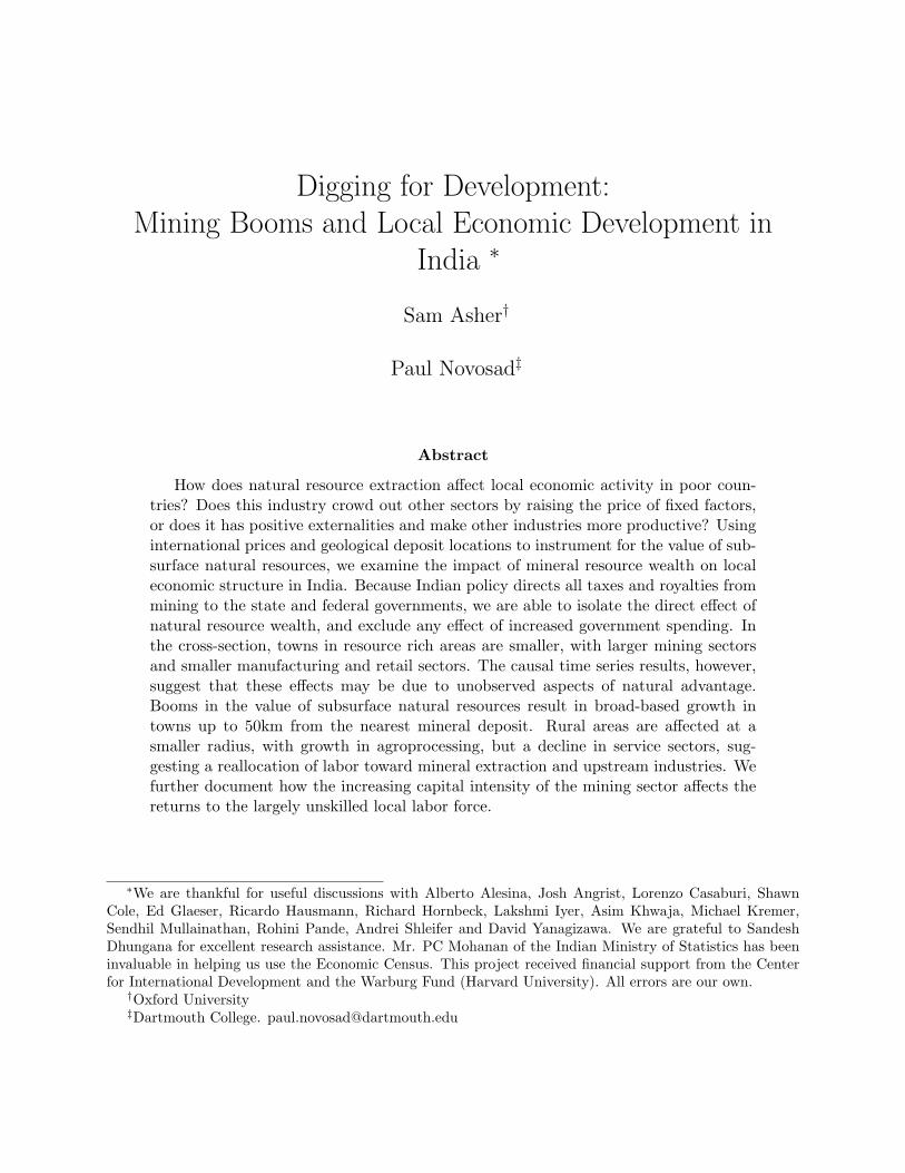
reserves (in one of three size categories). Figure 1 shows a map of mineral deposit locations.

10The Economic Census of 1998 was conducted with the house listing for the 1991 population census,while the 2005 Economic Census used codes from the 2001 population census.

8

Commodity prices come from the United States Geological Survey (Kelly and Matos, 2013).

All prices are annual averages in the United States. Where available, we use the price for the

ore as it is listed in the Indian deposit data. Where the ore price is unavailable, we match

deposits to the price of the processed output of the mineral deposit (e.g. we use the price

of aluminum for bauxite deposits).11 We match deposits to villages and towns based on the

geographic coordinates provided in the 2001 Population Census of India.

The unit of observation is the village or town. For each location, we desire a measure

that indicates the extent to which the price of nearby mineral deposits has increased or

decreased. There are two parts to this process: (i) creating a scalar measure that captures

the recent price movement in a given commodity; and (ii) combining these price measures

when locations are close to multiple deposits.

To capture recent changes in the value of a commodity, we use the mean price over

the economic measurement period, and normalize it by the baseline price, measured at the

beginning of the period. This measure is desirable in that a sustained increase in price results

in a larger measured shock than a transitory increase in price. Further, a level shift in price

at the beginning of the period results in a larger measured shock than a level shift in price

at the end of the period, which is desirable if mineral price changes have lagged effects.

We use a 10-year trailing average for the baseline price, in order to prevent transitory

shocks at the beginning of the measurement period from having too strong an effect on the

price shock. The measure for a period of T years, ending in year t is given by Equation 1.

PriceShockc,t−T→t =1T

∑t−1τ=t−T pc,τ

110

∑t−T−1τ=t−T−11 pc,τ

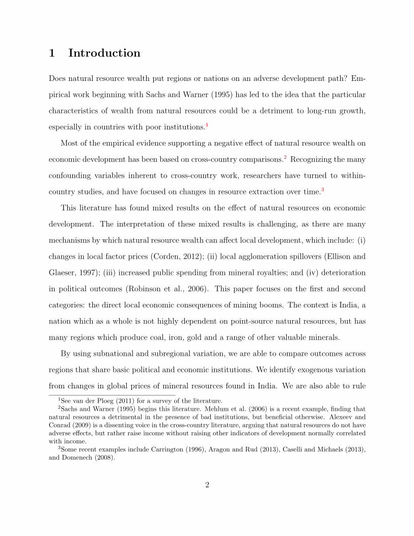
Figure 2 presents mineral-wise price shocks for the period 1998-2005, the second of two

periods in our sample.

11Because we rely mainly on changes in prices over time, this imputation is reasonable as long as unpro-cessed and processed ore comove.

9

For each location, we identify deposits within one of three concentric rings, with radii of

10km, 25km, and 50km. When multiple deposits fall within a zone, we take the sum of the

price shocks.12 Since commodity prices are increasing on average in the period, locations with

more deposits will on average experience larger price shocks; we include a flexible function

in the number of deposits near a location to control for this bias.

From a list of 45 minerals for which we have both deposit and price data, we discard

economically unimportant minerals, defined as those for which the Indian Bureau of Mines

does not publish production statistics or those whose average output per deposit is valued

at less than $20,000 in 2005, the most recent year for which we have Economic Census data.

We end up with 1325 deposits of 27 distinct minerals spread across 25 states in India. We

use the presence of deposits rather than the presence of mines, as deposit existence is more

likely to be exogenous than mine presence.13 More common measures of resource abundance,

such as share of GDP from primary commodities or mineral production value, are correlated

with institutional factors and are better described as measures of resource dependence. Our

use of mineral deposits avoids this endogeneity.

Table 1 shows key summary statistics separately for towns and villages.

12Our reasoning is that multiple deposits that are increasing in value create a larger shock to a localeconomy than a single deposit increasing in value. Results are largely robust to using a mean price shock.Future work will impute the total change in dollar value of reserves near a given location.

13Known deposits are endogenous to the extent that their existence depends on some exploration havingtaken place. Future work will test robustness using a set of deposits that were known at the beginning ofthe sample period.

10

5 Empirical strategy

The most common approach in the natural resource literature has been to regress the outcome

variable on a measure of natural resource wealth, as in equation 1:14

Yi = β0 + β1 ∗ RESi + ζ ∗X′i + εi, (1)

where i indexes locations, RESi is a measure of natural resource wealth, X′i is a vector of

location-specific controls and εi is an orthogonal error term.

This approach has had two major weaknesses. The first is with the measures of resource

dependence used. Any measure with GDP in the denominator (for example, the often used

primary export share of GDP) is subject to reverse causality: place that have failed to develop

advanced sectors will necessarily have a high resource share of their economies. Measures

of natural resource production are also endogenous: the extraction of natural resources may

not take place if the background infrastructure and institutions are inadequate.

To escape the endogeneity of both mineral production and GDP, we proxy mineral re-

source wealth with the value of known mineral deposits, based on international prices. Ge-

ography is clearly exogenous to other factors.15

Estimating Equation 1 to compare resource-rich and resource-poor areas suffers from an

additional omitted variable bias. Natural resources are not distributed at random; they are

more likely to appear in regions that are mountainous and inaccessible, and as discussed in

Section 3, resource-driven agglomerations are less likely to have other natural advantages

due to compensating differentials. Control variables can mitigate this to some extent, but

the high degree of selection on observables suggests that selection on unobservables may be

14This is the approach used, among others, by Alexeev and Conrad (2009), Sachs and Warner (2001),Michaels (2010), Black et al. (2005) and Mehlum et al. (2006).

15Knowledge of mineral deposits remains endogenous, which may bias our OLS results. But this will notaffect our time series results, which are limited to locations with known deposits, and locations with unknowndeposits will not have mining sectors.

11

significant as well (Altonji et al., 2005).

To better relate our work to the literature on cross-sectional estimation of the character-

istics of resource rich places, we run the standard OLS tests. We use Equation 2:

Yi = β0 + β1 ∗ RES10km,i + β2 ∗ RES25km,i + β3 ∗ RES50km,i + ζ ∗X′i + εi, (2)

where the multiple β coefficients capture the relationship between the economic outcome

and the distance from the mineral deposit.

To eliminate omitted variable bias due to differences between mineral and non-mineral

producing areas, we limit our study to mineral-rich areas, and rely on time series variation

in the value of subsurface wealth, exogenously driven by international prices. We estimate

Equation 3 to identify the effect of changes in mineral wealth on growth in the following

years:

Yi,t+1 − Yi,t = β0 + β1 ∗ pshocki,t + ζ ∗Xi,t + γs,t + εi,t, (3)

where pshocki,t is the change in value of nearby geological deposits as described above, Xi,t

is a vector of location controls, γs,t is a state-year fixed effect and εi,t is an orthogonal error

term. The coefficient β1 identifies the effect of a change in mineral wealth on the economic

outcome. As we are using interacted state-year fixed effects, our estimates are driven by

variation in commodity price changes within a given state and time period. Standard errors

are clustered at the district-level, which roughly corresponds to a shock radius of about

40km.

12

6 Results

6.1 Cross-section analysis

We begin by examining the cross-sectional relationship between subsurface mineral wealth

and the economic characteristics of villages and towns. Equation 2 is the estimating equation.

This method compares mineral rich to mineral poor regions within states, and estimates

separate coefficients for places within 10km, 25km and 50km of mineral deposits. The

reference group is composed of locations more than 50km from an economically valuable

mineral deposit. The results should be interpreted as correlations between mineral wealth

and economic outcomes, which are not necessarily causal.

Table 2 presents the cross-sectional relationship between mineral wealth, population and

non-farm employment. Column 1 regresses village population on proximity to a mineral

deposit, controlling for state fixed effects. In column 2, the dependent variable is non-farm

employment, and population is an additional control. Villages are smaller in mineral rich

regions, though this effect is muted in the villages closest to deposits. This is likely because

deposits are located in remote regions of low population density, with agglomerations near

the mines themselves.

Column 3 and 4 show the equivalent regressions for towns. Towns in mineral rich regions

are 5-6% smaller than towns in non-mineral regions; conditional on being within 50km

of a mine, distance to the deposit has little additional effect. Controlling for population,

employment is lower in towns nearest deposits, but 8% higher in towns that are 25-50km

from a deposit. Mining operations are often headquartered in district capitals, which could

explain these distance effects.

Table 3 presents estimates of Equation 2 on other characteristics of villages, controlling

for population, non-farm employment and state fixed effects. Column 1 shows that villages

nearest mines are likely to have higher employment in establishments with more than 50

13

employees.16 Column 2 shows that villages nearest deposits have marginally more diverse

non-farm economies, while villages in deposit regions but not directly on a deposit have

less diverse economies. Columns 3 through 5 regress the existence of local public goods on

the presence of mineral deposits. Villages in mining regions are 5-10% more likely to have

primary schools, but equally likely to have a paved approach road or access to electricity.

Column 6 shows that villages near mineral deposits are on average further from towns.17

Table 4 disaggregates rural employment effects by sector. The lack of relationship between

mineral deposits and total employment masks significant differences in economic structure

between mineral and non-mineral areas. Mining employment is higher. Villages nearest

mines have smaller retail sectors, and higher employment in schools, health clinics and public

administration. In addition to these larger sectors, villages in mining regions but further

from actual deposits also have larger non-farm employment in agroprocessing and hotels and

restaurants. These positive results are balanced in the total employment regressions by the

retail sector, which makes up a large share of rural non-farm employment. Non-agricultural

manufacturing employment is largely unaffected by mining, but is a small part of many

village economies. In summary, in the rural economy, mineral deposits are associated with

increased employment in the mining and social sectors, and reduced employment in retail

trade.

Table 5 shows the relationship between town characteristics and mineral deposits. Like

villages, towns very close to mineral deposits have weakly higher employment in establish-

ments with more than 50 employees. Industrial diversity is not affected by mineral deposits,

nor are the number of primary schools, paved roads or electrical connections. However,

towns in mining areas are considerably more remote; on average, they are 25-40% further

16We do not find a statistically significant relationship between deposits and average firm size. The vastmajority of economic census firms are very small, so an unreasonably large increase in large firms would berequired to substantially shift the mean size.

17The relationship is not significant at the shortest distance, perhaps because a high density of mineraldeposits may motivate a mining town.

14

from state capitals.

Table 6 describes the relationship between mineral deposits and the sectoral composition

of non-farm employment in towns. As with villages, the similarities in overall employment

numbers mask sectoral differences. Towns nearest to mineral deposits have 30% higher

employment in the mining sector, but significantly lower employment in manufacturing and

retail (respectively 16% and 12%). These effects decay as distance grows, and towns located

25-50km from mines have higher employment, controlling for population, in a broad spectrum

of industries - these are likely district capitals.

Towns nearest mineral deposits exhibit some classic characteristics of Dutch Disease:

enlarged resource sectors and diminished manufacturing sectors. The next section exploits

time series variation in the value of mineral resources to shed light on whether this result is

causal or driven by unobserved characteristics of resource-rich regions.

6.2 Time series analysis

Table 7 shows estimates from Equation 3, which identify the effect of exogenous changes

in mineral resource wealth on non-farm employment growth in nearby towns and villages.

The independent variable (Price Shock) is the average price of local minerals over the period

between census measurements, normalized by the 10-year moving average of the price at

the beginning of the period. Interacted time / state fixed effects are included, and standard

errors are clustered at the district level, which corresponds to the approximate range we

believe price shocks have a direct effect on the local economy.

Columns 1 and 2 show estimates on employment growth in villages. Increases in the

value of local mineral resources have positive and significant effects on non-farm employment

in the nearest villages. Limiting the sample to villages within 10km of a mineral deposit

(column 1), a doubling in the value of a single mineral deposit results in a 9% increase in

total employment. To examine the spatial dimension of this effect, we widen the sample to

15

locations within 50km of a mineral deposit, and allow separate coefficients for price changes

in minerals at different distances from the deposit. Column 2 indicates that the effect is

highly local: the effect is concentrated in villages nearest the mineral deposit; villages 10-

50km from deposits show only a statistically insignificant estimate of 2%.

Columns 3 and 4 show estimates in towns. Limiting the sample to the on average 225

towns per period within 10km of a mineral deposit (Column 3), we find that a doubling

in the value of a single nearby deposit results in a 17% increase in non-farm employment.

When we estimate the distance gradient (column 4), the effect is more dispersed: the point

estimate remains largest for towns nearest the deposit, but towns from 25-50km of a mineral

deposit also show a 5% increase in employment.

We next separate these employment effects into manufacturing and service sector em-

ployment. Table 8 shows estimates for villages. Columns 1 and 3 show that the overall

employment increase in nearby villages can be decomposed into a loss in service sector em-

ployment and an increase in manufacturing, the reverse prediction of a Dutch Disease model.

Columns 2 and 4 investigate the distance gradient. The increase in manufacturing jobs is

located nearest the mineral deposits, while the loss in service sector jobs affects a wider

region, extending up to 50km from the mineral deposit.18 We speculate that the villages

nearest mineral deposits are supplying inputs to the mine. The loss in service sector jobs

can be explained if rural retail employment is a low productivity diversification strategy. If

employment in a mine is preferable to retail sector employment, we would see people move

away from the retail sector when mine hiring increases.

Table 9 decomposes sectors further, roughly following 2-digit ISIC codes. The decompo-

sition of manufacturing into food- and non-food manufacturing shows that manufacturing

18The zero coefficient on the 0-10km price shock variable does not necessarily imply no loss in servicesector jobs in the villages nearest to the deposit. Villages nearest the deposits are also likely to be in the25-50km range of other similar deposits. A zero coefficient therefore indicates no additional effect of beingwithin 10km of a deposit, conditional on being 25-50km from a deposit.

16

growth is mainly in agro-processing, with little effect in other manufacturing sectors. This

is not surprising, if villages have a comparative advantage in processed agricultural goods

relative to other manufactured goods. The decline in services is relatively broad, affecting

retail trade, education and health and public administration. Retail trade is the most impor-

tant of these as a share of rural employment; however, the decline in government and social

services may have important welfare effects. An exception to the decline in village service

employment is an increase in employment in community services, which include libraries, mu-

seums and religious and community organizations. These are likely services funded directly

by the mining sector for purposes of corporate social responsibility; baseline employment in

community services is very small, so the growth in this sector is not economically substantive.

Table 10 decomposes resource-driven urban growth into manufacturing and service sec-

tors. Effects are largest in the manufacturing sector, which grows 19-21% in response to a

doubling in price of a single nearby deposit. Point estimates suggest service sector growth

in the range of 10-16%, though it is not statistically significant. While estimates for service

and manufacturing growth are not statistically different from each other, we can rule out the

notion that non-tradable growth is crowding out the tradable sector. As above, the distance

gradient shows an effect weakly declining in distance.

Table 11 further decomposes the sectoral effects of natural resource wealth. As with

the rural sector, the positive effect on manufacturing is concentrated in the processing of

agricultural commodities. The effect on non-agricultural tradable products is positive but

insignificant. Service sector growth is broad-based, with growth in employment in construc-

tion, retail trade, education, health and public administration. In short, resource booms

appear to result in broad based growth across all urban sectors. Non-agricultural manufac-

turing growth is somewhat lagging, with the smallest point estimate of all sectors, but is

nevertheless consistently positive and close to 10% across all specifications.

17

7 Conclusion

We provide new evidence on the relationship between local natural resource wealth and

economic development. We improve upon previous studies of local resource effects by con-

centrating on highly local effects within a large, poor country. Our economic estimates are

most significant in places within 10km of mineral deposits, suggesting that much of the work

on natural resources may be overlooking the highly localized impact of natural resource ex-

traction. We compare causal estimates of resource wealth to the cross-sectional relationship

between mineral wealth and development that has been most commonly studied, allowing

us to demonstrate the bias in the latter studies.

The cross sectional relationship between mineral deposits and economic structure are

consistent with views that natural resource wealth can inhibit economic development, or set it

onto a suboptimal growth path. Towns nearest mineral deposits are smaller, and controlling

for their population, have higher employment in the mining sector, but significantly smaller

manufacturing and retail trade sectors.

Exploiting exogenous variation in the value of mineral resources helps us understand the

extent to which cross-sectional estimates are biased by unobserved characteristics of resource-

rich regions. Contrary to the cross-sectional results, we find that exogenous increases in

mineral resource wealth result in broad-based economic growth in nearby towns, across all

manufacturing and service sectors. We find no evidence that growth in natural resource

wealth results in a decline in sectors that compete for local factors of production.

Our results are measured at a 7- or 8-year time horizon, and thus identify medium term

effects of resource wealth on local employment growth. It remains possible, but in our view,

unlikely, that natural resource wealth has an impact on the manufacturing sector that is

positive in the short term, but negative in the long term. Future work will attempt to

identify the longer-term effects of natural resource wealth in India.

18

The fixed geographic characteristics of local natural resources make it challenging to

identify a causal effect of resource wealth. Our results point to the importance of focusing on

evidence that is plausibly causal, as our cross-sectional results point to a very different story

from our causal time series results. In future work, we plan to investigate further dimensions

of the relationship between resource wealth and economic development that have been widely

discussed. In particular, several studies have found that natural resource are beneficial in

democratic and well-governed economies like Norway, but detrimental in autocratic and

poorly-governed economies like those of many sub-Saharan countries.

India is country with a consolidated democracy, but a wide range of governance quality

across its many states and territories. The very high quality of India’s democracy, controlling

for its level of wealth, may explain the positive effects of natural resource wealth that we

have found. Exploiting variation in the quality of governance across India allows us to test

whether the quality of governance has an important impact on the role of natural resource

in economic development.

19

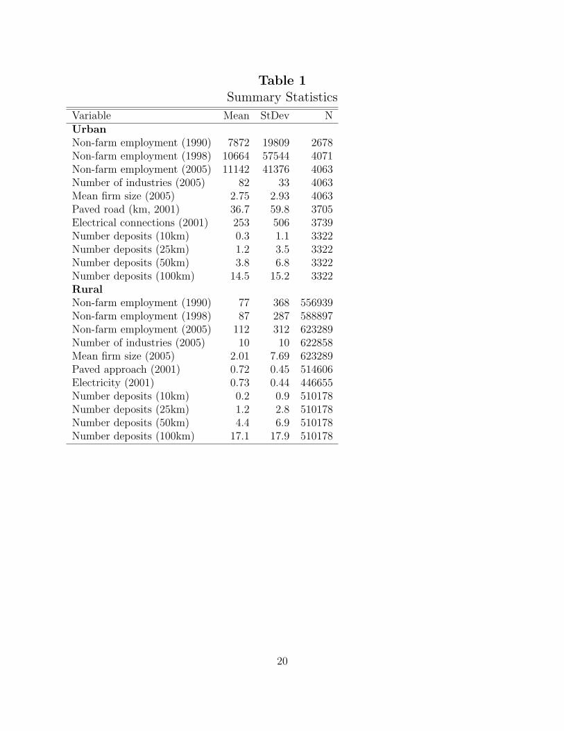
Table 1Summary Statistics

Variable Mean StDev NUrbanNon-farm employment (1990) 7872 19809 2678Non-farm employment (1998) 10664 57544 4071Non-farm employment (2005) 11142 41376 4063Number of industries (2005) 82 33 4063Mean firm size (2005) 2.75 2.93 4063Paved road (km, 2001) 36.7 59.8 3705Electrical connections (2001) 253 506 3739Number deposits (10km) 0.3 1.1 3322Number deposits (25km) 1.2 3.5 3322Number deposits (50km) 3.8 6.8 3322Number deposits (100km) 14.5 15.2 3322RuralNon-farm employment (1990) 77 368 556939Non-farm employment (1998) 87 287 588897Non-farm employment (2005) 112 312 623289Number of industries (2005) 10 10 622858Mean firm size (2005) 2.01 7.69 623289Paved approach (2001) 0.72 0.45 514606Electricity (2001) 0.73 0.44 446655Number deposits (10km) 0.2 0.9 510178Number deposits (25km) 1.2 2.8 510178Number deposits (50km) 4.4 6.9 510178Number deposits (100km) 17.1 17.9 510178

20

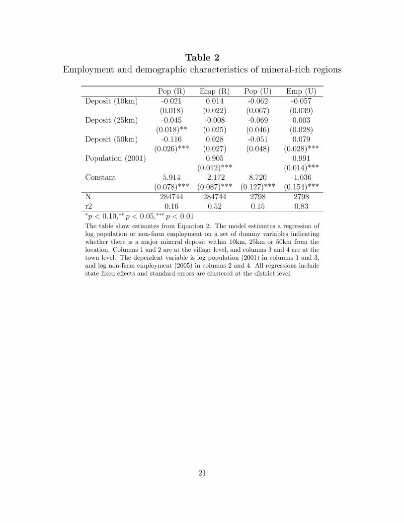
Table 2Employment and demographic characteristics of mineral-rich regions

Pop (R) Emp (R) Pop (U) Emp (U)Deposit (10km) -0.021 0.014 -0.062 -0.057

(0.018) (0.022) (0.067) (0.039)Deposit (25km) -0.045 -0.008 -0.069 0.003

(0.018)** (0.025) (0.046) (0.028)Deposit (50km) -0.116 0.028 -0.051 0.079

(0.026)*** (0.027) (0.048) (0.028)***Population (2001) 0.905 0.991

(0.012)*** (0.014)***Constant 5.914 -2.172 8.720 -1.036

(0.078)*** (0.087)*** (0.127)*** (0.154)***N 284744 284744 2798 2798r2 0.16 0.52 0.15 0.83∗p < 0.10,∗∗ p < 0.05,∗∗∗ p < 0.01The table show estimates from Equation 2. The model estimates a regression oflog population or non-farm employment on a set of dummy variables indicatingwhether there is a major mineral deposit within 10km, 25km or 50km from thelocation. Columns 1 and 2 are at the village level, and columns 3 and 4 are at thetown level. The dependent variable is log population (2001) in columns 1 and 3,and log non-farm employment (2005) in columns 2 and 4. All regressions includestate fixed effects and standard errors are clustered at the district level.

21

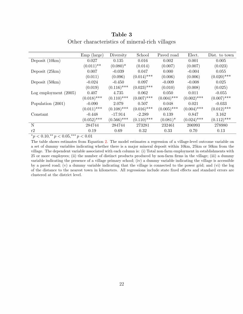
Table 3Other characteristics of mineral-rich villages

Emp (large) Diversity School Paved road Elect. Dist. to townDeposit (10km) 0.027 0.135 0.016 0.002 0.001 0.005

(0.011)** (0.080)* (0.014) (0.007) (0.007) (0.023)Deposit (25km) 0.007 -0.039 0.047 0.000 -0.004 0.055

(0.011) (0.096) (0.014)*** (0.006) (0.006) (0.020)***Deposit (50km) -0.024 -0.450 0.097 -0.009 -0.008 0.025

(0.019) (0.116)*** (0.023)*** (0.010) (0.008) (0.025)Log employment (2005) 0.407 4.735 0.062 0.050 0.011 -0.055

(0.018)*** (0.110)*** (0.007)*** (0.004)*** (0.002)*** (0.007)***Population (2001) -0.090 2.079 0.507 0.048 0.021 -0.033

(0.011)*** (0.108)*** (0.016)*** (0.005)*** (0.004)*** (0.012)***Constant -0.448 -17.914 -2.289 0.139 0.847 3.162

(0.052)*** (0.566)*** (0.110)*** (0.081)* (0.024)*** (0.112)***N 284744 284744 273281 232461 206993 278980r2 0.19 0.69 0.32 0.33 0.70 0.13∗p < 0.10,∗∗ p < 0.05,∗∗∗ p < 0.01The table shows estimates from Equation 2. The model estimates a regression of a village-level outcome variable ona set of dummy variables indicating whether there is a major mineral deposit within 10km, 25km or 50km from thevillage. The dependent variable associated with each column is: (i) Total non-farm employment in establishments with25 or more employees; (ii) the number of distinct products produced by non-farm firms in the village; (iii) a dummyvariable indicating the presence of a village primary school; (iv) a dummy variable indicating the village is accessibleby a paved road; (v) a dummy variable indicating that the village is connected to the power grid; and (vi) the logof the distance to the nearest town in kilometers. All regressions include state fixed effects and standard errors areclustered at the district level.

22

Table 4Economic structure of mineral-rich villages

Mining Ag Proc Constr. Manuf. Retail Ed&Health Hotels Community Gov.Deposit (10km) 0.031 0.011 0.004 0.017 -0.053 0.030 0.053 0.006 0.030

(0.007)*** (0.054) (0.008) (0.026) (0.022)** (0.017)* (0.021)** (0.026) (0.017)*Deposit (25km) 0.015 0.037 -0.003 -0.012 -0.053 0.036 0.026 -0.013 0.009

(0.005)*** (0.059) (0.009) (0.027) (0.020)** (0.019)* (0.020) (0.028) (0.019)Deposit (50km) 0.034 0.187 0.017 0.014 -0.001 0.100 0.134 -0.018 0.080

(0.005)*** (0.070)*** (0.010) (0.042) (0.033) (0.029)*** (0.027)*** (0.036) (0.031)**Population (2001) 0.051 0.421 0.106 0.862 0.901 0.646 0.505 0.576 0.434

(0.003)*** (0.030)*** (0.007)*** (0.022)*** (0.013)*** (0.017)*** (0.017)*** (0.017)*** (0.015)***Constant -0.306 -1.877 -0.586 -3.954 -3.949 -2.630 -2.840 -2.884 -2.340

(0.020)*** (0.194)*** (0.042)*** (0.166)*** (0.096)*** (0.112)*** (0.112)*** (0.108)*** (0.092)***N 284744 284744 284744 284744 284744 284744 284744 284744 284744r2 0.01 0.06 0.03 0.30 0.46 0.29 0.20 0.24 0.17∗p < 0.10,∗∗ p < 0.05,∗∗∗ p < 0.01The table shows estimates from Equation 2. The model estimates a regression of village-level employment in a given non-farm sector on aset of dummy variables indicating whether there is a major mineral deposit within 10km, 25km or 50km from the village. The sectors are(1) mining; (2) agroprocessing; (3) construction; (4) non-agricultural manufacturing; (5) retail trade; (6) education and health; (7) hotelsand restaurants; (8) community organizations; and (9) public administration. All regressions include state fixed effects and standard errorsare clustered at the district level.

23

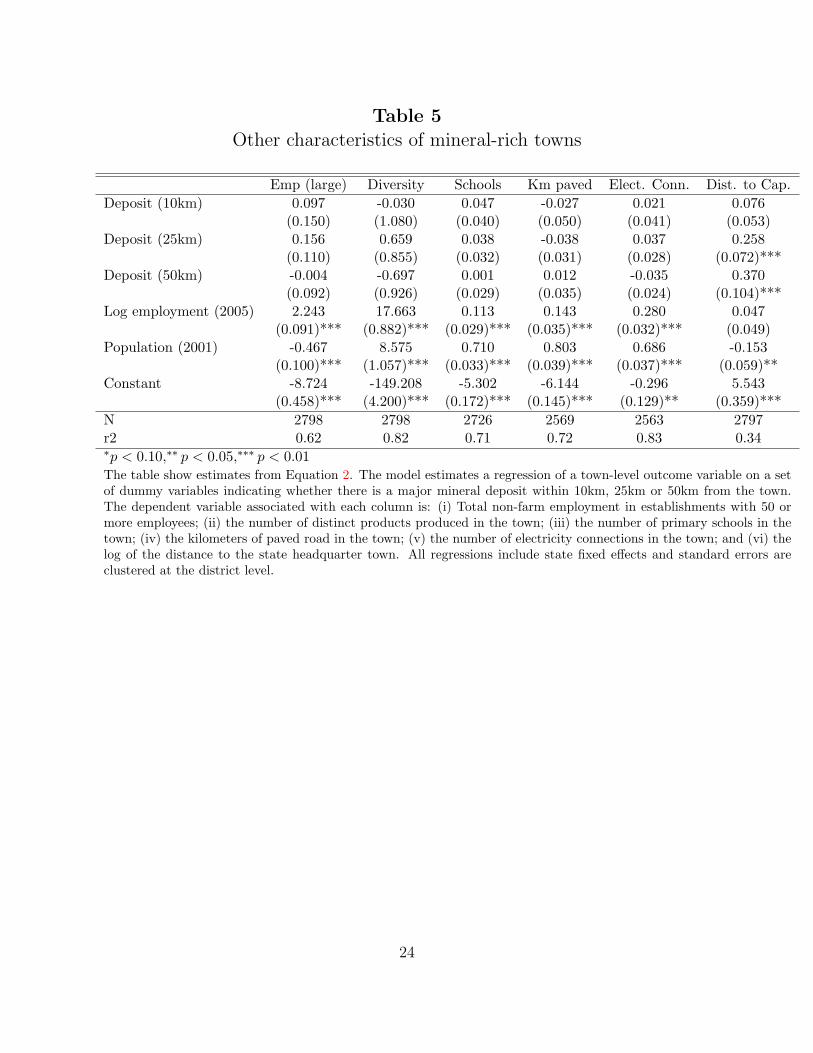
Table 5Other characteristics of mineral-rich towns

Emp (large) Diversity Schools Km paved Elect. Conn. Dist. to Cap.Deposit (10km) 0.097 -0.030 0.047 -0.027 0.021 0.076

(0.150) (1.080) (0.040) (0.050) (0.041) (0.053)Deposit (25km) 0.156 0.659 0.038 -0.038 0.037 0.258

(0.110) (0.855) (0.032) (0.031) (0.028) (0.072)***Deposit (50km) -0.004 -0.697 0.001 0.012 -0.035 0.370

(0.092) (0.926) (0.029) (0.035) (0.024) (0.104)***Log employment (2005) 2.243 17.663 0.113 0.143 0.280 0.047

(0.091)*** (0.882)*** (0.029)*** (0.035)*** (0.032)*** (0.049)Population (2001) -0.467 8.575 0.710 0.803 0.686 -0.153

(0.100)*** (1.057)*** (0.033)*** (0.039)*** (0.037)*** (0.059)**Constant -8.724 -149.208 -5.302 -6.144 -0.296 5.543

(0.458)*** (4.200)*** (0.172)*** (0.145)*** (0.129)** (0.359)***N 2798 2798 2726 2569 2563 2797r2 0.62 0.82 0.71 0.72 0.83 0.34∗p < 0.10,∗∗ p < 0.05,∗∗∗ p < 0.01The table show estimates from Equation 2. The model estimates a regression of a town-level outcome variable on a setof dummy variables indicating whether there is a major mineral deposit within 10km, 25km or 50km from the town.The dependent variable associated with each column is: (i) Total non-farm employment in establishments with 50 ormore employees; (ii) the number of distinct products produced in the town; (iii) the number of primary schools in thetown; (iv) the kilometers of paved road in the town; (v) the number of electricity connections in the town; and (vi) thelog of the distance to the state headquarter town. All regressions include state fixed effects and standard errors areclustered at the district level.

24

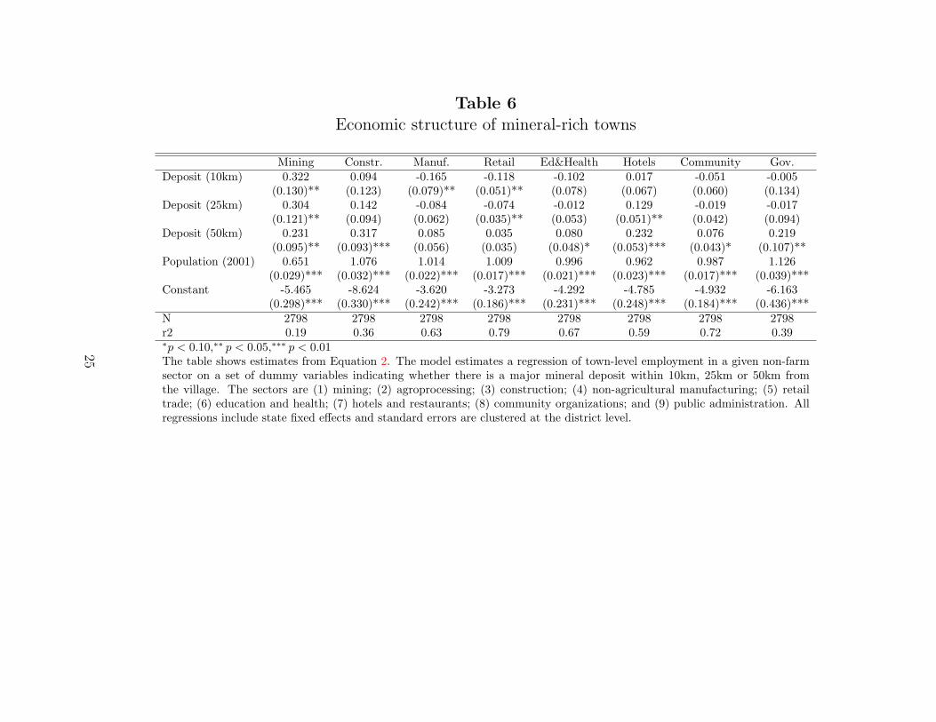
Table 6Economic structure of mineral-rich towns

Mining Constr. Manuf. Retail Ed&Health Hotels Community Gov.Deposit (10km) 0.322 0.094 -0.165 -0.118 -0.102 0.017 -0.051 -0.005

(0.130)** (0.123) (0.079)** (0.051)** (0.078) (0.067) (0.060) (0.134)Deposit (25km) 0.304 0.142 -0.084 -0.074 -0.012 0.129 -0.019 -0.017

(0.121)** (0.094) (0.062) (0.035)** (0.053) (0.051)** (0.042) (0.094)Deposit (50km) 0.231 0.317 0.085 0.035 0.080 0.232 0.076 0.219

(0.095)** (0.093)*** (0.056) (0.035) (0.048)* (0.053)*** (0.043)* (0.107)**Population (2001) 0.651 1.076 1.014 1.009 0.996 0.962 0.987 1.126

(0.029)*** (0.032)*** (0.022)*** (0.017)*** (0.021)*** (0.023)*** (0.017)*** (0.039)***Constant -5.465 -8.624 -3.620 -3.273 -4.292 -4.785 -4.932 -6.163

(0.298)*** (0.330)*** (0.242)*** (0.186)*** (0.231)*** (0.248)*** (0.184)*** (0.436)***N 2798 2798 2798 2798 2798 2798 2798 2798r2 0.19 0.36 0.63 0.79 0.67 0.59 0.72 0.39∗p < 0.10,∗∗ p < 0.05,∗∗∗ p < 0.01The table shows estimates from Equation 2. The model estimates a regression of town-level employment in a given non-farmsector on a set of dummy variables indicating whether there is a major mineral deposit within 10km, 25km or 50km fromthe village. The sectors are (1) mining; (2) agroprocessing; (3) construction; (4) non-agricultural manufacturing; (5) retailtrade; (6) education and health; (7) hotels and restaurants; (8) community organizations; and (9) public administration. Allregressions include state fixed effects and standard errors are clustered at the district level.

25

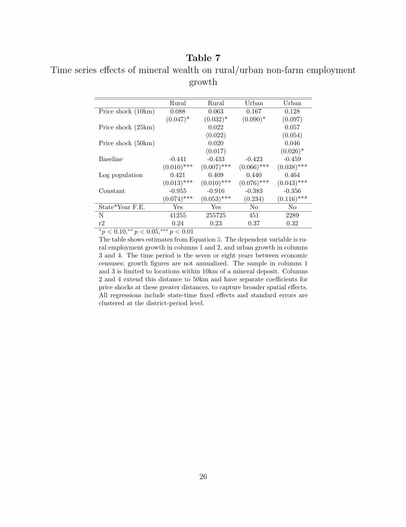
Table 7Time series effects of mineral wealth on rural/urban non-farm employment

growth

Rural Rural Urban UrbanPrice shock (10km) 0.088 0.063 0.167 0.128

(0.047)* (0.032)* (0.090)* (0.097)Price shock (25km) 0.022 0.057

(0.022) (0.054)Price shock (50km) 0.020 0.046

(0.017) (0.026)*Baseline -0.441 -0.433 -0.423 -0.459

(0.010)*** (0.007)*** (0.066)*** (0.038)***Log population 0.421 0.409 0.440 0.464

(0.013)*** (0.010)*** (0.076)*** (0.043)***Constant -0.955 -0.916 -0.383 -0.356

(0.074)*** (0.053)*** (0.234) (0.116)***State*Year F.E. Yes Yes No NoN 41255 255725 451 2289r2 0.24 0.23 0.37 0.32∗p < 0.10,∗∗ p < 0.05,∗∗∗ p < 0.01The table shows estimates from Equation 3. The dependent variable is ru-ral employment growth in columns 1 and 2, and urban growth in columns3 and 4. The time period is the seven or eight years between economiccensuses; growth figures are not annualized. The sample in columns 1and 3 is limited to locations within 10km of a mineral deposit. Columns2 and 4 extend this distance to 50km and have separate coefficients forprice shocks at these greater distances, to capture broader spatial effects.All regressions include state-time fixed effects and standard errors areclustered at the district-period level.

26

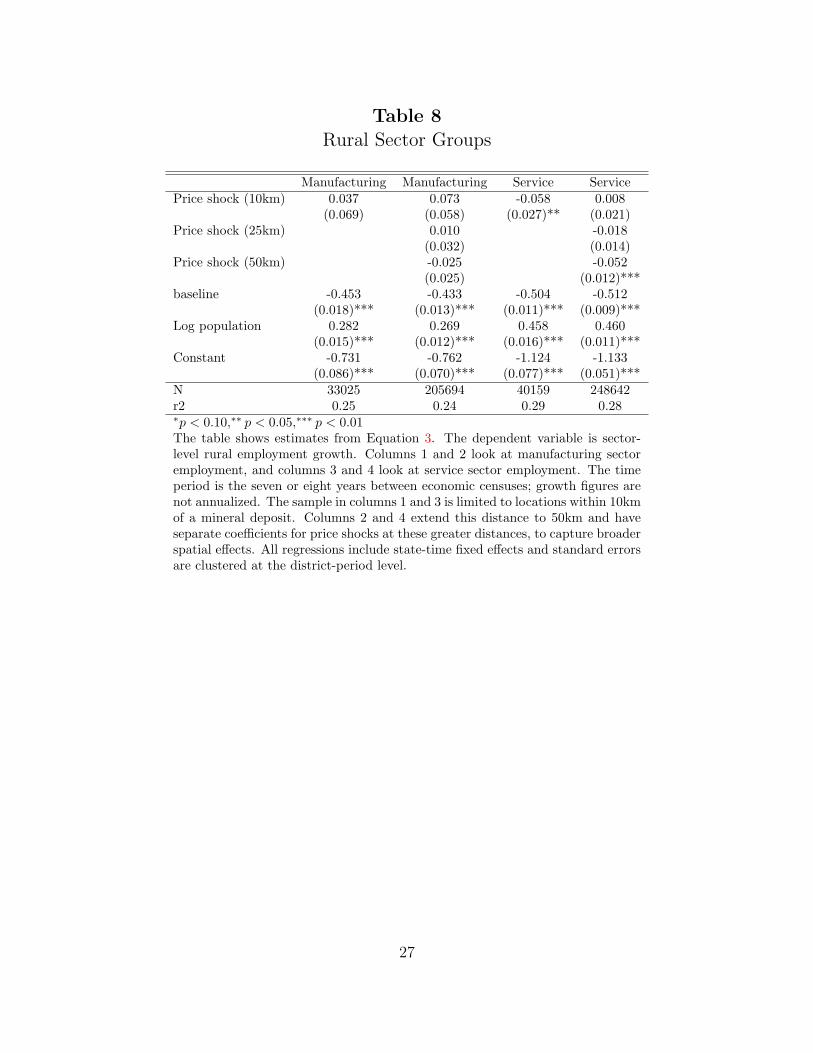
Table 8Rural Sector Groups

Manufacturing Manufacturing Service ServicePrice shock (10km) 0.037 0.073 -0.058 0.008

(0.069) (0.058) (0.027)** (0.021)Price shock (25km) 0.010 -0.018

(0.032) (0.014)Price shock (50km) -0.025 -0.052

(0.025) (0.012)***baseline -0.453 -0.433 -0.504 -0.512

(0.018)*** (0.013)*** (0.011)*** (0.009)***Log population 0.282 0.269 0.458 0.460

(0.015)*** (0.012)*** (0.016)*** (0.011)***Constant -0.731 -0.762 -1.124 -1.133

(0.086)*** (0.070)*** (0.077)*** (0.051)***N 33025 205694 40159 248642r2 0.25 0.24 0.29 0.28∗p < 0.10,∗∗ p < 0.05,∗∗∗ p < 0.01The table shows estimates from Equation 3. The dependent variable is sector-level rural employment growth. Columns 1 and 2 look at manufacturing sectoremployment, and columns 3 and 4 look at service sector employment. The timeperiod is the seven or eight years between economic censuses; growth figures arenot annualized. The sample in columns 1 and 3 is limited to locations within 10kmof a mineral deposit. Columns 2 and 4 extend this distance to 50km and haveseparate coefficients for price shocks at these greater distances, to capture broaderspatial effects. All regressions include state-time fixed effects and standard errorsare clustered at the district-period level.

27

28

Table 9Time series effects of mineral wealth on economic structure of nearest villages

Ag Proc Non-ag Manuf. Constr. Retail Ed&Health Hotels Community Gov.Price shock (10km) 0.142 -0.057 0.031 -0.110 -0.098 -0.008 0.113 -0.087

(0.089) (0.049) (0.019) (0.034)*** (0.043)** (0.037) (0.045)** (0.049)*Baseline sector employment -0.419 -0.454 -0.692 -0.531 -0.553 -0.427 -0.617 -0.524

(0.029)*** (0.013)*** (0.018)*** (0.014)*** (0.013)*** (0.013)*** (0.016)*** (0.012)***Log population 0.123 0.395 0.100 0.499 0.388 0.264 0.357 0.274

(0.014)*** (0.018)*** (0.008)*** (0.018)*** (0.015)*** (0.011)*** (0.015)*** (0.013)***Constant -0.507 -1.612 -0.496 -1.964 -1.117 -1.188 -1.735 -1.161

(0.087)*** (0.117)*** (0.064)*** (0.109)*** (0.077)*** (0.074)*** (0.089)*** (0.074)***N 41255 41255 41255 41255 41255 41255 41255 41255r2 0.25 0.27 0.41 0.30 0.31 0.20 0.34 0.31∗p < 0.10,∗∗ p < 0.05,∗∗∗ p < 0.01

Ag Proc Non-ag Manuf. Constr. Retail Ed&Health Hotels Community Gov.Price shock (10km) 0.101 0.008 0.003 0.010 -0.015 0.032 0.048 -0.020

(0.070) (0.039) (0.015) (0.025) (0.027) (0.029) (0.029) (0.032)Price shock (25km) 0.063 -0.029 0.018 -0.038 -0.029 0.010 0.045 -0.029

(0.043) (0.025) (0.011)* (0.017)** (0.021) (0.018) (0.021)** (0.020)Price shock (50km) -0.006 -0.037 0.019 -0.097 -0.060 -0.041 0.042 -0.040

(0.028) (0.021)* (0.007)*** (0.012)*** (0.019)*** (0.016)*** (0.018)** (0.016)**Baseline sector employment -0.390 -0.444 -0.720 -0.532 -0.559 -0.438 -0.623 -0.537

(0.020)*** (0.010)*** (0.010)*** (0.009)*** (0.010)*** (0.009)*** (0.011)*** (0.011)***Log population 0.126 0.388 0.094 0.497 0.382 0.252 0.364 0.252

(0.013)*** (0.014)*** (0.005)*** (0.012)*** (0.010)*** (0.008)*** (0.011)*** (0.010)***Constant -0.595 -1.614 -0.481 -1.969 -1.047 -1.124 -1.789 -1.025

(0.076)*** (0.088)*** (0.034)*** (0.073)*** (0.052)*** (0.054)*** (0.063)*** (0.058)***N 255725 255725 255725 255725 255725 255725 255725 255725r2 0.24 0.26 0.42 0.30 0.31 0.21 0.35 0.31∗p < 0.10,∗∗ p < 0.05,∗∗∗ p < 0.01The table shows estimates from Equation 3. The dependent variable is sector-level rural employment growth. The top panel limits the sampleto locations within 10km of a mineral deposit, while the bottom panel includes locations up to 50km from a mineral deposit, with separatecoefficients from shocks to minerals at different distances from locations. The sector used as dependent variables is: (1) agroprocessing; (2)non-ag manufacturing; (3) construction; (4) retail trade; (5) education and health; (6) hotels and restaurants; (7) community organizations;and (8) public administration. The time period is the seven or eight years between economic censuses; growth figures are not annualized. Allregressions include state-time fixed effects and standard errors are clustered at the district-period level.

29

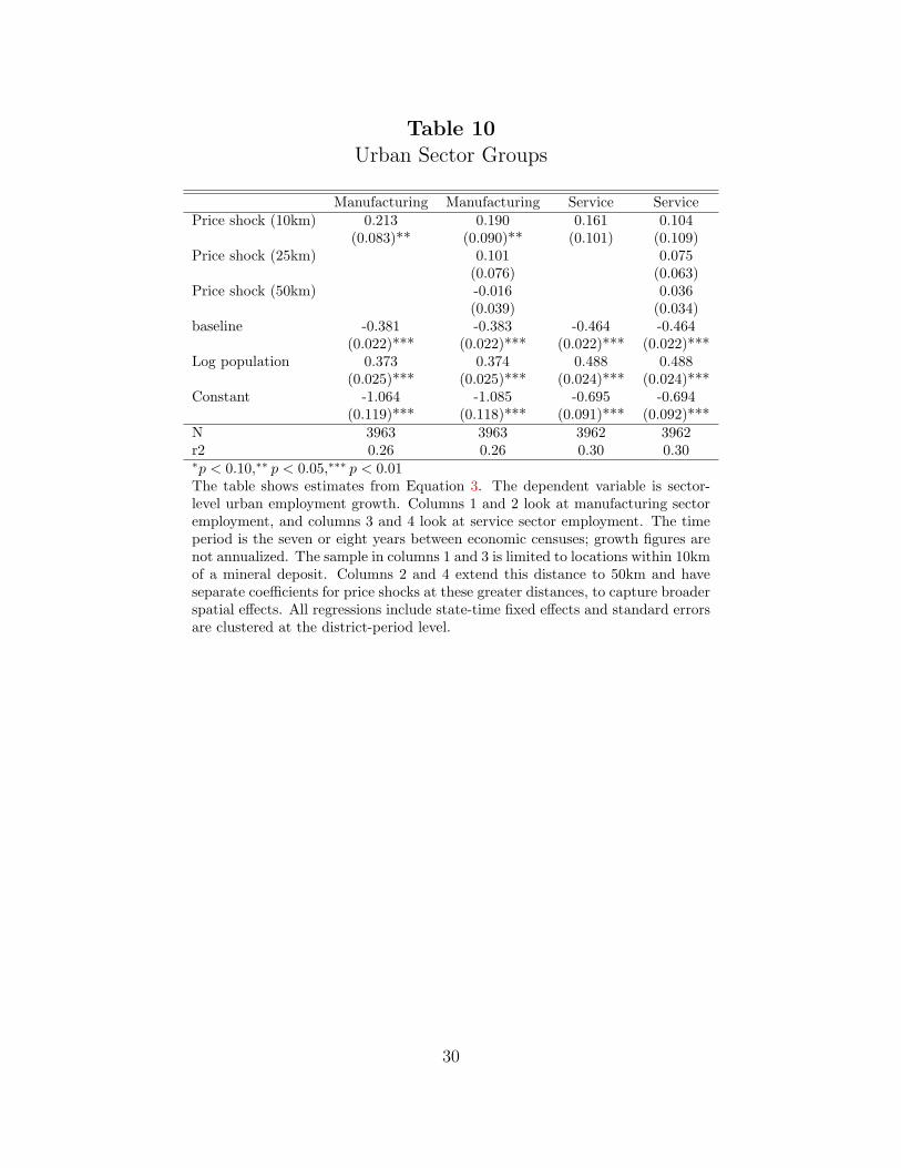
Table 10Urban Sector Groups

Manufacturing Manufacturing Service ServicePrice shock (10km) 0.213 0.190 0.161 0.104

(0.083)** (0.090)** (0.101) (0.109)Price shock (25km) 0.101 0.075

(0.076) (0.063)Price shock (50km) -0.016 0.036

(0.039) (0.034)baseline -0.381 -0.383 -0.464 -0.464

(0.022)*** (0.022)*** (0.022)*** (0.022)***Log population 0.373 0.374 0.488 0.488

(0.025)*** (0.025)*** (0.024)*** (0.024)***Constant -1.064 -1.085 -0.695 -0.694

(0.119)*** (0.118)*** (0.091)*** (0.092)***N 3963 3963 3962 3962r2 0.26 0.26 0.30 0.30∗p < 0.10,∗∗ p < 0.05,∗∗∗ p < 0.01The table shows estimates from Equation 3. The dependent variable is sector-level urban employment growth. Columns 1 and 2 look at manufacturing sectoremployment, and columns 3 and 4 look at service sector employment. The timeperiod is the seven or eight years between economic censuses; growth figures arenot annualized. The sample in columns 1 and 3 is limited to locations within 10kmof a mineral deposit. Columns 2 and 4 extend this distance to 50km and haveseparate coefficients for price shocks at these greater distances, to capture broaderspatial effects. All regressions include state-time fixed effects and standard errorsare clustered at the district-period level.

30

31

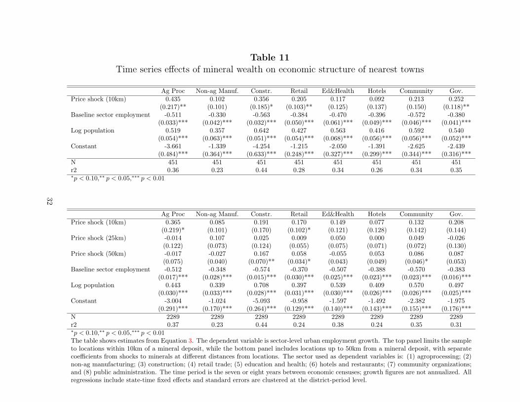
Table 11Time series effects of mineral wealth on economic structure of nearest towns

Ag Proc Non-ag Manuf. Constr. Retail Ed&Health Hotels Community Gov.Price shock (10km) 0.435 0.102 0.356 0.205 0.117 0.092 0.213 0.252

(0.217)** (0.101) (0.185)* (0.103)** (0.125) (0.137) (0.150) (0.118)**Baseline sector employment -0.511 -0.330 -0.563 -0.384 -0.470 -0.396 -0.572 -0.380

(0.033)*** (0.042)*** (0.032)*** (0.050)*** (0.061)*** (0.049)*** (0.046)*** (0.041)***Log population 0.519 0.357 0.642 0.427 0.563 0.416 0.592 0.540

(0.054)*** (0.063)*** (0.051)*** (0.054)*** (0.068)*** (0.056)*** (0.056)*** (0.052)***Constant -3.661 -1.339 -4.254 -1.215 -2.050 -1.391 -2.625 -2.439

(0.484)*** (0.364)*** (0.633)*** (0.248)*** (0.327)*** (0.299)*** (0.344)*** (0.316)***N 451 451 451 451 451 451 451 451r2 0.36 0.23 0.44 0.28 0.34 0.26 0.34 0.35∗p < 0.10,∗∗ p < 0.05,∗∗∗ p < 0.01

Ag Proc Non-ag Manuf. Constr. Retail Ed&Health Hotels Community Gov.Price shock (10km) 0.365 0.085 0.191 0.170 0.149 0.077 0.132 0.208

(0.219)* (0.101) (0.170) (0.102)* (0.121) (0.128) (0.142) (0.144)Price shock (25km) -0.014 0.107 0.025 0.009 0.050 0.000 0.049 -0.026

(0.122) (0.073) (0.124) (0.055) (0.075) (0.071) (0.072) (0.130)Price shock (50km) -0.017 -0.027 0.167 0.058 -0.055 0.053 0.086 0.087

(0.075) (0.040) (0.070)** (0.034)* (0.043) (0.049) (0.046)* (0.053)Baseline sector employment -0.512 -0.348 -0.574 -0.370 -0.507 -0.388 -0.570 -0.383

(0.017)*** (0.028)*** (0.015)*** (0.030)*** (0.025)*** (0.023)*** (0.023)*** (0.016)***Log population 0.443 0.339 0.708 0.397 0.539 0.409 0.570 0.497

(0.030)*** (0.033)*** (0.028)*** (0.031)*** (0.030)*** (0.026)*** (0.026)*** (0.025)***Constant -3.004 -1.024 -5.093 -0.958 -1.597 -1.492 -2.382 -1.975

(0.291)*** (0.170)*** (0.264)*** (0.129)*** (0.140)*** (0.143)*** (0.155)*** (0.176)***N 2289 2289 2289 2289 2289 2289 2289 2289r2 0.37 0.23 0.44 0.24 0.38 0.24 0.35 0.31∗p < 0.10,∗∗ p < 0.05,∗∗∗ p < 0.01The table shows estimates from Equation 3. The dependent variable is sector-level urban employment growth. The top panel limits the sampleto locations within 10km of a mineral deposit, while the bottom panel includes locations up to 50km from a mineral deposit, with separatecoefficients from shocks to minerals at different distances from locations. The sector used as dependent variables is: (1) agroprocessing; (2)non-ag manufacturing; (3) construction; (4) retail trade; (5) education and health; (6) hotels and restaurants; (7) community organizations;and (8) public administration. The time period is the seven or eight years between economic censuses; growth figures are not annualized. Allregressions include state-time fixed effects and standard errors are clustered at the district-period level.

32

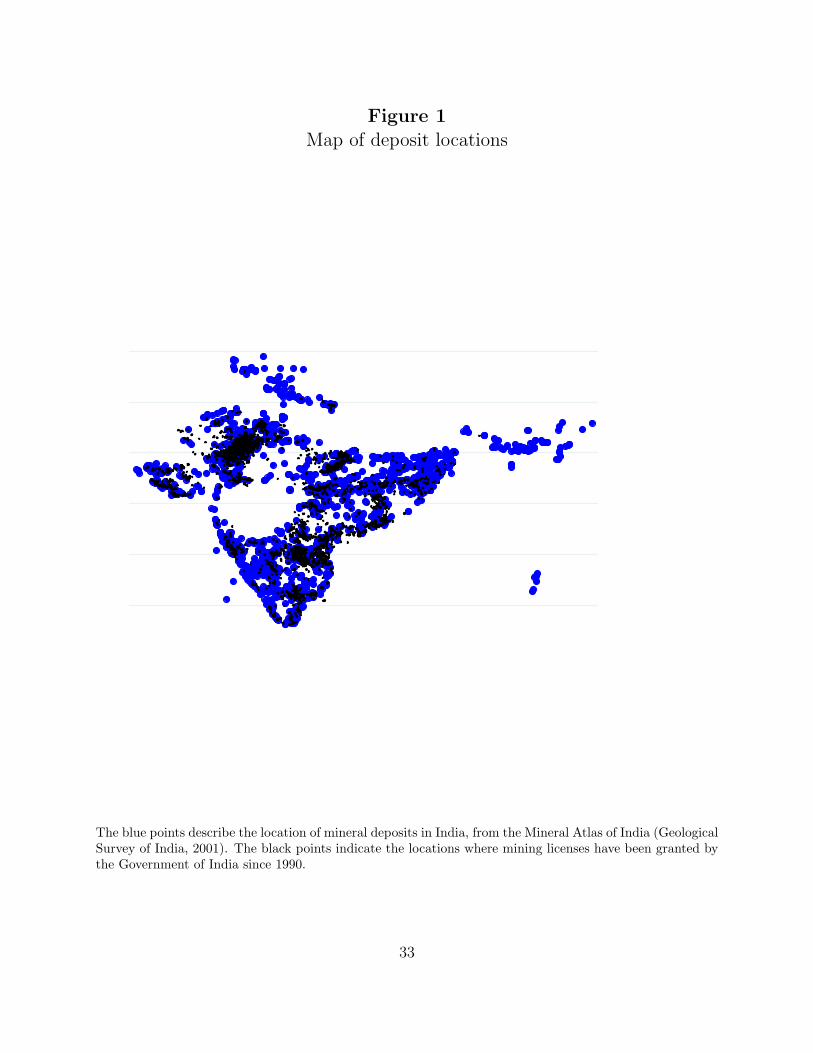
Figure 1Map of deposit locations

1015

2025

3035

latitude

70 75 80 85 90 95longitude

latitude latitude

The blue points describe the location of mineral deposits in India, from the Mineral Atlas of India (GeologicalSurvey of India, 2001). The black points indicate the locations where mining licenses have been granted bythe Government of India since 1990.

33

34

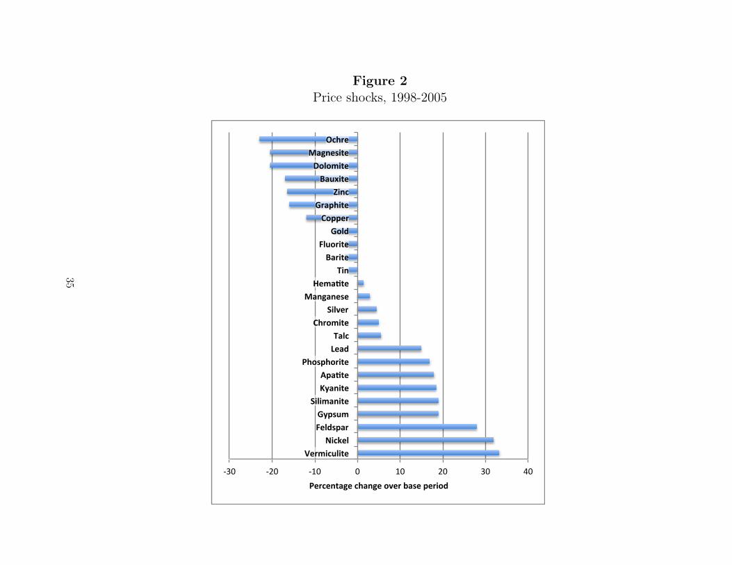
Figure 2Price shocks, 1998-2005

-­‐30   -­‐20   -­‐10   0   10   20   30   40  

Vermiculite  Nickel  

Feldspar  Gypsum  

Silimanite  Kyanite  Apa8te  

Phosphorite  Lead  Talc  

Chromite  Silver  

Manganese  Hema8te  

Tin  Barite  

Fluorite  Gold  

Copper  Graphite  

Zinc  Bauxite  

Dolomite  Magnesite  

Ochre  

Percentage  change  over  base  period  

35

References

Alexeev, Michael and Robert Conrad, “The elusive curse of oil,” The Review of Eco-nomics and Statistics, 2009, 91 (3), 586–598.

Altonji, Joseph G, Todd E Elder, and Christopher R Taber, “Selection on Observedand Unobserved Variables: Assessing the Effectiveness of Catholic Schools,” Journal ofPolitical Economy, 2005, 113 (1), 151–184.

Aragon, F M and J P Rud, “Natural Resources and Local Communities: Evidence froma Peruvian Gold Mine,” American Economic Journal: Economic Policy, 2013, 5 (2).

Asher, Sam and Paul Novosad, “Dirty Politics: Natural resource wealth and politics inIndia,” 2013.

Black, Dan, Terra McKinnish, and Seth Sanders, “The Economic Impact of the CoalBoom and Bust,” The Economic Journal, April 2005, 115 (503), 449–476.

Carrington, W.J., “The Alaskan labor market during the pipeline era,” Journal of PoliticalEconomy, 1996, 104 (1), 186–218.

Caselli, Francesco and Guy Michaels, “Do oil windfalls improve living standards? Ev-idence from Brazil,” American Economic Journal: Applied Economics, 2013, 5 (1),208–238.

Corden, W.M., “Booming Sector and Dutch Disease Economics : Survey and Consolida-tion,” Oxford Economic Papers, 2012, 36 (3), 359–380.

Domenech, Jordi, “Mineral resource abundance and regional growth in Spain, 1860a2000,”Journal of International Development, 2008, 20, 1122–1135.

Ellison, Glenn and Edward L Glaeser, “Geographic Concentration in U.S. Manufactur-ing Industries: A Dartboard Approach,” Journal of Political Economy, 1997, 105 (5),889–927.

Foster, Andrew D and Mark R Rosenzweig, “Agricultural Productivity Growth, RuralEconomic Diversity and Economic Reforms, India 1970-2000,” Economic Developmentand Cultural Change, 2004.

Geological Survey of India, Mineral Atlas of India, Kolkata: Geological Survey of India,2001.

Indian Bureau of Mines, Indian Minerals Year Book 2010, Nagpur, India: IBM Press,2011.

Kelly, Thomas D. and Grecia R. Matos, “Historical Statistics for Mineral and MaterialCommodities in the United States,” Technical Report, US Geological Survey 2013.

36

Marshall, Alfred, Principles of Economics, London: MacMillan, 1920.

Mehlum, Halvor, Karl Moene, and Ragnar Torvik, “Institutions and the ResourceCurse,” The Economic Journal, 2006, 116 (January), 1–20.

Michaels, Guy, “The long term consequences of resource-based specialization,” The Eco-nomic Journal, 2010, 121 (March), 31–57.

Murphy, Kevin M., Andrei Shleifer, and Robert W. Vishny, “The allocation oftalent: Implications for growth,” Quarterly Journal of Economics, 1991, 106 (2), 503–530.

Robinson, James, Ragnar Torvik, and Thierry Verdier, “Political foundations of theresource curse,” Journal of Development Economics, April 2006, 79 (2), 447–468.

Sachs, J.D. and A.M. Warner, “The curse of natural resources,” European economicreview, 2001, 45 (4-6), 827–838.

Sachs, Jeffrey and A.M. Warner, “Natural Resource Abundance and Economic Growth,”in G Meier and J Rauch, eds., Leading Issues in Economic Development, Vol. 3, NewYork: Oxford University Press, 1995.

van der Ploeg, Frederick, “Natural resources: curse or blessing?,” Journal of EconomicLiterature, 2011, 49 (2), 366–420.

37