Embed Size (px)
Citation preview

Dirty tricks for statistical mechanics:
time dependent things
Martin Grant
c© MG, August 2005, version 0.8
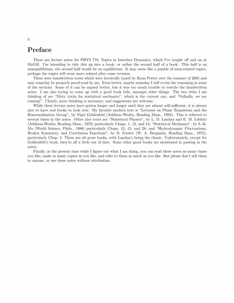
ii
Preface
These are lecture notes for PHYS 719, Topics in Interface Dynamics, which I’ve taught off and on atMcGill. I’m intending to tidy this up into a book, or rather the second half of a book. This half is onnonequilibrium, the second half would be on equilibrium. It may seem like a jumble of semi-related topics,perhaps the topics will seem more related after some revision.
These were handwritten notes which were heroically typed by Ryan Porter over the summer of 2005 andmay someday be properly proof-read by me. Even better, maybe someday I will revise the reasoning in someof the sections. Some of it can be argued better, but it was too much trouble to rewrite the handwrittennotes. I am also trying to come up with a good book title, amongst other things. The two titles I amthinking of are “Dirty tricks for statistical mechanics”, which is the current one, and “Valhalla, we arecoming!”. Clearly, more thinking is necessary, and suggestions are welcome.
While these lecture notes have gotten longer and longer until they are almost self-sufficient, it is alwaysnice to have real books to look over. My favorite modern text is “Lectures on Phase Transitions and theRenormalisation Group”, by Nigel Goldenfeld (Addison-Wesley, Reading Mass., 1992). This is referred toseveral times in the notes. Other nice texts are “Statistical Physics”, by L. D. Landau and E. M. Lifshitz(Addison-Wesley, Reading Mass., 1970) particularly Chaps. 1, 12, and 14; “Statistical Mechanics”, by S.-K.Ma (World Science, Phila., 1986) particularly Chaps. 12, 13, and 28; and “Hydrodynamic Fluctuations,Broken Symmetry, and Correlation Functions”, by D. Forster (W. A. Benjamin, Reading Mass., 1975),particularly Chap. 2. These are all great books, with Landau’s being the classic. Unfortunately, except forGoldenfeld’s book, they’re all a little out of date. Some other good books are mentioned in passing in thenotes.
Finally, at the present time while I figure out what I am doing, you can read these notes as many timesyou like, make as many copies as you like, and refer to them as much as you like. But please don’t sell themto anyone, or use these notes without attribution.
Contents
1 Droplet Growth 11.1 Avrami Theory of Droplet Growth . . . . . . . . . . . . . . . . . . . . . . . . . . . . . . . . . 11.2 Ostwald Ripening . . . . . . . . . . . . . . . . . . . . . . . . . . . . . . . . . . . . . . . . . . . 3
2 Dynamic Roughening (Quick and Dirty) 152.1 Model A, No Conservation Law . . . . . . . . . . . . . . . . . . . . . . . . . . . . . . . . . . . 182.2 Model B “Lite”, Local Conservation Only . . . . . . . . . . . . . . . . . . . . . . . . . . . . . 192.3 Model B, Conservation Law . . . . . . . . . . . . . . . . . . . . . . . . . . . . . . . . . . . . . 20
3 Driven Roughening and KPZ Equation 23
4 Renormalization Group for Driven Roughening 354.1 Appendix: Various Ugly Realities . . . . . . . . . . . . . . . . . . . . . . . . . . . . . . . . . . 50
5 Nonequilibrium Theory Primer 575.1 Brownian Motion and L-R Circuits . . . . . . . . . . . . . . . . . . . . . . . . . . . . . . . . . 575.2 Fokker–Planck Equation . . . . . . . . . . . . . . . . . . . . . . . . . . . . . . . . . . . . . . . 625.3 Appendix 1 . . . . . . . . . . . . . . . . . . . . . . . . . . . . . . . . . . . . . . . . . . . . . . 645.4 Master Equation and Fokker–Planck Equation . . . . . . . . . . . . . . . . . . . . . . . . . . 655.5 Appendix 2: H theorem for Master Equation . . . . . . . . . . . . . . . . . . . . . . . . . . . 725.6 Appendix 3: Derivation of Master Equation . . . . . . . . . . . . . . . . . . . . . . . . . . . . 745.7 Mori–Zwanzig Formalism . . . . . . . . . . . . . . . . . . . . . . . . . . . . . . . . . . . . . . 75
6 Multiple Scales Expansion 836.1 Multiple Scales Expansion (Basic Stuff) . . . . . . . . . . . . . . . . . . . . . . . . . . . . . . 836.2 Multiple Scales Expansion for Model B with z = 2 (subtle stuff) . . . . . . . . . . . . . . . . 93
6.2.1 Outer Region . . . . . . . . . . . . . . . . . . . . . . . . . . . . . . . . . . . . . . . . . 936.2.2 Zeroth Order Outer . . . . . . . . . . . . . . . . . . . . . . . . . . . . . . . . . . . . . 946.2.3 First–Order Outer . . . . . . . . . . . . . . . . . . . . . . . . . . . . . . . . . . . . . . 946.2.4 Inner Region . . . . . . . . . . . . . . . . . . . . . . . . . . . . . . . . . . . . . . . . . 946.2.5 Zeroth Order Inner . . . . . . . . . . . . . . . . . . . . . . . . . . . . . . . . . . . . . . 956.2.6 First–Order Inner . . . . . . . . . . . . . . . . . . . . . . . . . . . . . . . . . . . . . . 966.2.7 Other Stuff . . . . . . . . . . . . . . . . . . . . . . . . . . . . . . . . . . . . . . . . . . 101
6.3 Multiple Scales Expansion for Model A With z = 1 and z = 3 are Useless . . . . . . . . . . . 103
iii
iv CONTENTS
6.3.1 Outer Region . . . . . . . . . . . . . . . . . . . . . . . . . . . . . . . . . . . . . . . . . 1036.3.2 Inner Region . . . . . . . . . . . . . . . . . . . . . . . . . . . . . . . . . . . . . . . . . 1046.3.3 Zeroth Order . . . . . . . . . . . . . . . . . . . . . . . . . . . . . . . . . . . . . . . . . 1046.3.4 First Order . . . . . . . . . . . . . . . . . . . . . . . . . . . . . . . . . . . . . . . . . . 105
7 Fokker–Planck Equation 1097.1 Stationary Solutions . . . . . . . . . . . . . . . . . . . . . . . . . . . . . . . . . . . . . . . . . 1107.2 Time–Dependent Solutions . . . . . . . . . . . . . . . . . . . . . . . . . . . . . . . . . . . . . 1117.3 Boundary Conditions . . . . . . . . . . . . . . . . . . . . . . . . . . . . . . . . . . . . . . . . . 1197.4 Escape Rate . . . . . . . . . . . . . . . . . . . . . . . . . . . . . . . . . . . . . . . . . . . . . . 1207.5 Appendix: Langevin Equations and Fokker–Planck Equations . . . . . . . . . . . . . . . . . . 1227.6 Appendix: Friction and Amonton’s Law . . . . . . . . . . . . . . . . . . . . . . . . . . . . . . 1237.7 Some Numbers . . . . . . . . . . . . . . . . . . . . . . . . . . . . . . . . . . . . . . . . . . . . 129
7.7.1 Atomic Force Microscope and Kinetic Friction . . . . . . . . . . . . . . . . . . . . . . 130
8 Statistical Theory of the Decay of Metastable States 1358.1 Equation of Motion for the Distribution Function . . . . . . . . . . . . . . . . . . . . . . . . . 1358.2 Nucleation Rates . . . . . . . . . . . . . . . . . . . . . . . . . . . . . . . . . . . . . . . . . . . 139
9 Interfaces in Equilibrium and Out of Equilibrium 1519.1 Interfaces in Equilibrium . . . . . . . . . . . . . . . . . . . . . . . . . . . . . . . . . . . . . . . 1519.2 Roughening . . . . . . . . . . . . . . . . . . . . . . . . . . . . . . . . . . . . . . . . . . . . . . 1559.3 Interfaces in Non Equilibrium . . . . . . . . . . . . . . . . . . . . . . . . . . . . . . . . . . . . 1609.4 Roughening in Non Equilibrium . . . . . . . . . . . . . . . . . . . . . . . . . . . . . . . . . . . 1629.5 Dynamical Interfaces From Full Model . . . . . . . . . . . . . . . . . . . . . . . . . . . . . . . 1749.6 Curvilinear Coordinates . . . . . . . . . . . . . . . . . . . . . . . . . . . . . . . . . . . . . . . 177
10 Fluid Fingers 181
Chapter 1
Droplet Growth
There are two standard-ish cases of how droplets grow
• by just growing as fast as possible (into, say, a supersaturated background).
• by growing as fast as possible, consistent with diffusion of material or latent heat.
Both cases can, more or less, be solved exactly in non-trivial cases. The algebra is not difficult, but it is notwidely known.
1.1 Avrami Theory of Droplet Growth
Figure 1.1: Droplet Growth
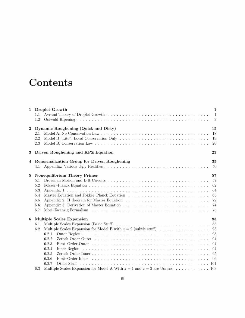
In a supersaturated solution, droplets of the stable phase nu-cleate and grow. Nucleation can be homogeneous — due tospontaneous thermal fluctuations — or heterogeneous — dueto large intrinsic fluctuations, such as dirt.
A physically relevant limit of this can be worked out incomplete detail. It is called the Kolmogorov–Avrami–Meyer–Johnson (KAMJ), or simply, the Avrami theory of dropletgrowth. In the Avrami theory, it is assumed that the super-saturation is negligibly depleted by the nucleating and growingdroplets. Furthermore, it is assumed that droplets do not inter-act. In fact, one of the main ways droplets potentially interactis by depleting the local supersaturation, so these are relatedassumptions. Experimentally these are good approximations ifthe supersaturation is large. This theory explains many experiments on nucleation and growth, arguablymost experiments, very well.
First let us determine the growth of a single droplet. These systems are overdamped, so we will startwith “Aristotle’s force law”:
force ∝ velocity
Here the force is due to the energetic difference between the metastable supersaturated solution, and thestable droplet phase. But we have assumed the supersaturation never decreases. Hence the force is constant,
1
2 CHAPTER 1. DROPLET GROWTH
andConst. ∝ Velocity
By force, I mean the thermodynamic force, and by energy I mean the thermodynamic free energy. In anycase, the solution for the velocity is now apparent
v = Const.
So the radius of a droplet R grows asR ∝ tn
where the growth exponentn = 1
This is a little fast and phenomenological, but all the ideas are correct and complete; we’ll do it more carefullylater.
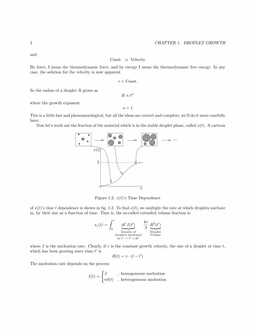
Now let’s work out the fraction of the material which is in the stable droplet phase, called x(t). A cartoon
...
t
x(t)
1
Figure 1.2: x(t)’s Time Dependence
of x(t)’s time t dependence is shown in fig. 1.2. To find x(t), we multiply the rate at which droplets nucleatein, by their size as a function of time. That is, the so-called extended volume fraction is
xe(t) =
∫ t
0
dt′ I(t′)︸ ︷︷ ︸
Density ofdroplets nucleated
in t′ → t′ + dt′
4π
3R3(t′)︸ ︷︷ ︸
DropletVolume
where I is the nucleation rate. Clearly, if v is the constant growth velocity, the size of a droplet at time t,which has been growing since time t′ is
R(t) = v · (t− t′)The nucleation rate depends on the process
I(t) =
J , homogeneous nucleation
nδ(t) , heterogeneous nucleation
1.2. OSTWALD RIPENING 3
Here, J is a constant, because it is determined by the degree of supersaturation. The constant n is pro-portional to the number of dirt sites available for nucleation; once they are used, no more heterogeneousnucleation takes place. (As an aside, the rate for homogeneous nucleation is much less than that for hetero-geneous nucleation. Hence only very pure systems show evidence of homogeneous nucleation.)
The extended volume fraction is a little too simple: the volume available for droplets to nucleate indecreases with time. The fractional change in volume fraction is
dx = (1− x)dxe
or
x = 1− e−xe
for early times, when x≪ 1 , we have x ≈ xe of course. The complete solution is
x(t) = 1− eR t0dt′I(t′) 4π
3 [v·(t−t′)]3
Generalizing this to diminish d is worth while; sometimes droplets nucleate and grow as discs or rods, forexample. The result, after doing the integral, is
x(t) =
1− e−Const.td , ( Heterogeneous)
1− e−Const.td+1
, ( Homogeneous)
The stretch exponent: “d” for heterogeneous nucleation, “d+ 1” for homogeneous nucleation, is often calledthe Avrami exponent. It is measurable from fits to the x(t) curve, providing an easy way to tell what kindof nucleation is taking place.
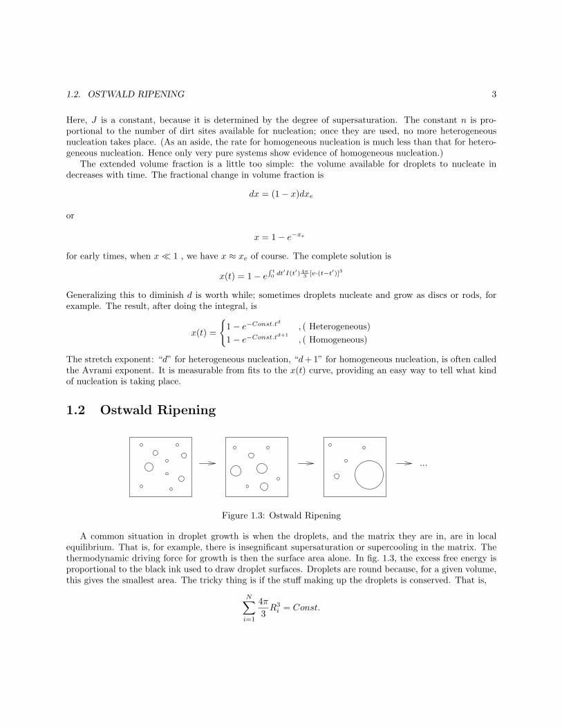
1.2 Ostwald Ripening
...
Figure 1.3: Ostwald Ripening
A common situation in droplet growth is when the droplets, and the matrix they are in, are in localequilibrium. That is, for example, there is insegnificant supersaturation or supercooling in the matrix. Thethermodynamic driving force for growth is then the surface area alone. In fig. 1.3, the excess free energy isproportional to the black ink used to draw droplet surfaces. Droplets are round because, for a given volume,this gives the smallest area. The tricky thing is if the stuff making up the droplets is conserved. That is,
N∑
i=1
4π
3R3i = Const.
4 CHAPTER 1. DROPLET GROWTH
where different droplets are labeled i = 1, 2, 3, ... N , each with radius Ri. If the system was initiallymetastable because it was supersaturated with salt, now almost all the salt is in the form of salt “droplets”,where the total amount of salt (now the total volume of all droplets) is fixed. A handy concept is the volumefraction of the droplet phase
φ =1
V
N∑
i=1
4π
3R3i
Growth takes place by material flowing between droplets, mediated by diffusion through the matrix: As amoment’s thought will make clear, big droplets grow while small droplets shrink and disappear. The averagesize of a droplet R(t) grows with time, and it turns out
R(t) ∼ tn
for late times, where n is the growth exponent, and
n = 1/3
The main quantity of intrest is the droplet size at time t, including the coarsening rate K in
R(t) = (Kt)n
which is independent of time, but dependent upon temperature T , and φ, for example. As well, one wantsto know the distribution of droplets of different sizes at time t, n(R, t), where
n(R, t) =
N∑
i=1
δ(R−Ri(t))
so that ∫
dRn(R, t) = N(t)
the total number of droplets, which decreases with time. Note that
R(t) =∑
i
Ri/∑
i
or equivalently
R(t) =
∫dRRn(R, t)∫dRn(R, t)
The last useful quantity is the two–point correlation function,
c(~r, t)c(~r′, t)− c2δ(~r − ~r′)where ~r denotes a point in space, and c(~r, t) is the local concentration, which we will assume to be dimen-sionless: c = 1 inside a droplet, and c = 0 outside a droplet. Clearly
∫
c ~dr = φV
=
N∑
i=1
4π
3R3i
1.2. OSTWALD RIPENING 5
So, alternatively,
c =N∑
i=1
4π
3R3i δ(~r − ~ri(t))
where ~vi(t) is a vector pointing to the center of a droplet of radius Ri. Fourier transforming gives thestructure factor
S(q, t) =
∫
~dr ei~q~r( ¯c(~ , t) c(0, t)r − c2
)
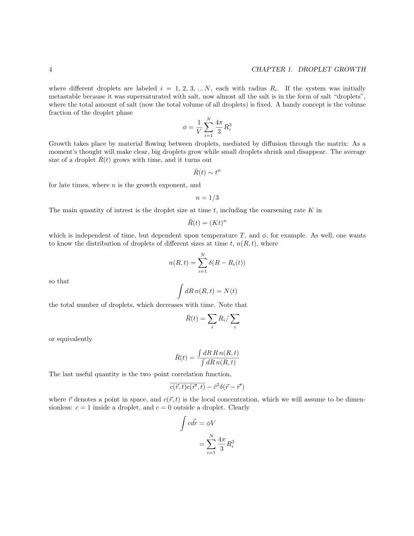
The phenomenology is straightforward. First, the interface moves so as to minimize surface area. The
Figure 1.4: Motion to Reduce Surface Area
thermodynamic force conjugate to surface free energy is curvature 1/R. We expect (in overdamped systems)
velocity ∝ force
so the interface velocity
v ∝ 1
R
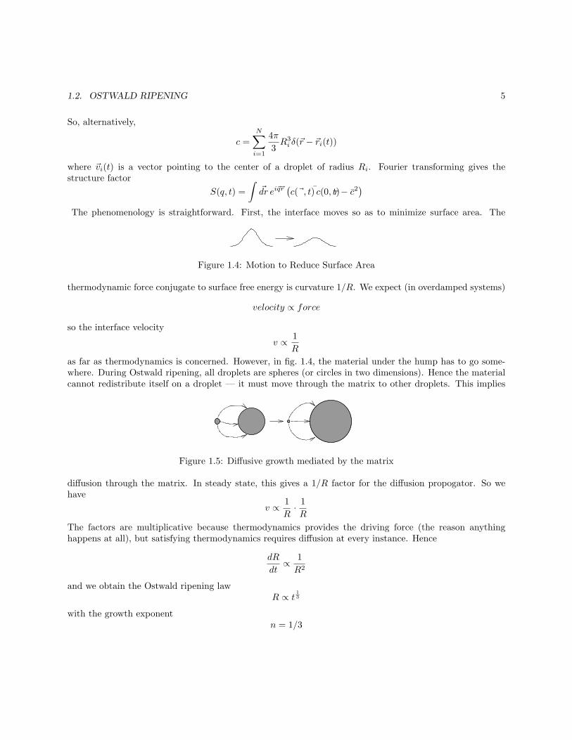
as far as thermodynamics is concerned. However, in fig. 1.4, the material under the hump has to go some-where. During Ostwald ripening, all droplets are spheres (or circles in two dimensions). Hence the materialcannot redistribute itself on a droplet — it must move through the matrix to other droplets. This implies
Figure 1.5: Diffusive growth mediated by the matrix
diffusion through the matrix. In steady state, this gives a 1/R factor for the diffusion propogator. So wehave
v ∝ 1
R· 1
R
The factors are multiplicative because thermodynamics provides the driving force (the reason anythinghappens at all), but satisfying thermodynamics requires diffusion at every instance. Hence
dR
dt∝ 1
R2
and we obtain the Ostwald ripening lawR ∝ t 1
3
with the growth exponentn = 1/3
6 CHAPTER 1. DROPLET GROWTH
All growth, and indeed all droplet correlations, are mixed up with this physics. Hence if we have aquantity
Q = Q(~r, t)
we do dimensional analysis. Replace t by a dependence upon all quantities which depend on t. These includethe average droplet size R(t), and perhaps the width of the interface w(t), among other things. Then
Q = Q(~r, R(t), w(t), ...)
Say the dimensions of Q are
[Q] = ldQ
where l is a length. Then
Q = ldQQ∗(r/l, R/l, w/l, ...)
Choose l = R and we have
Q = RdQQ∗(r/R, 1, w/R, ...)
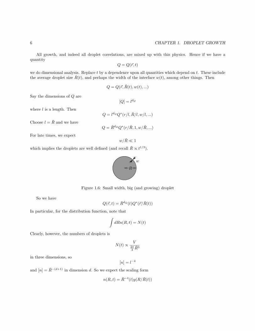
For late times, we expect
w/R≪ 1
which implies the droplets are well defined (and recall R ∝ t1/3).
w
R
Figure 1.6: Small width, big (and growing) droplet
So we have
Q(~r, t) = RdQ(t)Q∗(~r/R(t))
In particular, for the distribution function, note that
∫
dRn(R, t) = N(t)
Clearly, however, the numbers of droplets is
N(t) ∝ V4π3 R
3
in three dimensions, so
[n] = l−4
and [n] = R−(d+1) in dimension d. So we expect the scaling form
n(R, t) = R−4(t)g(R/R(t))
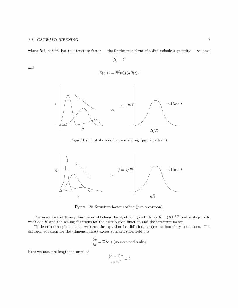
1.2. OSTWALD RIPENING 7
where R(t) ∝ t1/3. For the structure factor — the fourier transform of a dimensionless quantity — we have
[S] = ld
andS(q, t) = Rd(t)f(qR(t))
n
R
tg = nR4
R/R
all late t
or
Figure 1.7: Distribution function scaling (just a cartoon).
f = s/Rd
qR
all late t
or
tS
q
Figure 1.8: Structure factor scaling (just a cartoon).
The main task of theory, besides establishing the algebraic growth form R = (Kt)1/3 and scaling, is towork out K and the scaling functions for the distribution function and the structure factor.
To describe the phenomena, we need the equation for diffusion, subject to boundary conditions. Thediffusion equation for the (dimensionless) excess concentration field c is
∂c
∂t= ∇2c+ (sources and sinks)
Here we measure lengths in units of(d− 1)σ
ρkBT≡ l
8 CHAPTER 1. DROPLET GROWTH
where σ is the surface tension, and ρ is the number density. We measure times in units of
l2/Dζ∞Vm
where D is the diffusion constant, ζ∞ is the concentration above a flat surface, and Vm is the molar volume.The excess concentration is related to the concentration ζ by
c =ζ − ζ∞ζ∞
We will consider a steady–state limit where the concentration is everywhere relaxed to its local equilibriumvalue, that is
∇2c = (sources and sinks)
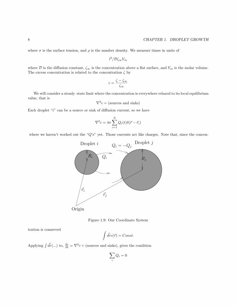
Each droplet “i” can be a source or sink of diffusion current, so we have
∇2c = 4π
N∑
i=1
Qi(t)δ(~r − ~ri)
where we haven’t worked out the “Q’s” yet. Those currents act like charges. Note that, since the concen-
RjRi
Droplet jDroplet i
Qi
~rj~ri
Qi = −Qj
Origin
Figure 1.9: Our Coordinate System
tration is conserved ∫
~drc(~r) = Const.
Applying∫~dr(...) to, ∂c∂t = ∇2c+ (sources and sinks), gives the condition
∑
i
Qi = 0
1.2. OSTWALD RIPENING 9
In fig. 1.9, Qj = −Qi, of course.Thermodynamics (the Gibbs–Thompson condition) requires that the excess concentration at the surface
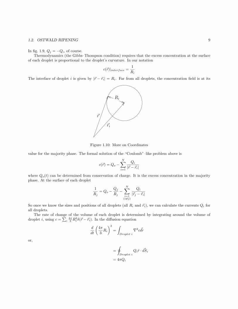
of each droplet is proportional to the droplet’s curvature. In our notation
c(~r)|interface =1
Ri
The interface of droplet i is given by |~r − ~ri| = Ri. Far from all droplets, the concentration field is at its
Ri
~r
~ri
Figure 1.10: More on Coordinates
value for the majority phase. The formal solution of the “Coulomb”–like problem above is
c(~r) = Qo −N∑
i=1
Qi|~r − ~ri|
where Qo(t) can be determined from conservation of charge. It is the excess concentration in the majorityphase. At the surface of each droplet
1
Rj= Qo −
QjRj−
N∑
i=1(i6=j)
Qi|~rj − ~ri|
So once we know the sizes and positions of all droplets (all Ri and ~ri), we can calculate the currents Qi forall droplets.
The rate of change of the volume of each droplet is determined by integrating around the volume ofdroplet i, using c =
∑
i4π3 R
3i δ(~r − ~ri). In the diffusion equation
d
dt
(4π
3Ri
)3
=
∫
Droplet i
∇2c ~dr
or,
=
∮
Droplet i
Qir · ~dSi
= 4πQi
10 CHAPTER 1. DROPLET GROWTH
This givesdRidt
=QiR2i
which completes the description. Given (Ri, ~ri) we can calculate the Qi’s. Then we can update the Ri’swith this equation of motion, and so on.
Note that we have been a little careless with some points. For example, we have not considered the timedependence of N(t) in the equation directly above, and we have used ∂c/∂t there, but not in our Coulomb–like solution of the steady–state problem. It turns out that considering these effects gives corrections to ourresults which vanish as t→∞ for d > 2. Two dimensions has logarithmic corrections which I won’t discusshere. You can check these things yourself.
We can solve these equations in the limit of φ → 0, which was originally done by Lifshitz and Slyozov.In that limit, clearly the droplets are far from each other. Hence, for distinct droplets i and j,
|~ri − ~rj | → ∞
and the solution of the steady–state problem becomes
1
Ri= Qo −
QiRi
or,
1 = QoRi −QiSumming over all droplets gives
∑
i
= Qo∑
i
Ri − 0
∑
i
Qi
so,
Qo =∑
i
/∑
i
Ri
or
Qo = 1/R
Putting this in the equation above gives1
Ri=
1
R− QiRi
Dropping the now superfluous “i” subscripts gives, on rearranging,
Q = R
(1
R− 1
R
)
Using this in the equation of motion gives
dR
dt=
1
R
(1
R− 1
R
)
So droplets with R < R shrink, while droplets with R > R grow, as we expected.
1.2. OSTWALD RIPENING 11
We can now work out the distribution function:
n(R, t) =
N∑
i=1
δ(R−Ri(t))
Taking the derivative
∂n(R, t)
∂t=
N∑
i=1
∂
∂tδ(R−Ri(t))
=
N∑
i=1
dRidt
∂
∂Riδ(R−Ri)
= −N∑
i=1
dRidt
∂
∂Rδ(R−Ri)
= − ∂
∂R
N∑
i=1
(dRidt
)
Ri=R
δ(R−Ri)
= − ∂
∂R
(∂Ri∂t
)
Ri=R
n(R, t)
or∂n(R, t)
∂t+
∂
∂R
(∂R
∂tn(R, t)
)
= 0
Note that we again ignored dN(t)/dt contributions. Using the equation of motion for R we obtain (and notethe potential confusion between Ri(t), an explicit function of time shortened to R(t) above, and the firstargument of the distribution function R, in n(R, t) which is not a function of time):
∂n(R, t)
∂t= − ∂
∂R
(1
R
(1
R(t)− 1
R
)
n(R, t)
)
Only R(t) is an explicit function of time here, not R.
We argued for a scaling form above
n(R, t) = R−4(t)g(R/R(t))
We’ll look for a solution in this form, with the scaled radius
z ≡ R/R(t)
That is:
n(R, t) = R−4(t)g(z)
12 CHAPTER 1. DROPLET GROWTH
Let’s slog through it. First consider the left–hand side of the equation
∂
∂tn(R, t) =
∂
∂t
(R−4(t)g(z)
)
= −4R−5g(z)dR
dt+ R−4 dg
dz
dz
dt
= −4R−5g(z)dR
dt+ R−4 dg
dz
(
− R
R2
dR
dt
)
= −4R−5g(z)dR
dt− R−5z
dg
dz
dR
dt
On the right–hand side of the equation we have
− ∂
∂R
(1
R
(1
R− 1
R
)
n(R, t)
)
= − ∂
∂R
(1
RR− 1
R2
)
n(R, t)−(
1
RR− 1
R2
)∂
∂Rn(R, t)
= −(
− 1
R2R+
2
R3
)
n(R, t)−(
1
RR− 1
R2
)1
R
∂
∂zn(R, t)
= − 1
R3
(
− 1
z2+
2
z3
)
R−4g(z)− 1
R3
(1
z− 1
z2
)
R−4 dg(z)
dz
= − 1
R7
(
− 1
z2+
2
z3
)
g(z)− 1
R7
(1
z− 1
z2
)dg
dz
Equating the two sides of the equation we have
−4R−5 dR
dtg(z)− R−5 dR
dtzdg
dz= − 1
R7
(
− 1
z2+
2
z3
)
g(z)− 1
R7
(1
z− 1
z2
)dg
dz
Multiplying both sides of the equation by (−R7) gives
R2 dR
dt
(
4g(z) + zdg
dz
)
=
(
− 1
z2+
2
z3
)
g(z) +
(1
z− 1
z2
)dg
dz
Since R = R(t) only, and g = g(z) only, this is trivially seperable
R2 dR
dt= k
where k is a constant, and(− 1z2 + 2
z3
)g(z) +
(1z − 1
z2
)dgdz
4g(z) + z dgdz= k
ClearlyR(t) = (kt)1/3
as expected. The equation for g(z) is, after some fiddling
(z2 − z − z4k)dg
dz= (4z3k − (2− z))g
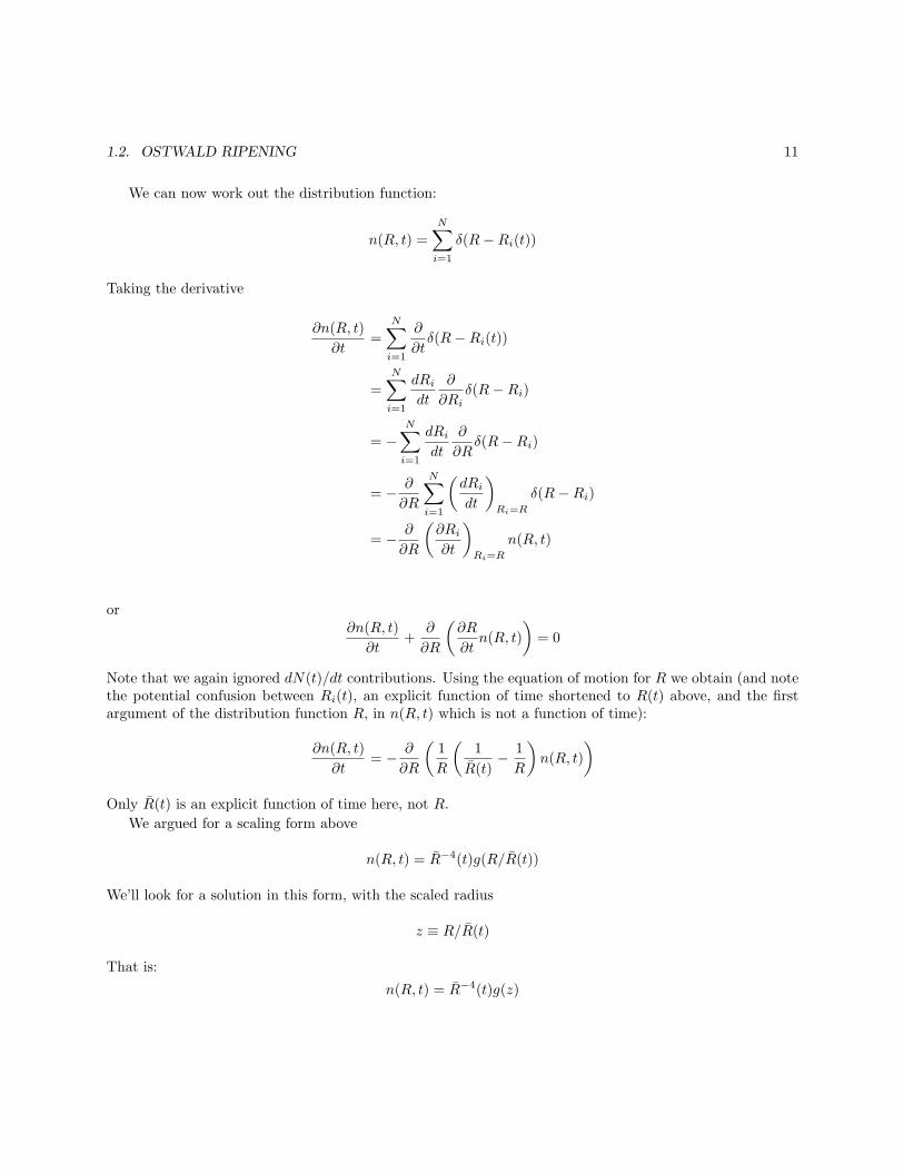
1.2. OSTWALD RIPENING 13
or,d ln g(z)
dz=
4z3k − 2 + z
z2 − z − z4K
The solution of this, consistant with normalization of n(R, t) and the extra requirement that there be nodroplets of arbitrarily large size (try it to find out) is
k = 4/9
and
g(z) =
34e25/3 z
2e
−1
1− 23z
(z+3)7/3( 32−z)1/3 , z < 3
2
0 , z > 32
z = R/R
R =(
49t)1/3
n(R, t) = R−4g(RR
)
g(z)
z3/2
Figure 1.11: Scaled Distribution Function (just a cartoon, not the actual function).

14 CHAPTER 1. DROPLET GROWTH
Chapter 2
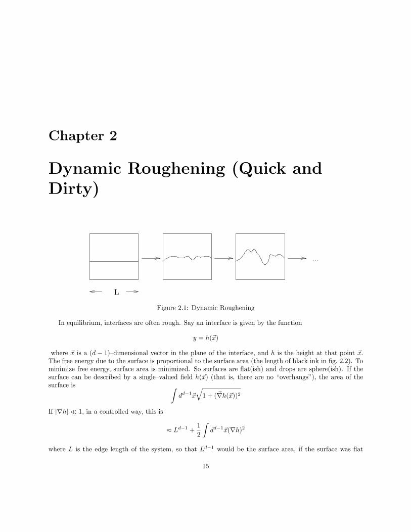
Dynamic Roughening (Quick andDirty)
...
L
Figure 2.1: Dynamic Roughening
In equilibrium, interfaces are often rough. Say an interface is given by the function
y = h(~x)
where ~x is a (d − 1)–dimensional vector in the plane of the interface, and h is the height at that point ~x.The free energy due to the surface is proportional to the surface area (the length of black ink in fig. 2.2). Tominimize free energy, surface area is minimized. So surfaces are flat(ish) and drops are sphere(ish). If thesurface can be described by a single–valued field h(~x) (that is, there are no “overhangs”), the area of thesurface is ∫
dd−1~x
√
1 + (~∇h(~x))2
If |∇h| ≪ 1, in a controlled way, this is
≈ Ld−1 +1
2
∫
dd−1~x(∇h)2
where L is the edge length of the system, so that Ld−1 would be the surface area, if the surface was flat
15
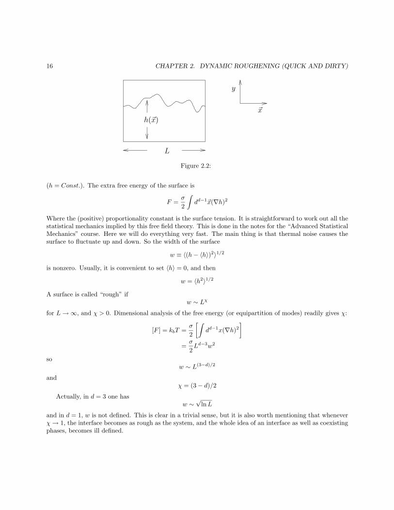
16 CHAPTER 2. DYNAMIC ROUGHENING (QUICK AND DIRTY)
y
~x
h(~x)
L
Figure 2.2:
(h = Const.). The extra free energy of the surface is
F =σ
2
∫
dd−1~x(∇h)2
Where the (positive) proportionality constant is the surface tension. It is straightforward to work out all thestatistical mechanics implied by this free field theory. This is done in the notes for the “Advanced StatisticalMechanics” course. Here we will do everything very fast. The main thing is that thermal noise causes thesurface to fluctuate up and down. So the width of the surface
w ≡ 〈(h− 〈h〉)2〉1/2
is nonzero. Usually, it is convenient to set 〈h〉 = 0, and then
w = 〈h2〉1/2
A surface is called “rough” ifw ∼ Lχ
for L→∞, and χ > 0. Dimensional analysis of the free energy (or equipartition of modes) readily gives χ:
[F ] = kbT =σ
2
[∫
dd−1x(∇h)2]
=σ
2Ld−3w2
sow ∼ L(3−d)/2
andχ = (3− d)/2
Actually, in d = 3 one hasw ∼
√lnL
and in d = 1, w is not defined. This is clear in a trivial sense, but it is also worth mentioning that wheneverχ→ 1, the interface becomes as rough as the system, and the whole idea of an interface as well as coexistingphases, becomes ill defined.
17
Correlation functions are simplest in Fourier space. Let
h(~q) ≡∫
dd−1xei~f ·~xh(~x)
and so on. Then it is easy to show that
〈h(~q)h(~q′)〉 = (2π)d−1δ(~q + ~q′)G(q)
where
G(q) =kBT
σ
1
q2
and
〈h(x)h(x′)〉 =
∫dd−1q
(2π)d−1ei~q·(~x−~x
′)G(q)
More generally, it is expected that
G(q) ∼ 1
q2−η
as q → 0, so this free energy gives
η = 0
The exponents η and χ are simply related:
χ = (3− d)/2− η/2
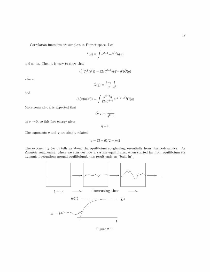
The exponent χ (or η) tells us about the equilibrium roughening, essentially from thermodynamics. Fordynamic roughening, where we consider how a system equilibrates, when started far from equilibrium (ordynamic fluctuations around equilibrium), this result ends up “built in”.
...
t = 0 increasing time
Lχw(t)
w = tχ/z
t
Figure 2.3:
18 CHAPTER 2. DYNAMIC ROUGHENING (QUICK AND DIRTY)
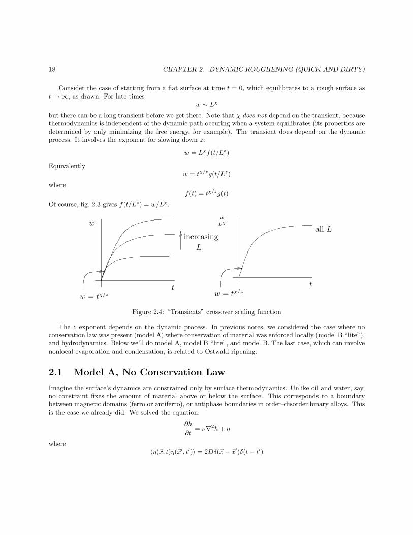
Consider the case of starting from a flat surface at time t = 0, which equilibrates to a rough surface ast→∞, as drawn. For late times
w ∼ Lχ
but there can be a long transient before we get there. Note that χ does not depend on the transient, becausethermodynamics is independent of the dynamic path occuring when a system equilibrates (its properties aredetermined by only minimizing the free energy, for example). The transient does depend on the dynamicprocess. It involves the exponent for slowing down z:
w = Lχf(t/Lz)
Equivalentlyw = tχ/zg(t/Lz)
wheref(t) = tχ/zg(t)
Of course, fig. 2.3 gives f(t/Lz) = w/Lχ.
wLχ
tt
all Lw
w = tχ/z w = tχ/z
increasing
L
Figure 2.4: “Transients” crossover scaling function
The z exponent depends on the dynamic process. In previous notes, we considered the case where noconservation law was present (model A) where conservation of material was enforced locally (model B “lite”),and hydrodynamics. Below we’ll do model A, model B “lite”, and model B. The last case, which can involvenonlocal evaporation and condensation, is related to Ostwald ripening.
2.1 Model A, No Conservation Law
Imagine the surface’s dynamics are constrained only by surface thermodynamics. Unlike oil and water, say,no constraint fixes the amount of material above or below the surface. This corresponds to a boundarybetween magnetic domains (ferro or antiferro), or antiphase boundaries in order–disorder binary alloys. Thisis the case we already did. We solved the equation:
∂h
∂t= ν∇2h+ η
where〈η(~x, t)η(~x′, t′)〉 = 2Dδ(~x− ~x′)δ(t− t′)
2.2. MODEL B “LITE”, LOCAL CONSERVATION ONLY 19
with D = kBTν/σ.
We can solve this much faster than before by dimensional analysis.
First let’s be really quick and dirty. The dimensions of
[∂h
∂t
]
=[∇2h
]
[h
t
]
=
[h
L2
]
so
t ∼ L2
and z is 2. Likewise
[∇2h
]= [η]
[h
L2
]
=[
(δ(x)δ(t))1/2]
=
[1
L(d−1)/2
1
L2/2
]
on using t ∼ L2. So we have
[h] ∼ L(3−d)/2
or,
w ∼ L(3−d)/2
and χ = (3− d)/2. Done!
We’ll do a more formal fiddling with dimensions — letting h = hoh∗, t = tot
∗, — and so on — below,when we do the Kardar–Parisi–Zhang equation.
2.2 Model B “Lite”, Local Conservation Only
This equation is
∂h
∂t= ν∇4h+ η
where
〈ηη′〉 = 2D(−∇2)δ(~x− ~x′)δ(t− t′)
Do the same trick, and you can read off
z = 4
χ = (3− d)/2
20 CHAPTER 2. DYNAMIC ROUGHENING (QUICK AND DIRTY)
2.3 Model B, Conservation Law
The full conserved case involves long–range diffusion, as well as the short–range surface diffusion involved inmodel B “lite” above.
To make life easy, lets only solve for z: we already know χ = (3− d)/2, regardless of the dynamics, if thesystem equilibrates.
The equations to satisfy for the excess concentration are
∇2c = 0
everywhere in space, which is the steady–state version of the diffusion equation, subject to boundary condi-tions at the surface:
c = k,
v = (n · ~∇c)Jump
where I’ve set multiplicative constants to unity, and (...)Jump = (...)Above Surface − (...)Below Surface. Thecurvature is k, and if the surface is fairly flat
k =∂2h
∂x2
letc = ei
~k·~xf(y)
(that is, fourier transform). Then
∇2c =
(
−k2 +∂2
∂y2
)
c = 0
The solution isc = coe
−k|y|
But one of the boundary conditions
v =
(∂c
∂y
)
Jump
at the surface, so (up to a constant)∂h
∂t= kco
But, at the surfacec = ∂2h/∂x2
soco = k2h
and,∂h
∂t= k3h
where I’ve ignored multiplicative constants, and minus signs (and incidentally thermal noise). Anyway, fromdimensions we see
z = 3
2.3. MODEL B, CONSERVATION LAW 21
for model B! This is the “same” 3 as that for Ostwald ripening. It is unsusual because it is not an evennumber. The odd number comes about explicitly from coupling to the bulk. It was from the ∇2c = 0 termabove.

22 CHAPTER 2. DYNAMIC ROUGHENING (QUICK AND DIRTY)
Chapter 3
Driven Roughening and KPZEquation
...
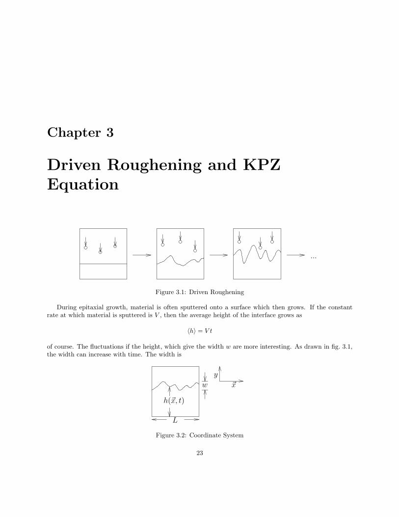
Figure 3.1: Driven Roughening
During epitaxial growth, material is often sputtered onto a surface which then grows. If the constantrate at which material is sputtered is V , then the average height of the interface grows as
〈h〉 = V t
of course. The fluctuations if the height, which give the width w are more interesting. As drawn in fig. 3.1,the width can increase with time. The width is
w
L
h(~x, t)
~x
y
Figure 3.2: Coordinate System
23
24 CHAPTER 3. DRIVEN ROUGHENING AND KPZ EQUATION
w =1
Ld
∫
ddx〈(h(x, t)− 〈h〉)2〉1/2
for example. Note that we will be using
d = dimension of surface
unlike almost all the other notes where d = dimension of system. Note the transformation
ddimensionof
surface
= ddimensionof wholespace
− 1
Its a little awkward to use the same notation.Like before we have
w = Lχf(t/Lz)
Our previous results, for V = 0, are
χo = (2− d)/2zo = 2
These were the solutions of model A where
∂h
∂t= ν∇2h+ η
〈η〉 = 0, 〈ηη〉 = 2Dδx,x′δt,t′
Note again the different notation. The fluctuation – dissipation relation gives
ν
D=kBT
σ
where σ is the surface tension.For the driven case, the equation of motion is
∂h
∂t= ν∇2h+
λ
2|∇h|2 + η
where λ is a constant proportional to the driving force (essentially V above). This is called the Kardas–Parisi–Zhang (KPZ) equation, or the noisy Burgers equation. One way to obtain it is as motivated abovefor the normal velocity v of an interface of local curvature K. As before, in a Taylor series expansion forsmall K (K ∼ 1/Radius of curvature)
v = λ+ νK +O(K2)
where λ and ν are constants. If the interface has no bubbles or overhangs, so that it is given by
y = h(~x, t)
then1
√
1 + |∇h|2∂h
∂t= λ+ ν
∇2h
(1 + |∇h|2)3/2
25
Expanding in powers of |∇h| gives
∂h
∂t= λ+ ν∇2h+
λ
2|∇h|2 + ...
Adding the random noise source η, and switching to the frame of the interface motion
h→ h+ λt
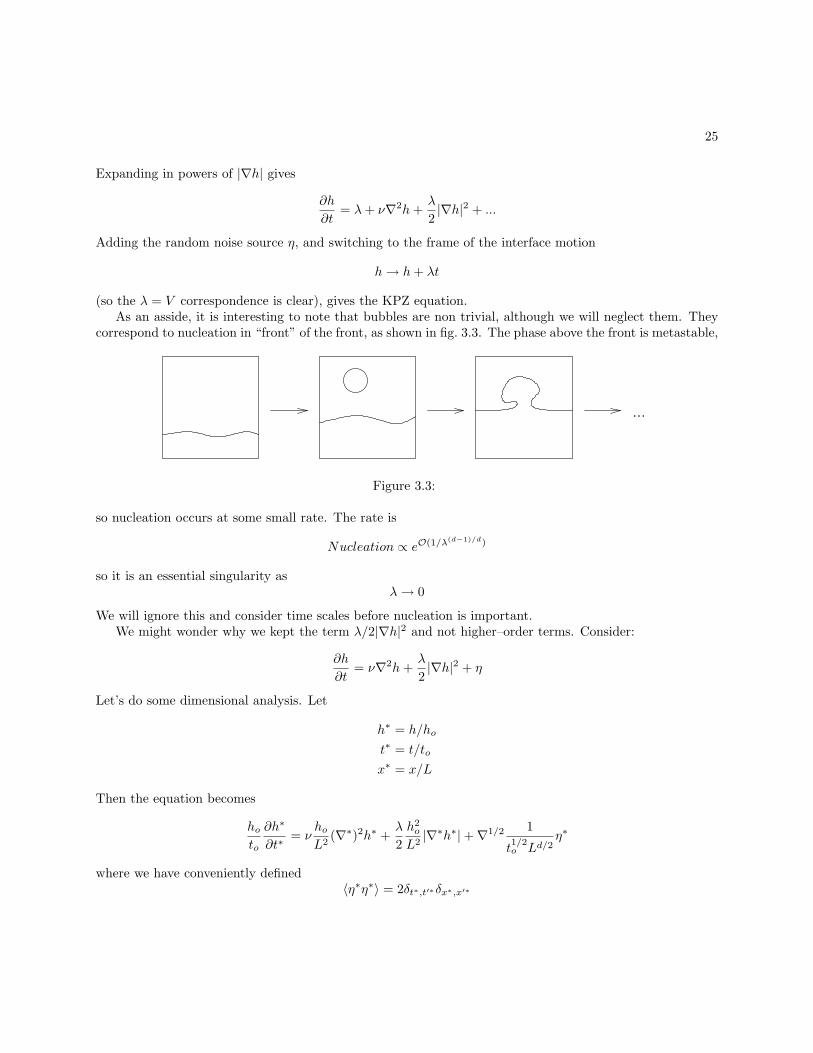
(so the λ = V correspondence is clear), gives the KPZ equation.As an asside, it is interesting to note that bubbles are non trivial, although we will neglect them. They
correspond to nucleation in “front” of the front, as shown in fig. 3.3. The phase above the front is metastable,
...
Figure 3.3:
so nucleation occurs at some small rate. The rate is
Nucleation ∝ eO(1/λ(d−1)/d)
so it is an essential singularity asλ→ 0
We will ignore this and consider time scales before nucleation is important.We might wonder why we kept the term λ/2|∇h|2 and not higher–order terms. Consider:
∂h
∂t= ν∇2h+
λ
2|∇h|2 + η
Let’s do some dimensional analysis. Let
h∗ = h/ho
t∗ = t/to
x∗ = x/L
Then the equation becomes
hoto
∂h∗
∂t∗= ν
hoL2
(∇∗)2h∗ +λ
2
h2o
L2|∇∗h∗|+∇1/2 1
t1/2o Ld/2
η∗
where we have conveniently defined〈η∗η∗〉 = 2δt∗,t′∗δx∗,x′∗
26 CHAPTER 3. DRIVEN ROUGHENING AND KPZ EQUATION
Fiddling around gives
∂h∗
∂t∗=
(νtoL2
)
(∇∗)2h∗ +1
2
(λtohoL2
)
|∇∗h∗|2 +
(Dtoh2oL
d
)1/2
η∗
If λ = 0, we can always make this equation dimensionless by choosing
to ≡ L2/ν
and
ho =
(DtoLd
)1/2
that is
ho =
(D
ν
)1/2
L(2−d)/2
Note that this incidentally gives the λ = 0 exponents, t ∼ Lzo with zo = 2, and w ∼ Lχo with χo = (2−d)/2.In fact, with λ ≡ 0, this is sufficient to solve the problem. However, note that the λ = 0 solution gives (withthese choices)
∂h∗
∂t∗= (∇∗)2h∗ +
1
2
(λD1/2
ν3/2L(2−d)/2
)
|∇∗h∗|2 + η∗
or∂h∗
∂t∗= (∇∗)2h∗ +
1
2λ(L)|∇∗h∗|2 + η∗
where
λ(L) =λD1/2
ν3/2L(2−d)/2
So we see the linear solution with λ = 0 is “stable” as L → ∞ for d > 2. Hence the critical dimension forthis term to become relavent is
dc = 2
(remember this means three–dimensional space with a two–dimensional surface) so this term looks potentiallyimportant and that it can potentially change values of χ and z, which in it does.
We can figure out how fast this λ nonzero behavior becomes important with a crossover scaling ansatz.Namely,
w = Lχof(λLφ)
simply from the form of the equation above, where f is a scaling function, χo = (2−d)/2 and (coincidentally)φ = (2− d)/2. But for λ nonzero (and L→∞) we must have
w ∝ Lχ
HencelimL→∞
f(λLφ) = (λLφ)(χ−χo)/φ
and,w = λ(χ−χo)/φLχ
27
This gives the amplitude’s dependence on λ. A similar result can be obtained for w = tχ/zf(λLφ).What about other terms that we have neglected? There are lots of them. For example, what about (to
pick one from a hat):λ2|∇2h|2
which might arise from a K2 contribution in v = λ+K +O(K2). Doing the same analysis gives a
λ2(L) =λ2D
1/2
ν3/2L−(d+2)/2
so it is not a problem for L→∞ in any dimension. One can consider other terms the same way. (This givesthe stability of the λ = 0 solution — the λ = 0 fixed point in the jargon — not any λ nonzero fixed pointthough. It is worth thinking about this a bit, since the λ = 0 fixed point is unstable anyway.)
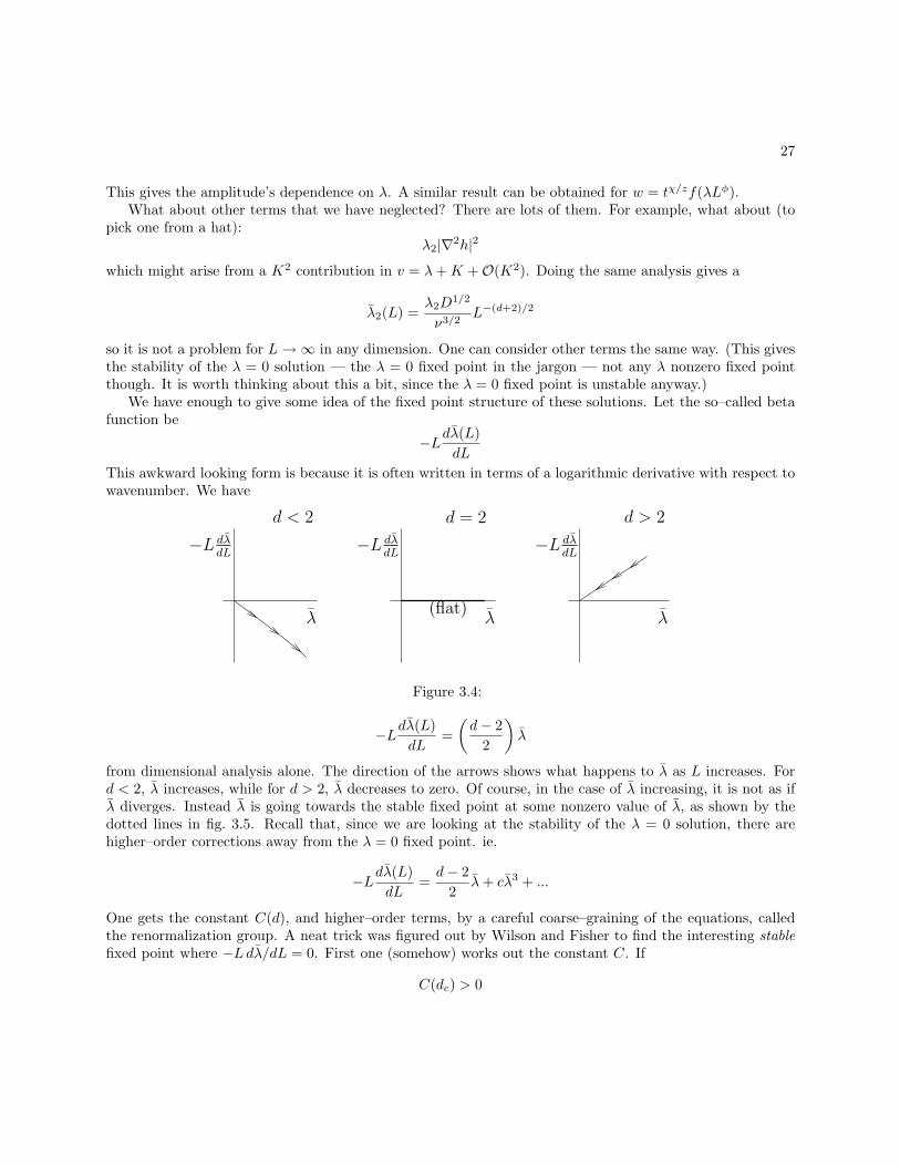
We have enough to give some idea of the fixed point structure of these solutions. Let the so–called betafunction be
−Ldλ(L)
dL
This awkward looking form is because it is often written in terms of a logarithmic derivative with respect towavenumber. We have
−L dλdL
λ
d < 2
−L dλdL
(flat)λ
d = 2
−L dλdL
λ
d > 2
Figure 3.4:
−Ldλ(L)
dL=
(d− 2
2
)
λ
from dimensional analysis alone. The direction of the arrows shows what happens to λ as L increases. Ford < 2, λ increases, while for d > 2, λ decreases to zero. Of course, in the case of λ increasing, it is not as ifλ diverges. Instead λ is going towards the stable fixed point at some nonzero value of λ, as shown by thedotted lines in fig. 3.5. Recall that, since we are looking at the stability of the λ = 0 solution, there arehigher–order corrections away from the λ = 0 fixed point. ie.
−Ldλ(L)
dL=d− 2
2λ+ cλ3 + ...
One gets the constant C(d), and higher–order terms, by a careful coarse–graining of the equations, calledthe renormalization group. A neat trick was figured out by Wilson and Fisher to find the interesting stable
fixed point where −Ldλ/dL = 0. First one (somehow) works out the constant C. If
C(dc) > 0
28 CHAPTER 3. DRIVEN ROUGHENING AND KPZ EQUATION
Interesting stablefixed point
Unstablefixed point
λ
−L dλdL
d < 2
Figure 3.5:
one has an upper critical dimension, and the new fixed point is accessible by the ǫ–expansion, where
ǫ = 2− d
is small. (Drawn in fig. 3.6).
λ λ λ
−L dλdL
−L dλdL −L dλ
dL
d = 2 d > 2d = 2− ǫ
ǫ
Figure 3.6: c > 0, upper critical dimension
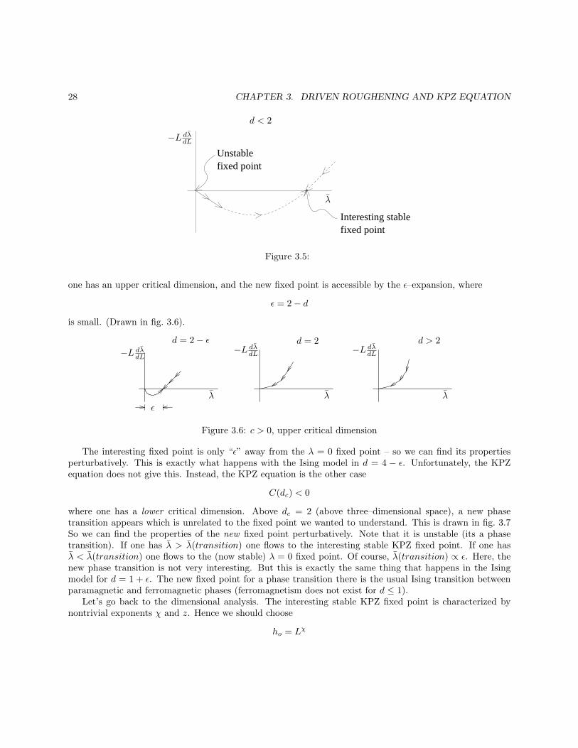
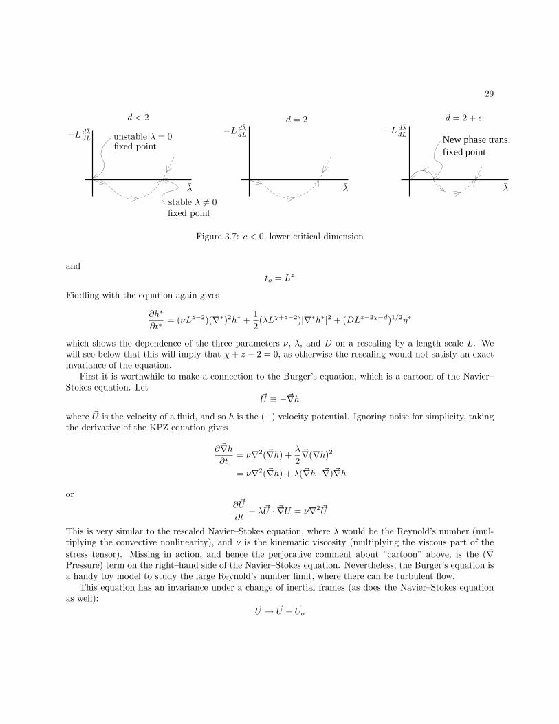
The interesting fixed point is only “ǫ” away from the λ = 0 fixed point – so we can find its propertiesperturbatively. This is exactly what happens with the Ising model in d = 4 − ǫ. Unfortunately, the KPZequation does not give this. Instead, the KPZ equation is the other case
C(dc) < 0
where one has a lower critical dimension. Above dc = 2 (above three–dimensional space), a new phasetransition appears which is unrelated to the fixed point we wanted to understand. This is drawn in fig. 3.7So we can find the properties of the new fixed point perturbatively. Note that it is unstable (its a phasetransition). If one has λ > λ(transition) one flows to the interesting stable KPZ fixed point. If one hasλ < λ(transition) one flows to the (now stable) λ = 0 fixed point. Of course, λ(transition) ∝ ǫ. Here, thenew phase transition is not very interesting. But this is exactly the same thing that happens in the Isingmodel for d = 1 + ǫ. The new fixed point for a phase transition there is the usual Ising transition betweenparamagnetic and ferromagnetic phases (ferromagnetism does not exist for d ≤ 1).
Let’s go back to the dimensional analysis. The interesting stable KPZ fixed point is characterized bynontrivial exponents χ and z. Hence we should choose
ho = Lχ
29
New phase trans.fixed point
−L dλdL
−L dλdL−L dλ
dL
λ λλ
stable λ 6= 0fixed point
fixed point
d < 2 d = 2 d = 2 + ǫ
unstable λ = 0
Figure 3.7: c < 0, lower critical dimension
and
to = Lz
Fiddling with the equation again gives
∂h∗
∂t∗= (νLz−2)(∇∗)2h∗ +
1
2(λLχ+z−2)|∇∗h∗|2 + (DLz−2χ−d)1/2η∗
which shows the dependence of the three parameters ν, λ, and D on a rescaling by a length scale L. Wewill see below that this will imply that χ+ z − 2 = 0, as otherwise the rescaling would not satisfy an exactinvariance of the equation.
First it is worthwhile to make a connection to the Burger’s equation, which is a cartoon of the Navier–Stokes equation. Let
~U ≡ −~∇h
where ~U is the velocity of a fluid, and so h is the (−) velocity potential. Ignoring noise for simplicity, takingthe derivative of the KPZ equation gives
∂~∇h∂t
= ν∇2(~∇h) +λ
2~∇(∇h)2
= ν∇2(~∇h) + λ(~∇h · ~∇)~∇h
or∂~U
∂t+ λ~U · ~∇U = ν∇2~U
This is very similar to the rescaled Navier–Stokes equation, where λ would be the Reynold’s number (mul-tiplying the convective nonlinearity), and ν is the kinematic viscosity (multiplying the viscous part of the
stress tensor). Missing in action, and hence the perjorative comment about “cartoon” above, is the (~∇Pressure) term on the right–hand side of the Navier–Stokes equation. Nevertheless, the Burger’s equation isa handy toy model to study the large Reynold’s number limit, where there can be turbulent flow.
This equation has an invariance under a change of inertial frames (as does the Navier–Stokes equationas well):
~U → ~U − ~Uo
30 CHAPTER 3. DRIVEN ROUGHENING AND KPZ EQUATION
where ~Uo is a constant, and~x→ ~x+ λ~Uot
(usually the λ dependence is not present in fluid mechanics). This is called Galilean invariance. Note that
~U · ~∇~U → ~U · ~∇~U − ~Uo · ~∇~U
while∂~U
∂t→ ∂~U
∂t+ λ~Uo · ~∇~U
under this transformation. So the two extra terms cancel. This is an exact invariance of the equation whichwe want to be satisfied under any fancy rescaling we do. Hence
λLχ+z−2
must be independent of L, andχ+ z = 2
In the KPZ equation itself, the transform is
h→ h+ ~ǫ · ~x
where ǫ is a vector of small magnitude, and
~x→ ~x+ ~ǫλ
2t
We need the small magnitude restriction since ǫ2 terms appear. This corresponds to Euclidean invariance:the equations are independent of the orientation of the (~x−y) coordinate system. You can check this yourself.We now have a hint, as well, of our coming problems with the critical dimension. This exact invariance giving
χ+ z = 2
follows in all dimensions. So we expect that, in all dimensions, there is a fixed point corresponding to this.But we know the λ = 0 fixed point, with
χo =2− d
2, zo = 2
is stable for d > 2, at least close to λ = 0. Hence there may be a phase transition between the λ = 0 fixedpoint (no Galilean invariance) and the λ 6= 0 fixed point (with Galilean invariance). In fact, it seems to bea likely thing indeed, unfortunately.
There’s one last trick we can do before jumping into the RG calculation. A Langevin equation, like theKPZ equation, is always equivalent to a Fokker–Planck equation.
A Langevin equation∂h
∂t= V (h) + η
where the random Gaussian noise is〈ηη′〉 = 2Dδt,t′
31
has a Fokker–Planck equation for the probability distribution P (h, t) of the form
∂P (h, t)
∂t=
∂
∂h
[
−V +D∂
∂h
]
P
This is shown in other notes. The functional generalization is the following. If a Langevin equation is of theform
∂h(~x, t)
∂t= V (h(~x, t)) + η(~x, t)
where〈η(~x, t)η(~x′, t)〉 = 2Dδ(~x− ~x′)δ(t− t′)
then the probability distribution function P ([h], t), (the awkward notation means P is a function of h),satisfies
∂P
∂t=
∫
d~xδ
δh(~x)
[
−V (h(~x)) +Dδ
δh(~x)
]
P
This can be obtained from the vector generalization of the simpler relation above, on interpreting∫d~x⇔
∑
i
and h(~x)⇔ hi, and so on.For the λ = 0 case, we have the results
∂h
∂t= ν∇2h+ η
and so∂P
∂t=
∫
d~xδ
δh(~x)
[
−ν∇2h+Dδ
δh
]
P
The equilibrium solution is∂Peq∂t
= 0
so,[
−ν∇2h+Dδ
δh
]
Peq = 0
Of course, the equilibrium distribution is determined by the extra surface free energy:
Peq = e−F/kBT = e− σ
2kBT
R
d~x(∇h)2
up to a multiplicative constant, where σ is surface tension. So we have
δPeqδh
= (Peq)
(σ
kBT∇2h
)
and henceν∇2h = D
σ
kBT∇2h
soν/D = σ/kBT
The equilibrium solution determines χ, since
w = Lχf(t/Lz)
32 CHAPTER 3. DRIVEN ROUGHENING AND KPZ EQUATION
(The exponent z describes transients on the way to equilibrium.) In this equilibrium case χ = χo = 2−d2 , as
worked out previously.As a further aside, note that the equilibrium distribution Peq = e−F/kBT implies that the Fokker Planck
equation is∂P
∂t= Γ
∫
d~xδ
δh(~x)
[δF
δh(~x)+ kBT
δ
δh(~x)
]
P
where
D ≡ ΓkBT
The Langevin equation becomesδh
δt= −Γ
δF
δh+ η
That is,
V = −ΓδF
δh(~x)
which is the fluctuation–dissipation relation.Finally, let us return to the KPZ equation
∂h
∂t= ν∇2h+
λ
2|∇h|2 + η
The Fokker–Planck equation is
∂P
∂t=
∫
d~xδ
δh(~x)
[
−ν∇2h− λ
2|∇h|2 +D
δ
δh
]
P
The steady–state solution (the analog of the equilibrium solution) is
∂Pss∂t
= 0
from which χ can be obtained. It is the solution of
0 =
∫
d~xδ
δh(~x)
[
−ν∇2h− λ
2|∇h|2 +D
δ
δh
]
Pss
We leave in the(∫dx δ
δh
)factor on the left side because it is not trivial this time. First, let’s see if we can
find something ignoring that factor:
[
−ν∇2h− λ
2|∇h|2 +D
δ
δh
]
Pss?= 0
Or, if for convenience we let
lnPss = − νDζss
then
∇2h+λD
2ν(∇h)2 ?
=δ
δhζss[h]
33
To get out these two terms we must have (schematically):
ζss =
∫
∇∇hh+∇∇hhh
that is
ζss =
∫
d~x
1
2|∇h|2 +A∇2h3 +Bh(∇h)2 + ...
︸ ︷︷ ︸
All possibilities of ∇∇hhh
Unfortunately, none of these extra terms, or any combination of them, can give the λ2 |∇h|2 term! Hence
this route to the steady–state solution is botched, and we have to solve the more conservative
0 =
∫
d~xδ
δh(~x)
[
−ν∇2h− λ
2|∇h|2 +D
δ
δh
]
Pss
If we could do this, we’d get χ. Since we know that χ+ z = 2, we’d be done.
As a further aside, not that we usually deal with the Langevin equation
∂h
∂t= blah+ blah
rather than the Fokker–Planck equation
∂P
∂t= woof + woof
despite the fact that they are equivalent. This is because the Langevin equation, at every time step, and foreach representation of the noise, is O(Ld). The Fokker–Planck equation, since it involves the probability,
which in equilibrium is ∼ e−F/kBT in terms of the extensive free energy, is O(eLd
) at each time step!
Averaging over all the noise in the Ld Langevin equation formally gives the eLd
Fokker–Planck equation.
Perhaps something more could be done with finding Pss numerically from the equation above. In anycase, it was noticed that, in d = 1 only,
Pss = e−νD
R
dx( dhdx )2
because the λ2
(dhdx
)2term integrates exactly to zero. This is the old equilibrium solution, so χ = χo in d = 1.
That is χ(d = 1) = 1/2. But χ+ z = 3/2, so z = 3/2, in contrast to zo = 2.
To show this, let’s consider only that extra term in the equation for the steady–state distribution above:
∫
dxδ
δh(x)
[
−λ2
(dh
dx
)2]
Pss
34 CHAPTER 3. DRIVEN ROUGHENING AND KPZ EQUATION
Since we are in d = 1, ~∇h is an ordinary derivative dh/dx. Anyway, taking the functional derivative gives
=
∫
dx limx′→x
δ
δh(x′)
[
−λ2
(dh
dx
)2]
Pss
=
∫
dx limx′→x
(
−λdhdx
d
dxδ(x− x′)
)
Pss +
∫
dx
(
−λ2
(dh
dx
)2)
ν
D
d2h
dx2Pss
=
∫
dx limx′→x
(
λd2h
dx2δ(x− x′)
)
Pss +
∫
dx
(
−λ2
(dh
dx
)2)
ν
D
d2h
dx2Pss
=(
λ limx′→x
δ(x− x′)Pss)∫
dxd2h
dx2−(λν
2DPss
)∫
dx
(dh
dx
)2d2h
dx2
= Const.
∫
dxd2h
dx2− Const.
∫
dx
(dh
dx
)2d2h
dx2
= Const.
∫
dxd2h
dx2− Const.
∫
dx1
3
d
dx
(dh
dx
)2
= Surface contributions at ∞= 0
SoPss = Const.e−
νD
R
dx( dhdx )2
in d = 1, and
χ = χo =1
2
Since χ+ z = 2, we have z = 3/2 in one dimension.That concludes what we can get “for free”. Now we’ll outline a renormalization group calculation.
Chapter 4
Renormalization Group for DrivenRoughening
Recall the KPZ equation∂h
∂t= ν∇2h+
λ
2|∇h|2 + η
where〈ηη′〉 = 2Dδx,x′δt,t′
We will use the renormalization group to attempt to solve this, integrating out small length scales in acontrolled way. An important trick which we will use is that, for d > 2, the λ = 0 fixed point is stable. So,with some care, we can perturb around this fixed point. Since
λ(L) ∼ L(2−d)/2
diverges as L → ∞ for d < 2, we will craftily perturb the small length scales, corresponding to largewavenumbers. It is convenient to do this in Fourier Space where the λ = 0 problem becomes trivial anduncoupled. Let
h(~k,w) ≡∫
ddx
∫
dtei~k·~x−iwth(~x, t)
Then the KPZ equation becomes
h(~k,w) = ho(~k,w) + Go(~k,w)
(
−λ2
)∫
~q,Ω
~q · (~k − ~q)h(~q,Ω)h(~k − ~q, w − Ω)
whereho(~k,w) = Go(~k,w)η(~k,w)
is the λ = 0 linear solution,Go(k,w) = (−iw + νk2)−1
is the “propagator”, the noise satisfies
〈η(~k,w)η(~k′, w′)〉 = 2D(2π)d+1δ(~k + ~k′)δ(w + w′)
35
36 CHAPTER 4. RENORMALIZATION GROUP FOR DRIVEN ROUGHENING
and ∫
~q,Ω
≡ 1
(2π)d+1
∫
|~q|<Λ
ddq
∫ ∞
−∞
dΩ
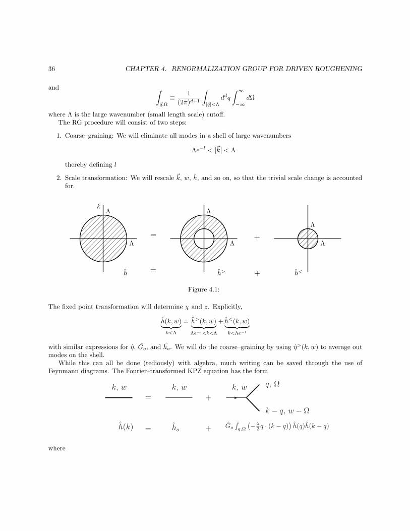
where Λ is the large wavenumber (small length scale) cutoff.The RG procedure will consist of two steps:
1. Coarse–graining: We will eliminate all modes in a shell of large wavenumbers
Λe−l < |~k| < Λ
thereby defining l
2. Scale transformation: We will rescale ~k, w, h, and so on, so that the trivial scale change is accountedfor.
=
=
+
+
Λ
ΛΛ
Λ
Λ
Λ
h h> h<
k
Figure 4.1:
The fixed point transformation will determine χ and z. Explicitly,
h(k,w)︸ ︷︷ ︸
k<Λ
= h>(k,w)︸ ︷︷ ︸
Λe−l<k<Λ
+ h<(k,w)︸ ︷︷ ︸
k<Λe−l
with similar expressions for η, Go, and ho. We will do the coarse–graining by using η>(k,w) to average outmodes on the shell.
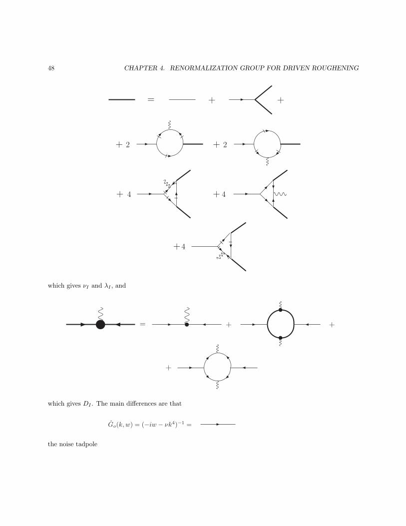
While this can all be done (tediously) with algebra, much writing can be saved through the use ofFeynmann diagrams. The Fourier–transformed KPZ equation has the form
+= Go∫
q,Ω
(−λ2 q · (k − q)
)h(q)h(k − q)hoh(k)
k, w k, w k, w q, Ω
k − q, w − Ω
= +
where
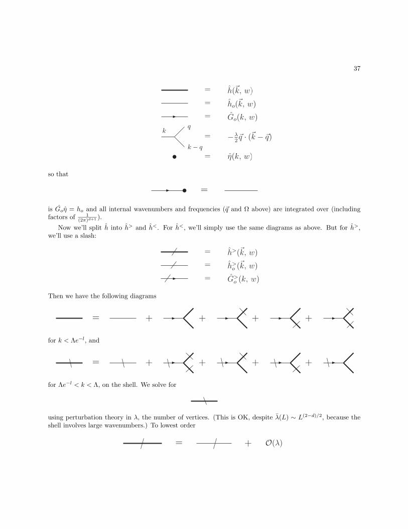
37
kq
k − q
h(~k, w)
ho(~k, w)
Go(k, w)
−λ2~q · (~k − ~q)
η(k, w)=
=
=
=
=
so that
=
is Goη = ho and all internal wavenumbers and frequencies (~q and Ω above) are integrated over (includingfactors of 1
(2π)d+1 ).
Now we’ll split h into h> and h<. For h<, we’ll simply use the same diagrams as above. But for h>,we’ll use a slash:
=
=
=
h>(~k, w)
h>o (~k, w)
G>o (k, w)
Then we have the following diagrams
= + + + +
for k < Λe−l, and
= + + + +
for Λe−l < k < Λ, on the shell. We solve for
using perturbation theory in λ, the number of vertices. (This is OK, despite λ(L) ∼ L(2−d)/2, because theshell involves large wavenumbers.) To lowest order
= + O(λ)
38 CHAPTER 4. RENORMALIZATION GROUP FOR DRIVEN ROUGHENING
To next order
= + + + + + O(λ2)
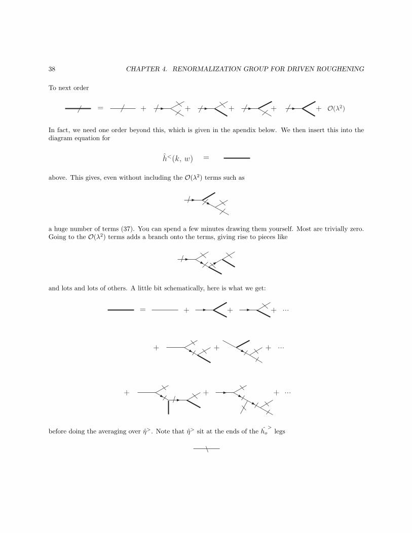
In fact, we need one order beyond this, which is given in the apendix below. We then insert this into thediagram equation for
h<(k, w) =
above. This gives, even without including the O(λ2) terms such as
a huge number of terms (37). You can spend a few minutes drawing them yourself. Most are trivially zero.Going to the O(λ2) terms adds a branch onto the terms, giving rise to pieces like
and lots and lots of others. A little bit schematically, here is what we get:
= + + + ...
+ + ...+
+ + + ...
before doing the averaging over η>. Note that η> sit at the ends of the ho>
legs
39
since ho>
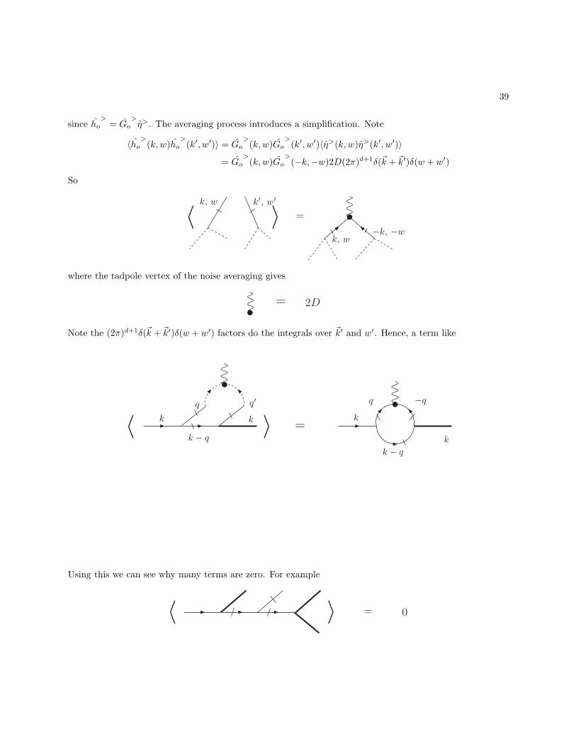
= Go>η>. The averaging process introduces a simplification. Note
〈ho>
(k,w)ho>
(k′, w′)〉 = Go>
(k,w)Go>
(k′, w′)〈η>(k,w)η>(k′, w′)〉= Go
>(k,w)Go
>(−k,−w)2D(2π)d+1δ(~k + ~k′)δ(w + w′)
So
〈 〉k, w k′, w′
=
−k, −wk, w
where the tadpole vertex of the noise averaging gives
= 2D
Note the (2π)d+1δ(~k + ~k′)δ(w + w′) factors do the integrals over ~k′ and w′. Hence, a term like
〈 k
q
〉q′
k
k − q=
k
k
k − q
Using this we can see why many terms are zero. For example
〉〈 = 0
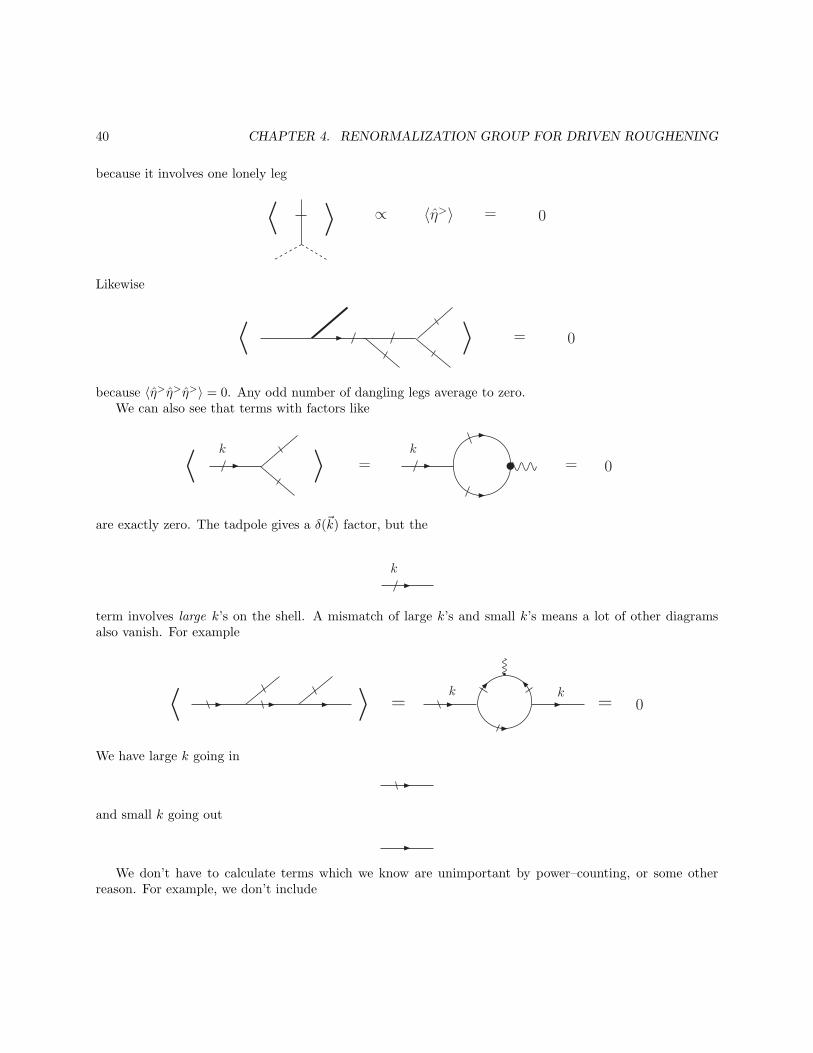
40 CHAPTER 4. RENORMALIZATION GROUP FOR DRIVEN ROUGHENING
because it involves one lonely leg
〈 〉 〈η>〉∝ = 0
Likewise
〉〈 = 0
because 〈η>η>η>〉 = 0. Any odd number of dangling legs average to zero.We can also see that terms with factors like
〈 〉 =k k
= 0
are exactly zero. The tadpole gives a δ(~k) factor, but the
k
term involves large k’s on the shell. A mismatch of large k’s and small k’s means a lot of other diagramsalso vanish. For example
〈 〉 = = 0kk
We have large k going in
and small k going out
We don’t have to calculate terms which we know are unimportant by power–counting, or some otherreason. For example, we don’t include
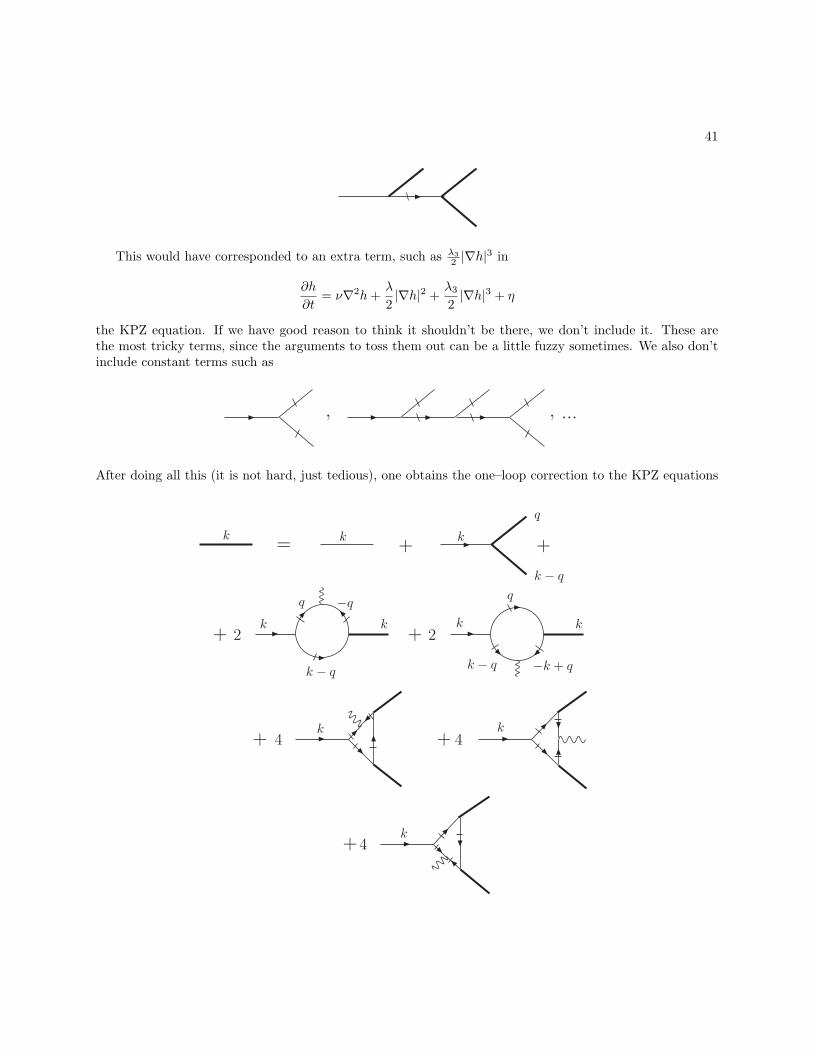
41
This would have corresponded to an extra term, such as λ3
2 |∇h|3 in
∂h
∂t= ν∇2h+
λ
2|∇h|2 +
λ3
2|∇h|3 + η
the KPZ equation. If we have good reason to think it shouldn’t be there, we don’t include it. These arethe most tricky terms, since the arguments to toss them out can be a little fuzzy sometimes. We also don’tinclude constant terms such as
, , ...
After doing all this (it is not hard, just tedious), one obtains the one–loop correction to the KPZ equations
k2+
k
k − q
2+k
q
k − q −k + q
k
4k
+k
4+
k4+
= + +
q
k − q
kk k
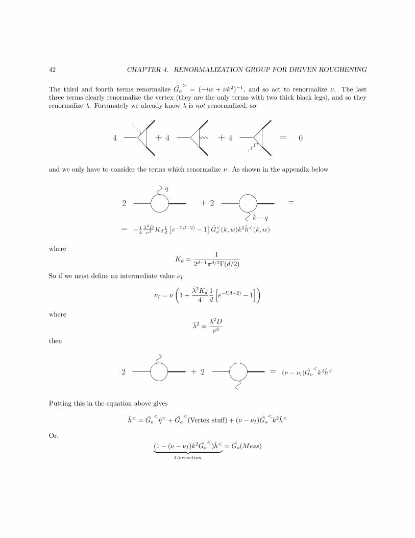
42 CHAPTER 4. RENORMALIZATION GROUP FOR DRIVEN ROUGHENING
The third and fourth terms renormalize Go>
= (−iw + νk2)−1, and so act to renormalize ν. The lastthree terms clearly renormalize the vertex (they are the only terms with two thick black legs), and so theyrenormalize λ. Fortunately we already know λ is not renormalized, so
4 + 4 + 4 = 0
and we only have to consider the terms which renormalize ν. As shown in the appendix below
+ 2 =
q
k − q− 1
4λ2Dν2 Kd
1d
[e−l(d−2) − 1
]G<o (k,w)k2h<(k,w)=
2
where
Kd =1
2d−1πd/2Γ(d/2)
So if we must define an intermediate value νI
νI = ν
(
1 +λ2Kd
4
1
d
[
e−l(d−2) − 1])
where
λ2 ≡ λ2D
ν3
then
2 + 2 = (ν − νi)Go<k2h<
Putting this in the equation above gives
h< = Go<η< + Go
<(Vertex stuff) + (ν − νI)Go
<k2h<
Or,
(1− (ν − νI)k2Go<
)h<︸ ︷︷ ︸
Correction
= Go(Mess)
43
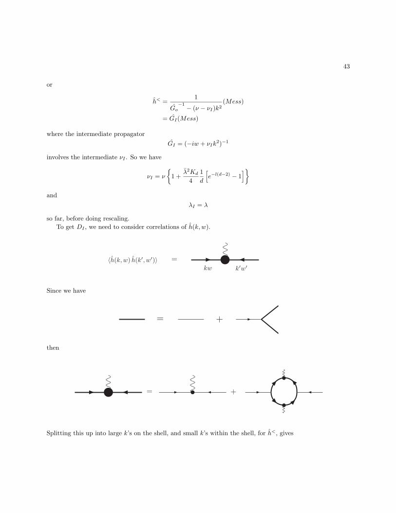
or
h< =1
Go−1 − (ν − νI)k2
(Mess)
= GI(Mess)
where the intermediate propagator
GI = (−iw + νIk2)−1
involves the intermediate νI . So we have
νI = ν
1 +λ2Kd
4
1
d
[
e−l(d−2) − 1]
and
λI = λ
so far, before doing rescaling.
To get DI , we need to consider correlations of h(k,w).
kw k′w′
=〈h(k,w) h(k′, w′)〉
Since we have
= +
then
= +
Splitting this up into large k’s on the shell, and small k’s within the shell, for h<, gives
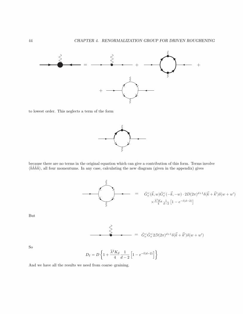
44 CHAPTER 4. RENORMALIZATION GROUP FOR DRIVEN ROUGHENING
= +
+
+
to lowest order. This neglects a term of the form
because there are no terms in the original equation which can give a contribution of this form. Terms involve〈hhhh〉, all four momentums. In any case, calculating the new diagram (given in the appendix) gives
= G<o (~k,w)G<o (−~k,−w) · 2D(2π)d+1δ(~k + ~k′)δ(w + w′)
× λ2Kd4
1d−2
[1− e−l(d−2)
]
But
= G<o G<o 2D(2π)d+1δ(~k + ~k′)δ(w + w′)
So
DI = D
1 +λ2Kd
4
1
d− 2
[
1− e−l(d−2)]
And we have all the results we need from coarse–graining.
45
We now implement the scale transformation. From our previous notes, we know that ν rescales as Lz−2,λ rescales as Lχ+z−2, and D rescales as Lz−2χ−d. Therefore, rescaling gives
ν(l) = e(z−2)lνI
D(l) = e(z−2χ−d)lDI
λ(l) = e(χ+z−2)lλI
Using relations for νI , DI , and λI above, and making l infinitesmal, gives the differential recursion relations.
dν(l)
dl= ν(l)
[
z − 2 +λ2Kd
4
(2− dd
)]
dD(l)
dl= D(l)
[
z − d− 2χ+λ2Kd
4
]
dλ(l)
dl= λ(l) [χ+ z − 2]
The fixed point is reached when dν/dl = dD/dl = dλ/dl = 0. So we have
z = 2− λ2Kd
4
(2− d
2
)
and (after some fiddling)
χ =2− d
2+λ2Kd
4
d− 1
d
where χ+ z = 2. To find χ and z we need λ = λD1/2/ν3/2. Of course
dλ
dl=
d
dl
(λD1/2
ν3/2
)
= λ
[1
λ
dλ
dl+
1
2
1
D
dD
dl− 3
2
1
ν
dν
dl
]
Collecting terms we obtaindλ
dl=
2− d2
λ+Kd2d− 3
4dλ3
to the order of our calculation. This has the unfortunate structure of a lower critical dimension at dc = 2,as anticipated above. So we can’t determine χ and z with RG.
RG will give results for other models. In particular, let us consider a version of model B “lite” with aKPZ nonlinearity.
∂h
∂t= ∇2(ν∇2h+
λ
2|∇h|2) + η
where〈η(~x, t)η(~x′, t′)〉 = 2D(−∇2)δ(~x− ~x′)δ(t− t′)
Since∂h
∂t= −~∇ · ~J
it is conserved, and ∫
d~xh(~x, t) = Const.
46 CHAPTER 4. RENORMALIZATION GROUP FOR DRIVEN ROUGHENING
New phase transition fixed pt.
−dλdl −dλdld < 2 d = 2 d = 2 + ǫ
λ λ λǫ
Figure 4.2: Lower critical dimension
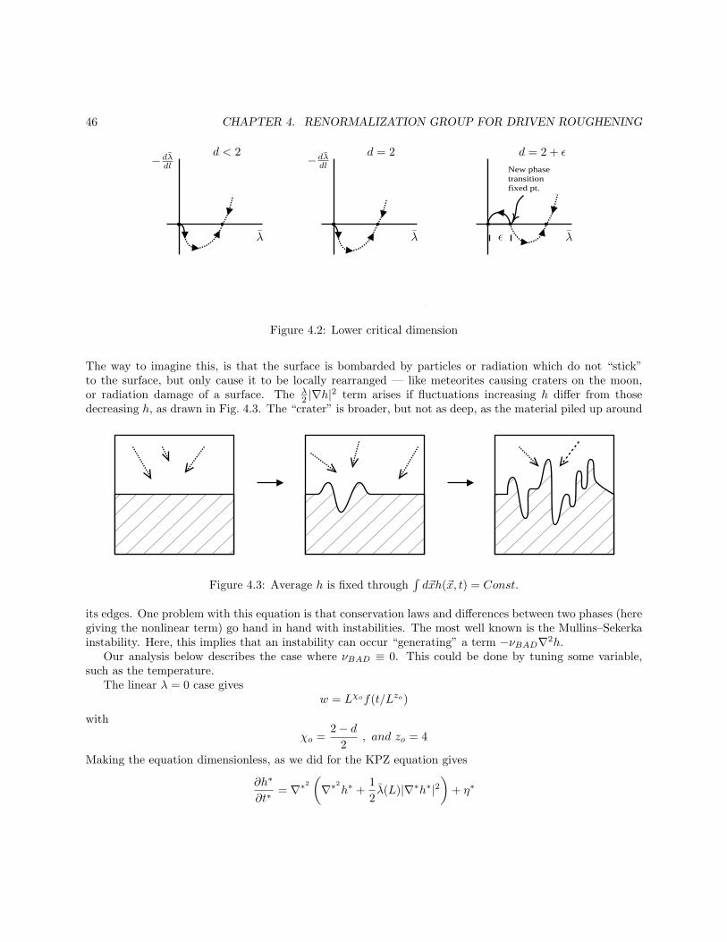
The way to imagine this, is that the surface is bombarded by particles or radiation which do not “stick”to the surface, but only cause it to be locally rearranged — like meteorites causing craters on the moon,or radiation damage of a surface. The λ
2 |∇h|2 term arises if fluctuations increasing h differ from thosedecreasing h, as drawn in Fig. 4.3. The “crater” is broader, but not as deep, as the material piled up around
Figure 4.3: Average h is fixed through∫d~xh(~x, t) = Const.
its edges. One problem with this equation is that conservation laws and differences between two phases (heregiving the nonlinear term) go hand in hand with instabilities. The most well known is the Mullins–Sekerkainstability. Here, this implies that an instability can occur “generating” a term −νBAD∇2h.
Our analysis below describes the case where νBAD ≡ 0. This could be done by tuning some variable,such as the temperature.
The linear λ = 0 case givesw = Lχof(t/Lzo)
with
χo =2− d
2, and zo = 4
Making the equation dimensionless, as we did for the KPZ equation gives
∂h∗
∂t∗= ∇∗2
(
∇∗2
h∗ +1
2λ(L)|∇∗h∗|2
)
+ η∗
47
where
〈η∗η′∗〉 = 2(−∇∗2
)δ(~x∗ − ~x′∗)δ(t∗ − t′∗)
and
λ(L) =λD1/2
ν3/2L(2−d)/2
again, so the critical dimension is
dc = 2
on scaling with χo and zo.
Rescaling with ho = Lχ and to = Lz gives
∂h∗
∂t∗= ∇∗2
(
(νLz−4)∇∗2
h∗ +1
2(λLχ+z−4)|∇∗h∗|2
)
+ (DLz−2χ−d−2)1/2η∗
This equation is, at least to lowest order as k → 0, invariant under a transformation
h→ h+ ~ǫ · ~x
and
~x→ ~x+ ~ǫλ
2t∇2
where ~ǫ is a constant magnitude vector. This is an operator relation which is short–hand for a transformationin Fourier space. It is true to leading order in k2, as you can check. It has been argued that it is not true ingeneral, and remains somewhat controversial. In fact, to one–loop order, explicit calculation shows it to betrue. If it is incorrect to higher order, then this indicates that there is no exact invariance here, unlike theKPZ equation, and so it can be that, unlike the KPZ equation, dc is an upper critical dimension. That is,there is no phase transition at d > dc describing how this invariance is broken. In fact, this is what turnsout: dc = 2 is an upper critical dimension, and we can calculate the nontrivial χ and z using an expansionis (2− d) = ǫ, where ǫ is small (not the same ~ǫ as above in the proposed invariance relation).
Splitting up h into h> and h<, the diagrams are the same as for the KPZ equation:
48 CHAPTER 4. RENORMALIZATION GROUP FOR DRIVEN ROUGHENING
= + +
2+2+
4+ 4+
4+
which gives νI and λI , and
= +
+
+
which gives DI . The main differences are that
Go(k,w) = (−iw − νk4)−1 =
the noise tadpole
49
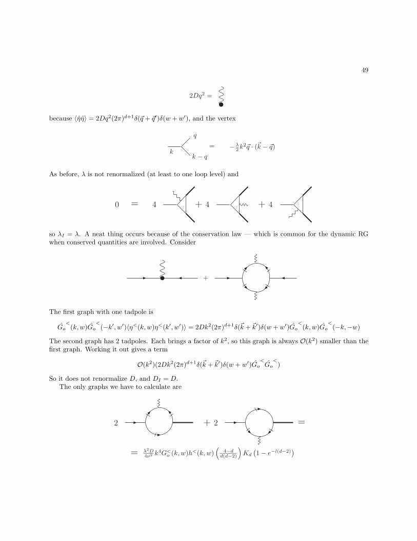
2Dq2 =
because 〈ηη〉 = 2Dq2(2π)d+1δ(~q + ~q′)δ(w + w′), and the vertex
q
k − qk= −λ2 k2~q · (~k − ~q)
As before, λ is not renormalized (at least to one loop level) and
4 + 4 + 40 =
so λI = λ. A neat thing occurs because of the conservation law — which is common for the dynamic RGwhen conserved quantities are involved. Consider
+
The first graph with one tadpole is
Go<
(k,w)Go<
(−k′, w′)〈η<(k,w)η<(k′, w′)〉 = 2Dk2(2π)d+1δ(~k + ~k′)δ(w + w′)Go<
(k,w)Go<
(−k,−w)
The second graph has 2 tadpoles. Each brings a factor of k2, so this graph is always O(k2) smaller than thefirst graph. Working it out gives a term
O(k2)(2Dk2(2π)d+1δ(~k + ~k′)δ(w + w′)Go<Go
<)
So it does not renormalize D, and DI = D.The only graphs we have to calculate are
2+2 =
= λ2D4ν2 k
4G<o (k,w)h<(k,w)(
4−dd(d−2)
)
Kd
(1− e−l(d−2)
)
50 CHAPTER 4. RENORMALIZATION GROUP FOR DRIVEN ROUGHENING
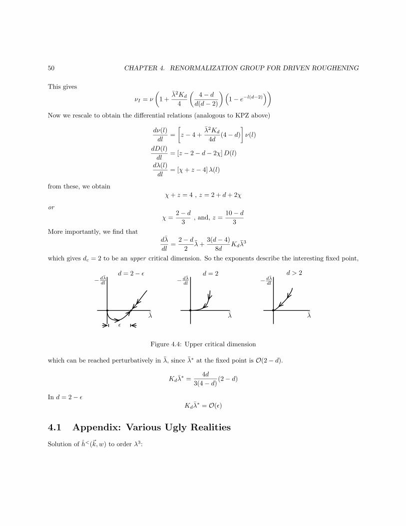
This gives
νI = ν
(
1 +λ2Kd
4
(4− dd(d− 2)
)(
1− e−l(d−2)))
Now we rescale to obtain the differential relations (analogous to KPZ above)
dν(l)
dl=
[
z − 4 +λ2Kd
4d(4− d)
]
ν(l)
dD(l)
dl= [z − 2− d− 2χ]D(l)
dλ(l)
dl= [χ+ z − 4]λ(l)
from these, we obtain
χ+ z = 4 , z = 2 + d+ 2χ
or
χ =2− d
3, and, z =
10− d3
More importantly, we find thatdλ
dl=
2− d2
λ+3(d− 4)
8dKdλ
3
which gives dc = 2 to be an upper critical dimension. So the exponents describe the interesting fixed point,
ǫ
λ
d = 2− ǫ d = 2 d > 2
λλ
−dλdl −dλdl−dλdl
Figure 4.4: Upper critical dimension
which can be reached perturbatively in λ, since λ∗ at the fixed point is O(2− d).
Kdλ∗ =
4d
3(4− d) (2− d)
In d = 2− ǫKdλ
∗ = O(ǫ)
4.1 Appendix: Various Ugly Realities
Solution of h<(~k,w) to order λ3:
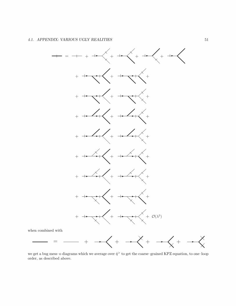
4.1. APPENDIX: VARIOUS UGLY REALITIES 51
= + + + +
+ ++
+ ++
+ ++
+ ++
+ ++
+ ++
+ ++
+ ++ O(λ3)
when combined with
= + + + +
we get a bug mess–o diagrams which we average over η> to get the coarse–grained KPZ equation, to one–looporder, as described above.
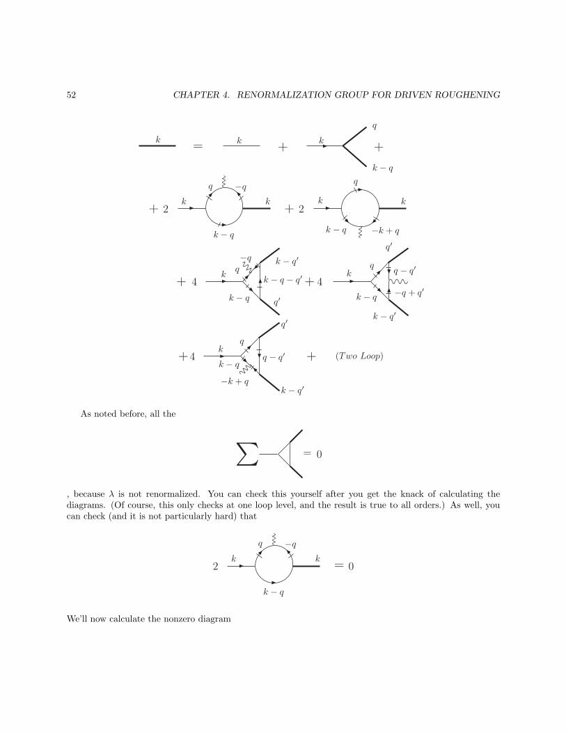
52 CHAPTER 4. RENORMALIZATION GROUP FOR DRIVEN ROUGHENING
k2+
k
k − q
2+k
q
k − q −k + q
k
k4+
= + +
q
k − q
kk k
qk − q′
q′
k − q − q′
k − q
k − q
k − q′
q′
q − q′
−q + q′
k4+
k − q−k + q
k − q′
q′
q − q′q
4k
+
+ (Two Loop)
As noted before, all the
∑= 0
, because λ is not renormalized. You can check this yourself after you get the knack of calculating thediagrams. (Of course, this only checks at one loop level, and the result is true to all orders.) As well, youcan check (and it is not particularly hard) that
=k
2k
k − q
0
We’ll now calculate the nonzero diagram
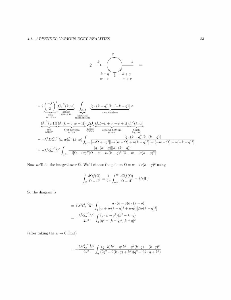
4.1. APPENDIX: VARIOUS UGLY REALITIES 53
2k
q
k − q −k + q
k
−w + rw − r
=
= 2
(−λ2
)2
︸ ︷︷ ︸
twovertices
Go<
(k,w)︸ ︷︷ ︸
arrowgoing in
∫
q,Ω︸︷︷︸
internalmomentum
[q · (k − q)][k · (−k + q)]︸ ︷︷ ︸
two vertices
×
Go>
(q,Ω)︸ ︷︷ ︸
toparrow
Go(k − q, w − Ω)︸ ︷︷ ︸
first bottomarrow
2D︸︷︷︸
noisevertex
Go(−k + q,−w + Ω)︸ ︷︷ ︸
second bottomarrow
h<(k,w)︸ ︷︷ ︸
thickleg out
= −λ2DGo<
(k,w)h<(k,w)
∫
q,Ω
[q · (k − q)][k · (k − q)][−iΩ + νq2][−i(w − Ω) + ν(k − q)2][−i(−w + Ω) + ν(−k + q)2]
= −λ2Go<h<∫
q,Ω
[q · (k − q)][k · (k − q)]−i[Ω + iνq2][Ω− w − iν(k − q)2][Ω− w + iν(k − q)2]
Now we’ll do the integral over Ω. We’ll choose the pole at Ω = w + iν(k − q)2 using
∫
Ω
dΩf(Ω)
Ω− iΓ ≡1
2π
∫ ∞
−∞
dΩf(Ω)
Ω− iΓ = if(iΓ)
So the diagram is
= +λ2Go<h<∫
q
q · (k − q)k · (k − q)[w + iν(k − q)2 + iνq2][2iν(k − q)2]
= −λ2Go
<h<
2ν2
∫
q
(q · k − q2)(k2 − k · q)[q2 + (k − q)2][k − q]2
(after taking the w → 0 limit)
= −λ2Go
<h<
2ν2
∫
q
(q · k)k2 − q2k2 − q2(k · q)− (k · q)2(2q2 − 2(k · q) + k2)(q2 − 2k · q + k2)
54 CHAPTER 4. RENORMALIZATION GROUP FOR DRIVEN ROUGHENING
Now we should reorganize to take account of the fact that k → 0 while q is large. In fact, we only need thecoefficient of the k2 term to renormalize ν.
= −λ2Go
<h<
4ν2
∫
q
1
q4(k · q)q2 + 2(k · q)2 − k2q2 +O(k3)
(
1− k·qq2 +O(k2)
)(
1− 2k·qq2 +O(k2))
= −λ2Go
<h<
4ν2
∫
q
1
q4[(k · q)q2 + 2(k · q)2 − k2q2][1 + 3
k · qq2
+ ...]
= −λ2Go
<h<
4ν2
∫
q
70 odd in q
k · qq2
+
∫
q
(2(k · q)2q4
− k2
q2
)
+ ...
= −λ2Go
<h<
4ν2
∫
q
(2k2q2
d · q4 −k2
q2
)
= −λ2Go
<h<
4ν2
(2
d− 1
)
k2
∫ddq
(2π)d1
q2︸ ︷︷ ︸
=R Λ
Λe−ldq qd−3
R dAngle
(2π)d
= 1−e−l(d−2)
d−2 Λd−2R dAngle
(2π)d
= 1−e−l(d−2)
d−2 Kd
where
Kd ≡Sd
(2π)d=
1
2d−1πd/2Γ(d2 )
and we can choose Λ ≡ 1. This gives the diagram to be
= −λ2Go
<h<
4ν2
(2
d− 1
)
k2
(1− e−l(d−2)
d− 2
)
Kd
= −λ2D
4ν2
(e−l(d−2) − 1
d
)
Kdk2Go
<(k,w)h<(k,w)
after rearranging, as given above.
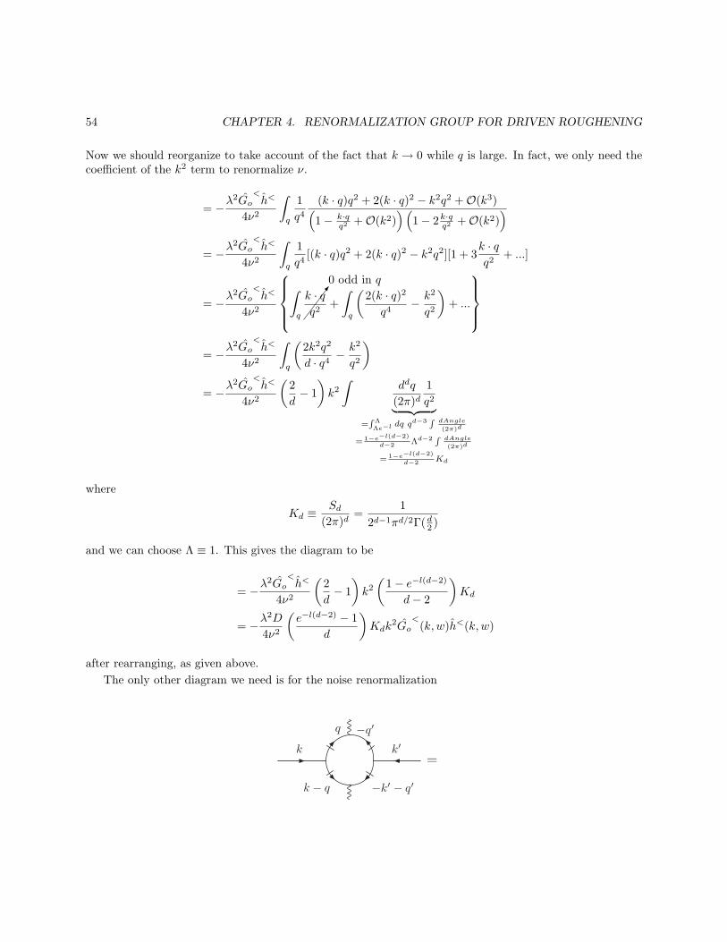
The only other diagram we need is for the noise renormalization
=
−k′ − q′k − q
k′k
q −q′
4.1. APPENDIX: VARIOUS UGLY REALITIES 55
= G<o (k,w)︸ ︷︷ ︸
arrow in
G<o (k′, w′)︸ ︷︷ ︸
arrow out
(
−λ2
)2
︸ ︷︷ ︸
two vertices
∫
qΩq′Ω′
︸ ︷︷ ︸
internalmomentum
q · (k − q)q′ · (k′ − q′)︸ ︷︷ ︸
two vertices
〈h>o (q,Ω)h>o (k − q, w − Ω)ho(q′,Ω′)h>o (k′ − q′, w′ − Ω′)〉
︸ ︷︷ ︸
both tadpoles
= Go<
(k,w)Go<
(k′, w′)λ2
4
∫
qΩq′Ω′
q · (k − q)q′ · (k′ − q′)Go>
(q,Ω)Go>
(k − q, w − Ω)
Go>
(q,Ω)Go>
(k′ − q′, w′ − Ω′)〈η>(q,Ω)η>(k − q, w − Ω)η>(q′,Ω′)η>(k′ − q′, w′ − Ω′)〉
where the 4–noise term is
〈....〉 = 4D2(2π)2(d+1)[δ(k)δ(k′)δ(w)δ(w′)+
+ δ(q + q′)δ(Ω + Ω′)δ(k + k′ − q − q′)δ(w + w′ − Ω− Ω′)+
+ δ(q + k′ − q′)δ(Ω + w′ − Ω′)δ(k − q + q′)δ(w − Ω + Ω′)]
which follows because η> is a Gaussian noise. Putting this in gives the diagram as
=Go<
(k,w)Go<
(k′, w′)2D(2π)d+1δ(~k + ~k′)δ(w + w′)×
λ2D
∫
qΩ
(q · (k − q))2Go>
(qΩ)Go>
(−q,−Ω)Go>
(k − q, w − Ω)Go>
(−k + q,−w + Ω)
where we have ignored the additive contribution giving “Const.δ(~k)δ(~k′)”. Let’s write this as
= Go<
(k)Go<
(−k)2D(2π)d+1δ(~k + ~k′)δ(w + w′)
(DI −DD
)
where the intermediate value for DI is
DI −DD
= λ2D
∫
q,Ω
(q · (k − q))2(Ω + iνq2)(Ω− iνq2)(Ω− w − iν(k − q)2)(Ω− w + iν(k − q))
To do the∫
Ω= 1
2π
∫∞
−∞dΩ integral Choose the two poles at Ω = iνq2 and Ω = w + iν(k − q)2 in the upper
half plane. Then
DI −DD
=λ2D
2ν
∫
q
(q · (k − q))2q2(−w + iν(q2 − (k − q)2))(−w + iν(q2 + (k − q)2))
+λ2D
2ν
∫
q
(q · (k − q))2(w + iν(q2 + (k − q)2))(w − iν(q2 − (k − q)2))(k − q)2
56 CHAPTER 4. RENORMALIZATION GROUP FOR DRIVEN ROUGHENING
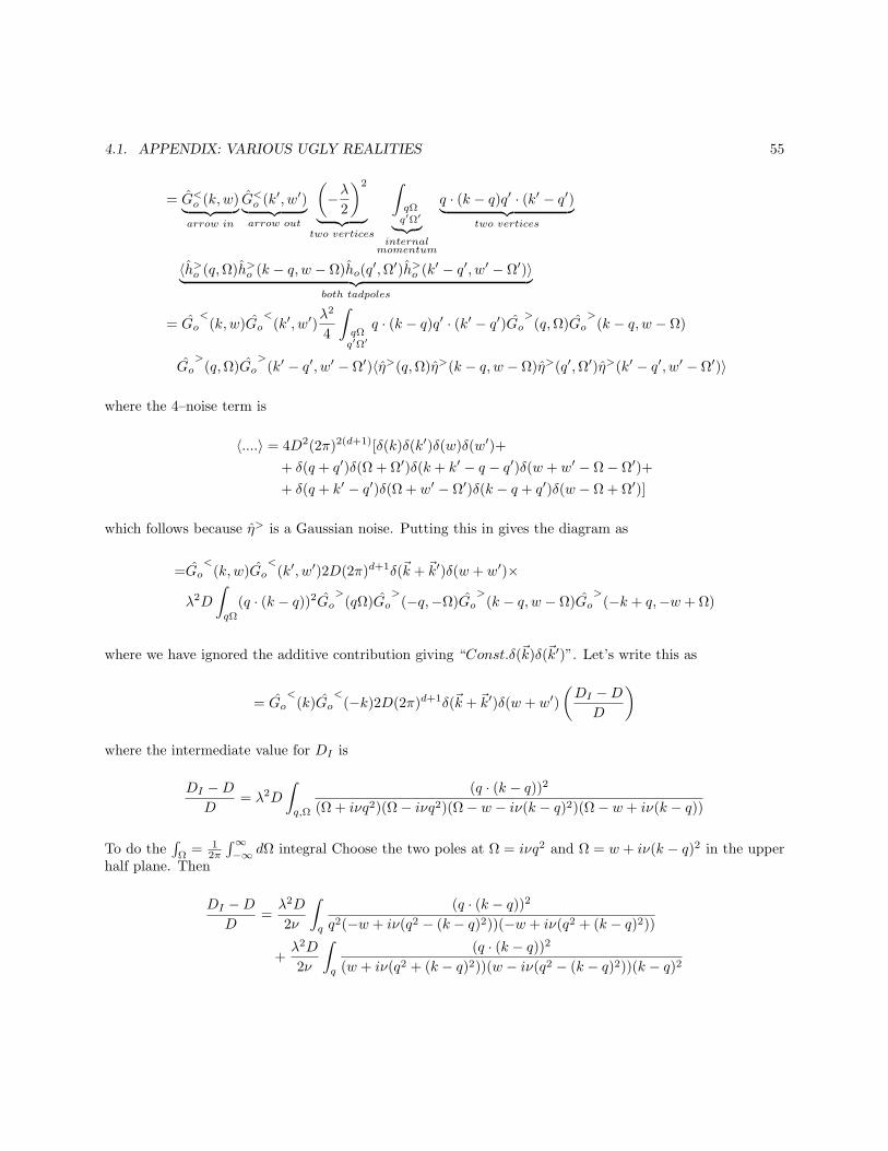
−∞ +∞ ℜeΩ
ℑmΩ
Figure 4.5:
Taking the w → 0 limit gives the fillowing
=λ2D
2ν3
∫ddq
(2π)d
[(q · (k − q))2
q2[(k − q)2 − q2][(k − q)2 + q2]− (q · (k − q))2
(k − q)2[q2 + (k − q)2][(k − q)2 − q2]
]
=λ2D
2ν3
∫ddq
(2π)d(q · (k − q))2
[(k − q)2 − q2][(k − q)2 + q2]
[1
q2− 1
(k − q)2]
=λ2D
2ν3
∫ddq
(2π)d(q · (k − q))2
q2(k − q)2[(k − q)2 + q2]
Taking the k → 0 limit gives
=λ2D
2ν3
∫
ddq1
2q2
=λ2D
4ν3
Kd
d− 2
(
1− e−l(d−2))
as given previously.The graphs for the conserved case are calculated the same way.
Chapter 5
Nonequilibrium Theory Primer
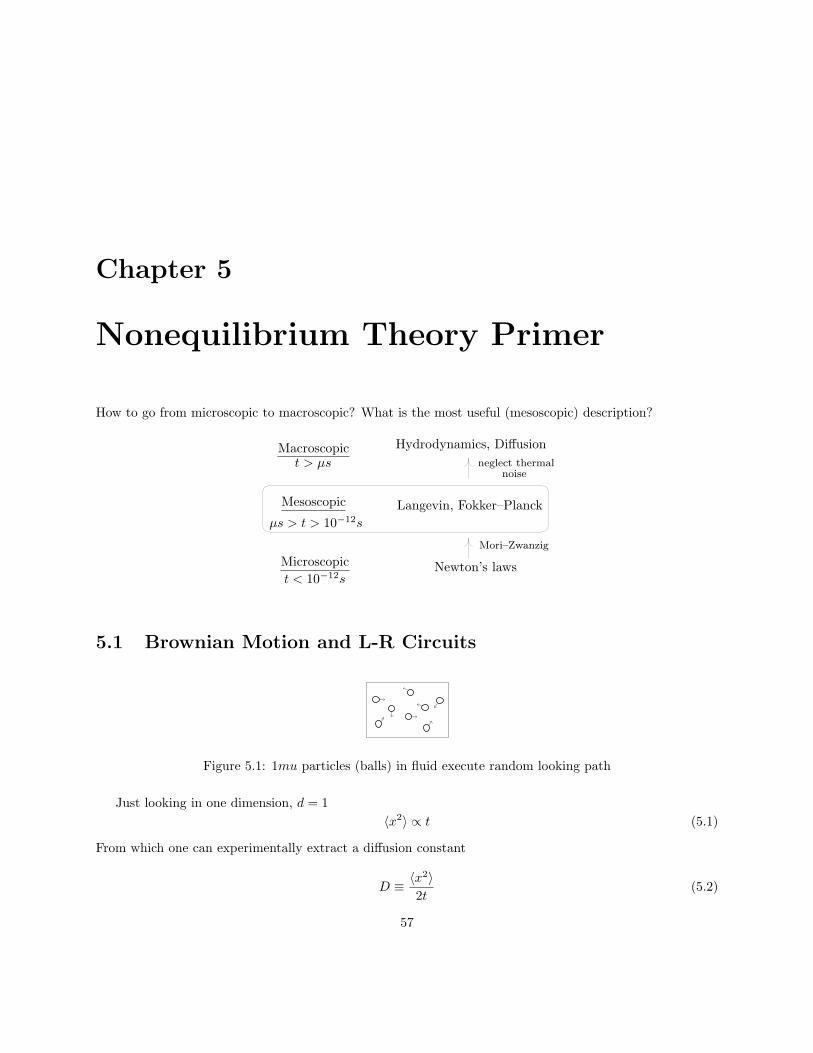
How to go from microscopic to macroscopic? What is the most useful (mesoscopic) description?
Macroscopict > µs
Mesoscopic
µs > t > 10−12s
Microscopic
t < 10−12sNewton’s laws
Mori–Zwanzig
Langevin, Fokker–Planck
neglect thermal
Hydrodynamics, Diffusion
noise
5.1 Brownian Motion and L-R Circuits
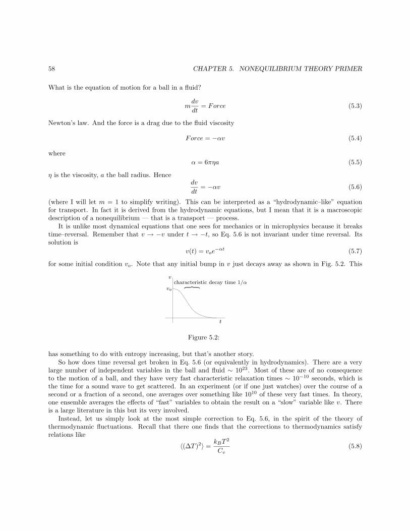
Figure 5.1: 1mu particles (balls) in fluid execute random looking path
Just looking in one dimension, d = 1
〈x2〉 ∝ t (5.1)
From which one can experimentally extract a diffusion constant
D ≡ 〈x2〉
2t(5.2)
57
58 CHAPTER 5. NONEQUILIBRIUM THEORY PRIMER
What is the equation of motion for a ball in a fluid?
mdv
dt= Force (5.3)
Newton’s law. And the force is a drag due to the fluid viscosity
Force = −αv (5.4)
where
α = 6πηa (5.5)
η is the viscosity, a the ball radius. Hencedv
dt= −αv (5.6)
(where I will let m = 1 to simplify writing). This can be interpreted as a “hydrodynamic–like” equationfor transport. In fact it is derived from the hydrodynamic equations, but I mean that it is a macroscopicdescription of a nonequilibrium — that is a transport — process.
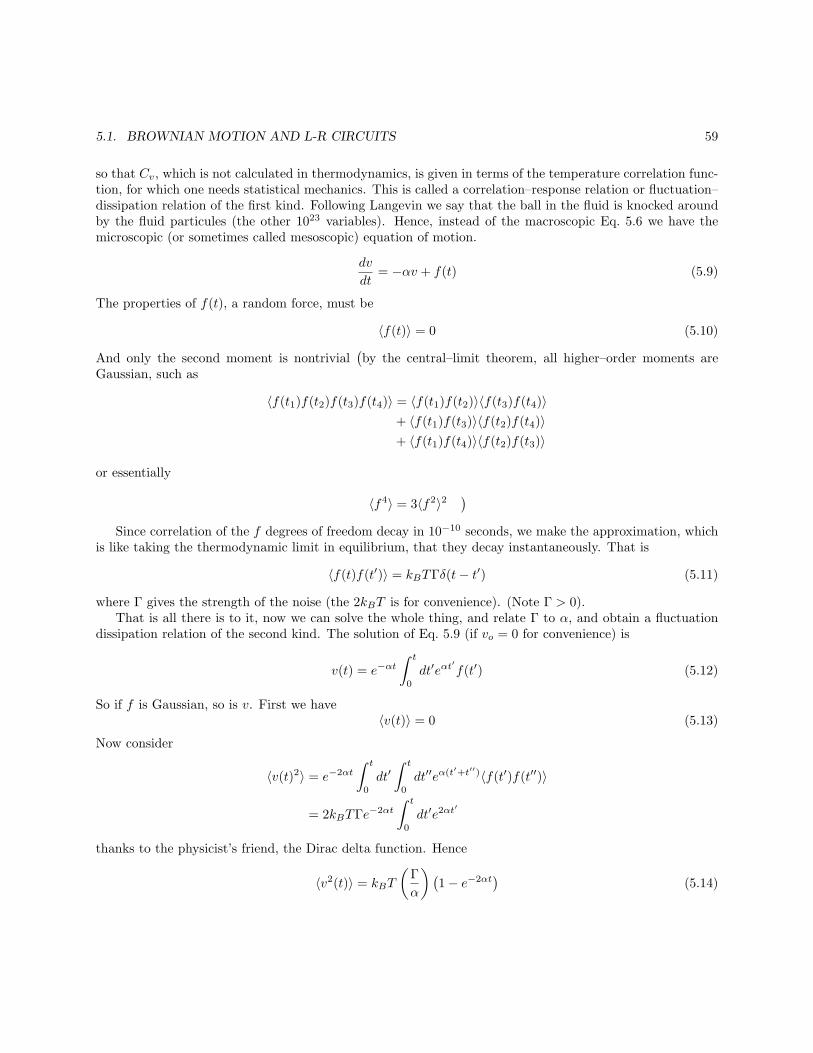
It is unlike most dynamical equations that one sees for mechanics or in microphysics because it breakstime–reversal. Remember that v → −v under t → −t, so Eq. 5.6 is not invariant under time reversal. Itssolution is
v(t) = voe−αt (5.7)
for some initial condition vo. Note that any initial bump in v just decays away as shown in Fig. 5.2. This
Figure 5.2:
has something to do with entropy increasing, but that’s another story.So how does time reversal get broken in Eq. 5.6 (or equivalently in hydrodynamics). There are a very
large number of independent variables in the ball and fluid ∼ 1023. Most of these are of no consequenceto the motion of a ball, and they have very fast characteristic relaxation times ∼ 10−10 seconds, which isthe time for a sound wave to get scattered. In an experiment (or if one just watches) over the course of asecond or a fraction of a second, one averages over something like 1010 of these very fast times. In theory,one ensemble averages the effects of “fast” variables to obtain the result on a “slow” variable like v. Thereis a large literature in this but its very involved.
Instead, let us simply look at the most simple correction to Eq. 5.6, in the spirit of the theory ofthermodynamic fluctuations. Recall that there one finds that the corrections to thermodynamics satisfyrelations like
〈(∆T )2〉 =kBT
2
Cv(5.8)
5.1. BROWNIAN MOTION AND L-R CIRCUITS 59
so that Cv, which is not calculated in thermodynamics, is given in terms of the temperature correlation func-tion, for which one needs statistical mechanics. This is called a correlation–response relation or fluctuation–dissipation relation of the first kind. Following Langevin we say that the ball in the fluid is knocked aroundby the fluid particules (the other 1023 variables). Hence, instead of the macroscopic Eq. 5.6 we have themicroscopic (or sometimes called mesoscopic) equation of motion.
dv
dt= −αv + f(t) (5.9)
The properties of f(t), a random force, must be
〈f(t)〉 = 0 (5.10)
And only the second moment is nontrivial(by the central–limit theorem, all higher–order moments are
Gaussian, such as
〈f(t1)f(t2)f(t3)f(t4)〉 = 〈f(t1)f(t2)〉〈f(t3)f(t4)〉+ 〈f(t1)f(t3)〉〈f(t2)f(t4)〉+ 〈f(t1)f(t4)〉〈f(t2)f(t3)〉
or essentially
〈f4〉 = 3〈f2〉2)
Since correlation of the f degrees of freedom decay in 10−10 seconds, we make the approximation, whichis like taking the thermodynamic limit in equilibrium, that they decay instantaneously. That is
〈f(t)f(t′)〉 = kBTΓδ(t− t′) (5.11)
where Γ gives the strength of the noise (the 2kBT is for convenience). (Note Γ > 0).That is all there is to it, now we can solve the whole thing, and relate Γ to α, and obtain a fluctuation
dissipation relation of the second kind. The solution of Eq. 5.9 (if vo = 0 for convenience) is
v(t) = e−αt∫ t
0
dt′eαt′
f(t′) (5.12)
So if f is Gaussian, so is v. First we have〈v(t)〉 = 0 (5.13)
Now consider
〈v(t)2〉 = e−2αt
∫ t
0
dt′∫ t
0
dt′′eα(t′+t′′)〈f(t′)f(t′′)〉
= 2kBTΓe−2αt
∫ t
0
dt′e2αt′
thanks to the physicist’s friend, the Dirac delta function. Hence
〈v2(t)〉 = kBT
(Γ
α
)(1− e−2αt
)(5.14)
60 CHAPTER 5. NONEQUILIBRIUM THEORY PRIMER
But equipartition says that in equilibrium (presumably reached as t→∞),
1
2m〈v2〉 =
1
2kBT
so〈v2(t =∞)〉 = kBT (5.15)
and we have the Einstein relation (implying α > 0).
α︸︷︷︸
macroscopic
= Γ︸︷︷︸
microscopic
(5.16)
and the second fluctuation–dissipation relation:
〈f(t)f(t′)〉 = 2kBTαδ(t− t′) (5.17)
Compare this to Eq. 5.8 and think. It is easy to calculate other things, and here is one useful one:
〈v(t′)v(t′ + t)〉 = 〈v(0)v(t)〉 = kBTe−α|t| (5.18)
For example, let’s say one wants 〈x2(t)〉, note that
x(t) =
∫ t
0
dt′v(t′)
so that
〈x2(t)〉 =
∫ t
0
dt′∫ t
0
dt′′〈v(t′)v(t′′)〉
=
∫ t
0
dt′∫ t
0
dt′′〈v(0)v(t′′ − t′)〉(5.19)
this takes a little fiddling. Let
τ = t′′ − t′, t =1
2(t′ + t′′)
so that the Jacobian is unity and
t′ = t− τ
2, t′′ = t+
τ
2
The domain of integration is the box sketched in Fig. 5.3, so
〈x2(t)〉 =
[∫ 0
−t
dτ
∫ t′=t
t′′=0
dt+
∫ t
0
dτ
∫ t′′=t
t′=0
dt
]
〈v(0)v(τ)〉
or,
〈x2(t)〉 =
[∫ 0
−t
dτ
∫ t+ τ2
− τ2
dt+
∫ t
0
dτ
∫ t− τ2
τ2
dt
]
〈v(0)v(τ)〉
The integrals are equal, and the t integral can be done to give
〈x2(t)〉 = 2
∫ t
0
(t− t′)〈v(0)v(t′)〉dt′ (5.20)
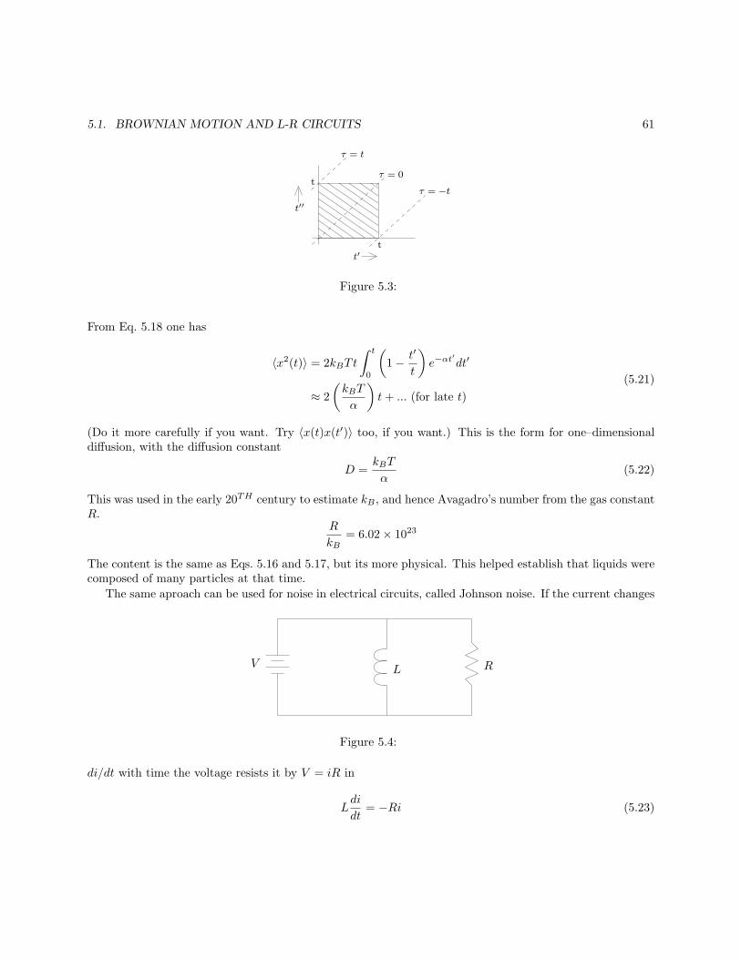
5.1. BROWNIAN MOTION AND L-R CIRCUITS 61
t
t
t′′
t′
τ = 0
τ = t
τ = −t
Figure 5.3:
From Eq. 5.18 one has
〈x2(t)〉 = 2kBTt
∫ t
0
(
1− t′
t
)
e−αt′
dt′
≈ 2
(kBT
α
)
t+ ... (for late t)
(5.21)
(Do it more carefully if you want. Try 〈x(t)x(t′)〉 too, if you want.) This is the form for one–dimensionaldiffusion, with the diffusion constant
D =kBT
α(5.22)
This was used in the early 20TH century to estimate kB , and hence Avagadro’s number from the gas constantR.
R
kB= 6.02× 10²³
The content is the same as Eqs. 5.16 and 5.17, but its more physical. This helped establish that liquids werecomposed of many particles at that time.
The same aproach can be used for noise in electrical circuits, called Johnson noise. If the current changes
VL R
Figure 5.4:
di/dt with time the voltage resists it by V = iR in
Ldi
dt= −Ri (5.23)
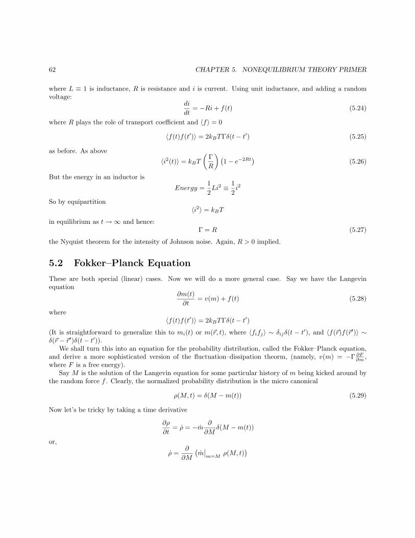
62 CHAPTER 5. NONEQUILIBRIUM THEORY PRIMER
where L ≡ 1 is inductance, R is resistance and i is current. Using unit inductance, and adding a randomvoltage:
di
dt= −Ri+ f(t) (5.24)
where R plays the role of transport coefficient and 〈f〉 = 0
〈f(t)f(t′)〉 = 2kBTΓδ(t− t′) (5.25)
as before. As above
〈i2(t)〉 = kBT
(Γ
R
)(1− e−2Rt
)(5.26)
But the energy in an inductor is
Energy =1
2Li2 ≡ 1
2i2
So by equipartition〈i2〉 = kBT
in equilibrium as t→∞ and hence:Γ = R (5.27)
the Nyquist theorem for the intensity of Johnson noise. Again, R > 0 implied.
5.2 Fokker–Planck Equation
These are both special (linear) cases. Now we will do a more general case. Say we have the Langevinequation
∂m(t)
∂t= v(m) + f(t) (5.28)
where〈f(t)f(t′)〉 = 2kBTΓδ(t− t′)
(It is straightforward to generalize this to mi(t) or m(~r, t), where 〈fifj〉 ∼ δijδ(t − t′), and 〈f(~r)f(~r′)〉 ∼δ(~r − ~r′)δ(t− t′)).
We shall turn this into an equation for the probability distribution, called the Fokker–Planck equation,and derive a more sophisticated version of the fluctuation–dissipation theorm, (namely, v(m) = −Γ ∂F
∂m ,where F is a free energy).
Say M is the solution of the Langevin equation for some particular history of m being kicked around bythe random force f . Clearly, the normalized probability distribution is the micro canonical
ρ(M, t) = δ(M −m(t)) (5.29)
Now let’s be tricky by taking a time derivative
∂ρ
∂t= ρ = −m ∂
∂Mδ(M −m(t))
or,
ρ =∂
∂M
(m∣∣m=M
ρ(M, t))
5.2. FOKKER–PLANCK EQUATION 63
The formal solution of this isρ(M, t) =
[
e−R t0dt′ ∂
∂M m(t′)|m=M
]
ρ(M, 0) (5.30)
Now let us get the complete distribution by averaging over all histories of random forcings:
P (M, t) = 〈ρ(M, t)〉 (5.31)
and of course P (M, 0) = ρ(M, 0). Hence,
P (M, t) = 〈e−R t0dt′ ∂
∂M m(t′)|m=M 〉P (M, 0)
or, recalling the Langevin equation 5.28:
P (M, t) = e−R t0dt′ ∂
∂M v(M)〈e−R t0dt′ ∂
∂M f(t)〉P (M, 0)
But if a variable u is Gaussian, with 〈u2〉 = σ2, then 〈eu〉 = eσ2/2, and here we have
〈f(t)f(t′)〉 = 2kBTΓδ(t− t′)so
〈e−R t0dt′ ∂
∂M f(t′)〉 = ekBTΓt ∂2
∂M2
andP (M, t) = et
∂∂M [−v+kBTΓ ∂
∂M ]P (M, 0)
or,∂P
∂t=
∂
∂M
(
−v(M) + kBTΓ∂
∂M
)
P (M, t) (5.32)
which is almost the Fokker–Planck equation. Note that the equilibrium solution, when ∂Peq/∂t = 0, is
v(M) = kBTΓ∂
∂MlnPeq(M) (5.33)
ButPeq(M) = e−F (M)/kBT (5.34)
Hence we must have
v(M) = −Γ∂F
∂M(5.35)
which is, again, the fluctuation–dissipation relation. In summary, we have shown the equivalence of theLangevin equation
∂m
∂t= −Γ
∂F
∂m+ f (5.36)
where f is a Gaussian random noise with
〈f(t)f(t′)〉 = 2kBTΓδ(t− t′) (5.37)
and the Fokker–Planck equation
∂P
∂t= Γ
∂
∂M
(∂F
∂M+ kBT
∂
∂M
)
P (M, t) (5.38)
with the equilibrium distributionPeq ∝ e−F (M)/kBT (5.39)
Next stop will be to show the limit in which the Master equation is equivalent to either the Fokker–Planckequation, or the Langevin equation.
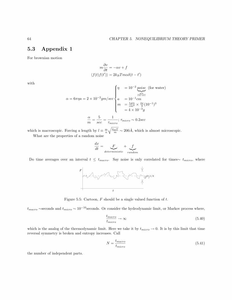
64 CHAPTER 5. NONEQUILIBRIUM THEORY PRIMER
5.3 Appendix 1
For brownian motion
m∂v
∂t= −αv + f
〈f(t)f(t′)〉 = 2kBTmαδ(t− t′)
with
α = 6πηa = 2× 10⁻²gm/sec
η = 10−2 poise︸ ︷︷ ︸gm
cm·sec
(for water)
a = 10−1cm
m = 1gmcm3 × 4π
3 (10−1)3
= 4× 10⁻³g
α
m=
5
sec=
1
τmicro; τmicro ∼ 0.2sec
which is macroscopic. Forcing a length by l ≡ mα
√kBTm ∼ 200A, which is almost microscopic.
What are the properties of a random noise
dx
dt= F
︸︷︷︸
deterministic
+ f︸︷︷︸
random
Do time averages over an interval t ≤ tmacro. Say noise is only correlated for times∼ tmicro, where
〈f2〉1/2
F
t
Figure 5.5: Cartoon, F should be a single valued function of t.
tmacro ∼seconds and tmicro ∼ 10−10seconds. Or consider the hydrodynamic limit, or Markov process where,
tmacrotmicro
→∞ (5.40)
which is the analog of the thermodynamic limit. Here we take it by tmicro → 0. It is by this limit that timereversal symmetry is broken and entropy increases. Call
N =tmacrotmicro
(5.41)
the number of independent parts.
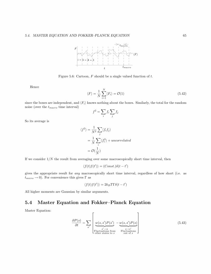
5.4. MASTER EQUATION AND FOKKER–PLANCK EQUATION 65
F
t
tmicro
tmacro
i = 1i = 2i = 3
〈F 〉
Figure 5.6: Cartoon, F should be a single valued function of t.
Hence
〈F 〉 =1
N
N∑
i=1
〈Fi〉 = O(1) (5.42)
since the boxes are independent, and 〈Fi〉 knows nothing about the boxes. Similarly, the total for the randomnoise (over the tmacro time interval)
f2 =∑
i
fi∑
j
fj
So its average is
〈f2〉 =1
N2
∑
j
〈fifj〉
=1
N
∑
i
〈f2i 〉+ uncorrelated
= O(1
N)
If we consider 1/N the result from averaging over some macroscopically short time interval, then
〈f(t)f(t′)〉 = (Const.)δ(t− t′)
gives the appropriate result for any macroscopically short time interval, regardless of how short (i.e. astmicro → 0). For convenience this gives Γ as
〈f(t)f(t′)〉 = 2kBTΓδ(t− t′)
All higher moments are Gaussian by similar arguments.
5.4 Master Equation and Fokker–Planck Equation
Master Equation:
∂P (s)
∂t=∑
s′
w(s, s′)P (s′)︸ ︷︷ ︸
s′→sFluctuations fromother states to s
−w(s, s′)P (s)︸ ︷︷ ︸
s→s′
Fluctuationsout of s
(5.43)
66 CHAPTER 5. NONEQUILIBRIUM THEORY PRIMER
In equilibrium∂Peq∂t
= 0 (5.44)
wherePeq(s) = e−E(s) (5.45)
(in units of temperature), so
w(s, s′)e−E(s′) = w(s′, s)e−E(s) (5.46)
which is the condition of detailed balance of fluctuations. One choice which satisfies this is due to Metropolis
WMetropolis(s, s′) =
e−∆E(s,s′) , ∆Es
1 , ∆Es′(5.47)
where ∆E(s, s′) = E(s)− E(s′). But the choice is somewhat arbitrary. For example, if we let
w(s, s′) = D(s, s′)e12 (E(s′)−E(s)) (5.48)
then detailed balance is satisfied provided
D(s, s′) = D(s′, s) (5.49)
With this transformation the particular Metropolis choise (Eq. 5.47) becomes:
DMetropolis(s, s′) = e−
12 |∆E(s,s′)| (5.50)
Note that all the equilibrium statistical mechanics is satisfied by Eq. 5.49 however.Hence, Eq. 5.43 becomes:
∂P (s)
∂t=∑
s′
D(s, s′)[
e12 (E(s′)−E(s))P (s′)− e− 1
2 (E(s′)−E(s))P (s)]
(5.51)
where D is only due to transport.Now we will derive the Fokker–Planck equation.Most fluctuations involve nearby states s and s′. So we can expand the transport matrix as (Kramers–
Moyal expansion)
D(s, s′) = Doδs,s′ +D2∂2
∂(s− s′)2 δs,s′ + .... (5.52)
Odd terms cannot appear since D(s, s′) = D(s′, s) and we are evidently writing D(s, s′) = f(s− s′).The first term, Doδs,s′ , gives no contribution to Eq. 5.51. So we consider the first nontrivial term
D(s, s′) = D2∂2
∂s2δs,s′ (5.53)
Note ∂2
∂(s−s′)2 has the same action on δs,s′ as ∂2/∂s2.
∂P (s)
∂t= D2
∑
s′
(∂2
∂s2δs,s′
)[
e−12∆EP (s′)− e 1
2∆EP (s′)]
(5.54)
5.4. MASTER EQUATION AND FOKKER–PLANCK EQUATION 67
or, on simplifying
∂P (s)
∂t= D2e
−E(s)
2∂2
∂s2
∑
s′
δs,s′eE(s′)
2 P (s′)−D2eE(s)
2 P (s)∂2
∂s2
∑
s′
δs,s′e−E(s)
2
or,∂P
∂t= D2e
−E(s)
2∂2
∂s2
(
eE(s)
2 P (s))
−D2eE(s)
2 P (s)∂2
∂s2
(
e−E(s)
2
)
(5.55)
Now consider∂
∂seE(s)
2 p(s) =1
2
∂E
∂seE2 P + e
E2∂P
∂s
and∂
∂se−
E2 = −1
2
∂E
∂Se−
E2 (5.56)
so∂2
∂s2
(
eE2 P)
=1
2
∂2E
∂s2eE2 P +
1
4
(∂E
∂s
)2
eE2 P +
2
2
∂E
∂seE2∂P
∂s+ e
E2∂2P
∂s2(5.57)
or
e−E2∂2
∂s2
(
eE2 P)
=1
2
∂2E
∂s2P +
1
4
(∂E
∂s
)2
P +∂E
∂s
∂P
∂s+∂2P
∂s2(5.58)
and from Eq. 5.56
∂2
∂s2e−E/2 = −1
2
∂2E
∂s2e−
E2 +
1
4
(∂E
∂s
)2
e−E2 (5.59)
or,
eE/2P∂2
∂s2e−E/2 = −1
2
∂2E
∂s2P +
1
4
(∂E
∂s
)2
P (5.60)
Using Eq. 5.58 and Eq. 5.60 in Eq. 5.55 (just subtract them):
∂P
∂t= D2
[∂2E
∂s2P +
∂E
∂s
∂P
∂s+∂2P
∂s2
]
Note how the 1/2 factor disappears, or,
∂P
∂t= D2
∂
∂s
[∂E
∂s+
∂
∂s
]
P (5.61)
called the Fokker–Planck equation. To check its consistancy with equilibrium, note
∂Peq∂t
= 0
or [∂E
∂s+
∂
∂s
]
Peq = 0
∂E
∂s= −∂ lnPeq
∂s
68 CHAPTER 5. NONEQUILIBRIUM THEORY PRIMER
orPeq ∝ e−E (5.62)
as it should.Evidently the Fokker–Planck equation can be rewritten as
∂P (s)
∂t=∑
s′
LFP (s, s′)P (s′) (5.63)
where
LFP (s, s′) = D2∂
∂s
[∂E
∂s+
∂
∂s
]
δs,s′ (5.64)
We’ll now return to the Master equation to give a similar form.Consider Eq. 5.51. The second piece on the right–hand side is
Piece =∑
s′
D(s, s′)[
−e− 12 (E(s′)−E(s))P (s)
]
(5.65)
The awkwardness is that P (s) is not summed out. First let the dummy index s′ be s′′, so
Piece =∑
s′′
D(s, s′′)[
−e− 12 (E(s′′)−E(s))P (s)
]
Now replace P (s) by∑
s′ δs,s′P (s′), giving
Piece =∑
s′
−
∑
s′
D(s, s′′)e−12 (E(s′′)−E(s))
︸ ︷︷ ︸
some function of s
δs,s′P (s)
(5.66)
Now put this back into Eq. 5.51 to get
∂P (s)
∂t=∑
s′
D(s, s′)e12 (E(s′)−E(s))P (s′)−
(∑
s′′
D(s, s′′)e−12 (E(s′′)−E(s))
)
δs,s′P (s′)
(5.67)
or,∂P (s)
∂t=∑
s′
LME(s, s′)P (s′) (5.68)
where
LME = D(s, s′)e12 (E(s′)−E(s)) −
(∑
s′′
D(s, s′′)e−12 (E(s′′)−E(s))
)
δs,s′ (5.69)
Making the Kramers–Moyal approximation
D(s, s′)→ D2∂2
∂s2δs,s′
5.4. MASTER EQUATION AND FOKKER–PLANCK EQUATION 69
should recoverLME(s, s′)→ LFP (s, s′)
Note there is still freedom to choose the symmetric matrix D(s, s′) in Eq. 5.69.In either the Fokker–Planck equation (Eq. 5.63) or the Master equation (Eq. 5.68), we can introduce a
transformation which makes L(s, s′) symmetric. Let
Λ ≡ e 12E(s)L(s, s′)e−
12E(s′) (5.70)
Then in Eq. 5.69 we have
ΛME(s, s′) = D(s, s′)−[∑
s′′
D(s, s′′)e−12 (E(s′′)−E(s))
]
δs,s′ (5.71)
which is symmetric, since D is symmetric.For the Fokker–Planck equation (Eq. 5.64)
ΛFP = D2eE(s)
2∂
∂s
[∂E
∂s+
∂
∂s
]
δs,s′e−E(s)/2
= D2
[∂2E
∂s2δs,s′ +
∂E
∂seE(s)/2 ∂
∂s
(
e−E(s)/2δs,s′)
+ eE(s)/2 ∂2
∂s2δs,s′e
−E(s)/2
] (5.72)
Now consider∂
∂sδs,s′e
−E(s)/2 = −1
2
∂E
∂se−E(s)/2δs,s′ + e−E(s)/2 ∂
∂sδs,s′ (5.73)
Taking one more derivative gives
∂2
∂s2δs,s′e
−E/2 = −1
2
∂2E
∂s2e−E/2δs,s′ +
1
4
(∂E
∂s
)2
e−E/2δs,s′ + e−E/2∂2
∂s2δs,s′ (5.74)
Using Eq. 5.73 and Eq. 5.74 in Eq. 5.72 gives
ΛFP (s, s′) = D2
[
1
2
∂2E
∂s2δs,s′ −
1
4
(∂E
∂s
)2
δs,s′ +∂2
∂s2δs,s′
]
(5.75)
so, letting
ρ(s) ≡ eE(s)
2 P (s) (5.76)
we have∂ρ(s)
∂t=∑
s′
Λ(s, s′)ρ(s) (5.77)
whereΛ(s, s′) = Λ(s′, s) (5.78)
and
ΛME(s, s′) = D(s, s′)−[∑
s′′
D(s, s′′)e−12 (E(s′′)−E(s))
]
δs,s′ (5.79)
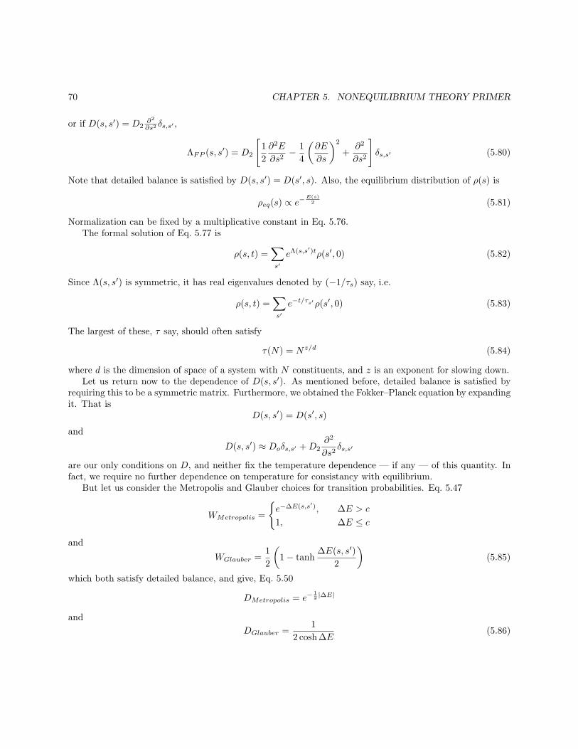
70 CHAPTER 5. NONEQUILIBRIUM THEORY PRIMER
or if D(s, s′) = D2∂2
∂s2 δs,s′ ,
ΛFP (s, s′) = D2
[
1
2
∂2E
∂s2− 1
4
(∂E
∂s
)2
+∂2
∂s2
]
δs,s′ (5.80)
Note that detailed balance is satisfied by D(s, s′) = D(s′, s). Also, the equilibrium distribution of ρ(s) is
ρeq(s) ∝ e−E(s)
2 (5.81)
Normalization can be fixed by a multiplicative constant in Eq. 5.76.The formal solution of Eq. 5.77 is
ρ(s, t) =∑
s′
eΛ(s,s′)tρ(s′, 0) (5.82)
Since Λ(s, s′) is symmetric, it has real eigenvalues denoted by (−1/τs) say, i.e.
ρ(s, t) =∑
s′
e−t/τs′ρ(s′, 0) (5.83)
The largest of these, τ say, should often satisfy
τ(N) = Nz/d (5.84)
where d is the dimension of space of a system with N constituents, and z is an exponent for slowing down.Let us return now to the dependence of D(s, s′). As mentioned before, detailed balance is satisfied by
requiring this to be a symmetric matrix. Furthermore, we obtained the Fokker–Planck equation by expandingit. That is
D(s, s′) = D(s′, s)
and
D(s, s′) ≈ Doδs,s′ +D2∂2
∂s2δs,s′
are our only conditions on D, and neither fix the temperature dependence — if any — of this quantity. Infact, we require no further dependence on temperature for consistancy with equilibrium.
But let us consider the Metropolis and Glauber choices for transition probabilities. Eq. 5.47
WMetropolis =
e−∆E(s,s′), ∆E > c
1, ∆E ≤ c
and
WGlauber =1
2
(
1− tanh∆E(s, s′)
2
)
(5.85)
which both satisfy detailed balance, and give, Eq. 5.50
DMetropolis = e−12 |∆E|
and
DGlauber =1
2 cosh ∆E(5.86)
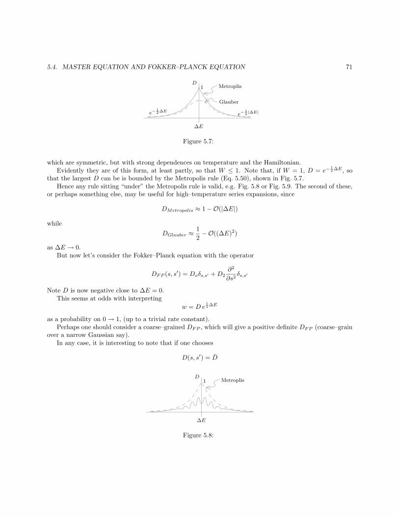
5.4. MASTER EQUATION AND FOKKER–PLANCK EQUATION 71
e−12∆E
e−12|∆E|
∆E
D1 Metroplis
Glauber
Figure 5.7:
which are symmetric, but with strong dependences on temperature and the Hamiltonian.Evidently they are of this form, at least partly, so that W ≤ 1. Note that, if W = 1, D = e−
12∆E , so
that the largest D can be is bounded by the Metropolis rule (Eq. 5.50), shown in Fig. 5.7.Hence any rule sitting “under” the Metropolis rule is valid, e.g. Fig. 5.8 or Fig. 5.9. The second of these,
or perhaps something else, may be useful for high–temperature series expansions, since
DMetropolis ≈ 1−O(|∆E|)
while
DGlauber ≈1
2−O((∆E)2)
as ∆E → 0.But now let’s consider the Fokker–Planck equation with the operator
DFP (s, s′) = Doδs,s′ +D2∂2
∂s2δs,s′
Note D is now negative close to ∆E = 0.This seems at odds with interpreting
w = D e12∆E
as a probability on 0→ 1, (up to a trivial rate constant).Perhaps one should consider a coarse–grained DFP , which will give a positive definite DFP (coarse–grain
over a narrow Gaussian say).In any case, it is interesting to note that if one chooses
D(s, s′) = D
∆E
D1 Metroplis
Figure 5.8:
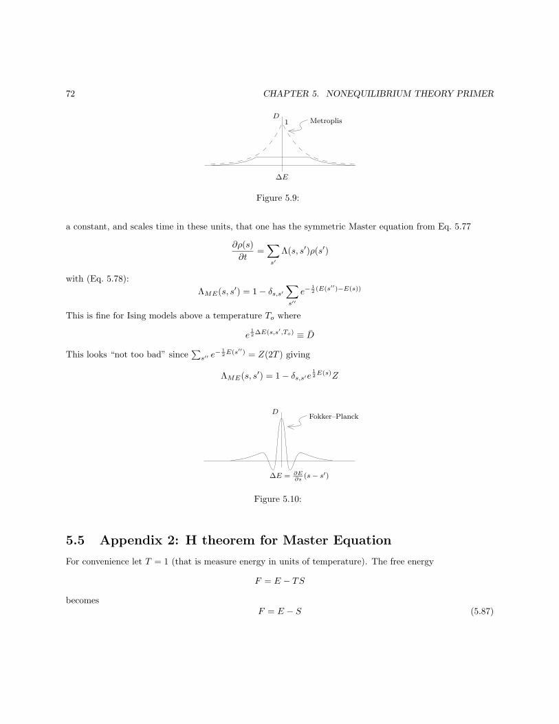
72 CHAPTER 5. NONEQUILIBRIUM THEORY PRIMER
∆E
D1 Metroplis
Figure 5.9:
a constant, and scales time in these units, that one has the symmetric Master equation from Eq. 5.77
∂ρ(s)
∂t=∑
s′
Λ(s, s′)ρ(s′)
with (Eq. 5.78):
ΛME(s, s′) = 1− δs,s′∑
s′′
e−12 (E(s′′)−E(s))
This is fine for Ising models above a temperature To where
e12∆E(s,s′,To) ≡ D
This looks “not too bad” since∑
s′′ e− 1
2E(s′′) = Z(2T ) giving
ΛME(s, s′) = 1− δs,s′e12E(s)Z
∆E = ∂E∂s
(s− s′)
DFokker–Planck
Figure 5.10:
5.5 Appendix 2: H theorem for Master Equation
For convenience let T = 1 (that is measure energy in units of temperature). The free energy
F = E − TS
becomesF = E − S (5.87)
5.5. APPENDIX 2: H THEOREM FOR MASTER EQUATION 73
which, in thermodynamics, is minimized in equilibrium. We will show that
∂F
∂t≤ 0 (5.88)
from the Master equation, whereF = 〈E〉 − 〈− lnP 〉
ThenF =
∑
s
EsPs +∑
s
Ps lnPs (5.89)
so,
dF
dt=∑
s
EsdPsdt
+∑
s
dPsdt
lnPs +>
0∑
s
dPsdt
(5.90)
Using∑
s Ps = 1 so that
d
dt
(∑
s
Ps
)
=d
dt1 = 0 (5.91)
HencedF
dt=∑
s
(Es + lnPs)Psdt
(5.92)
But, from Eq. 5.51dPsdt
=∑
s′
Ds,s′
e−12∆Es,s′Ps′ − e
12∆Es,s′Ps
(5.93)
is the Master equation, where
∆Es,s′ ≡ Es − Es′ (5.94)
Ds,s′ = Ds′,s (5.95)
and
Ds,s′ ≥ 0 (5.96)
Dropping all the subscripts gives
dF
dt=∑
s,s′
D
(E + lnP )e−12∆EP ′ − (E + lnP )e
12∆EP
(5.97)
Switching the (invisible) indices gives the equivalent equation,
dF
dt=∑
s,s′
D
(E′ + lnP ′)e12∆EP − (E′ + lnP ′)e−
12∆EP ′
(5.98)
Adding these together, dividing by 2, gives the handy symmetric form
dF
dt=∑
s,s′
D
2
(E − E′ + lnP − lnP ′)e−12∆EP ′ − (E − E′ + lnP − lnP ′)e
12∆EP
(5.99)
74 CHAPTER 5. NONEQUILIBRIUM THEORY PRIMER
or,
=∑
s,s′
D
2
(∆E + lnP − lnP ′)(e−12∆EP ′ − e 1
2∆EP )
=∑
s,s′
D
2
[
lnP +∆E
2− (lnP ′ − ∆E
2)
] [
e−12∆EP ′ − e 1
2∆EP]
dF
dt= −
∑
s,s′
D
2
[
ln(P ′e−12∆E)− ln(Pe
12∆E)
] [
e−12∆EP ′ − e 1
2∆EP]
(5.100)
Note that the term in the curly brackets is of the form
.... = (lnx− ln y)(x− y) (5.101)
But if lnx > ln y, then x > y so,
lnxMonotonicallyIncreasing
x
Figure 5.11:
(lnx− ln y)(x− y) ≥ 0 (5.102)
where the equality only applies for x = y. Hence, since D > 0 in Eq. 5.100 we have
dF
dt≤ 0 (5.103)
which is the H theorem for the canonical ensemble. The equality holds if
P ′e−12∆E = Pe
12∆E
i.e., forP ∝ e−E (5.104)
5.6 Appendix 3: Derivation of Master Equation
Write down a reasonable starting point for the dynamics of the probability P being in a state s ≡ Mi,where Mi is, say, an order parameter, and i denotes lattice positions.
As time goes on, the probability of being in state s increases because one makes transitions into this statefrom other states like s′ with probability W (s, s′). It can be handy to read this as W (s, s′) = W (s ← s′).Anyway,
W (s, s′)P (s′)
are contributions increasing P (s).
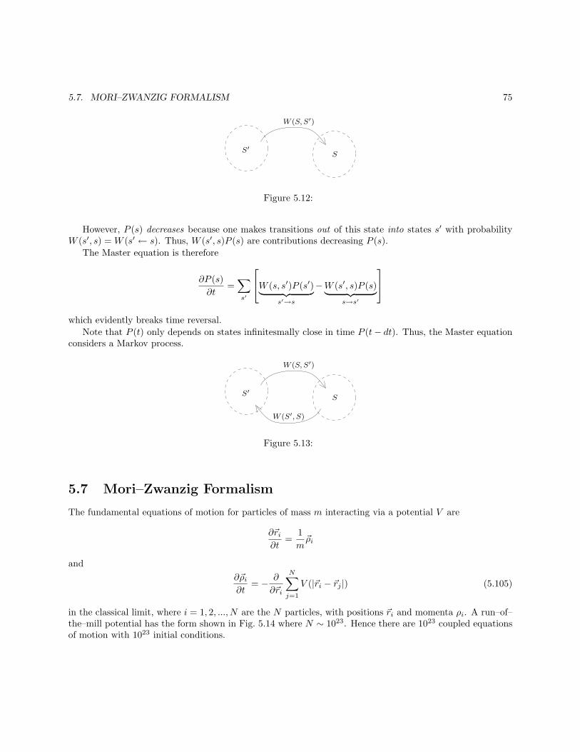
5.7. MORI–ZWANZIG FORMALISM 75
SS′
W (S, S′)
Figure 5.12:
However, P (s) decreases because one makes transitions out of this state into states s′ with probabilityW (s′, s) = W (s′ ← s). Thus, W (s′, s)P (s) are contributions decreasing P (s).
The Master equation is therefore
∂P (s)
∂t=∑
s′
W (s, s′)P (s′)︸ ︷︷ ︸
s′→s
−W (s′, s)P (s)︸ ︷︷ ︸
s→s′
which evidently breaks time reversal.
Note that P (t) only depends on states infinitesmally close in time P (t− dt). Thus, the Master equationconsiders a Markov process.
SS′
W (S, S′)
W (S′, S)
Figure 5.13:
5.7 Mori–Zwanzig Formalism
The fundamental equations of motion for particles of mass m interacting via a potential V are
∂~ri∂t
=1
m~ρi
and
∂~ρi∂t
= − ∂
∂~ri
N∑
j=1
V (|~ri − ~rj |) (5.105)
in the classical limit, where i = 1, 2, ..., N are the N particles, with positions ~ri and momenta ρi. A run–of–the–mill potential has the form shown in Fig. 5.14 where N ∼ 1023. Hence there are 1023 coupled equationsof motion with 1023 initial conditions.
76 CHAPTER 5. NONEQUILIBRIUM THEORY PRIMER
V
r200oK
5Ao
Figure 5.14:
Note that Eq. 5.105 has a time–reversal invariance:
if ~ri → ~ri
~ρi → −~ρit→ −t
(5.106)
then Eq. 5.105 is unchanged. This is in apparent contradiction with the second law of thermodynamics,where time–reversal symmetry is broken (the future has more entropy than the past).
The resolution is that out of the 1023 variables, most are of no consequence macroscopically: they varyon times ∼ 10−10 seconds. Only a few, often one or two or so, vary over macroscopic times ∼ seconds. Thiswide separation of time scales suggest taking the hydrodynamic limit
tmicrotmacro
∼ 10−10 → 0
It is only in this limit that time reversal symmetry is lost. This is analogous to taking the thermodynamiclimit N → ∞ in equilibrium, and considering symmetry breaking, below some curie temperature, in amagnet.
We will now show a method (there are many) which can be used to do this, due to Mori and Zwanzig.
As is well known, Eq. 5.105 can be written in the Hamiltonian form ( ~A) = (~ri, ~ρi),
∂ ~A
∂t= [ ~A,H] (5.107)
where [, ] is a Poisson bracket defined by
[B,C] =∑
all particles+ vectorindices
(∂B
∂~ri
∂C
∂~ρi− ∂B
∂~ρi
∂C
∂~ri
)
(5.108)
and the Hamiltonian is
H =∑
i
ρ2i
2m+
1
2
∑
i6=j
V (|ri − rj |) (5.109)
Note that if one has a quantityQ = Q(~ri(t), ~ρi(t))
then it also satisfies∂Q
∂t= [Q,H] (5.110)
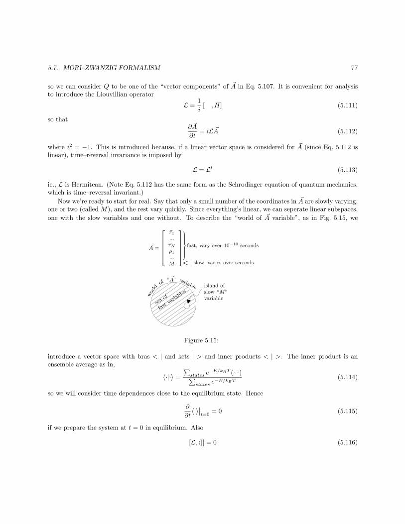
5.7. MORI–ZWANZIG FORMALISM 77
so we can consider Q to be one of the “vector components” of ~A in Eq. 5.107. It is convenient for analysisto introduce the Liouvillian operator
L =1
i[ ,H] (5.111)
so that∂ ~A
∂t= iL ~A (5.112)
where i2 = −1. This is introduced because, if a linear vector space is considered for ~A (since Eq. 5.112 islinear), time–reversal invariance is imposed by
L = Lt (5.113)
ie., L is Hermitean. (Note Eq. 5.112 has the same form as the Schrodinger equation of quantum mechanics,which is time–reversal invariant.)
Now we’re ready to start for real. Say that only a small number of the coordinates in ~A are slowly varying,one or two (called M), and the rest vary quickly. Since everything’s linear, we can seperate linear subspaces,
one with the slow variables and one without. To describe the “world of ~A variable”, as in Fig. 5.15, we
Figure 5.15:
introduce a vector space with bras < | and kets | > and inner products < | >. The inner product is anensemble average as in,
〈·|·〉 =
∑
states e−E/kBT (· ·)
∑
states e−E/kBT
(5.114)
so we will consider time dependences close to the equilibrium state. Hence
∂
∂t〈|〉∣∣t=0
= 0 (5.115)
if we prepare the system at t = 0 in equilibrium. Also
[L, 〈|] = 0 (5.116)
78 CHAPTER 5. NONEQUILIBRIUM THEORY PRIMER
since the averaging is over particle components, which L acts on. The projection operator onto the space ofslow variables is
℘ ≡ |M(0)〉〈M(0)|M(0)〉−1〈M(0)|or (in an obvious notation):
℘ = |Mo〉〈Mo| (5.117)
since we’ll let 〈M2o 〉 ≡ 1 for simplicity. Also we introduce the orthogonal projection
Q = 1− ℘ (5.118)
and our last piece of convenient book keeping is
〈Mo〉 = 0 (5.119)
Although the analysis below is for a scalar M , it is straight forward to consider several slow variables, or afield M(~r).
Initially,℘Mo = Mo
andQMo = 0 (5.120)
But as time goes on, M(t) will drift in and out of the Mo subspace. Hence we introduce
M||(t) = ℘M(t)
andM⊥(t) = QM(t) (5.121)
with M||(0) = Mo and M⊥(0) = 0. Clearly, from Eq. 5.121 we have
M||(t) = C(t)Mo (5.122)
whereC(t) = 〈M(0)M(t)〉 (5.123)
the correlation function, where C(0) = 1, for convenience as previously mentioned. Also, let
℘M(0) ≡ iΩoMo (5.124)
so thatiΩo = 〈MoMo〉 (5.125)
(where, if M is indeed a scalar, then Ωo vanishes by virtue of Eq. 5.115). Some properties and rearrangements
iL℘M(t) = iLM||(t)
= iLC(t)Mo
= C(t)iLMo
soiL℘M(t) = C(t)Mo (5.126)
5.7. MORI–ZWANZIG FORMALISM 79
Also,℘ iL℘M(t) = C(t)℘Mo
or℘ iL℘M(t) = C(t)iΩoMo (5.127)
Now consider the slow variableM(t) = M||(t)
︸ ︷︷ ︸
part whichstayed in slow
subspace
+ M⊥(t)︸ ︷︷ ︸
part whichdrifted into
fast subspace
(5.128)
Consider the parallel part, and we will derive the equation of motion for the correlation function C(t).
M||(t) = ℘iL(M||(t) +M⊥(t))
C(t)Mo = C(t)iΩoMo + 〈Mo|iLM⊥(t)〉Mo
C(t) = iΩoC(t)− 〈iLtMo|M⊥(t)〉
but L is HermiteanC(t) = iΩoC(t)− 〈Mo|M⊥(t)〉 (5.129)
Now consider the perpendicular part
M⊥(t) = QiL(M||(t) +M⊥(t))
= QiLC(t)Mo +QiLM⊥(t)
or (∂
∂t−QiLQ
)
M⊥ = C(t)QMo (5.130)
Hence
M⊥(t) = eQiLQt∫ t
0
dt′e−QiLQt′
C(t′)QMo (5.131)
by inspection, since M⊥(0) = 0.Using this above gives
C(t) = iΩoC(t)−∫ t
0
dt′〈MoeQiLQt|e−QiLQt′QMo〉C(t′)
= iΩoC(t)−∫ t
0
dt′〈e−QiLQtQMo|e−QiLQt′
QMo〉C(t′)
or, this can be written
C(t) = iΩoC(t)−∫ t
0
dt′D(t− t′)C(t′) (5.132)
where the drift termiΩo = 〈MoMo〉
the memory isD(t) = 〈f(0)f(t)〉
80 CHAPTER 5. NONEQUILIBRIUM THEORY PRIMER
and the “noise” isf(t) = etQiLQQMo (5.133)
To obtain the equation of motion for M(t), it is convenient to Laplace transform via
M(s) =
∫ ∞
0
dte−stM(t) (5.134)
Then
M(s) = M||(s) + M⊥(s)
= C(s)Mo +C(s)QMo
s−QiLQSo
M(s) = C(s)[Mo + f(s)] (5.135)
But from Eq. 5.132
sC(s)− *1C(0) = iΩoC(s)− D(s)C(s)
so,
C(s) =1
s− iΩo + D(s)
and from Eq. 5.135
M(s) =Mo + f(s)
s− iΩo + D(s)
or,∂M(t)
∂t= iΩoM(t) +
∫ t
0
dt′D(t− t′)M(t′) + f(t) (5.136)
where iΩo = 〈MoMo〉, D(t) = 〈f(0)f(t)〉, and f(t) = etQiLQQMo, as previously shown. (Here Ωo = 0.)So far, no approximation has been made. Eq. 5.136 is completely equivalent to
∂M
∂t= iLM
The whole approximation now arises by assuming that “f” (the fast variables) are uncorrelated on the timescales over which M (the slow variable) changes. That is
〈f(0)f(t)〉 ∝ δ(t)
We may now writeD(t) = Dδ(t)
and〈f(t)f(t′)〉 = 2Dδ(t− t′) (5.137)
(the factor of 2 arises because either t or t′ can be the greater now). Thus we can have the Langevin equation
∂M(t)
∂t= −DM(t) + f (5.138)
5.7. MORI–ZWANZIG FORMALISM 81
with〈f(t)f(t′)〉 = 2Dδ(t− t′)
Note that D > 0 from the form of the noise correlation.The trick in the method involves choosing the slow variables. Clearly, one must choose all conserved
variables since they satisfy∂M
∂t= ~∇ · ~J → 0
for large wavelengths. One must also choose broken symmetry variables, which are persistent in space, suchas order parameters. These also have ∂M
∂t → 0 as length scales → ∞. Finally it is prudent to add bilinear,and so on, combinations of these variables. It is in this way that nonlinear equations like,
∂M
∂t= −D[M +M3] + f
are derived. The extension to fields is also straightforward.Although this choice may seem arbitrary, recall that the usual derivation of equilibrium statistical me-
chanics requires two conserved variables, energy E and number of particles N , with all other variablesaveraged.

82 CHAPTER 5. NONEQUILIBRIUM THEORY PRIMER
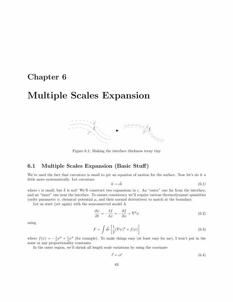
Chapter 6
Multiple Scales Expansion
ξ ξ
Figure 6.1: Making the interface thickness teeny tiny
6.1 Multiple Scales Expansion (Basic Stuff)
We’ve used the fact that curvature is small to get an equation of motion for the surface. Now let’s do it alittle more systematically. Let curvature
k = ǫk (6.1)
where ǫ is small, but k is not! We’ll construct two expansions in ǫ. An “outer” one far from the interface,and an “inner” one near the interface. To ensure consistency we’ll require various thermodynamic quantities(order parameter ψ, chemical–potential µ, and their normal derivatives) to match at the boundary.
Let us start (yet again) with the nonconserved model A
∂ψ
∂t= − δf
δψ= − ∂f
∂ψ+∇2ψ (6.2)
using
F =
∫
~dr
[1
2(∇ψ)2 + f(ψ)
]
(6.3)
where f(ψ) = − 12ψ
2 + 14ψ
4 (for example). To make things easy (at least easy for me), I won’t put in thenoise or any proportionality constants.
In the outer region, we’ll shrink all length scale variations by using the coorinate
~r = ǫ~r (6.4)
83
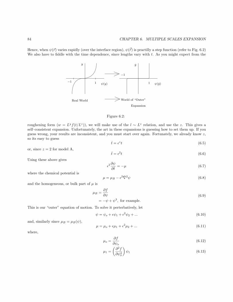
84 CHAPTER 6. MULTIPLE SCALES EXPANSION
Hence, when ψ(~r) varies rapidly (over the interface region), ψ(~r) is practilly a step function (refer to Fig. 6.2)We also have to fiddle with the time dependence, since lengths vary with t. As you might expect from the
−1
−1
11
y y
ψ(y) ψ(y)
Real World World of “Outer”
Expansion
Figure 6.2:
roughening form (w = Lχf(t/Lz)), we will make use of the l ∼ Lz relation, and use the z. This gives aself–consistent expansion. Unfortunately, the art in these expansions is guessing how to set them up. If youguess wrong, your results are inconsistent, and you must start over again. Fortunately, we already know z,so its easy to guess
t = ǫzt (6.5)
or, since z = 2 for model A,t = ǫ2t (6.6)
Using these above gives
ǫ2∂ψ
∂t= −µ (6.7)
where the chemical potential isµ = µB − ǫ2∇2ψ (6.8)
and the homogeneous, or bulk part of µ is
µB =∂f
∂ψ
= −ψ + ψ3, for example.
(6.9)
This is our “outer” equation of motion. To solve it perterbatively, let
ψ = ψo + ǫψ1 + ǫ2ψ2 + ... (6.10)
and, similarly since µB = µB(ψ),µ = µo + ǫµ1 + ǫ2µ2 + ... (6.11)
where,
µo =∂f
∂ψo(6.12)
µ1 =
(∂2f
∂ψ2o
)
ψ1 (6.13)
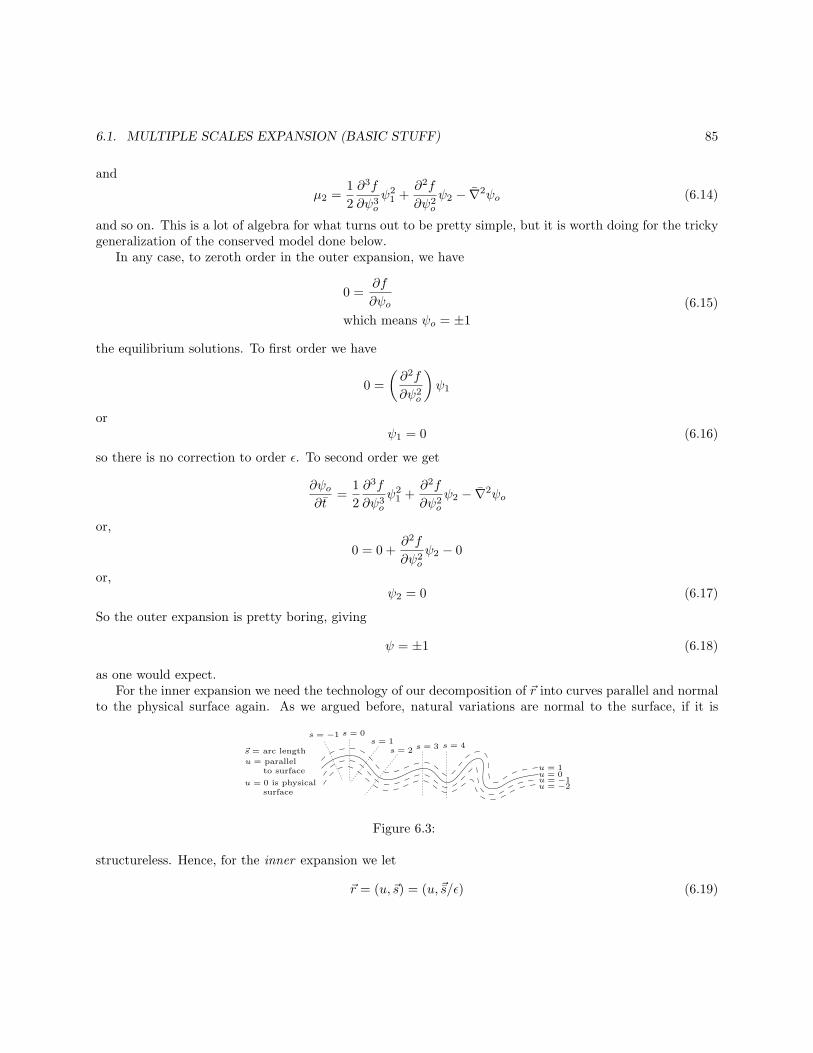
6.1. MULTIPLE SCALES EXPANSION (BASIC STUFF) 85
and
µ2 =1
2
∂3f
∂ψ3o
ψ21 +
∂2f
∂ψ2o
ψ2 − ∇2ψo (6.14)
and so on. This is a lot of algebra for what turns out to be pretty simple, but it is worth doing for the trickygeneralization of the conserved model done below.
In any case, to zeroth order in the outer expansion, we have
0 =∂f
∂ψo
which means ψo = ±1
(6.15)
the equilibrium solutions. To first order we have
0 =
(∂2f
∂ψ2o
)
ψ1
orψ1 = 0 (6.16)
so there is no correction to order ǫ. To second order we get
∂ψo∂t
=1
2
∂3f
∂ψ3o
ψ21 +
∂2f
∂ψ2o
ψ2 − ∇2ψo
or,
0 = 0 +∂2f
∂ψ2o
ψ2 − 0
or,ψ2 = 0 (6.17)
So the outer expansion is pretty boring, giving
ψ = ±1 (6.18)
as one would expect.For the inner expansion we need the technology of our decomposition of ~r into curves parallel and normal
to the physical surface again. As we argued before, natural variations are normal to the surface, if it is
s = −1 s = 0s = 1
s = 2 s = 3 s = 4
u = 1u = 0u = −1u = −2
~s = arc length
u = parallelto surface
u = 0 is physicalsurface
Figure 6.3:
structureless. Hence, for the inner expansion we let
~r = (u,~s) = (u, ~s/ǫ) (6.19)
86 CHAPTER 6. MULTIPLE SCALES EXPANSION
so that
∇2 =∂2
∂u2+ k
∂
∂u+
∂2
∂s2
=∂2
∂u2+ ǫk
∂
∂u+ ǫ2
∂2
∂s2
(6.20)
We will still rescale time as
t = ǫ2t (6.21)
but, since u is a function of time we must use care in taking time derivatives, i.e.
∂
∂t= ǫ2
∂
∂t+
(∂u
∂t
)∂
∂u
= ǫ2∂
∂t+ v
∂
∂u
(6.22)
by the chain rule. The scaling of the velocity v requires a little care. Note the dimensions
[v] =
[k−1
t
]
=
[ǫ−1k−1
ǫ−z t
]
= ǫz−1
[k−1
t
]
(6.23)
so for consistency we must write
v = ǫz−1v
= ǫv(6.24)
Since z = 2 here, and so we finally have∂
∂t= ǫ2
∂
∂t+ ǫv
∂
∂u(6.25)
Finally, the inner expansion is
ǫ2∂ψ
∂t+ ǫv
∂ψ
∂u= −µ (6.26)
where
µ =∂f
∂ψ− ∂2ψ
∂u2− ǫk ∂ψ
∂u− ǫ2 ∂
2ψ
∂s2(6.27)
Expanding to get the inner solution,
ψ = ψo + ǫψ1 + ǫ2ψ2 + ...
and
µ = µo + ǫµ1 + ǫ2µ2 + ... (6.28)
6.1. MULTIPLE SCALES EXPANSION (BASIC STUFF) 87
where
µo =∂f
∂ψo− ∂2ψo
∂u2(6.29)
µ1 =∂2f
∂ψ2o
ψ1 −∂2
∂u2ψ1 − k
∂ψo∂u
(6.30)
and
µ2 =1
2
∂3f
∂ψ3o
ψ21 +
∂2f
∂ψ2o
ψ2
− ∂2ψ2
∂u2− k ∂ψ1
∂u− ∂2ψo
∂s2
(6.31)
and so on.The zeroth order inner solution is
0 = µo
or,
0 =∂f
∂ψo− ∂2ψo
∂u2(6.32)
we know this solution from before to beψo = tanhu (6.33)
The first order solution is
v∂ψo∂u
= −µ1
or,
v∂ψo∂u
= − ∂2f
∂ψ2o
ψ1 +∂2
∂u2ψ1 + k
∂ψo∂u
(6.34)
Integrating this across the surface, after multiplying by ∂ψo/∂u, gives:
v
∫
du
(∂ψo∂u
)2
= −∫
du∂ψo∂u
(∂2f
∂ψ2o
− ∂2
∂u2
)
ψ1 + k
∫
du
(∂ψo∂u
)2
(6.35)
Doing two parts integrals on the second term in the first RHS integral gives
−∫
du∂ψo∂u
(
− ∂2
∂u2
)
ψ1 = −∫
duψ1
(
− ∂2
∂u2
)∂ψo∂u
(6.36)
and using the fact that the surface tension is
σ =
∫
du
(∂ψo∂u
)2
(6.37)
we have
vσ = −∫
duψ1
(∂2f
∂ψ2o
− ∂2
∂u2
)∂ψo∂u
+ kσ (6.38)
88 CHAPTER 6. MULTIPLE SCALES EXPANSION
but∂2f
∂ψ2o
=du
dψo
∂
∂u
∂f
∂ψo(6.39)
because ψo = ψo(u), so
vσ = −∫
duψ1∂
∂u
:0(∂f
∂ψo− ∂2ψo
∂u2
)
+ kσ
andv = k (6.40)
taking out the epsilons givesv = k (6.41)
finally! In passing note ψ1 is the solution of (from Eq. 6.34)
0 =
(
− ∂2f
∂ψ2o
+∂2
∂u2
)
ψ1 (6.42)
which I guess is simply ψ1 = 0.This is a lot of work for model A, which is some what unsatisfying since it is unintuitive. The real power
of the method can be demonstrated in the conserved case, model B. This is where,
∂ψ
∂t= ∇2 δf
δψ= ∇2
(∂f
∂ψ−∇2ψ
)
(6.43)
where F =∫~dr[12 (∇ψ)2 + f(ψ)
]again, and typically, f(ψ) = − 1
2ψ2 + 1
4ψ4.
For the outer region we again have~r = ǫ~r (6.44)
andt = ǫzt (6.45)
Here I shall simply use a result I know (but haven’t derived yet) z = 3 to write
t = ǫ3t (6.46)
This gives a consistent expansion; z = 2 or z = 4 will not. The outer equation of motion is then
ǫ3∂ψ
∂t= ǫ2∇2µ (6.47)
where, perturbativelyψ = ψo + ǫψ1 + ǫ2ψ2 + ...
and
µ = µo + ǫµ1 + ǫ2µ2 + ... (6.48)
µo = ∂f/∂ψo (6.49)
µ1 =
(∂2f
∂ψ2o
)
ψ1 (6.50)
6.1. MULTIPLE SCALES EXPANSION (BASIC STUFF) 89
and
µ2 =1
2
(∂3f
∂ψ3o
)
ψ21 +
(∂2f
∂ψ2o
)
ψ2 − ∇2ψo (6.51)
The zeroth order solution is
0 = ∇2µo
= ∇2
(∂f
∂ψo
)(6.52)
The physical solution of this is∂f
∂ψo= 0 (6.53)
which gives ψo = ±1 as before for model A. To first order we have
0 = ∇2µ1
or
0 = ∇2ψ1 (6.54)
The solution of this is nontrivial, so we’ll leave it like this. (ψ1 must be matched to the inner solution, whichprovides the boundary condition to solve the Laplace problem. Things are already looking pretty raunchy,so let’s go to the inner expansion.)
For the inner expansion we again have ~r = (u,~s) = (u, s/ǫ) and k = ǫk, so
∇2 =∂2
∂u2+ ǫk
∂
∂u+ ǫ2
∂2
∂s2(6.55)
for time, we have t = ǫzt again, with time derivative
∂
∂t= ǫz
∂
∂t+ ǫz−1v
∂
∂u
as before, or using z = 3,∂
∂t= ǫ3
∂
∂t+ ǫ2v
∂
∂u(6.56)
where v = ǫz−1~v = ǫ2v. The equation of motion for the inner expansion is
ǫ3∂ψ
∂t+ ǫ2v
∂ψ
∂u=
(∂2
∂u2+ ǫk
∂
∂u+ ǫ2
∂2
∂s2
)
µ (6.57)
which we solve perturbatively using
ψ = ψo + ǫψ1 + ǫ2ψ2 + ...
and
µ = µo + ǫµ1 + ǫ2µ2 + ... (6.58)
90 CHAPTER 6. MULTIPLE SCALES EXPANSION
where
µo =∂f
∂ψo− ∂2ψo
∂u2
µ1 =∂2f
∂ψ2o
ψ1 −∂2ψ1
∂u2− k ∂ψo
∂u
and
µ2 =1
2
∂3f
∂ψ3o
ψ21 +
∂2f
∂ψ2o
ψ2 −∂2ψ2
∂u2− k ∂ψ1
∂u− ∂2ψo
∂s2(6.59)
and so on. The zeroth order solution is
0 =∂2
∂u2µo
which is (you can check µo = A+Bu has A = B = 0)
µo = 0
or∂f
∂ψo− ∂2ψo
∂u2= 0 (6.60)
our old friend, ψo = tanhu. The first order expansion gives
0 =∂2
∂u2µ1 + k
∂µo∂u
Using µo = 0 from above we have∂2µ1
∂u2= 0 (6.61)
Here we can’t just set it to zero, (it has to match the outer solution of ∇2µ1 = 0) but we can certanly sayµ1 6= µ1(u), or
µ1 = µ1(s) (6.62)
writing out the form of µ1 gives
µ1(s) =∂2f
∂ψ2o
ψ1 −∂2
∂u2ψ1 − k
∂ψo∂u
(6.63)
which is pretty similar to what we had for model A, except for the µ1(s) factor, see Eq. 6.34. Multiplyingby ∂ψo
∂u and integrate over u again:
µ1(s)
∫
dudψodu
=
∫
dudψodu
(∂2f
∂ψ2o
− ∂2
∂u2
)
ψ1
︸ ︷︷ ︸
Zero, as before
− k∫
du
(dψodu
)2
︸ ︷︷ ︸
σ, as before
(6.64)
use∫
dudψodu
= ψo(above surface)− ψo(below surface)
= +1− (−1)
= ∆ψ, the equilibrium miscibility gap
(6.65)
6.1. MULTIPLE SCALES EXPANSION (BASIC STUFF) 91
Thereforeµ1(s)∆ψ = 0− kσ
and so the inner solutionµ1(s) = −k σ
∆ψ(6.66)
which must be matched to the outer expansion solution of ∇2µ1 = 0.Second order in the inner expansion gives
v∂ψo∂u
=∂2
∂u2µ2 +
0
k∂µ1
∂u+
0
∂2µo∂s2
(6.67)
Integrating over the surface gives
v∆ψ =∂µ2
∂u
∣∣above surface
−∂µ2
∂u
∣∣below surface
(6.68)
orv∆ψ = (n · ~∇µ2)above − (n · ~∇µ2)below (6.69)
where n is the unit vector normal to the surface.Reconstructing the expansion for
µ = µo + ǫµ1 + ǫ2µ2
in the inner region, we have (on putting the epsilons back in)
ψ = tanhu (6.70)
to lowest order, and
µ∣∣interface
= − σ
∆ψk (6.71)
vinterface∆ψ = (n · ∇µ)above − (n · ~∇µ)below (6.72)
For the last equation, note ∂µ1
∂u = 0 has been used in Eq. 6.68. From the outer expansion,
ψ = ±1 (6.73)
in the bulk regions, and∇2µ = 0 (6.74)
in those same regions. Note this is much trickier than model A. Here, the excess chemical potential atthe interface is proportional to the local curvature. The rate of change if the interface, its velocity, isregulated by a conservation law for ψ. (Note that if ∂ψ/∂t = ∇2µ, and becomes (∂u/∂t)∂ψ/∂u = ∇2µ, andintegrating over du gives, ∂u/∂t∆ψ = (n · ∇µ)jump). Unfortunately, this conservation law requires solving∂∇2µ everywhere in space! (This is the steady–state form of the conservation law.)
For linear roughening it is straightforward to solve this. We have
∇2µ = 0
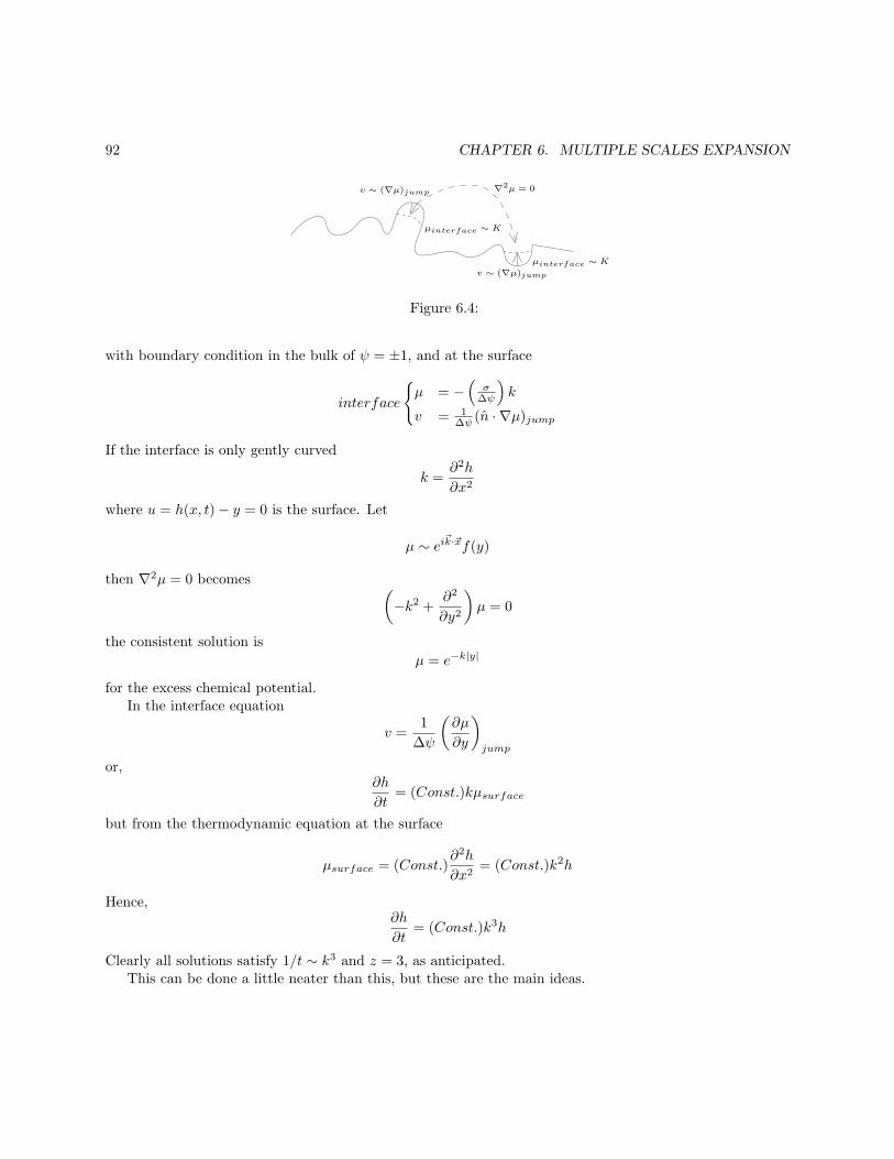
92 CHAPTER 6. MULTIPLE SCALES EXPANSION
µinterface ∼ K
µinterface ∼ K
v ∼ (∇µ)jump
v ∼ (∇µ)jump
∇2µ = 0
Figure 6.4:
with boundary condition in the bulk of ψ = ±1, and at the surface
interface
µ = −(
σ∆ψ
)
k
v = 1∆ψ (n · ∇µ)jump
If the interface is only gently curved
k =∂2h
∂x2
where u = h(x, t)− y = 0 is the surface. Let
µ ∼ ei~k·~xf(y)
then ∇2µ = 0 becomes(
−k2 +∂2
∂y2
)
µ = 0
the consistent solution is
µ = e−k|y|
for the excess chemical potential.In the interface equation
v =1
∆ψ
(∂µ
∂y
)
jump
or,∂h
∂t= (Const.)kµsurface
but from the thermodynamic equation at the surface
µsurface = (Const.)∂2h
∂x2= (Const.)k2h
Hence,∂h
∂t= (Const.)k3h
Clearly all solutions satisfy 1/t ∼ k3 and z = 3, as anticipated.This can be done a little neater than this, but these are the main ideas.
6.2. MULTIPLE SCALES EXPANSION FOR MODEL B WITH Z = 2 (SUBTLE STUFF) 93
6.2 Multiple Scales Expansion for Model B with z = 2 (subtlestuff)
As in other notes, we shall scale length with ǫ, and times with ǫz. Here we will choose z = 2, anticipating atransient regime involving diffusion where (Length) ∼ (time)1/2.
The Langevin equation is
∂ψ
∂t= ∇2 δF
δψ= ∇2µ
= ∇2
−∇2ψ +∂f
∂ψ
when stuck, we will choose
f = −ψ2
2+ψ4
4
6.2.1 Outer Region
In the outer region, all lengths scale the same way. Let
~r = ǫ~r
And for timet = ǫzt = ǫ2t
We have
ǫ2∂ψ
∂t= ǫ2∇2
−ǫ2∇2ψ +∂f
∂ψ︸ ︷︷ ︸
µ
The bulk part of the chemical potential is ∂f/∂ψ, and this will dominate the outer expansion to the orderwe require. Let us expand
ψ = ψo + ǫψ1 + ǫ2ψ2 + ...
and,µ = µo + ǫµ1 + ǫ2µ2 + ...
Of course the µ expansion is just a rearranged version of the ψ expansion. Hence
µo = ∂f/∂ψo
µ1 =(∂2f/∂ψ2
o
)ψ1
and
µ2 = −∇2ψo +1
2
(∂3f/∂ψ3
o
)ψ1 +
(∂2f/∂ψ2
o
)ψ2
We won’t need the second–order term here. Order by order we have the following:
94 CHAPTER 6. MULTIPLE SCALES EXPANSION
6.2.2 Zeroth Order Outer∂ψo∂t
= ∇2µo
The solution of this isµo = 0
which is∂f
∂ψo= 0
so that ψo is a constant and∂ψo∂t
=∂Const.
∂t= 0
for the choice, f = −ψ2/2 + ψ4/4, this gives ψo = ±1.
6.2.3 First–Order Outer∂ψ1
∂t= ∇2µ
Using the form for µ1 (and the fact that ψo is a constant)
∂ψ1
∂t=
(∂2f
∂ψ2o
)
∇2ψ1
or equivalently,∂µ1
∂t=
(∂2f
∂ψ2o
)
∇2µ1
where a choice of f gives ∂2f/∂ψ2o = 2. This is just the linear diffusion equation, for which we need the
boundary conditions at the interface from the inner solution. Note that this has [t] ∼ [L]2, as “built–in”from the choice of z = 2. We do not need the second–order terms.
6.2.4 Inner Region
As in other notes, for the inner region we need the interface–specific coordinate system:
~r = (u,~s)
where u is normal to the surface, and ~s runs along the surface. To the order we need, the Laplacian is
∇2 =∂2
∂u2+ k
∂
∂u+
∂2
∂s2
where k is the curvature of the interface. (In general there is a more complicated expression valid, at leastin principle, far from u = 0.) Scaling this as
~s = ǫ~s
andk = ǫk
6.2. MULTIPLE SCALES EXPANSION FOR MODEL B WITH Z = 2 (SUBTLE STUFF) 95
(that is, not scaling u), gives
∇2 =∂2
∂u2+ ǫk
∂
∂u+ ǫ2
∂2
∂s2
As well we must scale time accounting for motion of the interface at velocity v. This scales as v =(length/time) = ǫz−1, so
~v = ǫz−1v
and∂
∂t= ǫz
∂
∂t+ ǫz−1v
∂
∂uby the chain rule. Here we have z = 2, and the Langevin equation becomes
ǫ2∂ψ
∂t+ ǫv
∂ψ
∂u=
(∂2
∂u2+ ǫk
∂
∂u+ ǫ2
∂2
∂s2
)
µ
where
µ = −(∂2
∂u2+ ǫk
∂
∂u+ ǫ2
∂2
∂s2
)
ψ +∂f
∂ψ
We expand again viaψ = ψo + ǫψ1 + ǫ2ψ2 + ...
andµ = µo + ǫµ1 + ǫ2µ2 + ...
The forms of µo, µ1, and so on are determined by ψo, ψ1, and so on. In particular,
µo =∂f
∂ψo− ∂2ψo
∂u2
µ1 =∂2f
∂ψ2o
ψ1 −∂2ψ1
∂u2− k ∂ψo
∂u
and (which we will not need):
µ2 =1
2
∂3f
∂ψ3o
ψ21 +
∂2f
∂ψ2o
ψ2 −∂2ψ2
∂u2− k ∂ψ1
∂u− ∂2ψo
∂s2
Note that, although we are using the same notation for the outer and inner expansion, we must match theouter solution for, e.g., ψo to the inner solution for ψo. They are not the same function — except at thematching points.
6.2.5 Zeroth Order Inner
0 =∂2
∂u2µo
The solution to this is µo = 0 (consistent with the outer boundary condition µo = 0), so
∂f
∂ψo− ∂2ψo
∂u2= 0
For the particular choice of f = −ψ2/2 + ψ4/4, this gives ψo = tanhu, or the result ψo = tanh(u+Const.),which is matched to the outer solution ψo = ±1. Now we get to the heart of the matter.
96 CHAPTER 6. MULTIPLE SCALES EXPANSION
6.2.6 First–Order Inner
vdψodu
=∂2µ1
∂u2+ k
dµodu
Using the solution µo = 0 from above, we have
∂2µ1(u,~s)
∂u2= v(s)
dψo(u)
du
Integrating over u from −δ to +δ where δ is the matching point for the two expansions gives
dµ1
du
∣∣+ − ∂µ1
∂u
∣∣−
= ∆ψv
where ∆ψ = ψo(u = +δ)− ψo(u = −δ) which we will write as
∆ψ = ψ+ − ψ−
for the choice of f above, this gives ∆ψ = 2, because ψ± = ±1. This is one of the two expected boundaryconditions. The other will be of the form
µ1 = (Const.)︸ ︷︷ ︸
Gibbs–Thomsoncondition
k + (Const.)︸ ︷︷ ︸
kineticunder cooling
v
We will now go through some loop–de–loops to obtain this form ∂2µ1/∂u2 = vdψo/du. (We could equivalently
try to find the equations in terms of ψ1, but since the other boundary condition, and the outer solution arealready in terms of µ, let’s use µ1 and eliminate ψ1.) In any case, we have
∂2µ1
∂u2= v
dψodu
and
µ1 =∂2f
∂ψoψ1 −
∂2ψ1
∂u2− k ∂ψo
∂u
The second equation does not look useful because it involves the equivalently unknown µ1 and ψ1, but here
is a useful trick. Act on this with∫ +
−dudψodu (...) (Note that
∫ +
−du... ≡
∫ δ
−δdu...). This gives
∫ +
−
dudψodu
µ1 =
∫ +
−
dudψodu
(∂2f
∂ψ2o
ψ1 −∂2ψ1
∂u2
)
− kσ
where the surface tension
σ ≡∫ +
−
du
(dψodu
)2
In the right–hand–side integrand, note that
d2f
dψ2o
=1
dψo/du
d
du
(df
dψo
)
6.2. MULTIPLE SCALES EXPANSION FOR MODEL B WITH Z = 2 (SUBTLE STUFF) 97
Hence, using this, and doing two parts integrals to make d2ψ1
du2 → ψ1d2
du2 , gives
∫ +
−
dudψodu
µ1 =
∫ +
−
dud
du
(df
dψo− d2ψo
du2
)
− kσ
But now the integrand is µo, which is exactly zero, so:
∫ +
−
dudψodu
µ1 = −kσ
which is handy. Note if µ1 = µ1(~s) only, this would give µ1 = −kσ/∆ψ, which would be the boundarycondition. Here, however, we expect that µ, does have u dependence, which gives rise to the kinetic undercooling term.
Now reconsider the main equationd2µ1
du2= v
dψodu
The solution can be obtiained from inspection. One integral gives
dµ1
du= vψo +A(s)
where A(s) is unknown, although it is clearly A(s) = (dµ1/du)u(ψo=0). This is consistent with the boundarycondition (dµ1/du)|+ − (dµ1/du)|− = ~v∆ψ, above. Another integral gives
µ1 = v
∫ u
0
du′ψo(u′) +A(s)u+B(s)
where B(s) is unknown (and hence we can choose the lower limit of the indefinite integral to be whateverwe wish).
For definiteness, note that if ψo = tanhu∫ u
0
tanhudu = log coshu
=
|u|, large u
u2/2, small u
So it is a “cusp–like” thing (refer to Fig. 6.5).We can conveniently write the “cusp–like” thing as
C(u) ≡∫ u
0
du′ψo(u′)
so that, in the inner region:µ1(u, s) = v(s)C(u) +A(s)u+B(s)
where dC/du = ψo(u), and C(0) = 0. We just need a couple of tricks to deal with A and B.There is a big subtlety, however. We need the boundary conditions for the outer solution
∂[µ1]outer∂t
=
[∂2f
∂ψ2o
]
outer
∇2[µ1]outer
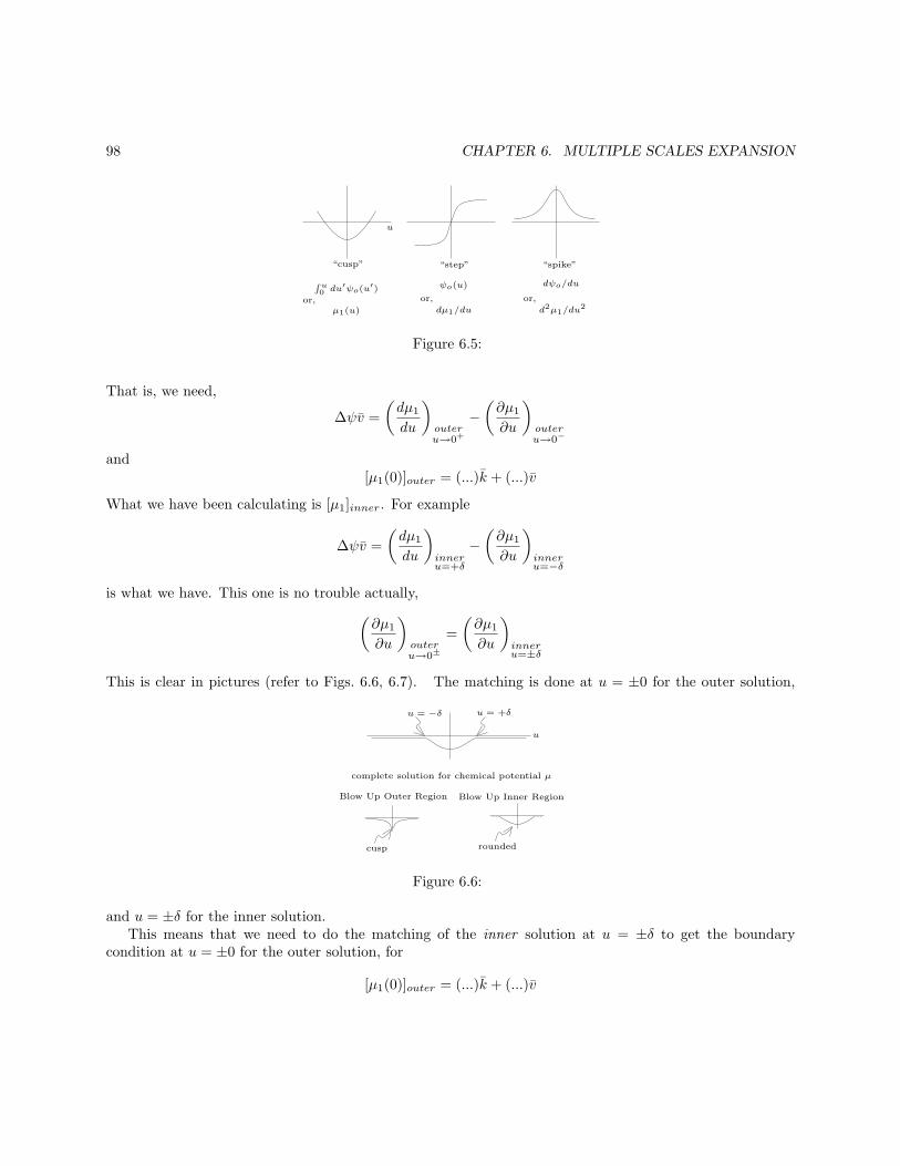
98 CHAPTER 6. MULTIPLE SCALES EXPANSION
“cusp” “step” “spike”
R u0 du′ψo(u
′) ψo(u) dψo/du
µ1(u) dµ1/du d2µ1/du2
or, or, or,
u
Figure 6.5:
That is, we need,
∆ψv =
(dµ1
du
)
outeru→0+
−(∂µ1
∂u
)
outeru→0−
and[µ1(0)]outer = (...)k + (...)v
What we have been calculating is [µ1]inner. For example
∆ψv =
(dµ1
du
)
inneru=+δ
−(∂µ1
∂u
)
inneru=−δ
is what we have. This one is no trouble actually,
(∂µ1
∂u
)
outeru→0±
=
(∂µ1
∂u
)
inneru=±δ
This is clear in pictures (refer to Figs. 6.6, 6.7). The matching is done at u = ±0 for the outer solution,
u = −δ u = +δ
complete solution for chemical potential µ
Blow Up Outer Region Blow Up Inner Region
u
cusp rounded
Figure 6.6:
and u = ±δ for the inner solution.This means that we need to do the matching of the inner solution at u = ±δ to get the boundary
condition at u = ±0 for the outer solution, for
[µ1(0)]outer = (...)k + (...)v
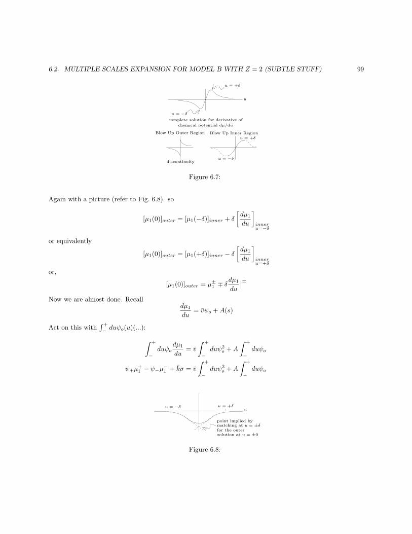
6.2. MULTIPLE SCALES EXPANSION FOR MODEL B WITH Z = 2 (SUBTLE STUFF) 99
u = −δ
u = −δ
u = +δ
u = +δ
complete solution for derivative of
Blow Up Outer Region Blow Up Inner Region
u
chemical potential dµ/du
discontinuity
Figure 6.7:
Again with a picture (refer to Fig. 6.8). so
[µ1(0)]outer = [µ1(−δ)]inner + δ
[dµ1
du
]
inneru=−δ
or equivalently
[µ1(0)]outer = [µ1(+δ)]inner − δ[dµ1
du
]
inneru=+δ
or,
[µ1(0)]outer = µ±1 ∓ δ
dµ1
du
∣∣±
Now we are almost done. Recalldµ1
du= vψo +A(s)
Act on this with∫ +
−duψo(u)(...):
∫ +
−
duψodµ1
du= v
∫ +
−
duψ2o +A
∫ +
−
duψo
ψ+µ+1 − ψ−µ
−1 + kσ = v
∫ +
−
duψ2o +A
∫ +
−
duψo
u = −δ u = +δu
point implied bymatching at u = ±δfor the outersolution at u = ±0
Figure 6.8:
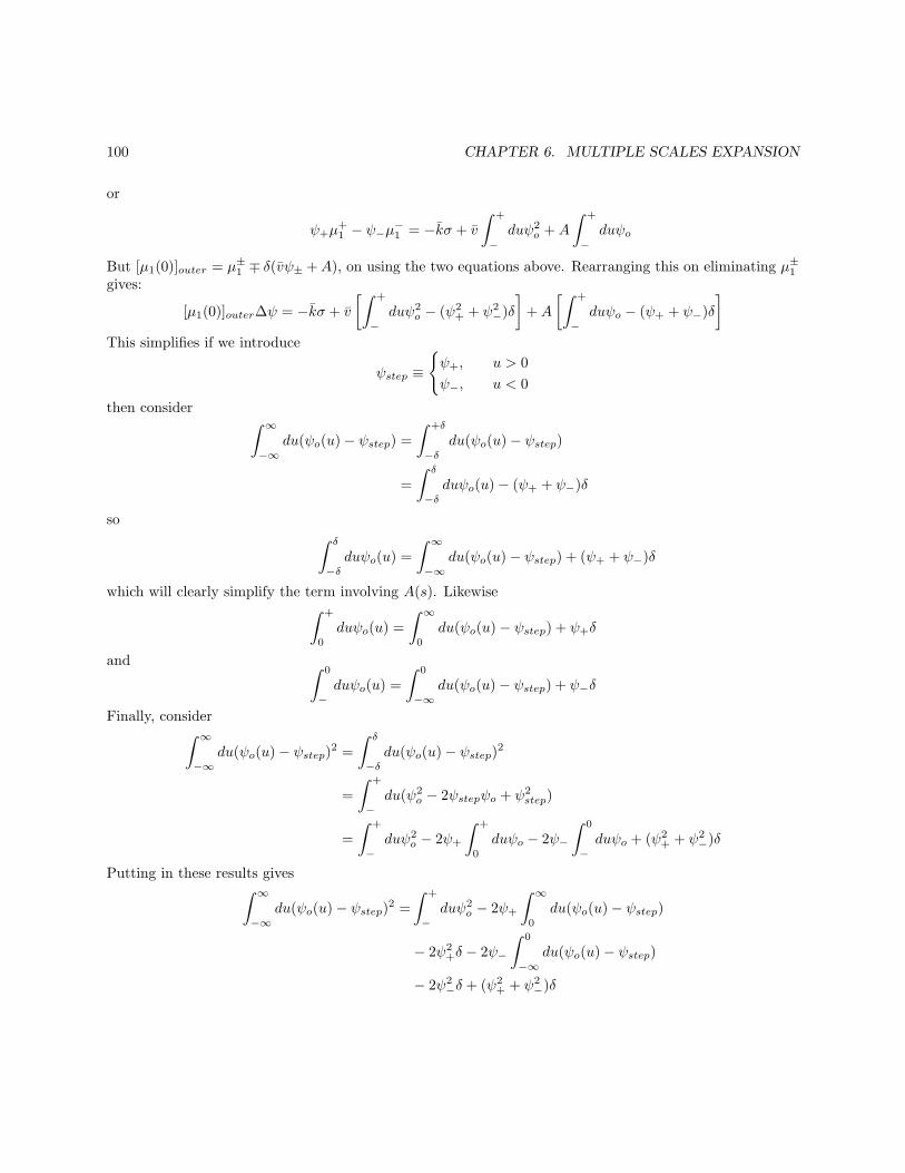
100 CHAPTER 6. MULTIPLE SCALES EXPANSION
or
ψ+µ+1 − ψ−µ
−1 = −kσ + v
∫ +
−
duψ2o +A
∫ +
−
duψo
But [µ1(0)]outer = µ±1 ∓ δ(vψ± +A), on using the two equations above. Rearranging this on eliminating µ±
1
gives:
[µ1(0)]outer∆ψ = −kσ + v
[∫ +
−
duψ2o − (ψ2
+ + ψ2−)δ
]
+A
[∫ +
−
duψo − (ψ+ + ψ−)δ
]
This simplifies if we introduce
ψstep ≡
ψ+, u > 0
ψ−, u < 0
then consider∫ ∞
−∞
du(ψo(u)− ψstep) =
∫ +δ
−δ
du(ψo(u)− ψstep)
=
∫ δ
−δ
duψo(u)− (ψ+ + ψ−)δ
so∫ δ
−δ
duψo(u) =
∫ ∞
−∞
du(ψo(u)− ψstep) + (ψ+ + ψ−)δ
which will clearly simplify the term involving A(s). Likewise∫ +
0
duψo(u) =
∫ ∞
0
du(ψo(u)− ψstep) + ψ+δ
and ∫ 0
−
duψo(u) =
∫ 0
−∞
du(ψo(u)− ψstep) + ψ−δ
Finally, consider∫ ∞
−∞
du(ψo(u)− ψstep)2 =
∫ δ
−δ
du(ψo(u)− ψstep)2
=
∫ +
−
du(ψ2o − 2ψstepψo + ψ2
step)
=
∫ +
−
duψ2o − 2ψ+
∫ +
0
duψo − 2ψ−
∫ 0
−
duψo + (ψ2+ + ψ2
−)δ
Putting in these results gives∫ ∞
−∞
du(ψo(u)− ψstep)2 =
∫ +
−
duψ2o − 2ψ+
∫ ∞
0
du(ψo(u)− ψstep)
− 2ψ2+δ − 2ψ−
∫ 0
−∞
du(ψo(u)− ψstep)
− 2ψ2−δ + (ψ2
+ + ψ2−)δ
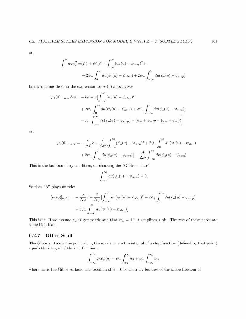
6.2. MULTIPLE SCALES EXPANSION FOR MODEL B WITH Z = 2 (SUBTLE STUFF) 101
or,
∫ +
−
duψ2o =(ψ2
+ + ψ2−)δ +
∫ ∞
−∞
(ψo(u)− ψstep)2+
+ 2ψ+
∫ ∞
0
du(ψo(u)− ψstep) + 2ψ−
∫ 0
−∞
du(ψo(u)− ψstep)
finally putting these in the expression for µ1(0) above gives
[µ1(0)]outer∆ψ =− kσ + v[∫ ∞
−∞
(ψo(u)− ψstep)2
+ 2ψ+
∫ ∞
0
du(ψo(u)− ψstep) + 2ψ−
∫ 0
−∞
du(ψo(u)− ψstep)]
−A[∫ ∞
−∞
du(ψo(u)− ψstep) + (ψ+ + ψ−)δ − (ψ+ + ψ−)δ
]
or,
[µ1(0)]outer =− σ
∆ψk +
v
∆ψ
[∫ ∞
−∞
(ψo(u)− ψstep)2 + 2ψ+
∫ ∞
0
du(ψo(u)− ψstep)
+ 2ψ−
∫ 0
−∞
du(ψo(u)− ψstep)]− A
∆ψ
∫ ∞
−∞
du(ψo(u)− ψstep)
This is the last boundary condition, on choosing the “Gibbs surface”∫ ∞
−∞
du(ψo(u)− ψstep) = 0
So that “A” plays no role:
[µ1(0)]outer =− σ
∆ψk +
v
∆ψ
[∫ ∞
−∞
du(ψo(u)− ψstep)2 + 2ψ+
∫ ∞
0
du(ψo(u)− ψstep)
+ 2ψ−
∫ 0
−∞
du(ψo(u)− ψstep)]
This is it. If we assume ψo is symmetric and that ψ± = ±1 it simplifies a bit. The rest of these notes aresome blah blah.
6.2.7 Other Stuff
The Gibbs surface is the point along the u axis where the integral of a step function (defined by that point)equals the integral of the real function.
∫ ∞
−∞
duψo(u) = ψ+
∫ ∞
uG
du+ ψ−
∫ uG
−∞
du
where uG is the Gibbs surface. The position of u = 0 is arbitrary because of the phase freedom of
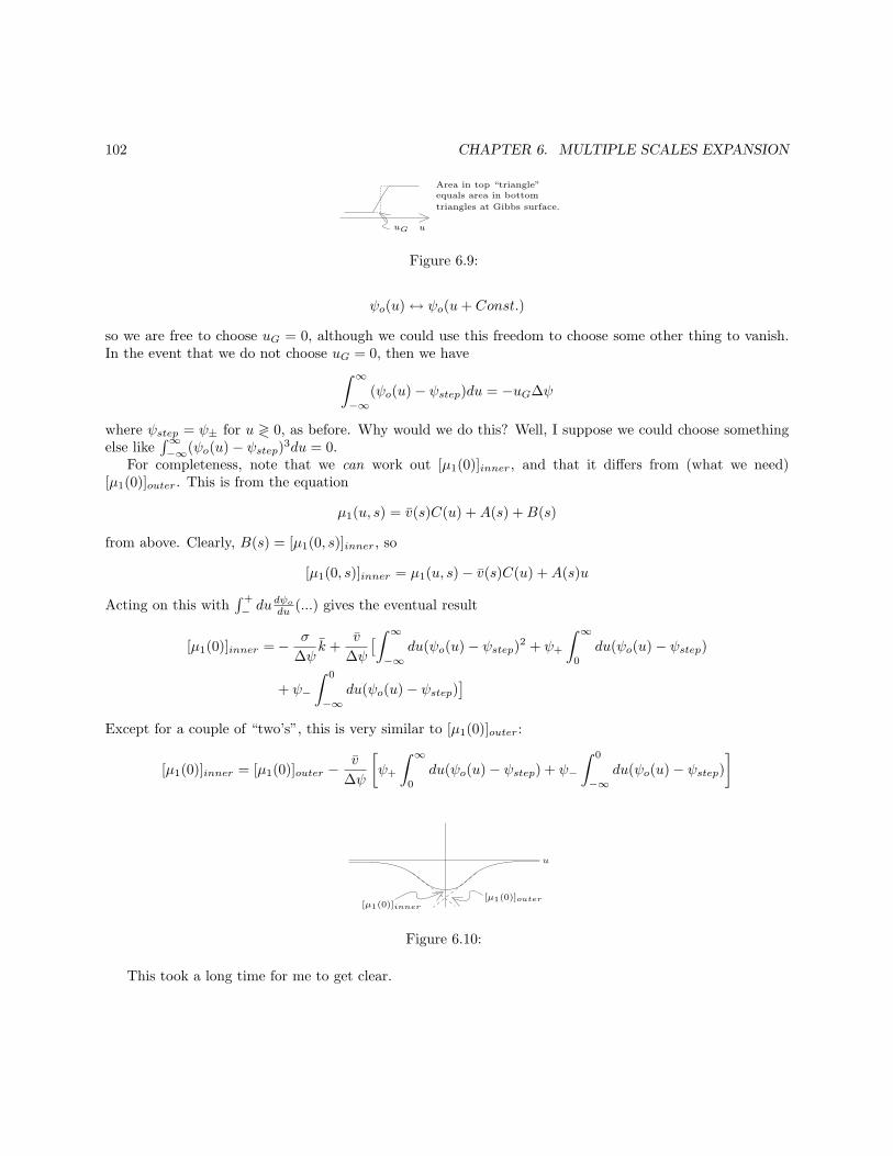
102 CHAPTER 6. MULTIPLE SCALES EXPANSION
uuG
Area in top “triangle”equals area in bottom
triangles at Gibbs surface.
Figure 6.9:
ψo(u)↔ ψo(u+ Const.)
so we are free to choose uG = 0, although we could use this freedom to choose some other thing to vanish.In the event that we do not choose uG = 0, then we have
∫ ∞
−∞
(ψo(u)− ψstep)du = −uG∆ψ
where ψstep = ψ± for u ≷ 0, as before. Why would we do this? Well, I suppose we could choose somethingelse like
∫∞
−∞(ψo(u)− ψstep)3du = 0.
For completeness, note that we can work out [µ1(0)]inner, and that it differs from (what we need)[µ1(0)]outer. This is from the equation
µ1(u, s) = v(s)C(u) +A(s) +B(s)
from above. Clearly, B(s) = [µ1(0, s)]inner, so
[µ1(0, s)]inner = µ1(u, s)− v(s)C(u) +A(s)u
Acting on this with∫ +
−dudψodu (...) gives the eventual result
[µ1(0)]inner =− σ
∆ψk +
v
∆ψ
[∫ ∞
−∞
du(ψo(u)− ψstep)2 + ψ+
∫ ∞
0
du(ψo(u)− ψstep)
+ ψ−
∫ 0
−∞
du(ψo(u)− ψstep)]
Except for a couple of “two’s”, this is very similar to [µ1(0)]outer:
[µ1(0)]inner = [µ1(0)]outer −v
∆ψ
[
ψ+
∫ ∞
0
du(ψo(u)− ψstep) + ψ−
∫ 0
−∞
du(ψo(u)− ψstep)]
u
[µ1(0)]outer[µ1(0)]inner
Figure 6.10:
This took a long time for me to get clear.
6.3. MULTIPLE SCALES EXPANSION FOR MODEL A WITH Z = 1 AND Z = 3 ARE USELESS 103
6.3 Multiple Scales Expansion for Model A With z = 1 and z = 3are Useless
Let’s quickly redo model A for z not equal to 2, and see what happens. Then the Langevin equation is
∂ψ
∂t= −δF
δψ≡ µ
= −∇2ψ +∂f
∂ψ
In the outer region, we scale ~r with ǫ~r = ǫ~r
and t with ǫz (anticipating that (length) ∼ (time)1/z):
t = ǫzt
This gives
6.3.1 Outer Region
ǫz∂ψ
∂t= ǫ2∇2ψ − ∂f
∂ψ= −µ
where, for definiteness, we may choose
f = −ψ2
2+ψ4
4
Solving perturbativelyψ = ψo + ǫψ1 + ǫ2ψ2 + ...
andµ = µo + ǫµ1 + ǫ2µ2 + ...
where µ is determined by ψ:
µo = ∂f/∂ψo
µ1 = (∂2f/∂ψ2o)ψ1
and
µ2 =1
2
(∂3f
∂ψ3o
)
ψ21 +
(∂2f
∂ψ2o
)
ψ2 − ∇2ψo
Using z ≥ 1, the zeroth order solution is
0 =∂f
∂ψo
which (for the choice of f above) givesψo = ±1
104 CHAPTER 6. MULTIPLE SCALES EXPANSION
the equilibrium solution. To first order we have
0 =
(∂2f
∂ψo
)
ψ1
For z ≥ 1 (note that ∂ψo/∂t = 0 because ψo is a constant). This gives
ψ1 = 0
Likewise to 2nd order we obtainψ2 = 0
and so on. In conclusion, the outer expansion, for any z ≥ 1 gives ψo = ±1, with no corrections at higherorders ψ1 = ψ2 = ... = 0.
6.3.2 Inner Region
As in other notes, the inner region has the expansion
ǫz∂ψ
∂t+ ǫz−1v
∂ψ
∂u= −µ
where
µ =∂f
∂ψ− ∂2ψ
∂u2− ǫk ∂ψ
∂u− ǫ2 ∂
2ψ
∂s2
Expanding again, we defineψ = ψo + ǫψ1 + ǫ2ψ2 + ...
and,µ = µo + ǫµ1 + ǫ2µ2 + ...
where
µo =∂f
∂ψo− ∂2ψ0
∂u2
µ1 =∂2f
∂ψ2o
ψ1 −∂2ψ1
∂u2− k ∂ψo
∂u
and
µ2 =1
2
∂3f
∂ψ3o
ψ21 +
∂2f
∂ψ2o
ψ2 −∂2ψ2
∂u2− k ∂ψ1
∂u− ∂2ψo
∂s2
6.3.3 Zeroth Order
For z > 1, the solution is0 = µo
or
0 =∂f
∂ψo− ∂2ψo
∂u2
6.3. MULTIPLE SCALES EXPANSION FOR MODEL A WITH Z = 1 AND Z = 3 ARE USELESS 105
For f = −ψ2/2 + ψ4/4, this gives the familiar result
ψo = tanhu
For z = 1, we have
v∂ψo∂u
= − ∂f
∂ψo+∂2ψo∂u2
This is nonlinear, so it is almost intractable. Multiplying by dψo/du and integrating
∫ +
−
du(...)∂ψo∂u≡∫ δ
−δ
du(...)∂ψo∂u
gives
vσ =
∫ +
−
du
(
− ∂f
∂ψo+∂2ψo∂u2
)∂ψo∂u
=
∫ +
−
du
(
− 1
(∂ψo/∂u)
∂f
∂u+
∂
∂u
(dψodu
))∂ψo∂u
=
∫ +
−
dud
du
(
−f +1
2
(∂ψo∂u
)2)
where the surface tension σ =∫ +
−du(dψo/du)
2. This gives
vσ =
[
−f +1
2
(∂ψo∂u
)2]+
−
= 0
From our outer solution ψo = Const.. Hence we obtain
v = 0
for z ≡ 1. Then we haveµo = 0
and ψo = tanhu, as for z > 1.
6.3.4 First Order
For z = 1, the first–order equation is∂ψo∂t
= −µ1
But ψo is not a function of time, soµ1 = 0
or,
0 = − ∂2f
∂ψ2o
ψ1 +∂2
∂u2ψ1 + k
∂ψo∂u
106 CHAPTER 6. MULTIPLE SCALES EXPANSION
Acting on this by∫ +
−du(...)dψo/du gives (as in other notes)
0 = 0 + kσ
So (!)k = 0
for z ≡ 1 and ψ1 is determined byd2ψ1
du2− ∂2f
∂ψ2o
ψ1 = 0
without going into this in any detail (note the interface is flat and not moving to all orders of the expansionwith z = 1), the solution to this is ψ1 = 0, which is consistent with the outer region solution.
For z = 2, as shown elsewhere, we getv = k
the Allen–Cahn equation.For z ≥ 3, we obtain
0 = µ1
as we did for z = 1. From the same tricks as above, this gives
k = 0
a flat surface to all orders, for z ≥ 3, and
d2ψ1
du2− ∂2f
∂ψ2o
ψ1 = 0
the solution of which isψ1 = 0
To Second Order (for z ≥ 3 only)
v∂ψo∂u
= −µ2
for z = 3, and µ2 = 0 for z > 3. Let us only consider z = 3.
v∂ψo∂u
= − ∂2f
∂ψ2o
ψ2 +∂2ψ2
∂u2
since ψ1 = 0, and ψo 6= ψo(s). But we have dealt with, essentially, this same term a few pages ago. Acting
on this with∫ +
−dudψodu (...) gives
vσ =
∫ +
−
dudψodu
(
− ∂2f
∂ψ2o
ψ2 +∂2ψ2
∂u2
)
︸ ︷︷ ︸
zero, as before when it was ψ1
so,v = 0
6.3. MULTIPLE SCALES EXPANSION FOR MODEL A WITH Z = 1 AND Z = 3 ARE USELESS 107
for z = 3. We can now anticipate that, for model A, we have a nontrivial solution only for z = 2, giving theinner solution
v = k
Other choices, z = 1, 3, 4, ... givev = 0
andk = 0
Note the expansion is not inconsistant. The outer solution, and the zeroth order inner solution simply givethe equilibrium solution ψ = tanhu, for example.
For completeness, for model A in a field, where
F =
∫
~dr1
2(∇ψ)2 + f(ψ)−H(ψ)
so thatδF
δψ= −∇2ψ +
∂f
∂ψ−H
a consistent (that is, useful) expansion hasH ≡ ǫH
where H = O(1). Everything follows for model A with z = 2 (despite the fact this gives the Kardar–Parisi–Zhang equation where z < 2!) except
v = k + H∆ψ
with ∆ψ = ψ+ − ψ−. The “equilibrium” outer solutions are shifted slightly from ψo = ±1 by a non–zeroψ1 ∝ H.

108 CHAPTER 6. MULTIPLE SCALES EXPANSION
Chapter 7
Fokker–Planck Equation
The Fokker–Planck equation gives the evolution of the probability distribution P (s, t) as a function of thestate of the system s and time t. We will consider the Fokker–Planck equation for homogeneous systems.These are called zero–dimensional systems, since spatial variations play no role. The equation is
∂P (s, t)
∂t= Γ
∂
∂s
(∂F
∂s+ kbT
∂
∂s
)
P (s, t) (7.1)
where Γ is a transport coefficient (a constant), kb is Boltzmann’s constant, and T is temperature. The freeenergy of a state s is F (s). As shown in other notes, this “Schroedinger” representation is equivalent to the“Heisenberg” representation of the Langevin equation:
∂s(t)
∂t= −Γ
∂F
∂s+ η(t) (7.2)
where η is a Gaussian noise, of zero mean, whose second moment is given by
〈η(t)η(t′)〉 = 2ΓkBTδ(t− t′) (7.3)
Returning to the Fokker–Planck equation, note it can be written as the conservation law:
∂P (s, t)
∂t= − ∂
∂sJ(s, t) (7.4)
where the probability current is given by
J(s, t) = −Γ
(∂F
∂s+ kBT
∂
∂s
)
P (s, t) (7.5)
The conserved form reflects the fact that the probability of being in all the states is normalized,∫
dsP (s, t) = 1 (7.6)
that is, the system must be somewhere, out of all the states with unit probability. A handy rearrangementof the current is
J(s, t) = −ΓkBTe−F/kBT
∂
∂s
(
eF/kBTP (s, t))
(7.7)
109
110 CHAPTER 7. FOKKER–PLANCK EQUATION
It is easy to check:
J(s, t) = −ΓkBTe−F/kBT
(1
kBT
∂F
∂seF/kBTP + eF/kBT
∂P
∂s
)
= −Γ
(∂F
∂sP + kBT
∂P
∂s
)
which is the same as Eq. 7.5.That concludes the perliminaries. We’ll now find solutions of the Fokker–Planck equation for a few
situations.
7.1 Stationary Solutions
If we have∂P
∂t= 0 (7.8)
then we are either in a steady state or, more likely, in equilibrium. We can solve for the distribution in boththese cases. From Eq. 7.4, Eq. 7.8 implies
∂P
∂t= 0 =
∂
∂sJ(s, t)
with the two casesJss = Const. (7.9)
for the steady state solution, and the important case
Jeq = 0 (7.10)
for the equilibrium.From Eq. 7.7, the equilibrium solution is
Jeq = 0 = −ΓkBTe−F/kBT
∂
∂s
(
eF/kBTPeq
)
(7.11)
in an obvious notation. HenceeF/kBTPeq = Const.
and we recover the distribution for the canonical ensemble,
Peq = Const.e−F/kBT (7.12)
where the constant is determined by normalization, Eq. 7.6.In the case of a steady state,
Jss = Const. = −ΓkBTe−F/kBT
∂
∂s
(
eF/kBTPss
)
(7.13)
On rearranging this, we have,∂
∂s
(
eF/kBTPss
)
= −(
JssΓkBT
)
eF/kBT
7.2. TIME–DEPENDENT SOLUTIONS 111
Doing an indefinite integral gives
Pss = Const.e−F/kBT − JssΓkBT
e−F/kBT∫
dseF/kBT (7.14)
where the constant is again determined by normalization.Similar results can be obtained for inhomogeneous systems.
7.2 Time–Dependent Solutions
There are few time–dependent solutions of the Fokker–Planck equation. A formal method, which is wellworth seeing, is to expand in eigenvectors, after noting the equation is linear in P (s, t):
∂P (s, t)
∂t= Γ
∂
∂s
(∂F
∂s+ kBT
∂
∂s
)
P (s, t)
or,
= ΓkBT∂
∂s
[
e−F/kBT∂
∂s
(
eF/kBTP)]
so,∂P (s, t)
∂t= −L(P (s, t)) (7.15)
where L is an operator. It is convenient to write it in matrix form.
∂P (s, t)
∂t= −
∑
s′
L(s, s′)P (s′, t) (7.16)
where
L(s, s′) =
−Γ ∂∂s
(∂F∂s + kBT
∂∂s
)δs,s′
−ΓkBT∂∂s
[e−F/kBT ∂
∂s
(eF/kBT δs,s′
)] (7.17)
Unfortuneatly, L is not a Hermitean operator. In the matrix form, since all elements are real, this is thesame as noting that L(s.s′) 6= L(s′, s). This awkwardness can be fixed by the not–particularly–obvioustransformed operator
Λ(s, s′) = e12F (s)/kBTL(s, s′)e−
12F (s′)/kBT (7.18)
which turns out to be symmetric, and hence Hermitean. The explicit form can be found from Eq. 7.17:
Λ(s, s′) = −ΓkBTe12F (s)/kBT
∂
∂s
[
e−F (s)/kBT∂
∂s
(
eF (s)/kBT δs,s′e− 1
2F (s)/kBT)]
so,
Λ(s, s′)
ΓkBT= −e 1
2F/kBT∂
∂s
[
e−12F/kBT
(1
2kBT
∂F
∂s+
∂
∂s
)
δs,s′
]
= −[
1
2kBT
∂2F
∂s2+
∂2
∂s2−(
1
2kBT
∂F
∂s
)2]
δs,s′
112 CHAPTER 7. FOKKER–PLANCK EQUATION
or,
Λ(s, s′) = −Γ
[
1
2
∂2F
∂s2+ kBT
∂2
∂s2− 1
4kBT
(∂F
∂s
)2]
δs,s′ (7.19)
which is clearly symmetric. From Eq. 7.16
∂P (s, t)
∂t= −
∑
s′
e−12F (s)/kBTΛ(s, s′)e
12F (s′)/kBTP (s′, t) (7.20)
Letρ(s, t) ≡ e 1
2F (s)/kBTP (s, t) (7.21)
and we have an equation of the original form
∂ρ(s, t)
∂t= −
∑
Λ(s, s′)ρ(s, t) (7.22)
which is well suited for linear algebra. We will look for solutions of the form
ρ(s, t) = ψ(s)e−λt (7.23)
From Eq. 7.22 we have the eigenvalue problem
λnψn(s) =∑
s′
Λ(s, s′)ψn(s′) (7.24)
where the subscript n denotes the eigenvalue. Since Λ is Hermetean, the eigenvalues λn are all real, and wecan construct an orthonormal basis set ψn, such that
∫
dsψn(s)ψm(s) = δn,m (7.25)
Usually the ψ’s form a complete set, so that we also have the completeness relation
∑
n
ψn(s)ψn(s′) = δ(s− s′) (7.26)
The form of Λ implies all the eigenvalues are positive in Eq. 7.23. Consider
∫
dsψn(s)
[∑
s′
Λ(s, s′)ψm(s′)
]
=
∫
dsψn(s)λmψm(s′)
= λmδn,m
(7.27)
So,
λn =
∫
dsψn(s)
[∑
s′
Λ(s, s′)ψn(s′)
]
(7.28)
Using the form of Λ(s, s′) below Eq. 7.18 gives,
λn = −ΓkBT
∫
dsψn(s)e12F/kBT
∂
∂s
[
e−F/kBT(∂
∂se
12F/kBTψn(s)
)]
7.2. TIME–DEPENDENT SOLUTIONS 113
Doing one parts integral gives,
λn = ΓkBT
∫
dse−F/kBT[∂
∂s
(
ψne12F/kBT
)]2
(7.29)
Evidentlyλn ≥ 0 (7.30)
whereλo = 0
is the equilibrium solution, from Eqs. 7.21 and 7.23.Solutions of the Fokker–Planck equation are facilitated by use of the Green function G(s, t; s′, 0), which
is the propagator from s′, t = 0 to s, t. The Green function satisfies
∂G(s, t; s′, 0)
∂t= Γ
∂
∂s
(∂F
∂s+ kBT
∂
∂s
)
G(s, t; s′, 0) (7.31)
The ugly arguments for G are because of its specified initial condition
G(s, 0; s′, 0) = δ(s− s′) (7.32)
Now, since Eq. 7.31 can be written as∂G
∂t= −LG (7.33)
thereby re–defining the operator L, the formal solution can be obtained as
G = e−LtG(t = 0) (7.34)
However, this is awkward, again because L is not a Hermetean operator. Hence we introduce,
g(s, t; s′, 0) = e12F (s)/kBTG(s, t; s′, 0) (7.35)
so that
g(s, t = 0; s′, 0) =
e12F (s)/kBT δ(s− s′)δ(s− s′)e 1
2F (s′)/kBT(7.36)
Clearly g satisfies∂g
∂t= −Λg
so that
g(s, t; s′, 0) = e−Λtg(s, 0; s′, 0)
= e−Λtδ(s− s′)e 12F (s′)/kBT
(7.37)
Now if the eigen functions form a complete set in Eq. 7.26, we have,
δ(s− s′) =∑
n
ψn(s)ψn(s′)
114 CHAPTER 7. FOKKER–PLANCK EQUATION
and usingG(s, t; s′, 0) = e−
12F (s)/kBT g(s, t; s′, 0)
we have, from Eq. 7.37,
G(s, t; s′, 0) = e−12F (s)/kBT e−Λt
∑
n
ψn(s)ψn(s′)e
12F (s′)/kBT
= e− 1
2kBT(F (s)−F (s′))
∑
n
(e−Λtψn(s)
)ψn(s
′)
so,
G(s, t; s′, 0) = e− 1
2kBT[F (s)−F (s′)]
∑
n
ψn(s)ψn(s′)e−λnt (7.38)
which gives the propogator from the eigenvalues and eigenvectors.With the Green function we can find the probability distribution at time t, given some initial distribution
at time t = 0 via,
P (s, t) =
∫
ds′G(s, t; s′, 0)P (s′, 0) (7.39)
By inspection, the Fokker–Planck equation, and the initial conditions for P (s, t) are satisfied by Eq. 7.39.Evidently, the Green function can also be interpreted as the transition probability from s′, t = 0 to s, t.With this identification, one can then obtain two–point distributions for equilibrium systems. For example,for a system prepared in equilibrium at time t = 0, the joint probability density of being in s, t and s′, 0is
P2(s, t; s′, 0) = G(s, t; s′, 0)Peq(s
′) (7.40)
wherePeq(s
′) = Const.e−F (s)/kBT
as above. (In all the expressions above, t = 0 can be replaced by t′, provided t→ t− t′ in the expression forthe Green function in Eq. 7.38, and t ≥ t′.)
Eq. 7.40 can be rewritten somewhat using the expression from Eq. 7.38. First, recall that λo = 0 givesthe equilibrium solution. Furthermore, from normalization of the eigenvectors,
∫
dsψ2o(s) = 1 (7.41)
sincePeq(s) ∝ eF (s)/kBT (7.42)
andPeq(s) ∝ e−
12F (s)/kBTψo(s) (7.43)
(the probability factor in Eq. 7.43 is because ψn’s have been normalized), consistency with a normalizedprobability gives
Peq = ψ2o(s)
and
ψo(s) =
(e−F/kBT
∫dse−F/kBT
)2
(7.44)
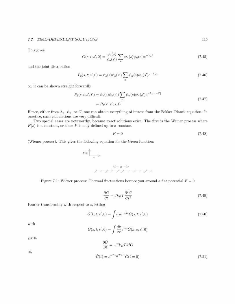
7.2. TIME–DEPENDENT SOLUTIONS 115
This gives
G(s, t; s′, 0) =ψo(s)
ψo(s′)
∑
n
ψn(s)ψn(s′)e−λnt (7.45)
and the joint distribution
P2(s, t; s′, 0) = ψo(s)ψo(s
′)∑
n
ψn(s)ψn(s′)e−λnt (7.46)
or, it can be shown straight forwardly
P2(s, t; s′, t′) = ψo(s)ψo(s
′)∑
n
ψn(s)ψn(s′)e−λn|t−t
′|
= P2(s′, t′; s, t)
(7.47)
Hence, either from λn, ψn, or G, one can obtain everything of intrest from the Fokker–Planck equation. Inpractice, such calculations are very difficult.
Two special cases are noteworthy, because exact solutions exist. The first is the Weiner process whereF (s) is a constant, or since F is only defined up to a constant
F = 0 (7.48)
(Wiener process). This gives the following equation for the Green function:
F (s)
s
Figure 7.1: Wiener process: Thermal fluctuations bounce you around a flat potential F = 0
∂G
∂t= ΓkBT
∂2G
∂s2(7.49)
Fourier transforming with respect to s, letting
G(k, t; s′, 0) =
∫
dse−iksG(s, t; s′, 0) (7.50)
with
G(s, t; s′, 0) =
∫dk
2πeiksG(k, s; s′, 0)
gives,∂G
∂t= −ΓkBTk
2G
so,
G(t) = e−ΓkBTk2tG(t = 0) (7.51)
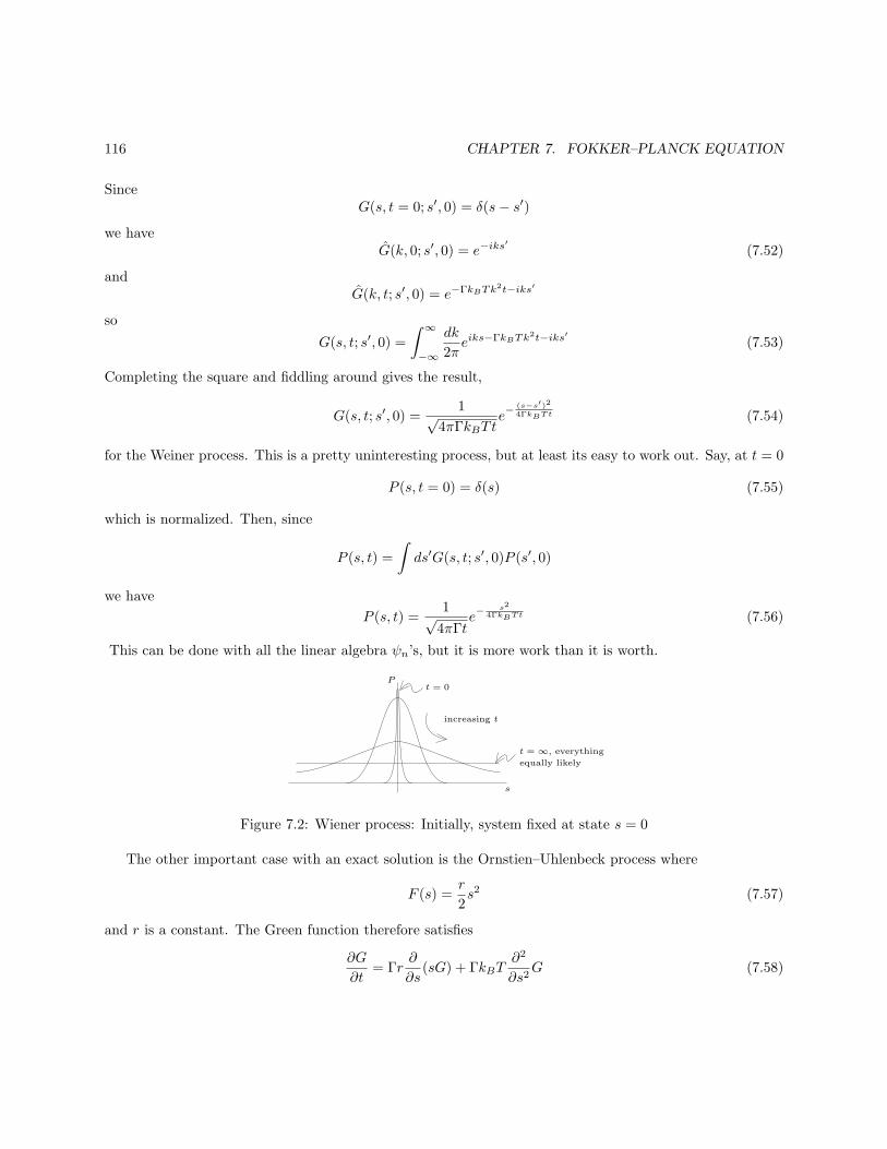
116 CHAPTER 7. FOKKER–PLANCK EQUATION
SinceG(s, t = 0; s′, 0) = δ(s− s′)
we haveG(k, 0; s′, 0) = e−iks
′
(7.52)
andG(k, t; s′, 0) = e−ΓkBTk
2t−iks′
so
G(s, t; s′, 0) =
∫ ∞
−∞
dk
2πeiks−ΓkBTk
2t−iks′ (7.53)
Completing the square and fiddling around gives the result,
G(s, t; s′, 0) =1√
4πΓkBTte−
(s−s′)2
4ΓkBTt (7.54)
for the Weiner process. This is a pretty uninteresting process, but at least its easy to work out. Say, at t = 0
P (s, t = 0) = δ(s) (7.55)
which is normalized. Then, since
P (s, t) =
∫
ds′G(s, t; s′, 0)P (s′, 0)
we have
P (s, t) =1√
4πΓte− s2
4ΓkBTt (7.56)
This can be done with all the linear algebra ψn’s, but it is more work than it is worth.
Pt = 0
increasing t
equally likely
t = ∞, everything
s
Figure 7.2: Wiener process: Initially, system fixed at state s = 0
The other important case with an exact solution is the Ornstien–Uhlenbeck process where
F (s) =r
2s2 (7.57)
and r is a constant. The Green function therefore satisfies
∂G
∂t= Γr
∂
∂s(sG) + ΓkBT
∂2
∂s2G (7.58)
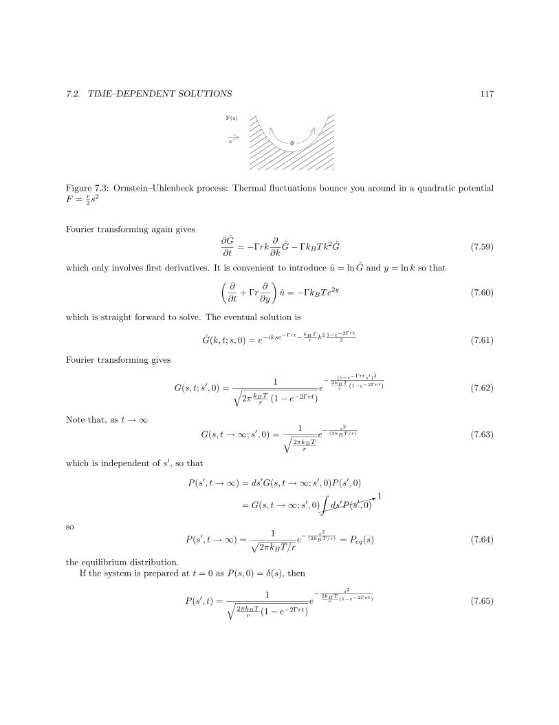
7.2. TIME–DEPENDENT SOLUTIONS 117
s
F(s)
Figure 7.3: Ornstein–Uhlenbeck process: Thermal fluctuations bounce you around in a quadratic potentialF = r
2s2
Fourier transforming again gives∂G
∂t= −Γrk
∂
∂kG− ΓkBTk
2G (7.59)
which only involves first derivatives. It is convenient to introduce u = ln G and y = ln k so that
(∂
∂t+ Γr
∂
∂y
)
u = −ΓkBTe2y (7.60)
which is straight forward to solve. The eventual solution is
G(k, t; s, 0) = e−ikse−Γrt−
kBT
r k2 1−e−2Γrt
2 (7.61)
Fourier transforming gives
G(s, t; s′, 0) =1
√
2π kBTr (1− e−2Γrt)e−
(s−e−Γrts′)2
2kBTr (1−e−2Γrt) (7.62)
Note that, as t→∞G(s, t→∞; s′, 0) =
1√
2πkBTr
e− s2
(2kBT/r) (7.63)
which is independent of s′, so that
P (s′, t→∞) = ds′G(s, t→∞; s′, 0)P (s′, 0)
= G(s, t→∞; s′, 0):1∫
ds′P (s′, 0)
so
P (s′, t→∞) =1
√
2πkBT/re− s2
(2kBT/r) = Peq(s) (7.64)
the equilibrium distribution.If the system is prepared at t = 0 as P (s, 0) = δ(s), then
P (s′, t) =1
√2πkBTr (1− e−2Γrt)
e− s2
2kBTr
(1−e−2Γrt) (7.65)
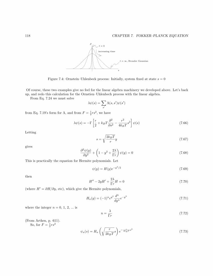
118 CHAPTER 7. FOKKER–PLANCK EQUATION
Pt = 0
increasing time
t = ∞, Broader Gaussian
s
Figure 7.4: Ornstein–Uhlenbeck process: Initially, system fixed at state s = 0
Of course, these two examples give no feel for the linear algebra machinery we developed above. Let’s backup, and redo this calculation for the Ornstien–Uhlenbech process with the linear algebra.
From Eq. 7.24 we must solve
λψ(s) =∑
s′
Λ(s, s′)ψ(s′)
from Eq. 7.19’s form for Λ, and from F = 12rs
2, we have
λψ(s) = −Γ
[r
2+ kBT
∂2
∂s2− r2
4kBTs2]
ψ(s) (7.66)
Letting
s =
√
2kBT
ry (7.67)
gives∂2ψ(y)
∂y2+
(
1− y2 +2λ
Γr
)
ψ(y) = 0 (7.68)
This is practically the equation for Hermite polynomials. Let
ψ(y) = H(y)e−y2/2 (7.69)
then
H ′′ − 2yH ′ +2λ
ΓrH = 0 (7.70)
(where H ′ = ∂H/∂y, etc), which give the Hermite polynomials,
Hn(y) = (−1)ney2 dn
dyne−y
2
(7.71)
where the integer n = 0, 1, 2, ... is
n =λ
Γr(7.72)
(From Artken, p. 611).So, for F = 1
2rs2
ψn(s) = Hn
(√r
2kBTs
)
e− r
4kBTs2
(7.73)
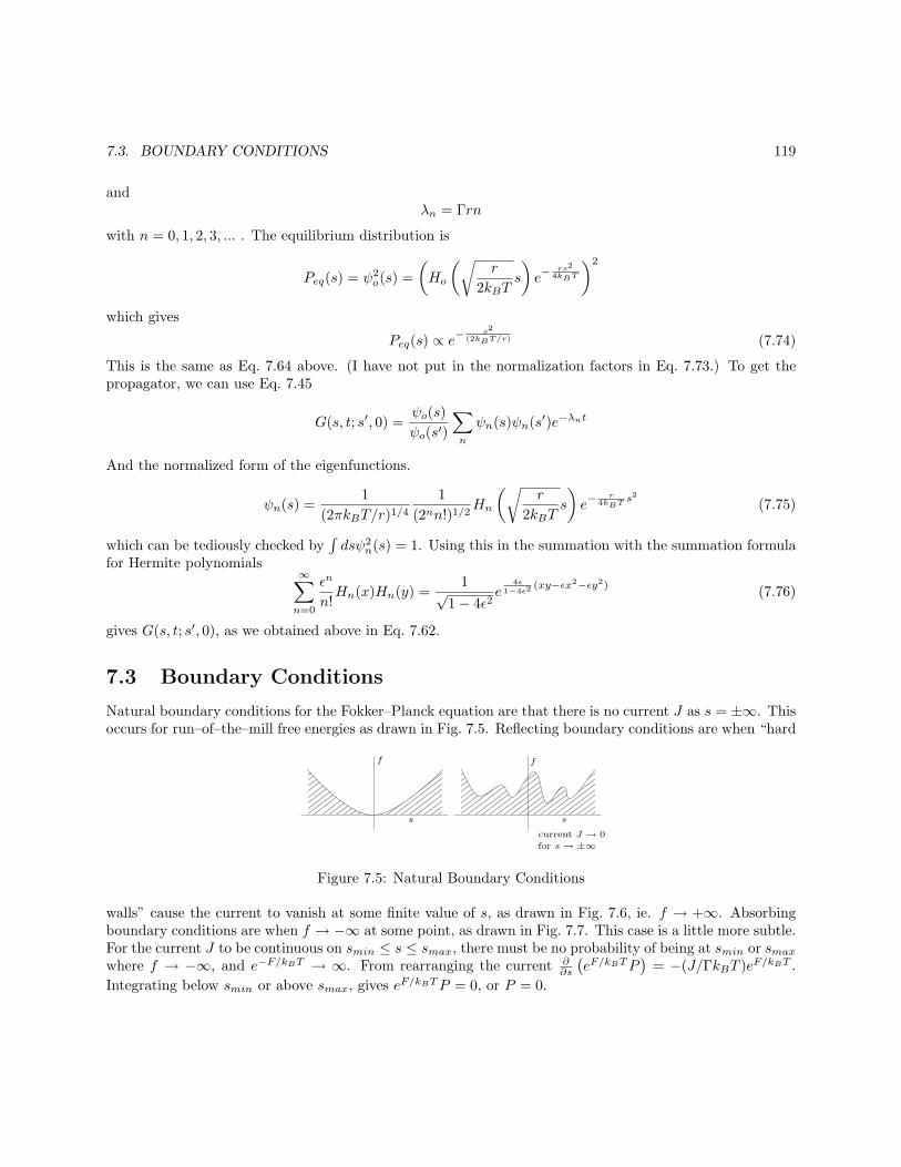
7.3. BOUNDARY CONDITIONS 119
andλn = Γrn
with n = 0, 1, 2, 3, ... . The equilibrium distribution is
Peq(s) = ψ2o(s) =
(
Ho
(√r
2kBTs
)
e− rs2
4kBT
)2
which gives
Peq(s) ∝ e−s2
(2kBT/r) (7.74)
This is the same as Eq. 7.64 above. (I have not put in the normalization factors in Eq. 7.73.) To get thepropagator, we can use Eq. 7.45
G(s, t; s′, 0) =ψo(s)
ψo(s′)
∑
n
ψn(s)ψn(s′)e−λnt
And the normalized form of the eigenfunctions.
ψn(s) =1
(2πkBT/r)1/41
(2nn!)1/2Hn
(√r
2kBTs
)
e− r
4kBTs2
(7.75)
which can be tediously checked by∫dsψ2
n(s) = 1. Using this in the summation with the summation formulafor Hermite polynomials
∞∑
n=0
ǫn
n!Hn(x)Hn(y) =
1√1− 4ǫ2
e4ǫ
1−4ǫ2(xy−ǫx2−ǫy2)
(7.76)
gives G(s, t; s′, 0), as we obtained above in Eq. 7.62.
7.3 Boundary Conditions
Natural boundary conditions for the Fokker–Planck equation are that there is no current J as s = ±∞. Thisoccurs for run–of–the–mill free energies as drawn in Fig. 7.5. Reflecting boundary conditions are when “hard
s
ff
s
current J → 0
for s → ±∞
Figure 7.5: Natural Boundary Conditions
walls” cause the current to vanish at some finite value of s, as drawn in Fig. 7.6, ie. f → +∞. Absorbingboundary conditions are when f → −∞ at some point, as drawn in Fig. 7.7. This case is a little more subtle.For the current J to be continuous on smin ≤ s ≤ smax, there must be no probability of being at smin or smaxwhere f → −∞, and e−F/kBT → ∞. From rearranging the current ∂
∂s
(eF/kBTP
)= −(J/ΓkBT )eF/kBT .
Integrating below smin or above smax, gives eF/kBTP = 0, or P = 0.
120 CHAPTER 7. FOKKER–PLANCK EQUATION
s
ff
ssmin sminsmax smax
current J = 0 at smin and smax
Figure 7.6: Reflecting Boundary Conditions
s
ff
ssmin sminsmax smax
P = 0 at smin and smax
Figure 7.7: Absorbing Boundary Conditions
7.4 Escape Rate
For a system prepared in a metastable state at s = 0, as drawn, we shall calculate the rate of escape to theground state. If the barrier is very high, then the limiting process is the current J at the top of the barrier.
f f
s ss∗ s∗seq seq
J
Figure 7.8: Escape from a metastable state
Clearly,
(Probability of being at s = 0)× (Escape rate) = J (7.77)
in fact, this defines the escape rate as
I =J
probability at s = 0(7.78)
We will simply calculate J and the probability seperately. From Eq. 7.13, for a constant steady state current,
J = −ΓkBTe−F/kBT
∂
∂s(eF/kBTP )
or,∫ seq
0
JeF/kBT ds = −ΓkBT
∫ seq
0
ds∂
∂s
(
eF/kBTP)
7.4. ESCAPE RATE 121
so,
J
∫ seq
0
dseF/kBT = −ΓkBT[
eF (seq)/kBTP (seq)− eF (0)/kBTP (0)]
Now we will assume that F (seq) is so much less than F (0) that we can treat this state as an absorbingboundary condition. In that case, P (seq) = 0, and we obtain,
J =ΓkBTe
F (0)/kBTP (0)∫ seq0
dseF/kBT(7.79)
Near s = 0, we are practically in equilibrium, if the barrier height is large. Hence for s close to 0,
P (s) = Const. e−F (s)/kBT
or,P (s) = P (0)e−(F (s)−F (0))/kBT (7.80)
From this probability distribution, we can obtain the probability at s = 0 as
prob.s=0 =
∫
arounds=0
P (s)ds
= P (0)eF (0)/kBT
∫
arounds=0
dse−F (s)/kBT
(7.81)
From these two equations, we can obtain the escape rate as
I =ΓkBT
∫
arounds=0
ds e−F (s)/kBT∫ seq0
ds eF (s)/kBT(7.82)
The first integral’s major contribution is around s = 0, where F is a parabola, while the second integral’s
Figure 7.9:
major contribution is around s = s∗ where F is an upside down parabola. In those regions,
F (s→ 0) = F (0) +1
2
∣∣∣∣
∂2F
∂s2
∣∣∣∣s=0
s2 + ... (7.83)
and
F (s→ s∗) = F (s∗)− 1
2
∣∣∣∣
∂2F
∂s2
∣∣∣∣s=s∗
(s− s∗)2 + ... (7.84)
122 CHAPTER 7. FOKKER–PLANCK EQUATION
Putting these forms in for F , and letting the integrals be from −∞ ≤ s ≤ ∞, since e−s2
is rapidly convergent,gives
I =ΓkBT
2π
(∣∣∣∣
∂2F
∂s2
∣∣∣∣s=s∗
∣∣∣∣
∂2F
∂s2
∣∣∣∣s=0
)1/2
e−(F (s∗)−F (0))/kBT (7.85)
which is Kramer’s result for the escape rate.
7.5 Appendix: Langevin Equations and Fokker–Planck Equations
Out of equilibrium, many–body system’s obey Aristotle’s law of motion, rather than Newton’s law of motion:
force ∝ velocity
in the over damped limit. The proportionality constant is a transport coefficient.Say force and velcoity only depend on a single variable x(t), as time goes on. Then
velocity =dx
dt= force(t)
Langevin noted that the force has two additive parts, a regular monotonic boring part which we will callf(x), and a stochastic part, which we will call η(t):
dx
dt= f + η
Since η is random, it has zero mean, and is Gaussian. Hence, only its second moment is segnificant:
〈η(t)η(t′)〉 = 2kBTDδ(t− t′)
The factors of 2kBT anticipate a result below; with D they give the intensity of the noise.It is not too hard to show that
f(x) = −D∂F∂x
where F (x) is the free energy. This is called a fluctuation dissipation relation. The algebra goes like this...We turn the Langevin equation into a “Fokker–Planck equation” as follows. Say X is a solution of the
Langevin equation for some history of x(H) being kicked around by η. The (micro–canonical) distributionis
ρ(X, t) = δ(X − x(t))with the equation of motion
∂ρ
∂t= −x ∂
∂Xδ(X − x(t))
=∂
∂X|x|x=Xρ(X, t)
This allows the formal solution
ρ(X, t) =[
e−R t0dt′ ∂
∂X x(t′)|x=X
]
ρ(X, 0)
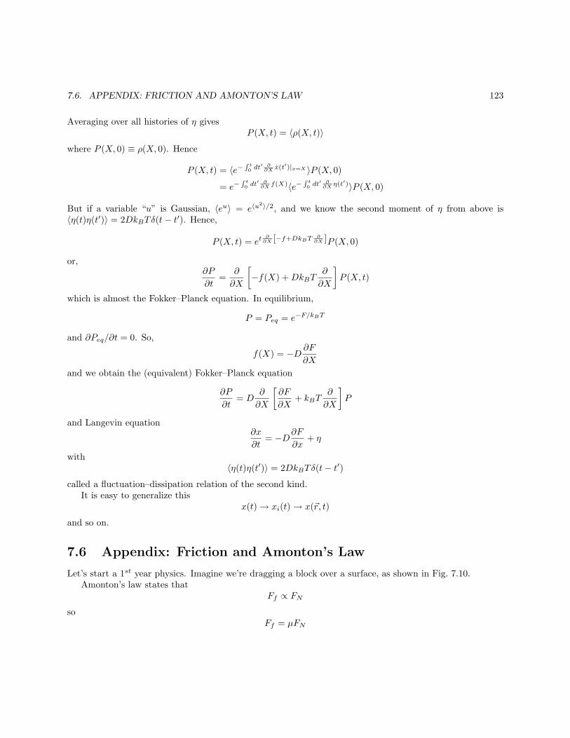
7.6. APPENDIX: FRICTION AND AMONTON’S LAW 123
Averaging over all histories of η givesP (X, t) = 〈ρ(X, t)〉
where P (X, 0) ≡ ρ(X, 0). Hence
P (X, t) = 〈e−R t0dt′ ∂
∂X x(t′)|x=X 〉P (X, 0)
= e−R t0dt′ ∂
∂X f(X)〈e−R t0dt′ ∂
∂X η(t′)〉P (X, 0)
But if a variable “u” is Gaussian, 〈eu〉 = e〈u2〉/2, and we know the second moment of η from above is
〈η(t)η(t′)〉 = 2DkBTδ(t− t′). Hence,
P (X, t) = et∂∂X [−f+DkBT
∂∂X ]P (X, 0)
or,∂P
∂t=
∂
∂X
[
−f(X) +DkBT∂
∂X
]
P (X, t)
which is almost the Fokker–Planck equation. In equilibrium,
P = Peq = e−F/kBT
and ∂Peq/∂t = 0. So,
f(X) = −D ∂F
∂X
and we obtain the (equivalent) Fokker–Planck equation
∂P
∂t= D
∂
∂X
[∂F
∂X+ kBT
∂
∂X
]
P
and Langevin equation∂x
∂t= −D∂F
∂x+ η
with〈η(t)η(t′)〉 = 2DkBTδ(t− t′)
called a fluctuation–dissipation relation of the second kind.It is easy to generalize this
x(t)→ xi(t)→ x(~r, t)
and so on.
7.6 Appendix: Friction and Amonton’s Law
Let’s start a 1st year physics. Imagine we’re dragging a block over a surface, as shown in Fig. 7.10.Amonton’s law states that
Ff ∝ FNso
Ff = µFN
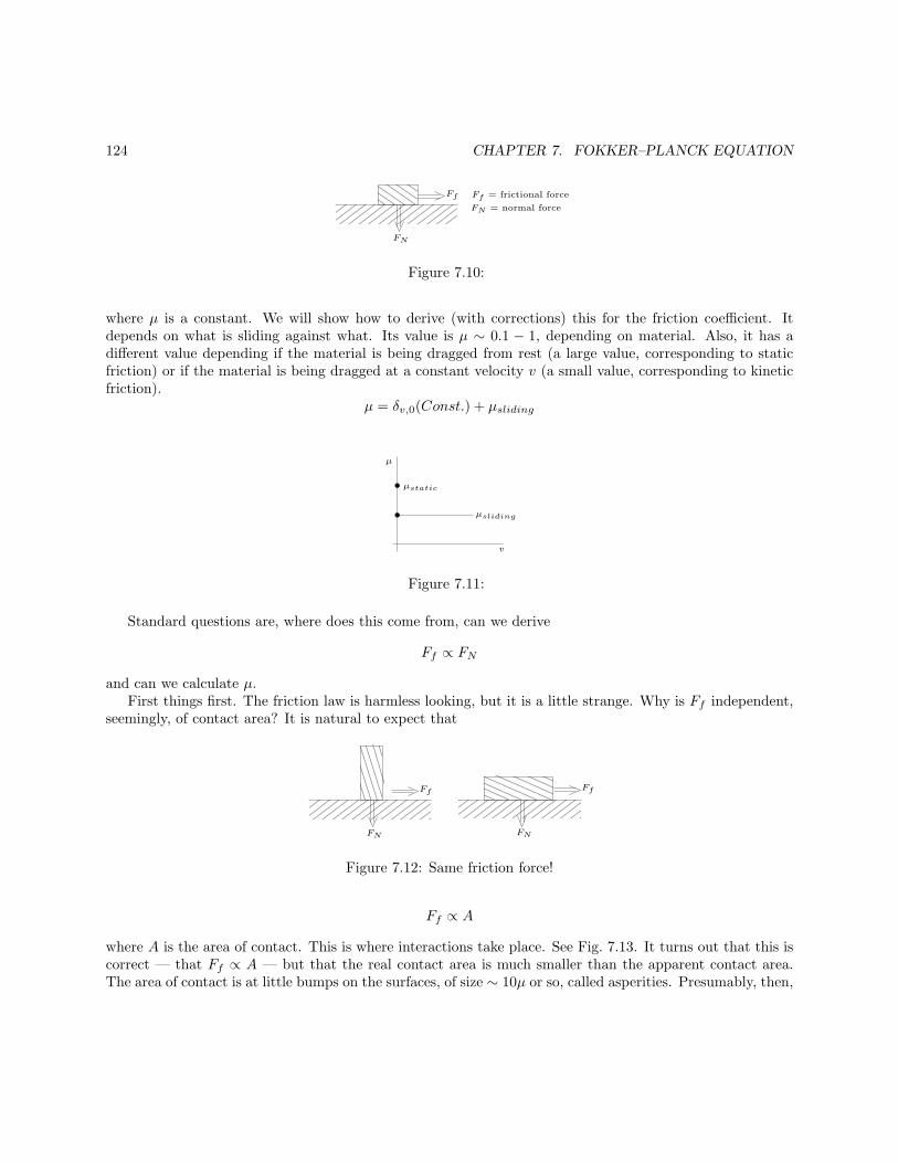
124 CHAPTER 7. FOKKER–PLANCK EQUATION
Ff
FN
FN = normal force
Ff = frictional force
Figure 7.10:
where µ is a constant. We will show how to derive (with corrections) this for the friction coefficient. Itdepends on what is sliding against what. Its value is µ ∼ 0.1 − 1, depending on material. Also, it has adifferent value depending if the material is being dragged from rest (a large value, corresponding to staticfriction) or if the material is being dragged at a constant velocity v (a small value, corresponding to kineticfriction).
µ = δv,0(Const.) + µsliding
µ
µstatic
µsliding
v
Figure 7.11:
Standard questions are, where does this come from, can we derive
Ff ∝ FN
and can we calculate µ.First things first. The friction law is harmless looking, but it is a little strange. Why is Ff independent,
seemingly, of contact area? It is natural to expect that
Ff Ff
FN FN
Figure 7.12: Same friction force!
Ff ∝ A
where A is the area of contact. This is where interactions take place. See Fig. 7.13. It turns out that this iscorrect — that Ff ∝ A — but that the real contact area is much smaller than the apparent contact area.The area of contact is at little bumps on the surfaces, of size ∼ 10µ or so, called asperities. Presumably, then,
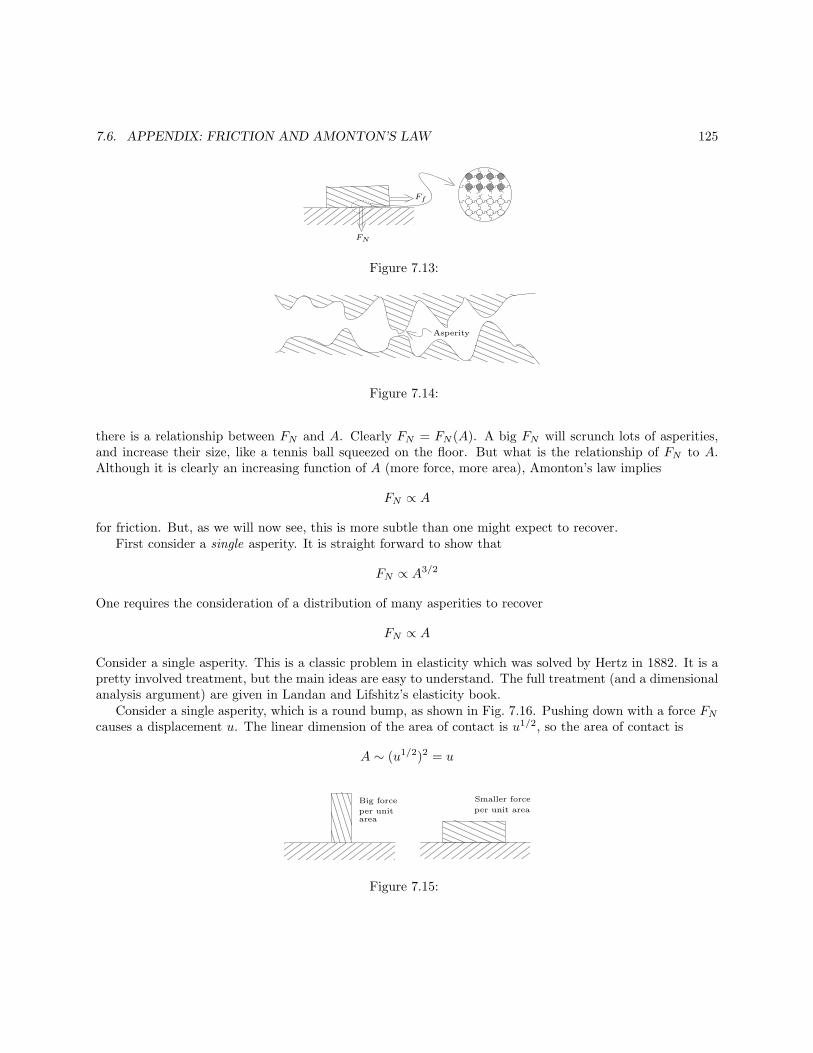
7.6. APPENDIX: FRICTION AND AMONTON’S LAW 125
Ff
FN
Figure 7.13:
Asperity
Figure 7.14:
there is a relationship between FN and A. Clearly FN = FN (A). A big FN will scrunch lots of asperities,and increase their size, like a tennis ball squeezed on the floor. But what is the relationship of FN to A.Although it is clearly an increasing function of A (more force, more area), Amonton’s law implies
FN ∝ A
for friction. But, as we will now see, this is more subtle than one might expect to recover.First consider a single asperity. It is straight forward to show that
FN ∝ A3/2
One requires the consideration of a distribution of many asperities to recover
FN ∝ A
Consider a single asperity. This is a classic problem in elasticity which was solved by Hertz in 1882. It is apretty involved treatment, but the main ideas are easy to understand. The full treatment (and a dimensionalanalysis argument) are given in Landan and Lifshitz’s elasticity book.
Consider a single asperity, which is a round bump, as shown in Fig. 7.16. Pushing down with a force FNcauses a displacement u. The linear dimension of the area of contact is u1/2, so the area of contact is
A ∼ (u1/2)2 = u
Big force
per unitarea
Smaller force
per unit area
Figure 7.15:
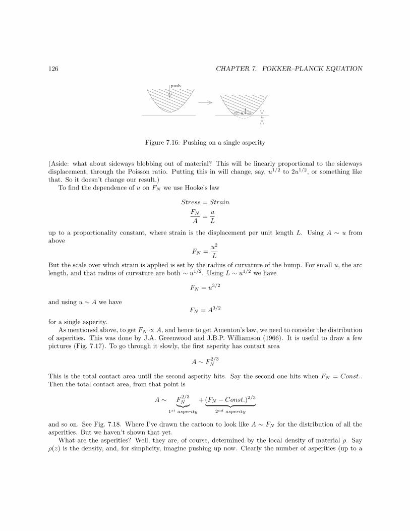
126 CHAPTER 7. FOKKER–PLANCK EQUATION
uu
12
push
Figure 7.16: Pushing on a single asperity
(Aside: what about sideways blobbing out of material? This will be linearly proportional to the sidewaysdisplacement, through the Poisson ratio. Putting this in will change, say, u1/2 to 2u1/2, or something likethat. So it doesn’t change our result.)
To find the dependence of u on FN we use Hooke’s law
Stress = Strain
FNA
=u
L
up to a proportionality constant, where strain is the displacement per unit length L. Using A ∼ u fromabove
FN =u2
L
But the scale over which strain is applied is set by the radius of curvature of the bump. For small u, the arclength, and that radius of curvature are both ∼ u1/2. Using L ∼ u1/2 we have
FN = u3/2
and using u ∼ A we haveFN = A3/2
for a single asperity.As mentioned above, to get FN ∝ A, and hence to get Amenton’s law, we need to consider the distribution
of asperities. This was done by J.A. Greenwood and J.B.P. Williamson (1966). It is useful to draw a fewpictures (Fig. 7.17). To go through it slowly, the first asperity has contact area
A ∼ F 2/3N
This is the total contact area until the second asperity hits. Say the second one hits when FN = Const..Then the total contact area, from that point is
A ∼ F2/3N︸︷︷︸
1st asperity
+(FN − Const.)2/3︸ ︷︷ ︸
2nd asperity
and so on. See Fig. 7.18. Where I’ve drawn the cartoon to look like A ∼ FN for the distribution of all theasperities. But we haven’t shown that yet.
What are the asperities? Well, they are, of course, determined by the local density of material ρ. Sayρ(z) is the density, and, for simplicity, imagine pushing up now. Clearly the number of asperities (up to a
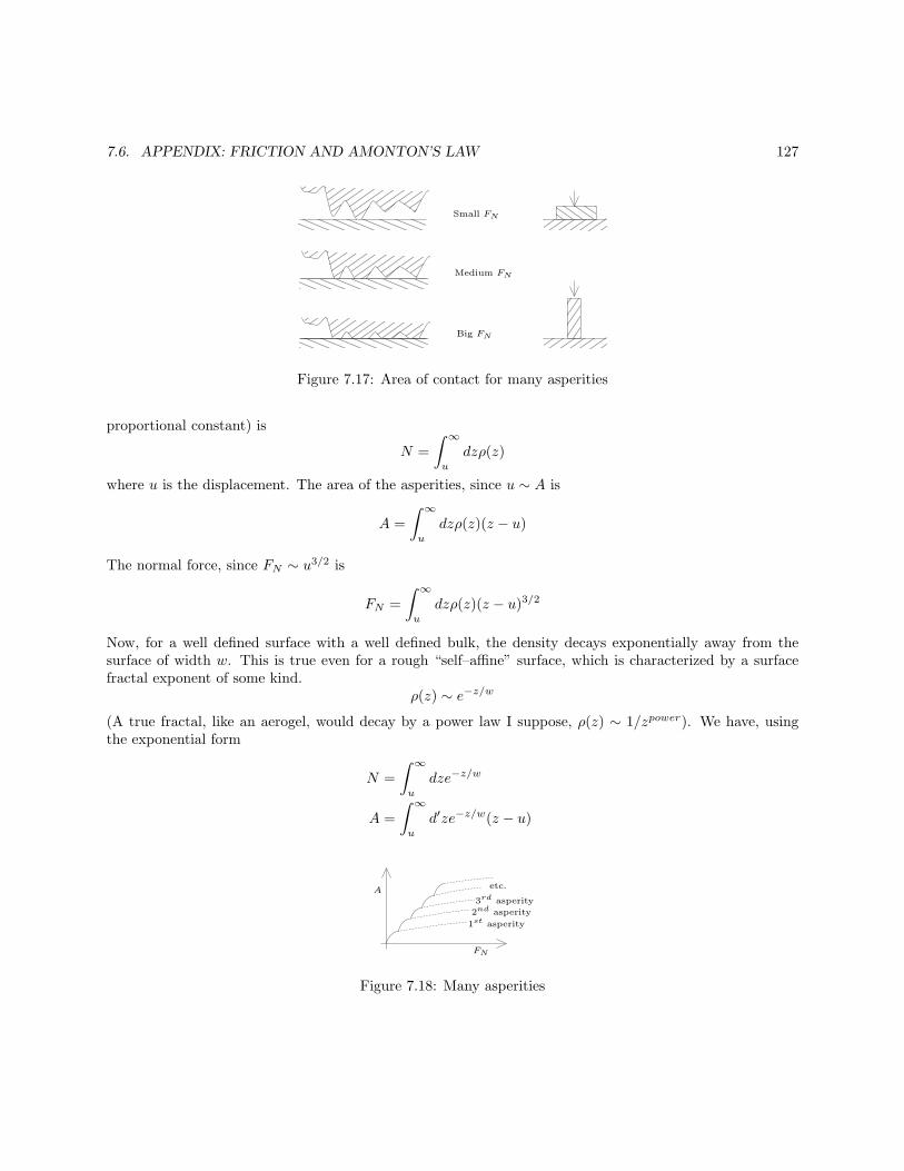
7.6. APPENDIX: FRICTION AND AMONTON’S LAW 127
Small FN
Medium FN
Big FN
Figure 7.17: Area of contact for many asperities
proportional constant) is
N =
∫ ∞
u
dzρ(z)
where u is the displacement. The area of the asperities, since u ∼ A is
A =
∫ ∞
u
dzρ(z)(z − u)
The normal force, since FN ∼ u3/2 is
FN =
∫ ∞
u
dzρ(z)(z − u)3/2
Now, for a well defined surface with a well defined bulk, the density decays exponentially away from thesurface of width w. This is true even for a rough “self–affine” surface, which is characterized by a surfacefractal exponent of some kind.
ρ(z) ∼ e−z/w
(A true fractal, like an aerogel, would decay by a power law I suppose, ρ(z) ∼ 1/zpower). We have, usingthe exponential form
N =
∫ ∞
u
dze−z/w
A =
∫ ∞
u
d′ze−z/w(z − u)
1st asperity
2nd asperity
3rd asperity
etc.A
FN
Figure 7.18: Many asperities
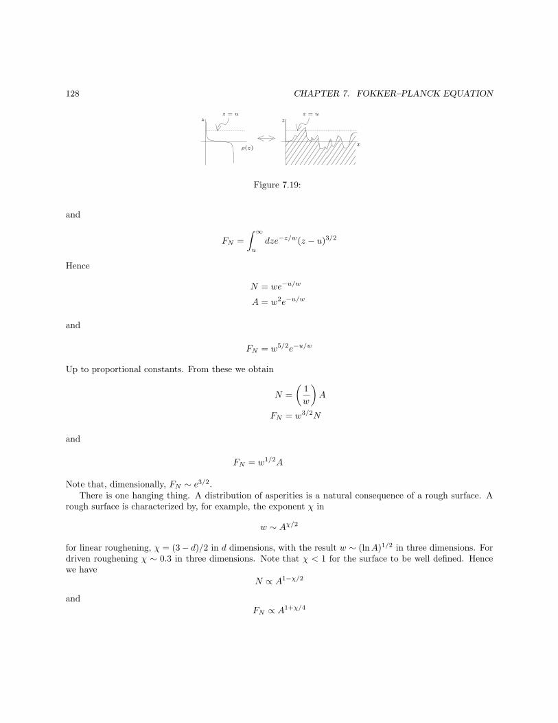
128 CHAPTER 7. FOKKER–PLANCK EQUATION
z = u z = u
ρ(z)
z z
x
Figure 7.19:
and
FN =
∫ ∞
u
dze−z/w(z − u)3/2
Hence
N = we−u/w
A = w2e−u/w
and
FN = w5/2e−u/w
Up to proportional constants. From these we obtain
N =
(1
w
)
A
FN = w3/2N
and
FN = w1/2A
Note that, dimensionally, FN ∼ e3/2.There is one hanging thing. A distribution of asperities is a natural consequence of a rough surface. A
rough surface is characterized by, for example, the exponent χ in
w ∼ Aχ/2
for linear roughening, χ = (3− d)/2 in d dimensions, with the result w ∼ (lnA)1/2 in three dimensions. Fordriven roughening χ ∼ 0.3 in three dimensions. Note that χ < 1 for the surface to be well defined. Hencewe have
N ∝ A1−χ/2
and
FN ∝ A1+χ/4
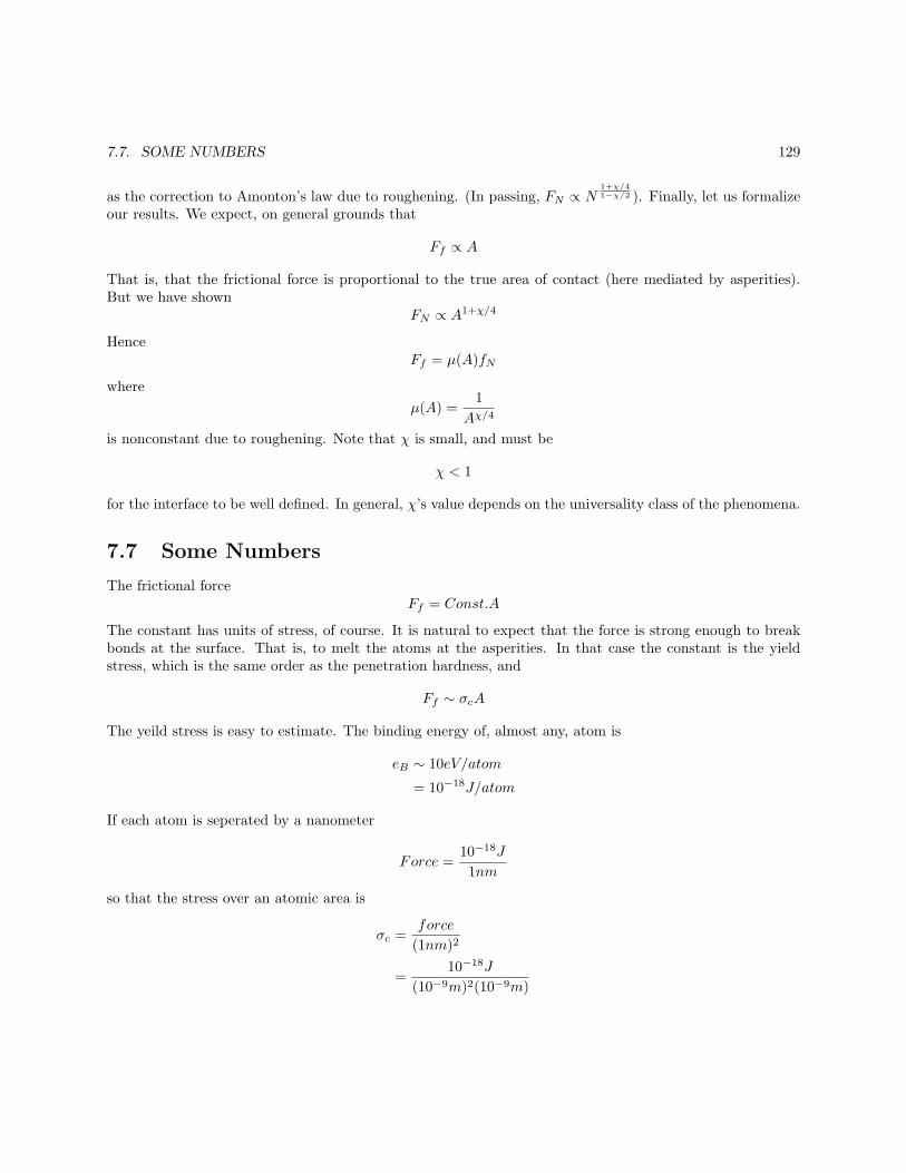
7.7. SOME NUMBERS 129
as the correction to Amonton’s law due to roughening. (In passing, FN ∝ N1+χ/41−χ/2 ). Finally, let us formalize
our results. We expect, on general grounds that
Ff ∝ A
That is, that the frictional force is proportional to the true area of contact (here mediated by asperities).But we have shown
FN ∝ A1+χ/4
HenceFf = µ(A)fN
where
µ(A) =1
Aχ/4
is nonconstant due to roughening. Note that χ is small, and must be
χ < 1
for the interface to be well defined. In general, χ’s value depends on the universality class of the phenomena.
7.7 Some Numbers
The frictional forceFf = Const.A
The constant has units of stress, of course. It is natural to expect that the force is strong enough to breakbonds at the surface. That is, to melt the atoms at the asperities. In that case the constant is the yieldstress, which is the same order as the penetration hardness, and
Ff ∼ σcA
The yeild stress is easy to estimate. The binding energy of, almost any, atom is
eB ∼ 10eV/atom
= 10−18J/atom
If each atom is seperated by a nanometer
Force =10−18J
1nm
so that the stress over an atomic area is
σc =force
(1nm)2
=10−18J
(10−9m)2(10−9m)
130 CHAPTER 7. FOKKER–PLANCK EQUATION
orσc = 109N/m2
(Aside: incidentally, since the penetration hardness and the yeild stress are comparable, µ ∼ 1).The area of contact is
FN = σcA
or using FN = mg, where m is mass and g is gravity, the asperity area:
A =1mg
σc=ρV g
σc
where ρ is density and V is volume. For a cube of material of edge length L
AsperityArea
ApparentArea=
A
L2=ρg
σcL
Taking ρ = 1gm/cm3 = 1000kg/m3, and g = 10m/s2, and L = 10cm
AsperityArea
ApparentArea=
1000kg/m3 × 10m/s20.1m
109N/m2
= 10−6
Hence the asperity area is one millionth of the total area, for something of size L ∼ 10cm. If each asperityhas a linear size 1µ↔ 10µ, then the total number of contacts
N =(1µ↔ 10µ)2
(1000kg/m3)(10cm)3×10m/s109N/m3
N = 100↔ 10000 points
As a final aside, note from the previous page that there is a cube where the asperity area equals theapparent area. This occurs at the (large) length
LBIG =σcρg
beyond which the material cannot hold up the cube at all. Putting in numbers gives LBIG ≈ 105m.Now we will switch to the effects of thermal noise, and velocity, on a single asperity. We will ignore the
normal force (by considering a fixed load), and work things out for an atomic force microscope. This provesan experimentally–realizable “asperity”.
7.7.1 Atomic Force Microscope and Kinetic Friction
Drag an atomic force microscope across a surface, what is the frictional force? This is done in detail inSang, Dube, and Grant Phys. Rev. Lett. 87 174301 (2001). Here we will just give the ideas, and a quickderivation. Clearly, as the tip is dragged across the surface, it catches on the bumps and then sproings overthe hill in a stick–slip motion as shown in Fig. 7.21. Under conditions of constant load (constant force inthe z direction) we need only consider the stretching of the spring in the x direction.
Combining these two potentials gives the total energy landscape the AFM spring is dragges over.
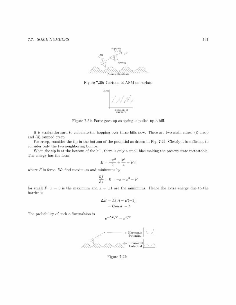
7.7. SOME NUMBERS 131
tip
support
spring
v
Atomic Substrate
Figure 7.20: Cartoon of AFM on surface
Force
position ofsupport
Figure 7.21: Force goes up as spring is pulled up a hill
It is straightforward to calculate the hopping over these hills now. There are two main cases: (i) creepand (ii) ramped creep.
For creep, consider the tip in the bottom of the potential as drawn in Fig. 7.24. Clearly it is sufficient toconsider only the two neighboring bumps.
When the tip is at the bottom of the hill, there is only a small bias making the present state metastable.The energy has the form
E =−x2
2+x4
4− Fx
where F is force. We find maximum and minimums by
∂f
∂x= 0 = −x+ x3 − F
for small F , x = 0 is the maximum and x = ±1 are the minimums. Hence the extra energy due to thebarrier is
∆E = E(0)− E(−1)
= Const.− F
The probability of such a fluctualtion ise−∆E/T = eF/T
HarmonicPotential
SinusoidalPotential
Figure 7.22:
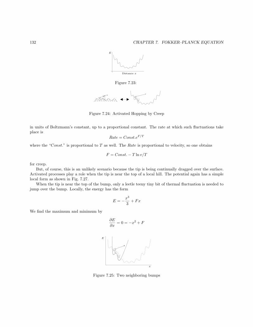
132 CHAPTER 7. FOKKER–PLANCK EQUATION
Distance x
E
Figure 7.23:
Figure 7.24: Activated Hopping by Creep
in units of Boltzmann’s constant, up to a proportional constant. The rate at which such fluctuations takeplace is
Rate = Const.eF/T
where the “Const.” is proportional to T as well. The Rate is proportional to velocity, so one obtains
F = Const.− T ln v/T
for creep.But, of course, this is an unlikely scenario because the tip is being continually dragged over the surface.
Activated processes play a role when the tip is near the top of a local hill. The potential again has a simplelocal form as shown in Fig. 7.27.
When the tip is near the top of the bump, only a leetle teeny tiny bit of thermal fluctuation is needed tojump over the bump. Locally, the energy has the form
E = −x3
3+ Fx
We find the maximum and minimum by
∂E
∂x= 0 = −x2 + F
E
x
Figure 7.25: Two neighboring bumps
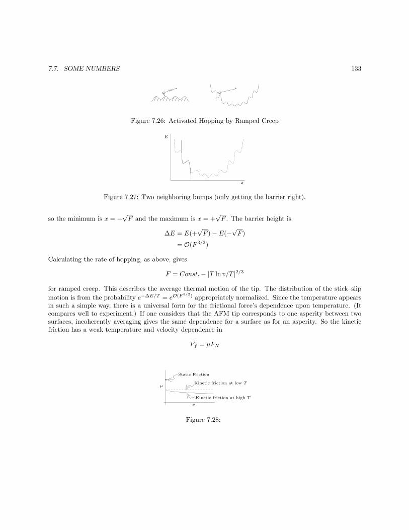
7.7. SOME NUMBERS 133
Figure 7.26: Activated Hopping by Ramped Creep
E
x
Figure 7.27: Two neighboring bumps (only getting the barrier right).
so the minimum is x = −√F and the maximum is x = +
√F . The barrier height is
∆E = E(+√F )− E(−
√F )
= O(F 3/2)
Calculating the rate of hopping, as above, gives
F = Const.− |T ln v/T |2/3
for ramped creep. This describes the average thermal motion of the tip. The distribution of the stick–slip
motion is from the probability e−∆E/T = eO(F 3/2) appropriately normalized. Since the temperature appearsin such a simple way, there is a universal form for the frictional force’s dependence upon temperature. (Itcompares well to experiment.) If one considers that the AFM tip corresponds to one asperity between twosurfaces, incoherently averaging gives the same dependence for a surface as for an asperity. So the kineticfriction has a weak temperature and velocity dependence in
Ff = µFN
Static Friction
Kinetic friction at low T
Kinetic friction at high T
µ
v
Figure 7.28:

134 CHAPTER 7. FOKKER–PLANCK EQUATION
Chapter 8
Statistical Theory of the Decay ofMetastable States
• Two kinds of nucleation phenomena:“inhomogeneous nucleation”“homogeneous nucleation”: The nucleating disturbance occurs spontaneously as thermodynamic fluc-tuation.
• Expression for the rate of a thermally activated process.
I = Ioe−Ea/kT
Ea: the activation energy.Io: fundamental fluctuation rate.
• Major limitation: purely classical
• We shall produce irreversible processes by letting the classical model system interact with a constant–temperature heat bath.
We shall assume that the heat bath exists and is well defined in the sense of being weakly coupled to— and thus not strongly affected by — the system of principle interest.
8.1 Equation of Motion for the Distribution Function
1. Classical system: N degree of freedom 1 ∼ 2N coordinatesthe first N : coordinatesthe last N : canonically conjugate momentum
ηi i : 1 ∼ 2N ηi ǫ (−∞,+∞)
In some cases, there is no need to include momenta in the set of η’s, because they have no internaldynamics.
135
136 CHAPTER 8. STATISTICAL THEORY OF THE DECAY OF METASTABLE STATES
For the system that does have its own dynamics, there must exist some Hamiltonian function E η.
ηi =∑
j
Aij∂E
∂ηj(8.1)
Aij =
δi+N,j i ≤ N−δi,j+N j ≤ N0 otherwise
(8.2)
Aij : antisymmetric matrix.if there is no internal dynamics, Aij = 0. (i, j ≤ 2N)
2. Distribution function ρ(η, t).Configuration η (η ≡ η1, η2, ..., η2N) space
∫
δηρη ≡∫ ∞
−∞
dη1...
∫ ∞
−∞
dη2Nρη = 1 (8.3)
∂ρ
∂t=
(∂ρ
∂t
)
dyn
+
(∂ρ
∂t
)
fluct
(8.4)
(∂ρ
∂t
)
dyn
= +∑
i
∂ρ
∂ηiηi = +
∑
ij
Aij∂E
∂ηj
∂ρ
∂ηi(8.5)
(∂ρ
∂t
)
fluct
=
∫
δη′ [P (η, η′)ρη′ − P (η′, η)ρη] (8.6)
result of interaction with the heat bath.
All irreversable effects will be introduced through these interactions with the heat bath.
What will be the form of P which contains the most important features of our physical models.
We assume that the heat bath interacts with each element (ηi) independently with a certain probabilityof action per unit time. Fluctuation–induced transition:
P (η, η′) =∑
i
∏
j 6=i
δ(ηj − η′j)Ri(η, η′) (8.7)
if in equilibrium (the thermal resevoir) before interact with system. (relaxation time τbath << τsystem)
Ri =
∫
ds
∫
ds′
(
e−ǫ(s′)/kT
ZR
)
Ti(s, ηi; s′, η′i)δ [ǫ(s) + Eη − ǫ(s′)− Eη′] (8.8)
ZR =∫dse−ǫ(s)/kT — partition function of the resevoir
Ti(s, ηi; s′, η′i) ∝ detailed transition rate between states s′, η′i and s, ηi;
Ti(s, ηi; s′, η′i) = Ti(s
′, η′i; s, ηi) detailed balance
8.1. EQUATION OF MOTION FOR THE DISTRIBUTION FUNCTION 137
rewrite Ri:
Ri = exp
(Eη′ − Eη
2kT
)
Ti(η, η′) (8.9)
Ti(η, η′) =1
ZR
∫
ds
∫
ds′ exp
[
−ǫ(s) + ǫ(s′)
2kT
]
Ti(s, ηi; s′, η′i)
× δ [ǫ(s) + Eη − ǫ(s′)− Eη′] (8.10)
Ti: Symmetric in η and η′
The only important information carried by Ti itself concerns the allowed size of the jump from η′i to ηiand the rate at which such jumps occur.
We assume Ti has Gaussian form:
Ti(η, η′) =2Γi
∆√
2λ∆exp
[
− (ηi − η′i)22∆
]
(8.11)
∆: mean–square jump size
mean–square change =
∫
Ti(η, η′) · (ηi − η′i)2dη′i
=
∫2Γi
∆√
2λ∆exp
[
− (ηi − η′i)22∆
]
· (ηi − η′i)2dη′i
=
∫2Γi√2λ∆
exp
[
− (ηi − η′i)22∆
]
dη′i
= 2Γi (8.12)
Thus, when ∆→ 0, mean–square change in ηi per unit time remains finite.
(∂fη∂t
)
fluct
=∑
i
2Γi
∆√
2λ∆
∫ ∞
−∞
dνie−ν2
i /2∆exp
(E(ηi + νi)− E(ηi)
2kT
)
ρ(ηi + νi)
− exp
(E(ηi)− E(ηi + νi)
2kT
)
ρ(ηi)
(8.13)
where η′i = ηi+νi. P , E are slowly varying functions of η (within ∆1/2). Expand (A) in powers of νi because
138 CHAPTER 8. STATISTICAL THEORY OF THE DECAY OF METASTABLE STATES
∆ is very small
exp
(E(ηi + νi)− E(ηi)
2kT
)
ρ(ηi + νi)− exp
(E(ηi)− E(ηi + νi)
2kT
)
ρ(ηi)
= exp
[1
2kT
(∂E
∂ηiνi +
1
2
∂2E
∂η2i
ν2i +O(ν3
i )
)]
·[
ρ(ηi) +∂ρ
∂ηiνi +
1
2
∂2ρ
∂η2i
ν2i
]
− exp
[1
2kT
(
−∂E∂ηi
νi −1
2
∂2E
∂η2i
ν2i +O(ν3
i )
)]
· ρ(ηi)
=
1 +1
2kT
(∂E
∂ηiνi +
1
2
∂2E
∂η2i
ν2i
)
ρ(ηi) +∂ρi∂ηi
νi +1
2
∂2ρ
∂η2i
ν2i
−
1− 1
2kT
(∂E
∂ηiνi +
1
2
∂2E
∂η2i
ν2i
)
ρ(ηi)
=∂ρ
∂ηiνi +
1
2kT
[
2∂E
∂ηiρ(ηi)νi
]
︸ ︷︷ ︸
F1
+1
2
∂2ρ
∂η2i
ν2i +
1
2kT
(∂E
∂ηi
∂ρ
∂ηiν2i +
∂2E
∂η2i
ρ(ηi)ν2i
)
︸ ︷︷ ︸
F2
F1 is proportional to νiF2 is proportional to ν2
i
We omit O(ν3i ), because the integral will vanish when ∆→ 0.
(∂ρηi∂t
)
fluct
=∑
i
2Γi
∆√
2λ∆
∫ ∞
−∞
dνie−ν2
i /2∆(F1 + F2)
∵ F1 ∝ νi So, F1e−ν2
i /2∆ is an odd function, so integral vanish.
(∂ρηi∂t
)
fluct
=∑
i
2Γi
∆√
2λ∆
∫ ∞
−∞
dνie−ν2
i /2∆ν2i
1
2
∂
∂ηi
(1
kT
∂E
∂ηiρ+
∂ρ
∂ηi
)
(∂ρηi∂t
)
fluct
=∑
i
Γi∂
∂ηi
(1
kT
∂E
∂ηiρ+
∂ρ
∂ηi
)
— Fokker–Planck equation
we let
Ji = −∑
j
Mij
(∂E
∂ηjρ+ kT
∂ρ
∂ηi
)
(8.14)
where Mij = ΓikT δij +Aij . So we have
∂ρη∂t
= −∑
i
∂Ji∂ηi
(8.15)
8.2. NUCLEATION RATES 139
now, we prove it. When i = j, Aij = Aii = 0
Ji = −∑
j
(ΓikT
δij +Aij
)(∂E
∂ηiρ+ kT
∂ρ
∂ηi
)
= − ΓikT
(∂E
∂ηiρ+ kT
∂ρ
∂ηi
)
∴∂ρη∂t
∣∣A
= −∑
i=j
∂Ji∂ηi
=∑
i
Γi∂
∂ηi
(1
kT
∂E
∂ηiρ+
∂ρ
∂ηi
)
=
(∂ρη∂t
)
fluct
when i 6= j, δij = 0
∴ Ji = −∑
j
Aij
(∂E
∂ηiρ+ kT
∂ρ
∂ηi
)
∂ρη∂t
∣∣B
= −∑
i6=j
∂Ji∂ηi
=∑
i6=j
Aij
(∂E
∂ηj
∂ρ
∂ηi+ ρ
∂2E
∂ηi∂ηj+ kT
∂2ρ
∂ηi∂ηj
)
∵ ∂2ρ∂ηi∂ηj
= ∂2ρ∂ηj∂ηi
(i 6= j), and Aij = −Aji(
∂2E∂ηi∂ηj
= ∂2E∂ηj∂ηi
)
∴∂ρη∂t
∣∣B
=∑
i6=j
Aij
(∂E
∂ηj
∂ρ
∂ηi
)
=
(∂ρη∂t
)
dyn
the gizt is Aij is an antisymmetry matrix.
8.2 Nucleation Rates
Eq. 8.15 is
∂ρη∂t
= −∑
i
∂Ji∂ηi
using Eq. 8.15 calculate the nucleation rate. Method is developed by Becker and Doring (rate of condensationof a supersaturated vapor.) Equilibrium solution for 8.15 is
ρoη ∝ exp(−Eη/kT ), Ji = 0
∵ E2 > E1 ∴ point (1) is more stable than point (2). From (2)→(1), the system point is to pass acrossthe lowest interrening saddle point of the function Eη. Say, this saddle point is η. η describes thefluctuation which nucleates the phase transition.
Find a steady–state solution, describes a finite probability current flowing across the saddle point η.
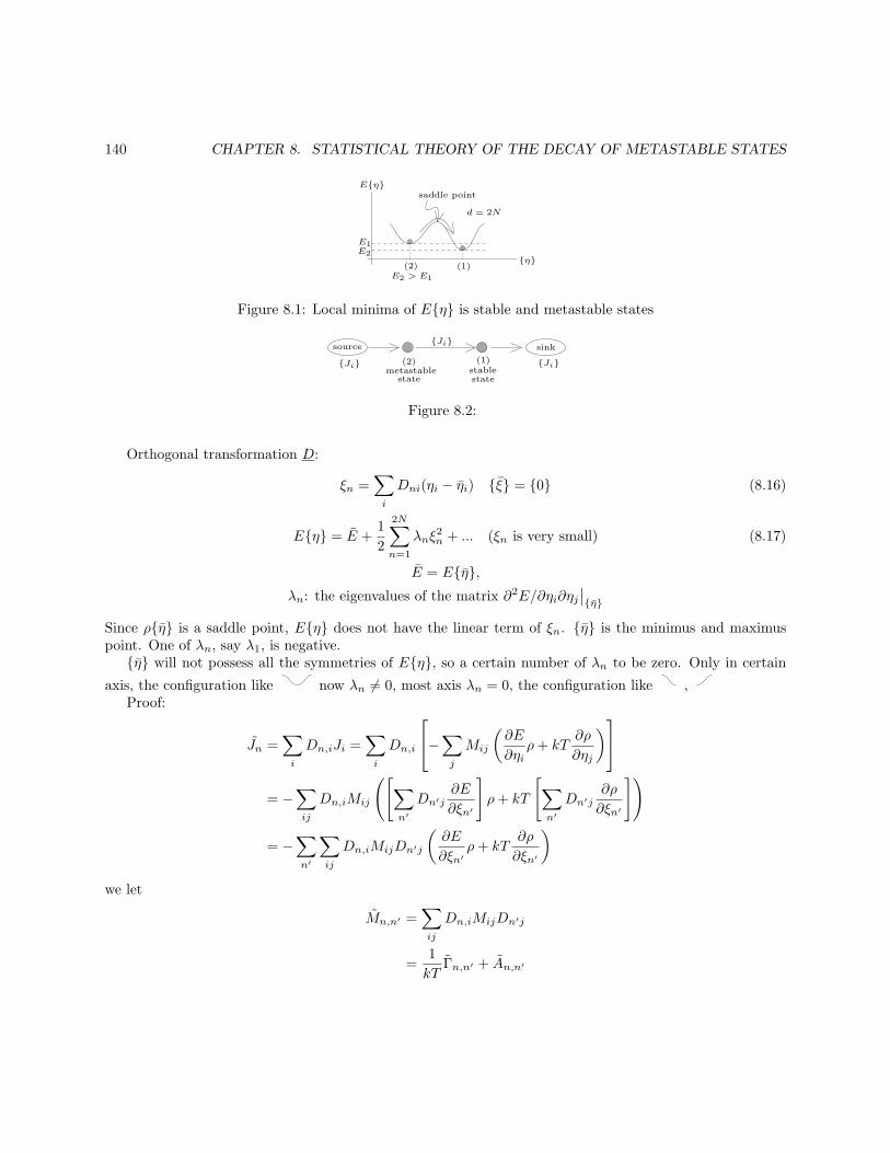
140 CHAPTER 8. STATISTICAL THEORY OF THE DECAY OF METASTABLE STATES
saddle point
d = 2N
Eη
E1E2
(2) (1)E2 > E1
η
Figure 8.1: Local minima of Eη is stable and metastable states
source sink
Ji Ji
Ji
(2) (1)metastable
statestablestate
Figure 8.2:
Orthogonal transformation D:
ξn =∑
i
Dni(ηi − ηi) ξ = 0 (8.16)
Eη = E +1
2
2N∑
n=1
λnξ2n + ... (ξn is very small) (8.17)
E = Eη,λn: the eigenvalues of the matrix ∂2E/∂ηi∂ηj
∣∣η
Since ρη is a saddle point, Eη does not have the linear term of ξn. η is the minimus and maximuspoint. One of λn, say λ1, is negative.η will not possess all the symmetries of Eη, so a certain number of λn to be zero. Only in certain
axis, the configuration like now λn 6= 0, most axis λn = 0, the configuration like ,Proof:
Jn =∑
i
Dn,iJi =∑
i
Dn,i
−∑
j
Mij
(∂E
∂ηiρ+ kT
∂ρ
∂ηj
)
= −∑
ij
Dn,iMij
([∑
n′
Dn′j∂E
∂ξn′
]
ρ+ kT
[∑
n′
Dn′j∂ρ
∂ξn′
])
= −∑
n′
∑
ij
Dn,iMijDn′j
(∂E
∂ξn′ρ+ kT
∂ρ
∂ξn′
)
we let
Mn,n′ =∑
ij
Dn,iMijDn′j
=1
kTΓn,n′ + An,n′
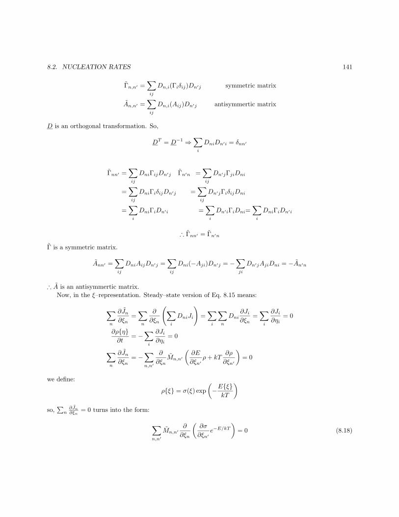
8.2. NUCLEATION RATES 141
Γn,n′ =∑
ij
Dn,i(Γiδij)Dn′j symmetric matrix
An,n′ =∑
ij
Dn,i(Aij)Dn′j antisymmertic matrix
D is an orthogonal transformation. So,
DT = D−1 ⇒∑
i
DniDn′i = δnn′
Γnn′ =∑
ij
DniΓijDn′j Γn′n =∑
ij
Dn′jΓjiDni
=∑
ij
DniΓiδijDn′j =∑
ij
Dn′jΓiδijDni
=∑
i
DniΓiDn′i =∑
i
Dn′iΓiDni=∑
i
DniΓiDn′i
∴ Γnn′ = Γn′n
Γ is a symmetric matrix.
Ann′ =∑
ij
DniAijDn′j =∑
ij
Dni(−Aji)Dn′j = −∑
ji
Dn′jAjiDni = −An′n
∴ A is an antisymmertic matrix.
Now, in the ξ–representation. Steady–state version of Eq. 8.15 means:
∑
n
∂Jn∂ξn
=∑
n
∂
∂ξn
(∑
i
DniJi
)
=∑
i
∑
n
Dni∂Ji∂ξn
=∑
i
∂Ji∂ηi
= 0
∂ρη∂t
= −∑
i
∂Ji∂ηi
= 0
∑
n
∂Jn∂ξn
= −∑
n,n′
∂
∂ξnMn,n′
(∂E
∂ξn′ρ+ kT
∂ρ
∂ξn′
)
= 0
we define:
ρξ = σ(ξ) exp
(
−EξkT
)
so,∑
n∂Jn∂ξn
= 0 turns into the form:
∑
n,n′
Mn,n′∂
∂ξn
(∂σ
∂ξn′e−E/kT
)
= 0 (8.18)
142 CHAPTER 8. STATISTICAL THEORY OF THE DECAY OF METASTABLE STATES
near the saddle point at ξ = 0
Eξ = E +1
2
2N∑
n=1
λnξ2n + ...
Eξ ≈ E +1
2
2N∑
n=1
λnξ2n for small ξn
we let
e−Eξ/kT = exp
− 1
kT
(
E +1
2
∑
n
λnξ2n
)
= Qξ
Since∑
n,n′
Mnn′∂
∂ξn
(∂σ
∂ξn′e−E/kT
)
= 0
So,∑
n,n′ Mnn′∂∂ξn
(∂σ∂ξn′
Qξ)
= 0
left =∑
n,n′
Mnn′
∂2σ
∂ξn∂ξn′Qξ+
∂σ
∂ξn′Qξ ·
(
− 1
kT
)
(λnξn)
=∑
n,n′
Mnn′∂2σ
∂ξn∂ξn′− 1
kT· Mnn′λnξn
∂σ
∂ξn′
Qξ
Mnn′ =Γnn′
kT+ Ann′ where Ann′ = −An′n
∵∂2σ
∂ξn∂ξn′=
∂2σ
∂ξn′∂ξn
∴∑
nn′
Ann′∂2σ
∂ξn∂ξn′= 0
So, we get∑
n,n′
[
Γn,n′∂2σ
∂ξn∂ξn′− λnξnMn,n′
∂σ
∂ξn′
]
= 0 (8.19)
(which is only valid near the saddle point.) The relevant solution of Eq. 8.19 has the form
σ(ξ) = f(u)
where u =∑′n Unξn. The prime on the summation here indicates that we omit all n’s for λn = 0. We now
have
′∑
n,n′
UnΓn,n′Un′
d2f
du2−
′∑
n,n′
λnξnMn,n′Un′
df
du= 0 (8.20)
8.2. NUCLEATION RATES 143
This equation makes sense only if the coefficient if df/du is proportional to u itself,
′∑
n,n′
λnξnMn,n′Un′ = κu = κ′∑
n
Unξn (8.21)
So we get,
λn
′∑
n′
Mn,n′Un′ = κUn (8.22)
Here κ appears as the eigenvalue. Eq. 8.20 now reads:
γd2f
du2− u df
du= 0 ; ν =
1
κ
′∑
n,n′
UnTn,n′Un′ (8.23)
Only ν < 0 corresponding to the nontrivial solution in this case, f(u) is an errorfunction. (The reason isf(u) = σ(ξ) is finite.)
Proof:From before, we have,
∂ρη∂t
= −∑
i
∂Ji∂ηi
Jn =∑
i
Dn,iJi = −∑
n′
Mn,n′
(∂E
∂ξn′ρ+ kT
∂ρ
∂ξn′
)
Eη = E +1
2
2N∑
n=1
λnξ2n + ...
ξn =∑
i
Dni(ηi − ηi)
Now,
〈ξn(t)〉 =
∫
δξ · ξnρ(ξ, t) (8.24)
d〈ξn〉dt
=
∫
δξd
dt(ξnρ(ξ, t))
=
∫
δξ · ξn ·d
dtρ(ξ, t)
and so, from the above equations,
d
dtρ(ξ, t) =
[
−∑
i
∂Ji∂ηi
]
=
[
−∑
i
∑
n′
∂Ji∂ξn′
·Dni
]
=
[
−∑
n′
∂
∂ξn′
(∑
i
JiDni
)]
=
[
−∑
n′
∂Jn′
∂ξn′
]
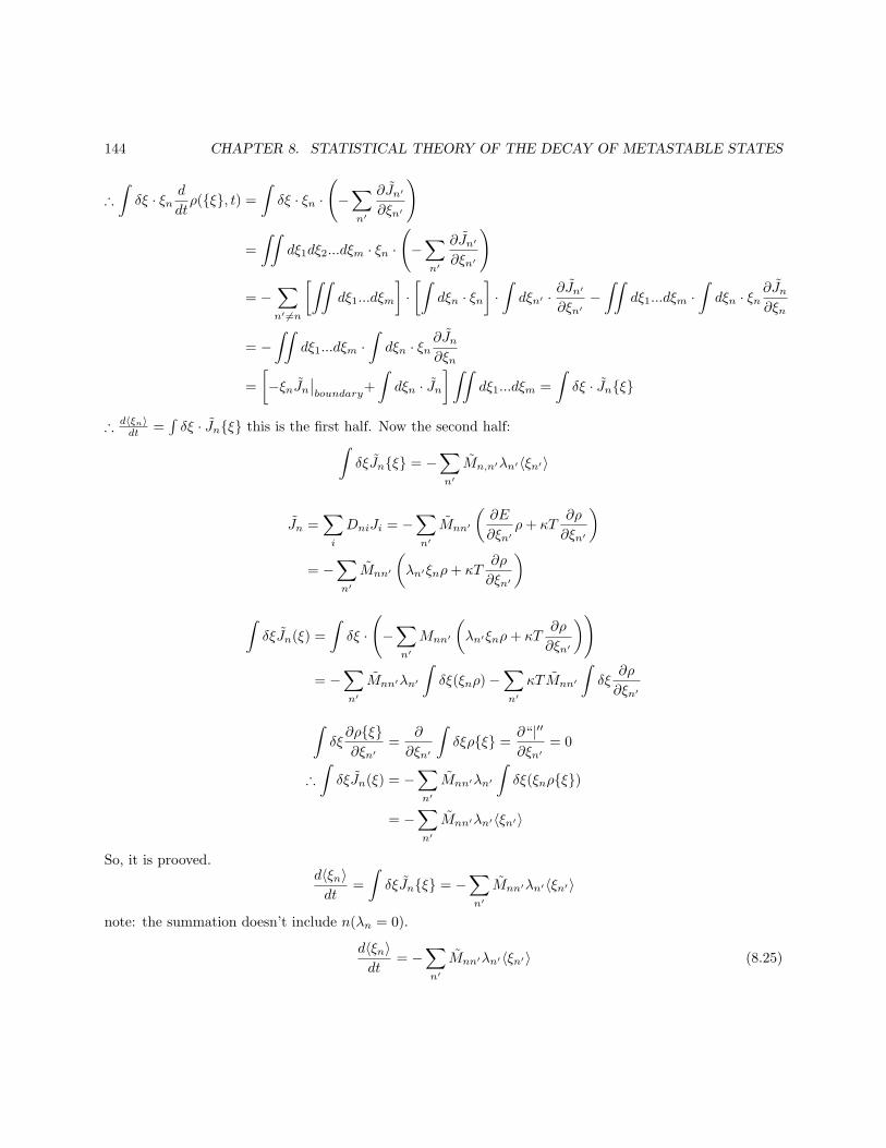
144 CHAPTER 8. STATISTICAL THEORY OF THE DECAY OF METASTABLE STATES
∴
∫
δξ · ξnd
dtρ(ξ, t) =
∫
δξ · ξn ·(
−∑
n′
∂Jn′
∂ξn′
)
=
∫∫
dξ1dξ2...dξm · ξn ·(
−∑
n′
∂Jn′
∂ξn′
)
= −∑
n′ 6=n
[∫∫
dξ1...dξm
]
·[∫
dξn · ξn]
·∫
dξn′ · ∂Jn′
∂ξn′−∫∫
dξ1...dξm ·∫
dξn · ξn∂Jn∂ξn
= −∫∫
dξ1...dξm ·∫
dξn · ξn∂Jn∂ξn
=
[
−ξnJn∣∣boundary
+
∫
dξn · Jn] ∫∫
dξ1...dξm =
∫
δξ · Jnξ
∴d〈ξn〉dt =
∫δξ · Jnξ this is the first half. Now the second half:
∫
δξJnξ = −∑
n′
Mn,n′λn′〈ξn′〉
Jn =∑
i
DniJi = −∑
n′
Mnn′
(∂E
∂ξn′ρ+ κT
∂ρ
∂ξn′
)
= −∑
n′
Mnn′
(
λn′ξnρ+ κT∂ρ
∂ξn′
)
∫
δξJn(ξ) =
∫
δξ ·(
−∑
n′
Mnn′
(
λn′ξnρ+ κT∂ρ
∂ξn′
))
= −∑
n′
Mnn′λn′
∫
δξ(ξnρ)−∑
n′
κTMnn′
∫
δξ∂ρ
∂ξn′
∫
δξ∂ρξ∂ξn′
=∂
∂ξn′
∫
δξρξ =∂“|′′∂ξn′
= 0
∴
∫
δξJn(ξ) = −∑
n′
Mnn′λn′
∫
δξ(ξnρξ)
= −∑
n′
Mnn′λn′〈ξn′〉
So, it is prooved.d〈ξn〉dt
=
∫
δξJnξ = −∑
n′
Mnn′λn′〈ξn′〉
note: the summation doesn’t include n(λn = 0).
d〈ξn〉dt
= −∑
n′
Mnn′λn′〈ξn′〉 (8.25)
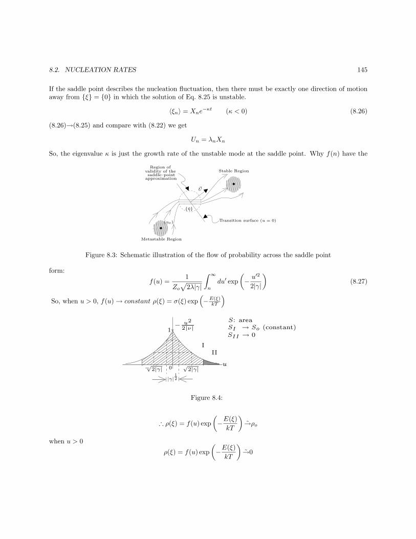
8.2. NUCLEATION RATES 145
If the saddle point describes the nucleation fluctuation, then there must be exactly one direction of motionaway from ξ = 0 in which the solution of Eq. 8.25 is unstable.
〈ξn〉 = Xne−κt (κ < 0) (8.26)
(8.26)→(8.25) and compare with (8.22) we get
Un = λnXn
So, the eigenvalue κ is just the growth rate of the unstable mode at the saddle point. Why f(n) have the
Region ofvalidity of thesaddle–point
approximation
Transition surface (u = 0)
~U
η
ηo
Metastable Region
Stable Region
Figure 8.3: Schematic illustration of the flow of probability across the saddle point
form:
f(u) =1
Zo√
2λ|γ|
∫ ∞
n
du′ exp
(
− u′2
2|γ|
)
(8.27)
So, when u > 0, f(u)→ constant ρ(ξ) = σ(ξ) exp(
−E(ξ)kT
)
Figure 8.4:
∴ ρ(ξ) = f(u) exp
(
−E(ξ)
kT
)
→ρo
when u > 0
ρ(ξ) = f(u) exp
(
−E(ξ)
kT
)
→0
146 CHAPTER 8. STATISTICAL THEORY OF THE DECAY OF METASTABLE STATES
here the configuration point is very near the saddle point, so, Eξ vary slowly. Since
ρξ = f(u) exp
(
−EξkT
)
in the metastable region ρξ ≈ ρoξ, in the stable region
ρξ ≈ 0∫
δηρη = 1
∫
δηρη ≈∫
u<0
δηρη =
∫
u<0
δη · f(u) exp
(
−E(η)
kT
)
=
∫
u<0
δη · 1
Zoexp
(
−EηkT
)
∴1
Zo
∫
(u<0)
δη exp
(
−EηκT
)
= 1
Zo is chosen so that ρ is normalized in the metastable region.
Metastable minimum is sharp, well isolated
Eη = Eo +1
2
∑
l
λ(0)l (ηl − ηlo)
2
where the foot subscript means the metastable minimum point.
∴ Zo ≈ e−Eo/kT∫
δη exp
−∑
l
1
kT
(1
2λ
(0)l (ηl − ηlo)2
)
= e−Eo/kT∏
l
∫
δηl · exp
− λ(0)l
2kT(ηl − ηlo)2
= e−Eo/kT∏
l
(
2λkT
λ(0)l
)1/2
= e−Fo/kT
here, Fo is the free energy of the metastable phase.
8.2. NUCLEATION RATES 147
Proof:
Jn =∑
i
Dn,iJi = −∑
n′
Mn,n′
(∂E
∂ξn′P + kT
∂ρ
∂ξn′
)
= −kT∑
n′
Mn,n′∂σ
∂ξn′e−E/kT
= −kT′∑
n′
Mn,n′Un′df
due−E/kT (8.28)
∵ f =
∫ −∞
u
1
Zo√
2λ| γ|exp
(
− u′2
2|γ|
)
du′
and λn∑′n′ Mn,n′Un′ = κUn
Jn = −kT∑
n′
Mn,n′Un′1
Zo√
2λ|γ|exp
(
− u2
2|γ|
)
e−E/kT exp
(
− 1
2kT
∑
n
λnξ2n
)
= e−E/kT
(
kT
Zo√
2λ|γ|
)(∑
n′
Mn,n′Un′
)
· λnλn· exp
− 1
2kT
∑
n
λnξ2n −
1
2|γ|
′∑
n,n′
UnUn′ξnξn′
= e−E/kT
(
kTκ
Zo√
2λ|γ|
)
Unλn
exp
− 1
2kT
∑
n
λnξ2n −
1
2|γ|
′∑
n,n′
UnUn′ξnξn′
(8.29)
Note: for n whose λn = 0, Jn = 0.
From Eq. 8.29 we can see: when ξn → 0 (near the saddle point)
Jn → e−E/kT
(
kTκ
Zo√
2λ|γ|
)
Unλn
so, at the saddle point
J//
Unλn
→ vector
We can proove that the magnitude of the current J must be constant along the direction of vectorUnλn
now. Eq. 8.29 is
Jn = e−E/kT
(
kTκ
Zo√
2λ|γ|
)
Unλn
exp
− 1
2kT
∑
n
λnξ2n −
1
2|γ|
′∑
n,n′
UnUn′ξnξn′
the quadratic form in Eq. 8.29 is:
Qξ =′∑
n,n′
Qn,n′ξnξn′
148 CHAPTER 8. STATISTICAL THEORY OF THE DECAY OF METASTABLE STATES
where Qn,n′ = λnkT δnn′ + 1
|γ|UnUn′
if ξn//Jo, then(
Jo =Unλn
)
′∑
n
Qn,n′ξn′ ∝′∑
n′
Qn,n′Un′
λn′=
1
kTUn +
Un|γ|
′∑
n′
U2n′
λn′(8.30)
λn
′∑
n′
Mn,n′Un′ = κUn
∴Unλn
=
∑
n′ Mn,n′Un′
κ
∴∑
n
U2n
λn=∑
n
Un
′∑
n′
Mn,n′Un′
κ
=1
κ
′∑
n,n′
UnMn,n′Un′
=1
κkT
′∑
n,n′
UnΓn,n′Un′
=γ
kT
= − |γ|kT
∴
′∑
n′
Qn,n′ξn′ ∝ 1
kTUn +
Un|γ|
′∑
n′
U2n′
λn
=1
kTUn +
Un|γ| ·
′∑
n
U2n
λn
=1
kTUn +
Un|γ|
(−|γ|)kT
= 0
∴ Jn = e−E/kT
(
kTκ
Zo√
2λ|λ|
)
Unλn
along
Unλ
.
The total nucleation rate, I, is the integral intensity of the current J . We can compute I by evaluating thetotal flux across any surface not parallel to J . We choose the surface ξ = 0.
8.2. NUCLEATION RATES 149
So, we have the final result
I =
∫
ξ1=0
δξJ1
=kBTκe
−E/kTU1
Zo√
2λ|ν|λ1
∫
ξ1=0
δξ exp
−1
2
′∑
n,n′
Qn,n′ξnξn′
=kBTκe
−E/kTU1
Zo√
2λ|ν|λ1
ζ
[
det
(
Q′′
2λ
)]−1/2
(8.31)
where the factor ζ denotes the volume of the saddle point subspace. The matrix Q′′ is the same as Q except
that we omit n = 1 and all the n’s for which λn = 0. Now, we evaluate det(Q′′
2λ
)
. let
1
2λQ′′ = Λ1/2PΛ1/2
Λn,n′ =λn
2λkTδn,n′
Pn,n′ = δn,n′ +kT
|ν|Un√λn
Un′√λn′
∵ det
(
Q′′
2λ
)
= (detΛ)(detP )
=
′′∏
n
(λn
2λkT
)
· (detP )
Since P has an eigenvalue which is parallel to the vector (Un/√λn), and has eigenvalue
1 +κT
|ν|
′′∑
n
U2n
λn=kBTU
21
|ν||λ1|
so,
det
(Q′′
2λ
)
= (detΛ)(detP )
=kTU2
1
|νλ1|
′′∏
n
(λn
2λkT
)
finally,
I = |κ|(
kT
2λ|λ1|
)1/2
ζe−E/kT
Zo
′′∏
n
(2kT
λn
)1/2
150 CHAPTER 8. STATISTICAL THEORY OF THE DECAY OF METASTABLE STATES
if we let Z ≡ e−E/kT ∏′′n
(2λkTλn
)1/2
≡ e−F /kT , then
I = |κ|(
kT
2λ|λ1|
)1/2
ζe−Fa/kT
whereFa = F − Fo
Fo is the excess free energy of the critically large nucleus.
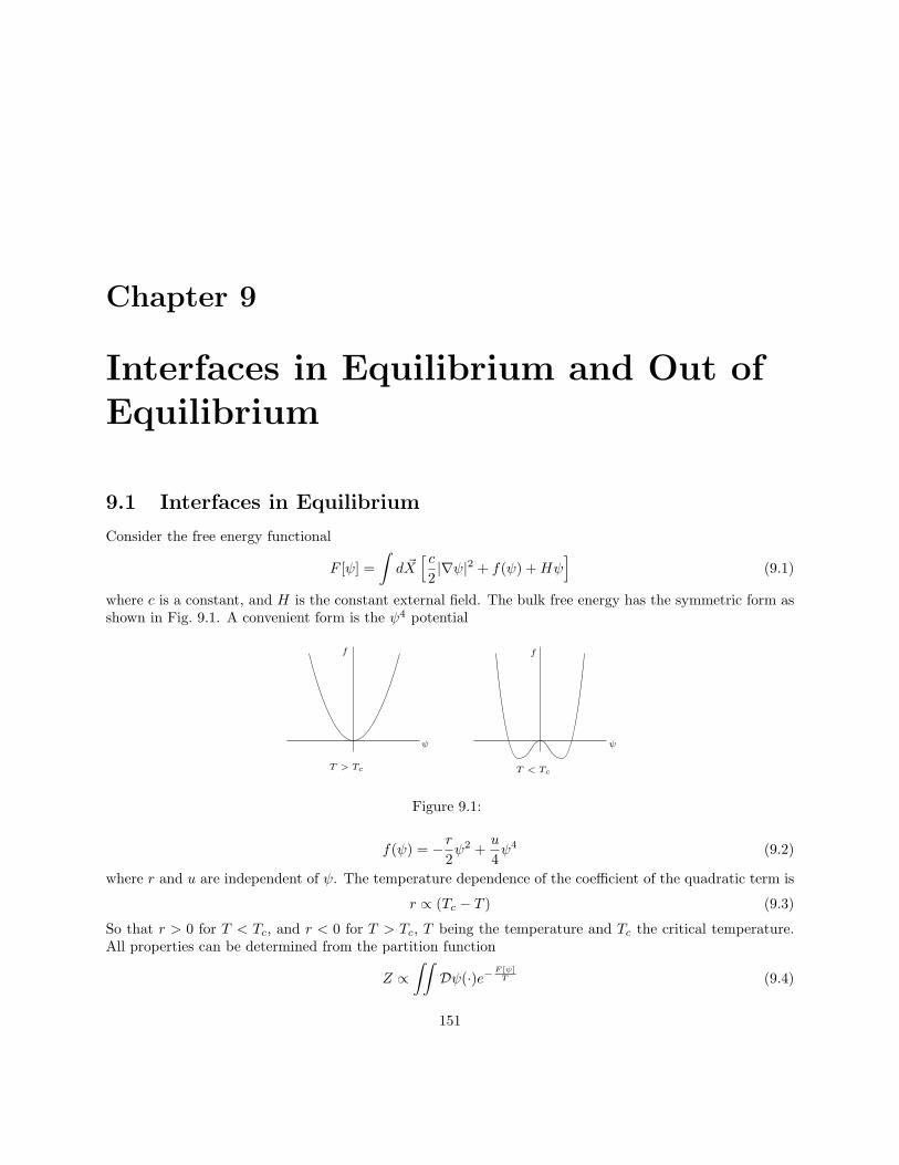
Chapter 9
Interfaces in Equilibrium and Out ofEquilibrium
9.1 Interfaces in Equilibrium
Consider the free energy functional
F [ψ] =
∫
d ~X[ c
2|∇ψ|2 + f(ψ) +Hψ
]
(9.1)
where c is a constant, and H is the constant external field. The bulk free energy has the symmetric form asshown in Fig. 9.1. A convenient form is the ψ4 potential
f f
ψψ
T > Tc T < Tc
Figure 9.1:
f(ψ) = −r2ψ2 +
u
4ψ4 (9.2)
where r and u are independent of ψ. The temperature dependence of the coefficient of the quadratic term is
r ∝ (Tc − T ) (9.3)
So that r > 0 for T < Tc, and r < 0 for T > Tc, T being the temperature and Tc the critical temperature.All properties can be determined from the partition function
Z ∝∫∫
Dψ(·)e−F [ψ]T (9.4)
151
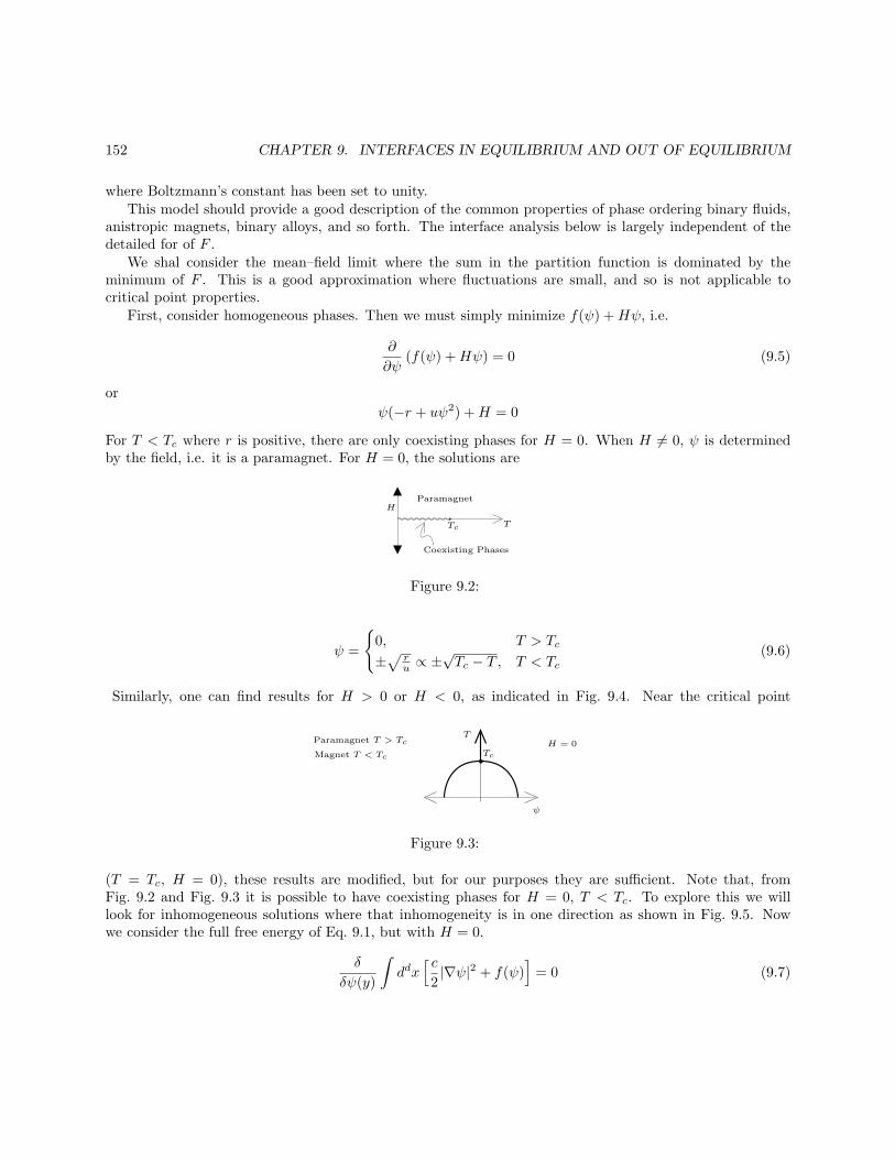
152 CHAPTER 9. INTERFACES IN EQUILIBRIUM AND OUT OF EQUILIBRIUM
where Boltzmann’s constant has been set to unity.This model should provide a good description of the common properties of phase ordering binary fluids,
anistropic magnets, binary alloys, and so forth. The interface analysis below is largely independent of thedetailed for of F .
We shal consider the mean–field limit where the sum in the partition function is dominated by theminimum of F . This is a good approximation where fluctuations are small, and so is not applicable tocritical point properties.
First, consider homogeneous phases. Then we must simply minimize f(ψ) +Hψ, i.e.
∂
∂ψ(f(ψ) +Hψ) = 0 (9.5)
or
ψ(−r + uψ2) +H = 0
For T < Tc where r is positive, there are only coexisting phases for H = 0. When H 6= 0, ψ is determinedby the field, i.e. it is a paramagnet. For H = 0, the solutions are
Paramagnet
Tc
H
T
Coexisting Phases
Figure 9.2:
ψ =
0, T > Tc
±√
ru ∝ ±
√Tc − T , T < Tc
(9.6)
Similarly, one can find results for H > 0 or H < 0, as indicated in Fig. 9.4. Near the critical point
Tc
ψ
TH = 0Paramagnet T > Tc
Magnet T < Tc
Figure 9.3:
(T = Tc, H = 0), these results are modified, but for our purposes they are sufficient. Note that, fromFig. 9.2 and Fig. 9.3 it is possible to have coexisting phases for H = 0, T < Tc. To explore this we willlook for inhomogeneous solutions where that inhomogeneity is in one direction as shown in Fig. 9.5. Nowwe consider the full free energy of Eq. 9.1, but with H = 0.
δ
δψ(y)
∫
ddx[ c
2|∇ψ|2 + f(ψ)
]
= 0 (9.7)
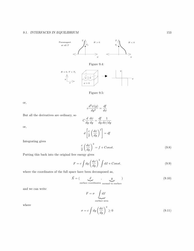
9.1. INTERFACES IN EQUILIBRIUM 153
Tc Tc
ψ ψ
T TH > 0 H < 0Paramagnet
at all T
Figure 9.4:
ψ
y
ψ < 0
ψ > 0
H = 0, T < Tc
y
x
Figure 9.5:
or,
cd2ψ(y)
dy2=
df
dψ
But all the derivatives are ordinary, so
Cd
dy
dψ
dy=df
dy
1
dψ/dy
or,
d
[
c
2
(dψ
dy
)2]
= df
Integrating gives
c
2
(dψ
dy
)2
= f + Const. (9.8)
Putting this back into the original free energy gives
F = c
∫
dy
(dψ
dy
)2 ∫
d~x+ Const. (9.9)
where the coordinates of the full space have been decomposed as,
~X = ( ~x︸︷︷︸
surface coordinates
, y︸︷︷︸
normal to surface
) (9.10)
and we can write
F = σ
∫
d~x
︸ ︷︷ ︸
surface area
where
σ = c
∫
dy
(dψ
dy
)2
≥ 0 (9.11)
154 CHAPTER 9. INTERFACES IN EQUILIBRIUM AND OUT OF EQUILIBRIUM
is the surface tension. Note that the extra free energy due to the presence of the ψ inhomogeneity (i.e., dueto the surface), is proportional to the surface area.
The form of ψ(y) can be found by solving the differential equation of Eq. 9.8. Let the constant bedetermined by having no gradients of ψ in the bulk phases. That is, dψ/dy = 0 for ψ =“±1”. That is
c
2
(dψ
dy
)2
= f(ψ)− f(±1) (9.12)
(of course by ±1 we mean f(ψ = ψeq) where ∂f/∂ψeq = 0.), or
√c
2
∫dψ
√
f(ψ)− f(±1)= y (9.13)
where we have chosen the interface to be symmetric about y = 0. Using the form of the ψ4 potential wherewe now choose r = 1 and u = 1 so that
f = −1
2ψ2 +
1
4ψ4 (9.14)
andψ = ±1
in equilibrium, we have
y =
√c
2
∫dψ
√14 −
ψ2
2 + ψ4
4
(9.15)
=√
2c
∫dψ
√
1− 2ψ2 + ψ4
=√
2c
∫dψ
(1− ψ2)
=√
2c arctanψ
or,ψ(y) = tanh y/
√2c (9.16)
which has the form indicated in Fig. 9.5. The integral giving the surface tension can now be done with thisexplicit form of ψ(y) following from the ψ4 potential. Eq. 9.16 in Eq. 9.11 gives
σ = c
∫ ∞
−∞
dy
(d
dytanh y/
√2c
)2
=
√c
2
∫ ∞
−∞
dY
(d
dYtanhY
)2
=
√c
2
∫ ∞
−∞
dY sech4Y
=
√c
2
[
−1
3tanh3 Y + tanhY
]∞
−∞
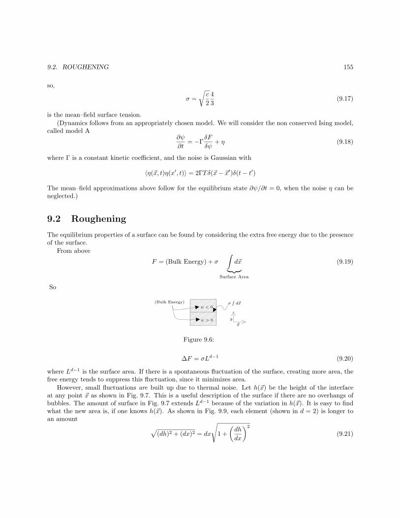
9.2. ROUGHENING 155
so,
σ =
√c
2
4
3(9.17)
is the mean–field surface tension.
(Dynamics follows from an appropriately chosen model. We will consider the non conserved Ising model,called model A
∂ψ
∂t= −Γ
δF
δψ+ η (9.18)
where Γ is a constant kinetic coefficient, and the noise is Gaussian with
〈η(~x, t)η(x′, t)〉 = 2ΓTδ(~x− ~x′)δ(t− t′)
The mean–field approximations above follow for the equilibrium state ∂ψ/∂t = 0, when the noise η can beneglected.)
9.2 Roughening
The equilibrium properties of a surface can be found by considering the extra free energy due to the presenceof the surface.
From above
F = (Bulk Energy) + σ
∫
d~x
︸ ︷︷ ︸
Surface Area
(9.19)
So
(Bulk Energy) σR
d~xψ < 0
ψ > 0 y
~x
Figure 9.6:
∆F = σLd−1 (9.20)
where Ld−1 is the surface area. If there is a spontaneous fluctuation of the surface, creating more area, thefree energy tends to suppress this fluctuation, since it minimizes area.
However, small fluctuations are built up due to thermal noise. Let h(~x) be the height of the interfaceat any point ~x as shown in Fig. 9.7. This is a useful description of the surface if there are no overhangs ofbubbles. The amount of surface in Fig. 9.7 extends Ld−1 because of the variation in h(~x). It is easy to findwhat the new area is, if one knows h(~x). As shown in Fig. 9.9, each element (shown in d = 2) is longer toan amount
√
(dh)2 + (dx)2 = dx
√
1 +
(dh
dx
)2
(9.21)
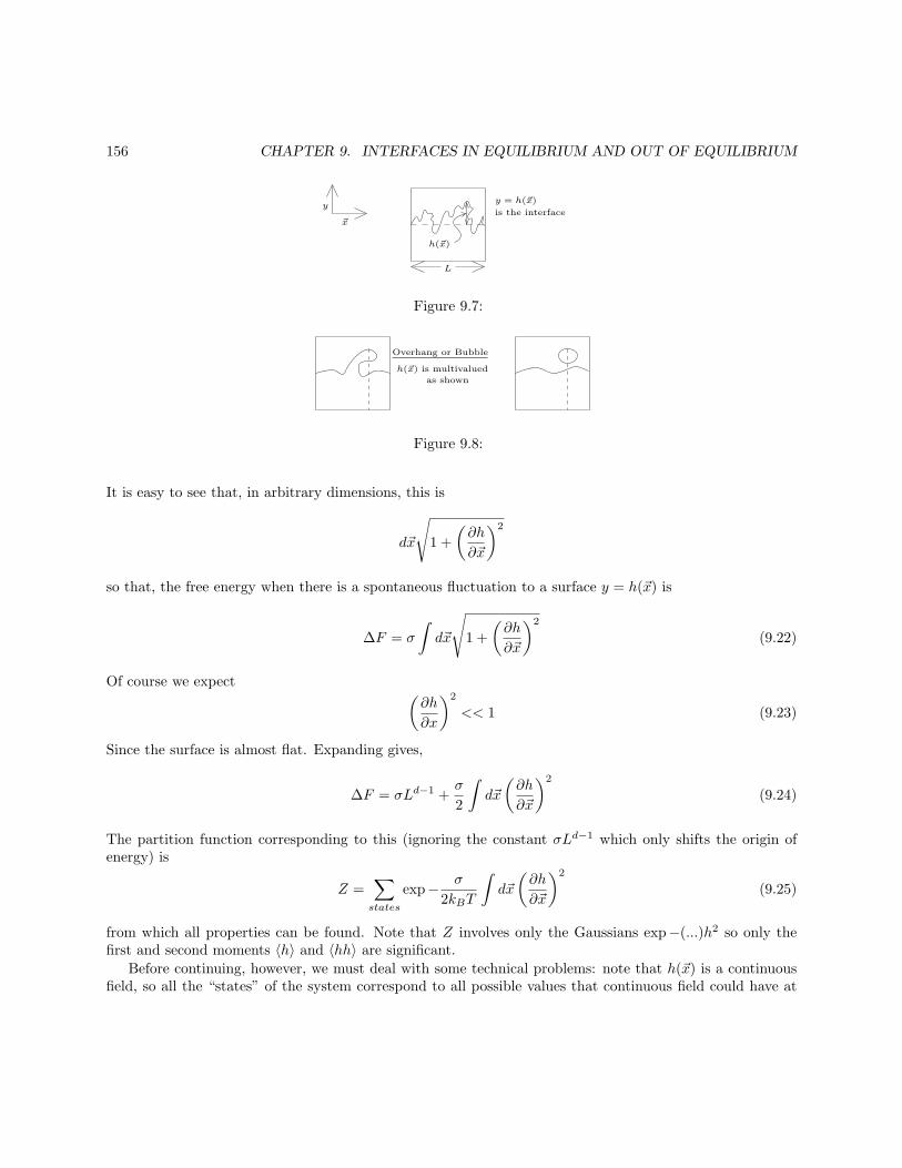
156 CHAPTER 9. INTERFACES IN EQUILIBRIUM AND OUT OF EQUILIBRIUM
y
~x
h(~x)
y = h(~x)
is the interface
L
Figure 9.7:
Overhang or Bubble
h(~x) is multivalued
as shown
Figure 9.8:
It is easy to see that, in arbitrary dimensions, this is
d~x
√
1 +
(∂h
∂~x
)2
so that, the free energy when there is a spontaneous fluctuation to a surface y = h(~x) is
∆F = σ
∫
d~x
√
1 +
(∂h
∂~x
)2
(9.22)
Of course we expect(∂h
∂x
)2
<< 1 (9.23)
Since the surface is almost flat. Expanding gives,
∆F = σLd−1 +σ
2
∫
d~x
(∂h
∂~x
)2
(9.24)
The partition function corresponding to this (ignoring the constant σLd−1 which only shifts the origin ofenergy) is
Z =∑
states
exp− σ
2kBT
∫
d~x
(∂h
∂~x
)2
(9.25)
from which all properties can be found. Note that Z involves only the Gaussians exp−(...)h2 so only thefirst and second moments 〈h〉 and 〈hh〉 are significant.
Before continuing, however, we must deal with some technical problems: note that h(~x) is a continuousfield, so all the “states” of the system correspond to all possible values that continuous field could have at
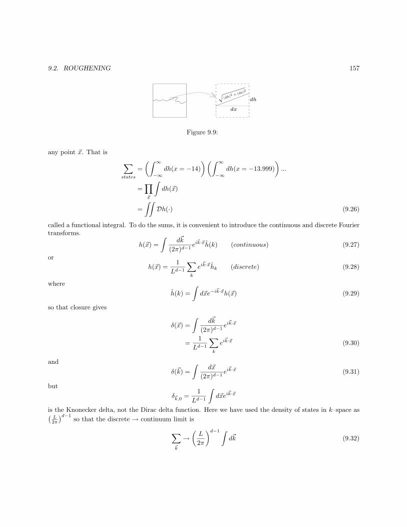
9.2. ROUGHENING 157
Figure 9.9:
any point ~x. That is
∑
states
=
(∫ ∞
−∞
dh(x = −14)
)(∫ ∞
−∞
dh(x = −13.999)
)
...
=∏
~x
∫
dh(~x)
=
∫∫
Dh(·) (9.26)
called a functional integral. To do the sums, it is convenient to introduce the continuous and discrete Fouriertransforms.
h(~x) =
∫d~k
(2π)d−1ei~k·~xh(k) (continuous) (9.27)
or
h(~x) =1
Ld−1
∑
k
ei~k·~xhk (discrete) (9.28)
where
h(k) =
∫
d~xe−i~k·~xh(~x) (9.29)
so that closure gives
δ(~x) =
∫d~k
(2π)d−1ei~k·~x
=1
Ld−1
∑
k
ei~k·~x (9.30)
and
δ(~k) =
∫d~x
(2π)d−1ei~k·~x (9.31)
but
δ~k,0 =1
Ld−1
∫
d~xei~k·~x
is the Knonecker delta, not the Dirac delta function. Here we have used the density of states in k–space as(L2π
)d−1so that the discrete → continuum limit is
∑
~k
→(L
2π
)d−1 ∫
d~k (9.32)
158 CHAPTER 9. INTERFACES IN EQUILIBRIUM AND OUT OF EQUILIBRIUM
and
Ld−1δ~k,0 → (2π)d−1δ(~k) (9.33)
we will flip back and forth between discrete and continuous transforms to make the algebra easier.Note that with the Fourier transforms
∫
d~x
(∂h
∂~x
)2
=
∫d~k
(2π)d−1 k2|h(k)|2
1Ld−1
∑
k k2|hk|2
(9.34)
so that modes of h are uncoupled in Fourier space. The partition function is therefore much easier to solvein Fourier space. Thus we need an expression for
∑
states using Fourier modes. An additional complication
results because hk is complex. Since h(~x) is real hk = h∗−k, so not all components are independent. We willdeal with this via a prime. To be precise
∑
states
=∏
~x
∫
dh(~x) =
′∏
~k
∫
d2hk (9.35)
where
d2hk = dℜe hk dℑmhk (9.36)
and′∏
~k
⇒ Restriction to half of k space to avoid double counting (9.37)
In fact, this restriction plays no role for our algebra below, but it is worth knowing.
Integration in ky > 0
only, for example
ky
kx
Figure 9.10:
Before grinding out our sums it is worth thinking a bit. We only need two moments,
〈h(~x1)〉
and
〈h(~x1)h(~x2)〉
However, space is translationally invariant, and isotropic in the ~x plane (the plane of the interface), so theproperties involving two points don’t depend on their exact positions, only the distance between them. Thatis
〈h(~x1)〉 Const. (9.38)
and
〈h(~x1)h(~x2)〉 = G(|~x1 − ~x2|)
9.2. ROUGHENING 159
~x1
|~x1 − ~x2|
~x2
0
Figure 9.11: ~x plane
Clearly, then, the Fourier transformed quantity satisfies
〈h(~k)h(~k′)〉 =
G(k)(2π)d−1δ(~k + ~k′)
or
GkLd−1δ~k+~k′,0
(9.39)
so the only nonzero two point correlation is
〈hkh−k〉 = 〈|hk|2〉 (9.40)
(The first moment 〈h〉 = 0 by symmetry.) So this is the only moment we will calculate. But,
〈|hk|2〉 =
∫d2hk|hk|2e−
σ2kBT
1
Ld−1 k2|hk|
2
∫d2hke
− σ2kBT
1
Ld−1 k2|hk|2
(9.41)
since all the other k’s cancel.Let hk = Reiθ, so we have
〈|hk|2〉 =
∫∞
0RdRR2 exp−
(σ
2kBT1
Ld−1 k2)
R2
∫∞
0RdR exp−
(σ
2kBT1
Ld−1 k2)
R2
which gives
〈|hk|2〉 =kBT
σk2Ld−1 (9.42)
and on using Eq. 9.31,〈h(~k)h(~k′)〉 = G(k)(2π)d−1δ(~k + ~k′) (9.43)
with
G(k) =kBT
σk2
This implies interface fluctuations are “self–affine”, since they are algebraically correlated (that is, by apower law). We define the surface correlation exponent η by
G(k) ∼ 1
k2−η(9.44)
for small k. Here, η = 0. The width w of the interface is the root–mean–square value of h at any point.That is
w2 = 〈h(~x)h(~x)〉 = 〈h(0)h(0)〉= 〈h2〉 (9.45)
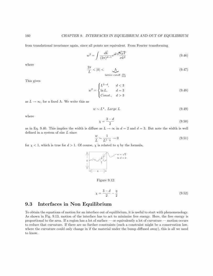
160 CHAPTER 9. INTERFACES IN EQUILIBRIUM AND OUT OF EQUILIBRIUM
from translational invariance again, since all points are equivalent. From Fourier transforming
w2 =
∫d~k
(2π)d−1e
* ~x=0
i~k·~x kBT
σk2(9.46)
where2π
L< |k| < Λ
︸︷︷︸
lattice cutoff 2π10A
(9.47)
This gives
w2 =
L3−d, d < 3
lnL, d = 3
Const., d > 3
(9.48)
as L→∞, for a fixed Λ. We write this as
w ∼ Lχ, Large L (9.49)
where
χ =3− d
2(9.50)
as in Eq. 9.40. This implies the width is diffuse as L → ∞ in d = 2 and d = 3. But note the width is welldefined in a system of size L since
w
L∼ 1
L1−χ→ 0 (9.51)
for χ < 1, which is true for d > 1. Of course, χ is related to η by the formula,
w ∼√L
in d = 2
L
L
Figure 9.12:
χ =3− d
2− η
2(9.52)
9.3 Interfaces in Non Equilibrium
To obtain the equations of motion for an interface out of equilibrium, it is useful to start with phenomenology.As shown in Fig. 9.13, motion of the interface has to act to minimize free energy. Here, the free energy isproportional to the area. If a region has a lot of surface — or equivalently a lot of curvature — motion occursto reduce that curvature. If there are no further constraints (such a constraint might be a conservation law,where the curvature could only change in if the material under the bump diffused away), this is all we needto know.
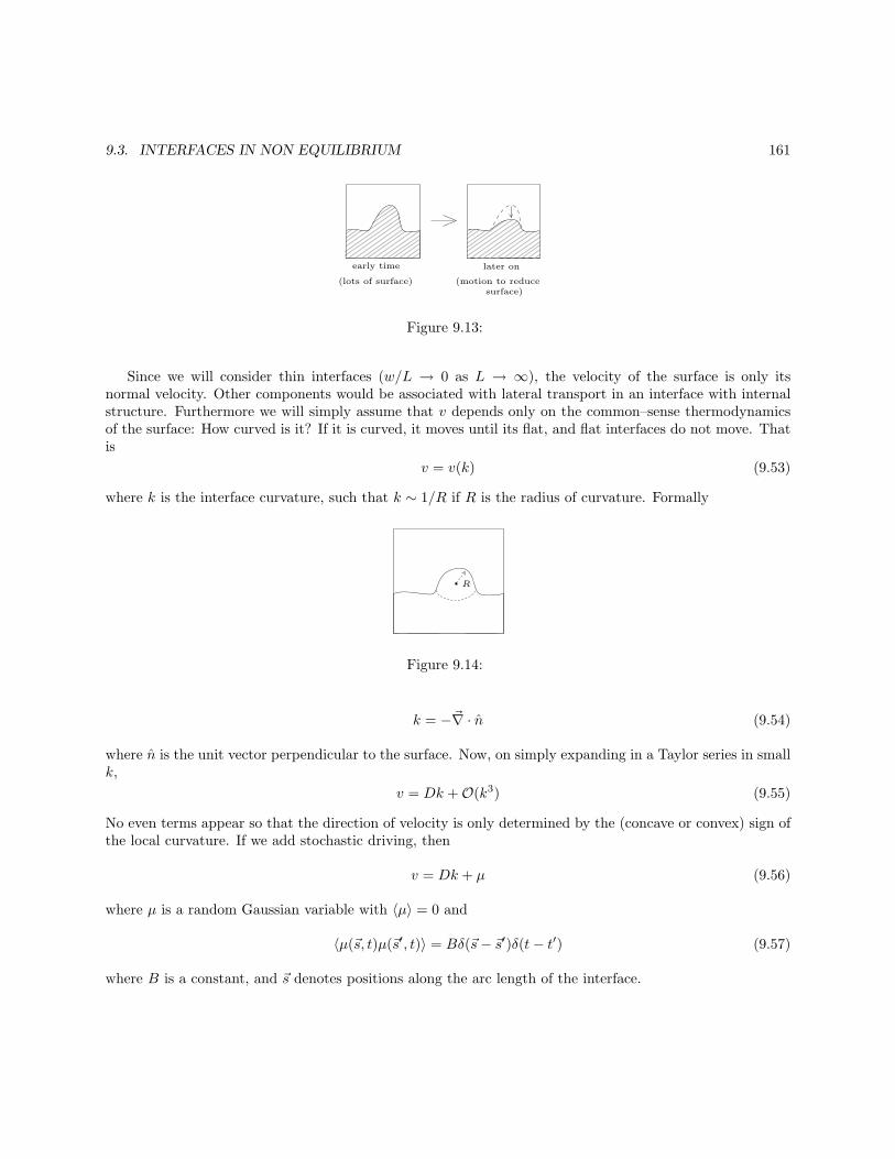
9.3. INTERFACES IN NON EQUILIBRIUM 161
early time
(lots of surface)
later on
(motion to reducesurface)
Figure 9.13:
Since we will consider thin interfaces (w/L → 0 as L → ∞), the velocity of the surface is only itsnormal velocity. Other components would be associated with lateral transport in an interface with internalstructure. Furthermore we will simply assume that v depends only on the common–sense thermodynamicsof the surface: How curved is it? If it is curved, it moves until its flat, and flat interfaces do not move. Thatis
v = v(k) (9.53)
where k is the interface curvature, such that k ∼ 1/R if R is the radius of curvature. Formally
R
Figure 9.14:
k = −~∇ · n (9.54)
where n is the unit vector perpendicular to the surface. Now, on simply expanding in a Taylor series in smallk,
v = Dk +O(k3) (9.55)
No even terms appear so that the direction of velocity is only determined by the (concave or convex) sign ofthe local curvature. If we add stochastic driving, then
v = Dk + µ (9.56)
where µ is a random Gaussian variable with 〈µ〉 = 0 and
〈µ(~s, t)µ(~s′, t)〉 = Bδ(~s− ~s′)δ(t− t′) (9.57)
where B is a constant, and ~s denotes positions along the arc length of the interface.
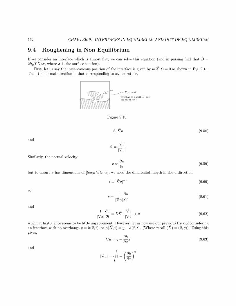
162 CHAPTER 9. INTERFACES IN EQUILIBRIUM AND OUT OF EQUILIBRIUM
9.4 Roughening in Non Equilibrium
If we consider an interface which is almost flat, we can solve this equation (and in passing find that B =2kBTD/σ, where σ is the surface tension).
First, let us say the instantaneous position of the interface is given by u( ~X, t) = 0 as shown in Fig. 9.15.Then the normal direction is that corresponding to du, or rather,
u( ~X, t) = 0
(overhangs possible, butno bubbles.)
Figure 9.15:
n||~∇u (9.58)
and
n =~∇u|~∇u|
Similarly, the normal velocity
v ∝ ∂u
∂t(9.59)
but to ensure v has dimensions of [length/time], we need the differential length in the u direction
l ≡ |~∇u|−1 (9.60)
so
v =1
|~∇u|∂u
∂t(9.61)
and1
|∇u|∂u
∂t= D~∇ ·
~∇u|∇u| + µ (9.62)
which at first glance seems to be little improvement! However, let us now use our previous trick of consideringan interface with no overhangs y = h(~x, t), or u( ~X, t) = y − h(~x, t). (Where recall ( ~X) = (~x, y)). Using thisgives,
~∇u = y − ∂h
∂xx (9.63)
and
|~∇u| =
√
1 +
(∂h
∂x
)2
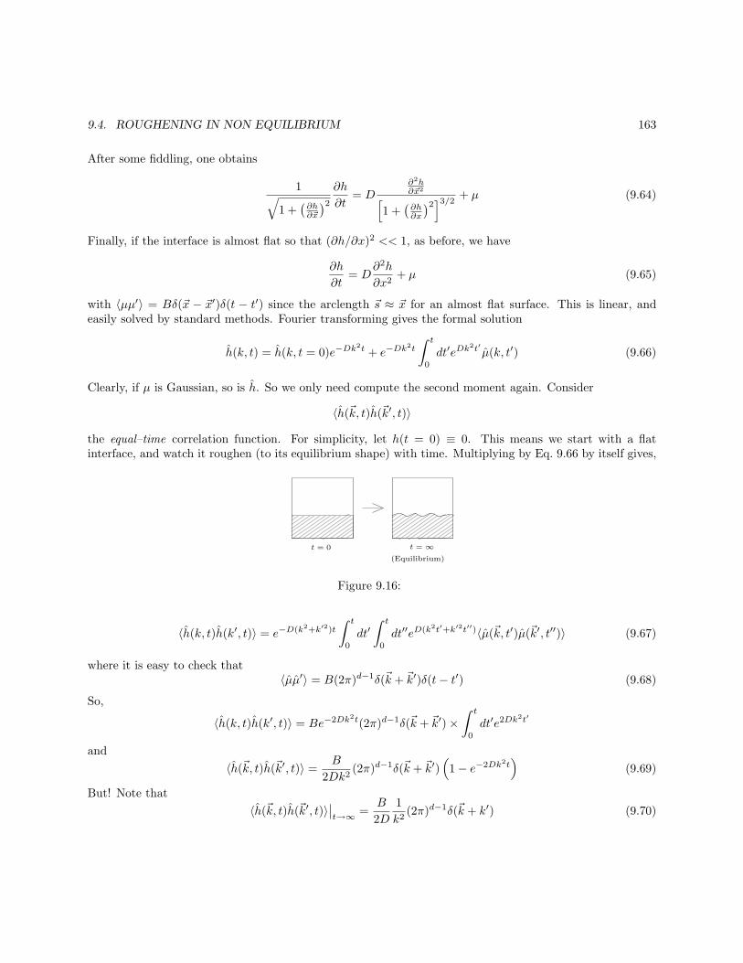
9.4. ROUGHENING IN NON EQUILIBRIUM 163
After some fiddling, one obtains
1√
1 +(∂h∂~x
)2
∂h
∂t= D
∂2h∂~x2
[
1 +(∂h∂x
)2]3/2
+ µ (9.64)
Finally, if the interface is almost flat so that (∂h/∂x)2 << 1, as before, we have
∂h
∂t= D
∂2h
∂x2+ µ (9.65)
with 〈µµ′〉 = Bδ(~x − ~x′)δ(t − t′) since the arclength ~s ≈ ~x for an almost flat surface. This is linear, andeasily solved by standard methods. Fourier transforming gives the formal solution
h(k, t) = h(k, t = 0)e−Dk2t + e−Dk
2t
∫ t
0
dt′eDk2t′ µ(k, t′) (9.66)
Clearly, if µ is Gaussian, so is h. So we only need compute the second moment again. Consider
〈h(~k, t)h(~k′, t)〉
the equal–time correlation function. For simplicity, let h(t = 0) ≡ 0. This means we start with a flatinterface, and watch it roughen (to its equilibrium shape) with time. Multiplying by Eq. 9.66 by itself gives,
t = 0 t = ∞(Equilibrium)
Figure 9.16:
〈h(k, t)h(k′, t)〉 = e−D(k2+k′2)t
∫ t
0
dt′∫ t
0
dt′′eD(k2t′+k′2t′′)〈µ(~k, t′)µ(~k′, t′′)〉 (9.67)
where it is easy to check that〈µµ′〉 = B(2π)d−1δ(~k + ~k′)δ(t− t′) (9.68)
So,
〈h(k, t)h(k′, t)〉 = Be−2Dk2t(2π)d−1δ(~k + ~k′)×∫ t
0
dt′e2Dk2t′
and
〈h(~k, t)h(~k′, t)〉 =B
2Dk2(2π)d−1δ(~k + ~k′)
(
1− e−2Dk2t)
(9.69)
But! Note that
〈h(~k, t)h(~k′, t)〉∣∣t→∞
=B
2D
1
k2(2π)d−1δ(~k + k′) (9.70)
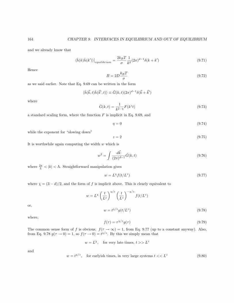
164 CHAPTER 9. INTERFACES IN EQUILIBRIUM AND OUT OF EQUILIBRIUM
and we already know that
〈h(k)h(k′)〉∣∣equilibrium
=2kBT
σ
1
k2(2π)d−1δ(k + k′) (9.71)
Hence
B = 2DkBT
σ(9.72)
as we said earlier. Note that Eq. 9.69 can be written in the form
〈h(~k, t)h(~k′, t)〉 ≡ G(k, t)(2π)d−1δ(~k + ~k′)
where
G(k, t) =1
k2−ηF (kzt) (9.73)
a standard scaling form, where the function F is implicit in Eq. 9.69, and
η = 0 (9.74)
while the exponent for “slowing down”
z = 2 (9.75)
It is worthwhile again computing the width w which is
w2 =
∫d~k
(2π)d−1G(k, t) (9.76)
where 2πL < |k| < Λ. Straightforward manipulation gives
w = Lχf(t/Lz) (9.77)
where χ = (3− d)/2, and the form of f is implicit above. This is clearly equivalent to
w = Lχ(t
Lz
)χ/z (t
Lz
)−χ/z
f(t/Lz)
or,
w = tχ/zg(t/Lz) (9.78)
where,
f(τ) = τχ/zg(τ) (9.79)
The common–sense form of f is obvious. f(τ → ∞) = 1, from Eq. 9.77 (up to a constant anyway). Also,from Eq. 9.78 g(τ → 0) = 1, so f(τ → 0) = tχ/z. By this we simply mean that
w = Lχ, for very late times, t >> Lz
and
w = tχ/z, for earlyish times, in very large systems t << Lz (9.80)
9.4. ROUGHENING IN NON EQUILIBRIUM 165
1
f(τ)
τ
τχz Const.
Figure 9.17:
These considerations are also true in more complicated, or different, models with different values of η, χ andz. As examples, I now go through a few other models.
Model 1: This one
Model 2: Local conservation
Model 3: Hydrodynamics
The dynamic roughening of interfaces close to equilibrium is fairly easy to explain with linear theory, andall quantities of interest can be calculated. Many of these considerations also apply to the roughening ofinterfaces which are far from equilibrium. We’ll assume the interface is in the ~x plane, with average position
x
y
y
x
or
h(x, t)
Figure 9.18:
being at y = 0. The height of the interface at any point and any time is h(~x, t). We’ll consider threedynamical models.
1. A system where no conservation laws impede the motion of the interface, like an antiphase boundaryin a binary alloy which orders like an antiferromagnet. Such a model can be derived from models Aor C, in the latter case where the conserved field is symmetrically coupled to the ordering field. Onefinds:
∂h
∂t= ν∇2h+ η (9.81)
where 〈η〉 = 0, and
〈η(~x, t)η(~x′, t′)〉 = 2νkBT
σδ(x− x′)δ(t− t′) (9.82)
where ν is a kinetic coefficient, and σ is surface tension.
2. A system where motion is limited by a conservation law, but where there is negligible diffusion inthe bulk. This describes some solid–state diffusion, and follows from Models B or C (for asymmetriccoupling), if long–range diffusion is neglected. One finds:
∂h
∂t= Γ∇4h+ ζ (9.83)
166 CHAPTER 9. INTERFACES IN EQUILIBRIUM AND OUT OF EQUILIBRIUM
where 〈ζ〉 = 0, and
〈ζ(~x, t)ζ(x′, t′)〉 = −2ΓkBT
σ∇2δ(x− x′)δ(t) (9.84)
where Γ is a kinetic coefficient. It is worthwhile, and not that hard, to do this for the case whenlong–range diffusion is included in models B and C.
3. A liquid–vapor system descrived by hydrodynamics. This is a long, though straightforward calculation,and is given below.
Say Fourier transforms are defined by
h(~k,w) =
∫
d~x dtei~k·~x+iwth(~x, t)
We’ll consider the correlation function
〈h(~x, t)h(~x′, t′)〉 = function(~x− ~x′, t− t′)
Translational invariance of space and time (in equilibrium) gives the equality. Hence we shall calculate thenontrivial Fourier transforms
S(k,w) =〈h(k,w)h(k′, w′)〉
(2π)dδ(k + k′)δ(w + w′)(9.85)
and
S(k) =〈h(k, t)h(k, t)〉
(2π)d−1δ(k + k′)(9.86)
which are usually called the inelastic and elastic structure factor. They are related to the real–space corre-lation function by
〈h(~x, t)h(0, 0)〉 =
∫dk
(2π)d−1
dw
2πe−i
~k·~x−iwtS(k,w) (9.87)
and
〈h(x, 0)h(0, 0)〉 =
∫d~k
(2π)d−1e−i
~k·~xS(k) (9.88)
Evidently we have the zeroth frequency sum rule
S(k) =
∫dw
2πS(k,w) (9.89)
and we have used Eq. 9.84 in Eq. 9.87 and Eq. 9.88 above.For interface fluctuations
S(k) =kBT
σ
1
k2(9.90)
So we must have ∫dw
2πS(k,w) =
kBT
σk2(9.91)
regardless of the dynamical model. This sum rule is enforced by the fluctuation dissipation relation for thenoise. For model 1, in Fourier space we have
−iwh = −νk2h+ η
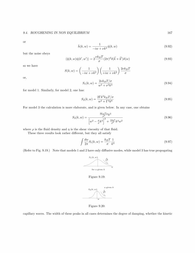
9.4. ROUGHENING IN NON EQUILIBRIUM 167
or
h(k,w) =1
−iw + νk2η(k,w) (9.92)
but the noise obeys
〈η(k,w)η(k′, w′)〉 = 2νkBT
σ(2π)dδ(~k + ~k′)δ(w) (9.93)
so we have
S(k,w) =
(1
−iw + νk2
)(1
+iw + νk2
)2νkBT
σ
or,
S1(k,w) =2νkBT/σ
w2 + ν2k4(9.94)
for model 1. Similarly, for model 2, one has:
S2(k,w) =2Γk2kBT/σ
w2 + Γ2k8(9.95)
For model 3 the calculation is more elaborate, and is given below. In any case, one obtains
S3(k,w) =
8kBTηρ2 k3
[
w2 − σρ k
3]2
+ 16η2
ρ2 k4w2
(9.96)
where ρ is the fluid density and η is the shear viscosity of that fluid.These three results look rather different, but they all satisfy
∫dw
2πSi(k,w) =
kBT
σ
1
k2(9.97)
(Refer to Fig. 9.19.) Note that models 1 and 2 have only diffusive modes, while model 3 has true propogating
w
S1(k, w)1k2
for a given k
Figure 9.19:
w
S2(k, w)1k4
a given k
Figure 9.20:
capillary waves. The width of these peaks in all cases determines the degree of damping, whether the kinetic
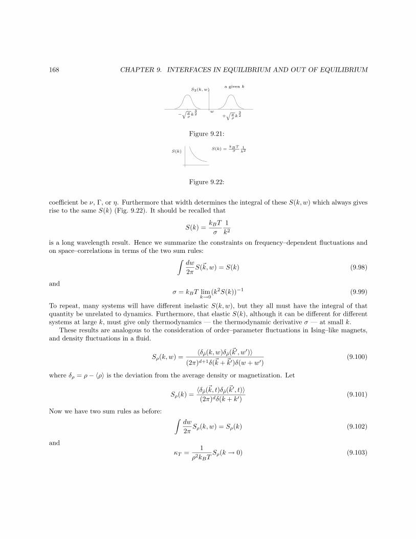
168 CHAPTER 9. INTERFACES IN EQUILIBRIUM AND OUT OF EQUILIBRIUM
w
S3(k, w)a given k
+q
σρk
32−
q
σρk
32
Figure 9.21:
S(k) =kBTσ
1k2S(k)
Figure 9.22:
coefficient be ν, Γ, or η. Furthermore that width determines the integral of these S(k,w) which always givesrise to the same S(k) (Fig. 9.22). It should be recalled that
S(k) =kBT
σ
1
k2
is a long wavelength result. Hence we summarize the constraints on frequency–dependent fluctuations andon space–correlations in terms of the two sum rules:
∫dw
2πS(~k,w) = S(k) (9.98)
andσ = kBT lim
k→0(k2S(k))−1 (9.99)
To repeat, many systems will have different inelastic S(k,w), but they all must have the integral of thatquantity be unrelated to dynamics. Furthermore, that elastic S(k), although it can be different for differentsystems at large k, must give only thermodynamics — the thermodynamic derivative σ — at small k.
These results are analogous to the consideration of order–parameter fluctuations in Ising–like magnets,and density fluctuations in a fluid.
Sρ(k,w) =〈δρ(k,w)δρ(~k
′, w′)〉(2π)d+1δ(~k + ~k′)δ(w + w′)
(9.100)
where δρ = ρ− 〈ρ〉 is the deviation from the average density or magnetization. Let
Sρ(k) =〈δρ(~k, t)δρ(~k′, t)〉(2π)dδ(k + k′)
(9.101)
Now we have two sum rules as before:∫dw
2πSρ(k,w) = Sρ(k) (9.102)
and
κT =1
ρ2kBTSρ(k → 0) (9.103)

9.4. ROUGHENING IN NON EQUILIBRIUM 169
w
for a given k
+ck−cknon propagating magnet
w
Sρ(k, w) Sρ(k, w)
(isothermal) fluid, soundspeed = c
Figure 9.23:
Sρ(k)κT ρ
2kBT
κT ρ2kBT
ξ2k2+1
k
Figure 9.24: There can be more complicated structure at large k, and different systems can have differentcomplicated structure.
is the isothermal compresibility or susceptibility (refer to figures 9.23 and 9.24). Before giving the derivationof S(k,w) for the fluid surface, its useful to set notation for scaling forms of S(k,w) and S(k) for surfaces.
We write (as k → 0),
S(k) ∼ 1
k2−η(9.104)
where η is an exponent usually not used, instead we usually use χ defined by
η
2=
3− d2− χ (9.105)
Of course in linear theory, η = 0 and χ = 3−d2 , where d is the dimension of full space. In an analogous way
we introduce the slowing down exponent z via (as k → 0, w → 0),
S(k,w) ∼ 1
k2−η+zf(wk−z) (9.106)
where f(Ω) is a scaling function, and Eq. 9.78 is satisfied for the frequency sum rule. For model 1, η = 0,z = 2 and
f1(Ω) =1
Ω2 + Ω2o
(9.107)
while for model 2, η = 0, z = 4 and
f2(Ω) =1
Ω2 + Ω2o
(9.108)
where Ω2o is a constant. The case for model 3 is more subtle, and it will be discussed below.
Model 3, capillary waves on a liquid surface. Capillary waves arise if one perturbs a fluid’s surface. Surfacetension σ acts as a restoring force, driving capillary waves. Dimensional analysis frequency, w(k) = w[σ, ρ, k]so,
w(k) =
√σ
ρ︸︷︷︸
like a simpleharmonic oscillator
k3/2︸︷︷︸
to makedimensions right
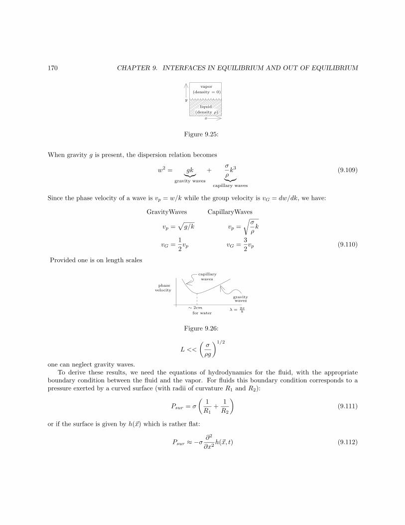
170 CHAPTER 9. INTERFACES IN EQUILIBRIUM AND OUT OF EQUILIBRIUM
liquid
(density ρ)
vapor
(density = 0)
y
x
Figure 9.25:
When gravity g is present, the dispersion relation becomes
w2 = gk︸︷︷︸
gravity waves
+σ
ρk3
︸︷︷︸
capillary waves
(9.109)
Since the phase velocity of a wave is vp = w/k while the group velocity is vG = dw/dk, we have:
GravityWaves CapillaryWaves
vp =√
g/k vp =
√σ
ρk
vG =1
2vp vG =
3
2vp (9.110)
Provided one is on length scales
λ = 2πk
gravitywaves
capillary
waves
∼ 2cm
for water
phasevelocity
Figure 9.26:
L <<
(σ
ρg
)1/2
one can neglect gravity waves.To derive these results, we need the equations of hydrodynamics for the fluid, with the appropriate
boundary condition between the fluid and the vapor. For fluids this boundary condition corresponds to apressure exerted by a curved surface (with radii of curvature R1 and R2):
Psur = σ
(1
R1+
1
R2
)
(9.111)
or if the surface is given by h(~x) which is rather flat:
Psur ≈ −σ∂2
∂x2h(~x, t) (9.112)
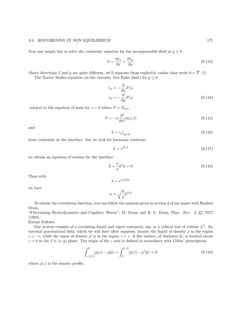
9.4. ROUGHENING IN NON EQUILIBRIUM 171
Now one simply has to solve the continuity equation for the incompressible fluid at y ≤ 0
0 =∂vx∂x
+∂vy∂y
(9.113)
(Since directions ~x and y are quite different, we’ll separate them explicitly, rather than write 0 = ~∇ · ~v).The Navier–Stokes equation (in the viscosity–free Euler limit) for y ≤ 0
vx = − ∂
∂xP/ρ
vy = − ∂
∂yP/ρ (9.114)
subject to the equation of state for z = 0 where P = Psur,
P = −σ ∂2
∂x2h(x, t) (9.115)
andh = vy
∣∣y=0
(9.116)
from continuity at the interface. Say we look for harmonic solutions
h ∼ ei~k·~x (9.117)
we obtain an equation of motion for the interface
h+σ
ρk3h = 0 (9.118)
Then withh ∼ eiw(k)t
we have
w =
√σ
ρk3/2
To obtain the correlation function, you can follow the analysis given in section 2 of my paper with RashmiDesai,“Fluctuating Hydrodynamics and Capillary Waves”, M. Grant and R. C. Desai, Phys. Rev. A 27, 2577(1983).Exerpt Follows:
Our system consists of a coexisting liquid and vapor contained, say, in a cubical box of volume L3. Anexternal gravitational field, which we will here–after suppress, locates the liquid of density ρ in the regionz < −ǫ, while the vapor of density ρ′ is in the region z < ǫ. A flat surface, of thickness 2ǫ, is located aboutz = 0 in the ~x ≡ (x, y) plane. The origin of the z axis is defined in accordance with Gibbs’ prescription:
∫ 0
−L/2
[ρ(z)− ρ]dz +
∫ L/2
0
[ρ(z)− ρ′]dz = 0 (9.119)
where ρ(z) is the density profile.
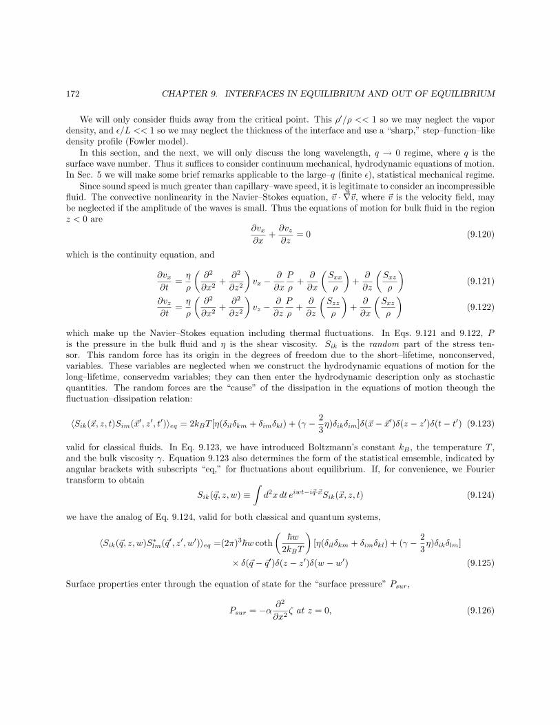
172 CHAPTER 9. INTERFACES IN EQUILIBRIUM AND OUT OF EQUILIBRIUM
We will only consider fluids away from the critical point. This ρ′/ρ << 1 so we may neglect the vapordensity, and ǫ/L << 1 so we may neglect the thickness of the interface and use a “sharp,” step–function–likedensity profile (Fowler model).
In this section, and the next, we will only discuss the long wavelength, q → 0 regime, where q is thesurface wave number. Thus it suffices to consider continuum mechanical, hydrodynamic equations of motion.In Sec. 5 we will make some brief remarks applicable to the large–q (finite ǫ), statistical mechanical regime.
Since sound speed is much greater than capillary–wave speed, it is legitimate to consider an incompressiblefluid. The convective nonlinearity in the Navier–Stokes equation, ~v · ~∇~v, where ~v is the velocity field, maybe neglected if the amplitude of the waves is small. Thus the equations of motion for bulk fluid in the regionz < 0 are
∂vx∂x
+∂vz∂z
= 0 (9.120)
which is the continuity equation, and
∂vx∂t
=η
ρ
(∂2
∂x2+
∂2
∂z2
)
vx −∂
∂x
P
ρ+
∂
∂x
(Sxxρ
)
+∂
∂z
(Sxzρ
)
(9.121)
∂vz∂t
=η
ρ
(∂2
∂x2+
∂2
∂z2
)
vz −∂
∂z
P
ρ+
∂
∂z
(Szzρ
)
+∂
∂x
(Sxzρ
)
(9.122)
which make up the Navier–Stokes equation including thermal fluctuations. In Eqs. 9.121 and 9.122, Pis the pressure in the bulk fluid and η is the shear viscosity. Sik is the random part of the stress ten-sor. This random force has its origin in the degrees of freedom due to the short–lifetime, nonconserved,variables. These variables are neglected when we construct the hydrodynamic equations of motion for thelong–lifetime, conservedm variables; they can then enter the hydrodynamic description only as stochasticquantities. The random forces are the “cause” of the dissipation in the equations of motion theough thefluctuation–dissipation relation:
〈Sik(~x, z, t)Sim(~x′, z′, t′)〉eq = 2kBT [η(δilδkm + δimδkl) + (γ − 2
3η)δikδim]δ(~x− ~x′)δ(z − z′)δ(t− t′) (9.123)
valid for classical fluids. In Eq. 9.123, we have introduced Boltzmann’s constant kB , the temperature T ,and the bulk viscosity γ. Equation 9.123 also determines the form of the statistical emsemble, indicated byangular brackets with subscripts “eq,” for fluctuations about equilibrium. If, for convenience, we Fouriertransform to obtain
Sik(~q, z, w) ≡∫
d2x dt eiwt−i~q·~xSik(~x, z, t) (9.124)
we have the analog of Eq. 9.124, valid for both classical and quantum systems,
〈Sik(~q, z, w)S∗lm(~q′, z′, w′)〉eq =(2π)3~w coth
(~w
2kBT
)
[η(δilδkm + δimδkl) + (γ − 2
3η)δikδlm]
× δ(~q − ~q′)δ(z − z′)δ(w − w′) (9.125)
Surface properties enter through the equation of state for the “surface pressure” Psur,
Psur = −α ∂2
∂x2ζ at z = 0, (9.126)
9.4. ROUGHENING IN NON EQUILIBRIUM 173
called the Laplace–Young relation, where α is the surface tension. The nonconserved variable ζ(~x, t) is theinstantaneous position of the Gibbs surface; it is hydrodynamically defined by
ζ = vz at z = 0. (9.127)
We note that a statistical mechanical approach gives
ζ(~x, t) =1
(ρ− ρ′)
∫ ǫ
−ǫ
dzδρ(~x, z, t) (9.128)
exactly. Where δρ(~x, z, t) is the fluctuation in number density, ρ′ is again the vapor density, and the integralruns over the surface region; see also Eq. 9.119 which defines the Gibbs interface.
The “boundary conditions” between the infinitesmally thin surface and the bulk liquid give
P = −α∂2ζ
∂x2+ 2η
∂vx∂z
+ Szz (9.129)
at z = 0, and
η
(∂vx∂z
+∂vz∂x
)
= −Sxz (9.130)
at z = 0. Equations 9.129 and 9.130 state that there is a mechanical equilibrium at the interface, and soboth the normal and tangential forces at z = 0 are balanced. If the surface tension is a function of positionx, there will be an additional contribution, ∂α/∂x, to the right–hand side of Eq. 9.130.
These equations are valid for fluctuations about equilibrium; they are valid for fluctuations about anonequilibrium steady state under restrictions discussed in the next section. The equations may be triviallymodified to apply to superfluid helium II in the limit if a “completely incompressable” superfluid.
We solved Eqs. 9.120–9.122, 9.127, 9.129, and 9.130 with the Fourier transform introduced in Eq. 9.126.The analysis is simplified with the use of the following Green’s–function identity:
(d2
dz2− q2
)1
2qe−q|z−z
′| = −δ(z − z′) (9.131)
It is then straightforward to obtain the following “equation of motion” for the interface:
∂2ζ(~q, t)
∂t2+ w2
c (q)ζ(~q, t) + 2ǫc(q)∂ζ(~q, t)
∂t= −q
2
ρ
∫ 0
−∞
dz eqz[Szz(~q, z, t)− Sxx(~q, z, t)− 2iSxz(~q, z, t)] (9.132)
valid in the small viscosity limit ǫc(q)/wc(q) << 1 where
wc(q) =
(α
ρ
)1/2
q3/2 (9.133)
is the characteristic frequency of the capillary waves, and
ǫc(q) =2η
ρq2 (9.134)
gives their viscous damping. This equation is also valid for superfluid helium II in the limit of a completelyincompressible superfluid.
174 CHAPTER 9. INTERFACES IN EQUILIBRIUM AND OUT OF EQUILIBRIUM
Equation 9.132 does not seem to have appeared in the literature before. Its relatively simple form tells usa great deal about the nature of the interface: (i) The equation is of form of a damped oscillator driven byspontaneous thermal fluctuations, and (ii) there are no special capillary–wave fluctuations in the equation,the thermal random force fluctuations are in the bulk and are coupled to the surface by the exp(qz) factor.
This surface–bulk coupling is an essential ingredient of any hydrodynamic theory of the liquid surface;the surface is not a seperable phase, it is a transition zone between two bulk phases and depends uponcoupling to the bulk phases as well as upon intrinsic surface properties. One can see this in an example aspedestrian as the nonanalytic dispersion relation for capillary waves, w2 ∼ q3: Two of the q’s come from thesurface (i.e., from the Fourier transform of the ~x plane), while the other q comes from coupling to the bulkfluid. We will discuss this point further in Sec. 4. Having obtained Eq. 9.132, we will now use in the nexttwo sections.End of Exerpt
9.5 Dynamical Interfaces From Full Model
The formal derivation of the interface equations of motion can be done from first principles of the equationof motion for the order parameters.
Say one is considering the nonconserved order parameter Ising model (model A)
∂ψ
∂t= −Γ
δF
δψ+ η (9.135)
〈ηη′〉 = 2kBTΓδ( ~X − ~X ′)δ(t− t′) (9.136)
where
F =
∫
d~x[ c
2(∇ψ)2 + f(ψ)
]
(9.137)
and the field H = 0, since we are considering an inhomogeneous phase. The bulk free energy has the form
f(ψ) = −r2ψ2 +
u
4ψ4 (9.138)
for example. To write out Eq. 9.135, it is necessary to take functional derivatives with δ/δψ(~x). Here is a
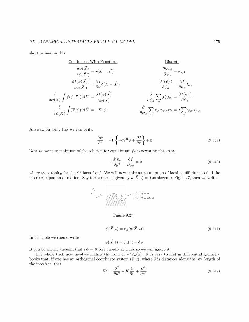
9.5. DYNAMICAL INTERFACES FROM FULL MODEL 175
short primer on this.
Continuous With Functions Discrete
δψ( ~X)
δψ( ~X ′)= δ( ~X − ~X ′)
∂∂ψβ∂ψα
= δα,β
δf(ψ( ~X))
δψ( ~X ′)=∂f
∂ψδ( ~X − ~X ′)
∂f(ψβ)
∂ψα=
∂f
∂ψαδα,β
δ
δψ(X)
∫
f(ψ(X ′))dX ′ =∂f(ψ( ~X)
∂ψ( ~X)
∂
∂ψα
∑
β
f(ψβ) =∂f(ψα)
∂ψα
δ
δψ( ~X)
∫
(∇′ψ)2d ~X ′ = −∇2ψ∂
∂ψα
∑
β,γ
ψβ∆β,γψγ = 2∑
β
ψβ∆β,α
Anyway, on using this we can write,
∂ψ
∂t= −Γ
−c∇2ψ +∂f
∂ψ
+ η (9.139)
Now we want to make use of the solution for equilibrium flat coexisting phases ψo:
−cd2ψody2
+∂f
∂ψo= 0 (9.140)
where ψo ∝ tanh y for the ψ4 form for f . We will now make an assumption of local equilibrium to find theinterface equation of motion. Say the surface is given by u( ~X, t) = 0 as shown in Fig. 9.27, then we write
y
~x
u( ~X, t) = 0
with ~X = (~x, y)
Figure 9.27:
ψ( ~X, t) = ψo(u( ~X, t)) (9.141)
In principle we should writeψ( ~X, t) = ψo(u) + δψ.
It can be shown, though, that δψ → 0 very rapidly in time, so we will ignore it.The whole trick now involves finding the form of ∇2ψo(u). It is easy to find in differential geometry
books that, if one has an orthogonal coordinate system (~s, u), where ~s is distances along the arc length ofthe interface, that
∇2 =∂2
∂u2+K
∂
∂u+
∂2
∂s2(9.142)
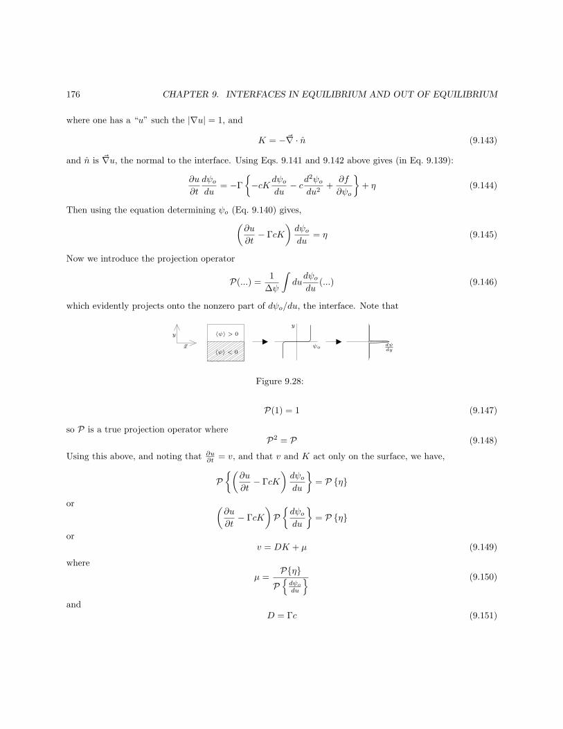
176 CHAPTER 9. INTERFACES IN EQUILIBRIUM AND OUT OF EQUILIBRIUM
where one has a “u” such the |∇u| = 1, and
K = −~∇ · n (9.143)
and n is ~∇u, the normal to the interface. Using Eqs. 9.141 and 9.142 above gives (in Eq. 9.139):
∂u
∂t
dψodu
= −Γ
−cK dψodu− cd
2ψodu2
+∂f
∂ψo
+ η (9.144)
Then using the equation determining ψo (Eq. 9.140) gives,
(∂u
∂t− ΓcK
)dψodu
= η (9.145)
Now we introduce the projection operator
P(...) =1
∆ψ
∫
dudψodu
(...) (9.146)
which evidently projects onto the nonzero part of dψo/du, the interface. Note that
〈ψ〉 > 0
〈ψ〉 < 0
y
~x
y
ψo dψdy
Figure 9.28:
P(1) = 1 (9.147)
so P is a true projection operator whereP2 = P (9.148)
Using this above, and noting that ∂u∂t = v, and that v and K act only on the surface, we have,
P(
∂u
∂t− ΓcK
)dψodu
= P η
or (∂u
∂t− ΓcK
)
Pdψodu
= P η
orv = DK + µ (9.149)
where
µ =PηPdψodu
(9.150)
andD = Γc (9.151)
9.6. CURVILINEAR COORDINATES 177
It remains to determine the form of µ. Since it is a linear combination of η’s, µ is a Gaussian variable withzero mean, so we only need its second moment:
〈µ(~s, t)µ(~s′, t′)〉 = Aδ(~s− ~s′)δ(t− t′) (9.152)
where the delta functions follow because it is random, and A is to be determined. In any case, this momentis
〈µµ′〉 =〈PηPη′〉
Pdψodu
Pdψodu′
(9.153)
But
Pdψodu
=1
∆ψ
∫
du
(dψodu
)2
=1
∆ψ
σ
c(9.154)
so Eq. 9.153 becomes,
〈µµ′〉 =
(∆ψc
σ
)21
(∆ψ)2
∫∫
dudu′dψodu
dψodu′× 2kBTΓδ(u− u′)δ(~s− ~s′)δ(t− t′)
usingδ( ~X − ~X ′) = δ(u− u′)δ(~s− ~s′)
so that
〈µµ′〉 = 2kBTΓ( c
σ
)2
∫
du
>σ/c
(dψodu
)2
δ(~s− ~s′)δ(t− t′)
or,
〈µµ′〉 =2kBT
σDδ(~s− ~s′)δ(t− t′) (9.155)
wherev = Dk + µ
as we wrote down before.
9.6 Curvilinear Coordinates
Its worth taking a minute to reconsider Eq. 9.142.
∇2 =∂2
∂u2+K
∂
∂u+
∂2
∂s2
where u( ~X, t) = 0 determines the surface. Note that any point is given by
~X(u, s) = ~R+ un(s) (9.156)

178 CHAPTER 9. INTERFACES IN EQUILIBRIUM AND OUT OF EQUILIBRIUM
y
~x
nn
s = 0s = 1
s = 2
s = 3
u = +1
u = 0
u = −1~X
~R
t
θ
Note, ~X = ~R + un
Figure 9.29:
The metric is
gαβ =d ~X
dwαd ~X
dwβ(9.157)
where
α = 1, 2, ..., d
w1 = u, w2 = s (9.158)
d ~X
ds=d~R
ds+ u
dn
ds;
d ~X
du= n(s)
The normal and tangent unit vectors are
n
tθ
Figure 9.30:
t = x cos θ + y sin θ
n = −x sin θ + y cos θ (9.159)
withd~R
ds= t (9.160)
Hence,
d ~X
ds= t
(
1− udθds
)
(9.161)
But the curvature is
K = −dθds
(9.162)
so the metric is
g =
(1 00 (1 + uK)2
)
(9.163)
9.6. CURVILINEAR COORDINATES 179
The Laplacian is
∇2 =∑
αβ
1√g
∂
∂wα√ggαβ
∂
∂wβ(9.164)
so
∇2 =1
1 + uK
∂
∂u(1 + uK)
∂
∂u+
∂
∂s(1 + uK)3
∂
∂s
or,
∇2 =∂2
∂u2+
K
1 + uK
∂
∂u+ (1 + uK)2
∂2
∂s2+ 3(1 + uK)u
∂K
∂s
∂
∂s(9.165)
But, at u = 0, or close to it
∇2 =∂2
∂u2+K
∂
∂u+
∂2
∂s2(9.166)
as used previously.

180 CHAPTER 9. INTERFACES IN EQUILIBRIUM AND OUT OF EQUILIBRIUM
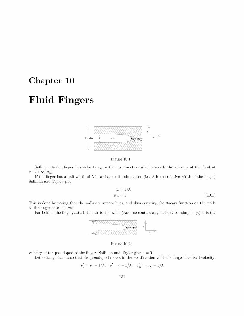
Chapter 10
Fluid Fingers
2 units 2λ air vo v∞x
y
Figure 10.1:
Saffman–Taylor finger has velocity vo in the +x direction which exceeds the velocity of the fluid atx→ +∞, v∞.
If the finger has a half width of λ in a channel 2 units across (i.e. λ is the relative width of the finger)Saffman and Taylor give
vo = 1/λ
v∞ = 1 (10.1)
This is done by noting that the walls are stream lines, and thus equating the stream function on the wallsto the finger at x→ −∞.
Far behind the finger, attach the air to the wall. (Assume contact angle of π/2 for simplicity.) v is the
vo v∞
x
y
v
v
Figure 10.2:
velocity of the pseudopod of the finger. Saffman and Taylor give v = 0.Let’s change frames so that the pseudopod moves in the −x direction while the finger has fixed velocity:
v′o = vo − 1/λ, v′ = v − 1/λ, v′∞ = v∞ − 1/λ
181
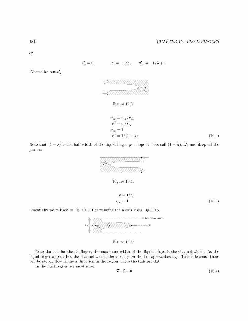
182 CHAPTER 10. FLUID FINGERS
or
v′o = 0, v′ = −1/λ, v′∞ = −1/λ+ 1
Normalize out v′∞
v′∞
v′
v′
Figure 10.3:
v′′∞ ≡ v′∞/v′∞v′′ = v′/v′∞
v′′∞ = 1
v′′ = 1/(1− λ) (10.2)
Note that (1 − λ) is the half width of the liquid finger pseudopod. Lets call (1 − Λ), λ′, and drop all theprimes.
v′∞v
v
Figure 10.4:
v = 1/λ
v∞ = 1 (10.3)
Essentially we’re back to Eq. 10.1. Rearranging the y axis gives Fig. 10.5.
v∞ v2λ2 units
axis of symmetry
walls
Figure 10.5:
Note that, as for the air finger, the maximum width of the liquid finger is the channel width. As theliquid finger approaches the channel width, the velocity on the tail approaches v∞. This is because therewill be steady flow in the x direction in the region where the tails are flat.
In the fluid region, we must solve~∇ · ~v = 0 (10.4)
183
given that
~v = (~∇φ)η (10.5)
where the velocity potential is proportional to the pressure.
I’m supposing that nothing of consequence happens to 10.5 when I change frames (and thus subtract
(~∇φ), for φ→ 0, from ~v). The liquid finger is determined by it being a line of constant pressure, say φ = 0.
Since ∇2φ = 0, in two dimensions, introduce a stream function ψ such that the complex velocity potentialw is
w = φ+ iψ (10.6)
where dw/dz is analytic (z = x+ iy). Thus
dφ
dx=dψ
dy,
dφ
dy= −dψ
dx(10.7)
[Or, ~∇ · ~v = 0 is satisfied by vx = dψ/dy if vy = −dψ/dx, which gives 10.7.] We must now solve one from
∇2
xyφψ
= 0 (10.8)
where ∇2 = ∂2
∂x2 + ∂2
∂y2 , or, ∂2
∂φ2 + ∂2
∂ψ2 , (the differential lengths |∇φ| as |∇ψ| don’t do anything). Saffmanand Taylor solve:
(∂2
∂φ2+
∂2
∂ψ2
)
y = 0 (10.9)
which is what I will attempt. First we need another picture. Note that if x · ~v is constant then
x · ~v ≡ vx =dφ
dx=
(φ
x
)η
=dψ
dy=ψ
y(10.10)
up to a constant, which should be no problem. Thus, for φ = 0, where vx = v, we have
ψ
y= v, at φ = 0 (10.11)
= 1/λ
Furthermore (from Fig. 10.5), for x→ −∞
v∞ =φ
x
1 ≡ φ
x=ψ
y(10.12)
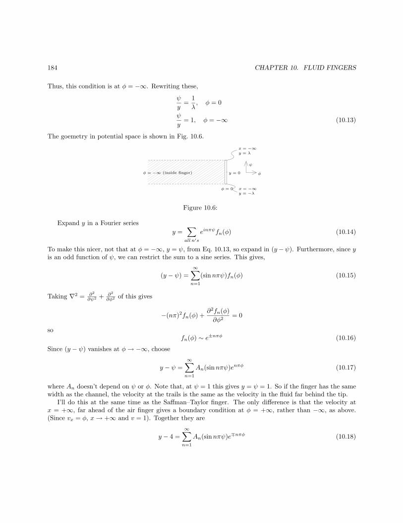
184 CHAPTER 10. FLUID FINGERS
Thus, this condition is at φ = −∞. Rewriting these,
ψ
y=
1
λ, φ = 0
ψ
y= 1, φ = −∞ (10.13)
The goemetry in potential space is shown in Fig. 10.6.
φ = −∞ (inside finger)
ψ
φ
x = −∞
x = −∞
y = λ
y = −λ
y = 0
φ = 0
Figure 10.6:
Expand y in a Fourier series
y =∑
all n′s
einπψfn(φ) (10.14)
To make this nicer, not that at φ = −∞, y = ψ, from Eq. 10.13, so expand in (y−ψ). Furthermore, since yis an odd function of ψ, we can restrict the sum to a sine series. This gives,
(y − ψ) =∞∑
n=1
(sinnπψ)fn(φ) (10.15)
Taking ∇2 = ∂2
∂ψ2 + ∂2
∂φ2 of this gives
−(nπ)2fn(φ) +∂2fn(φ)
∂φ2= 0
sofn(φ) ∼ e±nπφ (10.16)
Since (y − ψ) vanishes at φ→ −∞, choose
y − ψ =
∞∑
n=1
An(sinnπψ)enπφ (10.17)
where An doesn’t depend on ψ or φ. Note that, at ψ = 1 this gives y = ψ = 1. So if the finger has the samewidth as the channel, the velocity at the trails is the same as the velocity in the fluid far behind the tip.
I’ll do this at the same time as the Saffman–Taylor finger. The only difference is that the velocity atx = +∞, far ahead of the air finger gives a boundary condition at φ = +∞, rather than −∞, as above.(Since vx = φ, x→ +∞ and v = 1). Together they are
y − 4 =
∞∑
n=1
An(sinnπψ)e∓nπφ (10.18)
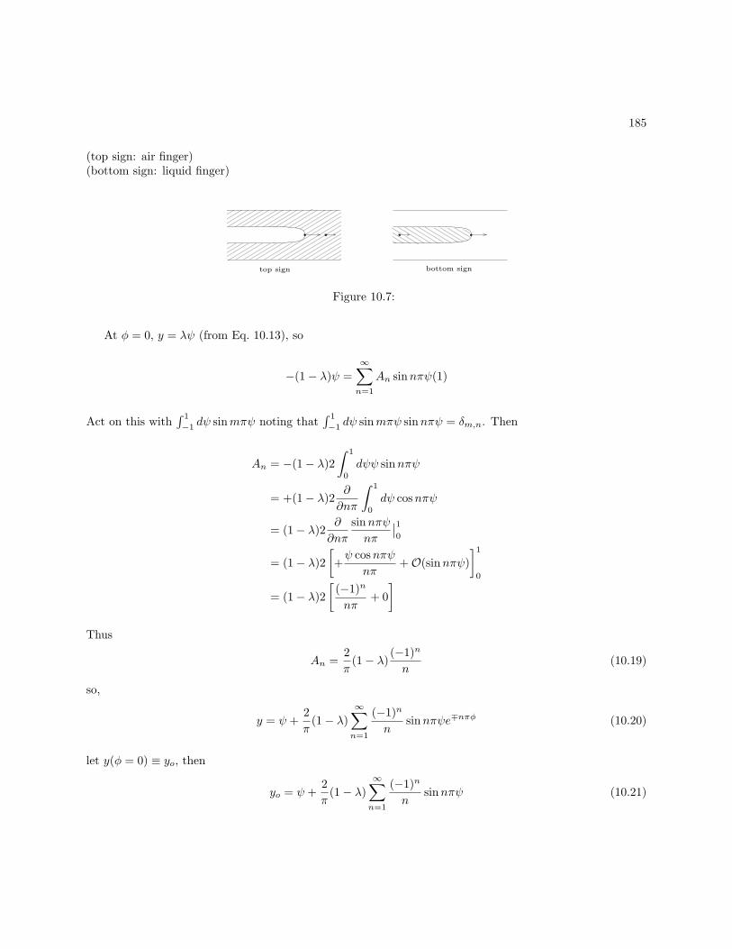
185
(top sign: air finger)(bottom sign: liquid finger)
top sign bottom sign
Figure 10.7:
At φ = 0, y = λψ (from Eq. 10.13), so
−(1− λ)ψ =
∞∑
n=1
An sinnπψ(1)
Act on this with∫ 1
−1dψ sinmπψ noting that
∫ 1
−1dψ sinmπψ sinnπψ = δm,n. Then
An = −(1− λ)2
∫ 1
0
dψψ sinnπψ
= +(1− λ)2∂
∂nπ
∫ 1
0
dψ cosnπψ
= (1− λ)2∂
∂nπ
sinnπψ
nπ
∣∣1
0
= (1− λ)2
[
+ψ cosnπψ
nπ+O(sinnπψ)
]1
0
= (1− λ)2
[(−1)n
nπ+ 0
]
Thus
An =2
π(1− λ)
(−1)n
n(10.19)
so,
y = ψ +2
π(1− λ)
∞∑
n=1
(−1)n
nsinnπψe∓nπφ (10.20)
let y(φ = 0) ≡ yo, then
yo = ψ +2
π(1− λ)
∞∑
n=1
(−1)n
nsinnπψ (10.21)
186 CHAPTER 10. FLUID FINGERS
Now we’ll do the sum. Consider∞∑
n=1
(−1)n
neinπψ =
∞∑
n=1
(−eiπψ
)n
n
=∞∑
n=1
rn
n
=
∞∑
n=1
∫ r
0
dr′r′n−1
=
∫ r
0
dr′∞∑
n=0
r′n
=
∫ r
0
dr′1
1− r′= − ln |1− r|= − ln
[1 + eiπψ
]
= − ln eiπψ2 2 cosπψ/2
Thus∞∑
n=1
(−1)n
neinπψ = − ln 2 cos
πψ
2− iψ
2ψ (10.22)
(Note that the e−nπ|φ| factors in 10.20 act to ensure convergence also.) Using this in 10.21 gives
yo = ψ +2
π(1− λ)
(
−π2ψ)
= ψ − ψ + λψ (10.23)
So, yo = λψ (as we already knew). From 10.20
dy
dψ= 1 +
2
π(1− λ)
∞∑
n=1
(−1)n
n(nπ) cosnπψe∓nπφ
But dydψ = dx
dφ . Thus,
dx
dφ= 1 + 2(1− λ)
∞∑
n=1
(−1)n cosnπψe∓nπφ
or,
dx = dφ+ 2(1− λ)∞∑
n=1
(−1)n cosnπψe∓nπφdφ
For the top sign (the air finger) we integrate from φ = 0 to φ = ∞, while x goes from xo to ∞. For thebottom sign (the liquid finger) we integrate from φ = −∞ to φ = 0, while x goes from −∞ to xo. (SeeFig. 10.7). Thus
∫ ∞/xo
xo/−∞
dx−∫ ∞/0
0/−∞
dφ = 2(1− λ)
∞∑
n=1
(−1)n cosnπψ
∫ ∞/0
0/−∞
e∓nπφdφ (10.24)
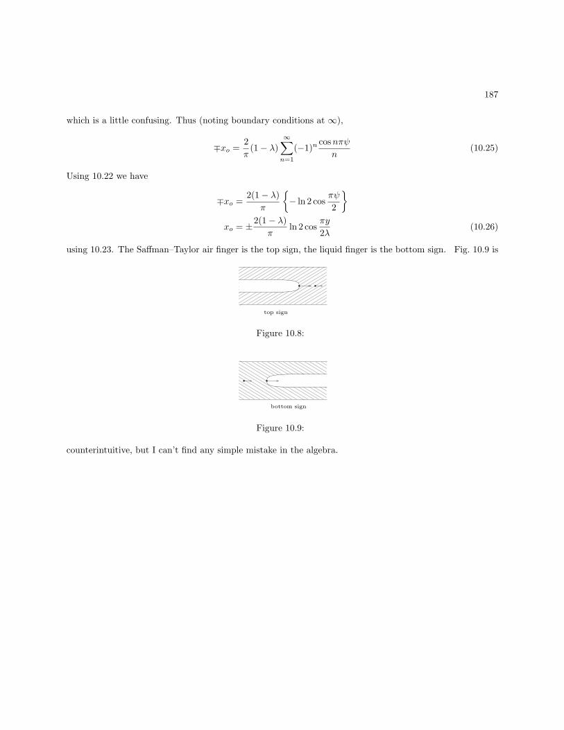
187
which is a little confusing. Thus (noting boundary conditions at ∞),
∓xo =2
π(1− λ)
∞∑
n=1
(−1)ncosnπψ
n(10.25)
Using 10.22 we have
∓xo =2(1− λ)
π
− ln 2 cosπψ
2
xo = ±2(1− λ)
πln 2 cos
πy
2λ(10.26)
using 10.23. The Saffman–Taylor air finger is the top sign, the liquid finger is the bottom sign. Fig. 10.9 is
top sign
Figure 10.8:
bottom sign
Figure 10.9:
counterintuitive, but I can’t find any simple mistake in the algebra.