DISCUSSION PAPER SERIES

IZA DP No. 11648

Adam CookIsaac Ehrlich

Was Higher Education a Major Channel through which the US Became an Economic Superpower in the 20th Century?

JUNE 2018

Any opinions expressed in this paper are those of the author(s) and not those of IZA. Research published in this series may include views on policy, but IZA takes no institutional policy positions. The IZA research network is committed to the IZA Guiding Principles of Research Integrity.The IZA Institute of Labor Economics is an independent economic research institute that conducts research in labor economics and offers evidence-based policy advice on labor market issues. Supported by the Deutsche Post Foundation, IZA runs the world’s largest network of economists, whose research aims to provide answers to the global labor market challenges of our time. Our key objective is to build bridges between academic research, policymakers and society.IZA Discussion Papers often represent preliminary work and are circulated to encourage discussion. Citation of such a paper should account for its provisional character. A revised version may be available directly from the author.

Schaumburg-Lippe-Straße 5–953113 Bonn, Germany

Phone: +49-228-3894-0Email: publications@iza.org www.iza.org

IZA – Institute of Labor Economics

DISCUSSION PAPER SERIES

IZA DP No. 11648

Was Higher Education a Major Channel through which the US Became an Economic Superpower in the 20th Century?

JUNE 2018

Adam CookState University of New York at Fredonia

Isaac EhrlichState University of New York at Buffalo, NBER, and IZA

ABSTRACT

IZA DP No. 11648 JUNE 2018

Was Higher Education a Major Channel through which the US Became an Economic Superpower in the 20th Century?*

This paper offers a thesis for why the US overtook the UK and other European countries in the 20th century in both aggregate and per capita GDP as a case study of recent models of endogenous growth, where “human capital” is the engine of growth. By human capital we mean an intangible asset, best thought of as a stock of embodied and disembodied knowledge comprising education, information, entrepreneurship, and productive and innovative skills, which is formed through investments in schooling, job training, and health as well as through research and development projects and informal knowledge transfers (cf. Ehrlich and Murphy 2007). The conjecture is that the ascendancy of the US as an economic superpower in the 20th century owes considerably to its faster human capital formation relative to that of the UK and “old Europe.” This paper assesses whether the thesis has legs to stand on through both stylized facts and a supplementary quasi-experimental empirical analysis. The stylized facts indicate that the US led other major developed countries in schooling attainments per adult population member, beginning in the latter part of the 19th century and lasting throughout the 20th century, especially at the secondary and tertiary levels. The quasi-experimental analysis constitutes the first attempt to test the hypothesis that the US’s ascendancy to a major economic power stems largely from the impact of the first Morrill Act of 1862, which launched the public higher education movement in the US through the establishment of land grant colleges and universities across the nation during the latter part of the 19th century. The higher education movement appears to have spearheaded a higher long-term rate of growth in

per capita income in the US relative to the UK and other major European countries.

JEL Classification: H1, I2, N1, N3, O0, O4, C21

Keywords: human capital, endogenous growth, Morrill Act, higher education, treatment effects, US

Corresponding author:Isaac EhrlichState University of New York at BuffaloDepartment of Economics415 Fronczak HallBuffalo, NY 14260USA

E-mail: mgtehrl@buffalo.edu

* The paper is an extension of Isaac Ehrlich’s NBER Working Paper 12868 titled “The Mystery of Human Capital as Engine of Growth, or Why the US Became the Economic Superpower in the 20th Century”, as well as his chapter with the same title in The Mystery of Capital and the Construction of Social Reality, B. Smith, D. Mark, and I. Ehrlich, eds. Chicago: Open Court, 2008. A related version was presented in the Asian Development Bank Institute and Asian Growth Research Institute workshop on “Public and Private Investment in Human Capital and Intergenerational Transfers in Asia,” held at Hotel Harmonie Cinq, Kitakyushu City, November 14-15, 2017. We are indebted to Jong-Wha Lee and other conference participants for useful comments and to Robert Tamura for sharing with us his country-data on educational enrollments in tertiary institutions.

3

PROLOGUE Common to the bulk of the “new” economic growth and development literature is the idea that the process by which less-developed countries break out of a poverty trap and achieve steady, self-sustaining growth in their real per-capita income is predicated on the persistent production and accumulation of “human capital.” This powerful concept is wrapped up in three layers of mystery. First, unlike physical capital, human capital is not a tangible asset. How, then, can we account for it empirically? Second, what explains its continuous formation over time? Third, how is such formation transformed into growth in real output and personal income? One of the objectives of this essay is to unwrap this apparent mystery through the exposition of a general-equilibrium paradigm of economic development whereby human capital, or knowledge, is the engine of growth, parental and public investments in children’s education empower its accumulation, and institutional and policy variables enable its productive returns and impact on long-term growth. We develop the paradigm in the context of an institutional environment that ensures a well-functioning market economy that competitively rewards and efficiently allocates human capital, measured imperfectly using indicators of schooling and training, to productive activities. The model also recognizes, however the role of externalities, such as market imperfections that adversely affect the accessibility and financing costs of schooling for those with borrowing constraints, or informal knowledge spillover effects emanating from workers and entrepreneurs with superior education and skills, which enhance the productivity of others with whom they interact. The way in which the political and legal frameworks governing the economy internalize these externalities may vary across different economies and as a consequence of accommodating economic and educational public policies, especially concerning higher education. Such factors ultimately account for differential long-term growth patterns in different countries. A more specific objective of the presentation is to illustrate the power of the “human capital hypothesis” to explain the differences that we observe in the long-term growth dynamics across specific countries. The case in point is the emergence of the US as the world economic superpower, overtaking the UK and Europe in general. The US was a relatively poor country throughout much of the 19th century. In the last few decades of that century, and especially during the 20th century, however, the US overtook the UK and other major European countries and then developed a considerable advantage over them not only in gross domestic product but also in per-capita GDP. The comparison of the US with the UK is not just because the UK had reigned as the world economic superpower, at least through the early part of the 19th century, but also because the US had inherited its basic institutional and cultural setting from the UK since its inception as a colony of the UK and a destination country for largely English-speaking immigrants. What may be less well known is that, over the same period, the US developed a considerable lead over Europe in the schooling attainments of its labor force, especially

4

at the higher education level. The gap remained significant throughout the entire 20th century, although it narrowed in the latter part of it and is continuing to narrow in the current decade. Largely accounting for this gap was the massive high school movement of 1915–1940, but an independent lead emerged as early as the 1860s with the US foray into tertiary education beginning with the first Morrill Act of 1862 and continuing especially with the massive higher education movement following World War II. A basic argument of this paper is that the US lead in knowledge formation, imperfectly measured as higher educational attainments, was perhaps a major, if not the major instrument through which the US overtook Europe as the economic superpower in the 20th century. To illustrate the case empirically, it is worth noting that, according to popular measures of real income often used for international comparisons – GDP, adjusted by purchasing power parity – the US maintains a considerably larger level of per-capita income relative to practically all the top 25 countries in the world, excluding small countries with populations of fewer than 5 million in 2013 (see Appendix A, Table A). In the early 1800s, however, the US had levels of GDP and GDP per capita that were considerably below those of the UK, and it was not until 1872 for the GDP and 1905 for the GDP per capita that the US overtook the UK. Figures 1 and 2 (see Appendix B) illustrate the comparisons poignantly. Abstracting from year-to-year and cyclical fluctuations, both the US and the UK graphs relating the logarithm of the GDP or the GDP per capita to chronological time appear to resemble an upward-sloping straight line in the long term. The slope of each line represents the long-term annual growth rate of the GDP or GDP per capita. The fundamental difference is that the slopes are higher for the US than for the UK. In other words, the US has overtaken the UK, because its long-term growth rates have been higher: over the 142-year period 1871–2012 (starting at the point of overtaking), the US versus the UK GDP growth rates were 3.31% versus 1.88% per annum, while the corresponding per- capita GDP growth rates were 1.8% versus 1.4%.1 In recent decades, these gaps have narrowed. For example, over the period 1961–2012, the comparative growth rates of the GDP in the US versus the UK were 2.99% versus 2.13%, while those for the per capita GDP were 1.95% versus 1.89%, respectively.2 Our basic thesis is that the differences in the long-term per- capita income

1 We take these statistics from the Maddison Project Database updated by Bolt and Zanden (2014). We convert all the figures into 1990 US dollars using the Geary–Khamis purchasing power parity (PPP) method. For 2009–2012, we compute the GDP using the real GDP growth rate estimates from the IMF. Similar graphs apply to other major European countries as well. For example, the growth rates of the GDP and GDP per capita (in parentheses) over the period 1850–2012—starting when the US overtook other major European countries in per capita GDP—were 3.34 (1.74) for the US; 1.9 (1.42) for the UK; 1.97 (1.6) for France; 2.21 (1.66) for Germany; 2.15 (1.53) for Italy; and 2.36 (1.67) for Spain. 2 The shorter-term trends have been uneven for other major European countries. Over the period 1961–2003, for example, the per- capita GDP growth rate in France and Italy was 0.21% and 0.40% higher than that in the US, respectively, while in Germany it was 0.14% lower. However, over the period 1976–2003, the US’s per - capita GDP growth was 0.28% higher than France’s, 0.47% higher than Germany’s, and .06% higher than Italy’s.

5

growth stem primarily not from differences in physical stocks, including land or other natural resources, but from differences in the rates of growth of human capital. Both human capital formation and its impact on growth, however, are ultimately conditional on supportive institutional and policy factors that reward knowledge formation and innovative entrepreneurship. In the following, we investigate whether this hypothesis is defensible. 1. THE “MYSTERY” OF GROWTH: THE HUMAN CAPITAL HYPOTHESIS The cause of the differences in wealth across nations has been a key puzzle of economic science since Adam Smith. Logically, the question involves both static and dynamic elements: why some nations perform better than others economically at a particular point in time, and why some nations become more successful than others over time. In the terminology of the current literature on economic growth and development, this two-part question relates to the determinants of the long-term rate of growth, as distinct from the level of per-capita real income or GDP, taking the latter to represent a scalar measure of personal economic welfare. A significant advance in the modern economic treatment of the problem emerged with the neoclassical growth model, which identifies the key factors contributing to a steady-state level of per- capita income and its associated capital–labor (K/L) ratio under any exogenously given rate of population growth and level of production technology. The model thus attributes persistent growth in per- capita income over time, which is a more relevant measure of private economic welfare than aggregate income, strictly to exogenous technological shocks. We can conveniently illustrate this inference through the following “neoclassical” aggregate production function: (1) Y = B(T)F(L, K), where Y is the economy’s aggregate output; F is a constant-returns-to-scale production function summarizing the impact of conventional labor (L) and physical capital (K) inputs on production; and B(T) represents a factor-neutral technological factor (T) which augments the impact of both inputs. In the standard neoclassical growth model, these inputs and per- capita income can grow over time through a dynamic process involving sufficiently high levels of investment in physical capital that exceed population growth. If technology is exogenously determined, the standard model suggests that in a balanced growth equilibrium, the steady-state level of per- capita real income (y) can approach the following steady state level:

(1a) y* B(T0)f(k*),

where f(k*) is subject to diminishing returns and k* (K/L)* is the “golden rule” or equilibrium capital to labor ratio under a given technology level, T0.

Growth in the equilibrium per- capita income level y* may thus occur, according to this analysis, through exogenous technological advances. We can interpret the role of

6

technology, B(T), more broadly to include any and all factors that enhance the utilization of the labor and physical capital resources available to the economy at a certain point in time. In principle, therefore, this factor also subsumes the economic and regulatory policies that facilitate the operational efficiency of the market economy within which a country uses its economic resources—a point that we will further underscore in later sections. Like technology, we assume for simplicity that the economy obtains these factors exogenously. They affect the level of output per capita at a particular point in time. In the last two hundred years or so, however, the world has witnessed a relatively new phenomenon in economic history: persistent and seemingly self-sustaining growth in per- capita real income over the long term in most of the so-called developed economies following the technological shock produced by the Industrial Revolution. Periodic and occasionally large business cycle disturbances notwithstanding, this phenomenon is continuing, although at a different pace in different countries. Furthermore, over the last century or so, the world has experienced episodes of economic takeoffs by less developed countries, transforming them from countries with relatively stagnant, low income levels into regimes of self-sustaining growth (e.g., the Asian Tigers), as well as episodes in which a relatively poor economy has overtaken a much wealthier one (e.g., the US versus Europe). If “exogenous” factors, such as accidental technological discoveries, are the key to this mystery, what accounts for the smooth and continuous, but also variable, productivity growth in different countries, especially when any country can rapidly imitate and adopt technological discoveries originating in another country? The answer which much of the recently developed “endogenous growth” literature offers (see, e.g., the articles in the Journal of Political Economy 1990, special issue, Ehrlich ed.), relies on identifying “technology” as “human capital” and modeling continuous and self-sustaining technological advances as the outcome of persistent investment in human capital treated as a decision variable within a dynamic, general-equilibrium framework. We can perhaps best define the concept of human capital as an intangible asset - a stock of embodied and disembodied knowledge, comprising education, information, health, entrepreneurship, and productive and innovative skills, which is formed through investments in schooling, job training, and health, as well as through research and development projects and informal knowledge transfers (see Ehrlich and Murphy 2007). Following this definition, human capital has two inherent dimensions: “embodied” and “disembodied.” The first is knowledge embodied in workers, or skill, which augments the productivity of labor and physical capital inputs at a point in time. The second is creative knowledge, which flows from the minds of scholars, scientists, inventors, and entrepreneurs and increases their capacity to accumulate new knowledge. This “disembodied” knowledge emerges in papers, books, patents, and algorithms and results in technological advances—product and process innovations—at the firm and industry levels. It is thus more likely that individuals will acquire and produce this form of knowledge in tertiary institutions of teaching and research. While these types of human

7

capital are distinct, they are also complementary, as creative knowledge feeds on previously accumulated embodied knowledge and facilitates the acquisition of new knowledge. In this view, technology as people popularly understand it—inventions, innovations, and scientific discoveries—does not “fall from heaven”: it stems from decisions that families, firms, and governments make to invest in schooling, job training, and research and development, making human capital the relevant “engine” or facilitator of growth. The fuel that feeds this engine is the rewards or rates of return on investments in knowledge formation or human capital, set by market forces and influenced by government policies. Skills and creative knowledge can accumulate continuously in a given economy, however, only if the underlying reward system in that economy supports sufficient investment in skills and creative knowledge beyond a critical level. How does one measure human capital empirically? The empirical literature associated with this concept typically identifies it as a function of years of schooling and job experience. Corresponding measures of educational quality, however, must supplement these measures. Also missing are education and research efforts at the firm level and knowledge transfers via social media, which become more important at advanced stages of development. Indeed, systematic econometric studies have yet to verify the hypothesis that investment in schooling serves as an engine of long-term growth (but see Section 6.C for some empirical insights). Nevertheless, we venture to apply this hypothesis here using as a case study the comparative long-term real income growth and educational attainment paths of the US versus the UK and other major European countries over the last century. Our dual hypotheses are the following: first, the US’s economic overtaking of Europe beginning in the late 19th century and its continuing dominance through the 20th century are due largely to the faster and more widespread schooling attainments at the upper-secondary and especially the tertiary level; and second, these differential schooling attainments, whether domestically produced or imported, are ultimately attributable to the higher reward that the US economy has offered to human capital attainments owing to accommodating political and institutional factors. To flesh out these arguments, we begin by surveying some historical evidence on the evolution of different schooling attainments in the US relative to Europe over the 20th century. 2. SUPPORTING EVIDENCE ON EDUCATIONAL ATTAINMENTS The following is a summary of illustrative data on comparative educational attainments and educational spending in selected categories involving the US and other European or OECD countries as reported in authoritative publications. Since year-to-year reports do not always involve the same categories, occasionally we select alternative years of data.

2.1. Data on Schooling Attainments in the US versus OECD Countries over the Last Century

8

Table 1: Average Years of Formal Educational Experience of the Population Aged 15–64 in 1913 and 1989 (Maddison’s Data)

The highlights of Table 1 (see Appendix A) include Maddison’s (1991) finding that, in 1913, average schooling years in the US (6.93) was lower than that of Germany (6.94) and the UK (7.28). Japan had the lowest attainment (5.10). Even at that time, though, the US already had the highest average higher-education attainments in years in 1913 (0.2), followed by the Netherlands (0.11) and France (0.10). In 1989, the US became the leader in schooling attainments at all levels. The average number of schooling years in the US shot up to 13.39, ahead of Japan (11.66), France (11.61), and the UK (11.28). Germany slipped to last place with 9.58. The average number of higher-education years attained in the US was 1.67, ahead of France (1.32), with other countries having substantially lower figures. Note that Japan, which was in the last place in average schooling attainments in 1913, rose to the second place in 1989.3 Unfortunately, no comparable data were available for the same countries in more recent years, but the following tables allow for such comparisons using other educational attainment measures. 2.2. Recent Evidence from the OECD’s Education at a Glance, 1998 and 2003 2.2.1. Schooling Attainments Table 2: Percentage of the Population that has attained at least Tertiary Education Type

A, by Age Group, 1998 and 2011

Table 2 (see Appendix A) shows that, in 1998, the percentage of the US population aged 25–64 who had completed tertiary type-A educational programs (defined as regular four-year college or university courses and advanced research programs), reached 27%, leading Norway’s 24%. In 1998, the US figure was decisively above Europe’s five major economies, the UK, Germany, France, Italy, and Spain (EU5), while the average for all the OECD countries was scarcely above half that of the US. A striking pattern in the educational gap is that it was larger among older age cohorts. In the age group 55–64, for example, the corresponding US percentage was 22% relative to just 9% for the OECD average. By 2011, Norway had surpassed the US in all the age groups that the table reports except for the oldest cohort. The mean attainments of all the OECD countries in all the age categories, however, were still substantially below those of the US. In the age groups 45–54 and 55–64 in particular, the US maintained a decisive edge of a three to two ratio over the corresponding OECD attainments. We should note in this context that tertiary type-B programs (not shown in Tables 2 and 3), which relate, in contrast, to vocational rather than academic institutions, are especially popular in some OECD countries (e.g., Canada, Japan, New Zealand, and Sweden).

3 Early comparative educational data are difficult to collect. Some economic historians believe, however, that the US relative advantage in education was apparent even before 1913, which would support the basic thesis of this paper even more strongly.

9

Nevertheless, even in total tertiary educational attainments, the US was second only to Canada in the 25–64 age group and was leading in the 55–64 age group in 2003.

Table 3: Distribution of the Population that has attained at least Upper-Secondary Education, by Age Group, 1998 and 2011

Table 3 (see Appendix A) indicates that, in 1998 and 2011, the US had the leading mean attainments in this category in the age group 25–64 (86% and 89%, respectively, relative to the OECD means of 61% and 75%) but much more so in the age group 55–64, while the next highest attainments for the age group 25–64 were in Germany (84% and 86%) and Japan (80% and 84%). The average US edge narrows, however, in younger age groups. These data indicate that some OECD countries have caught up with the US in terms of secondary schooling in more recent years, but the US again shows overwhelming leadership in terms of the proportion of the population that has attained at least tertiary education.

Table 4: Expected Years of Tertiary Education for All 17-Year-Olds (1998)

This table (see Appendix A) demonstrates more vividly that, while the US is still in a dominant position in terms of the expected number of years of tertiary type-A education, 2.7 years for both part-time and full-time workers, Finland (2.9) and Norway (2.7) have already caught up with the US, but France with 1.9 and the UK with 1.7 have not managed this yet. The attainment data tell a dynamic story: the US advantage is highest in the older age categories. The gap is narrowing for the younger ages as well as over time, which indicates that Europe is closing the educational gap. However, the US still holds a commanding lead in the category of those who hold at least tertiary type-A education, especially among older age cohorts. 2.2.2. Expenditures on Education Comparative schooling attainments, as Tables 1–4 illustrate, are but one dimension of an effective measure of human capital. Equally important is the quality of the education experience. A possible measure of quality that economists typically use is educational spending as reported in Table 5. In this context, we consider three alternative spending measures. The first compares total spending on all educational levels across countries by source of funding (private, public, and total) as a percentage of GDP. These measures represents private, public and total investment in education as a fraction of a country’s GDP, or total income (see part 5A). The second, compares the level of absolute spending per full-time equivalent (FTE) student, by different levels of education in US dollar-equivalents after converting them to dollar equivalents across states, using PPP (see part 5B). Finally we also compare across country the measure used in part 5B, but measures not in absolute terms but as a fraction of per-capita GDP. The latter measure represents investment in different levels of education as a fraction of per-capita income (see part 5C). By all spending measures the US is still exhibiting a leading position worldwide.

10

Table 5A: Expenditure on Educational Institutions as a Percentage of the GDP for All

Levels of Education by Source of Funds (1990, 2002, and 2010) (see Appendix A)

With 7.3% of the GDP in 2010, the US ranks among the top countries in terms of total expenditure from both public and private sources on educational institutions; only Denmark (8%), Iceland (7.7%), and South Korea (7.6%) surpass this figure, and it is similar to that of New Zealand (7.3%)—countries where the real GDP has also grown at a relatively rapid pace since 1990. Nevertheless, these numbers are not fully relevant, because they are not adjusted for variations in the level and composition of student populations across countries. More relevant are data on total spending per student, and these are much higher in the US than in other OECD countries, as shown below.

Table 5B: Annual Expenditures on Educational Institutions per Student (US Dollars Converted Using PPP) by Levels of Education Based on Full-Time Equivalents (2010)

(see Appendix A)

The US expenditure per student on all levels of secondary education in 2010 was $12,464, while the average among OECD countries was $9,014, but at this point the US already ranked behind Switzerland ($14,972) and Norway ($13,852) and had a similar spending level as Austria ($12,551). In the case of tertiary educational expenditures (both type A and type B), the US ($25,576) ranked in the top position, far above most other countries: only Switzerland ($23,714) had spending levels above $20,000. Note that the expenditures on tertiary education per student account for the direct monetary component of investment in tertiary education per person and as such can serve as a proxy for the full value of investment in innovative human capital, which, according to our thesis, leads to a faster pace of innovative human capital formation as an engine of a self-sustaining, long-term rate of economic growth. Table 5C: Expenditure per Student (Private and Public) Relative to the GDP per Capita by

Level of Education Based on Full-Time Equivalents (2010) (see Appendix A)

The US ratio here (27) is equal to the average of OECD countries in the case of all secondary expenditures (27), but at 55 it is still substantially above the average of OECD countries (41) in the case of all tertiary expenditures. To the extent that we can consider education as a consumption good, this ranking indicates only that higher education in the US is now a necessity rather than a luxury good (with the income elasticity of demand falling short of unity). However, these ratios may largely reflect differences in the weight of other types of spending on, for example, private consumption or public defense across different countries. 3. HOW THE US SCHOOLING ADVANTAGE EMERGED: MAJOR SOURCES AND TRENDS

3.1. The Secondary Schooling Advantage

11

Claudia Goldin (see, e.g., 2001) argues that the massive “high school movement of 1910–1940” was mainly responsible for the US advance over Europe. Her thesis is that, although advances in higher education were important, the massive secondary education system, which first emerged in the US, set the stage for the subsequent transition to the mass higher education movement. In 1910, the school enrollment rates for 5- to 19-year-olds were fairly similar among the world’s economic leaders (the ratio of enrollments relative to the US set at 1 was 0.93 in France, 0.96 in Germany, and 0.82 in the UK). However, by 1930, the US was three to four decades ahead of Britain and France, and the high school gap remained large until the 1950s. The median eighteen-year-old person was already a high school graduate in the early 1940s. This had a knock-on effect on the massive development of higher education institutions after World War II: when President Franklin Roosevelt signed the GI Bill in 1944, the average GI could attend college because (s)he had already graduated from high school. 3.2. The Morrill Acts and the Land Grant Institutions of Higher Learning What the previous explanation overlooks, however, is that the US already led in tertiary enrollment in 1913, as Maddison’s data show. The Morrill Acts (Land Grant Creation) of 1862 and 1890 may also have been responsible for this historical development and the related accommodating factors that made higher education in the US accessible to larger segments of the population relative to Europe. Rep. Justin Morrill was a Congressman from Vermont who managed to convince Congress and President Lincoln to launch a system of public higher education, which land grants from the federal government to the states would finance. Under the terms of the original Morrill Act, which the Hatch Act of 1887 later supplemented, the second Morrill Act of 1890, and the Smith–Lever Act of 1914, the government granted public funds in lieu of public lands to the states for the establishment and support of land grant colleges and universities as well as research stations that focused on agricultural and mechanical art studies and research. We are not including in this paper any systematic analysis of the role that the Morrill Acts played in the evolution of the higher education system in the US, but our empirical analysis of the 1862 Morrill Act in Section 6.4 alludes to the critical role that the Act played in launching the higher education movement in the US and in the ascendancy of the US to a major economic power in the 19th century and beyond. In 1961, 68 land grant public institutions and universities were located in the 50 states and Puerto Rico. Although at that time—following the explosion in tertiary institutions after World War II—these institutions, varying greatly in size from the University of California to Delaware State College, accounted for just less than 5% of all four-year institutions of higher learning, they still accounted for 48% of the total organized research expenditures, 40% of the doctorates conferred, 33% of the current-fund

12

income for educational and general purposes, and 28% of the value of plant assets in the US.4 3.3. The GI Bill of 1944 The public education system, which the land grant movement bolstered, received a huge impetus from the Servicemen’s Readjustment Act, popularly known as the GI Bill, which President Roosevelt signed in June 1944. The act mandated the federal government to subsidize tuition, fees, books, and educational materials for veterans meeting educational admission requirements and to contribute to the living expenses that they would incur while attending college or other approved institutions of their free choosing. The GI Bill created a massive higher education movement. Within the following seven years, approximately 8 million veterans received educational benefits. Of that number, approximately 2.3 million attended colleges and universities. The high school movement of 1910–1940 played a critical role in facilitating this development, since almost half of the soldiers returning home from World War II had a high school diploma and were thus eligible to enroll in colleges and universities. Not just the GI Bill but also the federal Pell grants and the legislation of tuition assistance support in many states enhanced the US’s lead in higher education. Again, Europe lagged behind the US in this regard for much of the second half of the 20th century. The British Education Act of 1955, for example, just guaranteed all youths a publicly funded elementary and secondary schooling. 3.4. Immigration and the Brain Drain Another key factor that accounts for a good part of the US schooling advantage is the immigration of human capital into the US. In an open economy, human capital is not necessarily just homegrown—the immigration of skilled and highly educated labor can import it. It is beyond the scope of this essay to assess the brain drain into the US systematically, but there is general agreement with the proposition that the US became a magnet for skilled labor and scientists, first from Europe and later from Asia as well, following the economic advances of the US in the 20th century, especially after World War II and in more recent decades. A 2005 study that the Committee on Science, Engineering, and Public Policy conducted provides support for this proposition, showing that the share of all the science and engineering doctorates awarded to international students rose from 23% in 1966 to 39% in 2000, the share of temporary residence among science and engineering post-doctoral scholars increased from 37% in 1982 to 59% in 2002, and more than one-third of US Nobel Laureates to date were foreign born.

4 See the Statistics of Land-Grant Colleges and Universities (LGCU), year ending June 1961, US Department of Health Education and Welfare, Office of Education. In June 2005, the LGCU national association had 214 members. These included 76 land grant universities (36% of the membership), of which 18 were the historically black public institutions created by the Second Morrill Act of 1890, and 27 public higher education systems (12% of the membership). In addition, tribal colleges became land grant institutions in 1994 and 33 are represented in the National Association of State Universities and Land-Grant Colleges through the membership of the American Indian Higher Education Consortium.

13

Recent studies also document that the share of highly skilled immigrants to the US, especially those with college and post-college degrees, has been rising since the mid-1970s, matching and even exceeding that of natives (see Ehrlich and Kim (2015)and the National Science Foundation Report on the Economic and Fiscal Consequences of Immigration (2017, Section 6.5)).

A number of caveats need to be recognized, however, for a more complete assessment of the US schooling advantage:

i. The US advantage at the tertiary level applies unequivocally to type-A institutions (regular four-year college/university courses) but less to tertiary type-B institutions, which are more vocational in nature. The latter type has remained more popular in Europe. In addition, the numbers do not include post-formal training and apprenticeships, which are more prevalent in Europe.

ii. However, schooling attainments, measured as the number of years of schooling or the percentage of the population with tertiary education, have institutional upper limits, for instance a PhD degree, thus becoming a less effective measure of knowledge formation in highly developed economies. It is thus critical to take into account another dimension of educational attainments, which is more open-ended—schooling quality as the level of spending per student captures. In this regard, the educational gap between the US and the major European countries remains significant, as Tables 5A,B and C illustrate. Furthermore, investments in knowledge at the firm level through general on-the-job training and specific research and development programs are becoming a more important means of knowledge formation in the more developed economies. The US may still hold a sizeable advantage over Europe in this supplementary human capital measure as well.

iii. Both schooling lengths and expenditure levels are in essence “inputs” into effective human capital formation. The picture is far more mixed concerning “output” or quality measures, such as math test scores. The evidence indicates that the distribution of US combined mathematics literacy scores of 15-year-old students is, in fact, below that of the average of OECD countries and in the mid-range of the EU5 countries (see Table 6 in appendix A). In contrast, at the tertiary level, US academic institutions are generally ranked higher than those in Europe and attract more international students and faculty. 4. WHENCE THE DIVERGENCE? CONTRIBUTING FACTORS

4.1. Educational Templates

Goldin (2001) and Goldin and Katz (1999) emphasize the implicit choice between general training (formal schooling) and specific training (apprenticeship or on-the-job training options). General training is more expensive, but it produces more transferable and flexible skills across geographical areas, occupations, and industries. The focus on general training in the US is attributable to the US’s development into a larger open-trade area than European countries. Its labor force in the early 20th century was more mobile and responsive to technological changes in manufacturing, telecommunications, large-scale farming, and retailing.

14

4.2. Economic Development The growth of the industrial and transportation sectors of the economy and the expanding size of the US domestic market raised the rate of return to education, secondary and higher education specifically. The intellectual high school movements that started in New England spread quickly to the rich agricultural areas in central and western states, where the rates of return to schooling were as high for blue-collar workers and farmers as for white-collar workers. The high school movement also gained momentum because of the decentralized educational system in the US, owing to the fiscal independence of local school boards. 4.3. Feedback Wealth Effects By the early 20th century, the US already had the highest income per capita, enabling families to finance the higher education of their offspring more easily. 4.4. Educational Policies The US educational system has been relatively democratic, secular, and gender and ultimately race neutral. In contrast, the educational systems in Germany, France, and other European countries were more rigid and elitist over much of the twentieth century. The differences in institutional restrictions appear especially in the context of tertiary education. In the US, publicly subsidized higher education started with the Morrill Acts (see Section 6.4), becoming massive in 1944, while in Europe this process began later—in some countries not until the 1960s and 1970s. In France, for example, the number of college students started to increase considerably only during the 1980s because of the knock-on effect of expanding secondary education: the government made a political decision to increase to 80% the percentage of age cohorts that would reach the level of the baccalaureate and to guarantee admissions to the first year of university studies to anyone with a high school diploma, regardless of its type. Although European tertiary institutions have become virtually tuition-free in recent decades, access to these colleges and universities remained much more restricted until recently. The US, in contrast, has practiced virtually universal admission to higher education, albeit with differences between community colleges and public and private colleges and universities. As noted in Section 2, however, the gap in higher education enrollments between the US and Europe is closing fast.5 4.5. The Political–Economic Systems Last, but not least, the US has had a more democratic political system; for example, suffrage was extended to all (white) US males early in the 19th century but much later in

5 For a survey of European school systems, see Section B (Structures and Schools) of Eurodice (2000).

15

almost all European countries. It has also had a freer and more decentralized economy, in which individuals, families, and firms can make resource allocation decisions in largely free markets, which the rule of law and the protection of property rights, including intellectual property, bolster. The US has also had less regulated labor markets and greater openness to external trade and immigration than Europe. These factors helped to produce a relatively high rate of return to human capital investments for the domestic population and a larger premium on completed education for skilled immigrants. The preceding analysis attributes the gap in educational attainments favoring the US in the 20th century to the interplay of two main forces: first, the feedback effects on the private demand for education that the new industrial economy, economic growth, and personal wealth generated; and second, the impact of the more open economy and society in the US on the returns to human capital formation, whether produced domestically or imported, and thereby on economic growth. As the items in Sections 4.1–4.3 above show, economic growth and affluence lead to a greater demand for education and knowledge and to a greater ability to finance private educational investments by overcoming the inherent imperfections in the capital market. The items in Sections 4.4–4.5 above trace the growth in educational attainments to institutional, political, and economic policies that lower the costs or raise the potential returns to investment, especially in higher education, thus enabling individuals and firms to capture more fully any external effects generated by education. These factors also encourage the immigration of workers with superior skills, education, and entrepreneurial ability. Put differently, the democratic capitalism exercised in the US has contributed to a higher rate of return to individual investment in human capital generally and in tertiary education in particular. While the two groups of factors represent apparently opposite directions of causality regarding the association between human capital formation and economic growth, they are in fact complementary. Greater investment in human capital as a proportion of the total production capacity raises productivity growth, while the demand for human capital investments is partly a by-product of economic growth, and regression analyses aiming to explain productivity growth as a function of educational spending need to account for this. However, these would provide a partial-equilibrium view of economic development. The endogenous growth, general-equilibrium model discussed below sees both human capital formation and productivity growth as endogenous outcomes of the underlying legal and political factors. Moreover, the schooling level of the electorate affects prudent political and economic policies. This view traces the critical causal factors especially to those summarized in Section 4.5. 5. LINKING HUMAN CAPITAL FORMATION WITH ECONOMIC GROWTH 5.1. The Endogenous Growth Hypothesis: Human Capital as the Engine of Growth The literature on endogenous growth attempts to move beyond the neoclassical model of economic growth in two important ways: (a) explaining persistent growth as a result of

16

factors that are endogenous to the economy rather than exogenous, unpredictable technological inventions; and (b) identifying “technology” as human capital or knowledge. According to this view, knowledge breeds greater knowledge. Some new knowledge translates into higher productivity of existing resources (process innovations) or skills (embodied human capital), and some emerges through new goods and machines (product innovation) or new ideas, patents, and manuscripts that account for what we may call “disembodied human capital.” Human capital is ultimately the source of both types of “technology,” and we can therefore consider it as the engine of growth (see Lucas 1988; Becker, Murphy, and Tamara 1990; Ehrlich and Lui 1991). While major technological innovations may often be the result of discrete and unpredictable breakthroughs in knowledge, deliberate investment in both learning and new knowledge can effect human knowledge formation. The unique property of investment in human capital, however, is that it can lead to persistent growth in knowledge on the assumption that knowledge is the only instrument of production that is not subject to diminishing returns, as John Maurice Clark (1923) put it. It is possible to formalize the idea in a simple way by considering an overlapping generations or dynastic model in which labor is fully employed, human capital is the sole capital asset in the economy, and the law of human capital accumulation of the representative agent or family is:

(2) Ht+1 = A (He + Ht) ht

α Here Ht and Ht+1 denote the human capital stocks of a representative agent in generations t and t + 1, respectively; A represents the technology of knowledge transfer; and (He

+ Ht) denotes the agent’s production capacity, with He representing a fixed personal endowment of ability or production capacity and Ht representing acquired knowledge at t. The control variable in this production law, 0 ≥ ht ≤ 1, represents the fraction of production capacity that the representative agent in generation t invests in the human capital formation of his or her offspring in generation t + 1. Although the rate of investment in human capital could in principle be subject to diminishing returns, if α in equation (2) is less than 1, we can specify the next generation’s human capital stock as a linear function of the human capital that the current generation, Ht, attains. The implicit argument is that the knowledge and skills that any given generation attains enhance both the creation of new knowledge and the productivity of intergenerational knowledge transfer to the overlapping future generation, thus escaping diminishing returns. Human capital can thus grow perpetually from one generation to another essentially because the level of productive knowledge that the current generation attains serves as an input into the production of knowledge in the succeeding generation. However, whether and the extent to which the latter exceeds the former (or Ht+1 > Ht) critically depend on whether the investment in human capital exceeds a threshold level: according to equation (2), if the optimal investment rate, ht, is not sufficiently high, the knowledge that generation t + 1 attains will be stuck at the level of generation t, Ht, producing a stagnant equilibrium level of output. In a decentralized market economy and a well-functioning free-market system, individuals and families, as well as the level of public spending that they demand from their local and federal government, affect investment in human capital directly. This is

17

particularly important in the case of investment in higher education (a major component of (ht), in which the direct and opportunity costs of investment are high and the access is limited for credit-constrained individuals and families. Government subsidization generally involves tuition and cost-of-living subsidies but may be in the form of capital endowments (unimproved lands), as in the case of the Morrill Act of 1862 (see Section 6.4). Formally, (3) (He + Ht+1) / (He + Ht) ≡ (1 + gt) = Aht + [He / (He + Ht)] > 1 iff Aht > 1. In a growth equilibrium, with Aht > 1 and t → ∞, the gross rate of growth of knowledge capital (1 + g) would converge on the steady-state level (1 + g*) = Ah*, which would be the same as the rate of growth of the agent’s production capacity or the per capita income growth. The production of human capital, however, is a necessary but not a sufficient condition for inducing productive economic activity. Implicit in this analysis is the assumption that accumulated human capital contributes to expansion in a desired output (Y) through the aggregate production function that Section 1 introduced and the accommodating role of efficient markets, which assure the allocation of skill and creative knowledge to their most productive uses. The endogenous growth paradigm indicates that, in a steady state of continuous growth, physical capital accumulation, including natural resources and productive land, would adjust to the pace of human capital accumulation, making the latter the economy’s engine of growth. At a given fertility level, continuous human capital formation will then lead to continuous expansion in real output per capita (y). Human capital (H) thus replaces the concept of “technology” (T) in equation (1). The model outlined in the preceding discussion is a closed-economy model. In an open economy, the expansion of output is also conditional on the ability of the economy to retain the human capital that it produces. The US was not the first to take off: the Industrial Revolution began in Europe. However, we can attribute the emergence of the US as an economic superpower to the ability of the US market to provide a high reward for human capital investments and thus both to retain domestically produced human capital and to attract human capital produced abroad (see Ehrlich and Kim, 2015 for further analysis of this process). 5.2. The Special Role of Higher Education in Economic Growth The previous analysis also rests on the simplifying assumption that workers are homogeneous. In reality, people are heterogeneous in terms of both their innate ability and their contributing family endowments. A more complete view of endogenous growth and development, based on human capital as an engine of growth, must recognize differences among individuals and families in terms of their capacity both to acquire and to implement knowledge. This is the framework that recent work on income growth and income inequality (Ehrlich and Kim 2007) uses to explain the dynamic pattern of both income growth and income distribution over different stages of economic development.

18

The story is simple: human capital, measured using average schooling attainments, has a direct effect on the skills and productivity of the existing labor force as well as an indirect effect on the emergence of new ideas and thus technological innovations and productivity growth. Those who are in a position to acquire more human capital, especially higher education, because of their personal ability or family inputs, are likely to be the “first movers” when it comes to creating new knowledge or implementing advances in knowledge that technological shocks trigger through innovative entrepreneurship, which contributes directly to the pace of economic growth (see Ehrlich, Li, and Liu 2017). Both schools and the labor market also allow for the socialization of knowledge, whereby the achievements of workers with superior knowledge can spill over to, and be shared by, other workers. These “spillover effects” tie population groups of different human capital attainments together over the development process as well as in a regime of persistent growth and ultimately produce stable income distributions. The existence of spillover effects and imperfections in the capital market also justify governments’ subsidization of education, especially higher education, to maximize social income and welfare. 5.3. The Role of Underlying Factors The endogenous growth models described above are general-equilibrium models. In such models, both human capital accumulation and income growth are “endogenous” choice variables: they attain self-sustaining growth as a consequence of the individual choices about optimal investments that individuals make for themselves and their offspring, motivated by a desire to maximize the return that they obtain on these investments. Individual welfare maximization in a decentralized market system thus leads to continuous, self-sustaining growth for the average person in the economy—a dynamic restatement of Adam Smith’s basic proposition. However, this also means that human capital accumulation and income growth are two sides of the same coin: while production functions (1) and (2) represent a causal relation flowing from per capita human capital formation (H) to per capita income (y), a faster-growing economy can also enhance the returns to investment in and accumulation of human capital. The primary causal factors are the underlying “parameters” that influence both variables: most importantly, the factors enhancing the incentives that individuals and families have to invest in their own and their offspring’s knowledge as well as the ability of the domestic economy to utilize the human capital that it generates or imports through immigration effectively in domestic production (see Ehrlich and Kim 2015). The basic parameters affecting both output and knowledge accumulation are knowledge production and transfer technologies—A and B (T) in equations 2 and 1—and population longevity (see Ehrlich and Lui 1991), which enable those investing in learning and training to recoup the benefits of their investments over a longer lifetime

19

horizon. Equally important, however, are “institutional” factors, such as the “rule of law,” a legal system that protects intellectual and property rights, and a free-enterprise system in which entrepreneurial human capital and competitive market forces rather than bureaucratic intervention determine the wages and rates of return on investment (see Ehrlich, Li, and Liu, 2017). They also include accommodating public educational policies that help to overcome capital market constraints in education financing and internalize spillover effects that basic science generates. These accommodating factors, including government regulations and tax policies, can greatly affect output growth through the way in which they enhance or discourage the incentives to invest in human capital. For example, under a heavily regulated system, let alone a command economy, bureaucracy rather than free markets determines the allocation and remuneration of resources, including education. The Soviet Union invested heavily in basic sciences, which it used largely to promote military might, not necessarily economic might. Its command economy system also fostered investment in “political capital,” promising bureaucratic power to apparatchiks, rather than investment in market-driven productive human capital (see Ehrlich and Lui 1999). A free-market system is better geared to reward human capital of the productive type through the market mechanism and is thus more likely to produce self-generating growth. Free trade and an open economy create greater opportunities for human capital accumulation but also greater challenges. Greater opportunities arise because investment in “disembodied knowledge,” such as new production processes or new products, is subject to scale economies, which make their returns higher in a larger market that is open to free trade. Greater challenges emerge because opportunities to migrate from one region or country to another mean that investment in human capital made in one place may actually wind up benefiting another. Public investment in human capital in Peru or in Ireland before 1986, for example, did not bring about an economic takeoff and self-sustaining growth partly because graduates of institutions of higher learning sought employment in the US market rather than in their own countries. Nonetheless, this does not refute the thesis that investment in human capital is the key to economic growth. It simply reflects the fact that we cannot expect investment that is not supported by a market system that assures an adequate reward for knowledge to yield its full economic benefits. A final underlying factor is the role of externalities inherent in both the production and the transfer of human capital. Private human capital, unlike physical capital, cannot serve as collateral in financial markets, which limits borrowing opportunities. This justifies a public role in the financing of education at all levels but especially in higher education, where investment is substantial, which enhances the accessibility to such educational opportunities according to talent rather than social class and borrowing constraints. Moreover, since higher education can generate spillover effects on the productivity of less educated workers that are not fully internalized through a private reward system, subsidizing it becomes an especially important role of government.

20

In this context, the establishment of a public higher education system can serve as a means of internalizing the range of externalities to which the preceding paragraph alluded. In Section 6.4, we attempt to test this theory by examining the role of the 1862 Morrill Act in bolstering the pace of human capital formation and accumulation and triggering a significant increase in the rate of economic growth. As our analysis in Section 6.4 indicates, the launching of the land grant public university system may have been a significant factor in explaining the higher rate of economic growth in the US relative to the UK and other major European economies and the ascendance of the US to the status of economic superpower in the 20th century. 6. EVIDENCE LINKING EDUCATION AND PRODUCTIVITY GROWTH 6.1. Evidence from Growth Accounting The estimates of the role of schooling in explaining per worker income variations or growth rely on a “growth accounting methodology,” following the works of Denison (1974) and Solow (1957). The technique ascribes changes in the aggregate economy (GDP per capita) to variations in aggregate measures of capital utilization and labor employment, with the labor employment index weighted by measures of the educational attainments of workers. Claudia Goldin and others estimate that, over the 20th century (actually since 1915), the expansion in the educational index has accounted for nearly a quarter of the 1.62% per year increase in US labor productivity. Hall and Jones (1999) estimate that, in 1988, educational attainments accounted for over 20% of the international variation in labor productivity across different countries. Studies using the growth accounting methodology invariably find a substantial unexplained residual variation in productivity, known as the “Solow residual.” They generally attribute it to “technological growth.” However, much of this residual variation may be ascribed to the indirect role of education in inducing technological advancements, as technology is a derivative of special knowledge or specific human capital. Indeed, this is the crux of the “endogenous growth” literature that identifies human capital as the engine of growth. 6.2. Evidence from Rates of Return to Education Human capital theory and related empirical work establishes well that education is the critical factor explaining the differences in earnings across individuals at a point in time. The human capital earnings-generating function that Jacob Mincer formulated links the logarithm of individual earnings to the number of years of schooling and a quadratic specification of the number of years of job market experience. This specification allows the measurement of the “rate of return to human capital” as the regression coefficient associated with the number of years of schooling. Table 7 (see Appendix A), based on a study by Heckman, Lochner, and Todd (2008), indicates that the real rate of return to schooling thus measured has been stable at over 10% for six decennial years but approached 13% in 1990. More import, by estimating separate regressions for white and black males, this study shows that, over the period 1940–1990, the rates of return

21

to black workers, initially lower than those of white workers, more than caught up with the latter in 1990, indicating that the US labor markets have become more competitive over time and better able to reward human capital regardless of race. The Mincerian linear regression model does not allow for the separate estimation of rates of returns using alternative levels of schooling. By relaxing various linearity restrictions implicit in the Mincer model, however, Heckman, Lochner, and Todd (2008) also estimate the rates of return for primary, secondary, and tertiary levels of schooling. Their results indicate that the rates of return are considerably higher for those actually completing high school and college education than for other levels of schooling.6 Other studies indicate that the rate of return, especially to college education, shoots upwards at times of rapid technological innovation, essentially because people with higher skill levels adapt more quickly to changes in technology. These studies focus on returns to education captured in market earnings. New work in economics indicates that these may greatly understate the individuals’ full returns to education, which are derived from various nonmarket activities as well, such as improved health, longevity, and implicit individual assessments of their own life-saving values. Ehrlich and Yin (2005), for example, estimate that both age-specific life expectancies and implicit private values of life saving are substantially higher for those with tertiary relative to high-school education.

6.3. Linking Investment in Schooling and Per Capita Income Growth Empirical studies linking educational attainments and economic growth do not reach uniform conclusions, partly because of disagreements about the quality of the available schooling data. Barro and Lee’s (1993) study, for example, indicates a positive but weak correlation between the overall schooling data that they assemble and the growth rates. Following Ehrlich and Kim (2007), we attempt here to offer a different perspective on the link between education and growth by stressing the correspondence between investments in education, rather than the level of educational attainments, and long-term growth rates of per capita income. According to our theoretical analysis, the steady-state rates of investment in human capital, which are endogenous outcomes of the underlying demographic, institutional, and public policy variables, are the critical determinant of the corresponding long-term growth rates of both per worker human capital stocks and per capita real output in a growth equilibrium regime. While the reported data on educational outlays are incomplete, we can impute the investment levels from time-series evidence on relatively long-term rates of growth of schooling attainments in different countries. We thus expect a systematic link between the equilibrium values of the average growth rates of schooling attainments per worker (H)

6 International comparisons using Mincer’s model or related techniques are hampered by the absence of comparable data. The existing evidence suggests, however, that the estimated rates of return in the US tend to be higher than those in other highly developed countries (see, e.g., Psacharopoulos and Patrinos 2002). Less developed countries may show unusually high rates of return to schooling during a takeoff period from stagnation to a continuous, self-sustaining

growth regime.

22

and the per capita GDP (GDPPC) over relatively lengthy periods in countries experiencing persistent growth. To test this hypothesis, we first estimate the expected growth rates of per capita GDP, [1 + g(GDPPC)*], and schooling attainments, [1 + g(H)*], which we predict from the underlying country-specific factors through the regression model described below, and then we compute their association using the following log-linear regression specification:

(3) Log[1 + g(GDPPC)]* = + log[1 + g(H)]* Specifically, we use Barro and Lee’s (2001) data on average schooling years attained by the population aged 15–65 and Summers and Heston’s (1991) estimates of the real GDPPC as proxies for our endogenous variables, along with data on the explanatory variables listed below, to construct a panel of 57 developing and developed countries over an intermediate-length period of 31 years (1960–1991). We first run fixed-effects regressions relating each of our two endogenous variables to a set of underlying country-specific factors. These include demographic variables (population longevity measures) and public policy variables (the share of government spending in GDP and a measure of the social security tax rate) as well as the chronological time and the interaction terms of these explanatory variables with time. (For an explanation of the role of these explanatory variables, see Ehrlich and Kim 2007.) The fixed-effects specification also accounts for the role of idiosyncratic institutional factors, which are unchanging over the sample period. This method allows us to generate multiple predicted values of g(GDPPC)* and g(H)* in each country over our sample period. We can then estimate equation (3) using an OLS regression model. Variant 1 of the model imposes a common intercept term (α) representing the same technology linking human capital formation to output growth in all countries, whereas variant 2 allows for variation in the latter, using a fixed-effects regression specification.7 The idea behind this experiment follows the basic thesis underlying our endogenous growth model. If human capital is the engine of growth, the equilibrium rates of growth

7 The analysis involves the following steps. In step 1, we run fixed-effects regressions of log(GDPPC) or log(H) as a dependent variable on a set of regressors as follows: t, t*log(Pi1), t*log(Pi2), t*log(G), t*log(PEN), log(Pi1), log(Pi2), log(G), and log(PEN), where t is the chronological time in years, PEN is a measure of the social security tax rate, Pi1 and Pi2 are probabilities of the survival of children to adulthood and of adults to old age, respectively, and G is the share of government spending in the GDP. (For details, see Ehrlich and Kim 2007.) In step 2, we compute multiple predicted country-specific growth rates of GDP and H over the entire sample period, g(GDPPC)* and g(H)*, based on the estimated regression coefficients involving t and the interaction terms of the basic explanatory variables with t from step 1. This produces a large scatter of observations for 1 + g(GDPPC)* and 1 + g(H)*, allowing a meaningful estimation of equation (3). In step 3, we then estimate variants 1 and 2 of equation (3) via OLS and fixed-effects regressions. Since the countries in our panel are at varying development stages, in additional regressions, which we skip here for simplicity, we also allow the intercept terms in variants 1 and 2 to drift downwards over time, which our model predicts to occur over the development process. These regressions produce very similar results to those that Table 8 reports and have even greater explanatory power.

23

of the two endogenous variables of the model—human capital attainments g(H) and real income g(GDPPC)—should be outcomes of the economy’s institutional and demographic factors, including the degree of government intervention in private economic activity. If these two variables are predicted separately from these underlying country-specific “parameters,” they should be closely related within countries. We present the results in Figure 3 (Appendix B) and Table 8 (Appendix A). Figure 3 shows the noisy scatter of the estimated expected growth rates of the per capita GDP and average schooling attainments within countries. The line through this scatter represents the estimated regression line of variant 1 of equation (3). Table 8 also shows the estimated results of variant (2) of equation (3), which we cannot depict graphically. The results in Table 8 indicate the existence of a statistically significant correlation between the predicted growth rates of per capita schooling attainments and the real income within countries in our panel. These results are experimental and preliminary. More complete measures of human capital formation and productivity growth over longer periods, and more elaborate sensitivity analyses, would be necessary to confirm the findings. 6.4. The Role of the 1862 Morrill Act in Enhancing Human Capital Formation and the Pace of per Capita Income Growth in the US Relative to the UK 6.4.1. The Morrill Act as a Natural Experiment Prior to the 1860s, higher education was mostly a privilege for the offspring of just a tiny fraction of the population in both the UK and the US. Both the UK and the early US universities (Harvard, est. 1636, and Yale, est. 1701, which were modeled after Oxford, est. 1096, and Cambridge, est. 1209) had strong ties to theological organizations. While tuition costs were low in both countries, the university required students (only males) to provide their own living arrangements. These expenses alone excluded all but the wealthiest families from sending their children to university. Similarly, the underlying growth rates of per capita GDP in the US and the UK were comparable (both were approximately 1.2‒1.4% per annum) during the period spanning from 1820 until around 1860. From 1860 onwards, however, the US developed a distinct advantage in the number of both universities per capita and student enrollments, largely due to the Morrill Act of 1862, and the per capita GDP growth rate, which lasted not just through the latter part of the 19th century but throughout much of the 20th century and beyond. In this section, we explore the hypothesis that the Morrill Act of 1862, and the consequent rapid expansion of the land grant public higher education system in the US, exerted an important influence on this development. The push to establish a secular public higher education system in the US started in the early 1850s. In 1853, Rep. Justin Morrill of Vermont introduced an act calling for such a system, but the bill failed due to congressional opposition to increased federal spending. President Buchanan vetoed the second attempt, which Rep. Morrill made in 1857, on similar grounds. In 1862, Morrill was finally successful in passing his “Land Grant Act.”

24

There seems to be a general consensus among historians about three coincident factors that converged in 1862 to help pass the Act. First, the US was already in the first phase of the Civil War, and the Southern “states’ rights” delegation, which was strongly opposed to the act, left Congress. The mission of the land grant university system—which included a focus on agriculture and mechanical arts (engineering)—also included military sciences, which increased the backing of the bill as a means of supporting the Union army. Second, President Lincoln was supportive of the bill. Third, a major motivating factor was the ingenious financing plan that Justin Morrill devised. Instead of direct financial support, Morrill suggested granting US states “scrips” of unimproved federal lands in exchange for building universities. Each Congressmen and Senator was given 30,000 acres of federal land that could be combined to finance the building effort and school expenses. Within the course of a decade, higher education became vastly more accessible and enrollments soon rose as well. To our knowledge, there was no comparable effort in the UK to pursue the establishment of a public university system until 1900. We assume that the random confluence of these unique factors, along with the strong cultural, legal, and economic similarities of the UK and the US and the comparable trends in per capita income growth in the US and the UK over the period preceding the Act, justifies the use of the Morrill Act as a quasi-natural experiment in access to higher education in the United States relative to the UK. We thus apply a quasi-experimental econometric design to measure the impact of the Morrill Act on human capital formation and per capita income growth in the US compared with the UK. In this context, we consider the Act as the “treatment,” the US as the treatment group, and the UK as the control group. We measure the impact of the 1862 Morrill Act on universities per capita, tertiary enrollments, and alternative measures of long-term GDP growth rate differences between the US and the UK and other control groups using the difference-in-differences methodology.8 6.4.2. The Difference-in-Differences Regression Models

We first estimate the MA’s effect on two indicators of higher education formation per capita: the number of universities founded per capita in the US vs. the number in the UK

8 We note that over the period we analyze in this paper, the US has also experienced a continuous reduction in fertility. This trend is predicted by more comprehensive human-capital-based endogenous growth models to accompany the upward trend in per-capita human capital formation and income growth. In this analysis, we do not attempt to link the Morrill Act with possible consequent changes in fertility, however, since we focus on the effects of the act on per-capita human capital formation and income growth. It can be shown, as in Ehrlich and Lui (1991, section V), that altruistic parents determine fertility, investment in children’s human capital, and savings in an overlapping-generation setting. Although fertility is a choice variable that can be affected by shifts in economic and educational policies, optimal investment in human capital and hence the rate of per-capita income growth can be shown to be independent of fertility and savings when the economy is in a growth equilibrium. These effects are expected to hold independently of any related changes in fertility or population growth and in particular, these endogenous changes do not affect the specification of the reduced-form DID regression equations we implement in the empirical analysis.

25

following the act, limiting the time horizon to avoid potential confounding effects from the “redbrick” university expansion in the UK.9 We augment the regression equation that we use to measure the treatment effect with a set of correlates designed to help make the differences between the treatment and the control group “as random as possible.” The data sources that we use to measure all the variables are discussed in Appendix A. Since GDP data are available only for decennial years until 1870, we also use decennial data to measure the corresponding higher education indicators.

The DiD estimator δ in the regression equations below represents the interaction between the post-Morrill Act period dummy and the US dummy variable . The land grant dummy variable takes the value of one after the ratification of the Morrill Act on 2 July 1862 and zero before that time.

Using the data on university founding across countries that Foldvari (2014) compiled, we test the impact of the first Morrill Act on the “number of universities per capita,” UNIVPC, using reduced-form regression equation (4):

itit

T

itUSAtiittit countryMAcountryYUNIVPC )()4(

In equation (4), βt represents year (Yt) fixed effects, γ i are country fixed effects, and δ measures the impact of the Morrill Act policy change on the stock of universities per capita in the US relative to the UK. We add a set of covariates, denoted by the vector X i t

T, to control for the effects of possible non-random differences between the US and the UK (or alternative control groups that we use in some of our DiD regressions), which may influence the Act’s treatment effect. The variable that we include as a covariate in Tables 9 and 10 is the average real GDP per capita.10

We use a similar specification to test the impact of the Act on tertiary enrollment rates (per 100 18‒24-year-old population members), Tertrate, using data from the National Center of Education Statistics (NCES), the US Census, and Tamura et al. (2015):

itit

T

itUSAtiittit countryMAcountryYTertrate )()5(

In equation (5), βt now represents the decennial year fixed effect (1820, 1830 ...) and δ captures the impact of the Morrill Act event on the difference in tertiary enrollment rates between the US and the UK.11

We then complete the analysis by estimating the MA’s impact on alternative specifications of the “long-term” real GDP per capita rate of growth in the US relative to

9 Beginning in 1900, the redbrick movement was a civic expansion of British higher education, similar in many ways to the earlier 1862 Morrill Act expansion. 10 We also test government spending as a fraction of the GDP as an additional covariate to control for the possible role of government expenditure beyond the land grant endowments in promoting the subsequent expansion of the US public university system. While the inclusion of this added correlate does not affect markedly the estimated magnitude of δ in Table 9, the data limitations causing a reduction in the sample size lower its associated t-statistic substantially. 11 The years reported vary by country, which creates sample size issues when comparing different countries. To resolve this problem without affecting the sample size, we round the years to the nearest decennial.

26

that in the UK (and other control variables), using the same reduced-form regression model:

itit

T

itUSAtiittyT countryMAcountryYgiy

)()1log()6( ,

In equation (6), βt is again the decennial year fixed effect (1820, 1830 ...), γ i are country fixed effects, and δ measures the impact of the Morrill Act policy on the per capita income growth in the United States over a T-year forward-looking time horizon. We add the vector of covariates, denoted Xi t

T, to this equation as well.

More specifically, we measure the dependent variable as the natural logarithm of the

average gross rate of real per capita income in country i in year t, )1log( , iyyTg ,12 over

alternative “forward-looking” time intervals, T (for T = 10, 20, 30, 50, or 100 years).13 Appendix B explains the method of calculating these forward-looking rates. The coefficient of interest, δ, now measures the impact of the Morrill Act on the natural log of the growth rate of real per capita income in the United States relative to that in the UK across the pre- and post-Morrill Act periods. 

We present the regression results concerning the impact of the Morrill Act on all three outcome indicators in Table 9 (see Appendix A).14

6.4.3. The Findings The results in Table 9 indicate that, after 1862, the United States experienced rapid expansion of its university system following the ratification of the Morrill Act. Compared with the UK, the US added 0.78 universities per 1000 population during the post-Morrill period. The estimated Morrill Act effect on the number of universities created per capita supports our choice of the Morrill Act as the exogenous policy shift (and the use of the quasi-experimental framework).

Table 9 further indicates the effect of the first Morrill Act on the tertiary enrollment rate in the United States relative to the UK. The result indicates that the first Morrill Act was associated with the US adding approximately 0.84 additional college enrollees relative to the rate of college enrollment in the UK control group.

Finally, Table 9 indicates the effect of the Morrill Land Grant Act of 1862 on the per capita GDP growth rates in the United States. Compared with the UK, the US experienced 1.54% faster 10-year average growth in per capita income during the post-Morrill period.

The results also indicate that the Morrill Act exerted a positive effect on forward-looking GDP per capita growth rates in the US relative to the UK extending not just over a 10-

12 The log transformation is useful for “drawing down” the long tail of the distribution (normalizing the distribution) of the growth rates. 13 We calculate T-year average growth rates in the GDP per capita, which Barro and Sala-i-Martin (1992) calculate as g = (1/T)[log(yt+T)/yt)], where y = GDP/N. 14 We correct the per capita GDP growth rate dependent variable in equation (6) for potential “forward-looking” biases, as Appendix B, Section II, describes.

27

year period but also over 20, 30, 50, and even 100-year periods. Not surprisingly, however, we find that the quantitative magnitude of the estimated treatment effect of the Morrill Act on the differential growth rate in the US over the UK diminished over time.

Several factors are likely to contribute to this pattern. The first is the attenuated effect of the Morrill Act due to other factors that contributed to the expansion of the higher education industry in the US over the 20th century, including important advances in the high school educational system. In addition, the observed drop-off in the estimated growth rate effects as the forward-looking time interval T rises must be partly the result of including the UK per capita GDP growth observations after 1900. This is because the UK (and other nations that form the control groups in Table 10) started to enact their own public higher education initiatives after that date, and these served to attenuate the average treatment effect of the Morrill Act on the US differential growth rate. This is most apparent when considering the magnitude of the drop-off in the DiD regressions comparing the US with the UK over the 50- and 100-year time horizons. In 1900, the United Kingdom began its “redbrick movement,” a civic university expansion aimed at training students in useful (primarily engineering and medicine) job skills.

6.4.4. Robustness Checks Using Alternative Control Groups

The most relevant control group in this analysis is the United Kingdom, because it implicitly controls for the role of similar political, economic, legal, and cultural institutions, which the two countries shared throughout the pre- and post-Morrill Act periods.

As robustness checks, we test the effects of the Morrill Act against data on additional country-level control groups. First, we include a “western British offshoots” (WBO) control group composed of the United Kingdom, Australia, New Zealand, and Canada. These countries were British colonies for much of the period that this study investigates and shared similar British-influenced institutions during the pre- and post-treatment periods. Second, we combine into a single control group the five largest economies of “old (Western) Europe” (the UK, France, Germany, Spain, and Italy—the “EU5”). Third, we combine both of these groups as well as the Netherlands, which was also among the largest and most prosperous economies in Europe during the treatment period, into an “All” control group.

Table 10 presents the results of the DiD regressions using these additional control groups. The results are broadly consistent with those that we reported using the United Kingdom control group. The DiD results based on the larger control groups (and thus larger sample sizes) provide further corroborating evidence of a significant increase in per capita GDP growth in the US relative to the UK as well as “old Europe” following the ratification of the 1862 Morrill Act, which in turn catapulted the US into the position of leading economic power in the 20th century.

6.4.5. Caveats, Limitations, and Future Research Our DiD regression analysis concerning the Morrill Act’s effect on the growth rate in the US relative to the UK is subject to one notable limitation: while the United States was the only country in the world to establish public land grant universities in 1862, the

28

Morrill Act was not the only legislation passed in the United States in 1862. The government passed both the Homestead Act (20 May) and the Pacific Railway Act (1 July) in 1862, and, like the Morrill Act, federal land grants financed them. It is unlikely that either of the latter two acts had any significant confounding influence on the estimated Morrill Act effects concerning the indicators of higher education formation. They may have accounted, however, for some of the increase in the US output level in the latter part of the 19th century, because these acts expanded both the size of and the accessibility to the Midwest and Rocky mountain regions of the United States and thus expanded the aggregate US production and trading opportunities. While the latter may amount to level effects, rather than persistent growth effects, on the GDP or GDP per capita, our available country-level data do not provide us with the opportunity to determine the degree to which they may have contributed to the magnitude of the growth effects that we ascribe to the Morrill Act. In a complementary and expanded version of this study, however, we plan to control for the influence of the Homestead Act and the Pacific Railroad Act by studying the impact of the Morrill Act on variations in growth rates across states, using state-level data.15

Epilogue: Looking Back and Looking Ahead Although the evidence assembled in this paper concerning the long-term growth dynamics of per capita GDP and schooling attainments is largely “circumstantial,” it appears to be remarkably consistent with the view that human capital formation—especially through the channel of public higher education—was the “secret weapon” through which the US was able to achieve its robust long-term rate of persistent, self-sustaining growth in productivity and per capita income. Moreover, it supports the hypothesis that the documented educational gap between the US and Europe in terms of average high school, and especially higher-education, attainments is a major factor explaining why the US overtook Europe as an economic superpower in the 20th century. Can the US maintain its lead in the 21st century? Table 11 (see Appendix A) summarizes the evidence on schooling attainments that Tables 2 and 3 show for the five major European countries (EU5: Germany, the UK, France, Italy, and Spain), expressed as percentages of the US’s attainments during the period 1998–2011, which may serve as a rough indicator of the trends over the last few decades as well. In this period, we see evidence of closing educational gaps, primarily for upper high school attainments, for which the simple average level of schooling attainment for the age group 25–64 in the EU5 rose from 64.9% to 77.3% of that of the US. The gaps are closing even faster at the tertiary type-A level, for which the corresponding simple average level of schooling attainments rose from 46.7% to 62.4%. Of all the EU5 countries, the UK has remarkably converged most closely with the US’s

15 Preliminary estimates confirm, however, that the Homestead and Pacific Rail Acts did not affect the impact of our estimated Morrill Act effects on the differences in per capita income growth rates across states, as we determine using the variations in the dates on which states actually adopted and implemented the Morrill Act.

29

schooling attainments at the tertiary level, rising from 55.6% in 1998 to 92% in 2011. More significantly, for the “youngest” age group relevant to tertiary education comparisons, 25–34, the UK has already surpassed the US in tertiary type-A educational attainments. However, as argued earlier, schooling attainments are subject to institutional upper limits (say, PhD education), thus becoming a less effective indicator of human capital formation at more advanced development levels, at which spending on educational quality and knowledge generated within firms may be more important supplementary measures of effective human capital. The US may maintain a significant lead over much of Europe in these measures. Indeed, the corresponding trends in long-term GDP and per capita GDP (GDPPC) growth rates present a more mixed picture. Figure 4 shows how the percentage differences in long-term real GDPPC growth rates between the US and the EU5 countries (based on Maddison data updated to 2010 and extrapolations to 2012) have evolved over the last 162 years, as we gradually shift the starting reference period from 1850 to 1991–2012. The long-term percentage differences indicate a consistent US advantage over the EU5 as a whole, although they also exhibit considerable noise and sensitivity to influential intermediate-term sub-periods. For example, during the Great Depression, the US’s absolute GDPPC gap with the EU5 declined significantly along with the its long-term growth rate advantage before rising again during recovery. During World War II and its aftermath, in contrast, the US’s absolute gap with the EU5 first rose sharply because of the collapse of the EU5 economies, but then it generally fell because of the exceptionally high GDPPC growth rates in the EU5 over the following two to three decades of European recovery (except for Spain). Since the 1980s, however, the gap has started to expand again in favor of the US. More recently, during the 2000–2010 period, the US’s absolute GDPPC advantage over the EU5 rose initially but not uniformly. One notable exception is the UK, where the US’s long-term GDPPC growth rate gap fell more steadily from the early 1930s and again especially from 1967, when the UK also made significant progress in relative educational attainments, and it has recently overtaken the US on the PCGDP long-term growth rate. In Germany, in contrast, the US’s GDPPC growth rate advantage intensified after 1967, but then it sharply rose and fell over much of the 2000–2010 period while the US’s educational advantage over the UK was falling but increasing relative to Germany and all the other EU5 countries. Thus, even this more recent evidence generally points to a positive correlation between the relative growth rates of tertiary schooling attainments and the per capita GDP.16 Clearly, there are other forces in play that explain the evolution of the comparative growth rates of the US and the EU5 over the 20th century, such as changes in labor, welfare, free-trade, and immigration policies, but the US advantage in human capital

16 Spain constitutes another example: while the US’s long-term growth rate of GDPPC in 1850–2003 slightly exceeded that of Spain, from 1877 Spain is reported to have had a higher growth rate, which expanded during World War II. Spain’s advantage held in recent years as well, but it also shows the highest percentage increase in higher-education attainments among the EU5, according to Table 11.

30

formation, as we judge using schooling attainments especially at the tertiary level, seems to provide a powerful explanation for its long-term growth rate advantage over Europe. Is the US losing this advantage? The closing schooling gaps might indicate that Europe could catch up with, and even surpass, this indicator of the US’s human capital formation and ensuing per capita income growth. However, as Figure 5 shows, the absolute historic gap between the US and the EU5 in per capita GDP levels is still far from closing, and it will continue to grow in absolute terms even if the respective growth rates converge. More importantly, future developments depend on the comparative trends in the underlying causal factors that produced the US’s long-term advantage in the first place. Looking back, it was ultimately the relative efficiency of the free-market and open-economy system in the US and the relatively higher reward that it provided to skills and creative knowledge that induced a higher rate of growth and efficient utilization of various components of human capital, whether domestically produced or imported. The democratic political system in the US also augmented the process of human capital formation through prudent government subsidization of education generally and higher education in particular, considerably ahead of similar efforts by Europe. These accommodating factors were a major determinant of the US’s ability to attract, and put to effective use, human capital from other countries as well. Looking ahead, therefore, one may conclude that continued support of an efficient economic environment that assures a competitive reward to investment in human capital and encourages its persistent formation and utilization could sustain the US’s lead for years to come. The US still enjoys a significant advantage in terms of the quality of its higher education system and innovative activities relative to Europe and other countries. At the same time, there are strong indications of the failure of the public elementary system in the US to produce competitive educational outcomes relative to other countries. Recognition of the current shortcomings in the public education system in the US, along with the challenge to compete with educational systems in other countries, may improve human capital formation in the US at all levels. Whether the US can maintain its lead is ultimately a secondary issue. World welfare would benefit the most if all countries adopted competitive economic and educational policies yielding continuous human capital formation, per capita income growth, and equitable income distributions.

31

References Barro, Robert J., and Jong-Wha Lee. 1993. “International Comparisons of Educational

Attainments.” Journal of Monetary Economics 32: 363–94. Barro, Robert J., and Jong-Wha Lee. 2001. “International Data on Educational

Attainment: Updates and Implications.” Oxford Economic Papers 53 (3): 541–63.

Barro, Robert J., and Xavier Sala-i-Martin. 1992. “Convergence.” Journal of Political Economy: 223–51.

Becker, Gary S., Kevin M. Murphy, and Robert Tamura. 1990. “Human Capital, Fertility, and Economic Growth.” Journal of Political Economy 98 (5), pt 2: S12–37.

Bolt, Jutta and Jan Luiten van Zanden. 2014. “The Maddison Project: Collaborative

Research on Historical National Accounts.” Economic History Review 67 (3): 627–51.

Clark, John M. 1923. “Overhead Costs in the Modern Industry.” Journal of Political Economy 31 (October): 606–36.

Denison, Edward F. 1974. Accounting for United States Economic Growth 1929–1969.

Washington, DC: Brookings Institution. Ehrlich, Isaac, ed. 1990. “The Problem of Economic Development. A Conference of the

Institute for the Study of Free Enterprise Systems.” Journal of Political Economy 98, (5), pt 2: S1–11.

Ehrlich, Isaac. 2007. The Mystery of Human Capital as Engine of Growth, or Why the

US Became the Economic Superpower in the 20th Century. NBER Working Papers 12868. National Bureau of Economic Research.

Ehrlich, Isaac, Dunli Li, and Zhiqiang Liu. 2017. “The Role of Entrepreneurial Human

Capital as a Driver of Endogenous Economic Growth.” Journal of Human Capital 11 (3): 310–51.

Ehrlich, Isaac, and Francis Lui. 1991. “Intergenerational Trade, Longevity, and

Economic Growth.” Journal of Political Economy 99 (5) (October): 1029–59. ______. 1999. “Bureaucratic Corruption and Endogenous Economic Growth.” Journal of

Political Economy 107 (6), pt 2: S270–93. Ehrlich, Isaac, and Jinyoung Kim. 2007. “The Evolution of Income and Fertility

Inequalities over the Course of Economic Development: A Human Capital Perspective.” Journal of Human Capital 1 (December): 137–74.

32

Ehrlich, Isaac, and Jinyoung Kim. 2015. “Immigration, Human Capital Formation, and Endogenous Economic Growth.” Journal of Human Capital 9 (4) (Winter): 518–63.

Ehrlich, Isaac, and Kevin Murphy. 2007. “Why Does Human Capital Need a Journal?”

Journal of Human Capital 1 (December): 1–7. Ehrlich, Isaac, and Yong Yin. 2005. “Explaining Diversities in Age-Specific Life

Expectancies and Values of Life Saving: A Numerical Analysis.” Journal of Risk and Uncertainty 31 (2): 129–62.

Eurodice. 2000. Key Data on Education in Europe—1999/2000 Edition. Brussels:

Eurostat. Fishlow, Albert. 1965. American Railroads and the Transformation of the Ante-bellum

Economy, Vol. 127. Cambridge, MA: Harvard University Press. Fogel, Robert William. 1962. “A Quantitative Approach to the Study of Railroads in

American Economic Growth: A Report of Some Preliminary Findings.” Journal of Economic History 22 (2): 163–97.

Foldvari, Peter. 2014. Foundation of Universities Dataset. https://www.clio-infra.eu/.

Goldin, Claudia. 2001. “The Human Capital Century and American Leadership: Virtues of the Past.” Journal of Economic History 61 (2): 263–92.

Goldin, Claudia, and Lawrence F. Katz. 1999. “The Higher Education: The Formative

Years in the United States, 1890 to 1940.” Journal of Economic Perspectives 13 (1): 37–62.

Hall, Robert, and Charles Jones. 1999. “Why Do Some Countries Produce So Much

More Output per Worker than Others?” Quarterly Journal of Economics 114 (February): 83–116.

Heckman, James J., Lance J. Lochner, and Petra E. Todd. 2008. “Earnings Functions

and Rates of Return.” Journal of Human Capital 2 (1): 1–31. Lucas, Robert E., Jr. 1988. “On the Mechanics of Economic Development.” Journal of

Monetary Economics 22 (1): 3–42. Maddison, Angus. 1991. Dynamic Forces in Capitalist Development: A Long-Run

Comparative View. Oxford: Oxford University Press. Maddison, Angus. 2003. Development Centre Studies: The World Economy; Historical

Statistics. Paris: OECD.

33

Maddison, Angus. 2013. “The Maddison-Project.” http://www.ggdc.net/maddison/maddisonproject/home.htm, 2013 version.

National Academies of Sciences, Engineering, and Medicine. 2017. The Economic and

Fiscal Consequences of Immigration. Washington, DC: The National Academies Press. https://doi.org/10.17226/23550.

National Research Council. 2005. Policy implications of international graduate students

and postdoctoral scholars in the United States. National Academies Press. Organisation for Economic Co-operation and Development (OECD). 2001–2007.

“Education at a Glance.” http://www.oecd.org/statisticsdata/0,3381,en_2649_37455_1_119656_1_1_37455,00.html.

Psacharopoulos, George, and Harry Anthony Patrinos. 2002. Returns to Investment in

Education: A Further Update. World Bank Policy Research Working Paper. Washington, DC: World Bank.

Snyder, T.D. ed., 1993. 120 years of American education: A statistical portrait. DIANE

Publishing. Solow, Robert M. 1957. “Technical Change and the Aggregate Production Function.”

Review of Economics and Statistics 39 (3) (August): 312–20. Summers, R. and Heston, A., 1991. The Penn World Table (Mark 5): an expanded set

of international comparisons, 1950–1988. The Quarterly Journal of Economics, 106(2), pp.327-368.

Tamura, Robert, Gerald P. Dwyer, John Devereux, and Scott Baier. 2015. Economic

Growth in the Long Run. Becker-Friedman Institute Working Paper. University of Chicago.

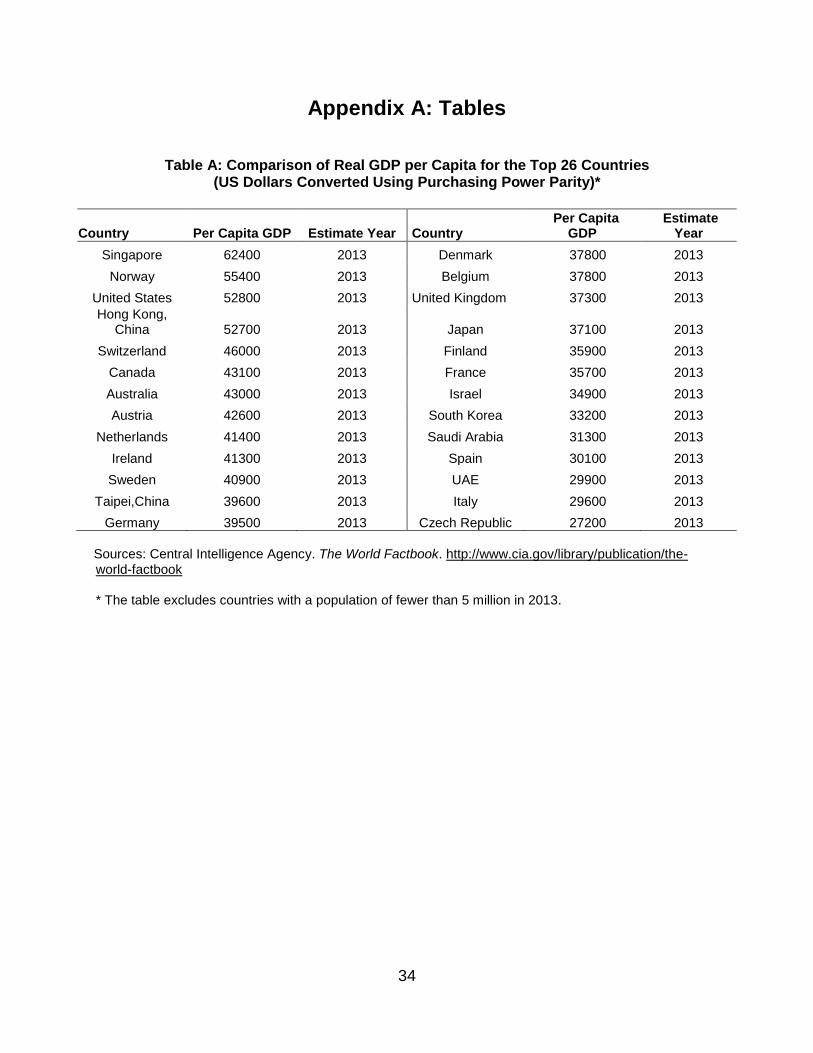
34

Appendix A: Tables

Table A: Comparison of Real GDP per Capita for the Top 26 Countries (US Dollars Converted Using Purchasing Power Parity)*

Country Per Capita GDP Estimate Year Country Per Capita

GDP Estimate

Year

Singapore 62400 2013 Denmark 37800 2013

Norway 55400 2013 Belgium 37800 2013

United States 52800 2013 United Kingdom 37300 2013

Hong Kong, China 52700 2013 Japan 37100 2013

Switzerland 46000 2013 Finland 35900 2013

Canada 43100 2013 France 35700 2013

Australia 43000 2013 Israel 34900 2013

Austria 42600 2013 South Korea 33200 2013

Netherlands 41400 2013 Saudi Arabia 31300 2013

Ireland 41300 2013 Spain 30100 2013

Sweden 40900 2013 UAE 29900 2013

Taipei,China 39600 2013 Italy 29600 2013

Germany 39500 2013 Czech Republic 27200 2013

Sources: Central Intelligence Agency. The World Factbook. http://www.cia.gov/library/publication/the-

world-factbook * The table excludes countries with a population of fewer than 5 million in 2013.

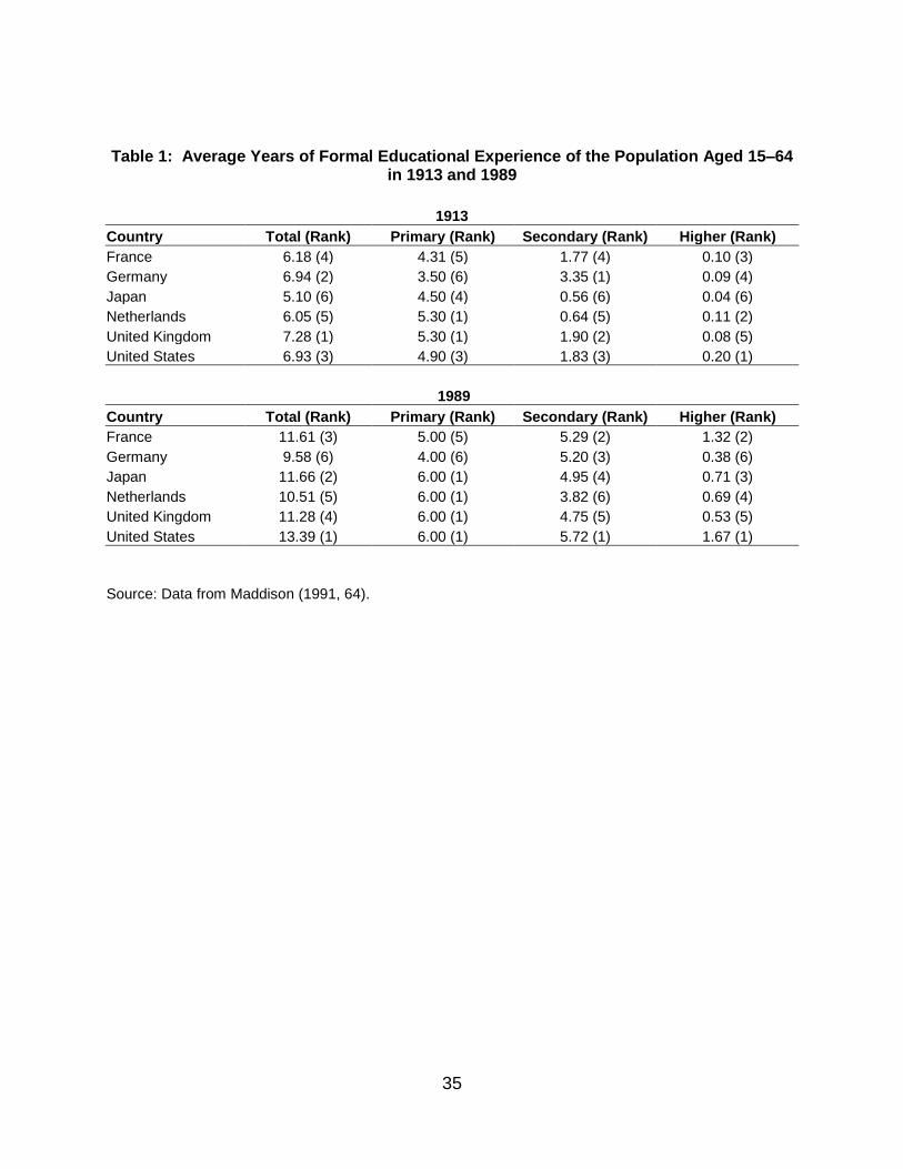
35

Table 1: Average Years of Formal Educational Experience of the Population Aged 15–64

in 1913 and 1989

1913

Country Total (Rank) Primary (Rank) Secondary (Rank) Higher (Rank)

France 6.18 (4) 4.31 (5) 1.77 (4) 0.10 (3)

Germany 6.94 (2) 3.50 (6) 3.35 (1) 0.09 (4)

Japan 5.10 (6) 4.50 (4) 0.56 (6) 0.04 (6)

Netherlands 6.05 (5) 5.30 (1) 0.64 (5) 0.11 (2)

United Kingdom 7.28 (1) 5.30 (1) 1.90 (2) 0.08 (5)

United States 6.93 (3) 4.90 (3) 1.83 (3) 0.20 (1)

1989

Country Total (Rank) Primary (Rank) Secondary (Rank) Higher (Rank)

France 11.61 (3) 5.00 (5) 5.29 (2) 1.32 (2)

Germany 9.58 (6) 4.00 (6) 5.20 (3) 0.38 (6)

Japan 11.66 (2) 6.00 (1) 4.95 (4) 0.71 (3)

Netherlands 10.51 (5) 6.00 (1) 3.82 (6) 0.69 (4)

United Kingdom 11.28 (4) 6.00 (1) 4.75 (5) 0.53 (5)

United States 13.39 (1) 6.00 (1) 5.72 (1) 1.67 (1)

Source: Data from Maddison (1991, 64).

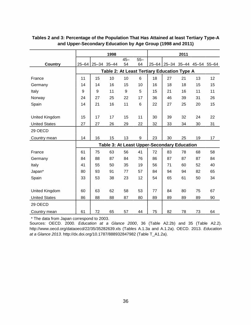
36

Tables 2 and 3: Percentage of the Population That Has Attained at least Tertiary Type-A

and Upper-Secondary Education by Age Group (1998 and 2011)

Country

1998 2011

25–64 25–34 35–44 45–54

55–64 25–64 25–34 35–44 45–54 55–64

Table 2: At Least Tertiary Education Type A

France 11 15 10 10 6 18 27 21 13 12

Germany 14 14 16 15 10 16 18 18 15 15

Italy 9 9 11 9 5 15 21 16 11 11

Norway 24 27 25 22 17 36 46 39 31 26

Spain 14 21 16 11 6 22 27 25 20 15

United Kingdom 15 17 17 15 11 30 39 32 24 22

United States 27 27 26 29 22 32 33 34 30 31

29 OECD

14 16 15 13 9 23 30 25 19 17 Country mean

Table 3: At Least Upper-Secondary Education

France 61 75 63 56 41 72 83 78 68 58

Germany 84 88 87 84 76 86 87 87 87 84

Italy 41 55 50 35 19 56 71 60 52 40

Japan* 80 93 91 77 57 84 94 94 82 65

Spain 33 53 38 23 12 54 65 61 50 34

United Kingdom 60 63 62 58 53 77 84 80 75 67

United States 86 88 88 87 80 89 89 89 89 90

29 OECD

61 72 65 57 44 75 82 78 73 64 Country mean

* The data from Japan correspond to 2003. Sources: OECD. 2000. Education at a Glance 2000, 36 (Table A2.2b) and 35 (Table A2.2).

http://www.oecd.org/dataoecd/22/35/35282639.xls (Tables A.1.3a and A.1.2a). OECD. 2013. Education

at a Glance 2013. http://dx.doi.org/10.1787/888932847982 (Table T_A1.2a).

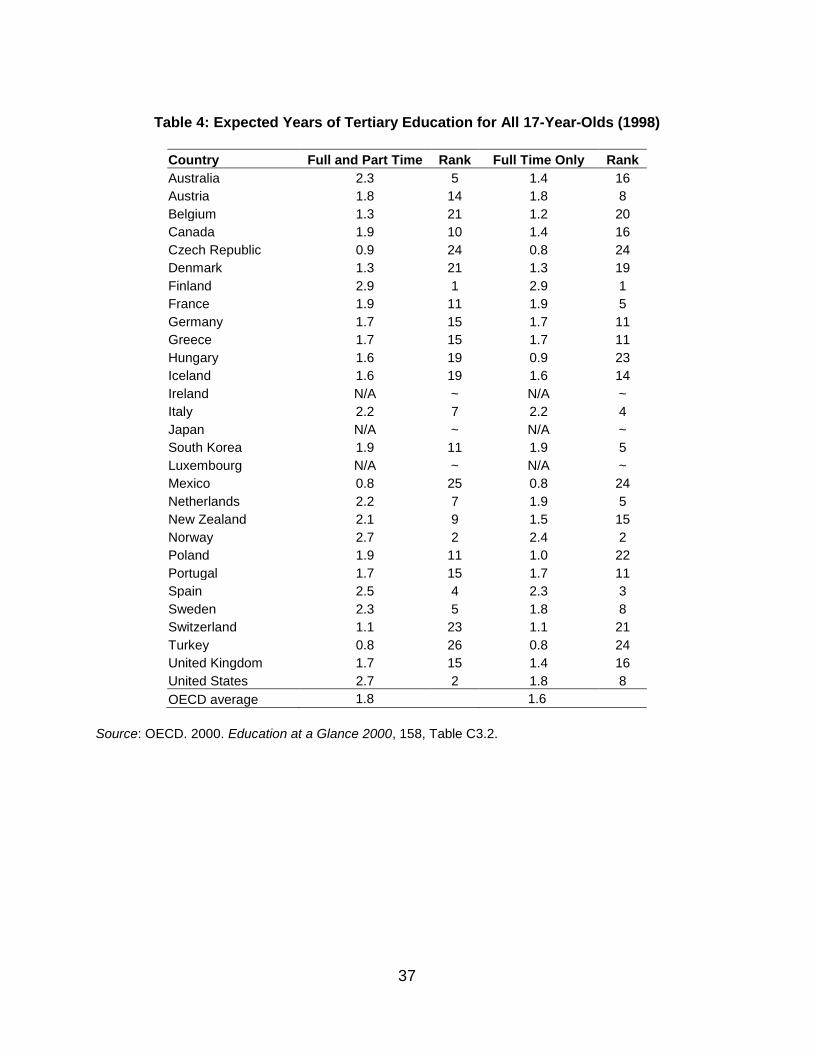
37

Table 4: Expected Years of Tertiary Education for All 17-Year-Olds (1998)

Country Full and Part Time Rank Full Time Only Rank

Australia 2.3 5 1.4 16

Austria 1.8 14 1.8 8

Belgium 1.3 21 1.2 20

Canada 1.9 10 1.4 16

Czech Republic 0.9 24 0.8 24

Denmark 1.3 21 1.3 19

Finland 2.9 1 2.9 1

France 1.9 11 1.9 5

Germany 1.7 15 1.7 11

Greece 1.7 15 1.7 11

Hungary 1.6 19 0.9 23

Iceland 1.6 19 1.6 14

Ireland N/A ~ N/A ~

Italy 2.2 7 2.2 4

Japan N/A ~ N/A ~

South Korea 1.9 11 1.9 5

Luxembourg N/A ~ N/A ~

Mexico 0.8 25 0.8 24

Netherlands 2.2 7 1.9 5

New Zealand 2.1 9 1.5 15

Norway 2.7 2 2.4 2

Poland 1.9 11 1.0 22

Portugal 1.7 15 1.7 11

Spain 2.5 4 2.3 3

Sweden 2.3 5 1.8 8

Switzerland 1.1 23 1.1 21

Turkey 0.8 26 0.8 24

United Kingdom 1.7 15 1.4 16

United States 2.7 2 1.8 8

OECD average 1.8 1.6

Source: OECD. 2000. Education at a Glance 2000, 158, Table C3.2.

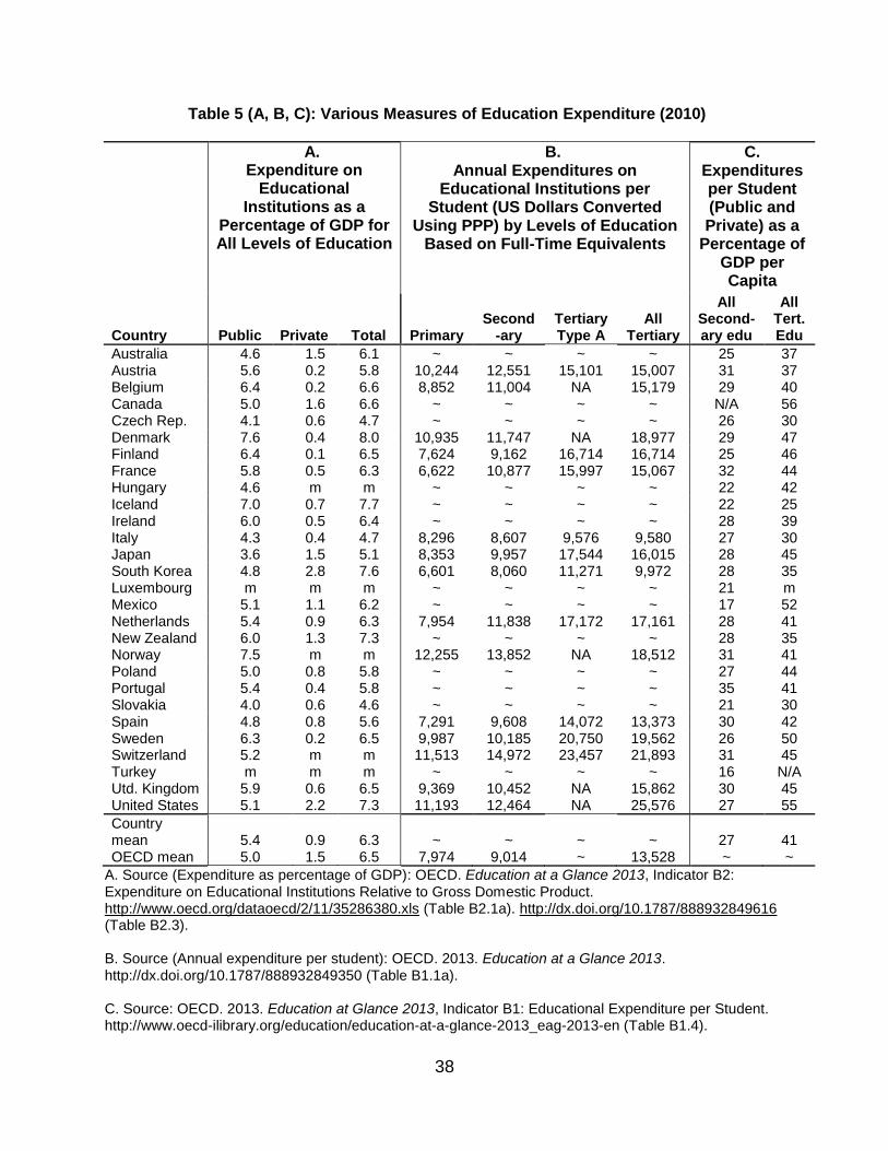
38

Table 5 (A, B, C): Various Measures of Education Expenditure (2010)

A.

Expenditure on Educational

Institutions as a Percentage of GDP for All Levels of Education

B. Annual Expenditures on

Educational Institutions per Student (US Dollars Converted

Using PPP) by Levels of Education Based on Full-Time Equivalents

C. Expenditures per Student (Public and Private) as a

Percentage of GDP per Capita

Country Public Private Total Primary Second

-ary Tertiary Type A

All Tertiary

All Second-ary edu

All Tert.Edu

Australia 4.6 1.5 6.1 ~ ~ ~ ~ 25 37 Austria 5.6 0.2 5.8 10,244 12,551 15,101 15,007 31 37 Belgium 6.4 0.2 6.6 8,852 11,004 NA 15,179 29 40 Canada 5.0 1.6 6.6 ~ ~ ~ ~ N/A 56 Czech Rep. 4.1 0.6 4.7 ~ ~ ~ ~ 26 30 Denmark 7.6 0.4 8.0 10,935 11,747 NA 18,977 29 47 Finland 6.4 0.1 6.5 7,624 9,162 16,714 16,714 25 46 France 5.8 0.5 6.3 6,622 10,877 15,997 15,067 32 44 Hungary 4.6 m m ~ ~ ~ ~ 22 42 Iceland 7.0 0.7 7.7 ~ ~ ~ ~ 22 25 Ireland 6.0 0.5 6.4 ~ ~ ~ ~ 28 39 Italy 4.3 0.4 4.7 8,296 8,607 9,576 9,580 27 30 Japan 3.6 1.5 5.1 8,353 9,957 17,544 16,015 28 45 South Korea 4.8 2.8 7.6 6,601 8,060 11,271 9,972 28 35 Luxembourg m m m ~ ~ ~ ~ 21 m Mexico 5.1 1.1 6.2 ~ ~ ~ ~ 17 52 Netherlands 5.4 0.9 6.3 7,954 11,838 17,172 17,161 28 41 New Zealand 6.0 1.3 7.3 ~ ~ ~ ~ 28 35 Norway 7.5 m m 12,255 13,852 NA 18,512 31 41 Poland 5.0 0.8 5.8 ~ ~ ~ ~ 27 44 Portugal 5.4 0.4 5.8 ~ ~ ~ ~ 35 41 Slovakia 4.0 0.6 4.6 ~ ~ ~ ~ 21 30 Spain 4.8 0.8 5.6 7,291 9,608 14,072 13,373 30 42 Sweden 6.3 0.2 6.5 9,987 10,185 20,750 19,562 26 50 Switzerland 5.2 m m 11,513 14,972 23,457 21,893 31 45 Turkey m m m ~ ~ ~ ~ 16 N/A Utd. Kingdom 5.9 0.6 6.5 9,369 10,452 NA 15,862 30 45 United States 5.1 2.2 7.3 11,193 12,464 NA 25,576 27 55

Country mean 5.4 0.9 6.3 ~ ~ ~ ~ 27 41 OECD mean 5.0 1.5 6.5 7,974 9,014 ~ 13,528 ~ ~

A. Source (Expenditure as percentage of GDP): OECD. Education at a Glance 2013, Indicator B2: Expenditure on Educational Institutions Relative to Gross Domestic Product. http://www.oecd.org/dataoecd/2/11/35286380.xls (Table B2.1a). http://dx.doi.org/10.1787/888932849616 (Table B2.3). B. Source (Annual expenditure per student): OECD. 2013. Education at a Glance 2013. http://dx.doi.org/10.1787/888932849350 (Table B1.1a). C. Source: OECD. 2013. Education at Glance 2013, Indicator B1: Educational Expenditure per Student. http://www.oecd-ilibrary.org/education/education-at-a-glance-2013_eag-2013-en (Table B1.4).

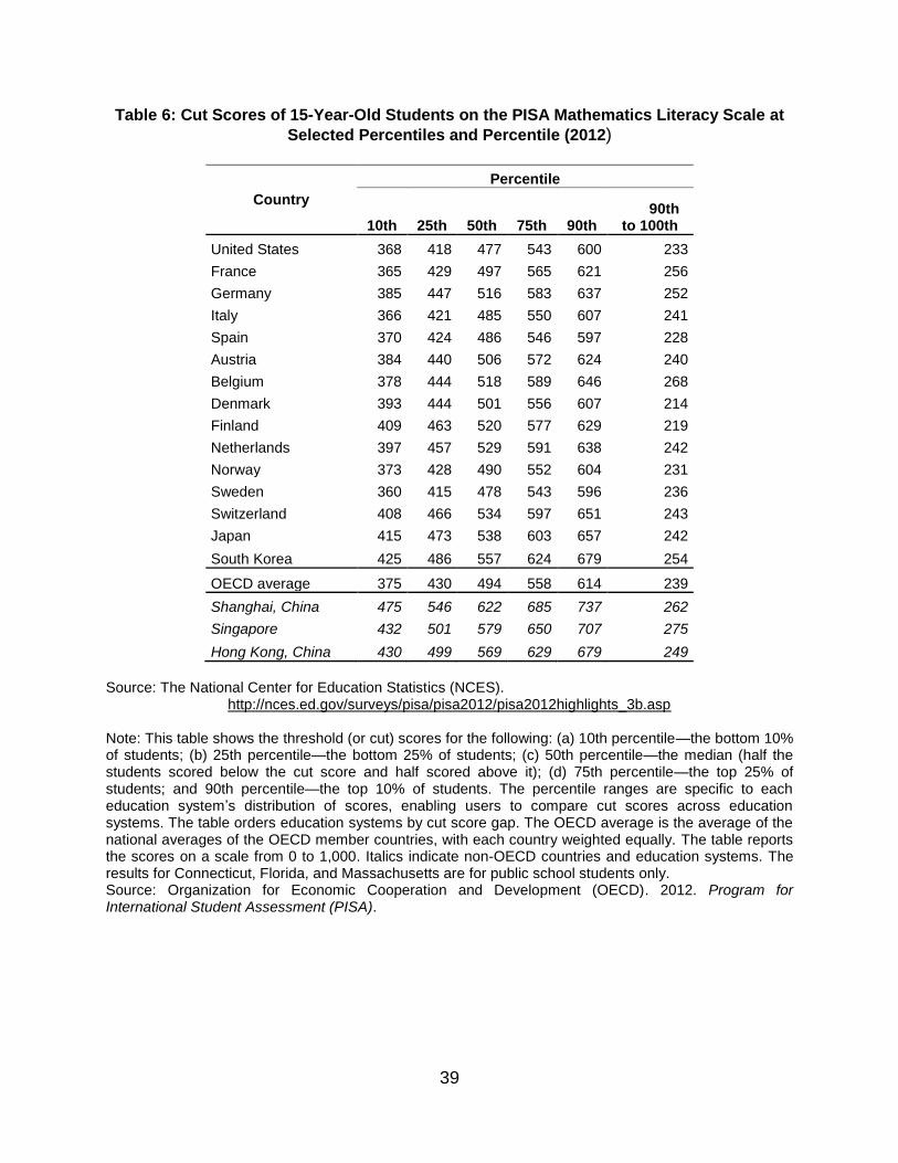
39

Table 6: Cut Scores of 15-Year-Old Students on the PISA Mathematics Literacy Scale at

Selected Percentiles and Percentile (2012)

Country

Percentile

10th 25th 50th 75th 90th 90th to 100th

United States 368 418 477 543 600 233

France 365 429 497 565 621 256

Germany 385 447 516 583 637 252

Italy 366 421 485 550 607 241

Spain 370 424 486 546 597 228

Austria 384 440 506 572 624 240

Belgium 378 444 518 589 646 268

Denmark 393 444 501 556 607 214

Finland 409 463 520 577 629 219

Netherlands 397 457 529 591 638 242

Norway 373 428 490 552 604 231

Sweden 360 415 478 543 596 236

Switzerland 408 466 534 597 651 243

Japan 415 473 538 603 657 242

South Korea 425 486 557 624 679 254

OECD average 375 430 494 558 614 239

Shanghai, China 475 546 622 685 737 262

Singapore 432 501 579 650 707 275

Hong Kong, China 430 499 569 629 679 249

Source: The National Center for Education Statistics (NCES).

http://nces.ed.gov/surveys/pisa/pisa2012/pisa2012highlights_3b.asp Note: This table shows the threshold (or cut) scores for the following: (a) 10th percentile—the bottom 10% of students; (b) 25th percentile—the bottom 25% of students; (c) 50th percentile—the median (half the students scored below the cut score and half scored above it); (d) 75th percentile—the top 25% of students; and 90th percentile—the top 10% of students. The percentile ranges are specific to each education system’s distribution of scores, enabling users to compare cut scores across education systems. The table orders education systems by cut score gap. The OECD average is the average of the national averages of the OECD member countries, with each country weighted equally. The table reports the scores on a scale from 0 to 1,000. Italics indicate non-OECD countries and education systems. The results for Connecticut, Florida, and Massachusetts are for public school students only. Source: Organization for Economic Cooperation and Development (OECD). 2012. Program for International Student Assessment (PISA).

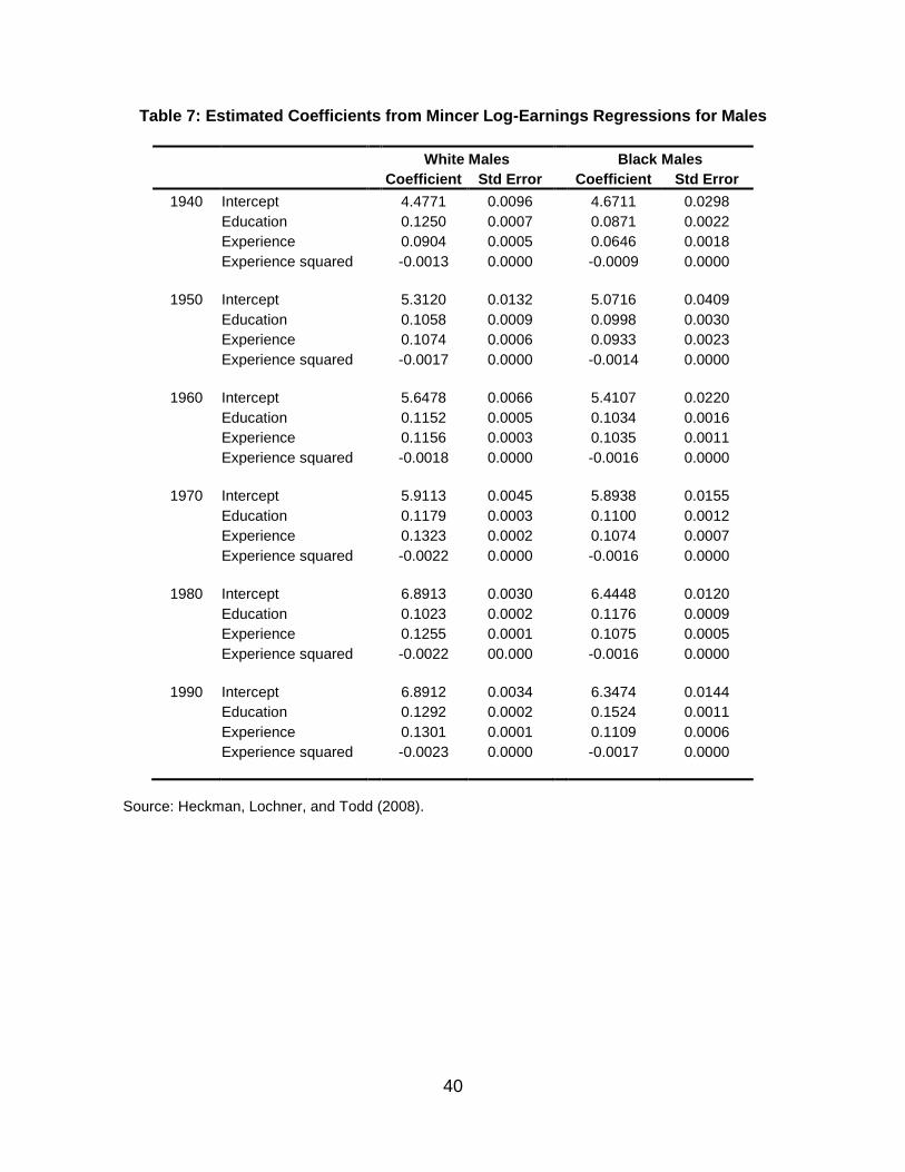
40

Table 7: Estimated Coefficients from Mincer Log-Earnings Regressions for Males

White Males Black Males

Coefficient Std Error Coefficient Std Error

1940 Intercept 4.4771 0.0096 4.6711 0.0298

Education 0.1250 0.0007 0.0871 0.0022

Experience 0.0904 0.0005 0.0646 0.0018

Experience squared -0.0013 0.0000 -0.0009 0.0000

1950 Intercept 5.3120 0.0132 5.0716 0.0409

Education 0.1058 0.0009 0.0998 0.0030

Experience 0.1074 0.0006 0.0933 0.0023

Experience squared -0.0017 0.0000 -0.0014 0.0000

1960 Intercept 5.6478 0.0066 5.4107 0.0220

Education 0.1152 0.0005 0.1034 0.0016

Experience 0.1156 0.0003 0.1035 0.0011

Experience squared -0.0018 0.0000 -0.0016 0.0000

1970 Intercept 5.9113 0.0045 5.8938 0.0155

Education 0.1179 0.0003 0.1100 0.0012

Experience 0.1323 0.0002 0.1074 0.0007

Experience squared -0.0022 0.0000 -0.0016 0.0000

1980 Intercept 6.8913 0.0030 6.4448 0.0120

Education 0.1023 0.0002 0.1176 0.0009

Experience 0.1255 0.0001 0.1075 0.0005

Experience squared -0.0022 00.000 -0.0016 0.0000

1990 Intercept 6.8912 0.0034 6.3474 0.0144

Education 0.1292 0.0002 0.1524 0.0011

Experience 0.1301 0.0001 0.1109 0.0006

Experience squared -0.0023 0.0000 -0.0017 0.0000

Source: Heckman, Lochner, and Todd (2008).

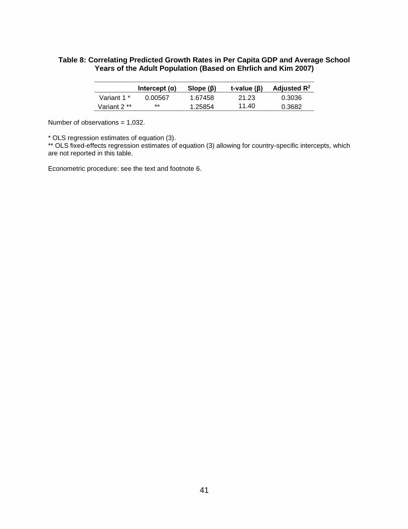
41

Table 8: Correlating Predicted Growth Rates in Per Capita GDP and Average School Years of the Adult Population (Based on Ehrlich and Kim 2007)

Intercept (α) Slope (β) t-value (β) Adjusted R2

Variant 1 * 0.00567 1.67458 21.23 0.3036

Variant 2 ** ** 1.25854 11.40 0.3682

Number of observations = 1,032. * OLS regression estimates of equation (3). ** OLS fixed-effects regression estimates of equation (3) allowing for country-specific intercepts, which are not reported in this table. Econometric procedure: see the text and footnote 6.

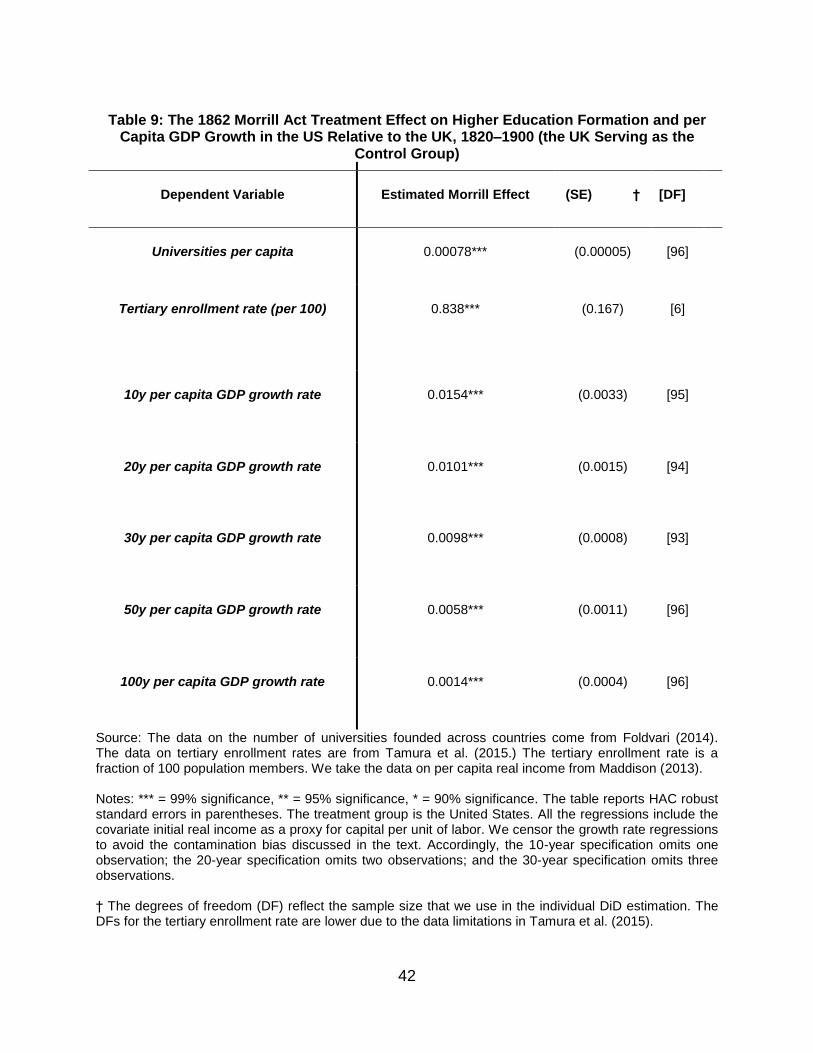
42

Table 9: The 1862 Morrill Act Treatment Effect on Higher Education Formation and per Capita GDP Growth in the US Relative to the UK, 1820–1900 (the UK Serving as the

Control Group)

Dependent Variable Estimated Morrill Effect (SE) † [DF]

Universities per capita 0.00078*** (0.00005) [96]

Tertiary enrollment rate (per 100) 0.838*** (0.167) [6]

10y per capita GDP growth rate 0.0154*** (0.0033) [95]

20y per capita GDP growth rate 0.0101*** (0.0015) [94]

30y per capita GDP growth rate 0.0098*** (0.0008) [93]

50y per capita GDP growth rate 0.0058*** (0.0011)

[96]

100y per capita GDP growth rate 0.0014*** (0.0004) [96]

Source: The data on the number of universities founded across countries come from Foldvari (2014). The data on tertiary enrollment rates are from Tamura et al. (2015.) The tertiary enrollment rate is a fraction of 100 population members. We take the data on per capita real income from Maddison (2013). Notes: *** = 99% significance, ** = 95% significance, * = 90% significance. The table reports HAC robust standard errors in parentheses. The treatment group is the United States. All the regressions include the covariate initial real income as a proxy for capital per unit of labor. We censor the growth rate regressions to avoid the contamination bias discussed in the text. Accordingly, the 10-year specification omits one observation; the 20-year specification omits two observations; and the 30-year specification omits three observations. † The degrees of freedom (DF) reflect the sample size that we use in the individual DiD estimation. The DFs for the tertiary enrollment rate are lower due to the data limitations in Tamura et al. (2015).

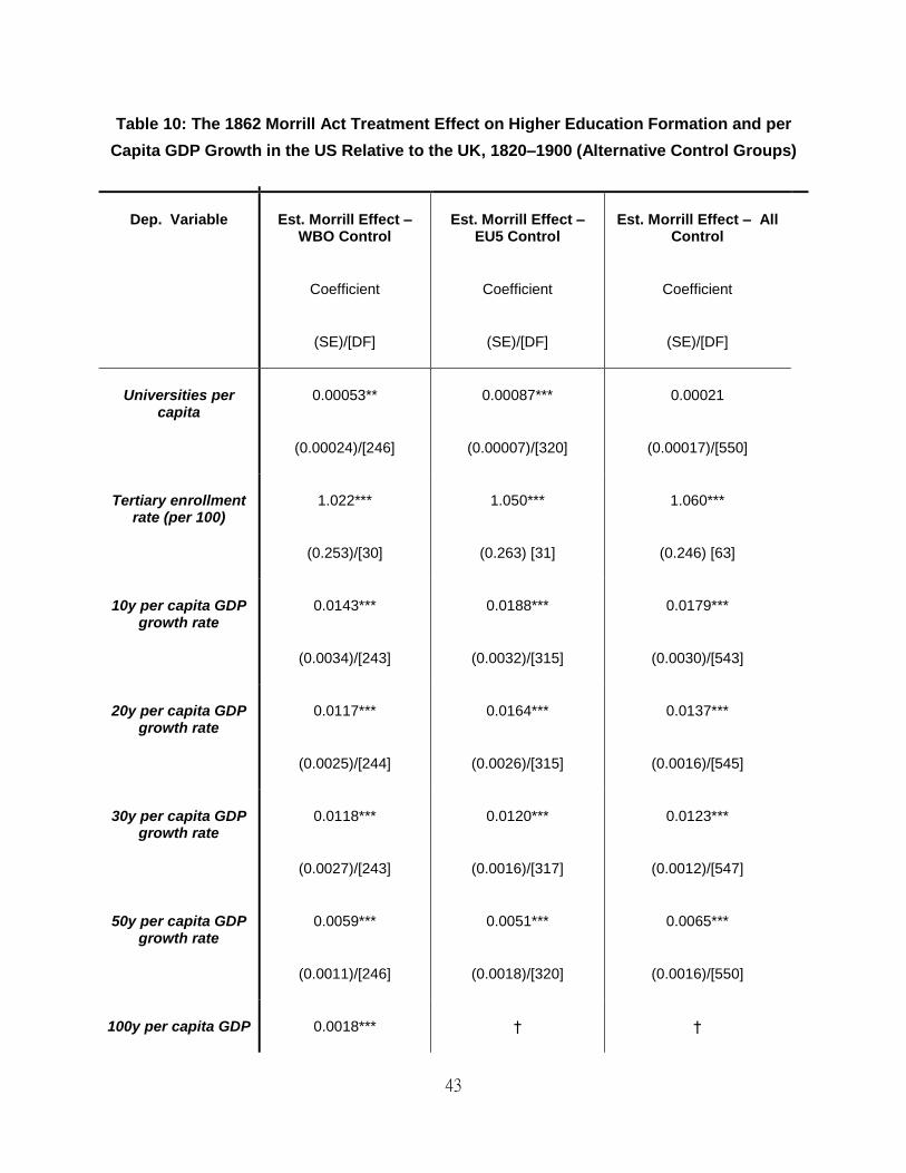
43

Table 10: The 1862 Morrill Act Treatment Effect on Higher Education Formation and per

Capita GDP Growth in the US Relative to the UK, 1820–1900 (Alternative Control Groups)

Dep. Variable Est. Morrill Effect – WBO Control

Coefficient

(SE)/[DF]

Est. Morrill Effect – EU5 Control

Coefficient

(SE)/[DF]

Est. Morrill Effect – All Control

Coefficient

(SE)/[DF]

Universities per capita

0.00053**

(0.00024)/[246]

0.00087***

(0.00007)/[320]

0.00021

(0.00017)/[550]

Tertiary enrollment rate (per 100)

1.022***

(0.253)/[30]

1.050***

(0.263) [31]

1.060***

(0.246) [63]

10y per capita GDP growth rate

0.0143***

(0.0034)/[243]

0.0188***

(0.0032)/[315]

0.0179***

(0.0030)/[543]

20y per capita GDP growth rate

0.0117***

(0.0025)/[244]

0.0164***

(0.0026)/[315]

0.0137***

(0.0016)/[545]

30y per capita GDP growth rate

0.0118***

(0.0027)/[243]

0.0120***

(0.0016)/[317]

0.0123***

(0.0012)/[547]

50y per capita GDP growth rate

0.0059***

(0.0011)/[246]

0.0051***

(0.0018)/[320]

0.0065***

(0.0016)/[550]

100y per capita GDP 0.0018*** † †

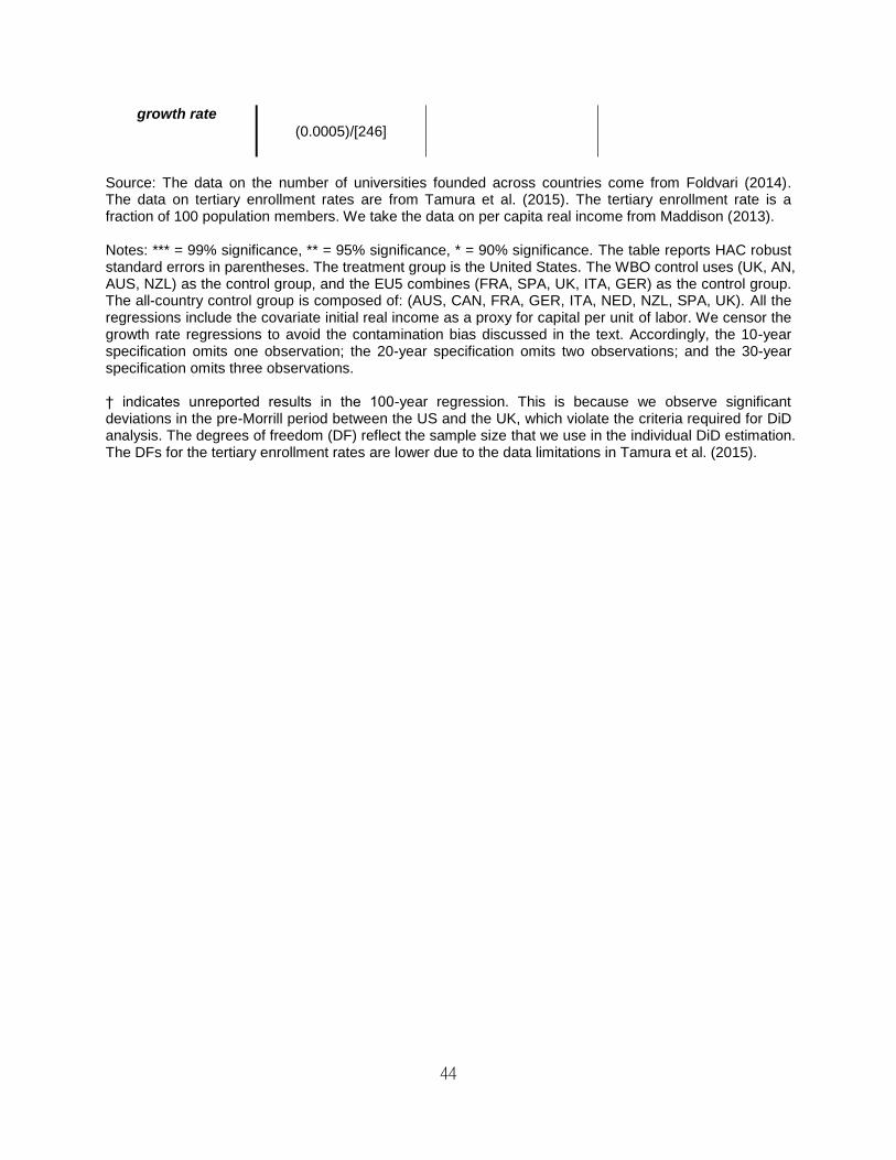
44

growth rate

(0.0005)/[246]

Source: The data on the number of universities founded across countries come from Foldvari (2014). The data on tertiary enrollment rates are from Tamura et al. (2015). The tertiary enrollment rate is a fraction of 100 population members. We take the data on per capita real income from Maddison (2013). Notes: *** = 99% significance, ** = 95% significance, * = 90% significance. The table reports HAC robust standard errors in parentheses. The treatment group is the United States. The WBO control uses (UK, AN, AUS, NZL) as the control group, and the EU5 combines (FRA, SPA, UK, ITA, GER) as the control group. The all-country control group is composed of: (AUS, CAN, FRA, GER, ITA, NED, NZL, SPA, UK). All the regressions include the covariate initial real income as a proxy for capital per unit of labor. We censor the growth rate regressions to avoid the contamination bias discussed in the text. Accordingly, the 10-year specification omits one observation; the 20-year specification omits two observations; and the 30-year specification omits three observations. † indicates unreported results in the 100-year regression. This is because we observe significant deviations in the pre-Morrill period between the US and the UK, which violate the criteria required for DiD analysis. The degrees of freedom (DF) reflect the sample size that we use in the individual DiD estimation. The DFs for the tertiary enrollment rates are lower due to the data limitations in Tamura et al. (2015).

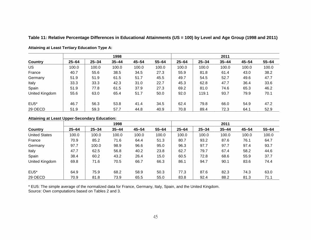
45

Table 11: Relative Percentage Differences in Educational Attainments (US = 100) by Level and Age Group (1998 and 2011)

Attaining at Least Tertiary Education Type A:

Attaining at Least Upper-Secondary Education:

1998 2011

Country 25–64 25–34 35–44 45–54 55–64 25–64 25–34 35–44 45–54 55–64

United States 100.0 100.0 100.0 100.0 100.0 100.0 100.0 100.0 100.0 100.0

France 70.9 85.2 71.6 64.4 51.3 80.7 93.2 87.6 76.1 64.7

Germany 97.7 100.0 98.9 96.6 95.0 96.3 97.7 97.7 97.4 93.7

Italy 47.7 62.5 56.8 40.2 23.8 62.7 79.7 67.4 58.2 44.6

Spain 38.4 60.2 43.2 26.4 15.0 60.5 72.8 68.6 55.9 37.7

United Kingdom 69.8 71.6 70.5 66.7 66.3 86.1 94.7 90.1 83.6 74.4

EU5* 64.9 75.9 68.2 58.9 50.3 77.3 87.6 82.3 74.3 63.0

29 OECD 70.9 81.8 73.9 65.5 55.0 83.8 92.4 88.2 81.3 71.1

* EU5: The simple average of the normalized data for France, Germany, Italy, Spain, and the United Kingdom. Source: Own computations based on Tables 2 and 3.

1998 2011

Country 25–64 25–34 35–44 45–54 55–64 25–64 25–34 35–44 45–54 55–64

US 100.0 100.0 100.0 100.0 100.0 100.0 100.0 100.0 100.0 100.0

France 40.7 55.6 38.5 34.5 27.3 55.9 81.8 61.4 43.0 38.2

Germany 51.9 51.9 61.5 51.7 45.5 49.7 54.5 52.7 49.6 47.7

Italy 33.3 33.3 42.3 31.0 22.7 45.3 62.8 47.7 36.4 33.6

Spain 51.9 77.8 61.5 37.9 27.3 69.2 81.0 74.6 65.3 46.2

United Kingdom 55.6 63.0 65.4 51.7 50.0 92.0 119.1 93.7 79.9 70.1

EU5* 46.7 56.3 53.8 41.4 34.5 62.4 79.8 66.0 54.9 47.2

29 OECD 51.9 59.3 57.7 44.8 40.9 70.8 89.4 72.3 64.1 52.9

46

Appendix B: Data Used in the DiD Regressions (Tables 9 and 10)

I. Universities founded and tertiary enrollment data

The historical data on the founding of colleges and universities across different countries that we use in our DiD regression analysis come from the clio-infra project17 that Peter Foldvari (2014) undertook. The annual data on higher education enrollments across countries that we use in our cross-country DiD regression analysis are primarily from Tamura et al. (2015). We take additional data on US tertiary enrollments per 100 18–24-year-old members of the population from the National Center of Education Statistics’ publication entitled 120 Years of American Education: A Statistical Portrait published in 1993 and the US Census of 1840 through 1860.

II. Per capita GDP data

We obtain the real per capita GDP data that we use in our cross-country DiD regression analysis (calculated in 1990 Geary–Khamis dollars) from the historical statistics that Maddison (2010) initially compiled on the GDP and per capita GDP and that Bolt and van Zanden (2014) later updated to span A.D. 1-2013. Note that the time span of the sample (1820–2013) is limited—the US achieved its independence only 40 years prior to the beginning of the Maddison (2010) real income per capita data series.

Following Barro et al.’s (1992) method, we construct average per capita income growth rates for successive forward-looking 10, 20, 30, 50, and 100-year time periods. The covariates that we include are the natural logarithm of initial real per capita income as a proxy for the initial stock of capital, which we take from the same data source.

A problem can arise in the application of this method, however, when we calculate the average per capita GDP growth rates for the treatment group. For example, when we consider the 50-year-forward average growth rate for the United States in 1850, 38 of the 50 years between 1850 and 1900 take place after the enactment of the first Morrill Act. As a result, some growth observations in the pre-event period will be biased upwards and thus “post-treatment-contaminated” by the impact of the Morrill Act. This contamination will therefore diminish the magnitude of the DiD estimator and consequently the estimated treatment effects. To combat this issue, we omit the offending observation years in different regressions (e.g., 1860 in the regression in which we measure the growth rate over a 10-year period; 1850 and 1860 in the regression in which we measure the growth rate over a 20-year period) and calculate the treatment effects without the downward bias.

Note, however, that the treatment effects related to the 50-year and 100-year growth rates must include all the available observations (including the biased ones) due to data limitations, which partly explains the larger drop-off in the estimated magnitude of the Morrill Act’s treatment effect in the corresponding regressions.

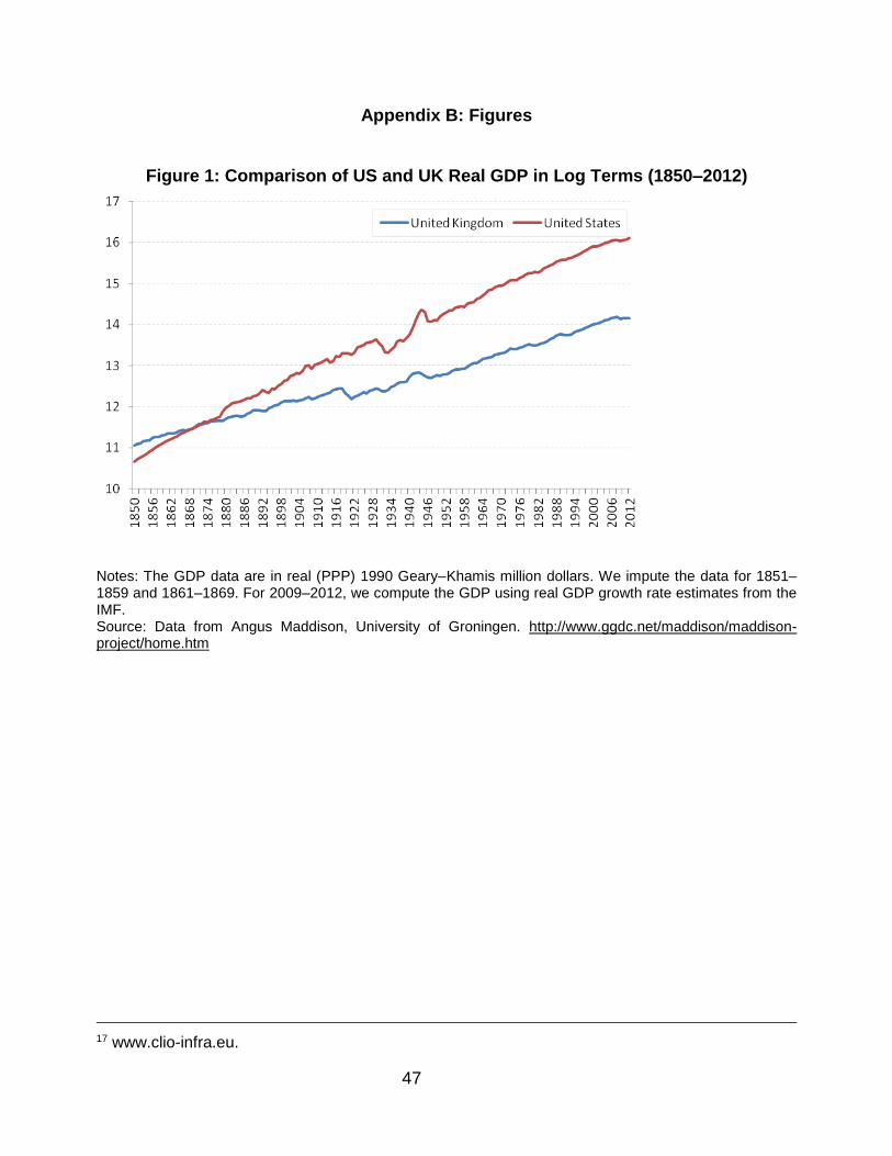
47

Appendix B: Figures

Figure 1: Comparison of US and UK Real GDP in Log Terms (1850–2012)

Notes: The GDP data are in real (PPP) 1990 Geary–Khamis million dollars. We impute the data for 1851–1859 and 1861–1869. For 2009–2012, we compute the GDP using real GDP growth rate estimates from the IMF. Source: Data from Angus Maddison, University of Groningen. http://www.ggdc.net/maddison/maddison-project/home.htm

17 www.clio-infra.eu.

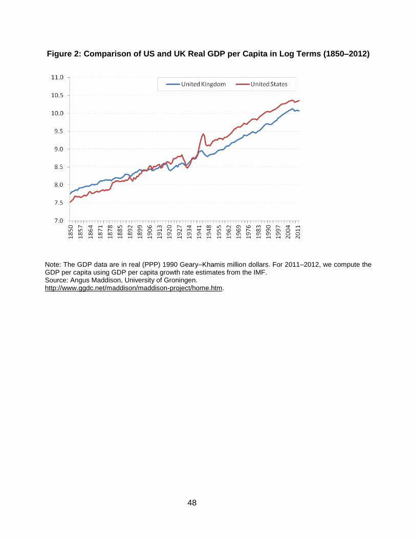
48

Figure 2: Comparison of US and UK Real GDP per Capita in Log Terms (1850–2012)

Note: The GDP data are in real (PPP) 1990 Geary–Khamis million dollars. For 2011–2012, we compute the GDP per capita using GDP per capita growth rate estimates from the IMF. Source: Angus Maddison, University of Groningen. http://www.ggdc.net/maddison/maddison-project/home.htm.

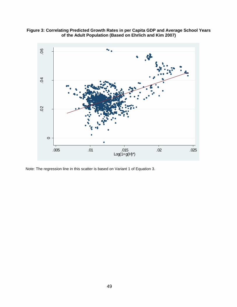
49

Figure 3: Correlating Predicted Growth Rates in per Capita GDP and Average School Years of the Adult Population (Based on Ehrlich and Kim 2007)

0

.02

.04

.06

Lo

g(1

+g

(GD

P)*

)

.005 .01 .015 .02 .025Log(1+g(H)*)

Note: The regression line in this scatter is based on Variant 1 of Equation 3.

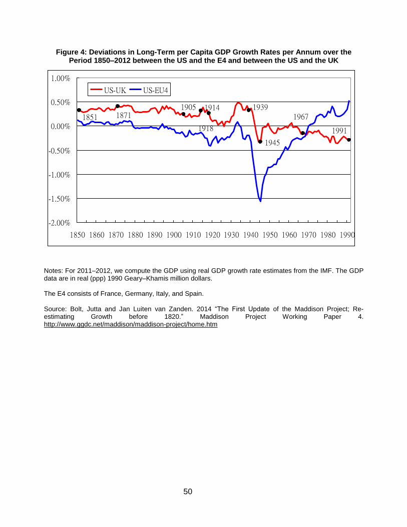
50

Figure 4: Deviations in Long-Term per Capita GDP Growth Rates per Annum over the Period 1850–2012 between the US and the E4 and between the US and the UK

Notes: For 2011–2012, we compute the GDP using real GDP growth rate estimates from the IMF. The GDP data are in real (ppp) 1990 Geary–Khamis million dollars. The E4 consists of France, Germany, Italy, and Spain. Source: Bolt, Jutta and Jan Luiten van Zanden. 2014 “The First Update of the Maddison Project; Re-estimating Growth before 1820.” Maddison Project Working Paper 4. http://www.ggdc.net/maddison/maddison-project/home.htm

1851 18711905 1914

1918

1939

1945

1967

1991

-2.00%

-1.50%

-1.00%

-0.50%

0.00%

0.50%

1.00%

1850 1860 1870 1880 1890 1900 1910 1920 1930 1940 1950 1960 1970 1980 1990

US-UK US-EU4

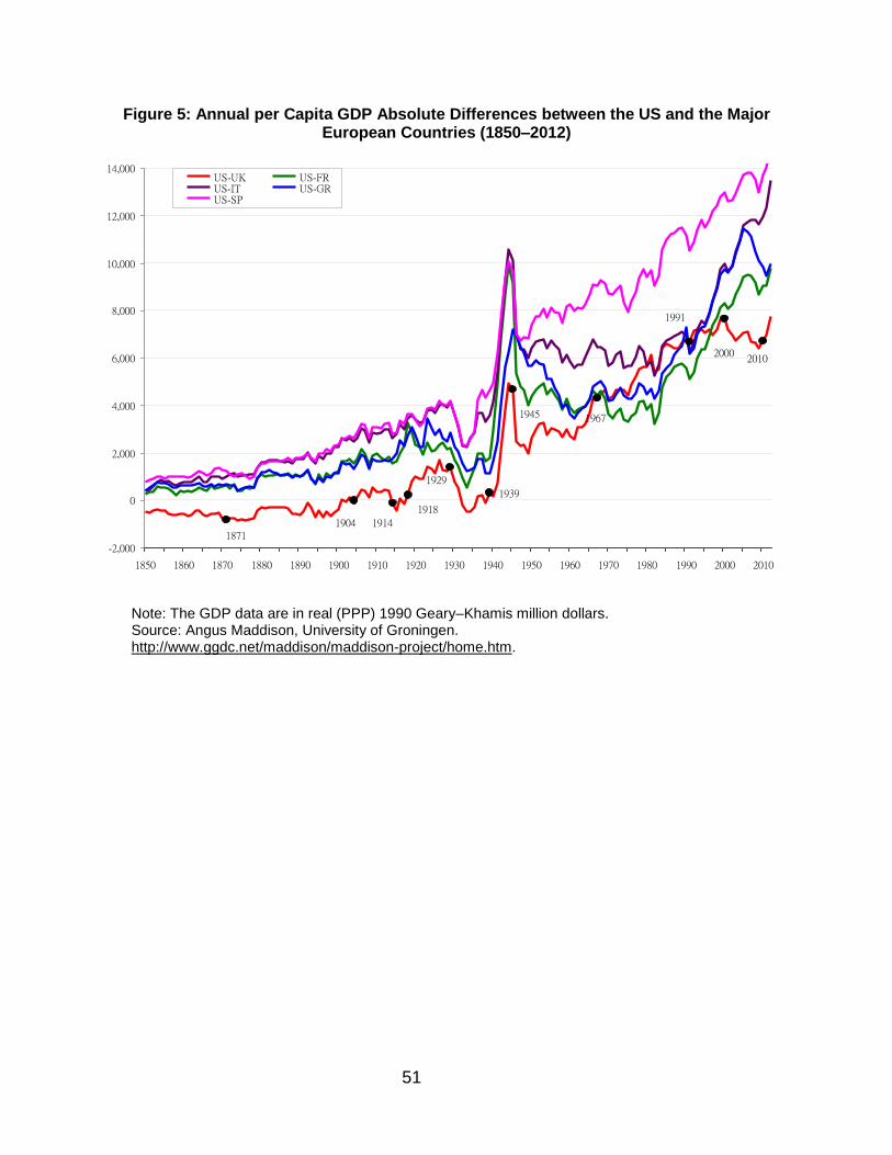
51

Figure 5: Annual per Capita GDP Absolute Differences between the US and the Major European Countries (1850–2012)

Note: See Figure 4.

Note: The GDP data are in real (PPP) 1990 Geary–Khamis million dollars. Source: Angus Maddison, University of Groningen. http://www.ggdc.net/maddison/maddison-project/home.htm.

2010

1991

19671945

1939

1929

18711904

1918

1914

2000

-2,000

0

2,000

4,000

6,000

8,000

10,000

12,000

14,000

1850 1860 1870 1880 1890 1900 1910 1920 1930 1940 1950 1960 1970 1980 1990 2000 2010

US-UK US-FRUS-IT US-GRUS-SP