Do context effects limit the usefulness of self-reported wellbeing measures?

Angus Deaton Center for Health and Wellbeing, Woodrow Wilson School Princeton University

Arthur A. Stone Department of Psychiatry and Behavioral Science Stony Brook University

28 July 2013

We are grateful to Gallup for granting us access to the Gallup-Healthways Wellbeing Index data. Both authors are consulting senior scientists with Gallup. We gratefully acknowledge financial support from Gallup and from the National Institute on Aging through the National Bureau of Economic Research, Grants 5R01AG040629–02 and P01 AG05842–14, and through Princeton’s Roybal Center, Grant P30 AG024928.

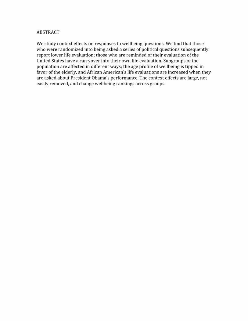
ABSTRACT    We  study  context  effects  on  responses  to  wellbeing  questions.  We  find  that  those  who  were  randomized  into  being  asked  a  series  of  political  questions  subsequently  report  lower  life  evaluation;  those  who  are  reminded  of  their  evaluation  of  the  United  States  have  a  carryover  into  their  own  life  evaluation.  Subgroups  of  the  population  are  affected  in  different  ways;  the  age  profile  of  wellbeing  is  tipped  in  favor  of  the  elderly,  and  African  American’s  life  evaluations  are  increased  when  they  are  asked  about  President  Obama’s  performance.  The  context  effects  are  large,  not  easily  removed,  and  change  wellbeing  rankings  across  groups.    

1

Introduction

There is currently much interest in using self-reported measures of subjective wellbeing (often

loosely referred to as measures of “happiness”) as guides to policy; these are seen as supple-

ments to standard measures of income or unemployment, and even as potential replacements.

Self-reports of wellbeing have the ability to tap into aspects of human experience that are not

captured by standard economic measures. Sen, Stiglitz, and Fitoussi (2009), reporting for a

Commission established by the former president of France, recommended a wider use of such

measures, see also Fleurbaey (2009) and Fleurbaey and Blanchet (2013). The OECD has recently

incorporated wellbeing measures into their measures of comparative country performance,

OECD (2011). In Britain, wellbeing measures are collected by the Office of National Statistics

and, with the support of Prime Minister David Cameron, measures are being used within White-

hall as part of the planning and policy evaluation process. The head of the British government’s

Behavioral Insights Team argues that the data will help people make better decisions about

where to live and what kind of careers to pursue, Jarrett (2011). In the extreme, Layard (2005)

has argued that happiness should be the only target for government policy, a Benthamite pre-

scription to be supported by self-reported happiness measures.

This paper presents experimental results on measuring wellbeing, and shows that ques-

tionnaire design can have large effects on self-reports of wellbeing, particularly on measures that

evaluate life as a whole. This makes these measures hostage to apparently irrelevant aspects of

the questionnaire, and the effects that we document are different for different subgroups of the

population and so can result in re-rankings of the wellbeing of groups that are likely to be im-

portant for policy. The topic of this paper is context effects, how responses are affected by pre-

ceding questions and other circumstances surrounding the questionnaire, but these are not the

2

only features of survey design that can affect wellbeing measures. In a related study of a differ-

ent aspect of survey design, Heffetz and Rabin (2013) find that happiness rankings depends on

how hard it is to reach people in telephone surveys, with hard to reach men happier than hard to

reach women, and vice versa. As a result, the number of callbacks called for by the survey design

can affect the rankings of different groups, just as do the context effects studied here.

Our results confirm arguments in the psychological literature that people either do not

have a stable inner sense of wellbeing that can easily be accessed by standard questions or, if

they do, are easily influenced in their reports of it. While we recognize the considerable

achievements of the “happiness” literature, particularly in establishing the correlates of self-

reported wellbeing measures, we argue that there are potentially serious and largely unaddressed

measurement problems stemming from the fact that people find some wellbeing questions diffi-

cult to interpret and to answer. As a result, answers can depend on how the questions are posed,

on the content of previous questions, on the order in which they are asked, and most likely on

other essentially irrelevant external circumstances. These findings call for caution in the use of

wellbeing measures as a general guide to policy. They also highlight the importance of devising

questionnaires that minimize the influence of questionnaire design, an issue that is currently far

from fully solved.

Our analysis maintains an important distinction, between evaluative, or overall life satis-

faction, measures, on the one hand, and hedonic measures (yesterday, were you happy, or wor-

ried, or stressed?) on the other, what Kahneman and Riis (2005) call “thinking about life” as op-

posed to “experiencing life.” The two sets of measures have different correlates both within

countries and across countries, and measure different aspects of people’s experience, Kahneman

and Deaton (2010), Stone et al (2010), Deaton and Stone (2013), Steptoe, Deaton and Stone

3

(2014). There is no general agreement about which, if either, is most relevant for policy: Evalua-

tive measures provide a direct assessment of how people rate their lives, and thus have an imme-

diate claim to consideration as a target for policy. But there is also a case for the integral over

time of instantaneous hedonic experience, something that can be calculated using combined

time-use and wellbeing surveys, such as the American Time Use Survey. The U-statistic—the

fraction of time spent in negative hedonic states is an example of this sort of measure, Kahneman

and Krueger (2006), Krueger (2010). The UK has recently conducted major survey using evalua-

tive, hedonic and eudemonic (meaningfulness) wellbeing questions, Office of National Statistics

(2012). In the experiments we report in this paper, the context effects work differently for evalu-

ative versus hedonic measures, with more serious distortions for the former. The possibility of

differential distortion thus needs to be taken into account when thinking about which concepts to

use.

For our analysis, it is useful to separate two main uses for wellbeing data, which we think

of as cross-section and time-series. Cross-section uses compare self-reported wellbeing (SWB)

across different groups, for example by gender, by age, by occupation, by employment status, or

by geographical location, across countries or across regions within countries. Such analyses are

relevant for evaluating (or monetizing) the effects on wellbeing of the death of a family member,

Oswald and Powdthavee (2008), of being unemployed, Clark and Oswald (1994)—which the

SWB literature argues are much more severe than implied by the loss of income—or for valuing

amenities such as pollution, Oswald and Wu (2009), safety, Dolan, Fujiwara, and Metcalfe

(2011), or aircraft noise, van Praag and Baarsma (2005). Wellbeing data are also used to evaluate

changes rather than differences, to monitor national progress with economic growth, Easterlin

(1974), Sacks, Stevenson, and Wolfers (2012), over the business cycle, or over specific events,

4

such as the Great Recession, Deaton (2012), floods, Luechinger and Raschky (2009), or Hurri-

cane Katrina, Kimball, Levy, Ohtake, and Tsutsui (2006). Measurement problems have different

implications for the two kinds of uses; averaging over time will eliminate different kinds of

measurement error than does averaging over individuals. We find that evaluative measures are

likely to be of limited use for short-run macroeconomic tracking, though hedonic questions,

which require less cognitive effort to answer, are likely to do better, though they may be of less

interest to policy makers.

If self-reports of wellbeing are to be used to guide public policy, project evaluation, or

macroeconomic policymaking, we need to ensure construct validity, i.e. that the measures actual-

ly capture the aspect of wellbeing that they target. This paper explores one possible source of

failure or bias, which is that responses can depend on the order in which questions are asked.

This is in part a technical issue: we would like to minimize bias due to order by avoiding certain

types of question sequence or by randomizing over respondents so that the context effects aver-

age out. However, there is a deeper issue: if people’s answers are sensitive to question-order con-

text or other irrelevant context, it may because they have difficulty interpreting or answering the

questions, compromising the reliability and usefulness of their response. Even if they understand

the question, they may not have the memory or cognitive facilities to provide a valid answer,

Schwarz (1999). In the worst case, there is “no there there”: responses are whatever happens to

be in people’s minds at the moment. There is also a concern if interest groups or other organiza-

tions can provide an external context that influences answers in a way that would change policies

in their favor.

The literature on context effects for measures of evaluative wellbeing is reviewed by

Schwarz and Strack (1999) who summarize their findings as follows: “reports of subjective

5

wellbeing (SWB) do not reflect a stable inner state of wellbeing. Rather they are judgments that

individuals form on the spot, based on information that is chronically or temporarily accessible at

that point in time, resulting in pronounced context effects.” (p. 61). In the cases we examine

here, prior questions (and their answers) cause people to reinterpret wellbeing questions, and in-

fluence their answers. Schwarz and Strack suggest a mental process in which respondents, uncer-

tain about how to answer a question about something they do not usually think about—an overall

evaluation of their life—review recent experiences or recent answers to help them interpret the

question and provide a handy answer. Studies have shown that the effects of context-setting

questions can persist through many intervening questions, Bishop (1987), and we replicate this

finding here.

Similar mental processes can also make answers sensitive to external events that are not

part of the questionnaire; sometimes these effects will cancel out on average—not everyone has

just had a fight with their spouse—but in other cases they may not—for example if the question

is taken to refer to some salient external event, such as the collapse of the stock market or victory

in the World Cup. Such a circumstance would likely result in pronounced bias even in average

responses.

We investigate a randomized experiment conducted by the Gallup Organization in their

daily polling. The experimental framework is useful to establish the existence of the context ef-

fects, as well as to establish causality: we document these results in Section 1. We study both

evaluative and hedonic wellbeing measures, and compare the effects on wellbeing with those on

other information that respondents provide. Section 2 investigates the processes in more detail

and enquires what feature of the previous questions generates the context effects. In Section 3,

we document the extent to which the context effects matter for the cross-section analysis of

6

wellbeing, such as whether women’s wellbeing is higher than men’s, or whether the wellbeing of

blacks is higher than that of whites. Sections 2 and 3 step away from the strict methodological

constraints of randomized controlled trials to what is essentially a subgroup analysis; this helps

provide insights into the mechanisms behind the experimental results.

Section 1: Data and experimental evidence

Beginning in January 2008, the Gallup Healthways Wellbeing Index (GHWBI) has collected da-

ta on around 1,000 randomly sampled people each day. The survey asks about a range of evalua-

tive and hedonic questions, as well as about demographics and health. This daily (usually even-

ing) survey is also used by Gallup for its political polling; the political questions change with the

election cycle, and involve voting intentions, assessments of how the President is performing,

and satisfaction about the “way things are going in the US.” During the period that will concern

us, these political questions were asked at the very beginning of the survey. Immediately follow-

ing is a life evaluation wellbeing question, the Cantril (1965) “self-anchoring striving scale.” The

Cantril question asks people to imagine a ladder with eleven rungs, marked zero to ten, where

zero is the worst possible life for you and ten is the best possible life for you, and to tell the in-

terviewer which rung best represents their current position. We refer to this measure as the lad-

der; note that the question does not mention the word “happiness,” although in the literature,

which does not always make the important distinction between evaluation and hedonics, this is

often referred to as a happiness measure. Much later in the interview—which typically lasts for

about 25 minutes—people are asked a series of “yesterday” questions of the form, “did you ex-

perience a lot of X yesterday”, where X ranges over the affective descriptors happiness, sadness,

enjoyment, smiling, worry, stress, anger, and physical pain.

7

The experiment analyzed here uses the fact that over a period of time Gallup randomly

split the daily sample of 1,000 respondents, with 500 people being asked the political questions

followed by the ladder question, and 500 receiving none, starting instead with the ladder ques-

tion. Because the political questions were changing periodically we have three different experi-

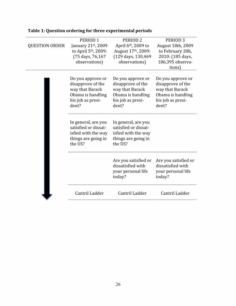
ments that we analyze separately and refer to by the periods during which they operated. Table 1

shows the sequence of questions for the treatment group and how they were posed in each peri-

od; in each case, the ladder is the next question, and for the control group, the ladder is the first

question.

The question about satisfaction with personal life that was added on April 6th, 2009 (be-

ginning of period 2), was intended as a buffer, transition, or cleansing question. By refocusing

the respondent away from the political questions, it is designed to remove or at least to mitigate

the effects of the political questions on the answers to the ladder (and subsequent) questions. The

only difference between periods 2 and 3 is the removal of the question about satisfaction with

how things are going in the US. In all three periods, these questions were asked only of a half of

the sample picked at random, the “form 1” or treatment sample. The “form 2” or control sample

was asked none of those questions. Note that although there is no variation in questions within

each period, there is no reason to expect the average experimental treatment effect to be constant

within each experiment; for example, if being asked to think about whether the President is doing

a good job affects the ladder score only if the respondent thinks not, then the average reported

ladder will change with the fractions who do or do not approve of the President.

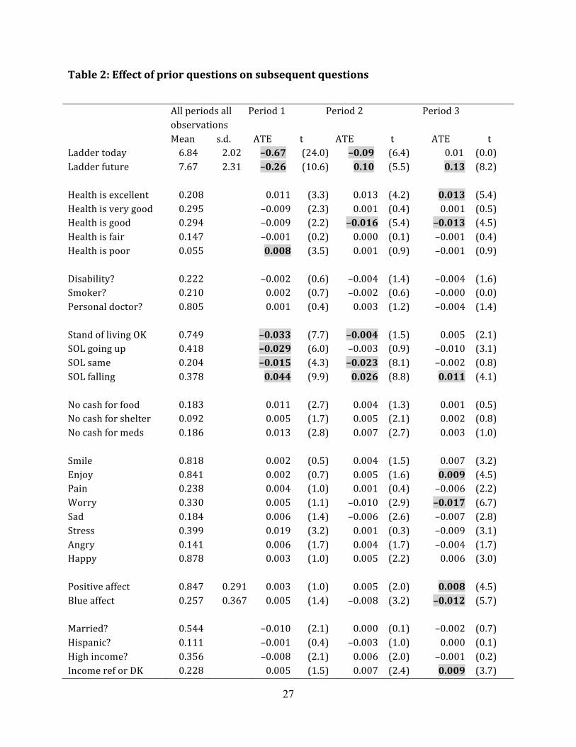
Table 2 documents the effect of being asked the prior questions in each of the three peri-

ods. The first column shows the means over the whole sample (both form 1 and form 2 respond-

ents) for all three periods. For the ladder today and ladder future the second column shows the

8

corresponding standard deviation; other variables are dichotomous, and the standard deviation is

not shown. On average, people rank their lives very highly, at 6.84 on the 0 to 10 scale, with a

standard deviation of 2.02. They think that the future will be even brighter; their mean expecta-

tion of the ladder five years hence is 7.67. The first column also reports the means of a range of

health related, demographic, and financial perception variables. The bottom of the first column

shows the hedonic wellbeing variables; positive experiences, such as smiling, enjoyment, and

happiness are experienced on a daily basis by more than 80 percent of the population, while

stress, worry, sadness, and anger are much rarer. Positive and “blue” affect, the averages of smil-

ing, enjoyment, and happiness, and of sadness and worry, respectively, are useful summary

measures.

The second and subsequent columns show the average treatment effects (ATEs) over the

three periods; the figures reported are the means of the experimental group (who received the

political questions, form 1, minus the means of the control group (who did not receive the ques-

tions, form 2. Asterisks indicate ATEs that are significantly different from zero at one percent or

less using conventional F-tests; given the large sample sizes here, a better trade-off between

Type I and Type II errors is given by Schwarz’s (1978) Bayesian test, which is that the F-statistic

exceed the logarithm of the sample size, and such cases are gray-shaded in the table.

The headline number is at the top of the second column. In period 1, before the introduc-

tion of the buffer question, those who were first asked the political question reduced their aver-

age ladder score by two thirds of a rung. For comparison, this number is larger than the drop in

mean ladder through 2008 as the financial crisis unfolded, Deaton (2012), and is comparable to

what would happen to the average if everyone in the country became unemployed, or to a reduc-

tion in average income of 89 percent (the coefficient of log income on the ladder is 0.30.) Be-

9

cause most of this effect vanished when the buffer question was added—see third column, where

the ATE is reduced to –0.09—there would have been a very large spurious increase in average

life evaluation beginning on April 6th, 2009 if the ladder had been taken at face value. If policy-

makers were unaware of the change in questionnaire design, or that the change could have such

large effects, there would be a serious failure of monitoring. The same would be true for compar-

isons of the ladder across surveys with identical ladder questions, but different preceding ques-

tions.

The introduction of the buffer question, in periods 2 and 3, although reducing the effect

on the ladder, causes the ATE on the expected future ladder to switch from significantly negative

to significantly positive. In period 3, without the question about the direction the US is going,

there is now no effect on the current ladder, but the positive effect on the expected future ladder

remains. The difference between periods 2 and 3 is the elimination of the question about “the

way things are going in the US”, while the President Obama approval question is asked in both,

so it is plausible that it is the “way things are going ” question that is doing the damage, at least

to the ladder. This would be consistent with an account in which people, when asked about their

own lives, use their answer to the “way things are going” question to shape their answer about

themselves. We shall offer more evidence below to support this contention. For the moment, it is

important to note that the buffer question, although moderating the biases, does not remove

them; these experiments, at least, do not offer a complete solution to the contamination of an-

swers by previous questions.

The table also looks for effects on a number of other questions in the poll; we have se-

lected other self-assessed questions, as well as questions whose interpretation should not be af-

fected by the political questions, such as marital status, race, income, whether or not the re-

10

spondent is a smoker, or has a regular doctor, and some intermediate cases, such as self-reported

health status on a 1 to 5 scale. The order of the variables in Table 2 is the same as the order in the

questionnaire though there are typically many intervening questions whose content itself changes

over time.

With one exception, there are no other ATEs that are close to as large as the ATE on the

ladder in Period 1, whether judged by the fraction of the mean response, or by statistical signifi-

cance. The exception is the standard of living question, where there is a reduction of 3.3 percent-

age points from the mean, and there is a 4.4 percentage point increase in those who say they ex-

pect their standard of living to fall, even larger than the effect on the ladder relative to the mean.

Once again, it is plausible that the question about the “way things are going in the US” is at least

in part responsible, if people who believe that things are getting worse are prompted to think so,

and if they extrapolate from the general answer to their own particulars. The standard of living

questions come after the health questions, which come after the current and future ladders, and

perhaps the effect on the standard of living mirrors people recalling their ladder responses when

asked the rather similar questions about their standard of living. The answers to the standard of

living questions are strongly predictive of the ladder, and Gallup, Newport (2011), Agarwal and

Harter (2012), and Deaton (2012) used them to correct the ladder. While the correction is plausi-

ble, it is far from clear that it is correct without a deeper understanding of the mechanisms at

work.

The effects on the hedonic measures are of considerable interest. In general, the ATEs for

the hedonics are relatively small and insignificant, with the exception of period 3, when positive

affect is enhanced and negative effect diminished by the treatment. One possible reason for the

relative robustness of the hedonic reports is that questions of the form “did you experience a lot

11

of sadness” yesterday are easily comprehensible, have a recall period that is short enough so that

affective states can be remembered, and require little cognitive effort compared with questions

about life as a whole. Even so, hedonic reports are not immune to the presence of the political

questions. In period 1, with no buffer, the reported prevalence of stress rises by about 5 percent

of the mean when respondents are asked the political questions. Most interesting is period 3,

where there is a buffer question and the only political question is about the performance of Presi-

dent Obama. In this experiment, those asked about the President are less likely to report negative

hedonics and more likely to report positive hedonics. The ATEs are about one percent of the

means, but for worry, there is a five percent reduction. As was the case for thinking about the

future, it appears that some people’s emotional balance improved when they are prompted to

think about President Obama, or did at that period, even if they are deeply worried about the fu-

ture of America. In the three periods, the fractions dissatisfied with the direction in which the US

was going were 79, 67, and 62 percent, while the fractions who disapproved of President Obama

were 27, 35, and 45 percent.

That the hedonic questions are asked near the end of the questionnaire may also account

for the fact that they are generally less contaminated by the opening questions. If we plot the size

of the ATEs (excluding those for the ladder, which are larger and non-dichotomous) against the

order in which they appear in the questionnaire we see no general decline in the ATEs with or-

der, with some questions—notably the standard of living questions—showing large effects rela-

tive to their positions. This finding is more consistent with “echo” effects of something in the

political questions, than with any general wearing off of the effects of those questions; it also

suggests that priming effects are more plausible than general shifts in mood, for example becom-

ing upset by being asked any political questions. It is also consistent with the political questions

12

causing a shift in mood or cognition that influences some questions more than others. We shall

provide further evidence on these issues in the next section.

Section 2: Investigating the mechanisms

The randomization allows us to compare those who did and did not answer the political ques-

tions, but it does not tell us what it is about the political questions that biases the subsequent an-

swers, or how the effect works. One of us, Deaton (2012), previously interpreted the political

questions as exerting a negative effect on the mood of the respondents: that people did not like

being asked about politics is plausible given the deep unpopularity of Congress and politicians at

the time. However, it is possible to do better than this conjecture because, for those who were

asked the political questions, we know what their answers were, and we can check whether their

wellbeing scores were different depending on their answers. For example, do people who disap-

prove of President Obama’s handling of his job have their ladder scores reduced more than those

who approve? There is no separate experimental manipulation for addressing this question, so

the analysis is akin to an ex-post subgroup analysis in a randomized controlled trial, and has the

same disadvantages. For example, support or opposition for President Obama is likely to be as-

sociated with other respondent characteristics, such as political affiliation, age, or race. Even so,

we can compare the outcomes for those who did not get the political questions from those who

did not, and separate the latter group by those who support and oppose President Obama or who

think the US is or is not going in the right direction.

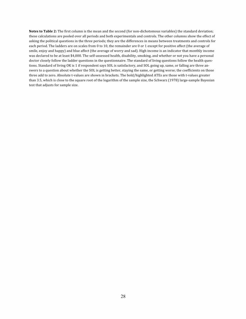
The big effects In Table 3 are associated with dissatisfaction with the way the country is

going. There are much smaller effects associated with approval or disapproval of President

Obama. It is not just the asking of the political questions that has the effect, rather it depends on

13

how people answer the questions and it depends on the questions actually being asked, which

presumably activates affective or cognitive processes that impact answers to later questions.

Among the people who were not asked the political questions, who were randomly selected, we

can presume that about 80 percent thought the country was going in the wrong direction (the

same rate as the other group that was asked their opinion), but their answers could not have been

affected by the political questions. For the people who were asked the political questions, and

who thought the country was going in the right direction, there is no significant difference in

ladder (or perhaps a small positive effect) compared with those who were not asked the question.

Thus, lower scores on the ladder come from both thinking the country is going in the wrong di-

rection and being asked to report the fact. Once again, this looks like a priming effect of an earli-

er question, but even more like Schwarz and Strack’s (1999) argument that, when asked a diffi-

cult question to which they have no ready answer, they reach back in the “stack” to find some-

thing that will serve as an answer (without awareness that they are doing so), in this case the

question about satisfaction about “the way things are going in the US.” For the purpose of well-

being analysis, particularly of evaluative wellbeing analysis, such effects are particularly discon-

certing because they suggest that people have little independent idea of how to evaluate their

lives, or that whatever idea they have is easily swayed by proximate information.

Once the transition question is introduced in period 2 (second panel of Table 3), the effect

of thinking about the way the country is going and being reminded of the fact is approximately

cut in half. For reasons that are not clear, the President Obama disapprovers who are reminded of

the fact now have a positive increment to the ladder after answering the transition question. Once

the country satisfaction question is dropped (third panel of Table 3), the political question has no

net effect on the ladder. However, this is not because there is nothing there, but because the Pres-

14

ident Obama approvers’ positive effect on the ladder is negated by the negative effect of the

Obama disapprovers. These signs make more sense than those in the second panel.

Section 3: Context effects and intergroup comparisons

A standard use of wellbeing measures is to make comparisons across groups, for example by

gender, by age, by employment status, by occupation, by education, or by place of residence.

Such comparisons are arguably useful in policy, for example by making people aware of differ-

ences before they make choices, or for incorporation into project evaluation. If context effects

operate differently for different subgroups of the population, such comparisons might be hostage

to these aspects of questionnaire design. There are two separate issues here. The first, one of sta-

tistical significance, is the straightforward question of whether the context effects are significant-

ly different across relevant groupings of the population. This can be analyzed by a subgroup

analysis of the randomized controlled trial in the Gallup data. The second question, about which

it is more difficult to be precise, is, given statistical significance, whether the differences are

large enough to matter for the kinds of comparisons that are usually made. Given that we do not

have a specific policy analysis in mind, we will typically judge importance by whether the con-

text effects change the wellbeing rankings of different groups.

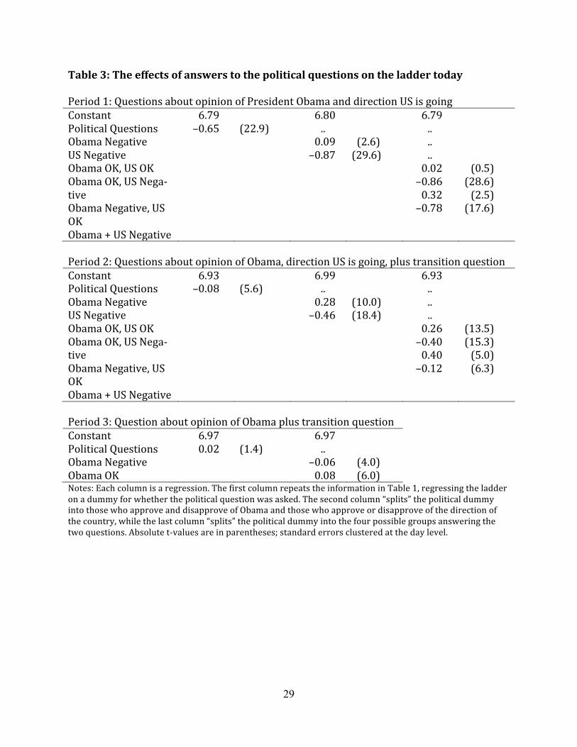
Table 4 looks at seven socio-demographic groups—gender, age, state of residence, edu-

cation, race, Hispanic status, high income—and also a time trend, motivated by our earlier ob-

servation that, changing approval ratings for the President, or changing satisfaction about the

way things are going in the US may change the sizes of the treatment effects. We look at the lad-

der and at the two summary measures, blue affect—the average of stress, worry, and sadness—

and positive affect—the average of happiness, smiling, and enjoyment. In each case, we present

15

the F–statistic for the interactions between the treatment and the set of categories for each socio-

demographic group; as before, asterisks indicate significance at one percent or less, and shading

indicates significance by the Schwarz test. Each time period in the Table is a separate experi-

ment; we continue to refer to them as periods, but the separate experimental status should be kept

in mind.

For the ladder, the F-statistics for the interactions are statistically significant at 1 percent

or less in 18 out of the 24 experiments; for age groups, state of residence, race, and Hispanic sta-

tus, they are significant in all three experimental comparisons. For age groups, race, Hispanic

status, and income, the F-statistics in at least one period are large enough to meet the more strin-

gent Schwarz test. All three incarnations of the political questions have treatment effects that dif-

fer across socioeconomic groups.

There are also differential treatment effects on the hedonics, more for blue affect than for

positive affect, though all are less pronounced than for the (evaluative) ladder. For blue affect,

the F-statistics exceed the one percent level in eleven out of twenty-four experiments, and for

positive affect, in only five. The Schwarz criterion is met for only two out of the three periods on

whether high income influences the treatment effects. Just as treatment effects were less pro-

nounced for hedonic wellbeing than evaluative wellbeing, so is the sensitivity of average treat-

ment effects to the background circumstances of the respondents.

The importance of the variation in treatment effects can be further investigated by a clos-

er evaluation of each case; here we focus on the cases where the F-statistics exceed the Schwarz

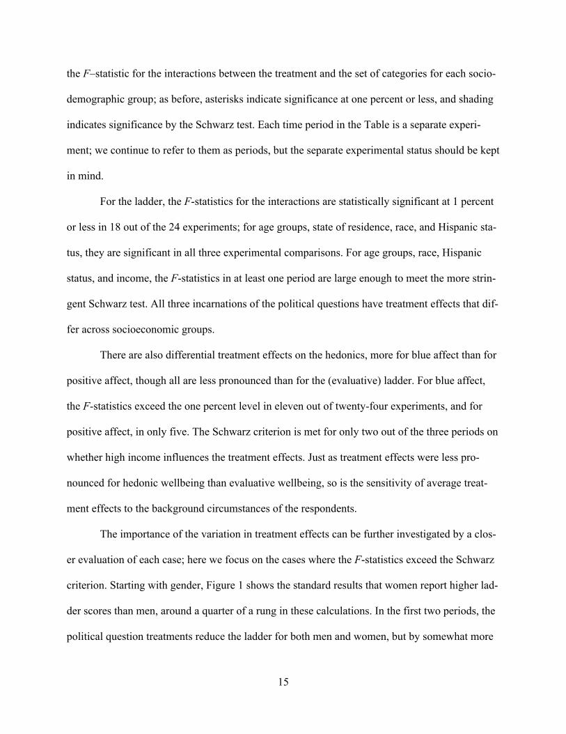
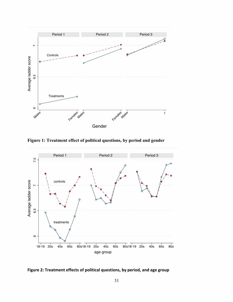
criterion. Starting with gender, Figure 1 shows the standard results that women report higher lad-

der scores than men, around a quarter of a rung in these calculations. In the first two periods, the

political question treatments reduce the ladder for both men and women, but by somewhat more

16

for men. In the third period, where the only political question is about President Obama’s per-

formance, there is a significant difference in the treatment effect for men and women; for men,

the President Obama question reduces the average ladder score by 0.016, while for women, it

increases it by 0.035. These numbers, interesting although they are, are small compared to the

main effect for women of 0.25, so they are not close to being able undercut the broader finding,

that women rate their lives more highly than do men. For blue or negative affect, the story is sim-

ilar. About five percent more women than men report blue affect on the previous day. In the first

period, where both political questions are asked, and where there is no buffer question, the treat-

ment effect for men is 1.4 percent, so that the political questions increase the percentage of men

reporting blue affect. For women, the effect is –0.16 percent, a reduction in blue effect, but es-

sentially zero. Once again, these effects are small relative to the main effect of being a woman on

blue affect, so if reversal of ranking is the main concern, there differences are far from large

enough to do so.

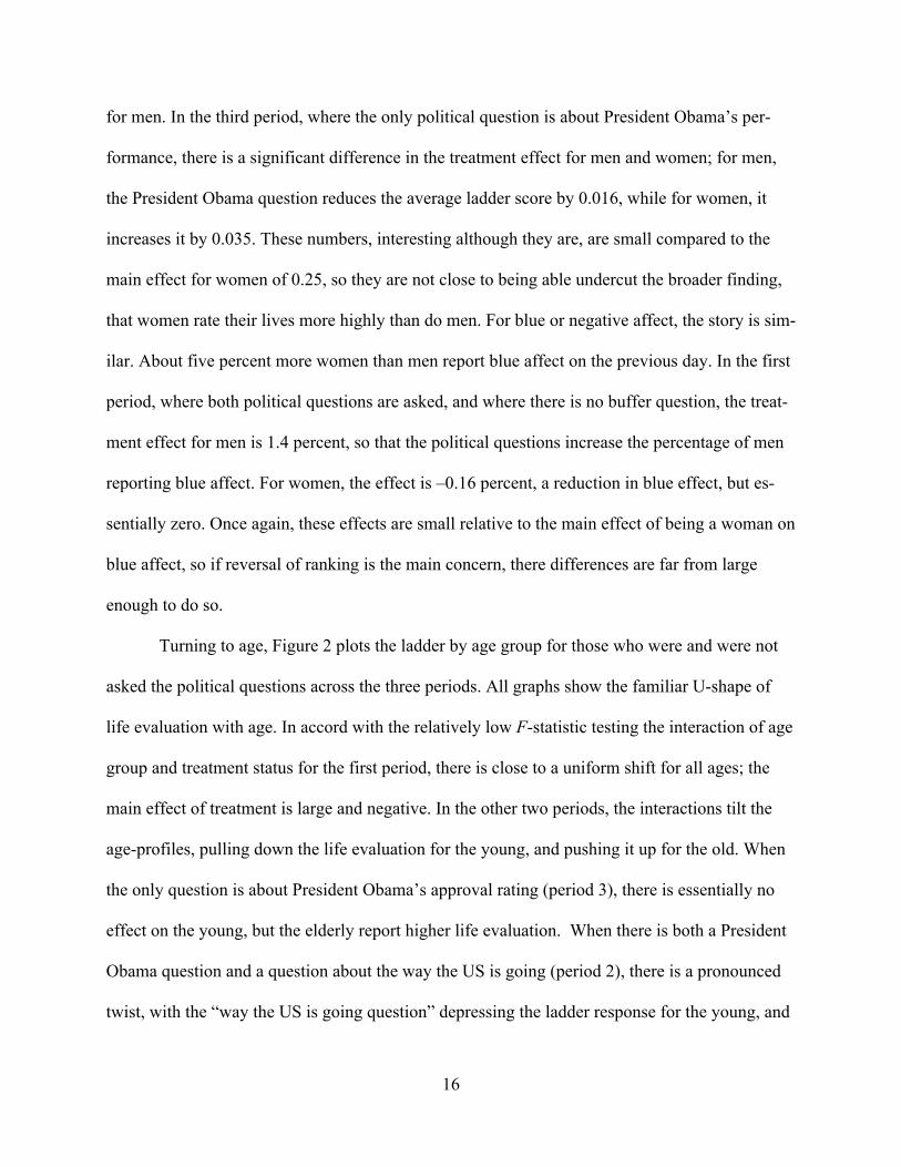
Turning to age, Figure 2 plots the ladder by age group for those who were and were not

asked the political questions across the three periods. All graphs show the familiar U-shape of

life evaluation with age. In accord with the relatively low F-statistic testing the interaction of age

group and treatment status for the first period, there is close to a uniform shift for all ages; the

main effect of treatment is large and negative. In the other two periods, the interactions tilt the

age-profiles, pulling down the life evaluation for the young, and pushing it up for the old. When

the only question is about President Obama’s approval rating (period 3), there is essentially no

effect on the young, but the elderly report higher life evaluation. When there is both a President

Obama question and a question about the way the US is going (period 2), there is a pronounced

twist, with the “way the US is going question” depressing the ladder response for the young, and

17

further enhancing it for the old. In some cases, these effects are large enough to change the rank-

ings of the age groups. In all three periods, those aged 80 and over report higher life evaluation

than those aged 18 and 19 when the political questions are present, but lower life evaluation in

their absence. That said, it is hard to imagine a policy context in which such small difference

would matter, given that the U-shape is preserved.

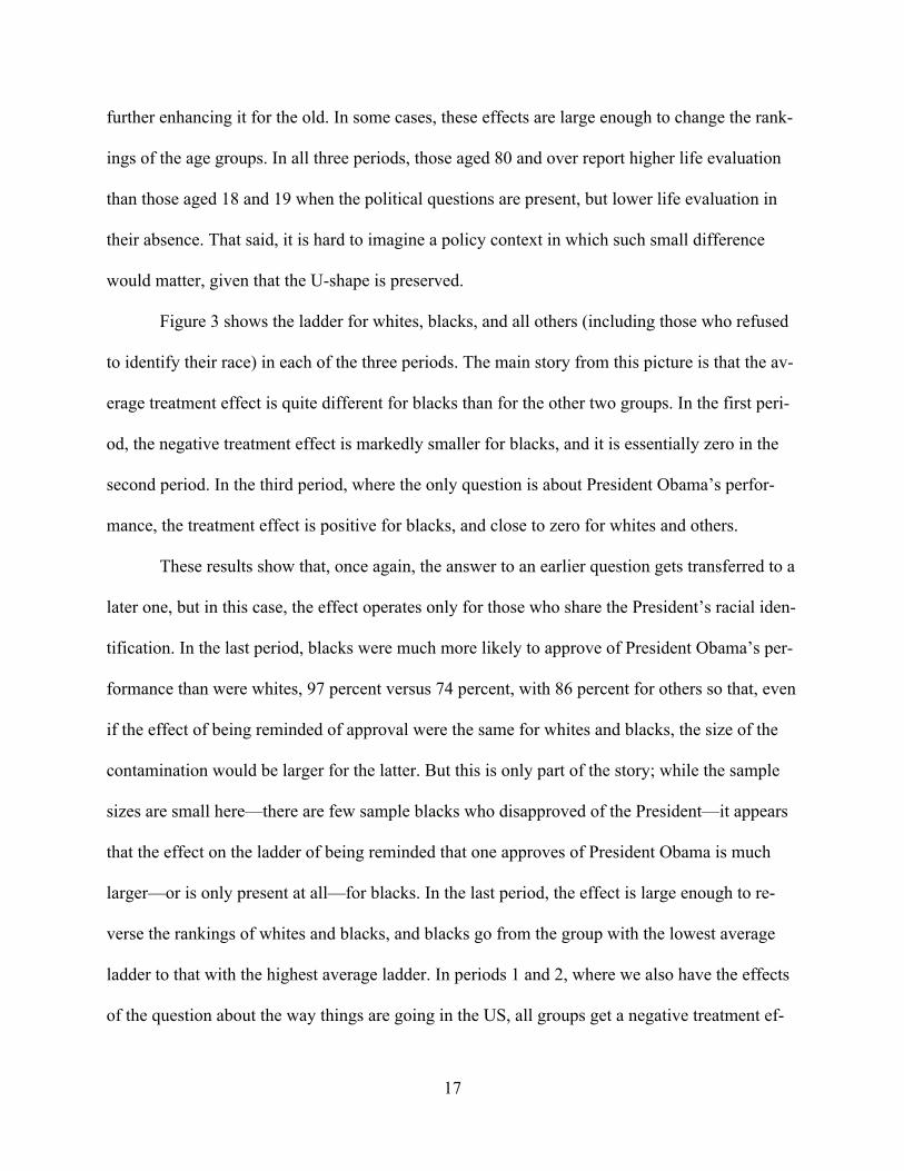
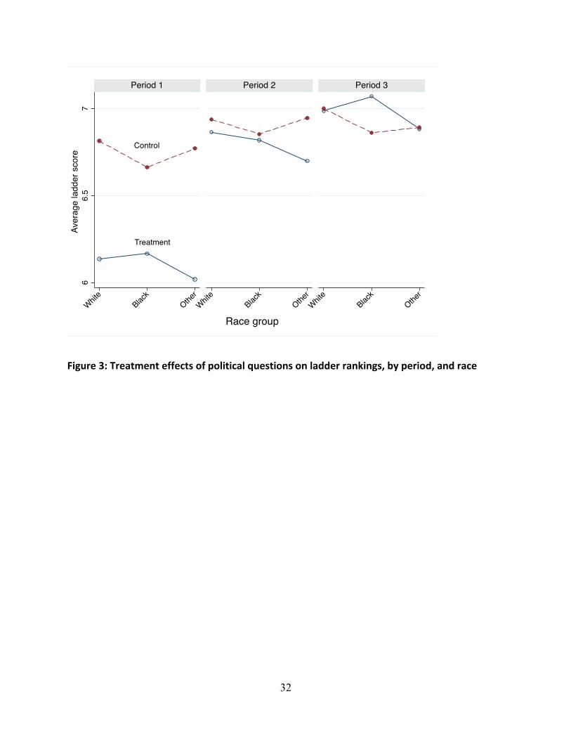
Figure 3 shows the ladder for whites, blacks, and all others (including those who refused

to identify their race) in each of the three periods. The main story from this picture is that the av-

erage treatment effect is quite different for blacks than for the other two groups. In the first peri-

od, the negative treatment effect is markedly smaller for blacks, and it is essentially zero in the

second period. In the third period, where the only question is about President Obama’s perfor-

mance, the treatment effect is positive for blacks, and close to zero for whites and others.

These results show that, once again, the answer to an earlier question gets transferred to a

later one, but in this case, the effect operates only for those who share the President’s racial iden-

tification. In the last period, blacks were much more likely to approve of President Obama’s per-

formance than were whites, 97 percent versus 74 percent, with 86 percent for others so that, even

if the effect of being reminded of approval were the same for whites and blacks, the size of the

contamination would be larger for the latter. But this is only part of the story; while the sample

sizes are small here—there are few sample blacks who disapproved of the President—it appears

that the effect on the ladder of being reminded that one approves of President Obama is much

larger—or is only present at all—for blacks. In the last period, the effect is large enough to re-

verse the rankings of whites and blacks, and blacks go from the group with the lowest average

ladder to that with the highest average ladder. In periods 1 and 2, where we also have the effects

of the question about the way things are going in the US, all groups get a negative treatment ef-

18

fect the size of which depends on the presence or otherwise of the buffer question. But the pres-

ence of the question about President Obama differentially favors blacks, so that in all three peri-

ods the treatment changes the order of the groups, either between blacks and other (in all three

periods), or between blacks and whites (periods 1 and 2.)

Hispanic status is another group where the treatments cause rank reversals in average

ladder scores. The culprit here is less the question about President Obama—though the question

slightly increases the ladder for Hispanics, and slightly decreases it for non-Hispanics—but the

question about the way things are going in the US. This has a negative effect on the ladder for all

groups, but much less for Hispanics than non-Hispanics. This difference is enough to reverse the

ladder rankings of Hispanics and non-Hispanics in all three periods; for the control groups, non-

Hispanics have ladder scores about 0.08 higher than Hispanics, and with treatment this switches

to about 0.08 lower.

The final category in Table 4 with large effects is high income. In this case, the large sta-

tistical effects do not turn into large substantive effects. Low-income respondents are less nega-

tively affected by the treatments than are high income respondents, but the effects are small rela-

tive to the very substantial effect of income on the ladder, so that there are no changes in ladder

rankings.

Section 4: Implications and conclusions

We have shown that answers to questions about wellbeing are sensitive to the context in which

the questions are asked, with previous questions conditioning the answers to questions about

wellbeing. The effects appear to be spillover or priming effects; answers to previous questions

with apparently similar content influence answers to subsequent questions. Within the period it

19

took to complete the questionnaire, the spillover effects did not evaporate quickly and affected

the answers to related questions that were asked much later in the questionnaire. Answers to

questions about life evaluation, which are not easily answered, appear to be more sensitive than

answers to questions about hedonic experience, at least for the hedonic questions with short re-

ferral periods (“yesterday”) used here. In accord with earlier literature, our results are consistent

with the view that people do not have an easily retrieved sense of how their lives are going and

so must answer the question by a cognitive process using their own feelings together with what-

ever information is at hand.

We also showed that context effects operate in different ways for different groups, for

example for the elderly versus the young, or for blacks relative to whites. Because the context

effects likely work by priming, by reminding people of their views about some perhaps loosely

related topic, the effects will generally be heterogeneous, in part because the distribution of an-

swers to the priming question is different in different groups—such as blacks’ versus whites’

views on President Obama’s performance—and in part because, even when they have the same

answers, the effect on subsequent answers can differ across groups. We showed that these differ-

ential effects can be large enough to change rankings of wellbeing across policy-relevant socio-

demographic groups. These observations may be important for evaluating group differences in

wellbeing, because true group effects can be confounded with differential context effects, which

could lead to erroneous conclusions. And unless the results of experiments of the types presented

here are known, investigators may be entirely unaware of this potential threat to the validity of

their studies.

We also reported on a technique for mitigating the impact of known context effects. The

experiments reported here used a buffer question between the context questions and the wellbe-

20

ing questions. The presence of this question removed most, but not all, of the context effects; re-

sidual effects are still significant, and are different for different substantive questions. Diener,

Inglehart, and Tay (2013) argue that context effects “in most cases can be controlled.” This as-

sessment rests on a very positive review of the evidence and expresses a sanguinity that we do

not share; they argue that the buffer question in the Gallup survey can “virtually eliminate” the

context effects. Yet the re-rankings of age and race groups in Section 3 happen in the presence of

the buffer question. As of now, we do not believe that there is any standard procedure to elimi-

nate context effects or, as mentioned earlier, even to let us know when they are present or im-

portant.

Context effects also pose problems for using evaluative measures to track social wellbe-

ing over time. Even if the obvious priming effects can be eliminated, for example by placing

evaluative questions first in the questionnaire, the sensitivity of life evaluation to previous ques-

tions raises the concern that they will also be affected by other unrelated stimuli that respondents

might experience prior to answering questions. Idiosyncratic stimuli—an ominous letter from the

tax authorities, or a disagreement with a business associate—will add to measurement error but

will usually cancel out over the population, but external stimuli common to the sample will not

do so. A possible example is the relationship between the stock market and life evaluation. For

those who are invested in the market, price fluctuations are clearly relevant for their future living

standards, and thus for life evaluation. But during the great recession of 2008–09, life evaluation

tracked the market closely, even for people with low incomes, who were unlikely to be directly

affected, Deaton (2012). It is possible that people rationally took the market as a signal of bad

times ahead, but while the ladder tracked the market, it tracked neither the unemployment rate

nor personal income. While it is impossible to rule out some forward-looking, rational explana-

21

tion, or the operation of “news” utility, Köszegi and Rabin (2009), Kimball and Willis (2006),

another explanation is that the heavy media coverage of the market in the spring of 2009, during

the first months of a new administration in Washington, led to deep fears about the future. Recall

that, in the experiments, it is not that the future of the US is irrelevant to individual’s assessment

of their own future, but that respondents need to be reminded that they think so before it affects

their own assessment, and that those who were randomized into not being reminded are not af-

fected. As the stock market recovered all of its losses (at least in nominal terms), the mean ladder

has not followed, suggesting that it is not the market itself that affects evaluative wellbeing, but

its salience.

The direct evidence in this paper applies only to the specific context questions that we

have analyzed. Although it is plausible that other, similar, reminders will have similar effects, we

do not know that this is true, so it is surely of great importance to institute a program to analyze

the effects of other context questions in other circumstances. The very large context effects in the

Gallup survey in the first period were entirely unanticipated when the questionnaire was de-

signed, and their discovery depended on the alertness of the Gallup statisticians. Other surveys

are likely to suffer from other biases that are unknown and unexpected.

Apart from context effects, the response of average evaluative wellbeing measures to in-

come and unemployment over typical short-term fluctuations can be expected to be small, per-

haps even too small to detect. Estimates of the effect of income on the ladder suggest a coeffi-

cient on log income of 0.30, so that a two percent decline in average income will decrease the

ladder by 0.006. Unemployment has a large effect on the evaluative wellbeing of individuals, but

a 5 percentage point increase in unemployment—large by business cycle standards—will change

the average ladder by very little. Even the UN’s World Happiness Report, Helliwell, Layard, and

22

Sachs (2012), which extols the virtues of wellbeing measures, and whose introduction states that

“regular large-scale collection of happiness data will improve macroeconomic policy-making”

(page 9), concludes “that subjective wellbeing data are not suitable for use as guides to short-

term macroeconomic policy, where in any case there are many more relevant data,” (page 19).

Our results support the second statement, but not the first.

One way of measuring wellbeing with minimal context effects is to work with hedonics,

rather than evaluative measures. Respondents’ recollections of affect on the day previous to the

survey appear to be relatively immune to priming questions, perhaps because questions about

hedonics ask for information that is readily accessible to respondents and that requires minimal

cognitive effort. Affect measures, especially when combined with data on duration, can give es-

timates of the quality of people’s lives that are the natural counterpart to Benthamite policymak-

ing. Kahneman and Krueger’s U-statistic, which measures the amount of time people spend be-

ing miserable, focuses on the worst off, and may be an attractive (negative) target for policy. Yet

hedonic measures are not a substitute for evaluative measures and the two types of wellbeing

measures tap somewhat different constructs. People’s own direct assessments of how their lives

are going provide a measure that goes beyond the hedonic content of their lives and, in theory,

captures the hedonic content and more. Life evaluation is sensitive to income and to education,

something that is less true for hedonics. There is also growing evidence that life evaluation is a

better guide to decision utility than are hedonics, which are best seen as an argument of life eval-

uation, see Benjamin, Heffetz, Kimball and Rees-Jones (2012, 2013). So we would lose much by

giving up evaluative measures, and we do not suggest doing so. But priority must be given to

developing a better understanding of how to control context effects, for example by appropriate

survey design, or by piloting surveys with varying question order.

23

We understand that this paper raises difficulties for much of wellbeing research as cur-

rently conducted, and proposes no solution to those difficulties. Yet it is better to be aware of the

problems than to ignore them. And knowing about them is the first step to finding ways of neu-

tralizing them and doing better.

List of works cited:

Agrawal, Sangeeta, and James K. Harter, 2011, “Context effect on life evaluation items: forming estimates for data prior to Jan. 6, 2009,” Gallup Technical Report. Benjamin, Daniel J, Ori Heffetz, Miles Kimball, and Alex Rees-Jones, 2012, “What do you think would make you happier? What do you think you would choose?” American Economic Review, 102(5), 2083–110. Benjamin, Daniel J, Ori Heffetz, Miles Kimball, and Alex Rees-Jones, 2013, “Can marginal rates of substitution be inferred from happiness data? Evidence from residency choices,” NBER Working Paper No. 18927, March. Bishop, George F., 1987, “Context effects on self-perceptions of interest in government and public affairs,” Chapter 10 in Hans_J. Hippler, Norbert Schwarz, and Seymour Sudman, eds., Social Information Processing and Survey Methodology, New York. Springer-Verlag. Cantril, Harvey, 1965, The pattern of human concern, New Brunswick, NJ. Rutgers University Press. Clark, Andrew E. and Andrew J. Oswald, 1994, “Unhappiness and unemployment,” Economic Journal, 104(424), 648–59. Deaton, Angus, 2012, “The financial crisis and the wellbeing of Americans,” Oxford Economic Papers, 64(1), 1–26. Deaton, Angus and Arthur A. Stone, 2013, “Two happiness puzzles,” American Economic Re-view, 103(3), 591–7. Diener, Ed, Ronald Inglehart, and Luous Tay, 2013, “Theory and validity of life satisfaction scales,” Social Indicators Research, 112(2), 497–527. Dolan, Paul Daniel Fujiwara and Robert Metcalfe, 2011, “A step toward evaluating utility the marginal and cardinal way,” CEPR Discussion Paper No 1062.

24

Easterlin, Richard A., 1974, “Does economic growth improve the human lot? Some empirical evidence,” in R. David and M. Reder, eds., Nations and households in economic growth: Essays in honor of Moses Abramovitz, Academic Press, 89–125. Fleurbaey, Marc, 2009, “Beyond GDP: the quest for a measure of social welfare,” Journal of Economic Literature, 47(4), 1029–75. Fleurbaey, Marc and Didier Blanchet, 2013, Beyond GDP: measuring welfare and assessing sus-tainability, Oxford. Oxford University Press. Heffetz, Ori and Matthew Rabin, 2013, “Conclusions regarding cross-group differences in hap-piness depend on difficulty of reaching respondents,” American Economic Review, forthcoming. Helliwell, John, Richard Layard, and Jeffrey Sachs, eds., The World Happiness Report, https://www.google.com/url?sa=t&rct=j&q=&esrc=s&source=web&cd=2&cad=rja&ved=0CDMQFjAB&url=http%3A%2F%2Fwww.earth.columbia.edu%2Fsitefiles%2Ffile%2FSachs%2520Writing%2F2012%2FWorld%2520Happiness%2520Report.pdf&ei=3QPvUamyIY-q4AP94YDgCg&usg=AFQjCNElcH3N-S7Qs__G2dNfiD9n49SiDQ&sig2=eGldSRhGJ1vUk2mO8aY3dg&bvm=bv.49641647,d.dmg Jarrett, Christian, 2011, “An insight into `nudge’”, The Psychologist, 24(6), 432–4. Kahenman, Daniel, and Angus Deaton, 2010, “High income improves evaluation of life but not emotional wellbeing,” PNAS, 107(38), 16489–93. Kahneman, Daniel, and Alan B. Krueger, 2006, “Developments in the measurement of subjec-tive well-being,” Journal of Economic Perspectives, 20(1), 3–24. Kahneman, Daniel, and Jason Riis, 2005, “Living, and thinking about it: two perspectives on life,” Chapter 11 in Felicia Huppert, Nick Baylis and Barry Keverne, eds., The science of well-being, Oxford. Oxford University Press, 285–304. Kimball, Miles and Robert Willis, 2006, “Utility and happiness,” University of Michigan, pro-cessed. Kimball, Miles, Helen Levy, Fumio Ohtake, and Yoshiro Tsutsui, 2006, “Unhappiness after Hur-ricane Katrina,” NBER Working Paper No. 12062. Köszegi, Botond, and Matthew Rabin, 2009, “Reference dependent consumption plans,” Ameri-can Economic Review, 99(3), 909–36. Krueger, Alan B., 2007, “Are we having more fun yet? Categorizing and evaluating changes in time allocation,” Brookings Papers on Economic Activity, 2007(2), 193–215. Luechinger, Simon and Paul A. Raschky, 2009, “Valuing flood disasters using the life satisfac-tion approach,” Journal of Public Economics, 93(3–4), 620–33.

25

Layard, Richard, 2005, Happiness: lessons from a new science, New York. Penguin. Newport, Frank, 2011, “Adjustments to the Gallup-Healthways life evaluation scores,” Septem-ber 8, http://www.gallup.com/poll/149006/Adjustments-Gallup-Healthways-Life-Evaluation-Scores.aspx OECD, 2011, How’s life? Measuring well-being, Paris. OECD Publishing. Office of National Statistics, 2012, First annual ONS experimental subjective well-being results, ONS. http://www.ons.gov.uk/ons/dcp171766_272294.pdf Oswald, Andrew J, and Nattavudh Powdthavee, 2008, “Death, happiness, and the calculation of compensatory damages,” Journal of Legal Studies, 37(52), S217–51 Oswald, Andrew J, and Stephen Wu, 2009, “Objective confirmation of subjective measures of human well-being: evidence from the U.S.A.,” Science, 327(5965), 576–9. Sacks, Daniel W., Betsey Stevenson, and Justin Wolfers, 2012, “Subjective wellbeing, income, economic development and growth,” in Philip Booth ed., ……and the pursuit of happiness, In-stitute for Economic Affairs, 59–97. Schwarz, Norbert, 1999, “Self-reports—How the questions shape the answers. American Psy-chologist, 54(2), 93–105. Schwarz, Norbert and Fritz Strack, 1999, “Reports of subjective well-being: judgmental process-es and their methodological implications,” Chapter 4 in Daniel Kahneman, Ed Diener and Norb-ert Schwarz, eds., Well-being: the foundations of hedonic psychology, New York. Russell Sage. Sen, Amartya K., Joseph E. Stiglitz, and Jean-Paul Fitoussi, 2009, Commission on the Measure-ment of Economic Performance and Social Progress, http://www.stiglitz-sen-fitoussi.fr/documents/rapport_anglais.pdf Steptoe, Andrew, Angus Deaton, and Arthur A. Stone, 2014, “Psychological wellbeing, health and ageing,” The Lancet, forthcoming. Stone, Arthur A., Joseph E. Schwartz, Joan E. Broderick, and Angus Deaton, 2010, “A snapshot of the age distribution of psychological well-being in the United States,” Proceedings of the Na-tional Academy of Sciences, 107(22), 9985–90/ van Praag, Bernard, and Barbara Baarsma, 2005, “Using happiness surveys to value intangibles: the case of airport noise,” Economic Journal, 115 (500), 224–46.

26

Table  1:  Question  ordering  for  three  experimental  periods  

 QUESTION  ORDER  

PERIOD  1  January  21st,  2009  to  April  5th,  2009:  (75  days,  76,167  observations)  

PERIOD  2  April  6th,  2009  to  August  17th,  2009:  (129  days,  130,469  observations)  

PERIOD  3  August  18th,  2009  to  February  28h,  2010:  (185  days,  186,395  observa-­‐

tions)      

Do  you  approve  or  disapprove  of  the  way  that  Barack  Obama  is  handling  his  job  as  presi-­‐dent?    

 Do  you  approve  or  disapprove  of  the  way  that  Barack  Obama  is  handling  his  job  as  presi-­‐dent?    

 Do  you  approve  or  disapprove  of  the  way  that  Barack  Obama  is  handling  his  job  as  presi-­‐dent?    

 In  general,  are  you  satisfied  or  dissat-­‐isfied  with  the  way  things  are  going  in  the  US?    

 In  general,  are  you  satisfied  or  dissat-­‐isfied  with  the  way  things  are  going  in  the  US?    

 

   Are  you  satisfied  or  dissatisfied  with  your  personal  life  today?    

 Are  you  satisfied  or  dissatisfied  with  your  personal  life  today?    

 Cantril  Ladder  

 Cantril  Ladder  

 Cantril  Ladder  

   

27

Table  2:  Effect  of  prior  questions  on  subsequent  questions  

  All  periods  all  observations  

Period  1    

Period  2   Period  3  

  Mean   s.d.   ATE   t   ATE   t   ATE   t  Ladder  today   6.84   2.02   –0.67   (24.0)   –0.09   (6.4)   0.01   (0.0)  Ladder  future   7.67   2.31   –0.26   (10.6)   0.10   (5.5)   0.13   (8.2)                    Health  is  excellent   0.208     0.011   (3.3)   0.013   (4.2)   0.013   (5.4)  Health  is  very  good   0.295     –0.009   (2.3)   0.001   (0.4)   0.001   (0.5)  Health  is  good   0.294     –0.009   (2.2)   –0.016   (5.4)   –0.013   (4.5)  Health  is  fair   0.147     –0.001   (0.2)   0.000   (0.1)   –0.001   (0.4)  Health  is  poor   0.055     0.008   (3.5)   0.001   (0.9)   –0.001   (0.9)                    Disability?   0.222       –0.002   (0.6)   –0.004   (1.4)   –0.004   (1.6)  Smoker?   0.210     0.002   (0.7)   –0.002   (0.6)   –0.000   (0.0)  Personal  doctor?   0.805     0.001   (0.4)   0.003   (1.2)   –0.004   (1.4)                    Stand  of  living  OK   0.749     –0.033   (7.7)   –0.004   (1.5)   0.005   (2.1)  SOL  going  up   0.418     –0.029   (6.0)   –0.003   (0.9)   –0.010   (3.1)  SOL  same   0.204     –0.015   (4.3)   –0.023   (8.1)   –0.002   (0.8)  SOL  falling   0.378     0.044   (9.9)   0.026   (8.8)   0.011   (4.1)                    No  cash  for  food   0.183     0.011   (2.7)   0.004   (1.3)   0.001   (0.5)  No  cash  for  shelter   0.092     0.005   (1.7)   0.005   (2.1)   0.002   (0.8)  No  cash  for  meds   0.186     0.013   (2.8)   0.007   (2.7)   0.003   (1.0)                    Smile   0.818     0.002   (0.5)   0.004   (1.5)   0.007   (3.2)  Enjoy   0.841     0.002   (0.7)   0.005   (1.6)   0.009   (4.5)  Pain   0.238     0.004   (1.0)   0.001   (0.4)   –0.006   (2.2)  Worry   0.330     0.005   (1.1)   –0.010   (2.9)   –0.017   (6.7)  Sad   0.184     0.006   (1.4)   –0.006   (2.6)   –0.007   (2.8)  Stress   0.399     0.019   (3.2)   0.001   (0.3)   –0.009   (3.1)  Angry   0.141     0.006   (1.7)   0.004   (1.7)   –0.004   (1.7)  Happy   0.878     0.003   (1.0)   0.005   (2.2)   0.006   (3.0)                    Positive  affect   0.847   0.291   0.003   (1.0)   0.005   (2.0)   0.008   (4.5)  Blue  affect   0.257   0.367   0.005   (1.4)   –0.008   (3.2)   –0.012   (5.7)                    Married?   0.544     –0.010   (2.1)   0.000   (0.1)   –0.002   (0.7)  Hispanic?   0.111     –0.001   (0.4)   –0.003   (1.0)   0.000   (0.1)  High  income?   0.356     –0.008   (2.1)   0.006   (2.0)   –0.001   (0.2)  Income  ref  or  DK   0.228     0.005   (1.5)   0.007   (2.4)   0.009   (3.7)  

28

Notes  to  Table  2:  The  first  column  is  the  mean  and  the  second  (for  non-­‐dichotomous  variables)  the  standard  deviation;  these  calculations  are  pooled  over  all  periods  and  both  experimentals  and  controls.  The  other  columns  show  the  effect  of  asking  the  political  questions  in  the  three  periods;  they  are  the  differences  in  means  between  treatments  and  controls  for  each  period.  The  ladders  are  on  scales  from  0  to  10,  the  remainder  are  0  or  1  except  for  positive  affect  (the  average  of  smile,  enjoy  and  happy)  and  blue  affect  (the  average  of  worry  and  sad).  High  income  is  an  indicator  that  monthly  income  was  declared  to  be  at  least  $4,000.  The  self-­‐assessed  health,  disability,  smoking,  and  whether  or  not  you  have  a  personal  doctor  closely  follow  the  ladder  questions  in  the  questionnaire.  The  standard  of  living  questions  follow  the  health  ques-­‐tions.  Standard  of  living  OK  is  1  if  respondent  says  SOL  is  satisfactory,  and  SOL  going  up,  same,  or  falling  are  three  an-­‐swers  to  a  question  about  whether  the  SOL  is  getting  better,  staying  the  same,  or  getting  worse;  the  coefficients  on  those  three  add  to  zero.  Absolute  t-­‐values  are  shown  in  brackets.  The  bold/highlighted  ATEs  are  those  with  t-­‐values  greater  than  3.5,  which  is  close  to  the  square  root  of  the  logarithm  of  the  sample  size,  the  Schwarz  (1978)  large-­‐sample  Bayesian  test  that  adjusts  for  sample  size.  

   

29

Table  3:  The  effects  of  answers  to  the  political  questions  on  the  ladder  today  

Period  1:  Questions  about  opinion  of  President  Obama  and  direction  US  is  going  Constant   6.79     6.80     6.79    Political  Questions   –0.65   (22.9)   ..     ..    Obama  Negative  US  Negative  

    0.09  –0.87  

(2.6)  (29.6)  

..  

..    

Obama  OK,  US  OK  Obama  OK,  US  Nega-­‐tive  Obama  Negative,  US  OK  Obama  +  US  Negative  

        0.02  –0.86  0.32  –0.78  

(0.5)  (28.6)  (2.5)  (17.6)  

 Period  2:  Questions  about  opinion  of  Obama,  direction  US  is  going,  plus  transition  question  Constant   6.93     6.99     6.93    Political  Questions   –0.08   (5.6)   ..     ..    Obama  Negative  US  Negative  

    0.28  –0.46  

(10.0)  (18.4)  

..  

..    

Obama  OK,  US  OK  Obama  OK,  US  Nega-­‐tive  Obama  Negative,  US  OK  Obama  +  US  Negative  

        0.26  –0.40  0.40  –0.12  

(13.5)  (15.3)  (5.0)  (6.3)  

 Period  3:  Question  about  opinion  of  Obama  plus  transition  question  Constant   6.97     6.97    Political  Questions   0.02   (1.4)   ..    Obama  Negative  Obama  OK  

    –0.06  0.08  

(4.0)  (6.0)  

Notes:  Each  column  is  a  regression.  The  first  column  repeats  the  information  in  Table  1,  regressing  the  ladder  on  a  dummy  for  whether  the  political  question  was  asked.  The  second  column  “splits”  the  political  dummy  into  those  who  approve  and  disapprove  of  Obama  and  those  who  approve  or  disapprove  of  the  direction  of  the  country,  while  the  last  column  “splits”  the  political  dummy  into  the  four  possible  groups  answering  the  two  questions.  Absolute  t-­‐values  are  in  parentheses;  standard  errors  clustered  at  the  day  level.      

30

Table  4:  Subgroup  analysis  of  average  treatment  effects,  Gallup  data,  ladder,  blue  af-­‐fect,  and  positive  affect    Period     F-­‐statistic  for  

Ladder  F-­‐statistic  for  Blue  affect  

F-­‐statistic  for  Positive  affect  

1  2  3  

Gender  (2  categories)    

0.41  6.39  

           7.40*  

8.29*  1.31  

           3.16  

0.83  0.02  

         0.02  1  2  3  

Age  groups  (8  categories)    

2.69*  20.23*  17.83*  

0.90  1.91  3.16*  

1.58  1.89  3.20*  

1  2  3  

State  (51  catego-­‐ries)  

2.14*  1.80*  1.74*  

1.20  2.57*  1.99*  

1.90  2.10*  1.90*  

1  2  3  

Education  (8  categories)  

4.57*  2.48  9.48*  

0.93  1.03  2.89*  

0.38  1.18  0.75  

1  2  3  

Race  (3  categories)  

8.66*  15.02*  26.56*  

6.30*  2.50  11.40*  

2.60  2.56  6.61*  

1  2  3  

Hispanic  (2  categories)  

8.88*  49.13*  10.40*  

2.23  7.04*  3.54  

6.53  0.01  0.84  

1  2  3  

High  income  (2  categories)  

5.98  13.02*  37.43*  

13.59*  14.46*  10.59*  

0.05  2.04  1.23  

1  2  3  

Time  (trend)  

9.32*  4.16  1.16  

5.21  5.68  0.29  

1.22  7.18*  0.56  

Notes:  The  sample  sizes  for  the  three  periods  are  75734,  76054,  and  129839.  For  the  high  income  row,  about  a  third  of  observations  are  missing.  F-­‐tests  in  bold  are  significant  by  the  Schwarz  criteria;  those  with  asterisks  have  p-­‐values  less  than  0.01.  

31

Figure 1: Treatment effect of political questions, by period and gender

Figure  2:  Treatment  effects  of  political  questions,  by  period,  and  age  group  

Aver

age

ladd

er s

core

Controls

Treatments

66.

57

Males

Female

sMale

s

Female

s 1Male

s

Period 1 Period 2 Period 3

Gender

controls

treatments

Aver

age

ladd

er s

core

66.

57

7.5

18-19 20s 40s 60s 80s18-19 20s 40s 60s 80s18-19 20s 40s 60s 80s

Period 1 Period 2 Period 3

age group

32

Figure  3:  Treatment  effects  of  political  questions  on  ladder  rankings,  by  period,  and  race  

ControlControl

Treatment

Aver

age

ladd

er s

core

66.

57

White

Black

OtherWhit

eBlac

kOthe

rWhit

eBlac

kOthe

r

Period 1 Period 2 Period 3

Race group