· Web viewthis will not happen prior to distribution of NHDPlus because the update process for the central NHD database at USGS was under development at the time these improvements

GIS Analysis to Understand Landscape Functional Changes in

the Rio Salado Subbasin, NM

GEOG 591 Term Project

by

Alexandra Permar

at

The University of North Carolina at Chapel Hill

in the

Curriculum for the Environment & Ecology

on

April 30, 2012

1

Table of Contents

I. Project Context: Research Interests 3a. Questions 4b. Methods 4

II. Preliminary Cast Study: Rio Salado Subbasin and La Jencia Watershed, NM 6a. La Jencia’s History 6b. Intended Analyses 8c. Data Acquisition 9d. Executed Analyses (files created) 9e. Information about the Data Used in this Project 12f. La Jencia Creek: Primary Channel 17g. Rio Salado Subbasin Overview 19h. La Jencia Watershed Overview 20i. La Jencia Subwatershed Overview 21j. NLCD 2001-2006 Rio Salado Subbasin Landcover Comparison Map 22k. NLCD 2001-2006 Rio Salado Subbasin Landcover Comparison Table 23l. Rio Salado Subbasin 2006 NLCD Landcover Types 25m. Rio Salado Subbasin Satellite Remotely Sensed Imagery 29n. La Jencia Watershed Comparative Analysis of Satellite Remotely Sensed 31

Enhanced Vegetative Index o. Elevational Gradient Analysis of Rio Salado Subbasin 33p. Slope Analysis of Rio Salado Subbasin 34q. Aspect Analysis of Rio Salado Subbasin 35r. Discharge Area Analysis of Rio Salado Subbasin 36s. Mean Annual Flow Thresholds in Rio Salado Subbasin 38t. Wetness Indices, Saturated Areas, and Return Flow in the Rio Salado 39

Subbasini. Rio Salado Watershed Mean Wetness Index Map 39

ii. Maps of Si Values with m=0.4517 m-1 and λ = 10.44716 40iii. Maps of Saturated Areas with m=0.4517 m-1 and λ = 10.44716 42iv. Maps of Return Flow with m=0.4517 m-1

and λ = 10.44716 45

2

I. Project Context: Research Interests

Soon the Clean Water Act will turn 40 years old. The Act was originally designed to regulate discharges of pollutants into United States water bodies, and to regulate surface water quality standards. While it originated in 1948 as the Federal Water Pollution Control Act, the contemporary Clean Water Act was reorganized and expanded in 1972 into the form it has today. The Environmental Protection Agency implements the CWA, and ensures that industry (as well as other entities) abides by its rules. In so doing the EPA enforces pollution control programs and surface water quality standards. The National Pollutant Discharge Elimination System (NPDES) in conjunction with the CWA regulates point source (e.g. pipes, ditches) pollutant discharges into navigable waters.

Despite the regulations and related water quality control monitoring programs in effect, there are thousands of water bodies around the U.S. that are contaminated, geomorphologically degraded, and otherwise impaired. Contemporary perceptions of the value of our water systems incite land managers, scientists, and governmental agencies to implement regulatory changes designed to improve the quality of the U.S. wetlands, rivers, and streams. Some of the participating organizations that are taking responsibility for improving the quality of our national water bodies include a variety of academic, non-profit, and non-governmental agencies. These entities – along with those previously mentioned – are engaging the water systems in ways designed to understand how they are impaired, and more so how those identified as impaired may be improved.

Ecological Integrity Assessments (EIAs) serve as one means of describing the overall ‘health’ of an ecosystem. These assessments are designed to comprehensively document a suite of site characteristics that – when taken together – tell a story about the overall quality of the system. Example ecological parameters include stream channel embedment, bank full height, density of overbank shrubs and trees, amount of in-stream filamentous algae, taxonomic assessment of macroinvertebrate diversity, and proximity of site to hayed-, pastured-, urbanized-, and/or ranched land. Integrity assessments are young enough, however, and human understandings of the indicators of ecosystem health are nascent enough that there are many open questions as to what ecological parameters signify landscape salubrity or degradation.

Contemporary efforts to repair degraded ecosystems are advancing more quickly than is the science understanding what degradation means. The result of this discord indicates that private and state funds are allocated to ecosystem restoration projects that may be insufficiently informed to effectively restore ‘healthy’ ecosystem function. Science has the ability to respond to the restructuralization of societal priorities in the form of riparian restoration with investment in understanding what ecological parameters gauge ecosystem function, and what types of restoration methods effectively restore healthy ecosystems. Efforts to understand ecology in ways that sufficiently inform land management and restoration entail interdisciplinary collaboration between multiple fields of study including ecology, hydrology, geomorphology, geology, geography, toxicology, mammalogy, herpetology, entymology, and atmospheric sciences to name a few.

3

Across the country natural resource management agencies are incorporating GIS data into their land management tools to effectively aid the accuracy, precision, and reliability of their land management decisions (Bauer et al. 1994). Advancements in technology have conferred higher-quality remote-sensing devices that provide humans with types of information about Earth’s surface that were previously undocumented. Examples include recurring measurements of hydrologic data via USGS in-stream gauges, flux towers measuring atmospheric gas exchange and plant gross primary productivity, and satellite-based optical- and thermal data acquired via Landsat, Ikonos, ASTER, MODIS, and other remote-sensing entities. GIS data can be used to characterize stream flow regimes, human land use/land cover (LULC), topographical landscape changes, phenological changes, wildfire location- and frequency, and more.

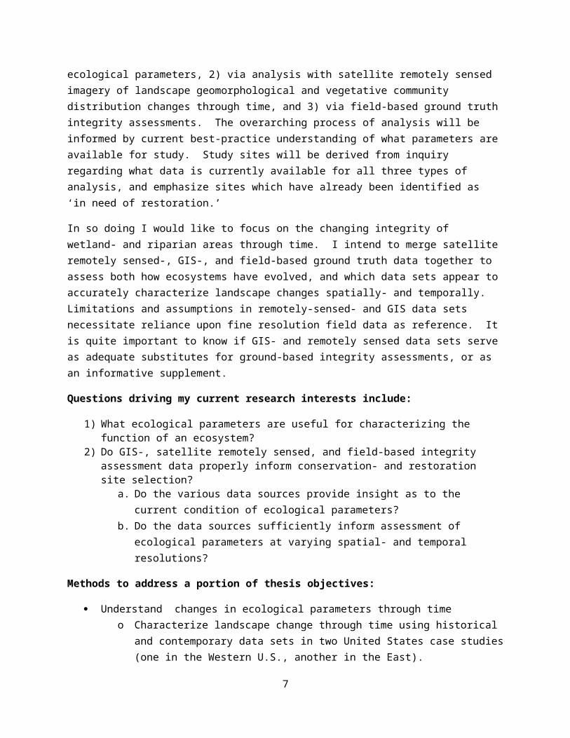
In order to understand the issues presented above, I intend to comprehensively analyze two landscape case studies in the Western- and Eastern U.S. in three ways: 1) via GIS analysis of hydrological and ecological parameters, 2) via analysis with satellite remotely sensed imagery of landscape geomorphological and vegetative community distribution changes through time, and 3) via field-based ground truth integrity assessments. The overarching process of analysis will be informed by current best-practice understanding of what parameters are available for study. Study sites will be derived from inquiry regarding what data is currently available for all three types of analysis, and emphasize sites which have already been identified as ‘in need of restoration.’

In so doing I would like to focus on the changing integrity of wetland- and riparian areas through time. I intend to merge satellite remotely sensed-, GIS-, and field-based ground truth data together to assess both how ecosystems have evolved, and which data sets appear to accurately characterize landscape changes spatially- and temporally. Limitations and assumptions in remotely-sensed- and GIS data sets necessitate reliance upon fine resolution field data as reference. It is quite important to know if GIS- and remotely sensed data sets serve as adequate substitutes for ground-based integrity assessments, or as an informative supplement.

Questions driving my current research interests include:

1) What ecological parameters are useful for characterizing the function of an ecosystem?2) Do GIS-, satellite remotely sensed, and field-based integrity assessment data properly inform

conservation- and restoration site selection?a. Do the various data sources provide insight as to the current condition of ecological

parameters?b. Do the data sources sufficiently inform assessment of ecological parameters at varying

spatial- and temporal resolutions?

Methods to address a portion of thesis objectives:

Understand changes in ecological parameters through time o Characterize landscape change through time using historical and contemporary data

sets in two United States case studies (one in the Western U.S., another in the East).

4

Derive and compare water budgets for case studies, addressing variables such as precipitation, evapotranspiration, consumptive water use, runoff, infiltration, and stored water.

Analyze changes in vegetative community patterns through time (abundance, distribution, types, species).

Evaluate changes in amounts- and types of urbanized infrastructure in case studies, and evaluate urbanization data in context of other data sets being used.

Where possible, contextualize case study changes with respect to natural landscape disturbances (including drought, fire, flooding) to ascertain what types and impacts disturbance have upon ecosystem function.

Evaluate relative impacts of anthropogenic land use (grazing, recreation, restructuralization of water resources) on ecosystem function.

Contextualize understanding of landscape changes through time with relevance to restoration site selection.

Monitor restoration projects through time to observe how they enable the landscape to withstand disturbance.

5

II. Preliminary Cast Study: Rio Salado Subbasin and La Jencia Watershed, NM

La Jencia’s History

La Jencia Land (Photo by Jes Alford)

La Jencia Creek and Conservation Ranch is physically located along Hwy 60 West, in the vicinity of Mile Marker 116 near Magdalena, NM. The 130,000 acres that comprise the historical ranch property has its original identity as the home of the Chiricahua Apache and Puertecito Navajo Native American people. In the latter half of the 19th century the land was coopted as a working cattle ranch. The current La Jencia Ranch occupies a geographic subset of its ancestral extent. In the time since its exchange of ownership, the ranch has become identified as a central site for the practice and propagation of conservation- and restoration practices. A number of bosque and channel restoration projects have been executed there over the years; these have entailed plantings of thousands of native trees and shrubs, and the removal of cattle to mitigate the effects

of grazing. La Jencia’s mission is to a) restore and protect the ranch's native lands and wildlife and b) provide educational and partnership opportunities to those interested in conservation.

The La Jencia Conservation Ranch is home to approximately 5 miles of the La Jencia Creek. In alignment with the Ranch’s mission and the New Mexico Riparian Ecosystem Restoration Initiative (RERI), three years of restoration efforts have been executed at the ranch. Restoration efforts led by the WildEarth Guardians of New Mexico have entailed the physical removal of nonnative riparian vegetation such as salt cedar (Tamarix spp.) and russian olive (Eleagnus angustifolia), and the planting of native vegetation including coyote willow (Salix exigua) and fremont cottonwood (Populus fremontii). Progress over the years had been measured by the planting of more than 50,000 native riparian trees and shrubs, and the formation of two habitat ponds alongside the creek channel to provide habitat to the Northern Leopard Frog (Rana pipiens, a state endangered species).

Since the channel is home to flooding events of enormous magnitude (two “100 year” floods have occurred in the past decade), channel incision-, erosion-, and riparian bank stability are all of major concern. Thus restoration efforts have also been focused on the control- and stability of the stream channel to enable it to resist erosion in response to high magnitude storm events.

Consequently in 2009 I collaborated with the WildEarth Guardians, the La Jencia Conservation Ranch, and the New Mexico Environment Department’s River Ecosystem Restoration Initiative to aid the Ranch’s restoration efforts. Goals included the improvement of ecological diversity, water quality and wildlife habitat along more than two miles of the Creek. Overarching methods were designed to

6

stabilize stream banks, restore cienegas and springs, enhance stream sinuosity, remove non-native vegetation, and plant native trees and shrubs.

During my time spent assisting restoration efforts throughout New Mexico, I sought to ascertain the scientific methods informing coordinated restoration efforts. I seek to understand the effectiveness of individual restoration techniques including the installation of post vane structures to induce meandering, living willow wattles for stream reconfiguration (sinuousity, induced meandering, sediment catchment and channel stability), gabions to prevent streambank erosion and induce channel stability, one-rock dams for the purpose of sediment collection, zuni bowls for the purpose of absorbing erosive water forces, check dams at nick points to prevent upstream migration of a nick point, streamside native vegetative plantings, and stream rock armament.

A time-series composite of La Jencia Creek before and after restoration

In 2012 I find myself reflecting upon past restoration efforts with an interest in understanding how restoration methodologies were informed in the time of my project participation, and how restoration efforts at large are informed in different scenarios across the globe. By means of inquiry and exploratory research I intend to not only understand current restoration methodologies but also to explore ways in which restoration efforts may be informed more comprehensively than current standards call for. In theory, if restoration efforts are comprehensively informed prior to their execution then they will efficiently materialize intended restoration outcomes that enable stream channels to withstand natural storm events and anthropogenic impact.

7

In an effort to understand the La Jencia watershed through GIS, I focused my GEOG 591 term project on the watershed and its larger geographic region including the Rio Salado subbasin (HUC-8: 13020209) in which it is embedded. My preliminary La Jencia watershed case study objectives are listed below. For a variety of data analysis-related reasons I have not yet fulfilled these objectives, and since case study commencement have revised my goals for understanding the La Jencia watershed and its greater geographic region (the Rio Salado subbasin).

Types of Analyses:

NLCD 1992, 2001, 2006 from-to assessment of change in classified land cover type through time Variable source area assessment of wetlands of interest WI assessment of Rio Salado subbasin and La Jencia watershed Calculation of % impervious cover in region surrounding wetlands of interest Assessment of flow accumulation at water bodies/stream reaches of interest and changes in this

value through time Assessment of hillslope slope- and aspect values for riparian regions surrounding wetlands of

interest Assessment of changes in subbasin- and watershed water inputs (precipitation) through time Assessment of water contaminant loading, changes through time

I began my term project by downloading about 118 GB of GIS information for the United States and the state of New Mexico from publicly available data sources. A list of downloaded files can be seen below:

Data Acquisition (downloaded from online resources)

ArcMap_Toolbars_Version10 ned_13_arc radx_largo35724164116 (303d, 305b streams) NM_wetlands (NWI polygons) NLCD 1992, 2001, 2006 landcover & impervious NLCD 2006 Change map NHDPlus FAC, FDR for all of region 13 NHDPlus Elevation for region 13b NHDPlus13V01_02_Catgrid NHDPlus13V01_02_Catshape NHDPlus13V01_02_streamgageevent NHDPlus13V01_03_Cat_Flowline_Attr NHDPlusV01_02_productionunit NHDPlus13V01_03_NHD nm_statsgo_09 (soils data) 7 NED DEMs for region of interest using ArcMap Toolbars v. 10 WebFTP - 1992-2001 Retrofit Data (NM) World_Topographic_Map

8

USGS_EDC_Elev_NED_3 USGS_EDC_Ortho_NAIP USGS_EDC_Ortho_NAIP_12 USGS_EDC_Ortho_NewMexico USGS_EDC_Ortho_Utah AZ_wetlands (NWI polygons)

Below is a list of ArcMap v. 10, Terrain Analysis Systems (TAS), and ENvironment for Visualizing Images (ENVI) files created using the data sources previously mentioned. The files listed here were created in pursuit of fulfilling the objectives listed above.

ArcMap Files (created)

%catchment_bare_rock_sand_clay_greaterthan_20 flow lines and table %catchment_deciduousforest_greaterthan_10 flow lines and table %catchment_evergreenforest_greaterthan_50 flow lines and table %catchment_evergreenforest_lessthan_10 flow lines and table %catchment_evergreenforest_lessthan_50 flow lines and table %catchment_grass_herb_greaterthan_50 flow lines and table %catchment_grass_herb_lessthan_10 flow lines and table %catchment_herbwetlands_lessthan_10 flow lines and table %catchment_mixedforest_lessthanequalto_10 flow lines and table %catchment_openwater_20 flow lines and table %catchment_precip_lessthan_12in flow lines and table %catchment_quarries_mines_pits_greaterthan_10 flow lines and table %catchment_shrubland_greaterthan_50 flow lines and table %catchment_shrubland_greaterthanequalto_10_and_lessthan_30 flow lines and table %catchment_shrubland_lessthan_10 flow lines and table %catchment_slope_greaterthan_point05 flow lines and table %catchment_woodywetlands_lessthan_10 flow lines and table MAFU_greaterthan_30 flow lines and table MAFU_greaterthan10_and_lessthanequalto_30 flow lines and table MAFU_lessthanequalto_10 flow lines and table nhdflowline_13020209 table NHDWaterbody_13020209 NHDWatershed_13020209 NHDArea_13020209 nlcd01_rsmask nlcd92_rsmask nlcd92_01_change nlcd92mosaic1_landcover_13020209 nlcd92_selet (selected NLCD attributes) nlcd2001_impervious_13020209

9

nlcd2001_landcover_13020209 nlcd2006_impervious_square nlcd2006_landcover_13020209 Rio_Salado_Watershed (mask) nlcd01_06_rsmask_change (raster & table) catshape_13020209 elev_rsmask rsmask_elev_hist rsmask_elev_stats rsmask_aspect rsmask_aspect_hist rsmask_slope rsmask_slope_hist rsmask_slope_stats stream_1000 NM_Subbasin_13020102_to_13020204 NM_Subbasin_13020201 NM_Subbasin_13020207 NM_Subbasin_13020209

TAS Files (created)

elev_rsmask (Rio Salado mask conversion from Arc to TAS) elev_rsmask_brfast (Fast breaching of Rio Salado elevation mask) elev_rsmask_brfast_WI (Wetness Index) elev_rsmask_brfast_LS (Sediment Transport Capacity Index) elev_rsmask_brfast_RSP (Relative Stream Power) local saturation deficit maps (3 different values) saturated area maps (3 different values) return flow maps (3 different files) VSA maps attempted TAS_26932140 TAS_65406101 TAS_98104065

ENVI Remotely Sensed Satellite Imagery

Original Glovis Landsat TM and Landsat ETM+ imagery of the larger geographic region including the Rio Salado subbasin

Spatial subsets of the Rio Salado subbasin and La Jencia watershed Atmospherically corrected images KT Transformed images Vegetation index (SR, SI, EVI) images

10

Classified images Post-classification accuracy assessment contingency tables, related statistics Change detection (1992 & 2001 images) contingency tables Post-classification change detection assessment

11

Information about the Data Used in this Project

NHDPlus Background

NHDPlus is an integrated suite of application-ready geospatial data products, incorporating many of the best features of the National Hydrography Dataset (NHD), the National Elevation Dataset (NED), and the National Watershed Boundary Dataset (WBD). NHDPlus includes a stream network based on the medium resolution NHD (1:100,000 scale), improved networking, feature naming, and “value-added attributes” (VAA). NHDPlus also includes elevation-derived catchments produced using a drainage enforcement technique first broadly applied in New England, and thus dubbed “The New-England Method.” This technique involves enforcing the 1:100,000-scale NHD drainage network by modifying the NED elevations to fit with the network via trenching and using the WBD, where certified WBD is available, to enforce hydrologic divides. The resulting modified digital elevation model (DEM) was used to produce hydrologic derivatives that closely agree with the NHD and WBD. An interdisciplinary team from the U.S. Geological Survey (USGS) and the U.S. Environmental Protection Agency (EPA) found this method to produce the best-quality agreement among the ingredient datasets among the various methods tested. The VAAs include greatly enhanced capabilities for upstream and downstream navigation, analysis, and modeling. Examples include rapidly retrieving all flowlines and catchments upstream of a given flowline, using structured queries rather than slower traditional flowline-by-flowline navigation; subsetting a stream level path sorted in hydrologic order for stream profile mapping, analysis, and plotting; and calculating cumulative catchment attributes using streamlined VAA hydrologic sequencing routing attributes. VAA-based routing techniques were used to produce the NHDPlus cumulative drainage areas and land cover, temperature, and precipitation distributions. These cumulative attributes are used to estimate mean annual flow and velocity. NHDPlus contains a static copy of the 1:100,000 scale NHD that has been extensively improved. While these updates will eventually make their way back to the central USGS NHD repository, this will not happen prior to distribution of NHDPlus because the update process for the central NHD database at USGS was under development at the time these improvements were being made. Consequently, NHDPlus will contain some temporary database keys. As a result, NHDPlus users may not make additional updates to the NHD portions of NHDPlus with the intent of sending these updates back to the central NHD database. Once the NHDPlus updates have been posted to the central NHD database, a fresh copy of the improved data can be pulled from the NHD Web site (http://nhdgeo.usgs.gov) and that copy will be usable for data maintenance. The geospatial datasets included in NHDPlus already have been used in an application to develop estimates of mean annual streamflow and velocity for each NHD Flowline in the conterminous United States. The results of these analyses are included with the NHDPlus data.

NHDPlus Data Details

NHDPlus Geospatial Dataset Coordinate SystemsAll vector data in shapefile format use the following projection/coordinate system:

12

Projection GEOGRAPHIC Datum NAD83 Zunits NO Units DD Spheroid GRS1980 Xshift 0.0000000000 Yshift 0.0000000000 All grid datasets (cat, fac, fdr, elev_cm) for the conterminous U.S. are stored in an Albers Equal-Area projection: Projection ALBERS Datum NAD83 Zunits NO2 Units METERS Spheroid GRS1980 Xshift 0.0000000000 Yshift 0.0000000000 Parameters 29 30 0.000 /* 1st standard parallel 45 30 0.000 /* 2nd standard parallel -96 0 0.000 /* central meridian 23 0 0.000 /* latitude of projection’s origin 0.00000 /* false easting (meters) 0.00000 /* false northing (meters)

elev cm (elevation grid) Description: An ESRI integer grid dataset that gives the elevation in centimeters (from the North American Vertical Datum of 1988). The elevation grid does not contain an associated value attribute table (VAT). The grid was derived from the 30-meter resolution NED and was projected into the national Albers projection. fac (flow accumulation grid) Description: An ESRI integer grid dataset that counts the number of cells draining to each cell in the grid. The flow accumulation grid does not contain an associated VAT.

fdr (flow direction grid) Description: The values in this grid are codes indicating the direction water would flow from each grid cell.

13

NHDFlowline (shapefile)Description: NHD linear features of types: stream/river, canal/ditch, pipeline, artificial path, coastline, and connector.

Subbasin (shapefile) Description: Boundaries of 8-digit Hydrologic Units (HUC8) used to assign NHD 1:100,000-scale Reach Codes. These HUC8 boundaries are a derivative of the 1:250,000-scale boundaries published by USGS in 1970. These boundaries are not compatible with the more recent Watershed Boundary Dataset.

14

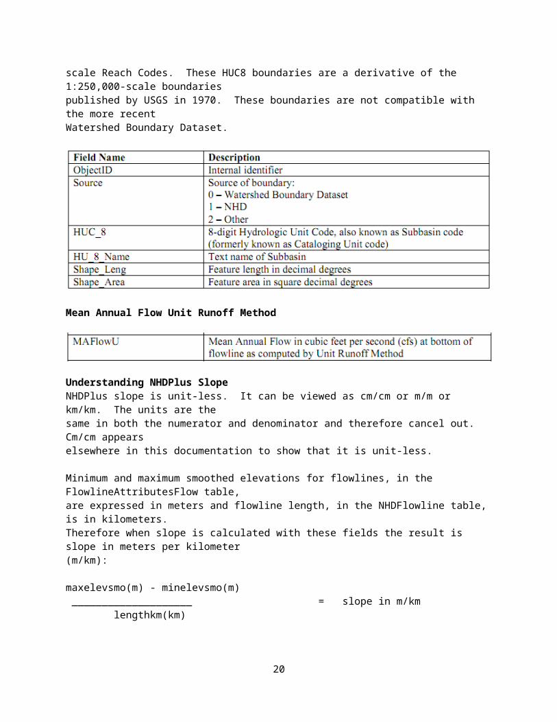
Mean Annual Flow Unit Runoff Method

Understanding NHDPlus Slope NHDPlus slope is unit-less. It can be viewed as cm/cm or m/m or km/km. The units are the same in both the numerator and denominator and therefore cancel out. Cm/cm appears elsewhere in this documentation to show that it is unit-less. Minimum and maximum smoothed elevations for flowlines, in the FlowlineAttributesFlow table, are expressed in meters and flowline length, in the NHDFlowline table, is in kilometers. Therefore when slope is calculated with these fields the result is slope in meters per kilometer (m/km):

maxelevsmo(m) - minelevsmo(m) ____________________ = slope in m/km lengthkm(km) To get the unit-less slope given in NHDPlus the units must be converted as follows: slope in m/km * 1 km/1000m = slope (unit-less) given in NHDPlus. NHDPlus slopes are constrained to be greater than or equal to 0.00005.

NOTE: The text above is taken directly from the NHDPlus User Guide (http://www.horizon-systems.com/nhdplus/)

National Landcover Database Details

NLCD2006 is a 16-class land cover classification scheme that has been applied consistently across the conterminous United States at a spatial resolution of 30 meters. NLCD2006 is based primarily on the unsupervised classification of Landsat Enhanced Thematic Mapper+ (ETM+) circa 2006 satellite data. NLCD2006 also quantifies land cover change between the years 2001 to 2006. The NLCD2006 land cover change product was generated by comparing spectral characteristics of Landsat imagery between 2001

15

and 2006, on an individual path/row basis, using protocols to identify and label change based on the trajectory from NLCD2001 products. It represents the first time this type of 30 meter resolution land cover change product has been produced for the conterminous United States. A formal accuracy assessment of the NLCD2006 land cover change product is planned for 2011.

NOTE: The text above is taken directly from the NLCD website: http://www.mrlc.gov/nlcd2006.php

EPA WATERS and the National Hydrography Dataset

WATERS uses the NHD addressing system to link EPA Water Program features, such as water monitoring sites, to the underlying surfacewater features (streams, lakes, swamps, etc).

NOTE: The text above is taken directly from the EPA WATERS website: http://www.epa.gov/waters/about/geography.html

TAS Data Details

Wetness Index assumption of D-infinity connectivity. DEM was modified with fast breaching (pit removal) and enforced drainage on all flats.

Satellite Remotely Sensed Imagery Processing (selected details)

1) Acquisition of 2 Landsat images collected on 2 different dates: September 23, 1992 & September 8, 2001 Image selection focused on vegetative growing season, <10% CC, relatively similar time of

year2) Images spatially subset to La Jencia watershed

Coordinates derived from catchment analysis of all subwatersheds contributing to La Jencia Creek watershed via 12-unit HUC tracking

3) Images atmospherically corrected (w/ altitude)4) Images processed via Kauth-Thomas Transformation, SI (Structural Index), SR (Simple Ratio), and

EVI (Enhanced Vegetation Index)

NOTE: It was my original intent to analyze La Jencia watershed ecological parameters using GIS. Unfortunately several characteristics of the data I acquired for this project did not enable me to work toward my overarching goal. As a result the information presented below is a small fraction of the analyses I tried to work through for my preliminary case study/GEOG 591 term project.

16

http://www.mrlc.gov/nlcd2006.php

La Jencia Creek: Primary Channel

Limitations were imposed upon my inquiry into the La Jencia watershed by the lack of available watershed- and subwatershed attribute data in NHDPlus region 13b. I therefore restricted my GIS inquiries to the larger Rio Salado subbasin. By searching the NHDPlus flowline attribute table in ArcMap 10 I identified stream reaches (highlighted in purple below) that comprise much of the major La Jencia stream channel (shown in aquamarine below). Following the image is a list of the primary channel component reaches with their associated HUC-14 reach codes and approximate length (measured in kilometers).

La Jencia Creek Main Channel Flowline (highlighted in blue)

17

NHDPlus Flowlines Comprising Main Channel of La Jencia Creek

GNIS_NAME LENGTHKM REACHCODEJencia Creek, La 2.628 13020209000280Jencia Creek, La 0.459 13020209000281Jencia Creek, La 0.309 13020209000282Jencia Creek, La 2.445 13020209000283Jencia Creek, La 1.199 13020209000284Jencia Creek, La 0.42 13020209000285Jencia Creek, La 4.633 13020209000287Jencia Creek, La 1.662 13020209000298Jencia Creek, La 0.436 13020209000297Jencia Creek, La 8.577 13020209000288Jencia Creek, La 0.196 13020209000290Jencia Creek, La 0.244 13020209000291Jencia Creek, La 0.834 13020209000296Jencia Creek, La 1.027 13020209000292Jencia Creek, La 0.701 13020209000293Jencia Creek, La 0.734 13020209000294Jencia Creek, La 1.201 13020209000289Jencia Creek, La 1.747 13020209000290Jencia Creek, La 3.104 13020209000286Jencia Creek, La 3.818 13020209000295Total 36.374

18

Rio Salado Subbasin Overview

In order to obtain a detailed overview of the Rio Salado subbasin and La Jencia watershed boundaries, I explored a variety of publicly available online data resources including the NHDPlus and EPA My WATERS Mapper. Importantly the NHDPlus hydrographic unit data for this geographic region (13b) does not contain attributes for HUC-10 watersheds (the La Jencia watershed) and HUC-12 subwatersheds (those which comprise La Jencia watershed). As an alternative to the NHDPlus data, I used the online EPA My WATERS Mapper to locate and identify all eight HUC-12 subwatersheds that comprise the larger La Jencia watershed (HUC-10: 1302020906) and their total area in square kilometers. A magnified view of the Rio Salado subbasin is outlined and shaded in aquamarine below. The Rio Salado subbasin is 3,632 km2 (893,383 acres) in area. Purple lines denote HUC-8 basin and HUC-10 watershed boundaries in the greater geographic region.

Rio Salado Watershed (HUC-8: 13020209) Near Socorro, NM

Notable geographic features in the greater geographic region of the Rio Salado subbasin include the Sevilleta National Wildlife Refuge to the east, the Magdalena Mountains to the Southeast, the San Mateo Mountains in the south-central region, the Cibola National Forest on the watershed’s southern lateral side, the Gila National Forest and associated Aldo Leopold Wilderness roughly to the southwest, the Zuni Mountains and associated Zuni Reservation to the watershed’s northwest, the San Mateo Mountains to the north, and the city of Albuquerque to the region’s northeast. Within the watershed reside the Datil-, Gallinas-, and Bear Mountains. Zooming into the image will reveal the landscape features discussed above.

19

La Jencia Watershed Overview

As mentioned previously, the La Jencia watershed is nested within the Rio Salado subbasin; in the image below the La Jencia watershed is outlined and highlighted in aquamarine. Note its size relative to the Rio Salado subbasin discussed above, and its geographic position with respect to Albuquerque and the Rio Grande.

La Jencia Watershed (HUC-10 1302020906)

Size: 768.604627 km2 (189,742.321 acres)

20

La Jencia Subwatershed Overview

A magnified view of the La Jencia watershed is shown below. Its eight component HUC-12 subwatersheds are outlined and highlighted in aquamarine. A table following the image below lists La Jencia’s subwatersheds and their relative areas (individual and total).

La Jencia Watershed: HUC-10 1302020906

La Jencia Creek Watershed Component SubwatershedsName Area (km2) HUC-12

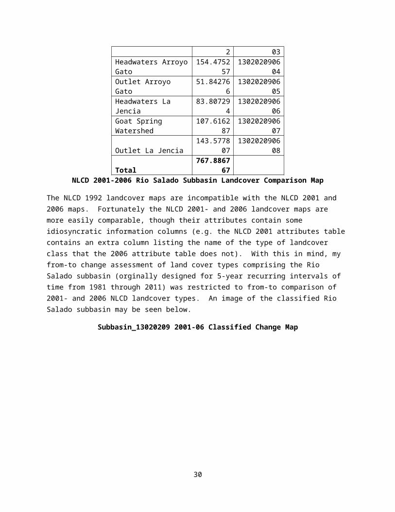
Gallinas Canyon 41.416177 130202090601Arroyo Montosa 62.522459 130202090602Dry Lake Canyon 122.62872 130202090603Headwaters Arroyo Gato 154.475257 130202090604Outlet Arroyo Gato 51.842766 130202090605Headwaters La Jencia 83.807294 130202090606Goat Spring Watershed 107.616287 130202090607Outlet La Jencia 143.577807 130202090608Total 767.88676

21

7NLCD 2001-2006 Rio Salado Subbasin Landcover Comparison Map

The NLCD 1992 landcover maps are incompatible with the NLCD 2001 and 2006 maps. Fortunately the NLCD 2001- and 2006 landcover maps are more easily comparable, though their attributes contain some idiosyncratic information columns (e.g. the NLCD 2001 attributes table contains an extra column listing the name of the type of landcover class that the 2006 attribute table does not). With this in mind, my from-to change assessment of land cover types comprising the Rio Salado subbasin (orginally designed for 5-year recurring intervals of time from 1981 through 2011) was restricted to from-to comparison of 2001- and 2006 NLCD landcover types. An image of the classified Rio Salado subbasin may be seen below.

Subbasin_13020209 2001-06 Classified Change Map

Legend: Blue is shrubland; brown is evergreen forest

22

NLCD 2001-2006 Rio Salado Subbasin Landcover Comparison Table

The classified change map above is supplemented with a table (below) whose highlighted rows signify change from a non-urban landcover type in 2001 to a differing landcover type in 2006. Note the overall area (km2) associated with the highlighted landcover class changes are small relative to the size of the entire Rio Salado subbasin. (For reference, a key to the NLCD landcover types follows the table below.)

Raster Calculation: NLCD2001*1000 + NLCD2006

2001-2006 NLCD Change Table

OID NLCD 2001

NLCD 2006

Pixel Count Pixels/Total Pixel % Area

(km2)

0 11 11 4490.00027869

20.02786

91.01237

8

1 11 52 261.61381E-

050.00161

40.05862

3

2 21 21 37260.00231271

30.23127

18.40116

1

3 22 22 19710.00122339

20.12233

94.44409

2

4 23 23 3090.00019179

5 0.019180.69671

5

5 31 31 173660.01077900

4 1.077939.1558

1

6 31 90 714.40694E-

050.00440

70.16008

7

7 41 41 6290.00039041

80.03904

21.41823

1

8 42 42 7400470.45934411

145.9344

11668.61

3

9 42 52 3010.00018682

90.01868

30.67867

7

10 43 43 53.10348E-

06 0.000310.01127

4

11 52 31 211.30346E-

050.00130

3 0.04735

12 52 42 533.28969E-

05 0.003290.11950

1

13 52 52 269809 0.1674693316.7469

3608.349

1

14 52 90 53.10348E-

06 0.000310.01127

4

15 71 52 106.20696E-

060.00062

10.02254

7

16 71 71 5740880.35633404

6 35.63341294.41

9

23

17 81 52 342.11037E-

05 0.002110.07666

1

18 81 71 95.58626E-

060.00055

90.02029

3

19 81 81 6390.00039662

50.03966

21.44077

9

20 82 82 1740.00010800

1 0.01080.39232

5

21 90 90 13530.00083980

2 0.083983.05066

3

Total161109

5 1 100 3632.6

11 - Open Water12 - Perennial Ice/Snow21 - Low Intensity Residential22 - High Intensity Residential23 - Commercial/Industrial31 - Bare Rock/Sand/Clay32 - Quarries/Strip Mines/Gravel Mines33 - Transitional41 - Deciduous Forest42 - Evergreen Forest43 - Mixed Forest51/52 - Shrubland61 - Orchards/Vinyards/Other71 - Grasslands/Herbaceous81 - Pasture/Hay82 - Row Crops83 - Small Grains84 - Fallow85 - Urban/Recreational Grasses90/91 - Woody Wetlands92 - Emergent Herbaceous Wetlands

Interestingly the table above indicates that no woody wetlands were lost in the time from 2001 to 2006; row #14 in the table indicates a small area of both shrubland and bare rock/sand/clay was classified as woody wetlands in 2006.

24

Rio Salado Subbasin 2006 NLCD Landcover Types

In order to understand the trajectory of ecological parameters such as vegetative community composition and anthropogenic development through time, it is relevant to visually interpret the current proportion of the Rio Salado subbasin comprised of landcover types such as shrubland, grassland/herbaceous, evergreen forest, bare rock/sand/clay, urban structures, open water, and wetlands (woody/emergent herbaceous). The following maps also facilitate interpretation of the degree to which the Rio Salado subbasin is urbanized. In the context of ecological parameterization it is common knowledge that distinct vegetation types differentially stabilize the landscape (particularly arid ones) in different ways. For example, evergreen forest (often associated with mountain ranges in this region) and grasslands help to stabilize easily erodible soils, but to differing extents; a high-magnitude flood event (e.g. 100-year flood) will likely cut and destabilize grassland riparian banks more easily than those lined by shrubs and trees. Grassland/herbaceous landcover has the ability, however, to enable arid soils (which might otherwise be bare) to withstand the forces associated with small to medium magnitude flooding events. The maps below indicate that – at a coarse spatial resolution – the majority of the Rio Salado subbasin is vegetated, and impacted by a small degree of urbanization. The maps below also illustrate that open water and woody wetlands comprise just a small fraction of the Rio Salado subbasin; the Rio itself and the Rio Grande to the east are primary anthropogenic water sources whose resources – along with groundwater – are extracted each year via anthropogenic water use.

Subbasin_13020209 2006 Shrubland Map

25

Subbasin_13020209 2006 Grass-Herb Map

Subbasin_13020209 2006 Evergreen Forest Map

26

Subbasin_13020209 2006 Bare Rock-Sand-Clay Map

Subbasin_13020209 2006 Developed (21-23) Map

27

Subbasin_13020209 2006 Open Water & Woody Wetlands Map

28

Rio Salado Subbasin Satellite Remotely Sensed Imagery

I used Glovis online to acquire satellite imagery, and later process it using ENVI. Below is a picture of the Rio Salado subbasin (Landsat 5 TM) displayed with RGB = bands 543. The Rio Salado subbasin is 3,632 km2 (893,383 acres) in area. The subbasin is geographically situated southwest of Albuquerque, NM; the proximal Interstate is I-25. La Jencia Creek flows northwestward into the Rio Salado, which empties eastward into the Rio Grande; the Rio Grande runs north-south through New Mexico, parallel to I-25 in this region.

Rio Salado Subbasin on September 23, 1992 (Landsat 5 TM, RGB=543)

29

Confluence of La Jencia Creek with Rio Salado, empties to Rio Grande to the East (R side of image)

30

La Jencia Watershed Comparative Analysis of Satellite Remotely Sensed Enhanced Vegetative Index

Satellite remotely sensed images processed using algorithms such as the Enhanced Vegetation Index (EVI) convey information about the presence/absence of vegetative communities in a given region. The EVI is responsive to canopy structural variations, including leaf area index (LAI), canopy type, plant physiognomy, and canopy architecture. Below is a set of two images acquired on two different dates that synchronize with the NLCD data sets, and convey (in value ranges) the distribution of vegetation communities across the larger La Jencia watershed, with darker regions corresponding to denser vegetation. Note differences between the two images, such as presence of tree/shrub vegetation to the west of the light Magdalena mountain range on the bottom half of the images. Similar differences cover the entire extent of both images.

La Jencia Watershed EVI September 23, 1992

31

La Jencia Watershed EVI September 8, 2001

32

Elevational Gradient Analysis of Rio Salado Subbasin

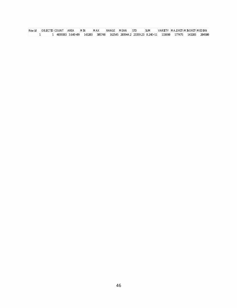
The NHD elevation data (measured in cm) for region 13b indicates the Rio Salado subbasin has a wide range of elevation values. The lowest point in the subbasin resides around 5,000 feet, while the highest point in the subbasin is situated around 10,000 feet. Elevational gradients – when combined with highly erodible soils and distributional vegetative community data – are important for understanding the potential for changes in ecological parameters relevant to EIAs through time. Landscape disturbances that impact ecosystem function such as landslides, concentrated cattle grazing, and high flow events all have the ability to restructure the landscape on relatively short times scales. Below a map illustrates the variation in elevation of the Rio Salado watershed; note the major channel of the Rio Salado coursing from the northwest to the southeast en route to the Rio Grande.

Subbasin_13020209 Elevation Map

Elevation Range: 1432.03 m (4,698 ft) to 3057.48 m (10,031 ft)

rsmask_elev_stats (min & max measured in cm):

Rowid OBJECTID COUNT AREA MIN MAX RANGE MEAN STD SUM VARIETY MAJORITY MINORITY MEDIAN1 1 4039383 3.64E+09 143203 305748 162545 203944.2 23359.23 8.24E+11 133690 177475 143203 204500

33

Slope Analysis of Rio Salado Subbasin

An extension of my interest in understanding the elevational gradients in this geographic region is supported by a zonal histogram analysis (ArcMap v. 10) of categorical slope values for the Rio Salado subbasin. The frequency distribution below presents the pixel counts associated with each of nine slope categories; while most of the pixels reside in the lowest slope category, there are a substantial number of pixels residing in slope categories with degree values greater than nine. Knowledge of steep slopes combined with soils data (erodibility, wetness), vegetative community data, and hydrologic data can inform identification of sites susceptible to erosion, degradation, and landscape restructuralization.

Rio Salado Watershed Slope Analysis

34

Aspect Analysis of Rio Salado Subbasin

Knowledge of the region’s aspect values can inform one’s understanding of the distribution of vegetation communities. Certain plants are typically associated with particular slopes, as is moisture (north-facing slopes are typially wetter than south-facing ones). It is therefore useful to visualize a distribution of the categorical aspect values (degree ranges) of a region to understand which aspects are more frequent relative to others. Combination of knowledge regarding a region’s aspect in conjunction with plant community data can inform one’s understanding of which plant communities may be found where, which plant species are native to a given restoration site selection, and which species may be best-suited to facilitate restoration goals.

Rio Salado Subbasin Aspect Analysis

Rio Salado Subbasin Aspect Categories & Associated Pixel Counts

OID LABEL Pixels0 Flat (-1) 9161 North (0-22.5) 2431342 Northeast (22.5-67.5) 5621573 East (67.5-112.5) 6941664 Southeast (112.5-157.5) 6064005 South (157.5-202.5) 4484516 Southwest (202.5-247.5) 3992117 West (247.5-292.5) 4452548 Northwest (292.5-337.5) 4255779 North (337.5-360) 214117

35

Discharge Area Analysis of Rio Salado Subbasin

In order to identify and understand wetland- and riparian corridors that are highly susceptible to erosion in an arid region such as the Rio Salado, it is useful to think about the relative sizes of the discharge areas into the region’s waterways. Below is a map illustrating (in green) NHD stream reaches that have 1000 upstream contributing cells (pixels) at their stream heads. A conversion of the 1000 pixel threshold is translated into upstream drainage area using the NHD DEM data (whose spatial resolution is 30 x 30 m). Thus the streams highlighted in green below are those which have 90 ha drainage areas.

Subbasin_13020209 Stream1000 Map

Magnified Subset Image of Stream_1000 (illustrating connectivity)

36

Calculation of stream_1000 drainage area:

1) Given that:a) One NHD DEM pixel has an area of 30 m x 30 m = 900 m2 (900 m2/pixel)b) 1 ha = 107,639 ft2 = 10,000 m2

and

Pixel Value1 = 1000a) 900 m2/pixel x 1000 pixels = 900,000 m2

b) so 900,000 m2/ 10,000 m2/ha = 90 ha

37

Mean Annual Flow Thresholds in Rio Salado Subbasin

Since the Rio Salado subbasin is situated at high elevation in an arid landscape, much of the natural stream network is comprised of ephemeral channels. The anthropogenic extraction of groundwater and rerouting of the region’s major rivers intensifies this fact. In order to identify waterways with low mean annual flow, I filtered the NHDPlus hydrologic data by thresholds of varying levels: a) stream reaches with mean annual flow ≤ 10 cfs, b) stream reaches with 10 cfs < mean annual flow ≤ 30 cfs, and c) stream reaches with mean annual flow > 30 cfs. A map below illustrates the results of this process. Note the Rio Grande is identified in aquamarine to the east.

Map of Flowlines with Varying Mean Annual Flow (MAFlowU) Thresholds

Legend: Purple denotes Rio Salado Watershed boundary | Aquamarine denotes streams/rivers with MAF > 30 cfs | Medium blue denotes streams/rivers with 10 < MAF ≤ 30 | Light blue (most common

lines) denote streams/rivers with MAF ≤ 10

38

Wetness Indices, Saturated Areas, and Return Flow in the Rio Salado Subbasin

Initially I desired to conceptualize the time-varying portions of the Rio Salado subbasin that can produce surface runoff (saturation overland flow), and the extent of the variable source area (saturated region as a proportion of total watershed area). I tried to calculate the Rio Salado subbasin’s wetness indices, regions of local saturation deficit and associated saturated areas, return flow, and the region’s variable source area. When combined together this information proves useful for understanding the hydrologic nature of the subbasin as a whole, and furthers understanding of the region’s wetting regime. In conjunction with supplementary data sources such as precipitation, evapotranspiration, consumptive water use, runoff, infiltration, one might develop a regional water budget and observe how this changes through time. In assessment of ecosystem function, it is helpful to conceptualize variation in the water budget through time in response to natural- and anthropogenic disturbances.

Below is a series of maps illustrating my attempt to conceptualize the average wetness index (WI), variation in saturated areas with changing local saturation deficits, and corresponding variation in the return flow for the region. Unfortunately all of these maps are inaccurate since I could not obtain accurate m and savg parameters specific to the Rio Salado geographic region. Other issues with the data complicated the process (e.g. the subbasin mask’s parameters were incompatible with local saturated areas even after mask reprojection in TAS). Due to these issues, the variable source area maps are replete with error and too unreliable to be included in this report. Still, some proof of concept is conveyed below.

Rio Salado Watershed Mean Wetness Index Map(elev_rsmask_brfast_meanWI.dep)

Average WI Value Range: -2.346851 to 23.40756 w/ calculated WIavg. = 10.44716

39

I. Maps of Si Values with m=0.4517 m-1 and λ = 10.44716

Si = 2.5 Map (S2.5 = 2.5+0.4517*(10.44716-'elev_rsmask_brfast_meanWI'))

Min to Max Range: -3.354214 to 8.279055

Si = 3.25 Map (S3.25 = 3.25+0.4517*(10.44716-'elev_rsmask_brfast_meanWI')


40

Si = 4.0 Map (S4.0 = 4.0+0.4517*(10.44716-'elev_rsmask_brfast_meanWI')


41

II. Maps of Saturated Areas with m=0.4517 m-1 and λ = 10.44716

sat2.5 Map ('s2.5'<=0)

sat2.5 Map ('s2.5'<=0) Zoom

NOTE: Region shown above is zoomed view of lower right-hand corner of Rio Salado watershed

42

sat3.25 Map ('s3.25'<=0)


43

sat4.0 Map ('s4.0'<=0)


44

III. Maps of Return Flow with m=0.4517 m-1 and λ = 10.44716

rf2.5 = (abs('s2.5'))*'sat2.5' Map

Return Flow Range: 0 to 3.354214


45

rf3.25 = (abs('s3.25'))*'sat3.25' Map



46

rf4.0 = (abs('s4.0'))*'sat4.0'



47

Documents

· Web viewthis will not happen prior to distribution of NHDPlus because the update process for the central NHD database at USGS was under development at the time these improvements