DOCUMENT RESUME IR 001 570 AUTHOR Salton, … · DOCUMENT RESUME ED 101 718 AUTHOR TITLE. INSTITUTION. SPONS AGENCY PUB DATE NOTE. EDRS PRICE DESCRIPTORS. IDENTIFIERS. IR 001 570

DOCUMENT RESUME

ED 101 718

AUTHORTITLE

INSTITUTION

SPONS AGENCYPUB DATENOTE

EDRS PRICEDESCRIPTORS

IDENTIFIERS

IR 001 570

Salton, GerardInformation Storage and Retrieval Scientific ReportNo. ISR-22.Cornell Univ., Ithaca, N.Y. Dept. of ComputerScience.National Science Foundation, Washington, D.C.Nov 74380p.

HF-S0.76 HC-$19,67 PLUS POSTAGE*Algorithms; *Computer Programs; Computer Science;Content Analysis; Data Bases; Data Processing;Dictionaries; Feedback; *Indexing; InformationProcessing; *Information Retrieval; *InformationStorage; Information Systems; information Theory;Item Analysis;* Thesauri*Pile Structures

ABSTRACTThe twenty-second in a series, this report describes

research in information organization and retrieval conducted by theDepartment of Computer Science at Cornell University. The reportcovers work carried out during the period summer 1972 through summer1974 and is divided into four parts: indexing theory, automaticcontent analysis, feedback searching, and dynamic file management.Twelve individual papers are presented. (Author/DGC)

0

DEPARTMENT OF COMPUTER SCIENCE

CORNELL UNIVERSITY

INFORMATION STORAGE AND RETRIEVAL

Ithaca, New YorkNovember 1974

Scientific Report No. ISR-22

to

The National Science Foundation

Gerard SaltonProject Director

Department of Computer Science

Cornell University

Information Storage and Retrieval

Scientific Report No. ISR-22

to

The National Science Foundation

Ithaca, New York Gerard Salton

November 1974. Project Director

OCopyright, 1974

by Cornell University

Use, reproduction, or publication, i whole or in part, is permitted

for any purpose of the United States Government.

U S DEPARTMENTOF HEALTH.

EDUCATION $ WELFARENATIONAL INSTITUTE OF

EDUCATIONTHIS DOCUMENT HAS BEEN REPRODUCED EXACTLY AS RECEIVED FROMTHE PERSON OR

ORGANIZATION ORIGINATING IT POINTS OF VIEW OR OPINIONSSTATED DO NOT NECESSARILY REPRESENT OFFICIAL NATIONAL

INSTITUTE OFEDUCATION POSITION OR POLICY

"PERMISSION TO REPRODUCE THIS COPY.RIGHTED MATERIAL HAS BEEN GRANTED BY

Oar ndLi CIA IVariPiii

To ERIC AND ORGANIZATIONS OPERATINGUNDER AGREEMENTS WITH THE NATIONAL IN.Stalin OF EDUCATION FURTHER REPRO-DUCTION OUTSIDE THE .ERIC SYSTEM RE-QUIRES PERMISSION OF THE COPYRIGHTOWNER

TABLE OF CONTENTS

Page

SUMMARY

PART ONE

INDEXING THEORY

I. SALTON, G., WONG, A. and YANG, C.S."A Vector Space Model for Automatic Indexing"

Abstract 1-1

1. Document Space Configuration 1-1

2. Correlation between Indexing Performance andSpace Density 1-10

3. Correlation between Space Density and IndexingPerformance 1-15

4. The Discrimination Value Model 1-18

References 1-30

II. WONG, A.

"An Investigation on the Effects of Different IndexingMethods on the Document Space Configuration"

Abstract . II-1

1. Introduction . II-1

2. Methodology 11-3

3. Cluster Measurements. 11-5

4. The Experiment II-7

5. The Results II-10

1. Discrimination Value Model 11-12

2. Invcrse Document Frequency 11-13

3. The HDVD Collectior 11-13

iii

TABLE OF CONTENTS (continued)

rage

II. Continued

4. The MOD Methods II-15

5. The MODI Methods 11-16

6. Conclusions 11-16

References 11-20

III. SALTON, G., YANG, C.S. and YU, C.T."A Theory of Term Importance in Automatic Text Analysis"

Abstract III-1

1. Document Space Configuration 111-2

2. The Discrimination Value Model 111-6

3. Discrimination Values and Document Frequencies 111-9

4. A Strategy for Automatic Indexing 111-20

5. Experimental Results 111-28

References 111-35

PART TWO

CONTENT ANALYSIS

IV. CRAWFORD, R."Negative Dictionary Construction"

1. Introduction IV-1

2. Negative Dictionaries IV-3

2.1) Common Words IV-3

2.2) The Negative Dictionary IV-5

3. Experimental Procedures IV-6

3.1) The SMART System IV-6

3.2) The Experiment Data Base IV-6

3.3) Evaluation Parameters IV-7

0iv


IV. Continued

Page

4. Manual Negative Dictionary Construction IV-7

4.1) Methods for .anual Negative DictionaryConstruction IV-7

4.2) Manual Negative Dictionary ConstructionPerformance Results IV-9

5. Automatic Methods of Negative DictionaryConstruction IV -1O

5.1) Frequency and Distribution of Terms IV-12

5.2) Discrimination Value IV-20

5.3) Relative Distribution Correlation IV-35

6. Experiments and Results IV-39

6.1) Manual Negative Dictionary Construction. . . . IV-43

6.2) Automatic Negative Dictionary Construction . . IV-43

7. Summary and Conclusions IV-67

References IV-68

V. van der MEULEN, A."Dynamically versus Statically Obtained Information Values"

Abstract V-1

1. Introduction V-2

2. Information Values and Their Derivation V-3

A) The Concept V-3

B) Thr Updating Method V-4

C) Dynamic versus Static Updating V-5

3. The Experiments V-7

4. Results V-7

5. Conclusion V-9

References V-13

v

l)

TABLE OF CONTENTSAcontinued)

rage

'VI. WELLLS, Y."Automatic Thesaurus Construction Through the Use ofPre-Defined Relevance Judgments"

Abstract VI-1

1. Introduction VI-1

2. Terminology and Definitions VI-3

3. Pseudo-Classification Procedure VI-8

4. Programming System VI-11

5. Implementation VI-16

References VI-17

PART THREE

FEEDBACK SEARCHING

VII. WONG, A., PECK, R. and van der MEULEN, A."Content Analysis and Relevance Feedback Abstract"

Abstract VII-1

1. Introduction VII-2

2. Experiments VII-5

A) Used Language Analysis Tools VII-5

B) Comparisons VII-6

3- Experimental Results VII-7

4. Conclusion VII-7

References VII-13

VIII. SARDANA, Karamvir"On Controlling the Length of the Feedback Query Vector"

Abstract VIII-1

1. Introduction VIII-1

A) Indexing VIII-1

B) Length of a Vector and Importance ofControlling It VIII-2

vi

TABLE OF =TENTS (continued)

VIII. Continued

Page

2. Earlier Results VIII-4

A) Murray's Strategy for Reducing the VectorLengths

B) Other Related Results by Murray VIII-5

3. Present Problem VIII-b

A) Origination VIII-b

B) Exact Definition and Scope of theProblem VIII-7

C) Methods and Solutions in Brief VIII-8

4. Vector Trimming Strategies VIII-9

A) Strategy I VIII-10

B) Strategy II VIII-14

C) Strategy III VIII-14

D) Strategy IV VIII-17

5. Experimental Environment MI-20

A) Retrieval System VIII-20

8) Data Collections VIII-20

C) Clustering Parameters VIII-21

D) Searching Parameters VIII-22

E) Evaluation Techniques VIII-22

6. Experimental Details VIII-23

A) Overall Flowchart of the Experiments VIII-23

B) Detailed Description of One of theExperiments VIII-23

7. Results VIII-26

A) Performance Curves Obtained VIII-26

B) Inference From the Performance Curves. VIII-32

C) Comparison of the Four Strategies VIII-30

D) Overall Comparison of the Four Strategies.. VIII -48

vii


VIII. Continued

Page

8. Dis:ussion VIII-49

A) Shortened Frequency Ranked Vectors VIII-49

B) A Few Categories of Weight Classes VIII-50

C) Use of Negative Dictionaries VIII-50

D) Ideal Indexing VIII-54

9. Summary and Conclusions VIII-55

References VIII-58

IX. KAPLAN, M."The Shortening of Profiles on the Basis of DiscriminationValues of Terms and Profile Space Density"

Abstract IX-1

1. Introduction IX-1

2. Density and Discrimination . . . IX-4

3. Experimental Design IX-7

4. Experimental Results IX-18

References IX-21

PART FOUR

DYNAMIC DOCUMENT SPACE

X. YANG, C.S."On Dynamic Document Space Modification Using TermDiscrimination Values"

Abstract X-1

1. Introduction to Dynamic Document Modification andTerm Discrimination Values X-1

2. Dynamic Document Space Modification Using TermDiscrimination Values X-6

3. Experiment X-7

4. Discussion of Results X-10


X. Continued

rage

5. Conclusion X-27

References X-28

XI. WONG, A. and van der MEULEN, A."The Use of Document Values for Dynamic Query Processing"

Abstract XI-1

1. Introduction XI-2

2. The Methodology XI-2

3. The Organization of the Experiments XI-3

A) The Collection XI-3

B) The Updating Strategies XI-4

4. The Results XI-6

A) The Straight Updating XI-6

B) The Balanced Updating XI-8

C) The Extended Balanced Updating XI-8

5. Conclusion XI-11

References XI-17

Appendix 1 XI-18

Appendix 2 XI-19

XII. SARDANA, K.

"Automatic Document Retirement Algorithms"

Abstract XII-1

1. Introduction XII-1

ix

TABLE or CONTENTS (continued)

Page

XII. Continued

2. The Algorithms XII-1

Al) Algorithm TY (Tai and Yang) XII-5

A2) Algorithm BS (Beall 6 Schnitzer) XII-9

A3) Algorithm Si XII-11

A4) Algorithm S2 XII-14

3. Experimental Results XII-16

A) Algorithms TY & S1 XII-19

B) Algorithm S2 XII-21

C) Algorithm S3 XII-22

D) P-R Curves XII-24

4. Overall Comparison of Various Algorithms XII-29

5. Summary and Conclusion XII-33

6. Suggestions for Further Research ..... . . . XII-35

References XII-37

Summary

The present report is the twenty-second in a series describing

research in information organization and retrieval conducted by the

Department of Computer Science at Cornell University. The report covering

work carried out for approximately two years (summer 1972 to summer 1974) is

divided into four parts: indexing theory (sections I to III), automatic

content analysis (sections IV to VI), feedback searching (sections VII to

IX), and dynamio file management (sections X to XII).

The normal schedule in the distribution of ISR reports has not been

maintained in recent years, due largely to the scarcity of publication funds.

For the same reason, a number of recently published articles covering related

research work are not being reprinted in the present report. Interested

readers may want to refer to the following additional items in particular:

a) Contributions to the Theory of Indexing (G. Salton, C.S. Yang,

and C.T. Yu), Proc. IFIP Congress 74, North Holland Publishing

Company, Amsterdam, 1974.

b) On the Specification of Term Values in Automatic Indexing

(G. Salton and C.S. Yang), Journal of Documentation, Vol. 29,

No. 4, December 1973, p. 351-372.

c) Proposals for a Dynamic Library (G. Salton), Information - Part 2,

Vol. 2, No. 3, 1973, p. 5-25.

d) Theory of Indexing and Classification (C.T. Yu), Doctoral Thesis,

Cornell University, Technical Report 73-181, Department of

Computer Science, Cornell University, Ithaca, YN_ August 1973,

238 pages.

xi

3

Some time has been devoted during the last year to the design of

an on-line implementation of the experimental SMART retrieval system, and

test runs of the on-line version have been made on the IBM 370/168 computer

at Cornell. The off-line version of the system continues to be used for

experiments at various locations in the United States and abroad.

In recent years, increasing attention has been paid to the study of

a variety of file organization and retrieval algorithms, including some that

have not yet found their way into operational implementation. Among these is

the use of clustered file manipulations instead of inverted directory searches,

vector matching processes instead of keyword coincidence counting, dynamic

document space modification, automatic file retirement procedures, and interactive

retrieval methodologies.

The present report thus includes studies dealing with feedback searching

and dynamic file modification. A great deal of emphasis has also been placed

on the generation of new indexing theories which assign specific functions in

content analysis to various indicators such as single terms, phrases, and

thesaurus categories. These theories are explained in Part I of the present

report.

Sections I and II by G. Salton, A. Wong, and C.S. Yang, and by A. Wong,

respectively, cover investigations relating the density of the document space

to the retrieval effectiveness obtainable with such a space. In particular,

the earlier work dealing with the determination of term discrimination values

makes it appear that "good" terms those indicative of information content

are those which increase the dissimilarity between documents, that is, which

spread out the document space. The experimental output in section I and II

confirms that a low-density space is associated with effective retrieval, and

vice-versa. Similarly, a high-density space provudes poor retrieval performance.

The theory in sections I and II is developed further in section

III by G. Salton, C.S. Yang, and C.T. Yu relating the discrimination value of

a term to its document frequency in a collection. The best discriminators

are terms with medium document frequency. This fact is used to construct

an optimum indexing vocabulary by turning high frequency single terms into

phrases thereby reducing the document frequency, and assembling low frequency

terms into thesaurus groups thus increasing the frequency. The effectiveness

of the resulting indexing vocabulary is assessed by citing appropriate

experimental evidence.

Sections IV to VI, constituting Part 2 of this report, deal with

various aspects of automatic content analysis. Section IV by R. Crawford

covers the construction and effectiveness of a variety of negative dictionaries

("stop lists") containing terms that should not be used for content identification.

This work leads to the generation of an indexing vocabulary of optimum size.

Section V by A. v.d. Meulen covers the operations of the so-called dynamic

information values. In that system all term weights are fixed initially at

some given value (say 1). Good terms, that is, those contained in useful

documents are then increased in weight dynamically in the course of the

operations. Bad terms are similarly demoted by reducing the term weights.

The last section, number VI, by K. Welles deals with experiments leading to

the construction of optimum term classifications (thesauruses) using the

pseudo-classification method. This process utilizes a classification criteron

based on user relevance assessments to group the terms rather than on the

more usual semantic term similarities.

The next three sections, VII to IX, constitute Part 3 of this

report, entitled feedback searching. Section VII by A. Wang, R. Peck,

and A. v.d. Meulen attempts to determine relationships betvlen the

effectiveness of the initial content analysis (indexing) and the use-

fulness of iterative feedback searching. It is found that differences in

the effectiveness of the initial indexing are preserved during the feed-

back operations. Section VIII by K. Sardana relates the length of the

feedback query to the effectiveness of the retrieval operation. It is

found that shorter feedback queries provide better retrieval; methods are

therefore given for reducing feedback query length. A similar reduction

in vector length is investigated by M. Kaplan in section IX, applied to the

centroid vectors (profiles) representing the document groups in a clustered

file organization.

Part 4, consisting of sections X to XII covers dynamic document space

modification procedures. In section X by C.S. Yang the term discrimination

values are used as parameters in the construction of appropriate document

space modification methods. A document "utility value", determined by earlier

user-system interactions, is similarly used for document space modification

in section XI by A. Wong and A. v.d. Meulen. Finally, in section XII by

K. Sardana a variety of automatic document retirement methods can be used

automatically to reduce the size of the collection by eliminating items

exhibiting low usefulness. Three retirement methods based respectively on

average term weight measurements, document space modification methods,

and the storage of special usage indicators are examined and their

effectiveness is evaluated.

xiv

All earlier ISR reports in this series are obtainable from the

National Technical Information Service in Springfield, Virginia. The

order numbers for the last few reports are PB 214-020 (ISR-21),

PB 211-061 (ISR-20), PB 204-946 (ISR-19) and PB 198-069 (ISR-18),

respectively.

G. Salton

xv

A Vector Space Model for Automatic Indexing

G. Salton, A. Wong, and C.S. Yang+

Abstract

I-1

In a document retrieval, or other pattern matching environment where

stored entities (documents) are compared with each other, or with incoming

patterns (search requests), it appears that the best indexing (property)

space is one where each entity lies as far away from the others as possible;

that is, retrieval performance correlates inversely with space density. This

result is used to choose an optimum indexing vocabulary for a collection of

documents. Typical evaluation results are shown demonstrating the usefulness

of the model.

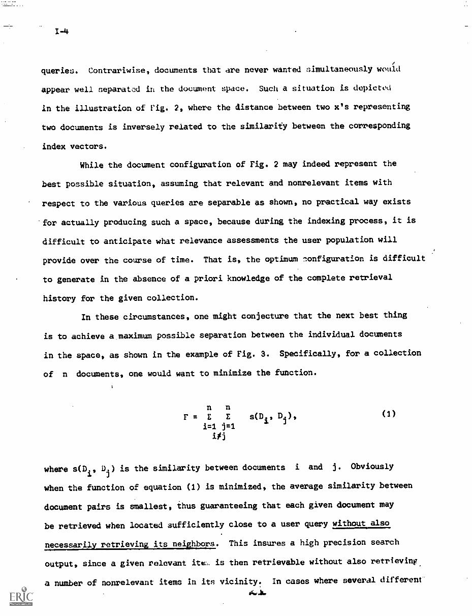
1. Document Space Configurations

Consider a document space, consisting of documents eacheach identified

byoneormzeindextermsT.;the terms may be weighted according to their

importance, or unweighted with weights restricted to 0 and 1.* A typical

three-dimensional index space is shown in Fig. 1, where each item is identified

by up to three distinct terms. The three dimensional example may be extended

to t dimensions when t different index terms are present. In that case,

each document D. is represented by a t-dimensional vector

Di

= (dil, dig, dit,,

representing the weight of the jth term.d1

+Department of Computer Science, Cornell University, Ithaca, N.Y., 14853

*Although we speak of documents and index terms, the present developmentapplies to any set of entities identified by weighted property vectors.

Ti

au (Ti T? ",1")

,1

tofi 001110.

401

T 4100,10.41 41010. V. 0.40 40,0

V;:cior ikprinental ion of

Docunr.rit Space

19u. I

Di

10 -10 00.00. T,%. al:

T5

1-3

Given the index vectors for two documents, it is possible to compute

a similarity coefficient between them s(D., D.), reflecting the degree of

similarity in the corresponding terms and term weights. Such a similarity

measure might be an inverse function of the angle between the correvonding

vector pairs --- when the term assignment for two vectors is identical, the

angle will be zero producing a maximum similarity measure.

Instead of representing each document by a complete vector originating

at the 0-point in the coordinate system, the relative position of the vectors

is preserved by considering only the envelope of the space. In that case, each

document is graphically identified by a single point whose position is specified

by the area where the corresponding document vector touches the envelope of

the space. Two documents with similar index terms are then represented by

points that are very close together in the space: obviously the distance

between two document points in the space is inversely correlated with the

similarity between the corresponding vectors.

Since the configuration of the document space is a function of the

manner in which terms and term weights are assigned to the various documents

of a collection, one may ask whether an optimum document space configuration

exists, that is, one which produces an optimum retrieval performance.*

If nothing special is known about the documents under consideration,

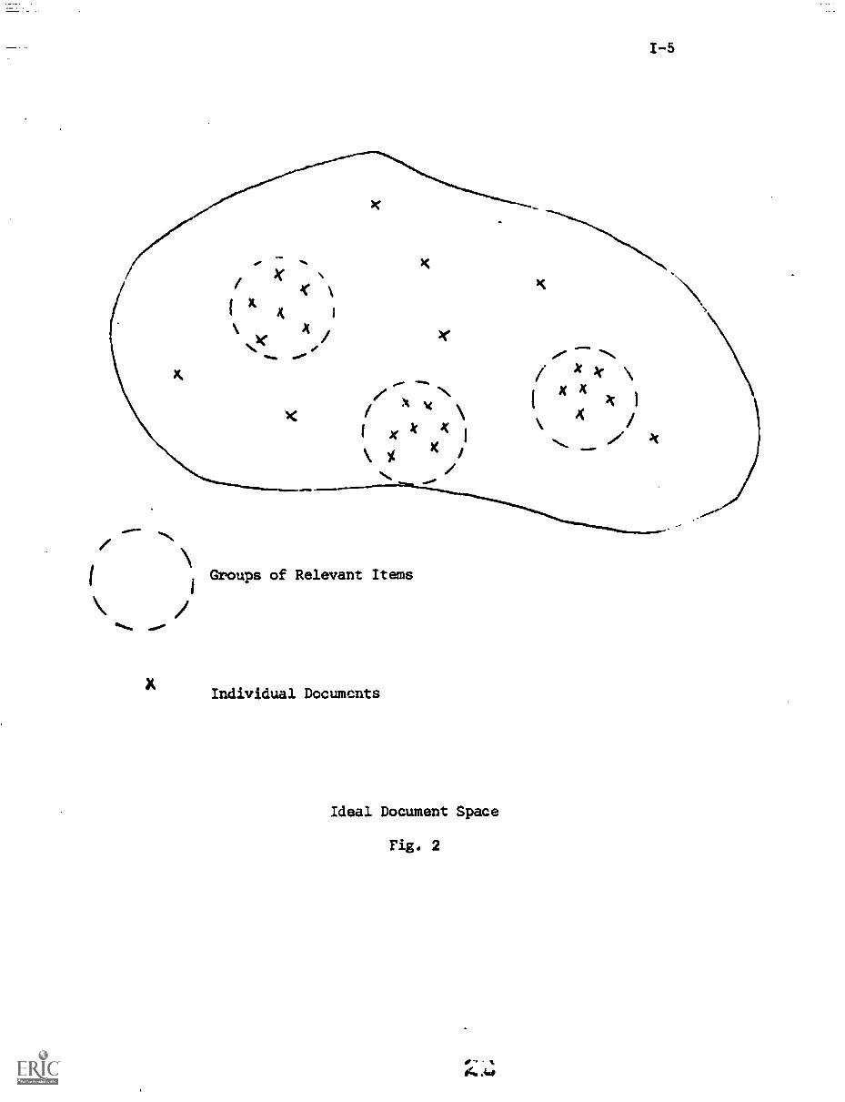
one might conjecture that an ideal document space is one where documents that

are jointly relevant to certain user queries are clustered together, thus

insuring that they would be retrievable jointly in response to the corresponding

*Retrieval performance is often measured by parameters such as recall and

precision, reflecting the ratio of relevant items actually retried, andof retrieved items actually relevant. The question concerning optimumspace configurations may then be more conventionally expressed in terms of

the relationship between document indexing on the one hand, and retrieval

performance on the other.

1-4

queries. Contrariwise, documents that are never wanted simultaneously would

appear well separated in the document space. Such a situation is depictod

in the illustration of rig. 2, where the distance between two x's representing

two documents is inversely related to the similarity between the corresponding

index vectors.

While the document configuration of Fig. 2 may indeed represent the

best possible situation, assuming that relevant and nonrelevant items with

respect to the various queries are separable as shown, no practical way exists

for actually producing such a space, because during the indexing process, it is

difficult to anticipate what relevance assessments the user population will

provide over the course of time. That is, the optimum lonfiguration is difficult

to generate in the absence of a priori knowledge of the complete retrieval

history for the given collection.

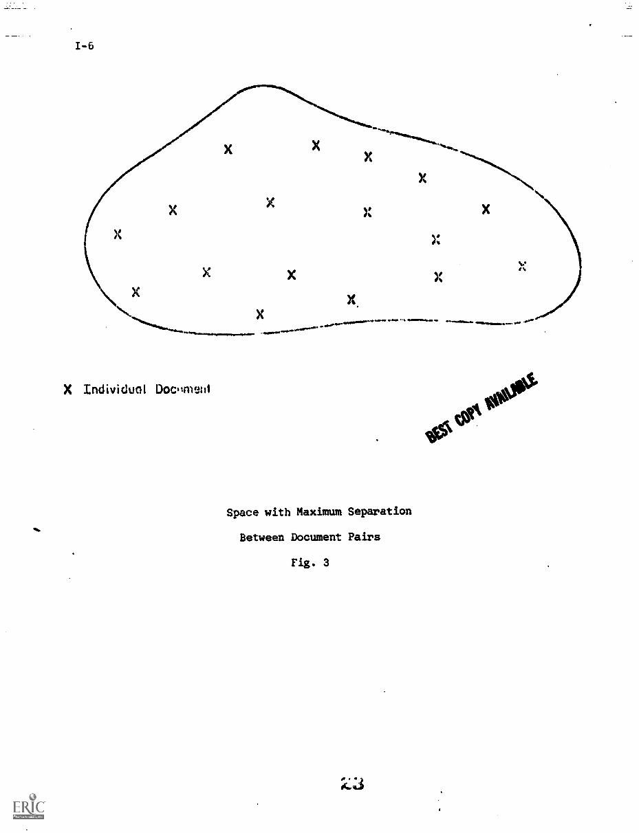
In these circumstances, one might conjecture that the next best thing

is to achieve a maximum possible separation between the individual documents

in the space, as shown in the example of Fig. 3. Specifically, for a collection

of n documents, one would want to minimize the function.

n nF = E E s(Di. D

J),

i=1 j=1

(1)

where s(D., D.) is the similarity between documents i and j. Obviously

when the function of equation (1) is minimized, the average similarity between

document pairs is smallest, thus guaranteeing that each given document may

be retrieved when located sufficiently close to a user query without also

necessarily retrieving its neighbors. This insures a high precision search

output, since a given relevant ite.. is then retrievable without also retrieving

a number of nonrelevant items in its vicinity. In cases where several different'

X

Groups of Relevant Items

Individual Documents

Ideal Document Space

Fig. 2

e-;

1-6

X

X

XX

X XX

X Individual Doc.tmeni

X.

Space with Maximum Separation

Between Document Pairs

Fig. 3

3

X

0$434°

itO

relevant items for a given query are located in the same general area of the

space, it may then also be possible to retrieve many of the relevant while

rejecting most of the nonrelevant. This produces both high recall and high

precision.*

Two questions then arise: first, is it in fact the case that a

separated document space leads to a good retrieval performance, and vice-versa

that improved retrieval performance implies a wider separation of the documents

in the space; second, is there a practical way of measuring the space separation.

In practice, the expression of equation (1) is difficult to compute since the

number of vector comparisons is proportional to n2

for a collection of n

documents.

For this reason, a clustered document space is best considered, where

the documents are grouped into classes, each class being represented by a

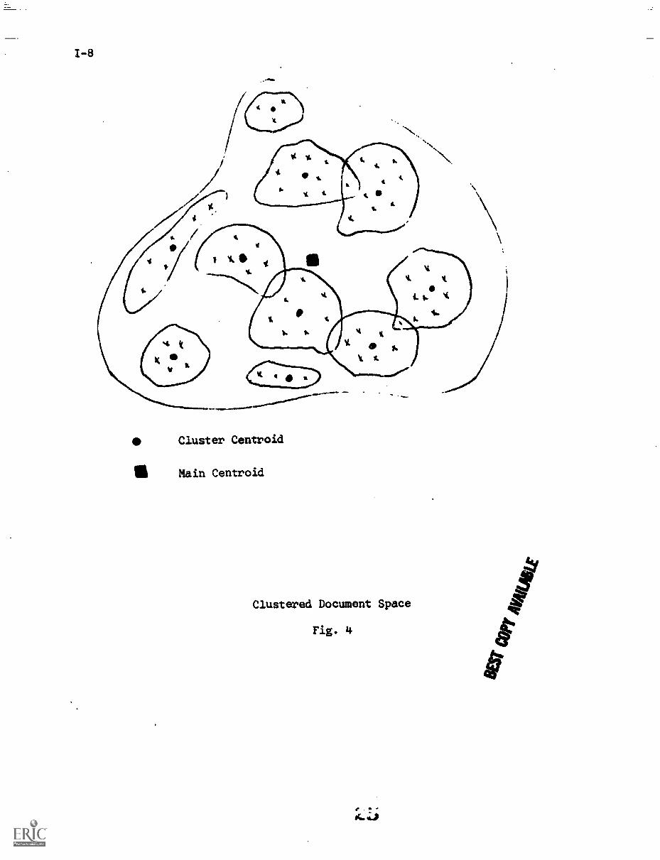
class centroid. A typical clustered document space is shown in Fig. 4, where

the various document groups are represented by circles and the centroids by

black dots located more or less at the center of the respective clusters.+

For a given document class K comprising m documents, each element of the

centroid C may then be defined as the average weight of the same elements

in the corresponding document vectors, that is

mc,

1E d. .

i=1

D.eK

(2)

$'l

*In practice, the best performance is achieved by obtaining for each usera desired recall level (a specified proportion of the relevant stems); atthat recall level, one then wants to maximize precision by retrieving asfew of the nonrelevant as possible.

+A number of well-known clustering methods exist for automatically generatinga clustered collection from the term vectors representing the individualdocuments. [1]

Aft

41 Cluster Centroid

111 Main Centroid

Clustered Document Space

Fig. 4

Corresponding to the centroid of each individual document cluster, a

centroid may be defined for the whole document space. This main centroid,

represented by a small rectangle in the center of Fig. 4, may then be obtained

from the individual cluster centroids in the same manner as the cluster centroids

are computed from the inuividual documents. That is, the main centroid of the

complete space is simply the average of the various cluster centroids.

In a clustered document space, the space density measure consisting

of the sum of all pairwise document similarities, introduced earlier as

equation (1), may be replaced by the sum of all similarity coefficients

between each document and the main centroid, that is

n

Q=Es(011).),i=1

(3)

where C* denotes the main centroid. Whereas the computation of equation (1)

requires n2

operations, an evaluation of equation (3) is proportional to n.

Given a clustered document space such as the one shown in Fig. 4, it is

necessary to decide what type of clustering represents most closely the

separated space shown for the unclustered case in Fig. 3. If one assumes that

documents that are closely related within a single cluster normally exhibit

identical relevance characteristics with respect to mos user queries, then

the best retrieval performance should be obtainable wit a clustered space

exhibiting tight individual clusters, but large intercl ster distances;

that is,

a) the average similarity between irs of documents within a single

cluster should be maximized, w le simultaneously

b) the average similarity betWeen different cluster centroids is

minimized.

I-10

TnP reverse obtains for cluster organizations not conducive to good

performance where the individual clusters should be loosely defined,

whereas the distance between different cluster centroids should be small.

In the remainder of this study, actual performance figures are

given relating document space density to retrieval performance, and con-

clusions are reached regarding good models for automatic indexing.

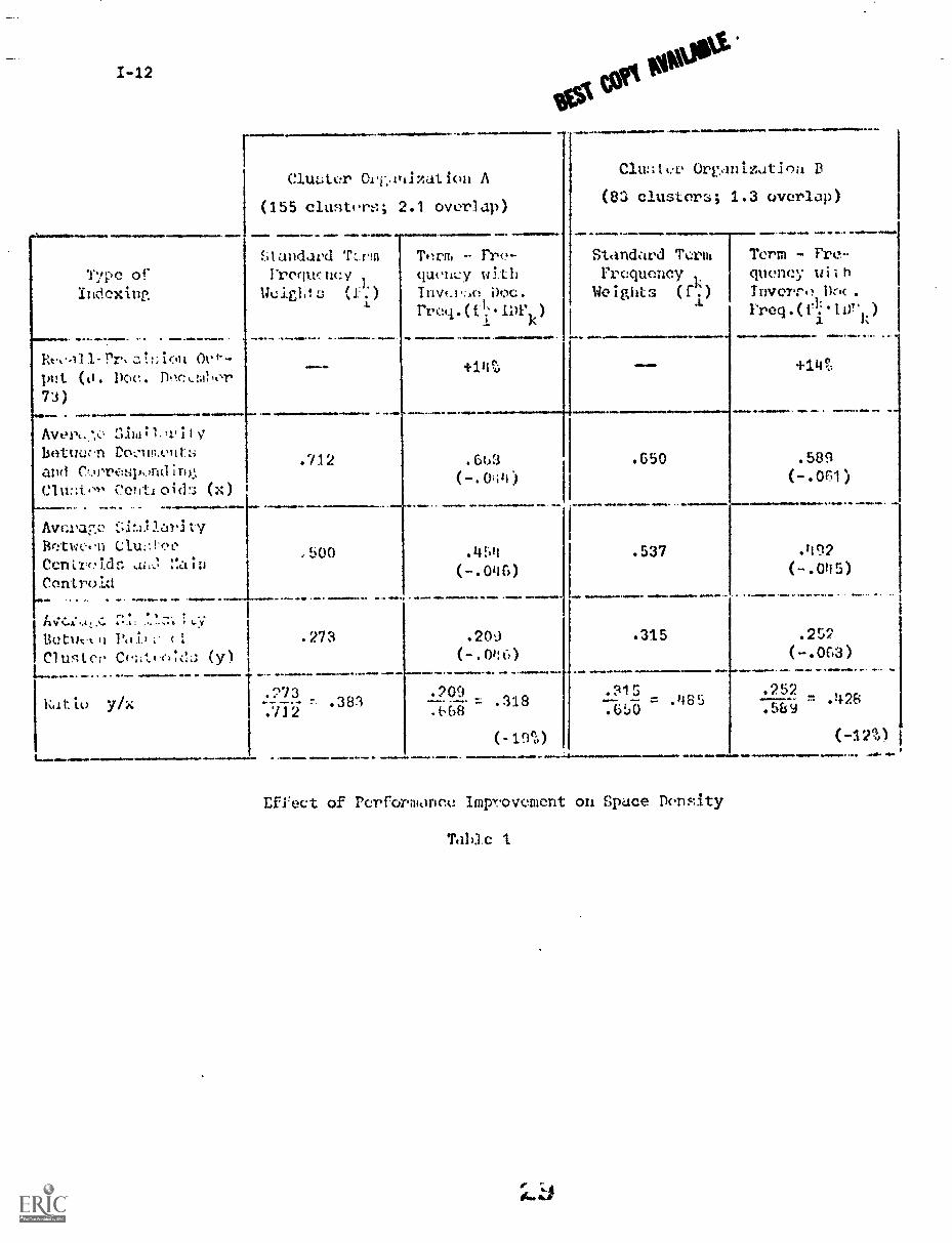
2. Correlation between Indexing Performance and Space Density

The main techniques useful for the evaluation of automatic indexing

methods are now well understood. In general, a simple straightforward

process can be used as a base-line criterion --for example, the use of

certain word stems extracted from documents or document abstracts, weighted

in accordance with the frequency of occurrence (fki) of each term k in

document i. This method is known as term-frequency weighting. Recall-

precision graphs can be used to compare the performance of this standard

process against the output produced by more refined indexing methods.

Typically, a recall-precision graph is a plot giving precision figures,

averaged over a number of user queries, at ten fixed recall levels, ranging

from 4.1 to 1.0 in steps of 0.1. The better indexing method will of course

produce higher precision figures at equivalent recall levels.

One of the best automatic term weighting procedures evaluated as

part of a recent study consisted of multiplying the standard term frequency

weight f. by a factor inversely related to the document frequency dk

of the term (the number of documents in the collection to which the term is

assigned). (2] Specifically, if dk is the document frequency of term k,

the inverse document frequency IDFk of term k may be defined as [31:

(IDF)k

= clog21 - flog

2dkI t 1.

A term weighting system proportional to 'irk) will assign the largest

weight to those terms which arise with high frequency in individual documents,

but are at the same time relatively rare in the collection as a whole.

It was found in the earlier study :hat the average improvement in recall

and precision (average precision improvement at the ten fixed recall points)

was about 14 percent for the system using inverse document frequencies over

the standard term frequency weighting. The corresponding space density

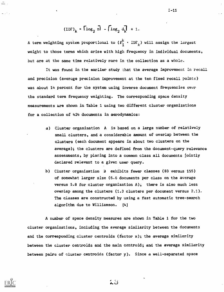
measurements are shown in Table 1 using two different cluster organizations

for a collection of 424 documents in aerodynamics:

a) Cluster organization A is based on a large number of relatively

small clusters, and a considerable amount of overlap between the

clusters (each document appears in about two clusters on the

average); the clusters are defined from the document-query relevance

assessments, by placing into a common class all documents jointly

declared relevant to a given user query.

b) Cluster organization B exhibits fewer classes (83 versus 155)

of somewhat larger size (6.6 documents per class on the average

versus 5.8 for cluster organization A), there is also much less

overlap among the clusters (1.3 clusters per document versus 2.1).

The classes are constructed by using a fast automatic tree-search

algorithm due to Williamson. [4]

A number of space density measures are shown in Table 1 for the two

cluster organizations, including the average similarity between the documents

and the corresponding cluster centroids (factor x); the average similarity

between the cluster centroids and the main centroid; and the average similarity

between pairs of :luster centroids (factor y). Since a well-separated space

law-wo

1-12

Typo ofIndoxing

put (a. Doc. DooLml,or73)

solmarownw.

betwecn Dos..-mehtzi

and C....ortz:spondlnk!,

elmto Co?ita oith; (x)

Avcra7.o ;;I!all.ctrity

Bete,, Clu;:!.eoCenmidn an..1Control:1

/CluL.ter OIT..vilzation A

(155 clustore.; 2.1 overlap)

.M.Pft 0*m11M orb. MMUMOV

.1andavd T:rml'rewnevWeighls (11.)

.712

500

lictut.,11 Poir z c 1 .273Cl u' Co:.40.n:dJ (y)L.-- ....... - . ....- ..- .. - --- I.". ..NM.. ...a.awa .. ..._-

1Rat it) 7/x

LANIMIN.

.273n .383

.712

TfIrm - Fro-

quon..:y with

Invt.pr..c! Doc.

Freq.0.1.'.1DFk

)

MMIIIIOPPM. -11.11wIloallia.loMma ././/0411 ...........

Clu:ttv Organizatioa

(83 clusters; 1.3 overlap)

...Om 4. - OM. orm... we. ow..

Standard TermFrequencyWeights

01

.60(-.0;;4)

( -.0'U

.209

(-.046)61100

?00

'318

(-10%)

.650

.537

.1

Term - Fre-

quency wilhTnverro Dc .

Freq.(fl."11)T )

.315

.589

(-.061)

.:415 =4.85

.650

.492(-.045)

.2S2

(-.063)-.252

.569.428

Effect of Performance Improvement on Spuce Density

Table 1.

(-12%)

1-13

corresponds to tight clusters (large x) and large differences between different

clusters (small y), the ratio y/x can be used to measure the overall space

density. (5]

It may be seen from Table 1, that all density measures are smaller for

the indexing system based on inverse document frequencies; that is, the

documents within individual clusters resemble each other less, and so do the

complete clusters themselves. However, the "spreading out" of the clusters

is greater than the spread of the documents inside eacil cluster. This accounts

for the overall decrease in space density between the two indexing systems.

The results of Table 1 would seem to support the notia that improved recall-

precision pe..formance is associated with decreased density in the document

space.

The reverse proposition, that is, whether decreased performance implies

increased space density may be tested by carrying out term weighting operations

inverse to the ones previously used. Specifically, since a weighting system

in inverse document frequency order produces a high recall-precision performance,

a system which weights the terms directly in order of their document frequencies

(terms occurring in a large number of documents receive the highest weights)

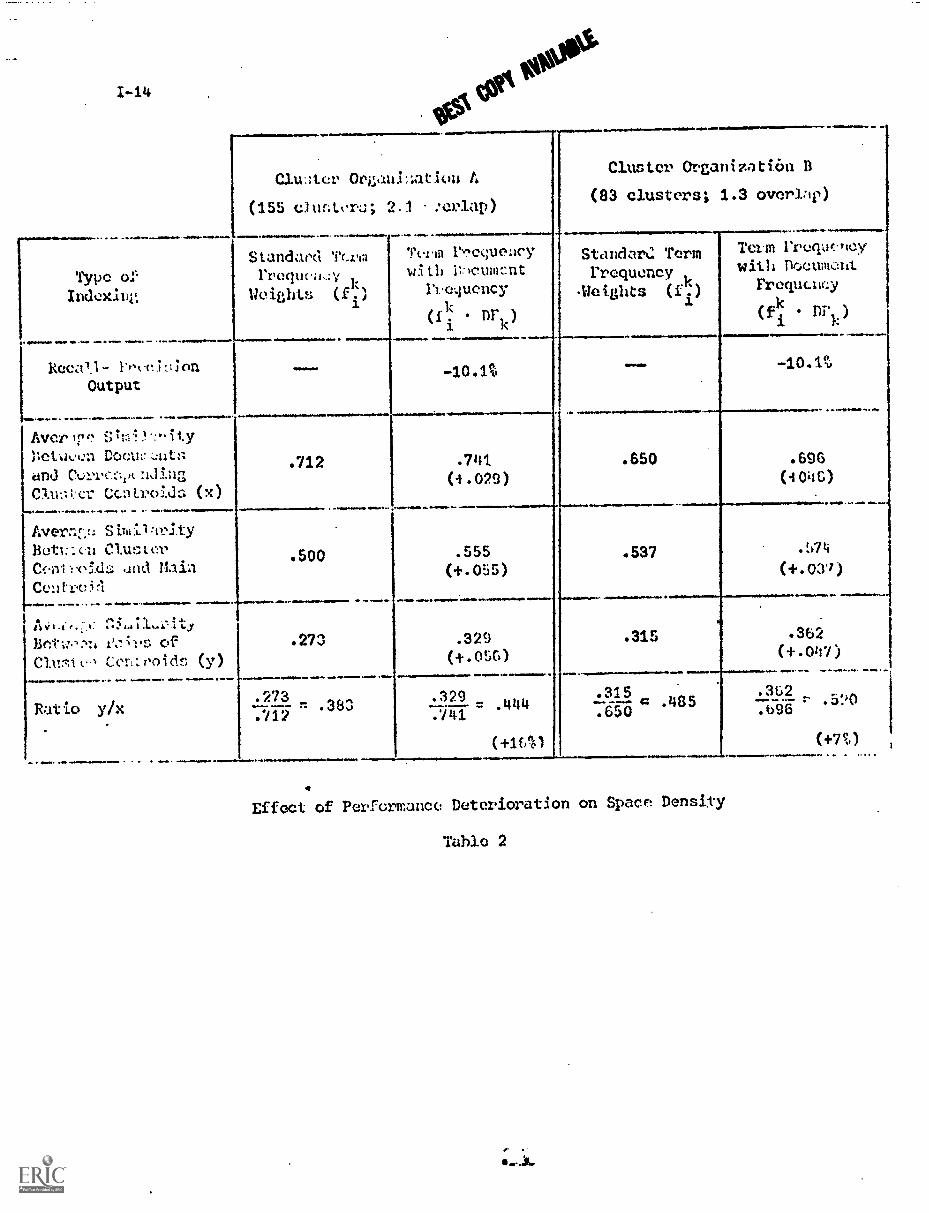
should be correspondingly poor. In the output of Table 2, a term weighting

system proportional to (fi DFk) is used, where fi is again the term

frequency of term k in document i, and DFk is defined as 10/(IDF)k. The

recall-precision figures of Table 2 show that such a weighting system produces

a decreased performance of about ten percent, compared with the standard.

The space density measurements included in Table 2 are the same as

those in Table 1. For the indexing system of Table 2, a general "bunching

up" of the space is noticeable, both inside the clusters and between clusters.

1-14

CluAtcv Org.1111::ation A

(155 cltuAora; 2.1 :crlap)

Type of rrecia. ,

Weights (C)

m O. **a. .1.

1.-

Rceel- r,y(ti:tion

Output

Cluster Organization 13

(83 clusters; 1.3 overW)

Tvvm rrequeacywith 11:lcummt

r):e.luency

(f. Drk)-. esAver irg S 71;1 i 1-: i ty

[)e1.11%.4.r.1 DOCU:: .3.12::-;

ani.1 C....,rctadiag

Clul:k-er ecntroiJa ()

Aver:1;-% SiNI1;trity

Butl:Icn ClutItor

..md /lain

Centre3i

nvrie.t

.712

11-r. ofCon:ooids (y)

0..01wIr

Ratio y/x

.500

-10.1%

.741

0.029)

r.273

.273

.712

.40 -we

.383

4

.555

(+.055)

4.400100..m00...4444mwo..000MMI.01011NOmm

.329

(+.056)

.329= .1444

( +114)

111StaucL Termfrequency

-Weights (ii)

Team rreclaf:Nay

with Dr4CUMOlit

Frequcmy

(f. Di"k

)

. wm.650

.537

-10.1%

`

.696

(0 04C)

.b7'4

(+.03q)

.315 .362(+.047)

485 .b96.315 .362

(+7%)

Effect of Performance Deterioration on Space Densiiy

Table 2

However, the similarity of the various cluster centroids increases more than that

between documents inside the clusters. This accounts for the higher y/x

factor by 16 and 7 percent for the two cluster organizations, respectively.

3. Correlation between Space Density and Indexing Performance

In the previous section it was shown that certain indexing methods which

operate effectively in a retrieval environment are associated with a decreased

density of the vectors in the document space, and contrariwise that poor

retrieval performance corresponds to a space that is more compressed.

The relation between space configuration and retrieval performance may,

however, also be considered from the opposite viewpoint. Instead of picking

document analysis and indexing systems with known performance characteristics

and testing their effect on the density of the document space, it is possible

artifically to change the document space configurations in order to ascertain

whether the expected changes in recall and precision are in fact produced.

The space density criteria previously given stated that a collection of

small tightly clustered documents with wide separation between individual

clusters should produce the best performance. The reverse is true of large

nonhomogeneous clusters that are not well separated. To achieve impro'ements

in performance, it would then seem to be sufficient to increase the similarity

between document vectors located in the same cluster, while decreasing the

similarity between different clusters or cluster centroids. The first effect

is achieved by emphasizing the terms that are unique to only a few clusters,

or terms whose cluster occurrence frequencies are highly skewed (that is, they

occur with large occurrence frequencies in some clusters, and with much lower

frequencies in many others). The second result is produced by deemphasizing

terms that occur in many different clusters.

I-1C

Two parameters may be introduced to be used in carrying out the

required transformations [5):

NC(k)

and CF(k,j)

The number of clusters in which term k occurs (a

term occurs in a cluster if it is assigned to at

least one document in that cluster);

the cluster frequency of term k in cluster j

that is, the number of documents in cluster j in

which term k occurs.

For a collection arranged into p clusters, the average cluster frequency

CF(k) may then be defined from CF(k,j) as

CF(k) =1

E CF(k,j).P j=1

Given the above parameters, the skewness of the occurrence frequencies

of the terms may now be measured by a factor such as

F1= ICF(k) - Cr(k,j)1.

On the other hand, a factor F2

inverse to NC(k) (for example, 1/NC(k))

can be used to reflect the rarity with which term k is assigned to the

various clusters. By multiplying the weight of each term k in each

cluster j by a factor proportional to F1 F2 a suitable spreading out

should be obtained in the document space. Contrariwise, the space will be

compressed when a multiplicative factor proportional to 1/F1 F2 is used.

The output of Table 3 shows that a modification of term weights by

the F1

F2factor produces precisely the anticipated effect: the similarity

between documents included in the same cluster (factor x) is now greater,

whereas the similarity between different cluster centrcids (factor y) has

11

1-17

Cluster Ove,anization A

(155 clusters; 2.1 overlap)

0111410.11

Cluster Organization B

(83 clusters; 1.3 overleap)

StandardCluster Density

(term frequencyweiLhts)

HighCluster DonaLty.

(emi.hasis of

low frequoncyand skewed tutus)

Standard HighCluster Density Cluster DrInnity

(term frequencyweights)

(emphin.is of

lovand skowd i.(1.0111:;)

Average Similarity

between Documents

and their Centroids(x)

Average Similarity

between Cluster

CentroiJa and

Hain Centroid

.712

.500

Average Similarity

uet.ecen

of Ceatroida (y)

.273

Ratio y/x.273 1".712

0.730

( +.018)

.477

.279

(-.0,14)

111111

.650 .553(+.003)

.537

1111

.52S

(-.009)

.315

.229. .0"

.730

(-18%)

.315.485

.650-

1111.11.

IIIINOMOIMPOI

.?81

(- .03't)

41. War. 0. aa

2e1 .430

Recall-Precision

Comparison00111111.110

r 1".+2.6%

ANY

0.1111

.0.11110W

Effect of Low Cluster Density on Performance

Table 3

+2.3%

1-18

decreased. Overall, the space density measure (y/x) decreases by 18 and

11 percent respectively for the two cluster organizations. The average

retrieval performance for the spread-out space shown at the bottom c...17

Table 3 is improved by a few percentage points.

The corresponding results for the compression of the space using

a transformation factor of 1/F1

F2are shown in Table 4. Here the

similarity between documents inside a cluster decreases, whereas the

similarity between cluster centroids increases. The overall space den-

sity measure (y/x) increases by 11 and 16 percent for the two cluster

organizations compared with the space representing the standard term

frequency weighting. This dense document space produces losses in recall

and precision performance of 12 to 13 percent.

Taken together, the results of Tables 1 to 4 indicate that retrieval

performance and document space density appear inversely related, in the

sense that effective (questionable) indexing methods in terms of recall

and precision are associated with separated (compressed) document spaces;

on the other hand, artificially generated alterations in the space densities

appear to produce the anticipated changes in performance.

The foregoing evidence thus confirms the usefulness of the "term

discrimination" model and of the automatic indexing theory based on it.

These (tiostions are examined briefly in the remainder of this study.

4. The Discrimination Value Model

For some years, a document indexing model known as the term dis-

crimination model has been used experimentally. [2,6] This model bases

the value of an index term on its "discrimination value" DV, that is, on

an index which measures the extent to which a given term is able to

increase the differences among document vectors when assigned as an index

Av-.v, Sim:1 10!ty

Let.w(-:.a Docaac:1:5

ali,:l thoir Contruid:

x). do..

x..11.4. t.3

:1...twoe4

(-.11Lrc.'dv

Y.ain Cent.1-: d

s7mnariLy

of Ck.r:loid (y)

r-- .Clunter Urgcatization A

(155 clu:A(.r::; 2.1 overlap)

11%115 IMP 9111 ..

StandardClu.:tor Clust(!t. 1)(11:12.12...(Lem !:roquency

woights)

01111

00. ..

.1.. on .so 1 I WO 1,11/2400,111 =........

Reitio y/x

. ...............

Roca1.1.-rrnci:tton

Comp.o., noTi

(emplia....1... on

high fL.,.:Aav)lcy

cva termq)alb* flim w

.712

-.500

.--10.-

.23

....

.273

.712

.681

(-.0:$1)

.523

(4.023)*.2nD

(1.01.7)

,.......1

.290= .426

(+11%). ,.....................110

4/1..... 011

-12.4%

...

1-19

(83 elu::ero; 1.3 ovq-Op)

.11 s

Stau(Idtql

Clustot,-(term frerwncy

Wei!

.650

.b37

... ....01

(o1h11111,:1:. oh

h10,and evul

.31')

76bli '1185

Effect of High CluzAr Deu:Aty 01. Performanco

Table 4

.64t)

(-.005)

O.. IMO WIM17110.041.

.164

.64')

.elooleam =now. ...

1-20

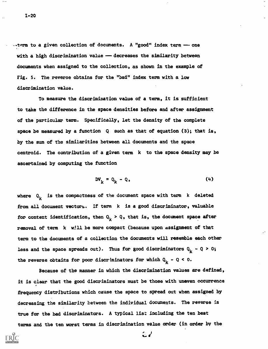
-..berm to a given collection of documents. A "good" index term --- one

with a high discrimination value --decreases the similarity between

documents when assigned to the collection, as shown in the example of

Fig. 5. The reverse obtains for the "bad" index term with a low

discrimination value.

To measure the discrimination value of a term, it is sufficient

to take the difference in the space densities before and after assignment

of the particular term. Specifically, let the density of the complete

space be measured by a function Q such as that of equation (3); that is,

by the sum of the similarities between all documents and the space

centroid. The contribution of a given term k to the space density may be

ascertained by computing the function

DVk

= Qk

- Q'

where Qk is the compactness of the document space with term k deleted

from all document vector'. If term k is a good discriminator, valuable

for content identification, then Qk > Q, that is, the document space after

removal of term k wall be more compact (because upon assignment of that

term to the documents of a collection the documents will resemble each other

less and the space spreads out). Thus for good discriminators Qk Q > 0;

the reverse obtains for poor discriminators for which Qk - Q < 0.

Because of the manner in which the discrimination values are defined,

it is clear that the good discriminators must be those with uneven occurrence

frequency distributions which cause the space to spread out when assigned by

decreasing the similarity between the individual documents. The reverse is

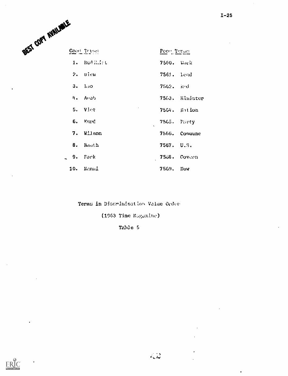
true for the bad discriminators. A typical list including the ten best

terms and the ten worst terms in discrimination value order (in order by the

Befo Assignment

of Term

X Document

0 ;v4r.lit; Ctit;tti,tij

1-21

Operation of

Good Discriminating Term

Fig. 5

After Astignment

of Term

1-22

Qk Q value) is shown in Table 5 for a collection of 425 articles in world

affairs from Time magazine. A total of 7569 terms are used for this collec-

tion, exclusive of the common English function words that have been deleted.

In order to translate the discrimination value model into a possible

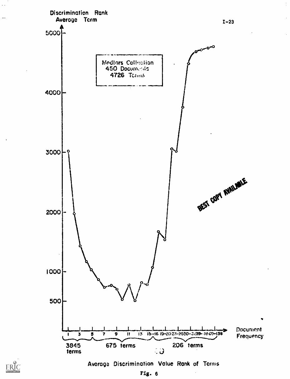
theory of indexing, it is necessary to examine the properties of good and

bad discriminators in greater detail. Fig. 6 is a graph of the terms assigned

to a sample collection of 450 documents in medicine, presented in order by

their document frequencies. For each class of terms those of document

frequency 1, document frequency 2, etc. ... the average rank of the

corresponding terms is given in discrimination value order (rank 1 is assigned

to the best discriminator and rank 4726 to the worst term for the 4726 terms

of the medical collection).

Fig. 6 shows that terms of low document frequency ---those that occur

in only one, or two, or three documents ---have rather poor average discrim-

ination ranks. The several thousand terms of document frequency 1 have an

average rank exceeding 3000 out of 4726 in discrimination value order. The

terms with very high document frequency --- at ledst one term in the medical

collection occurs in as many as 138 documents out of 450 ---are even worse

discriminators; the terms with document frequency greater than 25 have average

discrimination values in excess of 4000 in the medical collection. The best

discriminators are those whose document frequency is neither too low nor too

high.

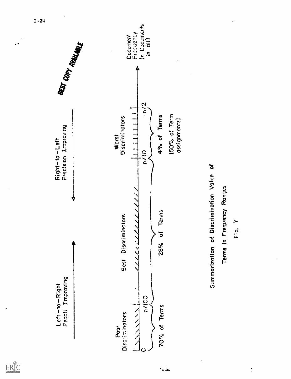
The situation relating document frequency to term discrimination value

is summarized in Fig. 7. The 4 percent of the terms with the highest document

frequency, representing about 50 percent of the total term assignments to the

documents of a collection, are the worst discriminators. The 71 percent of

Discrimination RankAverage Term

5000

4000

3000

2000

1000

500

L

1.--Medlnrs Coll,:::lion450 Docuro..., s

4726 RA mi.

MR VOIMMIIMII11.0... - Noloa.1111.1.111.

1-23

I 3 5 7 9 11 131b -16 19-20 23-?5.30- '9-130

3845 675 terms 206 termsterms ..k.)

Average Discrimination Value Rank of TermsFig. 6

DocumentFrequency

Left

-to-

Rig

htIm

wov

ing

Poo

rD

iscr

irnin

otor

s

C;

n/10

0

4111

111=

1*11

110.

70%

of T

erm

s

Bes

tD

iscr

imin

ctor

s

43-

4

Rig

ht-t

o- L

eft

Pre

cisi

on im

prov

ing

ser co

t4/

044.

Wor

stD

iscr

imin

ator

s

4.e.

../z/

L//,7

/7/./

i/;

;;

t II

1

26%

of T

erm

s

Sum

mar

izat

ion

of D

iscr

imin

atio

n V

alue

of

Ter

ms

in F

requ

ency

Rar

er:

F ;

g.7

n/!0

n/2

4% o

f Ter

ms

(50%

of T

G;-

11as

sign

ny3n

ts1

Doc

umen

tF

rzcu

er:;:

yr"

,.-..c

t;rne

nts

oil)

S ottin

CouTtzrrw OWTJ. eoGI)

a.11),70 onTpA nwa/

At )U '69SL VuuM 'OT

'TISL -1 e1 6 -

'sea *L9SL 11-"PH '8

aunmwoo 4114 L uosum °L

&10-4 'STIL PatiA '9

uoT11:0 '4014 40IA 'S

J°113PIIN 'COSL (se.4V '4

"t4TiL 0(11 °E

Puol 'f9SL 111,4

)1.70:1 '09SL 'T

..00j ;":.1. )1 WOO Idl# iot\sts4b

1-26

the terms with the lowest document frequency ale generally poor discrim-

inators. The best discriminators are the 25 percent whose document freq-

uency lies approximately between n/100 and n/10 for n documents.

If the model of Fig. 7 is a correct representation of the situation

relating to term importance, the following indexing strategy results [6,7]:

a) Terms with medium document frequency should be used for content

identification directly, without further transformation.

b) Terms with very high document frequency should be moved to the

left on the document frequency spectrum by transforming them

into entities of lower frequency; the best way of doing this

is by taking high-frequency terms and using them as components

of indexing phrases ---a phrase such as "programming language"

will necessarily exhibit lower document frequency than either

"program", or "language" alone.

c) Terms with very low document frequency should be moved to the

right on the document frequency spectrum by being transformed

into entities of higher frequency; one way of doing this is by

collecting several low frequency terms that appear semantically

similar and including them in a common term (thesaurus) class.

Each thesaurus class necessarily exhibits a higher document

frequency than any of the component members that it replaces.

The indexing theory which consists in using certain elements extracted

from document texts directly as index terms, combined with phrases made up

of high frequency components and thesaurus classes defined from low frequency

elements has been tested using document collections in aerodynamics (CRAN),

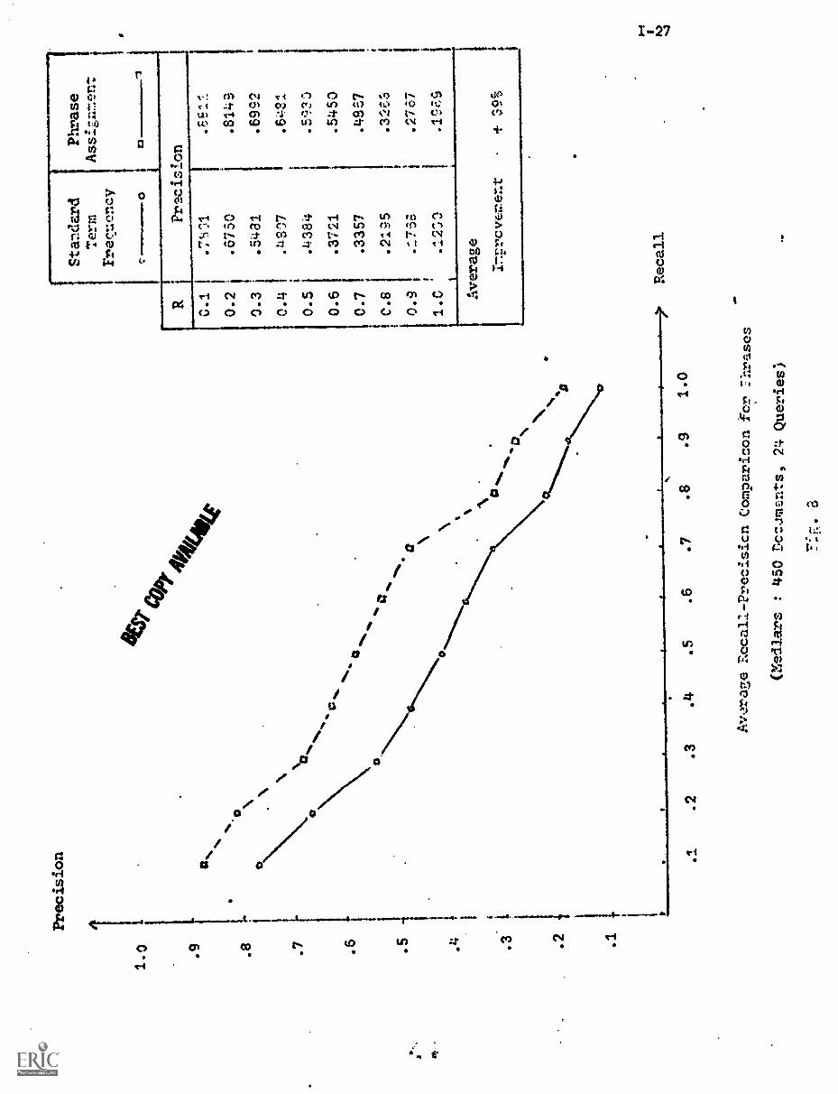
medicine (MED), and world affairs (TIME). [2,6,7) A typical recall-precision

plot showing the effect of the right-to-left phrase transformation is shown in

rig. 8 for the Medlars collection of 450 medical documents. When recall is

plotted against precision, the curve closest to the upper right-hand corner

Precision

1.0

1

.9 .8 .7 .6

T

.5

-3

.4 3 .2 .1

gt

o

0

\12

a

.4%

a

get C

O,o

, "Itti

te

a

a

.2

.3

.4

.5

.6

.7

Standard

Phrase

Term

Assizzment

Frecuency 0

-3

"S 0.2

0.3

0.4

0.5

0.6

0.77

0.9

1.0

Si.

.6750

.5481

.11307

.4384

.3721

.3357

.2195

7 -.00

.8149

.6992

.6421

.5';123

.5453

.4967

.32eS

.2767

.1tr:Z9

Average

Inprovement

los%

8Recall

.8

.9

1.0

Awrage Recall-?reds icn Co.. paricon fcr :hrases

(Medlars

: 450 DccJmznts, 24 Queries)

1-28

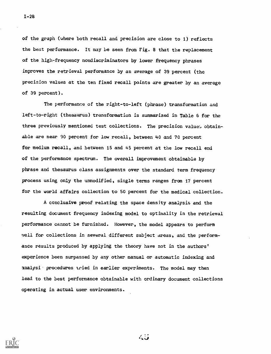
of the graph (where both recall and precision are close to 1) reflects

the best performance. It may be seen from Fig. 8 that the replacement

of the high-frequency nondiscriminators by lower frequency phrases

improves the retrieval performance by an average of 39 percent (the

precision values at the ten fixed recall points are greater by an average

of 39 percent).

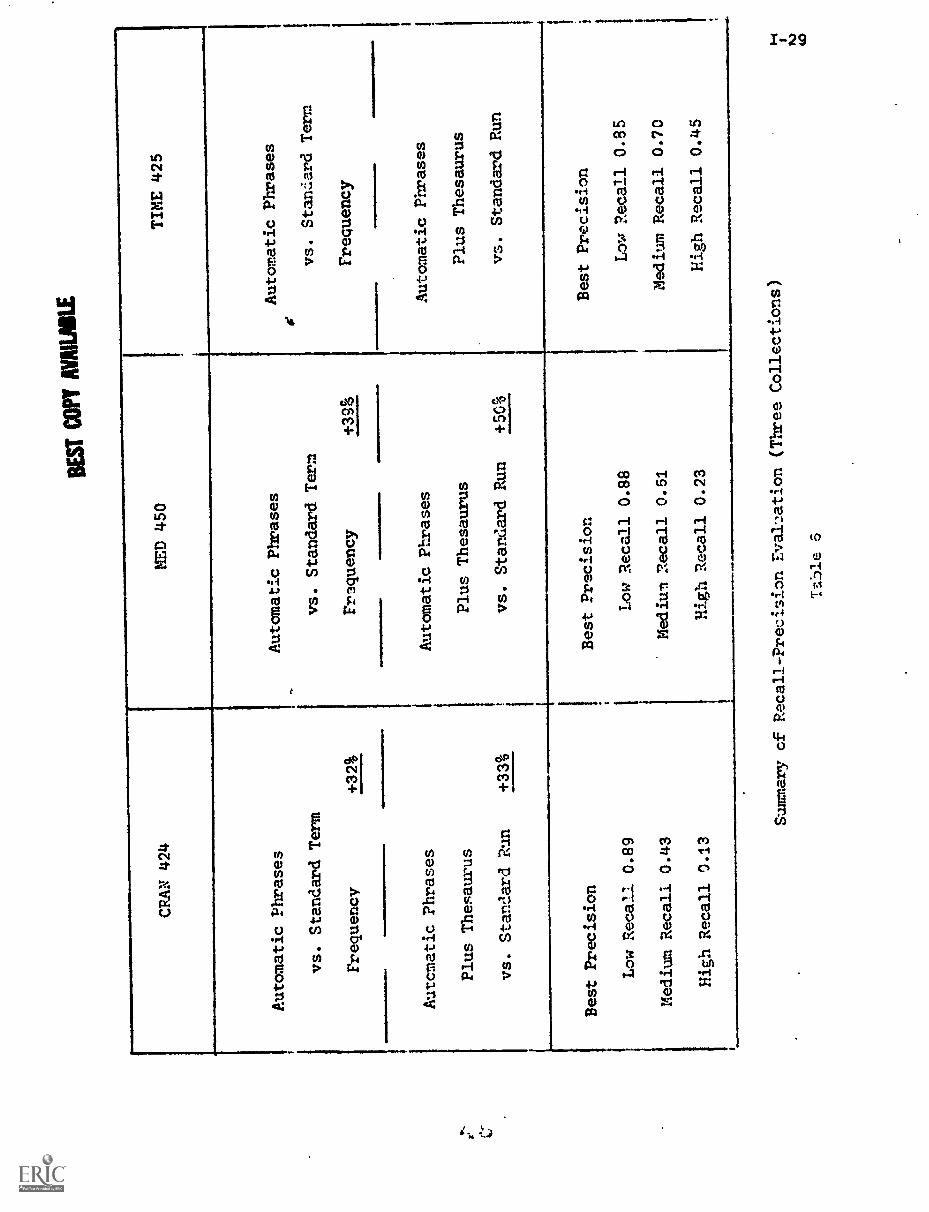
The performance of the right-to-left (phrase) transformation and

left-to-right (thesaurus) transformation is summarized in Table 6 for the

three previously mentioned test collections. The precision value:. obtain-

able are near 90 percent for low recall, between 40 and 70 percent

for medium recall, and between 15 and 45 percent at the low recall end

of the performance spectrum. The overall improvement obtainable by

phrase and thesaurus class assignments over the standard term frequency

process using only the unmodified, single terms ranges from 17 percent

for the world affairs collection to 50 percent for the medical collection.

A conclusive proof relating the space density analysis and the

resulting document frequency indexing model to optimality in the retrieval

performance cannot be furnished. However, the model appears to perform

well for collections in several different subject areas, and the perform-

ance results produced by applying the theory have not in the authors'

experience been surpassed by any other manual or automatic indexing and

analysi procedures tried in earlier experiments. The model may then

lead to the best performance obtainable with ordinary document collections

operating in actual user environments.

BE

ST C

OPY

AY

AR

MIL

E

CPA N 424

MED 450

TIME 425

Automatic Phrases

vs. Standard Term

Frequency

+32%

Autcmatic Phrases

Plus Thesaurus

vs. Standard Run

+33%

Automatic Phrases

vs. Standard Term

Frequency

+39%

Automatic Phrases

Plus Thesaurus

vs. Standard Run

+50%

Automatic Phrases

vs. Standard Term

Frequency

Automatic Phrases

Plus Thesaurus

vs. Standard Run

Best Precision

Low Recall 0.89

Medium Recall 0.43

High Recall 0.13

Best Precision

Low Recall 0.88

Mediun Recall 0.51

High Recall 0.23

Best Precision

Low Recall 0.85

Medium Recall 0.70

High Recall 0.45

Summary cf Recall-Precision

Eval,,ation (Three Collections)

Ta:Dle 6

1-30

References

[1] G. Salton, Automatic Information Organization and Retrieval, McGrawHill Book Co., New York, 1968, chapter 4.

[2] G. Salton and C.S. Yang, On the Specification of Term Values inAutomatic Indexing, Journal of Documentation, Vol. 29, No. 4, December1973, p. 351-372.

[3] K. Sparck Jones, A Statistical Interpretation of Term Specificity andits Application to Retrieval, Journal of Documentation, Vol. 28, No. 1,March 1972, p. 11-20.

[4] R.E. Williamson, Real-time Document Retrieval, Cornell University Ph.D.Thesis, Department of Computer Science, June 1974.

[5] A. Wong, An Investigation of the Effects rf Different Indexing Methodson the Document Space Configuration, Scientific Report No. ISR-22,Department of Computer Science, Cornell University., to appear.

[6] G. Salton, A Theory of Indexing, Technical Report No. TR-203, Departmentof Computer Science, Cornell University, March 1974.

[7] G. Salton, C.S. Yang, and C.T. Yu, Contribution to the Theory of Indexing,Proc. IFIP Congress-74, Stockholm, August 1974.

An Investigation on the Effects cf

Different Indexing Methods on the

Document Space Configuration

Anita Wong

Abstract

An attempt is made on the present study to gain a better under-

standing of the document space configuration through the use of

clustered document collections and different indexing methods.

1. Introduction

Previous work in automatic indexing and clustering in information

retrieval has mostly been done with the thought of improving the recall and/or

precision of the search result. Not too much work has been done to gain

a fuller understanding of the document space configuration itself, presumably

because this is not directly related to the improvement of the effectiveness

of the system. However it is quite likely that the configuration of the

document space does correlate in some way with the effectiveness of the

system.

It is natural for documents that are related to be closely similar

to each other.* But is this really the case for any indexing method? Or

is it possible that documents that are related are scattered throughout the

document space and surrounded by extraneous documents which are more or less

closely packed in groups?

* Experimental results were performed by Jones 111.

11-2

The problem would be easier to answer if the meaning of closeness

were better defined. Closeness should bear a different meaning in different

systems, depending ca the way the documents are retrieved. On a book shelf,

two books are said to be close together if they are physically close together.

Close is defined in this way because whenever one book is located, the other

is also found. In automatic retrieval, closeness would be proportional to

the matching function used for document retrieval. The physical distance

between the documents is less important in this respect.

In the SMART system, a document is retrieved by a query if the

similarity between the document and query is high. If the similarity relation

is assumed transitive, then documents relevant to the same query should be

similar to each other. It is therefore inconceivable that any indexing

method should place the related documents in any way other then "close"

together. However merely placing the related documents close together does

not necessarily guarantee good system performance. The unrelated documents

should be farther apart then the related ones. In other words, ideally,

documents should form clusters which do not overlap; documents within a

cluster are related while those in different clusters are not; and the

distance between two documents within a cluster is shorter than two

documents belonging to two different clusters. Consequently, a good indexing

method should index the documents in such a way that the related documents

are close together and non-related ones further apart.

Many different indexing methods Were tested over the years in the

SMART system, and recall and precision figures were generated. It is not

known if the indexing methods that produce good performance do in fact place

the documents in the way predicted above, or if the changes in configuration

of the document space can be explained in some other way. It is the aim

tuj

11-3

of the present work to elucidate the relationship between the configuration

of the document space with the performance of the system with different

indexing methods.

2. Methodology

An obvious way to solve the problem is to look at each document, and

at its relation with the other documents. This requires a computation of the

correlation of every document with every other documents, thus obtaining for

each indexing method a full document-document matrix. These matrices are

then compared row-wise in order to ascertain the relative changes of

the documents with respect to each other. This method is.not employed

here because the number of documents involved is usually large. Instead,

the documents are grouped, and each group it, treated as an entity with

respect to the documents not in the same group. Judging the movements of

groups of documents instead of individual items alone may be justified because

it is rather pointless to look at the motion of each document with respect

to every other, since there are so many documents that individual effects

would be hardly noticeable.

The discrimination value model 12) has been found to give improvements

in search performance. However, the discrimination values are determined by

lowering the sum of the correlations between the documents and their

centroid; in other words, the discrimination value is a function of the

distance between document vectors. The application of the discrimination

values would tend to increase the average distance between documents,

regardless of the relations between the documents. But it may be unreasonable

to have related documents farther apart. Consequently, it is important to

relate the average increase in distance between similar documents to the

I1-4

average increase in distance between all documents.

Since the inestigation is performed on clustered document

collections, the clustering methods to be used are discussed first.

Previous experiments were done with clustering methods that

produce clusters of different sizes with a large variance.* It was

found that a large cluster is represented by a longer centroid vec or.

In some cases, the centroid vectors were so long that they each included

75% of the terms occurring in the collection. The correlations between

these centroids, being high, have become less meaningful in distinguishing

one centroid from another. The problem could be overcome by using a

different method in forming the c ntroid vectors as in Murray and

Kerchner [3], [4], or by deleting some common terms. But the centroids

would then lack some of the terms occurring in the documents and thus the

centroid would not be the true centers of the document clusters. For this

reason clustering algorithms that produce smaller clusters are considered.

The clustering methods to be used are:

A. For each query, one cluster is constructed. The cluster contains

documents that are relevant to that query. This method is

chosen because the clusters are easy to obtain in an experimental

environment and also because it produces small clusters as shown

in Table 1. This method will be referred to as method RCL.

* The centroid vector of a cluster is formed by summing the normalizeddocument vectors. Let Di = 1 m be documents belonging to clusterc then the centroid vector for m D. .

c = E. 1-17= 1 .

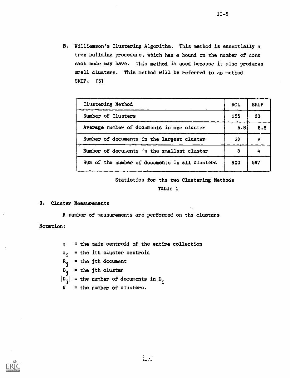
B. Williamson's Clustering Algorithm. This method is essentially a

tree building procedure, which has a bound on the number of sons

each node may have. This method is used because it also produces

small clusters. This method will be referred to as method

SKIP. [5]

Clustering Method RCL SKIP

Number of Clusters 155 83

Average number of documents in one cluster 5.8 6.6

Number of documents in the largest cluster 22 9

Number of docui..ents in the smallest cluster 3 4,

Sum of the number of documents in all clusters 900

.

547

Statistics for the two Clustering Methods

Table 1

3. Cluster Measurements

A number of measurements are performed on the clusters.

Notation:

c = the main centroid of the entire collection

c. = the ith cluster centroid

R.3

= the jth document

D,J

= the jth cluster

I.D,I = the number of documents in D.1

N = the number of clusters.

11-6

The measurements are:

1. The average correlation of the documents in cluster Diwith

their centroid, C.

R.+D.

1

cosine(R.3 ,C.)

IDi

The average for all the clusters

a = E A,/N

2.111ecorrelationbetweenclustercentroidC.with the main

centroid, C

B. = cosine(C1,C)

and the average of the Bi's

b = EBi/N

3. The correlation between two cluster centroids

Cif = cosine(Ci,Cj)

and the average of the C..'s13

C = E E C../N2

4. The ratio:the ave. corr. of the docs, with their centroid

the ave. corr. between cluster centroids and main centroid

Q1

= a/b

5. The ratio:Ave. corr. of the documents with their centroid

Ave. corr. between cluster centroids

Q2

= a/c.

11-7

4. The Experiment

The experiment was performed using the Cranfield 424 Thesaurus

Collection. The collection was first clustered using Williamson's Algorithm

SKIP, and then using the query relevant method, RCL. The Q values for

these two clustered document collections were calculated for the different

indexing methods listed below.

1. Cranfield 424 Thesaurus Collection.

2. Cranfield 424 Thesaurus Collection with the application of

discrimination values. The concept weight of the document

vectors were multiplied by the discrimination values resealed

to an effective range.

3. Cranfield 424 Thesaurus Collection with the application of

inverse document frequency. The concept-w.Aght of the document

vectors were modified by multiplying a function inversely

proportional to the document frequency (DF) of the term, i.e.

new concept weight = old concept weight x (LogDF

+

This model emphasizes the low frequency terms, and deemphasizes

the high frequency terms.

4. An indexing method that does not perform as well as the control

method (method 1). To create the collection, the Cranfield 424

Thesaurus collection is modified by deleting one hundred terms

which have discrimination values higher than 0.04. By deleting

the high discrimination value terms, it is evident that the

document vectors will be moved towards each other. However

the essential changes of the orientation of the document vectors

have yet to be determined. This method is referred to as HDVD.

u. An indexing method created for the purpose of this work. It is

believed that a good indexing method would place the documents

into natural clusters with the inter-cluster distance relatively

large. To achieve this result, the documents were .codified so as

to diminish the distance between documents within each cluster,

while increasing the length of the inter- cluster

distances. To diminish the distance between documents

within a Luster, the terms to be emphasized must be

those that are unique to a few clusters, that is, terms

that have low cluster frequency should be emphasized to

increase the correlation between documents within those

few clusters. To decrease the correlation between clusters,

terms that occur in relatively more clusters are deemphasized.

Using these two criteria, a value, val(t) is determined

for each concept t. The document collection is modified by

multiplying the original concept weights by this value. The

actual procedure is as follows:

1) For each cluster j, the document frequency of each

term t in the cluster is found. This is denoted by

CLUSFREQ(t,j) for term t and cluster j.

2) For each term the number of different clusters in

which it occurs (i.e. the cluster frequency of each

term) is found. It is denoted by NCLUS(t).

3) The value, val(t), for term t is determined by

the equation: val(t) = TMULT(t) x DAC(t), where

TMULT(t) is a step function which is inversely

proportional to the cluster frequency of term t and

DAC(t) is a function proportional to the skewness of

a term with respect to the clusters. They are defined

by the following uations:

Given that STEP and LOWLIM are some integers

2 if 1 < NCLUS(t) < STEP

1.75 if STEP < NCLUS(t) < 2 x STEP

TMULT (t) =1.50 if 2 x STEP < itCLUS(t) < 3 x STEP

1.25 if 3 x STEP < NCLUS(t) < 4 x STEP

1.00 if 4 x STEP < NCLUS(t) < LOWLIM

.50 if LOWLIM < NCUIS(t)

AVECLUS(t) = ( E CLUSFREQ(t,j))/NCLUS(t).jecluster

DAC(t) = ( E DAVECLUS(t) CLUSFREQ(t,j)(jecluster

t 1 ] 1/NCLUS(t)

AVECLUS(t) is the average document frequency for term t

and DAC(t) is the average of the sum of the deviation

of document frequen. y in the cluster from the average.

Examples:

1. a term t occurs in 3 clusters once in each

CLUSFREQ(t,i) = 1

AVECLUS(t) = 3/3 = 1

DAC(t) = (1 t 1 t 1)/3 = 1

2. a term occurs in 3 clusters.

CLUSFREQ(2,1) = 3

CLUSFREQ(t,2) = 1

CLUSFREQ(t,3) = 1

i = 1,2,3

AVECLUS(t) = :3 + 1 + 1)/3 = 1.2.

DAC(t) = (11.7 - 31 + 1) + (11.7 - 11 + 1) +

(11.7 - 11 + 1) }/3

= (2.3 + 1.7 + 1.7)/3 = 1.9.

The collection thus modified will be referred to as

MOD (STEP,LOWLIM).

The values 5 and 50 were used for STEP and LOWLIM.

They were chosen to make TMULT > 1 for approximately

half of the terms in the collection clustered using "SKIP".

With the apparent better result obtained from the

Relevant clustered collection, STEP and LOWLIM were

changed to 3 and 38 respectively, for the chwier collection

using SKIP, so that the number of terms with the same

TMULT value is approximately the same for SKIP MOD(3,38)

and RCL MOD(5,50).

6. For the sake of completeness another indexing method inverse

of the MOD(5,50) was tried to move the documents within a

cluster further away from each other as well as the clusters

to each other.

1. MODI(1)

Similar to the MOD method the mod inverse collectic. is

obtained by multiplying the original concept weights

of the document vectors by a step function IVAL(t),

defined as:

IVAL(t) = ITMULT(t).

.5 if 1 < NCLUS(t) < 20

ITMULT(t) = 1.0 if 20 < NCLUS(t) < 50

2.0 if 50 < NCLUS(t)

2 MODI(2)

In MODI(2) the skewness factor, DAC(t), in MOD is also

taken into consideration. IVAL(t) is defined as:

IVAL(t) = ITMULT(t) x (4 /DAC(t))

DAC(t) ranges from 1 to 4, thus 4 is picked here to

keep (4/DAC(t)) in the same range.

5. The Results

The results can be summarized by Tables 2, 3 which is broken

down into Tables 4 to 8 for clarity. The quantities a, b, c used here

are the same as those in Tables 2 and 3 and explained in page 6.

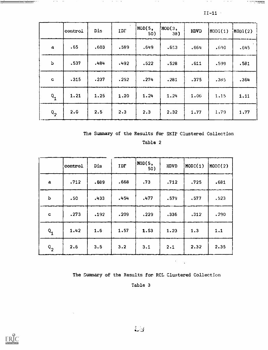
control Dis IDFMOD(5,

50)MOD(3,

38)HDVD MODI(1) MODI(2)

a .65 .603 .589 .649 .653 .664 .690 .645

b .537 .484 .492 .522 .528 .611 .599 .581

c .315 .237 .252 .274 .281 .375 .385 .364

Q1

1.21 1.25 1.20 1.24 1.24 1.06 1.15 1.11

Q22.0 2.5

-

2.3

_

2.3 2.32 1.77

-

1.79 1.77

The Summary of the Results for SKIP Clustered Collection

Table 2

control Dis IDFMOD(5

0,5 )HDVD MODI(1) MODI(2)

a .712 .689 .668

.

.73 .712 .725 .681

b .50 .433 .454 .477 .579 .577

_

.523

c .273 .192 .209 .229 .336 .312 .290

Q1

1.42 1.6 1.57

,

1.53

. ..

1.23

..

1.3 1.1

.

Q2 2.6 3.5

.

3.2 3.1 2.1 2.32

_ .

2.35

The Summary of the Results for RCL Clustered Collection

Table 3

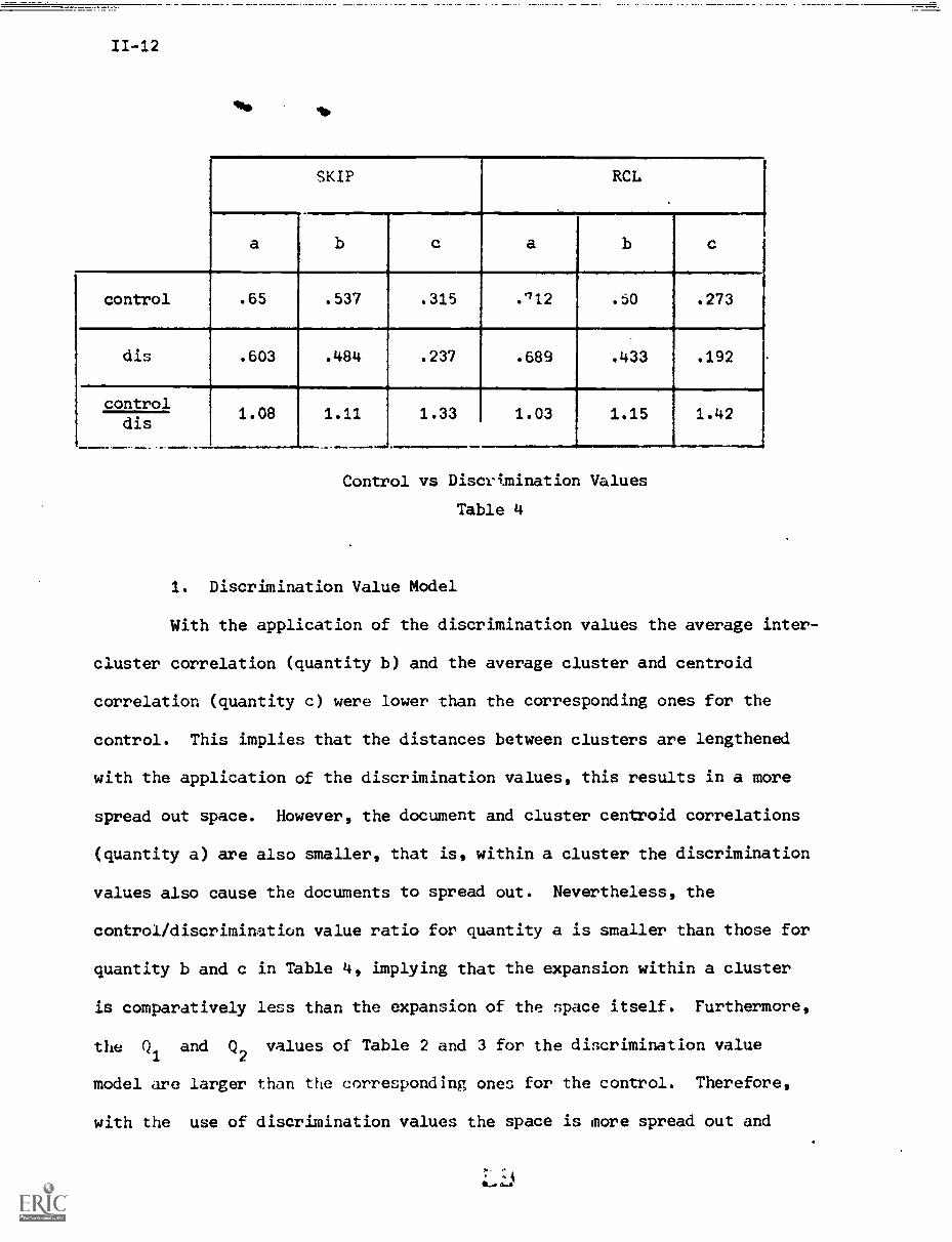
control

dis

controldis

SKIP RCL

a b c a b c

.65 .537 .315

.

.112 .50

.

.273

.603 .484 .237 .689 .433 .192

1.08 1.11

...4

1.33 1.03 1.15 1.42

Control vs Discrimination Values

Table 4

1. Discrimination Value Model

With the application of the discrimination values the average inter-

cluster correlation (quantity b) and the average cluster and centroid

correlation (quantity c) were lower than the corresponding ones for the

control. This implies that the distances between clusters are lengthened

with the application of the discrimination values, this results in a more

spread out space. However, the document and cluster centroid correlations

(quantity a) are also smaller, that is, within a cluster the discrimination

values also cause the documents to spread out. Nevertheless, the

control/discrimination value ratio for quantity a is smaller than those for

quantity b and c in Table 4, implying that the expansion within a cluster

is comparatively less than the expansion of the space itself. Furthermore,

the Q1

and Q2

values of Table 2 and 3 for the discrimination value

model are larger than the corresponding ones for the control. Therefore,

with the use of discrimination values the space is more spread out and

. 4 4

although the absolute sizes of the clusters are larger, relative

to the size of the entire space the clusters are smaller.

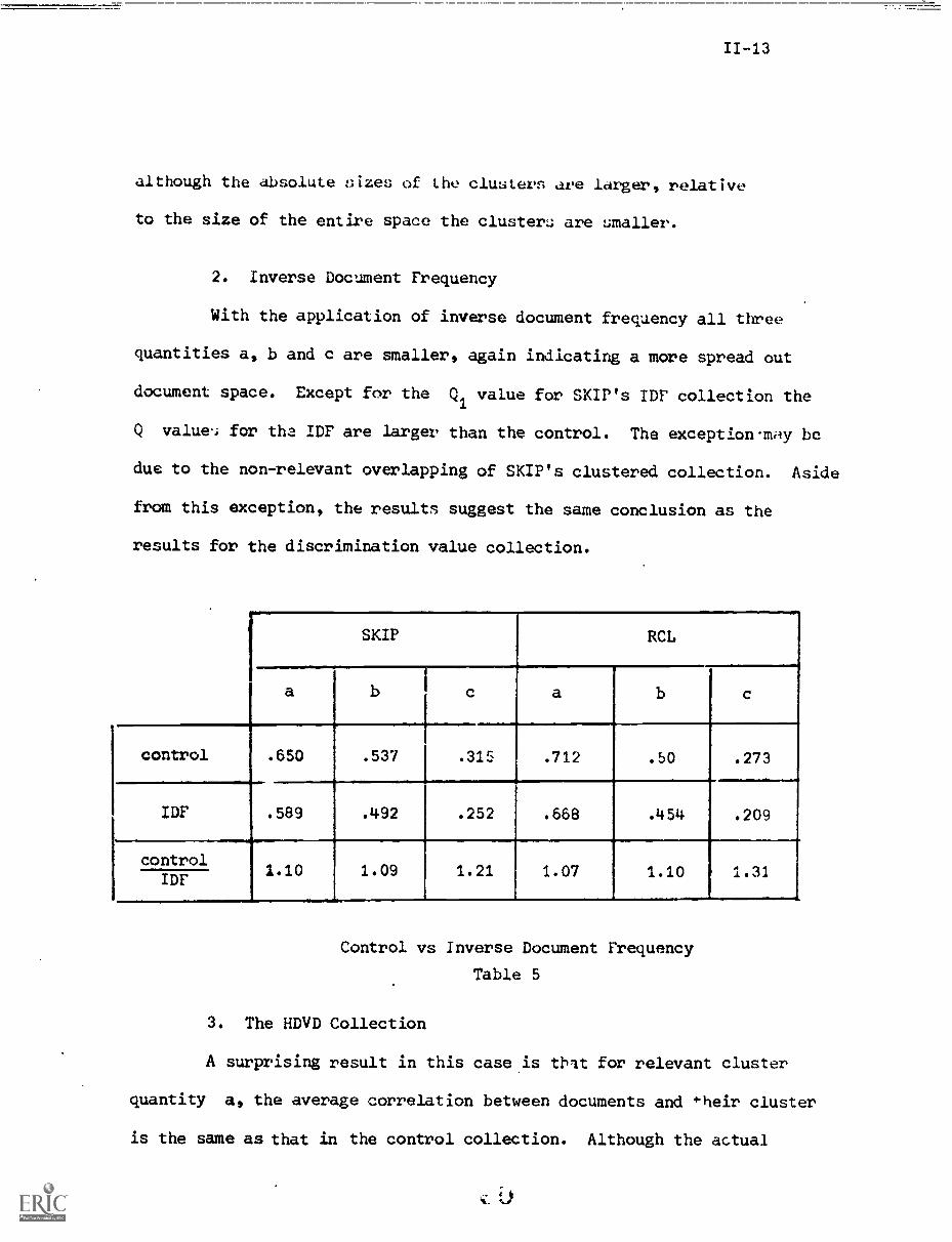
2. Inverse Document Frequency

With the application of inverse document frequency all three

quantities a, b and c are smaller, again indicating a more spread out

document space. Except for the Q1 value for SKIP's ID? collection the

Q value, for tha IDF are larger than the control. The exception may be

due to the non-relevant overlapping of SKIP's clustered collection. Aside

from this exception, the results suggest the same conclusion as the

results for the discrimination value collection.

SKIP RCL

a b c a b c

.-

control .650 .537 .315 .712 .50 .273

IDF .589 .492 .252 .668 .454 .209

control1.10 1.09 1.21 1.07 1.10 , 1.31

IDF

Control vs Inverse Document Frequency

Table 5

3. The HDVD Collection

A surprising result in this case is that for relevant cluster

quantity a, the average correlation between documents and *heir cluster

is the same as that in the control collection. Although the actual

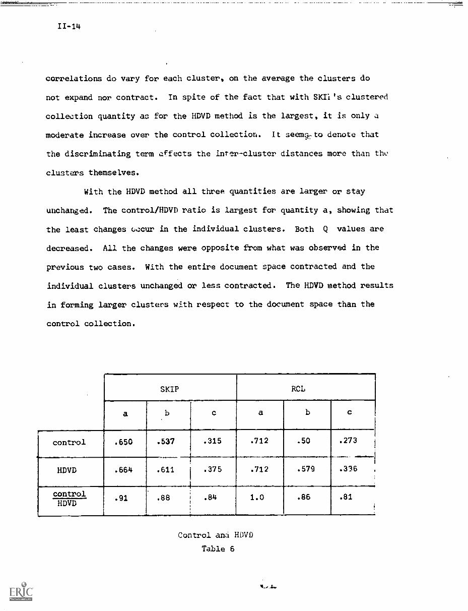
11-14

correlations do vary for each cluster, on the average the clusters do

not expand nor contract. In spite of the fact that with SKIi's clustered

collection quantity as for the HDVD method is the largest, it is only a

moderate increase over the control collection. It seem9,to denote that

the discriminating term affects the inter-cluster distances more than the

clusters themselves.

With the HDVD method all three quantities are larger or stay

unchanged. The control/HDVD ratio is largest for quantity a, showing that

the least changes c,ccur in the individual clusters. Both Q values are

decreased. All the changes were opposite from what was observed in the

previous two cases. With the entire document space contracted and the

individual clusters unchanged or less contracted. The HDVD method results

in forming larger clusters with respect to the document space than the

control collection.

SKIP RCL

a c a b

control .650

Ir

.537 .315 .712 .50 .273

HDVD .664 .611 .375

-

.712 .579 .336

control.91 .88 .84 1 . 0 .86 .81

HDVD

Control and HDVD

Table 6

SKIP MOD (51 50) SKIP MOD (3, 38) RCL MOD (5, 50

a b c a b c a b c

control .650 .537 .315

.

.

.650 .537 .315 .712

-

.50 .273

MOD .649

.

.522 .274

,

.653 .528 .281 .73 .477 .229

control1.0 1.03 1.5

-

1.0 1.02 1.12 .98 1.05 1.20MOD.

Control and the MOD Methods

Table 7

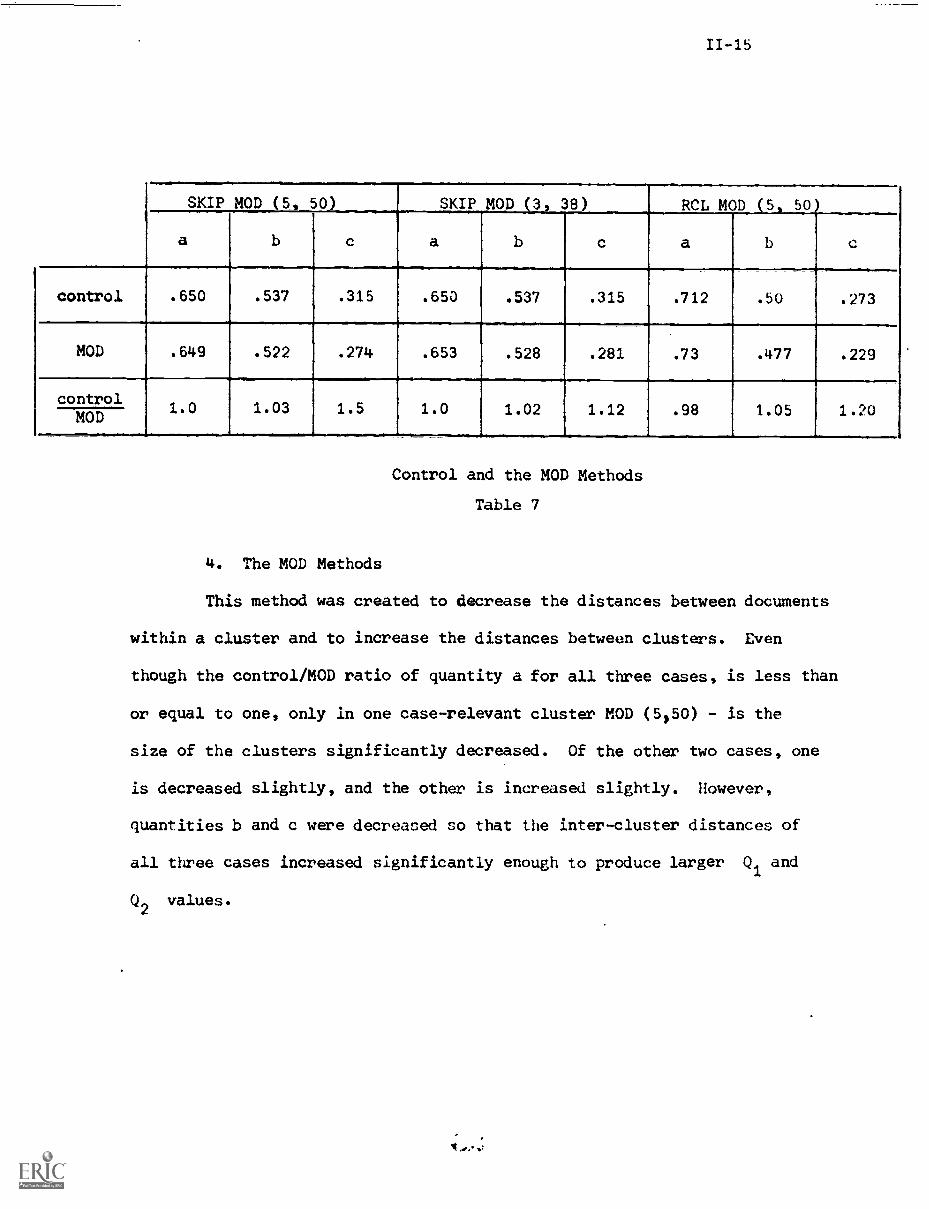
4. The MOD Methods

This method was created to decrease the distances between documents

within a cluster and to increase the distances between clusters. Even

though the control/MOD ratio of quantity a for all three cases, is less than

or equal to one, only in one case-relevant cluster MOD (5,50) - is the

size of the clusters significantly decreased. Of the other two cases, one

is decreased slightly, and the other is increased slightly. However,

quantities b and c were decreased so that the inter-cluster distances of

all three cases increased significantly enough to produce larger Q1 and

Q2

values.

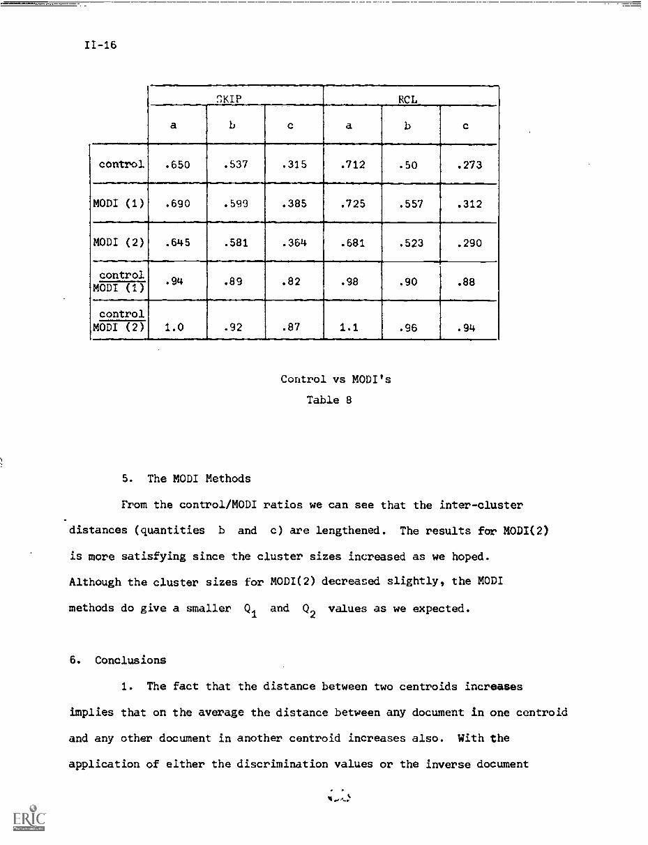
11-16

SKIP RCL

a b c a b c

control .650 .537 .315 .712 .50 .273

MODI (1) .690 .599 .385 .725 .557 .312

MODI (2) .645 .581 .364 .681 .523 .290

control.94 .89 .82 .98 .90 .88

MODI (1)

control1.0 .92 .87 1.1 .96 .94MODI (2)

Control vs MODI's

Table 8

5. The MODI Methods

From the control/MODI ratios we can see that the inter-cluster

distances (quantities b and c) are lengthened. The results for MODI(2)

is more satisfying since the cluster sizes increased as we hoped.

Although the cluster sizes for MODI(2) decreased slightly, the MODI

methods do give a smaller Q1 and Q2 values as we expected.

6. Conclusions

1. The fact that the distance between two centroids increases

implies that on the average the distance between any document in one centroid

and any other document in another centroid increases also. With the

application of either the discrimination values or the inverse document

11-17

frequency, the distance between documents increased. Moreover, the MOD

collections were constructed such that the inter-cluster distances are

larger. All these indexing methods are found to have better search

performance than the control method, as shown in Table 9. On the other

hand, the HDVD model and the MODI models show that a more contracted

document space produces deterioration in search performance. For the

discrimination model, the result that the distances between document

increase is obvious. However, it is not obvious for the inverse document

frequency model, where the correlations between documents are not taken

into consideration during construction. It can be concluded that a

spread out document space is beneficial for the retrieval performance.

2. Indexing methods that have been found to produce improvements.

in search performance as measured by recall and precision, do have relatively

more compact clusters with respect to the entire collection space. This

conclusion 4s justified by the observation that, in all cases (the

discrimination value, inverse document frequency and MOD) the increase

in distance between centroids is more than the expansion of the cluster

itself; whereas for the indexing methods that give less good search

performance the relative sizes of the clusters are larger. However, the

Q1

and Q2

values can not be depended upon to evaluate the search

performance of a collection in place of recall and precision. The

Q1

and Q2

values of the discrimination value model are larger than those

of the inverse document frequency model, but from the search result: in

Table 9, the discrimination value model does not necessarily perform 1,etter

than the inverse document frequency model. Similarly, the HDVD method

performs worse than MODI(2), but the Q1value of MODI(2) for RCL

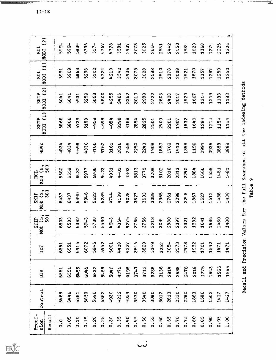
Preci-

sion

Control

DIS

IDF

SKIP

MOD (5,

50)

SKIP

MOD (3,

38)

RCL

MOD (5,

50)

HDVD

SKIP

MODI (1)

SKIP

MODI (2)

RCL

MODI (1)

RCL

MODI (2)

Recall

0.0

6468

6551

6551

6503

6437

6580

4834

5866

6041

5991

5994

0.05

6446

6551

6551

6503

6437

6558

4834

5866

6041

5969

5994

0.10

6361

6455

6415

6362

6390

6432

4698

5739

5931

5863

5834

0.15

5859

6045

6022

5943

5946

5977

4330

5188

5250

5296

5336

0.20

5696

5832

5845

5730

5622

5806

4160

4959

5053

'

5102

517+

0.25

5362

5488

5442

5430

5289

5423

3767

4698

4800

4724

4757

0.30

4930

5046

5001

4943

4744

4951

3161

4084

4255

4219

4328

0.35

4232

4275

4428

4354

4139

4403

2616

3290

3466

3542

3581

0.40

4054

4198

4327

4275

4028

4303

2559

3168

3362

3436

3437

0.45

3570

3747

3845

3766

3627

3813

2250

2854

3010

3073

3073

0.50

3546

3713

.3829

3756

3603

3775

2243

2825

2988

3028

3025

0.55

3080

3236

3349

3213

3089

3209

1909

2501

2722

2588

2664

0.60

3012

3136

3252

3094

2965

3102

1859

2409

2603

2510

2581

0.65

2813

2914

3054

2880

2761

2810

1709

2261

2428

2378

2442

0.70

2330

'

2538

2573

2397

2298

2313

1413

1907

2017

2008

2050

0.75

2280

2478

2478

2321

2248

2240

1359

1832

1929

1921

1984

0.80

1883

2018

1992

1932

1867

1884

1190

1640

1607

1670

1623

0.85

1586

1775

1701

1641

1627

1666

0994

1294

1314

1357

1368

0.90

1502

1643

1542

1535

1512

1555

0936

1214

1249

1297

1274

0.95

1427

1565

1471

1480

1438

1481

0888

1154

1183

1250

1226

1.00

1427

1565

1471

1480

1438

1481

0888

1154

1183

1250

1226

Recall and Precision Values for the Full Searches of all the Indexing Methods

Table 9

clustered collection is smaller than that of the HDVD method. Furthe,ore,

the difference its search performance between HDVD and control is more than

that between the control and MOD method, but the differences in Q values

are nearly the same. Nevertheless, the Q values do give a fairly

compatible ranking of the performance of the various methods compared to

the searches performed as in Table 9.

3. With the application of the HDVD method, the average correlation

of documents to their centroids over all clusters does not vary for the

relevant clustered collection. This is an indication that the deletion of

high discrimination value terms, nearly one seventh of the concepts in the

collection, has little effect within clusters. On the other hand, the sizes

of the clusters vary with the use of the inverse skewness factor, as shown

in MODI(1) and MODI(2) in Table 8. To a lesser extent the discrimination

value model and the inverse document frequency model are also emphasizing

the different effects of the terms. It bcc.vutes apparent that there are

various functions played by the terms under diff:reitt conditions, similar

to the idea that there are terms that promote recall and others that promote

precision. It is now obvious that terms are needed to distinguish documents

that belong to different clusters; whereas within a cluster, the terms

needed should have less discriminating power or should only discriminate

documents within the cluster.

References

[13 C.J. Van Rijsbergen and K. Sparck Jones, A Test for the Separation ofRelevant and Non-Relevant Documents in Experimental Retrieval Collections,Journal of Documentation, Vol. 29, No. 3, September 1973.

[21 K. Bonwit and J. Aste-Tonsmann, Negative Dictionaries, Scientific ReportNo. ISR-18 to the National Science Foundation and National Libraryof Medicine, Section VI, Department of Computer Science, Cornell University,October 1970.

13) D. Murray, Document Retrieval Based on Clustered Files, Report No. ISR-20to the National Science Foundation and National Library of Medicine,Department of Computer Science, Cornell University, Ithaca, June 1972.

[4] M. Kerchner, Dynamic Document Processing in Clustered Collections,Report ISR-19 to the National Science Foundation, Department of ComputerScience, Cornell University, Ithaca, 1971.

[51 R. Williamson, Real-time Document Retrieval, Ph.D. Thesis, Cornell

University, June 1974.

A Theory of Term Importance in Automatic

Text Analysis

G. Salton*, C.S. Yang*, and C.T. Yu*

Abstract

Most existing automatic conLeat analysis and indexing techniques

are based on word frequency characteristics applied largely in an ad hoc

manner. Contradictory requirements arise in this connection, in that terms

exhibiting high occurrence frequencies in individual documents are often

useful for high recall performance (to retrieve many relevant items), whereas

terms with low frequency in the whole collection are useful for high precision

(to reject nonrelevant items).

A new technique, known as discrimination value analysis ranks the text

words in accordance with how well they are able to discriminate the documents

of a collection from each other; that is, the value of a term depends on how

much the average separation between individual documents changes when the givcn

term is assigned for content identification. The best words are those which

achieve the greatest acparuaod.

The discrimination value analysis accounts for a number of important

phenomena in the content analysis of natural language texts:

a) the role and importance of single words;

b) the role of juxtaposed words (phrases);

c) the role of word groups or classes, as specified in a thesaurus.

Effective criteria can be given for assigning each term to one of these three

classes, and for constructing optimal indexing vocabularies.

* Department of Computer Science, Cornell University, Ithaca, N.Y. 14853

t Department of Computer Science, University of Alberta, Edmonton, Alberta

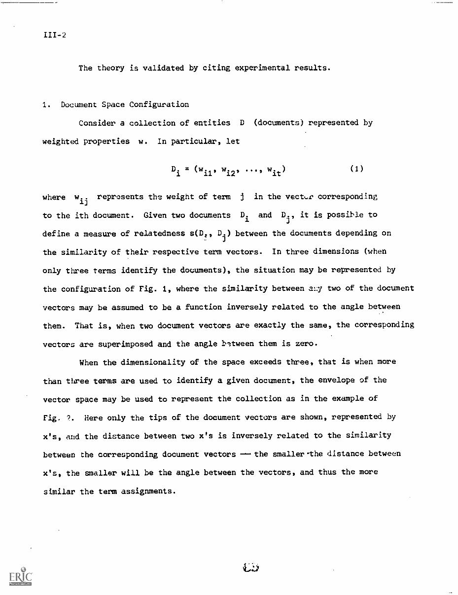
111-2

The theory is validated by citing experimental results.

1. Document Space Configuration

Consider a collection of entities D (documents) represented by

weighted properties w. In particular, let

1 1= (w.

1 19 wit, 9 ...9 ) (1)

where w.. represents the weight of term j in the vector correspondingij

totheithdocument.GiventwodocurmItsD.and D., it is possible to

define a measure of relatedness Dj) between the documents depending on

the similarity of their respective term vectors. In three dimensions (when

only three terms identify the documents), the situation may be represented by

the configuration of Fig. 1, where the similarity between at. two of the document

vectors may be assumed to be a function inversely related to the angle between

them. That is, when two document vectors are exactly the same, the corresponding

vectors are superimposed and the angle between them is zero.

When the dimensionality of the space exceeds three, that is when more

than three terms are used to identify a given document, the envelope of the

vector space may be used to represent the collection as in the example of

Fig. 7. Here only the tips of the document vectors are shown, represented by

x's, and the distance between two x's is inversely related to the similarity

between the corresponding document vectors --- the smallerthe distance between

x's, the smaller will be the angle between the vectors, and thus the more

similar the term assignments.

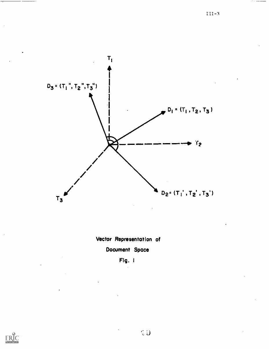
03 = (T"T iiT")1, 2 ,3

T3

/////sit

Ti

4

2 (T1 112 , 13 )

Vector Representation of

Document Space

Fig. I

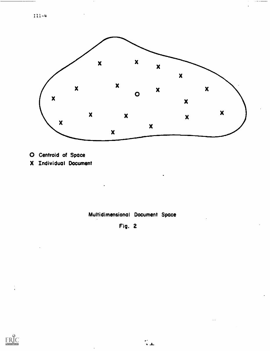
iii-14

0 Centroid of SpaceX Individual Document

Multidimensional Document Space

Fig. 2

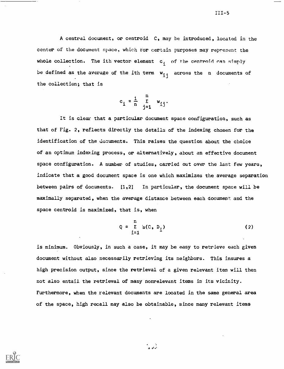
A central document, or centroid C, may be introduced, located in the

center of the document space, which for certain purposes may represent the

wholecollection.neithvectorelmehtc.of the centrnid ('an pimply

be defined as the average of the ith term w.. across the n documents of

the collection; that is

c. =1

E w...1 n

j=1ij

n

It is clear that a particular document space configuration, such as

that of Fig. 2, reflects directly the details of the indexing chosen for the

identification of the do:uments. This raises the question about the choice

of an optimum indexing process, or alternatively, about an effective document

space configuration. A number of studies, carried out over the last few years,

indicate that a good document space is one which maximizes the average separation

between pairs of documents. [1,2] In particular, the document space will be

maximally separated, when the average distance between each document and the

space centroid is maximized, that is, when

n

Q = E s(C, D.)i=1

(2)

is minimum. Obviously, in such a case, it may be easy to retrieve each given

document without also necessarily retrieving its neighbors. This insures a

high precision output, since the retrieval of a given relevant item will then

not also entail the retrieval of many nonrelevant items in its vicinity.

Furthermore, when the relevant documents are located in the same general area

of the space, high recall may also be obtainable, since many relevant items

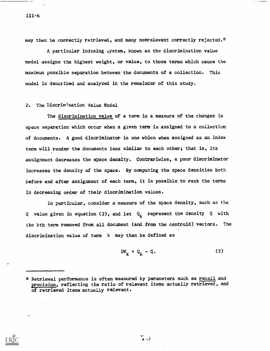
111-6

may then be correctly retrieved, and many nonrelevant correctly rejected.*

A particular indexing system, known as the discrimination value

model assigns the highest weight, or value, to those terms which cause the

maximum possible separation between the documents of a collection. This

model is described and analyzed in the remainder of this study.

2. The Discrim4nation Value Model

The discrimination value of a term is a measure of the changes in

space separation which occur when a given term is assigned to a collection

of documents. A good discriminator is one which when assigned as an index

term will render the documents less similar to each other; that is, its

assignment decreases the space density. Contrariwise, a poor discriminator

increases the density of the space. By computing the space densities both

before and after assignment of each term, it is possible to rank the terms

in decreasing order of their discrimination values.

In particular, consider a measure of the space density, such as the

Q value given in equation (2), and let Qk represent the density Q with

the kth term removed from all document (and from the centroid) vectors. The

discrimination value of term k may then be defined as

DVk

= Qk

- Q. (3)

* Retrieval performance is often measured by parameters such as recall andprecision, reflecting the ratio of relevant items actually retrieved, andof retrieved items actually relevant.

Obviously, if term Q is a good diszriminator, then its removal will cause

a compression in the document space (an increase in space density), because

its assignment would have resulted in an increase in space separation. Thus

for good discriminators Qk > Q and DVk is positive. The reverse is true

for poor discriminators whose removal causes a decrease in space density,

leading to negative discrimination values. A vast majority of the terms may

be expected to produce neither increase nor decrease in space density; in

such a case a discrimination value near zero is obtained. The operations of

a good discriminator are illustrated in the simplified drawing of Fig. 3.

In the retrieval experiments conducted earlier with three collections

in aerodynamics (Cranfield collection, 424 documents comprising 2651 distinct

terms), medicine (Medlars collection, 450 documents comprising 47 26 terms),

and world affairs (Time collection, 425 documents comprising 14098 terms), the

discrimination value model produced excellent retrieval results. [11 In

particular, a term weighting system which assigns to each term k a value

wkj consisting of the product of its frequency of occurrence in document

j (fkj

) multiplied by its discrimination.value DVk,

wkj = fkj DVk, (4)

produces recall and precision improvements of about ten percent over

methods where only the term frequencies fkj are taken into account.'

a

* Terms receiv. ng high weights accordingexhibit high occurrence frequencies inat the same time can distinguish thesethe collection.

to expression (4) are those whichcertain specified documents, anddocuments from the remainder of

111-8

Before Assignment

of Term

X Document

0 Main Centroid

Operation of

Good Discriminating Term

Fig. 3

After Assignment

of Term

111-9

It may be of interest to inquire what kind of terms are favored

by a weighting system such as that of expression (4), and what accounts for

the value of the discrimination model. Some experimental evidence relating

the discrimination values to certain frequency characteristics of the terms

in the document collections is presented in the next section. This in turn,

leads to an indexing theory to be examined in the remainder of this study.

3. Discrimination Values and Document Frequencies

Consider any term k assigned to a collection of documents, and let

dk

be its document frequency, defined as the number of documents in the

collection to which term k is assigned. More specifically,

dk = E bkj

j=1

where bkj = 1 whenever fkj L1, and bkj = 0 otherwise. It is instructive to

arrange the terms assigned to a document collection into disjoint sets in such

a way that the terms assigned to a given set have equal document frequencies

dk

= I. Moreover, for each such set of terms the average rank in decreasing

discrimination value order may be computed, thereby relating document frequencies

with discrimination values.*

A plot giving the average discrimination value rank for the terms

exhibiting certain document frequency ranges is shown in Figs. 4(a), (b), and

(c) for the collections in aerodynamics, medicine, and world affairs

(Cranfield, Medlars, and Time) respectively. It may be seen that ' Lishaped

curve is obtained in each case, with the following interpretation:

* For a set of t terms, the discrimination value rank ranges from 1 for the

best discriminator to t for the worst.

I I -10Disciminotion Rankof Average Term

2500

2000

1500

1000

500

200

Cranfield Collection424 Documents

2651 Terms

1 1

3 5 7 9

2101 terms

1 1 1 1 1 1 1 1

11 13-14 1 -19 24-26 33-36 49-86 79-95 159-214Documenftrowo."''

467 terms 83 terms Frequent

Average Discrimination Value Rank of TermsFig. 4(a)

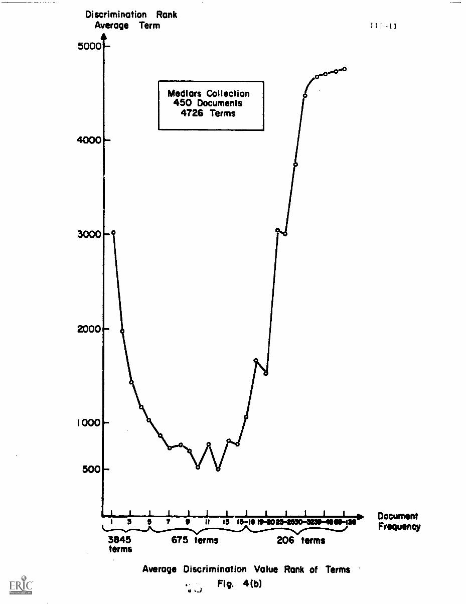
Discrimination RankAverage Term

50001.

4000

3000

2000

1000

500

Medlars Collection450 Documents

4726 Terms

3845terms

1 1 1 1 1 1 Document11 13 111-13 1040 23-21530-1210-41111111-1311

Frequency

675 terms 206 terms

Average Discrimination Value Ronk of TermsFig. 4(b)

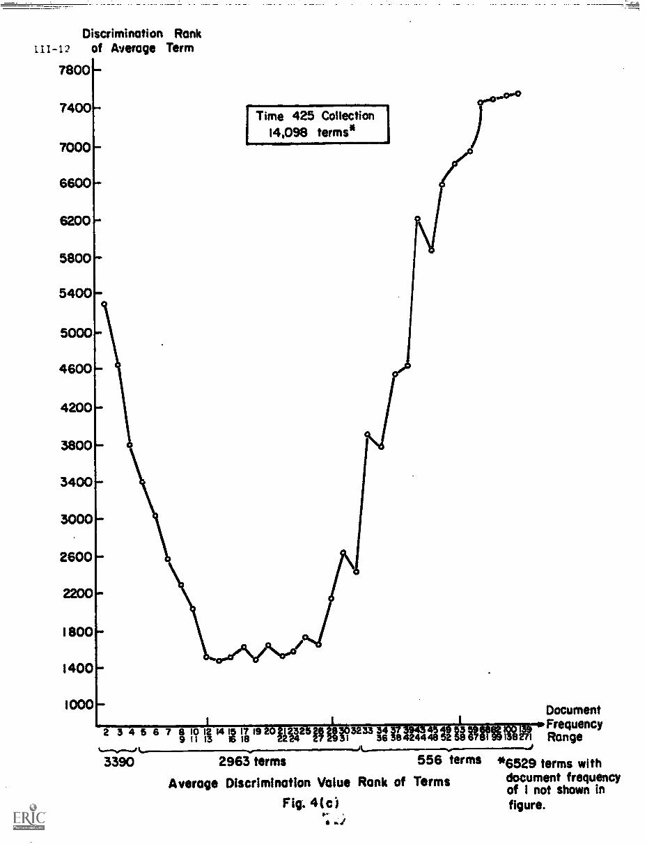
Discrimination Rank1II-12 of Average Term

7800 -

7400 -

7000 -

6600' -

6200 -

5800 -

5400 -

5000-

4600-

4200 -

3800 -

3400 -

3000 -

2600 -

2200 -

1 800 -

1400 -

1000 -

Time 425 Cot14,098 terms*

2 3 4 5 67 tl 111 14 2 192021222 242

3390

3 33

on

4:6 384 44 5 5i

DocumentFrequency

81 13: 1 Range

2963 terms 556 terms *6529 terms withAverage Discrimination Value Rank of Terms document frequency

of 1 not shown infigure.Fig. 4(c)

I.1

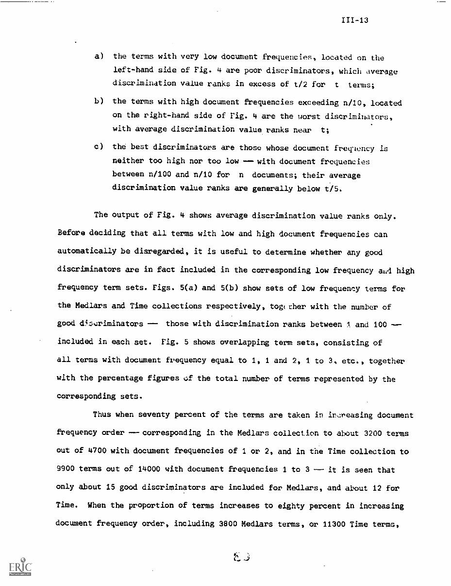
a) the terms with very low document frequencies, located on the

left-hand side of Fig. 4 are poor discriminators, which average

discrimination value ranks in excess of t/2 for t terms;

b) the terms with high document frequencies exceeding n/10, located

on the right-hand side of Fig. 4 are the worst discriminators,

with average discrimination value ranks near t;

c) the best discriminators are those whose document frequency is

neither too high nor too low with document frequencies

between n/100 and n/10 for n documents; their average

discrimination value ranks are generally below t/5.

The output of Fig. 4 shows average discrimination value ranks only.

Before deciding that all terms with low and high document frequencies can

automatically be disregarded, it is useful to determine whether any good

discriminators are in fact included in the corresponding low frequency aL.d high

frequency term sets. Figs. 5(a) and 5(b) show sets of low frequency terms for

the Medlars and Time collections respectively, together with the number of

good d4:;kximinators those with discrimination ranks between 1 and 100

included in each set. Fig. 5 shows overlapping term sets, consisting of

all terms with document frequency equal to 1, 1 and 2, 1 to 3, etc., together

with the percentage figures of the total number of terms represented by the

corresponding sets.

Thus when seventy percent of the terms are taken in increasing document

frequency order corresponding in the Medlars collection to about 3200 terms

out of 4700 with document frequencies of 1 or 2, and in the Time collection to

9900 terms out of 14000 with document frequencies 1 to 3 it is seen that

only about 15 good discriminators are included for Medlars, and about 12 for

Time. When the proportion of terms increases to eighty percent in increasing

document frequency order, including 3800 Medlars terms, or 11300 Time terms,

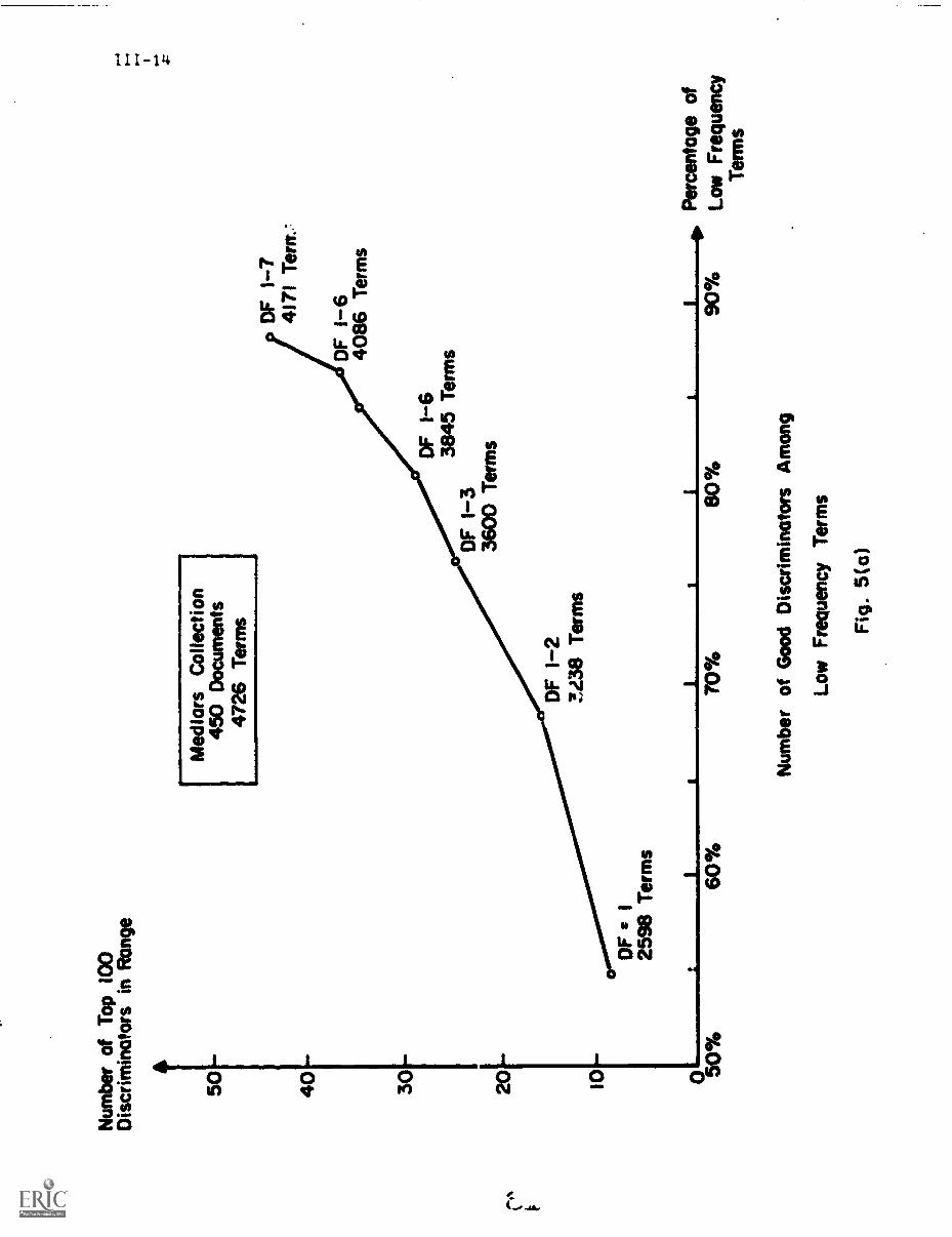
Num

ber

Dis

crim

inat

ors

of T

op 1

00in

Ran

ge

M e

dlar

s C

olle

ctio

n50

450

Doc

umen

ts

J47

26 T

erm

sA

r

DF

1-7

4171

Ter

ns.1

40D

F 1

-640

86 T

erm

s

30O

F 1

-638

45 T

erm

sO

F 1

-3

2036

00 T

erm

s

DF

1-2

3238

Ter

ms

10

DF

It1

2598

Ter

ms

0' 50

%I

ItI

I

70%

11

io.

80%

90%

Per

cent

age

ofLo

w F

requ

ency

60%

Ter

ms

Num

ber

of G

ood

Dis

crim

inat

ors

Am

ong

Low

Fre

quen

cy T

erm

s

Fig

. 5(a

)

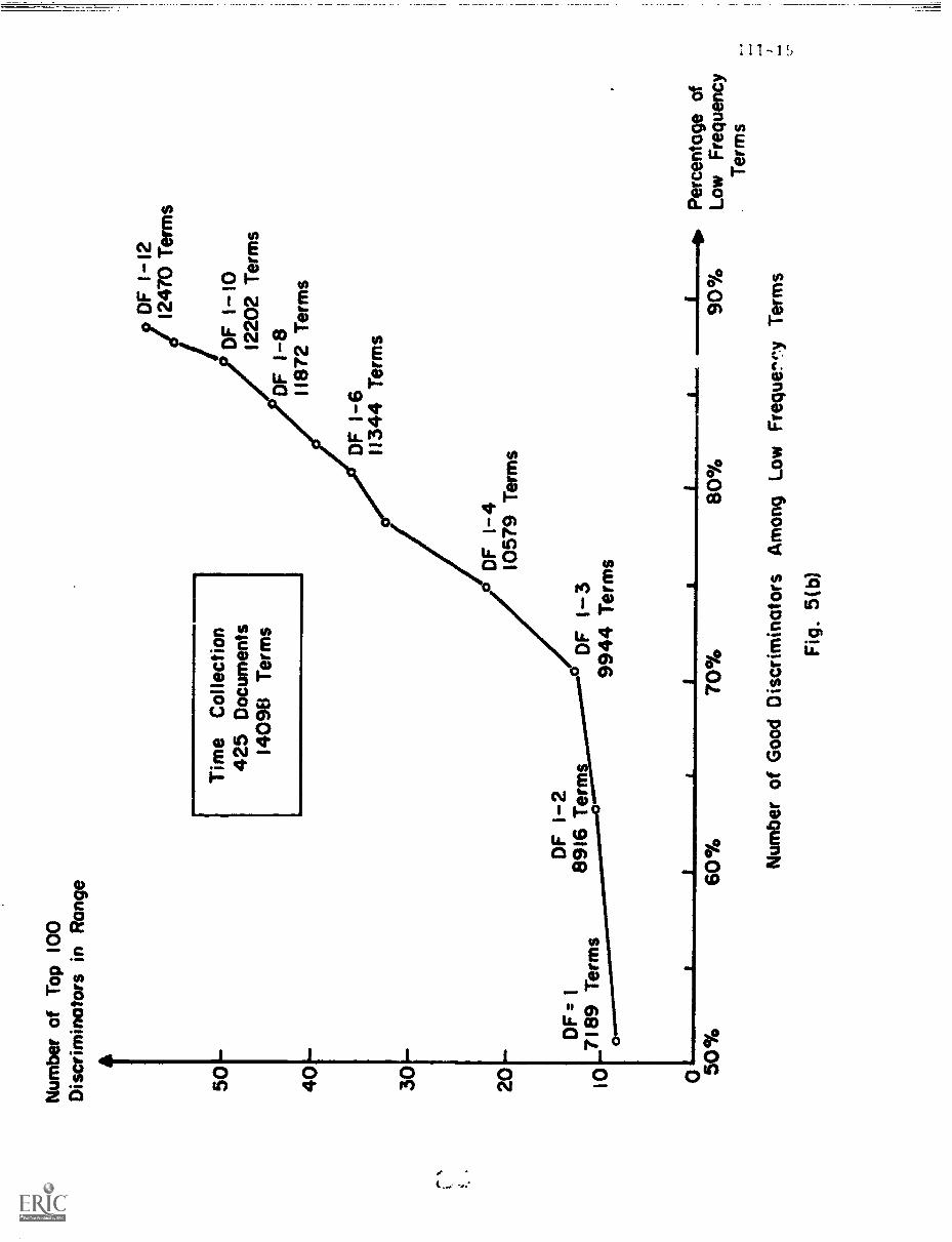
Num

ber

of T

op 1

00D

iscr

imin

ator

s in

Ran

ge

[Tim

e C

olle

ctio

n42

5 D

ocum

ents

1409

8 T

erm

s

DF

= 1

DF

1-2

8916

Ter

ms

7189

Ter

noci

DF

1-1

212

470

Ter

ms

/OF

1-1

012

202

Ter

ms

OF

1-8

1187

2 T

erm

s

DF

1-4

1057

9 T

erm

sDF

1-6

1134

4 T

erm

s

°D

F 1

-399

44 T

erm

s

60%

70%

80%

Per

cent

age

of90

%Lo

w F

requ

ency

Ter

ms

Num

ber

of G

ood

Dis

crim

inat

ors

Am

ong

Low

Fre

quen

t, T

erm

s

Fig

. 5(b

)

111-16

ranging in document frequency from 1 to the number of good discriminators

ri:. 1 to 30 for Medlars and 35 for Time. When so few good terms are included

amonb :ie mass of low frequency terms, it is obvious that special provisions

must be made in any indexing process for the utilization of these terms.

Consider now the very high - frequency terms those which according

to the output of Fig. 4 exhibit the lowest discrimination values. While the

number of such terms is not large, each of the terms accounts for a substantial

portion of the total term assignments to the locuments of a collection because

of the high document frequency involved.

The output of Fig. 6(a) for Medlars, and 6(b) for Time shows that about

four percen of the high-frequency terms present in a document collection,

accounts for forty to fifty percent of all term assig-ments, when the terms

are taken in decreasing document frequency order. The absolute number of

distinct terms is 200 approximately for the Medlars collection and about 500

for Time. In each case, less than 15 of these terms are classified as good

discriminators. When the proportion terms taken in high frequency order

increases to six percent, accounting for 46 percent of the term assignments

in Medlars, and 57 percent for Time, the number of good discriminators increases

to about 20 in each

The infor4.4tioa iacluded in Figs. 5 and 6 is summarized in Table 1.

In each case, certain cutoff percentages are given for terms taken either in

low document frequency or in high document frequency order. For each such

percentage, the number of good discriminators included in the corresponding

term .;et is stated for each of the three test collections. Thus when sixty

,(rcent of the terms aro taken in increasing document frequency order, not

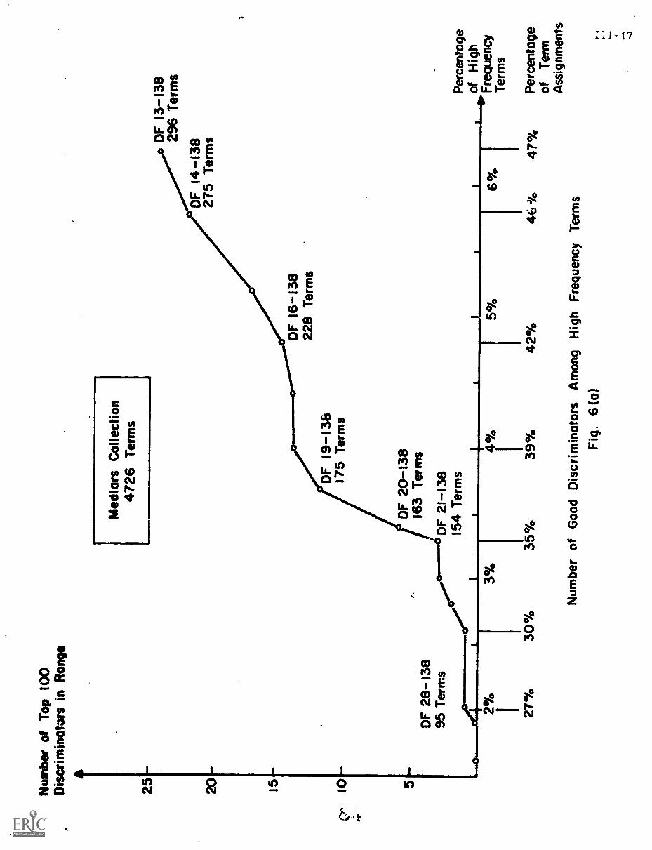
Num

ber

of T

op 1

00D

iscr

imin

ator

s in

Ran

ge

Med

lars

Col

lect

ion

4726

Ter

ms

25 20 15

DF

16

-138

228

Ter

ms

OF

19-

13b

1017

5 T

erm

s

5D

F 2

0-13

816

3 T

erm

sD

F 2

8-13

895

Ter

ms

OF

21-

138

154

Ter

ms

2%

Ll

27%

30%

3%

350/

0

I 4% 39%

OF

13-

138

296

Ter

ms

°DF

14-

138

275

Ter

ms

50/0

Per

cent

age

of H

igh

r---

"*F

requ

ency

6%

42%

4b J

/047

%

Num

ber

of G

ood

Dis

crim

inat

ors

Am

ong

Hig

h F

requ

ency

Ter

ms

Fig

. 6(o

)

Ter

ms

Per

cent

age

of T

erm

Ass

ignm

ents

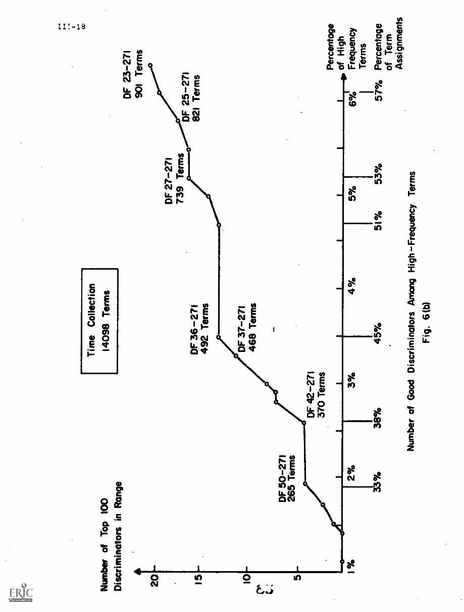
Num

ber

of T

op 1

00D

iscr

imin

ator

s in

Ran

ge

20 15

1%

DF

50-

271

265

Ter

ms

2%

33%

Tim

e C

olle

ctio

n14

098

Ter

ms

OF

36-

271

492

Ter

ms

DF

27-

271

739

Ter

ms

DF

23-

271

901

Ter

ms

DF

42-

271

370

Ter

ms

38%

OF

37-

271

468

Ter

ms

/M.

1

OF

25-

271

821

Ter

ms

3%

45%

4%5%

51%

53%

Num

ber

of G

ood

Dis

crim

inat

ors

Am

ong

Hig

h -F

requ

ency

Ter

ms

Fig

. 6 (

b)

Per

cent

age

of H

igh

6%F

requ

ency

ITer

ms

57%

Per

cent

age

of T

erm

Ass

ignm

ents

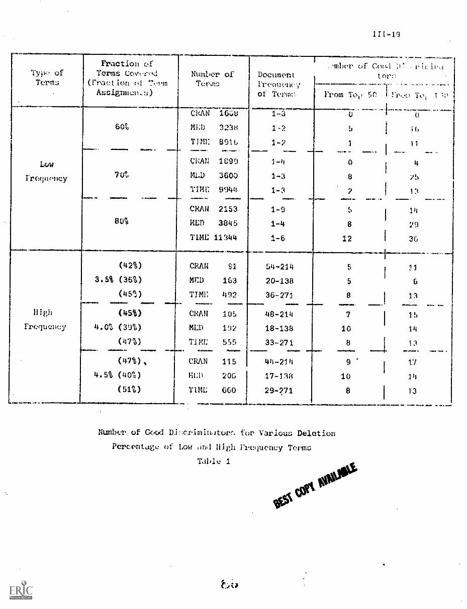
411011.11.1

Typo ofTerms

Fraction ofTerms Cove ri.d

(Fraction of TomAssignmun,$)

Number ofTenn;

DocumentIreouezwyot

Low

Irequoncy

6090

CRAN

MED

TIME

16UC

3238

MC1C90

3603

9944

1-3

1 2

1-2

CRAN

MLD

TIME

.M..04.111

1-4

1-3

1-3'SWUM 'MP .11111.041

80%

.rIIM 4.. V&

CRAN 2153

MED 3845

TIME 11344

1-0

1-4

(42%) CRAN 91 54-214

3.5% (36%) MED 163 20-138

(45b:) TIME 492- 36-271.01High (45%) CRAW 105 48-214

Frequency 4.0% (39%) MED 192 18-138

(47%) TIME 555 33-2710.4.111050.0.011.

(47%), CRAN 115 44-214

4.5% (40%) MED 206 17-138

(51%) TIME 660 29-271

.11.11.0.1.111

.,mher of Chi ;!tor:1

From To 5r I 1 'r 1

0

-nic I n,,

0

8

2woo e.

8

12

1

29

36

I.)

11

'15

1ii

5

5 1 6

8 131111.... I.e.. du

7 15

10 14

8 13

9 1.7

10 14

8

Number of Good DI::crimin.itum for Various Deletion

Percentage: of Low ond High Frequency Terms

Table 1

13

111-20

a single good discriminator is included among the 1668 terms for the

Cranfield collection; only 5 of the top terms, or 16 of the top 100,

are present among the 3238 Medlars terms; finally, for Time 1, out of

the top 50, or 11 of the top 100 are included among the first 8916 low

frequency terms.

The number of good discriminators included among the high frequency

terms for the three collections is similarly low, as shown in the bottom

half of Table 1.

The conclusion to be reached from the data of Figs. 5 and 6 and

of Table 1 is that very few good discriminators are included among the

bottom seventy percent, or among the top four percent when the terms

included in a collection of documents are taken in increasing document

frequency order. This fact is used to construct an indexing strategy

in the remainder of this study.

4. A Strategy for Automatic Indexing

Consider the graph of Fig. 7 in which the terms are once again

arranged in increasing document frequency order. If the assumption is

correct that the best terms for indexing puri. es are concentrated in the

set whose document frequency is neither too high nor too low --the

frequency being approximately between n/100 and n/10 ---then the following

term transformations should be undertaken:

a) Terms whose document frequency lies between n/100 and n/10

should be used for indexing purposes directly without any

transformation; these terms include the vast majority of the

good discriminators.

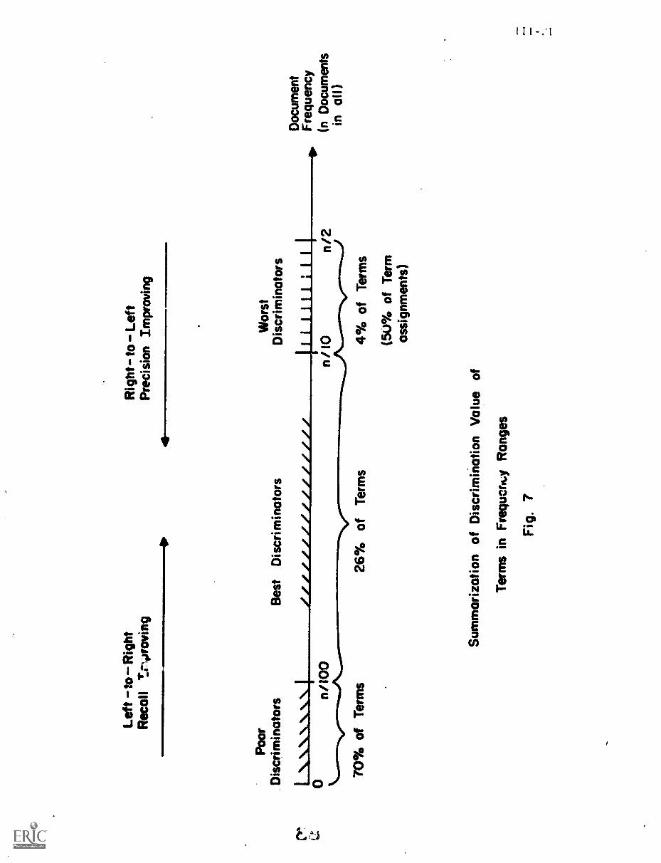
Left

-toR

ight

Rig

ht-t

o-Le

ftR

ecoi

l Try

rovi

ngP

reci

sion

Impr

ovin

g

Poo

rD

iscr

imin

ator

s

\.\.1

..10

70%

of T

erm

s

Bes

tD

iscr

imin

ator

s

26%

of T

erm

s

Wor

stD

iscr

imin

ator

s

1111

1111

111

n/10

n/2

Sum

mar

izat

ion

of D

iscr

imin

atio

n V

alue

of

Ter

ms

in F

requ

ency

Ran

ges

Fig

. 7

4% o

f Ter

ms

(50%

of T

erm

assi

gnm

ents

)

Doc

umen

tF

requ

ency

(n D

ocum

ents

in a

ll)

111-22

b) Terms whose document frequency is too high above n/10comprise the worst discriminators.. These terms are too

general in nature, or too broad, to per:nit proper discrimination

among the documents; hence their use produces an unacceptable

precision loss (it leads to the retrieval of too many items

that are extraneous). These terms should be transformed into

lower frequency terms ----right-to-left on the graph of rig. 7

thereby enhancing the precision performance.

c) Terms whose document frequency is too low below n/100

are so rare and specific that they cannot retrieve an acceptable

proportion of the documents relevant to a given' query; hence

their use depresses the recall performance. These terms should

be transformed into higher frequency terms left-to-right

on the grapl. of Fig. 7 --- thereby enhancing the recall performance.

It remains to des:tribe the right-to-left and left-to-right transformations

that may be used to generate seful indexing vocabularies. The obvious way of

transforming the :ugh frequency terms into lower frequency entities is to

combine them into indexing phrases. In general, a phrase such as "programming

language" exhibits a lower assignment frequency than either of the high

frequency components "language" or "program". The summary of Fig. 7 then

indicates that:

Indexing phrases should.be constructed from high

frequency single term components in order to enhanc.:

the precision performance of the retrieval system.

The other left-to-right transformation which is required for recall

enhancing purposes is now equally obvious. Low frequency terms with somewhat

similar properties, or meanings, can be combined into term classes, normally

specified by a thesaurus of related terms, or synonym dictionary. When a

single term is replaced for indexing purposes by a thesaurus class consisting

L.;

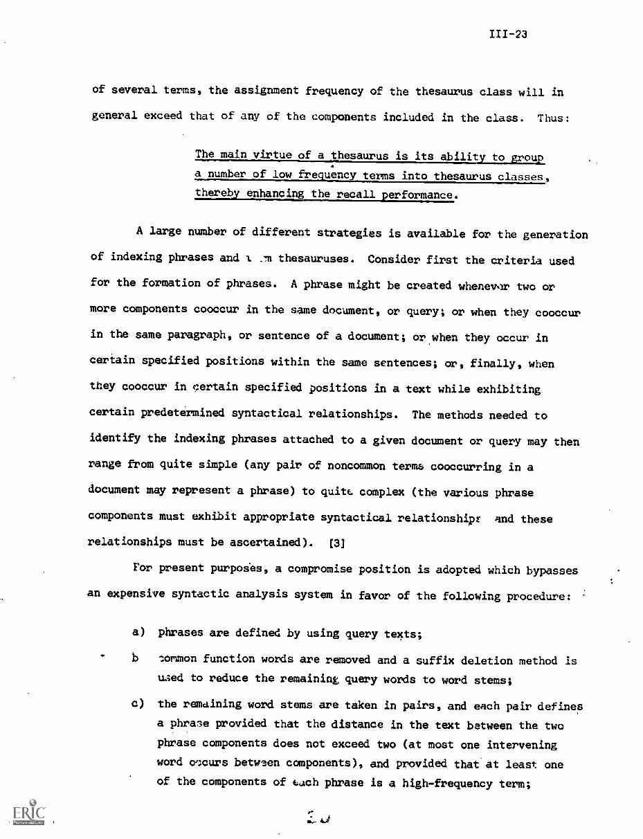
111-23

of several terms, the assignment frequency of the thesaurus class will in

general exceed that of any of the components included in the class. Thus:

The main virtue of a thesaurus is its ability to group

a number of low frequency terms into thesaurus classes,

thereby enhancing the recall performance.

A large number of different strategies is available for the generation

of indexing phrases and 1 ..1m thesauruses. Consider first the criteria used

for the formation of phrases. A phrase might be created whenev.m two or

more components cooccur in the same document, or query; or when they cooccur

in the same paragraph, or sentence of a document; or when they occur in

certain specified positions within the same sentences; or, finally, when

they cooccur in certain specified positions in a text while exhibiting

certain predetermined syntactical relationships. The methods needed to

identify the indexing phrases attached to a given document or query may then

range from quite simple (any pair of noncommon terms cooccurring in a

document may represent a phrase) to quite. complex (the various phrase

components must exhibit appropriate syntactical relationship: and these

relationships must be ascertained). [3]

For present purposes, a compromise position is adopted which bypasses

an expensive syntactic analysis system in favor of the following procedure:

a) phrases are defined by using query texts;

b lommon function words are removed and a suffix deletion method is

used to reduce the remaining query words to word stems;

c) the remaining word stems are taken in pairs, and each pair defines

a phrase provided that the distance in the text between the two

phrase components does not exceed two (at most one intervening

word cncurs between components), and provided that at least one

of the components of each phrase is a high-frequency term;

III -24

d) phrases for which both components are identical are eliminated;

e) duplicate phrases, where all components match an already existing

phrase are elminated.

The texts of all documents are checked for the presence of any phrase thus

defined from the query statements, and appropriate weights are assigned.

The phrase formation process is illustrated in Fig. 8 for a query

dealing with world affairs. It is seen that this query gives rise to eight

distinct phrases with adjacent components, plus seven additional phrases

for which the components are separated by one intervening word in the reduced

query text.

It remains to determine an appropriate weight to be assigned to each

phrase created by the foregoing process. Thus if terms p and q exhibit

weights wip and wig, respectively in document i, corresponding, for

example to the frequencies of occurrence of the respective terms in the

document, the phrase consisting of components p and q might be assignea

weight wipq defined as

wi +p

wigwipq

2

(5)

A somewhat more refined weighting method uses wipq in conjunction

with an "inverse document frequency" (IDF) factor which gives higher weights

to phrases that occur comparatively rarely in the collection. The original

inverse document frequency (IDF) factor, introduced by Sparck Jones, was

defined as [4] :

IDFk

= rlog2

n1 riog2 di? + 1,

QUERY: COALITION GOVERNMENT TO BE maim 1N ITALY BY TUT'

LEFT-WING f;OCIALISTS, THE REPUBLICANS, SOCIAL DLMOCRATS,

AND CHRISTIAN DEMOCRATS.

DELETE COMMON WORDS AND ELIMINATE SUFEIXCS:

COP L' GOVERN FORM ITALY LEFT-W SOCiAL REPUBLIC

SOCIAL DEMOCRAT CHRIST DEMOCRAT

PHRASES:

ADJACENT COMPONENTS

COALI GOVERN, GOVERN FORM 7

FORM ITALY, ITALY LEFT -WI

LEFT-W SOCIAL, SOCIAL REPUBLIC,

-REPtifst-feSeefikL4, SOCIAL DEMOCRAT,

DEMOCRAT CHRIST. efiR-1.S.TftF.eeRkf*

ONE TNTrRVITING ''OFD

COALI FORM, GOVF.RN ITALY,

FORM LEFT-W, ITALY SOCIAL,

LEFT-W REPUBLIC, -90CII.htetlAt,f

REPUBLIC DEMOCRAT,4.

SOC IAL CHRIST , 1:YEMetiAlHEIMOC+. Ai

* Duplicate Phrases Eliminated

.1. Identical Components EliminatedWord Order Immaterial

Sample Phrase Formation Process

Fig. 8

where IDFk

is the IDF factor for term k, and dk

is the document freq-

uency of term k in a collection of n documents. Clearly IDFk is

large when dk is small, and becomes small as dk approaches n.

By analogy, a phrase IDF factor may be defined as:

IDF = (log nlog d + log d

2

(6)

where d and dq are the respective document frequencies of phrase

components p and q.

In conformity with the composite weighting system of equation (4)

which uses the product of term frequencies and discrimination values, a

composite phrase weight Wipq for phrase pq in document i may then be

defined as the product of the IDF factor and the average component weight

(equations (5) and (6)):

log d + log d + w*% ip ll

W = [log n - --i

-Ipq2 2

In a retrieval environment, the phrases defined by the foregoing

prc-edure may be used to replace the original phrase components --- that is,

the original components may be removed from the document and query vectors

before the phrase identifiers are added. Alternatively, phrase'components

may be used in addition to the single term components. For the

experiments described in the next section, the former policy was used in

that phrases are introduced replacing the original component terms..

Consider now the converse to the right-to-left phrase formation

process, namely the left-to-right thesaurtogonstruction method. Here

A As before, the weighting system of expression (7) assigns high weightsto phrases with highly weighted components in individual documents butwith relatively low overall document freQuency in the collection.

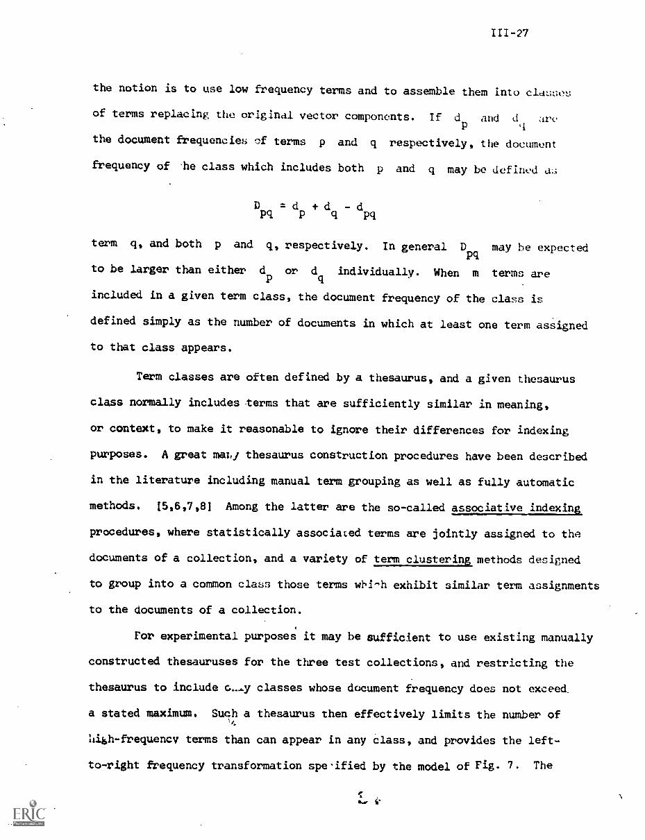
111-27

the notion is to use low frequency terms and to assemble them into claL;;;es

of terms replacing the original vector components. If d and d are

the document frequencies; of terms p and q respectively, the document

frequency of -he class which includes both p and q may be defined ,L3

D =d td -dq Pq

term q, and both p and q, respectively. In general Dpq may he expected

to be larger than either d or dq individually. When m terms are

included in a given term class, the document frequency of the class is

defined simply as the number of documents in which at least one term assigned

to that class appears.

Term classes are often defined by a thesaurus, and a given thesaurus

class normally includes terms that are sufficiently similar in meaning,

or context, to make it reasonable to ignore their differences for indexing

purposes. A great mat./ thesaurus construction procedures have been described

in the literature including manual term grouping as well as fully automatic

methods. [5,6,7,8] Among the latter are the so-called associative indexing

procedures, where statistically associated terms are jointly assigned to the

documents of a collection, and a variety of term clustering methods designed

to group into a common class those terms wtai-h exhibit similar term assignments

to the documents of a collection.

For experimental purposes it may be sufficient to use existing manually

constructed thesauruses for the three test collections, and restricting the

thesaurus to include classes whose document frequency does not exceed

a stated maximum. Such a thesaurus then effectively limits the number of

hibh-frequencv terms than can appear in any class, and provides the left-

to-right frequency transformation speified by the model of Fig. 7. The

t .

flue II'

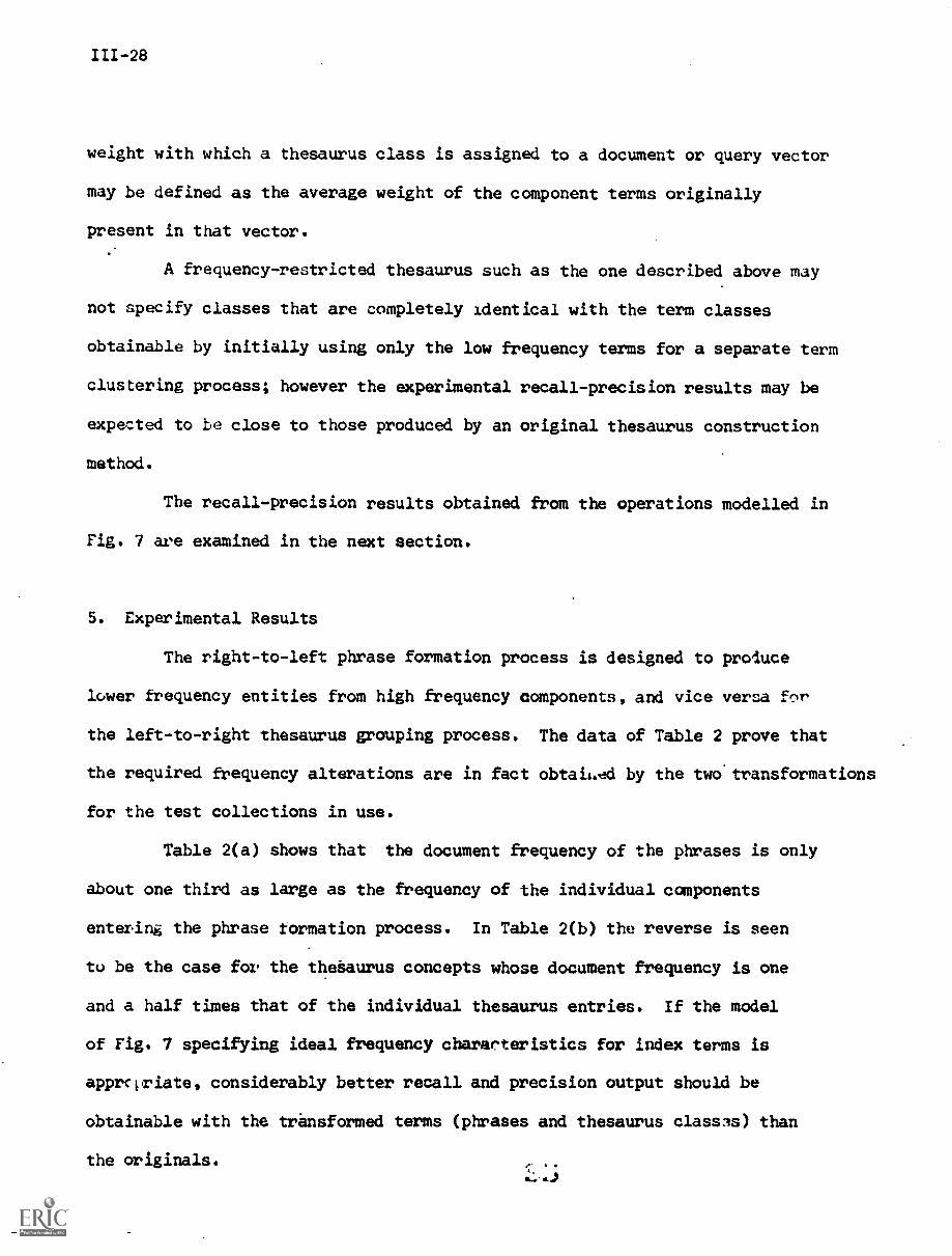
111-28

weight with which a thesaurus class is assigned to a document or query vector

may be defined as the average weight of the component terms originally

present in that vector.

A frequency-restricted thesaurus such as the one described above may

not specify classes that are completely identical with the term classes

obtainable by initially using only the low frequency terms for a separate term

clustering process; however the experimental recall-precision results may be

expected to be close to those produced by an original thesaurus construction

method.

The recall-precision results obtained from the operations modelled in

Fig. 7 are examined in the next section.

5. Experimental Results

The right-to-left phrase formation process is designed to produce

lower frequency entities from high frequency components, and vice versa for

the left-to-right thesaurus grouping process. The data of Table 2 prove that

the required frequency alterations are in fact obtaid by the two transformations

for the test collections in use.

Table 2(a) shows that the document frequency of the phrases is only

about one third as large as the frequency of the individual components

enteint, the phrase formation process. In Table 2(b) the reverse is seen

to be the case for the thesaurus concepts whose document frequency is one

and a half times that of the individual thesaurus entries. If the model

of Fig. 7 specifying ideal frequency characteristics for index terms is

apprciriate, considerably better recall and precision output should be

obtainable with the transformed terms (phrases and thesaurus classes) than

the originals.

111-29

.11W011111111110.11.

MinimumDocument

Average Document Frequency=11111.11.. 11111...1111.1.111111111111

Frequency Single T(Irms

needed for Entering PhrasesHigh-rrequency Phrano ProcessComponent

111111a1.00.110.0.effe

CRANFIELD (45) 10U 39

MEDLAkS (2?) 40 7

TIME 4q) 101 38

Average Document Frequency for Phraset;

Table 2(a)

MaximumDocumentFrequencyneeded forThe,,aurus

Class toInsureInclusion

Average Document Frequency

Single TermsEnt^r3ng

Thesaurus Process

ThesaurusClasses

CRANFIELD (60) 24 32

MEDLARS (40) 10 16

TIME (60) 17 31

Average Doer ent Frequency for Thesaurus Classes

Table 2(b)

stsiOsystt

111-30

Detailed recall-precision output is contained in Tables 3 and 4,

and in the summary in Table 5 for the various indexing methods applied to

the three test collections in aerodynamics, medicine, and world affairs.

Performance figures comparing the standard term frequency weighting (fki)

for single terms k in documents i with the phrase process are shown

in Table :. The phrase procedure uses the normal single terms in addition

to indexing phrases weighted in accordance with the formula of expression (7).

Table 3 contains precision figures averaged over 24 user queries

iza, each of the test collections at ten specified recall levels ranging in

magnitude from 0.1 to 1.0 in steps of 0.1. The percentage improvement in

precision for the phrase process over the standard is also given at each

recall level, together with an average improvement ranging from a high of

39 percent for the Medlars collection to a low of 17 percent for Time.

Table 4 contains output similar to that already shown in Table 3.

However the data in Table 4 apply to an indexing system using both left-to-

right (thesaurus) and right-to-left (phrase) transformations. It is seen

from Table 4 that the thesaurus transformation adds an additional average

improvement of 13 percent in precision for the Medlars collection; additional

advantages are also obtained for the Cranfield and Time collections.

The evaluation results are summarized ir. Table 5. It is seen that

average precision values of approximately 0.70, 0.40, and 0.20 at high,

medium, and low precision are transformed into average figures of 0.90,

0.60 and 0.30 approximately when the discrimination properties of the terms

are optimized. The retrieval results displayed in Tables 3, 4, and 5 have not

been surpassed by any manual or automatic indexing procedures previously

C.

%L

.+sBpas:Ji

aT412.;;

(1;ar:1:11pa.s 'SA Sz;&00.1.c. at:Elaa)

TTp.sa..! us:

sanTry, uoTs7.3s.z= a2r.,asAy

c%DU+

a.2,1aAv

77

-us:7?

S3EV

E85'

---c.

7SZ9'

cc.

SZOL'

7.S E9'

Z2-19'

6E+78'

2-

?af:pue;s

6S61'

CC%.1.T*

L91,2*

89LI'

egZe*

Sc ;Z'

/.9817'

LAC'

CStS'

TZLE'

0e65'

nBett*

I3 179

LC811°

2669'

TerG'

617:8'

0:71.9

128'

nTET'

,9T+

EWE'

%0.7,4

ccu.

%ZS+

vc

%Zi-t+

SZ9E'

%ZE+

OSTI-1°

%6.4+

-SCZS'

8Z+

£T09'

EC+

tnEL'

c74.

E6/8'

a/

O'T

SCZT°

6'

TC9I

8'

L.

9'

nCTE

ZenE'

17°

C.

ECC9'

ZT.

a

yLC

Z-U

P.Apy

4usuzfTssy

asE.atid

gaypa2puPz.s

e2ez

..lurs=2Issy

-ueAPV

asuazid

masT

3ATT

GSt 4 ITA

tZt NVED

.2

CRAM 424

MED 450

TIME 425

I

StandarA

Term

Frequency

Thesaurus

Plus

Fhrases

Advan-

zage

Standard

Term

Frequency

Thesaurus

Plus

?hrases

Standard

Advan-

tage

Frequency

Thes=us

Phrases

Advan-

tage

.6844

.3134

.2E35

.1989

.1631

.1255

.1176

.8745

.7

.5 *Z-87

.'5431

.4515

.378

.2379

.2319

.1556

.1375

27.8%

49.1

-^ OS.4:

55.1%

44.1%

49.3%

23.8%

23.0%

6.9:

.7801

.6750

.EJ.2.1

.4807

.4388

.3721

.3357

.2195

.1768

.1230

.8913

.8331

.70E7

.6443

.6099

.5548

.5179

.3949

.3505

.2424

13.( %

23.4%

28.8%

34.0%

39.1%

49.1%

54.3%

79.9%

98.2%

101.9%

.7495

.5452

.6331

.535,3

.5413

.5004

.385E

.3721

.3339

.3133 .)

I

.7681

.7006

.5822

.6389

.5915

.4842

.4790

n^

17-2:

18.0%

18.2%

25.3%

28.7;

Average

+37%

Average

+52%

Average

Ave''age (Phrac:es)

-rL

Average (Phrases)

+39

Average (Phrases)

-

Average Precision Values at Ten

Recall Points

P:-.rases vs. Stalrlarr')

.._,

CRAN 424

MED 450

TIME 425

Automatic Phrases

vs. Standard Term

Frequency

+32%

Automatic Phrases

vs. Standard Term

Frequency

+39%

Automatic Phrases

vs. Standard Term

.

Frequency

+17%

4

Automatic Phrases

Plus Thesaurus

vs. Standard Run

+37%

Automatic Phrases

Plus Thesaurus

7S. Standard Run

+52%

Automatic Phrases

Plus Thesaurus

vs. Standard Run

+18%

Best Precision

Low Recall 0.89

Medium Recall 0.43

High Recall 0.13

Best Precision

Low Recall 0.88

Medium Recall 0.61

High Recall 0.23

Best Precision

Low Recall 0.85

Medium Recall 0.70

High Recall 0.45

Summary o1 Recall-Precision Evaluation

(Three Collections)

Table 5

H H t-t

CO

III -34

tried with sample document collections and user queries. Furthermore,

because of the high average precision values produced by the indexing

theories described in this study, it is not likely that additional drastic

improvements in retrieval effectiveness are obtainable in the foreseeable

furture.

111-35

References

[1] G. Salton and C.S. Yang, On the Specification of Term Values in AutomaticIndexing, Journal of Documentation, Vol. 29, No 4, December 1973,p. 351-372.

[2] G. Salton, A. Wong, and C.S. Yang, A Vector Space Model for AutomaticIndexing, Technical Report No. 74-208, Department of Computer Science,Cornell University, Ithaca, N.Y., July 1974.

[ ] G. Salton and M.E. Lesk, Computer Evaluation of Indexing and TextProcessing, Journal of the ACM, Vol. 15, No. 1, January 1968, p. 8-36.

[4] K. Sparck Jones, A Statistical. Interpretation of Term Specificity andits Application to Retrieval, Journal of Documentation, Vol. 28, No. 1,March 1972, p. 11-20.

[5] K. Sparck Jones, Automatic Keyword Classifications, Butterworths, London,1971.

[6] C.C. Gotlieb and S. Kumar, Semantic Clustering of Index Terms, ACMJournal, Vol. 15, No. 4, October 1968, p. 493-513.

[7] G. Salton,Retrieval,Amsterdam,

Experiments in Automatic Thesaurus Construction for InformationInformation Processing 71, North Holland Publishing Co.,1972, p. 115-123.

[8] G. Salton, C.S. Yang, and C.T. Yu, Contributions to the Theory of Indexing,Proc. IFIP Congress-74, Stockholm, August 1974.

Negative Dictionary Construction

R. Crawford

1. Introduction

Effective information retrieval is based on the ability to

provide an accurate description of each item and to be able to discimin-

ate between the available information items. In the area of document

retrieval, a set of words (terms) chosen from the subject area of the

documents may be used to describe the documents. [1,2,31 If the set of

words used to describe each document is chosen properly, then each

document will have a description which is both accurate and unique in

relation to the other documents. The document descriptions should

reflect the same differences and similarities between documents as would

be noticed by a reader of the original documents.

Thus, for a collection of documents iu a particular subject area,

two problems are apparent. First, a set of terms must be chosen for use

in describing the documents in the collection. This set of chosen terms

is called a dictionary. The process of selecting the set of terms is

cal.Led dictionary construction. Second, specific terms from the

dictionary must be selected for use in describing each document. This

assignment of terms to describe documents is called context analysis or

document indexing. Both dictionary construction and document indexing

have been previously investigated, with both manual and automatic methods

considered. A large degree of success has been found in using fully

automatic procedures for document indexing. 13,4,51 Automatic dictionary

construction has not proved so successful and it is this area which is

IV-2

being presently investigated.

Dictionary construction may be conveniently considered in terms

of several specific areas.

(i) NEGATIVE DICTIONARY CONSTRUCTION.

The determination of which terms to exclude fr( the

document indexing process. This is defined m.

explicitly in the next section.

(ii) WORD STEMMING.

Entries in a dictionary may be grouped according to stems

by means of suffixing. This involves construction of

both Word. Form and Word Stem dictionaries.

(iii) THESAURUS CONSTRUCTION.

Terms having similar properties may be clustered to form

a single dictionary entry. These may be hierarchical in

structure and may be based on many different similarity

properties.

(iv) PHRASE DICTIONARIES.

Words or concepts used frequently in combloation are

identified.

(v) DICTIONARY UPDATING.

The dictionary for a dynamic document collection must also

be dynamic. This involves updating of the dictionary as

documents are added to or deleted from the collection, or

as word usage changes.

The remainder of this paper deals with the first of these areas;

negative dictionary construction. Further background of this specific

area is given in the following section.

IV-3

2. Negative Dictionaries

2.1 Common Words

The words used in the text of a document may be divided into

two classes, which might be described as "words important to the

meaning of the document" and "words important only to the structure

of the document". For example, consider the phrase;

"The role of the generality effort in retrieval systemevaluation is assessed, ..."

as used in a document in the field of information retrieval. Intuitively,

the words in t%is phrase could be divided into the following two classes:

"MEANING" "STRUCTURE"WORDS WORDS

ROLE THE

GENERALITY OF

EFFECT IN

RETRIEVAL IS

SYSTEM

EVALUATION

ASSESSED

Those words which are important only to the structure of the

documents are called function words or common words. Those words which

are important to the meaning of the sentence are called content words. If

only function words are classified as common, then the process of negative

dictionary construction is not difficult. However, a closer examination

of the previous example reveals some further problems, indicating that the

class of common words should possibly be expanded to include words other

than function words.

IV-4

Consider the use of the word "retrieval" in the above example.

Since this was taken from a document in the field of information retrieval,

some question may be raised as to the validity of using the word "retrieval"

to describe any document. It might be expected that many, or even all

of the documents in this collection would contain this word. Although

using "retrieval" to index each document in which it occurs may contribute

to the accuracy of the description of those documents, it will also serve

to make distinguishing among those documents more difficult. For this

reason, words which have a very high frequency of occurrence in a collection

may be considered to be common words.

Again examining the example given, consider the use of the word

"role". Although not strictly a function word, "role" would not appear

crucial to the meaning of the phrase to the same extent as "generality" or

"evaluation". In fact, the phrase could easily be reworded in several ways

to eliminate completely the word "role". Thus in this collection, retrieval

may be expedited by treating a word such as "role" as common because of its

usage. In a collection dealing with the theatre, for example, "role" might

in fact be a very important and meaningful word.

Words which are classed as common because of their high frequency

of occurrence in a particular collection, or because of their specific usage

in the collection are called collection-specific common words. Thus, it

is convenient to classify words in the following manner:

WORDS IN ADOCUMENTCOLLECTION

CONTENT WORDS COMMON WORDS

funciion words collection-specificcommon words.(frequency and/orusage)

A classification such as this may be useful in constructing a

negative dictionary using manual methods. Manual construction of

negative dictionaries is discussed further in Section 4. This model is

not, however, as useful when automatic negative dictionary construction

methods arc considered. Thus, new approaches to the problem of

classifying words in a collection have been considered, with the hope

that classifications which may be stated in more precise mathematical

terms may also be simpler to implement using automatic techniques. This

notion is expanded in Section 5.

2.2 The Negative Dictionary

A negative dictionary is defined as a list of words whose use is

proscribed for content analysis purposes. Based on the classification

outlined in the previous section, the negative dictionary for a collection

is composed of those terms in the collection which are either function

words or collection-specific common words.

The importance of accurate construction of negative dictionaries

has been demonstrated. Words which do not contribute to the effectiveness

of the information retrieval process must be excluded. Bergmark [6] has

shown that, in at least one case, the advantage of a thesaurus over a

word stem dictionary was due to more accurate determination of common

words, rather than to the clustering of the terms.

Negative dictionary construction is considered in detail in the

following sections. Section 3 describes briefly the experimental procedures

used, including the retrieval system, document collections, and evaluation

methods. In Section 4 manual negative dictionary construction is described

and some retrieval results presented. Section 5 includes discussion of

IV-6

possible techniques to be used in automatic construction of negative dic-

tionaries. In Section 6, the techniques of Section 5 are incorporated into

specific algorithms for use in negative dictionary construction. Several

algorithms are tested for retrieval effectiveness and these results are

presented. Finally the work is evaluated and conclusions are drawn in

Section 7.

3. Experimental Procedures

The retrieval system, document collections, and evaluation parameters

used in the experiments to follow are described briefly.

3.1 The SMART System

The SMART system is an automatic document retrieval system "designed

for the exploration, testing, and measurement of proposed algorithms for

document retrieval". (71 All the experiments discussed in the following

sections were performed using the SMART system as the experimental base.

As described by Williamson, (7) the SMART system takes documents

and search requests in natural language, performs a fully-automatic content

analysis of the texts, matches analyzed documents with analyzed search

requests, and retrieves those stored items believed to be most similar to

the queries. A description of the implementation of the SMART system may

be found in (71. Reports of previous work done using the SMART system

are numerous, including (81 and (9) .

3.2 The Experimental Data Base

Two document collections are chosen for use in the retrieval

experiments. The first i:, the Medlars collection of 1033 abstracts from

IV-7

the field of medicine, along with 35 queries for which relevancy judgements

were obtained. The second is the ophthalmology collection consisting of

852 documents and 35 queries. Again, a set of relevancy decisions for each

of the queries with each document was obtained. These collections are

suitably large to yield valid results, yet are of a size which allows extensive

experiments to be performed using the computer resources available.

3.3 Evaluation Parameters

Two principal measures have been chosen for use in evaluating the

retrieval effectiveness of the methods being tested. 1101 These measures

are precision (P) and recall (R), which are defined as follows:

Pnumber of relevant documents retrievednumber of documents Tetrieved

R =number of relevant documents retrievednumber of relevant documents in the collection

Thus, precision is the percentage of retrieved documents which are actually

relevant, whereas recall is the percentage of relevant documents actually

retrieved. In presenting retrieval results, these recall and precision values

are averaged over all search requests and displayed in the form of a graph.

The performance of different methods is compared using these precision-recall

graphs.

4. Manual Negative Dictionary Construction

4.1 Methods For Manual Negative Dictionary Construction

Dictionaries and keyword lists used for content analysis purposes

alwaye include a negative dictionary. Thus, the dictionary construction

process involves partitioning he terms in a collection into two sets of

IV -8

terms; those terms which are to be included in the indexing of the

documents (the inclusion list), and those terms to be excluded from the

indexing (the exclusion list). Generally, manual construction of a

dictionary proceeds from either of two directions. In one case, the

keyword list or inclusion list is selected from all the words in the col-

lection. The remaining terms thus form the exclusion list or negative

dictionary. In the other case, the emphasis is placed on determining which

terms to exclude from the indexing process and it is the negative dictionary

which is constructed first. Thus the remaining terms in this case form

the inclusion list. Although differing in description, these two approaches

to dictionary construction are not too diverse. In each case, all distinct

words in a collection are manually examined and a decision is made with

regard to their usefulness in indexing the documents.

There are interesting examples of experimental work involving

dictionary construction using each of the above approaches. In work performed

by Vaswani and Cameron, [11] a dictionary was constructed from a sample of

1,648 abstracts. Initially, a liit was constructed showing each word occurring

in the sample, along with the number of times the word occurred. The method

of then constructing the dictionary proceeded as follows:

"The list was studied very carefully by three people, twoof them being fairly familiar with the subject matter, whodecided intuitively which words to retain in the system askeywords, all others being excluded from further consider-ation".

Thus, the negative dictionary consisted of those terms "excluded from further

consideration".

In document retrieval experiments done using the SMART system, the

following procedure has been used for constructing negative dictionaries: [12]

IV-9

(i) A standard common word list is prepared consisting of

function words to be excluded from the dictionary;

(ii) A concordance listing is generated for a sample of the

document collection under consideration, giving the

context and the total frequency of occurrence for each

word;

(iii) The common word list is extended by adding new non-

significant words taken from the concordance listing;

many of the words added to form the ne ative dictionary

are either very high frequency words providing little

discrimination in the subject area under consideration,

or very low frequency words which produce few matches

between queries and documents.

The use of automatically generated aids such as concordance

listings and word frequency counts has proved helpful during manual

dictionary construction. Nevertheless, the construction process still

involves an intellectual decision with regard to each term in the collec-

tion, and many of these decisions must still be made somewhat intuitively.

4.2 Manual Negative Dictionary Construction-Performance Results

Using the manual negative dictionary construction method outlined

in the previous section, a negative dictionary was constructed for the

Medlars collection. The remaining (non-excluded) terms were then processed

three separate ways to produce the following three dictionaries:

(i) The Ml-word form (suffix-'s') dictionary, formed by stripping

the final s from all terms;

(ii) The M2-word stem dictionary, formed by automatic removal of

suffixes ds determined from a previously prepared standard

suffix list;

I11-10

(iii) The M3-thesaurus, or synonym dictionary, formed by manually

grouping dictionary entries into synonym categories, or

concept classes.

A recall-precision graph showing the performance of these three dictionary

types is given in Fig. 1.

The performance of the M3 thesaurus is clearly better than that of

either the M1 or M2 dictionaries, and may be attributed to a combination of

accurate common word recognition and careful term clustering. The perfor-

mance of the M1 word form and the M2 word stem dictionaries is quite

similar; however, the M1 dictionary gives better performance results at

all recall points except in the range of .10 to .30.

Based on these results, consideration is given as to which dictionary

type to use for testing of automatic negative dictionary construction methods.

The simple word form dictionary type is selected for several reasons. First

of all, use of a thesaurus presents both construction and analysis problems;

it may be difficult to determine whether performance changes are due to

common word recognition or to term clustering. Secondly, the performance

of the word stem dictionary in the manual case gives no reason to select it

over the word form dictionary. Finally, the word form dictionary is the

simplest to construct. Therefore, the M1 word form dictionary is selected

as the "control" dictionary for use in comparing the effectiveness of

manual and automatic negative dictionary construction methods.

5. Automatic Methods of Negative Dictionary Construction

In approaching the problem of automatic negative dictionary con-

struction, a first course of action may be to adhere closely to one of the

algorithms used in manual negative dictionary construction, attempting to

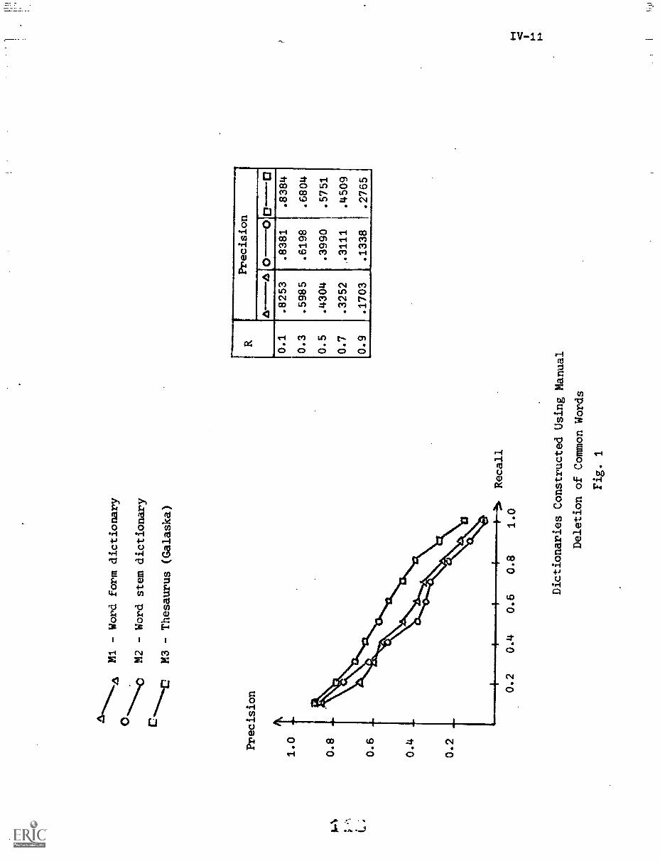
Precision

1.0

0.8

0.6

0.4

...

0.2

M1 - Word form dictionary

M2 - Word stem dictionary

M3 - Thesaurus (Galaska)

0.2

0.4

0.6

0.8

r Recall

1.0

,---

RPrecision

AA

C)

0,0

0.1

.8253

.8381

.8384

0.3

.5985

.6198

.6804

0.5

.4304

.3990

.5751

0.7

.3252

.3111

.4509

0.9

.1703

.1338

.2765

Dictionaries Constructed

Using Manual

Deletion of Common Words

Fig. 1

IV-12

automate each step of the manual process. Examples of the difficulties

found when this approach is used may be seen in each of the manual methods

outlined in the previous section. In the case of the method used by

Vaswani and Cameron, the problem arises at the point at which the manual

worker "decides intuitively" which terms to include in the dictionary.

It is difficult to ccinceive an automatic procedure which will duplicate

the intuitive decisions made by an individual. In the case of the manual

negative dictionary construction procedure used on the SMART system, the

problem of automation arises in the step involving examination of the

concordance listing. Although a manual worker may with high consistency

locate collection-specific common words by examining a concordance listing,

this process does not yield directly to automatic methods. Based on these

considerations, it is worthwhile to develop another approach to the problem

of automating the negative dictionary construction process.

The approach that is followed is to ,:onsider factors regarding terms

in a collection which may be measured and evaluated objectively. Several

factors are considered and tested. These are divided into the following

three areas:

(i) frequency and distribution,

(ii) discrimination value,

(iii) distribution correlation.

In the following three sections, each of these areas is discussed in detail.

5.1 Frequency and Distribution of Terms

Three basic statistics are considered for use in determining

which terms belong in the negative dictionary for a collection. These values,

IV-13

which may be easily computed for each term in a collection, are:

total frequency, which is the total number of occurrences of the

term in the collection; document frequency, which is the number of

documents in the collection in which the term occurs at least once;

and average usage, which gives the average number of times the term

is used within the documents in which it actually occurs (this is

simply total frequency divided by document frequency). For dis-

cussion purposes, three separate areas are considered, in which

these statistics are utilized. Terms of low frequency are discussed

in Section 5.1.1, terms of high frequency are discussed in Section

5.1.2, and a discussion of the average usage of terms is given in

Section 5.1.3.

5.1.1 Low Frequency

A consideration of terms with a low frequency of occurrence

is important due to the fact that the majority of the terms in a

collection occur only a very few times. For example, in the Medlars

collection of 1033 medical abstracts, there are 14,534 unique terms

in the text. Table 1 lists the number and percentage of terms with

specific low total frequencies in this collection. It can be seen from

this table that words of total frequency one account for almost half the

unique occurrences in the collection.

Consideration is given to placing this large number of single

occurrence terms on the exclusion list, and two advantages of doing so are

noted. First of all, many of these terms are actually errors in the text,

such as misspellings, improper hyphenation, etc. Excluding these terms

causes elimination (but not correction) of these errors during the document

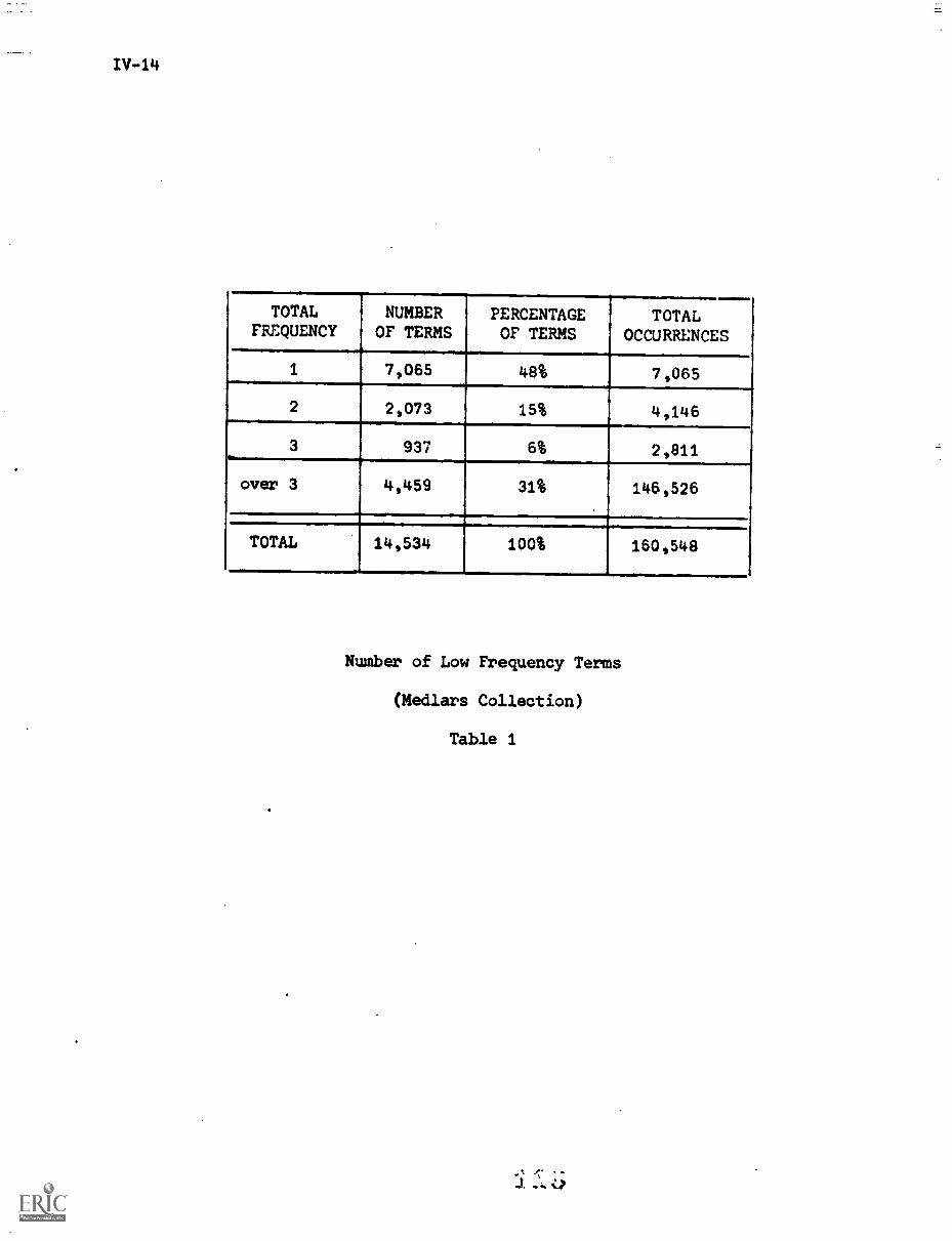
TOTALFREQUENCY

NUMBEROF TERMS

PERCENTAGEOF TERMS

TOTALOCCURRENCES

1 7,065 48% 7,065

2 2,073 15% 4,146

3 937 6% 2,811

over 3 4,459 31% 146,526

TOTAL 14,534 100% 160,548

Number of Low Frequency Terms

(Medlars Collection)

Table 1

IV-15

indexing process. Second of all, the size of the inclusion list is kept

much smaller by excluding single frequency terms. Although this is an

efficiency consideration, which may be considered as of lesser importance

than retrieval effectiveness, maintaining a dictionary of a size which may

be handled is an important factor.

Regardless of these two advantages, it is the effect of terms of

single occurrence on retrieval effectiveness which must be considered.

Very low frequency words may be expected to produce few matches

between queries and documents. [13] It may be argued that the few matches

which do occur will be important, and that low frequency words should

therefore be retained. Excluding very low frequency terms may therefore

cause a decrease in the level of precision of the retrieval results for

some queries.

For the two document collections used in this study, all terms

occurring once in a collection were matched against the terms in the queries

for that collection. In no case was there a match. All terms having a total

frequency of one could therefore be excluded without any resulting loss in

precision of retrieval results. Because it is difficult to generalize these

results to either the case of more queries in these present collections, or

to the case of larger collections, it is clear that some compromise must be

made regarding low frequency terms. This compromise is between retrieval

effectiveness and retrieval efficiency. When terms of very low total

frequency are excluded, the dictionary is kept small, increasing efficiency,

but the level of precision way drop, indicating d decrease in retrieval

effectiveness. The choice of a particular value of total frequency for use

in excluding low frequency terms depends on the levels of retrieval effectiveness

IV-16

and efficiency which are required.

The effect of deleting terms of total frequency one from the Medlars

collection is investigated experimentally. All 0,718 terms of frequency

one are deleted from the M1 word form dictionary to form the MA word form

(no frequency one) dictionary. The comparative performance of the M1 and

MA dictionaries is shown by means or a precision-recall graph in Fig. 2.

As discussed previously none of the deleted terms matched with any of the

query terms, so the performance of the M1 and MA dictionaries should be

similar. This is verified by the results shown in Fig. 2. Those slight

changes which do occur are a result of the decrease in the lengths of the

document vectors due to deletion of the low frequency terms.

5.1.2 High Frequency

Very high frequency words provide little or no discrimination in

the subject area of the document collection under consideration. It may,

therefore, be worthwhile for very high frequency words to be placed on the

exclusion list. Excluding very high frequency terms from the indexing

process may result in some decrease in the level of recall for certain

queries. (13] That is, there may be some documents relevant to a particular

query which are not retrieved by that query due to the exclusion of one or

more high frequency terms which would have provided a match between the

query and the documents. However, if high frequency terms are not excluded

from the indexing process, then a query may match significantly with

documents which are quite dissimilar. This may result in a low level of

precision for certain queries.

Oho

Precision

1.0

0.8

0.6

0.4

0.2

M1 - Word form dictionary

MA - Word form dictionary - terms of frequency one deleted

0.2

0.4

0.6

0.8

1.0

RPrecision

6--ii0-0

0.1

.8253

.8276

0.3

.5985

.5885

0.5

.4304

.4396

0.7

.3252

.3253

0.9

.1703

.1721

Manually Constructed Word Form Dictionaries

Effect of Frequency One Terms

Fig. 2

IV-18

Obviously, some compromise is necessary between the desire for

high recall and the need for high precision.. It may be possible, however,

to delete very high frequency terms so that precision increases, without

affecting recall to a very great extent. What is desired is a function,

based on either total frequency, or document frequency, or both, which

will enable determination of those high frequency terms which belong on

the negative exclusion list.

Consider the list of words in Table 2. These are the terms of

highest frequency in the Medlars collection of 1033 medical abstracts.

The words are given in decreasing order of document frequency. By

examining the total frequency given for each word, it is apparent that

an ordering by total frequency would have been quite different. In

particular, words such as CELL and CASE would occur much higher on this

list if it were ordered by total frequency.

The three lines drawn through Table 2 indicate levels of document

frequency of 20, 25, and 30 percent of total collection size. All the

terms occurring with a document frequency of 30% of collection size or

greater are clearly function words and belong in the negative dictonary.

for this collection. On the other hand, above a document frequency level

of 20% of collection size there are several terms which are clearly not

function words. At the document frequency level of 25% of collection

size, only the word PATIENT is not a function word, and it is clear that

the word PATIENT could easily be a collection- specific common word in a

medical collection.

Similar results to the above have been found for a collection of

852 abstracts in the field of ophthalmology, in that a document frequency

st)

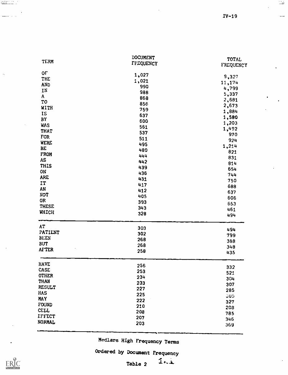
TERMDOCUMENTFREQUENCY

TOTALFREQUENCY

or 1,027 9,327THE 1,021 11,174AND 990 4,799IN 988 5,337A 868 2,681TO 856 2,673WITH 759 1,884IS 637 1,580BY 600 1,203WAS 561 1,492THAT 537 970FOR 511 924WERE 495 1,214BE 480 821FROM 444 831AS 442 814THIS 439 654ON 436 744ARE 431 750IT 417 688AN 412 637NOT 405 606OR 393 653THESE 343 461WHICH 328 494

AT 303 494PATIENT 302 799BEEN 268 388BUT 268 348AFTER 258 435

HAVE 256 332CASE 253 521OTHER 234 304THAN 233 307RESULT 227 285HAS 225 A5MAY 222 327FOUND 210 208CELL 208 785EFFECT 207 346NORMAL 203 369

Medlars High Frequency Terms

Ordered by Document Frequency

Table 2

IV-20

level of 25% of collection size provided a point above which terms could

be placed on the exclusion list with a high degree of confidence.

Thus, terms with a document frequency greater than some chosen

cutoff value should be placed in the negative dictionary. By choosing

tnis cutoff value properly, precision may be improved without any

significant reduction in recall.

5.1.3 Average Usage

it is worthwhile to investigate whethe," terms which belong in the

negative dictionary may be distinguished by their average usage from terms

which do not belong in the negative dictionary. In particular, it would

seem reasonable that terms which are of importance in a collection may be

used several times within the documents in which they occur, thus having

a high average usage. On the other hand, function words might be expected

to have a more random distribution, thus having a low or medium average

usage. Average usage values were examined for over 6000 terms from a

collection of 852 documents in the area of ophthalmology.

Table 3 lists some of the terms from this collection, ordered by

average usage. An examination of this list shows that content words, such

as LASER and CYST, cannot be distinguished from common words, such as WAS

and TO by means of average usage values. Average usage is therefore

rejected for use in automatic negative dictionary construction.

5.2 Discrimination Value

A document collection may be defined as a distribution of terms

taken from a specified set of terms. Thus, each term may be considered

as a possible index term on the basis of its distribution in relation to

the distribution of all other terms in the collectim. Developing this

TERMAVERAGEUSAGE

SPRAY 12.50

THE 9.38

OF 6.78

RUBELLA 4.70

CHOLINESTERASE 4.33

IN 4.15

AND 3.50

COLLAGEN 3.33

FIBER 3.13

CYCLODIALYSIS 3.00

LASER 2.91

CAPILLARY 2.84

A 2.67

TO 2.50

CYST 2.47

WAS 2.39

VESSEL 2.28

UVEI"IS 2.14

EYE 2.14

IS 2.13

Average Usage of Certain Terms

From Ophthalmology Abstracts

Table 3

IV-22

iclea, a term is considered to be a discriminator if its distribution is

such that it serves in distinguishing or discrimino4ing among the documents

in the collection. A term which does not serve in distinguishing among

the documents in the collection is a non-discriminator. For example, any

term which occurs 4.41 all the documents in a collection is a non-discriminator

in that collection, as it may not be used to distinguish among the documents

in any way.

It is useful then, to define some function for terms in a collection

which would indicate whether they are discriminators or non-discriminators.

Such a function, the discrimination, value, is sugge:.ted, based on the doc-

ument space similarity described by Aste-Tonsmann and Bonwit. (14] Some

notation and definitions are given and the discrimination value is derived

in the following section.

5.2.1 The Discrimination Value Function

A collection of N documents is represented by a set of document

vectors d., 1 < i < N. Each vector di is of length m, where m is the

number of terms used in indexing the documents in the collection. Then dij

th th. .

is the number of occurrences of the 1 term in the 3 document. Therefore,

1th.

a value of d.. = 0 indicates that the 1 term did not occur in document j.13

The nentrold, c, of a document collection is defined by c = (c1, c2, ..., cm)

where:

N

1.

1 r

3c. = L d..

N

The centroid represents a term by term average of the documents and is

considered to be the center of the set of documents (i.e. of the document

space).

IV-23

A measure of the correlation of two vectors dk and d1

is given by the

cosine function:

(40 )40 1cos(dk, d )

=1° 4 -dc 111111

where (d 0 d1

) is the inner product and lidk:12

= (dk, dk). For purposes of

calculation, this is conveniently expressed as:

cos(dk,

d1)

I d.Ldi2r 2

k 11

idid..k

11

where the sums are for i = 1 to m, the number of terms in the vectors.

Now the compactness or document space similarity, Q, is defined as:

N1r. r= L cos(c, d.) , 0 < Q < 1.

j=1

The value of Q is thus a function of the homogeneity of the documents in

the collection and the set of terms used in indexing the documents. Given

a standard index language, a collection of documents from diverse subject

areas will tend to have a low Q value, whereas a collection of documents

on very similar topics will tend to have a higher Q value. However, for

more homogeneous collections, the proper selection of index terms will

reduce the compactness of the document vectors, enabling better discrimination

and resulting in improved retrieval.

(i) This is the "NORMALIZED Q" of Aste-Tonsman and Bonwit. It is amore convenient measure than their Q and has a well definedrange.

d.

(ii) This may be maximized for a Rocchio centroid c'1

and not for c as defined. However, this is N Ild.11

negligible fOr does of approximately the samelength.

IV-24

Since Q is a function of the document vectors, deleting a single

term from all of the document vectors will normally change the value of Q.

Essentially, deletion of this term represents a new index language, differ-

ing from the initial one by only one term. The compactness of the collec-

tion with term i deleted (i.e. dii = 0, 0. < j < N) is given by Qi and is

defined as:

1Ncc

Qi = ir L coscai, 411

i=1

where dl is the jih document vector with term i deleted, and ci is the

centroid vector with term i deleted.

Then (Qi Q) is a measure of the change in document space compact-

ness due to the deletion of term i. If Qi > Q, the document space is

more compact with term i deleted and term i is a discriminator in the

collection. If Qi < Q, the document space is less compact with term i

deleted and term i is a non-discriminator in the collection. Since a

particular Qi value is only meaningful in comparison to the value of Q,

anewmeasureisdefined.ThediscriminationvalueD.of term i is

defined as:

Qi QD.1

=Q

*100

D. has the following properties:

(a) D. < 0 9 term i is a non-discriminator

(b) D > 0 , term i is a discriminator

(c) Di< D term j is a better discriminator than

J, term i.

(d) D.1

is not an explicit function of collection size,allowing comparison of values of Dicomputed for a term i occurringin several collections.

IV-25

The discrimination value thus provides a function by which all terms

in a collection may be ranked, from greatest non-discriminator to best

discriminator.

It is suggested that for each document collection, a discrimination

cutoff value exists such that all terms with a discrimination value below

this cutoff value should be placed in the negative dictionary for the

collection. Only terms with a discrimination value greater than the chosen

cutoff value are ust.d in indexing the documents. It is further suggested

that the discrimination cutoff value for any collection will be strictly

non-negative. That is, non-discriminators should always be placed in the

negative dictionary for a collection. For a discrimination cutoff value,

Dc, a term i in a collection may be classified as follows:

D. < 0-- ' term i is a non-discriminator

0 < D. <Dc ' term i is a poor discriminator

Dc

< D.' term i is a good discriminator.

The effective use of discrimination value in an algorithm for

negative dictionary construction is demonstrated in Section 6. The deter-

mination of a discrimination cutoff value and its usefulness are also shown.

5.2.2 The Set of Non-Discriminators

Discussion in the previous section concerned the computation of

discrimination value for specific terms in a collection. However, a

collection of documents includes a large number of terms, many of which bear

relation to one another. Thus, conclusions which may be drawn for

individual terms do not necessarily hold true for groups of terms. For a

given set of terms, each of which is a non-discriminator, it must be

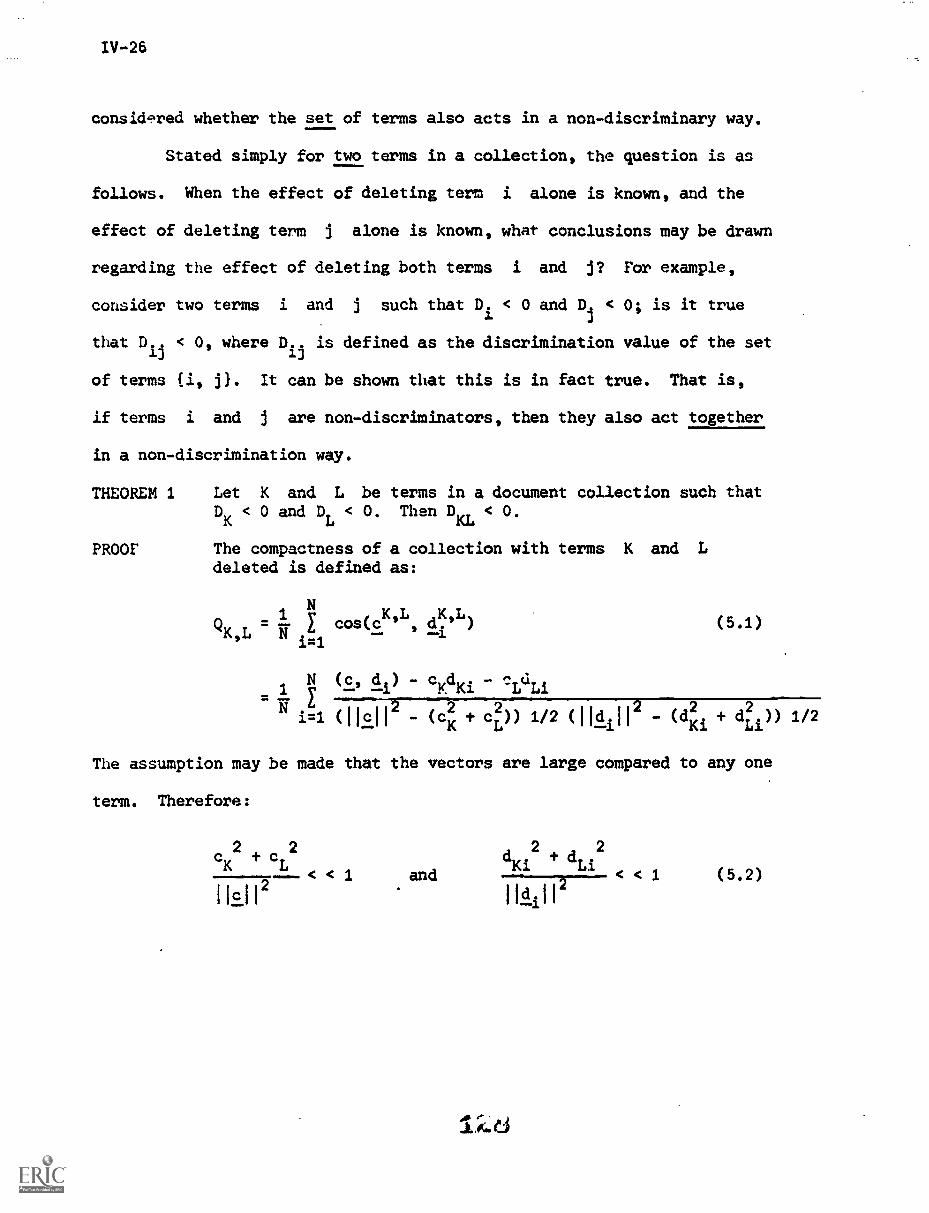
IV-26

consid ?red whether the set of terms also acts in a non-discriminary way.

Stated simply for two terms in a collection, the question is as

follows. When the effect of deleting term i alone is known, and the

effect of deleting term j alone is known, what conclusions may be drawn

regarding the effect of deleting both terms i and j? For example,

consider two term and D. < 0; is it true

that D.. < 0, where D..1) is defined as the discrimination value of the set13

of terms (i, j}. It can be shown that this is in fact true. That is,

if terms i and j are non-discriminators, then they also act together

in a non-discrimination way.

THEOREM 1 Let K and L be terms in a document collection such thatDK

< 0 and DL

< O. Then DKL

< 0.

PROOF The compactness of a collection with terms K and Ldeleted is defined as:

N KL KLQK,L N

.I I cos(c d.'--

1=1

(5.1)

N (c, d.) - cledK. c.d..1 _ Li

- TT2 2 2

i=1 Olen - (cK cL)) 1/2 (Ildill - (dKi + dia)) 1/2

The assumption may be made that the vectors are large compared to any one

term. Therefore:

cK2

+ c2

< <

Ilc112

anddKi

2 + du< < 1 (5.2)

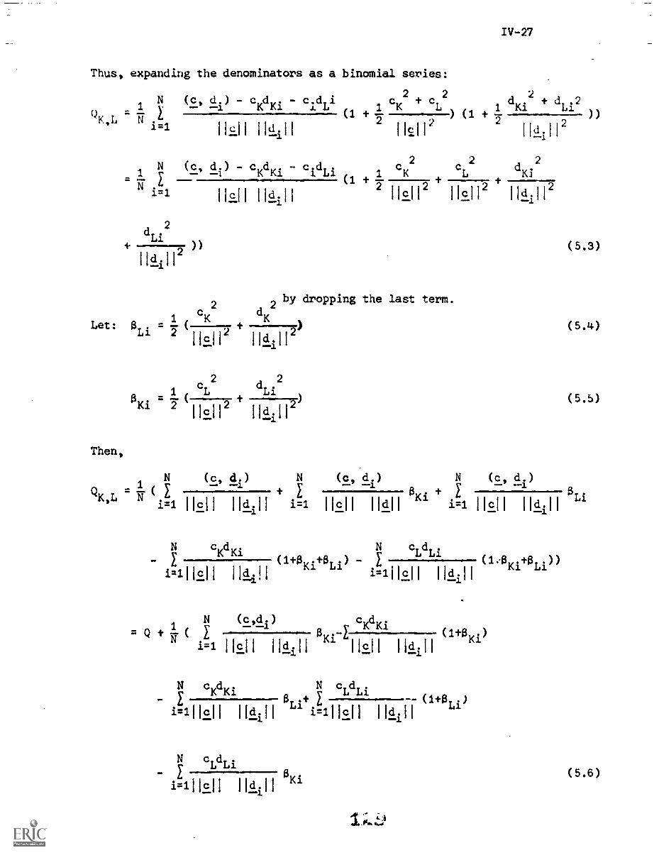
IV-27

Thus, expanding the denominators as a binomial series:

N. (c, di) - cKdKi - cidLi1

CK2+

c

2

L 1dKi

2+ d

Li2

QK L FI(1 +2 ))

= 2)

i=1 Hall 11,1111

(1 +

114 112

2 2N (c, dt) cvdv: ctd,,

1.1 1 cKcL d

KI

2

(1 +

i=1 Hal 1115.11 2 IlcII2 lIcI12 I1di112

d2Li

))

Ildill2

by dropping the last term.

1 ,cK2

dK2

Let: $ . = c +Li 2 lic112 ild.112)

ii_.2.11

0 .

2 2

1(

cL

T

dLi

Ki 2 lici12lid 112

Then,

(5.3)

(5.4)

(5.5)

N (c, di) (c, d.) N (c, d.)Q 4. - -K,L N

i=1 11c11 i=1 11c1I Ildll Ki

+

1-'21 11c11 Li

c d . N c d

/K Ki

(1+$ .+0 ) y L Li(1:0 .+8 ))

i=111c1I ildlll Ki Li .4.1=1

I II

Ki Li

N (c,di

°K

)Ki

= Q + (i

(1+0 i)i=1 11c1I 11c1I ['dill K

N c d c,d,iE K K1

0 .+ "i=111c1I

Li(11.01,i)

lldill

N c_ L

dLi

i=1112.11 'kill Ki(5.6)

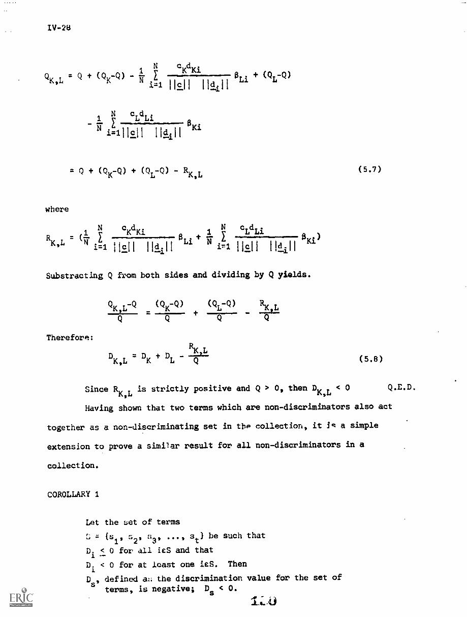
IV-28

N cvdv.Q (QK-Q) E + (Q -Q)

i=1 11sJlLl L

1 I cLdLi

1=111E1I Ildill Ki

Q (QK-Q) + (Q -Q) - K,L

where

N

R = (-1

c NKdKi ,1 1 L

dLi

)

c

K,L N11c11 11(111 1 irl 11c11

i

Substracting Q from both sides and dividing by Q yields.

Therefore:

QK L-Q (QK-Q) (QL-Q) RK L2-- =Q

LD D D -

RK-2--KL K L Q

(5.7)

(5.8)

Since RK,L

is strictly positive and Q > 0, then DK,L

< 0 Q.E.D.

Having shown that two terms which are non-discriminators also act

together as a non-discriminating set in the collection, it 5 a simple

extension to prove a similar result for all non-discriminators in a

collection.

COROLLARY 1

Let the set of terms

= {si, s2, a3, st} be such that

D. < 0 for all itS and that

D. < 0 for at least one ieS. Then

Ds

, defined a:: the discrimination value for the set of

terms, is negative; Ds < 0.

IV-29

PROOF

Since all the equations used in theorem 1 apply for sets of terms

as well as single terms, the corollary is easily proved by successive

application of theorem 1.

Thus, it may be concluded that deleting the set of all non-

discriminators in a collection has the effect of making the collection less

compact.

Further properties of the discrimination value function are

examined in the next section.

5.2.3 Analysis of the Discrimination Value Function

It is of interest to consider further the properties of the discrimina-

tion value function. In particular, it is important to determine whether

the discrimination value provides any new information regarding terms in a

collection, or if in fact the same information is obtainable from term

frequencies and distributions. Thus, the relationships betwoen the frequency,

the distribution, and the discrimination value of a term are considered.

Two approaches are used in investigating this area. First,

theoretical consideration is given to the effect of various frequencies

and distributions on the discrimination value. Second, experimental

results are presented, demonstrating the relationships which do exist

between discrimination value and the frequency and distribution of terms.

Yu and Wong [15] investigated the compactness function, Qi, upon

deletion of terms of...various frequencies and distributions. Although

specific conclusions could not be made, some general results were given.

These are as follows:

IV-30

(i) Any term occurring in nearly all of the documents is a

non-discriminator, irrespective of the number of occurrences

within each document. (This is intuitive, however it is not

trivial to show).

(ii) For a collection of N documents, a term occurring in N' of

the documents with a constant frequency, may be classified

as a non-discriminator if the following inequality is

satisfied:

N licli2

2 N'(i.e. --- is large)

--cK

(iii) A term occurring with a bunched up distribution, in only a

few documents, is a non-discriminator.

This third result (iii) may be invalid due to an assumption made

by Yu and Wong that for a collection of N documents and m distinct terms,

" 1

It is doubtful if this condition is met by any existing collections.

The Medlars collection was used to investigate experimentally the

relationship between term frequencies and discrimination value. The

discrimination value is computed for 000 terms from this collection and

these terms are then ordered by discrimination value. This ordered list

is divided into 31 groups of 200 terms each. Thus the first group consists

of the 200 terms with the highest discrimination values, and the last group

contains the 200 terms with the lowest discrimination values. Averages

are then computed giving the total frequency, document frequency, and

average usage of each group of 200 terms. Figs. 3, 4, and 5 show these

averages plotted in terms of the ordering by discrimination value.

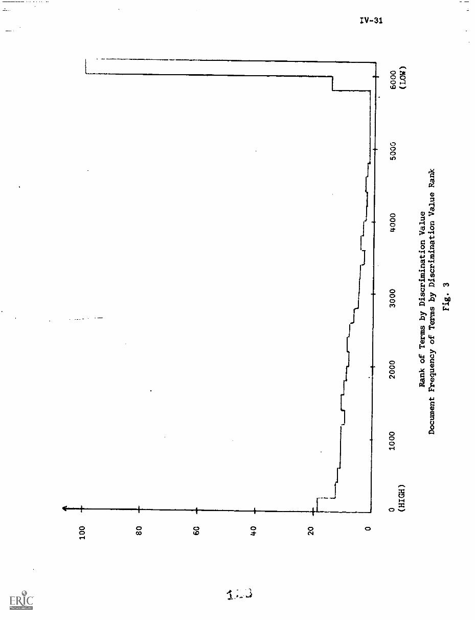
A

100

80

60

40

20 0

01000

2000

3000

4000

5000

6000

(HIGH)

(LOW)

Rank of Terms by Discrimination Value

Document Frequency of Terms by Discrimination Value Rank

Fig. 3

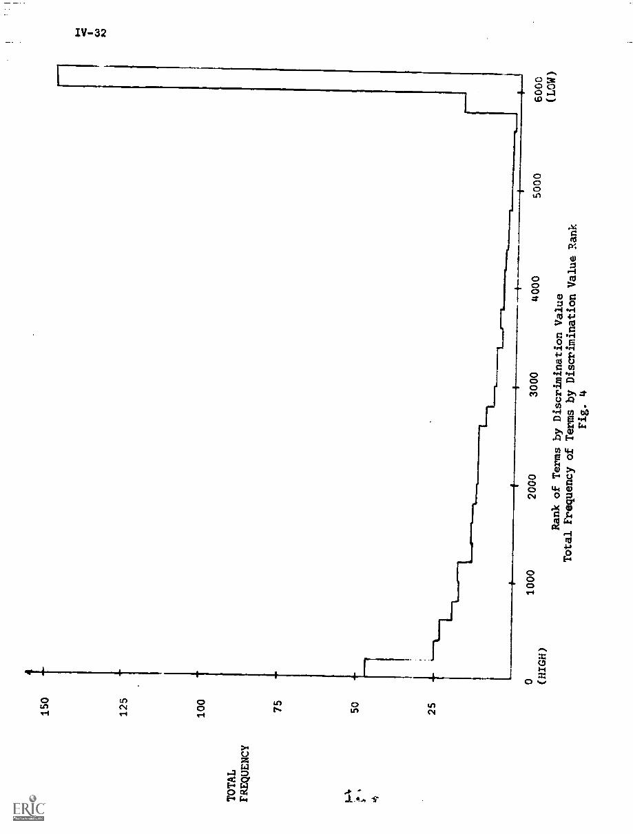
TOTAL

FREQUENCY

150

125

100

75

50

25

0 (HIGH)

1000

2000

3000

4000

Rank of Terms by Discrimination

Value

Total Frequency of Terms

by Discrimination Value Rank

Fig. 4

5000

6000

( L

OW

)

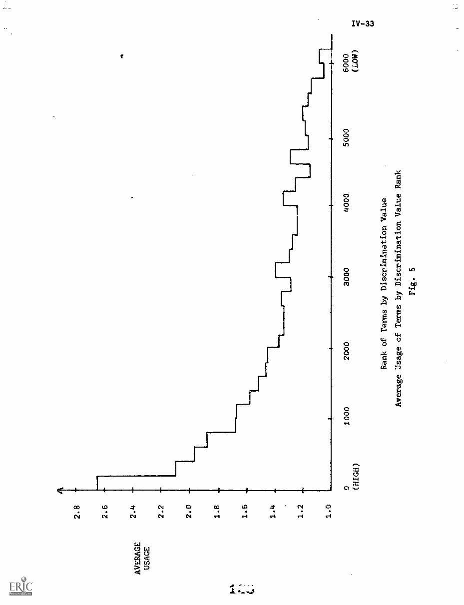
AVERAGE

2.8

2.6

2.4

***

USAGE

2.2

2.0

1.8

1.6

1.4

1.2

--

1.0

,-4-

01000

2000

3000

(HIGH)

1i____J__--

4000

5000

6000

(LOW)

Rank of Terms by Discrimination Value

Average Usage of Terms by Discrimination Value Rank

Fig. 5

Consider Fig. 3 for example. The left end of the graph shows that

the first (0-200) group of 200 terms (those with highest discrimination

value) had an average document frequency of 18. That is, the hest

discriminator: each occur in about 18 of the 1033 documents in the collection.

Proceeding then from left to right across the graph, the figures indicate

that as discrimination value decreases, so does document frequency, until

those terms with the very lowest discrimination value are reached. At

this point (5800), a large sump in document frequency occurs, with the

group of 200 terms of lowest discrimination value having an average

document frequency of about 100. The greatest difficulty in correlating

discrimination value with document frequency arises with the next to last

group of 200 terms of low discrimination value (5800-6000). In this case

the average document frequency of the terms is almost 15, a very similar

,slue to that of the best discriminators. Thus, very poor and very good

discriminators cannot be distinguished by means of document frequency.

The results for total frequency given in Fig. 4 show a similar

situaLlv to the one just discussed. Again there are terms at either

end of the discrimination value ordering which have similar total frequencies.

Fig. 5, which shows the r .ationship between discrimination value

and average usage, gives indication that this relationship may be fairly

direct. The group of terms with highest discrimination values (0-200)

shows an average usage of over 2.6, that is, when these good discriminators

are used within a document, they are used several times. As the

discrimination value decreases, the average usage of terms also tends to

decrease, although not monotonically. The results shown in Fig. 5 indicate

that the average usage of a term may possibly be used to determine whether

the term is a good discriminator or a non-discriminator. Since these

results are averages, taken for groups of 200 terms, it is necessary to

examine specific terms within the extreme groups (those with highest

and lowest discrimination values). Table 4 pres_nts the average usage

values for 16 good discriminators and 16 nor:- discriminators, along with

tneir document and total frequency values. These sample values are

sufficient to show that discrimination value is apparently based on morn

than the frequency and distribution of a term.

Both the theoretical and experimental analysis of discrimination

value, and its relationship to term frequency and distribution lead to

the same conclusion. The discrimination value of a term does not depend

only on the frequency and distribution of that term, but it depends also

on the frequencies and distributions of all other terms in the collection.

5.3 Relative Distribution Correlation

A measure is presented for possible use in determining objectively

which terms to place in the negative dictionary. It IF hypothesized that

content words and common words may be distinguished by 'he distribution of

the documents in which they occur. A common word tends to occur in a

somewhat random fashion, and the documents in which it occurs are not

expected to bear any relation to each other in subject matter. A content

word, on the other hand, tends to occur in documents of fairly homogeneous

subject matter. For example, the words JUST and PANCREAS each occur 10

times in the Medlars documents. However, the documents in which they occur

are distributed in the document space in a way exhibited in Fig. 6. The

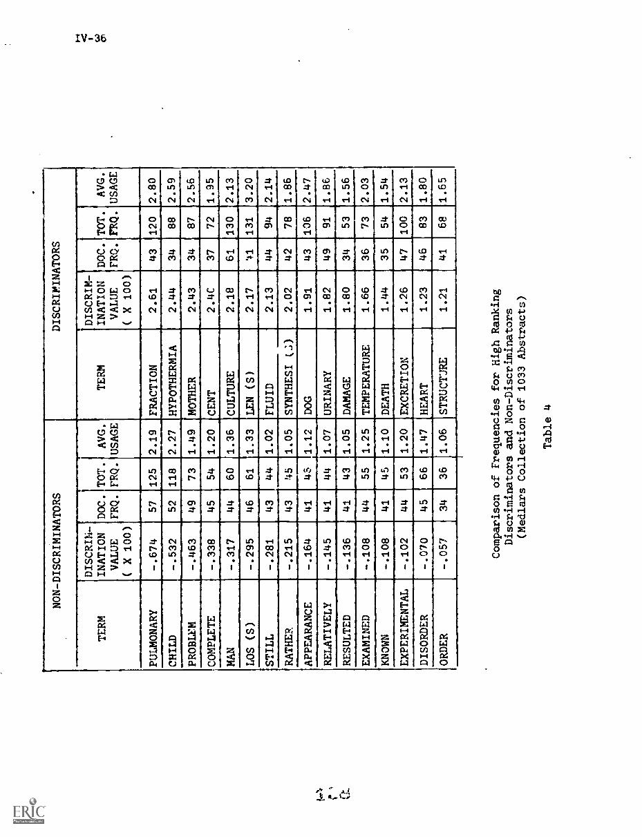
NON-DISCRIMINATORS

DISCRIMINATORS

TERM

DISCRIM-

INATION

VALUE

( X 100)

DOC.

FRQ.

TOT.

FRQ.

AVG.

USAGE

TERM

DISCRIM-

INATION

VALUE

( X 100)

DOC.

FRQ.

TOT.

FRQ.

AVG.

USAGE

PULMONARY

-.674

57

125

2.19

FRACTION

2.61

43

120

2.80

CHILD

-.532

52

118

2.27

HYPOTHERMIA

2.44

34

88

2.59

PROBLEM

-.463

49

73

1.49

MOTHER

2.43

34

87

2.56

COMPLETE

-.338

45

54

1.20

CENT

2.4C

37

72

1.95

MAN

-.317

44

60

1.36

CULTURE

2.18

61

130

2.13

LOS (S)

-.295

46

61

1.33

LEN (S)

2.17

'41

131

3.20

STILL

-.281

43

44

1.02

FLUID

2.13

44

94

2.14

RATHER

-.215

43

45

1.05

SYNTHESI (.7,)

2.02

42

78

1.86

APPEARANCE

-.164

41

45

1.12

DOG

1.91

43

136

2.47

RELATIVELY

-.145

41

44

1.07

URINARY

1.82

49

91

1.86

RESULTED

-.136

41

43

1.05

DAMAGE

1.80

34

53

1.56

EXAMINED

-.108

44

55

1.25

TEMPERATURE

1.66

36

73

2.03

KNOWN

-.108

41

45

1.10

DEATH

1.44

35

54

1.54

EXPERIMENTAL

-.102

44

53

1.20

EXCRETION

1.26

47

100

2.13

DISORDER

-.070

45

66

1.47

HEART

1.23

46

83

1.80

ORDER

-.057

34

36

1.06

STRUCTJRE

1.21

41

68

1.65

Comparison of Frequencies for High Ranking

Discriminators and Non-Discriminators

(Medlars Collection of 1033 Abstracts)

Table 4

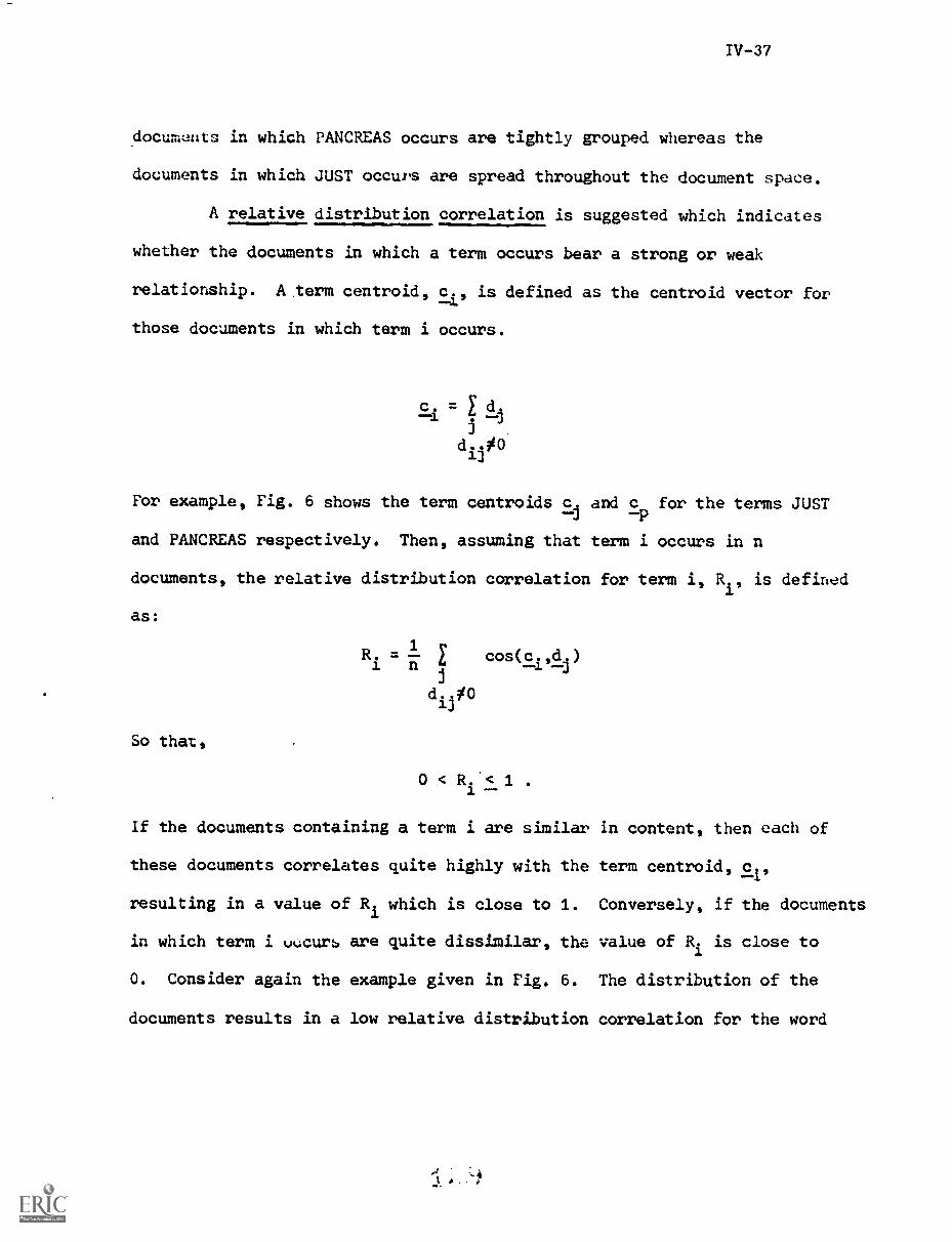
IV-37

documuuts in which PANCREAS occurs are tightly grouped whereas the

documents in which JUST occurs are spread throughout the document space.

A relative distribution correlation is suggested which indicates

whether the documents in which a term occurs bear a strong or weak

relationship. A term centroid, ci, is defined as the centroid vector for

those documents in which term i occurs.

c. = d.

d..#0

For example, Fig. 6 shows the term centroids c.1

and cP

for the terms JUST

and PANCREAS respectively. Then, assuming that term i occurs in n

documents, the relative distribution correlation for term i, Ri, is defined

as:

So that,

L aR. = 1

L cos(c.,d.)n

d..#0

0 < R. <1 .

1

If the documents containing a term i are similar in content, then each of

these documents correlates quite highly with the term centroid, ci,

resulting in a value of Ri which is close to 1. Conversely, if the documents

in which term i tA.curs are quite dissimilar, the value of Ri is close to

0. Consider again the example given in Fig. 6. The distribution of the

documents results in a low relative distribution correlation for the word

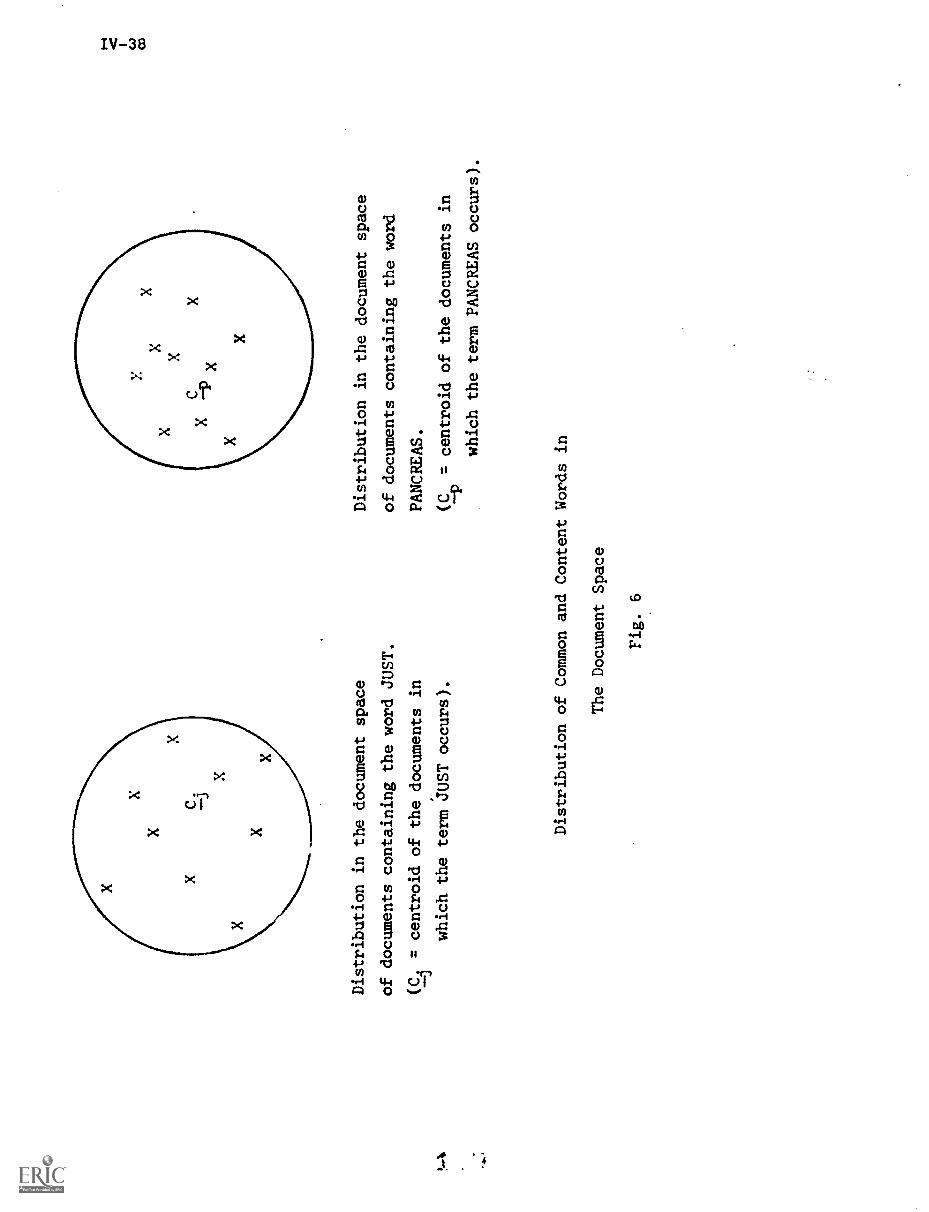
Distribution in the document

space

of documents containing the word JUST.

(C. = centroid of the documents in

which the term JUST occurs).

Distribution in the document

space

of documents containing the word

PANCREAS.

(CP

= centroid of the documents in

which the term PANCREAS occurs).

Distribution of Common and Content Words in

The Document Space

Fig. 6

IV-39

JUST but a somewhat higher correlation for the word PANCREAS.

The use of relative distribution correlation is investigated

experimentally using a set of 20 terms. These terms, along with their

relative distribution correlations are given in Table 5, ranked in

order of correlation.

Several of these terms, such as ANTIGEN (rank 4) and ANESTHESIA

(rank 11), are clearly content words. Other terms, such as WHOM (rank 6)

and THOUGH (rank 16), are apparently common words. Yet this ranking of

these terms by relative distribution correlation fails.to distinguish

between common and concent words. It is therefore concluded that the.

relative distribution relation does not provide information which is- _-

useful for purposes of negative dictionary construction.

6. Experiments and Results

An experimental procedure for testing of the negative dictionary

construction methods already discussed is outlined in Fig. 7. Each node

in Fig. 7 represents a dictionary. Each path between nodes of the tree

represents additional term deletions from the parent node dictionary.

Thus a path down any branch of the tree represents a series of successive

term deletions (and therefore additions to the negative exclusion list).

The root node, N1, represents the initial word list containing all distinct

word toklns in the document collection.

Table 6 shows the length of the dictionaries and the total length

of the document vectors for each of the dictionaries tested, using the

Medlars collection. Fig. 7 and Table 6 should'be referred to while

reading the following discussion.

re,

IV-40

RANK TERM

RELATIVEDISTRIBUTIONCORRELATION DOC. FRQ. TOT. FRQ.

1 ANESTHETIZED .5429 4 5

2 SEX .4653 7 8

3 ANTIBODY .4611 10 24

4 ANTIGEN .4545 8 12

5 COLOUR .4533 8 11

6 WHOM .4485 9 10

7 FEMALE .4359 8 11

8 BIRTH .4199 9 10

9 COLOR .4146 14 28

10 WHAT .4049 9 9

11 ANESTHESIA .4'36 11 18

12 EXACT .3894 7 7

13 THROUGH .3849 10 10

14 EVER .3703 11 12

15 INFANT .3791 18 33

16 THOUGH .3710 11 11

17 THROUGHOUT .3695 12 13

18 MALE .3674 13 18

19 CHILD .3601 17 24

20 TRUE .3369 14 14

Terms Ranked According to Relative Distribution Correlation

Tdble 5

MANUAL DELETION OF

COMMON WORDS

SUFFIX 'S'

REMOVED

Ml

WORD FORM

DELETION OF LOW

FREQUENCY TERMS

FULL

SUFFI ING

CLUSTERING

OF TERMS

M3

THESAURUS

Dictionaries Used to Test the

Negative Dictionary Construction Methods

Fig. 7

BE

STC

OPT

AV

AIL

AB

LE

AUTOMATIC DELETION OF

FREQUENCY ONE TERMS

REMOVAL OF SUFFIX '3'

STANDARD COMMON

WORDS DELETED

NON-DISCRIMINATORS

CA2")

NON-DISCRIMINA1ORS

DELETED

DELETED L N

2

STANDARD COMMON

WORDS DELETED

HIGH FREQUENCY

WORDS DELETED

NON-DISCRIMINATORS

DELETED

POOR

DISCRIMINATOFS

DELETE:

DICTIONARY DICTIONARY TOTAL LENGTH or

NAME LENGTH DOCUMENT VECTORS

Ni (WORD LIST) 13,471 84,265

MI (WORD FORM) 11,142 41,250

M2 (WORD STEM) 9,378 40,200

MA 5,424 37,206

Al 6,226 77,200

A2 5,961 54,200

A3 5,752 36,680

A4 6,196 62,393

A5 5,941 39,142

A6 5,771 36,960

Dictionary Statistics


Table 6

6.1 Manual Negative Dictionary Construction

Each of the nodes in the left subtree in Fig. 7 (nodes Ml, M2,

M3, and MA) represents a dictionary formed using manual negative

dictionary construction methods. The performance results for these dictionaries

were presented and discussed in Sections 4.2 and 5.1.1. I'or convenience,

these results are reproduced together in Fig. 8. Automatic negative dictionary

construction methods which provide an equivalent or higher level of per-

formance than these manually constructed dictionaries are desired.

6.2 Automatic Negative Dictionary Construction

Each of the nodes in the right subtree of Fig. 7 represents a

dictionary formed using automatic methods. Two automatic operations are

performed on the N1 word list to produce the Al automatic word form dictionary.

First, all terms of frequency one are deleted from the N1 dictionary. The

deletion oflow frequency terms is discussed in Section 5.1.1. It is

important to note that of the 7,245 terms which occur only once in the

Medlars collection, none occur in any of the queries used. Thus, no word

matches between queries and documents are lost due to deletion of these very

low frequency terms. Second, the suffix 'S' is removed from all terms. Use

of the simple word form dictionary allows accurate comparison of the negative

dictionary construction methods tested, without necessitating consideration

of other effects on retrieval, as would be necessary if a word stem

dictionary or thesaurus were used. A comparison of the performance of the

Ml-manual word form dictionary and of the Al-automatic word form dictionary

shown in Fig. 9. The performance of the M1 dictionary is superior to that

A

- Manual word form dictionary

M2 - Manual word stem dictionary

M3

- Manual thesaurus

(Galaska)

."."'"---0

MA - Manual word form dictionary - terms of frequency one deleted

Precision

1.0

-

0.8

4-

0.6

T.

1.."

10

0.4

-r

a-

C.2

4-

t> Recall

0.2

0.4

0.6

0.8

1.0

R

Precision

0.1

.8253

.8381

.8384

.8276

0.3

.5985

.6198

.6804

.5885

0.5

.4304

.3990

.5151

.4396

0.7

.3252

.3111

.4509

.3253

0.9

.1703

.1338

.2765

.1721

Manual Deletion of Common Words

Fig. 8

"``-

--a,

M1 - Manual word ivrm dictionary

0.-la Al

- Automatic word form dictionary - no common words deleted

Precision

1.0

0.8 -

0.6

0.4

0.2

0.2

0.4

0.6

0.8

1.0

Recall

RPrecision

11-6

00

0.1

0.3

0.5

0.7

0.9

.8253

.5985

.3252

.1703

.5508

.2994

.1750

.0913

.0421

'

Effect of Manual Common Word Deletion


Fig. 9

IV-46

of the Al dictionary, indicating the effect which manual deletion of

common words can have on retrieval performance. However, automatic

methods may be used to improve and refine the negative dictionary,

increasing the performance of the Al dictionary to a level above the

performance of the M1 dictionary.

As can be seen in Fig. 7, there are four leaf nodes in the subtree

with root Al, indicating four procedures used in refining the negative

dictionary. These four possible algorithms for negative dictionary con-

struction are considered in the next four sections.

6.2.1 Algorithm P1

Proposed algorithm P1 for negative dictionary construction is

outlined in Fig. 10. This algorithm involves use of a standard common

word list and the discrimination values of terms. Algorithm P1 closely

parallels the manual negative dictionary construction procedure, described

in Section 4.1. In each case the attempt is to first locate the function

words, and then to determine the collection-specific common words. For

this purpose, in both the manual and the P1 algorithms, a standard common

word list is used to determine the function words. However, in determining

collection - specific common words, the manual procedure involves manual

examination of word context in a concordance, whereas the P1 algorithm

involves use of discrimination value.

Algorithm P1 is not fully automatic due to the necessity of manually

constructing the standard common word list. However, this list may be

constructed only once and retained as a data set for repeated use with each

new collection processed. The use of a standard common word list may therefore

DOCUMENTABSTRACTS

FIND ALL UNIQUETERMS IN THEABSTRACTS

DELETE TERMSOF

FREQUENCY ONE

SUFFIX - 'S'REMOVAL

DELETEt.:TANDARD

COMMON WORDS

IV-47

Numerical Values applyto the application ofthe algorithm to theMedlars collection.

13,471 index terms

6,226 index terms

(265 terms)

5,961 index terms

DELETE (209 terms)NON-DISCRIMINATORS

5,752 index terms

Algorithm P1

For Negative Dictionary Construction

Fig. 10

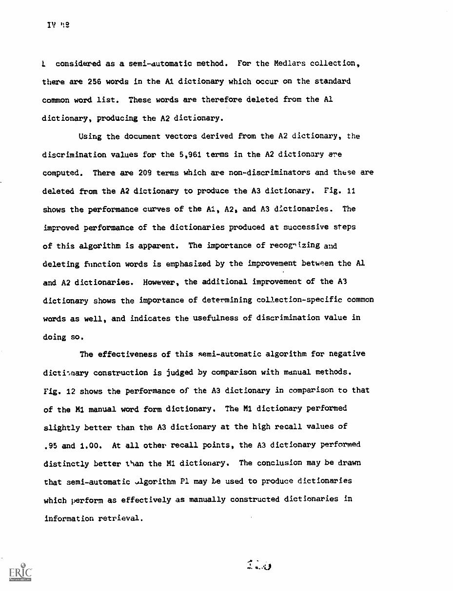
Iv

I considered as a semi-automatic method. For the Medlars collection,

there are 256 words in the Al dictionary which occur on the standard

common word list. These words are therefore deleted from the Al

dictionary, producing the A2 dictionary.

Using the document vectors derived from the A2 dictionary, the

discrimination values for the 5,961 terms in the A2 dictionary are

computed. There are 209 terms which are non-discriminators and these are

deleted from the A2 dictionary to produce the A3 dictionary. Fig. 11

shows the performance curves of the Al, A2, and A3 dictionaries. The

improved performance of the dictionaries produced at successive steps

of this algorithm is apparent. The importance of recognizing and

deleting function words is emphasized by the improvement between the Al

and A2 dictionaries. However, the additional improvement of the A3

dictionary shows the importance of determining collection-specific common

words as well, and indicates the usefulness of discrimination value in

doing so.

The effectiveness of this semi-automatic algorithm for negative

dictionary construction is judged by comparison with manual methods.

Fig. 12 shows the performance of the A3 dictionary in comparison to that

of the M1 manual word form dictionary. The M1 dictionary performed

slightly better than the A3 dictionary at the high recall values of

.95 and 1.00. At all other recall points, the A3 dictionary performed

distinctly better than the M1 dictionary. The conclusion may be drawn

that semi-automatic ..41gorithm P1 may be used to produce dictionaries

which perform as effectively as manually constructed dictionaries in

information retrieval.

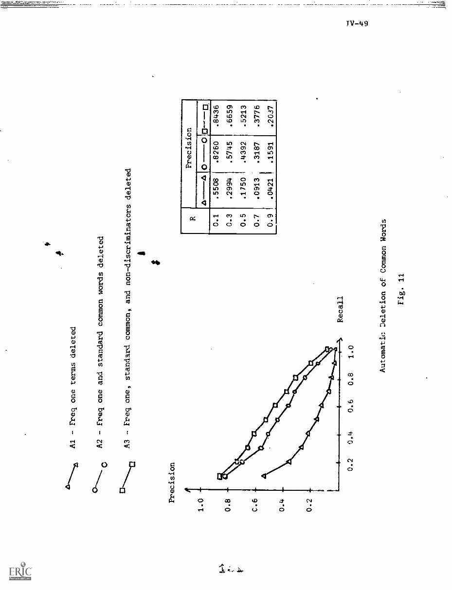
Precision

1.0

0.8

C.6

0.4

0.2

r

Al

Freq one terms deleted

A2 - Freq one and standard common words deleted

A3 - Freq one, standard common, and non-discriminators deleted

0.2

0.4

0.6

0.8

1.0

RPrecision

Att-----A0

C)Ch---C3

0.1

.5508

.8260

.8436

0.3

.2994

.5745

.6659

0.5

.1750

.4392

.5213

0.7

.0913

.3187

.3776

0.9

.0421

.1591

.2037

Automatic Deletion of Common Words

Fig. 11

1i

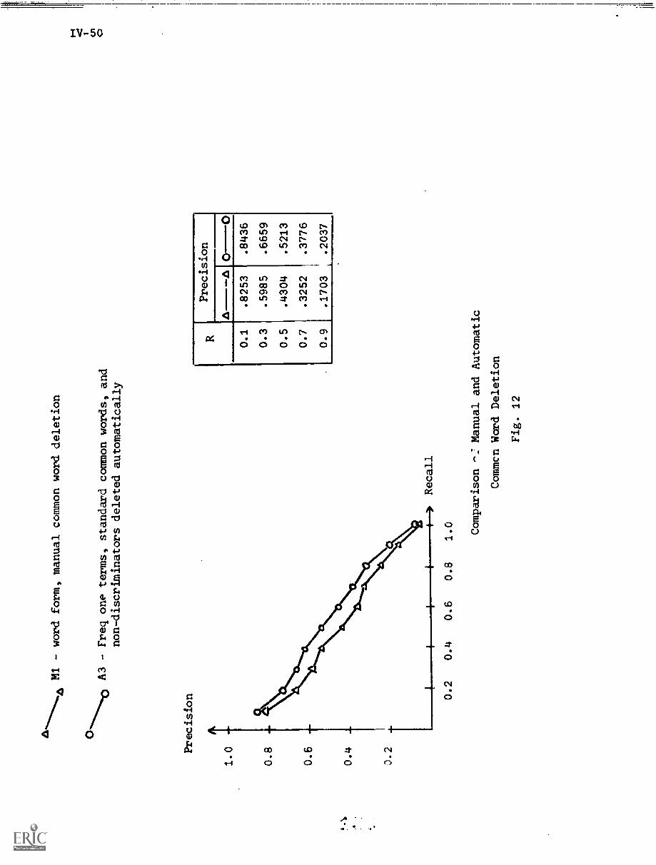
Oa

MI - word form, manual common word deletion

Precision

A1.0

0.8

0.6

0.4

3.2

1-4

1 VI

A3 - Freq one terms, standard common words, and

non-discriminators deleted automatically

0.2

0.4

0.6

e

0.8

> Recall

1.0

RPrecision

A---- A

0.----0

0.1

.8253

.8436

0.3

.5985

.6659

0.5

.4304

.5213

0.7

.3252

.3776

0.9

.1703

.2037

Comparison -2 Manual and Automatic

Commcn Word Deletion

Fig. 12

6.2.2 Algorithm P2

Algorithm P2, which is shown in Fig. 13, involves a single

automatic refinement of the Al dictionary. Testing of this algorithm

on the Medlars collection shows that it is not a useful algorithm

for automatic negative dictionary construction. The reason for this is

of interest, particularly as it provides insight into the discrimination

value function.

Computation of the discrimination values for each of the 6,226

terms in the Al dictionary shows that only 7 terms are non-discriminators.

These 7 non-discriminators each occur in over 73% of the documents, and

their total combined frequency of 37,875 accounts for over 25% of the total

occurrence of all terms in the collection. Thus, these are very high

frequency terms az... they have a dominating effect on the calculations

necessary to compute discrimination values. In a sense, the collection

is stable with respect to these seven terms. Deletion of any other

single term has only a very minor effect on the compactness of the

collection due to the dominance of these seven higli frequency terms. Since

the Al dictionarj contains no terms of very low frequency (i.e. frequency

one), the average frequency of all the terms is much higher than in the

N1 word list. This probably is what causes the poor results produced by

the P2 algorithm. It may be advisable then, to uelete very high frequency

terms to offset the effect of deleting very low frequency terms.

The results here show that when the average frequency of the terms

in a collection is greatly shifted, the discrimination values computed for

the remaining terms may not give a true indication of which terms are

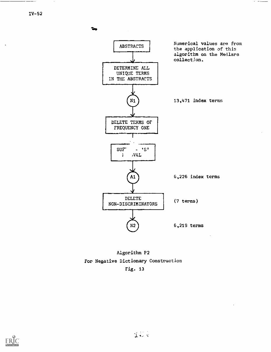
ABSTRACTS

DETERMINE ALLUNIQUE TERMS

IN THE ABSTRACTS

DELETE TERMS OFFREQUENCY ONE

SUF' - 'S'

i iVAL

DELETENON-DISCRIMINATORS

Numerical values are fromthe application of thisalgorithm on the Medlarscollection.

13,471 index terms

6,226 index terms

(7 terms)

6,219 terms

Algorithm P2

For Negative Dictionary Construction

Fig. 13

IV-53

non-discriminators in the original collection. The algorithm discussed

in the next section provSdes a solution to this difficulty.

6.2.3 Algorithm P3

Algorithm P3 for negative dictionary construction is shown in

Fig. 14. The Al dictionary is refined first ' deletion of all terms

occurring in 25% or more of the documents, as discussed in Section 5.1.2.

There are 30 such high frequency terms (see Table 2, Section 5.1.2) and

these are deleted from the Al dictionary to produce the A4 dictionary.

Discrimination values are computed for the 6,196 terms in the A4 dictionary.

Some of the terms which are non-discriminators, along with some of the best

discriminators in the collection are listed in Table 7. Altogether there

are 255 non-discriminators in the A4 dictionary, and these are deleted,

forming the A5 dictionary. It should be clear upon examination of each

step in Fig. 14 that the A5 dictionary is a fully automatically constructed

dictionary. Essentially three values are specified in executing this

algorithm. These are: the low frequency cutoff value, the high frequency

cutoff value, and the discrimination cutoff value. The choice of these

values has already been discussed; however, in the case of discrimination

cutoff value, several values are considered and tested in the next section.

Examination of the AS dictionary shows that there are 170 words in

it which are also on the standard common word list. It is intuitive that

deletion of these function words from the AS dictionary may increase its

level of performance in retrieval. To test this, the A6 dictionary is

constructed, by deleting all terms from the AS dictionary which occur on the

standard common word list.

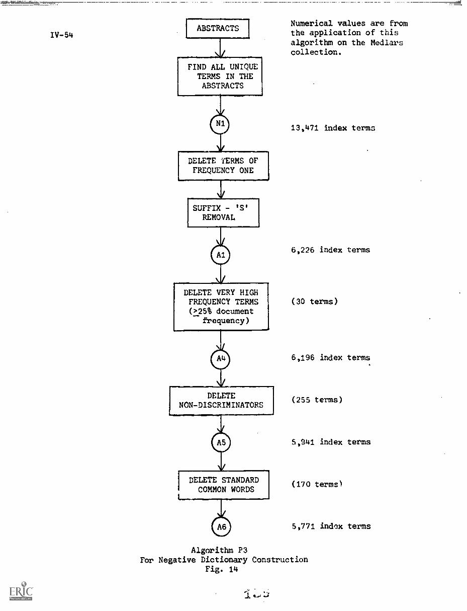
ABSTRACTS

FIND ALL UNIQUETERMS IN THEABSTRACTS

DELETE TERMS OFFREQUENCY ONE

SUFFIX - tStREMOVAL

DELETE VERY HIGHFREQUENCY TERMS(>25% document

frequency)

DELETENON-DISCRIMINATORS

I DELETE STANDARDCOMMON WORDS

Numerical values are fromthe application of thisalgorithm on the Medlarscollection.

13,471 index terms

6,226 index terms

(30 terms)

6,196 index terms

(255 terms)

5,941 index terms

(170 termsl

5,771 index terms

Algorithm P3For Negative Dictionary Construction

Fig. 14

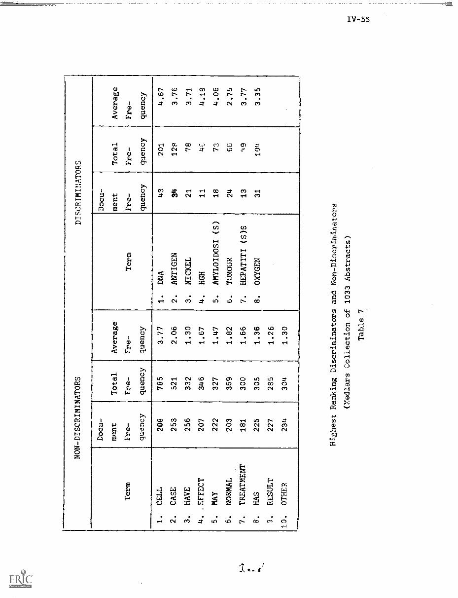
NON-DISCRIMINATORS

DISCRIMINATORS

Docu-

Docu-

ment

Total

Average

ment

Total

Average

Term

Fre-

Fre-

Fre-

Term

Fre-

Fre-

Fre-

quency

quency

quency

quency

quency

quency

1.

CELL

208

785

3.77

1.

DNA

43

201

4.67

2.

CASE

253

521

2.06

2.

ANTIGEN

34

129

3.76

3.

HAVE

256

332

1.30

3.

NICKEL

21

f78

3.71

4.

.EFFECT

207

346

1.67

4.

HGH

11

4C

4.18

5.

MAY

222

327

1.47

5.

AMYLOIDOSI (S)

18

73

4.06

6.

NORMAL

203

369

1.82

6.

TUMOUR

24

66

2.75

7.

TREATMENT

181

300

1.66

7.

HEPATITI (S)S

13

qg

3.77

8.

HAS

225

305

1.36

8.

OXYGEN

31

104

3.35

3.

RESULT

227

285

1.26

10.

OTHER

234

304

1.30

Highest Ranking Discriminators and Non-Discriminators

(Medlars Collection of 1033 Abstracts)

1

Table 7

tn u,

The performance curves for the Al, A4, A5, and A6 dictionaries

are given in Fig. 15. Possibly the most surprising result is the

performance of the A4 dictionary compared to the Al dictionary, as these

dictionaries differed by only 30 high frequency terms. The A4 dictionary

represents the performance which is obtained by simple deletion of very high

and very low frequency terms. The deletion of non-discriminators to form

the AS dictionary results in another significant increase in performance

level. However, no significant gain results from further refinement of

the AS to produce the A6 dictionary. Thus, it may be concluded that the

final semi-automatic step of deleting standard common words is not warranted.

The suggested P3 algorithm is therefore concluded with the formation of the

A5 dictionary.

The result of this algorithm P3 (the A5 dictionary) is compared to

the results of the algorithm P1 (the A3 dictionary) and the manual algorithm

(the M1 dictionary) in Fig. 16. The performance of the A5 dictionary is

distinctly better than that of the Ml dictionary, and slightly improved from

the performance of the A3 dictionary. The fully automatic algorithm for

negative dictionary construction, P3, is therefore superior to either the

manual algorithms now in use, or the semi-automatic algorithm, P1.

6.2.4 Algorithm P4

In Section 5.2.1 the idea of a discrimination cutoff value, Dc was

suggested, and the idea of the classification of terms into three areas;

non-discriminators, poor discriminators, and good discriminators, was discussed.

In the previous algorithms, only non-discriminators were deleted, that is, a

Al - Freq one terms deleted

44

Freq one and high freq term: deleted

AS - Freq one, high freq, and non-iiscriminators deleted

A6 - Freq one, high freq, non- discriminators, and

standard common words deletes'

Precision

A

1.0

0.2

0.4

0.6

0.8

1.0

RPrecision

46-1

1-1

)iS

-60-

00.1

.5508

.8264

.8304

.8415

0.2

.2994

.5779

.6689

.6716

0.5

.1750

.4153

.5332

.5246

0.7

.0913

.3026

.3717

.3768

0.9

.0421

.1501

.2022

.2023

Automatic Deletion of Common Words

Fig. 15

M1 - Word form, manual common word deletion

A3 - Automatic deletion of freq one terms,

standard common words,

co

and non-discriminators

411...""41110

AS - Automatic deletion of freq one terms, high freq terms,

and

non-discriminators

Precision

1..0 -

0.8 -

0.6

0.4

0.2

# >

Recall

0.2

0.4

0.6

0.8

1.0

Comparison of Manual and Automatic

Common Word Deletion

Fig. 16

RPrecision

0-0

kr-6

1111----

0.1

.8253

.8436

.8304

0.3

.5985

.6659

.6689

0.5

.4304

.5213

.5332

0.7

.3252

.3776

.3717

0.9

.1703

.2037

.2022

discrimination cutoff value of zero was chosen. Using the P4 algorithm

shown in Fig. 17 the effect of deleting poor discriminators in addition

to non - discriminators is tested. This algorithm is identical to the P3

algorithm discussed in the last section in its construction of the AS

dictionary. In the P4 algorithm, however, groups of terms are deleted

from the A5 dictionary in increasing order of discrimination value, that is,

the discrimination cutoff value is graduallj increased.

Table 8 shows the performance values (iii) for the dictionaries

resulting from deletion of an increasing number of terms. These diction-

aries are listed in decreasing order of the number of terms remaining in

the dictionary (i.e. the number of terms to be used in indexing the doc-

uments and queries). Thus, the AS (5940) is the original A5 dictionary

with all 5940 terms retained, while the A5 (250) is the A5 dictionary with

only the 250 best discriminators remaining. The results shown in Table 8

are displayed graphically in Fig. 18. The results for the Al dictionary

are included in both Table 8 and Fig. 18 for purposes of comparison.

Analysis of Fig. 18 shows that in fact the classification of terms

as good discriminators, poor discriminators, and non-discriminators is

reasonable. The points at the right end of Fig. 18 show the large

improvement in performance which occurs upon the deletion of non-discrim-

inators. However, moving across the graphs from right to left, very

(iii) These measures are described in 116].

ABSTRACTS

FIND ALL UNIQUE TERMS IN THE ABSTRACTS

DELETE TERMS OF FREQUENCY ONE

SUFFIX - 'S' REMOVAL

DELETE VERY HIGH FREQUENCY TERMS

COMPUTE DISCRIMINATION VALUE FOR ALL TERMS

DELETE NON-DISCRIMINATORS

FSET D =0

INCREASE D

DELETE ALL TERMS i FOR WHICH D.<Dc

Deletion of poordiscriminators,for increasingdiscrimination

STOP cutoff values.

Algorithm P4For Negative Dictionary Construction

Fig. 17

IV-61

DICTIONARY

(TERMS

RETAINED)

NORM

RECALL

NORM

PRECISION

NORM

RECALL

NORM

PRECISION

Al (6225) .7265 .5021 .0606 .4991

AS (5940) .7841 .7260 .1450 .6594

AS (5709) .7819 ./253 .1448 .6591

AS (5459) .7819 .7250 .1440 .6580

A5 (5209) .7819 .7250 .1441 .6581

AS (4960) .7819 .7245 .1439 .6575

A5 (4712) .7819 .7245 .1439 .5:-.76

AS (4212) .7800 .7228 .1437 .6562

A5 (3715) .7786 .7213 .1439 .6552

A5 (2717) .7741 .7212 .1430 .6544

AS (2000) .7654 .7149 .1337 .6500

AS (1500) .7625 .7135 .1343 .6490

A5 (1000) .7525 .7066 .1192 .6425

AS (500) .7337 .6466 .0982 .5883

A5 (250) .6586 .4353 .0640 .4610

Retrieval Performance UponSuccessive Reduction of Index Terms byTncreasing Discrimination Cutoff Value


Table 8

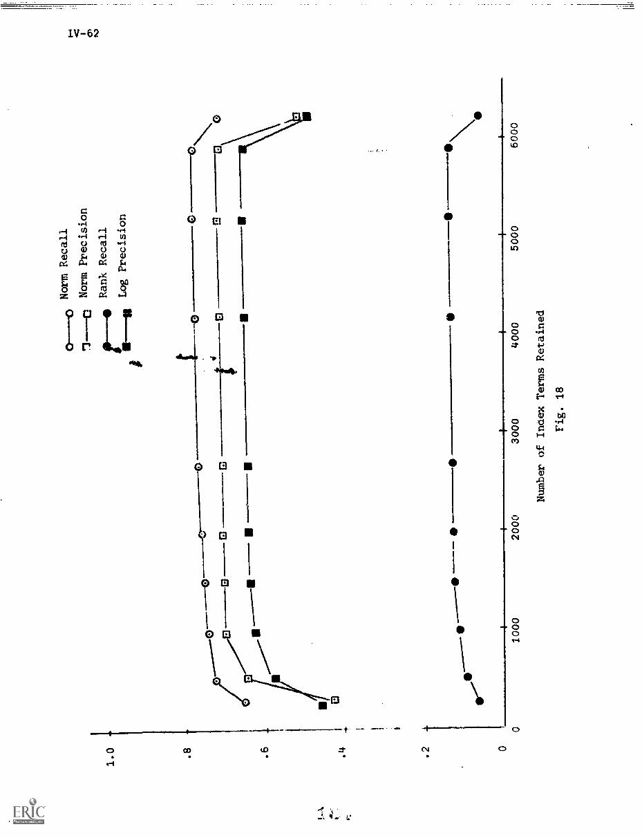
1.0 .8

.6 .4 .2 0

0

0

Norm Recall

Norm Precision

Rank Recall

Log Precision

1000

2000

3000

4000

Number of Inaex Terms Retained

Fig. 18

5000

6000

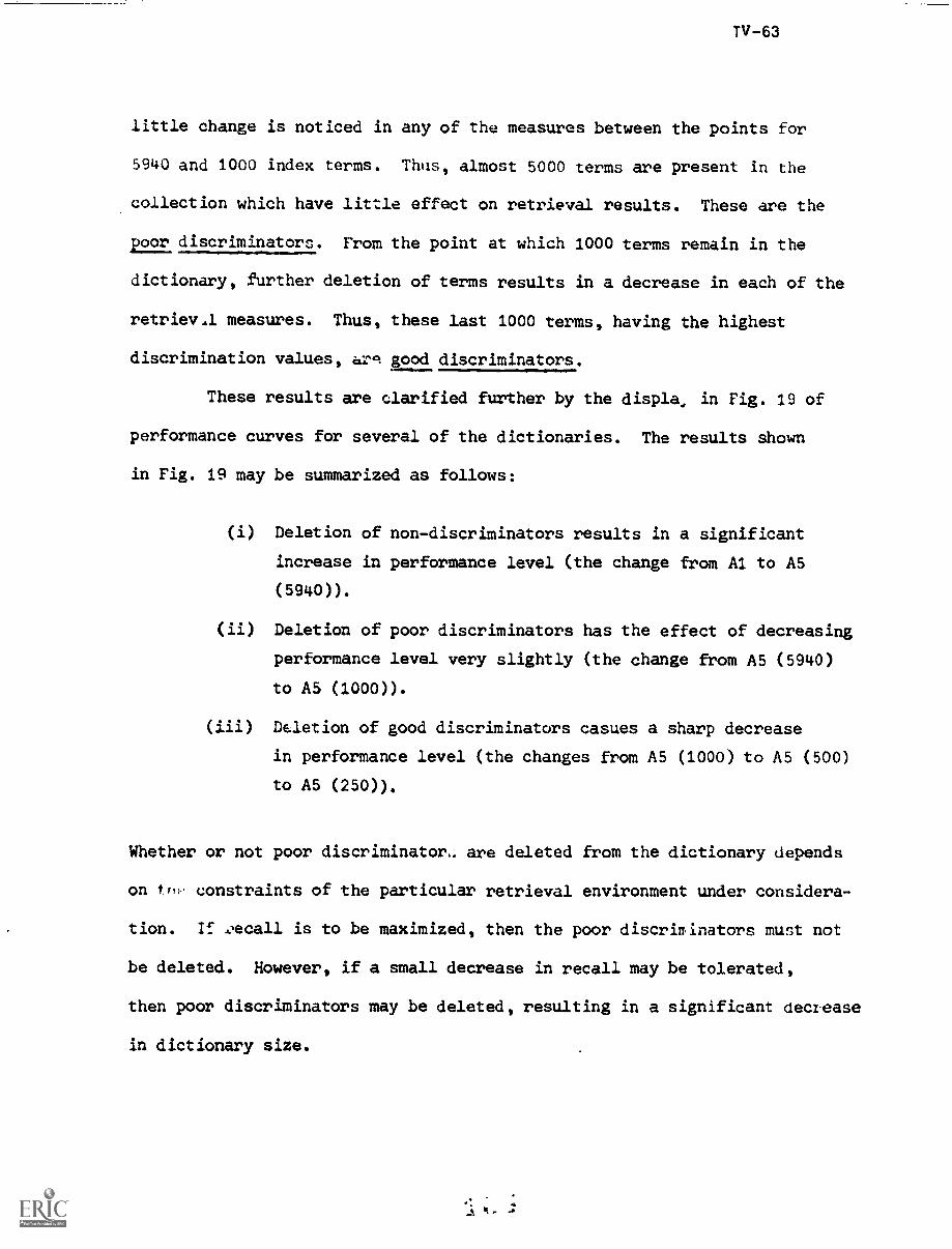
little change is noticed in any of the measures between the points for

5940 and 1000 index terms. Thus, almost 5000 terms are present in the

collection which have little effect on retrieval results. These are the

poor discriminators. From the point at which 1000 terms remain in the

dictionary, further deletion of terms results in a decrease in each of the

retrieval measures. Thus, these last 1000 terms, having the highest

discrimination values, arg good discriminators.

These results are clarified further by the displa, in Fig. 19 of

performance curves for several of the dictionaries. The results shown

in Fig. 19 may be summarized as follows:

(i) Deletion of non-discriminators results in a significant

increase in performance level (the change from Al to AS

(5940)).

(ii) Deletion of poor discriminators has the effect of decreasing

performance level very slightly (the change from AS (5940)

to AS (1000)).

(iii) Deletion of good discriminators casues a sharp decrease

in performance level (the changes from A5 (1000) to A5 (500)

to A5 (250)).

Whether or not poor discriminator- are deleted from the dictionary depends

on tr'- constraints of the particular retrieval environment under considera-

tion. If A.,ecall is to be maximized, then the poor discrininators must not

be deleted. However, if a small decrease in recall may be tolerated,

then poor discriminators may be deleted, resulting in a significant decrease

in dictionary size.

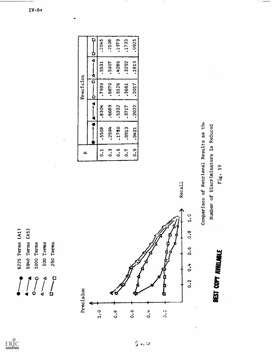
Precision

1.0

0.8

0.6

0.4

3G

6225 Terms (A1)

5940 Terms (A5)

1000 Terms

500 Terms

250 Terms

0.2

0.4

0.6

0.8

1.0

BE

ST C

OPY

AV

AIL

AB

LE

e

RPrecision

0-0

kr-i

i0.1

.5508

.8304

.7939

.5531

.2145

0.3

.2994

.6689

.6670

.5307

.2108

0.5

.1750

.5332

.5126

.4286

.1979

0.7

.0913

.3717

.3661

.3292

.1793

0.9

.0421

.2022

.2017

.1813

.0925

Recall

Comparison of Retrieval Results as the

Number of Discriminators is Reduced

Fig. 19

6.2.5 Conclusions and Verification

On the basis of the results presented, it is concluded that fully

automatic methods may be used for constructing negative dictionaries

which provide for a higher level of retrieval performance than do standard

manual methods. In particular, the P4 algorithm is an efficient and

effective algorithm for use in negative dictionary construction. In

addition, it has been found that a dictionary of index terms may be greatly

reduced in size by deletion of poor discriminators without affecting

retrieval performance significantly.

Since these conclusions are based on tests performed on a single

collection, it is worthwhile to verify the results using another document

collection. The Ophthalmology collection is used, with results being

compared for three manually constructed dictionaries and one automatically

constructed dictionary. The manually constructed dictimaries are a word

form dictionary, a word stem dictionary, and a thesaurus. The automatically

constructed dictionary is the AS dictionary, constructed according to

algorithm P4. There are 3762 terms (discriminators) in this A5 dictionary.

Since there is adequate space available in the present utility for

handling this dictionary, no deletion of poor discriminators is necessary.

The performance of the manual word form, manual word stem, manual

thesaurus, and automatic A5 dictionaries is shown in Fig. 20. The A5

dictionary performs better at all recall values than each of the manually

constructed dictionaries. Thus, the conclusion that automatic negative

dictionary construction methods are effective, is substantiated.

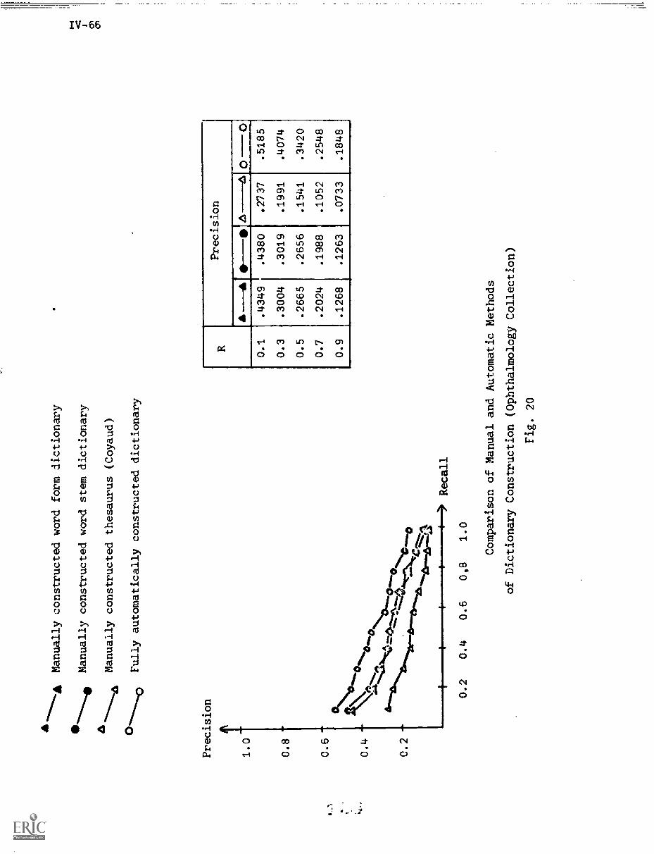
"'"- -'111

Manually constructed


A--...110)


0,0

Precision

1.0

0.8

C.6

0.4

0.2

word form dictionary

word stem dictionary

thesaurus (Coyaud)

Fully automatically constructed dictionary

k1) "**b°.°40

0.2

0.4

0.6

0,8

1.0

Recall

RPrecision

----61.---1,

A -----160-0

0.1

.4349

.4380

.2737

.5185

0.3

.3004

.3019

.1991

.4074

0.5

.2665

.2656

.1541

.3420

0.7

.2024

.1988

.1052

.2548

0.9

.1268

.1263

.0733

.1848

Comparison of Manual and Automatic Methods

of Dictionary Construction (Ophthalmology Collection)

Fig. 20

7. Summary and Conclusions

Negative dictionary construction algorithms are described in this

study that use manual, semi-automatic, and fully automatic methods to

determine common words. The intention is to show that dictionaries

constructed by fully automatic methods perform equivalent to or better

than dictionaries formed manually. Experimental evidence from two

document collections indicates that automatic negative dictionary con-

struction methods are more effective than standard manual negative

dictionary construction methods, and are therefore to be preferred.

In addition to the general results regarding negative dictionary

construction, important results are found regarding the discrimination

value function. The usefulness of discrimination value is verified both

theoretically and experimentally, and its properties are more fully

explored. The relationships of words in a collection are examined, in

terms of frequency, distribution, and discrimination value. Finally,

experimental results are given which show that dictionary size may be

greatly reduced retaining only good discriminators, while maintaining

retrieval performance.

References

[1] H.P. Luhn, IBM J. Res. Develop. 1, No. 4, 1957..

121 "Potentialities of Auto-Encoding of ScientificLiterature", IBM Res. Cent. Rep. No. RC-101, 1959.

[31 G. Salton, "Automatic Text Analysis", Science, Vol. 168,April 1970.

[4] C.W. Cleverdon and E.M. Keen, "Factors Determining thePerformance of Indexing Systems", Aslib Cranfield (England)Res. Proj. Rep. Vols. 1 and 2, 1966.

[5] G. Salton, "A Comparison Between Manual and Automatic IndexingMethods", American Documentation, Vol. 20, No. 1, January 1969.

[6] D. Bergmark, "The Effect of Common Words on Retrieval Performance",Scientific Report No. ISR-18 to the National Science Foundationand to the National Library of Medicine, Department of ComputerScience, Cornell University, October, 1970.

171 D. Williamson, R. Williamson, and M. Lesk, "The Cornell Implementationof the SMART System", Report No. ISR-16 to the National ScienceFoundation, Department of Computer Science, Cornell University,September 1969.

[8] G. Salton, editor, The SMART Retrieval System (Prentice Hall,New Jersey, 1971).

(9] , et al., "Information Storage and Retrieval", Departmentof Computer Science, Cornell University, Rep. Nos. ISR-11, ISR-12,ISR-13, ISR-14, ISR-15, ISR-16, ISR-17, ISR-18, ISR-19 to theNational Science Foundation (1966-1971).

[10] J.J. Rocchio, "Performance Indices for Document Retrieval Systems",Report No. ISR-8 to the National Science Foundation, HarvardUniversity, December 1964.

[11] P.K.T. Vaswani and J.B. Cameron, "Statistical Word Associations andTheir Use in Document Indexing and Retrieval", National PhysicalLaboratory, Com. Sci. 42, April 1970.

[12] G. Salton and M.E. Lesk, "Information Analysis and DictionaryConstruction", Report No. ISR-11 to the National Science Foundation,Department of Computer Science, Cornell University, June 1966.

[13] G. Salton, Automatic Information Organization and Retrieval

(McGraw-Hill, New York, 1968).

(14] J. Aste-Tonsman and K. Bonwit, "Negative Dictionaries",Report No. ISR-18 to the National Science Foundation andto the National Library of Medicine, Department of ComputerScience, Cornell University, October, 1970.

[15] C. Yu and A. Wong, "Modification of the Document Space Similarity",Project Report, Department of Computer Science, Cornell University,June 1971.

[161 G. Salton and M.E. Lesk, "Computer Evaluation of Indexing andText Processing", Report No. ISR-12 to the National ScienceFoundation, Department of Computer Science, Cornell University,June, 1967.

V-1

Dynamically versus Statically Obtained

Information Values

A. van der Meulen

Abstract

An evaluation is made of the effectiveness of dynamically

updated parameters, known as "information values", and a comparison

is made with a statistical approach in which parameter values are

computed once rather than being continually changed.

Information values are quantities which may be assigned to

dictionary items in order to reflect the descriptive power of the

various keywords. The main objective of the usage of tnformation

values is the improvement of system performance by taking into

account the usefulness of the index terms in content analysis.

Simultaneously a means of control over the index vocabulary is

obtained, since an information value displays the quality of

its associated keyword.

The procedure of assigning information values is based on

the philosophy that keywords which help to retrieve relevant

documents are more valuable than those which participate in

retrieving nonrelevant documents. In particular the utilization

of user relevancy decisions is examined in two different ways.

First, the collected data reflecting the retrieval history of a

system is u;ed to compute information values in a rather statistical

J.

V-2

way. Second, each retrieval result is used on its own to change and

update the current information values.

1. Introduction

The investigations described in t%is report may be regarded as

an extension of earlier work done with information values [1]. It is

suggested there that a realistic dynamic updating be carried out rather

than the simplified simulation used earlier which will be referred as

the "static" updating approach. The process of using the retrieval

results of each previous search to improve the results of the next will

be called dynamic updating.

A known example of dynamic system updating is the "dynamic

document modification procedure". [2] Imperfect document indexes can be

improved by utilizing the retrieval results as evaluated by the user

(feedback). After each search the indexes of the retrieved documents

are slightly changed in such a way that a new user who wants similar

tnformatiov will find his relevant documents ranked higher and his

retrieved nonrelevant documents ranked lower. One might wonder whether

this process of continuous index modifications is stable in that finally,

after intensive system use, the system performance reaches an optimum;

this question has not been investigated yet for dynamic document space

modification.

Another type of dynamic updating is proposed for the so-called

information values, quantities which give a numeric value for the quality

(discrimination powei) of the identifiers (keywords) used in the indexing

process. In previous experiments [1] with these value a statistical

V-3

approach is used for practical reasons. It differs from the dynamic

strategy in that the retrieval results are stored for a whole set

of queries from which in turn the information values are computed.

In tha dynamic approach, however, the retrieval results for each

individual query are affected by the results obtained for the

previous one, since the updating occurs continuously (after each

search).

2. Information Values and their Derivation

A. The Concept

In regular relevance feedback, the user judges the retrieved

documents as either relevant or not relevant to his query. This

information is then fed back into the system and used to redefine

the query for subsequent -iearch iterations. These relevance

judgments may also be used automatically to construct a weighted

dictionary, as is explained in the next section.

Specifically, with each identifier one can associate a

numerical value, herein referred to as the information value.

This information value is initially set equal to one, and is changed

only when the corresponding concept occurs both in the query and in

a retrieved document. The information value is then increased if

that retrieved document is declared relevant, or else it is

decreased. In the indexing process, these information values may

be used in addition to the existing identifier frequency weights;

that is, each vector-weight is formed as the product of both.

V-4

This will result in document and query vectors in which the prominent

descriptors are emphasized, while the lesser ones are suppressed.

The whole procedure is simple to implement. An attempt is thus

made to determine whether the process leads to an improvement in system

performance that is, a lifting of the recall-precision curve.

B. The Updating Method

Initially, the information value of each concept is set equal

to one. From that point the value is increased (or decreased) each

time the corresponding concept co-occurs both in a query and the

relevant (or nonrelevant) documents retrieved in response to that query.

The specific increment-decrement function chosen is the one

proposed by Sage 13], herein referred to as the "sine-function" because

of its resemblance to the regular sine. If i is an identifier which

co-occurs both in a query and in its associated retrieved document, define:

v. = the information value of identifier i1

(initially set equal to one)

v. *= the information value of identifier i1

after updating

x.1

= arc sin (v.1- 1), the transposed information value.

Then, v.1

= 1 + sin (x.1 )

and similarly v.* is calculated by

v.*= 1 + sin (x.1+ Ax.) (1)

1

where Ax is a function of the old information value, calculated as

w/2 1)(11

Ax.(2)

where C is an arbitrary constant, set eqaul to 8 in these experiments.

V-5

Axi is added in equation (1) if the retrieved document

containing term i is judged relevant by the user; or it is

subtracted in the information value calculation if the corresponding

document is judged nonrelevant.

C. Dynamic versus Static Updating

The information values are increased as long as their

identifiers occur in relevant retrieved documents, but are decreased

in response to nonrelevant retrieval. Each new query is transformed

by the weighted dictiondry in the following way:

Q = (v1w1, v2w2

, o.., vnwn) (3)

where Idi is the regular frequency weight of identifier i and vi

the corresponding information value. Notice also that new incoming

documents will be indexed in a similar way, using the weighted dictionary.

An intuitive explanation for the existen of an equilibrium

value follows. Consider again identifier i and the corresponding

information value v.. The similarity measure between the query

and the document vector is computed as the cosine of the angle between

them.Asaresultofeachrelevantretrievalv.is updated.

Consequently the term yields a greater influence on the direction

of the corresponding vector in the index-space. Since identifier

is emphasized, more documents containing that identifies aoe

retrieved when a larger correlation coefficient is oitained.

As long as this promoted identifier is successful in retrieving

relevant documents, the corresponding information value will he

increased. If, however, nonrelevant documents are retrieved because

of an excessively high value for a given concept, then the self-

correcting feedback mechanism comes into play and the information value

V-6

will be set back agaii.

The assumption is that in this way each identifier eventually

achieves an equilibrium veue which is characteristic of its descriptive

power.

The mechanism described above defines a dynamic dictionary update

procedure, wherein the dictionary is modified after each query search.

In thi-i situation each query is indexed only after the dictionary has

been altered in response to all previously searched queries.

The first experiment with information values uses labor saving

batching techniques. The document collection is searched by a batch of

queries indexed with the unmodified dictionary. Sufficient information

is stored to allow updating the information values on the basis of the

two highest ranked retrieved documents associated with each query.

This procedure, however, may exaggerate the information values

obtained, since the self-correcting capacity of the feedback process

described earlier is never invoked. Specifically, a good or bad term

will be continually changed based on its retrieval effectiveness using

its initial information value, rather than its retrieval effectiveness

using its perhaps modified information value. Nevertheless, since a

relatively small number of updates normally occurs, it seems plausible

that these values may still give a good indication of the information

value of the associated identifiers.

It is interesting to draw a comparison between dynamic and

static updating; the more realistic dynamic approach is simulated within

the SMART system. Details of the dynamic experiments are described in

the next section.

V-7

3. The Experiments

Information values ar-e changed according to an algorithm which

takes into account the co-occurrence of concepts in he retrieved

documents and the associated query. Information values are increased

if the retrieved documents are relevant and decreased otherwise.

The dynamic updating is done immediately after each query'of the

query update collection has been searched. Updated information

values are used in indexing the next query, and the retrieval results

again modify the information values.

For the purpose of comparing the static and the dynamic

approach, two dynamic experiments are carried out as follows:

a) Information values are dynamically obtained using 200

queries belonging to the Cranfield 1400th document

collection. The information values obtained are then

used to reindex a test collection of 25 queries. This

query test collection is run as a batch, and retrieval

results obtained will therefore be called semi-dynamic.

b) The fully dynamic approach is used in Ye'lich the 25

queries of the test collection are also run dynamically

in the same way as the queries of the update collection.

4. The Results

Before discussing the comparative results of the dynamic

versus the static approach, the latter will be examined first.

Results obtained earlier with the static approach were not

satisfactory [1] and after similar experiments have been done with

so-called utility values f4], using the same updating function,

V-8

the reasons for the failure become clearer. They are the following:

if Ile obviously wrong choice of a factor in the updating

algorithm which produces increment and decrement steps

that are too large.

b) The use of nonoptimally chose, initial (starting)

information values. Instead of initializing all informa-

tion values equal to one (reducing equation (3) to only

frequency weights) one could have taken advantage of the

available discrimination values for this collection. By

using the discrimination values as starting values for

the dynamic information values, a better system performance

can immediately be obtained. In this case it will be

nece. .ary to scale the discrimination values in such a way

that the average equals 1 (see c).

c) No provision is made for balancing. Balancing means keeping

the average information value equal to 1 in order not to

promote or suppress terms not yet updated. In the experiments

done with utility values this is shown to be e critical factor.

d) The query test collection was not chosen randomly and after

the earlier experiments [1] were done, it was found that

the test collection was related to one specific subset of

the document collection. This means that keywords specific

for that part!xolar field are not likely to be updated by

the updatliAx q10,xy collection which concerns other topics.

Since the same defects have to be valid for the dynamic strategy,

one may not expect an absolute improvement of the system performance,

but rather a relative improvement over the statistically obtained Informa-

tion va2uel is lnticipated.

V-9

The results of the present experiment A (Fig. 1) indicate

that running the test collection in a batch using informatior

values dynamically obtained from the updating collection gives

better results than when the static values are used. The

improvement is slight though, because the test collection has

unfortunately not been chosen randomly. Since the query test collection

is directed to a specific field and thus utilizes keywords describing

this field, the associated information values are not likely to have

been updated by the update collection in which they did not occur.

Much more interesting therefore is experiment B, where the

query test collection itself is used in a dynamic way (Fig. 2).

Here the concepts of each subsequent query are updated by the previous

one.

If the dynamic approach really works as it should, that is,

if the good properties of the feedback mechanism mentioned earlier are

utilized, this experiment should show clearly the dynamic effects.

Fig. 2 shows indeed that system performance is improved considerably

compared with both the static and the semi-dynamic rase.

5. Conclusim

For a given collection and a given updating algorithm the

static and dynamic updating strategy have been compared. The static

information values were obtained in an earlier project and did not

perform very well, partly because of defects in the updating algorithm

discovered later. In order to draw a fair comparison between statically

Precision

0.5

0.4

0.3

%.1111t.1.1 W:Lh

System performance without using information values.

.....

System performance using dynamically obtainedinformation values used in a semi-dynamic strategy.

0.2

0.l

11

System performance 1...using statically ,

..

obtained information '.,..........values. ".

NsI..

Comparion of statically and semi-dynamically

obtained information valut.gi

Fig. 1

Stroaft....

111140...

O. 0.4 .0Renal,

Precision

0.5

System performance using dynamically obtained informationvalues.

0.2

0.1

System performance without using informationvalues.

System performance 'Nousirn semi-dynamicallyobtained information values.

Comparison of !;4.mi-dyndmif:aliy dud fully

dynamically obtained information vdlueti

Fig. 2

0. 0.4 0.61

0.8

V-12

and dynamically obtained information values all conditions are kept the

same.

The results show that in the two dynamic experiments carried out,

dynamic updating is superior to static updating. The fLost experiment

is a mixture of dynamic and static updating in that the testcollect is

processed as a batch; the second experiment is fully dynamic and the

results of this experiment show in particular a considerable improvement

over the static strategy.

V-13

References

[1] A. Wong, R. Peck, and A. van der Meulen, An Adaptive Dictionaryin a Feedback Environment, Report No. ISR-21, Dept. ofComputer Science, Cornell University, December 1972.

[2] M.D. Kerchner, Dynamic Document Processing in ClusteredCollections, Report No. ISR -19 to the National ScienceFoundation, Information Storage and Retrieval, Department ofComputer Science, Cornell University, Tscember 1971.

[3] C.R. Sage, R.R. Anderson, and P.F. Fitzwater, AdaptiveInformation Dissimination, American Documentation, Vol. 15,No. 3, July 1965.

[4] A. Wong and A. van der Meulen, The Use of Utility Valuesfor Dynamic Query-Document Retrieval, Project Report,Department of Computer Science, Cornell University Fali 1972.

VI-1

Automatic Thesaurus Construction Through The

Use of Pie- Defined Relevance Judgments

Kenneth Welles

Aba tract

A method for totally automatic construction of thesauri

is proposed which relies upon accumulation of match-mis-match

influences to converge. :results so far, while not conclusive,

are promising.

1. Introduction

It is now an accepted fact that the use of term class-

ification thesauri improve the operation of information storage

and retrieval systems. There are many different approaches to

the construcion of such a thesaurus, ranging from completely

by hand to totally automatic. This paper deals with a proposed

system of creating a thesaurus totally automatically.

Automatic term classification algorithms have mainly

centered on two areas, term co-occurrence as an indication of

synonymy, and predetermined relevance judgments as a source of

information about synonymy. My work deals with the latter

aspect. The basis for such a system is a set of documents, a

set of requests, and a .iet of judgments as to which documents

should and should not be retrieved by each request. From this

VI-2

information, the machine can construct a set of classifications of terms

(synonym classes) which improve the retrieval effectiveness of the

given queries substantially. The rationale behind such a construction

is this: if the set of requests was comprehensive, then any similar

requests presented in the future will also benefit from the resulting

thesaurus.

The starting point in this area is a paper by Jackson of the

construction of precisely such a system. Li] A program was written to

the specifications of Jackson's paper. Early in the project it was

discovered that a minimal collection (about 80% of the ADI collection

of documents and queries) requires more than 30 minutes to run on the

360-65 without attaining the first of several iterations. This is

obviously an impractical program to implement.

Examination of the program shows that a substantial portion of

the run time is spent on constructing, maintaining, and observing what

Jackson calls "degeneracy conditions", which assure convergence. A

different approach is proposed in this paper. In order to decide which

terms are to be considered synonymous, each pair of terms is examined.

If these two terms are considered synonymous, then any query-document

pair where one term is in the query and the other term is in the

document, will have this term pair counted as a match. This increases

the number of matching terms in this query-document pair, and so

increases the calculated matching coefficient for this query-document

pair. If the que. y-locument pair is defined as relevant, then this

increase in matc.Aing is good. If the query-document pair is defined as

not relevant, then this increase is bad (for the purposes of constructing

VI-3

d thesaurus which causes the calculated matches to agree with the

defined relevancies). If the amount of good outweights the bad,

the pair is considered synonymous, and when all such synonym pairs

have been considered, the query-document --,et is re-examined for

the next iteration. Hopefully, after several iterations, the set

of synonym pairs will stabilize in a way that gives the calculated

relevance of the query-document set closest resemblance to the

defined relevance set.

2. Terminology c.od Definitions

Before continuing with the technical aspects of the proposed

program, some definitions are necessary. There are four possible

term classes, and for any given query, document and term, the term

falls into one of these classes (see figure 1). If the term is not

nresent in either the query or the document, it is class A. If the

term is in the query, but not in the document, it is in class B. If

the term is in the document but not in the query, it is ir. class C.

Finally, if the term is in both query and document, then the term is

in class D.

All correlations betwee4 queries and documents aro calculated

during each program iteration (since the correlations change from Gne

iteration to the next). For each query, the correlation values of the

defined relevant and defined not relevant documents are considered.

The lowest correlation value of a defined relevant document and the

highest correlation value of a defined not relevant document are

determined. A value midway between these values is taken as the

VI-14

match value (see figure 2). If any query-document pair exhibits a

correlation higher than this match value, then this pair is said to

be calculated relevant. If the correlation is less than or equal to

this match value, the pair is said to be calculated not relevant.

Each query-document pair falls into one of four classes (see

figure 3). If the pair is calculated not relevant and defined not

relevant (by the initial relevance data), then it is in class R. If

the pair is calculated relevant, but defined not relevant, it is in

class S. If the pair is calculated not relevant, but defth e's. relevant,

it is in class T. If the pair is defined and calculated relevant, it

is in class U.

If all the query-document pairs are either class R or class U,

then the calculated matches all correspond to the defined matches and

no further modifications are needed. However, if there exist query-

document pairs in classes S or T, the term space must be modified to

cause calculations to agree with definitions.

The cosine correlation is used to calculate the match between a

query and document. If the possibility of synonyms is ignored, this

value becomes:

D

B+C+D

where B, C and D are the number cf terms in classes B, C and D

respectively. However, if any term in class b is a synonym of any term in

class C, then this pair of terms is considered a match, and is counted as

a class D term instead of a class B term. All term pairs with one class B

term and one class C term are considered "potential synonym pairs" for this

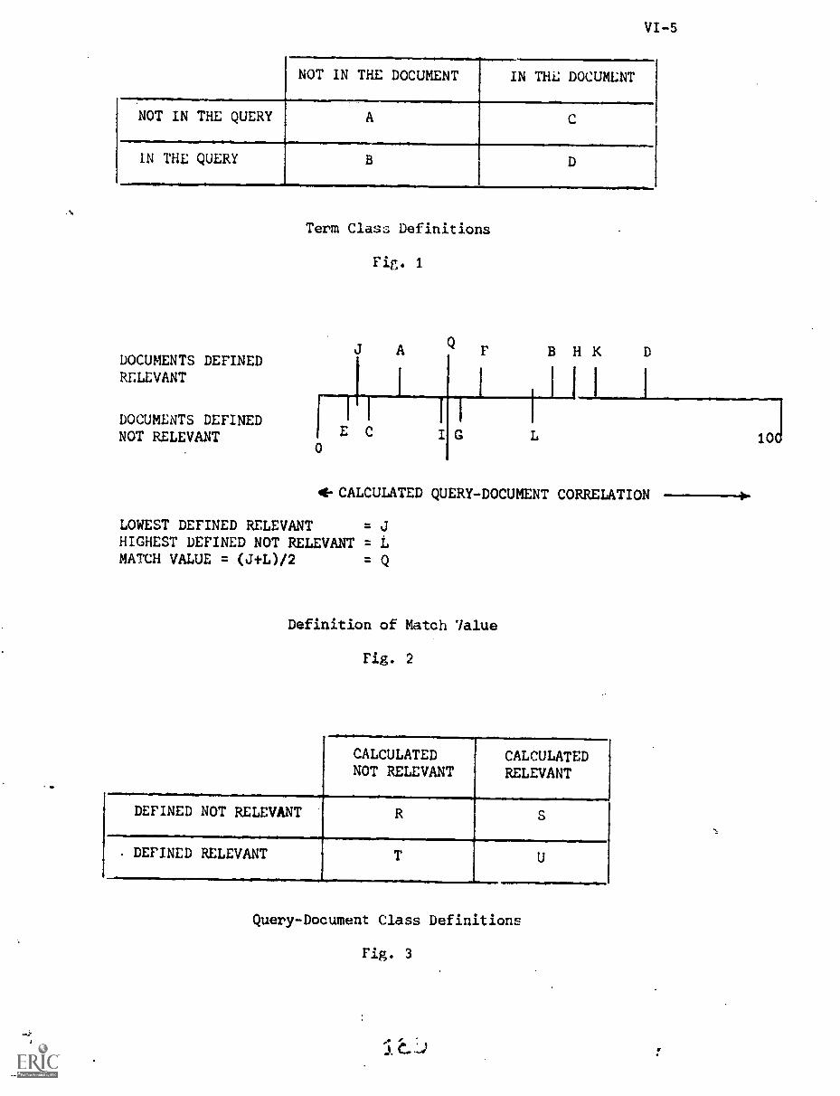
VI-5

NOT IN THE DOCUMENT IN THE DOCUMENT

NOT IN THE QUERY A

IN THE QUERY B D

DOCUMENTS DEFINEDRELEVANT

DOCUMENTS DEFINEDNOT RELEVANT

Term Class Definitions

Fig. 1

A QF B H K

E C I

4E-CALCULATED QUERY-DOCUMENT CORRELATION

LOWEST DEFINED RELEVANTHIGHEST DEFINED NOT RELEVANT =MATCH VALUE = (J+L)/2 = Q

Definition of Match 7alue

Fig. 2

CALCULATEDNOT RELEVANT

CALCULATEDRELEVANT

DEFINED NOT RELEVANT..

R S

DEFINED RELEVANT T U

Query-Document Class Definitions

Fig. 3

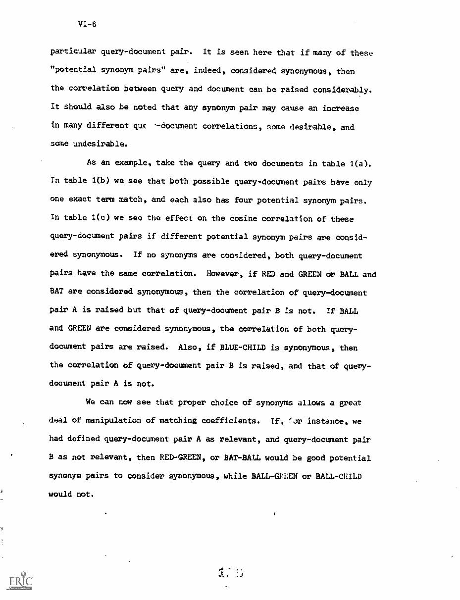
VI-6

particular query-document pair. It is seen here that if many of these

"potential synonym pairs" are, indeed, considered synonymous, then

the correlation between query and document can be raised considerably.

It should also be noted that any synonym pair may cause an increase

in many different qu --document correlations, some desirable, and

some undesirable.

As an example, take the query and two documents in table 1(a).

In table 1(b) we see that both possible query-document pairs have only

one exact term match, and each also has four potential synonym pairs.

In table 1(c) we see the effect on the cosine correlation of these

query-document pairs if different potential synonym pairs are consid-

ered synonymous. If no synonyms are considered, both query-document

pairs have the same correlation. However, if RED and GREEN or BALL and

BAT are considered synonymous, then the correlation of query-document

pair A is raised but that of query-document pair B is not. If BALL

and GREEN are considered synonymous, the correlation of both query-

document pairs are raised. Also, if BLUE-CHILD is synonymous, then

the correlation of query-document pair B is raised, and that of query-

document pair A is not.

We can now see that proper choice of synonyms allows a great

deal of manipulation of matching coefficients. If, 'or instance, we

had defined query-document pair A as relevant, and query-document pair

B as not relevant, then RED-GREEN, or BAT-BALL would be good potential

synonym pairs to consider synonymous, while BALL -GFIEN or BALL-CHILD

would not.

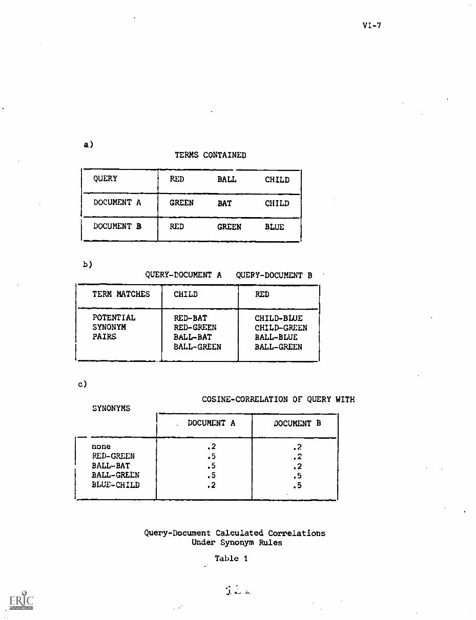
a)

TERMS CONTAINED

QUERY RED BALL CHILD

DOCUMENT A GREEN BAT CHILD

DOCUMENT B RED GREEN BLUE

b)

QUERY-DOCUMENT A QUERY-DOCUMENT B

TERM MATCHES CHILD

POTENTIALSYNONYMPAIRS

c)

1111..

SYNONYMS

RED-BATRED-GREENBALL -BAT

BALL-GREEN

RED

CHILD-BLUECHILD-GREENBALL-BLUEBALL-GREEN

COSINE-CORRELATION OF QUERY WITH

. DOCUMENT A DOCUMENT B

noneRED-GREENBALL-BATBALL-GREENBLUE-CHILD

.2

.5

.5

.5

.2

.2

.2

.5

.5

Query-Document Calculated CorrelationsUnder Synonym Rules

Table 1

.3,

VI-8

3. Pseudo-Classification Procedure

A term matrix is set up which has a numerical value for z...ach

term pair. If this value exceeds a user-defined "threshold of

synonymy", then the corresponding pair of terms is considered synon-

ymous (for use in calculating the matching function). The term

matrix is initially set to all zeroes (no synonyms).

At the start of each iteration, all query-document cosine

correlations are calculated and stored. The correlations are calculated

not only with direct term matches, but also counting any pair of terms

which is a "potential synonym pair" for this query and document, and

which is defined synonymous by the term matrix. Since the entries in

the term matrix vary from one iteration to the next, the calculated

correlations will also vary.

After all the correlations have been stored, each query-

document pair is again considered in turn, and the previously stored

correlation value and the query-document class (R, S, T 4r U) to

which this pair corresponds is used to calculate a number. This

number, which may be positive or negative, is the "term modifier"

and is added to each entry in the term matrix which corresponds to

a "potential synonym pair" for this particular query-document pair.

After this calculation, the number of query-document pairs

in classes S and T is counted and output as an indication of the

degree of convergence to the desired state. The modified term matrix

is then utilized in the next iteration for calculation of the matching

function. Iteration continues until the program converges (all

query-document pairs are in class R or U) or operator intervention

occurs.

VI-9

The heart of the program is the action of the term modifier.

Any one term pair may be a "potential synonym pair" for many

different query-document pairs. Thus, alter each iteration, the

corresponding term matrix entry will be changed by an amount equal

to the sum of the term modifiers for all query-document pairs which

include this term pair as a "potential synonym pair."

If this set of query-document pairs consists entirely of class

T pairs, then one would wish to raise the correlation of the pairs so

that they might become class U pairs. If the modifier is a positive

number for a class T query-document pair, then the net effect of many

class T pairs will be to raise the term matrix entry above the

'oreshold of synonymy. This, in turn, would increase the correlation

of the query-document pairs, which is the desired r "sult.

Conversely, if we are presented with class S query-document

pairs, we wish to lower the correlation by causing synonym pairs

which contribute to the correlation to become "potential synonym

pairs" below the "threshold of synonymy," i.e., to cause them to

no longer be synonymous. If the term modifier is negative for class

S query-document pairs, it will have the desired effect.

Query-document pairs of the S or T classes are called

mismatched pairs because the calculated results do not agree with

the defined ,elevancies. The degree of mismatch is the amount that

the calculated correlation differs from the match value. If the

degree of mismatch is large, then many "potential synonym pairs" which

are (or are not) synonyms must be modified until they are not (or are)

synonyms. If a term modifier is made large in magnitude, then it

VI-l0

will have a greater effect on the term matrix than other smaller term

modifiers. This causes (on the average) a greater amount of change

in the number of "potential synonym pairs" which actually change

status to or from synonymy. It is therefore desirable that the term

modifier should vary in magnitude with the degree of mismatch in

classes S and T.

At first it would seem that, because query-document pairs in

classes R and U need not be changed, the corresponding term modifiers

should be zero. This was tried and found to cause oscillation and

prevent convergence. The reason is that the correctly matched pairs

do nothing to maintain their status quo, When the mismatched query-

document pairs modify the term space to correct their own mismatch,

they disturb tne balance of synonymy in correctly matched pairs.

To prevent the res.Utant oscillation of query-document pairs between

classes R and S, and classes T and U, it is necessary to give term

modifiers of classes R and U small negative and positive values

respectively. The term modifier of class R should be proportional

to minus the number of pairs in class T and U. The term modifier

of class U should be proportional to the number of pairs in classes

R and S. This assures stability of solution in the fully or nearly

fully convergent case (almost all pairs in class R or U).

To assure continuity of the term modifier in class S, the

term modifier is equal to the term modifi.%1, of class R (a constant)

minus the absolute value of the mismatch of the class S query-

document pair. Similarly, the class T term modifier is equal to the

value of the class U term modifier plus the absolute value of the

mismatch.

VI-11

4. Programming System

A sample program as implemented in FORTRAN IV is shown

in the appendix, as an example of this algorithm. All arithmetic

is performed with integer and binary variables and arrays. Binary

variables are treated as integers with value 0 or 1.

In section A, the document vectors, query vectors, and

relevance judgments are read in. This is the main data. The

term-term matrix 4nd synonym matrix are zeroed, and initial values

for all other variables are set up.

In section B, the correlation coefficient is calculated,

taking into account (statements 500 and on) any synonym term

matches as well as direct term matches. The calculated correlation

of query (J) and document (I) is stored in correlation (J, I).

In section C, the dynamic matching threshold is calculated

for each query, and stored in matchvalue (J).

In section D, each query-document pair is considered in turn.

The "term-modifier" (variable name is MODIFIER) is calculated from

the relevance judgment (relevant (J, I)) and calculated correlation

(correlation (J, I)) of the pair, and the dynamic match value

(matchvalue (J)) of this query.

In section E, all term pairs are examined, and all which are

"potential synonym pairs" for this query document pair (termterm

(Kl,K2)) are modified by the "term modifier".

After sections D and E have been completed for all query-

document pairs, the modified term-term matrix (termterm (K1,K2) is

examined in section F. From the data in this matrix, the synonym

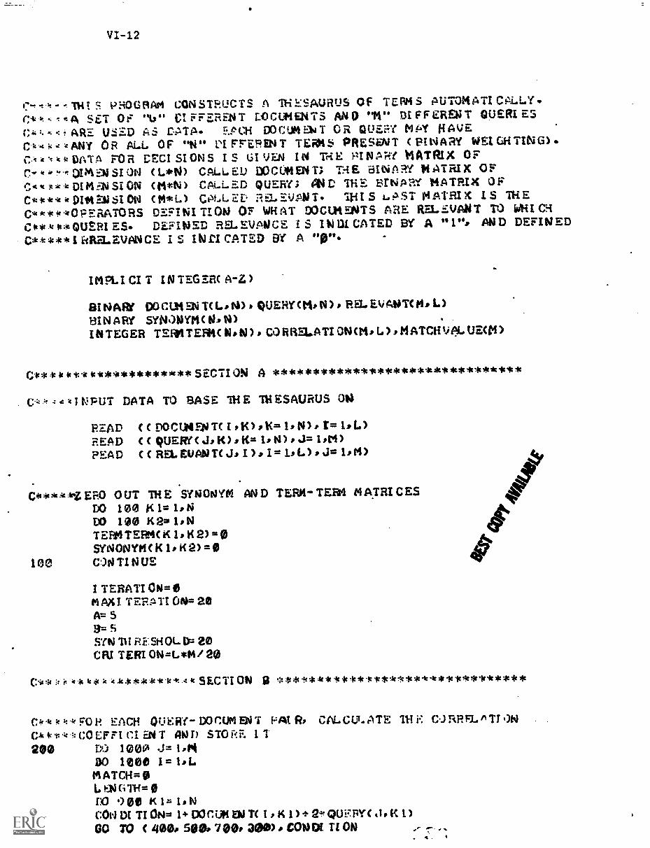
VI-12

TH P ROG RA14 CONSTRUCTS A IN EsptuRuS OF TEi 4 S AUTON A TI C ALLY .

C4,4! ,4A SET OF "L," CI r r raIrNT LOCLMENTS AND "M" DI FFERENT QUERI ESC4,1. ARE USED AS laTA. EPCH DOCLM EhT CR QUEFe HAVEC. t: z ANY OR ALL OF "N" FFERENT TEMS PRESENT C PIWARY W L GHTI(VG).

DATA FOR CECI SI ON S I $ GI Val IN Tri E NARY MATRIX OFCi?""..TOIMiNS/ON CL*N) CALLED DOCUMENT; T-iE 8101AR? MATRIX OF

t gic.k DIMFN SI ON (MAO CALLED QUERY; 44D THF. BINARY MATRIX OFC44fc** DIt4EN SI ON M*L) ED Ft F.A/PN T. Ili I S LAST 14/1l:Inc IS THEC****440PERATORS DEFINI TION OF WHAT DOCUMENTS ARE Ra.EVP14T TO NHI CiCo* kftleQUERI ES. DEFINED RE. I.:VANCE LS IN Di GATED BY A "1" AND DEFINED01": *41 * I Illta.EVPNCE I Z INDI CATED BY A "0".

IMPLI CI T IN TEGERC A-2)

BINARY DO CLM TM, tsb) * QUERY CM ) REL ANTC L)BINARY SYNONYM( 14N)INTEGER TERM TERKC Wahl), CO fiRILATI ONCM, L ) MATCHVPL UECt4)

Cit* 0*ic 4:************ SECT/ ON A *******************************

I IsIFUT DATA TO BASE THE THESAURUS ON

READ CC DOCUMENTC Is.10,1<= 1,N): II= IL)READ C C QUERYC.110K= 14) J= 1M)?EAD C C RELEVANTCJa I ) I= LPL), J= I'M)

Cicie gg kZEF.O OUT THE SYNONYMDO 100 lilmt 1, NDO 100 K2=1NTER4TER4C 1K 2) =SYNONYMOC1K2)=0

100 CONTINUE

I TERATI ON= 0MAXI TETRA TI ON= 20A= 59= SSIN TH SHOL CP 20CRI TERI ON=L*M/ 20

AN D TER14- TERM MATRI C ES

41"*"/"1"44""eic k SECTION I) ***1:**************************

C F O H EACH QUERY- DOC:UM Eti T lz At RP CAL CLL ATE TH E TT ON

4.t:.k t: CO EFFI CI EN ANT) STORE. 17200 DO 1000 = t sly

DO 1000 I= 1LMATCH=L t...146THist

) 00 K 1= 1NCON DI TI ON= I+ DOCLX4 EN TC I s KI)÷ 23,QUFRYC do IC I)GO TO ( /400, 500700, 300)o CONDI T/ ON .

. 4 .

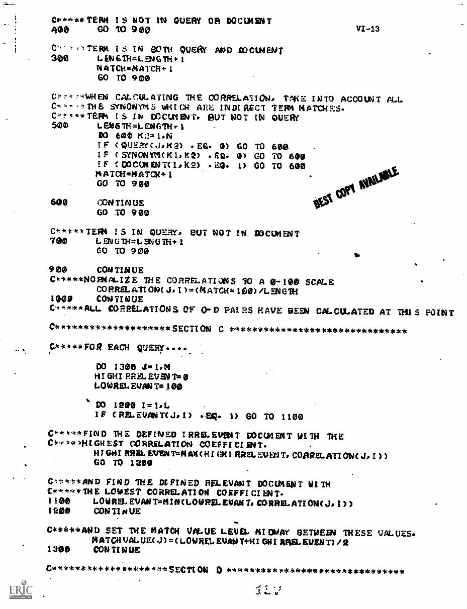
Cegik**TEIV4 I s NOT IN QUERY OR DOcU4ENT400 GO 10 900

C.: TERN i s IN 80111 QUERY AND EOCU4EN1300 LENGTH=LENGTHt 1

NATC14.=MATCH÷ 1GO TO 9 00

VI-13

(.:!r'l.--,W1184 CAL MIL A TING 1H E CO RREL Ai I ON) INC E ACCOUNT ALL:1,11i Vti ON Yin Zi WN t CH AM:. IN DI fiEC1 7EFM N ATM F:S

C t4c TEA% IS IN CO CUP! 0i Ty eUT NOT IN QUERY500 L Eai G TH =1. EN Gill P

RO 600 24: la NF QUERY K 2) Efl 0) GO TO 600

I F SYNONYM( K 1. K2) EQ. 0) GO TO 600F CUN EN T( I K 2) EQ. 1) GO TO 600

GO TO 900to,,A

016**.14 A TCHIBI4ATCH+ 1

600 CONTINUEGO TO 9 00

C11*.ie k TER4 IS IN QUERY, BUT NOT IN Mamas)T700 L aticiTH=L mulli+ 1

GO TO 9 00 I.

900 CONTINUECk****NOMPLIZE THE CORRFLATIMS 10 A 0- 100 SCALE

CORRELATION( JP (MATCH* 1E00) /L MOTH1000 CONTINUE

**** ALL CORRELATIONS OF D PAI RS HAVE BEEN CAL CU L ATED AT THl S POINT

c****Ae***************sEcTi ON C 4:...%*****************************

C.* it '4C Fo R EACH QUERy.

DO 1300 J= IsMIII GH I RR 8. EV aV TaLOWRELEUANT= .100

* DO 1200 I= IP,.I F (RFL EVAN Jo I ) 1) GO TO 1100

C""*FIND THE DEFINED IRRELEvENT DOCU4FAIT WI1H THECle:f,***HIGH EST CORRELATION COEFFI CI EN T

HIGHI HAM EVEN TzNAX C H I GH I RREL UEtiT, CO,R2EL ATI C 11GO TO 1200

Ct:14tticAND FIND THE DEFINED RELEVANT 90ce1ENT WITHC* * ** +THE LOWEST CORRELATION COEFFI CI 1.N T1 100 LOWREL. EVAN T=I4In(ta0WRIEL EVAN T, CORRE. ATI ON( J: I) )1200 CONTINUE

40,

C*****AND SET TH E MATCH Vft.UE LEVEL NI DWAY BETWEEN THESE VALUES.MATCH VAL UE( 4) = ( LOWREL EVAN T+H I GU I MEL EVENT) /2

1300 CONTINUE

C * * ** ** tt *it it41+ .4'44*** it .11* SECTI ON 0 44**,k,k************ititgem**********

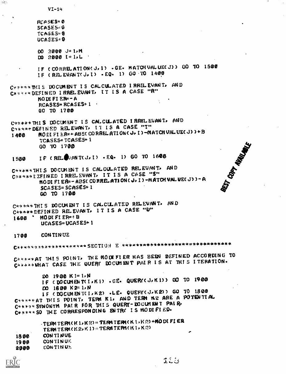
VI-14

'VASES= 0SCASE5-zTCASES,-,UCASES.0

DO 2000 J= 1,14DO 2000 I= 1st.

I F CORRELATION( J, 1) GE MATCH VAL UEC J) ) GO TO 1500I F ( Ra. EVAN TS' Js I) EQ. 1) GO TO 1400

CY t4.--1/41,,THI E.-. DOCUMENT I S CALCULATED I RREL EVAN T AND

Cit .4e DEFINED I RREL EUAN T, IT IS A CASE "R"MO DI FI A

RCASES= RCASES+ 1GO TO 1700

C *t-* * *mI S 1X CUM EN T I S CALCULATED I RREL EVAN TP AND

C.ticle***DEF/ N Ra.EUAN T, 1 1 IS A CASE "T"1400 MOLT FI :R = + ABS( CO RREL ATI ON( I ) -MATCH VALUE( )+ 8

TCAS ES= TCASES+ 1GO TO 1700

1500 I F C RELCIN T( J2 I) EQ 1) GO TO 16e0

C** Jog TH I S DOCUMENT I S CAL CUL A TED RELEVANT ANDCe.1/4:0.9. L'EFINED I RRE1-. EVAN T, IT IS A CASE "S"

MOD! FI EEO- ABS( CORRELATION( ,61, I ) -MATCH VAL UEC J) ) -ASCA SES= SCASES+ 1GO TO 1760

Cl.:*414THI S DOCUMENT I S CALCULATED RELEVANT, ANDC*****DEF/N ED REL EVAN To IT IS A CASE "1,1"1600 * MO DI FI ER=.113

UCASES= ()CASES+ 1

1700 CONTINUE

CP***"************* SECTI E ************it*****************

C iciVr THI .5 POINT, THE MO DI FI ER 14AS BEEN DEFINED ACCORDING TO

C-44.44WHAT CASE 114E QUERY DOCUMENT PAIR I S AT /141 S ITERATION.

DO 1900 K1=1,14I F C DOCU4EN V I s K 1) GE. QUERY( JAC 1) ) GODO 18 00 K2= 1,N

F C DOCUM T( I , k 2) L E. QUERY (J, K 2) ) GO

C* k4-4- AT TH/ S POINTS TERM K is AND TER4 K2 ARE A

C***** SYNONYM PAI R FOR 'VII S QUERY- DOCU'1EN T PM Flo

C* e lc SO 114E CORRESPONDING EN TRH' I S MO DI FI ED.

TE144TE:PM (1( 1,1( 2) = TEFV4 TERM (K 1,)( r) +No DI FI ERTER14TER44( It 22 K 1) TERN TERM( KI, K

18 00 CONTINUE1900 CONIIN2000 CON TIN U!!.

TO 19 00

TO 18 00PO TEN TI AL.

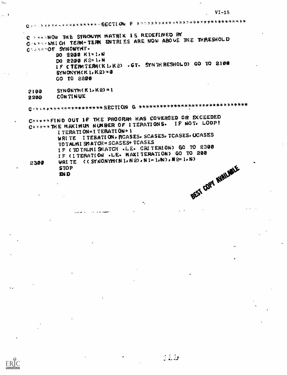
C :

VI-15

4 4* 12 4* 4 4 4: : Ic *. SEC T I ON F .A4. It lc is "f le it le 4 **

C .N TKS SYNONY01 MATR/ K IS REDEFINED 13f

O. 1OH I CH TERM-. TERI ENT RI ES ARE NOW ABOVE THE IHRESKOL D

C ''OF SYNONYM?.DO 2200 K1i,114DO 2200 ii2= IsNI F C TEFO! TEM( K Is K 2) G T SYN 1H RESHOL D) GO TO 2100

SYNONYMC I: K2) 'a 0GO TO 2200

2100 SYNONYtviC K K

2200 CONTINUE

C t 'A, kit* t:qc kt4tic********SECTION G le*****************.!calc****ic******

C x* 4 FIND OUT I F THE PROGRAM HAS CO VERGED OR DC CEEDED

C4 '4 ic, fell4 E M AK I tal 1141 N (.149ER OF I TERA TI ON S. IF NOT. LOOP!TERATI ON= I TERAT/ ON+ 1

W RI TE ITERATIONS, RCA SESs SCA SES. TCASES, °CASESTO TALVII SFIATCIi= SCASES+ TCAS ES

I F C TALMI SNATCH L E. CRI T ERI ON ) GO TO 2300IF CI TEEIATI Ord .LE. MAXI TERATI ON) GO TO 200

2300 WRI TE C C SYNONYM( N Is N 2) s N I= Ist4) It N)

STOP

*A1$COQ°

V1-16

matrix is changed to reflect the updated state of calculated synonymy.

In section G, program status is printed out and a decision is

made whether to iterate (back to section B) or print out and halt.

5. Implementation

A program essentially identical to this, but modified for a

DEC PUP -11/20 was run for small and large collections of data.

small data sets, convergence was reached in two to five iterations.

The larger data set was about 80% of the ADI collection, and while

resulcs are promising, convergence on this data set has not yet been

attained.

VI-17

References

11] D.M. Jackson, The Construction of Retrieval Environments andPsuedo-Claairicalion Based on External Relevance, InformationStorage and Retrieval, Vol. 6, p. 167-219, 1970.

Content Analysis and Relevance Feedback

A. Wong, R. Peck, and A. van der Meulsn

Abstrae

VII-1

Content analysis is a vital part of any automatic document

retrieval system where natural language has to be analyzed in order to

detect the information carrying parts. The assignment of appropriate

identifiers to the documents and queries "the indexing process"

can be carried out on different levels of complexity which generally

agree with different levels of system performance.

A device for indexing improvement of a quite different nature

is the "user feedback" technique which can be applied in an interactive

retrieval system. The initial indexing which is a result of a rather

imperfect content analysis can be corrected and improved by using the

judgment of the user concerning the relevancy or non-relevancy of his

retrieved documents.

This report deals with the question: how critical is the quality

of the content (language) analysis which results in the i:iitial indexing

in an interactive retrieval system? Since in such a system feedback

techniques will improve system performance substantially one could doubt

if original defferences in content analysis will still affect the final

performance. If such differences in indexing refinement turn out to be

retained after the feedback is applied, every improvement in initial

indexing should be put into practice; in addition a good justification

exists for working in the area of automatic dictionary construction.

V11-2

1. Introduction

The performance of a document retrieval system depends heavily

on the transformation of the natural language of the document into an

artificial retrieval language. The document description in such a

retrieval language results in a much shorter representation compared

with the original one, and It is this indexing process which determines

how effectively thk. document can be retrieved.

If one defines as "ideal indexing process" as a process which

results in retrieval of only relevant documents in response to

queries, it is likely that, even with the most refined techniques,

ideal indexing does not exist. The two reasons are:

- the transformation of the author's ideas into a written text

may be imperfect; moreover, during indexing usually only

title and abstract are considered.

- the existing language analysis tools are imperfect.

The first reason in particular will always limit the quality of the

indexing process even if ideal language analysis devices were available.

When dealing with large collections of documents, the automation

of text analysis becomes a necessity, since manual indexing may not

then be a realistic alternative. Evaluation tests for a long period

have shown that manual indexing vas superior to automatic indexing.

Nowadays the roles incline to change. This is mainly due to the fact

that in modern interactive retrieval systems the implementation of

user feedback strategies (index corrective mechanisms) yield a

considerable improvement in system performance. To be sure, those

VII -3

interactive strategies are in principle also applicable to computerized

retrieval systems supplied with manually indexed documents; but usually

such a system organization does not allow the implementation of an

effective feedback algorithm.

Concentrating first on the automatic content analysis tools,

one may distinguish two basically different approaches:

a) Non-lingusitic computer techniques.

Examples art.:

- the automatic stemming of words followed by the counting of

their frequency of occurrence;

- procedures for the automatic detection of common words;

- statistical procedures for the automatic construction of

dictionaries; and

- the automatic creation of weighted dictionaries, where the

weight reflects the description power of an identifier.

b) Computer oriented linguistic techniques.

In those procedures the syntactical meanings of sentences are

taken into account rather than mere keywords; also phrases may

be recognized in an explicit way.

Such a syntactical analysi3, was supposed to fill the gap

between a pure mechanical analysis (category a) and an intellectual

manual one. To date the situation however is such that appli-

cation of the now existing linguistic techniques deteriorate

system performance, rather than providing a substantial improvement.

In this report therefore only statistical language analysis

will be considered (category a).

VII-4

The retrieval results obtained with the available automatic indexing

devices are far from satisfactory, and one might doubt if it ever will

become possible to improve the initial indexing sufficiently.

To simplify the indexing problem, user feedback techniques may be

used, based on the premise that index colvections can be made dynamically

during the course of the search by utilyzing the judgment of the user con-

cerning the relevancy of his retrieved documents (1). One may refer to

"relevance feedback" and "document modification" as corrective indexing

techniques which allow both the reindexing of a query (relevance feedback)

as well the reindexing of documents (document modification). It should be

mentioned here that those corrected indexes are not static entities, but

dynamic, in tune with actions performed by the system users.

Relevance feedback in particular has proved to be a powerful technique

which increases system performance significantly, since queries are in

general short and poorly formulated. One must ask then how imperfect the

initial indexing may be while still yielding results after feedback applica-

tion which are comparable to those of the more refined initial indexing;

in other words is the final feedback result a function of the initial indexing?

If final results appear to be independent of initial indexing,

most efforts concerning content analysis and in particular dictionary

construction might be less meaningful than they originally appear to be.

If those results show some improvement due to better initial indexing what

compromise must be made between indexing expedience and returns in terms

of system performance after feedback is applied? But if the final results

are highly dependent on the quality of initial indexing the answer is clear.

All efforts directed towards content analysis improvement remain of

particular importance.

VII-5

2. Experiments

The purpose of the experiments is to investigate the influence

of language analysis tools on final system performance after a sufficient

number of feedback iterations have been executed. "Sufficient" here means

that a new iteration will not further affect the obtained system perfor-

mance. In the SMART environment two or at most three iterations are

normally sufficient. The experiments are likely to be dependent on the type

of feedback algorithm used, which will be Rocchio's in all cases.

A) Used Language Analysis Tools

The main analysis tools provided by SMART include three dictionaries:

- the word-form dictionary,

- the word-stem dictionary, and

- the thesaurus

The word-stem dictionary (suffic deletion) is a refinement of the word-form

dictionary (plural s endings deletion), and the thesaurus (grouping of

related terms) is a refinement of the word-stem dictionary.

An improvement which can be applied to each of the existing dictionaries

is the application of the so-called "discrimination values" [2], that is,

of quantities which reflect the descriptive power of the dictionary items

(terms). More specifically, the discrimination value is a measure of the

change in average correlation of a document collection to its center-of-

mass (centroid), measured first using the term as an index, and again with

that term deleted. If the collection moves closer together, when term i is

deleted, that is, if the average correlation with the centroid increases, that

term is valuable in distinguishing individual documents.

The application of discrimination values can be carried out in

two possible ways:

- deletion of bad discriminators which process however will

not be considered in this report, and

- creation of a weighted thesaurus 13).

B) Comparisons

Two collections are considered in order to justify generalizing

the results obtained in these experiments. They are:.

- the TIME collection consisting of 425 documents in the

political science field provided with 83 queries, and

- the ADI collection consisting of 82 documents in documentation

provided with 32 queries.

Two main experiments are carried out: first a comparison is made

between four different dictionaries using the TIME collection. Compared

are the system performances using a word-form dictionary and a thesaurus

both with and without discrimination value application. System

performances before and after two feedback iterations are considered.

Second a comparison of a word-stem dictionary and a thesaurus using

the ADI collection is made. System performances before and after three

feedback iterations are considered.

In the comparison of feedback results no attempt is made to go

into complex evaluation schemes (4,5]. The system performances are

expressed in simple recall-precision curves, which are suitable for the

outlined purposes.

V11-7


The results for both collections (Figs. 1, 2, 3, and 4) clearly

demonstrate that in all the investigated cases differences in initial

performance are retained in the final precision-recall curves. In

Figures 1, 2, and 1, the word-form dictionary serves as reference curve

and is compared with the weighted word-form dictionary, the thesaurus,

and the weighted thesaurus. In Fig. 4 a word-stem dictionary is compared

with a thesaurus.

From the recall-precision curves one may draw the remarkable

conclusion that the shape of each curve, reflecting a special dictionary

performance, remains invariant after the feedback operations, however

the position of the curves is lifted. Also the relative ordering of

results of various dictionaries remains invariant.

In the case of the TIME collection a better initial performance

curve is inclined to lift relatively more (Figs. 1, 2, and 3); this

results in a spread out of the final curves. The ADI collection shows a

slight "wash-out" effect in that initial differences are diminished. It

has to be noted that the initial word-stem dictionary performance is

fairly poor (low recall-precision curve), which explains the wash-out

effect.

4. Conclusion

The results indicate clearly that the final system performance,

that is, the final retrieval result after user feedback is applied, is

highly dependent on the system performance of the initial indexing process.

.9 'r

.8

.7

.6

- = word-form dictionary

= weighted word-formdictionary

1C. -

.5 -

Initial runs

\A

Second iterationfeedback runs

t-,Precision `x,. -x

Performance comparison between a weighted andan unweighted word-form dictionary, before and

Recall after two feedback iterations (TIME collection)Fig. 1

.4L----

0

0 .2 .4 .6 1.)

.8

.7

.6

T

t

f

.4 1

'" "" ""

-

om

VII-9

- = word-form dictionary

= thesaurus

Initial runs

Precision

x_

\__Second iterationfeedback runs

ttNho

.4A

-.ft...A.' -

Performance comparison between a thesaurusand a word-form dictionary before and aftertwo feedback iterations (TIME collection)

Fig. 2

.8

A

).

1.0

9 VII-10

IN, a. low .11.

x

Initial runs

Precision

word-form dictionary

= weighted thesaurus

411"`x,

Second iterationfeedback runs

x,

* -4

A4 '\Recall x,_

___..Performance comparison between a weightedthesaurus and a word-form dictionary beforeand after two feedback iterations. (TIME collection)

Fig. 3

01.0

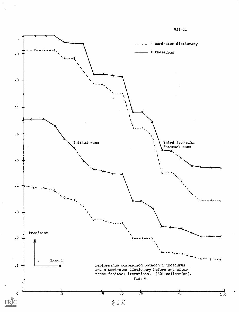
.7

.6

.4

.2

.1

0

VII-11

- = word-stem dictionary

= thesaurus

10-

Initial runs Third iterationfeedback runs

X.

X

OM. -x-

Precision

K,

Recall

-

A

4- -4

- - - - X

Performance comparison between a thesaurusand a word-stem dictionary before and afterthree feedback iterations. (ADI collection).

Fig. 4

lir 7 .tl

VII-12

It must be noted that this conclusion is derived for the application

of Rocchio's feedback algorithm; other feedback mechanisms such as for

example the replacement of the original query by the index of a retrieved

relevant document, might yield different results. Unfortunately no evaluations

between different feedback strategies are available, but Rocchio's is at least

the most established one.

It is for this feedback strategy that one may state that every tool

which improves the indexing performance as an outcome of the content analysis

of natural language is beneficial because initial differences in system

performance are retained after user feedback is applied.

References

[1] G. Salton, The SMART Retrieval System, Prentice Hall Inc.,Englewood Cliffs, N.J., 1971.

[2] K. Bonwit and J. Aste-Tonsmann, Negative Dictionaries, InformationStorage and Retrieval Report No. ISR-18, to tne National ScienceFoundation, Section VI, Department of Computer Science, CornellUniversity, October 1970.

[3] A. Wong, R. Peck, and A. van der Meulen, An Adaptive DictionarN,in a Feedback Environment, Term project report, Department ofComputer Science, Cornell University, May 1972.

[4] G. Salton, The Performance of Interactive Information Retrieval,Information Processing Letters 1 (1971), North Holland PublishingCompany.

[5] C. Cirillo, Y.K. Chang, and J. Razon, Evaluation of Feedback RetrievalUsing Modified Freezing, Residual collection and Test and ControlGroup, Information Storage and Retreival, Report No. ISR-16, tothe National Science Foundation, Section X, Department of ComputerScience, Cornell University, September 1969.

On Controlling the Length of the

Feedback Query Vectors

Karamvir Sardana

Abstract

VIII-1

Various strategies for reducing the lengths of feedback

vectors, which get elongated during regular feedback processing,

are tested. The results show that the strategies based on the

knowledge of the discrimination values of the concepts, are quite

successful. The best aajteged me-hod retains the top best

discriminating concepts in every feedback query vector.

1. Introduction

A) Indexing

All automatic document retrieval systems use some method

or other for converting a natural language document or a query into

a form that is representative of the corresponding document or the

query and can be stored internally in a computer. This process is

xnown as indexing and is quite important because much of the

efficiency of document retrieval systems depends on it. In the SMART

automatic retrieval system [1], indexing transforms a piece of

natural language text into its representative concept-weight (c-w)

vector form meant for internal storage in the machine. A concept or

a term is an atomic entity, a word or a phrase used to describe the document

V111-2

whereas the associated weight denotes the concept's importance in the

document. In the existing SMART system, which is taken as a test

environment in the present study, the weight of a concept is normally a

linear function of its frequency of occurrence in the text of a document

or a query. In this report, the c-w vectors used in the SMART system are

referred to as standard vectors or simply as vectors.

B) Length of a Vector and Importance of Controlling it

The length of a document or a query vector (referred to simply as

a vector in the sequel) is defined to be the number of index terms or

concepts (that is, the ones with nonzero weights) constituting the vector.

The length of a vector affects the overall retrieval process in the

following ways:

i) The storage space occupied by a vector depends on the number

of c-w pairs, that is, the length of the vector, and the

storage needed for one c-w pair. In the present SMART system,

each c-w pair occupies one computer word of storage.

ii) The process of correlating two vectors is frequently used for

document searching in retrieval systems. The correlation

measure widely used in the SMART system can be graphically

interpreted as the cosine of the angle between the two vectors

in the n-- dimensional Euclidean space. The cosine correlation

coefficient between the vectors

, p2, n,P 2 p p p ), where p1 is the weight of the

.thconcept

and

(q1, q

2, q

n)

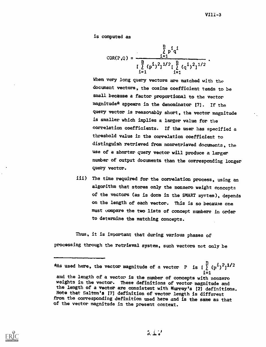
V111-3

is computed as

n . .

COR(P,Q) = i=1

(pi)211/21E (qi)211 2

LT-1 i=1

When very long query vectors are matched with the

document vectors, the cosine coefficient tends to be

small because a factor proportional to the vector

magnitude* appears in the denominator 171. If the

query vector is reasonably short, the vector magnitude

is smaller which implies a larger value for the

correlation coefficients. If the user has specified a

threshold value in the correlation coefficient to

distinguish retrieved from nonretrieved documents, the

use of a shorter query vector will produce a larger

number of output documents than the corresponding longer

query vector.

iii) The time required for the correlation process, using an

algorithm that stores only the nonzero weight concepts

of the vectors (as is done in the SMART system), depends

on the length of each vector. This is so because one

must compare the two lists of concept numbers in order

to determine the matching concepts.

Thus, it is important that during various phases of

processing through the retrieval system, such vectors not only be

i 2 1/2*As used here, the vector magnitude of a vector P is I (p )i=1

and the length of a vector is the number of concepts with nonzeroweights in the vector. These definitions of vector magnitude andthe length of a vector are consistent with Murray's (2] definitions.Note that Salton's (7] definition of vector length is differentfrom the corresponding definition used here and is the same as thatof the vector magnitude in the present context.

VI41-4

fully representative of their intended meaning but also be short and

concise to give high correlation coefficients and to save on storage and

searching costs.

This implies that there is a definite need for controlling the

length of vectors which have a tendency to grow long as a result of

retrieval processing. This must be done by trimming the elongated

and unwieldy vectors such that their shorter versions carry the gist of

the corresporiing originally long vectors.

2. earlier Results

A) Murray's Strategy for Reducing the Vector Lengths

Earlier experiments in this area have been conducted by Murray 12]

for controlling the lengths of profile vectors. A profile vector (cluster

centroid) is a vector that represents all the vectors in a cluster. Murray

suggests reducing the lengths of profile vectors by chopping off 80% or so

of the concepts with the lowest weights (and thus the frequencies in the

standard vectors), which according to his recommendations, results in only

a slight decrease in retrieval performance. This method can similarly be

used for reducing any vector length for that matter.

The idea is to remove those concepts in a vector which because

of their relatively small weights, will not affect the orientation of the

vector in the vector space by much and, therefore, will not appreciably

influence the correlations of this vector with any other. Further, a

detailed analysis by Murray shows the following justification for using

this strategy:

VIII-5

Let P be a vector whose length is to be reduced and Q

be another vector with which the vector Q is to be (cosine)

correlated during the course of document searching. Then, the

contribution to the total correlation, by matching-conceptb with

weights pi and q1, is

i iCONTRIBUTION = 2-- =

IP] IQl (pj)231/2 N1)211/2

i=1 j=1

For a fixed vector Q, the values of qi/IQI are fixed and

variations in contribution are due to Pi/IPI, called the correlation

contribution ratio.

Now, as in the present strategy for reducing the vector

lengths, the lowest weight terms of vector P are thrown out, the

correlation loss due to these terms is small and the retrieval per-

formance is not affected.

This strategy is valuable because a vector can be trimmed

to only 20% of its original length while sacrificing only a little

in retrieval performance.

B) Other Related Results by Murray

Some other related and interesting row:tits regarding profile

vectors by Murray are presented, to be used later on in the

discussion. These results are:

i) Weighted profile vectors are significantly better in

performance than unweighted profile vectors.

ii) Profile vectors consisting of concepts whose weights are

VIII-6

rank values* give superior performance when base values aresmall. A rank value is the difference between a base valueand the rank assigned to the term if all terms in the vectorare ordered by decreasing frequency. The base value is a

constant chosen large enough to insure that all weights arepositive in the profile vectors.

iii) Profiles with concept weights based on frequency ranks** give

performance better than the standard or rank value vectors.

Such profiles avoid correlation domination by larger weightterms while at the same time allowing smaller weight terms tohave a relatively little more say in determining the correlations.

iv) Selection of good index terms is more valuable than making finefrequency distinctions among important index terms.

v) Using a few broad categories, typically four, of weight classes

gives performance equivalent to that obtained by using a largernumber of weight classes as used in the standard weighted vectors.

3. Present Problem

A) Origination

Rocchio-type formulae are widely used for relevance feedback, and they

have been shown to result in an improved retrieval performance Ill. One side

effect of using relevance feedback in this manner is the growth in the length

*The vectors formed in this way are called rank value vectors.

**The frequency ranked vectors are constructed by arranging the conceptsconstituting a vector in increasing frequency order and then assigningthe weight of a concept equal to its rank in such a list. The conceptswith the same frequencies are assigned the same rank. It should benoticed that the frequency ranked vectors are essentially the rank valuevectors for which the base value is chosen in such a way that theminimum weight of the concepts equals unity.

VIII-7

of the feedback query vectors (fqv's). The elongation of the fqv's

can amount to as much as twelve times the average length of the

corresponding original query vectors. To some extent, the growth

in the lengths of the query vectors is quite desirable because

as Murray [2] has also observed, the original queries tend to be

short and omit the background material that might really be

helpful. On the other hand, too long a set of query vector; with

possibly a lot of unimportant terms could damage the retrieval

performance in addition to using up more storage and costing more

in retrieval searches. The idea, then, is to reduce the elongated

fqv's to their optimum length somehow.

Furthermore, it would be interesting to see if relevance

feedback can, in some way, be reinforced by using the knowledge of

discrimination values (dv's) of concepts in the fqv's. The theory

of discriminating power of individual concepts has been expounded

by Bonwit and Aste-Tonsman 13] and developed further by Crawford [4].

B) Exact Definition and Scope of the Problem

The problem at hand is to discover strategies to trim the

fqv's to vectors of manageable shorter lengths such that the

retrieval performance obtained by using the trimmed versions of

the fqv's is better than or at least equivalent (if possible) to

that obtained by using the original elongated fqv's. Second part

of the pr9blem is to discover means to augment the relevance feedback

by using the dv's of concepts utilizing ideas of Bonwit and

VIII-S

Aste-Tonsman [3] and Crawford 114]. The results are to be compared with

Murray's work [21.

It is worth recalling that some work in feedback reinforcement by

term dv's has already been done by Bjorklof 15] and Doeppner, Finley and

Peterson 16] using some strategies which have not met with much success.

C) Methods and Solutions in Brief

It is proposed to use the information of dv's of concepts in

achieving both the ends. Briefly, the procedure to be used is as follows:

i) Take a document collection and the associated queries. After

the original iteration of document searching, do one iteration

of regular Rocchio-type feedback. Note its performance and

save the resulting fqv's.

ii) Order the concepts in each elongated fqv in decreasing dv order.

iii) Retain top n concepts of the ordered vector, where n depends

on the particular vector and the strategy used, as explained

later.

iv) Reorder the shortened vector back to the original ordering of

the concepts.

v) Do the original iteration of document retrieval search using

the trimmed fqv's and compare its performance to that of the

regular feedback from step (i) above.

The motivation for this approach is as follows. In Murray's work,

the lowest weight concepts are shown to have small correlation ratios and

discarding such terms is not considered to be harmful. On the other hand, the

theory of dv's of terms and specifically their non-monotonic relationship with

VIII -9

frequency of occurrence of the corresponding terms, as shown by

Crawford 14], indicates that some presently low weight but good

discriminating terms could be of potential importance in the

present and futijre correlating process. Thus, throwing away such

potentially valuable terms might hurt the retrieval performance,

while retaining them might really help.

4. Vector Trimming Strategies

First, some notations are given and operations are defined:

i) Notations:

a) X0

a Y: Operator 0 operates on the initial

vector X to yield the final vector Y.

b) V : Elongated fqv which is to be reduced

in length.

c) A-- orde : Original alphabetical order (of the

concept numbering). Thus a vector

in A-order means that its concepts

are numbered in original alphabetical

order.

d) D-order : Decreasing dv order (of the concept

numbering). Thus a vector in fl -order

means that its concepts are numbered

in decreasing dv order.

ii) Possible Operators, 0:

a) A/D : Concepts of the initial vector are

renumbered from A-order to D-order

to yield the final vector.

VIII-10

b) D/A

c) Murray n

d) Fixed n

: Concepts of the initial vector are

renumbered from D -order to A-order to

yield the final vector.

From the initial vector, top n% of the

total number of concepts in their

decreasing weight order are retained to

form the inal vector.

: The final vector is composed of fixed

top n concepts of the initial vector.

If the length of the initial vector is

less than n, then both the final and the

initial vectors are identical.

e) DV Rank n : The final vector is composed of all

concepts of the initial vector with dv

rank (to be defined shortly) less than or

equal to n.

Utilizing these notations and operators, Fig. 1 is a tree illustration

of the algorithms of all the four strategies for reducing the vector lengths.

Assuming the original query vectors, Q of Fig. 2(a) for illustration purposes,

a brief description of each of the strategies follows:

A) Strategy I

As described earlier, this is Murray's [2] strategy and for every

vector V, it retains the top n% of the total number of concepts in their

decreasing weight order to produce a shortened length vector V1. Suggested

value of n is around 20. Fig. 3 shows the vectors V1 obtained from vectors

V of Fig. 2(b), by 70% reduction in length.

For the following three strategies, the first common step is to renumber

the concepts of each elongated vector V from their A-ordering to P-ordering.

4

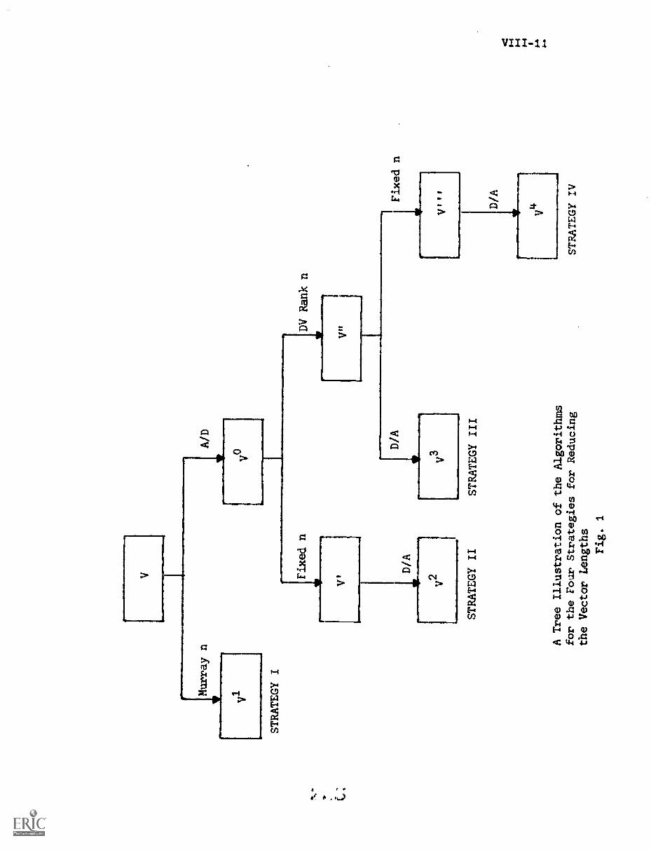
V

Murray n

STRATEGY I

A/D

1/

0

Fixed n

V' D/A

DV Rank n

V"

D/A

Fixed n

V3

STRATEGY II

STRATEGY III

A Tree Illustration of the Algorithms

for the Four Strategies for Reducing

the Vector Lengths

Fig. 1

D/A

V4

STRATEGY IV

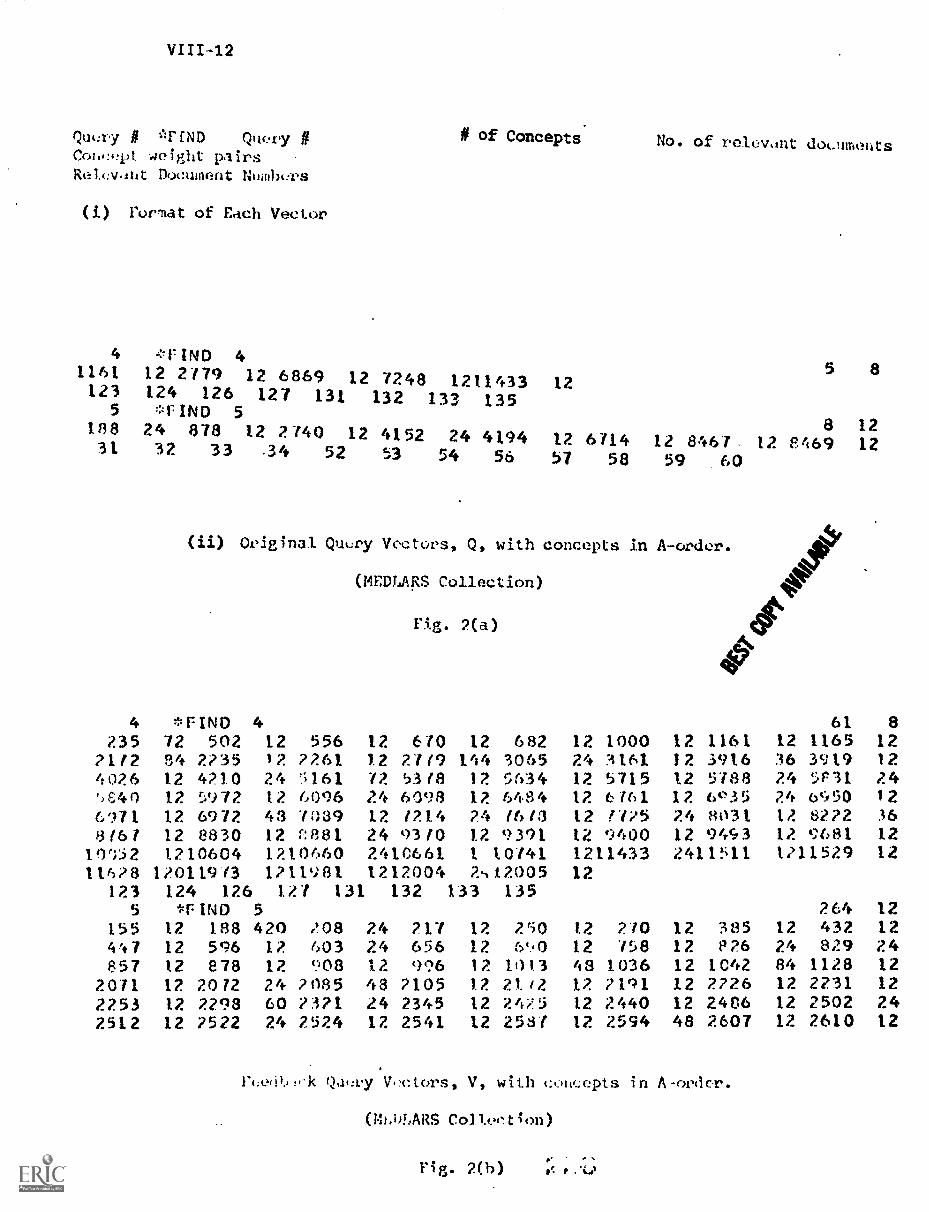
VIII -12

Query # %:F END Query #Colo:.v.weight pairsRelev.nat Document Numbers

(i) Furliat of Each Vector

# of Concepts

4 i'FIND 41161 12 2779 12 6869 12 7248 1211433 12123 124 126 127 131 132 133 135

5 *FIND 5188 24 878 12 2 740 12 4152 24 419431 32 33 .34 52 53 54 56

12 6/1457 58

(ii) Original Query Voetovs, Q, with concepts

(MEDLAS Collection)

No. of relovilnt douuments

12 846759 60

in A-order.

5 8

8 1212 8469 12

4 *FIND 4

F3.g. 2(a)

61 8

235 72 502 12 556 12 670 12 682 12 1000 12 1161 12 1165 1221/2 84 2235 ) 2 2261 1.2 270 144 3065 24 3161 12 3916 36 3919 124026 12 4210 24 '3161 12 5318 12 5634 12 5715 12 5788 24 5r31 245C40 12 5972 12 6096 24 6098 12 6'.34 12 6161 12 6035 24 6550 12

97 I 12 6972 43 1039 12 /214 24 1613 12 t125 24 8031 12 8222 36

816t 12 8830 12 P881 24 93(0 12 9391 12 9400 12 9453 12 9681 121.0';52 1210604 1210660 2410661 1 10/41 1211433 2411511 1211529 1211628 12011913 1211981 1212004 2N12005 12

123 124 126 12/ 131 132 133 1355 *FIND 5 264 12

155 12 188 420 208 24 217 12 2t.i0 t2 210 12 85 12 432 1241,7 12 596 12 603 24 656 12 60 12 158 12 P26 24 829 24857 t2 878 12 908 12 996 12 1013 48 1036 12 1042 84 1128 12

2071 12 2012 24 2085 48 2105 12 21/2 12 2191 12 2?26 12 2231 12

2253 12 2298 60 l321 24 2345 12 2425 12 2440 12 2486 12 2502 242512 12 2522 24 2524 12 2541 12 2581 12 2594 48 2607 12 2610 12

ree(11.,-1( Voctors, V, with couQepts in A-ordcr.

(ML WARS Colleotion)

Fig. 2(h) .. 'CP

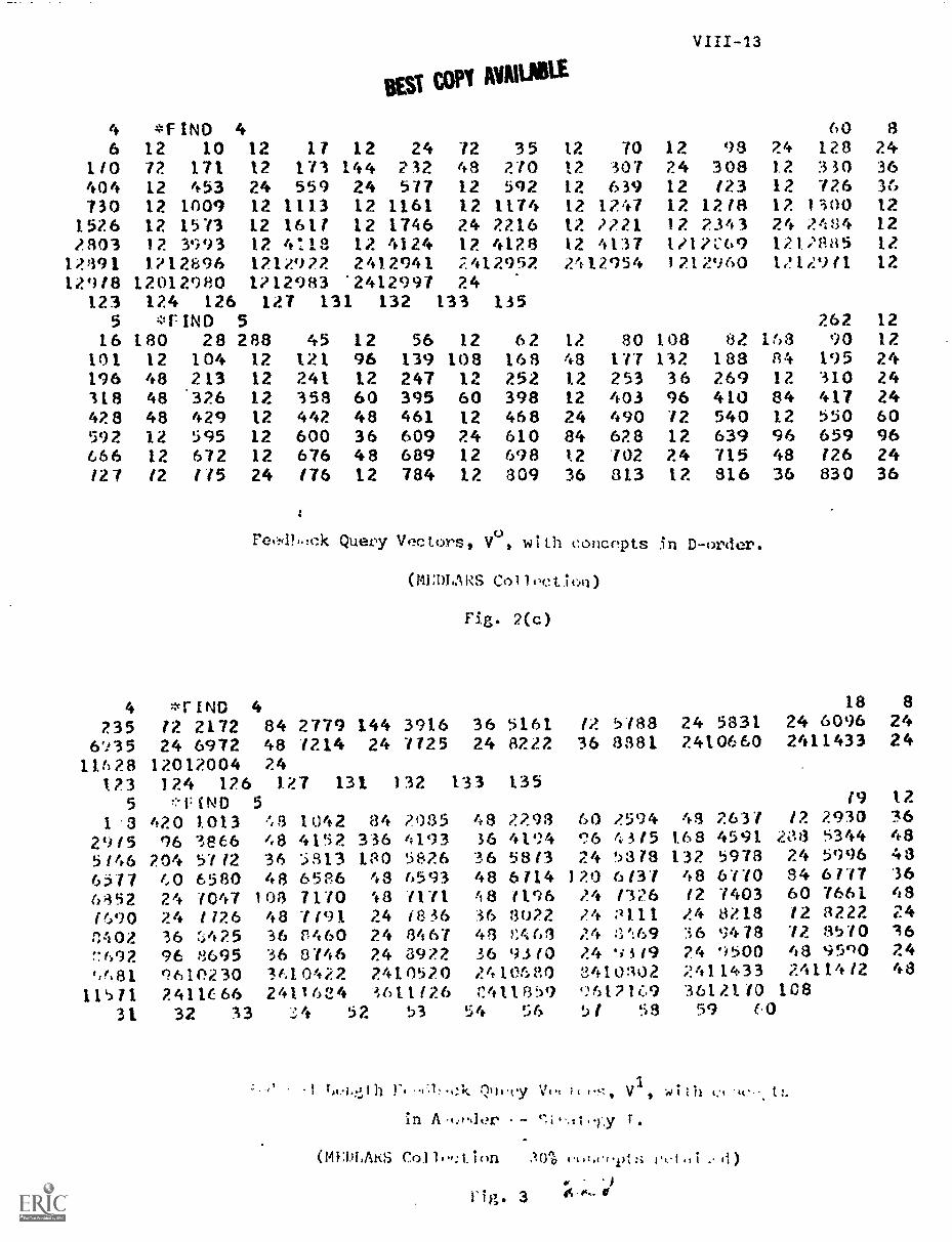
1/111-13

BEST COPY AVRIUBLE

4 *FIND 4 60 86 12 10 12 17 12 24 72 35 12 70 12 98 24 128 24

1/0 72 171 12 171 144 232 48 270 12 307 24 308 12 330 36404 12 453 24 559 24 577 12 592 12 639 12 123 12 726730 12 1009 12 1113 12 1161 12 1174 12 1247 12 12/8 12 1300 12

1526 12 1573 12 161/ 12 1746 24 2216 12 2221 12 2343 24 2484 12

2803 12 3993 12 4118 12 4124 12 4128 12 4137 1212C69 1.1.2885 12

12391 1212896 1212922 2412941 2.412952 2412954 1212960 12129/1 12

12918 12012980 1212983 '2412997 24123 124 126 127 131 132 133 135

5 *FIND 5 262 12

16 180 28 288 45 12 56 12 62 12 80 108 82 168 90 12

101 12 104 12 121 96 139 108 168 48 177 132 188 84 195 24196 48 213 12 241 12 247 12 252 12 253 36 269 12 310 24318 48 .326 12 358 60 395 60 398 12 403 96 410 84 417 24428 48 429 12 442 48 461 12 468 24 490 12 540 12 550 60592666

1212

595672

1212

600676

36 60948 689

2412

610698

84t2

628102

1224

639715

9648

659126

9624

127 12 115 24 176 12 784 12 809 36 313 12 816 36 830 36

Fe,,A1),Ick Query Vectors, V°, with concepts 3n D-order.

(MEDARS Colloctioo

4 -11-1N0 4

Fig. 2(c)

18 8

235 12 2172 84 2779 144 3916 36 5161 12 5.188 24 5831 24 6096 24

6'J35 24 6972 48 1214 24 1125 24 8222 36 8381 2410660 2411433 24

11628 12012004 24123 124 126 127 131 ) 32 133 135

5 *FIND 5 (9 12

1.3 420 1.013 ,8 1042 84 2.035 48 2298 60 2594 43 2637 12 2930 36

29/5 96 3866 48 4152 336 4193 36 4194 4315 168 4591 288 5344 48

5/46 204 5712 6 '5313 130 5826 36 5813 24 5378 132 5978 24 5996 48

6577 /A 6580 48 6536 48 593 48 6/14 ) 20 6/3/ 8 6170 84 6177 66452 24 1047 103 7110 48 1171 48 /196 24 /126 12 7403 60 7661 81f.,90 24 /126 48 7(91 24 1836 36 3022 24 0111 24 8218 12 8222 24

n402 36 :425 36 5460 24 8467 43 1:63 24 :1':69 36 9478 72 8510 16

692 96 8695 36 8/46 24 8922 36 93(0 24 'i3/9 24 I5500 48 95')0 24

,,r141, 9610230 300422 2410520 2.41me0 .3410302 24'1433 2411412 48

11')71 2411066 2411624 4,611(26 "4t1859 961211.9 36121/0 10831 32 33 -.::.4 52 53 54 56 51 59 59 O

h tA chlt i !-: V1 , WI ih t:t t

in A-(..eder - T.

(MEDLAhS 30% 40,pu;1

A stn. grig. 3

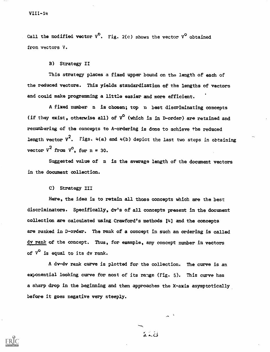
VIII -14

Call the modified vector V°. Fig. 2(c) shows the vector Vo

obtained

from vectors V.

B) Strategy II

This strategy places a fixed upper bound on the length of each of

the reduced vectors. This yields standardization of the lengths of vectors

and could make programming a little easier and more efficient.

A fixed number n is chosen; top n best discriminating concepts

(if they exist, otherwise all) of V° (which is in D-order) are retained and

renumbering of the concepts to A-ordering is done to achieve the reduced

length vector V2

. Figs. 4(a) and 4(b) depict the last two steps in obtaining

vector V2from Vo for n = 30.

Suggested value of n is the average length of the document vectors

in the document collection.

C) Strategy III

Here, the idea is to retain all those concepts which are the best

discriminators. Specifically, dv's of all concepts present in the document

collection are calculated using Crawford's methods 14] and the concepts

are ranked in D-order. The rank of a concept in such an ordering is called

dv rank of the concept. Thus, for example, any concept number in vectors

of V° is equal to its dv rank.

A dv-dv rank curve is plotted for the collection. The curve is an

exponential looking curve for most of its range (Fig. 5). This curve has

a sharp drop in the beginning and then approaches the X-axis asymptotically

before it goes negative very steeply.

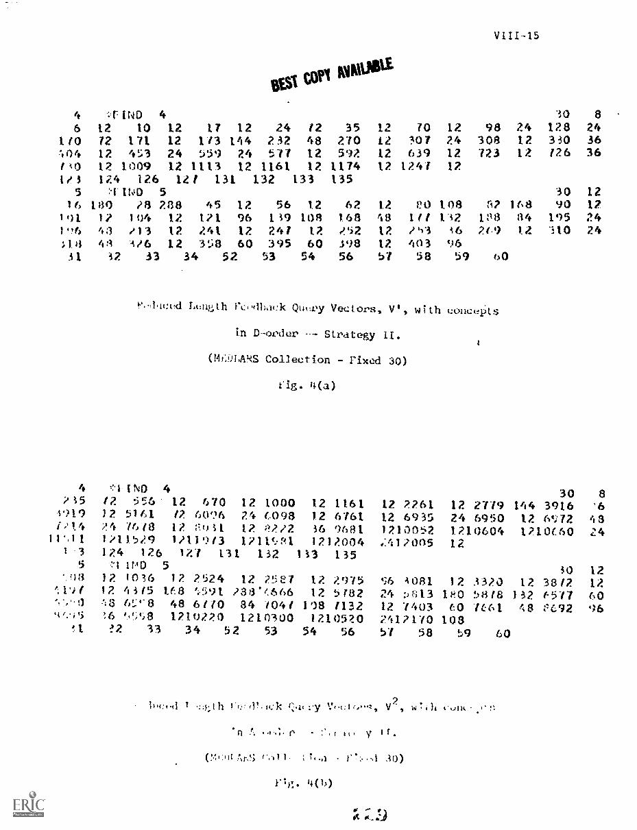
4 -*I ND 4

VIII-15

30 8

6 12 10 12 17 12 24 12 35 12 70 12 98 24 128 241/0 72 171 12 113 144 232 48 270 12 307 24 308 12 330 36404 12 453 24 559 24 577 12 592 12 639 12 723 12 126 36f) 12 1009 12 1113 12 1161 12 1174 12 1241 12

1/3 124 126 121 131 132 133 1355 1 IND 5 30 12

16 180 18 238 45 12 56 12 62 1.2 VO 1.08 ri? 168 90 12101 12 104 12 121 96 139 108 1.68 48 1 /1 1'32 1:113 84 195 2416 43 /13 12 241 12 2.41 12 /'i2 12 1'13 16 29 1.2 7110 24

4A 416 12 358 60 395 60 398 12 403 9631 32 33 34 52 53 54 56 57 58 59 (30

4'15s919(%141111

1 3

5:)3

`. I 'i

Lt:np...th rcona,1( Quk:vy Vectors, V', with conc4ts

tn D-wder -- Strategy II.

(MOLARS Collection - Fixed 30)

fig. 4(a)

*i-IND 4/2 556' 12 670 12 1000 12 116112 5761 12 60(Y6 24 0.098 1.2 676144 1618 12 t 1, i 1 1? ;!222 36 96811/11529 11119/3 1211(.,P1 1212004124 126 121 131 132 113 13511PD 5

12 1036 12 2524 12 25U7 12 297512 43(5 t68 188'1.666 12 5(82f;3 61.:e8 48 6110 84 /041 108 113216 Y:58 1210220 1210300 1210520

-212 33 34 52 53 54 56

30 812 2261 12 2779 144 3916 '612 6935 24 6950 12 672 481210052 1210604 1710(60 24.:411005 12

30 12';6 4081 12 3310 12 38 /2 1224 :)/A13 11::0 5818 132 6577 6012 1403 60 1t61 48 f'692 962411170 10351 58 59 60

211:,d T h tek v

- I it; y r.

(!11:.)1 Ar.S ; 30)

I lg. 40

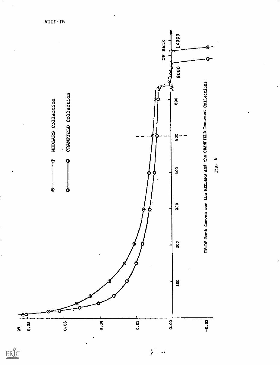
DV 0.08

0.06

0.04

0.02

0.00

MEDLARS

Col

lect

ion

00

CR

AN

FIE

LD

Col

lect

ion

100

200

3C0

400

500 1

600

-0.02

DV-DV Rank Curves far the MEDLARS and the CRANFIELD Document Collections

Fig.

5

DV

Rar

.k

8000

1400

0

VIII-17

A value m for dv rank cutoff is determined from the curve; all

concepts in e with dv rank < m are retained and then final

renumbering of the concepts from D-order to A-order yields the final

reduced length vector V3. These last two steps for obtaining V3

from V° are exhibited by vectors of Figs. 6(a) and 6(b).

A recommended value of m, the dv rank cutoff, is the one near

the foot of the first steep of the dv-dv rank curve. More exactly,

that value of m is chosen where the slope of the curve is < es

where e is a constant for the particular collection. A value of

t = 0.00004 giving m = 500 is found appropriate for the document

collections used in this project. A method for determining n for

a particular document collection is given later in Section 6(B).

D) Strategy IV

This strategy is an intermediate between the last two

strategies and using it the length of any reduced length vector is the

minimum of the lengths obtained by using strategies II and III. It is

same as the previous strategy except that the length of each vector

is further trimmed to n just before the concepts are renumbered back

to A-ordering. Thus, in addition to using a dv rank cutoff m like

Strategy III, it also places an upper bound n on the length of each

vector like Strategy II, to yield the final reduced length vector

V4

(Figs. 7(a) and 7(b)).

Note that this strategy is also equivalent to using Strategy II

with a maximum fixed upper bound on lengths being equal to n, and :11

addition, trimming the vectors further down such that all concepts

with dv rank greater than m are eliminated.

.N.1111.18

Pp

6110

i IND12 10f? (a

41.212

171 i3

12144

24232

12.'g8

35ell0

04 12 ef '13 241? 3 ).2.4 1:6 127 111 132 133 135

5 :.11N0 516 PIO i3 :38 45 12 54 12 1,2

1 0)1 1 2 I 04 12 121. 96 12..9 108 16131126 `;3 213 12 241. 12 241 12 "52

k,6 12 60 -',9523 ".3 27 12 .1;42 48 1161 12 .1.63

1t2 33 34 52 53 54 56

1212

124812

2451

113 8/0 12. c8 24 1:8 24

108 12 430 36

121,0 1.08 IV. 168 4,0 12/ I 132 1 Pt) 1;4 195

36 269 12 0 ).4t; 96 410 ei4 1,1^;',i0 12

5f3 59 to

(yi t h Q.11( ; et i h cot-lc:opt s

In 1).-utdt.r. - 11: nit egy If r

OV 13.,11kC011-ction -

e1g (-()

4 i':c) 4, 5!6 12 1, 19 1r. ':.

; .11 /;,.1.4 2 c, i3 1..1.!!().,211: 1? 1,J04 24

1: 1 124 126 12 1 31. I 72 1 ;3 1 t511.'D 5

t2 1013 t I. 4 12 ?5,13./1 1,, ;312 :2 4i. / 1.2 1A3 i;51.11

0.3 1:;0 5:3/3 1a2 .r:!, 1 60 4'!, :8/1. '.8 i 403 f.,0 1161 ie; 8 " "10 24 P0z2

I 2 I. o300 1.1' 520 !.1:11. /9233 4 52 1,3 4

.1 1 cy

13 3.1t,1 (2

1.210(t.0 1.'!11511 1; 1.../3 1.2

-;8 121?. 2 ;'J15 '36 'Cr)). I2

?;.:8 1%6 12 24 e?.4

1.3 /0 ;' r I 1.03 i +32 2"6 !. V.15 7.6 ::.,;33 ?.

1,31,-110 1.013

53 59 AO

:7.1. t it. y 111

ct )11 4,, t ii.11 ak 1.00)

V`

VIII-19

4 *FIND 4 18 86 12 10 12 17 12 24 72 35 12 70 12 98 24 128 24

170 72 171 12 173 I44 232 48 270 12 307 24 308 12 330 36404 12 453 24123 124 126 127 131 132 133 135

5 *FIND 5 30 1216 180 28 288 45 12 56 12 62 12 30 108 82 168 90 12

101 12 104 12 111 96 139 108 168 1,8 111 132 188 34 195 24196 48 213 12 241 12 247 12 252 12 253 36 269 12 310 24318 48 326 12 358 60 395 60 398 1.2 403 0631 32 33 34 52 53 54 q6 51 58 59 60

Reduced 1Aligth Feedback Query Vectors, V"; with

in D-urder -- Strategy IV

(Mr.DLARS Collection - DV Rank 500/Fixed 30)Fig. 7(a)

cOnOepts

4 *FIN-) 418 8235 12 5Z6 12 2 779 144 3916 36 3919 12 5161 72 6761 12 6935 2469/2

11:;n148 72141212004

24 16/824

1210052 1210604 1210(60 24.C;11 1:'11'' t3 12

123 124 126 127 131 132 133 1355 *FIND 5 10 12

'ma 12 1036 12 2524 12 2581 12 2915 96 011 12 3320 12 3812 12

4197 12 4375 168 45(4 238 '666 12 5/82 24 130 4:4/3 132 6511 1:0

:.310 48 6598 48 6110 84 1041 108 11 32_ 12 1 tio3 1.-o (661 48 8692 1.6

[1695 36 4;598 1210220 1210300 1,10520 2;1.'110 10831 32 33 34 52 53 54 56 57 53 'A 60

R-duced 4re.c.J1).wk Qu,,vy Vectors, V , with tmcev:s

In a, r rJL-.1! IV

(nD(,ARS Colloction - UV R,Ink oo/r1:-.Qd i())

rig. 1(b)

VIII-20

As compared to the last strategy, the advantage of using this

strategy is seen in getting standardized fixed length vectors, although

some loss in performance is expected due to the loss of good discriminators

(upto dv rank cutoff m) in some of the vectors.

5, Experimental Environment

A) Retrieval System

The SMART automatic document retreival system is used as the test

bed for conducting the experiments. This retrieval system is a major facility

for conducting experiments to test and evaluate various document retrieval

strategies.

B) Data Collections

Two different SMART document collections used in the present series

of experiments are MEDLARS and CRANFIELD. The MEDLARS collection used is a

450 document subset of the originally larger collection dealing with varied

medical literature; the associated number of queries is 30. The Indexing

procedure used for representation of the documents and the queries in the

machine utilizes a word stem dictionary.

On the other hand, the CRANFIELD collection consists of a more

homogeneous set of 424 documents dealing with aerodynamics; the associated

queries form a 125 query subset of originally 155 query collection. The

indexing process used for this collection makes use of a word form dictionary.

The procedure of indexing making use of dictionaries has been discussed in

detail by Salton 17).

VIII-21

In many respects, these two document -ollections are

different enough to warrant putting a great deal of confidence into

the results based on the experiments done on them.

C) Clustering Parameters

The experiments are conducted on clustered document collections

because Murray 12] has shown that document retrieval based on clustered

files is more efficient than the one based on inverted files or

individual documents, for instance.

A clustered CRANFIELD document collection is available as a

SMART collection, while the MEDLARS collection was clustered for this

experiment. The clustering parameters used are:

i) SMART routine CLUSTER is used for clustering by Rocchio's

algorithm 18].

ii) The loose documents are placed with the centroid with

which they correlate the highest.

iii) The algorithm is allowed to choose an optimum number of

documents to be batched for checking as possible cluster

roots.

iv) For Rocchio's density test, to be a cluster point, at

least 4 documents must have a correlation greater than

0.3 and at least 8 documents must have a correlation

greater than 0.1 with it.

v) Minimum and maximum number of documents in each cluster

are 8 and 25 respectively, excluding the loose documents

blended in later on, as determined by step (ii) above.

.:$

VIII-22

D) Searching Parameters

The SMART routine SEARCH is used for document searching experiment::.

The parameters used throughout this study are as follows:

i) Feedback Parameters

a) The number of documents retrieved for each iteration is 30.

b) Among the top 10 relevant documents, all the relevant ones are

added to and the top nonrelevant subtracted from the original

query to form the first iteration query. Only one iteration of

feedback is carried out for the present experiments.

ii) Cluster Searching Parameters

a) At least 40 documents are correlated with the query on each

iteration.

b) At least 3 and at most 10 cluster nodes are expanded for each

iteration.

c) Any nodes whose cosine correlation with the query is within

0.01 of the latest node selected for expansion are also expanded.

E) Evaluation Techniques

The basic evaluation technique used for the comparison of various

retrieval search runs, is the Precision-Recall (P-R) curve [7] . Even

though none of the fluid or frozen feedback searches provide the true

retrieval performance while the more exact test and control group feedback

method [9] is time consuming, the fluid searches are chosen with the intention

of making relative comparisons only.

The "ranking" and "feedback" effects occurring in relevance feedback,

as discussed by Hall and Weiderman [10] are analyzed manually. Particularly,

the "feedback effect", which measures the improvement in retrieval performance

VIII-23

due to the new relevant retrieved documents, is considered.

6. Experimental Details

A) Overall' Flowchart of the Experiments

Fig. e is an overall flowchart of the document retrieval

search experiments. Basically, as discussed in Section 3(C) also,

an experiment to test out a strategy consists of the following

four steps:

i) Perform document retreival SEARCH (SMART routine) on

a collection, using one Rocchio-type feedback iteration.

Obtain the P-R curves for the original (ORIG) and

feedback (FDBK) iterations.

ii) Shorten the elongated fqv's using one of the Vector

Trimming Strategies to get the reduced length vectors.

iii) Use these modified fqv's to SEARCH the document collection

without any further feedback. Obtain the P-R curve for

this modified (MOD) iteration.

iv) Compare the SEARCH results for the FDBK and the MOD

iterations.

B) Detailed Description of One of the Experiments

To give an idea of how these experiments are performed down

to their inner det,_ls, a detailed description of one of the

experiments is presented.

Table 1 details the steps of the experiment using the MEDLARS

document collection and Strategy III for the length reduction of the

vector:;. rigs. 2 and 6 give computer output examples of the vvotom

at various stages through the experiment.

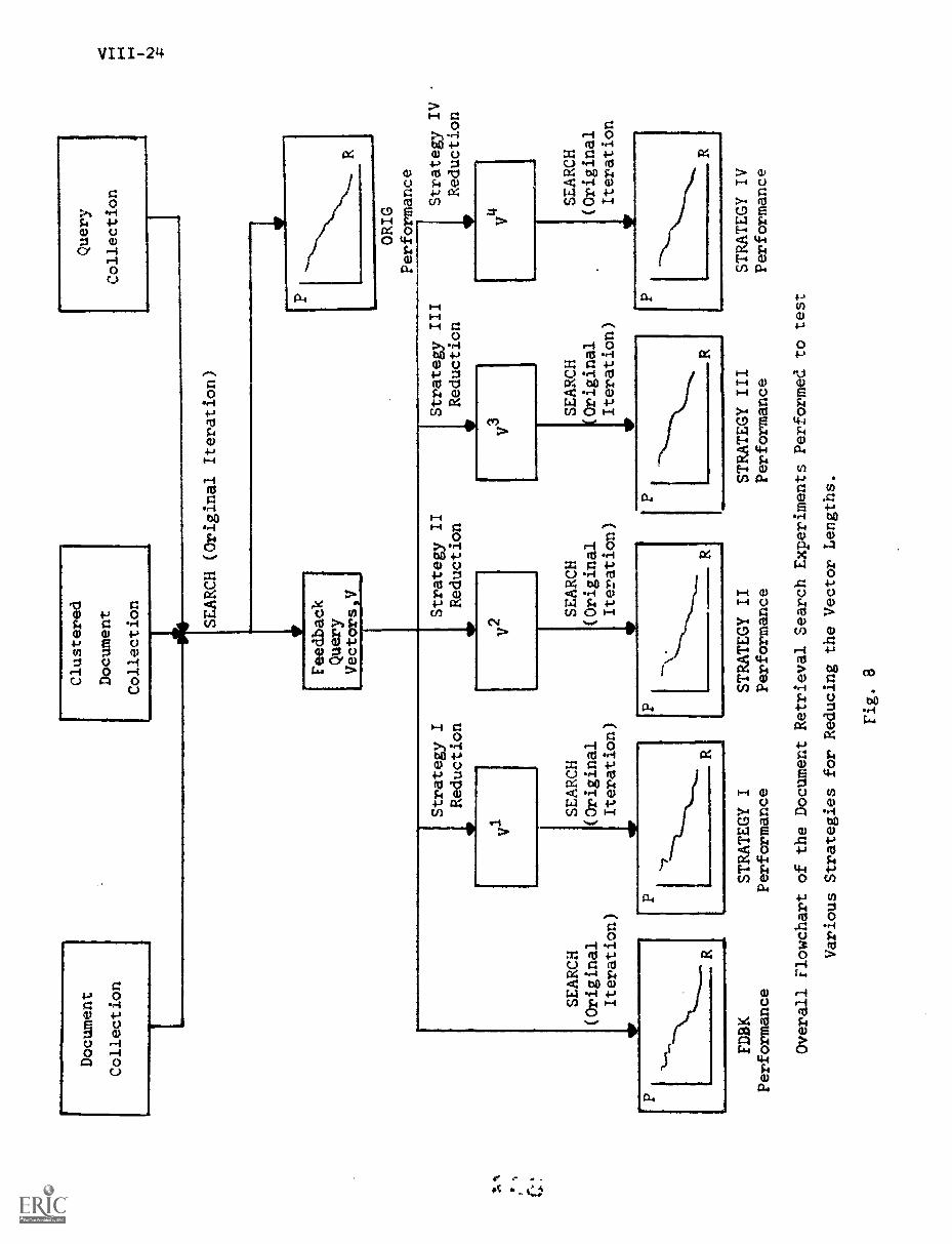
Document

Collection

Clustered

Document

Collection

Query

Collection

SEARCH (Original Iteration)

.111

ALM

IIIM

EIII

MO

ON

Feedback

Query

Vectors ,V

ORIG

Performance

SEARCH

(Original

Iteration)

FDBK

Performance

Strategy I

Reduction

VI [SEARCH

(Original

Iteration)

Strategy II

Reduction

V2 1SEARCH

(Original

Iteration)

STRATEGY I

Performance

STRATEGY II

Performance

Strategy III

Reduction

V3

SEARCH

(Original

Iteration)

+or

IR

STRATEGY III

Performance

V4

Strategy IV

Reduction

SEARCH

(Original

Iteration

3

Overall Flowchart of the Document Retrieval Search Experiments Performed to test

Various Strategies for Reducing the Vector Lengths.

Fig. 8

STRATEGY IV

Performance

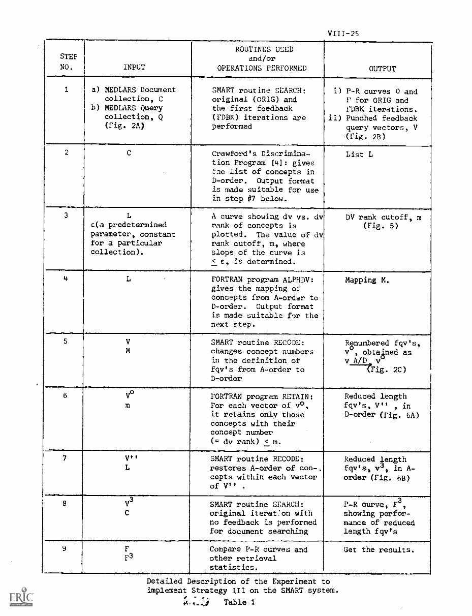
VIII-25

STEP

NO. INPUT

ROUTINES USEDand/or

OPERATIONS PERFORMED OUTPUT.

1 a) MEDLARS Documentcollection, C

b) MEDLARS Querycollection, Q(Fig. 2A)

SMART routine SEARCH:original (ORIG) andthe first feedback(FDBK) iterations areperformed

.

i) P-R curves 0 andF for ORIG andFDBK iterations.

ii) Punched feedbackquery vectors, V(rig. 2B)

2 C Crawford's Discrimina-Lion Program [4]: givesThe list of concepts inD-order. Output formatis made suitable for usein step #7 below.

List L

3 Lc(a predeterminedparameter, constantfor a particularcollection).

.

A curve showing dv vs. dvrank of concepts isplotted. The value of dvrank cutoff, m, whereslope of the curve is< E , is determined.

DV rank cutoff, m(Fig. 5)

.

4 L FORTRAN program ALPHDV:gives the mapping ofconcepts from A-order toD-order. Output formatis made suitable for thenext step.

Mapping M.

5

.

V

MSMART routine RECODE:changes concept numbersin the definition offqv's from A- -order to

D-order

Renumbered fqv's,v°, obtained asv_A/12, v°

Mg. 2C)

6 V°m

,

FORTRAN program RETAIN:For each vector of v0,it retains only thoseconcepts with theirconcept number(= dv rank) < m.

Reduced lengthfqv's, V" , in

D-order (Fig. 6A)

. .

7 V"L

SMART routine RECODE:restores A-order of con-.cepts within each vectorof V'' .

Reduced lengthfqv's, v3, in A-order (Fig. 6B)

8 V3

C

SMART routine SEARCH:original iterat'on withno feedback is performedfor document searching

P-R curve, F3,showing perfor-mance of reducedlength fqv's

9 F

F3Compare P-R curves andother retrievalstatistics.

Get the results.

Detailed Description of the Experiment toimplement Strategy III on the SMART system.

.:, ...L0 Table 1

VIII-26

For this part of the experiment, the value of parameter e

first determined for the MEDLARS collection by trial and error, such that

the dv rank cutoff lies at the foot of the first sharp drop of the dv-dv

rank curve (Fig. 5). The value of e is found to be 0.00004 and the same

value of c is used for the CRANFIELD collection. This value is determined

just once for the whole collection.

Another important point about this experiment is that during the

length reduction of the vectors, care was taken to prevent the query from

getting zeroed out completely. Thus, if after the application of the

strategy, the reduced query vector happened to contain no concept at all,

the algorithm took care that at least 5 concepts (if present in the

original query vector, otherwise equal to number of concepts in it) were

retained. Similar precaution was taken during the application of other

strategies as well.

7. Results

A) Performance Curves Obtained

First, the effect of variation of individual parameters n and m

(n and m are the parameters used in the description of various strategies

in Section 4) is studied for each strategy separately and performance curves

are obtained. The best curve obtained for each strategy is taken and

comparisons are made between these.

Figs. 9(a) to 9(d) show the performance curves obtained for each

individual of the four strategies, using the MEDLARS document collection.

Fig. 9(e) shows the comparison of the best P-R curves -- one obtained for each

if the strategies. Furthermore, in each of these figures, the average and

the range of number of concepts present in the fqv's and the total number

BE

ST C

OPY

AV

AIL

AB

LE

Precision

Symbol

Parameter

%concepts

retained

V 0 0

30

50

100

SIP

No. of

concepts

Avg./Range

32/1-95

54/1-159

109/2-318

9/2-22

Total retrieved

Re:ovant

Documcnts among

Top 10/Top 30

149/191

144/193

155/200 FDBX

106/172 ORIG

0.1

0.2

0.3

0.4

0.5

0.6

Performance Curves for the MEDLARS Collection -- Strategy 1

Fig. 9(a)

0.7

0.8

0.9Recall

1.0

411Precision

0.91.

0.8

0.7

0.6

0.5

0.4

0.3

0.2

0.1

TT

OSymbol

WO

0 0

Parameter

No. of

r.,

concepts

in Fixed nAvg./Range

30

40

70

OM

B

WO

27/2-30

35/2-40

59/2-70

109/2-318

9/2-22

Total Retrieved

Relevant

Doc=nts among

Top 10/Tcp 30

1,51/207

15U204

155/202

155/200

FDAK

106/172

ORIG

BE

ST C

OPY

AV

AIL

AB

LE

0.0

C.1

0.2

0.3

0.',

0.5

0.6

0.7

0.8

0.9

1.0

Recall

Performance Curves for t:.e MIMLARS Collection -- Strategy II.

Fig. 9(5)

1 Pr

ecis

ion

0.6I 3

0.7

0

0.6

0.5

0.4

0.3

0.2

0.10.0

0

BE

ST C

OPT

AV

AIU

SIL

Parameter

Symbol

in DV Rank

No. of

concepts

tal Itetrieved

Ra:cvant

Z..zccr.ts anong

0 O 0

800

500

200

4111

11

Avg./Range Top 1:$/Top 30

28/1-94

162/219

i9/1-6S

163/221

9/1-30

142/190

109/2-318

155/200 :OM

9/2-22

C6 /172

ORIG

-0

0.1

0.2

C.3

0 . 1

+C

. . ;

0.6

Perf

orm

ance

Cur

ves

for

the

M£D

LA

RS

Col

lect

ion

Fig. 9(c)

11.1

1

0.7

0.8

Strategy III

0.9

CALL1.0

tPre

cisi

on0.

90 0 V

0.8

0.7

0.6

0.5

0.4

0.3

0.2

0.1

Symbol

V 0

Parameter

m/n in

DV Rank m

Fixed n

800/30

500/30

00

No. of

concepts

Avg./Range

21/2-30

18/2-30

109/2-318

9/2-22

1:otal .7trieved

DOeumen",:s among

Top 10/Top 30

153/219

154/218

155/200

FDBK

106/172

ORIG

BEST COPY

AV

AIL

AB

LE

0.0

0.1

0.2

C.3

0.4

0.5

0.6

0.7

3.a

0.9

.0

mr.ALLI

Performance Curves for the MEDLARS Collection -- Strategy :V

Fig.

9(d

)

Precision

BE

ST C

OPT

AV

AIL

AB

LE

0.6

0.7

0.6

0.5

0.14

0.3

0.2

\k:

"CRIj

4,\\Vfi

\C-(\\ **'N

0\43

0

Sym

bol

9 V 0

Parameter

Murray 33

Fixed 30

DV Rank 500

Fixed 30/

DV Rank 800

Ink

010

No. of

concepts

Avg . /Range

32/1-95

27/2-30-

19/1-68

18/2-30

1C9/2-318

9/2-22

Total Retrieved

Relevant

Document5

=lo

ngTop 10/Top 30

149/191

161/207

163/221

154/218

155/200 FMK

106/172

ORIG

O

0.1f 3.0

0.1

0.2

0.3

it0.4

b.5

0.6

Comparison of the Performance ofi Various Strategies

Fig. 9(e)

for

C.7

0.8

the MELLARS Collection

vc!

0.9RECALL")

of re.Levant documents retrieved among the top 10 and the top 30 ranks for

the whole query collection are also given. For comparison purposes, the

P-R curves obtained for ORIG and FDBK iterations are included in each of

the figures.

Fig. 10 shows the comparison of the best P-R curves obtained for

the various strategies for the CRANFIELD collection, except that Strategy

IV was not tried, because results of using this strategy were expected to be similar

to those obtained for the MEDLARS collection.

B) Inference from the Performance Curves

In the following analysis, all comparisons are made with respect

to the performance curve obtained by the first regular feedback (FDBK)

iteration.

Tables 2, 3, 4 and 5 give such a comparative analysis for the four

individual Strategies I, II, III, and IV, for the two collections used.

Inference from these tables for each of the strategies is given below:

i) Strategy I

The use of this strategy for the reduction in the length

of the fqv's results in almost consistent loss of performance

by as much as 0.06 in precision at any recall level.

ii) Strategy II

Reduction in the lengths of the fqv's, using this

strategy, results in almost equivalent or better performance

than that obtained by using elongated fqv's. Keeping

maximum length of shortened fqv's equal to the average

length of the document vectors seems reasonable and gives

almost the best results, for high recall values, which is most

likely what the user desires. Using this formula, the length

1

0.8

0.7

0.6

0.5

0.4

0.3

0.1

0

Precision

BE

STC

OPT

AV

AIL

SIL

ESymbol

Parameter

0 C V 0 0

No. of

concepts

Avg./Range

Total Retrieved

R21e7ant

r.oc:Iments among

Top 10/Top 30

::array 50

57/1-201

Fixed 62

51/1-62

aurray 30

34/1-120

DV Rank 500

32/1-129

00 AIM

114/2-403

9/4-22

;00/547

409/571

392/560

435/574

4C;6/567 FMK

289/522

ORIG

Vt"

1"..!

0.0

0.1

0.2

0.3

0.4

0.5

0.6

0.7

Comparison of the Performance of Various Strategies for the CRPTIELD Collection

.rig. 10

0.9

0.9

1.0

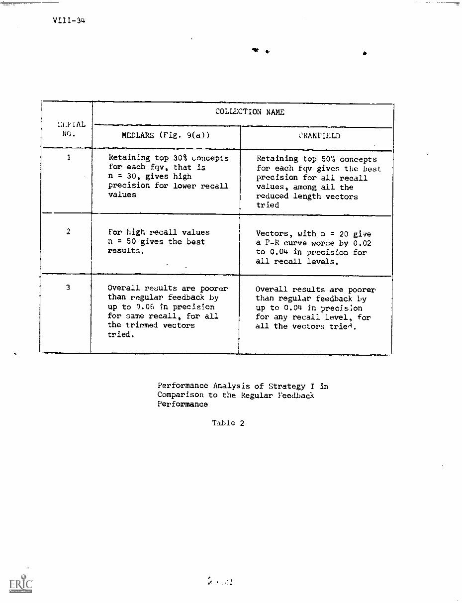
VIII-34

it 4.

L.LPLAL

NO.

COLLECTION NAME

MEDLARS (Fig. 9(a))

---CRANFIELD

1

-Retaining top 30% conceptsfor each fqv, that isn = 30, gives highprecision for lower recallvalues

Retaining top 50% conceptsfor each fqv gives the bestprecision for all recallvalues, among all thereduced length vectorstried

2 For high recall valuesn = 50 gives the bestresults.

Vectors, with n = 20 givea P-R curve worse by 0.02to 0.04 in precision forall recall levels.

3 Overall results are poorerthan regular feedback byup to 0.06 in precisionfor same recall, for allthe trimmed vectorstried.

Overall results are poorerthan regular feedback byup to 0.04 in precis.onfor any recall level, forall the vectors trieA.

Performance Analysis of Strategy I inComparison to the Regular FeedbackPerformance

Table 2

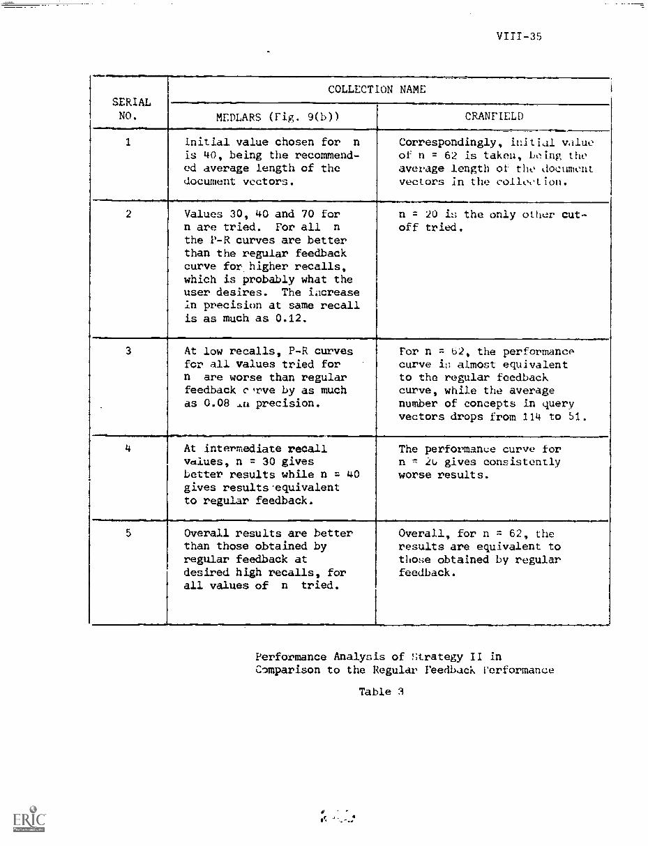
VIII -35

SERIALNO.

COLLECTION NAME

MEDLARS (Fig. 9(b)) CRANFIELD

1 Initial value chosen for n

is 40, being the recommend-ed average length of thedocument vectors.

Correspondingly, initial valueof n = 62 is taken, being theaverage length ott the documentvectors in the collection.

2 Values 30, 40 and 70 forn are tried. For all n

the P-R curves are betterthan the regular feedbackcurve for higher recalls,which is probably what theuser desires. The iacreasein precision at same recallis as much as 0.12.

n = 20 is the only other cut-off tried.

3 At low recalls, P-R curvesfor all values tried forn are worse than regularfeedback c 'rye by as muchas 0.08 ...0 precision.

For n = b2, the performancecurve is almost equivalentto the regular feedbackcurve, while the averagenumber of concepts in queryvectors drops from 114 to 51.

4 At intermediate recallvalues, n = 30 givesbetter results while n = 40gives results. equivalentto regular feedback.

The performance curve forn = tt., gives consistently

worse results.

5 Overall results are betterthan those obtained byregular feedback atdesired high recalls, forall values of n tried.

Overall, for n = 62, theresults are equivalent tothose obtained by regularfeedback.

Performance Analysis of strategy II inComparison to the Regular Feedback Performance

Table 3

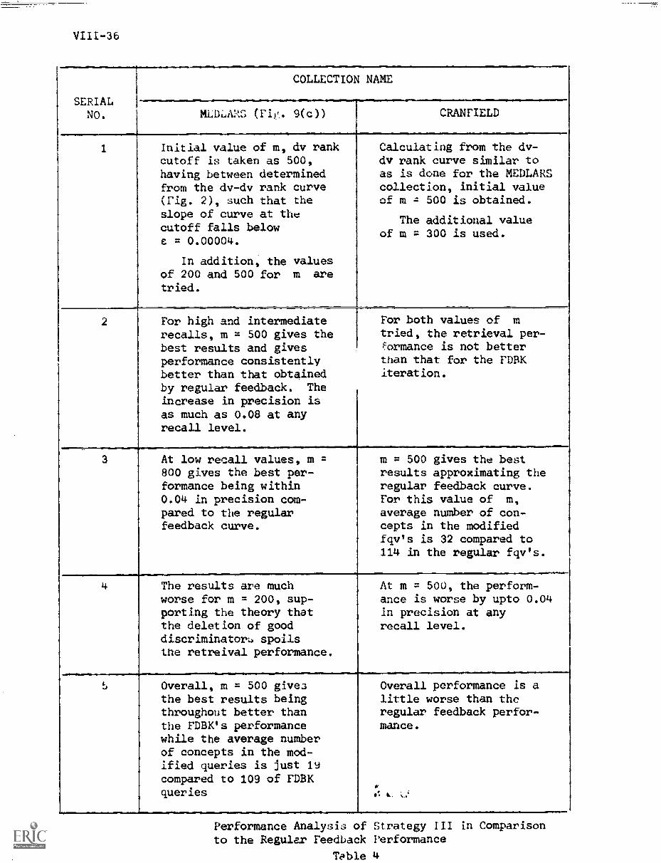
VIII-36

SERIALNO.

COLLECTION NAME

MIAL,X2 S (Fix. 9(c)) CRANFIELD

1 Initial value of m, dv rankcutoff is taken as 500,having between determinedfrom the dv-dv rank curve(rig. 2), such that theslope of curve at thecutoff falls belowe = 0.00004.

In addition, the valuesof 200 and 500 for m aretried.

Calculating from the dv-dv rank curve similar toas is done for the MEDLARScollection, initial valueof m = 500 is obtained.

The additional valueof m = 300 is used.

2 For high and intermediaterecalls, m = 500 gives thebest results and givesperformance consistentlybetter than that obtainedby regular feedback. Theincrease in precision isas much as 0.08 at anyrecall level.

For both values of mtried, the retrieval per-Formance is not betterthan that for the FDBKiteration.

3 At low recall values, m =800 gives the best per-formance being within0.04 in precision com-pared to the regularfeedback curve.

m = 500 gives the bestresults approximating theregular feedback curve.For this value of m,

average number of con -cepts in the modifiedfqv's is 32 compared to114 in the regular fqvis.

4 The results are muchworse for m = 200, sup-porting the theory thatthe deletion of gooddiscriminators spoilsthe retreival performance.

At m = 500, the perform-ance is worse by upto 0.04in precision at anyrecall level.

I.J Overall, m = 500 give3the best results beingthroughout better thanthe FDBK's performancewhile the average numberof concepts in the mod-ified queries is just 19compared to 109 of FDBKqueries

Overall performance is alittle worse than theregular feedback perfor-mance.

ti ...

Performance Analysis of Strategy III in Comparisonto the Regular Feedback Performance

Table 4

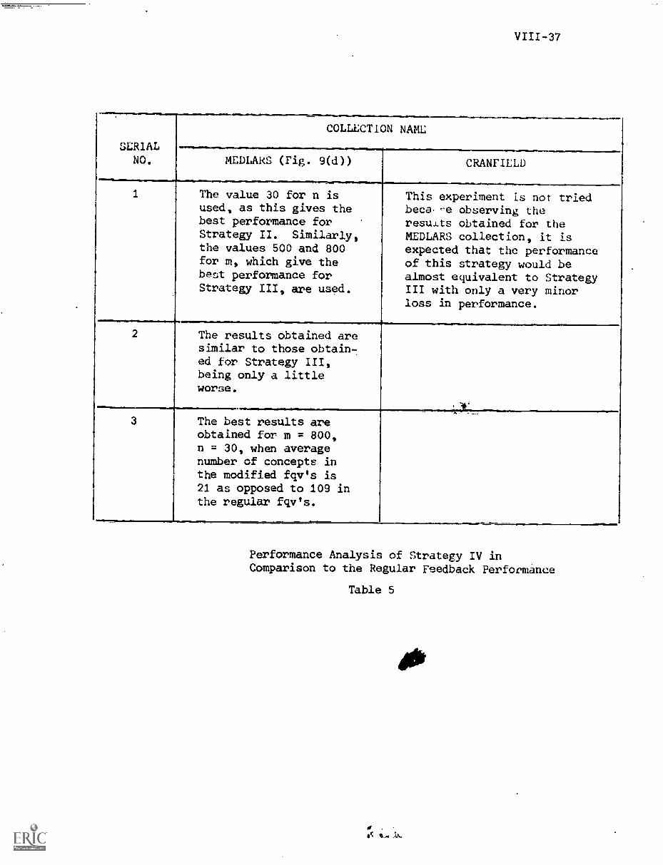
SERIALNO.

COLLECTION NAME

MEDLARS (Fig. 9(d)) CRANFIELD

1 The value 30 for n isused, as this gives thebest performance forStrategy II. Similarly,the values 500 and 800for m, which give thebest performance forStrategy III, are used.

This experiment is not triedbeca.-e observing theresui.ts obtained for theMEDLARS collection, it isexpected that the performanceof this strategy would bealmost equivalent to StrategyIII with only a very minorloss in performance.

2 The results obtained aresimilar to those obtain-ed for Strategy III,being only a littleworse.

3 The best results areobtained for m = 800,n = 30, when averagenumber of concepts inthe modified fqv's is21 as opposed to 109 inthe regular fqv's.

Performance Analysis of Strategy IV inComparison to the Regular Feedback Performance

Table 5

reduction is around 70% for the MEDLARS collection and

around S(Y, for the CRANFIELD collection.

The increase in precision at any recall level is up to

0.12 for the MEDLARS collection while for the CRANFIELD

collection, the performance results obtained with elongated

and shortened fqv's are equivalent.

iii) Strategy III

The use of this strategy for trimming the fqv's has

,,,esulted in an improvement in performance up to 0.08 in

precision at high recalls, compared to the FDBK curve for the

MEDLARS collection. On the other hand, similar experiment

on the CRANFIELD collection, shows a consistent loss of

precision, being as much as 0.04. It should then be inferred,

for the time being, that use of this strategy may give

results anywhere in the range of a slight loss of performance

to an appreciable improvement in performance, the benefit

being that length reduction is from 70-80%.

In the case of both the collections, the initial values

of dv rank cutoff, m, arc chosen from the respective dv-dv

rank curves by comparing the slope of the curve to the vale*

of c (here 0.00004). In both the cases, m, derived this way

happens to he around 500 and this value of m gives the best

results in both the cases. This supports the calculation of

m from the dv-dv rank curve in the suggested manner.

iv) Strategy IV

As expected, the application of this strategy for reduction

in the length of the fqv's results in a minor loss of

performance compared to that of the previous strategy (Fig. 9(e)).

Suggested values of m and n are the ones calculated for

Strategy III and Strategy II respectively.

e: a..

VIII-39

C) Comparison of the Four Strategies

The comparison of the four strategies is done in thrLI

different ways, in the following manner:

i) P-R Curves

Fig. 9(e) shows the comparison of the best P-R

curves -- one obtained for each of the four strategies,

for trimming the fqv's using the MEDLARS collection.

Fig. 10 shows the corresponding comparison for the

CRANFIELD collection. The deductions from these

figures are given below, separately for the two

collections.

a) MEDLARS Collection

1) Strategy III with m = 500 is the overall

best.

2) For this best strategy, at intermediate and

high recalls, the precision is better than that for

the regular feedback by as much as 0.08 at any

recall level.

3) At very low recall level, this strategy

gives a little worse performance than that for the

regular feedback.

4) The average number of concepts in the

shortened fqv's, using Strategy III is only 19

compared to 109 in standard feedback query vectors -

a reduction of approximately 80% in the length.

5) Compared to this, Strategy I (Murray's

method) with 22 as the average number of concepts

in the reduced length fqv's, that is, with

approximately same 80% reduction in length, gives

consistently worse performance compared to the

regular feedback. The precision is worse by as

much as 0.06 at any recall level.

6) For approximately 70% reduction in length, even

Strategy II performs better than Murray's method.

b) CRANFIELD Collection

1) Among vectors with 50% concepts chopped off,

Strategy II with n = 62 and average number of concepts

equal to 51 is the best along with the almost equivalently

performing Strategy I with 50% concepts removed, that is

with average number of concepts equal to 57 (Fig. 10).

2) With 70% reduction in the length of the vectors,

Strategy I (n = 30 and the average number of concepts = 32)

and Strategy III = 500 and the average number of

concepts = 34) are almost equivalent in performance, though

Strategy I has a slight edge over the latter (Fig. 10).

3) All the strategies tried give a little loss of

up to 0.04 in precision but the average number of concepts

is reduced by 50-70%.

ii) Overall Performance Indices

Here, four overall performance indices are compared

for the best P-R curves obtained. These indices are Normalized

Precision, Rank Recall and Log Precision [7]. Table 6 gives such

comparison for the two collections. The figures obtained,

substantiate the conclusions of the previous sub-section (1).

iii) Individual Query Behavior

a) Necessity of the Analysis

The analysis done so far has clearly established that

for the MEDLARS collection, the reduced length fqv's

give superior performance compared to the regular feedback

with its elongated fqv's. Thus, one gets the advantages

both ways -- smaller search costs because of the reduced

length vectors and better retrieval performance. Moreover,

VIII-41

TYPEOF

ESEARCH

R EF A

ORIG QUERYVECTORS

1st FDBKQUERYVECTORS

REDUCED LENGTH 1ST FEEDBACK QUERY VECTORS

STRATEGYI

STRATEGYII

STRATEOYIII

STRATEGYIV

0 SURERMANCE n=30% n=30 m=500 m=500,n=30

NORM RECALL 0.6563 0.7646 0.7134 0.7502 0.7794 0.7594

NORM PRECI-SION 0.5898 0.7301 0.6312 0.7234 0.7497 0.7333

RANK RECALL 0.1399 0.2513 0.2278 0.2354 0.2335 0.2377

LOG PRECI-SION 0.4837 0.6165 0.5837 0.6205 0.6268 0.6272

(a) MEDLARS Collection

TYPEOFSEARCH

ER EF A

ORIG QUERYVECTORS

1st FDBKQUERYVECTORS

REDUCED LENGTH 1ST FDBK QUERY VECTORS

STRATEGYI

STRATEGYII

STRATEGYIII

STRATEGYIV

0 SURERMANCE \ n=30% n=50% n=62 m=500

NORM RECALL 0.7496 0.8178 0.7997 0.7963 0.8216 0.7933 -

NORM PRECI-SION 0.6125 0.7359 0.7178 0.7180 0.7384 0.7172 -

RANK RECALL 0.2048 0.3312 0.3199 0.3249 0.3308 0.3261

LOG PRECI-SION 0.4330 0.5712 0.5596 0.5637 0.5689 0.5598 -

---

(b) CRANFIELD Collection

Comparison of the Performance Indices for theMEDLARS and the CRANFIELD Collections

Table 6

VIII-42

Murray's method (Strategy I) is worse with a poorer

retrieval performance.

On the other hand, the comparatively worse

performance reflected by the P-R curves for the

CRANFIELD collection for Strategy III is somewhat

unexpected. However another surprise occurs, when

one looks at the Table in Fig. 10 and finds that for

the whole query collection, the total number of

relevant retrieved documents among the top 10 ranks

compared with those among the top 30 ranks are

405/574 for Strategy III and 392/560 for Strategy I

both for approximately 70% reduction in the length of

_rectors, compared to 406/567 for the regular feedback.

Therefore, if one considers the total number of

the relevant retrieved documents as a criterion for

the better performance, Strategy III really is the

better of the two. The use of the total number

of relevant retrieved documents as a criterion of

retrieval performance is justified when one considers

that from the user's point of view, the number of

relevant among the retrieved documents is the more

important thing; the rank of a relevant among the

retrieved documents is a secondary consideration.

Yet, the ranking of the relevant documents among the

retrieved affects the P-R curves to quite an extent,

making the true evaluation a little difficult.

This situation is further complicated by the

undesirable "ranking effect" during feedback [8].

Most of the relevant documents used for positive

feedback improve their ranks after the feedback

iteration. This helps in improving the P-R curve

which shows a better performance, even though from

VIII-43

the user's point of view, no improvement has taken

place. This is so because he has already seen these

relevant documents and it does not give him any new

information if these very documents improve in their

rankings. We will give the name "positive ranking

effect" to such a "ranking effect".

In addition, "negative raaking effect" could

also occur. Suppose that after feedback, the relevant

retrieved documents tha. the user has already "seen"

decrease in ranks. This could happen, for instance,

when relevant documents are located in two distinct

regions of the document space and when one group is

retrieved, the other is not. This results in a

decrease in retrieval performance shown by the P-R

curve, even though from the user's point of view it .

does not. Again, he is not concerned with whatever

happens to the ranks of the documents he has already

seen.

Ail this calls for a more detailed analysis of

the iLcividual query behavior, so that a truer

nictlue of the actual improvement in retrieval

performance can be formed.

b) CRANFIELD Collection -- Query Behavior

1) Effect of Various Concepts on Retrievability

Table 7 shows the effects of various concepts

on retrievability of the individual queries for the

CRANFIELD collection. From the whole query

collection, three typical queries, called of

Type A, B and C respectively, are chosen as

examples. Using queries of Type A, the performance

of Strategy III is better than that of Strategy I

while the reverse is true for queries of Type B.

Furthermore, queries of Types A and B show how

the presence of good discriminating concepts and/or

the absence of poor discriminators helps in the

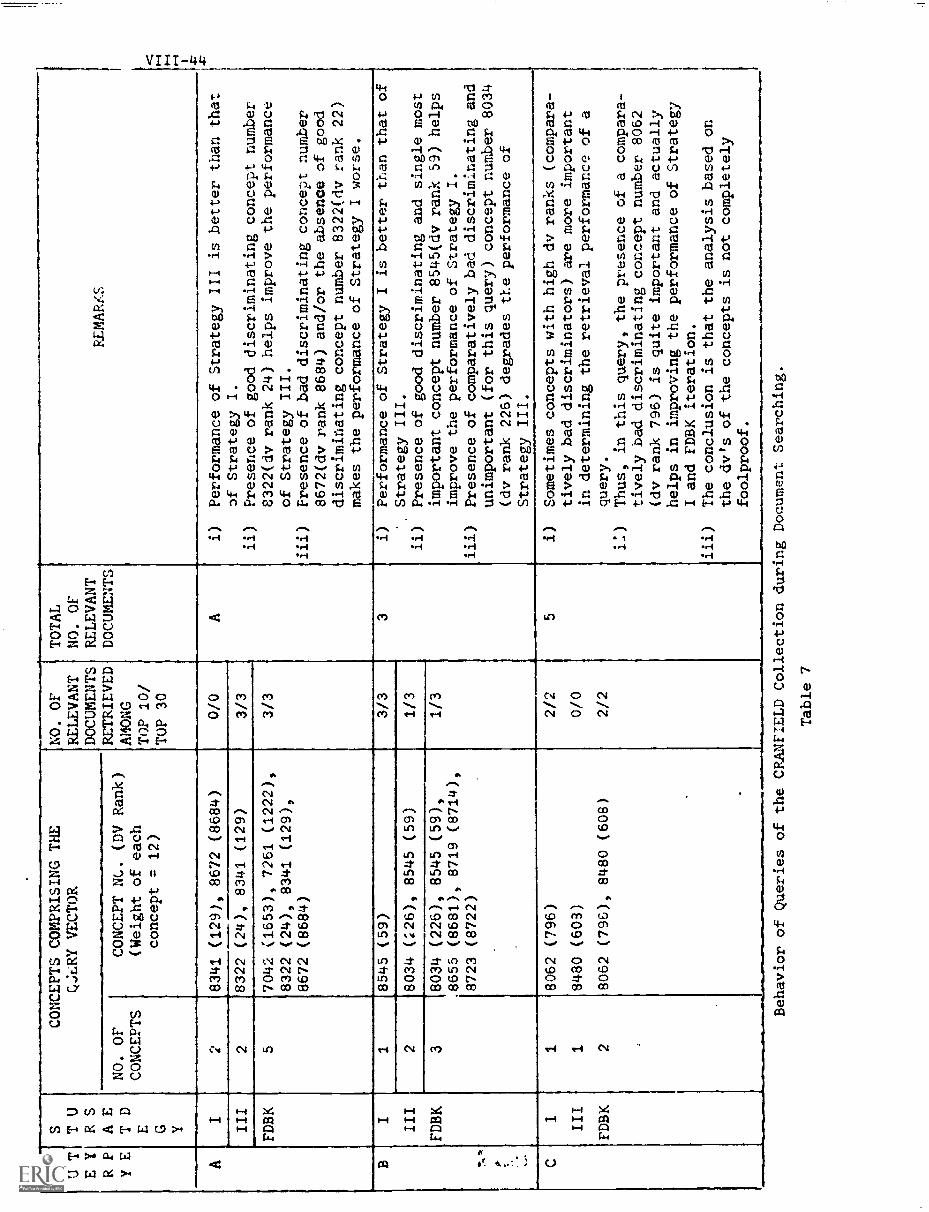
Q UT

E Y

RPYE

S T U

RS

A E

T E

CONCEPTS COMPRISING THE

Q.:LRY VECTOR

NO. OF

RELEVANT

DOCUMENTS

RETRIEVED D

AM ON

TOP 10/

TOTAL

NO. OF

RELEVANT

DOCUMENTS

REMARKS

NO. OF

CONCEPTS

CONCEPT NC. (DV Rank)

(Weight of each

Gconcept = 12)

TOP 30

Y

AI

28341 (129), 8672 (8684)

0/0

Ai)

Performance of Strategy III is better than that

III

28322 (24), 8341 (129)

3/3

of Strategy I.

ii)

Presence of good discriminating concept number

FDBK

57042 (1653), 7261 (1222),

3/3

8322(dv rank 24) helps improve the performance

8322 (24), 8341 (129),

of Strategy III.

8672 (8684)

iii)

Fresence of bad discriminating concept number

8672(dv rank 8684) and/or the absence of good

discriminating concept number 8322(dv rank 22)

makes the performance of Strategy I worse.

BI

18545 (59)

3/3

3i)

Performance of Strategy I is better than that of

III

28034 (;26), 8545 (59)

1/3

Strategy III.

ii)

Presence of good discriminating and single most

FDBK

38034 (226), 8545 (59),

1/3

important concept number 8545(dv rank 59) helps

8655 (8681), 8719 (8714),

improve the performance of Strategy I.

8723 (8722)

iii)

Presence of comparatively bad discriminating and

unimportant (for this query) concept number 8034

(dv rank 226) degrades the performance of

...

Strategy III.

C1

18062 (796)

2/2

5i)

Sometimes concepts with high dv ranks (compara-

III

18480 (603)

0/0

tively bad discriminators) are more important

in determining the retrieval performance of a

FDBK

28062 (796), 8480 (608)

2/2

query.

i.:)

Thus, in this query, the presence of a compara-

tively bad discriminating concept number 8062

(dv rank 796) is quite important and actually

helps in improving the performance of Strategy

.

I and FDBK iteration.

iii)

The conclusion is that the analysis based on

the dv's of the concepts is not completely

foolproof.

Behavior of Queries of the CRANFIELD Collection during Document Searching.

Table 7

VIII-45

improvement of retrieval performance. This is

a pleasing result because it supports the hypothesis

used as a basis for this project. However, there are

comparatively very few queries of Type C, which

shows that sometimes concepts with numerically high

dv ranks (relatively poor discriminators) are

more important in improving retrieval performance

than the ones with numerically low dv ranks

(relatively good discriminators). One can conclude

that even though the theory of dv's is not completely

foolproof, yet in the majority of cases it decides

the state of affairs.

2) "Ranking Effect" and Retrievability

To determine the influence of the "rank ing

effects" -- both positive and negative, the

documents retrieved by queries for the best case

(that is, for the best parameter) of each of the

strategies tried, are examined query by query for

the whole of the query collection. The procedure

used has been to note the ranks of the relevant

documents retrieved in the ORIG iteration among

the top 10 ranks (denote the set of these documents

by 2). As these are the documents used for

positive feedback (in the present series of

experiments) and thus have already been "seen" by

the user, the ranks of these same document:; of

the set S are observed in the retrieved documents

obtained for the other iterations. If the ranks

of these documents have increased compared to

their corresponding ranks in the retrieved

documents of the ORIG iteration, during any of the

regular or a modified feedback iteration, the

results for this iteration suffer from the "1.0nitive

ranking effect", that is the performance has been

overestimated compared to what it should be.

On the other side, if the rank of any document

of the set S decreases compared to its rank in the

retrieved documents of the ORIG iteration, during any

regular or a modified feedback iteration, the results

for this iteration have the influence of the "negative

ranking effect". In other words, the performance has

been underestimated compared to what it should be.

Table 8 depicts the documents retrieved by tw,)

typical types of queries, called Type D and Type E,

affected by such biases. For both the queries, the

performance obtained for the FDBK iteration does not

suffer from any appreciable ranking effect, that is,

the documents of the set S basically retain the same

ranks among the top 10 in the FDBK iteration as in the

ORIG iteration's retrieved documents. For the query

of Type D, comparatively the Strategy III retrieval

results get underestimated while for the query of Type

E. enmparatively the Strategy I results get under-

estimated. Since, the Type D queries are approximately

20 in number compared to approximately 4 of Type E

queries in the whole collection, it is concluded, that

the Strategy III results remain somewhat underestimated

compared to the Strategy I results.

c) MEDLARS Collection -- Query Behavior

The effect of the various concepts on the retrieval

performance for the MEDLARS collection is found to be

similar to the findings for the CRANFIELD collection.

It is, however, surprising to find that for the

MEDLARS collection, the queries of Type E are absent, while

there are at least 5 instances of the queries of Type D.

Thus, the Strategy III results remain underestimated compared

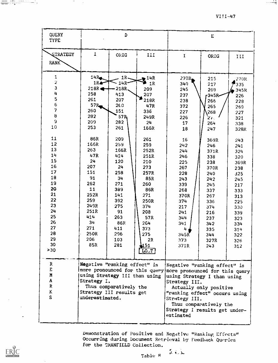
QUERYTYPE

VITI-47

E

'TRATEGY OkIG III ORIG III

1

2

3

4

5

6

7

8

9

10

14 1R 14R1R 14R 1R

218R 218R 209258 413 207261 207 218R57 2E0 47R

260 151 336282 57 249R209 282 24253 261 166R

2708340245237

238372227

226

17

18

11

1213

14

1516

17

18192021

2223

24

252627

28

29

30

>30

RE

MAR

KS

86R 209 261166R 259 259263 166R 252R47R 414 251R24 120 210

207 24 273151 258 257R91 34 85R

262 271 26011 389 86R

252R 141 271259 392 250R249R 275 374251R 91 208414 263 57R34 86R 264

271 411 373250R 296 275206 103 2R85R 281 51

LO,,T

16242244246

225267

228

24333926837OR374

217241344341

4

345R373371R

Negative "ranking effect" ismore pronounced for this queryusing Strategy III than usingStrategy I.Thus comparatively the

Strategy III results getunderestimated.

215217269

345R266265268

264247

369R246371R338

238370R240242245337267336374216237342335344

327R243

270k335345R226228269227321

338328k

243241

324

320369R238325245217

333313225330339

323334314322326312

Negative "ranking effect" ismore pronounced for this queryusing Strategy I than usingStrategy III.Actually only positive

'ranking effect" occurs usingStrategy III.Thus comparatively the

Strategy I results get under-estimated

Demonstration of Positive and Negative "Ranking Effects"Occurring during Document Retrieval by Feedback Queriesfor the :IRANFIELD Collection.

Table ti

Fof. 14-

to the Strategy I results for the MEDLARS collection also.

In spite of these odds, the Strategy III results have been

better.

D) Overall Comparison of the Four Strategies

Comparison of the vector trimming strategies by the P-R curves shows

the Strategy III to be superior for the MEDLARS collection -- it gives a

performance better than the regular feedback while the average number of

concepts in the modified fqv's are just 20% of the original length of the

regular fqv's. Strategy I (Murray's method), on the other hand gives con-

sistently worse performance. This is true in spite of the fact that the

strategy III results get underestimated in comparison to the Strategy I

results as shown above.

For the CRANFIELD collection, the performance shown by the P-R

curves for Strategy III is worse than the regular feedback performance though

almost equivalent to the performance for Strategy I. But, the individual

query behavior and the actual total relevant retrieved documents (among the.

top 10 ranks / the top 30 ranks) for the whole query collection using

Strategy III (405/574) compared to those for Strategy I (392/560) and the

regular feedback (406/567), show the Strategy III performance to be almost

equivalent to the regular feedback performance.

This shows that Strategy III may be used for reducing the lengths

of Cult elongated fqv's with almost equivalent or better retrieval performance,

while Strategy I always results in some degradation of performance compared

to that of the regular feedback. Whenever vectors of fixed length are

desired, Strategy II or Strategy IV may be used -- the latter being a little

better.

et;

VIII-49

One remarkable point about all.the strategies is that a

reduction in the lengths of the fqv'a by even 80% maintains the

performance much closer to the regular feedback (Ft)BK) rather

than to the original (ORIG) iteration.

8. Discussion.

In view of Murray's work on the construction of superior

profiles 12) and in view of the present study, a few interesting

questions arise concerning the initial indexing process and the

application of the length reducing strategies used in conjunction

with the various indexing methods. The purpose of this Section is to

discuss such problems and propose some solutions.

Murray suggests using a shortened frequency ranked profile

and finds that using a few broad weight categories, typically four,

gives performance equivalent to that obtained by using a larger

number of weight classes as in the standard weighted vectors.

Even though Murray's work concerns the profile vectors, it would

be expected that his results could be carried over to the indexing

process for the vectors in general. Some experiments in document

retrieval, using Murray's ideas, might prove the validity of this

assumption, which is made in the following discussion.

A) Shortened Frequency Ranked Vectors

Murray's construction of the shortened frequency ranked vectors

is performed by first forming the frequency ranked vectors and then

deleting the lowest weight c-ncepts. It is easy to see that Strategy

III, in addition to Murray's Strategy, can also be used for reducing

the lengths of the frequency ranked vectors. This is so, because

the only difference between these and the standard vectors is in the

formation of the c-w pairs to represent the vectors; there is no

difference in the structure of the vectors.

B) A Few Categories of Weight Classes

An interesting question is: which length reducing strategy should

be used when considering the vectors using only two or four weight classes?

Here, using Murray's strategy of chopping off low weight concepts could wipe

out some lower weight classes completely. If only one weight class is left,

.1-he resulting vector is equivalent to an unweighted vector (multiplied by a

constant), which, according to Murray, could result in decreased retrieval

performance. In such a case, a length reducer like Strategy III could be

useful. This would, hopefully, retain all the original weight classes ---

the idea being that it gives a chance of "survival" to the lower weight

but good discriminating terms to show their wc.rth in subsequent retrieval

operations, e.g. during feedback.

C) Use of Negative Dictionaries

The best adjudged method for reducing the lengths of the fqv's is to

retain the best discriminating concepts in each vector above an appropriately

chosen cutoff m (Strategy III). Deleting the poor discriminators from each

vector suggests the use of negative dictionaries. One idea that occurs is

to initially index the documents and the queries utilizing Crawford's [4]

negative dictionaries which use the same dv rank cutoff m as the one

determined for use in Strategy III. In that case, since no vector can have

concepts above dv rank cutoff m at any time, there is no need for using

4

VIII-51

length reducing Strategy III (or any other) at any stage of the

retrieval processing. This would save computation time in addition

to usual savings in storage and searching costs. The aim here is

to examine the usefulness of this idea.

The above possibility is depicted by the flowchart it. rig. 11(a).

On the other hand, Fig. 11(b) shows both the use of a negative dictionary

with a dv rank cutoff m' at the indexing stage and the use of a

length reducer with a smaller dv rank cutoff m to shorten the

length of the fqv's.

In one of his experiments using the MEDLARS collection and a

negative dictionary construction algorithm, Crawford has studied the

effect on the retrieval performance of deleting poor discriminators

from the document and the query collections. He concludes that for

the MEDLARS collection, a dv rank cutoff of m' = 1000 for the negative

dictionaries is the best in the sense that there is very little change

in any of the performance measures for the dv rank cutoff between 1000

and 5940, while the performance decreases sharply by deleting the

concepts below the dv rank cutoff of 1000.

In this project, a dv rank cutoff of m = 500 was found

optimal for using Strategy III to reduce the lengths of the fqv's.

It seems that for the same collection, m would be < m'. If

m = then using this cutoff in the negative dictionaries avoids

the use of Strategy III for subsequent length reduction of the fqv's

(Fig. 11(a)). If m' >m, a comparison between the performance must be

obtained for the processes shown by Figs. 11(a) and 11(b). We examine the

two possibilities specifically for the MEDLARS collection and tale

et.

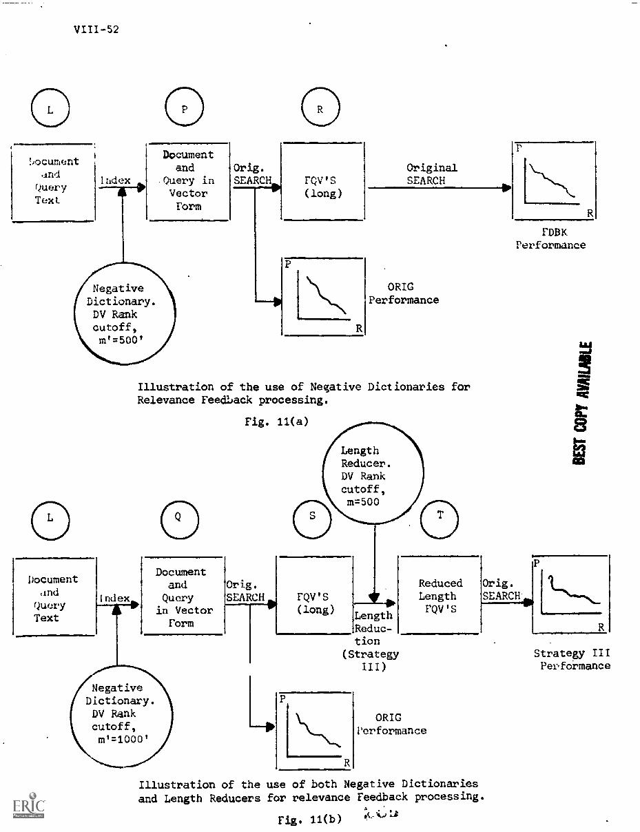
Iiocument

dndQueryText

Index

Documentand

Query inVectorForm

NegativeDictionary.DV Rankcutoff,m'=500'

Documentand

QueryText

Index

Orig.SEARCH FQV'S

(long)

OriginalSEARCH

ORIGPerformance

Illustration of the use of Negative Dictionaries forRelevance Feedback processing.

NegativeDictionary.DV Rankcutoff,re=1000'

Documentand

Queryin Vector

Form

Fig. 11(a)

OrSEARCH

LengthReducer.DV Rankcutoff,m=500

FQV'S(long)

LengthReduc-t ion

(StrategyIII)

R

OP

P

R

FDBKPerformance

Reduced Orig.Length SEARCHFQV'S

ORIGPerformance

Illustration of the use of both Negative Dictionariesand Length Reducers for relevance Feedback processing.

Fig. 11(b)

Strategy IIIPerformance

VIII -53

m = 500 and m' = 1000 based on previous experiments.

1. '.rawford's results show that the retrieval performance

obtainfA by using 'he dv rank cutoff of 500 in the negative dictionary

(Fig. 11(a)) is appreciably worse than the retrieval performance

obtained by using the corresponding cutoff of 1u0t (Fig. 11(b)). This

implies that after the original document search of Fig. 11(b), the

relevant documents retrieved would be more in number and/or have ranks

higher (numerically lower) than the corresponding relevant documents

retrieved using steps in Fig. 11(a). Thus the fqv's formed by using

positive feedback at stage R in Fig. 11(b) would, in general, be

better formed and be composed of comparatively more concepts above

dv rank of 500 (the best discriminating concepts) than in the fqv's

at stage S in Fig. 11(a).

Moreover, trimming the fqv's of stage S by a length reducer

employing a dv rank cutoff of m = 500 would retain all those oonroptc

above dv rank 500 in reduced length fqv's (at stage T in Fig. 11(h))

that are present in the elongated fqv's originally. Thus the number

of the best discriminating concepts (the ones above dv rank 500) in

the reduced length fqv's at stage T (Pig. 11(b)) would be more than

in the regular fqv's at stage R (Fig. 11(a)). Because the concepts

with dv ranks above 500 are the ones that most affect the retrieval

performance (Fig. 9(c)), this means that performance of the process

depictcl in Fig. 11(b) should be better than or at least equivalent to

that of Fig. 11(a).

VIII-54

2. Secondly, using a smaller dv rank cutoff of 500 at the

indexing stage could completely zero out some queries at stage P in

Fig. 11(a), while the probability of this happening at stage Q in Fig. 11(W

after using a dv rank cutoff of 1000 in the negative dictionary is

comparatively smaller. Furthermore, the query that gets wiped out at

stage P in Fig. 11(a) has a lesser chance of getting zeroed out after

reducing the length of the corresponding fqv at stage T in Fig. 11(b).

The reason is that the fqv formed at stage S would, in general, have

more concepts above dv rank 500 compared to the original query vectors

of stage L.

The conclusion is in favor of using the processing steps of

Fig. 11(b) rather than those of Fig. 11(a). In other words, the performance

would be better by using a relaxed dv rank cutoff in the negative dictionaries

at the indexing stage followed by a subsequent length reduction of the

vectors using a stricter dv rank cutoff rather than using the stricter

cutoff in the negative dictionaries while avoiding to use any length

reduction of the vectors later on. The exact tradeoffs between the improve-

ment in retrieval performance and savings in computation time should be

further investigated experimentally.

D) Ideal Indexing

An ideal indexing would be the one in which the weight of a concept

is a true indicator of the worth of the concept with respect to the particular

document collection and with respect to other concepts in the mme vector.

An indexing method, it seems, should consider the frequencies and the

distributions of all the terms in the collection. In this regard, use of

the dv of a term by the indexing process is important, because dv of a term

VIII-55

not only depends on the frequency and the distribution of that

term, but also on the frequencies and the distributions of all

the other terms in the collection [4].

If such an indexing scheme is nsed, then Strategy III for

reducing the vector lengths would not De appropriate. The reason

for this is that the term dv's have already been used in determining

the true overall weights of the concepts in the particular context,

and therefore it would seem more reasonable to chop off the low

overall weight (and thus truly unimportant) terms rather than to use

the dv's of the concepts again to help in reducing the vector lengths.

In such a case, Murray's method (Strategy I) which eliminates the

low weight concept: from elongated vectors, would be a good choice

for reducing the vector lengths.


This study has made an attempt to use the dv's of the concepts

to help in

a) reducing the lengths of the elongated vectors (the fqv's,

in particular), and

b) the reinforcement of feedback.

Questions that arise in view of this work and the previous

work in indexing, especially that by Murray (21, are examined.

The specific conclusions are:

VIII-56

i) Strategies for controlling the lengths of the fqv's and

based on using the knowledge of the dv's of the concepts

have been found quite successful.

ii) In particular, a length reducing strategy based on retaining

the top best discriminating concepts only (Strategy ITT of

this report), has been adjudged to be the most successful.

This results in reducing the lengths of the vectors by 70-80%,

thus saving on the storage and searching costs while at the

same time attaining better or almost equal performance than

that obtained with the elongated fqv's of Rocchio-type feedback.

iii) In comparison, Murray's strategy results in decreased performance

than the regular feedback for the experiments conducted.

iv) When fixed length query ve,tors are desired after trimming,

Strategy IV is useful and it gives only a minor loss in

performance compared to the best adjudged Strategy III.

v) An interesting fact is that, the use of any strategy for

80% length reduction of the fqv's results in retrieval performance

being much closer to the regular feedback with elongated vectors

than to the performance of the original iteration without feedback.

Th;.s means that all the strategies tried are good in the respect

that they retain much of the benefits of the regular feedback

with at best a comparatively little loss in performance.

vi) It is observed 'chat Strategy III could be useful whin used along

with Murray's proposal of using only a few, typically four,

broad categories of weight classes.

vii) It is shown that the retrieval performance is better using a

relaxed dv rank cutoff in the negative dictionaries during initial

indexing stage followed by a subsequent length reduction of the vectors

employing a stricter dv rank cutoff rather than using the stricter

cutoff in the negative dictionaries while avoiding to use any

length reduction of the vectors later on.

VIII-57

One should note that for a large-scale application of

Strategy III as a length reducer, many of the experimental derail:;

would be saved if all the concepts occurring in the document and

the query collections are renumbered in their decreasing dv order.

A final remark is that the results of this project temi to

support the view that the dv's and the frequencies of the concepts

are important in determining the indexing process and should play

a joint role in the design of an ideal indexing scheme.

VIII-58

References

[1] G. Salton, Editor, The SMART Retrieval system - Experiments in AutomaticDocument Processing, Prentice Hall, Englewood Cliffs, N.J., 1971

12] D.M. Murray, Document Retrieval Based on Clustered Files, Ph.D. Thesis,information Storage and Retrieval, Report ISR-20 to the NationalScie,sce Foundation, Department of Computer Science, Cornell University,Lthaca, N.Y., June 1972.

13] K. Bonwit and J. Aste-Tonsman, Negative Doctionaries, InformationStorage and Retrieval, Report ISR-18 to the National ScienceFoundation, Section VI, Department of Computer Science, CornellUniversity, Ithaca, N.Y., October 1970.

[4] R. Crawford, Negative Dictionary Construction, Chdpter IV, this report,Department of Computer Science, Cornell Pniversity, Ithaca, N.Y.

[5] K. Bjorklof, Relevance Feedback Based on Term Discrimination Values,Information Storage and Retrieval, Report ISR-21 to the NationalLibrary of Medicine, Section IX, Department of Computer Science,Cornell University, Ithaca, N.Y., December 1072.

[6] T. Doeppner, M. Finley and R.A. Peterson, Positive and Negative Feedbaer.using Reinforcement Procedures Based on Term Discrimination, InformationStorage and Retrieval, Report ISR-21 to the National Library ofMedicine, Section X, Department of Computer Science, Cornel University,

Ithaca, N.Y., December 1972.

[7] G. Salton, Autocratic Information Organization and Retrieval, McGrawHill Book Co., 1968.

[8] J.J. Rocchio, Document Retrieval Systems -- Optimization andEvaluation, Ph.D. Thesis, Information Storage and Retrieval, ReportISR -1O to the National Science Foundation, Harvard ComputationLaboratory, Cambridge, Mass., March 1966.

(9] Y.K. Chang, C. Cirillo and J. Razon, "Evaluation of Feedback Retrievalusing Modified Freezing, Residual Collection, and Test and Control

Groups", Chapter 17, the SMART Retrieval System -- Experiments inAutomatic Document Processing, Editor - G. Salton, Prentice Hall,Englewood Cliffs, N.J., 1971.

[10] H.A. Hall and N.H. Weiderman, The Evaluation Problem in RelevanceFeedback Systems, Information Storage and Retrieval, Report ISR-12tc the National Science Foundation, Section XII, Department of ComputerScience, Cornell University, Ithaca, N.Y., June 1967.

t+,

IX-1

The Shortening of Profiles on the Basis of

Discrimination Values of Terms and

Profile Space Density

Marc A. Kaplan

Abstract

The problem of long profile vectors which naturally arise

in a clustered file environment is discussed. A method to reduce

profile length is suggested and tested. The method involves

eliminating those concept weight pairs whose concepts have poor

discrimination values as defined previously by Bonwit and

Aste-Tonsmann.

1. Introduction

Any information retrieval system which is to operate on a

large data base and which is to provide on-line service to users

must be designed to provide reasonable response time for the user.

In a SMARTlike 11] environment where documents and queries

are represented as vectors of numbers and a query-document correlation

function must be computed to evaluate the degree of similarity

between each query and document one cannot hope to compute all of the

correlations between a given query and every document in the

collection and still give the user reasonable response time. Therefore,

one seeks strategies which will reduce the number of correlations

which must be computed before the retrieval system can produce an

"an swer " .

iX-2

One such strategy is to use a clustered file organization for

the document space. in this organization whole groups of documents,

called clusters, are represented by one pseudo-document, called the

centroid or profile of the cluster. The centroid of a cluster is supposed

to be representative of all the documents in its cluster. Thus the

system need only correlate a query with all of the centroids in the

document space and then with all of the documents under those few centroids

which seem most promising rather than with each and every document in the

entire collection.

One problem with clustered files is that the profile vectors are

often unreasonably long, that is, the profile vectors contain many non-

zero entries. Since in a usual implementation only the non-zero terms

are stored, long vectors require more storage than vectors with few non-

zero concept weights. (Typically vectors are stored as lists of non-

zero concept-weight pairs rather than as a list of ordered weights, one

for each possible concept number.

These long profile vectors occur because the profile, P, of a

cluster is usually given by a formula such as:

(i) P = D./ni.i

where i ranges over each document in the cluster.h.

D. is the 1 document vector

n. is some non-zero normalizing factor

Thus the profile of a given cluster has as many different non-zero concepts

as there are distinct terms in the whole cluster.

IX-3

Not only do all of these non-zero terms require considerable

storage but they must also certainly increase the time required

to .:.orTute a correlation value. This is so since all the concept-

weight pairs in the profile vector must be read into the computer

and then checked against all of the loncepts in the query vector.

Even if none of the concepts match, the given correlation algorithm

must at least search through the long profile vector to determine

this.

So one must naturally ask if there is any way by which one

can "shorten" the profiles of a clustered collection of documents

without app* 3ciably degrading the performance of the system with

regard to recall and precision levels. If this coult be achieved

one would have a better retrieval system than the original system

with long profiles since storage and CPU time would be conserved and

the user would be served faster.

Experiments made by Murray 12) suggest that one can indeed

shorten centroid vectors merely by deleting some of the concept-

weight pairs. He states:

... profiles 7.3n be subjected to considerable deletion oflow welFtht frequent) terms with little change in thequality 0'- teIrch output... Experiments... indicated thatthe deletion of SO% of the lowest weight terms drops the

only to 5%."

Murray's approach is local. He examines each profile individually

without considering the others and deletes those terms of lowest

frequency. Might not some high frequency terms also be good

wbjeets ftr deletion? Murray says:

"On tne other hand, an attempt to remove or combine relatedoccui ,ences of high weight profile terms results in muchpoorer performance. Such procedures are to be avoided."

IX-4

In this paper the experiment is based on a different approach

towards finding the appropriate terms to delete from the profiles of a

collection. What is desired is a technique for finding terms which are

not important or may even be detrimental in computing query-ceutroid

correlations. The experimenter does not wish to prejudge that terms

should be deleted simply because they are of high, low or medium frequency.

Nor does he want to guess how many terms should be deleted or kept. What

then is Lie to do?

Bonwit and Aste-Tonsmann 13] have conducted research in the

construction of what they call "negative dictionaries", that is lists

of words which are best not considered as concepts in a collection of

documents; which are best deleted from document vectors. One- may ask

whether their technique might not be applicable to the present problem?

2. Density and Discrimination

Bonwit and Aste-Tonsmann define document space density Q as:

1(ii) Q = ir L cos(P,D.)

where N = number of documents.th

the ] document vector

P = centroid of documents given by (i)with n. w N for all i

cos is the usual cosine correlation functionas used in the SMART system

Now define vector VI

as vector V with the set I of terms

deleted (that is, set to zero). Then Q1, the density of the document

4,

IX-5

space with the set I of terms deleted is defined as:

I I(iii) = NN L cowI,Dk)

kwhere k ranges over the set of integers for which

Iis s not identically the zero vector

N' = number of documents for which Dk

is

non-zero (usually for small sets I,

N' =kN.)

The discrimination value, ak, of term k is now defined to be:

(iv) ak

= 100 * (QK - Q)/Q where K = (k)

The greater the value of ak, the better the discrimination value of

term k is said to be Intuitively if ak is large and positive then

the deletion of term k from the document set causes t..c. space to

"contract ", thus term k is thought to be a good term, necessary to

help distinguish one document from another. If ak is close to

zero then the deletion of term k should not affect the document

space significantly at all. Finally if ak is negative then term

k is a bad discriminator, its deletion will almost certainly

improve the document space!

What one seeks is to find the optimum deletion set of terms,

I. The hypothesis is made that that set I for which Q1 is

minimized should be the "best" set of terms to delete.

In their experiments Bonwit and Aste-Tonsmann attempt to

construct set I in the following way:

1. Compute ak for each term k.

IX-6

2. Construct an ordered set K, K=(ki,k2,...,kt), such that

a > a,k K+1

for i = 1,2,...,t-1, where t is the number of

unique terms in the document space.

3. Let Kp=(kpi1,kp+2,...,kt). Note that Ko = K and Kt = the

empty set. K is the set of all but the best p discriminators.

4. Now one assumes that in a good deletion set, I, one should

want the wrst discriminators, that is one only wishes to keep

the best, say p, discriminators as terms in the document

space. Thus the problem of finding which of the 2t

subsets

of K to use as the deletion set is reduced by the above

assumption to finding which of the t subsets of the type

K to use as a deletion set.

5. Find p to minimize QK . Then I = Kp is the desired deletion

set.

Bonwit and Aste-Tonsmann found that for the particular collection

with which they worked that K was indeed a good deletion set. Retrieval

performance as measured by normalized recall was actually improved by

deleting the set of terms K . In fact, they found that for a sequence

of document spaces, each given by deleting more and more of the "bad"

discriminators, normalized recall was greatest almost at the point where

QKwas minimal.

pOne should notice that the deletion set K as computed above

does not depend on any parameters external to the document space itself.

There is no need to choose any frequency cutoff value nor is it necessary

arbitrarily to decide the percentage of the original terms which one

wishes to keep.

IX-7

3. Experimental Design

The discrimination value approach is applied to the problem

of long vectors by considering the set of profile vectors, apart

from the rest of the collection, to be a document space. The

algorithm given in part 2 is then applied to the set of profiles

in order to compute the hopefully "optimum" deletion set Kp.

Existing FORTRAN programs [4] were modified by the experimenter

so as to automatically compute the values QK for 1 = 0,1,...,h,1

where h equals the number of positive discriminators. The smallest

alue of 1 which minimized QK was considered to be p, the optimum1

number of positive discriminators to retain in the collection of

profiles.

Having computed p the profile vectors were then modified

by the deletion of all but the best p discriminators.

(It should be pointed out that the procedure actually used

in computing the values, QK , is not precisely the same algorithm as1

given in part 2, although the results which are obtained in using

the FORTRAN procedure are believed to be well described by the

procedure given in section 2. The actual computations that are made

are done by first computing Q in a straightforward manner, but

some of the results of necessary intermediate calculations are

retained. Then a simple and quick computation of the values of

ak is made by recomputing just a few intermediate values. Once

the values of ak are computed, they are sorted and a note is made

of how many positive values exist. Now to compute the values, QK 9

1

the program first computes QK and saves some intermediate results.1

IX -8

The successive valut of QK2

,QK3

,...,QKh are computed one after another

by merely accounting for the effect of adding but one more term to the

profile space. The interested reader is referred to the programlisting

if he wishes to see the details of the computation.)

For each collection used in the experiment two sample searches

were made. The first search was run with the original profile vectors.

The second search was run with the modified profile vectors. Except for

the use of different profile collections, the SEARCH routine of the SMART

system, on which these tests were made, was given the same search parameters

for each of the two runs. SEARCH results were compared using routines

AVERAGE and VERIFY.

Two different collections were used in this study, both are

available on disc packs on the Cornell University 360 computing system.

The first, the document collection called ADIABTH DOCS was used along with

its associated TREES, the original profile collection, and QUESTS, a set

of queries for which relevancy decisions have been made externally to

the SMART system (82 documents, 35 queries and 13 profiles). The small

size of the collection allowed for economical debugging of programs and

the experimental procedure. Results obtained with this collection were

encouraging enough to warrant the use of a larger collection for further

study.

The second collection used was CRN4S DOCS(424 documents), QUESTS30

.(30 queries), and KTREE (29 profiles). The KTREE centroid collection

was created especially for this study by the experimenter, using the

CLUSTER routine of the SMART system. (See computer run contained' herein

iEsT

CO

PY

AV

4114

1LE

CLUSTER

COLLECTIO'i

CRN4S

JCCS

4/L4..RF:.cLusTEPED.0.45iyqploccHiotsCLUSTERING ALGORITHM

TO Fnwil WISTER

cottxcirom

CRNiqL

!TREE

THE FOLLnING PARAmFTERS

WILL BE use!):

WILL LOOSE

ITEMS BE PLACED kITH

TH' CEVTROID or HIGHEST

CORRELATION - YES

THE mivt:rk or ijS

TP24E,. F.ATCHED FR CLUSTERING

-1

(IF n At. OFT!!:!U VALUE

WILL BE CALC9LATED.)

SCFATC

PPE USED

HA

sl

mo

c)

THE FIRST 17E

TO AL USEV AS A PlSg/RLE

CLUSTLX liOCT

1_DRPHOW

fOON.PC3.

PEKTP

00

UMITVC

BY WORK

MINCOR -

0.800E-01

MOLT -

1

THE CUSITY TEST

CARD.

Tn BE A CUISTE1 POINT,

AT KAST

7 ITEMS MUST HAVE A

CORRELATION nRATER THAN

0.20000

re!3 AT LEAST

15 ITUIS MUST hAVE A

CORRELATION GREATER THAN

0.10000

p THE CLUSTER SIZE CONTROL

CAPr).

THE M/NImirl Nui.ilER OF

ITEMS IN EAC4 CLUSTER

IS

15

THE IAXT"JI

DF TIP'S I% EAC4

CLUSTER IS

Zt1

Cluster Parameters

1-+

4 1 tD

SEARCH.- T4E. _AD/AoTH

wESIS

COLLECTION IS USFO TO StARCH AGATksT THE

AT LUST _Ss !Ms 'AiLL

C LISTEa FeR EACH SEAKCH

AnTARTH _O0cS

Tyr FlasT EIGHT CHAKArTERI OF THE rA:"E

rAC4 RESULT CrILECTUE Is

10,!sur14

OPTIONS FOR SEARCH :ANiUER

LTPM

04/S ruLT

PREY guLT

1ft

miN CORP

0,2000E nn

POS KILT

NEG roLT

POs RAr:K CUT

.0

0

UNLESS

0

STOPAi L

rio^RFC CUToFT

:41'E:

COLLECTIOm

TYPL COPR.

TIFMAL

ITEPISXMULT$

COPMWGHTS

FR=FLUID

UNITVC

WGHTC ORPEO

PEP DRPEO

COSINE

ABNORMAL

NO

NO

BY towl

POS.NON,

0,n

..

-,

ULG kANK-Cuf---PiiSCORRi&

CFG CORR CUT

POS ATLEST

NEG ATLEST

POS NONOBE

NEG Nowak

a1.0000

locion

aa

__A

0

OUXBIEs

PKET

SILEbTAL

'Mkt WILL BE

2 sEARElls 040E.

THE mAxIHIpt NuBER OF QUERIES In EACH BATCH

Ts

7

Sear

ch P

aram

eter

s

Fig.

2

11 7 $ 4

..pA

RA

ME

TE

KS

FO

R T

RF

E.

-

ITE

RA

TIO

N.

_Q.-

- --

._LT

I1M

_to

FPE

LA

ILIN

_Pa

r_V

AN

TE

DC

I10(

._2

0__

._...

TIL

VIL

LT

IMP

EL

soor

tiEss

Pcc

,i0.

opc

i,0.

0m

u/o

. nP

UY

0.0

r /k

itL

i .0

P iL

LC

F0.

0PA

L L

C P

I0.

AP

AU

LY0.

0K

um_a

. o_

_PF

CE

CI1

0.: 0

pPIC

FCp)

0.0

INC

tiLV

0.0

PAC

'ILV

0.0

PVC

KV

0.0

PIC

FIV

e_.0

_P

F.0

FLY

_0.

._0

PV

CF

LV__

__00

SE

LFC

TIo

rir

nino

n1

',Aru

m)

3G

AP

3276

7.00

rPsL

om0.

01R

EJE

CT

ION

PP

4r)0

000.

00P

wA

crat

R0.

00P

EP

CO

L0.

0%

TIM

WA

N0.

0P

RIN

T Ir

G.

_-

._

_SO

NS

_hO

CO

RR

ELA

TIO

NS

NO

RA

NK

SY

E'S

Par

amet

ers

for

Tre

e S

earc

hes

Fig.

3

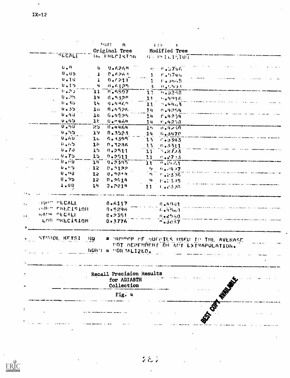
9

A

IX-12

r,lit fl

Original Tree Modified Treer)LCAL1 NT -IN i it I. 1 ;;;I"ii:7-

tor-0

Lnn

1, (.1.2r" I.

1 C.4.2f,-A

1 Oer 711 14 0.e.Ip9 I

11 n597 1114 11.32'11 111.4.1 9 efiy1 11io n.452F. 1 ti3C 1a.t452e) 114

3.f.: ti.P4Ati 14;)5 (1.4464 vi19 0.352i 11414, 114.439. 12)lb 0.12RA 11VD 0.2S11 1115 0 P .)11 11Ve 9 *Pifir)3.z (1.11,2

it.

1k Uee,04412 n .1614

-r,

q14 O.:N.11u 33

nt.CALL

r'ic I.. I

°I<LCACIOW.am../11.1.

0.4.117

0052.9A0.3910 3776

r.'..;7.44.

11.Y)1A

f,.4."1r.''144+,3n 4,:54r.'041,42W11%0.e-inti,5147Vc.a.34311,6iti

:',.:2,4r.:,

f'.;!3-4.1.-

1.,:-.; v.;1 e 3 PI

.1111.1.1.1.11111.1. ..1.111.1111-

111WIIIM

0.4901. .

. _

4 Fir, ..3

. .1110

Isa_.. _ _________._A.66!.7

waameaswwwwwww1IIm

sMi01. Kr TS: NO = 111.4841-11 r.F I. S Tilt-. .Avt1iv7TnEprmf*Nr ON At'Y L fqAPULATION.

WW1 = "OR 1ALI2LO

Sub ..../

Recall Precision Resultsfor ADIABTHCollect ion

Fig. 4

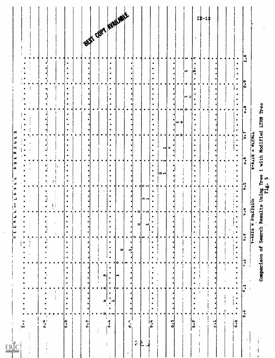
aJ

;.)

cc

a.

41

.4$

a.

#.1

us

X

,

o

1

a.

IP!

1

II

1

0000

:

oo oo '

oo

.

'

j ooCD

0

C

3 #4

IIII el

I

e.

r.

3 O 00 o oO

I

a)

3

3

0000

o o ,

. w oo 0000

!

C. O

rt

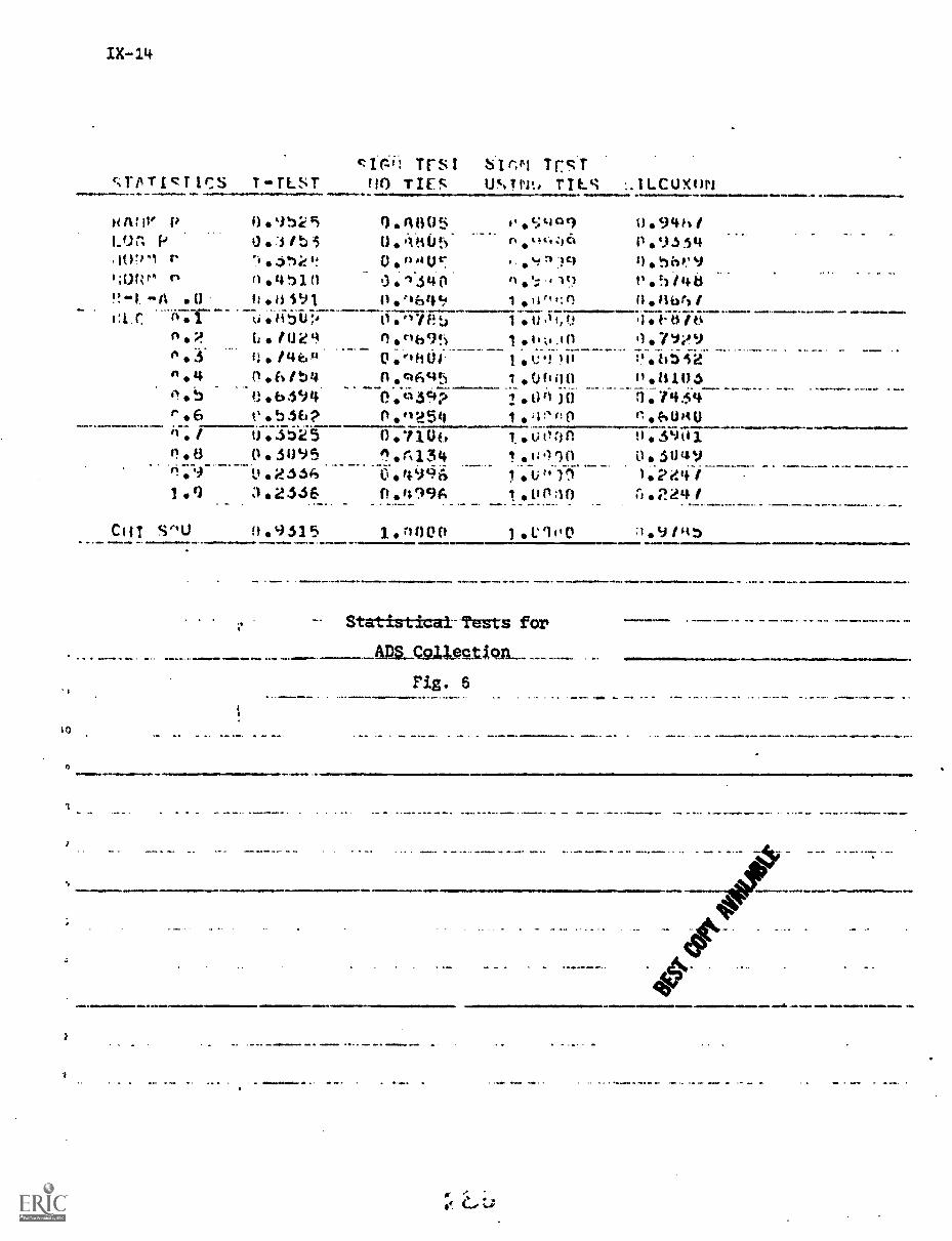
10

;TPTIT ICs TLSTirs1 S1 r,P1 TES

(U) TIES W. TILS ILCUXIM

8 A: iv I) f) .9!) 5 0.n805 I, .t:;tin9........

0.94tItLot; P 1.:J/5i 0 4, 'iMP,i fi ttc.:)6. 8'. `)334,1()'r "1 r ..i 0 j!.) 6!

_0 "MUr. , ki r.) 31C) $) 0 hilk' 9

I WM " r1 11 .4'11 ci 0 .1..51'0 n..1 lt) I' !)/14.8_ !'....1. It 0 t:0591 11 '46ift, *I .10,:fl O. ilbr) I

1:i.r. n.1 ka .iiiv,.. 0 . wilt tj 1 11, f, f.1 1.t.ts It.n..%! 11. /1U4 n tvb9s 1 .1..,..in .).7q$?9,_.fl .3. f: Pt e.,,, 0 ."11Uir--- letiii!ii- :,-... 'S

^ 4 (I * 6 Ibti n c4A95 1 WI Op.__ 00 W.6

1..6 t' bits? (111:)518 I ,i1:,(:0 114-ILIAU11 / tl ..25 0 *110E., 1.011:A ti 39 0 111.8 0 3895 1.1:134 1 .1z .)10 it , 3o tty".'a_

W. 56 C5- - -.

-1-1-. OA"; 1 ..-.1) "- 1.2elet1 .0 3.2546 ft ft99et 1,011;10 ri 2 4

CUT S"u 0.9315 1 one() 3,1.'100

Statistical Tests for

Fig. 6

M

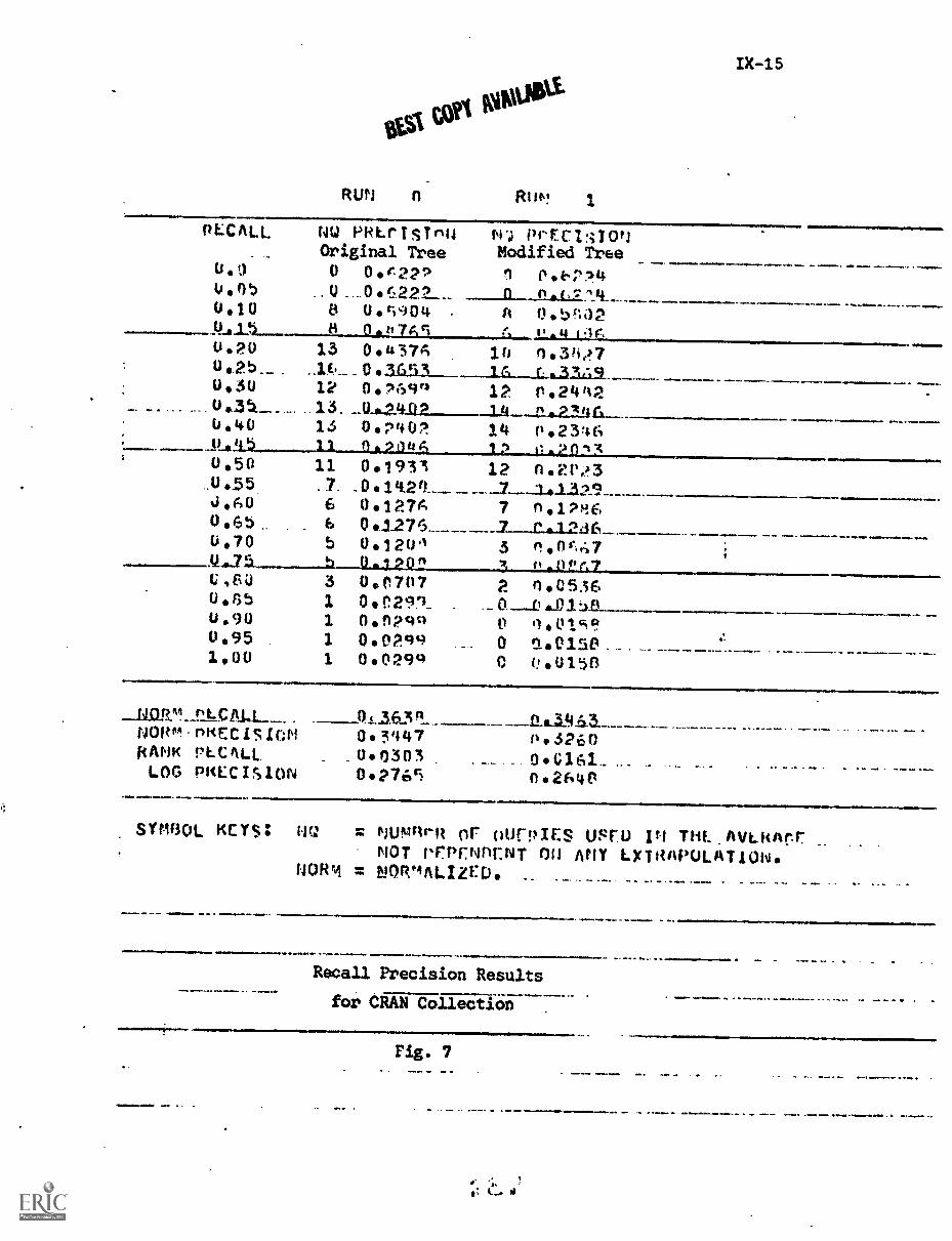
tat Ritillfig.

RUN n RI if,' 1

PLC ALL

0.1

0.10Q..15

ffl

Original0

88

PRIrTSPINTree

0.(-22

Pr;

Modifiedn

PrECI3TONTree

fsr!).40.c904Okft7Ari

Ar,

05,1a2.1,1100.

0.20 13 0.1137g) irs

1 & (.L3119-0.30 12 0.769n 12 v.2442

13 00400.40 14 0.P402 14 P.2346

.

0.50 13. 0.1931 12 0.2r,?3.0.55 .7. _0 14.29_

f1.16J.60 6 0.127A 70.65 6 001275 2 c.12A60.70 5 0.1204 3

.0120n 3 140r7

U,S0 3 00(1707 2 r) .053E,1 osn291_

U.90 1 0.n290 #1.010.95 1 00Pq9 0 0..01514

S.

1.00 1 00294 0 0.015S

NO2""_ PLcAL1_ 0,363nopm PK EC IS WI 0.3,147 o.3260RANK PLCALL _0.0303 . 0.0161.LOG PRECISION 0.2761i n.2610

SYM6OL KEY: = MUMM-R or ourpics usru 111 TH. AVLRACT _MOT rrPFNMENT ON AMY LXTRAPULATION

NORM = DJOirgALIZED.

Recall Precision Results

for CRAN Collection

Fig. ?

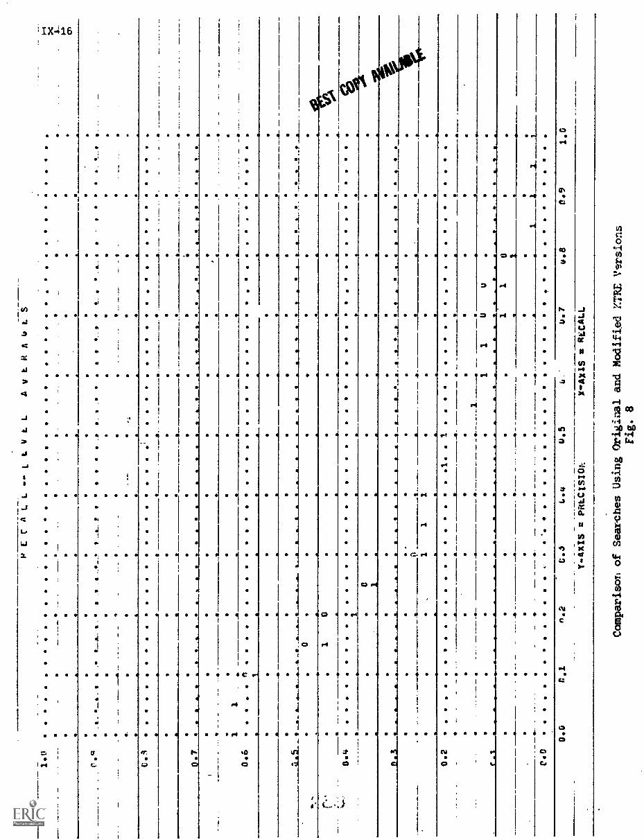
1.0

RE

C A

LL

' ' ' '

LL V E L

a

A VER AtiES

I

Pc,

-_

* . t

a.

a ..

2a...

a .

.

_2 _

a

.. _

_iv

__a_I'

tttttt

.

._

....

a

a

:

..t

a

_ a a

C.i

aa

a__

a-4

1 I

a.

_11.

--t

-I-

-

'iv

0.7

****

.t

-a1

1-.

1ka

*---

--_

--2.

0.6

A

ai -0

a-

-

9--

&--

.a

a_a

a_a_

__ a

_...a

.__

--.

.-

.r.

10

a

0.4

-go

10 1

0.3

.a

aa

**a_

_a

.....

.a

-2

0.fi

a

11

1-a

.

0.2

1a

a..

...0_

__a

1a

-- 11

r.1._

.___ - .

-.._

a....

...a

._

..1

1.--

-0--

1-

.---

.---

la

.1.-

--.

---

a1

.111

0.6

t.I

n.2

C.4

u,5

to

.

0.7

u.8

YAXIS = PRECISION

XAX1S = RECALL

.

a lo

a

- a-

____

t_-P

___

a___

__

:.

111A

st__

_- ill

0.9

1.0

Comparison of Searches Using Original and Modified Y.TRE Vsrsions

Fig. 8

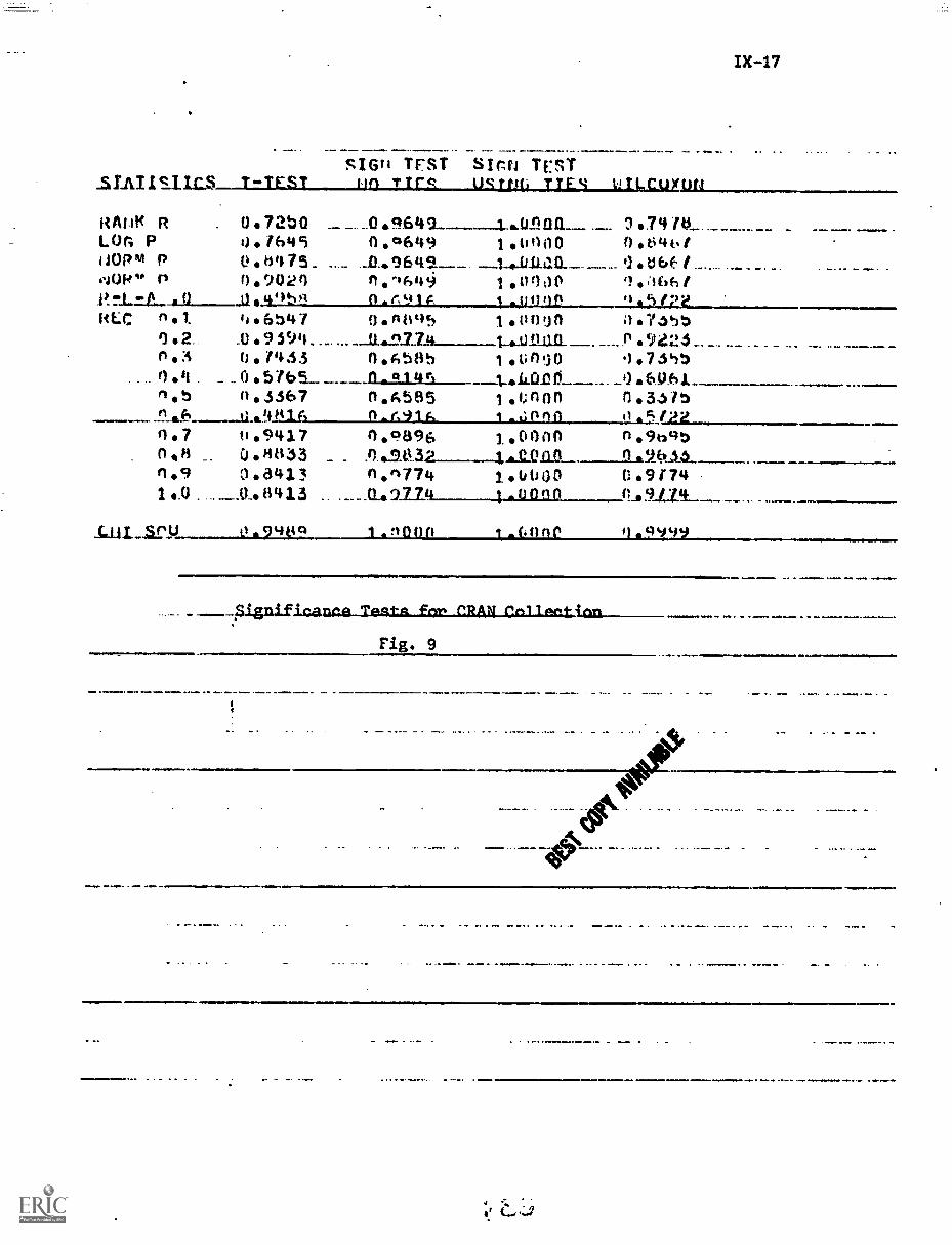
_SLAT I SIMS T-TEST

_ .

sIGN TrST Sim TrsT110 TIN us trq, TJ LALC_uxon

RAW( RLO( P110P m PeJofew P

0.72b0O. 16450,b4750.9U2n.11,44t01

_0.9649_ n lag/0_0 .646 IQ.uw. I

n .0649

no'6490.r9lc

1.0000takikal1,00001 -9 11,9 P

9 Ms6 1

22Z112.?1(U: n 4.6647 0.'1845 1 ,009n 0.75

0.2.. _0.9394 11.411774 1-4...UV an n .9224 _.

0.A585 1 .u090n .3 0. (463 1.760 sal . _ 0 .5765_ n_0145 6L.L.0.00 1).6.061nob n .3367 0,A585 1 .0w ().3.51

n-ii,91 A 1_, %; 0 n ci 0,22ti .9417 0"896 1,00on no9bqb

n 0.86633R.9 o.8413 n,e1774 1.0600 0.917424.0 _0_66413 . ._...a..917.4 1,enon n_.91/1_,

0.94eQ .9000 1.60! P 0.9949

IX-17

TaAtot for cm rn1 tent ;nn

Fig. 9

for a description of the parameters used to create the profile collection.)

This collection was used because it was the largest available collection

which the experimenter could afford to use that was easily accessible on

the SMART system.


The results of the experiment are promising. As shown in Table 1

the storage requirements, in bytes, for the profile collections as maintained

in the SMART system have been cut by about 30%. Also the number of concepts

in the longest profile in a profile collection is cut by 33% in the case

of the CRN4S collection and 47% in the case of the ADIABTH collection.

Recall and precision performance is meanwhile hardly affected at all.

In the case of the CRN4S collection recall level averages are almost identical

for searches using the two different centroid collections, with perhaps a

slight advantage gained by using the original centroid collection instead of

the modified collection. However, the results of the VERIFY routine would

indicate that the difference is likely due to chance. (The overall chi-square

measure was greater than .9989 for each of the three statistical tests useu:

t-test, sign test, Wilcoxon test). Document level averages are also non-signifz.,

icantly different for the CRN4S collection. (Compter output gives a chi-

square of 1.0000 for each test.) For the ADIABTH collection examination of

recall level average curves seem to show a slight trend towards the modified

tree giving slightly lower precision in the low recall region of the curve and

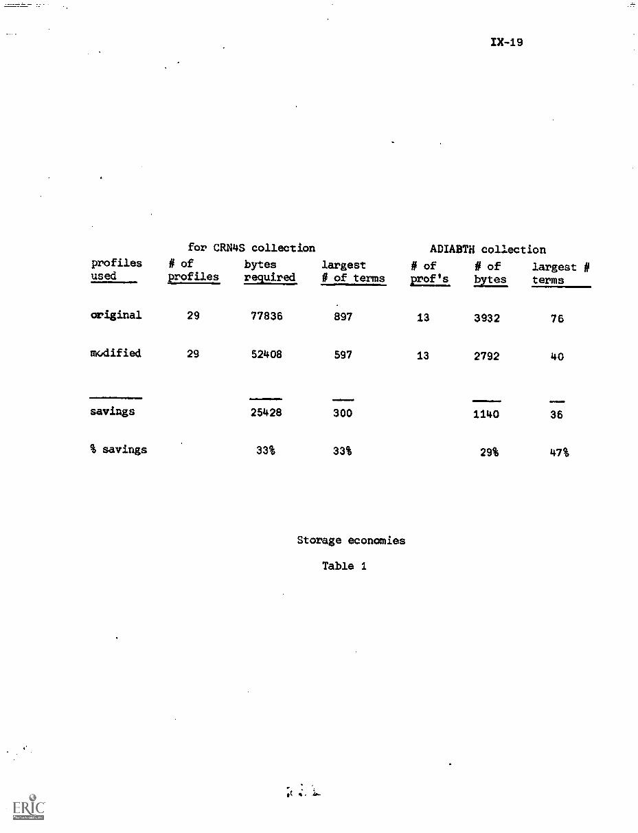
for CRN4S collection ADIABTN collectionprofiles # of bytes largest # of # of largest #used profiles required # of terms =LE bytes terms

original

modified

savings

% savings

29 77836 897 13 3932 76

29 52408 597 13 2792 40

4...1.01110.11 .11111110110. 11.0.25428 300 1140 36

33% 33% 29% 47%

Storage economies

Table 1

Ix-2a

higher precision in the high recall region of the curve, as compared to the

results obtained with TREE1. But the significance tests show that this

difference is perhaps 50% due to chance.

Glancing over the term statistics for terms thrown out and terms

kept one can find terms of relatively high, low or medium frequencies for

both collections which were either kept or deleted. This holds for both

document frequency (number of profiles in which the term in question occurs)

and overall frequency (summed weight of term throughout profile col4ection).

Thus it appears that Murray's suggestion that high frequency terms should

never be thrown is not necessarily to be followed in the future. The

suggestion arose because Murray, in only looking at the profiles locally,

could not tell whether or not a high frequency term was a good discriminator

or a bad one, while it happens that for the most part low frequency terms

are usually poor discriminators. The procedure suggested herein however,

by its very definition, considers terms as they affect the profile space

globally and hence can distinguish between "good" and "bad" high frequency

terms.

References

[1) Gerard Salton, The SMART Retrieval System, Prentice-Hall, Inc., 1971.

[2] Daniel McClure Murray, Document Retrieval Based on Clustered Files,Information Storage and Retrieval, Report No. 20, Department ofComputer Science, Cornell University, 1972.

[3] K. Bonwit and J. Aste-Tonsmann, Negative Dictionaries, InformationStorage and Retrieval, Report No. 18, Department of ComputerScience, Cornell University, 1970.

[4] These programs were made available to me by the SMAP" staff atCornell University, as of this writing they reside Card FilesMNQ.D1, MNQ.D2, and MNQ.D3, the modified versions mad in thisreport are included herein.

X-1

On Dynamic Document Space Modification

Using Term Discrimination Values

C.S. Yang

Abstract

Brauen's algorithm for dynamic document space modification

has been shown to improve retrieval effectiveness. He adds new

terms to document vectors and some terms in the document vectors

are increased in weight. In this study, term discrimination

values are utilized so that only good terms are either added to

documents or increased in weight. This can keep document vectors

relatively short and poor terms are prevented from overriding

good terms. The storage and retrieval effectiveness for a new

version of the document space modification algorithm is studied.

1. Introduction to Dynamic Document Modification and Term

Discrimination Values

In the SMART system, each document or query is represented

by a vector. Document vectors may be constructed by elaborate

manual work or by automatic methods. Manual construction may produce

better results, but it requires too much human effort. The tendency

therefore is to construct document vectors automatically by utilizing

document abstracts and a dictionary, where the dictionary itself

may also be constructed automatically. As a result, the well-

X- 2

formation of automatically constructed vectors is questioned. Besides,

Brauen 11] states that "even though the vocabulary in many scientific

fields is essentially standardized, it does not remain constant over

time. Vocabulary in fact changes with new developments, new personnel,

and other factors. As a result, document vectors, which are reasonably

well defined at one time, may appear to be ill-defined five years later.

Given a group of users knowledgeable in some field and given that these

users submit a set of roughly similar queries, one might then expect

that similar sets of documents will satisfy all these queries. A

strategy designed to "group" document vectors about the user queries

to which they are relevant may then aid the retrieval performance of

similar queries submitted in the future."

These considerations motivate the desire to modify document vectors

by user's opinions. Brauen has suggested the following algorithm for

Dynamic Document Space Modification (DDSM):

1) An initial query qo is submitted and processed. Relevance

feedback iterations are performed until some modified query

qn returns a list of documents satisfactory to the user.

2) Each relevant document vector identified by the user during

the feedback proceas is then modified as follows:

Let D be a document relevant to go.

a) If concept Ci belongs to qo but does not belong to

D, then add Ci

to D with weight D = BETA. (1)

b) If concept Ci belongs to both qo and D, then modify

D' by

Di = Di + GAMMA * (120-Di) (2)

X-3

c) If concept Ci belongs to D but does not belong to

getherlincdif""Y

DiDi Di

f'DELTA

4 (3)

Brauen has shown that this algorit'll does improve retrieval

performance because documents teLL .0 center around those queries

to which they are relevant. [1] But two questions need to be considered:

1) From equation 1, new terms are added to the document vectors.

After the document space is modified by many queries,

is it possible that so many new terms are added to

the document vectors that the vectors are unreasonably

long? If so, document storage becomes a serious

problem. On the other hand, the COSINE correlation

between two vectors is a term matching process. It

takes more time to calculate the correlation between

longer vectors.

2) Are all terms in the original queries good ones? If

this is not necessarily the case, is it wise to judge

the usefulness of a term which is in the query but not

in the document before the term is added to the document

vector? Similarly, is it wise to judge the usefulness

of a term which is in both the query and the document

before it is increased in weight?

With respect to the first question, several observations

are made based on experiments using the CRN4S DOCS document space

(424 documents) and CRN4S QUESTS query space (155 queries). The

results of the earlier experiments show that many documents are

significantly increased in length. A typical example is the

X-4

following:

Query 4 has 12 concept terms and document 18 has 76. Query

4 retrieves document 18 as a relevant document with rank 6. Eight terms

in Query 4 but not in document 18 are added to document 18. Later on,

Query 5 also retrieves document 18 with rank 6 as a relevant document.

Seven terms are added to this document. Document 18 thus increases

fisom 76 terms to 91 terms after being modified by only two queries.

When a document vector has been lengthened to a certain extent

i. it possible that relatively few new terms will be added to it? To

obtain an estimation of this, consider how the longest vector (document

234) in CRN4S DOCS behaves. This document has 186 terms. Query 23

retrieves it with rank 5. It is found that 6 out of the 8 terms in

query 23 are not in document 234. If a long vector is lengthened so

quickly, an originally short vector (short vectors in CRN4S DOCS have

lengths of about thirty terms) will probably double or triple in length

after being modified by many queries.

The above arguments support xhe desirability of limiting document

lengths. A natural way to do this is to modify Brauen's algorithm so

that only good terms are added to documents (by equation 1) and poor

terms are deleted from document vectors (by equation 2).

The "goodness" of a term was first studied by Bonwit and

Aste-Tonsmann [2]. A term is considered to be a good term, i.e., a

discriminator, if its distribution is such that it serves to distinguish

or discriminate among documents in the collection. Otherwise it is a

non-discriminator. For example, if a term occurs in almost all documents

in a collection, it may not be a good discriminator since it may have

little effect in distinguishing among the documents.

.ts- 4

X- 5

A formuletion of a term discrimination value functicx

developed by Crawford L3] is introduced as follows:

. Let D1, DN be a collection of N documents. Each

document, Di, is represented by a vector Di = (Dii, Di2, ..., Dim)

where M is the number of terms in the dictionary for the collection

and D.. is the weight of concept j in document 1.1.3

The eentroid vector, C = (C1, CM), of the document

collection is defined as

1 rC3. =

NL Dij

i111. 1, 2, *ire, M

The Compactness, Q, of the document collection is

NQ = I COS(C, Di), 0 < Q < 1.

" i=1

The Compactness of the document collection with term i deleted

is

N1 r i--- L COS(C , D

i)Qi N

jral

where Ci

and DA7

are respectively the centroid vector and jth

document vector with term i deleted. The Discrimination Value,

Vi, of term i is defined as

V. =44

* 100

Since a good term can distinguish among the documents, its

existence makes the document space more sparse, i.e., less compact.

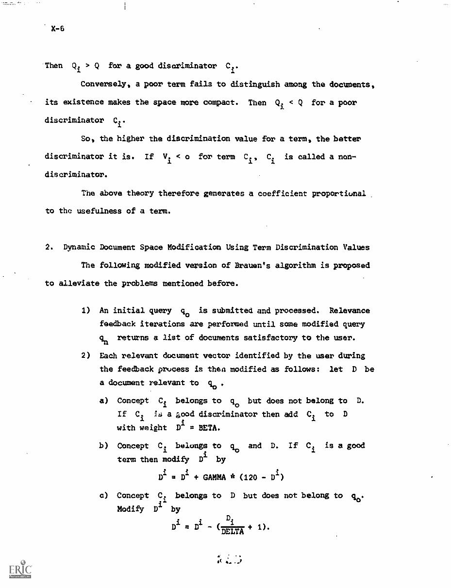
X-6

Then Qi > Q for a good discriminator Ci.

Conversely, a poor term fails to distinguish among the documents,

its existence makes the space more compact. Then Q5 < Q for a poor

discriminator Ci

So, the higher the discrimination value for a term, the better

discriminatoritis.IfV.1 < o for term C., C. is called a non-

discriminator.

The above theory therefore generates a coefficient proportional

to the usefulness of a term.

2. Dynamic Document Space Modification Using Term Discrimination Values

The following modified version of Brauen's algorithm is proposed

to alleviate the problems mentioned before.

1) An initial query qo is submitted and processed. Relevance

feedback iterations are performed until some modified query

qn returns a list of documents satisfactory to the user.

2) Each relevant document vector identified by the user during

the feedback process is then modified as follows: let D be

a document relevant to qo

a) Concept Ci belongs to qo but does not belong to D.

IfC.isag,00ddiscriminatort1maddC.to Dwith weight Di = BETA.

b) Concept Ci belongs to qo and D. If Ci is a good

term then modify DI by

Di = Di + GAMMA * (120 - Di)

c) Concept Ci belongs to D but does not belong to q0.

Modify Di

by

niD

4. 1)= " `DELTA --*

X-7

Poor discriminators in the queries are not added to

document vectors by the extra condition in (a). Also, poor terms

in the documents do not gain weight by the condition in (b).

From the point of view of performance, if a document space is full

of poor terms with high weights, they will override the effect of

good terms and hence the retrieval effectiveness will deteriorate.

3. Experiment

The following data bases are used:

Document Space: CRN4S DOCS (424 documents)

Query Space: CRN4S QUESTS (155 queries)

Tree Structure: REW-CRN4S TREE (63 first level centroids,

14 second level centroids, 1 root node)

Brauen calls two queries similar if they have three or more

terms in common. Otherwise two queries are nonsimilar. He divides

the 155 queries into two subsets. 125 of them are used to modify

the document space and are called the Modification Set. Among the

remainder of the thirty queries, fifteen are similar to some queries

in the Modification Set and fifteen are not similar to any query in

the Modification Set. The thirty queries are used to test the

effectiveness of the document collection modified by the 125 queries.

His convention is adopted in this experiment. Both sets of queries

are shown in Table 1.

A new load module called SMARTDSM has been set up to

accommodate the document space modification and the Retirement

policy. The latter is not discussed in this paper. One can choosea

,t;

X-8

QueryNumber

CranfieldQuery

Number

numberof Similar

QueriesSimilarQueries

1 12 0 -

2 15 0 -

3 48 0 -

4 66 0 -

5 72 0 -

6 87 0 -

7 90 0 -

8 96 0 -

9 100 0 -

10 104 0 -

11 106 0 -

12 117 0 -

13 119 0 -

14 121 0 -

15 124 0 -

16 6 3 24,33,56

17 9 3 4,5,111

18 24 7 6,23,29,33,49,56,147

19 27 3 28,47,58

20 30 6 13,28,109,110,113,150

21 33 8 6,24,34,36,56,63,77,86

22 39 7 13,28,37,41,58,150,151

23 51 3 46,50,118

24 57 4 14,56,83,115

25 63 5 33,109,110,147,148

26 78 3 1,83,135

27 81 6 82,94,95,136,143,144

r28 146 3 133,134,145

29 147 5 23,24,49,63,148

30 148 3 49,63,147

Summary of Information

Test Set Queries

Table 1S.

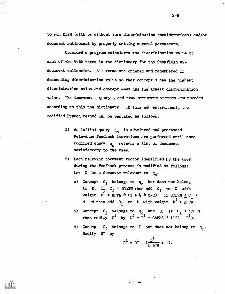
X-9

to run DDSM (with or without term discrimination considerations) and/or

document retirement by properly setting several parameters.

Crawford's program calculates the e,.scrimination value of

each of the 4439 terms in the dictionary for the Cranfield 424

document collection. All terms are ordered and renumbered in

descending discrimination value so that concept 1 has the highest

discrimination value and concept 4439 has the lowest discrimination

value. The document-, query-, and tree-structure vectors are recoded

according to this new dictionary. In this new environment, the

modified Erauen method can be restated as follows:

1) An initial query Ro is submitted and processed.

Relevance feedback iterations are performed until some

modified query gn returns a list of documents

satisfactory to the user.

2) Each relevant document vector identified by the user

during the feedback process is modified as follows:

Let D be a document relevant to .go.

a) Concept Ci belongs to qo but does not belong

to D. If C. < GTERM

weight Di = BETA * (1

NTERM then

b) Concept Ci

then modify

add C. to

then add C. to D with

+ * ONE). If GTERM < Ci <

D with weight D1 = BETA.

belongs to go and D. If Ci < NTERM

Di by Di = Di + GAMMA * (120 - D1).

c) Concept Ci belongs to D but does not belong to go.

Modify D1 by

iDl = D1

D iN(DELTA

X-10

GAMMA = 0.225 and DELTA = 8 are the optimal values obtained by Brauen

and are used throughout this study.

In (a), the parameter ONE can be set to 1 or O. If ONE = 1,

more emphasis is put on the very high discrimination value terms added

to documents. If ONE = 0, all terms added are treated equally. If ONE = 1

and BETA = 20, terms with very high discrimination values are added with

normal weight 30 and other terms added have weight 20.

The distribution of discrimination values of the 4439 terms is

shown in Fig. 1. The first 407 terms in the dictionary have discrimina-

tion values greater than 0.01. They are considered to be very good terms.

The last 80 terms have negative discrimination values. Their document

frequencies range from 46 to 219. These are therefore very high

frequency terms.

Table 2 shows the seven sets of GTERM and NTERM cutoffs used in

this experiment. The 125 queries modify the document space for each set

of cutoffs. Two iterations are run. Relevant documents in each iteration

with rank above 30 are modified. If every query modifies six documents

on the average, there are 6x125=750 modifications, and each document is

modified 750/424 t 1.77 times. The remaining thirty queries then test

the retrieval performance of the resulting document spaces. The number

of terms added to the document space is also counted.

4. Discussion of Results

Table 2 summarizes the experimental conditions. No document space

modification is performed for set O. This is a standard search run used

for comparison.

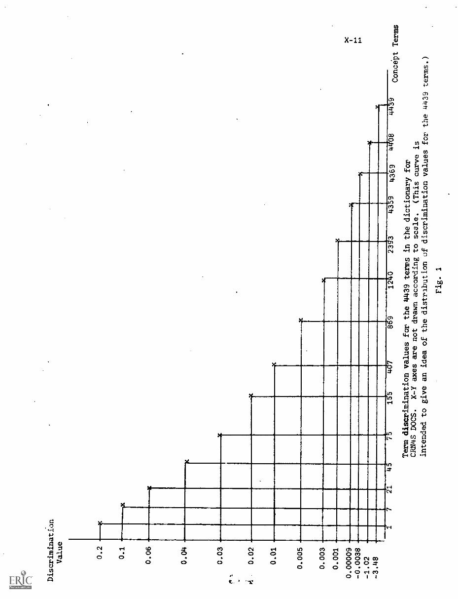
Discrimination

Value

0.2

0.1

0.06

0.04

0.03

s

Pi

0.02-

0.01

0.005

K

0.003

0.001

0.00009

-0.0038

-1.02

-3.48

I

17

21

45

75

1e5

4

1x

7869

1240

2313

4359

4369

4J08

Term discrimination values for the 4439 terms

CRN4S DOCS.

X-Y axes are not drawn according

intended to give an idea of the distribution

Fig. 1

4419

Concept Terms

in the dictionary for

to scale.

(This curve is

of discrimination values for the 4439 terms.)

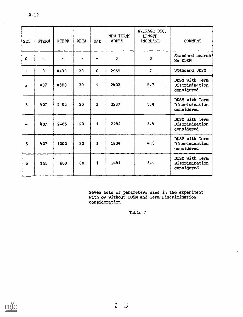
X-12

SET GTERM NTERM BETA ONENEW TERMSADDFD

AVERAGE DOC.LENGTHINCREASE COMMENT

r

0 - - - _ 0 0

.

Standard searchNo DDSM

1 0 44394

30 0 2969 7

4

Standard DDSM

2

..

407 4360 30 1 2403 5.7DDSM with TermDiscriminationconsidered

,

3 407 2465 30 1 2287 5.4DDSM with TermDiscriminationconsidered




Seven sets of parameters used in the experimentwith or without DDSM and Term Discriminationconsideration

Table 2

X-13

There is no cutoff in the DDSM for Set 1. This is the

standard Brauen method. 2969 terms are added to the 424 documents.

Each document is lengthened by 7 terms on the average.

For Set 2, only the eighty negative discrimination value

terms are deleted. Because of the high frequencies of the 80 terms,

the number of terms added to the collection is decreased quickly from

2969 to 2403.

Set 6 exhibits the largest cutoff. Compared with the

standard DDSM (Set 1) where 2969 terms are added, the number of terms

2T-6413.441.)added is decreased by

(2969 -61441)100% = 51.5%.

Sets 3 and 4 have intermmediate cutoff values and

,2969-22872969

) x 100% = 23% of the terms are prevented from being added

to the document collection.

The seven sets are tested with the similar and nonsimilar test

sets respectively. Their retrieval performances are shown in Tables

3 to 6 and plotted in Fig. 2 to 7. The performances can be

summarized as follows:

1) Similar queries in the oth iteration.

The original Brauen's DDSM (Set 1) shows a considerable

superiority over all others. Sets 2, 3, 4, 5, and 6 are

almost the same at all recall levels. They have poorer

precision than that of Set 0 at very low recall levels

but are universally better at recall levels above 0.3.

The significance tests show that the superiority of any

one of the five sets (Sets 2, 3, 4, 5, 6) to the other

four sets is not significant. One may conclude that

these five sets have approximately the same performance

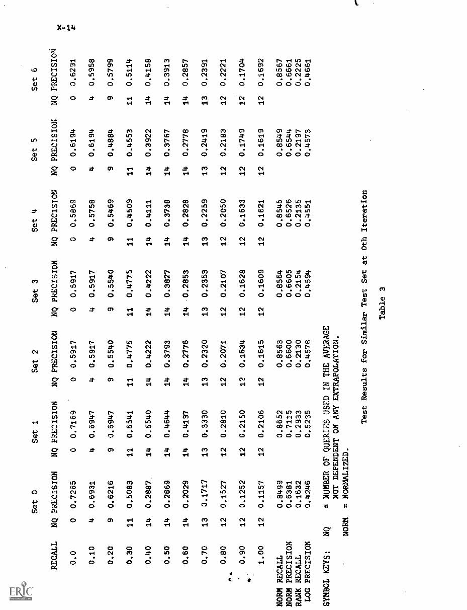
RECALL

Set 0

Set 1

Set 2

NQ PRECISION

NQ PRECISION

NQ PRECISION

Set 3

liQ PRECISION

Set 4

NQ PRECISION

Set 5

NQ PRECISION

Set 6

NQ PRECISION

0.0

00.7265

00.7169

00.5917

00.5917

00.5869

00.6194

00.6291

0.10

40.6931

40.6947

40.5917

40.5917

40.5758

40.6194

40.5958

0.20

90.6216

90.6947

90.5540

90.5540

90.5469

90.4884

90.5799

0.30

11

0.5083

11

0.6541

11

0.4775

11

0.4775

11

0.4509

11

0.4553

11

0.5114

0.40

14

0.28

87.

14

0.5540

14

0.4222

14

0.4222

14

0.4111

14

0.3922

14

0.4158

0.50

14

0.2869

14

0.4644

14

0.3793

14

0.3827

14

0.3738

14

0.3767

14

0.3913

0.60

14

0.2029

14

0.4137

14

0.2776

14

0.2853

14

0.2828

14

0.2778

14

0.2857

0.70

13

0.1717

13

0.3330

13

0.2320

13

0.2353

13

0.2259

13

0.2419

13

0.2391

0.80

12

0.1527

12

0.2810

12

0.2071

12

0.2107

12

0.2050

12

0.2183

12

0.2221

Ia

0.90

12

0.1252

12

0.2150

12

0.1634

12

0.1628

12

0.1633

12

0.1749

12

0.1704

1.00

12

0.1157

12

0.2106

12

0.1615

12

0.1609

12

0.1621

12

0.1619

12

0.1692

NORM RECALL

0.8499

0.8652

0.8563

0.8564

0.8545

0.8549

0.8567

NORM PRECISION

0.6381

0.7115

0.6600

0.6605

0.6526

0.6544

0.6661

RANK RECALL

0.1632

0.2933

0.2130

0.2154

0.2135

0.2197

0.2225

LOG PRECISION

0.4246

0.5235

0.4578

0.4594

0.4551

0.4573

0.4661

SYMBOL KEYS:

NQ

= NUMBER OF QUERIES USED IN THE AVERAGE

NOT DEPENDENT ON ANY EXTRAPOLATION.

NORM

= NORMALIZED.

Test Results for Similar Test Set at 0th Iteration

Table 3

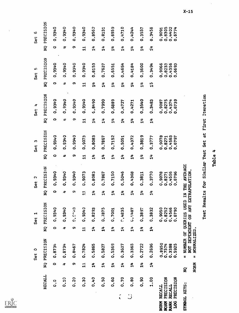
RECALL

Set 0

Set 1

Set 2

NQ PRECISION

NQ PRECISION

NQ PRECISION

Set 3

NQ PRECISION

Set 4

NQ PRECISION

Set 5

NQ PRECISION

Set 6

NQ PRECISION

0.0

00.8734

00.9340

00.9340

00.9340

00.93140

00.9340

00.9340

0.10

40.8734

40.9340

40.9340

40.9340

40.9340

40.9340

40.9340

0.20

90.8467

90.C40

90.9340

90.9340

90.9340

90.9340

90.9340

0.30

11

0.7824

11

0.9340

11

0.9073

11

0.9073

11

0.9340

11

0.9340

11

0.9340

0.40

14

0.5865

14

0.8293

14

0.8083

14

0.8083

14

G.8490

14

0.8153

14

0.8562

0.50

14

0.5827

14

0.1875

14

0.7867

14

0.7867

14

0.7990

14

0.7637

14

0.8131

0.60

14

0.5369

14

0.7001

14

0.7150

14

0.7152

14

0.6889

14

0.6551

14

0.6959

0.70

14

0.3607

14

e.4835

14

0.5046

14

0.5051

14

0.4727

14

0.4654

14

0.4710

0.80

14

0.3365

14

G.1:487

14

0.4368

14

0.4372

14

0.4271

14

0.4184

14

0.4244

0.90

14

0.2722

14

0.3897

14

0.3811

14

0.3819

14

0.3540

14

0.3600

14

0.3557

1.00

14

0.2696

14

0.3832

14

0.3770

14

0.3777

14

0.3483

15

0.3494

14

0.3458

NORM RECALL

0.8950

0.9050

0.9078

0.9078

0.9087

0.9066

0.9091

NORM PRECISION

0.7574

0.8252

0.8271

0.8271

0.8275

0.8233

0.8305

RANK RECALL

0.3388

0.4566

0.4556

0.4563

0.4374

0.4356

0.4402

LOG PRECISION

0.5925

0.6790

0.6796

0.6797

0.6739

0.6693

0.6774

SYMBOL KEYS:

NQ



NORM

= NORMALIZED.

Test Results for Similar Test Set at First Iteration

Table 4

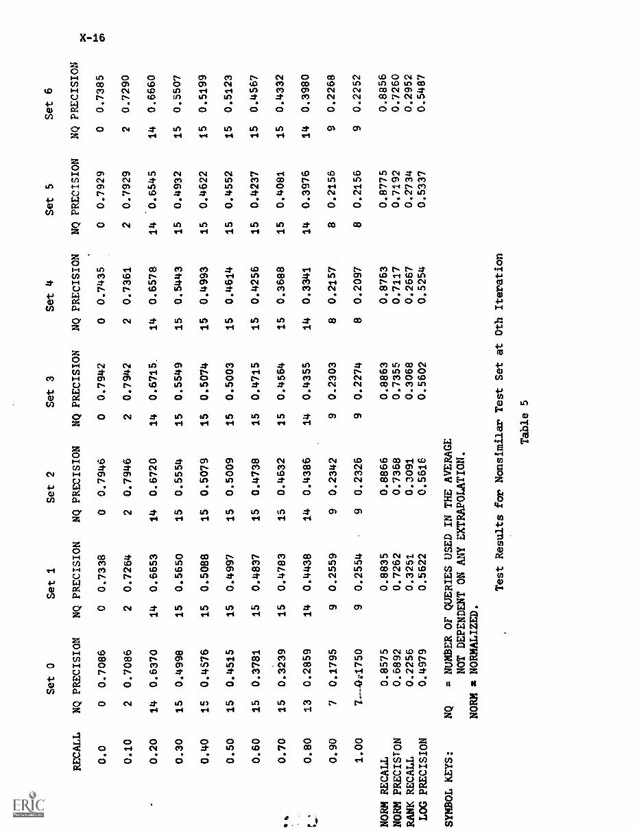
RECALL

0.0

Set 0

NQ PRECISION

00.7086

Set 1

NQ PRECISION

00.7338

Set 2

NQ PRECISION

00.7946

Set 3

NQ PRECISION

00.7942

Set 4

NQ PRECISION

00.7435

Set 5

NQ PRECISION

00.7929

Set 6

NQ PRECISION

00.7385

x r I-4

cr,

0.10

20.7086

20.7264

20.7946

20.7942

20.7361

20.7929

20.7290

0.20

14

0.6370

14

0.6653

14

0.6720

14

0.6715.

14

0.6578

14

0.6545

14

0.6660

0.30

15

0.4998

15

0.5650

15

0.5554

15

0.5549

15

0.5443

15

0.4932

15

0.5507

0.40

15

0.4576

15

0.5088

15

0.5079

15

0.5074

15

0.4993

15

0.4622

15

0.5199

0.50

15

0.4515

15

0.4997

15

0.5009

15

0.5003

15

0.4614

15

0.4552

15

0.5123

0.60

15

0.3781

15

0.4837

15

0.4738

15

0.4715

15

0.4256

15

0.4237

15

0.4567

lp

0.70

15

0.3239

15

0.4783

15

0.4632

15

0.4564

15

0.3688

15

0.4081

15

0.4332

r0.80

13

0.2859

14

0.4438

14

0.4386

14

0.4355

14

0.3341

14

0.3976

14

0.3980

0.90

70.1795

90.2559

90.2342

90.2303

80.2157

80.2156

90.2268

1.00

7.-441750

90.2554

-

90.2326

90.2274

80.2097

80.2156

90.2252

NORM RECALL

0.8575

0.8835

0.8866

0.8863

0.8763

0.8775

0.8856

NORM PRECISION

0.6892

0.7262

0.7368

0.7355

0.7117

0.7192

0.7260

RANK RECALL

0.2256

0.3251

0.3091

0.3068

0.2667

0.2734

0.2952

LOG PRECISION

0.4979

0.5622

0.5616

0.5602

0.5254

0.5337

0.5487

SYMBOL kEYS:

NQ



NORM

NORMALIZED.

Test Results for Nonsimilar Test Set at 0th Iteration

Table 5

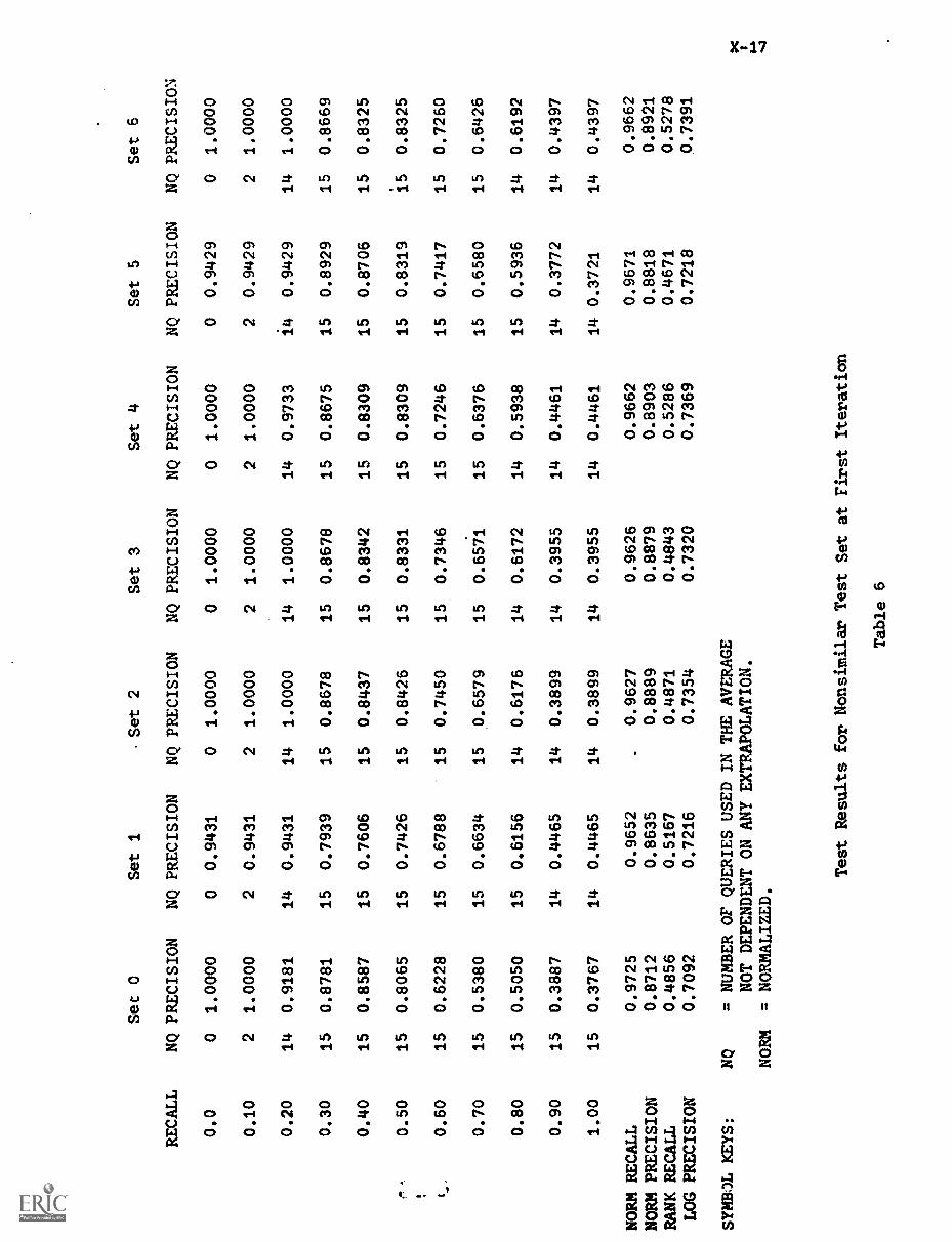
RECALL

Sec 0

NQ PRECISION

Set 1

NQ PRECISION

Set 2

NQ PRECISION

Set 3

NQ PRECISION

Set 4

NQ PRECISION

0.0

01.0000

00.9431

01.0000

01.0000

01.0000

0.10

21.0000

20.9431

21.0000

21.0000

21.0000

0.20

14

0.9181

14

0.9431

14

1.0000

14

1.0000

14

0.9733

0.30

15

0.8781

15

0.7939

15

0.8678

15

0.8678

15

0.8675

0.40

15

0.8587

15

0.7606

15

0.8437

15

0.8342

15

0.8309

0.50

15

0.8065

15

0.7426

15

0.8426

15

0.8331

15

0.8309

0.60

15

0.6228

15

0.6788

15

0.7450

15

0.7346

15

0.7246

0.70

15

0.5380

15

0.6634

15

0.6579

15

0.6571

15

0.6376

0.80

15

0.5050

15

0.6156

14

0.6176

14

0.6172

14

0.5938

0.90

15

0.3887

14

0.4465

14

0.3899

14

0.3955

14

0.4461

1.00

15

0.3767

14

0.4465

14

0.3899

14

0.3955

14

0.4461

NORM RECALL

0.9725

0.9652

.0.9627

0.9626

0.9662

NORM PRECISION

0.8712

0.8635

0.8889

0.8879

0.8903

RANK RECALL

0.4856

0.5167

0.4871

0.4843

0.5286

LOG PRECISION

0.7092

0.7216

0.7354

0.7320

0.7369

SYMBas KEYS:

NQ



NORM

= NORMALIZED.

Test Results for Nonsimilar Test Set at First Iteration

Table 6

Set 5

Set 6

NQ PRECISION

NQ PRECISION

00.9429

01.0000

20.9429

21.0000

14

0.9429

14

1.0000

15

0.8929

15

0.8669

15

0.8706

15

0.8325

15

0.8319

15

0.8325

15

0.7417

15

0.7260

15

0.6580

15

0.6426

15

0.5936

14

0.6192

14

0.3772

14

0.4397

14 0.3721

14

0.4397

0.9671

0.9662

0.8818

0.8921

0.4671

0.5278

0.7218

0.7391

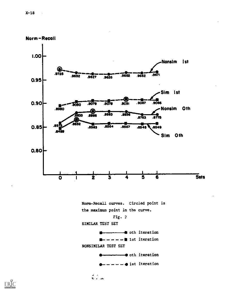
Norm Recoil

100

'9725 .9652

0.95

0.90 ..1.9050

0.85

0.80

9671

0.90

.9827 .9826 9662 .9662

.9078 .9078 .9091 .908? .9086O

Nonsim

Sim 1st

1st

e9eo Nonsim 0th.

ANItir."1"148.9783 .errs

.8545 .8549

Sim 0th

Norm-Recall curves. Circled point is

the maximum point in the curve.

Fig. 2

SIMILAR TEST SET

III--51 oth iterationa----- 1st iteration

NONSIMILAR TEST SET

oth iteration

1st iteration

Sets

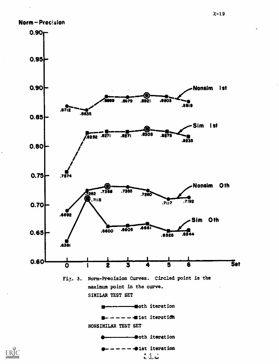
Norm Prectiion

0.90

0.95

0.90

0.85

0.80

0.75

0.70

0.65

0.60

'4-49

."...Nonslin 1st

e559 .11679 .8921 .5903.8818

.9712am%

"4"1"411#.8635

1..~ 11000.Sint 1st

.11233

! .7574

.6311

1 1 1 t 1

0 i 2 3 4 5 6

Fi.3. 3. Norm-Precision Curves. Circled point is the

maximum point in the curve.

SIMILAR TEST SET

oth iteration

-111st iteratidriNONSIMILAR TEST SET

oth iteration

0 -- -01st iterationo .

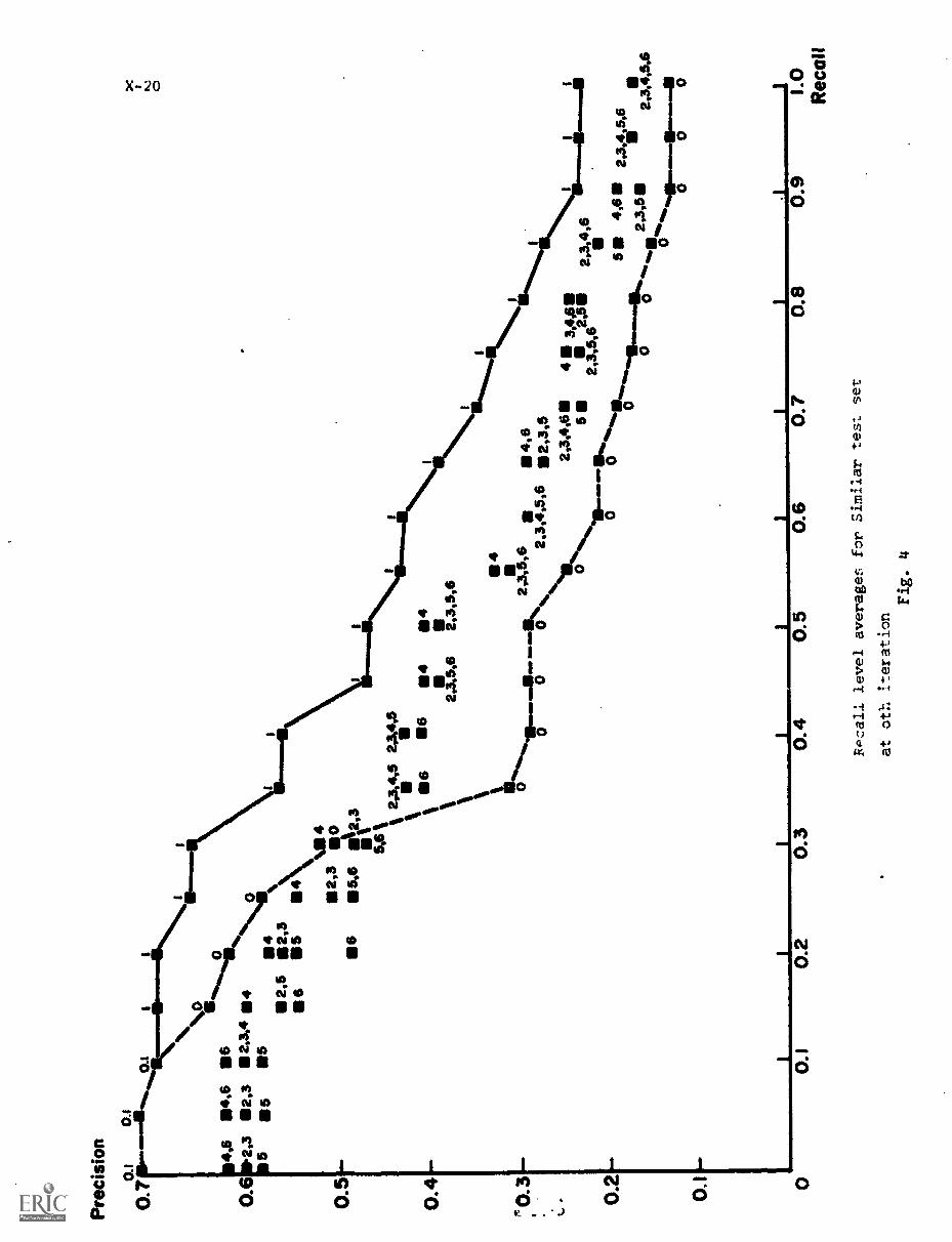
Pre

cisi

on

01

OA

0.70."'"Wo OA

11

%Is

0.6

0.5

0.4

'`0.3

I., 0.

2

14,6

Ns3

N740.....411sNo

`0 II

4,6 0 6

6111%,

2,3

112.

3,4

124

0as

as

00.

1

2,5

s11

4 2,3

5 6

N ON

2,3 5,6

4M

OS

AL

3

566

0.2

0

2,3,

4,5

6 6 0

4 0

al4

L3,5

,6

4

2,3,

596

0 S

.2,

3,4,

5,6

o

4,6

52,3

,523

,46 5

o

43,

4,6

2,51

52,

3,4,

62,

3,5,

6

55 4

,6.

2,3,

4 5,

6

02,

3,6

2,3,

4,5,

60

"ftft

als

1

0.3

0.4

0.5

1 0.6

0.7

FPcall level averages for Similar test

at oth iteration

Fig.

set

0.8

00

00

.1 0.9

1.0

Rec

all

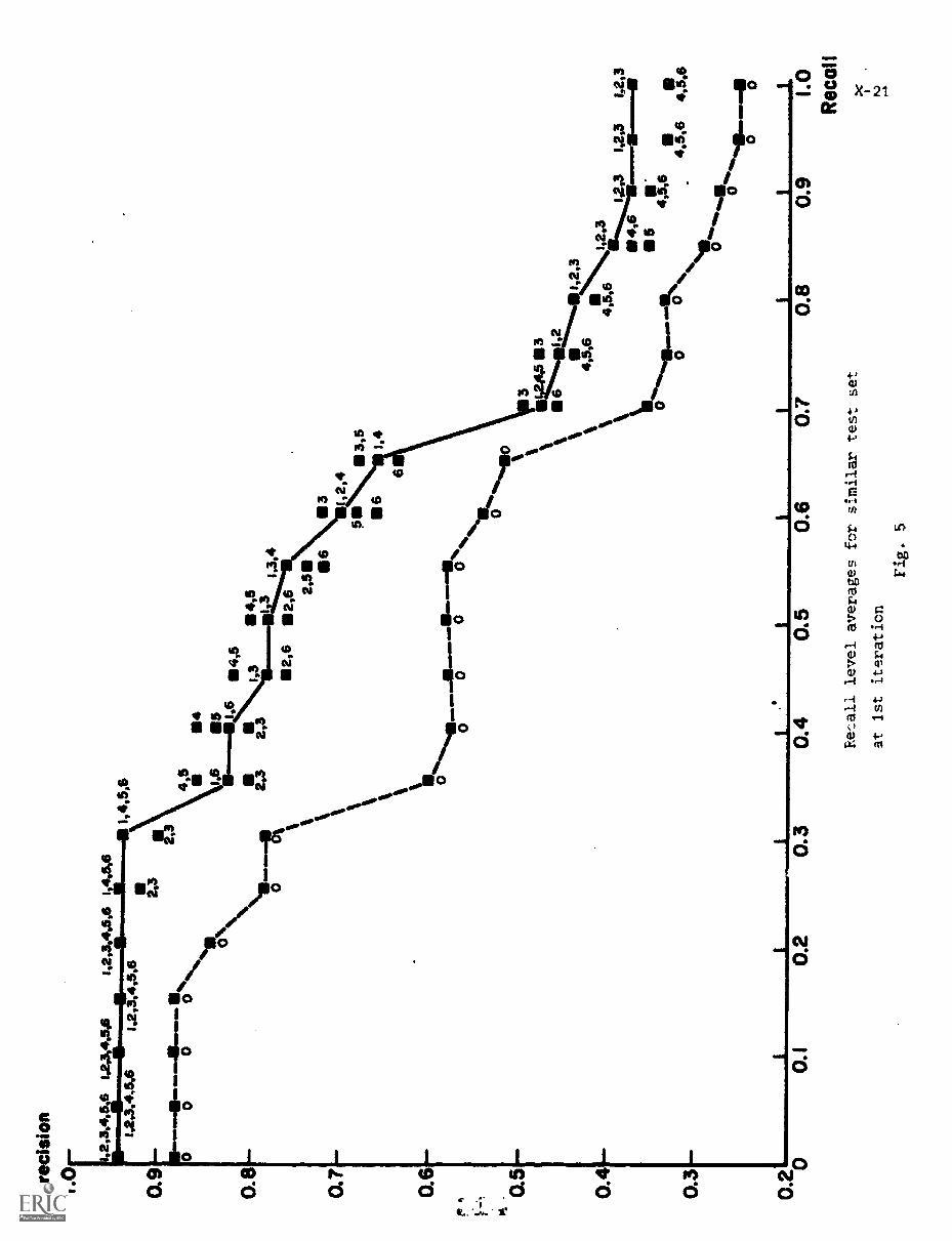
Pre

cisi

on1.

0

0.9

0.8

0.7

0.6

it0.

5

0.4

0.3

1,2,

3,4,

5,6

1.2,

3495

s642

,3,4

,5,6

1,4

,5,6

1,2

,3,4

,54

1,4,5,6

020

2.3

2,3

4,5

1.6

4 5 464,

51,

34,

52,

32,

32,

311

31,

3,4

2,6

II2,

6 2,51

1\11

611

3 1,2,

4

o0

ON

3,5

61,

4

6

36

1,2

1,2,

34,

5,6

1.1

2 3

4,5,

61,

213

1,2,

3IA

34,

6

1146

41...

....1

1L5

5'4,

5,6

O0

'14%

4,5,

64,

5,6

.,0

'4%

44_ 0

0.1

0.2

0.3

0.4

0.5

0.6

0.7

Rec

all l

evel

ave

rage

s fo

r si

mila

r te

st s

etat

1st

iter

atio

nFi

g. 5

0.8

0.9

1.0

Rec

oil

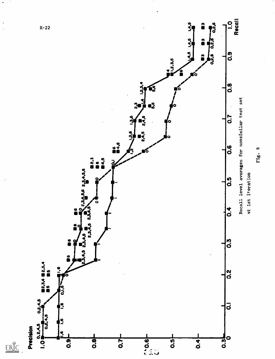
Pre

cisi

on0,

2,4,

50,

2,4,

50

IIIm

.II..I

IL11

2,3,

4 II

2,3,

40,

2, 4

,5as

1,6

1,6

!,60,

4611

"

66

ate;

III;6

2,3,

4,5

2,3,

4,5

avtli

um 2

,4,5

,62,

3,4,

5\

2,3

bia1

110

111

6 4,5

0,1

$64,

5

N

% 1

,21,

3,6

1,3,

6

\E2,

11,5

2,41

1,5

2111

4:11

1,2,

3,4

0/4 \

II.

5,6

5,6

101.

-"m

ill'

0qi

. ii o

6`1

13

\3

3 3

4,5

1,4,

51,

4,5

0,6

0,2,

60,

2,6

0,2,

6

4 1,2,

3,5

0.1

0.2

0.3

0.4

0.5

0.6

0.7

0.8

0.9

1.0

Rec

oil

Recall level averages for nonsimilar test set

at 1st iteration

Fig.

6

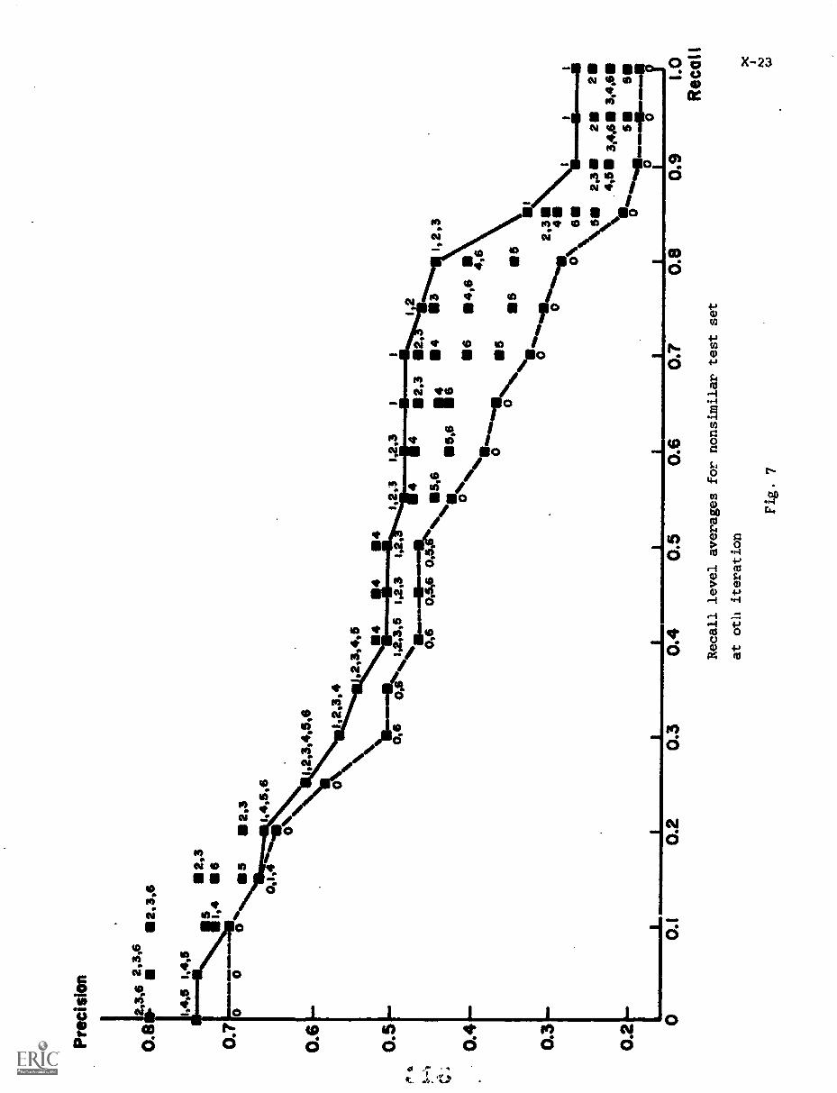
Pre

cisi

on

2,3

5 1,4

50%

.5

2,3

0,1,

4".1,

4,5,

6

0.1

1,2,

3,4,

5,6

01

2,3,

42,

3,4,

5 4 4

40,

11r1

5%%

1,2,

3,5

1,2,

31,

2,1,

2'3

1,2,

3

1

2,3

4,6

1 23,

4,6

i 23,

4,6

%4

12,3

a5 -

61=

-7;7

5,N

15,6

116,

6I:

0%%

sii..

O,, ft-

11 0

12, 4

116 .6 0

1,2

Is 3

1,2,

3

II4,6

4,6

5 5

I

2,38

0% 6

8 \ lice.

,,,40

......

4.5.

...65

.

iI

I0

0f

0.2

0.3

0.4

0.5

0.6

0.7

0.8

0.9

1.0

Rec

oil

Recall level averages for nonsimilar test set

at oth iteration

Fig. 7

X24

which is superior to that of Set 0 but inferior to that of

Set 1.

2) Nonsimilar queries in the oth iteration.

Slight cutoffs (Sets 2, 3, 4) are better than Set 1 at low

recall levels (below 0.2) and equal to Set 1 at all other

recall levels. Severe cutoffs seem to degrade the performance.

3) Similar queries in the first iteration.

Sets 1, 2, 3, 4 and 5 are practically equal in performance.

The significance tests show that none is substantially better

than the others. A very large cutoff like the one used for

Set 6 produces a slight deterioration in performance. Compared

with the standard search run (Set 0), all the six sets are by

far superior.

4) Nonsimilar _queries in the first iteration.

Sets of 2, 3, 4, 5 and 6 have essentially the same performance.

They are all better than Set 1 at recall levels below 0.6.

From the above observation, one can reach the following conclusions:

Except for the similar test set in the oth iteration, the cutoff of poor

terms seems to maintain the performance of the standard DDSM. In the

first iteration, the nonsimilar queries show a somewhat better performance.

But too large a cutoff like Set 6 will tend to degrade performance. As

a compromise, an intermediate cutoff like Set 3 is suggested. Considerable

storage can be saved while effectiveness is still maintained.

The inferior performance of Sets 2, 3, 4, 5 and 6 in the oth

iteration for similar queries is understandable. For most queries qs, in

the similar test set, (except queries 6, 9, 63, 78) one can find one or more

queries, q, in the modification set with the following properties:

X-25

(i) qs and qm have almost the same relevant document

set (say, D1, D2, ..., Dr)

(ii) Some negative discrimination value terms (say, C1,

C2, ..., Cn) are in both qs and qm but not in the

relevant documents (D1, D2 ..., Dr). These terms

are very high frequency terms.

Since no cutoff occurs for Brauen's original P,SM, when qm

retrieves some of (Di, ..., Dr) as relevant documents (say, D1, ...,

Dk) and modifies them, (C1, Cn) are added to these documents.

Afterwards, when qs in the similar test set is submitted, documents

Dv 9 Dk will have high correlation with qs because C1, C2, ...

Cn appear in both qs and D1, D2, ..., Dk. If a cutoff is used,

Cl, C2, ..., Cn are not added to D1, D2, ..., Dk when they are

modified by qm. This explains why Brauen's stand DDSM works

especially well for similar queries in the oth iteration.

As mentioned above, terms C4, C2, ..., Cn are very high

frequency negative discrimination value terms. Some of them even

appear in half of the documents in the CRN4S DOCS collection, so

they will probably appear in the queries very frequently. Actually

Jones 15] showed that, for three independent collections, half of the

query terms are high frequency terms. (Table 7) If many queries

are submitted-- in this experiment each document is modified only

1.77 times on the average --- then each document will be modified

many times, and these high frequency terms will enter into all

document vectors in the long run. In case this happens, the effect

of these terms will be negligible. Set 1 will then have roughly

the same performance as set 2 through 5 for similar queries in the

oth

iteration.

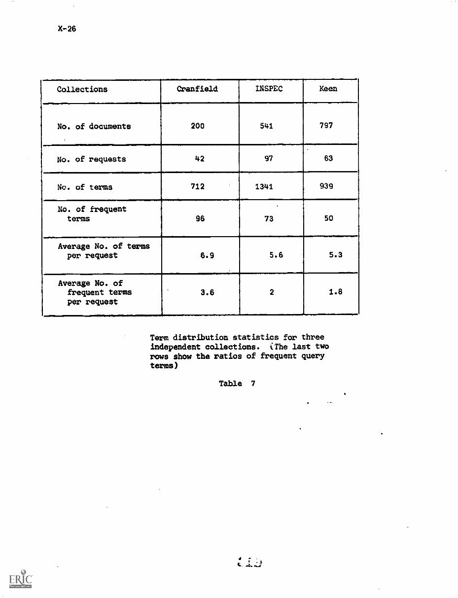
X-26

Collections Cranfield INSPEC Keen

No. of documents 200 541 797

No. of requests 42 97 63

.

No. of terms 712

.

1341

,

939

No. of frequentterms 96 73 50

Average No. of termsper request 6.9 5.6 5.3

.

Average No. offrequent termsper request

,

3.6 2 1.8

Term distribution statistics for threeindependent collections. iThe last tworows show the ratios of frequent queryterms)

Table 7

X-27

5. Conclusion

Sets 3 and 4 use NTERM = 2465. From Fig. 2 and Fig. 3, one

can see that these sets actually achieve the same effectiveness as

set 1. So, at least 4439 - 2465 = 1974 low discrimination value

terms do not contribute much to retrieval effectiveness. For this

value of NTERM. (2969-2287)x 100% = 23% of the new terms are

2969

eliminated. A reasonable portion of the memory storage can there-

fore be saved.

This study also shows that the term discrimination value

concept is acceptable. Slight cutoffs of nondiscriminators do not

deteriorate retrieval performance. But neither do they improve

effectiveness. One might suspect that additional work might be

done in the theory of term discrimination values. Other approaches

of defining term goodness on a sound theoretical ground is probably

the most urgent. It is believed that, with a good judgment of the

usefulness of terms, the proposed version of DDSM should lead to

better results --both in performance and storage considerations.

X-28

References

[1] Brauen, T.L., Document Vector Processing, ISR-17, Report to theNational Science Foundation, Department of Computer Science, CornellUniversity, September 1969.

[2] Bonwit, K. and A!,te-Tonsmann, J., Negative Dictionary, Report ISR-18to the National Science Foundation, Section VI, Department of ComputerScience, Cornell University, October 1970.

[3] Crawford, R., Automatic Dictionary and Thesaurus Construction, ScientificReport No. ISR-22, Cornell University, to be published.

[4] Salton, Go, The SMART Retrieval System, Prentice Hall, 1971.

[5] Jones, K.S., A Statistical Interpretation of Term Specificity and itsApplication in Retrieval, Journal of Documentation, Vol. 28, No. 1,March 1972.

XI-1

The Use of Document Values for Dynamic

Query Document Processing

A. Wong and A. van der Meulen

Abstract

In the field of document retrieval it might be advantageous

to take into account the utility of documents in the collection;

that is, the average usefulness of a specific document for a

given user population in terms of satisfaction of the users'

information need.

In this report the following two questions are investigated:

a) how to improve system performance by assigning so-called

utility values to each document, and

b) how to base a document retirement policy on those

quantities.

A feedback environment provides the possibility for

automatically creating a list of utility values. These values are

then based on the retrieval history of a document. That is, for all

the queries for which a particular document is retrieved, user

judgments about its relevancy are utilized to compute a quantity which

reflects the usefulness of a document for the collection and its users.

Utility values may then be used during the retrieval process

to promote the retrieval of satisfactory documents and suppress the

retrieval of obsolete and mediocre documents. Another application

of the availability of document quality values is a document retirement

policy based on the utility value score in the collection. Documents

t..

XI-2

with low utility values may be placed in an auxiliary file to keep

the main file more current and up to date.

1. Introduction

The performance of a document retrieval system is generally

evaluated by means of two well known system parameters; recall and

precision, which are based on the average user judgments about relevancy

or non-relevancy of the retrieved documents.

Keeping track of user decisions might be quite beneficial for

future users since provision can be made for detecting the quality of

the judged documents. l%y automatically creating a new document property

called the utility value, which represents the average judgment of the

user population about a given document, it seems plausible that system

performance can be improved by using this value in the retrieval process.

Out of date documents or questionable publications, even if indexed in a

proper way, will no longer be retrieved since their corresponding low

utility values do prevent this.

The goal of this investigation is twofold:

a) system improvement by suppressing documents which are likely

to be non - relevant and promoting relevant items in the course

of the retrieval process;

b) system retirement by transferring out cf date and mediocre

documents to an auxiliary file.

2. The Methodology

If the retrieval history of a set of queries in a system is known

in the form of relevancy decisions of the user for the retrieved documents,

one may use this information in deciding which documents are generally

XI-3

useful and which ones are not. In an on line system the relevancy

decisions are rendered as part of the feedback procedures and the

bookkeeping can be done in a very convenient way.

The procedure proposed is to assign to each document in the

collection a so-called utility value which is set equal to 1

initially. This value is increased if a document is retrieved and

found to be relevant, and decreased if retrieved and judged to be

nonrelevant. The increment-decrement function is so chosen that the

utility values range between 0 and 2 and are not able to exceed these

values. (For a comprehensive description of this function, see 11],

and Appendix 1.)

The utility value is then a system parameter which can be

applied in the retrieval algorithm immediately since it reflects the

utility as judged by the users. The new retrieval function Rf will

be:

Rf = cos(q,d) * U.V.

That is the product of utility value (U.V.) and the cosine correlation

function (cos(q,d)).

3. The Organization of the Experiments

A. The Collection

The SMART retrieval system provides the Cranfield 1400

collection with 225 queries. This is a suitable collection for the

experiments in that a maximum in updating of the utility values can be

achieved. The query collection is split into an "updating collection"

and a "test collection". The updating query collection Is used to

obtain utilit" rYalues for all the retrieved documents while the test

XI-4

collection serves as a means for evaluating the influence of the retrieval

algorithm mentioned in 2.

A set of 17 randomly chosen queries will serve as test collection.

A comparison will be made between the retrieval results of the 17 queries

without the use of and with the usage of utility values. In principal

208 queries were available to serve as updating collection. For practical

reasons, however, a subset of 157 queries was actually used.

In an on-line retrieval system, which will be simulated in these

experiments, the number of feedback iterations is likely to be at least

one. That means that relevancy decisions for the first iteration are

available for 157 queries. These retrieved documents will be used to

determine utility values for the retrieved documents. For every query

30 documents are retrieved which requires in practice 30 relevancy

decisions for each user. The number is chosen rather high in order to

obtain a fair amount of updating and therefore probably more significant

results.

B. The Updating Strategies

The most realistic way to implement an updating procedure is to

do so dynamically. That is, each utility value changed after a search

will be used in the retrieval algorithm and influences the retrievability

of that specific document in later searches.

In the SMART environment the updating collection is run as a

batch, the utility values being assigned afterwards and applied for the

first time while running the test collection. (For a more complete

discussion about static and dynamic updating of values see 11]). Similar

experiments 12] concerning the updating of weighted dictionaries have

shown that dynamic updating is superior to static results. If, for the

XI-5

experiments to be described in this report, the static approach

turns out to be satisfactory a dynamic test might be useful at

a later time.

Three different updating strategies are applied, namely

I The Straight Updating

For each query in the updating collection, the 30 retrieved

documents are updated in accordance with the unmodified increment-

decrement function mentioned. The utility values are increased if a

retrieved document is relevant, and decreased 'otherwise. An

arbitrary factor in the updating function which governs the stepsize

of the increment or decrement is chosen equal to 8 (according to Sage,

Ref. £3]). It is not a priori clear whether this value is optimal.

II The Balanced Updating

Since the average number of relevant retrieved documents for a

query is approximately 5, an average of 25 documents will be decreased

in utility value in strategy I. Thus for the whole collection the

average utility value will become less than 1. Documents which are

not updated have therefore a hitt:9.r probability of being retrieved than

updated ones since their utility value is still intact.

To eliminate this effect the number of decreased documents

is kept equal to the number of increased ones. Thus in strategy II,

all relevant documents included in the 30 retrieved ones are

increased, and an equal number of the highest ranked nonrelevant

documents is decreased.

XI-6

III The Extended Balanced Updating

A disadvantage of the balanced updating strategy II is that

the number of updatings is much smaller than in the case of method I.

In strategy I, 30 utility values per query are updated, whereas for

strategy II this number is reduced to about 10 (5 values increased and

5 decreased).

In order to combine the benefits of the maximum number of

updatings (30) per query while preventing a decrease in the average

utility value, Method III, the extended balanced updating is developed.

In addition to the usage of all retrieved documents this method provides

also an exact balancing. The sum of all the decrement steps is made

equal for each query to the sum of all the increment steps. The

decrement steps in particular will be chosen to be rank-dependent,

that is, higher ranked nonrelevant documents are subject to a greater

decrease in utility value than lower ranked ones. The rationale behind

this is of course that high ranking nonrelevant documents should be

suppressed. An extensive treatment of Method III is given in Appendix 2.

After applying these three strategies to the retrieval results

of the query updating colleltion, one obtains a list of utility values

which will be used in the retrieval algorithm for the query test

collection:

Rf = cos(q,d) x U.V.

4. The Results

A. The Straight Updating

The results obtained using Method I (Fig. 1) are not promising.

A possible explanation is the fact that almost all utility values are

XI-8

decreased. The drop in average utility value promotes the retrieval

of documents that were not updated and degrades system performance.

The retrieval algorithm consists of the product of utility value and

cosine correlation. For this reason documents with utility value

equal to 1 are ranked high, even when their actual correlation might

be relatively low.

B. The Balanced Updating

The results obtained with Method II are considerably better

(Fig. 2) than those of the unbalanced updating method. They show that

the idea of balancing to keep the average utility value approximately

equal to 1, is justified. Still a detoriation of system performance

can be seen.

C. The Extended Balanced Updating

The results with this rather complicated algorithm (see

Appendix 2) are better than those for both Method I and II (Fig. 3).

They indicate that taking into account all the 30 available relevancy

decisions per query is advantageous. In Method II the number of

documents to be decreased in utility value is chosen equal to the

number of documents to be increased. The stepsizes however are subject

to the current size of the utility value, and therefore an exact

balancing is not obtained. In Method III, however, the algorithm is

devised such that for every query the sum of the increment steps is

equal to the sum of the decrement steps, where all 30 retrieved

documents are considered.

Since.the results with Method III are the best obtained, and

since no self-evident new philosophy for a fourth method could be

found, a more complete analysis of the Sage increment-decrement

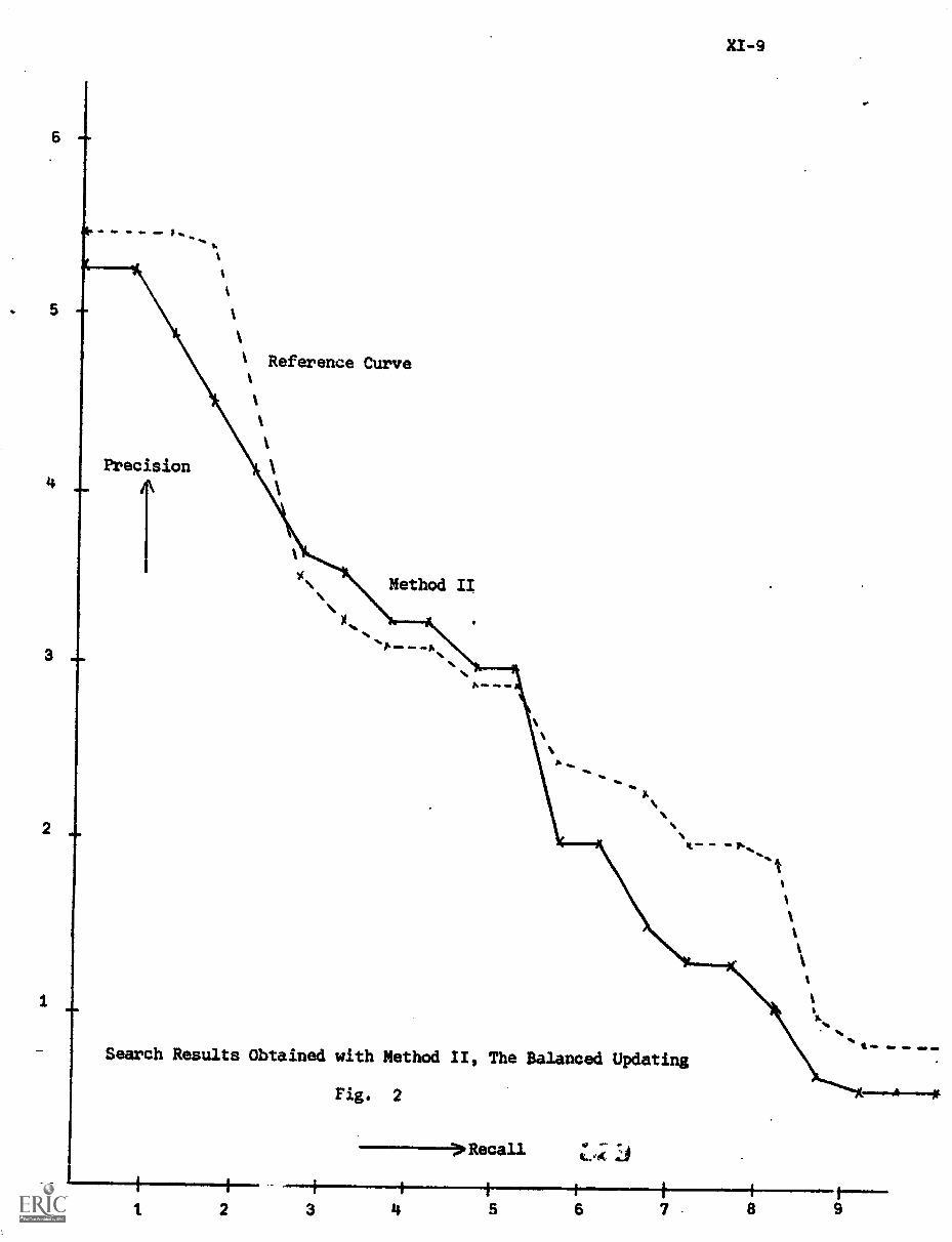
6

go.

Reference Curve

4

3

2

I

Mem

00

Search Results Obtained with Method II, The Balanced Updating

Fig. 2

Recall t

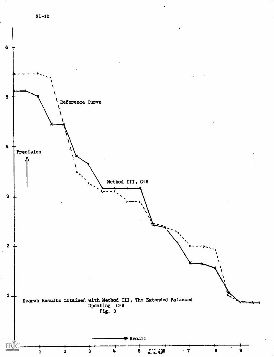
XI-10

Precision

A

Reference Curve

Method III, C=8

X

S.

S.

S.

e ow a.

Search Results Obtained with Method III, The Extended BalancedUpdating C=8

Fig. 3

Recall

0. 41* 46)6tr 7 8 9

XI-11

function was carried out. This function forms the basis of the iterative

algorithm used in III, and as already mentioned, the constant C (see

Appendix 1) which influences the stepsize has been set equal to 8 in

all experiments. Decreasing this constant gives worse results, but

increasing the value uields a remarkable system performance improvement

(Fig. 4, 5, 6, and 7). A constant of approximately 17 turns out to be

optimal in that the recall-precision curve for search r-sults -(Fig. 6)

has been lifted maximally compared with the reference curve.

It is a property of the algorithm that it is not particulary

critical to changes in C. The starting value 8 was apparently much

too small, that is, the updating step was too large (C occurs in the

denominator). In the range 13 to 25 however, the retrieval results are

not considerably affected by the change in C.

A Student T test was carried out in order to verify the

sigeficance of the results obtained with Method III, C=17. The

outcome of the test (T statistic = 3.99 with 20 degrees of freedom)

indicates that there is zero likelihood for the two sets of performance

figures (reference versus Method III, C=17) to have originated in the

same distribution.

5. Conclusion

The experiments described in this report support unmistakably

the usefulness of a new system parameter called utility value. The

assignment of such a function to each document in the collection

provides means for improving system performance. It has been shown that

a careful approach of the concept is required, since it is found that

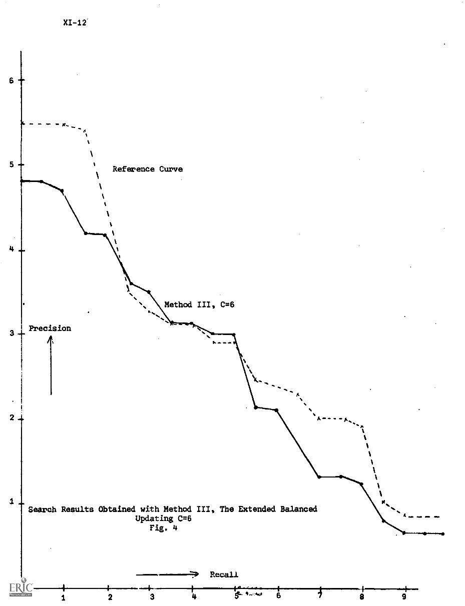
XI -12

"" X.

1

Reference Curve1

t

Precision3 t

2

0

Method III, C=6

-

A

A...


Fig. 4

111111111(, Recall

t

4 ono OM ow.

4 6

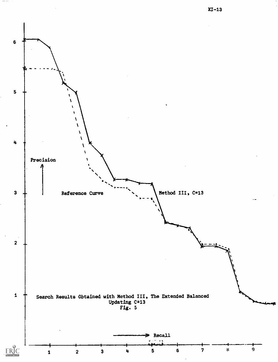
6

5

4

2

1

0

Reference Curve Method III, C=13

XI-13

1.6


Fig. 5

Recall

1 2 3 4 5 6 7 Et 9

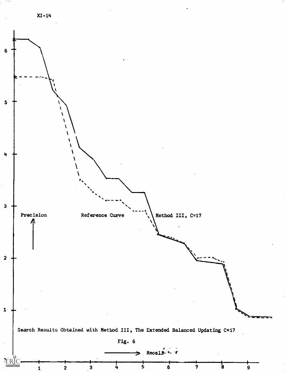
XI-14

Precision

A

Reference Curve Method III, C=17

Search Results Obtained with Method III, The Extended Balanced Updating C=17

1

Fig. 64

-----------1, Recalit-A-

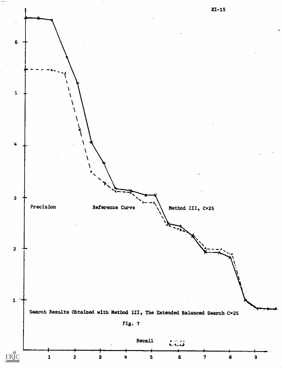
5

4

3

Precision

2

1

.Reference Curve

XI-15

Method III, C=25

Search Results Obtained with Method III, The Extended Balanced Search C=25

0

Fig. 7

RecallIL,44)-4

1 2 3 4 5 6 7 8 9

XI-16

balancing keeping the average utility value 1 as well as the

usage of heuristically determined constants are critical factors in

applying a successful updating algorithm.

It is clear that any document retirement policy based on

document values can only be justified is such values have a realistic

meaning, that is, after applying them system performance has to be

improved. This investigation has proved that the latter may be possible.

XI-17

References

1 A. Wong, R. Peck, and A. van der Meulen, An Adaptive Dictionaryin a Feedback Environment, Term Project Report, Spring 1972,Department of Computer Science, Cornell University.

2 A. van der Meulen, Dynamic versus Static Information Values,to be published.

3 C.R. Sage, R.R. Anderson, and D.P. Fitzwater, Adaptive InformationDissemination, American Documentation, Vol. 16, No. 3, July 1965.

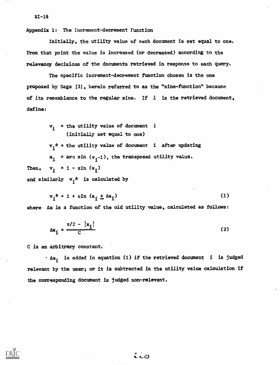
XI-18

Appendix 1: The Increment-decrement Function

Initially, the utility value of each document is set equal to one.

From that point the value is increased (or decreased) according to the

relevancy decisions of the documents retrieved in response to each query.

The specific increment-decrement function chosen is the one

proposed by Sage [3], herein referred to as the "sine-function" because

of its resemblance to the regular sine. If i is the retrieved document,

define:

v. = the utility value of document i

(initially set equal to one)

v.* = the utility value of document i after updating

xi = arc sin (vi-1), the transposed utility value.

Then, vi = 1 sin (xi)

and similarly vi* is calculated by

v.1 * = 1 + sin (x. + Ax ) (1)

where Ax is a function of the old utility value, calculated as follows:

v/2 - lxilAx =

i C(2)

C is an arbitrary constant.

Axi is added in equation (1) if the retrieved document i is judged

relevant by the user; or it is subtracted in the utility value calculation if

the corresponding document is judged non-relevant.

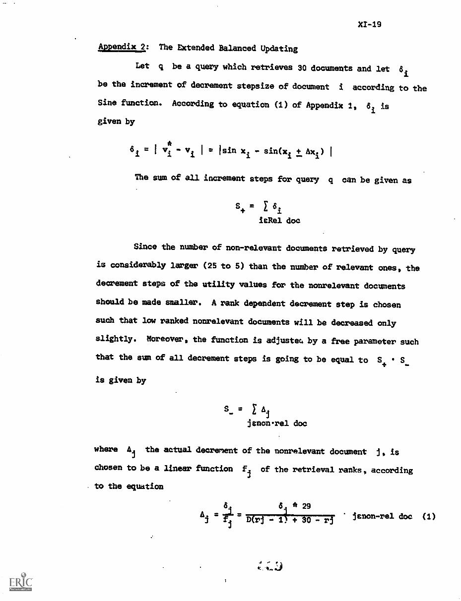
XI-19

Appendix 2: The Extended Balanced Updating

Let q be a query which retrieves 30 documents and let 6i

be the increment of decrement stepsize of document i according to the

Sine function. According to equation (1) of Appendix 1, 6, is

given by

61.=1111,-111.1r-Isinx.-sin(x. + Ax.)--

The sum of all increment steps for query q can be given as

S+

= 1 6i

ieRel doc

Since the number of non-relevant documents retrieved by query

is considerably larger (25 to 5) than the number of relevant ones, the

decrement steps of the utility values for the nonrelevant documents

should be made smaller. A rank dependent decrement step is chosen

such that low ranked nonrelevant documents will be decreased only

slightly. Moreover, the function is adjusteG by a free parameter such

that the sum of all decrement steps is going to be equal to Si. S_

is given by

s. = E Ai

janorel doc

where Ai the actual decrement of the nonrelevant document 1, is

chosen to be a linear function fj of the retrieval ranks, according

to the equation

6 *29A r-

1 D(1,1 - + 30 -

4 e

janon-rel doc (1)

XI-20

D is constant for one query but its value is changed for the

next one because the number and ranks of relevant and nonrelevant

documents change from query to query. The implementation of this method

requires an iterative algorithm in order to find D for each query such

that S-

= S+

(2a)

or / Aj = di (2h)

jeNon-rel Doc ieRel Doc

Consider first an illustration of equation (1) in c.rder to render

the method clearer.. A nonrelevant document retrieved in rank 1 will be

decreased by 6j, that is, the unmodified Sine function (f1=1). A nora.

relevant document retreived in rank 30 will be decreased by ba (f1 = D).

All nonrelevant documents with ranks in between will be decreased subject

to the linear function (1).

The value of D on the ocher hand is determined by equation (2)

and cannot be explicitly computed. An initial value for D must be

chosen and equation (2) can be evaluated. D has to be changed in an

iterative way until IS_ - Si] < e, where c is small.

The procedure guarantees an almost exact balancing of the amount

of increase and decrease of utility values per query.

Following is an example illustrating how the document values are

changed due to one query.

30 documents are retrieved by a query. Some are found relevant.

The document values of these 30 documents, after a number of previous

updatings, will be changed according to the relevancy decision of the

present query (see Table 1).

S+

the sum of the increased document values for the relevant

documents 320, 467, 322, and 321, is found to be 0.3760, using equation

Doc. No. Rank Old Doc..Vilue

New Doc.Value

320 R 1 1.0941 1.1818

476 R 3 0.9980 1.0920

322 R 4 0.9879 1.0820

321 R 7 0.9959 1.0898

107 2 0.9980 0.9325

478 5 1.0000. 0.9645

479 6 0.9959 0.9653

734 7 0.9980 0.9740

190 9 0.9889 0.9672

452 10 0.9962 0.9763

1251 11 0.9697 0.9518

1163 12 0.9939 0.9770

1149 13 0.9817 0.9661

422 14 0.9979 0.9832

255 15 1.0916 1.0886

47 16 1.0564 1.0438

1162 17 0.9970 0.9847

837 18 0.9780 0.9665

1209 19 1.0000 0.9889

150 20 0.9883 0.9778

34 21 1.0000 0.9899

1254 22 1.0000 0.9903

979 23 0.9914 0.9821

626 24 0.9981 0.9892

1235 25 1.0000 0.9914

1370 26 0.9360 0.9281

538 27 0.9959 0.9879

425 28 0.9814 0.9738

818 29 1.0767 1.0686

363 30 1.0000 0.9928

Alterations in Document Values

Table 1

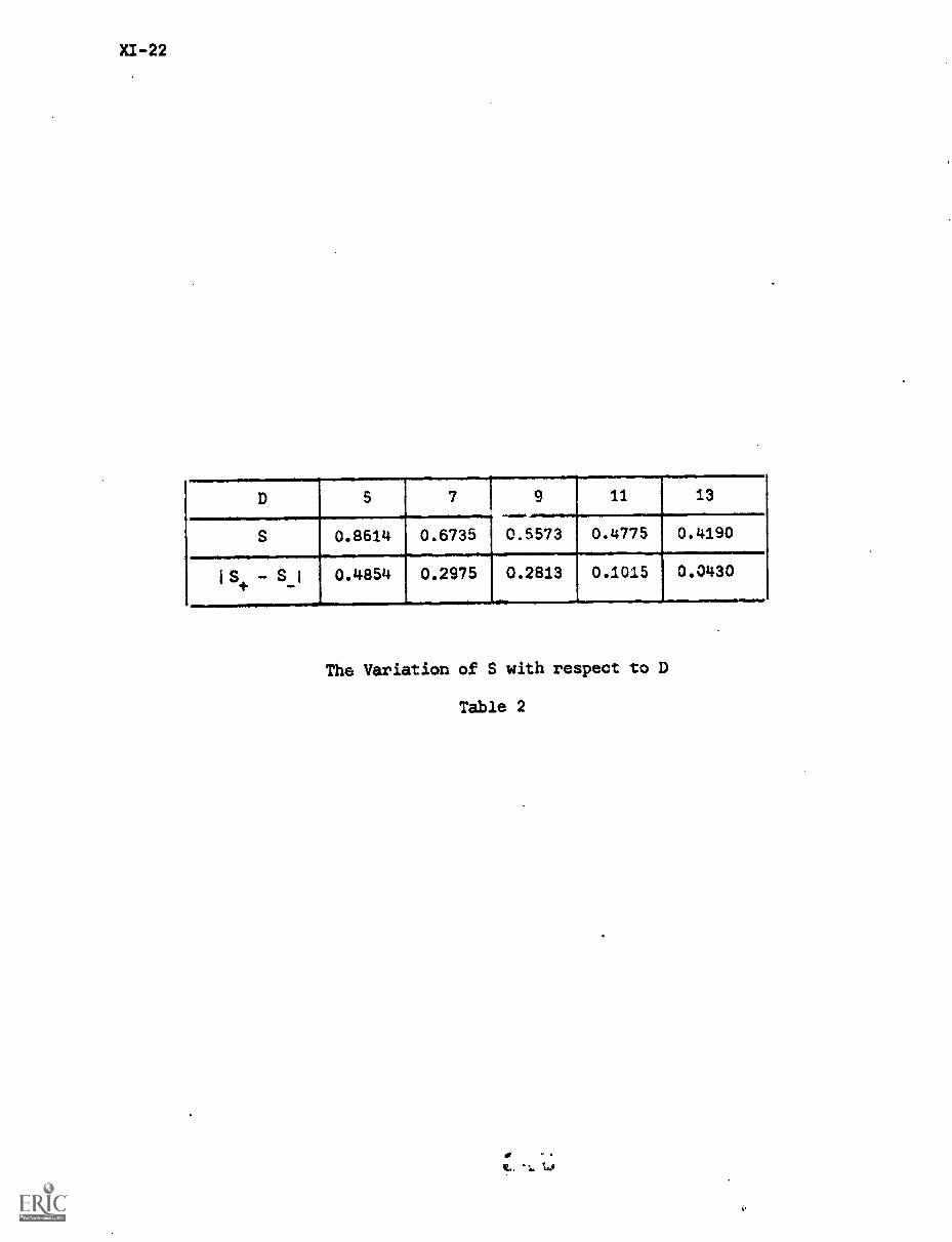
D 5 7 9 11 13

S 0.8614 0.6735 0.5573 0.4775 0.4190

1S1.

- S-

1 0.4854 0.2975 0.2813 0.1015 0.0430

The Variation of S with respect to D

Table 2

XI-23

1 of Appendix 1.

Aits are found interatively by changing the value of D,

such that S+

is equal to S_ to within a tolerance, which is

0.05 in this case.

For the variation of S. for different values of D, see

Table 2.

For the present query, D = 13 is used.

Automatic Document Retirement Algorithms

K. Sardana

Abstract

XII-1

Some existing and proposed algorithms for automatic document

retirement in a retrieval system are analyzed for their computational

complexities and their effects on storage costs and the retrieval

performance of the system. It is found that various retirement algorithms

exhibit almost equivalent performance, especially at high recall; therefore,

it is preferable to use those algorithms which provide low cost bounds.

1. Introduction

Two automatic document retirement algorithms have been proposed

by Tai and Yang (referred to as TY in the sequel) [1] and Beall and

Schnitzer (referred to as BS it be sequel) [2]. It is, however, not clear

what algorithm should be used in practice, what costs are involved in

executing the algorithms, what savings obtained and at how much loss

or gain in retrieval performance, etc. The idea of the present study

is to look into these questions with special reference to TY algorithm.

Some more algorithms are proposed and overall comparisons are made between

different algorithms when used with and without document .'ector modification

(DVM). [41

2. The Algorithms

Both the TY and BS algorithms for document retirement are based on

utilizing users' relevancy judgments in updating the documents. The

X11-2

algorithms that we propose also rely on users' relevancy judgments. We

assume that relevancy judgments on retrieved documents for various queries

are available as input to the retirement algorithms. The computational

complexity of the algorithms will consist of the costs of modifying the

documents, computing "use indices" for documents, etc. for the express usage

of the algorithms and the cost of making retirement decisions.

The general philosophy used here is to give the algorithms and

their computational complexities. As we will not be able to give proofs

of correctness of these heuristic algorithms, we resort to experimental

methods in the next section to evaluate the performance of the methods in

an experimental environment. Finally overall comparisons between algorithms

are 1119'! .

Criteria of Evaluation of Algorithms

In determining the computational complexity of the algorithms, we

assume the following:

a) Asymptotic complexity will be used so that a machine independent

cost analysis can be done. However, constants will be

considered when finer decisions are involved.

b) The model of the computing device is a random access machine

which assumes that enough core memory is available for the

entire program to fit in.

c) The worst case computational complexity will be derived rather

than expected complexity as the former is easier to get hands on.

d) The basic steps in the computation to be considered for time

complexity are additions (adds), multiplications (mults) and

comparisons (comps).

X11-3

e) The cost criterioz. is uniform rather than logarithmic i.e.

a unit of each kind of operation will have some uniform

cost regardless of the size of the numbers involved.

A detailed discussion on choosing the above criteria may be

found in [3].

Input: A set of documents (D) and a set of queries {Q} and users'

relevancy judgments on (D) for (Q).

Output: A set of documents {D'} {D} to be retired to a

secondary store such that future retrieval processing with

remaining (DI {D'} documents using future queries is

exp,.7.ted to be overall efficient considering the space

s by retirement, gain or loss in system performance

. cost of execution of the algorithm.

Some Desirable Features of Algorithms

To achieve the above mentioned goal of retiring documents, the

following features (among others) of the algorithms seem to be desirable:

a) Irretrievable documents or documents not relevant to any

query should be retired. This, however, assumes that the

indexing is perfect.

b) The selection of various parameters for the algorithm should be

pretty straightforward in any practical implementation.

c) The algorithm should not assume any unnecessary attributes of

the document space, e.g. documents with same average weights, etc.

We note that

of the above

each of the TY or BS algorithms does not have one or the other

features.

XII -4

Methods

In the following algorithms, we mention the step to retrieve the

documents and to do DVM for a query. However, the costs of these steps

are not considered in determining the computational complexity of a

retirement algorithm as these step are not part of th' retirement

algorithm, per se.

It may be argued that the analysis of computational complexity of

such isolated algorithms does not make much sense insofar as the envir-

onment in which they are going to be used is known. Thus, for instance,

one may consider the effect of complexity of a retirement algorithm on the

asymptotic complexity of the overall retrieval process. The cost of

matching a query with n documents, each document having on the average

m concepts, is 0(mn) and the cost of selecting top r documents for

showing to the user is 0(n) using the median algorithm [5] implying the

overall retrieval process to be 0(mn)/query. Since most of the additional

algorithms, like the retirement algorithms considered here, cost less than

0(mn)/query (see later), the asymptotic complexity of the overall retrieval

process does not change. It may, then, be concluded that the analysis

of such algorithms is not important. The viewpoint taken here is that in

document retrieval, where the cost of answering a query is quite high,

the reduction of costs of all sub-algorithms should be considered important.

The algorithms are expressed in Pseudo-Algol for clarity and ease

in deriving the computational complexities. For convenience, we assume a

kind of macro facility available in the language with four keywords:

"defmacro X" defines a macro named X, the code between begmacro and

XII-5

endmacro is body of the the macro named X (assuming "defmacro X" precedes

this). The body of the macro X is textually substituted for call "macro X".

Al) Algorithm TY (Tai and Yang)

The TY algorithm [1] shown in Fig. 1(a) is basically the following,

suitably modified to work with a batch of queries (BATCHSIZE is the

number of queries in a batch and BATCHNUM is the number of batches to be

processed):

a) For each query qij in a batch, retrieve r number of documents.

Form the sets RELij, NRELij and BOT.. consisting of top RELTOP3.3

relevant retrieved, at most NONLIM nonrelevant among top

NONTOP retrieved and bottom-most ranking documents NUMBOT in

number respectively.

b) After doing 'Arm (optional) using the queries in a batch.

multiply the weights of concepts of document vectors in REL..

NREL.. and BO Tij by constants FR(>1), FN(<1) and FB(<I)

respectively.

c) After every document vector multiplication by FN or FB, compute

the average weight AVGwT of the document and retire it if

AVGWT < CUTOFF, some chosen constant.

The idea of this algorithm is to reward the top relevant retrieved

documents and to penalize the top nonrelevant retrieved and the bottom-most

ranking documents for each query by respectively increasing or decreasing

all the weights of the concepts of the documents by the same factor at a

time. The information on the usefulness of a document is thus carried in

the weights of the vector itself. When the average weight per concept of

a document falls below a chosen threshold, meaning that the document has

been penalized more than it has been rewarded, the document in ret ir'ed.

X11-6

Computational Complexity:

Let

n = total number of documents (roughly 400-1500) in the special

subject area of the query; thus for a query in Astrophysics,

n is the number of documents in this particular subcollection

rather than the whole Physics library. .

q = total number c7 queries in the same area = 0(n) say.

m = average number of concepts/document.

r = number of documents retrieved.

We also assume that

i) IRELill + INRELO + IBOT..13 1 r, where IX( denotes

the cardinality of set X. This is not an unreasonable

assumption to make and conforms in practice.

ii) IRE Lij 1".. cr for some constant c(<1).

Let us first determine the cost associated with SETUP code of Fig. 1(b),

used in line (7) of algorithm TY of Fig. 1(a). Costs associated with lines

(8), (9) and (10) are constant. Cost of line (6) is -r comps/query (- stands

for approximately) because from the given ranked list of documents obtained

from line (4), this many comparisons may be needed to form sets RELij and

NREL...

Next we determine the cost of T&Y code of Fig. 1(c) used in line (10)

of Fig. 1(a). Lines (4), (7) and (13) together cost -111 mults/documents/query

i.e. "mr multi /query over all documents in sets REL, NREL and BOT. Similarly

cost of lines (8), (9), (14) and (15) over documents in sets NREL and BOT

is "mr adds, "r multi: (actually divisions to calculate AVGWT) and -r comps

per query.

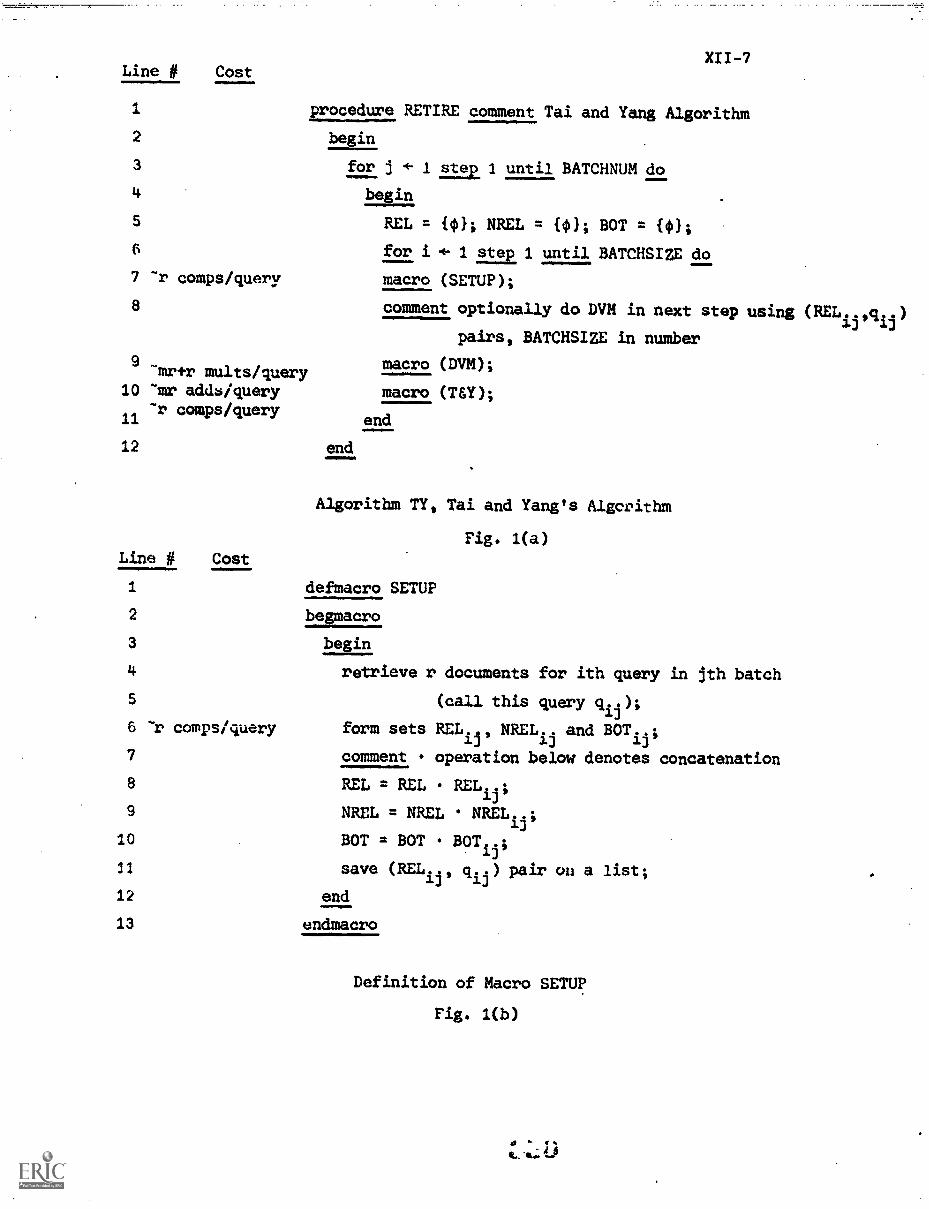
Line # CostX11-7

1 procedure RETIRE comment Tai and Yang Algorithm

2 begin

3 for j 4- 1 s p 1 until BATCHNUM do

4 begin

5 REL = {0}; NREL = {0}; BOT = (0);

6 for i F 1 step 1 until BATCHSIZE do

7 "r comps/query macro (SETUP);

a comment optionally do DVM in next step using (REL..13 ,q )ij

pairs, BATCHSIZE in number

m9mrtr molts /query

macro (DVM);

10 "mr adds /query macro (TgY);"r comps/query

11 end

12 end

Algorithm TY, Tai and Yang's Algorithm

Fig. 1(a)Line # Cost

1 defmacro SETUP

2 begmacro

3 begin.

4 retrieve r documents for ith query in jth batch

5 (callthisquerYclip;6 "r comps/ query formsetsRELij"

13NRELijand

BOT...'

7 comment operation below denotes concatenation

8 REL = REL REL.

9 NREL = NREL NRELij,

10 BOT = BOT BOT...13'

11 save (RELij, qij) pair cm a list;

12 end

13 endmacro

Definition of Macro SETUP

Fig. 1(b)

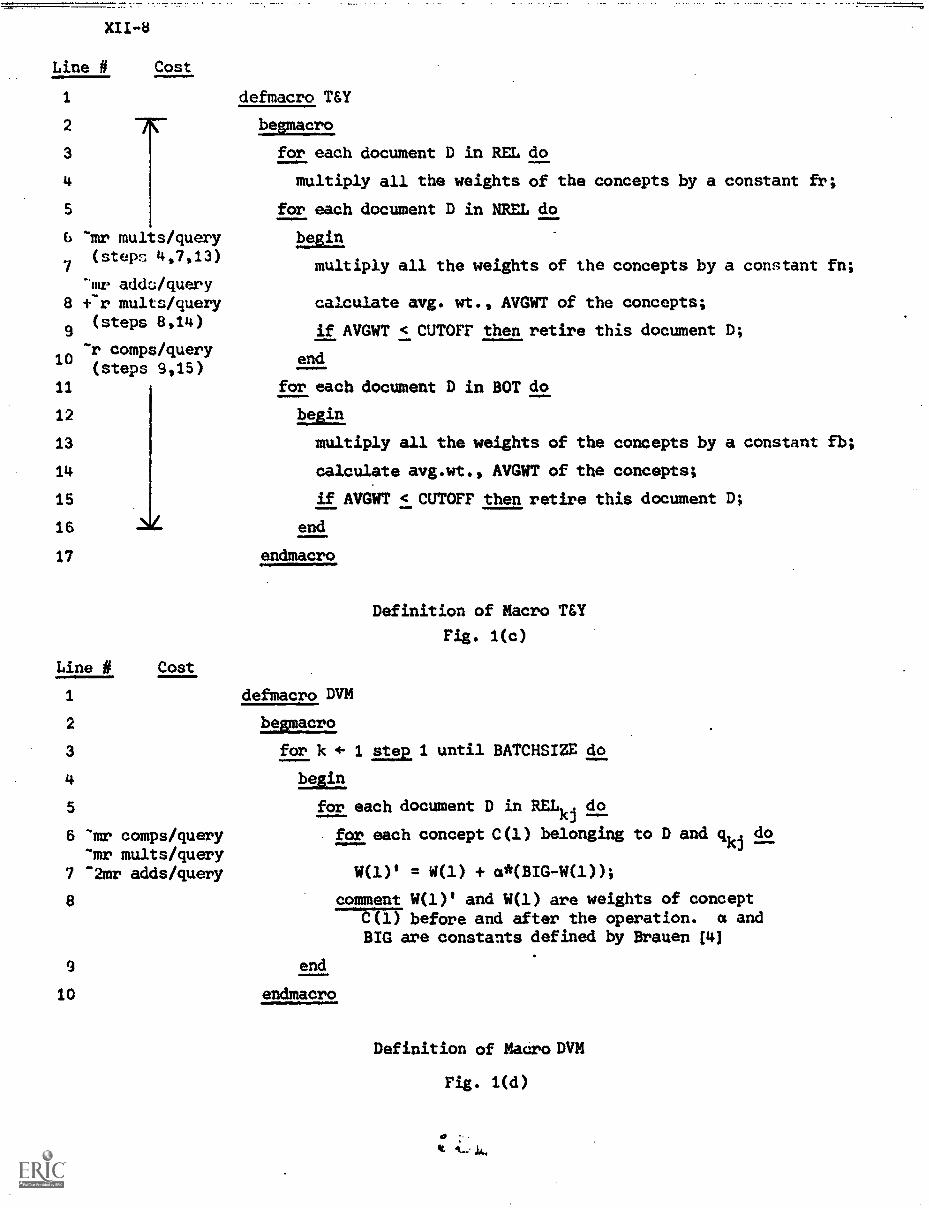
Line # Cost

1

2

3

4

5

6 'mr mults/query

7(steps 4,7,13)

Imr adds/query8 s-r mults/query calculate avg. wt., AVGWT of the concepts;

(steps 8,14)9 if AVGWT < CUTOFF then retire this document D;

-r comps/query10

(steps 9,15)

defmacro T&Y

begmacro

for each document D in REL do

multiply all the weights of the concepts by a constant fr;

for each document D in NREL do

begin

multiply all the weights of the concepts by a constant fn;

end

11 for each document D in BOT do

12 begin

13 multiply all the weights of the concepts by a constant fb;

14 calculate avg.wt., AVGWT of the concepts;

15 if AVGWT < CUTOFF then retire this document D;

16 end

17 endmacro

Definition of Macro TO

Fig. 1(c)

Line # Cost

1 defmacro DVM

2 begmacro

3 for k 1 step 1 until BATCHSIZE do

4 begin

5 for each document D in RELkj do

6 "mr comps/query for each concept C(1) belonging to D and qkj do-mr mults/query

7 -2mr adds/query W(1)' = W(1) + a*(BIG-W(1));

8

9

10

comment W(1)' and W(1) are weights of conceptC(1) before and after the operation. a andBIG are constants defined by Brauen [4]

end

endmacro

Definition of Macro DVM

Fig. 1(d)

.

41. °L... k.

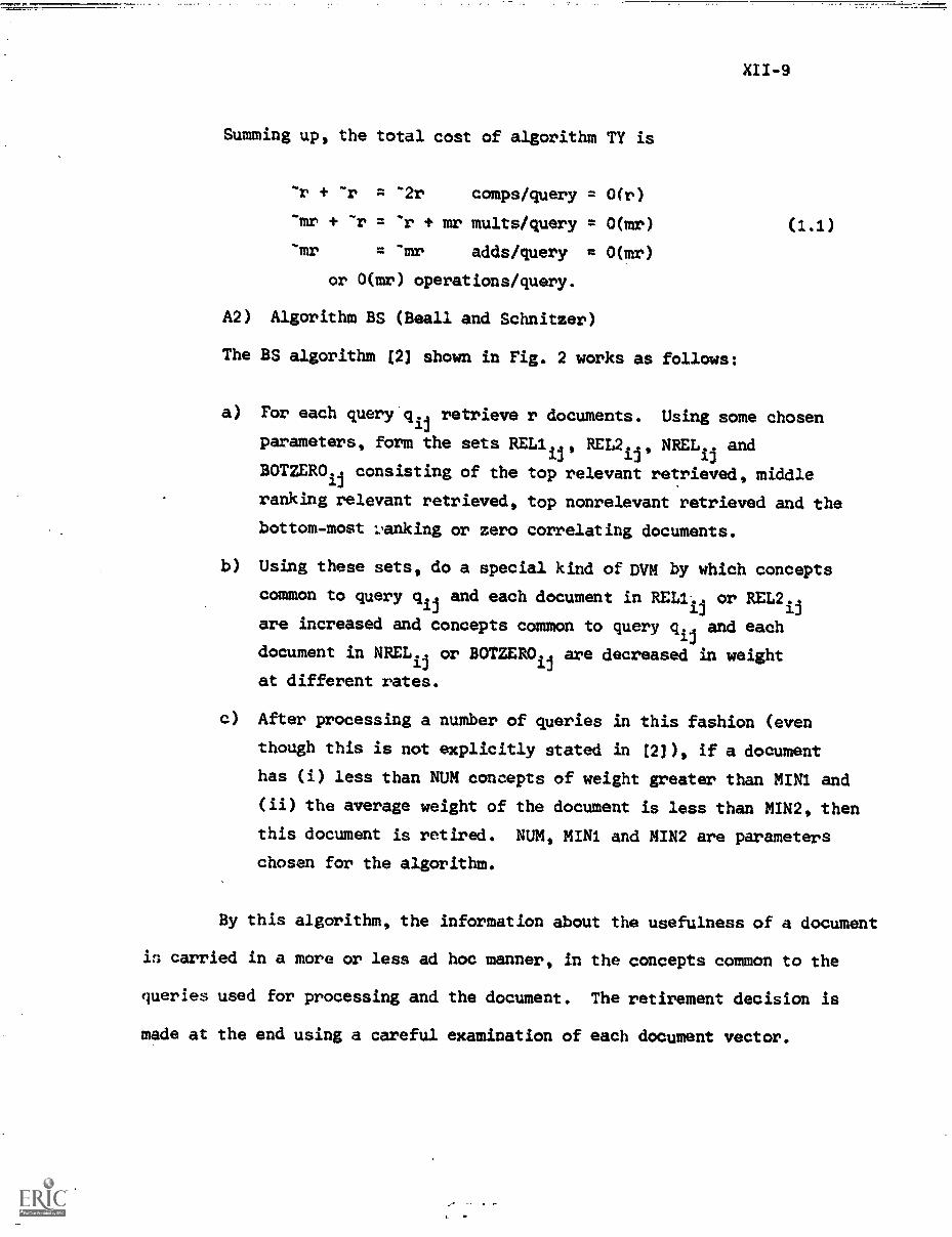
X11-9

Summing up, the total cost of algorithm TY is

"r + "r = "2r comps/query = 0(r)

"mr + "r = 'r + mr mults/query = 0(mr)

"mr = "mr adds/query = 0(mr)

or 0(mr) operations/query.

A2) Algorithm BS (Beall and Schnitzer)

The BS algorithm [2] shown in Fig. 2 works as follows:

a) For each query qij retrieve r documents. Using some chosen

parameters, form the sets RELlii, REL2ij, NRELij and

BOTZERO.,1]

consisting of the top relevant retrieved, middle

ranking relevant retrieved, top nonrelevant retrieved and the

bottom-most l'anking or zero correlating documents.

b) Using these sets, do a special kind of DVM by which concepts

common to query qij and each document in RELlij or REL2ij

are increased and concepts common to query qij and each

documentinNREL.ij orBOTZER.Olj are decreased in weight

at different rates.

c) After processing a number of queries in this fashion (even

though this is not explicitly stated in [21), if a document

has (i) less than NUM concepts of weight greater than MINI and

(ii) the average weight of the document is less than MIN2, then

this document is retired. NUM, MINI and MIN2 are parameters

chosen for the algorithm.

By this algorithm, the information about the usefulness of a document

in carried in a more or less ad hoc manner, in the concepts common to the

queries used for processing and the document. The retirement decision is

made at the end using a careful examination of each document vector.

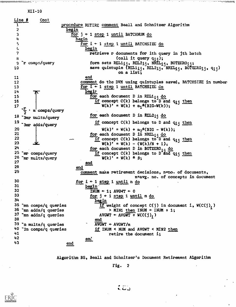
XII-10

Line # Cost

1

2

3

4

5

7

a9 -r comps/query

10

11

12

1314 -PC-1516

17

18

19

2021222324

25 -mr26 -mr27

28

29

.r

"3mr mults/query

'3mr adds/query

procedure RETIRE comment Beall and Schnitzer Algorithmbegin,

for j + 1 step 1 until BATCHNUM dobegin

for i 4- 1 step 1 until BATCHSIZE dobeginretrieve r documents for ith query in jth batch

(call it query qi);form sets RELlii, REL2ij, NRtLij, BOTZER0ii;save quintuple (RELlij, REL2ij, NRELij, BOtZEROij,

on a list;

m comps/query

comps/querymults/query

3031

32

3334

35 'mn comps/q queries36 -mn adds/q queries37 "mn adds/q queries38

39 'n mults/q queries40 -2n comps/q queries414243 end

qij)

endcomment do the DVM using quintuples saved, BATCHSIZE in numberfor i 4- 1 step 1 until BATCHSIZE do

begifor each document D in RELlij do

if concept C(k) belongs to D and qij thenW(k)' = W(k) + aet(BIG-W(k));

for each document

if concept C(k)

W(k)' = W(k)for each document

if concept C(k)W(k)' = W(k)

for each documentif concept C(k)

W(k)' = W(k)end

endcomment make retirement decisions, n=no. of documents,

m=avg. no. of concepts in documentfor i 4- 1 2122.1 until n do

beginINUM ÷ 1; AVGWT 4- 0for j f 1 step 1 until m dobegin

if weight of concept C(j) in document i, W(C(j)i)> MINI then INUM f INUM + 1;

AVGWT 4- AVGWT + W(C(j)i)endAVGWT 4- AVGWT/m

if INUM < NUM and AVGWT < MIN2 thenretire the document i;

D in REL2ij do

belongs to D and qij then

+ m2*(BIG - W(k));D in NREL3.3 .. do

belongs to D and qij then- (W(k)/N + 1);D in BOTZER0i4 dobelongs to D dnd qij then* 0;

ens.'

Algorithm BS, Beall and Schnitzer's Document Retirement Algorithm

Fig. 2

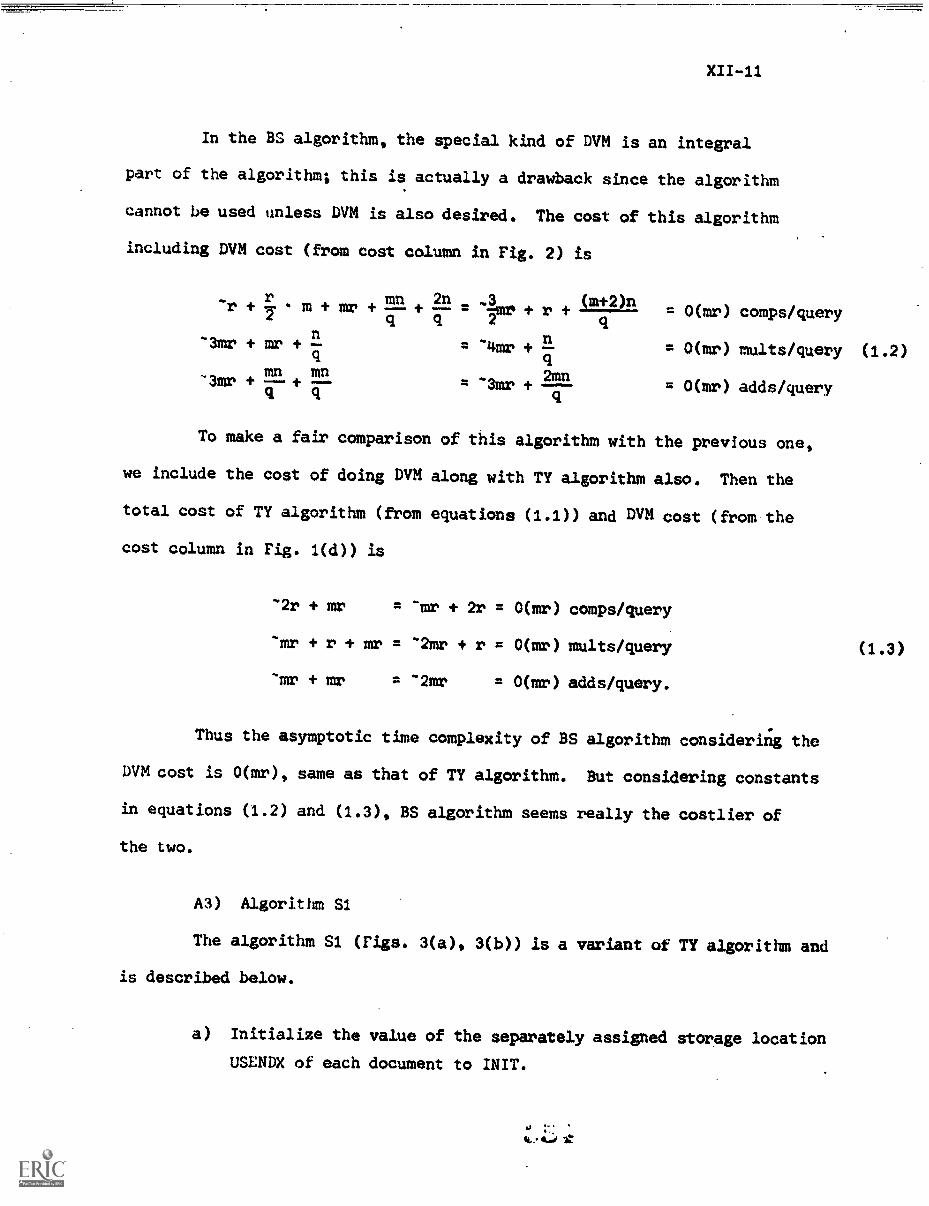
XII-11

In the BS algorithm, the special kind of DVM is an integral

part of the algorithm; this is actually a drawback since the algorithm

cannot be used unless DVM is also desired. The cost of this algorithm

including DVM cost (from cost column in Fig. 2) is

r mn 2n ,3 (m+2)n"r +2

m + mr + -+ -- = mr + r + = 0(mr) comps/queryq q 2 qn

-3mr + mr +q

= -4mr + a = 0(mr) mults/query (1.2)q

mn mn-3mr + --.4. m -3mr + ..1!2a = 0(mr) adds/queryq q q

To make a fair comparison of this algorithm with the previous one,

we include the cost of doing DVM along with TY algorithm also. Then the

total cost of TY algorithm (from equations (1.1)) and DVM cost (from the

cost column in Fig. 1(d)) is

-2r + mr = -mr + 2r = 0(mr) comps/query

`mr + r + mr = -2mr + r = O(mr) mults/query (1.3)

-mr + mr -2mr = 0(mr) adds/query.

Thus the asymptotic time complexity of BS algorithm considering the

DVM cost is 0(mr), same as that of TY algorithm. But considering constants

in equations (1.2) and (1.3), BS algorithm seems really the costlier of

the two.

A3) Algorithm Si

The algorithm S1 (Figs. 3(a), 3(b)) is a variant of TY algorithm and

is described below.

a) Initialize the value of the separately assigned storage location

USENDX of each document to INIT.

0..041.01!

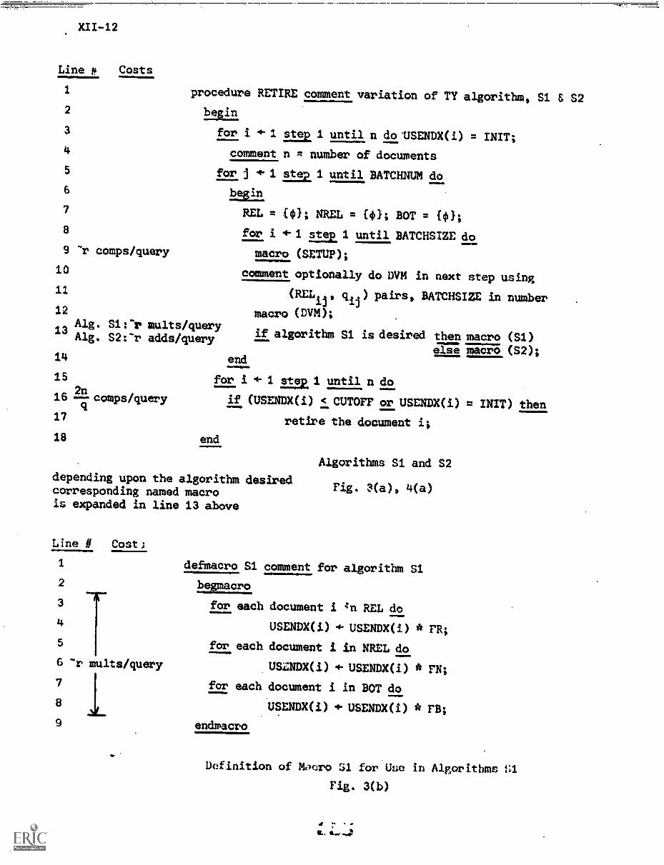
XII-12

Line fit Costs

1 procedure RETIRE comment variation of TY algorithm, S1 & S22 begin

3 for i 4.1 2122. 1 until n do -USENDX(i) = INIT;4 comment n = number of documents

5 for j 1 2122. 1 until BATCHNUM do

6begin.

7 REL = CO); NREL = {0}; BOT = 4);8 for i 4-1 212E1 until BATCHSIZE do9 "r comps/query macro (SETUP);

10 comment optionally do DVM in next step using11 (RELij, qij) pairs, BATCHSIZE in number12 macro (DVM);

Alg. mults/query13 if algorithm Si is desired then macro (S1)Alg. S2: "r adds/queryelse macro (S2);

14 end

15 for i 4- 1 21210. until n do2n

16 ---comps/query if (USENDX(i) < CUTOFF or USENDX(i) = INIT) then17 retire the document i;18 end

depending upon the algorithm desiredcorresponding named macrois expanded in line 13 above

Line # Cost;

1

2

3

5

6 "r mults/query

:9

OP

Algorithms S1 and S2

Fig. 3(a), 4(a)

defmacro S1 comment for algorithm S1

begmacro

for each document i 4n REL do

USENDX(i) f USENDX(i) * FR;

for each document i in NREL do

USENDX(i) 4- USENDX(i) * FN;

for each document i in BOT do

USENDX(i) USENDX(i) * FB;

endmacro

Definition of Macro 31 for Um in Algorithms !A

Fig. 3(b)

XII-13

b) Retrieve r documents for query qij. Form the sets RELij,

RELij and BOT. just like in TY algorithm.

c) After doing the DVM (optional) using the queries in a batch,

multiply the USENDX of a document by rR(>1), FN(<1) or

FB(<1) according as this document appears in the set RELij,

NRELij or BOT respectively.

After processing a BATCHNUM number of batches of queries

using steps (b) and (c) repeatedly, if a document's USENDX = INIT

or USENDX < CUTOFF, some chosen parameter, then this document

is retired. Go to step (a).

Note, here DVM does not directly take part into retirement decisions

as in TY algorithm, but does so indirectly by choosing which documents get

retrieved or not thus affecting their USENDX values. The main difference

between TY algorithm and the present one is: The former uses AVGWT of the

documents to denote the useful index for a document and, therefore, since

the document vectors are modified by DVM and the multipliers FR, FN or FB,

AVGWT needs to be computed for each document vector before making a

retirement decision. The latter algorithm uses a location USENDX for each

document and its value gets modified by multipliers FR, FN or FB while

not by DVM directly. The retirement decision is based on USENDX values.

Another difference is that as shown, the TY algorithm makes

retirement decisions aiter processing every batch of queries (5 used here)

while S1 algorithm does so after processing a set of queries (125 used

here). But both algorithms may be adjusted to any retirement frequency, in

which case the asymptotic cost of TY algorithm does not change while the cost

of S1 algorithm may approach 0(n) when retirement decision is made after

processing every query.

X11-14

is


As shown in the cost column of Fig. 3(a), the cost of this algorithm

-r t.2n

comps/query = 0(r) comps/query

-r mults/query = 0(r) mults/query

or 0(r) operations/query since q = 0(n).

This algorithm is thus asymptotically better than TY algorithm in

time complexity by a factor of m, the average number of concepts in a

document vector. However the space complexity has been increased by

0(n) in using probabl:: one computer word or halfword USENDX location for

each of the n documents. This is reasonable considering that the space

. required is on a cheap off-line device while the time saved decreases

the important on-line response time.

A4) Algorithm S2

This algorithm (Figs. 4(a), 4(b)' another variant of TY algorithm,

resembles algorithm S1 cl^'ely. Here in step (b) the USENDX of a document

is increased or decreased by constant values by additions or subtractions

rather than by multiplications (as is done in algorithm S1) whenever a

document ends up in the set REL. or NREL. or SOT.aj ijs


From the cost column of Fig. 4(a), the time complexity of this

algorithm is

2n-r comps/query = 0(r) comps/query

adds/query = 0(r) adds/query(1.5)

Line # Cost

13.1 defmacro S2 comment this macx) is for algorithm S2

13.2

13.4

begmacro

13.3 for each document i in REL do

USENDX(i) *.USENDX(i) + FREL;

13.5 for each document i in NREL do-r adds/query

13.6 USENDX(i) 4. USENDX(i) + FNREL;

13.7 for each document i in BOT do

13.8 USENDX(i) + USENDX(i) + FBUT;

13.9 endmacro

Definition of Macro S2 for Use in Algorithm S2

Fig. 4(b)

or 0(r) operations/query.

Remarks similar to algorithm S1 apply here also.

A5) Algorithm S3

Algorithm S3, Fig. 5, differs from algorithm S2 in step (b) in two respects:

i) Instead of assigning a fixed positive USENDX to a document

appearing in set RELij algorithm S3 assigns a variable

index1--depending upon the number p of relevant retrieved

documents (i.e. p = IREL111) for a query. The idea is to

assume that every relevant retrieved document is useful

in satisfying 1-th of the query. However for nonrelevant

documents in set NRELij'

a constant negative use index

(40) is assigned.

ii) The bottom set of documents, BOTij is not considered in the

hope that RELij ij

and NREL sets are enough in determining the

use indices of documents.


The time and space complexity of this algorithm is the same as

that of algorithm S2 and is given by equations (1.5).


Since the performance of document retirement algorithms (like

most information retrieval algorithms) depends upon the unpredictable

future queries, it is meaningless to talk about a proof of correctness

of such algorithms. Therefore, we resort to experimental methods to

evaluate the success of these algorithms.

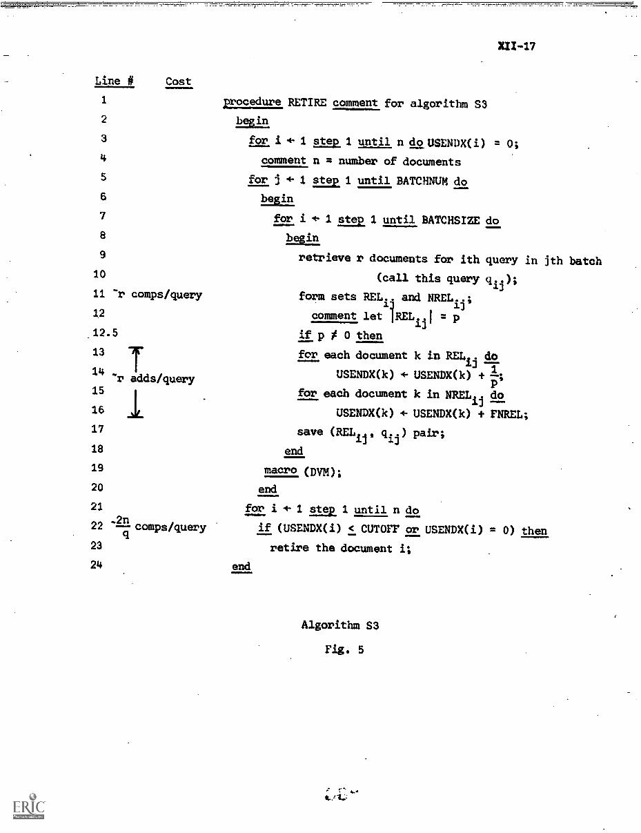
X.II -17

Line # Cost

1 2rocedure RETIRE comment for algorithm S3

2 begin,

3 for i 4-1 step 1 until n do USENDX(1) = 0;

4 comment n = number of documents

5 for j 4- 1 step 1 until BATCHNUM do

6 begin

7 for i a 1 step 1 until BATCHSIZE do

8 begin

9 retrieve r documents for ith query in jth batch10 (call this query gip;

11 -r comps/query form sets REL. and NREL.1.11 '

12 comment let IRELijI = p

12.5 if p 0 0 t_hen

" T for each document k in RELij do

USENDX(k) USENDX(k) +14 .r adds/query

13*

41.

for each document k in NRELij do

16 USENDX(k) F USENDX(k) + FNREL;

17 save (RELij, qij) pair;

18 end

19 macro (DVM);

20 end

21 for i 4- 1 step 1 until n do

22 "lacomps/query if (USENDX(i) < CUTOFF or USENDX(i) = 0) then

23 retire the document i;

24 end

Algorithm S3

Fig. 5

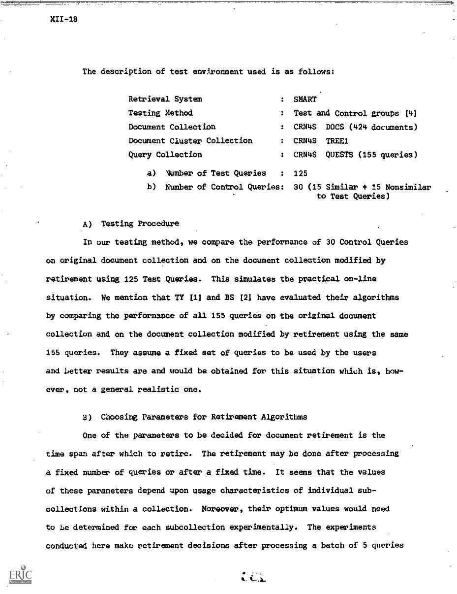
The description of test environment used is as follows:

Retrieval System

Testing Method

Document Collection

Document Cluster Collection

Query Collection

SMART

Test and Control groups [4]

CRN4S DOCS (424 documents)

CRN4S TREE1

CRN4S QUESTS (155 queries)

a) lumber of Test Queries 125

b) Number of Control Queries: 30 (15 Similar + 15 Nonsimilarto Test Queries)

A) Testing Procedure

In our testing method, we compare the performance of 30 Control Queries

on original document collection and on the document collection modified by

retirement using 125 Test Queries. This simulates the practical on-line

situation. We mention that TY [1] and BS [2] have evaluated their algorithms

by comparing the performance of all 155 queries on the original document

collection and on the document collection modified by retirement using the same

155 queries. They assume a fixed set of queries to be used by the users

and better results are and would be obtained for this situation which is, how-

ever, not a general realistic one.

B) Choosing Parameters for Retirement Algorithms

One of the parameters to be decided for document retirement is the

time span after which to retire. The retirement may be done after processing

a fixed number of queries or after a fixed time. It seems that the values

of these parameters depend upon usage characteristics of individual sub-

collections within a collection. Moreover, their optimum values would need

to be determined for each subcollection experimentally. The experiments

conducted here make retirement decisions after processing a batch of 5 queries

XII-19

for the TY algorithm and after processing the total number of 125 test

queries for the others.

A discussion on choosing the other parameters follows.

a) Algorithms TY and SI

We consider a procedure for choosing positive parameters

FR(>1), FN(<1) and FB(<I) used in algorithms TY and ,31. Suppose initial value

of USENDX assigned to each document is INIT; in case of algorithm TY, INIT

is the average weight of each document assumed to be constant over all

documents.

Notation 3.1: Let count 1/m/n of a document for nonnegative integers

1, m and n stand for 1, m and n appearances of the document in classes REL,

NREL and BOT respectively.

Then the final value of USENDX for this document is:

INIT * (FR)1 * (FN)m * (FB1n. (3.1)

Definition 3.1: A count 11/m

1/n

1is equivalent to (less than)

a count 12/m

2/n

2of a document if the final value of USENDX obtained by

11/m

1/n

1is algebraically equal to (less than) the final value of USENDX

obtained by 12/m2/n2 i.e.

(FR)11 * (FN)ml * (FB)ni = (<) (FR)12 * (FN)m2 * (FB)n2.

Lemma 3.1: Suppose that for algorithm TY without DVM and for

algorithm S1 with or without DVM, a appearances of a document in class REL

are offset by appearances of the same document in class NREL or by c

appearances.of the same document in class BOT, i.e.:

XII-20

then

a/b/0 0/0/0 :I a/0/c, (3.2)

a a

FN = (FR) and FB = (FR) c(3.3)

Moreover, to retire all the documents with counts 1/m/n or less,

the retirement cutoff for USENDX may be taken as

i a aCUTOFF = INIT * (FR)1 * (FN)m * (FB)n = INIT * (m)1 -m- n'iY (3.4)

a

Proof: a/1)/0 = 0/0/0 emo (FR)a * (FN)b = 1 FN = (FR) ba

a/0/c E 0/0/0 -o (FR)a * (FB)c = 1 FB = (FR) c

Rest of the lemma is obvious.

Note that the above lemma does not obviously apply to algorithm

TY used with DVM since the average weight of a document also gets changed

by DVM process and equation (3.1) may not hold.

Now the problem of choosing parameters FR, FN, FB and CUTOFF boils

down to comparatively easy problem of choosing reasonable values of a, b, c

and 1, m, n and any initial values INIT and FR, both >1.

Example:

Let a = 1, b = 2, c = 8, i.e. 1/2/0 = 0/0/0 = 1/0/8. Also assume

1 = 0, m = 3, n = 0, i.e. we decide to retire all documents with counts

< 0/3/0.

Choose INIT = 12

FR = 1.56a- --

Then equation (3.3) -4 FN = (FR)b

=

and 1 1 3 = (FR)CT

=

1

2(1.56) 1

8(1.56)

=

=

0.8007

0.946

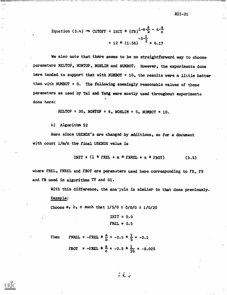
XII -21

-m.a - n.aEquation (3.4) ! CUTOFF = INIT * (FR) b c

1

= 12 * (1.56) ` = 6.17

We also note that there seems to be no straightforward way to choose

parameters RELT0i, NONTOP, NONLIM and NUMBOT. However, the experiments done

here tended to support that with NUMBOT = 10, the results were a little better

than with NUMBOT = O. The following seemingly reasonable values of these

parameters as used by Tai and Yang were mostly used throughout experiments

done here:

RELTOP = 30, NONTOP = 6, NONLIM = 5, NUMBOT = 10.

b) Algorithm S2

Here since USENDX's are changed by additions, so for a document

with count 1/m/n the final USENDX value is

INIT + (1 * FREL + m * FNREL + n * FBOT) (3.5)

where FREL, FNREL and FBOT are parameters used here corresponding to FR, FN

and FB used in algorithms TY and Si.

With this difference, the ana'ysis is similar to that done previously.

Example:

Choose a, b, c such that 1/5/0 E.: 0/0/0 E: 1/0/20

INIT = 0.0

FREL = 0.5

Then FNREL = -FREL * = -0 5 * 1= -0.1.

5

FBOT = -FREL * -11= -0.5 * =20

XII -22

To retire documents with count < 0/0/10

CUTOFF = INIT + 10 * FBOT = 0.0 + 10* -0.025 = - 0.25

c) Algorithm S3

In this algorithm, documents appearing in BOT set are not considered.

To retire documents with count < 0/10/ -, choosing a "reasonable" value of

FNREL = -1/20, use

CUTOFF-;10 * FNREL = 10e1- = 0.5.20

We further note thd following:

1) In addition to retiring documents with counts 1/m/n or less, it

is probably desirable to retire documents whose USENDX does not

change at all. Such documents have either count of 0/0/0

meaning that they are either never retrieved or have some count

11/m

1/n

1sue.- that

(FR)11 * (FN)

m1 * (FB)

n1 = 1 for TY and S1 algorithms

or (3.7)

11* FREL + m

1* FNREL + n1 * FBOT = 0 for S2 and

S3 algorithms.

The latter category of documents may be useful although the iuems

are still retired; however, the number of such documents is

expected to be small. Since there seems to be no particular

reason why this "latter category" of documents should be retired,

we may modify the. algorithms to prevent their retirement. There

are two ways:

i) Choose FR, FN and FB (or FREL, FNREL and FBOT) in such

a way that the probability of (3.7) getting satisfied

for some nontrivial count 11/m

1/n

1'is close to zero.

For example, in (3.6) choose FNREL = 0.1 + el, FBOT =

- 0.025 + e2with FREL = 0.5 for some small values of E1

and e2.

XII-23

ii) Depending upon the algorithm being used, choose the parameters

FR > FN > PH > 1, INIT = 1 and CUTOFF > 1 (or FREL > FNREL >

FBOT > 0, INIT = 0 and CUTOFF > 0). Since the USENDX of a

document may only increase, (3.7) will never be satisfied for

some nontrivial count 11/m1/n1. This means that the documents

retired based on the criterion of unchanged USENDX can only

have count 0/0/0.*

In the experiments done here none of the above approaches is

used. Thus, for instance, no particular attention is given

to choosing the parameters in the sense of above approach (a).

However, it is found in the experiments that about 2%

documents are in this "latter category" and their retirement

actually does not degrade the performance significantly.

In practice, probably the second approach should be used

which has another advantage also: FREL, FNREL, FHOT and

CUTOFF may be chosen to be positive integers and since the

USENDX's are reinitialized after processing a group of

queries, the magnitude of a USENDX would fit in a halfword.

Thus the storage required for USENDX's is reduced to half.

2) If it is desired to retire a fixed % of documents say e.g.

to maintain a fixed number of active documents in the store,

then the retirement cutoff may be determined as follows:

*This approach was actually considered at the time the project was originallyconceived. At that time it was felt that it might be desirable. to use allthe past information on the usefulness of a document in making futureretirement decisions. So after making every retirement decision, theUSENDX's of documents should not be reinitialized. In the case of theapproach being considered, this means that all the USENDX's would growwithout bound requiring unbounded storage. Therefore, this approach wasabandoned and the algorithms were programmed as shown in the text. Presently,however, it seems that reinitializing of USENDX's after every retirementdecision step may actually help in keeping the document space more up-to-date.(In practice, the optimum frequency of reinitialization of USENDX's may haveto be determined experimentally.)

VVt

XI/-24

If d documents are to be retainea, then from the USENDX's

of n documents determine the d + 1st largest USENDX by the

median algorithm (51 in 0(n) steps. Take this value to be

CUTOFF (note some care may have to be taken to retain d documents

in case dth and d + 1st largest USENDX's are the same).

This procedure takes 0(n) comps/q queries or 0(n/q) comps/query

of 0(c) comps/query for some constant c because we have assumed

q = 0(n). Thus, the asymptotic cost of the algorithm does not

change with this technique.

We also note that for a fixed retirement, algorithms S1 and

S2 yield the same result; thus it is preferable to use the

cheaper algorithm S2 in this regard.

C) P-R Curves

The Precision-Recall (P-R) curves obtained for the various algorithms

without and with DVM are shown in Figs. 6-9. BS algorithm's performance

curves are not obtained since this algorithm is quite costly and its results

are not expected to 1.3 better than those of TY algorithm. For each algorithm

the P-R curves are given for the original document collection and the collection

obtained after various percentages of retirement of documents by the respective

algorithms. Observations from these curves are briefly summarized below:

i) The performance almost monotonically degrades as the retirement

rate is increased for any of the algorithms, with or without

DVM.

ii) The rate of degradation of performance with the increase in

retirement rate with or without DVM, is the smallest for TY

algorithm upto 0.5 recall while for recall beyond 0.5 all the

algorithms seem to fare equally bad. Typically, for about

18% document retirement without DVM at 0.5 recall level, the

losses in precision for algorithms TY, Si, S2 and S3 are

0.050, 0.055, 0.072 and 0.070 respectively.

ce

Original Document Collection

After 9% Retirement (fr = 1.23, NUMBOT = 0)

CUTOFF = 6

ar,6

After 17% Retirement (CUTOFF = 5)

crop


Precision

1.0 -

RE-

PRECISION

CALL

-- - - -A-----6

CI----7

00

0.1

0.7215

0.6995

0.7181

0.7033

0.3

0.5170

0.4904

0.5317

0.4745

0.5

0.4241

0.3830

0.3732

0.3454

0.7

0.2871

0.2476

0.2204

0.1916

0.9

0.1784

0.1467

0.0906

0.0939

0.2

.4

.6

.8

a)

No DVM

1.0

Recall

00A1



te.A


croZ3After

26% Retirement (fr = 1.23, CUTOFF = 6)

Precision

1.0

'RE-

CALL

PRECISION

0-----4.--4,

/D

p- -fl

0.1

0.7208

0.7275

0.7269

0.7199

0.3

0.59bS

0.5958

0.6009

0.5703

0.5

0.5524

0.5512

0.5395

0.5121

0.7

0.4221

0.4143

0.3372

0.2440

0.9 ,0.2755

0.1672

0.1577

0.0964

0.2

.4

.6

.8

1.0

b)

With DVM

Algorithm TY, Tai and Yang's Algorithm

Retirement Experiment - CRN4S DOCS Collection

Parameters: fr = 1.56, fn = 0.8, fb = 0.95, NUMBOT = 10, MIT = 12

RELTOP = 30, NONTOP = 6, NONLIM = 5 unless otherwise

explicitly stated

Recall

0.4)


vrAr After 5%Retirement (CUTOFF = pamo)

After 11% Retirement (CUTOFF = 4.435)

ArttAfter 18% Retirement (CUTOFF = 5.827)

cr-IrAfter 27% Retirement (CUTOFF

= 7.284)

Precision

1.0

.8

feII

F..

1.4.

A

-ok

ZiN

tir

1

ast\ '4k

.1

.'N

stm

.2..4;1r.;.,..

At*

1.

>R

ecal

l

RE-

CALL0-0

PRECISION

v---v

----

a!-----a

0.----0

0.1

0.7215

0.7215

0.6545

0.6620

0.6846

0.3

0.5170

0.5160

0.5168

0.5045

0.4666

0.5

0.4241

0.4227

0.4074

0.3690

0.3138

0.7

0.2871

0.2850

0.2851

0.2220

0.1811

0.9-

0.1784

0.1743

0.1109

0.0704

0.0726

0.2

.4

.6

a)

No DVM

.8

1 . 0




trat, After 18%Retirement (CUTOFF = 5.933)

cr-C1 After

26% Retirement (CUTOFF = 7.284)

Precision

1.0

0.2

.

RE-

CALL

i

PRECISION

0v---v

G... - ...

ier

- A

'0'

0.1

0.7208

0.7201

0.7190

0.6885

0.6612

0.3

0.5989

0.5983

0.5973

0.5735

0.5177

0.5

0.5524

0.5514

0.5480 10.5105

0.365!..;

0.7

0.4221

0.4190

0.3887

0.3325

0.2129

0.9

0.2755

0.2719

0.2208

0.1347

0.0885

649t

-41-444.-N

ss`

T's\

v;

s_ N

it4k

-**"

.1N

a,sk

Nti.

...1

0..7

4

.4I .6

.8

b)

With DVM

Algorithm S1


Parameters: fr = 1.56, fn = 0.8, fb = 0.95, NUMBOT = 10, INIT = 12

RELTOP = 30, NONTOP = 6, NONLIM = 5

Fig. 7

1.0

4

tr-"fi


After 5% Retirement (CUTOFF =

After 11% Retirement (CUTOFF

Afte 19% Retirement (CUTOFF

0,40 After 27% Retirement (CUTOFF

Precision

1.0

-1.000)

= -0.374)

= -0.224)

= -0.124)

CALL

PRECISION

10

vp_____17

.._ _

0-----01

c)

a0.1

0.7215

0.7223

0.6806

0.6368

0.5660

0.3

0.5170

0.5141

0.5010

0.4912

0.4461

0.5

p0.4241

0.4064

0.3854

0.3516

0.2988

0.?

0.2871

0.2780

0.2659

0.2190

0.1545

1.9

0.1784

0.1734 .0.1179,0.0766

0.0759

0.2

.4

.6

a) No DVM

41-z

alz.

.40

.8

1.0

Recall



.--- After 17% Retirement (CUTOFF


0-43 After 35% Retirement (CUTOFF

Precision

1.0

\+,

42.1

b°1:

4.%

kts,

4%%

6.,

g, 6\O

---d

. 2

N.4

43

.

=-1.000)

= -0.230)

= -0.110)

= 0,000)

RE-

PRECISION

CALL0-0

v----v

----,

Ar----A,

0----17

0.1

0.7208

0.7122

0.6586

0.6556

0.5552

0.3

0.5989

L'405

0.5789

0.5300

0.4670.

0.5

0.5524

0.5441

0.5031

0.4581

0.3878

0.7

0.4221

0.3933

0.3598

0.2439

0.2065

0.9 _0.2755

0.2421

0.1504

0.1251

0.1258,

.4

0.2

.4

.6

.8

1.0

L) With DVM

Algorithm S2

Retirement Experiment -

DOCS Collection

Parameters: FREL = 0.5, FNREL =

0.1, FBOT = -0.025, NUMBOT = 10,

INIT = 0.0, RELTOP = 30, NONTOP =

6, NONLIM = 5

Fig. 8.

Rec

all

..-O


or...0


AAfter 6% Retia.ement.(CUTOFF u -1.000)

After 10% Retirement (CUTOFF = -0..425)

.After .".7% Retirement (CUTOFF = -0.2.13d)

tr--A

After 18% Retirement.(CUTOFF = -0.270)

&AID

After 28% Retirement (CUTOFF = -0.170)

0..4

After 28% Retirement (CUTOFF = -0.200)

0..40 After 54% Retirement (CUTOF1- = 0.1n))

Precision

1.0

No

RE-

PRECIJION

CALL0-0

al~Y

A0.1

0.7215

0.1215

0.6169

0.5661

0.3314

0.3

0.5170

0.5090

0.4355

0.3723

0.1934

0.5

0.4241

0.441

0.3541

0.2874

0.1266

0.7

0.2871

0.2794

0.2277

0.1504

0.0159

,0.9

10.178410.4707

0.1009

0.0587

0.0159

.6\..

..\4

44'

.,)

4 A

,44

\4 .

, A..

7 --

...6

+"

V `

-'"I'N

. -v.

.... .

....,

.4-

6111

1o ...........**

0..0

.

0.2

.4

.6

a)

No DVM

.8

1.0

Recall

Precision

1.0 .8 -

.6

.2

MttN

N.N

1:42

,74a

Stk re4IS $11NA

N.7,t,

RE-

CALL

PRECISION

.........a--.A

cl--13

0.1

0.7208

0.7226

0.7140

0.6875

0.3

0.5989

0.6026

0.5745

0.4942

0.5

0.5524

0.55.44

0.4677

0.3441

0.7

0.4221

0.4129

0.2966

0.2346

0.9

,0.2755_0.2306

_0.1.504

0.0870

0.2

.4

.6

.8

1.0

b)

With nvm (Relevant documents

divided into 3 cllsses, top 10,

middle 10 and bottom 10 and assigned

relative weight 3, 2 and 1 respectively,

the weighted contribution of.each

document is used)

Algorithm S3


Parameters:

FNREL = 1/20, RELTOP = 30,

NONTOP = 20, NONLIM = 20, INIT = 0.00

Fig. 9

Recall

XII-29

iii) The only difference in retirement methods with and without

DVM is in that all the P-R curves with DVM are higher than

the corresponding curves without DVM but relative to each

individual group, the performance is similar in both the cases.

iv) For retirement upto 10% or so, the performance is much like

the one with the original collection for TY algorithm. The

same is true for other algorithms upto retirement of about

6%. However, the retirement of 6% or so for algorithms Si,

S2 and S3 is obtained by retiring only the documents whose

USENDX remains stationary after processing 125 queries since

CUTOFF values of 0.000 for S1 algorithm and of -1.000 for S2

and S3 algorithms were so chosen that no USENDX of documents

would be below these values.

This means that for collections like CRN1400 which contains

a "ound 30% documents not relevant to any query, since USENDX

for such documents has a high probability of remaining

invariant, such idle documents would be retired by either

of the algorithms S1, S2 or S3 without affecting the retrieval

performance. The same may not hold for TY algorithm.

v) Only S3 algorithm was tried for document retirement as high as

64% and that too only without DVM (Fig. 9(a)). The performance

gets progressively worse cowpared to the performance of the

original collection. It is then expected that same would be

true of other algorithms also even though it is not very clear

as to by how much the TY algorithm will deteriorate at such

high retirement rate.

4. Overall Comparison of Various Algorithms

Figs. 10 and 11 give the overall comparison of various algorithms.

Fig. 10 given the sample comparison between the various algorithms - at

17-19% retirement without DVM and at 26-28% retirement with DVM. It is found that

C.


After 17% Retirement (Algorithm TY).

After 18% Retirement (Algorithm Si)

After 19% Retirement (Algorithm S2)

After 17% Retirement (Algorithm S3)

.

Precision

RE-

CALL

PRECISION

.7.,___v

dr._

10 A

M O

ID.a

lMO

Nii0--.0

0.1

0.7215

0.7181

0.6620

0.6368

0.6169

0.3

10.5170

0.5317

0.5045

0.4812

0.4355

0.5

0.4241

0.3732

0.3690

0.3516

0.3541

0.7.

0.2871

0.2204

0.2220

0.2190

0.2277

,0.9

0.1784_

0.0906

i0.0704

0.076s

0.1009

AV

1/4

elm

s..

1401 *a

sh 4

442

0.2

.4.6

a) No DVM

.81

. 0


v..../7

After 26% Retirement (Algorithm TY)

After 26% Retirement (Algorithm Si)

r-

te.-a After 27% Retirement (Algorithm S2)

cr-43 After

28% Retirement (Algorithm S3 with some

modification as given in Fig. 9)

$ 'a O

Precision

1.0

RE-

PRECISION

CALL0-

VV

0.1

0.7208

0.7199

0.6612

0.6556

0.6875

0.3

0.5989

0.5703

0.5177

0.5300

0.4942

0.5

0.5524

0.5121

0.36b9

0.4581

0.3441

0.7

0.4221

0.2440

0.2129

0.2439

0.2346

0.9

0.2755

0.0954

0.0885

0.1251

0.0870

ktN

,k r

llk11:4-7NN

.4i a'

\ N.4

0

2S

k4

v*, titas41

0.2

.4

.6

.8

b) With DVM

Fig. 10

Comparison of Various Algorithms

Retirement Experiment - CRNItS DOCS Collection

Comparison made for 17-19% Retirementwithout DVM

and 26-28% Retirement with DVM

1.0

,

I

Alzorith m

Compared

RETIREMENT %

I-

Running

Time of

the Algorithm

per query

5e

710

11

16

17

18

20

25

26

28

SI

-o

-TY

ZIT

0(r)

S2

-o

0(r)

S3

-o

-TY

QTY

OW

A)

No DVM

0. ,

Algorithm

Compared

RETIREMENT %

Running

Time of

the Algorithm

parr

'7

5

1

6_

10

11

16

17

18

20

25

26

28

S1

'o

>TY

QTY

<TY

OW

S2

>TY

!0(r)

S3 modified

as shown in

,Fig. 9

-o

io

<TY

0(r)

Overall good

algorithms

(in order)

comments

Not

e:B) With DVM

Running time of algorithms TY and BS is 0(mr) per query

141---S3, S2, S1

-o

o - Original,

1,14

S1, S2,

S3SI, S2, S3

.ry

-014

-tor <TY

Tai and Yang Algorithm,

- Just a little worse,

-- Almost equivalent, >

Better than

Comparison of Document Retirement Algorithms, S1

S2, and S3 with TY

Fig. 11

XII-32

most of the curves are clustered together beyond 0.5 recall while some

differences are apparent at low recall especially from the inserted recall-

precision tables. Except for retirement of less than 10% when all the

algorithms give performance close to the original, TY algorithm seems to

give overall better P-R curves. For this reason and because the running

time of TY algorithm is 0(mr) operations/query compared to 0(r) operations/

query for algorithms S1, S2 and S3, the latter algorithms are compared with

TY algorithm closely at different retirement rates.

The results are tabulated in Fig. 11 for with and without DSM cases

separately. The following observations are made:

i) Upto about 7% retirement, algorithm S3, S2 and S1 give results

equivalent to the original document collection and/or better

than TY algorithm.

ii) For 8 - 17% retirement algorithms Si, S2 and S3 give performance

equivalent to or a little worse than TY algorithm.

iii) For 18 - 28% retirement, algorithms S1, S2 and S3 give performance

starting from equivalent to worse than TY algorithm.

iv) Algorithm S1 seems to do overall better than S2 and S3 algorithms.

Considering that algorithm- Si, S2 and S3 cost 0(r) operations/query

compared to 0(mr) operations/query for TY algorithm and that the former

algorithms give performance almost equivalent to the latter especially for

high recall, a safe conclusion may be made that cheaper algorithms should

be used for document retirement.


This paper has attempted to study the behavior of various automatic

document retirement algorithms including the previously known ones an some

new proposed algorithms. The cost of using these algorithms is analyzed and

the effects of these algorithms ..n the storage costs and performance of the

retrieval system are examined. The conclusions are summarized below:

i) Without cost consideratioa, algorithm TY probably is the best of

the algorithms tried. This algorithm costs 0(mr) operations/query.

ii) .Allocating a computer word or so for USENDX for each document

i.e. at the expense of 0(n) additional space (this is, however,

cheap off device storage), the running cost using algorithm

S1 is 0(r) operations/query with performance very much like

algorithm TY especially at high recall. Algorithm Si is

m (on the average m = 200) times faster than algorithm TY in

running time.

iii) The performance of algorithm S1 is like algorithm TY for upto

about 18% retirement and even then El gets worse for low recalls

(< 0.5) mostly.

iv) With algorithms TY and Si, the performance with upto 13%

retirement is pretty clogs to the performance of the original

document collection.

v) Even with algorithms S2 and S3 which re ire :;(n) aelditional

off-line space for USENDX's of documents and cost the least

in time ctomplexity (i.e. 'r comparisons/query) , tbs performance

with upto 10 - 12% retirement is close to the oilt:Inal

performance.

vi) With algorfthms Si, S2 and S3, a retirement of - 10t that

retires all the documents whose USENDX's do not change after

processing q ("125 or so: queries keeps the system performance

almost exactly equal to the original performanze. Note: as

said at the end of Section 2(b), such retirement surely retires

documents which never get retrieved nor end up in BOT set.

a

XII -34

The documents which are not relevant to any queries also

have a very good chance of retirement.

Implementation of retiring such documents with TY algorithm

is difficult since initial AVGWT of each document is different

and even if these values are calculated for each document,

they need to be stored and this requires 0(n) space which the

TY algorithm mainly tries to avoid.

vii) In view of the previous point, it is expected that with document

collections like CRN1400, which contains almost-30% documents

not relevant to any queries at all, the algorithms Si, S2 and

S3 will retire at least these 30% documents or so, without

any loss in performance. (In practice, the numb( of such

,etired documents would be less than 30% since some of these

documents will have counts 11/m

1/n

1such that Final USENDX 0 INIT.)

This may not be true of TY algorithm. In such situations,

algorithms Si, S2 and S3 are expected to perform better than

TY algorithm.

viii) Fc7., all the algorithms tried, the performance gets almost monon-

tonically worse with the increase in the retirement rate.

ix) The BS algorithm, which is not tried, is expected to perform no

better than TY algorithm while it is the most expensive (in

time complexity) of the algorithms considered.

x) The rate of degradation of performance with the increase in

retirement rate, with or without DVM, is the smallest for TY

algorithm upto 0.5 recall while for recall bevonel 0.5 all

the algorithms seem to fare equally bad.

.11{) The only difference in retirement methods w'th and without DSM

is in that all the performance curves with DVM are higher than

the corresponding curves without DVM. However, relative to

each individual group, the performance is similar in both the

cases.

t

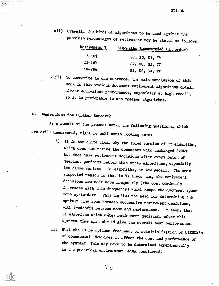
XII -35

xii) Overall, the kinds of algorithms to be used against thepossible percentages of retirement may be stated as follows:

Retirement % Algorithm Recommended (in order)

5-10% S3, S2, Si, TY

11-18% S2, S3, Sl, TY

18-26% S1, S2, S3, TY

x1ii) To summarize in one sentence, the main conclusion of thiswork is that various document retirement algorithms obtainalmost equivalent performance, especially at high recall;so it is preferable to use cheaper algorithms.

6. Suggestions for Further Research

As a result of the present work, the following questions, which

are still unanswered, might be well worth looking into:

i) It is not quite clear why the tried version of TY algorithm,which does not retire the documents with unchanged AVGWTbut does make retirement decisions after every batch ofqueries, performs better than other algorithms, especiallyits close variant - S1 algorithm, at low recall. The mainsuspected reason is that in TY algox .hm, the retirement

decisions are made more frequently (the cost obviouslyincreases with this frequency) which keeps the document spacemore up-to-date. This imr lies the need for determining theoptimum time span between successive retirement decisions,with tradeoffs between cost and performance. It seems thatS1 algorithm which mAAs retirement decisions after thisoptimum time span should give the overall best performance.

ii) What should be optimum frequency of reinitialization of USENDX'sof documents? How does it affect the cost and performance ofthe system? This may have to be determined experimentallyin the practical environment being considered.

XII -36

iii) How will random retirement of documents behave compared

to other algorithms?

iv) How will the relative results of different algorithms vary

with the use of different collections? In addition, it would

be nice to see some research done to resolve the following

questions.

v) How can the ideas of obsolescence of literature based on

statistical analysis of the collections, as used by Brookes

[6], etc. be combined with the document retirement based on

relevancy decisions? We feel that the analysis of this question

would require the use of collections larger than the ones

presently available for the SMART system.

vi) How will the retirement and/or the promotion of documents

between different levels of storage affect the cost of

transportation of documents, cost of modifying the clusters

and/or the centroids, optimum reorganization points for the

data Base, cost of modifying the thesaurus, stability of the

document space, etc.? How will the retrieval performance

which also considers the system efficiency factor (not

considered in this report) i.e. the time required to search

through the hierarchical data base to find the desired

information, behave as a result of these?

vii) How much of the work done and ideas used in paging algorithms

of operating systems may be useful in the area of document

retirement?

viii) Lastly, it might be nice to see all the ideas of document

retirement put together into making a viable model and theory

of document retirement.

XII-37

References

11) M., K. and C.S. Yang, !'Document Retirement in Automatic RetrievalSystems", Report ISR-21 to the National Library of Medicine,Section VII, Department of Computer Science, Cornell University,Ithaca, N.Y.. December 1972.

121 Beall, J.C. and M.D. Schnitzer, "A Method for Automatic DocumentRetirement", CS 435 Project Report, Department of Computer Science,Cornell University, Ithaca, N.Y., Spring 1973.

131 Aho, A.V., J.E. Hoperoft, J.D. Ullman, The Design and Analysis ofComputer Algorithms, Addison-Wesley Publishing Co., 1974.

14) Brauen, T.L. "Document Vector Moditication", Chapter 24 in The SMARTRetrieval System ---'Experiments in Automatic Document Processing,G. Salton editor, Prentice Hall, Inc., Englewood Cliffs, N.J., 1971.

15] Blum, M., R.E. Floyd, V. Pratt, R.L. Rivest and R.E. Tarjan, "LitearTime Bounds for Median Computations", Conference Record of the FourthACM Symposium on Theory of Computing, 1972, pp. 119-124.

[6] &Jokes, B.C., "Optimum P% Library of Scientific Periodicals", Nature,Vol. 232, August 13, 1971, pp. 458-461.