Documentation for the GAMIT GPS Analysis Software - …simon/gtgk/GAMIT.pdf · Documentation for the GAMIT GPS Analysis Software ... Release 10.0 - December 2000. 6 ... time reading

15 February 2002

Documentation for the GAMIT GPS

Analysis Software

Department of Earth, Atmospheric, and Planetary SciencesMassachusetts Institute of Technology

Scripps Institution of OceanographyUniversity of California at San Diego

Release 10.0 - December 2000

6 December 2000

Table of Contents

1. Overview of GAMIT Processing

2. Data Analysis: Theory2.1 Introduction to GPS Measurements2.2 Dual-Band Processing2.3 Modeling the Satellite Orbits2.4 Estimation by Least Squares2.5 References

3. File Structure and Naming Conventions3.1 Introduction3.2 Site-occupation-specific Files3.3 Solution-specific Files3.4 Experiment-specific Files3.5 Global Files

4. Creating Data Input Files4.1 Introduction and File Organization4.2 Preparing the Coordinate (L-) file4.3 Creating the Station Information File4.4 Creating a Scenario File4.5 Using MAKEXP4.6 Creating T- and G-files from Broadcast Ephemerides4.7 Creating Satellite Clock (J-) Files4.8 Running MAKEX4.9 Description of the X-File4.10 Creating Station Clock (K- and I-) Files

5. Batch Processing5.1 Introduction5.2 Running FIXDRV5.3 Executing the Batch Run5.4 Evaluating the Solutions5.5 Multi-session Processing

6. Data Editing6.1 Introduction6.2 Automatic Cleaning using AUTCLN6.3 Scanning the Residuals to Identify Slips6.4 Interactive Editing using CVIEW6.5 Strategies for Editing

6 December 2000

7. Running the Modules Individually7.1 Introduction7.2 Running ARC7.3 Running MODEL7.4 Running CFMRG7.5 Running SOLVE7.6 Running AUTCLN

8. Atmospheric Delay Models8.1 Description of the Atmospheric Delay8.2 Algorithms for the Atmospheric Propagation Delay8.3 Estimating a Zenith Delay Parameter8.4 Estimating Gradients8.5 Water Vapor Radiometer (WVR) Data8.6 References

9. Utility Programs and Auxiliary Tables9.1 Plotting and Computing Statistics from GAMIT Solutions9.2 Creating RINEX or FICA Files from NGS ARGO Files9.3 Creating RINEX Files from FICA Files9.4 Creating X-files from C-files (Utility CTOX)9.5 Creating RINEX Files from X- and E-Files9.6 Converting a hi.raw file to sited. or station.info9.7 Creating K-files from Clock Log Information9.8 Creating W-files from Weather Log Information9.9 Creating and Maintaining Datum, Time, and Ephemeris Tables

10. Automatic Batch Processing10.1 Overview10.2 Template files10.3 Using sh_gamit

10.4 Using sh_glred

AppendicesA.1 Summary of GAMIT ProcessingA.2 Antenna SpecificationsA.3 Exchange Formats for Observation and Orbital DataA.4 Modeling Satellite Clock Variations due to SAA.5 Scripps Orbit and Permanent Array CenterA.6 Editing with SINCLN and DBLCLN

Chapter 1 1

11 October 2000

1. Overview of GAMIT Processing

GAMIT is a comprehensive GPS analysis package developed at MIT and Scripps for theestimation of three-dimensional relative positions of ground stations and satellite orbits.The software is designed to run under any UNIX operating system supporting X-Windows; we have implemented thus far versions for Sun (OS/4 and Solaris 2), HP,IBM/RISC, DEC, and LINUX on Intel-based workstations. The maximum number ofstations and sessions allowed is determined by dimensions set at compile time and can betailored to fit the requirements and capabilities of the analyst's computational environment.The primary output of GAMIT is a loosely constrained solution (H-) file of parameterestimates and covariances which can be passed to GLOBK for combination of data toestimate station positions and velocities and orbital and Earth-rotation parameters. WithRelease 9.9 GAMIT and GLOBK can be run with little effort or intervention by the analystusing a new suite of processing scripts described in Chapter 10. In order to diagnoseproblems with the processing, however, the new user will want to understand both thetheory and organization of each of the GAMIT modules, and hence should spend sometime reading through this manual and executing the program in a more deliberate mannerthan is required in routine processing.

At the start of processing the analyst has available a preliminary set of station coordinates(L-file), the broadcast ephemeris (E-file or RINEX navigation file) for the satellitesobserved, an ensemble of phase and pseudo-range observations, and auxiliary informationavailable from the log sheets (tracking scenarios, antenna heights, and meteorological data).This information should be organized into sessions, defined as spans during which a groupof stations tracks simultaneously the phases of two or more satellites. In order toaccommodate combination with continuously operating stations, sessions are today usuallyorganized into 24-hr spans covering a single UTC day. It is not difficult, however, toorganize a session across a day boundary if that is more efficient for a particular localsurvey (see Chapter 4). The data and other information are prepared in the proper formats,and each session is analyzed individually or combined with other sessions to yieldestimates of improved station coordinates and orbital parameters.

The analysis software is composed of distinct modules, which perform the functions ofpreparing the data for processing, generating reference orbits for the satellites, computingresidual observations (O-C's) and partial derivatives from a geometrical model, detectingoutliers or breaks in the data, and performing a least squares analysis. Although themodules can be run individually, they are tied together through the data flow, particularlyfile-naming conventions, in such a way that most processing is best done with shell scriptsand a sequence of batch files set up by two driver modules—MAKEXP ("makeexperiment") for the data preparation and FIXDRV ("fixed-table driver") for the modeling,editing, and estimation. Though much of the data editing is performed automatically, thesolution residuals can be displayed or plotted so that manual editing of problematical datacan be performed. The primary steps in the data analysis are summarized below, withreference to the modules used in each step. Details are given in Chapter 4–6, and asummary table in Appendix 1.

Chapter 1 2

11 October 2000

1) Setup the program and processing directories

The software is distributed with a top-level directory (which must be aliased to gg foryour login) containing shell scripts ( /com ), source code ( /gamit, /kf, and /libraries ),tables ( /tables ), documentaion ( /doc and /help ), map grids ( /maps, for GMTplotting), and example command files and tables (/templates). Within the main sourcedirectories are sub-directories for each of the main modules of GAMIT or GLOBK and/bin directores constaining executables. Your Unix path must contain ~/gg/com ,~/gg/gamit/bin , and ~/gg/kf/bin in order to run the software anywhere on yoursystem.

You should create an "experiment" directory that will contain a subdirectory for theRINEX files, a subdirectory for experiment-specific tables, and subdirectories for eachsession to be processed (see Section 4.1 for details of the directory structure).

2) Prepare the data.

Generate an L-file of a priori coordinates for the experiment epoch from an existingGLOBK apr file (gapr_to_l) or by performing a fit to the pseudoranges on the RINEXfile ( sh_rx2apr ).

Enter antenna and receiver occupation information (from log sheets) into tablestation.info using templates and an editor.

Create all of the other data-preparation input files using program MAKEXP.

Execute the programs MAKEJ and MAKEX (and possibly MAKEK) to read thereceiver data files (in RINEX or FICA format) and generate the clock (J- and K-) andobservation (X-) files to be used in the analysis.

Obtain initial conditions (G-file) for GAMIT's orbital integrator (ARC) by copying aG-file from SOPAC, executing script sh_sp3fit to fit the ARC model to an IGS "sp3"file, or executing the script sh_bcfit to fit the ARC model to the broadcast elements in aRINEX navigation file.

2) Set up and execute batch processing.

Edit templates to create control files sittbl. and sestbl. for the batch analysis run.

Execute program FIXDRV to create batch files for the analysis.

Execute the batch job to perform processing.

ARC creates a T-file by numerical integration of the initial conditions in the G-file.

MODEL computes the theoretical values of the observations ("observables") andpartial derivatives of these observations with respect to the parameters to beestimated, and writes them to an output (C-) file for editing and estimation.

AUTCLN performs automatic (batch) editing of cycle slips and outliers in thephase observation.

CFMRG writes a (M-) file defining the way observations are to be combined, andSOLVE performs the least squares analysis, writing the "print" output to a Q-fileand the adjustments and covariance matrix to an H-file for combination with othersessions and experiments using GLOBK.

Chapter 1 3

11 October 2000

3) Evaluate the solution by examining the output (Q-file) from SOLVE (chi-square valueand size of parameter adjustments) and the phase rms for each station from AUTCLN(autcln.post.sum ). If a station shows problem you may need to look at sky-plots of thephase residuals, created by sh_oneway from the .DPH files produced by AUTCLN, or useCVIEW to look at the phase residuals in more detail on the screen.

The standard processing sequence for unedited data includes one or two passes throughMODEL, AUTCLN, and SOLVE. If you have good a priori coordinates and orbits, asingle pass usually sufficient for a good solution, but a second pass using AUTCLN inpostfit mode will allow better handling of poor data and provide quality statistics for eachof the stations in the network. produce . If the a priori coordinates and orbits are not highlyaccurate, then the additional pass is also necessary to improve these to the level at which theautomatic editing is robust and the adjustments are within a linear range. With poorlybehaved data, it may also be necessary to examine with CVIEW the phase residuals fromthe initial solution and to add instructions for deleting data to the AUTCLN command file,or, more rarely, to fix remaining small cycle slips interactively.

Chapter 2 presents a brief summary of the theoretical elements of GPS data analysis. Itintroduces GAMIT nomenclature and includes references that describe in greater detail thealgorithms used by the program. Chapter 3 describes in detail the files used and theirnaming conventions; it need not be read carefully the first time through. Chapter 4describes the steps in data preparation. The details of running FIXDRV and executing andinterpreting the batch analysis runs are given in Chapter 5. Chapter 6 describes theprocedures for automatic and interactive editing. Chapters 7–9 are included for referencebut need not be read to carry out most processing tasks. Chapter 7 describes the individualmodules in more detail. Chapter 8 the various options available for modeling thetropospheric delay; and Chapter 9 the various utility programs and auxiliary data files, onlya few of which need concern most analysts. Chapter 10 describes how to use the newautomatic processing scripts. Finally, the Appendices provide a summary of theprocessing and file names, information on antenna specifications, data formats, and a rarelyused procedure for handling non-simultaneous sampling times under SA.

Note on manual style: All of the programs in the GAMIT and GLOBK (/kf) directories arenamed for Unix in lowercase. For emphasis, however, and to distinguish (Fortran)programs from (C-) shell scripts, we have written them in uppercase in this manual.

Chapter 2 1

14 February 2002

2. Data Analysis: Theory

2.1 Introduction to GPS Measurements

High-precision geodetic measurements with GPS are performed using the carrier beatphase, the output from a single phase-tracking channel of a GPS receiver. It is thedifference between the phase of the carrier wave implicit in the signal received from thesatellite, and the phase of a local oscillator within the receiver. The carrier beat phase canbe measured with sufficient precision that the instrumental resolution is a millimeter or lessin equivalent path length. For the highest relative-positioning accuracies, carrier beat phaseobservations must be obtained simultaneously at each epoch from several stations (at leasttwo), for several satellites (at least two), and at both the L1 (1575.42 MHz) and L2(1227.6 MHz) GPS frequencies. The dominant source of error in a phase measurement orseries of measurements between a single satellite and ground station is the unpredictablebehavior of the time and frequency standards ("clocks") serving as reference for thetransmitter and receiver. Even though the GPS satellites carry atomic frequency standards,the instability of these standards would still limit positioning to the several meter level wereit not for the possibility of eliminating their effect through signal differencing.

A second type of GPS measurement is the pseudo-range, obtained using the 300-m-wavelength CA ("coarse acquisition") code or 30-m-wavelength P ("protected") codetransmitted by the satellites. Pseudo-ranges provide the primary GPS observation fornavigation but are not precise enough to be used alone in geodetic surveys. However, theyare useful for synchronizing receiver clocks, resolving ambiguities and repairing cycle slipsin phase observations, and as an adjunct to phase observations in estimating satellite orbits.

For a single satellite, differencing the phases (or pseudo-ranges) of signals receivedsimultaneously at each of two ground stations eliminates the effect of bias or instabilities inthe satellite clock. This measurement is commonly called the between-stations-difference,or single- difference observable. If the stations are closely spaced, differencing betweenstations also reduces the effects of tropospheric and ionospheric refraction on thepropagation of the radio signals If the ground stations have hydrogen-maser oscillators(with stabilities approaching 1 part in 1015 over several hours), then single differences can,in principle, be useful, as they are for VLBI. In practice, however, it is seldom costeffective to use hydrogen masers and single difference observations in GPS surveys.Rather, we form a double difference by differencing the between-station differences alsobetween satellites to cancel completely the effects of variations in the station clocks. In thiscase the observations are just as accurate with low-cost crystal oscillators as with an atomicfrequency standard (though the use of the latter may make editing a bit easier).

Since the phase biases of the satellite and receiver oscillators at the initial epoch areeliminated in doubly-differenced observations, the doubly-differenced range (in phaseunits) is the measured phase plus an integer number of cycles. (One cycle has awavelength of 19 cm at L1 and 24 cm at L2 for code-correlating receivers; half these valuesfor squaring-type receiver channels.) If the measurement errors, arising from errors in the

Chapter 2 2

14 February 2002

models for the orbits and propagation medium as well as receiver noise, are smallcompared to a cycle, there is the possibility of determining the integer values of the biases,thereby obtaining from the initially ambiguous doubly differenced phase an unambiguousmeasure of doubly differenced range. Resolution of the phase ambiguities allows a moreprecise measure of the relative positions of the stations (see, e.g., Blewitt [1989], Dongand Bock [1989] ).

GAMIT incorporates difference-operator algorithms that map the carrier beat phases intosingly and doubly differenced phases. These algorithms extract the maximum relativepositioning information from the phase data regardless of the number of data outages, andtake into account the correlations that are introduced in the differencing process. (See Bocket al. [1986] and Schaffrin and Bock [1988] for a detailed discussion of these algorithms.)An alternative, (nearly) mathematically equivalent approach to processing GPS phase datais to use formally the (one-way) carrier beat phases but estimate the phase offset due to thestation and satellite clocks at each epoch. This approach is used by AUTCLN to computeone-way phase residuals for editing and display.

In order to provide the maximum sensitivity to geometric parameters, the carrier phase mustbe tracked continuously throughout an observing session. If there is an interruption of thesignal, causing a loss of lock in the receiver, the phase will exhibit a discontinuity of aninteger number of cycles. This discontinuity may be only a few cycles ("cycle-slips") dueto a low signal-to-noise ratio, or it may be thousands of cycles, as can occur when thesatellite is obstructed at the receiver site. Initial processing of phase data is often performedusing time differences of doubly differenced phase ("triple differences", or "Doppler"observations) in order to obtain a preliminary estimate of station or orbital parameters in thepresence of cycle slips. The GAMIT software uses triple differences in editing but not inparameter estimation. Rather, it allows estimation of extra free bias parameters wheneverthe automatic editor has flagged an epoch as a possible cycle slip or, in the program "quick"mode, whenever there is a gap in the data. Various algorithms to detect and repair cycleslips are described by Blewitt [1990], and also in Chapter 6 of this document.

Although phase variations of the satellite and receiver oscillators effectively cancel indoubly differenced observations, errors in the time of the observations, as recorded by thereceiver clocks, do not. However, the pseudo-range measurements, together withreasonable a priori knowledge of the station coordinates and satellite position, can be usedto determine the offset of the station clock to within a microsecond, adequate to keep errorsin the doubly differenced phase observations below 1 mm.

General background and an error analysis for the carrier-beat phase observable may befound in Chapter 5 of King et al. [1985] and Chapter 2 of Feigl [1991].

2.2 Dual-Band Processing

A major source of error in single-frequency GPS measurement is the variable delayintroduced by the ionosphere. For day-time observations near solar maximum this effect

Chapter 2 3

14 February 2002

can exceed several parts per million of the baseline length. Fortunately, the ionosphericdelay is dispersive and can be reduced to a millimeter or less (at mid-latitudes) by forming aparticular linear combination (LC, sometimes called L3) of the L1 and L2 phasemeasurements:

φ LC = 2.546 φ L1 − 1.984 φ L2

(See, e.g., Bender and Larden [1985], Bock et al. [1986], or Dong and Bock [1989]) Forming LC, however, magnifies the effect of other error sources. On short baselineswhere the ionospheric errors cancel in between-station (single) differencing, it is preferableto treat L1 and L2 as two independent observables, rather than form the linear combination.For baselines longer than a few kilometers, on the other hand, on which ionospheric errorsare uncorrelated, it is preferable to form LC and completely eliminate the effects of theionosphere. In the general case, the optimal choice of dual-band observable must liesomewhere between these two extremes [Bock et al., 1986; Schaffrin and Bock, 1988].That is, one must balance the amplification in noise introduced by forming LC against thebenefits gained by eliminating ionospheric effects. In practice, most networks of extentgreater than a few kilometers are processed using the LC observable.

In examining phase data for cycle slips, it is often useful to plot several combinations of theL1 and L2 residuals. Single-cycle slips in L1 or L2 will appear as jumps of 2.546 or 1.984cycles, respectively, in LC. Single-cycle slips in both L1 and L2 (a more commonoccurrence) appear as jumps of 0.562 cycles in LC, which, though smaller, may be moreevident than the jumps in L1 and L2 because the ionosphere has been eliminated. If the L2phase is tracked using codeless techniques, the carrier signal recorded by the receiver is attwice the L2 frequency, leading to half-cycle jumps when it is combined with full-wavelength data. Hence, a jump of a "single" L2 cycle will appear as 0.892 in LC andsimultaneous jumps in (undoubled) L1 and (doubled) L2 will appear as 1.654 cycles inLC. Another useful combination is the difference between L2 and L1 with both expressedin distance units:

φ LG = φ L2 − 0.779 φ L1

sometimes called "LG" because the L2 phase is scaled by the "gear" ratio (f2/f1 = 60/77 =1227.6/1575.42). In the LG phase all geometrical and other non-dispersive delays (e.g.,the troposphere) cancel, so that we have a direct measure of the ionospheric variations. One-cycle slips in L1 and L2 are of course difficult to detect in the LG phase in thepresence of much ionospheric noise since they are equivalent to only 0.221 LG cycles.

If precise (P-code) pseudorange is available for both GPS frequencies, then a "wide-lane"(WL) combination of L1, L2, P1, and P2 can be formed which is free of both ionosphericand geometric effects and is simply the difference in the integer ambiguities for L1 and L2:

WL = n2 - n1 = φ L2 − φ L1 + (P1 + P2 ) (f1 - f2)/(f1 + f2)

Chapter 2 4

14 February 2002

The WL observable can be used to fix cycle slips in one-way data [Blewitt, 1990] butshould be combined with LG and doubly differenced LC to rule out slips of an equalnumber of cycles at L1 and L2.

Using wide-lane observations averaged over a satellite pass is the most efficient approachto resolving the wide-lane (n2 - n1 ) phase ambiguities (see, e.g. Blewitt, 1989; Dong andBock, 1989) though clock jumps and inter-channel receiver biases can sometimes producespurious results. To provide a check the algorithm used by GAMIT employs both thepseudoranges and the "phase wide-lane" with ionospheric constraints to resolve the wide-lane ambiguities [Bender and Larden, 1985; Dong and Bock, 1989; Feigl et al., 1993].

2.3 Modeling the Satellite Motion

A first requirement of any GPS geodetic experiment is an accurate model of the satellites'motion. The (3-dimensional) accuracy of the estimated baseline, as a fraction of its length,is roughly equal to the fractional accuracy of the orbital ephemerides used in the analysis.The accuracy of the Broadcast Ephemerides computed regularly by the Department ofDefense using pseudorange measurements from 5 stations is typically 5-10 parts in 107

(10-20 m), well within the design specifications for the GPS system but not accurateenough for the study of crustal deformation. By using phase measurements from a globalnetwork of over 50 stations, however, the International GPS Service for Geodynamics(IGS) [Beutler et al., 1994a], is able to determine the satellites' motion with an accuracy of2–10 parts in 109 (5–20 cm). For GPS surveys prior to about 1991, the global trackingnetwork was much smaller but can still be used to achieve accurate results for regionalsurveys. If we include in our analysis observations from widely separated stations whosecoordinates are well known (from VLBI, SLR, or global GPS measurements), thefractional accuracy of the baselines formed by these stations is transferred through theorbits to the baselines of a regional network. For example, a 10 mm uncertainty in therelative position of sites 2500 km apart introduces an (approximate) uncertainty of only 1mm in the components of a 250 km baseline. This scheme can be used successfully evenwith regional fiducial sites, transferring, for example, the relative accuracy of 250-500 kmbaselines to a network less than 100 km in extent.

The motion of a satellite can be described, in general, by a set of six initial conditions(Cartesian position and velocity, or osculating Keplerian elements, for example) and amodel for the forces acting on the satellite over the span of its trajectory. To modelaccurately the motion, we require knowledge of the acceleration induced by gravitationalattraction of the sun, moon, and higher order terms in the Earth's gravity field, and somemeans to account for the action of non-gravitational forces due, for example, to solarradiation pressure and gas emission by the spacecraft's batteries and attitude-controlsystem. For GPS satellites non-gravitational forces are the most difficult to model andhave been the source of considerable research over the past 15 years (see Colombo [1986]Lichten and Bertiger [1989], Beutler et al. [1994b] for more discussion).

Chapter 2 5

14 February 2002

In principle, a trajectory can be generated either by analytical expressions or by numericalintegration of the equations of motion; in practice, numerical integration is almost alwaysused, for both accuracy and convenience. The position of the satellite as a function of timeis then read from a table (ephemeris) generated by the numerical integration. The equationsof motion and numerical integrator used by GAMIT were adapted from the PlanetaryEphemeris Program, developed originally at MIT's Lincoln Laboratory. A detaileddescription of the equations and algorithms may be found in Ash [1972].

In modeling the phase and pseudorange observations, we must take into account not onlythe motion of the center of mass of the satellite but also meter-level offsets between thecenter of mass and the phase-center of the transmitting antenna. These offset are negligiblefor regional networks but can introduce centimeter-level errors for baselines approaching anEarth radius. Also important are temporary phase excursions of several decimeters lastingup to a half-hour during the maneuvers the satellites execute to keep their solar panelsfacing the Sun when the orbital plane is nearly aligned with the Earth-Sun direction. Forthe satellites in each orbital plane, this alignment occurs for several weeks twice a year, theso-called "eclipse season". Yoaz Bar-Sever and colleagues at JPL have spent considerableeffort developing models of the satellites' orientation, even to point of making the behaviormore predictable by getting DoD to apply a small bias about the yaw axis—a change thatwas implemented gradually between June, 1994, and November, 1995. See Bar-Sever[1996] for a complete discussion.

2.4 Estimation by Least Squares

GAMIT incorporates a weighted least squares algorithm to estimate the relative positions ofa set of stations, orbital and Earth-rotation parameters, zenith delays, and phase ambiguitiesby fitting to doubly differenced phase observations. Since the functional (mathematical)model relating the observations and parameters is non-linear, the least-squares fit for eachsession may need to be iterated until convergence, i.e., until the corrections to the estimatedstation coordinates and other parameters are negligible. Data can be viewed and editedinteractively without iteration since CVIEW uses the pre-fit residuals, partial derivatives,and parameter adjustments to compute and display "predicted" post-fit residuals (seeSection 6.5). Automatic editing is more effective near convergence, however, sinceAUTCLN uses pre-fit residuals.

In current practice, the GAMIT solution is not usually used directly to obtain the finalestimates of station positions from a survey. Rather, we use GAMIT to produce estimatesand an associated covariance matrix of station positions and (optionally) orbital and Earth-rotation parameters ("quasi-observations") which are then input to GLOBK [Herring,1997] or other similar programs to combine the data with those from other networks andtimes to estimate positions and velocities [Feigl et al., 1993; Dong et al., 1997]. In ordernot to bias the combination, GAMIT generates the solution used by GLOBK with onlyloose constraints on the parameters, defining the reference frame only at the GLOBK stageby imposing constraints on station coordinates. Since phase ambiguities must be resolved

Chapter 2 6

14 February 2002

(if possible) in the phase processing, however, GAMIT generates several intermediatesolutions with user-defined constraints before loosening the constraints for its finalsolution. These steps are described in detail in Section 5.4.

The most rigorous way to handle the phase ambiguities is to keep them free for an initialcombination of all of the data to be used in the study, and then use the estimateduncertainties (appropriately scaled) of station coordinates and possibly orbital parametersfrom the combination as constraints in an iteration in which the GAMIT processing isrepeated. In practice, however, it is often possible to avoid the iteration by applying in theinitial solution sufficiently tight, but statistically conservative constraints on coordinates andorbital parameters and using conservative criteria for assigning the phase ambiguities tointeger values. These issues are discussed in Dong and Bock [1989] and Blewitt [1989]and Chapter 5 of this manual.

2.5 References

Ash, M. E., Determination of Earth Satellite Orbits, Tech. Note 1972-5, 258 pp.,Massachusetts Institute of Technology, Lincoln Laboratory, Lexington, 1972.

Bar-Sever, Y., A new model for GPS yaw attitude, Journal of Geodesy, 70, 714–723,1996.

Bender, P. L. and D. R. Larden, GPS carrier phase ambiguity resolution over longbaselines, in Goad C. C. (ed), Proceedings of the First International Symposium onPrecise Positioning with the Global Positioning System, Volume 1, National GeodeticSurvey , Rockville, Maryland, 357-361, 1985.

Beutler, G., I. I. Mueller, and R. E. Neilan, The International GPS Service forGeodynamics: development and start of official service on January 1, 1994, BulletinGeodesique, 68, 39–70, 1994a.

Beutler, G., E. Brockmann, W. Gurtner, U. Hugentobler, L. Mervart, and M. Rothacher,Extended orbit modeling techniques at the CODE Processing Center of the InternationalGPS Service for Geodynamics (IGS): theory and initial results, Manuscripta Geodaetica,19, 367–386, 1994b

Blewitt, G., Carrier phase ambiguity resolution for the Global Positioning System appliedto geodetic baselines up to 2000 km, Journal of Geophysical Research, 94, 1187-1203,1989.

Blewitt, G., An automatic editing algorithm for GPS data, Geophysical Research Letters,1990.

Chapter 2 7

14 February 2002

Bock Y., S. A. Gourevitch, C. C. Counselman III, R. W. King, and R. I. Abbot,Interferometric analysis of GPS phase observation, Manuscripta Geodaetica, 11, 282-288,1986.

Colombo, O. L, Ephemeris errors of GPS satellites, Bulletin Geodesique, 60, 64–84,1986.

Dong, D.-N., and Y. Bock, GPS network analysis with phase ambiguity resolutionapplied to crustal deformation studies in California, Journal of Geophysical Research, 94,3949-3966, 1989.

Dong, D.-N., T. A. Herring, and R. W. King, Estimating regional deformation from acombination of space and terrestrial geodetic data, Journal of Geodesy, 72, 200–214,1998.

Fiegl, K. L, R. W. King, T. A. Herring, M. Rotchacher, A scheme for reducing the effectof selective availability on precise geodetic measurements from the Global PositioningSystem, Geophysical Research Letters, 18, 1289–1292, 1991.

Feigl, K. L., Geodetic Measurement of Tectonic Deformation in Central California, Ph. D.thesis, Massachusetts Institute of Technology, 223 pp., 1991.

Feigl, K. L, D. C. Agnew, Y. Bock, D.-N. Dong, A. Donnellan, B. H. Hager, T. A.Herring, D. D. Jackson, R. W. King, S. K. Larsen, K. M. Larson, M. H. Murray, Z.-K.Shen, Measurement of the velocity field in central and southern California,Journal ofGeophysical Research, 98, 21667–21712, 1993.

Herring, T. A., D.-N. Dong, and R. W. King, Submilliarcsecond determination of poleposition by GPS measurements, Geophysical Research Letters, 18, 1893-1896, 1991.

Herring, T. A., GLOBK: Global Kalman filter VLBI and GPS analysis program Version3.2 Internal Memorandum, Massachusetts Institute of Technology, Cambridge, 1995.

King, R. W., J. Collins, E. M. Masters, C. Rizos, A. Stolz, Surveying with GPS,Monograph No. 9, School of Surveying, University of New South Wales, Sydney, 1985;reprinted by Ferd. Dummlers Verlag, Bonn, 1987.

Lichten, S. M., and W. J. Bertiger, Demonstration of sub-meter GPS orbit determinationand 1.5 parts in 108 three-dimensional baseline accuracy, Bulletin Geodesique, 63, 167-189, 1989.

Lindqwister, U. J., S. M. Lichten, and G. Blewitt, Precise regional baseline estimationusing a priori orbital information, Geophysical Research Letters, 17, 219-222, 1990.

Chapter 2 8

14 February 2002

McCarthy, D. D., IERS Standards (1992), IERS Technical Note 13, Observatoire deParis, July, 1992.

Murray, M. H., Global Positioning System Measurement of Crustal Deformation inCentral California, Ph. D. thesis, Massachusetts Institute of Technology, 223 pp., 1991.

Schaffrin, B., and Y. Bock, A unified scheme for processing GPS phase observations,Bulletin Geodesique, 62, 142–160, 1988.

Shimada, S., and Y. Bock, Crustal deformation measurements in central Japan determinedby a GPS fixed-point network, Journal of Geophysical Research, 97, 11437–12455,1992.

Chapter 3 1

11 October 2000

3. File Structure and Naming Conventions

3.1 Introduction

Before running GAMIT it is necessary to understand its file naming conventions. All theprogram modules adhere to specific conventions for the naming of files for a particularexperiment. This assures a unique definition of each experiment, facilitates data filemanagement, and allows for ease of interactive processing and troubleshooting. There arefour types of files:

1) site-occupation-specific2) solution-specific3) experiment-specific4) global

Each file is distinguished either by its first character (types 1 and 2) or a unique name (type3). Type 1 files are named using 4-character station codes and the day of the observations.Type 2 and 3 files have an experiment (survey) or solution name, chosen by the analyst,embedded within the file name. Type 4 files have specific names that are hard-wired in thesoftware (though these names are often elaborated using links). These naming conventionsallow the software to perform the bookkeeping necessary to process large quantities ofdata.

The remaining sections of this chapter describe the contents and format of the files of eachtype, and how the file is created and used by the software. A summary of all the file namesis also given in Appendix 1, and templates for user-created files may be found in thegamit/example directory that accompanies the software distribution . Although file nameswill sometimes be shown in upper-case for clarity, lower-case is the preferred standard forUNIX operating systems.

3.2 Site-occupation-specific Files

X-file : Observation data file containing the L1 and L2 carrier beat phases andpseudo-ranges, signal amplitudes, initial station coordinates and antennaoffsets, start and stop times, and the identification of the satellitestracked in each receiver channel.

Format : xsitey.dayExample : xvndn7.002 . This X-file has been created by program MAKEX from

the data recorded at station VNDN (Vandenberg) on day 2 of 1987.Notes : X-file names correspond directly to four-letter station codes used in the

L- and throughout the software. The X-file names that appear in the D-file (see below) define all subsequent site-specific names.

Type : ASCIICreated by : MAKEX, utilities CTOX, XTOX, XUPInput to : MODEL, and optionally MAKEK, BCTOT, FIXDRV, and CVIEW

Chapter 3 2

11 October 2000

C-file : Primary file for data analysis, created by MODEL from an X-file andused as input to AUTCLN, SINCLN, DBLCLN, CVIEW, and SOLVE;contains observations (O's), prefit residuals (O-C's, observed-computed values), partial derivatives, and auxiliary information.

Format : csitey.dayExample : cvndn7.002Notes : Direct correspondence to X-files but binary and with partials. Once the

data on the C-files have been cleaned, program CTOX is run to makeclean X-files for further processing.

Type : BinaryOutput of : MODEL, AUTCLN, SINCLN, DBLCLN, CVIEWInput to : AUTCLN, SINCLN, DBLCLN, SCAN, CVIEW, SOLVE

E-file : Broadcast Ephemeris data in either RINEX or FICA format. It is usedby BCTOT to create an initial G-file and/or a T-file from the broadcastephemeris parameters, and by MAKEJ and MAKEK to generate satelliteand receiver clock files.

Format : esitey.day or sitedayn.yynExample : evndn7.002 or vndn0020.87nNotes : The parameters and format of the E-file are described in Appendix 4.Type : ASCIIOutput of : RINEX translators or utility FICACHOPInput to : BCTOT, MAKEJ, MAKEK

K-file : Receiver clock data computed by MAKEX or MAKEK using nominalsite coordinates, broadcast ephemeris, and pseudo-range. It is used byFIXDRV to estimate the coefficients of a linear or cubic polynomialmodel for clock behavior during the session.

Format : ksitey.dayExample : kvndn7.002Notes : The parameters and format of the station-specific K-file are described in

4.9. For receivers which do not record the broadcast ephemeris, thereis a session - specific K-file of different format; this file is described inSection 9.4.

Type : ASCIIOutput of : MAKEX, MAKEKInput to : FIXDRV and utilities CALCK and PLOTK.

Chapter 3 3

11 October 2000

P-file : <P>rint file for a MODEL run - provides a record of the run.

Format : psitey.dayExample : pvndn7.002Notes : Direct correspondence to X- and C-filesType : ASCIIOutput of : MODEL

V-file : Print file for a SINCLN run - contains a record of the editingperformed.

Format : vsitey.dayExample : vvndn7.002Notes : Direct correspondence to C-fileType : ASCIIOutput of : MODEL

W-file : <W>eather file - contains meteorological data for modeling the effect oftropospheric refraction on the satellite signals.

Format : wsitey.dayExample : wvndn7.002Notes : This file is optional and is described in Section 9.5. If not available,

default meteorological data are used.Created by : UserInput to : MODEL

Z-file : Water Vapor Radiometer (WVR) file - contains WVR data for modelingthe effects of wet tropospheric delay on the satellite signals.

Format : zsitey.dayExample : zvndn7.002Notes : This file is optional and is described in Section 9.5.Created by : UserInput to : FIXDRV, MODEL

Chapter 3 4

11 October 2000

3.3 Solution-specific Files

These files are specific to a particular experiment and should be unique with regards to allother experiments in order to facilitate efficient data management.

D-file : FIXDRV file - defines the number of sessions in each experiment, thenumber of receivers per session, the coordinate (L-) file, the ephemeris(T-), station-clock (I-), satellite-clock (J-), and data files (X- or C-) persession, and the order in which the sessions should be processed.

Format : dxxxxy.day where xxxx is the solution name. The rest of the filenameis arbitrary but FIXDRV looks at the sixth character to set up the defaultvalue of the year. The three characters of the extent may be thebeginning day of the experiment, but this is not necessary.

Example : dcalf7.002Notes : The D-file is the primary input file to FIXDRV. As such, its name

defines all subsequent experiment-specific files. The user can identifythe experiment name in any manner. Prior to executing FIXDRV, theuser creates the D-file, using program MAKEXP or manually. SeeSection 5.2.

Type : ASCIICreated by : MAKEXP or userInput to : FIXDRV

Session Control Table : Input control file for FIXDRV, specifying the type of analysis andthe a priori measurement errors and satellite constraints. See Section5.2.

Format : sestbl .Notes: : The file name is hard-wired, but links may be used to define different

versions of the table.Type : ASCIICreated by : User from templateInput to : FIXDRV

Site Control Table : Input control file for FIXDRV, specifying for each site the clock andatmospheric model to be used, and the a priori coordinate constraints.See Section 5.2

Format : sittbl.Notes: : The file name is hard-wired, but links may be used to define different

versions of the table.Type : ASCIICreated by : User from templateInput to : FIXDRV

Chapter 3 5

11 October 2000

AUTCLN (detailed) output file: Complete record of the editing process; can be ignored anddeleted if the solution completed successfully. See sections 6.2 and 7.6.

Format : autcln.outType : ASCIICreated by : AUTCLN

AUTCLN summary file: Summary of editing; useful for evaluating results. See sections6.2 and 7.6.

Format : autcln.pref.sum or autcln.post.sumType : ASCIICreated by : AUTCLN

A-file : ASCII version of the T-file, optionally generated for scrutiny by theanalysis or for export.

Format : axxxxy.dayType : ASCIIOutput of : TTOASCInput to : None

B-file : Primary <B>atch file - controls the batch (automatic) mode of dataprocessing.

Format : bxxxxx.bat where xxxxx are the first five characters of the D-file name.Example : bcalf7.batNotes : The primary B-file contains a sequence of secondary B-files which

execute in an order prescribed by FIXDRV the individual modules ofthe software. Its name corresponds to that of the D-file.

Type : ASCIIOutput of : FIXDRV

B-file : Secondary <B>atch file - controls the execution of one programmodule.

Format : bxxxxx.nnn where xxxxx are the first five characters of the D-file nameand nnn is the sequence number of the batch file.

Examples : bcalf7.001, bcalf7.015Notes : Each secondary batch files contains the input stream for one execution

of a program module. For example, the first line of bcalf7.bat might bearc < bcalf7.001 . That is, the program module ARC will receive itsinstructions from bcalf7.001 .

Type : ASCIIOutput of : FIXDRVInput to : ARC, MODEL, CFMRG, SOLVE, DBLCLN

Chapter 3 6

11 October 2000

G-file : A file of orbital initial conditions for all satellites on the T-file.

Format : gxxxxy.dayExample : gcalf7.002Notes : The G-file contains initial conditions and nongravitational force

parameters for each GPS satellite at a particular UTC epoch. The G-fileinitial conditions serve as starting points for a numerical integration ofthe satellite orbits and the generation of a T-file. The name of the G-fileis arbitrary but would normally include the day and year of the initialconditions as in the example above (day 002, 1987); in any case itshould match the name of the corresponding T-file. The filename of theG-file created by SOLVE is the same except that the 6th character isincremented by one letter. The format of the G-file is described inSection 4.10

Type : ASCIIOutput of : BCTOT, TTOG, SOLVEInput to : ARC, SOLVE

H-file : Covariance matrix and parameter adjustments for solution generatedwith loose constraints, used as input to GLOBK.

Format : hxxxxy.dayExample : hcalf7.002Type : ASCIIOutput of : SOLVEInput to : HTOH, HTOGLB, HTOSNX

I-file : <I>ite file - contains a site by site, session by session record of thestation clock offset, rate, and acceleration, used optionally by MODEL.

Format : ixxxxx.xxxExample : icalf 7.002Notes : The I-file name is specified in the D-file.Type : ASCIIOutput of : MAKEI, FIXDRV, SOLVEInput to : MODEL, SOLVE

Chapter 3 7

11 October 2000

J-file : Satellite clock parameters transmitted by the satellites and recorded bythe receivers.

Format : jxxxxy.dayExample : jcalf7.002Notes : This file is used by MODEL to compute the receiver clock corrections

epoch-by-epoch, and also to correct the modeled phase for large satelliteclock drifts (e.g., under SA conditions) when observations are notrecorded simultaneously at all sites.

Type : ASCIICreated by : MAKEJInput to : MODEL

M-file : <M>erge file - sets up the data and parameters for the least-squaresanalysis in SOLVE.

Format : mxxxx1.day , mxxxxa.dayExample : mcalf1.002, mcalfa.002Notes : The M-file name is derived from the D-file name. The initial M-file is

created by CFMRG (using a FIXDRV-written batch file) to set up theinitial SOLVE, SINCLN, DBLCLN, or CVIEW run. After estimatingadjustments to the parameters, SOLVE writes a new M-file with thesame name and with the adjustments included. In the usual processingsequence generated by FIXDRV, the 6th character of the M-file namefor the "quick" solution is "1", and for standard solutions "a". If thereare multiple solutions of a given type, the M-file is overwritten (re-created by CFMRG) each time.

Type : BinaryOutput of : CFMRGInput to : SOLVE, SINCLN, DBLCLN, SCAN, CVIEW

N-file : <N>oise file contains station-specific, elevation-dependent values usedto reweight phase observations in SOLVE after postfit editing byAUTCLN.

Format : nxxxx1.day nxxxxa.dayExample : ncalf1.002, ncalfa.002Notes : The file has the structure of the error model: section of the SOLVE

batch file. SOLVE reads it to overrides the batch-file input.Type : ASCIIOutput of : Shell-script sh_sigelvInput to : SOLVE

Chapter 3 8

11 October 2000

O-file : Solution output file for a SOLVE run, an abbreviated form of the Q-fileused for plotting, statistics, and input to GPSNET.

Format : oxxxx1.day oxxxxa.dayExample : ocalf1.002, ocalfa.002Notes : This file is designed to be interfaced with a network adjustment program

or the BSL series of programs to calculate statistics. Its use is optionalbut strongly recommended for detecting blunders. The name of the O-file corresponds directly to the Q-file from which it was copied.

Type : ASCIIOutput of : SOLVEInput to : Network-adjustment, statistics, and plotting programs

Q-file : Print file for a SOLVE run - contains a record of the analysis.

Format : qxxxx1.day, qxxxxa.dayExample : qcalf1.002, qcalfa.002Notes : The Q-file naming conventions are identical to those of the M-files. For

a batch run, the file qcalf1.002 in our example will be created by the"quick" solution of SOLVE (see Chapter 5), qcalfa.002 by the "regular"solution. As for M-files, multiple passes through SOLVE (to iterateparameter estimates or editing) will cause the Q-files from the previousiteration to be overwritten.

Type : ASCIIOutput of : SOLVE

T-file : <T>abular ephemeris file for all satellites in a session or series ofsessions - contains satellite state vectors at equally-spaced intervals(default 15 minutes for ARC) for later interpolation in MODEL. Thename should match that of the G-file.

Format : txxxxy.dayExample : tcalf7.002 , this T-file is associated with a G-file with initial conditions

on day 002 of 1987Type : BinaryOutput of : ARC, BCTOT, NGSTOT, sh_bctot, sh_sp3fitInput to : FIXDRV, MODEL, TTONGS, TTOASC

U-file : Ocean tide components for all stations in the session, created byOCTTAB from a global file of station components ( stations.oct ) or agrid of components by latitude and longitude (grid.oct).

Format : uxxxxy.dayType : ASCIIOutput of : OCTTABInput to : MODEL

Chapter 3 9

11 October 2000

V-file (1) : Print file for DBLCLN - contains a record of the editing performed.

Format : vdblcln.outType : ASCII

V-file (2) : Print file for SCANM (one of two files for SCANRMS -contains asummary of rms values and jumps for each double-differencecombination.

Format : vxxxx 1.day.sort , vxxxx a.day.sort, vxxxx 1.day.worst , vxxxx a.day.worstType : ASCII

Y-files : <Y>aw files, of two types. An ASCII version (6th character is last digitof year) giving times of eclipses and yaw rates for each satelliteobserved during the session is written by ARC from information in theglobal file svnav.dat and computed eclipse information. A binaryversion (6th character is t ) giving the angle of departure from nominalyaw at the epochs of the observations in the session is written byYAWTAB, using the T-file and ASCII y-file as input for thecomputations. Both of these files are discussed in Section 7.2

Format : yxxxxy.dayExample : ypgga5.267Type : ASCIIOutput of : ARCInput to : YAWTAB

Format : yxxxxy.dayExample : ypggat.267Type : BinaryOutput of : YAWTABInput to : MODEL

Chapter 3 10

11 October 2000

3.4 Experiment-specific Files

These files contain information collected for a particular experiment, such as antennaheights and time-dependent site coordinates.

Session information or scenario file : Satellites and times to be processed (Section 4.5).

Format : session.info (formerly makex.sceno)Type : ASCIICreated by : User or MAKEXPInput to : MAKEX, FIXDRV

Station information file : Receiver, antenna, and occupation-time information for each session (see Section 4.3)

Format : station.infoNotes : Prepared from site logs (replaces files hi.raw and sited., no longer used)Type : ASCIICreated by : User, or HI2STNFO from hi.rawInput to : MAKEX, FIXDRV, MODEL

L-file : Station coordinate file - contains a list of the best available coordinatesof the sites occupied during a particular experiment (see Section 4.2).

Format : lxxxxx.day in the working directory, where xxxx is the solution namefrom the D-file name.

Example : lsv4x7.002Notes : The L-file stores the a priori coordinates for a particular date, determined

by reading a file of positions and velocities from, e.g., VLBI, SLR, or aglobal GPS analysis. An updated L-file is written by SOLVE.

Type : ASCIICreated by : User, GLBTOL, SVTOL, SOLVEInput to : MAKEX, MAKEK, FIXDRV, MODEL

Site description file : Antenna phase center offsets to be applied to the site coordinates.(Supplanted by station.info but still usable if the latter does not exist.)

Format : sited. in the working directory; in general, expmt.makex.sited.Example : trex18.makex.sitedType : ASCIICreated by : HIInput to : MAKEX, FIXDRV, MODEL

Chapter 3 11

11 October 2000

3.5 Global Files

These files are global in the sense that they can be used for many experiments over the timeinterval for which they are valid (usually for at least a year). The name of the files must beexactly specified as indicated below. There must be a copy of these files (or a link of thesame name) in each working directory.

gdetic.dat: Table of parameters of geodetic datums

Format : gdetic.datNotes : The format of this file is described in Section 9.8. It can be augmented

at any time to include additional datums.Type : ASCIICreated by : UserInput to : FIXDRV, MODEL, SOLVE

svnav.dat : Table giving NAVSTAR numbers, block number (I or II), spacecraftmass, and yaw parameters for each GPS satellite (listed by PRNnumber)

Format : svnav.datNotes : See Section 9.8Type : ASCIICreated by : UserInput to : MAKEX, ARC, MODEL

antmod.dat : Table of antenna phase center offsets and, optionally, variations as afunction of elevation and azimuth.

Format : antmod.datNotes : See Section 4.3, 5.2 and Appendix 7Type : ASCIICreated by : MITInput to : MODEL

rcvant.dat : Table of correspondences between GAMIT 6-character codes and thefull (20-character) names of receivers and antennas used in RINEX andSINEX files.

Format : rcvant.datNotes : See Section 4.3 and Appendix 7Type : ASCIICreated by : MIT, SIO, or user from IGS standardsInput to : MODEL (eventually XTORX and HTOSNX)

Chapter 3 12

11 October 2000

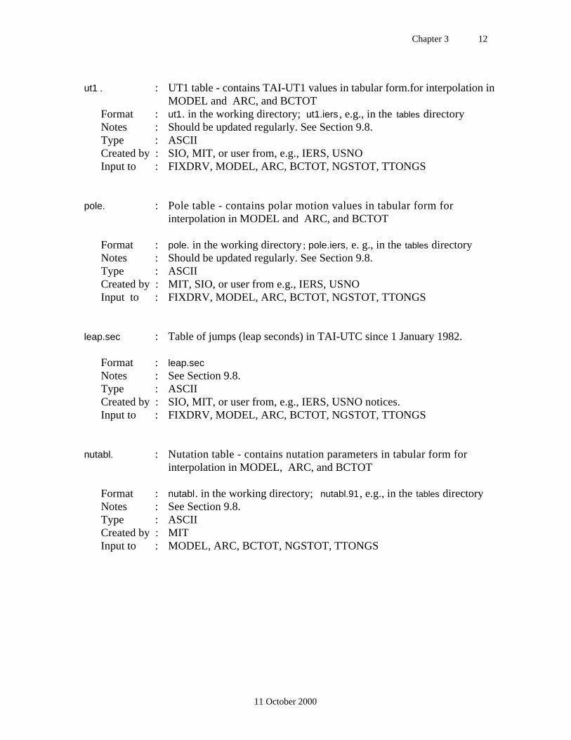
ut1 . : UT1 table - contains TAI-UT1 values in tabular form.for interpolation inMODEL and ARC, and BCTOT

Format : ut1. in the working directory; ut1.iers , e.g., in the tables directoryNotes : Should be updated regularly. See Section 9.8.Type : ASCIICreated by : SIO, MIT, or user from, e.g., IERS, USNOInput to : FIXDRV, MODEL, ARC, BCTOT, NGSTOT, TTONGS

pole. : Pole table - contains polar motion values in tabular form forinterpolation in MODEL and ARC, and BCTOT

Format : pole. in the working directory ; pole.iers, e. g., in the tables directoryNotes : Should be updated regularly. See Section 9.8.Type : ASCIICreated by : MIT, SIO, or user from e.g., IERS, USNOInput to : FIXDRV, MODEL, ARC, BCTOT, NGSTOT, TTONGS

leap.sec : Table of jumps (leap seconds) in TAI-UTC since 1 January 1982.

Format : leap.secNotes : See Section 9.8.Type : ASCIICreated by : SIO, MIT, or user from, e.g., IERS, USNO notices.Input to : FIXDRV, MODEL, ARC, BCTOT, NGSTOT, TTONGS

nutabl. : Nutation table - contains nutation parameters in tabular form forinterpolation in MODEL, ARC, and BCTOT

Format : nutabl. in the working directory; nutabl.91, e.g., in the tables directoryNotes : See Section 9.8.Type : ASCIICreated by : MITInput to : MODEL, ARC, BCTOT, NGSTOT, TTONGS

Chapter 3 13

11 October 2000

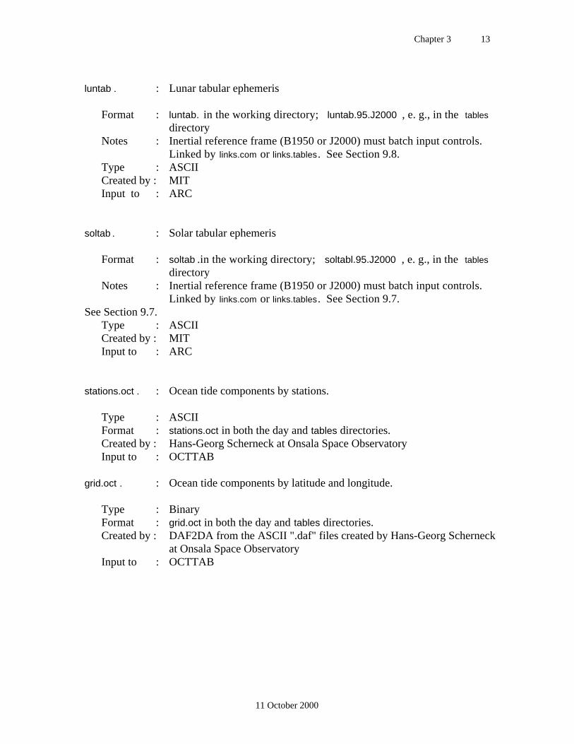
luntab . : Lunar tabular ephemeris

Format : luntab. in the working directory; luntab.95.J2000 , e. g., in the tables

directoryNotes : Inertial reference frame (B1950 or J2000) must batch input controls.

Linked by links.com or links.tables. See Section 9.8.Type : ASCIICreated by : MITInput to : ARC

soltab . : Solar tabular ephemeris

Format : soltab .in the working directory; soltabl.95.J2000 , e. g., in the tables

directoryNotes : Inertial reference frame (B1950 or J2000) must batch input controls.

Linked by links.com or links.tables. See Section 9.7.See Section 9.7.

Type : ASCIICreated by : MITInput to : ARC

stations.oct . : Ocean tide components by stations.

Type : ASCIIFormat : stations.oct in both the day and tables directories.Created by : Hans-Georg Scherneck at Onsala Space ObservatoryInput to : OCTTAB

grid.oct . : Ocean tide components by latitude and longitude.

Type : BinaryFormat : grid.oct in both the day and tables directories.Created by : DAF2DA from the ASCII ".daf" files created by Hans-Georg Scherneck

at Onsala Space ObservatoryInput to : OCTTAB

Chapter 4 1

15 February 2002

4. Creating Data Input Files

4.1 Introduction and file organization

The first, and in many ways most difficult step in analyzing GPS data, is organizing thedata, both field notes and receiver output, in such a way that it can be handled efficiently bythe processing programs. It is during this process that you must make tentative decisionsabout how many days to analyze, what stations should be included and over what timespan, and how frequently to sample the data. In short, this is the time to start taking carefulnotes and to plan your analysis strategy. This is also the time when you discover that youare missing log sheets, data files, or a priori coordinates for particular stations, and youmust send frantic e-mail to fill in the holes.

The main GAMIT modules (beginning with FIXDRV, ARC, and MODEL) require seventypes of input:

• Raw phase and pseudo-range data in the form of ASCII X-files (one for each stationwithin each session)

• Station coordinates in the form of an L-file

• Receiver and antenna information for each site (file station.info)

• Satellite list and scenario (file session.info)

• Initial conditions for the satellites' orbits in a G-file (or a tabulated ephemeris in a T-file)

• Satellite and station clock values (I-, J-, and K-files)

• Control files for the analysis (sestbl. and sittbl.)

• "Standard" tables to provide lunar/solar ephemerides, the Earth's rotation, geodeticdatums, and spacecraft and instrumentation information (see below).

The X-files are the key organizational structure because all X-files for a given session arewritten with the same start and stop times, selection of satellites, and sampling interval.This imposed rigidity has certain advantages. The primary one is that the process ofcreating the X-files (program MAKEX) acts as a filter, catching most of the problems withmissing or invalid data, mismatched time tags, and poorly behaved receiver clocks thatwould cause greater loss of time if discovered later.

The first step is to create working directories for the processing. The recommendedorganization (and the one used by sh_gamit) is a "survey" or continuous network directory(e.g., emed98, scec99, scign99) under which you will have "day" directories for each dayor session (e.g. /312 for day 312). Parallel to the day directories are directories containingthe RINEX files (e.g., /rinex ), orbit files (.e.g. /brdc for navigation files and /igs for IGSSP3 files), and the GAMIT tables relevant to the survey ( /tables ). (The directories forGLOBK processing of the survey, /gsoln and /glbf, can also go at this level.)

Chapter 4 2

15 February 2002

You begin the pre-processing by creating links within the day directory to the data files andtables necessary to set up the batch processing. The first step is to create links to theGAMIT global files: geodetic datums (gdetic.dat), lunar and solar ephemerides (luntab. and

soltab.), nutations (nuttab.), Earth rotation (ut1. and pole.), ocean tides (stations.oct andgrid.oct), leap seconds (leap.sec), and spacecraft, receiver, and antenna characteristics(svnav.dat, antmod.dat, rcvant.dat). This is usually accomplished in two steps. First, inthe /tables directory, execute script links.tables, which will create links for the global filesto ~/gg/tables. Then from each day directory you execute links.day, which will create linksfor global files and survey-specific files to ../tables. Links.day will also create links fromthe day directory to ../tables for the six control and survey-specific files needed byGAMIT: station.info, session.info, .sestbl., sittbl., autcln.cmd. and lfile. Hence, you cankeep a single copy of these files in /tables, avoiding the possibility of processing differentsessions with different input controls. If you are simply performing a test with a singleday's data, you execute links.com to link tables directly to ~/gg/tables and copy all theother files into the day directory. The link scripts, like all the scripts in /com are self-documenting—simply type the name with no arguments to see the proper syntax.

We describe the linking of the RINEX files in Section 4.5, preparation of the L-file,station.info, and session.info Sections 4.2–4.4, and the control files for FIXDRV (sestbl.

and sittbl.) in Chapter 5. The navigation file is simply a RINEX "n" file, named eitheraaaannnn.YYn or eaaaY.DDD and should be linked or copied into the day directory from the/rinex or /brdc directory or directly from an IGS Data Center.

4.2 Preparing the coordinate (L-) file

The L-file contains the coordinates of all the stations to be used in the experiment. Onlygeocentric (spherical) coordinates are supported, in the following format:

VLBI FIDUCIALS: GLB223 (1987.0) + TIES CONVERTED TO SV4Created by mhm 10/1/90ENDFTOR FORT7266 N36 29 8.22850 W121 46 23.7842 6370574.9754 noam 1990.238ONSA ONSAGPS N57 13 13.29164 E 11 55 31.84348 6363045.6176 eura 1990.238OVRO OVRO7114 N37 2 50.52769 118 17 37.65749 6371527.9644 noam 1990.238

You may include as many comment lines as you wish, terminated by "END". The formatis (A12,5X,A1,I2,1X,I2,1X,F8.5,1X,A1,I3,1X,I2,1X,F8.5,F12.3). The plate name andreference epoch at the end of each line are comments and not used by the program. Withineach day directory, the usual name of the L-file is the same as the D-file except for the firstcharacter(i.e., lprojy.ddd) , with a link provided to an experiment-wide L-file ( lfile.) in../tables.

The L-file is usually created by program GAPR_TO_L from a GLOBK apr file, which hasCartesian coordinates and velocities in free format:

Chapter 4 3

15 February 2002

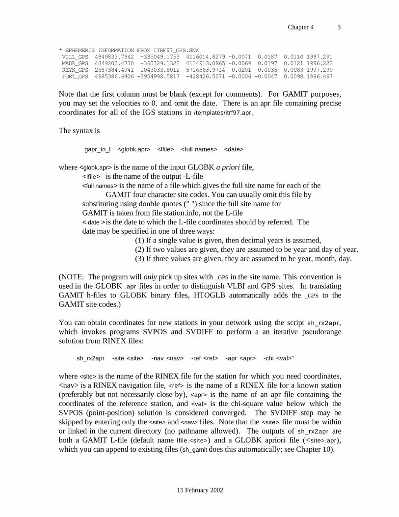
* EPHEMERIS INFORMATION FROM ITRF97_GPS.SNX VILL_GPS 4849833.7942 -335049.1753 4116014.8279 -0.0071 0.0187 0.0110 1997.291 MADR_GPS 4849202.4770 -360329.1322 4114913.0865 -0.0069 0.0197 0.0121 1996.222 REYK_GPS 2587384.4941 -1043033.5012 5716563.9714 -0.0201 -0.0035 0.0083 1997.299 FORT_GPS 4985386.6406 -3954998.5817 -428426.5071 -0.0006 -0.0047 0.0098 1996.497

Note that the first column must be blank (except for comments). For GAMIT purposes,you may set the velocities to 0. and omit the date. There is an apr file containing precisecoordinates for all of the IGS stations in /templates/itrf97.apr.

The syntax is

gapr_to_l <globk.apr> <lfile> <full names> <date>

where <globk.apr> is the name of the input GLOBK a priori file,<lfile> is the name of the output -L-file<full names> is the name of a file which gives the full site name for each of the

GAMIT four character site codes. You can usually omit this file by substituting using double quotes (" ") since the full site name for GAMIT is taken from file station.info, not the L-file< date > is the date to which the L-file coordinates should by referred. The date may be specified in one of three ways:

(1) If a single value is given, then decimal years is assumed,(2) If two values are given, they are assumed to be year and day of year.(3) If three values are given, they are assumed to be year, month, day.

(NOTE: The program will only pick up sites with _GPS in the site name. This convention isused in the GLOBK .apr files in order to distinguish VLBI and GPS sites. In translatingGAMIT h-files to GLOBK binary files, HTOGLB automatically adds the _GPS to theGAMIT site codes.)

You can obtain coordinates for new stations in your network using the script sh_rx2apr,which invokes programs SVPOS and SVDIFF to perform a an iterative pseudorangesolution from RINEX files:

sh_rx2apr -site <site> -nav <nav> -ref <ref> -apr <apr> -chi <val>"

where <site> is the name of the RINEX file for the station for which you need coordinates,<nav> is a RINEX navigation file, <ref> is the name of a RINEX file for a known station(preferably but not necessarily close by), <apr> is the name of an apr file containing thecoordinates of the reference station, and <val> is the chi-square value below which theSVPOS (point-position) solution is considered converged. The SVDIFF step may beskipped by entering only the <site> and <nav> files. Note that the <site> file must be withinor linked in the current directory (no pathname allowed). The outputs of sh_rx2apr areboth a GAMIT L-file (default name lfile.<site>) and a GLOBK apriori file (<site>.apr),which you can append to existing files (sh_gamit does this automatically; see Chapter 10).

Chapter 4 4

15 February 2002

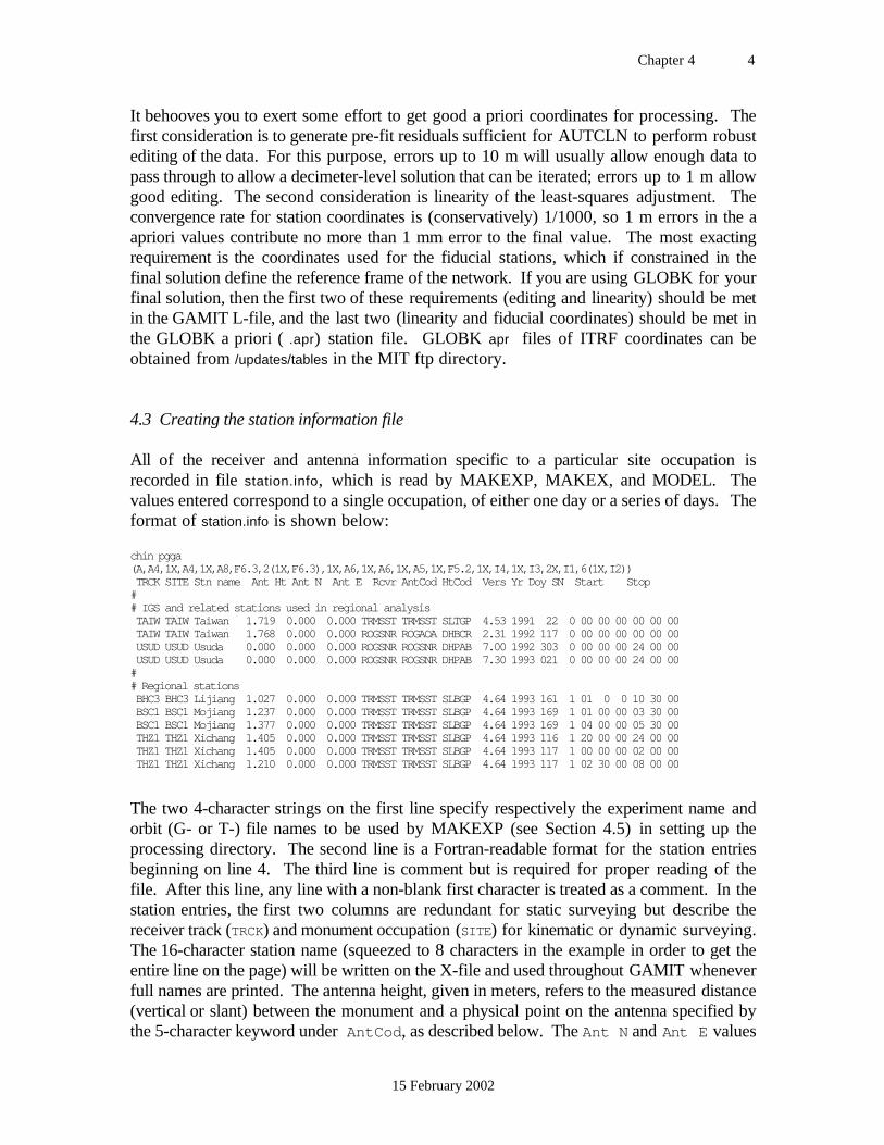
It behooves you to exert some effort to get good a priori coordinates for processing. Thefirst consideration is to generate pre-fit residuals sufficient for AUTCLN to perform robustediting of the data. For this purpose, errors up to 10 m will usually allow enough data topass through to allow a decimeter-level solution that can be iterated; errors up to 1 m allowgood editing. The second consideration is linearity of the least-squares adjustment. Theconvergence rate for station coordinates is (conservatively) 1/1000, so 1 m errors in the aapriori values contribute no more than 1 mm error to the final value. The most exactingrequirement is the coordinates used for the fiducial stations, which if constrained in thefinal solution define the reference frame of the network. If you are using GLOBK for yourfinal solution, then the first two of these requirements (editing and linearity) should be metin the GAMIT L-file, and the last two (linearity and fiducial coordinates) should be met inthe GLOBK a priori ( .apr) station file. GLOBK apr files of ITRF coordinates can beobtained from /updates/tables in the MIT ftp directory.

4.3 Creating the station information file

All of the receiver and antenna information specific to a particular site occupation isrecorded in file station.info, which is read by MAKEXP, MAKEX, and MODEL. Thevalues entered correspond to a single occupation, of either one day or a series of days. Theformat of station.info is shown below:

chin pgga(A,A4,1X,A4,1X,A8,F6.3,2(1X,F6.3),1X,A6,1X,A6,1X,A5,1X,F5.2,1X,I4,1X,I3,2X,I1,6(1X,I2)) TRCK SITE Stn name Ant Ht Ant N Ant E Rcvr AntCod HtCod Vers Yr Doy SN Start Stop## IGS and related stations used in regional analysis TAIW TAIW Taiwan 1.719 0.000 0.000 TRMSST TRMSST SLTGP 4.53 1991 22 0 00 00 00 00 00 00 TAIW TAIW Taiwan 1.768 0.000 0.000 ROGSNR ROGAOA DHBCR 2.31 1992 117 0 00 00 00 00 00 00 USUD USUD Usuda 0.000 0.000 0.000 ROGSNR ROGSNR DHPAB 7.00 1992 303 0 00 00 00 24 00 00 USUD USUD Usuda 0.000 0.000 0.000 ROGSNR ROGSNR DHPAB 7.30 1993 021 0 00 00 00 24 00 00## Regional stations BHC3 BHC3 Lijiang 1.027 0.000 0.000 TRMSST TRMSST SLBGP 4.64 1993 161 1 01 0 0 10 30 00 BSC1 BSC1 Mojiang 1.237 0.000 0.000 TRMSST TRMSST SLBGP 4.64 1993 169 1 01 00 00 03 30 00 BSC1 BSC1 Mojiang 1.377 0.000 0.000 TRMSST TRMSST SLBGP 4.64 1993 169 1 04 00 00 05 30 00 THZ1 THZ1 Xichang 1.405 0.000 0.000 TRMSST TRMSST SLBGP 4.64 1993 116 1 20 00 00 24 00 00 THZ1 THZ1 Xichang 1.405 0.000 0.000 TRMSST TRMSST SLBGP 4.64 1993 117 1 00 00 00 02 00 00 THZ1 THZ1 Xichang 1.210 0.000 0.000 TRMSST TRMSST SLBGP 4.64 1993 117 1 02 30 00 08 00 00

The two 4-character strings on the first line specify respectively the experiment name andorbit (G- or T-) file names to be used by MAKEXP (see Section 4.5) in setting up theprocessing directory. The second line is a Fortran-readable format for the station entriesbeginning on line 4. The third line is comment but is required for proper reading of thefile. After this line, any line with a non-blank first character is treated as a comment. In thestation entries, the first two columns are redundant for static surveying but describe thereceiver track (TRCK) and monument occupation (SITE) for kinematic or dynamic surveying.The 16-character station name (squeezed to 8 characters in the example in order to get theentire line on the page) will be written on the X-file and used throughout GAMIT wheneverfull names are printed. The antenna height, given in meters, refers to the measured distance(vertical or slant) between the monument and a physical point on the antenna specified bythe 5-character keyword under AntCod, as described below. The Ant N and Ant E values

Chapter 4 5

15 February 2002

refer to the offsets of the center of the antenna from the monument. The station.info valuesare added to the coordinates of the monument in computing the antenna phase-centerposition.

For static surveying, the appropriate entry in station.info is selected by matching the stationid (TRCK), the year (Yr) , day-of-year (Doy), and the start and stop times in station.info

with the station and time requested by MAKEX or MODEL. You must observe thefollowing rules:

1) If the start and stop times are 0 0 0 0 0 0 or 0 0 0 24 0 0, the antennainformation entered for a day will be used throughout the day and for all days followinguntil a later entry is encountered in the table. Thus, in the example, the initial entry forTAIW is valid from 0h UTC on day 22 of 1991 until 0h UTC on day 117 of 1992.

2) If the start and stop times are any other values, the information is valid only withinthe listed times. The example shows for the regional stations five specific cases.Lijiang is the simplest, with a single set of values used for a single session, 0100–1030on day 161. Mojiang was observed on day 169 with two different antenna setups, to becombined into a single session for processing. Finally, Xichang was observed in twosessions, the first of which crosses a day boundary. Since the epoch entries do not allowfor a different day number to be entered for the start and stop times (a deficiency we willeventually correct), you must make two entries for the first session. The start time for astation must be at or before the beginning of its X-file as specified by session.info, notthe setup time listed on the log sheet (the program does not look within the X-file to notethat the actual beginning of tracking was later in the session). Note that the sessionnumber currently has no meaning in the context of station.info entries.

3) Multiple entries for a station need not be contiguous but must be in chronologicalorder (Release 9.44 will detect this for you, but earlier releases will pick up withoutwarning the last entry before one later than the date of your session).

4) After the first two lines, any entry with a non-blank character in column one willbe treated as a comment, allowing you to document the history of a tracker or experiment.

Besides documenting the analysis, the receiver type (Rcvr) and firmware/software version(Vers) are used by MAKEX in filtering the sample time (some receivers have offsets fromthe even minute) and determining whether a receiver has full- or half-wavelength L2observations. Note that the firmware codes used by GAMIT are numerical and do notnecessarily correspond to the manufacturer's designations; for correct processing, thefirmware version does not always need to be strictly correct and in some cases is definedartificially in GAMIT to account for non-standard or erroneous sampling (see Section 4.7).

Most important among the entries in station.info are the antenna type and specification ofhow the height-of-instrument (HI) was measured in the field since this directly affects theestimated heights from the analysis. This information is typed into station.info in the formof keywords and later converted by GAMIT to L1 and L2 phase-center offsets. Forexample, in the station.info given above, station BHC3 on day 161 used a Trimble SST(TRMSST) antenna whose slant-height to the bottom of the outer edge of the ground plane

Chapter 4 6

15 February 2002

(SLBGP) was measured as 1.027 m. For historical reasons, all measurements to the antennareference point (ARP) are specified as DHPAB ("direct height to pre-amp base"), as shownin the example for IGS station USUD. Complete descriptions of all of the antennas allowedby GAMIT and the models used to compute their effective phase centers are given inAppendix 2. To verify current information for your version of the software, seesubroutines hisub.f and ant_alias.f in gamit/lib and rcvant.dat and antmod.dat in gg/tables.

In most cases the entries in station.info for a field survey must be entered manually fromthe log sheets, using as a template, e.g., gg/tables/station.info. A current station.info for allof the continuous stations processed by SOPAC can be found on the SOPAC web page andin updates/tables in the MIT GAMIT/GLOBK ftp directory. If your are processing RINEXfiles generated elsewhere and all of the header information is completely correct, thensh_gamit will perform updates of the template station.info for you automatically. If youwant to merge several station.info files created for different surveys, you can use theprogram MSTINF:

mstinf -f <infile> -w <outfile> -s <file_list> -l <sites_list>

where <infile> is a reference station.info file with definitive inforamtion, <outfile> is thename of the merged output station.info file, <file_list> are the names of one or morestation.info files to be merged, and <sites_list> are the names of one or more stations toinclude in the merged file. Only the first two arguments are required. If <sites_list> isomitted, then all of the stations in the reference file will be included in the output file. Theoption -u <site_list_file> may be used, where <site_list_file> is a file containing thestations to be included (one name per line, with the first column blank).

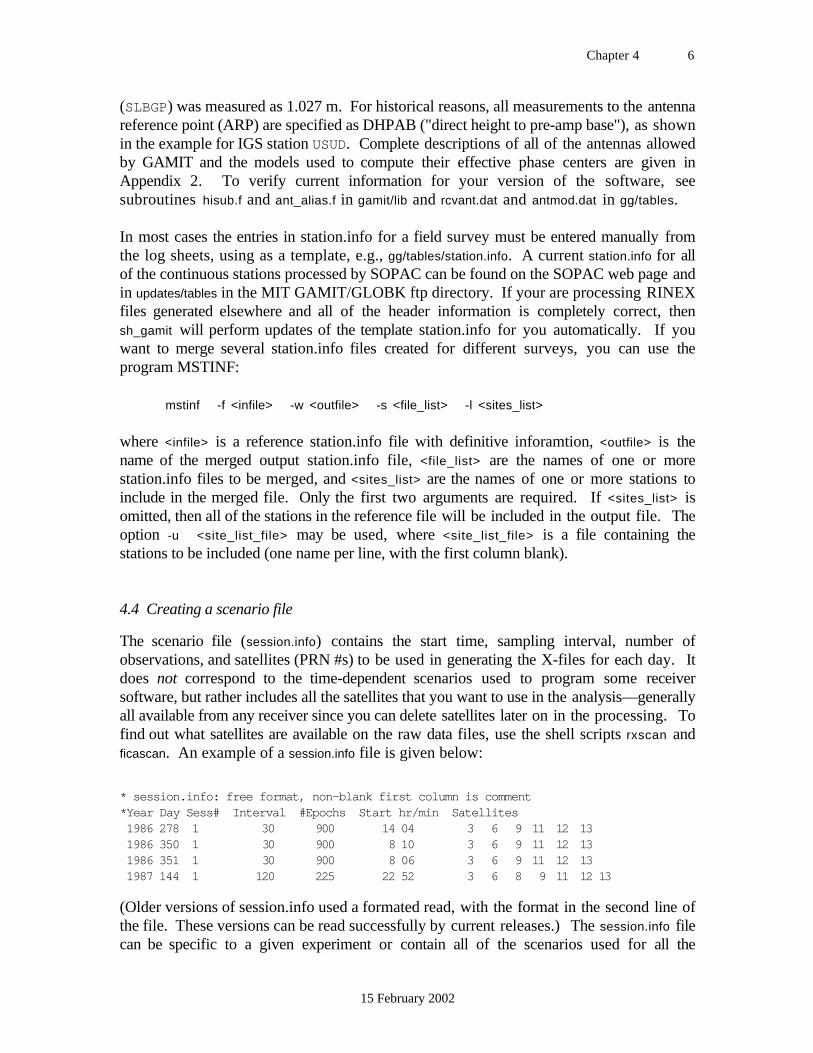
4.4 Creating a scenario file

The scenario file (session.info) contains the start time, sampling interval, number ofobservations, and satellites (PRN #s) to be used in generating the X-files for each day. Itdoes not correspond to the time-dependent scenarios used to program some receiversoftware, but rather includes all the satellites that you want to use in the analysis—generallyall available from any receiver since you can delete satellites later on in the processing. Tofind out what satellites are available on the raw data files, use the shell scripts rxscan andficascan. An example of a session.info file is given below:

* session.info: free format, non-blank first column is comment*Year Day Sess# Interval #Epochs Start hr/min Satellites 1986 278 1 30 900 14 04 3 6 9 11 12 13 1986 350 1 30 900 8 10 3 6 9 11 12 13 1986 351 1 30 900 8 06 3 6 9 11 12 13 1987 144 1 120 225 22 52 3 6 8 9 11 12 13

(Older versions of session.info used a formated read, with the format in the second line ofthe file. These versions can be read successfully by current releases.) The session.info filecan be specific to a given experiment or contain all of the scenarios used for all the

Chapter 4 7

15 February 2002

experiments processed at your facility. An experiment-specific file can be generatedautomatically by program MAXEXP (see below) using the input start/stop time and thesatellites available on the navigation file.

4.5 Using MAKEXP

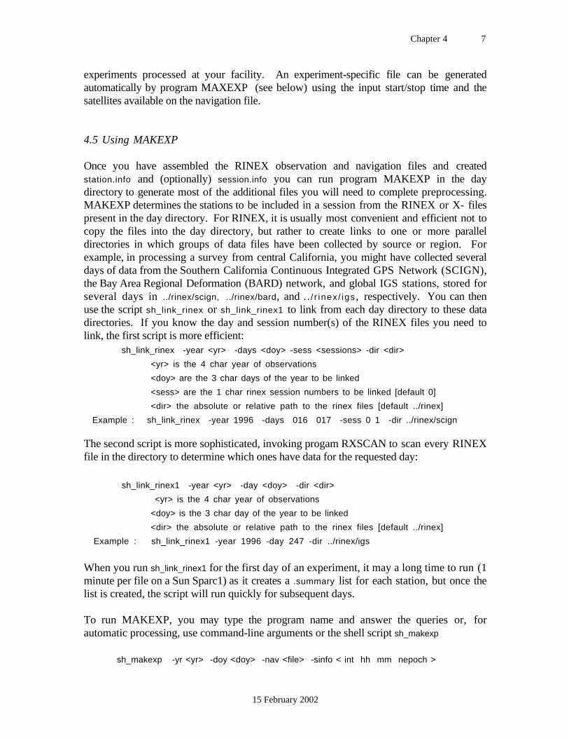
Once you have assembled the RINEX observation and navigation files and createdstation.info and (optionally) session.info you can run program MAKEXP in the daydirectory to generate most of the additional files you will need to complete preprocessing.MAKEXP determines the stations to be included in a session from the RINEX or X- filespresent in the day directory. For RINEX, it is usually most convenient and efficient not tocopy the files into the day directory, but rather to create links to one or more paralleldirectories in which groups of data files have been collected by source or region. Forexample, in processing a survey from central California, you might have collected severaldays of data from the Southern California Continuous Integrated GPS Network (SCIGN),the Bay Area Regional Deformation (BARD) network, and global IGS stations, stored forseveral days in ../rinex/scign, ../rinex/bard, and ../ r inex / igs , respectively. You can thenuse the script sh_link_rinex or sh_link_rinex1 to link from each day directory to these datadirectories. If you know the day and session number(s) of the RINEX files you need tolink, the first script is more efficient:

sh_link_rinex -year <yr> -days <doy> -sess <sessions> -dir <dir>

<yr> is the 4 char year of observations

<doy> are the 3 char days of the year to be linked

<sess> are the 1 char rinex session numbers to be linked [default 0]

<dir> the absolute or relative path to the rinex files [default ../rinex]

Example : sh_link_rinex -year 1996 -days 016 017 -sess 0 1 -dir ../rinex/scign

The second script is more sophisticated, invoking progam RXSCAN to scan every RINEXfile in the directory to determine which ones have data for the requested day:

sh_link_rinex1 -year <yr> -day <doy> -dir <dir>

<yr> is the 4 char year of observations

<doy> is the 3 char day of the year to be linked

<dir> the absolute or relative path to the rinex files [default ../rinex]

Example : sh_link_rinex1 -year 1996 -day 247 -dir ../rinex/igs

When you run sh_link_rinex1 for the first day of an experiment, it may a long time to run (1minute per file on a Sun Sparc1) as it creates a .summary list for each station, but once thelist is created, the script will run quickly for subsequent days.

To run MAKEXP, you may type the program name and answer the queries or, forautomatic processing, use command-line arguments or the shell script sh_makexp

sh_makexp -yr <yr> -doy <doy> -nav <file> -sinfo < int hh mm nepoch >

Chapter 4 8

15 February 2002

in which the required entries are year (yr), day-of-year (doy), navigation file (file), and thesession span information—sampling interval (int), hour (hh), minute (mm), and number ofepochs (nepoch) (a more complete list of options is given as help when you type the nameof the shell-script). In interactive use, you will be asked to enter the year, day-of-year,session number, and navigation file. When invoked, MAKEXP will then the workingdirectory for RINEX or X-files with the input date, compare the 4-character station namesand date with the TRCK codes and dates in station.info, and write to the screen a summaryof the available stations. If a scenario file (session.info) exists, MAKEXP will use it todetermine the start and stop times and the satellites to be used in the session. If thesession.info file has only a single entry in it, MAKEXP will "edit" the entry to set the yearand day-of-year but keep the start time, sampling interval, number of epochs and thesatellite list intact. If there is no scenario file, you will be asked to input the samplinginterval, number of epochs, and start time; the program will generate a satellite list from thenavigation file. With the shell script, editing of an existing scenario file is invoked byomitting the -sinfo option. If you have used sh_link_rinex1 to include in the day directoryonly files with data you need for processing, then you can enter 999 and 99 for day andsession, respectively, telling MAKEXP that you want to use all the RINEX files present togenerate the list of stations to be processed. If you enter either 0 or 1 for the sessionnumber, MAKEXP will search for both in compiling its station list (GAMIT changes allsession numbers of 0 to 1 internally). New options (Release 10.05) with command-line orsh_makexp input are –srin to search all RINEX files in the directory for data matching theinput date; -xver <char> to use X-files with a 6th character other than the last digit of theyear (useful to select previously cleaned X-files). Type sh_makexp to see a complete list ofoptions and examples.

The screen output of MAKEXP contains a summary of the stations found (X-files to becreated), satellites included, and the session times. It concludes with instructions for thenext steps:

Now run, in order:

sh_sp3fit -f <sp3 file> OR sh_bcfit bctot.inp OR copy a g-file from SOPAC

sh_check_sess -sess 278 -type gfile -file <g-file>

makej <nav-file> <jfile> OR copy a j-file from SOPAC

sh_check_sess -sess 278 -type jfile -file jvent7.278

makex <makex-batchfile>

fixdrv <dfile> OR run interactively

The script sh_sp3fit generates satellite initial conditions (G-file) by fitting the ARC model tothe tabulated ephemerides in "SP3" format from an IGS analysis center. The input <sp3

file> must be present or linked in the local directory (pathnames are not allowed.Alternatively you can create these files from the broadcast ephemeris on a RINEXnavigation file or copy GAMIT-format files directly from SOPAC. The second step(sh_check_sess) is optional but assures that the satellites requested in session.info areavailable on the orbital (G- and T-) files. Program MAKEJ creates a (J-) file of satelliteclock values from the navigation message. Then you may again use sh_check_sess to

Chapter 4 9

15 February 2002

assure that the satellites requested in session.info are available on the J-file. ProgramMAKEX creates the GAMIT observation (X-) files from the RINEX files. Each of thesesteps is described in the following sections of this chapter. Finally, program FIXDRVreads the analysis controls, described in Chapter 5, and creates a batch file for GAMITprocessing.

Creating the input files for MAKEJ, MAKEX, and FIXDRV from templates is not difficultand may be necessary for experiments with multiple sessions or a mixture of RINEX andFICA files. For large experiments or permanently operating arrays, however, usingMAKEXP can save a great deal of time and manual effort. (Yet one more level ofsophistication is provided by the new shell script getready, which runs the completeGAMIT sequence from a small set of input files. The script, written by Eric Calais while atSIO, is internally well documented and can be found in gamit/com.)

Although MAKEXP is usually run from RINEX files, you can use it again at a later stageof processing from X-files simply to generate a new station list (D-file) for FIXDRV. Inthis case, you do not need to have present or linked either the RINEX observation files or anavigation file.

4.6 Creating T- and G-files from External Ephemerides

Orbital information is input to GAMIT in the form of a tabular ephemeris (T-) file, whichcontains the positions of all the satellites at 15-minute intervals throughout the observationspan, or a G-file of initial conditions which are integrated by ARC (in the batch run) tocreate a T-file.

If the satellite orbits are to be adjusted to fit the observations, then the T-file must alsocontain partial derivatives of position (as a function of time) with respect to six "initialconditions" and other parameters describing the orbit of each satellite. ARC generates thepartials by numerically integrating their force equations (termed "variational equations")simultaneously with the equations of motion. If the G-file of initial conditions wasobtained from a global orbit solution performed using GAMIT with a compatible version ofARC (e.g., by SOPAC), it can be used directly in ARC to produce a T-file consistent withthe solution. Integration of instantaneous position and velocity values obtained byevaluating the broadcast message parameters or extracted from an external Earth-fixedephemeris (in SP #3 format) produced by another software package or an incompatibleversion of ARC will not reproduce the original accuracy since model differences will causethe orbit to deviate from the original orbit as the integration proceeds away from the initialepoch. The original accuracy can be obtained, however, by estimating initial conditions forARC using externally derived positions and velocities over the full session as pseudo-observations. The most accurate and reliable method of obtaining a starting T-file is tofollow this procedure using the shell script sh_sp3fit and an SP #3 file from an IGSanalysis center:

sh_sp3fit -f <sp3 file> -d <yr doy> -o <orbit name> -i <equator prec> -r <radmod> -t

Chapter 4 10

15 February 2002

where <sp3 file> is the name of the external file (e.g., igs08523.sp3 for day 3 of week 852).The year and day-of-year may be omitted if your session.info contains only a single entry(i.e., continuous-array style), but if you have a single session.info for an entire survey, thenyou must specify the requested year and day in the command line. <orbit name> is the 4-character name for the G- and T-files, nominally read from the first line of station.info.<equator prec> specifies the inertial reference frame and precession constant for the G- andT-files; the defaults are the conventional J2000 IAU76, but you may specify B1950 IAU68

for compatiblity with older GAMIT and SOPAC processing (see the discussion of inertialframe in Section 5.2). <radmod> specifies the radiation-presssure (non-gravitational force)model to be used with the orbit; the default is BERNE (see sections 5.2 and 7.2). The finalargument ( -t ), if entered, causes sh_sp3fit to create (integrate) a T-file from the initialconditions (G-file) estimated from the fit. The default is to skip this step, deferring theintegration to the first step of the GAMIT batch run. In addition to a G- and (optionally) T-file, sh_sp3fit will generate two print files (sp3fit.f it and sp3fit.rms) summarizing thequality of the fit, and a Y-file of satellite yaw parameters for the orbital span (see Section7.2).

An alternative but less accurate means of generating an initial orbit is to use the scriptsh_bcfit to perform a fit of the GAMIT model to the broadcast elements in a navigation file.Before doing so, you should run the program BCCHECK to determine the consistency ofthe elements and to filter outliers:

bccheck <RINEX nav file> <yr> <doy>

will produce a new navigation file ( <RINEX nav file>.bcchecked ) containing only elementswhose differences from the elements at the midpoint of the day are less than 1000 m. Theprint file bccheck.out will give you a summary of the times and differences of the elementsin the file, with any deleted marked by an asterisk. Next execute

sh_bcfit <input file>

where <input file> is the bctot.inp produced by MAKEXP:

b indicates batch inputauto2360.94n.bcchecked RINEX navigation filexpver4.236 X-file to determine session scenariotvent4.236 output T-filey 'yes' to transform the orbit to an inertial frameJ2000 designation of the inertial frame

If you don't have an X-file or wish to create a T-file for a longer span, you can do so bychanging the input file to match an alternate set of questions asked by BCTOT:

b indicates batch inputauto2360.94n.bcchecked RINEX navigation file

blank line to indicate no X-filetvent4.236 output T-file

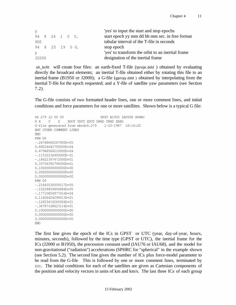
Chapter 4 11

15 February 2002

y 'yes' to input the start and stop epochs94 8 24 1 0 0. start epoch yy mm dd hh mm sec. in free format900 tabular interval of the T-file in seconds94 8 25 19 0 0. stop epochy 'yes' to transform the orbit to an inertial frameJ2000 designation of the inertial frame

sh_bcfit will create four files: an earth-fixed T-file (tproje.ddd ) obtained by evaluatingdirectly the broadcast elements; an inertial T-file obtained either by rotating this file to aninertial frame (B1950 or J2000); a G-file (gprojy.ddd ) obtained by interpolating from theinertial T-file for the epoch requested; and a Y-file of satellite yaw parameters (see Section7.2).

The G-file consists of two formatted header lines, one or more comment lines, and initialconditions and force parameters for one or more satellites. Shown below is a typical G file:

86 279 12 00 00 GPST B1950 IAUT68 SPHRC8 X Y Z XDOT YDOT ZDOT DRAD YRAD ZRADG-file generated from ebrdc6.279 1-10-1987 18:16:20ANY OTHER COMMENT LINESENDPRN 06-.24748600267000D+050.88024642750000D+040.47948566210000D+04-.11532236900000D-01-.18622397472000D+010.33736392796000D+010.10000000000000D+000.00000000000000D+000.00000000000000D+00PRN 09-.21643530559117D+05-.15228859494884D+05-.17710854977416D+040.11606424294013D+01-.12653416265926D+01-.34787168623116D+010.10000000000000D+000.00000000000000D+000.00000000000000D+00END

The first line gives the epoch of the ICs in GPST or UTC (year, day-of-year, hours,minutes, seconds), followed by the time type (GPST or UTC), the inertial frame for theICs (J2000 or B1950), the precession constant used (IAU76 or IAU68), and the model fornon-gravitational ("radiation") accelerations (SPHRC for "spherical" in the example shown(see Section 5.2). The second line gives the number of ICs plus force-model parameter tobe read from the G-file This is followed by one or more comment lines, terminated byEND. The initial conditions for each of the satellites are given as Cartesian components ofthe position and velocity vectors in units of km and km/s. The last three ICs of each group

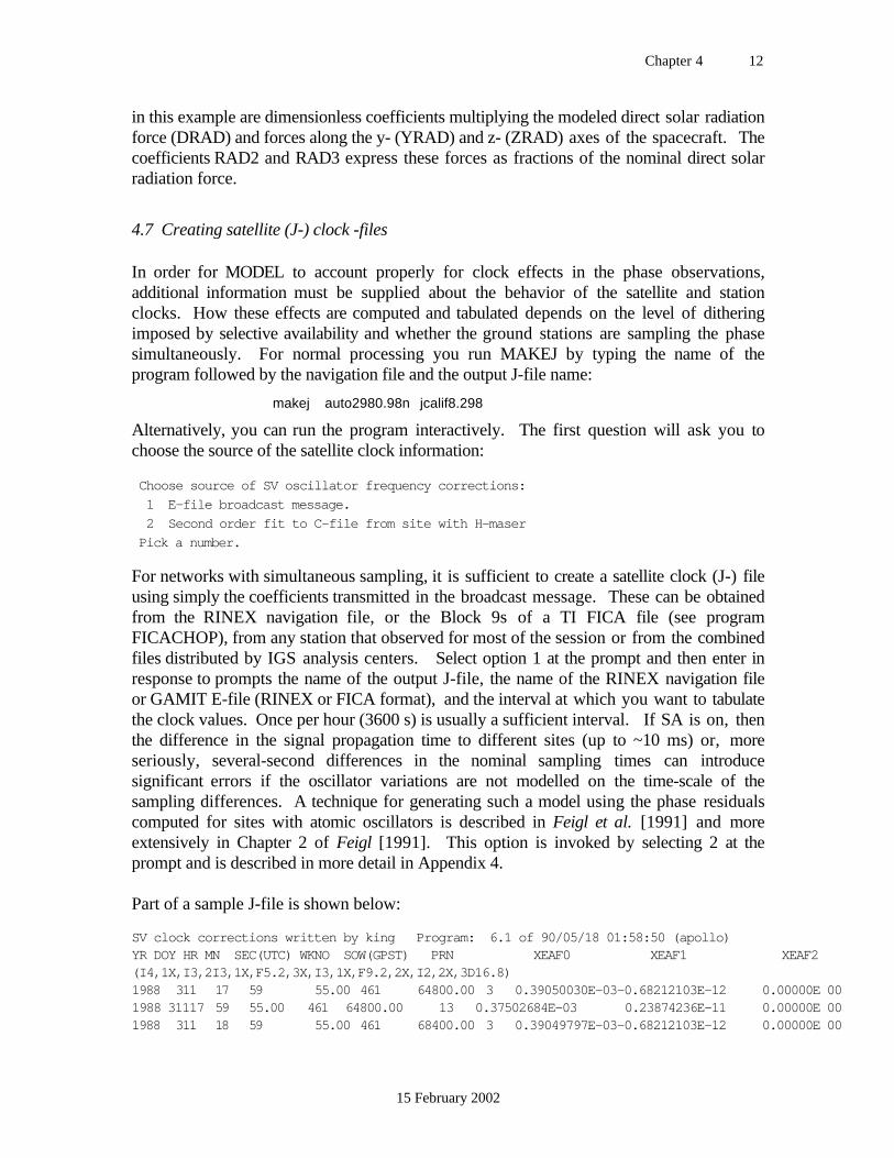
Chapter 4 12

15 February 2002

in this example are dimensionless coefficients multiplying the modeled direct solar radiationforce (DRAD) and forces along the y- (YRAD) and z- (ZRAD) axes of the spacecraft. Thecoefficients RAD2 and RAD3 express these forces as fractions of the nominal direct solarradiation force.

4.7 Creating satellite (J-) clock -files

In order for MODEL to account properly for clock effects in the phase observations,additional information must be supplied about the behavior of the satellite and stationclocks. How these effects are computed and tabulated depends on the level of ditheringimposed by selective availability and whether the ground stations are sampling the phasesimultaneously. For normal processing you run MAKEJ by typing the name of theprogram followed by the navigation file and the output J-file name:

makej auto2980.98n jcalif8.298

Alternatively, you can run the program interactively. The first question will ask you tochoose the source of the satellite clock information:

Choose source of SV oscillator frequency corrections:

1 E-file broadcast message.

2 Second order fit to C-file from site with H-maser

Pick a number.

For networks with simultaneous sampling, it is sufficient to create a satellite clock (J-) fileusing simply the coefficients transmitted in the broadcast message. These can be obtainedfrom the RINEX navigation file, or the Block 9s of a TI FICA file (see programFICACHOP), from any station that observed for most of the session or from the combinedfiles distributed by IGS analysis centers. Select option 1 at the prompt and then enter inresponse to prompts the name of the output J-file, the name of the RINEX navigation fileor GAMIT E-file (RINEX or FICA format), and the interval at which you want to tabulatethe clock values. Once per hour (3600 s) is usually a sufficient interval. If SA is on, thenthe difference in the signal propagation time to different sites (up to ~10 ms) or, moreseriously, several-second differences in the nominal sampling times can introducesignificant errors if the oscillator variations are not modelled on the time-scale of thesampling differences. A technique for generating such a model using the phase residualscomputed for sites with atomic oscillators is described in Feigl et al. [1991] and moreextensively in Chapter 2 of Feigl [1991]. This option is invoked by selecting 2 at theprompt and is described in more detail in Appendix 4.

Part of a sample J-file is shown below:

SV clock corrections written by king Program: 6.1 of 90/05/18 01:58:50 (apollo)YR DOY HR MN SEC(UTC) WKNO SOW(GPST) PRN XEAF0 XEAF1 XEAF2(I4,1X,I3,2I3,1X,F5.2,3X,I3,1X,F9.2,2X,I2,2X,3D16.8)1988 311 17 59 55.00 461 64800.00 3 0.39050030E-03-0.68212103E-12 0.00000E 001988 31117 59 55.00 461 64800.00 13 0.37502684E-03 0.23874236E-11 0.00000E 001988 311 18 59 55.00 461 68400.00 3 0.39049797E-03-0.68212103E-12 0.00000E 00

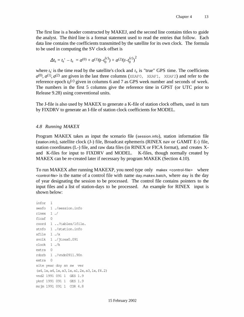
Chapter 4 13

15 February 2002

The first line is a header constructed by MAKEJ, and the second line contains titles to guidethe analyst. The third line is a format statement used to read the entries that follow. Eachdata line contains the coefficients transmitted by the satellite for its own clock. The formulato be used in computing the SV clock offset is

∆ts = ts' – ts = a(0) + a(1)(t–t0(c)) + a(2)(t–t0

(c))2

where ts' is the time read by the satellite's clock and ts is "true" GPS time. The coefficientsa(0), a(1), a(2) are given in the last three columns (XEAF0, XEAF1, XEAF2) and refer to thereference epoch t0(c) given in columns 6 and 7 as GPS week number and seconds of week.The numbers in the first 5 columns give the reference time in GPST (or UTC prior toRelease 9.28) using conventional units.

The J-file is also used by MAKEX to generate a K-file of station clock offsets, used in turnby FIXDRV to generate an I-file of station clock coefficients for MODEL.

4.8 Running MAKEX

Program MAKEX takes as input the scenario file (session.info), station information file(station.info), satellite clock (J-) file, Broadcast ephemeris (RINEX nav or GAMIT E-) file,station coordinates (L-) file, and raw data files (in RINEX or FICA format), and creates X-and K-files for input to FIXDRV and MODEL. K-files, though normally created byMAKEX can be re-created later if necessary by program MAKEK (Section 4.10).

To run MAKEX after running MAKEXP, you need type only makex <control-file> where<control-file> is the name of a control file with name day.makex.batch, where day is the dayof year designating the session to be processed. The control file contains pointers to theinput files and a list of station-days to be processed. An example for RINEX input isshown below:

infor 1

sesfo 1 ./session.info

rinex 1 ./

ficaf 0

coord 1 ../tables/lfile.

stnfo 1 ./station.info

xfile 1 ./x

svclk 1 ./jtrex0.091

clock 1 ./k

extra 0

rdorb 1 ./vndn0911.90n

extra 0

site year doy sn sw ver

(a4,1x,a4,1x,a3,1x,a1,2x,a3,1x,f4.2)

vnd2 1991 091 1 GES 1.9

yknf 1991 091 1 GES 1.9

mojm 1991 091 1 COR 4.8

Chapter 4 14

15 February 2002

vndn 1991 091 1 TRM 3.25

The first 12 lines indicate which of the input and output files are to be used and thedirectories in which they reside. The first six columns are not read by the program butprovide hints to the users (all lines must be present in the order given). A "1" following thename indicates that the file is to be used (input or output), a "0" that it will not be used.Complete file names are useful for documentation, but if the file (or link) is in the workingdirectory (i.e., the one in which MAKEX is being run), an abbreviated filename may beused (see, e.g., the rinex and stnclk entries above). For the input RINEX or FICAfiles, no filename is given since MAKEX constructs the filename from the station and daynames which follow in the input stream. FICA files must be named [ site ][y ].[day ].fic (notethat only the last digit of the year is used, with no session number), and RINEX files[si te] [d a y ][f].[yr ]o , where f is the file sequence number and o indicates that it is an"observation" file. Similarly, for X- and K- files, only the first letter is given. In theabove example, if the input data file were FICA, the rinex entry would have been "0" and " ./" (or directory path) would appear after ficaf. The GAMIT E-file (rdorb above) issimply an orbit file in either RINEX nav-file format or FICA Block 9 (TI4100) format(created with FICACHOP). The first line gives the information file, a log of MAKEXruns written to the current directory with name dd.makex.infor (091.makex.infor in theexample given).

Line 13 of the batch input is a comment that provides column headers for the list of stationfiles which follow. Line 14 gives the format for reading the key characters of the site filename. The format shown in the example allows reading of a four-character site code(VND2), the year (1991), session number (1), and the day number (091). In the currentGAMIT release, the session number should always be 0 or 1 (treated equivalently insideGAMIT) since the software does not yet support multiple sessions in the naming of X-files(multiple sessions can be combined by SOLVE in estimation, but that's another story—seeSection 5.6). Beginning with GAMIT release 9.6 (MAKEX version 9.57), MAKEX willscan all RINEX or FICA files for data within the span requested in session.info, so you caninclude within the day directory multiple RINEX filenames with arbitrary session numbers.If you have not used one of the sh_link_rinex scripts and want to have MAKEX search fordata, you can specify one or more directories in the rinex or fica lines of the batch file;e.g.,

rinex 1 ../rinex/scign/ ../rinex/bard/ ../rinex/igs/

The receiver software (or firmware) and version in the last two fields of the MAKEX batchinput file are required in order to have time tags correctly matched. The 3-charactersoftware ID is derived by MAKEXP from the receiver type and software version enteredinto station.info. Designators for software versions currently supported, and theirsampling times are listed in Table 4.1 and documented in subroutine gamit/makex/sett im.f. In several cases, we have arbitrarily added an additional digit to the version number inorder to distinguish time tags set by the operator.

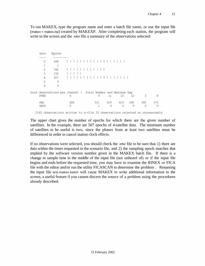
Chapter 4 15

15 February 2002

To run MAKEX, type the program name and enter a batch file name, or use the input file(makex < makex.inp) created by MAKEXP. After completing each station, the program willwrite to the screen and the .infor file a summary of the observations selected:

Sats Epochs---- ---------

0 498 ! ! ! ! ! ! ! ! ! ! ! ! ! ! ! ! ! !1 12 342 ! ! ! ! ! ! ! ! ! ! ! !3 152 ! ! ! ! !4 507 ! ! ! ! ! ! ! ! ! ! ! ! ! ! ! ! ! ! !5 06 0

Good observations per channel : Total Number and Maximum GapPRNS 6 9 11 13 12 3 8

OBS 606 511 419 619 240 395 375GAPS 0 1 0 2 0 0 0

3165 observations written to x-file 35 observations rejected as unreasonable

The upper chart gives the number of epochs for which there are the given number ofsatellites. In the example, there are 507 epochs of 4-satellite data. The minimum numberof satellites to be useful is two, since the phases from at least two satellites must bedifferenced in order to cancel station clock effects.

If no observations were selected, you should check the .infor file to be sure that 1) there aredata within the times requested in the scenario file, and 2) the sampling epoch matches thatimplied by the software version number given in the MAKEX batch file. If there is achange in sample time in the middle of the input file (not unheard of) or if the input filebegins and ends before the requested time, you may have to examine the RINEX or FICAfile with the editor and/or run the utility FICASCAN to determine the problem . Renamingthe input file test.makex.batch will cause MAKEX to write additional information to thescreen, a useful feature if you cannot discern the source of a problem using the proceduresalready described.

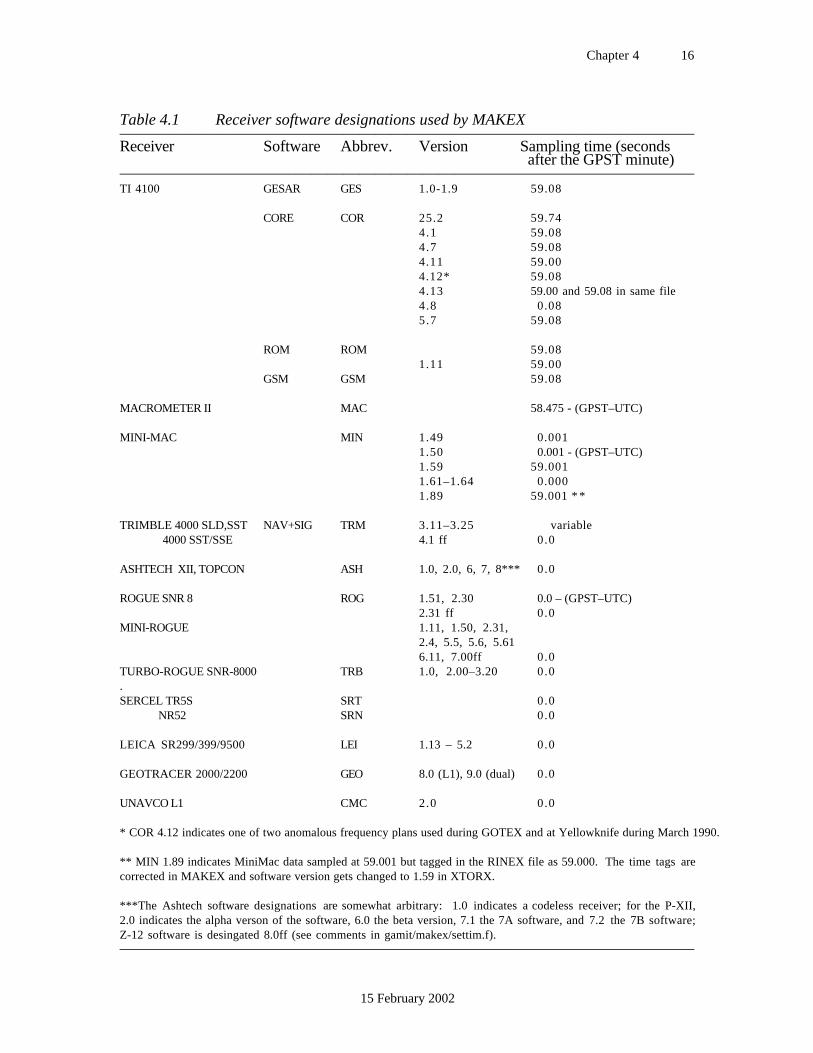
Chapter 4 16

15 February 2002

Table 4.1 Receiver software designations used by MAKEX————————————————————————————————————Receiver Software Abbrev. Version Sampling time (seconds

after the GPST minute)————————————————————————————————————TI 4100 GESAR GES 1.0-1.9 59.08

CORE COR 25.2 59.744.1 59.084.7 59.084.11 59.004.12* 59.084.13 59.00 and 59.08 in same file4.8 0.085.7 59.08

ROM ROM 59.081.11 59.00

GSM GSM 59.08

MACROMETER II MAC 58.475 - (GPST–UTC)

MINI-MAC MIN 1.49 0.0011.50 0.001 - (GPST–UTC)1.59 59.0011.61–1.64 0.0001.89 59.001 * *

TRIMBLE 4000 SLD,SST NAV+SIG TRM 3.11–3.25 variable 4000 SST/SSE 4.1 ff 0.0

ASHTECH XII, TOPCON ASH 1.0, 2.0, 6, 7, 8*** 0.0

ROGUE SNR 8 ROG 1.51, 2.30 0.0 – (GPST–UTC)2.31 ff 0.0

MINI-ROGUE 1.11, 1.50, 2.31,2.4, 5.5, 5.6, 5.616.11, 7.00ff 0.0

TURBO-ROGUE SNR-8000 TRB 1.0, 2.00–3.20 0.0.SERCEL TR5S SRT 0.0 NR52 SRN 0.0

LEICA SR299/399/9500 LEI 1.13 – 5.2 0.0

GEOTRACER 2000/2200 GEO 8.0 (L1), 9.0 (dual) 0.0

UNAVCO L1 CMC 2.0 0.0

* COR 4.12 indicates one of two anomalous frequency plans used during GOTEX and at Yellowknife during March 1990.

** MIN 1.89 indicates MiniMac data sampled at 59.001 but tagged in the RINEX file as 59.000. The time tags arecorrected in MAKEX and software version gets changed to 1.59 in XTORX.

***The Ashtech software designations are somewhat arbitrary: 1.0 indicates a codeless receiver; for the P-XII,2.0 indicates the alpha verson of the software, 6.0 the beta version, 7.1 the 7A software, and 7.2 the 7B software;Z-12 software is desingated 8.0ff (see comments in gamit/makex/settim.f).––––––––––––––––––––––––––––––––––––––––––––––––––––––––––––––––––––––––

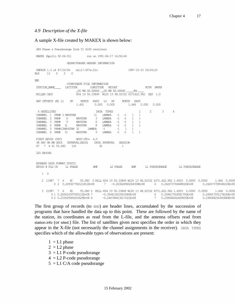
Chapter 4 17

15 February 2002

4.9 Description of the X-file

A sample X-file created by MAKEX is shown below:

GPS Phase & Pseudorange from TI 4100 receivers

MAKEX (Apollo 92-06-01) run on 1991-06-17 16:50:44

GESAR/PHASER HEADER INFORMATION

UNPACK 1.3 of 87/10/06 mill7.007a.fic 1987-10-15 18:04:23BLK 13 0 3 0

END COORDINATE FILE INFORMATION STATION_NAME____ LATITUDE LONGITUDE HEIGHT RCVR SWVER _DG MN SS.SSSSS __DG MN SS.SSSSS ____(M).___ MILLER CADT N34 19 50.33849 W120 13 48.02332 6371422.962 GES 1.0

ANT OFFSETS (M) L1 UP NORTH EAST L2 UP NORTH EAST 1.491 0.000 0.000 1.466 0.000 0.000

6 SATELLITES DATA TYPES 1 2 3 4 CHANNEL 1 PRN# 3 NAVSTAR 11 LAMBDA -1 -1 1 1 CHANNEL 2 PRN# 6 NAVSTAR 3 LAMBDA -1 -1 1 1 CHANNEL 3 PRN# 9 NAVSTAR 6 LAMBDA -1 -1 1 1 CHANNEL 4 PRN# 11 NAVSTAR 8 LAMBDA -1 -1 1 1 CHANNEL 5 PRN#12NAVSTAR 10 LAMBDA -1 -1 1 1 CHANNEL 6 PRN# 13 NAVSTAR 9 LAMBDA -1 -1 1 1

FIRST EPOCH (UTC) GPST-UTC= 4.0 YR DAY HR MN SECS INTERVAL(SECS) DATA INTERVAL SESSION 87 7 6 41 55.080 120 30 1

225 EPOCHS

EPANDED DATA FORMAT STATIC EPOCH # FLG CH L1 PHASE AMP L2 PHASE AMP L1 PSEUDORANGE L2 PSEUDORANGE

1 0

2 11987 7 6 43 55.080 0 MILL N34 19 50.33849 W120 13 48.02332 6371.422.962 1.4910 0.0000 0.0000 1.466 0.0000 0 2 0.209327782121811E+08 7 -0.263626960264358E+08 6 0.242673706688020E+08 0.242673708548210E+08

3 21987 7 6 45 55.080 0 MILL N34 19 50.33849 W120 13 48.02332 6371.422.962 1.4910 0.0000 0.0000 1.466 0.0000 0 1 0.283412097505112E+08 7 -0.354413610923080E+08 6 0.249617918581700E+08 0.249617931178260E+08 0 2 0.233529585203629E+08 8 -0.244768413617021E+08 7 0.238068262469650E+08 0.238068256365880E+08

The first group of records (to END) are header lines, accumulated by the succession ofprograms that have handled the data up to this point. These are followed by the name ofthe station, its coordinates as read from the L-file, and the antenna offsets read fromstation.info (or sited.) file. The list of satellites given next specifies the order in which theyappear in the X-file (not necessarily the channel assignments in the receiver). DATA TYPESspecifies which of the allowable types of observations are present:

1 = L1 phase2 = L2 phase3 = L1 P-code pseudorange4 = L2 P-code pseudorange5 = L1 C/A code pseudorange

Chapter 4 18

15 February 2002

The LAMBDA, or "wavelength" codes given for each channel indicate, for each data type,whether it is ambiguous and whether the ambiguity spacing is full or half wavelength. Allphase observables are converted to full wavelength on the X-file.

0 = observable is not present for this channel-1 = ambiguity spacing is one wavelength (e.g., 19 cm for L1 phase)-2 = ambiguity spacing is one-half wavelength1 = no ambiguity2 = no ambiguity (original observable was half wavelength)

The usual value of LAMBDA is -1 (code-correlating receivers) or -2 (L2 from codelessreceivers) for phase observations, 1 for pseudo-range observations. X-file data arerequired to be evenly spaced, so the observation times are specified by a start epoch, anobservation interval, and the number of epochs. INTERVAL is the actual interval on the X-file; DATA INTERVAL refers to the raw data file interval (usually the receiver samplinginterval) and is used by the editing routines to determine if gaps in the X-file are due tosparse sampling or missing data. The observations at each time are identified by an epochnumber, an integer which specifies the number of satellites for which there are data at thatepoch, and the GPS time (or UTC prior to Release 9.28). The station coordinates andantenna offsets are repeated at each epoch to allow for kinematic processing. For staticprocessing with a change of antenna height during the session, the X-file will also reflectthe change, but values read from station.info during actual processing (by programMODEL) override those in the X-file. Then for each channel, there are eight numbersgiven: a flag indicating whether the data are valid (=0) or have been flagged (set non-zero—see gamit/includes/errflg.h for a key) by other modules; the channel number; theL1 phase (cycles); the amplitude of the L1 signal using RINEX conventions; the L2 phase;the L2 amplitude; the L1 pseudo-range (meters); and the L2 pseudo-range. Note thatphases in the X-files are in the "Doppler" convention (increasing phase is decreasingrange), and therefore have the opposite sign to phases in the corresponding RINEX files.

4.10 Creating station clock (K- and I-) files

The offset from GPS time (or UTC) of each receiver's clock must be accounted for inmodeling the theoretical value of the phase observations at each epoch. If the positions ofthe receiver and a satellite are known, along with the offset of the satellite's clock, then thepseudorange observation provides a direct measure of the receiver clock offset:

∆tr = p1 – ρ

c + ∆t s

where ρ is the calculated range to the satellite, p1 is the observed pseudo-range and c is thespeed of light. Recall (Section 2.1) that an accuracy of about one microsecond in receiver-clock offset is necessary to achieve an accuracy of one millimeter in the estimated baselinevector. In order to achieve this accuracy, the computation is performed in MODEL usingthe station and satellite positions (from the L- and T-files) calculated for the theoreticalphase observable. In this case, one microsecond (300 m) in the theoretical values is easily

Chapter 4 19

15 February 2002

achieved. Sufficient accuracy in the measured pseudorange is also achieved easily if P-code range is available. If only C/A code is available, and particularly under conditions ofselective availability (SA), some care must be exercised. At present, MODEL computes thereceiver-clock offset using an average of values calculated from all of the satellites visible ateach epoch, detecting and removing anomalous values caused by pseudorange outliers orbad SV clock values.

Strictly speaking, it is not necessary to provide GAMIT with any more information about areceiver's clock than that incorporated in the pseudoranges at each epoch. There are a fewpractical reasons, however, why it is useful to generate a more explicit model of thereceiver-clock behavior at an earlier stage in the processing. Doing so provides a way ofdetecting poor receiver performance, for example. Also, for receivers with poor andunmodeled clocks numerical problems are sometimes created in SOLVE when there areseveral-hour gaps between observations. Hence we input to MODEL tables of coefficientswhich effectively model these variations. For the receiver clock, MAKEX generates anestimate of the offset at an epoch interval of 120s for Ashtech and Trimble receivers, whoseclocks reset often, and 600s for other receivers, using satellite elements from the broadcastephemeris. These estimates are written into the K-file:

RDRK 14 1992 73 19 43 53.0000 0.07132594 0.00018337 0.00007289 RDRK 18 1992 73 19 43 53.0000 0.07109620 -0.00000169 0.00007330 RDRK 19 1992 73 19 43 53.0000 0.07405061 0.00000424 0.00007332 RDRK 14 1992 73 19 45 53.0000 0.07153746 0.00018337 0.00001910 RDRK 18 1992 73 19 45 53.0000 0.07095191 -0.00000169 0.00001955 RDRK 19 1992 73 19 45 53.0000 0.07389223 0.00000424 0.00001934 RDRK 14 1992 73 19 47 53.0000 0.07175308 0.00018337 0.00096434 RDRK 18 1992 73 19 47 53.0000 0.07080949 -0.00000169 0.00096493 RDRK 19 1992 73 19 47 53.0000 0.07373656 0.00000424 0.00096463 RDRK 14 1992 73 19 49 53.0000 0.07197269 0.00018337 0.00090899 RDRK 18 1992 73 19 49 53.0000 0.07066900 -0.00000169 0.00090950 RDRK 19 1992 73 19 49 53.0000 0.07358361 0.00000424 0.00090935

The first column gives the station code, followed by the satellite PRN number, year, day ofyear, hours, minutes, and seconds (always UTC). The eighth column is the observedpseudo-range to the satellite at the time given, in units of seconds, followed by the offset ofthe satellite clock (from GPS time) computed from the transmitted clock corrections. Thefinal number is the receiver clock correction computed using the formula above.

Any differences in receiver clock values computed using the data from different satellites atthe same time are due to errors in the pseudo-range measurements, the satellite clockmodels, or the geometrical models (station coordinates and satellite ephemeris). In theabove K-file, for example, the corrections computed at 19h 43m 53.s using data fromsatellites 14, 10, and 19 differ by up to 0.4 microseconds, equivalent to a radial positionerror of 120 meters (probably due to errors in the broadcast ephemeris). Differencesbetween receiver clock values computed for a given satellite at different times could reflectmodel errors but are usually dominated by actual receiver clock drift. In our example, thereis a change between 19h 43mand 19h 45mof 54 microseconds, indicating a drift in thereceiver oscillator of 4.5 parts in 107 (54x10-6 / 120 ). This high drift rate is typical of thecrystal oscillators in many of today's lightweight receivers (the above example was a

Chapter 4 20

15 February 2002

Trimble 4000 SST). More stable (thermally controlled) crystals can achieve stabilities of 1part in 108 (TI 4100) or better (Macrometer II). Rubidium, cesium, or hydrogen-maseroscillators can achieve even higher stabilities (10-11 to 10-15 ).

The ~1 ms jump in clock value at 19h 47m 53.s is a feature of the Trimble 4000 SST andAshtech P12 receivers, indicating that the clock has been reset to keep it within 1 ms of thenominal sampling time. Both the recorded sampling time and the pseudorangemeasurement will show a discontinuity of exactly 1 ms. Some RINEX translators can beset to remove the discontinuity at translation, but this is not necessary since MODEL willaccount for it in its epoch-by-epoch estimate of the receiver clock offset, and FIXDRV willremove the discontinuities in fitting the low-order polynomial used in modeling the phaseobservations.

It is possible to have anomalous ("bad") values in the K-file—computed clock offsets thatare many milliseconds off due to bad pseudorange measurements. The presence of theseanomalous blunder points will be indicated by very large residuals (> 500 microseconds) inthe polynomial clock fit done by FIXDRV. You can tabulate and plot the fit residuals usingthe script sh_plotk, but usually the quickest way to find the problem is just to scan visuallythe last column of the K-file; most often the bad values are among the first few of thesession. If sh_plotk or the polynomial fit in FIXDRV shows the clock behavior to be bad,and you determine that the problem is not a bad K-file, then you should proceed but be onthe alert for a problem with this station in the analysis. Rapidly drifting clocks are morelikely to cause an abnormal number of cycle slips (see the autcln.sum file, described inSection 6.2). Large jumps in the clock or rapid drift accompanied by several-hour gaps inthe data may cause the residuals to get large, introducing numerical problems in SOLVE.The best remedy for this is to use the apply_phase_clk option in AUTCLN (see Section6.2).

FIXDRV will read the K-file for each site and create a session I-file, similar to the J-file forsatellite clocks, tabulating the coefficients of a low-order polynomial for each receiver'sclock. If you want to recreate a K-file after running MAKEX, you can do so easily byrunning MAKEK, which will prompt you for the name of input E-, L-, and X-files and forthe tabulation interval.

Chapter 5 1

14 February 2002

5. Batch Processing

5.1 Introduction

Batch processing is accomplished by invoking sequentially and with appropriate input filesthe GAMIT modules that perform the required computations. The command or "batch"files to invoke the modules are created, for each standard type of analysis, by programFIXDRV. The batch run set up by FIXDRV would typically go through the followingsteps:

• generation of an orbital ephemeris with partials (ARC)

• generation of residuals and partials (MODEL)

• automatic edit of residuals (AUTCLN)

• solution (CFMRG/SOLVE)

• regeneration of residuals and partials with an improved model (MODEL)

• automatic edit of residuals (AUTCLN)

• solution (CFMRG/SOLVE)

The double pass through MODEL and SOLVE serves two purposes: 1) the model obtainedfrom the first solution can be used to flatten the residuals, allowing for improved editingand also the display of post-fit (one-way) residuals for evaluation; 2) adjustments to stationcoordinates are reduced to a few centimeters, assuring that non-linearities do not degradethe final estimates. In most cases, the results of your processing can be assessed throughinspection of the print output (Q-file) of the final solution and the data statistics compiled byAUTCLN (autcln.sum.post). If there are problems, then one or more steps of the batch jobcan be run individually, or FIXDRV (and occasionally MAKEX) can be run to repeat thecomplete processing sequence.

If you have prepared the data in a "day" directory as described in Chapter 4, then youshould have available as files or links all of the tables necessary to run FIXDRV and toexecute the GAMIT batch run: station and scenario tables (station.info and session.info),ephemerides (G- and T-files), raw observations (X-file), satellite and station clock values(J- and K-files), a priori station coordinates (L-file), lunar and solar ephemerides (luntab.and soltab.), and tables for earth rotation values (nutabl., ut1., and pole.), TAI-UTC(leap.sec), geodetic datums (gdetic.dat), ocean tides (stations.oct and grid.oct), antennaphase-center offsets or models (antmod.dat), receiver and antenna names (rcvant.dat), andsatellite yaw parameters table (svnav.dat). Three additional files are needed: the list of X-files to be processed (D-file), and control tables for the analyses (sestbl. and sittbl.) Thesecan be easily created from templates (from gamit/example), as described below. If youhave used MAKEXP for data preparation, you will have already a D-file.

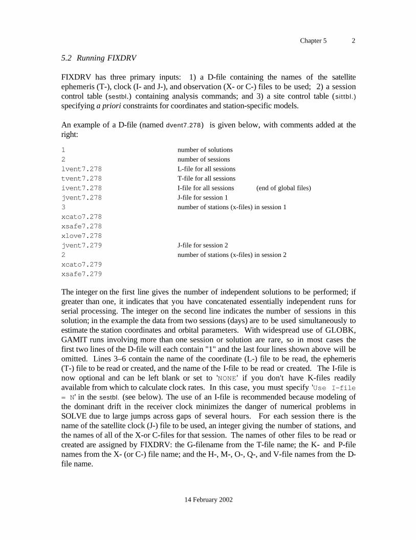
Chapter 5 2

14 February 2002

5.2 Running FIXDRV

FIXDRV has three primary inputs: 1) a D-file containing the names of the satelliteephemeris (T-), clock (I- and J-), and observation (X- or C-) files to be used; 2) a sessioncontrol table (sestbl.) containing analysis commands; and 3) a site control table (sittbl.)

specifying a priori constraints for coordinates and station-specific models.

An example of a D-file (named dvent7.278) is given below, with comments added at theright:

1 number of solutions

2 number of sessions

lvent7.278 L-file for all sessions

tvent7.278 T-file for all sessions

ivent7.278 I-file for all sessions (end of global files)

jvent7.278 J-file for session 1

3 number of stations (x-files) in session 1

xcato7.278xsafe7.278xlove7.278jvent7.279 J-file for session 2

2 number of stations (x-files) in session 2

xcato7.279xsafe7.279

The integer on the first line gives the number of independent solutions to be performed; ifgreater than one, it indicates that you have concatenated essentially independent runs forserial processing. The integer on the second line indicates the number of sessions in thissolution; in the example the data from two sessions (days) are to be used simultaneously toestimate the station coordinates and orbital parameters. With widespread use of GLOBK,GAMIT runs involving more than one session or solution are rare, so in most cases thefirst two lines of the D-file will each contain "1" and the last four lines shown above will beomitted. Lines 3–6 contain the name of the coordinate (L-) file to be read, the ephemeris(T-) file to be read or created, and the name of the I-file to be read or created. The I-file isnow optional and can be left blank or set to 'NONE' if you don't have K-files readilyavailable from which to calculate clock rates. In this case, you must specify 'Use I-file= N ' in the sestbl. (see below). The use of an I-file is recommended because modeling ofthe dominant drift in the receiver clock minimizes the danger of numerical problems inSOLVE due to large jumps across gaps of several hours. For each session there is thename of the satellite clock (J-) file to be used, an integer giving the number of stations, andthe names of all of the X-or C-files for that session. The names of other files to be read orcreated are assigned by FIXDRV: the G-filename from the T-file name; the K- and P-filenames from the X- (or C-) file name; and the H-, M-, O-, Q-, and V-file names from the D-file name.

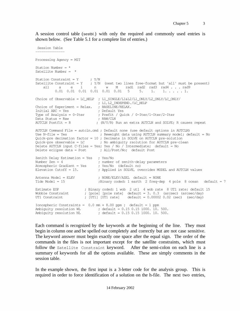
Chapter 5 3

14 February 2002

A session control table (sestbl.) with only the required and commonly used entries isshown below. (See Table 5.1 for a complete list of entries.)

Session Table---------------

Processing Agency = MIT

Station Number = *Satellite Number = *

Station Constraint = Y ; Y/NSatellite Constraint = Y ; Y/N (next two lines free-format but 'all' must be present) all a e i n w M rad1 rad2 rad3 rad4 . . . rad9 0.01 0.01 0.01 0.01 0.01 0.01 5 5. 1. 1. . . . . 1.

Choice of Observable = LC_HELP ; L1_SINGLE/L1&L2/L1_ONLY/L2_ONLY/LC_ONLY/ ; L1,L2_INDEPEND./LC_HELPChoice of Experiment = Relax. ; BASELINE/RELAX.Initial ARC = Yes ; Default YesType of Analysis = 0-Iter ; Prefit / Quick / 0-Iter/1-Iter/2-IterData Status = Raw ; RAW/CLNAUTCLN Postfit = R ; (N/Y/R) Run an extra AUTCLN and SOLVE; R causes repeat

AUTCLN Command File = autcln.cmd ; Default none (use default options in AUTCLN)Use N-file = Yes ; Reweight data using AUTCLN summary model; default = NoQuick-pre decimation factor = 10 ; Decimate in SOLVE on AUTCLN pre-solutionQuick-pre observable = LC ; No ambiguity rsolution for AUTCLN pre-cleanDelete AUTCLN input C-files = Yes; Yes / No / Intermediate; default = NoDelete eclipse data = Post ; All/Post/No; default Post

Zenith Delay Estimation = Yes ; Yes/NoNumber Zen = 4 ; number of zenith-delay parametersAtmospheric Gradient = Yes ; Yes/No (default no)Elevation Cutoff = 15. ; Applied in SOLVE, overrides MODEL and AUTCLN values

Antenna Model = ELEV ; NONE/ELEV/AZEL default = NONETide Model = 15 ;Binary coded: 1 earth 2 freq-dep 4 pole 8 ocean default = 7

Estimate EOP ; Binary coded: 1 wob 2 ut1 4 wob rate 8 UT1 rate; default 15Wobble Constraint ; [pole] [pole rate] default = 3. 0.3 (arcsec) (arcsec/day)UT1 Constraint ; [UT1] [UT1 rate] default = 0.00002 0.02 (sec) (sec/day)

Ionospheric Constraints = 0.0 mm + 8.00 ppm ; default = 1 ppmAmbiguity resolution WL ; default = 0.15 0.15 1000. 10. 500.Ambiguity resolution NL ; default = 0.15 0.15 1000. 10. 500.

Each command is recognized by the keywords at the beginning of the line. They mustbegin in column one and be spelled out completely and correctly but are not case sensitive.The keyword answer must begin exactly one space after the equal sign. The order of thecommands in the files is not important except for the satellite constraints, which mustfollow the Satellite Constraint keyword. After the semi-colon on each line is asummary of keywords for all the options available. These are simply comments in thesession table.

In the example shown, the first input is a 3-letter code for the analysis group. This isrequired in order to force identification of a solution on the h-file. The next two entries,

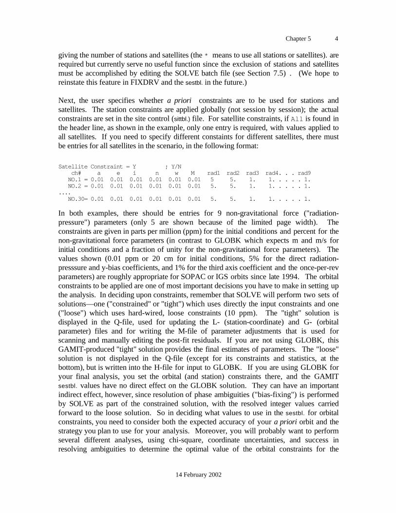
Chapter 5 4

14 February 2002

giving the number of stations and satellites (the * means to use all stations or satellites). arerequired but currently serve no useful function since the exclusion of stations and satellitesmust be accomplished by editing the SOLVE batch file (see Section 7.5) . (We hope toreinstate this feature in FIXDRV and the sestbl. in the future.)

Next, the user specifies whether a priori constraints are to be used for stations andsatellites. The station constraints are applied globally (not session by session); the actualconstraints are set in the site control (sittbl.) file. For satellite constraints, if All is found inthe header line, as shown in the example, only one entry is required, with values applied toall satellites. If you need to specify different constaints for different satellites, there mustbe entries for all satellites in the scenario, in the following format:

Satellite Constraint = Y ; Y/N ch# a e i n w M rad1 rad2 rad3 rad4. . . rad9 NO.1 = 0.01 0.01 0.01 0.01 0.01 0.01 5 5. 1. 1. . . . . 1. NO.2 = 0.01 0.01 0.01 0.01 0.01 0.01 5. 5. 1. 1. . . . . 1..... NO.30= 0.01 0.01 0.01 0.01 0.01 0.01 5. 5. 1. 1. . . . . 1.

In both examples, there should be entries for 9 non-gravitational force ("radiation-pressure") parameters (only 5 are shown because of the limited page width). Theconstraints are given in parts per million (ppm) for the initial conditions and percent for thenon-gravitational force parameters (in contrast to GLOBK which expects m and m/s forinitial conditions and a fraction of unity for the non-gravitational force parameters). Thevalues shown (0.01 ppm or 20 cm for initial conditions, 5% for the direct radiation-presssure and y-bias coefficients, and 1% for the third axis coefficient and the once-per-revparameters) are roughly appropriate for SOPAC or IGS orbits since late 1994. The orbitalconstraints to be applied are one of most important decisions you have to make in setting upthe analysis. In deciding upon constraints, remember that SOLVE will perform two sets ofsolutions—one ("constrained" or "tight") which uses directly the input constraints and one("loose") which uses hard-wired, loose constraints (10 ppm). The "tight" solution isdisplayed in the Q-file, used for updating the L- (station-coordinate) and G- (orbitalparameter) files and for writing the M-file of parameter adjustments that is used forscanning and manually editing the post-fit residuals. If you are not using GLOBK, thisGAMIT-produced "tight" solution provides the final estimates of parameters. The "loose"solution is not displayed in the Q-file (except for its constraints and statistics, at thebottom), but is written into the H-file for input to GLOBK. If you are using GLOBK foryour final analysis, you set the orbital (and station) constraints there, and the GAMITsestbl. values have no direct effect on the GLOBK solution. They can have an importantindirect effect, however, since resolution of phase ambiguities ("bias-fixing") is performedby SOLVE as part of the constrained solution, with the resolved integer values carriedforward to the loose solution. So in deciding what values to use in the sestbl. for orbitalconstraints, you need to consider both the expected accuracy of your a priori orbit and thestrategy you plan to use for your analysis. Moreover, you will probably want to performseveral different analyses, using chi-square, coordinate uncertainties, and success inresolving ambiguities to determine the optimal value of the orbital constraints for the

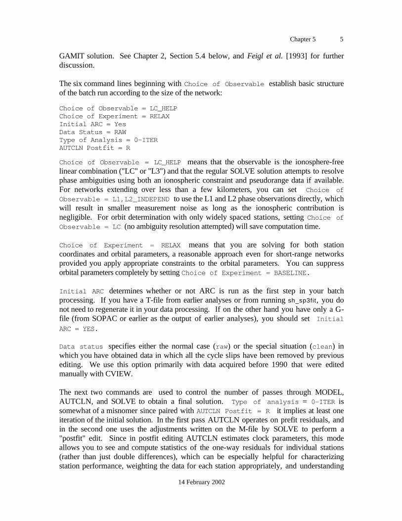
Chapter 5 5

14 February 2002

GAMIT solution. See Chapter 2, Section 5.4 below, and Feigl et al. [1993] for furtherdiscussion.

The six command lines beginning with Choice of Observable establish basic structureof the batch run according to the size of the network:

Choice of Observable = LC_HELPChoice of Experiment = RELAXInitial ARC = YesData Status = RAWType of Analysis = 0-ITERAUTCLN Postfit = R

Choice of Observable = LC_HELP means that the observable is the ionosphere-freelinear combination ("LC" or "L3") and that the regular SOLVE solution attempts to resolvephase ambiguities using both an ionospheric constraint and pseudorange data if available.For networks extending over less than a few kilometers, you can set Choice ofObservable = L1,L2_INDEPEND to use the L1 and L2 phase observations directly, whichwill result in smaller measurement noise as long as the ionospheric contribution isnegligible. For orbit determination with only widely spaced stations, setting Choice ofObservable = LC (no ambiguity resolution attempted) will save computation time.

Choice of Experiment = RELAX means that you are solving for both stationcoordinates and orbital parameters, a reasonable approach even for short-range networksprovided you apply appropriate constraints to the orbital parameters. You can suppressorbital parameters completely by setting Choice of Experiment = BASELINE.

Initial ARC determines whether or not ARC is run as the first step in your batchprocessing. If you have a T-file from earlier analyses or from running sh_sp3fit, you donot need to regenerate it in your data processing. If on the other hand you have only a G-file (from SOPAC or earlier as the output of earlier analyses), you should set Initial

ARC = YES.

Data status specifies either the normal case (raw ) or the special situation (clean ) inwhich you have obtained data in which all the cycle slips have been removed by previousediting. We use this option primarily with data acquired before 1990 that were editedmanually with CVIEW.

The next two commands are used to control the number of passes through MODEL,AUTCLN, and SOLVE to obtain a final solution. Type of analysis = 0-ITER issomewhat of a misnomer since paired with AUTCLN Postfit = R it implies at least oneiteration of the initial solution. In the first pass AUTCLN operates on prefit residuals, andin the second one uses the adjustments written on the M-file by SOLVE to perform a"postfit" edit. Since in postfit editing AUTCLN estimates clock parameters, this modeallows you to see and compute statistics of the one-way residuals for individual stations(rather than just double differences), which can be especially helpful for characterizingstation performance, weighting the data for each station appropriately, and understanding

Chapter 5 6

14 February 2002

problems in the solution. With AUTCLN Postfit = R (for "redo"), as opposed to simplyYes), if the quality of fit improves significantly between these two solutions (ratio ofnrms values > 1.5), a third one is performed to insure linearity in the adjustments. Otheroptions for Type of analysis , described later, are useful mainly for primary orbitdetermination (at SOPAC) and specialized solutions.

AUTCLN Command file allows you to input controls for AUTCLN. The autcln.cmd fileshould be present and contain the postfit controls apply_phs_clk , use_postfit , and(usually) pf_remove_bf described in Section 6.2. The command Use N-file = Yesinvokes the shell-script sh_segelv to read the summary file from the postfit AUTCLN runand write into a file to be read by SOLVE values of coefficients of an elevation-dependentmodel for the a priori errors assigned to the data from each station (see Data Weighting laterin this section, but note that if Use N-file is specified, you do not need to also specifyStation Error —and in fact, you should not do so because you likely want uniformweighting to be used in the pre-fit SOLVE run).

To reduce the computational cost of using the post-fit mode, you can reduce the samplingrate (Quick-pre decimation factor = 10) and by-pass ambiguity resolution (Quick-pre observable = LC) in the initial solution. The next controls determine whether C-files are saved or regenerated. To take full advantage of the iterative scheme, you shouldset Delete AUTCLN input C-files = Yes. This option is also most conserving ofdisk space but will increase run time a small amount compared with the saving the initial C-files temporarily ( Intermediate ) or permanently ( No ). Unless you suspect a problemwith AUTCLN and want to examine all the input and output C-files, there is no need toelect this last option.

The AUTCLN command file is also the mechanism for explicitly removing from thesolution data which might be corrupted by satellite rotations during or after eclipses or by abad clock determination. These features are implemented by Delete eclipse data andEdit AUTCLN command file, explained below Table 5.1. In Release 9.6 both of theseoptions, as well as postfit editing are commanded in the batch file using the new scriptsh_autedit (replacing sh_autedt and avedit. The script reads the "base" autcln.cmd file andedits it appropriately to incorporate eclipse and clock editing, creating for the batch run theAUTCLN input file(s) autcln.cmd.prefit and (optionally) autcln.cmd.postfit.

The most appropriate way of handling the atmosphere depends on the size of the networkand the accuracy desired. For networks less than a few kilometers in extent, theatmospheric delay effectively cancels between stations, so you do not want to estimate anyatmospheric parameters. For larger networks, you should estimate one or more zenith delayparameters for each station ( Zenith Delay Estimation = Y). The zenith delayparameters for regional stations will be highly correlated, but there is sufficient precision inthe estimation algorithm that these high correlations will not degrade your estimates ofstation coordinates and the differences in zenith delay between stations will be welldetermined. (If you wish to see in the output the uncertainty of the differences, then youcan add tight constraints to one of the zenith delays in the SOLVE batch file; see Section

Chapter 5 7

14 February 2002

7.5). The default is to estimate a single zenith delay for each station with an a prioriconstraint of 0.5 meters. You may allow a variation in the zenith delay during theobservation span by specifying a piecewise-linear model with stochastic constraints.Number Zen is the number of "knots" in the model; hence, for a new value every 3 hrs of a24-hr session, you would set Number Zen = 9 . A knot spacing between 1 and 4 hours isreasonable for most situations, the trade off being resolution versus program size and runtime. The allowed variation between tabular points in the estimation is defined by a Gauss-Markov process with a default value of 0.02 m / √hr. The default correlation time is set to100 hr, making the process effectively a random walk. Specification of these parameters isdocumented in Table 5.1 and discussed further in Section 8.3. A new feature with release9.58 is the ability to estimate a north-south and an east-west gradient in atmospheric delay,given as the differences in meters at 10 degrees elevation (see Section 8.4). The final entryfor atmospheric modeling is the minimum elevation angle for accepting observations. Inthe presence of modeling deficiencies for the atmospheric delay or the phase-centervariations of the antenna, estimated station heights can be quite sensitive to this cutoffangle.

Antenna Model refers to the use an elevation-dependent or elevation-and-azimuth-dependent model for the effective phase center of the receiver antenna. The default is to useno model, but elevation-dependent models have now been developed by NOAA(http:/www.grdl.noaa.gov/GRD/GPS ) for most commonly used antennas and areincluded in the GAMIT file antmod.dat (see also rcvant.dat).

Tide Model , used to apply models for the time-variable displacements in stationcoordinates due to tides, is a binary-coded variable, allowing you to easily select anycombination you want to use or test. The first (1) and second (2) bits control theIERS/IGS standard models for diurnal and semi-diurnal Earth tides [IERS Conventions1996, IERS Tech. Note 21, Observatoire de Paris, July, 1996] and should always be set.The third (4) bit controls the pole tide, also coded according to IERS standards. Thiscomponent is not always applied in GAMIT, however, because it has only long-period(primarily annual and 460 days) effects on station coordinates and can be added byGLOBK. (GLOBK will detect whether it has been applied in GAMIT and apply it or not,as instructed, to make the H-files from different processing compatible.) The mostcomplicated part of the tide model is loading due to ocean tides because this effect must becomputed (external to GAMIT) using a convolution of a model of the ocean tidesthemselves and the geometry of the land-sea interface. With Release 10.0 we haveimplemented corrections based on the model developed by Hans-Georg Scherneck ofChalmers University (Sweden). These are applied in one of two ways—by reading from atable (stations.oct) containing corrections for 465 global tracking stations(GPS/SLR/VLBI), or by interpolating from a 0.5 x 0.5 degree global grid (grid.oct). Ineither case, program OCTTAB obtains the horizontal and vertical amplitudes and phases of11 tidal constituents for each station in the session (D-file), and writes these into a U-filethat has a format similar to the Scherneck station table. The values from the station tablewill be used if the station being processed is within 10 km of a station given in the table;otherwise they will be interpolated from the grid. The file octtab.out records the source of

Chapter 5 8

14 February 2002

tides for each station in the session. The Scherneck station table (stations.oct) and the U-file are relatively small and can be easily examined. The grid table (grid.oct) , however,is large and has been formatted (at MIT) as a direct-access binary file to conserve space andallow for efficient reading. The version distributed with the software is written with big-ENDIAN binary representation (used by Sun and HP), but OCTTAB automaticallyconverts it to little-ENDIAN when it is read on a little-ENDIAN (Intel or DEC) machine.

By default corrections to Earth rotation parameters are estimated for each session(Estimate EOP = 15). If your solution includes 24-hr tracking from a global set ofstations, then you can estimate well pole ("wobble") position and UT1 rate but not a UT1offset since this is perfectly correlated with the nodes of the satellites' orbits. In order tohave a full convariance matrix available for GLOBK, however, it is preferable (andnecessary in versions prior to January, 1995) to turn on all six EOPs but with tightconstraints on the UT1 offset in the GAMIT solution. The default constraints for UT1 rateand pole position and rate are rather loose, so these should be tightened to match theuncertainty in your a priori tables (~ 0.0001 sec/day, 0.001 arcsec, 0.0005 arc/day forIERS Bulletin A or B finals) if you have only a regional network and want to assesscarefully the results of the GAMIT analysis.

The final set of the sestbl. inputs shown control resolution of phase ambiguities in thesolution. Unfortunately, no GPS analysis group or software package (to our knowledge)has automated ambiguity resolution to the point where you can uncritically apply aparticular algorithm to all situations. GAMIT uses a combination of pseudo-rangeobservations, if available, and phase observations with an ionospheric constraint to provideflexibility and redundancy. This approach, together with some fairly conservativethreshhold criteria makes the process reasonably but not perfectly failsafe for mostnetworks. Tuning the algorithm for your particular network and evaluating the results isdiscussed in Section 5.5.

There are a number of optional entries in the sestbl. that may be invoked for special casesand to excercise greater control over the processing. These are summarized in Table 5.1and further discussed below.

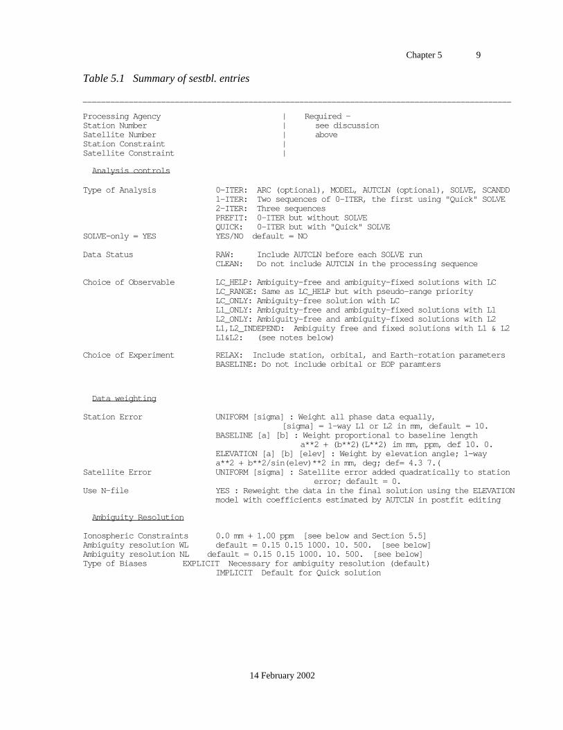
Chapter 5 9

14 February 2002

Table 5.1 Summary of sestbl. entries

_____________________________________________________________________________________________

Processing Agency | Required —Station Number | see discussionSatellite Number | aboveStation Constraint |Satellite Constraint |

Analysis controls

Type of Analysis 0-ITER: ARC (optional), MODEL, AUTCLN (optional), SOLVE, SCANDD1-ITER: Two sequences of 0-ITER, the first using "Quick" SOLVE2-ITER: Three sequencesPREFIT: 0-ITER but without SOLVEQUICK: 0-ITER but with "Quick" SOLVE

SOLVE-only = YES YES/NO default = NO

Data Status RAW: Include AUTCLN before each SOLVE runCLEAN: Do not include AUTCLN in the processing sequence

Choice of Observable LC_HELP: Ambiguity-free and ambiguity-fixed solutions with LCLC_RANGE: Same as LC_HELP but with pseudo-range priorityLC_ONLY: Ambiguity-free solution with LCL1_ONLY: Ambiguity-free and ambiguity-fixed solutions with L1L2_ONLY: Ambiguity-free and ambiguity-fixed solutions with L2L1,L2_INDEPEND: Ambiguity free and fixed solutions with L1 & L2L1&L2: (see notes below)

Choice of Experiment RELAX: Include station, orbital, and Earth-rotation parametersBASELINE: Do not include orbital or EOP paramters

Data weighting

Station Error UNIFORM [sigma] : Weight all phase data equally,[sigma] = 1-way L1 or L2 in mm, default = 10.

BASELINE [a] [b] : Weight proportional to baseline length a**2 + (b**2)(L**2) im mm, ppm, def 10. 0.

ELEVATION [a] [b] [elev] : Weight by elevation angle; 1-way a**2 + b**2/sin(elev)**2 in mm, deg; def= 4.3 7.(

Satellite Error UNIFORM [sigma] : Satellite error added quadratically to station error; default = 0.

Use N-file YES : Reweight the data in the final solution using the ELEVATION model with coefficients estimated by AUTCLN in postfit editing

Ambiguity Resolution

Ionospheric Constraints 0.0 mm + 1.00 ppm [see below and Section 5.5]Ambiguity resolution WL default = 0.15 0.15 1000. 10. 500. [see below]Ambiguity resolution NL default = 0.15 0.15 1000. 10. 500. [see below]Type of Biases EXPLICIT Necessary for ambiguity resolution (default)

IMPLICIT Default for Quick solution

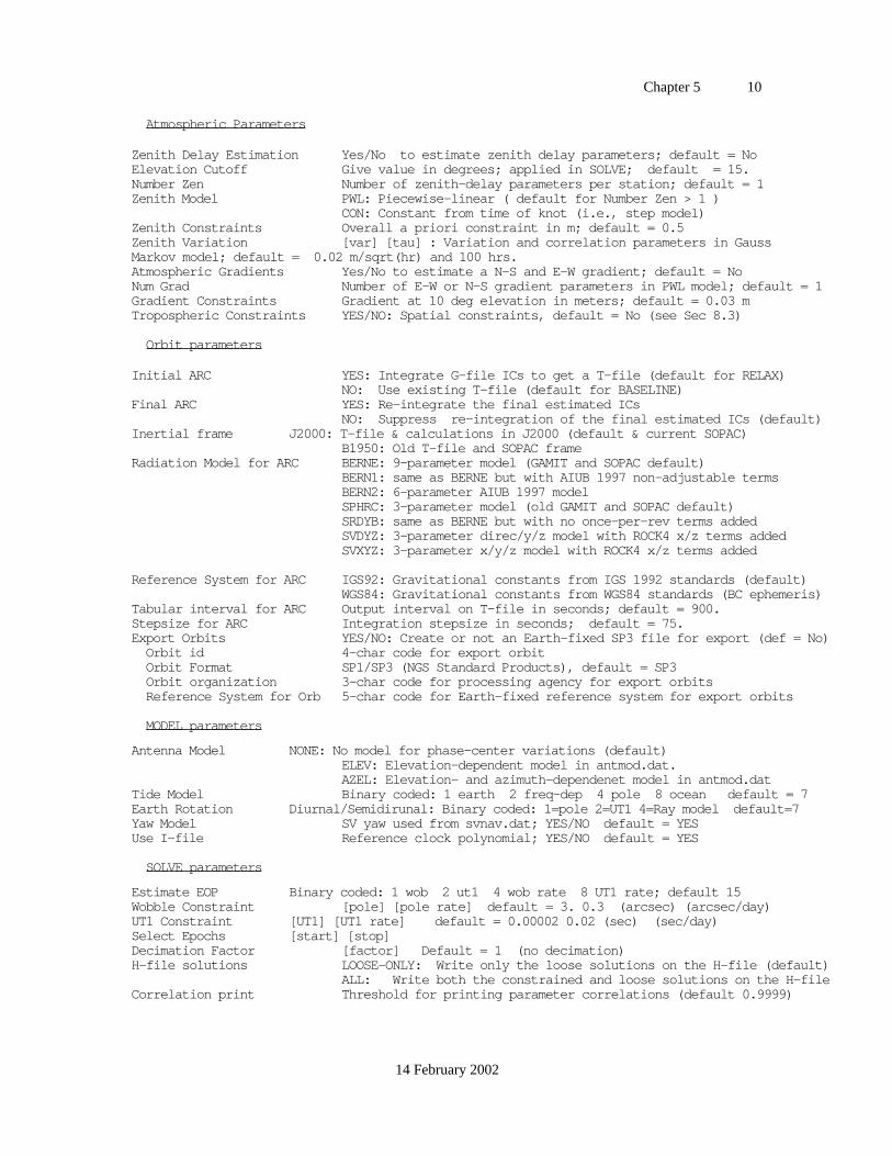
Chapter 5 10

14 February 2002

Atmospheric Parameters

Zenith Delay Estimation Yes/No to estimate zenith delay parameters; default = NoElevation Cutoff Give value in degrees; applied in SOLVE; default = 15.Number Zen Number of zenith-delay parameters per station; default = 1Zenith Model PWL: Piecewise-linear ( default for Number Zen > 1 )

CON: Constant from time of knot (i.e., step model)Zenith Constraints Overall a priori constraint in m; default = 0.5Zenith Variation [var] [tau] : Variation and correlation parameters in Gauss Markov model; default = 0.02 m/sqrt(hr) and 100 hrs.Atmospheric Gradients Yes/No to estimate a N-S and E-W gradient; default = NoNum Grad Number of E-W or N-S gradient parameters in PWL model; default = 1Gradient Constraints Gradient at 10 deg elevation in meters; default = 0.03 mTropospheric Constraints YES/NO: Spatial constraints, default = No (see Sec 8.3)

Orbit parameters

Initial ARC YES: Integrate G-file ICs to get a T-file (default for RELAX)NO: Use existing T-file (default for BASELINE)

Final ARC YES: Re-integrate the final estimated ICsNO: Suppress re-integration of the final estimated ICs (default)

Inertial frame J2000: T-file & calculations in J2000 (default & current SOPAC)B1950: Old T-file and SOPAC frame

Radiation Model for ARC BERNE: 9-parameter model (GAMIT and SOPAC default)BERN1: same as BERNE but with AIUB 1997 non-adjustable termsBERN2: 6-parameter AIUB 1997 modelSPHRC: 3-parameter model (old GAMIT and SOPAC default)SRDYB: same as BERNE but with no once-per-rev terms addedSVDYZ: 3-parameter direc/y/z model with ROCK4 x/z terms addedSVXYZ: 3-parameter x/y/z model with ROCK4 x/z terms added

Reference System for ARC IGS92: Gravitational constants from IGS 1992 standards (default)WGS84: Gravitational constants from WGS84 standards (BC ephemeris)

Tabular interval for ARC Output interval on T-file in seconds; default = 900.Stepsize for ARC Integration stepsize in seconds; default = 75.Export Orbits YES/NO: Create or not an Earth-fixed SP3 file for export (def = No) Orbit id 4-char code for export orbit Orbit Format SP1/SP3 (NGS Standard Products), default = SP3 Orbit organization 3-char code for processing agency for export orbits Reference System for Orb 5-char code for Earth-fixed reference system for export orbits

MODEL parameters

Antenna Model NONE: No model for phase-center variations (default)ELEV: Elevation-dependent model in antmod.dat.AZEL: Elevation- and azimuth-dependenet model in antmod.dat

Tide Model Binary coded: 1 earth 2 freq-dep 4 pole 8 ocean default = 7Earth Rotation Diurnal/Semidirunal: Binary coded: 1=pole 2=UT1 4=Ray model default=7Yaw Model SV yaw used from svnav.dat; YES/NO default = YESUse I-file Reference clock polynomial; YES/NO default = YES

SOLVE parameters

Estimate EOP Binary coded: 1 wob 2 ut1 4 wob rate 8 UT1 rate; default 15Wobble Constraint [pole] [pole rate] default = 3. 0.3 (arcsec) (arcsec/day)UT1 Constraint [UT1] [UT1 rate] default = 0.00002 0.02 (sec) (sec/day)Select Epochs [start] [stop]Decimation Factor [factor] Default = 1 (no decimation)H-file solutions LOOSE-ONLY: Write only the loose solutions on the H-file (default)

ALL: Write both the constrained and loose solutions on the H-fileCorrelation print Threshold for printing parameter correlations (default 0.9999)

Chapter 5 11

14 February 2002

Cleaning parameters

Clean Option AUTCLN: Use kf program AUTCLN for cleaning (default)SINCLN: Use GAMIT program SINCLNDBLCLN: Use GAMIT programs SINCLN plus DBLCLN

AUTCLN Command File [filename] Default none (use default options in AUTCLN)Quick-pre decimation factor Set (e.g. 10) to save time in autcln-pre SOLVEQuick-pre observable Options same as Choice of Observable; set = LC to save timeQuick-pre elevation cutoff Set lower to see get low-el residuals flatter in AUTCLN postfitAUTCLN Postfit Yes/No to invoke postfit editing (requires an extra solution)Edit AUTCLN Command File Add delete commands to autcln.cmd for bad clocks Y/N default = NODelete eclipse data POST: Add delete commands for 30 min after eclipse (default)

ALL: Add delete commands for eclipse and post-eclipseIteration XFILES: On iteration, run AUTCLN on original data (default)

CFILES: On iteration, run AUTCLN on previously cleaned dataNO: Do not delete data during or after eclipse.

SCANDD control BOTH: Run SCANDD after each solution (default)IFBAD: Run SCANDD only if the nrms > 1.0FIRST: Run SCANDD only after the quick solutionFULL: Run SCANDD only after the full solutionNONE: Do not run SCANDD at all.

File handling

X-compress = YES Uncompress/compress X-files default = NODelete all input C-files YES/NO default = NODelete MODEL input C-files YES/NO default = NODelete AUTCLN input C-files YES/NO/Intermediate default = NOUpdate T/L files T_AND_L (default), T_ONLY, L_ONLY, NONE (Applies only to update for full solution after quick)Update tolerance Minimum adjustment for updating L-file coords, default 0.3 mRun CTOX = YES Make clean X-files from C-files default = NO

Analysis controls . The Type of Analysis , as discussed above, is almost always 0-ITERor 1-ITER . The most common use of 2-ITER would be in determining orbits, where highcorrelations require multiple iterations to achieve convergence. In this case the initialsolution would be performed using the "quick" algorithm in which SOLVE estimates(implicitly) an extra bias parameter at each gap or flagged (by AUTCLN) point in thedouble-difference observations, rendering the parameter estimates less accurate but alsoless sensitive to cycle slips. If you iterate, you must decide whether you want to updatecoordinates only, orbit only, or both for the second solution (see Update T/L filesunder File handling in the explanation of Table 5.1). PREFIT will generate batch files forARC, MODEL, and AUTCLN, but not CFMRG or SOLVE. It is a convenient way togenerate C-files for inspection with CVIEW, trial editing with AUTCLN, or for input toMAKEJ when you have mismatched time tags in the presence of SA. QUICK will generatethe standard 0-ITER sequence but set SOLVE for a "quick" solution. A separatecommand, SOLVE-only , allows you to set up a batch run from C-files, executing onlyCFMRG and SOLVE. As discussed above, Data Status determines whether AUTCLN(or SINCLN/DLBCLN) is included in the run. Among the Choice of Observableselections, the only one not already explained is L1&L2. With this choice ambiguities areresolved simultaneously for L1 and L2 (as in the L1,L2_INDEPEND option) but with anionospheric constraint which remains in the final solution. This option has not beenrecently tested and so should be used with caution. Choice of Experiment is discussedabove.

Chapter 5 12

14 February 2002

Data weighting . For analysts who wish to experiment with non-uniform weighting of thephase data, several options are available. If you are not estimating orbital parameters andexpect a non-negligible contribution from orbital errors, you may wish to weight theobservations according to baseline length, as described by Bock et al. [1986] —seeChapter 2 for references]. In this case you specify Station error = BASELINE a b,where a is the constant component in mm and b the baseline-length component in parts permillion; the two terms are combined quadratically. A second (and mutually exclusive)approach is to assign errors according to elevation angle: Station error = ELEVATION

a b, where a is again a constant and b2 multiplies a term inversely proportional the sine ofthe elevation angle. The default values (4.3 and 7. ) are chosen (rather arbitrarily) such thatan observation at 40° (the median elevation of a typical session at mid-latitudes) has thesame weight as with UNIFORM option with the one-way L1 sigma equal to 10 mm, andan observation at 20° has half the weight. This option can be invoked on a station-by-station basis by editing the SOLVE batch file (see Section 7.5) but can only be invokeduniformly for all stations from the sestbl. The most powerful and now recommendedoption is to use weight the data by elevation angle based on the actual scatter of theresiduals from each station. This option is implemented via a (new) N-file in which thecoefficients a and b of the ELEVATION model have been estimated by AUTCLN frompostfit editing. To invoke this option, specify AUTCLN postfit = Yes and Use N-file= Yes in the sestbl. and insert the appropriate postfit-edit commands in the autcln.cmd file,as described earlier in this chapter. With any of the three station-weight options, you canspecify an additional term by which a particular satellite's observations can bedownweighted. Set Satellite error = UNIFORM a, where a is a constant in mm to beadded quadratically to the station error.

Ambiguity resolution . These inputs allow you signficant control over the criteria used toresolve phase ambiguities. Ionospheric Constraints specifies the constraint applied tothe ionosphere in estimating the wide-lane (L2–L1) phase ambiguity. In this input, unlikemost of the others in the sestbl., you must follow the format to the right of the = signexactly. The two Ambiguity resolution entries specify the decision-function and chi-square search parameters to be used for widelane (WL) and narrow-lane (NL) resolution.The fourth parameter is the maximum baseline length (in km) over which you want toattempt to resolve ambiguities. Strategies for choosing these parameters are discussed inSection 5.5. The Type of Biases entry specifies whether ambiguity parameters arecarried through explicitly or solved for implicitly. Selecting IMPLICIT reduces the size ofthe SOLVE output (Q-) file but precludes resolving ambiguities.

Atmospheric parameters . Most of the entries for this group were explained in the standardsetup. The only additional entry is Tropospheric Constraints , which allows you toassume a spatial correlation among zenith delay parameters using the structure functiondescribed by Treuhaft and Lanyi [1986] (see Section 8.6). We have tested this constraintin only a limited way (with slightly positive results). It is currently coded only for a singlezenith-delay parameter per station.

Chapter 5 13

14 February 2002

Orbit parameters . The first two entries control whether or not ARC is run to create a T-fileprior to the first MODEL run (Initial ARC ) and after the final SOLVE (Final ARC). Asindicated above, you may surpress the initial integration if you already have a T-file. Youdo not need to create a T-file from the estimated orbital parameters unless you need it forfurther processing or wish to create an SP3 file for export. The next entry sets the inertialframe for the orbital integration in ARC, the orbital ephemerides themselves (T-file), andthe calculation of the theoretical observable in MODEL. In a fundamental sense the frameis arbitrary; as long as you transform coordinates and ephemerides consistently between theEarth-fixed and inertial frames, the choice of inertial frame matters only if you arecombining inertial orbital parameters with those from an external source. The currentconvention for astronomical and IGS use is the equator and equinox of Julian epoch2000.0, designated J2000 and corresponding to 0h UTC on 1 January, 2000. If you planto use G- or T-files from SOPAC and/or you are starting anew in you processing and wantto be consistent with the rest of the world, you should specify J2000, which is the currentGAMIT default. The default for releases 9.4 or earlier was 'B1950', designating Bessilianepoch 1950.0. You should specify this if you wish to repeat a solution you havepreviously run. If you specify J2000 but have a B1950 G-file (or vice versa), ARC willautomatically convert the G-file before integrating, saving the old file with an additionalextent (.B1950 or .J2000). The next two entries specify the dynamical model to be used inthe integration of initial conditions. The default gravitational field (Reference systemfor ARC = IGS92 ) is from the IGS/IERS 1992 standards (see McCarthy [1992] in thereferences in Chapter 2), but you can specify the WGS84 field if you wish to performcomparisons with a DoD orbit. There are two commonly used models for non-gravitational("radiation pressure") accelerations on the satellites. Prior to mid-1995, GAMIT andSOPAC orbits were generated with "spherical" or "flat-plate" model that had threeadjustable parameters: coefficients representing a "direct" (Sun-facing), "y-bias" (along thespacecraft y-axis), and "z" (along the Earth-facing spacecraft axis) accelerations. A morecomprehensive and demonstrably better model uses 9 adjustable parameters including bothconstant and once-per-revolution accelerations (as described by Colombo [1986]). Theparticular form of this model we employ is close to that described by Beutler et al. [1994]and hence is designated BERNE. These and two other models available are described inSection 7.2. The last two entries in this group control the integration stepsize and T-filetabular interval. The default from release 9.2 forward is a 75-second stepsize and 900-second (15-minute) tabular interval. These are reduced from the former 168-second and1350-second (22.5-minute) intervals to provide consistency with IGS standards. There aredifferences between a 75-second and 168-second integration stepsize for eclipsingsatellites—up to 20 cm over 1 day (±12 hrs from a midpoint epoch) and up to 60 cm over 3days. The differences (errors) for some eclipsing satellites in the 75-second integrationcompared with one with a 150-second stepsize are less than 5 cm over 1 day but up to 30cm over 3 days. The tabular spacing can remain at 15 minutes for these smaller stepsizesproviding the former is an integer multiple of the latter. The final group of entries are usedif you wish to create an NGS SP#1 or SP#3 format ephemeris file from the final ARCintegration (done routinely at SOPAC processing but rarely elsewhere). The 4-characterOrbit id gets used in the export file name. The Orbit organization and Reference

Chapter 5 14

14 February 2002

system for Orb are written onto the header of the file (see the SP#1 and SP#3 formatdescriptions). Since these are Earth-fixed orbits, the reference system refers to theterrestrial frame used to define the station coordinates in the GAMIT or GLOBK solution(e.g. ITR94 for ITRF94).

MODEL parameters . Besides the antennas phase-center model (Antenna model), discussedabove, there are controls to specify the model used for solid-Earth tides, Earth rotation,satellite yaw, and receiver clocks. Tide Model is binary coded to allow inclusion ofconstant-Love-number tides ("1" bit), the frequency-dependent (K1) radial tide ("2" bit),pole tide ("4" bit), and ocean-loading effects ("8" bit), all modeled according to IGS 1992standards. The default (= 7) is to include the direct solid-Earth tide, including thefrequency-dependent term, and the pole tide. We do not yet have ocean-tide componentsfor a sufficient number of stations to include these in the model. Earth Rotation allowsyou to disable the addition of diurnal and semi-diurnal terms to the UT1 and pole anglesread from tables. With Release 9.8, we have changed from an older model [Herring andDong, J. Geophys. Res., 99, 18071. 1994] to a more recent one [J. Ray, privatecommunication, 1998]. In order to distinguish these models in the GAMIT output(including h-files for GLOBK), we added a third bit ("4"), so that the current default valueis 7. Yaw Model allows you to disable modelling of satellite yaw (rotation of the antennaaway from the Earth-pointing position). With the modifications in Release 9.7 of the yawcode to have all stations read a common table of yaw values, we have found no cases forwhich the yaw model degrades the solution (which occasionally occured before in regionalprocessing due to different stations getting different yaw angles because of differentsatellite rise times). Finally, you have the option (Use I-file ) of not including in thetheoretical observable a piece-wise polynomial model of the station clock, computed byFIXDRV from the K-file samples written into the I-file. Since the receiver clock ratecancels in double differences (all channels are sampled simultaneously), it does not need tobe modeled. However, using the I-file is recommended to prevent numerical problemswhich sometimes occur in SOLVE if there is a large station clock drift and a long gap in thedata from a satellite (from its setting and then rising again). The only time you might wantto omit the I-file is if you have inadvertently deleted it or the K-files and don't want torecreate them using MAKEK or MAKEX.

SOLVE parameters . Estimation of Earth rotation parameters (Estimate EOP) should beconsidered in most analyses, as discussed above. The estimation control is binary coded,with the "1" bit used for pole position, the "2" bit for UT1 offsets, the "4" bit for pole rate,and the "8" bit for UT1 rate. The units of the a priori constraint are arcseconds andarcseconds per day for pole and (time) seconds and (time) seconds per day for UT1. Bydefault, corrections to the constant and rate of UT1 and pole position are estimated for eachsession (Estimate EOP = 15) but you may want to tighten the constraints if you haveonly regional data in your analysis. The two remaining commands for SOLVE allow youto use only part of the data, either for sensitivity tests or to reduce the run time. To use apartial span, enter the stop and start epoch numbers (determined from the X-file or usingCVIEW) after Select epochs = . To use only every nth point set Decimation factor= n. These two controls may be used together. H-file solutions controls what

Chapter 5 15

14 February 2002

solutions are written into the H-file for use by GLOBK. The default is now to write onlythe two (biases free and biases-fixed) loosely constrained solutions, not the solutionsproduced by the input GAMIT constraints, in order to reduce the size of the H-files. If youneed to have the constrained solutions in the H-file (e.g., for debugging or post-processingwith FONDA), then you should specify H-file solutions = ALL .

Cleaning parameters. There are eight controls for cleaning the data—seven listed here andone under File Control. Clean Option specifies what programs are used. AUTCLN is thedefault and recommended in all cases, but the use of the old GAMIT-directory programsSINCLN and DBLCLN is explained in Appendix 6. The use of AUTCLN Command File,AUTCLN Postfit, and the File Control entry Delete AUTCLN input C-files has beendiscussed earlier in this section. Edit AUTCLN Command File invokes an option forscript sh_autedit to extract messages about clock errors from the P-file created by MODELand to add commands to autcln.cmd to delete these data in cleaning. With the currentAUTCLN, this option should never be needed. There are three options for handlingeclipse data, implemented by edits to the AUTCLN command file invoked by sh_autedit.The default is Delete eclipse data = POST, which will unweight observationsoccuring during the first half-hour following an eclipse, the period during which the yawmodel always fails. ALL will unweight data during the eclipse as well, and NO will keep allof the data. The Iteration command controls whether the second MODEL/AUTCLNsequence in a 1-ITER or 2-ITER run uses the original X-files (default) or the C-file createdfrom the last run. Finally, since a SCANDD run is one of the most time-consuming partsof the processing and may be useful only at the end, and then only when the normalizedrms from SOLVE suggests the presence of cycle slips, SCANDD control allows you tospecify when in the batch sequence SCANDD gets executed. For unclean data, FIXDRValways writes a line for SCANDD into the batch file after each solution, but SCANDDcontrol determines whether or not it is dummied by a comment character (#). WithSCANDD control = BOTH (the default), SCANDD will be executed unconditionally afterthe quick and full solutions. Option FIRST causes execution after the quick solution only,FULL after the full solution only, and NONE after neither. Option IFBAD will write into thebatch file csh commands to look at the normalized rms in the Q-file; only if the nrms isgreater than 1.0 will SCANDD be run.

File handling . These entries allow you some control over the files used or created in yourbatch run, and hence the amount of disk space required to process a survey. If X-compress = yes , then the batch script will expect the X-files to be compressed at thebeginning of the run and will compress them again at the end. The next group of entriesallows you to delete the input C-files from one or more processing steps. The default is tosave all C-files so that you check the editing for each interation. At the other extreme,setting Delete all input C-files = yes will assure that no more than two sets of C-files are resident at the same time and will leave only the last set on the disk at the end. Theupdate T/L files command allows you to use the adjusted values of coordinate and/ororbital parameters in successive iterations. The most command case for most users occurswhen you want to update the coordinates for new stations for postfit editing and in order toachieve final adjustments are within a linear range for least-squares estimation (see Section

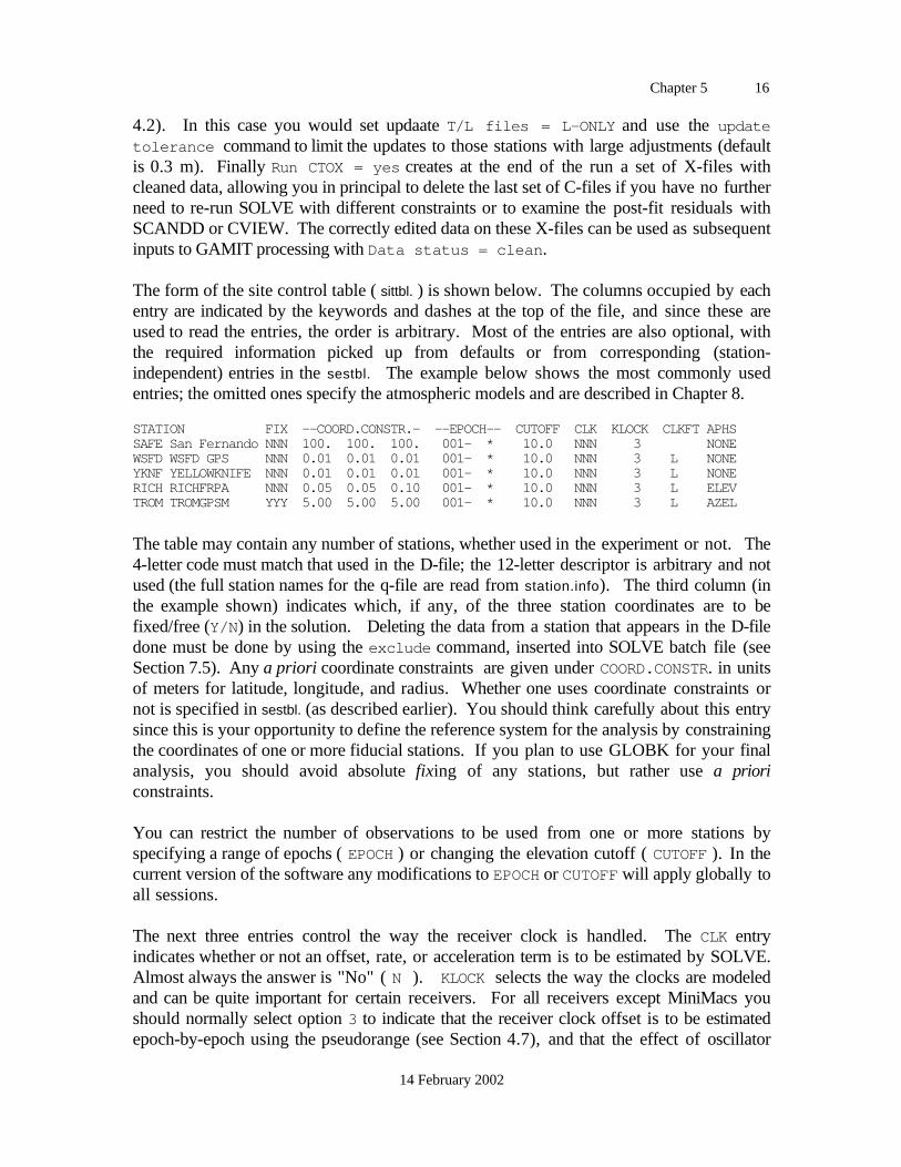
Chapter 5 16

14 February 2002

4.2). In this case you would set updaate T/L files = L-ONLY and use the updatetolerance command to limit the updates to those stations with large adjustments (defaultis 0.3 m). Finally Run CTOX = yes creates at the end of the run a set of X-files withcleaned data, allowing you in principal to delete the last set of C-files if you have no furtherneed to re-run SOLVE with different constraints or to examine the post-fit residuals withSCANDD or CVIEW. The correctly edited data on these X-files can be used as subsequentinputs to GAMIT processing with Data status = clean .

The form of the site control table ( sittbl. ) is shown below. The columns occupied by eachentry are indicated by the keywords and dashes at the top of the file, and since these areused to read the entries, the order is arbitrary. Most of the entries are also optional, withthe required information picked up from defaults or from corresponding (station-independent) entries in the sestbl. The example below shows the most commonly usedentries; the omitted ones specify the atmospheric models and are described in Chapter 8.

STATION FIX --COORD.CONSTR.- --EPOCH-- CUTOFF CLK KLOCK CLKFT APHSSAFE San Fernando NNN 100. 100. 100. 001- * 10.0 NNN 3 NONEWSFD WSFD GPS NNN 0.01 0.01 0.01 001- * 10.0 NNN 3 L NONEYKNF YELLOWKNIFE NNN 0.01 0.01 0.01 001- * 10.0 NNN 3 L NONERICH RICHFRPA NNN 0.05 0.05 0.10 001- * 10.0 NNN 3 L ELEVTROM TROMGPSM YYY 5.00 5.00 5.00 001- * 10.0 NNN 3 L AZEL

The table may contain any number of stations, whether used in the experiment or not. The4-letter code must match that used in the D-file; the 12-letter descriptor is arbitrary and notused (the full station names for the q-file are read from station.info). The third column (inthe example shown) indicates which, if any, of the three station coordinates are to befixed/free (Y/N ) in the solution. Deleting the data from a station that appears in the D-filedone must be done by using the exclude command, inserted into SOLVE batch file (seeSection 7.5). Any a priori coordinate constraints are given under COORD.CONSTR. in unitsof meters for latitude, longitude, and radius. Whether one uses coordinate constraints ornot is specified in sestbl. (as described earlier). You should think carefully about this entrysince this is your opportunity to define the reference system for the analysis by constrainingthe coordinates of one or more fiducial stations. If you plan to use GLOBK for your finalanalysis, you should avoid absolute fixing of any stations, but rather use a prioriconstraints.

You can restrict the number of observations to be used from one or more stations byspecifying a range of epochs ( EPOCH ) or changing the elevation cutoff ( CUTOFF ). In thecurrent version of the software any modifications to EPOCH or CUTOFF will apply globally toall sessions.

The next three entries control the way the receiver clock is handled. The CLK entryindicates whether or not an offset, rate, or acceleration term is to be estimated by SOLVE.Almost always the answer is "No" ( N ). KLOCK selects the way the clocks are modeledand can be quite important for certain receivers. For all receivers except MiniMacs youshould normally select option 3 to indicate that the receiver clock offset is to be estimatedepoch-by-epoch using the pseudorange (see Section 4.7), and that the effect of oscillator

Chapter 5 17

14 February 2002

variations on the phase is to be modeled with a low-order polynomial. Since the MiniMacreceivers keep their clocks synchronized with the GPS satellites, it is preferable to assumean offset of 0. by selecting option 1. The third option ( 2 ) uses the low-order polynomialfor both the epoch offset and oscillator variations. This approach will model receiver clockoffsets as well as will Option 3 if the receiver clock stability is sufficient (better than ~ 10-8)to keep deviations from the polynomial less than 1 microsecond throughout the observationspan. The crystals in the TI 4100 and MACROMETER II usually meet this requirementbut those in the newer low-power receivers do not unless they are locked to an externalatomic oscillator (as at some IGS tracking stations). The order of the polynomial to beused by FIXDRV may be specified under CLKFT as linear ( L ) or cubic ( C ), or left forFIXDRV to decide from the fit by leaving this column blank. If KLOCK is not specified, thethe way the clock is handled is determined by the receiver type, with all receivers exceptMiniMacs set to option 3 (epoch-by-epoch estimation).

The final column shown in the example is for invoking a model for variations in the phasecenter of the receiving antenna ( APHS ). The use of a model for all stations can becontrolled using the sestbl. entry, but the sittbl. entries override the sestbl. if the former arepresent. So to avoid confusion, you may want to omit this column from the sittbl. exceptfor those analyses in which you need to control the model separately for each station.

The usual way to run FIXDRV is to give the name of the D-file as a command-lineargument. In this case, there are no further prompts necessary. If an I-file exists, it will beused; if not, it will be created by fitting polynomials to the clock values given in the K-files.If you wish to choose an alternate I-file, or recreate the I-file even though it exists, youshould run FIXDRV interactively by not specifying the D-file as a command-line argument.In this case, FIXDRV will prompt you for the name of the D-file. It will then ask what youwant to do about the I-file: use the old one, save the old one and create a new one, oroverwrite the old one. Most of the time you probably want to "Use the old one" (option 3)and avoid a time-consuming recalculation of all the clock coefficients, but if you haveadded a station to the D-file since last running FIXDRV or have updated the K-file byrerunning MAKEX or MAKEK with improved station coordiantes, you should create anew I-file.

When you run FIXDRV to create an I-file, you will get a display for each station indicatinghow well the station clock (as represented by the values in the K-file) fits a linearpolynomial and a cubic polynomial that also includes "steps" representing unexpectedclock jumps or, for many receivers, programmed resets of 1 or 2 milliseconds to keep thesampling time synchronized with GPS time. Typical rms values for field receivers are several milliseconds for the linear fit (without jumps) and 50-1000 microseconds for thecubic fit with jumps. See the discussion in Chapter 4.10 to determine whether largervalues may cause problems in your processing.

Chapter 5 18

14 February 2002

5.3 Executing the Batch Run

The output of FIXDRV is a command file (shell script) named b{ expmt}.bat which invokesthe GAMIT modules in the appropriate order for the type of analysis you have requested(see the example on the following page). To execute the analysis run in foreground typecsh {batch file name}; in background type gbat {batch file name}. (If your system recognizesthe batch file as a command file [use chmod +x under UNIX ], you can of course omit thecsh when running in foreground.) All of the required modules will then be executedautomatically to perform the processing sequence you have defined with FIXDRV.Beginning with release 9.5, the first lines of the batch file remove any existing files loggingthe status of the batch run (GAMIT.status) and warnings (GAMIT.warning) or aborts(GAMIT.fatal). Most messages generated by the GAMIT modules and AUTCLN are nowwritten into these files instead of directly to the screen (or b{ expmt}. bat.log if the job wasexecuted using the gbat). They provide a convenient method of determining if a GAMITrun executed successfully. During execution, you can monitor the progress of abackground job by typing tail GAMIT.status. The first code now executed by ARC,MODEL, CFMRG, and SOLVE is a check for the existence of GAMIT.fatal; if it's found,indicating that the previous step in the batch sequence has failed, the current module willterminate also. This feature is designed to avoid the common problem of overlooking thefailure of a previous step in evaluating the success of a run.

For most of the modules, the command references a secondary B-file containing the inputstream for one execution of the specified module. Each input stream contains replies to allthe queries that the user would encounter when running the module interactively. In thecase of AUTCLN, there are command-line arguments rather than a secondary batch filegiven. For AUTCLN, these arguments are the command file name (optional), a characterindicating whether input C-files are overwritten (' .') or the 6th character incremented ('+'),and the name of a D-file (to be read for the C-file names) and the 6th character of the inputC-files (which may be different from the names in the D-file). (See Chapter 7 for moredetail.).

The sequence of program executions is listed in the primary B-file and the individualresponses are listed in the secondary B-files. An example of a primary B-file for a 1-ITERATION analysis with postfit editing by AUTCLN is shown below. It is usually moreefficient for regional networks to perform a 0-ITERATION analysis, repeating it ifnecessary to correct problems, we show the 1-ITERATION case here to document thisfeature of GAMIT. In this example, we have set Update T/L files = L_ONLY since wedo not expect to improve the orbit from the regional data; and we have set Delete inputAUTCLN C-files = I , indicating that the only time a second set of C-files is retained is forthe postfit editing step, avoiding an unnecessary rerun of MODEL.

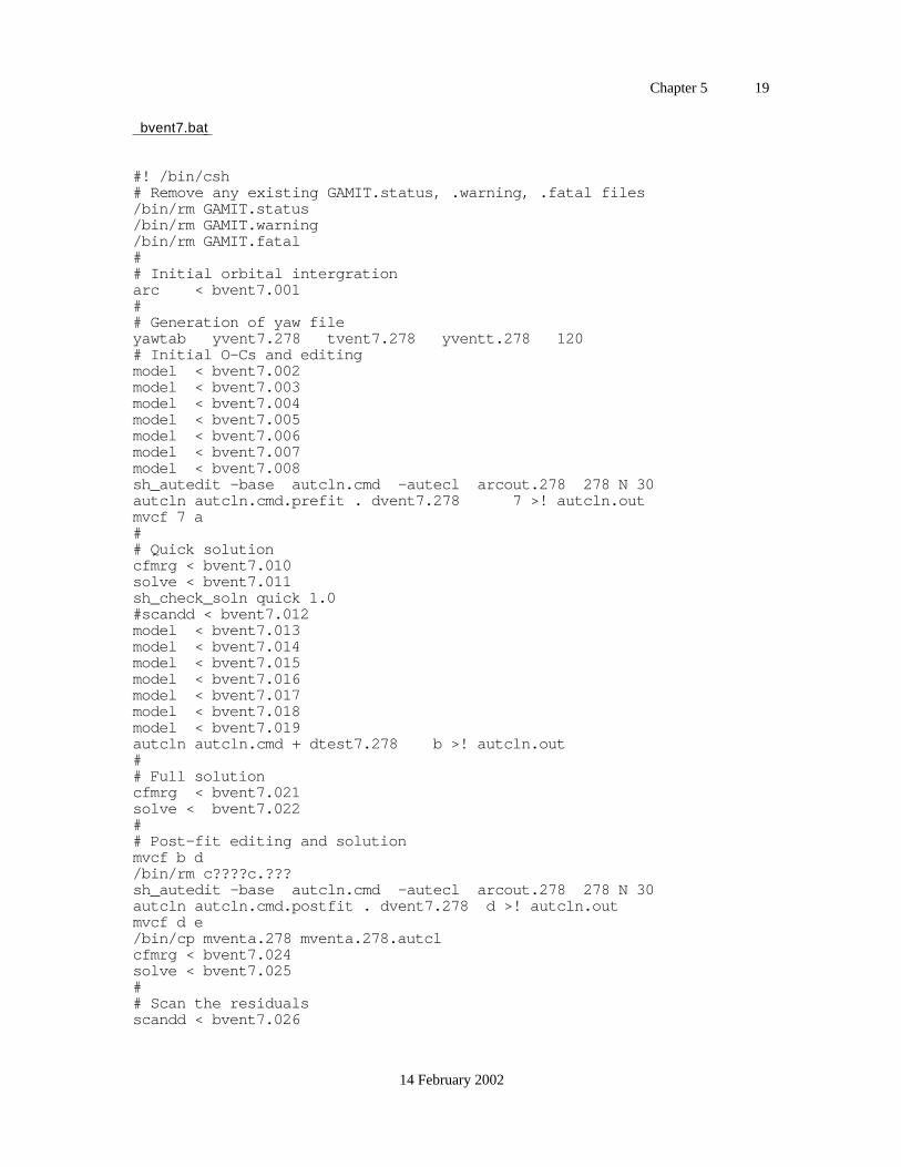
Chapter 5 19

14 February 2002

bvent7.bat

#! /bin/csh# Remove any existing GAMIT.status, .warning, .fatal files/bin/rm GAMIT.status/bin/rm GAMIT.warning/bin/rm GAMIT.fatal## Initial orbital intergrationarc < bvent7.001## Generation of yaw fileyawtab yvent7.278 tvent7.278 yventt.278 120# Initial O-Cs and editingmodel < bvent7.002model < bvent7.003model < bvent7.004model < bvent7.005model < bvent7.006model < bvent7.007model < bvent7.008sh_autedit -base autcln.cmd -autecl arcout.278 278 N 30autcln autcln.cmd.prefit . dvent7.278 7 >! autcln.outmvcf 7 a## Quick solutioncfmrg < bvent7.010solve < bvent7.011sh_check_soln quick 1.0#scandd < bvent7.012model < bvent7.013model < bvent7.014model < bvent7.015model < bvent7.016model < bvent7.017model < bvent7.018model < bvent7.019autcln autcln.cmd + dtest7.278 b >! autcln.out## Full solutioncfmrg < bvent7.021solve < bvent7.022## Post-fit editing and solutionmvcf b d/bin/rm c????c.???sh_autedit -base autcln.cmd -autecl arcout.278 278 N 30autcln autcln.cmd.postfit . dvent7.278 d >! autcln.outmvcf d e/bin/cp mventa.278 mventa.278.autclcfmrg < bvent7.024solve < bvent7.025## Scan the residualsscandd < bvent7.026

Chapter 5 20

14 February 2002

Listed below are explanations for each module execution in the batch file.

ARC Generate an orbital ephemeris (T-file) with partials using as initial conditions a G-file produced by sh_sp3fit, sh_bctot, or copied from SOPAC. This step can be skipped ifyou've already created a T-file using sh_sp3_fit or sh_bcfit or copied one from SOPAC.

YAWTAB Generate a table of yaw values for each SV at each observation epoch usingas input the T-file and short table of yaw values written by ARC.

MODEL Compute prefit residuals ("O-C's") and partial derivatives for theobservations on each X-file; create C-files with the same names (except for the first letter)as the X-files.

AUTCLN Read the C-files output by MODEL and search for cycle slips and outliers inthe pre-fit one-way and double-difference residuals, inserting extra biases at allquestionable gaps; create the "a" series C-files (i.e., with the year digit replaced by "a")with these corrections to the phase data and prefit residuals.

CFMRG Set up the M-file for the least squares fit: define and select the parameters tobe adjusted and the C-files to be read.

SOLVE Perform a least-squares estimate of station coordinates and orbitalparameters; update the M-file with the parameter adjustments (in order to edit post-fitresiduals); write the "a" L-file with an adjusted set of coordinates and the "a" G-file withan adjusted set of orbital initial conditions. The M-file and Q-file from quick solutions arealways named with the sixth character "1".

SCANDD Using the updated M-file to create predicted post-fit"residuals, scan alldouble-difference combinations to produce a summary of potential cycle slips remaining.This step has been commented out by FIXDRV since we set SCANDD control = FULL toindicate that SCANDD (a time-consuming step) should be executed only at the end of thefull solution.

MODEL Recompute O-C's and partials from the original X-files using the new L-file. Create "b" series C-files.

AUTCLN Re-clean the data using the flatter residuals obtained from the iteratedcoordinates and orbits. Output "b" series C-files.

CFMRG Create a new M-file with the names of the "b" series C-files; the "regularsolution" M-file always has "a" as its sixth character.

Chapter 5 21

14 February 2002

SOLVE Perform a least-squares estimate of station coordinates and orbitalparameters, attempting to resolve phase ambiguities if specified by the type of analysis.This executation of SOLVE will also update the M-file with the parameter adjustments inorder to view or edit the post-fit residuals. It will also write overwrite the "a" L-file andcreate a "b" G-file. Like the M-file, the Q-file from the this solution is named with the sixthcharacter "a".

AUTCLN Re-clean the data using residuals flattened by the 'predicted' parameteradjustments on the M-file. The input C-files are those generated by the MODEL run inputto the last AUTCLN and SOLVE runs (the "b" series now renamed "d").

CFMRG Regenerate the "a" M-file for the final solution.

SOLVE Repeat the full solution with the re-edited data.

The shellscript executed just before each AUTCLN run copies a "base" AUTCLNcommand file (specified by autcln_cmd in the sestbl., usually autcln.cmd) into eitherautcln.cmd.prefit or autcln.cmd.postfit, uncommenting in the latter case the commands forpost-fit editing (see Section 6.2) and in both cases adding (optionally) commands toexclude data corrupted by eclipses (Delete eclipse data in the sestbl.).

There are two important principles to remember using batch files to carry out an analysis.The first is that you often need to exert control over the execution by commenting out (with# signs) certain lines of the primary B-file. When you execute your initial batch run, youmay want to comment all of the command lines after the first SOLVE in order to inspect thequick solution before reintegrating the orbit, re-MODELing the observations, andperforming the regular solution. There are many things—some beyond your control, someyou should have caught but didn't—that can cause the quick solution to be bad (see Section5.4). Another example of the need to comment command lines is when you havepreviously run ARC and don't want to repeat the integration at the beginning of the batchsolution, or when you want to postpone the final ARC integration until after you haveinspected the Q-file from your solution (though both of these controls can be implementedusing sestbl. commands). Finally, if your batch run fails in the middle for any reason,you can comment the command-lines that have executed successfully and continue the runafter the interruption.

The second important principle concerns the naming conventions for the various files. Ofmost concern are the C-file names. FIXDRV will establish a sequence which incrementsthe sixth character each time a new C-file is written. In the cleaning sequences (QUICK, 1-ITER, or 2-ITER ) the C-files written by the first MODEL run will begin with the yearnumber, e.g., "7" for 1987, and the sequence will continue "a", "b", etc. (With AUTCLNthe incrementing is done using a "+" rather than a "." in the command line if you do notwish to delete the input C-files, or using the mvcf (or copyc ) script to rename the files.) If,for example, you choose to by-pass AUTCLN (by commenting the command line) andperform manual editing with CVIEW, then you should request CVIEW to write output C-

Chapter 5 22

14 February 2002

files with the sixth character incremented (this is an easy and natural procedure—seeChapter 6). Then you can continue the batch sequence without having to edit the names ofthe C-files in the secondary B-files for MODEL and CFMRG. Special rules apply for 0-ITER with clean data runs, in which only one set of new C-files is created. In order toaccommodate multi-session solutions within a single day, the output C-file from MODEL isthe same as the input X-file. Thus if your input X-files are named with 6th character "a"and "p", for example, designating "am" and "pm" sessions, these letters will be retained inthe C-file. The 0-ITER options with clean data (only) also allow for C-files rather thanX-files in the D-file; in this case the C-files output by MODEL will be incremented by oneletter (e.g. "a" => "b", "p" => "q"). It is partly because of the inherent complicaton of filenaming (but also to reduce processing time) that many analysts prefer to use always 0-ITER (no quick solution), just repeating it with updated coordinates or orbits if the a priorivalues of these are sufficiently bad to cause problems for AUTCLN or adjustments that areoutside of the linear range (see the discussion in Section 4.2.

Table 5.2 below summarizes the assignment of the sixth character and disposition of the C-files for the most common processing sequences. The input files for MODEL are assumedto be X-files and hence always have the last digit of the year as their sixth character.

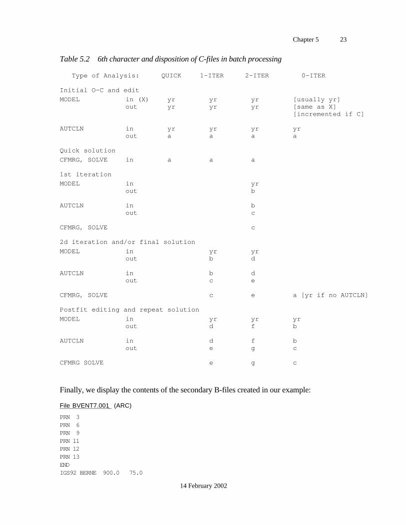
Chapter 5 23

14 February 2002

Table 5.2 6th character and disposition of C-files in batch processing

Type of Analysis: QUICK 1-ITER 2-ITER 0-ITER

Initial O-C and edit

MODEL in (X) yr yr yr [usually yr]out yr yr yr [same as X]

[incremented if C]

AUTCLN in yr yr yr yrout a a a a

Quick solution

CFMRG, SOLVE in a a a

1st iteration

MODEL in yrout b

AUTCLN in bout c

CFMRG, SOLVE c

2d iteration and/or final solution

MODEL in yr yrout b d

AUTCLN in b dout c e

CFMRG, SOLVE c e a [yr if no AUTCLN]

Postfit editing and repeat solution

MODEL in yr yr yrout d f b

AUTCLN in d f bout e g c

CFMRG SOLVE e g c

Finally, we display the contents of the secondary B-files created in our example:

File BVENT7.001 (ARC)

PRN 3PRN 6PRN 9PRN 11PRN 12PRN 13ENDIGS92 BERNE 900.0 75.0

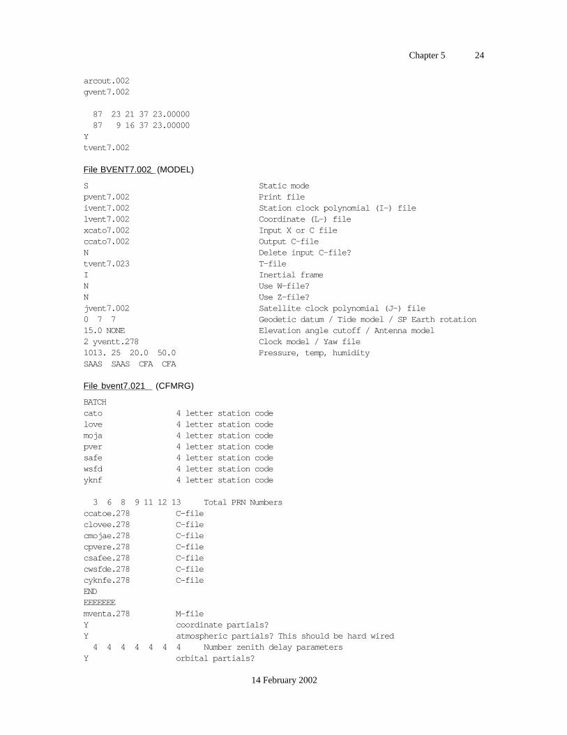
Chapter 5 24

14 February 2002

arcout.002gvent7.002

87 23 21 37 23.00000 87 9 16 37 23.00000Ytvent7.002

File BVENT7.002 (MODEL)

S Static modepvent7.002 Print fileivent7.002 Station clock polynomial (I-) filelvent7.002 Coordinate (L-) filexcato7.002 Input X or C fileccato7.002 Output C-fileN Delete input C-file?tvent7.023 T-fileI Inertial frameN Use W-file?N Use Z-file?jvent7.002 Satellite clock polynomial (J-) file0 7 7 Geodetic datum / Tide model / SP Earth rotation15.0 NONE Elevation angle cutoff / Antenna model2 yventt.278 Clock model / Yaw file1013. 25 20.0 50.0 Pressure, temp, humiditySAAS SAAS CFA CFA

File bvent7.021 (CFMRG)

BATCHcato 4 letter station codelove 4 letter station codemoja 4 letter station codepver 4 letter station codesafe 4 letter station codewsfd 4 letter station codeyknf 4 letter station code

3 6 8 9 11 12 13 Total PRN Numbersccatoe.278 C-fileclovee.278 C-filecmojae.278 C-filecpvere.278 C-filecsafee.278 C-filecwsfde.278 C-filecyknfe.278 C-fileENDEEEEEEEmventa.278 M-fileY coordinate partials?Y atmospheric partials? This should be hard wired 4 4 4 4 4 4 4 Number zenith delay parametersY orbital partials?

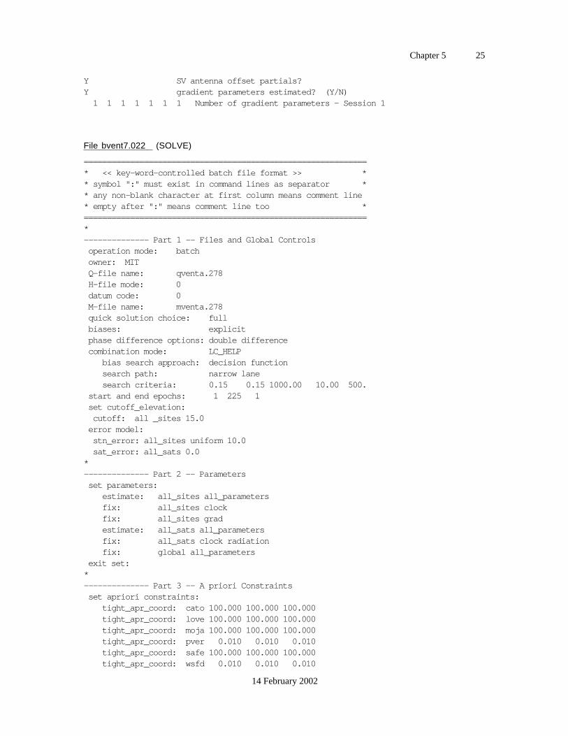
Chapter 5 25

14 February 2002

Y SV antenna offset partials?Y gradient parameters estimated? (Y/N) 1 1 1 1 1 1 1 Number of gradient parameters - Session 1

File bvent7.022 (SOLVE)

=============================================================* << key-word-controlled batch file format >> ** symbol ":" must exist in command lines as separator ** any non-blank character at first column means comment line* empty after ":" means comment line too *=============================================================*-------------- Part 1 -- Files and Global Controls operation mode: batch owner: MIT Q-file name: qventa.278 H-file mode: 0 datum code: 0 M-file name: mventa.278 quick solution choice: full biases: explicit phase difference options: double difference combination mode: LC_HELP bias search approach: decision function search path: narrow lane search criteria: 0.15 0.15 1000.00 10.00 500. start and end epochs: 1 225 1 set cutoff_elevation: cutoff: all _sites 15.0 error model: stn_error: all_sites uniform 10.0 sat_error: all_sats 0.0*-------------- Part 2 -- Parameters set parameters: estimate: all_sites all_parameters fix: all_sites clock fix: all_sites grad estimate: all_sats all_parameters fix: all_sats clock radiation fix: global all_parameters exit set:*-------------- Part 3 -- A priori Constraints set apriori constraints: tight_apr_coord: cato 100.000 100.000 100.000 tight_apr_coord: love 100.000 100.000 100.000 tight_apr_coord: moja 100.000 100.000 100.000 tight_apr_coord: pver 0.010 0.010 0.010 tight_apr_coord: safe 100.000 100.000 100.000 tight_apr_coord: wsfd 0.010 0.010 0.010

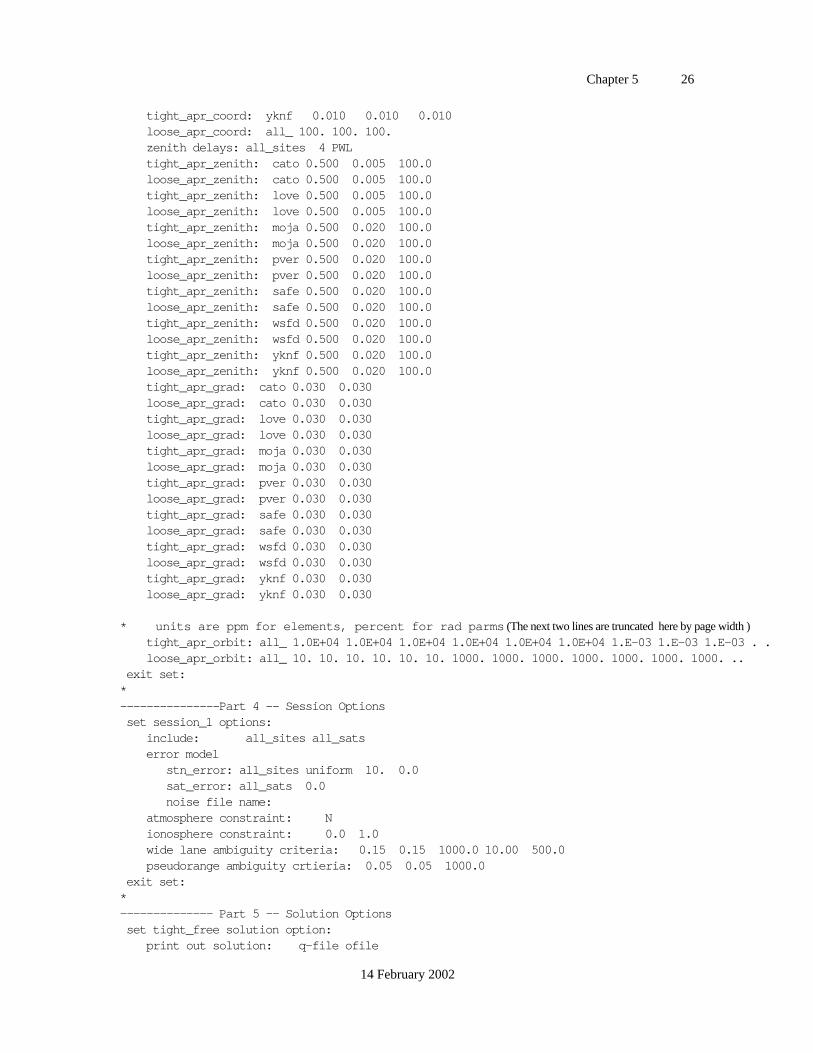
Chapter 5 26

14 February 2002

tight_apr_coord: yknf 0.010 0.010 0.010 loose_apr_coord: all_ 100. 100. 100. zenith delays: all_sites 4 PWL tight_apr_zenith: cato 0.500 0.005 100.0 loose_apr_zenith: cato 0.500 0.005 100.0 tight_apr_zenith: love 0.500 0.005 100.0 loose_apr_zenith: love 0.500 0.005 100.0 tight_apr_zenith: moja 0.500 0.020 100.0 loose_apr_zenith: moja 0.500 0.020 100.0 tight_apr_zenith: pver 0.500 0.020 100.0 loose_apr_zenith: pver 0.500 0.020 100.0 tight_apr_zenith: safe 0.500 0.020 100.0 loose_apr_zenith: safe 0.500 0.020 100.0 tight_apr_zenith: wsfd 0.500 0.020 100.0 loose_apr_zenith: wsfd 0.500 0.020 100.0 tight_apr_zenith: yknf 0.500 0.020 100.0 loose_apr_zenith: yknf 0.500 0.020 100.0 tight_apr_grad: cato 0.030 0.030 loose_apr_grad: cato 0.030 0.030 tight_apr_grad: love 0.030 0.030 loose_apr_grad: love 0.030 0.030 tight_apr_grad: moja 0.030 0.030 loose_apr_grad: moja 0.030 0.030 tight_apr_grad: pver 0.030 0.030 loose_apr_grad: pver 0.030 0.030 tight_apr_grad: safe 0.030 0.030 loose_apr_grad: safe 0.030 0.030 tight_apr_grad: wsfd 0.030 0.030 loose_apr_grad: wsfd 0.030 0.030 tight_apr_grad: yknf 0.030 0.030 loose_apr_grad: yknf 0.030 0.030

* units are ppm for elements, percent for rad parms (The next two lines are truncated here by page width ) tight_apr_orbit: all_ 1.0E+04 1.0E+04 1.0E+04 1.0E+04 1.0E+04 1.0E+04 1.E-03 1.E-03 1.E-03 . . loose_apr_orbit: all_ 10. 10. 10. 10. 10. 10. 1000. 1000. 1000. 1000. 1000. 1000. 1000. .. exit set:*---------------Part 4 -- Session Options set session_1 options: include: all_sites all_sats error model stn_error: all_sites uniform 10. 0.0 sat_error: all_sats 0.0 noise file name: atmosphere constraint: N ionosphere constraint: 0.0 1.0 wide lane ambiguity criteria: 0.15 0.15 1000.0 10.00 500.0 pseudorange ambiguity crtieria: 0.05 0.05 1000.0 exit set:*-------------- Part 5 -- Solution Options set tight_free solution option: print out solution: q-file ofile

Chapter 5 27

14 February 2002

update file option: m-file l-file g-file input_m file name: mventa.278 output_m file name: mventa.278 input_l file name: lvent7.278 output_l file name: lventa.278 coord_upd_tol: 0.03 input_g file name: gvent7.278 output_g file name: gventa.278 correl_prt: 0.999900exit set:* set tight_fix solution option: print out solution: q-file ofile update file option: m-file l-file g-file input_m file name: mvent1.278 output_m file name: mvent1.278 input_l file name: lvent7.278 output_l file name: lventa.278 coord_upd_tol: 0.03 input_g file name: gvent7.278 output_g file name: gventa.278 correl_prt: 0.999900 exit set: set loose_free solution option: update file option: exit set: set loose_fix solution option: print out solution: exit set:

5.4 Evaluating the Solutions

There are two first-order criteria for determining if a solution is acceptable: 1) are thereadequate data to perform a reasonable estimate, and 2) do the data fit the model to theirnoise level. The primary indicator that the first criterion has been met is the magnitude ofthe uncertainties of the baseline components. If these are larger than you expect with the apriori constraints you have applied to station coordinates and orbital parameters, then aquick look in the Q-file or autcln.sum file will usually reveal that large quantities of datahave been discarded by AUTCLN. For the second criterion, the primary indicator is the"normalized rms” (nrms) of the solution; i.e., the square root of chi-square per degree offreedom. If the data were randomly distributed and the a priori weights were correct, thenrms would be close to unity. In practice with the default weighting scheme, a goodsolution usually produces a nrms of about 0.25. Anything larger than 0.5 means that thereare cycle slips that have not been removed or associated with extra bias parameters (seeSections 2.1 and 6.1), or that there is a serious modeling problem (e.g., bad coordinates ofthe fixed stations or an unmodeled satellite "burn"). If the final solution of a batchsequence meets these two criteria, there is usually no need to look carefully at any other

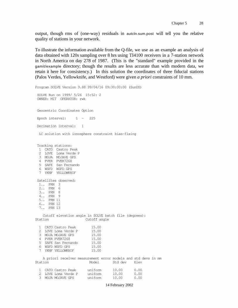
Chapter 5 28

14 February 2002

output, though rms of (one-way) residuals in autcln.sum.post will tell you the relativequality of stations in your network.

To illustrate the information available from the Q-file, we use as an example an analysis ofdata obtained with 120s sampling over 8 hrs using TI4100 receivers in a 7-station networkin North America on day 278 of 1987. (This is the "standard" example provided in thegamit/example directory; though the results are less accurate than with modern data, weretain it here for consistency.) In this solution the coordinates of three fiducial stations(Palos Verdes, Yellowknife, and Westford) were given a priori constraints of 10 mm.

Program SOLVE Version 9.88 99/04/16 09:30:00:00 (SunOS)

SOLVE Run on 1999/ 5/26 15:52: 2 OWNER: MIT OPERATOR: rwk

Geocentric Coordinates Option

Epoch interval: 1 - 225

Decimation interval: 1

LC solution with ionosphere constraint bias-fixing

Tracking stations: 1 CATO Castro Peak 2 LOVE Loma Verde P 3 MOJA MOJAVE GPS 4 PVER PVER7268 5 SAFE San Fernando 6 WSFD WSFD GPS 7 YKNF YELLOWKNIF

Satellites observed: 1.. PRN 3 2.. PRN 6 3.. PRN 8 4.. PRN 9 5.. PRN 11 6.. PRN 12 7.. PRN 13

Cutoff elevation angle in SOLVE batch file (degrees):Station Cutoff angle

1 CATO Castro Peak 15.00 2 LOVE Loma Verde P 15.00 3 MOJA MOJAVE GPS 15.00 4 PVER PVER7268 15.00 5 SAFE San Fernando 15.00 6 WSFD WSFD GPS 15.00 7 YKNF YELLOWKNIF 15.00

A priori receiver measurement error models and std devs in mmStation Model Std dev Elev

1 CATO Castro Peak uniform 10.00 0.00 2 LOVE Loma Verde P uniform 10.00 0.00 3 MOJA MOJAVE GPS uniform 10.00 0.00

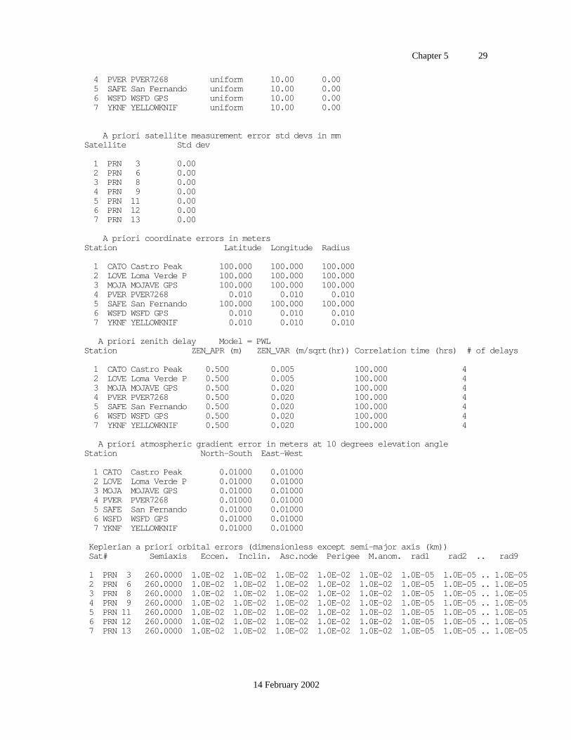
Chapter 5 29

14 February 2002

4 PVER PVER7268 uniform 10.00 0.00 5 SAFE San Fernando uniform 10.00 0.00 6 WSFD WSFD GPS uniform 10.00 0.00 7 YKNF YELLOWKNIF uniform 10.00 0.00

A priori satellite measurement error std devs in mmSatellite Std dev

1 PRN 3 0.00 2 PRN 6 0.00 3 PRN 8 0.00 4 PRN 9 0.00 5 PRN 11 0.00 6 PRN 12 0.00 7 PRN 13 0.00

A priori coordinate errors in metersStation Latitude Longitude Radius

1 CATO Castro Peak 100.000 100.000 100.000 2 LOVE Loma Verde P 100.000 100.000 100.000 3 MOJA MOJAVE GPS 100.000 100.000 100.000 4 PVER PVER7268 0.010 0.010 0.010 5 SAFE San Fernando 100.000 100.000 100.000 6 WSFD WSFD GPS 0.010 0.010 0.010 7 YKNF YELLOWKNIF 0.010 0.010 0.010

A priori zenith delay Model = PWLStation ZEN_APR (m) ZEN_VAR (m/sqrt(hr)) Correlation time (hrs) # of delays

1 CATO Castro Peak 0.500 0.005 100.000 4 2 LOVE Loma Verde P 0.500 0.005 100.000 4 3 MOJA MOJAVE GPS 0.500 0.020 100.000 4 4 PVER PVER7268 0.500 0.020 100.000 4 5 SAFE San Fernando 0.500 0.020 100.000 4 6 WSFD WSFD GPS 0.500 0.020 100.000 4 7 YKNF YELLOWKNIF 0.500 0.020 100.000 4

A priori atmospheric gradient error in meters at 10 degrees elevation angleStation North-South East-West

1 CATO Castro Peak 0.01000 0.01000 2 LOVE Loma Verde P 0.01000 0.01000 3 MOJA MOJAVE GPS 0.01000 0.01000 4 PVER PVER7268 0.01000 0.01000 5 SAFE San Fernando 0.01000 0.01000 6 WSFD WSFD GPS 0.01000 0.01000 7 YKNF YELLOWKNIF 0.01000 0.01000

Keplerian a priori orbital errors (dimensionless except semi-major axis (km)) Sat# Semiaxis Eccen. Inclin. Asc.node Perigee M.anom. rad1 rad2 .. rad9

1 PRN 3 260.0000 1.0E-02 1.0E-02 1.0E-02 1.0E-02 1.0E-02 1.0E-05 1.0E-05 .. 1.0E-05 2 PRN 6 260.0000 1.0E-02 1.0E-02 1.0E-02 1.0E-02 1.0E-02 1.0E-05 1.0E-05 .. 1.0E-05 3 PRN 8 260.0000 1.0E-02 1.0E-02 1.0E-02 1.0E-02 1.0E-02 1.0E-05 1.0E-05 .. 1.0E-05 4 PRN 9 260.0000 1.0E-02 1.0E-02 1.0E-02 1.0E-02 1.0E-02 1.0E-05 1.0E-05 .. 1.0E-05 5 PRN 11 260.0000 1.0E-02 1.0E-02 1.0E-02 1.0E-02 1.0E-02 1.0E-05 1.0E-05 .. 1.0E-05 6 PRN 12 260.0000 1.0E-02 1.0E-02 1.0E-02 1.0E-02 1.0E-02 1.0E-05 1.0E-05 .. 1.0E-05 7 PRN 13 260.0000 1.0E-02 1.0E-02 1.0E-02 1.0E-02 1.0E-02 1.0E-05 1.0E-05 .. 1.0E-05

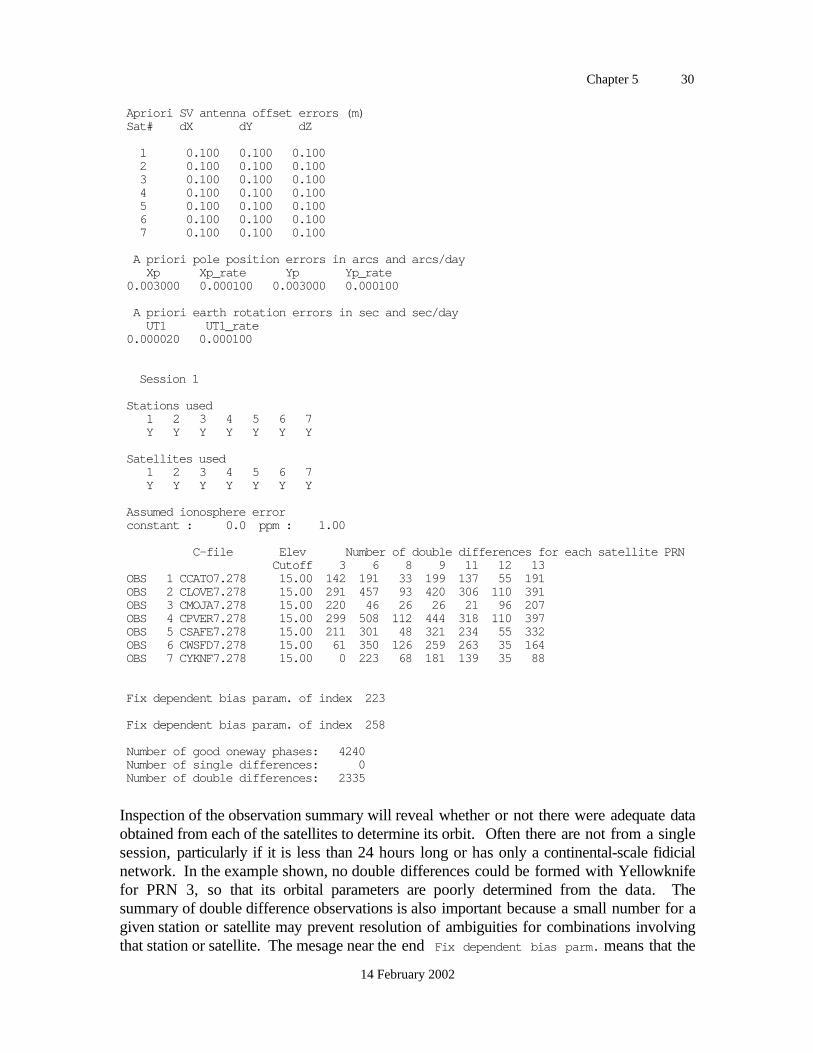
Chapter 5 30

14 February 2002

Apriori SV antenna offset errors (m) Sat# dX dY dZ

1 0.100 0.100 0.100 2 0.100 0.100 0.100 3 0.100 0.100 0.100 4 0.100 0.100 0.100 5 0.100 0.100 0.100 6 0.100 0.100 0.100 7 0.100 0.100 0.100

A priori pole position errors in arcs and arcs/day Xp Xp_rate Yp Yp_rate 0.003000 0.000100 0.003000 0.000100

A priori earth rotation errors in sec and sec/day UT1 UT1_rate 0.000020 0.000100

Session 1

Stations used 1 2 3 4 5 6 7 Y Y Y Y Y Y Y

Satellites used 1 2 3 4 5 6 7 Y Y Y Y Y Y Y

Assumed ionosphere error constant : 0.0 ppm : 1.00

C-file Elev Number of double differences for each satellite PRN Cutoff 3 6 8 9 11 12 13 OBS 1 CCATO7.278 15.00 142 191 33 199 137 55 191 OBS 2 CLOVE7.278 15.00 291 457 93 420 306 110 391 OBS 3 CMOJA7.278 15.00 220 46 26 26 21 96 207 OBS 4 CPVER7.278 15.00 299 508 112 444 318 110 397 OBS 5 CSAFE7.278 15.00 211 301 48 321 234 55 332 OBS 6 CWSFD7.278 15.00 61 350 126 259 263 35 164 OBS 7 CYKNF7.278 15.00 0 223 68 181 139 35 88

Fix dependent bias param. of index 223

Fix dependent bias param. of index 258

Number of good oneway phases: 4240 Number of single differences: 0 Number of double differences: 2335

Inspection of the observation summary will reveal whether or not there were adequate dataobtained from each of the satellites to determine its orbit. Often there are not from a singlesession, particularly if it is less than 24 hours long or has only a continental-scale fidicialnetwork. In the example shown, no double differences could be formed with Yellowknifefor PRN 3, so that its orbital parameters are poorly determined from the data. Thesummary of double difference observations is also important because a small number for agiven station or satellite may prevent resolution of ambiguities for combinations involvingthat station or satellite. The mesage near the end Fix dependent bias parm. means that the

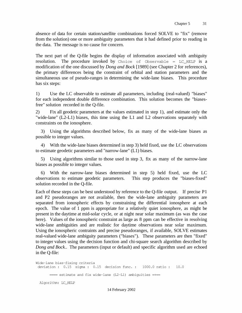
Chapter 5 31

14 February 2002

absence of data for certain station/satellite combinations forced SOLVE to "fix" (removefrom the solution) one or more ambiguity parameters that it had defined prior to reading inthe data. The message is no cause for concern.

The next part of the Q-file begins the display of information associated with ambiguityresolution. The procedure invoked by Choice of Observable = LC_HELP is amodification of the one discussed by Dong and Bock [1989] (see Chapter 2 for references),the primary differences being the constraint of orbital and station parameters and thesimultaneous use of pseudo-ranges in determining the wide-lane biases. This procedurehas six steps:

1) Use the LC observable to estimate all parameters, including (real-valued) "biases"for each independent double difference combination. This solution becomes the "biases-free" solution recorded in the Q-file.

2) Fix all geodetic parameters at the values estimated in step 1), and estimate only the"wide-lane" (L2-L1) biases, this time using the L1 and L2 observations separately withconstraints on the ionosphere.

3) Using the algorithms described below, fix as many of the wide-lane biases aspossible to integer values.

4) With the wide-lane biases determined in step 3) held fixed, use the LC observationsto estimate geodetic parameters and "narrow-lane" (L1) biases.

5) Using algorithms similar to those used in step 3, fix as many of the narrow-lanebiases as possible to integer values.

6) With the narrow-lane biases determined in step 5) held fixed, use the LCobservations to estimate geodetic parameters. This step produces the "biases-fixed"solution recorded in the Q-file.

Each of these steps can be best understood by reference to the Q-file output. If precise P1and P2 pseudoranges are not available, then the wide-lane ambiguity parameters areseparated from ionospheric effects by constraining the differential ionosphere at eachepoch. The value of 1 ppm is appropriate for a relatively quiet ionosphere, as might bepresent in the daytime at mid-solar cycle, or at night near solar maximum (as was the casehere). Values of the ionospheric constraint as large as 8 ppm can be effective in resolvingwide-lane ambiguities and are realistic for daytime observations near solar maximum.Using the ionospheric contraints and precise pseudoranges, if available, SOLVE estimatesreal-valued wide-lane ambiguity parameters ("biases"). These parameters are then "fixed"to integer values using the decision function and chi-square search algorithm described byDong and Bock.. The parameters (input or default) and specific algorithm used are echoedin the Q-file:

Wide-lane bias-fixing criteria deviation : 0.15 sigma : 0.15 decision func. : 1000.0 ratio : 10.0

==== estimate and fix wide-lane (L2-L1) ambiguities =+==

Algorithm: LC_HELP

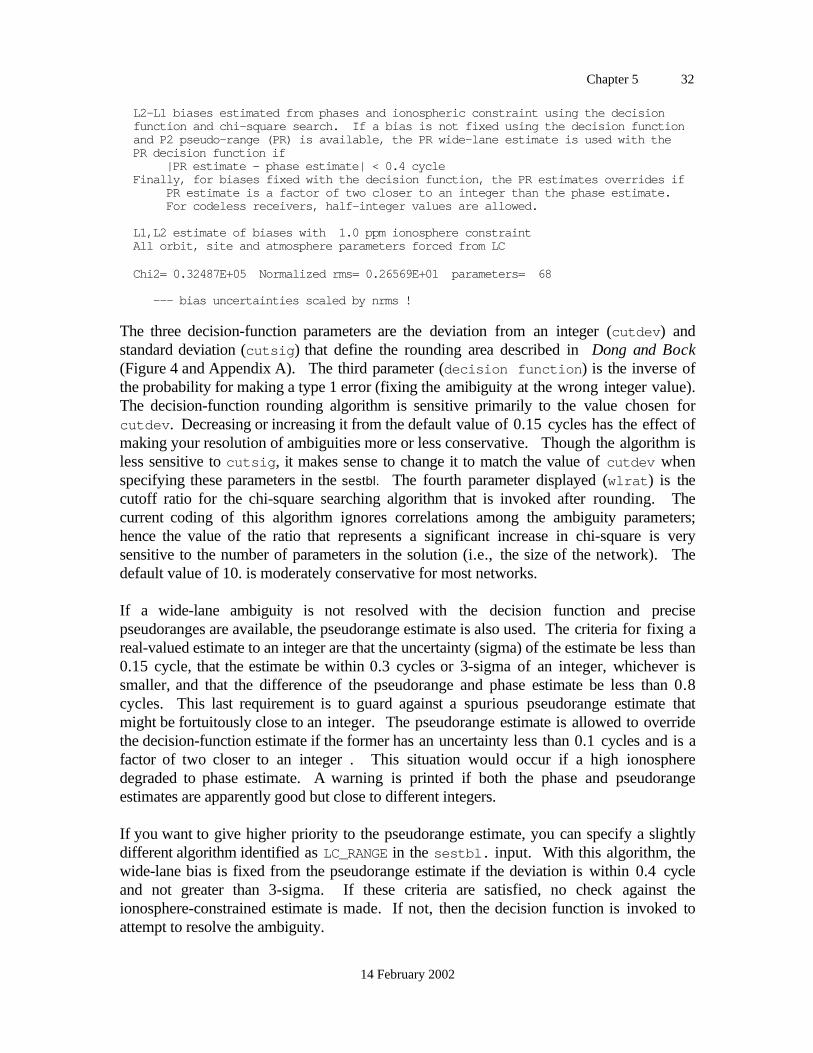
Chapter 5 32

14 February 2002

L2-L1 biases estimated from phases and ionospheric constraint using the decision function and chi-square search. If a bias is not fixed using the decision function and P2 pseudo-range (PR) is available, the PR wide-lane estimate is used with the PR decision function if |PR estimate - phase estimate| < 0.4 cycle Finally, for biases fixed with the decision function, the PR estimates overrides if PR estimate is a factor of two closer to an integer than the phase estimate. For codeless receivers, half-integer values are allowed.

L1,L2 estimate of biases with 1.0 ppm ionosphere constraint All orbit, site and atmosphere parameters forced from LC

Chi2= 0.32487E+05 Normalized rms= 0.26569E+01 parameters= 68

--- bias uncertainties scaled by nrms !

The three decision-function parameters are the deviation from an integer (cutdev ) andstandard deviation (cutsig ) that define the rounding area described in Dong and Bock(Figure 4 and Appendix A). The third parameter (decision function ) is the inverse ofthe probability for making a type 1 error (fixing the amibiguity at the wrong integer value).The decision-function rounding algorithm is sensitive primarily to the value chosen forcutdev . Decreasing or increasing it from the default value of 0.15 cycles has the effect ofmaking your resolution of ambiguities more or less conservative. Though the algorithm isless sensitive to cutsig , it makes sense to change it to match the value of cutdev whenspecifying these parameters in the sestbl. The fourth parameter displayed (wlrat ) is thecutoff ratio for the chi-square searching algorithm that is invoked after rounding. Thecurrent coding of this algorithm ignores correlations among the ambiguity parameters;hence the value of the ratio that represents a significant increase in chi-square is verysensitive to the number of parameters in the solution (i.e., the size of the network). Thedefault value of 10. is moderately conservative for most networks.

If a wide-lane ambiguity is not resolved with the decision function and precisepseudoranges are available, the pseudorange estimate is also used. The criteria for fixing areal-valued estimate to an integer are that the uncertainty (sigma) of the estimate be less than0.15 cycle, that the estimate be within 0.3 cycles or 3-sigma of an integer, whichever issmaller, and that the difference of the pseudorange and phase estimate be less than 0.8cycles. This last requirement is to guard against a spurious pseudorange estimate thatmight be fortuitously close to an integer. The pseudorange estimate is allowed to overridethe decision-function estimate if the former has an uncertainty less than 0.1 cycles and is afactor of two closer to an integer . This situation would occur if a high ionospheredegraded to phase estimate. A warning is printed if both the phase and pseudorangeestimates are apparently good but close to different integers.

If you want to give higher priority to the pseudorange estimate, you can specify a slightlydifferent algorithm identified as LC_RANGE in the sestbl. input. With this algorithm, thewide-lane bias is fixed from the pseudorange estimate if the deviation is within 0.4 cycleand not greater than 3-sigma. If these criteria are satisfied, no check against theionosphere-constrained estimate is made. If not, then the decision function is invoked toattempt to resolve the ambiguity.

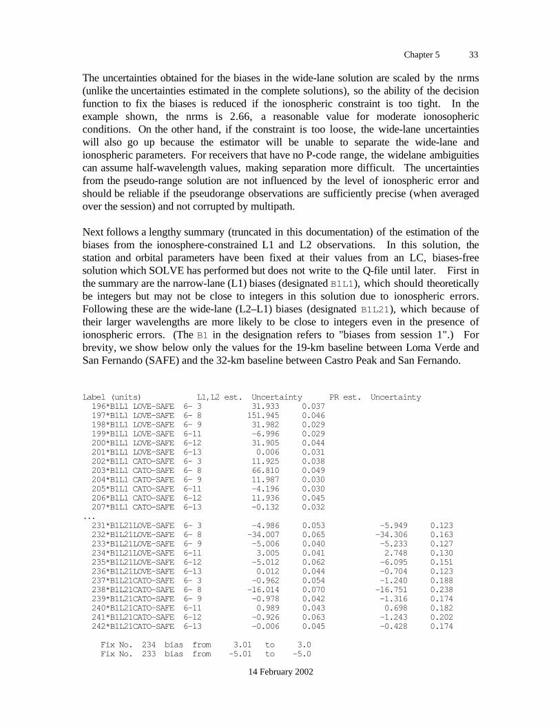
Chapter 5 33

14 February 2002

The uncertainties obtained for the biases in the wide-lane solution are scaled by the nrms(unlike the uncertainties estimated in the complete solutions), so the ability of the decisionfunction to fix the biases is reduced if the ionospheric constraint is too tight. In theexample shown, the nrms is 2.66, a reasonable value for moderate ionosophericconditions. On the other hand, if the constraint is too loose, the wide-lane uncertaintieswill also go up because the estimator will be unable to separate the wide-lane andionospheric parameters. For receivers that have no P-code range, the widelane ambiguitiescan assume half-wavelength values, making separation more difficult. The uncertaintiesfrom the pseudo-range solution are not influenced by the level of ionospheric error andshould be reliable if the pseudorange observations are sufficiently precise (when averagedover the session) and not corrupted by multipath.

Next follows a lengthy summary (truncated in this documentation) of the estimation of thebiases from the ionosphere-constrained L1 and L2 observations. In this solution, thestation and orbital parameters have been fixed at their values from an LC, biases-freesolution which SOLVE has performed but does not write to the Q-file until later. First inthe summary are the narrow-lane (L1) biases (designated B1L1), which should theoreticallybe integers but may not be close to integers in this solution due to ionospheric errors.Following these are the wide-lane (L2–L1) biases (designated B1L21), which because oftheir larger wavelengths are more likely to be close to integers even in the presence ofionospheric errors. (The B1 in the designation refers to "biases from session 1".) Forbrevity, we show below only the values for the 19-km baseline between Loma Verde andSan Fernando (SAFE) and the 32-km baseline between Castro Peak and San Fernando.

Label (units) L1,L2 est. Uncertainty PR est. Uncertainty 196*B1L1 LOVE-SAFE 6- 3 31.933 0.037 197*B1L1 LOVE-SAFE 6- 8 151.945 0.046 198*B1L1 LOVE-SAFE 6- 9 31.982 0.029 199*B1L1 LOVE-SAFE 6-11 -6.996 0.029 200*B1L1 LOVE-SAFE 6-12 31.905 0.044 201*B1L1 LOVE-SAFE 6-13 0.006 0.031 202*B1L1 CATO-SAFE 6- 3 11.925 0.038 203*B1L1 CATO-SAFE 6- 8 66.810 0.049 204*B1L1 CATO-SAFE 6- 9 11.987 0.030 205*B1L1 CATO-SAFE 6-11 -4.196 0.030 206*B1L1 CATO-SAFE 6-12 11.936 0.045 207*B1L1 CATO-SAFE 6-13 -0.132 0.032... 231*B1L21LOVE-SAFE 6- 3 -4.986 0.053 -5.949 0.123 232*B1L21LOVE-SAFE 6- 8 -34.007 0.065 -34.306 0.163 233*B1L21LOVE-SAFE 6- 9 -5.006 0.040 -5.233 0.127 234*B1L21LOVE-SAFE 6-11 3.005 0.041 2.748 0.130 235*B1L21LOVE-SAFE 6-12 -5.012 0.062 -6.095 0.151 236*B1L21LOVE-SAFE 6-13 0.012 0.044 -0.704 0.123 237*B1L21CATO-SAFE 6- 3 -0.962 0.054 -1.240 0.188 238*B1L21CATO-SAFE 6- 8 -16.014 0.070 -16.751 0.238 239*B1L21CATO-SAFE 6- 9 -0.978 0.042 -1.316 0.174 240*B1L21CATO-SAFE 6-11 0.989 0.043 0.698 0.182 241*B1L21CATO-SAFE 6-12 -0.926 0.063 -1.243 0.202 242*B1L21CATO-SAFE 6-13 -0.006 0.045 -0.428 0.174

Fix No. 234 bias from 3.01 to 3.0 Fix No. 233 bias from -5.01 to -5.0

Chapter 5 34

14 February 2002

Fix No. 242 bias from -0.01 to 0.0 Fix No. 240 bias from 0.99 to 1.0 Fix No. 236 bias from 0.01 to 0.0 Fix No. 231 bias from -4.99 to -5.0 Fix No. 245 bias from 6.02 to 6.0 Fix No. 248 bias from 0.01 to 0.0 Fix No. 247 bias from 4.99 to 5.0 Fix No. 232 bias from -34.01 to -34.0 Fix No. 238 bias from -16.00 to -16.0 Fix No. 239 bias from -0.97 to -1.0 Fix No. 235 bias from -5.02 to -5.0 Fix No. 237 bias from -0.96 to -1.0 Fix No. 243 bias from 6.02 to 6.0 Fix No. 246 bias from -1.95 to -2.0 Fix No. 244 bias from 16.05 to 16.0 Fix No. 241 bias from -0.92 to -1.0

--- bias uncertainties scaled by nrms !

In the example shown, SOLVE resolved all of the wide-lane ambiguities for LOVE–SAFE(Nos. 231–236) and CATO–SAFE (Nos. 237–242) using the decision function with theionosphere-constrained phase estimate. In four cases the phase and pseudorange estimatesare inconsistent; in each of those the phase estimate was closer to an integer and hence tookprecedent. The uncertainties in the pseudorange estimates would have been a factor of twosmaller had we used 30-s rather than 120-s sampling.

Next in the Q-file is a summary of both the narrow-lane and wide-lane biases after theresolution of as many as possible of the wide-lanes. The narrow-lane bias estimates areslightly changed, and have smaller uncertainties, but will be close to integers in the separateL1 and L2 solution only if ionospheric effects are small (as is in fact the case for thisexperiment). The main purpose of this summary is to highlight the wide-lane biases thathave been fixed at integers and those for regional baselines that remain unresolved. Usingthis summary and the preceeding one, you should evaluate whether or not it may bepossible to resolve the remaining (regional) wide-lane ambiguities by changing theionospheric constraint or editing the data. You can use CVIEW to inspect the residuals forthe station–satellite combinations in question to see whether, for example, the departurefrom an integer is due to an excursion in only part of the pass—in the phase estimate due tothe ionosphere or in the pseudo-range estimate due to multipath—in which case you couldunweight the offending data. Note that the pseudorange estimate is made using the fullone-way span of data for each station and satellite so that multipath corruption of the wide-lane combination may not be visible if you display only double differences in CVIEW.(The use of one-way, rather than doubly differenced pseudorange was instituted to handlethe high pseudorange noise of early P-code receivers. Future versions of SOLVE willprovide the option of using doubly differenced pseudorange to reduce the influence ofreceiver range biases and to make the phase and pseudoranges for each double-differenceambiguity parameter consistent.)

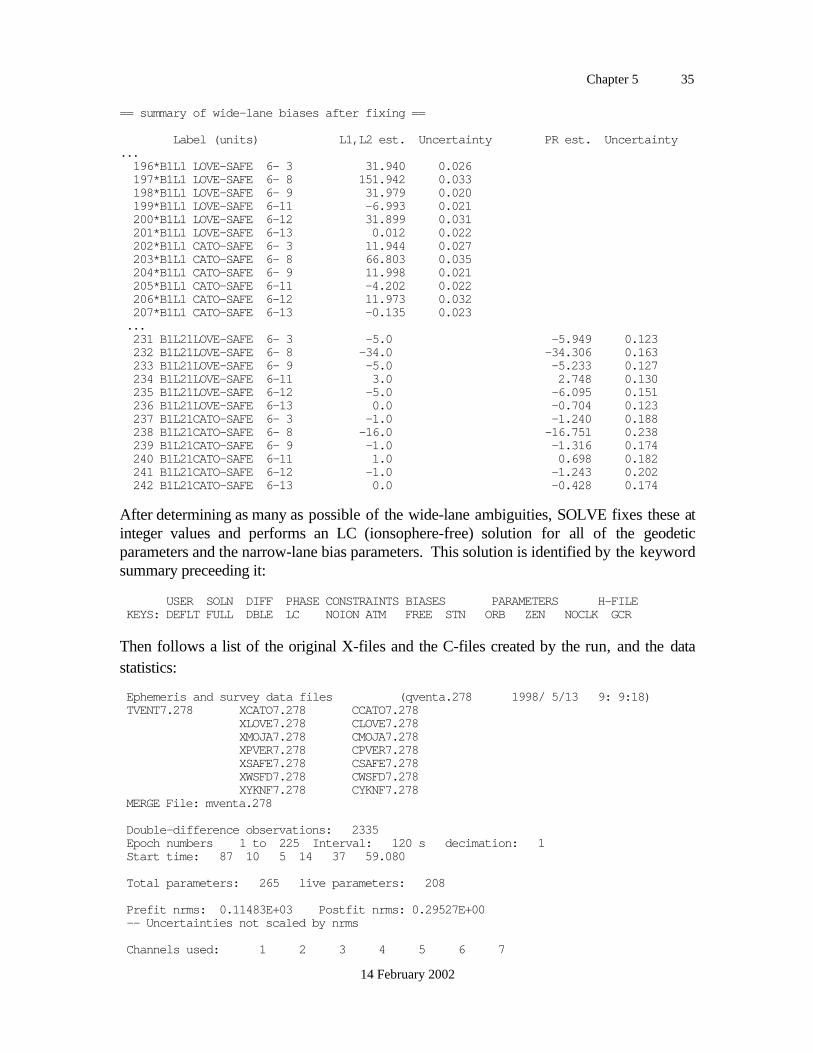
Chapter 5 35

14 February 2002

== summary of wide-lane biases after fixing ==

Label (units) L1,L2 est. Uncertainty PR est. Uncertainty... 196*B1L1 LOVE-SAFE 6- 3 31.940 0.026 197*B1L1 LOVE-SAFE 6- 8 151.942 0.033 198*B1L1 LOVE-SAFE 6- 9 31.979 0.020 199*B1L1 LOVE-SAFE 6-11 -6.993 0.021 200*B1L1 LOVE-SAFE 6-12 31.899 0.031 201*B1L1 LOVE-SAFE 6-13 0.012 0.022 202*B1L1 CATO-SAFE 6- 3 11.944 0.027 203*B1L1 CATO-SAFE 6- 8 66.803 0.035 204*B1L1 CATO-SAFE 6- 9 11.998 0.021 205*B1L1 CATO-SAFE 6-11 -4.202 0.022 206*B1L1 CATO-SAFE 6-12 11.973 0.032 207*B1L1 CATO-SAFE 6-13 -0.135 0.023 ... 231 B1L21LOVE-SAFE 6- 3 -5.0 -5.949 0.123 232 B1L21LOVE-SAFE 6- 8 -34.0 -34.306 0.163 233 B1L21LOVE-SAFE 6- 9 -5.0 -5.233 0.127 234 B1L21LOVE-SAFE 6-11 3.0 2.748 0.130 235 B1L21LOVE-SAFE 6-12 -5.0 -6.095 0.151 236 B1L21LOVE-SAFE 6-13 0.0 -0.704 0.123 237 B1L21CATO-SAFE 6- 3 -1.0 -1.240 0.188 238 B1L21CATO-SAFE 6- 8 -16.0 -16.751 0.238 239 B1L21CATO-SAFE 6- 9 -1.0 -1.316 0.174 240 B1L21CATO-SAFE 6-11 1.0 0.698 0.182 241 B1L21CATO-SAFE 6-12 -1.0 -1.243 0.202 242 B1L21CATO-SAFE 6-13 0.0 -0.428 0.174

After determining as many as possible of the wide-lane ambiguities, SOLVE fixes these atinteger values and performs an LC (ionsophere-free) solution for all of the geodeticparameters and the narrow-lane bias parameters. This solution is identified by the keywordsummary preceeding it:

USER SOLN DIFF PHASE CONSTRAINTS BIASES PARAMETERS H-FILE KEYS: DEFLT FULL DBLE LC NOION ATM FREE STN ORB ZEN NOCLK GCR

Then follows a list of the original X-files and the C-files created by the run, and the datastatistics:

Ephemeris and survey data files (qventa.278 1998/ 5/13 9: 9:18) TVENT7.278 XCATO7.278 CCATO7.278 XLOVE7.278 CLOVE7.278 XMOJA7.278 CMOJA7.278 XPVER7.278 CPVER7.278 XSAFE7.278 CSAFE7.278 XWSFD7.278 CWSFD7.278 XYKNF7.278 CYKNF7.278 MERGE File: mventa.278

Double-difference observations: 2335 Epoch numbers 1 to 225 Interval: 120 s decimation: 1 Start time: 87 10 5 14 37 59.080

Total parameters: 265 live parameters: 208

Prefit nrms: 0.11483E+03 Postfit nrms: 0.29527E+00 -- Uncertainties not scaled by nrms

Channels used: 1 2 3 4 5 6 7

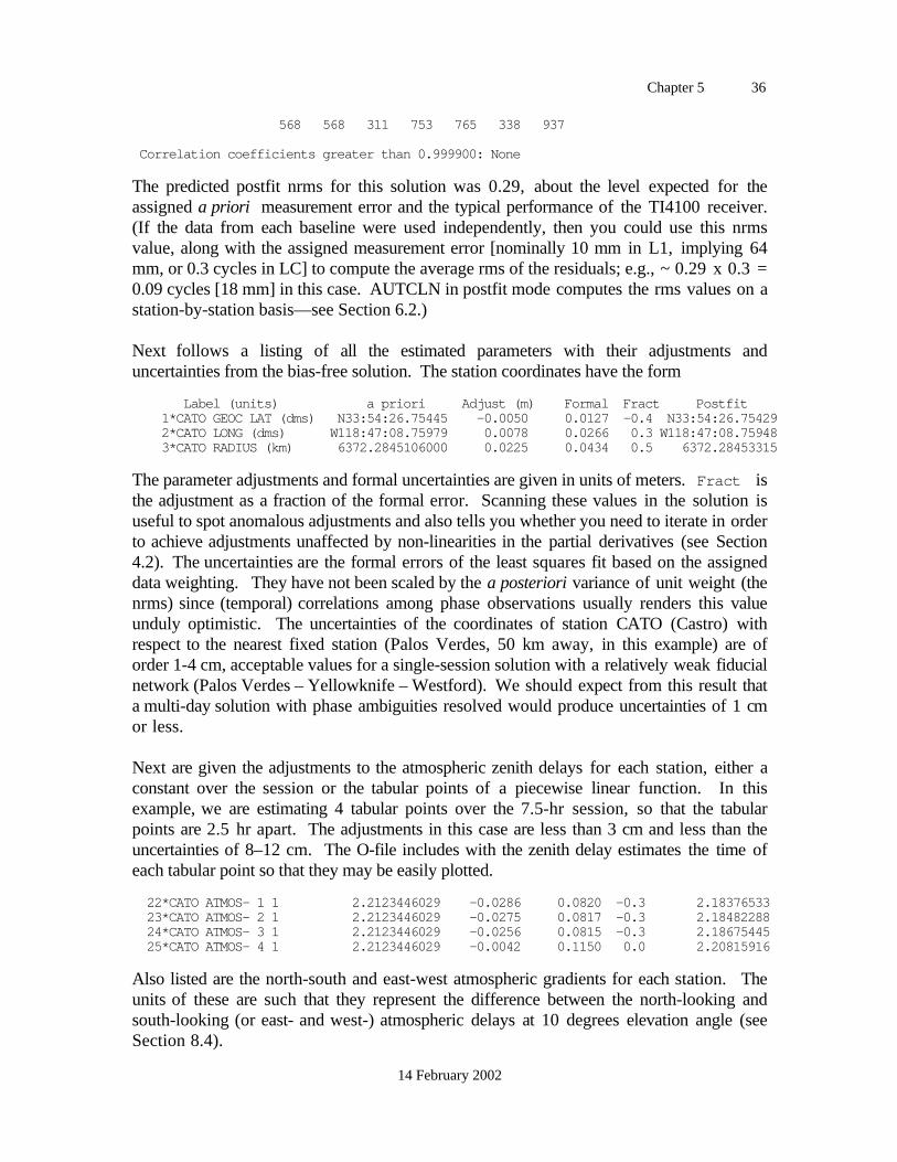
Chapter 5 36

14 February 2002

568 568 311 753 765 338 937

Correlation coefficients greater than 0.999900: None

The predicted postfit nrms for this solution was 0.29, about the level expected for theassigned a priori measurement error and the typical performance of the TI4100 receiver.(If the data from each baseline were used independently, then you could use this nrmsvalue, along with the assigned measurement error [nominally 10 mm in L1, implying 64mm, or 0.3 cycles in LC] to compute the average rms of the residuals; e.g., ~ 0.29 x 0.3 =0.09 cycles [18 mm] in this case. AUTCLN in postfit mode computes the rms values on astation-by-station basis—see Section 6.2.)

Next follows a listing of all the estimated parameters with their adjustments anduncertainties from the bias-free solution. The station coordinates have the form

Label (units) a priori Adjust (m) Formal Fract Postfit 1*CATO GEOC LAT (dms) N33:54:26.75445 -0.0050 0.0127 -0.4 N33:54:26.75429 2*CATO LONG (dms) W118:47:08.75979 0.0078 0.0266 0.3 W118:47:08.75948 3*CATO RADIUS (km) 6372.2845106000 0.0225 0.0434 0.5 6372.28453315

The parameter adjustments and formal uncertainties are given in units of meters. Fract isthe adjustment as a fraction of the formal error. Scanning these values in the solution isuseful to spot anomalous adjustments and also tells you whether you need to iterate in orderto achieve adjustments unaffected by non-linearities in the partial derivatives (see Section4.2). The uncertainties are the formal errors of the least squares fit based on the assigneddata weighting. They have not been scaled by the a posteriori variance of unit weight (thenrms) since (temporal) correlations among phase observations usually renders this valueunduly optimistic. The uncertainties of the coordinates of station CATO (Castro) withrespect to the nearest fixed station (Palos Verdes, 50 km away, in this example) are oforder 1-4 cm, acceptable values for a single-session solution with a relatively weak fiducialnetwork (Palos Verdes – Yellowknife – Westford). We should expect from this result thata multi-day solution with phase ambiguities resolved would produce uncertainties of 1 cmor less.

Next are given the adjustments to the atmospheric zenith delays for each station, either aconstant over the session or the tabular points of a piecewise linear function. In thisexample, we are estimating 4 tabular points over the 7.5-hr session, so that the tabularpoints are 2.5 hr apart. The adjustments in this case are less than 3 cm and less than theuncertainties of 8–12 cm. The O-file includes with the zenith delay estimates the time ofeach tabular point so that they may be easily plotted.

22*CATO ATMOS- 1 1 2.2123446029 -0.0286 0.0820 -0.3 2.18376533 23*CATO ATMOS- 2 1 2.2123446029 -0.0275 0.0817 -0.3 2.18482288 24*CATO ATMOS- 3 1 2.2123446029 -0.0256 0.0815 -0.3 2.18675445 25*CATO ATMOS- 4 1 2.2123446029 -0.0042 0.1150 0.0 2.20815916

Also listed are the north-south and east-west atmospheric gradients for each station. Theunits of these are such that they represent the difference between the north-looking andsouth-looking (or east- and west-) atmospheric delays at 10 degrees elevation angle (seeSection 8.4).

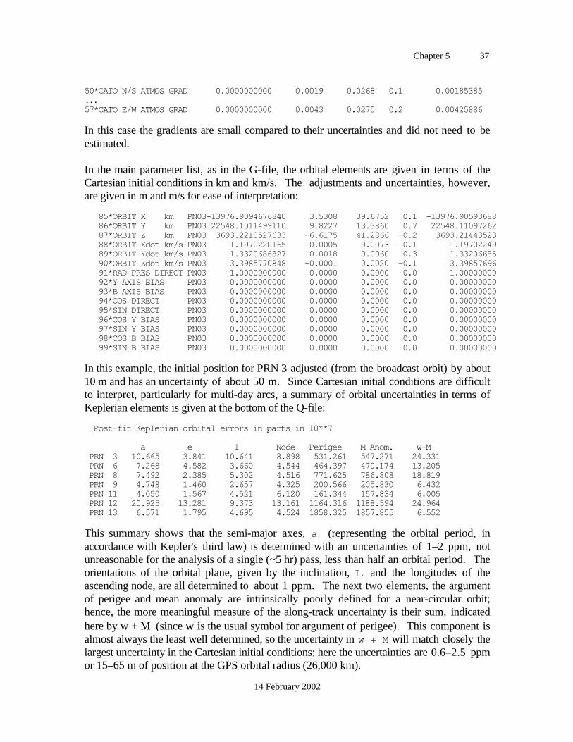
Chapter 5 37

14 February 2002

50*CATO N/S ATMOS GRAD 0.0000000000 0.0019 0.0268 0.1 0.00185385...57*CATO E/W ATMOS GRAD 0.0000000000 0.0043 0.0275 0.2 0.00425886

In this case the gradients are small compared to their uncertainties and did not need to beestimated.

In the main parameter list, as in the G-file, the orbital elements are given in terms of theCartesian initial conditions in km and km/s. The adjustments and uncertainties, however,are given in m and m/s for ease of interpretation:

85*ORBIT X km PN03-13976.9094676840 3.5308 39.6752 0.1 -13976.90593688 86*ORBIT Y km PN03 22548.1011499110 9.8227 13.3860 0.7 22548.11097262 87*ORBIT Z km PN03 3693.2210527633 -6.6175 41.2866 -0.2 3693.21443523 88*ORBIT Xdot km/s PN03 -1.1970220165 -0.0005 0.0073 -0.1 -1.19702249 89*ORBIT Ydot km/s PN03 -1.3320686827 0.0018 0.0060 0.3 -1.33206685 90*ORBIT Zdot km/s PN03 3.3985770848 -0.0001 0.0020 -0.1 3.39857696 91*RAD PRES DIRECT PN03 1.0000000000 0.0000 0.0000 0.0 1.00000000 92*Y AXIS BIAS PN03 0.0000000000 0.0000 0.0000 0.0 0.00000000 93*B AXIS BIAS PN03 0.0000000000 0.0000 0.0000 0.0 0.00000000 94*COS DIRECT PN03 0.0000000000 0.0000 0.0000 0.0 0.00000000 95*SIN DIRECT PN03 0.0000000000 0.0000 0.0000 0.0 0.00000000 96*COS Y BIAS PN03 0.0000000000 0.0000 0.0000 0.0 0.00000000 97*SIN Y BIAS PN03 0.0000000000 0.0000 0.0000 0.0 0.00000000 98*COS B BIAS PN03 0.0000000000 0.0000 0.0000 0.0 0.00000000 99*SIN B BIAS PN03 0.0000000000 0.0000 0.0000 0.0 0.00000000

In this example, the initial position for PRN 3 adjusted (from the broadcast orbit) by about10 m and has an uncertainty of about 50 m. Since Cartesian initial conditions are difficultto interpret, particularly for multi-day arcs, a summary of orbital uncertainties in terms ofKeplerian elements is given at the bottom of the Q-file:

Post-fit Keplerian orbital errors in parts in 10**7

a e I Node Perigee M Anom. w+M PRN 3 10.665 3.841 10.641 8.898 531.261 547.271 24.331 PRN 6 7.268 4.582 3.660 4.544 464.397 470.174 13.205 PRN 8 7.492 2.385 5.302 4.516 771.625 786.808 18.819 PRN 9 4.748 1.460 2.657 4.325 200.566 205.830 6.432 PRN 11 4.050 1.567 4.521 6.120 161.344 157.834 6.005 PRN 12 20.925 13.281 9.373 13.161 1164.316 1188.594 24.964 PRN 13 6.571 1.795 4.695 4.524 1858.325 1857.855 6.552

This summary shows that the semi-major axes, a, (representing the orbital period, inaccordance with Kepler's third law) is determined with an uncertainties of 1–2 ppm, notunreasonable for the analysis of a single (~5 hr) pass, less than half an orbital period. Theorientations of the orbital plane, given by the inclination, I, and the longitudes of theascending node, are all determined to about 1 ppm. The next two elements, the argumentof perigee and mean anomaly are intrinsically poorly defined for a near-circular orbit;hence, the more meaningful measure of the along-track uncertainty is their sum, indicatedhere by w + M (since w is the usual symbol for argument of perigee). This component isalmost always the least well determined, so the uncertainty in w + M will match closely thelargest uncertainty in the Cartesian initial conditions; here the uncertainties are 0.6–2.5 ppmor 15–65 m of position at the GPS orbital radius (26,000 km).

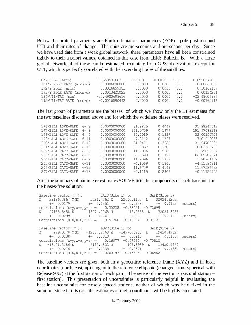
Chapter 5 38

14 February 2002

Below the orbital parameters are Earth orientation parameters (EOP)—pole position andUT1 and their rates of change. The units are arc-seconds and arc-second per day. Sincewe have used data from a weak global network, these parameters have all been constrainedtightly to their a priori values, obtained in this case from IERS Bulletin B. With a largeglobal network, all of these can be estimated accurately from GPS observations except forUT1, which is perfectly correlated with the ascending nodes of the satellites.

190*X POLE (arcs) -0.0558591603 0.0000 0.0030 0.0 -0.05585730 191*X POLE RATE (arcs/d) -0.0006000000 0.0000 0.0001 0.0 -0.00060000 192*Y POLE (arcs) 0.3016859381 0.0000 0.0030 0.0 0.30169137 193*Y POLE RATE (arcs/d) 0.0013425023 0.0000 0.0001 0.0 0.00134251 194*UT1-TAI (sec) -23.4900699616 0.0000 0.0000 0.0 -23.49006996 195*UT1-TAI RATE (sec/d) -0.0016590442 0.0000 0.0001 0.0 -0.00165916

The last group of parameters are the biases, of which we show only the L1 estimates forthe two baselines discussed above and for which the widelane biases were resolved.

196*B1L1 LOVE-SAFE 6- 3 0.0000000000 31.8825 0.4043 31.88247512 197*B1L1 LOVE-SAFE 6- 8 0.0000000000 151.9709 0.1379 151.97088168 198*B1L1 LOVE-SAFE 6- 9 0.0000000000 32.0019 0.1557 32.00194728 199*B1L1 LOVE-SAFE 6-11 0.0000000000 -7.0142 0.1227 -7.01419035 200*B1L1 LOVE-SAFE 6-12 0.0000000000 31.9471 0.3680 31.94708296 201*B1L1 LOVE-SAFE 6-13 0.0000000000 -0.0367 0.2209 -0.03666700 202*B1L1 CATO-SAFE 6- 3 0.0000000000 11.7906 0.5686 11.79058587 203*B1L1 CATO-SAFE 6- 8 0.0000000000 66.8599 0.1798 66.85989321 204*B1L1 CATO-SAFE 6- 9 0.0000000000 11.9096 0.1738 11.90961172 205*B1L1 CATO-SAFE 6-11 0.0000000000 -4.1569 0.1845 -4.15694811 206*B1L1 CATO-SAFE 6-12 0.0000000000 11.6759 0.4143 11.67586633 207*B1L1 CATO-SAFE 6-13 0.0000000000 -0.1115 0.2805 -0.11150922

After the summary of parameter estimates SOLVE lists the components of each baseline forthe biases-free solution:

Baseline vector (m ): CATO(Site 1) to SAFE(Site 5) X 22126.3867 Y(E) 5021.4762 Z 22600.1150 L 32024.3253 +- 0.0279 +- 0.0351 +- 0.0238 +- 0.0122 (meters) correlations (x-y,x-z,y-z) = 0.20228 -0.68451 -0.72699 N 27155.5488 E 16974.1265 U 112.2888 L 32024.3253 +- 0.0099 +- 0.0267 +- 0.0420 +- 0.0122 (Meters) Correlations (N-E,N-U,E-U) = -0.51360 -0.12804 0.01121

Baseline vector (m ): LOVE(Site 2) to SAFE(Site 5) X 299.0178 Y(E) -12367.2768 Z -14970.5286 L 19420.4962 +- 0.0238 +- 0.0313 +- 0.0210 +- 0.0133 (meters) correlations (x-y,x-z,y-z) = 0.16977 -0.67687 -0.75822 N -18401.3186 E 6195.4832 U 403.8989 L 19420.4962 +- 0.0076 +- 0.0235 +- 0.0371 +- 0.0133 (Meters) Correlations (N-E,N-U,E-U) = -0.60197 -0.13845 0.06462

The baseline vectors are given both in a geocentric reference frame (XYZ) and in localcoordinates (north, east, up) tangent to the reference ellipsoid (changed from spherical withRelease 9.92) at the first station of each pair. The sense of the vector is (second station –first station). This presentation of uncertainties is particularly helpful in evaluating thebaseline uncertainties for closely spaced stations, neither of which was held fixed in thesolution, since in this case the estimates of their coordinates will be highly correlated.

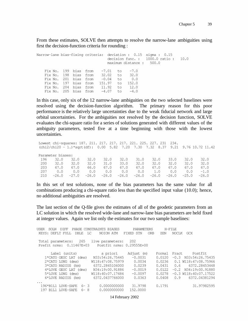
Chapter 5 39

14 February 2002

From these estimates, SOLVE then attempts to resolve the narrow-lane ambiguities usingfirst the decision-function criteria for rounding :

Narrow-lane bias-fixing criteria: deviation : 0.15 sigma : 0.15 decision func. : 1000.0 ratio : 10.0 maximum distance : 500.0

Fix No. 199 bias from -7.01 to -7.0 Fix No. 198 bias from 32.02 to 32.0 Fix No. 201 bias from -0.04 to 0.0 Fix No. 197 bias from 151.97 to 152.0 Fix No. 204 bias from 11.92 to 12.0 Fix No. 205 bias from -4.07 to -4.0

In this case, only six of the 12 narrow-lane ambiguities on the two selected baselines wereresolved using the decision-function algorithm. The primary reason for this poorperformance is the relatively large uncertainties due to the weak fiducial network and largeorbital uncertainties. For the ambiguities not resolved by the decision function, SOLVEevaluates the chi-square ratio for a series of solutions generated with different values of theambiguity parameters, tested five at a time beginning with those with the lowestuncertainties.

Lowest chi-squares: 187. 211. 217. 217. 217. 221. 225. 227. 231 234. (chi2/chi20 - 1.)*sqrt(df): 0.00 5.82 7.20 7.30 7.32 8.37 9.21 9.76 10.72 11.42

Parameter biases: 196 32.0 32.0 32.0 32.0 32.0 31.0 32.0 33.0 32.0 32.0 200 32.0 32.0 32.0 31.0 33.0 32.0 32.0 32.0 32.0 32.0 203 67.0 67.0 66.0 67.0 67.0 67.0 67.0 67.0 67.0 67.0 207 0.0 0.0 0.0 0.0 0.0 0.0 1.0 0.0 0.0 -1.0 210 -26.0 -27.0 -26.0 -26.0 -26.0 -26.0 -26.0 -26.0 -25.0 -26.0

In this set of test solutions, none of the bias parameters has the same value for allcombinations producing a chi-square ratio less than the specified input value (10.0); hence,no additional ambiguities are resolved.

The last section of the Q-file gives the estimates of all of the geodetic parameters from anLC solution in which the resolved wide-lane and narrow-lane bias parameters are held fixedat integer values. Again we list only the estimates for our two sample baselines:

USER SOLN DIFF PHASE CONSTRAINTS BIASES PARAMETERS H-FILE�� KEYS: DEFLT FULL DBLE LC NOION ATM FIXED STN ORB ZEN NOCLK GCX

Total parameters: 265 live parameters: 202 Prefit nrms: 0.11467E+03 Postfit nrms: 0.29555E+00

Label (units) a priori Adjust (m) Formal Fract Postfit 1*CATO GEOC LAT (dms) N33:54:26.75445 -0.0031 0.0120 -0.3 N33:54:26.75435 2*CATO LONG (dms) W118:47:08.75979 0.0034 0.0236 0.1 W118:47:08.75966 3*CATO RADIUS (km) 6372.2845106000 0.0239 0.0431 0.6 6372.28453448 4*LOVE GEOC LAT (dms) N34:19:00.91886 -0.0019 0.0122 -0.2 N34:19:00.91880 5*LOVE LONG (dms) W118:40:07.17484 -0.0097 0.0278 -0.3 W118:40:07.17522 6*LOVE RADIUS (km) 6372.0437766000 0.0363 0.0408 0.9 6372.04381294... 196*B1L1 LOVE-SAFE 6- 3 0.0000000000 31.9798 0.1791 31.97982595 197 B1L1 LOVE-SAFE 6- 8 0.0000000000 152.0000

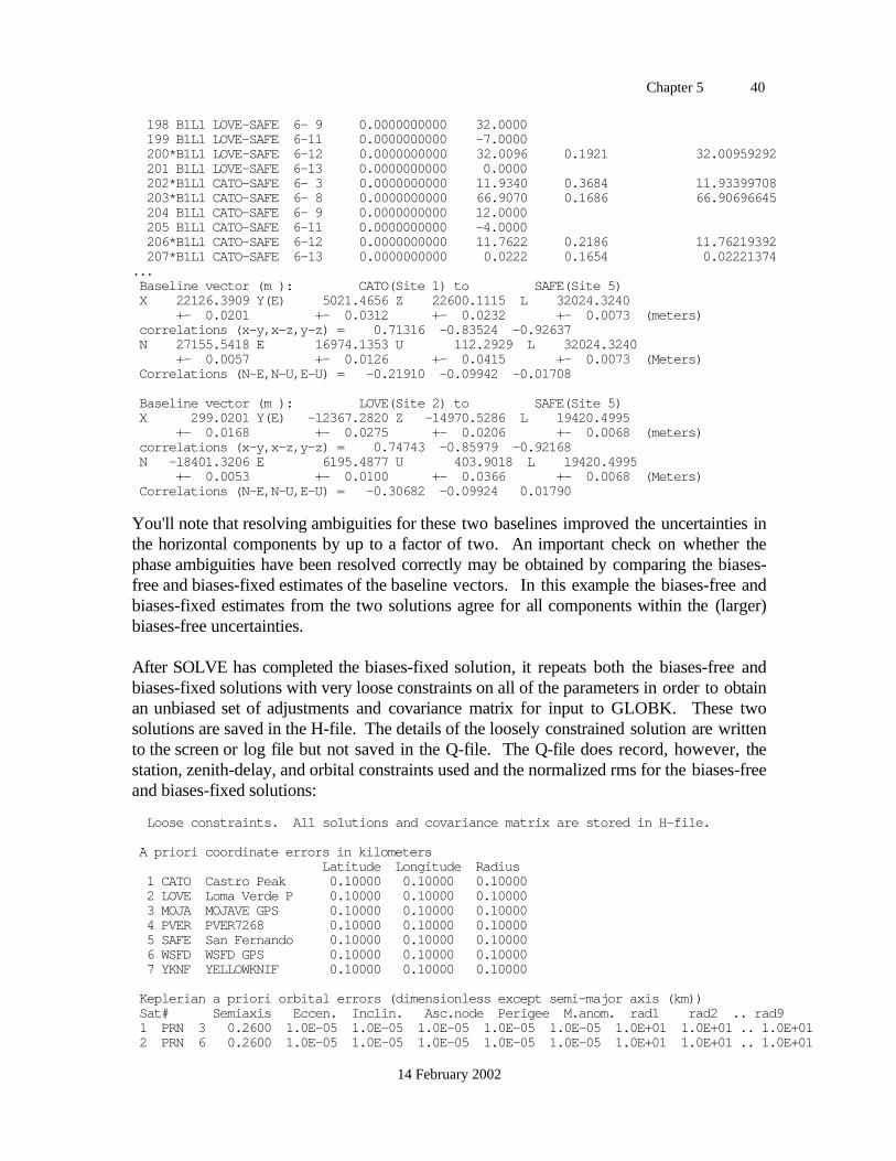
Chapter 5 40

14 February 2002

198 B1L1 LOVE-SAFE 6- 9 0.0000000000 32.0000 199 B1L1 LOVE-SAFE 6-11 0.0000000000 -7.0000 200*B1L1 LOVE-SAFE 6-12 0.0000000000 32.0096 0.1921 32.00959292 201 B1L1 LOVE-SAFE 6-13 0.0000000000 0.0000 202*B1L1 CATO-SAFE 6- 3 0.0000000000 11.9340 0.3684 11.93399708 203*B1L1 CATO-SAFE 6- 8 0.0000000000 66.9070 0.1686 66.90696645 204 B1L1 CATO-SAFE 6- 9 0.0000000000 12.0000 205 B1L1 CATO-SAFE 6-11 0.0000000000 -4.0000 206*B1L1 CATO-SAFE 6-12 0.0000000000 11.7622 0.2186 11.76219392 207*B1L1 CATO-SAFE 6-13 0.0000000000 0.0222 0.1654 0.02221374... Baseline vector (m ): CATO(Site 1) to SAFE(Site 5) X 22126.3909 Y(E) 5021.4656 Z 22600.1115 L 32024.3240 +- 0.0201 +- 0.0312 +- 0.0232 +- 0.0073 (meters) correlations (x-y,x-z,y-z) = 0.71316 -0.83524 -0.92637 N 27155.5418 E 16974.1353 U 112.2929 L 32024.3240 +- 0.0057 +- 0.0126 +- 0.0415 +- 0.0073 (Meters) Correlations (N-E,N-U,E-U) = -0.21910 -0.09942 -0.01708

Baseline vector (m ): LOVE(Site 2) to SAFE(Site 5) X 299.0201 Y(E) -12367.2820 Z -14970.5286 L 19420.4995 +- 0.0168 +- 0.0275 +- 0.0206 +- 0.0068 (meters) correlations (x-y,x-z,y-z) = 0.74743 -0.85979 -0.92168 N -18401.3206 E 6195.4877 U 403.9018 L 19420.4995 +- 0.0053 +- 0.0100 +- 0.0366 +- 0.0068 (Meters) Correlations (N-E,N-U,E-U) = -0.30682 -0.09924 0.01790

You'll note that resolving ambiguities for these two baselines improved the uncertainties inthe horizontal components by up to a factor of two. An important check on whether thephase ambiguities have been resolved correctly may be obtained by comparing the biases-free and biases-fixed estimates of the baseline vectors. In this example the biases-free andbiases-fixed estimates from the two solutions agree for all components within the (larger)biases-free uncertainties.

After SOLVE has completed the biases-fixed solution, it repeats both the biases-free andbiases-fixed solutions with very loose constraints on all of the parameters in order to obtainan unbiased set of adjustments and covariance matrix for input to GLOBK. These twosolutions are saved in the H-file. The details of the loosely constrained solution are writtento the screen or log file but not saved in the Q-file. The Q-file does record, however, thestation, zenith-delay, and orbital constraints used and the normalized rms for the biases-freeand biases-fixed solutions:

Loose constraints. All solutions and covariance matrix are stored in H-file.

A priori coordinate errors in kilometers Latitude Longitude Radius 1 CATO Castro Peak 0.10000 0.10000 0.10000 2 LOVE Loma Verde P 0.10000 0.10000 0.10000 3 MOJA MOJAVE GPS 0.10000 0.10000 0.10000 4 PVER PVER7268 0.10000 0.10000 0.10000 5 SAFE San Fernando 0.10000 0.10000 0.10000 6 WSFD WSFD GPS 0.10000 0.10000 0.10000 7 YKNF YELLOWKNIF 0.10000 0.10000 0.10000

Keplerian a priori orbital errors (dimensionless except semi-major axis (km)) Sat# Semiaxis Eccen. Inclin. Asc.node Perigee M.anom. rad1 rad2 .. rad9 1 PRN 3 0.2600 1.0E-05 1.0E-05 1.0E-05 1.0E-05 1.0E-05 1.0E+01 1.0E+01 .. 1.0E+01 2 PRN 6 0.2600 1.0E-05 1.0E-05 1.0E-05 1.0E-05 1.0E-05 1.0E+01 1.0E+01 .. 1.0E+01

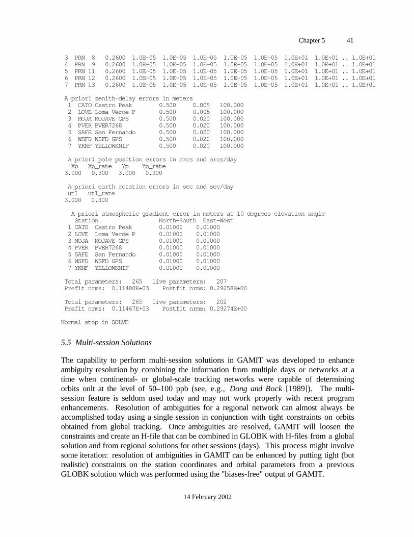
Chapter 5 41

14 February 2002

3 PRN 8 0.2600 1.0E-05 1.0E-05 1.0E-05 1.0E-05 1.0E-05 1.0E+01 1.0E+01 .. 1.0E+01 4 PRN 9 0.2600 1.0E-05 1.0E-05 1.0E-05 1.0E-05 1.0E-05 1.0E+01 1.0E+01 .. 1.0E+01 5 PRN 11 0.2600 1.0E-05 1.0E-05 1.0E-05 1.0E-05 1.0E-05 1.0E+01 1.0E+01 .. 1.0E+01 6 PRN 12 0.2600 1.0E-05 1.0E-05 1.0E-05 1.0E-05 1.0E-05 1.0E+01 1.0E+01 .. 1.0E+01 7 PRN 13 0.2600 1.0E-05 1.0E-05 1.0E-05 1.0E-05 1.0E-05 1.0E+01 1.0E+01 .. 1.0E+01

A priori zenith-delay errors in meters 1 CATO Castro Peak 0.500 0.005 100.000 2 LOVE Loma Verde P 0.500 0.005 100.000 3 MOJA MOJAVE GPS 0.500 0.020 100.000 4 PVER PVER7268 0.500 0.020 100.000 5 SAFE San Fernando 0.500 0.020 100.000 6 WSFD WSFD GPS 0.500 0.020 100.000 7 YKNF YELLOWKNIF 0.500 0.020 100.000

A priori pole position errors in arcs and arcs/day Xp Xp_rate Yp Yp_rate 3.000 0.300 3.000 0.300

A priori earth rotation errors in sec and sec/day ut1 ut1_rate 3.000 0.300

A priori atmospheric gradient error in meters at 10 degrees elevation angle Station North-South East-West 1 CATO Castro Peak 0.01000 0.01000 2 LOVE Loma Verde P 0.01000 0.01000 3 MOJA MOJAVE GPS 0.01000 0.01000 4 PVER PVER7268 0.01000 0.01000 5 SAFE San Fernando 0.01000 0.01000 6 WSFD WSFD GPS 0.01000 0.01000 7 YKNF YELLOWKNIF 0.01000 0.01000



Normal stop in SOLVE

5.5 Multi-session Solutions

The capability to perform multi-session solutions in GAMIT was developed to enhanceambiguity resolution by combining the information from multiple days or networks at atime when continental- or global-scale tracking networks were capable of determiningorbits onlt at the level of 50–100 ppb (see, e.g., Dong and Bock [1989]). The multi-session feature is seldom used today and may not work properly with recent programenhancements. Resolution of ambiguities for a regional network can almost always beaccomplished today using a single session in conjunction with tight constraints on orbitsobtained from global tracking. Once ambiguities are resolved, GAMIT will loosen theconstraints and create an H-file that can be combined in GLOBK with H-files from a globalsolution and from regional solutions for other sessions (days). This process might involvesome iteration: resolution of ambiguities in GAMIT can be enhanced by putting tight (butrealistic) constraints on the station coordinates and orbital parameters from a previousGLOBK solution which was performed using the "biases-free" output of GAMIT.

Chapter 5 42

14 February 2002

If a multi-session GAMIT run is necessary, some thought should be given to file namingand the organization of of the data. The current restriction of X- and C-files to 9 characterslimits the analyst's ability to differentiate between sessions within the same day. Thisproblem can be avoided in preparation and cleaning of the data by using separate directoriesfor each session. When finally combining the clean data in a multi-session solution, youcan then rename the X- (or C-files) so that the 6th character is different ("a" for "am" and"p" for "pm" is one such scheme). It is also usually convenient to run the multi-sessionsolutions in a new directory, with links made to the input X- (or C-) files in the originalsession directories.

Chapter 6 1

12 October 2000

6. Data Editing

6.1 Introduction

Continuously tracked, doubly differenced carrier phase observations provide anextraordinarily precise data set for estimating GPS orbital parameters and relative sitepositions; but the strength of the data can be realized only if it is edited properly to be freeof cycle slips within each tracking session. Sometimes this is impossible, and we areforced to introduce additional "bias" (offset) parameters that effectively break the phase datainto shorter and thus weaker segments. The goal of the analyst (and/or the analysissoftware) is to remove cycle slips while introducing as few additional parameters aspossible. Too many additional bias parameters weakens the solution, but residual cycleslips not absorbed by bias parameters produce erroneous estimates of the importantgeodetic parameters. To put the problem in perspective, recall that the most common slip inthe ionosphere-free linear combination (LC), corresponding to one-cycle slips in L1 andL2, is 0.52 cycles, or 10 cm in equivalent pathlength. Since our usual goal is few-millimeter estimates of station positions, a single undetected slip can be (but not always is)quite serious.

Strictly speaking, we require only that all cycle slips be fixed (or covered by biasparameters) in the doubly differenced phases since those are the data used by SOLVE in itsestimation. As a practical matter, however, the editing process is much simpler if cycleslips can be identified and repaired in the data from a single station and satellite. This "one-way" observable is dominated by variations in the station and satellite oscillators("clocks"), which must be removed in the editing process. Analysis programs use twoapproaches to accomplish this task. With modern receivers the pseudoranges at both theL1 and L2 frequencies can be combined with the phases to produce a "wide-lane"observable that is free of both oscillator and ionospheric effects (see the paper by Blewitt[1990] referenced in Chapter 2). This approach breaks down when the pseudoranges arenoisy (from multipath or a poorly functioning receiver) and for equal slips in the L1 and L2phases, which show no break in the wide-lane. A second approach, used in conjunctionwith the widelane, determines the source and size of a cycle slip by comparing a number ofdouble difference combinations.

With the large number of satellites and stations now used in most surveys, automaticediting is essential for the sanity of the analyst. Fortunately, AUTCLN, the automaticeditor developed by Tom Herring, has reached a level of maturity that it can handle bothregional and global networks with only occasional manual intervention. In its postfit modeit can remove clock effects and provide reliable statistics for the performance of eachstation. The key to efficient processing is learning to use the outputs of SOLVE,AUTCLN, and the scanning routines to determine quickly if a problem exists, and then touse the interactive editor, CVIEW, together with AUTCLN to perform an effective fix. In

Chapter 6 2

12 October 2000

the next three sections we describe the most important features of these programs and howto run them. Then in Section 6.5, we discuss efficient strategies for editing.

6.2 Automatic editing using AUTCLN

AUTCLN uses the residuals written to the C-file by MODEL, performs automatic editing,and writes an output C-file with outliers removed, cycle-slips repaired, and extra bias flagsinserted for slips that cannot be reliably repaired. A new feature in AUTCLN 3.0 estimatesstation and satellite oscillator variations ("phase clocks") and allows reading of an M-fileupdated by SOLVE so that editing can be performed on (one-way) predicted postfitresiduals (see the formula in Section 6.4). AUTCLN is invoked with four command-linearguments:

autcln [ command-file ] [ out C-file series ] [ D-file ] [ input C-file series ]

or [ list of C-files ]

The first argument gives the AUTCLN command-file name. The command file can beomitted by substituting ' ' for the file name, and AUTCLN will use the default values forall parameters. For a GAMIT batch run, FIXDRV invokes the script sh_autedit which willalways create a command file of the name autcln.cmd.prefit , even if there is no "base"command file present, and optionally a command file of the name autcln.cmd.postfit . Thesecond command-line argument is a single character used to determine the name(s) of theoutput C-files. If an alphameric character is given (e.g., a), then the output C-file nameswill be the same as the input but with this character substituted for the 6th character of theinput series (usually the last digit of the year or a letter). Two special characters are used:. to keep the same 6th character as the input files, overwritting the input files; + to createnew files with the 6th character incremented (i.e., [ yr] => a, a => b). If no character isgiven (i.e., ' ' used), then no updated C-files will be written. The input C-files arespecified either by a D-file name followed by a character indicating the series (6th characterof name), or by a complete list of the C-files to be used. FIXDRV creates one of twoforms of the AUTCLN command-line:

autcln autcln.cmd.prefit . dvent7.278 7

if the input C-files are to be deleted (overwritten and then incremented using the mvcf

script), or

autcln autcln.cmd.prefit + dvent7.278 7

if the old C-files are to be retained.

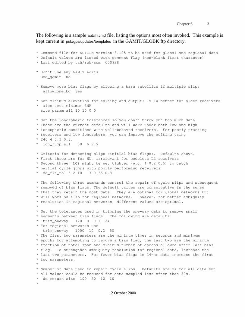
Chapter 6 3

12 October 2000

The following is a sample autcln.cmd file, listing the options most often invoked. This example iskept current in pub/gps/updates/templates in the GAMIT/GLOBK ftp directory.

* Command file for AUTCLN version 3.125 to be used for global and regional data* Default values are listed with comment flag (non-blank first character)* Last edited by tah/rwk/scm 000928

* Don't use any GAMIT edits use_gamit no

* Remove more bias flags by allowing a base satellite if multiple slips allow_one_bg yes

* Set minimum elevation for editing and output: 15 10 better for older receivers* also sets minimum SNR site_param all 10 10 0 0

* Set the ionospheric tolerances so you don't throw out too much data.* These are the current defaults and will work under both low and high* ionospheric conditions with well-behaved receivers. For poorly tracking* receivers and low ionosphere, you can improve the editing using* 240 4 0.3 0.8.* ion_jump all 30 6 2 5

* Criteria for detecting slips (initial bias flags). Defaults shown.* First three are for WL, irrelevant for codeless L2 receivers* Second three (LC) might be set tighter (e.g. 4 0.2 0.5) to catch* partial-cycle jumps with poorly performing receivers* dd_fit_tol 5 2 10 3 0.35 0.8

* The following three commands control the repair of cycle slips and subsequent* removed of bias flags. The default values are conservative in the sense* that they retain the most data. They are optimal for global networks but* will work ok also for regional networks. However, for better ambiguity* resolution in regional networks, different values are optimal.** Set the tolerances used in trimming the one-way data to remove small* segments between bias flags. The following are defaults:* trim_oneway 120 8 0.1 24* For regional networks use trim_oneway 1000 10 0.2 50* The first two parameters are the minimum times in seconds and minimum* epochs for attempting to remove a bias flag; the last two are the minimum* fraction of total span and minimum number of epochs allowed after last bias* flag. To strengthen ambiguity resolution for regional data, increase the* last two parameters. For fewer bias flags in 24-hr data increase the first* two parameters.** Number of data used to repair cycle slips. Defaults are ok for all data but* all values could be reduced for data sampled less often than 30s.* dd_return_site 100 50 10 10*

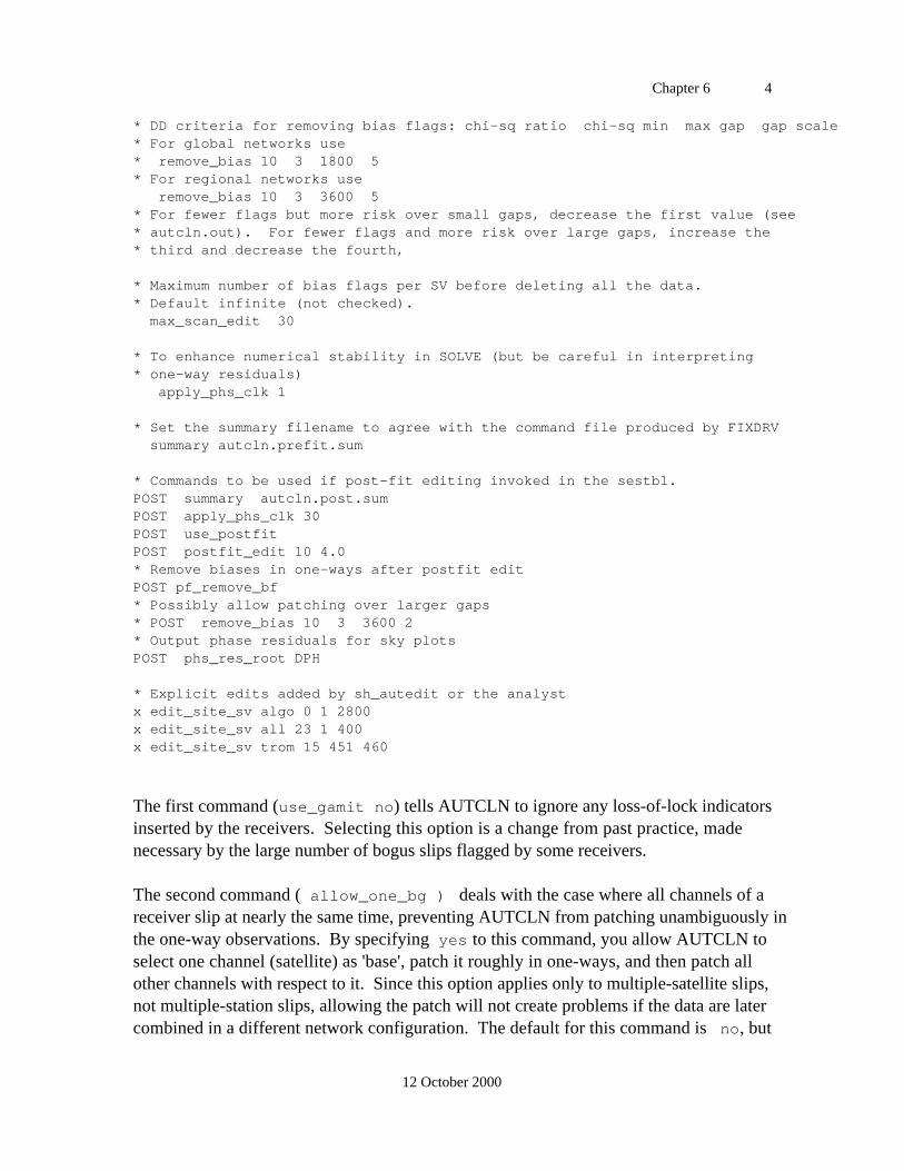
Chapter 6 4

12 October 2000

* DD criteria for removing bias flags: chi-sq ratio chi-sq min max gap gap scale* For global networks use* remove_bias 10 3 1800 5* For regional networks use remove_bias 10 3 3600 5* For fewer flags but more risk over small gaps, decrease the first value (see* autcln.out). For fewer flags and more risk over large gaps, increase the* third and decrease the fourth,

* Maximum number of bias flags per SV before deleting all the data.* Default infinite (not checked). max_scan_edit 30

* To enhance numerical stability in SOLVE (but be careful in interpreting* one-way residuals) apply_phs_clk 1

* Set the summary filename to agree with the command file produced by FIXDRV summary autcln.prefit.sum

* Commands to be used if post-fit editing invoked in the sestbl.POST summary autcln.post.sumPOST apply_phs_clk 30POST use_postfitPOST postfit_edit 10 4.0* Remove biases in one-ways after postfit editPOST pf_remove_bf* Possibly allow patching over larger gaps* POST remove_bias 10 3 3600 2* Output phase residuals for sky plotsPOST phs_res_root DPH

* Explicit edits added by sh_autedit or the analystx edit_site_sv algo 0 1 2800x edit_site_sv all 23 1 400x edit_site_sv trom 15 451 460

The first command (use_gamit no) tells AUTCLN to ignore any loss-of-lock indicatorsinserted by the receivers. Selecting this option is a change from past practice, madenecessary by the large number of bogus slips flagged by some receivers.

The second command ( allow_one_bg ) deals with the case where all channels of areceiver slip at nearly the same time, preventing AUTCLN from patching unambiguously inthe one-way observations. By specifying yes to this command, you allow AUTCLN toselect one channel (satellite) as 'base', patch it roughly in one-ways, and then patch allother channels with respect to it. Since this option applies only to multiple-satellite slips,not multiple-station slips, allowing the patch will not create problems if the data are latercombined in a different network configuration. The default for this command is no, but

Chapter 6 5

12 October 2000

yes will usually provide better editing. Occasionally, however, AUTCLN will make amistake in using this mode ( yes ) when the slips are at slightly different epochs.

The next command sets the minimum elevation angles for AUTCLN to examine (firstvalue) and retain (second value) the data. Additional commands, with all replaced by thestation code, can be added to raise the cutoff for poorly functioning receivers or lower it formodern receivers in cases where you want to examine very low elevation data.

The next four commands control the removal of bad data. The ion_jump criteria areapplied to the undifferenced ("one-way") LG observations in attempting to detect noisefrom bad receiver performance. The thresholds must be set high enough so that LG noisefrom high ionosopheric fluctuations is not confused with receiver noise. The default values(shown) are set high enough that the ionosphere does not trigger rejection even for polarand equatorial stations near solar maximum, and thus they provide only a loose filter forbad data. If you need a tighter filter to detect problems with older receivers tracking in mid-latitude regions, you may reset the the ion_jump parameters to [station] 240 4 0.30.8.

If you find from CVIEW or your scan output that AUTCLN is failing to detect some cycleslips, then you should alter the parameters of the dd_fit_tol command. The first three( 5 2 10 ) apply to the widelane (WL) observable and are thus relevant only for P-codereceivers; the second three ( 3 0.35 0.8 ) apply to the doubly differenced LC observable.They specify, respectively, the ratio of an allowed jump to the rms of the segment of databeing examined, the minimum value of a jump that will be flagged, and the maximum valueabove which all jumps will be flagged. The tolerance of the maximum jump allowedwithout incurring a bias flag will fall between the minimum and maxium specified with theintermediate values set by the ratio times the local rms. Thus the default values for LCallow for a maximum jump between 0.35 and 0.8 cycles. Values this high imply that thereceiver is not likely to allow one-cycle slips in L1 and L2 (leading to 0.5 in LC). To detectthese small slips, which often occur in older receivers, you should reset the LC values to 40.2 0.5.

The trim_oneway command is used to remove small segments of data that may encumberthe repair of cycle slips or the resolution of the overall phase ambiguity. The first twovalues ( 120 8 ) are the minimum time in seconds and the minimum number of epochsbetween bias flags. If you find segments (using CVIEW) for which a single gap of, forexample, 5 or 10 minutes would result in a more reliable cycle slip repair than wouldmultiple smaller gaps, then you should increase these values. The second two values ( 0.124 ) are the minimum fraction of the total span and the minimum number of epochsallowed after the last bias flag. Since SOLVE attempts to resolve the ambiguity using onlythe last segment of data, removing even a fairly long but noisy segment of data at the end

Chapter 6 6

12 October 2000

may result in lower parameter uncertainties by allowing resolution of additionalambiguities.

The next group of entries control the repairing of cycle slips and subsequent removal ofbias flags. They provide your primary control for the final stage of editing. Thedd_return_size command sets the number of data used on each side in the repair; thedefault values ( 100 50 10 ) imply segments of 50 minutes, 25 minutes, and 5 minutes forone-way WL and doubly differenced LC and LG, respectively, for data sampled at 30sintervals. For 120s sampling you probably want to reduce these values by factors of 2 to4. The remove_bias command sets the actual criteria used to remove a bias flag. Thealgorithm uses a comparison of the chi-square for the data segment (set bydd_return_size ) for the "best" choice of integer with the chi-square for the next bestchoice. The first value ( 10 ) gives the threshold ratio and the second ( 3 ) a minimumvalue used to make the comparison more robust (see the description of the command inSection 7.6). Increasing the first value provides a more conservative edit (fewer bias flagsremoved), and decreasing it a more agressive one. The last two values control how largegaps are treated. The third ( 3600 seconds ) sets the maximum gap for which a bias flagwill be removed; the fourth ( 5.0 ) is a "gap factor" that scales the computed chi-squaresuch that it becomes harder to remove a bias flag for large gaps (see the exact definition inSection 7.6). In Section 7.6 we describe how you can use the AUTCLN output todetermine why a bias flag was inconveniently or improperly left or removed and how youcan tune the remove_bias values to change the action.

The max_scan_edit command sets limit on the number of bias flags added to the data fora particular station and satellite before AUTCLN decides it would be better off deleting allof the data from that combination.

The apply_phs_clk command invokes estimation of satellite and station oscillatorvariations epoch by epoch. Its primary use in AUTCLN is in 'postfit' mode (see below),in which the adjustments from SOLVE are used to flatten the residuals on which AUTCLNworks to repair cycle slips. The phase-clock estimation is performed iteratively, with theargument of the command indicating how many iterations may be performed. A dozen ormore iterations may be necessary to get a good estimate, but if you are not invoking postfitediting, you should use apply_phs_clk with a single iteration, which will serve to removelarge jumps the data that often create numerical problems in SOLVE. Keep in mind,however, when you use apply_phs_clk with only one iteration that errors in the clockestimates will produce artifacts (fractional-cycle jumps) in the one-way (undifferenced)phase residuals in CVIEW. These cancel in double differences and of course are no more aproblem than the much greater clock noise present when you do not remove part of theclock terms at all—it's just that in the latter case the one-way residuals are so large (> 100cycles) that you don't expect to use them for editing. (Note that the default number of

Chapter 6 7

12 October 2000

iterations for apply_phs_clk is 30, appropriate for post-fit editing, so the 1 is required isyou want to save computation time in the pre-fit mode.)

Finally in this section we have an explicit entry for the AUTCLN summary file (discussedbelow). This assures that the pre-fit and post-fit summaries will be saved with different filenames.

As discussed in Section 5.2, we now recommend using the postfit feature of AUTCLNeven though this will increase computation time by 30 to 80% and the postfit AUTCLNwill occasionally fail with bad data. The situations most likely to be helped are the recoveryof low-elevation data for estimating atmospheric parameters and the need to detect andremove data affected by systematic, low-amplitude errors resulting from poorly modeledsatellite yaw, multipathing, or severe short-period tropospheric water vapor. Equallyimportant, however, is the ability to examine one-way residuals (in the autcln.sum file andwith CVIEW) generated by apply_phs_clk and use_postfit to study the performanceof stations at all levels of quality and to isolate a problem station or satellite when the pre-fitedit has failed to produce satisfactory results. There are two new controls in postfit mode.The command postfit_edit allows removal of data based on its deviation from the meanof the series, rather than just point to point changes. The first argument indicates at whatiteration you want AUTCLN to start this process, the second the sigma criterion to apply,and the third the maximum residual (in cycles) for which a data point can be restored if itwas previously removed because it was close to a bias flag. The defaults are to start editingat the 10th iteration, to use a 4-sigma criterion, and not to restore any previuously deleteddata. The command pf_remove_bf allows AUTCLN to remove bias flags in one-wayresiduals after editing. It is reasonable to forego the threshold editing (to avoid lopping thetops off large oscillations) but still invoke postfit bias-flag removal.

The final set of commands in the example, edit_site_sv, allow you to control the resultsby asking AUTCLN explicitly to delete (unweight) certain segments of data that you haveidentified by CVIEW to be problematic or have determined from other information (stationor satellite logs) should be ignored. The first argument is the station 4-character code, orall; the second is the satellite PRN number, with 0 signifying all satellites; the third andfourth are the range of epochs over which data should be unweighted. The shell commandsh_autedit written into the batch file by FIXDRV creates additional edit_site_sv

commands for autcln.cmd.pre and autcln.cmd.post in response to sestbl. entries controllingthe use of data during and after satellite eclipses.

Other entries in the autcln.cmd file are described in Section 7.6. Note in particular thecommands which allow you to use flags inserted by CVIEW (use_cview_edit), controlthe tolerance for clock resets ( clk_reset_tol ), specify station-specific editing(site_params ), and remove extra bias flags at the beginning of a station-satellite datasegment (remove_first_bia).

Chapter 6 8

12 October 2000

AUTCLN produces two output files which are quite useful for diagnosing problems.Usually you will need to examine only the summary file, autcln.sum . The first two tablesprovide a compact indication of whether one or more stations or satellites are anomalous.The first is a summary of the clock behavior :

Clock and Range noise statistics at iteration 3 Site/PRN Allan SD@100 # Range rms # sec (ppb) (mm) BRLD 19.761493 2832 596.9 16210 TRM KAIN 19.931665 2879 675.1 15939 TRM KIT3 .527232 2879 729.9 16307 TRB KUM6 10.105467 719 2061.0 3462 TRM . . . PRN_01 .384611 1188 PRN_02 .411166 1039 PRN_05 .422517 984

The Allen standard deviation at 100s is given (in parts per billion) for each station andsatellite. Station clock values in excess of 50 ppb (5 parts in 108) indicate variations largerthan those expected for well-tuned crystal oscillators in any of the commonly usedreceivers. Atomic oscillators (Rubidium, Cesium, or Hydrogen-maser) should showvalues below 1 ppb. A bad clock does not necessarily mean bad phase data but increasesthe chances of cycle slips and degrades the ability of AUTCLN to perform a proper edit.The fourth column gives the rms of range noise in millimeters for each station. For P-codereceivers under non-AS conditions, these values should be under a meter; under AS, somewill increase to 1000–2000 mm. Values larger than this usually mean lots of bad rangedata or bad prefit residuals (station coordinate errors > 10 m). The 3rd and 5th columns ofthe list are simply the number (#) of observations used in the calculation.

Following the clock summary is a listing of the number of bias flags added during theinitial double-difference scan:

DDScan bias flags added report for pass 1 SITE PN01 02 05 06 07 09 14 15 16 22 23 24 25 26 27 28 29 31 BRLD 6 2 10 8 14 18 6 4 10 6 4 12 7 0 2 2 0 0 KAIN 0 0 0 0 0 0 0 0 1 1 0 0 0 0 0 1 0 0 KIT3 0 0 0 0 0 0 0 0 0 0 0 0 0 2 0 0 0 0 KUM6 0 2 0 0 2 4 0 0 0 0 0 2 0 0 0 0 0 0 KUMB 0 0 0 0 0 0 0 0 0 0 0 0 0 0 0 1 0 0 LHAS 0 0 0 0 0 0 0 0 0 0 0 0 0 1 0 0 0 1

In this example station BRLD is performing poorly relative to the others but may not havefatal errors. Many bias flags added can mean either bad prefit residuals or bad phase data.Too many flags for a satellite at more than one station usually represents the effect of anumodeled acceleration of the satellite (e.g., umodeled thrusting).

If you have selected postfit editing in AUTCLN, the next four tables give the actual postfitphase statistics for each station and satellite after correcting the residuals for adjustments in

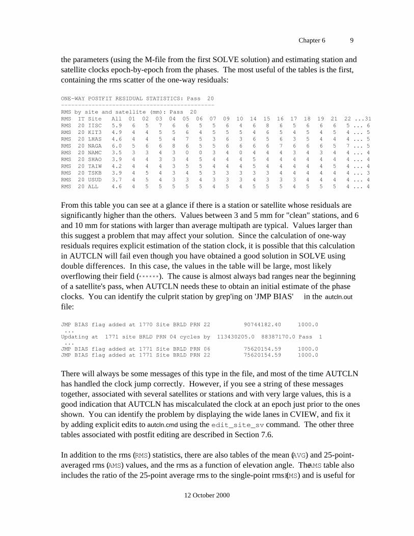
Chapter 6 9

12 October 2000

the parameters (using the M-file from the first SOLVE solution) and estimating station andsatellite clocks epoch-by-epoch from the phases. The most useful of the tables is the first,containing the rms scatter of the one-way residuals:

ONE-WAY POSTFIT RESIDUAL STATISTICS: Pass 20---------------------------------------------RMS by site and satellite (mm): Pass 20RMS IT Site All 01 02 03 04 05 06 07 09 10 14 15 16 17 18 19 21 22 ...31RMS 20 IISC 5.9 6 5 7 6 6 5 5 6 4 6 8 6 5 6 6 6 5 ... 6RMS 20 KIT3 4.9 4 4 5 5 6 4 5 5 5 4 6 5 4 5 4 5 4 ... 5RMS 20 LHAS 4.6 4 4 5 4 7 5 3 6 3 6 5 6 3 5 4 4 4 ... 5RMS 20 NAGA 6.0 5 6 6 8 6 5 5 6 6 6 6 7 6 6 6 5 7 ... 5RMS 20 NAMC 3.5 3 3 4 3 0 0 3 4 0 4 4 4 3 4 3 4 4 ... 4RMS 20 SHAO 3.9 4 4 3 3 4 5 4 4 4 5 4 4 4 4 4 4 4 ... 4RMS 20 TAIW 4.2 4 4 4 3 5 5 4 4 4 5 4 4 4 4 4 5 4 ... 4RMS 20 TSKB 3.9 4 5 4 3 4 5 3 3 3 3 3 4 4 4 4 4 4 ... 3RMS 20 USUD 3.7 4 5 4 3 3 4 3 3 3 4 3 3 3 4 4 4 4 ... 4RMS 20 ALL 4.6 4 5 5 5 5 5 4 5 4 5 5 5 4 5 5 5 4 ... 4

From this table you can see at a glance if there is a station or satellite whose residuals aresignificantly higher than the others. Values between 3 and 5 mm for "clean" stations, and 6and 10 mm for stations with larger than average multipath are typical. Values larger thanthis suggest a problem that may affect your solution. Since the calculation of one-wayresiduals requires explicit estimation of the station clock, it is possible that this calculationin AUTCLN will fail even though you have obtained a good solution in SOLVE usingdouble differences. In this case, the values in the table will be large, most likelyoverflowing their field (******). The cause is almost always bad ranges near the beginningof a satellite's pass, when AUTCLN needs these to obtain an initial estimate of the phaseclocks. You can identify the culprit station by grep'ing on 'JMP BIAS' in the autcln.out

file:

JMP BIAS flag added at 1770 Site BRLD PRN 22 90744182.40 1000.0 ...Updating at 1771 site BRLD PRN 04 cycles by 113430205.0 88387170.0 Pass 1 ...JMP BIAS flag added at 1771 Site BRLD PRN 06 75620154.59 1000.0JMP BIAS flag added at 1771 Site BRLD PRN 22 75620154.59 1000.0

There will always be some messages of this type in the file, and most of the time AUTCLNhas handled the clock jump correctly. However, if you see a string of these messagestogether, associated with several satellites or stations and with very large values, this is agood indication that AUTCLN has miscalculated the clock at an epoch just prior to the onesshown. You can identify the problem by displaying the wide lanes in CVIEW, and fix itby adding explicit edits to autcln.cmd using the edit_site_sv command. The other threetables associated with postfit editing are described in Section 7.6.

In addition to the rms (RMS) statistics, there are also tables of the mean (AVG) and 25-point-averaged rms (AMS) values, and the rms as a function of elevation angle. The AMS table alsoincludes the ratio of the 25-point average rms to the single-point rms (RMS) and is useful for

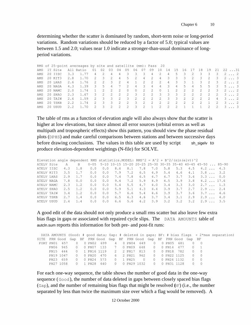
Chapter 6 10

12 October 2000

determining whether the scatter is dominated by random, short-term noise or long-periodvariations. Random variations should be reduced by a factor of 5.0; typical values arebetween 1.5 and 2.0; values near 1.0 indicate a stronger-than-usual dominance of long-period variations.

RMS of 25-point avereages by site and satellite (mm): Pass 20AMS IT Site All Ratio 01 02 03 04 05 06 07 09 10 14 15 16 17 18 19 21 22 ...31AMS 20 IISC 3.3 1.77 4 2 4 4 3 3 3 4 2 4 5 3 2 3 3 3 2 ... 2AMS 20 KIT3 2.8 1.70 2 3 2 4 5 2 4 2 4 3 3 3 2 3 2 3 2 ... 3AMS 20 LHAS 2.6 1.76 2 2 3 2 4 1 2 2 2 4 3 3 1 3 2 3 2 ... 2AMS 20 NAGA 4.3 1.39 3 5 4 7 2 4 3 4 4 3 4 5 4 5 5 3 5 ... 3AMS 20 NAMC 2.0 1.74 1 2 2 2 0 0 2 2 0 1 2 2 2 2 2 3 2 ... 2AMS 20 SHAO 2.3 1.67 3 2 2 2 2 3 2 2 3 3 3 2 2 2 2 2 3 ... 2AMS 20 TAIW 2.6 1.59 2 3 3 2 3 2 2 2 2 3 3 2 2 2 2 4 3 ... 2AMS 20 TSKB 2.2 1.74 2 3 3 2 2 3 2 2 2 2 2 2 2 2 1 2 3 ... 2AMS 20 USUD 2.2 1.70 2 3 2 2 2 3 2 1 2 2 2 1 1 1 2 2 3 ... 3

The table of rms as a function of elevation angle will also always show that the scatter ishigher at low elevations, but since almost all error sources (orbital errors as well asmultipath and tropospheric effects) show this pattern, you should view the phase residualplots (DPHS) and make careful comparisons between stations and between successive daysbefore drawing conclusions. The values in this table are used by script sh_sigelv toproduce elevation-dependent weightings (N-file) for SOLVE.

Elevation angle dependent RMS statistics.MODEL: RMS^2 = A^2 + B^2/(sin(elv))^2ATELV Site A B 0-05 5-10 10-15 15-20 20-25 25-30 30-35 35-40 40-45 45-50 ... 85-90ATELV IISC 4.3 1.8 0.0 0.0 8.6 8.1 7.8 7.0 5.8 5.3 4.5 4.2 ... 4.3ATELV KIT3 3.5 1.7 0.0 0.0 7.9 7.2 6.5 4.9 5.4 4.6 4.1 3.8 ... 3.2ATELV LHAS 2.9 1.7 0.0 0.0 7.4 7.8 6.5 4.7 4.7 3.7 3.6 3.3 ... 0.0ATELV NAGA 7.8 0.0 0.0 0.0 9.4 7.2 5.9 4.9 4.5 3.9 3.8 4.2 ... 17.6ATELV NAMC 2.3 1.2 0.0 0.0 5.4 5.5 4.7 4.0 3.4 3.3 3.0 2.7 ... 1.3ATELV SHAO 2.5 1.2 0.0 0.0 5.9 5.1 4.3 4.4 3.9 3.7 2.7 2.9 ... 2.4ATELV TAIW 3.4 1.2 0.0 0.0 5.7 6.6 5.4 4.6 3.9 3.7 3.6 3.7 ... 4.6ATELV TSKB 2.7 1.4 0.0 0.0 6.5 6.3 4.6 3.7 3.4 3.1 2.9 2.9 ... 4.0ATELV USUD 2.4 1.4 0.0 0.0 6.6 5.6 4.2 3.9 3.2 3.2 3.2 2.9 ... 3.5

A good edit of the data should not only produce a small rms scatter but also leave few extrabias flags in gaps or associated with repaired cycle slips. The DATA AMOUNTS table ofautcln.sum reports this information for both pre- and post-fit runs:

DATA AMOUNTS (Good: # good data; Gap: # deleted in gaps; BF: # bias flags < 2*max separation)SITE PRN Good Gap BF PRN Good Gap BF PRN Good Gap BF PRN Good Gap BF FORT PN01 657 0 0 PN02 699 4 0 PN04 649 0 0 PN05 681 0 0 PN06 945 0 0 PN07 133 7 0 PN09 648 0 0 PN14 477 0 1 PN15 444 0 1 PN16 1119 2 2 PN17 813 0 0 PN18 782 0 0 PN19 1047 0 0 PN20 470 6 2 PN21 962 0 0 PN22 1125 0 0 PN23 659 0 0 PN24 573 0 1 PN25 0 0 0 PN26 1132 0 0 PN27 1058 0 1 PN28 640 0 0 PN29 1032 0 0 PN31 1128 0 0

For each one-way sequence, the table shows the number of good data in the one-waysequence (Good), the number of data deleted in gaps between closely spaced bias flags(Gap), and the number of remaining bias flags that might be resolved (BF) (i.e., the numberseparated by less than twice the maximum size over which a flag would be removed). A

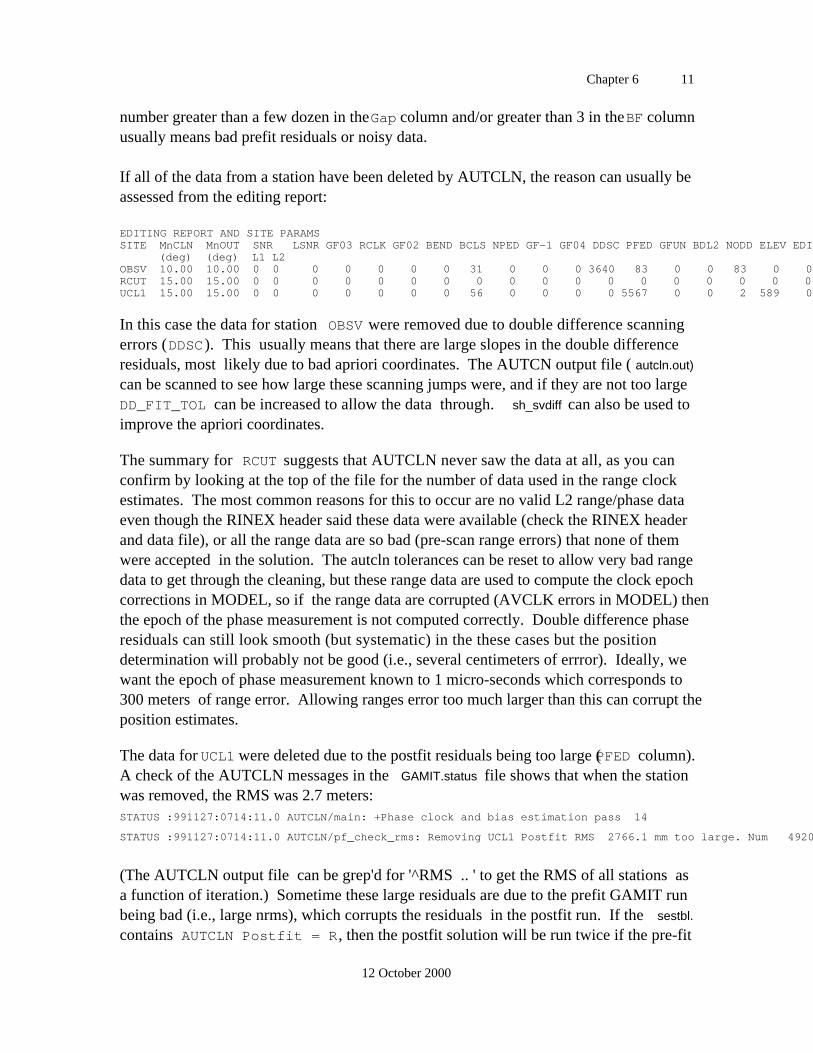
Chapter 6 11

12 October 2000

number greater than a few dozen in the Gap column and/or greater than 3 in the BF columnusually means bad prefit residuals or noisy data.

If all of the data from a station have been deleted by AUTCLN, the reason can usually beassessed from the editing report:

EDITING REPORT AND SITE PARAMSSITE MnCLN MnOUT SNR LSNR GF03 RCLK GF02 BEND BCLS NPED GF-1 GF04 DDSC PFED GFUN BDL2 NODD ELEV EDIT MMRG ELCL Good (deg) (deg) L1 L2OBSV 10.00 10.00 0 0 0 0 0 0 0 31 0 0 0 3640 83 0 0 83 0 0 0 0 0RCUT 15.00 15.00 0 0 0 0 0 0 0 0 0 0 0 0 0 0 0 0 0 0 0 0 0UCL1 15.00 15.00 0 0 0 0 0 0 0 56 0 0 0 0 5567 0 0 2 589 0 0 0 0

In this case the data for station OBSV were removed due to double difference scanningerrors (DDSC ). This usually means that there are large slopes in the double differenceresiduals, most likely due to bad apriori coordinates. The AUTCN output file ( autcln.out)

can be scanned to see how large these scanning jumps were, and if they are not too largeDD_FIT_TOL can be increased to allow the data through. sh_svdiff can also be used toimprove the apriori coordinates.

The summary for RCUT suggests that AUTCLN never saw the data at all, as you canconfirm by looking at the top of the file for the number of data used in the range clockestimates. The most common reasons for this to occur are no valid L2 range/phase dataeven though the RINEX header said these data were available (check the RINEX headerand data file), or all the range data are so bad (pre-scan range errors) that none of themwere accepted in the solution. The autcln tolerances can be reset to allow very bad rangedata to get through the cleaning, but these range data are used to compute the clock epochcorrections in MODEL, so if the range data are corrupted (AVCLK errors in MODEL) thenthe epoch of the phase measurement is not computed correctly. Double difference phaseresiduals can still look smooth (but systematic) in the these cases but the positiondetermination will probably not be good (i.e., several centimeters of errror). Ideally, wewant the epoch of phase measurement known to 1 micro-seconds which corresponds to300 meters of range error. Allowing ranges error too much larger than this can corrupt theposition estimates.

The data for UCL1 were deleted due to the postfit residuals being too large (PFED column).A check of the AUTCLN messages in the GAMIT.status file shows that when the stationwas removed, the RMS was 2.7 meters:STATUS :991127:0714:11.0 AUTCLN/main: +Phase clock and bias estimation pass 14

STATUS :991127:0714:11.0 AUTCLN/pf_check_rms: Removing UCL1 Postfit RMS 2766.1 mm too large. Num 4920 Limit 190.3 mm

(The AUTCLN output file can be grep'd for '^RMS .. ' to get the RMS of all stations asa function of iteration.) Sometime these large residuals are due to the prefit GAMIT runbeing bad (i.e., large nrms), which corrupts the residuals in the postfit run. If the sestbl.

contains AUTCLN Postfit = R, then the postfit solution will be run twice if the pre-fit

Chapter 6 12

12 October 2000

GAMIT solution is bad. Check the P-file for AVCLK errors, and then possibly the I- andK-files to pinpoint the time and cause, and the Q-file for the sizes of the adjustements. Inthe case shown here, the prefit AUTCLN run detected many DD scan errors, so most likeythe a priori coordinates for the site are bad.

The other tables in the autcln.sum file and the use of the autcln.out file for tracing problemsare discussed in Chapter 7.

If you have the setenv variable of your .login file referencing the stdrel/help directory, youcan take advantage of an extensive on-line help file for AUTCLN. To view the currentparameter defaults, type autcln defaults.

6.3 Scanning the residuals to identify slips

With the postfit editing capability of AUTCLN, it is seldom any longer necessary toperform a separate scan of the phase residuals to identify problematic data. Severalprograms and scripts are available, however. All take as input the M-file from a quick orfull solution and operate on the predicted postfit LC doubly differenced residuals. Themost commonly used program, an optional part of the batch sequence, is SCANDD. Youcan run it directly by typing the program name and the M-file from the SOLVE solution:

scandd mventa.278

Omitting the M-file will put SCANDD into an interactive mode, allowing you to select onlycertain stations, scan pre-fit (rather than post-fit) residuals, or scan a set of C-files withdifferent 6th character.

SCANDD calculates the LC root-mean square (rms) of each double-difference series andsearches for jumps in the doubly differenced LC residuals. It also identifies all possiblecycle slips and compiles a list of corrections that can be used directly as input to CVIEW.SCANDD produces three output files, each with a slightly different summary of the doublydifferenced residuals. The file most analysts find easiest to use in identifying potentialcycle slips is called vscan.out, which lists the largest LC "jumps" for each double-differenceseries. A distinction is made between jumps that are associated with bias flags ("flagged"),which do not corrupt a "full" or "regular" SOLVE solution, and those that have not hadextra bias flags assigned ("unflagged"). You can obtain a sorted version of this file byrunning the shell script sortv to sort the file vscan.out by epoch and produce two additionalfiles, one listing the largest slip for every double difference combination, the other (moreuseful for large networks) listing only the 80 worst slips. Shown below is the output ofthe second of these files, named vxxxx1.ddd. worst , where the experiment name ( xxxx ),type of solution (1), and day number (ddd) are taken from the M-file name.

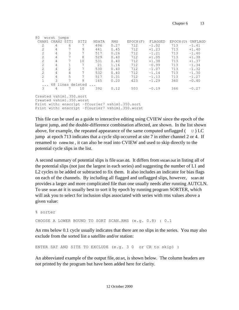
Chapter 6 13

12 October 2000

80 worst jumps CHAN1 CHAN2 SIT1 SIT2 NDATA RMS EPOCH(F) FLAGGED EPOCH(U) UNFLAGD 2 4 6 7 496 0.27 712 -1.02 713 -1.41 2 4 7 9 441 0.45 712 +1.23 713 +1.40 2 4 3 7 517 0.26 712 -1.21 713 -1.40 2 4 7 8 529 0.40 712 +1.05 713 +1.38 2 4 7 10 531 0.40 712 +1.38 713 +1.37 2 4 1 7 21 1.16 712 -0.99 713 -1.34 2 4 2 7 530 0.40 712 -1.07 713 -1.32 2 4 4 7 532 0.40 712 -1.14 713 -1.30 2 4 5 7 517 0.31 712 -1.13 713 -1.27 1 3 7 9 165 0.20 423 -1.29 360 -0.40 ... 68 lines deleted ... 3 4 7 10 392 0.12 503 -0.19 366 -0.27

Created vshim1.350.sortCreated vshim1.350.worstPrint with: enscript -fCourier7 vshim1.350.sortPrint with: enscript -fCourier7 vshim1.350.worst

This file can be used as a guide to interactive editing using CVIEW since the epoch of thelargest jump, and the double-difference combination affected, are shown. In the list shownabove, for example, the repeated appearance of the same computed unflagged ( U ) LCjump at epoch 713 indicates that a cycle slip occurred at site 7 in either channel 2 or 4. Ifrenamed to cview.list , it can also be read into CVIEW and used to skip directly to thepotential cycle slips in the list.

A second summary of potential slips is file scan.dd. It differs from vscan.out in listing all ofthe potential slips (not just the largest in each series) and suggesting the number of L1 andL2 cycles to be added or subtracted to fix them. It also includes an indicator for bias flagson each of the channels. By including all flagged and unflagged slips, however, scan.dd

provides a larger and more complicated file than one usually needs after running AUTCLN.To use scan.dd it is usually best to sort it by epoch by running program SORTER, whichwill ask you to select for inclusion slips associated with series with rms values above agiven value:

% sorter

CHOOSE A LOWER BOUND TO SORT SCAN.RMS (e.g. 0.8) : 0.1

An rms below 0.1 cycle usually indicates that there are no slips in the series. You may alsoexclude from the sorted list a satellite and/or station:

ENTER SAT AND SITE TO EXCLUDE (e.g. 3 0 or CR to skip) :

An abbreviated example of the output file, dd.srt, is shown below. The column headers arenot printed by the program but have been added here for clarity.

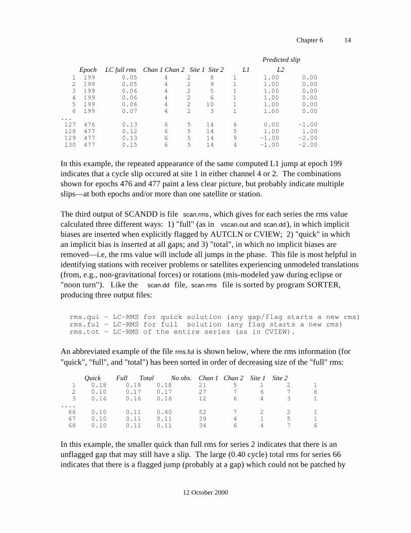
Chapter 6 14

12 October 2000

Predicted slip

Epoch LC full rms Chan 1 Chan 2 Site 1 Site 2 L1 L2 1 199 0.05 4 2 8 1 1.00 0.00 2 199 0.05 4 2 9 1 1.00 0.00 3 199 0.06 4 2 5 1 1.00 0.00 4 199 0.06 4 2 6 1 1.00 0.00 5 199 0.06 4 2 10 1 1.00 0.00 6 199 0.07 4 2 3 1 1.00 0.00... 127 476 0.13 6 5 14 6 0.00 -1.00 128 477 0.12 6 5 14 5 1.00 1.00 129 477 0.13 6 5 14 9 -1.00 -2.00 130 477 0.15 6 5 14 4 -1.00 -2.00

In this example, the repeated appearance of the same computed L1 jump at epoch 199indicates that a cycle slip occured at site 1 in either channel 4 or 2. The combinationsshown for epochs 476 and 477 paint a less clear picture, but probably indicate multipleslips—at both epochs and/or more than one satellite or station.

The third output of SCANDD is file scan.rms , which gives for each series the rms valuecalculated three different ways: 1) "full" (as in vscan.out and scan.dd ), in which implicitbiases are inserted when explicitly flagged by AUTCLN or CVIEW; 2) "quick" in whichan implicit bias is inserted at all gaps; and 3) "total", in which no implicit biases areremoved—i.e, the rms value will include all jumps in the phase. This file is most helpful inidentifying stations with receiver problems or satellites experiencing unmodeled translations(from, e.g., non-gravitational forces) or rotations (mis-modeled yaw during eclipse or"noon turn"). Like the scan.dd file, scan.rms file is sorted by program SORTER,producing three output files:

rms.qui - LC-RMS for quick solution (any gap/flag starts a new rms)rms.ful - LC-RMS for full solution (any flag starts a new rms)rms.tot - LC-RMS of the entire series (as in CVIEW).

An abbreviated example of the file rms.ful is shown below, where the rms information (for"quick", "full", and "total") has been sorted in order of decreasing size of the "full" rms:

Quick Full Total No obs. Chan 1 Chan 2 Site 1 Site 2 1 0.18 0.18 0.18 21 5 1 2 1 2 0.10 0.17 0.17 27 7 6 7 6 3 0.16 0.16 0.16 12 6 4 3 1.... 66 0.10 0.11 0.40 52 7 2 2 1 67 0.10 0.11 0.11 39 4 1 5 1 68 0.10 0.11 0.11 34 6 4 7 6

In this example, the smaller quick than full rms for series 2 indicates that there is anunflagged gap that may still have a slip. The large (0.40 cycle) total rms for series 66indicates that there is a flagged jump (probably at a gap) which could not be patched by

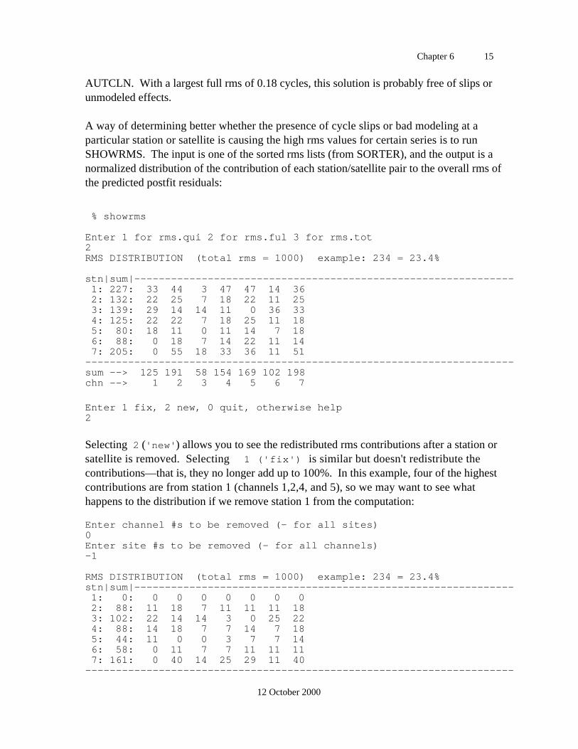
Chapter 6 15

12 October 2000

AUTCLN. With a largest full rms of 0.18 cycles, this solution is probably free of slips orunmodeled effects.

A way of determining better whether the presence of cycle slips or bad modeling at aparticular station or satellite is causing the high rms values for certain series is to runSHOWRMS. The input is one of the sorted rms lists (from SORTER), and the output is anormalized distribution of the contribution of each station/satellite pair to the overall rms ofthe predicted postfit residuals:

% showrms

Enter 1 for rms.qui 2 for rms.ful 3 for rms.tot2RMS DISTRIBUTION (total rms = 1000) example: 234 = 23.4%

stn|sum|-------------------------------------------------------------- 1: 227: 33 44 3 47 47 14 36 2: 132: 22 25 7 18 22 11 25 3: 139: 29 14 14 11 0 36 33 4: 125: 22 22 7 18 25 11 18 5: 80: 18 11 0 11 14 7 18 6: 88: 0 18 7 14 22 11 14 7: 205: 0 55 18 33 36 11 51----------------------------------------------------------------------sum --> 125 191 58 154 169 102 198chn --> 1 2 3 4 5 6 7

Enter 1 fix, 2 new, 0 quit, otherwise help2

Selecting 2 ('new') allows you to see the redistributed rms contributions after a station orsatellite is removed. Selecting 1 ('fix') is similar but doesn't redistribute thecontributions—that is, they no longer add up to 100%. In this example, four of the highestcontributions are from station 1 (channels 1,2,4, and 5), so we may want to see whathappens to the distribution if we remove station 1 from the computation:

Enter channel #s to be removed (- for all sites)0Enter site #s to be removed (- for all channels)-1

RMS DISTRIBUTION (total rms = 1000) example: 234 = 23.4%stn|sum|-------------------------------------------------------------- 1: 0: 0 0 0 0 0 0 0 2: 88: 11 18 7 11 11 11 18 3: 102: 22 14 14 3 0 25 22 4: 88: 14 18 7 7 14 7 18 5: 44: 11 0 0 3 7 7 14 6: 58: 0 11 7 7 11 11 11 7: 161: 0 40 14 25 29 11 40----------------------------------------------------------------------

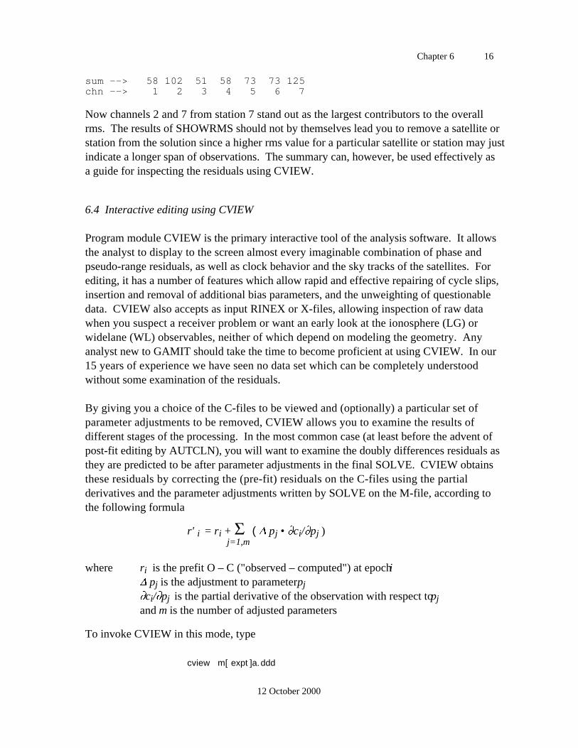
Chapter 6 16

12 October 2000

sum --> 58 102 51 58 73 73 125chn --> 1 2 3 4 5 6 7

Now channels 2 and 7 from station 7 stand out as the largest contributors to the overallrms. The results of SHOWRMS should not by themselves lead you to remove a satellite orstation from the solution since a higher rms value for a particular satellite or station may justindicate a longer span of observations. The summary can, however, be used effectively asa guide for inspecting the residuals using CVIEW.

6.4 Interactive editing using CVIEW

Program module CVIEW is the primary interactive tool of the analysis software. It allowsthe analyst to display to the screen almost every imaginable combination of phase andpseudo-range residuals, as well as clock behavior and the sky tracks of the satellites. Forediting, it has a number of features which allow rapid and effective repairing of cycle slips,insertion and removal of additional bias parameters, and the unweighting of questionabledata. CVIEW also accepts as input RINEX or X-files, allowing inspection of raw datawhen you suspect a receiver problem or want an early look at the ionosphere (LG) orwidelane (WL) observables, neither of which depend on modeling the geometry. Anyanalyst new to GAMIT should take the time to become proficient at using CVIEW. In our15 years of experience we have seen no data set which can be completely understoodwithout some examination of the residuals.

By giving you a choice of the C-files to be viewed and (optionally) a particular set ofparameter adjustments to be removed, CVIEW allows you to examine the results ofdifferent stages of the processing. In the most common case (at least before the advent ofpost-fit editing by AUTCLN), you will want to examine the doubly differences residuals asthey are predicted to be after parameter adjustments in the final SOLVE. CVIEW obtainsthese residuals by correcting the (pre-fit) residuals on the C-files using the partialderivatives and the parameter adjustments written by SOLVE on the M-file, according tothe following formula

r' i = ri + ( pj • ci/ pj ) j=1,m

where ri is the prefit O – C ("observed – computed") at epoch i pj is the adjustment to parameter pjci/ pj is the partial derivative of the observation with respect to pj

and m is the number of adjusted parameters

To invoke CVIEW in this mode, type

cview m[ expt ]a.ddd

Chapter 6 17

12 October 2000

If you have used AUTCLN in its post-fit mode, you have a choice of two sets of residualsto examine. With the “a” M-file, you will get the doubly differences residuals from thefinal SOLVE solution, just as before. In this case the one-way residuals made available byAUTCLN’s corrections to phase clocks will be “nearly” flat but will in fact not representthe actual post-fit residuals because the corrections for parameters adjustments have beentaken from the final SOLVE M-file whereas in correcting clocks AUTCLN used parameteradjustments from the previous (“AUTCLN pre-”) SOLVE solution, recorded on the M-filenow named with “p” as the sixth character (see the batch-file seqence in Section 5.3). Tobest evaluate the one-way residuals, you should give CVIEW the name of this earlier M-file. Since this M-file will contain the names of versions of the C-files (the “b” versionswith a 0-ITER run, whereas the final “a” M-file has the “d” versions), you will need tohave saved these earlier C-files or substitute the later ones (which are equivalent for thispurpose). This can be accomplished easily by using additional optional command-linearguments when invoking CVIEW:

cview m[ expt ]p.ddd ddd d

The last argument ( d ) corresponds to the version of the C-files that are currently present inyour day directory. The day number is also included because it was added as a secondcommand-line argument to earlier versions of CVIEW for use with multi-sessionprocessing (in which a single M-file may have C-files from more than one day). InvokingCVIEW in this mode is usually the best way to examine the data if you have usedAUTCLN in post-fit mode since you can see problems directly in the one-way residualswithout having to infer from the double differences the station and satellite at fault. Thedoubly differenced residuals, however, will not be those from the final SOLVE—thoughthey will usually be very close—so if there is a question about systematic signatures, youmay have to invoke CVIEW a second time with the “a” M-file. This is usuallyunnecessary.

There is one additional mode for CVIEW that is sometimes useful; namely viewing the(doubly differenced) residuals as they are passed to AUTCLN from MODEL or to SOLVEfrom AUTCLN. The first case is interesting if AUTCLN has performed poorly for one ormore stations or satellites and you want to determine why (e.g. poor a priori coordinatesleading to large pre-fit residuals and deletion by AUTCLN of most or all of the data). Thesecond is interesting if the solution nrms and SCANDD output suggests mismodeling of asatellite (e.g., from “burn”) and you want to see the effect before SOLVE has “smeared” itinto the residuals of other satellites in the least squares adjustment. To view pre-fits, aswell as to select a sub-set of C-files, you must invoke CVIEW with no arguments on thjecommand line. In this case, the program will prompt you for the name(s) of an M-file orC-file(s). Responding with the M-file name results in a display of all the C-files, givingyou the opportunity to select a subset of the files and/or to change the sixth character of the

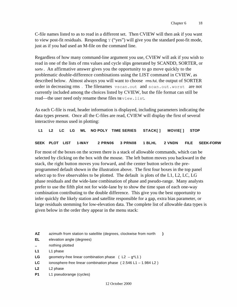
Chapter 6 18

12 October 2000

C-file names listed to as to read in a different set. Then CVIEW will then ask if you wantto view post-fit residuals. Responding Y (“yes”) will give you the standard post-fit mode,just as if you had used an M-file on the command line.

Regardless of how many command-line argument you use, CVIEW will ask if you wish toread in one of the lists of rms values and cycle slips generated by SCANDD, SORTER, orsortv . An affirmative answer gives you the opportunity to go move quickly to theproblematic double-difference combinations using the LIST command in CVIEW, asdescribed below. Almost always you will want to choose rms.ful, the output of SORTERorder in decreasing rms . The filenames vscan.out and scan.out.worst are notcurrently included among the choices listed by CVIEW, but the file format can still beread—the user need only rename these files to cview.list.

As each C-file is read, header information is displayed, including parameters indicating thedata types present. Once all the C-files are read, CVIEW will display the first of severalinteractive menus used in plotting:

L1 L2 LC LG WL NO POLY TIME SERIES STACK[ ] MOVIE[ ] STOP

SEEK PLOT LIST 1-WAY 2 PRN06 3 PRN08 1 BLHL 2 VNDN FILE SEEK-FORW

For most of the boxes on the screen there is a stack of allowable commands, which can beselected by clicking on the box with the mouse. The left button moves you backward in thestack, the right button moves you forward, and the center button selects the pre-programmed default shown in the illustration above. The first four boxes in the top panelselect up to five observables to be plotted. The default is plots of the L1, L2, LC, LGphase residuals and the wide-lane combination of phase and pseudo-range. Many analystsprefer to use the fifth plot not for wide-lane by to show the time span of each one-waycombination contributing to the double difference. This give you the best opportunity toinfer quickly the likely station and satellite responsible for a gap, extra bias parameter, orlarge residuals stemming for low-elevation data. The complete list of allowable data types isgiven below in the order they appear in the menu stack:

AZ azimuth from station to satellite (degrees, clockwise from north )

EL elevation angle (degrees)

.. nothing plotted

L1 L1 phase

LG geometry-free linear combination phase ( L2 – g*L1 )

LC ionosphere-free linear combination phase ( 2.546 L1 – 1.984 L2 )

L2 L2 phase

P1 L1 pseudorange (cycles)

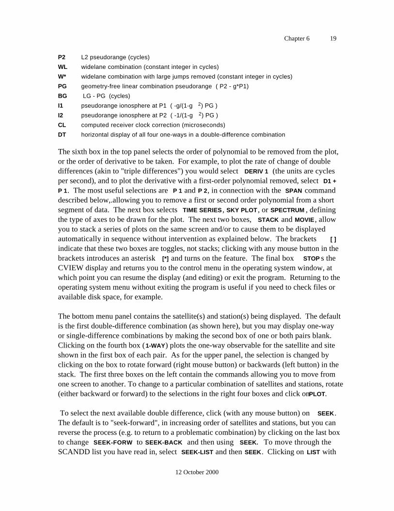
Chapter 6 19

12 October 2000

P2 L2 pseudorange (cycles)

WL widelane combination (constant integer in cycles)

W* widelane combination with large jumps removed (constant integer in cycles)

PG geometry-free linear combination pseudorange ( P2 - g*P1)

BG LG - PG (cycles)

I1 pseudorange ionosphere at P1 ( -g/(1-g 2) PG )

I2 pseudorange ionosphere at P2 ( -1/(1-g 2) PG )

CL computed receiver clock correction (microseconds)

DT horizontal display of all four one-ways in a double-difference combination

The sixth box in the top panel selects the order of polynomial to be removed from the plot,or the order of derivative to be taken. For example, to plot the rate of change of doubledifferences (akin to "triple differences") you would select DERIV 1 (the units are cyclesper second), and to plot the derivative with a first-order polynomial removed, select D1 +

P 1. The most useful selections are P 1 and P 2, in connection with the SPAN commanddescribed below,.allowing you to remove a first or second order polynomial from a shortsegment of data. The next box selects TIME SERIES , SKY PLOT , or SPECTRUM , definingthe type of axes to be drawn for the plot. The next two boxes, STACK and MOVIE , allowyou to stack a series of plots on the same screen and/or to cause them to be displayedautomatically in sequence without intervention as explained below. The brackets [ ]

indicate that these two boxes are toggles, not stacks; clicking with any mouse button in thebrackets introduces an asterisk [*] and turns on the feature. The final box STOP s theCVIEW display and returns you to the control menu in the operating system window, atwhich point you can resume the display (and editing) or exit the program. Returning to theoperating system menu without exiting the program is useful if you need to check files oravailable disk space, for example.

The bottom menu panel contains the satellite(s) and station(s) being displayed. The defaultis the first double-difference combination (as shown here), but you may display one-wayor single-difference combinations by making the second box of one or both pairs blank.Clicking on the fourth box (1-WAY) plots the one-way observable for the satellite and siteshown in the first box of each pair. As for the upper panel, the selection is changed byclicking on the box to rotate forward (right mouse button) or backwards (left button) in thestack. The first three boxes on the left contain the commands allowing you to move fromone screen to another. To change to a particular combination of satellites and stations, rotate(either backward or forward) to the selections in the right four boxes and click on PLOT.

To select the next available double difference, click (with any mouse button) on SEEK.The default is to "seek-forward", in increasing order of satellites and stations, but you canreverse the process (e.g. to return to a problematic combination) by clicking on the last boxto change SEEK-FORW to SEEK-BACK and then using SEEK. To move through theSCANDD list you have read in, select SEEK-LIST and then SEEK. Clicking on LIST with

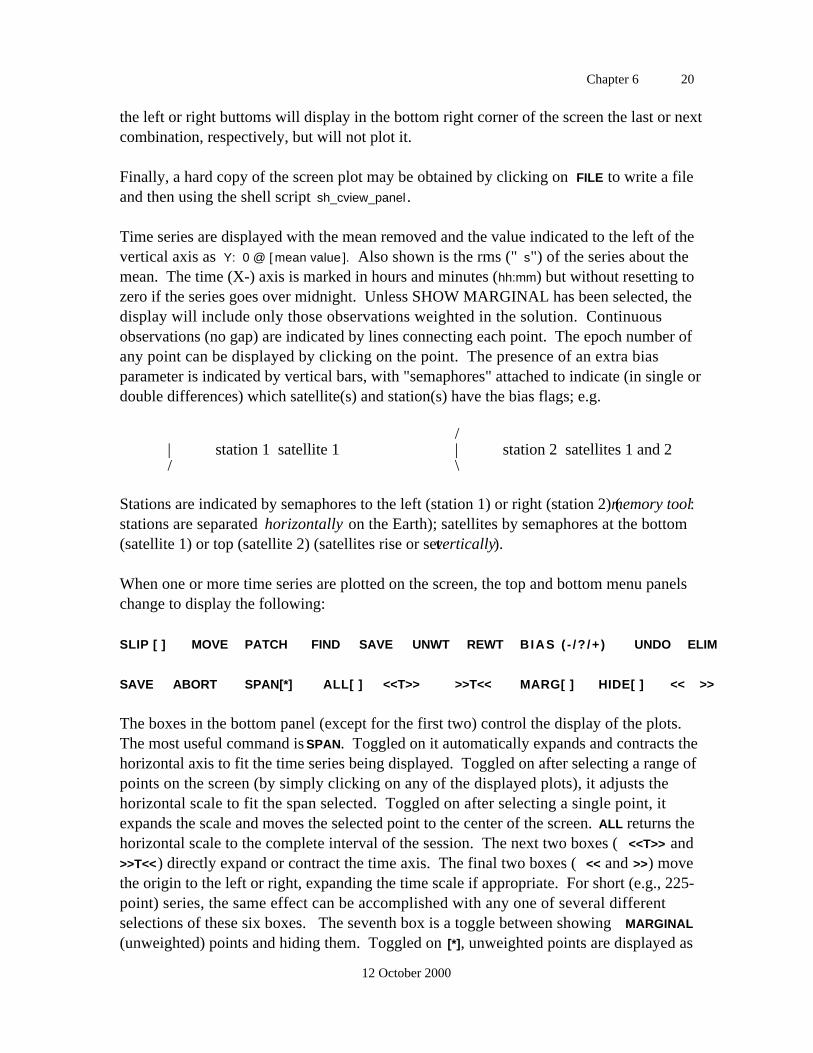
Chapter 6 20

12 October 2000

the left or right buttoms will display in the bottom right corner of the screen the last or nextcombination, respectively, but will not plot it.

Finally, a hard copy of the screen plot may be obtained by clicking on FILE to write a fileand then using the shell script sh_cview_panel .

Time series are displayed with the mean removed and the value indicated to the left of thevertical axis as Y: 0 @ [ mean value ]. Also shown is the rms (" s") of the series about themean. The time (X-) axis is marked in hours and minutes (hh:mm) but without resetting tozero if the series goes over midnight. Unless SHOW MARGINAL has been selected, thedisplay will include only those observations weighted in the solution. Continuousobservations (no gap) are indicated by lines connecting each point. The epoch number ofany point can be displayed by clicking on the point. The presence of an extra biasparameter is indicated by vertical bars, with "semaphores" attached to indicate (in single ordouble differences) which satellite(s) and station(s) have the bias flags; e.g.

/| station 1 satellite 1 | station 2 satellites 1 and 2/ \

Stations are indicated by semaphores to the left (station 1) or right (station 2) (memory tool:stations are separated horizontally on the Earth); satellites by semaphores at the bottom(satellite 1) or top (satellite 2) (satellites rise or set vertically).

When one or more time series are plotted on the screen, the top and bottom menu panelschange to display the following:

SLIP [ ] MOVE PATCH FIND SAVE UNWT REWT BIAS ( - /? /+ ) UNDO ELIM

SAVE ABORT SPAN[*] ALL[ ] <<T>> >>T<< MARG[ ] HIDE[ ] << >>

The boxes in the bottom panel (except for the first two) control the display of the plots.The most useful command is SPAN. Toggled on it automatically expands and contracts thehorizontal axis to fit the time series being displayed. Toggled on after selecting a range ofpoints on the screen (by simply clicking on any of the displayed plots), it adjusts thehorizontal scale to fit the span selected. Toggled on after selecting a single point, itexpands the scale and moves the selected point to the center of the screen. ALL returns thehorizontal scale to the complete interval of the session. The next two boxes ( <<T>> and>>T<<) directly expand or contract the time axis. The final two boxes ( << and >>) movethe origin to the left or right, expanding the time scale if appropriate. For short (e.g., 225-point) series, the same effect can be accomplished with any one of several differentselections of these six boxes. The seventh box is a toggle between showing MARGINAL

(unweighted) points and hiding them. Toggled on [*], unweighted points are displayed as

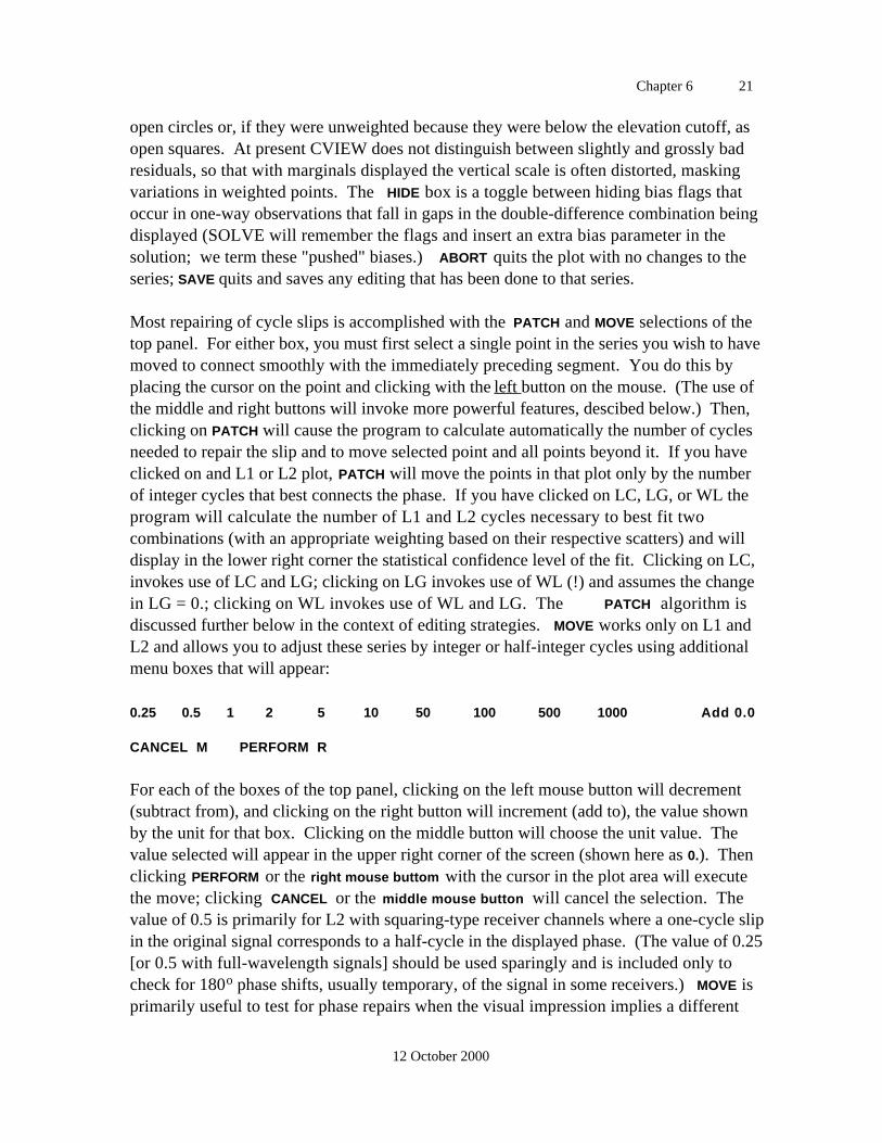
Chapter 6 21

12 October 2000

open circles or, if they were unweighted because they were below the elevation cutoff, asopen squares. At present CVIEW does not distinguish between slightly and grossly badresiduals, so that with marginals displayed the vertical scale is often distorted, maskingvariations in weighted points. The HIDE box is a toggle between hiding bias flags thatoccur in one-way observations that fall in gaps in the double-difference combination beingdisplayed (SOLVE will remember the flags and insert an extra bias parameter in thesolution; we term these "pushed" biases.) ABORT quits the plot with no changes to theseries; SAVE quits and saves any editing that has been done to that series.

Most repairing of cycle slips is accomplished with the PATCH and MOVE selections of thetop panel. For either box, you must first select a single point in the series you wish to havemoved to connect smoothly with the immediately preceding segment. You do this byplacing the cursor on the point and clicking with the left button on the mouse. (The use ofthe middle and right buttons will invoke more powerful features, descibed below.) Then,clicking on PATCH will cause the program to calculate automatically the number of cyclesneeded to repair the slip and to move selected point and all points beyond it. If you haveclicked on and L1 or L2 plot, PATCH will move the points in that plot only by the numberof integer cycles that best connects the phase. If you have clicked on LC, LG, or WL theprogram will calculate the number of L1 and L2 cycles necessary to best fit twocombinations (with an appropriate weighting based on their respective scatters) and willdisplay in the lower right corner the statistical confidence level of the fit. Clicking on LC,invokes use of LC and LG; clicking on LG invokes use of WL (!) and assumes the changein LG = 0.; clicking on WL invokes use of WL and LG. The PATCH algorithm isdiscussed further below in the context of editing strategies. MOVE works only on L1 andL2 and allows you to adjust these series by integer or half-integer cycles using additionalmenu boxes that will appear:

0.25 0.5 1 2 5 10 50 100 500 1000 Add 0.0

CANCEL M PERFORM R

For each of the boxes of the top panel, clicking on the left mouse button will decrement(subtract from), and clicking on the right button will increment (add to), the value shownby the unit for that box. Clicking on the middle button will choose the unit value. Thevalue selected will appear in the upper right corner of the screen (shown here as 0.). Thenclicking PERFORM or the right mouse buttom with the cursor in the plot area will executethe move; clicking CANCEL or the middle mouse button will cancel the selection. Thevalue of 0.5 is primarily for L2 with squaring-type receiver channels where a one-cycle slipin the original signal corresponds to a half-cycle in the displayed phase. (The value of 0.25[or 0.5 with full-wavelength signals] should be used sparingly and is included only tocheck for 180o phase shifts, usually temporary, of the signal in some receivers.) MOVE isprimarily useful to test for phase repairs when the visual impression implies a different

Chapter 6 22

12 October 2000

number of cycles than the number calculated by PATCH . Most of the time PATCH alonewill do the trick.

The BIAS box allows you to add ( right mouse button ), remove ( left mouse button ),or locate ( center mouse button ) extra bias parameters at epochs with questionable cycleslips. It can be used with a single epoch or a range of epochs (the latter being usefulprimarily in removing bias flags). ELIM will eliminate bias flags in all one-way data inseries displayed unless a narrower span is defined by brackets. FIND will attempt to assistyou in locating the (one-way) satellite and station combination associated with a cycle slipor extra bias parameter following a gap by changing the display to put as the first satelliteand station the one in which the gap occurred. Clicking on SAVE or ABORT, followed byPLOT or SEEK will restore the original sequence. (Be careful here, though, because youmay end up using intervening commands that erase CVIEW's memory of the lastcombination. It's a good idea to jot down on paper the combination on the screen beforeinvoking FIND, so that when you're finished editing a particular epoch you can return to theright place in the search sequence. ) UNWEIGHT flags data points to be omitted from thesolution by SOLVE; REWEIGHT removes the flag. All of these commands are to beexecuted after you have selected a point or range of points on the screen by clicking onthem with the mouse.

Note that for double differences, the corrections you make are applied to the first satelliteand first station displayed for the double-difference combination. The importance of beingaware of this feature is discussed in the next section.

The eighth and ninth boxes allow you to reverse your immediately previous action. UNDO

reverses the effects of PATCH , MOVE , WEIGHT , REWEIGHT , BIAS, and ELIM , all of thecommands that actually change the data. CANCEL simply removes the selection of pointsyou have made in anticipation of a move. The SLIP box is unused at present.

The MOVIE function is useful for viewing an entire set of residuals quickly to infer itscharacter, locate a problem, or verify at the end of editing that everything is clean. IfSTACK is invoked, all of the plots will be superimposed on the screen. This is a powerfulfeature for discerning the nature of the residuals but it can become a mess if there are toomany series. Once you start the MOVIE, you can stop it by clicking anywhere on thescreen with the middle mouse button (click once only and wait for the current frame tofinish being written to the screen). Following this by PLOT will show you the series thatwas on the screen when you stopped, allowing you to hit the panic button when you seesomething you don't like If you start the MOVIE with the right button, plotting will stopat the first series with LC RMS > 1.0.

When you have exercised all of the commands and gained some experience in data editing,you can use CVIEW in a more automatic mode, using the mouse buttons to reduce the

Chapter 6 23

12 October 2000

number of hand motions required. When the cursor is in the plot area of the screen, themouse buttons take on different functions. The left button puts brackets on the data asdescribed above. The middle button acts as SEEK or ABORT according to commanddisplayed at the bottom. The right button executes the sequence FIND + PATCH, withPATCHing being performed only if the correct satellite and station was "found"; a secondclick on the right button will SAVE and re-PLOT. To UNDO the PATCHing, use the left

button .

Fixing cycle-slips in double differences is straightforward if you remember certain rules. Ifa particular receiver channel slips one or more cycles, a break will appear in all datacombinations that include that channel. For example, a slip in the L2 phase at station 1received from satellite 3 will appear in all double difference plots LC, LG, and WL thatinclude station 1 and satellite 3. The first step is to identify the station and satellite forwhich the slip occurred . One way to do this is to make use of the sorted output ofSCANDD (e.g., vscan.out.worst ), marking on the printout or in the file displayed by aneditor the satellite and station common to all occurences of the slip at a partrcular epoch (seeSection 6.3). If you have run AUTCLN in post-fit mode, you can identify the source(s) ofthe slip by viewing each of the one-ways contributing to the double difference. In the casewhere there is a gap or extra bias flag in only one station and satellite combination of thedouble difference, then the FIND command will identify for you the combination and moveit to the ( 1, 1 ) position in the display. With this display, you can use PATCH (or MOVE)

to fix the slip, and then return to the original order of the double difference combination byclicking on SAVE or ABORT. If there is no gap or several gaps, then you should check allfour one-way series. Multiple slips are not uncommon since a satellite or receiver may"hiccup", affecting multiple stations or channels, respectively. In cases of very high noisein the one-ways (due to bad clocks or ionosphere), you may have to deduce the culpritchannel by displaying several combinations of double differences. For example, supposethat for three stations and three satellites the following combinations had a cycle-slip at aparticular epoch of observation:

(station 1 - station 2) - (satellite 1 - satellite 3)




It is clear that the cycle-slip occurred at station 2 and satellite 3. Thus the slip should befixed with satellite 3 and station 2 appearing first when the double difference combination isselected in the menu. In some cases the location of the cycle-slip is ambiguous. Forexample, if only two stations are observing, it is impossible to determine at which site aslip occurred. In this case, the slip can be fixed at either site, The only requirement is thatall double-difference plots be free of cycle slips, i.e, that the cycle-slips are fixedconsistently.

Chapter 6 24

12 October 2000

Remember: All editing operations are applied only to the first satellite and station in thedouble difference combination, so if the tedit is made in double differences, you may haveto switch the order before executing the operation (bias, unweight, reweight, patch, move)

Once the correct satellite and station are identified as responsible for a cycle slip, the nextstep is to determine its size and whether it occurred in L1 or L2. If the ionosphericfluctuation between epochs is much less than a cycle (or a half-cycle with codeless trackingchannels), it will be obvious in the separate plots of L1 and L2 how many cycles slipped ineach channel. If the ionospheric fluctuations are large, however, only LC may besufficiently smooth to discern the size of the slip. In the most difficult cases, it may benecessary to examine all four phase series (L1, L2, LC, and LG) to deduce the combinationof L1 and L2 cycles (and/or half-cycles) responsible for the LC jump. Table 6.1 gives themost common residual LC and LG jumps that occur for combinations of slips in L1 and L2for the cases of full-wavelength and half-wavelength L2. The bold-faced entries,representing LC jumps of less than one cycle, are the most dangerous since they can escapedetection if the fluctuations in L1 and L2 due to the ionosphere are very large.

Using PATCH in CVIEW allows you to avoid computing the L1 and L2 combinationsexplicitly. Used with LC or LG, PATCH will make a best estimate of the jumps byexamining these two time series and apply integer corrections to L1 and L2. The statisticalconfidence of the estimate is displayed, allowing you to assess whether to retain or add afree-bias flag at the break. This is a useful feature even when you believe that there is noslip, in order to reinforce your subjective judgement of the confidence of the connectionmade by AUTCLN. PATCH uses up to 15 points on either side of the slip (usually also agap) in estimating its correction. Its estimate and confidence level are reliable as far as theLC and LG residuals are concerned. There are times, however, when the analyst isjustified in raising the confidence level based on the appearance of L1 and L2. If LC andLG are noisy compared with L1 and L2 (which can occur if multipathing dominatesionospheric fluctuations), then using PATCH or MOVE on L1 and L2 separately is moreconvenient. In this case Table 6.1 is particularly useful.

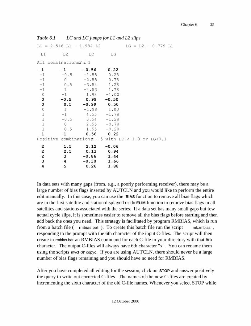
Chapter 6 25

12 October 2000

Table 6.1 LC and LG jumps for L1 and L2 slips

LC = 2.546 L1 - 1.984 L2 LG = L2 - 0.779 L1

L1 L2 LC LG

All combinations 1

-1 -1 -0.56 -0.22-1 -0.5 -1.55 0.28-1 0 -2.55 0.78-1 0.5 -3.54 1.28-1 1 -4.53 1.780 -1 1.98 -1.000 -0.5 0.99 -0.500 0.5 -0.99 0.500 1 -1.98 1.001 -1 4.53 -1.781 -0.5 3.54 -1.281 0 2.55 -0.781 0.5 1.55 -0.281 1 0.56 0.22

Positive combinations 5 with LC < 1.0 or LG<0.1

2 1.5 2.12 -0.062 2.5 0.13 0.942 3 -0.86 1.443 4 -0.30 1.664 5 0.26 1.88

In data sets with many gaps (from. e.g., a poorly performing receiver), there may be alarge number of bias flags inserted by AUTCLN and you would like to perform the entireedit manually. In this case, you can use the BIAS function to remove all bias flags whichare in the first satellite and station displayed or the ELIM function to remove bias flags in allsatellites and stations associated with the series. If a data set has many small gaps but fewactual cycle slips, it is sometimes easier to remove all the bias flags before starting and thenadd back the ones you need. This strategy is facilitated by program RMBIAS, which is runfrom a batch file ( rmbias.bat ). To create this batch file run the script mk.rmbias ,responding to the prompt with the 6th character of the input C-files. The script will thencreate in rmbias.bat an RMBIAS command for each C-file in your directory with that 6thcharacter. The output C-files will always have 6th character "x". You can rename themusing the scripts mvcf or copyc. If you are using AUTCLN, there should never be a largenumber of bias flags remaining and you should have no need for RMBIAS.

After you have completed all editing for the session, click on STOP and answer positivelythe query to write out corrected C-files. The names of the new C-files are created byincrementing the sixth character of the old C-file names. Whenever you select STOP while

Chapter 6 26

12 October 2000

editing, CVIEW will give you the opportunity to continue editing and/or to save the editedC-files by issuing the following prompt:

You may:

1 Write new C-files, incrementing series letter

2 Write new C-files, incrementing series letter and deleting old C-files

3 Overwrite input C-files

4 Not write any C-files

5 Not write any C-files but save vcview.out

Only 1 and 4 will let you continue editing

Pick a number

With modern data sets, for which any editing is can usually be accomplished by addingedit_sv_site commands to AUTCLN, you will have used CVIEW only for diagnosingproblems and you may select 4 or 5 to avoid writing out the C-files. If you have performededits, particularly cycle-slip repair, which you wish to keep, then you should select 1, 2, or3. The simplest course is to overwrite the input C-files, but if you have spent a long timeediting and don’t want to chance a (rare) system problem, then 1 is the safest option. Inthis case you may need to rename the C-files (change 6th character) to match what SOLVEis expecting (from the M-file) using the script mvcf after finishing with CVIEW. If youselect options 1 or 4, you will get the prompt

Do you wish to continue editing (Y/N)

A "yes" (Y) reply will return you to the editing screen, after performing an interim save ofthe C-files if you have chosen option 1. A "no" ( N) reply will exit the CVIEW, eitherdirectly if you have selected option 4, or after writing out the C-files if you have selectedoption 1. When you are engaged in a long editing sessions, it is prudent to STOP editingperiodically to save the C-files. (Neither the hardware we have used nor the software wehave written is immune to unexpected crashes.)

Option 5 at the end of editing will write out a file ( vcview.out ) of all the edits you havemade in the session. Running the (interactive) program AUTEDT or (better) the shell scriptsh_cvedt extracts from vcview.out the information about which data you have unweightedand appends to the autcln.cmd file the appropriate edit_site_sv commands for AUTCLN.

Chapter 6 27

12 October 2000

6.5 Strategies for Editing

When used in its postfit mode, AUTCLN will usually produce a near-optimal editing of thedata from almost any survey, including those performed in the 1980s and 1990s with firstor second generation receivers. For these older surveys, or modern ones spanning only afew hours and including only two or three stations, it is efficient to view all of the data withCVIEW to satisfy yourself that AUTCLN has recovered all of the useful data and not leftany unnecessary bias flags. If you find problems, you may elect to perform the editmanually, especially with small data sets, but most of the time you can induce AUTCLN todo the right thing by changing its input parameters and/or pre-deleting (with theedit_site_sv command) short spans of noisy data. This approach has two advantagesover manual editing: 1) it transfers the burden of editing from the (expensive, slow, andfallible) analyst to the (cheap, fast, and slightly less fallible) cpu; 2) the autcln.cmd file nowmaintains the record of all edits, so that you can reprocess the data, from RINEX files ifnecessary, as modeling and editing algorithms improve.

The preferred strategy for networks with more than two or three stations is to first examinethe outputs of SOLVE (q-file) and AUTCLN ( autcln.post.sum and the sky-plots of phaseresiduals [DPHS] produced with sh_gamit) to determine if there were any problems with therun. If so, then you can use the outputs of SCANDD (sorted versions of vscan.out andscan.rms) with CVIEW to identify the station or satellite and cause of the problem and addcontrols to autcln.cmd to fix it. Since SCANDD is fairly time-consuming to run, it'susually most efficient to omit it from the standard batch solution and repeat the run if yoususpect problems.

The most obvious indicator of a bad solution is the nrms value in the Q-file. As discussedin Section 5.4, values above 0.3 usually signify a problem, and for many surveys youshould expect most values to be near 0.2. If you are processing several days of a survey atone time, grep'ing on nrms for all of the q-files will give you an indication of problemdays. If the nrms is abnormally high, you should then look at the scan.rms output ofSCANDD (or rms.ful after running SORTER) to see if a single satellite or station is causinga problem. If you find values greater than about 0.2 cycles, you should examine theresiduals visually with CVIEW to understand the cause of the problem.

Even without a high nrms, you should examine the autcln.sum file to ascertain whetherthere are problems with a station or satellite. If a receiver or clock is malfunctioning, or ifyou have a bad a priori coordinate for the station, AUTCLN may have deleted largequantities of data or added an excessive number of bias flags. The first three tables in thesummary file will tell you quickly if there is a major problem. With postfit editing, thetable of one-way phase residuals will characterize precisely the preformance of each stationand satellite. With either postfit or prefit editing, you should also make sure that in theDATA AMOUNTS listing there are small numbers in the Gap (data deleted in gaps) and BF

Chapter 6 28

12 October 2000

(bias flags remaining) columns and that the number of data retained ( Good column) arecomparable to those for other stations. If you find anomalies, the other tables in the fileand CVIEW can help you determine the source of the problem. If you have run AUTCLNin post-fit mode, there will a summary of the rms of the residuals for each station andsatellite, allowing quick identification of outliers. (See the explanation for these tables insections 6.2 and 7.6 and the on-line help for AUTCLN.)

If you suspect problems at a station from its postfit rms, you should run sortv on thevscan.out file from SCANDD. Usually, looking at vxxxxa.ddd. worst will tell you if thereare any potential slips. It would be unusual for there to be more than one or two of these(if any) after AUTCLN unless there is a station with a malfunctioning receiver.

For regional networks, there is one additional and very important editing consideration ifyou plan to attempt ambiguity resolution in the analysis. The present version of SOLVEassigns the (one allowed) explicit ambiguity parameter to the last segment of the double-difference series; that is, the data after the last extra bias parameter (shown by a bar inCVIEW). This is because the extra bias parameters are all estimated implicitly. In order tomaximize the probability that the ambiguity for a series will be resolved, you want to havethe last segment as long as possible. This means that for stations in a regional network youshould not leave an extra bias parameter in the latter part of an otherwise continuous series,but rather unweight the data at the end containing these extra biases. The last entry in thetrim_oneway_tol command for AUTCLN gives you some control over this, but it's stillpossible to have a too-short segment at the end of a double difference sequence. Forwidely spaced fiducial stations where there is no chance to resolve ambiguites, leaving anextra bias parameter associated with a few points at the end is of little consequence. Theimportant thing in this case is to avoid breaking up with bias flags long segments of data,wherever they are located in the observing span.

Once you have identified any editing problems with the solution, you should make takecorrective action and then rerun the solution from the appropriate step. If the problem isbad data from station or satellite you can begin with AUTCLN, after removing the bad datafrom consideration using the edit_site_sv command in the (base) autcln.cmd file (takingadvantage of CVIEW's ability to generate these entries automatically for short segmentsremoved using the UNWT command—see the last paragraph of Section 6.4). If theproblem is a bad a priori station coordinate, you should begin with MODEL after updatingthe L- or T-file. If you suspect a bad orbit, you can first repeat the SOLVE run with thesatellite excluded ( exclude: PN04 , e.g., in the Session Options ) to test yourhypothesis, and then add edit_site_sv entries to the autcln.cmd file to provide apermanent record and assure exclusion in future runs. Occasionally the appearance of baddata can be traced back to a problem with the information in the RINEX file (e.g., namedincorrectly) or the auxilliary files of GAMIT ( UT1., pole., station.info ).

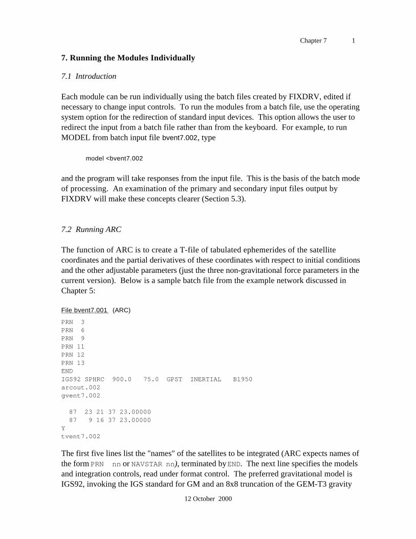
Chapter 7 1

12 October 2000

7. Running the Modules Individually

7.1 Introduction

Each module can be run individually using the batch files created by FIXDRV, edited ifnecessary to change input controls. To run the modules from a batch file, use the operatingsystem option for the redirection of standard input devices. This option allows the user toredirect the input from a batch file rather than from the keyboard. For example, to runMODEL from batch input file bvent7.002, type

model <bvent7.002

and the program will take responses from the input file. This is the basis of the batch modeof processing. An examination of the primary and secondary input files output byFIXDRV will make these concepts clearer (Section 5.3).

7.2 Running ARC

The function of ARC is to create a T-file of tabulated ephemerides of the satellitecoordinates and the partial derivatives of these coordinates with respect to initial conditionsand the other adjustable parameters (just the three non-gravitational force parameters in thecurrent version). Below is a sample batch file from the example network discussed inChapter 5:

File bvent7.001 (ARC)

PRN 3PRN 6PRN 9PRN 11PRN 12PRN 13ENDIGS92 SPHRC 900.0 75.0 GPST INERTIAL B1950arcout.002gvent7.002

87 23 21 37 23.00000 87 9 16 37 23.00000Ytvent7.002

The first five lines list the "names" of the satellites to be integrated (ARC expects names ofthe form PRN nn or NAVSTAR nn), terminated by END. The next line specifies the modelsand integration controls, read under format control. The preferred gravitational model isIGS92, invoking the IGS standard for GM and an 8x8 truncation of the GEM-T3 gravity

Chapter 7 2

12 October 2000

field. However, most GAMIT analyses prior to release 9.25, including the GARNERorbits generated at SIO, have used MERIT standards, so if you are reintegrating a G-filefor regional analysis but combining the H-files with those generated elsewhere, be carefulthat the gravitational models are consistent. In multiyear anlysis for station positions andvelocities, there is no serious problem in having used different gravitational models togenerate the orbits since the adjustments of initial conditions will absorb most of the modeldifferences.

The only radiation pressure model available in the past has been a "flat-plate" or "spherical"(SPHRC) model in which adjustable parameters were defined for the Sun direction("direct"), spacecraft y-axis ("y-bias"), and the Earth-pointing (spacecraft z) axis ("z-bias).Only the first two of these are well determined and usually estimated. A better geometricmodel is defined by the Sun-pointing axis, y-axis, and a third axis orthogonal to both ofthese. Investigators at AIUB (Berne) ( Beutler et al., [1994]; see references in Chapter 2)have termed this third axis "x", but we designate it the "b-axis" to distinguish it from thespacecraft x-axis. This parameterization is available by specifying SRDYB, which allowsthree adjustable parameters, or BERNE, which allows the three constants plus once-per-revaccelerations (sine and cosine terms) along each of these three axes, for a total of 9parameters. Beutler et al. [1994] (and the AIUB standard processing) incorporate intothese formulations the ROCK4 model described by Fliegel et al. [ J.Geophys. Res ., 97,559–568, 1992], modified to lump the "X" and "Z" forces into a single "direct" force (M.Rothacher, personal communication, 1994). Tests carried out at MIT thus far have shownno improvement (in fact, a slight degradation) using the ROCK4 model, so we do notinclude it in BERNE or SRDYB. A second difference between the GAMIT and Berneseformulations is that we include shadowing only in the constant, direct solar term, whereasBerne includes it for all 9 terms. Two additional parameterizations are available: SRDYZuses the same adjustable parameters as SPHRC but includes the original formulation of theROCK4 model, with the additional forces applied along the X and Z axes. Finally,SRXYZ uses adjustable parameters and ROCK4 forces along the spacecraft x, y, and zaxes. The details of these formulations may be found in the code and documentation ofsubroutine ertorb.f in the /arc directory.

The next two entries on the same line are for the T-file tabular interval and integration step-size, both given in seconds. The nominal values are 900 (15 minutes) and 75 seconds,respectively. The tabular interval must be an even multiple of the integration step-size. Thefinal three entries give the time type (GPST or UTC) desired for the T-file (GPST is nowdefault), and the reference frame, which in the current version must be 1950.0 inertial.

The next two lines give the filenames of the ARC printed output and the input G-filecontaining the initial conditions and initial values of the non-gravitational force parameters.There is then a blank line (for historical reasons), followed by the start and stop times ofthe integration, given as (2-digit) year, day-of-year, hours, minutes, seconds. The times

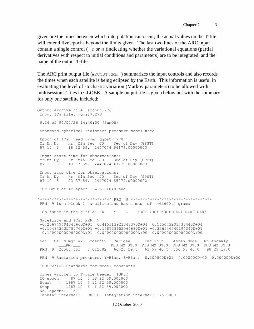
Chapter 7 3

12 October 2000

given are the times between which interpolation can occur; the actual values on the T-filewill extend five epochs beyond the limits given. The last two lines of the ARC inputcontain a single control ( Y or N )indicating whether the variational equations (partialderivatives with respect to initial conditions and parameters) are to be integrated, and thename of the output T-file.

The ARC print output file (ARCOUT.ddd ) summarizes the input controls and also recordsthe times when each satellite is being eclipsed by the Earth. This information is useful inevaluating the level of stochastic variation (Markov parameters) to be allowed withmultisession T-files in GLOBK. A sample output file is given below but with the summaryfor only one satellite included:

Output archive file: arcout.278 Input ICs file: ggpst7.278

9.16 of 94/07/26 14:40:00 (SunOS)

Standard spherical radiation pressure model used

Epoch of ICs, read from: ggpst7.278 Yr Mn Dy Hr Min Sec JD Sec of Day (GPST) 87 10 5 18 22 59. 2447074 66179.00000000

Input start time for observations: Yr Mn Dy Hr Min Sec JD Sec of Day (GPST) 87 10 5 13 7 59. 2447074 47279.00000000

Input stop time for observations: Yr Mn Dy Hr Min Sec JD Sec of Day (GPST) 87 10 5 23 37 59. 2447074 85079.00000000

TDT-GPST at IC epoch = 51.1840 sec

******************************* PRN 9 ********************************** PRN 9 is a block 1 satellite and has a mass of 462600.0 grams

ICs found in the g-file: X Y Z XDOT YDOT ZDOT RAD1 RAD2 RAD3

Satellite and ICs: PRN 9 -0.256749494345660D+05 0.415313921343370D+04 0.565073203730440D+04 -0.104843035787760D+01 -0.158739652566680D+01 -0.336546540194340D+01 0.100000000000000D+01 0.000000000000000D+00 0.000000000000000D+00

Sat Se mimjr Ax Eccen'ty Perigee Inclin'n Ascen.Node Mn Anomaly ___KM.___ DDD MM SS.S DDD MM SS.S DDD MM SS.S DDD MM SS.S PRN 9 26560.651 0.012882 66 23 29.5 63 59 40.5 356 53 45.0 98 29 17.0

PRN 9 Radiation pressure, Y-Bias, Z-Bias: 0.100000D+01 0.000000D+00 0.000000D+00

IERS92/IGS Standards for model constants

Times written to T-file header (GPST) IC epoch: 87 10 5 18 22 59.000000 Start : 1987 10 5 11 22 59.000000 Stop : 1987 10 6 1 22 59.000000 No. epochs: 57 Tabular interval: 900.0 Integration interval: 75.0000

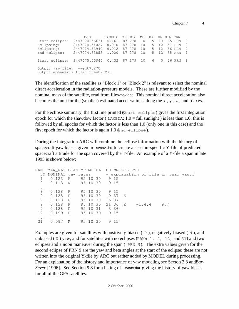
Chapter 7 4

12 October 2000

PJD LAMBDA YR DOY MO DY HR MIN PRN Start eclipse: 2447074.56631 0.161 87 278 10 5 13 35 PRN 9 Eclipsing: 2447074.54027 0.010 87 278 10 5 12 57 PRN 9 Eclipsing: 2447074.53940 0.912 87 278 10 5 12 56 PRN 9 End eclipse: 2447074.53853 1.000 87 278 10 5 12 55 PRN 9

Start eclipse: 2447075.03940 0.432 87 279 10 6 0 56 PRN 9

Output yaw file: yvent7.278 Output ephemeris file: tvent7.278

The identification of the satellite as "Block 1" or "Block 2" is relevant to select the nominaldirect acceleration in the radiation-pressure models. These are further modified by thenominal mass of the satellite, read from file svnav.dat. This nominal direct acceleration alsobecomes the unit for the (smaller) estimated accelerations along the x-, y-, z-, and b-axes.

For the eclipse summary, the first line printed ( Start eclipse ) gives the first integrationepoch for which the shawdow factor ( LAMBDA; 1.0 = full sunlight ) is less than 1.0; this isfollowed by all epochs for which the factor is less than 1.0 (only one in this case) and thefirst epoch for which the factor is again 1.0 ( End eclipse ).

During the integration ARC will combine the eclipse information with the history ofspacecraft yaw biases given in svnav.dat to create a session-specific Y-file of predictedspacecraft attitude for the span covered by the T-file. An example of a Y-file a span in late1995 is shown below:

PRN YAW_RAT BIAS YR MO DA HR MN ECLIPSE 39 NOMINAL yaw rates - explanation of file in read_yaw.f 1 0.123 P 95 10 30 9 15 2 0.113 N 95 10 30 9 15 ... 9 0.128 P 95 10 30 9 15 9 0.128 P 95 10 30 9 37 E 9 0.128 P 95 10 30 15 37 9 0.128 P 95 10 30 21 36 E -134.4 9.7 9 0.128 P 95 10 31 3 36 12 0.199 U 95 10 30 9 15 ... 31 0.097 P 95 10 30 9 15

Examples are given for satellites with positively-biased ( P ), negatively-biased ( N ), andunbiased ( U ) yaw, and for satellites with no eclipses (PRNs 1, 2, 12, and 31) and twoeclipses and a noon maneuver during the span ( PRN 9). The extra values given for thesecond eclipse of PRN 9 are the yaw and beta angles at the start of the eclipse; these are notwritten into the original Y-file by ARC but rather added by MODEL during processing.For an explanation of the history and importance of yaw modeling see Secton 2.3 and Bar-Sever [1996]. See Section 9.8 for a listing of svnav.dat giving the history of yaw biasesfor all of the GPS satellites.

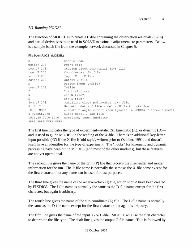
Chapter 7 5

12 October 2000

7.3 Running MODEL

The function of MODEL is to create a C-file containing the observation residuals (O-Cs)and partial derivatives to be used in SOLVE to estimate adjustments to parameters. Belowis a sample batch file from the example network discussed in Chapter 5:

File bvent7.002 (MODEL)

S Static Modepcato7.278 Print fileivent7.278 Station clock polynomial (I-) filelvent7.278 Coordinates (L) filexcato7.278 Input X or C-fileccato7.278 output C-fileN Delete input C-file?tvent7.278 T-fileI Inertial frameN use W-file?N use Z-file?jvent7.278 Satellite clock polynomial (J-) file0 7 7 Geodetic datum / Tide model / SP Earth rotation 0.0 NONE elevation angle cutoff (now ignored in MODEL) / antenna model3 yventt.278 Clock model / Yaw file1013.25 20.0 50.0 pressure, temp, humiditySAAS SAAS NMFH NMFW

The first line indicates the type of experiment—static (S), kinematic (K), or dynamic (D)—and is used to guide MODEL in the reading of the X-file. There is an additional key-letterinput possible ('O') if the X-file is 'old-style', written prior to October, 1991, and doesn'titself have an identifier for the type of experiment. The "hooks" for kinematic and dynamicprocessing have been put in MODEL (and most of the other modules), but these featuresare not yet operational.

The second line gives the name of the print (P) file that records the file-header and modelinformation for the run. The P-file name is normally the same as the X-file name except forthe first character, but any name can be used for test purposes.

The third line gives the name of the receiver-clock (I) file, which should have been createdby FIXDRV. The I-file name is normally the same as the D-file name except for the firstcharacter, but again is arbitrary.

The fourth line gives the name of the site-coordinate (L) file. The L-file name is normallythe same as the D-file name except for the first character, but again is arbitrary.

The fifth line gives the name of the input X- or C-file. MODEL will use the first characterto determine the file type. The sixth line gives the output C-file name. This is followed by

Chapter 7 6

12 October 2000

an input ('Y' or 'N') indicating whether the input C-file should be deleted at the end of theMODEL run. If the the input data file is an X-file, MODEL will not delete it regardless ofthe entry on the seventh line.

The eighth line gives the name of the satellite ephemeris (T) file. The T-file name isarbitrary except for the first character. For single-day T-files, use of the last digit of theyear and the day of year are convenient.

The ninth line indicates whether the MODEL computations are to be performed in an earth-fixed ('E') or inertial ('I') coordinate system. At present, only inertial frame computationsare supported by ARC and MODEL.

The next group of questions tell MODEL whether you wish to use an input table for surfacemeteorological data (W-file) or water-vapor-radiometry data (Z-file). If the response toeither of these questions is "Y", the name of the file should be added as an additional linefollowing the question response. Use of these tables is relatively untested.

The next line gives the name of the satellite clock (J) file. The name is arbitrary but isusually the same as the D-file except for the first letter. The J-file should have been createdfrom an E-file using MAKEJ. With Selective Availability invoked, a large J-file, computedusing observations at a site with an atomic frequency standard, may be necessary.

Line 13 has three integers designating the geodetic datum and the models to be used forsolid-earth and ocean tides and short-period (diurnal and semidiurnal) oscillations of UT1and pole. The current version of GAMIT works properly only in spherical (internallyCartesian) coordinates, so ' 0' should always be specified for the datum. The integercontrolling the tide model is binary coded—the first (1) bit for the default frequency-independent model for solid-earth tides, the second (2) bit for a frequency-dependent modelfor the K1 solid-earth tide,the third (4) bit for the pole tide, and the fourth (8) bit for oceantides. The default (7) is to apply the first three models. Previous versions of GAMIT didnot use the pole tide, but GLOBK will detect this an add it when combining h-files.Application of ocean tides requires an additional input table (otide.) and is still being tested

Line 14 was formerly used for the elevation cutoff angle, but this can no longer becontrolled in MODEL; hence the zero entry. The other entry on this line is a keywordindicating the model to be used for antenna phase-center variations. The default is NONE,but a table ( antmod.dat ) may be used to provide an elevation-dependent ( ELEV ) orelevation-and-azimuth-dependent (AZEL) model. See Appendix 7 for the current state-of-knowledge of the mean and time-variable locations of the L1 and L2 phase centers forcommonly used GPS antenna.

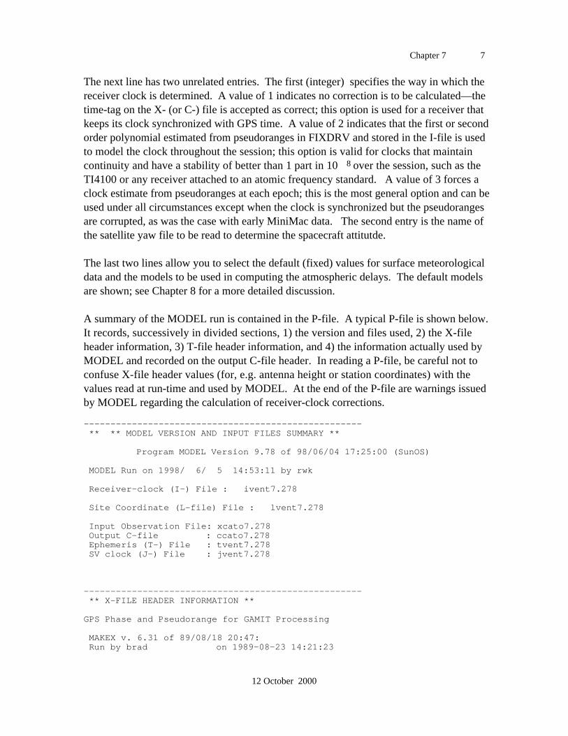
Chapter 7 7

12 October 2000

The next line has two unrelated entries. The first (integer) specifies the way in which thereceiver clock is determined. A value of 1 indicates no correction is to be calculated—thetime-tag on the X- (or C-) file is accepted as correct; this option is used for a receiver thatkeeps its clock synchronized with GPS time. A value of 2 indicates that the first or secondorder polynomial estimated from pseudoranges in FIXDRV and stored in the I-file is usedto model the clock throughout the session; this option is valid for clocks that maintaincontinuity and have a stability of better than 1 part in 10 8 over the session, such as theTI4100 or any receiver attached to an atomic frequency standard. A value of 3 forces aclock estimate from pseudoranges at each epoch; this is the most general option and can beused under all circumstances except when the clock is synchronized but the pseudorangesare corrupted, as was the case with early MiniMac data. The second entry is the name ofthe satellite yaw file to be read to determine the spacecraft attitutde.

The last two lines allow you to select the default (fixed) values for surface meteorologicaldata and the models to be used in computing the atmospheric delays. The default modelsare shown; see Chapter 8 for a more detailed discussion.

A summary of the MODEL run is contained in the P-file. A typical P-file is shown below.It records, successively in divided sections, 1) the version and files used, 2) the X-fileheader information, 3) T-file header information, and 4) the information actually used byMODEL and recorded on the output C-file header. In reading a P-file, be careful not toconfuse X-file header values (for, e.g. antenna height or station coordinates) with thevalues read at run-time and used by MODEL. At the end of the P-file are warnings issuedby MODEL regarding the calculation of receiver-clock corrections.

---------------------------------------------------- ** ** MODEL VERSION AND INPUT FILES SUMMARY **

Program MODEL Version 9.78 of 98/06/04 17:25:00 (SunOS)

MODEL Run on 1998/ 6/ 5 14:53:11 by rwk

Receiver-clock (I-) File : ivent7.278

Site Coordinate (L-file) File : lvent7.278

Input Observation File: xcato7.278 Output C-file : ccato7.278 Ephemeris (T-) File : tvent7.278 SV clock (J-) File : jvent7.278

---------------------------------------------------- ** X-FILE HEADER INFORMATION **

GPS Phase and Pseudorange for GAMIT Processing

MAKEX v. 6.31 of 89/08/18 20:47: Run by brad on 1989-08-23 14:21:23

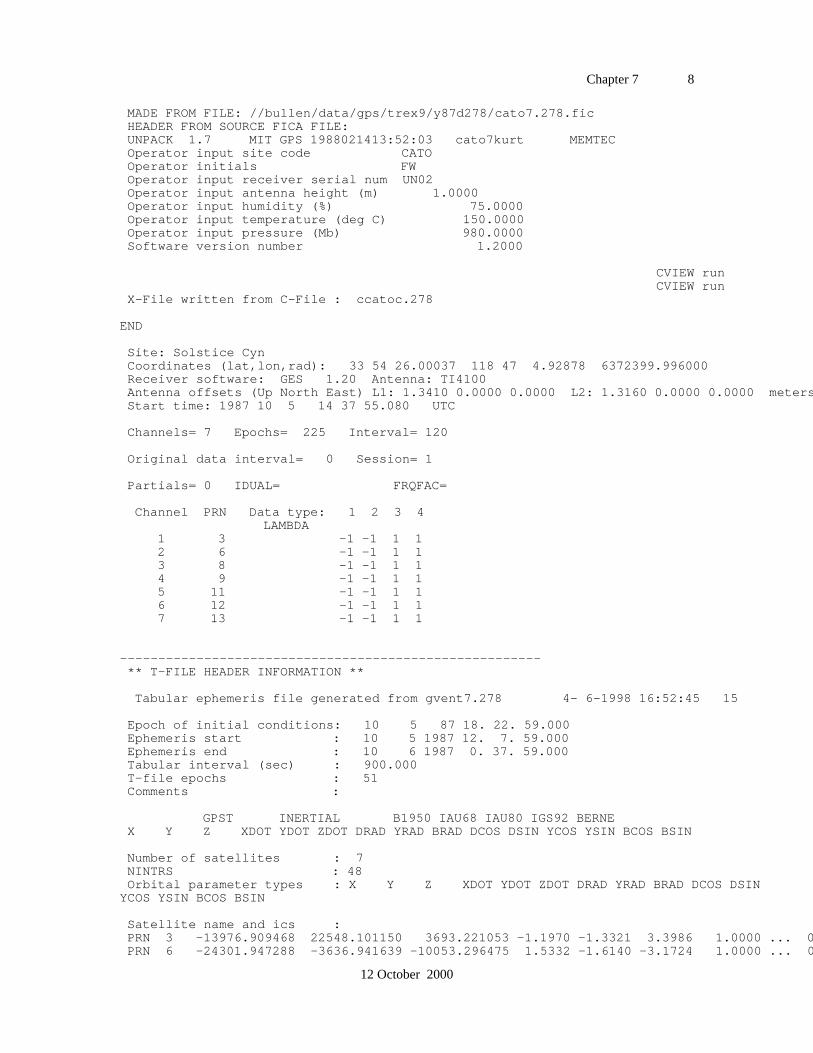
Chapter 7 8

12 October 2000

MADE FROM FILE: //bullen/data/gps/trex9/y87d278/cato7.278.fic HEADER FROM SOURCE FICA FILE: UNPACK 1.7 MIT GPS 1988021413:52:03 cato7kurt MEMTEC Operator input site code CATO Operator initials FW Operator input receiver serial num UN02 Operator input antenna height (m) 1.0000 Operator input humidity (%) 75.0000 Operator input temperature (deg C) 150.0000 Operator input pressure (Mb) 980.0000 Software version number 1.2000

CVIEW run CVIEW run X-File written from C-File : ccatoc.278

END

Site: Solstice Cyn Coordinates (lat,lon,rad): 33 54 26.00037 118 47 4.92878 6372399.996000 Receiver software: GES 1.20 Antenna: TI4100 Antenna offsets (Up North East) L1: 1.3410 0.0000 0.0000 L2: 1.3160 0.0000 0.0000 meters Start time: 1987 10 5 14 37 55.080 UTC

Channels= 7 Epochs= 225 Interval= 120

Original data interval= 0 Session= 1

Partials= 0 IDUAL= FRQFAC=

Channel PRN Data type: 1 2 3 4 LAMBDA 1 3 -1 -1 1 1 2 6 -1 -1 1 1 3 8 -1 -1 1 1 4 9 -1 -1 1 1 5 11 -1 -1 1 1 6 12 -1 -1 1 1 7 13 -1 -1 1 1

------------------------------------------------------- ** T-FILE HEADER INFORMATION **

Tabular ephemeris file generated from gvent7.278 4- 6-1998 16:52:45 15

Epoch of initial conditions: 10 5 87 18. 22. 59.000 Ephemeris start : 10 5 1987 12. 7. 59.000 Ephemeris end : 10 6 1987 0. 37. 59.000 Tabular interval (sec) : 900.000 T-file epochs : 51 Comments :

GPST INERTIAL B1950 IAU68 IAU80 IGS92 BERNE X Y Z XDOT YDOT ZDOT DRAD YRAD BRAD DCOS DSIN YCOS YSIN BCOS BSIN

Number of satellites : 7 NINTRS : 48 Orbital parameter types : X Y Z XDOT YDOT ZDOT DRAD YRAD BRAD DCOS DSINYCOS YSIN BCOS BSIN

Satellite name and ics : PRN 3 -13976.909468 22548.101150 3693.221053 -1.1970 -1.3321 3.3986 1.0000 ... 0.0000 PRN 6 -24301.947288 -3636.941639 -10053.296475 1.5332 -1.6140 -3.1724 1.0000 ... 0.0000

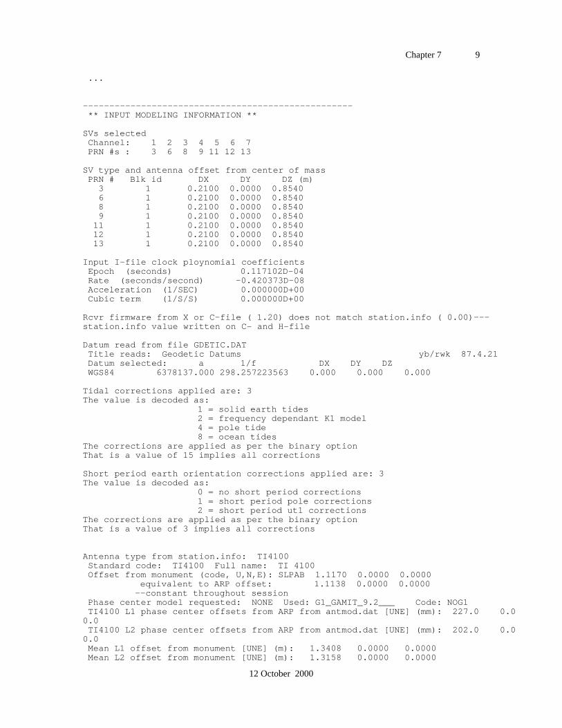
Chapter 7 9

12 October 2000

...

--------------------------------------------------- ** INPUT MODELING INFORMATION **

SVs selected Channel: 1 2 3 4 5 6 7 PRN #s : 3 6 8 9 11 12 13

SV type and antenna offset from center of mass PRN # Blk id DX DY DZ (m) 3 1 0.2100 0.0000 0.8540 6 1 0.2100 0.0000 0.8540 8 1 0.2100 0.0000 0.8540 9 1 0.2100 0.0000 0.8540 11 1 0.2100 0.0000 0.8540 12 1 0.2100 0.0000 0.8540 13 1 0.2100 0.0000 0.8540

Input I-file clock ploynomial coefficients Epoch (seconds) 0.117102D-04 Rate (seconds/second) -0.420373D-08 Acceleration (1/SEC) 0.000000D+00 Cubic term (1/S/S) 0.000000D+00

Rcvr firmware from X or C-file ( 1.20) does not match station.info ( 0.00)---station.info value written on C- and H-file

Datum read from file GDETIC.DAT Title reads: Geodetic Datums yb/rwk 87.4.21 Datum selected: a 1/f DX DY DZ WGS84 6378137.000 298.257223563 0.000 0.000 0.000

Tidal corrections applied are: 3The value is decoded as: 1 = solid earth tides 2 = frequency dependant K1 model 4 = pole tide 8 = ocean tidesThe corrections are applied as per the binary optionThat is a value of 15 implies all corrections

Short period earth orientation corrections applied are: 3The value is decoded as: 0 = no short period corrections 1 = short period pole corrections 2 = short period ut1 correctionsThe corrections are applied as per the binary optionThat is a value of 3 implies all corrections

Antenna type from station.info: TI4100 Standard code: TI4100 Full name: TI 4100 Offset from monument (code, U,N,E): SLPAB 1.1170 0.0000 0.0000 equivalent to ARP offset: 1.1138 0.0000 0.0000 --constant throughout session Phase center model requested: NONE Used: G1_GAMIT_9.2___ Code: NOG1 TI4100 L1 phase center offsets from ARP from antmod.dat [UNE] (mm): 227.0 0.00.0 TI4100 L2 phase center offsets from ARP from antmod.dat [UNE] (mm): 202.0 0.00.0 Mean L1 offset from monument [UNE] (m): 1.3408 0.0000 0.0000 Mean L2 offset from monument [UNE] (m): 1.3158 0.0000 0.0000

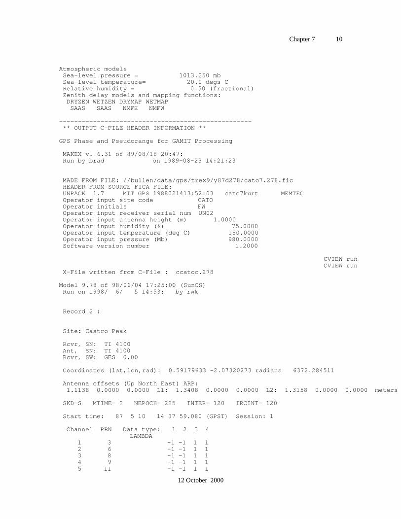
Chapter 7 10

12 October 2000

Atmospheric models Sea-level pressure = 1013.250 mb Sea-level temperature= 20.0 degs C Relative humidity = 0.50 (fractional) Zenith delay models and mapping functions: DRYZEN WETZEN DRYMAP WETMAP SAAS SAAS NMFH NMFW

--------------------------------------------------- ** OUTPUT C-FILE HEADER INFORMATION **

GPS Phase and Pseudorange for GAMIT Processing

MAKEX v. 6.31 of 89/08/18 20:47: Run by brad on 1989-08-23 14:21:23

MADE FROM FILE: //bullen/data/gps/trex9/y87d278/cato7.278.fic HEADER FROM SOURCE FICA FILE: UNPACK 1.7 MIT GPS 1988021413:52:03 cato7kurt MEMTEC Operator input site code CATO Operator initials FW Operator input receiver serial num UN02 Operator input antenna height (m) 1.0000 Operator input humidity (%) 75.0000 Operator input temperature (deg C) 150.0000 Operator input pressure (Mb) 980.0000 Software version number 1.2000

CVIEW run CVIEW run X-File written from C-File : ccatoc.278

Model 9.78 of 98/06/04 17:25:00 (SunOS) Run on 1998/ 6/ 5 14:53: by rwk

Record 2 :

Site: Castro Peak

Rcvr, SN: TI 4100 Ant, SN: TI 4100 Rcvr, SW: GES 0.00

Coordinates (lat,lon,rad): 0.59179633 -2.07320273 radians 6372.284511

Antenna offsets (Up North East) ARP: 1.1138 0.0000 0.0000 L1: 1.3408 0.0000 0.0000 L2: 1.3158 0.0000 0.0000 meters

SKD=S MTIME= 2 NEPOCH= 225 INTER= 120 IRCINT= 120

Start time: 87 5 10 14 37 59.080 (GPST) Session: 1

Channel PRN Data type: 1 2 3 4 LAMBDA 1 3 -1 -1 1 1 2 6 -1 -1 1 1 3 8 -1 -1 1 1 4 9 -1 -1 1 1 5 11 -1 -1 1 1

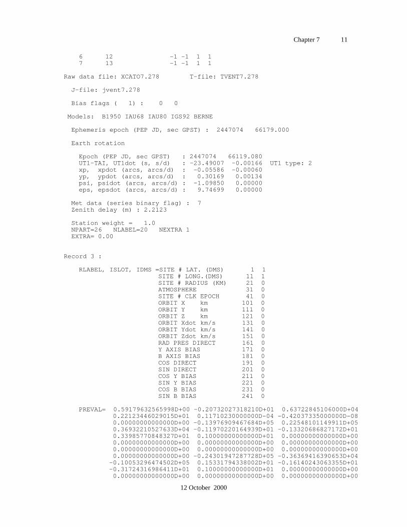
Chapter 7 11

12 October 2000

6 12 -1 -1 1 1 7 13 -1 -1 1 1

Raw data file: XCATO7.278 T-file: TVENT7.278

J-file: jvent7.278

Bias flags ( 1) : 0 0

Models: B1950 IAU68 IAU80 IGS92 BERNE

Ephemeris epoch (PEP JD, sec GPST) : 2447074 66179.000

Earth rotation

Epoch (PEP JD, sec GPST) : 2447074 66119.080 UT1-TAI, UT1dot (s, s/d) : -23.49007 -0.00166 UT1 type: 2 xp, xpdot (arcs, arcs/d) : -0.05586 -0.00060 yp, ypdot (arcs, arcs/d) : 0.30169 0.00134 psi, psidot (arcs, arcs/d) : -1.09850 0.00000 eps, epsdot (arcs, arcs/d) : 9.74699 0.00000

Met data (series binary flag) : 7 Zenith delay (m) : 2.2123

Station weight = 1.0 NPART=26 NLABEL=20 NEXTRA 1 EXTRA= 0.00

Record 3 :

RLABEL, ISLOT, IDMS =SITE # LAT. (DMS) 1 1 SITE # LONG.(DMS) 11 1 SITE # RADIUS (KM) 21 0 ATMOSPHERE 31 0 SITE # CLK EPOCH 41 0 ORBIT X km 101 0 ORBIT Y km 111 0 ORBIT Z km 121 0 ORBIT Xdot km/s 131 0 ORBIT Ydot km/s 141 0 ORBIT Zdot km/s 151 0 RAD PRES DIRECT 161 0 Y AXIS BIAS 171 0 B AXIS BIAS 181 0 COS DIRECT 191 0 SIN DIRECT 201 0 COS Y BIAS 211 0 SIN Y BIAS 221 0 COS B BIAS 231 0 SIN B BIAS 241 0

PREVAL= 0.59179632565998D+00 -0.20732027318210D+01 0.63722845106000D+04 0.22123446029015D+01 0.11710230000000D-04 -0.42037335000000D-08 0.00000000000000D+00 -0.13976909467684D+05 0.22548101149911D+05 0.36932210527633D+04 -0.11970220164939D+01 -0.13320686827172D+01 0.33985770848327D+01 0.10000000000000D+01 0.00000000000000D+00 0.00000000000000D+00 0.00000000000000D+00 0.00000000000000D+00 0.00000000000000D+00 0.00000000000000D+00 0.00000000000000D+00 0.00000000000000D+00 -0.24301947287728D+05 -0.36369416390653D+04 -0.10053296474502D+05 0.15331794338002D+01 -0.16140243063355D+01 -0.31724316986411D+01 0.10000000000000D+01 0.00000000000000D+00 0.00000000000000D+00 0.00000000000000D+00 0.00000000000000D+00

Chapter 7 12

12 October 2000

0.00000000000000D+00 0.00000000000000D+00 0.00000000000000D+00 0.00000000000000D+00 0.26708660387432D+04 -0.21097415555649D+05 0.16134956701078D+05 0.23822396282475D+01 -0.16491869581020D+01 -0.25422889115928D+01 0.10000000000000D+01 0.00000000000000D+00 0.00000000000000D+00 0.00000000000000D+00 0.00000000000000D+00 0.00000000000000D+00 0.00000000000000D+00 0.00000000000000D+00 0.00000000000000D+00 -0.25674949434566D+05 0.41531392134337D+04 0.56507320373044D+04 -0.10484303578776D+01 -0.15873965256668D+01 -0.33654654019434D+01 0.10000000000000D+01 0.00000000000000D+00 0.00000000000000D+00 0.00000000000000D+00 0.00000000000000D+00 0.00000000000000D+00 0.00000000000000D+00 0.00000000000000D+00 0.00000000000000D+00 -0.81237872687489D+04 -0.98838109221874D+04 0.23389414394361D+05 0.20904296667312D+01 -0.31751918542911D+01 -0.66573089221972D+00 0.10000000000000D+01 0.00000000000000D+00 0.00000000000000D+00 0.00000000000000D+00 0.00000000000000D+00 0.00000000000000D+00 0.00000000000000D+00 0.00000000000000D+00 0.00000000000000D+00 -0.14938585132190D+05 0.10564066754801D+05 0.19579413854459D+05 -0.31835280614272D+01 -0.82201988393225D+00 -0.19824156922850D+01 0.10000000000000D+01 0.00000000000000D+00 0.00000000000000D+00 0.00000000000000D+00 0.00000000000000D+00 0.00000000000000D+00 0.00000000000000D+00 0.00000000000000D+00 0.00000000000000D+00 -0.15948840452290D+05 0.93986557781736D+04 0.19029837926710D+05 0.52050149665399D+00 -0.32470509987392D+01 0.20508523425603D+01 0.10000000000000D+01 0.00000000000000D+00 0.00000000000000D+00 0.00000000000000D+00 0.00000000000000D+00 0.00000000000000D+00 0.00000000000000D+00 0.00000000000000D+00 0.00000000000000D+00 -0.55859160277778D-01 -0.60000000000003D-03 0.30168593809399D+00 0.13425022500666D-02 -0.23490069961604D+02 -0.16590441639308D-02--------------------------------------------------- ** END HEADER INFO -- BEGIN PROCESSING MESSAGES

No valid data for RCLOCK at epoch 50 No valid data for RCLOCK at epoch 65 No valid data for RCLOCK at epoch 199 MODEL warning in EPOCH_CLK: receiver clock correction from PRN03 at epoch 202 is enormous: 1.2030E+02 seconds! MODEL warning in EPOCH_CLK: receiver clock correction from PRN03 at epoch 202 is enormous: 1.2030E+02 seconds!

PRN Ngood 03 109 06 89 08 33 09 137 11 113 12 61 13 165

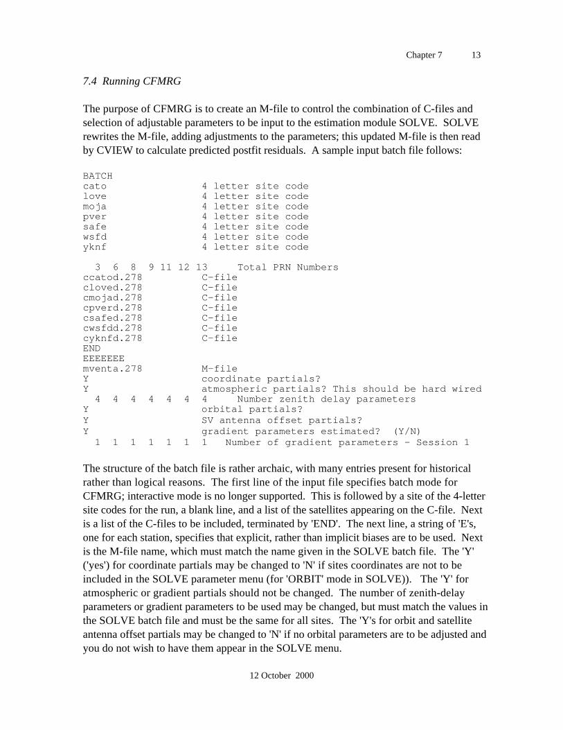
Chapter 7 13

12 October 2000

7.4 Running CFMRG

The purpose of CFMRG is to create an M-file to control the combination of C-files andselection of adjustable parameters to be input to the estimation module SOLVE. SOLVErewrites the M-file, adding adjustments to the parameters; this updated M-file is then readby CVIEW to calculate predicted postfit residuals. A sample input batch file follows:

BATCHcato 4 letter site codelove 4 letter site codemoja 4 letter site codepver 4 letter site codesafe 4 letter site codewsfd 4 letter site codeyknf 4 letter site code

3 6 8 9 11 12 13 Total PRN Numbersccatod.278 C-filecloved.278 C-filecmojad.278 C-filecpverd.278 C-filecsafed.278 C-filecwsfdd.278 C-filecyknfd.278 C-fileENDEEEEEEEmventa.278 M-fileY coordinate partials?Y atmospheric partials? This should be hard wired 4 4 4 4 4 4 4 Number zenith delay parametersY orbital partials?Y SV antenna offset partials?Y gradient parameters estimated? (Y/N) 1 1 1 1 1 1 1 Number of gradient parameters - Session 1

The structure of the batch file is rather archaic, with many entries present for historicalrather than logical reasons. The first line of the input file specifies batch mode forCFMRG; interactive mode is no longer supported. This is followed by a site of the 4-lettersite codes for the run, a blank line, and a list of the satellites appearing on the C-file. Nextis a list of the C-files to be included, terminated by 'END'. The next line, a string of 'E's,one for each station, specifies that explicit, rather than implicit biases are to be used. Nextis the M-file name, which must match the name given in the SOLVE batch file. The 'Y'('yes') for coordinate partials may be changed to 'N' if sites coordinates are not to beincluded in the SOLVE parameter menu (for 'ORBIT' mode in SOLVE)). The 'Y' foratmospheric or gradient partials should not be changed. The number of zenith-delayparameters or gradient parameters to be used may be changed, but must match the values inthe SOLVE batch file and must be the same for all sites. The 'Y's for orbit and satelliteantenna offset partials may be changed to 'N' if no orbital parameters are to be adjusted andyou do not wish to have them appear in the SOLVE menu.

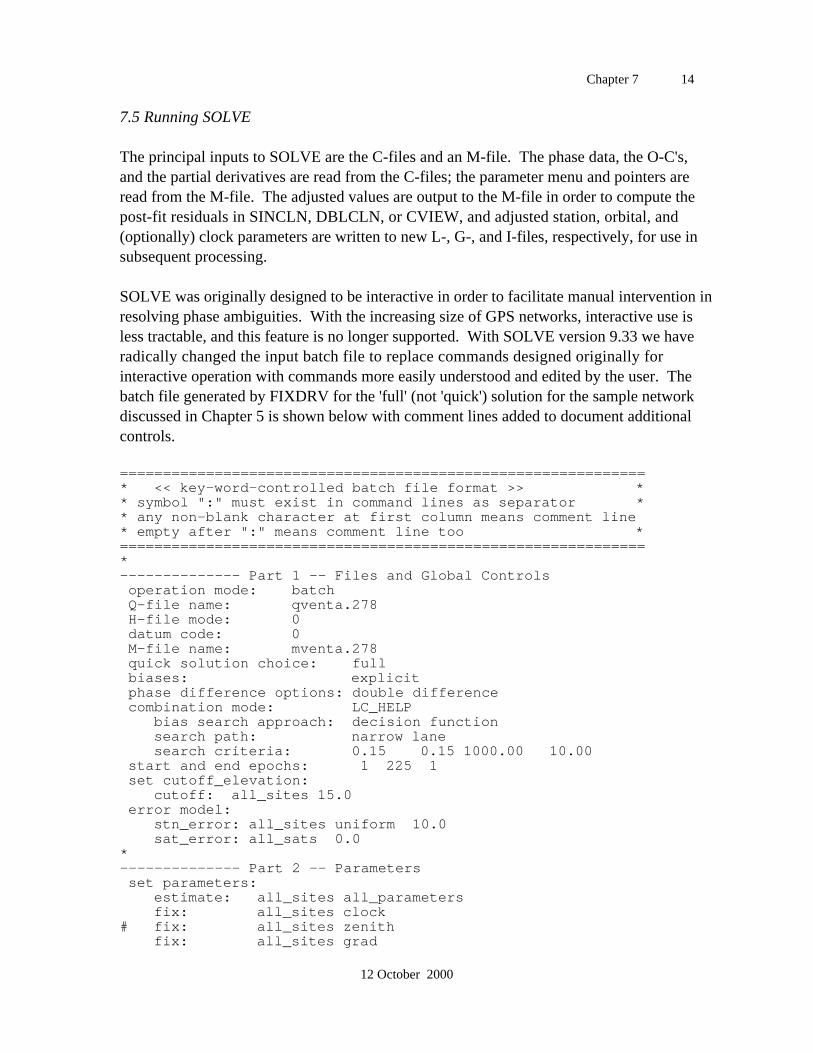
Chapter 7 14

12 October 2000

7.5 Running SOLVE

The principal inputs to SOLVE are the C-files and an M-file. The phase data, the O-C's,and the partial derivatives are read from the C-files; the parameter menu and pointers areread from the M-file. The adjusted values are output to the M-file in order to compute thepost-fit residuals in SINCLN, DBLCLN, or CVIEW, and adjusted station, orbital, and(optionally) clock parameters are written to new L-, G-, and I-files, respectively, for use insubsequent processing.

SOLVE was originally designed to be interactive in order to facilitate manual intervention inresolving phase ambiguities. With the increasing size of GPS networks, interactive use isless tractable, and this feature is no longer supported. With SOLVE version 9.33 we haveradically changed the input batch file to replace commands designed originally forinteractive operation with commands more easily understood and edited by the user. Thebatch file generated by FIXDRV for the 'full' (not 'quick') solution for the sample networkdiscussed in Chapter 5 is shown below with comment lines added to document additionalcontrols.

=============================================================* << key-word-controlled batch file format >> ** symbol ":" must exist in command lines as separator ** any non-blank character at first column means comment line* empty after ":" means comment line too *=============================================================*-------------- Part 1 -- Files and Global Controls operation mode: batch Q-file name: qventa.278 H-file mode: 0 datum code: 0 M-file name: mventa.278 quick solution choice: full biases: explicit phase difference options: double difference combination mode: LC_HELP bias search approach: decision function search path: narrow lane search criteria: 0.15 0.15 1000.00 10.00 start and end epochs: 1 225 1 set cutoff_elevation: cutoff: all_sites 15.0 error model: stn_error: all_sites uniform 10.0 sat_error: all_sats 0.0*-------------- Part 2 -- Parameters set parameters: estimate: all_sites all_parameters fix: all_sites clock# fix: all_sites zenith fix: all_sites grad

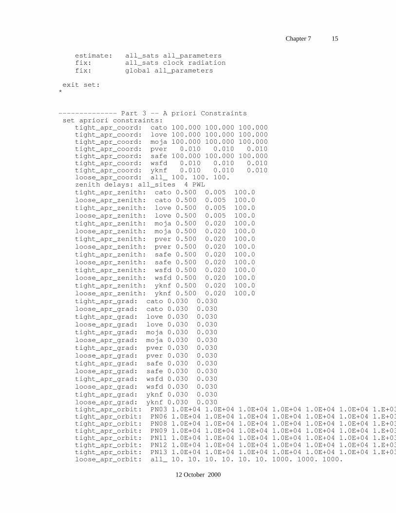
Chapter 7 15

12 October 2000

estimate: all_sats all_parameters fix: all_sats clock radiation fix: global all_parameters

exit set:*

-------------- Part 3 -- A priori Constraints set apriori constraints: tight_apr_coord: cato 100.000 100.000 100.000 tight_apr_coord: love 100.000 100.000 100.000 tight_apr_coord: moja 100.000 100.000 100.000 tight_apr_coord: pver 0.010 0.010 0.010 tight_apr_coord: safe 100.000 100.000 100.000 tight_apr_coord: wsfd 0.010 0.010 0.010 tight_apr_coord: yknf 0.010 0.010 0.010 loose_apr_coord: all_ 100. 100. 100. zenith delays: all_sites 4 PWL tight_apr_zenith: cato 0.500 0.005 100.0 loose_apr_zenith: cato 0.500 0.005 100.0 tight_apr_zenith: love 0.500 0.005 100.0 loose_apr_zenith: love 0.500 0.005 100.0 tight_apr_zenith: moja 0.500 0.020 100.0 loose_apr_zenith: moja 0.500 0.020 100.0 tight_apr_zenith: pver 0.500 0.020 100.0 loose_apr_zenith: pver 0.500 0.020 100.0 tight_apr_zenith: safe 0.500 0.020 100.0 loose_apr_zenith: safe 0.500 0.020 100.0 tight_apr_zenith: wsfd 0.500 0.020 100.0 loose_apr_zenith: wsfd 0.500 0.020 100.0 tight_apr_zenith: yknf 0.500 0.020 100.0 loose_apr_zenith: yknf 0.500 0.020 100.0 tight_apr_grad: cato 0.030 0.030 loose_apr_grad: cato 0.030 0.030 tight_apr_grad: love 0.030 0.030 loose_apr_grad: love 0.030 0.030 tight_apr_grad: moja 0.030 0.030 loose_apr_grad: moja 0.030 0.030 tight_apr_grad: pver 0.030 0.030 loose_apr_grad: pver 0.030 0.030 tight_apr_grad: safe 0.030 0.030 loose_apr_grad: safe 0.030 0.030 tight_apr_grad: wsfd 0.030 0.030 loose_apr_grad: wsfd 0.030 0.030 tight_apr_grad: yknf 0.030 0.030 loose_apr_grad: yknf 0.030 0.030 tight_apr_orbit: PN03 1.0E+04 1.0E+04 1.0E+04 1.0E+04 1.0E+04 1.0E+04 1.E+03 1.E+03 1.E+03 tight_apr_orbit: PN06 1.0E+04 1.0E+04 1.0E+04 1.0E+04 1.0E+04 1.0E+04 1.E+03 1.E+03 1.E+03 tight_apr_orbit: PN08 1.0E+04 1.0E+04 1.0E+04 1.0E+04 1.0E+04 1.0E+04 1.E+03 1.E+03 1.E+03 tight_apr_orbit: PN09 1.0E+04 1.0E+04 1.0E+04 1.0E+04 1.0E+04 1.0E+04 1.E+03 1.E+03 1.E+03 tight_apr_orbit: PN11 1.0E+04 1.0E+04 1.0E+04 1.0E+04 1.0E+04 1.0E+04 1.E+03 1.E+03 1.E+03 tight_apr_orbit: PN12 1.0E+04 1.0E+04 1.0E+04 1.0E+04 1.0E+04 1.0E+04 1.E+03 1.E+03 1.E+03 tight_apr_orbit: PN13 1.0E+04 1.0E+04 1.0E+04 1.0E+04 1.0E+04 1.0E+04 1.E+03 1.E+03 1.E+03 loose_apr_orbit: all_ 10. 10. 10. 10. 10. 10. 1000. 1000. 1000.

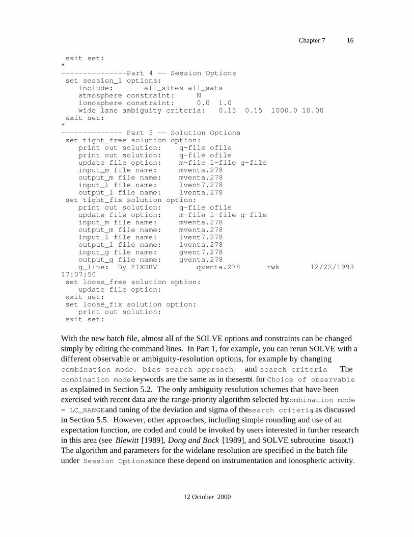
Chapter 7 16

12 October 2000

exit set:*---------------Part 4 -- Session Options set session_1 options: include: all_sites all_sats atmosphere constraint: N ionosphere constraint: 0.0 1.0 wide lane ambiguity criteria: 0.15 0.15 1000.0 10.00 exit set:*-------------- Part 5 -- Solution Options set tight_free solution option: print out solution: q-file ofile print out solution: q-file ofile update file option: m-file l-file g-file input_m file name: mventa.278 output_m file name: mventa.278 input_l file name: lvent7.278 output_l file name: lventa.278 set tight_fix solution option: print out solution: q-file ofile update file option: m-file l-file g-file input_m file name: mventa.278 output_m file name: mventa.278 input_l file name: lvent7.278 output_l file name: lventa.278 input_g file name: gvent7.278 output_g file name: gventa.278 g_line: By FIXDRV qventa.278 rwk 12/22/199317:07:50 set loose_free solution option: update file option: exit set: set loose_fix solution option: print out solution: exit set:

With the new batch file, almost all of the SOLVE options and constraints can be changedsimply by editing the command lines. In Part 1, for example, you can rerun SOLVE with adifferent observable or ambiguity-resolution options, for example by changingcombination mode, bias search approach, and search criteria Thecombination mode keywords are the same as in the sestbl. for Choice of observableas explained in Section 5.2. The only ambiguity resolution schemes that have beenexercised with recent data are the range-priority algorithm selected by Combination mode= LC_RANGE and tuning of the deviation and sigma of the search criteria, as discussedin Section 5.5. However, other approaches, including simple rounding and use of anexpectation function, are coded and could be invoked by users interested in further researchin this area (see Blewitt [1989], Dong and Bock [1989], and SOLVE subroutine bisopt.f)The algorithm and parameters for the widelane resolution are specified in the batch fileunder Session Options since these depend on instrumentation and ionospheric activity.

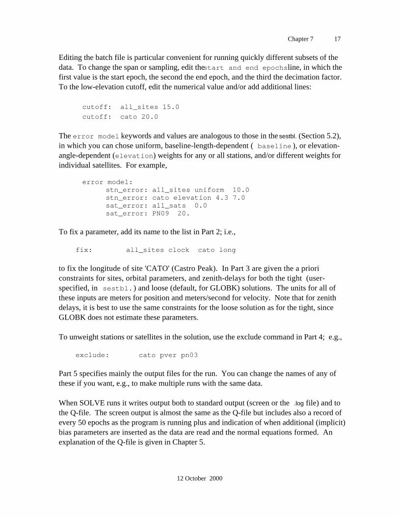
Chapter 7 17

12 October 2000

Editing the batch file is particular convenient for running quickly different subsets of thedata. To change the span or sampling, edit the start and end epochs line, in which thefirst value is the start epoch, the second the end epoch, and the third the decimation factor.To the low-elevation cutoff, edit the numerical value and/or add additional lines:

cutoff: all_sites 15.0

cutoff: cato 20.0

The error model keywords and values are analogous to those in the sestbl. (Section 5.2),in which you can chose uniform, baseline-length-dependent ( baseline ), or elevation-angle-dependent (elevation) weights for any or all stations, and/or different weights forindividual satellites. For example,

error model: stn_error: all_sites uniform 10.0

stn_error: cato elevation 4.3 7.0 sat_error: all_sats 0.0

sat_error: PN09 20.

To fix a parameter, add its name to the list in Part 2; i.e.,

fix: all_sites clock cato long

to fix the longitude of site 'CATO' (Castro Peak). In Part 3 are given the a prioriconstraints for sites, orbital parameters, and zenith-delays for both the tight (user-specified, in sestbl.) and loose (default, for GLOBK) solutions. The units for all ofthese inputs are meters for position and meters/second for velocity. Note that for zenithdelays, it is best to use the same constraints for the loose solution as for the tight, sinceGLOBK does not estimate these parameters.

To unweight stations or satellites in the solution, use the exclude command in Part 4; e.g.,

exclude: cato pver pn03

Part 5 specifies mainly the output files for the run. You can change the names of any ofthese if you want, e.g., to make multiple runs with the same data.

When SOLVE runs it writes output both to standard output (screen or the .log file) and tothe Q-file. The screen output is almost the same as the Q-file but includes also a record ofevery 50 epochs as the program is running plus and indication of when additional (implicit)bias parameters are inserted as the data are read and the normal equations formed. Anexplanation of the Q-file is given in Chapter 5.

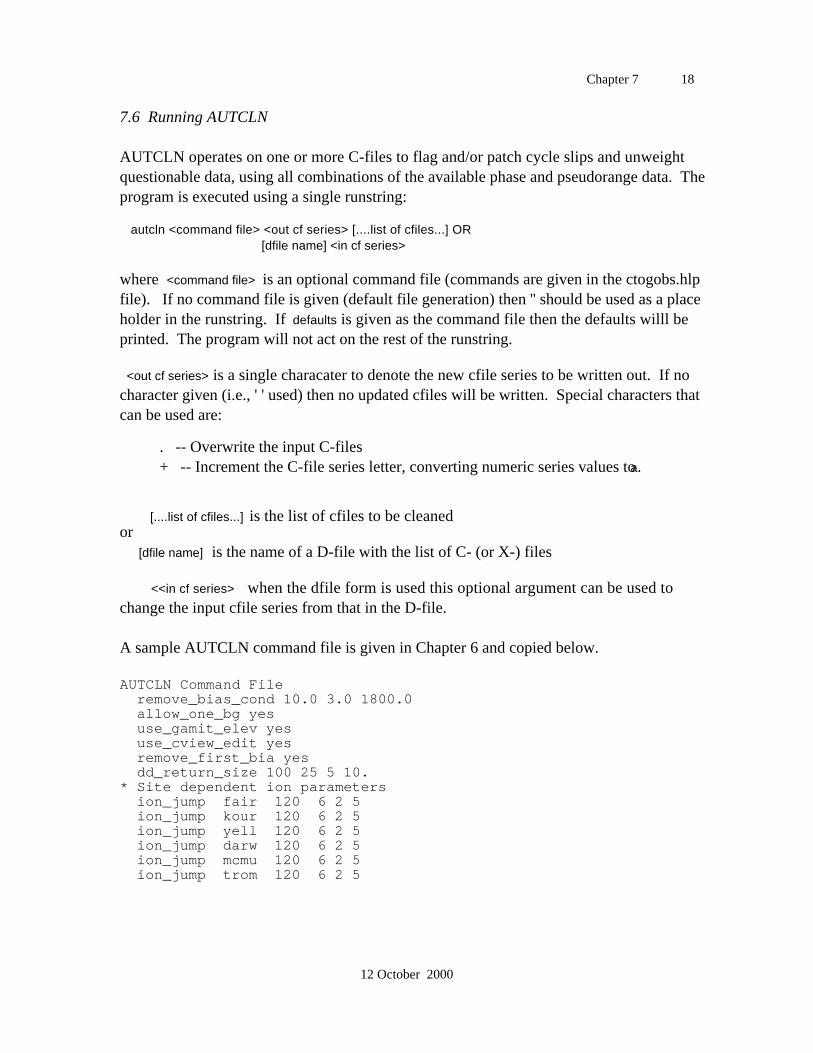
Chapter 7 18

12 October 2000

7.6 Running AUTCLN

AUTCLN operates on one or more C-files to flag and/or patch cycle slips and unweightquestionable data, using all combinations of the available phase and pseudorange data. Theprogram is executed using a single runstring:

autcln <command file> <out cf series> [....list of cfiles...] OR [dfile name] <in cf series>

where <command file> is an optional command file (commands are given in the ctogobs.hlpfile). If no command file is given (default file generation) then '' should be used as a placeholder in the runstring. If defaults is given as the command file then the defaults willl beprinted. The program will not act on the rest of the runstring.

<out cf series> is a single characater to denote the new cfile series to be written out. If nocharacter given (i.e., ' ' used) then no updated cfiles will be written. Special characters thatcan be used are:

. -- Overwrite the input C-files + -- Increment the C-file series letter, converting numeric series values to a.

[....list of cfiles...] is the list of cfiles to be cleanedor [dfile name] is the name of a D-file with the list of C- (or X-) files

<<in cf series> when the dfile form is used this optional argument can be used tochange the input cfile series from that in the D-file.

A sample AUTCLN command file is given in Chapter 6 and copied below.

AUTCLN Command File remove_bias_cond 10.0 3.0 1800.0 allow_one_bg yes use_gamit_elev yes use_cview_edit yes remove_first_bia yes dd_return_size 100 25 5 10.* Site dependent ion parameters ion_jump fair 120 6 2 5 ion_jump kour 120 6 2 5 ion_jump yell 120 6 2 5 ion_jump darw 120 6 2 5 ion_jump mcmu 120 6 2 5 ion_jump trom 120 6 2 5

Chapter 7 19

12 October 2000

A non-blank character in the first column denotes a comment. All commands are caseinsensitive. A complete list, copied nearly verbatum from the on-line help file(kf/help/autcln.hlp ) is given below:

end Last command issued. An end-of-file (EOF) will have the same effect.

use_postfit <mfile name>

Used to invoke postfit editing. The argument may be all or part of the m-file updatedwith adjustments by SOLVE. If no argument is given then the name is assumed tobe m[dfnm]a.ddd where [dfnm] are the four characters from the D-file name givenin the AUTCLN runstring. If one character is given this is assumed to be the seriesname (i.e., a, b..). If less than seven characgers are given these are used as thebeginning of the name of the M-file; if 7 or more, they are assumed to be thecomplete M-file name. If the M-file cannot be opened, then a warning message isprinted and prefit residuals will be used. The M-file does not need to contain all ofthe stations being used by AUTCLN. Note: Care should be taken that the M-filegoes with the current C-files (i.e., that MODEL has not been re-run using differentparameter values since the M-file was created).

apply_phs_clk [MAX Iter] [Non-int] [Converged %] [Over shoot]

This command will invoke a new feature in which will generate one-way phaseresiduals which should have all the clock effects from the ground sites and satellitesremoved. The processs is done iteratively with the arguments allowing the usersome control. MAX Iter is the maximum number of iterations (default 30). Non-int is the number of iterations before a non-integer bias parameter will be used inestimating the clock offset (default 3). Converged % gives the percent change inthe rms of the one-way residuals between iterations that will be taken to mean thesolution has converged (default 0.1 %). Over shoot can be used to speedconvergence. At each iteration, the mean offsets of the one-way residuals arecomputed and removed. The overshoot is a multiplier used so that more than themean is removed at each iteration. The default is 1.5, and values greater 2 seem tocause solutions to diverge. All of the arguments are optional with the default beingused for any values not passed. Invoking this option will normally double theAUTCLN runtime. The solution will not be affected unless there are pathologicalclocks that cause numerical problems in SOLVE, in which case apply_phase_clkwill usually fix the problem. With this option on, the RMS scatters of the one-wayresiduals are computed and added to the summary file. These can be useful whenattempting to diagnose problems. Caution: The one-way residuals will look flat inCVIEW only when the same M-file is used in AUTCLN.

postfit_edit [Start Iter] [Nsigma] [Max Restore] [Max rms]

This commands allows editing of phase residuals using an n-sigma criterion.Apply_phs_clk is invoked when this option is used. Start Iter denotes theiteration nmber in apply_phs_clk before editing starts. Several iterations should bemade before editing. The default is 9. Nsigma is the multiplier threshold in sigma

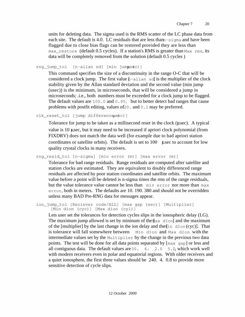
Chapter 7 20

12 October 2000

units for deleting data. The sigma used is the RMS scatter of the LC phase data fromeach site. The default is 4.0. LC residuals that are less than n-sigma and have beenflagged due to close bias flags can be restored provided they are less thanmax_restore (default 0.5 cycles). If a station's RMS is greater than Max rms, itsdata will be completely removed from the solution (default 0.5 cycles )

rng_jump_tol [n-allan sd] [min jump (sec)]

This command specifies the size of a discontinuity in the range O-C that will beconsidered a clock jump. The first value [n-allan sd] is the multiplier of the clockstability given by the Allan standard deviation and the second value (min jump(usec)) is the minimum, in microseconds, that will be considered a jump inmicroseconds; .i.e., both numbers must be exceeded for a clock jump to be flagged.The default values are 100.0 and 0.95, but to better detect bad ranges that causeproblems with postfit editing, values of 20. and 0.1 may be preferred.

clk_reset_tol [jump difference (sec)]

Tolerance for jump to be taken as a millisecond reset in the clock ( sec). A typical

value is 10 sec, but it may need to be increased if apriori clock polynomial (fromFIXDRV) does not match the data well (for example due to bad apriori stationcoordinates or satellite orbits). The default is set to 100 sec to account for lowquality crystal clocks in many receivers.

rng_resid_tol [n-sigma] [min error (m)] [max error (m)]

Tolerance for bad range residuals. Range residuals are computed after satellite andstation clocks are estimated. They are equivalent to doubly differenced rangeresiduals are affected by poor station coordinates and satellite orbits. The maximumvalue before a point will be deleted is n-sigma times the rms of the range residuals,but the value tolerance value cannot be less than min error nor more than maxerror, both in meters. The defaults are 10. 190. 380 and should not be overriddenunless many BAD Pre-RNG data for messages appear.

ion_jump_tol [Reciever code/ALL] [max gap (sec)] [Multiplier][Min dion (cyc)] [Max dion (cyl)]

Lets user set the tolerances for detection cycles slips in the ionospheric delay (LG).The maximum jump allowed is set by mininum of the [Max dIon] and the maximumof the [multiplier] by the last change in the ion delay and the [Min dIon (cyc)]. Thatis tolerance will fall somewhere between Min dIon and Max dIon with theintermediate values set by the Multiplier by the change in the previous two datapoints. The test will be done for all data points separated by [max gap] or less andall contiguous data. The default values are 30. 6. 2.0 5.0, which work wellwith modern receivers even in polar and equatorial regions. With older receivers anda quiet ionosphere, the first three values should be 240. 4. 0.8 to provide moresensitive detection of cycle slips.

Chapter 7 21

12 October 2000

rng_noise [Receiver code/ALL] [noise (mm)]

Lets user specify the apriori values for the standard deviation of the rangemeasurements by site (initial values only). They will be updated during theAUTCLN run and the updated values reported in the clock and range statistics in theoutput and summary file.

max_rclk_iterations [max iterations]

Maximum number of range clock iterations. The solution for the estimate of thesatellite and station clocks is iterated to determine the statistics of the range noise andclock Allan standard deviations. The iteration stops either at [max iterations] or untilthe convergence criteria are met.

rel_clk_weight [weight]

Weight to be given to the clock noise model based on previous iteration's estimate ofthe Allan standard deviations of the clocks relative to data noise while estimating theclocks. Typical value is to down weight the clock statistics by a factor of 10 relativeto the data.

rng_clk_root [range clock root of file names]

Lead part of the name to be given to the range clock solution output. If no root isgiven then the range clock solution will not be output. For example crng willproduce output files named crng.PIN1 and crng.PRN_21. A cplot command filewill also be generated called <root>.plt

phs_clk_root [phase clock root of file names]

Lead part of the name to be given to the phase clock solution output. If no root isgiven then the phase clock solution will not be output. See rng_clk_root.

phs_res_root [phase residual root of file names]

Lead part of the name to be given to the one-way phase residual (to the prefit model)output. If no root is given then the phase will not be output. See rng_clk_rootand residual_site.

sng_diff_root [single difference file root]

Lead part of the name for single difference between stationsfiles (These may be usedwith the program mon_data to processing single difference kinematic data). Thesingle differences are between first site and subsequent sites. The residual_sitelist is used select which sites to write to single difference files, which are onlygenerated if C-files are written out.

residual_site [List of four character codes/ALL/NONE]

Lets the user specify which sites should be output to the phase residual or singledifference files

summary_file [Name of summary file/6]

Name of a summary file. If the command is not given, the summary is written to afile named autcln.sum. If 6 is given as the file name then the summary is written tostandard out.

Chapter 7 22

12 October 2000

rcv_allan_sd [site code/ALL] [Allan standard deviation (ppb@100sec)]

Allows the user to specify the Allan standard deviations of the clocks at each site.These are updated during AUTCLN run.

remove_bias_cond [Chi**2 Ratio] [min chi**2] [max gap] <large gap scale>

Sets the constrasts for removing biases. A bias flag is removed if

X = C2/(C1+min*exp(-C1/min)) > ratio

where C1 is the smallest chi**2 obtained during trial fixes to integer values; C2 isthe next smallest; min is min chi**2 in the command; and ratio is Chi**2 Ratioin the command. In addition, the gap must be smaller than max gap. The defaultvalues of Chi**2 Ratio, min chi**2, and max gap are 12., 3., and 3600.(sec), respectively. The final argument large gap scale is optional; if it isspecified, then the value of X computed from the data is reduced by 1 + large gapscale*atan(gap/min data)) where gap is the gap in the data and min data is thesmaller of the number of data in the left and right segments about the gap. Thedefault value of large gap scale is 5.0

allow_one_bg [yes/no]

Deals with the case where all channels of a receiver slip at nearly the same time. Byspecifiying yes you allow AUTCLN to select one channel as a base, patch it roughlyin one-ways, and the patch all other channels with respect to it.

use_gamit_elev [yes/no]

If yes is specified (default), then the cutoff angle specified in the C-file will be usedin editing and outputting data, the safest approach for rerunning old data (cutoffpassed from the C-file to the X-file via CTOX). With new data a better approach isto use the min_elev command of AUTCLN and to control use of data by SOLVEwith the GAMIT sestbl. input.

use_cview_edit [yes/no]

Allows user to specify if the CVIEW unweight flag (-1) should be used or not. Ifyes is specified then the CVIEW unweight flag will not be overridden by AUTCLN.The default is no.

use_mm_range [yes/no]

Allows user to specify if MiniMac range measurements should be used. The defaultis not to use them (no). (If ranges are not used then MiniMac should be connected toa very good clock.)

ignore_gaps [yes/no]

Lets user specify that gaps should be ignored when forming acceptable doubledifferences during cleaning. The default is no; this option should only be used forcleaned data when the GAMIT elevation cutoff and CVIEW edits are used.

Chapter 7 23

12 October 2000

flag_gaps [yes/no]

Lets user specify if gaps in the one-way data should be flagged with a bias flag. Thedefault is no, but is automatically set to yes when the allow_one_bg yes is given

gap_size [cf_code/ALL] [number of epochs]

Lets user specify the number of epochs allowed in a gap so that it will not beflagged. At setting of 1 (default) will cause all gaps to be flagged. Specifyinggap_size automatically turns on the flag_gaps option.

remove_ms_jump [yes/no]

Lets user decide if millisecond jumps are in the clock are removed when C-files arewritten. The default is to remove the jumps (yes).

remove_first_bia [yes/no]

By default AUTCLN puts a bias flag at the beginning of each one-way sequence aspart of its internal bookkeeping. This has no influence on the SOLVE solution, butthe extranesous flags will be removed before C-files are written if yes is specifiedfor this command. The writing of single-difference files requires the initial bias, soyes should not be specified when single difference files are to be written.

edit_site_sv [Site Code] [PRN] [Start Epoch] [Stop Epoch]

Allows user to specify site/satellite combinations over specific epoch ranges to beedited and not used in determining clock behavior and double difference editing.Useful for treating bad satellite range data. ALL may be used delete all sites for aspecified specified satellite; 0 may be used for the PRN number to delete all satellitesover the specified epoch range.

phs_fit_tol [4 values all in cycles]

Tolerances in deciding if a cycle slip has occurred in the pre-fit clock fit to the one-way phase data. The values and their defaults are as follows:

(1) deviation of mean phase residual from range solution in pass 1 (1000.);

(2) deviation of worst phase residual from range solution in pass 1 (500.);

(3) deviation of pass 2 mean phase from pass 1 phase solution (200.);

(4) deviation of pass 2 worst phase residual from pass 1 phase solution (100.).

Values 3 and 4 are normally much less than values 1 and 2. The actual deviations beingflagged can be viewed by setting status_report Pass1_slips Pass2_slips.

status_report [List of options]

Allows user to tailor the output of the program by selecting which quanities will beoutput in autcln.out. The options come from the following list:

CLK_JMP_PROC - possible clock jump detection

CLK_JMP_VAL - value of clock jump when one is found

BIAS_ADDED - BIAS flag added during one-way phase processing

PASS1_SLIPS - Number of cycles added in Pass 1 one-way clean

PASS2_SLIPS - Number of cycles added in Pass 2 one-way clean

Chapter 7 24

12 October 2000

DD_TRIALS - List each double difference combination tried

DD_ESTIMATES - Estimates of cycle slip during the DD fix.

DD_SCAN - Details of scan flag showing sites and svs used.

ELEV_DIST - Distribution of final (weighted) data by elev

RUN_PARAMS - Dump of parameters used in run.

ALL may also be used, and then -option to turn off particular output; e.g.,status_report all -clk_jmp_proc. The status reports are sent to standard out.

dd_report [DD Report file name] [option]

Allows user to specify a file of the format readable by CVIEW and to specify which typesof double differences should by output to this file (i.e., ALL, FIXED, NOT_FIXED). If thefile name dd.srt is used then the file can be directly read into CVIEW to allow checking ofthe cleaning results.

min_elevation [Min clean elevation (deg)] <Min output elev (deg)>

Minimum elevation to which data will be cleaned. Once this value has been set inAUTCLN, the data below this elevation will not be useable later without further cleaning.The minimum output elevation is optional and is the elevation cutoff to be applied when theC-files are written. This command is ignored if use_gamit_elev = yes.

trim_oneway_tol [min_dtl_bias] [min_good_bias] [min_dtr_end] [min_good_end]

Set the tolerances used in triming the one-way data to remove small segments of data(defaults in parentheses):

min_dtl_bias - mininum time in seconds between bias flags (120 s)

min_good_bias - mininum epochs between bias flags and maximum epochs over which a bias flag will be removed in one-way data (8)

min_dtr_end - Fraction of total duration of data allowed for a bias flag at the end of the one-way sequence (0.1)

min_good_end - Number of epochs of data allowed after last bias flag (24)

dd_return_size [Max WL] [Max LC] [Max LG] <One way fix tol>

Set the number of data to be used for cycle skip repair (defaults in parentheses):

Max WL - widelane estimates (100), applies to one-ways

Max LC - LC (50), applies to double differences

Max LG - LG (10), applies to one-ways or double differences

These values should be decreased if there is significant curvature in the data, which mightapply particularly to LG with a high ionosphere. They cannot be set less than 5. Oneway fix tol is an optional argument that sets the maximum duration over which one-wayL1/L2 range data will be be patched using the widelane and LG.

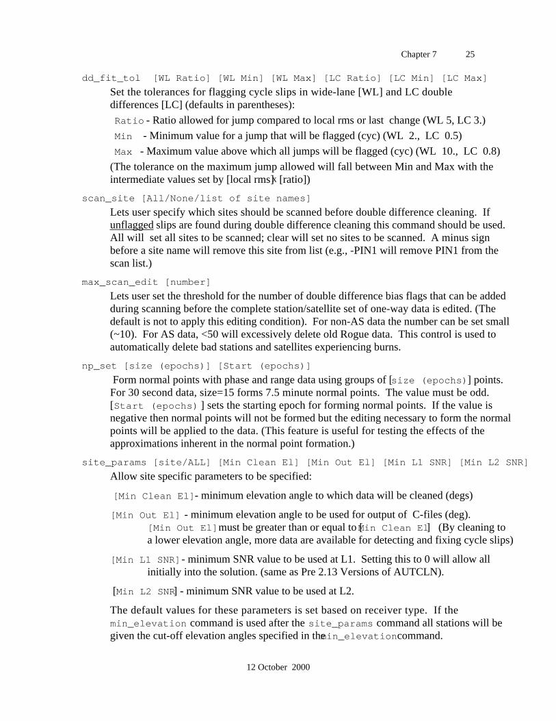
Chapter 7 25

12 October 2000

dd_fit_tol [WL Ratio] [WL Min] [WL Max] [LC Ratio] [LC Min] [LC Max]

Set the tolerances for flagging cycle slips in wide-lane [WL] and LC doubledifferences [LC] (defaults in parentheses):

Ratio - Ratio allowed for jump compared to local rms or last change (WL 5, LC 3.)

Min - Minimum value for a jump that will be flagged (cyc) (WL 2., LC 0.5)

Max - Maximum value above which all jumps will be flagged (cyc) (WL 10., LC 0.8)

(The tolerance on the maximum jump allowed will fall between Min and Max with theintermediate values set by [local rms] x [ratio])

scan_site [All/None/list of site names]

Lets user specify which sites should be scanned before double difference cleaning. Ifunflagged slips are found during double difference cleaning this command should be used.All will set all sites to be scanned; clear will set no sites to be scanned. A minus signbefore a site name will remove this site from list (e.g., -PIN1 will remove PIN1 from thescan list.)

max_scan_edit [number]

Lets user set the threshold for the number of double difference bias flags that can be addedduring scanning before the complete station/satellite set of one-way data is edited. (Thedefault is not to apply this editing condition). For non-AS data the number can be set small(~10). For AS data, <50 will excessively delete old Rogue data. This control is used toautomatically delete bad stations and satellites experiencing burns.

np_set [size (epochs)] [Start (epochs)]

Form normal points with phase and range data using groups of [size (epochs)] points.For 30 second data, size=15 forms 7.5 minute normal points. The value must be odd.[Start (epochs) ] sets the starting epoch for forming normal points. If the value isnegative then normal points will not be formed but the editing necessary to form the normalpoints will be applied to the data. (This feature is useful for testing the effects of theapproximations inherent in the normal point formation.)

site_params [site/ALL] [Min Clean El] [Min Out El] [Min L1 SNR] [Min L2 SNR]

Allow site specific parameters to be specified:

[Min Clean El] - minimum elevation angle to which data will be cleaned (degs)

[Min Out El] - minimum elevation angle to be used for output of C-files (deg).[Min Out El] must be greater than or equal to [Min Clean El] (By cleaning toa lower elevation angle, more data are available for detecting and fixing cycle slips)

[Min L1 SNR] - minimum SNR value to be used at L1. Setting this to 0 will allow all initially into the solution. (same as Pre 2.13 Versions of AUTCLN).

[Min L2 SNR] - minimum SNR value to be used at L2.

The default values for these parameters is set based on receiver type. If themin_elevation command is used after the site_params command all stations will begiven the cut-off elevation angles specified in the min_elevation command.

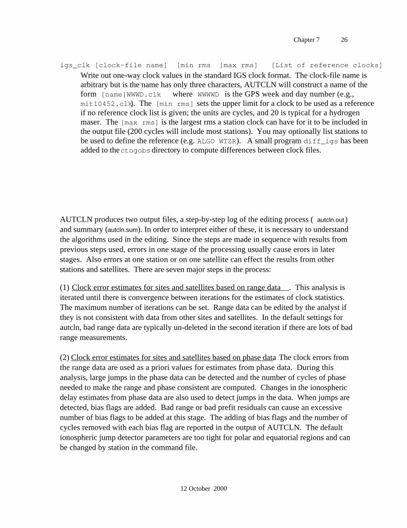
Chapter 7 26

12 October 2000

igs_clk [clock-file name] [min rms ]max rms] [List of reference clocks]

Write out one-way clock values in the standard IGS clock format. The clock-file name isarbitrary but is the name has only three characters, AUTCLN will construct a name of theform [name]WWWD.clk where WWWWD is the GPS week and day number (e.g.,mit10452.clk). The [min rms] sets the upper limit for a clock to be used as a referenceif no reference clock list is given; the units are cycles, and 20 is typical for a hydrogenmaser. The [max rms] is the largest rms a station clock can have for it to be included inthe output file (200 cycles will include most stations). You may optionally list stations tobe used to define the reference (e.g. ALGO WTZR). A small program diff_igs has beenadded to the ctogobs directory to compute differences between clock files.

AUTCLN produces two output files, a step-by-step log of the editing process ( autcln.out)and summary (autcln.sum). In order to interpret either of these, it is necessary to understandthe algorithms used in the editing. Since the steps are made in sequence with results fromprevious steps used, errors in one stage of the processing usually cause erors in laterstages. Also errors at one station or on one satellite can effect the results from otherstations and satellites. There are seven major steps in the process:

(1) Clock error estimates for sites and satellites based on range data . This analysis isiterated until there is convergence between iterations for the estimates of clock statistics.The maximum number of iterations can be set. Range data can be edited by the analyst ifthey is not consistent with data from other sites and satellites. In the default settings forautcln, bad range data are typically un-deleted in the second iteration if there are lots of badrange measurements.

(2) Clock error estimates for sites and satellites based on phase data. The clock errors fromthe range data are used as a priori values for estimates from phase data. During thisanalysis, large jumps in the phase data can be detected and the number of cycles of phaseneeded to make the range and phase consistent are computed. Changes in the ionosphericdelay estimates from phase data are also used to detect jumps in the data. When jumps aredetected, bias flags are added. Bad range or bad prefit residuals can cause an excessivenumber of bias flags to be added at this stage. The adding of bias flags and the number ofcycles removed with each bias flag are reported in the output of AUTCLN. The defaultionospheric jump detector parameters are too tight for polar and equatorial regions and canbe changed by station in the command file.

Chapter 7 27

12 October 2000

(3) The default action next is to add bias flags to all gaps in the data. This can be changedin the command file, but is not recommended.

(4) The default action next is to scan all contiguous one-way data and to form doubledifferences with triplets of the data to see if there are jumps in the double differences.When a jump is found, more double differences are formed to assess if the one-way databeing analyzed have the jump. (This is done by switching the satellite and station to see ifthe jump persists.) Bad prefit residuals can cause many biases to be added at this stage.Unmodeled accelerations of the satellites can also cause many bias flags to be added atdifferent stations.

(5) Cleaning of data using as many observables as possible. This step involves trying toassess the number of cycles of slip at each bias flag in the one-way data and whether thebias flag can be reliably removed. Small segments of data (i.e., closely spaced bias flags)are removed before any attempt is made to resolve biases. Three criteria are used tocompute the number of cycles: (1) continuity of LC, (2) continuity of LG, and(3)continuity of the widelane. Different number of data are used in each of these with thewidelane typically being the longest and LG the shortest. The sequence AUTCLN uses isto first try to resolve the integers in one-ways if P-code L1 and L2 range data are availableusing the widelane and LG continuity. If this fails then double differences are used and LCcontinuity is also considered. The default setting in autcln is to not allow one-way bias flagremoval because this became unreliable once AS was turned on. To patch in doubledifferences, AUTCLN finds another station and satellite combination which does not havea bias flag or gap around the time of the flag which is being evaluted. Stations andsatellites are scanned in sequence until AUTCLN finds a combination that can be used toremove the bias flag or runs out of stations and satellites to try. The default is to output aline for each combination tried. The last one output is the one which was used to determinethe number of cycles. A common occurrence is that all satellites at a station have bias flagsat or near the same time (due to a power failure for example). In these cases, there is anoptional feature to "allow one bias or gap" (the allow_one_bg command) at this time. Inthis case, autcln first determines if bias flags can be removed if it ignores the bias flags onboth satellites being used in the double difference. If the bias flag can removed, then itresolves the cycles slips on the first one-way data sequence to be tested and removes thebias flag. When later bias flags are encounted at this time for this station, they will bepatched relative to the first one-way sequence where the bias flag was removed. "Force?T" appears in autcln.out for those bias flags removed this way. (There is no explicit bookkeeping to ensure that this happens). When data are very "broken up" with many bias flagsand gaps, AUTCLN can make mistakes in this procedure, so this is normally the mostunreliable part of the cleaning process. Only loss of lock on all satellites at a station istreated in this way. If all stations lose lock on a satellite at the same time then the bias flagswill be not removed unless they can be patched in one-ways. While data are being used forpatching, they are also checked for jumps. When a jump is found, autcln scans each of the

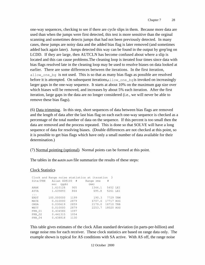
Chapter 7 28

12 October 2000

one-way sequences, checking to see if there are cycle slips in them. Because more data areused than when the jumps were first detected, this test is more sensitive than the orginalscanning and sometimes detects jumps that had not been previously detected. In manycases, these jumps are noisy data and the added bias flag is later removed (and sometimesadded back again later). Jumps detected this way can be found in the output by grep'ing onLCDD. If they are large, then AUTCLN has become confused about where a slip islocated and this can cause problems.The cleaning loop is iterated four times since data withbias flags resolved late in the cleaning loop may be used to resolve biases on data looked atearlier. There are some differences between the iterations. In the first iteration,allow_one_bg is not used. This is so that as many bias flags as possible are resolvedbefore it is attempted. On subsequent iterations, allow_one_bg is invoked on increasinglylarger gaps in the one-way sequence. It starts at about 10% on the maximum gap size overwhich biases will be removed, and increases by about 5% each iteration. After the firstiteration, large gaps in the data are no longer considered (i.e., we will never be able toremove these bias flags).

(6) Data trimming. In this step, short sequences of data between bias flags are removedand the length of data after the last bias flag on each each one-way sequence is checked as apercentage of the total number of data on the sequence. If this percent is too small then thedata are removed and the process repeated. This is done so that SOLVE will have a longsequence of data for resolving biases. (Double differences are not checked at this point, soit is possible to get bias flags which have only a small number of data available for theirdetermination.)

(7) Normal pointing (optional). Normal points can be formed at this point.

The tables in the autcln.sum file summarize the results of these steps:

Clock Statistics

Clock and Range noise statistics at iteration 3 Site/PRN Allan SD@100 # Range rms # sec (ppb) (mm) ARAK 1.610128 905 1344.1 5452 LEI AYVA 1.635893 864 695.8 5261 LEI ... ERDT 100.000000 1199 190.3 7729 TRM MATE 0.010000 2879 6707.6 17717 ROG ONSA 0.030619 2859 2179.0 18710 TRB WETT 0.010000 2879 2253.7 18020 ROG PRN_01 0.434580 1097 PRN_02 0.441315 1054 PRN_04 0.438818 1130

This table gives estimates of the clock Allan standard deviation (in parts-per-billion) andrange noise rms for each receiver. These clock statistics are based on range data only. Theexample shown is typical for AS conditions with SA active. With AS off, the range noise

Chapter 7 29

12 October 2000

for a Rogue SNR-8 or TurboRogue will approach that of the Trimble SSE (< 1 m). Valuesmuch larger than a few meters usually mean lots of bad range data or bad prefit residuals(station coordinate errors of >10 m). Very bad range data can be seen with AVCLCK errorsin the MODEL output P-file. Also autcln.out will list bad range measurements (butsometimes here the station or satellite may be incorrectly listed especially when there are alot of bad data). If there are AVCLCK errors, then the edit_site_sv command can be usedto pre-edit these values in AUTCLN. With each clock and range statistic is also the numberof data used to calculate it. For the example here, the two regional stations (ARAK andAVYA) observed for only 8 hours whereas the three IGS stations (MATE, ONSA, andWETT) observed for 24 hours.

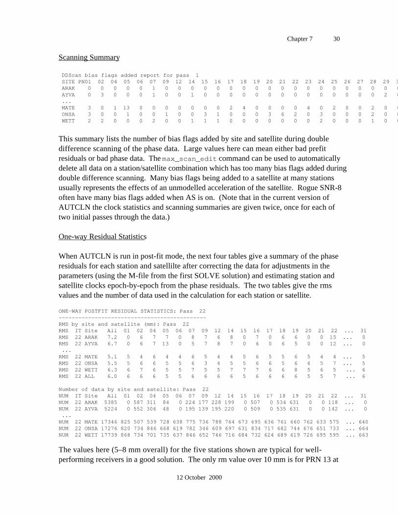
Chapter 7 30

12 October 2000

Scanning Summary

DDScan bias flags added report for pass 1 SITE PN01 02 04 05 06 07 09 12 14 15 16 17 18 19 20 21 22 23 24 25 26 27 28 29 31 ARAK 0 0 0 0 0 1 0 0 0 0 0 0 0 0 0 0 0 0 0 0 0 0 0 0 0 AYVA 0 3 0 0 0 1 0 0 1 0 0 0 0 0 0 0 0 0 0 0 0 0 0 2 0 ... MATE 3 0 1 13 0 0 0 0 0 0 0 2 4 0 0 0 0 4 0 2 0 0 2 0 0 ONSA 3 0 0 1 0 0 1 0 0 3 1 0 0 0 3 6 2 0 3 0 0 0 2 0 8 WETT 2 2 0 0 0 2 0 0 1 1 1 0 0 0 0 0 0 0 2 0 0 0 1 0 0

This summary lists the number of bias flags added by site and satellite during doubledifference scanning of the phase data. Large values here can mean either bad prefitresiduals or bad phase data. The max_scan_edit command can be used to automaticallydelete all data on a station/satellite combination which has too many bias flags added duringdouble difference scanning. Many bias flags being added to a satellite at many stationsusually represents the effects of an unmodelled acceleration of the satellite. Rogue SNR-8often have many bias flags added when AS is on. (Note that in the current version ofAUTCLN the clock statistics and scanning summaries are given twice, once for each oftwo initial passes through the data.)

One-way Residual Statistics

When AUTCLN is run in post-fit mode, the next four tables give a summary of the phaseresiduals for each station and satellilte after correcting the data for adjustments in theparameters (using the M-file from the first SOLVE solution) and estimating station andsatellite clocks epoch-by-epoch from the phase residuals. The two tables give the rmsvalues and the number of data used in the calculation for each station or satellite.

ONE-WAY POSTFIT RESIDUAL STATISTICS: Pass 22---------------------------------------------RMS by site and satellite (mm): Pass 22RMS IT Site All 01 02 04 05 06 07 09 12 14 15 16 17 18 19 20 21 22 ... 31RMS 22 ARAK 7.2 0 6 7 7 0 8 7 6 8 0 7 0 6 6 0 0 15 ... 0RMS 22 AYVA 6.7 0 6 7 13 0 5 7 8 7 0 6 0 6 5 0 0 12 ... 0 ...RMS 22 MATE 5.1 5 4 6 4 4 6 5 4 4 5 6 5 5 6 5 4 4 ... 5RMS 22 ONSA 5.5 5 6 6 5 5 6 3 4 5 5 6 6 5 6 6 5 7 ... 5RMS 22 WETT 6.3 6 7 6 5 5 7 5 5 7 7 7 6 6 8 5 6 5 ... 6RMS 22 ALL 6.0 6 6 6 5 5 6 6 6 6 5 6 6 6 6 5 5 7 ... 6

Number of data by site and satellite: Pass 22NUM IT Site All 01 02 04 05 06 07 09 12 14 15 16 17 18 19 20 21 22 ... 31NUM 22 ARAK 5385 0 587 311 84 0 224 177 228 199 0 507 0 534 631 0 0 118 ... 0NUM 22 AYVA 5224 0 552 306 48 0 195 139 195 220 0 509 0 535 631 0 0 142 ... 0 ...NUM 22 MATE 17346 825 507 539 728 638 775 736 788 764 673 695 636 761 660 762 633 575 ... 640NUM 22 ONSA 17276 820 734 846 668 619 782 346 609 697 631 834 717 682 744 676 651 733 ... 664NUM 22 WETT 17739 868 734 701 735 637 846 652 746 716 684 732 624 689 619 726 695 595 ... 663

The values here (5–8 mm overall) for the five stations shown are typical for well-performing receivers in a good solution. The only rm value over 10 mm is for PRN 13 at

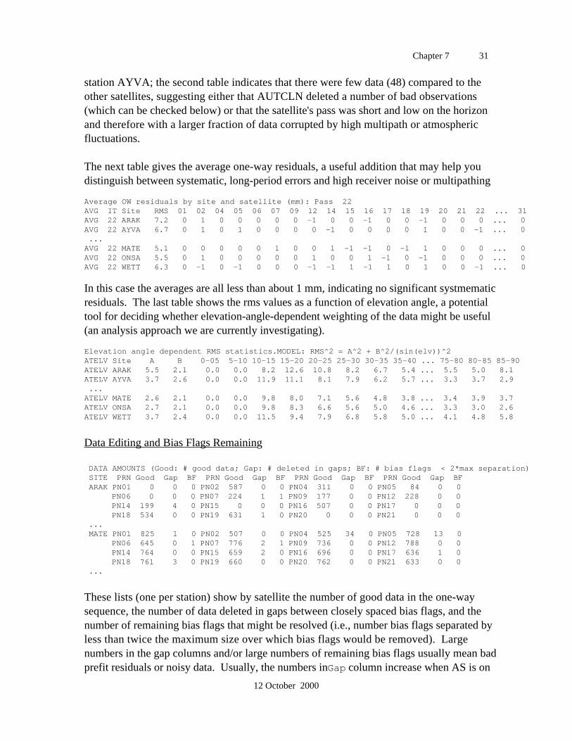
Chapter 7 31

12 October 2000

station AYVA; the second table indicates that there were few data (48) compared to theother satellites, suggesting either that AUTCLN deleted a number of bad observations(which can be checked below) or that the satellite's pass was short and low on the horizonand therefore with a larger fraction of data corrupted by high multipath or atmosphericfluctuations.

The next table gives the average one-way residuals, a useful addition that may help youdistinguish between systematic, long-period errors and high receiver noise or multipathing

Average OW residuals by site and satellite (mm): Pass 22AVG IT Site RMS 01 02 04 05 06 07 09 12 14 15 16 17 18 19 20 21 22 ... 31AVG 22 ARAK 7.2 0 1 0 0 0 0 0 -1 0 0 -1 0 0 -1 0 0 0 ... 0AVG 22 AYVA 6.7 0 1 0 1 0 0 0 0 -1 0 0 0 0 1 0 0 -1 ... 0 ...AVG 22 MATE 5.1 0 0 0 0 0 1 0 0 1 -1 -1 0 -1 1 0 0 0 ... 0AVG 22 ONSA 5.5 0 1 0 0 0 0 0 1 0 0 1 -1 0 -1 0 0 0 ... 0AVG 22 WETT 6.3 0 -1 0 -1 0 0 0 -1 -1 1 -1 1 0 1 0 0 -1 ... 0

In this case the averages are all less than about 1 mm, indicating no significant systmematicresiduals. The last table shows the rms values as a function of elevation angle, a potentialtool for deciding whether elevation-angle-dependent weighting of the data might be useful(an analysis approach we are currently investigating).

Elevation angle dependent RMS statistics.MODEL: RMS^2 = A^2 + B^2/(sin(elv))^2ATELV Site A B 0-05 5-10 10-15 15-20 20-25 25-30 30-35 35-40 ... 75-80 80-85 85-90ATELV ARAK 5.5 2.1 0.0 0.0 8.2 12.6 10.8 8.2 6.7 5.4 ... 5.5 5.0 8.1ATELV AYVA 3.7 2.6 0.0 0.0 11.9 11.1 8.1 7.9 6.2 5.7 ... 3.3 3.7 2.9 ...ATELV MATE 2.6 2.1 0.0 0.0 9.8 8.0 7.1 5.6 4.8 3.8 ... 3.4 3.9 3.7ATELV ONSA 2.7 2.1 0.0 0.0 9.8 8.3 6.6 5.6 5.0 4.6 ... 3.3 3.0 2.6ATELV WETT 3.7 2.4 0.0 0.0 11.5 9.4 7.9 6.8 5.8 5.0 ... 4.1 4.8 5.8

Data Editing and Bias Flags Remaining

DATA AMOUNTS (Good: # good data; Gap: # deleted in gaps; BF: # bias flags < 2*max separation) SITE PRN Good Gap BF PRN Good Gap BF PRN Good Gap BF PRN Good Gap BF ARAK PN01 0 0 0 PN02 587 0 0 PN04 311 0 0 PN05 84 0 0 PN06 0 0 0 PN07 224 1 1 PN09 177 0 0 PN12 228 0 0 PN14 199 4 0 PN15 0 0 0 PN16 507 0 0 PN17 0 0 0 PN18 534 0 0 PN19 631 1 0 PN20 0 0 0 PN21 0 0 0 ... MATE PN01 825 1 0 PN02 507 0 0 PN04 525 34 0 PN05 728 13 0 PN06 645 0 1 PN07 776 2 1 PN09 736 0 0 PN12 788 0 0 PN14 764 0 0 PN15 659 2 0 PN16 696 0 0 PN17 636 1 0 PN18 761 3 0 PN19 660 0 0 PN20 762 0 0 PN21 633 0 0 ...

These lists (one per station) show by satellite the number of good data in the one-waysequence, the number of data deleted in gaps between closely spaced bias flags, and thenumber of remaining bias flags that might be resolved (i.e., number bias flags separated byless than twice the maximum size over which bias flags would be removed). Largenumbers in the gap columns and/or large numbers of remaining bias flags usually mean badprefit residuals or noisy data. Usually, the numbers in Gap column increase when AS is on

Chapter 7 32

12 October 2000

especially for SNR-8 receivers. More than 3 bias flags remaining usually indicates that thedata is noisy and broken up into small pieces. (Bad data at one site can often lead toadditional biases at other sites, so it usually the site with the most bias flags that is causingthe problems.)

Elevation-angle Statistics

ELEVATION ANGLE HISTOGRAMSITE 0- 5 5-10 10-15 15-20 20-25 25-30 30-35 35-40 40-45 45-50 ... 80-85 85-90 Min (dg)ARAK 0 0 0 505 502 591 429 437 537 361 ... 40 15.01AYVA 0 0 0 575 499 545 419 436 511 323 ... 40 15.01 ...MATE 0 0 0 1415 1643 1704 1400 1448 1249 1383 ... 54 15.00ONSA 0 0 0 1834 1789 1621 1419 1500 1467 1058 ... 79 15.00WETT 0 0 0 1641 1624 1650 1529 1468 1441 1073 ... 208 15.01

This table shows the number of good data or good normal points in elevation bins.Correctly operating receivers should have about the same number in 15-20 degree bin as inthe 20-25. (The above example is for 24 hours with 15-point normal points).

Bias Flag Report

This report provides an overall summary of the number of bias flags in the clean data andwhy they were added.

BIAS FLAG REPORT: Types ORG-Original JMP-Big Jump ION-Ion Jump GAP-Data Gap DDS-DD scan WLS-Wide Lane DDC-DD cleaningSITE # Flagged | # Remaining | # Edited | # with jump ORG JMP ION GAP DDS WLS DDC| ORG JMP ION GAP DDS WLS DDC| ORG JMP ION GAP DDS WLS DDC| ORG JMP ION GAP DDS WLS DDCARAK 10 0 0 8 2 0 2| 0 0 0 1 0 0 0| 1 0 0 2 1 0 1| 9 0 0 1 0 0 0AYVA 9 0 0 1 8 0 0| 0 0 0 1 0 0 0| 0 0 0 0 0 0 0| 9 0 0 0 0 0 0 ...MATE 63 0 0 12 33 0 0| 8 0 0 1 0 0 0| 26 0 0 6 28 0 0| 29 0 0 1 5 0 0ONSA 4 0 0 138 36 0 6| 1 0 0 16 0 0 0| 2 0 0 55 29 0 1| 1 0 0 7 1 0 0WETT 65 0 0 11 13 0 2| 10 0 0 2 1 0 0| 31 0 0 5 10 0 0| 24 0 0 0 1 0 0

The report is in four sections:

# Flagged are the numbers of bias flags added or encountered during cleaning (Entriesexplained below).

# Remaining are the numbers of bias flags left in the cleaned data.

# Edited are the numbers of bias flags removed by deleting the data affected by the biasflag (as opposed to the bias flag removed by reliably resolving the integer number of cyclesat the flag).

# with jump are the numbers of bias flags which were resolved to non-zero integervalues. The difference #Flagged - (#Remaining+#Edited+#with jump) gives an idea of thenumber of bias flags added that were not really needed. (It is not possible to tell how manyreal jumps were in the edited data).

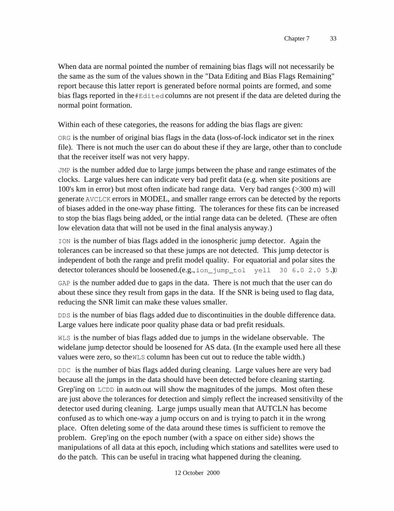
Chapter 7 33

12 October 2000

When data are normal pointed the number of remaining bias flags will not necessarily bethe same as the sum of the values shown in the "Data Editing and Bias Flags Remaining"report because this latter report is generated before normal points are formed, and somebias flags reported in the #Edited columns are not present if the data are deleted during thenormal point formation.

Within each of these categories, the reasons for adding the bias flags are given:

ORG is the number of original bias flags in the data (loss-of-lock indicator set in the rinexfile). There is not much the user can do about these if they are large, other than to concludethat the receiver itself was not very happy.

JMP is the number added due to large jumps between the phase and range estimates of theclocks. Large values here can indicate very bad prefit data (e.g. when site positions are100's km in error) but most often indicate bad range data. Very bad ranges (>300 m) willgenerate AVCLCK errors in MODEL, and smaller range errors can be detected by the reportsof biases added in the one-way phase fitting. The tolerances for these fits can be increasedto stop the bias flags being added, or the intial range data can be deleted. (These are oftenlow elevation data that will not be used in the final analysis anyway.)

ION is the number of bias flags added in the ionospheric jump detector. Again thetolerances can be increased so that these jumps are not detected. This jump detector isindependent of both the range and prefit model quality. For equatorial and polar sites thedetector tolerances should be loosened.(e.g., ion_jump_tol yell 30 6.0 2.0 5.0)

GAP is the number added due to gaps in the data. There is not much that the user can doabout these since they result from gaps in the data. If the SNR is being used to flag data,reducing the SNR limit can make these values smaller.

DDS is the number of bias flags added due to discontinuities in the double difference data.Large values here indicate poor quality phase data or bad prefit residuals.

WLS is the number of bias flags added due to jumps in the widelane observable. Thewidelane jump detector should be loosened for AS data. (In the example used here all thesevalues were zero, so the WLS column has been cut out to reduce the table width.)

DDC is the number of bias flags added during cleaning. Large values here are very badbecause all the jumps in the data should have been detected before cleaning starting.Grep'ing on LCDD in autcln.out will show the magnitudes of the jumps. Most often theseare just above the tolerances for detection and simply reflect the increased sensitivilty of thedetector used during cleaning. Large jumps usually mean that AUTCLN has becomeconfused as to which one-way a jump occurs on and is trying to patch it in the wrongplace. Often deleting some of the data around these times is sufficient to remove theproblem. Grep'ing on the epoch number (with a space on either side) shows themanipulations of all data at this epoch, including which stations and satellites were used todo the patch. This can be useful in tracing what happened during the cleaning.

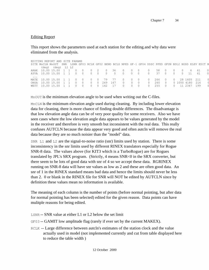
Chapter 7 34

12 October 2000

Editing Report

This report shows the parameters used at each station for the editing.and why data wereeliminated from the analysis.

EDITING REPORT AND SITE PARAMSSITE MnCLN MnOUT SNR LSNR GF03 RCLK GF02 BEND BCLS NPED GF-1 GF04 DDSC PFED GFUN BDL2 NODD ELEV EDIT MMRG ELCL Good (deg) (deg) L1 L2ARAK 10.00 15.00 1 1 0 0 0 2 0 36 0 0 0 0 58 0 0 0 6 61 0 6 5359AYVA 10.00 15.00 1 1 0 0 0 0 0 0 0 0 0 0 37 0 0 0 11 61 0 11 5214 ...MATE 10.00 15.00 1 1 0 0 0 0 79 77 0 0 0 0 266 0 0 28 1605 211 0 1605 166ONSA 10.00 15.00 1 1 0 0 0 0 249 167 0 0 0 0 260 0 0 1050 4180 216 0 4180 16388WETT 10.00 15.00 1 1 0 0 0 0 142 17 0 0 0 0 255 0 0 11 2347 199 0 2347 16793

MnOUT is the minimum elevation angle to be used when writing out the C-files.

MnCLN is the minimum elevation angle used during cleaning. By including lower elevationdata for cleaning, there is more chance of finding double differences. The disadvantage isthat low elevation angle data can be of very poor quality for some receivers. Also we haveseen cases where the low elevation angle data appears to be values generated by the modelin the receiver and therefore is very smooth but inconsistent with the real data. This reallyconfuses AUTCLN because the data appear very good and often autcln will remove the realdata because they are so much noisier than the "model" data.

SNR L1 and L2 are the signal-to-noise ratio (snr) limits used by station. There is someinconsistency in the snr limits used by different RINEX translators especially for RogueSNR-8 data. The values above (for KIT3 which is a TurboRogue) are for Roguestranslated by JPL's SRX program. (Strictly, 4 means SNR<0 in the SRX converter, butthere seem to be lots of good data with snr of 4 so we accept these data. RGRINEXrunning on SNR-8 data will have snr values as low as 2 and these are often good data. Ansnr of 1 in the RINEX standard means bad data and hence the limits should never be lessthan 2. 0 or blank in the RINEX file for SNR will NOT be edited by AUTCLN since bydefinition these values mean no information is available.

The meaning of each column is the number of points (before normal pointing, but after datafor normal pointing has been selected) edited for the given reason. Data points can havemulitple reasons for being edited.

LSNR -- SNR value at either L1 or L2 below the set limit

GF03 -- GAMIT low amplitude flag (rarely if ever set by the current MAKEX).

RCLK -- Large difference between autcln's estimates of the station clock and the valueactually used in model (not implemented currently and cut from table displayed hereto reduce the table width )

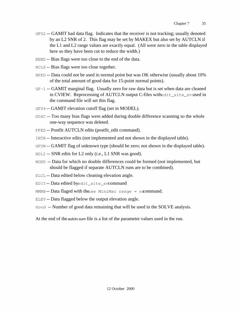
Chapter 7 35

12 October 2000

GF02 -- GAMIT bad data flag. Indicates that the receiver is not tracking; usually denotedby an L2 SNR of 2. This flag may be set by MAKEX but also set by AUTCLN ifthe L1 and L2 range values are exactly equal. (All were zero in the table displayedhere so they have been cut to reduce the width.)

BEND -- Bias flags were too close to the end of the data.

BCLS -- Bias flags were too close together.

NPED -- Data could not be used in normal point but was OK otherwise (usually about 10%of the total amount of good data for 15-point normal points).

GF-1 -- GAMIT marginal flag. Usually zero for raw data but is set when data are cleanedin CVIEW. Reprocessing of AUTCLN output C-files with edit_site_sv used inthe command file will set this flag.

GF04 -- GAMIT elevation cutoff flag (set in MODEL).

DDSC -- Too many bias flags were added during double difference scanning so the wholeone-way sequence was deleted.

PFED -- Postfit AUTCLN edits (postfit_edit command).

INTR -- Interactive edits (not implemented and not shown in the displayed table).

GFUN -- GAMIT flag of unknown type (should be zero; not shown in the displayed table).

BDL2 -- SNR edits for L2 only (i.e., L1 SNR was good).

NODD -- Data for which no double differences could be formed (not implemented, butshould be flagged if separate AUTCLN runs are to be combined).

ELCL -- Data edited below cleaning elevation angle.

EDIT -- Data edited by edit_site_sv command

MMRB -- Data flaged with the use MiniMac range = no command.

ELEV -- Data flagged below the output elevation angle.

Good -- Number of good data remaining that will be used in the SOLVE analysis.

At the end of the autcln.sum file is a list of the parameter values used in the run.

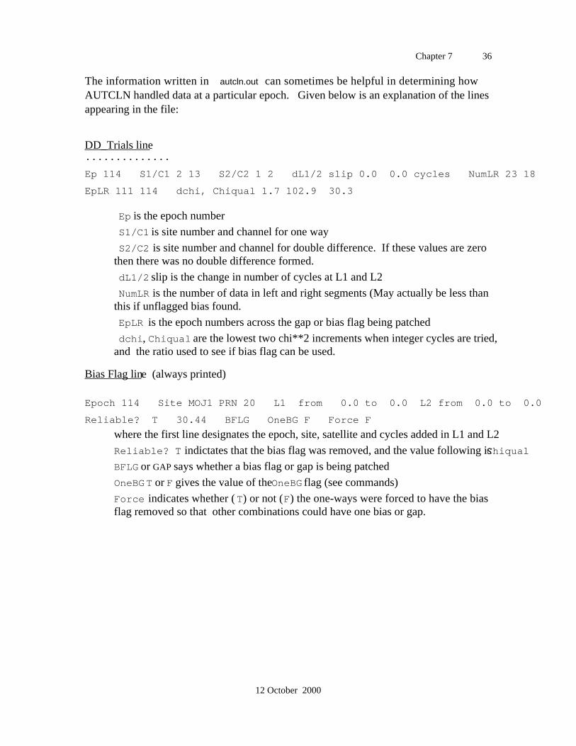
Chapter 7 36

12 October 2000

The information written in autcln.out can sometimes be helpful in determining howAUTCLN handled data at a particular epoch. Given below is an explanation of the linesappearing in the file:

DD_Trials line..............

Ep 114 S1/C1 2 13 S2/C2 1 2 dL1/2 slip 0.0 0.0 cycles NumLR 23 18

EpLR 111 114 dchi, Chiqual 1.7 102.9 30.3

Ep is the epoch number

S1/C1 is site number and channel for one way

S2/C2 is site number and channel for double difference. If these values are zerothen there was no double difference formed.

dL1/2 slip is the change in number of cycles at L1 and L2

NumLR is the number of data in left and right segments (May actually be less thanthis if unflagged bias found.

EpLR is the epoch numbers across the gap or bias flag being patched

dchi, Chiqual are the lowest two chi**2 increments when integer cycles are tried,and the ratio used to see if bias flag can be used.

Bias Flag line (always printed)

Epoch 114 Site MOJ1 PRN 20 L1 from 0.0 to 0.0 L2 from 0.0 to 0.0

Reliable? T 30.44 BFLG OneBG F Force F

where the first line designates the epoch, site, satellite and cycles added in L1 and L2

Reliable? T indictates that the bias flag was removed, and the value following is Chiqual

BFLG or GAP says whether a bias flag or gap is being patched

OneBG T or F gives the value of the OneBG flag (see commands)

Force indicates whether (T) or not (F) the one-ways were forced to have the biasflag removed so that other combinations could have one bias or gap.

Chapter 8 1

13 August 1997

8. Atmospheric Delay Models

8.1 Description of the atmospheric delay

As the GPS signal travels from the satellite to the receiver, it propagates through theatmosphere of the earth, where it is retarded and its path changed from a straight line to acurved one. If we take the simplified mathematical model for the observable to be one inwhich the signal is assumed to be propagating in a straight line and at the speed of light invacuum, then the "atmospheric delay" is defined to be the difference between the trueelectrical path length and this assumed straight-line length. Using this definition, theatmospheric delay is a term to be added to the simplified model.

The atmospheric delay in the zenith (i.e., vertical) direction varies from about 6 to 8nanoseconds (190 to 240 cm, or 10-12 cycles of phase at L1-band) depending onmeteorological conditions and site location. The atmospheric delay increases withdecreasing elevation angle approximately with the cosecant of the elevation angle, so thatthe atmospheric delay at an elevation angle of 20 degrees may be from 30-36 cycles of L1phase.

The atmospheric delay is usually broken down into two components. The first componentis due to the mixture of all constituents, but it is assumed that the mean molar mass of theseconstituents is equal to the mean molar mass of only the " dry" (all except water vapor)constituents. Assuming that the atmosphere is in hydrostatic equilibrium, the "zenithdelay" due to these components is very well modeled (standard deviation of approximately0.5 mm) using the surface pressure, which represents the total weight of the atmosphere.This component of the atmospheric propagation delay is usually termed the "dry" or"hydrostatic" delay, and accounts for nearly all ( 90-100%) of the atmospheric propagationdelay.

The second component of the atmospheric delay is due to water vapor, and includes acorrection for the "dry mean molar mass" assumption used to derive the dry delay (seeabove). This component of the atmospheric propagation delay is called the "wet delay" andis equal to zero if there is no water vapor present anywhere along the path of the signal.However, there usually is water vapor present along the path of the signal and it is poorlypredicted using measurements of conditions at the site alone. This difficulty is caused bythe "unmixed" condition of atmospheric water vapor, which means that the water vapor ispresent in "blobs" throughout the troposphere. Because of this condition, models for thewet delay are notoriously inaccurate and can have RMS errors of several cm (zenith), out ofa total (zenith) wet delay of 0-40 cm.

Chapter 8 2

13 August 1997

8.2 Algorithms for the atmospheric propagation delay

The atmospheric propagation delay is the implemented in the following manner:

ATDEL(EL) = DRYZEN * DRYMAP(EL) + WETZEN * WETMAP(EL)

where EL is the elevation angle of the satellite, DRYZEN is the dry zenith delay, WETZENis the wet zenith delay, DRYMAP is the "mapping function" for the dry delay (see below)and WETMAP is the mapping function for the wet delay. A mapping function is amathematical model for the elevation dependence of the respective delays. The mappingfunctions (for both the dry and the wet terms) are approximately equal to the cosecant ofelevation, but there are significant deviations from this "cosecant law" due both to thecurvature of the earth and the curvature of the path of the GPS signal propagating throughthe atmosphere.

Many expressions for the four terms DRYZEN, DRYMAP, WETZEN, and WETMAPappear in the scientific literature. For microwave observations there is little controversyabout the expressions for the dry zenith delay. Since the wet zenith delay cannot beaccurately modeled from surface measurements, the expressions used are not critical. Thechoice of mapping function can be important, however, particularly for elevation cutoffangles below 15 degrees. The model to be used in GAMIT for each of the four terms isspecified by keywords in the sittbl. (see Section 5.2), a portion of which is shown belowwith the default choices and values of the surface pressure, temperature, and relativehumidity.

SITE FIX --COORD.CONSTR.- DZEN DMAP WMAP ---MET._VALUE---- WFILECATO Castro Peak NNN 100. 100. 100. SAAS NMFH NMFW 1013.25 20.0 50.0 NONE

DZEN:

The default model [ SAAS ] for the dry zenith delay is that described by Saastamoinen[1972]. If there is a W-file of meterological data, the actual pressure at the station, asinterpolated from the file is used to determine the delay. If there is no W-file ( NONE, thedefault) the model takes the surface pressure given in the sittbl. and reduces it to pressure atthe station using the station's height and small corrections for gravitational variations withlatitude. You can also input directly a constant value for the dry zenith delay by specifyingthe model as CNNN where NNN is the range-equivalent of the delay in centimeters; e.g.,C230 sets the delay as 230 cm. This feature is useful mainly for error analysis.

WZEN:

The default model [ SAAS ] for the wet delay is also from Saastamoinen [1972]. It makesuse of both the surface temperature and the relative humidity/dewpoint, either from the

Chapter 8 3

13 August 1997

meteorological data file or from the default values. The default values of temperature andhumidity (20 degrees C and 50%) serve to make the a priori delay "reasonable" fortemperate climates. As for the dry zenith delay, you may set a constant value using CNNN asthe input model except that the constant delay is given in millimeters (NOT centimeters).This feature is useful because, as mentioned above, the true wet zenith delay is often notcorrelated with surface measurements. You can use C000 (i.e., zero wet zenith delay) andestimate a zenith delay correction which, if the correct pressure was used for the dry zenithdelay, will represent the mean wet zenith delay. An additional option for the wet delay is todetermine the value from water-vapor radiometer data, as described in Section 8.5 below;in this case set the WZEN code to WVR.

DMAP and WMAP:

Beginning with GAMIT release 9.6, the default mapping functions for both the hydrostatic("dry") and water-vapor ("wet") delays are the those developed recently by Arthur Niell ofthe MIT's Haystack Observatory [ Niell , 1996]. If these are entered explicitly into thesittbl., the codes are NMFH and NMFW for DMAP and WMAP, respectively. These replace theCfA-2.2 [ CFA] model developed at the Harvard-Smithsonian Center for Astrophysics[Davis et al., 1985] for analysis of VLBI data. You should expect no significant differencebetween the Niell and CfA mapping functions for observations above 15 degrees elevationangle. (The other recent mapping function is the MTT model developed by Herring[1992], but this has not yet been coded in GAMIT.) GAMIT also supports two oldermapping functions which were commonly used for analysis of microwave observationsprior to 1985—one developed by Marini and Murray [1974] [MARI ] and one by Chao[1972] [ CHAO ]

8.3 Estimating a zenith delay parameter

Since the water vapor contribution to atmospheric delay is poorly modeled using surfacemeteorological data, GAMIT allows estimation of corrections to the zenith delay. Thepartial derivative of phase or pseudorange with respect to the zenith delay parameter issimply the mapping function, approximately equal to the cosecant of the elevation angle ofthe satellite as viewed from the station. For stations in a regional network the elevationangles viewing a particular satellite will be nearly equal, producing high correlations amongthe estimated zenith delays. Even for stations a few meters apart, however, separate zenithdelays can be estimated without causing numerical problems in SOLVE; although theuncertainties in all of the zenith-delay parameters will be large, the relative values of theestimates themselves can be trusted. To extract from the solution the uncertainties of thedifferences, however, you should fix or tightly constrain one of the values.

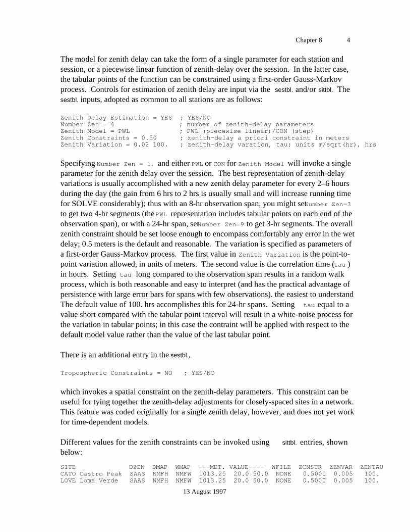
Chapter 8 4

13 August 1997

The model for zenith delay can take the form of a single parameter for each station andsession, or a piecewise linear function of zenith-delay over the session. In the latter case,the tabular points of the function can be constrained using a first-order Gauss-Markovprocess. Controls for estimation of zenith delay are input via the sestbl. and/or sittbl. Thesestbl. inputs, adopted as common to all stations are as follows:

Zenith Delay Estimation = YES ; YES/NONumber Zen = 4 ; number of zenith-delay parametersZenith Model = PWL ; PWL (piecewise linear)/CON (step)Zenith Constraints = 0.50 ; zenith-delay a priori constraint in metersZenith Variation = 0.02 100. ; zenith-delay varation, tau; units m/sqrt(hr), hrs

Specifying Number Zen = 1, and either PWL or CON for Zenith Model will invoke a singleparameter for the zenith delay over the session. The best representation of zenith-delayvariations is usually accomplished with a new zenith delay parameter for every 2–6 hoursduring the day (the gain from 6 hrs to 2 hrs is usually small and will increase running timefor SOLVE considerably); thus with an 8-hr observation span, you might set Number Zen=3to get two 4-hr segments (the PWL representation includes tabular points on each end of theobservation span), or with a 24-hr span, set Number Zen=9 to get 3-hr segments. The overallzenith constraint should be set loose enough to encompass comfortably any error in the wetdelay; 0.5 meters is the default and reasonable. The variation is specified as parameters ofa first-order Gauss-Markov process. The first value in Zenith Variation is the point-to-point variation allowed, in units of meters. The second value is the correlation time ( tau )in hours. Setting tau long compared to the observation span results in a random walkprocess, which is both reasonable and easy to interpret (and has the practical advantage ofpersistence with large error bars for spans with few observations). the easiest to understandThe default value of 100. hrs accomplishes this for 24-hr spans. Setting tau equal to avalue short compared with the tabular point interval will result in a white-noise process forthe variation in tabular points; in this case the contraint will be applied with respect to thedefault model value rather than the value of the last tabular point.

There is an additional entry in the sestbl.,

Tropospheric Constraints = NO ; YES/NO

which invokes a spatial constraint on the zenith-delay parameters. This constraint can beuseful for tying together the zenith-delay adjustments for closely-spaced sites in a network.This feature was coded originally for a single zenith delay, however, and does not yet workfor time-dependent models.

Different values for the zenith constraints can be invoked using sittbl. entries, shownbelow:

SITE DZEN DMAP WMAP ---MET. VALUE---- WFILE ZCNSTR ZENVAR ZENTAUCATO Castro Peak SAAS NMFH NMFW 1013.25 20.0 50.0 NONE 0.5000 0.005 100.LOVE Loma Verde SAAS NMFH NMFW 1013.25 20.0 50.0 NONE 0.5000 0.005 100.

Chapter 8 5

13 August 1997

PVER PVER7268 SAAS NMFH NMFW 1013.25 20.0 50.0 NONE 0.5000 0.020 100.SAFE San Fernando SAAS NMFH NMFW 1013.25 20.0 50.0 NONE 0.5000 0.020 100.YKNF YELLOWKNIFE SAAS NMFH NMFW 1013.25 20.0 50.0 NONE 0.5000 0.020 100.AROG ARO GPS SAAS NMFH NMFW 1013.25 20.0 50.0 NONE 0.5000 0.020 100.RICH RICHFRPA SAAS NMFH NMFW 1013.25 20.0 50.0 NONE 0.5000 0.020 100.TROM TROMGPSM SAAS NMFH NMFW 1013.25 20.0 50.0 NONE 0.5000 0.020 100.

It is currently a requirement that the number of zenith delays in the session be the same forall stations.

8.4 Estimating gradients

The effects of azimuthal asymmetry in the atmospheric delay are not included in MODELbut may be estimated in SOLVE. The coded partials imply a model of the form

ATDEL(EL,AZ) = GRADNS*AZMAP(EL)*COS(AZ) + GRADEW*AZMAP(EL)*SIN(AZ)

where EL is the elevation angle, AZ the azimuth, and AZMAP the mapping function forgradients, given by

AZMAP = 1./ ( SIN(EL)*TAN(EL) + C )

and C is a constant equal to 0.003 [ Chen and Herring , 1997]. Since the gradientparameters, GRADNS and GRADEW, have small and non-intuitive values near the zenith(i.e., for AZMAP = 1 ), we rescale them to represent the difference between the the north(or east) and south (or west) delay at 10 degrees elevation. At 10 degrees the rms scatter ofgradients observed from VLBI observations are about 5 mm. Our default a prioriconstraint is 30 mm.

8.5 Water vapor radiometer (WVR) data

A water-vapor radiometer is a multichannel radiometer which measures the brightnesstemperatures of the atmosphere. The main contributions to this radiation below 100 GHzare atmospheric oxygen, water vapor, and liquid water. The several frequencies of theWVR are used to solve for these various components and the wet delay. The algorithm forthe delay currently implemented is

Wet delay = A + B * T1 + C * T2

where A, B, and C are user-defined constants, and T1 and T2 are the brightnesstemperatures (not linearized) at two frequencies. The name of the WVR data file (Z-file)must also be entered. The Z-file is of the format:

Chapter 8 6

13 August 1997

This is a comment line

.

.

This is the last comment line

END

Header line #1

Header line #2

YYYY DDD HH MM YYYY DDD HH MM SITE

Header line #3

Header line #4

YYYY DDD HH MM SS AZ EL T1 T2 TS

.

.

The actual entries are free format. They include the year, day-of-year, hours , minutes andseconds for the WVR observation, the azimuth and elevation (in degrees) of theobservation, the brightness temperatures (in Kelvins), and the surface temperatures (indegrees Celsius). In order to interpolate the brightness temperatures, they must beconverted to quivalent zenith brightness temperatures. This is done in the followingmanner: Saturation effects are taken into account by determining the optical depth using

Ti = T0 exp (- i ) + Teff [1 - exp(- i)]

where ti is the optical depth at the frequency of the brightness temperature Ti, T0=2.9 K isthe big-bang background temperature, and T eff is the "effective" temperature of theatmosphere [Chandraesker, 1960; Wu, 1979]. We use the approximations

Teff = 0.94 * Ts

where T s is the surface temperature in Kelvins [ Wu , 1979]. The optical depth is thenmapped to the zenith using

= (zen) * WETCHAO(elevation)

where the function WETCHAO is the wet Chao mapping function given above. The zenithbrightness temperatures are then calculated from the zenith opacities using the expressionabove. These zenith brightness temperatures are then interpolated to the epoch of the GPSmeasurement, and the zenith delay is calculated using the user-defined WVR constants.The wet delay away from the zenith is computed using the Chao wet mapping function.Note: For consistency with the interpolation scheme, the user must choose 'CHAO' for the

Chapter 8 7

13 August 1997

wet mapping function if WVR is chosen for the zenith wet delay. If this is not done, theprogram will display a warning and the wet mapping function will be changed to 'CHAO'.

8.6 References

Chandrasekhar, S., Radiative Transfer, Dover, New York, 1960.

Chao, C. C., A model for tropospheric calibration from daily surface and radiosondeballoon measurements, Tech. Mem. 391-350 , Jet Propulsion Laboratory, Pasadena,California, 1972.

Davis, J.L., T.A. Herring, I.I. Shapiro, A.E.E. Rogers, G. Elgered, Geodesy by radiointerferometry: Effects of atmospheric modeling errors on estimates of baseline length,Radio Science, 20, 1593-1607, 1985.

Chen, G., and T. A. Herring, Effects of atmospheric azimuth asymmetry on the analysis ofspace geodetic data, ournal of Geophysical Research, 102, 20489–20502, 1997.

Herring, T. A., Modeling atmospheric delays in the anlaysis of space geodetic data,Proceedings of the Symposium on Refraction of Transatmospheric Signals in Geodesy ,Publications on Geodesy, No. 36, ed. by De Munck and Spoelstra, 247, NetherlandGeodetic Commission, Delft, Netherlands, 1992.

Marini, J.W., C.W. Murray, Correction of radio range tracking data for atmosphericrefraction at elevations above 10 degrees, unpublished memorandum, 1974.

Niell, A. E., Global mapping functions for the atmospheric delay at radio wavelengths,Journal of Geophysical Research, 101, 3227–3246, 1996.

Treuhaft, R. N., and G. E. Lanyi, The effect of the dynamic wet troposphere on VLBImeasurements, Geodesy and Geophysics Preprint No. 141, Jet Propulsion Laboratory,Pasadena, 1986.

Saastamoinen, J., Atmospheric correction for the troposphere and stratosphere in radioranging of satellites, in The Use of Artificial Satellites for Geodesy , Geophys. Monogr.Ser. , Vol. 15, edited by S.W. Henriksen et al., pp. 247-251, American GeophysicalUnion, Washington, D.C., 1972.

Wu, S.C., 1979: Optimum frequencies of a passive microwave radiometer for tropospheric path-length correction. IEEE Trans. Ant. Prop., AP 20, 181-187.

Chapter 9 1

3 April 2000

9. Utility Programs and Auxiliary Tables

9.1 Plotting and computing statistics from GAMIT solutions

The most useful way to view the results of a GAMIT analysis is by examing the baselinerepeatability from day-to-day. The shell script sh_gamit_baseline will do this from the o-files produced by SOLVE. The instructions for running the script can be generated bytyping its name with no arguments; these are reproduced below:

Use GMT to make a multiple panel GAMIT baseline plots with uncertaintyscaling. It also creates inputs for wrms/nrms scatter plots, which canbe plotted with /stdrel/com/sh_globk_scatter

Requirements : GMT(netcdf/gmt/ghostscript)

: gamit/bin/poly01 (linked to gamit/utils)

USAGE : sh_gamit_baseline <options>.

EXAMPLES: for time-series plots

sh_gamit_baseline -o o* -b PIN2_VNDP PIN2_YAM2

sh_gamit_baseline -u 1 -o o* -b PIN2_VNDP PIN2_YAM2

=+=+=+=+=+=+=+=+=+=+=+=+=OPTIONS+=+=+=+=+=+=+=+=+=+=+=+=+=+

-o[files] list : ofile names. MUST have this.

-f[ile] file : Baseline names. -b[aseline] list : command line argument for baselines. If -f and

-b are both omitted, all baselines are plotted.

-free : Biases free solution--Default.

-fixed : Biases fixed solution.

-d[elete] <sites/baselines etc> : names of unwanted sites.

-df file : file contains the names of unwanted sites.

-[delete_file] : Makes life easier for -d

-u[nc_scale] value : scale all uncertainties by this.. Default =1.

-y[scale] min max : vertical scale. If not issued it will be calculated.

-x[scale] min max : horizontal scale. If not issued it will be calculated.

-frame value : gmt border day-axis frame ticks. Default =1.

-anot value : gmt border day-axis label intervals. Default =1

-a ext : Add more descriptors to postscript file name. Default is psgamit.#

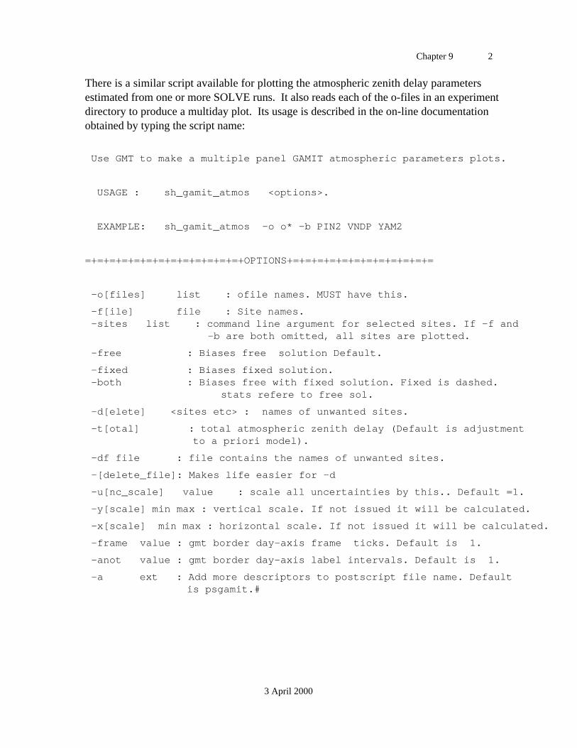
Chapter 9 2

3 April 2000

There is a similar script available for plotting the atmospheric zenith delay parametersestimated from one or more SOLVE runs. It also reads each of the o-files in an experimentdirectory to produce a multiday plot. Its usage is described in the on-line documentationobtained by typing the script name:

Use GMT to make a multiple panel GAMIT atmospheric parameters plots.

USAGE : sh_gamit_atmos <options>.

EXAMPLE: sh_gamit_atmos -o o* -b PIN2 VNDP YAM2

=+=+=+=+=+=+=+=+=+=+=+=+=+OPTIONS+=+=+=+=+=+=+=+=+=+=+=+=

-o[files] list : ofile names. MUST have this.

-f[ile] file : Site names. -sites list : command line argument for selected sites. If -f and -b are both omitted, all sites are plotted.

-free : Biases free solution Default.

-fixed : Biases fixed solution. -both : Biases free with fixed solution. Fixed is dashed.

stats refere to free sol.

-d[elete] <sites etc> : names of unwanted sites.

-t[otal] : total atmospheric zenith delay (Default is adjustment to a priori model).

-df file : file contains the names of unwanted sites.

-[delete_file]: Makes life easier for -d

-u[nc_scale] value : scale all uncertainties by this.. Default =1.

-y[scale] min max : vertical scale. If not issued it will be calculated.

-x[scale] min max : horizontal scale. If not issued it will be calculated.

-frame value : gmt border day-axis frame ticks. Default is 1.

-anot value : gmt border day-axis label intervals. Default is 1.

-a ext : Add more descriptors to postscript file name. Default is psgamit.#

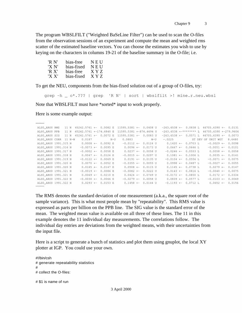
Chapter 9 3

3 April 2000

The program WBSLFILT ("Weighted BaSeLine Filter") can be used to scan the O-filesfrom the observation sessions of an experiment and compute the mean and weighted rmsscatter of the estimated baseline vectors. You can choose the estimates you wish to use bykeying on the characters in columns 19-21 of the baseline summary in the O-file; i.e.

'R N' bias-free N E U 'X N' bias-fixed N E U

'R X' bias-free X Y Z'X X' bias-fixed X Y Z

To get the NEU, components from the bias-fixed solution out of a group of O-files, try:

grep -h _ o*.??? | grep 'R N' | sort | wbslfilt >! mine.r.neu.wbsl

Note that WBSLFILT must have *sorted* input to work properly.

Here is some example output:

---------

ALS0_ARO0 RMS 11 N 45242.5761 +- 0.0082 E 11595.5381 +- 0.0408 U -263.6538 +- 0.0838 L 46705.6390 +- 0.0131

ALS0_ARO0 PPB 11 N 45242.5761 +-174.6840 E 11595.5381 +-874.4694 U -263.6538 +-******** L 46705.6390 +-279.9606

ALS0_ARO0 SIG 11 N 45242.5761 +- 0.0072 E 11595.5381 +- 0.0083 U -263.6538 +- 0.0571 L 46705.6390 +- 0.0073

ALS0_ARO0 CORR 11 N-W 0.0187 N-U 0.0883 W-U -.0225 ST DEV OF UNIT WGT 8.6480

ALS0_ARO0 1991.315 N 0.0008 +- 0.0092 E -0.0112 +- 0.0124 U 0.1420 +- 0.0703 L -0.0029 +- 0.0098

ALS0_ARO0 1991.316 N -0.0073 +- 0.0095 E 0.0096 +- 0.0173 U 0.0667 +- 0.0646 L -0.0051 +- 0.0101

ALS0_ARO0 1991.317 N -0.0002 +- 0.0058 E 0.0237 +- 0.0058 U -0.0246 +- 0.0553 L 0.0058 +- 0.0058

ALS0_ARO0 1991.318 N 0.0047 +- 0.0124 E -0.0015 +- 0.0297 U 0.1081 +- 0.1006 L 0.0035 +- 0.0141

ALS0_ARO0 1991.319 N -0.0122 +- 0.0069 E 0.0191 +- 0.0135 U -0.0104 +- 0.0556 L -0.0071 +- 0.0075

ALS0_ARO0 1991.320 N 0.0070 +- 0.0052 E -0.0355 +- 0.0055 U 0.0998 +- 0.0487 L -0.0027 +- 0.0055

ALS0_ARO0 1991.320 N 0.0165 +- 0.0147 E 0.0508 +- 0.0115 U 0.1145 +- 0.0738 L 0.0279 +- 0.0147

ALS0_ARO0 1991.321 N -0.0019 +- 0.0086 E -0.0082 +- 0.0222 U 0.0143 +- 0.0816 L -0.0040 +- 0.0075

ALS0_ARO0 1991.321 N 0.0069 +- 0.0210 E 0.0424 +- 0.0749 U -0.0172 +- 0.0850 L 0.0172 +- 0.0334

ALS0_ARO0 1991.322 N -0.0030 +- 0.0066 E -0.0279 +- 0.0058 U 0.0839 +- 0.0577 L -0.0103 +- 0.0069

ALS0_ARO0 1991.322 N 0.0293 +- 0.0153 E 0.1458 +- 0.0144 U -0.1193 +- 0.0712 L 0.0652 +- 0.0156---------

The RMS denotes the standard deviation of one measurement (a.k.a., the square root of thesample variance). This is what most people mean by "repeatability". This RMS value isexpressed as parts per billion on the PPB line. The SIG value is the standard error of themean. The weighted mean value is available on all three of these lines. The 11 in thisexample denotes the 11 individual day measurements. The correlations follow. Theindividual day entries are deviations from the weighted means, with their uncertainties fromthe input file.

Here is a script to generate a bunch of statistics and plot them using gnuplot, the local XYplotter at IGP. You could use your own.

#!/bin/csh# generate repeatability statistics## collect the O-files:

# $1 is name of run

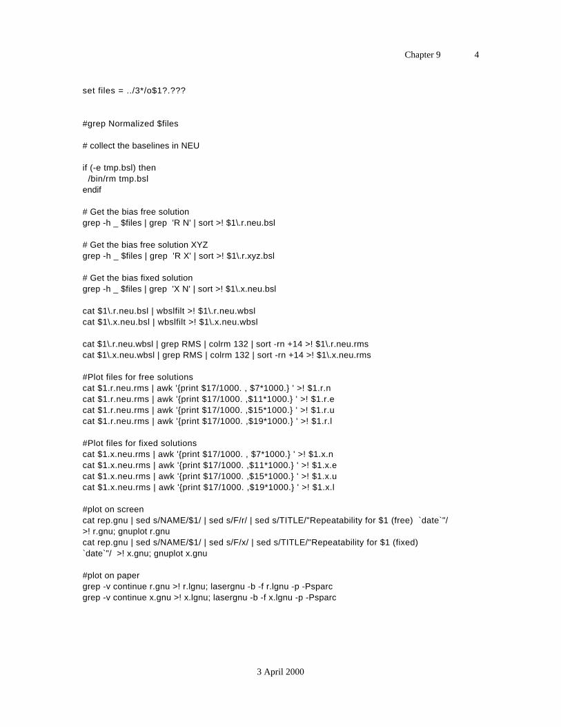
Chapter 9 4

3 April 2000

set files = ../3*/o$1?.???

#grep Normalized $files

# collect the baselines in NEU

if (-e tmp.bsl) then /bin/rm tmp.bslendif

# Get the bias free solutiongrep -h _ $files | grep 'R N' | sort >! $1\.r.neu.bsl

# Get the bias free solution XYZgrep -h _ $files | grep 'R X' | sort >! $1\.r.xyz.bsl

# Get the bias fixed solutiongrep -h _ $files | grep 'X N' | sort >! $1\.x.neu.bsl

cat $1\.r.neu.bsl | wbslfilt >! $1\.r.neu.wbslcat $1\.x.neu.bsl | wbslfilt >! $1\.x.neu.wbsl

cat $1\.r.neu.wbsl | grep RMS | colrm 132 | sort -rn +14 >! $1\.r.neu.rmscat $1\.x.neu.wbsl | grep RMS | colrm 132 | sort -rn +14 >! $1\.x.neu.rms

#Plot files for free solutionscat $1.r.neu.rms | awk '{print $17/1000. , $7*1000.} ' >! $1.r.ncat $1.r.neu.rms | awk '{print $17/1000. ,$11*1000.} ' >! $1.r.ecat $1.r.neu.rms | awk '{print $17/1000. ,$15*1000.} ' >! $1.r.ucat $1.r.neu.rms | awk '{print $17/1000. ,$19*1000.} ' >! $1.r.l

#Plot files for fixed solutionscat $1.x.neu.rms | awk '{print $17/1000. , $7*1000.} ' >! $1.x.ncat $1.x.neu.rms | awk '{print $17/1000. ,$11*1000.} ' >! $1.x.ecat $1.x.neu.rms | awk '{print $17/1000. ,$15*1000.} ' >! $1.x.ucat $1.x.neu.rms | awk '{print $17/1000. ,$19*1000.} ' >! $1.x.l

#plot on screencat rep.gnu | sed s/NAME/$1/ | sed s/F/r/ | sed s/TITLE/"Repeatability for $1 (free) `date`"/>! r.gnu; gnuplot r.gnucat rep.gnu | sed s/NAME/$1/ | sed s/F/x/ | sed s/TITLE/"Repeatability for $1 (fixed)`date`"/ >! x.gnu; gnuplot x.gnu

#plot on papergrep -v continue r.gnu >! r.lgnu; lasergnu -b -f r.lgnu -p -Psparcgrep -v continue x.gnu >! x.lgnu; lasergnu -b -f x.lgnu -p -Psparc

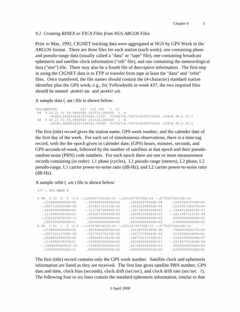
Chapter 9 5

3 April 2000

9.2 Creating RINEX or FICA Files from NGS ARGOS Files

Prior to May, 1992, CIGNET tracking data were aggregated at NGS by GPS Week in theARGOS format. There are three files for each station (each week), one containing phaseand pseudo-range data (usually called a "data" or "tape" file), one containing broadcastephemeris and satellite clock information ("orb" file), and one containing the meteorologicaldata ("met") file. There may also be a fourth file of descriptive information. The first stepin using the CIGNET data is to FTP or transfer from tape at least the "data" and "orbit"files. Once transfered, the file names should contain the (4-character) standard stationidentifier plus the GPS week; e.g., for Yellowknife in week 437, the two required filesshould be named yknf437.dat and yknf437.orb.

A sample data ( .dat ) file is shown below:

YELLOWKNIFE 437 143 198 5 22 88 5 24 21 51 59.0800000 251519.080000 1 6 -69283.6838536321073582.10107 53744718.7507536299753069 .45818 40.5 39.5 88 5 24 21 51 59.0800000 251519.080000 1 6 -69283.6838536321194922.50099 53744718.7507536299753069 .45818 40.5 39.5

The first (title) record gives the station name, GPS week number, and the calender date ofthe first day of the week. For each set of simultaneous observations, there is a time-tagrecord, with the the epoch given in calender date, (GPS) hours, minutes, seconds, andGPS seconds-of-week, followed by the number of satellites at that epoch and their pseudo-random noise (PRN) code numbers. For each epoch there are one or more measurementrecords containing (in order) L1 phase (cycles), L1 pseudo-range (meters), L2 phase, L2pseudo-range, L1 carrier power-to-noise ratio (dB-Hz), and L2 carrier power-to-noise ratio(dB-Hz).

A sample orbit ( .orb ) file is shown below:

437 : GPS WEEK #

6 88 5 25 0 0 0.0 -.116699375212D-03 -.192130755750D-10 -.277555756156D-16.122880000000D+05 -.925000000000D+01 .101825670448D-08 .183378419704D+00

-.586733222008D-06 .531821721233D-02 .104252249002D-04 .515364718437D+04 .259200000000D+06 -.111758708954D-07 .192736365505D+01 -.726431608200D-07 .111949619933D+01 .254187500000D+03 .202961194281D+01 -.621168731314D-08

-.232152527227D-10 .100000000000D+01 .437000000000D+03 .000000000000D+00.100000000000D+01 .000000000000D+00 .000000000000D+00 .430080000000D+05

6 88 5 25 1 0 0.0 -.116767827421D-03 -.192130755750D-10 -.277555756156D-16.163840000000D+05 -.687500000000D+01 .101647091580D-08 .708491445227D+00-.396743416786D-06 .531794375274D-02 .104773789644D-04 .515364661980D+04.262800000000D+06 .186264514923D-08 .192734131190D+01 -.614672899246D-07.111949607937D+01 .253406250000D+03 .202958492564D+01 -.621847331009D-08

-.292869342041D-10 .100000000000D+01 .437000000000D+03 .000000000000D+00.100000000000D+01 .000000000000D+00 .000000000000D+00 .430080000000D+05

The first (title) record contains only the GPS week number. Satellite clock and ephemerisinformation are listed as they are received. The first line gives satellite PRN number, GPSdate and time, clock bias (seconds), clock drift (sec/sec), and clock drift rate (sec/sec 2).The following four or six lines contain the standard ephemeris information, similar to that

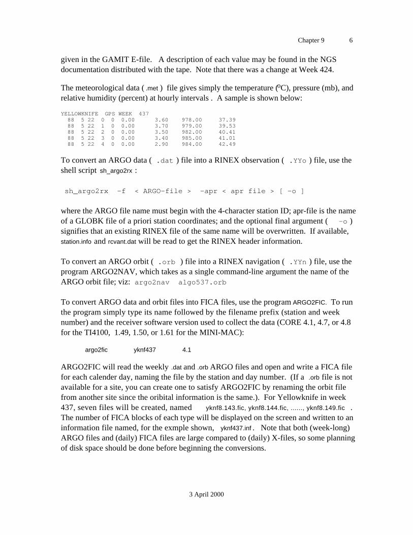
Chapter 9 6

3 April 2000

given in the GAMIT E-file. A description of each value may be found in the NGSdocumentation distributed with the tape. Note that there was a change at Week 424.

The meteorological data ( .met ) file gives simply the temperature (oC), pressure (mb), andrelative humidity (percent) at hourly intervals . A sample is shown below:

YELLOWKNIFE GPS WEEK 437 88 5 22 0 0 0.00 3.60 978.00 37.39 88 5 22 1 0 0.00 3.70 979.00 39.53 88 5 22 2 0 0.00 3.50 982.00 40.41 88 5 22 3 0 0.00 3.40 985.00 41.01 88 5 22 4 0 0.00 2.90 984.00 42.49

To convert an ARGO data ( .dat ) file into a RINEX observation ( .YYo ) file, use theshell script sh_argo2rx :

sh_argo2rx -f < ARGO-file > -apr < apr file > [ -o ]

where the ARGO file name must begin with the 4-character station ID; apr-file is the nameof a GLOBK file of a priori station coordinates; and the optional final argument ( -o )signifies that an existing RINEX file of the same name will be overwritten. If available,station.info and rcvant.dat will be read to get the RINEX header information.

To convert an ARGO orbit ( .orb ) file into a RINEX navigation ( .YYn ) file, use theprogram ARGO2NAV, which takes as a single command-line argument the name of theARGO orbit file; viz: argo2nav algo537.orb

To convert ARGO data and orbit files into FICA files, use the program ARGO2FIC. To runthe program simply type its name followed by the filename prefix (station and weeknumber) and the receiver software version used to collect the data (CORE 4.1, 4.7, or 4.8for the TI4100, 1.49, 1.50, or 1.61 for the MINI-MAC):

argo2fic yknf437 4.1

ARGO2FIC will read the weekly .dat and .orb ARGO files and open and write a FICA filefor each calender day, naming the file by the station and day number. (If a .orb file is notavailable for a site, you can create one to satisfy ARGO2FIC by renaming the orbit filefrom another site since the oribital information is the same.). For Yellowknife in week437, seven files will be created, named yknf8.143.fic, yknf8.144.fic, ......, yknf8.149.fic .The number of FICA blocks of each type will be displayed on the screen and written to aninformation file named, for the exmple shown, yknf437.inf . Note that both (week-long)ARGO files and (daily) FICA files are large compared to (daily) X-files, so some planningof disk space should be done before beginning the conversions.

Chapter 9 7

3 April 2000

9.3 Creating RINEX files from FICA files

Program FIC2RX (in the /makex directory) can be used to create RINEX observation andnavigation files from FICA files. It has been tested for TI4100 blocks 101, 6, and 9 (allfrom GESAR), and is coded (but untested) for the TI4100 using CORE or ROM software,and for MiniMac, Rogue, and Trimble receiver blocks, as well as the short (RINEX-like)blocks (70, 80, 1080, 1180, 1280, 1380) created for all receivers near the end of FICA'suseful lifetime. To run the program type

fic2rx <fica-file name> <l-file name>

If either of the command-line arguments is omitted, the program will prompt you to enterthem. Omission of the L-file is allowed but will result in zeroes being entered for theapproximate station coordinate in the RINEX header. FIC2RX is currently coded(MAKEX version 9.58 of March, 1997) to remove the nearest integer of the initial phase asper RINEX standards, but this feature of the code may be easily commented out.

9.4 Creating X-files from C-files (Utility CTOX)

In order to conserve disk space and maintain "clean" archival data files, it is useful toconvert edited C-files back to X-files whenever possible. This is done using the programCTOX. It can be run from a single C-file or a list of C-files contained in a D-file. Whenyou invoke the program, it will prompt you for the name of the input C- or D-file. If a D-file is used as input, CTOX will give you the opportunity to change the series letterassociated with the input C--files. Finally, you will be prompted for the series letter to beassociated with the output X-files.

9.5 Creating RINEX files from X- and E-files

Whenever data are exchanged with another institution, they should be transcribed in toRINEX format. This is easily accomplished using the program XTORX (in the /makex

directory). XTORX accepts two command-line arguments: the first is the name of theinput X-file or D-file containing a list of X-files; the second, used only in the case of a D-file, gives the series letter associated with the X-files (which might have a different seriesletter in the D-file list).

(Program ETORX to write RINEX navigation files from FICA Blk 9 files to be written)

9.6 Converting a hi.raw file to sited. or station.info

Prior to release 9.0, antenna height information was recorded by the analyst in a "raw" fileread by program HI, which converted the actual measurements into L1 and L2 offsets,written in the "station description" (sited.) file. The sited. file can still be read by MAKEX,FIXDRV, and MODEL, but it is recommended that these files be converted into a

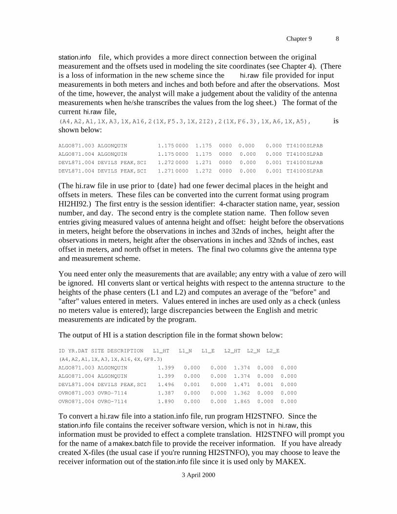
Chapter 9 8

3 April 2000

station.info file, which provides a more direct connection between the originalmeasurement and the offsets used in modeling the site coordinates (see Chapter 4). (Thereis a loss of information in the new scheme since the hi.raw file provided for inputmeasurements in both meters and inches and both before and after the observations. Mostof the time, however, the analyst will make a judgement about the validity of the antennameasurements when he/she transcribes the values from the log sheet.) The format of thecurrent hi.raw file,(A4,A2,A1,1X,A3,1X,A16,2(1X,F5.3,1X,2I2),2(1X,F6.3),1X,A6,1X,A5), isshown below:

ALGO871.003 ALGONQUIN 1.175 0000 1.175 0000 0.000 0.000 TI4100SLPAB

ALGO871.004 ALGONQUIN 1.175 0000 1.175 0000 0.000 0.000 TI4100SLPAB

DEVL871.004 DEVILS PEAK,SCI 1.272 0000 1.271 0000 0.000 0.001 TI4100SLPAB

DEVL871.004 DEVILS PEAK,SCI 1.271 0000 1.272 0000 0.000 0.001 TI4100SLPAB

(The hi.raw file in use prior to {date} had one fewer decimal places in the height andoffsets in meters. These files can be converted into the current format using programHI2HI92.) The first entry is the session identifier: 4-character station name, year, sessionnumber, and day. The second entry is the complete station name. Then follow sevenentries giving measured values of antenna height and offset: height before the observationsin meters, height before the observations in inches and 32nds of inches, height after theobservations in meters, height after the observations in inches and 32nds of inches, eastoffset in meters, and north offset in meters. The final two columns give the antenna typeand measurement scheme.

You need enter only the measurements that are available; any entry with a value of zero willbe ignored. HI converts slant or vertical heights with respect to the antenna structure to theheights of the phase centers (L1 and L2) and computes an average of the "before" and"after" values entered in meters. Values entered in inches are used only as a check (unlessno meters value is entered); large discrepancies between the English and metricmeasurements are indicated by the program.

The output of HI is a station description file in the format shown below:

ID YR.DAT SITE DESCRIPTION L1_HT L1_N L1_E L2_HT L2_N L2_E

(A4,A2,A1,1X,A3,1X,A16,4X,6F8.3)

ALGO871.003 ALGONQUIN 1.399 0.000 0.000 1.374 0.000 0.000

ALGO871.004 ALGONQUIN 1.399 0.000 0.000 1.374 0.000 0.000

DEVL871.004 DEVILS PEAK,SCI 1.496 0.001 0.000 1.471 0.001 0.000

OVRO871.003 OVRO-7114 1.387 0.000 0.000 1.362 0.000 0.000

OVRO871.004 OVRO-7114 1.890 0.000 0.000 1.865 0.000 0.000

To convert a hi.raw file into a station.info file, run program HI2STNFO. Since thestation.info file contains the receiver software version, which is not in hi.raw, thisinformation must be provided to effect a complete translation. HI2STNFO will prompt youfor the name of a makex.batch file to provide the receiver information. If you have alreadycreated X-files (the usual case if you're running HI2STNFO), you may choose to leave thereceiver information out of the station.info file since it is used only by MAKEX.

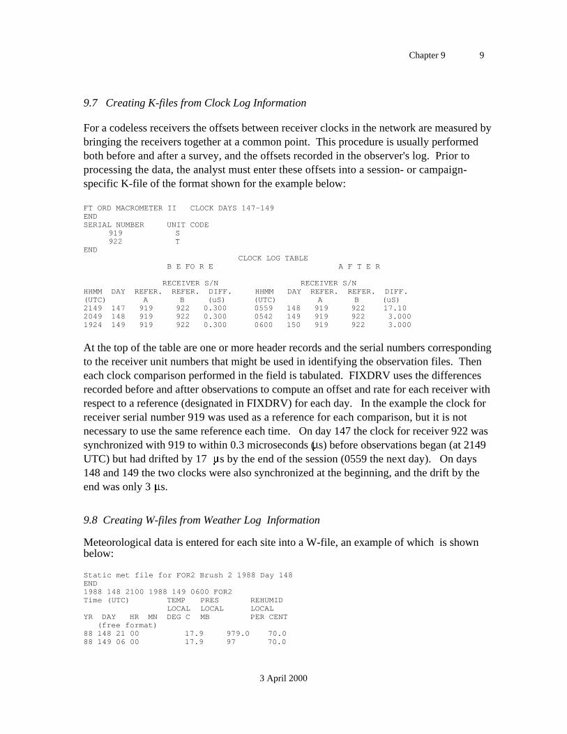
Chapter 9 9

3 April 2000

9.7 Creating K-files from Clock Log Information

For a codeless receivers the offsets between receiver clocks in the network are measured bybringing the receivers together at a common point. This procedure is usually performedboth before and after a survey, and the offsets recorded in the observer's log. Prior toprocessing the data, the analyst must enter these offsets into a session- or campaign-specific K-file of the format shown for the example below:

FT ORD MACROMETER II CLOCK DAYS 147-149ENDSERIAL NUMBER UNIT CODE

919 S922 T

END CLOCK LOG TABLE

B E FO R E A F T E R

RECEIVER S/N RECEIVER S/NHHMM DAY REFER. REFER. DIFF. HHMM DAY REFER. REFER. DIFF.(UTC) A B (uS) (UTC) A B (uS)2149 147 919 922 0.300 0559 148 919 922 17.102049 148 919 922 0.300 0542 149 919 922 3.0001924 149 919 922 0.300 0600 150 919 922 3.000

At the top of the table are one or more header records and the serial numbers correspondingto the receiver unit numbers that might be used in identifying the observation files. Theneach clock comparison performed in the field is tabulated. FIXDRV uses the differencesrecorded before and aftter observations to compute an offset and rate for each receiver withrespect to a reference (designated in FIXDRV) for each day. In the example the clock forreceiver serial number 919 was used as a reference for each comparison, but it is notnecessary to use the same reference each time. On day 147 the clock for receiver 922 wassynchronized with 919 to within 0.3 microseconds ( s) before observations began (at 2149UTC) but had drifted by 17 s by the end of the session (0559 the next day). On days148 and 149 the two clocks were also synchronized at the beginning, and the drift by theend was only 3 s.

9.8 Creating W-files from Weather Log Information

Meteorological data is entered for each site into a W-file, an example of which is shownbelow:

Static met file for FOR2 Brush 2 1988 Day 148END1988 148 2100 1988 149 0600 FOR2Time (UTC) TEMP PRES REHUMID

LOCAL LOCAL LOCALYR DAY HR MN DEG C MB PER CENT (free format)88 148 21 00 17.9 979.0 70.088 149 06 00 17.9 97 70.0

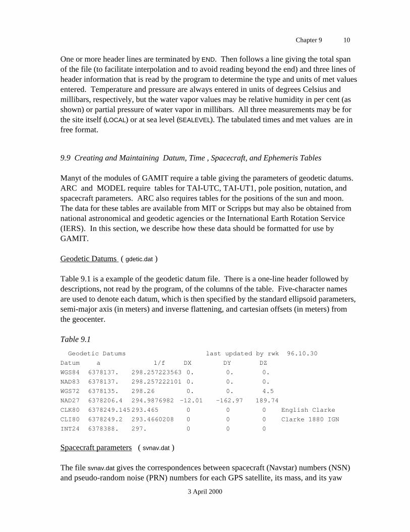
Chapter 9 10

3 April 2000

One or more header lines are terminated by END. Then follows a line giving the total spanof the file (to facilitate interpolation and to avoid reading beyond the end) and three lines ofheader information that is read by the program to determine the type and units of met valuesentered. Temperature and pressure are always entered in units of degrees Celsius andmillibars, respectively, but the water vapor values may be relative humidity in per cent (asshown) or partial pressure of water vapor in millibars. All three measurements may be forthe site itself (LOCAL) or at sea level (SEALEVEL). The tabulated times and met values are infree format.

9.9 Creating and Maintaining Datum, Time , Spacecraft, and Ephemeris Tables

Manyt of the modules of GAMIT require a table giving the parameters of geodetic datums.ARC and MODEL require tables for TAI-UTC, TAI-UT1, pole position, nutation, andspacecraft parameters. ARC also requires tables for the positions of the sun and moon.The data for these tables are available from MIT or Scripps but may also be obtained fromnational astronomical and geodetic agencies or the International Earth Rotation Service(IERS). In this section, we describe how these data should be formatted for use byGAMIT.

Geodetic Datums ( gdetic.dat )

Table 9.1 is a example of the geodetic datum file. There is a one-line header followed bydescriptions, not read by the program, of the columns of the table. Five-character namesare used to denote each datum, which is then specified by the standard ellipsoid parameters,semi-major axis (in meters) and inverse flattening, and cartesian offsets (in meters) fromthe geocenter.

Table 9.1

Geodetic Datums last updated by rwk 96.10.30

Datum a 1/f DX DY DZ

WGS84 6378137. 298.257223563 0. 0. 0.

NAD83 6378137. 298.257222101 0. 0. 0.

WGS72 6378135. 298.26 0. 0. 4.5

NAD27 6378206.4 294.9876982 -12.01 -162.97 189.74

CLK80 6378249.145293.465 0 0 0 English Clarke

CLI80 6378249.2 293.4660208 0 0 0 Clarke 1880 IGN

INT24 6378388. 297. 0 0 0

Spacecraft parameters ( svnav.dat )

The file svnav.dat gives the correspondences between spacecraft (Navstar) numbers (NSN)and pseudo-random noise (PRN) numbers for each GPS satellite, its mass, and its yaw

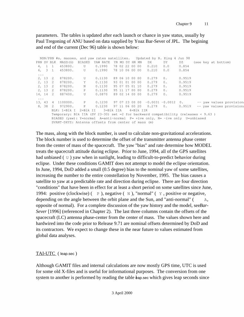
Chapter 9 11

3 April 2000

parameters. The tables is updated after each launch or chance in yaw status, usually byPaul Tregoning of ANU based on data supplied by Yoaz Bar-Sever of JPL. The beginingand end of the current (Dec 96) table is shown below:

NSN/PRN #s, masses, and yaw rates satellites. Updated by R. King 4 Jun 98PRN SV BLK MASS(G) BIASED YAW RATE YR MO DY HR MN DX DY DZ (see key at bottom) 4, 1 1 453800. U 0.1990 78 02 22 00 00 0.210 0.0 0.854 6, 3 1 453800. U 0.1990 78 10 06 00 00 0.210 0.0 0.854 ... 2, 13 2 878200. U 0.1130 89 06 10 00 00 0.279 0. 0.9519 2, 13 2 878200. Y 0.1130 93 01 01 00 00 0.279 0. 0.9519 2, 13 2 878200. N 0.1130 95 07 05 01 10 0.279 0. 0.9519 2, 13 2 878200. P 0.1130 95 11 17 00 00 0.279 0. 0.951914, 14 2 887400. U 0.0870 89 02 14 00 00 0.279 0. 0.9519 ...13, 43 4 1100000. P 0.1230 97 07 23 00 00 -0.0031 -0.0012 0. -- yaw values provisional 8, 38 2 972900. P 0.1230 97 11 06 00 20 0.279 0. 0.9519 -- yaw values provisional BLK: 1=Blk I 2=Blk II 3=Blk IIA 4=Blk IIR Temporary: Blk IIA (SV 23-30) set =2 for backward compatibility (releases < 9.63 ) BIASED (yaw): Y=normal A=anti-normal P= +ive only, N= -ive only U=unbiased SVANT-DXYZ: Antenna offsets from center of mass (m)

The mass, along with the block number, is used to calculate non-gravitational accelerations.The block number is used to determine the offset of the transmitter antenna phase centerfrom the center of mass of the spacecraft. The yaw "bias" and rate determine how MODELtreats the spacecraft attitude during eclipse. Prior to June, 1994, all of the GPS satelliteshad unbiased ( U ) yaw when in sunlight, leading to difficult-to-predict behavior duringeclipse. Under these conditions GAMIT does not attempt to model the eclipse orientation.In June, 1994, DoD added a small (0.5 degree) bias to the nominal yaw of some satellites,increasing the number to the entire constellation by November, 1995. The bias causes asatellite to yaw at a predictable rate and direction during eclipse. There are four direction"conditions" that have been in effect for at least a short period on some satellites since June,1994: positive (clockwise) ( P ), negative ( N ), "normal" ( Y , positive or negative,depending on the angle between the orbit plane and the Sun, and "anti-normal" ( A,opposite of normal). For a complete discussion of the yaw history and the model, see Bar-Sever [1996] (referenced in Chapter 2). The last three columns contain the offsets of thespacecraft (LC) antenna phase-center from the center of mass. The values shown here andhardwired into the code prior to Release 9.71 are nominal offsets determined by DoD andits contractors. We expect to change these in the near future to values estimated fromglobal data analyses.

TAI-UTC ( leap.sec )

Although GAMIT files and internal calculations are now mostly GPS time, UTC is usedfor some old X-files and is useful for informational purposes. The conversion from onesystem to another is performed by reading the table leap.sec which gives leap seconds since

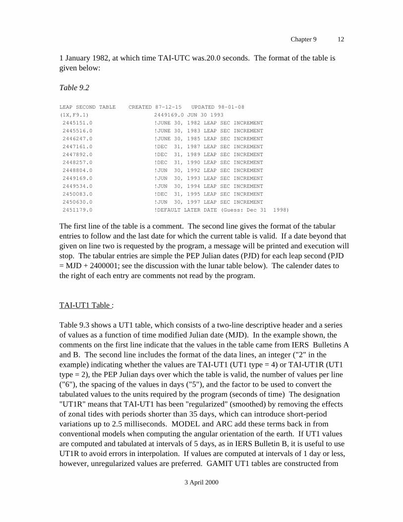
Chapter 9 12

3 April 2000

1 January 1982, at which time TAI-UTC was.20.0 seconds. The format of the table isgiven below:

Table 9.2

LEAP SECOND TABLE CREATED 87-12-15 UPDATED 98-01-08

(1X,F9.1) 2449169.0 JUN 30 1993

2445151.0 !JUNE 30, 1982 LEAP SEC INCREMENT



2447161.0 !DEC 31, 1987 LEAP SEC INCREMENT



2448804.0 !JUN 30, 1992 LEAP SEC INCREMENT





2451179.0 !DEFAULT LATER DATE (Guess: Dec 31 1998)

The first line of the table is a comment. The second line gives the format of the tabularentries to follow and the last date for which the current table is valid. If a date beyond thatgiven on line two is requested by the program, a message will be printed and execution willstop. The tabular entries are simple the PEP Julian dates (PJD) for each leap second (PJD= MJD + 2400001; see the discussion with the lunar table below). The calender dates tothe right of each entry are comments not read by the program.

TAI-UT1 Table :

Table 9.3 shows a UT1 table, which consists of a two-line descriptive header and a seriesof values as a function of time modified Julian date (MJD). In the example shown, thecomments on the first line indicate that the values in the table came from IERS Bulletins Aand B. The second line includes the format of the data lines, an integer ("2" in theexample) indicating whether the values are TAI-UT1 (UT1 type = 4) or TAI-UT1R (UT1type = 2), the PEP Julian days over which the table is valid, the number of values per line("6"), the spacing of the values in days ("5"), and the factor to be used to convert thetabulated values to the units required by the program (seconds of time) The designation"UT1R" means that TAI-UT1 has been "regularized" (smoothed) by removing the effectsof zonal tides with periods shorter than 35 days, which can introduce short-periodvariations up to 2.5 milliseconds. MODEL and ARC add these terms back in fromconventional models when computing the angular orientation of the earth. If UT1 valuesare computed and tabulated at intervals of 5 days, as in IERS Bulletin B, it is useful to useUT1R to avoid errors in interpolation. If values are computed at intervals of 1 day or less,however, unregularized values are preferred. GAMIT UT1 tables are constructed from

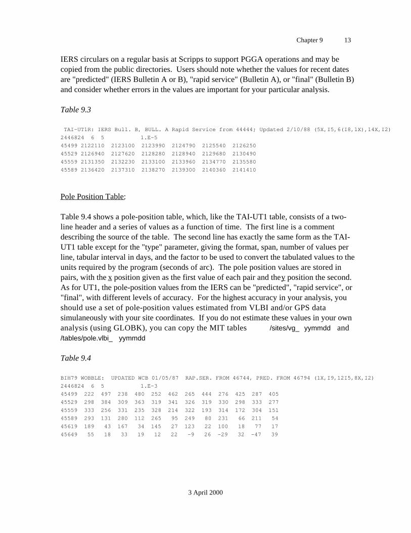
Chapter 9 13

3 April 2000

IERS circulars on a regular basis at Scripps to support PGGA operations and may becopied from the public directories. Users should note whether the values for recent datesare "predicted" (IERS Bulletin A or B), "rapid service" (Bulletin A), or "final" (Bulletin B)and consider whether errors in the values are important for your particular analysis.

Table 9.3

TAI-UT1R: IERS Bull. B, BULL. A Rapid Service from 44444; Updated 2/10/88 (5X,I5,6(I8,1X),14X,I2) 2 2445499

2446824 6 5 1.E-5

45499 2122110 2123100 2123990 2124790 2125540 2126250

45529 2126940 2127620 2128280 2128940 2129680 2130490

45559 2131350 2132230 2133100 2133960 2134770 2135580

45589 2136420 2137310 2138270 2139300 2140360 2141410

Pole Position Table:

Table 9.4 shows a pole-position table, which, like the TAI-UT1 table, consists of a two-line header and a series of values as a function of time. The first line is a commentdescribing the source of the table. The second line has exactly the same form as the TAI-UT1 table except for the "type" parameter, giving the format, span, number of values perline, tabular interval in days, and the factor to be used to convert the tabulated values to theunits required by the program (seconds of arc). The pole position values are stored inpairs, with the x position given as the first value of each pair and the y position the second.As for UT1, the pole-position values from the IERS can be "predicted", "rapid service", or"final", with different levels of accuracy. For the highest accuracy in your analysis, youshould use a set of pole-position values estimated from VLBI and/or GPS datasimulaneously with your site coordinates. If you do not estimate these values in your ownanalysis (using GLOBK), you can copy the MIT tables /sites/vg_ yymmdd and/tables/pole.vlbi_ yymmdd

Table 9.4

BIH79 WOBBLE: UPDATED WCB 01/05/87 RAP.SER. FROM 46744, PRED. FROM 46794 (1X,I9,12I5,8X,I2) 2445499

2446824 6 5 1.E-3

45499 222 497 238 480 252 462 265 444 276 425 287 405

45529 298 384 309 363 319 341 326 319 330 298 333 277

45559 333 256 331 235 328 214 322 193 314 172 304 151

45589 293 131 280 112 265 95 249 80 231 66 211 54

45619 189 43 167 34 145 27 123 22 100 18 77 17

45649 55 18 33 19 12 22 -9 26 -29 32 -47 39

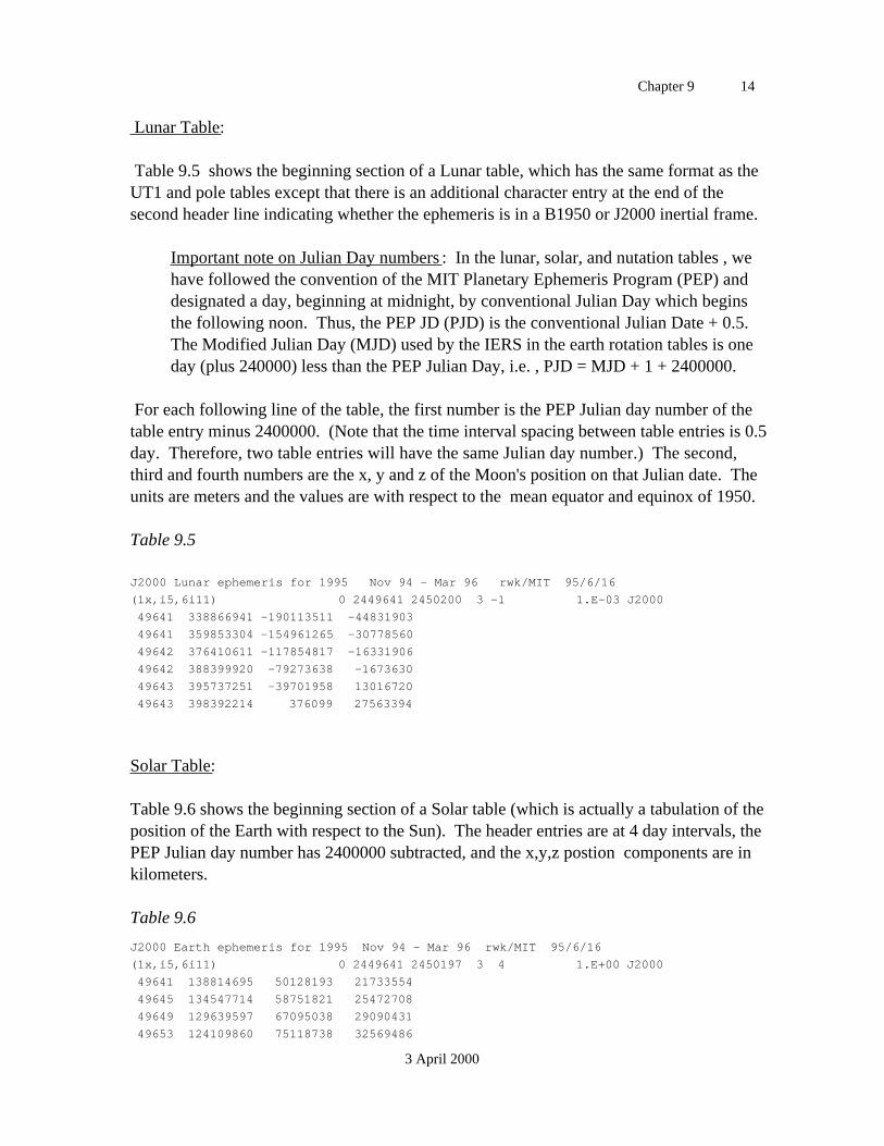
Chapter 9 14

3 April 2000

Lunar Table:

Table 9.5 shows the beginning section of a Lunar table, which has the same format as theUT1 and pole tables except that there is an additional character entry at the end of thesecond header line indicating whether the ephemeris is in a B1950 or J2000 inertial frame.

Important note on Julian Day numbers : In the lunar, solar, and nutation tables , wehave followed the convention of the MIT Planetary Ephemeris Program (PEP) anddesignated a day, beginning at midnight, by conventional Julian Day which beginsthe following noon. Thus, the PEP JD (PJD) is the conventional Julian Date + 0.5.The Modified Julian Day (MJD) used by the IERS in the earth rotation tables is oneday (plus 240000) less than the PEP Julian Day, i.e. , PJD = MJD + 1 + 2400000.

For each following line of the table, the first number is the PEP Julian day number of thetable entry minus 2400000. (Note that the time interval spacing between table entries is 0.5day. Therefore, two table entries will have the same Julian day number.) The second,third and fourth numbers are the x, y and z of the Moon's position on that Julian date. Theunits are meters and the values are with respect to the mean equator and equinox of 1950.

Table 9.5

J2000 Lunar ephemeris for 1995 Nov 94 - Mar 96 rwk/MIT 95/6/16

(1x,i5,6i11) 0 2449641 2450200 3 -1 1.E-03 J2000

49641 338866941 -190113511 -44831903

49641 359853304 -154961265 -30778560

49642 376410611 -117854817 -16331906

49642 388399920 -79273638 -1673630

49643 395737251 -39701958 13016720

49643 398392214 376099 27563394

Solar Table:

Table 9.6 shows the beginning section of a Solar table (which is actually a tabulation of theposition of the Earth with respect to the Sun). The header entries are at 4 day intervals, thePEP Julian day number has 2400000 subtracted, and the x,y,z postion components are inkilometers.

Table 9.6

J2000 Earth ephemeris for 1995 Nov 94 - Mar 96 rwk/MIT 95/6/16

(1x,i5,6i11) 0 2449641 2450197 3 4 1.E+00 J2000

49641 138814695 50128193 21733554

49645 134547714 58751821 25472708

49649 129639597 67095038 29090431

49653 124109860 75118738 32569486

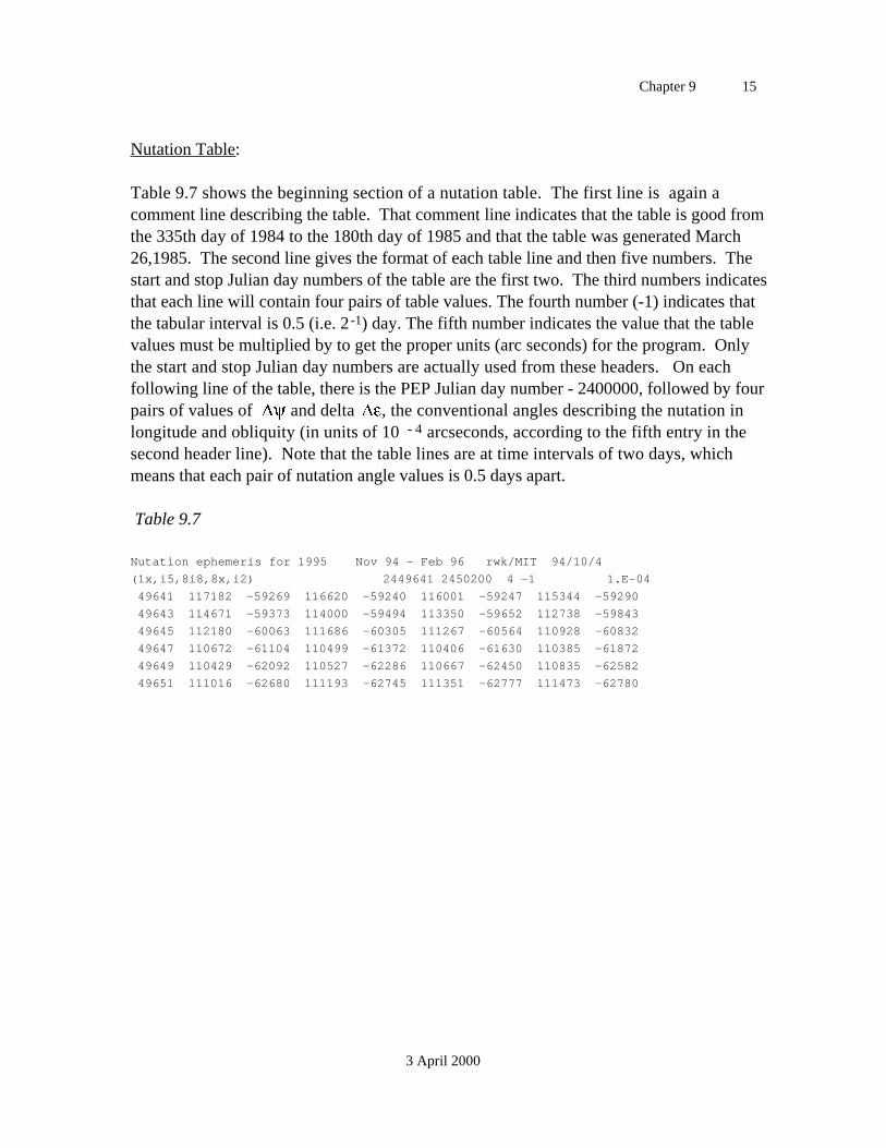
Chapter 9 15

3 April 2000

Nutation Table:

Table 9.7 shows the beginning section of a nutation table. The first line is again acomment line describing the table. That comment line indicates that the table is good fromthe 335th day of 1984 to the 180th day of 1985 and that the table was generated March26,1985. The second line gives the format of each table line and then five numbers. Thestart and stop Julian day numbers of the table are the first two. The third numbers indicatesthat each line will contain four pairs of table values. The fourth number (-1) indicates thatthe tabular interval is 0.5 (i.e. 2 -1) day. The fifth number indicates the value that the tablevalues must be multiplied by to get the proper units (arc seconds) for the program. Onlythe start and stop Julian day numbers are actually used from these headers. On eachfollowing line of the table, there is the PEP Julian day number - 2400000, followed by fourpairs of values of and delta , the conventional angles describing the nutation inlongitude and obliquity (in units of 10 - 4 arcseconds, according to the fifth entry in thesecond header line). Note that the table lines are at time intervals of two days, whichmeans that each pair of nutation angle values is 0.5 days apart.

Table 9.7

Nutation ephemeris for 1995 Nov 94 - Feb 96 rwk/MIT 94/10/4

(1x,i5,8i8,8x,i2) 2449641 2450200 4 -1 1.E-04

49641 117182 -59269 116620 -59240 116001 -59247 115344 -59290

49643 114671 -59373 114000 -59494 113350 -59652 112738 -59843

49645 112180 -60063 111686 -60305 111267 -60564 110928 -60832

49647 110672 -61104 110499 -61372 110406 -61630 110385 -61872

49649 110429 -62092 110527 -62286 110667 -62450 110835 -62582

49651 111016 -62680 111193 -62745 111351 -62777 111473 -62780

Chapter 10 1

16 November 2000

10. Automatic Batch Processing

10.1 Overview

Once you understand the file structure and analysis tools of GAMIT, you can savesignificant time in processing large quantities of data by using the automatic processingscript sh_gamit and the related scripts sh_glred . Sh_gamit takes you, with a singlecommand, from raw or RINEX data over a range of days to a solution and sky plots ofphase data as a record of the GAMIT analysis. Sh_glred uses the GAMIT results toproduce time series of day-to-day repeatability and a solution (h- or SINEX) file that maybe combined with those from other epochs to estimate station velocities. The onlypreparation required is setting up the control files, most of which are common to allanalyses of a particular era, and assembling the non-IGS data in one or more directories onyour system.

The first step in running the scripts is to create an experiment directory and then to copyinto it the templates directory from the GAMIT/GLOBK source directory. You will thenneed to edit one or more files in this directory to tailor the processing to the configuration ofyour computer system and GPS network:

process.defaults : Edit to specify your computation environment, sources for internal andexternal data and orbit files, start time and sampling interval, and instructions for archivingthe results.

sites.defaults : Edit to specify which local and IGS stations are to be used and how stationlog data are to be handled.

station.info : Make sure that this file is current (from SOPAC) for all IGS stations you willuse in your analysis. If the RINEX files for your local network contain IGS-standardreceiver and antenna codes and the correct height information refers to the ARP, then nofurther entries are required. If not, then you must manually enter the GAMIT codes andheight values into the file. You can give station.info priority over the RINEX headers usingthe xstnfo option in sites.defaults .

lfile. and .apr files : The template files will contain accurate coordinates for IGS stations,and the script will attempt to calculate coordinates for any new station via a pseudorangesolution, or (if you say so) use the coordinates in the RINEX header. When GAMIT runs,these coordinates will be updated from the phase solution so that for successive days onwhich the same station is observed, the accurate coordinates will be used.

sestbl. and sittbl. : Edit these to set the appropriate options for your analysis. Make surethat any station for which you specify tight constraints in sittbl. has accurate coordinates inthe apr file (aprf in process.defaults).

You may also choose to create under the experiment directory a /rinex directory and tocopy into it all of your local RINEX files. Alternatively, you can specify inprocess.defaults the directory structures for searching for raw and RINEX files on your

Chapter 10 2

16 November 2000

local and remote systems, as explained in Section 10.3. All other directories and filesrequired by GAMIT will be created by the script.

Once you have edited appropriately the template files, you can start the processing fromwithin the experiment directory by giving sh_gamit simply the 4-character code for theexperiment and a range of days to process:

sh_gamit -expt emed -d 1999 235 236 237 238 >&! sh_gamit.log

The time span can also be specified using -s <start_day> <stop_day> to indicate a range ofconsecutive days, or -r <days> to indicate that you want to process a single day <days>

before the current date. You may also override some of the parameters specified inprocess.defaults:

-orbit <type> Type of orbit (IGSP IGSR IGSF SIOP SIOR SIOF)

-eops <name> EOP series to be used ( usno [default], bull_b )

-c Do not compress X-files and RINEX files when done (default compress)

-archive Copy solution files to an archive and remove the day directory (default no)

-e Do not erase C-files when done (default is to erase)

-pres Plot phase residuals as postscript skyplots (default no)

-nogifs Do not create gif files of sky plots (default is to create from postscript)

-netext <char> Add network specific suffix (character) to day directory names (e.g. 035r)

-sessinfo Sampling interval, #epochs, start time (HH MM) (e.g. 30 2880 0 0 )

-mailto User name and machine (e.g. [email protected] )

Most of the time the parameters may be omitted in favor of the values you have specified inprocess.defaults for the whole experiment. The overrides are useful, however, if you wishto test the effect of processing a day with a different orbit, EOP table, or session length, inwhich case you can create a directory for the same day by appending a character to its name(e.g., -netext t ). Finally, you may launch sh_gamit from anywhere on the system byspecifying the full path name of the processing directory with -dir <path>. When the scriptruns, it will write to the screen a record of each step, which you may choose to redirect to afile (e.g., >&! sh_gamit.log). Though the current version of this log is cryptic in parts, youshould be able to use it together with GAMIT.fatal file, and the source code for sh_gamit toidentify the point and reason for failure should that occur. We welcome user feedback toimprove the displayed information.

When processing of each day is completed, sh_gamit will send a mail message to yougiving the number of stations used, the nrms values from the Q-file, the rms of the one-way phase residuals for the two best and two worst stations from the AUTCLN postfitsummary file, and a list of any large adjustments to station coordinates. These statisticswill let you know whether you need to examine the GAMIT output further for possiblereprocessing.

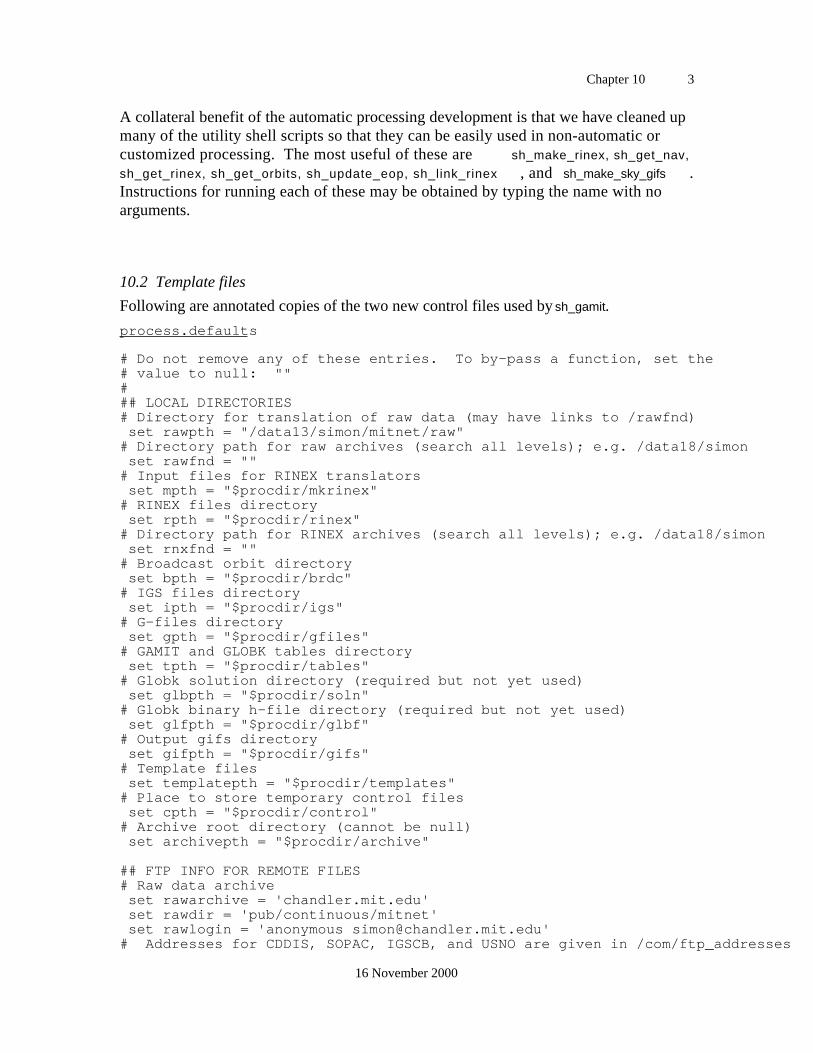
Chapter 10 3

16 November 2000

A collateral benefit of the automatic processing development is that we have cleaned upmany of the utility shell scripts so that they can be easily used in non-automatic orcustomized processing. The most useful of these are sh_make_rinex, sh_get_nav,

sh_get_rinex, sh_get_orbits, sh_update_eop, sh_link_rinex , and sh_make_sky_gifs .Instructions for running each of these may be obtained by typing the name with noarguments.

10.2 Template files

Following are annotated copies of the two new control files used by sh_gamit.

process.defaults

# Do not remove any of these entries. To by-pass a function, set the# value to null: ""### LOCAL DIRECTORIES# Directory for translation of raw data (may have links to /rawfnd) set rawpth = "/data13/simon/mitnet/raw"# Directory path for raw archives (search all levels); e.g. /data18/simon set rawfnd = ""# Input files for RINEX translators set mpth = "$procdir/mkrinex"# RINEX files directory set rpth = "$procdir/rinex"# Directory path for RINEX archives (search all levels); e.g. /data18/simon set rnxfnd = ""# Broadcast orbit directory set bpth = "$procdir/brdc"# IGS files directory set ipth = "$procdir/igs"# G-files directory set gpth = "$procdir/gfiles"# GAMIT and GLOBK tables directory set tpth = "$procdir/tables"# Globk solution directory (required but not yet used) set glbpth = "$procdir/soln"# Globk binary h-file directory (required but not yet used) set glfpth = "$procdir/glbf"# Output gifs directory set gifpth = "$procdir/gifs"# Template files set templatepth = "$procdir/templates"# Place to store temporary control files set cpth = "$procdir/control"# Archive root directory (cannot be null) set archivepth = "$procdir/archive"

## FTP INFO FOR REMOTE FILES# Raw data archive set rawarchive = 'chandler.mit.edu' set rawdir = 'pub/continuous/mitnet' set rawlogin = 'anonymous [email protected]'# Addresses for CDDIS, SOPAC, IGSCB, and USNO are given in /com/ftp_addresses

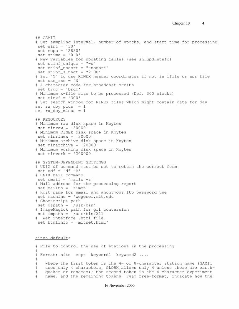
Chapter 10 4

16 November 2000

## GAMIT# Set sampling interval, number of epochs, and start time for processing set sint = '30' set nepc = '2880' set stime = '0 0'# New variables for updating tables (see sh_upd_stnfo) set stinf_unique = "-u" set stinf_nosort = "-nosort" set stinf_slthgt = "2.00"# Set "Y" to use RINEX header coordinates if not in lfile or apr file set use_rxc = "N"# 4-character code for broadcast orbits set brdc = 'brdc'# Minimum x-file size to be processed (Def. 300 blocks) set minxf = '300'# Set search window for RINEX files which might contain data for dayset rx_doy_plus = 1set rx_doy_minus = 1

## RESOURCES# Minimum raw disk space in Kbytes set minraw = '30000'# Minimum RINEX disk space in Kbytes set minrinex = '30000'# Minimum archive disk space in Kbytes set minarchive = '20000'# Minimum working disk space in Kbytes set minwork = '200000'

## SYSTEM-DEPENDENT SETTINGS# UNIX df command must be set to return the correct form set udf = 'df -k'# UNIX mail command set umail = 'mailx -s'# Mail address for the processing report set mailto = 'simon'# Host name for email and anonymous ftp password use set machine = 'wegener.mit.edu'# Ghostscript path set gspath = '/usr/bin'# ImageMagick path for gif conversion set impath = '/usr/bin/X11'# Web interface .html file. set htmlinfo = 'mitnet.html'

sites.defaults

# File to control the use of stations in the processing## Format: site expt keyword1 keyword2 ....## where the first token is the 4- or 8-character station name (GAMIT# uses only 4 characters, GLOBK allows only 4 unless there are earth-# quakes or renames); the second token is the 4-character experiment# name, and the remaining tokens, read free-format, indicate how the

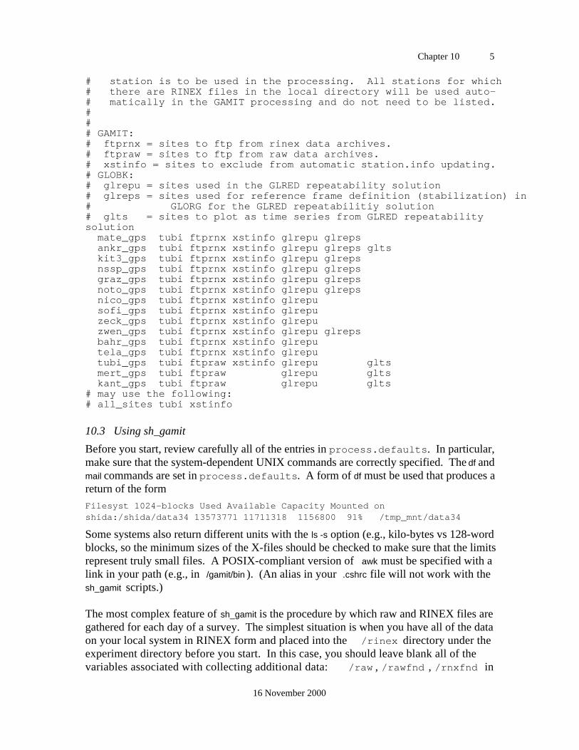
Chapter 10 5

16 November 2000

# station is to be used in the processing. All stations for which# there are RINEX files in the local directory will be used auto-# matically in the GAMIT processing and do not need to be listed.### GAMIT:# ftprnx = sites to ftp from rinex data archives.# ftpraw = sites to ftp from raw data archives.# xstinfo = sites to exclude from automatic station.info updating.# GLOBK:# glrepu = sites used in the GLRED repeatability solution# glreps = sites used for reference frame definition (stabilization) in# GLORG for the GLRED repeatabilitiy solution# glts = sites to plot as time series from GLRED repeatabilitysolution mate_gps tubi ftprnx xstinfo glrepu glreps ankr_gps tubi ftprnx xstinfo glrepu glreps glts kit3_gps tubi ftprnx xstinfo glrepu glreps nssp_gps tubi ftprnx xstinfo glrepu glreps graz_gps tubi ftprnx xstinfo glrepu glreps noto_gps tubi ftprnx xstinfo glrepu glreps nico_gps tubi ftprnx xstinfo glrepu sofi_gps tubi ftprnx xstinfo glrepu zeck_gps tubi ftprnx xstinfo glrepu zwen_gps tubi ftprnx xstinfo glrepu glreps bahr_gps tubi ftprnx xstinfo glrepu tela_gps tubi ftprnx xstinfo glrepu tubi_gps tubi ftpraw xstinfo glrepu glts mert_gps tubi ftpraw glrepu glts kant_gps tubi ftpraw glrepu glts# may use the following:# all_sites tubi xstinfo

10.3 Using sh_gamit

Before you start, review carefully all of the entries in process.defaults. In particular,make sure that the system-dependent UNIX commands are correctly specified. The df andmail commands are set in process.defaults. A form of df must be used that produces areturn of the form

Filesyst 1024-blocks Used Available Capacity Mounted onshida:/shida/data34 13573771 11711318 1156800 91% /tmp_mnt/data34

Some systems also return different units with the ls -s option (e.g., kilo-bytes vs 128-wordblocks, so the minimum sizes of the X-files should be checked to make sure that the limitsrepresent truly small files. A POSIX-compliant version of awk must be specified with alink in your path (e.g., in /gamit/bin ). (An alias in your .cshrc file will not work with thesh_gamit scripts.)

The most complex feature of sh_gamit is the procedure by which raw and RINEX files aregathered for each day of a survey. The simplest situation is when you have all of the dataon your local system in RINEX form and placed into the /rinex directory under theexperiment directory before you start. In this case, you should leave blank all of thevariables associated with collecting additional data: /raw , /rawfnd , /rnxfnd in

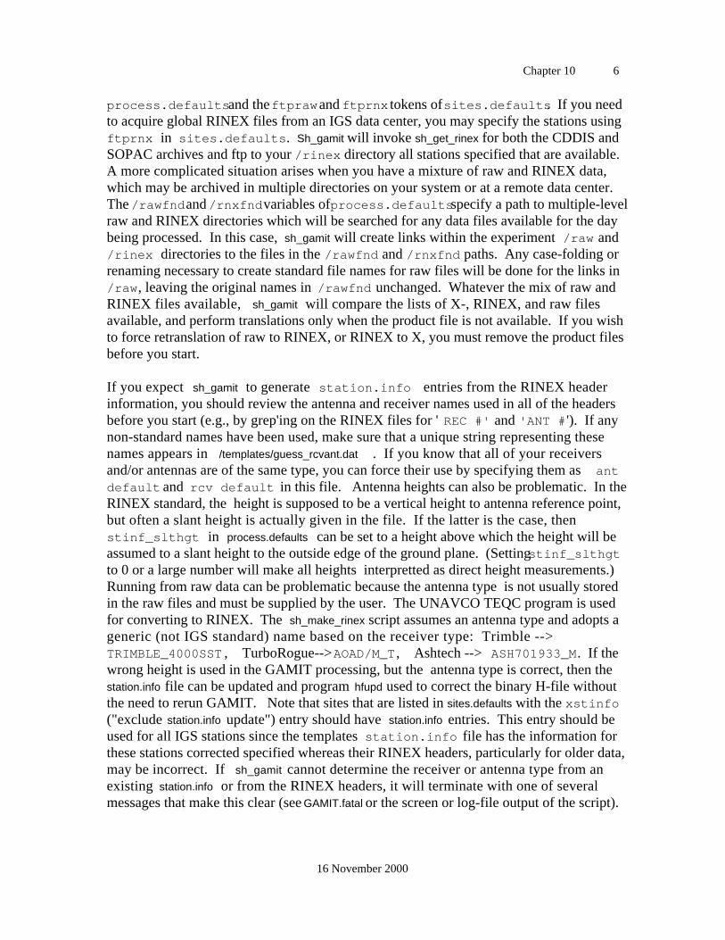
Chapter 10 6

16 November 2000

process.defaults and the ftpraw and ftprnx tokens of sites.defaults. If you needto acquire global RINEX files from an IGS data center, you may specify the stations usingftprnx in sites.defaults. Sh_gamit will invoke sh_get_rinex for both the CDDIS andSOPAC archives and ftp to your /rinex directory all stations specified that are available.A more complicated situation arises when you have a mixture of raw and RINEX data,which may be archived in multiple directories on your system or at a remote data center.The /rawfnd and /rnxfnd variables of process.defaults specify a path to multiple-levelraw and RINEX directories which will be searched for any data files available for the daybeing processed. In this case, sh_gamit will create links within the experiment /raw and/rinex directories to the files in the /rawfnd and /rnxfnd paths. Any case-folding orrenaming necessary to create standard file names for raw files will be done for the links in/raw, leaving the original names in /rawfnd unchanged. Whatever the mix of raw andRINEX files available, sh_gamit will compare the lists of X-, RINEX, and raw filesavailable, and perform translations only when the product file is not available. If you wishto force retranslation of raw to RINEX, or RINEX to X, you must remove the product filesbefore you start.

If you expect sh_gamit to generate station.info entries from the RINEX headerinformation, you should review the antenna and receiver names used in all of the headersbefore you start (e.g., by grep'ing on the RINEX files for ' REC #' and 'ANT #'). If anynon-standard names have been used, make sure that a unique string representing thesenames appears in /templates/guess_rcvant.dat . If you know that all of your receiversand/or antennas are of the same type, you can force their use by specifying them as antdefault and rcv default in this file. Antenna heights can also be problematic. In theRINEX standard, the height is supposed to be a vertical height to antenna reference point,but often a slant height is actually given in the file. If the latter is the case, thenstinf_slthgt in process.defaults can be set to a height above which the height will beassumed to a slant height to the outside edge of the ground plane. (Setting stinf_slthgtto 0 or a large number will make all heights interpretted as direct height measurements.)Running from raw data can be problematic because the antenna type is not usually storedin the raw files and must be supplied by the user. The UNAVCO TEQC program is usedfor converting to RINEX. The sh_make_rinex script assumes an antenna type and adopts ageneric (not IGS standard) name based on the receiver type: Trimble -->TRIMBLE_4000SST , TurboRogue-->AOAD/M_T , Ashtech --> ASH701933_M. If thewrong height is used in the GAMIT processing, but the antenna type is correct, then thestation.info file can be updated and program hfupd used to correct the binary H-file withoutthe need to rerun GAMIT. Note that sites that are listed in sites.defaults with the xstinfo("exclude station.info update") entry should have station.info entries. This entry should beused for all IGS stations since the templates station.info file has the information forthese stations corrected specified whereas their RINEX headers, particularly for older data,may be incorrect. If sh_gamit cannot determine the receiver or antenna type from anexisting station.info or from the RINEX headers, it will terminate with one of severalmessages that make this clear (see GAMIT.fatal or the screen or log-file output of the script).

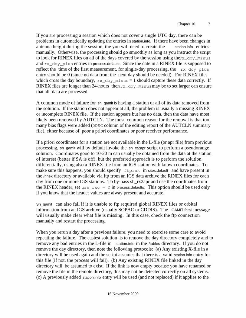
Chapter 10 7

16 November 2000

If you are processing a session which does not cover a single UTC day, there can beproblems in automatically updating the entries in station.info. If there have been changes inantenna height during the session, the you will need to create the station.info entriesmanually. Otherwise, the processing should go smoothly as long as you instruct the scriptto look for RINEX files on all of the days covered by the session using the rx_doy_minusand rx_doy_plus entries in process.defaults. Since the date in a RINEX file is supposed toreflect the time of the first measurement, for single-day processing, the rx_doy_plusentry should be 0 (since no data from the next day should be needed). For RINEX fileswhich cross the day boundary, rx_doy_minus = 1 should capture these data correctly. IfRINEX files are longer than 24-hours then rx_doy_minus may be to set larger can ensurethat all data are processed.

A common mode of failure for sh_gamit is having a station or all of its data removed fromthe solution. If the station does not appear at all, the problem is usually a missing RINEXor incomplete RINEX file. If the station appears but has no data, then the data have mostlikely been removed by AUTCLN. The most common reason for the removal is that toomany bias flags were added (DDSC column of the editing report of the AUTCLN summaryfile), either because of poor a priori coordinates or poor receiver performance.

If a priori coordinates for a station are not available in the L-file (or apr file) from previousprocessing, sh_gamit will by default invoke the sh_rx2apr script to perform a pseudorangesolution. Coordinates good to 10-20 m can usually be obtained from the data at the stationof interest (better if SA is off), but the preferred approach is to perform the solutiondifferentially, using also a RINEX file from an IGS station with known coordinates. Tomake sure this happens, you should specify ftprnx in sites.default and have present inthe /rinex directory or available via ftp from an IGS data archive the RINEX files for eachday from one or more IGS stations. To by-pass sh_rx2apr and use the coordinates fromthe RINEX header, set use_rxc = Y in process.defaults. This option should be used onlyif you know that the header values are alway present and accurate.

Sh_gamit can also fail if it is unable to ftp required global RINEX files or orbitalinformation from an IGS archive (usually SOPAC or CDDIS). The GAMIT.fatal messagewill usually make clear what file is missing. In this case, check the ftp connectionmanually and restart the processing.

When you rerun a day after a previous failure, you need to exercise some care to avoidrepeating the failure. The easiest solution is to remove the day directory completely and toremove any bad entries in the L-file in station.info in the /tables directory. If you do notremove the day directory, then note the following protocols: (a) Any existing X-file in adirectory will be used again and the script assumes that there is a valid station.info entry forthis file (if not, the process will fail). (b) Any existing RINEX file linked in the daydirectory will be assumed to exist. If the link is now empty because you have renamed orremove the file in the remote directory, this may not be detected correctly on all systems.(c) A previously added station.info entry will be used (and not replaced) if it applies to the

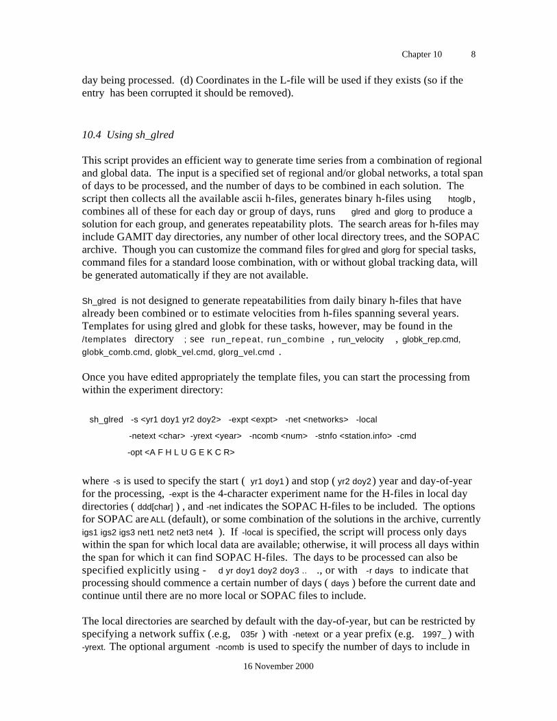
Chapter 10 8

16 November 2000

day being processed. (d) Coordinates in the L-file will be used if they exists (so if theentry has been corrupted it should be removed).

10.4 Using sh_glred

This script provides an efficient way to generate time series from a combination of regionaland global data. The input is a specified set of regional and/or global networks, a total spanof days to be processed, and the number of days to be combined in each solution. Thescript then collects all the available ascii h-files, generates binary h-files using htoglb ,combines all of these for each day or group of days, runs glred and glorg to produce asolution for each group, and generates repeatability plots. The search areas for h-files mayinclude GAMIT day directories, any number of other local directory trees, and the SOPACarchive. Though you can customize the command files for glred and glorg for special tasks,command files for a standard loose combination, with or without global tracking data, willbe generated automatically if they are not available.

Sh_glred is not designed to generate repeatabilities from daily binary h-files that havealready been combined or to estimate velocities from h-files spanning several years.Templates for using glred and globk for these tasks, however, may be found in the/templates directory ; see run_repeat, run_combine , run_velocity , globk_rep.cmd,

globk_comb.cmd, globk_vel.cmd, glorg_vel.cmd .

Once you have edited appropriately the template files, you can start the processing fromwithin the experiment directory:

sh_glred -s <yr1 doy1 yr2 doy2> -expt <expt> -net <networks> -local

-netext <char> -yrext <year> -ncomb <num> -stnfo <station.info> -cmd

-opt <A F H L U G E K C R>

where -s is used to specify the start ( yr1 doy1 ) and stop ( yr2 doy2 ) year and day-of-yearfor the processing, -expt is the 4-character experiment name for the H-files in local daydirectories ( ddd[char] ) , and -net indicates the SOPAC H-files to be included. The optionsfor SOPAC are ALL (default), or some combination of the solutions in the archive, currentlyigs1 igs2 igs3 net1 net2 net3 net4 ). If -local is specified, the script will process only dayswithin the span for which local data are available; otherwise, it will process all days withinthe span for which it can find SOPAC H-files. The days to be processed can also bespecified explicitly using - d yr doy1 doy2 doy3 .. ., or with -r days to indicate thatprocessing should commence a certain number of days ( days ) before the current date andcontinue until there are no more local or SOPAC files to include.

The local directories are searched by default with the day-of-year, but can be restricted byspecifying a network suffix (.e.g, 035r ) with -netext or a year prefix (e.g. 1997_ ) with-yrext. The optional argument -ncomb is used to specify the number of days to include in

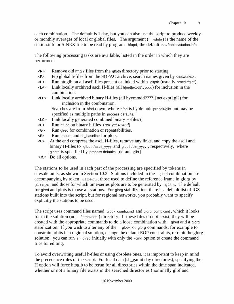
Chapter 10 9

16 November 2000

each combination. The default is 1 day, but you can also use the script to produce weeklyor monthly averages of local or global files. The argument ( -stnfo ) is the name of thestation.info or SINEX file to be read by program hfupd; the default is .. /tables/station.info .

The following processing tasks are available, listed in the order in which they areperformed:

<R> Remove old h*.gl? files from the glfpth directory prior to starting. <F> Ftp global h-files from the SOPAC archive, search names given by <networks> . <H> Run htoglb on all ascii files present or linked within glfpth (usually procdir/glbf).

<LA> Link locally archived ascii H-files (all h[net|expt]?.yyddd) for inclusion in the combination.

<LB> Link locally archived binary H-files (all hyymmdd????_[net|expt].gl?) for inclusion in the combination.

Searches are from hfnd down, where hfnd is by default procdir/glbf but may be specified as multiple paths in process.defaults.

<LC> Link locally generated combined binary H-files (<U> Run hfupd on binary h-files (not yet tested).<G> Run glred for combination or repeatabilities.<E> Run ensum and sh_baseline for plots.<C> At the end compress the ascii H-files, remove any links, and copy the ascii and

binary H-files to glbpth/ascii_yyyy and glbpth/bin_yyyy , respectively, where glbpth is specified by process.defaults [default glbf]

<A> Do all options.

The stations to be used in each part of the processing are specified by tokens insites.defaults, as shown in Section 10.2. Stations included in the glred combination areaccompanying by token glrepu , those used to define the reference frame in glorg byglreps, and those for which time-series plots are to be generated by glts. The defaultfor glred and plots is to use all stations. For glorg stabilization, there is a default list of IGSstations built into the script, but for regional networks, you probably want to specifyexplicitly the stations to be used.

The script uses command files named globk_comb.cmd and glorg_comb.cmd , which it looksfor in the solution (not /templates ) directory. If these files do not exist, they will becreated with the appropriate commands to do a loose combination with glred and a glorg

stabilization. If you wish to alter any of the globk or glorg commands, for example toconstrain orbits in a regional solution, change the default EOP constraints, or omit the glorgsolution, you can run sh_glred initially with only the -cmd option to create the commandfiles for editing.

To avoid overwriting useful h-files or using obsolete ones, it is important to keep in mindthe precedence rules of the script. For local data (sh_gamit day directories), specifying theH option will force htoglb to be rerun for all directories within the time span indicated,whether or not a binary file exists in the searched directories (nominally glbf and

Chapter 10 10

16 November 2000

glbf/bin_yyyy). Omitting H will cause no new binary files to be created, so it is notpossible to retranslate only a selected group of ascii H-files. This is not an importantlimitation, however, because retranslated htoglb runs quickly. For remote data (locallylinked or ftp'd from SOPAC), setting H will also force htoglb to be rerun on any ascii H-files present or linked (by LA) in the H-file (glbf) directory, but you can safely set F sincethe script will not re-ftp any remote (ascii) H-files that are present.

Output H-files from the combination are named HYYMMDD_[expt][netext].GLX and written into the solution directory. The script creates a separate .gdl file for each day with a similarname, each pointing to the combined GLX H-file in the solution directory. When ensum isrun, it will create SUM. and VAL. files by concatenating all .org files present, so you can runsh_glred separately for different time spans and create plots that combine the spans.

Examples

Combine regional files from sh_gamit with global files from SOPAC, one day at a time andgenerate repeatability plots:

sh_glred -d 1999 235 1999 250 -net igs1 igs2 igs3 -netext r -expt emed -opt F H G E C

Regenerate repeatability plots from existing binary h-files (e.g with different stabilzation):

sh_glred -d 1999 235 1999 250 -net igs1 igs2 igs3 -netext r -expt emed -opt G E

Combine existing regional and global binary h-files into monthly averages: " sh_glred - d 1999 235 2000 120 -ncomb 30 -net igs1 igs2 igs3 -expt emed -opt G LB

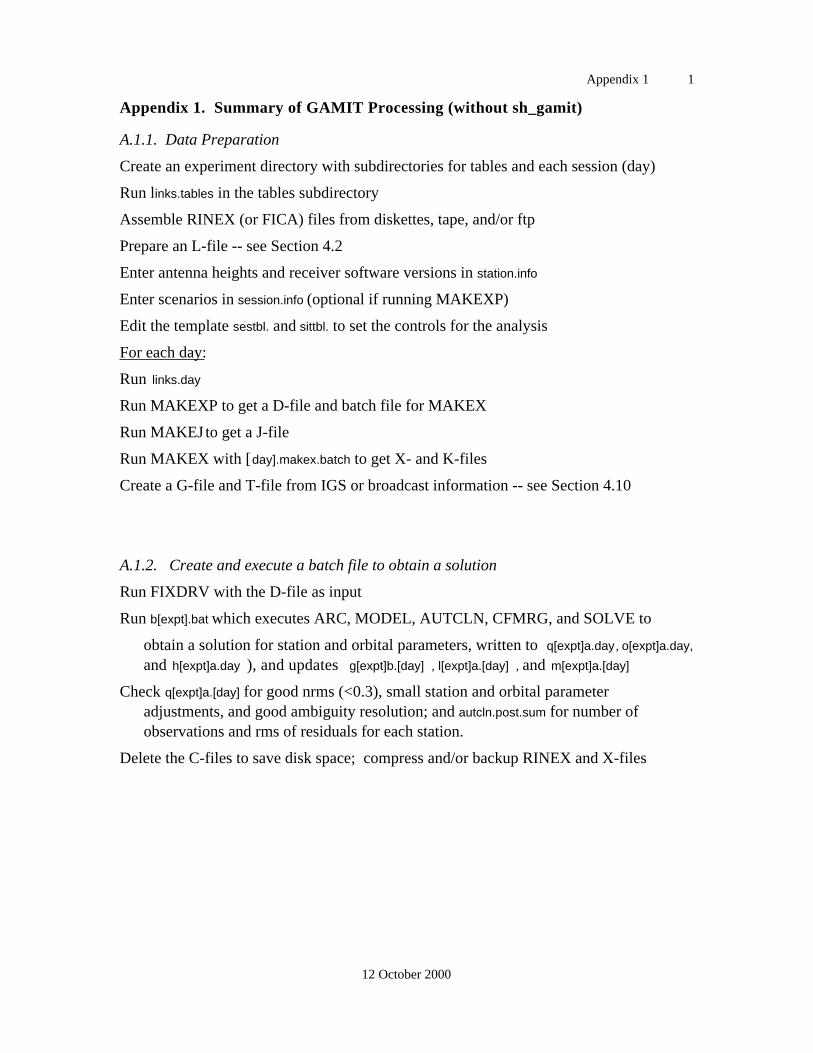
Appendix 1 1

12 October 2000

Appendix 1. Summary of GAMIT Processing (without sh_gamit)

A.1.1. Data Preparation

Create an experiment directory with subdirectories for tables and each session (day)

Run links.tables in the tables subdirectory

Assemble RINEX (or FICA) files from diskettes, tape, and/or ftp

Prepare an L-file -- see Section 4.2

Enter antenna heights and receiver software versions in station.info

Enter scenarios in session.info (optional if running MAKEXP)

Edit the template sestbl. and sittbl. to set the controls for the analysis

For each day:

Run links.day

Run MAKEXP to get a D-file and batch file for MAKEX

Run MAKEJ to get a J-file

Run MAKEX with [day].makex.batch to get X- and K-files

Create a G-file and T-file from IGS or broadcast information -- see Section 4.10

A.1.2. Create and execute a batch file to obtain a solution

Run FIXDRV with the D-file as input

Run b[expt].bat which executes ARC, MODEL, AUTCLN, CFMRG, and SOLVE to

obtain a solution for station and orbital parameters, written to q[expt]a.day , o[expt]a.day,

and h[expt]a.day ), and updates g[expt]b.[day] , l[expt]a.[day] , and m[expt]a.[day]

Check q[expt]a.[day] for good nrms (<0.3), small station and orbital parameteradjustments, and good ambiguity resolution; and autcln.post.sum for number ofobservations and rms of residuals for each station.

Delete the C-files to save disk space; compress and/or backup RINEX and X-files

Appendix 1 2

12 October 2000

A.1.3 File-naming conventions

A - file: ASCII version of the T-file (tabular ephemeris)

B - file: controls the batch mode of data processing

C - file: observed – computed (O-C's), partial derivatives

D - file: driver file of sessions and receivers

E - file: broadcast ephemeris, in FICA Blk 9 or RINEX navigation file format

G - file: orbital initial conditions and non-gravitational parameter values

H - file: adjustments and full variance-covariance matrix for input to GLOBK

I - file: receiver clock polynomial input

J - file: satellite clock polynomial coefficients

K - file: values of receiver clock offset during observation span, from pseudorange

L - file: station coordinates

M - file: controls merging of data (C-) files for SOLVE and editing programs

N - file: data-weight overrides for SOLVE created from autcln.sum.postfit

O - file: record of the analysis (reduced form of Q-file) for post-processing analysis

P - file: record of a MODEL run

Q - file: record of the analysis (SOLVE run)

S - file: station coordinates and antenna offsets — no longer used

T - file: tabular ephemeris

U - file: ocean tide constituents

V- file: editing output of SINCLN, DBLCLN, and SCANRMS

W - file: meteorological data

X - file: input observations

Y - file: satellite yaw parameters

Z - file: water-vapor radiometer data

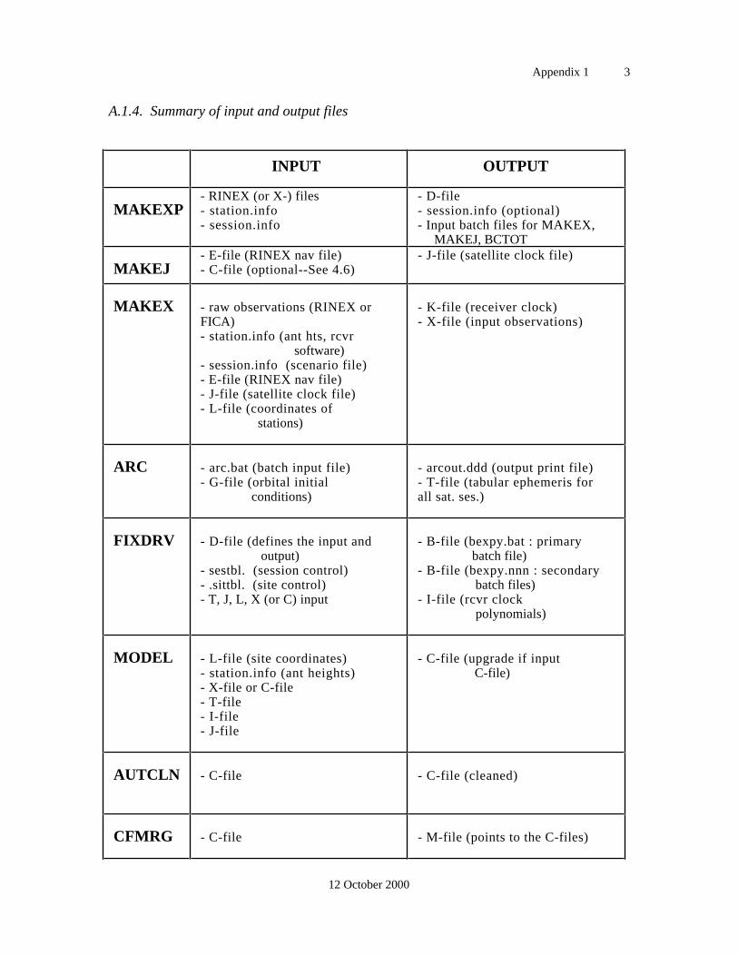
Appendix 1 3

12 October 2000

A.1.4. Summary of input and output files

INPUT OUTPUT

MAKEXP- RINEX (or X-) files- station.info- session.info

- D-file- session.info (optional)- Input batch files for MAKEX, MAKEJ, BCTOT

MAKEJ- E-file (RINEX nav file)- C-file (optional--See 4.6)

- J-file (satellite clock file)

MAKEX - raw observations (RINEX orFICA)- station.info (ant hts, rcvr software)- session.info (scenario file)- E-file (RINEX nav file)- J-file (satellite clock file)- L-file (coordinates of stations)

- K-file (receiver clock)- X-file (input observations)

ARC - arc.bat (batch input file)- G-file (orbital initial conditions)

- arcout.ddd (output print file)- T-file (tabular ephemeris forall sat. ses.)

FIXDRV - D-file (defines the input and output)- sestbl. (session control)- .sittbl. (site control)- T, J, L, X (or C) input

- B-file (bexpy.bat : primary batch file)- B-file (bexpy.nnn : secondary batch files)- I-file (rcvr clock polynomials)

MODEL - L-file (site coordinates)- station.info (ant heights)- X-file or C-file- T-file- I-file- J-file

- C-file (upgrade if input C-file)

AUTCLN - C-file - C-file (cleaned)

CFMRG - C-file - M-file (points to the C-files)

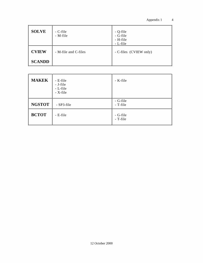
Appendix 1 4

12 October 2000

SOLVE - C-file- M-file

- Q-file- G-file- H-file- L-file

CVIEW

SCANDD

- M-file and C-files - C-files (CVIEW only)

MAKEK - E-file- J-file- L-file- X-file

- K-file

NGSTOT - SP3-file- G-file- T-file

BCTOT - E-file - G-file- T-file

Appendix 2 1

30 November 1999

Appendix 2. Antenna Specifications

A.2.1 Introduction

Accurate and consistent modeling of the antenna phase centers continues to be one of themost vexing problems in GPS analysis. For purposes of discussion it is useful to dividethe problem into horizontal and vertical effects, and to consider for the latter the "absolute"and relative models.

For most of the antennas there are horizontal offsets of a few millimeters of the L1 and/orL2 phase centers from the mechanical center of the antenna. These are sometimes notrepeatable among individual antennas of a particular type and can be over 5 mm foranalyses using the ionospheric-free (LC) combination of L1 and L2 phase. These offsetscan be determined by measurements of the antenna phase pattern in an anechoic chamber[Schupler et al. , 1991; Rocken et al. , 1995] or by analysis of short baseline fieldmeasurements in which the antennas are rotated between sessions [Braun et al., 1996].

The vertical positions of the phase centers of all GPS antennas show significant elevation-dependent motions, which if not modeled make estimated station heights dependent on theelevation cutoff angle of the observations at each station. The size of the effect can varyfrom a few millimeters for matched antennas in a regional network in which all stationshave nearly the same horizon, to several centimeters for some combinations of mismatchedantennas. The vertical phase center, as a function of elevation angle, can be mapped forindividual antennas using anechoic chamber measurements [ Schupler et al., 1991 ] ordifferentially for pairs of antennas by estimating coefficients of a polynomial or spherical-harmonic model [Mader and McKay, 1996; Rothacher et al. 1995]. When the "absolute"models determined from anechoic chamber measurements are used in analyses of globaltracking data, station heights differ 6-12 cm from values inferred from SLR and VLBI data,implying a GPS scale error of ~10 –8 . More likely, there is some aspect of the anechoicchamber measurements that is not yet understood. The difference in elevation-dependentvariations from anechoic chamber measurements of pairs of antennas, however, agreereasonably well (25%) with those inferred from estimated from field measurements overshort baselines, allowing inference of the vertical phase center, independent of elevation-angle cutoff, at the level of about 5 mm for some antennas. For others, the agreement ispoorer, presumably indicating significant effects that depend on the electrical environmentof the measurements. For example, Elosequi et al. [1995] demonstrated centimeter-leveleffects from the pillar used to support the antenna.

Although an effective "absolute" model for vertical offsets remains illusive, the IGS issuedin June, 1996, a provisional differential model that represents usefully the mean verticaland horizontal offsets for many of the commonly used antennas [ Rothacher and Mader ,1996]. This model, designated IGS_01, arbitrarily assumes no elevation-dependent termsfor the Dorne-Margolin choke ring antennas used in the global network and applieselevation-dependent variations for other antennas. Since the release of IGS_01, the USNational Geodetic Survey and Geodynamics Research Division of NOAA have carried out

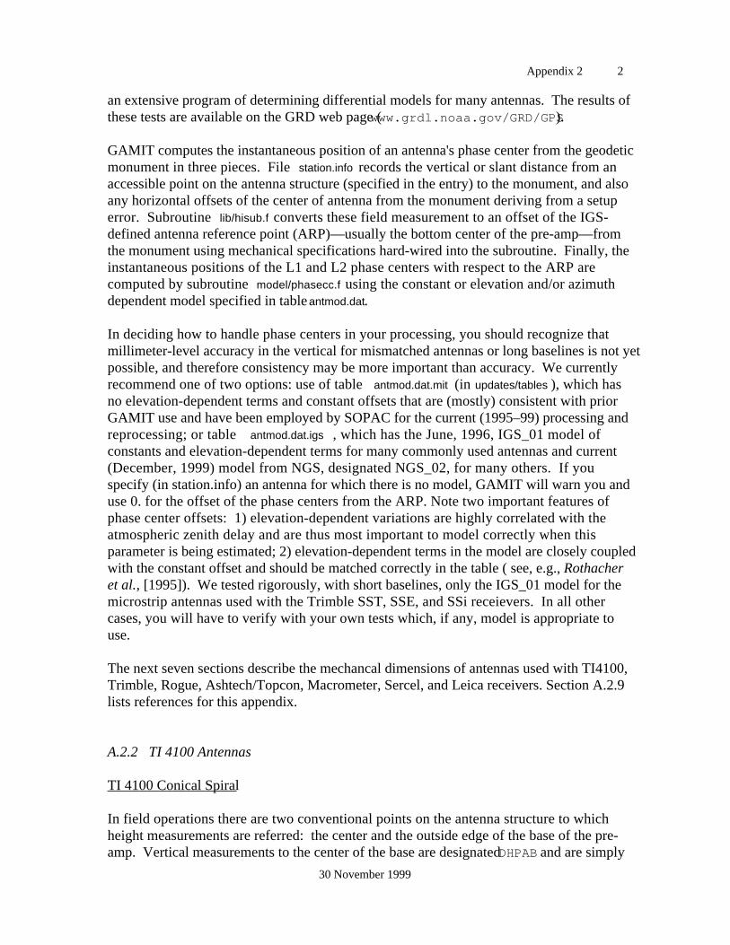
Appendix 2 2

30 November 1999

an extensive program of determining differential models for many antennas. The results ofthese tests are available on the GRD web page (www.grdl.noaa.gov/GRD/GPS).

GAMIT computes the instantaneous position of an antenna's phase center from the geodeticmonument in three pieces. File station.info records the vertical or slant distance from anaccessible point on the antenna structure (specified in the entry) to the monument, and alsoany horizontal offsets of the center of antenna from the monument deriving from a setuperror. Subroutine lib/hisub.f converts these field measurement to an offset of the IGS-defined antenna reference point (ARP)—usually the bottom center of the pre-amp—fromthe monument using mechanical specifications hard-wired into the subroutine. Finally, theinstantaneous positions of the L1 and L2 phase centers with respect to the ARP arecomputed by subroutine model/phasecc.f using the constant or elevation and/or azimuthdependent model specified in table antmod.dat.

In deciding how to handle phase centers in your processing, you should recognize thatmillimeter-level accuracy in the vertical for mismatched antennas or long baselines is not yetpossible, and therefore consistency may be more important than accuracy. We currentlyrecommend one of two options: use of table antmod.dat.mit (in updates/tables ), which hasno elevation-dependent terms and constant offsets that are (mostly) consistent with priorGAMIT use and have been employed by SOPAC for the current (1995–99) processing andreprocessing; or table antmod.dat.igs , which has the June, 1996, IGS_01 model ofconstants and elevation-dependent terms for many commonly used antennas and current(December, 1999) model from NGS, designated NGS_02, for many others. If youspecify (in station.info) an antenna for which there is no model, GAMIT will warn you anduse 0. for the offset of the phase centers from the ARP. Note two important features ofphase center offsets: 1) elevation-dependent variations are highly correlated with theatmospheric zenith delay and are thus most important to model correctly when thisparameter is being estimated; 2) elevation-dependent terms in the model are closely coupledwith the constant offset and should be matched correctly in the table ( see, e.g., Rothacheret al., [1995]). We tested rigorously, with short baselines, only the IGS_01 model for themicrostrip antennas used with the Trimble SST, SSE, and SSi receievers. In all othercases, you will have to verify with your own tests which, if any, model is appropriate touse.

The next seven sections describe the mechancal dimensions of antennas used with TI4100,Trimble, Rogue, Ashtech/Topcon, Macrometer, Sercel, and Leica receivers. Section A.2.9lists references for this appendix.

A.2.2 TI 4100 Antennas

TI 4100 Conical Spiral

In field operations there are two conventional points on the antenna structure to whichheight measurements are referred: the center and the outside edge of the base of the pre-amp. Vertical measurements to the center of the base are designated DHPAB and are simply

Appendix 2 3

30 November 1999

added to the table values to get the L1 and L2 phase centers. Slant height measurements tothe edge of the base are designated SLPAB and converted to vertical heights using thepythagorean rule and a base radius of 0.8415 m.

The values given in the antmod.dat.mit for the early series 100 and 2000 antennas,designated TI_100 and TI2000, respectively but both aliased to TI4100, are taken fromSims [1985]. For the newer and more common 4000 series antennas, designated TI4000,the values were determined by Schupler et al. [1992] and confirmed by our own analysis.Use of the Schupler et al. variable phase-center model will increase the heights (relative toother antenna types) estimated from LC observations by about 15 mm.

TI 4100 FRPA-2 microstrip

These antennas have been used only at the CIGNET fiducial stations at Richmond(Florida), Mojave (California), and Kauai (Hawaii). The offsets given in antmod.dat.mit

are based on UNAVCO short baseline tests (personal communication, John Braun, 21 May1994). They are untested in MIT or SOPAC analyses.

A.2.3 Trimble Antennas

Trimble 4000 SST

The 4000 SST antenna ( TRMSST ), part # 145321 and usually designated "4000ST L1/L2Geodetic", is a microstrip which has a round ground plane with horizonally scalloped andvertically beveled edges. Below the ground plane is a small square box containing the pre-amp. Field height measurements are commonly made to the outer edge of the groundplane—either the top, middle, or bottom of the beveled edge. Subroutine hisub is coded toaccept slant height measurements to the top ( SLTGP , radius 0.2403 m), middle ( SLMGP ,radius 0.2413 m), or bottom ( SLBGP , radius 0.2403 m) of the ground plane, and also adirect height to the bottom of the ground plane ( DHBGP). If the Trimble measuring rod isused, the height measurement is usually made to the inside of one or more of the notches(radius 0.2334), on either the top (SLTGN) or bottom (SLTBGN) of the ground plane. Thebottom of the ground plane is 0.060 m, the middle 0.0615 m, and the top 0.063 m abovethe ARP (base of pre-amp).

With no elevation-dependent model, Trimble specifications and UNAVCO tests put the L1phase center 6.2 mm above, and the L2 phase center 4.7 mm above the top of the groundplane. Use of the variable phase-center model will increase heights estimated from LCobservations by about 15 mm. Rotation tests and anechoic chamber measurements suggestthat there are differences of at least several millimeters, in both the vertical and horizontaldirections (C. Rocken, personal communication, 1995; Rothacher and Mader, 1996). TheIGS_01 model reflects these differences.

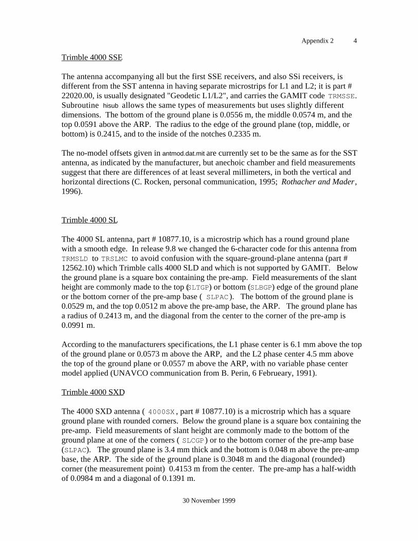
Appendix 2 4

30 November 1999

Trimble 4000 SSE

The antenna accompanying all but the first SSE receivers, and also SSi receivers, isdifferent from the SST antenna in having separate microstrips for L1 and L2; it is part #22020.00, is usually designated "Geodetic L1/L2", and carries the GAMIT code TRMSSE.Subroutine hisub allows the same types of measurements but uses slightly differentdimensions. The bottom of the ground plane is 0.0556 m, the middle 0.0574 m, and thetop 0.0591 above the ARP. The radius to the edge of the ground plane (top, middle, orbottom) is 0.2415, and to the inside of the notches 0.2335 m.

The no-model offsets given in antmod.dat.mit are currently set to be the same as for the SSTantenna, as indicated by the manufacturer, but anechoic chamber and field measurementssuggest that there are differences of at least several millimeters, in both the vertical andhorizontal directions (C. Rocken, personal communication, 1995; Rothacher and Mader,1996).

Trimble 4000 SL

The 4000 SL antenna, part # 10877.10, is a microstrip which has a round ground planewith a smooth edge. In release 9.8 we changed the 6-character code for this antenna fromTRMSLD to TRSLMC to avoid confusion with the square-ground-plane antenna (part #12562.10) which Trimble calls 4000 SLD and which is not supported by GAMIT. Belowthe ground plane is a square box containing the pre-amp. Field measurements of the slantheight are commonly made to the top (SLTGP) or bottom (SLBGP) edge of the ground planeor the bottom corner of the pre-amp base ( SLPAC ). The bottom of the ground plane is0.0529 m, and the top 0.0512 m above the pre-amp base, the ARP. The ground plane hasa radius of 0.2413 m, and the diagonal from the center to the corner of the pre-amp is0.0991 m.

According to the manufacturers specifications, the L1 phase center is 6.1 mm above the topof the ground plane or 0.0573 m above the ARP, and the L2 phase center 4.5 mm abovethe top of the ground plane or 0.0557 m above the ARP, with no variable phase centermodel applied (UNAVCO communication from B. Perin, 6 Februeary, 1991).

Trimble 4000 SXD

The 4000 SXD antenna ( 4000SX , part # 10877.10) is a microstrip which has a squareground plane with rounded corners. Below the ground plane is a square box containing thepre-amp. Field measurements of slant height are commonly made to the bottom of theground plane at one of the corners ( SLCGP) or to the bottom corner of the pre-amp base(SLPAC). The ground plane is 3.4 mm thick and the bottom is 0.048 m above the pre-ampbase, the ARP. The side of the ground plane is 0.3048 m and the diagonal (rounded)corner (the measurement point) 0.4153 m from the center. The pre-amp has a half-widthof 0.0984 m and a diagonal of 0.1391 m.

Appendix 2 5

30 November 1999

According to the manufacturers specifications, the L1 phase center is 6.2 mm above the topof the ground plane or 0.0574 m above the ARP, and the L2 phase center 4.6 mm abovethe top of the ground plane or 0.0558 m above the ARP, with no variable phase centermodel applied (UNAVCO communication from B. Perin, 6 February, 1991).

A.2.4 Rogue Antennas

Dorne-Margolin with Choke Ring

There are three antennas used with Rogue, MiniRogue, and TurboRogue receivers, allvariations of a Dorne-Margolin element mounted with the circular ground plane and chokerings based on a JPL design. The antennas used with the original Rogue SNR-8 werebuilt at JPL and are designated model "R" ( ROGSNR, DMRCHR, or ROGDMR ); the earlymodels built by Allen Osborne Associates (AOA) are designated model "B" ( ROGAOA,DMBCHR, or ROGDMB); and the AOA models currently distributed with the TurboRogue aredesignated model "T" (TRBROG, DMTCHR, or ROGDMT,). If the antenna is mounted on atripod, height measurements are usually made to the bottom of the choke ring or anunderlying baseplate. If the antenna is spike-mounted on the ground, the measurement ismade to the bottom of the baseplate. In some permanent mounts surveyed by theodolite,the direct height may be specified to the the top of the choke rings (DHTCR).

For the "R" model, the ARP is the bottom of a base plate, 0.381 mm in diameter and 6 mmthick. The choke ring above is 64 mm high, so that the top of the choke ring is 70 mmabove the ARP. Measurements made to the bottom of the assembly are all to the ARP,whether designated "pre-amp base" (DHPAB) or "bottom of choke ring" (DHBCR or SLBCR).

The "B" model replaced the thin baseplate with one 11 mm high and 351 mm in diameter,and increased the choke ring height to 70 mm. For this model the ARP is the bottom of thechoke rings, not the bottom of the baseplate, so that the top of the choke rings is still 70mm above the ARP.

The "T" model has a choke ring 67 mm high including the baseplate and a pre-amp 35 mmhigh. The ARP is the bottom of the pre-amp, so that the top of the choke rings is 102 mmabove the ARP. The width of the choke rings is 381 mm.

According to the manufacturers' nominal specifications, with no variable model, the L1phase center is 8 mm, and the L2 phase center 26 mm above the top of the choke rings forall three models.

A.2.5 Ashtech Antennas

There have been primary three models, with several variatiions each, of the Ashtech dual-frequency micro-strip antennas. The first two models (both part #700228) both use a BallCorporation microstrip patch and have a 28-cm ground plane but have different amplifiers

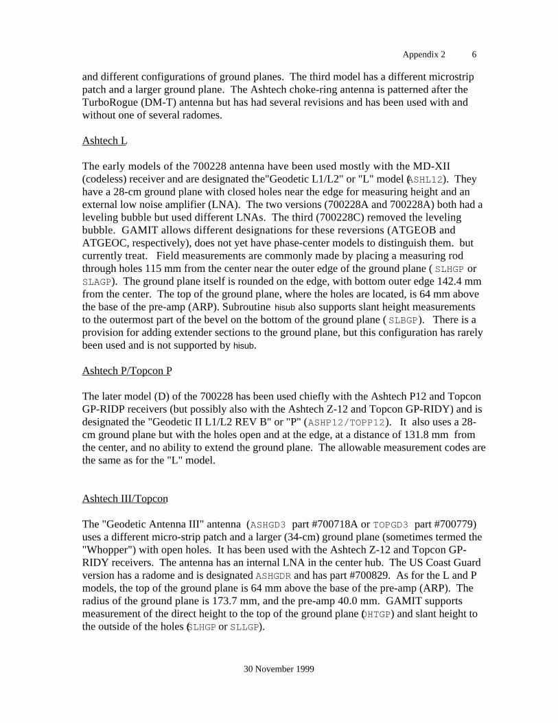
Appendix 2 6

30 November 1999

and different configurations of ground planes. The third model has a different microstrippatch and a larger ground plane. The Ashtech choke-ring antenna is patterned after theTurboRogue (DM-T) antenna but has had several revisions and has been used with andwithout one of several radomes.

Ashtech L

The early models of the 700228 antenna have been used mostly with the MD-XII(codeless) receiver and are designated the"Geodetic L1/L2" or "L" model (ASHL12). Theyhave a 28-cm ground plane with closed holes near the edge for measuring height and anexternal low noise amplifier (LNA). The two versions (700228A and 700228A) both had aleveling bubble but used different LNAs. The third (700228C) removed the levelingbubble. GAMIT allows different designations for these reversions (ATGEOB andATGEOC, respectively), does not yet have phase-center models to distinguish them. butcurrently treat. Field measurements are commonly made by placing a measuring rodthrough holes 115 mm from the center near the outer edge of the ground plane ( SLHGP orSLAGP). The ground plane itself is rounded on the edge, with bottom outer edge 142.4 mmfrom the center. The top of the ground plane, where the holes are located, is 64 mm abovethe base of the pre-amp (ARP). Subroutine hisub also supports slant height measurementsto the outermost part of the bevel on the bottom of the ground plane ( SLBGP). There is aprovision for adding extender sections to the ground plane, but this configuration has rarelybeen used and is not supported by hisub.

Ashtech P/Topcon P

The later model (D) of the 700228 has been used chiefly with the Ashtech P12 and TopconGP-RIDP receivers (but possibly also with the Ashtech Z-12 and Topcon GP-RIDY) and isdesignated the "Geodetic II L1/L2 REV B" or "P" (ASHP12/TOPP12). It also uses a 28-cm ground plane but with the holes open and at the edge, at a distance of 131.8 mm fromthe center, and no ability to extend the ground plane. The allowable measurement codes arethe same as for the "L" model.

Ashtech III/Topcon

The "Geodetic Antenna III" antenna (ASHGD3 part #700718A or TOPGD3 part #700779)uses a different micro-strip patch and a larger (34-cm) ground plane (sometimes termed the"Whopper") with open holes. It has been used with the Ashtech Z-12 and Topcon GP-RIDY receivers. The antenna has an internal LNA in the center hub. The US Coast Guardversion has a radome and is designated ASHGDR and has part #700829. As for the L and Pmodels, the top of the ground plane is 64 mm above the base of the pre-amp (ARP). Theradius of the ground plane is 173.7 mm, and the pre-amp 40.0 mm. GAMIT supportsmeasurement of the direct height to the top of the ground plane (DHTGP) and slant height tothe outside of the holes (SLHGP or SLLGP).

Appendix 2 7

30 November 1999

At the present time, the effective phase centers of the Ashtech microstrip antennas isuncertain. Short baseline GPS and anechoic chamber measurements give inconsistentresults. In table antmod.dat.mit we have maintained the offsets determined for Release 9.2,which place the L1 phase center ~33 mm, and the L2 phase center ~13 mm above theground plane. Previous GAMIT releases assumed that both L1 and L2 phase centers are inthe ground plane. The IGS_01 model in antmod.dat.igs gives elevation-dependent modelsfor these antennas but they are based on limited, non-redundant tests and do not have thereliability of the models for the Trimble microstrip or the choke-ring antennas

Ashtech Dorne-Margolin with Choke Ring

There have been 14 different versions of the Ashtech choke-ring antenna, some triviallydifferent and some with changes that might affect the phase pattern. All have beendesigned to be mechanically and electrically equivalent to the Turbo-Rogue ("T") antenna,and in the current version of antmod.dat are assigned the same (null) model as the D-M T.To allow tracking of small potential changes, however, each of these models is assigned adifferent name, both by the IGS and in GAMIT (see rcvant.dat ). One possibly importantdifference arises when the antenna is used with the Ashtech-supplied conical radome.Tests at UNAVCO [ Rocken et al ., 1995] and MIT [ Niell et al., 1996] suggest that thephase center changes in vertical by 5–15 mm when this radome is used, but similar tests atAIUB (Bern) and NGS obtain differences less than 3 mm [ Rothacher and Mader , 1996].The use of a centered spherical radome of the type currently imployed by SCIGN producesno significant change in the phase pattern.

A.2.6 MACROMETER Antennas

Min-Mac 2816 AT

The Macrometer antenna used with the Mini-Mac 2816 AT is a crossed dipole above a thicksquare ground plane ( MINXDP or MIN6AT ). The ARP is the base of the ground planestructure, which contains the pre-amp. GAMIT supports only direct height measurementsto the ARP (DHPAB) or reference to the L1 phase center (L1PHC).

According to the manufacturer's specifications, the L1 phase center is 107.1 mm, and theL2 phase center 91.7 mm above the ARP [J. Ladd, private communication, 1989]. Use ofan elevation-dependent model corrects this by several centimeters.

A.2.7 SERCEL Antennas

For the SERCEL TR5S and NR52 antennas, we have only scant information conveyed byK. Feigl from the log sheets for the Djibouti 1991 observations. There are no mechanicaldimensions coded in hisub, so that only measurements to the ARP ( DHPAB) are allowed.The difference between the L1 and L2 phase centers is unknown. In antmod.dat , we

Appendix 2 8

30 November 1999

currently give for the TR5S (SRTR5S) phase center offsets from the ARP of 264 mm for theTR5S (SRTR5S) and 210 mm for the NR52 (SRNR52).

A.2.8 Leica Antennas

The Leica SR299/SR399 " Sensor", AT201/302, and AT303 antennas are attached directlyto a rotating bubble level ("carrier"; e.g. GRT44), or a "stop/go" kinematic pole via a screwhole on the bottom of the antenna. The ARP is defined as the bottom of the antennahousing, coincident with the top of the carrier. With the carrier mount and tripod,measurements are commonly made using a pull-down tape measure attached to a "height-hook", with the top of the tape measure (the read point) located 0.350 m below the ARP.You can specify a direct height to the ARP (DHPAB) or a direct height read from the height-hook tape (DHHHK). In using values recorded on field logsheets, be aware that the heighthook tape suggests to the operator adding 0.449 m to the measured value to account forboth the offset to the ARP (0.350 m) and the nominal L1 phase center (0.091 m above theARP). Be sure that you understand what value has been recorded. Also, the Sensorantennas may be used with a "ranging pole" (different from a "stop/go kinematic pole") viaan "adaptor with 5/8-in thread"; in this configuration the ARP, corresponding to the top ofthe pole, is 12 mm lower with respect to the phase centers. The range-pole configuration isnot coded in GAMIT. With the choke-ring antennas (AT303 and AT504), you may alsospecify slant-height measurements to the outside bottom edge of the choke rings (SLBCR).

The IGS_01 phase-center model in antmod.dat.igs has three elevation-dependent models forthe phase center, corresponding respectively to the SR299 or SR399 internal antennas(LC299I or LC399I), and the series 200 external antenna with (LC202G) or without(LC202N) a ground plane. The AT303 was intended by Leica to be slightly different fromthe IGS standard (DM-T TurboRogue antenna), so antmod.dat includes the NGS_02model for this antenna. The AT503 (LC_503) is assumed be the same as the DM-T.

A.7.8 References

Braun, J., C. Rocken, C. M. Meertens, and J. Johnson, GPS antenna mixing and phasecenter corrections, Eos Trans. AGU, 1993 Fall Meeting Supplement, p. 197, 1993.

Elosegui, P., J. L. Davis, R. T. K. Jaldehag, J. M. Johansson, A. E. Niell, and I. I.Shapiro, Goedesy using the Global Positioning System: The effects of signal scattering onestimates of site position, Journal of Geophysical Research, 100, 9921–9934, 1995.

Mader, G. L., and J.R. MacKay, Calibration of GPS antennas,http://www.grdl.noaa.gov/GPS/PROJECTS/ANTCAL , March, 1996.

Appendix 2 9

30 November 1999

Niell, A. E., R. W. King, S. C. McClusky, T. A. Herring, Radome effects on GPS heightmeasurements with choke-ring antennas, Eos Trans. AGU, Spring Meeting Supplement,S71, 1996.

Rocken, C., GPS antenna mixing problems, UNAVCO Memo, November 12, 1992.

Rocken, C., and C. Meertens, Antenna phase center information, UNAVCO Memo, May16, 1991, updated May 8, 1992.

Rocken, C., C. Meertens, J. Braun, M. Exner, and B. Stephens, UNAVCO ARI antennatests, October, 1995.

Rothacher, M., S. Schaer, L. Mervart, and G. Beutler, Determination of antenna phasecenter variations using GPS data, paper presented at the 1995 IGS Workshop, Potsdam,May 15–17, 1995..

Rothacher, M., and G. Mader, Combination of antenna phase center offsets and variation:antenna calibration set IGS_01, anonymous ftp ubeclu.unibe.ch, June, 1996.

Schupler, B. R., and T. A. Clark, How different antennas affect the GPS observable, GPSWorld, November/December, 1991.

Schupler, B., R. L. Allshouse, and T. A. Clark, GPS antennas — measurements andmultipath, DOSE Investigators Working Group Meeting, October, 1992.

Sims, M. L., Phase center variations in the TI 4100 GPS receiver system's conical spiralantenna, Proc. 1st Int. Sym. Positioning with GPS , Rockville, MD, pp. 227–244, 1985.

Appendix 3 1

21 January 1997

Appendix 3. Description of Data Exchange Formats

Two formats (FICA and RINEX) have been used to distribute GPS phase and pseudorangedata from single tracking sessions, and a third (ARGOS) used by NGS to distribute week-long data from CIGNET stations prior to 1992. In addition, each of these formats has afile or blocks defined to contain ephemeris and clock information broadcast by the satellitesFinally, orbital ephemerides in tabular (XYZ per epoch) format are distributed in the SP1 orSP3 ("Standard Product") format developed by NGS and now used by the IGS. TheARGOS format is described in Chapter 9 (section 9.2); the others are described below.

A.3.1 RINEX

The Receiver INdependent EXchange format for GPS data provides the current IGSstandard for the distribution of phase and pseudorange data ("o" file) and the navigationmessage ("n") file recorded by a receiver. There is also a less used file for meteorologicaldata. Version 1 of the RINEX formats is described in ["A Common Exchange Format forGPS Data by Gurtner, W., G. Mader, and D. MacArthur, in Proceedings of the FifthInternational Geodetic Symposium on Satellite Systems , Las Cruces, New Mexico, 1989]and reprinted in CIGNET Bulletin 2 (3) , May–June, 1989. Version 2 is described inCIGNET Bulletin 3 (3) , September–October, 1990. A sample of a Version 1 RINEXnavigation file is given in the section A.3.3.

A 3.2 FICA

TI4100 data prior to 1989 were usually distributed in the Floating-Integer-Character-ASII(FICA) format devised by the Applied Research Laboratory at the University of Texas. Adescription of the format and definitions of the standard TI 4100 blocks and (ad hoc) MIT-defined blocks used to create an acceptable input file for MAKEX from NGS ARGOformat, see the comments in subroutines blknnn.f in gamit/makex .

A.3.3 Description of the E-file

The E-file consists of one or more "blocks" of Broadcast Ephemeris data as recorded by thereceiver from the satellites' transmissions. For convenience we have not introduced a newformat for these data; rather, they may be either in RINEX navigation file format(preferred) or in FICA format as defined by GESAR Block 9 for the TI 4100. To create anE-file for from a TI FICA file, use the program FICACHOP and specify Block 9.

An example of a RINEX navigation file, with an ephemeris block for only one satellite, isgiven below:

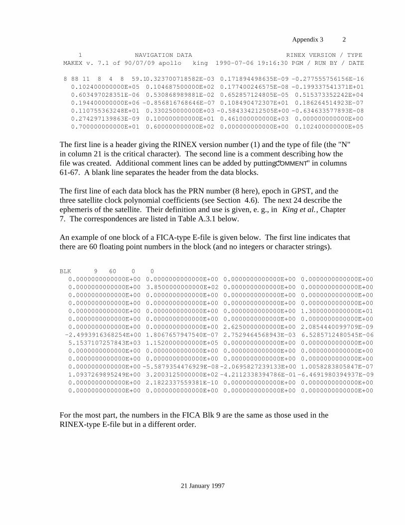
Appendix 3 2

21 January 1997

1 NAVIGATION DATA RINEX VERSION / TYPE MAKEX v. 7.1 of 90/07/09 apollo king 1990-07-06 19:16:30 PGM / RUN BY / DATE

8 88 11 8 4 8 59.10.323700718582E-03 0.171894498635E-09 -0.277555756156E-160.102400000000E+05 0.104687500000E+02 0.177400246575E-08 -0.199337541371E+010.603497028351E-06 0.530868989881E-02 0.652857124805E-05 0.515373352242E+040.194400000000E+06 -0.856816768646E-07 0.108490472307E+01 0.186264514923E-070.110755363248E+01 0.330250000000E+03 -0.584334212505E+00 -0.634633577893E-080.274297139863E-09 0.100000000000E+01 0.461000000000E+03 0.000000000000E+000.700000000000E+01 0.600000000000E+02 0.000000000000E+00 0.102400000000E+05

The first line is a header giving the RINEX version number (1) and the type of file (the "N"in column 21 is the critical character). The second line is a comment describing how thefile was created. Additional comment lines can be added by putting "COMMENT" in columns61-67. A blank line separates the header from the data blocks.

The first line of each data block has the PRN number (8 here), epoch in GPST, and thethree satellite clock polynomial coefficients (see Section 4.6). The next 24 describe theephemeris of the satellite. Their definition and use is given, e. g., in King et al., Chapter7. The correspondences are listed in Table A.3.1 below.

An example of one block of a FICA-type E-file is given below. The first line indicates thatthere are 60 floating point numbers in the block (and no integers or character strings).

BLK 9 60 0 0 0.0000000000000E+00 0.0000000000000E+00 0.0000000000000E+00 0.0000000000000E+00 0.0000000000000E+00 3.8500000000000E+02 0.0000000000000E+00 0.0000000000000E+00 0.0000000000000E+00 0.0000000000000E+00 0.0000000000000E+00 0.0000000000000E+00 0.0000000000000E+00 0.0000000000000E+00 0.0000000000000E+00 0.0000000000000E+00 0.0000000000000E+00 0.0000000000000E+00 0.0000000000000E+00 1.3000000000000E+01 0.0000000000000E+00 0.0000000000000E+00 0.0000000000000E+00 0.0000000000000E+00 0.0000000000000E+00 0.0000000000000E+00 2.6250000000000E+00 2.0854440099709E-09-2.4993916368254E+00 1.8067657947540E-07 2.7529464568943E-03 6.5285712480545E-06

5.1537107257843E+03 1.1520000000000E+05 0.0000000000000E+00 0.0000000000000E+00 0.0000000000000E+00 0.0000000000000E+00 0.0000000000000E+00 0.0000000000000E+00 0.0000000000000E+00 0.0000000000000E+00 0.0000000000000E+00 0.0000000000000E+00 0.0000000000000E+00 -5.5879354476929E-08 -2.0695827239133E+00 1.0058283805847E-07 1.0937269895249E+00 3.2003125000000E+02 -4.2112338394786E-01 -6.4691980394937E-09 0.0000000000000E+00 2.1822337559381E-10 0.0000000000000E+00 0.0000000000000E+00 0.0000000000000E+00 0.0000000000000E+00 0.0000000000000E+00 0.0000000000000E+00

For the most part, the numbers in the FICA Blk 9 are the same as those used in theRINEX-type E-file but in a different order.

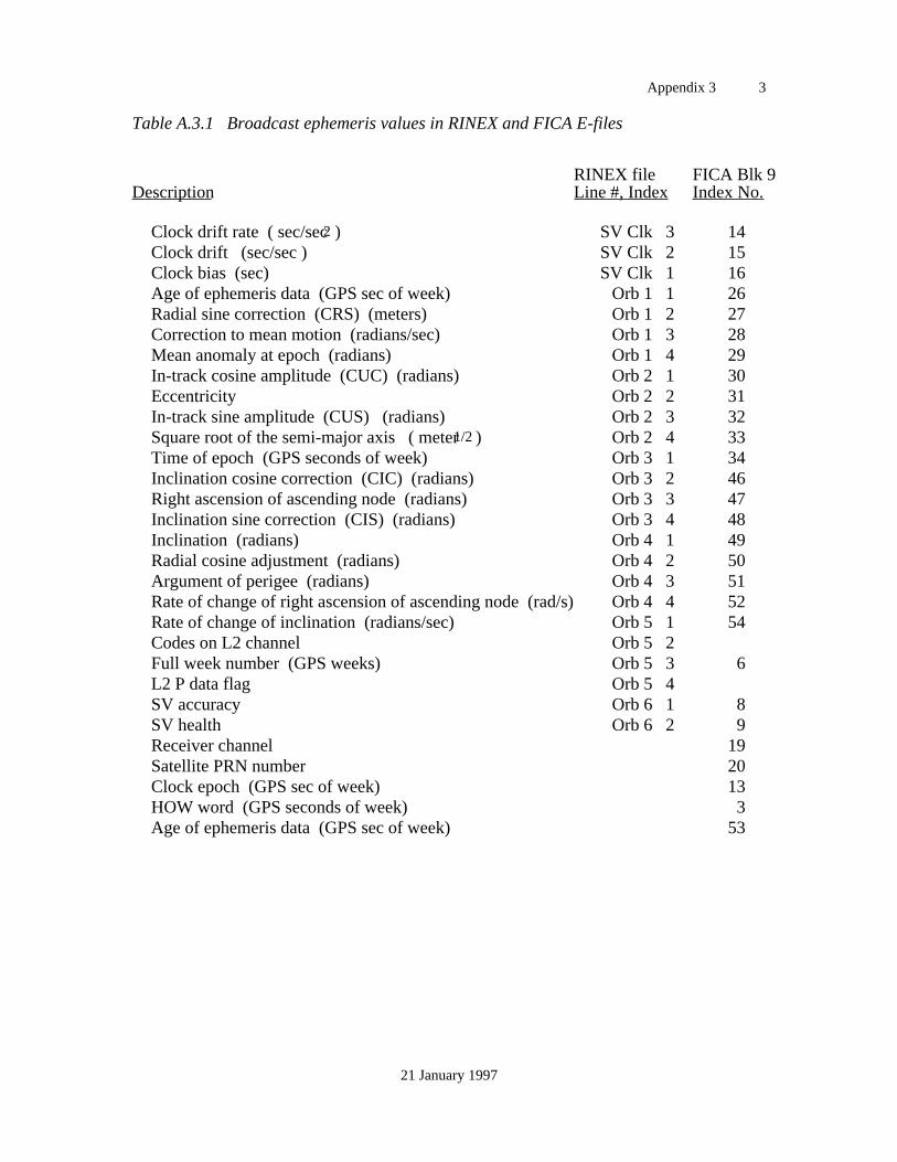
Appendix 3 3

21 January 1997

Table A.3.1 Broadcast ephemeris values in RINEX and FICA E-files

RINEX file FICA Blk 9Description Line #, Index Index No.

Clock drift rate ( sec/sec2 ) SV Clk 3 14Clock drift (sec/sec ) SV Clk 2 15Clock bias (sec) SV Clk 1 16Age of ephemeris data (GPS sec of week) Orb 1 1 26Radial sine correction (CRS) (meters) Orb 1 2 27Correction to mean motion (radians/sec) Orb 1 3 28Mean anomaly at epoch (radians) Orb 1 4 29In-track cosine amplitude (CUC) (radians) Orb 2 1 30Eccentricity Orb 2 2 31In-track sine amplitude (CUS) (radians) Orb 2 3 32Square root of the semi-major axis ( meter1/2 ) Orb 2 4 33Time of epoch (GPS seconds of week) Orb 3 1 34Inclination cosine correction (CIC) (radians) Orb 3 2 46Right ascension of ascending node (radians) Orb 3 3 47Inclination sine correction (CIS) (radians) Orb 3 4 48Inclination (radians) Orb 4 1 49Radial cosine adjustment (radians) Orb 4 2 50Argument of perigee (radians) Orb 4 3 51Rate of change of right ascension of ascending node (rad/s) Orb 4 4 52Rate of change of inclination (radians/sec) Orb 5 1 54Codes on L2 channel Orb 5 2Full week number (GPS weeks) Orb 5 3 6L2 P data flag Orb 5 4SV accuracy Orb 6 1 8SV health Orb 6 2 9Receiver channel 19Satellite PRN number 20Clock epoch (GPS sec of week) 13HOW word (GPS seconds of week) 3Age of ephemeris data (GPS sec of week) 53

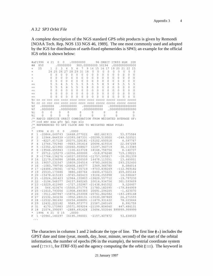
Appendix 3 4

21 January 1997

A 3.2 SP3 Orbit File

A complete description of the NGS standard GPS orbit products is given by Remondi[NOAA Tech. Rep. NOS 133 NGS 46, 1989]. The one most commonly used and adoptedby the IGS for distribution of earth-fixed ephemerides is SP#3; an example for the officialIGS orbit is shown below:

#aP1996 4 21 0 0 .00000000 96 ORBIT ITR93 HLM IGS## 850 .00000000 900.00000000 50194 .0000000000000+ 25 1 2 3 4 5 6 7 9 14 15 16 17 19 20 21 22 23+ 24 25 26 27 28 29 31 18 0 0 0 0 0 0 0 0 0+ 0 0 0 0 0 0 0 0 0 0 0 0 0 0 0 0 0+ 0 0 0 0 0 0 0 0 0 0 0 0 0 0 0 0 0+ 0 0 0 0 0 0 0 0 0 0 0 0 0 0 0 0 0++ 5 5 6 5 5 5 5 5 5 5 8 5 6 5 5 5 5++ 5 5 5 6 5 5 5 8 0 0 0 0 0 0 0 0 0++ 0 0 0 0 0 0 0 0 0 0 0 0 0 0 0 0 0++ 0 0 0 0 0 0 0 0 0 0 0 0 0 0 0 0 0++ 0 0 0 0 0 0 0 0 0 0 0 0 0 0 0 0 0%c cc cc ccc ccc cccc cccc cccc cccc ccccc ccccc ccccc ccccc%c cc cc ccc ccc cccc cccc cccc cccc ccccc ccccc ccccc ccccc%f .0000000 .000000000 .00000000000 .000000000000000%f .0000000 .000000000 .00000000000 .000000000000000%i 0 0 0 0 0 0 0 0 0%i 0 0 0 0 0 0 0 0 0/* RAPID SERVICE ORBIT COMBINATION FROM WEIGHTED AVERAGE OF:/* cod emr esa gfz jpl ngs sio/* REFERENCED TO GPS CLOCK AND TO WEIGHTED MEAN POLE:/** 1996 4 21 0 0 .0000P 1 -20844.049743 16468.077022 682.661913 53.575584P 2 12944.844539 -10393.087331 -20299.519500 -249.520521P 3 -8227.617128 20375.326181 -15102.650518 4.597767P 4 13744.791940 -9683.391414 20694.419314 22.047268P 5 -12352.621960 -20060.938827 12297.360719 36.113385P 6 -19546.655943 -1100.613728 18148.758754 8.140737P 7 20712.125279 -16356.600000 -518.876248 719.138221P 9 -17764.134276 -16037.093050 -11757.505817 -18.951339P 14 12179.034086 18588.450559 14478.113351 13.465001P 15 19057.231547 15809.204514 -9780.269336 293.252400P 16 -1083.799746 -26408.146377 2349.366780 8.084014P 17 -24486.194361 -4762.735719 -9703.838269 -112.969182P 19 25533.173686 3886.160764 -6400.473223 459.005144P 20 -15478.615183 -9745.065423 19106.255998 14.598467P 21 -12024.261423 12964.155803 -19620.557712 -19.797230P 22 -3194.548377 24157.840245 10016.934756 301.593609P 23 -15229.612960 -1727.102967 -21438.845352 9.526407P 24 544.423674 -15500.071774 21780.182095 -179.844909P 25 -11610.793056 11908.640383 20691.294205 -1.623070P 26 -3511.667947 -15876.253008 -20761.862582 -183.285168P 27 21532.343236 -3952.280131 -15530.087869 26.271555P 28 -12532.981692 20254.408891 -11879.931632 78.225844P 29 12432.222182 9589.973773 21587.240169 8.991759P 31 4170.173983 15571.909204 -21199.804060 447.486131P 18 21074.399097 -2889.491428 15694.503544 999999.999999* 1996 4 21 0 15 .0000P 1 -20941.140297 16195.390001 -2157.407872 53.634533 ...

The characters in columns 1 and 2 indicate the type of line. The first line (#a) includes theGPST date and time (year, month, day, hour, minute, second) of the start of the orbitalinformation, the number of epochs (96 in the example), the terrestrial coordinate systemused (ITR93, for ITRF-93) and the agency computing the the orbit (IGS). The keyword in

Appendix 3 5

21 January 1997

columns 41–45 indicates the type of data used to compute the orbit. For individual analysiscenters this will indicate.e.g. doubly differenced carrrier phase ( d ), but for the IGScombined orbit the orbits of the individual analysis centers are the "observations". Thesecond line (##) repeats the start time but in terms of GPS week ( 850) plus seconds ofweek and Modified Julian Day plus fraction-of-day; it also gives the interval of thetabulated ephemerides in seconds (900).

The third to the seventh lines (+ ) have the number of satellites followed by their respectivePRN numbers. The 8th to the 12th lines ( ++) indicate the accuracy of the orbit of eachsatellite, given by the exponent of 2 in millimeters; e.g., 5 implies an accuracy of 25 mm,or 3.2 cm. Lines 13–18 are reserved for addition of character (%c), floating-point (%f) orinteger (%i) variables to the format. Lines 19–22 have free-form comments (/*).

For each epoch there is a header line ( * ) and data lines (P ) for each satellite. The datalines contain Cartesian coordinates in kilometers andthe clock offset in microseconds.

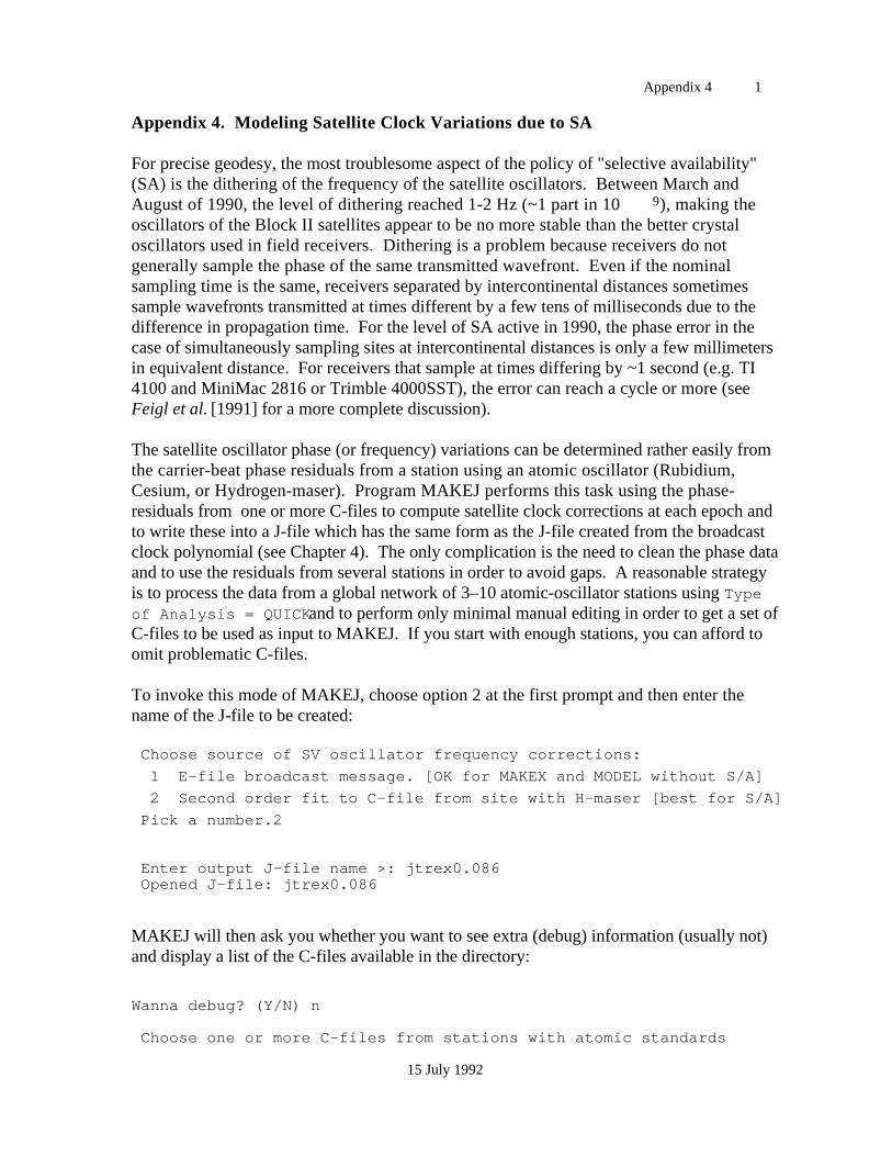
Appendix 4 1

15 July 1992

Appendix 4. Modeling Satellite Clock Variations due to SA

For precise geodesy, the most troublesome aspect of the policy of "selective availability"(SA) is the dithering of the frequency of the satellite oscillators. Between March andAugust of 1990, the level of dithering reached 1-2 Hz (~1 part in 10 9), making theoscillators of the Block II satellites appear to be no more stable than the better crystaloscillators used in field receivers. Dithering is a problem because receivers do notgenerally sample the phase of the same transmitted wavefront. Even if the nominalsampling time is the same, receivers separated by intercontinental distances sometimessample wavefronts transmitted at times different by a few tens of milliseconds due to thedifference in propagation time. For the level of SA active in 1990, the phase error in thecase of simultaneously sampling sites at intercontinental distances is only a few millimetersin equivalent distance. For receivers that sample at times differing by ~1 second (e.g. TI4100 and MiniMac 2816 or Trimble 4000SST), the error can reach a cycle or more (seeFeigl et al. [1991] for a more complete discussion).

The satellite oscillator phase (or frequency) variations can be determined rather easily fromthe carrier-beat phase residuals from a station using an atomic oscillator (Rubidium,Cesium, or Hydrogen-maser). Program MAKEJ performs this task using the phase-residuals from one or more C-files to compute satellite clock corrections at each epoch andto write these into a J-file which has the same form as the J-file created from the broadcastclock polynomial (see Chapter 4). The only complication is the need to clean the phase dataand to use the residuals from several stations in order to avoid gaps. A reasonable strategyis to process the data from a global network of 3–10 atomic-oscillator stations using Typeof Analysis = QUICK and to perform only minimal manual editing in order to get a set ofC-files to be used as input to MAKEJ. If you start with enough stations, you can afford toomit problematic C-files.

To invoke this mode of MAKEJ, choose option 2 at the first prompt and then enter thename of the J-file to be created:

Choose source of SV oscillator frequency corrections:

1 E-file broadcast message. [OK for MAKEX and MODEL without S/A]

2 Second order fit to C-file from site with H-maser [best for S/A]

Pick a number.2

Enter output J-file name >: jtrex0.086 Opened J-file: jtrex0.086

MAKEJ will then ask you whether you want to see extra (debug) information (usually not)and display a list of the C-files available in the directory:

Wanna debug? (Y/N) n

Choose one or more C-files from stations with atomic standards

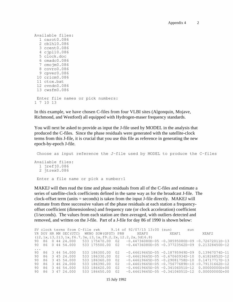
Appendix 4 2

15 July 1992

Available files: 1 carot0.086 2 cblhl0.086 3 ccent0.086 4 cjpl10.086 5 clock.doc 6 cmadc0.086 7 cmojm0.086 8 covro0.086 9 cpver0.086 10 cricm0.086 11 ctox.bat 12 cvndn0.086 13 cwsfm0.086

Enter file names or pick numbers:1 7 10 13

In this example, we have chosen C-files from four VLBI sites (Algonquin, Mojave,Richmond, and Westford) all equipped with Hydrogen-maser frequency standards.

You will next be asked to provide as input the J-file used by MODEL in the analysis thatproduced the C-files. Since the phase residuals were generated with the satellite-clockterms from this J-file, it is crucial that you use this file as reference in generating the newepoch-by-epoch J-file.

Choose as input reference the J-file used by MODEL to produce the C-files

Available files: 1 jrefj0.086 2 jtrex0.086

Enter a file name or pick a number:1

MAKEJ will then read the time and phase residuals from all of the C-files and estimate aseries of satellite-clock coefficients defined in the same way as for the broadcast J-file. Theclock-offset term (units = seconds) is taken from the input J-file directly. MAKEJ willestimate from three successive values of the phase residuals at each station a frequency-offset coefficient (dimensionless) and frequency rate (or clock acceleration) coefficient(1/seconds). The values from each station are then averaged, with outliers detected andremoved, and written on the J-file. Part of a J-file for day 86 of 1990 is shown below:

SV clock terms from C-file rwk 9.14 of 92/07/15 13:00 (sun) sunYR DOY HR MN SEC(UTC) WKNO SOW(GPST) PRN XEAF0 XEAF1 XEAF2(i2,1x,i3,2i3,1x,f6.7,3x,i3,1x,f9.2,2x,i2.2,2x,3d16.8)90 86 0 44 24.000 533 175470.00 02 -0.44736080D-05 -0.38595080D-09 -0.72672011D-1390 86 0 44 54.000 533 175500.00 02 -0.44736080D-05 -0.37723562D-09 0.21328450D-12...90 86 3 44 54.000 533 186300.00 02 -0.44619665D-05 -0.18795949D-09 0.13967074D-1190 86 3 45 24.000 533 186330.00 02 -0.44619665D-05 -0.67060934D-10 0.61826852D-1290 86 3 45 54.000 533 186360.00 02 -0.44619665D-05 -0.29081758D-10 0.14717717D-1390 86 3 46 24.000 533 186390.00 02 -0.44619665D-05 -0.75677689D-10 -0.79131662D-1290 86 3 46 54.000 533 186420.00 02 -0.44619665D-05 -0.34106051D-12 0.00000000D+0090 86 3 47 24.000 533 186450.00 02 -0.44619665D-05 -0.34106051D-12 0.00000000D+00

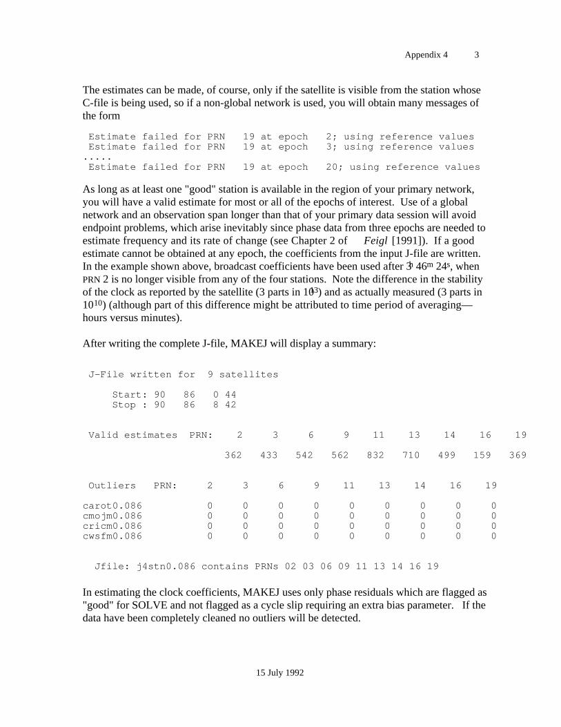
Appendix 4 3

15 July 1992

The estimates can be made, of course, only if the satellite is visible from the station whoseC-file is being used, so if a non-global network is used, you will obtain many messages ofthe form

Estimate failed for PRN 19 at epoch 2; using reference values Estimate failed for PRN 19 at epoch 3; using reference values..... Estimate failed for PRN 19 at epoch 20; using reference values

As long as at least one "good" station is available in the region of your primary network,you will have a valid estimate for most or all of the epochs of interest. Use of a globalnetwork and an observation span longer than that of your primary data session will avoidendpoint problems, which arise inevitably since phase data from three epochs are needed toestimate frequency and its rate of change (see Chapter 2 of Feigl [1991]). If a goodestimate cannot be obtained at any epoch, the coefficients from the input J-file are written.In the example shown above, broadcast coefficients have been used after 3h 46m 24s, whenPRN 2 is no longer visible from any of the four stations. Note the difference in the stabilityof the clock as reported by the satellite (3 parts in 1013) and as actually measured (3 parts in1010) (although part of this difference might be attributed to time period of averaging—hours versus minutes).

After writing the complete J-file, MAKEJ will display a summary:

J-File written for 9 satellites

Start: 90 86 0 44 Stop : 90 86 8 42

Valid estimates PRN: 2 3 6 9 11 13 14 16 19

362 433 542 562 832 710 499 159 369

Outliers PRN: 2 3 6 9 11 13 14 16 19

carot0.086 0 0 0 0 0 0 0 0 0cmojm0.086 0 0 0 0 0 0 0 0 0cricm0.086 0 0 0 0 0 0 0 0 0cwsfm0.086 0 0 0 0 0 0 0 0 0

Jfile: j4stn0.086 contains PRNs 02 03 06 09 11 13 14 16 19

In estimating the clock coefficients, MAKEJ uses only phase residuals which are flagged as"good" for SOLVE and not flagged as a cycle slip requiring an extra bias parameter. If thedata have been completely cleaned no outliers will be detected.

Documents

Documentation for the GAMIT GPS Analysis Software - …simon/gtgk/GAMIT.pdf · Documentation for the GAMIT GPS Analysis Software ... Release 10.0 - December 2000. 6 ... time reading