Does Antidumping Protection raise Market Power?: Evidence by … · by Jozef Konings and Hylke Vandenbussche Catholic University of Leuven, Belgium and CEPR, London August 2002 Abstract

Does Antidumping Protection raise Market Power?: Evidence from EU Firm Level Data by Jozef KONINGS Hylke VANDENBUSSCHE Financial Economics Center for Economic Studies Discussions Paper Series (DPS) 02.12 http://www.econ.kuleuven.be/ces/discussionpapers/default.htm

August 2002

1

Does Antidumping Protection raise Market Power ? Evidence from EU Firm Level Data

by Jozef Konings and Hylke Vandenbussche

Catholic University of Leuven, Belgium and CEPR, London

August 2002 Abstract

This paper empirically tests the effects of Anti-Dumping (AD) protection on

the price-cost margin of firms. To this end, we use a rich panel data set of 1,666 EU

producers that were involved in AD cases initiated in 1996. Our findings indicate that

price-cost margins in most cases significantly increase in the period of protection

compared to a period before protection. In industries where competition is very tough

before protection, we fail to find an increase in price-cost margins, while in industries

with positive markups before protection, trade policy raises market power between

3% points and 15 % points, depending on the sector. Our results are robust to

alternative specifications and estimation techniques, controlling for unobservable

fixed effects and potential endogeneity of the regressors. Our findings are also

consistent with recent theoretical models that deal with the economic effects on price

behaviour in response to AD protection.

JEL-codes: F13, L13, L41 Keywords: market power, price-cost margins, antidumping cases, European producers Address for correspondence: Hylke Vandenbussche, Catholic University of Leuven (KULeuven), Department of Applied Economics, Naamsestraat 69, 3000 Leuven, [email protected] We are grateful to the Belgian Fund for Scientific Research (FWO) for financial support of grant n° G.0122.98. We thank Jim Harrigan, Jim Markusen, Pertti Haaparanta, and other participants of the Nordic workshop 2002 in international trade. We also thank Johan Van Biesebroeck, Frank Verboven, Ana Xavier for useful comments.

2

I. Introduction

Over the last two decades consecutive multilateral trade talks of the

GATT/WTO have resulted in a general reduction of tariffs, voluntary export restraints

and quotas. At the same time a rise in new forms of trade protection has occurred, in

particular the use of antidumping (AD) measures has increased rapidly. Blonigen and

Prusa (2001) indicate in a recent review of the literature that since 1980 GATT/WTO

members have filed more complaints under the AD statute than under all other trade

laws combined. Moreover, an increased number of AD duties are now levied in any

one year worldwide than were levied in the entire period 1947-1970.

A number of papers have shown that trade liberalization has a disciplining

effect on firms’ pricing behavior. Levinsohn (1993) for Turkey and Harrison (1994)

for Chile estimate the effects of trade liberalization on price mark-ups and find that

mark-ups mostly go down after trade liberalization. A similar result is found by

Krishna and Mitra (1998) for India. Finally, Botasso and Sembenelli (2001) find

evidence that the introduction of the EU single market program, which implied the

removal of non-tariff barriers within the EU, has led to a reduction of market power,

but only in the so called ‘sensitive’ sectors. All these papers have looked at what

happens to market power when trade liberalization takes place. However, given the

enormous increase in the use of AD actions it is interesting to analyze the reverse

question: What happens to firms’ market power once protection is achieved. If

protection were granted to firms that operate in perfectly competitive markets, we

would not expect protection to increase market power. However, a number of recent

theoretical papers have shown that the antidumping legislation (AD) in imperfectly

competitive industries can give rise to strategic price setting behavior of domestic

3

firms which may result in increased market power of domestic firms.1 This paper tests

empirically whether AD protection gives rise to an increase in market power. For this

purpose we use firm level data of European Union firms to estimate the price-cost

ratios before and after receiving AD protection. Our findings suggest that price-cost

margins are significantly higher during the protection period compared to the period

before the protection. This result is robust to alternative econometric specifications

and estimation techniques. It is robust to potential business cycle effects tha t may

affect the price-cost margins of firms, it is also robust to the inclusion of fixed effects

which capture other variables that are likely to have an effect on price-cost margins

like technology, or the amount of sunk costs or advertising outlays at the firm level.

This finding also remains the same when we control for potential endogeneity of the

explanatory variables by using IV GMM estimation techniques.

The rest of the paper is structured as follows. Section II discusses the effect of

antidumping measures on domestic prices as predicted by the literature. It will

become clear that antidumping measures are likely to push domestic prices up

irrespective of the mode of competition that is considered. Section III explains the

econometric methodology and the data that we use. In section IV we discuss our

findings and section V is a concluding one.

II. Theoretical background

An antidumping duty is very similar to a tariff and we know that the positive

effect of tariffs on prices is very robust across a very wide range of oligopoly

specifications (Helpman and Krugman, 1989). Simply consider what happens in a

1 Fischer (1992), Reitzes (1993), Prusa (1994), Veugelers and Vandenbussche (1999), Pauwels, Vandenbussche and Weverbergh (2001) among others.

4

duopoly model with a home and a foreign firm. A duty on foreign imports when

competition is in strategic complements results in an increase of the domestic price

(Brander, 1995). Hence, duty protection implies that the home price will be higher

under protection than under free trade. The same result holds under competition in

strategic substitutes (Cournot) competition. A duty on foreign imports results in a

higher output for the protected domestic firm and a lower output for the foreign firm.

It can be shown that the drop in foreign output is larger than the increase in domestic

output, resulting in a higher domestic price after duty protection. This gives us a clear

prediction for our empirical work. Based on the theory we then expect to find that

European firms when protected by antidumping duties2 have an increase in market

power3.

The models described above are however static in nature. In recent years a

number of dynamic models have been developed, taking into account that firms

involved in antidumping cases may have incentives to behave strategically to

influence antidumping outcomes (Ethier and Fischer, 1987; Reitzes, 1993; Prusa,

1994; Vandenbussche et al. 2001). This implies that in the period before protection,

prices can differ from what they would be under free trade. Empirical predictions on

how prices are to move in the period just before protection are not straightforward

since some models predict a pro-competitive effect while others predict an

anticompetitive effect, depending on whether strategic substitutes or complements are

assumed and depending on how the duty is determined. In contrast, second period

results, when antidumping measures are actually imposed, are the same in all these

2 In the EU, antidumping measures can either take the form of a duty or of a price-undertaking. While a duty is like a tariff, a price-undertaking is a voluntary price increase by the importers. Price-undertakings are believed to induce collusion and raise market power (Belderbos et al, 2002). 3 A few exceptions exist with respect to this general result. When demand is very convex, Cournot reaction functions can become upward sloping and the effect of a tariff on domestic prices can be different than the one described here. Also, a few papers have shown that tariff and quota protection in

5

models namely, domestic prices go up vis-à-vis free trade when a duty is imposed. It

is on this result that we focus in the empirical analysis.

One additional remark is in order here. So far we have discussed the effects of

trade policy under a fixed number of firms. The question can be raised what would

happen to market power when trade policy would trigger entry. A number of papers

have argued that in general when entry is free, the effects of commercial policy can be

dampened by entry and exit (Head and Ries, 1999; Markusen and Venables, 1988).

The rate of entry is a function of how much it costs to get into or out of a certain

industry. Sunk cost are an important entry-barrier. Therefore it can be expected that

especially in industries where sunk costs are large, trade policy is likely to have larger

effects than in industries with free entry as shown by Bernard and Jensen (1999).

However, in this paper we do not want to engage in discussing or explaining the

different levels of market power we observe in different industries even before

protection takes place. The question of interest here is whether we observe a

significant change in market power after antidumping protection sets in and can we

absolutely sure that antidumping policy is the explanatory variable accountable for

that change.

III. Empirical Methodology and Data

III.1. Methodology

Our methodology is based Roeger (1995), which starts from the approach

introduced by Hall (1988, 1990) to estimate price-cost margins. Under constant

returns to scale in production, assuming two input factor, labor and capital, the primal

a dynamic context under certain conditions can result in more competition rather than less (R. Deneckere and C. Davidson, 1985 and J. Rotemberg and G. Saloner, 1989)

6

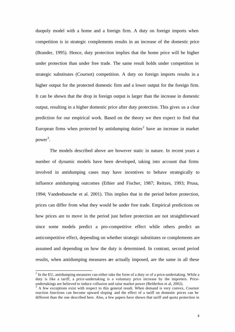
Solow residual (SR) can be related to price over marginal cost (µ=P/MC). Using

lower case letters to denote natural logarithms we can write the primal SR as

itititititititit klklqSR lll θαµαα +∆−∆−=∆−−∆−∆= )()1()1( (1)

where subscript i stands for firm i , subscript t stands for time t, q, l and k stand for the

natural logarithm of output, employment and capital, lα is labor’s share in output and

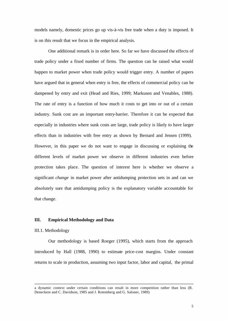
θ is the Hicks-neutral rate of technical progress. A similar expression as (1) can be

obtained for the dual Solow residual (DSR) or

itititititititit rwprwDSR lll θαµαα +∆−∆−=∆−∆−−∆= )()1()1( (2)

where w and r are the natural logarithms of the wage rate and the rental price of

capital and pit is the price of firm i in period t. The problem with estimating (1) and

(2) is that the explanatory variables are correlated with the unobservable productivity

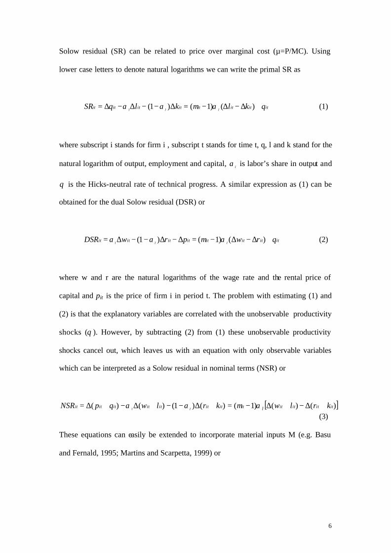
shocks (θ ). However, by subtracting (2) from (1) these unobservable productivity

shocks cancel out, which leaves us with an equation with only observable variables

which can be interpreted as a Solow residual in nominal terms (NSR) or

[ ])()()1()()1()()( ititititlitititititititit krlwkrlwqpNSR ll +∆−+∆−=+∆−−+∆−+∆= αµαα (3)

These equations can easily be extended to incorporate material inputs M (e.g. Basu

and Fernald, 1995; Martins and Scarpetta, 1999) or

7

[ ])()()()()1()()1()()()(

itititmitititit

itititmitititititit

krmplwkrmplwqpNSR

mlml

mlml

+∆+−+∆++∆−=+∆−−−+∆−+∆−+∆=

ααααµαααα (4)

or this can be written as

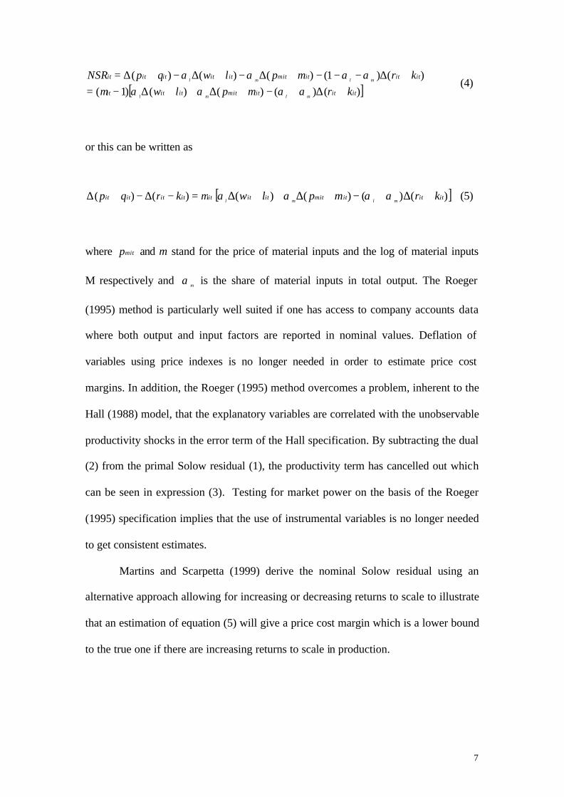
ititititit krqp µ=−∆−+∆ )()( [ ])()()()( itititmititit krmplw mlml +∆+−+∆++∆ αααα (5)

where mitp and m stand for the price of material inputs and the log of material inputs

M respectively and mα is the share of material inputs in total output. The Roeger

(1995) method is particularly well suited if one has access to company accounts data

where both output and input factors are reported in nominal values. Deflation of

variables using price indexes is no longer needed in order to estimate price cost

margins. In addition, the Roeger (1995) method overcomes a problem, inherent to the

Hall (1988) model, that the explanatory variables are correlated with the unobservable

productivity shocks in the error term of the Hall specification. By subtracting the dual

(2) from the primal Solow residual (1), the productivity term has cancelled out which

can be seen in expression (3). Testing for market power on the basis of the Roeger

(1995) specification implies that the use of instrumental variables is no longer needed

to get consistent estimates.

Martins and Scarpetta (1999) derive the nominal Solow residual using an

alternative approach allowing for increasing or decreasing returns to scale to illustrate

that an estimation of equation (5) will give a price cost margin which is a lower bound

to the true one if there are increasing returns to scale in production.

8

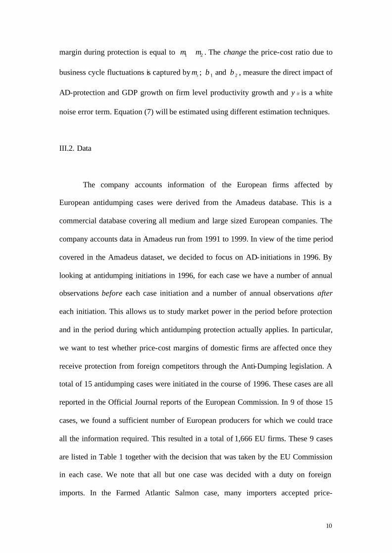
Equation (5) shows that in order to obtain an estimate of the price cost margin

(µ), we need information on sales growth4, growth in the wage bill, growth in material

costs and growth in the value of capital. The company accounts information we have

allowed us to get firm level data on these variables. The profit and loss account

provided us the information on sales, the wage bill and material costs in consecutive

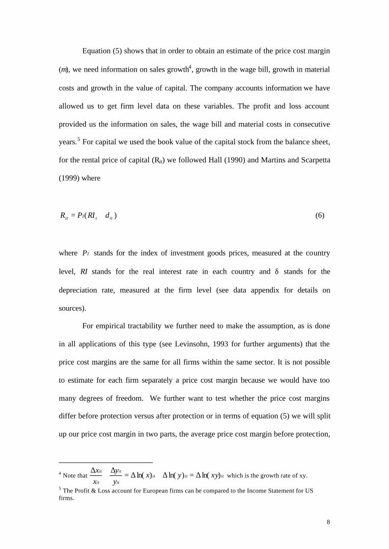
years.5 For capital we used the book value of the capital stock from the balance sheet,

for the rental price of capital (Rit) we followed Hall (1990) and Martins and Scarpetta

(1999) where

)( ittIit RIPR δ+= (6)

where IP stands for the index of investment goods prices, measured at the country

level, RI stands for the real interest rate in each country and δ stands for the

depreciation rate, measured at the firm level (see data appendix for details on

sources).

For empirical tractability we further need to make the assumption, as is done

in all applications of this type (see Levinsohn, 1993 for further arguments) that the

price cost margins are the same for all firms within the same sector. It is not possible

to estimate for each firm separately a price cost margin because we would have too

many degrees of freedom. We further want to test whether the price cost margins

differ before protection versus after protection or in terms of equation (5) we will split

up our price cost margin in two parts, the average price cost margin before protection,

4 Note that itititit

it

it

itxyyx

yy

xx

)ln()ln()ln( ∆=∆+∆=∆

+∆

which is the growth rate of xy.

5 The Profit & Loss account for European firms can be compared to the Income Statement for US firms.

9

i.e. the years 1991-96 and the average price cost margin during protection, which

starts one year after the initiation of an AD case, i.e. the years 1997-99.

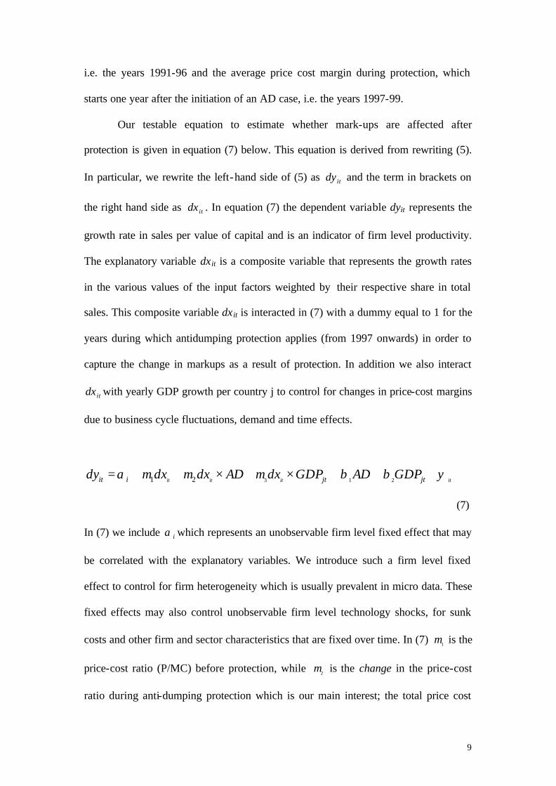
Our testable equation to estimate whether mark-ups are affected after

protection is given in equation (7) below. This equation is derived from rewriting (5).

In particular, we rewrite the left-hand side of (5) as itdy and the term in brackets on

the right hand side as itdx . In equation (7) the dependent variable dyit represents the

growth rate in sales per value of capital and is an indicator of firm level productivity.

The explanatory variable dx it is a composite variable that represents the growth rates

in the various values of the input factors weighted by their respective share in total

sales. This composite variable dx it is interacted in (7) with a dummy equal to 1 for the

years during which antidumping protection applies (from 1997 onwards) in order to

capture the change in markups as a result of protection. In addition we also interact

itdx with yearly GDP growth per country j to control for changes in price-cost margins

due to business cycle fluctuations, demand and time effects.

itititit jtjtiit GDPADGDPdxADdxdxdy ψββµµµα +++×+×++=21321

(7)

In (7) we include iα which represents an unobservable firm level fixed effect that may

be correlated with the explanatory variables. We introduce such a firm level fixed

effect to control for firm heterogeneity which is usually prevalent in micro data. These

fixed effects may also control unobservable firm level technology shocks, for sunk

costs and other firm and sector characteristics that are fixed over time. In (7) 1µ is the

price-cost ratio (P/MC) before protection, while 2µ is the change in the price-cost

ratio during anti-dumping protection which is our main interest; the total price cost

10

margin during protection is equal to 21 µµ + . The change the price-cost ratio due to

business cycle fluctuations is captured by 3µ ; 1β and 2β , measure the direct impact of

AD-protection and GDP growth on firm level productivity growth and itψ is a white

noise error term. Equation (7) will be estimated using different estimation techniques.

III.2. Data

The company accounts information of the European firms affected by

European antidumping cases were derived from the Amadeus database. This is a

commercial database covering all medium and large sized European companies. The

company accounts data in Amadeus run from 1991 to 1999. In view of the time period

covered in the Amadeus dataset, we decided to focus on AD-initiations in 1996. By

looking at antidumping initiations in 1996, for each case we have a number of annual

observations before each case initiation and a number of annual observations after

each initiation. This allows us to study market power in the period before protection

and in the period during which antidumping protection actually applies. In particular,

we want to test whether price-cost margins of domestic firms are affected once they

receive protection from foreign competitors through the Anti-Dumping legislation. A

total of 15 antidumping cases were initiated in the course of 1996. These cases are all

reported in the Official Journal reports of the European Commission. In 9 of those 15

cases, we found a sufficient number of European producers for which we could trace

all the information required. This resulted in a total of 1,666 EU firms. These 9 cases

are listed in Table 1 together with the decision that was taken by the EU Commission

in each case. We note that all but one case was decided with a duty on foreign

imports. In the Farmed Atlantic Salmon case, many importers accepted price-

11

undertakings but for those that did not, a duty was imposed. The remaining 6 cases

initiated in 1996 could not be fully traced for one of the following three reasons.

Either the name of the EU firms filing for protection was not mentioned in the case

reports in the Official Journal. Or, in some cases where we had the names of the EU

firms involved, we could not trace these firms in our company accounts data set. A

final reason was that often the product definition was too wide to allow us a search via

CSO code or name, the classification system used in Amadeus (see below). In the

group of 6 cases where we did not have enough information, only one resulted in a

duty (handbags), while 4 other cases were terminated without protection

(Dihydrostreptomycin; Luggage & travel goods; Briefcases & Schoolbags; Video

Tapes) and in a last case (pocket lighters), we failed to find the Commission’s

decision in the Official Journal.

In order to compose our sample of firms for which we are relatively certain

they would be affected by antidumping protection we proceeded in various steps. We

first traced the companies that were mentioned in the filing of a case reported in the

Official Journal. The number of EU firms involved in the filing of the complaint to

the EU is given in the last column of Table 1. We identified their 7 digit CSO activity

code, the classification used in the Amadeus company accounts dataset6,

corresponding to the product that was under the AD investigation. However, the

sample of firms involved in the formulation of the antidumping complaint was

relatively small. To expand our sample of EU firms we used an interesting property of

the antidumping legislation, which is that when protection is granted, it does not only

apply to the firms that actually filed a complaint but it applies to all firms in the EU

producing that particular product. This allowed us to increase our sample by searching

6 The CSO code is an activity code that is used by the British Statistical Office and defines the activities of firms at a 7-digit level of detail.

12

for all EU firms that were likely to benefit from AD-protection. A search for all EU

firms producing the same 7-digit CSO code as the firms in our initial sample

increased the sample but still resulted in a relatively small number of firms. To

increase the sample more, we identified from our initial sample of firms, the

corresponding four-digit primary CSO activity codes7. This corresponds with an

aggregation within the product line. We retrieved all firms that are classified in the

corresponding four digit CSO activity primary codes (see data appendix for more

detail). This way we were able to have a sufficiently large sample of EU firms that

were producing the product under protection or a close substitute and were getting

protection. We then retrieved the company accounts of all these firms between 1991

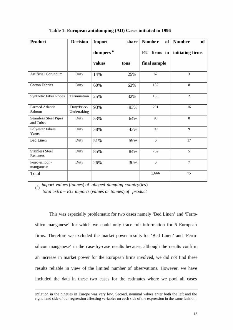
and 1999. Table 1 shows for each case we considered, the final decision of the EU in

column 1, the share of imports of the extra-EU countries that are named in the AD

investigation as alleged dumpers in column 2, the number of EU firms that we used in

our estimations in column 3 and the number of initiating EU firms in column 4.

We note that in all but one case, the EU Commission imposed a duty after

initiation. Only the case involving ‘Synthetic Fiber Ropes’ was ‘terminated’ without

protection. While we were able to trace more firms than reported in table 1, a number

of firms did not report all the information we required for our estimation (sales, wage

bill, materials, capital).8

7 By turning to the primary CSO codes, we only include firms in our sample for who the product belongs to their main activity. 8 We did not deflate the time series of nominal values of output and input factors we used for two reasons. First, balance sheet items like fixed tangible assets (K) are reported at historic cost, excluding inflation. Profit and Loss (income statement) items like material costs could be subject to inflation but

13

Table 1: European antidumping (AD) Cases initiated in 1996

Product Decision Import share

dumpers a

values tons

Number of

EU firms in

final sample

Number of

initiating firms

Artificial Corundum Duty 14% 25% 67 3

Cotton Fabrics Duty 60% 63% 182 8

Synthetic Fiber Robes Termination 25% 32% 155 2

Farmed Atlantic Salmon

Duty/Price-Undertaking

93% 93% 291 16

Seamless Steel Pipes and Tubes

Duty 53% 64% 98 8

Polyester Fibers Yarns

Duty 38% 43% 99 9

Bed Linen Duty 51% 59% 6 17

Stainless Steel Fasteners

Duty 85% 84% 762 5

Ferro-silicon-manganese

Duty 26% 30% 6 7

Total 1,666 75

(a) productoftonnesorvaluesimportsEUextratotal

iescountrydumpingallegedoftonnesvaluesimport)(

)()(−

This was especially problematic for two cases namely ‘Bed Linen’ and ‘Ferro-

silico manganese’ for which we could only trace full information for 6 European

firms. Therefore we excluded the market power results for ‘Bed Linen’ and ‘Ferro-

silicon manganese’ in the case-by-case results because, although the results confirm

an increase in market power for the European firms involved, we did not find these

results reliable in view of the limited number of observations. However, we have

included the data in these two cases for the estimates where we pool all cases

inflation in the nineties in Europe was very low. Second, nominal values enter both the left and the right hand side of our regression affecting variables on each side of the expression in the same fashion.

14

together. Noteworthy is also the fact that for all cases the import shares of the alleged

dumping countries, the so-called ‘named’ countries, is fairly large.

A number of further remarks are in order here. First, our sample may

underestimate the total number of firms producing the product under investigation.

The reason is that some firms may be producing the product in question but not as

their main activity. Firms that produce the product not as their main activity were

excluded from our sample although it is clear that those firms enjoyed protection too.

Second, our estimates of the change in price-cost ratios are likely to be a lower bound

of the true effect for the following reason. We do not have information on the relative

importance of the product under investigation in the total product portfolio of a firm.

The company accounts that we use refer to the firm’s total operations and not to the

financial flows associated with the production of the single product under

investigation. This suggests that if we find any effect of AD on firm’s market power

that it is most likely to be a lower bound of the true effect. Thirdly, our sample based

on case initiations in 1996 mostly contains duty cases. This is rather coincidental

since we know that the EU next to duties is also a heavy user of price-undertakings,

which can be seen as price-fixing agreements between the Commission and the

foreign importer. The only case in which price-undertakings were imposed together

with duties was Farmed Atlantic Salmon. The case involving Synthetic Fiber Ropes is

the only termination in our sample. A termination in the European antidumping policy

means that while a complaint was filed by the European industry, the Commission

after having looked into the case, decides not to impose measures, after which the

case is terminated. Since we have only one price-undertaking case and one

termination case, our data do not really allow us to make strong inferences on the

15

effects of price-undertakings or terminations. Our results however do seem to suggest

that price-undertakings result in higher market power changes than duties, while a

termination does not lead to a change in market power, which is what one would

expect on the basis of theoretical predictions in the AD literature (see for example

Veugelers and Vandenbussche, 1999).

In order to capture a change in market power after 1997, in our analysis we

use a dummy equal to zero for the years before protection and equal to 1 in the years

after protection. There are several reasons why we decided not to use the exact duty

levels for each case. While some cases are decided with ad-valorem duties, others

have specific duties or a combination of both. In cases concluded with price-

undertakings, the level of protection is not revealed. This makes it difficult to get

consistent duty levels across cases. In a case involving multiple defending countries,

each country gets a different duty level. Also, differences arise between the level of

provisional and final duties. The use of duty levels imposes the additional problem

that we would not be able to report the results for the Synthetic Fibre ropes case

separately because the duty level for that case is 0%, hence we would not obtain

results for the period after 1997. Moreover, the use of the duty levels in a case-by-case

does not add anything compared to a dummy since in the EU there is no variation in

the duty level over time and the duty is constant per case.

IV. Results

We start by reporting results for the pooled sample, where we pool all AD

cases together, to obtain an idea of the average effect of protection on price cost

margins. In table 2 we show the results of estimating (7) with OLS (1), fixed effects

(2) random effects (3) and robust regression (4). This latter estimation technique is

16

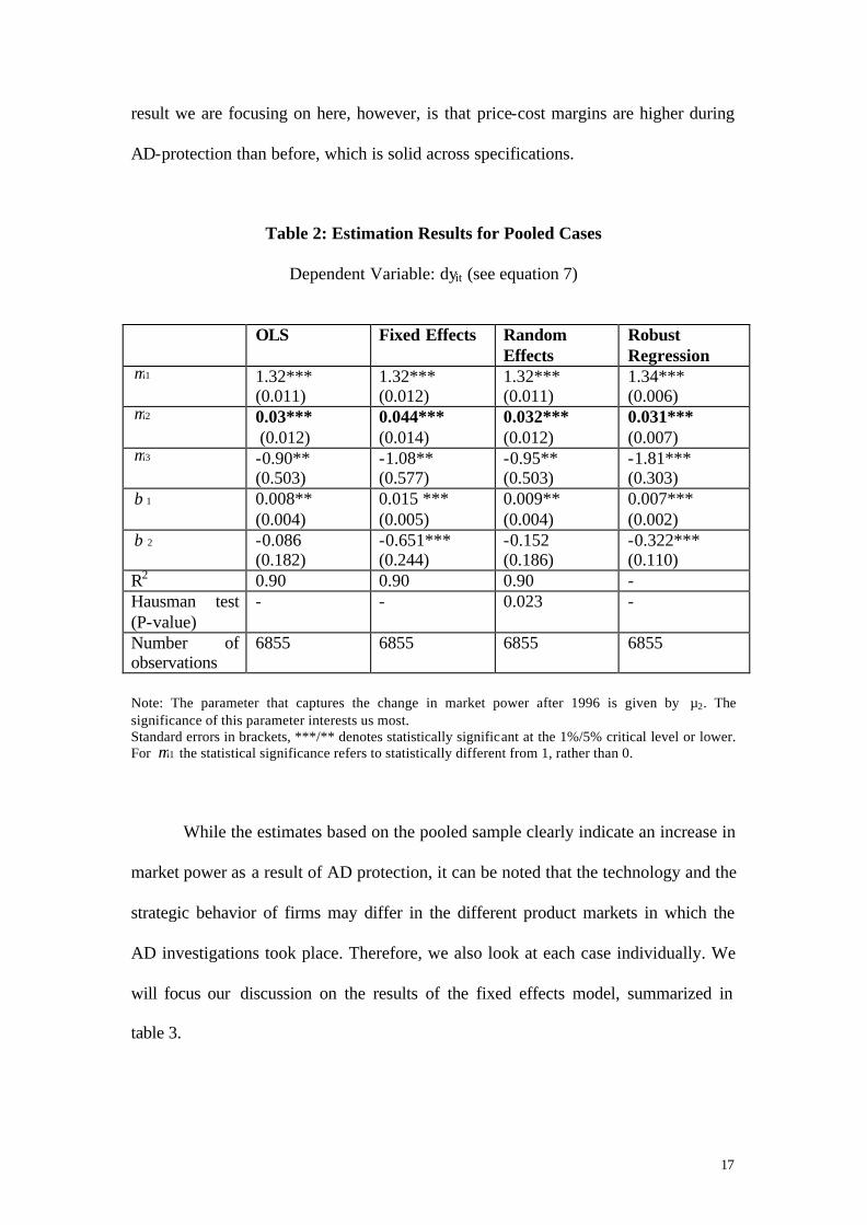
one which controls for potential outliers in the data, by weighting observations

according to their distance to their average in the sample. We note that the average

increase in price-cost ratios, given by µ2, is in the order of 3 to 4% points and

significant at the 1% level. This result holds independently of the estimation method.

Since the Roeger (1995) method deals with the endogeneity problem inherent in the

Hall (1986) method, the need for using IV estimates is less of a necessity as was also

pointed out by Oliveira-Martins and Scarpetta (1999). This implies that the estimates

from the methods listed in table 2 can be considered consistent. For completeness in

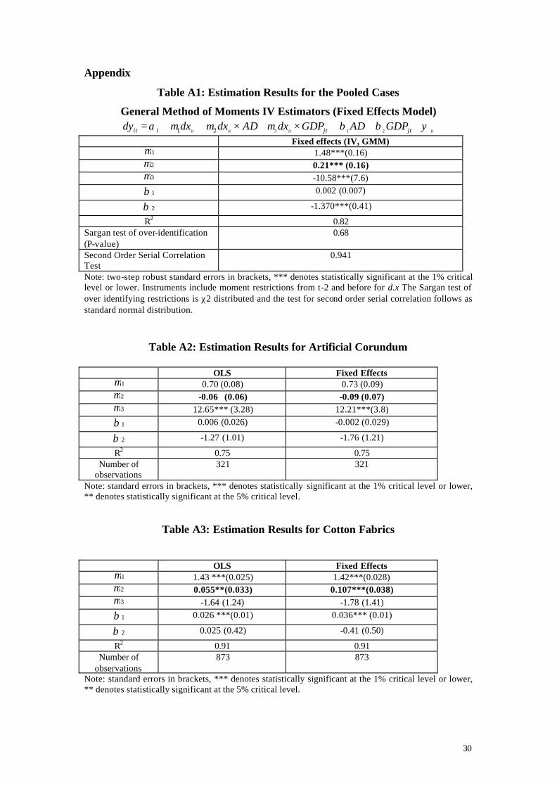
the appendix in table A1 we report the results where we instrument the right hand side

variables of (7), using the general methods of moments technique of Arellano and

Bond (1991).9 We note that the coefficient µ2 is significant and positive at the 1%

level suggesting there is an increase in price-cost margins during the protection

period. However, the levels of markup before and after protection differ substantially

between estimation methods. From table 2 we see that the estimated price-cost margin

lies around 30% before protection and is raised with about 3 to 4% points during

protection. Under the instrumental variable approach markups tend to be higher both

before protection and during protection. The average increase in market power for the

IV estimates ranges between 25% and 34% points, which seems rather high. The main

9 Endogeneity of the explanatory variables may occur if for instance productivity shocks have an effect on the usage of input factors or on the payment of wages, in which case dx may be endogenous. We use the general method of moments proposed by Arellano and Bond (1991). This method exists in using lagged values of the variable that is potentially endogenous as instruments. The instruments that can be used are all available moment restrictions for dx dating t-2 and before, since they are not correlated with the contemporaneous error term, but may be well correlated with the contemporaneous explanatory variables. The model is estimated in first differences to control for potential unobserved fixed effects. Since we use the lagged values of the explanatory variables we generate an increasing number of instruments as the panel progresses, which increases the efficiency of the estimates. To test whether our instruments are valid we report a Sargan test of over-identifying restrictions, which is χ2 distributed. We also report a test of second order serial correlation, which is standard Normal distributed. This test is useful to detect serial correlation, in which case a static model would not be valid. Since we estimate equation (7) in this case in first differences, what matters is the absence of second order serial correlation in order to have no first order serial correlation in the levels equation of (7). All the parameters in that case are then consistently estimated.

17

result we are focusing on here, however, is that price-cost margins are higher during

AD-protection than before, which is solid across specifications.

Table 2: Estimation Results for Pooled Cases

Dependent Variable: dyit (see equation 7)

OLS Fixed Effects Random

Effects Robust Regression

1µ 1.32*** (0.011)

1.32*** (0.012)

1.32*** (0.011)

1.34*** (0.006)

2µ 0.03*** (0.012)

0.044*** (0.014)

0.032*** (0.012)

0.031*** (0.007)

3µ -0.90** (0.503)

-1.08** (0.577)

-0.95** (0.503)

-1.81*** (0.303)

1β 0.008** (0.004)

0.015 *** (0.005)

0.009** (0.004)

0.007*** (0.002)

2β -0.086 (0.182)

-0.651*** (0.244)

-0.152 (0.186)

-0.322*** (0.110)

R2 0.90 0.90 0.90 - Hausman test (P-value)

- - 0.023 -

Number of observations

6855 6855 6855 6855

Note: The parameter that captures the change in market power after 1996 is given by µ2. The significance of this parameter interests us most. Standard errors in brackets, ***/** denotes statistically significant at the 1%/5% critical level or lower. For 1µ the statistical significance refers to statistically different from 1, rather than 0.

While the estimates based on the pooled sample clearly indicate an increase in

market power as a result of AD protection, it can be noted that the technology and the

strategic behavior of firms may differ in the different product markets in which the

AD investigations took place. Therefore, we also look at each case individually. We

will focus our discussion on the results of the fixed effects model, summarized in

table 3.

18

Table 3: Fixed Effects Results of Estimating Market Power (equation 7)10

Protection cases

Number of EU firms

(1)

µ1

before protection

(2)

Before AD

(3)

µ2

Change after protection

(4)

During AD

(5)

R2

Artificial corundum 67 0.76 (0.090)

P = MC -0.095 (0.077)

P = MC 0.75

Cotton fabrics 182 1.42*** (0.028)

P > MC 0.107*** (0.038)

P > MC 0.91

Farmed Atlantic Salmon 291 1.14*** (0.056)

P > MC 0.157** (0.07))

P > MC 0.71

Seamless Pipes and Tubes

98 0.989 (0.058)

P = MC -0.02 (0.06)

P = MC 0.80

Polyester Fiber and yarns

99 1.37*** (0.04)

P > MC 0.128** (0.06)

P > MC 0.86

Stainless steel fastener 762 1.40*** (0.015)

P > MC 0.03** (0.016)

P > MC 0.94

Termination Case

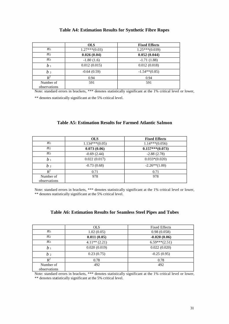
Synthetic Fiber Ropes 155 1.25*** (0.039)

P > MC 0.052 (0.044)

P > MC 0.94

Note: in brackets you find the standard deviation. *** indicates significance at the 1% level, ** at the 5% level. If µ1 is statistically different from 1 this is equivalent to a consumer price that exceeds marginal cost

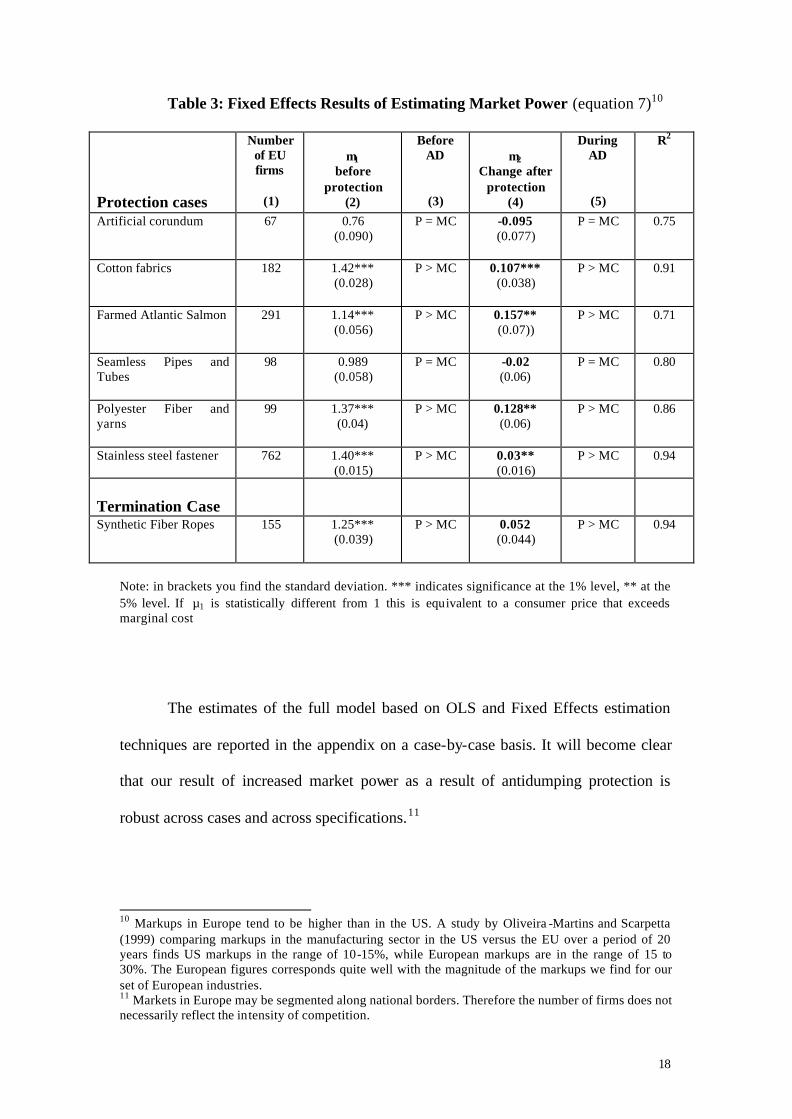
The estimates of the full model based on OLS and Fixed Effects estimation

techniques are reported in the appendix on a case-by-case basis. It will become clear

that our result of increased market power as a result of antidumping protection is

robust across cases and across specifications.11

10 Markups in Europe tend to be higher than in the US. A study by Oliveira -Martins and Scarpetta (1999) comparing markups in the manufacturing sector in the US versus the EU over a period of 20 years finds US markups in the range of 10-15%, while European markups are in the range of 15 to 30%. The European figures corresponds quite well with the magnitude of the markups we find for our set of European industries. 11 Markets in Europe may be segmented along national borders. Therefore the number of firms does not necessarily reflect the intensity of competition.

19

Column 2 of table 3 suggests that prior to antidumping protection, two products have

prices close to marginal cost. The two products facing tough competition are

‘Artificial Corundum’ that belongs to the Chemical industry, and ‘Seamless pipes and

tubes’ that belongs to the Steel industry. For those products, we observe from Table 3

that the effect of antidumping protection does not have an impact at all on price-cost

margins. These results correspond with the theoretical prediction that in competitive

markets, tariff protection does not affect markups. This may suggest that in Chemicals

and Steel, domestic European competition is sufficient to discipline prices, even after

protection. Also, from Table 1 we recall that the import share of the named countries,

for example in the ‘Artificial corundum’ case was relatively small compared to the

other cases. The competitive situation in the market even after antidumping protection

could be due to a sufficient amount of imports originating from non-dumping

countries. An alternative explanation could be the low degree of product

differentiation in the chemical sector. Homogeneous products make it more likely for

competition to be tough and prices to be close to marginal cost. For the ‘Seamless

pipes and tubes’ however, the source of competition is likely to be largely domestic

since the import share of the non-named countries is relatively small. The steel sector

is known for its overcapacity world wide, and its large amount of state aid, at least in

the past, usually in terms of subsidies, which are likely to keep consumer prices low.

From column (2) in table 3 it seems that the other industries are characterized

by imperfect competition prior to protection with prices all exceeding marginal costs.

We also can note that the initial price-cost margin is different in different sectors.

In the ‘Farmed Atlantic Salmon’ case we find a positive markup before

protection and the highest increase in markup during antidumping protection. Farmed

Atlantic Salmon is the only agricultural product in our sample and only one country

20

was under investigation for dumping into the EU namely Norway. Table 1 shows that

in 1996, Norway had an import share both in values and in tons of about 93% of

‘Farmed Atlantic Salmon’ in the EU. Hence, potential import diversion after

protection is very limited. Given that Norway seems to be almost the only source

country for the imports of Farmed Atlantic Salmon, other extra-EU importers will

benefit little from Norway’s conviction. This no doubt makes it easier for European

producers of Salmon to raise their prices after antidumping protection, knowing that

other extra-EU importers have only very small market shares in the EU and cannot

discipline the market after Norway’s conviction. While total Norwegian imports in

1996 was about 500 million ECU, total sales of the 309 EU farmers was about 1.2

billion USD (≅1.2 billion ECU). The fact that this case was settled for many

Norwegian importers with the acceptance of price-undertakings, could be another

additional reason why the change in market power is large.

It is also interesting to point out the results for ‘Synthetic Fiber Ropes’. This

AD case was terminated without imposing a duty. While our estimates indicate a

positive market power before protection, we do not find a statistically significant

increase in price-cost margins during antidumping protection. However, we do not

want to focus too much on these results given that ‘Synthetic Fiber Ropes’ is the only

‘Termination’ case in our sample. Although in 1996 in total 5 cases were terminated,

the 4 other termination cases did not give us enough information to be used.

A few additional remarks are in order here. Of course an increase in markups

can be the result of two distinct causes. Either price has increased or costs have gone

down. (Marginal) Cost data are not revealed in the AD case investigations. However,

theoretically we have strong arguments to believe that prices go up as a result of

protection. It is far less clear in what direction costs move with protection. Most likely

21

costs will not go down with protection. This would suggest that the increase in market

power that we find is mainly due to an increase in consumer prices.

Our findings are also consistent with earlier work that shows little or no

effects of so called import diversion in response to AD protection. Konings,

Vandenbussche and Springael (1999) show that for all antidumping cases initiated

between 1985 and 1990 there was no trade diversion from the alleged dumpers on to

other existing or new importers into the European Union, suggesting that the

antidumping mechanism works well in keeping imports out. The results we report

here of increased markups after protection for the EU industry is consistent with this

earlier finding of relatively low import diversion as a result of protection.

V. Robustness Tests

The PCM-method

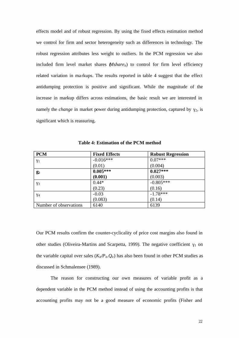
The price-cost margin PCM-method is an alternative method to estimate the

effect of a change in the trade regime on firms’ markups (Tybout, 2001). Using the

PCM method translates into the following regression

itjtititititit GDPMshareADQPKPCM εγγγγγ +++++= 43210 )/(

The dependent variable PCMit is variable profits measured as firm level sales minus

material costs and labor costs divided by the sales figure. The second term on the

RHS is the firm level capital stock (Kit) over firm level sales. The next term AD is a

dummy in each case from 1997 onwards and GDPjt is the yearly gdp growth rate for

each country j in the sample. The results on the pooled sample of AD cases based on

6,140 observations are shown in table 4 below where we report the results of a fixed

22

effects model and of robust regression. By using the fixed effects estimation method

we control for firm and sector heterogeneity such as differences in technology. The

robust regression attributes less weight to outliers. In the PCM regression we also

included firm level market shares (Mshareit) to control for firm level efficiency

related variation in markups. The results reported in table 4 suggest that the effect

antidumping protection is positive and significant. While the magnitude of the

increase in markup differs across estimations, the basic result we are interested in

namely the change in market power during antidumping protection, captured by γ2, is

significant which is reassuring.

Table 4: Estimation of the PCM method

PCM Fixed Effects Robust Regression γ1 -0.016***

(0.01) 0.07*** (0.004)

γ2 0.005*** (0.001)

0.027*** (0.003)

γ3 0.44* (0.23)

-0.805*** (0.16)

γ4 -0.03 (0.083)

-1.78*** (0.14)

Number of observations 6140 6139

Our PCM results confirm the counter-cyclicality of price cost margins also found in

other studies (Oliveira-Martins and Scarpetta, 1999). The negative coefficient γ1 on

the variable capital over sales (Kit/Pit.Qit) has also been found in other PCM studies as

discussed in Schmalensee (1989).

The reason for constructing our own measures of variable profit as a

dependent variable in the PCM method instead of using the accounting profits is that

accounting profits may not be a good measure of economic profits (Fisher and

23

McGowan (1983)). However, as an extra robustness test we check the average

accounting profit margin before and after 1996 to see whether average accounting

profits are different in the period before and during protection. The accounting profit

margin in our company dataset Amadeus is defined as ‘company profits before tax

over operating revenue’. While we find the average in the period 1991-1996 to be

2.5% with a standard deviation of 0.075, in the period 1997-99 we find the average

accounting profit margin to equal 4.1% with a standard deviation of 0.075. Running

the PCM regression, now using the accounting profit as a dependent variable yielded

a positive and significant coefficient in the fixed effects regression at a significance

level of 1%, suggesting a positive effect of antidumping protection on company

accounting profits.

A Counterfactual Control group:

In order to make sure that the significant increase in market power we obtain

for the firms located in one of the EU-15 countries is not simply a time or an industry

effect, we construct a counterfactual. This control group we use is composed of firms

in the same industries but in countries outside the EU-15 namely Norway,

Switzerland and Iceland. However, in one antidumping case, Farmed Atlantic

Salmon, Norway was involved as the defendant country. Many of the Norwegian

importers of Farmed Atlantic Salmon obtained price-undertakings for their sales into

the EU market. Price-undertakings are known to be a collusive device which may not

only raise the market power of European producers but also of foreign firms active on

the European market (Vandenbussche and Wauthy, 2001). For this reason we decided

not to include the Norwegian firms involved in the ‘Farmed Atlantic Salmon case’

into our counterfactual. The results for the PCM method on the counterfactual can be

24

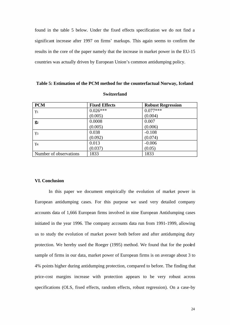
found in the table 5 below. Under the fixed effects specification we do not find a

significant increase after 1997 on firms’ markups. This again seems to confirm the

results in the core of the paper namely that the increase in market power in the EU-15

countries was actually driven by European Union’s common antidumping policy.

Table 5: Estimation of the PCM method for the counterfactual Norway, Iceland

Switzerland

PCM Fixed Effects Robust Regression γ1 0.026***

(0.005) 0.077*** (0.004)

γ2 0.0008 (0.005)

0.007 (0.006)

γ3 0.038 (0.092)

-0.108 (0.074)

γ4 0.013 (0.037)

-0.006 (0.05)

Number of observations 1833 1833

VI. Conclusion

In this paper we document empirically the evolution of market power in

European antidumping cases. For this purpose we used very detailed company

accounts data of 1,666 European firms involved in nine European Antidumping cases

initiated in the year 1996. The company accounts data run from 1991-1999, allowing

us to study the evolution of market power both before and after antidumping duty

protection. We hereby used the Roeger (1995) method. We found that for the pooled

sample of firms in our data, market power of European firms is on average about 3 to

4% points higher during antidumping protection, compared to before. The finding that

price-cost margins increase with protection appears to be very robust across

specifications (OLS, fixed effects, random effects, robust regression). On a case-by

25

case basis we find that in those industries where market power before protection is

low, antidumping duty protection has little effect on markups. While industries where

prices are well above marginal cost before protection, benefited most in terms of

market power increases after protection with changes in market power ranging

between 3 to 15% points depending on the sector.

Our results suggest that in the majority of EU AD cases protection is

associated with a reduction of allocative efficiency, reflected in increased prices,

which has a negative impact on European consumer welfare. However, in this paper

we did not investigate the potential impact of AD protection on employment and

wages, which could also enter the welfare objective of the EU. The empirical analysis

of how price-cost margins may jointly be determined with wage setting in labor

markets is an interesting avenue for further research.

26

References

M. Arellano and S. Bond (1991),”Some tests of Specification for Panel Data: Monte

Carlo Evidence and an Application to Employment Equations”, The Review of

Economic Studies, 58, pp. 277-297.

S. Basu and J. Fernald (1995),”Returns to scale in US production: estimates and

implications”, Journal of Political Economy, vol. 105, pp. 249-283.

A. Bernard and B. Jensen (1999),”Exceptional Export Performance: cause, effect or

both?”, Journal of International Economics, 47: 1-25.

R. Belderbos, H. Vandenbussche and R. Veugelers (2001), “Antidumping jumping

FDI in the EU”, CEPR discussion paper n° 2320.

B. Blonigen and T Prusa (2001), “Antidumping”, NBER working paper n° 8398, July

2001.

A. Botasso and A. Sembenelli (2001),”Market Power, productivity and the EU single

market program: evidence from a panel of Italian firms”, European Economic

Review 45, pp. 167-186.

J. Brander (1995),”Strategic Trade Policy”, in Handbook of International Economics,

Notrh-Holland.

R. Deneckere and C. Davidson (1985),”Incentives to Form Coalitions with Bertrand

Competition”, Rand Journal of Economics, vol. 16, n° 4, pp. 473-486.

J. Rotemberg and G. Saloner (1989),”Tariffs versus Quotas with implicit collusion”,

Canadian Journal of Economics 22, pp. 237-44.

I. Domowitz, R.G. Hubbard and B.C. Petersen (1988),”Market structure and cyclical

fluctuations in US manufacturing”, Review of Economics and Statistics 70, pp. 55-

66.

27

W. Ethier and R. Fischer (1987),”The New Protectionism”, Journal of International

Economic Integration 2(2) p 1-11.

R. Fischer (1992) “Endogenous probability of protection and firm behavior”, Journal

of International Economics 32, p149-163.

F. Fisher and J. McGowan (1983),”On the Misuse of Accounting Rates of Return to

infer monopoly profits”, American Economic Review, vol. 73, n° 1, pp. 82-97.

R. Hall (1988), ‘The relation between price and marginal cost in the US industry”,

Journal of Political Economy 96, pp. 921-47.

R. E. Hall (1990). “The Invariance Property of Solow’s Productivity Residual” in: P.

Diamond ed., Growth, Productivity, Unemployment, MIT press, Cambridge MA.

J. Harrigan (2001) (ed.), Handbook of International Trade, Basil Blackwell.

A.E. Harrison (1991), “The new trade protection: price effects of antidumping and

countervailing measures in the US”, World Bank Working Paper, Washington

D.C.

A.E. Harrison (1994). ‘Productivity, imperfect competition and trade reform’, Journal

of International Economics, 36, 53-73.

K. Head and J. Ries (1999),”Rationalization effects of tariff reductions”, Journal of

International Economics 47 (2), pp. 295-329.

E. Helpman and P. Krugman (1989), Trade Policy and Market structure, MIT press,

Cambridge.

IMF-Financial Statistics 1991-1999.

28

J. Konings, P.Van Cayseele and F.Warzynski (2001),”The dynamics of industrial

markups in two small open economies: does national competition policy matter

?”, International Journal of industrial Organization, vol. 19 (5), pp.841-859.

J. Konings, H. Vandenbussche and L. Springael (1999),”Import Diversion as a result

of European Antidumping Policy”, NBER working paper 7340.

J. Konings, H. Vandenbussche and R. Veugelers (2001), ‘Union wage bargaining and

EU antidumping policy’, Oxford Economic Papers, vol.53 n°2, pp.297-317.

P.Krishna and D. Mitra (1998),”Trade Liberalization, market discipline and

productivity growth: new evidence from India”, Journal of Development

Economics 56 (2), pp. 447-462.

J. Levinsohn (1993),”Testing the imports-as-market-discipline hypothesis”, Journal of

International Economics, 35, pp. 1-22.

J. Markusen and A. Venables (1988),”Trade Policy with Increasing returns and

imperfect competition: contradictory results from competing assumptions”,

Journal of International Economics, 24, pp. 299-316.

J. Oliveira-Martins and S. Scarpetta (1999),”The levels and cyclical behaviour of

Mark-ups across industries and market structures”, OECD Economics department,

working paper n° 213.

OECD, Main Economic Indicators.

W. Pauwels, H. Vandenbussche and M. Weverbergh (2001),”Strategic Behavior under

European Antidumping Policy”, International Journal of the Economics of business,

vol. 8, n° 1, pp. 79-103

N. Pavcnik (2002),”Trade Liberalization, Exit, and Productivity Improvements: evidence

from Chilean Plants”, Review of Economic Studies, 69, pp. 245-276.

29

T. Prusa (1994), “Pricing Behavior in the Presence of Antidumping Law”, Journal of

Economic Integration, 9 (2), pp. 260-289.

J. Reitzes (1993),”Antidumping Policy”, International Economic Review, vol. 34, n 4.

W. Roeger (1995),”Can Imperfect competition explain the difference between Primal

and Dual Productivity measures? Estimates from US manufacturing”, Journal of

Political Economy, vol. 103, n° 21.

R. Schmalensee (1989), “Studies of Structure and Performance”, in the Handbook of

Industrial Organization, by R. Schmalensee and R. Willig (ed.), p.1555.

R.W. Staiger and F.A. Wolak (1994), “Measuring Industry-Specific Protection:

Antidumping in the United States”, Brookings Papers on Economic Activity:

Microeconomics, pp. 51-118.

J. Tybout (2001),”Plant and Firm level evidence on ‘New’ Trade theories”, in

Handbook of International trade by J. Harrigan (ed.)

H. Vandenbussche and X. Wauthy (2001),”Inflicting injury through quality”,

European Journal of Political Economy, vol.17, pp. 101-116.

E. Vermulst and P. Van Waer (1992), “The calculation of Injury margins in EC

Antidumping Proceedings”, Journal of World Trade, pp. 5-42.

R. Veugelers and H. Vandenbussche (1999), “European Antidumping Policy and the

Profitability of National versus International Collusion”, European Economic

Review, January, 47 (1)

30

Appendix

Table A1: Estimation Results for the Pooled Cases

General Method of Moments IV Estimators (Fixed Effects Model)

itititit jtjtiit GDPADGDPdxADdxdxdy ψββµµµα +++×+×++= 21321 Fixed effects (IV, GMM)

1µ 1.48***(0.16) 2µ 0.21*** (0.16) 3µ -10.58***(7.6)

1β 0.002 (0.007)

2β -1.370***(0.41)

R2 0.82 Sargan test of over-identification (P-value)

0.68

Second Order Serial Correlation Test

0.941

Note: two-step robust standard errors in brackets, *** denotes statistically significant at the 1% critical level or lower. Instruments include moment restrictions from t-2 and before for d.x The Sargan test of over identifying restrictions is χ2 distributed and the test for second order serial correlation follows as standard normal distribution.

Table A2: Estimation Results for Artificial Corundum

OLS Fixed Effects 1µ 0.70 (0.08) 0.73 (0.09) 2µ -0.06 (0.06) -0.09 (0.07) 3µ 12.65*** (3.28) 12.21***(3.8)

1β 0.006 (0.026) -0.002 (0.029)

2β -1.27 (1.01) -1.76 (1.21)

R2 0.75 0.75 Number of

observations 321 321

Note: standard errors in brackets, *** denotes statistically significant at the 1% critical level or lower, ** denotes statistically significant at the 5% critical level.

Table A3: Estimation Results for Cotton Fabrics

OLS Fixed Effects

1µ 1.43 ***(0.025) 1.42***(0.028) 2µ 0.055**(0.033) 0.107***(0.038) 3µ -1.64 (1.24) -1.78 (1.41)

1β 0.026 ***(0.01) 0.036*** (0.01)

2β 0.025 (0.42) -0.41 (0.50)




31

Table A4: Estimation Results for Synthetic Fibre Ropes

OLS Fixed Effects

1µ 1.27***(0.03) 1.25***(0.039) 2µ 0.026 (0.04) 0.052 (0.044) 3µ -1.80 (1.6) -1.71 (1.88)

1β 0.012 (0.015) 0.012 (0.018)

2β -0.64 (0.59) -1.54**(0.85)



Note: standard errors in brackets, *** denotes statistically significant at the 1% critical level or lower,

** denotes statistically significant at the 5% critical level.

Table A5: Estimation Results for Farmed Atlantic Salmon

OLS Fixed Effects

1µ 1.134***(0.05) 1.14***(0.056) 2µ 0.073 (0.06) 0.157***(0.073) 3µ -0.69 (2.44) -2.88 (2.78)

1β 0.022 (0.017) 0.033*(0.020)

2β -0.73 (0.68) -2.26**(1.00)




Table A6: Estimation Results for Seamless Steel Pipes and Tubes

OLS Fixed Effects

1µ 1.02 (0.05) 0.98 (0.058) 2µ 0.011 (0.05) -0.020 (0.06) 3µ 4.11** (2.21) 6.59***(2.51)

1β 0.020 (0.019) 0.022 (0.020)

2β 0.23 (0.75) -0.25 (0.95)




32

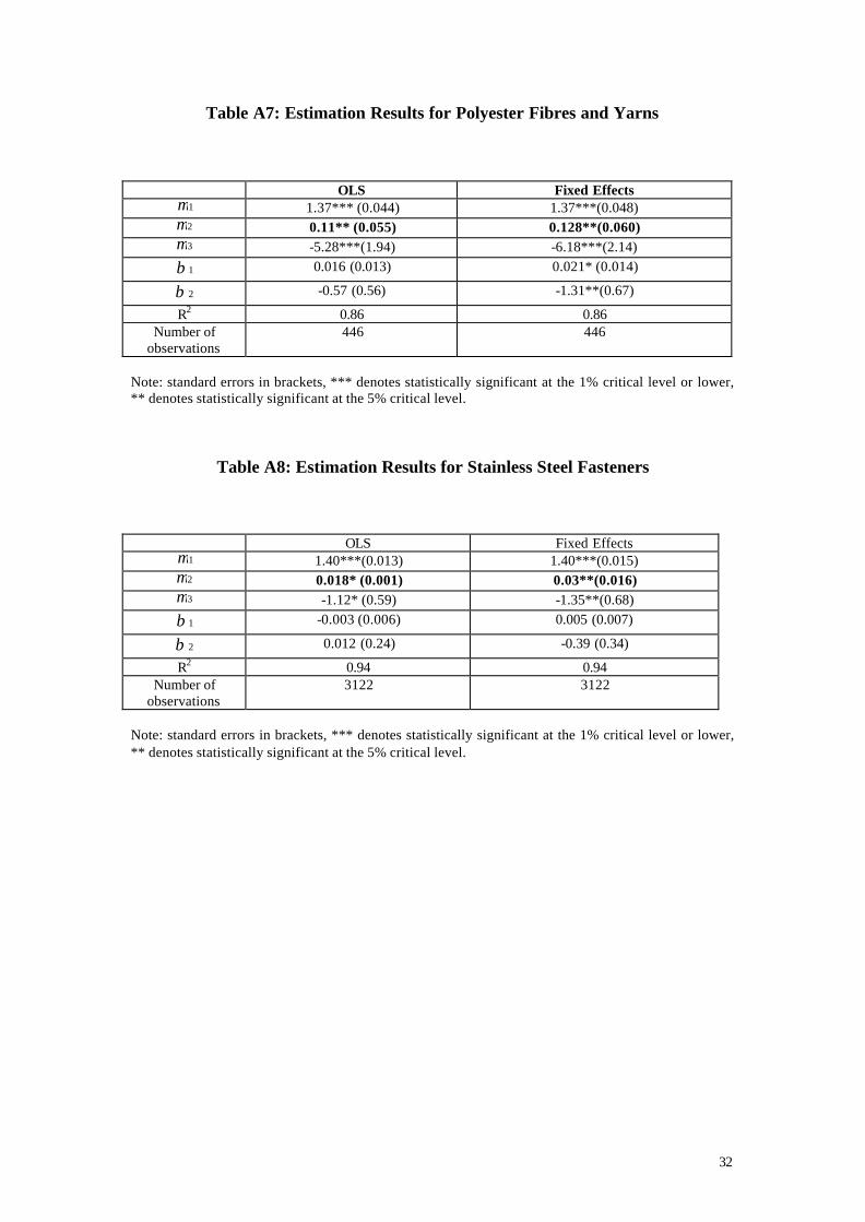
Table A7: Estimation Results for Polyester Fibres and Yarns

OLS Fixed Effects 1µ 1.37*** (0.044) 1.37***(0.048) 2µ 0.11** (0.055) 0.128**(0.060) 3µ -5.28***(1.94) -6.18***(2.14)

1β 0.016 (0.013) 0.021* (0.014)

2β -0.57 (0.56) -1.31**(0.67)




Table A8: Estimation Results for Stainless Steel Fasteners

OLS Fixed Effects 1µ 1.40***(0.013) 1.40***(0.015) 2µ 0.018* (0.001) 0.03**(0.016) 3µ -1.12* (0.59) -1.35**(0.68)

1β -0.003 (0.006) 0.005 (0.007)

2β 0.012 (0.24) -0.39 (0.34)




33

Data Appendix

Construction of the data set

The data that we use are based on all European AD cases that were initiated in

the European Union in 1996. The final data set covers 9 different cases and more than

1,666 European firms for which usable information on sales and input usage needed

for the analysis could be retrieved. For most of the cases only the firms that filed the

complaints are mentioned in the Official Journal reports of the European Commission.

However, once protection is granted, all EU firms producing the product benefit from

protection. The data source that we used to obtain the company account information is

the Amadeus database. This is a commercial database covering all medium and large

sized European companies.12 In order to compose our sample of firms for which we

are relatively certain they would be affected by antidumping protection we proceeded

in various steps.

We first traced the companies that were mentioned in the filing of a case

reported in the Official Journal published by the European Commission. We identified

the 7-digit CSO activity code13 corresponding to the product that was under the AD

investigation. However, the sample of firms involved in the formulation of the

antidumping complaint was too small. To expand our sample of EU firms we turned

to a property of the antidumping legislation which is that when protection is granted it

does not only apply to the firms that actually filed a complaint but it applies to all EU

firms producing that particular product. Hence, we retrieved all EU firms that had in

their description of activities that particular 7-digit CSO code. This still resulted in a

12 For companies located in the UK, Germany, France and Italy, firms are included that satisfy at least of the following criteria: the number of employees larger than 150, operating revenue at least 15 million Euro and total assets of at least 30 million Euro. For the companies located in other countries these criteria collapse to 100 employees, operating revenue of at least 20 million Euro and total assets of at least 100 million Euro.

34

relatively small number of firms. To increase the sample size more, we identified

from our initial sample of complaining firms, the four-digit primary CSO codes. This

corresponds with an aggregation within the product/activity line. We retrieved the

company accounts of these firms between 1991 and 1999. This allowed us to have a

period before protection and a period during which protection was in place which

would allow us to compare market power of these firms both before and during

protection.

Measurement of the Variables Pit .Qit: Firm level operating revenue in each year, source: Amadeus Rit Kit: Book value of tangible fixed assets for each firm in each year times the price of

capital, Rit , defined as

)( ittIit RIPR δ+= (8)

IP : the price index of investment goods for plant and machinery, measured at the

country level. The data stem from the AMECO-database from the ECFIN

department at the European Commission. We are grateful to Werner Roeger

for providing this data.

RI: stands for the real interest rate in each country. The data stem from the ECFIN

department at the European Commission. We thank Werner Roeger for

making these data available to us.

δ: stands for the depreciation rate, measured at the firm level (total depreciation

divided by tangible fixed assets); source: own computations based on

Amadeus

13 The CSO code is a product code that is used by the British Statistical Office and defines the activities of firms at a 7-digit level of detail.

35

Wit Lit: total wage bill in the firm consisting of the price of labor (PL) times employment (L) ; source: Amadeus

PitM Mit: total material costs in the firm consisting of the price of materials (PM) times

materials (M) ; source: Amadeus GDP growth: growth rate in gross domestic product in each country; source: OECD Main Economic Indicators Anti-Dumping Cases: source: ‘The Official Journal of the European Union’ various issues in the ‘C-series’ for notifications of case initiations and the ‘L-series’ for reports on the final decisions.

Documents

Does Antidumping Protection raise Market Power?: Evidence by … · by Jozef Konings and Hylke Vandenbussche Catholic University of Leuven, Belgium and CEPR, London August 2002 Abstract