Does Taking One Step Back Get You Two Steps Forward…wise.xmu.edu.cn/labor2008/files/papers/p35_xinxin chen_does taking... · Does Taking One Step Back Get You Two Steps Forward?

Does Taking One Step Back Get You Two Steps Forward? Grade Retention and School Performance in Rural China

Xinxin Chen* College of Economics, Zhejiang Gongshang University

149 Jiaogong Road, Hangzhou 310035, China

Yaojiang Shi and Weiwei Zhao Northwest Social Science Development Research Center, Northwest University

Xi’an 710067, China

Scott Rozelle Freeman Spogli Institute, Stanford University

616 Serra Street, CA 94305, USA

* Corresponding author. Mailing address: 149 Jiaogong Road, College of Economics, Zhejiang Gongshang University, Hangzhou 310035, China Tel: 86-571-88211232; Fax: 86-571-28008035. E-mail: [email protected]


Abstract

Despite the rise in grade retention in China recently, little work has been done to understand the impact of grade retention on the educational performance of students in China. This paper seeks to redress this shortcoming and examines this impact on 1649 students in 36 elementary schools in Shaanxi province. With a dataset that was collected from a survey designed specifically to capture school performance of students before and after they were retained, we use Difference-in-Difference, Propensity Score Matching and Difference-in-Difference Matching approaches to analyze the effect of grade retention on school performance. Although the descriptive analysis shows that grade retention helps to improve the scores of the students that were retained, somewhat surprisingly, the results from the multivariate analysis consistently show that there is no significant positive effect of grade retention on school performance of the students. In fact, in some cases (e.g., for the students who repeat grade 2), grade retention is shown to hurt school performance.

JEL: I21, I28, O53

Keywords: Grade retention; Educational performance; Human capital

1


In the past, because of fiscal considerations, many provincial departments of

education set maximum limits on the percentage of students in each cohort who could be

retained during their primary school years. For example, in Gansu Province, primary

school principals were instructed to retain no more than three percent of the students in

any of the six grades that constitute elementary education (Guangming Daily, 2000). The

reasoning was that since China was relatively poor, fiscally, mass education demanded

that students move rapidly through the periods of compulsory education.

While the logic of such policies may be understandable from a budgetary

perspective, the experience of educators internationally suggests that such a policy might

adversely affect a certain segment of students. Specifically, the empirical literature

outside of China has shown that in some cases students benefit from grade retention

(Alexander et al., 1994; Kerzner, 1982). Grade retention is good for students, who were

behind in their studies (and received failing or near failing grades), since they are

allowed to relearn the material and catch up with their peers. If this literature is correct,

those who are retained should show relative improvement in the years after they were

retained.

In recent years, perhaps because China’s fiscal situation has improved

dramatically (Wang and Zhou, 2005), the Ministry of Education eliminated the

restrictions on the maximum number of students that could be retained (Ministry of

2

Education, 2006). In some provinces local school administrators were allowed more

authority in deciding how many students would be retained each year. In addition, in

some areas, the funding formulas were relaxed to allow schools who had relatively high

rates of retention to continue to receive a per student subsidy (or allocation) for all

students, even those that were repeating a grade (CCTV, 2006). The idea was that this

might improve the quality of education, a result that would be consistent with the

findings cited above. However, it has been reported that in some localities school

officials may have taken advantage of the new compensation rules and artificially

inflated the retention rates purely for the fiscal gain for the school (CCTV, 2006).

As retention rates rose in some areas, new concerns, also grounded in the debate

within the international education literature, surfaced. In contrast to the empirical

literature that finds retention improves school performance of students (as discussed

above), other research criticizes the casual use of grade retention (Holmes, 1989; Fine,

1991; Grissom and Shepard, 1989). While students who repeat a grade do get a chance to

catch up, they also may experience a negative psychological effect. Many educators

believe that grade retention destroys the self-respect and confidence of students and can

actually decrease educational performance (Royce et al., 1983). There also is a cost to the

family, which has to pay for the associated costs of another year of education, and

retention extends the time that their child could complete his/her compulsory education

and delays for their entrance into the labor force (Yang et al., 1991). If grade retention is

3

associated with poorer education performance, then local policies that encourage high

rates of grade retention could systematically be hurting students.

Somewhat surprisingly, little work has been done to understand whether or not

grade retention in the context of China helps or hurts the educational performance of

children. There are discussions of grade retention in China’s social science literature

(Huang, 1998; Yu, 1999; Wen, 2002; Li, 2004). But, these papers are at best based on

descriptive statistics. Most of them are case studies and use anecdotes as evidence. Given

the fundamental importance in trying to develop better policies for improving education,

there is a need to more rigorously understand empirically how grade retention affects

school performance.

The overall goal of this paper is to examine the effect of grade retention on the

educational performance of elementary school students in China. It is possible that a

better understanding of the impact of grade retention will provide policy makers with the

information they need to make (or not make) changes to the administration of the

educational system in China’s rural areas. To meet this goal, we pursue three specific

objectives. First, we compare the change of scores over time of students that were

retained with students that were not retained. Second, we examine the determinants of

grade retention in rural China in order to find what types of students are most likely to

repeat a grade during their elementary school years. Third, we examine whether or not

grade retention improves or hurts the school performance of rural students by comparing

their performance relative to their peers, both before and after they were retained.

4

To meet these objectives, we will rely on a set of data that we collected in 2006,

a data collection effort that was designed specifically to examine changes in school

performance of children before and after they were retained. With this data set, we focus

our attention on two types of students: the students who were retained in grade 2, 3 or 4

and their fellow students in the same grades that were not retained. Using these different

subsets of students, we compare changes in scores before and after the students repeated

their grades. A descriptive analysis is supplemented by a more rigorous multivariate

analysis on the effects of grade retention on the educational performance using several

approaches, including a Difference-in-Difference approach (DD), Propensity Score

Matching (PSM) and a combination of these two approaches (DDM).

This study is unique in several respects. First, it contributes to the limited

understanding of the effects of grade retention on the school performance in China by

examining how children's grades correlate with grade retention. To date the empirical

literature on grade retention and school performance in China is almost nonexistent.

Second, we use the most up-to-date evaluation methods, instead of the more traditional

OLS approaches.

There are limitations in our approach, however. For example, we focus on

students from one small, poor part of China, a fact that limits our ability to say anything

about China in general. In addition, since we only examine the effect of grade retention

on the performance of the students who were retained in grade 2, grade 3 or grade 4, our

conclusions can not necessarily be generalized to those students who are retained in

5

grade 1 (the most common grade during which students are retained) or in any grade that

is greater than grade 5.

Data

The data used in this paper come from a survey executed by the authors in 2006.

The survey was designed specifically to examine the changes in school achievement of

children before and after they repeated at least one grade. While the survey in part relied

on recall data—especially for some of the control variables—we were able to use records

and rely on multiple sources of information for our two key variables—scores of school

achievement and grade retention.

The sample was drawn from 36 primary schools in 12 towns in Shaanxi province,

one of the nation’s poorest provinces in northwest China. The sample was drawn using a

multi-stage, clustering design with random selection procedures employed at each stage.

In the first stage 6 counties were selected from the total of 93 counties in Shaanxi

province. In the second stage the survey team randomly selected 2 townships in each

county. The 2 townships were chosen from a list of all townships in the county that were

ranked according to per capita income. One township was chosen from the townships

that were relatively rich and the other from the townships that were relatively poor. In the

third stage a list of all primary schools was created in each township (where schools were

limited to all primary schools that included 6 years of schooling—or all wanxiao). From

this list 3 primary schools were chosen randomly.

6

The sample students were selected during the final stage of the sampling. The

sample design consisted of all students that were in the entering each of the sixth grade

classes in each of the sample schools. On average there were 1.4 sixth grade classes per

school, ranging from 1 to 3. When the data were collected in September, the students had

just begun a new school year. Therefore, all of the sample students had just completed

the fifth grade less than 2 months previously (as the school year in China runs between

early September and mid-July). In total, the sample included 1649 children and their

families. Approximately 45 percent of sample students were girls. The ages of the

students ranged between 10 and 16; however, most of the students (73%) were either 11

or 12.

Our main measure of education achievement is based on the math and Chinese

language scores of the students from 2001/2 (their first grade year) to 2005/6 (their fifth

grade year). Fortunately, in China every student in almost every elementary school

(including, at least, all of the schools in our sample) keeps in his/her possession a booklet

that contains a comprehensive record of the math and Chinese scores for each semester

of his/her schooling. This means that the school achievement variables that we use in our

analysis are record-based (not from recall). In other words, the information on school

achievement is not from recall, but is from each student’s grade book. The scores were

copied by our enumerator with the assistance of the homeroom teacher.

In this paper, we focus on second term math and Chinese scores because the

scores for these classes are based on a single year-end test that is standardized. The

7

exams are standardized in two dimensions. First, the questions are the same for all

students within the schools in the same township. Second, the final exams were graded

according to a single set of criteria by a township-wide panel of teachers (which is done

to make the scores more objective).

We also collected detailed information on the grade retention histories of each

student. The students reported which grade they repeated. They also told us how many

times that they repeated each grade. All this information is also available on their

booklets and the enumerator (with the help of the homeroom teacher) was asked to verify

the information as well. As it turns out, only about 8 students repeated more than one

grade. Because they were so special, these students were dropped from the analysis.

Therefore, in our analysis we are looking exclusively at students that were retained for

one year and comparing them to students that were not retained.

Even with standardized grades, one thing that we are worried about is that the

effect of grade retention might be magnified or attenuated if a student was moved from a

“fast or accelerated” class to a “slower” one after he or she was retained. If this were the

case then the effect of grade retention on a student’s grades might be confounded with

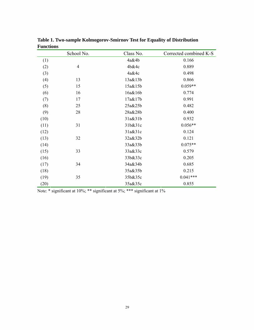
the class placement decision. This is not an issue in 67 percent of the schools that we

surveyed since there was only one class per grade (and, as such, there was no choice in

terms of class placement). When we interviewed teachers and principals in the other

schools, we were told that it was a policy in rural schools not to divide the classes into

accelerated and/or slower ones. Most scholars familiar with rural education—especially

8

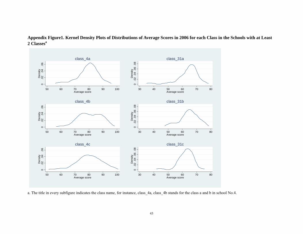
education in poor areas—concurred with this observation. In order to test this proposition,

in schools with 2 fifth grade classes (8 out of 36 schools in total) and 3 fifth grade classes

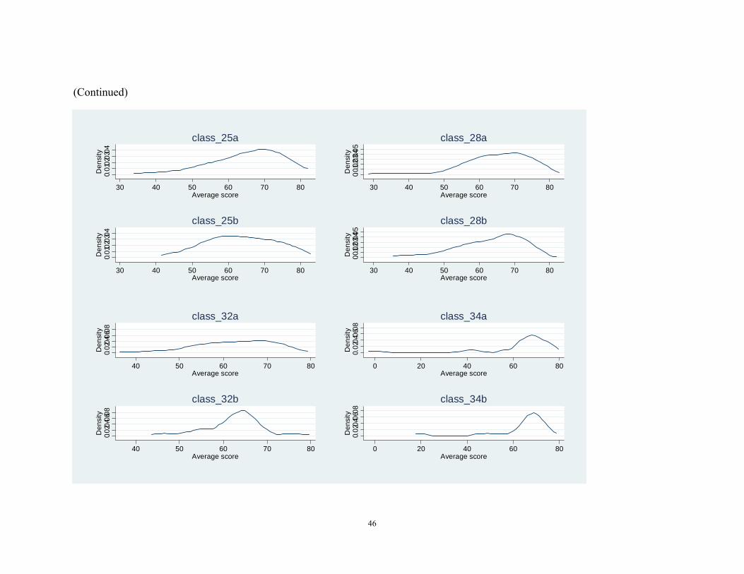
(4 out of 36 schools) we used kernel distribution plots to graph the distributions of the

grades and compared them with each other (Appendix Figure 1). A casual comparison of

the distribution of the grades among the classes within the same school showed that,

indeed, the distributions of the classes appeared similar. To confirm this statistically, we

used a two-sample Kolmogorov-Smirnov test to determine if the distributions of the

scores between any two classes in the same school were equal (Table 1). In all but 4

schools, we can not reject the hypothesis that any two classes in the same school have the

same grade distributions.1 In summary, it appears as if ex-retention class placement bias

is not an issue impacting our analysis.

Another issue on grade retention that we are concerned about is on what criteria

was the grade retention made. In particular, it is important to know if grade retention is a

process that is mostly based on rules set by the school or if it is mostly a process that is in

the hands of parents. Although during our survey and fieldwork this ended up being a

difficult question to ask and get consistent answers, we believe that the survey results

clearly support the conclusion that the grade retention decision is mostly in the hands of

the school authorities, mostly is based on rules and only in a minority number of cases is

subject to negotiations between parents and teachers/school administrators. Almost 100

percent of teachers and school administrators that were surveyed replied that grade

retention was rule based and not subject to negotiations with parents. It is easy in the case

9

of many schools (and/or school districts) to find written rules for grade retention posted

in the school office, in school files and posted on school websites. In addition, more than

60 percent of the parents of children that were retained told us the same thing. Moreover,

although around 40 percent of the parents of students that were retained said that they

were involved in the decision to retain their child, in fact, when looking at the scores of

their children, in all but a small fraction of the cases their children’s grades were such

that they should have been retained on the basis of school rules. Hence, it may be that

although parents may have believed they played a role in their child’s retention decision,

the final decision may have turned out the same whether the parent had visited the school

or not. There are very few cases that a parent requested his/her child be retained when

his/her grades was sufficiently high (that is, above the failing cutoff line).

In addition to school achievement and grade retention information, we also

included information in the survey that could be used to create variables to control for

other observed factors that might be expected to affect school achievement (that can be

used as control variables). Two sets of variables were collected. In a set of questions

about student characteristics, we collected information about each student’s gender, age

and asked them whether or not they were student cadres. The survey form also included

questions on the characteristics of the student’s parents and family. The dataset includes

variables on each parent’s age and education attainment as well as the household’s land

holdings and the total number of other household members.

10

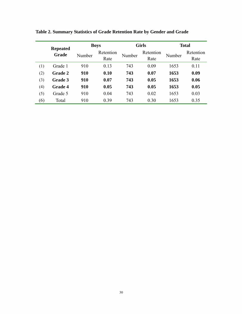
Grade Retention in China

Based on our data, one of the results which stands out above all others is the high

rate of grade retention in our sample schools. Out of the 1653 students in the sample

schools, 35 percent of the students in rural primary school repeated at least one grade

before they entered grade 6 (Table 1, columns 1 and 2). If such high rates of retention are

common throughout China, it is clear that in the mid-2000s the prohibition against

retaining a maximum of five percent of students is no longer binding. In fact, references

to high retention rates are increasingly common in the literature (Wang and Wang, 1999).

For example, China Central TV station reported that the retention rate in some

elementary schools in Gansu Province was as high as 30 percent (CCTV, 2006). These

high rates reported in areas outside of our sample area imply that our data may well be

capturing what is a fairly common phenomenon. Internationally, however, such high

rates are less common. In the US, for example, the estimated grade retention rates of the

students aged 14 and under range from 6.69 percent to 1.23 percent between the first

grade and the fifth grade (Eide and Showalter, 2001). Interestingly, in our sample more

boy students (39%) were retained than girl students (30 percent—columns 3 to 6).

Although the overall retention rate is high for primary school, in general, the rates

at which students are asked to repeat grades vary over the six years of schooling. Clearly,

the rate is highest for first grade. Fully 11 percent of first graders repeat their first year of

elementary school (Table 1). Such a finding, however, is not special. In the US, for

11

example, retention rates are almost always substantially higher in the first grade than in

subsequent grades (Eide and Showalter, 2001).

The other pattern in the retention data that is somewhat remarkable is that after

grade 1, the retention rates fall steadily (Table 1). Between grades 2 and 4, the retention

rate falls from 9 percent to 6 percent to 5 percent.2 By the fifth grade, only 3 percent of

students were retained. Interestingly, of the nearly 600 students that repeated grades, only

8 of them repeated more than one grade.

So who are these students that were retained for at least one grade? To answer this,

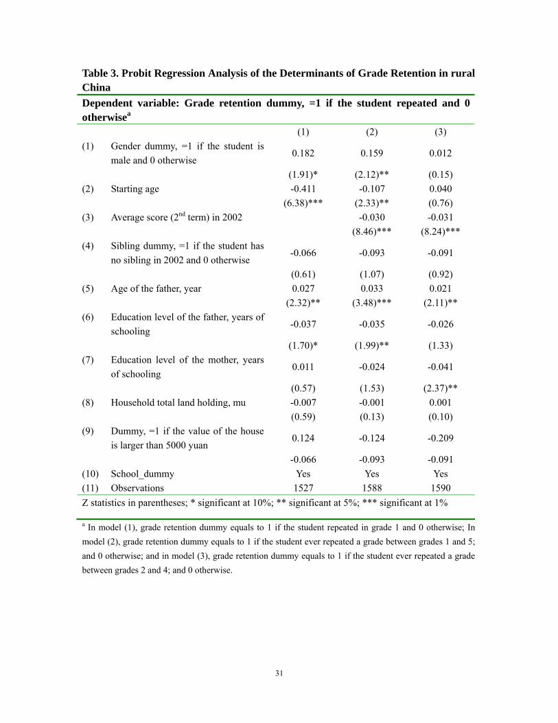
we ran a probit regression to examine the determinants of repeating a grade (Table 3).3

In other words, on the left hand side we included a variable that equaled one if the

student was retained (and zero otherwise); on the right hand side we included a series of

student, school and parent characteristics. We repeated the regressions with three

alternative dependent variables, depending if the student was retained in the first grade or

not (column 1); if the student was ever retained in the second to fourth grades (column 3);

and if the student was ever retained during any year in which she/he was in elementary

school.

According to our descriptive regression results, we find that certain types of

students tend to repeat grades more often than others, although the results differ between

the regressions that include first grade repeaters (columns 1 and 2) and those that do not

include them (column 3). For example, we find that, ceteris paribus, young boy students

are more likely to be retained than young girl students in the first grade (row 1, column

12

1). Looking at students’ entire time at elementary school (including the first grade) boy

students are also more likely to be retained for one of the grades (row 1, column 2). The

gender effect, however, is not observed during grades 2 to 4. Also, the age at which a

child starts school is negatively associated with the tendency to repeat grades—especially

for the first and second regressions (row 2, columns 1 and 2). However, like the gender

effect, this correlation also disappears during grades 2 to 4 (column 3). In addition, the

scores that students earned during the beginning year of elementary school are associated

closely with whether those students repeated any grades (either grades 1 to 5—row 3,

column 2; or grades 2 to 4—column 3). Perhaps not surprisingly, students that have

higher grades in the first grade tend to have a lower probably of repeating a grade during

the subsequent years. Finally, in all of the regressions, several of the other control

variables (e.g., age of father) are robustly correlated with grade retention—regardless of

the nature of the dependent variable.

Grade Retention and School Performance

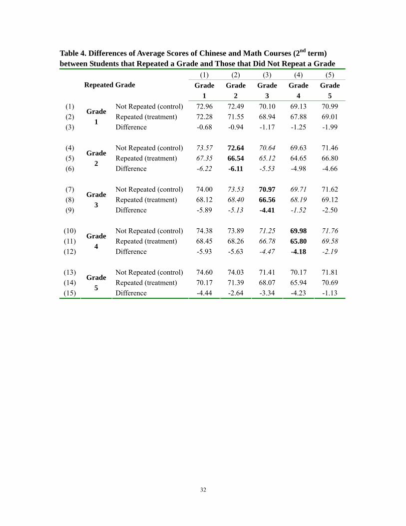
Most importantly, especially in our analysis, when students were retained, there

was a relative improvement to their school performance. Based on descriptive statistics

using our data, when we examine changes in the scores of students before and after they

were retained in the second grade, the gap in the scores is narrowing between the

students who were retained during their second grade years and those that were not

retained. It is true that the scores of those that were retained were lower than those that

were not retained—both before and after the year that students repeated. However, their

13

grades, on average, were 6.22 points lower before they were retained and only 5.53

points lower after they were retained.

This same pattern holds for those students that were retained in the third and

fourth grades. For the students retained in the third grade, the gap in the scores (between

the year before and the year after retention) dropped from 5.13 to 1.52. For the students

retained in the fourth grade, the gap dropped from 4.47 to 2.19. The implication of these

findings (should they hold up in the multivariate analysis—see below) is that grade

retention appears to be helping students by improving their grades in a relative sense.

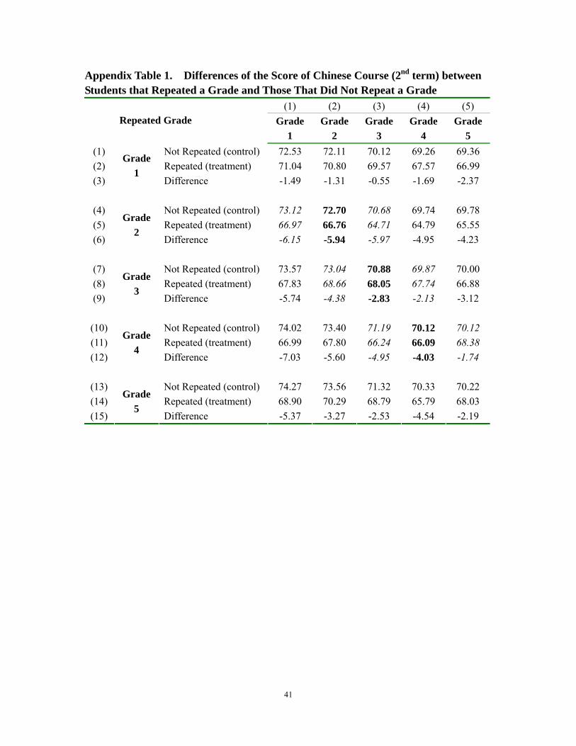
The narrowing gap is also fairly robust in several dimensions. For example, the

narrowing of the gap is found to persist over time (or in the long run). In other words, the

gap in the scores of grade 5 between those that were retained in grade 2 (grade 3) and

those that were not retained was narrower than the gap in the scores in grade 1 (grade 2).

In addition, the falling gap shows up when we look at Math Scores and Chinese Scores

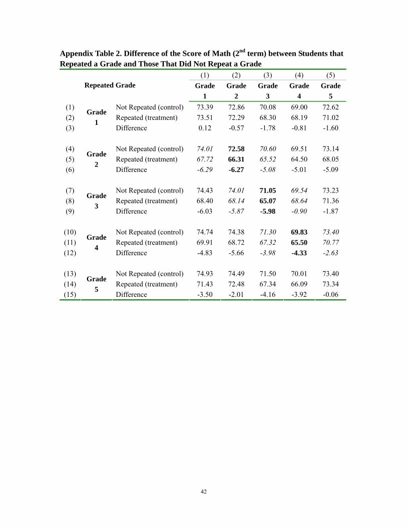
separately (Appendix Tables 2 and 3). To show this it can be seen that for the students

retained in the second grade, the gap in the scores between them and those not retained

dropped from 6.15 to 5.97 in Chinese language and from 6.29 to 5.08 in math.

In short, then, the descriptive results show that grade retention may be helping

students. Although those that were retained have grades lower than those that were not

retained, the gap is narrowing over time. Such a finding would mean that something (for

example, allowing students a chance to catch up or allowing them to mature age-wise) is

helping contribute positively to the school performance of individuals. However, it is

14

important to remember that our results to this point are descriptive. It is possible that

when other factors are held constant, this positive result will disappear. We also do not

know if the point estimate is positive if it is statistically significant or not (that is, it could

be statistically equal to zero). In fact, the education literature contains many papers that

discuss the tendency of other factors to affect grades. For example, one paper finds that

girl students outperform the boy students (ERIC Development Team, 2005) in reading

and writing in some grades. Other papers have found that the starting age of a student

also affects school performance (Fredriksson and Öckert, 2005). Because of these effects

(and possible interactions between them and retention and grades), multivariable analysis

is needed to more fully explore the impacts of grade retention on the school performance.

Methodology

The objective of this study is to examine the effects of the grade retention on the

student’s educational performance. In order to evaluate the effects of grade retention,

conceptually we are making grade retention the treatment. In other words, our sample

students are divided into a treatment group (those that were retained by the school and

had to repeat a grade) and a control group (those that never repeated a grade). More

specifically, the treatment group includes all the students who ever repeated the second

grade, third grade or fourth grade. The control group includes all the students who were

never retained, but does not include any students who were retained in either the first or

fifth grade (which are dropped from the sample). With this set up, we are interested in

15

understanding the mean impact of “treatment on the treated,” which is the average impact

of grade retention among those treated (Smith and Todd, 2005):

( ) ( ) ( )1 0 1 0( ) | , 1 | , 1 | , 1TT E Y Y X D E Y X D E Y X D= − = = = − = (1)

where we denote Y1 as the outcome (the grades of students—in our case) after the student

was retained and Y0 as the outcome if a student was not retained. In equation (1), our

treatment is denoted by D=1 which stands for the students who were retained for at least

one grade and for whom Y1 is observed and D=0 stands for those who were not retained

for whom Y0 is observed. Because in reality we do not observe either the counterfactual

mean, ( )0 | , 1E Y X D = , or the mean outcome for the students had they not been retained

in a grade after they were retained, we need to employ a difference-in-difference

estimation approach (DD). Using the DD approach allows us to compare the outcomes

before and after a student repeated a grade with students not affected by the treatment

(those who were not retained).

In equation (1) let t and t' denote time periods after and before the change of

grade retention. When doing so, the standard DD estimate is given by:

[ ] [ ]( | 1) ( | 1) ( | 0) ( | 0)t t t tDD E Y D E Y D E Y D E Y D′ ′= = − = − = − = (2)

The idea of using a DD estimator to estimate the effect of the treatment on the treated is

that it allows us to correct for the differences before and after the treatment (that is for the

grades before and after a student was retained) by subtracting the simple difference for

the control group (not retained students). By comparing the before-after change of treated

groups with the before-after change of control groups, any common trends, which will

16

show up in the outcomes of the control groups as well as the treated groups, will be

differenced out (Smith 2004).

In addition to the standard DD estimator, we implement three other DD

estimators: an “unrestricted” version that includes Yt' as a right hand variable, an

“adjusted” version that includes other covariates in addition to the treatment variable (in

our case they are a series of control variables from 2002 or the pre-program period), and

an unrestricted/adjusted model that combines the features of both the “unrestricted” and

“adjusted” model. The unrestricted and adjusted DD estimators relax the implicit

restrictions in the standard DD estimator that the coefficient associated with Yt'

(pre-program outcome) and covariates in t' (pre-program period) equals one. The

combination of unrestricted and adjusted DD estimators relaxes both of these

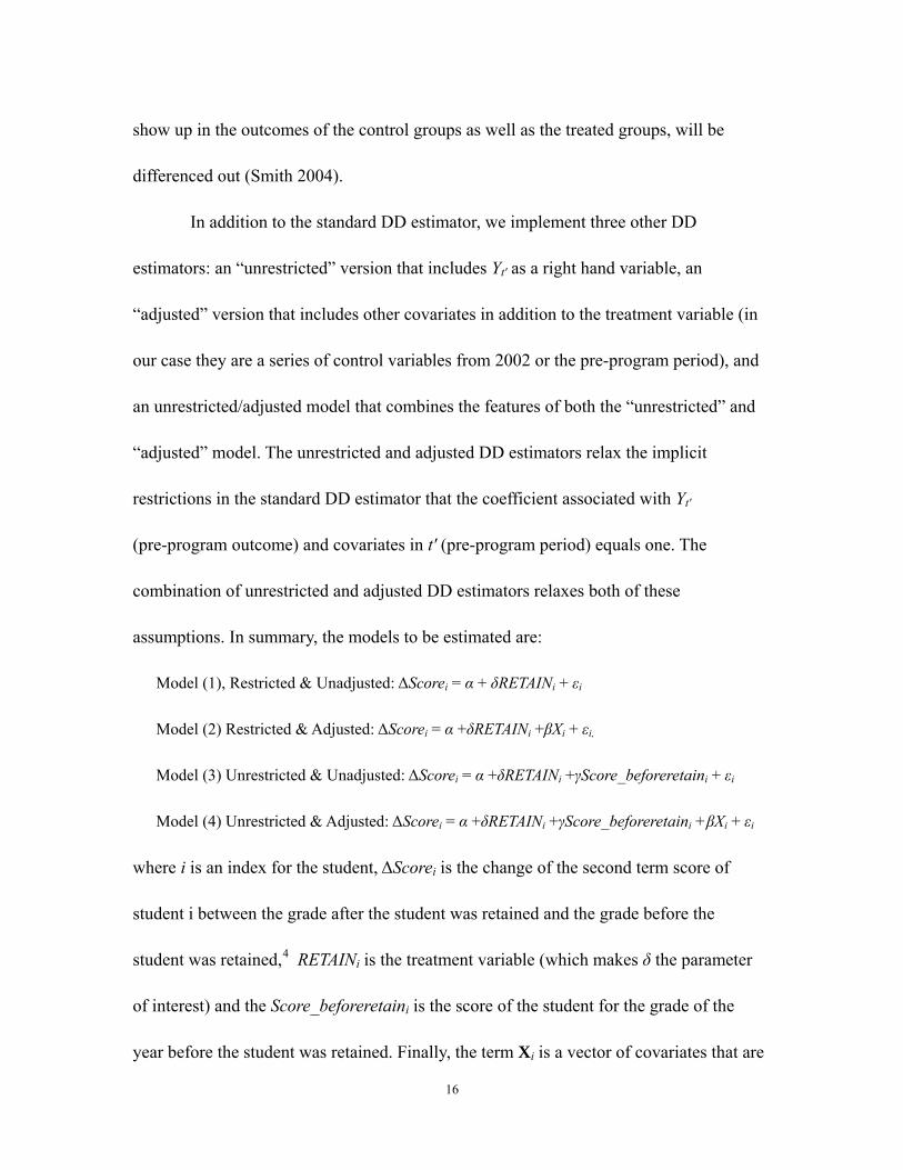
assumptions. In summary, the models to be estimated are:

Model (1), Restricted & Unadjusted: ΔScorei = α + δRETAINi + εi

Model (2) Restricted & Adjusted: ΔScorei = α +δRETAINi +βXi + εi,

Model (3) Unrestricted & Unadjusted: ΔScorei = α +δRETAINi +γScore_beforeretaini + εi

Model (4) Unrestricted & Adjusted: ΔScorei = α +δRETAINi +γScore_beforeretaini +βXi + εi

where i is an index for the student, ΔScorei is the change of the second term score of

student i between the grade after the student was retained and the grade before the

student was retained,4 RETAINi is the treatment variable (which makes δ the parameter

of interest) and the Score_beforeretaini is the score of the student for the grade of the

year before the student was retained. Finally, the term Xi is a vector of covariates that are

17

included to capture the characteristics of students, parents and households. Throughout

our analysis, Xi also includes a set of 12 town indicator or dummy variables.

Alternative Estimation Approaches

It is important to remember that the identification of the causal effects using DD

relies on the assumption that absent the policy change (or grade retention in our case), the

average change in t tY Y ′− would have been the same for the treated and the control

groups. Formally, this is called the “parallel trend” assumption, which can be expressed

as:

0, 0, 0, 0,( | 1) ( | 1) ( | 0) ( | 0)t t t tE Y D E Y D E Y D E Y D′ ′= − = = = − = (3)

As might be expected, the effectiveness of DD depends on the validity of this

assumption. And the reality of our question (understanding the effect of grade retention

on the grades of students) may mean that even though we control for a large number of

observable variables in 2002 in the adjusted and unrestricted versions of the DD

estimates, there could be other unobservable factors that may compromise the parallel

trend assumption. Because of the potential existence of other differences between

students retained and students not retained, we also use propensity score matching (PSM),

which is an approach that does not require the parallel trend assumption. PSM allows the

analyst to match the treated and the controls when observable characteristics of students,

who were retained, and observable characteristics of students, who were not retained, are

continuous (Rosenbaum et al. 1985). With the right data, it is possible to estimate the

propensity scores of all students and compare the outcomes of students who were

18

retained and those who were not retained that have similar propensity scores.5 In this

way, then, we can obtain the mean impact of the treatment on the treated (Dehejia and

Wahba, 2002; Smith and Todd, 2005):

{ }1 0 1 | 1 0( | 1) ( | 1) ( | ( ), 0)Z DE Y Y D E Y D E E Y p Z D=− = = = − = (4)

where ( ) Pr( 1| )p Z D Z≡ = is the propensity score. Matching is based on the assumption

that outcomes (Y0, which is a score of the student—in our case) are independent of

participation (grade retention) conditional on a set of observable characteristics

(Rosenbaum and Rubin, 1983). Because of this assumption, we do not need to worry

about unobservable heterogeneity. By matching students who were retained and students

who were not retained with similar values of Pr( 1| )D Z= , any differences

in 0( )E Y between the two groups are assumed to be differenced out when calculating the

above equation. The assumption of matching is that 0 0( | , 1) ( | , 0)E Y Z D E Y Z D= = = .

The observable covariates Z should include the characteristics that determine grade

retention. In our analyses, Z includes a number of variables including student, parent and

household characteristics. We also include township fixed effects to control for

unobservable factors at the township level that may affect grade retention.

To implement PSM successfully, however, the nature of the students who were

retained and the nature of the students who were not retained must meet certain criteria.

Importantly, the common support of propensity scores for participating and

non-participating students should be fairly wide. Intuitively, wide common support

means that there must be a fairly large overlap in the propensity scores between the

19

treated and control groups. In our sample, the common support is fairly wide.6 This

means that we can estimate the average treatment effect for the treated of a large portion

of the sample.7

To eliminate the bias due to time-invariant unobservable differences between

retained students and non-retained students, we extend the cross-sectional PSM approach

to a longitudinal setting and implement a difference-in-differences matching (DDM)

strategy. With DDM we can exploit the data on the retained students in the grade before

they repeated to construct the required counterfactual, instead of just using the data in a

grade after they repeated (as was used in the traditional PSM analysis—which was

describe above). The advantage of DDM is that the assumptions that justify DDM

estimation are weaker than the assumptions necessary for DD or the conventional PSM

estimator. DDM only requires that in the absence of treatment, the average outcomes for

treated and controls would have followed parallel paths:

)0),(|()0),(|()1),(|()1),(|( '' ,0,0,0,0 =−===−= DZPYEDZPYEDZPYEDZPYE tttt (6)

Assumptions embedded in equation (6) are weaker than the assumptions

necessary for DD. Intuitively, DDM removes time invariant unobservable differences

between retained students and non-retained students conditional on P(Z), a clear

advantage over cross-sectional PSM.8

Although the above matching methods can significantly improve the reliability

of matching estimators, producing results that have been shown to be very close to those

based on a randomized design counsel that geographic mismatch between matched

20

observations should be avoided (Smith and Todd, 2005; Abadie and Imbens, 2006). In

our case when we use PSM, even if we have added a set of township dummies when

estimating the propensity scores, students that are from different townships, but that have

similar propensity scores, may still be matched as a pair of treatment and control

observations. Abadie and Imbens (2006) propose a method to eliminate the bias caused

by imprecise matching of covariates between treatment and control observations using

nearest neighbor matching.9

In making specific choices about the methodology, our approach is to minimize

potential bias whenever possible. To minimize geographic mismatch, we enforce exact

matching by township.10 To do this, each treatment observation is matched to three

control observations with replacement, which is few enough to enable exact matching by

township for nearly all observations, but enough to reduce the asymptotic efficiency loss

significantly (Abadie and Imbens, 2006). When we use this method for matching, we

report our results as multi-dimensional matching results to differentiate this approach to

matching from the traditional or basic matching approach that we also use (which was

described above).11 This approach has been shown to prevent the estimates from relying

too heavily on just a few control observations. In other words, because we are not sure

what is the best approach, apriori, we use all of the approaches and hope that our results

are the same—regardless of the exact approach adopted.

Results of Multivariate Analysis

21

The results of our DD analysis using the restricted specifications (that is, Models

1 and 2) demonstrate that the findings of the multivariate analysis are consistent with the

descriptive analysis. For example, when we use the Restricted and Unadjusted

specification of the empirical model (Table 5, column 1), the results show that, ceteris

paribus, the scores of the students that were retained in grades 2, 3 and 4 rose relatively

more than those students who never repeated a grade during this period of elementary

school (row 1). The coefficient on the variable of interest is statistically significant. This

finding (from the most simple model) suggests that grade retention actually improves the

performance of students that were retained, the same finding as that of the descriptive

statistics that were reported in Table 4. This result does not change much when we use

the Restricted and Adjusted specification (which is the same specification as in column 1,

but also controls for a number of observable covariates—column 2, row 1). If these

results were to hold up throughout the rest of the paper, we might conclude that there is

actually a benefit that is accruing to students from the recent relaxation of restrictions on

the maximum number of students that can be retained in a single year.

When we use the unrestricted specification (either the unadjusted or adjusted

version of the model—that is Models 3 or 4), however, the results change sharply (Table

5, columns 3 and 4). By controlling for the performance of the student when they were in

grade 1 (or the year before any of the students were retained—which is accomplished by

including the variable, Score_grade1i), the sign on the coefficient of the grade retention

variable during grades 2, 3 and 4 becomes negative (row 1). The coefficient of interest is

22

negative and significant in the model that includes both Score_grade1i and the other

covariates (or the Unrestricted and Adjusted Model, column 4, row 1). In general, this

result demonstrates that the scores of students that repeated a grade (either grade 2 or 3 or

4), in fact, dropped relative to the scores of those students that had never repeated a grade.

Therefore, the most important finding in table 5 is that—at least for the unrestricted

model—we can reject the hypothesis that grade retention improves school performance.

These results also show the importance of controlling for a student’s ability (or,

at least, the grades earned in grade 1). The t-ratios associated with the coefficient of the

Score_grade1i variable are very high. Moreover, the higher adjusted R-square statistics in

models that include grade 1 scores show that the Unrestricted versions of the model

(columns 3 and 4) fit the data better. In other words, when analyzing the effect of grade

retention on school performance it is important to control for a student’s ability (or

his/her beginning scores). Therefore, in the rest of the paper, we focus on the Unrestricted

models.

The same basic results hold when we look at the short term effects of grade

retention in grade 2 or grade 3 or grade 4 (Table 6).12 Whether using the Unadjusted

version of the model (columns 1, 3 and 5) or the Adjusted version of the model (columns

2, 4 and 6), we can not find any significant positive effect of grade retention on school

performance. This is true for those that repeat grade 2 (columns 1 and 2), grade 3

(columns 3 and 4), and grade 4 (columns 5 and 6). In other words, our results are

23

consistent with those in the international literature that raise concerns that grade retention

is not beneficial to the average student (Holmes, 1989; Fine, 1991).

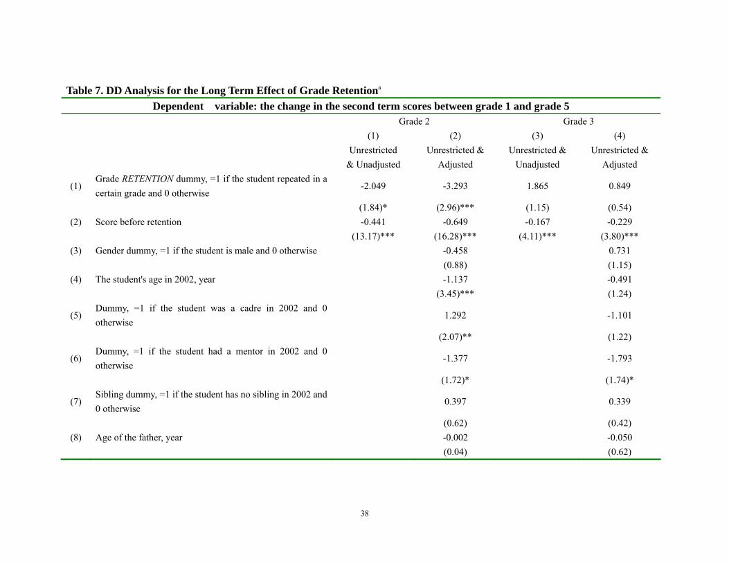
The results remain almost the same when we examine the long term effects of

grade retention in grades 2 and 3. In this paper, the long term effect of grade retention is

defined as the change in score of a student between grade 1 and grade 5. This means that

we are measuring a three year effect in the case of those students that were retained in

grade 2 and a two year effect in the case of those students that were retained in grade 3.

When doing so, the results remain consistent and show that there is no positive long term

effect of grade retention (Table 7). This is true if the student repeated grade 2 (columns 1

and 2) or grade 3 (columns 3 and 4). It also is true regardless of the version of the model

that we run. In fact, for those students that repeated grade 2, their scores not only did not

rise, they actually dropped (significantly) by more than 3 points.

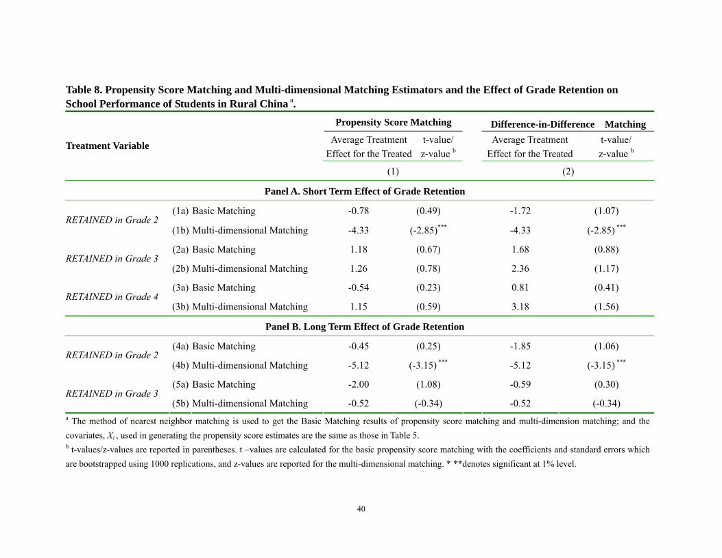
Results from Alternative Methods

The results of cross-sectional PSM analysis—regardless of the method of

matching—also reveal that grade retention has no significant positive effect on the school

performance of students. When examining the effect of grade retention on school

performance for all the students who were ever retained in any grade (that is, either grade

2 or grade 3 or grade 4) using Basic Matching methods, there are no cases in which the

coefficient on the treatment variable (RETAIN) is positive and significant (Table 8,

column 1, rows 1a, 2a, 3a, 4a, and 5a). The same is true when using Multi-dimensional

24

Matching (column 1, rows 1b, 2b, 3b, 4b, and 5b). In fact, the results from the PSM

analysis are quite similar to those from the DD analysis.

Finally, the findings continue to remain largely consistent when using Difference

in Difference Matching (DDM—Table 8, column 2). Regardless if we use Basic

Matching (rows 1a, 2a, 3a, 4a, and 5a) or Multi-dimensional matching (rows 1b, 2b, 3b,

4b, and 5b), none of the coefficients of the treatment variables are positive and significant.

In fact, when using Multi-dimensional Matching, in the case of those students that were

retained in grade 2, the coefficients are negative and significant.

Hence, whether using DD, PSM or DDM, there is no evidence that grade

retention in our sample of students has improved school performance. This is true if we

look at the effect in the short- or long-run. In fact, there is some evidence that when

students repeated grade 2, retention appears to have a negative effect on school

performance. While we have no basis on which to determine the exact mechanism that is

causing the fall in grades, it is consistent with an explanation that often appears in the

international literature that suggests that when students are retained the fall in their self-

esteem, in fact, offsets any positive effect of allowing the student another year to catch up

(Kellam, et al., 1975).

Summary and Conclusions

In this paper we have tried to understand whether or not grade retention helps or

hurts school performance of the students that were retained for a year of schooling during

25

their elementary school years. The issues has gained prominence since in recent years

retention rates—at least anecdotally—have begun to rise. Policy makers—who at one

time restricted retention rates to not exceed a maximum level—should want to know how

school performance of children is being affected when local educators raise the

frequency of grade retention. According to the international literature, it is possible that

grade retention can either benefit students (by giving them time to mature and catch up)

or hurt them (by harming self esteem and/or removing them from their original set of

peers).

According to the results in this paper, we show—perhaps somewhat

surprisingly—that there is no positive effect of grade retention on school performance of

the students that were retained. Whether in the short term (the year immediately after a

student was retained) or longer term (by grade 5), we can reject the hypothesis that grade

retention improves the scores of the students that were retained. This result is true for

students that were retained in grade 2, grade 3 and grade 4. In fact, in the analysis of

some students that were retained (especially those that were retained in grade 2) grade

retention was shown to have a statistically significant and negative effect on school

performance.

Based on these results, it is possible to conclude that the conscious or

unconscious decision to relax the rule to limit retention rates to a maximum level (which

was originally made by education officials to limit the use of scarce fiscal resources that

were allocated for public education) has actually had little benefit for—and may have

26

had negative effects on—the school performance of the sample students. It is unclear

why retentions rates have risen in recent years. If, as some have suggested, the rise in

retention rates is due to some unintended incentive of funding arrangements that allows

local elementary schools to increase revenues when student enrollments are

higher—including the participation of students that have been retained—there needs to

be investigation into ways to curb such actions.

There are also other, more far-reaching actions that these results may be

advocating. It is also possible that grade retention would have a more positive effect on

students if there were more complementary educational services available—such as

counseling, tutoring sessions or, at the very least, an effort made by schools to make

grade retention a more positive thing—and try in some way to reduce the stigma that

could lead to falling self esteem. We understand that our current results are not rich

enough to provide evidence on which any of these further actions could be justified.

However, the paper does produce results that should lead to calls for further research

efforts that can be designed to better understand the effect of grade retention on the

school performance of rural children.

27

References Abadie, A., and G. Imbens. 2006. “Large sample properties of matching estimators for

average treatment effects.” Econometrica 74: 235-267. Abadie, A. (1998). Semiparametric estimation of instrumental variables models for causal

effects. In Working Paper. Cambridge, MA: MIT Economics Department. http://www.nwnu.edu.cn/yjzx/kcxzh.htm Alexander, K. L., Entwisle, D. R., and Dauber, S. L. 1994. On the success of failure. New

York: University of Cambridge Press. China Central TV (CCTV). 2006. “the Amazing High retention Rate.” 9.16:

http://bbs.cctv.com/cache/forumbook.jsp?id=8914299&pg=1&agMode=1 Dehejia, R. H., and S. Wahba. 1999. “'Causal Effects in Nonexperimental Studies:

Reevaluating the Evaluation of Training Programs.” Journal of American Statistical Association 94: 1053-1062.

Dehejia, R. H., and S. Wahba. 2002. “Propensity Score-Matching Methods for Nonexperimental Causal Studies.” The Review of Economics and Statistics 84: 151-161.

Eide E. R. and M. H. Showalter, 2001. “The effect of grade retention on educational and labor market outcomes.” Economics of Education Review 20 : 563-576.

ERIC development team. 2001. “Gender Differences in Educational Achievement within Racial and Ethnic Groups.”, ED455341, http://www.eric.ed.gov/ERICDocs/data/ericdocs2sql/content_storage_01/0000019b/80/17/34/2d.pdf

Fredriksson, P., and Öckert B. 2005. “Is Early Learning Really More Productive? The Effect of School Starting Age on School and Labor Market Performance.” working paper, IZA DP No. 1659

Fine, M. 1991. Framing dropouts: notes on the politics of an urban public high school. Albany, NY: SUNY Press.

Grissom, J. B., and L. A. Shepard. 1989. “Repeating and dropping out of school.” in L. A. Shepard, and M. L. Smith, Flunking grades: research and policies on retention (pp. 34–63). London: Falmer.

Guangming Daily, 2000. “Gansu will gradually abolish grade retention in the elementary schools.” 3.28

Holmes, C. T. 1989. “Grade level retention effects: a meta-analysis of research studies.” in L. A. Shepard, & M. L. Smith, Flunking grades: research and policies on retention (pp. 16–33). London: Falmer.

Huang Zh. 1998. “Retention shouldn’t be abolished.” Management of Elementary and Middle Schools 3

Kellam, S. G., Branch, J. D., Agrawal, K. C., & Ensminger, M. E. 1975. Mental health and going to school: the Woodlawn Program of assessment, early intervention, and evaluation.Chicago, IL: University of Chicago Press. Kerzner, R. L. 1982. The effect of retention on achievement. Union, NJ: Kean College of

http://www.nwnu.edu.cn/yjzx/kcxzh.htm

http://bbs.cctv.com/cache/forumbook.jsp?id=8914299&pg=1&agMode=1

28

New Jersey. Family, Home and Social Sciences at Brigham Young University. Li H. 2004. “Retention, a Topic that Should be Readdressed.” Jiaoyuzhongheng. 3 Ministry of Education. 2006. “the law of compulsory education in China.”

http://www.moe.edu.cn/edoas/website18/info20369.htm Rosenbaum, P., and D. B. Rubin. 1983. “The central role of the propensity score in

observational studies for causal effects.” Biometrika 70: 41–55 Rosenbaum, P., and D. B. Rubin. 1985. “Constructing a control group using multivariate

matched sampling methods that incorporate the propensity score.” American Statistician 39: 33–38

Royce, J. M., R. B. Darlington, & H. W. Murray. 1983. “Pooled analysis: findings across studies.” in Consortium for Longitudinal Studies, As the twig is bent: lasting effects of preschool programs. Hillsdale, NJ: Erlbaum 411–459.

Smith, J. 2004. “Evaluating the Local Economic Development Policies: Theory and Practice.” Unpublished, College Park, Maryland.

Smith, J., and P. Todd. 2005. “Does Matching Overcome Lalonde's Critique of Nonexperimental Estimators?” Journal of Econometrics 125:305-353.

Wang, C., and F. Zhou. 2005. “Reforming fiscal policy after tax for fee reform in China.” Working paper, World Bank, Washington DC.

Wang, l., and Wang J. 1999. “Current situation of basic education in Northwest China.”, http://www.nwnu.edu.cn/yjzx/kcxzh.htm

Wen X. 2002. “Promotion or Retention, which is More Efficient.” Information of Education. 5:17-18

Yang N. 1991. “Analysis on the Dropping out and Grade retention in the Elementary and Middle Schools in China, People’s Education 3.

Yu Z. 1999. “There should be a Retention System in Elementary Schools.” Management of Elementary and Middle Schools 9

29

Table 1. Two-sample Kolmogorov-Smirnov Test for Equality of Distribution Functions

School No. Class No. Corrected combined K-S(1) 4a&4b 0.166 (2) 4b&4c 0.889 (3)

4 4a&4c 0.498

(4) 13 13a&13b 0.866 (5) 15 15a&15b 0.059** (6) 16 16a&16b 0.774 (7) 17 17a&17b 0.991 (8) 25 25a&25b 0.482 (9) 28 28a&28b 0.400

(10) 31a&31b 0.932 (11) 31b&31c 0.056** (12)

31 31a&31c 0.124

(13) 32 32a&32b 0.121 (14) 33a&33b 0.075** (15) 33a&33c 0.579 (16)

33 33b&33c 0.205

(17) 34 34a&34b 0.685 (18) 35a&35b 0.215 (19) 35b&35c 0.041*** (20)

35 35a&35c 0.855

Note: * significant at 10%; ** significant at 5%; *** significant at 1%

30

Table 2. Summary Statistics of Grade Retention Rate by Gender and Grade

Boys Girls Total Repeated

Grade Number Retention Rate Number Retention

Rate Number Retention Rate

(1) Grade 1 910 0.13 743 0.09 1653 0.11 (2) Grade 2 910 0.10 743 0.07 1653 0.09 (3) Grade 3 910 0.07 743 0.05 1653 0.06 (4) Grade 4 910 0.05 743 0.05 1653 0.05 (5) Grade 5 910 0.04 743 0.02 1653 0.03 (6) Total 910 0.39 743 0.30 1653 0.35

31

Table 3. Probit Regression Analysis of the Determinants of Grade Retention in rural China Dependent variable: Grade retention dummy, =1 if the student repeated and 0 otherwisea

(1) (2) (3) (1) Gender dummy, =1 if the student is

male and 0 otherwise 0.182 0.159 0.012

(1.91)* (2.12)** (0.15) (2) Starting age -0.411 -0.107 0.040 (6.38)*** (2.33)** (0.76) (3) Average score (2nd term) in 2002 -0.030 -0.031 (8.46)*** (8.24)*** (4) Sibling dummy, =1 if the student has

no sibling in 2002 and 0 otherwise -0.066 -0.093 -0.091

(0.61) (1.07) (0.92) (5) Age of the father, year 0.027 0.033 0.021 (2.32)** (3.48)*** (2.11)** (6) Education level of the father, years of

schooling -0.037 -0.035 -0.026

(1.70)* (1.99)** (1.33) (7) Education level of the mother, years

of schooling 0.011 -0.024 -0.041

(0.57) (1.53) (2.37)** (8) Household total land holding, mu -0.007 -0.001 0.001 (0.59) (0.13) (0.10) (9) Dummy, =1 if the value of the house

is larger than 5000 yuan 0.124 -0.124 -0.209

-0.066 -0.093 -0.091 (10) School_dummy Yes Yes Yes (11) Observations 1527 1588 1590 Z statistics in parentheses; * significant at 10%; ** significant at 5%; *** significant at 1%

a In model (1), grade retention dummy equals to 1 if the student repeated in grade 1 and 0 otherwise; In model (2), grade retention dummy equals to 1 if the student ever repeated a grade between grades 1 and 5; and 0 otherwise; and in model (3), grade retention dummy equals to 1 if the student ever repeated a grade between grades 2 and 4; and 0 otherwise.

32

Table 4. Differences of Average Scores of Chinese and Math Courses (2nd term) between Students that Repeated a Grade and Those that Did Not Repeat a Grade

(1) (2) (3) (4) (5)

Repeated Grade Grade

1 Grade

2 Grade

3 Grade

4 Grade

5 (1) Not Repeated (control) 72.96 72.49 70.10 69.13 70.99 (2) Repeated (treatment) 72.28 71.55 68.94 67.88 69.01 (3)

Grade 1

Difference -0.68 -0.94 -1.17 -1.25 -1.99

(4) Not Repeated (control) 73.57 72.64 70.64 69.63 71.46 (5) Repeated (treatment) 67.35 66.54 65.12 64.65 66.80 (6)

Grade 2

Difference -6.22 -6.11 -5.53 -4.98 -4.66


Grade 3

Difference -5.89 -5.13 -4.41 -1.52 -2.50


Grade 4

Difference -5.93 -5.63 -4.47 -4.18 -2.19


Grade 5

Difference -4.44 -2.64 -3.34 -4.23 -1.13

33

Table 5. Difference in Differences Analysis for the Effect of Grade Retention on School Performance a Dependent variable: The Change in the second term scores between Grade 1 and Grade 5

(1) (2) (3) (4) Restricted &

Unadjusted Restricted &

Adjusted Unrestricted &

Unadjusted Unrestricted &

Adjusted (1) Grade RETENTION dummy, =1 if the student ever

repeated in grade 2, 3 or 4 and 0 otherwise 2.501 1.481 -0.154 -2.213

(2.64)*** (1.47) (0.20) (2.77)*** (2) Score before retention -0.435 -0.655

(13.28)*** (16.00)*** (3) Gender dummy, =1 if the student is male and 0

otherwise 1.058 -0.534

(1.58) (1.02) (4) The student's age in 2002, year -0.069 -1.003

(0.16) (2.85)*** (5) Dummy, =1 if the student was a cadre in 2002 and

0 otherwise -2.272 1.222

(3.00)*** (1.93)* (6) Dummy, =1 if the student had a mentor in 2002

and 0 otherwise -1.968 -1.375

(1.75)* (1.72)* (7) Sibling dummy, =1 if the student has no sibling in

2002 and 0 otherwise 0.294 0.466

(0.36) (0.72) (8) Age of the father, year -0.061 0.000

(0.75) (0.00)

34

(Continued) (9) Education level of the father, years of schooling -0.108 0.024 (0.53) (0.18) (10) Education level of the mother, years of schooling 0.127 0.211 (0.80) (1.74)* (11) Household total land holding in 2002, mu -0.013 0.017 (0.14) (0.25) (12) Number of household members in 2002, person 0.134 0.290 (0.43) (1.16) (13) Dummy, =1 if the value of the house is larger than

5000 yuan in 2002 and 0 otherwise -0.318 -0.498

(0.44) (0.89) (14) Town dummy Yes Yes (15) Observations 1396 1346 1396 1346 (16) R-squared 0.01 0.10 0.25 0.44 Robust t statistics in parentheses; * significant at 10%; ** significant at 5%; *** significant at 1% a. The sample here excludes the students who repeated in Grade 1, 5 and 6 and the regression models used in this table are the following specifications respectively:

Model (1), Restricted & Unadjusted: ΔScorei = α + δRETAINi + εi Model (2) Restricted & Adjusted: ΔScorei = α +δRETAINi +βXi + εi,

Model (3) Unrestricted & Unadjusted: ΔScorei = α +δRETAINi +γScore_beforeretaini + εi Model (4) Unrestricted & Adjusted: ΔScorei = α +δRETAINi +γScore_beforeretaini +βXi + εi

where i is an index for the student, ΔScorei is the change of the second term score of student i between the first grade and the fifth grade, RETAINi is the treatment variable (which makes δ the parameter of interest) and the Score_beforeretaini is the score of the student for the first grade. Finally, the term Xi is a vector of covariates that are included to capture the characteristics of students, parents and households

35

Table 6. Difference in Differences Analysis for the Short Term Effect of Grade Retention on School Performance a Dependent variable: the change in the second term scores right before and after the student repeated

Grade 2 Grade 3 Grade 4 (1) (2) (3) (4) (5) (6)

Unrestricted

& UnadjustedUnrestricted & Adjusted

Unrestricted & Unadjusted

Unrestricted & Adjusted

Unrestricted & Unadjusted

Unrestricted & Adjusted

(1) Grade RETENTION dummy =1 if the student repeated in a certain grade and 0 otherwise e

-2.319 -1.964 0.489 0.039 1.243 0.738

(2.19)** (1.93)* (0.45) (0.04) (1.07) (0.66) (2) Score before retentionb -0.438 -0.568 -0.495 -0.567 -0.274 -0.473

(18.65)*** (18.56)*** (19.84)*** (17.46)*** (10.44)*** (13.50)***

(3) Gender dummy =1 if the student is male and 0 otherwise

-0.352 -1.357 -0.561

(0.72) (2.76)*** (1.15) (4) The student's age in 2002, year -1.381 -0.813 -0.995

(4.35)*** (2.50)** (3.06)***

(5) Dummy, =1 if the student was a cadre in 2002 and 0 otherwise

1.855 0.893 1.097

(3.51)*** (1.66)* (2.01)**

(6) Dummy, =1 if the student had a mentor in 2002 and 0 otherwise

-0.795 -1.216 -0.755

(1.06) (1.51) (0.97)

(7) Sibling dummy, =1 if the student has no sibling in 2002 and 0 otherwise

-0.269 0.219 0.555

(0.43) (0.36) (0.90) (8) Age of the father, year 0.088 0.065 -0.041

(1.37) (1.08) (0.68)

36

(Continued)

(9) Education level of the father, years of schooling

0.206 -0.071 -0.050

(1.83)* (0.64) (0.40)

(10) Education level of the mother, years of schooling

0.117 0.306 0.177

(1.20) (2.54)** (1.59) (11) Household total land holding in 2002, mu -0.113 -0.005 0.079

(1.97)** (0.07) (1.29)

(12) Number of household members in 2002, person

0.079 0.261 0.266

(0.33) (1.11) (1.17)

(13) Dummy, =1 if the value of the house is larger than 5000 yuan in 2002 and 0 otherwise

-0.422 0.142 -0.207

(0.80) (0.26) (0.39) (14) Town dummy Yes Yes Yes (15) Observations 1395 1345 1389 1339 1395 1345 (16) R-squared 0.28 0.41 0.33 0.43 0.12 0.31

Robust t statistics in parentheses; * significant at 10%; ** significant at 5%; *** significant at 1%

a. The sample here excludes the students who repeated in Grade 1, 5 and 6 and the regression models used in this table are the following specifications respectively:

Model (1) and (3) Unrestricted & Unadjusted: ΔScorei = α +δRETAINi +γScore_beforeretaini + εi Model (2) and (4) Unrestricted & Adjusted: ΔScorei = α +δRETAINi +γScore_beforeretaini +βXi + εi

where i is an index for the student, ΔScorei is the change of the second term score of student i between the grade right after the student was retained and the grade right before the student was retained, for grade 2 in column (1) and (2) ΔScorei is the change in scores between grade 1 and grade 3, for grade 3 in column (3) and (4) ΔScorei is the change in scores between grade 2 and grade 4, for grade 4 in column (5) and (6) ΔScorei is the change in scores between grade 3 and grade 5. RETAINi is the treatment variable (which makes δ the parameter of interest) and the Score_beforeretaini is the score of the

37

student for the grade of the year before the student was retained. Finally, the term Xi is a vector of covariates that are included to capture the characteristics of students, parents and households. b. The score before retention is the score in the year right before the student repeated, that is, the 2nd term score in 2002 for model (1) and (2), the 2nd term score in 2003 for model (3) and (4)and in 2004 for the in the model (3) and (4).

38

Table 7. DD Analysis for the Long Term Effect of Grade Retentiona Dependent variable: the change in the second term scores between grade 1 and grade 5

Grade 2 Grade 3 (1) (2) (3) (4) Unrestricted

& Unadjusted Unrestricted &

Adjusted Unrestricted &

Unadjusted Unrestricted &

Adjusted

(1) Grade RETENTION dummy, =1 if the student repeated in a certain grade and 0 otherwise

-2.049 -3.293 1.865 0.849

(1.84)* (2.96)*** (1.15) (0.54) (2) Score before retention -0.441 -0.649 -0.167 -0.229

(13.17)*** (16.28)*** (4.11)*** (3.80)*** (3) Gender dummy, =1 if the student is male and 0 otherwise -0.458 0.731

(0.88) (1.15) (4) The student's age in 2002, year -1.137 -0.491

(3.45)*** (1.24)

(5) Dummy, =1 if the student was a cadre in 2002 and 0 otherwise

1.292 -1.101

(2.07)** (1.22)

(6) Dummy, =1 if the student had a mentor in 2002 and 0 otherwise

-1.377 -1.793

(1.72)* (1.74)*

(7) Sibling dummy, =1 if the student has no sibling in 2002 and 0 otherwise

0.397 0.339

(0.62) (0.42) (8) Age of the father, year -0.002 -0.050

(0.04) (0.62)

39

(Continued) (9) Education level of the father, years of schooling 0.026 -0.063

(0.19) (0.36) (10) Education level of the mother, years of schooling 0.219 0.129

(1.83)* (0.86) (11) Household total land holding in 2002, mu 0.015 -0.011

(0.22) (0.12) (12) Number of household members in 2002, person 0.281 0.176

(1.12) (0.57)

(13) Dummy, =1 if the value of the house is larger than 5000 yuan in 2002 and 0 otherwise

-0.530 -0.420

(0.95) (0.59) (14) Town dummy Yes Yes (15) Observations 1396 1346 1390 1340 (16) R-squared 0.25 0.44 0.04 0.14 Robust t statistics in parentheses; * significant at 10%; ** significant at 5%; *** significant at 1%

a. The sample here excludes the students who repeated in Grade 1, 5 and 6 and the regression models used in this table are the following specifications respectively:

Model (1) and (3) Unrestricted & Unadjusted: ΔScorei = α +δRETAINi +γScore_beforeretaini + εi Model (2) and (4) Unrestricted & Adjusted: ΔScorei = α +δRETAINi +γScore_beforeretaini +βXi + εi

where i is an index for the student, ΔScorei is the change of the second term score of student i between the first grade and the fifth grade, ΔScorei is the change in scores between grade 1 and grade 5, RETAINi is the treatment variable (which makes δ the parameter of interest) and the Score_beforeretaini is the score of the student for the first grade. Finally, the term Xi is a vector of covariates that are included to capture the characteristics of students, parents and households.

40

Table 8. Propensity Score Matching and Multi-dimensional Matching Estimators and the Effect of Grade Retention on School Performance of Students in Rural China a.

Propensity Score Matching Difference-in-Difference Matching Average Treatment

Effect for the Treatedt-value/ z-value b

Average Treatment Effect for the Treated

t-value/ z-value b

Treatment Variable

(1)

(2)

Panel A. Short Term Effect of Grade Retention

(1a) Basic Matching -0.78 (0.49) -1.72 (1.07) RETAINED in Grade 2

(1b) Multi-dimensional Matching -4.33 (-2.85)*** -4.33 (-2.85) ***

(2a) Basic Matching 1.18 (0.67) 1.68 (0.88) RETAINED in Grade 3

(2b) Multi-dimensional Matching 1.26 (0.78) 2.36 (1.17)

(3a) Basic Matching -0.54 (0.23) 0.81 (0.41) RETAINED in Grade 4

(3b) Multi-dimensional Matching 1.15 (0.59) 3.18 (1.56)

Panel B. Long Term Effect of Grade Retention


(4b) Multi-dimensional Matching -5.12 (-3.15) *** -5.12 (-3.15) ***


(5b) Multi-dimensional Matching -0.52 (-0.34) -0.52 (-0.34) a The method of nearest neighbor matching is used to get the Basic Matching results of propensity score matching and multi-dimension matching; and the covariates, Xi , used in generating the propensity score estimates are the same as those in Table 5. b t-values/z-values are reported in parentheses. t –values are calculated for the basic propensity score matching with the coefficients and standard errors which are bootstrapped using 1000 replications, and z-values are reported for the multi-dimensional matching. * **denotes significant at 1% level.

41

Appendix Table 1. Differences of the Score of Chinese Course (2nd term) between Students that Repeated a Grade and Those That Did Not Repeat a Grade

(1) (2) (3) (4) (5)


1 Grade

2 Grade

3 Grade

4 Grade


Grade 1

Difference -1.49 -1.31 -0.55 -1.69 -2.37


Grade 2

Difference -6.15 -5.94 -5.97 -4.95 -4.23


Grade 3

Difference -5.74 -4.38 -2.83 -2.13 -3.12


Grade 4

Difference -7.03 -5.60 -4.95 -4.03 -1.74


Grade 5

Difference -5.37 -3.27 -2.53 -4.54 -2.19

42

Appendix Table 2. Difference of the Score of Math (2nd term) between Students that Repeated a Grade and Those That Did Not Repeat a Grade

(1) (2) (3) (4) (5)


1 Grade

2 Grade

3 Grade

4 Grade


Grade 1

Difference 0.12 -0.57 -1.78 -0.81 -1.60


Grade 2

Difference -6.29 -6.27 -5.08 -5.01 -5.09


Grade 3

Difference -6.03 -5.87 -5.98 -0.90 -1.87


Grade 4

Difference -4.83 -5.66 -3.98 -4.33 -2.63


Grade 5

Difference -3.50 -2.01 -4.16 -3.92 -0.06

43

Appendix Figure1. Kernel Density Plots of Distributions of Average Scores in 2006 for each Class in the Schools with at Least 2 Classesa

0.0

2.0

4.0

6D

ensi

ty

50 60 70 80 90 100Average score

class_4a

0.0

2.0

4.0

6D

ensi

ty

50 60 70 80 90 100Average score

class_4b

0.0

2.0

4.0

6D

ensi

ty

50 60 70 80 90 100Average score

class_4c

0.0

2.0

4.0

6.0

8D

ensi

ty

30 40 50 60 70 80Average score

class_31a

0.0

2.0

4.0

6.0

8D

ensi

ty30 40 50 60 70 80

Average score

class_31b

0.0

2.0

4.0

6.0

8D

ensi

ty


class_31c

a. The title in every subfigure indicates the class name, for instance, class_4a, class_4b stands for the class a and b in school No.4.

44

(Continued) 0

.02

.04

.06

Den

sity


class_33a

0.0

2.0

4.0

6D

ensi

ty


class_33b

0.0

2.0

4.0

6D

ensi

ty


class_33c0

.02

.04

.06

Den

sity

20 40 60 80Average score

class_35a

0.0

2.0

4.0

6D

ensi

ty


class_35b

0.0

2.0

4.0

6D

ensi

ty


class_35c

45

(Continued) 0.

01.02.

03.04

Den

sity

20 40 60 80 100Average score

class_13a

0.01.

02.03.

04D

ensi

ty


class_13b

0.0

2.04.0

6D

ensi

ty


class_15a

0.0

2.04.0

6D

ensi

ty


class_15b

0.01.

02.03.

04D

ensi

ty


class_16a

0.01.

02.03.

04D

ensi

ty


class_16b

0.0

1.02.0

3D

ensi

ty


class_17a

0.01

.02.0

3D

ensi

ty


class_17b

46

(Continued) 0.

01.02.

03.04

Den

sity


class_25a

0.01.

02.03.

04D

ensi

ty


class_25b

0.01.0

2.03.0

4.05

Den

sity


class_28a

0.01.0

2.03.0

4.05

Den

sity


class_28b

0.02.

04.06.

08D

ensi

ty


class_32a

0.02.0

4.06.0

8D

ensi

ty


class_32b

0.02.

04.06.

08D

ensi

ty


class_34a

0.02.

04.06.

08D

ensi

ty


class_34b

47

Endnotes 1 In fact, even in the 4 schools in which the distributions of the classes differed, there is no evidence that teachers or administrators were running a de facto acceleration program. We can see this because in these four pairs of classes (2 classes in each of 4 schools), there are exactly the same number (19) of students that had been retained and placed in the class with the grade distribution that had a higher mean as the number (19) of students that had been retained and placed in the class with the grade distribution that had a lower mean. 2 In this paper we will mainly focus on the students that repeat grades 2, 3 and 4. We do so, since it is only for these students that we can compare the changes of their scores from before and after the year that they were retained. Unfortunately, since we do not have a grade before grade 1 and do not observe a grade after grade 5 (since we are surveying sixth graders), we can not use these observations as part of our treatment group (since we can observe the effect of retention on grade change). In our sample those that were retained in grades 2, 3 and 4 accounted for 57 percent of all the students who had ever been retained; this accounts for 20 percent of the entire sample (and a higher amount of the usable sample, since we drop those that were retained during grades 1 and 5 from the analysis (they are not part of either the treatment or control group). 3 It should be noted that the purpose of running this regression is for purely descriptive reasons—to see what factors are correlated with the tendency for an individual to be retained. We are not at all trying to assign causation. 4 In our analysis, when we examine the short-term effect of grade retention on the student’s school performance, ΔScorei is the change of the second term score of student i between the grade just after the student was retained and the grade right before the student was retained. For example, in the case of the effect of grade retention in grade 2, ΔScorei is the final grade from the third grade minus the final grade from the first grade; while when we examine the long-term effect of grade retention on the student’s school performance, ΔScorei is the change of the second term score of student i between the fifth grade and first grade. 5 We need to note, however, that a recent study found that the propensity score matching method is sensitive to the covariates used to estimate the scores and that combination of matching with DD was superior (Smith and Todd 2004). We account for this comment below. 6 The results are available upon request. 7 Once we determine that PSM is feasible, we next need to choose the method of matching. In our analysis, we choose to use the nearest neighbor matching method with replacement. Following Smith and Todd (2005), we match on the log odds-ratio and standard errors are bootstrapped using 1000 replications. We also use a balancing test that follows Dehejia and Wahba (1999, 2002) that is satisfied for all covariates. The results of the balancing tests are available upon request.

While PSM is often used in program evaluations, it relies on a key underlying assumption: outcomes are independent of grade retention conditional on a set of observable characteristics. Formally, this assumption can be written as:

0 0( | ( ), 1) ( | ( ), 0)E Y P Z D E Y P Z D= = =

In other words, there would be no need to worry about unobservable heterogeneity. However, even though we control for unobservable differences at the township level using fixed effects when

48

estimating the propensity score, there may still be systematic differences between the outcomes of retained students and not-retained students. The systematic differences could arise, for example, because the student’s decision to repeat his grade is based on some unmeasured household or personal characteristics. Such differences could violate the identification conditions required for matching (Smith and Todd, 2005). 8 Using outcomes from experimental data as a benchmark, Smith and Todd (2004) found that DDM performed better than DD or PSM methods. In performing DDM we match by using the log odds-ratios and the same nearest neighbor matching methods with replacement that were used in our PSM approach (which were described above). In addition, we also compute the “adjusted” version where the control units are weighted by the number of times that they are matched to a treated unit. The standard errors also are bootstrapped using 1000 replications.

Although the above matching methods can significantly improve the reliability of matching estimators, producing results that have been shown to be very close to those based on a randomized design (Smith and Todd, 2005; Abadie and Imbens, 2006), Smith and Todd (2005) counsel that geographic mismatch between matched observations should be avoided. In our case, when we use PSM, even if we have added a set of township dummies when estimating the propensity scores, students that are from different townships but have similar propensity scores may still be matched as a pair of treatment and control observations. Abadie and Imbens (2006) propose a method to eliminate bias caused by imprecise matching of covariates between treatment and control observations using nearest neighbor matching. 9 They also developed a formula to estimate standard errors for matching with a fixed number of nearest neighbors that are asymptotically consistent and which can accommodate unobserved heterogeneity in the treatment effect. In this paper, we use the nearest neighbor matching algorithm with bias adjustment developed by Abadie and Imbens (2006). 10 This is accomplished by assigning an arbitrarily high weight to the exact matching variable in defining the matching criteria. 11 Matching is based on a set of covariates which are time-invariant or were measured in 2002. The weighting matrix uses the Mahalanobis metric, which is the inverse of the sample variance/covariance matrix of the matching variables. We chose a set of 11 matching variables (see Table 5) for household level matching. Furthermore, we use the propensity scores as a diagnostic tool to restrict the sample used in each matching estimation to those with common support We also visually examined the graphs of the propensity scores and trimmed the sample if there was a large imbalance between control observations and treatment observations with similar propensity scores. 12 In this paper we define short term effects as the grade of student that was retained in the year immediately following his/her year of retention. In other words, the short term effect on students that were retained in grade 2 is seen by examining how, ceteris paribus, scores change between grades 1 and 3. Likewise, the short-term effect on students that were retained in grade 3 (or grade 4) is seen by examining how scores change between grades 2 and 4 (or grades 3 and 5).

Documents

Does Taking One Step Back Get You Two Steps Forward…wise.xmu.edu.cn/labor2008/files/papers/p35_xinxin chen_does taking... · Does Taking One Step Back Get You Two Steps Forward?