Does the pyloric neuron exhibit resonance?

Does the pyloric neuron exhibit resonance?

Karina Aliaga

UBMTP

December 10, 2008

I. Abstract

Many experiments have been performed on the crab Cancer Borealis with regards to

determining the existence of resonance in neurons found in the STG. Membrane resonance is a

property that many neurons exhibit where there is high impedance at a preferred frequency. If

membrane resonance exists, then the neuron is capable of differentiating between its inputs

thereby been able to recognize an oscillatory input at a preferred frequency where the largest

response will be produced. This paper describes the different methods applied to a pyloric

neuron in order to determine the existence of resonance in the cell.

II. Introduction

Numerous studies have been made on the crab Cancer borealis, which is a large red

deep-water crab of the eastern coast of North America. For purposes of the experiment, the crab

Cancer borealis goes through a two step dissection process which will be discussed later on. At

the completion of the dissection process, the crustacean stomagastric nervous system (STNS) is

extracted. The STNS is composed of four ganglia including the commissural ganglia (CoGs),

the esophageal ganglion (OG) and the stomatogastric ganglion (STG) as shown in Figure 1. For

purposes of the experiment, we are going to focus on the STG. The STG is composed of thirty

neurons from which eleven to fourteen neurons belong to the pyloric network. The pyloric

network is composed of motor neurons with the exception of the AB neuron. These neurons

send signals that are transmitted to the digestive muscles of the crab through the corresponding

neuronal axons (Warrick 1992). In our experiment, we primarily focus on understanding signals

involved in the pyloric neuron (PY).

Many studies show that some neurons are capable of exhibiting resonance. Resonance is

a property that characterizes the frequency at which neurons respond best to inputs of injected

current (Hutcheon 2000). In a rhythmic system, a post-synaptic

neuron receives repetitive synaptic current at a given frequency.

Consequently, the post-synaptic neuron will respond best when

the synaptic current is at its resonant frequency. Since at the

resonant frequency the voltage response is the greatest, an action

potential has the best chance of being produced.

Figure 1: STNS as it should appear after the fine dissection.

In addition to understanding the concept behind resonance, it is important to know how

does resonance arises from a biological perspective. Membrane resonance arises from the

interplay between the cell’s active and passive property. There are two mechanisms involved in

these properties; one of these mechanism blocks the voltage responses at low frequencies

meanwhile the other mechanism blocks the voltage responses at high frequencies. In every cell,

the semi-permeable cell membrane separates the interior of the cell from the extracellular liquid

therefore acting as a capacitor with its corresponding resistance. Consequently, the outer

membrane serves as a filter that allows the voltage responses at low frequencies to go through

and blocking those at high frequencies. This demonstrates the characteristic of a low pass filter

which is found in every cell including the pyloric neuron (Hutcheon 2000).

By a cell portraying the passive property, it does not guarantee that it will produce

resonance since the cell must also exhibit an active property as well. The active property is

characterized by the cell’s block of voltage responses at low frequencies therefore it is referred

as a high pass filter. In addition, there must be a significant voltage change in response to the

input current. Also, it must activate slowly relative to the membrane time constant. In other

words, the activation time constant for the voltage gated current should be slower than the

membrane time constant in order for resonance to be produced. The characteristics of an active

property are found in a hyperpolarized current (Ih) which will be referred later on. If all of these

conditions are met, then resonance should be created at the intermediate frequencies where

inputs of current will produce voltage changes at frequencies too high to be opposed by the Ih

current and too low to be counteracted by the passive properties of the membrane. If there is a

lack of a gap between both frequencies then this will result in the absence of resonance

(Hutcheon 2000).

Mathematically, resonance is defined as a property of impedance. Impedance is the

frequency dependent relationship between the amplitudes of oscillatory signals (Hutcheon 2000).

Recalling Ohm’s law, resistance is defined as voltage divided by current however; these factors

are dependent on time and not by frequency such as impedance. Consequently, we use a method

called fast Fourier transforms (FFT) to fix this problem. The fast Fourier transform is a mapping

of a function as a signal that is defined in one domain as time into another domain as frequency

where the function is represented in terms of sines and cosines. As a result, impedance is

calculated by taking the fast Fourier transform of the voltage response over the fast Fourier

transform of the input current. The current used for purposes of the experiment is a zap current

which is just a signal that goes through many frequencies over time. Each frequency in the input

is isolated briefly in time so that the frequency response can be analyzed.

Many neurons in the STG have been studied in order to determine if resonance exits. If

resonance is found, than this means the neuron is able to differentiate between its inputs so that it

can recognize an oscillatory input at a preferred frequency where the largest response will be

produced. Consequently, many experiments were performed on the pyloric neuron in order to

determine if there exists a preferred frequency by this cell.

III. Methods

A. Dissection Process

All of the experiments were performed on the crab Cancer borealis, a large red deep-

water crab of the eastern coast of North America. Before it goes through the dissection process,

the crab is stored in a tank that resembles an artificial seawater environment. Once prepared for

the dissection, the crab is placed in ice for approximately half an hour in order to anesthetize it

and make the dissection process, an easier one. During the crude dissection, the stomach of the

crab is extracted in a process that takes approximately fifteen minutes. Following that procedure,

the stomatogastric nervous system is extracted in a process called fine dissection. The purpose

of this dissection is to take the STNS and place it in a Petri dish which should resemble Figure 1.

In addition, the STG is identified and desheathed in order to expose the cells around the ganglion

where the pyloric neuron will be encountered. There are approximately twenty four to thirty

neurons found surrounding the ganglion, but only five of them are the pyloric neurons, therefore

a final procedure is required in order to properly identify the PY neuron.

In order to identify the PY neuron, vaseline wells in the Petri dish are built around the

lateral ventricular nerve (lvn) and the medial ventricular nerve (mvn). In addition, the

stomatogastric nervous system is submerged in a saline solution composed of 11 mM KCl, 13

mM CaCl2.2H2O, 26 mM MgCl2

.6H2O, 440 mM NaCl, 11.2 mM Trizma base, and 5.1 mM

Maleic acid. The saline solution has to be within a temperature that lies between 10 and 13 º C

as well as having a pH of 7.4-7.5 which will permit the survival of the STNS

(cancer.rutgers.edu). The vaseline wells built around the nerves will contain two electrodes

around it. The first electrode is placed anywhere outside the vaseline well while the second

electrode is placed inside the vaseline well. Both of these electrodes are utilized in the

calculation of the difference in voltage response once the zap current has been applied. After

placing the electrodes in the Petri dish, microelectrodes must be used to identify the pyloric

neuron. Before using the microelectrode to pierce the neuron, it must be filled with a 0.6 M

K2SO4 and 0.02 M KCl solution (cancer.rutgers.edu). The microelectrodes are then attached to

the manipulators in order to accurately pierce the specified neuron.

By performing an intracellular recording and an extracellular recording, the pyloric

neuron can be correctly identified. First, an extracellular recording of the lvn and mvn is

performed using a differential AC amplifier. Secondly, by using an axoclamp amplifier the

intracellular recording of the pyloric neuron is accomplished. As observed in the figure below,

the intracellular recording will show repetitive burst of the pyloric neuron which should be in

phase with the PY bursts observed in the extracellular recording of the lvn. Since there is

another neuron called VD that portrays these same characteristics, the extracellular recording of

these PY bursts should be out of phase with the extracellular recordings of the mvn.

Figure 2: The first bursts shown are from the intracellular recording of the pyloric neuron. It is followed by the extracellular recordings of lvn and mvn.

B. Current Clamp Procedure

The experiment is performed by a process called current clamping. This process involves

obtaining two microelectrodes and inserting them in to the pyloric neuron. To ensure the

presence of these microelectrodes in the preferred neuron, the cell is depolarized through one

electrode and the response is recorded through the second electrode. By analyzing the response,

the presence of the microelectrodes in the pyloric neuron can be verified. Consequently, a

current is injected through an electrode with a low resistance and the voltage is measured

through the second electrode with a high resistance.

Once the current clamp procedure is set up correctly, the next step is to stop the

neuromodulators from entering the stomagastric ganglion (STG). By adding 10-7

mM tetrodotix

to the Petri dish, the neuromodulators will be attenuated since TTX blocks action potentials in

nerves by binding to the pores of the voltage-gated, sodium channels in the nerve cell membrane.

As a result, the pyloric neuron shows no rhythm due to the addition of this chemical.

C. Existence of hyperpolarized current (Ih)

In the pyloric neuron we can find different kinds of ionic currents, however we focus on

the hyperpolarized current (Ih) since it possesses an active property required for resonance to

exist. If an active property exists in the neuron then it must serve as a high pass filter. To prove

the existence of the hyperpolarized current, a step current is injected into the cell which ranges

from 1nA to 7nA with increments of 1nA. This procedure is performed using the software called

Scope (Nadim 2006). By recording the voltage response due to the inserted current, the sag as

observed in Figure 3 should be produced.

After the presence of the Ih current has been verified, a zap current is injected using a

microelectrode. Since different step currents were injected in the previous step, it can be

observed which step current produced the most visible sag confirming the presence of Ih.

Consequently, this value in nanoamperes is used when injecting the zap current so that the

voltages response obtained will be the one at which Ih activates.

In addition to using the step functions as a procedure to proving the existence of Ih,

Cesium Chloride was used as well. Approximately, 10 mM CsCl was added to the Petri dish

with the purpose of blocking this hyperpolarizing current. Theoretically, if resonance does exist,

the appropriate voltage response should be reached before the addition of Cesium Chloride,

however; this respond should disappear after adding this Ih blocker and similarly come back as

the Cesium Chloride is washed out. This procedure was confirmed experimentally and will be

discussed later on.

Figure 3: Figure 3: It demonstrates the voltage response due to an injected step current, but most importantly it shows the sag (the upward deviation of the step current from the red line) thereby proving the existence of Ih.

D. Dynamic Clamp Technique

The Dynamic Clamp technique allows for the injection of an artificial current that resembles

a current that would flow through a real membrane. Consequently, an artificial Ih current can be

injected into the pyloric neuron by using equation (1). In this artificial Ih, the conductance

applied can be changed.

𝐼(𝑉, 𝑡) = 𝑔 𝑚(𝑉 − 𝐸𝑟𝑒𝑣 ) (1)

In this equation, 𝑔 represents the maximum conductance, m is the activation gate and 𝐸𝑟𝑒𝑣 is the

reversal potential.

Experimentally, the following parameters are used:

Dynamic Clamp Protocol

V (voltage) -50mV

K (slope) 4.0

Tlow (Time constant) 270mS

Thigh (Time constant) 1800mS

IV. Experimental Results

In order to determine the presence of Ih in the pyloric neuron, as mentioned before, a step

current was injected and we looked for a resulting sag current. However, at specific step

currents, the sag becomes more visible than others. Experimentally, step currents that ranged

from -1nA to -7nA were injected and consequently, different Ih sag responses were observed.

The figure below shows the different Ih sag responses due to the different input of currents,

thereby demonstrating that when a step current of -7nA is used, the pyloric neuron depolarizes

thus it producing the greatest sag response.

However, when the injected current ranges -3nA to

-5nA, there is no visible sag due to the fact that Ih

only activates sufficiently to inhibit the neuron from

further hyper polarization.

Consequently, we want to use a step current that

clearly shows the Ih sag response since it means that Ih

gets activated. In the experiment, -7nA of injected

current showed a visible sag response as observed in

Figure 5. In addition, this current injection drops the

voltage to -120mV which is lower than when Ih

usually activates.

Figure 4: Ih sag response due to changes in injected current ranging from -1nA to -7nA.

Figure 5: The first graph shows the 7nA of injected current follow by its voltage response.

For every experiment performed, a zap current was

injected at different amplitudes in order to find the best

voltage response. In addition, the zap current ranged in

frequency from 0.1Hz to 20Hz and it was run for 180

seconds with 3 pre-cycles. Since the presence of Ih is

most visible at 7nA, we injected a zap current of -7nA

and recorded its voltage response as seen in Figure 6.

In Figure 6. the voltage response due to the injected

zap current is observed to range from -20mV to -

120mV. As the time increases, the change in voltage decreases accordingly.

After performing many experiments, the data was analyzed using two different methods

in order to compare the results. Both of these methods which for our purposes will be referred to

as Method1 and Method2 are run in a program called Matlab. The idea behind Method1 is to use

the data from the injected current and find a baseline that will serve a midpoint of these data.

Since the injected current is a zap current then it is composed of sine curves, therefore this

method takes one cycle at a time and collects the intersection point of the curve with the

baseline. This process is repeated with the corresponding data for the voltage response. By

having both measurements, resistance can be calculated for each cycle by simply following

ohm’s law. This procedure is repeated for the duration of the experiment and different resistance

points are collected which are plotted for further analysis. Figure 7 shows the impedance graph

using Method1 made out of different resistance points. In addition, Method2 is introduced in

order to compare the data results and increase the accuracy of the conclusions. Method2 uses

Figure 6: The graph on the top shows the injected zap current, followed by its corresponding voltage response when using the current clamping technique.

fast Fourier transforms in order to calculate impedance. This method involves taking the

injected current and applying FFT to convert its domain from time to frequency. This procedure

is similarly done with the voltage response. As a result, impedance is calculated by taking the

FFT of voltage and divided by the FFT of the injected current whose plot of impedance vs.

frequency produces a smooth graph unlike Method1.

Resonance as mentioned before is a property in which a neuron responds best to inputs of

injected current. Consequently, if resonance were present it would appear as a bump in the graph

reflecting a preferred frequency. However, Figure 7 shows no visible peak therefore resonance

is not perceived in this experiment. Nonetheless, in order to assure this conclusion cesium

chloride was used to block the Ih. If resonance in fact did not exist, upon the addition of CsCl,

there would be no significant difference in the Impedance vs. Frequency graphs as observed in

the experiment.

The procedure involving the addition of CsCl involved a two step process. First, a -6nA

of injected current was required to active Ih. The voltage response recorded as observed in

Figure 7: This shows the Impedance vs. Frequency graph using Method1.

Figure 8 shows the voltage ranging from -20mV to -140mV. In addition, the impedance vs.

frequency graph using both Method1 and Method2 were performed as well as shown in Figure 9.

Secondly, 10mM of CsCl was added to the Petri dish and 6nA of injected current was applied

thereby giving the voltage response observed in Figure 8. By comparing both voltage responses,

Figure 8: The graphs shown above display the voltage responses before and after the addition of CsCl.

Figure 9: The graphs on the left show the Impedance vs. Frequency for before the addition of CsCl. The graphs on the right show the Impedance vs. Frequency for after the addition of CsCl

there is no significant change that could show a signature of resonance in the pyloric neuron.

However, to clarify these results, the impedance vs. frequency graphs using both Method1 and

Method2 were created for the data gathered before and after the addition of CsCl as shown in

Figure 9. Even though, the Ih current was blocked by using CsCl, there was no significant

difference in the impedance graph thereby confirming that resonance is not presence in the

pyloric neuron. According to the above graphs, impedance decreases as frequency increases and

there is no preferred frequency found in this neuron.

In order to explain the reasons for not finding resonance in the pyloric neuron, a new

procedure was conducted called dynamic clamping. In order to be able to compare the effect of

this procedure data was gathered for before and after the addition of this artificial current. For

the control experiment, -1nA of injected current was required for the activation of Ih since it

hyperpolarize the neuron to approximately -90mV as observed in figure 10. Similarly, an

artificial Ih current with a conductance of 30µS was applied and it hyperpolarized the neuron to -

70mV. In addition figure 10 the Ih sag can be clearly seen in the voltage response upon the

addition of the artificial Ih current.

Figure 10: The graph shows the step current injection for the control experiment and variable experiment. In addition, the voltage responses are also shown for before and after the Ih injection.

After injecting the step currents, a zap current was applied for before and after dynamic

clamp as observed in figure 11. In figure 11, the voltage response before dynamic clamp is

observed where the pyloric neuron hyperpolarized from -30mV to -90mV. In this graph, the

biggest change in voltage occurs between 50 seconds and 100 seconds, however this change in

voltage is very minimal. On the other hand, the voltage response for after dynamic clamp clearly

shows a sign of resonance. The graph appears to have a greater voltage response between 70

seconds and 110 seconds in comparison to the voltage response before dynamic clamp which

was minimal.

Even though it is clearly visible the voltage

response with the zap injection after dynamic

clamp, the artificial Ih injection of current

was applied with different gh conductance.

Experimentally, the gh ranged from 10 nS to

Figure 11: the graphs on the left show the zap injection and voltage response before dynamic clamp. However, the graphs on the right show the zap injection and voltage response after dynamic clamp.

Figure 12: This graphs shows Impedance vs. Frequency using Method2. The first line refers to gh=10nS, the second line

refers to gh=15nS and the third line refers to gh=30nS .

30nS and it was observed that as the gh

increased, resonance was observed more

clearly as shown in figure 12. In addition,

there is a higher impedance peak as

resonance increases as demonstrated by

both Method1 and Method2.

Figure 13: This graph shows the Impedance vs. Frequency using Method1.

V. The Model

The Hodgkin and Huxley model consists of a set of nonlinear ordinary differential

equations that attempts to describe the initiation and propagation of action potentials in neurons

(Nelson 2008). In other words, it represents the ion flows in an electrical circuit diagram shown

in Figure 1. By using this model, we run different simulations that contribute to the

understanding of resonance in a neuron. In addition, we will use parameters similar to those

applied in the experiments to be able to compare and discuss the results gathered.

In a simple electrical circuit diagram as showed in Figure 14, the semi-permeable cell

membrane separates the interior of the cell from the extracellular

liquid therefore it acts as a capacitor. In addition, there are ions

movements across the membrane due to pumps which for our

purposes will be refer as a leakage current (Il) and Ih current,

each with its own resistance. In addition, if an input current is

injected into the cell, a charge might be added to the capacitor or

leak through the channels in the cell membrane. Since there is an

active ion transport through the cell membrane, the ion concentration inside the cell is different

from that in the extracellular liquid. Consequently, by applying the Nernst equation, the

equilibrium potential of each ion can be determined (Peterson 2008).

Mathematical equations can be derived to explain the electrical circuit diagram.

According to the conservation of electric charge on a piece of membrane, the applied current can

be split in a capacitive current which charges the capacitor and other currents which for purposes

Figure 4: This graph demonstrates the relationship between an electrical circuit and a cell therefore explaining the Hodgkin and Huxley model.

of the experiment will only be referred to the leak current and Ih current as shown in equation

(1).

𝐼𝑒𝑥 𝑡 = 𝐼𝑙 𝑡 + 𝐼ℎ 𝑡 (1)

From the definition of capacitance, it is known that:

𝐶𝑑𝑣

𝑑𝑡= − 𝐼(𝑡) (2)

In equation (2), C represents the capacitance and v is the voltage across the capacitor. However,

in biological terms, 𝑑𝑣

𝑑𝑡 is the voltage across the membrane and 𝐼(𝑡) is the sum of the ionic

currents which pass through the cell membrane.

From Ohm’s law, it is known that voltage is current times resistance, consequently equation (3)

can be utilized for each ion c:

𝐼𝑐 =𝑉𝑐

𝑅𝑐 (3)

Since conductance (g) is the reciprocal for resistance, all the ionic currents can be rearranged into

the following equation (4).

𝐼𝑐 =1

𝑅𝑐𝑉𝑐 𝐼𝑐 = 𝑔𝑐𝑉𝑐 (4)

However, v in equation (4) represents the driving force for the ionic flow which is the difference

between the ion equilibrium potential and the voltage across the membrane as shown below:

𝐼𝑐 = 𝑔𝑐(𝑉 − 𝐸𝑐) (5)

For purposes of our model, we will be only considering the leakage current and the Ih current.

The leakage current 𝐼𝑙 is defined by equation (6); where the leak channels, which account for the

permeability of the cell membrane to ions, are represented by a voltage independent conductance

(Buchholtz 1992).

𝐼𝑙 = 𝑔𝑙 (𝑉 − 𝐸𝑙 ) (6)

The hyperpolarized activated current 𝐼ℎ is defined in equation (7) and describes the voltage gated

ion channels represented by a nonlinear conductance 𝑔ℎ therefore the function is voltage and

time dependent.

𝐼ℎ = 𝑔ℎ 𝑟 (𝑉 − 𝐸ℎ ) (7)

In addition, if the 𝐼ℎ current has its entire ion channels open then it will transmit a current with a

maximum conductance. However, some of its channels might be blocked therefore, the

probability that a channel is open is called an activation variable denoted as r whose value ranges

from zero to one (Buchholtz 1992). The activation variable which is time dependent is

calculated as follows:

𝑑𝑟

𝑑𝑡=

𝑟∞−𝑟

𝜏 𝜏 =

𝐶𝑟

1+𝑒(𝑣−𝑣𝑘𝑟 ) 𝑆𝑘𝑟 (8)

𝑟∞ =1

1+𝑒 (𝑣−𝑣𝑟) 𝑆𝑟 (9)

𝜏 represents the time constant or in other words the time course for approaching an equilibrium

value in equation (8). Also, 𝑉𝑟 is the voltage required to have half of the number of channels

open and 𝑆𝑟 is simply the slope of the function 𝑟∞ (Buchholtz 1992).

Consequently, the complete Hodgkin Huxley differential equation for the purposes of our model

is as follows:

𝐶𝑑𝑣

𝑑𝑡= 𝐼𝑒𝑥 − 𝑔𝑙 (𝑉 − 𝐸𝑙 ) − 𝑔ℎ 𝑟 (𝑉 − 𝐸ℎ ) (10)

𝑑𝑟

𝑑𝑡=

𝑟∞−𝑟

𝜏 (11)

The external current applied is simply a sine function representing the exact zap current used

experimentally.

The parameters used for this model are given as follows:

Leak Current Ih Current Activation Variable Time Constant

𝐼𝑙 = 𝑔𝑙 (𝑉 − 𝐸𝑙 ) 𝐼ℎ = 𝑔ℎ 𝑟 (𝑉 − 𝐸ℎ ) 𝑟∞ =

1

1 + 𝑒(𝑣−𝑣𝑟) 𝑆𝑟 𝑇 =

𝐶𝑟

1 + 𝑒(𝑣−𝑣𝑘𝑟 ) 𝑆𝑘𝑟

𝑔𝑙 = 0.1 µ𝑆 𝑔ℎ = 0.037 µ𝑆 𝑣𝑟 = −70 𝑚𝑉 𝑉𝑘𝑟 = −110 𝑚𝑉

𝐸𝑙 = −70 𝑚𝑉 𝐸ℎ = -10 mV 𝑆𝑟 = 7 𝑚𝑉 𝑆𝑘𝑟 = −13 𝑚𝑉

VI. Model Results

By using numerical methods through a program called XPP, we were able to analyze the

results of the differential equation in the Hodgkin and Huxley model. In addition, the software

called MATLAB was used to produce the Impedance vs. Frequency graphs showed throughout

the paper. Since the experimental data let us to believe that resonance does not exist in the

pyloric neuron, we use the model to investigate the reasons for this result. Consequently, it is

believed that the hyperpolarized current found in the pyloric neuron it is not strong enough to

produce resonance. Therefore, one of the factors that might affect the strength of the Ih current

which is conductance (Gh).

By analyzing equation (7) for the hyperpolarized current, it can be deducted

mathematically that an increment in Gh will lead to a stronger Ih current. Consequently, the

predicted model was used to test this idea by analyzing the different voltage responses according

to the corresponding Gh that ranged from from 0 µS to 0.4 µS. Most importantly, the impedance

vs. frequency graphs for the different Gh was calculated as observed in Figure 15. It’s clearly

seen that when Gh is 0 µS there is no visible impedance peak.

Figure 15: Impedance vs. Frequency graph for changes in Ih conductance.

As expected, resonance is not visible since when Gh is 0 µS, the Ih current is very weak and

almost non-existing. As a result when conductance was increased, resonance becomes more

visible, especially when Gh is 0.4 µS as showed in Figure 15.

Through the model, it was observed that Ih conductance is not the only factor that affects

resonance. By considering different values of τ (Ih time constant), it was determined that τ

changes the resonant frequency. For instance, in Figure 16 the values of τ were decreased by

decreasing the rate constant (Cr) which ranged from 375 s to 3000 s. When the rate constant is at

3000 s, the resonant frequency is approximately 3Hz however, when rate constant is 375 s the

resonant frequency is approximately 10 Hz. Consequently, as τ decreases, the resonant

frequency increases thereby observing a right shift of the resonance graph.

In addition to changing the Ih conductance and time constant, changes in capacitance

were also tested using the Hodgkin and Huxley model. By using the model, the Impedance vs.

Figure 16: Impedance vs. Frequency graph for different values of τ

Frequency graphs were plotted for different capacitance values that ranged from 10nF to 60nF as

observed in Figure 17.

As predicted, the resonant frequency does not change when changes in capacitance are

made. However, as capacitance increases, there is a better filter at higher frequencies thus the

resonance peak is observed more clearly.

Figure 17: Impedance vs. Frequency graph for changes in Capacitance.

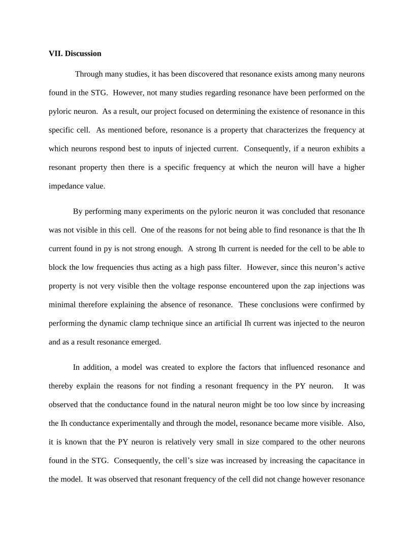
VII. Discussion

Through many studies, it has been discovered that resonance exists among many neurons

found in the STG. However, not many studies regarding resonance have been performed on the

pyloric neuron. As a result, our project focused on determining the existence of resonance in this

specific cell. As mentioned before, resonance is a property that characterizes the frequency at

which neurons respond best to inputs of injected current. Consequently, if a neuron exhibits a

resonant property then there is a specific frequency at which the neuron will have a higher

impedance value.

By performing many experiments on the pyloric neuron it was concluded that resonance

was not visible in this cell. One of the reasons for not being able to find resonance is that the Ih

current found in py is not strong enough. A strong Ih current is needed for the cell to be able to

block the low frequencies thus acting as a high pass filter. However, since this neuron’s active

property is not very visible then the voltage response encountered upon the zap injections was

minimal therefore explaining the absence of resonance. These conclusions were confirmed by

performing the dynamic clamp technique since an artificial Ih current was injected to the neuron

and as a result resonance emerged.

In addition, a model was created to explore the factors that influenced resonance and

thereby explain the reasons for not finding a resonant frequency in the PY neuron. It was

observed that the conductance found in the natural neuron might be too low since by increasing

the Ih conductance experimentally and through the model, resonance became more visible. Also,

it is known that the PY neuron is relatively very small in size compared to the other neurons

found in the STG. Consequently, the cell’s size was increased by increasing the capacitance in

the model. It was observed that resonant frequency of the cell did not change however resonance

became more visible for larger values in capacitance since there was a better filter of the voltage

response for higher frequencies. As a result, the absence of resonance in the PY neuron can be

explained due to the cell being very small in size. Finally, the PY neuron is a follower neuron

therefore it might not have a preferred resonant frequency since it receives signals from AB and

LP neuron.

VIII. Matlab Script

A. Script for finding resonance using Method2

function [zf]=resonantdetectA(dat, ChannelCl, ChannelCs)

% the version of resonantdetect for loaded ascii files%

sample_rate = 4000;

% Reading the files %

Y=dat(:,ChannelCs).*100;

X=dat(:,ChannelCl).*10;

% Calculation of power spectrums of data %

z1=fft(Y);

z2=fft(X);

PX = abs(z1.*conj(z1)/size(z1,1));

f=(0:(size(z1,1)-1))*(sample_rate/size(z1,1));

s1=z1.*conj(z2);

s2=z2.*conj(z2);

zf=s1(1:2000,1)./s2(1:2000,1);

% phasezf=phase(zf(1:500,1));

anglezf=angle(zf(1:2000,1));

zf=abs(zf);

% filtering%

h = fspecial('average', [9 9]);

Afzf = imfilter(zf, h, 'replicate');

% Afzf = imfilter(Afzf, h, 'replicate');

anglezf = imfilter(anglezf, h, 'replicate');

% cd C:\Documents and Settings\UBM\My Documents\MATLAB\MATLABRESULTS;

prompt={'The experiment category :'};

def={['PD_ZAP']};

dlgTitle='Type';

lineNo=1;

answer=inputdlg(prompt,dlgTitle,lineNo,def);

answer(1,1),

ff=f';

zfout = [ff(7:2000,1) Afzf(7:2000,1) anglezf(7:2000,1)];

zfname = ['z' char(answer(1,1))];

wk1write(zfname,zfout);

% Plots %

figure(3);

subplot(4,1,1), plot(Y);

tit1=['FFT of the response File '];

subplot(4,1,2), plot(X);

tit3=['FRC by FFT method : File '];

subplot(4,1,3), plot(f(3:2000), Afzf(3:2000)), title(tit3), xlabel('Frequency (Hz)'), title('Impedance'),axis([0 10 5

30]);

subplot(4,1,4), plot(f(3:2000),anglezf(3:2000)), title(tit3), xlabel('Frequency (Hz)'), title('Angle');

Z1=[];

F1=f;

B. Script for finding resonance using Method1

% find the frequency-response for each cycle

function [amp] = freq_amp(recordfile,channel)

srate=4000;

uptime=[];

out=[];

original=dlmread(recordfile);

original(:,3)=original(:,3)*10;

original(:,4)=original(:,4)*100;

%drop first/end 4000points=1sec

trustart=0;

truend=0;

original=original(trustart*4000+1:size(original,1)-truend*4000,:);

baseline=(max(original(:,channel))+min(original(:,channel)))/2

shiftbase=original(:,channel)-baseline;

for i=1:size(shiftbase,1)-1

if ((shiftbase(i)<0) && (shiftbase(i+1)>0))

uptime=[uptime;i];

end

end

for j=1:size(uptime,1)-1

t=uptime(j+1)-uptime(j);

period=t/(srate);

f=1/period;

ch1=max(original(uptime(j):uptime(j+1),1))-min(original(uptime(j):uptime(j+1),1));




out=[out;ch1 ch2 ch3 ch4 f];

% out=[out;ch1 ch2 ch3 ch4 f uptime(j) uptime(j+1)];

end

if (size(out)~=[0,0])

out(:,6)=out(:,3)./out(:,1);

%out(:,7)=out(:,4)./out(:,2);

out(:,7)=out(:,4)./out(:,3);

%tital

% newtitle=[strrep(recordfile,'_',':'),', ',num2str(channel),' (',num2str(baseline),'), (',num2str(trustart),',

',num2str(truend),')'];

% suptitle(newtitle)

%reset all plot

%reset all graph

% subplot (3,2,1)

% hold off

% subplot (3,2,2)

% hold off

% subplot (3,2,3)

% hold off

% subplot (3,2,4)

% hold off

% subplot (3,2,5)

% hold off

% subplot (3,2,6)

% hold off

%scatter plot

% subplot (3,2,1)

% scatter(out(:,5),out(:,1),5,'filled')

% title(['1 (',num2str(channel),')'])

%

% subplot (3,2,2)



%

% subplot (3,2,3)



%

% subplot (3,2,4)



%

% subplot (3,2,5)


% title(['3/1 (',num2str(channel),')'])

%

% subplot (3,2,6)

scatter(out(:,5),out(:,7),5,'filled')

% title(['4/2 (',num2str(channel),')'])

%

% save([recordfile,'_',num2str(channel),'_(',num2str(trustart),', ',num2str(truend),').txt'],'out','-ASCII')

% saveas(gcf,[recordfile,'_',num2str(channel),'_(',num2str(trustart),', ',num2str(truend),').jpg'])

figure(10)

subplot(2,1,1)

x=max(length(original(:,3)),1);

plot((1:x)*.00025, original(:,3))

subplot(2,1,2)

plot((1:x)*.00025, original(:,4))

end

amp=out;

C. Script used in XPP model

par A=-10 gl=0.1 El=-70 gh=0.037 Eh=-10 vr=-70 Sr=7

par c=20 cr=3000 vkr=-110 skr=-13

par fmax=.01 fmin=0.0001 dur=180000

logval=log(fmax/fmin)/dur

Iex=A*sin(2*pi*(fmin/logval)*(exp(logval*t)-1))-5

aux Ix=Iex

# define currents

#Iex=A*heav(t>10000)*heav(t<140000)

#aux Ix=Iex

Il=gl*(v-El)

Ih=gh*r*(v-Eh)

aux ihx=ih

# define activation fraction of the h current

rinf=1/(1+exp((v-vr)/Sr))

taur=cr/(1+exp((v-vkr)/Skr))

aux rx=r

aux rinfx=rinf

# ODEs

v'=(Iex-Il-Ih)/c

r'=(rinf-r)/taur

@ total=60000 dt=1,xlo=0,xhi=180000,ylo=-70,yhi=-40

@ total=180000 dt=1,xlo=0,xhi=180000,ylo=-90,yhi=-30

@ bounds=10000000

init v=-60 r=0.3280024747199

done

References

Buchholtz, Frank, & Golowasch, Jorge, & Epstein, Irving, & Marder, Eve. “Mathematical

Model of an Identified Stomatogastric Ganglion Neuron.” Journal of Neurophysiology

67(1992): 332-340.

Buchholtz, Frank, & Epstein, Irving, & Marder, Eve. “Models of Subthreshold Membrane

Resonance in Neocortical Neurons.” Journal of Neurophysiology 76(1996): 698-714.

Harris-Warrick, Ronald M., Eve Marder, and Allen I. Selverston, eds. Dynamic Biological

Networks : The Stomatogastric Nervous System. New York: MIT P, 1992.

Hutcheon, Bruce, & Yarom, Yosef. “Resonance, oscillation and the intrinsic frequency

preferences of neurons.” Trends in Neurosciences 23(2000): 216-222.

Kilman, Valerie L., and Eve Marder. "Ultrastructure of the stomatogastric ganglion neuropil of

the crab, Cancer borealis." The Journal of Comparative Neurology 374 (1998): 362-75.

Nadim, Farzan. “Software.” The STG Lab at Rutgers University and NJIT. 2006 November 1,

2008. http://cancer.rutgers.edu/software/index.html

Nadim, Farzan. “Cancer Borealis.” The STG Lab at Rutgers University and NJIT. 2006

November 1, 2008.

http://cancer.rutgers.edu/stg_lab/protocols/cancer_borealis%20saline.htm

Nelson, Mark and Rinsel, John. “The Hodgkin-Huxley Model.” November 1, 2008.

http://www.genesis-sim.org/GENESIS/iBoG/iBoGpdf/chapt4.pdf

http://cancer.rutgers.edu/software/index.html