Embed Size (px)
Citation preview

www.brainproducts.com
Brain Products Press Release December 2013, Volume 49
Downloads & Support
Ocular Correction ICA by Dr. Markus Plank
EEG recordings are often compromised by noise resulting from
muscular activity, environmental disturbances, blinks, saccades,
smooth pursuit, and other eye movements. Electro-Ocular
(EOG) artifacts are particularly severe, since eye movements
can hardly be suppressed over a sustained period of time. In
order to overcome the obvious problem of losing trials when
rejecting data portions contaminated by EOG artifacts, several
methods have been proposed to attenuate EOG processes and
consequently correct the contaminated EEG data, one of which
is Independent Component Analysis (ICA; Makeig, Bell, Jung,
& Sejnowski, 1996). ICA separates the EEG signal mixtures
recorded at the scalp into temporally maximally independent
component time courses, allowing for the removal of artifactual
processes. While the selection of artifactual components is
subjective and up to the user, Jung and colleagues (1998) showed
that “ocular” components (representing eye movements and
blinks) have characteristic patterns in both their time courses
as well as their topographies which can be used as selection
criteria (Figure 1). Interestingly, ICA-based attenuation of
ocular artifacts succeeds even in the absence of designated
eye channels. This is a major advantage over regression-based
algorithms, for example of Gratton, Coles and Donchin (1983).
Now here’s where the transformation Ocular Correction ICA as
implemented in BrainVision Analyzer 2 comes into play. It is a
specialized version of the general ICA transformation, which
identifies and pre-selects components with time-courses that
are potentially associated with eye movements and blinks.
Before delving into the intricacies of the transformation
parameters and settings, I would like to raise your attention
towards the crucial necessity of proper data pre-processing
for optimal, reliable and valid ICA results. In detail, data
should have undergone at least the following steps:
• Filtering. High-pass filtering (low cutoff ) is recommended
for removal of slow drifts resulting, for example, from slow
body movements or sweating, which ICA cannot handle well.
In case of higher sampling rates it might also make sense to
apply a low-pass filter (high cutoff ). This prevents higher
frequency content from using up additional components.
• Raw Data Inspection/Artifact Rejection. This step is suggested
for marking non-stereotypical artifacts such as punctual bursts
of electromyographic (EMG) activity, whole-body startle
reactions, rare non-EEG glitches across all channels and other
artifacts. ICA might separate each of these into separate
components, massively reducing the number of components
left for capturing remaining processes. Since data portions
that have been marked as “Bad Intervals” are disregarded by
Ocular Correction ICA, please select rejection criteria such
that blink periods are not marked. I am emphasizing this here
since blinks and other eye movements are supposed to be
used by the transformation Ocular Correction ICA.
1.1 The Transformation
Once your data fulfills these requirements, you can access
the transformation via Transformations > Artifact Rejection/
Reduction > Ocular Correction ICA. The core steps of this
transformation are visualized in Figure 2 (you can find
more details on these steps in the dedicated chapter of the
Analyzer User Manual). I strongly recommend applying the
transformation in semiautomatic mode for every history file,
since only then you will be able to visually inspect and adjust
the component selection accomplished automatically by
Analyzer.
In detail, the steps are as following:
(1) Blink marker placement. At this stage, a specified (eye
or scalp) channel is scanned for blinks, and blink markers
are placed. When not using existing markers, two detection
algorithms are available: The Mean Slope algorithm of Gratton
et al. (1983) will detect any high-amplitude activity in the
scanned channels (potentially including non-blink artifacts). By
contrast, the Value Trigger algorithm has been optimized for
the detection of prototypical blink patterns. Please note that
horizontal eye movements will not be detected and marked.
A
B
time
time
ampl
itude
ampl
itude
Figure 1: Prototypical channel projections (topographies; left) and activation profiles (time courses; right) of Independent Components representing vertical eye movements and blinks [A] and horizontal eye movements [B]. Please note that due to the nature of the ICA algorithm topographies and/or time courses could also be inverted in polarity.
Figure 2: Steps of the transformation Ocular Correction ICA.
(1) place/use
blink markers
(2)apply ICA
(3)identify ocular components
(4)remove ocular components
page 1 of 4
2professional

www.brainproducts.com
Brain Products Press Release December 2013, Volume 49
(2) ICA decomposition. In this step you define the amount
of data to be fed into ICA, both in terms of the number of
channels and time points. Channels that are not selected for
ICA will be displayed below the component activations, which
might be quite helpful for the comparison of component
activations and actual VEOG and HEOG channel activity.
Regarding the minimum number of data points (samples)
there is a simple rule of thumb: You should use at least as many
data points as the number of channels squared times 20 (less
than 64 channels) or times 30 (more than 64 channels). Of course
this is only a minimum recommendation, which in practice often
is not sufficient, as the data should include the relevant
information content to be decomposed (for example, enough
eye movements and blinks). Therefore, I suggest to use longer,
representative data intervals or even the whole data (provided
that it can be afforded with respect to memory constraints).
Please keep in mind that “Bad Intervals” are neglected by ICA.
The ICA procedures available to you (e.g., Infomax, Fast ICA)
have already been addressed in a previous Support Tip
[ h t t p : // w w w . b r a i n p r o d u c t s . c o m / p r o d u c t d e t a i l s .
php?id=17&tab=3]. The resulting ICA and Inverse ICA weight
matrices can also be saved to text files.
(3) Criterion-based identification of “ocular” components. Once ICA has been accomplished, the extracted components
are evaluated in terms of their consistency and similarity
to the EEG data. For identification of components related to
VEOG activity only the time intervals limited by blink markers
are used. By contrast, for identification of components related
to HEOG activity all data is used. There are three methods
available, each using different measures:
a. Sum of Squared Correlations with VEOG/HEOG is a correlative
score between the component activations and the activity of
the VEOG/HEOG channels selected in step 1. This option does
not require the VEOG/HEOG channels to be fed into ICA.
b. Relative VEOG/HEOG Variance calculates the share of each
ICA component in the variance of the selected ocular channel
activation. This method requires the specified VEOG/HEOG
channel(s) to be also fed into ICA.
c. Global Field Power (only available for VEOG) calculates the
contribution of each component to the Global Field Power of
all channels used for ICA during blink intervals. Here, both
the activation profiles as well as the channel projections of
the components are evaluated. This option does not require
the VEOG channel to be fed into ICA.
For all methods the components will be ranked according to
their score with respect to the selected “ocular” measure.
Afterwards, component scores are compared to the threshold
specified in the field Total Value to Delete [%]. Depending
on this threshold one or more components will be pre-
selected as “ocular” and subsequently marked for removal
(in red) in the semi-automatic interactive view of the
transformation.
(4) Removal of “ocular” components. Analyzer will then open
the component activations from step 2 in an interactive view,
where “ocular” components selected for rejection are marked
in red. The interactive view allows for an evaluation and further
fine-tuning of the automatic component selection accomplished
in step 3. After clicking Finish, the marked components will be
removed from the data. You can utilize various visualization
tools in the interactive view in order to make informed decisions.
In the following, I will explain a couple of these in more detail.
1.2 The Interactive View
Prior to examining the contents of the interactive view, I
recommend checking the Operation Infos of the newly created
“Ocular Correction ICA” node, in particular whether the algorithm
has converged. Only in this case the ICA decomposition and
the displayed data are valid and can be interpreted. As can be
seen in Figure 3, the interactive view displays the component
Figure 3: [A] Component activations (scaled by a factor of 75) of components F00, F01, F11 and F24 as well as upper and lower VEOG channel activity. Blinks are represented by interval markers, highlighted in blue. [B] Table containing the criterion score (%) of all components for VEOG and HEOG activity as well as a color code on whether the component will be removed (red) or retained (green). In the current example, components have been sorted based on their VEOG criterion score. [C] Topography of the component highlighted in the criterion table. The map represents the “normed” component projections towards the channels (unit-less weights, units can be neglected). [D] Display settings. In this part of the interactive view, you can adjust the information displayed in the main window, for example the component scaling with respect to the channel amplitudes.
page 2 of 4
www.brainproducts.com
Brain Products Press Release December 2013, Volume 49
activations (labeled by “F” followed by a number) in the main
view. In the current example, interval markers were selected
for marking blink periods. The table in the upper right corner
lists the criterion score (%) of all components for VEOG and
HEOG activity. The red and green cells in the first column
of the table represent the components that will be removed
or retained, respectively: components that are marked in
red have been categorized as “ocular” components and
will be removed; components marked in green will be kept.
By double-clicking the colored cell you can change its
assignment. You can sort the table based on the VEOG and
HEOG criterion scores by clicking the respective field in the
table header (also see Figure 3). I generally suggest dedicating
some time to the careful examination of all components (red
and green) one by one following the sorting order with
respect to VEOG and HEOG criterion scores separately.
Below the table you can find a topographic mapping view of
the component currently selected in the criterion table. The
map represents an interpolated representation of the
component projections (unit-less weights) towards the channels.
By using the options available below the mapping view, you can
scale the component activations with respect to the channel
amplitudes (ICA Scaling), or use the drop-down list to switch
between the component activations (ICA Components), the
cleaned/corrected channel data after removing the components
currently selected as “ocular” (Correction), or the simultaneous
display of the projections of all components towards the
channels (Topographies).
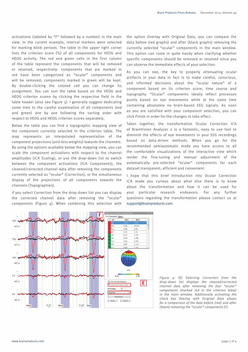
If you select Correction from the drop-down list you can display
the corrected channel data after removing the “ocular”
components (Figure 4). When combining this selection with
the option Overlay with Original Data, you can compare the
data before (red graphs) and after (black graphs) removing the
currently selected “ocular” components in the main window.
This option can come in quite handy when clarifying whether
specific components should be removed or retained since you
can observe the immediate effects of your selection.
As you can see, the key to properly attenuating ocular
artifacts in your data in fact is to make careful, conscious,
and informed decisions about the “ocular nature” of a
component based on its criterion score, time course and
topography. “Ocular” components ideally reflect processes
purely based on eye movements while at the same time
containing absolutely no brain-based EEG signals. As soon
as you are satisfied with your component selection, you can
click Finish in order for the changes to take effect.
Taken together, the transformation Ocular Correction ICA
of BrainVision Analyzer 2 is a fantastic, easy to use tool to
diminish the effects of eye movements in your EEG recordings
based on data-driven methods. When you go for the
recommended semiautomatic mode you have access to all
the comfortable visualizations of the interactive view which
render the fine-tuning and manual adjustment of the
automatically pre-selected “ocular” components for each
dataset transparent, efficient and convenient.
I hope that this brief introduction into Ocular Correction
ICA made you curious about what else there is to know
about the transformation and how it can be used for
your particular research endeavors. For any further
questions regarding the transformation please contact us at
page 3 of 4
Figure 4: [E] Selecting Correction from the drop-down list displays the cleaned/corrected channel data after removing the four “ocular” components (marked red in the criterion table) in the main window. Additionally activating the check box Overlay with Original Data allows for a comparison of the data before (red) and after (black) removing the “ocular” components [F].

www.brainproducts.com
Brain Products Press Release December 2013, Volume 49
References
Croft, R. J., & Barry, R. J. (2000). Removal of ocular artifact from the EEG: a review. Neurophysiol Clin, 30(1), 5-19.
Gratton, G., Coles, M. G., & Donchin, E. (1983). A new method for off- line removal of ocular artifact. Electroencephalogr Clin Neurophysiol, 55(4), 468-484.
Hillyard, S. A., & Galambos, R. (1970). Eye movement artifact in the CNV. Electroencephalogr Clin Neurophysiol, 28(2), 173-182.
Jung, T. P., Humphries, C., Lee, T. W., Makeig, S., McKeown, M. J., Iragui, V., & Sejnowski, T. J. (1998). Extended ICA removes artifacts from electroencephalographic recordings. Advances in Neural Information Processing Systems 10, 10, 894-900.
Makeig, S., Bell, A. J., Jung, T. P., & Sejnowski, T. J. (1996). Independent component analysis of electroencephalographic data. Advances in Neural Information Processing Systems, 8, 145-151.
Overton, D. A., & Shagass, C. (1969). Distribution of eye movement and eyeblink potentials over the scalp. Electroencephalogr Clin Neurophysiol, 27(5), 546.
Schlögl, A., Keinrath, C., Zimmermann, D., Scherer, R., Leeb, R., & Pfurtscheller, G. (2007). A fully automated correction method of EOG artifacts in EEG recordings. Clin Neurophysiol, 118(1), 98-104.
Further reading: Physiological basics of ocular artifacts.
Electro-oculographic (EOG) artifacts result from two processes:
First, rotations of the eyeballs alter the orientation of the
electric fields generated by the corneo-retinal dipole.
Whereas the cornea is electrically positive, the retina is
negative. As a result, rotations of the corneo-retinal dipole
differentially interfere with cortically generated electric
fields over the scalp. Interestingly, even sleep EEG recordings
are contaminated with this type of horizontal EOG artifacts
(Schlögl et al., 2007). A second source of EOG artifacts arises
from contact of the eyelid with the (negative) cornea during
blinks, eliciting a burst of negativity (Overton & Shagass,
1969). EOG amplitude has been found to be attenuated
approximately with the square of the distance to the eyes with
frontal channels being affected most severely (Croft & Barry,
2000). Due to principles of volume conduction artifacts spread
throughout all layers of cortex, skull, and tissue, and are
present at any scalp site, where they interfere with the
detection and analysis of cortical responses of interest.
Hillyard and Galambos (1970) were the first to report such
modulations of the auditory CNV in all recorded scalp EEG
channels: whereas upward eye movements caused the CNV
to be positive, downward eye movements resulted in a
negative CNV.
page 4 of 4


![Case Report Surgical Correction of Hallermann-Streiff Syndrome: … · 2017. 3. 23. · nose), congenital cataracts, bilateral microphthalmia, and proportionate dwarfism [3]. Ocular](https://img.pdfslide.net/doc/110x75/60fa652a8b23401a032c5859/case-report-surgical-correction-of-hallermann-streiff-syndrome-2017-3-23-nose.jpg)