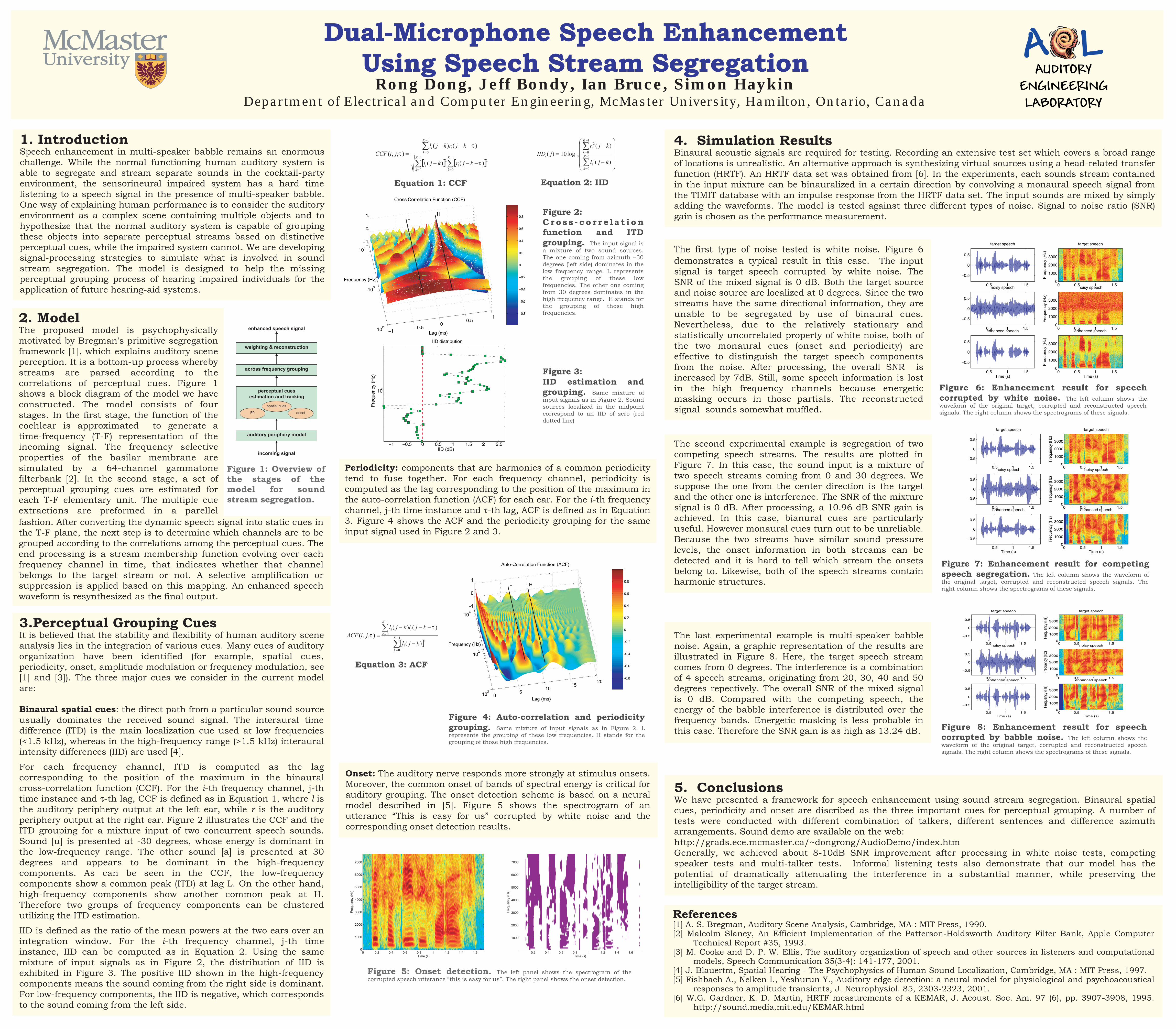
1. IntroductionSpeech enhancement in multi-speaker babble remains an enormous challenge. While the normal functioning human auditory system is able to segregate and stream separate sounds in the cocktail-party environment, the sensorineural impaired system has a hard time listening to a speech signal in the presence of multi-speaker babble. One way of explaining human performance is to consider the auditory environment as a complex scene containing multiple objects and to hypothesize that the normal auditory system is capable of grouping these objects into separate perceptual streams based on distinctive perceptual cues, while the impaired system cannot. We are developing signal-processing strategies to simulate what is involved in sound stream segregation. The model is designed to help the missing perceptual grouping process of hearing impaired individuals for the application of future hearing-aid systems.

References[1] A. S. Bregman, Auditory Scene Analysis, Cambridge, MA : MIT Press, 1990.[2] Malcolm Slaney, An Efficient Implementation of the Patterson-Holdsworth Auditory Filter Bank, Apple Computer

Technical Report #35, 1993.[3] M. Cooke and D. P. W. Ellis, The auditory organization of speech and other sources in listeners and computational

models, Speech Communication 35(3-4): 141-177, 2001.[4] J. Blauertm, Spatial Hearing - The Psychophysics of Human Sound Localization, Cambridge, MA : MIT Press, 1997.[5] Fishbach A., Nelken I., Yeshurun Y., Auditory edge detection: a neural model for physiological and psychoacoustical

responses to amplitude transients, J. Neurophysiol. 85, 2303-2323, 2001.[6] W.G. Gardner, K. D. Martin, HRTF measurements of a KEMAR, J. Acoust. Soc. Am. 97 (6), pp. 3907-3908, 1995.

http://sound.media.mit.edu/KEMAR.html

Dual-Microphone Speech Enhancement Dual-Microphone Speech Enhancement Using Speech Stream SegregationUsing Speech Stream Segregation

Rong Dong, Jeff Bondy, Ian Bruce, Simon HaykinDepartment of Electrical and Computer Engineering, McMaster University, Hamilton, Ontario, Canada

5. ConclusionsWe have presented a framework for speech enhancement using sound stream segregation. Binaural spatial cues, periodicity and onset are discribed as the three important cues for perceptual grouping. A number of tests were conducted with different combination of talkers, different sentences and difference azimuth arrangements. Sound demo are available on the web: http://grads.ece.mcmaster.ca/~dongrong/AudioDemo/index.htmGenerally, we achieved about 8-10dB SNR improvement after processing in white noise tests, competing speaker tests and multi-talker tests. Informal listening tests also demonstrate that our model has the potential of dramatically attenuating the interference in a substantial manner, while preserving the intelligibility of the target stream.

Figure 2: Unitary Excitatory and Inhibitory Conductances

3.Perceptual Grouping Cues It is believed that the stability and flexibility of human auditory scene analysis lies in the integration of various cues. Many cues of auditory organization have been identified (for example, spatial cues, periodicity, onset, amplitude modulation or frequency modulation, see [1] and [3]). The three major cues we consider in the current model are:

Binaural spatial cues: the direct path from a particular sound source usually dominates the received sound signal. The interaural time difference (ITD) is the main localization cue used at low frequencies (<1.5 kHz), whereas in the high-frequency range (>1.5 kHz) interaural intensity differences (IID) are used [4].

For each frequency channel, ITD is computed as the lag corresponding to the position of the maximum in the binaural cross-correlation function (CCF). For the i-th frequency channel, j-th time instance and τ-th lag, CCF is defined as in Equation 1, where l is the auditory periphery output at the left ear, while r is the auditory periphery output at the right ear. Figure 2 illustrates the CCF and the ITD grouping for a mixture input of two concurrent speech sounds. Sound [u] is presented at -30 degrees, whose energy is dominant in the low-frequency range. The other sound [a] is presented at 30 degrees and appears to be dominant in the high-frequency components. As can be seen in the CCF, the low-frequency components show a common peak (ITD) at lag L. On the other hand, high-frequency components show another common peak at H. Therefore two groups of frequency components can be clustered utilizing the ITD estimation.

IID is defined as the ratio of the mean powers at the two ears over an integration window. For the i-th frequency channel, j-th time instance, IID can be computed as in Equation 2. Using the same mixture of input signals as in Figure 2, the distribution of IID is exhibited in Figure 3. The positive IID shown in the high-frequency components means the sound coming from the right side is dominant. For low-frequency components, the IID is negative, which corresponds to the sound coming from the left side.

Periodicity: components that are harmonics of a common periodicity tend to fuse together. For each frequency channel, periodicity is computed as the lag corresponding to the position of the maximum in the auto-correlation function (ACF) for each ear. For the i-th frequency channel, j-th time instance and τ-th lag, ACF is defined as in Equation 3. Figure 4 shows the ACF and the periodicity grouping for the same input signal used in Figure 2 and 3.

Onset: The auditory nerve responds more strongly at stimulus onsets. Moreover, the common onset of bands of spectral energy is critical for auditory grouping. The onset detection scheme is based on a neural model described in [5]. Figure 5 shows the spectrogram of an utterance “This is easy for us” corrupted by white noise and the corresponding onset detection results.

4. Simulation ResultsBinaural acoustic signals are required for testing. Recording an extensive test set which covers a broad range of locations is unrealistic. An alternative approach is synthesizing virtual sources using a head-related transfer function (HRTF). An HRTF data set was obtained from [6]. In the experiments, each sounds stream contained in the input mixture can be binauralized in a certain direction by convolving a monaural speech signal from the TIMIT database with an impulse response from the HRTF data set. The input sounds are mixed by simply adding the waveforms. The model is tested against three different types of noise. Signal to noise ratio (SNR) gain is chosen as the performance measurement.

Figure 3: IID estimation and grouping. Same mixture of input signals as in Figure 2. Sound sources localized in the midpoint correspond to an IID of zero (red dotted line)

−1 −0.5 0 0.5 1 1.5 2 2.5

103

IID (dB)

Freq

uenc

y (H

z)

IID distribution

Equation 3: ACF

[ ]∑

∑−

=

−

=

−

−−−= 1

0

2

1

0

)(

)()(),,( K

ki

K

kii

kjl

kjlkjljiACF

ττ

0.5 1 1.5

−0.5

0

0.5

target speech

0.5 1 1.5

−0.5

0

0.5

noisy speech

0.5 1 1.5

−0.5

0

0.5

enhanced speech

Time (s)

target speech

Freq

uenc

y (H

z)

0 0.5 1 1.50

1000

2000

3000

noisy speech

Freq

uenc

y (H

z)

0 0.5 1 1.50

1000

2000

3000

enhanced speech

Freq

uenc

y (H

z)

Time (s)0 0.5 1 1.5

0

1000

2000

3000

Equation 1: CCF

[ ] [ ]∑ ∑

∑−

=

−

=

−

=

−−−

−−−=

1

0

1

0

22

1

0

)()(

)()(),,(

K

k

K

kii

K

kii

kjrkjl

kjrkjljiCCF

τ

ττ

Equation 2: IID

−

−=

∑

∑−

=

−

=1

0

2

1

0

2

10

)(

)(log10)( K

ki

K

ki

i

kjl

kjrjIID

0.5 1 1.5

−0.5

0

0.5

target speech

0.5 1 1.5

−0.5

0

0.5

noisy speech

0.5 1 1.5

−0.5

0

0.5

enhanced speech

Time (s)

target speech

Freq

uenc

y (H

z)

0 0.5 1 1.50

1000

2000

3000

noisy speech

Freq

uenc

y (H

z)

0 0.5 1 1.50

1000

2000

3000

enhanced speech

Freq

uenc

y (H

z)

Time (s)0 0.5 1 1.5

0

1000

2000

3000

Figure 6: Enhancement result for speech corrupted by white noise. The left column shows the waveform of the original target, corrupted and reconstructed speech signals. The right column shows the spectrograms of these signals.

Figure 7: Enhancement result for competing speech segregation. The left column shows the waveform of the original target, corrupted and reconstructed speech signals. The right column shows the spectrograms of these signals.

0.5 1 1.5

−0.5

0

0.5

target speech

0.5 1 1.5

−0.5

0

0.5

noisy speech

0.5 1 1.5

−0.5

0

0.5

enhanced speech

Time (s)

target speech

Freq

uenc

y (H

z)

0 0.5 1 1.50

1000

2000

3000

noisy speech

Freq

uenc

y (H

z)

0 0.5 1 1.50

1000

2000

3000

enhanced speech

Freq

uenc

y (H

z)

Time (s)0 0.5 1 1.5

0

1000

2000

3000

Figure 8: Enhancement result for speech corrupted by babble noise. The left column shows the waveform of the original target, corrupted and reconstructed speech signals. The right column shows the spectrograms of these signals.

The first type of noise tested is white noise. Figure 6 demonstrates a typical result in this case. The input signal is target speech corrupted by white noise. The SNR of the mixed signal is 0 dB. Both the target source and noise source are localized at 0 degrees. Since the two streams have the same directional information, they are unable to be segregated by use of binaural cues. Nevertheless, due to the relatively stationary and statistically uncorrelated property of white noise, both of the two monaural cues (onset and periodicity) are effective to distinguish the target speech components from the noise. After processing, the overall SNR is increased by 7dB. Still, some speech information is lost in the high frequency channels because energetic masking occurs in those partials. The reconstructed signal sounds somewhat muffled.

The second experimental example is segregation of two competing speech streams. The results are plotted in Figure 7. In this case, the sound input is a mixture of two speech streams coming from 0 and 30 degrees. We suppose the one from the center direction is the target and the other one is interference. The SNR of the mixture signal is 0 dB. After processing, a 10.96 dB SNR gain is achieved. In this case, bianural cues are particularly useful. However monaural cues turn out to be unreliable. Because the two streams have similar sound pressure levels, the onset information in both streams can be detected and it is hard to tell which stream the onsets belong to. Likewise, both of the speech streams contain harmonic structures.

The last experimental example is multi-speaker babble noise. Again, a graphic representation of the results are illustrated in Figure 8. Here, the target speech stream comes from 0 degrees. The interference is a combination of 4 speech streams, originating from 20, 30, 40 and 50 degrees repectively. The overall SNR of the mixed signal is 0 dB. Compared with the competing speech, the energy of the babble interference is distributed over the frequency bands. Energetic masking is less probable in this case. Therefore the SNR gain is as high as 13.24 dB.

Figure 5: Onset detection. The left panel shows the spectrogram of the corrupted speech utterance “this is easy for us”. The right panel shows the onset detection.

A LAUDITORY

ENGINEERINGLABORATORY

weighting & reconstruction

across frequency grouping

perceptual cues estimation and tracking

auditory periphery model

F0 onset

spatial cues

incoming signal

enhanced speech signal

Figure 1: Overview of the stages of the model for sound stream segregation.

fashion. After converting the dynamic speech signal into static cues in the T-F plane, the next step is to determine which channels are to be grouped according to the correlations among the perceptual cues. The end processing is a stream membership function evolving over each frequency channel in time, that indicates whether that channel belongs to the target stream or not. A selective amplification or suppression is applied based on this mapping. An enhanced speech waveform is resynthesized as the final output.

2. ModelThe proposed model is psychophysically motivated by Bregman's primitive segregation framework [1], which explains auditory scene perception. It is a bottom-up process whereby streams are parsed according to the correlations of perceptual cues. Figure 1 shows a block diagram of the model we have constructed. The model consists of four stages. In the first stage, the function of the cochlear is approximated to generate a time-frequency (T-F) representation of the incoming signal. The frequency selective properties of the basilar membrane are simulated by a 64-channel gammatone filterbank [2]. In the second stage, a set of perceptual grouping cues are estimated for each T-F elementary unit. The multiple cue extractions are preformed in a parellel

Figure 2: C r o s s - c o r r e l a t i o n function and ITD grouping. The input signal is a mixture of two sound sources. The one coming from azimuth −30 degrees (left side) dominates in the low frequency range. L represents the grouping of these low frequencies. The other one coming from 30 degrees dominates in the high frequency range. H stands for the grouping of those high frequencies.

−1−0.5

00.5

1

102

103

104

−1

0

1

Cross−Correlation Function (CCF)

Lag (ms)

Frequency (Hz)

−0.8

−0.6

−0.4

−0.2

0

0.2

0.4

0.6

0.8LH

Figure 4: Auto-correlation and periodicity grouping. Same mixture of input signals as in Figure 2. L represents the grouping of these low frequencies. H stands for the grouping of those high frequencies.

Time (s)

Freq

uenc

y (H

z)

0 0.2 0.4 0.6 0.8 1 1.2 1.4 1.60

1000

2000

3000

4000

5000

6000

7000

0.2 0.4 0.6 0.8 1 1.2 1.4 1.6

1000

2000

3000

4000

5000

6000

7000

Freq

uenc

y (H

z)

Time (s)