Embed Size (px)
Citation preview
NASA-CR-199569 // /)
Sensitivity Analysis for Aeroacoustic and AeroelasticDesign of Turbomachinery Blades
Christopher B. LorenceGraduate Research Assistant
and
Kenneth C. HallPrincipal Investigator
Department of Mechanical Engineering and Materials ScienceSchool of Engineering
Duke UniversityDurham, NC 27708-0300
DUKESCHOOL OFENGINEERING
A Final Technical Report on Research Conducted UnderNASA Grant NAG3-1433
(Grant Title: Aeroacoustic Sensitivity Analysis and Optimal AeroacousticDesign of Turbomachinery Blades)
Submitted to NASA Lewis Research Center£ £-.1^95^9) May 1995-'(NIP3-95-05S90) SENSITIVITYANALYSIS FOR AEROACOUSTIC ANDAEROELASTIC DESIGN OFTURBOMACHINERY BLADES Final Report(Duke Univ.) 162 p
N96-13226
Unclas
63/07 0073244
https://ntrs.nasa.gov/search.jsp?R=19960003217 2018-08-03T21:09:24+00:00Z
Abstract
A new method for computing the effect that small changes in the airfoil shape andcascade geometry have on the aeroacoustic and aeroelastic behavior of turbomachin-ery cascades is presented. The nonlinear unsteady flow is assumed to be composed ofa nonlinear steady flow plus a small perturbation unsteady flow that is harmonic intime. First, the full potential equation is used to describe the behavior of the non-linear mean (steady) flow through a two-dimensional cascade. The small disturbanceunsteady flow through the cascade is described by the linearized Euler equations. Us-ing rapid distortion theory, the unsteady velocity is split into a rotational part thatcontains the vorticity and an irrotational part described by a scalar potential. Theunsteady vorticity transport is described analytically in terms of the drift and streamfunctions computed from the steady flow. Hence, the solution of the linearized Eulerequations may be reduced to a single inhomogeneous equation for the unsteady poten-tial. The steady flow and small disturbance unsteady flow equations are discretizedusing bilinear quadrilateral isoparametric finite elements. The nonlinear mean flowsolution and streamline computational grid are computed simultaneously using New-ton iteration. At each step of the Newton iteration, LU decomposition is used to solvethe resulting set of linear equations. The unsteady flow problem is linear, and is alsosolved using LU decomposition. Next, a sensitivity analysis is performed to deter-mine the effect small changes in cascade and airfoil geometry have on the mean andunsteady flow fields. The sensitivity analysis makes use of the nominal steady andunsteady flow LU decompositions so that no additional matrices need to be factored.Hence, the present method is computationally very efficient. To demonstrate how thesensitivity analysis may be used to redesign cascades, a compressor is redesigned forimproved aeroelastic stability and two different fan exit guide vanes are redesignedfor reduced downstream radiated noise. In addition, a framework detailing how thetwo-dimensional version of the method may be used to redesign three-dimensionalgeometries is presented.
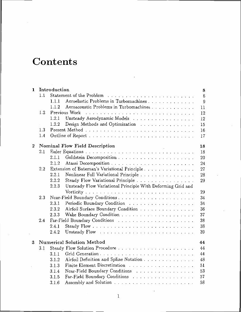
Contents
1 Introduction 81.1 Statement of the Problem 8
1.1.1 Aeroelastic Problems in Turbomachines 91.1.2 Aeroacoustic Problems in Turbomachines 11
1.2 Previous Work 121.2.1 Unsteady Aerodynamic Models 121.2.2 Design Methods and Optimization 15
1.3 Present Method 161.4 Outline of Report 17
2 Nominal Flow Field Description 182.1 Euler Equations 18
2.1.1 Goldstein Decomposition 202.1.2 Atassi Decomposition 24
2.2 Extension of Bateman's Variational Principle 272.2.1 Nonlinear Full Variational Principle 282.2.2 Steady Flow Variational Principle 292.2.3 Unsteady Flow Variational Principle With Deforming Grid and
Vorticity 292.3 Near-Field Boundary Conditions 34
2.3.1 Periodic Boundary Condition 342.3.2 Airfoil Surface Boundary Condition 362.3.3 Wake Boundary Condition 37
2.4 Far-Field Boundary Conditions 382.4.1 Steady Flow 382.4.2 Unsteady Flow 39
3 Numerical Solution Method 443.1 Steady Flow Solution Procedure 44
3.1.1 Grid Generation 443.1.2 Airfoil Definition and Spline Notation 483.1.3 Finite Element Discretization 513.1.4 Near-Field Boundary Conditions 533.1.5 Far-Field Boundary Conditions 573.1.6 Assembly and Solution 58
2 CONTENTS
3.2 Unsteady Flow Solution Procedure 613.2.1 Drift Function and Rotational Velocity Calculation 613.2.2 Unsteady Grid Generation 633.2.3 Finite Element Discretization 643.2.4 Near-Field Boundary Conditions 663.2.5 Far-Field Boundary Conditions 703.2.6 Assembly and Solution 75
4 Sensitivity Analysis 764.1 General Procedure 764.2 Steady Flow Sensitivity Analysis 79
4.2.1 Prescribing the Perturbation 794.2.2 Near-Field Boundary Conditions 804.2.3 Far-Field Boundary Conditions 824.2.4 Sensitivity of the Stream Function 83
4.3 Unsteady Flow Sensitivity Analysis 844.3.1 Sensitivity of the Drift Function 844.3.2 Sensitivity of the Rotational Velocity 844.3.3 Sensitivity of the Blade Structural Dynamics 854.3.4 Sensitivity of the Grid Motion 864.3.5 Sensitivity of the Finite Element Assembly 864.3.6 Near-Field Boundary Conditions 874.3.7 Far-Field Boundary Conditions 88
5 Results 895.1 Aeroelastic Analysis and Design of a Compressor 89
5.1.1 Steady Flow Through a Compressor 895.1.2 Unsteady Flow Through a Compressor 905.1.3 Sensitivity Analysis 955.1.4 Redesign of a Compressor for Aeroelastic Stability 1005.1.5 Computational Efficiency 105
5.2 Aeroacoustic Analysis and Design of a Fan Exit Guide Vane 1075.2.1 Steady Flow Through a Fan Exit Guide Vane 1085.2.2 Unsteady Flow Through a Fan Exit Guide Vane 1095.2.3 Sensitivity Analysis 1105.2.4 Redesign of an EGV for Reduced Acoustic Response 1155.2.5 Computational Efficiency 125
5.3 Modern Fan Exit Guide Vane 1255.3.1 Nominal Analysis 1265.3.2 Sensitivity Analysis 1275.3.3 Redesign of EGV for Reduced Acoustic Response 129
5.4 Summary 132
CONTENTS 3
6 Application to Three-Dimensional Problems 1346.1 Acoustic Modes in an Annular Duct 1346.2 Calculation of Far-Field Unsteady Pressure 1386.3 Calculation of the Outgoing Pressure 139
7 Conclusions and Future Work 1437.1 Conclusions 1437.2 Future Work '. 144
7.2.1 Other Flow Models 1447.2.2 Multidisciplinary Optimization 1457.2.3 Multiple Blade Rows 1457.2.4 Three-Dimensional Problems 146
A Nomenclature 148
B Sensitivity of the NACA Modified Four-Digit Airfoil Definition 152
Bibliography 155
List of Figures
1.1 Axial compressor or fan characteristic map showing principal types offlutter and regions of occurrence (adapted from [3]) 10
1.2 Typical compressor resonance (or Campbell) diagram (adapted from[5]) 11
2.1 Contours of drift function, A(z,j/), and stream function, ^(x,y), for atypical fan exit guide vane 22
2.2 Left, contours of the stream function, \t, near a solid plane boundary.Right, contours of the drift function, A, near an airfoil stagnation point. 23
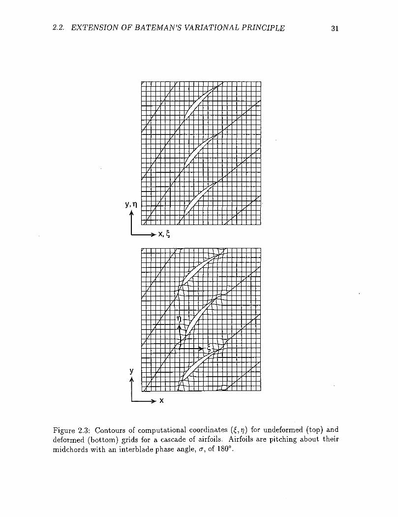
2.3 Contours of computational coordinates (£, 77) for undeformed (top) anddeformed (bottom) grids for a cascade of airfoils. Airfoils are pitchingabout their midchords with an interblade phase angle, cr, of 180°. . . 31
2.4 Locations of boundaries for a typical cascade 352.5 Coordinate systems for downstream far-field analysis 42
3.1 Typical computational grid for a fan exit guide vane 453.2 Typical computational grid in (E, \?) coordinates. The computational
node numbering convention is also illustrated 473.3 Typical distribution of boundary grid points 483.4 Detail of airfoil spline definition. Arrows indicate direction of airfoil
spline 493.5 Typical computational grid illustrating modifications for airfoils with
blunt trailing edges. Multiple passages shown for clarity. The high-lighted lines define the actual computational grid 50
4.1 Overview of quantities in sensitivity analysis 77
5.1 Steady surface pressure of cascade of NACA 5506 airfoils. M_oo = 0.5,n.oo = 55°, 6 = 45° 90
5.2 Aerodynamic damping of cascade of NACA 5506 airfoils vibrating inplunge at frequencies of 0.4, 0.8, and 1.6 for a range of interblade phaseangles 92
5.3 Aerodynamic damping of cascade of NACA 5506 airfoils pitching abouttheir midchords at frequencies of 0.4, 0.8, and 1.6 for a range of in-terblade phase angles 93
LIST OF FIGURES 5
5.4 Imaginary part of unsteady surface pressure of NACA 5506 airfoilspitching about their midchords. w = 0.4, a = 60° 94
5.5 Sensitivity of steady surface pressure of cascade of NACA 5506 airfoilsto perturbations in thickness, camber, stagger, gap, and reflex. M.^ =0.5, O_oo = 55°, 0 = 45° 96
5.6 Real part of sensitivity of unsteady surface pressure of NACA 5506 air-foils pitching about their midchords due to perturbations in thickness,camber, stagger, gap, reflex, and frequency, u = 0.4, a = 60° 98
5.7 Imaginary part of sensitivity of unsteady surface pressure of NACA5506 airfoils pitching about their midchords due to perturbations inthickness, camber, stagger, gap, reflex, and frequency, u = 0.4, a — 60°. 99
5.8 Steady surface pressure of cascade of redesigned airfoils. M-oo = 0.5,fi-oo = 55° 102
5.9 Real and imaginary parts of unsteady surface pressure of redesignedairfoils (Redesign A) pitching about their midchords. u> = 0.4, a = 60°. 103
5.10 Real and imaginary parts of unsteady surface pressure of redesignedairfoils (Redesign B) pitching about their midchords. u = 0.4, cr = 60°. 104
5.11 Accuracy of sensitivity analysis for various perturbation amplitudes. . 1055.12 Aerodynamic damping of cascade of redesigned airfoils (Redesign A)
pitching about their midchords at a frequency of 0.4 for a range ofinterblade phase angles 106
5.13 Aerodynamic damping of cascade of redesigned airfoils (Redesign B)pitching about their midchords at a frequency of 0.4 for a range ofinterblade phase angles 107
5.14 Schematic showing wake/EGV interaction. Inserts in blade passageshow contours of "drift" (top) and a streamline computational grid(bottom) 108
5.15 Steady surface pressure for cascade of NACA 8508-65 airfoils. 0 =16°, fi-oo = 30°, M_oo = 0.5, G = 1.0 109
5.16 Unsteady surface pressure of cascade of NACA 8508-65 airfoils due toincoming vortical gust at IxBPF. u = 3.7687, a = -144° Ill
5.17 Unsteady surface pressure for cascade of NACA 8508-65 airfoils dueto incoming vortical gust at 2xBPF. u = 7.54, a = -288° 112
5.18 Contours of magnitude of unsteady pressure for cascade of NACA8508-65 airfoils due to incoming vortical gust at IxBPF. u = 3.77,a = -144° 113
5.19 Contours of magnitude of unsteady pressure for cascade of NACA8508-65 airfoils due to incoming vortical gust at 2xBPF. u = 7.54,cr = -288° 114
5.20 Sensitivity of unsteady surface pressure on NACA 8508-65 airfoils dueto perturbations in thickness, camber, stagger, gap, and reflex, u =7.54, cr = —288°. n, suction surface; A, pressure surface 116
5.21 Sensitivity of unsteady surface pressure on NACA 8508-65 airfoils dueto perturbations in thickness, camber, stagger, gap, and reflex, u =7.54, a = —288°. D, suction surface; A, pressure surface 117
LIST OF FIGURES
5.22 Steady surface pressure for cascade of redesigned airfoils. M.^ = 0.5,fi-oo = 30° 119
5.23 Real and imaginary parts of unsteady surface pressure for redesignedairfoils due to incident vortical gust at 2xBPF. u; = 7.54, a = —317°. 120
5.24 Accuracy of sensitivity analysis for various perturbation amplitudes. . 1215.25 Contours of unsteady pressure for cascade of redesigned airfoils due to
incoming vortical gust at IxBPF. u — 3.77, cr = -158.4° 1225.26 Contours of unsteady pressure for cascade of redesigned airfoils due to
incoming vortical gust at 2xBPF. u = 7.54, a = -317° 1235.27 Contours of magnitude of unsteady pressure for radial station near the
hub of a modern fan exit guide vane due to incoming vortical gust at2xBPF. M_oo = 0.32, G = 0.46, w = 12.5, a = -288° 126
5.28 Contours of magnitude of unsteady pressure for radial station near themidspan of a modern fan exit guide vane due to incoming vortical gustat 2xBPF. A/.,*, = 0.56, G = 0.71, w = 7.7, a = -288° 127
5.29 Contours of magnitude of unsteady pressure for radial station near thetip of a modern fan exit guide vane due to incoming vortical gust at2xBPF. M_oo = 0.40, G = 0.90, u = 10.4, a = -288° 128
5.30 Contours of magnitude of unsteady pressure for radial station nearthe hub of a redesigned modern fan exit guide vane due to incomingvortical gust at 2xBPF. Af_oo = 0.32, G = 0.46, u> = 12.5, a = -288°. 130
5.31 Contours of magnitude of unsteady pressure for radial station near themidspan of a redesigned modern fan exit guide vane due to incomingvortical gust at 2xBPF. M-^ = 0.56, G = 0.71, u = 7.7, a = -288°. 130
5.32 Contours of magnitude of unsteady pressure for radial station near thetip of a redesigned modern fan exit guide vane due to incoming vorticalgust at 2xBPF. M_oo = 0.40, G = 0.90, u = 10.4, a- = -288° 133
6.1 Annular duct geometry 1356.2 Typical radial mode shapes fj,mn for annular duct. Hub-to-tip ratio,
TH/^T — 0-5; solid line, n = 0; dashed line, n = 1; dotted line, n = 2.Left, Fourier mode m = 1; center, Fourier mode m = 2; right, Fouriermode m = 8 137
List of Tables
5.1 Sensitivity of steady forces and moment. The nominal steady lift,L, is 0.2907, the nominal drag, D, is —0.0177, the nominal momentabout the leading edge, MLE, is —0.1215, and the nominal lift in the^-direction, Ly, is 0.1931 97
5.2 Sensitivity of aerodynamic damping. The nominal aerodynamic damp-ing in torsion, EX, is —0.0214, and the damping in plunging, ES, is0.8882 100
5.3 Sensitivity of incidence angle to design variables, and resulting pertur-bations in stagger angle and reflex for a unit change in design variables. 101
5.4 Computational times for present method using 129 x 49 node grid. . 1065.5 Change in steady flow quantities due to unit perturbations in ten design
variables. The nominal steady lift, L, is 0.3942, the nominal drag,D, is —0.0168, the nominal moment about the leading edge, MLE, is—0.1837, and the nominal lift in the y-direction, Ly, is 0.3743 115
5.6 Change in unsteady flow quantities due to unit perturbations in tendesign variables. The nominal magnitude of the upstream pressurewave, |pup|, is 0.102, and the magnitude of the downstream pressurewave, |pdown|, is 0.249 118
5.7 Computational times for present method using 129 x 49 node grid. . 1255.8 Change in steady and unsteady flow quantities due to unit perturba-
tions in ten design variables near the hub of a modern fan exit guidevane. The nominal lift in the cascade direction, Ly, is 0.4425, the nom-inal magnitude of the upstream pressure wave, |pup|, is 0.099, and themagnitude of the downstream pressure wave, |pdown|, is 0.350 129
5.9 Change in steady and unsteady flow quantities due to unit perturba-tions in ten design variables near the midspan of a modern fan exitguide vane. The nominal lift in the cascade direction, Ly, is 0.6579,the nominal magnitude of the upstream pressure wave, |pup|, is 0.209,and the magnitude of the downstream pressure wave, |pdown|, is 0.200. 131
5.10 Change in steady and unsteady flow quantities due to unit perturba-tions in ten design variables near the tip of a modern fan exit guidevane. The nominal lift in the cascade direction, Ly, is 0.8140, the nom-inal magnitude of the upstream pressure wave, |pup|, is 0.103, and themagnitude of the downstream pressure wave, |pdown|, is 0.263 132
Chapter 1
Introduction
1.1 Statement of the Problem
As the efficiency of modern aircraft engines continues to increase, aeroacoustic andaeroelastic considerations will play an increasingly important role in the design ofturbomachinery blading. Government regulations and community standards demandreduced levels of noise from aircraft, while competitive pressures require increasedefficiency and reliability from modern designs. Unfortunately, aeroacoustic and aeroe-lastic performance can be very difficult to predict, due primarily to the complexityof the unsteady aerodynamic flowfield. In recent years, however, the computationalmodeling of these unsteady flows has substantially improved.
Although current unsteady aerodynamic computational methods may improve theprediction of aeroelastic phenomena, they provide very little insight to the designeras to how to improve the aeroelastic behavior. As a result, the steady aerodynamicdesign and aeroelastic design phases during the development of fan, compressor, andturbine blading remain largely decoupled. After the airfoil shapes have been designedto satisfy their steady aerodynamic requirements, detailed aeroelastic studies are per-formed to determine whether the blades will meet design standards for flutter stabilityand fatigue. These studies can be very computationally expensive, particularly be-cause of the expense of determining the unsteady aerodynamic flowfield. If the bladefails to meet these requirements, the blade is redesigned, and the process is repeated.This redesign process increases the time and expense necessary to design a blade andmisses an opportunity to design for steady and unsteady aerodynamic performancesimultaneously.
In current aeroacoustic analyses, the primary emphasis has been on the choice ofthe number of blades and vanes so that the so-called lower order modes do not prop-agate [1]. Furthermore, steady blade loading, thickness, and camber effects are onlyapproximated, if they are considered at all [2]. Hence, improved steady and unsteadyaerodynamic modeling, particularly through the use of computational fluid dynamic(CFD) techniques, will lead to more accurate predictions of blade row response toincoming gusts, and help to illustrate the relationship between the blade shape andthe radiated noise.
1.1. STATEMENT OF THE PROBLEM 9
The goal of this research is to provide a framework for development and a real-istic implementation of useful design tools (as opposed to analysis tools) for design-ing turbomachinery blading for improved aeroacoustic and aeroelastic performance.These tools should be very computationally efficient, yet still model the dominantflow physics. In addition, these tools should provide physical insight that will lead toguidelines for future blade designs.
1.1.1 Aeroelastic Problems in Turbomachines
Aeroelastic phenomena arise from the interaction between inertial, elastic, and aero-dynamic forces [3]. For turbomachinery applications, this interaction may be illus-trated by examining a simplified version of the equation of motion for an airfoil
mx + ex + kx = Fmotion(x, z, x) + FgU8t(i) (1.1)
On the left-hand side of Eq. (1.1), x is the displacement, the dots represent timederivatives, m is the mass of the blade, c represents the structural damping, and k isthe blade stiffness.
The right-hand side consists of two forces. The first force is due to self-inducedoscillations and is a function of the displacement, velocity, and acceleration of theblade. If this force increases the energy of the vibration, the amplitude of the vibra-tion increases, and blade failure may occur. Such an unstable self-induced vibrationis referred to as flutter. The second force on the right-hand side is due to an exter-nally excited oscillating motion (gust) where the force is independent of the bladedisplacement. The external forcing induces a response which in some cases may leadto high cycle fatigue failure of the blade, and is referred to as forced response [4].
These two aeroelastic phenomena, flutter and forced response, are two majortypes of aeroelastic problems encountered in modern aircraft engines. Both of thesephenomena can lead to fatigue failure of one or more of the blades, and therefore areof great interest to aircraft engine designers.
Flutter
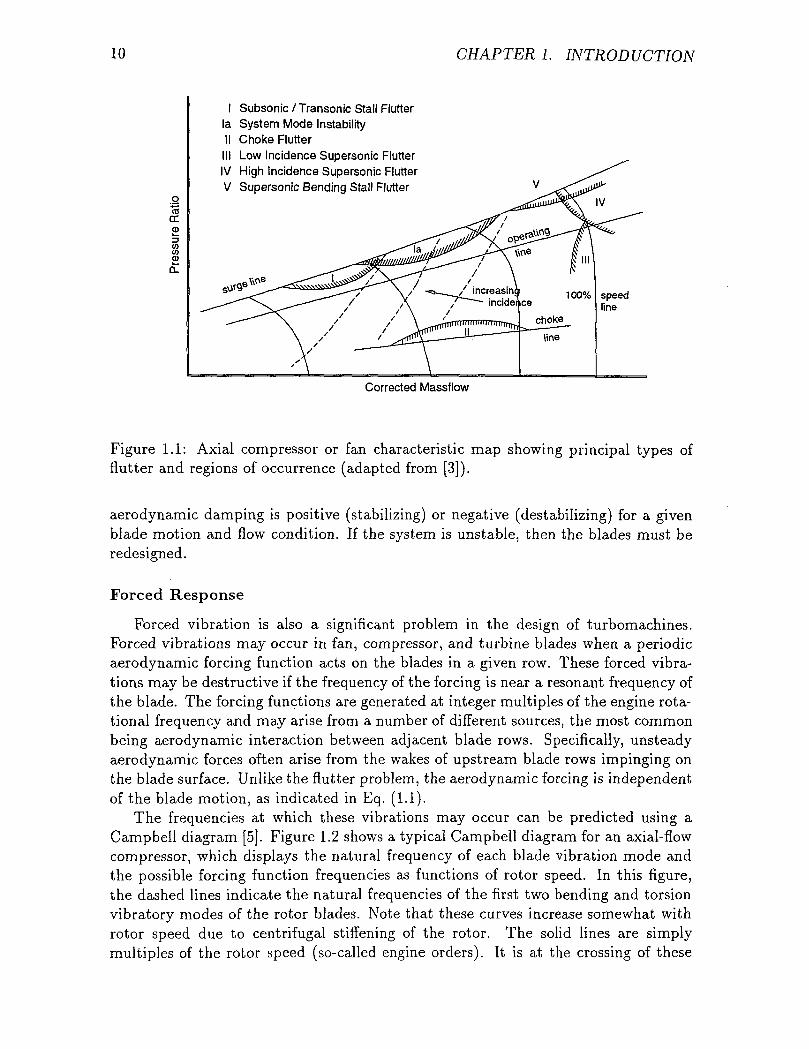
Self-excited blade vibrations that are sustained by the unsteady aerodynamicforces are of great concern to engine designers. If the aerodynamic forces producedby the blade vibration add energy to the blade motion, the vibration will grow expo-nentially until a limit cycle is reached or the blade fails. This aeroelastic phenomenais known as flutter. Flutter tends to occur near one of the lower natural frequenciesof the blades. In modern engines, flutter may be encountered in a wide range of op-erating conditions. As a result, there are significant constraints on the design of fan,compressor, and turbine blading. Figure 1.1 shows the operating map for a typical fanor compressor, showing the boundaries for the most common types of flutter [3]. Thisfigure illustrates the complexity of the design problem for a compressor. Deviationsfrom the operating line can easily lead to one of the indicated types of flutter. Becausethe structural damping of the blades is usually small, the aerodynamic damping is ofprimary interest. The unsteady aerodynamics problem is to determine whether the
10 CHAFTER 1. INTRODUCTION
acr
I Subsonic / Transonic Stall Flutterla System Mode InstabilityII Choke FlutterIII Low Incidence Supersonic FlutterIV High Incidence Supersonic FlutterV Supersonic Bending Stall Flutter
Corrected Massflow
Figure 1.1: Axial compressor or fan characteristic map showing principal types offlutter and regions of occurrence (adapted from [3]).
aerodynamic damping is positive (stabilizing) or negative (destabilizing) for a givenblade motion and flow condition. If the system is unstable, then the blades must beredesigned.
Forced Response
Forced vibration is also a significant problem in the design of turbomachines.Forced vibrations may occur in fan, compressor, and turbine blades when a periodicaerodynamic forcing function acts on the blades in a given row. These forced vibra-tions may be destructive if the frequency of the forcing is near a resonant frequency ofthe blade. The forcing functions are generated at integer multiples of the engine rota-tional frequency and may arise from a number of different sources, the most commonbeing aerodynamic interaction between adjacent blade rows. Specifically, unsteadyaerodynamic forces often arise from the wakes of upstream blade rows impinging onthe blade surface. Unlike the flutter problem, the aerodynamic forcing is independentof the blade motion, as indicated in Eq. (1.1).
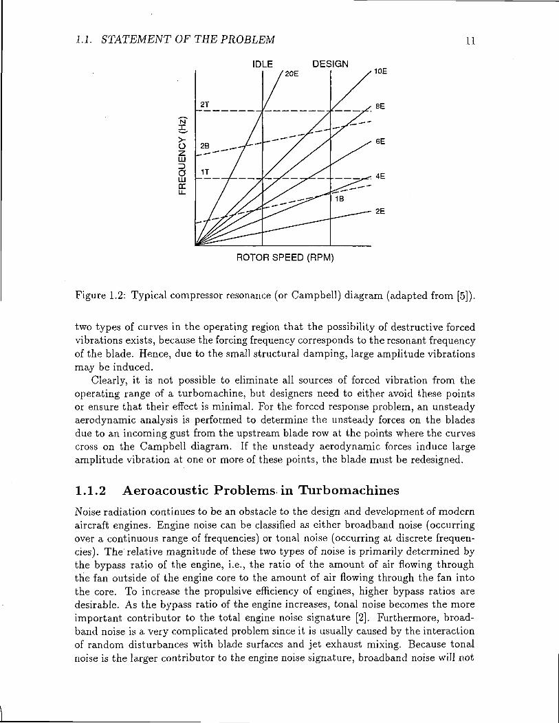
The frequencies at which these vibrations may occur can be predicted using aCampbell diagram [5]. Figure 1.2 shows a typical Campbell diagram for an axial-flowcompressor, which displays the natural frequency of each blade vibration mode andthe possible forcing function frequencies as functions of rotor speed. In this figure,the dashed lines indicate the natural frequencies of the first two bending and torsionvibratory modes of the rotor blades. Note that these curves increase somewhat withrotor speed due to centrifugal stiffening of the rotor. The solid lines are simplymultiples of the rotor speed (so-called engine orders). It is at the crossing of these
J.I. STATEMENT OF THE PROBLEM 11
IDLE DESIGN'20E '10E
N
oz111^oujcc
2E
ROTOR SPEED (RPM)
Figure 1.2: Typical compressor resonance (or Campbell) diagram (adapted from [5]).
two types of curves in the operating region that the possibility of destructive forcedvibrations exists, because the forcing frequency corresponds to the resonant frequencyof the blade. Hence, due to the small structural damping, large amplitude vibrationsmay be induced.
Clearly, it is not possible to eliminate all sources of forced vibration from theoperating range of a turbomachine, but designers need to either avoid these pointsor ensure that their effect is minimal. For the forced response problem, an unsteadyaerodynamic analysis is performed to determine the unsteady forces on the bladesdue to an incoming gust from the upstream blade row at the points where the curvescross on the Campbell diagram. If the unsteady aerodynamic forces induce largeamplitude vibration at one or more of these points, the blade must be redesigned.
1.1.2 Aeroacoustic Problems in Turbo machines
Noise radiation continues to be an obstacle to the design and development of modernaircraft engines. Engine noise can be classified as either broadband noise (occurringover a continuous range of frequencies) or tonal noise (occurring at discrete frequen-cies). The relative magnitude of these two types of noise is primarily determined bythe bypass ratio of the engine, i.e., the ratio of the amount of air flowing throughthe fan outside of the engine core to the amount of air flowing through the fan intothe core. To increase the propulsive efficiency of engines, higher bypass ratios aredesirable. As the bypass ratio of the engine increases, tonal noise becomes the moreimportant contributor to the total engine noise signature [2]. Furthermore, broad-band noise is a very complicated problem since it is usually caused by the interactionof random disturbances with blade surfaces and jet exhaust mixing. Because tonalnoise is the larger contributor to the engine noise signature, broadband noise will not
12 CHAFTER 1. INTRODUCTION
be considered in this report.The source of tonal noise is nonuniformities in the flowfield such as inlet dis-
tortion, inlet angle of attack, or convected wakes from upstream blade rows. Thenoise is produced by an interaction between the flow nonuniformity (or "gust"), theblade row, and the duct surrounding the blade row coupling to produce propagatingacoustic modes. Currently, most tonal noise reduction methods are aimed at eitherreducing the strength of the gust by increasing the distance between blade rows, orby modifying the duct through the use of casing treatment. In addition, blade countsare carefully chosen. Pressure waves that decay as they propagate are referred toas "cut-off." Propagating pressure waves are referred to as "cut-on," and it is thesewaves which result in audible noise. Acousticians use analytical models of the duct tochoose blade and vane counts to prevent lower order pressure modes from propagat-ing [1]. All three of these noise reduction techniques, increasing blade row spacing,casing treatment, and modifying blade/vane counts are not desirable because thesemethods add weight and expense to the finished engine.
The unsteady aerodynamics problem is to determine the response of a blade rowto an incoming gust, determine the.pressure field generated by the wake-blade in-teraction and determine whether these pressure waves will propagate outside of theengine. Most unsteady aerodynamic methods, however, are best viewed as analysistools rather than design tools. They are capable of solving the direct problem wherethe shape of the airfoil as well as the flow conditions are specified. Unfortunately,except through trial and error or extensive parametric studies, these analyses do notprovide physical insight into how, for example, to design blade shapes to reduce theiracoustic response without compromising their aerodynamic efficiency. An additionalcomplication is that the frequencies associated with aeroacoustic analysis are ap-proximately an order of magnitude higher than those found in aeroelastic problems,requiring finer discretization of the governing equations of the unsteady flowfield andincreased computational expense.
1.2 Previous Work
1.2.1 Unsteady Aerodynamic Models
The first unsteady aerodynamic analyses were semi-analytical methods that weredesigned to determine the unsteady surface pressure on a cascade of two-dimensionalflat plates due to bending or torsional vibration. In the semi-analytical approach,a number of point singularities are placed on the blade surface, and an appropriatekernel function is used to calculate the unsteady flowfield. One of the first suchanalyses was performed by Whitehead [6], who considered uniform, incompressible,undeflected flow over the plates. Because the flow is not deflected, however, there is nosteady loading on the blade, and the model failed to predict experimentally observedbending flutter. To include the effect of steady loading, Whitehead later allowed theblades to deflect the mean flow, resulting in steady loading on the blades [7], andbending flutter was predicted. This provided numerical evidence that steady blade
1.2. PREVIOUS WORK 13
loading (and therefore the blade shape design) had an important effect on flutterin aircraft engines. Later, Atassi and Akai [8] distributed point singularities alongthe surface of an airfoil with finite camber and thickness. This model allowed themto analyze incompressible flows through more realistic cascades, also showing theimportance of steady loading and blade shape on flutter.
Both Whitehead [9] and Smith [10] investigated subsonic compressible flows overflat plate airfoils. Smith's approach was developed primarily for noise analysis in anattempt to determine the propagation characteristics of acoustic modes generated bya cascade of airfoils. Smith also measured the acoustic waves experimentally, andfound that the theory and experiment agreed well for the unloaded blade case, butthe theory was inadequate to deal with the extra sound sources introduced by steadyblade loading, and underestimated the generated wave amplitude in this case. BothWhitehead and Smith found that steady loading is extremely important to predictcorrectly the amplitudes of the outgoing pressure waves.
Advanced designs required researchers to analyze transonic and supersonic flows.Adamczyk and Goldstein [11] and others [12, 13, 14] investigated vibrating flat platesin supersonic flow which is axially subsonic. Unfortunately, these models did notpredict flutter at the experimentally observed frequencies and Mach numbers. Moresophisticated models, such as the in-passage shock model developed by Goldstein,Braun, and Adamczyk [15], analyzed supersonic cascades with finite strength shocks.The in-passage shock model predicted experimentally observed supersonic bendingflutter, at least for low reduced frequencies. The design problem was also beginningto be considered. Bendiksen [16] used a perturbation analysis to include effects dueto steady loading, thickness, camber, angle of attack, and shock motion, showing thatthese effects are important in flutter prediction.
Finally, some three-dimensional problems have been considered using a semi-analytical approach. Namba [17] has developed a lifting surface analysis to determinethe unsteady flow over vibrating three-dimensional flat plate cascades in the sub-sonic, transonic, and supersonic regimes. Although his approach demonstrates theimportance of three-dimensional effects, its application is primarily limited to lightlyloaded fan blades.
Although these semi-analytical methods have developed greatly over the years,they are insufficient to analyze most unsteady aerodynamic problems in modern en-gines, especially at off-design conditions. The blades in modern designs are heavilyloaded, and violate a number of the assumptions used in the semi-analytical approach.
As computers became more powerful, so-called field methods became an impor-tant research area. Using this approach, a set of governing equations (i.e., potential,Euler, or Navier-Stokes) is solved using computational fluid dynamics techniques.This approach has the advantage that many of the effects not included in the analyt-ical models may be easily incorporated, e.g., arbitrary blade geometries, complicatedshock structures, and various flow models.
In the area of field methods, two main approaches have emerged. These are re-ferred to as time-marching and time-linearized methods. Using the time-marchingapproach, the unsteady governing equations of the fluid motion are time-accuratelymarched subject to some appropriate set of unsteady boundary conditions. For ex-
14 CHAPTER 1. INTRODUCTION
ample, to analyze a flutter problem, the airfoils are prescribed to vibrate at somefixed frequency and interblade phase angle. Once the initial transients have decayed,the unsteady flowfield is found to be periodic in time. The advantage to this ap-proach is that nonlinear flow effects are incorporated, and finite blade motions maybe considered.
Two-dimensional, time-accurate Euler solution methods have been developed byGiles [18] and others. Three-dimensional unsteady flow problems have been in-vestigated by Ni and Sharma [19] using a time-accurate Euler method, but theirresults require several hours of supercomputer time to obtain a solution. Otherthree-dimensional methods have been developed to investigate rotor-stator interac-tion. Saxer and Giles [20] used an Euler method and Rai [21] used a Navier-Stokesanalysis. Although these methods model many of the important physical mechanismsof the unsteady flow problem, the massive amount of time required to march theseequations time-accurately will prevent this type of analysis from being used for designpurposes for many years to come, especially for three-dimensional problems.
The second approach in field methods is the use of linearized analyses to investigatesmall perturbation unsteady flows. Using this approach, the flow is assumed to becomposed of a nonlinear mean or steady flow plus a small unsteady perturbation flow.The linearized equations which describe the unsteady perturbation are linear variablecoefficient equations in the unknown complex amplitude of the harmonic motion ofthe flow.
Verdon and Caspar [22] determined the mean flow through a subsonic cascadeusing a steady full potential method. They then linearized the potential equationabout the mean flow to solve for the small disturbance unsteady flow. Whiteheadand Grant [23] and Hall [24] used a similar approach but used finite elements insteadof finite differences to discretize the linearized equations. Verdon and Caspar laterextended their model to transonic flows using shock fitting to model the shock mo-tion [25]. Although these potential methods work well for subsonic flutter problems,their use for forced response and aeroacoustic applications has been limited becausethe model does not in general include unsteady vorticity, as would have to be includedto determine the response of a blade row to an incoming vortical gust.
Within a linearized potential framework, Goldstein [26] developed a velocity split-ting technique that includes unsteady vorticity and entropy. Goldstein assumed anisentropic and irrotational mean flow, and split the unsteady velocity into rotationaland irrotational parts. The rotational unsteady velocity, which contains the unsteadyvorticity, is expressed analytically using the drift and stream functions from the steadyflow solution. The rotational velocity appears in an inhomogeneous source term inthe linearized potential equation. Hence, unsteady flows with vorticity could be an-alyzed without having to numerically solve the Euler equations. Unfortunately, thisanalysis could only be applied to flat plate airfoils. Atassi and Grzedzinski [27] de-veloped a modification to this method that allowed real airfoils to be analyzed. Halland Verdon [28] implemented this technique and showed that vortical gust effectscould be modeled accurately without the computational expense of solving the Eulerequations.
Even with vortical gust extensions, the linearized potential formulation has its
1.2. PREVIOUS WORK 15
limits. For transonic flows with strong shocks, the Euler equations must be solved.Also, the potential formulation does not translate well to three-dimensional applica-tions due to the assumption of irrotational steady flow. For these and other reasons,linearized methods continue to advance.
Hall and Crawley [29] originally solved the linearized Euler equations using aNewton iteration technique to solve the nonlinear steady Euler equations and a directmethod to solve the unsteady linearized Euler equations. This approach also usedshock fitting to model the shock motion. There were some problems with this method,however. For example, the direct solution method prevented fine computational gridsfrom being used on typical workstation computers, particularly if the analysis wereto be extended to three dimensions. To circumvent this and other problems, Halland Clark [30] and Holmes and Chuang [31] implemented linearized Euler methodsusing an iterative solution method rather than a direct solution. In addition, Hall,Clark, and Lorence [32] and Lindquist and Giles [33] showed that transonic aeroelasticproblems can be modeled appropriately within a linearized framework using shockcapturing. Using a similar technique, Clark and Hall [34] have implemented a methodfor solving the linearized Navier-Stokes equations so that stall flutter problems maybe analyzed. Finally, Hall and Lorence [35] extended the linearized Euler analysis tothree dimensions and showed the importance of three-dimensionality on the unsteadyflow in fans.
Linearized methods require significantly less computational time than their time-marching counterparts. For most unsteady aerodynamic flows of interest, the lin-earized approach requires one to two orders of magnitude less computational timethan an equivalent time-marching calculation. Although for some complex appli-cations, time-accurate time-marching methods may be employed, in most cases, alinearized analysis is sufficient to model the unsteady flowfield.
1.2.2 Design Methods and Optimization
A substantial body of work exists on the inverse design and optimal design of airfoils.Most of this work, however, is directed at achieving desirable steady flow properties.In an inverse method, a pressure distribution is specified and the analysis producesan airfoil shape (if possible) that will produce the desired distribution. For exam-ple, Lighthill [36] developed an inverse design method based on conformal mappingtechniques. More recently, a number of investigators have proposed inverse designtechniques based on modern computational fluid dynamic algorithms (e.g., [37]).
More popular are optimal design techniques, where an initial airfoil shape is spec-ified, and the analysis attempts to minimize some quantity (e.g., steady aerodynamiclosses) while satisfying some appropriate constraints (e.g., the blade maintains thecorrect turning). A number of investigators have used nonlinear programming tech-niques to solve this problem (e.g., [38]), and Jameson has suggested that this problemmay be viewed as an optimal control problem [39].
Researchers have also developed some optimization techniques for aeroelasticproblems in turbomachinery. For example, Crawley and Hall [40] developed a methodto calculate an optimal distribution of "mistuning" for a blade row. These techniques,
16 CHAPTER 1. INTRODUCTION
however, have focused on structural optimization rather than optimization of the un-steady aerodynamic behavior.
One of the key ingredients in optimization algorithms is the evaluation of thesensitivity of the quantity to be optimized (for example, the flutter stability or ef-ficiency of a cascade) to a small change in a physical parameter (such as the airfoilshape). Sensitivity analysis of structures has been an active area of research for thepast decade [41, 42]. Recently, researchers have begun to develop similar sensitivityanalysis techniques for steady aerodynamic problems. For example, Taylor et al [43]and Baysal and Eleshaky [44] have computed the effect of modifying the shape of anozzle on the flow in the nozzle. Their work was based on a sensitivity analysis ofthe discretized Euler equations. Most recently, such techniques have been applied toairfoil design [45]. Despite these advances, only a few unsteady sensitivity analyseshave been reported, for example the semi-analytical panel method of Murthy andKaza [46]. Other unsteady sensitivity analyses have been computed by differencingtwo slightly different nominal unsteady solutions. The use of these types of finitedifferences, as opposed to analytical perturbations, are not as desirable because oftheir increased computational expense and susceptibility to truncation error.
1.3 Present Method
In this report, strategies for efficient aeroacoustic and aeroelastic design of turboma-chinery blades will be examined. An essential part of these strategies is a new methodfor computing the sensitivity of unsteady flows in cascades due to small changes inblade geometry. The approach is general in nature and may be applied to differentgoverning equations and numerical schemes. Consequently, an appropriate equationset must be chosen. For many aeroacoustic and aeroelastic problems in turbomachin-ery, an inviscid flow analysis is sufficient to model the dominant physical mechanismsof the unsteady flowfield. Hence, a linearized potential or linearized Euler frameworkwould be applicable. Since vortical gusts must be analyzed, however, the traditionallinearized potential method is not appropriate. The linearized Euler approach, whileincorporating complete inviscid physics, is still computationally expensive to solvedirectly, as the present method requires. Therefore, a linearized potential model withvortical gust extensions is the logical choice. This is the method that will be used inthis report to demonstrate the sensitivity analysis procedure.
Specifically, the nominal analysis used here is a linearized harmonic unsteady po-tential method based on a deforming grid variational principle and finite elementmethod by Hall [24] extended using rapid distortion theory to include the effect ofincident vortical gusts due to wake interaction. The sensitivity analysis procedure isas follows. First, the nominal flow equations are discretized and solved using a finiteelement procedure. Next, a perturbation analysis is performed on the discretizedequations from the nominal finite element analysis. This leads to a set of linear equa-tions for the sensitivity of the unsteady potential due to small changes in the airfoilshape. If the nominal unsteady analysis is computed with LU decomposition, the sen-sitivities may then be computed by back-substitution. Consequently, the sensitivity
1.4. OUTLINE OF REPORT 17
of the unsteady potential may be computed very efficiently.Once the sensitivities have been calculated, a range of approaches exist for improv-
ing the aeroacoustic and aeroelastic performance of the cascade. For example, thecalculated sensitivities may be used by themselves as a guide to redesign the airfoil.A more thorough approach would be to perform an optimization on the aeroacous-tic or aeroelastic behavior of the cascade, subject to appropriate constraints. Theradiated noise, for example, could be minimized subject to the constraint that thedesired steady flow turning is achieved. The results shown in this report will essen-tially be a compromise between these two methods, where the calculated sensitivitiesare post-processed such that design changes satisfy steady aerodynamic constraints.The framework for the use of this technique in more complicated design situationswill also be discussed.
1.4 Outline of Report
In Chapter 2, the governing equations and basic theory of the nominal flow analysiswill be presented. This includes both the steady flow potential equation and thelinearized potential equation and the vortical gust extension. Use of a deformingcomputational grid will be discussed, as will the theoretical description of the steadyand unsteady boundary conditions.
Chapter 3 contains a discussion of the basic numerical discretization scheme, basedon Hall's finite element method. The grid generation procedure will be discussed, aswill the implementation of the boundary conditions, with particular emphasis on thenonreflecting far-field boundary conditions. Finally, the matrix assembly and solutionwill be described.
In Chapter 4, the sensitivity analysis procedure will be examined in detail for boththe steady and unsteady flow equations. Although the procedure will be applied tothe present potential method, this chapter should clarify how the sensitivity analysiswould be performed on other governing equations and discretization schemes.
In Chapter 5, results of the sensitivity analysis will be presented, demonstratinghow the analysis may be used to redesign blade rows for improved aeroelastic andaeroacoustic performance. Also, the computational efficiency of the method will bediscussed, as will its range of effectiveness.
In Chapter 6, three-dimensional flow considerations will be examined. Specifical-ly, application of the analysis in an actual design environment will be discussed , withparticular emphasis on how three-dimensional problems could be analyzed using thepresent method.
Finally, in Chapter 7, some conclusions from the present analysis will be presentedas well as some recommendations for future work in this area.
Chapter 2
Nominal Flow Field Description
In this chapter, the equations and boundary conditions governing the steady andsmall disturbance unsteady flow through a two-dimensional cascade of airfoils areintroduced. Section 2.1 contains a description of the rapid distortion theory usedso that unsteady vortical flows may be modeled within a potential flow framework.This theory results in a set of sequentially coupled partial differential equations thatmust be solved numerically to obtain the unsteady flow. In Section 2.2, an extensionof a variational principle originally developed by Bateman [47] is described. Thisvariational principle has as its Euler-Lagrange equation the potential flow equationdeveloped in Section 2.1. This variational principle will be used in Chapter 3 toconstruct a finite element description of the steady and unsteady flow. Finally, inSections 2.3 and 2.4, the steady flow and small disturbance unsteady flow boundaryconditions will be discussed, including the far-field nonreflecting boundary conditions.
2.1 Euler Equations
The equations governing the fluid motion through a cascade of airfoils may be derivedfrom the integral conservation laws of mass, momentum, and energy, along with theequation of state for an ideal gas. For this analysis, the flow is assumed to be inviscidand compressible, and the fluid is assumed to be a perfect gas with specific heat ratio7 = CP/CU (a complete list of symbols used in this report is given in Appendix A).Consequently, the governing equations of the fluid are the Euler equations, which inconservation form are
^ + V - ( A * ) = 0 (2.1)
^ + V-/5vv + Vp = 0 (2.2)
d01 \ 1 ' nr I • \ .. i J • o' / * \^ - t )/Ot \7 —
where p is the density, v is the velocity, and p is the pressure. These quantities arerelated by the state equation for a perfect gas
p = pRuTf (2.4)
18
2.1. EULER EQUATIONS 19
where RU is the universal gas constant and T/ is the temperature. The superscript "'"indicates that the quantity is unsteady. For this discussion, it is useful to define theentropy of the fluid, Sf. This is most easily accomplished using the thermodynamicrelation defined by Gibbs,
ff ds} ̂ C p d f j - ^ d p (2.5)
The temperature dependence may be removed through the use of the state equation,Eq. (2.4), resulting in
dp dpdsf = ̂ - cp-t (2.6)
P PEquation (2.6) may then be integrated to obtain the entropy change between twofluid states.
It is further assumed that the nonlinear time-varying flow may be split into twoparts: a nonlinear mean or steady flow and a small unsteady perturbation flow thatis harmonic in time. In other words, each of the variables in the above equations maybe expanded in a perturbation series. Furthermore, it is assumed that the steady flowis irrotational and homentropic, so that the steady velocity may be written as thegradient of a scalar velocity potential, $. Under these assumptions, the perturbationseries for the flow variables may be written as
p(x,y, t ) = R(x,y) + p(x,y}e^
v(x,y, i) = V$(x,y) + v(x,y)e*-"
p(x,y , t ) = P(x,y) + p(x,y)e*-"
s f (x ,y , t ) =
total flow nonlinear small harmonicmean disturbance
To obtain the steady and unsteady flow equations, these expansions are substi-tuted into the governing equations, Eqs. (2.1)-(2.6), collecting terms of equal order.The zeroth-order terms result in the steady flow equations, while the first-order termsdescribe the unsteady flow. The zeroth-order continuity equation is
V • (.RV$) = 0 (2.8)
The zeroth-order momentum equation and equation of state may be integratedand combined to obtain the steady form of Bernoulli's Equation, i.e.,
= PT
or ^" Tf-l
1 - (V*)2 (2-9)
(2.10)
20 CHAPTER 2. NOMINAL FLOW FIELD DESCRIPTION
where px and PT are the total pressure and density, respectively, and CT is the totalspeed of sound. Substituting Eq. (2.9) into Eq. (2.8) results in an equation for themean flow that is only a function of the potential and the steady speed of sound,
V2$ = v* • V(V<D)2 (2.11)
whereC2 = C$ - 1^- ( V$)2 (2.12)
Note that the steady flow is completely described by a single equation for the scalarpotential $. It is indeed nonlinear, as was noted earlier.
Having described the equation governing the steady flow, we now consider theunsteady small disturbance equations. Collection of the first-order terms results in thefollowing set of equations describing the behavior of the small disturbance unsteadyflow
~ (v - s/V$/2) + [(v - s/V*/2) - V] V$ + V = 0 (2.14)
where D/Dt = d/dt + V$ • V is the convective derivative. Note that while the steadyflow may be described using a single equation, the unsteady flow is governed by asystem of four simultaneously coupled equations. Computationally, this descriptionof the unsteady flow would result in a very large system of equations to solve. Hence,a more compact description of the unsteady flow is desired.
2.1.1 Goldstein Decomposition
Equations (2.14) and (2.15) may be simplified further using the Goldstein velocitydecomposition [26]. The unsteady velocity, v, is split into a rotational part, VH, andan irrotational part that is written as the gradient of a scalar velocity potential, ^,so that
v = V<£ + v* (2.16)
It should be noted that there is no unique choice for v^ and <j>, since it is the combi-nation of the two that results in the actual unsteady flow velocity. However, if VR ischosen such that
=0 (2.17)Dt L J \RJ
then the unsteady pressure is only a function of the unsteady potential, so that
2.1. EULER EQUATIONS 21
Substituting Eqs. (2.16) and (2.18) into the linearized momentum and continuityequations [Eqs. (2.14) and (2.15)] results in a system of equations for the unsteadyentropy, rotational velocity, and velocity potential, i.e.,
= 0 (2.19)Dt
Dt1
+ [(vfi r- 5/V$/2) • V] V$ = 0 (2.20)
Note that the equations for entropy, rotational velocity, and velocity potential are nowonly sequentially coupled. Although four equations still must be solved, they neednot be solved simultaneously. As a result, a numerical solution to these equationsmay be obtained for considerably less computational cost than the earlier set ofsimultaneously coupled equations. Furthermore, in this report, the effect of unsteadyentropy will not be investigated, so it is assumed that s/ = 0. Consequently, onlyEqs. (2.20) and (2.21) must be solved.
Goldstein [26] showed that Eq. (2.20) may be solved analytically for certain casesin terms of two functions. One is the well-known stream function, ^f(x, y}. The otheris the drift function, A(x,j /) , which is denned as the time it takes a mean flow fluidparticle to move between two points on a streamline, i.e.,
A(z, y) = A(x0, y0) + 77^ (2.22)
where the location (XQ, j/o) is a point upstream of (x, y) on the same steady streamline,|V$| is the magnitude of the steady flow velocity, and the differential distance dil> ismeasured along the streamline. The drift and stream functions are often referred toas the Lagrangian coordinates of the fluid.
Figure 2.1 shows contours of the drift and stream functions for a typical fanexit guide vane. Note that upstream of the cascade, the drift function contours arealigned between the blade passages, while downstream of the airfoils the contours areno longer aligned. This indicates that there is circulation around the airfoil, i.e., thesteady velocities are different on the two sides of the airfoil surface. Furthermore,note that the drift contours are well-behaved in the interior of the blade passages,but change rapidly near the blade and wake surfaces. This is due to the presence of astagnation point at the leading edge of the airfoil. Examining Eq. (2.22) shows that ifthe steady velocity is zero at some point (i.e., a stagnation point), the drift functionbecomes infinite. This property of the drift function is problematic in the derivationof a general expression for the rotational velocity over airfoils, so a detailed analysisof the drift function behavior near a stagnation point is warranted.
Consider the steady flow field near a stagnation point. Sufficiently close to a solidboundary, the boundary appears to be a plane surface (unless the boundary happens
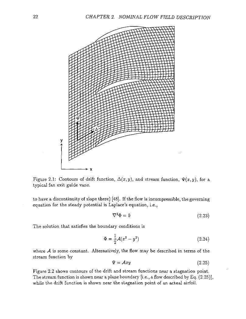
22 CHAPTER 2. NOMINAL FLOW FIELD DESCRIPTION
Figure 2.1: Contours of drift function, A(x,typical fan exit guide vane.
), and stream function, fy(z,y}, for a
to have a discontinuity of slope there) [48]. If the flow is incompressible, the governingequation for the steady potential is Laplace's equation, i.e.,
The solution that satisfies the boundary conditions is
$ = -
(2.23)
(2.24)
where A is some constant. Alternatively, the flow may be described in terms of thestream function by
tf = Axy (2.25)
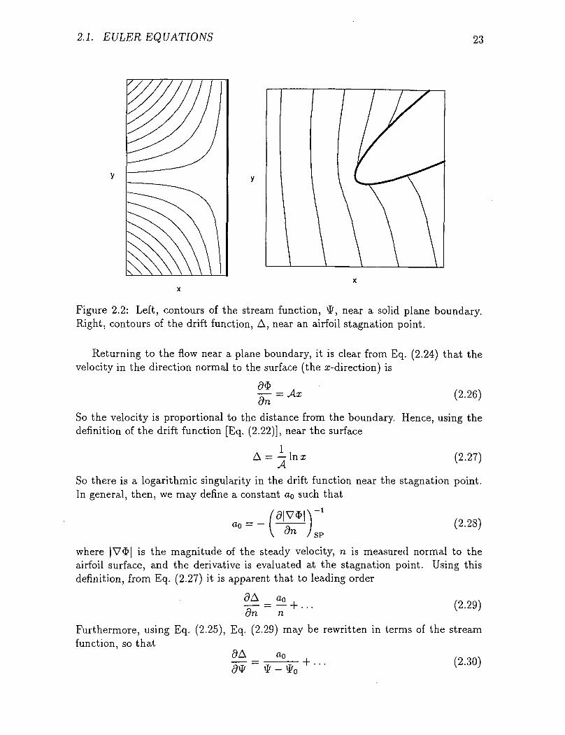
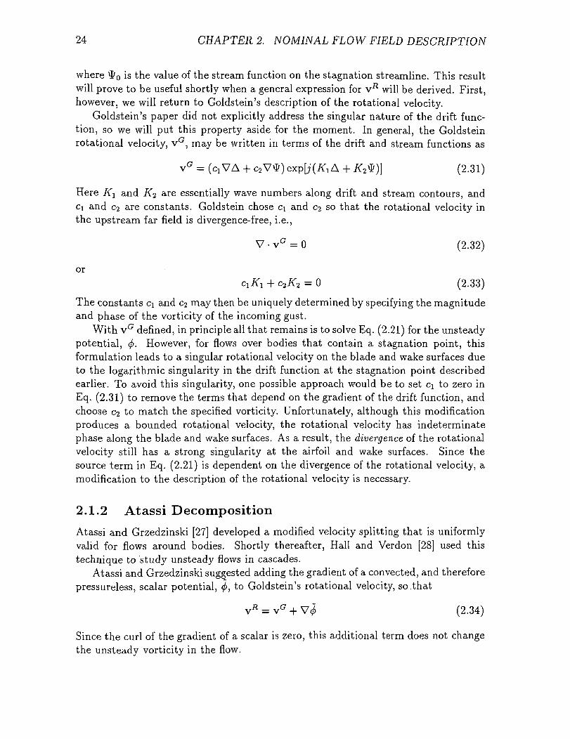
Figure 2.2 shows contours of the drift and stream functions near a stagnation point.The stream function is shown near a plane boundary [i.e., a flow described by Eq. (2.25)],while the drift function is shown near the stagnation point of an actual airfoil.
2.1. EULER EQUATIONS 23
Figure 2.2: Left, contours of the stream function, \&, near a solid plane boundary.Right, contours of the drift function, A, near an airfoil stagnation point.
Returning to the flow near a plane boundary, it is clear from Eq. (2.24) that thevelocity in the direction normal to the surface (the x-direction) is
(2.26)— = Axon
So the velocity is proportional to the distance from the boundary. Hence, using thedefinition of the drift function [Eq. (2.22)], near the surface
A = — In xA
(2.27)
So there is a logarithmic singularity in the drift function near the stagnation point.In general, then, we may define a constant a0 such that
, v i
/5|V$|\GO = — I —o— 1 (2.28)
V dn JSP
where |V$| is the magnitude of the steady velocity, n is measured normal to theairfoil surface, and the derivative is evaluated at the stagnation point. Using thisdefinition, from Eq. (2.27) it is apparent that to leading order
(2.29)_ a0
dn n
Furthermore, using Eq. (2.25), Eq. (2.29) may be rewritten in terms of the streamfunction, so that
24 CHAPTER 2. NOMINAL FLOW FIELD DESCRIPTION
where \I/0 is the value of the stream function on the stagnation streamline. This resultwill prove to be useful shortly when a general expression for VR will be derived. First,however, we will return to Goldstein's description of the rotational velocity.
Goldstein's paper did not explicitly address the singular nature of the drift func-tion, so we will put this property aside for the moment. In general, the Goldsteinrotational velocity, VG, may be written in terms of the drift and stream functions as
v° = (d VA + c2 W) exp[j(K, A + K^)] (2.31)
Here K\ and KI are essentially wave numbers along drift and stream contours, andGI and c2 are constants. Goldstein chose c\ and c2 so that the rotational velocity inthe upstream far field is divergence-free, i.e.,
V • VG = 0 (2.32)
ordid + c?K2 = 0 (2.33)
The constants c\ and c2 may then be uniquely determined by specifying the magnitudeand phase of the vorticity of the incoming gust.
With VG defined, in principle all that remains is to solve Eq. (2.21) for the unsteadypotential, <f>. However, for flows over bodies that contain a stagnation point, thisformulation leads to a singular rotational velocity on the blade and wake surfaces dueto the logarithmic singularity in the drift function at the stagnation point describedearlier. To avoid this singularity, one possible approach would be to set GI to zero inEq. (2.31) to remove the terms that depend on the gradient of the drift function, andchoose c2 to match the specified vorticity. Unfortunately, although this modificationproduces a bounded rotational velocity, the rotational velocity has indeterminatephase along the blade and wake surfaces. As a result, the divergence of the rotationalvelocity still has a strong singularity at the airfoil and wake surfaces. Since thesource term in Eq. (2.21) is dependent on the divergence of the rotational velocity, amodification to the description of the rotational velocity is necessary.
2.1.2 Atassi Decomposition
Atassi and Grzedzinski [27] developed a modified velocity splitting that is uniformlyvalid for flows around bodies. Shortly thereafter, Hall and Verdon [28] used thistechnique to study unsteady flows in cascades.
Atassi and Grzedzinski suggested adding the gradient of a convected, and thereforepressureless, scalar potential, </>, to Goldstein's rotational velocity, so.that
VH = VG + V^ (2.34)
Since the curl of the gradient of a scalar is zero, this additional term does not changethe unsteady vorticity in the flow.
2.1. EULER EQUATIONS 25
This potential may not be simply chosen arbitrarily. First of all, this new form ofVH must satisfy Eq. (2.20). This is true if
= 0 (2.35)JLS lj
which implies that it has no pressure associated with it [see Eq. (2.18)]. Since it isconvected, the potential propagates the same way as the Goldstein rotational velocity,i-e-,
where $ is an as yet undetermined function. Using the form of <fr given in Eq. (2.36),the rotational velocity may be written as
(2.37)
We wish to determine the potential ^ such that VR is zero on the blade andwake surfaces, which will produce the desired result that the normal and tangentialcomponents of the rotational velocity field are regular along the blade and wakesurfaces. In terms of the unit surface tangent, s, and the unit surface normal, n, wewant
VR . s = (VG + V<^) • s = 0 (2.38)
andVH • n = (VG + V^) • n = 0 (2.39)
The first condition, Eq. (2.38), is satisfied if $ is a constant. To illustrate this,consider the tangential component of VR. Using Eq. (2.37), if <l is constant, then
(d + JK&) + (c2 + JK^) ^- = 0 (2.40)
Since the airfoil surface and wake is a stagnation streamline, d^/ds is zero. Hence,if $ is chosen such that
* = 7T (2-41)-ftl
then Eq. (2.40) [and therefore Eq. (2.38)] is satisfied. This choice of $ removes thedominant singularity in vc which is on the order of VA. In fact, this is equivalentto setting GI to zero in Eq. (2.31) and choosing c^ to match the specified vorticity, assuggested earlier.
Unfortunately, VR may still have indeterminate phase. The singular behavior ofthe normal component of VR is only completely eliminated when ^ satisfies Eq. (2.39).To eliminate this singular behavior, we will proceed by splitting <^> into two parts, sothat
^ = ^1 + ^2 (2.42)
where, ^ is the potential associated with the constant $ given in Eq. (2.41), and <^>2
is still to be determined. So as not to violate Eq. (2.38), ^2 will be chosen so that its
26 CHAPTER 2. NOMINAL FLOW FIELD DESCRIPTION
value will be zero on the blade and wake surfaces, while allowing $2 to be dependenton the stream function, \I/.
Considering both parts of ^, the normal component of VR may be written as
° 2.43)^ '
In light of the choice of <^i , this reduces to
CIK,c2 -- — + -^r- — = 0 (2.44)
dn ^ '
or
Next, we wish to determine the behavior of the first term in Eq. (2.45) near thesurface of the airfoil. Performing a Taylor expansion of c^/dA about the stagnationpoint gives
This equation, combined with the expression for <9A/<9\P obtained in the earlier dis-cussion of the behavior of the drift function near a stagnation point [Eq. (2.30)], leads
0 (2'47)
As was shown earlier, <^>2 has the form
Substituting this expression into Eq. (2.47) gives
" ] d~ = 0 (2.48)
Also, because the cascade is periodic, a similar boundary condition must be appliedon the next adjacent blade surface. Hence, the value of the stream function at thissurface is required. The stream function may be computed by integrating the massflux over the blade-to-blade gap
Qdy (2.49)o
where G is the blade-to-blade gap measured in the y-direction, and Q is the massflux. Typically, the upstream steady density, R-oo, the upstream free stream velocity,V-oo, and the upstream flow angle, fi_oo, are specified. Using these values, the streamfunction may be written as
tf (z, y + G) = #0 + #-oo V-ooG cos fi.oo (2.50)
2.2. EXTENSION OF BATEMAN'S VARIATION'AL PRINCIPLE 27
Consequently, since the potential should vanish at the blade and wake surfaces, welet $2 take the form
(2.51)
where B is a constant independent ofboundary condition [Eq. (2.48)] gives
R V G ros Hi v—QO r —OO *—' ^v/O u U — QQ
'. Substituting this functional form into the
cos
+ jK2B sin = 0
solving for B gives
„ _
(2.52)
(2.53)
After performing some algebra, the final expression for </> is obtained, i.e.,
27T(1+ 7sm
R-oa V-oo G COS fi_r
x exp[;(/^i A + K^)] (2.54)
This expression for <^ results in a rotational velocity that is regular along the bladeand wake surfaces, so that the divergence of the rotational velocity may be calculateddespite the presence of a stagnation point. Note that the complete expression for VR
is relatively simple, and may be calculated once the steady flow has been computedand the desired magnitude and phase of the unsteady vorticity has been chosen. Nowthat a uniformly valid expression for VR has been written, then, the next task is tocalculate the unsteady velocity potential, <f>, using Eq. (2.21).
2.2 Extension of Bateman's Variational Principle
Now that the governing equations have been developed, it is useful to consider howthese equations will be solved numerically. Essentially there are two choices: finitedifferences and finite elements. Both of these methods have been used to solve thelinearized potential equation for blade motion and pressure gust analyses [22, 23].In addition, Hall and Verdon used finite differences to solve the linearized potentialequation with rapid distortion theory to analyze vortical gusts [28]. For this report,a finite element discretization of the field equations is used. There are three mainreasons for this approach. First, finite element techniques are versatile, elegant, andrelatively easy to implement. Second, it is believed that a finite element approach willreduce the overall truncation error because the governing equation is solved in the
28 CHAPTER 2. NOMINAL FLOW FIELD DESCRIPTION
integral sense instead of the differential sense. Truncation errors tend to be higherin derivative evaluation than integral evaluation. Finally, a potential method forblade motion analyses developed by Hall [24] was readily available. The details ofthe finite element procedure will be given in Chapter 3. This section will describe thevariational principle on which the finite element method is based and its applicationto the current work, including the effect of unsteady vorticity.
2.2.1 Nonlinear Full Variational Principle
First, consider irrotational and homentropic flow. Bateman [47] developed a varia-tional principle that states that for a steady flow, the volume integral of the pressuremust have an extreme value, and the associated Euler-Lagrange equation is the steadyconservation of mass. Hall [24] later extended this principle for application to cas-cades by considering temporally periodic flow. In this case, the pressure integratedover a domain S and over a period A is extremized. In functional form,
H = - / // p dx dy dt + - I I Qj)ds dt (2.55)A JA J Jz A JA Jr
where Q is the prescribed mass flux on the boundary and s is the distance along theboundary F. Taking the first variation of H and setting to zero gives
<m = - / H Sp dx dy dt + i / { Q 8$ ds dt = 0 (2.56)A JA J JT, A JA. Jr
Bernoulli's Equation says that
H (*)'+§ =c (2-57)
where C is a constant. Since we have assumed that the flow is homentropic, thevariation of the pressure may be written as
Sp = -p V « ^ - V ^ + — 5(t>\ (2.58)
Substituting this expression into the equation for 511, using the divergence theoremand integration by parts gives
/ / ^ ' (fflr) ~t~ !T~ ^ dx dy dt
1 / • / • / . d<j>\ -H / <P [Q — P-^~ 06 ds dt = 0 (2.59)
A A / r V Pdn) v V '
To extremize H, 5H must be zero for all permissible variations in ^. Therefore,Eq. (2.59) says that the conservation of mass must be satisfied in the domain E. Onthe boundary F, Dirichlet boundary conditions may be imposed, since then S<f> will be
2.2. EXTENSION OF BATEMAN'S VARIATIONAL PRINCIPLE 29
zero, or the Neumann boundary condition may be used, so that pd^/dn = Q. Thisis the so-called natural boundary condition.
Since the steady and unsteady flow is governed by the conservation of mass, thisvariational principle is the appropriate choice to be discretized and solved. For thisprinciple to be used, however, the temporal integration must be removed. This maybe accomplished through the use of the earlier assumption that the unsteady flow isharmonically varying with frequency u. With the temporal behavior of the potentialrepresented by assumed mode shapes, the resulting steady and unsteady variationalprinciples for the spatial behavior of the flow may then be discretized and solvedusing traditional finite element techniques.
2.2.2 Steady Flow Variational Principle
For steady flows, the variational principle is quite simple. Since the pressure, P,the potential, $, and the density, R, are all independent of time, the functional IIbecomes
Hsteady = // P dx dy + j> Q$ ds (2.60)
To extremize this equation, the first variation is set to zero, resulting in
Using the divergence theorem, this becomes
<5nsteady = If 6P dx dy + j> Q 8$ ds
8$ds = Q (2.61)
= // [V - (#V$)] <5$ dx dy + I Q - R^-\ £$ ds (2.62)j t/s «r v (/it/ /
<msteady
The Euler-Lagrange equation of this variational principle is the steady conserva-tion of mass, Eq. (2.8). The natural boundary condition is the Neumann conditionRd$/dn = Q. Finally, it should be noted that the steady conservation of mass isnonlinear in the steady potential, $ due to the dependence of R on $. Consequently,nonlinear finite element techniques will be required.
2.2.3 Unsteady Flow Variational Principle With DeformingGrid and Vorticity
The variational principle for the unsteady flow is considerably more complicated thanits steady flow counterpart. Part of this complexity is due to the fact that the lin-earized potential equation is more complicated than the steady flow potential equa-tion, as was shown earlier. In addition, we will see that an extension to the variationalprinciple is useful for the analysis of blade motion problems.
Up to this point, the theoretical development in this chapter has been mainlyconcerned with the forced response (or gust) problem, i.e., how to include the effect
30 CHAPTER 2. NOMINAL FLOW FIELD DESCRIPTION
of unsteady vorticity within a linearized potential framework. There is an additionalcomplication inherent in the flutter (blade vibration) problem, however. Previousmethods for solving the potential equation have used grids that are fixed in space.While this is numerically convenient, the airfoil boundary conditions must be appliedat the mean airfoil location instead of the instantaneous location. As a result, extrap-olation terms must be added to the unsteady airfoil boundary conditions to transferthe boundary conditions from the instantaneous location of the airfoil to its meanposition. These terms contain steady velocity gradients that are difficult to evaluatenumerically. Consequently, the accuracy of numerical calculations using fixed gridsis limited.
One way to eliminate these extrapolation terms is to use a computational gridthat continuously deforms with the airfoil motion. This procedure has been shown tobe an effective technique for improving the accuracy of linearized analyses [30, 31, 35].
In this report, it is assumed that the grid motion is a small harmonic perturbationabout the mean grid location. We introduce computational coordinates (£,77,1") sothat the grid deforms in the physical coordinate system (x,2/ , t ) , but appears station-ary in the computational coordinate system. Said another way, the computationalcoordinates are "attached" to the deforming grid. To illustrate, Figure 2.3 showscontours of the computational coordinate system for deformed and undeformed gridsfor a cascade of airfoils pitching about their midchords. Note that the computationalcoordinates do indeed "deform" with the blade motion. Mathematically, the twocoordinate systems are related by the perturbation series
7)6*"- (2.63)
})^ (2.64)
t(£,T1,T) = T (2.65)
Note that to zeroth order, the physical and computational coordinates are the same.The terms / and g are first-order perturbations that map the computational coordi-nate system to the moving physical system. The flow decomposition described earliermay be expressed in a similar fashion, i.e.,
p(x,y , t ) =
v(x,y, t ) =
p(x ,y , t ) = P(t,r,)(Z.vb)
total flow nonlinear small harmonicmean disturbance
To first order, the gradient operator, V, and time derivative operator, d/dt, op-erators may be expressed in terms of the computational coordinate operators V and
2.2. EXTENSION OF BATEMAN'S VARIATION'AL PRINCIPLE 31
y,r\i \.
yi \
5
*x,%
B¥
e
&
m
Figure 2.3: Contours of computational coordinates (£,77) for undeformed (top) anddeformed (bottom) grids for a cascade of airfoils. Airfoils are pitching about theirmidchords with an interblade phase angle, a, of 180°.
32 CHAPTER 2. NOMINAL FLOW FIELD DESCRIPTION
dj dr as follows:
-fr, - 9n -and
d_ _ d_ _ df_ ,dt dr dr
(2.67)
(2.68)
where f is the vector of grid motion perturbation functions, (/, g}T.Now that the coordinate systems have been described, the unsteady variational
principle may be expressed in the computational coordinate system. By assuminga harmonic time dependence, the temporal integration in the functional II may becarried out. In the computational coordinate system, the unsteady functional is
= A L JL * L 1 ds dr (2.69)
The expression for p in the computational coordinate system may be derived bysubstituting the coordinate transformation operators from Eqs. (2.67) and (2.68) intothe unsteady nonlinear Bernoulli Equation, i.e.,
P = + (2.70)
Also, to first order, the inverse of the transformation matrix [J] may be written as
i-i _[! + /* (2.71)
To obtain an expression for the small disturbance unsteady flow, the functional inEq. (2.69) is expanded in powers of </>, /, and g retaining up to quadratic terms.The first-order terms in the functional will result in the steady flow Euler-Lagrangeequation. Because the steady flow Euler-Lagrange equation is satisfied by the meanflow potential $, these terms will not contribute to the unsteady flow functional.Therefore, only the second-order terms will contribute. Hence, the functional may bewritten as
= \ I If \R [-A JA J Js 2 L
-T1\
L>
V/ '
- fT (2.72)
Note that the surface integral terms have been omitted for the time being. Next, thetime integral needs to be evaluated. As was stated earlier, it is assumed that theunsteady flow variables (and the blade motion, if any) vary harmonically. Hence, theunsteady flow may be represented as a Fourier series in time. These Fourier modes

2.2. EXTENSION OF BATEMAN'S VARIATION 'AL PRINCIPLE 33
may be analyzed individually and summed, since the governing equation is linear.Therefore, it may be assumed that, for example,
fl£ 77, r) -> Re [flf, fie*"] = \ [tffc r))e^ + +(£, ,7)^] (2.73)
where ^(£,77) is now the complex amplitude of the unsteady potential, and ^(£,77)is its complex conjugate. The other unsteady variables are represented in a similarfashion. Substitution of this assumption into the unsteady flow functional, Eq. (2.72),results in
linear = \ jj^ R {-V'/V> + ~ [V/ V'<& V'$TV>
£ drj
V • f
+ complex conjugate terms (2-74)
where [J] = [J]T[J] — [Ij. Note that none of the boundary conditions have beendiscussed as yet. Additional terms will be added to the variational principle in thenext section to specify the boundary conditions.
At this point, it should be noted that no vorticity has been included in the un-steady functional. Although the grid motion and unsteady vorticity problems areusually analyzed separately in practice, the vortical terms will be added here forcompleteness.
The divergence theorem says that for any vector V,
f f - n d s = 0 (2.75)
Consider the case where V = <j)RvR. The divergence theorem may be written as
(I V • RvR~$ d£ drj - I RvR •n^ds = Q (2.76)
Note that because the rotational velocity and grid motion terms in the functional areboth second order, there is no coupling between the two, i.e., there will be no termsin the functional that depend on both the rotational velocity and the grid motion.Consequently, Eq. (2.76) may be written in the computational coordinate system.
We wish to add terms to the unsteady functional II so that the Euler-Lagrangeequation will contain the appropriate rotational velocity terms appearing in Eq. (2.21).Because the terms in Eq. (2.76) sum to zero, Eq. (2.76) and its associated complexconjugate expression may be added to the functional given in Eq. (2.74). Leavingaside the boundary terms for the moment, taking the variation of Eq. (2.74) includ-ing the rotational velocity terms and applying the divergence theorem results in the
34 CHAPTER 2. NOMINAL FLOW FIELD DESCRIPTION
Euler-Lagrange equation for the unsteady flow. This linearized potential equationmay be written as
V - RV't - V •
= -V • ^ [J]V'$ + V
+V • i
+ V'$[J] V'$ + u2f • V'$ - V • tfv* (2.77)O I Z J
Note that if there is no grid motion, Eq. (2.77) may be rearranged into the form ofEq. (2.21), the original equation to be solved.
In summary, then, Bateman's variational principle may be extended to includeboth the flutter and forced response problems typically encountered in turbomachin-ery. The next two sections will describe the boundary conditions required for cascades,and Chapter 3 will discuss how Eq. (2.77) and the boundary conditions are discretizedand solved numerically.
2.3 Near-Field Boundary Conditions
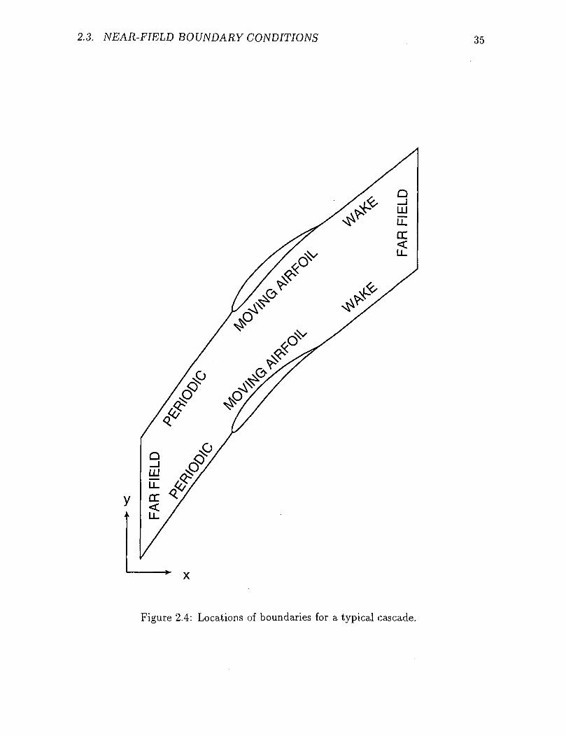
Now that the governing equations have been developed, appropriate boundary condi-tions need to be imposed. Figure 2.4 shows the locations of the four types of boundaryconditions for cascades. In this report, the periodic, airfoil surface, and wake con-ditions will be referred to as "near-field" boundary conditions and will be discussedin this section. The remaining "far-field" boundary conditions are somewhat morecomplicated and will be discussed in the next section.
2.3.1 Periodic Boundary Condition
Steady Flow
In this analysis, all of the airfoils in a given blade row are assumed to be identical.Hence, the steady flow over each blade is the same. The periodic boundary conditionis that the difference in the steady potential between two adjacent periodic boundariesis a constant, i.e.,
$(£, T, + KG) = $(£, 77) + KGV-n (2.78)
where G is the blade-to-blade gap, V_oo is the specified upstream velocity in the y-direction, and K is the blade number, where the reference blade number is zero. Thisboundary condition is applied on the periodic surfaces shown in Fig. 2.4.
2.3. NEAR-FIELD BOUNDARY CONDITIONS 35
•*• x
Figure 2.4: Locations of boundaries for a typical cascade.
36 CHAPTER 2. NOMINAL FLOW FIELD DESCRIPTION
Unsteady Flow
Clearly, computing the unsteady flow around every airfoil in a blade row would be aformidable computational task. Hence, we wish to reduce the size of the numericalcalculation. Lane [49] showed that any vibration of the blades of a cascade maybe decomposed into a sum of traveling waves with a fixed interblade phase angle.Accordingly, in this analysis, it is assumed that any incoming disturbance or blademotion may be decomposed into a sum of Fourier modes, i.e., the unsteady flowis periodic in the circumferential direction. Since the governing equation is linear,the flow solutions for each of the individual modes may be superposed to form thecomplete flow solution.
Hence, the flow around any blade may be computed by simply using the interbladephase angle (or circumferential wave number) to account for the distance between theblade to be analyzed and a reference blade. The periodic boundary condition maythen be expressed as
t(t,ri + KG) = <l>(t,ri)e>'« (2.79)
where a is the interblade phase angle.The periodic boundary condition is not included explicitly in the variational prin-
ciple. Its application will be discussed in Chapter 3.
2.3.2 Airfoil Surface Boundary Condition
Steady Flow
On the surface of the blade, no flow must pass through the blade. For the steadyflow analysis, there is no blade motion or incoming disturbance, so this condition issimply
d$°— = 0 (2.80)on
where n is measured normal to the airfoil surface. Note that this condition is thenatural boundary condition from the steady flow variational principle [Eq. (2.62)].Since it is a natural boundary condition, no boundary condition need actually beimposed here to obtain the correct solution.
Unsteady Flow
For unsteady flows, the airfoil surface boundary condition is also the natural boundarycondition of the variational principle. The motion of the blades induces an upwashon the airfoil surface (which is the source of the unsteadiness for flutter problems).If VR is nonzero on the blade surface (such as in the case of the original Goldsteinformulation) then the upwash due to the rotational velocity must also be accountedfor. The natural boundary condition from the variational principle is obtained fromthe first variation of the functional II that includes the rotational velocity terms, i.e.,
2.3. NEAR-FIELD BOUNDARY CONDITIONS 37
+ <f R( ju f • n - [ J ] V $ - n " + v H . n - ^ ] 8$ ds = 0 (2.81)j r \ c//t j
So the boundary condition isa j
^ = jwf • n - [J] V$ • n + VH • n (2.82)
The first term on the right hand side of Eq. (2.82) is the upwash due to the translationof the airfoil. The second term is an additional upwash required to counter a down-wash produced by shearing motion of the grid and resulting shearing of the steadypotential field in the vicinity of the airfoil surface. Note that there is no upwash dueto local rotation of the airfoil, nor are there extrapolation terms due to the differencebetween the mean and instantaneous position of the blade surface. These are notrequired because the mean potential field moves with the grid due to the grid motionassumption imposed earlier. The last term on the right hand side of Eq. (2.82) is theupwash associated with a nonzero rotational velocity on the blade surface.
2.3.3 Wake Boundary Condition
Steady Flow
The wake boundary conditions have characteristics of both the periodic and airfoilsurface boundary conditions described earlier. The first boundary condition is thatthe wake is considered to be an impermeable surface, so the steady no throughflowcondition applies, Eq. (2.80). Second, there is a jump in potential at the trailing edgewhich is equal to the circulation around the blade. If the jump in potential acrossthe wake is equal to the jump in potential at the trailing edge, the Kutta conditionis automatically satisfied. The boundary condition is then
Wake = (2.83)
where |$] is the jump in the steady potential. An equivalent boundary condition isthat the pressure is continuous across the wake. Hence, the steady pressure continuitycondition is
[PJ = 0 (2.84)
where \P\ is the steady pressure jump across the wake. For the wake to coincide withthe grid boundary, an additional equation will be required to enforce the pressurecontinuity condition.
Unsteady Flow
For unsteady flows, the wake oscillates harmonically about its mean position with anunknown displacement, r. Thus, as in the steady case, there is an auxiliary equationto enforce the unsteady pressure continuity. In one dimension, the unsteady pressureis linearly related to the unsteady potential, i.e.,
< (2-85)
= - R u + - - = 0
38 CHAPTER 2. NOMINAL FLOW FIELD DESCRIPTION
The pressure continuity equation may then be written as
(2.86)
where [...] represents the jump across the wake. Specifically, the jump in potentialis
|0] = (f>ue~jcr - tf (2.87)
where <f)u is the potential on the upper wake surface of the computational domain (seeFig. 2.4), and <f>f is the potential on the lower wake surface.
The other boundary condition applied on the wake is that conservation of massmust be satisfied. In particular, the upwash due to the wake displacement must beaccounted for. This additional upwash may be written as
d<f> . ,^ = -fl-fl-+Jwr (2-88an os os v '
where dQjds is the mean flow tangential velocity along the wake. The first term isa "ramp" effect due to a change in wake displacement along the wake. The secondterm is the upwash due to the translation of the wake. However, these effects are inaddition to the grid deformation effects given by Eq. (2.82). Therefore, the completeupwash on the wake surface is
^ = juf • n - [J] V$ • n + VR • n + |^ + ju>r (2.89)dn ds ds ^ '
Consequently, a term must be added to the variational principle to account for thisadditional upwash due to the motion of the wake. Taking the first variation of themodified variational principle and setting to zero gives
= [Eq. (2.81)1 + / -R [ -^-TT + J'wr ) (S^e'ff - Sj*) ds = 0 (2.90)1 v ' /r _ \ fix fix I V / v '
2.4 Far-Field Boundary Conditions
The boundary conditions at the far field are of a different nature than the near-field conditions, particularly for unsteady flows. Specifically, the far-field boundaryconditions isolate the computational domain from influences outside the blade rowbeing examined. Unsteady waves from the airfoil must pass out of the computationaldomain unreflected, so that the reflection of these waves does not corrupt the unsteadysolution. For this reason, it is crucial to apply highly nonreflective far-field boundaryconditions.
2.4.1 Steady Flow
First, the steady flow boundary conditions must be enforced at the far field of thecomputational domain, as shown in Fig. 2.4. The steady far-field boundary conditions
2.4. FAR-FIELD BOUNDARY CONDITIONS 39
are specified using four parameters: the total pressure, pr, the total density, /?x,the inflow circumferential velocity, V_oo, and the mass flux through the cascade,Qoo = RooU<x>. For a fluid with ratio of specific heats 7, these four quantities may bedetermined once the inflow Mach number and flow angle are known.
Upstream, the inflow circumferential velocity is used to specify the steady poten-tial, $, at the far field, i.e.,
$(T/) = V-^y (2.91)
Note that since this is a Dirichlet boundary condition, the variation of the steadypotential, 6$, is zero. Hence, the boundary integral in the first variation of thesteady variational principle, Eq. (2.62), is zero.
Downstream, the steady mass flux is is specified, i.e.,
<9$R-fa = Qoo (2.92)
In this case, a Neumann boundary condition is applied, which is the natural bound-ary condition of the steady variational principle. Note that because the governingequation is the steady conservation of mass, specifying the mass flux at the exit ofthe domain also fixes the mass flow at the cascade inlet.
2.4.2 Unsteady Flow
There are two main approaches for imposing nonreflecting boundary conditions atthe far field. The first approach, developed by Verdon et al [50], matched an an-alytical description of the far-field behavior to the numerically calculated near-fieldsolution. This approach was also applied to the linearized Euler equations by Halland Crawley [29]. The advantage of this method is that the far-field solutions maybe obtained with very little computational expense, since the far-field behavior maybe described analytically. There are two main disadvantages to this approach, how-ever. First, it does not lend itself well to three-dimensional problems. The annulargeometry makes analytical solutions extremely difficult to obtain, except for specialcases. Second, the assumption that the circumferential eigenmodes of the solutionare Fourier modes is only exact if the computational grid is uniformly spaced in thecircumferential direction in the far field. In addition, the method does not accountfor the truncation error associated with the field discretization scheme.
To alleviate these and other problems, Hall [24] and Hall, Lorence, and Clark [51]developed a numerically exact method for constructing nonreflecting far-field bound-ary conditions. In this approach, the eigenmodes of the unsteady fluid motion in thefar field are obtained using the discretized governing equations. These eigenmodesare then used to construct nonreflecting boundary conditions. Although the numeri-cally exact behavior is obtained using this method, it is much more computationallyexpensive than the analytical approach.
Initially, the numerically exact method was implemented in the present method.Unfortunately, the sensitivity analysis (to be described in Chapter 4) of this methodbecomes extremely computationally expensive due to the need to compute the sen-sitivities of the eigenvectors. To reduce the computational expense of the present
40 CHAPTER 2. NOMINAL FLOW FIELD DESCRIPTION
method, the analytical approach was chosen to demonstrate the present method. Forthe cases to be considered here, the error associated with this approach is actuallyquite small. In the future, particularly for three-dimensional applications, it would beuseful to find a computationally efficient procedure to perform the sensitivity analysison the exact approach.
In this section, the method for computing the analytical description of the un-steady potential in the far field is described. Only the homogeneous (i.e., the right-hand side of Eq. (2.77) is zero) problem will be described here. It should be notedthat there is never any grid motion in the far field. If there is an incoming acoustic orvortical gust, the problem is inhomogeneous, and the particular solution is computednumerically. The computation of the particular solution will be described in Chapter3.
Continuous Far-Field Potential
In the upstream far field, the unsteady potential is continuous in the circumferentialdirection. Downstream, the jump in potential associated with the wake requires anadditional discontinuous part of the unsteady potential. The continuous part of thepotential is derived in the same fashion upstream and downstream, and is describedhere.
In the far field, it is assumed that the steady flow is uniform and the unsteadyflow is a small harmonic perturbation about the steady flow. Under these conditions,the unsteady flow is governed by the convective wave equation, i.e.,
- CVc = 0 (2.93)
where the total derivative is
:& - ! + I/A + VAn ,— <-,, T I/ « -f- K _Dt dt dx dy
Here <j>c is the continuous unsteady potential, U and V are the steady flow velocities inthe x- and y-directions, and C is the steady flow speed of sound. Next, it is assumedthat the unsteady potential in the far field may be decomposed into a sum of Fouriermodes, so that
00
<t> c (x ,y , t )= ^ dm exp [jut + jamx + j/3my] (2.94)m=— oo
where dm are the Fourier coefficients, am are the as yet undetermined axial wavenumbers, and f3m — (a + 27rm)/C? are the specified circumferential wave numbers.The axial wave numbers may be obtained by substituting Eq. (2.94) into Eq. (2.93),which gives
^ '
2.4. FAR-FIELD BOUNDARY CONDITIONS 41
These wavenumbers correspond to upstream going and downstream going pressurewaves. The direction of propagation may be determined as follows. If the am pairare complex, the direction may be determined on physical grounds by the direction ofexponential decay. For example, at the upstream far field, the wave that decays in thepositive x-direction must be a downstream going mode, since if it were an upstreamgoing mode, that would imply that the wave generated in the computational domainwould eventually have infinite amplitude, which is not physically possible. Wavesthat decay exponentially are referred to as "subresonant".
If the am pair are purely real, the waves propagate unattenuated. These arereferred to as "superresonant" modes. Their direction of propagation may be deter-mined by examining the group velocity [51], which is defined as
(2.96)
The group velocity is the speed at which a packet of waves of a given wave numbermoves. If the group velocity is positive, there is a net flux of energy in the positivex-direction. Hence, the wave propagates in the positive x-direction.
Finally, the coefficients dm may be determined from a Fourier transform of theunsteady potential in the far field, i.e.,
1 rG
dm = -= \ &(zff,y)exp(-jj0my) dy (2.97)(-7 JO
where Xs is the x-coordinate at the far-field boundary being examined. Once allof the Fourier coefficients and wave numbers have been obtained, only the outgoingpressure waves are retained. All incoming modes are set to zero, since they comefrom outside of the computational domain. The outgoing modes are then summedusing Eq. (2.94) to determine the new continuous unsteady potential, </>c.
Discontinuous Far-Field Potential
Next, an expression for the discontinuous part of the downstream far-field potentialdue to the wake is required. The wake is modeled here as a vorticity wave thatconvects with the free stream. The geometry for this analysis is shown in Fig. 2.5.Here the x- and y-axes form the usual coordinate system, shifted so that the originis at the downstream far-field boundary. The XT- and j/r-axes are rotated throughthe angle 6 to align with the wake boundary. The wake boundary is aligned with thesteady free stream velocity, Vr. The conversion between the two coordinate systemsis given by
xr — x cos 9 + y sin 9
yr = —x sin 9 + y cos 0
andx = XT cos 0 — yr sin 6
y = XT sin & + yr cos 6
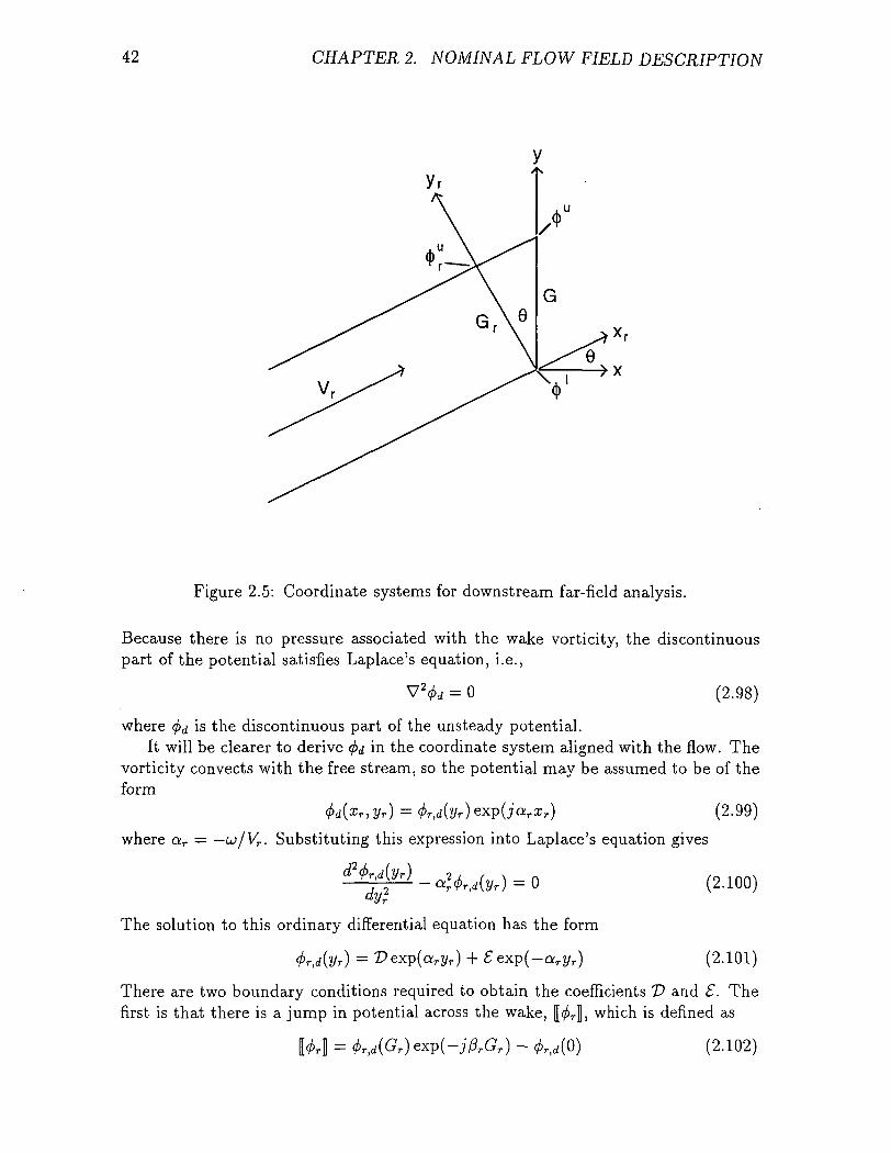
42 CHAPTER 2. NOMINAL FLOW FIELD DESCRIPTION
Figure 2.5: Coordinate systems for downstream far-field analysis.
Because there is no pressure associated with the wake vorticity, the discontinuouspart of the potential satisfies Laplace's equation, i.e.,
= 0 (2.98)
where <^ is the discontinuous part of the unsteady potential.It will be clearer to derive (f>d in the coordinate system aligned with the flow. The
vorticity convects with the free stream, so the potential may be assumed to be of theform
(/>d(xr, 2/r) = (t>r,d(yr) exp(;arzr) (2.99)
where ar = —u/VT. Substituting this expression into Laplace's equation gives
gM-aXiforHOdy.
The solution to this ordinary differential equation has the form
<t>r,d(yr) = 2?exp(ov3/r) + £exp(—a ry r)
(2.100)
(2.101)
There are two boundary conditions required to obtain the coefficients T> and £. Thefirst is that there is a jump in potential across the wake, f^rj, which is defined as
M = <f>r,d(GT)eXp(-jP rG r) ~ (2.102)
2.4. FAR-FIELD B0 UNDARY CONDITIONS 43
where j3r may be determined from the interblade phase angle, <j, and the coordinatetransformation
_ <T—u sin L (2.103)Gcos 0 v '
The second boundary condition is that the wake motion is periodic
?r) (2.104)
After using these two boundary conditions, some algebra results in the expression for<t>T,d
(2.105)rGT ~ jPrGT} I - eXp(~arGr - j j3TGT)
The next task is to determine |̂ r|. Using the notation of Figure 2.5, it is clear that
[^r] = <^Jf exp(—j 0rGT) — <f>f (2.106)
Since the behavior of <j>d is known in the xr direction,
<^f = (f>u exp(jarGsm 0) (2.107)
Substituting this expression into Eq. (2.106) and simplifying results in
|̂ r] = <^"exp(— j&] — <j>1 (2.108)
So the complete expression for the discontinuous unsteady potential is
xexp(aryr) exp(-aryr)
1 - exp(arGT - j/3TGr) 1 - exp(-aTGT - jj3TGT}_
Finally, for this expression to be used in the present method, it must be converted tothe original coordinate system, so that
x, y] = —-[^rf exp[jaT(x cos 0 -f- y sin 0)]
xexp[o;r(—x sin ^ + y cos 0)] exp[—a r(—x sin 0 + y cos
+-exp(-arGr-jprGT) \ (2'UO)
This expression is added to the continuous downstream unsteady potential to deter-mine the complete solution at the downstream far field.
Chapter 3
Numerical Solution Method
In this chapter, the methods for numerical solution of the governing equations andboundary conditions described in Chapter 2 for the steady and small disturbance un-steady flow through a two-dimensional cascade of airfoils are presented. Section 3.1contains a description of the steady solution procedure. The first step in the steadysolution process is the choice of a computational grid upon which to discretize thegoverning equations and boundary conditions. After the equations governing the gen-eration of the computational grid have been discussed, the finite element discretizationof the steady flow variational principle and the associated boundary conditions willbe presented. To complete the steady flow analysis, the matrix assembly and solutionof the discretized equations and boundary conditions will be described. In Section3.2, the unsteady solution procedure will be developed, beginning with the numericalcalculation of the drift function and rotational velocity, as well as the generation ofthe grid deformation. Next, the unsteady finite element discretization of the fieldequations and boundary conditions is presented, with particular emphasis on the nu-merical discretization of the far-field boundary conditions. Finally, the assembly andsolution procedure for the discretized unsteady flow equations is described.
3.1 Steady Flow Solution Procedure
3.1.1 Grid GenerationIn any computational fluid dynamic analysis, the choice of a computational gridupon which to discretize the governing equations is crucial. Poor computationalgrids may reduce the accuracy of the discretization scheme or, in some cases, reducethe stability of the solution procedure. For cascade flows, the computational gridstypically used are referred to as C, O, and H grids (or some combination thereof).The grid topology for each of these grids looks much like the letter used to identifythem. In this investigation, H grids will be used. H grids, unlike their C andO counterparts, provide good resolution throughout the computational domain, notjust near the airfoil. This is important because the accurate resolution of acousticand vortical waves is critical to evaluating the aeroacoustic performance of a bladerow. Another important reason for using an H grid is that the matrix containing
44
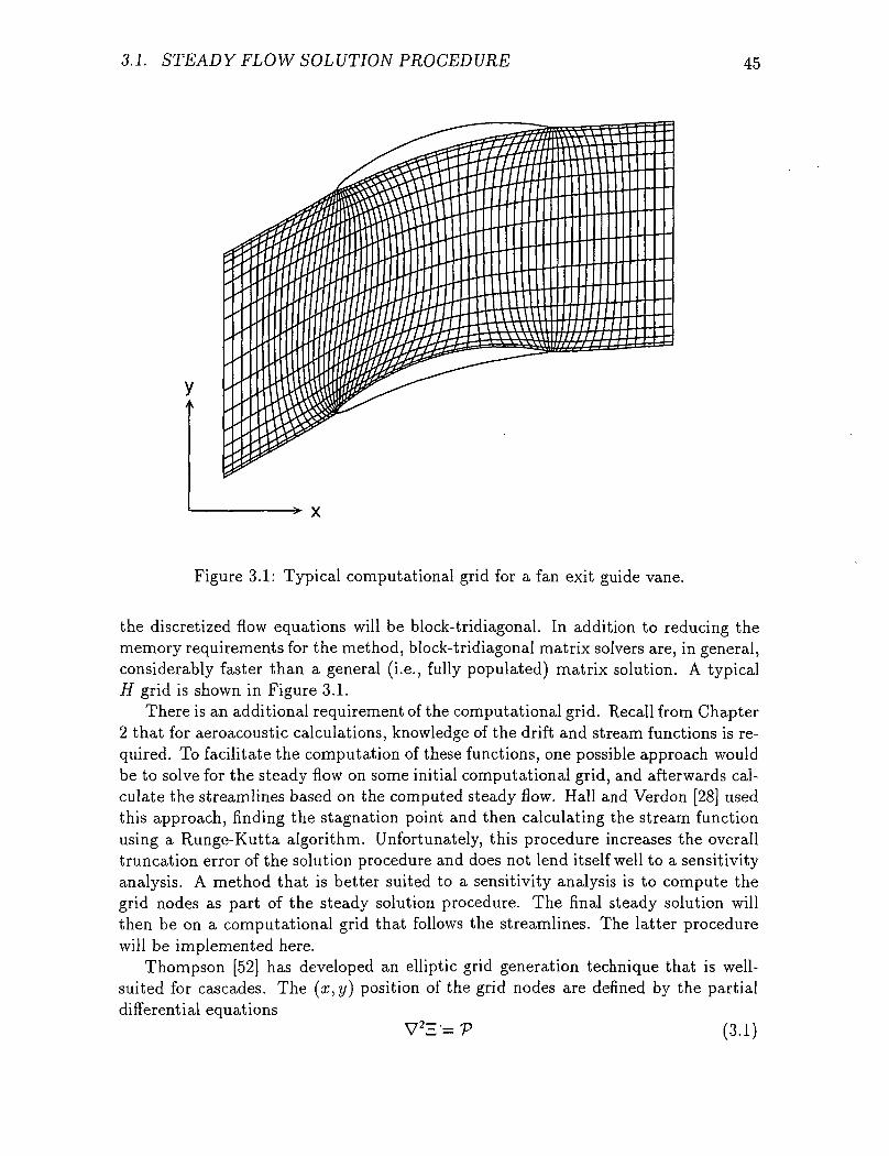
3.1. STEADY FLOW SOL UTION PROCED URE 45
-> x
Figure 3.1: Typical computational grid for a fan exit guide vane.
the discretized flow equations will be block-tridiagonal. In addition to reducing thememory requirements for the method, block-tridiagonal matrix solvers are, in general,considerably faster than a general (i.e., fully populated) matrix solution. A typicalH grid is shown in Figure 3.1.
There is an additional requirement of the computational grid. Recall from Chapter2 that for aeroacoustic calculations, knowledge of the drift and stream functions is re-quired. To facilitate the computation of these functions, one possible approach wouldbe to solve for the steady flow on some initial computational grid, and afterwards cal-culate the streamlines based on the computed steady flow. Hall and Verdon [28] usedthis approach, finding the stagnation point and then calculating the stream functionusing a Runge-Kutta algorithm. Unfortunately, this procedure increases the overalltruncation error of the solution procedure and does not lend itself well to a sensitivityanalysis. A method that is better suited to a sensitivity analysis is to compute thegrid nodes as part of the steady solution procedure. The final steady solution willthen be on a computational grid that follows the streamlines. The latter procedurewill be implemented here.
Thompson [52] has developed an elliptic grid generation technique that is well-suited for cascades. The (x,y) position of the grid nodes are denned by the partialdifferential equations
V2E = P (3.1)
46 CHAPTERS. NUMERICAL SOLUTION METHOD
V2# = Q (3.2)
where P and Q are functions which are used to control the grid spacing. Lines ofconstant H and H define the grid lines.
Equations (3.1) and (3.2) may be inverted to obtain partial differential equationsfor the unknown grid node locations in terms of the known computational coordinatesE and H, i.e.,
and2 - 2 2 -
(3.4). ^ '
where
-=7
The next task is to choose the grid spacing functions P and Q so that the gridfollows the flow streamlines. These functions may be obtained through the fluid dy-namic definitions of the velocity potential and stream function. Consider an inviscid,irrotational, compressible flow. In terms of the stream function, ^, and the density,R, the steady conservation of mass may be written as
. - _~ d x \ R d x ) ~ d y \ R 9 y ) (3-5)
which, after rearranging, may be written in the form
vM> = !2™? + !2^ (36)R dx dx R dy dy ^ '
Finally, writing the right hand side of Eq. (3.6) in terms of the steady velocity po-tential, $, gives
V2* = |V$ x V.R| (3.7)
Note the similarity between Eq. (3.7) and Eq. (3.2). If we choose V = 0 andQ = |V$ x V.R|, then lines of constant H will correspond to streamlines, providedthe boundary conditions around the computational domain are consistent with thedefinition of the stream function. Furthermore, note that if the flow is incompressible,|V$ x VR\ = 0, and no grid spacing functions are necessary in the grid generationequations (i.e., P = Q = 0). Regardless of the compressibility of the flow, it shouldbe noted that lines of constant E do not correspond to contours of the drift function,A, nor is this a requirement of the computational grid. The drift function may becalculated after the steady flow solution has been obtained.
Figure 3.2 shows a typical computational grid in the (E, $) coordinate system.If the grid generation equations, Eqs. (3.3)-(3.4), were solved without the influence
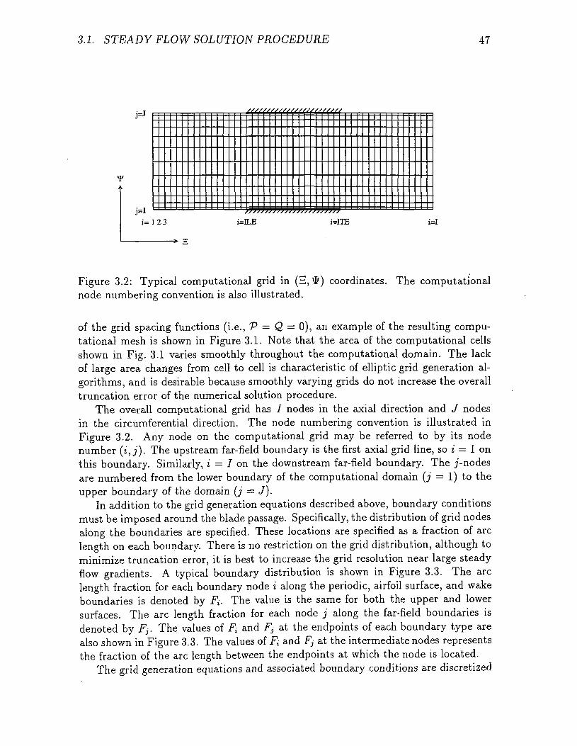
3.1. STEADY FLOW SOL UTION PROCED URE 47
f
i=123 i=ILE i=ITE i=
Figure 3.2: Typical computational grid in (H,\I>) coordinates. The computationalnode numbering convention is also illustrated.
of the grid spacing functions (i.e., P = Q = 0), an example of the resulting compu-tational mesh is shown in Figure 3.1. Note that the area of the computational cellsshown in Fig. 3.1 varies smoothly throughout the computational domain. The lackof large area changes from cell to cell is characteristic of elliptic grid generation al-gorithms, and is desirable because smoothly varying grids do not increase the overalltruncation error of the numerical solution procedure.
The overall computational grid has / nodes in the axial direction and J nodesin the circumferential direction. The node numbering convention is illustrated inFigure 3.2. Any node on the computational grid may be referred to by its nodenumber (i,j). The upstream far-field boundary is the first axial grid line, so i = 1 onthis boundary. Similarly, i = I on the downstream far-field boundary. The j-nodesare numbered from the lower boundary of the computational domain (j = 1) to theupper boundary of the domain (j = J).
In addition to the grid generation equations described above, boundary conditionsmust be imposed around the blade passage. Specifically, the distribution of grid nodesalong the boundaries are specified. These locations are specified as a fraction of arclength on each boundary. There is no restriction on the grid distribution, although tominimize truncation error, it is best to increase the grid resolution near large steadyflow gradients. A typical boundary distribution is shown in Figure 3.3. The arclength fraction for each boundary node i along the periodic, airfoil surface, and wakeboundaries is denoted by F±. The value is the same for both the upper and lowersurfaces. The arc length fraction for each node j along the far-field boundaries isdenoted by Fj. The values of Fi and Fj at the endpoints of each boundary type arealso shown in Figure 3.3. The values of Fi and Fj at the intermediate nodes representsthe fraction of the arc length between the endpoints at which the node is located.
The grid generation equations and associated boundary conditions are discretized
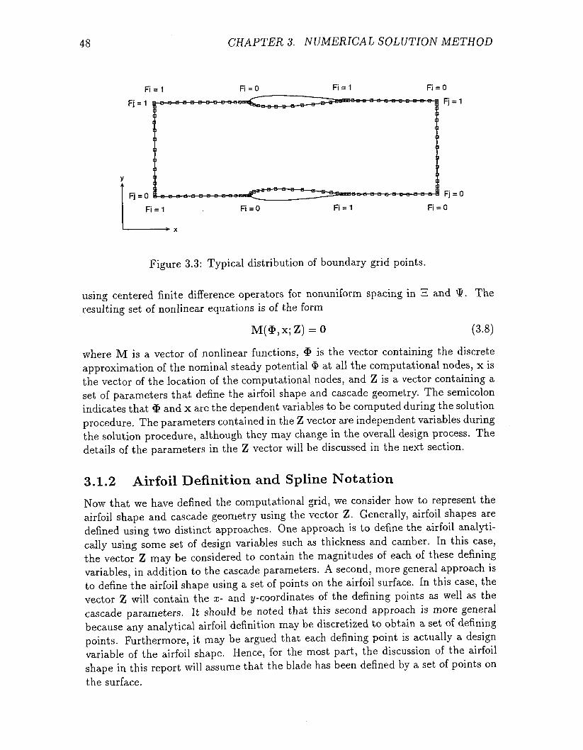
48 CHAPTER 3. NUMERICAL SOLUTION METHOD
Fi = 0
Fj =
Fj = 0
Fi = 0
Figure 3.3: Typical distribution of boundary grid points.
using centered finite difference operators for nonuniform spacing in £ and \P. Theresulting set of nonlinear equations is of the form
M($,x;Z) = 0 (3.8)
where M is a vector of nonlinear functions, 3> is the vector containing the discreteapproximation of the nominal steady potential $ at all the computational nodes, x isthe vector of the location of the computational nodes, and Z is a vector containing aset of parameters that define the airfoil shape and cascade geometry. The semicolonindicates that $ and x are the dependent variables to be computed during the solutionprocedure. The parameters contained in the Z vector are independent variables duringthe solution procedure, although they may change in the overall design process. Thedetails of the parameters in the Z vector will be discussed in the next section.
3.1.2 Airfoil Definition and Spline Notation
Now that we have defined the computational grid, we consider how to represent theairfoil shape and cascade geometry using the vector Z. Generally, airfoil shapes aredefined using two distinct approaches. One approach is to define the airfoil analyti-cally using some set of design variables such as thickness and camber. In this case,the vector Z may be considered to contain the magnitudes of each of these definingvariables, in addition to the cascade parameters. A second, more general approach isto define the airfoil shape using a set of points on the airfoil surface. In this case, thevector Z will contain the x- and ^-coordinates of the defining points as well as thecascade parameters. It should be noted that this second approach is more generalbecause any analytical airfoil definition may be discretized to obtain a set of definingpoints. Furthermore, it may be argued that each defining point is actually a designvariable of the airfoil shape. Hence, for the most part, the discussion of the airfoilshape in this report will assume that the blade has been defined by a set of points onthe surface.
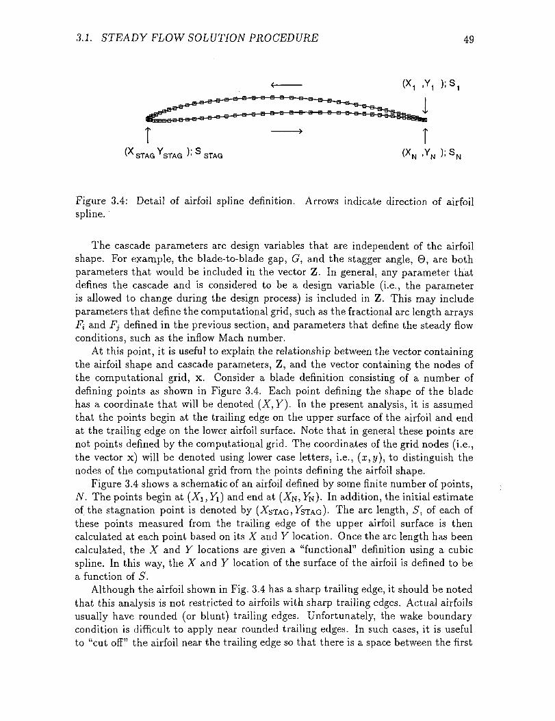
3.1. STEADY FLOW SOLUTION PROCEDURE 49
T' G ' •STAG 'STAG '• STAG
Figure 3.4: Detail of airfoil spline definition. Arrows indicate direction of airfoilspline.
The cascade parameters are design variables that are independent of the airfoilshape. For example, the blade-to-blade gap, G, and the stagger angle, 0, are bothparameters that would be included in the vector Z. In general, any parameter thatdefines the cascade and is considered to be a design variable (i.e., the parameteris allowed to change during the design process) is included in Z. This may includeparameters that define the computational grid, such as the fractional arc length arraysFi and Fj defined in the previous section, and parameters that define the steady flowconditions, such as the inflow Mach number.
At this point, it is useful to explain the relationship between the vector containingthe airfoil shape and cascade parameters, Z, and the vector containing the nodes ofthe computational grid, x. Consider a blade definition consisting of a number ofdefining points as shown in Figure 3.4. Each point defining the shape of the bladehas a coordinate that will be denoted (X,Y). In the present analysis, it is assumedthat the points begin at the trailing edge on the upper surface of the airfoil and endat the trailing edge on the lower airfoil surface. Note that in general these points arenot points defined by the computational grid. The coordinates of the grid nodes (i.e.,the vector x) will be denoted using lower case letters, i.e., (z,j/), to distinguish thenodes of the computational grid from the points defining the airfoil shape.
Figure 3.4 shows a schematic of an airfoil defined by some finite number of points,N. The points begin at (Xi, FI) and end at (X^, VN). In addition, the initial estimateof the stagnation point is denoted by (^"STAG, FSTAG)- The arc length, 5, of each ofthese points measured from the trailing edge of the upper airfoil surface is thencalculated at each point based on its X and Y location. Once the arc length has beencalculated, the X and Y locations are given a "functional" definition using a cubicspline. In this way, the X and Y location of the surface of the airfoil is defined to bea function of S.
Although the airfoil shown in Fig. 3.4 has a sharp trailing edge, it should be notedthat this analysis is not restricted to airfoils with sharp trailing edges. Actual airfoilsusually have rounded (or blunt) trailing edges. Unfortunately, the wake boundarycondition is difficult to apply near rounded trailing edges. In such cases, it is usefulto "cut off" the airfoil near the trailing edge so that there is a space between the first
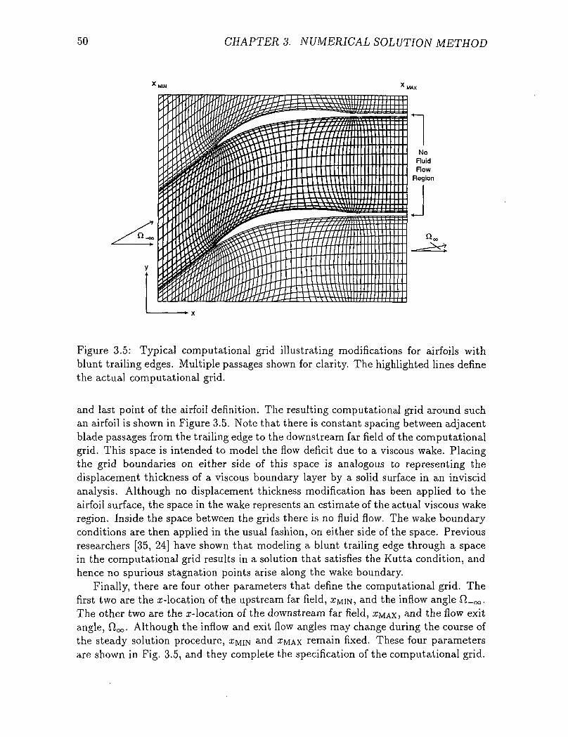
50 CHAPTER 3. NUMERICAL SOLUTION METHOD
Figure 3.5: Typical computational grid illustrating modifications for airfoils withblunt trailing edges. Multiple passages shown for clarity. The highlighted lines definethe actual computational grid.
and last point of the airfoil definition. The resulting computational grid around suchan airfoil is shown in Figure 3.5. Note that there is constant spacing between adjacentblade passages from the trailing edge to the downstream far field of the computationalgrid. This space is intended to model the flow deficit due to a viscous wake. Placingthe grid boundaries on either side of this space is analogous to representing thedisplacement thickness of a viscous boundary layer by a solid surface in an inviscidanalysis. Although no displacement thickness modification has been applied to theairfoil surface, the space in the wake represents an estimate of the actual viscous wakeregion. Inside the space between the grids there is no fluid flow. The wake boundaryconditions are then applied in the usual fashion, on either side of the space. Previousresearchers [35, 24] have shown that modeling a blunt trailing edge through a spacein the computational grid results in a solution that satisfies the Kutta condition, andhence no spurious stagnation points arise along the wake boundary.
Finally, there are four other parameters that define the computational grid. Thefirst two are the x-location of the upstream far field, XMIN, and the inflow angle fi_oo.The other two are the x-location of the downstream far field, ZMAX, and the flow exitangle, OOQ. Although the inflow and exit flow angles may change during the course ofthe steady solution procedure, ZMIN and ZMAX remain fixed. These four parametersare shown in Fig. 3.5, and they complete the specification of the computational grid.
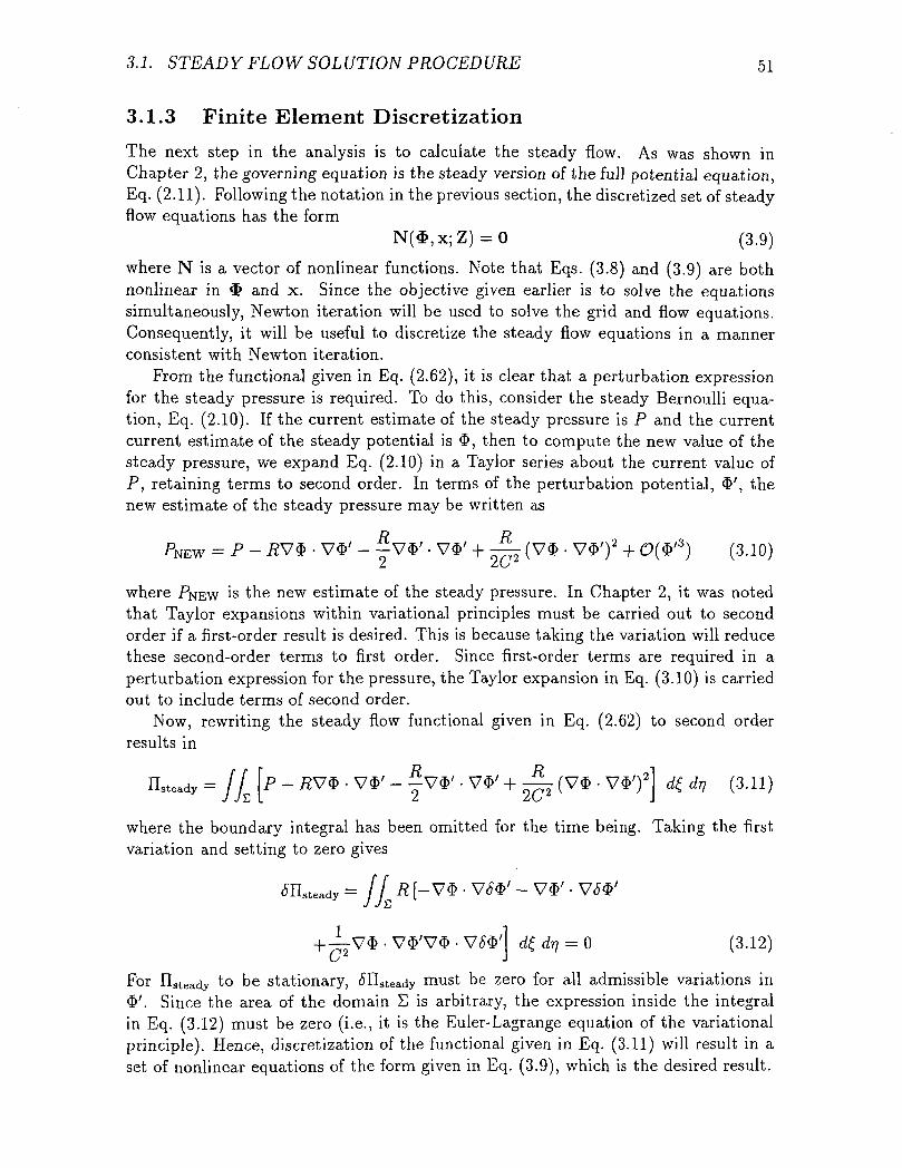
3.1. STEADY FLOW SOLUTION PROCEDURE 51
3.1.3 Finite Element Discretization
The next step in the analysis is to calculate the steady flow. As was shown inChapter 2, the governing equation is the steady version of the full potential equation,Eq. (2.11). Following the notation in the previous section, the discretized set of steadyflow equations has the form
N($,x;Z) = 0 (3.9)
where N is a vector of nonlinear functions. Note that Eqs. (3.8) and (3.9) are bothnonlinear in $ and x. Since the objective given earlier is to solve the equationssimultaneously, Newton iteration will be used to solve the grid and flow equations.Consequently, it will be useful to discretize the steady flow equations in a mannerconsistent with Newton iteration.
From the functional given in Eq. (2.62), it is clear that a perturbation expressionfor the steady pressure is required. To do this, consider the steady Bernoulli equa-tion, Eq. (2.10). If the current estimate of the steady pressure is P and the currentcurrent estimate of the steady potential is $, then to compute the new value of thesteady pressure, we expand Eq. (2.10) in a Taylor series about the current value ofP, retaining terms to second order. In terms of the perturbation potential, $', thenew estimate of the steady pressure may be written as
PNEW = p- 7?V$ • W - W • V$' + - (V$ • W) + 0($') (3.10)
where PNEW is the new estimate of the steady pressure. In Chapter 2, it was notedthat Taylor expansions within variational principles must be carried out to secondorder if a first-order result is desired. This is because taking the variation will reducethese second-order terms to first order. Since first-order terms are required in aperturbation expression for the pressure, the Taylor expansion in Eq. (3.10) is carriedout to include terms of second order.
Now, rewriting the steady flow functional given in Eq. (2.62) to second orderresults in
Hsteady = P ~ #V$ • V*' - W - V*' + ~ (Vd> - V*')'f W - V*' +
where the boundary integral has been omitted for the time being. Taking the firstvariation and setting to zero gives
= JJ R [~Ollsteadyj ju
I I_l v$ • V$'V$ • V£$' d£ drj = 0 (3.12)
For Hsteady to be stationary, £nsteady must be zero for all admissible variations in<&'. Since the area of the domain £ is arbitrary, the expression inside the integralin Eq. (3.12) must be zero (i.e., it is the Euler-Lagrange equation of the variationalprinciple). Hence, discretization of the functional given in Eq. (3.11) will result in aset of nonlinear equations of the form given in Eq. (3.9), which is the desired result.
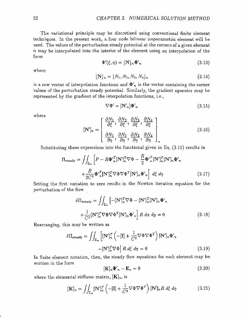
52 CHAPTER 3. NUMERICAL SOLUTION METHOD
The variational principle may be discretized using conventional finite elementtechniques. In the present work, a four node bilinear isoparametric element will beused. The values of the perturbation steady potential at the corners of a given elementn may be interpolated into the interior of the element using an interpolation of theform
*U»?)=LNJn* /n (3.13)
whereLNJ n =LM,^2,^3 ,^4jn (3.14)
is a row vector of interpolation functions and $'n is the vector containing the cornervalues of the perturbation steady potential. Similarly, the gradient operator may berepresented by the gradient of the interpolation functions, i.e.,
whereON*
(3.15)
(3.16)dNi dN* dN4
dr) ' dr) ' dr) ' dr)
Substituting these expressions into the functional given in Eq. (3.11) results in
R,,nsteady = P-
dr, (3.17)
Setting the first variation to zero results in the Newton iteration equation for theperturbation of the flow
steady =<5IIJ ./£„
+ ̂ [N'£V$V$T[N']n$'n R d x d y =
Rearranging, this may be written as
<msteady = [N']I -[I] +
(3.18)
^c/r/ = 0 (3.19)
In finite element notation, then, the steady flow equations for each element may bewritten in the form
[K]n$'n-En = 0 (3.20)
where the elemental stiffness matrix, [K]n, is
(3.21)[K]n = // [Nil (-[I] + ̂ V$V$T) [N']nJR d( dr,J JZn V L> /
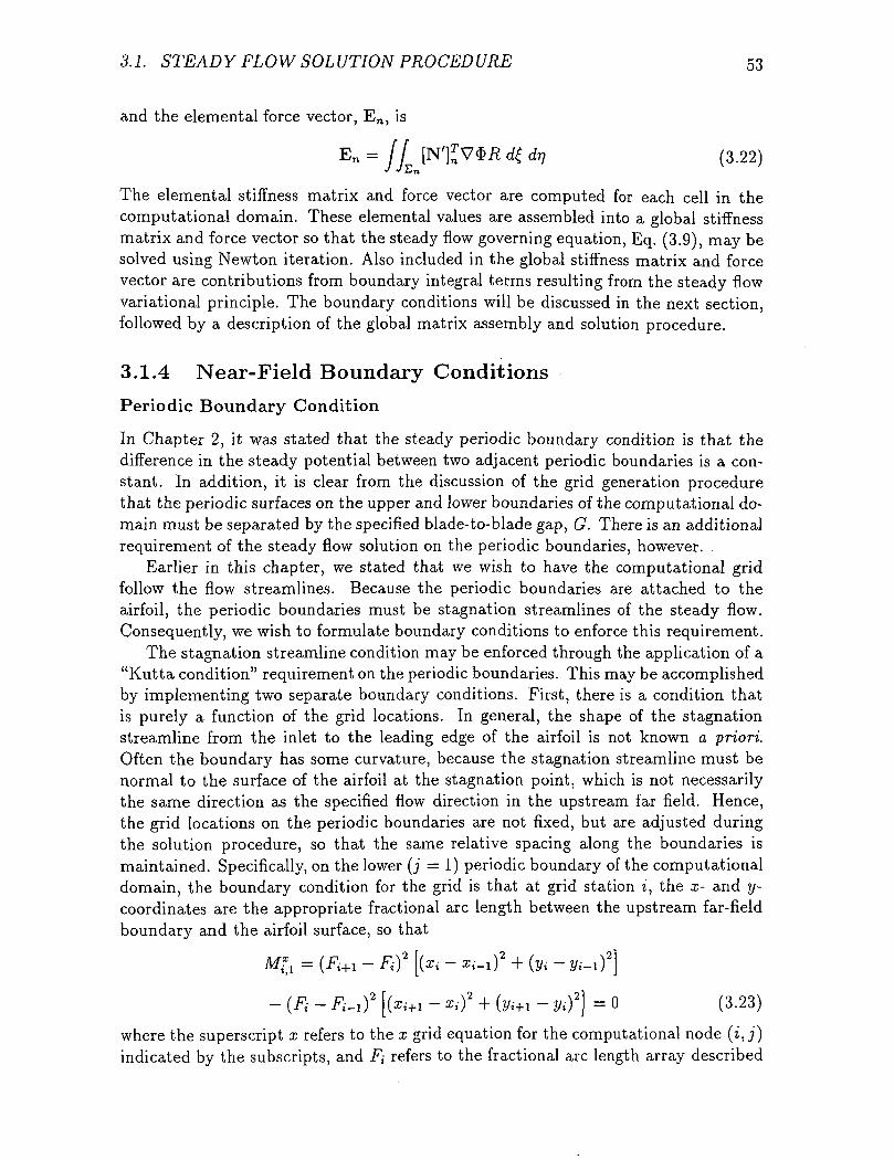
3.1. STEADY FLOW SOLUTION PROCEDURE 53
and the elemental force vector, En, is
En = // [N'^VStf d£ dr, (3.22)J ./Sn
The elemental stiffness matrix and force vector are computed for each cell in thecomputational domain. These elemental values are assembled into a global stiffnessmatrix and force vector so that the steady flow governing equation, Eq. (3.9), may besolved using Newton iteration. Also included in the global stiffness matrix and forcevector are contributions from boundary integral terms resulting from the steady flowvariational principle. The boundary conditions will be discussed in the next section,followed by a description of the global matrix assembly and solution procedure.
3.1.4 Near-Field Boundary Conditions
Periodic Boundary Condition
In Chapter 2, it was stated that the steady periodic boundary condition is that thedifference in the steady potential between two adjacent periodic boundaries is a con-stant. In addition, it is clear from the discussion of the grid generation procedurethat the periodic surfaces on the upper and lower boundaries of the computational do-main must be separated by the specified blade-to-blade gap, G. There is an additionalrequirement of the steady flow solution on the periodic boundaries, however. .
Earlier in this chapter, we stated that we wish to have the computational gridfollow the flow streamlines. Because the periodic boundaries are attached to theairfoil, the periodic boundaries must be stagnation streamlines of the steady flow.Consequently, we wish to formulate boundary conditions to enforce this requirement.
The stagnation streamline condition may be enforced through the application of a"Kutta condition" requirement on the periodic boundaries. This may be accomplishedby implementing two separate boundary conditions. First, there is a condition thatis purely a function of the grid locations. In general, the shape of the stagnationstreamline from the inlet to the leading edge of the airfoil is not known a priori.Often the boundary has some curvature, because the stagnation streamline must benormal to the surface of the airfoil at the stagnation point, which is not necessarilythe same direction as the specified flow direction in the upstream far field. Hence,the grid locations on the periodic boundaries are not fixed, but are adjusted duringthe solution procedure, so that the same relative spacing along the boundaries ismaintained. Specifically, on the lower (j = 1) periodic boundary of the computationaldomain, the boundary condition for the grid is that at grid station i, the x- and y-coordinates are the appropriate fractional arc length between the upstream far-fieldboundary and the airfoil surface, so that
- (Fi - Fi-tf [(Z.VH - z,)2 + (yi+i - ytf] = 0 (3.23)
where the superscript x refers to the x grid equation for the computational node (i, j)indicated by the subscripts, and Fi refers to the fractional arc length array described
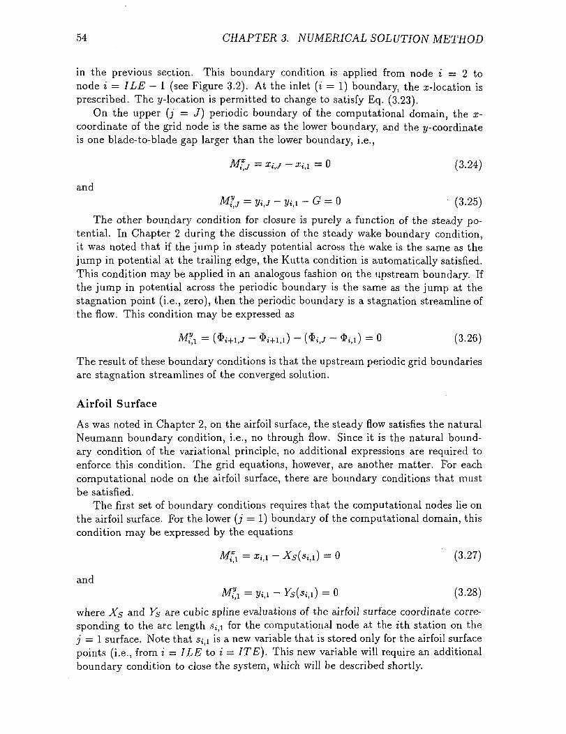
54 CHAPTERS. NUMERICAL SOLUTION METHOD
in the previous section. This boundary condition is applied from node i = 2 tonode i = ILE — 1 (see Figure 3.2). At the inlet (i = 1) boundary, the x-location isprescribed. The y-location is permitted to change to satisfy Eq. (3.23).
On the upper (j = J) periodic boundary of the computational domain, the x-coordinate of the grid node is the same as the lower boundary, and the t/-coordinateis one blade-to-blade gap larger than the lower boundary, i.e.,
Mf,j = *i,J - *i,i = 0 (3.24)
and
M?,J = yi,J ~ J/«M -G = Q (3.25)
The other boundary condition for closure is purely a function of the steady po-tential. In Chapter 2 during the discussion of the steady wake boundary condition,it was noted that if the jump in steady potential across the wake is the same as thejump in potential at the trailing edge, the Kutta condition is automatically satisfied.This condition may be applied in an analogous fashion on the upstream boundary. Ifthe jump in potential across the periodic boundary is the same as the jump at thestagnation point (i.e., zero), then the periodic boundary is a stagnation streamline ofthe flow. This condition may be expressed as
M^ = ($t-+liJ - $,-+lil) - ($,-,j - $;,!) = 0 (3.26)
The result of these boundary conditions is that the upstream periodic grid boundariesare stagnation streamlines of the converged solution.
Airfoil Surface
As was noted in Chapter 2, on the airfoil surface, the steady flow satisfies the naturalNeumann boundary condition, i.e., no through flow. Since it is the natural bound-ary condition of the variational principle, no additional expressions are required toenforce this condition. The grid equations, however, are another matter. For eachcomputational node on the airfoil surface, there are boundary conditions that mustbe satisfied.
The first set of boundary conditions requires that the computational nodes lie onthe airfoil surface. For the lower (j = 1) boundary of the computational domain, thiscondition may be expressed by the equations
Affi = xitl - Xs(sitl) = 0 (3.27)
and,l) = Q (3.28)
where ^5 and YS are cubic spline evaluations of the airfoil surface coordinate corre-sponding to the arc length Sit\ for the computational node at the zth station on thej = 1 surface. Note that s^i is a new variable that is stored only for the airfoil surfacepoints (i.e., from i = ILE to i = ITE). This new variable will require an additionalboundary condition to close the system, which will be described shortly.
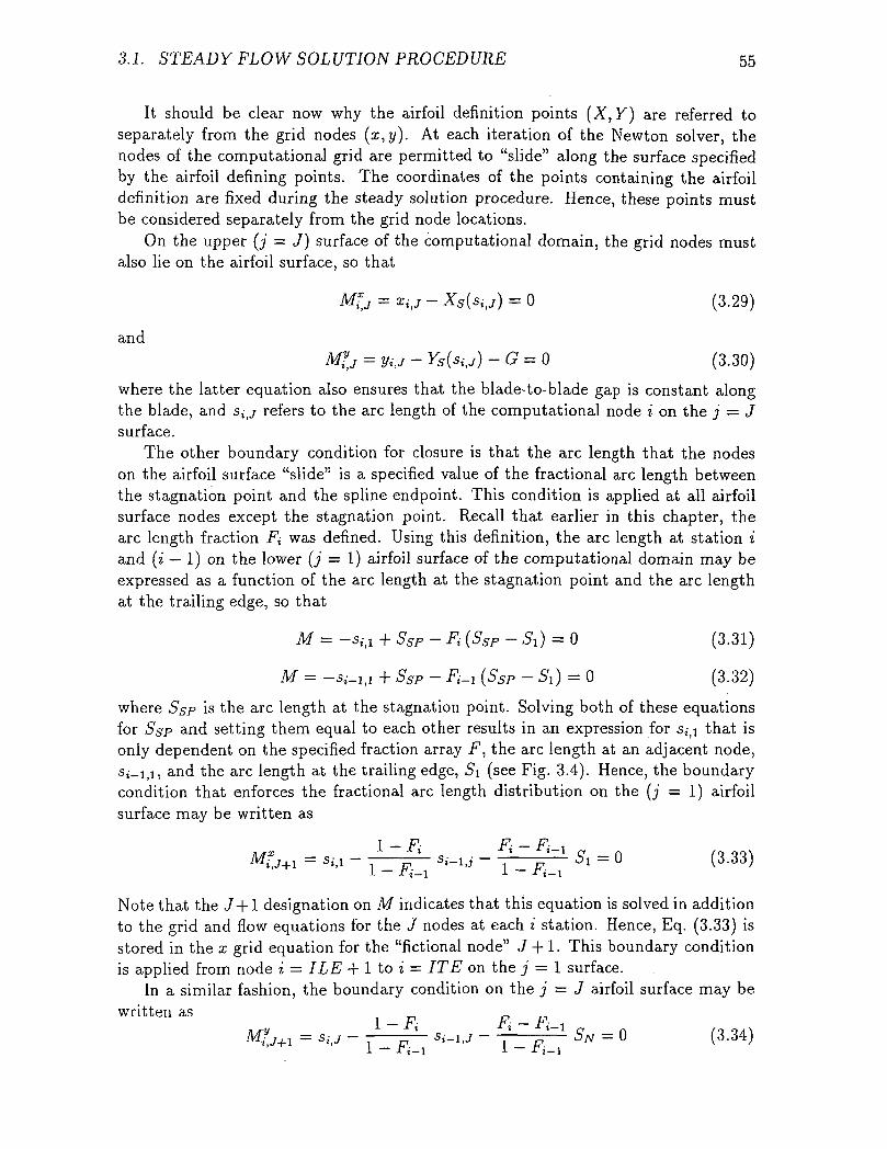
3.1. STEADY FLOW SOLUTION PROCEDURE 55
It should be clear now why the airfoil definition points (X, Y) are referred toseparately from the grid nodes (x,y). At each iteration of the Newton solver, thenodes of the computational grid are permitted to "slide" along the surface specifiedby the airfoil defining points. The coordinates of the points containing the airfoildefinition are fixed during the steady solution procedure. Hence, these points mustbe considered separately from the grid node locations.
On the upper (j = J] surface of the computational domain, the grid nodes mustalso lie on the airfoil surface, so that
,j) = Q (3.29)
and-G = 0 (3.30)
where the latter equation also ensures that the blade-to-blade gap is constant alongthe blade, and s^j refers to the arc length of the computational node i on the j = Jsurface.
The other boundary condition for closure is that the arc length that the nodeson the airfoil surface "slide" is a specified value of the fractional arc length betweenthe stagnation point and the spline endpoint. This condition is applied at all airfoilsurface nodes except the stagnation point. Recall that earlier in this chapter, thearc length fraction F+ was defined. Using this definition, the arc length at station iand (i — 1) on the lower (j = 1) airfoil surface of the computational domain may beexpressed as a function of the arc length at the stagnation point and the arc lengthat the trailing edge, so that
M = -sit! + SSP - Fi (SSP - Si) = 0 (3.31)
M = -Si.!,! + SSP - F^ (SSp - 5j) = 0 (3.32)
where SSP is the arc length at the stagnation point. Solving both of these equationsfor SSP and setting them equal to each other results in an expression for S,-FI that isonly dependent on the specified fraction array F, the arc length at an adjacent node,s,-_i,i, and the arc length at the trailing edge, Si (see Fig. 3.4). Hence, the boundarycondition that enforces the fractional arc length distribution on the (j = 1) airfoilsurface may be written as
.> - THSr1 Si = 0 (3.33)i r i— i
Note that the J+l designation on M indicates that this equation is solved in additionto the grid and flow equations for the J nodes at each i station. Hence, Eq. (3.33) isstored in the x grid equation for the "fictional node" J + l. This boundary conditionis applied from node i = ILE + 1 to i = ITE on the j = 1 surface.
In a similar fashion, the boundary condition on the j = J airfoil surface may bewritten as
!—±- *_ l f j - /_ t'1 SN = 0 (3.34)f i— \ 1 -Ti— l
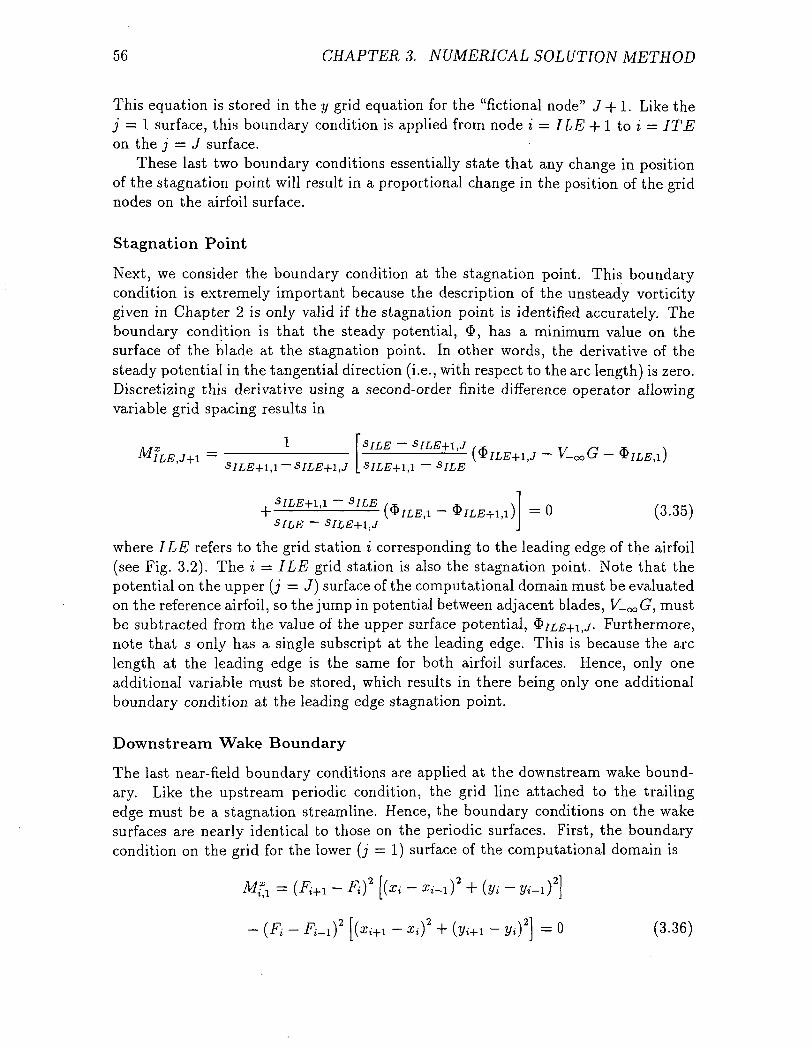
56 CHAPTERS. NUMERICAL SOLUTION METHOD
This equation is stored in the y grid equation for the "fictional node" J + 1. Like thej = 1 surface, this boundary condition is applied from node i = ILE +1 to i = ITEon the j = J surface.
These last two boundary conditions essentially state that any change in positionof the stagnation point will result in a proportional change in the position of the gridnodes on the airfoil surface.
Stagnation Point
Next, we consider the boundary condition at the stagnation point. This boundarycondition is extremely important because the description of the unsteady vorticitygiven in Chapter 2 is only valid if the stagnation point is identified accurately. Theboundary condition is that the steady potential, $, has a minimum value on thesurface of the blade at the stagnation point. In other words, the derivative of thesteady potential in the tangential direction (i.e., with respect to the arc length) is zero.Discretizing this derivative using a second-order finite difference operator allowingvariable grid spacing results in
1SILE+I,I—SILE+I,J
SILE+I,I —
SILE — SILE+I,J
. . . . . = 0 (3.35)— SILE+I,J
where ILE refers to the grid station i corresponding to the leading edge of the airfoil(see Fig. 3.2). The i = ILE grid station is also the stagnation point. Note that thepotential on the upper (j = J) surface of the computational domain must be evaluatedon the reference airfoil, so the jump in potential between adjacent blades, V-^G^ mustbe subtracted from the value of the upper surface potential, $ILE+\,J- Furthermore,note that s only has a single subscript at the leading edge. This is because the arclength at the leading edge is the same for both airfoil surfaces. Hence, only oneadditional variable must be stored, which results in there being only one additionalboundary condition at the leading edge stagnation point.
Downstream Wake Boundary
The last near-field boundary conditions are applied at the downstream wake bound-ary. Like the upstream periodic condition, the grid line attached to the trailingedge must be a stagnation streamline. Hence, the boundary conditions on the wakesurfaces are nearly identical to those on the periodic surfaces. First, the boundarycondition on the grid for the lower (j = 1) surface of the computational domain is
- x,-)2 + (y,-+i - y,f = 0 (3.36)
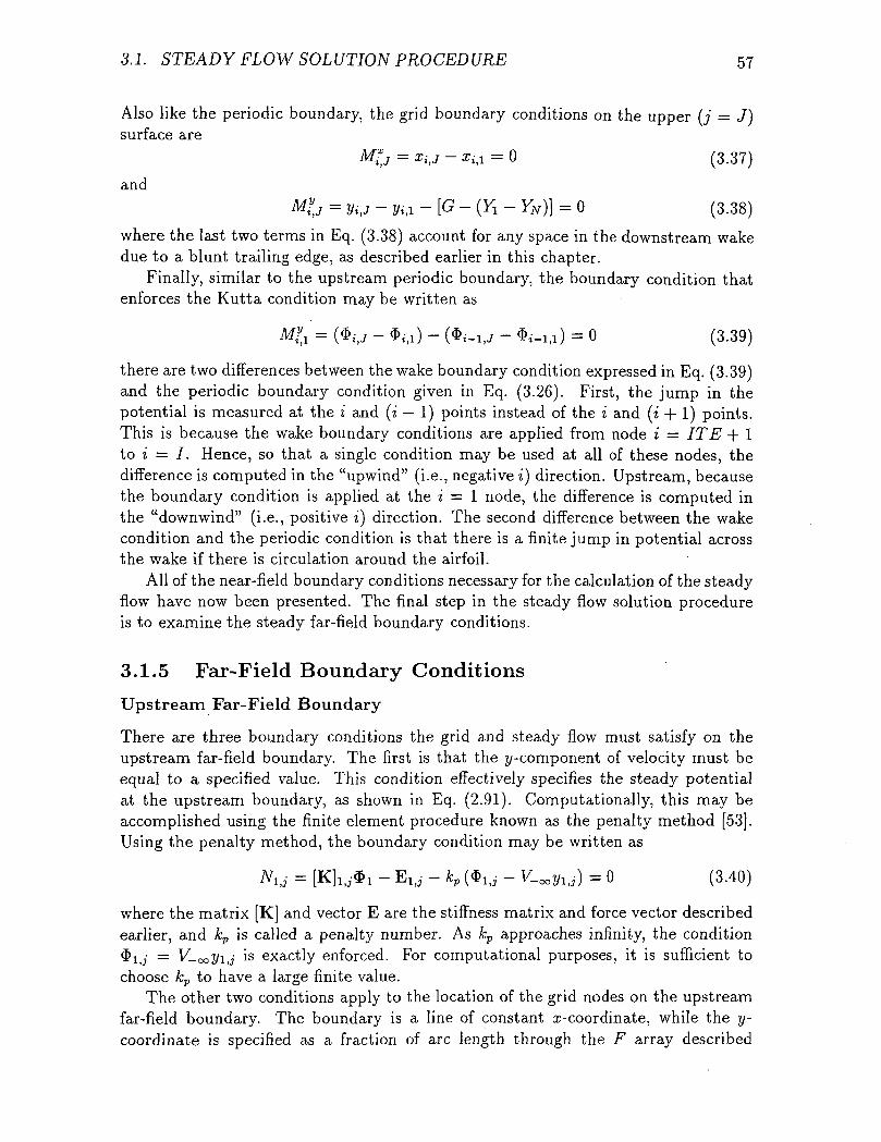
3.1. STEADY FLOW SOLUTION PROCEDURE 57
Also like the periodic boundary, the grid boundary conditions on the upper (j = J)surface are
M*J = X^J ~ *.M = 0 (3.37)
andMi,j = Vi,J - yi,i ~[G- (Yl - YN}\ = 0 (3.38)
where the last two terms in Eq. (3.38) account for any space in the downstream wakedue to a blunt trailing edge, as described earlier in this chapter.
Finally, similar to the upstream periodic boundary, the boundary condition thatenforces the Kutta condition may be written as
M?,i = (*i,J ~ $.M) - ($i-i,J ~ $i-u) = 0 (3.39)
there are two differences between the wake boundary condition expressed in Eq. (3.39)and the periodic boundary condition given in Eq. (3.26). First, the jump in thepotential is measured at the i and (i — 1) points instead of the i and (i + 1) points.This is because the wake boundary conditions are applied from node i = ITE + 1to i = /. Hence, so that a single condition may be used at all of these nodes, thedifference is computed in the "upwind" (i.e., negative i) direction. Upstream, becausethe boundary condition is applied at the i = 1 node, the difference is computed inthe "downwind" (i.e., positive i) direction. The second difference between the wakecondition and the periodic condition is that there is a finite jump in potential acrossthe wake if there is circulation around the airfoil.
All of the near-field boundary conditions necessary for the calculation of the steadyflow have now been presented. The final step in the steady flow solution procedureis to examine the steady far-field boundary conditions.
3.1.5 Far-Field Boundary Conditions
Upstream Far-Field Boundary
There are three boundary conditions the grid and steady flow must satisfy on theupstream far-field boundary. The first is that the y-component of velocity must beequal to a specified value. This condition effectively specifies the steady potentialat the upstream boundary, as shown in Eq. (2.91). Computationally, this may beaccomplished using the finite element procedure known as the penalty method [53].Using the penalty method, the boundary condition may be written as
Nlti = [Kh,,-*! - EU - kp ($!,, - V-^J = 0 (3.40)
where the matrix [K] and vector E are the stiffness matrix and force vector describedearlier, and kp is called a penalty number. As kp approaches infinity, the condition$1)j = V_ooJ/i,j is exactly enforced. For computational purposes, it is sufficient tochoose kp to have a large finite value.
The other two conditions apply to the location of the grid nodes on the upstreamfar-field boundary. The boundary is a line of constant z-coordinate, while the y-coordinate is specified as a fraction of arc length through the F array described
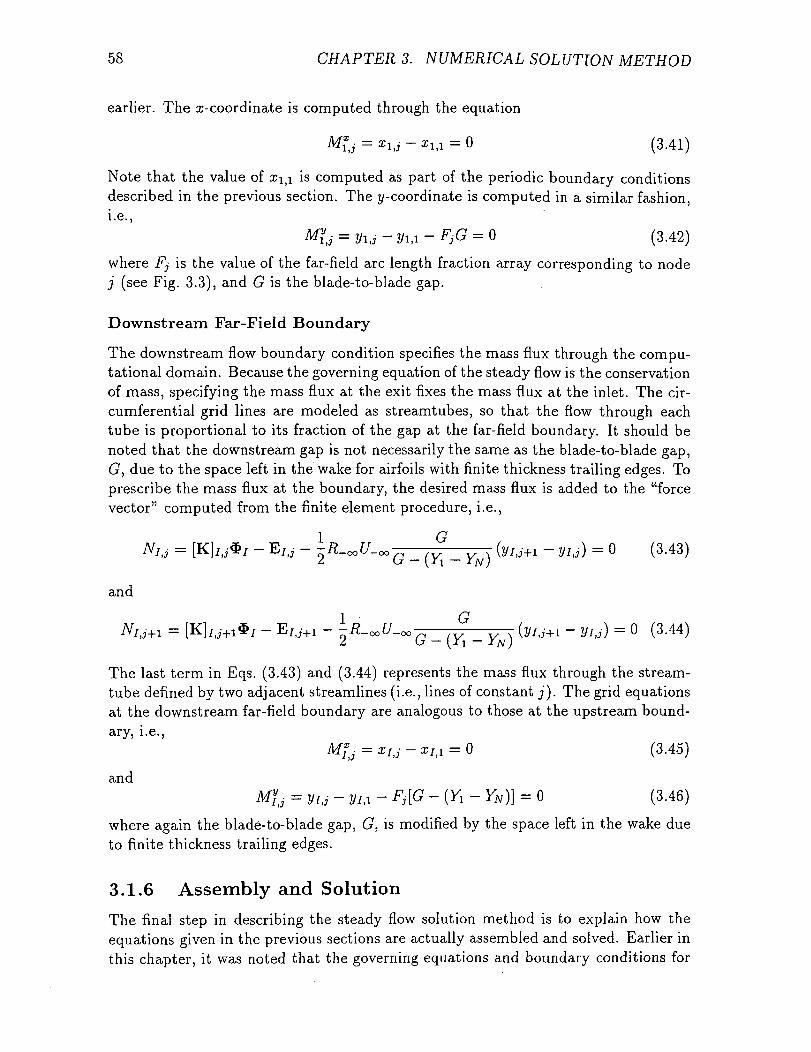
58 CHAPTERS. NUMERICAL SOLUTION METHOD
earlier. The a;- coordinate is computed through the equation
Mfj = xij - xi.i = 0 (3.41)
Note that the value of x^i is computed as part of the periodic boundary conditionsdescribed in the previous section. The ^/-coordinate is computed in a similar fashion,i.e.,
M?j = yi,j ~ 2/1,1 - FjG = 0 (3.42)
where Fj is the value of the far-field arc length fraction array corresponding to nodej (see Fig. 3.3), and G is the blade-to-blade gap.
Downstream Far-Field Boundary
The downstream flow boundary condition specifies the mass flux through the compu-tational domain. Because the governing equation of the steady flow is the conservationof mass, specifying the mass flux at the exit fixes the mass flux at the inlet. The cir-cumferential grid lines are modeled as streamtubes, so that the flow through eachtube is proportional to its fraction of the gap at the far-field boundary. It should benoted that the downstream gap is not necessarily the same as the blade-to-blade gap,G, due to the space left in the wake for airfoils with finite thickness trailing edges. Toprescribe the mass flux at the boundary, the desired mass flux is added to the "forcevector" computed from the finite element procedure, i.e.,
and
NIij+l = [K]/J+1$/ - E/J+1 - Ifl^t/^— — £_— (y/i-+1 - y/ij) = 0 (3.44)2 G - (Yi - YN)
The last term in Eqs. (3.43) and (3.44) represents the mass flux through the stream-tube defined by two adjacent streamlines (i.e., lines of constant j}. The grid equationsat the downstream far-field boundary are analogous to those at the upstream bound-ary, i.e.,
M?,j = xi,i ~ */,i = ° (3-45)
and2//,i - Fj[G - (Y, - YN}} = 0 (3.46)
where again the blade-to-blade gap, G, is modified by the space left in the wake dueto finite thickness trailing edges.
3.1.6 Assembly and Solution
The final step in describing the steady flow solution method is to explain how theequations given in the previous sections are actually assembled and solved. Earlier inthis chapter, it was noted that the governing equations and boundary conditions for
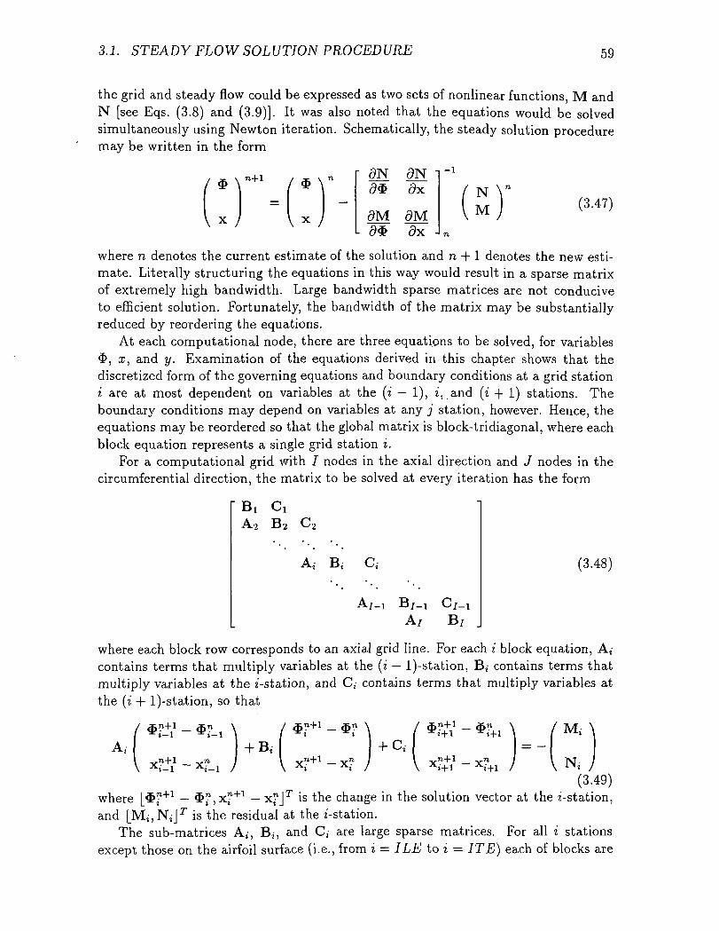
3.1. STEADY FLOW SOLUTION PROCEDURE 59
the grid and steady flow could be expressed as two sets of nonlinear functions, M andN [see Eqs. (3.8) and (3.9)]. It was also noted that the equations would be solvedsimultaneously using Newton iteration. Schematically, the steady solution proceduremay be written in the form
n+l dN<9x
dM dM<9x
-i
(3.47)
where n denotes the current estimate of the solution and n + 1 denotes the new esti-mate. Literally structuring the equations in this way would result in a sparse matrixof extremely high bandwidth. Large bandwidth sparse matrices are not conduciveto efficient solution. Fortunately, the bandwidth of the matrix may be substantiallyreduced by reordering the equations.
At each computational node, there are three equations to be solved, for variables$, x, and y. Examination of the equations derived in this chapter shows that thediscretized form of the governing equations and boundary conditions at a grid stationi are at most dependent on variables at the (i — 1), z, and (i + 1) stations. Theboundary conditions may depend on variables at any j station, however. Hence, theequations may be reordered so that the global matrix is block-tridiagonal, where eachblock equation represents a single grid station i.
For a computational grid with I nodes in the axial direction and J nodes in thecircumferential direction, the matrix to be solved at every iteration has the form
' BJ CiA2 62
A,-
/_i B/_a
A/
(3.48)
where each block row corresponds to an axial grid line. For each i block equation, A;contains terms that multiply variables at the (i — l)-station, B, contains terms thatmultiply variables at the i-station, and C,- contains terms that multiply variables atthe (i + l)-station, so that
A,-S&1 - *?_!
+ B,-,1+1s-i - xi-1
$,n+1 -..,1+1 _•*•»' •
C,-M,-
Nt-(3.49)
where [^"+1 — $",x"+1 — x"JT is the change in the solution vector at the z-station,and (_M;,N;Jr is the residual at the i-station.
The sub-matrices A,-, B,-, and C,- are large sparse matrices. For all i stationsexcept those on the airfoil surface (i.e., from i = ILE to i = ITE) each of blocks are
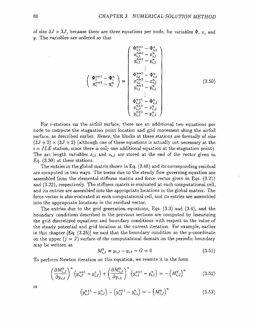
60 CHAPTER 3. NUMERICAL SOLUTION METHOD
of size 3J x 3J, because there are three equations per node, for variables <fr, x, andy. The variables are ordered so that
,,X
,,"+1 _ „,"
i^t1 _ $«.
1,.7
xi,J -
(3.50)
For i-stations on the airfoil surface, there are an additional two equations pernode to compute the stagnation point location and grid movement along the airfoilsurface, as described earlier. Hence, the blocks at these stations are formally of size(3 J + 2) x (3 J + 2) (although one of these equations is actually not necessary at thei = ILE station, since there is only one additional equation at the stagnation point).The arc length variables s^i and s^j are stored at the end of the vector given inEq. (3.50) at these stations.
The entries in the global matrix shown in Eq. (3.48) and its corresponding residualare computed in two ways. The terms due to the steady flow governing equation areassembled from the elemental stiffness matrix and force vector given in Eqs. (3.21)and (3.22), respectively. The stiffness matrix is evaluated at each computational cell,and its entries are assembled into the appropriate locations in the global matrix. Theforce vector is also evaluated at each computational cell, and its entries are assembledinto the appropriate locations in the residual vector.
The entries due to the grid generation equations, Eqs. (3.3) and (3.4), and theboundary conditions described in the previous sections are computed by linearizingthe grid discretized equations and boundary conditions with respect to the value ofthe steady potential and grid location at the current iteration. For example, earlierin this chapter [Eq. (3.25)] we said that the boundary condition on the ^-coordinateon the upper (j = J) surface of the computational domain on the periodic boundarymay be written as
M?tJ = yi,j - yiti -G = Q (3.51)
To perform Newton iteration on this equation, we rewrite it in the form
(3-52)
or(3.53)
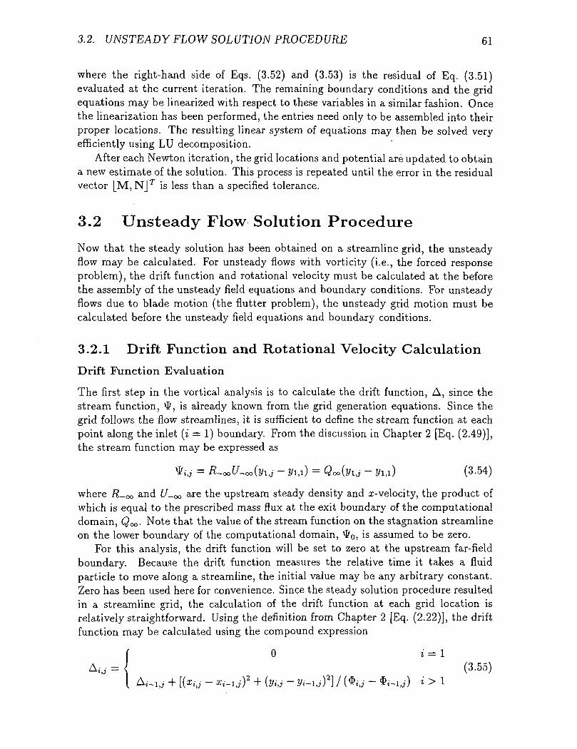
3.2. UNSTEADY FLOW SOL UTION PROCEDURE 61
where the right-hand side of Eqs. (3.52) and (3.53) is the residual of Eq. (3.51)evaluated at the current iteration. The remaining boundary conditions and the gridequations may be linearized with respect to these variables in a similar fashion. Oncethe linearization has been performed, the entries need only to be assembled into theirproper locations. The resulting linear system of equations may then be solved veryefficiently using LU decomposition.
After each Newton iteration, the grid locations and potential are updated to obtaina new estimate of the solution. This process is repeated until the error in the residualvector |_M,NJT is less than a specified tolerance.
3.2 Unsteady Flow Solution Procedure
Now that the steady solution has been obtained on a streamline grid, the unsteadyflow may be calculated. For unsteady flows with vorticity (i.e., the forced responseproblem), the drift function and rotational velocity must be calculated at the beforethe assembly of the unsteady field equations and boundary conditions. For unsteadyflows due to blade motion (the flutter problem), the unsteady grid motion must becalculated before the unsteady field equations and boundary conditions.
3.2.1 Drift Function and Rotational Velocity Calculation
Drift Function Evaluation
The first step in the vortical analysis is to calculate the drift function, A, since thestream function, \&, is already known from the grid generation equations. Since thegrid follows the flow streamlines, it is sufficient to define the stream function at eachpoint along the inlet (i = 1) boundary. From the discussion in Chapter 2 [Eq. (2.49)],the stream function may be expressed as
tfij = fl_ootf-oo(j/ij - yi.i) = Qoo(yi,j - yi.i) (3-54)
where R-<x> and U-oo are the upstream steady density and z-velocity, the product ofwhich is equal to the prescribed mass flux at the exit boundary of the computationaldomain, Q<x>- Note that the value of the stream function on the stagnation streamlineon the lower boundary of the computational domain, \I/o, is assumed to be zero.
For this analysis, the drift function will be set to zero at the upstream far-fieldboundary. Because the drift function measures the relative time it takes a fluidparticle to move along a streamline, the initial value may be any arbitrary constant.Zero has been used here for convenience. Since the steady solution procedure resultedin a streamline grid, the calculation of the drift function at each grid location isrelatively straightforward. Using the definition from Chapter 2 [Eq. (2.22)], the driftfunction may be calculated using the compound expression
0 t = l(3.55)
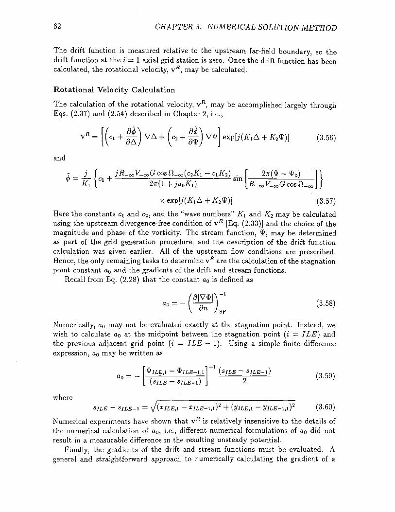
62 CHAPTERS. NUMERICAL SOLUTION METHOD
The drift function is measured relative to the upstream far-field boundary, so thedrift function at the i = I axial grid station is zero. Once the drift function has beencalculated, the rotational velocity, VR, may be calculated.
Rotational Velocity Calculation
The calculation of the rotational velocity, VR, may be accomplished largely throughEqs. (2.37) and (2.54) described in Chapter 2, i.e.,
\ + #2#)] (3.56)
and
<^=4-U + 27r(l
x ««?[;(#! A + #2W)] (3.57)
Here the constants Cj and 02, and the "wave numbers" KI and /^2 may be calculatedusing the upstream divergence-free condition of VR [Eq. (2.33)] and the choice of themagnitude and phase of the vorticity. The stream function, \£, may be determinedas part of the grid generation procedure, and the description of the drift functioncalculation was given earlier. All of the upstream flow conditions are prescribed.Hence, the only remaining tasks to determine VR are the calculation of the stagnationpoint constant ao and the gradients of the drift and stream functions.
Recall from Eq. (2.28) that the constant ao is defined as
(3.58)SP
Numerically, ao may not be evaluated exactly at the stagnation point. Instead, wewish to calculate CQ at the midpoint between the stagnation point (i = ILE] andthe previous adjacent grid point (i = ILE — 1). Using a simple finite differenceexpression, ao may be written as
SILE - SILE-I = \J(XILE,\ - z/r,E-i,i)2 + (VILE.I - yiLE-i,i)2 (3.60)where
Numerical experiments have shown that v^ is relatively insensitive to the details ofthe numerical calculation of ao; i-e., different numerical formulations of OQ did notresult in a measurable difference in the resulting unsteady potential.
Finally, the gradients of the drift and stream functions must be evaluated. Ageneral and straightforward approach to numerically calculating the gradient of a
3.2. UNSTEADY FLOW SOL UTION PROCED URE 63
function is to use a generalized coordinate transformation [54]. Specifically, the gra-dient will be evaluated in the (E, H) grid generation coordinate system. This may beaccomplished by considering the derivatives with respect to x and y using the chainrule, i.e.,
d <9E 8 dH d
anddx dx dz, dx dH
d__dE_d_ dH ddy dy dE dy dH
(3.61)
(3.62)
Ideally, however, we only wish to evaluate derivatives with respect to .r, and H. Thismay be accomplished using the transformation matrix [J], which is defined as
dE_ dSdx dy
dH dH(3.63)
dx dy
To obtain the derivatives we desire, the matrix [J] may be inverted, resulting in
dy/dH dH dy/dEdEdx
dEdy
dx
dx/dH dH _ dx/dE
where
imi = f—^L- dx dy^I L J l \dEdH dHdE
-i
(3.64)
(3.65)
(3.66)
Combining the above expressions, the derivatives in Eqs. (3.61) and (3.62) may berewritten as
and
dx
_dy E dEdH
(3,T)
(3.68)
Note that now all derivatives are with respect to ,=, and H. These derivatives may becomputed using centered finite differences modified for variable spacing in E and H.The gradients of the drift and stream functions (or any other scalar) may be evaluatedusing this approach. Once the gradients have been calculated, the rotational velocitymay be determined at each computational node.
3.2.2 Unsteady Grid Generation
For flutter problems, the motion of the computational grid must be computed beforethe calculation of the unsteady flow. The motion of the grid boundaries is easily
64 CHAPTERS. NUMERICAL SOLUTION METHOD
specified. The motion of the grid on the airfoil surface is required to match thevibrational mode shape of the blade motion. There is no grid motion in the farfield to simplify the implementation of the far-field boundary conditions. Finally, theperiodic and wake boundaries must smoothly connect these specified boundaries.
Previous researchers have solved Laplace's equation to determine the grid motionthroughout the computational domain [30, 35, 24]. Laplace's equation was used sothat the grid motion varies smoothly throughout the computational domain. As aresult, derivatives of the grid motion may be computed with minimal truncation error.Furthermore, in finite difference discretizations using centered differences, grid motionthat does not vary smoothly may excite sawtooth modes in the unsteady solution.
In the present method, sawtooth modes are not admitted into the finite elementsolution, so the grid motion need not be as smooth as for centered finite differenceschemes. The truncation error of the derivatives must still be kept to a minimum,however. In this report, the calculation of the grid motion will be performed usinga linear distribution of the grid motion over a few adjacent grid lines. A linear dis-tribution is quite simple to implement, results in a relatively smooth distribution ofgrid motion, and does not significantly increase the overall truncation error of theunsteady solution method. For most cases examined in the present work, approxi-mately five grid nodes in each direction were sufficient to obtain the correct unsteadysolution. Mathematically, this may be expressed as
fij = Li LJ TAIR (3.69)
where fAiR is the grid motion at the nearest grid point on the airfoil surface, andLi and LJ are functions that contain fractional values to distribute the grid motionsmoothly.
3.2.3 Finite Element Discretization
The next step is to compute the stiffness matrix and force vector for the unsteady flowequations. The variational principle governing the unsteady flow was developed inChapter 2 [Eq. (2.74)]. As for the steady flow, the variational principle is discretizedusing bilinear quadrilateral isoparametric elements. Since the unsteady flow problemis linear, however, the solution may be computed in one iteration. At each elementn, the values of the unsteady potential at each of the corners are interpolated intothe interior of the domain using the interpolation
0B (3-70)
Similarly, the gradient operator may be written as
n (3.71)
Substituting these expressions into the unsteady functional given in Eq. (2.74), resultsin
linear = \ /£ R {-^[N'£[N']n0n + ̂ [^[N'£ V'd> V'd>
3.2. UNSTEADY FLOW SOLUTION PROCEDURE 65
V'<I>r[][N'Un + V - fV'
// V-^INJn^n^*/ (3.72)•/ -/2n
+
Setting the first variation of this functional to zero results in the discretized governingequations for the unsteady flow
R -[N']I[N']n + ±
([I] - ^ V'$ V'$T) [N']n - ^f - V* [NJ n
v • fv'$T - -v'$r[j]v /$v'$T [N']n
/ • f -^^ = 0 (3.73)
From this form of the first variation, it is clear that the local stiffness matrix, [k]n,may be written as
R - N ' n
f <*, (3.74)
and the corresponding unsteady force vector, en, is
"= IL ^«^ •'Sn \ ,
'$T[J] + V • fV'$T - --V'$T[J] V$V'$T [N']n
V - f - V'$T[J]V'$ [NJn + V - #v*|NJn e^ ̂ (3-75)
As in the steady flow calculation, the elemental stiffness matrix and force vector arecomputed for each cell in the computational domain and assembled into a globalstiffness matrix and force vector. The next section describes the unsteady boundaryconditions which also contribute terms to the global stiffness matrix and force vector.
66 CHAPTERS. NUMERICAL SOLUTION METHOD
3.2.4 Near-Field Boundary Conditions
Periodic Boundary Condition
In Chapter 2, it was noted that the periodic boundary condition would be enforcedas part of the numerical solution procedure. This is not the only way to apply thiscondition, however. In Hall's original linearized potential formulation [24], a Lagrangemultiplier was used to enforce cascade periodicity on the upstream periodic boundary.Although this approach will result in the correct solution, it does not lend itself wellto the sensitivity analysis procedure. Consequently, in this work a slightly differentapproach is used to enforce cascade periodicity.
Examining the periodic boundary condition, Eq. (2.79), shows that the unsteadypotential on the upper and lower periodic surfaces of the computational domain arenot independent. Hence, the value of the unsteady potential on one of the periodicboundaries need not be calculated explicitly. The number of equations at each axialstation in the periodic region may then be reduced by one. This new vector of thediscretized unsteady potential and the original vector are related by a simple linearrelationship. If the original unsteady potential vector is denoted by 0, and the newreduced vector by <£, then
<£=[!]<£ (3-76)where
11
(3.77)
Note that the matrix [I] is rectangular, of size J x (J — 1).The variational principle describing the flow may be written as
II = ^j>T[k}(t> - ~$Te = min (3.78)Li
where [k] is the global stiffness matrix and e is the force vector. Substituting thesolution vector transformation equation, Eq. (3.76), results in
where the overbars again denote the complex conjugate. Setting the first variation ofthis expression to zero gives
SU = [l]T[k][I}4> - [J]Te = 0 (3.80)
This is the equation that must be computed. In practice, Eq. (3.80) means that theperiodicity condition is enforced by pre- and/or post-multiplying the stiffness matricesand force vectors by [I]T and [I], respectively, once the block stiffness matrices andforce vectors have been computed. Hence, the block stiffness matrices [a;], [bj], and[c;] and block force vector e,- at each station i are replaced according to the followingtable
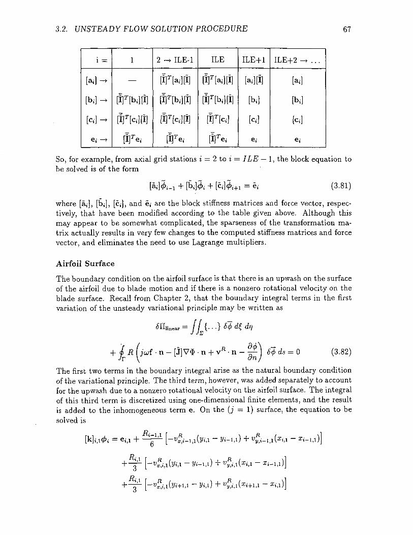
3.2. UNSTEADY FLOW SOLUTION PROCEDURE 67
i =
[a,-] ->
[b,-] ->
N -
e, -»•
1
—
fr[b,][i]
ffiTN[i]
[I]Te,
2 -> ILE-1
frwnSr[b,-]fflmem
[I]Te,-
ILE
«Twin[i]T[b,][i]
fiFM[I]Te,.
ILE+1
[a,][I]
[b,]
N
e,
ILE+2 -> . . .
[a,-]
N
N
e,
So, for example, from axial grid stations i = 2 to i = ILE — 1, the block equation tobe solved is of the form
[a,-] Ji-i = e; (3.81)
where [a,-], [b,-], [c,-], and e, are the block stiffness matrices and force vector, respec-tively, that have been modified according to the table given above. Although thismay appear to be somewhat complicated, the sparseness of the transformation ma-trix actually results in very few changes to the computed stiffness matrices and forcevector, and eliminates the need to use Lagrange multipliers.
Airfoil Surface
The boundary condition on the airfoil surface is that there is an upwash on the surfaceof the airfoil due to blade motion and if there is a nonzero rotational velocity on theblade surface. Recall from Chapter 2, that the boundary integral terms in the firstvariation of the unsteady variational principle may be written as
R juf • n - [J] V$ • n + VR n -on
ds = 0 (3.82)
The first two terms in the boundary integral arise as the natural boundary conditionof the variational principle. The third term, however, was added separately to accountfor the upwash due to a nonzero rotational velocity on the airfoil surface. The integralof this third term is discretized using one-dimensional finite elements, and the resultis added to the inhomogeneous term e. On the (j = 1) surface, the equation to besolved is
= e,-tl
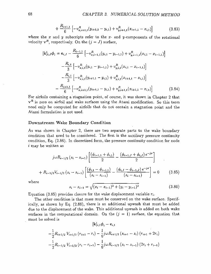
68 CHAPTERS. NUMERICAL SOLUTION METHOD
- ' (3-83)
where the x and y subscripts refer to the x- and y-components of the rotationalvelocity VR, respectively. On the (j = J) surface,
[k],-,j& = etW --
— 3D
(3.84)
For airfoils containing a stagnation point, of course, it was shown in Chapter 2 thatvfi is zero on airfoil and wake surfaces using the Atassi modification. So this termneed only be computed for airfoils that do not contain a stagnation point and theAtassi formulation is not used.
Downstream Wake Boundary Condition
As was shown in Chapter 2, there are two separate parts to the wake boundarycondition that need to be considered. The first is the auxiliary pressure continuitycondition, Eq. (2.86). In discretized form, the pressure continuity condition for nodei may be written as
, . >=0 (3.85)i -"^-i/^'i-i/j v0' "»-*/ / \
L v6* Ai-U
where /
(3.86)
Equation (3.85) provides closure for the wake displacement variable r;.The other condition is that mass must be conserved on the wake surface. Specif-
ically, as shown by Eq. (2.88), there is an additional upwash that must be addeddue to the displacement of the wake. This additional upwash is added on both wakesurfaces in the computational domain. On the (j = 1) surface, the equation thatmust be solved is
[k]t-,!<k - e,-,!
--Ri+i/2 VJ+i/2 (r,-+i - r;) - -jwRi+l/2 (si+l - s^ (rt+1 + 2r<)
--^_i/2 Vi-i/2 (rt - r;_i) - -
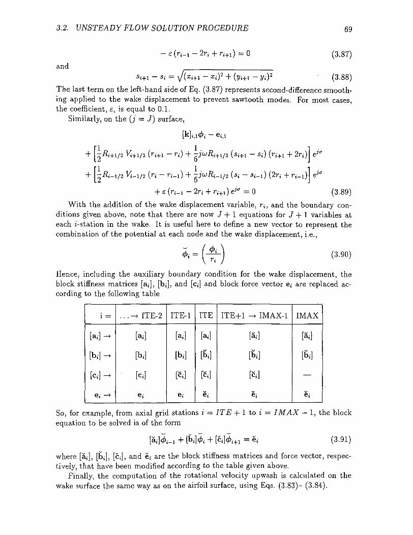
3.2. UNSTEADY FLOW SOLUTION PROCEDURE 69
(3.87)
and
si+1 - si = \ x i + i - x,-)2 + (j/i+i - i/,-)2 ' (3.88)
The last term on the left-hand side of Eq. (3.87) represents second-difference smooth-ing applied to the wake displacement to prevent sawtooth modes. For most cases,the coefficient, e, is equal to 0.1.
Similarly, on the (j = J) surface,
VJ+1/2 ,-+i - ri) + -D
; - r,_a) + -D
si+i - Si) (r,-+1
Si - s^) (2r,-
+ e (r,-,! - 2r,- + ri+1 ) e^ = 0
2r;)
(3.89)
With the addition of the wake displacement variable, r,-, and the boundary con-ditions given above, note that there are now J + 1 equations for J + 1 variables ateach i-station in the wake. It is useful here to define a new vector to represent thecombination of the potential at each node and the wake displacement, i.e.,
(3.90)
Hence, including the auxiliary boundary condition for the wake displacement, theblock stiffness matrices [a;], [b,-], and [c;] and block force vector e,- are replaced ac-cording to the following table
i =
[ad -
M -
N-
e; ->
. . . -> ITE-2
W
[b,]
N
e;
ITE-1
w[b,]
pye;
ITE
wft]
[«.']
w6i
ITE+1 -> IMAX-1
[«.']
[b,-]
N
\je,
IMAX
W
[b,]
—
w6i
So, for example, from axial grid stations i = ITE + 1 to i = IMAX — 1, the blockequation to be solved is of the form
[a,-] <£,-_! + [b,-]</>,- + [cij^i-t-i = e,- (3.91)
where [a,-], [b;], [c,], and e; are the block stiffness matrices and force vector, respec-tively, that have been modified according to the table given above.
Finally, the computation of the rotational velocity upwash is calculated on thewake surface the same way as on the airfoil surface, using Eqs. (3.83)- (3.84).
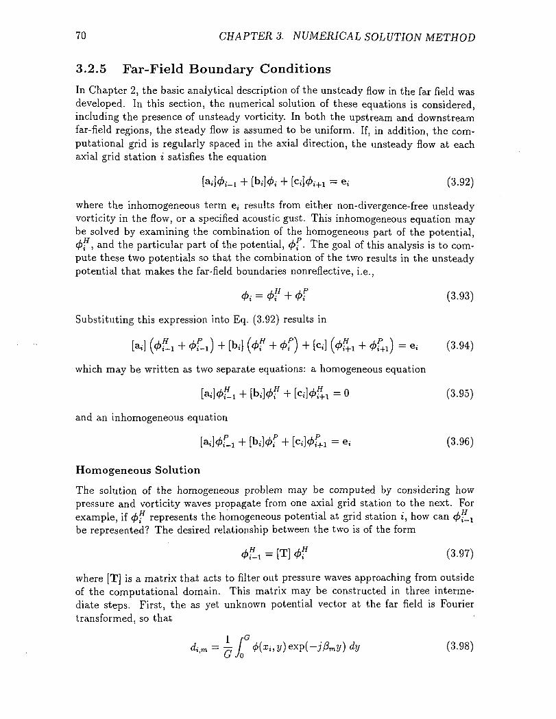
70 CHAPTERS. NUMERICAL SOLUTION METHOD
3.2.5 Far-Field Boundary Conditions
In Chapter 2, the basic analytical description of the unsteady flow in the far field wasdeveloped. In this section, the numerical solution of these equations is considered,including the presence of unsteady vorticity. In both the upstream and downstreamfar-field regions, the steady flow is assumed to be uniform. If, in addition, the com-putational grid is regularly spaced in the axial direction, the unsteady flow at eachaxial grid station i satisfies the equation
[a;]̂ + [b,-]<fc + [c,-]<fc+1 = e< (3.92)
where the inhomogeneous term e,- results from either non- divergence-free unsteadyvorticity in the flow, or a specified acoustic gust. This inhomogeneous equation maybe solved by examining the combination of the homogeneous part of the potential,<f>i , and the particular part of the potential, 0,- . The goal of this analysis is to com-pute these two potentials so that the combination of the two results in the unsteadypotential that makes the far-field boundaries nonreflective, i.e.,
& = 4>? + <tf (3.93)
Substituting this expression into Eq. (3.92) results in
?-i + Ci) + [b.-] (>f + 0f ) + N «! + 0f+1) = e, (3.94)
which may be written as two separate equations: a homogeneous equation
[a,-]^ + [bt]<£? + [c,-]̂ = 0 (3.95)
and an inhomogeneous equation
[a^L + [b^f + [c^f+1 = e, (3.96)
Homogeneous Solution
The solution of the homogeneous problem may be computed by considering howpressure and vorticity waves propagate from one axial grid station to the next. Forexample, if 0f represents the homogeneous potential at grid station z, how can $?_ l
be represented? The desired relationship between the two is of the form
0f_i = [T] 4? (3-97)
where [T] is a matrix that acts to filter out pressure waves approaching from outsideof the computational domain. This matrix may be constructed in three interme-diate steps. First, the as yet unknown potential vector at the far field is Fouriertransformed, so that
di,m = ^ 1° 4(xi, y) exp(-j/3my) dy (3.98)(j Jo
3.2. UNSTEADY FLOW SOLUTION PROCEDURE 71
where di>m are the Fourier coefficients at axial grid station i. In the present method,the coefficients are computed using the trapezoidal rule. Typically, the coefficientvector d, is much smaller in length than the number of computational nodes in thecircumferential direction, since truncation error increases greatly for higher harmonicsof the principal circumferential wave number. For most cases considered here, fiveFourier modes (—2 < m < 2) are sufficient to describe the unsteady flow. In matrixnotation, Eq. (3.98) may be written in the form
d; = [F^f (3.99)
where [Fa] is a (generally rectangular) matrix that represents the discretized form ofthe trapezoidal rule.
The next step in the analysis is to filter and propagate these Fourier modes to thenext grid station. In the far field, since the steady flow is assumed to be uniform, thewave numbers of the wave propagation are known analytically. From the analysis inChapter 2, the harmonic behavior of the potential may be written as
oo
4>(x,y} = H! dmexp\jam(x-x e)+jPmy] (3.100)m=—oo
where Xg is the x-coordinate of the far-field boundary being examined. Therefore, ifthe spacing between nodes on adjacent axial grid stations is known, then the propa-gation of the Fourier coefficients may be expressed as
"i—l,m = "«,m exP [~J&m(xi ~ xi-\) ~ ] Pm\Hi ~ J/i-l)J (3.101)
where
U* + V-2 -am — £2 _ jji
and
(3.103)
In matrix notation, the filter and propagation relationship may be written as
di_! = [F2]d,- (3.104)
where [F2] is square and diagonal, and the diagonal entries are the above exponentialexpression for outgoing modes; the entries corresponding to incoming modes are zero
'so that their contribution is not included in the final solution.The third step in the solution process is to perform an inverse Fourier transform
on the Fourier coefficients d,_i to recover the the new values of the potential at eachnode. In matrix form, this may be written as
^ = [F3] d,-_! (3.105)
where the (also generally rectangular) matrix [Fa] is the discrete matrix form of theinverse Fourier transform.
72 CHAPTERS. NUMERICAL SOLUTION METHOD
Taken together, these three steps result in
<£?_! = [F3] [F2] [F!] 0f = [T] tf (3.106)
so the transition matrix, [T], is now known. Now that the behavior of the continuouspart of the potential has been described, the particular part due to incoming gustsmay be calculated.
Particular Solution
The particular solution may be calculated by considering the propagation character-istics of the incoming acoustic or vortical gust. Because the waves convect with thesteady flow and the steady flow is uniform in the far field, the convection relationmay be expressed as
0£n = *n^f (3-107)where
zn = exp [/nap(z<+i - Xi) + jn(3p(yi+l - y$] (3.108)
For a pressure gust, the wave numbers ap and j3p have the same form as those foram and (3m as shown above in Eqs. (3.102) and (3.103). For a vortical gust, the wavenumbers ap and j3p are defined as
,
and
(3,09)
ftf = § (3.110)
with U and V being the x- and y-components of the steady velocity at the far field.Consequently, the equation that describes the particular solution in the far field,
Eq. (3.96), may be written as
[a^f + [b,-]<£f + z [c,-]tf = * (3.111)
So the particular solution may be computed by solving the above linear system, i.e.,
<Af = f- W + N + z [c,-]l ' et (3.112)LZ J
Equation (3.112) gives a relatively simple result that is best applied when a vorticalgust is present. For an acoustic gust, there is a simpler approach. The unsteadypressure is linearly related to the potential by the expression
p(x, y) = -R \ju + V$ • V] i(x«, ye) exp \jap(x - xs) + j(3p(y - ys)} (3.113)
where (xff ,yg) refers to a coordinate at the far-field boundary. Hence, the particularsolution may be specified once the magnitude and phase of the gust has been chosen,
it,V\
3.2. UNSTEADY FLOW SOLUTION PROCEDURE 73
Now that the general procedure for calculating the homogeneous and particularparts of the unsteady potential have been described, the actual implementation foreach boundary may be examined.
Upstream Far-Field Boundary
At the upstream far-field boundary, the homogeneous part of the potential satisfiesEq. (3.95) with i = 1.
[ai]^ + [bjj^f + [ca]0f = 0 (3.115)
where the block matrices and potential vectors have been modified in the periodicboundary conditions using Eq. (3.76). The transition matrix from Eq. (3.106), maybe modified in a similar fashion, i.e.,
[T] -* [lHT][i] = [t] (3.116)
Hence, Eq. (3.115) may be written as
[b1])^f + [c1]0f = 0 (3.117)
and in light of Eq. (3.93), some algebra results in
ft]& + [£i]52- = (ft] + z [£!]) 0f = el (3.118)
whereft]=([ai][t] + [b1]) (3.119)
Hence, the far-field boundary conditions modify the block matrix [bi] and the blockforce vector eY
Downstream Far-Field Boundary
The downstream far-field boundary conditions are assembled in an analogous fashionat axial grid station /, with the appropriate change in the direction of propagation ofthe pressure modes in the homogeneous solution. The only major difference is thatthe wake must be accounted for. Recall from Chapter 2 that there is a continuousand discontinuous part to the unsteady potential in the downstream far field
4 = <l>c + <t>d (3.120)
Both the continuous and discontinuous parts of the potential must propagate cor-rectly. The transition matrix, [T], derived earlier, only applies to the continuous partof the potential. The discontinuous part propagates out of the domain as a vorticitywave. Hence, a new transition matrix may be defined as
[T*] = [T][I-D] + z[D] (3.121)
where [D] is the matrix operator that computes the discontinuous part of the poten-tial, and [I] is the identity matrix. The J + 1 equation is the propagated form of the
74 CHAPTER 3. NUMERICAL SOLUTION METHOD
mass conservation boundary condition. Since there is no grid motion in the far field,the conservation of mass boundary condition is
(3.122)On Os
In discrete form, Eq. (3.122) may be written as
- r/)= 0 (3.123)
Solving for r/+1 gives
d/dn+ = rI+l (3.124)
or(3.125)
So the new transition matrix, with the additional row and column for the wakedisplacement, has the structure
(3.126)
In the wake boundary conditions, we introduced a new vector that contains the po-tential and wake displacement, so that
/ \<t>l+l
\ rI+i )
= [T]
L ^0
Q \
/ \*/
V rf /
Hence, Eq. (3.126) may be written as
(3.127)
(3.128)
Using this new transition matrix, the matrix equation at the downstream far fieldmay be written as
-! + [bj] = - [a/ & = e}
where in this case
(3.129)
(3.130)
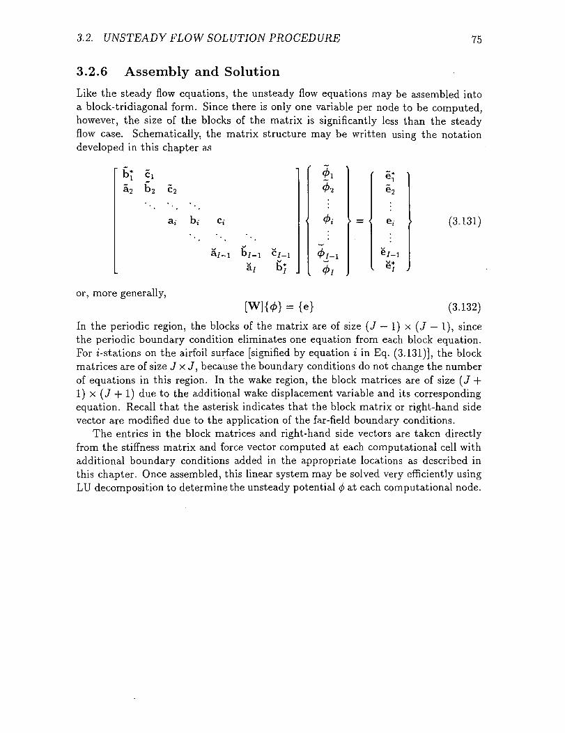
3.2. UNSTEADY FLOW SOLUTION PROCEDURE 75
3.2.6 Assembly and Solution
Like the steady flow equations, the unsteady flow equations may be assembled intoa block-tridiagonal form. Since there is only one variable per node to be computed,however, the size of the blocks of the matrix is significantly less than the steadyflow case. Schematically, the matrix structure may be written using the notationdeveloped in this chapter as
c;
a/
02
(3.131)
or, more generally,[W]{0} = {e} (3.132)
In the periodic region, the blocks of the matrix are of size (J — 1) x (J — 1), sincethe periodic boundary condition eliminates one equation from each block equation.For z-stations on the airfoil surface [signified by equation i in Eq. (3.131)], the blockmatrices are of size J x J, because the boundary conditions do not change the numberof equations in this region. In the wake region, the block matrices are of size (J +l ) x ( J + l) due to the additional wake displacement variable and its correspondingequation. Recall that the asterisk indicates that the block matrix or right-hand sidevector are modified due to the application of the far-field boundary conditions.
The entries in the block matrices and right-hand side vectors are taken directlyfrom the stiffness matrix and force vector computed at each computational cell withadditional boundary conditions added in the appropriate locations as described inthis chapter. Once assembled, this linear system may be solved very efficiently usingLU decomposition to determine the unsteady potential <f> at each computational node.
Chapter 4
Sensitivity Analysis
Chapters 2 and 3 described a general method to calculate the steady and small dis-turbance unsteady flow over a two-dimensional cascade of airfoils due to blade motionand incoming gusts. The next task (and the primary goal of this report) is to deter-mine the effect small changes in the airfoil shape or cascade geometry have on thesteady and unsteady flow fields. In Section 4.1, the general procedure for this sensi-tivity analysis will be described. The sensitivity analysis makes use of the nominalsteady and unsteady flow LU decompositions so that no additional matrices needto be factored, resulting in a very computationally efficient procedure. Section 4.2contains a description of the steady flow sensitivity analysis procedure, including adiscussion of how the perturbation of the airfoil shape is prescribed. In a similarfashion, the sensitivity of the unsteady flow is considered in Section 4.3.
4.1 General Procedure
The quantities of interest to be calculated in this report may be separated into fourgroups: first is the nominal steady potential and grid locations, 3? and x; second,the perturbation of the steady potential and grid due to small changes in the airfoilgeometry, $' and x'; third, the nominal unsteady potential, 0; and fourth, the per-turbation of the unsteady potential due to small changes in the airfoil geometry, </>'.Chapters 2 and 3 described how the nominal steady flow (i.e., <& and x) and nominalunsteady flow (i.e., </>) are calculated. This section describes a general procedure forcalculating the remaining quantities, which are referred to as perturbations of theirassociated nominal quantities. Throughout this chapter, a prime (') will be used todenote these perturbations.
It should be noted that the perturbation of the steady potential, $', and thenominal unsteady potential, </>, are not of the same order. Figure 4.1 illustrates thesetwo separate perturbations. In Chapters 2 and 3, the perturbation series we examinedwere expanded using a small parameter on the order of the blade displacement, f.Here we expand the equations in perturbation series using a small parameter on theorder of the change in geometry, which is denoted here by e. Hence, the perturbationof the unsteady potential, (j>' is not formally second order. Instead, it is first order in
76
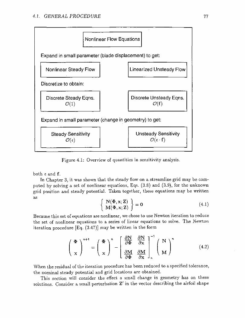
4.1. GENERAL PROCEDURE 11
Nonlinear Flow Equations
Expand in small parameter (blade displacement) to get:
Nonlinear Steady Flow Linearized Unsteady Flow
Discretize to obtain:
Discrete Steady Eqns.0(1)
Discrete Unsteady Eqns.0(f)
Expand in small parameter (change in geometry) to get:
Steady Sensitivity Unsteady Sensitivity0(e • f)
Figure 4.1: Overview of quantities in sensitivity analysis.
both f. and f.In Chapter 3, it was shown that the steady flow on a streamline grid may be com-
puted by solving a set of nonlinear equations, Eqs. (3.8) and (3.9), for the unknowngrid position and steady potential. Taken together, these equations may be writtenas
N(*,x;Z) \ _M($ ,x ;Z) J
(4.1)
Because this set of equations are nonlinear, we chose to use Newton iteration to reducethe set of nonlinear equations to a series of linear equations to solve. The Newtoniteration procedure [Eq. (3.47)] may be written in the form
n+l <9N 5N ldx
dM dM<9x
-f
(4.2)
When the residual of the iteration procedure has been reduced to a specified tolerance,the nominal steady potential and grid locations are obtained.
This section will consider the effect a small change in geometry has on thesesolutions. Consider a small perturbation Z' in the vector describing the airfoil shape
78 CHAPTER 4. SENSITIVITY ANALYSIS
and cascade geometry. This will result in a perturbation of the steady potential andthe grid location. The perturbed solution will satisfy the equations
_(4.3)
where the primed quantities are small perturbation quantities arising from the pre-scribed perturbation in the geometry Z'. Expanding Eq. (4.3) in a Taylor series aboutthe nominal solution gives
r 5N <9Ndx
5M dM(4.4)
where we have grouped the terms so that left-hand side of Eq. (4.4) contains termsinvolving the perturbations of the dependent variables $ and x, and the inhomo-geneous right-hand side contains terms involving the prescribed perturbation of theindependent variable Z. To solve for the unknown perturbations $' and x', Eq. (4.4)is rearranged slightly to obtain
f <9N
cbc -
(4.5)
Note the similarity of Eq. (4.5) to Eq. (4.2). The same matrix must be "inverted" toobtain the perturbed steady solution that was used in the last iteration of the Newtonsolver. In other words, the same system of equations as in the nominal calculationmust be solved, only with a different right-hand side due to the perturbation Z'.Therefore, if Eq. (4.2) has been computed using LU decomposition, and the factoredmatrix has been saved, then the sensitivity analysis may be obtained for virtually noadditional computational work. This is because the perturbations $' and x' may becomputed through a simple back-substitution, which requires significantly less com-putational time than a complete solution. Furthermore, the relative computationalsavings increases with the number of design variables examined. The perturbationof each design variable will result in a new right-hand side of Eq. (4.5), each onlyrequiring a back-substitution, so many design variables may be examined before thecost of the sensitivity analysis approaches the cost of the single nominal calculation.
Consequently, the main task of the steady flow sensitivity analysis is to determinethe prescribed perturbation Z' and its associated matrices dN/dZ and <9M/<9Z. Thedetails of the computation of these quantities will be examined in Section 4.2.
Having computed the perturbation of the steady potential and grid due to achange in geometry in addition to the nominal solution, we now consider the smalldisturbance unsteady flow. From Chapter 3, we know that the discretized unsteadyflow may be represented by a linear system of equations of the form
= {e($,x,vfi,f,u,,<r)} (4.6)
4.2. STEADY FLOW SENSITIVITY ANALYSIS 79
After solving Eq. (4.6), the perturbation of the unsteady potential due to a changein the geometry may be calculated. The governing equations of the perturbed un-steady flowfield due to small changes in geometry, frequency, rotational velocity, in-terblade phase angle, and mode shape will be of the form
[W(* + $', x + x', u + u/, a + a')} {cf> + (/>'}
= e($ + $', x + x', v* + VR>, f + f, u + w', a- + a1} (4.7)
Expanding the discretized form of Eq. (4.7) in a perturbation series and collectingterms of first order gives the desired equation for the unknown discrete approximationto the perturbation of the unsteady potential, (/>', i.e.,
dvR
dW raw
VR> +
aw]
de-da \
aw(4.8)
or, more succinctly[W]<£' = e' — [W]'</> (4-9)
Note that the computation of x' and <&' has already been described. Section 4.3contains a discussion of the computation of u' and f for the flutter problem, and VR
for the forced response problem. In addition, Section 4.3 will contain a discussion ofthe assembly of the right-hand side of Eq. (4.8).
Note that the sensitivity analysis procedure outlined in this section is not limitedto the flow model and discretization scheme chosen in the present method. Equa-tions (4.1)-(4.9) may be applied to any linearized flow model, such as the linearizedEuler or Navier-Stokes equations. Finite difference and finite volume discretizationsalso may be used. The only requirement to obtain the computational efficiency of theprocedure described in this chapter is that the nominal flow equations must be solvedusing LU decomposition or some other algorithm designed to solve a linear system ofequations for multiple right-hand sides.
4.2 Steady Flow Sensitivity Analysis
4.2.1 Prescribing the Perturbation
The first step in the steady flow sensitivity analysis is to prescribe the perturbationin the vector containing the airfoil shape and cascade geometry, Z'. In general,the basis functions chosen to prescribe the geometry perturbation may be chosenarbitrarily. There is no limit on the number of functions that may be chosen, nor isthere a restriction (such as orthogonality) on the choices. To provide physical insight,however, these functions should be chosen so that they are meaningful to the designer.In this work, the basis functions may be classified into two groups, cascade geometryand airfoil shape basis functions.
80 CHAPTER 4. SENSITIVITY ANALYSIS
Recall from Chapter 3 that cascade geometry parameters refer to variables thatdefine the cascade behavior independently of the actual airfoil shape. For example,the stagger angle, 0, and the blade-to-blade gap, G, are both variables that areindependent of the airfoil shape. Airfoil shape parameters refer to variables thatdefine the airfoil shape, for example, the magnitude of the camber and thickness.
The details of the generation of the actual perturbation of the airfoil shape ishighly dependent on the type of airfoil definition used. Although the details will notbe discussed here, Appendix B contains a detailed description of how the perturbationof shapes from a common airfoil series (the NACA modified four digit series) maybe generated. In the current discussion, however, it is sufficient to assume thatperturbation of the airfoil shape or cascade geometry is prescribed and is containedin the vector Z'.
Once the airfoil shape perturbation has been defined, the next task in the steadysensitivity analysis is to define the entries in the 3M/5Z and <9N/<9Z matrices shownin Eq. (4.4). These matrices are extremely sparse because nearly all of the inhomo-geneous terms in Eq. (4.4) arise from the boundary conditions. In practice, thesematrices need not actually be formed; it is sufficiently straightforward to computethe matrix-vector product [the right-hand side of Eq. (4.4)] directly.
There are three main sources of inhomogeneous terms in Eq. (4.4). First, thenear-field boundary conditions, contribute terms because these conditions require thegrid to remain on the airfoil surface. Any change in the airfoil shape, then, willinfluence the location of the grid points. Second, there is a contribution from the far-field boundary conditions primarily due to changes in the blade-to-blade gap. Finally,there are inhomogeneous terms due to the the grid equations, Eq. (3.8), because ofthe requirement that the grid follow the flow streamlines.
4.2.2 Near-Field Boundary Conditions
Periodic Boundary Condition
Consider the steady periodic boundary conditions, Eqs. (3.23)-(3.25). Taking thederivative of the boundary condition equations with respect to the shape variablesdescribed earlier and multiplying by the perturbation of the vector containing theairfoil shape results in terms that contribute to the right-hand side of Eq. (4.4).Assuming that the fractional arc length array F,- is not a design variable, the boundaryconditions on the j = 1 periodic boundary of the computational domain do not resultin inhomogeneous terms in Eq. (4.4), i.e,
*-^*-.On the j = J surface, although the boundary condition governing the z-location isonly dependent on the grid, the y-location is also dependent on the blade-to-bladegap, so there is an inhomogeneous term associated with the boundary condition onthe y-grid equation, i.e.,
4.2. STEADY FLOW SENSITIVITY ANALYSIS 81
and
^Z'=-ff (442)
where G' is the perturbation in the blade-to-blade gap. Hence, the periodic boundaryconditions are not directly dependent on the airfoil shape.
Airfoil Surface Boundary Conditions
The next set of boundary conditions to consider are those that constrain the gridpoints to lie on the airfoil surface, Eqs. (3.27)-(3.30). On the j = 1 surface, there areinhomogeneous terms that result from the spline evaluation, i.e.,
Z' = -X^KO (4.13)
and
Z'^-Y^) (4.14)
where X's and Y$ are the perturbations in the cubic spline evaluation of the airfoilsurface coordinates corresponding to the arc length s,-^. Similarly, on the j ' = Jsurface,
z' = -X'3(ailj) (4.15)
and
^ Z' = -Y&SU) - G' (4.16)
where the latter equation also includes perturbations of the blade-to-blade gap, G'.The next two boundary conditions are those that require the grid to move propor-
tionally to the movement of the stagnation point, Eqs. (3.33)-(3.34). These conditionsare applied at every airfoil surface grid location except the stagnation point. On thej = 1 surface,
while on the j — J surface,
Recall that Si and SN are the arc length of the first and last points, respectively, ofthe set of points defining the surface of the airfoil, as shown in Fig. 3.4.
The final surface boundary condition to consider is the condition at the stagnationpoint, Eq. (3.35). This boundary condition requires that the grid node at the leadingedge of the airfoil be located at the stagnation point. The right-hand side term isfound to be
. (4.19)dZ SILE+I,I
82 CHAPTER 4. SENSITIVITY ANALYSIS
The term shown here arises from the steady periodicity condition. The potentialon the upper surface must be evaluated on the reference airfoil. From the steadyupstream far-field boundary conditions it can be shown that the steady potential onthe upper periodic surface and the steady potential on the lower periodic surface arerelated through the parameters G and Vloo- Specifically,
$,-,i = $i,j - G V_oo (4.20)
so clearly there is an inhomogeneous term arising from perturbations in the blade-to-blade gap.
Downstream Wake Boundary Conditions
The final set of near-field boundary conditions to consider are those on the down-stream wake boundary, Eqs. (3.36)-(3.38). Recall from Chapter 3 that the steadywake boundary conditions are nearly identical to the boundary conditions applied onthe periodic surfaces. Hence, like the periodic boundary, there are no inhomogeneousterms in the perturbation of the boundary conditions on the j ' = 1 surface, i.e.,
*-«On the j — J surface, the inhomogeneous terms account for perturbations in theblade-to-blade gap as well as the possibility of a blunt trailing edge, so that
(4.22)
Z' = - (G' - (Y? - Y^}} (4.23)
4.2.3 Far-Field Boundary Conditions
Upstream Far-Field Boundary Conditions
On the inflow boundary, only the equations governing the computational grid location,Eqs. (3.41)-(3.42), may result in inhomogeneous terms. Since the x-coordinate of theupstream boundary is fixed in this analysis, however, it is not considered to be a designvariable, and therefore only the boundary condition on the y-coordinate actually hasan inhomogeneous part to consider. Linearization of the boundary conditions resultsin the expressions
Z' - 0 (4.24)
and
^ Z' = -F0G' (4.25)
where it is assumed that the fractional arc length array in the far field, Fj, is not adesign variable, i.e., it is not subject to change in the design process.
4.2. STEADY FLOW SENSITIVITY ANALYSIS 83
Downstream Far-Field Boundary Conditions
The boundary conditions at the exit boundary are more complicated, mainly due tothe possibility of a blunt trailing edge. It is assumed here that any perturbation inblade-to-blade gap G' is constant throughout the computational domain. Hence, ifthe airfoil being analyzed has a blunt trailing edge, the space in the grid representingthe viscous wake from the trailing edge of the airfoil to the far-field boundary (seeFig. 3.5) is constant regardless of the perturbation of the gap. The size of the spacerepresenting the wake is only affected by perturbations in the first and last points ofthe airfoil definition. Consequently, the inhomogeneous terms arising from the flowboundary conditions, Eqs. (3.43)-(3.44), may be written as
8Z ~ dZ ~ 2°° G- (Y, -Y N )
<„, (v, v, ^ , .[G ~ (Yl ~ YN>] (4'26)
The terms arising from the grid boundary conditions, Eqs. (3.45)-(3.46), are similarto those for the inflow boundary, modified for the possibility of airfoil shapes with ablunt trailing edge, i.e.,
dMx
— p Z' = 0 (4.27)o LI
Z' = -Fi (G' - (Yi - Y^}} (4.28)
4.2.4 Sensitivity of the Stream Function
The final step in the steady sensitivity analysis is to consider the inhomogeneousterms due to a perturbation in the stream function, \I/'. Inhomogeneous terms arisebecause in this analysis the stream function at any node j is linearly related to theblade-to-blade gap, i.e.,
*,- = Q^FjG (4.29)
where Q^ is the prescribed mass flux at the exit of the computational domain andFJ is the fractional arc length array value at node j. Consequently, a perturbation inthe gap results in a perturbation of the stream function, so that
*;. = Q^FjG' (4.30)
Hence, any perturbation in the gap results in inhomogeneous terms in Eq. (4.4) arisingfrom the field grid generation equations, Eqs. (3.3)-(3.4). These inhomogeneous termsmay be written as
32X
84 CHAPTER 4. SENSITIVITY ANALYSIS
and* d*y
dZ
' (4,2)where the primes in the denominator of some of the terms refer to the perturbationof the finite difference representation of the d/d^/ operator. Note that the terms inEqs. (4.31) and (4.32) only appear if there is a perturbation in the gap.
4.3 Unsteady Flow Sensitivity Analysis
4.3.1 Sensitivity of the Drift Function
For forced response problems, the first unsteady quantity that must be examined isthe rotational velocity, vfl. In Chapter 2 it was shown that the rotational velocityis a function of the drift function, A, the stream function, ^, in addition to thecascade geometry and prescribed flow conditions. Since the method for computingthe sensitivity of the cascade geometry and stream function were presented earlierin this chapter, only the sensitivity of the drift function needs to be determined tocalculate the sensitivity of the rotational velocity.
Since the perturbed grid will still follow the flow streamlines, the sensitivity of thedrift function may be calculated by linearizing Eq. (3.55), i.e.,
( , , } ( }l *J 4-lJ ( }
Note that the drift function at the inlet boundary remains prescribed to be zero,as shown in Eq. (3.55). Earlier in this chapter, the steady flow sensitivity analysisprocedure was described, which resulted in expressions for the grid perturbations x'and y' and the steady potential perturbation $'. Hence, the summation in Eq. (4.33)may be computed in a straightforward manner.
4.3.2 Sensitivity of the Rotational Velocity
The sensitivity of the rotational velocity, VR, may be computed through careful ap-plication of the chain rule to the definition of the rotational velocity, Eq. (2.37).Considering that the coefficients Ci and c2 as well as the wave numbers K\ and K2
may have perturbations associated with them in addition to the perturbations al-ready discussed in this chapter, the sensitivity of the rotational velocity, VR/, may bewritten as
VR' = {[(c( + JK{$ + jK, $') VA + (Cl + JK, $) (V'A + VA')
4.3. UNSTEADY FLOW SENSITIVITY ANALYSIS 85
( ~ d$\4- I c2 + jK,$ + — 1 (V* +
X VA + ( c2 i A + K2V)] (4.34)
where V refers to the perturbation of the finite difference representation of the gra-dient operator due to the grid perturbation. Recall from Chapter 3 that the gradientoperator used in this report is evaluated using a generalized coordinate transformationto the C^-,H} grid generation coordinate system [see Eqs. (3.67) and (3.68)]. Hence,perturbations in the grid locations result in a perturbation of the discretized gradientoperator.
4.3.3 Sensitivity of the Blade Structural Dynamics
For flutter problems, the first task in the unsteady sensitivity analysis is to determinethe perturbation of the blade motion. Once the perturbation in the vibratory modeshape of the blade is known, the perturbation of the grid motion may be calculated,so the complete unsteady sensitivity analysis may be computed.
Thus far, very little has been said about the structure of the blade. In Chapters2 and 3, it was assumed that the vibratory frequency and mode shape are specifiedas part of the flutter problem description. The question then becomes, how do smallchanges in the blade shape affect the frequency and mode shape of the vibration?
It is beyond the scope of the present analysis to discuss a complete structuralmodel of a turbomachine blade. In this analysis it is assumed that there is someindependent structural model of the blades (e.g., a finite element model) that isused to calculate the frequency and mode shape of vibration. For turbomachineryblades, unlike aircraft wings, it is reasonable to assume that the ratio of the massof the structure to the mass of the fluid is sufficiently high that the effect of steadyaerodynamic loading on the calculation of the structural modes may be neglected.Hence, the sensitivity of the blade vibration may be calculated independently fromthe present analysis.
The sensitivity of the equations describing the blade structure may be calculatedusing some of the techniques described earlier or by using similar methods developedfor analysis of structures [41, 42]. In any event, it is clear that the frequency andmode shape of vibration are functions of the design variables. For example, if theairfoil is described using the modified NACA four digit definition (see Appendix B),the sensitivity of the frequency can be written as
, du . du , du .. du . du . .
^ e ^ t ' + r ' (4'35)
where mt, mc, lt, tc, and rt are the shape definition variables of the NACA airfoildescription, as discussed in Appendix B. Similarly, the sensitivity of the mode shape
86 CHAPTER 4. SENSITIVITY ANALYSIS
df , df , df a df „. df ,f = 7f~m + 1T~ mc + W£t + -Zftc + 7j-r (4.36)dmt drnc d£t oic drt
v 'To calculate the derivatives in Eqs. (4.35)-(4.36), a sensitivity analysis must be
performed on the structural model used to compute the nominal natural frequencyand mode shape of vibration. Once the derivatives of the frequency and mode shapehave been computed, Eqs. (4.35)-(4.36) may then be substituted into the overallunsteady sensitivity analysis expression, Eq. (4.8).
4.3.4 Sensitivity of the Grid Motion
Now that the sensitivity of the blade motion has been determined, the next task isto compute the perturbation of the grid motion in the computational domain. InChapter 3, the field grid motion was shown to be a linear interpolation of the motionon the airfoil surface [Eq. (3.69)]. Hence, the sensitivity analysis is quite simple,since the distribution fractions L{ and Lj do not change, (i.e., they are not designvariables). The perturbation of the grid motion, then, may be written as
fk = Lt L3 fV (4.37)
where f^IR is the sensitivity of the blade mode shape calculated earlier.
4.3.5 Sensitivity of the Finite Element Assembly
Now that all of the perturbation terms have been computed, the right-hand side ofEq. (4.8) may be formed. The matrices on the right-hand side of this equation arelarge sparse matrices that may be obtained by linearizing the computer code whichassembles the global matrix [W] and vector e. The elemental stiffness matrix andforce vector, along with all of the unsteady boundary conditions, all have a first-ordersensitivity that may be computed using the methods shown in this chapter.
For example, the sensitivity of the elemental stiffness matrix, [k] [defined inEq. (3.74)] may be computed by linearizing the matrix with respect to all of thevariables it is a function of, and multiplying by the actual perturbation, i.e.,
(4.38)'Since $' and x' may be determined from the steady flow sensitivity analysis, and(J may be computed from the structural sensitivity analysis, the sensitivity of thestiffness matrix may be computed. To increase the efficiency of the right-hand sidecalculation, the perturbation of the stiffness matrix is multiplied by the appropriateentries in the <£ vector at the element level. The details of this procedure do notsubstantially increase the understanding of the sensitivity analysis procedure, andare best understood by examining the actual computer code.
The sensitivity of the force vector, e, [see Eq. (3.75)] may be computed in a similarfashion, i.e.,
de de . de , de R/ de „. . • .e' = ^-$' + — x' + —J + J—VR + — f 4.39Hax ou OVH of
4.3. UNSTEADY FLOW SENSITIVITY ANALYSIS 87
Like the sensitivity of the stiffness matrix, the sensitivity of the force vector [i.e., theright-hand side of Eq. (4.39)] is best computed at the element level.
4.3.6 Near-Field Boundary ConditionsPeriodic Boundary Condition
The periodic boundary condition may contribute inhomogeneous terms to the un-steady sensitivity equation because the transformation matrix [I] [see Eq. (3-77)] isa function of the interblade phase angle, a. As a result, for example, the linearizedform of the block equation to be solved at z-stations from i = 2 to i = ILE — 1 [seeEq. (3.81)] may be written as
+i (4.40)
Although this appears to be a formidable equation to solve, the sparseness of the [I]matrix requires very few entries to be perturbed. Hence, the nominal [a,-], [b,-], and[c,-] matrices need not be stored in their entirety to perform the sensitivity analysis.
Airfoil Surface Boundary Condition
The sensitivity of the unsteady airfoil surface boundary condition need only be con-sidered when VR is not zero on the surface. As described in Chapter 3, VR is zeroon the airfoil surface and wake for airfoils using the Atassi modification of the rota-tional velocity. For geometries where this is not the case (e.g., flat plate airfoils usingthe Goldstein formulation), the equation to be solved on the airfoil surfaces may bederived by linearizing Eqs. (3.83) and (3.84) about the nominal solution.
Downstream Wake Boundary Conditions
Now consider the perturbation of the downstream wake boundary conditions, given byEqs. (3.85)-(3.89). The wake displacement has a perturbation that must be computedalong with the perturbation to the unsteady potential. The first boundary condition,Eq. (3.85) enforces the pressure continuity across the wake. The appropriate form ofthe perturbation of the pressure continuity equation may be obtained by linearizingEq. (3.85) about the nominal solution.
The other condition is the conservation of mass on the wake surface, given byEqs. (3.87)-(3.89). In matrix form, the linearized form of the block equation to besolved at i-stations from i = ITE + 1 to i = I MAX - 1 [see Eq. (3.91)] may bewritten as
[*]?,._! + [b,-]£ + [c,]^.+1 = cj- - [*]'&_! - [bj'fc - [c,]'0,+1 (4.41)
Finally, the perturbation of the rotational velocity may be computed in the sameway as on the airfoil surface, if it is required.
88 CHAPTER 4. SENSITIVITY ANALYSIS
4.3.7 Far-Field Boundary Conditions
Upstream Far-Field Boundary Conditions
There are new inhomogeneous terms at the far-field boundaries as well. At the up-stream far field, the equation to be solved is
[bjj^'j + [ci]0'2 = 6j — [bj] 0j — [cjj'^2 (4.42)
where the inhomogeneous term e^ is
e^ = f [bj]' + z [GI] + 2r[ci]'j 01 + f[b^] + .z[c;i]) <p'^ (4.43)
and
The perturbation of the transition matrix, [T], using the notation of Chapter 3, is
[t]' = [F3]'[F2][F!] + [FaHF^Fa] + [FslpFaJpFa]' (4.45)—' P
and the perturbation of the particular part of the potential, <p ,
(-!&] + &]+*[€
- (-^frl + \W + W + ̂ ^1 + ̂ ') ^ (4.46)
Hence, it is useful to retain the nominal [ai], [bi], and [GI] matrices for the sensitivityanalysis.
Downstream Far-Field Boundary Conditions
Downstream, the equations are somewhat more complicated, since the wake has aperturbation associated with it. The equation to be solved at the downstream far-field boundary, is
[W/-i + [b/]^/ = e*/ - [a/]'^ - [&,]>, (4.47)
where
\ z z i \ z /
The perturbation of the downstream transition matrix, [T*]', is
[T*]' = [T]'[I - D] + [T][I - D]' + z'[D] + z[D]' (4.49)
and the perturbation of the particular part of the potential is
(--[a/] + [b/]+ *[£/]) ^', = 6^\ z /
( z rv i i rx T i fu T _L J\t. i i -.fii T I j, IA K.n\la/J + —[a./] + [t>/J + z [c/j + ^[c/j I <pi ^4.oUJ
The nominal [a/], [b/], and [c/] matrices are also stored for use in the sensitivityanalysis.
Chapter 5
Results
This chapter will illustrate how the present method may be used to analyze typicalaeroelastic and aeroacoustic problems encountered in turbomachines. The resultsof the sensitivity analysis will be used to suggest design changes to improve theunsteady aerodynamic behavior. The newly redesigned airfoils will then be analyzedand compared to the initial design to assess the effectiveness of the procedure. Thecomputational cost of the procedure will also be examined. In Section 5.1, the flutterstability of a compressor rotor will be analyzed as an example of a typical aeroelasticproblem. The aeroacoustic capabilities of the present method will be demonstrated inSections 5.2 and 5.3, where the acoustic response of two fan exit guide vanes (EGV)due to an upstream vortical rotor wake will be examined. Finally, Section 5.4 willsummarize the conclusions from the results of the analysis.
In the computational results presented here, lengths are nondimensionalized by theairfoil chord, c, steady and unsteady velocities by the upstream steady velocity |V_oo j,frequencies by |V_oo|/c, pressures by -R-ooI'VioJ, lifts per unit span by .R.oolVl^lc,and moments per unit span by -fiLoolVi^jc2.
5.1 Aeroelastic Analysis and Design of a Com-pressor
5.1.1 Steady Flow Through a CompressorTo demonstrate the aeroelastic capabilities of the present sensitivity analysis, a linearcascade of NACA four digit series airfoils will be analyzed. The nominal cascadeconsidered here is similar to modern compressor cascades, and is composed of NACA5506 airfoils. The inflow Mach number M_oo is 0-5, the inflow angle fi_oo (measuredfrom the axial direction) is 55°, the stagger angle 0 is 45°, and the blade-to-bladegap G is 0.9.
The steady flow through the cascade was computed using two different computa-tional grids — a 65 x 17 node #-grid and a 129 x 33 node grid. Figure 5.1 shows thenominal steady surface pressure, P, for these two different grid resolutions. Note thegood agreement between the coarse grid and fine grid solutions, indicating that the
89
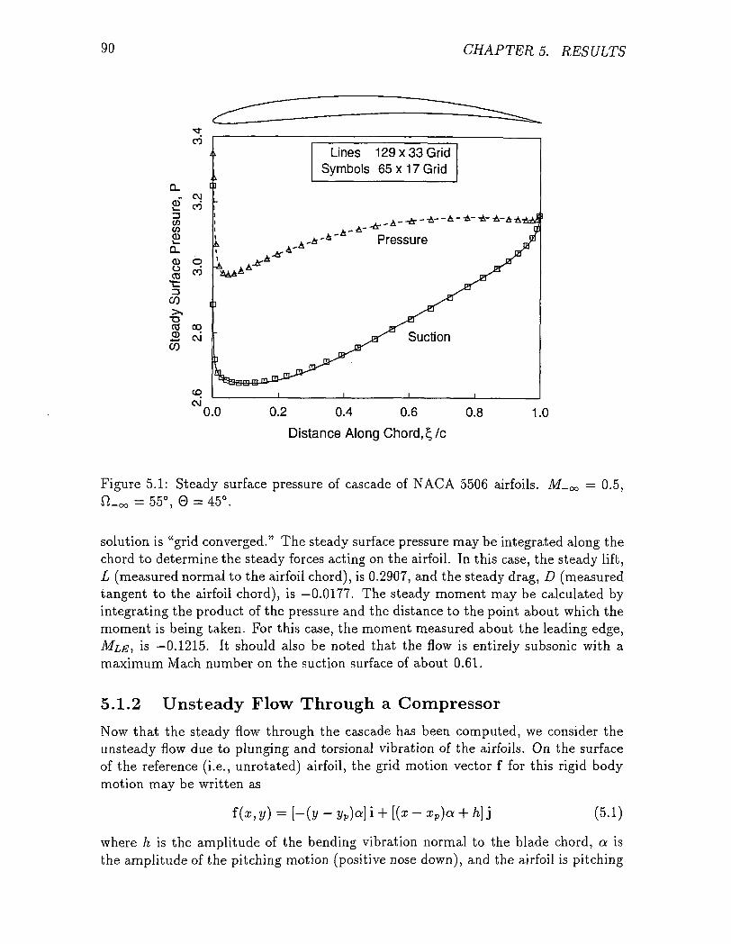
90 CHAPTERS. RESULTS
Lines 129x33 GridSymbols 65x17 Grid
0.2 0.4 0.6
Distance Along Chord,
Figure 5.1: Steady surface pressure of cascade of NACA 5506 airfoils. M_oo = 0.5,ft-oo = 55°, 0 = 45°.
solution is "grid converged." The steady surface pressure may be integrated along thechord to determine the steady forces acting on the airfoil. In this case, the steady lift,L (measured normal to the airfoil chord), is 0.2907, and the steady drag, D (measuredtangent to the airfoil chord), is —0.0177. The steady moment may be calculated byintegrating the product of the pressure and the distance to the point about which themoment is being taken. For this case, the moment measured about the leading edge,MLE, is —0.1215. It should also be noted that the flow is entirely subsonic with amaximum Mach number on the suction surface of about 0.61.
5.1.2 Unsteady Flow Through a Compressor
Now that the steady flow through the cascade has been computed, we consider theunsteady flow due to plunging and torsional vibration of the airfoils. On the surfaceof the reference (i.e., unrotated) airfoil, the grid motion vector f for this rigid bodymotion may be written as
f (z, y) = [-(y- yp)a] i + [(z - xp)a + h] j (5.1)
where h is the amplitude of the bending vibration normal to the blade chord, a isthe amplitude of the pitching motion (positive nose down), and the airfoil is pitching
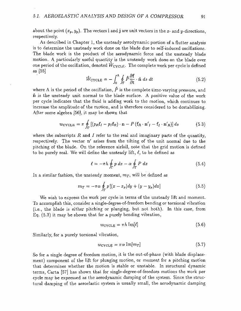
5.1. AEROELASTIC ANALYSIS AND DESIGN OF A COMPRESSOR 91
about the point (xp, j/p). The vectors i and j are unit vectors in the x- and y-directions,respectively.
As described in Chapter 1, the unsteady aerodynamic portion of a flutter analysisis to determine the unsteady work done on the blade due to self-induced oscillations.The blade work is the product of the aerodynamic force and the unsteady blademotion. A particularly useful quantity is the unsteady work done on the blade overone period of the oscillation, denoted WCYCLE- The complete work per cycle is definedas [55]
rA r - <9fW^^-l^P-.Adsdt (5.2)
where A is the period of the oscillation, P is the complete time-varying pressure, andn is the unsteady unit normal to the blade surface. A positive value of the workper cycle indicates that the fluid is adding work to the motion, which continues toincrease the amplitude of the motion, and is therefore considered to be destabilizing.After some algebra [56], it may be shown that
[(pRfi - pifR) • n - P (fR • n'/ - f/ • n'R)] ds (5.3)
where the subscripts R and I refer to the real and imaginary parts of the quantity,respectively. The vector n' arises from the tilting of the unit normal due to thepitching of the blade. On the reference airfoil, note that the grid motion is definedto be purely real. We will define the unsteady lift, I, to be defined as
i = —irh <p p dx — a <p P dx (5.4)Jr Jr
In a similar fashion, the unsteady moment, my, will be defined as
mT = -ira i p [(x - xp)dy + (y - yp)dx] (5.5)./r
We wish to express the work per cycle in terms of the unsteady lift and moment.To accomplish this, consider a single-degree-of-freedom bending or torsional vibration(i.e., the blade is either pitching or plunging, but not both). In this case, fromEq. (5.3) it may be shown that for a purely bending vibration,
WCYCLE = nh lm[l] (5.6)
Similarly, for a purely torsional vibration,
WCYCLE = T« Im[mr] (5.7)
So for a single degree of freedom motion, it is the out-of-phase (with blade displace-ment) component of the lift for plunging motion, or moment for a pitching motionthat determines whether the motion is stable or unstable. In structural dynamicterms, Carta [57] has shown that for single-degree-of-freedom motions the work percycle may be expressed as the aerodynamic damping of the system. Since the struc-tural damping of the aeroelastic system is usually small, the aerodynamic damping
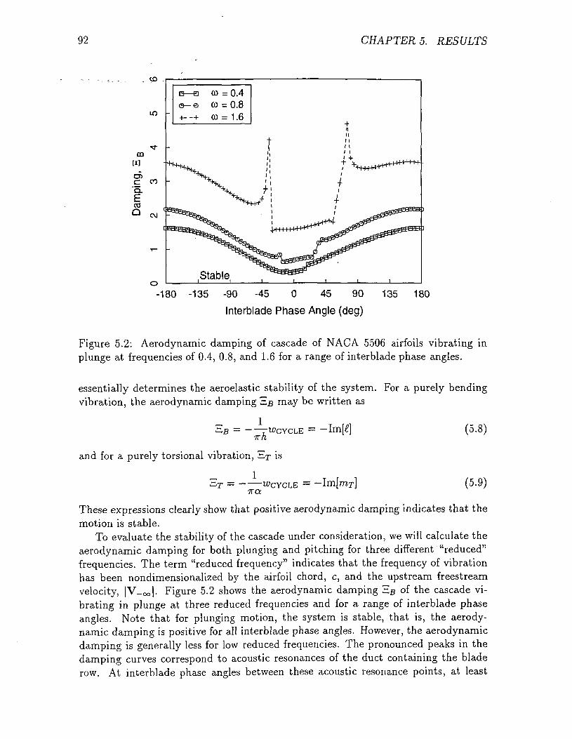
92 CHAPTER 5. RESULTS
m[i]05c'a.
03a
CO
cvj -
-180 -135 -90 -45 0 45 90
Interblade Phase Angle (deg)
135 180
Figure 5.2: Aerodynamic damping of cascade of NACA 5506 airfoils vibrating inplunge at frequencies of 0.4, 0.8, and 1.6 for a range of interblade phase angles.
essentially determines the aeroelastic stability of the system. For a purely bendingvibration, the aerodynamic damping EB may be written as
.*"* p ^~^ TTTfl
and for a purely torsional vibration, ^T is
17TO:
(5.8)
(5.9)
These expressions clearly show that positive aerodynamic damping indicates that themotion is stable.
To evaluate the stability of the cascade under consideration, we will calculate theaerodynamic damping for both plunging and pitching for three different "reduced"frequencies. The term "reduced frequency" indicates that the frequency of vibrationhas been nondimensionalized by the airfoil chord, c, and the upstream freestreamvelocity, |V_oo|. Figure 5.2 shows the aerodynamic damping EB of the cascade vi-brating in plunge at three reduced frequencies and for a range of interblade phaseangles. Note that for plunging motion, the system is stable, that is, the aerody-namic damping is positive for all interblade phase angles. However, the aerodynamicdamping is generally less for low reduced frequencies. The pronounced peaks in thedamping curves correspond to acoustic resonances of the duct containing the bladerow. At interblade phase angles between these acoustic resonance points, at least
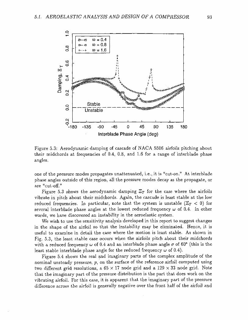
5.1. AEROELASTIC ANALYSIS AND DESIGN OF A COMPRESSOR 93
09—E3 0) = 0.4
o-e (0 = 0.8+--+ 00 = 1.6
CM
'-180 -135 -90 -45 0 45 90
Interblade Phase Angle (deg)
135 180
Figure 5.3: Aerodynamic damping of cascade of NACA 5506 airfoils pitching abouttheir midchords at frequencies of 0.4, 0.8, and 1.6 for a range of interblade phaseangles.
one of the pressure modes propagates unattenuated, i.e., it is "cut-on." At interbladephase angles outside of this region, all the pressure modes decay as the propagate, orare "cut-off."
Figure 5.3 shows the aerodynamic damping ET for the case where the airfoilsvibrate in pitch about their midchords. Again, the cascade is least stable at the lowreduced frequencies. In particular, note that the system is unstable (E/r < 0) forseveral interblade phase angles at the lowest reduced frequency u> of 0.4. In otherwords, we have discovered an instability in the aeroelastic system.
We wish to use the sensitivity analysis developed in this report to suggest changesin the shape of the airfoil so that the instability may be eliminated. Hence, it isuseful to examine in detail the case where the motion is least stable. As shown inFig. 5.3, the least stable case occurs when the airfoils pitch about their midchordswith a reduced frequency u> of 0.4 and an interblade phase angle a of 60° (this is theleast stable interblade phase angle for the reduced frequency u of 0.4).
Figure 5.4 shows the real and imaginary parts of the complex amplitude of thenominal unsteady pressure, p, on the surface of the reference airfoil computed usingtwo different grid resolutions, a 65 x 17 node grid and a 129 x 33 node grid. Notethat the imaginary part of the pressure distribution is the part that does work on thevibrating airfoil. For this case, it is apparent that the imaginary part of the pressuredifference across the airfoil is generally negative over the front half of the airfoil and
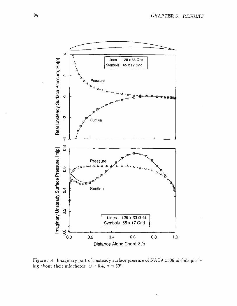
94 CHAPTERS. RESULTS
Q.
CDGC
It/3COCD
CDOCO
CO
0303
"coCDo:
COc'O3CO
cvj
CJ
Lines 129x33 GridSymbols 65x17 Grid
qC)
Lines 129x33 GridSymbols 65 x 17 Grid
"0.0 0.2 0.4 0.6
Distance Along Chord,1
0.8 1.0
Figure 5.4: Imaginary part of unsteady surface pressure of NACA 5506 airfoils pitch-ing about their midchords. u = 0.4, a = 60°.
5.1. AEROELASTIC ANALYSIS AND DESIGN OF A COMPRESSOR 95
positive over the aft half. Thus, since the airfoil pitches about its midchord (positivenose up), the unsteady pressure does positive aerodynamic work (corresponding tonegative aerodynamic damping) on the airfoil over most of the airfoil, making thecascade unstable in pitch for these conditions.
5.1.3 Sensitivity Analysis
Having computed the nominal flow through the cascade, the effect of five differentdesign parameters on the steady flowfield will now be studied. Two of these pa-rameters are from the NACA four digit airfoil definition, i.e., the magnitudes of theairfoil thickness and camber. (See Appendix B for a discussion of the NACA airfoildefinition.) Each of these quantities are measured in fractions of the airfoil chord c.Also considered are the effect of changes in the cascade stagger angle 6, and blade-to-blade gap G. Finally, an additional design variable, the reflex, is introduced here.The reflex parameter modifies the height of the mean line
hm = hc + rcsin(27r£/c) (5.10)
where hm is the height of the mean line, hc is the height of the mean line due tocamber, r is the magnitude of the reflex in fractions of chord, c is the chord, and £ isthe distance along the airfoil chord. Reflex has been added to provide an "S shape"parameter to the design, to allow more flexibility in the airfoil shape than the strictNACA definition.
Figure 5.5 shows the sensitivity of the steady surface pressure to changes in thesefive geometry variables. The sensitivities are computed using the present sensitivityanalysis; all results were computed on a 65 x 17 node grid. To check these results, thesensitivities using a finite difference approach are also computed. The finite-differenceresult is computed by solving for the steady flow about two slightly different airfoils,differencing the two solutions, and dividing the result by the difference in the airfoilparameter. Note the excellent agreement between the two solutions indicating thatthe effect of small changes in the design variables is linear, and that the presentsensitivity analysis correctly predicts the sensitivities. Also, not surprisingly, thelargest sensitivity in pressure occurs near the leading edge of the airfoil.
Next, the surface pressure sensitivities were integrated to obtain the sensitivity ofthe steady lift and drag (measured normal to and along the chord) and the momentabout the leading edge. These results are given in Table 5.1. The sensitivity tochanges in maximum camber location is also shown. In addition, the sensitivity ofthe lift in the y-direction (the cascade direction) is tabulated. The steady lift in the2/-direction is a measure of the turning done by the cascade and hence is related to thesteady work done by the cascade. Table 5.1 shows that the lift in the ^-direction ismost sensitive to changes in camber, stagger angle, and reflex. Since these parameterscontrol the metal angle of the trailing edge, and the deviation between the exit flowangle and the metal angle is small for cascades, one would expect them to have astrong influence on the steady lift.
Next, the sensitivities of the unsteady surface pressure to changes in geometry arecomputed. Figures 5.6 and 5.7 show the real and imaginary parts, respectively, of
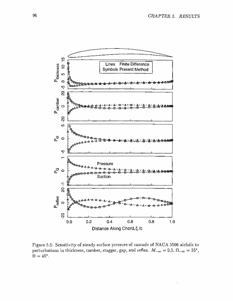
96 CHAPTER 5. RESULTS
Lines Finite DifferenceSymbols Present Method
- A- A- A- A- -A- -A- -A- - A- -A - A- A- A-
0.2 0.4 0.6
Distance Along Chord,
Figure 5.5: Sensitivity of steady surface pressure of cascade of NACA 5506 airfoils toperturbations in thickness, camber, stagger, gap, and reflex. M_oo = 0.5, fi_oo = 55°,0 = 45°.
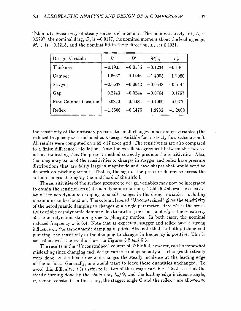
5.1. AEROELASTIC ANALYSIS AND DESIGN OF A COMPRESSOR 97
Table 5.1: Sensitivity of steady forces and moment. The nominal steady lift, L, is0.2907, the nominal drag, D, is —0.0177, the nominal moment about the leading edge,
, is —0.1215, and the nominal lift in the ^/-direction, Ly, is 0.1931.
Design Variable
Thickness
Camber
Stagger
Gap
Max Camber Location
Reflex
-0
1
-0
0
0
-1
L1
.1935
.5637
.6632
2743
0873
.5506
-0
0
-0
-0
0
-0
D1
.0135
.1446
.0642
.0244
.0083
.1476
A
-0
-1
-0
-0
-0
1
f'LE
.1234
.4003
.0548
.0764
.1060
9235
L'y
-0.1464
1.2080
-0.5144
0.1767
0.0676
-1.2008
the sensitivity of the unsteady pressure to small changes in six design variables (thereduced frequency-u is included as a design variable for unsteady flow calculations).All results were computed on a 65 x 17 node grid. The sensitivities are also comparedto a finite difference calculation. Note the excellent agreement between the two so-lutions indicating that the present method correctly predicts the sensitivities. Also,the imaginary parts of the sensitivities to changes in stagger and reflex have pressuredistributions that are fairly large in magnitude and have shapes that would tend todo work on pitching airfoils. That is, the sign of the pressure difference across theairfoil changes at roughly the midchord of the airfoil.
The sensitivities of the surface pressure to design variables may now be integratedto obtain the sensitivities of the aerodynamic damping. Table 5.2 shows the sensitiv-ity of the aerodynamic damping to small changes in the design variables, includingmaximum camber location. The column labeled "Unconstrained" gives the sensitivityof the aerodynamic damping to changes in a single parameter. Here E'x is the sensi-tivity of the aerodynamic damping due to pitching motions, and E'# is the sensitivityof the aerodynamic damping due to plunging motion. In both cases, the nominalreduced frequency u is 0.4. Note that as expected, stagger and reflex have a stronginfluence on the aerodynamic damping in pitch. Also note that for both pitching andplunging, the sensitivity of the damping to changes in frequency is positive. This isconsistent with the results shown in Figures 5.2 and 5.3.
The results in the "Unconstrained" column of Table 5.2, however, can be somewhatmisleading since changing each design variable independently also changes the steadywork done by the blade row and changes the steady incidence at the leading edgeof the airfoils. Generally, one would want to leave these quantities unchanged. Toavoid this difficulty, it is useful to let two of the design variables "float" so that thesteady turning done by the blade row, Ly/G, and the leading edge incidence angle,a, remain constant. In this study, the stagger angle 0 and the reflex r are allowed to
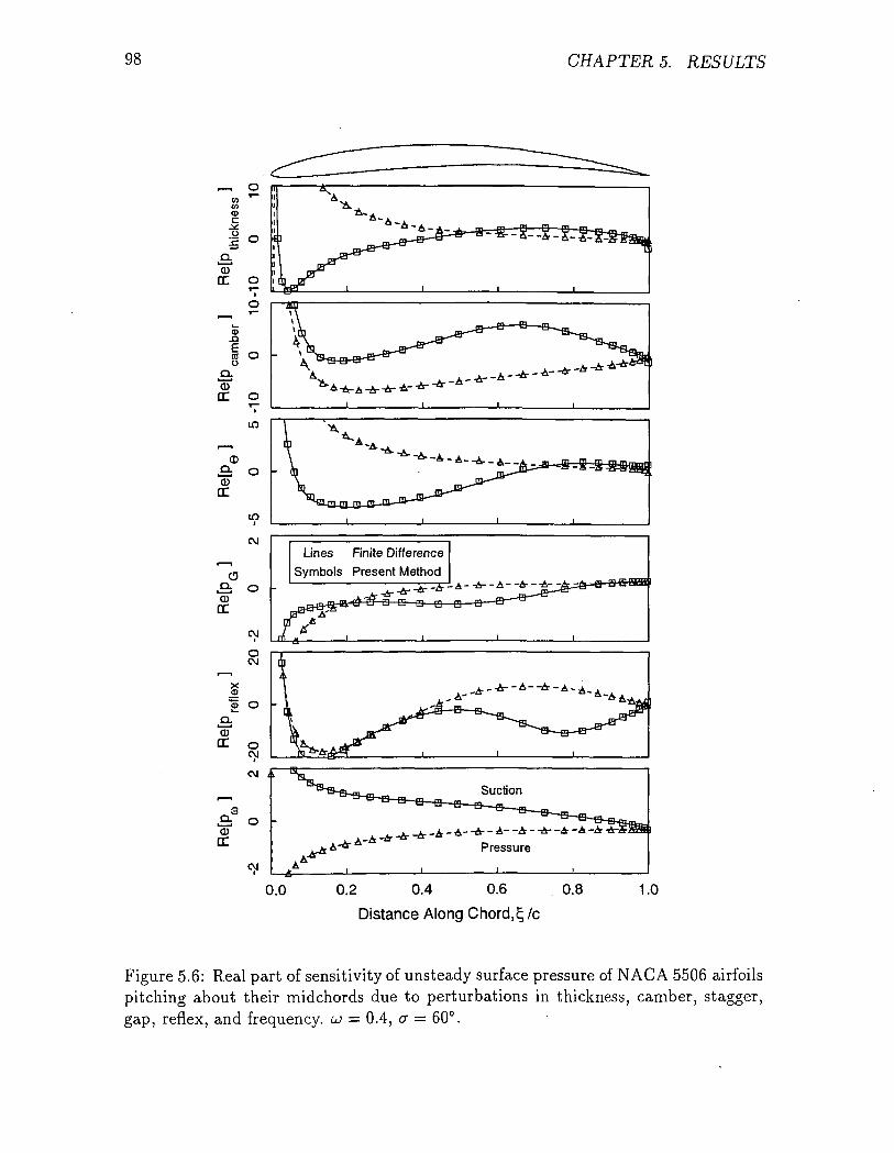
98 CHAPTERS. RESULTS
r-, O
(ft T~inoc
±L
CL
CDDC O
T—I
O
IDXI
03DC O
I
in
<D£: O(U
DC
up
CM
O
CDDC
CM
OCM
X<OCD O
a.CO
DC<vCM
£: O0)
DC
CM
Lines Finite Difference
Symbols Present Method
Suction
-A-A--A--A--A--A--A-A-
Pressure
0.0 0.2 0.4 0.6 0.8
Distance Along Chord,cj/c1.0
Figure 5.6: Real part of sensitivity of unsteady surface pressure of NACA 5506 airfoilspitching about their midchords due to perturbations in thickness, camber, stagger,gap, reflex, and frequency. u> = 0.4, cr = 60°.
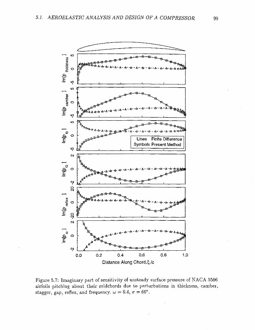
5.1. AEROELASTIC ANALYSIS AND DESIGN OF A COMPRESSOR 99
-a—a—B-
- A- A- -A- -A- - A- -A- - •&- -A - A- -A- A-A A
— in
=Zt - A - -A- - A - -A- - -A- -A- -A -A- -&-A-A
Lines Finite DifferenceSymbols Present Method
-A- -A- -A- - A- -A- - -A- -A- -A -A- -A
0.0 0.2 0.4 0.6
Distance Along Chord,
0.8 1.0
Figure 5.7: Imaginary part of sensitivity of unsteady surface pressure of NACA 5506airfoils pitching about their midchords due to perturbations in thickness, camber,stagger, gap, reflex, and frequency, u = 0.4, a = 60°.
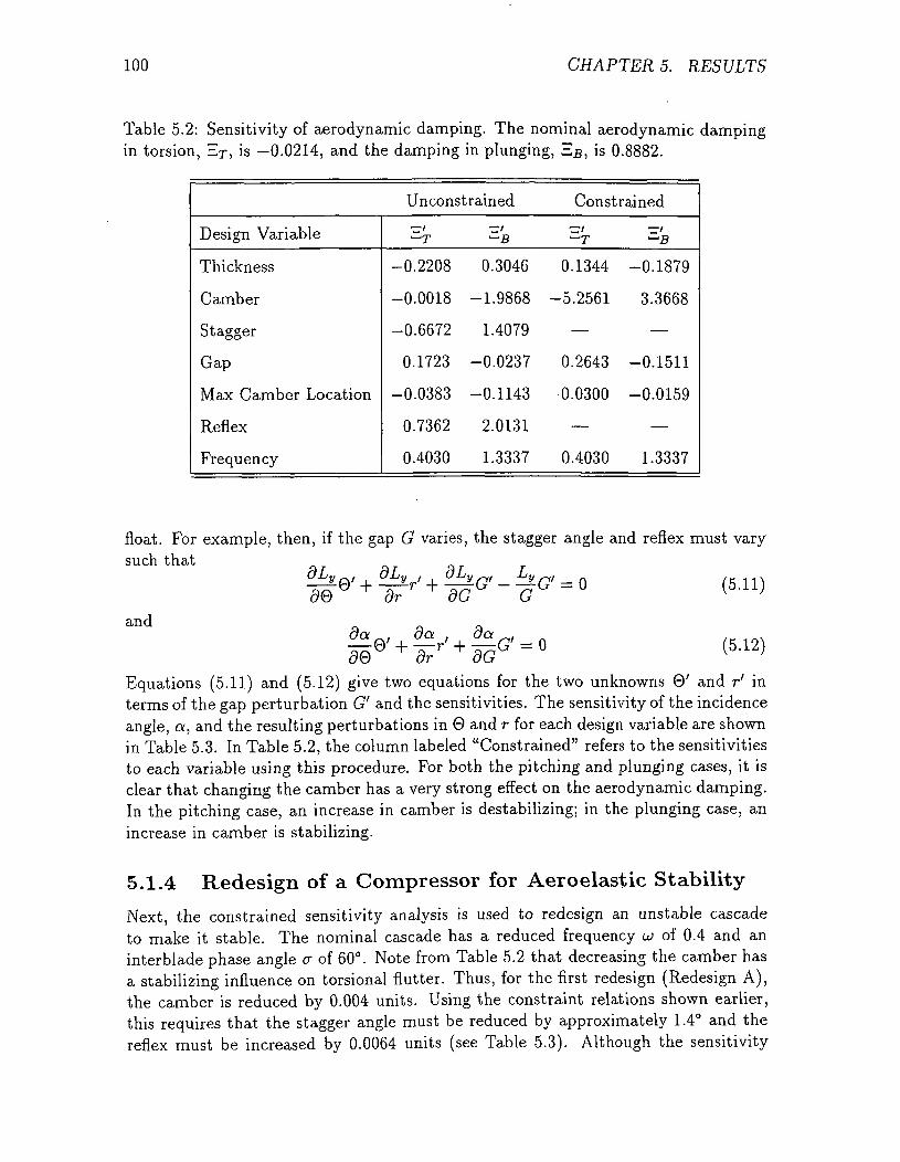
100 CHAPTERS. RESULTS
Table 5.2: Sensitivity of aerodynamic damping. The nominal aerodynamic dampingin torsion, ET, is —0.0214, and the damping in plunging, E#, is 0.8882.
Unconstrained
Design Variable
Thickness
Camber
Stagger
Gap
Max Camber Location
Reflex
Frequency
^7/
— T
-0.2208
-0.0018
-0.6672
0.1723
-0.0383
0.7362
0.4030
77'. O
0.3046
-1.9868
1.4079
-0.0237
-0.1143
2.0131
1.3337
Constrained
™'— T
0.1344
-5.2561
—
0.2643
0.0300
—
0.4030
— /. n
-0.1879
3.3668
—
-0.1511
-0.0159
—
1.3337
float. For example, then, if the gap G varies, the stagger angle and reflex must varysuch that
OLV ^, OLu I . OLy^f Ly ̂ , . .
> -—G =0 (5.11)
and
oG(5.12)
Equations (5.11) and (5.12) give two equations for the two unknowns 0' and r' interms of the gap perturbation G' and the sensitivities. The sensitivity of the incidenceangle, a, and the resulting perturbations in 0 and r for each design variable are shownin Table 5.3. In Table 5.2, the column labeled "Constrained" refers to the sensitivitiesto each variable using this procedure. For both the pitching and plunging cases, it isclear that changing the camber has a very strong effect on the aerodynamic damping.In the pitching case, an increase in camber is destabilizing; in the plunging case, anincrease in camber is stabilizing.
5.1.4 Redesign of a Compressor for Aeroelastic Stability
Next, the constrained sensitivity analysis is used to redesign an unstable cascadeto make it stable. The nominal cascade has a reduced frequency u of 0.4 and aninterblade phase angle a of 60°. Note from Table 5.2 that decreasing the camber hasa stabilizing influence on torsional flutter. Thus, for the first redesign (Redesign A),the camber is reduced by 0.004 units. Using the constraint relations shown earlier,this requires that the stagger angle must be reduced by approximately 1.4° and thereflex must be increased by 0.0064 units (see Table 5.3). Although the sensitivity
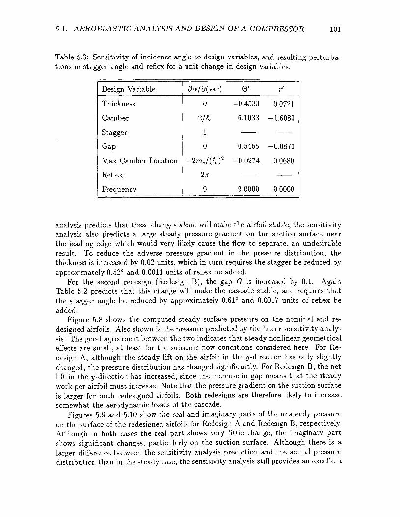
5.1. AEROELASTIC ANALYSIS AND DESIGN OF A COMPRESSOR 101
Table 5.3: Sensitivity of incidence angle to design variables, and resulting perturba-tions in stagger angle and reflex for a unit change in design variables.
Design Variable
Thickness
Camber
Stagger
Gap
Max Camber Location
Reflex
Frequency
da/d(var)
0
2/4
1
0
-2mc/(4)2
2?r
0
0'
-0.4533
6.1033
0.5465
-0.0274
0.0000
r'
0.0721
-1.6080
-0.0870
0.0680
0.0000
analysis predicts that these changes alone will make the airfoil stable, the sensitivityanalysis also predicts a large steady pressure gradient on the suction surface nearthe leading edge which would very likely cause the flow to separate, an undesirableresult. To reduce the adverse pressure gradient in the pressure distribution, thethickness is increased by 0.02 units, which in turn requires the stagger be reduced byapproximately 0.52° and 0.0014 units of reflex be added.
For the second redesign (Redesign B), the gap G is increased by 0.1. AgainTable 5.2 predicts that this change will make the cascade stable, and requires thatthe stagger angle be reduced by approximately 0.61° and 0.0017 units of reflex beadded.
Figure 5.8 shows the computed steady surface pressure on the nominal and re-designed airfoils. Also shown is the pressure predicted by the linear sensitivity analy-sis. The good agreement between the two indicates that steady nonlinear geometricaleffects are small, at least for the subsonic flow conditions considered here. For Re-design A, although the steady lift on the airfoil in the y-direction has only slightlychanged, the pressure distribution has changed significantly. For Redesign B, the netlift in the y-direction has increased, since the increase in gap means that the steadywork per airfoil must increase. Note that the pressure gradient on the suction surfaceis larger for both redesigned airfoils. Both redesigns are therefore likely to increasesomewhat the aerodynamic losses of the cascade.
Figures 5.9 and 5.10 show the real and imaginary parts of the unsteady pressureon the surface of the redesigned airfoils for Redesign A and Redesign B, respectively.Although in both cases the real part shows very little change, the imaginary partshows significant changes, particularly on the suction surface. Although there is alarger difference between the sensitivity analysis prediction and the actual pressuredistribution than in the steady case, the sensitivity analysis still provides an excellent
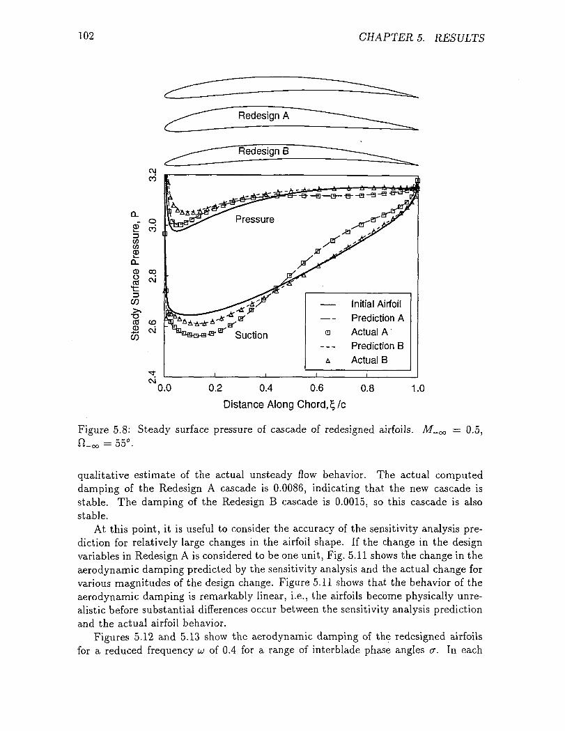
102 CHAPTERS. RESULTS
Initial AirfoilPrediction AActual APrediction B
Actual B
CM0.2 0.4 0.6
Distance Along Chord,
Figure 5.8: Steady surface pressure of cascade of redesigned airfoils. M-c
ft-oo = 55°.= 0.5,
qualitative estimate of the actual unsteady flow behavior. The actual computeddamping of the Redesign A cascade is 0.0086, indicating that the new cascade isstable. The damping of the Redesign B cascade is 0.0015, so this cascade is alsostable.
At this point, it is useful to consider the accuracy of the sensitivity analysis pre-diction for relatively large changes in the airfoil shape. If the change in the designvariables in Redesign A is considered to be one unit, Fig. 5.11 shows the change in theaerodynamic damping predicted by the sensitivity analysis and the actual change forvarious magnitudes of the design change. Figure 5.11 shows that the behavior of theaerodynamic damping is remarkably linear, i.e., the airfoils become physically unre-alistic before substantial differences occur between the sensitivity analysis predictionand the actual airfoil behavior.
Figures 5.12 and 5.13 show the aerodynamic damping of the redesigned airfoilsfor a reduced frequency u of 0.4 for a range of interblade phase angles a. In each
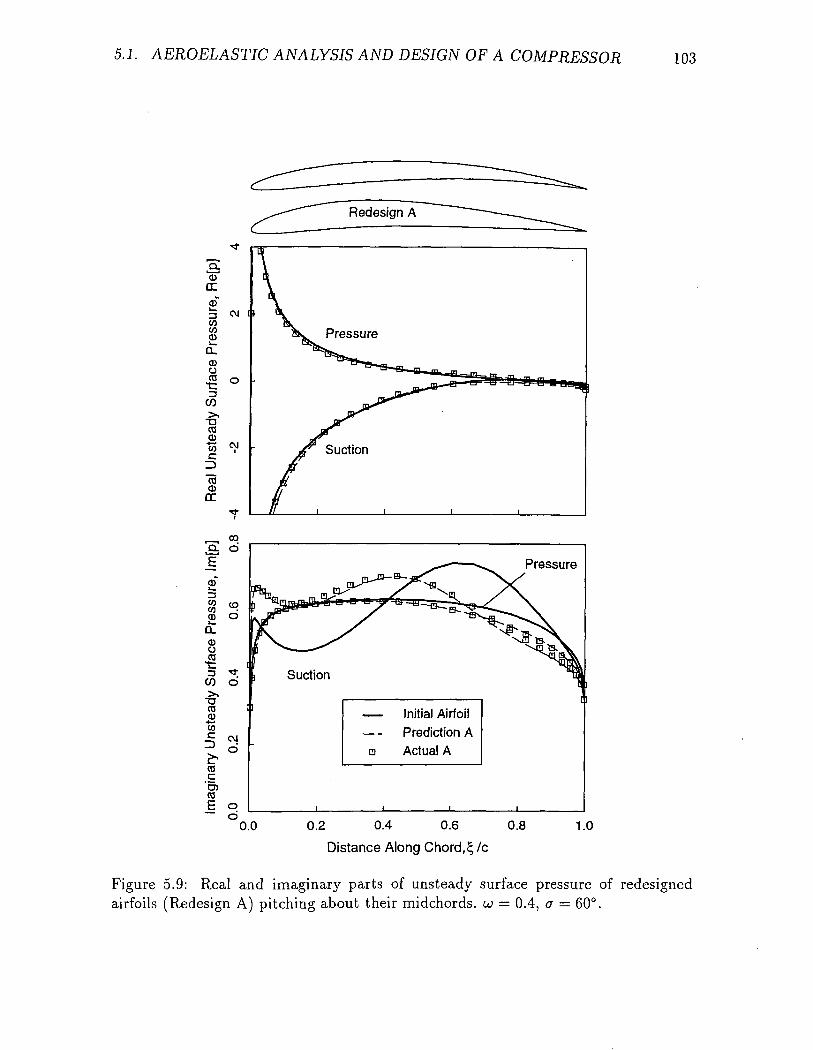
5.1. AEROELASTIC ANALYSIS AND DESIGN OF A COMPRESSOR 103
co c&COC pj
?. °£•CO.c
COE o
i
•
— Initial Airfoil— Prediction Aa Actual A
L
i i i i
0.0 0.2 0.4 0.6 0.8
Distance Along Chord,<; /c
1.0
Figure 5.9: Real and imaginary parts of unsteady surface pressure of redesignedairfoils (Redesign A) pitching about their midchords. u> = 0.4, a = 60°.
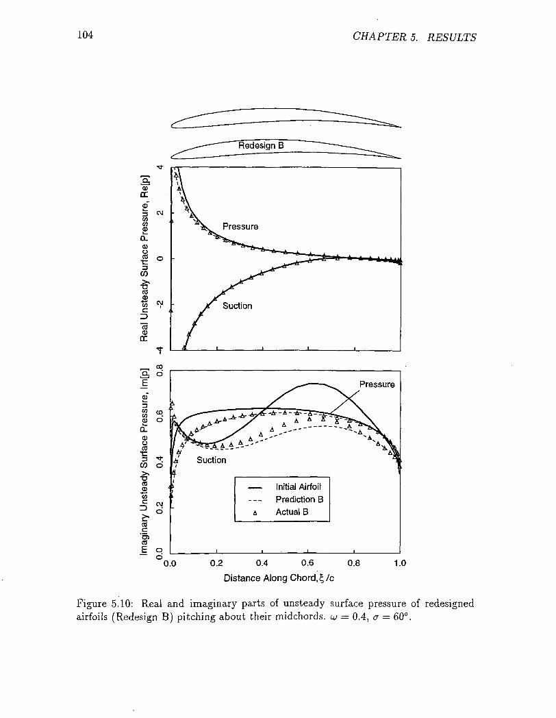
104 CHAPTER 5. RESULTS
0)ccof
WwCO
CL0
t:3
CO
CO
"(0CDo:
t0)*-•05
I3CO
'o>co
1I — Initial Airfoil
— Predictions^ Actual B
i i0.0 0.2 0.4 0.6 0.8
Distance Along Chord, 4 /c
1.0
Figure 5.10: Real and imaginary parts of unsteady surface pressure of redesignedairfoils (Redesign B) pitching about their midchords. u = 0.4, a = 60°.
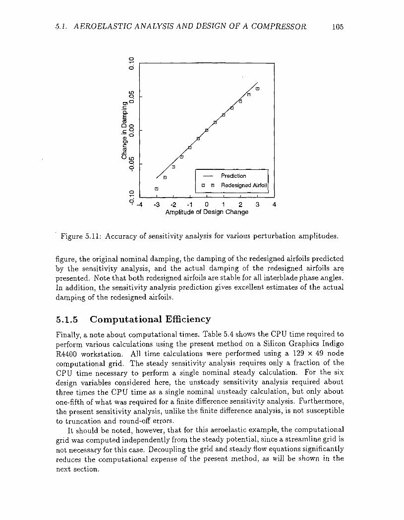
5.1. AEROELASTIC ANALYSIS AND DESIGN OF A COMPRESSOR 105
o
d
inp0)0c'a.toQ o
D)
qo'
oi™d
Prediction
a a Redesigned Airfoil
- 3 - 2 - 1 0 1 2 3Amplitude of Design Change
Figure 5.11: Accuracy of sensitivity analysis for various perturbation amplitudes.
figure, the original nominal damping, the damping of the redesigned airfoils predictedby the sensitivity analysis, and the actual damping of the redesigned airfoils arepresented. Note that both redesigned airfoils are stable for all interblade phase angles.In addition, the sensitivity analysis prediction gives excellent estimates of the actualdamping of the redesigned airfoils.
5.1.5 Computational Efficiency
Finally, a note about computational times. Table 5.4 shows the CPU time required toperform various calculations using the present method on a Silicon Graphics IndigoR4400 workstation. All time calculations were performed using a 129 x 49 nodecomputational grid. The steady sensitivity analysis requires only a fraction of theCPU time necessary to perform a single nominal steady calculation. For the sixdesign variables considered here, the unsteady sensitivity analysis required aboutthree times the CPU time as a single nominal unsteady calculation, but only aboutone-fifth of what was required for a finite difference sensitivity analysis. Furthermore,the present sensitivity analysis, unlike the finite difference analysis, is not susceptibleto truncation and round-off errors.
It should be noted, however, that for this aeroelastic example, the computationalgrid was computed independently from the steady potential, since a streamline grid isnot necessary for this case. Decoupling the grid and steady flow equations significantlyreduces the computational expense of the present method, as will be shown in thenext section.
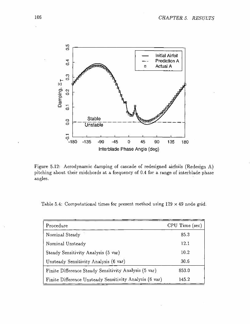
106 CHAPTERS. RESULTS
'-180 -135 -90 -45 0 45 90
Interblade Phase Angle (deg)
135 180
Figure 5.12: Aerodynamic damping of cascade of redesigned airfoils (Redesign A)pitching about their midchords at a frequency of 0.4 for a range of interblade phaseangles.
Table 5.4: Computational times for present method using 129 x 49 node grid.
Procedure CPU Time (sec)
Nominal Steady
Nominal Unsteady
Steady Sensitivity Analysis (5 var)
Unsteady Sensitivity Analysis (6 var)
85.3
12.1
10.2
30.6
Finite Difference Steady Sensitivity Analysis (5 var) 853.0
Finite Difference Unsteady Sensitivity Analysis (6 var) 145.2
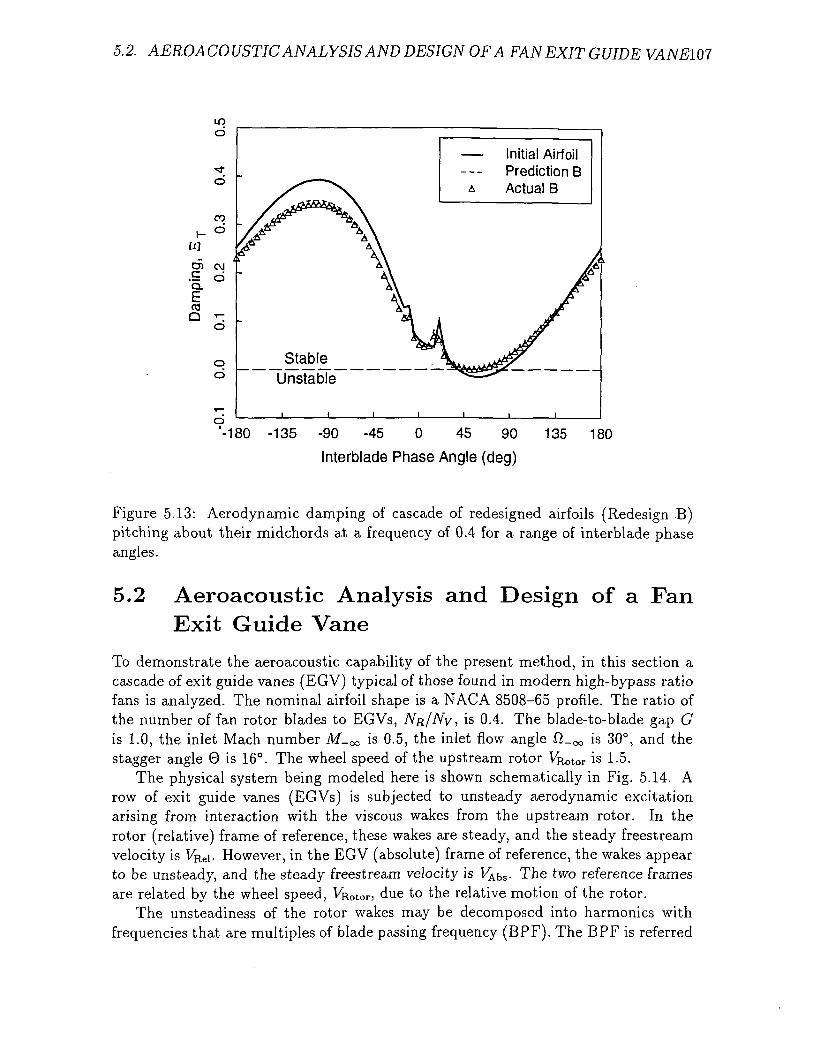
5.2. AERO A CO USTIC ANALYSIS AND DESIGN OF A FAN EXIT G UIDE VANE107
ino
— Initial Airfoil— Prediction B
Actual B
_Stable_Unstable
o'-180 -135 -90 -45 0 45 90
Interblade Phase Angle (deg)
135 180
Figure 5.13: Aerodynamic damping of cascade of redesigned airfoils (Redesign B)pitching about their midchords at a frequency of 0.4 for a range of interblade phaseangles.
5.2 Aeroacoustic Analysis and Design of a FanExit Guide Vane
To demonstrate the aeroacoustic capability of the present method, in this section acascade of exit guide vanes (EGV) typical of those found in modern high-bypass ratiofans is analyzed. The nominal airfoil shape is a NACA 8508-65 profile. The ratio ofthe number of fan rotor blades to EGVs, NR/NV, is 0.4. The blade-to-blade gap Gis 1.0, the inlet Mach number M-^ is 0.5, the inlet flow angle Sl-.̂ is 30°, and thestagger angle 0 is 16°. The wheel speed of the upstream rotor VR.otor is 1.5.
The physical system being modeled here is shown schematically in Fig. 5.14. Arow of exit guide vanes (EGVs) is subjected to unsteady aerodynamic excitationarising from interaction with the viscous wakes from the upstream rotor. In therotor (relative) frame of reference, these wakes are steady, and the steady freestreamvelocity is VRei- However, in the EGV (absolute) frame of reference, the wakes appearto be unsteady, and the steady freestream velocity is VABS- The two reference framesare related by the wheel speed, VRot0r, due to the relative motion of the rotor.
The unsteadiness of the rotor wakes may be decomposed into harmonics withfrequencies that are multiples of blade passing frequency (BPF). The BPF is referred
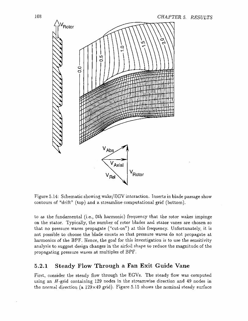
108 CHAPTERS. RESULTS
'Rotor
VRel Rotor
Figure 5.14: Schematic showing wake/EGV interaction. Inserts in blade passage showcontours of "drift" (top) and a streamline computational grid (bottom).
to as the fundamental (i.e., Oth harmonic) frequency that the rotor wakes impingeon the stator. Typically, the number of rotor blades and stator vanes are chosen sothat no pressure waves propagate ("cut-on") at this frequency. Unfortunately, it isnot possible to choose the blade counts so that pressure waves do not propagate atharmonics of the BPF. Hence, the goal for this investigation is to use the sensitivityanalysis to suggest design changes in the airfoil shape to reduce the magnitude of thepropagating pressure waves at multiples of BPF.
5.2.1 Steady Flow Through a Fan Exit Guide Vane
First, consider the steady flow through the EGVs. The steady flow was computedusing an //-grid containing 129 nodes in the streamwise direction and 49 nodes inthe normal direction (a 129x49 grid). Figure 5.15 shows the nominal steady surface
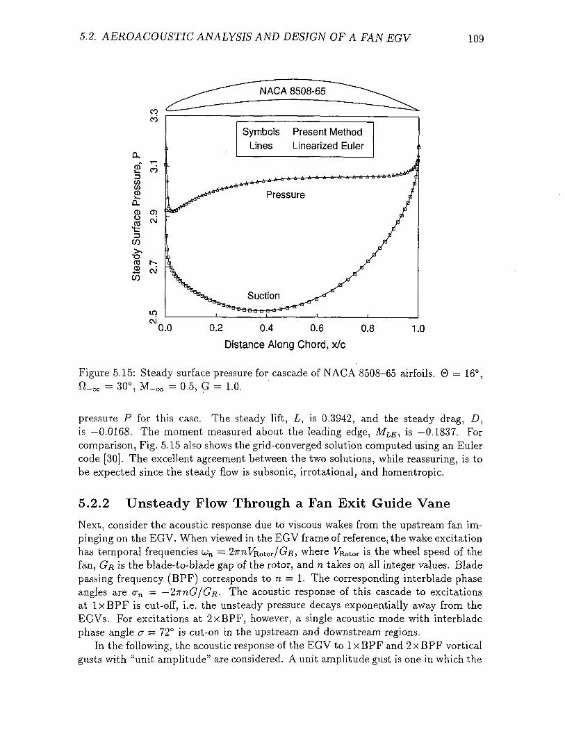
5.2. AEROACOUSTIC ANALYSIS AND DESIGN OF A FAN EGV 109
0.
I
CO
CO
CO -Symbols
LinesPresent MethodLinearized Euler
^Mr̂ A *̂!
0.2 0.4 0.6 0.8
Distance Along Chord, x/c
1.0
Figure 5.15: Steady surface pressure for cascade of NACA 8508-65 airfoils. 0 = 16°,n.^ = 30°, M_oo = 0.5, G = 1.0.
pressure P for this case. The steady lift, L, is 0.3942, and the steady drag, D,is —0.0168. The moment measured about the leading edge, MLE, is —0.1837. Forcomparison, Fig. 5.15 also shows the grid-converged solution computed using an Eulercode [30]. The excellent agreement between the two solutions, while reassuring, is tobe expected since the steady flow is subsonic, irrotational, and homentropic.
5.2.2 Unsteady Flow Through a Fan Exit Guide Vane
Next, consider the acoustic response due to viscous wakes from the upstream fan im-pinging on the EGV. When viewed in the EGV frame of reference, the wake excitationhas temporal frequencies u>n = 27rnVR.otor/GrR, where VRot0r is the wheel speed of thefan, GR is the blade-to-blade gap of the rotor, and n takes on all integer values. Bladepassing frequency (BPF) corresponds to n = 1. The corresponding interblade phaseangles are crn = —2^nG/GR. The acoustic response of this cascade to excitationsat IxBPF is cut-off, i.e. the unsteady pressure decays exponentially away from theEGVs. For excitations at 2xBPF, however, a single acoustic mode with interbladephase angle a = 72° is cut-on in the upstream and downstream regions.
In the following, the acoustic response of the EGV to IxBPF and 2xBPF vorticalgusts with "unit amplitude" are considered. A unit amplitude gust is one in which the
110 CHAPTERS. RESULTS
magnitude of the perturbation velocity normal to the steady flow direction would beunity at the leading edge of the airfoil if the steady flow were uniform and undeflectedby the EG V. The real and imaginary parts of the unsteady surface pressure computedusing the present analysis are shown in Figs. 5.16 and 5.17. Also shown for compari-son is the pressure distribution computed using the linearized Euler analysis of Halland Clark [30]. The agreement between these two theories is quite good, especiallyconsidering the high reduced frequency (u = 7.54) of the 2xBPF case. These resultsindicate that the 129x49 grid is sufficiently fine to resolve the acoustic behavior ofthe EGV — at least up to 2xBPF. They also indicate that the rotational velocityhas been formulated and computed correctly.
Figures 5.18 and 5.19 show contours of the magnitude of the unsteady pressurefor the IxBPF and 2xBPF cases, respectively. In both cases, note that the unsteadypressure is somewhat larger in the downstream region than in the upstream region.The unsteady pressure in the far field of the 2xBPF case was Fourier transformed inthe circumferential direction to determine the magnitude of the single cut-on pressurewave upstream and downstream (cr = 72°). For this case, the magnitude of the cut-on unsteady pressure wave (for a unit strength gust) is 0.102 upstream and 0.249downstream.
5.2.3 Sensitivity Analysis
Next, the change in the steady and unsteady aerodynamic response due to smallchanges in the EGV geometry is considered. The steady sensitivity analysis wasperformed using eight different design variables. Five of these variables correspondto the modified NACA definition parameters: magnitude of thickness, maximumthickness location, magnitude of camber, maximum camber location, and leadingedge radius. Two design variables define the placement of the airfoils in the cascade:the blade-to-blade gap G and stagger angle 0. The final design variable is the reflex,which was defined earlier.
Using the steady sensitivity analysis outlined in the previous section, the sensitiv-ity of the lift, drag, and moment to changes in the design variables were computed.These results are given in Table 5.5. Like the previous example, Table 5.5 showsthat the steady work is very sensitive to changes in camber, reflex, and stagger angle.This is not too surprising since these parameters affect the trailing edge metal angleof the airfoil and hence the turning (work). On the other hand, the steady work isinsensitive to changes in the maximum thickness location and the size of the leadingedge radius.
Next, the sensitivities of the unsteady pressure to small changes in the designvariables for the 2xBPF case were computed. In addition to the eight design vari-ables described above, the frequency u and interblade phase angle a of the excitationhave been added. Figures 5.20 and 5.21 show the real and imaginary parts, respec-tively, of the sensitivity of the unsteady surface pressure to changes in five of thesedesign variables. Also shown are the sensitivities calculated using a finite-differenceapproach, i.e. the difference of the pressures calculated using the nominal analysis ontwo slightly different airfoils normalized by the difference in geometry. The nearly
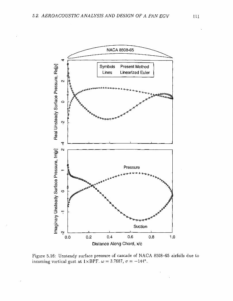
5.2. AERO ACOUSTIC ANALYSIS AND DESIGN OF A FAN EGV 111
Symbols Present Method
Lines Linearized Euler
0.2 0.4 0.6 0.8
Distance Along Chord, x/c
Figure 5.16: Unsteady surface pressure of cascade of NACA 8508-65 airfoils due toincoming vortical gust at IxBPF. u = 3.7687, a = -144°.
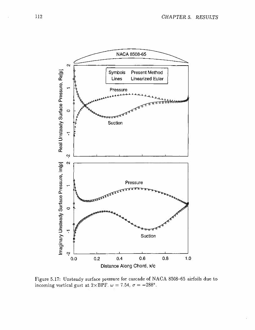
112 CHAPTER 5. RESULTS
CM
a.CDcr.
COCD
CDOCOt3
CO
73CO0)COc
"COCD
DC
a.E
toCOCD
CDOCOtlCO>«TJcCStoc
03
'D5CO
Symbols Present MethodLines Linearized Euler
O -
cvj
<N
O '-
0.0 0.2 0.4 0.6 0.8
Distance Along Chord, x/c
Figure 5.17: Unsteady surface pressure for cascade of NACA 8508-65 airfoils due toincoming vortical gust at 2xBPF. u = 7.54? a = —288°.
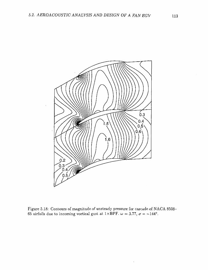
5.2. AEROACOVSTIC ANALYSIS AND DESIGN OF A FAN EGV 113
Figure 5.18: Contours of magnitude of unsteady pressure for cascade of NAG A 8508-65 airfoils due to incoming vortical gust at IxBPF. u> — 3.77, a = —144°.
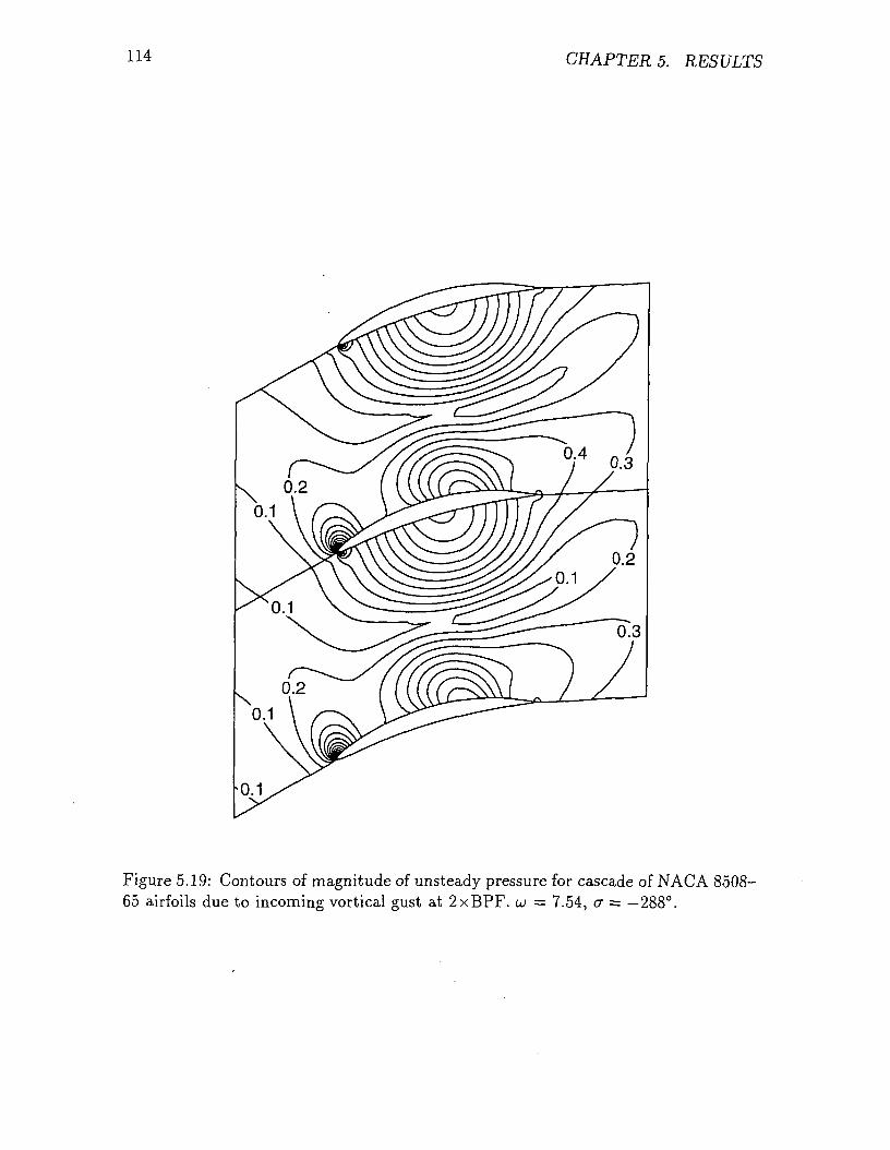
114 CHAPTERS. RESULTS
Figure 5.19: Contours of magnitude of unsteady pressure for cascade of NAG A 8508-65 airfoils due to incoming vortical gust at 2xBPF. u = 7.54, cr = —288°.
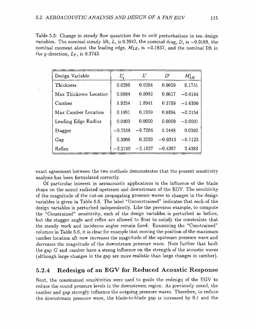
5.2. AEROACOUSTIC ANALYSIS AND DESIGN OF A FAN EGV 115
Table 5.5: Change in steady flow quantities due to unit perturbations in ten designvariables. The nominal steady lift, L, is 0.3942, the nominal drag, D, is —0.0168, thenominal moment about the leading edge, MLB, is —0.1837, and the nominal lift inthe ?/-direction, Ly, is 0.3743.
Design Variable
Thickness
Max Thickness Location
Camber
Max Camber Location
Leading Edge Radius
Stagger
Gap
Reflex
0
0
1
0
0
-0
0
-2
L'y
.0289
.0084
.9254
.1991
.0000
.7558
.3008
.2190
0
0
1
0
0
-0
0
-2
V
.0284
.0082
.8941
.1959
.0000
.7266
.3220
.1827
0
0
0
0
0
0
-0
-0
D'
.0059
.0017
.3799
.0394
.0000
.2448
.0313
.4387
A
0
-0
-1
-0
-0
0
-0
2
4'LE
.1751
.0164
.6300
.2154
.0001
.0392
.1123
.4383
exact agreement between the two methods demonstrates that the present sensitivityanalysis has been formulated correctly.
Of particular interest in aeroacoustic applications is the influence of the bladeshape on the sound radiated upstream and downstream of the EGV. The sensitivityof the magnitude of the cut-on propagating pressure waves to changes in the designvariables is given in Table 5.6. The label "Unconstrained" indicates that each of thedesign variables is perturbed independently. Like the previous example, to computethe "Constrained" sensitivity, each of the design variables is perturbed as before,but the stagger angle and reflex are allowed to float to satisfy the constraints thatthe steady work and incidence angles remain fixed. Examining the "Constrained"columns in Table 5.6, it is clear for example that moving the position of the maximumcamber location aft now increases the magnitude of the upstream pressure wave anddecreases the magnitude of the downstream pressure wave. Note further that boththe gap G and camber have a strong influence on the strength of the acoustic waves(although large changes in the gap are more realistic than large changes in camber).
5.2.4 Redesign of an EGV for Reduced Acoustic Response
Next, the constrained sensitivities were used to guide the redesign of the EGV toreduce the sound pressure levels in the downstream region. As previously noted, thecamber and gap strongly influence the outgoing pressure waves. Therefore, to reducethe downstream pressure wave, the blade-to-blade gap is increased by 0.1 and the
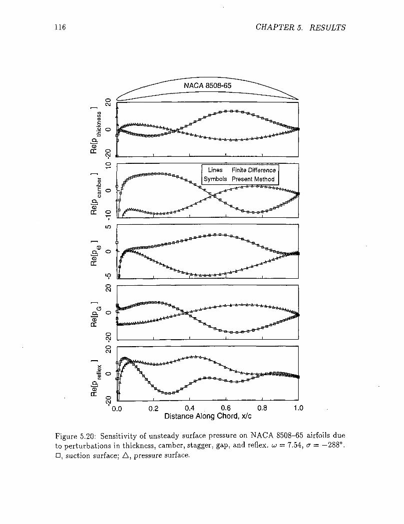
116 CHAPTERS. RESULTS
oCM
™^inin<Dc.*.y o
Q.CD
DC oCM
Lines Finite DifferenceSymbols Present Method
0.4 0.6Distance Along Chord, x/c
Figure 5,20: Sensitivity of unsteady surface pressure on NACA 8508-65 airfoils dueto perturbations in thickness, camber, stagger, gap, and reflex, u = 7.54, a = -288°.D, suction surface; A, pressure surface.
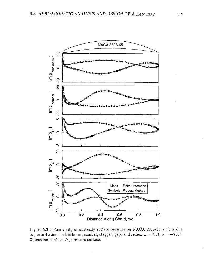
5.2. AERO ACOUSTIC ANALYSIS AND DESIGN OF A FAN EGV 117
Lines Finite DifferenceSymbols Present Method
0.2 0.4 0.6 0.8Distance Along Chord, x/c
Figure 5.21: Sensitivity of unsteady surface pressure on NACA 8508-65 airfoils dueto perturbations in thickness, camber, stagger, gap, and reflex, u — 7.54, a = —288°.n, suction surface; A, pressure surface.
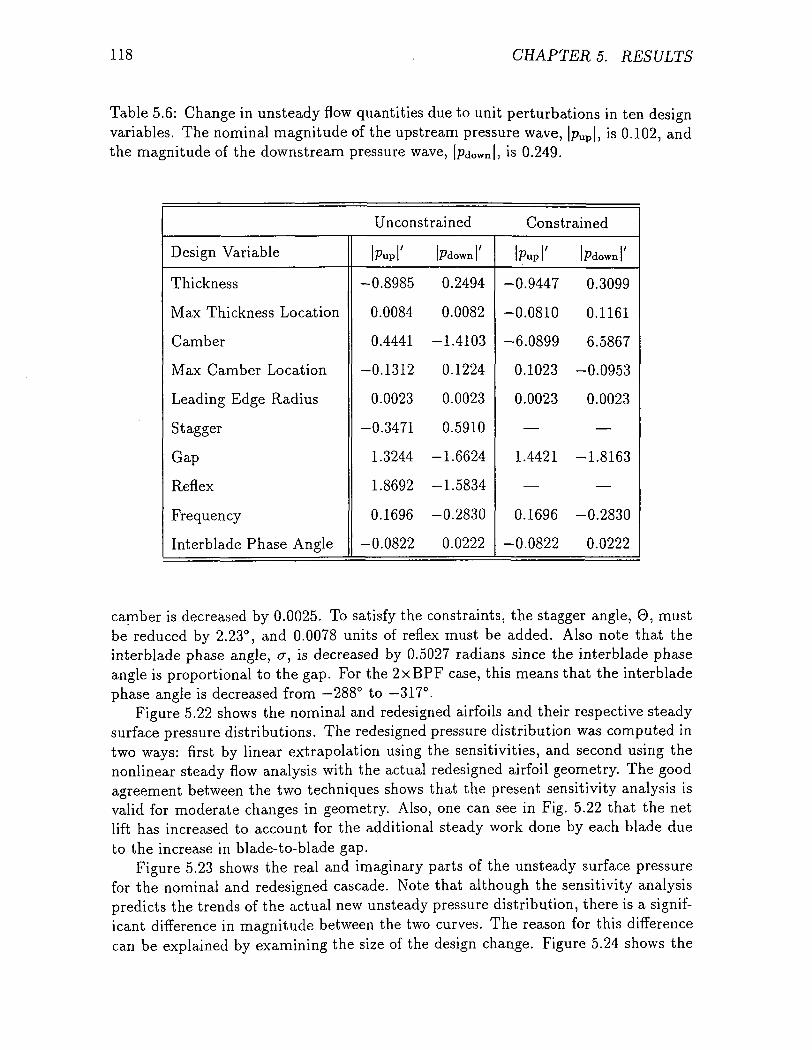
118 CHAPTERS. RESULTS
Table 5.6: Change in unsteady flow quantities due to unit perturbations in ten designvariables. The nominal magnitude of the upstream pressure wave, |pup|, is 0.102, andthe magnitude of the downstream pressure wave, |pdown|, is 0.249.
Unconstrained Constrained
Design Variable
Thickness
Max Thickness Location
Camber
Max Camber Location
Leading Edge Radius
Stagger
Gap
Reflex
Frequency
Interblade Phase Angle
IPupl' bdown '
-0.8985 0.2494
0.0084 0.0082
0.4441 -1.4103
-0.1312 0.1224
0.0023 0.0023
-0.3471 0.5910
1.3244 -1.6624
1.8692 -1.5834
0.1696 -0.2830
-0.0822 0.0222
|Pup|' bdownl'
-0.9447 0.3099
-0.0810 0.1161
-6.0899 6.5867
0.1023 -0.0953
0.0023 0.0023
— —
1.4421 -1.8163
— —
0.1696 -0.2830
-0.0822 0.0222
camber is decreased by 0.0025. To satisfy the constraints, the stagger angle, 0, mustbe reduced by 2.23°, and 0.0078 units of reflex must be added. Also note that theinterblade phase angle, a, is decreased by 0.5027 radians since the interblade phaseangle is proportional to the gap. For the 2xBPF case, this means that the interbladephase angle is decreased from —288° to —317°.
Figure 5.22 shows the nominal and redesigned airfoils and their respective steadysurface pressure distributions. The redesigned pressure distribution was computed intwo ways: first by linear extrapolation using the sensitivities, and second using thenonlinear steady flow analysis with the actual redesigned airfoil geometry. The goodagreement between the two techniques shows that the present sensitivity analysis isvalid for moderate changes in geometry. Also, one can see in Fig. 5.22 that the netlift has increased to account for the additional steady work done by each blade dueto the increase in blade-to-blade gap.
Figure 5.23 shows the real and imaginary parts of the unsteady surface pressurefor the nominal and redesigned cascade. Note that although the sensitivity analysispredicts the trends of the actual new unsteady pressure distribution, there is a signif-icant difference in magnitude between the two curves. The reason for this differencecan be explained by examining the size of the design change. Figure 5.24 shows the
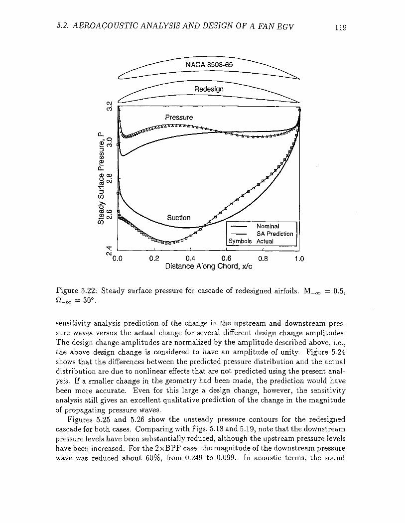
5.2. AEROACOUSTIC ANALYSIS AND DESIGN OF A FAN EGV 119
NominalSA Prediction
Symbols Actual
0.2 0.4 0.6 0.8Distance Along Chord, x/c
1.0
Figure 5.22: Steady surface pressure for cascade of redesigned airfoils. M_oo = 0.5,O.^ = 30°.
sensitivity analysis prediction of the change in the upstream and downstream pres-sure waves versus the actual change for several different design change amplitudes.The design change amplitudes are normalized by the amplitude described above, i.e.,the above design change is considered to have an amplitude of unity. Figure 5.24shows that the differences between the predicted pressure distribution and the actualdistribution are due to nonlinear effects that are not predicted using the present anal-ysis. If a smaller change in the geometry had been made, the prediction would havebeen more accurate. Even for this large a design change, however, the sensitivityanalysis still gives an excellent qualitative prediction of the change in the magnitudeof propagating pressure waves.
Figures 5.25 and 5.26 show the unsteady pressure contours for the redesignedcascade for both cases. Comparing with Figs. 5.18 and 5.19, note that the downstreampressure levels have been substantially reduced, although the upstream pressure levelshave been increased. For the 2xBPF case, the magnitude of the downstream pressurewave was reduced about 60%, from 0.249 to 0.099. In acoustic terms, the sound
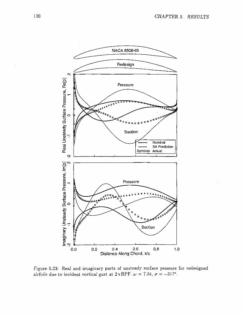
120 CHAPTER 5. RESULTS
0.2 0.4 0.6 0.8Distance Along Chord, x/c
1.0
Figure 5.23: Real and imaginary parts of unsteady surface pressure for redesignedairfoils due to incident vortical gust at 2xBPF. u = 7.54, a = -317°.
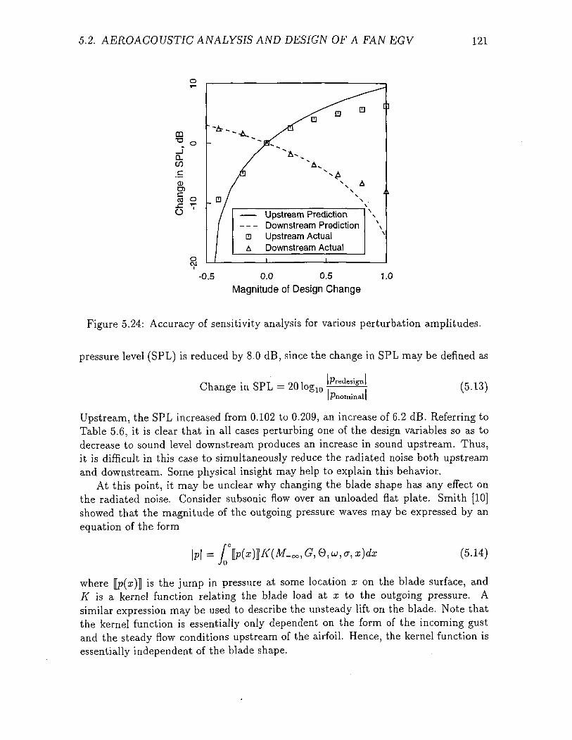
5.2. AEROACOUSTIC ANALYSIS AND DESIGN OF A FAN EGV 121
CD•a
D.CO
CDD5
CO O
N A
Upstream PredictionDownstream Prediction
n Upstream ActualA Downstream Actual
-0.5 0.0 0.5 1.0Magnitude of Design Change
Figure 5.24: Accuracy of sensitivity analysis for various perturbation amplitudes,
pressure level (SPL) is reduced by 8.0 dB, since the change in SPL may be defined as
iPredesignlChange in SPL = 20 Iog10
Ifl'nominal(5.13)
Upstream, the SPL increased from 0.102 to 0.209, an increase of 6.2 dB. Referring toTable 5.6, it is clear that in all cases perturbing one of the design variables so as todecrease to sound level downstream produces an increase in sound upstream. Thus,it is difficult in this case to simultaneously reduce the radiated noise both upstreamand downstream. Some physical insight may help to explain this behavior.
At this point, it may be unclear why changing the blade shape has any effect onthe radiated noise. Consider subsonic flow over an unloaded flat plate. Smith [10]showed that the magnitude of the outgoing pressure waves may be expressed by anequation of the form
\ P \ = (5.14)
where |p(a;)] is the jump in pressure at some location x on the blade surface, andK is a kernel function relating the blade load at x to the outgoing pressure. Asimilar expression may be used to describe the unsteady lift on the blade. Note thatthe kernel function is essentially only dependent on the form of the incoming gustand the steady flow conditions upstream of the airfoil. Hence, the kernel function isessentially independent of the blade shape.
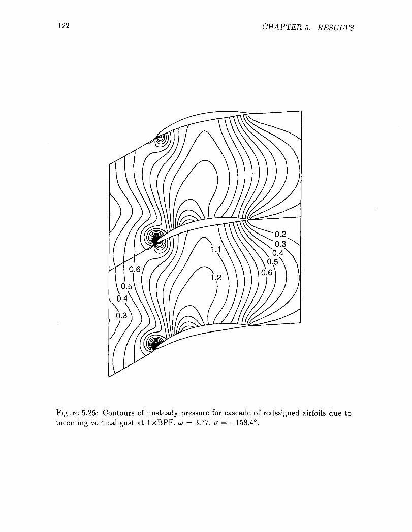
122 CHAPTERS. RESULTS
Figure 5.25: Contours of unsteady pressure for cascade of redesigned airfoils due toincoming vortical gust at IxBPF. u = 3.77, a = -158.4°.
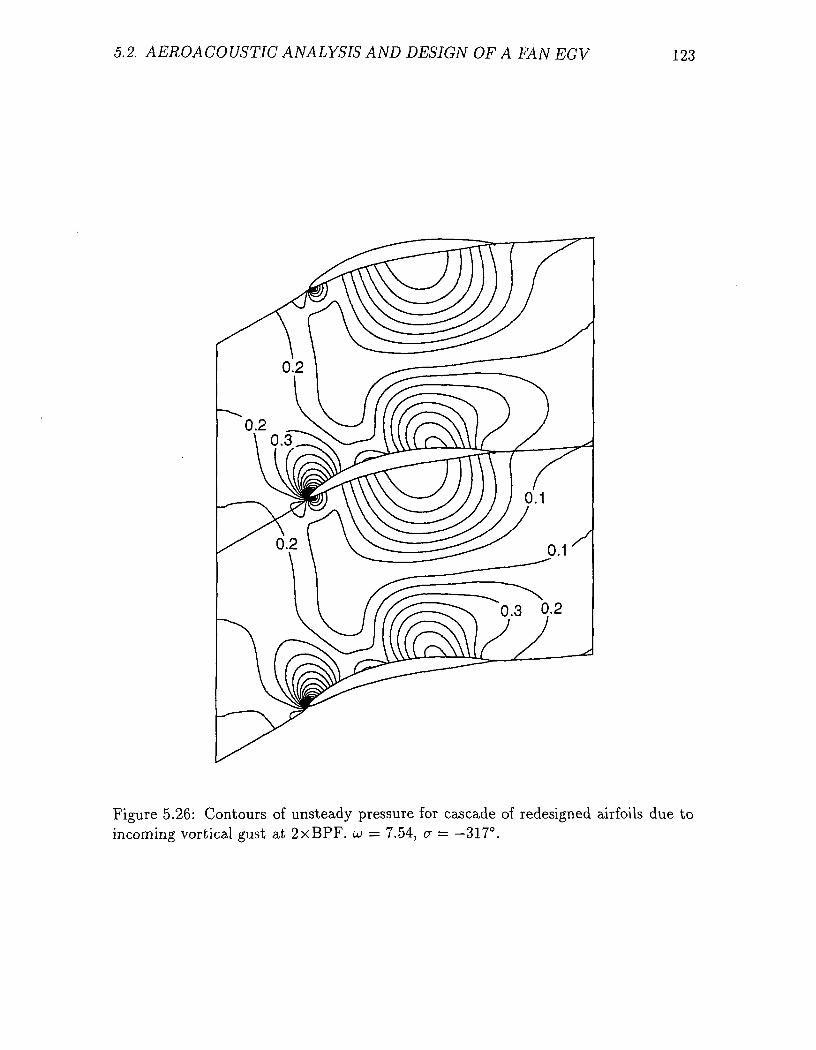
5.2. AEROACOUSTIC ANALYSIS AND DESIGN OF A FAN EGV 123
Figure 5.26: Contours of unsteady pressure for cascade of redesigned airfoils due toincoming vortical gust at 2xBPF. u = 7.54, u = —317°.
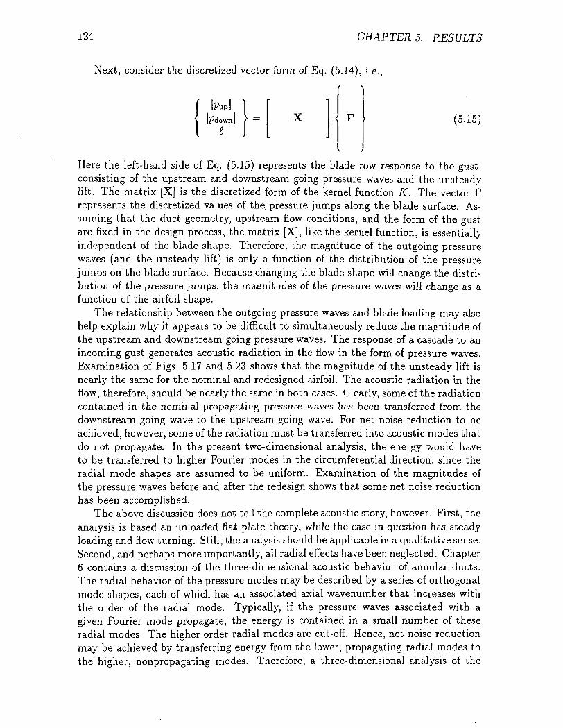
124 CHAPTERS. RESULTS
Next, consider the discretized vector form of Eq. (5.14), i.e.,
(5.15)
Here the left-hand side of Eq. (5.15) represents the blade row response to the gust,consisting of the upstream and downstream going pressure waves and the unsteadylift. The matrix [X] is the discretized form of the kernel function K. The vector Frepresents the discretized values of the pressure jumps along the blade surface. As-suming that the duct geometry, upstream flow conditions, and the form of the gustare fixed in the design process, the matrix [X], like the kernel function, is essentiallyindependent of the blade shape. Therefore, the magnitude of the outgoing pressurewaves (and the unsteady lift) is only a function of the distribution of the pressurejumps on the blade surface. Because changing the blade shape will change the distri-bution of the pressure jumps, the magnitudes of the pressure waves will change as afunction of the airfoil shape.
The relationship between the outgoing pressure waves and blade loading may alsohelp explain why it appears to be difficult to simultaneously reduce the magnitude ofthe upstream and downstream going pressure waves. The response of a cascade to anincoming gust generates acoustic radiation in the flow in the form of pressure waves.Examination of Figs. 5.17 and 5.23 shows that the magnitude of the unsteady lift isnearly the same for the nominal and redesigned airfoil. The acoustic radiation in theflow, therefore, should be nearly the same in both cases. Clearly, some of the radiationcontained in the nominal propagating pressure waves has been transferred from thedownstream going wave to the upstream going wave. For net noise reduction to beachieved, however, some of the radiation must be transferred into acoustic modes thatdo not propagate. In the present two-dimensional analysis, the energy would haveto be transferred to higher Fourier modes in the circumferential direction, since theradial mode shapes are assumed to be uniform. Examination of the magnitudes ofthe pressure waves before and after the redesign shows that some net noise reductionhas been accomplished.
The above discussion does not tell the complete acoustic story, however. First, theanalysis is based an unloaded flat plate theory, while the case in question has steadyloading and flow turning. Still, the analysis should be applicable in a qualitative sense.Second, and perhaps more importantly, all radial effects have been neglected. Chapter6 contains a discussion of the three-dimensional acoustic behavior of annular ducts.The radial behavior of the pressure modes may be described by a series of orthogonalmode shapes, each of which has an associated axial wavenumber that increases withthe order of the radial mode. Typically, if the pressure waves associated with agiven Fourier mode propagate, the energy is contained in a small number of theseradial modes. The higher order radial modes are cut-off. Hence, net noise reductionmay be achieved by transferring energy from the lower, propagating radial modes tothe higher, nonpropagating modes. Therefore, a three-dimensional analysis of the
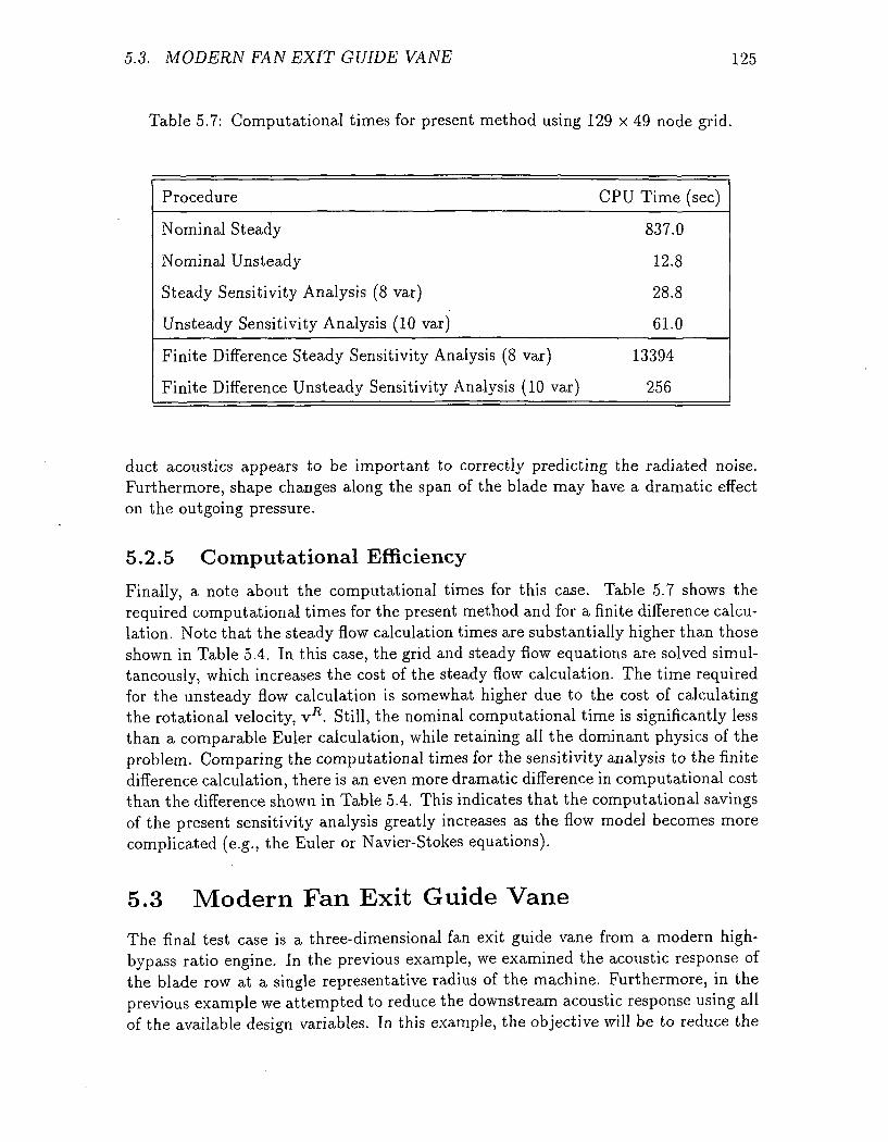
5.3. MODERN FAN EXIT GUIDE VANE 125
Table 5.7: Computational times for present method using 129 x 49 node grid.
Procedure
Nominal Steady
Nominal Unsteady
Steady Sensitivity Analysis (8 var)
Unsteady Sensitivity Analysis (10 var)
Finite Difference Steady Sensitivity Analysis (8 var)
Finite Difference Unsteady Sensitivity Analysis (10 var)
CPU Time (sec)
837.0
12.8
28.8
61.0
13394
256
duct acoustics appears to be important to correctly predicting the radiated noise.Furthermore, shape changes along the span of the blade may have a dramatic effecton the outgoing pressure.
5.2.5 Computational EfficiencyFinally, a note about the computational times for this case. Table 5.7 shows therequired computational times for the present method and for a finite difference calcu-lation. Note that the steady flow calculation times are substantially higher than thoseshown in Table 5.4. In this case, the grid and steady flow equations are solved simul-taneously, which increases the cost of the steady flow calculation. The time requiredfor the unsteady flow calculation is somewhat higher due to the cost of calculatingthe rotational velocity, VR. Still, the nominal computational time is significantly lessthan a comparable Euler calculation, while retaining all the dominant physics of theproblem. Comparing the computational times for the sensitivity analysis to the finitedifference calculation, there is an even more dramatic difference in computational costthan the difference shown in Table 5.4. This indicates that the computational savingsof the present sensitivity analysis greatly increases as the flow model becomes morecomplicated (e.g., the Euler or Navier-Stokes equations).
5.3 Modern Fan Exit Guide Vane
The final test case is a three-dimensional fan exit guide vane from a modern high-bypass ratio engine. In the previous example, we examined the acoustic response ofthe blade row at a single representative radius of the machine. Furthermore, in theprevious example we attempted to reduce the downstream acoustic response using allof the available design variables. In this example, the objective will be to reduce the
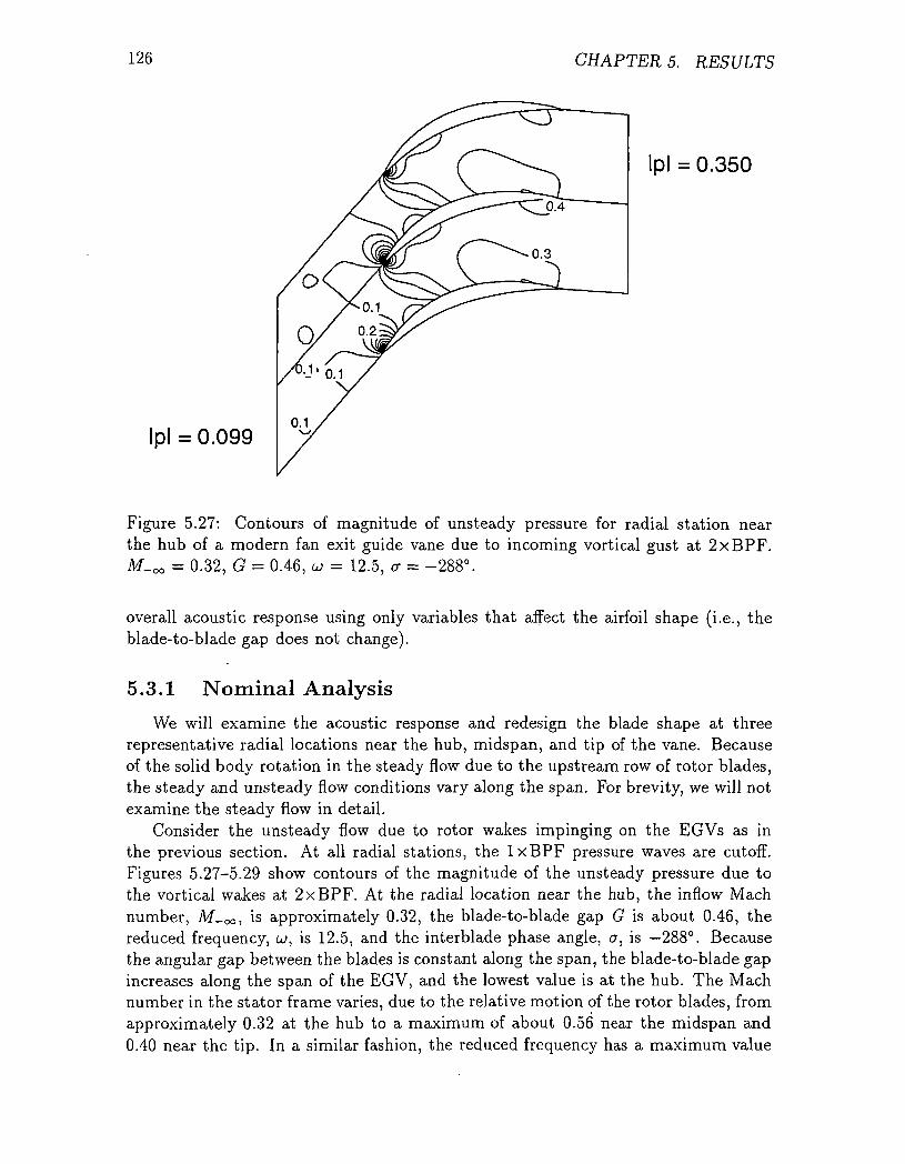
126 CHAPTERS. RESULTS
Ipl = 0.099
Ipl = 0.350
Figure 5.27: Contours of magnitude of unsteady pressure for radial station nearthe hub of a modern fan exit guide vane due to incoming vortical gust at 2xBPF.M-oo = 0.32, G = 0.46, w = 12.5, a = -288°.
overall acoustic response using only variables that affect the airfoil shape (i.e., theblade-to-blade gap does not change).
5.3.1 Nominal Analysis
We will examine the acoustic response and redesign the blade shape at threerepresentative radial locations near the hub, midspan, and tip of the vane. Becauseof the solid body rotation in the steady flow due to the upstream row of rotor blades,the steady and unsteady flow conditions vary along the span. For brevity, we will notexamine the steady flow in detail.
Consider the unsteady flow due to rotor wakes impinging on the EGVs as inthe previous section. At all radial stations, the IxBPF pressure waves are cutoff.Figures 5.27-5.29 show contours of the magnitude of the unsteady pressure due tothe vortical wakes at 2xBPF. At the radial location near the hub, the inflow Machnumber, M_oo, is approximately 0.32, the blade-to-blade gap G is about 0.46, thereduced frequency, u>, is 12.5, and the interblade phase angle, a, is —288°. Becausethe angular gap between the blades is constant along the span, the blade-to-blade gapincreases along the span of the EGV, and the lowest value is at the hub. The Machnumber in the stator frame varies, due to the relative motion of the rotor blades, fromapproximately 0.32 at the hub to a maximum of about 0.56 near the midspan and0.40 near the tip. In a similar fashion, the reduced frequency has a maximum value
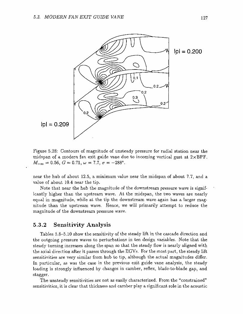
5.3. MODERN FAN EXIT GUIDE VANE 127
Ipl = 0.209
Ipl = 0.200
Figure 5.28: Contours of magnitude of unsteady pressure for radial station near themidspan of a modern fan exit guide vane due to incoming vortical gust at 2xBPF.M_oo = 0.56, G = 0.71, w = 7.7, a = -288°.
near the hub of about 12.5, a minimum value near the midspan of about 7.7, and avalue of about 10.4 near the tip.
Note that near the hub the magnitude of the downstream pressure wave is signif-icantly higher than the upstream wave. At the midspan, the two waves are nearlyequal in magnitude, while at the tip the downstream wave again has a larger mag-nitude than the upstream wave. Hence, we will primarily attempt to reduce themagnitude of the downstream pressure wave.
5.3.2 Sensitivity Analysis
Tables 5.8-5.10 show the sensitivity of the steady lift in the cascade direction andthe outgoing pressure waves to perturbations in ten design variables. Note that thesteady turning increases along the span so that the steady flow is nearly aligned withthe axial direction after it passes through the EG Vs. For the most part, the steady liftsensitivities are very similar from hub to tip, although the actual magnitudes differ.In particular, as was the case in the previous exit guide vane analysis, the steadyloading is strongly influenced by changes in camber, reflex, blade-to-blade gap, andstagger.
The unsteady sensitivities are not as easily characterized. From the "constrained"sensitivities, it is clear that thickness and camber play a significant role in the acoustic
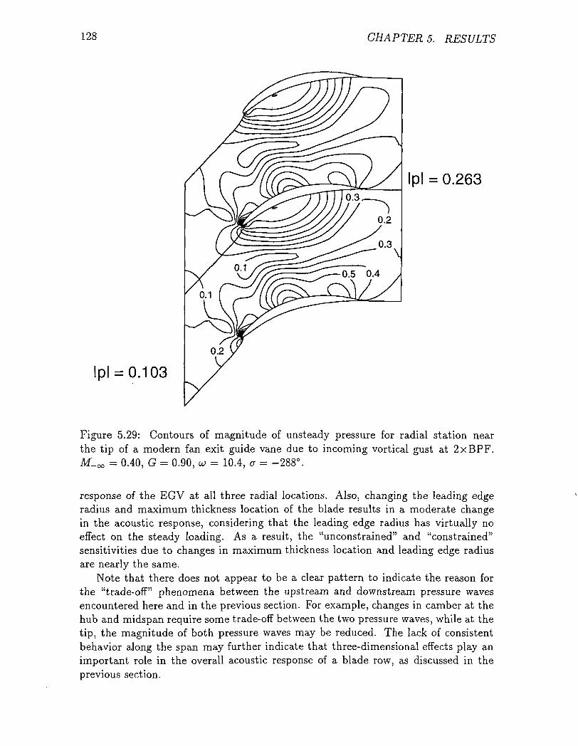
128 CHAPTERS. RESULTS
lpl = 0.103
Ipl = 0.263
Figure 5.29: Contours of magnitude of unsteady pressure for radial station nearthe tip of a modern fan exit guide vane due to incoming vortical gust at 2xBPF.M-oo = 0.40, G = 0.90, w = 10.4, a = -288°.
response of the EGV at all three radial locations. Also, changing the leading edgeradius and maximum thickness location of the blade results in a moderate changein the acoustic response, considering that the leading edge radius has virtually noeffect on the steady loading. As a result, the "unconstrained" and "constrained"sensitivities due to changes in maximum thickness location and leading edge radiusare nearly the same.
Note that there does not appear to be a clear pattern to indicate the reason forthe "trade-off" phenomena between the upstream and downstream pressure wavesencountered here and in the previous section. For example, changes in camber at thehub and midspan require some trade-off between the two pressure waves, while at thetip, the magnitude of both pressure waves may be reduced. The lack of consistentbehavior along the span may further indicate that three-dimensional effects play animportant role in the overall acoustic response of a blade row, as discussed in theprevious section.
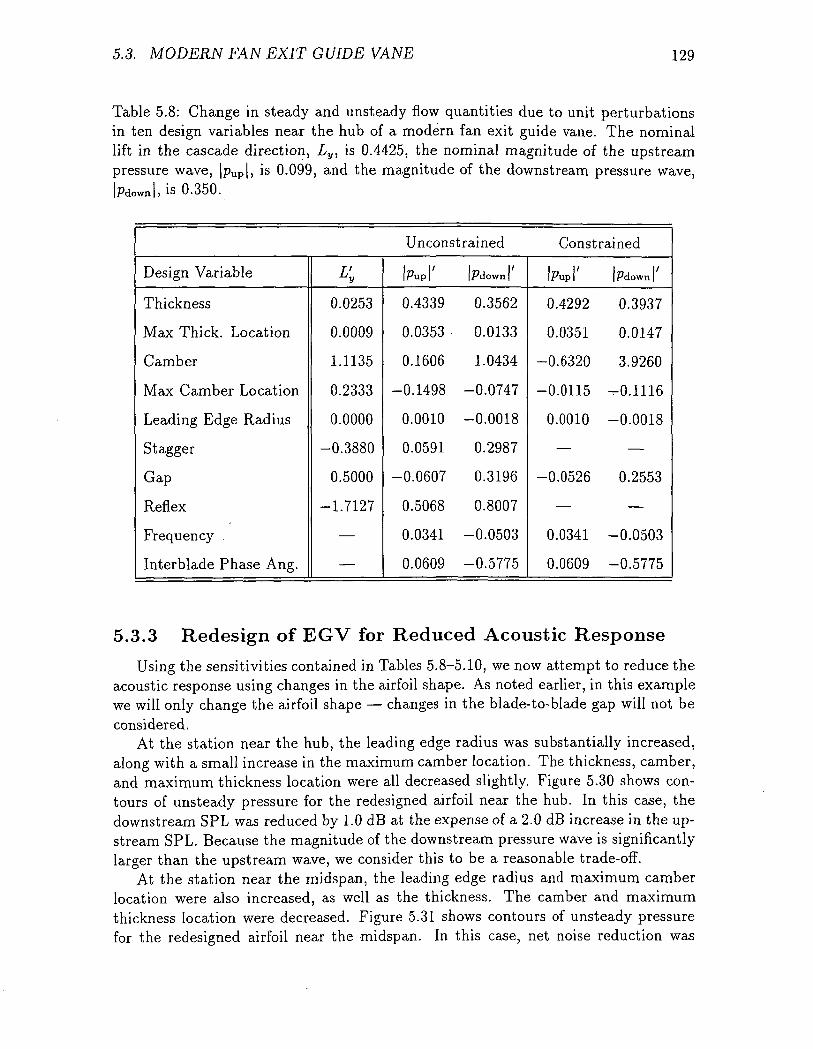
5.3. MODERN FAN EXIT GUIDE VANE 129
Table 5.8: Change in steady and unsteady flow quantities due to unit perturbationsin ten design variables near the hub of a modern fan exit guide vane. The nominallift in the cascade direction, Ly, is 0.4425, the nominal magnitude of the upstreampressure wave, |pup|, is 0.099, and the magnitude of the downstream pressure wave,
l, is 0.350.
Unconstrained Constrained
Design Variable
Thickness
Max Thick. Location
Camber
Max Camber Location
Leading Edge Radius
Stagger
Gap
Reflex
Frequency
Interblade Phase Ang.
L'y
0.0253
0.0009
1.1135
0.2333
0.0000
-0.3880
0.5000
-1.7127
—
—
IPup ' bdown)'
0.4339 0.3562
0.0353 0.0133
0.1606 1.0434
-0.1498 -0.0747
0.0010 -0.0018
0.0591 0.2987
-0.0607 0.3196
0.5068 0.8007
0.0341 -0.0503
0.0609 -0.5775
W (Pdown 1'
0.4292 0.3937
0.0351 0.0147
-0.6320 3.9260
-0.0115 -0.1116
0.0010 -0.0018
— —
-0.0526 0.2553
— —
0.0341 -0.0503
0.0609 -0.5775
5.3.3 Redesign of EGV for Reduced Acoustic Response
Using the sensitivities contained in Tables 5.8-5.10, we now attempt to reduce theacoustic response using changes in the airfoil shape. As noted earlier, in this examplewe will only change the airfoil shape — changes in the blade-to-blade gap will not beconsidered.
At the station near the hub, the leading edge radius was substantially increased,along with a small increase in the maximum camber location. The thickness, camber,and maximum thickness location were all decreased slightly. Figure 5.30 shows con-tours of unsteady pressure for the redesigned airfoil near the hub. In this case, thedownstream SPL was reduced by 1.0 dB at the expense of a 2.0 dB increase in the up-stream SPL. Because the magnitude of the downstream pressure wave is significantlylarger than the upstream wave, we consider this to be a reasonable trade-off.
At the station near the midspan, the leading edge radius and maximum camberlocation were also increased, as well as the thickness. The camber and maximumthickness location were decreased. Figure 5.31 shows contours of unsteady pressurefor the redesigned airfoil near the midspan. In this case, net noise reduction was
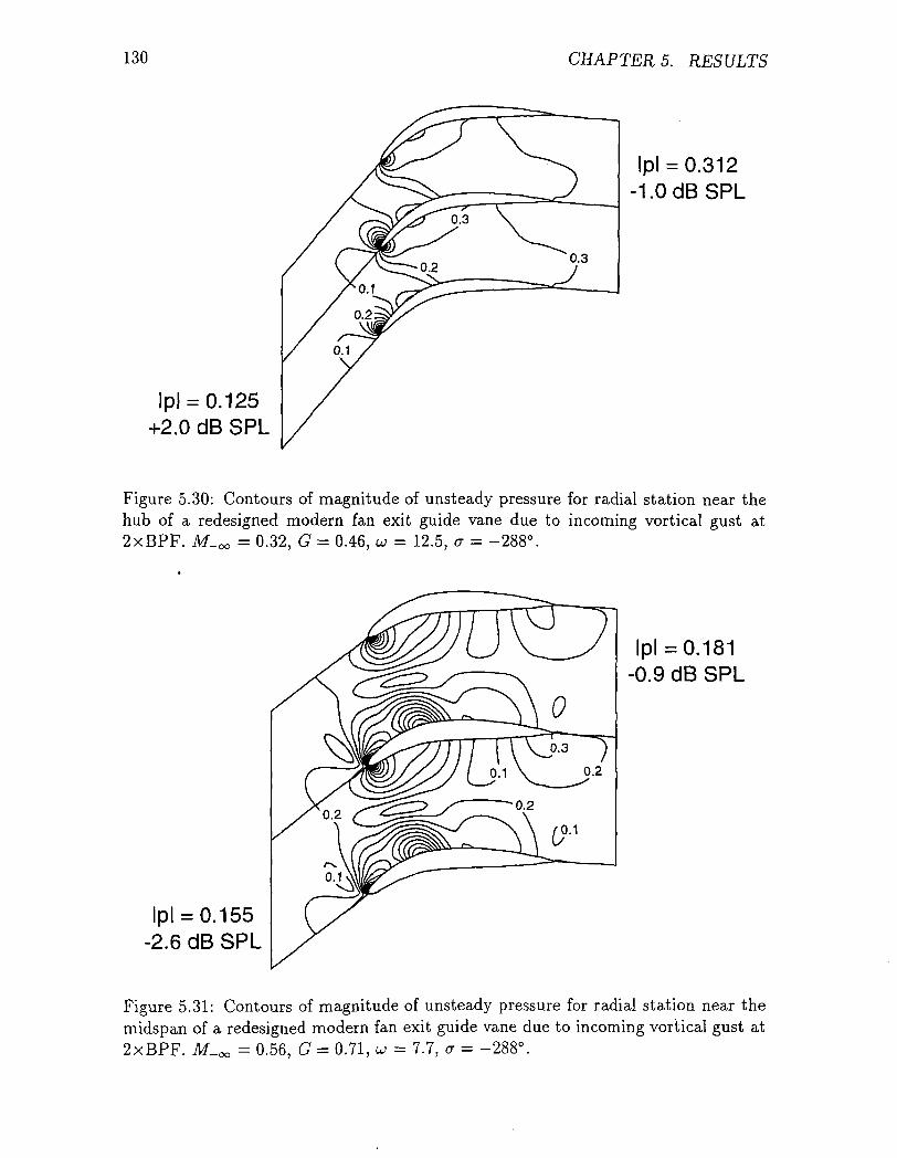
130 CHAPTERS. RESULTS
lpl = 0.125+2.0 dB SPL
lpl = 0.312-LOdBSPL
Figure 5.30: Contours of magnitude of unsteady pressure for radial station near thehub of a redesigned modern fan exit guide vane due to incoming vortical gust at2xBPF. M_oo = 0.32, G = 0.46, w = 12.5, a = -288°.
lpl= 0.181-0.9 dB SPL
lpl = 0.155-2.6 dB SPL
Figure 5.31: Contours of magnitude of unsteady pressure for radial station near themidspan of a redesigned modern fan exit guide vane due to incoming vortical gust at2xBPF. M-oo = 0.56, G = 0.71, u = 7.7, a = -288°.
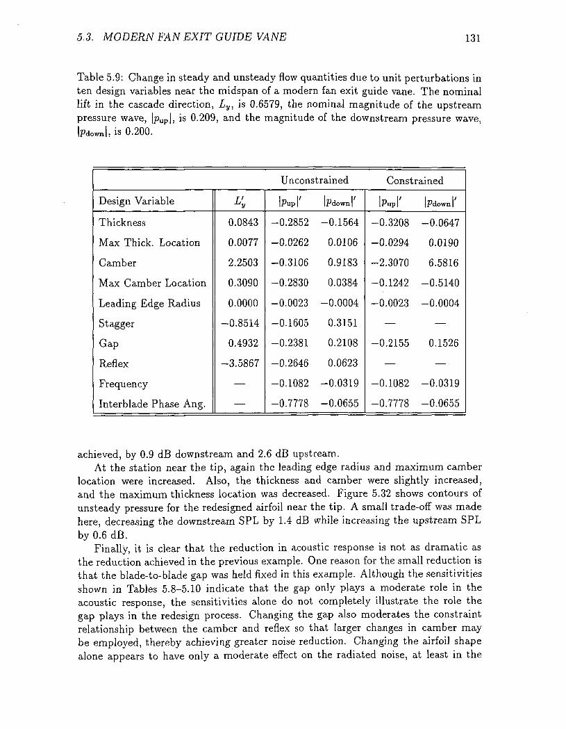
5.3. MODERN FAN EXIT GUIDE VANE 131
Table 5.9: Change in steady and unsteady flow quantities due to unit perturbations inten design variables near the midspan of a modern fan exit guide vane. The nominallift in the cascade direction, Ly, is 0.6579, the nominal magnitude of the upstreampressure wave, \pup\, is 0.209, and the magnitude of the downstream pressure wave,|pdown|, is 0.200.
Unconstrained Constrained
Design Variable
Thickness
Max Thick. Location
Camber
Max Camber Location
Leading Edge Radius
Stagger
Gap
Reflex
Frequency
Interblade Phase Ang.
L'y
0.0843
0.0077
2.2503
0.3090
0.0000
-0.8514
0.4932
-3.5867
—
—
|pup ' bdown '
-0.2852 -0.1564
-0.0262 0.0106
-0.3106 0.9183
-0.2830 0.0384
-0.0023 -0.0004
-0.1605 0.3151
-0.2381 0.2108
-0.2646 0.0623
-0.1082 -0.0319
-0.7778 -0.0655
|Pup ' l^downl'
-0.3208 -0.0647
-0.0294 0.0190
-2.3070 6.5816
-0.1242 -0.5140
-0.0023 -0.0004
— —
-0.2155 0.1526
— —
-0.1082 -0.0319
-0.7778 -0.0655
achieved, by 0.9 dB downstream and 2.6 dB upstream.At the station near the tip, again the leading edge radius and maximum camber
location were increased. Also, the thickness and camber were slightly increased,and the maximum thickness location was decreased. Figure 5.32 shows contours ofunsteady pressure for the redesigned airfoil near the tip. A small trade-oif was madehere, decreasing the downstream SPL by 1.4 dB while increasing the upstream SPLby 0.6 dB.
Finally, it is clear that the reduction in acoustic response is not as dramatic asthe reduction achieved in the previous example. One reason for the small reduction isthat the blade-to-blade gap was held fixed in this example. Although the sensitivitiesshown in Tables 5.8-5.10 indicate that the gap only plays a moderate role in theacoustic response, the sensitivities alone do not completely illustrate the role thegap plays in the redesign process. Changing the gap also moderates the constraintrelationship between the camber and reflex so that larger changes in camber maybe employed, thereby achieving greater noise reduction. Changing the airfoil shapealone appears to have only a moderate effect on the radiated noise, at least in the
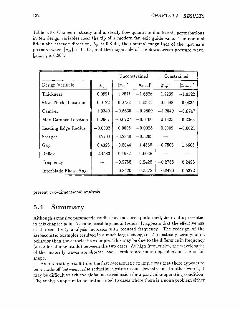
132 CHAPTER 5. RESULTS
Table 5.10: Change in steady and unsteady flow quantities due to unit perturbationsin ten design variables near the tip of a modern fan exit guide vane. The nominallift in the cascade direction, Ly, is 0.8140, the nominal magnitude of the upstreampressure wave, |pup|, is 0.103, and the magnitude of the downstream pressure wave,
is 0.263.
Unconstrained Constrained
Design Variable
Thickness
Max Thick. Location
Camber
Max Camber Location
Leading Edge Radius
Stagger
Gap
Reflex
Frequency
Interblade Phase Ang.
L'y
0.0921
0.0122
1.9340
0.2967
-0.0002
-0.7708
0.4326
-2.4583
—
—
biipl' |Pdown|'
1.2871 -1.6826
0.0782 0.0534
-0.5630 -0.2809
-0.0227 -0.0706
0.0008 -0.0025
-0.2338 -0.5205
-0.8044 1.4336
0.1682 0.6038
-0.2758 0.2425
-0.8420 0.5372
IPup ' bdown '
1.2239 -1.8322
0.0698 0.0335
-3.2040 -6.6747
0.1325 0.3363
0.0009 -0.0021
— —
-0.7506 1.5608
— —
-0.2758 0.2425
-0.8420 0.5372
present two-dimensional analysis.
5.4 Summary
Although extensive parametric studies have not been performed, the results presentedin this chapter point to some possible general trends. It appears that the effectivenessof the sensitivity analysis increases with reduced frequency. The redesign of theaeroacoustic examples resulted in a much larger change in the unsteady aerodynamicbehavior than the aeroelastic example. This may be due to the difference in frequency(an order of magnitude) between the two cases. At high frequencies, the wavelengthsof the unsteady waves are shorter, and therefore are more dependent on the airfoilshape.
An interesting result from the first aeroacoustic example was that there appears tobe a trade-off between noise reduction upstream and downstream. In other words, itmay be difficult to achieve global noise reduction for a particular operating condition.The analysis appears to be better suited to cases where there is a noise problem either
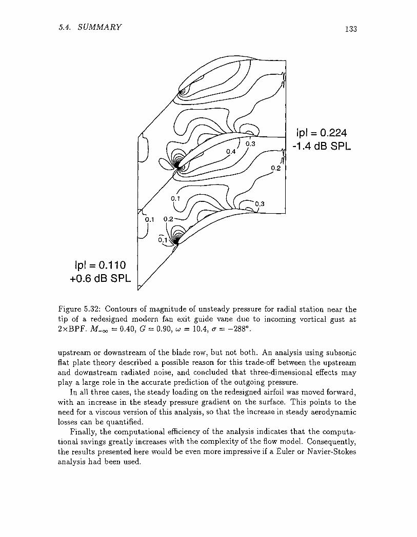
5.4. SUMMARY 133
lpl = 0.110+0.6 dB SPL
Ipl = 0.224-1.4dBSPL
Figure 5.32: Contours of magnitude of unsteady pressure for radial station near thetip of a redesigned modern fan exit guide vane due to incoming vortical gust at2xBPF. M-oo = 0.40, G = 0.90, w = 10.4, a = -288°.
upstream or downstream of the blade row, but not both. An analysis using subsonicflat plate theory described a possible reason for this trade-off between the upstreamand downstream radiated noise, and concluded that three-dimensional effects mayplay a large role in the accurate prediction of the outgoing pressure.
In all three cases, the steady loading on the redesigned airfoil was moved forward,with an increase in the steady pressure gradient on the surface. This points to theneed for a viscous version of this analysis, so that the increase in steady aerodynamiclosses can be quantified.
Finally, the computational efficiency of the analysis indicates that the computa-tional savings greatly increases with the complexity of the flow model. Consequently,the results presented here would be even more impressive if a Euler or Navier-Stokesanalysis had been used.
Chapter 6
Application to Three-DimensionalProblems
Although the preceding development is well-suited to the design and analysis oftwo-dimensional cascades, it is not entirely obvious how to analyze an actual three-dimensional blade row using this method. This chapter provides a framework foranalyzing three-dimensional aeroacoustic problems using the present two-dimensionalprocedure. Section 6.1 contains a discussion of the general three-dimensional problemand the importance of the annular nature of the geometry. In addition, an analyti-cal procedure for calculating the natural acoustic modes of an annular duct will bedeveloped. Next, Section 6.2 contains a discussion of how the unsteady pressure atthe far field of a three-dimensional blade row may be calculated. Finally, in Section6.3, a general method for calculating the magnitude of the outgoing three-dimensionalpressure waves in the far field from the computed two-dimensional unsteady potentialwill be described. Also, the application of the sensitivity analysis to the calculationprocedure described in this chapter will be discussed.
6.1 Acoustic Modes in an Annular Duct
The fluid in an axial flow turbomachine is typically modeled as flow through anannular duct. A schematic of such a duct is shown in Figure 6.1. The duct has aninner (or hub) radius, r#, and an outer (or tip) radius, TT- A key parameter definingthe duct geometry is the so-called hub-to-tip ratio, TH/TT- As this ratio approachesunity, the flow becomes nearly two-dimensional. For lower hub-to-tip ratios, however,annular effects become more significant.
The first step in analyzing the three-dimensional acoustic behavior of a blade rowis to examine the natural acoustic modes in an annular duct such as the one shown inFigure 6.1. For a completely general steady flow, this would be a formidable problemto solve analytically. Fortunately, the steady flow field is relatively uniform awayfrom the blade row (i.e., the far field). Furthermore, in this analysis, all streamtubecontraction effects are neglected, i.e., the hub and tip radii are constants along theaxis of the turbomachine. It is also assumed that there is no radial component of the
134
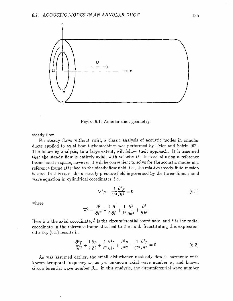
6.1. ACOUSTIC MODES IN AN ANNULAR DUCT 135
U
Figure 6.1: Annular duct geometry.
steady flow.For steady flows without swirl, a classic analysis of acoustic modes in annular
ducts applied to axial flow turbomachines was performed by Tyler and Sofrin [62].The following analysis, to a large extent, will follow their approach. It is assumedthat the steady flow is entirely axial, with velocity U. Instead of using a referenceframe fixed in space, however, it will be convenient to solve for the acoustic modes in areference frame attached to the steady flow field, i.e., the relative steady fluid motionis zero. In this case, the unsteady pressure field is governed by the three-dimensionalwave equation in cylindrical coordinates, i.e.,
(6.1)
where a2 i d i a2 a2
+ f af + f2 a02
Here x is the axial coordinate, 9 is the circumferential coordinate, and f is the radialcoordinate in the reference frame attached to the fluid. Substituting this expressioninto Eq. (6.1) results in
dpaf2
_ _ _ =
c2 at2 ~ (6.2)
As was assumed earlier, the small disturbance unsteady flow is harmonic withknown temporal frequency cu, as yet unknown axial wave number or, and knowncircumferential wave number (3m. In this analysis, the circumferential wave number
136 CHAPTER 6. APPLICATION TO THREE-DIMENSIONAL PROBLEMS
will be referred to by an integer m that denotes the circumferential mode number,i.e.,
(& + 2irm)0Pm = ^ QG ' (6.3)
where QQ is the angular gap between the blades. For now, the radial behavior ofthe unsteady pressure is still unknown. Hence, the behavior of the unsteady pressuremay be written in the form
p(r, 0, x, t) = n(f) exp[jm6 + jax + jut] (6.4)
where /j,(f) is some as yet undetermined function. Substituting this functional forminto Eq. (6.2) results in
Ida n--£r dr r2
w™C2
If a new variable a* is defined such that
*"=^-«2
(6.5)
(6.6)
then Eq. (6.5) may be written as
. = 0 (6.7)
Equation (6.7) is simply Bessel's Equation. The solution, therefore, is composed ofBessel functions of order m, i.e.,
= AJm(a*r) (a*r) (6.8)
The constants A and B are determined by the boundary conditions on the radialbehavior of the unsteady pressure. Because the hub and tip are solid surfaces, theflow tangency boundary condition requires that radial component of velocity on thesesurfaces must be zero. From the radial momentum equation, then, the radial (ornormal) component of the pressure gradient at the hub and tip surfaces must be zero,i.e.,
dp
anddpdr
= 0
= 0
(6.9)
(6.10)
Application of the boundary conditions results in a homogeneous system of equationsfor the constants A and B. Cramer's rule implies that if the constants A and B arenot both zero, then
dJm / * \ d 1m i if \-^(a ftf) -jjr(a*rH)
dJ
= 0 (6.11)
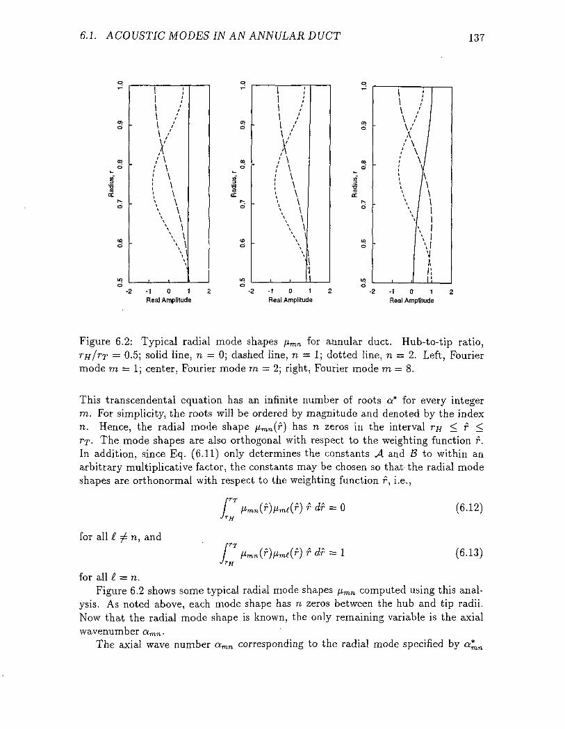
6.1. ACOUSTIC MODES IN AN ANNULAR DUCT 137
o>o
<£>
6
- 2 - 1 0 1 2Real Amplitude
13cc
i ;i /\ /\ /\ /\i \/ \ j/ \ /
VA
1 / ^\ / '\ /
\ /\ j\ ii%i \i \i \
ii,i i
- 2 - 1 0 1 2Real Amplitude
- 2 - 1 0 1 2Real Amplitude
Figure 6.2: Typical radial mode shapes [Mmn for annular duct. Hub-to-tip ratio,TH/TT = 0.5; solid line, n = 0; dashed line, n = 1; dotted line, n = 2. Left, Fouriermode m = 1; center, Fourier mode m = 2; right, Fourier mode m = 8.
This transcendental equation has an infinite number of roots a* for every integerTO. For simplicity, the roots will be ordered by magnitude and denoted by the indexn. Hence, the radial mode shape nmn(f) has n zeros in the interval r# < f <Tf. The mode shapes are also orthogonal with respect to the weighting function f.In addition, since Eq. (6.11) only determines the constants A and B to within anarbitrary multiplicative factor, the constants may be chosen so that the radial modeshapes are orthonormal with respect to the weighting function f, i.e.,
for all i ^ n, and
/:[TT
JrH
f df = 0
f df = I
(6.12)
(6.13)
for all i = n.Figure 6.2 shows some typical radial mode shapes fimn computed using this anal-
ysis. As noted above, each mode shape has n zeros between the hub and tip radii.Now that the radial mode shape is known, the only remaining variable is the axialwavenumber amn.
The axial wave number amn corresponding to the radial mode specified by a*mn
138 CHAPTER 6. APPLICATION TO THREE-DIMENSIONAL PROBLEMS
may be determined from the roots of Eq. (6.11), and Eq. (6.6), so that
77171 /^2 77171 y\J. IT: J
In summary, if the steady flow relative to the frame of reference is zero, the behaviorof unsteady pressure waves in an annular duct may be determined by the temporalfrequency u, the circumferential mode number m, and the hub and tip radii, r// andrT.
6.2 Calculation of Far-Field Unsteady Pressure
We wish to apply the sensitivity analysis procedure developed in this report to thecomplete three-dimensional flowfield. At first glance, it would appear that one pos-sible approach would be to simply solve the three-dimensional governing equationsof the fluid instead of the two-dimensional versions developed here. To obtain thecomputational efficiency of the present method, however, the nominal steady andunsteady flow equations must be solved using LU decomposition, i.e., the discretizedflow equations must be solved directly. Unfortunately, a direct solution of the three-dimensional flow equations is not feasible on current computers. Hence, an alternativeapproach to calculating the three-dimensional flowfield needs to be developed.
Because even iterative fully three-dimensional unsteady aerodynamic analyses ofcascades have only recently become available for use on modern workstation com-puters, most cascade analyses have used a two-dimensional aerodynamic model. Theblades are analyzed in what is referred to as "strip-theory." In this approach, the un-steady aerodynamic loads at a number of radial locations along the blade surface arecomputed using a two-dimensional aerodynamic model. In the aeroelastic problem,these aerodynamic loads are then integrated along the span to obtain modal forces.In the aeroacoustic problem, the unsteady pressure at the far field p(r, x) may becomputed from these iaerodynamic loads using a Green's function approach, i.e.,
p(r ,x)= np(r0,xo)lG(r,x]ro,x0}dY (6.15)Jr
where |p(rOi xo)I is the jump in pressure at the point (r0,z0) on the blade surface,and G is the Green's function derived for a specific annular geometry and steady flowcondition [1, 58]. The Green's function may be considered an "influence coefficient"relating the loads on the surface to the pressure in the far field. The Green's functionapproach relies on a relatively idealized model, however. Typically, the model doesnot include blade thickness or camber, and may only approximate the actual steadyloading on the blade.
The linearized potential analysis described in this report improves on the Green'sfunction approach by solving the governing equations of the steady and unsteadyflow using modern computational fluid dynamic techniques. Arbitrary blade shapesmay be analyzed, the actual steady blade loading is accounted for, and the far-fieldpressure is computed with the rest of the unsteady flow solution.
6.3. CALCULATION OF THE OUTGOING PRESSURE 139
Although the strip theory approach for modeling quasi-three-dimensional effects isa simple and straightforward method, it should be noted that in some cases the resultscomputed in this way may be misleading. In particular, Hall and Lorence [35] foundthat real three-dimensional effects may be extremely important in the aeroelasticbehavior of fans and compressors with low hub-to-tip ratios.
With this in mind, the next step is to calculate the magnitudes of the actualthree-dimensional outgoing pressure waves in the duct using the two-dimensionalanalysis developed in this report. Specifically, the two-dimensional unsteady potentialcalculated at the far field will be matched with a three-dimensional analysis of thesurrounding duct.
6.3 Calculation of the Outgoing Pressure
As described earlier in this chapter, Tyler and Sofrin developed an analytical descrip-tion of the small disturbance behavior of acoustic modes in annular ducts. However,their analysis is limited to flows without mean flow swirl. For more general steadyflows, a more complicated model is required. For example, Kerrebrock [59] has de-veloped an analytical model for certain cases of swirling flows. General analyticalsolutions for flows in annular ducts, however, are not available. If the mean flow fieldis axisymmetric, however, the shape of the eigenmodes in the circumferential direc-tion will be Fourier modes. Hall, Lorence, and Clark [51] developed a procedure totake advantage of this behavior in their formulation of fully three-dimensional non-reflecting boundary conditions for the linearized Euler equations. Their method willbe adapted here to compute the magnitude of the actual three-dimensional outgoingpressure waves using the unsteady potential computed from the analysis developedin this report.
The modeling of the three-dimensional flowfield begins with the full unsteadyEuler equations in cylindrical coordinates expressed in the rotating frame of reference,which may be written as
<9U 1 drH(6.16)
Here x, 9, and r are the coordinates in the axial, circumferential, and radial directions.Also, U is the vector of conservation flow variables, and F, G, and H are the fluxvectors, and S is a source term due to rotation. These terms are given by
U =
P
pu
pv
pw
e
pu
pv? +pA A Apuv
puw
pul
G =
pv
pvuA O , Av* +p
pvw*pvl
140 CHAPTER 6. APPLICATION TO THREE-DIMENSIONAL PROBLEMS
H =
pw
puw
pvw
w* +
pwl
p
S =
0
0
-pw(v/r - 2ft)
0
where p is the density, p is the pressure, e is the internal energy, and / is the rothalpy.Here we have assumed that the coordinate system is rotating about the z-axis withrotational speed fi. The pressure, p, and the rothalpy, / are given by
p = (7 - ft V
and= _ + 2+
7 - 1 p 2 2
where r is the distance from the x-axis (r = vV2 + z<2}- Note that u, t), and w are nowthe flow velocities in the axial, circumferential, and radial directions, respectively.
It is assumed that the mean flow, U, is axisymmetric and uniform in the axialdirection. The small disturbance behavior in the far field is then governed by
au ou U ~ (6.17)
where u is the perturbation flow and <9F/<9U, dG/dU, dH/dU, and dS/dU areJacobians based on the mean flowfield, U.
As discussed in Chapter 2, it is assumed that the shape of the eigenmodes inthe circumferential direction are Fourier modes. In addition, it is assumed that thefrequency of the unsteady excitation is u and the interblade phase angle is a. Usingthese assumptions, the unsteady conservation variables may be expressed as the series
u ( x , 0 , r , < ) = wmnu (r) jamnx (6.18)=—oo n=—oo
where (3m == (a + 2?rm) is the circumferential wave number of the roth Fourier mode,QG is the angular gap between any two adjacent airfoils, wmn is a coefficient whichindicates how much of a given mode umn is contained in the solution u.
Substituting Eq. (6.18) into Eq. (6.17), and noting that each term in the seriesmust vanish gives
[I] umn + jaTi
1 d
'dFUT d\3
ur
(6.19)
6.3. CALCULATION OF THE OUTGOING PRESSURE 141
Equation (6.19) is an eigenvalue problem for the mnth eigenvalue amn and associatedradial eigenvector umn(r). Because the hub and tip casings are solid surfaces, thiseigenvalue problem is solved subject to the condition that there be no radial flow onthese surfaces. Since no closed form solution exists for Eq. (6.19) (except for a fewspecial cases), the eigenmodes and eigenvalues must be found numerically. This maybe accomplished by discretizing Eq. (6.19) on a one-dimensional computational gridwhich extends from the hub to the tip of the duct at the far-field boundary. Thederivatives in Eq. (6.19) may be approximated using finite difference operators. Foreach Fourier mode m, the resulting eigenvalue problem will be of the form
[Mm]umn = amn[Nm]ur (6.20)
where [Mm] and [Nm] are sparse, complex, non-Hermitian matrices of size 5K x 5Kwhere K is the number of grid points in the radial direction.
To determine the direction the eigenmodes travel, we examine the wave numbersof the eigenmodes. As described in the far-field boundary condition section of Chapter2, waves that have complex wave numbers decay as they propagate and hence do notcontribute to the radiated noise. We only wish to examine the waves which propagateunattenuated (i.e., the wave number is purely real). Recall from Chapter 2 that thedirection of propagation is determined by the group velocity, given by Eq. (2.96).Because the propagating pressure waves have distinct eigenvalues, we may calculateda/du using the expression [60]
(6.21)JN,
where v^n and umn are the left and right eigenvectors of the mode. Hence, once theeigenvalues and left and right eigenvectors of the individual modes are known, thegroup velocity may be determined, which specifies the direction of propagation.
The next step is to determine the far-field values of the conservation variables fromthe two-dimensional analysis. Because the steady flow is subsonic, there is a simplelinear relationship between the primitive and conservation variables, i.e., u = £[up],where up is the vector of primitive variables and £ is a linear operator. Hence, forsimplicity, we write the primitive variables in terms of the unsteady potential,that
so
up =
pu
V
w
p
H f- ~~c~2(
= d4>/dx
= d(f>/dy
= 0
= -R (jt-
(6.22)
Note that the radial component of the velocity, w, is zero because the potential hasbeen calculated using a two-dimensional aerodynamic model.
142 CHAPTER 6. APPLICATION TO THREE-DIMENSIONAL PROBLEMS
Next, the unsteady conservation variables are Fourier transformed at each radialstation at the far field. The mth Fourier coefficient is given by
° m (6.23)fc><3 JO
Equation (6.23) may be approximated numerically using the trapezoidal rule.For each Fourier mode, in general the vector um is composed of both incoming
and outgoing eigenvectors, umn. We wish to modify the solution (now denoted u^d)so that only the contribution due to the outgoing propagating modes are retained. Toaccomplish this, we discretize Eq. (6.19) to obtain the eigenmode description of themth Fourier mode. Having computed these mode shapes, we expand u^d as a sum ofeigenvectors as in Eq. (6.18) Using the biorthogonality condition, the coefficient wmn
may be expressed asvr fNju
mnl J71) -Wmn ~
Hence, to eliminate all but the outgoing propagating modes from the solution, we let
lnold\^..new _ V^ ,. m n . m m _ [17 1.,o (K oc-\Um ~ 2_> Umn T ,„ , - - [AnJUm (6.25)
nprop ^mni^mj^-mn
In this form, Eq. (6.25) acts like a linear filter, removing all but the propagatingoutgoing modes. This process is repeated for each Fourier mode. The modifiedFourier coefficients u^ew are then summed using Eq. (6.18) to form the new solutionu at the far-field boundary. The new solution may then be used to calculate thesound pressure level (SPL), sound power level (PWL), or other measure of the soundoutput from the blade row. The process may then be repeated for other multiples ofthe blade passing frequency (BPF) to determine the complete tonal noise signatureof the blade row.
Equation (6.25) is an important result. Recall that the computation of the eigen-analysis required only the duct geometry and the steady flow at the far field. Hence,the matrix [Zm] is not dependent on the airfoil shape if the steady flow angle at thefar field does not change.
The calculation of the perturbation of the radiated tonal noise, then, is actuallyquite straightforward. From Eq. (6.25), the perturbed solution at the far field maybe written as
/new try 1,,/oU \r* 1',,old I c. i)c\Um = [*m]Um - [L m \U m (6.26)
where the primes refer to the perturbed quantities. If the duct geometry and steadyflow at the far field do not change (a very reasonable assumption), then [Zm]' iszero, and there is simply a linear relationship between the perturbation of the solu-tion calculated by the two-dimensional analysis and the perturbed three-dimensionalradiated noise.
In summary, because of the simplicity of the model, this method is an efficientapproach to more realistic three-dimensional modeling of the aeroacoustic behaviorof a blade row. Furthermore, the method is well-suited to the sensitivity analysisdeveloped in this report, and is consistent with three-dimensional analysis techniquescurrently in use.
Chapter 7
Conclusions and Future Work
This chapter summarizes the important features of the present method, and includesthe important conclusions from the computed results. In addition, some suggestionsfor future work in this area are offered.
7.1 Conclusions
This report has presented a new method for calculating the aeroacoustic and aeroelas-tic response of a cascade to small changes in the airfoil or cascade geometry. Previousmethods have calculated the steady and unsteady aerodynamic behavior of a cascadebased on the airfoil shape and flow conditions. The present method addresses howthe steady and unsteady flowfields are dependent on the airfoil shape and cascade ge-ometry. The information from this sensitivity analysis can be used to suggest designchanges for improved aeroacoustic and/or aeroelastic performance. In this report,the procedure has been applied to the linearized potential equation. The method isgeneral in nature, however, and may be applied to other flow models.
The present method begins with the assumption that the nonlinear unsteady flowmay be split into a nonlinear steady (or mean) flow, and a small disturbance un-steady flow that is harmonic in time. The steady flow is modeled by the steady formof the full potential equation, which is discretized using a variational finite elementtechnique. The discretized steady equations are solved using Newton iteration withLU decomposition at each iteration. Once the steady flow has been computed, theunsteady flow is governed by a set of variable coefficient differential equations (thediscretized form of the linearized potential equation), where the coefficients are de-pendent on the steady flow. The linearized potential equation is also discretized bya variational finite element procedure. For flutter problems, the variational principleincorporates a deforming grid to improve the accuracy of the unsteady solution. Forforced response problems, the variational principle includes the effect of incident vor-tical gusts using rapid distortion theory. The discretized small disturbance equationsare solved using a single LU decomposition.
The sensitivities of the steady and unsteady flow to changes in design variablesare computed in a straightforward fashion by expanding the steady and unsteady flow
143
144 CHAPTER?. CONCLUSIONS AND FUTURE WORK
equations in perturbation series and collecting terms of equal order. The resultingequations for the sensitivities may be solved very efficiently by performing one forwardand one back substitution for each design variable using the LU factors obtained fromthe nominal solutions.
To demonstrate the effectiveness of the procedure, representative examples ofaeroelastic and aeroacoustic problems in turbomachinery were presented. In the firstexample, a cascade of compressor blades that was aeroelastically unstable in torsionwas redesigned to be aeroelastically stable. In the second example, a fan exit guidevane was redesigned to significantly reduce the downstream acoustic response. In thefinal example, a fan exit guide vane was redesigned to reduce the overall acousticresponse using only changes in the blade shape. In all three cases, the redesignwas accomplished while keeping the steady work done by the cascade and the airfoilincidence angle unchanged.
Analysis of the computed results indicates that the sensitivity analysis gives excel-lent predictions of the the actual redesigned airfoil response. In addition, it appearsthat the effectiveness of the modifying the blade shape to improve unsteady aero-dynamic performance increases with frequency, i.e., high frequency problems appearto be more heavily dependent on the details of the airfoil shape. For aeroacousticproblems, there appears to be a trade-off between upstream and downstream acousticradiation, indicating that it may be difficult to simultaneously reduce the upstreamand downstream radiated noise, at least in the present two-dimensional analysis. Fi-nally, the sensitivity analysis was found to be computationally very efficient, with thesensitivity analysis requiring a fraction of the time necessary for the nominal calcu-lation, and orders of magnitude less time than a finite difference calculation wouldrequire. Furthermore, the computational efficiency dramatically increases with thesize of the problem, so the savings will be even more dramatic for flow models withincreased sophistication.
7.2 Future Work
Although the results presented here are extremely encouraging, more work needs tobe done to fully realize the potential of this method as a design tool. This sectionwill discuss some possible avenues for future research.
7.2.1 Other Flow Models
Throughout this report, it was emphasized that the sensitivity analysis procedurepresented here is general in nature and may be applied to a wide variety of flowmodels and discretization schemes. Hence, the first logical extension of the presentmethod is to apply it to a more sophisticated flow model.
Linearized Euler analyses of unsteady flow problems have become more commonin recent years [30, 31, 35]. Unlike the linearized potential formulation, the Eulerequations allow transonic problems including shocks to be modeled accurately byincluding the effect of vorticity and entropy generation. One advantage of this ap-

7.2. FUTURE WORK 145
proach is that a sensitivity analysis using the linearized Euler equations could be usedto predict the movement of the shock location due to changes in the airfoil shape.
A more powerful application would be to apply the sensitivity analysis proce-dure to the linearized Navier-Stokes equations. Recently, Clark and Hall [34] usedthe linearized Navier-Stokes equations to examine stall flutter in cascades. Althoughthey used an iterative approach to calculate the steady and unsteady solutions, theirprocedure could be used to generate the matrix entries for a direct solution method.There are several advantages in using a Navier-Stokes-based approach. For example,the steady losses due to blade shape changes can be quantified. This would allow thedesigner to examine the actual trade-off between steady efficiency and unsteady per-formance. Another example is that the sensitivity analysis could be used to examinestall flutter problems. Specifically, the analysis could suggest design changes to helpprevent flow separation, or at least blade design changes which suppress stall flutter.Although Navier-Stokes-based analyses are relatively immature, a sensitivity analysisbased on the Navier-Stokes equations would be a powerful design tool.
7.2.2 Multidisciplinary Optimization
As was demonstrated in Chapter 5, the aeroacoustic and aeroelastic design strategycurrently implemented involves simply using the results of the sensitivity analysis di-rectly. A more sophisticated design strategy would be to consider finding the optimaldesign of an airfoil for an operating condition. For example, a designer may wishto minimize the radiated noise subject to the constraint that the desired turning isachieved. Additional constraints may be necessary. For example, a constraint on thesurface pressure gradient may be imposed so that the flow does not separate. Theresulting optimal solution may be determined through the use of a nonlinear con-strained minimization procedure [63]. The problem is nonlinear because the acousticbehavior of the cascade is a nonlinear function of the blade shape. Efficient opti-mization procedures require accurate estimates of the sensitivity of the cost functionbeing optimized to changes in the design variables. The previously described sensitiv-ity analysis is well-suited to such a procedure because the sensitivities are calculatedaccurately and efficiently.
Another advantage of an optimal design procedure is that it may be multidisci-plinary. The sensitivity analysis procedure developed in this report only addressesthe aerodynamic behavior of the aeroelastic or aeroacoustic problem under consider-ation. Similar analyses could be performed, for example, on the equations governingthe blade structure. In the optimization procedure, both the structural and aero-dynamic sensitivities could be combined to create a multidisciplinary optimal designprocedure.
7.2.3 Multiple Blade Rows
In this report, the blade row being analyzed is assumed to be isolated in an infinitelylong duct. In reality, of course, these blade rows are not isolated, and in fact the bladerows in a turbomachine are spaced together quite closely. As a result, it is necessary
146 CHAPTER 7. CONCLUSIONS AND FUTURE WORK
to model the blade row interaction to obtain a more complete model of the flowfieldwithin a turbomachine. Unfortunately, blade row interaction is a very complicatedproblem to model because of the relative motion between blade rows. This relativemotion produces a shifting of the frequencies of the acoustic, vortical, and entropicwaves as they propagate from one blade row to the next. Furthermore, the bladerows reflect these waves at a number of shifted frequencies and scattered interbladephase angles, violating the assumption that the solution is harmonic in time with afixed interblade phase angle.
Recently, Hall and Silkowski [64] and Hanson [65] have developed a techniqueto analyze blade row interaction by analyzing each blade row independently, andcomputing the reflection and transmission coefficients for each pressure and vorticitymode in the duct. A set of linear equations may then be constructed that couplestogether these coefficients to determine the interaction. Although these methods sofar have used only flat-plate unsteady aerodynamics, in principle any linearized so-lution procedure could be used to model the unsteady flowfield. Hence, the presentsensitivity analysis could be applied to this procedure. Changes to the airfoil shapeor cascade geometry will result in perturbations in the reflection and transmission co-efficients associated with the blade row. Also, perturbations in the incoming pressureand vorticity waves to a blade row will also affect its unsteady response. Once thesesensitivities are calculated, the coupling equations may be expanded in a perturbationseries. The first-order terms will determine the change in the blade row interactiondue to a change in the blade shape.
7.2.4 Three-Dimensional Problems
In Chapter 6, some aspects of the three-dimensionality of unsteady flows in tur-bomachines were examined. A framework was then presented of how the presenttwo-dimensional analysis could be used to analyze three-dimensional problems. Al-though the approach described in Chapter 6 is clearly better than simply ignoringthree-dimensional effects, it does not model fully the annular nature of the bladerow. To do this, a fully three-dimensional model is required. Unfortunately, mostthree-dimensional unsteady aerodynamic models are extremely computationally ex-pensive, due to the large number of computational nodes required. Potential methodsare generally not suitable for three-dimensional analyses because they are unable tomodel the mean flow swirl produced by the rotating blades. As a result, the Eulerequations model the minimum amount of physics necessary to realistically examinethe three-dimensional unsteady aerodynamic problem. Three-dimensional linearizedanalyses are relatively new, the first implementation being the Euler method of Halland Lorence [35].
Unfortunately, even if a linearized solver has been obtained, extending the pre-vious two-dimensional approach to three dimensions is not a straightforward task.In particular, LU factorization requires far too much computer time and computerstorage to be feasible. To overcome this problem, Hall and Lorence used an iterativemethod to compute the steady and unsteady flowfields. This approach, however, isnot useful for the sensitivity analysis because the computation of the sensitivities
7.2. FUTURE WORK 147
would take as much time as the nominal calculation.One possible approach to the three-dimensional sensitivity analysis would be to use
a preconditioned conjugate gradient (CG) method, such as GMRES [66]. Burgreenand Baysal [67] have used such an approach for steady aerodynamic optimizationproblems. In addition, to reduce the computational expense, they used the domaindecomposition scheme developed by Eleshaky and Baysal [68], where the computa-tional domain is divided into subdomains, each of which contains internal cells andboundary/interface cells. In this method, the subdomains are solved independentlyafter the influences of the boundary cells is calculated. Unfortunately, the GMRESalgorithm would still have to be applied for each right-hand side, which significantlyreduces the efficiency of the sensitivity analysis.
A solution method developed for solution of a system of linear equations withmultiple right-hand sides is required. Consider the following approach. Instead ofinsisting on exactly factoring the large sparse matrices in the steady and unsteadysolution procedure, an approximate but accurate factorization based on the Lanczosalgorithm may be sufficient. The Lanczos algorithm is a recursive algorithm whichfactors a matrix into a symmetric tridiagonal matrix and an orthonormal matrix con-taining the so-called Lanczos vectors at each iteration [69]. In principle, the recursivealgorithm exactly factors the matrix after n iterations where n is the number of un-knowns. However, unlike LU decomposition, the recursion may be stopped after onlym iterations where m <C n to obtain an approximate factorization of the matrix.In this case, only m Lanczos vectors are retained, and the solution to the system ofequations may be obtained for considerably less computational effort than solving thesystem exactly. Furthermore, the Lanczos vectors only depend on the matrix, notthe right-hand side, so once the Lanczos vectors have been computed, the solution formultiple right-hand sides may be obtained for little additional computational effort.
The proposed algorithm is similar in many respects to the popular GMRES algo-rithm. In fact, the conjugate gradient algorithm may be derived from the Lanczosalgorithm. One of the disadvantages of the conjugate gradient method, as notedearlier, is that it is a "one-shot" method. For each right hand side, the GMRESalgorithm must be restarted. The Lanczos approach, on the other hand, retains theapproximately factored matrix for reuse. This approach has the potential to extendthe encouraging results presented in this report to three dimensions.
Appendix A
Nomenclature
Roman
[A], [B], [C] Steady block matrices[a],[b],[c] Unsteady block matrices
[a], [b], [c] Unsteady block matrices in periodic region
[a], [b], [c] Unsteady block matrices in wake region-(0|V*|/0n)i>
C Speed of soundc Blade chordGI , c2 Coefficients in Goldstein rotational velocity[D] Matrix operator for </>£>d Vector of Fourier coefficientsE Steady force vectore Unsteady force vector[FI] Discrete Fourier transform matrix in far field[F2] Filter and propagation matrix in far field[F3] Discrete inverse Fourier transform matrix in far fieldF Fractional arc length arrayf Vector of grid motion/ x-coordinate of grid motionG Blade-to-blade gapGT Blade-to-blade gap in rotated coordinate systemg ^-coordinate of grid motionH y-computational coordinate for grid generation[I] Identity matrix/ Number of computational nodes in axial direction[I] Modified identity matrix for periodic boundary conditions[J] Jacobian of coordinate transformation
[J] [J]T[J]-fflJ Number of computational nodes in circumferential directionJm Bessel function of the first kind
148
149
JK Steady stiffness matrixK\, KI "Wave numbers" in Goldstein rotational velocityk Unsteady stiffness matrixkp Penalty numberL Grid motion distribution arrayM Vector of grid equationsM Mach numberm Circumferential mode numberN Vector of steady flow equations[NJ Row vector of interpolation functionsNR Number of rotor bladesNy Number of stator vanesn Unit normal to surfacen Normal directionP Steady pressurep Unsteady pressureQ Steady prescribed mass fluxq Unsteady prescribed mass fluxR Steady densityRU Universal gas constantr Wake displacementr* Radial coordinate in three-dimensional analysisTH Hub radiusTT Tip radiusS Arc length of points in airfoil definitions Unit tangent to surfaces Tangential dirctionSf Entropy of fluid[T] Transition matrix in far-field analysisTf Temperature of fluidt TimeU Steady velocity in x-directionV Steady velocity in y-directionVT Steady free stream velocity in rotated coordinate systemVg Group velocityv VelocityVG Goldstein rotational velocityvfi Rotational velocity[W] Global matrix of discretized unsteady flow equationsX z-component of points in airfoil definitionx Vector of computational grid coordinatesx First physical coordinateXT Rotated x-coordinate for far-field analysisx* Axial coordinate in three-dimensional analysis
150 APPENDIX A. NOMENCLATURE
Y i/-component of points in airfoil definitionYm Bessel function of the second kindy Second physical coordinatej/r Rotated ^-coordinate for far-field analysisZ Vector of cascade geometry definition2 Coefficient of propagation in far field
Greek
a, /3,-y, 8 Coefficients of grid generation equationsa Axial wave numberctr Axial wave number in rotated coordinate systemap Axial wave number of 4>P
P Circumferential wave number/?r Circumferential wave number in rotated coordinate systemftp Circumferential wave number of <pp
F Surface in variational principle7 Ratio of specific heats Cp/CvA Drift function8 Variational symbol£ Coefficient of smoothing in wake77 y computational coordinate0 Stagger angleQG Angular gap in three-dimensional analysis0 Angle of rotation for discontinuous potential analysis9* Circumferential coordinate in three-dimensional analysisK Blade numberA Period in variational principleE ^-computational coordinate for grid generationEB Aerodynamic damping due to plunging vibrationEX Aerodynamic damping due to torsional vibration£ x-computational coordinateII Variational functionalTT cos-1(—1)p DensityE Domain in variational principlea Interblade phase angler t-computational coordinate$ Vector of nodal values of $$ Steady potential
$ Coefficient of potential in rapid distortion theory4> Vector of nodal values of <f>cf)H Homogeneous part of vector of nodal values of <j>(j) Particular part of vector of nodal values of $
151
0 Reduced form of <f> in periodic boundary conditions
</> Form of 4> in wake boundary conditions(/> Unsteady potential<j) Complex conjugate of (f><j> Potential in rapid distortion theory<j)u Unsteady potential on upper surface of comp. domain<f>* Unsteady potential on lower surface of comp. domain<f>c Continuous part of far-field potential<f>d Discontinuous part of far-field potential4>'d Discontinuous part of far-field potential in rotated sys.\1/ Stream function\I/o Stream function value on stagnation streamliner/> Distance in streamwise directionfi Wheel speed of rotor in three-dimensional analysisfi_oo Inlet flow anglefioo Exit flow angleu> Frequency
ScriptA Constant in stagnation point analysisB Constant in rapid distortion theory analysisC Constant in Bernoulli's equationT>, £ Coefficients in discontinuous far field analysisP Grid spacing function for E grid generation equationQ Grid spacing function for H grid generation equation '
Superscriptsx z-grid equationy y-grid equation
Subscripts—oo Upstream far fieldco Downstream far field1 Associated with grid i-stationj Associated with grid ./-station0 Reference valueT Total or stagnation quantity
Appendix B
Sensitivity of the NACA ModifiedFour-Digit Airfoil Definition
As an example of how airfoil shapes and their perturbations are calculated, the NACAmodified four-digit series of airfoils will be examined [61]. The NACA four-digitdefinition allows the specification of five variables to determine the airfoil shape: themagnitude of maximum thickness, mt, the magnitude of the maximum camber, mc,the chordwise location of the maximum thickness, £t, the chordwise location of themaximum camber, £c, and the leading edge radius, rt.
The thickness distribution is defined by the following two equations:
a\x + a2x2 + a3x3 (B.I)
ahead of the location of maximum thickness, and
±yt = do + ̂ (1 - x) + d2(l - z)2 + d3(l - xf (B.2)
aft of the maximum thickness location, where lengths have been nondimensionalizedby the blade chord, c. The positive sign of yt corresponds to the upper surface of theairfoil, while the negative sign refers to the lower surface.
The four coefficients d0, di, d2> and d3 are determined from four boundary condi-tions. The first is that the thickness at the maximum thickness location is one-halfthe magnitude of the maximum thickness. Second, the thickness at the trailing edgeis zero. Third, the slope of the thickness distribution at the maximum thickness lo-cation is zero. Fourth, the slope of the thickness distribution at the trailing edge isspecified, so that the airfoil has a finite wedge angle at the trailing edge. The specifiedslope may be determined from the following curve fit:
dytdx
= -mt (0.775 + 2.51667x - 13.625z2 + 35.8333x3 - 12.5z4) (B.3)
TE
where TE refers to the trailing edge of the airfoil.The four coefficients a0, ai, 02, and 03 are also determined from four boundary
conditions. First, as before, the magnitude of the thickness at the maximum thicknesslocation is specified. Second, the slope of the thickness distribution at the maximum
152
153
thickness location is zero. The third condition is that the curvature (or second deriva-tive) of the thickness distribution at the maximum thickness location is the same asthat computed from the aft coefficients. Fourth, the leading edge radius is speci-fied, i.e., the thickness at the leading edge radius location is the leading edge radius(yt — x)- According to the definition, the leading edge radius is
n = 1.1019 (B.4)
where / is the first digit following the dash in the designation and the value of / doesnot exceed 8.
For each set of coefficients, a linear matrix equation may be constructed. Thesolution of these two equations results in the coefficients. Functionally, it is clear that
) (B.5)
and, r t) (B.6)
where d and a are vectors containing the defining coefficients.The specification of the mean line is considerably more straightforward. The mean
line is defined by two equations:
ym = ̂ (24x - x2) (B.7)*-c
ahead of the maximum camber location, and
aft of the maximum camber location. Note that the shape of the mean line is simplytwo parabolas connected together with Cl continuity.
The actual airfoil definition is the superposition of the mean line and the thicknessdistribution, i.e.,
T/AIR = y m ± y t (B.9)
where the surface is determined by the sign of yt. In practice, the airfoil definitionpoints are calculated at some finite number of locations, N. This set of (x, y] locationsis then rotated through the stagger angle, 0, about a specified rotation point (x r ,y r),so that
Xi = (a AIR,- - xr) cos 0 - (yAiR; - yr) sin 0
•1 = 1 ,2 , . . . ,^" (B.10)
Yi - (a: AIR; - xr) sin 0 + (yAlR; - 2/r) cos 0
where Xi and Yi are the airfoil defining shape points discussed in Chapter 3. The arclength, Si, is then computed at each point, and the X and Y locations are splined
154 APPENDIX B. SENSITIVITY OF THE NACA AIRFOIL DEFINITION
as a function of S. The X and Y locations may be used to form the airfoil shapeportion of the vector Z in the grid and steady flow equations, Eqs. (3.8) and (3.9).
Now that the airfoil definition and spline generation procedure has been explained,the perturbation of the airfoil defining points, Z', may be computed. Consider theeffect of a small change in the magnitude of the airfoil camber, m'c. The perturbationof the unrotated points defining the airfoil shape is
'
ahead of the maximum camber location, and
c - (B.ll)
AIR = - [(1 - 24) + 24* - z
aft of the maximum camber location. Because the z-locations of the defining pointsdo not change, x'MR is zero.
In general, then, the perturbation of the y-locations of the defining points may bewritten as:
dym , dym , ( dyt , dyt ,-m + £ ±
This perturbation at each point is then rotated through the stagger angle, so that
X- = (xAiRi - x'r) cos 0 -
(B.14)
— (x AIR. - xr)Q' sin 0 + (J/AIR; - 2/r)0' cos 0
Y!= (xtjsk - <) sin 0 + (yAm- - y'r) cos 0
(B.15)
— zr)0' cos 0 - (j/AiRi - yr)Q' sin 0
where 0' is the perturbation in the stagger angle, and x'r and y'T are the perturbationsin the x- and y-location of the rotation point, which are included here for complete-ness. The perturbation in the arc length at each point, 5"', may also be computed.The perturbations are then cubic splined as a function of arc length.
In summary, then, this appendix has shown how the vector of defining pointsthat form part of the vector Z could be calculated for an actual airfoil shape. Theperturbation in these points, Z', due to small changes in airfoil defining parametersmay be calculated by perturbing the analytical expressions that define the airfoil.
Bibliography
[1] Groeneweg, J. F., Sorfin, T. G., Rice, E. J., and Gliebe, P. R., "TurbomachineryNoise," Aeroacoustics of Flight Vehicles: Theory and Practice, Volume 1: NoiseSources, H. H. Hubbard (ed.), NASA Reference Publication 1258, August 1991. I/
[2] Gliebe, P. R., "Aeroacoustics in Turbomachines and Propellers — Future Re-search Needs," Unsteady Aerodynamics, Aeroacoustics, and Aeroelasticity of Tur-bomachines and Propellers, H. M. Atassi (ed.), Springer-Verlag, New York, 1993.
[3] Dowell, E. H. (ed.), Curtiss, H. C., Scanlan, R. H., and Sisto, F., A ModernCourse in Aeroelasticity, Second Revised and Enlarged Edition, Kluwer Aca-demic Publishers, Dordrecht, The Netherlands, 1989.
[4] Snyder, L. E., and Burns, D. W., "Forced Vibration and Flutter Design Method-ology," Chapter 22 in AGARD Manual on Aeroelasticity in Axial-Flow Turbo-machines, Structural Dynamics and Aeroelasticity, Vol. 2, M. F. Platzer and F.0. Carta (eds.), AGARD-AG-298, March 1987.
[5] Verdon, J. M., "Unsteady Aerodynamics for Turbomachinery Aeroelastic Appli-cations," Unsteady Transonic Aerodynamics, D. Nixon (ed.), AIAA, Washington,DC, 1989.
[6] Whitehead, D. S., "Force and Moment Coefficients for Vibrating Aerofoils inCascade," Aeronautical Research Council, London, Reports and Memoranda3254, February 1960.
[7] Whitehead, D. S., "Bending Flutter of Unstalled Cascade Blades at Finite Deflec-tion," Aeronautical Research Council, London, Reports and Memoranda 3386,October 1962.
[8] Atassi, H., and Akai, T. J., "Aerodynamic Force and Moment on OscillatingAirfoils in Cascade," ASME Paper 78-GT-181, 1978.
[9] Whitehead, D. S., "Vibration and Sound Generation in a Cascade of Flat Platesin Subsonic Flow," Aeronautical Research Council, Reports and Memoranda3685, 1970.
[10] Smith, S. N., "Discrete Frequency Sound Generation in Axial Flow Turboma-chines," Aeronautical Research Council, Reports and Memoranda 3709, March1972.
155
156 BIBLIOGRAPHY
[11] Adamczyk, J. J., and Goldstein, M. E., "Unsteady Flow in a Supersonic Cascadewith Subsonic Leading-Edge Locus," AIAA Journal, Vol. 16, December 1978, pp.1248-1254.
[12] Verdon, J. M., and McCune, J. E., "Unsteady Supersonic Cascades in SubsonicAxial Flow," AIAA Journal, Vol. 13, No. 2, February 1975, pp. 193-201.
[13] Nagashima, T., and Whitehead, D. S., "Linearized Supersonic Unsteady Flow inCascades," Aeronautical Research Council, Reports and Memoranda 3811, 1977.
[14] Bendiksen, 0. 0., "Bending-Torsion Flutter in Supersonic Cascades," AIAAJournal, Vol. 19, No. 6, June 1981, pp. 774-781.
[15] Goldstein, M. E., Braun, W., and Adamczyk, J. J., "Unsteady Flow in a Su-personic Cascade With Strong In-Passage Shocks," Journal of Fluid Mechanics,Vol. 83, 1977, pp. 569-604.
[16] Bendiksen, 0. 0., "Role of Shocks in Transonic/Supersonic Compressor Flutter,"AIAA Journal, Vol. 24, July 1986, pp. 1179-1186.
[17] Namba, M., "Three-Dimensional Flows," Chapter 4 in AGARD Manual onAeroelasticity in Axial-Flow Turbomachines, Unsteady Turbomachinery Aero-dynamics, Vol. 1, M. F. Platzer and F. 0. Carta (eds.), AGARD-AG-298, March1987.
[18] Giles, M. B., "Calculation of Unsteady Wake/Rotor Interaction," AIAA Journalof Propulsion, Vol. 4, No. 4, July-August, 1988, pp. 356-362.
[19] Ni, R. H., and Sharma, O., "Using Three-Dimensional Euler Flow Simulationsto Assess Effects of Periodic Unsteady Flow Through Turbines," AIAA Paper90-2357.
[20] Saxer, A. P., and Giles, M. B., "Inlet Radial Temperature Redistribution in aTransonic Turbine Stage," AIAA Paper 90-1543.
[21] Rai, M. M., "Three-Dimensional Navier-Stokes Simulations of Turbine Rotor-Stator Interaction, Part I — Methodology," Journal of Propulsion and Power,Vol. 5, May-June 1989, pp. 305-311; "Part II — Results," pp. 312-319.
[22] Verdon, J. M., and Caspar, J. R., "Subsonic Flow Past an Oscillating CascadeWith Finite Mean Flow Deflection," AIAA Journal, Vol. 18, No. 5, May 1980,pp.1 540-548.
[23] Whitehead, D. S., and Grant, R. J., "Force and Moment Coefficients of High De-flection Cascades," Proceedings of the 2nd International Symposium on Aeroe-lasticity in Turbomachines, P. Suter (ed.), Juris-verlag Zurich, 1981, pp. 85-127.
[24] Hall, K. C., "Deforming Grid Variational Principle for Unsteady Small Distur-bance Flows in Cascades," AIAA Journal, Vol. 31, No. 5, 1993, pp. 891-900.
BIBLIOGRAPHY 157
[25] Verdon, J. M., and Caspar, J. R., "A Linearized Unsteady Aerodynamic Analysisfor Transonic Cascades," Journal of Fluid Mechanics, Vol. 149, December 1984,pp. 403-429.
[26] Goldstein, M. E., "Unsteady Vortical and Entropic Distortions of Potential FlowsRound Arbitrary Obstacles," Journal of Fluid Mechanics, Vol. 93, Part 3, Dec.1978, pp. 433-468.
[27] Atassi, H. M., and Grzedzinski, J., "Unsteady Disturbances of Streaming Mo-tions Around Bodies," Journal of Fluid Mechanics, Vol. 209, Dec. 1989, pp.385-403.
[28] Hall, K. C., and Verdon, J. M., "Gust Response Analysis for Cascades Operatingin Nonuniform Mean Flows," AIAA Journal, Vol. 29, No. 9, 1991, pp. 1463-1471.
[29] Hall, K. C., and Crawley, E. P., "Calculation of Unsteady Flows in Turboma-chinery Using the Linearized Euler Equations," AIAA Journal, Vol. 27, June1989, pp. 777-787.
[30] Hall, K. C., and Clark, W. S., "Linearized Euler Prediction of Unsteady Aero-dynamic Loads in Cascades", AIAA Journal, Vol. 31, No. 3, 1993, pp. 540-550.
[31] Holmes, D. G., and Chuang, H. A., "2D Linearized Harmonic Euler Flow Anal-ysis for Flutter and Forced Response," Unsteady Aerodynamics, Aeroacoustics,and Aeroelasticity of Turbomachines and Propellers, H. M. Atassi (ed.), Springer-Verlag, New York, 1993.
[32] Hall, K. C., Clark, W. S., and Lorence, C. B., "A Linearized Euler Analysisof Unsteady Transonic Flows in Turbomachinery," Transactions of the ASME:Journal of Turbomachinery, Vol. 116, No. 3, July 1994, pp. 477-488.
[33] Lindquist, D. R., and Giles, M. B., "Validity of Linearized Unsteady Euler Equa-tions with Shock Capturing," AIAA Journal, Vol. 32, No. 1, January 1994, pp.46-53.
[34] Clark, W. S., and Hall, K. C., "A Numerical Model of Stall Flutter in Cascades,"To be presented at the ASME 40th Gas Turbine and Aeroengine Congress andExposition, Houston, TX, 1995.
[35] Hall, K. C., and Lorence, C. B., "Calculation of Three-Dimensional UnsteadyFlows in Turbomachinery Using the Linearized Harmonic Euler Equations,"Transactions of the ASME: Journal of Turbomachinery, Vol. 115, No. 4, 1993,pp. 800-809.
[36] Lighthill, M. J., "A New Method of Two-Dimensional Aerodynamic Design,"Aeronautical Research Council, Reports and Memorandum 2112, 1945.
[37] Giles, M. B., and Drela, M., "Two-Dimensional Transonic Aerodynamic DesignMethod," AIAA Journal, Vol. 25, 1987, pp. 1199-1206.
158 BIBLIOGRAPHY
[38] Bock, K. W., "Aerodynamic Design by Optimization," in AGARD, Computa-tional Methods for Aerodynamic Design (Inverse) and Optimization, AGARD-CP-463.
[39] Jameson, A., "Aerodynamic Design via Control Theory," NASA Contract ReportCR-181749.
[40] Crawley, E. F., and Hall, K. C., "Optimization and Mechanisms of Mistuning inCascades," Transactions of the ASME: Journal of Engineering for Gas Turbinesand Power, Vol. 107, No. 2, 1985, pp. 418-426.
[41] Adelman, H. M., and Haftka, R. T., "Sensitivity Analysis of Discrete StructuralSystems," AIAA Journal, Vol. 24, No. 5, 1986, pp. 823-832.
[42] Haug, E. J., Choi, K. K., and Komkov, V., Design Sensitivity Analysis of Struc-tural Systems, Academic Press, Orlando, 1986.
[43] Taylor, A. C., Ill, Hou, G. W., and Korivi, V. M., "Methodology for CalculatingAerodynamic Sensitivity Derivatives," AIAA Journal, Vol. 30, No. 10, 1992, pp.2411-2419.
[44] Baysal, 0., and Eleshaky, M. E., "Aerodynamic Design Optimization Using Sen-sitivity Analysis and Computational Fluid Dynamics," AIAA Journal, Vol. 30,No. 3, 1992, pp. 718-725.
[45] Sadrehaghighi, I., Smith, R. E., and Tiwari, S. N., "Grid and Design Vari-ables Sensitivity Analyses for NACA Four-Digit Wing-Sections," Presented atthe AIAA 31st Aerospace Sciences Meeting, Reno, NV,. January 11-14, 1993.AIAA Paper 93-0195.
[46] Murthy, D. B., and Kaza, K. R. V., "Semianalytical Technique for SensitivityAnalysis of Unsteady Aerodynamic Computations," Journal of Aircraft, Vol. 28,No. 8, 1991, pp. 481-488.
[47] Bateman, H., "Irrotational Motion of a Compressible Fluid," Proc. NationalAcademy of Sciences, Vol. 16, 1930, p. 816.
[48] Batchelor, G. K., An Introduction to Fluid Dynamics, Cambridge UniversityPress, Cambridge, 1967.
[49] Lane, F, "System Mode Shapes in the Flutter of Compressor Blade Rows," Jour-nal of the Aeronautical Sciences, Vol. 23, No. 1, January, 1956, pp. 54-66.
[50] Verdon, J. M., Adamczyk, J. J., and Caspar, J. R., "Subsonic Flow Past an Os-cillating Cascade With Steady Blade Loading — Basic Formulation," UnsteadyAerodynamics, R. B. Kinney (ed.), University of Arizona, Tuscon, AZ, July,1975, pp. 827-851.
BIBLIOGRAPHY 159
[51] Hall, K. C., Lorence, C. B., and Clark, W. S., "Nonreflecting Boundary Con-ditions for Linearized Unsteady Aerodynamic Calculations," Presented at theAIAA 31st Aerospace Sciences Meeting, Reno, NV, January 11-14, 1993. AIAAPaper 93-0882.
[52] Thompson, J. F., Thames, F. C., and Mastin, C. W., "Automatic NumericalGeneration of Body-Fitted Curvilinear Coordinate System for Field ContainingAny Number of Arbitrary Two-Dimensional Bodies," Journal of ComputationalPhysics, Vol. 15, July 1974, pp. 299-319.
[53] Cook, R. D., Malkus, D. S., and Plesha, M. E., Concepts and Applications ofFinite Element Analysis, Third Edition, John Wiley and Sons, New York, 1989.
[54] Anderson, D. A., Tannehill, J. C., and Fletcher, R. H., Computational FluidMechanics and Heat Transfer, Hemisphere Publishing Corporation, New York,1984.
[55] Verdon, J. M., "Linearized Unsteady Aerodynamic Theory," Chapter 2 inAGARD Manual on Aeroelasticity in Axial-Flow Turbomachines, Unsteady Tur-bomachinery Aerodynamics, Vol. 1, M. F. Platzer and F. 0. Carta (eds.),AGARD-AG-298, March 1987.
[56] Lorence, C. B., "An Investigation of Three-Dimensional Unsteady Flows in Tur-bomachinery Using the Linearized Euler Equations," M. S. Thesis, Duke Uni-versity, Durham, NC, December 1991.
[57] Carta, F. 0., "Unsteady Aerodynamics and Gapwise Periodicity of Oscillat-ing Cascaded Airfoils," Transactions of the ASME: Journal of Engineering forPower, Vol. 105, No. 3, July 1983, pp. 565-574.
[58] Ventres, C. S., Theobald, M. A., and Mark,'W. D., "Turbofan Noise Generation,Volume 1: Analysis", NASA Contract Report CR-167952, July 1982.
[59] Kerrebrock, J. L., "Small Disturbances in Turbomachine Annuli with Swirl,"AIAA Journal, Vol. 15, No. 6, June 1977, pp. 794-803.
[60] Plaut, R. H., and Huseyin, K., "Derivatives of Eigenvalues and Eigenvectors inNon-Self-Adjoint Systems," AIAA Journal, Vol. 11, No. 2, February, 1973.
[61] Abbott, I. H., and von Doenhoff, A. E., Theory of Wing Sections, Dover Publi-cations, New York, 1959.
[62] Tyler, J. M., and Sofrin, T. G., "Axial Flow Compressor Noise Studies," SAETransactions, Vol. 79, 1962, pp. 309-332.
[63] Gill, P. E., Murray, W., and Wright, M. H., Practical Optimization, AcademicPress, San Diego, CA, 1981.
160 BIBLIOGRAPHY
[64] Hall, K. C., and Silkowski, P. D., "The Influence of Neighboring Blade Rowson the Unsteady Aerodynamic Response of Cascades," To be presented at theASME 40th Gas Turbine and Aeroengine Congress and Exposition, Houston,TX, 1995.
[65] Hanson, D. B., "Mode Trapping in Coupled 2D Cascades — Acoustic and Aero-dynamic Results," AIAA Paper 93-4417.
[66] Saad, Y., and Schultz, M. H., "GMRES: A Generalized Minimum Residual Al-gorithm for Solving Nonsymmetric Linear Systems," SIAM Journal of ScientificStatistical Computing, Vol. 7, No. 3, July 1986, pp. 856-869.
[67] Burgreen, G. W., and Baysal, 0., "Three-Dimensional Aerodynamic Shape Op-timization of Wings Using Sensitivity Analysis," Presented at the 32nd AIAAAerospace Sciences Meeting, Reno, NV, Jan. 10-13, 1994. AIAA Paper 94-0094.
[68] Eleshaky, M. E., and Baysal, 0., "Preconditioned Domain DecompositionScheme for Three-Dimensional Aerodynamic Sensitivity Analysis," Presentedat the 12th AIAA Computational Fluid Dynamics Conference, July 1993. AIAAPaper 93-3392.
[69] Golub, G. H., and Van Loan, C. F., Matrix Computations, Second Edition, JohnsHopkins University Press, Baltimore, MD, 1989.