Dynamic Revenue

Analysis: Experience of

the States

Peter Bluestone and Carolyn Bourdeaux

September 25, 2015

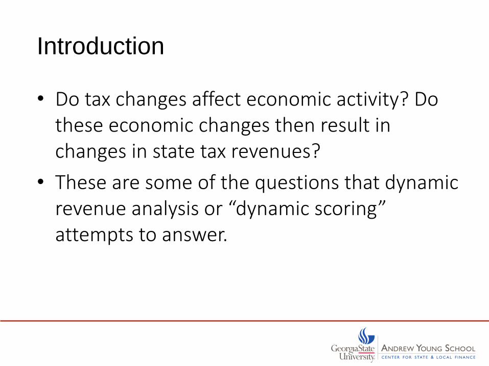
Introduction

• Do tax changes affect economic activity? Do these economic changes then result in changes in state tax revenues?

• These are some of the questions that dynamic revenue analysis or “dynamic scoring” attempts to answer.

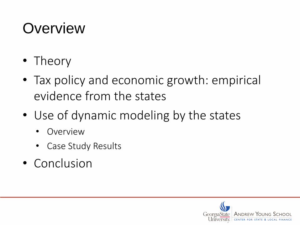
Overview

• Theory

• Tax policy and economic growth: empirical evidence from the states

• Use of dynamic modeling by the states• Overview

• Case Study Results

• Conclusion

Supply-Side Links to Dynamic

Revenue Analysis

• Perhaps no economist is as associated with supply-side economics and the “dynamic effects” of tax changes as Arthur Laffer...

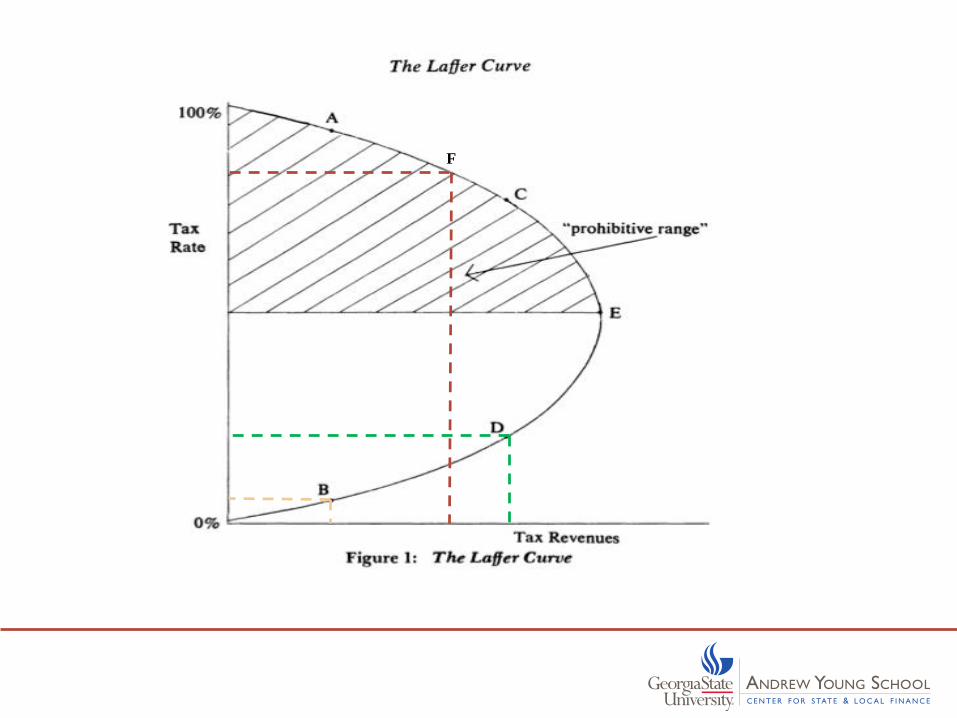
F

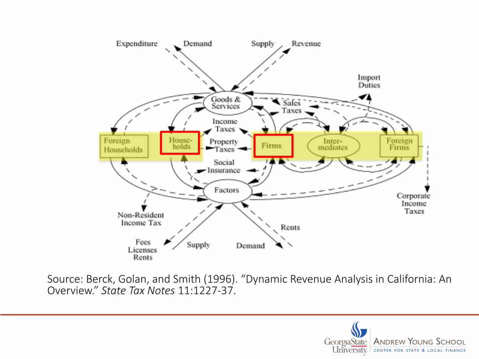
Source: Berck, Golan, and Smith (1996). “Dynamic Revenue Analysis in California: An Overview.” State Tax Notes 11:1227-37.

Empirical Evidence:

Effect of Taxes on State Economies

• Taxes generally create a drag on state economies.

• Key reviews of the early literature found: – Taxes had a statistically significant negative impact on state

economic output—

– The size of the effect was potentially subject to measurement error and most likely small.

• Recent studies find a negative effect of tax changes on economic variables, but typically the effect is small.

• Some evidence that government spending on productive services can offset the negative effects of taxes.

Experience of the States

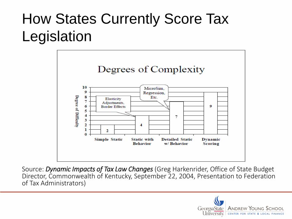
How States Currently Score Tax

Legislation

Source: Dynamic Impacts of Tax Law Changes (Greg Harkenrider, Office of State Budget Director, Commonwealth of Kentucky, September 22, 2004, Presentation to Federation of Tax Administrators)

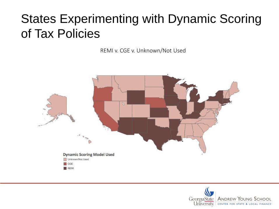
States Experimenting with Dynamic Scoring

of Tax Policies

REMI v. CGE v. Unknown/Not Used

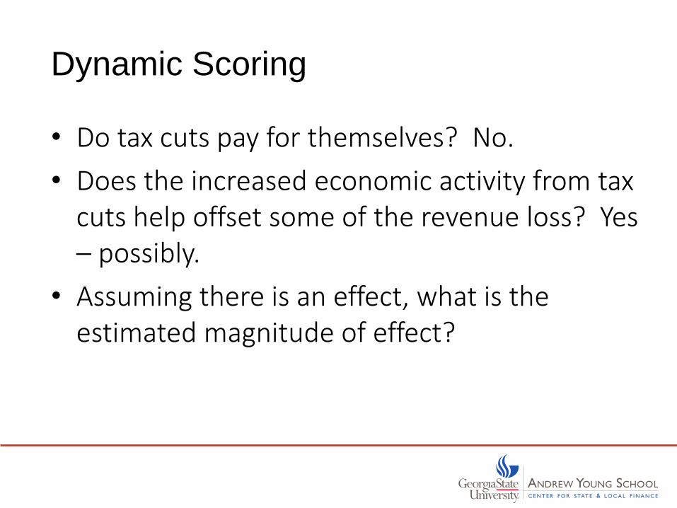
Dynamic Scoring

• Do tax cuts pay for themselves? No.

• Does the increased economic activity from tax cuts help offset some of the revenue loss? Yes – possibly.

• Assuming there is an effect, what is the estimated magnitude of effect?

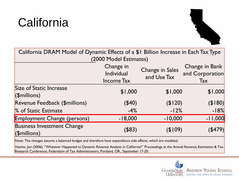
California

California DRAM Model of Dynamic Effects of a $1 Billion Increase in Each Tax Type

(2000 Model Estimates)

Change in

Individual

Income Tax

Change in Sales

and Use Tax

Change in Bank

and Corporation

Tax

Size of Static Increase

($millions)$1,000 $1,000 $1,000

Revenue Feedback ($millions) ($40) ($120) ($180)

% of Static Estimate -4% -12% -18%

Employment Change (persons) -18,000 -10,000 -11,000

Business Investment Change

($millions)($83) ($109) ($479)

Note: The changes assume a balanced budget and therefore have expenditure side effects, which are modeled.

Vasche, Jon (2006). “Whatever Happened to Dynamic Revenue Analysis in California?” Proceedings at the Annual Revenue Estimation & Tax

Research Conference, Federation of Tax Administrators, Portland, OR., September 17-20.

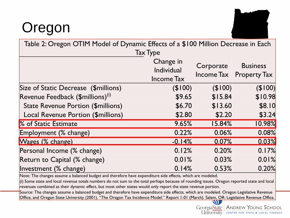
OregonTable 2: Oregon OTIM Model of Dynamic Effects of a $100 Million Decrease in Each

Tax Type

Change in

Individual

Income Tax

Corporate

Income Tax

Business

Property Tax

Size of Static Decrease ($millions) ($100) ($100) ($100)

Revenue Feedback ($millions)(i) $9.65 $15.84 $10.98

State Revenue Portion ($millions) $6.70 $13.60 $8.10

Local Revenue Portion ($millions) $2.80 $2.20 $3.24

% of Static Estimate 9.65% 15.84% 10.98%

Employment (% change) 0.22% 0.06% 0.08%

Wages (% change) -0.14% 0.07% 0.03%

Personal Income (% change) 0.12% 0.20% 0.17%

Return to Capital (% change) 0.01% 0.03% 0.01%

Investment (% change) 0.14% 0.53% 0.20%Note: The changes assume a balanced budget and therefore have expenditure side effects, which are modeled.

(i) Some state and local revenue totals numbers do not sum to the total perhaps because of rounding issues. Oregon reported state and local

revenues combined as their dynamic effect, but most other states would only report the state revenue portion.

Source: The changes assume a balanced budget and therefore have expenditure side effects, which are modeled. Oregon Legislative Revenue

Office, and Oregon State University (2001). “The Oregon Tax Incidence Model.” Report 1-01 (March). Salem, OR: Legislative Revenue Office.

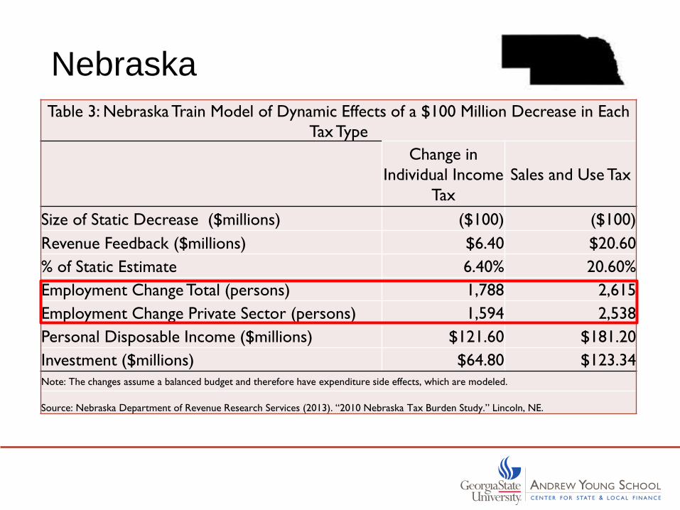
Nebraska

Table 3: Nebraska Train Model of Dynamic Effects of a $100 Million Decrease in Each

Tax Type

Change in

Individual Income

Tax

Sales and Use Tax

Size of Static Decrease ($millions) ($100) ($100)

Revenue Feedback ($millions) $6.40 $20.60

% of Static Estimate 6.40% 20.60%

Employment Change Total (persons) 1,788 2,615

Employment Change Private Sector (persons) 1,594 2,538

Personal Disposable Income ($millions) $121.60 $181.20

Investment ($millions) $64.80 $123.34 Note: The changes assume a balanced budget and therefore have expenditure side effects, which are modeled.

Source: Nebraska Department of Revenue Research Services (2013). “2010 Nebraska Tax Burden Study.” Lincoln, NE.

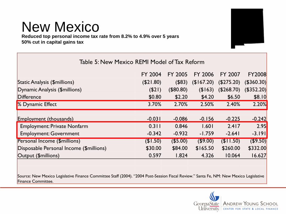
New Mexico

Table 5: New Mexico REMI Model of Tax Reform

FY 2004 FY 2005 FY 2006 FY 2007 FY2008

Static Analysis ($millions) ($21.80) ($83) ($167.20) ($275.20) ($360.30)

Dynamic Analysis ($millions) ($21) ($80.80) ($163) ($268.70) ($352.20)

Difference $0.80 $2.20 $4.20 $6.50 $8.10

% Dynamic Effect 3.70% 2.70% 2.50% 2.40% 2.20%

Employment (thousands) -0.031 -0.086 -0.156 -0.225 -0.242

Employment: Private Nonfarm 0.311 0.846 1.601 2.417 2.95

Employment: Government -0.342 -0.932 -1.759 -2.641 -3.191

Personal Income ($millions) ($1.50) ($5.00) ($9.00) ($11.50) ($9.50)

Disposable Personal Income ($millions) $30.00 $84.00 $165.50 $260.00 $332.00

Output ($millions) 0.597 1.824 4.326 10.064 16.627

Source: New Mexico Legislative Finance Committee Staff (2004). “2004 Post-Session Fiscal Review.” Santa Fe, NM: New Mexico Legislative

Finance Committee.

Reduced top personal income tax rate from 8.2% to 4.9% over 5 years

50% cut in capital gains tax

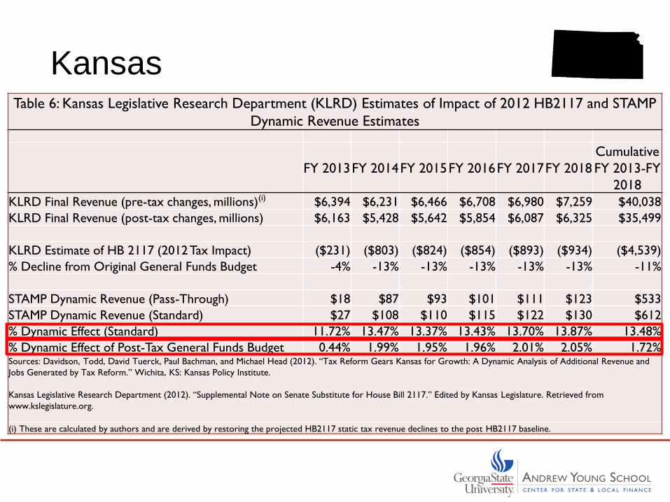
KansasTable 6: Kansas Legislative Research Department (KLRD) Estimates of Impact of 2012 HB2117 and STAMP

Dynamic Revenue Estimates

FY 2013FY 2014FY 2015FY 2016FY 2017FY 2018

Cumulative

FY 2013-FY

2018

KLRD Final Revenue (pre-tax changes, millions)(i) $6,394 $6,231 $6,466 $6,708 $6,980 $7,259 $40,038

KLRD Final Revenue (post-tax changes, millions) $6,163 $5,428 $5,642 $5,854 $6,087 $6,325 $35,499

KLRD Estimate of HB 2117 (2012 Tax Impact) ($231) ($803) ($824) ($854) ($893) ($934) ($4,539)

% Decline from Original General Funds Budget -4% -13% -13% -13% -13% -13% -11%

STAMP Dynamic Revenue (Pass-Through) $18 $87 $93 $101 $111 $123 $533

STAMP Dynamic Revenue (Standard) $27 $108 $110 $115 $122 $130 $612

% Dynamic Effect (Standard) 11.72% 13.47% 13.37% 13.43% 13.70% 13.87% 13.48%

% Dynamic Effect of Post-Tax General Funds Budget 0.44% 1.99% 1.95% 1.96% 2.01% 2.05% 1.72%Sources: Davidson, Todd, David Tuerck, Paul Bachman, and Michael Head (2012). “Tax Reform Gears Kansas for Growth: A Dynamic Analysis of Additional Revenue and

Jobs Generated by Tax Reform.” Wichita, KS: Kansas Policy Institute.

Kansas Legislative Research Department (2012). “Supplemental Note on Senate Substitute for House Bill 2117.” Edited by Kansas Legislature. Retrieved from

www.kslegislature.org.

(i) These are calculated by authors and are derived by restoring the projected HB2117 static tax revenue declines to the post HB2117 baseline.

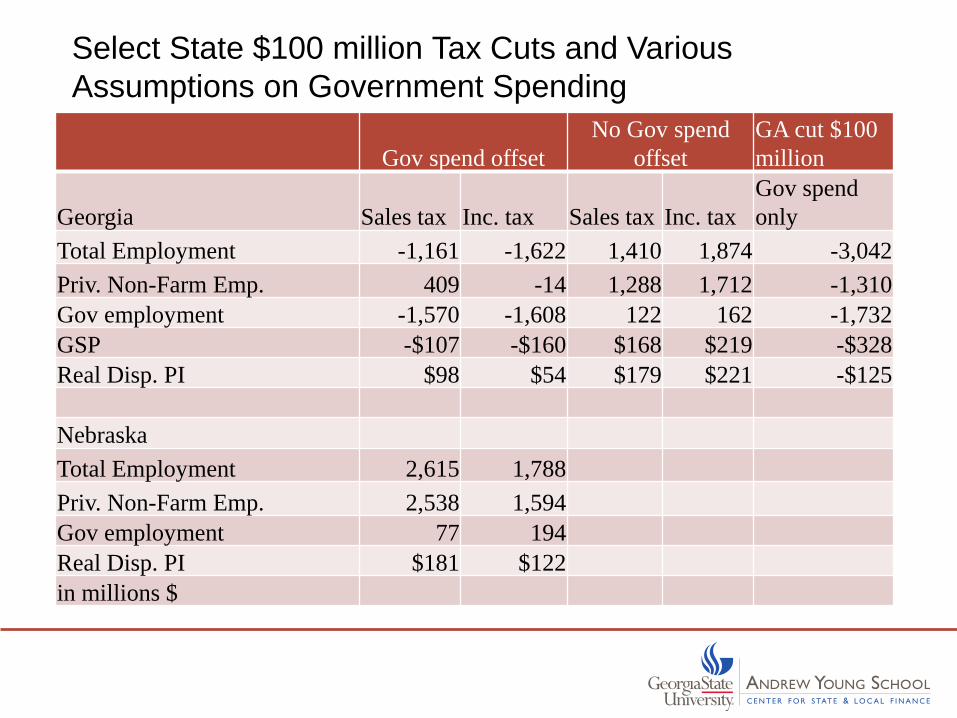
Select State $100 million Tax Cuts and Various

Assumptions on Government Spending

Gov spend offset

No Gov spend

offset

GA cut $100

million

Georgia Sales tax Inc. tax Sales tax Inc. tax

Gov spend

only

Total Employment -1,161 -1,622 1,410 1,874 -3,042

Priv. Non-Farm Emp. 409 -14 1,288 1,712 -1,310

Gov employment -1,570 -1,608 122 162 -1,732

GSP -$107 -$160 $168 $219 -$328

Real Disp. PI $98 $54 $179 $221 -$125

Nebraska

Total Employment 2,615 1,788

Priv. Non-Farm Emp. 2,538 1,594

Gov employment 77 194

Real Disp. PI $181 $122

in millions $

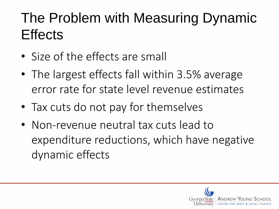
The Problem with Measuring Dynamic

Effects

• Size of the effects are small

• The largest effects fall within 3.5% average error rate for state level revenue estimates

• Tax cuts do not pay for themselves

• Non-revenue neutral tax cuts lead to expenditure reductions, which have negative dynamic effects

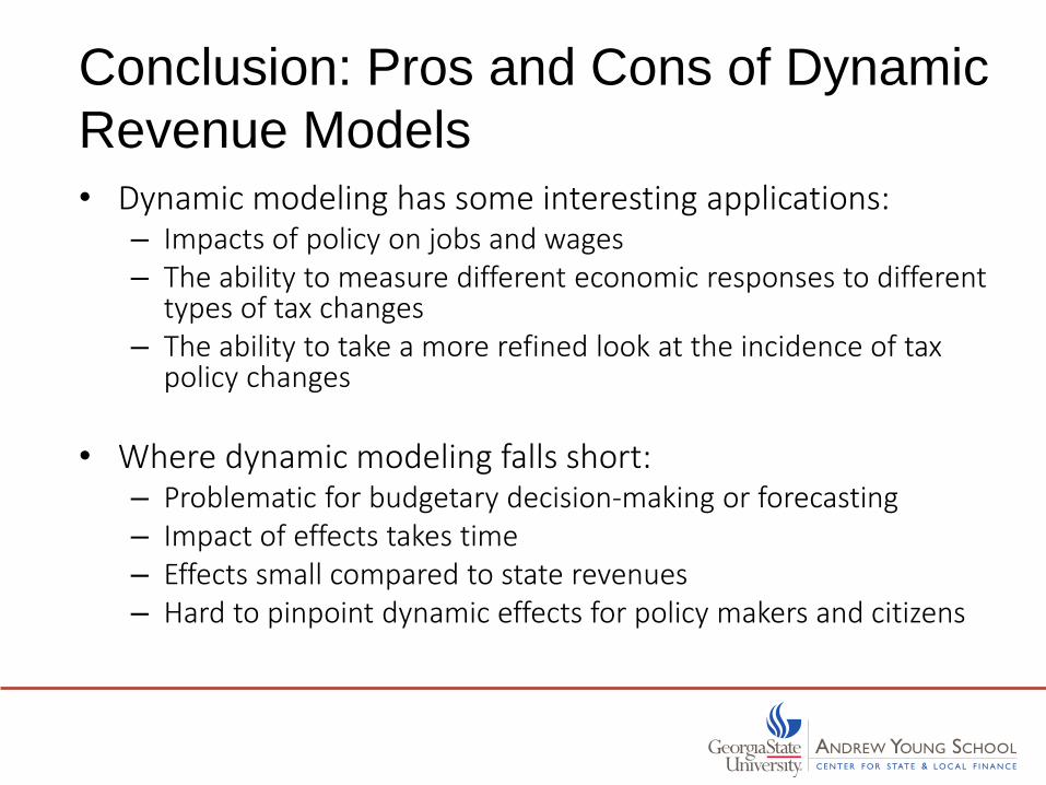
Conclusion: Pros and Cons of Dynamic

Revenue Models

• Dynamic modeling has some interesting applications:– Impacts of policy on jobs and wages– The ability to measure different economic responses to different

types of tax changes– The ability to take a more refined look at the incidence of tax

policy changes

• Where dynamic modeling falls short:– Problematic for budgetary decision-making or forecasting – Impact of effects takes time– Effects small compared to state revenues– Hard to pinpoint dynamic effects for policy makers and citizens

Conclusion: Important Questions for

Policy Makers

• First, what do policymakers want to learn from dynamic revenue estimation? – Inform a policy debate– May not be appropriate for the budgetary process

• Second, states need to consider the resources required to develop, customize and then interpret the results from a dynamic model. – Models are costly and require annual updating– Models are complicated– Not a few states have abandoned their efforts at dynamic

revenue estimation due to this cost and complexity

Thank You

Peter Bluestone

Pbluestone@gsu.edu

http://cslf.gsu.edu/publications/

Dynamic Revenue Analysis: Experience of the States

June 26, 2015