Dynamic Spherical Volumetric Simplex Splines withApplications in Biomedical Simulation

Yunhao Tan, Jing Hua∗

Wayne State UniversityHong Qin

Stony Brook University

Abstract

This paper presents a novel computational framework based on dy-namic spherical volumetric simplex splines for simulation of genus-zero real-world objects. In this framework, we first develop an ac-curate and efficient algorithm to reconstruct the high-fidelity digi-tal model of a real-world object with spherical volumetric simplexsplines which can represent with accuracy geometric, material, andother properties of the object simultaneously. With the tight cou-pling of Lagrangian mechanics, the dynamic volumetric simplexsplines representing the object can accurately simulate its physicalbehavior because it can unify the geometric and material propertiesin the simulation. The visualization can be directly computed fromthe object’s geometric or physical representation based on the dy-namic spherical volumetric simplex splines during simulation with-out interpolation or resampling. We have applied the framework forbiomechanic simulation of brain deformations, such as brain shift-ing during the surgery and brain injury under blunt impact. Wehave compared our simulation results with the ground truth ob-tained through intra-operative magnetic resonance imaging and thereal biomechanic experiments. The evaluations demonstrate the ex-cellent performance of our new technique presented in this paper.

CR Categories: I.3.5 [Computer Graphics]: ComputationalGeometry and Object Modeling—Physically based modeling

1 Introduction

Physically-based modeling and simulation of digitized real-worldmodels are still extremely challenging tasks. Among many impor-tant aspects of simulation, the accuracy is of utmost importancesince only physically realistic simulation can be used to representthe true reality and provide valuable information for the simulation-based assessment and analysis. In existing approaches, several dif-ferent representations are typically required throughout the simu-lation of real-world models in computerized environments. Thatis to say, each stage within the entire physical simulation pipeline,including modeling (e.g., meshing, material modeling), simulation,analysis, visualization, typically takes as input a different represen-tation of the modeled object, which requires costly and error-pronedata conversions throughout the entire simulation process. It willcertainly introduce error into the pipeline. For instance, in orderto simulate the brain deformation, a linear solid mesh needs to begenerated for finite element methods (FEMs) from the voxel-basedrepresentation of the brain representing the geometry of the brain(which has a highly convoluted cortical surface and many subtlesub-cortical structures). Then, manual material editing needs to beconducted to assign material properties to solid meshes. The FEM

∗Correspondence to: Jing Hua. Email: jinghua@cs.wayne.edu

properties are linearly interpolated during simulation and resampledonce again to voxels’ intensities for visualization. Certainly, con-versions among volumetric datasets, solid meshes, finite elements,and voxels based on linear interpolation or resampling will intro-duce error. In addition, more errors will be brought into the pipelineas the constructed linear solid mesh may not well represent bothgeometry and material distribution simultaneously. The geometric,physical, and mechanical properties are not tightly integrated intothe simulation. As a result, the current practice impedes the accu-rate modeling and simulation of digital models of real-world ob-jects. With ever-improving computing power comes the strong de-mand for more accurate, robust, and powerful solid modeling andsimulation paradigms that are efficacious for the modeling, simu-lation, analysis, and visualization of digital models of real-worldobjects.

To overcome the aforementioned deficiencies, we develop an inte-grated computational framework based on dynamic spherical volu-metric simplex splines (DSVSS) that can greatly improve the accu-racy and efficacy of modeling and simulation of heterogenous ob-jects since the framework can not only reconstruct with high accu-racy geometric, material, and other quantities associated with het-erogeneous real-world models, but also simulate the complicateddynamics precisely by tightly coupling these physical propertiesinto simulation. The integration of geometric modeling, materialmodeling, and simulation is the key to the success of simulation ofreal-world objects. In contrast to existing techniques, our frame-work uses a single representation that requires no data conversion.The advantages of our framework result from many attractive prop-erties of multivariate splines. In comparison with tensor-productNURBS, multivariate simplex splines are non-tensor-product in na-ture. They are essentially piecewise polynomials of the lowest pos-sible degree and the highest possible continuity everywhere acrosstheir entire tetrahedral domain. For example, given an object ofsimplex splines with degreen, it can achieveCn−1 continuity.Furthermore,C0, other varying continuities, and even discontinu-ity can be accommodated through different knot and control pointplacements and/or different arrangements of domain tetrahedra in3D. Furthermore, simplex splines are ideal to represent heteroge-neous material distributions through the tight coupling of controlpoints and their attributes. From dynamic simulation’s point ofview, they are finite elements which can be directly brought intofinite element formulations and physics-based analysis without los-ing any information. Finite elements can be derived directly fromthe simplex spline representation, which can also be visualizedvia volumetric ray-casting without discretization [Hua et al. 2004].Trivariate simplex splines are obtained through the projection ofn-dimensional simplices onto 3D. Projecting them one step fur-ther onto 2D for visualization results in bivariate simplex splines ofone degree higher than the original solid model, therefore, simplexsplines facilitate the visualization task with an analytical, closed-form formulation. It is not necessary to perform any resamplingand/or interpolation operations. Local adaptivity and local/globalsubdivision via knot insertion can be readily achieved.

On the application front, in recent years, tremendous efforts frombiomedical research communities have been devoted into the brainsimulation since accurate simulation of brain deformations can havemany potential applications, e.g., computer-aided surgical plan-

ning/surgery, computer-assisted disease/injury positioning, accu-rate radiation therapy, and many other medical benefits [Maguireet al. 1991]. Various methods are emerging for simulation of thebrains in different physical environments. However, most brain vol-ume simulation techniques still depend on linear geometric repre-sentation and FEMs as we have already described above. No ad-vanced computational models are available for better simulation.As we all know, the brain is a highly convoluted organ rich of geo-metric, anatomical, and material variations. In order to obtain re-alistic deformation simulation of the brain, it is very important toconstruct a digital model which can simultaneously represent itsgeometry, imaging intensities, and material properties, and then in-tegrate the properties into the biomechanic simulation. Considerthat the human brain is topologically equivalent to a solid sphere,our proposed dynamic spherical volumetric simplex splines are per-fect for modeling, simulation, and analysis of such an object. Thespherical volumetric simplex splines are defined over a solid spher-ical tetrahedralization. In this paper, we apply and evaluate oursimulation framework on various human brain deformations.

Our contributions in this paper can be summarized as follows:

• We develop a physical simulation framework which seam-lessly integrates geometric properties, physical properties,and dynamic behaviors together. The consistent, uniform rep-resentation throughout each stage of modeling and simulationis a single degreen spherical volumetric simplex spline. Itis ideal for simulating complex, heterogenous real-world ob-jects.

• The heterogenous model reconstructed from the digitalizationof a real-world object is faithful and of high-fidelity in termsof its geometry and material distribution. The model recon-struction procedure is automatic, and the maximal fitting errorto the original data can be controlled by user’s specificationinteractively.

• During the simulation, the geometry and physical proper-ties of the volumetric model can be computed using theanalytic representation without any need for numerical ap-proximations such as cubic interpolation or quadratic resam-pling. Hence, physical simulation, including all downstreamprocesses, such as analysis and evaluation, can be achievedmore accurately and robustly.

• We apply the dynamic spherical simplex splines scheme inthe simulation and analysis of brain models. The unifiedscheme can achieve very accurate simulation compared withthe ground-truth results because it can tightly integrate thegeometric and material properties in the simulation. Ourframework has great potential to provide simulation-based as-sessment for innovative computer-aided diagnosis of brain in-jury cases.

2 Previous Work

Our paper is related to the theory and application of multivariatesimplex splines and physically based simulation. This section re-views the related, previous work in these fields.

2.1 Multivariate Simplex Splines

From projection’s point of view, univariate B-splines can be in-tuitively formulated as volumetric shadows of higher dimensionalsimplices, i.e., we can obtain B-splines of arbitrary degreen bytaking a simplex in the(n + 1)-dimensional space and volumetri-cally projecting it ontoR1. Motivated by this idea of Curry and

Schoenberg, C. de Boor [de Boor 1976] presented a brief descrip-tion of multivariate simplex splines. In essence, multivariate sim-plex splines are the volumetric projection of higher dimensionalsimplices onto a lower dimensional spaceRm. Simplex splineshave many attractive properties such as piecewise polynomials overgeneral tetrahedral domains, local support, higher-order smooth-ness, and positivity, making them potentially ideal in engineeringdesign applications [Greiner and Seidel 1994]. From the point ofview of blossoming, Dahmenet al. [Dahmen et al. 1992] proposedtriangular B-splines. Later, Greiner and Seidel [Greiner and Seidel1994] demonstrated their practical feasibility in graphics and shapedesign.

In contrast to theoretical advances, the application of simplexsplines has been rather under-explored. Pfeifle and Seidel devel-oped a faster evaluation technique for quadratic bivariate DMS-spline surfaces [Pfeifle and Seidel 1994] and applied it to the scat-tered data fitting of triangular B-spline [Pfeifle and Seidel 1996].Recently, Rosslet al. [Pauly et al. 2002] presented a novel approachto reconstruct volume from structure-gridded samples using trivari-ate quadric super splines defined on a uniform tetrahedral partition.They used Bernstein-Bezier techniques to compute and evaluate thetrivariate spline and its gradient. Hua and Qin presented a volumet-ric sculpting framework that employs trivariate scalar nonuniformB-splines as underlying representation [Hua and Qin 2001; Hua andQin 2003]. More recently, they applied trivariate simplex splines tothe representation of solid geometry, the modeling of heterogeneousmaterial attributes, and the reconstruction of continuous volumetricsplines from discretized volumetric inputs via data fitting [Hua et al.2005]. Tanet al. applied the hierarchical simplex splines to volumereconstruction from planar images [Tan et al. 2007].

2.2 Physically Based Modeling and Simulation

Free-form deformable models were first introduced to the model-ing community by Terzopouloset al. [Terzopoulos and Fleischer1988], and they have been improved by a number of researchersover the past 20 years. Celniker and Gossard developed an inter-esting prototype system [Celniker and Gossard 1991] for interac-tive free-form design based on the finite-element optimization ofenergy functionals proposed in [Terzopoulos and Fleischer 1988].Bloor and Wilson developed related models using similar energiesand numerical optimization [Bloor and Wilson 1990]. Welch andWitkin extended the approach to trimmed hierarchical B-splines forinteractive modeling of free-form surfaces with constrained varia-tional optimization [Welch and Witkin 1992]. Terzopoulos and Qin[Terzopoulos and Qin 1994; Qin and Terzopoulos 1995b] deviseddynamic physical-based generalization of NURBS (D-NURBS).Later, they further developed dynamic triangular B-splines [Qin andTerzopoulos 1995a] paradigm for high topology surface modeling.The new paradigm on simplex spline finite elements is substantiallymore sophisticated and is expected to produce even more true-to-life simulation results.

As for simulation of digital models of real-world objects, re-searchers mainly focused on FEM meshing, which can represent theshape of the objects, and physical laws, which govern the model’sbehavior. Zhanget al. presented a method for 3D mesh genera-tion from imaging data [Zhang et al. 2005]. They further designedan algorithm for automatic 3D mesh generation for a domain withmultiple materials. In general, the main objective of FEM mesh-ing is to construct a nicely-shaped elements which can representboth geometry and material of the real-world models for accurateand robust simulation. However, due to the linear representations,it cannot accurately represent the geometric and physical propertiesin simulation. For simulation-based assessment of real-world ob-jects, e.g., the brain, the main goal is to obtain an objective analysis

result from the realistic simulation of the objects. In brain defor-mation simulation, researchers have been using it for many clinicalapplications [Maguire et al. 1991].

3 Dynamic Spherical Volumetric SimplexSplines

In this section, we first briefly review the theoretical background ofvolumetric simplex splines. Then, we formalize them to the spher-ical volumetric simplex splines with details on spherical domainconstruction. We further generalize the splines with physical dy-namics and develop dynamic spherical simplex splines which canbe used for modeling and simulation of real-world models.

3.1 Volumetric Simplex Splines

A degreen volumetric simplex spline,M(x|x0, · · · ,xn+3), canbe defined as a function ofx ∈ R3 over the half open convex hullof a point setV = [x0, · · · ,xn+3), depending on then + 4 knotsxi ∈ R3, i = 0, · · · , n + 3. The volumetric simplex splines maybe formulated recursively, which facilitates point evaluation and itsderivative and gradient computation. Whenn = 0,

M(x|x0, · · · ,x3) =

1|VolR3 (x0,··· ,x3)| , x ∈ [x0, · · · ,x3),

0, otherwise,

and whenn > 0, select four pointsW = xk0 ,xk1 ,xk2 ,xk3from V, such thatW is affinely independent, then

M(x|x0, · · · ,xn+3) =

3Xj=0

λj(x|W)M(x|V \ xkj), (1)

whereP3

j=0 λj(x|W) = 1 andP3

j=0 λj(x|W)xkj = x.

The directional derivative ofM(x|V) with respect to a vectord isdefined as follows:

DdM(x|V) = n

3Xj=0

µj(d|W)M(x|V \ xkj), (2)

whered =P3

j=0 µj(d|W)xkj andP3

j=0 µj(d|W) = 0.

3.2 Spherical Simplex Spline Volume

Generally, volumetric simplex spline can take as input any domainwith arbitrary geometry and topology due to its non-tensor-productnature. Namely, spherical simplex spline volume is defined by vol-umetric simplex splines over a spherical volumetric domain. Herewe choose the sphere domain since mapping most organic objectsin the biomedical research field to a sphere results in less distortionand more uniform distribution of sampling points, which reducesthe difficulty in the fitting procedure. Note that, our volumetricsimplex spline volumes represent not only boundary geometry, butalso interior geometry. They can represent physical or material at-tributes over the entire solid as well.

3.2.1 Spherical Volumetric Simplex Splines

Now denoteS3 = x ∈ R3, ‖x‖ ≤ c a solid sphere inR3. With-out loss of generality, letS3 be a unit solid sphere, i.e.,c = 1.Let T be an arbitrary “proper” tetrahedralization ofS3. Here,“proper” means that every pair of domain tetrahedra are disjoint,or share exactly one vertex, one edge, or one face. To each ver-tex t of the tetrahedralizationT, we assign a knot cloud, which

is a sequence of points[t0, t1, · · · , tn], wheret0 ≡ t. We callt primary-knot and[t1, · · · , tn] sub-knots. For every tetrahedronI = (p,q, r, s) ∈ T, we require

• all the tetrahedra[pi,qj , rk, sl] with i + j + k + l ≤ n arenon-degenerate.

• the set

Ω = interior(∩i+j+k+l≤n[pi,qj , rk, sl]) (3)

is not empty.

• if I is a boundary tetrahedron, the sub-knots assigned to theboundary vertices must lie outside ofS3.

We then define, for each tetrahedronI ∈ T andi + j + k + l = n(in the following, we useβ to denote 4-tuple(i, j, k, l)), the knotsets

V Iβ = [p0, · · · ,pi,q0, · · · ,qj , r0, · · · , rk, s0, · · · , sl]. (4)

The basis functions of normalized simplex splines are then definedas

NIβ(u) = |det(pi,qj , rk, sl)|M(u|V I

β ). (5)

These basis functions can be shown to be all non-negative and toform a partition of unity. The volumetric spherical simplex splinevolume is the combination of a set of basis functions with controlpointscI

β :

s(u) =XI∈T

X|β|=n

cIβNI

β(u). (6)

The “generalized” control pointscIβ are now(k + 3)-dimensional

vectors, including control points(px, py, pz) for the solid geome-try, and control coefficients(g1, · · · , gk) for the attributes, wherek denotes the number of attributes associated with the geometry.The spherical simplex splines are ideal to model genus-zero, het-erogeneous solid objects. The number of physical properties isapplication-oriented. For a concise expression of the formulation,without loss of generality, we will deal with only one physical at-tribute in the following formulas.

3.2.2 Initial Construction of Spherical Volumetric Domain

Theoretically, domain tetrahedralization,T, can be an arbitrarytetrahedralization of a unit solid sphere,S3, as aforementioned inSection 3.2.1. However, in practice, two important aspects of thedomain tetrahedralization should be carefully considered:

• T should be as uniform as possible, i.e., minimizemax(V olI∈T)

min(V olI′∈T). Uniform tetrahedralization at the same hierar-

chical level will decrease the recursion time while hierarchicalstructure is needed.

• T should avoid bad-shaped tetrahedra in Delaunay tetrahe-dralization. Bad-shaped tetrahedra, for instance, slivers, willincrease numerical error during the evaluation.

Constrained Delaunay tetrahedralization [Edelsbrunner 2001] canobserve the second requirement, but it will introduce very large andvery small tetrahedra thus can not comply with the first require-ment. Instead, we tetrahedralize a regular icosahedron and thenmake use of harmonic volumetric mapping to map the tetrahedral-ization to a solid sphere. As a result, the solid sphere tetrahedral-ization is uniform and its quality is better than what constrainedDelaunay tetrahedralization can offer.

Figure 1 shows the flow of domain establishment and the knots dis-tribution. Note that, in Figure 1(d), the sub-knots associated with

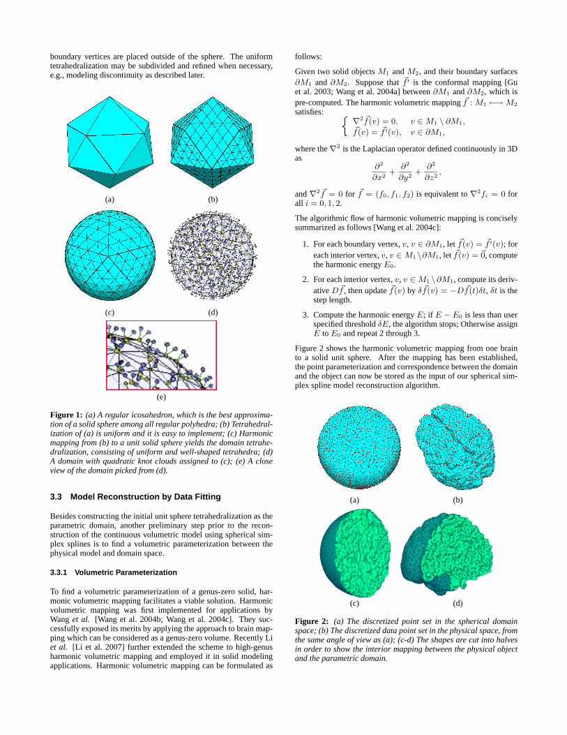
boundary vertices are placed outside of the sphere. The uniformtetrahedralization may be subdivided and refined when necessary,e.g., modeling discontinuity as described later.

(a) (b)

(c) (d)

(e)

Figure 1: (a) A regular icosahedron, which is the best approxima-tion of a solid sphere among all regular polyhedra; (b) Tetrahedral-ization of (a) is uniform and it is easy to implement; (c) Harmonicmapping from (b) to a unit solid sphere yields the domain tetrahe-dralization, consisting of uniform and well-shaped tetrahedra; (d)A domain with quadratic knot clouds assigned to (c); (e) A closeview of the domain picked from (d).

3.3 Model Reconstruction by Data Fitting

Besides constructing the initial unit sphere tetrahedralization as theparametric domain, another preliminary step prior to the recon-struction of the continuous volumetric model using spherical sim-plex splines is to find a volumetric parameterization between thephysical model and domain space.

3.3.1 Volumetric Parameterization

To find a volumetric parameterization of a genus-zero solid, har-monic volumetric mapping facilitates a viable solution. Harmonicvolumetric mapping was first implemented for applications byWanget al. [Wang et al. 2004b; Wang et al. 2004c]. They suc-cessfully exposed its merits by applying the approach to brain map-ping which can be considered as a genus-zero volume. Recently Liet al. [Li et al. 2007] further extended the scheme to high-genusharmonic volumetric mapping and employed it in solid modelingapplications. Harmonic volumetric mapping can be formulated as

follows:

Given two solid objectsM1 andM2, and their boundary surfaces∂M1 and ∂M2. Suppose that~f ′ is the conformal mapping [Guet al. 2003; Wang et al. 2004a] between∂M1 and∂M2, which ispre-computed. The harmonic volumetric mapping~f : M1 7−→ M2

satisfies: ∇2 ~f(v) = 0, v ∈ M1 \ ∂M1,~f(v) = ~f ′(v), v ∈ ∂M1,

where the∇2 is the Laplacian operator defined continuously in 3Das

∂2

∂x2+

∂2

∂y2+

∂2

∂z2,

and∇2 ~f = 0 for ~f = (f0, f1, f2) is equivalent to∇2fi = 0 forall i = 0, 1, 2.

The algorithmic flow of harmonic volumetric mapping is conciselysummarized as follows [Wang et al. 2004c]:

1. For each boundary vertex,v, v ∈ ∂M1, let ~f(v) = ~f ′(v); foreach interior vertex,v, v ∈ M1\∂M1, let ~f(v) = ~0, computethe harmonic energyE0.

2. For each interior vertex,v, v ∈ M1 \∂M1, compute its deriv-ativeD ~f , then update~f(v) by δ ~f(v) = −D ~f(t)δt, δt is thestep length.

3. Compute the harmonic energyE; if E − E0 is less than userspecified thresholdδE, the algorithm stops; Otherwise assignE to E0 and repeat 2 through 3.

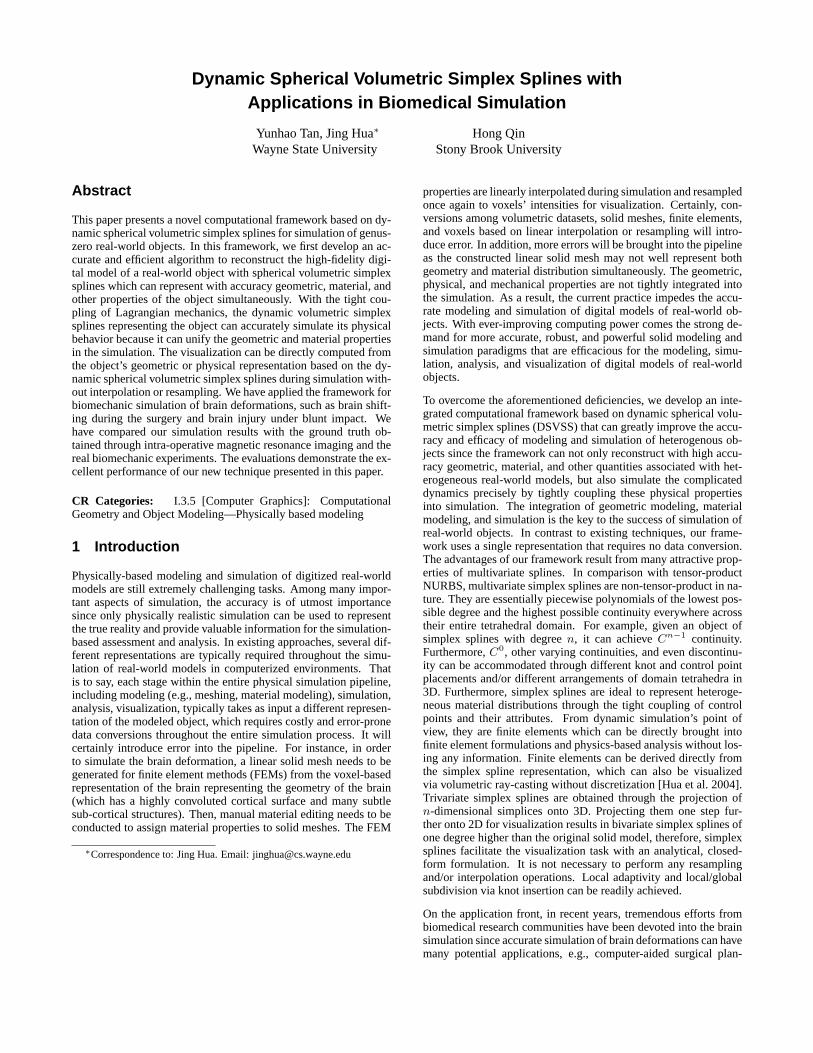
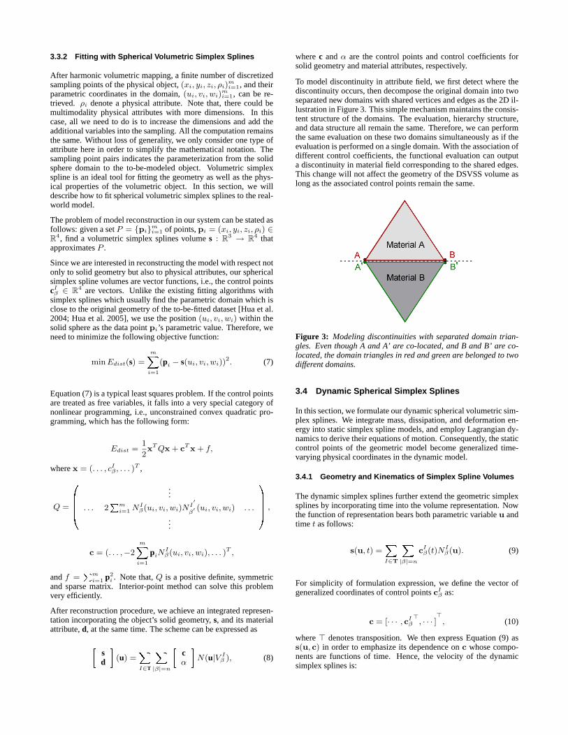
Figure 2 shows the harmonic volumetric mapping from one brainto a solid unit sphere. After the mapping has been established,the point parameterization and correspondence between the domainand the object can now be stored as the input of our spherical sim-plex spline model reconstruction algorithm.

(a) (b)

(c) (d)

Figure 2: (a) The discretized point set in the spherical domainspace; (b) The discretized data point set in the physical space, fromthe same angle of view as (a); (c-d) The shapes are cut into halvesin order to show the interior mapping between the physical objectand the parametric domain.

3.3.2 Fitting with Spherical Volumetric Simplex Splines

After harmonic volumetric mapping, a finite number of discretizedsampling points of the physical object,(xi, yi, zi, ρi)

mi=1, and their

parametric coordinates in the domain,(ui, vi, wi)mi=1, can be re-

trieved. ρi denote a physical attribute. Note that, there could bemultimodality physical attributes with more dimensions. In thiscase, all we need to do is to increase the dimensions and add theadditional variables into the sampling. All the computation remainsthe same. Without loss of generality, we only consider one type ofattribute here in order to simplify the mathematical notation. Thesampling point pairs indicates the parameterization from the solidsphere domain to the to-be-modeled object. Volumetric simplexspline is an ideal tool for fitting the geometry as well as the phys-ical properties of the volumetric object. In this section, we willdescribe how to fit spherical volumetric simplex splines to the real-world model.

The problem of model reconstruction in our system can be stated asfollows: given a setP = pim

i=1 of points,pi = (xi, yi, zi, ρi) ∈R4, find a volumetric simplex splines volumes : R3 → R4 thatapproximatesP .

Since we are interested in reconstructing the model with respect notonly to solid geometry but also to physical attributes, our sphericalsimplex spline volumes are vector functions, i.e., the control pointscIβ ∈ R4 are vectors. Unlike the existing fitting algorithms with

simplex splines which usually find the parametric domain which isclose to the original geometry of the to-be-fitted dataset [Hua et al.2004; Hua et al. 2005], we use the position(ui, vi, wi) within thesolid sphere as the data pointpi’s parametric value. Therefore, weneed to minimize the following objective function:

min Edist(s) =

mXi=1

(pi − s(ui, vi, wi))2. (7)

Equation (7) is a typical least squares problem. If the control pointsare treated as free variables, it falls into a very special category ofnonlinear programming, i.e., unconstrained convex quadratic pro-gramming, which has the following form:

Edist =1

2xT Qx + cT x + f,

wherex = (. . . , cIβ , . . . )T ,

Q =

0BBB@

...

. . . 2Pm

i=1 NIβ(ui, vi, wi)N

I′

β′ (ui, vi, wi) . . .

...

1CCCA ,

c = (. . . ,−2

mXi=1

piNIβ(ui, vi, wi), . . . )

T ,

andf =Pm

i=1 p2i . Note that,Q is a positive definite, symmetric

and sparse matrix. Interior-point method can solve this problemvery efficiently.

After reconstruction procedure, we achieve an integrated represen-tation incorporating the object’s solid geometry,s, and its materialattribute,d, at the same time. The scheme can be expressed as

sd

(u) =

XI∈T

X|β|=n

cα

N(u|V I

β ), (8)

wherec andα are the control points and control coefficients forsolid geometry and material attributes, respectively.

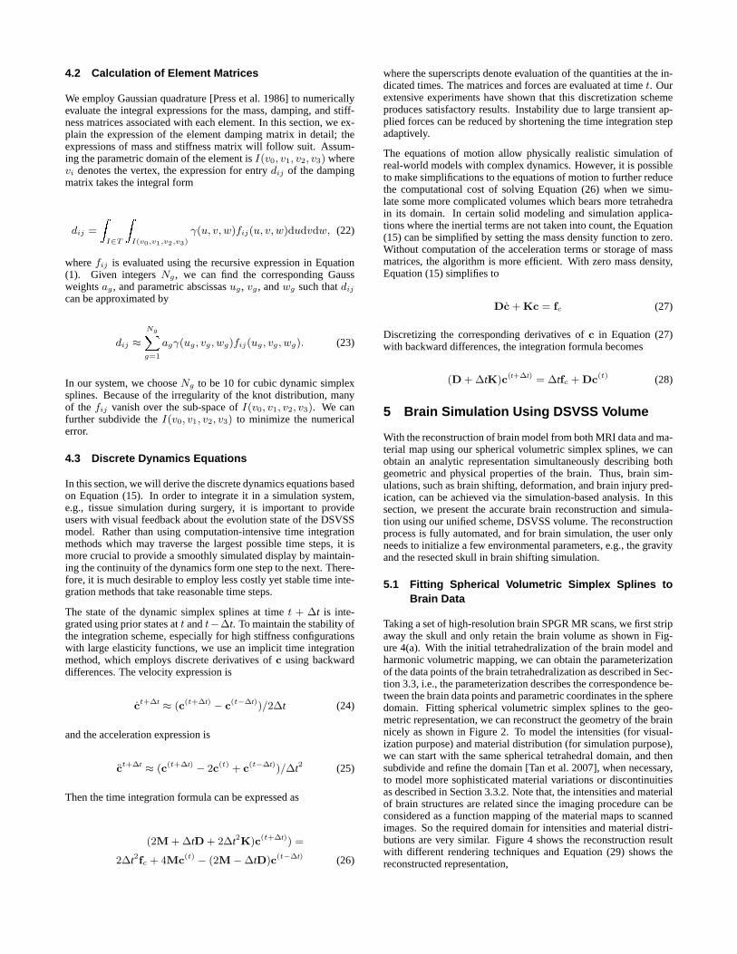
To model discontinuity in attribute field, we first detect where thediscontinuity occurs, then decompose the original domain into twoseparated new domains with shared vertices and edges as the 2D il-lustration in Figure 3. This simple mechanism maintains the consis-tent structure of the domains. The evaluation, hierarchy structure,and data structure all remain the same. Therefore, we can performthe same evaluation on these two domains simultaneously as if theevaluation is performed on a single domain. With the association ofdifferent control coefficients, the functional evaluation can outputa discontinuity in material field corresponding to the shared edges.This change will not affect the geometry of the DSVSS volume aslong as the associated control points remain the same.

Figure 3: Modeling discontinuities with separated domain trian-gles. Even though A and A’ are co-located, and B and B’ are co-located, the domain triangles in red and green are belonged to twodifferent domains.

3.4 Dynamic Spherical Simplex Splines

In this section, we formulate our dynamic spherical volumetric sim-plex splines. We integrate mass, dissipation, and deformation en-ergy into static simplex spline models, and employ Lagrangian dy-namics to derive their equations of motion. Consequently, the staticcontrol points of the geometric model become generalized time-varying physical coordinates in the dynamic model.

3.4.1 Geometry and Kinematics of Simplex Spline Volumes

The dynamic simplex splines further extend the geometric simplexsplines by incorporating time into the volume representation. Nowthe function of representation bears both parametric variableu andtime t as follows:

s(u, t) =XI∈T

X|β|=n

cIβ(t)NI

β(u). (9)

For simplicity of formulation expression, we define the vector ofgeneralized coordinates of control pointscI

β as:

c = [· · · , cIβ

>, · · · ]

>, (10)

where> denotes transposition. We then express Equation (9) ass(u, c) in order to emphasize its dependence onc whose compo-nents are functions of time. Hence, the velocity of the dynamicsimplex splines is:

s(u, t) = Jc, (11)

where the overstruck dot denotes a time derivative and Jacobianmatrix J(u) is the concatenation of the vectors∂s/∂cI

β . As-sumingm tetrahedral in the parametric domain,β traversesk =(n + 1)(n + 2)(n + 3)/6 possible tetrads whose components sumto n. Becauses is a 4-vector andc is anM = 4mk dimensionalvector,J is a4×M matrix, which is expressed as

J =

2664· · · ,

2664

NIβ 0 0 0

0 NIβ 0 0

0 0 NIβ 0

0 0 0 NIβ

3775 , · · ·

3775 , (12)

whereNIβ(u) = ∂sx

∂cIβx

=∂sy

∂cIβy

= ∂sz

∂cIβz

= ∂sd

∂cIβd

.

The subscriptsx, y, z andd denote derivatives of the componentsof the 4-vector: Cartesian coordinates and physical property, re-spectively. Apparently, the solid volume can be presented as theproduction of the product of the Jacobian matrix and the general-ized coordinate vector,

s(u, c) = Jc. (13)

3.4.2 Lagrange Equations of Motion

Lagrange dynamics are widely used in physics-based shape de-sign. In this section, we derive the equations of motion of dy-namic simplex splines by applying Lagrangian dynamics [Gossick1967]. We express the kinetic energy due to the prescribed massdistribution functionµ(u, v, w), and a Raleigh dissipation energydue to a damping density functionγ(u, v, w). Both energy func-tions are defined over the parametric domain of the volume. Themass distribution function and damping density function are recon-structed with spherical volumetric simplex splines as well, as de-scribed in Section 3.3.2. 3D thin-plate-like energy under tensionenergy model [Celniker and Gossard 1991; Halstead et al. 1993;Welch and Witkin 1992; Terzopoulos 1986] is employed here inorder to define an elastic potential energy,

U =1

2

ZZZ(α1,1s

2u + α2,2s

2v + α3,3s

2w+

β1,1s2uu + β1,2s

2uv + β1,3s

2uw + β2,2s

2vv+

β2,3s2vw + β3,3s

2ww)dudvdw. (14)

The subscripts ons denote the parametric partial derivatives. Theαi,j(u, v, w) andβi,j(u, v, w) are elasticity functions which con-trol tension and rigidity, respectively. Other energies, requir-ing greater computational cost, are also applicable, for instance,the non-quadratic, curvature-based energies in [Terzopoulos et al.1987; Moreton and Sequin 1992]. Applying the Lagrangian formu-lation, we obtain the second-order equations of motion

Mc + Dc + Kc = fc, (15)

where the mass matrix is

M =

ZZZµJ>Jdudvdw, (16)

the damping matrix is

D =

ZZZγJ>Jdudvdw, (17)

and the stiffness matrix is

K =

ZZZ(α1,1J

>u Ju + α2,2J

>v Jv + α3,3J

>wJw+

β1,1J>uuJuu + β1,2J

>uvJuv + β1,3J

>uwJuw+

β2,2J>vvJvv + β2,3J

>vwJvw + β3,3J

>wwJww)dudvdw. (18)

M, D and K are all M × M matrices. The generalized forceobtained through the principle of virtual work [Gossick 1967] doneby the applied force distributionf(u, v, w, t) is

fc =

ZZZJ>f(u, v, w, t)dudvdw. (19)

4 Finite Element Framework

The evolution of the vector of generalized coordinates,c(t), is de-termined by the second-order nonlinear differential equation. Equa-tion (15) with physical parameter dependent matrices, does not havean analytical solution. Instead, we obtain an efficient numerical im-plementation using finite-element techniques.

Standard finite element methods explicitly integrate the individualelement matrices into the global matrices that appear in the discreteequations of motion [Kardestuncer 1987]. Although applicable insome environments, it is infeasible in our infrastructure because ofits unacceptably high computational cost. Instead, we pursue an it-erative matrix solver to avoid the cost of assembling the global ma-tricesM, D, andK, working instead with the individual dynamicsimplex spline element matrices. We construct finite element datastructures, similar to [Qin and Terzopoulos 1995a], which facili-tates the parallel computation of element matrices.

4.1 Data Structures for Dynamic Simplex Spline FiniteElements

We define an element data structure which contains the geometricspecification of the tetrahedron patch element along with its phys-ical properties. In each element, we allocate an elemental mass,damping, and stiffness matrix, and include the quantities such as themassµ(u, v, w), dampingγ(u, v, w), and elasticityαi,j(u, v, w)andβi,j(u, v, w) functions. A complete dynamic simplex splineconsists of an ordered array of elements with additional informa-tion. The element structure includes pointers to appropriate com-ponents of the global vectorc. Neighboring tetrahedra will sharesome generalized coordinates.

The physical parameters, such as massµ(u, v, w), dampingγ(u, v, w), and elasticity,αi,j(u, v, w) andβi,j(u, v, w), need tobe measured and computed before the calculation of element ma-trices. In this paper, as the goal of the applications is to simulatethe biomechanical behavior of the brain, we directly adoptµ andγfrom the brain study conducted by Zhanget al. [Zhang et al. 2002].According to the relationship of elastic moduli of elastic isotropicmaterials [Ting 1996],α andβ can be computed from Bulk modu-lus and Poisson’s ratio as follows

α = 3B(1− 2υ), (20)

β =3B(1− 2υ)

(2 + 2υ), (21)

whereB is the Bulk modulus andυ is the Poisson’s ratio of braintissues.

4.2 Calculation of Element Matrices

We employ Gaussian quadrature [Press et al. 1986] to numericallyevaluate the integral expressions for the mass, damping, and stiff-ness matrices associated with each element. In this section, we ex-plain the expression of the element damping matrix in detail; theexpressions of mass and stiffness matrix will follow suit. Assum-ing the parametric domain of the element isI(v0, v1, v2, v3) wherevi denotes the vertex, the expression for entrydij of the dampingmatrix takes the integral form

dij =

ZI∈T

ZI(v0,v1,v2,v3)

γ(u, v, w)fij(u, v, w)dudvdw, (22)

wherefij is evaluated using the recursive expression in Equation(1). Given integersNg, we can find the corresponding Gaussweightsag, and parametric abscissasug, vg, andwg such thatdij

can be approximated by

dij ≈NgXg=1

agγ(ug, vg, wg)fij(ug, vg, wg). (23)

In our system, we chooseNg to be 10 for cubic dynamic simplexsplines. Because of the irregularity of the knot distribution, manyof the fij vanish over the sub-space ofI(v0, v1, v2, v3). We canfurther subdivide theI(v0, v1, v2, v3) to minimize the numericalerror.

4.3 Discrete Dynamics Equations

In this section, we will derive the discrete dynamics equations basedon Equation (15). In order to integrate it in a simulation system,e.g., tissue simulation during surgery, it is important to provideusers with visual feedback about the evolution state of the DSVSSmodel. Rather than using computation-intensive time integrationmethods which may traverse the largest possible time steps, it ismore crucial to provide a smoothly simulated display by maintain-ing the continuity of the dynamics form one step to the next. There-fore, it is much desirable to employ less costly yet stable time inte-gration methods that take reasonable time steps.

The state of the dynamic simplex splines at timet + ∆t is inte-grated using prior states att andt−∆t. To maintain the stability ofthe integration scheme, especially for high stiffness configurationswith large elasticity functions, we use an implicit time integrationmethod, which employs discrete derivatives ofc using backwarddifferences. The velocity expression is

ct+∆t ≈ (c(t+∆t) − c(t−∆t))/2∆t (24)

and the acceleration expression is

ct+∆t ≈ (c(t+∆t) − 2c(t) + c(t−∆t))/∆t2 (25)

Then the time integration formula can be expressed as

(2M + ∆tD + 2∆t2K)c(t+∆t)) =

2∆t2fc + 4Mc(t) − (2M−∆tD)c(t−∆t) (26)

where the superscripts denote evaluation of the quantities at the in-dicated times. The matrices and forces are evaluated at timet. Ourextensive experiments have shown that this discretization schemeproduces satisfactory results. Instability due to large transient ap-plied forces can be reduced by shortening the time integration stepadaptively.

The equations of motion allow physically realistic simulation ofreal-world models with complex dynamics. However, it is possibleto make simplifications to the equations of motion to further reducethe computational cost of solving Equation (26) when we simu-late some more complicated volumes which bears more tetrahedrain its domain. In certain solid modeling and simulation applica-tions where the inertial terms are not taken into count, the Equation(15) can be simplified by setting the mass density function to zero.Without computation of the acceleration terms or storage of massmatrices, the algorithm is more efficient. With zero mass density,Equation (15) simplifies to

Dc + Kc = fc (27)

Discretizing the corresponding derivatives ofc in Equation (27)with backward differences, the integration formula becomes

(D + ∆tK)c(t+∆t) = ∆tfc + Dc(t) (28)

5 Brain Simulation Using DSVSS Volume

With the reconstruction of brain model from both MRI data and ma-terial map using our spherical volumetric simplex splines, we canobtain an analytic representation simultaneously describing bothgeometric and physical properties of the brain. Thus, brain sim-ulations, such as brain shifting, deformation, and brain injury pred-ication, can be achieved via the simulation-based analysis. In thissection, we present the accurate brain reconstruction and simula-tion using our unified scheme, DSVSS volume. The reconstructionprocess is fully automated, and for brain simulation, the user onlyneeds to initialize a few environmental parameters, e.g., the gravityand the resected skull in brain shifting simulation.

5.1 Fitting Spherical Volumetric Simplex Splines toBrain Data

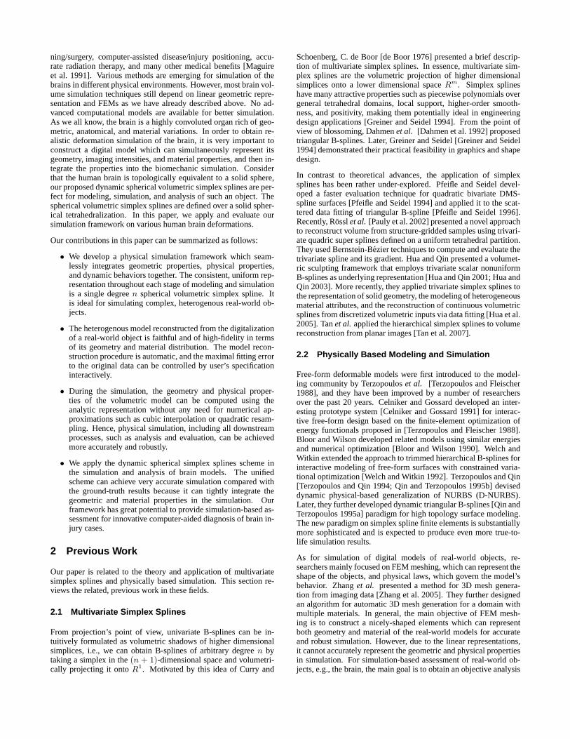
Taking a set of high-resolution brain SPGR MR scans, we first stripaway the skull and only retain the brain volume as shown in Fig-ure 4(a). With the initial tetrahedralization of the brain model andharmonic volumetric mapping, we can obtain the parameterizationof the data points of the brain tetrahedralization as described in Sec-tion 3.3, i.e., the parameterization describes the correspondence be-tween the brain data points and parametric coordinates in the spheredomain. Fitting spherical volumetric simplex splines to the geo-metric representation, we can reconstruct the geometry of the brainnicely as shown in Figure 2. To model the intensities (for visual-ization purpose) and material distribution (for simulation purpose),we can start with the same spherical tetrahedral domain, and thensubdivide and refine the domain [Tan et al. 2007], when necessary,to model more sophisticated material variations or discontinuitiesas described in Section 3.3.2. Note that, the intensities and materialof brain structures are related since the imaging procedure can beconsidered as a function mapping of the material maps to scannedimages. So the required domain for intensities and material distri-butions are very similar. Figure 4 shows the reconstruction resultwith different rendering techniques and Equation (29) shows thereconstructed representation,

(a) (b) (c)

Figure 4: (a) An axial view of a slice high-resolution brain SPGRMRI dataset; (b) Volume visualization of the reconstructed DSVSSvolume; (c) The volume is split to show its reconstructed interiorintensities.

24 s

dI

35 (u) =

XI∈T

X|β|=n

24 c

αd

αI

35N(u|V I

β ), (29)

wheres denotes the solid geometry of the brain,d denotes the re-constructed physical attributes of the brain, andI denotes the re-constructed image intensities from the high-resolution SPGR MRIsequence. c, αd and αI are the control points and control co-efficients. The accuracy of the data fitting is documented in theexperimental result section. After obtaining high-quality DSVSSvolume representation of the brain model, we can use it to sim-ulate brain deformation during surgery for computer-assisted sur-gical planning/surgery, or even for an innovative simulation-baseddiagnosis for brain injury under blunt impact.

5.2 Brain Shifting during Surgery

As known by brain surgery professionals, after a patient’s skull isopen, the brain will behave increasing deformation, known as brainshifting, during ongoing surgical procedures, predominantly dueto the gravity and the drainage of cerebrospinal fluid. This willinevitably lead to the repositioning of the surgical targets embed-ded in brain. As a compensation to increase the spatial accuracyof modern neuronavigation systems, intraoperative magnetic reso-nance imaging (IMRI) is widely used for quantitative analysis andvisualization of this phenomenon [Nimsky et al. 2000]. Neverthe-less, despite its virtually real-time aspects, IMRI only provides verylow-resolution intraoperative MR image which can never substitutethe high-resolution pre-operative SPGR MR image used to deter-mine with high accuracy key dimensions of the brain and the loca-tions of the surgical targets embedded in the brain. We employ ourdynamic spherical volumetric simplex splines model into the brainsimulation to compute the brain shifting.

In our framework, brain shifting can be simulated by applying con-stant gravity force~G to the brain. The material properties thatwe used in our experiments were obtained fromthe biomechan-ics groupat Wayne State University (WSU). After setting up thephysical parameters of an individual brain, we also need to take thenature boundary of the brain, the skull, into consideration. The factis that no matter what manner the brain behaves deformation, it liesinside the skull, i.e., its nature boundary will not exceed the skull.Therefore, spatial geometric constraints need to be enforced. Weadd the soft constraints with forces. When there is shifting outsidethe boundary, we insert corresponding forces along the opposite di-rection of the movement to the simulation procedure.

Figure 5 illustrates the brain shifting simulation using our frame-work when taking out the resected skull over the right temporal

(a) (b) (c)

Figure 5: (a) One slice view of IMRI image; (b) The reconstructedDSVSS volume, where the cross-sectional view displays the DSVSS-captured image intensities reconstructed from the pre-operativehigh-resolution SPGR images; (c) The brain deformation simulatedusing our system, where the cross-sectional view is captured, fromthe same view angle as (b), to show the displacement from (b), andthe green contour indicates the extent of displacement at the bound-ary. In (b) and (c) the red arrow denotes the orientation of gravity,and its position denotes the resected skull.

lobe. The green contour shows the deformation clearly. Our shift-ing simulation results highly agree with the fact captured by IMRI.The experiments show that it is effective to use our model to recovermotion and deformation from image data. Based on 20 simulationexperiments, quantitative comparison between the IMRI volumesand our simulated brain volumes by co-registration shows that oursystem can achieve an excellent accuracy of92.2%. The accuracyof a single simulation, denoted byA, is calculated as the normalizedsum of squared differences between the two volumes,

A = 1−P

a ‖S −R‖2Pa ‖R‖2

, (30)

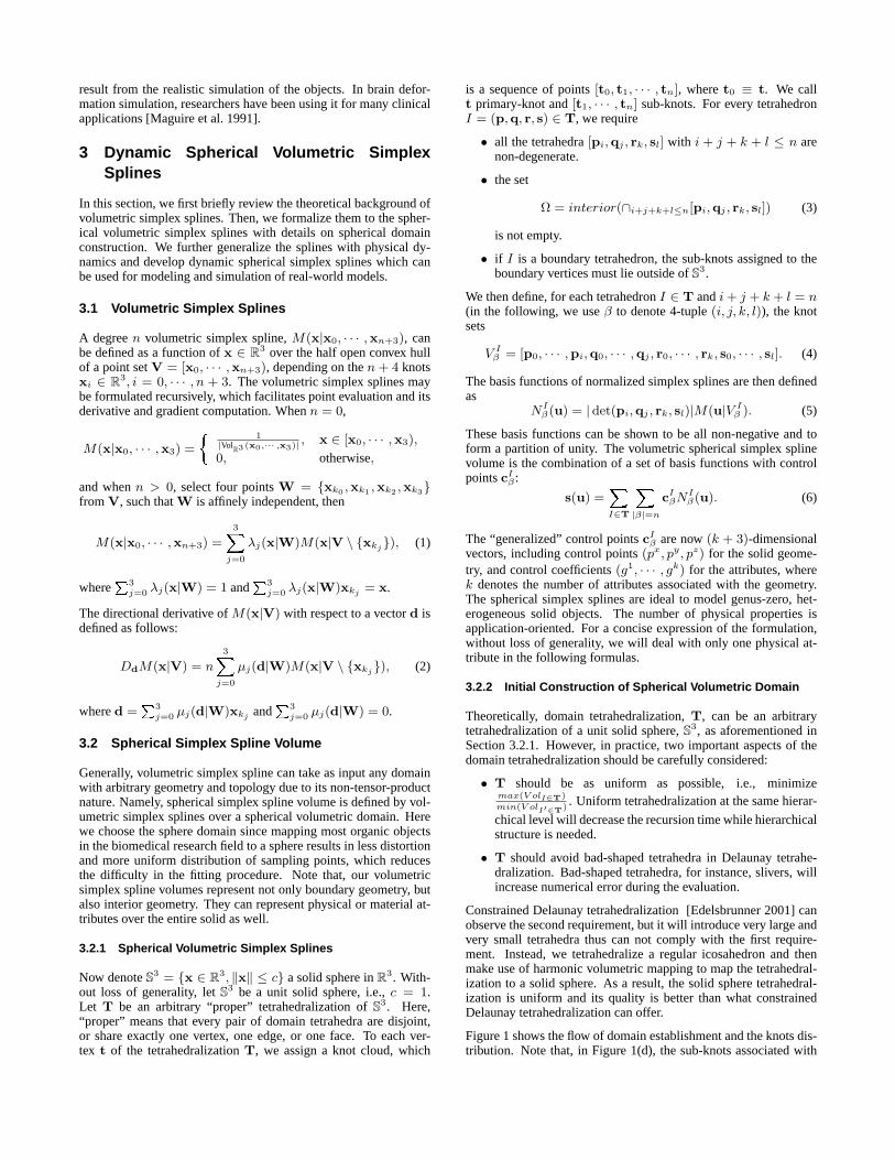
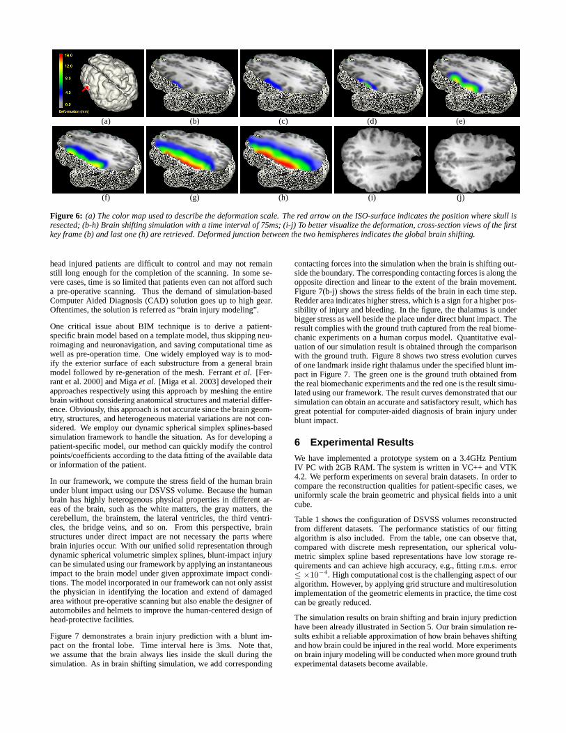
whereS is the volume obtained from our shifting simulation re-sults andR is the registered IMRI volume. To make the compari-son substantial and intra-sequence, we first register MRI volume toIMRI volume. Figure 6 depicts another brain shifting simulation.The skull is resected over the left temporal lobe. The color mapis blended into the figure to better visualize the deformation scale.Note that, when surgical tools are operating in the brain, there willbe larger shifting and deformation.

As demonstrated from the available comparison and evaluation,our framework can accurately simulate the deformation of thebrain (e.g.s(t)) and simultaneously present high-quality and high-resolution visualization using the transformed SPGR image inten-sities,I , modeled in the reconstructed simplex spline volume (seeEquation (29)). It is very promising to use the framework in bothsurgical planning (e.g., predicting the shifting of the targets) andcomputer-assisted surgery (e.g., repositioning the targets with high-resolution display,I , automatically computed based on the realisticdeformation of the reconstructed brain,s(t)).

5.3 Brain Injury Prediction

Here, we refer the brain injury prediction as a procedure of find-ing out the extent and location of the injury in the brain during ablunt impact. The injury frequently occurs to automobiles driversduring the collision and sports players during the acute sports activ-ities such as football. Current brain surgeons and professionals relyindispensably on those modern neuroimaging and neuronavigationsystems to pinpoint the injury. Clinically, the identification of thesite and extend of injury within the brain without subjecting thepatient to an imaging scanning, has its advantages. For instance,

(a) (b) (c) (d) (e)

(f) (g) (h) (i) (j)

Figure 6: (a) The color map used to describe the deformation scale. The red arrow on the ISO-surface indicates the position where skull isresected; (b-h) Brain shifting simulation with a time interval of 75ms; (i-j) To better visualize the deformation, cross-section views of the firstkey frame (b) and last one (h) are retrieved. Deformed junction between the two hemispheres indicates the global brain shifting.

head injured patients are difficult to control and may not remainstill long enough for the completion of the scanning. In some se-vere cases, time is so limited that patients even can not afford sucha pre-operative scanning. Thus the demand of simulation-basedComputer Aided Diagnosis (CAD) solution goes up to high gear.Oftentimes, the solution is referred as “brain injury modeling”.

One critical issue about BIM technique is to derive a patient-specific brain model based on a template model, thus skipping neu-roimaging and neuronavigation, and saving computational time aswell as pre-operation time. One widely employed way is to mod-ify the exterior surface of each substructure from a general brainmodel followed by re-generation of the mesh. Ferrantet al. [Fer-rant et al. 2000] and Migaet al. [Miga et al. 2003] developed theirapproaches respectively using this approach by meshing the entirebrain without considering anatomical structures and material differ-ence. Obviously, this approach is not accurate since the brain geom-etry, structures, and heterogeneous material variations are not con-sidered. We employ our dynamic spherical simplex splines-basedsimulation framework to handle the situation. As for developing apatient-specific model, our method can quickly modify the controlpoints/coefficients according to the data fitting of the available dataor information of the patient.

In our framework, we compute the stress field of the human brainunder blunt impact using our DSVSS volume. Because the humanbrain has highly heterogenous physical properties in different ar-eas of the brain, such as the white matters, the gray matters, thecerebellum, the brainstem, the lateral ventricles, the third ventri-cles, the bridge veins, and so on. From this perspective, brainstructures under direct impact are not necessary the parts wherebrain injuries occur. With our unified solid representation throughdynamic spherical volumetric simplex splines, blunt-impact injurycan be simulated using our framework by applying an instantaneousimpact to the brain model under given approximate impact condi-tions. The model incorporated in our framework can not only assistthe physician in identifying the location and extend of damagedarea without pre-operative scanning but also enable the designer ofautomobiles and helmets to improve the human-centered design ofhead-protective facilities.

Figure 7 demonstrates a brain injury prediction with a blunt im-pact on the frontal lobe. Time interval here is 3ms. Note that,we assume that the brain always lies inside the skull during thesimulation. As in brain shifting simulation, we add corresponding

contacting forces into the simulation when the brain is shifting out-side the boundary. The corresponding contacting forces is along theopposite direction and linear to the extent of the brain movement.Figure 7(b-j) shows the stress fields of the brain in each time step.Redder area indicates higher stress, which is a sign for a higher pos-sibility of injury and bleeding. In the figure, the thalamus is underbigger stress as well beside the place under direct blunt impact. Theresult complies with the ground truth captured from the real biome-chanic experiments on a human corpus model. Quantitative eval-uation of our simulation result is obtained through the comparisonwith the ground truth. Figure 8 shows two stress evolution curvesof one landmark inside right thalamus under the specified blunt im-pact in Figure 7. The green one is the ground truth obtained fromthe real biomechanic experiments and the red one is the result simu-lated using our framework. The result curves demonstrated that oursimulation can obtain an accurate and satisfactory result, which hasgreat potential for computer-aided diagnosis of brain injury underblunt impact.

6 Experimental Results

We have implemented a prototype system on a 3.4GHz PentiumIV PC with 2GB RAM. The system is written in VC++ and VTK4.2. We perform experiments on several brain datasets. In order tocompare the reconstruction qualities for patient-specific cases, weuniformly scale the brain geometric and physical fields into a unitcube.

Table 1 shows the configuration of DSVSS volumes reconstructedfrom different datasets. The performance statistics of our fittingalgorithm is also included. From the table, one can observe that,compared with discrete mesh representation, our spherical volu-metric simplex spline based representations have low storage re-quirements and can achieve high accuracy, e.g., fitting r.m.s. error≤ ×10−4. High computational cost is the challenging aspect of ouralgorithm. However, by applying grid structure and multiresolutionimplementation of the geometric elements in practice, the time costcan be greatly reduced.

The simulation results on brain shifting and brain injury predictionhave been already illustrated in Section 5. Our brain simulation re-sults exhibit a reliable approximation of how brain behaves shiftingand how brain could be injured in the real world. More experimentson brain injury modeling will be conducted when more ground truthexperimental datasets become available.

(a) (b) (c) (d) (e)

(f) (g) (h) (i) (j)

Figure 7: (a) The color map used to describe the stress field. The red arrow on the ISO-surface indicates the position where a blunt impactoccurs. (b-j) Brain injury simulation with a time interval of 3ms. The blunt impact occurs at the front lobe. Simulation results indicate that inaddition to the spot directly under the impact, there are some other positions where bleeding may happen.

Figure 8: Comparison of stress evolutions of the right thalamus under a blunt impact. The green one is the simulation curve obtained fromthe real biomechanic experiments and the red one is the result simulated using our framework.

Subject Degree Data Points Tetrahedra Control Points Knots Fitting r.m.s. Error

A 2 60298 2500 3871 1683 3.0375×10−4

B 3 72357 2500 12431 2244 2.1483×10−4

C 2 79593 4320 6525 2769 1.9743×10−4

D 3 86226 4320 21117 3682 1.5290×10−4

Table 1: Statistics of 3D reconstruction.

7 Conclusion

In this paper, we have developed a novel simulation frameworkbased on dynamic spherical volumetric simplex splines. We haveintroduced an automatic and accurate algorithm to fit the digitalmodels of real-world objects with a single spherical volumetric sim-plex spline which can represent with accuracy geometric and ma-terial properties of objects simultaneously. With the integration ofthe Lagrangian mechanics, the dynamic volumetric simplex splinerepresenting the real-world object can accurately simulate its phys-ical behavior. We have applied the framework in the biomechanicssimulation of the brain, such as brain shifting during the surgery andbrain injury under sudden impact. We have compared the simulatedresults with the ground truth obtained through interactive magneticresonance imaging and the ground truth from real biomechanic ex-periments. The experimental results have demonstrated the excel-lent performance of our technique, which can be effectively used indeformation-based brain simulation and simulation-based diagno-sis/assessment. The robustness and accuracy result from the tightintegration of the geometric and material properties into the simu-lation. In the near future, we will investigate more powerful simu-lation schemes based on our novel digital representations. Hierar-chical simulation will also be explored to speed up the simulationfor real-time applications. On the application side, we will developa DSVSS model of an entire head, which allow us to simulate morebehaviors of the brain.

Acknowledgements

The authors would like to thank Dr. Liying Zhang at the Bio-medical Engineering Department of WSU for providing us all thedata and real biomechanic experimental results for evaluation. Thiswork is supported in part by the research grants awarded to Dr.Jing Hua, including the National Science Foundation grant IIS-0713315, the National Institute of Health grant 1R01NS058802-01A2, the Michigan Technology Tri-Corridor grants MTTC05-135/GR686 and MTTC05-154/GR705, and the Michigan 21st Cen-tury Jobs Funds 06-1-P1-0193.

References

BLOOR, M., AND WILSON, M. 1990. Representing PDE surfacesin terms of B-splines.Computer-Aided Design 22, 6, 324–331.

CELNIKER, G., AND GOSSARD, D. 1991. Deformable curve andsurface finite elements for free-form shape design.ComputerGraphics 25, 4, 257–266.

DAHMEN , W., MICCHELLI , C. A., AND SEIDEL, H.-P. 1992.Blossoming begets B-spline bases built better by B-patches.Mathematics of Computation 59, 199, 97–115.

DE BOOR, C. 1976. Splines as linear combinations of B-splines.In Approximation Theory II, Academic Press, New York, 1–47.

EDELSBRUNNER, H. 2001. Geometry and Topology for MeshGeneration. Cambridge University Press. Edited by P.G.Ciarletand A.Iserles and R.V.Kohn and M.H.Wright.

FERRANT, M., WARFIELD, S., NABAVI , A., JOLESZ, F., ANDK IKINIS , R. 2000. Registration of 3D intraoperative MR im-ages of the brain using a finite element biomechanical model. InMICCAI, 19–28.

GOSSICK, B. 1967. Hamilton’s principle and physical systems.Academic Press. New York and London.

GREINER, G., AND SEIDEL, H. P. 1994. Modeling with triangularB-splines.IEEE Computer Graphics and Applications 14, 2, 56–60.

GU, X., WANG, Y., CHAN , T., THOMPSON, P., AND YAU , S.2003. Genus zero surface conformal mapping and its applicationto brain surface mapping. InInformation Processing in MedicalImaging, 172–184.

HALSTEAD, M., KASS, M., AND DEROSE, T. 1993. Efficient,fair interpolation using catmull-clark surfaces. InIn Computer-Graphics Proceedings, Annual Conference Series, Proc. ACM-Siggraph93, 35–44.

HUA , J., AND QIN , H. 2001. Haptic sculpting of volumetric im-plicit functions. InProceedings of 9th Pacific Conference onComputer Graphics and Applications, 254–264.

HUA , J., AND QIN , H. 2003. Haptics-based dynamic implicitsolid modeling. InIEEE Trans. on Visualization and ComputerGraphics, vol. 10.

HUA , J., HE, Y., AND QIN , H. 2004. Multiresolution heteroge-neous solid modeling and visualization using trivariate simplexsplines. InProceedings of the Ninth ACM Symposium on SolidModeling and Applications, 47–58.

HUA , J., HE, Y., AND QIN , H. 2005. Trivariate simplex splinesfor inhomogeneous solid modeling in engineering design.ASMETransactions: Journal of Computing and Information Science inEngineering 5, 2, 149–157.

KARDESTUNCER, H. 1987.Finite Element Handbook. McGraw-Hill. New York.

L I , X., GUO, X., WANG, H., HE, Y., GU, X., AND QIN , H. 2007.Harmonic volumetric mapping for solid modeling applications.In In Proceedings of the 2007 ACM Symposium on Solid andPhysical Modeling (SPM’07), 109–120.

MAGUIRE, G., NOZ, M., RUSINEK, H., JAEGER, J., KRAMER,E., SANGER, J., AND SMITH , G. 1991. Graphics applied tomedical image registration. InIEEE Computer Graphics Appli-cation, vol. 11, 20–28.

M IGA , M., SINHA , T. K., CASH, D. M., GALLOWAY , R., ANDWEIL , R. 2003. Cortical surface registration for image-guidedneurosurgery using laser-range scanning.IEEE Transactions onMedical Imaging 22, 8, 973–985.

MORETON, H., AND SEQUIN, C. 1992. Functional optimizationfor fair surface design.Computer Graphics 26, 2, 167–176.

NIMSKY, C., GANSLANDT, O., CERNY, S., HASTREITER, P.,GREINER, G., AND FAHLBUSCH, R. 2000. Quantificationof, visualization of, and compensation for brain shift using in-traoperative magnetic resonance imaging.Neurosurgery 47, 5,1070–1080.

PAULY, M., GROSS, M., AND KOBBELT, L. 2002. Efficient sim-plification of point-sampled surfaces.IEEE Visualization 02 Pro-ceedings, 163–170.

PFEIFLE, R., AND SEIDEL, H.-P. 1994. Fast evaluation ofquadratic bivariate DMS spline surfaces. InProceedings ofGraphics Interface ’94, 182–189.

PFEIFLE, R., AND SEIDEL, H.-P. 1996. Scattered data approxi-mation with triangular B-splines.Advance Course on Fairshape,253–263.

PRESS, W., FLANNEY, B., TEUKOLSKY, S., AND VERTTERING,W. 1986. Numerical Recipes: The Art of Scientific Computing.Cambridge University Press. Cambridge.

QIN , H., AND TERZOPOULOS, D. 1995. Dynamic manipulationof triangular B-splines. InIn Proceedings of Third Symposiumon Solid Modeling and Applications (Solid Modeling ’95), 351–360.

QIN , H., AND TERZOPOULOS, D. 1995. Dynamic NURBS withgeometric constraints for physics-based shape design.ComputerAided Design 27, 2, 111–127.

TAN , Y., HUA , J.,AND DONG, M. 2007. 3D reconstruction from2D images with hierarchical continuous simplicies.The VisualComputer 23, 9-11, 905–914.

TERZOPOULOS, D., AND FLEISCHER, K. 1988. Deformable mod-els. The Visual Computer 4, 6, 306–331.

TERZOPOULOS, D., AND QIN , H. 1994. Dynamic NURBS withgeometric constraints for interactive sculpting. InACM Transac-tions on Graphics, vol. 13, 103–136.

TERZOPOULOS, D., PLATT, J., BARR, A., AND FLEISCHER, K.1987. Elastically deformable models.Computer Graphics 21, 4,205–214.

TERZOPOULOS, D. 1986. Regularization of inverse visual prob-lems involving discontinuities. InIEEE Transactions on PatternAnalysis and Machine Intelligence, vol. 8, 413–424.

TING, T. 1996.Anisotropic Elasticity. Oxford University Press.

WANG, Y., GU, X., CHAN , T., THOMPSON, P., AND YAU , S.2004. Intrinsic brain surface conformal mapping using a vari-ational method. InSPIE International Symposium on MedicalImaging.

WANG, Y., GU, X., CHAN , T., THOMPSON, P., AND YAU , S.2004. Volumetric harmonic brain mapping. InIn ISBI’04: IEEEInternaltional Symposium on Biomedical Imaging: Macro toNano, 1275–1278.

WANG, Y., GU, X., AND YAU , S. 2004. Volumetric harmonicmap. Communications in Information and Systems 3, 3, 191–202.

WELCH, W., AND WITKIN , A. 1992. Variational surface model-ing. Computer Graphics 26, 2, 157–166.

ZHANG, L., BAE, J., HARDY, W., MONSON, K., MANLEY, G.,GOLDSMITH, W., YANG, K., AND K ING, A. 2002. Computa-tional study of the contribution of the vasculature on the dynamicreponse of the brain.Stapp Car Crash Journal 46, 145–164.

ZHANG, Y., BAJAJ, C., AND SOHN, B. 2005. 3D finite elementmeshing from imaging data. InComputer Methods in AppliedMechanics and Engineering (CMAME) on Unstructured MeshGeneration, vol. 194, 5083–5106.