DYNAMIC TORSIONAL SHEAR TEST FOR HOT MIX …ufdcimages.uflib.ufl.edu/UF/E0/00/09/14/00001/pham_l.pdfDYNAMIC TORSIONAL SHEAR TEST FOR HOT MIX ASPHALT By ... CHAPTER 1 INTRODUCTION

DYNAMIC TORSIONAL SHEAR TEST FOR HOT MIX ASPHALT

By

LINH V. PHAM

A THESIS PRESENTED TO THE GRADUATE SCHOOL OF THE UNIVERSITY OF FLORIDA IN PARTIAL FULFILLMENT

OF THE REQUIREMENTS FOR THE DEGREE OF MASTER OF ENGINEERING

UNIVERSITY OF FLORIDA

2003

Copyright 2003

by

Linh V. Pham

This document is dedicated to the graduate students of the University of Florida.

ACKNOWLEDGMENTS

I would like to thank my advisor, Dr. Bjorn Birgisson, for his supervision and

guidance throughout the project. Without his expertise, I would not have been able to

finish this task. I would like to thank the other members of my committee, Dr. Reynaldo

Roque and Dr. David Bloomquist, for their time and knowledge that kept me on the right

track.

I would like to thank D.J Swan, George Loop and Daniel Darku. Their expertise in

the field helped my work go much faster and easier. I also want to thank the entire

Geotech group for their friendship and support throughout my stay in Gainesville.

Finally, I would like to spend a special thank to my parent, my brother and friend in

Vietnam. I am always blessed by their love, encouragement and support.

iv

TABLE OF CONTENTS Page ACKNOWLEDGMENTS ................................................................................................. iv

LIST OF TABLES........................................................................................................... viii

LIST OF FIGURES ........................................................................................................... ix

ABSTRACT..................................................................................................................... xiii

CHAPTER

1 INTRODUCTION ........................................................................................................1

1.1 Background.............................................................................................................1 1.2 Problem Statement..................................................................................................2 1.3 Objectives ...............................................................................................................2 1.4 Scope.......................................................................................................................3

2 LITERATURE REVIEW .............................................................................................4

2.1 Axial Complex Modulus.........................................................................................4 2.2 Torsional Complex Modulus ..................................................................................8 2.3 Solid Specimen versus Hollow Specimen ............................................................10

2.3.1 Distribution of Shear ..................................................................................10 2.3.2 Comparison of Solid and Hollow Specimens.............................................11

3 MATERIALS PREPARATION AND TESTING PROGRAM.................................13

3.1 Granite Mixtures...................................................................................................13 3.2 Sample Preparations .............................................................................................16 3.3 Testing Program....................................................................................................16

4 IMPROVEMENT OF COMPLEX MODULUS TESTING PROGRAM..................17

4.1 New MTS Controlling System .............................................................................17 4.2 Temperature Control.............................................................................................19 4.3 Some Test Issues...................................................................................................20

v

4.3.1 Calibration ..................................................................................................20 4.3.2 Control Issue...............................................................................................20 4.3.3 Seating Load...............................................................................................22 4.3.4 End plate and Glue .....................................................................................23

4.4 Complex Modulus Testing Setup .........................................................................23 4.4 Torsional Shear Modulus Testing Setup...............................................................27

5 SIGNAL AND DATA ANALYSIS ...........................................................................30

5.1 Test Signal ............................................................................................................30 5.2 Data Analysis........................................................................................................34

5.2.1 Iterative Curve Fit Method .........................................................................34 5.2.2 Regression Method.....................................................................................36 5.2.3 FFT Method................................................................................................37 5.2.4 Evaluation of Data Interpretation Method..................................................40 5.2.5 Computer Program .....................................................................................41

6 AXIAL COMPLEX MODULUS TEST RESULTS ..................................................48

6.1 Result of Complex Modulus Test .........................................................................48 6.1.1 Dynamic Modulus Results .........................................................................48 6.1.2 Phase Angle Results ...................................................................................51 6.1.3 Discussion of Testing Results ....................................................................53

6.2 Master Curve Construction...................................................................................57 6.2.1 Time-temperature Superposition Principle.................................................57 6.2.2 Constructing Master Curve using Sigmoidal Fitting Function...................58

6.3 Predictive Equation...............................................................................................61

7 TORSIONAL SHEAR TEST RESULTS...................................................................64

7.1 Result of Torsional Shear Test .............................................................................64 7.1.1 Stress versus Strain Study ..........................................................................64 7.1.2 Dynamic Torsional Shear Modulus Results ...............................................66 7.1.3 Phase Angle Results ...................................................................................68

7.2 Poisson Ratio ........................................................................................................72 7.3 Summary...............................................................................................................74

8 CONCLUSION AND RECOMMENDATION .........................................................76

8.1 Conclusion ............................................................................................................76 8.1.1 Testing Procedures and Setup ....................................................................76 8.1.2 Signal and Data Analysis............................................................................77 8.1.3 Axial Complex Modulus Test ....................................................................77 8.1.4 Torsional Shear Test...................................................................................78

vi

8.2 Recommendation ..................................................................................................79 APPENDIX A MIX DESIGN.............................................................................................................80

B DATA FROM TESTING ...........................................................................................87

LIST OF REFERENCES.................................................................................................115

BIOGRAPHICAL SKETCH ...........................................................................................117

vii

LIST OF TABLES

Table page 4.1 Suggested value for P gain for GCTS system..............................................................22

5.1 Evaluation of data interpretation method.....................................................................40

7.1 Poisson ratio.................................................................................................................74

viii

LIST OF FIGURES

Figure page 2.1 Stress and strain signal of axial complex modulus test.................................................5

2.2 Relation among E*, E’ and E”......................................................................................6

2.3 Torsional shear test for HMA Column .........................................................................8

2.4 Description of the non-uniformity of shear stresses across a specimen for different ratios of inner to outer radii......................................................................................11

2.5 Difference in torque between hollow and solid specimens to achieve the same average strain............................................................................................................12

3.1 Gradation Plot for Coarse Mixture .............................................................................15

3.2 Gradation Plot for Fine Mixture .................................................................................15

4.1 Temperature control by circulating water...................................................................19

4.2 LVDT calibration device. ...........................................................................................20

4.3 Effect of using P gain..................................................................................................22

4.4 Texture end plate for torsional shear test....................................................................23

4.5 Complex modulus testing setup in the triaxial cell .....................................................24

4.6 Picture of sample set up in triaxial cell for complex modulus test. ............................26

4.7 Torsional shear testing set up.....................................................................................27

4.8 Picture of torsional shear testing set up. .....................................................................29

5.1 Typical test signal. ......................................................................................................30

5.2 Dynamic sinusoid component of the signal. ...............................................................31

5.3 Signal in higher scale ..................................................................................................31

5.4 Noise signal.................................................................................................................32

ix

5.5 Signal after filtering ....................................................................................................33

5.6 Noise filter function in Lab View. ..............................................................................33

5.7 Test signal in time domain..........................................................................................38

5.8 Test signal in frequency domain .................................................................................38

5.9 Strain with missing peak data .....................................................................................39

5.10 Flow chart of data analysis program.........................................................................43

5.11 Complex Modulus Program......................................................................................44

5.12 Torsional Shear Modulus Program. ..........................................................................44

5.13 Output page of Torsional Shear Modulus Program. .................................................45

5.15 Linear regression versus quadratic regression analysis ............................................47

6.1 Dynamic Modulus |E*| of GAF1 at 250C ...................................................................49



6.4 Dynamic Modulus |E*| of GAC1 at 250C...................................................................50



6.7 Phase angle of GAF1 mixture at 250C........................................................................51



6.10 Phase angle of GAC1 mixture at 250C ....................................................................52

6.11 Phase angle of GAC1 mixture at 100C .....................................................................52

6.12 Phase angle of GAC1 mixture at 400C .....................................................................53

6.13 Average Complex Modulus result at 10 Hz 250C.....................................................53

6.14 Average Complex Modulus result at 10Hz at 100C..................................................54

6.15 Average Complex Modulus result at 10Hz at 400C..................................................54

x

6.16 Average of phase angle at 250C................................................................................55



6.19 Average of phase angle at 4Hz at 250C ....................................................................56



6.22 Sigmoidal Function...................................................................................................59

6.23 Log complex modulus master curve for coarse mix.................................................60

6.24 Log complex modulus master curve for fine mix.....................................................60

6.24 Actual values versus Predicted value of E* at 250C for 16Hz test. ..........................62



7.1 Torsional shear stress versus shear strain. ..................................................................65

7.2 Phase angle versus shear strain level. .........................................................................65

7.3 Dynamic Torsional Shear Modulus |G*| of GAF1 at 250C ........................................66



7.6 Dynamic Torsional Shear Modulus |G*| of C1 at 250C..............................................67



7.9 Phase angle of GAF1 mixture at 250...........................................................................69

7.10 Phase angle of GAF1 mixture at 100.........................................................................69

7.11 Phase angle of GAF1 mixture at 400.........................................................................70

7.12 Phase angle of GAC1 mixture at 250 ........................................................................70


xi


7.15 Average of torsional shear modulus at 10 Hz at 250C.............................................71

7.16 Average of torsional shear modulus at 10 Hz at 100C..............................................72

7.17 Average of torsional shear modulus at 10 Hz at 400C..............................................72

7.18 Poisson ratio of coarse mixture C2 ...........................................................................73

7.19 Poisson ratio of fine mixture F2................................................................................73

xii

Abstract of Thesis Presented to the Graduate School

of the University of Florida in Partial Fulfillment of the Requirements for the Degree of Master of Engineering

DYNAMIC TORSIONAL SHEAR TEST ON HOT MIX ASPHALT

By

Linh V. Pham

August 2003

Chair: Bjorn Birgisson Major Department: Civil and Coastal Engineering

The development of torsional shear test provides a new approach to studying shear

deformation of hot mix asphalt. Study on simple shear test (SST) suggested that a

laboratory which measures primarily shear deformation appears to be the most effective

way to define the propensity of a mix for rutting. An understanding of its mechanics and

procedures is fundamental for understanding how the test can be used. With complex

modulus |E*| now formally integrated into the 2002 AASHTO Pavement Design Guide,

the complex shear modulus obtained from torsional shear test measurements has the

potential for being a simple alternative to the more involved triaxial type of test needed to

obtain the confined axial complex modulus.

The purpose of this study was to establish the testing and interpretation

methodology needed to obtain the torsional complex shear modulus. A number of issues

such as the length of testing time, loading level, and temperature control related to the

test were studied. Because a good understanding of the axial complex modulus test is

xiii

needed in the first place, further examination on testing set up, testing procedure and data

analysis of previous studies on axial complex modulus was also carried out.

xiv

CHAPTER 1 INTRODUCTION

1.1 Background

The complex modulus (/E*/) has been proposed as a Superpave simple

performance test (Wictzak et al., 2002). The complex modulus is also the proposed

stiffness measure of asphalt concrete in the new Superpave design (2001 ). The dynamic

complex modulus test, as currently being advocated, is performed without any confining

stress. The lack of confinement means the complex modulus is unable to simulate field

conditions where a pavement material is surrounded by adjacent materials providing

confinement during loading. This lack of confinement makes the mobilization of the

shear characteristics under confinement of the mixture impossible to measure and

describe. The torsional shear test, which is a direct test to measure the shear

characteristics of a mixture may therefore be more appropriate. The torsional shear

modulus may be a useful parameter in characterizing the shear behavior of HMA

mixtures. A study of simple shear test (SST) conducted by Harvey et al., (2001) suggests

that a laboratory test which measures primarily shear deformation would be the most

effective way to define the propensity of rutting for a mixture.

In the linear viscoelastic range (75 to 200 µstrains), the dynamic modulus of

asphalt mixtures can be investigated by either an axial or torsional complex modulus test.

These two tests can be performed on the same sample, so that sample variability is

reduced. The axial complex modulus test can provide E* and phase angle. The torsional

complex modulus test can provide the dynamic shear modulus G* and the phase angle

1

2

δ of a mixture . The complex shear modulus G* can then be used in combination with

E* to obtain the complex Poisson’s ratio, ν∗. Harvey et al.(2001) concluded that G* can

be related to E* using Equation 1.1:

)1(2**υ+

=EG (1.1)

in which the Poisson’s ratio can be taken as a constant. However, previous work by

Monismith et al. (2000) has shown that the Poisson’s ratio is actually dependent upon

frequency.

1.2 Problem Statement

With complex modulus |E*| now formally integrated into 2002 AASHTO

Pavement Design Guide, there is a growing need for simple measurement of the complex

modulus of a mixture. The complex shear modulus obtained from torsional shear test

has the potential to be a simple alternative to the more involved confined axial complex

modulus test.

1.3 Objectives

The objectives of this research are as follows:

• The testing and interpretation methodology needed to obtain the complex shear modulus from a torsional shear test.

• A comparison of the torsional shear test to the hollow cylinder torsional shear test to obtain an estimate of the error associated with the testing of solid cylinders.

• A comparison of the torsional shear complex modulus to the axial complex modulus from a triaxial test to obtain the complex Poisson’s ratio.

• A comparison to predicted complex modulus results using the predictive equation by Witzhak et al., (2002).

• A focus on the systematic identification of the issues related to the measurement and interpretation of the complex modulus.

3

• The completion of a testing set up, testing procedure and an analysis of previous studies on axial complex modulus.

1.4 Scope

A brief review of theory of axial complex modulus and torsional complex modulus

is presented in Chapter 2. Chapter 3 will describe the material and the mixtures used in

the study. It also presents the testing program. Chapter 4 will outline the previous study,

the improvement on controlling issue and data acquisition system. Axial complex

modulus and torsional shear modulus testing set up and procedures will also be presented.

Chapter 5 will outline the data analysis method, testing signal analysis and the problems

related to data analysis. Chapter 6 will present the test result and analysis for axial

complex modulus test. Chapter 7 will present the test result and analysis for torsional

shear test. Conclusions and Recommendations will be presented in Chapter 8.

CHAPTER 2 LITERATURE REVIEW

2.1 Axial Complex Modulus

A mechanistic – empirical design approach is in the new AASHTO 2002 pavement

design procedure. This means that the mechanistic design model is coupled with the

empirical performance characteristics of hot mix asphalt for pavement design. The

mechanistic behavior of asphalt mixtures is characterized by temperature dependent

stiffness, strength, and viscosity. The prediction of pavement life based on mechanistic-

empirical performance criteria requires the ability to address temperature effects and to

track changes and damage in the material over the projected life span of a pavement.

The complexity of Superpave models and the AASHTO 2002 performance criteria

guidelines can be greatly reduced by the introduction of parameters that can be used to

characterize the temperature dependency of through its projected life span. The axial

complex modulus is potentially one such parameter. Research by numerous groups has

shown that the complex modulus can be used to characterize the temperature dependency

of a mixture’s stiffness and viscosity over time. Papazian (1962) first proposed the

dynamic modulus test on hot mix asphalt. He applied a sinusoidal load to a cylindrical

sample to measure the ratio of stress and strain amplitudes. Thus, the axial complex

modulus test measures the amplitude ratio and the time delay in the responding signal, as

shown in Figure 2.1.

4

5

Time

Stre

ss/S

trai

nσ0

ε0

δ

Figure 2.1 Stress and strain signal of axial complex modulus test

The dynamic modulus is defined as

0

0*εσ

=E (2.1)

where σ0 is the stress amplitude,

ε0 is the strain amplitude.

The complex modulus is composed of a storage modulus (E’) that represents the

elastic component and loss modulus (E”) that represents the viscous component.

The storage and the loss modulus can be obtained by measuring the lag in the

response between the applied stress and the measured strain. This lag or phase angle (δ)

is described previously in Figure 2.1. The relationship between E*, E’ and E” are

described in Figure 2.2

= −

'"tan 1

EEδ (2.2)

)sin(.*" δEE = (2.3)

)cos(.*' δEE = (2.4)

6

δ

E* E” = E*sin(δ)

E’=E*cos(δ)

Figure 2.2 Relation among E*, E’ and E”

The phase angle can be determined in the laboratory by measuring the time

difference between the peak stress and the peak strain. This time can be converted to δ

using the following relationship:

)360( 0⋅⋅= ftlagδ (2.5)

where f is the frequency of dynamic load (in Hz),

tlag is the time difference between the signals (in seconds).

In the calculation of phase angle, the stress signal has the form )sin( 1δω +⋅ tA , the

strain signal has the form )sin( 2δω +⋅ tB , with the phase angle equaling 21 δδ − .A δ of

zero indicates a purely elastic response and a δ of 900 indicates a purely viscous response.

The procedure for the axial dynamic modulus test is based on ASTM D 3947. It

suggests the use of a standard triaxial cell to apply stress or strain amplitude to a material

at 16Hz, 4Hz and 1Hz. It also recommends that the test be carried out at temperatures of

50C, 250C, and 400C. The main reason for using a sinusoidal stress loading is simplicity.

One problem with triaxial testing is that other stresses can be induced on a sample,

such as end effects due to loading. However, end effects are usually minimized by

7

maintaining the ratio between the diameter and the height of specimen and by reducing

the friction around the ends of the specimen.

According to Witczak et al. (2000), a ratio of 1.5 is adequate for complex modulus

testing. A minimum diameter of 100 mm is also recommended as a part of the complex

modulus testing procedure. These minimums were recommended for mixtures with

nominal aggregate size of 12.5 mm, 19 mm, 25 mm and 37.5 mm (Witczak et al., 2000).

To minimize the end effects, lubrication between the end platens and the sample is

recommended to reduce friction and prevent localized stress conditions (Harvey et al.,

2001). A rubber membrane is often used between the end platen and the sample. In cases

where a more compliant membrane is used to reduce friction, it is important to measure

the deformation of the sample by means of an on-specimen gauge system. This prevents

measuring any deflection of the membrane or frame compliance (Perraton et al., 2001).

Since the interpretation of the complex modulus is based on the assumption of

linear viscoelasticity of the mixture, it is necessary to maintain a fairly low strain level

during testing to avoid any non-linear effects. Maintaining a stress level that result in a

strain response that is close to linear is critical to achieve a test that is reproducible and

allow for proper analysis. ASTM D 3497 recommends using an axial stress amplitude of

241.3 kPa (35 psi) at all temperatures, as long as the total deformation is less than 2500.

Daniel and Kim (1998) showed successful triaxial compression testing results with stress

levels under 96.5 kPa for 150C testing. Witczak et al. (2000) suggested the strain

amplitudes of 75 to 200 microstrain in order to maintain linearity during triaxial

compression testing. This range of strain amplitude, 75 to 200 microstrain, is used in the

study.

8

2.2 Torsional Complex Modulus

The principle of torsional complex modulus test is to apply a cyclic torsional force

to the top of specimen, and measure the displacement on the outside diameter (Figure

2.3). Knowing the torsional stress and strain, the shear modulus is then calculated based

on the theory of elasticity. The torsional force is generated by a piston that can move

laterally. The specimen is glued to the platens at the top and bottom ends. The bottom is

rigidly fixed and the top is connected to a torsional load actuator. The frequencies used in

the test are the same as those used in the axial complex modulus test.

r 0 r i

max

HMASpecimen

l

Torque at peakRotation

Rigidly Fixedat Bottom

max (r) maxrl=

= Single AmplitudeShearing Strain

Figure 2.3 Torsional shear test for HMA Column

The dynamic shear modulus is calculated from the following relationship:

γτ

=*G (2.6)

9

assuming that pure torque, T, is applied to the top of a HMA column, the shearing stress

varies linearly across the radius of the specimen. The average torsional shear stress, on a

cross section of a specimen τavg is defined as

τavg = S/A (2.7)

where A is the net area of the cross section of the specimen, i.e A = π(ro2-ri

2),

ro and ri are the outside and inside radius of a hollow specimen, respectively. (For

a solid specimen, ri = 0), and

S is the total magnitude of shearing stress.

S can be calculated as

(2.8) ∫=o

i

r

rr drrS )2( πτ

where τr is the shear stress at the distance r from the axis of the specimen, i.eτr = τmr/ro,

where τm is the maximum shearing stress at r = 0.

On the other hand, the torque, T, can be calculated from

Jr

rdrrTo

i

r

r

mr∫ ==

τπτ )2( (2.9)

where J is the area polar of inertia, J = π(ro4 – ri

4)/2.

From Equation 2.9, τm can be expressed as

τm = Tro/J (2.10)

From Equation (2.7) (2.8) and (2.10), one can write the equation for τavg as

JT

rrrr

io

ioavg 22

33

32

−

−=τ (2.11a)

or

10

JTreqavg =τ (2.11b)

where req is defined as the equivalent radius. It can be seen in Equation (2.9a) that

req = 2/3ro for a solid specimen. req = 2/3 (ro3 – ri

3)/(ro2 – ri

2) for hollow specimen.

In practice, req is defined as the average of the inside and outside radii.

Shear strain is calculated in the Equation 2.12:

l

r eqθγ = (2.12)

where l is the length of specimen, and θ is the angle of twist. The angle of twist, θ , can

be measured either using an LVDT or a proximitor,

In order to maintain the linear relationship between shear stress and shear strain,

shear strain should be below a certain range. From the study on axial complex modulus

testing, shear strains smaller than 200 microstrain were found reasonable.

2.3 Solid Specimen versus Hollow Specimen

2.3.1 Distribution of Shear

The level of shear stress non-uniformity across a specimen is typically quantified

with the following non-uniformity coefficients (1):

dr1rr

1βo

i

r

rAvg

avgio3

minmax

∫ −×−

=

−=

τττ

τττ

avg

R

A plot of these two coefficients is given below.

11

0

0.2

0.4

0.6

0.8

1

1.2

1.4

1.6

0 0.1 0.2 0.3 0.4 0.5 0.6 0.7

ri/ro

R

0

0.05

0.1

0.15

0.2

0.25

0.3

0.35

0.4

0.45

β 3

R

β3

Figure 2.4. Description of the non-uniformity of shear stresses across a specimen for different ratios of inner to outer radii.

2.3.2 Comparison of Solid and Hollow Specimens

The use of hollow specimens over solid specimens or torsional complex modulus

testing provides no advantage. This is because testing occurs solely in the linear range

across the specimen, regardless if the specimen is hollow or solid. The equations

presented above ensure this is true as long as testing is at low strain levels across the

specimen. If testing were to result in large strains (non-linear range), large creep strains,

or failure were to occur, the equations would no longer be valid, and solid and hollow

specimen testing could not be equated. The fact that there is more stress uniformity in a

hollow specimen only means that the same material tested as a hollow specimen needs

less torque to achieve the same average strain and shear stress across it. The following

12

figure depicts the decrease in torque needed to maintain the same strain level between a

Figure 2.5. Difference in torq

hollow and solid specimen.

ue between hollow and solid specimens to achieve the same average strain.

0

5

10

15

20

25

30

0 0.1 0.2 0.3 0.4 0.5 0.6

ri/ro

Perc

ent D

ecre

ase

in T

orqu

e

CHAPTER 3 MATERIALS PREPARATION AND TESTING PROGRAM

3.1 Granite Mixtures

Six granite mixtures were used to prepare testing specimens. All of these mixtures

were developed according to Superpave mix design method.. Mixture design

methodology is very well documented over the years. A detailed description of

Superpave mix design method can be found in FHWA report number FHWA-SA-95-003,

1995

Superpave mix design method uses volumetric properties of the mix to decide on

the optimum asphalt content. Mixtures are compacted to provide a laboratory density

equal to the estimated field density after various levels of traffic. In this project all the

mixtures were designed corresponding to traffic level 5 (<30 million ESALs). The

number of gyrations can be varied to simulate anticipated traffic. The percent air voids at

Ni (N-initial), Nd (N-design), and Nm (N-maximum) are measured to evaluate the

mixture quality. The mixture should have at least 11 percent air voids at N i, 4 percent air

voids at N d, and at least 2 percent air voids at N m. Asphalt content for all of the

mixtures were determined according to Superpave mix design criteria, such that each mix

had 4% air voids at NDesign = 109 revolutions. AC-30 asphalt was used for all of granite

mixture in this study.

Job Mix Formulas for the mixtures used in this project were developed based on

Bensa’s (Nukunya 2001) oolitic limestone mixtures by substituting the volume occupied

by limestone in the HMA with Georgia Granite stone. For these mixtures No. 7 stone was

13

14

used as coarse material, No. 89 stone as intermediate material, W-10 screens as screen

material and Granite filler as filler material.

One coarse-graded (GAC1) and one fine-graded (GAF1) were used as the basis

mixtures. From those, two more coarse gradation and two more fine gradations were then

produced by changing the coarse or fine portions of the basic gradations to produce more

gradation of substandard void structure and permeability. The purpose of this was to test

the effect of void structure and gradation on the rutting performance of mixtures.

In all, six granite mixtures were used: GAC1, GAC2, GAC3 for the coarse

gradations and GAF1, GAF2, GAF3 for fine gradations. In fact, GAF3 mixture was

derived from the fine mixture (GAF1) but was adjusted to fall below the restricted zone

to achieve a higher VMA and permeability, thus it can be considered a coarse mix as

well.

The detail gradations are shown in Table 3.1 and Figure 3.1 and 3.2 For more

information on mixture properties and aggregate gradation, see Appendix B

Table 3.1 Gradation of granite mixtures. Percent Passing (%)

Sieve size (mm) GAC1 GAC2 GAC3 GAF1 GAF2 GAF3 19 100 100 100 100 100 100 12.5 97.39 90.9 97.3 94.7 90.5 94.6 9.5 88.99 72.9 89.5 84.0 77.4 85.1 4.75 55.46 45.9 55.4 66.4 60.3 65.1 2.36 29.64 28.1 33.9 49.2 43.2 34.8 1.18 19.24 18.9 23.0 32.7 34.0 26.0 0.6 13.33 13.2 16.0 21.0 23.0 18.1 0.3 9.30 9.2 11.2 12.9 15.3 12.5 0.15 5.36 5.6 6.8 5.9 8.7 7.7 0.075 3.52 3.9 4.7 3.3 5.4 5.8

15

Gradation Chart C1, C2 & C3

0

10

20

30

40

50

60

70

80

90

100

Sieve size (mm)^0.45

Perc

ent p

assi

ng (%

)

C1C2C3

0.0750.15

0.3 0.6 1.18 2.36 4.75 9.5 12.5 19

Figure 3.1 Gradation Plot for Coarse Mixture

Gradation Chart F1, F2 & F3

0

10

20

30

40

50

60

70

80

90

100

Sieve size (mm)^0.45

Perc

ent p

assi

ng (%

)

F1F2F3

0.0750.15

0.3 0.6 1.18 2.36 4.75 9.5 12.5 19

Figure 3.2. Gradation Plot for Fine Mixture

16

3.2 Sample Preparations

Cylindrical samples with a diameter of 100 mm and a height of 150 mm were

prepared with the optimum asphalt content. First, the aggregates and asphalt binder were

heated to 1500C ( 3000F) for 3 hours prior to mixing. Once the mixing is completed, the

mixture is reheated to 1350C (2750 F) in 2 hours before compaction. The sample were

then compacted to 7% + 0.5% air voids on Superpave Gyratory compactor. There was no

cooling period and long term over aging period in this process.

After the samples were compacted and cooled, the bulk density of the sample were

determined according to AASHTO166 to see if the required air voids were met. Finally,

the ends of the sample were cut using a wet saw to make parallel ends that are

perpendicular to sample sides.

3.3 Testing Program

Three samples, which satisfy the air voids condition in each of six mixtures, are

prepared. The axial complex modulus test is carried out first in room temperature (250 C),

then in 100 C and 400 C. In each temperature, four testing frequencies of 16Hz, 10Hz,

4Hz and 1Hz are applied. Then samples are moved to torsional complex modulus test.

The same testing sequence, temperature and frequency will be carried out.

Finally, three more samples will be prepared for hollow cylinder testing.

Unfortunately because sample has to be broken up after torsional complex modulus test,

more sample need to be prepared if something goes wrong during the test.

The detail sample information used in the tests is presented in Appendix B

CHAPTER 4 IMPROVEMENT OF COMPLEX MODULUS TESTING PROGRAM

The complex modulus test was conducted on MTS 810 load frame. This is a

hydraulic loading system that has the maximum capacity of 100 kN (22 Kip) of applying

load. A load cell connected on the top actuator will measure and control the amount of

force applied to the sample. The system will stop automatically when the applied stress

exceeds the maximum or minimum force that assigned to the load cell. The system can be

controlled by force mode and displacement mode.

The torsional shear test was conducted on GCTS system. This hydraulic system has

the capacity of applying both vertical and torsional load. Axial force can be applied in 5

kips range. The torsional movement is created due to a hydraulic actuator positioned

horizontally. The horizontal actuator is also controlled by a load cell and a LVDT. The

maximum horizontal movement is 2 inches and the maximum torsional force that can be

applied is 500 in-lbf.

4.1 New MTS Controlling System

The MTS and GCTS are controlled by Testar IIm controller program provided by

MTS. This is an upgrade from Testar IIs controller system. The old controller system is

only capable of control one station. It means that only MTS or GCTS system can be used.

More over, it doesn’t have the data acquisition build in on board, therefore the output

signal (i.e. displacement ) has to be recorded using a separated software. This may cause

the problem of phase lag between the input applied load signal and output displacement

signal. This is important because the phase lag is important in the dynamic test. More

17

18

over, the output signal is subjected to a lot of noise. Also it needs to write a program to

monitor the output signal and save the digital signal to a spreadsheet file. All of those

problems have happened before and they brought a lot of difficulties in order to receive a

good dynamic test result.

The new controller system has much higher capability and performance quality

than the old one. It is capable of control four stations, which is very crucial in order to

operate the torsional shear test on GCTS load frame. However, the greater advantage of

the system is that the date acquisition capacity is improved greatly. The new Testar IIm

controller program has the capacity of recording up to 12 output signals. Therefore, a

very complicated test, which may include thermocouple, pressure transducer, LVDT can

be carried out. The output signal and input signal can be viewed during the test with the

meter option in the controller program. It helps to watch for a limit of the measurement

device.

The new controller system also provides the chart option, which shows the ongoing

input signal and output signal of test result. Normally, LVDT signals are looked during

the complex modulus test. Torsional force command and actual applied torsional force

are looked during torsional shear test. Therefore, possible error of testing set up or of

measurement device can be noticed, thus the reliability of the test can be assured.

Testing sequences are programmed due to multi purpose test ware model 793.10

tool. This program is capable of creating complex test procedures that include command,

data acquisition, event detection and external control instructions. It permits to generate a

test control program based on profile created with a text editor application, a spreadsheet

19

application, or the Model 793.11 profile editor application. Real- time trend or fatigue

data can be acquired and monitored.

4.2 Temperature Control

One significant improvement in the testing program was the introduction of

temperature controlling unit. In the previous research, the tests were carried out in the

room temperature only. It needs the heating unit and cooling unit separately because of

cost effective reason. It will be very expensive if one unit can do both heating and

chilling water. The temperature cooling and heating unit work based on the principle of

circulating water through the triaxial cell. For cooling unit, it needs to create a water

pressure of at least 10 psi in order to circulate the water, then water has to be filled up to

the top of the cell before circulating. For heating unit, it needs to fill up water above the

top of the sample only. It takes 1 hour and 30 minutes for sample from room temperature

to 100C or 400C. The working principle of the two unit are plotted in the figure below:

Cooling unit

Water out

Heating unit

Water in

Figure 4.1 Temperature control by circulating water.

20

4.3 Some Test Issues

4.3.1 Calibration

Before carrying out the testing and program, the machine and LVDT need to be

checked. Because after testing in dynamic mode for a while, all the bold, nuts and the

connectors may loose, cause the system unstable and cause shacking and noise signal

during the test. Therefore, it’s important to tight up the machine before testing. For

LVDT, after using for some time in variable environment and temperature, the excitation

voltage will reduce gradually cause the reducing in the range of LVDT. And because the

measurement needs to be very accuracy, it needs to set up the schedule to calibrate the

LVDT and re-adjust the excitation voltage. The LVDT can be calibrated using this

accurate calibration device

Figure 4.2 LVDT calibration device.

4.3.2 Control Issue

The control program controls the system by sending command signal to the

hydraulic servo valve. Then the program will receive the feed back signal pointing how

the command is realized. In theory, the feed back signal is supposed to coincident with

control command. For low frequency, i.e 4Hz, 1Hz or lower, this can be achieved easily.

But for higher frequencies, i.e. 10Hz, 16Hz, feed back signal may be exceed or below the

command signal, which means the actual applied load is higher or below or even have the

21

noisy shape compare to the designed load. It can easily be seen in the signal window

provided in the program.

It is noted that the stiffness of the system is affected by the stiffness of the

specimen. Furthermore, the stiffness of the specimen is temperature dependent, high or

low according to high and low testing temperature. Thus, the stiffness of the system is

changed during the test. Because of that, when running the test in a high frequency, one

may encounter the shacking of the system. That may cause the noisy shape in the feed

back load signal and LVDT deformation signal.

This can be corrected by modifying the gains in the control program. It is

worthwhile to know that there is four gain options provided to compensate a signal to the

command. They are P, I, D and F gains:

• Proportional gain (P Gain) increases system response.

• Integral gain (I Gain) increases system accuracy during static or low-frequency operation and maintains the mean level at high frequency operation.

• Derivative gain (D Gain) improves the dynamic stability when high proportional gain is applied.

• Feed forward gain (F gain) increases system accuracy during high-frequency operation.

P gain is used most of the time. It introduces a control factor that is proportional to

the error signal. Proportional gain increases the system response by boosting the effect of

error signal on the servo valve. As proportional gain increases, the error decreases and the

feedback signal tracks the command signal more closely. Higher gain setting increase the

speed of the system response, but too much proportional gain can cause the system to

become unstable. Too little proportional gain can cause the system to become sluggish.

Gain setting for different control modes may vary greatly. For example, the gain for force

22

may be as low as 1 while the gain for strain may be as high as 10000. The rule of thumb

is adjust gain as high as it will go without going unstable.

Figure 4.3 Effect of using P gain.

For MTS system, because of its heavy weight and high capacity, the stiffness of the

specimen doesn’t have much effect on the stability of the system. P gain of 16 is used.

However, for GCTS system, using appropriate P gains in each frequency and temperature

is more important. Firstly, its lighter weight makes it easier to vibrate during the test.

Secondly, because the specimen is glued to bottom and top end plate, which are fixed to

the triaxial chamber and torsional head consecutively, this set up makes the stability of

the system more dependent on the stiffness of the specimen. Throughout experiment, for

the particular GCTS system in the Material Lab, the value of P gain is suggested as

below. The variation depends on the stiffness of the mix. Higher gain is for stiffer mix.

Table 4-1. Suggested value for P gain for GCTS system Frequency 100 C 250 C 400 C 1Hz 0.6 0.5 0.3– 0.5 4Hz 0.6 0.5 0.3 – 0.5 10Hz 0.45 – 0. 55 0.4 0.2-0.3 16 Hz 0.65 – 0.75 0.5 0.2 – 0.5

4.3.3 Seating Load

Using adequate seating load will help the stabilization of the specimen and the

system during testing. High seating load proves to give better deformation signal than

low seating load. However, too high seating load may cause permanent deformation of

23

specimen. Seating load of 200N (25 kPa), 600N(75 kPa) and 800N (100 kPa) are used for

400 C, 250C and 100 C respectively.

4.3.4 End plate and Glue

It needs textures end plate for torsional shear test. Texture surface helps to increase

the contact surface and of the glue to the end plates. Plus, it creates the interlock in the

glue, therefore, the glue will not deform in torsional mode. Otherwise, the glue may

deform and increase the phase angle during the test.

Figure 4.4 Texture end plate for torsional shear test.

The glue used in the test was epoxy. It needs about 8 hours for epoxy to develop its

full strength. It is observed that changing in the type of glue doesn’t cause the change in

the shear modulus. In order to remove the specimen and epoxy after the test, the

specimen need to be heated up to 3200 F in 1 hour.

4.4 Complex Modulus Testing Setup

The sample was set up inside the triaxial cell. Because the sample will work in

water environment during heating and chilling process, a thin membrane is used to cover

the sample. The thickness of membrane is 0.012”. Using the membrane too thick will

influence the measurement of phase angle later.

24

Triaxial chamber

MembraneRigid clamp

Axial LVDT

Base platen

Sample

Top platenAxial rod

O ring

Figure 4.5 Complex modulus testing setup in the triaxial cell

The axial LVDT is mounted in the middle of the sample using a rigid clamp. In

order to get the constant space (50 mm) between two clamp, two spacer are used to

maintain the shape of the clamp. When the clamp is tightened to the sample, these

spacers will be taken out. Each half of the clamp is attached at 4 points along 900

intervals.

In order to reduce eccentricity, a ball joint on the tip of the actuator is used. A high

viscosity vacuum grease and rubber membrane was used as a lubricant between the end

platens and the sample. This will allow the sample to expand radially without

unnecessary friction.

25

Two high resolutions, hermetically sealed LVDT were used to measure vertical

deformation. The range of the LVDT is 4.0 mm. These sensors have a maximum

resolution of 0.076µm (16-bit). For a better result, two more LVDT can be added.

The procedure of the test is described in a chronicle order as below:

• Apply the seating load. For a particular temperature, seating load remains the same, but it will increase when the temperature decrease.

• Start the test. Start recording the signal. The rate of recording the signal is determined to be 50 points per cycle, therefore it will vary with testing frequency, For example, for 1Hz test, the recording rate is one point every 0.02 second, and for 16 Hz test, the recording rate is one point for every 0.00125 second. Start applying the cyclic load. The response of the sample will be steady after few cycle, therefore it isn’t necessary for the test to be long. It is determined that the test will take place 50 cycle for each frequency. The test was carried out from higher frequency to lower frequency. The load level was designed to reach the strain amplitudes between 75 and 200 microstrain to maintain linearity. These strain levels were recognized within the linear range based on prior testing (Wictzak et al, 2000; Pellinen et al, 2002). However, it was observed that for complex modulus test, the linear range goes beyond this range, up to more than 300 microstrain. It is suggested that for the first trial, the load level for 100C, 250 C and 400C would be 4000 N, 2000N and 1200N consecutively. The test was carried out from higher frequency to lower frequency. The testing frequencies (16 Hz, 4Hz and 1 Hz) were recommended in ASTM D 3497. The testing temperature of 100C and 400C were recommended in ASH TO 2002. Room temperature is used in order to provide more data.

• When the cyclic load is terminated, stop recording the signal and remove the load.

Normally, one trial test was performed first in order to verify the set up and ensure

excessive eccentricity does not occur (by looking at the signal chart)

26

Figure 4.6 Picture of sample set up in triaxial cell for complex modulus test.

27

4.4 Torsional Shear Modulus Testing Setup

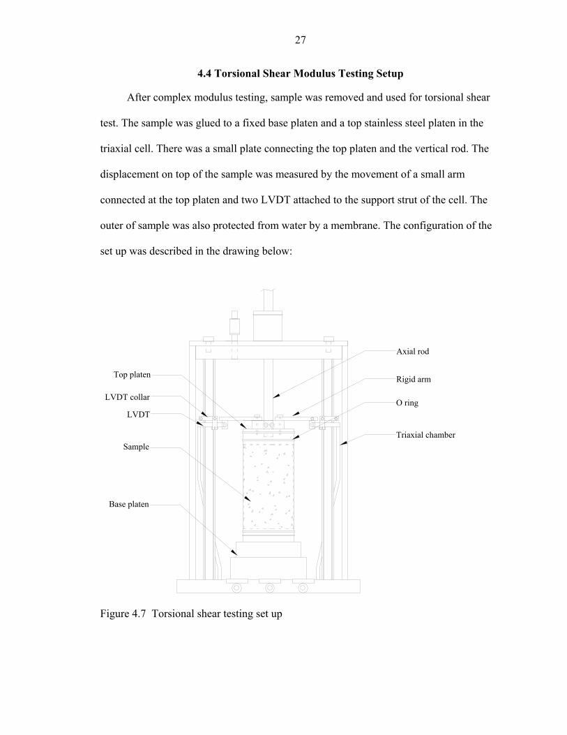
After complex modulus testing, sample was removed and used for torsional shear

test. The sample was glued to a fixed base platen and a top stainless steel platen in the

triaxial cell. There was a small plate connecting the top platen and the vertical rod. The

displacement on top of the sample was measured by the movement of a small arm

connected at the top platen and two LVDT attached to the support strut of the cell. The

outer of sample was also protected from water by a membrane. The configuration of the

set up was described in the drawing below:

Sample

Base platen

Axial rod

Top platen

LVDT collar

LVDT

Rigid arm

O ring

Triaxial chamber

Figure 4.7 Torsional shear testing set up

28

Basically, this test was performed as same as complex modulus test in term of

frequency and temperature control. The torsional force was introduced at 16 Hz, 10 Hz,

4Hz and 1 Hz. The test was carried out at room temperature (250C), then 100C and 400C.

The procedure of the test is described in chronicle order as below:

• Apply the seating load. The seating load was the same as complex modulus test. They were 200 N at 400C, 600N at 250C and 800N at 100C.

• Apply the seating torque. The reason for applying seating torque is that it prevents the torque force from going below zero in high frequency because of control problem mentioned above.

• Start recording the signal. The rate of recording is 50 points per cycle. Two LVDT are used, thus the result would be the average of those two.

• Start applying the cyclic torsional force. The magnitude of the force was selected in order to get the strain in range of 75 to 200 microstrain. The torsional force may vary depend on the stiffness of the mixture. The torsional force remained the same for a particular temperature and increases when the temperature decreases. Also, the torsional force may vary depend on the stiffness of the mixture. It is suggested that the first trial would be 12000N-mm, 20000N-mm and 30000N-mm for 400C, 250C and 100C successively. Because the GCTS system is lighter than MTS system, therefore it is less stable, and then it needs longer time for the signal to stabilize. It ‘s suggested that the duration of 16 Hz test is 150 cycles, 100 cycles for 10 Hz and 50 cycles for 4 and 1 Hz test. Also it needs to change the P gain according to control section above.

• After the applying cyclic torsional force is terminated, stop recording the signal, remove the seating load, and remove the seating torque to before test level.

Normally, one trial test is performed at first to verify the load level and the

feedback signal before the whole test sequence is carried out. The picture of a sample set

up in the triaxial chamber is presented in the next page.

29

Figure 4.8 Picture of torsional shear testing set up.

CHAPTER 5 SIGNAL AND DATA ANALYSIS

5.1 Test Signal

The response of a sample under cyclic load is composed of two parts: creep

response and elastic response. Complex modulus analysis requires the removal of the

permanent creep component from the cyclic strain response. Figure 5.1 presents a typical

deformation signal recorded after the test. The dynamic deformation-time response is

shown in Figure 5.2, once the creep component has been eliminated after regression

analysis.

0 10 20 30 40 50 60

Time (s)

Def

orm

atio

n

Creep component

Figure 5.1 Typical test signal.

30

31

0 10 20 30 40 50 60

Time (s)

Def

orm

atio

n

Figure 5.2. Dynamic sinusoid component of the signal.

The first part of the signal is still curved because the regression equation is based

on the last 10 cycles, but is applied for the whole signal.

Although recording very small deformation, one hundredth of a millimeter, it can

be observed that the deformation signal is smooth and clean. Also, the response achieves

a stable state in a sort period of time. This is important because the duration of the test

can be reduced significantly. Figure 5.3 will show the signal in Figure 5.2 on a larger

scale.

20 22 24 26 28 30

Time (s)

Def

orm

atio

n

Figure 5.3 Signal in higher scale

32

Some factors that may affect the quality of signal are shortly discussed below.

It was observed that sometimes the strain signal is affected by noise of the testing

system and environment. Figure 5.4 displays a strain signal with noise. Noise is a high

frequency electrical vibration, caused by several factors such as the vibration of the

system during the test, the quality of measurement device, or the instability of data

acquisition card.

Figure 5.4 Noise signal.

Noise will cause error in the calculation of modulus and phase angle. Low levels

of noise will cause higher amplitude in strain signal when using curve-fitting method for

data interpretation. High levels of noise may damage the signal totally. One solution to

reduce the level of noise is to increase the excitation voltage of the LVDT. The curve

fitting technique, the regression method, works pretty well with noise data. However, in

order to eliminate noise signal completely, it is better to have the noise filter option in

data acquisition card. A Fast Fourier Transform Analysis (FFT) can be performed with

the resulting file. There are several available programs, which are strong in signal

processing, including Mat lab, Lab View that provides the FFT filter option. A program

33

based on the FFT filtering method was created using Lab View. The FFT requires 2m data

points and it was an error at the first part and last past of data. Thus, it needs to start the

test after 6,7 seconds after recording the data and wait 6,7 second after finishing the test

to stop recording data. Figure 5.5 is a plot of a signal after filtering. Figure 5.6 is a plot of

an example of filtering function in Lab View. When using the filtering option in such

program, it should be noticed that phase angle would be changed. Therefore, a regression

analysis should be performed first in order to get phase angle.

Figure 5.5 Signal after filtering

Figure 5.6 Noise filter function in Lab View.

34

Another problem that may happen is the misshaping of the sinusoid of stress signal

or skewing of the stress signal. The signal can be wider at the bottom half than the top

half or the trend of signal is stiffer in removing load part of the sinusoid than the loading

part. These are testing issues and can be eliminated by properly applied seating load and

tuning the system.

5.2 Data Analysis

5.2.1 Iterative Curve Fit Method

Zhang et al. (1996) (University of Minnesota) proposed that the stress and strain

functions were of the form seen in Equation 5.1.

F(t) = A + Bt + Ccos(ωt-δ) (5.1)

The parameter C is half of the amplitude of the wave and δ is a phase shift. The

angular frequency (ω ), in rad/s, is found based on the test frequency (f), in Hz, as

presented in Equation 5.2

ω = 2.π.f (5.2)

The phase lag can be calculated in Equation 5.3 by determining the best-fit curves

for both the stress and the strain.

δ = δe - δs (5.3)

In order to match the predicted equation to the data, a non-linear least squared error

regression technique is used. Since the phase lag is unknown and inside the trigonometric

operator, a standard linear regression cannot be used to calculate all of the variables. So

to find the optimal signal, the δ was guessed at many points through out the possible

range until the error was minimized. Zhang et al. (1996) employed a bracketed search

technique where he would guess δ at regular intervals. He would then find out which

35

range the lowest error was in and search the system again in that reduced range. For

every guess of δ , the set of matrices seen in Equation 2.12 were used to solve Equation

2.9.

×−×=

−

−

−

∑∑∑

∑∑∑∑ ∑∑

∑∑

)()cos()(

)(

)(cos)cos(.)cos(

)cos(.

)cos(

2

2

i

ii

i

i

iii

i

tFttFt

tF

CBA

tttt

tttt

ttn

δωωωδω

δω

δω

After the least squared error values for A, B, and C were found, the least squared

error was compared to the other guesses of δ. A minimum number of 4 guesses must be

used per iteration to reduce the scope of the search. The search algorithm used is:

Step1: Set δstart=0, δend=180, ∆δ =(δstart - δend)/M (M is an integer, M>1)

Step 2: Calculate δj=δstart + j*∆δ (j=1, 2, 3, …, M)

Step 3: Solve for A, B, and C using Equation 2.12 (j=1, 2, 3, …, M)

Step 4: Calculate the squared error for all values of j (j=1, 2, 3, …, M)

Step 5: Select the value d that provided that least squared error (δk)

Step 6: Check Convergence:

If ∆δ > Tolerance, then update the range of ∆ and repeat (δstart=δk - ∆δ ,

δend=δk + ∆δ , ∆δ = (δstart - δend)/M

If ∆δ < Tolerance, then stop

By repeating this system several times, Zhang et al. (1996) showed that the δ could

be roughly predicted. There is a problem associated with this method. It is only designed

to read the signal of a sinusoid on a straight line. Since this is an iterative method, it can

be very time consuming. The level of acceptable error is also very important to balance

with the time restraints.

36

5.2.2 Regression Method

Using a regression method with trigonometric function, the stress and strain signal

can be described with:

F(t) = A0 + A1.t +A2.t2 + . . . + Am.tm-1 + B. cos(wt) + C.sin(wt) (5.4)

This equation has a polynomial degree of m – 1. In order to find all the

coefficients, a least square error regression approach can be used. The unknown

coefficients satisfy following matrix equation:

BxA =⋅

where:

A is an m+2 by m+2 symmetric matrix with the following configuration:

for i = 1 to m and j = 1 to m )1)(1(,

−−∑=ji

ji ta

for i = 1 to m and j = m+1 )()1(, tCosta i

ji ⋅⋅=−∑ ω

) for i = 1 to m and j = m+2 ()1(, tSinta iji ⋅⋅=

−∑ ω

) for i = m+1 and j=1 to m ()1(, tCosta jji ⋅⋅=

−∑ ω

) for i = m+2 and j = 1 to m ()1(, tSinta jji ⋅⋅=

−∑ ω

∑ ⋅⋅== ++++ )().(1,22,1 tCostSinaa mmmm ωω

)

)

(21,1 tCosa mm ⋅= ∑++ ω

(22,2 tSina mm ⋅= ∑++ ω

x is an m+2 matrix with : Tm CBAAAx ]...[ 10=

and B is an m+2 column matrix with:

37

for i = 1 to m ∑ ⋅= − Ftb i

i)1(

∑ ⋅⋅=+ FtCosbm )(1 ω

∑ ⋅=+ FtSinbm ).(2 ω

The algorithm to solve this matrix equation has been written by Swan (2001).

Normally, the degree of polynomial of 2 (m=3) is used in the analysis.

The amplitude of the sinusoid can be calculated using Equation 5.5 and the phase

angle then can be calculated using Equation 5.6:

22 CBAmplitude += (5.5)

)(tan 1

CBAnglePhase −= (5.6)

5.2.3 FFT Method

In case of complex signal containing noise, the signal can be transformed from

time domain into frequency domain using concept of Fourier transform. Then the

amplitude of the signal of testing frequency can be picked up. Normally, with digital

data, which is recorded at a specified interval, Discrete Fourier Transform (DFT) is used.

This is a computer algorithm that is deigned to change a complex signal into a serious of

sinusoids at discrete frequency intervals. An example of the transformation of a typical 4

Hz axial strain signal can be seen in Figure 5.7 and Figure 5.8. For a perfectly clean

sinusoid signal, there should be a spike at the given frequency and all other values should

be zero.

38

Figure 5.7 Test signal in time domain

Figure 5.8 Test signal in frequency domain

The DFT is performed using Equation 5.7

)...2sin(..)...2.(cos(1

0 npki

npkxy

n

kkp

ππ+= ∑

−

=

(5.7)

The value of yp is the complex output in frequency space where p is a counter

integer representing frequency as seen in Equation 5.8

nrateSamplingpFrequency ).(

= (5.8)

39

The amplitude of the sinusoid represented by p is given in Equation 5.9 where N is

the number of samples recorded in the signal.

N

yAmpitude p2

= (5.9)

The phase angle of each sinusoid can be calculated by finding the angle that is

represented by the complex components of yp.

This method may have a leaking problem, which means if the testing frequency did

not occur at one of the discrete points in frequency space, therefore the magnitude was

reduced and split between the closest frequencies on either side of the true frequency.

This provided results that seemed to vary depending on the number of points tested. An

example of this effect can be seen in Figure 5.9

Figure 5.9 Strain with missing peak data

The way this was corrected was to find an integer value of p for the testing

frequency using equation 5.8. Since the sampling rate was constant and so was the testing

frequency, the only variable that was easy to manipulate was the number of samples

examined. To manipulate this, the mean value of the signal was added before and after

the sample until the signal was the correct length. The value of p for the testing frequency

40

can then be calculated using Equation 5.10, where N’ is the modified number of samples

in the signal.

rateSamplingNfp frequncyTesting

'.= (5.10)

It lets to the conclusion that when using DFT analysis, if only a few cycles were

used (i.e. under 20 cycles with 50 data points per cycle) then the magnitude of the signal

may not accurately reflect the true value. Therefore higher data recording rate should be

used.

5.2.4 Evaluation of Data Interpretation Method.

In order to evaluate the methods calculating complex modulus, the idea of

generating artificial signals are introduced. Then the modulus and phase angle are known

before hand. For example, these signals below are generated. Three methods: Iterative

Curve Fit, Regression, FFT are evaluated.

Here is the artificial signal. Strain and stress pure signals of 20 Hz, added white

noise and creep trend. Phase angle of 720, dynamic modulus of 21.22 MPa, scan rate of

500 points/sec. The summary of the analysis is presented in table 5.1

Table 5.1 Evaluation of data interpretation method

Pure signal Pure signal with noise

Signal with noise and creep

Calculation method

Phase Angle E* Phase

Angle E* Phase Angle E*

Iterative Curve Fit 72 21.22 73.6 23.03 72.91 22.15

Regression Analysis 72 21.22 73.53 23.03 72.88 22.0.4

FFT 67.97 19 68.04 19.81 73.62 18.57

From above results and results from the test, some conclusion can be made:

41

• For the pure signal, Iterative Curve Fit and Regression methods give an exact

result. FFT gives the result a little bit lower than designed value.

• For the signal with noise, due to the noise, Iterative Curve Fit method and Regression method give the result slightly higher than designed result. FFT method gives the result lower than designed values.

• Most of the time, Iterative Curve Fit method gives the good result but still gives the unexpected result sometimes. Regression method is very stable, therefore is the best method available.

5.2.5 Computer Program

In chapter 2, the equations to calculate complex modulus and torsional shear

modulus have been mentioned. In this section, more detail about how the data analysis

program is written and the modified version of torsional shear modulus from the original

axial complex modulus is illustrated.

Figure 5.10 describes the flow chart of data analysis program written by Swan

(2001). The program was written by Visual Basic for Excel. This has an advantage of

analyzing column data in a familiar Excel environment. The modified version for

calculating torsional shear modulus based on the same flow chart, only a change in the

calculation of torsional shear stress and shear strain has been introduced.

For complex modulus program:

areaSurfacecolumnForcecolumnstressAxial = (5.11)

)50( mmlengthSpacercolumncementLVDTdisplacolumnstrainAxial = (5.12)

For torsional shear modulus program:

JrTorque

columnstressShear 0×= (5.13)

42

Ll

rcementLVDTdisplacolumnstrainShear

××

= 0 (5.14)

where: r0 is the radius of sample, r0 = 50mm

J is the area polar of inertia, J = π*ro4/2

l is the length from center of sample to measurement point, l = 107.7mm

L is the height of sample, L = 150mm

The input data file was recorded in a standard order that the program can

understand. Any change in that order will need a change in the program.

At first, the load and deformation data column are converted to stress and strain

data column. The regression analysis will work with a pair column of time and stress or

time and strain. The program automatically determines the duration of the test and the

number of loop required. The number of loop equal to the total number of test cycles

divided by number of test cycles used for calculating dynamic modulus. 10 cycles of

complex modulus was chosen.

Besides the dynamic modulus and phase angle, the analysis program was also

designed to write down the best-fit signal equation and the least square errors.

Figure 5.11 and 5.12 will show the data input page of Complex Modulus Program

and Torsional Shear program. It is shown that the time, stress and strain data column,

start time and stop time of the test as well as degree of polynomial of regression analysis

are predetermined. Only input needed is test frequency.

43

Convert Data to Stress and Strain

Input Test Frequency

Column Data for 10 CyclesRead Time. Stress & Strain

AnalysisCall Regression

Call Write R

Call Write Regression Equation2

Get Modulus &

Output Page

Phase Angle

Num

ber of Loop = 10/Frequency

Number of lTotal of test cycle/1

oop = 0

Figure 5.10 Flow chart of data analysis program.

44

Figure 5.11 Complex Modulus Program

Figure 5.12 Torsional Shear Modulus Program.

Besides the version of complex modulus program for two axial LVDT, the version

of torsional shear modulus for LVDT, there are versions of complex modulus program

for four axial LVDT and torsional shear modulus for proximitor.

Figure 5.13 will present the output file torsional shear modulus program of a 10Hz

test.

45

Figure 5.13 Output page of Torsional Shear Modulus Program.

The output page of axial complex modulus program has a similar format. It

contains all the information necessary such as shear stress, shear strain amplitude, phase

46

angle… It noticed that the signal equation is only for last 10 cycles. Also, for the stress

signal equation, the creep component has the value approximate to zero.

The calculation of modulus as an average of 10 test cycles gave a better result than

an average of 5 test cycles. Figure 5.14 shows the dynamic modulus calculated as an

average modulus of 10 cycles versus 5 cycles. It was shown that the results is less

scattered if we calculate the modulus for average of 10 cycles than that of 5 cycles. It

was noted that in previous study, the quality of signal was much less than that of present

study.

1000

1500

2000

2500

3000

3500

4000

0 3 6 9 12 15

Time (s)

Dyn

amic

Mod

ulus

(kPa

)

Avg of 5Avg of 10

Figure 5.14 Calculation of Modulus, average of 10 cycles versus 5 cycles

Figure 5.15 presents linear regression analysis on a10 Hz complex modulus test

versus quadratic regression analysis. It was observed that there is almost no different

between two analyses. As seen in figure 5.1, quadratic trend of creep component of test

data developed only in first 10 or 20 cycles, therefore the different between quadratic and

linear regression is expected in this zone. However, the regression analysis is calculated

for every 10 cycles, there is almost no different between linear and quadratic in that

range. After that, the creep component developed almost linearly (Figure 5.1)

47

1000

1400

1800

2200

2600

3000

0 2 4 6 8

Time(s)

E*(M

Pa) Linear

Quadratic

Figure 5.15 Linear regression versus quadratic regression analysis

With new control system, it was observed that a test gets to its stable state very

soon. For example, in figure 5.13 and figure 5.15, the dynamic modulus remains almost

constant after second or third points. Therefore, the duration of the test doesn’t need to be

long. For axial complex modulus test, the duration of 50 cycles was found sufficient. For

torsional shear modulus test, the duration of 150 cycles for 16 Hz test, 100 cycles for

10Hz test, 50 cycles for 4Hz and 1 Hz test were found sufficient.

CHAPTER 6 AXIAL COMPLEX MODULUS TEST RESULTS

6.1 Result of Complex Modulus Test

In Chapter Four , the procedures for complex modulus testing were been

presented. In the following, axial complex modulus test results are presented from three

coarse-graded granite mixture GAC1, GAC2, GAC3 and three fine granite mixture

GAF1, GAF2, GAF3. Three specimens for each mixture were tested. For temperature

effects on the complex modulus , three test temperatures of 400C, 250C and 100C were

used. The testing frequencies included 16Hz, 10 Hz, 4 Hz and 1Hz.

6.1.1 Dynamic Modulus Results

Figure 6.1 through 6.3 plot the result of dynamic modulus |E*| for the GAF1

mixture, which had a typical response for the fine-graded mixtures. Figures 6.4 through

6.6 show the complex modulus results for the GAC1 mixture, which had a typical

response for the coarse-graded mixtures. The results for the other mixtures (GAC2,

GAC3, GAF2, and GAF3) are provided in Appendix B.

The plots show the typical results of |E*| from the test. Although there is some

degree of variability in the testing results, a consistent value of |E*| plus a consistent

trend of |E*| versus frequency were obtained. The results clearly show |E*| increasing

with increasing frequency. That was expected because it is known that asphalt concrete

get stiffer with increased loading rate (e.g. Sousa, 1987).

48

49

0

1000

2000

3000

4000

5000

0 5 10 15 20

Frequency (Hz)

|E*|

(MPa

) F1-01

F1-02

F1-03

Ave

Figure 6.1 Dynamic Modulus |E*| of GAF1 at 250C

0

2000

4000

6000

8000

10000

0 5 10 15 20

Frequency (Hz)

|E*|(

MPa

)

F1-01

F1-02

F1-03

Ave


0

400

800

1200

1600

2000

0 5 10 15 20

Frequency (Hz)

|E*|(

MPa

F1-01

F1-02

F1-03

Ave


50

0

1000

2000

3000

4000

5000

0 4 8 12 16 20

Frequency (Hz)

|E*|(

MPa

)

C1-01

C1-02

C1-03

Ave

Figure 6.4 Dynamic Modulus |E*| of GAC1 at 250C

0

2000

4000

6000

8000

10000

0 5 10 15 20

Frequency (Hz)

|E*|(

MPa

)

C1-01

C1-02

C1-03

Ave


0

400

800

1200

1600

2000

0 5 10 15 20

Frequency (Hz)

|E*|(

MPa

)

C1-01

C1-02

C1-03

Ave


51

6.1.2 Phase Angle Results

Figure 6.7 to 6.12 show the phase angle with frequency for the GAF1 and GAC1

mixtures. For 250C and 400C, the results clearly show that the phase angle increases

with increasing frequency. For higher temperatures, this trend becomes even more

pronounced. Phase angles increase from 300 to 400 at 250C and from 280 to 500 at 400C.

For 100C tests, the phase angle decreased slightly at 4Hz test, but increases with

frequency up to 16 Hz. .

0

10

20

30

40

50

0 5 10 15 20

Frequency (Hz)

Phas

e An

gle

(Deg

rees

)

F1-01

F1-02

F1-03

Figure 6.7 Phase angle of GAF1 mixture at 250C

0

10

20

30

40

50

0 5 10 15 20

Frequency (Hz)

Phas

e An

gle

(Deg

rees

)

F1-0

F1-0

F1-0


SumAvg

1

2

3

SumAvg

52

0

10

20

30

40

50

60

0 5 10 15 20

Frequency (Hz)

Phas

e An

gle

(Deg

rees

)F1-01

F1-02

F1-03

Sum


0

10

20

30

40

50

0 5 10 15 20

Frequency (Hz)

Phas

e An

gle

(Deg

rees

)

C1-01

C1-02

C1-03

Sum

Avg

AveAvg

Figure 6.10 Phase angle of GAC1 mixture at 250C

0

10

20

30

40

50

0 5 10 15 20

Frequency (Hz)

Phas

e An

gle

(Deg

rees

)

C1-01

C1-02

C1-03

Sum

Avg


53

0

15

30

45

60

75

0 5 10 15 20

Frequency (Hz)

Phas

e An

gle

(Deg

rees

)C1-01

C1-02

C1-03


6.1.3 Discussion of Testing Results

Figures 6.13 through 6.15 show the dynamic mod

temperature.

0

1000

2000

3000

4000

5000

Mixtures

Dyn

amic

mod

ulus

(MPa

)

Figure 6.13 Average Complex Modulus result at 10 Hz

SumAvg

ulus at 10 Hz for each

C1C2C3F1F2F3

250C

54

0

2000

4000

6000

8000

10000

12000

Mixtures

Dyn

amic

mod

ulus

(MPa

)C1

C2

C3

F1

F2

F3

Figure 6.14 Average Complex Modulus result at 10Hz at 100C

0

400

800

1200

1600

2000

Mixtures

Dyn

amic

mod

ulus

(MPa

)

C1

C2

C3

F1

F2

F3

Figure 6.15 Average Complex Modulus result at 10Hz at 400C

It was observed that the coarse mixtures ranked consistently for different

temperatures. The magnitude of the dynamic modulus for the GAC1 mixture has the

lowest value of . The GAC2 and GAC3 mixtures have almost the same dynamic

modulus. For example at100C, |E*| of GAC1 is 2090 (MPa), |E*| of GAC2 and GAC3 are

3020 and 3172 (MPa) consecutively.

For the fine-grade mixtures, the GAF2 mixture consistently showed the highest

dynamic modulus, with GAF3 is stiffer than GAF1 at 250C and 100C but softer at 400 C.

This is maybe because the test for these mixtures contains some degree of variability.

From the gradation of these mixtures (Table 3.1), GAF2 has higher percentage of coarse

55

aggregate remaining on 12.5mm and 9.5mm sieve than GAF3 and GAF1, which provides

better aggregate interlock. Therefore the stiffness of GAF2 is higher than the other two

mixtures. For coarse mixtures, GAC2 also has higher percentage of coarse aggregate than

GAC1 and GAC2, and GAC2 is stiffer than GAC1 and GAC3

Figures 6.16 through 6.18 present a summary of phase angles for all the mixture

tested. These plots show very consistent average results. Within the same frequency,

phase angles are higher at higher temperatures. This is reasonable because the sample

will be softer at higher temperature, the viscosity of asphalt binder is lower, and thus it

results in a less elastic response of strain versus stress. Except for the 4 Hz test at 100C,

the entire test shows the phase angle increases with increasing frequency.

Figure 6.19 through 6.21 present the average of phase angle of the mixtures for

4Hz test.

0

10

20

30

40

50

0 5 10 15 20

Frequencies (Hz)

Phas

e A

ngle

(Deg

ree) C1

C2C3F1F2F3

Figure 6.16 Average of phase angle at 250C

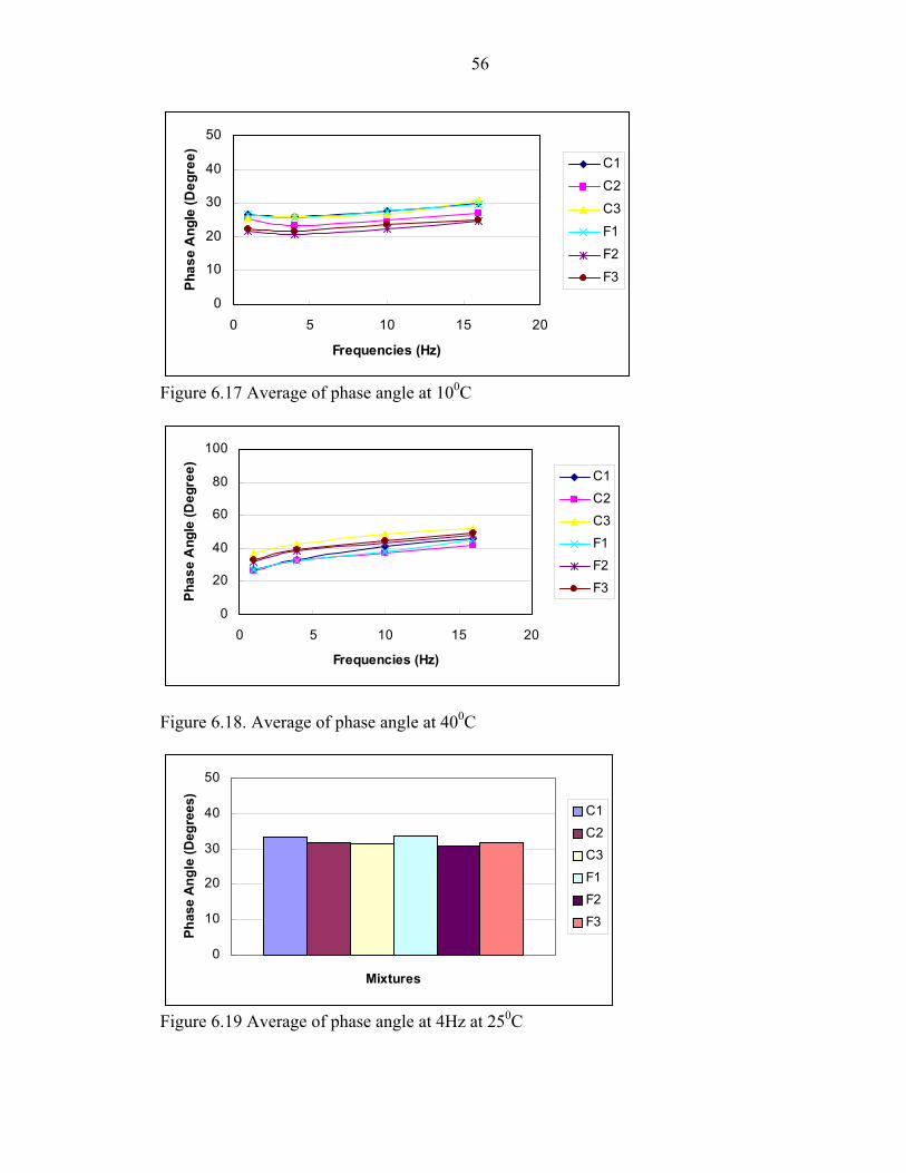
56

0

10

20

30

40

50

0 5 10 15 20

Frequencies (Hz)

Phas

e A

ngle

(Deg

ree) C1

C2C3F1F2F3

Figure 6.17 Average of phase angle at 100C

0

20

40

60

80

100

0 5 10 15 20

Frequencies (Hz)

Phas

e A

ngle

(Deg

ree) C1

C2C3F1F2F3

Figure 6.18. Average of phase angle at 400C

0

10

20

30

40

50

Mixtures

Phas

e A

ngle

(Deg

rees

)

C1C2C3F1F2F3

Figure 6.19 Average of phase angle at 4Hz at 250C

57

0

10

20

30

40

50

Mixtures

Phas

e A

ngle

(Deg

rees

)C1C2C3F1F2F3


0

10

20

30

40

50

Mixtures

Phas

e A

ngle

(Deg

rees

)

C1C2C3F1F2F3


6.2 Master Curve Construction

A master curve of an asphalt mix allows comparison of linear visco-elastic

materials when testing has been conducted using different loading times (frequencies)

and test temperatures. A master curve can be constructed utilizing the time temperature

superposition principle, which describes the visco-elastic behavior of asphalt binders and

mixtures.

6.2.1 Time-temperature Superposition Principle

Test data collected at different temperatures can be “shifted” relative to the time of

loading frequency, so that the various curves can be aligned to form a single master

58

curve. The shift factor a(T) defines the required shift at a given temperature, i.e, a

constant by which the frequency must be divided to get a reduced frequency fr for the

master curve:

)(Taff r = or log(fr) = log(f) + log[a(T)]

Master curves can be constructed using an arbitrarily selected reference

temperature Tr to which all data are shifted. At the reference temperature, the shift factor

a(Tr) = 1.

6.2.2 Constructing Master Curve using Sigmoidal Fitting Function.

For a testing frequency or a given time dependency, the generalized power law is a

widely accepted mathematical model for bituminous material response. However, a new

method of developing master curves for asphalt mixtures by Pellinen was used in this

thesis (Pellinen et al., 2002). In his study, master curves were constructed fitting a

sigmoidal function to the measured compressive dynamic (complex) modulus test data

using non-linear least square regression. In the experimental shift approach, the fitting

function for master curve construction is a sigmoidal function defined by Equation (6.1):

)log(1)*log(

rfeE γβ

αδ −++= (6.1)

where

log(/E*/) = log of dynamic modulus,

δ = minimum modulus value,

fr = reduced frequency,

α = span of modulus value,

β, γ = shape parameter.

59

The parameter γ influences the steepness of the function (rate of change between

minimum and maximum) and β influences the horizontal position of the turning point,

shown in Figure (6.16).

The shifting was done using an experimental approach by solving shift factors

simultaneously with the coefficients of the sigmoidal function, without assuming any

functional form of a(T) versus temperature. The master curve of the mix can be

constructed using the Solver Function in an Microsoft Excel spreadsheet. The

justification of using a sigmoidal function for fitting the compressive dynamic data is

based on the physical observations of the mix behavior. The upper part of the sigmoidal

function approaches asymptotically the maximum stiffness of the mix, which is

dependent on limiting binder stiffness at cold temperatures. At high temperatures, the

compressive loading causes aggregate influence to be more dominant than the viscous

binder influence. The modulus starts to approach a limiting equilibrium value, which is

dependent of the aggregate gradation. Thus, the sigmoidal function captures the physical

behavior of the asphalt mixture observed in the mechanical testing using compressive

cyclic loading through entire temperature range.

Log Reduced Frequency

Sigmoidal Function

(pos)

δ

γ (increase)

log/

E*/ (neg)β

β

δ+α

Figure 6.22 Sigmoidal Function

60

The results of complex modulus tests for all mixtures tested are presented in the

master curves in Figures 6.17 and Figure 6.18 below. All the data were shifted to the

reference temperature of 250 C.

Master Curve For Coarse Mix

1

2

3

4

5

-3 -1 1 3 5


log(

E*) (

MPa

) C1

C2

C3

Figure 6.23 Log complex modulus master curve for coarse mix

Master Curve For Fine Mix

1

2

3

4

5

-3 -1 1 3 5


log(

E*) (

MPa

) F1

F2

F3

Figure 6.24 Log complex modulus master curve for fine mix

61

6.3 Predictive Equation

Many predictive techniques for determining the dynamic modulus of asphalt

concrete mixes have evolved over the past 30 years. The predictive equation developed

by Witzack et al. at the University of Maryland is one of the most comprehensive mixture

dynamic modulus models available today (Witzack et al., 2002). That equation is

presented below:

)).log(39353.0)log(313351.0603313.0(34

238384

42

200200

1)(005470.0)(00017.0)(003958.0)(0021.0871977.3

)(802208.0)(058097.0

)(002841.0)(001767.0)(029232.0249937.1*log

η×−×−−++−+−

++

−×−

×−×−×+−=

f

abeff

beffa

epppp

VVV

V

pppE

(6.2)

where:

/E*/ = dynamic modulus, 105 psi

η = bitumen viscosity, 106 Poise,

f = loading frequency, Hz,

Va = air void content, percent,

Vbeff = effective bitumen content, percent by volume,

P34 = cumulative percent retained on 19-mm sieve,

P38 = cumulative percent retained on 9.5-mm sieve.

P4 = cumulative percent retained on 4.76-mm, and

P300 = percent passing 0.pp75-mm sieve.

It is noted that for the mixtures used in the test, p34 = 0, using p12 in the equation

(6.2) instead of p34 will give a better result than using p34 = 0.

62

The regression model above has the capability of predicting the dynamic modulus

of dense-graded HMA mixtures over a range of temperatures, rates of loading, and aging

conditions. Figure 6.24 through 6.26 plot the predicted dynamic modulus versus the

measured values for six mixtures at 16 Hz. It was observed that the predictive model

underestimates the real performance of the mixes. However, the predicted values are

proportion to the actual ones. For example, the predictive model predicts GAF2 mix

having the highest modulus among fine mixtures and GAC2 mix having the highest

modulus among the coarse mixtures, which is consistent with experimental results.

Therefore the predictive equation can help to estimate the performance of mixtures

during the mix design and pavement thickness design processes although it only provides

approximate values.

0

2000

4000

6000

8000

C1 C2 C3 F1 F2 F3Mixtures

E*(M

Pa)

Actual ValuesPredictived Values

Figure 6.24 Actual values versus Predicted value of E* at 250C for 16Hz test.

63

0

3000

6000

9000

12000

15000


E*(M

Pa)



0

500

1000

1500

2000

2500

3000


E*(M

Pa)



The comparison of the predicted values dynamic modulus actual dynamic modulus

at other frequencies will be presented in appendix B.

CHAPTER 7 TORSIONAL SHEAR TEST RESULTS

7.1 Result of Torsional Shear Test

Chapter 4 described the procedures for the Torsional Shear Test. In order to

investigate the relationship between this test and axial complex modulus test, the test was

performed under the same temperature and frequency conditions as used for the axial

testing in Chapter 6. The same 18 samples from the same six mixtures were tested at

250C first. The temperature then was reduced to 100C. Finally, the samples were heated

up and tested at 400C. Full frequency sweep of 16 Hz, 10Hz, 4Hz and 1 Hz were used.

It was noted that at 100C, because of controlling problem of the servo-hydraulic

system, the applied force for 16Hz test was much higher than the command force,

therefore the result of the test at this frequency doesn’t reflect the right answer. Thus, for

100C, the results are only reported for 1Hz, 4Hz and 10Hz tests.

7.1.1 Stress versus Strain Study

The primary concern of the test was the relationship of torsional shear stress and

torsional shear strain in term of micro strain. By draw the stress versus strain curve, the

linearity of the result, the magnitude of applying load, and the variation of the modulus in

designed testing strain can be investigated. Figure 7.1 shows the torsional stress versus

strain curve at 1 Hz and 10Hz test. The linearity relationship is observed between shear

stress and shear strain.

64

65

0

0.05

0.1

0.15

0.2

0.25

0.3

0 0.0001 0.0002 0.0003 0.0004

Torsional Shear Strain

Tors

iona

l She

ar S

tress

(MPa

)

1Hz10Hz

Figure 7.1 Torsional shear stress versus shear strain.

Figure 7.2 show the relationship between phase angle and shear strain. It shows that

higher shear strain results in smaller phase angle. It is reasonable because higher shear

strain will result in higher interlock among particles in the sample, therefore the viscous

effect of asphalt binder is reduced, which result in faster deformation response of

specimen under loading.

0.0

10.0

20.0

30.0

40.0

50.0

60.0

0 0.00005 0.0001 0.00015 0.0002 0.00025 0.0003

Torsional Shear Strain

Phas

e An

gle

(Deg

rees

)

1Hz10Hz

Figure 7.2 Phase angle versus shear strain level.

66

7.1.2 Dynamic Torsional Shear Modulus Results

Figures 7.3 through 7.5 present the results of the dynamic torsional shear

modulus |G*| for the GAF1 mixture, which was found to be representative for

fine-graded mixtures. Similarly, Figures 7.4 through 7.6 show the results for the

dynamic torsional shear modulus |G*| for the GAC1 mixture, which was also

representative for the coarse-graded mixtures. The results for the other mixtures

are shown in Appendix B.

0500

10001500200025003000

0 5 10 15 20

Frequency (Hz)

Mod

ulus

(MPa

) F1-01

F1-02

F1-03

Sum

|G*|

(MPa

)

Avg

Figure 7.3 Dynamic Torsional Shear Modulus |G*| of GAF1 at 250C

0

1000

2000

3000

4000

5000

0 3 6 9 12

Frequency (Hz)

Mod

ulus

(MPa

) F1-01

F1-02

F1-03

Sum

Avg|G*|

(MPa

)


67

0

200

400

600

800

1000

0 5 10 15 20

Frequency (Hz)

Mod

ulus

(MPa

) F1-01

F1-02

F1-03

Sum


0

400

800

1200

1600

2000

0 4 8 12 16 20

Frequency (Hz)

|G*|(

MPa

)

C1-01

C1-02

C1-03

Avg

|G*|

(MPa

) |G

*| (M

Pa)

Avg

Figure 7.6 Dynamic Torsional Shear Modulus |G*| of C1 at 250C

0

1000

2000

3000

4000

0 3 6 9 12

Frequency (Hz)

Mod

ulus

(MPa

) C1-01

C1-02

C1-03

Sum

Avg

|G*|

(MPa

)


68

0

200

400

600

800

0 5 10 15 20

Frequency (Hz)

Mod

ulus

(MPa

)C1-01

C1-02

C1-03

Sum

Avg|G*|

(MPa

)


The results show a high degree of consistency for the different conditions and

samples tested Similar to the dynamic axial modulus test results in Chapter 6 |G*|

increases with increased frequency, as expected.

At 250C, |G*| increases from about 400 MPa at 1Hz test to 900 MPa at 16Hz test

for the GAC1 mixture and from 500 MPa at 1Hz test to 1200 MPa at 16Hz test for the

GAF1mixture.

At 100C, G* increases from 1100 MPa (1Hz) to 2100 MPa (16Hz) for the

GAC1mixture and from 2000 MPa (1Hz) to 3000 MPa (16Hz) for the GAF1 mixture.

At 400C, |G*| increases from 140 MPa (1hz) to 390 MPa (16Hz) for the GAC1

mixture and from 200 MPa (1Hz) to 480 (16Hz) for the GAF1 mixture.

7.1.3 Phase Angle Results

Because the phase angle varies according to strain level, therefore it exists a

variability in the test result . Figures 7.9 through 7.14 show the measured phase angles for

the GAF1 and GAC1 mixtures. It was observed that phase angle for the torsional shear

test is higher than the axial complex modulus test about 120 on average. One possible

explanation for this difference is the anisotropic nature of hot mix asphalt samples. .

69

there is also a variability associated with the test results at 100 C and 250 C, thus it is

not very clear that the phase angle increases or decreases with varying frequencies.

However, at test temperatures of 400 C, the phase angle increases with increasing

frequency.

0

10

20

30

40

50

60

0 10 20

Frequency (Hz)

Phas

e An

gle

(deg

rees

)

F1-01

F1-02

F1-03

Sum

Ave

Figure 7.9 Phase angle of GAF1 mixture at 250

0

10

20

30

40

50

60

0 3 6 9 12

Frequency (Hz)

Phas

e An

gle

(deg

rees

)

F1-01

F1-02

F1-03

Sum

Ave


70

0

20

40

60

80

100

0 5 10 15 20

Frequency (Hz)

Phas

e A

ngle

(deg

rees

)F1-01

F1-02

F1-03

Sum

Ave


0

20

40

60

80

100

0 10 20Frequency (Hz)

Phas

e An

gle (d

egre

es)

C1-01

C1-02

C1-03

Sum

Ave

Figure 7.12 Phase angle of GAC1 mixture at 250

0

20

40

60

80

100

0 3 6 9 12Frequency (Hz)

Phas

e An

gle (d

egre

es)

C1-01

C1-02

C1-03

Sum

Ave


71

0

20

40

60

80

100


Phas

e An

gle

(deg

rees

)

C1-01

C1-02

Sum

Ave


Figures 7.15 through 7.17 plot the magnitude of dynamic torsional shear modulus

|G*|ranked consistently for the different temperatures tested. The Coarse-graded GAC1

mix had the lowest modulus, with the fine-grade mixture GAF2 showing the highest

dynamic torsional shear modulus, with other mixtures showing similar results.

0

400

800

1200

1600

2000

Mixtures

Tors

iona

l she

ar m

odul

us

(MPa

)

C1

C2

C3

F1

F2

F3

Figure 7.15 Average of torsional shear modulus at 10 Hz at 250C

72

0

1000

2000

3000

4000

5000

Mixtures

Tors

iona

l she

ar m

odul

us

(MPa

)

C1

C2

C3

F1

F2

F3


0

200

400

600

800

1000

Mixtures

Tors

iona

l she

ar m

odul

us

(MPa

)

C1

C2

C3

F1

F2

F3


7.2 Poisson Ratio

The Torsional shear complex modulus can be related to axial complex modulus by

the Poisson ratio. Harvey et al. (2001) concluded that the Poisson’s ratio could be taken

to be constant, resulting in the following relationship between G* and E*:

)1(2**ν+

=EG (7.1a)

or

1*2

*−=

GEν (7.1b)

73

For each test, the Poisson ratio was calculated using Equation (7.1b). Figures 7.18

and 7.19 show typical results for the Poisson’s ratio at different temperatures for the

coarse-graded GAC2 mixture and the fine-graded GAF2 mixture. It can be observed that

Poisson ratio is not constant, but varies according to loading rate.

0.00

0.20

0.40

0.60

0.80

1.00

0 5 10 15 20

Frequencies (Hz)

Pois

son

ratio

25 dc10 dc40 dc

Figure 7.18 Poisson ratio of coarse mixture C2

0.00

0.20

0.40

0.60

0.80

1.00

0 5 10 15 20

Frequencies (Hz)

Pois

son

ratio

25 dc10 dc40 dc

Figure 7.19 Poisson ratio of fine mixture F2

Although there is some degree of variability in the Poisson ratio results, it was

observed that for 100C, Poisson ratio increases with higher frequency. That means the

rate of changing in |E*| is faster than the rate of change in |G*|. For 250C and 400C, the

Poisson’s ratio drop from 1Hz test to 4Hz test for the coarse-graded GAC2 mixture.

74

However, the fine-graded GAF2 mixture showed a smaller drop between 1 Hz and 4 Hz

than the GAC2 mixture at 250C, and no drop at 400C for the fine-graded GAF2 mixture.

The reasons for this variability may be that the characteristic of asphalt samples change at

some point, where the interlock between the aggregates has more effect or the viscosity

of asphalt binder has more effect.

Table 7.1 shows the Poisson ratio calculations for all the mixtures.

Table 7.1 Poisson ratio GAC1 GAC2 GAC3 GAF1 GAF2 GAF3 40dc 1Hz 0.059 0.562 0.200 0.447 0.025 -0.117 4Hz 0.054 0.305 0.062 0.284 0.067 -0.133 10Hz 0.113 0.317 0.218 0.335 0.176 -0.027 16Hz 0.277 0.478 0.316 0.481 0.290 0.097 25dc 1Hz 0.323 0.149 0.029 0.305 0.188 0.077 4Hz 0.293 0.110 0.015 0.219 0.160 0.042 10Hz 0.268 0.169 0.079 0.267 0.301 0.095 16Hz 0.377 0.299 0.219 0.396 0.418 0.218 10dc 1Hz 0.250 0.284 0.206 0.123 0.233 0.107 4Hz 0.254 0.359 0.219 0.175 0.355 0.075 10Hz 0.331 0.413 0.184 0.257 0.460 0.217 16Hz N/A 0.523 N/A N/A N/A N/A

7.3 Summary

The consistent results for the dynamic torsional shear test presented in this chapter

have shown that this test may be a useful tool for studying the deformational

characteristics of asphalt concrete during shear. After the axial complex modulus test,

instead of wasting the sample, it is of great advantage to use the sample for studying the

dynamic shear modulus. With the observation that the phase angles in the torsional shear

test is higher than for the axial test, implies that the dynamic torsional shear modulus test

may be sensitive to the anisotropy in the sample during testing.

75

Although the torsional shear test is preformed on a solid specimen, and therefore

the stress distribution in the sample varies, due to its simplicity, it can be regarded as a

promising test to study the shear stress state of mixtures and an important step before

studying torsional shear stress in hollow cylinder of asphalt concrete.

CHAPTER 8 CONCLUSION AND RECOMMENDATION

8.1 Conclusion

8.1.1 Testing Procedures and Setup

Over the past year, a lot of improvements on the testing apparatus, system control

and data acquisition in the complex modulus program have been made. The introduction

of new controller system Test Start IIm brought much higher capability and performance

quality than the old Test Start IIs. The capacity of controlling test frame increased from

one to four kips, permiting the operation of the torsional shear test on GCTS load frame.

The data acquisition capacity is also improved greatly. The new Testar IIm

controller program has the capacity of recording up to 12 output signals. Therefore, a

very complicated test, which may include thermocouple, pressure transducer, LVDT can

be carried out. The ability to view the output signal and input signal separately or

simultaneously helps to examine the set up and quality of signal during the test.

Another significant improvement in the testing program was the introduction of

temperature controlling unit. It permits to test specimen in various temperature than only

room temperature like previously.

Finally, a new testing set up and procedure has been introduced for torsional shear

modulus test. The new simple test set up provides a tool to study shear capacity of

cylindrical specimen after axial complex modulus test.

76

77

8.1.2 Signal and Data Analysis

With new data acquisition system, the quality of the signal increased greatly.

Although recording very small deformation, one over thousand millimeters, the

deformation signals recorded are smooth and clean. Also, it gets to stable state in a

shorter period of time. Therefore, it is clear that one doesn’t need to perform 1000 cycles

(D.J Swan 2001) per test. The duration of the test reduced to 50 cycles for complex

modulus test. For torsional shear modulus test, the stable state of signal takes longer time.

The duration of 150 cycles for 16 Hz test, 100 cycles for 10 Hz test, 50 cycles for 4Hz

and 1 Hz test were found suitable.

The regression analysis proved to be a dependable technique to analyze sinusoid

signal. With a closer look at test result data, the calculation of axial complex modulus and

torsional shear modulus as an average of 10 cycles gave a better result than an average of

5 cycles.

8.1.3 Axial Complex Modulus Test

The results form axial complex modulus test clearly show that |E*| increasing with

increasing frequency as expected because it is known that asphalt concrete get stiffer with

increased loading rate (Sousa, 1987). The test results also showed phase angle increases

with increasing frequency. For a higher temperature such as 250C and 400C, this trend is

better to observe. For 100C tests, it was shown that phase angle decreases at 4Hz test and

go up again. This may be because of controlling issue. At this temperature and frequency,

it was noticed that the MTS system vibrates more than normal. Therefore the result may

be affected. The values of phase angle are almost the same through different mixtures.

The mixtures performed consistently throughout different temperatures and

frequencies. The magnitude of complex modulus of GAC1 mixture has the lowest value.

78

GAC2 and GAC3 mixtures have almost the same value. For fine mixtures, GAF2 mixture

consistently shows the highest magnitude, GAF3 and GAF1 performed likely GAC2 and

GAC3.

The predictive model underestimates the real performance of the mixes. However,

the predicted values are proportion to the actual one. For example, the predictive model

predicts GAF2 mix having the highest modulus among fine mixtures and GAC2 mix

having the highest modulus among the coarse mixtures. That is also shown in the actual

values. Therefore the predictive equation can help to estimate the performance of

mixture during the mix design process although it only gives the approximate values.

8.1.4 Torsional Shear Test

The consistent result of torsional shear test has shown that this test is a promising

tool to study the deformational characteristic of asphalt concrete during shear. After axial

complex modulus test, instead of wasting the sample, with a simple set up, it is of great

advantage to use the sample for studying dynamic shear modulus.

The torsional shear test is a dependable test. The results of the test are consistent

throughout different samples. Coarse mix GAC1 has shown the lowest modulus

magnitude, fine mixture GAF2 has shown the highest result when the other mixtures have

shown the similar results. Like |E*|, because sample gets stiffer with higher frequency,

|G*| increases with increased frequency.

Torsional shear modulus can be related to axial complex modulus by Poisson ratio.

Poisson ratio is not constant but it varies according to loading rate. Although it exits some

degree of inconsistent among the results of Poisson ratio, it was observed that for 100C,

Poisson ratio increase with higher frequency. That means the rate of changing |E*| is

faster than the rate of changing |G*|. For 250C and 400C, sometime Poisson ratio drop

79

from 1Hz test to 4Hz test and increase back again at 10 Hz test and 16 Hz test. The

reason may be on the control issue during the test or characteristic of asphalt sample

change at some point, where the interlock between the aggregate has more effect or the

viscosity of asphalt binder has more effect.

It is observed that the phase angles in torsional shear test is higher than those of

axial test, and the trend of Poisson ratio constantly show a turning point poses the

question of anisotropy of asphalt concrete during shear.

Although torsional shear test is preformed on a solid specimen, therefore the stress

distribution in the sample vary, due to its simplicity, it can be regarded as a promising test

to study the shear stress state of sample and an important step before studying torsional

shear stress in hollow cylinder of asphalt concrete

8.2 Recommendation

In order to have a better confirmation of Poisson ratio and phase angle, further

research with larger frequency sweeps and temperature ranges should to be carried out.

In this study, the torsional shear test program has only a limited purpose of

introducing an alternative tool of studying shear stress in asphalt concrete. More research

needs to be carried out in order to benefit the simplicity of the test in the asphalt

pavement industry.

Based on the testing procedure, set up and study of torsional shear test on solid

specimen, further study of hollow cylinder will be interesting and necessary.

APPENDIX A MIX DESIGN

Table A.1: Mixture C1 Properties

Property Symbol Blend Design Superpave Criteria

1 2 3 % AC 5.00 5.50 6.00 6.63

Bulk Specific Gravity of Compacted Mix

Gmb at Ndes 2.308 2.324 2.337 2.345

Maximum Theoretical Specific Gravity Gmm 2.505 2.485 2.471 2.442

Percent Air Voids in Compacted Mix Va 7.84 6.46 5.43 3.98 4.0%

Percent VMA in Compacted Mix

VMA (%) 18.37 18.25 18.24 18.50 14% Minimum

Percent VFA in Compacted Mix

VFA (%) 57.34 64.58 70.26 78.51 65% to 75%

Effective Specific Gravity of Aggregate Gse 2.712 2.711 2.717 2.710

Asphalt Absorption Pba 0.37 0.35 0.44 0.34 Effective Asphalt

Content of Mixture Pbe 4.65 5.17 5.59 6.32

Dust to Asphalt ratio Dust prop.(%) 0.76 0.68 0.63 0.56 0.6% to 1.2%

%Gmm at Nini 83.07 83.62 84.72 86.02 89% Maximum %Gmm at Ndes 92.16 93.53 94.57 96.02 %Gmm at Nmax 93.40 94.84 96.17 97.60 98% Maximum Asphalt Specific

Gravity Gb 1.035 1.035 1.035 1.035

Bulk Specific Gravity of Aggregate Gsb

Table A.2: C1 Batch Sheet

Sieve #7 stone # 89 stone W-10 scr Filler Size "3/4 0.0 311.7 1260.9 2734.3 "1/2 73.9 311.7 1260.9 2734.3 "3/8 311.7 311.7 1260.9 2734.3 #4 311.7 1260.9 1260.9 2734.3 #8 311.7 1260.9 1991.9 2734.3

#16 311.7 1260.9 2286.3 2734.3 # 30 311.7 1260.9 2453.8 2734.3 #50 311.7 1260.9 2567.8 2734.3 100 311.7 1260.9 2679.3 2734.3 200 311.7 1260.9 2734.3 2734.3

<200

81

82



1 2 3 % AC 4.5 5 5.5 5.26

Bulk Specific Gravity

of Compacted Mix

Gmb at Ndes 2.367 2.390 2.411 2.399

Maximum Theoretical

Specific Gravity Gmm 2.531 2.511 2.492 2.500



VMA (%) 15.908 15.542 15.241 15.448 14% Minimum


VFA (%) 59.149 68.891 78.542 73.812 65% to 75%






Gravity Gb 1.035 1.035 1.035 1.035


of Aggregate


Sieve size #7 #89 W-10 filler 12.5(1/2) 256.5 767.7 1530.7 2718.8 9.5(3/8) 767.7 767.7 1530.7 2718.8 4.75(#4) 767.7 1530.7 1530.7 2718.8 2.36(#8) 767.7 1530.7 2033.8 2718.8

1.18(#16) 767.7 1530.7 2295.0 2718.8 600(#30) 767.7 1530.7 2457.1 2718.8 300(#50) 767.7 1530.7 2568.6 2718.8

150(#100) 767.7 1530.7 2672.7 2718.8 75(#200) 767.7 1530.7 2718.8 2718.8

<75(#200) 767.7 1530.7 2718.8 2830.4

83



1 2 3 % AC 4.5 5 5.5 5.25


Gmb at Ndes 2.373 2.387 2.396 2.391

Maximum Theoretical


Percent AirVoids in Compacted Mix Va 5.798 4.592 3.401 4.051 4.0%


VMA (%) 15.660 15.602 15.737 15.680 14% Minimum


VFA (%) 62.979 70.570 78.391 74.163 65% to 75%


Asphalt Absortion Pba 0.273 0.311 0.262 0.305 Effective Asphalt



%Gmm at Nini 85.051 85.565 86.319 86.071 89% Maximum%Gmm at Ndes 94.202 95.408 96.599 95.949 %Gmm at Nmax 94.751 96.054 98.266 96.820 98% MaximumAsphalt Specific

Gravity Gb 1.035 1.035 1.035 1.035

Bulk Specific Gravity of Aggregate


Sieve size #7 #89 W-10 Filler

12.5(1/2) 77.4 295.6 1257.0 2688.4

9.5(3/8) 295.6 295.6 1257.0 2688.44.75(#4) 295.6 1257.0 1257.0 2688.4

2.36(#8) 295.6 1257.0 1864.5 2688.41.18(#16) 295.6 1257.0 2171.8 2688.4600(#30) 295.6 1257.0 2368.2 2688.4

300(#50) 295.6 1257.0 2503.6 2688.4150(#100) 295.6 1257.0 2627.6 2688.4

75(#200) 295.6 1257.0 2688.4 2688.4<75(#200) 295.6 1257.0 2688.4 2820.3

84

Table A.7: Mixture F1 Properties Property Symbol Blend Design Superpave Criteria

1 2 3 % AC 5.000 5.500 6.000 5.680


of Compacted Mix

Gmb at Ndes 2.348 2.364 2.402 2.374

Maximum Theoretical




VMA (%) 16.937 16.833 15.941 16.631 14% Minimum


VFA (%) 63.718 72.240 85.033 75.852 65% to 75%






Gravity Gb 1.035 1.035 1.035 1.035


of Aggregate

Table A.8: F1 Batch Sheet

Sieve size #7 #89 W-10 Filler 12.5(1/2) 147 447.53 940.01 2709.69.5(3/8) 448 447.53 940.01 2709.64.75(#4) 448 940.01 940.01 2709.62.36(#8) 448 940.01 1422.1 2709.61.18(#16) 448 940.01 1886 2709.6600(#30) 448 940.01 2212.6 2709.6300(#50) 448 940.01 2440.3 2709.6150(#100) 448 940.01 2637 2709.675(#200) 448 940.01 2709.6 2709.6<75(#200) 448 940.01 2709.6 2801.7

85


1 2 3 % AC 4.500 5.000 5.500 4.560


Gmb at Ndes 2.430 2.448 2.466 2.433

Maximum Theoretical




VMA (%) 13.653 13.455 13.269 13.574 14% Minimum


VFA (%) 69.340 80.401 91.064 71.195 65% to 75%






Gravity Gb 1.035 1.035 1.035 1.035


Table A.10: F2 Batch Sheet Sieve size #7 #89 W-10 Filler 12.5(1/2) 265.0 631.1 1109.9 2644.8 9.5(3/8) 631.1 631.1 1109.9 2644.8 4.75(#4) 631.1 1109.9 1109.9 2644.8 2.36(#8) 631.1 1109.9 1586.5 2644.8 1.18(#16) 631.1 1109.9 1844.7 2644.8 600(#30) 631.1 1109.9 2150.7 2644.8 300(#50) 631.1 1109.9 2367.9 2644.8 150(#100) 631.1 1109.9 2549.9 2644.8 75(#200) 631.1 1109.9 2644.8 2644.8 <75(#200) 631.1 1109.9 2644.8 2794.4

86


1 2 3 % AC 4.500 5.000 5.500 5.140


Gmb at Ndes 2.376 2.398 2.419 2.404

Maximum Theoretical Specific Gravity Gmm 2.531 2.510 2.490 2.505

Percent AirVoids in Compacted Mix Va 6.123 4.457 2.859 4.026 4.0%


VMA (%) 15.556 15.206 14.906 15.103 14% Minimum


VFA (%) 60.638 70.687 80.819 73.344 65% to 75%


Asphalt Absortion Pba 0.471 0.451 0.445 0.465 Effective Asphalt



%Gmm at Nini 84.957 85.666 87.010 85.215 89% Maximum %Gmm at Ndes 93.877 95.543 97.141 95.974 %Gmm at Nmax 94.945 96.828 98.219 97.306 98% Maximum

Asphalt Specific Gravity Gb 1.035 1.035 1.035 1.035


Table A.12: F3 Batch Sheet

Sieve size #7 #89 W-10 Filler 12.5(1/2) 150.6 418.8 981.5 2647.0 9.5(3/8) 418.8 418.8 981.5 2647.0 4.75(#4) 418.8 981.5 981.5 2647.0 2.36(#8) 418.8 981.5 1831.4 2647.0

1.18(#16) 418.8 981.5 2078.5 2647.0 600(#30) 418.8 981.5 2300.5 2647.0 300(#50) 418.8 981.5 2459.3 2647.0

150(#100) 418.8 981.5 2593.7 2647.0 75(#200) 418.8 981.5 2647.0 2647.0

<75(#200) 418.8 981.5 2647.0 2810.3

APPENDIX B DATA FROM TESTING

Table B.1 Test results of GAC1-01 CM Test Torsional shear test

Frequency (Hz) Modulus Phase angle Shear modulus Phase angle Poisson ratio250C

1 1303.86 29.97 453.13 46.236 0.44 4 2071.11 33.12 688.39 46.809 0.50 10 2643.84 35.62 883.95 47.211 0.50 16 3114.98 38.35 934.94 48.268 0.67

100C 1Hz 3311.15 26.65 1343.76 38.080 0.23 4Hz 4610.87 27.10 1850.95 35.121 0.25

10 Hz 5455.19 27.70 2108.11 38.513 0.29 16Hz 5675.454 29.707

400C 1Hz 363.08 27.48 154.93 53.54 0.17 4Hz 534.40 31.69 303.81 54.60 -0.12

10 Hz 761.67 39.12 346.88 54.04 0.10 16 Hz 877.51 44.25 390.31 61.38 0.12

Table B.2 Test results of GAC1-02

CM Test Torsional shear test

Modulus Phase angle Shear modulus Phase angle Poisson ratio 250C 1Hz 1100.328 29.656 410.20 45.57 0.34 4Hz 1718.309 32.540 703.29 45.38 0.22

10 Hz 1936.028 33.372 871.48 45.18 0.11 16 Hz 2263.275 34.691 939.66 46.71 0.20

100C 1Hz 2854.84 28.379 1162.82 30.04 0.23 4Hz 4172.083 28.793 1669.79 26.30 0.25

10 Hz 5183.959 31.691 2002.51 28.00 0.29 16Hz 5662.587 33.915

400C 1Hz 350.5393 26.575 171.00 41.86 0.02 4Hz 534.4002 31.693 223.41 45.46 0.20

10 Hz 650.6851 43.310 275.83 42.59 0.18 16 Hz 864.067 44.246 287.20 44.85 0.50

88

89

Table B.3: Test results of GAC1-03 CM Test Torsional shear test

250C Modulus Phase angle Shear modulusPhase angle Poisson ratio 1Hz 1096.08955 32.212 459.43 41.517 0.19 4Hz 1727.34337 34.073 741.95 41.230 0.16

10 Hz 2279.40553 36.026 948.84 41.226 0.20 16 Hz 2503.6949 37.716 987.21 43.606 0.27

100C 1Hz 3647.52287 24.76 1419.11 34.329 0.29 4Hz 4865.85095 22.64 1922.11 31.649 0.27

10 Hz 6052.66942 24.14 2159.80 33.606 0.40 16Hz 6874.64678 26.25

400C 1Hz 277.876451 27.3 142.30 N/A -0.02 4Hz 412.685452 34.9 175.60 N/A 0.18

10 Hz 568.036593 40.4 267.30 N/A 0.06 16 Hz 674.678647 49.8 268.70 N/A 0.26

Table B.4: Average results of GAC1 mixtures

CM Test Torsional shear test 250C Modulus Phase angle Shear modulusPhase angle Poisson ratio 1Hz 4Hz 1166.76 30.61 440.92 44.44 0.32

10 Hz 1838.92 33.25 711.21 44.47 0.29 16 Hz 2286.43 35.01 901.42 44.54 0.27

2627.32 36.92 953.94 46.19 0.38 100C 1Hz 3271.17 26.59 1308.56 34.15 0.25 4Hz 4549.60 26.18 1814.28 31.02 0.25

10 Hz 5563.94 27.84 2090.14 33.37 0.33 16Hz 6070.90 29.96 N/A N/A N/A

400C 1Hz 330.50 27.11 156.08 47.70 0.06 4Hz 493.83 32.77 234.28 50.03 0.05

10 Hz 660.13 40.96 296.67 48.31 0.11 16 Hz 805.42 46.10 315.40 53.11 0.28

90


Frequency (Hz) Modulus Phase angle Shear modulus Phase angle Poisson ratio 250C

1 1583.78 31.47 725.49 46.14 0.09 4 2434.27 32.88 1185.26 44.18 0.03 10 3269.99 36.90 1519.52 43.54 0.08 16 3830.72 36.78 1522.25 40.79 0.26

100C 1Hz 6061.74 27.97 2231.06 36.69 0.36 4Hz 8541.50 26.34 2831.94 38.70 0.51

10 Hz 9593.76 29.31 3099.87 43.77 0.55 16Hz 10790.20 32.29 3223.70 48.66 0.67

400C 1Hz 561.68 28.30 164.10 54.80 0.71 4Hz 812.05 34.61 327.78 57.22 0.24

10 Hz 1243.41 40.47 495.21 56.37 0.26 16 Hz 1379.56 45.34 539.00 62.66 0.28

Table B.6: Test results of GAC2-02

CM Test

Torsional shear test

250C Modulus Phase angle Shear modulus Phase angle Poisson ratio 1Hz 1561.877 27.54 577.77 44.03 0.35 4Hz 2333.198 30.30 929.86 45.28 0.25

10 Hz 3097.026 32.59 1150.62 45.76 0.35 16 Hz 3407.896 35.80 1161.02 47.70 0.47

100C 1Hz 5925.276 24.13 2562.29 41.71 0.16 4Hz 7893.833 22.18 3297.22 39.47 0.20

10 Hz 8086.137 22.50 3362.42 43.59 0.20 16Hz 9682.021 24.09 47.35

400C 1Hz 598.0498 25.95 212.74 45.49 0.41 4Hz 873.4768 30.58 333.76 48.56 0.31

10 Hz 1148.445 35.80 418.06 50.04 0.37 16 Hz 1346.895 40.67 420.00 56.63 0.60

91



10 Hz 3045.261 34.52 1355.09 42.916 0.12 16 Hz 3411.141 37.60 1415.29 45.082 0.21

100C 1Hz 5309.258 23.50 1942.73 36.283 0.37 4Hz 6778.303 21.60 2411.06 35.294 0.41

10 Hz 7929.146 23.00 2599.89 37.747 0.52 16Hz 8986.652 24.50 44.107

400C 1Hz 606.3527 25.77 N/A N/A 4Hz 903.7759 31.23 N/A N/A

10 Hz 1215.728 35.41 N/A N/A 16 Hz 1525.934 39.72 N/A N/A

Table B.8: Average results of GAC2 mixtures

CM Test Torsional shear test Modulus Phase angle Shear modulusPhase anglePoisson ratio

250C 1Hz 1570.09 30.17 683.34 44.78 0.15 4Hz 2395.25 31.79 1079.21 44.38 0.11

10 Hz 3137.43 34.67 1341.74 44.07 0.17 16 Hz 3549.92 36.72 1366.19 44.52 0.30

100C 1Hz 5765.43 25.20 2245.36 38.23 0.28 4Hz 7737.88 23.37 2846.74 37.82 0.36

10 Hz 8536.35 24.94 3020.73 41.70 0.41 16Hz 9819.63 26.96 3223.70 46.71 0.52

400C 1Hz 588.69 26.67 188.42 50.14 0.56 4Hz 863.10 32.14 330.77 52.89 0.30

10 Hz 1202.53 37.23 456.63 53.20 0.32 16 Hz 1417.46 41.91 479.50 59.65 0.48

92

C2- Complex Modulus250C.

010002000300040005000

0 5 10 15 20

Frequency (Hz)

|E*|(

MPa

)C2-01

C2-02

C2-03

Avg

Figure B.1: Dynamic Modulus |E*| of GAC2 at 250C

C2- Phase Angle250C.

0

10

20

30

40

50

0 5 10 15 20

Frequency (Hz)

Phas

e An

gle

(Deg

rees

)

C2-01

C2-02

C2-03

Avg

Figure B.2: Phase Angle of GAC2 at 250C

C2- Torsional Shear Modulus250C.

0500

10001500200025003000

0 5 10 15 20

Frequency (Hz)

|G*|(

MPa

)

C2-01

C2-02

C2-03

Avg

Figure B.3: Torsional Shear Modulus |G*| of GAC2 at 250C

93


0

3000

6000

9000

12000

0 5 10 15 20

Frequency (Hz)

|E*|(

MPa

)C2-01

C2-02

C2-03

Avg



0

10

20

30

40

50

0 5 10 15 20

Frequency (Hz)

Phas

e An

gle

(Deg

rees

)

C2-01

C2-02

C2-03

Avg



0

1000

2000

3000

4000

5000

0 3 6 9 12

Frequency (Hz)

|G*|(

Mpa

)

C2-01

C2-02

C2-03

Avg


94


0

500

1000

1500

2000

0 5 10 15 20

Frequency (Hz)

|E*|(

MPa

)C2-01

C2-02

C2-03

Avg



0

10

20

30

40

50

0 5 10 15 20

Frequency (Hz)

Phas

e An

gle

(Deg

rees

)

C2-01

C2-02

C2-03

Avg



0

200

400

600

800

1000

0 5 10 15 20

Frequency (Hz)

|G*|(

MPa

)

C2-01

C2-02

Avg


95

Table B.9: Test results of GAC3-01 250C CM Test Torsional shear test

Frequency Modulus Phase angle Shear modulus Phase angle Poisson ratio

1 1512.82 30.24 705.12 48.80 0.073 4 2418.74 32.27 1092.53 48.35 0.107 10 3311.68 34.00 1359.85 48.46 0.218 16 3847.78 35.88 1392.07 49.82 0.382

100C 1Hz 5102.89 25.05 2133.22 41.86 0.196 4Hz 6889.12 25.74 2831.02 40.83 0.217

10 Hz 7344.13 26.29 3161.98 42.60 0.161 16Hz 7903.65 29.51

400C 1Hz 520.74 32.55 220.59 45.20 0.180 4Hz 741.50 37.74 350.81 49.09 0.057

10 Hz 1079.15 42.36 473.73 51.65 0.139 16 Hz 1243.98 46.45 488.86 61.55 0.272

Table B.10: Test result of GAC3-02

CM Test Torsional shear test 250C Modulus Phase angle Shear modulus Phase angle Poisson ratio 1Hz 1456.23 29.502 737.10 43.16 -0.012 4Hz 2115.96 30.614 1141.04 42.78 -0.073

10 Hz 2673.70 32.603 1414.96 41.76 -0.055 16 Hz 3014.73 34.603 1421.77 43.82 0.060

100C 1Hz 5697.396 26.54 2344.26 39.11 0.215 4Hz 7259.575 26.37 2973.07 38.51 0.221

10 Hz 7683.208 26.87 3183.99 41.06 0.207 16Hz 8204.877 32.75

400C 1Hz 605.19 41.55 248.65 48.42 0.217 4Hz 837.46 47.84 392.82 52.06 0.066

10 Hz 1277.34 55.38 493.73 55.05 0.294 16 Hz 1363.01 57.50 501.91 57.64 0.358

96

Table B.12: Average test results of GAC3 mixture CM Test Torsional shear test

250C Modulus Phase angle Shear modulusPhase anglePoisson ratio 1Hz 4Hz 1484.52 29.87 721.11 45.98 0.03

10 Hz 2267.35 31.44 1116.79 45.56 0.02 16 Hz 2992.69 33.30 1387.41 45.11 0.08

3431.25 35.24 1406.92 46.82 0.22 100C 1Hz 4Hz 5400.14 25.79 2238.74 40.48 0.21

10 Hz 7074.35 26.05 2902.05 39.67 0.22 16Hz 7513.67 26.58 3172.98 41.83 0.18

8054.26 31.13 400C 1Hz 562.97 37.05 234.62 46.81 0.20 4Hz 789.48 42.79 371.81 50.57 0.06

10 Hz 1178.24 48.87 483.73 53.35 0.22 16 Hz 1303.50 51.98 495.38 59.60 0.32

97


0

1000

2000

3000

4000

5000

0 5 10 15 20

Frequency (Hz)

|E*|(

MPa

)C3-01

C3-02

Avg



0

10

20

30

40

50

0 5 10 15 20

Frequency (Hz)

Phas

e An

gle

(Deg

rees

)

C3-01

C3-02

Avg



0

500

1000

1500

2000

2500

0 5 10 15 20

Frequency (Hz)

|G*|

(MPa

)

C3-01

C3-02

Avg

Figure B.12: Torsional Shear Modulus of GAC3 at 250C

98


0

2000

4000

6000

8000

10000

0 5 10 15 20

Frequency (Hz)

|E*|

(MPa

) C3-01

C3-02

Avg



0

10

20

30

40

50

0 5 10 15 20

Frequency (Hz)

Phas

e An

gle

(Deg

rees

)

C3-01

C3-02

Avg



0

1000

2000

3000

4000

5000

0 4 8 12

Frequency (Hz)

|G*|

(MPa

) C3-01

C3-02

Avg


99


0

500

1000

1500

2000

2500

0 10 20

Frequency (Hz)

|E*|(

MPa

) C3-01

C3-02

Avg



0

20

40

60

80

0 5 10 15 20

Frequency (Hz)

Phas

e An

gle

(Deg

rees

)

C3-01

C3-02

Avg



0

500

1000

1500

2000

2500

0 5 10 15 20

Frequency (Hz)

|G*|(

MPa

)

C3-01

C3-02

Avg


100

Table B.13: Test results of GAF1-01 250C CM Test Torsional shear test

Frequency (Hz) Modulus Phase angle Shear modulus Phase angle Poisson ratio 1 1541.00 30.91 507.58 46.62 0.518 4 2164.08 32.21 802.75 45.97 0.348

10 2867.31 34.96 1001.81 45.74 0.431 16 3180.32 38.17 1007.39 44.95 0.578

100C 1Hz 4785.19 27.54 2125.88 39.25 0.125 4Hz 6462.40 26.22 2738.58 38.74 0.180

10 Hz 7833.51 27.81 3086.33 42.82 0.269 16Hz 8208.79 29.00

400C 1Hz 679.74 28.32 200.25 46.09 0.697 4Hz 989.18 32.93 365.88 48.30 0.352

10 Hz 1269.15 38.99 444.30 51.46 0.428 16 Hz 1400.32 45.37 478.55 58.51 0.463

Table B.14: Test results of GAF1-02

CM Test Torsional shear test 250C Modulus Phase angle Shear modulus Phase angle Poisson ratio 1Hz 1256.39 32.32 579.52 46.17 0.084 4Hz 1913.54 33.54 923.48 45.89 0.036

10 Hz 2539.45 35.55 1165.96 46.80 0.089 16 Hz 2928.30 37.80 1200.80 47.80 0.219

100C 1Hz 4505.17 25.59 2133.69 41.96 0.056 4Hz 6052.02 24.32 2770.40 41.57 0.092

10 Hz 6947.63 25.46 3045.25 45.19 0.141 16Hz 7109.95 28.14

400C 1Hz 517.47 25.89 211.61 46.85 0.223 4Hz 747.87 30.77 335.03 49.20 0.116

10 Hz 986.24 36.69 429.12 53.30 0.149 16 Hz 1145.64 43.54 405.20 58.60 0.414

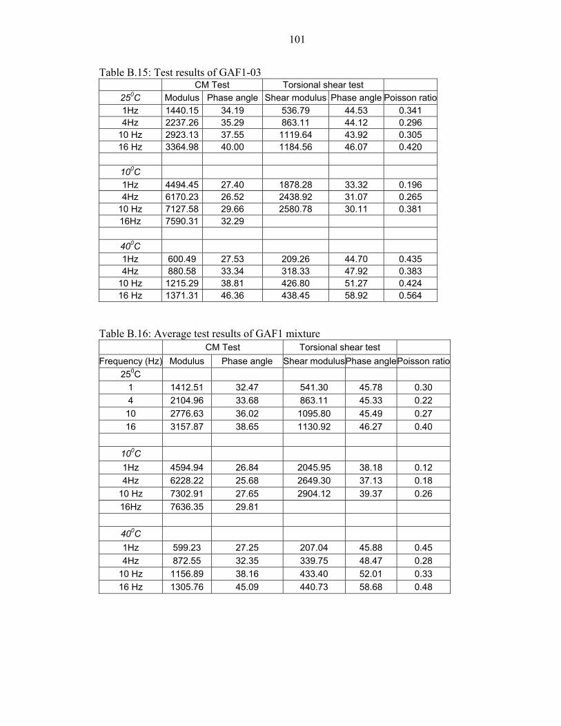
101

Table B.15: Test results of GAF1-03 CM Test Torsional shear test


10 Hz 2923.13 37.55 1119.64 43.92 0.305 16 Hz 3364.98 40.00 1184.56 46.07 0.420

100C 1Hz 4494.45 27.40 1878.28 33.32 0.196 4Hz 6170.23 26.52 2438.92 31.07 0.265

10 Hz 7127.58 29.66 2580.78 30.11 0.381 16Hz 7590.31 32.29

400C 1Hz 600.49 27.53 209.26 44.70 0.435 4Hz 880.58 33.34 318.33 47.92 0.383

10 Hz 1215.29 38.81 426.80 51.27 0.424 16 Hz 1371.31 46.36 438.45 58.92 0.564

Table B.16: Average test results of GAF1 mixture

CM Test Torsional shear test Frequency (Hz) Modulus Phase angle Shear modulusPhase angle Poisson ratio

250C 1 1412.51 32.47 541.30 45.78 0.30 4 2104.96 33.68 863.11 45.33 0.22

10 2776.63 36.02 1095.80 45.49 0.27 16 3157.87 38.65 1130.92 46.27 0.40

100C 1Hz 4594.94 26.84 2045.95 38.18 0.12 4Hz 6228.22 25.68 2649.30 37.13 0.18

10 Hz 7302.91 27.65 2904.12 39.37 0.26 16Hz 7636.35 29.81

400C 1Hz 599.23 27.25 207.04 45.88 0.45 4Hz 872.55 32.35 339.75 48.47 0.28

10 Hz 1156.89 38.16 433.40 52.01 0.33 16 Hz 1305.76 45.09 440.73 58.68 0.48

102

Table B.17: Average test result of GAF2-01 250C CM Test Torsional shear test

Frequency (Hz) Modulus Phase angle Shear modulusPhase anglePoisson ratio 1 2159.48 28.30 904.46 43.845 0.19 4 2863.20 31.02 1353.55 42.706 0.06

10 3649.15 31.08 1541.01 44.520 0.18 16 4259.60 33.77 1703.58 45.600 0.25

100C 1Hz 6415.04 22.31 2559.79 43.16 0.25 4Hz 8915.92 21.37 3161.20 45.34 0.41

10 Hz 10320.82 23.27 3615.89 48.81 0.43 16Hz 10733.67 26.14

400C 1Hz 511.02 34.90 270.27 44.754 -0.05 4Hz 874.76 42.41 433.42 47.575 0.01

10 Hz 1261.83 48.60 541.23 49.206 0.17 16 Hz 1528.67 53.15 564.49 53.298 0.35

Table B.18: Test result of GAF2-02

CM Test Torsional shear test 250C Modulus Phase angle Shear modulusPhase anglePoisson ratio 1Hz 2395.02 28.52 959.49 44.00 0.25 4Hz 3538.80 29.97 1389.42 42.83 0.27

10 Hz 4487.30 33.28 1606.88 39.44 0.40 16 Hz 5001.15 36.25 1624.30 42.35 0.54

100C 1Hz 7870.45 22.31 3169.42 45.41 0.24 4Hz 10044.84 21.37 3739.12 49.92 0.34

10 Hz 11349.56 23.27 3816.49 52.36 0.49 16Hz 11623.68 26.14

400C 1Hz 560.92 32.30 N/A N/A N/A 4Hz 936.84 37.74 N/A N/A N/A

10 Hz 1357.72 42.59 N/A N/A N/A 16 Hz 1619.37 46.82 N/A N/A N/A

103

Table B.19: Test result of GAF2-03 CM Test Torsional shear test

250C Modulus Phase angle Shear modulusPhase anglePoisson ratio 1Hz 2586.90 29.70 1142.18 44.88 0.13 4Hz 3822.28 31.68 1665.02 44.32 0.15

10 Hz 5057.65 33.65 1924.55 43.15 0.31 16 Hz 5754.92 36.36 1965.97 43.96 0.46

100C 1Hz 6390.72 20.24 2656.10 43.16 0.20 4Hz 8563.34 19.24 3252.70 45.34 0.32

10 Hz 9927.46 20.20 50.88 0.47 3387.51

38.96 637.69 16 Hz 1776.74 44.88 707.76 55.23

16Hz 10638.62 22.19

400C 1Hz 743.44 27.69 319.83 47.19 0.16 4Hz 1174.97 34.80 499.96 49.80 0.18

10 Hz 1539.15 51.17 0.21 0.26

Table B.20: Test result of GAF3 mixture

CM Test Torsional shear test Modulus Phase angle Shear modulusPhase anglePoisson ratio

250C 1Hz 2380.47 28.84 1002.05 44.24 0.19 4Hz 3408.09 30.89 1469.33 43.29

16 Hz 5005.22 35.46 1764.62 43.97 0.42

100C 1Hz 6892.07 21.62 2795.10 43.91 0.23 4Hz 9174.70

16Hz 10998.66 24.82

400C 1Hz 605.13 31.63 295.05 45.97 0.03 4Hz 995.52 38.32 466.69 48.69 0.07

10 Hz 1386.23 50.19 0.18 43.39 589.46 1641.59 48.28 636.13 54.27 0.29

0.16 10 Hz 4398.03 32.67 1690.81 42.37 0.30

20.66 3384.34 46.86 0.36 10 Hz 10532.62 22.25 3606.63 50.68 0.46

16 Hz

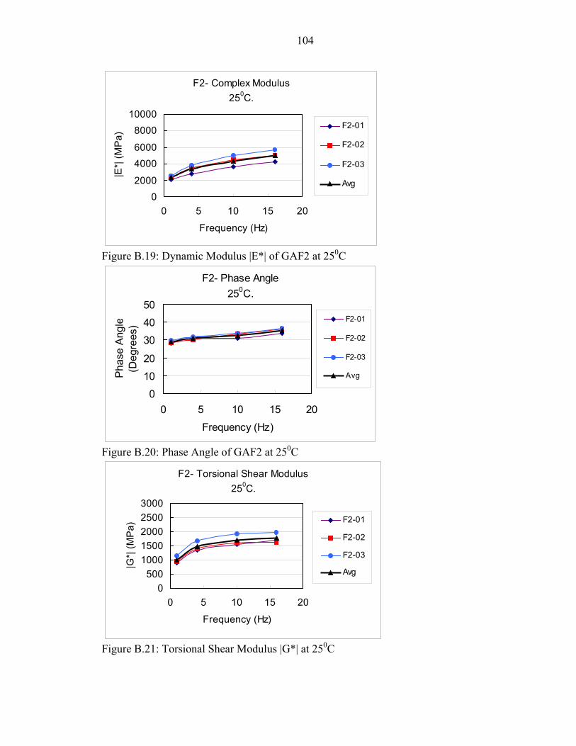
104

F2- Complex Modulus250C.

02000

40006000

800010000

0 5 10 15 20

Frequency (Hz)

|E*|

(MPa

)F2-01

F2-02

F2-03

Avg

Figure B.19: Dynamic Modulus |E*| of GAF2 at 250C

F2- Phase Angle250C.

01020

304050

0 5 10 15 20Frequency (Hz)

Phas

e An

gle

(Deg

rees

)

F2-01

F2-02

F2-03

Avg

Figure B.20: Phase Angle of GAF2 at 250C

F2- Torsional Shear Modulus250C.

0500

10001500200025003000

0 5 10 15 20

Frequency (Hz)

|G*|

(MPa

) F2-01

F2-02

F2-03

Avg

0C Figure B.21: Torsional Shear Modulus |G*| at 25

105


0

3000

6000

9000

12000

15000

0 5 10 15 20

Frequency (Hz)

|E*|

(MPa

)F2-01

F2-02

F2-03

Avg



0

10

20

30

40

50

0 5 10 15 20

Frequency (Hz)

Phas

e An

gle

(Deg

rees

)

F2-01

F2-02

F2-03

Avg



0

1200

2400

3600

4800

6000

0 4 8 12

Frequency (Hz)

|G*|

(MPa

)

F2-01

F2-02

F2-03

Avg

Figure B.24: Torsional Shear Modulus |G*| at 100C

106


0

500

1000

1500

2000

2500

0 5 10 15 20

Frequency (Hz)

|E*|

(MPa

)F2-01

F2-02

F2-03

Avg

0C Figure B.25: Dynamic Modulus |E*| of GAF2 at 40


0

20

40

60

80


Phas

e An

gle

(Deg

rees

)

F2-01

F2-02

F2-03

Avg



0

200

400

600

800

1000

0 10 20

Frequency (Hz)

|G*|

(MPa

) F2-01

F2-03

Avg

Figure B.27: Torsional Shear Modulus |G*| at 400C

107

Table B.21: Test results of GAF3-01 250C CM Test Torsional shear test

Frequency (Hz) Modulus

1789.18 31.15 754.31 45.85 0.186 2642.67 32.01 1196.40 45.86 0.104 3300.90 33.53 1367.34

5623.01 22.72 2560.06 36.78 0.098 7233.16 20.94 3377.92 36.00 0.071 8635.45 22.24 3641.77 46.50 0.186

400C 1Hz 400.05 34.99 186.31 51.55 0.074 4Hz 662.75 40.55 320.54 54.01 0.034

10 Hz 951.56 47.10 397.16 54.29 0.198 16 Hz 1097.15 53.43 410.21 60.900

Phase angle Shear modulus Phase anglePoisson ratio 1 4

10 45.56 0.207 16 3637.87 35.92 1352.80 47.47 0.345

100C 1Hz 4Hz

10 Hz 16Hz 9744.74 24.49

0.337 Table B.22: Test results of GAF3-02

CM Test Torsional shear test 250C Modulus Phase angle Shear modulus Phase anglePoisson ratio 1Hz 1535.74 29.70 714.43 45.886 0.075 4Hz 2383.45 31.10 1118.62 45.573 0.065

10 Hz 3019.61 32.29 1400.88 47.291 0.078 16 Hz 3488.99

100C 1Hz 4869.69 19.03 2352.94 42.210 0.035 4Hz 6514.29 18.62 3000.80 42.531 0.085

10 Hz 7704.64 20.53 3174.56 42.653 0.213 16Hz 8215.63 22.77

400C

4Hz 596.53 38.35 N/A N/A N/A 10 Hz 857.03 42.98 N/A N/A N/A 16 Hz 1005.57 47.93 N/A N/A

34.91 1426.77 50.286 0.223

1Hz 372.68 31.87 N/A N/A N/A

N/A

108

Table B.23: Test results of GAF3-03 CM Test Torsional shear test

Shear modulus Phase angle Poisson ratio 1Hz 1435.905 30.098 742.16 46.50 -0.033 4Hz 2175.691 32.487 1139.13 46.45 -0.045

10 Hz 2804.171 35.531 1396.67 46.47 0.004 16 Hz 3185.771

1Hz 5059.309 25.385 2109.86 42.33 0.199 4Hz 5822.952 24.858 2719.84 43.36 0.070

10 Hz 7530.491 28.135 2992.86 47.83 0.258 16Hz 8435.616

400C 1Hz 360.37 50.24 -0.253 31.874 241.25

388.62 53.19 -0.247 10 Hz 851.1315 42.812 514.11 54.03 -0.172 16 Hz 1029.717 47.210 541.40 58.49 -0.049

250C Modulus Phase angle

38.442 1452.31 47.34 0.097

100C

30.171

4Hz 585.4404 37.722

Table B.24: Average test results of GAF3 mixture

CM Test Torsional shear test Modulus

736.97 46.08 0.08

4Hz 2400.60 31.86 1151.38 45.96 0.04 10 Hz 3041.56 33.78 1388.30 46.44 0.10 16 Hz 3437.54 36.42 1410.63 48.36 0.22

2340.95 40.44 0.11 4Hz 6523.47 21.47 3032.85 40.63 0.08

10 Hz 7956.86 23.64 3269.73 45.66 0.22 16Hz 8798.66 25.13

0C

1Hz 377.70 32.91 213.78 50.89 -0.12 4Hz 614.91 38.87 354.58 53.60 -0.13

10 Hz 886.58 44.30 455.63 54.16 -0.03 16 Hz 1044.15 49.53 475.80 59.70 0.10

Phase angle Shear modulusPhase anglePoisson ratio250C 1Hz 1586.94 30.32

100C 1Hz 5184.00 22.38

40

109


0

1000

2000

3000

4000

5000

0 5 10 15 20

Frequency (Hz)

|E*|

(MPa

)F3-01

F3-02

F3-03

Avg

0Figure B.28: Dynamic Modulus |E*| of GAF3 at 25 C


0

10

20

30

40

50

0 5 10 15 20

Frequency (Hz)

Phas

e An

gle

(Deg

rees

)

F3-01

F3-02

F3-03

Avg

0Figure B.29: Phase Angle of GAF3 at 25 C


0500

100015002000

25003000

0 5 10 15 20

Frequency (Hz)

|G*|

(MPa

)

F3-01

F3-02

F3-03

Avg

Figure B.30: Torsional Shear Modulus |G*| of GAF3 at 250C

110


0

3000

6000

9000

12000

0 5 10 15 20

Frequency (Hz)

|E*|

(MPa

)F3-01

F3-02

F3-03

Avg

0Figure B.31: Dynamic Modulus |E*| of GAF3 at 10 C


0

10

20

30

40

50

0 5 10 15 20

Frequency (Hz)

Phas

e An

gle

(Deg

rees

)

F3-01

F3-02

F3-03

Avg

0Figure B.32: Phase Angle of GAF3 at 10 C


0

1000

2000

3000

4000

5000

0 3 6 9 12

Frequency (Hz)

|G*|

(MPa

)

F3-01

F3-02

F3-03

Avg


111


0

400

800

1200

1600

2000

0 5 10 15 20

Frequency (Hz)

|E*|

(MPa

)F3-01

F3-02

F3-03

Avg



0

20

40

60

80

0 5 10 15 20

Frequency (Hz)

Phas

e An

gle

(Deg

rees

)

F3-01

F3-02

F3-03

Avg



0200

400600

8001000

0 5 10 15 20

Frequency (Hz)

|G*|

(MPa

)

F3-01

F3-03

Avg


112

0

3000

6000

9000

12000

15000


E*(M

Pa)


Figure B.34: Actual vs Predicted |E*| of 10Hz test at 100C

0

2000

4000

6000

8000

C1 C2 C3 F1 F2 F3

Mixtures

E*(M

Pa)



0

500

1000

1500

2000

2500

3000


E*(M

Pa)


0C Figure B.34: Actual vs Predicted |E*| of 10Hz test at 40

113

0

3000

6000

9000

12000

15000


E*(M

Pa)



0

2000

4000

6000

8000

C1 C2 C3 F1 F2 F3

Mixtures

E*(M

Pa)

Actual Values

Predictived Values

0Figure B.36: Actual vs Predicted |E*| of 4Hz test at 25 C

0

500

1000

1500

2000

2500

3000


E*(M

Pa)



114

0

2000

4000

6000

8000

10000

C1 C2 C3 F1 F2 F3

Mixtures

E*(M

Pa)

Actual Values

Predictived Values


0

1000

2000

3000

4000

5000

C1 C2 C3 F1 F2 F3

Mixtures

E*(M

Pa)

Actual Values

Predictived Values


0

500

1000

1500

2000

C1 C2 C3 F1 F2 F3

Mixtures

E*(M

Pa)

Actual Values

Predictived Values


LIST OF REFERENCES

American Association of State Highway and Transportation Officials (AASHTO) TP 7-94. Test Method for Determining the Permanent Deformation and Fatigue Cracking Characteristics of Hot Mix Asphalt (HMA) using the Simple Shear Test (SST) Device. Washington DC (1994).

American Society for Testing and Materials (ASTM) D 3497-79. Standard Test Method for Dynamic Modulus of Asphalt Mixtures. Philadelphia (Reapproved 1995).

Daniel JS, Kim YR. Relationship Among Rate Dependent Stiffness of Asphalt Concrete Using Laboratory and Field Test Methods. Presented at the 77th Annual Transportation Research Board Meeting, Washington DC (1998).

Findley WN, Lai J, Onaran K. Creep and Relaxation of Nonlinear Viscoelastic Materials. Dover Publication Inc ., Toronto (1989).

Harvey J, Weissman S, Long F, and Monismith C. Test to Evaluate the Stiffness and Permanent Deformation Characteristics of Asphalt/Binder – Aggregates Mixes, and Their Use in Mix Design and Analysis. Journal of the Association of Asphalt Paving Technologists, Vol. 70, Preprint (2001).

Huang YH. Pavement Analysis and Design. Prentice-Hall, Upper Saddle River, New Jersey (1993).

Kim D. Deformational Characteristics of Soils at Small to Intermediate Strains from Cyclic Tests. PhD Dissertation. University of Texas at Austin (1991).

Kim JS. Complex Modulus from Indirect Tensile Test. Master of Engineering Thesis. University of Florida (2002 ).

Lambe, Whitman. Soil Mechanics. John Wiley & Son, New York (1968).

National Highway Institute. Introduction to Mechanistic Design on New and Rehabilitated Pavement. ERES Consultant. Course 131064 (2001).

Papazian HS. The Response of Linear Viscoelastic Materials in the Frequency Domain with Emphasis on Asphalt Concrete. Proceedings, International Conference of the Structural Design of Asphalt Pavements (1962).

115

116

Pelinen TK, Witczak MW, Bonaquist RF. Asphalt Mix Master Curve Construction using Sigmodal Fitting Function with Non-Linear Least Squares Optimization Technique. 15th ASCE Engineering Mechanics Conference. Columbia University, New York (2002).

Perraton D, Carter A, Tremblay D, Langois P. Rheological Properties, Thermal Cracking and Rutting Resistance of Stone Matrix Asphalt. Canadian Technical Asphalt Association, pp 423-450 (2001).

Sousa JMB, and Monismith CL. Dynamic Response of Paving Material. Transportation Record. Vol. 1136, pp 57-68 (1987).

Swan DJ. Evaluation of the Testing Procedure and Data Analysis for the Uniaxial Complex Modulus Test on Hot Mix Asphalt. Master of Engineering Thesis. University of Florida (2002).

Witczack MW, Bonaquist R, Von Quintus H, and Kaloush K. Specimen Geometry and Aggregate Size Effects in Uniaxial Compression and Constant Height Shear Tests. Journal of the Association of Asphalt Paving Technologists, Vol. 69, pp 733-792 (2000)

Witczack MW, Fonesca OA. Revised Model for Dynamic (Complex) Modulus of Ashalt Mixtures. Transportation Research Record 1540, pp 15-23 (1996)

Witczack MW, Kaloush K, Pellinen T, El-Basyouny M, Quintus HV. Simple Performance Test for Superpave Mix Design. NCHRP Report 465, pp 6 (2002)

Zhang Z, Drescher A, Newcomb D. Viscoelastic Analysis of Diametral Compression Test on Asphalt Concrete. University of Minnesota (1996).

BIOGRAPHICAL SKETCH

Linh Viet Pham was born on April 18, 1976 in Viet Tri, Phu Tho, Vietnam. After

graduating from Thang Long high school in Hanoi, he enrolled in Hanoi University of

Civil Engineering. Besides Civil Engineering, he studied English and French and got an

award to visit France in summer 1995. He was also an active member of Youth Union of

University. After receiving his Bachelor in 1999, he worked in a joint venture between

University of Saskatchewan, Canada and TDC Company in Hanoi, Vietnam. In 2001, he

was accepted by University of Florida for his application in Master of Engineering.

117

Documents

DYNAMIC TORSIONAL SHEAR TEST FOR HOT MIX …ufdcimages.uflib.ufl.edu/UF/E0/00/09/14/00001/pham_l.pdfDYNAMIC TORSIONAL SHEAR TEST FOR HOT MIX ASPHALT By ... CHAPTER 1 INTRODUCTION