DYNAMICS OF FINANCIAL INCLUSION AND

WELFARE IN KENYA

ISAAC WACHIRA MWANGI

A THESIS SUBMITTED TO THE SCHOOL OF ECONOMICS,

IN PARTIAL FULFILLMENT OF THE REQUIREMENTS FOR

THE AWARD OF THE DEGREE OF DOCTOR OF

PHILOSOPHY IN ECONOMICS OF THE UNIVERSITY OF

NAIROBI

NOVEMBER, 2017

ii

Declaration

This thesis is my original work and has not been presented for a degree in any

other University.

Isaac Wachira Mwangi

Signature…………………… Date……………………………..

Reg. No: X80/99129/2015

This thesis has been submitted for examination with our approval as University

supervisors.

Dr. Bethuel K. Kinuthia

Signature…………………… Date……………………………..

Prof. Rosemary Atieno

Signature…………………… Date……………………………..

iii

Dedication

I dedicate this work to my lovely wife, Ruth Ngima and my two beautiful

daughters Amara Wamuyu and Arianna Wanjiru for their invaluable support, love

and encouragement throughout the PhD programme.

iv

Acknowledgement

I owe this milestone achievement unto the Almighty God, from whom I drew all

the strength and inspiration to move on even when things looked tough. To my

supervisors, Dr. Bethuel Kinyanjui and Prof. Rosemary Atieno, your great effort,

constructive criticism, valuable insights, patience and great sacrifice in guiding me

unconditionally throughout the research process cannot go unnoticed.

I also wish to express my sincere gratitude to the faculty, teaching and non-

teaching staff and the leadership, School of Economics, University of Nairobi

starting with Dr. Anthony Wambugu for giving me an opportunity to pursue my

PhD program from this leading University and instilling in me the requisite tools

to analyze emerging issues.

I also thank the Governor, Central Bank of Kenya for according me study leave to

pursue my PhD, the head, Kenya School of Monetary Studies Research Centre for

the support infrastructure, the Government of Kenya and the African Economic

Research Consortium for the PhD scholarship.

Many thanks also go to my family, parents and siblings for what they had to put up

with and for their moral support throughout my academic journey and for shaping

me to be who I am. I also wish to appreciate my classmates both in the University

of Nairobi and University of Dar es salaam for their collaboration and

encouragement throughout the PhD journey.

Lastly, I make a special mention of my friends Peter, Njoroge, Isabel, Charles,

Eunice and Edward who encouraged me all the way until the PhD became. Finally,

I wish to register my great appreciation and gratitude to all others who made

contributions in one way or another and whose names are not mentioned here.

v

Abbreviations and Acronyms

AFI Alliance for Financial Inclusion

CBK Central Bank of Kenya

CMA Capital Markets Authority

DFID Department for International Development

DTM Deposit Taking Microfinance

DTS Deposit Taking SACCOs

ERS Economic Recovery Strategy

FI Financial Inclusion

FSD Financial Sector Deepening

FSP Financial Service Providers

GDP Gross Domestic Product

IRA Insurance Regulatory Authority

KDHS Kenya Demographic Health Survey

KIHBS Kenya Integrated Household Budgetary Survey

KNBS Kenya National Bureau of Statistics

MDG Millennium Development Goals

MFI Microfinance Institution

MTP Medium Term Plan

OECD Organization for Economic Cooperation and Development

vi

PCA Principal Component Analysis

RBA Retirement Benefits Authority

SACCO Savings and Credit Cooperative Society

SASRA SACCOs and Societies Regulatory Authority

WMS Welfare Monitoring Survey

vii

Definition of Terms

Transaction Account - An account which is not perceived to be savings by a

consumer and accrues no interest

Credit - Any form of debt on which an economic agent pays interest for the

facility

Savings - A store of monetary value for which some interest accrues to the

consumer

Investment - A financial product for which money is spent either to buy stocks,

property or for business

Insurance - A financial product on which premium is paid by a consumer in

return for compensation when a risk occurs

Pension - A form of deferred savings where benefits only accrue to an economic

agent upon retirement

Prudential regulation - Operation guidelines issued by statutory government

agencies to regulate the financial system

Formal strand - Financial Inclusion channel offering prudentially regulated

financial products from banks, insurance firms, mobile financial service providers,

DTMs, DTSs and pension funds

Informal strand - Financial inclusion channels whose operations are not governed

by prudential guidelines but are governed by informal agreements

Financial Inclusion - use of credit, savings and investments, transactionary and

insurance and pension financial products from prudentially regulated institutions

viii

Financial Exclusion - Inability to access mainstream financial services

Unbanked - Persons whose information on where they seek financial services is

unknown

Mobile banking - Access to banking services such as account based savings,

payment systems and other products through an electronic mobile device

Financial Deepening - Increased provision of financial services

Index of Financial Inclusion - Aggregated portfolio usage of financial services

Stochastic Dominance - Ordering of possible outcomes in a probability

distribution based on individual preferences

Kolmogorov-Smirnof Test - A stochastic test that compares two cumulative

distributions based on the largest vertical distance between two cumulative

distributions

Per adult equivalent consumption expenditure - Money metric measure of

welfare capturing overall per capital monthly consumption spending expressed in

Kenya shillings

Welfare – Proxied using the money metric measure (consumption expenditure per

adult equivalent) as well as vulnerability to poverty

Headcount Poverty - Living below a minimum a preset poverty line

Vulnerability as Expected Poverty - Probability that a household will fall or

remain in poverty in the next period

ix

Abstract

Financial inclusion (FI) is not an objective in itself, but only to the extent that it

helps improve welfare. Evidence linking FI and welfare is however less conclusive

despite growing interest. Understanding this link is often hampered first by, lack of

a substantive and universally acceptable measure of FI comparable across time and

geography and secondly by lack of empirical evidence. To address this gap, an

empirical examination on Kenya using GMM was preceded by the modeling of FI

to establish its determinants. The inter-temporal variation in household

consumption to generate vulnerability as expected poverty was also analyzed to

inform on the impact of FI on household vulnerability to poverty. Financial Access

surveys (2006, 2009, 2013 and 2016) organized into 126 cohorts provided a solid

empirical basis for tracking FI and its impact on welfare. Per capita income was

found to be one of the main drivers of FI pointing to operation of the demand

following hypothesis in Kenya. In terms of welfare impacts, transactionary, credit,

insurance and portfolio usage of financial services significantly raise consumption

expenditure per adult equivalent by 74.3, 81.6, 39.8 and 3.473 percent respectively

all things held constant. This welfare impact is also extended towards poverty

reduction. Safe for vulnerability to poverty in rural areas, FI was found to

significantly lower vulnerability to poverty among urban households as well as

headcount poverty in both rural and urban areas. The study recommends a

reduction in transactionary costs by financial service providers to consolidate gains

from financial inclusion, increased investment in human capital development by

the government to supplement financial inclusion, employment creation and

increased provision of basic services by government to enable households release

part of their income towards improving household welfare.

Key words: Pseudo panel estimation, financial inclusion, welfare, vulnerability,

transition matrix, dynamic regression

x

Table of Contents

Declaration ..............................................................................................................ii

Abbreviations and Acronyms ................................................................................v

Definition of Terms...............................................................................................vii

List of Tables........................................................................................................xv

List of Figures ....................................................................................................xviii

Chapter One: Dynamics of Financial Inclusion, Welfare and Vulnerability to

Poverty .....................................................................................................................1

1.1 Introduction................................................................................................1

1.2 Overview of Kenya's Financial Sector and Poverty Reduction Policies.....5

1.2.1 Evolution of Kenya's financial landscape ................................................5

1.2.2 Poverty Reduction Policies ....................................................................11

1.3 Problem Statement ........................................................................................16

1.4 Research Questions .......................................................................................18

1.5 Research Objectives......................................................................................18

1.5.1 General Objectives .................................................................................18

1.5.2 Specific Objectives.................................................................................18

1.6 Scope of the study.........................................................................................19

1.7 Organization of the Study .............................................................................19

Chapter Two: Measures and Extent of Financial Inclusion in Kenya ............20

2.1 Introduction...................................................................................................20

2.2 Literature on Measurement of FI ..................................................................23

2.2.1 Theoretical Literature .............................................................................24

2.2.2 Empirical Literature ...............................................................................27

xi

2.2.3 Overview of literature ............................................................................37

2.3 Theoretical Framework .................................................................................39

2.3.1 Constructing the Index of Financial Inclusion .......................................40

2.3.2 Stochastic Dominance Testing ...............................................................41

2.4 Conceptual Framework .................................................................................42

2. 5 Data ..........................................................................................................43

2.6 Discussion of Findings..................................................................................44

2.6.1 Correlation Coefficients .........................................................................47

2.6.2 Disaggregated Financial Product Usage.................................................49

2.6.3 Index of Financial Inclusion (IFI) ..........................................................59

2.7 Stochastic Dominance Tests of FI ................................................................64

2.8 Conclusions and Policy Implications ............................................................69

Chapter Three: Determinants of Financial Inclusion in Kenya.......................72

3.1 Introduction...................................................................................................72

3.2 Literature on Determinants of FI ..................................................................75

3.2.1 Theoretical Literature .............................................................................75

3.2.2 Empirical Literature ...............................................................................79

3.2.3 Overview of literature ............................................................................84

3.3 Empirical Framework ...................................................................................85

3.3.1 Empirical Model.....................................................................................87

3.3.2 Description of variables and Apriori Expectations ....................................90

3.3.3 Data ........................................................................................................91

3.4 Econometric Results and Discussion ........................................................92

xii

3.4.2 Descriptive Statistics ..............................................................................97

3.5. Determinants of Financial Inclusion and Access channels .......................100

3.5.1 Econometric results of the static and dynamic model of FI .................100

3.6 Conclusions and Policy Implications ..........................................................111

Chapter Four: Impact of FI on Consumption Expenditure ...........................113

4.1 Introduction.................................................................................................113

4.2 Literature Review........................................................................................115

4.2.1 Theories on the link between FI and Welfare ......................................115

4.2.2 Causality and Impact of FI on welfare .................................................121

4.2.3 Theories of consumption..........................................................................123

4.2.4 Overview of literature ..........................................................................127

4.3 Theoretical/Empirical Framework ..............................................................128

4.3.1 Welfare Determination.............................................................................128

4.3.2 Empirical Model ......................................................................................129

4.3.3 Description of variables and Apriori Expectations ..................................132

4.4 Discussion of Results ..................................................................................136

4.4.1 Descriptive Statistics ............................................................................136

4.4.2 Consumption Expenditure across the Country .....................................138

4.5. Econometric Results and Discussion .........................................................140

4.5.2 Static Analysis of FI impact on Consumption Expenditure .................146

4.6 Conclusions and Policy Implications ..........................................................163

Chapter Five: Impact of Financial Inclusion on Vulnerability to Poverty ...165

5.1 Introduction.................................................................................................165

xiii

5.2 Literature on Vulnerability to Poverty ........................................................169

5.2.1 Theoretical Literature Review..............................................................170

5.3 Empirical Literature ....................................................................................172

5.3.1 Measuring Vulnerability to Poverty .....................................................172

5.3.2 Financial Inclusion (FI) and Vulnerability as Expected Poverty (VEP).......................................................................................................................182

5. 4 Overview of Literature...............................................................................192

5.5 Construction of a vulnerability index .....................................................193

5.5.1 Theoretical Framework ............................................................................196

5.5.2 Expected Poverty Transition Matrix ....................................................197

5.6 Empirical Model .........................................................................................198

5.6.1 Vulnerability as Expected Poverty .......................................................198

5.6.2 Headcount Poverty ...............................................................................199

5.7 Description of variables and Apriori Expectations .....................................199

5.8 Data .............................................................................................................200

5.9 Discussion of Results ..................................................................................202

5.9.2 Descriptive Statistics ............................................................................205

5.9.3 Poverty Status of the Representative Household .................................206

5.9.4 VEP profile of sampled households .....................................................215

5.9.4 Econometric estimation of Vulnerability .............................................218

5.10 Conclusions and Policy Implications ........................................................233

Chapter Six: Summary, Conclusions and Policy Recommendations ............235

6.1 Conclusions.................................................................................................235

xiv

6.2 Summary of Research Findings ..................................................................237

6.2.1 Measures and Extent of FI in Kenya ....................................................238

6.2.2 Determinants of FI in Kenya ................................................................239

6.2.3 Impact of FI on Consumption Expenditure in Kenya ..........................241

6.2.4 Impact of FI on VEP in Kenya .............................................................242

6. 3 Contribution to existing knowledge...........................................................244

6.4: Recommendations for policy .....................................................................245

6.4.1 Measures and Extent of FI in Kenya ....................................................246

6.4.2 Determinants of FI in Kenya ................................................................246

6.4.3 Impact of FI on Consumption Expenditure in Kenya ..........................247

6.4.4 Impact of FI on VEP in Kenya.............................................................247

6.5 Limitations of the study and suggestions for further studies ......................248

References............................................................................................................250

Appendices ..........................................................................................................278

Appendix for the Entire Thesis .........................................................................294

xv

List of Tables

Table 1.1: Vulnerability to Poverty by Region.......................................................14

Table 2.1 Summary of FI indicators by County .....................................................44

Table 2.2: County Index of FI (IFI) Ranking .........................................................45

Table 2.3: FI correlation matrix..............................................................................47

Table 3.1a: Test for over identified restrictions......................................................94

Table 3.1b: Multicollinearity Test ..........................................................................95

Table 3.1c: Durbin-Wu Haussmann Test for Endogeneity ....................................96

Table 3.2 Summary Statistics and Measurement of Variables ...............................97

Table 3.7a Determinants of FI (Model Corrected for Nickel/Huwicz bias).........102

Table 3.7b Determinants of Financial Access Strands (Model Corrected for

Nickel/Huwicz bias) .............................................................................................107

Table 4.1 Summary Statistics on Household Characteristics ...............................137

Table 4.6: Durbin-Wu-Haussmann Test for Endogeneity....................................144

Table 4.8 Dynamic estimation of Consumption Expenditure ..............................147

Table 4.9 Consumption function with Transactionary-Education interaction......155

Table 4.10 Consumption function with IFI-Education interaction.......................157

Table 5.0: Multicollinearity Test ..........................................................................204

Table 5.1: Descriptive Statistics ...........................................................................205

Table 5.2: Vulnerability to poverty classification (FGT Approach) ....................207

xvi

Table 5.5: Vulnerability Transition Matrix (Overall Rural and Urban Poverty)..207

Table 5.8: Household Characteristics of the Poor and Vulnerable Population ....216

Table 5.9: Profiling Income Group Movement in 2013 and 2016 .......................217

Table 5.10: Bourguignon, Goh and Kim's (2004) Vulnerability Probability .......217

Table 5.12a: Determinants of Rural VEP .............................................................223

Table 5.12b: Determinants of Urban VEP............................................................226

Table 5.13a: Determinants of Rural Headcount Poverty......................................228

Table 5.13b: Determinants of Urban Headcount Poverty ....................................230

Table 5.13c: Odds Ratios for Rural and Urban Headcount Poverty in 2016 .......232

Table 3.1: Haussmann Specification Tests ...........................................................280

Table 3.3: Determinants of Single Product Usage (Full sample static analysis)..280

Table 3.4: Determinants of Financial Access Channels .......................................281

Table 3.5: Determinants of FI (Static Model) .....................................................282

Table 3.6 Determinants of FI (Dynamic Model) ..................................................284

Table 4.5: Consumer Expenditure by Region ......................................................285

Table 4.4: Main Economic Activity of Household Head .....................................286

Table 4.3: Aggregate distribution of income source by education .......................286

Table 4.4: Expenditure Distribution by Survey Year ...........................................287

Table 5.4: Distribution of poor by main income source .......................................290

xvii

Table 5.3: Poverty Status and Cluster by education (2009-2016) ........................291

Table 5.6: Status of Poverty and Consumption expenditure in 2016 ...................291

Table 5.7: Regional Poverty and Consumption Expenditure Cycle in Kenya .....292

Table 5.11a: Determinants of Rural VEP in 2013 before instrumenting .............292

Table 5.11b: Determinants of Urban VEP in 2013 before instrumenting ............293

xviii

List of Figures

Fig 1.1: Financial Inclusion Initiatives in Kenya since 2006 ...................................7

Fig 2. 1 Conceptual Framework .............................................................................42

Fig. 2.2 Financial Access Channels (Mobile money in formal) .............................48

Fig. 2.5 Formal Financial Product Usage ...............................................................49

Fig 2.6: Financial Inclusion Overlap in 2016 .........................................................51

Fig 2.7: Single Financial Product Usage by Category............................................51

Fig 2.8 Geospatial mapping of single financial product usage...............................55

Fig 2.9: Product usage based on Education ............................................................57

Fig 2.10: Index of FI (IFI) ......................................................................................59

Fig 2.11: Rural /Urban Progression of Financial Access Strand:2006-2016..........62

Fig 2.12: Gender/Education Progression of Financial Access:2006-2016.............63

Fig 2.13: Generalized Lorenz curves (Cohort vs Full sample)...............................65

Fig 2.14: IFI Cumulative Distribution Functions (FOSD and SOSD) ...................68

Fig 3. 1: Conceptual Framework ............................................................................87

Fig 4.1 Conceptual Framework ............................................................................127

Fig 4.2: Consumption Expenditure across the Country........................................138

Fig 5.3: Poverty Transition Map of the Representative Households....................209

Fig 5.4: Poverty and Education status of Household Head ..................................210

Fig 5.7: Geospatial Mapping of the IFI and Poverty using ArcGIS .....................213

xix

1

Chapter One: Dynamics of Financial Inclusion, Welfare

and Vulnerability to Poverty

1.1 Introduction

This thesis aimed at developing both single product and composite measures of

financial inclusion (FI) and to establish how it links to welfare and vulnerability to

poverty1 in Kenya. This is motivated by the need to raise FI to the universal level

even though the attainment of this goal is impaired by lack of an appropriate

measure of FI. Global Partnership for Financial Inclusion (2011) recognizes the

critical role FI setting play in monitoring and evaluation of policies and targets.

Latest figures from the 2016 FinAccess report reported increased uptake of formal

financial services among Kenyan adults from a mere 25 percent in 2006 to 75

percent in 2015. Total financial exclusion appears to have dipped to 17.4 percent,

marking significant expansion of financial services (CBK, KNBS & FSD, 2016).

This pace of FI however does not match the speed of poverty (living below $2 a

day) reduction, raising policy questions on the contribution of FI in lowering

poverty which averaged 39.9 percent in 2016 (OPHI, 2016) down from 45.92

percent in 2005 (KIHBS 2005/06). Failure to halve the number of people living in

abject poverty relative to the 1990 levels under MDG1 has put into question the

effectiveness of the existing policy initiatives. This calls for a broadened approach

that not only targets the poor ex-ante but one that targets the vulnerable ex-post.

1 A multidimensional fact of life manifested through low income, illiteracy, premature death, earlymarriage, large families, malnutrition and illness and injury which locks them to low standards ofliving (World Bank, 2000a).

2 http://data.worldbank.org/country/kenya

2

Linking FI to household welfare is critical in shaping policy initiatives to improve

livelihoods through enhanced financial service provision. This link is evidenced by

the work of Demirguc-Kunt and Klapper, 2012; Beck et al., 2004; Sarma, 2008;

and Honohan, 2008; McKinnon, 1974; Kalunda, 2014; Aduda & Kalunda, 2012

and Gurley and Shaw, 1955. However, not all studies associate FI with positive

welfare impacts. They include; Diagne & Zeller, 2001; Bernejee et al., 2009;

Crepon et al., 2014; Angelucci, Karlan & Zinman, 2013 among others.

Kenya's Vision 2030, Welfare Monitoring Surveys, Millennium Development

Goals (MDGs) and Financial Sector Medium Term Plan (MTP), 2012-2017

recognize the need to adopt newer strategies aimed at tackling poverty. KNBS

(2006) in the KIHBS 2005/2006 singled out poverty as a major impediment to the

improvement of welfare among rural dwellers.

Despite lack of a universally acceptable definition of FI, most of the definitions

appear to converge on access. The World Savings Bank Institute (2009) ostensibly

defined FI as enhanced access to appropriate, convenient, usable, valuable and

affordable financial services and products to the widest part of the population

through delivery of basic banking services to the low income population and the

unbanked as a way out of poverty. Deb and Kubzansky (2012) definition

associates FI with financial access, financial capability and engagement with the

financial system. McKillop and Wilson (2009) define FI from an exclusion angle

as the inability, reluctance or difficulties that deny people access to mainstream

financial services. FI in the context of this study is defined as the delivery of

prudentially regulated financial services to a vast majority of the adult population

without frills and encompasses use of credit, savings, transactionary and insurance

3

products as defined in AFI3 (2014). The domain of FI is considerably huge and

varies from country to country impairing comparability.

Some of the theories invoked in studies on FI include; capital market

imperfections theory seen as a critique to Fama (1970) efficient market hypothesis

(EFM), modern development theories by Mckinnon and Shaw (1973) and Bagehot

(1873), financial repression theories by Keynes (1936) and Tobin (1965) among

others. Keynes (1936) and Tobin (1965) financial repression arguments had for a

long time advocated for a strong government to maintain low interest rates and

inflationary monetary policies though at the expense of financial development.

Savings and investments fall while credit rationing rise in a financially repressed

regime since the range of financial products available is not only limited but is also

characterized by controlled interest rates.

Financial development theories also revolve around the demand following

hypothesis; supply leading hypothesis; or independent hypothesis. The demand

following hypothesis of financial development in Latin America and the Caribbean

(LACs) linked low FI to reduced demand for financial services where usage of

credit and deposit accounts among poor households appeared fell by 4.5 and 10

percent respectively. At the macro level LACs credit to private sector as a

percentage of GDP averaged 33.9 percent against 105.3 percent for OECD and

73.6% for East Asian countries (Bebczuk, 2008). Even though the data allude to a

higher financial exclusion among the poor, their study poked holes on the use of

aggregated figures for policy in financial markets. This result supports IMF (2012)

on Kenya where persons in the highest income quintile enjoyed four times higher

probability of using a formal account compared to the poorest quintile.

3 FI as a state where all working age adults including those currently excluded from the financialsystem have effective access to formal financial services, credit, savings, payment and insurance

4

Given that most financial institutions situate their businesses in non-poverty zones

in order to maximize profits, testing whether the demand following hypothesis on

Kenya's financial system holds could offer insights on places where the

government can come in to promote FI since financial service providers may avoid

them. Empirical evidence on the link between FI, welfare and vulnerability to

poverty at the micro level in Kenya remains scanty hindering the formulation of

effective policies to enhance growth and poverty alleviation (World Bank, 2014).

This study extends this debate to capture the role of FI on vulnerability to poverty.

Introspection into vulnerability to poverty dates back to the early 1980's in Sen

(1981) monograph on "Poverty and Dynamics" where landless agricultural

labourers were found to have a higher vulnerability risk. It would appear that no

such study has been conducted in Kenya using a pseudo panel framework to

provide evidence based examination of the link between FI and welfare based on

repeated cross sections at the micro level hence this study offers unique solutions

for policy.

In addition, there is no study in Kenya that has made an attempt at invoking Sarma

(2008) formulae to develop an index of FI (IFI) based on portfolio usage of

financial services or has made effort to rank counties on the basis of their FI status

since the introduction of the county governance structure in Kenya following the

promulgation of the new constitution in 2010. This ranking is considered

important since superimposition of welfare indicators on the FI map can help draw

solutions that factor in peculiarities in counties due to their heterogeneity. This

thesis is based on the four waves of FinAccess survey data which captures the

financial access landscape, usage of financial services by individuals in Kenya and

impact. Quality of financial services therefore falls outside the purview of this

study.

5

1.2 Overview of Kenya's Financial Sector and Poverty Reduction Policies

The evolution of the financial sector in Kenya has been fast since the late 1980s.

This is motivated by the need to enhance stability in the financial markets and

efficiency in the supply of financial services at the least cost and to a vast majority.

The reforms in the financial sector are mainly geared towards improving welfare

of the entire population through increased consumption spending and poverty

reduction. FSD (2015) states that the main objective of FI is to create a

competitive, highly efficient, stable, safe and more inclusive financial system to

enhance inclusive growth, savings and investments through Kenya's development

blueprint, the Vision 2030 (GoK, 2007). This section narrates the developments in

the financial sector before and after 2006 when the first major survey on the

profile of Kenya's financial landscape was launched in Kenya. The section also

discusses the programs rolled out in post-independence Kenya towards poverty

reduction and welfare improvement. Since poverty values are derived from the

consumption expenditure variable, we use the multidimensional poverty indicators

across sub-national regions to illustrate the strides made in improving welfare in

Kenya.

1.2.1 Evolution of Kenya's financial landscape

The first major effort in instituting reforms in the financial sector dates back to

1989 when the World Bank extended a $170 million adjustment credit (World

Bank, 1990). This coincided with the 1986-1990 reform package popularly known

as the Structural Adjustment Program (SAPs) whose main objectives were to

liberalize financial markets, establishment of a Capital Markets Authority to

monitor and develop equity markets among other requirements. The Basel I

guidelines were issued in 1988 by the Basel Committee to enhance capital

adequacy among banks to minimize credit risks. This was followed by the

enactment of Basel II guidelines in 2004 whose main objective was to ensure that

6

commercial bank reserves match the risk profile from a bank's lending and

investment practices. Basel II is founded on three pillars targeting minimum

capital requirements, supervisory review process and market discipline (CBK,

2013).

More prudential guidelines (Basel III) were issued in 2010 in response to the 2008

global financial crisis with a sharp focus on capital adequacy, liquidity and

countercyclical macro-prudential issues. In a bid to enhance the vibrancy and the

global competitiveness of the financial sector to promote increased savings and

investment needs in line with Kenya's Vision 2030, the Government of Kenya

identified a number of strategies that would help achieve this in its national

blueprint launched in 2008. These include; proper legal and institutional reforms, a

reformed banking sector with few strong banks and deepened financial markets

(GoK, 2007). This has led to the introduction of credit reference bureaus,

streamlined informal finance, savings and credit cooperative societies (SACCOs)

and microfinance institutions (MFIs).

The Vision 2030 recognizes the financial sector as key among the six sectors

driving the economy (GoK, 2007). Huge expansion of the financial sector has led

to the licensing of at least 3 credit reference bureaus, amendment of the MFI Act

to govern Deposit Taking Microfinance (DTMs) formation, introduction of a

regulatory framework for SACCOs by SACCOs and Societies Regulatory

Authority (SASRA) which led to the creation of Deposit Taking SACCOs (DTSs)

among other reforms. The minimum capital requirement for banks was raised from

Ksh 500 million to Ksh 2 billion to enhance protection of customer deposits and

investments and encourage small banks to consolidate into fewer, larger and

stronger ones (CBK, 2013). In 2005, the Department for International

Development (DFID) helped establish Kenya's Financial Sector Deepening

7

programme (FSDK) to stimulate wealth creation and lower poverty through FI

targeted at the low income population segment and small businesses (FSD, 2014).

Kenya’s financial sector as at 31st December 2015 comprised of 42 licensed

commercial banks (26 locally owned and 14 foreign owned private commercial

banks and 3 government owned), 8 representative offices of foreign banks, 12

Deposit Taking Microfinance (DTMs), 15 Money Remittance Providers (MRPs),

80 foreign exchange bureaus, 1 postal savings bank, 3 licensed credit reference

bureaus (CRBs) and 1 mortgage finance company (CBK, 2015). Kenya’s financial

system is classified into three broad strands namely; formal (commercial banks,

mobile payment systems and deposit taking SACCOs and prudentially regulated

Microfinance institutions (MFIs) ), other formal (unregulated SACCOs and MFIs

registered under the law) and informal lenders (FSD, 2011). DTMs are governed

by the revised Microfinance Act No. 19 of 2006 which enable them to accept

deposits while the DTSs are governed by the SACCO societies Act No. 14 of 2008

to strengthen and regulate deposit taking credit unions4.

Other reforms undertaken in the sector include the licensing of Credit Reference

Bureaus (CRBs) in February, 2009 to collect and share information on credit

worthiness of potential borrowers with three bureaus having been licensed by

2016; roll-out of mobile money transfer service M-PESA in 2006 and Yu Cash in

2009, Orange money, Mobikash and Mshwari; licensing of currency centers by

CBK to facilitate cash transfers with an aim of lowering money transfer costs,

regulatory framework governing consumer protection and the introduction of

agency banking by commercial banks and DTMs in 2010 and 2012 respectively

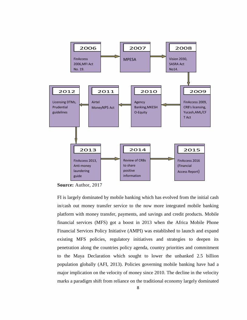
(CBK, 2014). These developments are summarized in figure 1.1.

Fig 1.1: Financial Inclusion Initiatives in Kenya since 2006

4 National Council for Law Reporting

8

Source: Author, 2017

FI is largely dominated by mobile banking which has evolved from the initial cash

in/cash out money transfer service to the now more integrated mobile banking

platform with money transfer, payments, and savings and credit products. Mobile

financial services (MFS) got a boost in 2013 when the Africa Mobile Phone

Financial Services Policy Initiative (AMPI) was established to launch and expand

existing MFS policies, regulatory initiatives and strategies to deepen its

penetration along the countries policy agenda, country priorities and commitment

to the Maya Declaration which sought to lower the unbanked 2.5 billion

population globally (AFI, 2013). Policies governing mobile banking have had a

major implication on the velocity of money since 2010. The decline in the velocity

marks a paradigm shift from reliance on the traditional economy largely dominated

2008

Vision 2030,SASRA ActNo14.

2007

MPESA

2013

FinAccess 2013,Anti-moneylaunderingguide

2014

Review of CRBsto sharepositiveinformation

2015

FinAccess 2016(FinancialAccess Report)

2006

FinAccess2006,MFI ActNo. 19.

2009

FinAccess 2009,CRB's licensing,Yucash,AML/CFT Act

2010

AgencyBanking,MKESHO-Equity

2011

AirtelMoneyNPS Act

2012

Licensing DTMs,Prudentialguidelines

9

by cash outside banks (M3) to a modern non cash economy largely attributed to

the increased FI due to internet and mobile banking (Mbiti & Weil, 2013).

Between 2012 when DTMs were licensed and 31st December 2015, the number of

licensed DTMs had grown to 12. The net advances accounted for 66 percent of the

DTMs total assets (Ksh. 69.5 billion). The number of deposit and loan accounts

averaged 932,000 and 342,000 respectively with a value of Ksh 40.6 billion and

47.1 for deposits and outstanding loans respectively. The agency banking model

developed in 2010 had by 31st December, 2015 seen the establishment of 40,592

and 1,154 agents by 17 commercial banks and 3 DTMs respectively. This is

attributed to the increased confidence and acceptance of the agency banking model

as an efficient and effective financial service delivery channel.(CBK, 2015). The

agency banking model enables commercial banks and DTMs to contract nonbank

retail agents such as pharmacies, petrol stations, and supermarkets among other

outfits as outlets of financial services especially in areas with few or no bank

branches (CBK, 2014).

In relation to credit information sharing (CIS), a total of 11.2 million and 163,614

credit report requests had been made by subscribing banks and customers

respectively between 2010 when CIS was launched and 31st December, 2015

(CBK, 2015). This information sharing is very critical in reducing information

asymmetry on the risk profile of potential borrowers. Locally, the country

witnessed the establishment of Financial Sector Regulators Forum in 2009 under a

memorandum of understanding signed between CBK, RBA, CMA, IRA and

SASRA to foster cooperation, share information and enhance policy coordination

between the five financial regulators (CBK, 2015).

10

Regionally, the East Africa Community (EAC) Monetary Union (EAMU) on

January, 2015 ratified a protocol5 with partner states to harmonize the regulatory

framework governing the financial system in the region with the promotion of

financial deepening and inclusion as one of the objectives. Plans are underway to

roll out the East Africa Financial Services Commission (EAFSC) to manage

financial and banking services among member states (CBK, 2015).

Consumer protection which has received overwhelming support in recent times is

motivated by the huge uptake of financial services and surge in financial

innovation which doesn't match the level of financial education of users of

financial products. Users of new products are disadvantaged by the information

asymmetry hence the need for laws protecting them. Legislation of consumer

protection is considered as a counter mechanism to market failure due to its ability

to correct the information asymmetry problem through disclosures (CBK, 2014).

The CBK has since 2015 published the interest rates charged by all commercial

banks as a way of reducing the information asymmetry and ensuring that

consumers are well informed before they even seek financial services. This is

aimed at reducing the interest rate spread in the country and lower idiosyncratic

risks associated with new financial products. The frustration on the part of

consumers of banking services is evidenced by the recent enactment of a new law

through Parliament to cap interest rates6 in Kenya, with effect from September

2016.

6 Amendment of the Banking Act, 2016 sets Kenya's interest rate cap at 4 percent above the baserate and 70 percent of the base rate payable to savers

11

Assessment of the contribution of FI on welfare outcomes in a manner that mostly

benefits the poor require a FI strategy which goes beyond access, to one that

focuses on developing a reliable measure of financial usage to inform policy.

Access to financial access points (mobile money agents, bank agents, insurance

service providers and stand-alone ATMs) in Kenya is by far considered to be much

deeper than that of its peers, Tanzania and Uganda having grown from 59 percent

in 2013 to 73 percent in 2015 as measured by the population living within a three

kilometer radius to a financial access touch point7. Kenya's population living

within a 5 kilometer radius proximity to a financial access point in 2013 was

approximately 77 percent as compared to 35 percent and 43 percent for Tanzania

and Uganda respectively (FSD, 2014).The report however cited skewness in the

distribution of financial services as a major drawback since 69 percent of the

access points were found to be located in areas with low poverty incidence.

Given this development, Kenya’s FI model is seen to follow the demand following

hypothesis where demand for financial services is triggered by economic growth

and profit motive for the financial institutions which lead to the emergence of a

myriad financial access points. The report emphasizes the need to introduce a

geospatial dimension to the demand side data to map household access to financial

services across the country. This model however limits the efficacy of FI in

reducing poverty since financial access points mostly find their way to developed

regions which mostly are dominated by population with least poverty likelihood.

1.2.2 Poverty Reduction Policies

Since gaining independence in 1963, Kenya's struggle with illiteracy, disease and

poverty identified in the Sessional Paper No. 1 on African Socialism and its

Application to Planning in Kenya (GoK, 1965) as key development challenges has

7 FSD (2015). 2015 FinAccess geospatial mapping survey key findings

12

persisted. These issues have shaped policy debates for the last half century.

Despite the protracted efforts in fighting these problems, the eradication of poverty

has remained elusive to date hindering national development. Poor formulation

and implementation of policy related to poverty could be blamed for the rise in

multidimensional poverty which manifests itself in form of; increased deprivation

of health, education, water and housing (OPHI, 2013). After the Basic Needs

Approach of 1970, then came the District Focus for Rural Development (DFRD)

launched in 1983 its main focus being enhancing economic activities in the rural

areas followed by the introduction of Sessional Paper No. 1 of 1986 on Economic

Management for Renewed Growth.

The Bretton Woods institutions (IMF and World Bank) got more involved in the

1980s to push the government to up its fight against poverty which had started

gaining momentum across the country. Top on their agenda was the

implementation of the Structural Adjustment Programs (SAPs) to stimulate

economic recovery within 18 months through tight fiscal and monetary policies.

However, the programs failed for advocating for financial liberalization and huge

cuts in government spending and especially on labour force, leaving a vast

majority more impoverished and poorer (GoK, 2000).

To counter the worsening poverty, the government adopted the Social Dimensions

of Development (SDD) policy in 1994 to cushion the poor against the adverse

effects of the SAPs. Another initiative undertaken in 1990 was the enactment of

the Non-Governmental Coordination Act (NGCA) to coordinate NGO efforts in

reducing poverty. The DFRD strategy was implemented alongside the five year

development plans since 1966. These strategies however didn't achieve the desired

results since poverty continued to escalate having shot up to 47 percent and 29

percent in rural and urban areas respectively in 1994 (WGoK, 1994). This was

followed by the establishment of the District Poverty Alleviation Secretariats, the

13

main objective being the harmonization of poverty eradication programmes at the

grassroots.

In 1999, the Participatory Poverty Assessment Reports (PPARs) and the National

Poverty Eradication Plan (NPEP 1999-2015) were also rolled out the agenda being

poverty eradication. The fight against poverty got a boost after 2000 when the

Poverty Reduction Strategy Paper (PSRP 2000-2003) was launched. The

establishment of these outfits was meant to enhance coordination of efforts to

counter poverty across the country to minimize duplication and fix the weak

linkages between institutions involved in poverty eradication programmes (GoK,

2008).

The measures of poverty have also witnessed a paradigm shift with absolute

poverty line rising from Ksh. 980 and Ksh. 1,490 per capita per month to Ksh.

1,562 and Ksh. 2913 in 2016 for rural and urban areas respectively. The food

poverty line currently stands at Ksh. 988 and Ksh. 1,474 for rural and urban areas

respectively (KNBS, 2006). Since the 1990s, economic aggregates reveal that

poverty only reduced by 17 percent from 57 percent in 2000 to 39.9 percent in

2016 (OPHI, 2016) a far cry from the MDG halved poverty projection. Oxford

Poverty and Human Development Initiative (OPHI) based on the 2008-2009

Kenya Demographic Health Survey (KNBS, 2008) and 2013-2014 Kenya

Demographic Health Survey (KNBS, 2014) portrayed a 39.9 percent overall

poverty incidence down from 47.8 percent in 2013 and a 28.3 percent vulnerability

to poverty probability up from 27.4 percent in 2013 for the entire population

(OPHI, 2016).

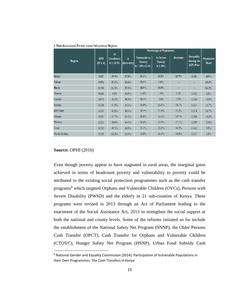
This marks a marginal improvement in welfare from the 45.9 percent incidence of

poverty reported in 2005 (KNBS, 2006). Deeper interrogation of the data revealed

that headcount poverty for Kenya averaged 17.3 and 51.4 percent for urban and

rural areas respectively while vulnerability to poverty averaged 21.3 and 31.9

14

percent respectively signaling serious welfare disparities across the country. A

household residing in a rural setup has a higher probability of succumbing to

poverty as compared to a household in the urban setup. A closer look at regional

performance revealed a very high poverty incidence in North Eastern province

standing at 83.3 percent up from 56.5 percent in 2013 followed by Western 50.0

percent down from 56.5 percent in 2013 and Nyanza 47.7 percent down from 52.2

percent over the same period. Nairobi reported the least poverty incidence rate at

4.8 percent though slightly higher than the 3.9 percent reported in 2013 (OPHI,

2016).

In terms of vulnerability to poverty, Western, Eastern and Nyanza lead the pack

with a vulnerability probability of 36.6, 31.0 and 30.8 percent respectively.

Vulnerability to poverty in 2016 was lowest in Nairobi averaging 12.6 percent

again signaling serious disparities in terms of vulnerability to poverty between

rural and urban residents. This could partly be explained by the ease of accessing

vital installations such as banks, hospitals, and schools among other infrastructure

in urban areas. Poverty severity and inequality was also highest in North Eastern

province averaging 64.3 percent and 0.26 respectively while it was lowest in

Nairobi region averaging 1.0 percent and 0.03 for severity and inequality

respectively. Of interest to this study is to assess how financial inclusion may have

impacted on the poverty reduction in the country and particularly in the urban

areas where significant progress has been made. This is represented in Table 1.1.

Table 1.1: Vulnerability to Poverty by Region

15

Source: OPHI (2016)

Even though poverty appear to have stagnated in rural areas, the marginal gains

achieved in terms of headcount poverty and vulnerability to poverty could be

attributed to the existing social protection programmes such as the cash transfer

programs8 which targeted Orphans and Vulnerable Children (OVCs), Persons with

Severe Disability (PWSD) and the elderly in 21 sub-counties of Kenya. These

programs were revised in 2013 through an Act of Parliament leading to the

enactment of the Social Assistance Act, 2013 to strengthen the social support at

both the national and county levels. Some of the reforms initiated so far include

the establishment of the National Safety Net Program (NSNP), the Older Persons

Cash Transfer (OPCT), Cash Transfer for Orphans and Vulnerable Children

(CTOVC), Hunger Safety Net Program (HSNP), Urban Food Subsidy Cash

8 National Gender and Equality Commission (2014). Participation of Vulnerable Populations intheir Own Programmes: The Cash Transfers in Kenya

16

Transfer (UFSCT), Persons with Severe Disability Cash Transfer (PWSDCT)

among others.

Geospatial analysis of and superimposition of poverty statistics on FI indicators,

offer insight on the link between FI and poverty. FSD (2014) report revealed a

skewed distribution of financial access points where 69 percent are located in areas

with the lowest incidence of poverty serving paltry 30 percent of the population.

Only 1 percent of all financial access points is located in the poorest areas limiting

the effectiveness of FI as a poverty alleviation tool.

1.3 Problem Statement

The overarching goal of financial inclusion is to draw the unbanked population

into the formal financial system where they can enjoy unlimited access to

appropriate and affordable financial services. Kenya has witnessed tremendous

growth in the use of financial services since 2006. Usage of formal financial

services averaged 75.3 percent (CBK, FSD, KNBS, 2016) in 2015. Despite this

protracted growth, concerns abound on the computation of FI and the ability of the

financial system to pull the underprivileged segments of the population within the

ambit of the formal financial system.

The incidence of poverty in the country currently average 39.9 percent (OPHI,

2016). Theory and empirical evidence predict a reduction in poverty and income

inequality from increased access to financial services (Beck, 2016; Aghion and

Bolton, 1997; Kaboski and Townsend, 2012). Beck (2016) asserts that lack of

appropriate; payment, saving, credit and insurance services by the poor limit full

participation in the modern economy to improve lives. This also limits their

response to transitory changes in income lowering their financial strength to

improve wellbeing as economic agents resort to the more expensive informal

financial services.

17

World Bank (2012) considers FI to be integral in reducing vulnerability to poverty

through increased savings and credit facilities which smoothen the poor's

consumption and mitigate against economic shocks. Households use a portfolio of

financial services to manage the ebbs and flows from transitory changes in income

and build buffer stocks to manage risks (FSD, 2011). Vulnerability risks often

cause significant irreversible losses in the absence of sufficient assets or insurance

to smooth consumption that locks households into a vicious cycle and perpetual

poverty (Jacoby and Skoufias, 1997).

Despite the progress made in promoting financial inclusion, policy design and

implementation of policy tools is hampered, first by the lack of a substantive, and

quantifiable measure of FI that encompasses all products from the entire financial

system and second, by lack of empirical evidence linking FI, welfare, and

vulnerability9 to poverty especially at micro level. Most studies concentrate on the

headcount poverty measure because of its ease of computation and simplicity

leaving out the dynamic aspects (Columbus, 2001). Understanding household

susceptibility to future poverty is critical in policy formulation. This warrants a

systematic examination of the link between the different dimensions of financial

inclusion and welfare outcomes in Kenya. .

Construction of an index of financial inclusion (IFI) from the different dimensions

offers a unique way of analyzing FI in the entire financial system. Honohan (2008)

contends that composite indices face numerous challenges. However, despite their

shortcomings, composite indices provide a good approximation of certain

phenomena which can be improved upon as more data become available.

Composite measures should however be supplemented by single product measures

9 Actual usage of financial services and products captured in terms of; regularity, frequency andduration of time used (AFI, 2011)

18

since reliance on nationally aggregated FI indicators risk masking significant

exclusion of finance at both individual and county levels. .

This study is unique in that it pioneers an autoregressive examination of financial

inclusion welfare nexus based on repeated cross sections organized in cohorts to

track the dynamics of FI and welfare.

1.4 Research Questions

i. What is the extent of and the distribution of financial inclusion in Kenya?

ii. What are the determinants of financial inclusion in Kenya

iii. Does financial inclusion affect household consumption expenditure in

Kenya?

iv. Does financial inclusion affect ex-post and ex-ante poverty?

1.5 Research Objectives

1.5.1 General Objectives

The broad objective of the study is to measure FI, assess its distribution and

estimate its impact on welfare and vulnerability to poverty among households in

Kenya.

1.5.2 Specific Objectives

The guiding specific objectives for the broad research objectives are as follows:

i. To construct single and composite measures of financial inclusion and

establish their stochastic distribution at the national and county levels

ii. To examine the determinants of financial inclusion in Kenya

19

iii. To estimate the impact of financial inclusion on household consumption

expenditure in Kenya

iv. To estimate the impact of financial inclusion on both ex-post and ex-ante

poverty among Kenyan households

1.6 Scope of the study

This study is limited to the dynamics of FI and welfare in Kenya from 2006 to

2016. In this study welfare refers to the money metric measure (consumption

expenditure per adult equivalent) as well as vulnerability to poverty. In particular,

the study generated both single product FI measures as well as a composite

measure (IFI) for each county to map and compare FI across Kenya. This was

followed by an estimation of the impact of financial inclusion on household

welfare. The study used the FinAccess, 2006, 2009, 2013 and 2016 data with the

household head as the unit of analysis. The analysis is limited to the usage and

impact dimensions of FI. Future studies should focus on the quality dimension.

1.7 Organization of the Study

The remaining chapters are organized as follows. Chapter two delves into the

measurement of FI and its stochastic distribution. Chapter three investigates the

determinants of FI. Chapter four explores the impact of FI on the money metric

measure of welfare. Chapter five focused on measurement of vulnerability to

poverty, the role of FI and the poverty transition matrix for the Kenyan households

between 2009 and 2016 while chapter six presents a summary of findings,

conclusions and policy recommendations from the study.

20

Chapter Two: Measures and Extent of Financial Inclusion

in Kenya

2.1 Introduction

This chapter explores financial inclusion (FI) in Kenya based on single product

usage and Sarma (2008) composite index of FI (IFI). A composite IFI reduces

multiple dimensions of FI into a single measure for effective policy formulation.

This essentially offers a valuable instrument for ranking the FI status of the various

counties. The county with the highest FI index is used as a reference point to

benchmark with as a best practice. This study suggests that targeting composite

indices could be easier than targeting a multitude of single product usage

indicators. Persons using a wide range of financial services at their disposal would

be considered to be highly financially included as opposed to those using a single

financial product.

Recent years have witnessed a surging interest in the measurement and

determination of FI at the global front. AFI (2011) however contends that while

there is consensus on the need to intensify the compilation of FI data, no standard

has been set on what to measure and how to go about it. Management of transitory

changes in income through building of buffer stocks is impaired by lack of

consensus on a proper measure of FI. Countries use different methodologies to

collect similar indicators due to differences in sophistication something which led

to the establishment of the FIDWG to harmonize this (FSD, 2011). The framework

is credited with the collection of the core set of FI indicators along the access and

usage dimension. These indicators capture the most basic and fundamental aspects

of FI in a standardized format across countries to enhance comparability.

Chakrabarty (2014) and Honohan (2008) posit that development of an IFI is

however not without challenges. First, the IFI is sensitive to geographical sampling

21

and second the index varies with the number of dimensions included. However, in

spite of the challenges, the IFI measure provides a better approximation of certain

phenomena creating room for further improvement subject to data availability.

Financial exclusion could either be voluntary or involuntary (Amidzic, 2014).

Voluntary financial exclusion can arise if individuals who meet the minimum

requirements for FI opt not to participate in financial markets on personal, cultural

or religious grounds.

Involuntary financial exclusion stems from the imposition of barriers such as high

interest rate, discrimination, lack of collateral and non-developed markets. Stiglitz

and Weiss (1981) cite indiscriminate lending and information asymmetry as some

of the factors behind involuntary exclusion. Other barriers cited in the literature

include; limited income, poor credit rating, credit unworthiness, geographical

location, population characteristics and cultural factors (Kempson and Whyley,

1999; Hannig and Jansen, 2010).

Barriers to financial access have also been classified in the literature along

macroeconomic factors namely; macroeconomic fundamentals, developments in

the financial sector and political factors or microeconomic factors namely; firm

profile, technology, religion, culture among others (Rau, 2004). Supply of

financial services enhances access while demand enhances usage. The authors also

posit that expansion of financial services creates affordability, security,

competitiveness and efficiency leading to low transaction costs, increased

investment and safe and secure customer deposits. Financial services assume a

geographical dimension through provision of financial products to the underserved

segments of the population especially in rural areas; a product dimension in form

of accessible and affordable services tailored to the needs of the low income

population and a time dimension through maintenance of a permanent relationship

with households towards stable and sustainable policies.

22

The various measures of FI are subjected to stochastic dominance analysis to

establish their dominance on the basis of household characteristics, dimension of

usage and geographical distribution. Claessens (2006) results posit that FI is far

from becoming universal especially in developing countries as evidenced in the

2012 Global Findex data by Demirguc-Kunt and Klapper (2012) where hardly a

quarter African adults hold an account in a formal institution. Claessens (2006)

attributes this to failure by countries to include FI in the public policy agenda.

Statistics on savings also paint a dark picture of the savings culture in sub Saharan

Africa where only 14 percent of the 40 percent adults with a savings product

obtain it from the formal access channel.

FI helps bring the lower segments of the population within the ambit of the formal

financial system while the government and policy makers use the FI indicators to

set national targets and strategies to achieve them. Vision 2030 recognizes the

financial sector as part of the six main economic drivers in Kenya (GoK, 2008). FI

is considered to be critical in the implementation of monetary policy given that it

operates under the formal access channel. The effectiveness of monetary

transmission can only succeed if the largest segment of the population is

financially included. Where only a small segment of the population is financially

included, only policies that operates under the informal access channel where the

majority can succeed.

The Global Partnership for Financial Inclusion (2011) and the Alliance for

Financial Inclusion (AFI) which established the Financial Inclusion Data Working

Group (FIDWG) for peer to peer exchange to promote and share information on

the measurement of FI also cite FI as being instrumental in informing financial

inclusion policy, providing a basis for the measurement, monitoring and evaluation

of financial inclusion policies and targets both locally and internationally. An

innovation in the measurement of FI in Kenya is captured by incorporating the

23

number of transactionary products held, savings and investment, credit and

insurance and pension in the IFI.

The main objective in this chapter was to generate measures of financial inclusion

and establish their stochastic dominance. These dominance tests are used to

compare distributions of FI indicators both inter-temporally and spatially to draw

an ordinal assessment of FI changes over several measures. A stochastic

dominance testing of FI is done to establish the cumulative distributions and

dominance of the various measures of FI along the household characteristics. This

broad objective was broken down into the following specific research objectives:

1) To construct financial inclusion measures and examine their nature based

on Kenya's FinAccess survey data

2) To conduct a geo spatial mapping of financial inclusion across Kenya

3) To apply stochastic dominance analysis to establish relative degree of

financial inclusion among population subgroups

This study provides a measure of FI following Sarma (2008) formula on Kenyan

data to aggregate usage of financial products from the formal access channel.

Subjecting the FI measure to stochastic dominance analysis establishes its

distribution along the household's demographic profile. Proximity to a financial

access point does not automatically translate to increased uptake of financial

services. About 77 percent of Kenya’s population lived within a 5km radius to a

financial access point (FSD, 2014). The chapter emphasizes the need to introduce

a geospatial dimension to the demand side data to establish FI gaps in Kenya.

2.2 Literature on Measurement of FI

Kenya's economic blueprint, the vision 2030 recognizes the critical role that the

financial sector plays in accelerating economic growth and improving livelihoods.

24

Interest in this topic is also motivated by both theory and empirical evidence which

associate growth in FI with accelerated economic growth and poverty reduction

(World Bank, 2002). This is echoed by DFID (2004) where developments in the

financial sector are considered to be a key building block to private sector

development. This section summarizes the key theoretical underpinnings and a

review of the main empirical literature on measurement of FI. Measurement of

economic variables such as financial inclusion is founded on the application of the

social inclusion, insider outsider models and classical and modern measurement

theories in finance.

2.2.1 Theoretical Literature

Financial inclusion thinking is mainly shaped by financial development theories.

FI forms a key tenet of financial development10 as one of its main indicators even

though the twin concepts manifest the 'chicken and egg' problem. Nobel laureate

Sen (1981) consider FI as a consequence of development. This makes it possible to

impose theories of financial development in studies on FI. Raza et al. (2014)

presents size, depth, access, efficiency and stability of the financial system as some

of the indicators of financial development. Earlier theories of development

however focused on labour and capital with little mention of finance which is

perceived to be responsible for lowering income inequality and accelerating

economic growth. Rajan and Zingales (1998) through cross country comparisons

established the causal link between finance and economic growth.

Emerging theories are now focusing on the growth in modern finance and its

composition. These include; Greenwood and Scharfstein (2013) who attributes the

observed growth in finance to asset management and provision of household

10 Factors, policies and institutions that promote effective financial intermediation and markets aswell as deep and broadened access to capital and financial services (Financial Development Index,2008).

25

credit. The biggest portion in the growth of assets is attributed to the growth in its

value. Household credit expansion is attributed to growth in residential mortgage

and consumer debt such as credit cards. Besides consumption smoothing, access

to credit leads to overinvestment in housing and consumption. Shadow banking

where non-bank financial entities offer traditional banking services such as a credit

in a less stable way if not checked can lead to a financial crisis like the one

witnessed in 2007. Merton and Bodie (1995) considers shadow banking model as

one that runs contrary to the tenets of traditional banking whose primary role was

to dampen effects of risk through intermediating financial services to parties that

can bear risks most easily.

Measurement of usage of financial services borrows heavily from the classical

theory and the modern measurement theories. Classical theory of measurement by

Campbell (1953) argues that measurement entail assignment of numbers to

represent properties based on physical laws discovered through the derived

measurement processes. Measurement is merely the assignment of numbers to

reality. Derived measures of certain phenomena such as financial inclusion are

therefore obtained through the indirect process. While challenging Campbell

(1953) definition of measurement, Stevens (1959) provided a broader definition

linking measurement to the assignment of numerals to objects on the basis of

predefined rules now popularly known as the modern measurement theory by

Abdel-Magid (1979). Measurement however presupposes what is to be measured

hence one must in the first place know what needs measurement.

One other theoretical strand used to motivate measurement of financial inclusion is

theory of banking and intermediation. Financial intermediation theories provide

means through which financial services flow from the surplus units to the deficit

units. Philippon, T. (2015) argues that intermediation is organized in two ways.

One, financial intermediation occurs under one roof in traditional banking where a

26

bank for example makes a loan, keeps it on its books and earns a net interest

income. This income is what compensates for the screening costs, monitoring costs

and for risk management. Secondly, under the originate and distribute model,

financial intermediation occurs as a daisy chain where transactions occur inside the

roof. Origination fees, asset management fees and trading profits are also

considered.

To understand financial intermediation better the author raises three key

considerations which include; measurement of the income of financial

intermediaries, definition and construction of the quantity of the intermediated

asset and computation of the unit cost of intermediation and quality adjustments.

In the context of this chapter, the definition and construction of the quantity of

intermediated assets is key. Greenwood and Jovanovic (1990) contends that

financial intermediaries facilitate migration of funds to areas where social returns

are higher.

The theory of social inclusion also plays a key role in the measurement of financial

inclusion by enhancing inclusion of all into the financial system, equally and

without discrimination. Social inclusion theory helps in informing about; social

bases of collective action, risk management, legitimacy of change processes and

inequality and exclusion. The foundations of effective institutions are governed by

the expanded sense of 'we' plus the social norms and an inclusive social structure

(Woolcock, 2013). Social inclusion is increasingly being viewed as an essential

tool in fighting poverty and increasing wellbeing. Sen (1981) hypothesized

exclusion in poverty terms by looking at it in terms of relative deprivation of basic

needs. Social inclusion therefore provides the capability to maximize one's welfare

from access to a wide array of financial services.

Lindbeck and Snower (2001) insider outsider model bends on the notion of

economic inclusion. This theory shows how certain economic agents in the market

27

enjoy more privileges than others. This explains the observed disparities in the

degree of FI in financial markets. Insiders command a higher economic rent or

surplus as compared to the outsiders. The insider outsider status helps in

explaining why certain population segments are financially excluded while others

are more financially included.

Lastly the legal structures as posited by Porta (1997; 1998) counts when designing

financial products. Formal financial services are subject to prudential regulation.

The existing legal framework in the financial sector governs the establishment of

financial sector regulators as well as the formulation of prudential guidelines.

Porta (1998) argues that strong institutions for protecting and matching the

investor needs enhance financial development. The decision about the dimensions

of FI to consider and the product categories in the context of this study was

informed by the set rules that classify financial service providers under the formal

channel.

2.2.2 Empirical Literature

2.2.2.1 Measurement of FI

While existing literature suggests several approaches for the construction of an

index of FI (IFI), no consensus has been reached on the most appropriate measure.

The first attempt at measuring FI is attributed to Beck et al., (2005) using the

dimensions of physical access, affordability and eligibility to inform on banking

sector outreach. This was later followed by indices of FI developed by Sarma

(2008), Honohan (2008), Chakravarty and Pal (2013), Sarma (2012), Amidzic et

al., (2014) among others.

While Sarma (2008) emphasize the need to incorporate the dimensions of usage,

availability and accessibility in developing the FI index, there is need to pay close

attention to each dimension so as to ensure consistency before aggregation of

28

individual products is done. It's on this premise that this study focuses on the

generation of the IFI on the basis of the usage dimension in the formal strand. In

most countries today, challenges of access and availability have been reduced

significantly with the emergence of mobile and internet banking. The dimensions

of FI have recently been redefined to capture; access, usage, quality and impact

(Hannig and Jansen, 2010 and FSD, 2013).

Demirguc Kunt and Klapper, 2013; Hannig and Jansen, 2010 FI measures focused

on ownership of an account, saving or loan product. While Amidzic et al., (2014)

relied on the percentage of regulated deposit and loan accounts to proxy the usage

dimension, this study finds the two indicators to be insufficient since it locks out

savings, investment, insurance and pension products. Inclusion of these products

from the formal channel provides a more encompassing measure of FI usage.

Amidzic et al., (2014) recommended the inclusion of mobile banking data when

measuring financial outreach where data is available. A household with a current

account, postbank account and a mobile money account is considered to be more

sophisticated financially, than one with only one transactionary product say, a

current account. The same applies to usage of more than one product under credit,

transactionary, savings and insurance. It's on the basis of this that household usage

of financial services from the four dimensions of FI is aggregated.

Uptake of financial services in Sub Saharan Africa remain low (34.2 percent

compared to developed world where FI exceeds 90 percent (World Bank, 2014).

This, points to a 65.8 percent departure from the much touted universal access.

South Africa however appears to be doing much better as compared to its peers.

World Bank (2015) economic update on South Africa places the country in the

same category with high income economies with respect to indicators of financial

access. This is however dampened by over 12 million South Africans who remain

unbanked and under-banked.

29

On the analysis of formal payments, savings and credit, the report concludes that

FI in South Africa is not only pro-growth but also pro poor and with great potential

to lower inequality. The report raises the need for disaggregation of data since the

aggregated data which reported a strong access to financial services could be

masking significant inequalities in access. Less than universal access in developed

countries could be rationalized by low demand rather than inadequate access to

financial services (World Bank, 2015).

Thorsten et al. (2010) asserts that biases in FI is also prevalent among urban

dwellers whose mean financial exclusion stood at 15.8 percent compared to 30.6

percent for rural dwellers. Demirguc-Kunt and Klapper (2012) found financial

exclusion to be highest in the lowest income quintile (77 percent). The number of

formal accounts held by adults, account for 41 percent (24 percent in sub Saharan

Africa) against a global target of 90 percent and 89 percent for the developing and

developed countries respectively. This discrepancy creates two reinforcing

inequities for the poor. First it limits their financial strength to improve their

wellbeing through participation in financial markets and second, it aggravates the

marginalization of the poor from the formal economy.11 This adversely affects

their response to transitory changes in income as they resort to more expensive

credit facilities from money lenders, substitute savings with livestock or gold

pending any emergencies where they pawn assets12.

Lack of a composite measure of FI limits understanding of the complex nature of

FI as well as the link between FI and welfare outcomes. Measurement of FI

requires a multidimensional approach to aggregate information from several

dimensions. The multidimensional approach was used in constructing the Ease of

11 Dan Radcliffe and Rodger Voorhies, Bill & Melinda Gates Foundation1 (2012). A digital pathwayto financial inclusion

12 2014 Global Partnership for Financial Inclusion: Why Financial Inclusion?

30

Doing Business Index (Doing Business 2012), the Human Development Index

(HDI), Multidimensional Poverty Index (MPI), Gender Inequality Index (GII) by

the United Nations Development Programme (UNDP) and Sarma (2008) and

Chakravarty (2010) FI index. Data collection on FI mainly revolves around access,

usage, and quality and impact dimensions. The data is further classified as either

demand side (individuals or firms) or supply side (financial service providers).

The Global Partnership for Financial Inclusion (CGAP) established by G20 has

helped develop basic and secondary indicators of FI based on the four dimensions.

These include; payments, savings, remittances, insurance and point of sale. The

International Monetary Fund (IMF) has also intensified the collection of supply

side indicators in its Financial Access Surveys (FAS) at the global front to enhance

comparability of access and usage indicators among households and non-financial

corporation's across countries.

FAS indicators are collected from financial sector regulators and currently stand at

47 indicators from both geographical and usage dimensions in 189 countries (IMF,

2015). The core set of FI indicators by AFI provided a first attempt at generating a

common measurement of FI based on basic and fundamental aspects to enhance

the dimensions of access and usage (AFI, 2011). AFI (2011) indicates that the

dimensions of access and usage are different in that individuals may opt not to use

the financial services despite their availability due to socio-economic reasons,

costs among others.

The World Bank's Development Research Group spearheaded the Global Financial

Inclusion Index (Global Findex) to fill the data gap on the financial inclusion

landscape. This initiative led to the creation of the first comprehensive demand

side FI indicators based on financial product usage. The data is considered to be

rich in enhancing cross country comparability, demographic covariates and

tracking countries (148) performance over time on the core set of indicators

31

namely bank accounts, savings, borrowing, payments and insurance (Demirguc

Kunt & Klapper, 2012).

The key indicators are; percentage account holding in formal institutions among

adults, percentage share of adults with formal savings account, percentage share of

adults using a formal account to borrow and percentage share of adults using an

informal source to borrow (family and friends). The measure of financial depth

adopted (private sector credit to GDP ratio) in 2010 revealed a sharp disparity

between sub Saharan Africa and high income countries at 24 percent and 172

percent respectively. A higher financial depth however does not automatically

translate to a broadened access to financial services even though the correlation is

positive (Demirguc Kunt & Klapper, 2012).

The proportion of adults with a formal account in Kenya stood at 42 percent

compared to 54 percent and 80 percent for South Africa and Mauritius respectively

(Demirguc Kunt & Klapper, 2012). While aggregate borrowing in sub Saharan

Africa stood at 47 percent borrowing from the formal access channel remained

small in Kenya averaging 10 percent compared to Mauritius 14 percent Use of

such single indicators has come under criticism for failing to inform on the breadth

of FI. Aduda and Kalunda (2012) in review of theoretical and empirical literature

on FI and financial stability reinforce the pivotal role played by FI in enhancing

financial development. Although the paper provides the status of FI in Kenya it

does not construct a financial inclusion index based on a portfolio of financial

services.

Financial inclusion in Kenya has grown from 25 percent in 2006 to 75 percent in

2016 (CBK, KNBS & FSD, 2016). This aggregated measure however masks

significant exclusion of finance at both individual and county levels. For example,

Kalunda (2014) established that the uptake of financial services among small scale

farmers in Nyeri where usage of bank accounts stood at 93.8 percent. This could

32

be attributed to ongoing reforms in the financial sector summarized in Fig. 1 which

include; changing the regulatory framework to accommodate DTMs, DTSs,

agency banking, internet and mobile banking among others.

Kempson and Whyley (1999) argued that quite a large number of households are

marginally financially included with one or two financial products as compared

with a few who are totally financially excluded from the formal financial services.

Claessens (2006) expounds on the measurement of the access dimension using

availability of financial services, cost, range type and quality of financial services.

Other dimensions considered by the authors included; reliability, convenience,

continuity and flexibility of financial services. Failure to attain universal access in

the use of financial services was linked to the failure to include financial inclusion

in the public policy agenda. Determination of who is banked or not is based on the

revealed use rather than access.

Whereas studies on the measurement of FI borrow heavily from the work of

Chakravarty and Pal (2010) and Sarma (2008), several other pieces of literature on

measurement of FI at micro and macro levels have come up including; Sarma and

Pias (2011) and Amidzic et al. (2014) based on factor analysis and Park and

Mercado (2015). Chakravarty and Pal (2013) describe FI as the delivery of

financial services to its people. The domain of financial services is considered to

be very huge and varies from one country to another. Their approach in generating

the FI index follows the human development index (HDI) to aggregate several

dimensions into a single index of FI.

Chakravarty and Pal (2013) cite sensitivity to geographical sampling and the

number of dimensions included as key considerations in the generation of

composite indices. The authors targeted sub-National regions (17 states) in India

between 1972 and 2009 in developing a FI index to assess the performance of the

entire financial system over time and across cross sections. The construction of the

33

index was based on six dimensions; geographic penetration demographic

penetration; Deposit accounts per 1000 people; Credit account per 1000 people;

Deposit income ratio and Credit income ratio. The index of FI increased with the

number of households using institutional credits

Honohan (2005) argues that broadly, two main approaches exist whether usage of

financial services is derived from household survey data or from inferences drawn

on the use of intermediary accounts from existing data. Percentage ownership of a

bank account from a formal financial intermediary among adults is the most

commonly used indicator of FI (World Bank, 2005). This indicator is however

criticized due to its inability to determine the distinct and active accounts in a case

where individuals hold multiple accounts (Honohan, 2008). This raises the need to

consolidate the multiple accounts to match the number of individuals with

accounts. A non-linear aggregation of loan and transactionary deposit accounts is

closely correlated with household usage of financial services (Honohan, 2008).

The only challenge is that use of the two dimensions rocks out the role of savings

and investments as well as insurance and pension.

The use of single indicators to measure FI has been challenged by Sarma (2008)

due to their inability to inform on the extent of FI as evidenced by the Indian case

where usage of financial services remains high despite a low density of bank

branches. A similar picture was observed in Russia which ranked highest on the

usage of bank accounts per 1000 adults despite having a lower bank branch density

per 100,000 adults as compared to Thailand, Malaysia and Colombia. Albania also

ranked 4th in terms of loan income ratio but 85th in terms of bank branches per

100,000 adults in Beck et al., (2007). Individual measures therefore provide an

incomplete picture of the level of inclusivity in the entire financial system.

Individual measures mainly use categorical variables (1 and 0) to represent

financial included and financially excluded persons respectively.

34

Sarma (2008) recommends the use of a composite index to measure the level of FI

based on a combination of various banking sector indicators. The composite index

(IFI) lie between 1 (complete financial inclusion) and 0 (complete financial

exclusion). The IFI applies a three dimensional approach on macroeconomic data

based on banking sector outreach to capture accessibility, availability and usage.

Accessibility proxied using bank penetration is measured using the number of

bank accounts per 1000 adult population with a -1 weight. The number of bank

branches and ATMs per 100,000 adult population measures availability, while the

ratio of credit plus deposit to GDP measured usage with each of the dimensions

carrying a 0.5 weight.

Using an econometric technique, Honohan (2008) developed a composite cross

country FI index based on 160 countries. The main focus was on the use of formal

financial intermediaries proxied by the use of services from the formal access

channel in this context. Given that certain countries had no household survey data

to provide the percentage uptake of bank accounts, an alternative estimation

technique was used to estimate the number of bank accounts. While the scholar

admits that composite indices are characterized by numerous shortcomings due to

the imputation procedures followed in developing the index, he posits that the

composite index provides a good approximation which can be improved upon as

more data become available.

Amidzic (2014) in assessing countries FI standing based on a composite index

cites robust measurement of FI as an outstanding challenge. The authors applied a

geometric mean approach to construct an index of FI based on the dimensions of

outreach, usage and quality. Key considerations included; geographic and

demographic penetration, deposit and lending, dispute resolution, disclosure

requirement and cost of usage. The constructed composite index was later used to

rank countries hence offering an additional tool for surveillance and policy. The

35

number of ATM machines and bank branches indicators rescaled by land mass and

adult population were used. Measurement of usage was based on the percentage of

adults with atleast one type of regulated deposit/loan account. However, the index

generation ignored quality indicators due to data limitations.

Demirguc-kunt et al., (2015) posited that measurement of financial inclusion helps

in identifying opportunities to remove the barriers to financial access. The authors

confirmed that FI is centered on usage rather than access. Their findings

established that by 2014, 62 percent of adults globally enjoyed holding an account

in a bank or other financial institution or with a mobile money provider up from 51

percent in 2011. This increase in the number of accounts held was attributed to

innovations in technology and particularly mobile money especially in developing

countries. They also mentioned the huge potential to raise FI among women and

the poor. In addition, the authors argued that holding a bank account is not enough;

rather, government and private sector should strengthen FI by channeling wages

through the accounts as opposed to cash payments. Account usage could also be

spurred by digitizing payments such as utility bills and school fees which largely

relied on cash.

2.2.2.2 Stochastic Dominance

Stochastic Dominance (SD) is a concept applied in decision theory when

confronted with a choice between two phenomena (Bawa, 1982). SD presents a

stochastic ordering of possible outcomes in a probability distribution based on

individual preferences. The simplest method of testing for stochastic dominance is

through a Kolmogorov-Smirnov (KS) dominance test. The KS test provides a

comparative analysis of two cumulative frequency distributions at a time.

Chakravarty, Laha and Roy (1967) argue that KS test helps decide if a sample was

drawn from a population with a specific distribution. The D captures the maximum

vertical deviation (supremum) between the two subgroups curves.

36

A small P value implies that the two subgroups were sampled from populations

characterized by different distributions hence may differ in terms of median and

distribution curve. If the p value is less than the critical value, the null hypothesis

that the two samples were drawn from the same distribution is rejected. Its

therefore preferred when rejected at all critical values. The closer the D value is to

0, the more likely the two samples were drawn from the same distribution.

Faced with two samples picked from two distributions say, urban (u) and rural (r),

stochastic dominance tests helps in estimating the parameter beta which informs

on the dominant stochastic pattern. Assuming expu uF and expr rF , uF

first order stochastically dominates rF if and only if r u . A stochastic

dominance testing allows households faced with a choice to make judgment on a

preference or random variable as more risky compared to another over the entire

utility path. Most often, the decision maker has a preference ordering over all

possible outcomes. This technique is used to explore the robustness of IFI

comparisons on selected household characteristics.

The first order stochastic dominance (FOSD) test provides a comparative analysis

of the different cumulative distribution functions of the IFI. This is generated

based on regions, cluster, gender, education and marital status. Both a first-order

and second-order stochastic dominance (SOSD) tests are carried out to determine

the most dominant path. The second order stochastic dominance test is conducted

where there is an intersection of the CDF (Ravallion, 1994; Davidson and Duclos,

1998; 2000). The Kolmogorov-Smirnov test based on the largest vertical distance

between two cumulative frequency curves is mainly used in measuring first-order

stochastic dominance.

Some of the approaches applied in conducting stochastic dominance tests include;

receiver operating characteristics (ROC) curves, Lorenz and generalized Lorenz

37

curves, cumulative distribution functions among others. Generalized Lorenz curve

(glcurve) offers better empirical applications as compared to the normal Lorenz

curve (Shorrocks, 1983). The Lorenz curve offers minimum variation which

conceals interpretation of the observed differences. The larger variation in the

mean income makes it easier to explain glcurves hence offering a clearer picture of

the dominance relationships. This is generated through scaling up of the Lorenz

curve at each point by the population mean of the variable of interest ordered in

ascending order.

The cumulative mean ppis plotted against p . Financial product usage for

transactionary, credit, savings and insurance assumes a certain cumulative

distribution function (CDF). The glcurve generates two new variables with the

ordinates for each product at each point. Assuming the CDF for transactionary

products is F(t), then the glcurve at each point p (GL(p)) is p=F(t). The GL curve

for each product therefore plots the cumulative total product usage divided by the

population size against cumulative population share GL(1)=mean(t). This curve

helps in testing for dominance along the various segments, say rural urban

subgroups.

Other scholars who have successfully used the stochastic dominance technique

include; Davidson (2006) and Davidson and Duclos (2000) in the analysis of

income distribution.

2.2.3 Overview of literature

Measurement of FI is one issue that has elicited much interest globally in the

recent past. However, despite the myriad efforts that have featured in the literature,

there's still no consensus on the most appropriate measure. Earlier attempts at

measuring FI using single product indicators has been challenged for failing to

incorporate the portfolio financial product usage mentality which characterize the

38

modern day consumer. The main dimensions scholars are focusing on are mainly

access, usage, impact and quality. The dimension of access mainly captures the

supply side while the usage dimension mainly focuses on the demand side.

The access challenge is considerably low today, thanks to the emergence of mobile

and internet banking which have led a financial revolution in how people transact.

The mobile banking platform in Kenya especially has transformed Kenya's

financial sector to a silicon valley helping in a big way to overcome the

geographical barriers to financial access. Focus has shifted towards usage since

access does not always guarantee uptake of financial services. The impact and

quality dimensions are also slowly gaining momentum owing to the central

position held by the financial system in spurring economic growth.

The index of FI (IFI) in the context of this paper is based on Sarma (2008).

However, it departs in two ways. First, aggregation is done on the basis of the

usage dimension only. Second, indicators of usage are generated from all

intermediaries in the formal access channel rather than bank alone. These include;

banks, insurance, mobile money, DTMs, DTSs and pension. This approach also

differs slightly from Amidzic et al., (2014) where a geometric mean was applied

on the dimensions of outreach, usage and quality based on; geographic and

demographic penetration, deposit and lending, dispute resolution, disclosure

requirement and cost of usage. Aggregation is based on the usage of

transactionary, credit, savings & investments and insurance & pension products. .

Amidzic et al. (2014) factor analysis approach also excluded usage of insurance

services which form part of the IFI in this context. The generated indicator is used

to supplement the single product usage indicators.

As to the sufficiency of the usage dimension in informing on the usage of financial

services, Honohan (2008) contends that a nonlinear aggregation of loan products

and transactionary deposit accounts from household surveys exhibit a high

39

correlation with the usage of financial services. This study extends this line of

thought by including indicators of savings/investment product usage from

prudentially regulated financial institutions. An assessment of both the breadth

(use of transactionary products) alongside the depth (credit to private sector) using

a regression analysis inform on whether access/usage of financial services is

independent. A positive but imperfect correlation signals a distinct access to

financial services dimension which could be skewed. The literature also

established that Kolmogorov-Smirnov test computed from the largest vertical

distance between two cumulative frequency curves is applied to measure first

order stochastic dominance.

Literature related to FI lacks a comprehensive measure of FI which can be relied

upon in drawing a comparative analysis across the counties. Even the little data

available has not been subjected to stochastic dominance tests to establish which

frequency distribution is dominant. This study is the first of its kind in Kenya to

employ Sarma (2008) index of financial inclusion (IFI) formulae based on

repeated cross sectional survey data. The need to measure FI is motivated by

Claessens (2006) argument that the profile of a household with a credit facility

differs from that of a household with a savings or bank account. A stochastic

dominance analysis is then pursued to establish the dominance structures of

financial product usage based on the individual demographic profile.

2.3 Theoretical Framework

The theoretical framework employed in the construction of FI indicators is the

modern measurement theory (1979) where assignment of numerals to objects is

based on predefined rules. Sarma (2008) provides the aggregation formulae for the

construction of IFI. This framework is considered to be superior in the

construction of IFI since it provides a formula that easily aggregates sub-indices

from various FI dimensions hence offering a unique reference point in the index

40

generation. The framework uses single product indicators to aggregate portfolio

usage of financial services among households based on the utility attached to each

product. The derived measures of FI are then subjected to a stochastic dominance

test.

2.3.1 Constructing the Index of Financial Inclusion

In terms of methodology, the IFI measure borrows heavily from leading scholarly

work by Sarma (2008; 2012), Chakravarty & Pal (2013) and Amidzic et al. (2014)

three step procedure; normalization of indicators, determination of sub-indices for

each dimension and aggregation of the sub-indices. We assumed that the financial

system has 1k dimensional activities drawn from transactionary, credit, savings

and insurance. One's financial sophistication is evidenced by the number of

financial instruments chosen rationally (Collins, Murdoch, Rutherford, and

Ruthven, 2009).The attained FI level from each dimension is denoted by ix whose

lower and upper bounds are defined by im and iM , that is, ,i i ix m M .

Functioning i is represented by a real valued function , ,i i iA x m M , which is

continuous in its arguments and associated with each ,i i ix m M . The difference

from the real valued function 1 rA yields the shortfall from the actual value of

the index. The index of FI (IFI) is derived from the averaging of the individual

indicators.

The normalization process is expressed as follows;

kiki

k

xnx

M

Where; kix is the raw value of the kth indicator for individual i, Mk the maximum

possible value of the indicator across cross sections while nxki is the normalized

value of the indicator. The construction of the IFI in the context of this study

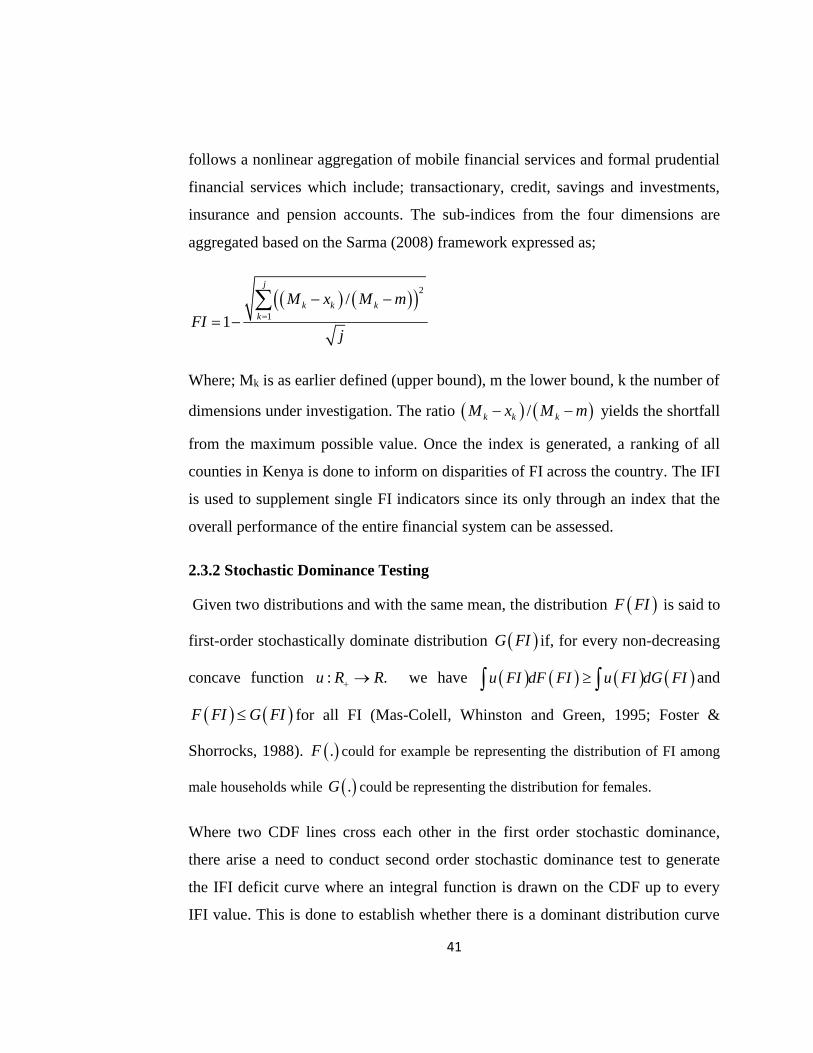
41

follows a nonlinear aggregation of mobile financial services and formal prudential

financial services which include; transactionary, credit, savings and investments,

insurance and pension accounts. The sub-indices from the four dimensions are

aggregated based on the Sarma (2008) framework expressed as;

21

/

1

j

k k kk

M x M m

FIj

Where; Mk is as earlier defined (upper bound), m the lower bound, k the number of

dimensions under investigation. The ratio /k k kM x M m yields the shortfall

from the maximum possible value. Once the index is generated, a ranking of all

counties in Kenya is done to inform on disparities of FI across the country. The IFI

is used to supplement single FI indicators since its only through an index that the

overall performance of the entire financial system can be assessed.

2.3.2 Stochastic Dominance Testing

Given two distributions and with the same mean, the distribution F FI is said to

first-order stochastically dominate distribution G FI if, for every non-decreasing

concave function : .u R R we have u FI dF FI u FI dG FI and

F FI G FI for all FI (Mas-Colell, Whinston and Green, 1995; Foster &

Shorrocks, 1988). .F could for example be representing the distribution of FI among

male households while .G could be representing the distribution for females.

Where two CDF lines cross each other in the first order stochastic dominance,

there arise a need to conduct second order stochastic dominance test to generate

the IFI deficit curve where an integral function is drawn on the CDF up to every

IFI value. This is done to establish whether there is a dominant distribution curve

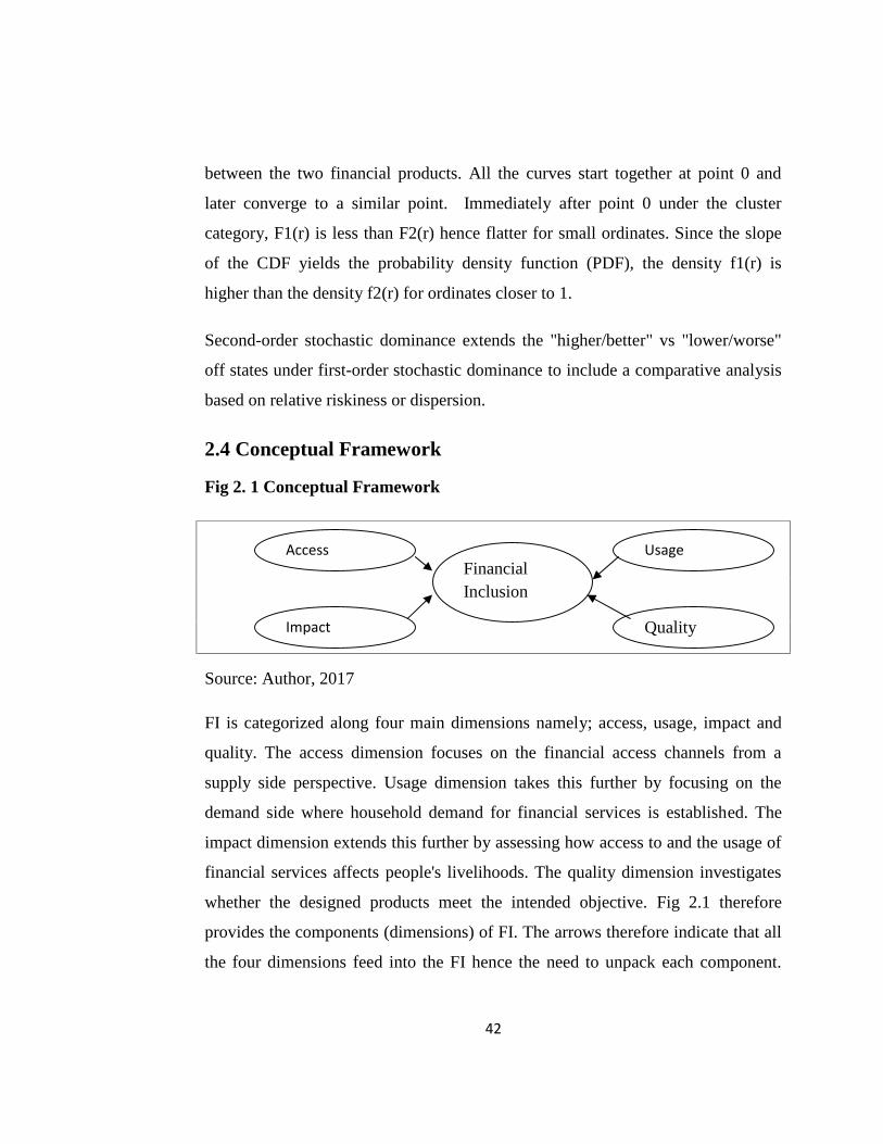
42

between the two financial products. All the curves start together at point 0 and

later converge to a similar point. Immediately after point 0 under the cluster

category, F1(r) is less than F2(r) hence flatter for small ordinates. Since the slope

of the CDF yields the probability density function (PDF), the density f1(r) is

higher than the density f2(r) for ordinates closer to 1.

Second-order stochastic dominance extends the "higher/better" vs "lower/worse"

off states under first-order stochastic dominance to include a comparative analysis

based on relative riskiness or dispersion.

2.4 Conceptual Framework

Fig 2. 1 Conceptual Framework

Source: Author, 2017

FI is categorized along four main dimensions namely; access, usage, impact and

quality. The access dimension focuses on the financial access channels from a

supply side perspective. Usage dimension takes this further by focusing on the

demand side where household demand for financial services is established. The

impact dimension extends this further by assessing how access to and the usage of

financial services affects people's livelihoods. The quality dimension investigates

whether the designed products meet the intended objective. Fig 2.1 therefore

provides the components (dimensions) of FI. The arrows therefore indicate that all

the four dimensions feed into the FI hence the need to unpack each component.

Impact

Access UsageFinancialInclusion

Quality

43

This chapter focuses on the usage dimension which has been used in constructing

the measures of FI.

2. 5 Data

Both the cohort and yearly full sample data have been used in constructing the

measures of FI. This technique of forming panels using repeated cross sectional

survey data is used to overcome scarcity of panel data in developing countries.

Repeated cross sectional surveys are less prone to attrition and non-response bias

(Meng et al. 2014). Population subgroups were formed based on time invariant

characteristics namely; gender, place of residence and birth year from the four

FinAccess survey datasets (2006, 2009, 2013 and 2016) totaling 504 observations.

The pseudo panel targeted households born between 1934 and 1994. The 2006

survey includes individuals aged 18 to 62, the 2009 survey, 21 to 65 (3 years

older), the 2013 survey, 24 to 68 (6 years older after 2006) and the 2016 survey, 27

to 71 year olds (9 years older after 2006). The first observation, which is cohort

one therefore captures individuals aged 18 to 22 in 2006, 21 to 25 in 2009, 24 to

28 in 2012 and 27 to 31 in 2016. This methodological framework by Deaton, 1986

was also used by Ackah et al. (2007) in Ghana. The short age bands may however

lead to fewer respondents in a cohort despite the large cross section dimension.

Large age cohort bands may also not be good since they reduce the cross section

dimension.

Gender variable is disaggregated to generate panels for males and females

respectively while the geographical aspect is captured by the seven regions (44

counties), formerly provinces with the exception of North Eastern region which

has 3 counties namely; Mandera, Wajir and Garissa for missing in the 2013 wave

due to logistical constraints. A key consideration in cohort analysis is the tradeoff

between the number of cohorts and number of observations for each cohort.

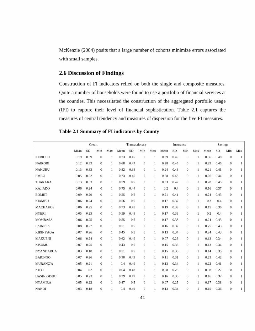
44

McKenzie (2004) posits that a large number of cohorts minimize errors associated

with small samples.

2.6 Discussion of Findings

Construction of FI indicators relied on both the single and composite measures.

Quite a number of households were found to use a portfolio of financial services at

the counties. This necessitated the construction of the aggregated portfolio usage

(IFI) to capture their level of financial sophistication. Table 2.1 captures the

measures of central tendency and measures of dispersion for the five FI measures.

Table 2.1 Summary of FI indicators by County

Credit Transactionary Insurance Savings

Mean SD Min Max Mean SD Min Max Mean SD Min Max Mean SD Min Max

KERICHO 0.19 0.39 0 1 0.73 0.45 0 1 0.39 0.49 0 1 0.36 0.48 0 1

NAIROBI 0.12 0.33 0 1 0.68 0.47 0 1 0.28 0.45 0 1 0.29 0.45 0 1

NAKURU 0.13 0.33 0 1 0.82 0.38 0 1 0.24 0.43 0 1 0.21 0.41 0 1

EMBU 0.05 0.22 0 1 0.73 0.45 0 1 0.28 0.45 0 1 0.26 0.44 0 1

THARAKA 0.13 0.33 0 1 0.59 0.5 0 1 0.33 0.47 0 1 0.28 0.45 0 1

KAJIADO 0.06 0.24 0 1 0.75 0.44 0 1 0.2 0.4 0 1 0.16 0.37 0 1

BOMET 0.09 0.29 0 1 0.55 0.5 0 1 0.21 0.41 0 1 0.24 0.43 0 1

KIAMBU 0.06 0.24 0 1 0.56 0.5 0 1 0.17 0.37 0 1 0.2 0.4 0 1

MACHAKOS 0.06 0.25 0 1 0.73 0.45 0 1 0.19 0.39 0 1 0.15 0.36 0 1

NYERI 0.05 0.23 0 1 0.59 0.49 0 1 0.17 0.38 0 1 0.2 0.4 0 1

MOMBASA 0.06 0.25 0 1 0.55 0.5 0 1 0.17 0.38 0 1 0.24 0.43 0 1

LAIKIPIA 0.08 0.27 0 1 0.51 0.5 0 1 0.16 0.37 0 1 0.25 0.43 0 1

KIRINYAGA 0.07 0.26 0 1 0.45 0.5 0 1 0.13 0.34 0 1 0.24 0.43 0 1

MAKUENI 0.06 0.24 0 1 0.62 0.49 0 1 0.07 0.26 0 1 0.13 0.34 0 1

KISUMU 0.07 0.25 0 1 0.43 0.5 0 1 0.15 0.36 0 1 0.13 0.34 0 1

NYANDARUA 0.03 0.18 0 1 0.51 0.5 0 1 0.15 0.36 0 1 0.14 0.35 0 1

BARINGO 0.07 0.26 0 1 0.38 0.49 0 1 0.11 0.31 0 1 0.23 0.42 0 1

MURANG'A 0.05 0.21 0 1 0.4 0.49 0 1 0.13 0.34 0 1 0.22 0.41 0 1

KITUI 0.04 0.2 0 1 0.64 0.48 0 1 0.08 0.28 0 1 0.08 0.27 0 1

UASIN GISHU 0.05 0.23 0 1 0.39 0.49 0 1 0.16 0.36 0 1 0.16 0.37 0 1

NYAMIRA 0.05 0.22 0 1 0.47 0.5 0 1 0.07 0.25 0 1 0.17 0.38 0 1

NANDI 0.03 0.18 0 1 0.4 0.49 0 1 0.13 0.34 0 1 0.15 0.36 0 1

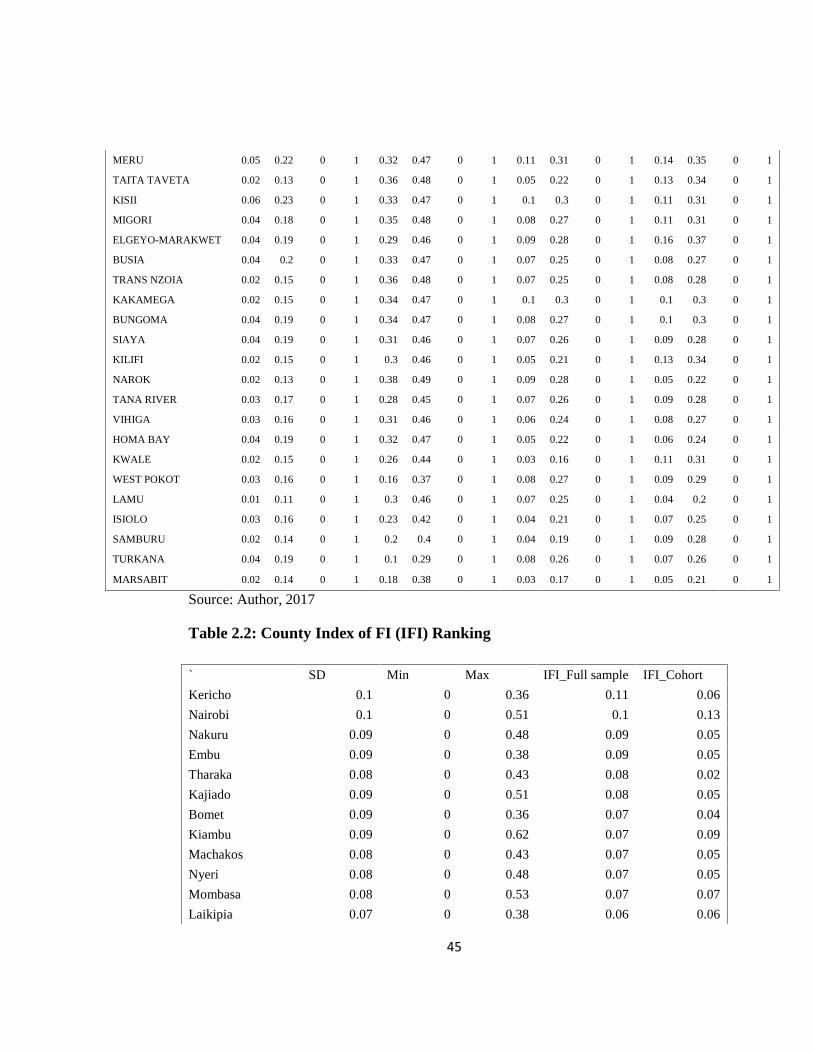
45

MERU 0.05 0.22 0 1 0.32 0.47 0 1 0.11 0.31 0 1 0.14 0.35 0 1

TAITA TAVETA 0.02 0.13 0 1 0.36 0.48 0 1 0.05 0.22 0 1 0.13 0.34 0 1

KISII 0.06 0.23 0 1 0.33 0.47 0 1 0.1 0.3 0 1 0.11 0.31 0 1

MIGORI 0.04 0.18 0 1 0.35 0.48 0 1 0.08 0.27 0 1 0.11 0.31 0 1

ELGEYO-MARAKWET 0.04 0.19 0 1 0.29 0.46 0 1 0.09 0.28 0 1 0.16 0.37 0 1

BUSIA 0.04 0.2 0 1 0.33 0.47 0 1 0.07 0.25 0 1 0.08 0.27 0 1

TRANS NZOIA 0.02 0.15 0 1 0.36 0.48 0 1 0.07 0.25 0 1 0.08 0.28 0 1

KAKAMEGA 0.02 0.15 0 1 0.34 0.47 0 1 0.1 0.3 0 1 0.1 0.3 0 1

BUNGOMA 0.04 0.19 0 1 0.34 0.47 0 1 0.08 0.27 0 1 0.1 0.3 0 1

SIAYA 0.04 0.19 0 1 0.31 0.46 0 1 0.07 0.26 0 1 0.09 0.28 0 1

KILIFI 0.02 0.15 0 1 0.3 0.46 0 1 0.05 0.21 0 1 0.13 0.34 0 1

NAROK 0.02 0.13 0 1 0.38 0.49 0 1 0.09 0.28 0 1 0.05 0.22 0 1

TANA RIVER 0.03 0.17 0 1 0.28 0.45 0 1 0.07 0.26 0 1 0.09 0.28 0 1

VIHIGA 0.03 0.16 0 1 0.31 0.46 0 1 0.06 0.24 0 1 0.08 0.27 0 1

HOMA BAY 0.04 0.19 0 1 0.32 0.47 0 1 0.05 0.22 0 1 0.06 0.24 0 1

KWALE 0.02 0.15 0 1 0.26 0.44 0 1 0.03 0.16 0 1 0.11 0.31 0 1

WEST POKOT 0.03 0.16 0 1 0.16 0.37 0 1 0.08 0.27 0 1 0.09 0.29 0 1

LAMU 0.01 0.11 0 1 0.3 0.46 0 1 0.07 0.25 0 1 0.04 0.2 0 1

ISIOLO 0.03 0.16 0 1 0.23 0.42 0 1 0.04 0.21 0 1 0.07 0.25 0 1

SAMBURU 0.02 0.14 0 1 0.2 0.4 0 1 0.04 0.19 0 1 0.09 0.28 0 1

TURKANA 0.04 0.19 0 1 0.1 0.29 0 1 0.08 0.26 0 1 0.07 0.26 0 1

MARSABIT 0.02 0.14 0 1 0.18 0.38 0 1 0.03 0.17 0 1 0.05 0.21 0 1

Source: Author, 2017

Table 2.2: County Index of FI (IFI) Ranking

` SD Min Max IFI_Full sample IFI_Cohort

Kericho 0.1 0 0.36 0.11 0.06

Nairobi 0.1 0 0.51 0.1 0.13

Nakuru 0.09 0 0.48 0.09 0.05

Embu 0.09 0 0.38 0.09 0.05

Tharaka 0.08 0 0.43 0.08 0.02

Kajiado 0.09 0 0.51 0.08 0.05

Bomet 0.09 0 0.36 0.07 0.04

Kiambu 0.09 0 0.62 0.07 0.09

Machakos 0.08 0 0.43 0.07 0.05

Nyeri 0.08 0 0.48 0.07 0.05

Mombasa 0.08 0 0.53 0.07 0.07

Laikipia 0.07 0 0.38 0.06 0.06

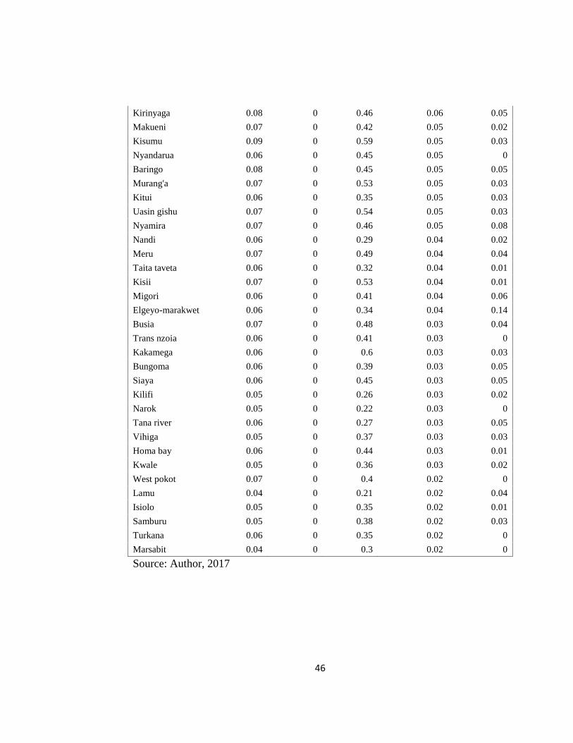
46

Kirinyaga 0.08 0 0.46 0.06 0.05

Makueni 0.07 0 0.42 0.05 0.02

Kisumu 0.09 0 0.59 0.05 0.03

Nyandarua 0.06 0 0.45 0.05 0

Baringo 0.08 0 0.45 0.05 0.05

Murang'a 0.07 0 0.53 0.05 0.03

Kitui 0.06 0 0.35 0.05 0.03

Uasin gishu 0.07 0 0.54 0.05 0.03

Nyamira 0.07 0 0.46 0.05 0.08

Nandi 0.06 0 0.29 0.04 0.02

Meru 0.07 0 0.49 0.04 0.04

Taita taveta 0.06 0 0.32 0.04 0.01

Kisii 0.07 0 0.53 0.04 0.01

Migori 0.06 0 0.41 0.04 0.06

Elgeyo-marakwet 0.06 0 0.34 0.04 0.14

Busia 0.07 0 0.48 0.03 0.04

Trans nzoia 0.06 0 0.41 0.03 0

Kakamega 0.06 0 0.6 0.03 0.03

Bungoma 0.06 0 0.39 0.03 0.05

Siaya 0.06 0 0.45 0.03 0.05

Kilifi 0.05 0 0.26 0.03 0.02

Narok 0.05 0 0.22 0.03 0

Tana river 0.06 0 0.27 0.03 0.05

Vihiga 0.05 0 0.37 0.03 0.03

Homa bay 0.06 0 0.44 0.03 0.01

Kwale 0.05 0 0.36 0.03 0.02

West pokot 0.07 0 0.4 0.02 0

Lamu 0.04 0 0.21 0.02 0.04

Isiolo 0.05 0 0.35 0.02 0.01

Samburu 0.05 0 0.38 0.02 0.03

Turkana 0.06 0 0.35 0.02 0

Marsabit 0.04 0 0.3 0.02 0

Source: Author, 2017

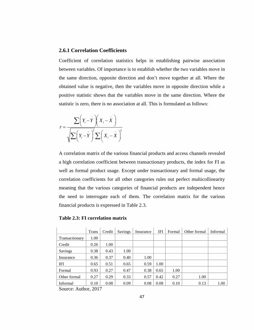
47

2.6.1 Correlation Coefficients

Coefficient of correlation statistics helps in establishing pairwise association

between variables. Of importance is to establish whether the two variables move in

the same direction, opposite direction and don’t move together at all. Where the

obtained value is negative, then the variables move in opposite direction while a

positive statistic shows that the variables move in the same direction. Where the

statistic is zero, there is no association at all. This is formulated as follows:

2 2

i i

i i

Y Y X Xr

Y Y X X

A correlation matrix of the various financial products and access channels revealed

a high correlation coefficient between transactionary products, the index for FI as

well as formal product usage. Except under transactionary and formal usage, the

correlation coefficients for all other categories rules out perfect multicollinearity

meaning that the various categories of financial products are independent hence

the need to interrogate each of them. The correlation matrix for the various

financial products is expressed in Table 2.3.

Table 2.3: FI correlation matrix

Trans Credit Savings Insurance IFI Formal Other formal Informal

Transactionary 1.00

Credit 0.26 1.00

Savings 0.38 0.43 1.00

Insurance 0.36 0.37 0.40 1.00

IFI 0.65 0.51 0.65 0.59 1.00

Formal 0.93 0.27 0.47 0.38 0.65 1.00

Other formal 0.27 0.29 0.33 0.57 0.42 0.27 1.00

Informal 0.10 0.08 0.09 0.08 0.08 0.10 0.13 1.00

Source: Author, 2017

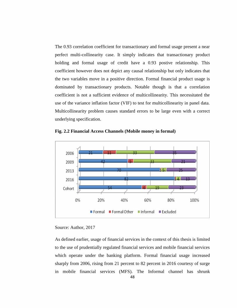
48

The 0.93 correlation coefficient for transactionary and formal usage present a near

perfect multi-collinearity case. It simply indicates that transactionary product

holding and formal usage of credit have a 0.93 postive relationship. This

coefficient however does not depict any causal relationship but only indicates that

the two variables move in a positive direction. Formal financial product usage is

dominated by transactionary products. Notable though is that a correlation

coefficient is not a sufficient evidence of multicollinearity. This necessitated the

use of the variance inflation factor (VIF) to test for multicollinearity in panel data.

Multicollinearity problem causes standard errors to be large even with a correct

underlying specification.

Fig. 2.2 Financial Access Channels (Mobile money in formal)

Source: Author, 2017

As defined earlier, usage of financial services in the context of this thesis is limited

to the use of prudentially regulated financial services and mobile financial services

which operate under the banking platform. Formal financial usage increased

sharply from 2006, rising from 21 percent to 82 percent in 2016 courtesy of surge

in mobile financial services (MFS). The Informal channel has shrunk

49

tremendously from 32.8 percent in 2006 to only 3.97 percent in 2016. The

excluded category has also fallen sharply from 35.2 percent in 2006 to 12.7

percent in 2016. Formal and other Formal channels combined, FI now stands at 83

percent up from 32 percent in 2006 reflecting a massive 160 percent increase

attributable to reforms undertaken in the financial sector, such as the introduction

of MFS in March 2007, introduction of Agency Banking in 2010, introduction of

DTMs, introduction of CRBs, amongst others.

2.6.2 Disaggregated Financial Product Usage

Usage of single financial product varies with individual preferences often

motivated by the expected utility attached to each. As such it is important to

disaggregate each product to its components to understand the contribution of each

to the particular dimension. Figure 2.2 in the appendix provides the financial usage

trends between 2006 and 2009 along the various access channels. Figure 2.3 in the

appendix on the other hand presents a cross tabulation of FI channels and gender

while Figure 2.4 presents a cross tabulation between FI and location of the

household. Figure 2.5 presents the performance of the various FI products between

2006 and 2016.

Fig. 2.5 Formal Financial Product Usage

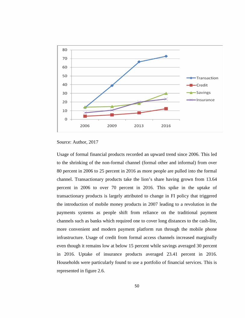
50

Source: Author, 2017

Usage of formal financial products recorded an upward trend since 2006. This led

to the shrinking of the non-formal channel (formal other and informal) from over

80 percent in 2006 to 25 percent in 2016 as more people are pulled into the formal

channel. Transactionary products take the lion’s share having grown from 13.64

percent in 2006 to over 70 percent in 2016. This spike in the uptake of

transactionary products is largely attributed to change in FI policy that triggered

the introduction of mobile money products in 2007 leading to a revolution in the

payments systems as people shift from reliance on the traditional payment

channels such as banks which required one to cover long distances to the cash-lite,

more convenient and modern payment platform run through the mobile phone

infrastructure. Usage of credit from formal access channels increased marginally

even though it remains low at below 15 percent while savings averaged 30 percent

in 2016. Uptake of insurance products averaged 23.41 percent in 2016.

Households were particularly found to use a portfolio of financial services. This is

represented in figure 2.6.

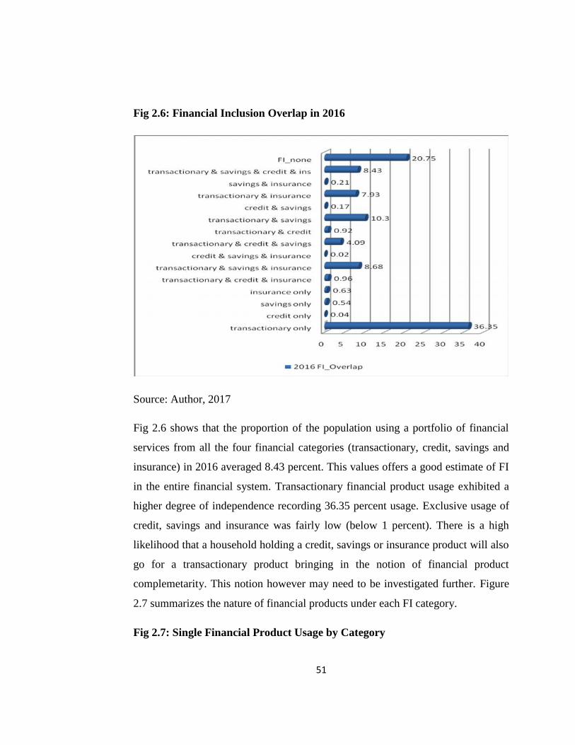
51

Fig 2.6: Financial Inclusion Overlap in 2016

Source: Author, 2017

Fig 2.6 shows that the proportion of the population using a portfolio of financial

services from all the four financial categories (transactionary, credit, savings and

insurance) in 2016 averaged 8.43 percent. This values offers a good estimate of FI

in the entire financial system. Transactionary financial product usage exhibited a

higher degree of independence recording 36.35 percent usage. Exclusive usage of

credit, savings and insurance was fairly low (below 1 percent). There is a high

likelihood that a household holding a credit, savings or insurance product will also

go for a transactionary product bringing in the notion of financial product

complemetarity. This notion however may need to be investigated further. Figure

2.7 summarizes the nature of financial products under each FI category.

Fig 2.7: Single Financial Product Usage by Category

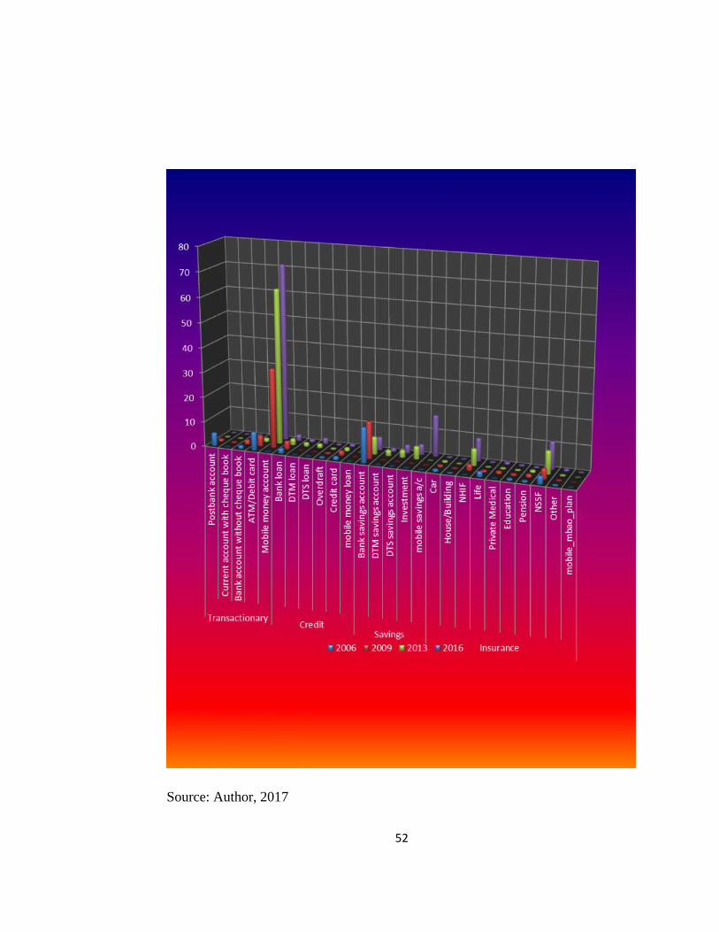
52

Source: Author, 2017

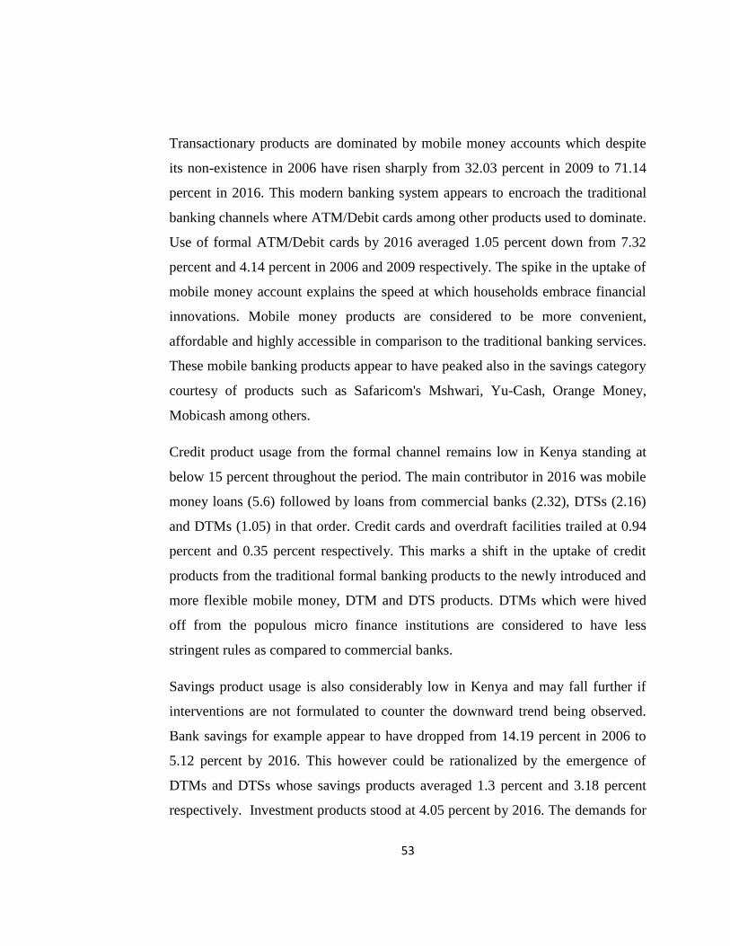
53

Transactionary products are dominated by mobile money accounts which despite

its non-existence in 2006 have risen sharply from 32.03 percent in 2009 to 71.14

percent in 2016. This modern banking system appears to encroach the traditional

banking channels where ATM/Debit cards among other products used to dominate.

Use of formal ATM/Debit cards by 2016 averaged 1.05 percent down from 7.32

percent and 4.14 percent in 2006 and 2009 respectively. The spike in the uptake of

mobile money account explains the speed at which households embrace financial

innovations. Mobile money products are considered to be more convenient,

affordable and highly accessible in comparison to the traditional banking services.

These mobile banking products appear to have peaked also in the savings category

courtesy of products such as Safaricom's Mshwari, Yu-Cash, Orange Money,

Mobicash among others.

Credit product usage from the formal channel remains low in Kenya standing at

below 15 percent throughout the period. The main contributor in 2016 was mobile

money loans (5.6) followed by loans from commercial banks (2.32), DTSs (2.16)

and DTMs (1.05) in that order. Credit cards and overdraft facilities trailed at 0.94

percent and 0.35 percent respectively. This marks a shift in the uptake of credit

products from the traditional formal banking products to the newly introduced and

more flexible mobile money, DTM and DTS products. DTMs which were hived

off from the populous micro finance institutions are considered to have less

stringent rules as compared to commercial banks.

Savings product usage is also considerably low in Kenya and may fall further if

interventions are not formulated to counter the downward trend being observed.

Bank savings for example appear to have dropped from 14.19 percent in 2006 to

5.12 percent by 2016. This however could be rationalized by the emergence of

DTMs and DTSs whose savings products averaged 1.3 percent and 3.18 percent

respectively. Investment products stood at 4.05 percent by 2016. The demands for

54

savings appear to have shifted towards mobile savings accounts whose uptake

since its inception has risen to 16.35 percent.

Usage of insurance and pension products remain low but have been rising

following the improvement of government/employee funded medical schemes.

The National Social Security Fund (NSSF) appears to dominate accounting for

11.09 percent followed by the National Hospital Insurance Fund (NHIF) at 9.11

percent. All other products scored below 1 percent. Financial product usage when

looked at along gender dimensions reveal disparities in the uptake since 2006.

Uptake of transactionary products by both genders appears to be on the rise. This

has seen the proportion of non-users fall from over 80 percent in 2006 to below 30

percent in 2013. However the change is minimal when it comes to credit and

savings products where non usage by both genders stabilized around 86 and 69

percent for credit and savings products respectively. In almost all the four

categories, males appear to record higher financial product usage than their female

counterparts. Penetration of mobile money based insurance plan is far from

universal with its market share remaining below 1 percent. The survey findings

portray a fall in the uptake of investment products since 2006 for both genders.

The geographical distribution of the various categories of financial services in the

counties is summarized in figure 2.8.

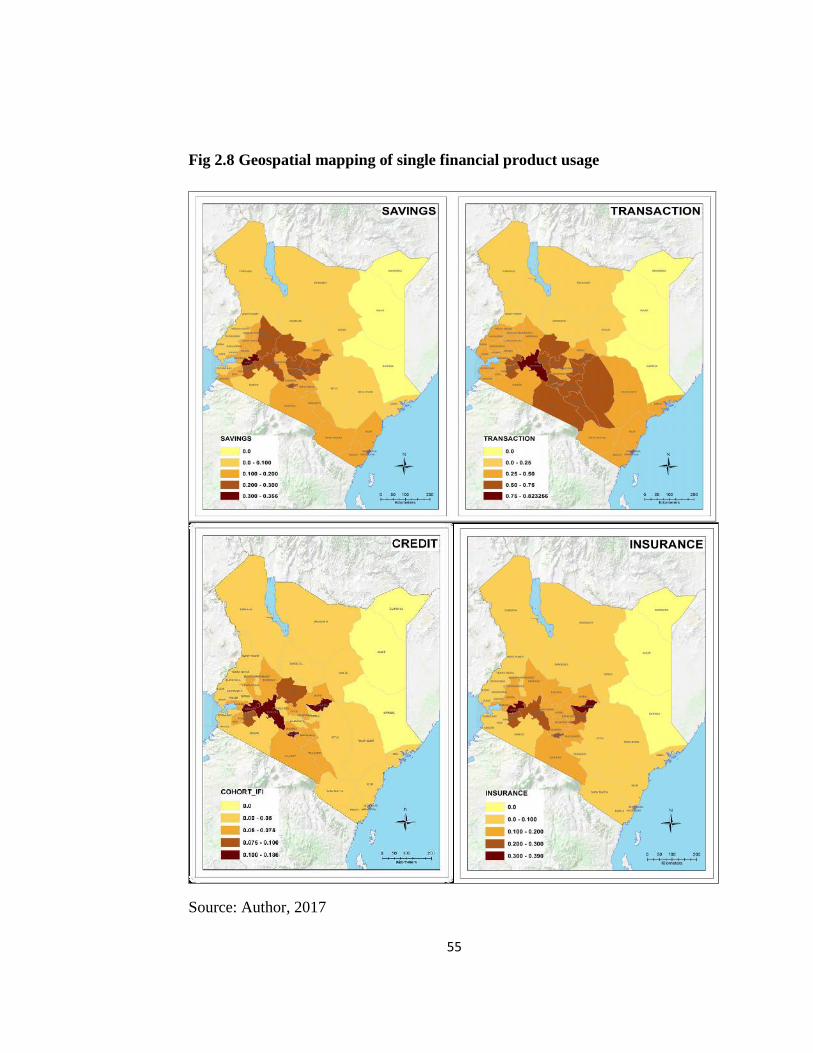
55

Fig 2.8 Geospatial mapping of single financial product usage

Source: Author, 2017

56

Kericho reported the highest uptake of savings, credit and insurance products in

the country while Nakuru County ranked highest in the uptake of transactionary

financial services. In general, the uptake of transactionary services dominated the

other product categories in most counties with insurance and credit uptake

recording low uptake as indicated in the shading. Nairobi County’s uptake of

financial services was dominated by credit products even though the uptake of

transactionary, savings and insurance was also considerable higher as compared to

the other counties. Counties in the North Rift and Upper Eastern recorded dismal

performance. Narok County which is in the South Rift also performed poorly in

the FI ranking.

Geographical separation of households accounts for the differences in the usage of

formal financial products in both the rural and urban areas. Individuals excluded

from the use of transactionary products in rural and urban areas fell from 92 and

76 percent in 2006 to 35 and 18 percent for rural and urban clusters respectively in

2016. This reduction in the excluded category however appear to widen the

transactionary product usage gap between rural and urban areas. Mobile money

accounts which takes the lions share in the transactionary product usage since its

licensing recorded a higher uptake in the urban areas (79.98 percent) than rural

areas (63.69 percent).

The market for post bank accounts, bank accounts and ATMs/debit cards appear to

have dipped following the introduction of mobile money. Despite the introduction

of DTMs and DTSs which has recorded higher uptake in rural areas, the

proportion of the population without any form of formal credit product has

stabilized around 87 percent. This low uptake of formal products is also

experienced in the savings and insurance markets and especially among the rural

populace. Given that most formal jobs are in the urban areas, NSSF and NHIF

which are a statutory deduction are skewed towards the urban populace.

57

Fig 2.9 portrays how education influences the uptake of formal financial products.

Education mirrors uptake of formal financial services pointing to the central

position held by human capital development on the financial sector. Prior to year

2009, usage of transactionary products was dominated by ATMs/debit cards. A

paradigm shift from sharp reliance on traditional banking products to mobile

banking was orchestrated by the introduction of both internet and mobile banking.

Higher education and especially tertiary level top this uptake. Individuals with no

education recorded no uptake along all the four categories of formal financial

product usage. Recent introduction of DTM and DTS loans appear to be

encroaching into the market for bank loans, credit cards and overdraft facilities.

This also applies to the savings products. NHIF and NSSF appear to take the lions

share when it comes to the usage of insurance services and especially among the

skilled persons. This is illustrated in fig 2.9.

Fig 2.9: Product usage based on Education

Transactionary

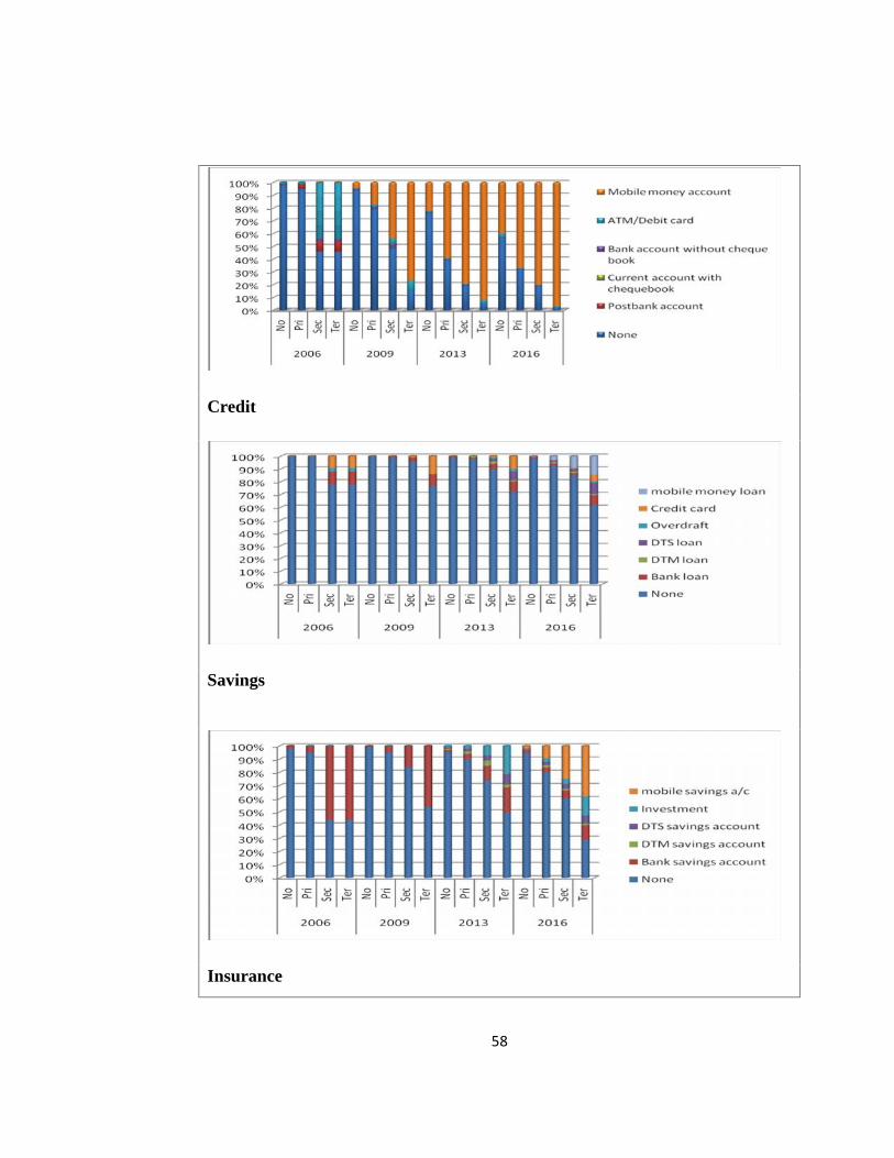
58

Credit

Savings

Insurance

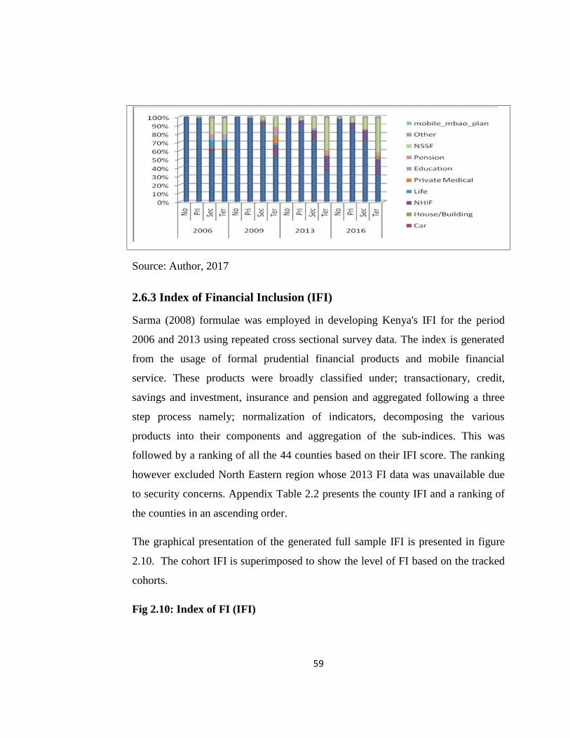
59

Source: Author, 2017

2.6.3 Index of Financial Inclusion (IFI)

Sarma (2008) formulae was employed in developing Kenya's IFI for the period

2006 and 2013 using repeated cross sectional survey data. The index is generated

from the usage of formal prudential financial products and mobile financial

service. These products were broadly classified under; transactionary, credit,

savings and investment, insurance and pension and aggregated following a three

step process namely; normalization of indicators, decomposing the various

products into their components and aggregation of the sub-indices. This was

followed by a ranking of all the 44 counties based on their IFI score. The ranking

however excluded North Eastern region whose 2013 FI data was unavailable due

to security concerns. Appendix Table 2.2 presents the county IFI and a ranking of

the counties in an ascending order.

The graphical presentation of the generated full sample IFI is presented in figure

2.10. The cohort IFI is superimposed to show the level of FI based on the tracked

cohorts.

Fig 2.10: Index of FI (IFI)

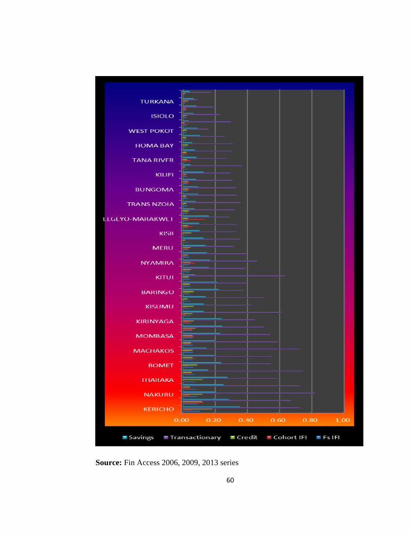
60

Source: Fin Access 2006, 2009, 2013 series

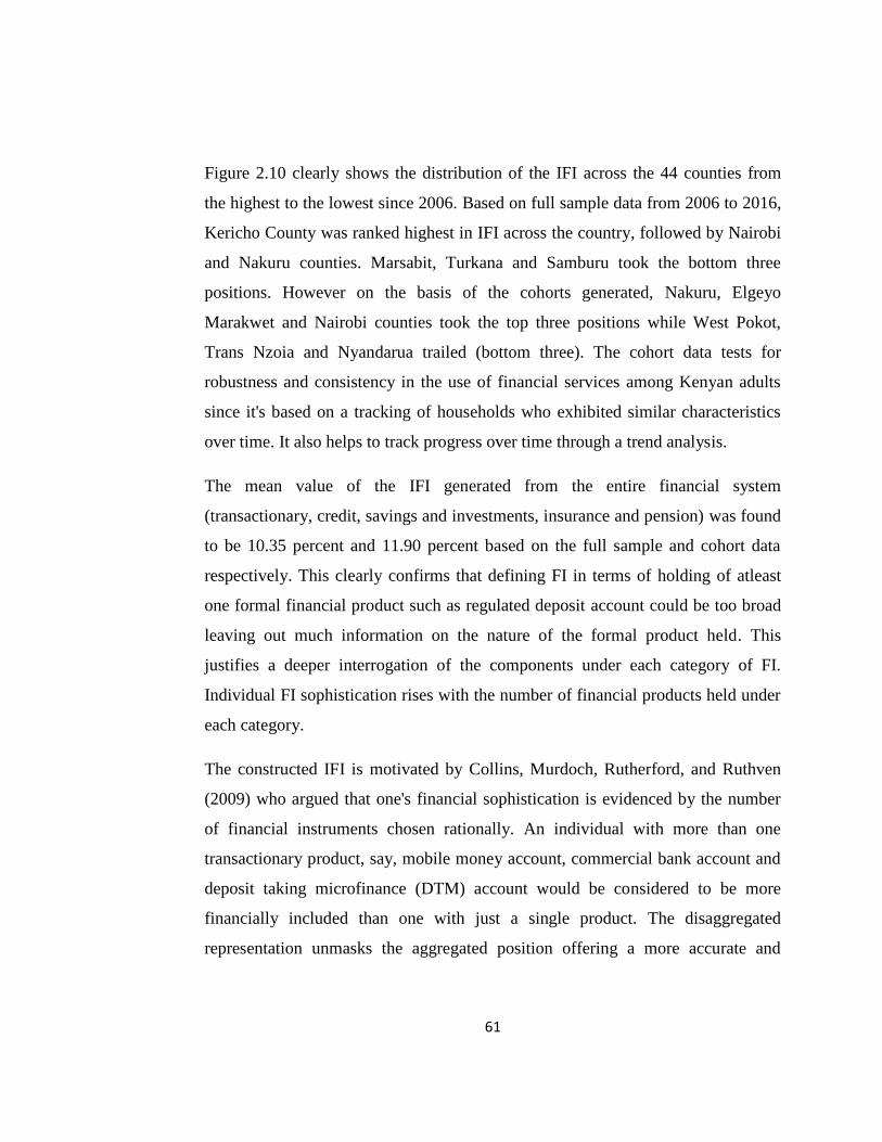
61

Figure 2.10 clearly shows the distribution of the IFI across the 44 counties from

the highest to the lowest since 2006. Based on full sample data from 2006 to 2016,

Kericho County was ranked highest in IFI across the country, followed by Nairobi

and Nakuru counties. Marsabit, Turkana and Samburu took the bottom three

positions. However on the basis of the cohorts generated, Nakuru, Elgeyo

Marakwet and Nairobi counties took the top three positions while West Pokot,

Trans Nzoia and Nyandarua trailed (bottom three). The cohort data tests for

robustness and consistency in the use of financial services among Kenyan adults

since it's based on a tracking of households who exhibited similar characteristics

over time. It also helps to track progress over time through a trend analysis.

The mean value of the IFI generated from the entire financial system

(transactionary, credit, savings and investments, insurance and pension) was found

to be 10.35 percent and 11.90 percent based on the full sample and cohort data

respectively. This clearly confirms that defining FI in terms of holding of atleast

one formal financial product such as regulated deposit account could be too broad

leaving out much information on the nature of the formal product held. This

justifies a deeper interrogation of the components under each category of FI.

Individual FI sophistication rises with the number of financial products held under

each category.

The constructed IFI is motivated by Collins, Murdoch, Rutherford, and Ruthven

(2009) who argued that one's financial sophistication is evidenced by the number

of financial instruments chosen rationally. An individual with more than one

transactionary product, say, mobile money account, commercial bank account and

deposit taking microfinance (DTM) account would be considered to be more

financially included than one with just a single product. The disaggregated

representation unmasks the aggregated position offering a more accurate and

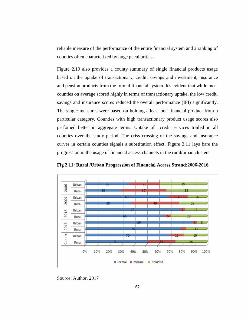
62

reliable measure of the performance of the entire financial system and a ranking of

counties often characterized by huge peculiarities.

Figure 2.10 also provides a county summary of single financial products usage

based on the uptake of transactionary, credit, savings and investment, insurance

and pension products from the formal financial system. It's evident that while most

counties on average scored highly in terms of transactionary uptake, the low credit,

savings and insurance scores reduced the overall performance (IFI) significantly.

The single measures were based on holding atleast one financial product from a

particular category. Counties with high transactionary product usage scores also

perfomed better in aggregate terms. Uptake of credit services trailed in all

counties over the study period. The criss crossing of the savings and insurance

curves in certain counties signals a substitution effect. Figure 2.11 lays bare the

progression in the usage of financial access channels in the rural/urban clusters.

Fig 2.11: Rural /Urban Progression of Financial Access Strand:2006-2016

Source: Author, 2017

63

Financial Inclusion has improved in both rural and urban areas currently standing

at 78 and 89 percent respectively. This reflects achievements in the uptake of

mobile financial services (MFS), which overcomes distance and difficult terrains

to deliver services in remote areas. Mobile banking is seen as a solution to cream

skimming due to the shared infrastructure by the creamy and non-creamy

population segments in both rural and urban areas. The Informal sector has seen

dramatic decline in rural and urban FI from a high of 37 percent and 25 percent in

2006 respectively to less than 10 percent in 2016, a reduction of over 270 percent.

However, the excluded have not dropped dramatically from 2006 to date since

almost a third of the rural population and almost 20 percent of the urban

population has no access to financial services, formal or informal. Gender and

education progression of financial access strands is presented in figure 2.13.

Fig 2.12: Gender/Education Progression of Financial Access:2006-2016

Source: Author, 2017

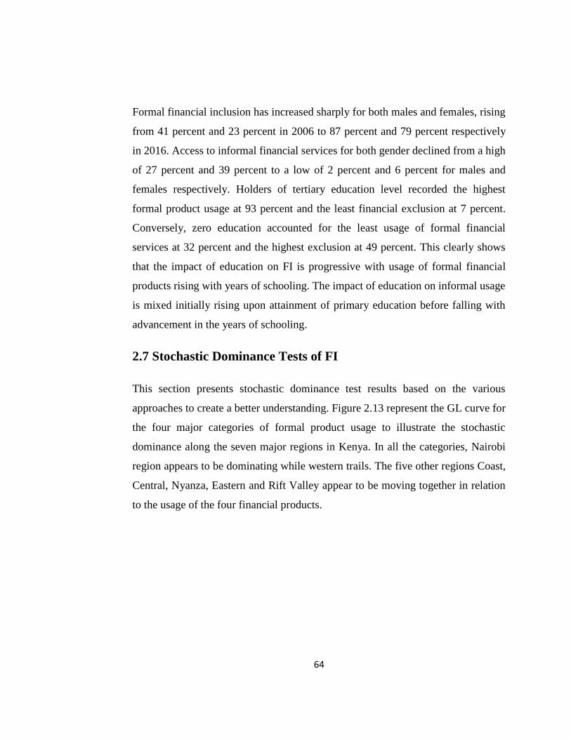
64

Formal financial inclusion has increased sharply for both males and females, rising

from 41 percent and 23 percent in 2006 to 87 percent and 79 percent respectively

in 2016. Access to informal financial services for both gender declined from a high

of 27 percent and 39 percent to a low of 2 percent and 6 percent for males and

females respectively. Holders of tertiary education level recorded the highest

formal product usage at 93 percent and the least financial exclusion at 7 percent.

Conversely, zero education accounted for the least usage of formal financial

services at 32 percent and the highest exclusion at 49 percent. This clearly shows

that the impact of education on FI is progressive with usage of formal financial

products rising with years of schooling. The impact of education on informal usage

is mixed initially rising upon attainment of primary education before falling with

advancement in the years of schooling.

2.7 Stochastic Dominance Tests of FI

This section presents stochastic dominance test results based on the various

approaches to create a better understanding. Figure 2.13 represent the GL curve for

the four major categories of formal product usage to illustrate the stochastic

dominance along the seven major regions in Kenya. In all the categories, Nairobi

region appears to be dominating while western trails. The five other regions Coast,

Central, Nyanza, Eastern and Rift Valley appear to be moving together in relation

to the usage of the four financial products.

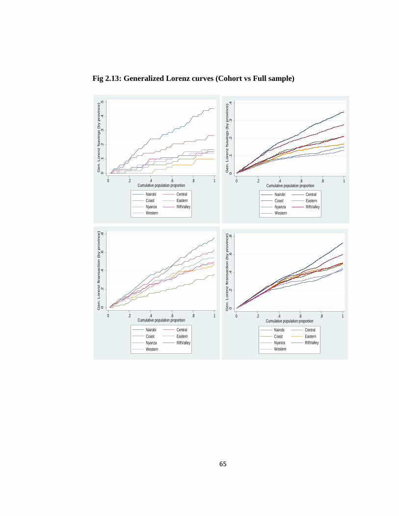
65

Fig 2.13: Generalized Lorenz curves (Cohort vs Full sample)

0.1

.2.3

.4.5

Ge

n. L

ore

nz fsa

vin

gs (

by p

rovin

ce

)

0 .2 .4 .6 .8 1Cumulative population proportion

Nairobi CentralCoast EasternNyanza RiftValleyWestern

0.1

.2.3

.4G

en. L

ore

nz fsa

vin

gs (

by p

rovin

ce

)

0 .2 .4 .6 .8 1Cumulative population proportion

Nairobi CentralCoast EasternNyanza RiftValleyWestern

0.2

.4.6

.8G

en. L

ore

nz ftr

an

saction

(b

y p

rovin

ce

)

0 .2 .4 .6 .8 1Cumulative population proportion

Nairobi CentralCoast EasternNyanza RiftValleyWestern

0.2

.4.6

.8G

en. L

ore

nz ftr

an

saction

(b

y p

rovin

ce

)

0 .2 .4 .6 .8 1Cumulative population proportion

Nairobi CentralCoast EasternNyanza RiftValleyWestern

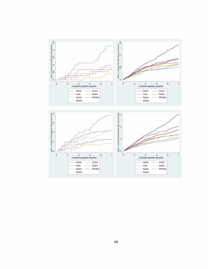
66

0.0

5.1

.15

.2.2

5G

en. L

ore

nz fcre

dit (

by p

rovin

ce

)

0 .2 .4 .6 .8 1Cumulative population proportion

Nairobi CentralCoast EasternNyanza RiftValleyWestern

0.0

5.1

.15

Ge

n. L

ore

nz fcre

dit (

by p

rovin

ce

)

0 .2 .4 .6 .8 1Cumulative population proportion

Nairobi CentralCoast EasternNyanza RiftValleyWestern

0.1

.2.3

.4G

en. L

ore

nz fin

su

ran

ce (

by p

rovin

ce

)

0 .2 .4 .6 .8 1Cumulative population proportion

Nairobi CentralCoast EasternNyanza RiftValleyWestern

0.1

.2.3

Ge

n. L

ore

nz fin

su

ran

ce (

by p

rovin

ce

)

0 .2 .4 .6 .8 1Cumulative population proportion

Nairobi CentralCoast EasternNyanza RiftValleyWestern

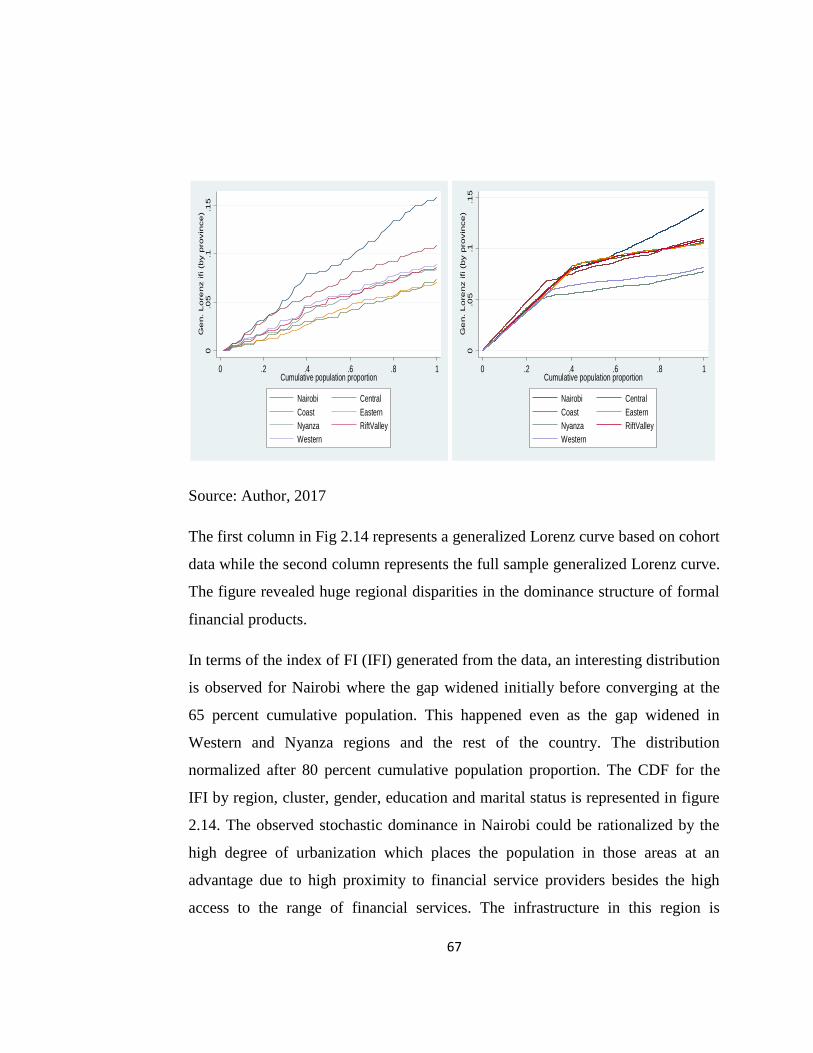
67

0.0

5.1

.15

Ge

n. L

ore

nz ifi (

by p

rovin

ce

)

0 .2 .4 .6 .8 1Cumulative population proportion

Nairobi CentralCoast EasternNyanza RiftValleyWestern

0.0

5.1

.15

Ge

n. L

ore

nz ifi (

by p

rovin

ce

)

0 .2 .4 .6 .8 1Cumulative population proportion

Nairobi CentralCoast EasternNyanza RiftValleyWestern

Source: Author, 2017

The first column in Fig 2.14 represents a generalized Lorenz curve based on cohort

data while the second column represents the full sample generalized Lorenz curve.

The figure revealed huge regional disparities in the dominance structure of formal

financial products.

In terms of the index of FI (IFI) generated from the data, an interesting distribution

is observed for Nairobi where the gap widened initially before converging at the

65 percent cumulative population. This happened even as the gap widened in

Western and Nyanza regions and the rest of the country. The distribution

normalized after 80 percent cumulative population proportion. The CDF for the

IFI by region, cluster, gender, education and marital status is represented in figure

2.14. The observed stochastic dominance in Nairobi could be rationalized by the

high degree of urbanization which places the population in those areas at an

advantage due to high proximity to financial service providers besides the high

access to the range of financial services. The infrastructure in this region is

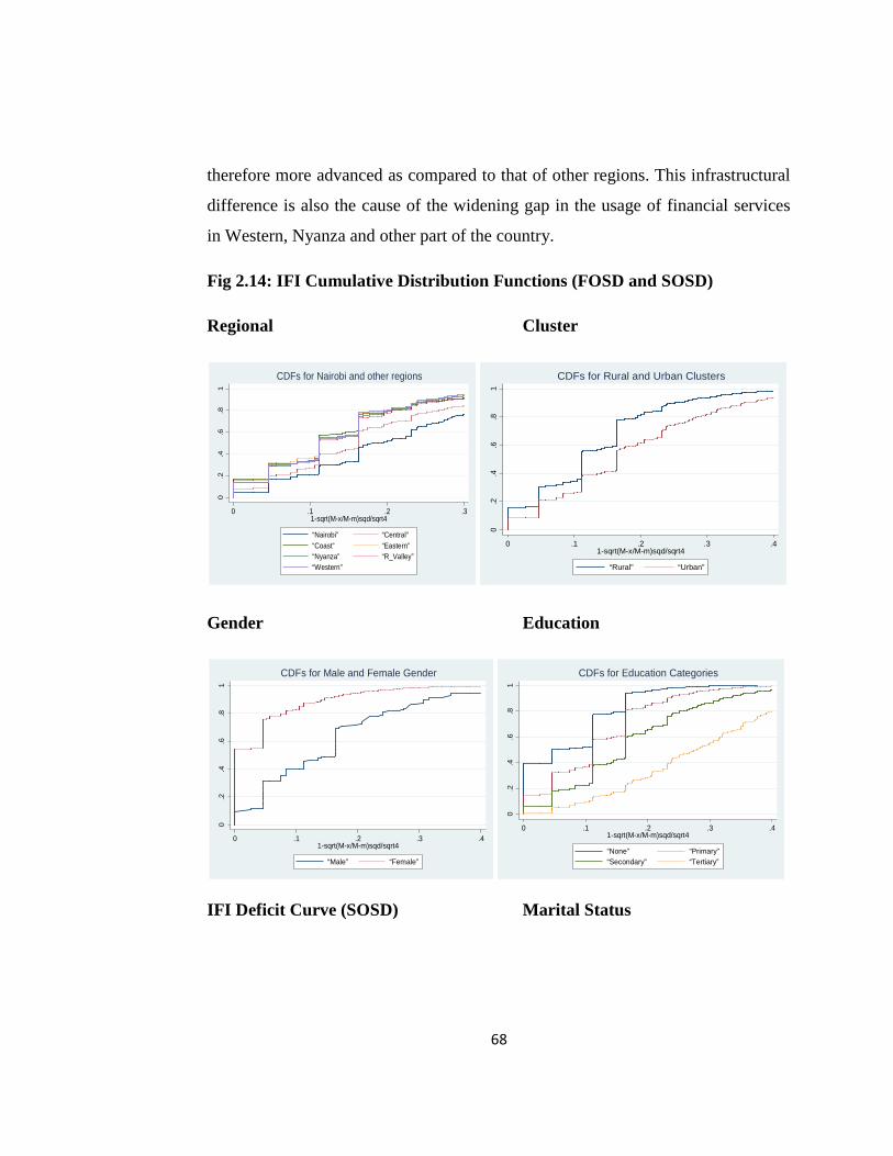
68

therefore more advanced as compared to that of other regions. This infrastructural

difference is also the cause of the widening gap in the usage of financial services

in Western, Nyanza and other part of the country.

Fig 2.14: IFI Cumulative Distribution Functions (FOSD and SOSD)

Regional Cluster

0.2

.4.6

.81

0 .1 .2 .31-sqrt(M-x/M-m)sqd/sqrt4

“Nairobi” “Central”“Coast” “Eastern”“Nyanza” “R_Valley”“Western”

CDFs for Nairobi and other regions

0.2

.4.6

.81

0 .1 .2 .3 .41-sqrt(M-x/M-m)sqd/sqrt4

“Rural” “Urban”

CDFs for Rural and Urban Clusters

Gender Education

0.2

.4.6

.81

0 .1 .2 .3 .41-sqrt(M-x/M-m)sqd/sqrt4

“Male” “Female”

CDFs for Male and Female Gender

0.2

.4.6

.81

0 .1 .2 .3 .41-sqrt(M-x/M-m)sqd/sqrt4

“None” “Primary”“Secondary” “Tertiary”

CDFs for Education Categories

IFI Deficit Curve (SOSD) Marital Status

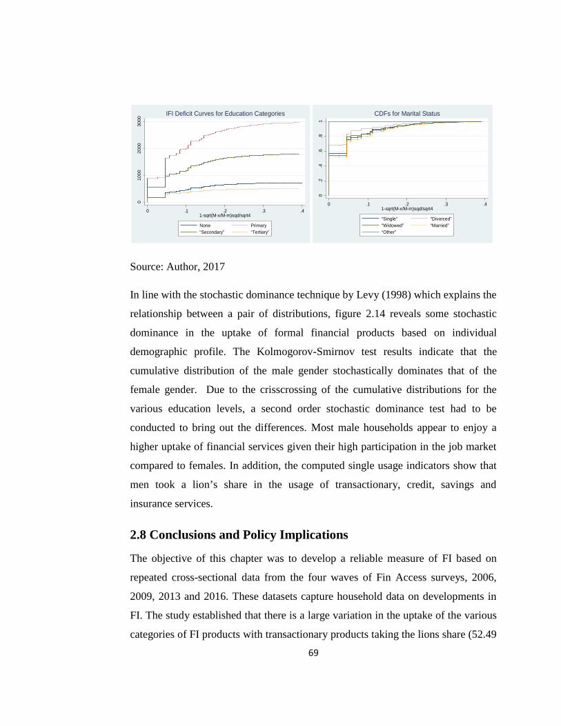
69

010

0020

0030

00

0 .1 .2 .3 .41-sqrt(M-x/M-m)sqd/sqrt4

None Primary“Secondary” “Tertiary”

IFI Deficit Curves for Education Categories

0.2

.4.6

.81

0 .1 .2 .3 .41-sqrt(M-x/M-m)sqd/sqrt4

“Single” “Divorced”“Widowed” “Married”“Other”

CDFs for Marital Status

Source: Author, 2017

In line with the stochastic dominance technique by Levy (1998) which explains the

relationship between a pair of distributions, figure 2.14 reveals some stochastic

dominance in the uptake of formal financial products based on individual

demographic profile. The Kolmogorov-Smirnov test results indicate that the

cumulative distribution of the male gender stochastically dominates that of the

female gender. Due to the crisscrossing of the cumulative distributions for the

various education levels, a second order stochastic dominance test had to be

conducted to bring out the differences. Most male households appear to enjoy a

higher uptake of financial services given their high participation in the job market

compared to females. In addition, the computed single usage indicators show that

men took a lion’s share in the usage of transactionary, credit, savings and

insurance services.

2.8 Conclusions and Policy Implications

The objective of this chapter was to develop a reliable measure of FI based on

repeated cross-sectional data from the four waves of Fin Access surveys, 2006,

2009, 2013 and 2016. These datasets capture household data on developments in

FI. The study established that there is a large variation in the uptake of the various

categories of FI products with transactionary products taking the lions share (52.49

70

percent) followed by savings and investment (21.65 percent), insurance (16.9

percent) and credit (8.96 percent) in that order. The disparity is also evident along

the different counties where Kericho, Nairobi and Nakuru accounted for the lions

share in terms of the index of financial inclusion (IFI) as compared to the rest of

the country. Marsabit, Turkana and Samburu trailed all other counties by recording

the lowest IFI. In terms of regional uptake, out of the seven regions considered,

Eastern region trailed in the usage of formal financial services hence stochastically

dominated by all other regions. Nairobi region which is predominantly urban was

ranked highest. This could be rationalized by the proximity of the urban population

to financial access channels.

The study findings signaled a paradigm shift from the over reliance on traditional

transactionary banking products such as debit/ ATM cards, bank accounts among

other to the more flexible and readily accessible mobile money accounts. Policy on

mobile financial services led to a revolution in the financial sector leading to

deepened financial markets. A similar picture was observed in the uptake of

savings following the amendment of the Microfinance Act and the SACCO Act

that brought in DTM and DTS savings which appear to be encroaching into the

market for traditional bank savings and investments to increase its market share.

The same picture is reflected in the use of credit products where uptake of bank

loans is falling. But even with the introduction of new products, savings and credit

usage has remained low since 2006 and more particularly among the rural

populace.

Gender disparity in the uptake of financial products since 2006 persists. The FI

distribution of the male gender stochastically dominates the female distribution

across all financial products. The distribution of the urban cluster also dominates

usage of the more flexible mobile financial products as compared to the

distribution of the rural population. The distribution of insurance services on the

71

other hand is stochastically dominated by that of NHIF and NSSF products which

takes the lions share. In all the categories of formal product usage, that is;

transactionary, credit, savings and insurance, the distribution for tertiary education

to a large extent appear to stochastically dominate the other education levels.

This chapter recommends that the government should encourage even distributions

of financial services to all counties to minimize the dominance by certain segments

of the population. With the low credit counts reported, the government through the

credit information sharing (CIS) Kenya should intensify the compilation of credit

reports by extending it to the agriculture sector which is the mainstay of our

country’s economy to ensure that the rural population mainly involved in

agriculture benefit from low cost credit products. In addition, more effort should

be put to ensure that DTMs and DTMs get the necessary support to increase their

market share in the supply of financial services. Given the sharp focus accorded on

the access and usage of financial inclusion in this chapter, it will be interesting to

see how the impact and quality dimensions of FI plays out in future.

72

Chapter Three: Determinants of Financial Inclusion in

Kenya

3.1 Introduction

Access to financial services forms a key tenet of financial inclusion (FI).

Demirguc-Kunt and Klapper (2012) posits that close to 3 billion people face

exclusion from formal financial services globally. This exclusion is more

pronounced in Africa, Asia, Latin America and the Middle East where 2.2 billion

of the unbanked adults are found. Usage of formal services is mainly skewed

towards the wealthy triggering a surge in the global efforts to unearth barriers to FI

especially among the less privileged who rely on informal mechanisms such as

holding savings in form of assets such as livestock and other risky and more

expensive credit from informal money lenders (Collins et al., 2009; Susan and

Zarazua, 2011).

Enhanced access to a broad range of prudentially regulated financial services

devoid of both price and non-price barriers are often linked to improved

livelihoods (Collins et al., 2009). Rochadi (2010) breaks down the objectives of FI

into four distinct goals namely; affordable access to a wide range of financial

services, choice and security institutions, financial and institutional sustainability

and competition.

Despite the growing interest in FI, literature specific to determinants of FI at the

micro level remains scanty (Allen et al., 2012). Susan and Zarazua (2011) study on

Kenya and Uganda singled out agro-ecological and socio-cultural factors as some

of the barriers to FI. A huge uptake of financial services is an indicator that the war

against price and non-price barriers to financial access and usage is being won.

Financial exclusion due to frictions in the financial system (Galor and Zeira, 1993)

only serve to worsen the plight of the poor as they resort to disposing their limited

73

assets to meet their basic needs. This challenge is aggravated by the presence of

imperfections in the market which manifest in form of; information asymmetry

(Stiglitz and Weiss, 1981), adverse selection and moral hazard. These

imperfections force the players to charge high interest rates among other

requirements such as collateral in order to cushion themselves against default

risks.

Total market failure occurs when lenders keep on adjusting the interest rate on

loans to factor in the risk profile of borrowers. The interest charged reaches a point

where only high risk borrowers can participate. At this rate, not even the lender is

comfortable to offer credit facility since they are not sure of recouping their

returns. Lack of this collateral, poor credit history, lack of guarantors and high

interest rate charge on loans limit access to financial services leading to persistent

poverty and poor welfare.

Banerjee and Newman (1993) explain the process of economic development where

poor human capital development and particularly occupational choice is linked to

initial resource constraints. This in turn affects the source of livelihood by

individuals and the overall economic growth and welfare state. Addressing moral

hazard is mainly done through monitoring or incentivizing borrowers so that they

declare the true outcome. This is captured in the state verification models

(Diamond, 1984). The full impact of market imperfections can only be understood

through studies on financial products usage and barriers to usage. Persons

subjected to non-price barriers such as geographical location or lack of markets

face a vertical supply curve at the origin with demand curves which never intersect

creating another access problem.

World Bank (2008) posits that without an inclusive financial system, poor

individuals and small enterprises have to rely on their own limited savings and

earnings to build their human capital and pursue growth opportunities. The point

74

of intersection between the supply and demand curve depends on the relative cost

of providing financial services and income of users of financial services.

Strengthening of the institutional infrastructure, market liberalization, increased

competition and technological innovations offer solutions to an improved uptake

of financial services.

Even though remarkable progress has been recorded in the uptake of financial

services, lack of a proper understanding of the drivers of FI from a household

perspective poses serious challenges to expanding financial services to the less

privileged in the society. Its only through an empirical study that barriers to FI can

be identified and mitigation strategies developed to reverse the trend. The

disaggregation of FI measures to the county levels is expected to bring out the

peculiar features that characterize the various counties.

National mitigation strategies to minimize financial exclusion should therefore be

tailored to the specific barriers faced by each county. Financial exclusion which is

mainly dominated by the bottom of the pyramid population (extremely poor) can

be unlocked through intensive research of the determinants of FI (FSD, 2013).

Data on FI reveals a huge segment of the population without any form of access to

financial services. An inclusive financial system accelerates growth and

development through increased supply of financial services as well as increased

access and usage of a range of financial services.

The main objective of this chapter was to explore the determinants of financial

inclusion in Kenya from both a single and composite measurement perspective.

The specific objectives as derived from the broad objectives for this chapter

include;

1) To examine the determinants of single financial product usage in Kenya

2) To examine the determinants of usage of a portfolio of financial services

75

3) To examine the determinants of choice of financial access channel

3.2 Literature on Determinants of FI

Studies on the determinants of FI invoke theories of financial development. Sen

(1981) argued that FI is a consequence of financial development. Both supply side

and demand side factors act as barriers to FI. They include; gender (Demirguc-

Kunt et al., 2013; Hoyos et al., 2014; Camara and David, 2015); human capital

development (Demirguc-Kunt and Klapper, 2012; Nelson and Phelps, 1996);

institutions (Acemoglu et al., 2001; La Porta et al., 1997; Mayer and Sussman,

2001), interest groups (Rajan and Zingales, 2003), inflation (Huybens and Smith,

1999; Boyd et al., 2001), autarky (Do and Levchenko, 2004; Bekaert et al., 2002),

geographical barriers (Acemoglu et al., 2001; Sachs, 2003; Levine, 2003), resource

endowment (Diamond, 1997; Easterly and Levine, 2003), income per capita

(Greenwood and Jovanovic, 1990; Levine, 2005; Jaffee and Levonian, 2001),

culture (Stulz and Williamson, 2003). Kempson and Whyley (1999) cite credit

unworthiness, geographical location, and cultural factors.

Other barriers include; both cost and non-cost factors, the main one being lack of

money as cited by an average of 80 percent of all non-account holders (AfDB,

2013). 30 percent of the adult non account holders cited ; cost, distance and

insufficient documentation as barriers to financial access in Africa (Demirguc-

Kunt and Klapper, 2012).

3.2.1 Theoretical Literature

The role of institutions in enhancing financial development is well established in

literature. Financial development according to Acemoglu et al. (2001) trail areas

where institutions were established by the colonialists. These institutions shape the

path of development. The settler mortality hypothesis explains how colonizers

established extractive states in areas that they felt were not fit for settlement

76

probably due to the malaria scourge. Geographical location which largely operates

from the demand side appears to define the kind of institutions to be established.

Development of the financial system takes place faster under the Common Law

setting as compared to the French civil law. Acemoglu et al. (2001) further states

that economic institutions are the ones which inform the incentives and constraints

that shape human interaction and economic outcomes.

Porta (1997; 1998) in his legal origin seminal contribution argues that the source

of the legal code matters in enhancing efficiency in contract enforcement. This

knowledge is what informed the establishment of financial sector regulators and

also the formulation of prudential guidelines to govern the formal financial sector.

Porta (1998) further argues that strong institutions for protecting and matching the

investor needs enhance financial development.

Countries governed by the Common Law from the British for example appear to

value private property ownership while the French Civil Law advocates for state

property ownership since inefficiency impairs financial development. The law and

finance theory posit that legal traditions which shape differences in financial

development differ on the basis of their emphasis on either private or state

property ownership rights as well as their ability to adjust to the dynamics of the

commercial and financial conditions. This implies that the pace of financial

development is determined by past legal traditions. The political channel opines

that legal traditions vary depending on how they prioritize private property rights

and those of investors in firms. The international differences in financial

development are therefore informed by how private property and investors are

protected. This rationale is what gave birth to the English common law.

The legal adaptability channel on the other hand shows that differences in legal

traditions are shaped by the ability to adapt to changing commercial and financial

conditions. Those legal systems that adapt quickly to minimize friction between

77

the economy's needs and the legal system's capabilities are considered to be more

effective in promoting financial development (Beck et al., 2001). It's difficult

however to establish the exact channel through which legal traditions influence

financial development.

The political and finance theory also recognizes the critical role played by the

political process and interest groups in shaping financial development (Ranjan and

Zingales, 2003). This theory challenges the significance of the legal traditions in

shaping financial development by arguing that whereas financial development has

changed significantly over the last century, the legal traditions across countries

appear not to have changed at all. Legal traditions are therefore more of a fixed

factor compared to political factors which change over time.

Pagano and Volpin (2001) associates politically closed economies with low

reliance on external funding for fear that it may end up diluting their political

power. Kenya in the 1991 for example, broke ranks with the Breton woods

institutions leading to withdrawal of external finance for failing to comply with

some of the recommendations under the structural adjustment programs (SAPs) of

reducing the size of the public service. Economic reforms in the early 2000

renewed Kenya's relations with the Bretton Woods institutions weakening the

political pressures. This led to the opening up to international trade and finance in

line with Rajan and Zingales (2003) predictions leading to accelerated financial

system development. Political interests often shape the manner in which a country

opens up its economy hence affecting the pace of financial development.

The role of policy frameworks such as fiscal and monetary policy has also been

mentioned in the literature as being key in influencing the direction of financial

development. This is in the context of macroeconomic policies, openness of the

financial markets as well as financial liberalization. Christensen (2004) associates

poor management of fiscal policy and particularly increased government

78

borrowing to a crowding out effect of private investors. This hinders the

development of the financial system which is mainly driven by the private sector.

While openness of the economy to the outside world is considered to be a key

determinant of financial development, Chinn and Ito (2006) argued that opening

the financial sector only works well in an environment where there are strong

institutions and legal systems. Advocates of financial liberalization further argue

that it works best in an environment of economic stability devoid of many

uncertainties. Inflation was also mentioned as one of the macroeconomic variables

that affect financial development (Huybens and Smith, 1999). Economic

uncertainties especially in the macroeconomic fundamentals lead to a surge in

inflation and reduced participation in the financial market. This limits the

expansion of the financial sector curtailing development (Boyd et al., 2001).

The endowment theory also challenged the efficacy of the legal traditions in

shaping financial development and instead advocated for the role played by

geography, topology and disease environment of a country as being critical in

shaping the development of legal and financial institutions. Geography shapes

financial development through proximity to the equator. Countries closer to the

tropics are likely to experience low crop yields and high disease prevalence

hindering large scale farming which is critical for specialization, innovation and

institutional development (Sachs, 2003). Landlocked countries also limit

international trade.

Other theoretical frameworks consider the role of economic growth (income per

capita), population, religion, ethnicity, culture among others as being critical in

determinants of FI (Huang (2011). Culture and finance for example associate

Catholiscm and Islam with xenophobia and close-mindedness which inhibit

competition in financial markets due to the presence of strong hierarchical political

structures. Huang (2010) however conceives that existing theories do not offer

79

solutions as to which variables play a primary role in determining financial

development.

This model uncertainty problem according to Levine and Renelt (1992) pushes

economic thinking to fragile and non-robust results when a cross section model is

estimated. The authors therefore recommend the use of an extreme bounds

analysis and the Bayesian method to counter the model uncertainty problem. This

study introduces a new innovation to tackle model uncertainty problem by

applying repeated cross sectional survey data (pseudo panel) to estimate the

determinants of financial inclusion on a small sample made of cohort panels.

3.2.2 Empirical Literature

Despite the orchestrated growth in financial inclusion in Kenya, usage of financial

services and especially for the rural poor remains a mirage. This is especially so in

Kenya and other sub Saharan African countries where access to financial services

trail the high income economies. Campero and Kaiser (2013) categorize

determinants of FI into either supply side (distance, cost among others) or demand

side (individual specific factors such as income, education and age as well as

behavioral traits and perceptions). The study however mentions a number of non-

financial factors such as telecommunications development, individual

characteristics, and culture and policy implementation as potential barriers to FI.

World Bank (2015) echoes these sentiments by arguing that attitudes and

perceptions held by individuals shape the choice of financial services. Tuesta et al.,

2015; Honohan and King, 2012; Allen et al., 2012 associate usage of formal

financial services to education level, income, gender, urbanization and age.

Alliance for Financial Inclusion (2014; 2010) asserts that barriers to financial

inclusion vary from country to country the main ones being; high transaction costs

in the delivery of small scale financial services across large geographic distances,

lack of data, infrastructure constraints such as poor road and communication

80

network, poor security systems, trust, low financial literacy and information

asymmetry. Emergence of formal and semi-formal financial services targeting the

poor has contributed heavily to the changing financial landscape13.

Using the financial access survey data for Kenya and Uganda, Johnson and Nino-

Zarazua (2011) singled out age, employment, education and gender as some of the

determinants of FI. The authors challenged the notion that urban areas enjoy

higher access to financial services in comparison to rural areas. They established

that what matters most are region specific characteristics. More women than men

accounted for a higher overall financial exclusion. In trying to link poverty with

financial inclusion, the authors adopted food security as an indicator of poverty.

Estimation using a logistic technique established that those individuals

experiencing food shortages sometimes reported a lower probability of financial

inclusion although the risk of financial exclusion remained low.

A regional assessment of the geographical spread of financial services could help

bring out the role of other socioeconomic and cultural factors besides physical

proximity. In terms of regional spread, North Eastern and Coast provinces reported

a much higher probability of financial exclusion compared to Nairobi. Nyanza and

Eastern are half as likely while Central is less likely. The study further established

that formal financial inclusion is not significantly associated with province or rural

when other factors are held constant (Johnson and Nino-Zarazua, 2011).

Honohan and King (2012) applied multivariate probit and OLS regressions on the

financial access survey data for selected African countries. Their research on cause

and effect of financial access in banking the world established that FI increased

with urbanization, male gender, education, and age. The variable gender however

produced a non-significant relationship with FI. The authors also associated access

13 The 2014 Alliance for Financial Inclusion (AFI) Global Policy Forum

81

to formal financial services with improved incomes especially where access to

finance changed gradually. Financial literacy, ownership of mobile phone and trust

in commercial banks exhibited a positive relationship with financial access.

Chithra and Selvam (2013) in a study on determinants of FI in China using Sarma

(2008) index singled out socioeconomic factors, income, literacy and population as

some of the main determinants. They also established a very close link between FI

and banking variables, mainly deposit and credit penetration. The ratio of credit to

deposits and investment ratio was however not significant in explaining FI. Singh

and Kodan (2012) appeared to support the role of income per capita in influencing

FI in addition to the level of urbanization. The findings however differed with

Chithra and Selvam (2013) in relation to literacy which was found not to

significantly explain FI. Sex ratio and unemployment were also found not to be

significant.

Sarma, 2008; Honohan, 2008; Sarma and Pias, 2011 identified low income groups,

ethnic minorities, immigrants and the aged as leading in financial exclusion but

also argued that the rural poor located far away from the FSPs bore a higher risk of

being excluded. Other factors include; adult literacy, urbanization, infrastructure

and especially communication development, distance, cost and identity proof

(Agrawal, 2008). Park and Mercado (2015) cited per capita income, rule of law

and demographic characteristics as the main constraints to FI in developing

countries.

With the advent of mobile and agency banking for both commercial banks and

DTMs, the distance covered to reach a FSP has been falling especially for the

urban leaving it as a barrier only associated with the rural poor due to poor

infrastructural facilities. Hannig and Jansen (2010) argue that policy makers are

currently involved in developing mechanisms to overcome barriers to access

through narrowing the gap between documentation threshold required by banks

82

and quality of documentation prevalent among low income clients. Regulators are

expected to decide on the level of risk they can take to promote financial inclusion.

Most risks to the financial sector are attributed to the large number of vulnerable

clients with limited balances and small value transactions. The authors associate

greater FI with improved financial stability.

Demirguc-Kunt et al. (2013) presents a very strong case of gender differences in

the use of financial services based on individual level data covering 98 developing

countries. The analysis of the Global Findex data established significant gender

gaps in the usage of financial services. This echoes IMF (2012) Financial Access

Survey which indicated that usage of accounts among men was higher than that of

women even though the disparity was not so pronounced. Cross country variation

in the use of financial services to is associated with legal discrimination of women

and gender norms (Demirguc-Kunt et al., 2013). These legal restrictions include;

the ability to work and head a household while gender norms include; violence

against women and early marriage. Lack of systematic indicators of financial

inclusion is seen as the main drawback to the enhancement of gender parity in the

formal financial system.

Findings from Allen et al. (2014) in their analysis of financial development and

financial inclusion in Africa singled out population density as one of the most

important variable shaping FI in Africa. Using the Global Findex data, the authors

classified FI into three broad measures namely; percentage of adults with a formal

account; percentage of adults with a formal loan and percentage of adults using

mobile banking. The study asserted that considerable barriers associated with

infrastructural handicaps have been overcome by mobile banking.

Whereas a formal access to credit gap was established for Africa, a statistically

significant financial inclusion gap along formal accounts could not be established

even though it was consistent with the emergence of alternative delivery channels

83

such as bank branch expansion to underserved areas in Kenya (Allen et al., 2014).

The paper acknowledges that in spite of the huge success of mobile banking in

Kenya, the success was only limited to sending and receiving money calling for a

different approach such as agency banking to promote financial inclusion

especially along the savings and credit channel. Proper identification of barriers to

financial inclusion helps in shaping policy formulation through a targeted

approach.

Adult literacy rate averages 87.4 percent in Kenya (Kippra, 2012). However, low

levels of human capital development as captured by the level of education may be

a contributing factor to financial exclusion. The FinAccess survey (2013) show the

proportion of financially excluded among those with no education averages 60.7

percent compared to only 1.8 percent among those with tertiary education.

Improved human capital development through education can therefore have lasting

impact on financial inclusion which will in turn promote growth and improved

welfare. This is echoed by IMF (2012) where progression towards formal FI

appeared to rise with age (25-64) and level of education (tertiary education).

Han and Melecky (2013) on formal financial inclusion in 123 countries covering

124,000 persons contend that low costs and close proximity to financial

intermediaries promote high usage of formal accounts. Elimination of barriers to

operation of formal accounts holds the key to increased financial inclusion.

Akudugu (2013) in estimating a logit model on determinants of FI in formal

financial markets in Ghana using the World Bank, 2012 Global Financial Inclusion

Index found a 40 percent level of inclusion along the formal strand with money

poverty being one of the determinants. The study cites rules and regulations in

operations which hinder them from enrolling the rural populace as the main

challenges facing formal financial markets. Formal financial access in Ghana is

considered to be a preserve of the financially well up people. This explains why

84

participation in formal financial markets by the poor was 62 percent less than that

of the rich.

Fadun (2014) and Ayyagari (2013) examined the role of financial inclusion and

outreach in Nigeria and India respectively and established that financial inclusion

is dominant in urban areas with the highest concentration of formally included

persons being recorded in South West Nigeria (49 percent against 19 percent for

North West). A whopping 80.4 percent of the financially excluded adults reside in

rural Nigeria the main determinants being; geographical separation from banks,

low economic activity and poor literacy rates. Similar findings were reported in

Clarke, Xu and Zou (2006). Kempson and Whyley (1999) cited credit

unworthiness, geographical location and culture as some of the barriers to FI. It

would be interesting to see how issues discussed in these studies play out in

Kenya.

3.2.3 Overview of literature

Some of the theoretical foundations used to motivate this chapter included the role

of institutions in enhancing financial development, political and finance theories

that shape financial development through political processes and interest groups,

openness of economies, endowment theories, fiscal and monetary policies, among

others. Empirical literature on the determinants of FI has identified a number of

socioeconomic factors which shape household choice of financial services. Access

to a broad range of financial services is considered to be instrumental in shaping

key economic outcomes such as household income, consumption expenditure and

poverty eradication. However, the attainment of this objective is often complicated

by the limited access to a broad range of financial services which is approximated

to be in the range of 3 billion adults globally. This huge proportion of the

financially excluded adults poses a serious threat to the attainment economic

development and poverty eradication.

85

Beck et al. (2014) argue that financial intermediation only stabilize the economy in

the medium term in low income countries. The issue of costs and the risk of

missing targeted markets pose a major challenge to government organs trying to

broaden access. Morduch (1999) dimensions of access comprise of; reliability,

convenience, continuity and flexibility of financial services. Financial exclusion

could either be voluntary (cultural or religious reasons) or involuntary (external

factors such as lack of education, income, price, weak contract enforcement,

discrimination among others) (Amidzic et al., 2014).

Key barriers cited in the literature include; limited income, financial illiteracy and

gender discrimination. The barriers however appear to vary with the financial

product. Much of the literature reviewed dwelt largely on the determinants of

single product usage without concerning itself with the determinants of FI from a

composite index perspective. In addition, the categorization of formal financial

products along transactionary, credit, savings and insurance offers an exhaustive

way of capturing access to a broad range of financial services in Kenya. None of

the reviewed literature has incorporated the four dimensions of FI in their analysis

hampering investigation of the performance of the entire financial system. This

broad spectrum helps in drawing a quick comparative analysis to inform on what

drives FI from the demand side. This in turn guides financial service providers in

designing products that are tailored to customer needs.

3.3 Empirical Framework

Deaton (1985; 1986) and Christiaensen and Subbarao (2004) pseudo panel

technique was used in analyzing the determinants of FI in this chapter. This

technique provides a mechanism through which household relationships are

analyzed on the basis of cohort means from repeated cross sections in the absence

of true panel. In a case where the data has a small T and a large N, Econometrica

(1981) suggests that use of a one way fixed effects model could lead to a Nickel

86

bias where the demeaning process creates a correlation between the regressor and

the error term. Anderson-Hsiao estimator which uses the second lag of the

dependent variable to instrument the dependent variable in first differences also

despite being consistent fails to factor in all potential orthogonality conditions

(Arrelano and Bond, 1991).

The more powerful Arellano and Bond estimator which allows for the use of

lagged values of the instrumented variable is considered to be more robust where

T is small and N large. This estimator sets up a GMM with a system of equations

carrying different instruments in each equation. This estimator is however

weakened by stating that the lagged levels offer weak instruments for first

differenced variables and especially those close to a random walk (Arellano and

Bover (1995) and Blundell and Bond (1998)).

Arellano and Bover (1995) and Blundell and Bond (1998) therefore recommends

the inclusion of both the lagged levels and lagged differences now the so called

system GMM which is an improved version of the original differenced GMM.

Arellano and Bover (1995) forward orthogonal deviations transforms each

observation by subtracting the average of all future observations for all

observations except the last irrespective of any existing gaps (Roodman, 2006).

This helps overcome the magnified gaps in the first differenced transformation

where one period of missing data is replaced with two missing differences.

Given that single product measures of FI are binary, panel estimation for binary

data is applied based on both fixed effects and random effects. The determination

of the most consistent method of estimation is done using Haussmann specification

test. Estimation of single product usage of financial services (categorical) applies

both fixed (FE) and Random effects (RE) estimation for binary data to bring out

the drivers and barriers to FI. The index of FI (IFI) is subjected to GMM

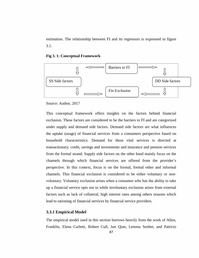
87

estimation. The relationship between FI and its regressors is expressed in figure

3.1.

Fig 3. 1: Conceptual Framework

Source: Author, 2017

This conceptual framework offers insights on the factors behind financial

exclusion. These factors are considered to be the barriers to FI and are categorized

under supply and demand side factors. Demand side factors are what influences

the uptake (usage) of financial services from a consumers perspective based on

household characteristics. Demand for these vital services is directed at

transactionary; credit, savings and investments and insurance and pension services

from the formal strand. Supply side factors on the other hand mainly focus on the

channels through which financial services are offered from the provider’s

perspective. In this context, focus is on the formal, formal other and informal

channels. This financial exclusion is considered to be either voluntary or non-

voluntary. Voluntary exclusion arises when a consumer who has the ability to take

up a financial service opts not to while involuntary exclusion arises from external

factors such as lack of collateral, high interest rates among others reasons which

lead to rationing of financial services by financial service providers.

3.3.1 Empirical Model

The empirical model used in this section borrows heavily from the work of Allen,

Franklin, Elena Carletti, Robert Cull, Jun Qian, Lemma Senbet, and Patricio

Barriers to FI

SS Side factors DD Side factors

Fin Exclusion

88

Valenzuela (2014) which focused on the determinants of FI in Africa. The

estimable model can be stated as follows;

...................................................................................(1)i i iFI X Where; FIi captures the constructed financial inclusion measure (single product

and composite measure).

represents the parameter estimates

iX represents a vector of explanatory variables which include; age, gender,

location, education

i represents the error term

Given the panel setup, households with similar characteristics are tracked in

successive surveys to establish the dynamic relationship of parameters in a linear

model The error component structure is assumed to have zero mean and constant

variance The GMM is applied to derive the parameters after which lagged values

of the endogenous variable from an auxiliary regression are used as instruments in

a dynamic model (Mckenzie, 2004). The static model is expressed as;

1 2 3 4 5 6 7

8 9 10 11 12 13 tan ...(2)it it it it it it it it

it it it it it it it

fi income age agesq hhsize hhsqrd male education

married banktrust socialcapital finlit urban dis ce u

The instruments included in the model are subjected to the Sargan-Hansen test of

over identified restrictions to assess whether the instruments are jointly exogenous.

This is in addition to the autoregressive test for autocorrelation to check for the

presence of serial correlation among residuals. Deeper lags help overcome the

serial correlation problem.

89

The main weakness associated with this model is that it assumes that repeated

observations of the households are independent hence ignoring the unmeasured or

unobservable differences. To factor in both cross sectional and time heterogeneity,

the households are organized into cohorts. The constructed pseudo panel is

estimated using cohort (c) means rather than individual observations.

The estimable model includes robust standard errors derived using generalized

least squares (GLS) estimation. It’s good to note that GMM estimation method

makes use of orthogonality conditions to allow for efficient estimation in the

presence of heteroscedasticity of unknown form. The model assumes that

instrumental variables are orthogonal to the errors (Roodman, 2006). The

instrumental variable regression is also unbiased in the presence of autocorrelation

since the reported standard errors allow for asymptotically correct inference in the

presence of autocorrelation of almost any form. Besides, the estimation corrects

the variance covariance matrix for heteroscedasticity and autocorrelation

(Roodman, 2006). The determinants of FI are estimated using panel regression for

binary outcomes in the case of single product measures while GMM estimation is

applied on the estimation of determinants of IFI (Arrelano and Bover, 1995).

Random effects estimators (RE) which captures a weighted average of fixed and

between effects leads to consistent estimators if individual effects are uncorrelated

with the other regressors. However in a case where individual effects are

correlated with regressors, then fixed effects estimators (FE) are more consistent

since RE will be inefficient. Results from the panel estimation with robust standard

errors are compared with those from a pooled estimation based on a full sample.

These results may however not be sufficient for policy since a static cohort panel

assumes independence between the response variables given the covariates

justifying the need for a dynamic estimation with a lagged dependent variable as a

regressor.

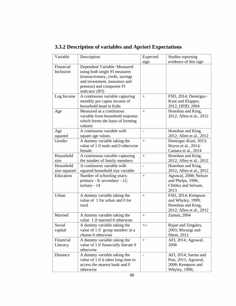
90

3.3.2 Description of variables and Apriori Expectations

Variable Description Expectedsign

Studies reportingevidence of this sign

FinancialInclusion

Dependent Variable: Measuredusing both single FI measures(transactionary, credit, savingsand investment, insurance andpension) and composite FIindicator (IFI)

Log Income A continuous variable capturingmonthly per capita income ofhousehold head in Kshs

+ FSD, 2014; Demirguc-Kunt and Klapper,2012; DFID, 2004

Age Measured as a continuousvariable from household responsewhich forms the basis of formingcohorts

+ Honohan and King,2012; Allen et al., 2012

Agesquared

A continuous variable withsquare age values

- Honohan and King,2012; Allen et al., 2012

Gender A dummy variable taking thevalue of 1 if male and 0 otherwisefemale

+ Demirguc-Kunt, 2013;Hoyos et al., 2014;Camara et al., 2014

Householdsize

A continuous variable capturingthe number of family members

+ Honohan and King,2012; Allen et al., 2012

Householdsize squared

A continuous variable withsquared household size variable

- Honohan and King,2012; Allen et al., 2012

Education Number of schooling years;primary - 8; secondary - 12;tertiary - 14

+ Agrawal, 2008; Nelsonand Phelps, 1996;Chithra and Selvam,2013

Urban A dummy variable taking thevalue of 1 for urban and 0 forrural

+ FSD, 2014; Kempsonand Whyley, 1999;Honohan and King,2012; Allen et al., 2012

Married A dummy variable taking thevalue 1 if married 0 otherwise

+ Zaman, 2004

Socialcapital

A dummy variable taking thevalue of 1 if group member in achama 0 otherwise

+/- Rajan and Zingales,2003; Mwangi andShem, 2012

FinancialLiteracy

A dummy variable taking thevalue of 1 if financially literate 0otherwise

+ AFI, 2014; Agrawal,2008

Distance A dummy variable taking thevalue of 1 if it takes long time toaccess the nearest bank and 0otherwise

- AFI, 2014; Sarma andPias, 2011; Agrawal,2008; Kempson andWhyley, 1999;

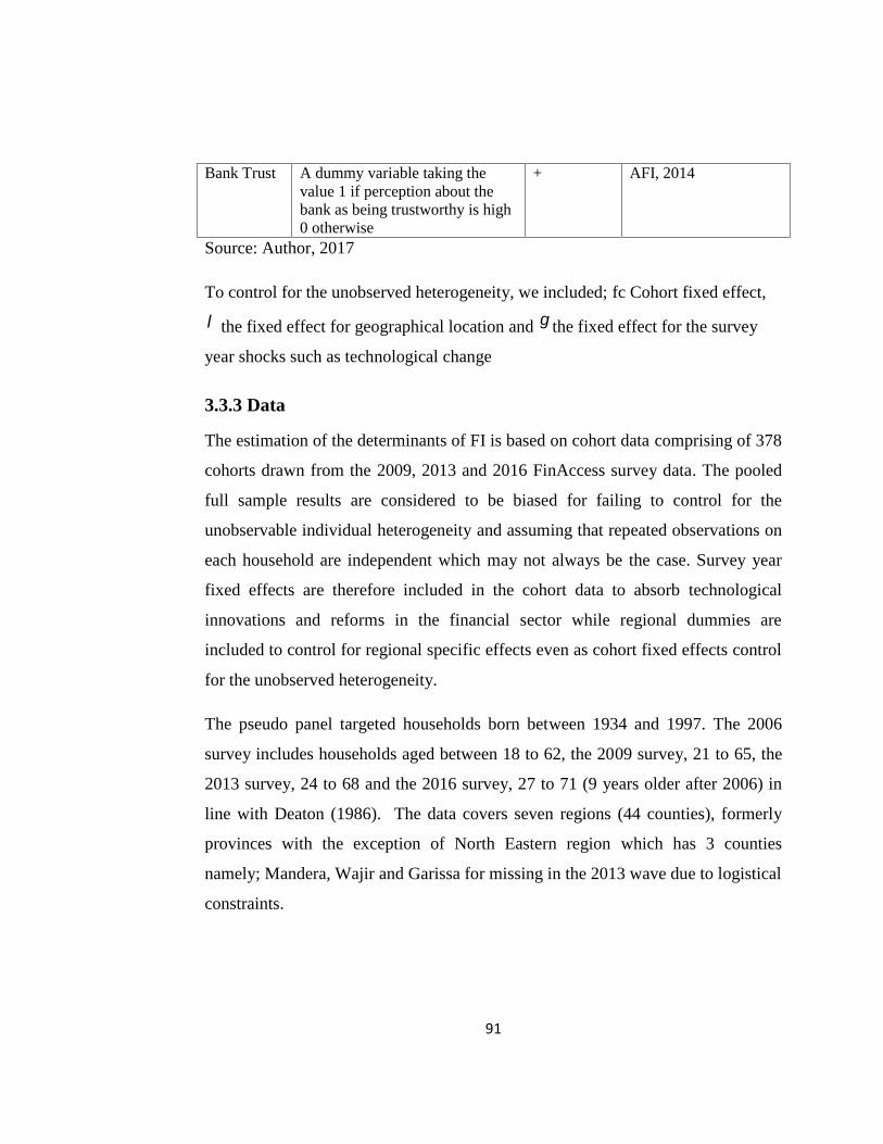
91

Bank Trust A dummy variable taking thevalue 1 if perception about thebank as being trustworthy is high0 otherwise

+ AFI, 2014

Source: Author, 2017

To control for the unobserved heterogeneity, we included; fc Cohort fixed effect,

the fixed effect for geographical location and the fixed effect for the survey

year shocks such as technological change

3.3.3 Data

The estimation of the determinants of FI is based on cohort data comprising of 378

cohorts drawn from the 2009, 2013 and 2016 FinAccess survey data. The pooled

full sample results are considered to be biased for failing to control for the

unobservable individual heterogeneity and assuming that repeated observations on

each household are independent which may not always be the case. Survey year

fixed effects are therefore included in the cohort data to absorb technological

innovations and reforms in the financial sector while regional dummies are

included to control for regional specific effects even as cohort fixed effects control

for the unobserved heterogeneity.

The pseudo panel targeted households born between 1934 and 1997. The 2006

survey includes households aged between 18 to 62, the 2009 survey, 21 to 65, the

2013 survey, 24 to 68 and the 2016 survey, 27 to 71 (9 years older after 2006) in

line with Deaton (1986). The data covers seven regions (44 counties), formerly

provinces with the exception of North Eastern region which has 3 counties

namely; Mandera, Wajir and Garissa for missing in the 2013 wave due to logistical

constraints.

92

3.4 Econometric Results and Discussion

This section provides a detailed account of the determinants of FI based on a panel

estimation using both FE and RE as well as GMM estimation. Interpretation of the

determinants is based on the odds ratios since coefficients only inform on the

signs. The odds ratio informs on the ratio between the probability that an event

will occur (success) and the probability that an event doesn't occur (failure). The

odds ratio is therefore a monotonic transformation of probability of events

occurrence hence increase with the increase in probability and vice versa.

3.4.1 Diagnostic Tests

Bias in FI elasticities could emanate from errors of specification, measurement or

omission of variables. Differencing individual panels was used in GMM

estimation to control for this. On the other hand, heteroscedasticity is corrected by

decomposing data into between and within dimensions and computing the exact

heteroscedasticity on both dimensions. The main problem that characterizes

repeated cross sectional data is its failure to track same individuals over time

limiting the use of historical attributes in computing deviations from the mean.

Establishing which model between FE and RE is consistent in panel estimation

requires a Haussmann specification test. This was applied in the five

autoregressive dynamic models of FI and the three autoregressive models of

financial access channels. The difference in the estimated coefficients is bigger

when RE is efficient and smaller otherwise. On the other hand, FE model is

consistent when individual effects are correlated with other regressors. However if

that assumption doesn't hold, both FE or RE estimators are consistent but RE being

more efficient is adopted. In our case, the Haussmann test results (Appendix Table

3.1) reported a large test statistic with a huge difference between RE and FE

estimation only under the transactionary and formal transmission channels. This

justifies the use of FE estimation in the two autoregressive models. RE estimation

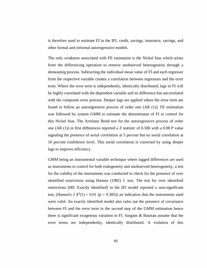
93

is therefore used to estimate FI in the IFI, credit, savings, insurance, savings, and

other formal and informal autoregressive models.

The only weakness associated with FE estimation is the Nickel bias which arises

from the differencing operation to remove unobserved heterogeneity through a

demeaning process. Subtracting the individual mean value of FI and each regressor

from the respective variable creates a correlation between regressors and the error

term. Where the error term is independently, identically distributed, lags in FI will

be highly correlated with the dependent variable and its difference but uncorrelated

with the composite error process. Deeper lags are applied where the error term are

found to follow an autoregressive process of order one (AR (1)). FE estimation

was followed by system GMM to estimate the determinants of FI to control for

this Nickel bias. The Arrelano Bond test for the autoregressive process of order

one (AR (1)) in first differences reported a Z statistic of 0.586 with a 0.08 P value

signaling the presence of serial correlation at 5 percent but no serial correlation at

10 percent confidence level. This serial correlation is corrected by using deeper

lags to improve efficiency.

GMM being an instrumental variable technique where lagged differences are used

as instruments to control for both endogeneity and unobserved heterogeneity, a test

for the validity of the instruments was conducted to check for the presence of over

identified restrictions using Hansen (1982) J. test. The test for over identified

restrictions (H0: Exactly identified) in the IFI model reported a non-significant

test, (Hansen's J X2(1) = 0.01 (p = 0.385)) an indication that the instruments used

were valid. An exactly identified model also rules out the presence of covariance

between FI and the error term in the second step of the GMM estimation hence

there is significant exogenous variation in FI. Sargans & Basman assume that the

error terms are independently, identically distributed. A violation of this

94

assumption means we use heteroscedasticity robust standard errors. This is

captured in Table 3.1a.

Table 3.1a: Test for over identified restrictions

Panel 1: IFI ModelSargan test of overid. restrictions: chi2(4) = 4.16 Prob > chi2 = 0.385

(Not robust, but not weakened by many instruments.)

Hansen test of overid. restrictions: chi2(4) = 4.15 Prob > chi2 = 0.386

(Robust, but weakened by many instruments.)

Difference-in-Hansen tests of exogeneity of instrument subsets:

GMM instruments for levels

Hansen test excluding group: chi2(2) = 0.51 Prob > chi2 = 0.774

Difference (null H = exogenous): chi2(2) = 3.64 Prob > chi2 = 0.162Panel ii: Formal Access Strands ModelSargan test of overid. restrictions: chi2(2) = 3.03 Prob > chi2 0.22

(Not robust, but not weakened by many instruments.)

Hansen test of overid. restrictions: chi2(2) = 3.43 Prob > chi2 0.18

(Robust, but weakened by many instruments.)

Difference-in-Hansen tests of exogeneity of instrument subsets:

GMM instruments for levels

Hansen test excluding group: chi2(0) = 0.96 Prob > chi2 .

Difference (null H = exogenous): chi2(2) = 2.47 Prob > chi2 0.29

Source: Author, 2017

Multicollinearity test was carried out on the determinants of IFI among Kenyan

households. Multicollinearity arises from a violation of the Ordinary Least Squares

(OLS) assumption due to a correlation of explanatory variables in a model. Where

the multicollinearity score is high, an inflation of the variance of OLS estimates

occurs leading to a reduction in the t-statistic hence a Type-2 error where the

researcher ends up accepting the null hypothesis which otherwise ought to have

been rejected. Under extreme cases of perfect multicollinearity, the estimated

parameters are indeterminate and their standard errors infinite. The test results for

multicollinearity based on variance inflation factor (VIF) are summarized in Table

3.1b.

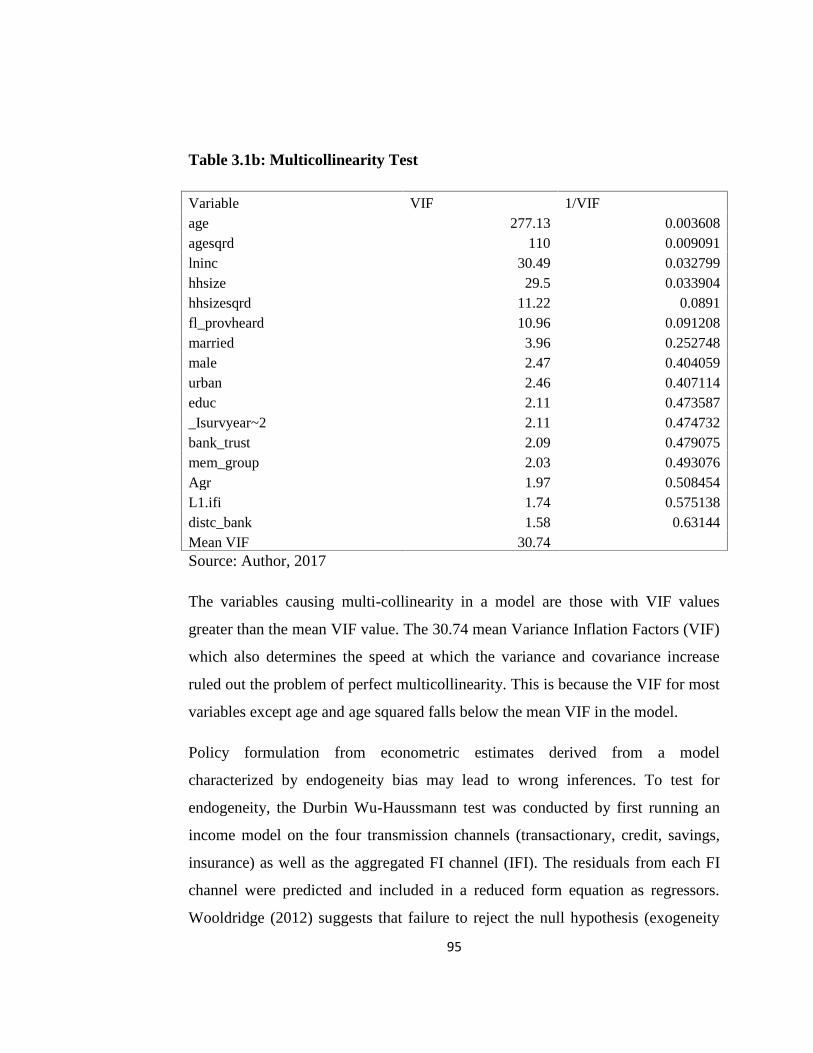
95

Table 3.1b: Multicollinearity Test

Variable VIF 1/VIFage 277.13 0.003608agesqrd 110 0.009091lninc 30.49 0.032799hhsize 29.5 0.033904hhsizesqrd 11.22 0.0891fl_provheard 10.96 0.091208married 3.96 0.252748male 2.47 0.404059urban 2.46 0.407114educ 2.11 0.473587_Isurvyear~2 2.11 0.474732bank_trust 2.09 0.479075mem_group 2.03 0.493076Agr 1.97 0.508454L1.ifi 1.74 0.575138distc_bank 1.58 0.63144Mean VIF 30.74Source: Author, 2017

The variables causing multi-collinearity in a model are those with VIF values

greater than the mean VIF value. The 30.74 mean Variance Inflation Factors (VIF)

which also determines the speed at which the variance and covariance increase

ruled out the problem of perfect multicollinearity. This is because the VIF for most

variables except age and age squared falls below the mean VIF in the model.

Policy formulation from econometric estimates derived from a model

characterized by endogeneity bias may lead to wrong inferences. To test for

endogeneity, the Durbin Wu-Haussmann test was conducted by first running an

income model on the four transmission channels (transactionary, credit, savings,

insurance) as well as the aggregated FI channel (IFI). The residuals from each FI

channel were predicted and included in a reduced form equation as regressors.

Wooldridge (2012) suggests that failure to reject the null hypothesis (exogeneity

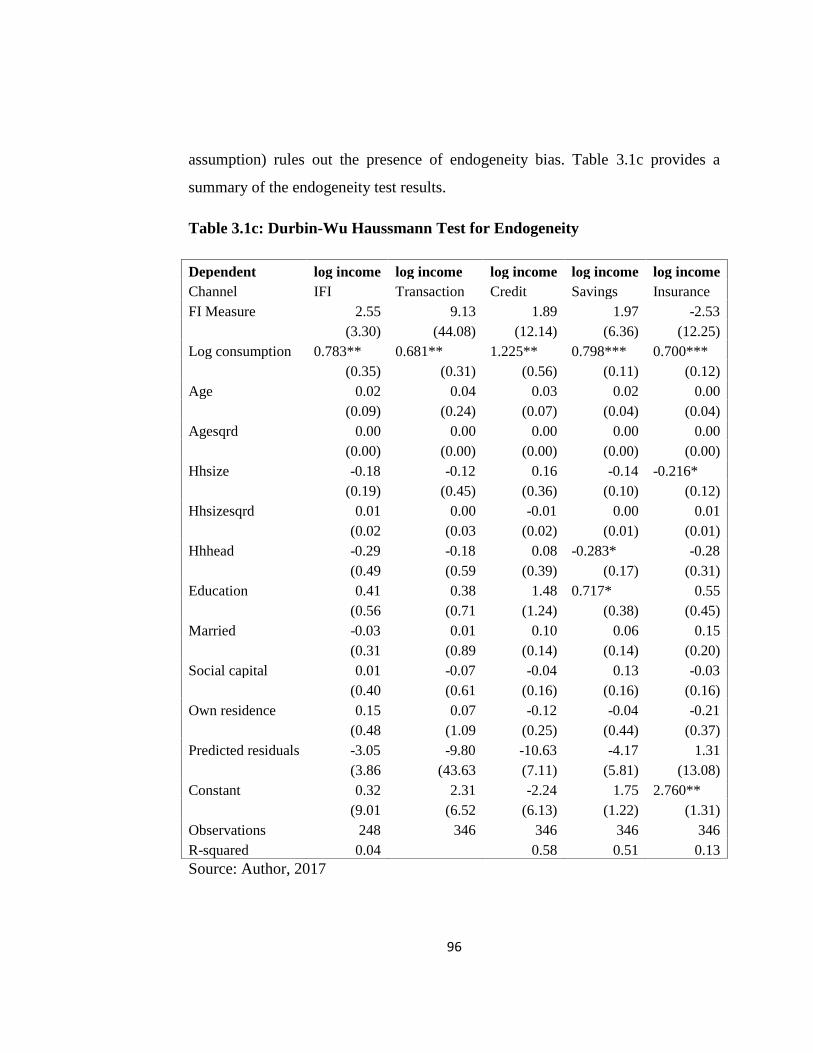
96

assumption) rules out the presence of endogeneity bias. Table 3.1c provides a

summary of the endogeneity test results.

Table 3.1c: Durbin-Wu Haussmann Test for Endogeneity

Dependent log income log income log income log income log incomeChannel IFI Transaction Credit Savings InsuranceFI Measure 2.55 9.13 1.89 1.97 -2.53

(3.30) (44.08) (12.14) (6.36) (12.25)Log consumption 0.783** 0.681** 1.225** 0.798*** 0.700***

(0.35) (0.31) (0.56) (0.11) (0.12)Age 0.02 0.04 0.03 0.02 0.00

(0.09) (0.24) (0.07) (0.04) (0.04)Agesqrd 0.00 0.00 0.00 0.00 0.00

(0.00) (0.00) (0.00) (0.00) (0.00)Hhsize -0.18 -0.12 0.16 -0.14 -0.216*

(0.19) (0.45) (0.36) (0.10) (0.12)Hhsizesqrd 0.01 0.00 -0.01 0.00 0.01

(0.02 (0.03 (0.02) (0.01) (0.01)Hhhead -0.29 -0.18 0.08 -0.283* -0.28

(0.49 (0.59 (0.39) (0.17) (0.31)Education 0.41 0.38 1.48 0.717* 0.55

(0.56 (0.71 (1.24) (0.38) (0.45)Married -0.03 0.01 0.10 0.06 0.15

(0.31 (0.89 (0.14) (0.14) (0.20)Social capital 0.01 -0.07 -0.04 0.13 -0.03

(0.40 (0.61 (0.16) (0.16) (0.16)Own residence 0.15 0.07 -0.12 -0.04 -0.21

(0.48 (1.09 (0.25) (0.44) (0.37)Predicted residuals -3.05 -9.80 -10.63 -4.17 1.31

(3.86 (43.63 (7.11) (5.81) (13.08)Constant 0.32 2.31 -2.24 1.75 2.760**

(9.01 (6.52 (6.13) (1.22) (1.31)Observations 248 346 346 346 346R-squared 0.04 0.58 0.51 0.13Source: Author, 2017

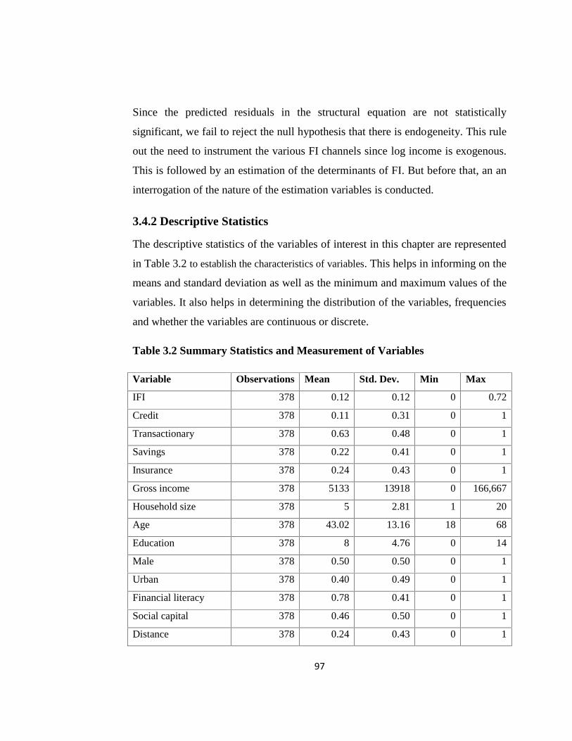
97

Since the predicted residuals in the structural equation are not statistically

significant, we fail to reject the null hypothesis that there is endogeneity. This rule

out the need to instrument the various FI channels since log income is exogenous.

This is followed by an estimation of the determinants of FI. But before that, an an

interrogation of the nature of the estimation variables is conducted.

3.4.2 Descriptive Statistics

The descriptive statistics of the variables of interest in this chapter are represented

in Table 3.2 to establish the characteristics of variables. This helps in informing on the

means and standard deviation as well as the minimum and maximum values of the

variables. It also helps in determining the distribution of the variables, frequencies

and whether the variables are continuous or discrete.

Table 3.2 Summary Statistics and Measurement of Variables

Variable Observations Mean Std. Dev. Min Max

IFI 378 0.12 0.12 0 0.72

Credit 378 0.11 0.31 0 1

Transactionary 378 0.63 0.48 0 1

Savings 378 0.22 0.41 0 1

Insurance 378 0.24 0.43 0 1

Gross income 378 5133 13918 0 166,667

Household size 378 5 2.81 1 20

Age 378 43.02 13.16 18 68

Education 378 8 4.76 0 14

Male 378 0.50 0.50 0 1

Urban 378 0.40 0.49 0 1

Financial literacy 378 0.78 0.41 0 1

Social capital 378 0.46 0.50 0 1

Distance 378 0.24 0.43 0 1

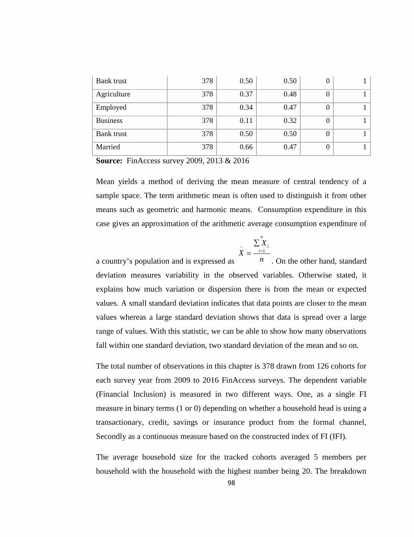
98

Bank trust 378 0.50 0.50 0 1

Agriculture 378 0.37 0.48 0 1

Employed 378 0.34 0.47 0 1

Business 378 0.11 0.32 0 1

Bank trust 378 0.50 0.50 0 1

Married 378 0.66 0.47 0 1

Source: FinAccess survey 2009, 2013 & 2016

Mean yields a method of deriving the mean measure of central tendency of a

sample space. The term arithmetic mean is often used to distinguish it from other

means such as geometric and harmonic means. Consumption expenditure in this

case gives an approximation of the arithmetic average consumption expenditure of

a country’s population and is expressed as1

n

ii

XX

n

. On the other hand, standard

deviation measures variability in the observed variables. Otherwise stated, it

explains how much variation or dispersion there is from the mean or expected

values. A small standard deviation indicates that data points are closer to the mean

values whereas a large standard deviation shows that data is spread over a large

range of values. With this statistic, we can be able to show how many observations

fall within one standard deviation, two standard deviation of the mean and so on.

The total number of observations in this chapter is 378 drawn from 126 cohorts for

each survey year from 2009 to 2016 FinAccess surveys. The dependent variable

(Financial Inclusion) is measured in two different ways. One, as a single FI

measure in binary terms (1 or 0) depending on whether a household head is using a

transactionary, credit, savings or insurance product from the formal channel,

Secondly as a continuous measure based on the constructed index of FI (IFI).

The average household size for the tracked cohorts averaged 5 members per

household with the household with the highest number being 20. The breakdown

99

of age revealed that the average age for the sampled households averaged 43 years

falling between 18 and 68 years for the youngest and oldest member of household

respectively. Education variable which is measured in terms of schooling years of

the representative household in the cohort averaged 8 years meaning that a

majority of the sampled households only went as far as primary education is

concerned (8 years of schooling). Secondary school attainment is represented

using 12 schooling years while tertiary education level is represented using 14

years of schooling.

The male population and the urbanized population captured as 1 and 0 averaged

0.5 and 0.4, signaling equitable distribution of the sampled population. The study

identified a number of financial related terms to test households’ financial literacy

levels. 78 percent of the households were found to be conversant with the listed

financial inclusion terms. The study also incorporated the role of social capital in

shaping FI from both the demand and supply side. This variable was captured by

assessing whether a household is a member of atleast one chama (investment

group). 46 percent of the adult population was found to have subscribed to a group

membership.

Per adult equivalent income of the representative household was found to average

Ksh. 5,133 lying between Ksh 13,918 and Ksh. 166,667. This is captured as log

per capita income in the econometric estimation. The distance variable captured as

1 if distance is long and 0 otherwise showed that 24 percent of the sampled

households felt that the distance covered to get to the nearest financial service

provider was long. The challenge of travelling long distance to the nearest bank

especially among the poor appears to have been largely addressed by mobile

financial services which enhance a shared infrastructure for both creamy and non-

creamy households mainly in urban and rural households respectively. 57 percent

of the sampled households were also found to hold a perception that interest

100

charged by commercial banks is high. 66 percent of the household heads were also

found to be married.

3.5. Determinants of Financial Inclusion and Access channels

Understanding the determinants of FI from both a demand (usage) and supply

(access) perspective is what shapes policy discussions.

Given that three waves of the financial access survey are considered, econometric

estimation of the determinants of FI includes three survey year dummies to capture

unobservable time effects for each wave. Other variables included are the

demographic and socioeconomic characteristics of the representative households.

This chapter provides a cohort estimation of the determinants of both the

composite and single financial product usage as well as the choice of financial

access channel using panel estimation techniques.

3.5.1 Econometric results of the static and dynamic model of FI

Results from the full sample econometric estimation of the determinants of FI

from the product usage and access channels based on the 2006, 2009, 2013 and

2016 data is presented in Appendix Tables 3.3 and 3.4 respectively. As mentioned

earlier, pooled full sample estimation assumes that households are independent

hence ignore both cross sectional and time heterogeneity inherent in the data.

Econometric results on the static and dynamic estimation of the determinants of FI

usage (transactionary, credit, savings, insurance and IFI) and financial access

channels using cohort data are presented in Appendix Tables 3.5 and 3.6 followed

by Arrelano and Bover (1995) system GMM estimation to correct for Nickel bias

associated with FE models (Econometrica, 1981). A dynamic analysis of FI

informs on the impact of past decisions made by households on financial

deepening. Static results made use of the 504 observations (126 cohorts multiplied

by 4 survey years) while dynamic estimation made use of 378 observations (126

101

cohorts multiplied by 3 survey years) since a lagging of the dependent variable

leads to a loss of one survey year. RE in the results table stands for Random

Effects while FE stands for Fixed Effects whose selection was informed by

Haussmann specification test.

Omission of a lagged dependent variable in a static model limits a correlation

between the demeaned lagged dependent variable and the demeaned lag process.

This justifies use of a dynamic estimation to assess whether households past

actions have any bearing on current choices.

The R-squared which shows the degree of variation in the dependent variable

explained by the model ranged between 34 percent and 71 percent for

transactionary, credit, savings and insurance models. These values imply that the

model explains between 34 and 71 percent of the variation in FI.. This being a

pseudo panel, the model is well cast hence a good fit. Log per capita income is

instrumental in driving access to FI along access transmission channels except

under the informal access channel. However, as mentioned earlier panel estimation

of FI using FE model has its own limitations. This arises from the Huwicz/Nickel

bias associated with fixed effects estimation with a small time dimension on many

cross-sections. Literature shows that this problem leads to the underestimation of

the autoregressive coefficient and proposed the use of system GMM for dynamic

panels with a small T and a large N (Arrelano & Bover, 1995; Arrelano & Bond,

1991). The next section therefore runs an econometric estimation of the

determinants of financial inclusion using system GMM. GMM is also considered

to be superior in that it’s able to control for endogeneity assuming that per capital

income and FI are potentially endogenous. This is represented in Table 3.7a.

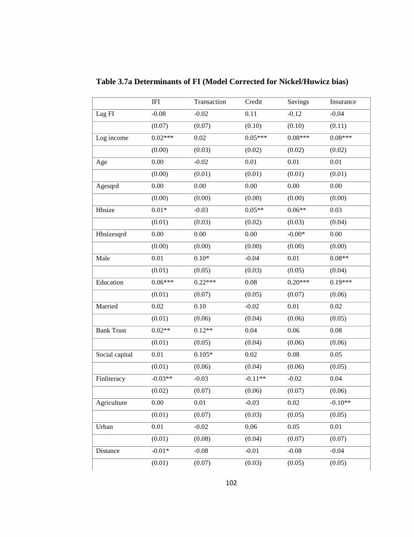
102

Table 3.7a Determinants of FI (Model Corrected for Nickel/Huwicz bias)

IFI Transaction Credit Savings Insurance

Lag FI -0.08 -0.02 0.11 -0.12 -0.04

(0.07) (0.07) (0.10) (0.10) (0.11)

Log income 0.02*** 0.02 0.05*** 0.08*** 0.08***

(0.00) (0.03) (0.02) (0.02) (0.02)

Age 0.00 -0.02 0.01 0.01 0.01

(0.00) (0.01) (0.01) (0.01) (0.01)

Agesqrd 0.00 0.00 0.00 0.00 0.00

(0.00) (0.00) (0.00) (0.00) (0.00)

Hhsize 0.01* -0.03 0.05** 0.06** 0.03

(0.01) (0.03) (0.02) (0.03) (0.04)

Hhsizesqrd 0.00 0.00 0.00 -0.00* 0.00

(0.00) (0.00) (0.00) (0.00) (0.00)

Male 0.01 0.10* -0.04 0.01 0.08**

(0.01) (0.05) (0.03) (0.05) (0.04)

Education 0.06*** 0.22*** 0.08 0.20*** 0.19***

(0.01) (0.07) (0.05) (0.07) (0.06)

Married 0.02 0.10 -0.02 0.01 0.02

(0.01) (0.06) (0.04) (0.06) (0.05)

Bank Trust 0.02** 0.12** 0.04 0.06 0.08

(0.01) (0.05) (0.04) (0.06) (0.06)

Social capital 0.01 0.105* 0.02 0.08 0.05

(0.01) (0.06) (0.04) (0.06) (0.05)

Finliteracy -0.03** -0.03 -0.11** -0.02 0.04

(0.02) (0.07) (0.06) (0.07) (0.06)

Agriculture 0.00 0.01 -0.03 0.02 -0.10**

(0.01) (0.07) (0.03) (0.05) (0.05)

Urban 0.01 -0.02 0.06 0.05 0.01

(0.01) (0.08) (0.04) (0.07) (0.07)

Distance -0.01* -0.08 -0.01 -0.08 -0.04

(0.01) (0.07) (0.03) (0.05) (0.05)

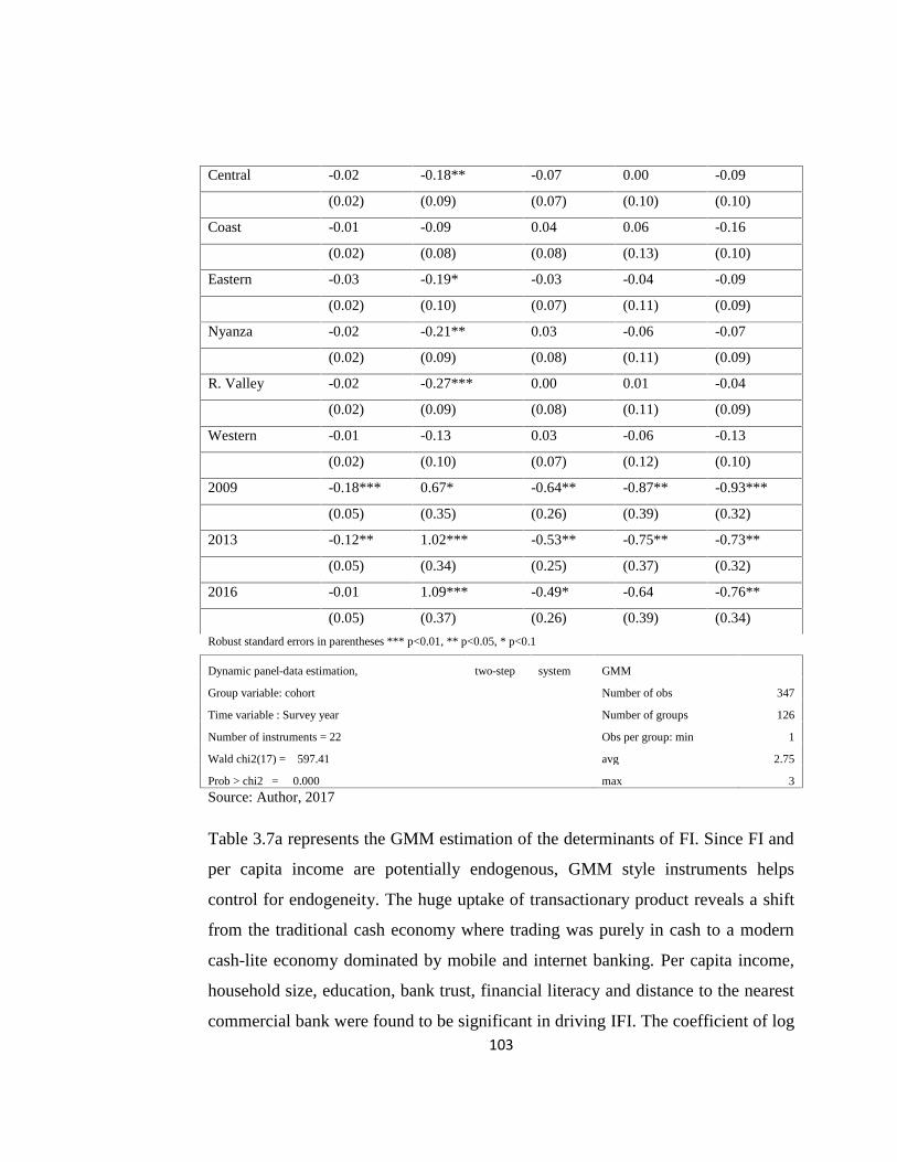
103

Central -0.02 -0.18** -0.07 0.00 -0.09

(0.02) (0.09) (0.07) (0.10) (0.10)

Coast -0.01 -0.09 0.04 0.06 -0.16

(0.02) (0.08) (0.08) (0.13) (0.10)

Eastern -0.03 -0.19* -0.03 -0.04 -0.09

(0.02) (0.10) (0.07) (0.11) (0.09)

Nyanza -0.02 -0.21** 0.03 -0.06 -0.07

(0.02) (0.09) (0.08) (0.11) (0.09)

R. Valley -0.02 -0.27*** 0.00 0.01 -0.04

(0.02) (0.09) (0.08) (0.11) (0.09)

Western -0.01 -0.13 0.03 -0.06 -0.13

(0.02) (0.10) (0.07) (0.12) (0.10)

2009 -0.18*** 0.67* -0.64** -0.87** -0.93***

(0.05) (0.35) (0.26) (0.39) (0.32)

2013 -0.12** 1.02*** -0.53** -0.75** -0.73**

(0.05) (0.34) (0.25) (0.37) (0.32)

2016 -0.01 1.09*** -0.49* -0.64 -0.76**

(0.05) (0.37) (0.26) (0.39) (0.34)

Robust standard errors in parentheses *** p<0.01, ** p<0.05, * p<0.1

Dynamic panel-data estimation, two-step system GMM

Group variable: cohort Number of obs 347

Time variable : Survey year Number of groups 126

Number of instruments = 22 Obs per group: min 1

Wald chi2(17) = 597.41 avg 2.75

Prob > chi2 = 0.000 max 3

Source: Author, 2017

Table 3.7a represents the GMM estimation of the determinants of FI. Since FI and

per capita income are potentially endogenous, GMM style instruments helps

control for endogeneity. The huge uptake of transactionary product reveals a shift

from the traditional cash economy where trading was purely in cash to a modern

cash-lite economy dominated by mobile and internet banking. Per capita income,

household size, education, bank trust, financial literacy and distance to the nearest

commercial bank were found to be significant in driving IFI. The coefficient of log

104

per capita income (proxy for money income) and its relationship with FI supports

the demand following hypothesis which predicts that increased growth of the

economy creates demand for financial services.

Increase in household income per capita was found to have a positive impact on

credit (5.3 percent), savings (7.6 percent), insurance (7.7 percent) and portfolio

usage of financial services (IFI) by 2.1 percent at 1 percent confidence level.

Acemoglu et al. (2001) argued that financial development trails economic

development hence increase in per capita income per capita boost access to

financial services. This finding elucidates the pivotal role economic growth plays

in driving the uptake of formal financial services reaffirming the existing causal

relationship (Kunt and Klapper, (2012); Sarma, (2008); Honohan, (2008); Sarma

and Pias, (2011); Park and Mercado, (2015); Akudugu, (2013) and IMF, (2012).

These studies predicted a positive link between money income and FI. This result

raises a question as to whether FI also exhibits a reverse causality with per capita

income. This question will be answered in the next chapter when we estimate the

welfare function to establish whether FI influences household welfare.

Transactionary usage of financial services was however found not to be sensitive

to per capita income. This could be rationalized by the domination of

transactionary products by mobile financial services whose infrastructure is

enjoyed almost equally by both the rural and urban households irrespective of their

level of income.

Empirical work by Tuesta et al., (2015) and Honohan and King (2012) identified

gender, education level and income as some of the drivers of formal access. In this

study, male headed households recorded a 9.29 and 7.99 percent higher uptake of

transactionary and insurance products as compared to female headed households.

Similarly, higher education largely reinforced the uptake of formal financial

services given that portfolio usage of financial services (IFI), transactionary,

105

savings and insurance rose by 6.3, 21.6, 20 and 18.5 percent respectively at 1

percent confidence level. This positive impact between schooling and FI builds on

Kalunda (2014) who found a positive link between level of education and FI.

Financial literacy was found to lower the uptake of IFI and credit products by 3.16

and 11 percent respectively at 5 percent confidence level. This negative coefficient

indicates that financially literate households are cautious when it comes to the

uptake of formal financial services and especially credit and savings. Nowadays,

most financial institutions practice what is popularly known as indiscriminate

lending which forces many households to practice impulse borrowing. Those who

are financially literate are slow when it comes to this uptake as evidenced by the

negative coefficient. While involvement in Agriculture is largely insignificant in

relation to the uptake of financial services, it lowers the probability of accessing

insurance services by 10.1 percent at 10 percent confidence level. This is mainly

because most insurance products in the market target housholds who are formally

employed locking out those engaging in informal activities such as agriculture.

In relation to age of the household head, IMF (2012) survey on financial access

established that young adults enjoyed increased access to financial services. This is

supported by the positive coefficient of age variable in our model which portray a

quadratic relationship even though no significant relationship was established.

Financial institutions often ration credit to persons approaching or falling above

retirement age because of their limited capacity to service the loans. Young

person's often enjoy more affordable and cheaper financial services and especially

credit since they have a longer lifespan allowing them to negotiate for more

flexible repayment installments.

Household size exhibited a quadratic relationship with respect to IFI, credit and

savings usage initially raising FI by 0.8, 5.1 and 5.8 percent respectively before

assuming a decline as household size increased further. What this study is however

106

not able to tell is the turning point which gives room for further research to

establish the optimal household size for each transmission channel. Social capital

was also found to be instrumental in influencing the uptake of transactionary

products at 10 percent raising transactionary usage of financial services by 10.5

percent.

Except under transactionary transmission channel where the coefficient of FI was

was negative, urbanized population exhibited a positive though non-significant

relationship with all other transmission channels, that is IFI, transactionary, credit

and insurance. This could be rationalized by the proximity to financial services by

urban residents as compared to the rural residents who rely on cashless money

transfer services such as mobile money dues to the limited formal financial

services in rural areas. Kempson and Whyley (1999) singled out geographical

location especially among rural dwellers as a barrier to FI. Commendable progress

towards reducing financial exclusion in rural areas has been made especially

following the high penetration of internet and mobile banking. Johnson and Nino-

Zarazua (2011) argued that urban dwellers are not always more financially

included. Uptake of formal financial services grew much slower between 2009 and

2013 as compared to the period 2006 to 2009 (FSD, 2013). Urban residents are

more likely to use bank services while their rural counterparts are more likely to

use mobile money products to overcome the distance. This is because it takes

considerably less time for a rural resident to get to a mobile agent than to a bank

branch or bank agent.

Any comprehensive study on the demand (usage) for financial services cannot be

complete without looking at the other side of the coin which is the determinants of

choice of a financial access strand (supply) which comprise; formal, formal other

and informal financial access strands. This is represented in Table 3.7b.

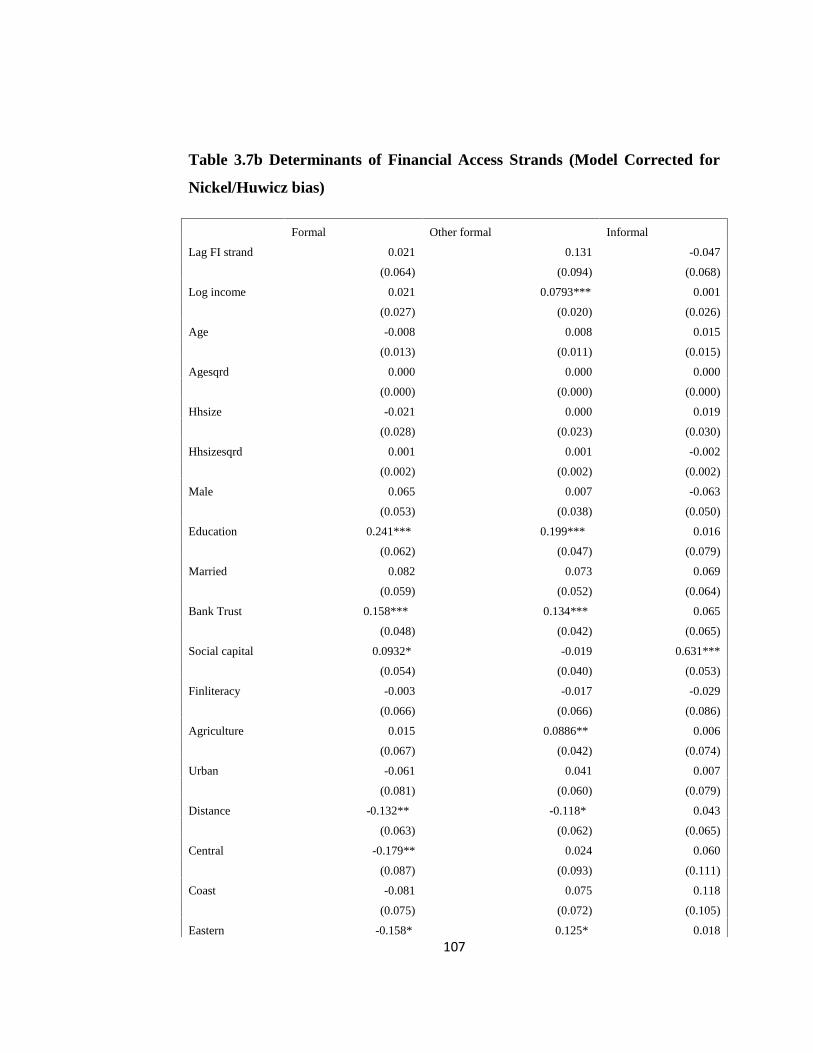
107

Table 3.7b Determinants of Financial Access Strands (Model Corrected for

Nickel/Huwicz bias)

Formal Other formal Informal

Lag FI strand 0.021 0.131 -0.047

(0.064) (0.094) (0.068)

Log income 0.021 0.0793*** 0.001

(0.027) (0.020) (0.026)

Age -0.008 0.008 0.015

(0.013) (0.011) (0.015)

Agesqrd 0.000 0.000 0.000

(0.000) (0.000) (0.000)

Hhsize -0.021 0.000 0.019

(0.028) (0.023) (0.030)

Hhsizesqrd 0.001 0.001 -0.002

(0.002) (0.002) (0.002)

Male 0.065 0.007 -0.063

(0.053) (0.038) (0.050)

Education 0.241*** 0.199*** 0.016

(0.062) (0.047) (0.079)

Married 0.082 0.073 0.069

(0.059) (0.052) (0.064)

Bank Trust 0.158*** 0.134*** 0.065

(0.048) (0.042) (0.065)

Social capital 0.0932* -0.019 0.631***

(0.054) (0.040) (0.053)

Finliteracy -0.003 -0.017 -0.029

(0.066) (0.066) (0.086)

Agriculture 0.015 0.0886** 0.006

(0.067) (0.042) (0.074)

Urban -0.061 0.041 0.007

(0.081) (0.060) (0.079)

Distance -0.132** -0.118* 0.043

(0.063) (0.062) (0.065)

Central -0.179** 0.024 0.060

(0.087) (0.093) (0.111)

Coast -0.081 0.075 0.118

(0.075) (0.072) (0.105)

Eastern -0.158* 0.125* 0.018

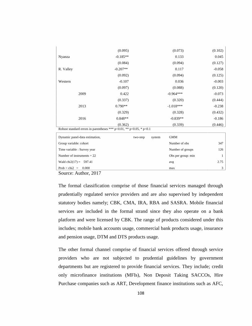
108

(0.095) (0.073) (0.102)

Nyanza -0.185** 0.133 0.045

(0.084) (0.094) (0.127)

R. Valley -0.207** 0.117 -0.058

(0.092) (0.094) (0.125)

Western -0.107 0.036 -0.003

(0.097) (0.088) (0.120)

2009 0.422 -0.964*** -0.073

(0.337) (0.320) (0.444)

2013 0.790** -1.018*** -0.238

(0.329) (0.328) (0.432)

2016 0.848** -0.839** -0.186

(0.362) (0.339) (0.446)Robust standard errors in parentheses *** p<0.01, ** p<0.05, * p<0.1

Dynamic panel-data estimation, two-step system GMM

Group variable: cohort Number of obs 347

Time variable : Survey year Number of groups 126

Number of instruments = 22 Obs per group: min 1

Wald chi2(17) = 597.41 avg 2.75

Prob > chi2 = 0.000 max 3

Source: Author, 2017

The formal classification comprise of those financial services managed through

prudentially regulated service providers and are also supervised by independent

statutory bodies namely; CBK, CMA, IRA, RBA and SASRA. Mobile financial

services are included in the formal strand since they also operate on a bank

platform and were licensed by CBK. The range of products considered under this

includes; mobile bank accounts usage, commercial bank products usage, insurance

and pension usage, DTM and DTS products usage.

The other formal channel comprise of financial services offered through service

providers who are not subjected to prudential guidelines by government

departments but are registered to provide financial services. They include; credit

only microfinance institutions (MFIs), Non Deposit Taking SACCOs, Hire

Purchase companies such as ART, Development finance institutions such as AFC,

109

HELB, ICDC among others. Lastly, the informal strand targets financial services

that are not subjected to regulation despite having relatively well defined

organizational structures. They include; shopkeepers/supply chain credit,

employers, shylocks and other informal money lenders as well as groups like

chamas, ROSCAs, ASCAs among others. Any household who doesn't fit in any of

the listed classification is considered to be financially excluded from all access

strands. Given the differences in the various access strands, this chapter extends

the debate on the determinants of FI to inform on factors that influence a

household decision on the most suitable access strand.

The main objective of FI as discussed earlier is to enhance universal FI by pulling

all households into the formal channel. This is analyzed using a static model as

well as a dynamic estimation. Given that choice of a financial access channel is

informed by both present and past information, a static analysis yields necessary

but not sufficient condition for the determination of demand for a financial access

channel. Appendix Table 3.4 columns 6 to 8 represent the static estimation of

determinants of financial access strands in Kenya while a lagged dependent

variable is included as a regressor in the dynamic panel.

GMM dynamic estimation in Table 3.6 revealed that per capita income promote

the uptake of financial products from other formal channel at 1 percent

significance level. The positive coefficient for income implies that growth in per

capita income leads to a 7.93 percent increase in the uptake of other formal

financial services. These other formal financial services include non-deposit taking

SACCOs and MFIs among others. The positive but insignificant coefficient under

the informal strand suggests that the demand for financial services from this strand

is not dependent on income. This further confirms that formal financial service

providers consider the income of households in their target markets when

110

designing their products. This qualifies the operation of the demand following

hypothesis in the financial markets.

One very important variable in driving usage of the informal channel is the social

capital which was found to have a 63.1 percent positive and significant impact on

the informal strand. The effect of social capital on the formal strand was small

raising it by a mere 9.32 percent at 10 percent confidence level. Social capital is

quite strong among rural households who form themselves into small groups

whose membership helps in providing guarantorship whenever a member wants to

apply for a specific financial product. These informal mechanisms are often

adopted by players in the informal markets to counter the stringent requirements

often imposed by formal financial service providers leading to credit rationing.

The distance to the nearest commercial bank was also found to significantly

explain the reduced demand for the formal strand at 5 percent level of significance.

Long duration taken by a household to get to the nearest bank acts as a

disincentive the pursuit of financial services from the formal strand leading to a

substitution effect as households resort to informal financial service providers. The

estimated model associate increase in the distance to the nearest bank to a 13.2 and

11.8 percent reduction in the uptake of formal and other formal financial services.

Education in this model accounts for a 24.1 and 19.9 percent increase in the uptake

of formal and other formal financial services in Kenya at 1 percent confidence

level. This shows how important education is in shaping financial decisions on

uptake of various financial services. Bank trust which was used to instrument FI

was also found to be highly significant at 1 percent in explaining formal and other

formal financial services. Trust in commercial banks raises the uptake of the

formal and other formal strand 15.8 and 13.4 percent respectively. Involvement in

agriculture which is considered to be the mainstay of Kenya's economy by the

111

household head only raises the chances of accessing other formal financial strand

by 8.86 percent.

In terms of regional dummies, households living in Central, Eastern, Nyanza and

Rift Valley recorded a 17.9, 15.8, 18.5 and 20.7 percent lower probability of

accessing the formal strand than households living within Nairobi.

3.6 Conclusions and Policy Implications

This chapter aimed at investigating the determinants of FI in Kenya. A logistic

estimation of single product usage based on a full sample static and a dynamic

cohort panel was used. This was followed by a GMM estimation of the

determinants of FI to correct for Nickel/Huwicz bias due to the small T and large

N (Econometrica, 1981). Given the difficulties faced in getting a true panel for

tracking same households over time, repeated cross sectional survey data was used

to form the pseudo panel with 126 cohorts totaling to 378 observations for three

waves of FinAccess survey. The dynamic panel estimation results based on the

generated cohort data is used to supplement the full sample static estimation. The

FinAccess 2006, 2009, 2013 and 2016 surveys capture FI developments in Kenya

during the period.

The coefficient of the lagged dependent variable was found to be strongly negative

and significant in influencing FI under the IFI and savings functions in the FE/RE

panel estimation. This significant relationship however disappears upon

controlling for Nickel bias in the GMM model. Lagged transactionary product

holding reinforces the uptake of FI. This cements the adaptive expectations theory

where past actions shape future happenings. A static estimation is therefore a

necessary but insufficient condition while estimating FI. Failure to capture the

lagged dependent variable could lead to biased inference while formulating

policies. Per capita income was also found to have a positive and significant

impact on FI in all categories except under the transactionary and informal access

112

channel. The same applies to years of schooling which exhibited a strong positive

and significant relationship on IFI, transactionary, savings and insurance product

uptake and formal and other formal access channels. The positive coefficients

indicate that human capital development through education is critical in enhancing

household welfare.

The positive and significant coefficient for log per capita income on the formal and

other formal financial access channel shows that formal access channels are

sensitive to reforms in the financial sector as compared to the informal strand.

Increase in the level of education also reinforces the uptake of formal financial

services while the impact of social capital on informal access channel was much

greater than that of formal access channel. The urbanized population also reported

a significant increase in the uptake of insurance, formal other and informal

financial access channels implying that proximity to financial service providers

facilitate access to financial services hence a higher FI score.

This chapter therefore recommends economic empowerment of masses through

increased economic activities which would raise per capita income found to be a

significant in promoting FI. Secondly, human capital development through

education and literacy programs should be included in school curriculum given its

positive impact. Lastly, mainstream financial service providers should factor in

social capital when designing credit products given its significant positive

contribution in driving access to financial services from the informal strand.

113

Chapter Four: Impact of FI on Consumption Expenditure

4.1 Introduction

The economic pillar of Vision 2030 and financial sector Medium Term Plan

(MTP), 2012-2017 has identified financial inclusion as a core pillar for the

promotion of economic growth and poverty alleviation (GoK, 2003). A vibrant

financial sector is expected to mobilize savings for financing productive

investments. This vision was preceded by Welfare Monitoring Surveys introduced

in 1992, 1994 and 1997 to monitor activities aimed at alleviating poverty;

Millennium Development Goals (MDGs) which aimed at halving the population

locked in poverty by 2015 (UN, 2000); and the Economic Recovery Strategy for

Wealth and Employment Creation (GoK, 2008) introduced to jumpstart the

economy with emphasis on the significance of credit in enhancing economic

growth, employment and alleviation of poverty.

Recent literature by Amidzic et al., 2014; Demirguc-Kunt and Klapper, 2012;

Beck et al., 2004; Sarma, 2008; Honohan, 2008 associate access to a broad range

of financial services to improved welfare. A more inclusive financial system is

associated with immense welfare benefits. In particular, an inclusive digital

financial system yields; enhanced financial services, connections to peers and

institutions as well as providing a basic account where individuals can build up

their savings for transactionary, precautionary and speculative purposes. This is

evidenced by a randomized control trial (RCT) conducted in Western Kenya where

traditional savings account led to a 45 percent increase in productive investment

and 27-40 percent higher personal expenditures (Dupas and Robinson, 2013).

Access to a range of financial services helps people invest in income generating

114

activities thus work their way out of poverty through reduced transaction costs and

vulnerability to poverty shocks and also through provision of reliable services14.

Use of consumption expenditure to measure welfare is considered to be important

for policy and particularly while measuring poverty and testing response

mechanisms and preparedness in the wake of income fluctuations. This is besides

assessing interactions between individual consumption expenditure and changes in

the demographic and socioeconomic characteristics. The determinants of

consumption expenditure such as income, asset base, price, capital gains among

other variables captured in the consumption theories by Keynes, 1936; Friedman,

1957; Modigliani, 1963 and Duesenberry, 1949 help shape the overall economic

growth through the consumption channel. The huge multiplier effect of

consumption on national income is what elevates the need to understand consumer

behaviour both in the short run and in the long run. A comprehensive analysis of

its determinants can go a long way in accelerating the overall economic growth

through increased income.

The broad objective of this chapter is to extend the existing literature on the link

between financial inclusion and welfare through evidence based examination from

Kenya. The specific research objectives as generated from the broad objectives

include;

1. To estimate the effect of single product measures of FI on consumption

expenditure in Kenya

2. To estimate the effect of composite FI index on consumption expenditure

in Kenya

14 United Nations Secretary Generals Special Advocate for Inclusive Finance for Development:Financial Inclusion in Post 2015 Development. It cites a global 90% target in the usage of a formalfinancial account

115

This chapter is motivated by earlier theories of financial development to represent

the link between financial inclusion and poverty. The use of the money metric

measure in Kenya dates back to the late 90's (GoK, 1997; 2000). The non-money

metric measures such as the asset index is suitable for measuring long term welfare

since its computation mainly relies on ownership of durables. The asset index

measure is challenged for failing to control for differences in the utility values

attached to various items by individuals in different localities. Consumption

expenditure which is more of a flow variable is therefore a better measure of

changes in social welfare.

4.2 Literature Review

4.2.1 Theories on the link between FI and Welfare

The main theories linking finance and economic development where this study

falls include; theories on direct and indirect transmission channels, the finance

growth hypothesis, theories of investment, the modern development theories, the

finance intermediation theories and the efficient markets hypothesis (EMH) based

on information asymmetry in the financial markets (Fama, 1970).

The causal link between financial inclusion and welfare is captured in the existing

financial development theories. Theories linking financial inclusion and welfare

are transmitted through either the direct or indirect channels. Under the direct

channel, increase in financial inclusion improves household welfare by reducing

income inequality and poverty through broadened access to transactionary, credit,

savings and insurance products. This raises income of the underprivileged

population through investment in productive activities and interest earnings from

savings.. Copestake (2007) suggests that financial inclusion provides a platform

for reducing poverty especially in the low income countries.

116

Growing literature reveal that the financial system help avail the necessary

resources for meeting the day to day transactions towards consumption, investment

and overall economic growth (King and Levine, 1993; Rajan and Zingales, 1998).

This literature stream extends early theories linking growth, development and

finance based on capital, labour and institutions where finance is captured as a

regressor in a growth function.

This direct effect between financial intermediation through broadened supply of

financial services is however not without challenges. Most developing countries

are characterized by information asymmetry which leads to adverse selection and

moral hazard especially in credit markets (Stiglitz and Weiss, 1981). These

imperfections act as a barrier to formal access to financial services for the poor

leading to persistent poverty (Levine, 2008). Aghion and Bolton (1997) associate

market imperfections in the financial with adverse effects on the poor who lack

collateral often required to access credit.

Keynes (1937) recognized the critical role played by financial intermediaries in his

theory of demand by stating that they are a source of profitable savings which

helps in building capital and provide a source of credit from the pooled savings.

Greenwood and Jovanovic (1990) however in their nonlinear inverted U

hypothesis argue that financial development does not impact on the population

uniformly. They argue that initially, financial development increases income

inequality since only the rich are able to take advantage of the demand for

financial services. However, as benefits from the financial development spread out

across the economy, the poor also benefit lowering income inequalities.

On the other hand the indirect channel of financial development linking financial

inclusion and welfare works through the finance growth nexus of financial

development theory. This indirect effect theory which works through the growth

stimulating effect is traced back to Schumpeter, 1934 and Mckinnon, 1973. Romer

117

(1986) on endogenous growth theories argued that accumulation of savings and

capital mobilization by financial intermediaries lead to improvement in technology

and economic growth. Developed financial markets lead to increased savings,

capital mobilization, technological improvement and economic growth.

This indirect theory is also supported by the Financial Structuralist theory which

associates a well-developed financial system and increased saving and economic

growth (Aghion & Bolton, 1997). The Financial Repressionist theory advocates

for the liberalization of financial markets to promote savings, investments and

economic growth. This indirect effect theory is also supported by the trickledown

theory which associates poverty reduction with economic growth as wealth is

redistributed from the rich to the poor (Aghion and Bolton, 1997).

The finance growth nexus revolves around four major theoretical underpinnings

namely; supply leading or finance led growth hypothesis Schumpeter (1911);

McKinnon (1973); Merton (1988); Chuah and Thai (2004), demand following

hypothesis or growth led finance Robinson (1952); Lucas (1988); Demetriades and

Hussein (1996); bi-directional causality hypothesis (Greenwood and Jovanovic

(1990) and the independent hypothesis by Lucas (1988) and Stern (1989). Nobel

Laureate Robert Lucas (1988) and Stern (1989) however consider finance as an

overstressed determinant of economic growth, even though recent literature has

helped build a consensus that the finance-growth nexus holds. The operation of the

finance growth nexus in the indirect channel of FI transmission offers insight on

the concentration of FI on the 'haves' and the 'have nots’.

The finance growth nexus stem from the Schumpeterian (1911) school; Modigliani

Miller theory and Fama (1970) Efficient Markets Hypothesis (EMH). Schumpeter

(1934) emphasized the role of banks in spurring economic development.

Schumpeter (1934); Greenwood and Jovanocovic (1990); Kind and Levine (1993)

118

associate financial development to increased productivity from the savings

allocative efficiency.

The finance led growth theory or supply leading hypothesis perceive growth and

development as a consequence of financial development which includes financial

inclusion often transmitted through a supply leading effect. Levine (2005; 1997;

Merton and Bodie (2005); Rajan and Zingales (1998) describe finance as the heart

that drives economic growth using aggregated data. The human capital theory

(HCT) in support of this hypothesis asserts that people require access to financial

services in order to be able to invest in their human capital through schooling.

It is the returns to schooling that help individuals to lead better lives from the

incremental wages. Levine (1997) and King and Levine (1993) recognizes the

immense role played by financial intermediation theory in linking deficit units

(borrowers) with surplus units (lenders). In particular, the study acknowledges the

role played by financial intermediaries, both formal and informal in mobilizing

savings among other financial services and argues that a first order relationship

exists between financial development and economic growth.

On the other hand, the growth led finance theory or demand following theory

developed by critics of the supply leading theory implies that financial

development arises from accelerated growth. An economy experiencing high

growth rates releases surplus responsible for financial development (Robinson

1952; Lucas, 1988; Demetriades and Hussein, 1996). The demand following

hypothesis alluded that the demand for financial services is triggered by increase

in financial development while the supply leading hypothesis argued that

economic growth is induced by increase in the supply of financial services from

the traditional to the modern sectors of the economy.

This latter hypothesis founded on financial intermediation dominates in the early

stages of development hence relevant for most developing economies which are

119

still in the precondition to take off stage. It describes developed countries and

developing countries which are in the take off stage of development. Emergence of

financial markets is therefore a consequence of a thriving economy which

stimulates demand for financial services by other sectors of the economy.

Greenwood and Jovanovic (1990) bidirectional causality hypothesis characterized

by non-diminishing returns to capital presents a possibility of multiple equilibria

from the reciprocal externalities in the finance growth nexus. The lower

equilibrium is observed in the early stages of development characterized by low

risk less productive investments while the upper equilibrium emerges where

markets are fairly developed and sophisticated by recent technology. Economic

growth enhances FI as financial intermediation identifies persons with great

potential for technological innovation in the financial sector. Both finance and

consumption expenditure per adult equivalent in this model is endogenous hence

defined from within the model.

Ncube15 (2016) posits that the link between financial system development and

economic development draws from the functions of the system. Aspects such as

liquidity, turnover, and efficiency in pricing have a positive impact on current and

future economic growth and productivity. The authors associate liquidity in

financial markets with accelerated investment growth.

Modern theories of development mainly focus on the evolution of growth, income

inequalities, their persistence and benefits associated with an efficient financial

system16. Financial market imperfections in the capital accumulation theories for

example shape key decisions on human and physical capital accumulation through

credit channels where economic agents borrow to build this capital. These

15 Digital Financial Services and Regulatory Policies in Africa

16 Chapter One: Access to Finance and Development, Theory and Measurement

120

financial market imperfections also influence the extent to which poor talented

individuals can raise funds to initiate projects in theories touching on

entrepreneurship.

An efficient payment system facilitates better integration into modern market

economies which increase income earning opportunities of the poor. Access to

savings and credit on the other hand enable the poor to overcome poverty through

investment in human capital development and microenterprises as well as asset

accumulation to increase income generating. Access to efficient savings, credit and

insurance facilitate consumption smoothing among the poor in the wake of

transitory changes in both income and expenditure (Beck, 2016).

Institutional quality is associated with welfare improvement through the indirect

channel which feeds into household welfare through the economic growth channel.

The literature suggest that the quality of institutions shapes the incentives for

investment in both physical and human capital, technological progress and

innovations. The institutions also determine property rights and transaction costs

which have serious implications on market size, specialization and technological

progress (Dhrifi, 2013).

IMF (2015) presents four classifications of growth and development channels

namely; endogenous growth model by Arrow (1962); Romer (1986) and

Lucas(1962) where savings promote growth through the investment channel;

capital allocation channel which tackles the information asymmetry problem

through financial markets, institutions and instruments model where financial

inflows are channeled to the domestic economy through the external sector and

lastly the theoretical model which ties together financial constraints, economic

growth, wealth inequality and poverty.

121

4.2.2 Causality and Impact of FI on welfare

The role of finance on welfare outcomes and economic growth has been cited

heavily in the literature. Much of the available evidence on the impact of FI on

welfare is mixed with some literature establishing a significant effect even as

others find no link. Whereas access to a wide range of financial services is not a

panacea to economic development, it acts as a prerequisite to poverty eradication

and sustainable economic development. Gupta (1987) contends that economic

growth is either determined via the financial structuralist approach or the financial

repression approach. The former approach highlights financial depth and the

composition of aggregate finance while the latter recognizes the critical role

played by price in influencing growth. The trickle down effects of finance and

economic growth on welfare outcomes such as consumption is huge (Todaro,

1997).

Randomized control trials (RCTS) are based on individual product categories since

the impact varies by product. Focusing on the counterfactual to establish what

would have happened without FI have been widely adopted in the literature. Gine

and Townsend (2004) on the difference in welfare among intermediated wage

earners and non-intermediated wage earners established a positive and significant

impact between access to financial services and welfare. Firms which were

previously constrained were found to gain more in terms of efficiency in the scale

of operations. Expansion in the financial sector was found to lead to a huge

increase in household income by between 17 - 201 percent. This is echoed by

Jeong and Townsend (2007) model of occupational choice and financial deepening

where positive gains to credit market expansion has been established.

A recent study by Buera et al. (2012) established that the consumption measure of

welfare grows by approximately 10 percent with the expansion in credit limit by

up to one and a half times the annual wage. This study provides vital information

122

on the welfare impacts between the rich and the poor. In particular, the study

established that the welfare gains of FI are larger among the poor rising by

approximately 8 percent of their permanent consumption in a general equilibrium

framework. In a similar fashion, Kaboski and Townsend (2012) established a very

strong relationship between financial intermediation and consumption.

However, the impact appeared to vary with households’ participation in

investment activities and whether one was a borrower or not. However, despite the

personal income and business income rising with the increased intermediation,

actual business startups stalled. Karlan and Zinman (2009) study on South Africa

revealed that even though access to credit raised borrower wellbeing as well as

income and food consumption, they were subjected to high stress levels. Bauchet

et al., (2011), Attanasio et al., (2011), Pitt and Khandker (1998) also found a

positive effect on household welfare.

A recent RCT in the rural Western Kenya on female market vendors by Dupas and

Robison (2013) established a significant link between savings and household

expenditure. Again, private expenditure for the users of a savings product

increased by 13 percent. Research indicates that results from studies focusing on

the link between savings and household welfare are more positive and consistent

as opposed to those focusing on the impact of credit usage. Notable though is that

the impact also varies with the sampled population given that a similar RCT on

rickshaw drivers conflicting results. Commitment savings in Malawi were also

found to exhibit a positive relationship with consumption expenditure (Brune,

Gine, Goldberg and Yang, 2016).

Not all studies however link financial intermediation with positive welfare effects

(Bernerjee et al., 2015; Crepon et al., 2014; Angelucci, Karlan and Zinman, 2013).

Bernerjee et al., (2015) for example in their randomized control trial on the role of

micro credit failed to establish any positive link on average monthly consumption

123

expenditure per capita 15 to 18 months later. Instead, households’ expenditure on

durables increased significantly leading to an increase in profitability. Crepon et

al. (2014) posit that even though access to microcredit led to a significant increase

in asset investment and profit, the gains were offset by a reduction in casual labour

income hence neutralizing the overall consumption effect. Although credit to

Mexican households revealed a general increase in their wellbeing, no significant

effect was established between FI and household consumption, (Angelucci et al.,

2013).

Tanzania's National Panel Survey (TzNPS), 2011 which mainly collects data on

livings standards presents a direct link between a range of financial services such

as use of SACCO, formal bank, and mobile money on household consumption

which is used in this chapter as a measure of welfare. The two wealthiest quintiles

were found to take a lion's share in the access to financial services. Access also

appeared skewed towards urban households. The report further claims that usage

of savings, insurance and mobile financial services can help households escape

poverty and mitigate against risks hence lower their vulnerability to poverty.

4.2.3 Theories of consumption

Welfare estimation informs on policies relevant to boosting consumption and

improved living standards. Such analysis draws heavily from the standard

consumer theory drawn from the traditional demand theory where an individual's

main objective is to maximize utility from the consumption of various goods and

services subject to certain constraints. Due to the unobservable nature of utility, an

observable measure of utility (consumption expenditure) is adopted as an indicator

of individual welfare.

This is also informed by; Ravallion, 1992; Murkherjee and Benson, 2003 who

view consumption expenditure as a smoother and less erroneous measure of

welfare as compared to income besides providing a more accurate measure of the

124

standard of living. By duality, expressing consumer decisions in terms of

expenditure (cost) functions simply provides a measure of the amount of money

required to derive a given level of utility by a rational consumer hence a good

money metric measure of welfare. FI is included as a treatment variable in a

conventional welfare function to establish its impact in addition to other control

variables.

Consumption forms a key component of aggregate demand. Branson (1989)

projects consumption expenditure to be two thirds of the aggregate expenditure in

the whole world. Consumption expenditure per adult equivalent is employed as a

proxy for consumer income in line with Keynes (1936) absolute income

hypothesis (AIH) which captures consumption as a function of disposable income

(psychological law). Increase in income leads to an increase in consumption

expenditure though not by as much as the increase in income (increases at a

decreasing rate). The marginal propensity to consume (MPC) is lower than the

average propensity to consume (APC) despite APC falling with income.

The relative income hypothesis (RIH) developed by Duessenbery (1949) to

counter AIH posits consumption is not just a function of absolute income; rather

it's also a function of the average income of the surrounding environment. This

theory states that an individual's consumption level is influenced by the

environment in which they stay hence citing interdependence in consumer

behaviour rather than the independence of individual consumption argued by

Keynes. Where consumption is high in the surrounding environment, there is a

tendency for the people around to also consume more. Milton Friedman (1957)

also another critic of Keynes AIH in his permanent income hypothesis (PIH)

argued that consumption is a function of permanent income hypothesis rather than

current income. Transitory changes in income therefore have no effect on

125

consumption. This is because consumers smooth their expenditure patterns

through borrowing and lending.

Ando, Modigliani and Blumberg (1963) life cycle hypothesis (LCH) posits that

consumption is a function of lifetime expected income. An individual's

consumption is expressed as a function of the available resources, rate of return of

capital employed (ROCE), spending plan and its age. The model also assumes

constant prices, stable interest rates, and no bequest hence production is driven by

savings. It's on the basis of this theory that age is seen to assume a quadratic

relationship with income and consumption. Young people who are yet to attain a

working age are said to earn little or no income at all. After they reach the working

age, income is seen to rise with experience while it starts falling upon attaining the

retirement age. This theory has however been criticized for assuming price

stability and the absence of bequest since market prices are known to be volatile

and bequests are common.

Decisions on consumer expenditure are influenced by a range of factors which

include; income, price, education, occupation, age, household size, macro

variables (Deaton, 2001; Zeldes, 2005; Eswaran and Kotwai, 2006) such as

interest rates, capital gains, savings, unanticipated shocks, consumer attitudes,

liquidity constraints, expectations among others. An individual decision on where

to spend their income is informed by the objective of maximizing utility subject to

the resource constraints. A rational consumer faced with a basket of goods will

therefore go for that commodity bundle which yields maximum utility. The

differences in the choices made can be traced back to the factors that characterize

individual consumers. This knowledge is what shapes policy formulation on how

welfare can be enhanced.

Modeling all the information about individuals is however not easy but every

effort is made to capture the main influencing factors besides age, education,

126

marital status, gender, which profile the demographic structure of the sampled

individuals. The geographical location is described as one very important variable

in explaining welfare by Burney et al. (1991). This literature revealed that the

urbanized population enjoys higher welfare since their consumption expenditure is

considerably higher than that of the rural population.

Expenditure per capita is usually high for small families but keeps falling as the

aggregate consumption expenditure is shared over a bigger family (Gupta, 1986).

Lanjouwand Ravallion (1995) echoed these sentiments by providing evidence of a

negative relationship between household size and consumption expenditure in

developing countries. The middle age group is associated with a higher

expenditure pattern but it evens out as they approach old age. The high middle age

expenditure is explained by their desired to build their asset base through purchase

of consumer durables in both rural and urban areas. Consumption expenditure also

increases with level of education (Knight, Shi and Quheng, 2010).

Occupational differences when looked at from an agricultural, salaried and

business perspective is said to have varying effects on consumption expenditure

(Jain, and Tendulkar, 1973). Professionals and salaried people in both rural and

urban areas are associated with a higher consumption expenditure pattern as

compared to those in business and agriculture. The urban population involved in

agriculture also has a higher expenditure pattern as compared to those in business

due to their adoption of modern technology. Consumption expenditure among

businessmen is however higher among the rural populace as compared to those

involved in agriculture. This sectoral difference in consumption expenditure can be

traced back to the level of FI of the household head. FI for business people is

expected to lead to higher consumer welfare.

127

4.2.4 Overview of literature

The reviewed literature on the estimation of a welfare function revealed lack of a

consensus on the real impact of FI on welfare. This raises the need to conduct

more empirical based evidence on the impact in Kenya. It was found that the best

way to understand the implications of FI on welfare is to look at the whole issue

from a counter factual to establish what effect a lack of FI would have. The review

also established that the impact varies with the individual financial products.

Usage of savings product was found to have a positive significant and more

consistent impact as compared to credit facilities.

The literature also discussed the effect of control variables in a conventional

welfare model. Studies carried out in Kenya in rural Western province targeting

female market vendors and rickshaw drivers using RCT reported conflicting

impacts an indication that the impact of FI varies with a number of considerations.

The twin tests yielded mixed evidence leaving the researcher with a number of

questions as to the real effect of FI. This makes this study worthy to be

investigated to respond to this research gap.

In terms of theoretical framework, the chapter reviewed several consumption

theories including Keynes (1936) absolute income hypothesis, Duessenberry

(1949) relative income hypothesis and Ando, Modigliani and Blumberg (1963) life

cycle hypothesis. The absolute income hypothesis that places consumption as a

function of disposable income was found to be suitable for this study with

consumption expenditure per adult equivalent being employed as a proxy for

consumer income.

The impact of FI is conceptualized in figure 4.1 to show its relationship with

various outcomes.

Fig 4.1 Conceptual Framework

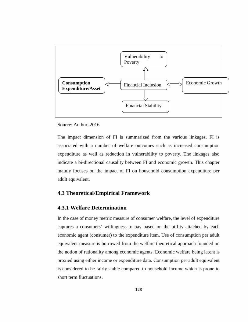
128

Source: Author, 2016

The impact dimension of FI is summarized from the various linkages. FI is

associated with a number of welfare outcomes such as increased consumption

expenditure as well as reduction in vulnerability to poverty. The linkages also

indicate a bi-directional causality between FI and economic growth. This chapter

mainly focuses on the impact of FI on household consumption expenditure per

adult equivalent.

4.3 Theoretical/Empirical Framework

4.3.1 Welfare Determination

In the case of money metric measure of consumer welfare, the level of expenditure

captures a consumers’ willingness to pay based on the utility attached by each

economic agent (consumer) to the expenditure item. Use of consumption per adult

equivalent measure is borrowed from the welfare theoretical approach founded on

the notion of rationality among economic agents. Economic welfare being latent is

proxied using either income or expenditure data. Consumption per adult equivalent

is considered to be fairly stable compared to household income which is prone to

short term fluctuations.

Financial Inclusion Economic Growth

Financial Stability

Vulnerability toPoverty

ConsumptionExpenditure/Assets

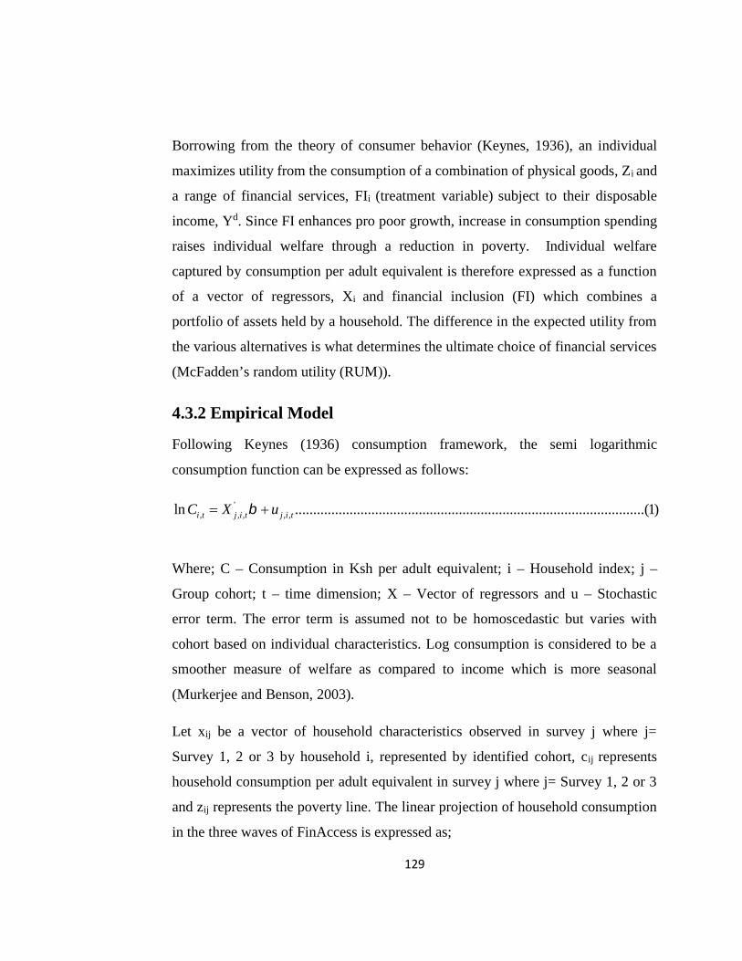
129

Borrowing from the theory of consumer behavior (Keynes, 1936), an individual

maximizes utility from the consumption of a combination of physical goods, Zi and

a range of financial services, FIi (treatment variable) subject to their disposable

income, Yd. Since FI enhances pro poor growth, increase in consumption spending

raises individual welfare through a reduction in poverty. Individual welfare

captured by consumption per adult equivalent is therefore expressed as a function

of a vector of regressors, Xi and financial inclusion (FI) which combines a

portfolio of assets held by a household. The difference in the expected utility from

the various alternatives is what determines the ultimate choice of financial services

(McFadden’s random utility (RUM)).

4.3.2 Empirical Model

Following Keynes (1936) consumption framework, the semi logarithmic

consumption function can be expressed as follows:

', , , , ,ln ................................................................................................(1)i t j i t j i tC X u

Where; C – Consumption in Ksh per adult equivalent; i – Household index; j –

Group cohort; t – time dimension; X – Vector of regressors and u – Stochastic

error term. The error term is assumed not to be homoscedastic but varies with

cohort based on individual characteristics. Log consumption is considered to be a

smoother measure of welfare as compared to income which is more seasonal

(Murkerjee and Benson, 2003).

Let xij be a vector of household characteristics observed in survey j where j=

Survey 1, 2 or 3 by household i, represented by identified cohort, cij represents

household consumption per adult equivalent in survey j where j= Survey 1, 2 or 3

and zij represents the poverty line. The linear projection of household consumption

in the three waves of FinAccess is expressed as;

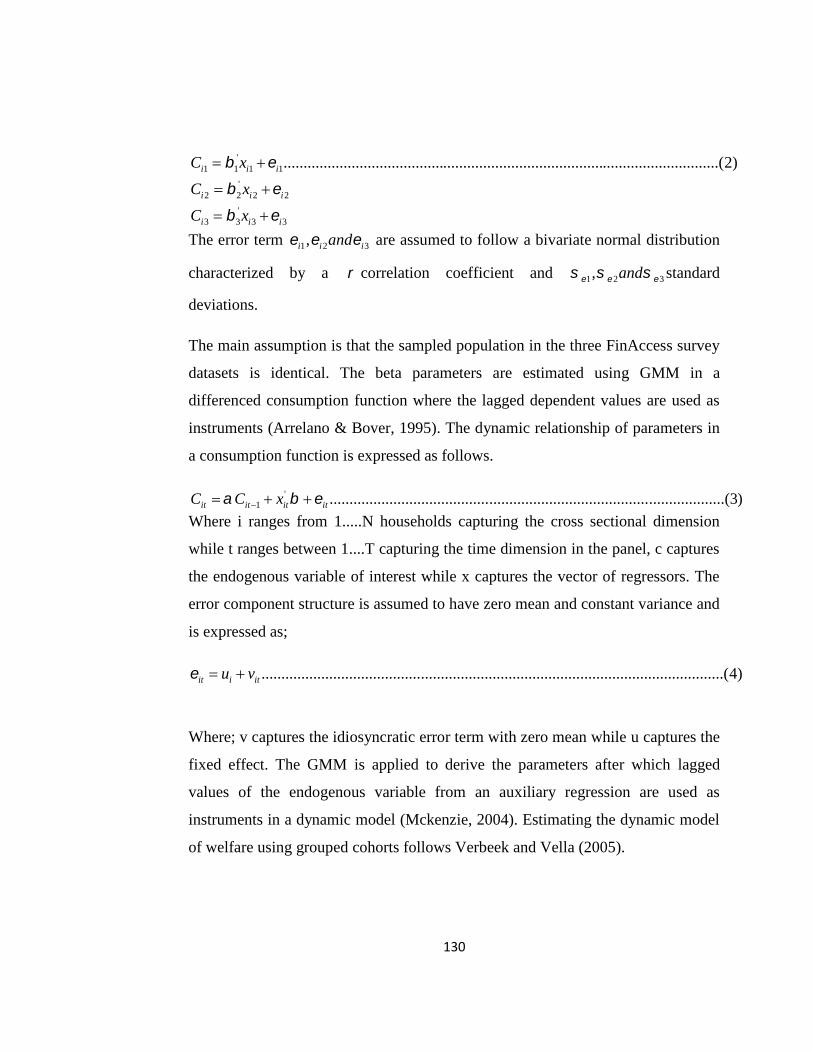
130

'1 1 1 1

'2 2 2 2

'3 3 3 3

.............................................................................................................(2)i i i

i i i

i i i

C x

C x

C x

The error term 1 2 3,i i iand are assumed to follow a bivariate normal distribution

characterized by a correlation coefficient and 1 2 3, and standard

deviations.

The main assumption is that the sampled population in the three FinAccess survey

datasets is identical. The beta parameters are estimated using GMM in a

differenced consumption function where the lagged dependent values are used as

instruments (Arrelano & Bover, 1995). The dynamic relationship of parameters in

a consumption function is expressed as follows.

'1 ...................................................................................................(3)it it it itC C x

Where i ranges from 1.....N households capturing the cross sectional dimension

while t ranges between 1....T capturing the time dimension in the panel, c captures

the endogenous variable of interest while x captures the vector of regressors. The

error component structure is assumed to have zero mean and constant variance and

is expressed as;

....................................................................................................................(4)it i itu v

Where; v captures the idiosyncratic error term with zero mean while u captures the

fixed effect. The GMM is applied to derive the parameters after which lagged

values of the endogenous variable from an auxiliary regression are used as

instruments in a dynamic model (Mckenzie, 2004). Estimating the dynamic model

of welfare using grouped cohorts follows Verbeek and Vella (2005).

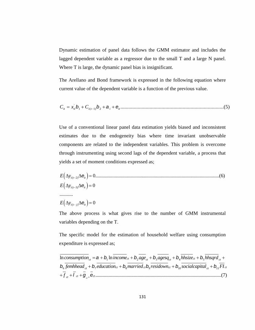
131

Dynamic estimation of panel data follows the GMM estimator and includes the

lagged dependent variable as a regressor due to the small T and a large N panel.

Where T is large, the dynamic panel bias is insignificant.

The Arellano and Bond framework is expressed in the following equation where

current value of the dependent variable is a function of the previous value.

'1 ( 1) 2 ..............................................................................(5)it it i t i itC x C

Use of a conventional linear panel data estimation yields biased and inconsistent

estimates due to the endogeneity bias where time invariant unobservable

components are related to the independent variables. This problem is overcome

through instrumenting using second lags of the dependent variable, a process that

yields a set of moment conditions expressed as;

( 2)

( 3)

( )

0......................................................................................................(6)

0

...........

0

i t it

i t it

i t j it

E y

E y

E y

The above process is what gives rise to the number of GMM instrumental

variables depending on the T.

The specific model for the estimation of household welfare using consumption

expenditure is expressed as;

1 2 3 4 5

6 7 8 9 10 11

ln ln

....................................ct

ct ctct ct ct ct

ctct ct ctct ct

ct ctct

consumption income age agesq hhsize hhsqrd

femhhead education married residown socialcapital FI

f

.....................................................................(7)

132

The observed cohorts means (‘bars on variables’) are used to represent the

population mean (Deaton, 1986). A lagged dependent variable is included in the

model to capture the effect of past consumption spending on current consumption.

The FI variable measures both the single product (transactionary, credit, savings

and insurance) and the composite measure of FI (IFI). Five autoregressive

dynamic panels are estimated each representing a particular FI measure. The

cohort panels used in the dynamic estimation represents all households since for

each survey; the households are grouped in a cohort based on time invariant

characteristics.

The money metric measure of welfare (consumption per adult equivalent) was

expressed in logarithmic form to capture the elasticity. Alternative measures of

welfare suggested in literature include; the asset index based on the assets owned

by the households though it falls outside the purview of this paper.

Given the potential endogeneity bias between FI and per adult equivalent

consumption expenditure, the variable bank trust (Bertrand, Mullainathan &

Shafir, 2004) is included in the first step estimation to minimize biasedness arising

from the residuals.

4.3.3 Description of variables and Apriori Expectations

Variable Description Expectedsign

Studies reporting evidenceof this sign

Welfare Dependent Variable: Proxiedby a money metric measure,that is, consumptionexpenditure per adultequivalent

Log Income A continuous variablecapturing monthly per capitaincome of household head inKshs

+ FSD, 2014; Cull, Robert,Tilman Ehrbeck, and NinaHolle, 2014; Beck et al,2007; Demirguc-Kunt andKlapper, 2012

Age Measured as a continuous + Honohan and King, 2012;

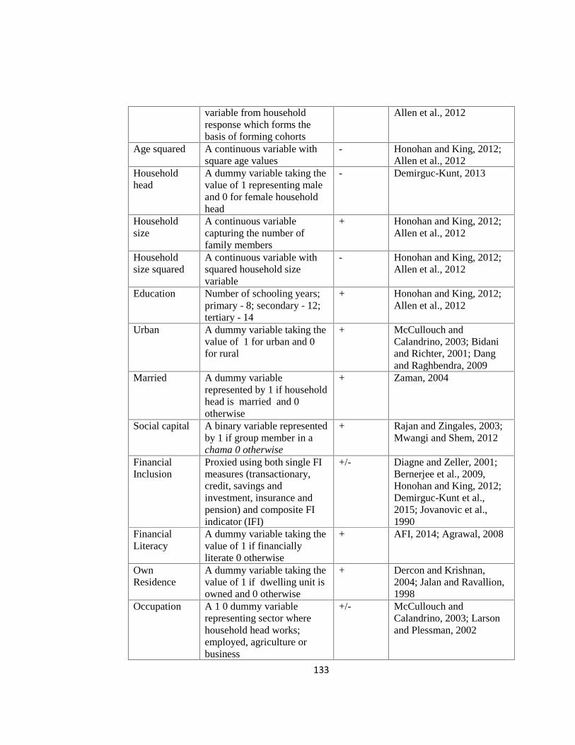
133

variable from householdresponse which forms thebasis of forming cohorts

Allen et al., 2012

Age squared A continuous variable withsquare age values

- Honohan and King, 2012;Allen et al., 2012

Householdhead

A dummy variable taking thevalue of 1 representing maleand 0 for female householdhead

- Demirguc-Kunt, 2013

Householdsize

A continuous variablecapturing the number offamily members

+ Honohan and King, 2012;Allen et al., 2012

Householdsize squared

A continuous variable withsquared household sizevariable

- Honohan and King, 2012;Allen et al., 2012

Education Number of schooling years;primary - 8; secondary - 12;tertiary - 14

+ Honohan and King, 2012;Allen et al., 2012

Urban A dummy variable taking thevalue of 1 for urban and 0for rural

+ McCullouch andCalandrino, 2003; Bidaniand Richter, 2001; Dangand Raghbendra, 2009

Married A dummy variablerepresented by 1 if householdhead is married and 0otherwise

+ Zaman, 2004

Social capital A binary variable representedby 1 if group member in achama 0 otherwise

+ Rajan and Zingales, 2003;Mwangi and Shem, 2012

FinancialInclusion

Proxied using both single FImeasures (transactionary,credit, savings andinvestment, insurance andpension) and composite FIindicator (IFI)

+/- Diagne and Zeller, 2001;Bernerjee et al., 2009,Honohan and King, 2012;Demirguc-Kunt et al.,2015; Jovanovic et al.,1990

FinancialLiteracy

A dummy variable taking thevalue of 1 if financiallyliterate 0 otherwise

+ AFI, 2014; Agrawal, 2008

OwnResidence

A dummy variable taking thevalue of 1 if dwelling unit isowned and 0 otherwise

+ Dercon and Krishnan,2004; Jalan and Ravallion,1998

Occupation A 1 0 dummy variablerepresenting sector wherehousehold head works;employed, agriculture orbusiness

+/- McCullouch andCalandrino, 2003; Larsonand Plessman, 2002

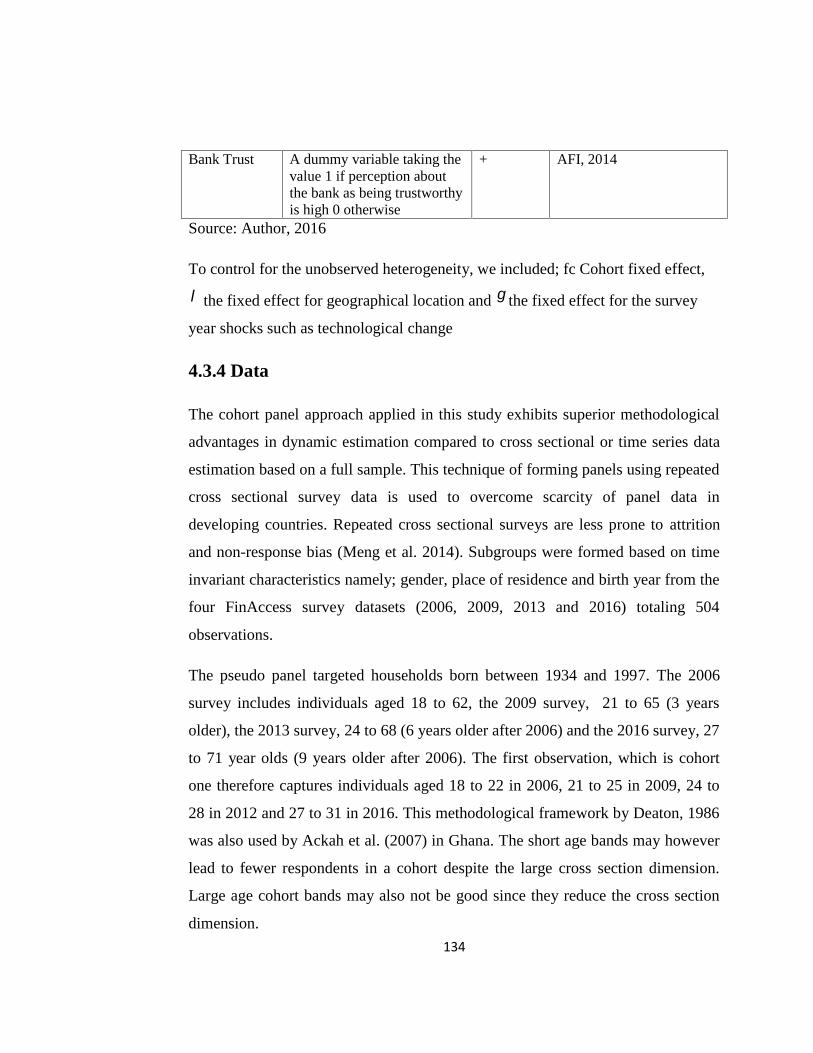
134

Bank Trust A dummy variable taking thevalue 1 if perception aboutthe bank as being trustworthyis high 0 otherwise

+ AFI, 2014

Source: Author, 2016

To control for the unobserved heterogeneity, we included; fc Cohort fixed effect,

the fixed effect for geographical location and the fixed effect for the survey

year shocks such as technological change

4.3.4 Data

The cohort panel approach applied in this study exhibits superior methodological

advantages in dynamic estimation compared to cross sectional or time series data

estimation based on a full sample. This technique of forming panels using repeated

cross sectional survey data is used to overcome scarcity of panel data in

developing countries. Repeated cross sectional surveys are less prone to attrition

and non-response bias (Meng et al. 2014). Subgroups were formed based on time

invariant characteristics namely; gender, place of residence and birth year from the

four FinAccess survey datasets (2006, 2009, 2013 and 2016) totaling 504

observations.

The pseudo panel targeted households born between 1934 and 1997. The 2006

survey includes individuals aged 18 to 62, the 2009 survey, 21 to 65 (3 years

older), the 2013 survey, 24 to 68 (6 years older after 2006) and the 2016 survey, 27

to 71 year olds (9 years older after 2006). The first observation, which is cohort

one therefore captures individuals aged 18 to 22 in 2006, 21 to 25 in 2009, 24 to

28 in 2012 and 27 to 31 in 2016. This methodological framework by Deaton, 1986

was also used by Ackah et al. (2007) in Ghana. The short age bands may however

lead to fewer respondents in a cohort despite the large cross section dimension.

Large age cohort bands may also not be good since they reduce the cross section

dimension.

135

Gender variable is disaggregated to generate panels for males and females

respectively while the geographical aspect is captured by the seven regions (44

counties), formerly provinces with the exception of North Eastern region which

has 3 counties namely; Mandera, Wajir and Garissa for missing in the 2013 wave

due to logistical constraints. A key consideration in cohort analysis is the tradeoff

between the number of cohorts and number of observations for each cohort.

McKenzie (2004) posits that a large number of cohorts minimize errors associated

with small samples.

Deaton (1986) and Bourguignon, Goh and Kim’s (2004) recommends the use of a

cohort mean based approach to track the effect of FI on the household welfare.

Cull et al. (2013) posits that the channel where access to financial services

influence income is at least as plausible as the likely mechanism where passing a

threshold level of income opens up the opportunity for an individual to access

formal banking services. The main problem in estimating a welfare function is

endogeneity. This problem is associated with omission of variables, measurement

errors as well as simultaneity bias. Failure to control for this may lead to the

rejection of a true null (Type I error) or failure to reject a false null (Type II error).

The reviewed literature pointed to a bidirectional causal relationship between the

FI and welfare which may lead to wrong inferences if the endogeneity problem is

not corrected.

The study employed the cohort approach discussed in chapter three due to its

methodological advantages in dynamic estimation. The estimation is however

based on the last three FinAccess survey datasets (2009, 2013 and 2016). Despite

the significant role played by the 2006 survey data, the dataset was omitted since

this study rides on the money metric measure of welfare (consumption

expenditure) which is missing in the 2006 FinAccess survey data. The year

136

however offers a reference point since it's the first time when the FinAccess round

of surveys was first implemented in Kenya.

The observed cohort means represent the population mean (Deaton, 1986). A key

consideration in cohort analysis is the tradeoff between the number of cohorts and

number of observations for each cohort. McKenzie (2004) posits that a large

number of cohorts minimize errors associated with small samples.

The subgroup means were tracked over time using the repeated cross sections

(Deaton, 1985) to inform on the dynamic transformation of both FI and household

welfare. This method of estimating using subgroups is similar to the method of

using instrumental variables to represent a certain phenomenon where the group

indicators serve as instruments. Verbeek-Nijman (2005) estimator yields the best

estimators when cross sections are fewer while Deaton's (1986) estimator is

recommended for larger surveys. Verbeek and Vella (2005) justify the use of fixed

effects estimators in pseudo panel estimation for as long as a lagged dependent

variable is included. Pooled estimation using the full sample leads to biased

estimates since it's not able to control for unobserved heterogeneity since it

assumes household independence in the repeated cross sections.

4.4 Discussion of Results

This section first interrogates the descriptive statistics of the variables used in the

analysis of FI impact on household welfare. This includes measures of central

tendencies, dispersion and cross tabulations of key variables.

4.4.1 Descriptive Statistics

Table 4.1 provides a snapshot of the means and standard deviation of variables

relevant to the estimation of a welfare function. A descriptive statistics table helps

inform on the distribution of the variables, their frequencies and nature, that is,

whether the variables are continuous or categorical. Consumption per adult

137

equivalent is expressed in Kenya shillings while education is expressed both in

levels as well as number of schooling years. Appendix Tables 4.2 presents the

level of consumption expenditure by survey year while Appendix Table 4.3

presents the aggregated distribution of income by education.

Table 4.1 Summary Statistics on Household Characteristics

Variable Observations Mean Std. Dev. Min Max

Household size 378 5 2.81 1 20

Age 378 43 13.16 18 68

Education 378 8 4.76 0 14

Female hh head 378 0.26 0.44 0 1

Urban 378 0.40 0.49 0 1

Financial literacy 378 0.78 0.41 0 1

Social capital 378 0.46 0.50 0 1

Consumption exp 378 6810 19864 0 263933

Gross income 378 5133 13918 0 166668

Own residence 378 0.65 0.48 0 1

Married 378 0.66 0.47 0 1

IFI 378 0.12 0.12 0 0.72

Credit 378 0.11 0.31 0 1

Transactionary 378 0.63 0.48 0 1

Savings 378 0.22 0.41 0 1

Insurance 378 0.24 0.43 0 1

Agriculture 378 0.37 0.48 0 1

Employed 378 0.34 0.47 0 1

Business 378 0.11 0.32 0 1

Source: FinAccess survey 2009, 2013 & 2016

The descriptive statistics table represents the demographic profile of the 378

observations from the 2009, 2013 and 2016 FinAccess surveys. Year 2006

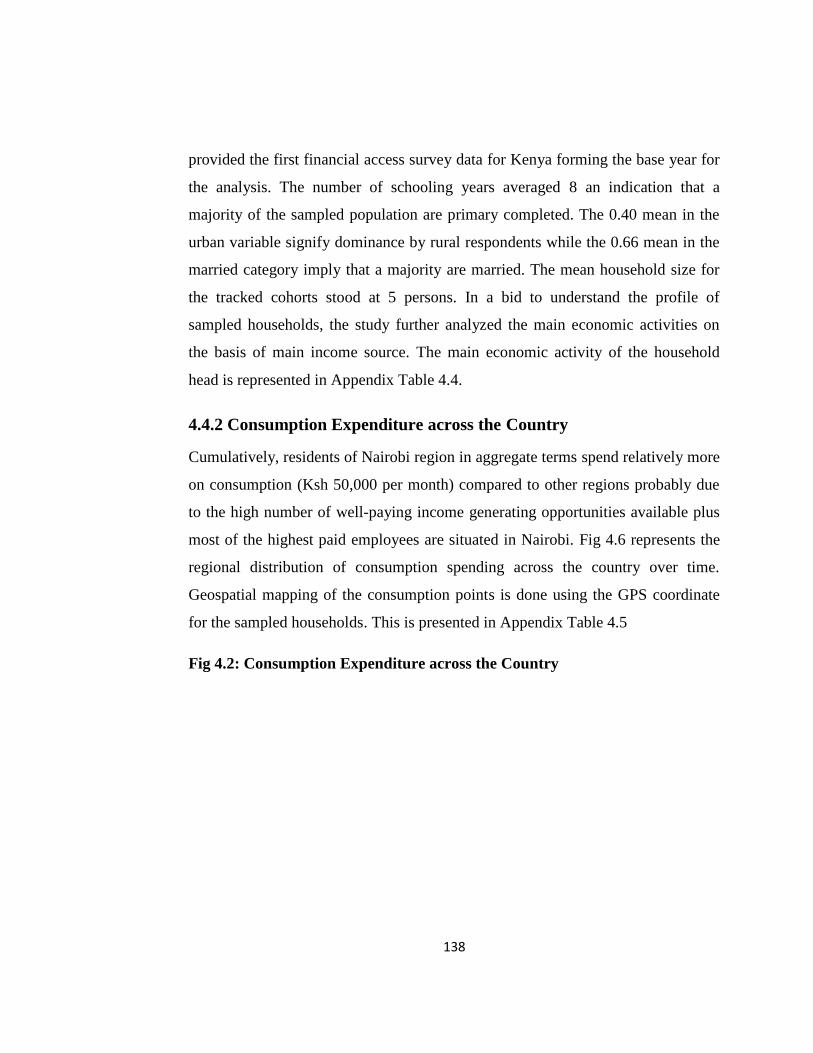
138

provided the first financial access survey data for Kenya forming the base year for

the analysis. The number of schooling years averaged 8 an indication that a

majority of the sampled population are primary completed. The 0.40 mean in the

urban variable signify dominance by rural respondents while the 0.66 mean in the

married category imply that a majority are married. The mean household size for

the tracked cohorts stood at 5 persons. In a bid to understand the profile of

sampled households, the study further analyzed the main economic activities on

the basis of main income source. The main economic activity of the household

head is represented in Appendix Table 4.4.

4.4.2 Consumption Expenditure across the Country

Cumulatively, residents of Nairobi region in aggregate terms spend relatively more

on consumption (Ksh 50,000 per month) compared to other regions probably due

to the high number of well-paying income generating opportunities available plus

most of the highest paid employees are situated in Nairobi. Fig 4.6 represents the

regional distribution of consumption spending across the country over time.

Geospatial mapping of the consumption points is done using the GPS coordinate

for the sampled households. This is presented in Appendix Table 4.5

Fig 4.2: Consumption Expenditure across the Country

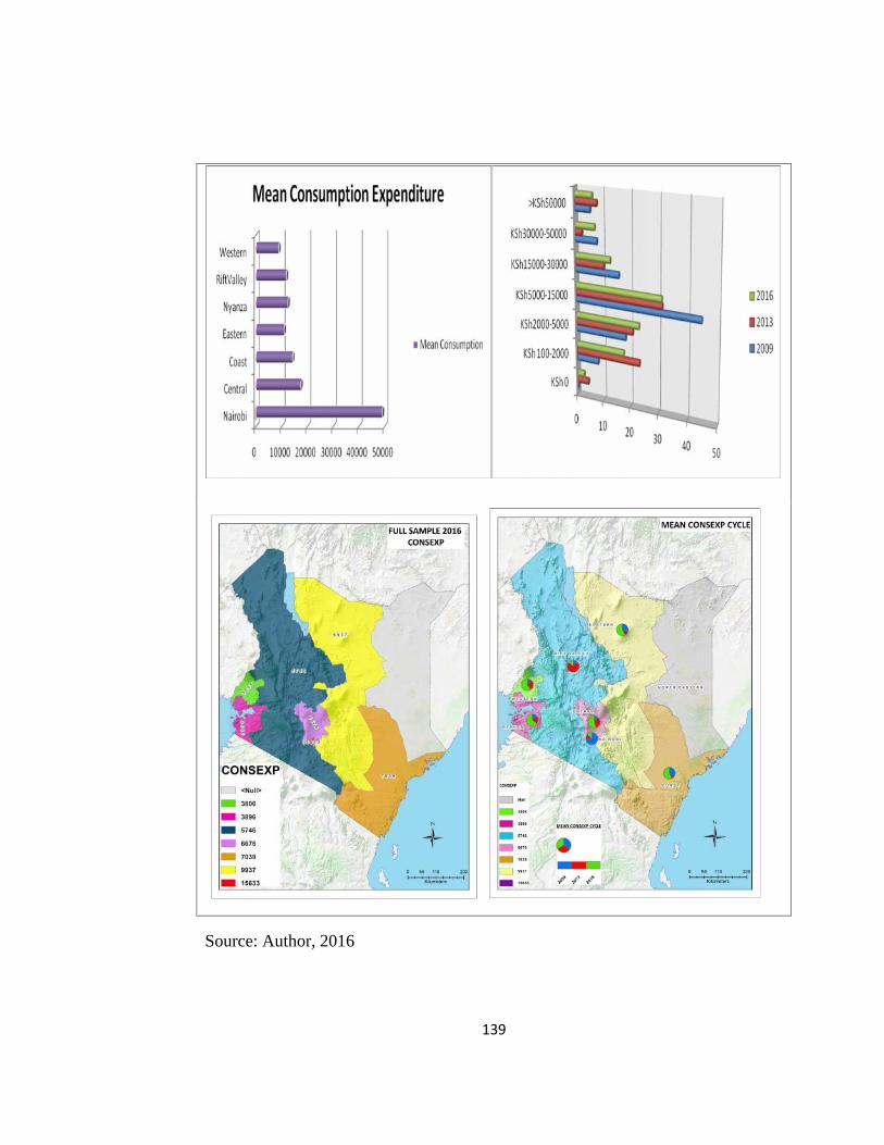
139

Source: Author, 2016

140

Fig 4.2 represents the average consumption expenditure for the seven regions in

Kenya based on the 378 cohorts for the 2009, 2013 and 2016 survey. North

Eastern region is excluded due to missing 2013 data. Western region trails other

regions with its average consumption expenditure per month falling below Ksh

10,000. This finding appears to corroborate OPHI (2016) findings based on the

KDHS 2013-2014 data where Western region recorded dismal performance in

terms of poverty incidence while Nairobi outshined all other regions. Urban

households stand a higher chance of enjoying improved living standards as

compared to rural households who face deprivation from many fronts.

An interesting observation from the expenditure distribution by survey year is that

in 2009, everyone experienced expenditure in excess of Ksh 100. However as time

progressed, the percentage population spending between Ksh 0 - 100 rose sharply

in 2013 before stabilizing in 2016. A majority in 2009 spent an average Ksh

30,000 - 50,000 while in both 2013 and 2016 consumption expenditure averaged

Ksh 5,000 - 15,000. The inscribed pie charts present the progression of per adult

equivalent consumption expenditure over the three waves.

The geospatial maps show that consumption expenditure has been trailing in

Western region but is highest in Nairobi region. In aggregate terms, consumption

expenditure has improved in 2016 (green shading) in the pie chart.

4.5. Econometric Results and Discussion

This section delves into the impact of FI on consumption per adult equivalent

among Kenyan households. The indirect channel of financial development

recognizes the pivotal role played by economic growth in reducing poverty and

income inequalities. The usefulness of FI in improving welfare largely depends on

the circumstances surrounding the uptake of financial products as well as the

degree of financial literacy. The issue as to whether growth is pro-finance emerged

141

justifying the inclusion of per capital income (money income) as one of the

regressors in a FI model to establish causality.

The difference in the estimated coefficients is wider when Random effects (RE)

estimation is not efficient and smaller when it’s efficient. Fixed Effects (FE) model

is consistent when the individual effects are correlated with other regressors.

However if that assumption doesn't hold, both FE and RE are consistent even

though RE is more efficient. A Haussmann test on each of the FI channels selected

FE estimation for the portfolio usage (IFI) and transactionary channel and RE for

savings, insurance and credit channels. Given that individuals assign utility

differently to each of the financial products, this section employed five

autoregressive dynamic panel data models (Arrelano and Bover, 1995) of

consumption expenditure per adult equivalent to analyze the impact of

transactionary, credit, savings, insurance and IFI) in Kenya. The estimation is

carried out both before and after controlling for the unobserved heterogeneity from

survey year and region specific effects.

4.5.1 Diagnostic Tests

The main weakness associated with pseudo panel data estimation is that it

diminishes the efficiency of the cross sectional dimension while at the same time

introducing heteroscedasticity in the time dimension (Deaton, 1986). Specification

errors, measurement or omission of variables could also trigger bias in

consumption expenditure elasticities. This is partly solved through differencing of

the individual panels. Any heteroscedasticity inherent in the model is corrected by

decomposing the data into between and within dimensions and computing the

exact heteroscedasticity on both dimensions. Failure of repeated cross sectional

data to track same individuals over time, limits computation of mean deviations

over time. Conventionally, the Breusch Pagan test is conducted to check if the

model is suffering from heteroscedasticity. Under the two step robust procedure,

142

the standard covariance matrix is robust to panel specific autocorrelation and

heteroscedasticity. Use of robust standard errors was also applied to correct for

potential correlation between household errors over time.

Use of orthogonality conditions in GMM estimation facilitates efficient estimation

in the presence of heteroscedasticity of unknown form. The orthogonality

conditions assume that all instrumental variables are orthogonal to the errors hence

uncorrelated with errors in the original regression. The instrumental variable

approach is also unbiased since the reported standard errors allow for

asymptotically correct inference in the presence of autocorrelation of almost any

form (Roodman, 2006). Testing for serial correlation was done using the

autoregressive test for autocorrelation of residuals. The Arrelano & Bond AR (1)

test reported Z = -0.57 with Pr > Z = 0.5656. This rules out the problem of serial

correlation.

The instruments used in this chapter were subjected to the Sargan-Hansen

hypothesis test to assess whether they are jointly exogenous. The dependent

variable (per adult equivalent log consumption expenditure) is specified in lagged

differences. Since focus is to establish the dynamics of consumption expenditure,

the lagged dependent variable in first differences is instrumented using the second

lag of per adult equivalent consumption expenditure. The instruments set include

survey year dummies and other individual characteristics. The autoregressive test

for autocorrelation is used to check for the presence of serial correlation among

residuals.

A test for the validity of the instruments was conducted Hansen (1982) to establish

if the model is over identified. The test for over identified restrictions (H0: Exactly

identified) reported a non-significant test, (Hansen's J X2(5) = 3.71002 (P =

0.5919)) an indication that the instruments used were valid. An exactly identified

model also rules out the presence of covariance between consumption expenditure

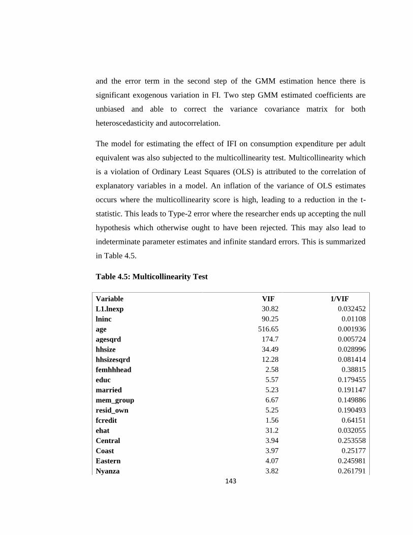
143

and the error term in the second step of the GMM estimation hence there is

significant exogenous variation in FI. Two step GMM estimated coefficients are

unbiased and able to correct the variance covariance matrix for both

heteroscedasticity and autocorrelation.

The model for estimating the effect of IFI on consumption expenditure per adult

equivalent was also subjected to the multicollinearity test. Multicollinearity which

is a violation of Ordinary Least Squares (OLS) is attributed to the correlation of

explanatory variables in a model. An inflation of the variance of OLS estimates

occurs where the multicollinearity score is high, leading to a reduction in the t-

statistic. This leads to Type-2 error where the researcher ends up accepting the null

hypothesis which otherwise ought to have been rejected. This may also lead to

indeterminate parameter estimates and infinite standard errors. This is summarized

in Table 4.5.

Table 4.5: Multicollinearity Test

Variable VIF 1/VIFL1.lnexp 30.82 0.032452lninc 90.25 0.01108age 516.65 0.001936agesqrd 174.7 0.005724hhsize 34.49 0.028996hhsizesqrd 12.28 0.081414femhhhead 2.58 0.38815educ 5.57 0.179455married 5.23 0.191147mem_group 6.67 0.149886resid_own 5.25 0.190493fcredit 1.56 0.64151ehat 31.2 0.032055Central 3.94 0.253558Coast 3.97 0.25177Eastern 4.07 0.245981Nyanza 3.82 0.261791

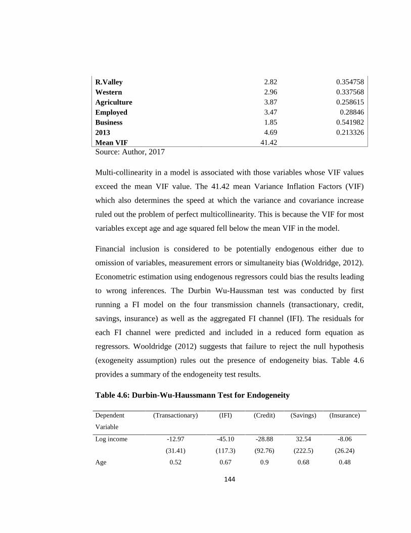
144

R.Valley 2.82 0.354758Western 2.96 0.337568Agriculture 3.87 0.258615Employed 3.47 0.28846Business 1.85 0.5419822013 4.69 0.213326Mean VIF 41.42Source: Author, 2017

Multi-collinearity in a model is associated with those variables whose VIF values

exceed the mean VIF value. The 41.42 mean Variance Inflation Factors (VIF)

which also determines the speed at which the variance and covariance increase

ruled out the problem of perfect multicollinearity. This is because the VIF for most

variables except age and age squared fell below the mean VIF in the model.

Financial inclusion is considered to be potentially endogenous either due to

omission of variables, measurement errors or simultaneity bias (Woldridge, 2012).

Econometric estimation using endogenous regressors could bias the results leading

to wrong inferences. The Durbin Wu-Haussman test was conducted by first

running a FI model on the four transmission channels (transactionary, credit,

savings, insurance) as well as the aggregated FI channel (IFI). The residuals for

each FI channel were predicted and included in a reduced form equation as

regressors. Wooldridge (2012) suggests that failure to reject the null hypothesis

(exogeneity assumption) rules out the presence of endogeneity bias. Table 4.6

provides a summary of the endogeneity test results.

Table 4.6: Durbin-Wu-Haussmann Test for Endogeneity

Dependent (Transactionary) (IFI) (Credit) (Savings) (Insurance)

Variable

Log income -12.97 -45.10 -28.88 32.54 -8.06

(31.41) (117.3) (92.76) (222.5) (26.24)

Age 0.52 0.67 0.9 0.68 0.48

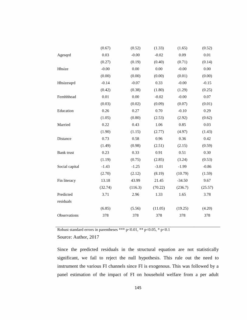
145

(0.67) (0.52) (1.33) (1.65) (0.52)

Agesqrd 0.03 -0.00 -0.02 0.09 0.01

(0.27) (0.19) (0.40) (0.71) (0.14)

Hhsize -0.00 0.00 0.00 -0.00 0.00

(0.00) (0.00) (0.00) (0.01) (0.00)

Hhsizesqrd -0.14 -0.07 0.33 -0.00 -0.15

(0.42) (0.38) (1.80) (1.29) (0.25)

Femhhhead 0.01 0.00 -0.02 -0.00 0.07

(0.03) (0.02) (0.09) (0.07) (0.01)

Education 0.26 0.27 0.70 -0.10 0.29

(1.05) (0.80) (2.53) (2.92) (0.62)

Married 0.22 0.43 1.06 0.85 0.03

(1.90) (1.15) (2.77) (4.97) (1.43)

Distance 0.73 0.58 0.96 0.36 0.42

(1.49) (0.98) (2.51) (2.15) (0.59)

Bank trust 0.23 0.33 0.91 0.51 0.30

(1.19) (0.75) (2.85) (3.24) (0.53)

Social capital -1.43 -1.25 -3.01 -1.99 -0.86

(2.70) (2.12) (8.19) (10.79) (1.59)

Fin literacy 13.18 43.99 21.45 -34.50 9.67

(32.74) (116.3) (70.22) (236.7) (25.57)

Predicted

residuals

3.71 2.96 1.33 1.65 3.78

(6.85) (5.56) (11.05) (19.25) (4.20)

Observations 378 378 378 378 378

Robust standard errors in parentheses *** p<0.01, ** p<0.05, * p<0.1

Source: Author, 2017

Since the predicted residuals in the structural equation are not statistically

significant, we fail to reject the null hypothesis. This rule out the need to

instrument the various FI channels since FI is exogenous. This was followed by a

panel estimation of the impact of FI on household welfare from a per adult

146

equivalent consumption expenditure approach. As mentioned earlier, fixed effects

estimation of panel data may lead to Hurwicz/Nickel bias (Wooldridge, 2012)

when the data has a short time dimension and many cross sections. FE estimation

ends up underestimating the autoregressive coefficient leading to a bias of order

1/T. Arrelano and Bover (1995) therefore recommends the use of a system GMM

estimation to carry out an autoregressive dynamic estimation of the model

parameters. The dependent variable is log consumption expenditure per adult

equivalent while the independent variables include the household characteristics.

4.5.2 Static Analysis of FI impact on Consumption Expenditure

A GMM estimation which follows the two step procedure established varying

effects of the various categories of FI on consumer welfare. Linear static welfare is

estimated using five transmission channels based on cohort data. Pooled estimation

from the full sample data assumes that households in the repeated cross sections

are independent which may not be the case due to unobserved heterogeneity. The

essence of panel estimation is to remove those fixed effects through differencing.

The region fixed effects were controlled for to analyze how regional peculiarities

affect household welfare.

OPHI (2016) already predicted glaring disparities in household welfare across the

eight regions in Kenya. The only weakness associated with a static model is that it

ignores the impact of the lagged dependent variable which tests for the presence of

adaptive expectations hence the need to estimate an autoregressive dynamic panel

with the lagged dependent variable as a regressor. The results for static welfare

estimation are captured in Appendix Table 4.7.

4.5.3 Linear Dynamic Estimation

This section mainly focuses on the dynamic estimation of the linear model to

assess how FI accounts for differences in household consumption expenditure over

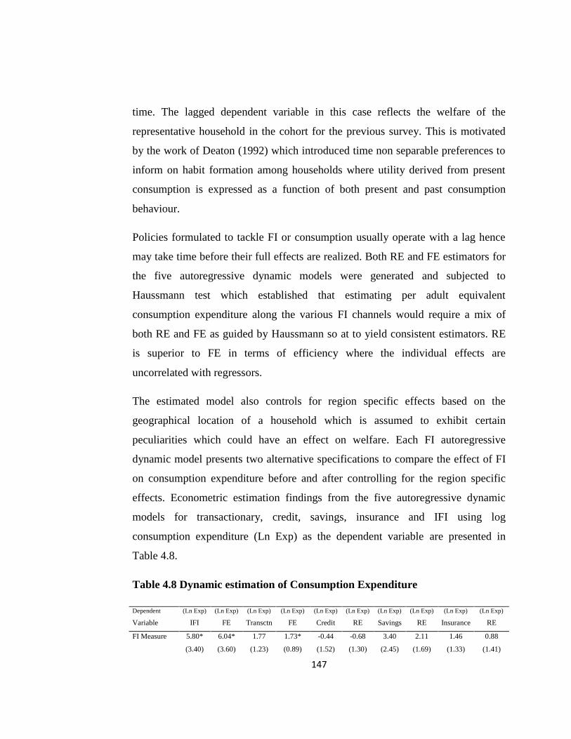
147

time. The lagged dependent variable in this case reflects the welfare of the

representative household in the cohort for the previous survey. This is motivated

by the work of Deaton (1992) which introduced time non separable preferences to

inform on habit formation among households where utility derived from present

consumption is expressed as a function of both present and past consumption

behaviour.

Policies formulated to tackle FI or consumption usually operate with a lag hence

may take time before their full effects are realized. Both RE and FE estimators for

the five autoregressive dynamic models were generated and subjected to

Haussmann test which established that estimating per adult equivalent

consumption expenditure along the various FI channels would require a mix of

both RE and FE as guided by Haussmann so at to yield consistent estimators. RE

is superior to FE in terms of efficiency where the individual effects are

uncorrelated with regressors.

The estimated model also controls for region specific effects based on the

geographical location of a household which is assumed to exhibit certain

peculiarities which could have an effect on welfare. Each FI autoregressive

dynamic model presents two alternative specifications to compare the effect of FI

on consumption expenditure before and after controlling for the region specific

effects. Econometric estimation findings from the five autoregressive dynamic

models for transactionary, credit, savings, insurance and IFI using log

consumption expenditure (Ln Exp) as the dependent variable are presented in

Table 4.8.

Table 4.8 Dynamic estimation of Consumption Expenditure

Dependent (Ln Exp) (Ln Exp) (Ln Exp) (Ln Exp) (Ln Exp) (Ln Exp) (Ln Exp) (Ln Exp) (Ln Exp) (Ln Exp)

Variable IFI FE Transctn FE Credit RE Savings RE Insurance RE

FI Measure 5.80* 6.04* 1.77 1.73* -0.44 -0.68 3.40 2.11 1.46 0.88

(3.40) (3.60) (1.23) (0.89) (1.52) (1.30) (2.45) (1.69) (1.33) (1.41)

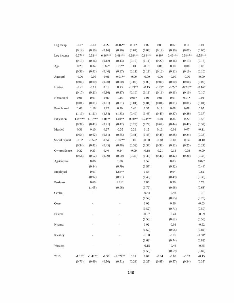
148

Lag lnexp -0.17 -0.18 -0.22 -0.46** 0.11* 0.02 0.03 0.02 0.11 0.01

(0.14) (0.19) (0.16) (0.20) (0.07) (0.09) (0.12) (0.10) (0.07) (0.08)

Log income 0.27** 0.33** 0.36*** 0.41*** 0.68*** 0.69*** 0.40* 0.49*** 0.54*** 0.55***

(0.13) (0.16) (0.12) (0.13) (0.10) (0.11) (0.22) (0.16) (0.13) (0.17)

Age 0.23 0.34 0.67* 0.76** 0.01 -0.01 0.08 0.10 0.08 0.08

(0.36) (0.41) (0.40) (0.37) (0.11) (0.11) (0.13) (0.11) (0.10) (0.10)

Agesqrd -0.00 -0.00 -0.01 -0.01** -0.00 -0.00 -0.00 -0.00 -0.00 -0.00

(0.00) (0.00) (0.00) (0.00) (0.00) (0.00) (0.00) (0.00) (0.00) (0.00)

Hhsize -0.21 -0.13 0.01 0.13 -0.21** -0.15 -0.29* -0.22* -0.23** -0.16*

(0.17) (0.21) (0.16) (0.17) (0.10) (0.11) (0.16) (0.13) (0.10) (0.10)

Hhsizesqrd 0.01 0.01 -0.00 -0.00 0.01* 0.01 0.01 0.01 0.01* 0.01

(0.01) (0.01) (0.01) (0.01) (0.01) (0.01) (0.01) (0.01) (0.01) (0.01)

Femhhhead 1.63 1.16 1.22 0.20 0.40 0.37 0.16 0.08 0.08 0.05

(1.10) (1.21) (1.34) (1.33) (0.49) (0.46) (0.49) (0.37) (0.38) (0.37)

Education 1.06*** 1.19*** 1.04** 1.04** 0.70** 0.74*** -0.10 0.34 0.22 0.56

(0.37) (0.41) (0.41) (0.42) (0.29) (0.27) (0.67) (0.44) (0.47) (0.37)

Married 0.36 0.10 0.27 -0.35 0.29 0.15 0.10 -0.03 0.07 -0.11

(0.54) (0.62) (0.61) (0.65) (0.41) (0.45) (0.48) (0.38) (0.34) (0.33)

Social capital -0.32 -0.522 -0.54 -1.02** 0.09 -0.00 -0.18 -0.08 0.14 -0.10

(0.34) (0.41) (0.45) (0.48) (0.32) (0.37) (0.36) (0.31) (0.25) (0.24)

Ownresidence 0.32 0.33 0.40 0.34 -0.09 -0.18 -0.21 -0.13 -0.03 -0.00

(0.54) (0.62) (0.59) (0.60) (0.30) (0.38) (0.46) (0.42) (0.30) (0.38)

Agriculture 0.86 1.08 0.52 0.83 0.82*

(0.84) (0.79) (0.57) (0.52) (0.44)

Employed 0.63 1.84** 0.53 0.64 0.62

(0.92) (0.91) (0.46) (0.49) (0.38)

Business 0.60 1.81* 0.86 0.30 0.78

(1.05) (0.96) (0.72) (0.96) (0.68)

Central - - -0.54 -0.98 -1.01

(0.52) (0.65) (0.78)

Coast - - 0.03 0.56 -0.03

(0.52) (0.71) (0.50)

Eastern - - -0.37 -0.41 -0.59

(0.53) (0.62) (0.58)

Nyanza - - 0.02 -0.03 -0.52

(0.60) (0.64) (0.82)

RValley - - -1.00 -0.76 -1.50*

(0.62) (0.74) (0.82)

Western - - -0.15 -0.46 -0.65

(0.58) (0.69) (0.87)

2016 -1.19* -1.42** -0.58 -1.027** 0.17 0.07 -0.94 -0.60 -0.13 -0.15

(0.70) (0.69) (0.50) (0.51) (0.23) (0.25) (0.85) (0.57) (0.34) (0.35)

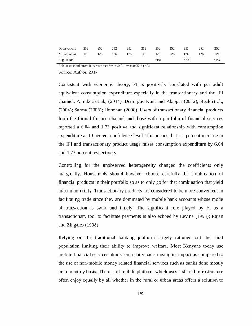
149

Observations 252 252 252 252 252 252 252 252 252 252

No. of cohort 126 126 126 126 126 126 126 126 126 126

Region RE YES YES YES

Robust standard errors in parentheses *** p<0.01, ** p<0.05, * p<0.1

Source: Author, 2017

Consistent with economic theory, FI is positively correlated with per adult

equivalent consumption expenditure especially in the transactionary and the IFI

channel, Amidzic et al., (2014); Demirguc-Kunt and Klapper (2012); Beck et al.,

(2004); Sarma (2008); Honohan (2008). Users of transactionary financial products

from the formal finance channel and those with a portfolio of financial services

reported a 6.04 and 1.73 positive and significant relationship with consumption

expenditure at 10 percent confidence level. This means that a 1 percent increase in

the IFI and transactionary product usage raises consumption expenditure by 6.04

and 1.73 percent respectively.

Controlling for the unobserved heterogeneity changed the coefficients only

marginally. Households should however choose carefully the combination of

financial products in their portfolio so as to only go for that combination that yield

maximum utility. Transactionary products are considered to be more convenient in

facilitating trade since they are dominated by mobile bank accounts whose mode

of transaction is swift and timely. The significant role played by FI as a

transactionary tool to facilitate payments is also echoed by Levine (1993); Rajan

and Zingales (1998).

Relying on the traditional banking platform largely rationed out the rural

population limiting their ability to improve welfare. Most Kenyans today use

mobile financial services almost on a daily basis raising its impact as compared to

the use of non-mobile money related financial services such as banks done mostly

on a monthly basis. The use of mobile platform which uses a shared infrastructure

often enjoy equally by all whether in the rural or urban areas offers a solution to

150

cream skimming often practiced by the traditional lending channels. These mobile

bank accounts include; KCB M-PESA, MCo-op Cash and M-shwari but excludes

Equitel since at the time of data collection it had not been launched.

Being the biggest component of household ownership of transactionary products,

mobile bank accounts multiplier effect on welfare on Kenya's population is

immense. This also shows that the gains from digital financial services and

especially those rolling on a mobile platform are fast. This huge contribution on

welfare probably accounts for the positive and significant coefficient in the IFI

variable. These findings supports the literature on the operation of the growth led

finance hypothesis in Kenya as postulated by Robinson (1952); Lucas (1988);

Demetriades and Hussein (1996).

The impact of savings deposit instruments and insurance product which currently

average 32.43 percent in the formal sector on household welfare exhibited a

positive relationship both before and after controlling for sector and regional

specific effects. However the coefficient is not significant in explaining welfare.

The impact of savings on economic growth is usually transmitted through

technical progress, investment growth size of capital stock and stock of human

capital in line with the endogenous growth models prediction by Arrow (1962);

Romer (1986) and Lucas (1962). A disaggregation of savings product usage

revealed that it was dominated by mobile savings.

The line showing the difference between holding mobile money as a transactionary

product and holding it as a savings product is so thin hence could have affected the

sign and the coefficient of savings. To a large extent, holding savings in a mobile

money account ends up translating to consumption. The theory of consumer

behaviour posits that consumption is inversely related to savings since the

marginal propensity to save falls with increase in the marginal propensity to

consume. The second largest component of savings from the FinAccess data is

151

bank savings which again closely resembles current accounts in banks mainly used

for transactionary purposes. The savings variable may therefore have picked the

transactionary motive of households leading to a positive but non-significant

effect.

The weak relationship between insurance and pension product usage in the

autoregressive dynamic panel could be rationalized by the domination of NSSF

product in the insurance and pension category. Pension products including NSSF

will most likely deliver, it's intended objective to retirees. Given that majority of

the sampled population falls below the retirement age, the welfare gains from such

financial product holding could therefore be insignificant in the short run. It's also

understood that most pension funds follow a pooling model when choosing

investment options which makes them settle for long term investment facilities

with longer maturity periods hence may not deliver immediate welfare gains.

The effect of NHIF which accounts for the second largest share in insurance and

pension product usage may also not be very significant since despite denting a

household monthly income, benefits are only derived when one falls sick. This

insurance component mainly affects only 34 percent of the sampled populations

who fall in the employed category whose contributions are statutorily deducted

from their salary and another smaller segment of non-employed who probably

service it voluntarily. Most rural households some of whom pay directly from their

informal incomes take long before they visit health centers where the insurance

fund can be utilized without paying.

The insurance product is usually embraced due to its ability to cushion against

risks from unexpected occurrences but only benefits the insured when the risk

occurs. Given this development, the real effect of insurance product holding on

welfare may not be significant especially in the short run since the insurance

industry operates under the indemnity principle whose sole objective is to restore

152

the household back to their initial position before the risk occurred. FSD (2016)

shows that 32 percent of Kenyans service their insurance obligation in cash while

45.9 percent have their premiums paid directly by employers from the salary or

through a check off system. Those who use mobile financial services to pay

insurance premiums averaged 15.7 percent.

The effect of credit uptake among households in this model appears to contradict

theory which associates credit usage to positive welfare effects. This is because

besides the coefficient being non-significant, the coefficient took a negative sign

implying that uptake of credit products does not yield the desired results at the end

of the day but only aggravates the plight of the poor households. Buera et al.

(2012) predicted that the impact of credit on consumption expenditure averages 10

percent. Usage of credit facilities from the formal strand has for a long time been

dominated by bank loans, credit cards and overdraft facilities. It will be interesting

to see the contribution of DTM and DTS loans on gross loans which for now

remain relatively low. The inverse relationship between credit and welfare could

be attributed to indiscriminate borrowing arising from the increased aggression on

the part of service providers who want to maintain high sales volumes to increase

their networth.

In most instances, lenders decision to extend credit to a household is based on a

situational analysis only at the point of application. Moral hazard could also pose a

serious problem in the credit markets since financial institutions hardly bother to

know how beneficiaries conduct themselves once their loan has been approved. It's

possible that part of the extended loan is diverted from its intended objective hence

lowering the expected utility. The beneficiaries could be also suffering from poor

resource management hence end up spending the loans only to smooth

consumption at the expense of investment smoothing.

153

Given that credit recorded a mere 14 percent uptake, its effect on overall welfare

could be diminished by the low figures. Beck17 (2016) recognizes the need to

target the increased access to both credit and insurance services more closely

through improved institutional framework to ensure a level playing field for all

players. This would have positive welfare effects at individual level and also

guarantee positive aggregate growth effects. The breakdown of loans indicates that

despite banks being the main source of loans, its share remains low. FSD (2016)

report indicates that day-to-day household needs (recurrent expenditure) accounts

for the highest percentage use of credit services (57.3 percent) followed by

education (21.5 percent) and business (15.8 percent) in that order. Loans for

agriculture take a paltry 11.5 percent.

This paints a dark picture on the potential of using credit instruments to improve

household welfare given that loans for productive activities such as supporting

business and agriculture only average 27.3 percent yet 75 percent of Kenya's total

population rely on agriculture for living. The analysis further established that only

1.4 and 2.0 percent of households in rural and urban areas respectively borrowed

from banks/SACCO to mitigate against major shocks in the last two years (FSD,

2016). Households will therefore not embrace credit facilities from banks to

smoothing consumption but would rather apply other mechanisms such as

liquidating assets. This explanation offers insight on why the coefficient for

savings is positive while that of credit is negative and insignificant.

Similar to transactionary usage, IFI was found to be positive and significant in

explaining household welfare at 10 percent confidence level. Given that this

variable aggregates portfolio holding of the various categories of FI, its coefficient

appear to have picked the dominant effect of transactionary product holding which

average 77 percent in the data. This result is consistent with Sarma (2008) finding

17 Beck (2016). Financial Inclusion in Africa

154

of a strong positive relationship between FI and welfare. The big question is on

how policy makers can improve the significant relationship between the IFI and

transactionary financial product holding.

One way would be to action the government to lower the transaction fees which

appear to neutralize gains from the improved payment systems given that mobile

and bank accounts dominate the transactionary channel. A single money

transaction for example on a mobile platform is often taxed twice for both the

sender and the receiver. If these costs can be reduced, the welfare gains from

innovations in payment systems could have a bigger multiplier effect given the

high uptake of transactionary financial services.

The lagged consumption expenditure among holders of transactionary products at

5 percent confidence level led to a significant reduction in household welfare. The

operation of the permanent income hypothesis posits that consumption is

maintained at a constant level in all periods regardless of the fortunes. Households

who recorded higher consumption patterns in the past are likely to experience

lower welfare levels in the future. The lagged consumption expenditure variable

was also significant among holders of credit products before controlling for sector

and region specific effects. Use of lagged consumption expenditure in a pseudo

panel however poses methodological challenges since the households being

tracked over time are not the same. However, use of the representative household

in the cohort helps correct the problem since the same representative household is

used even in previous surveys in the cohort.

Per capita income among Kenyan households was found to have a strong positive

and significant relationship on welfare at 10 percent for both single product usage

as well as portfolio holding. This result reinforces the theory of consumer

behaviour which associates increase in consumption to growth in per capita

income. Households who enjoy higher income levels reported higher consumption

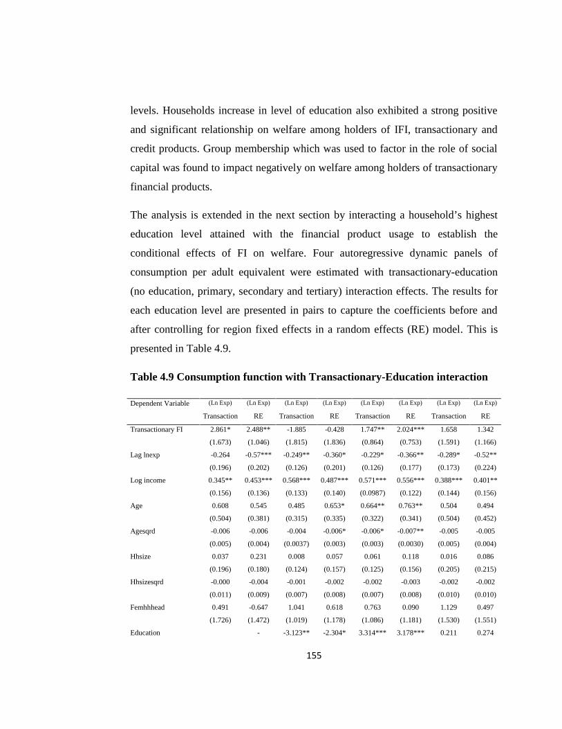
155

levels. Households increase in level of education also exhibited a strong positive

and significant relationship on welfare among holders of IFI, transactionary and

credit products. Group membership which was used to factor in the role of social

capital was found to impact negatively on welfare among holders of transactionary

financial products.

The analysis is extended in the next section by interacting a household’s highest

education level attained with the financial product usage to establish the

conditional effects of FI on welfare. Four autoregressive dynamic panels of

consumption per adult equivalent were estimated with transactionary-education

(no education, primary, secondary and tertiary) interaction effects. The results for

each education level are presented in pairs to capture the coefficients before and

after controlling for region fixed effects in a random effects (RE) model. This is

presented in Table 4.9.

Table 4.9 Consumption function with Transactionary-Education interaction

Dependent Variable (Ln Exp) (Ln Exp) (Ln Exp) (Ln Exp) (Ln Exp) (Ln Exp) (Ln Exp) (Ln Exp)

Transaction RE Transaction RE Transaction RE Transaction RE

Transactionary FI 2.861* 2.488** -1.885 -0.428 1.747** 2.024*** 1.658 1.342

(1.673) (1.046) (1.815) (1.836) (0.864) (0.753) (1.591) (1.166)

Lag lnexp -0.264 -0.57*** -0.249** -0.360* -0.229* -0.366** -0.289* -0.52**

(0.196) (0.202) (0.126) (0.201) (0.126) (0.177) (0.173) (0.224)

Log income 0.345** 0.453*** 0.568*** 0.487*** 0.571*** 0.556*** 0.388*** 0.401**

(0.156) (0.136) (0.133) (0.140) (0.0987) (0.122) (0.144) (0.156)

Age 0.608 0.545 0.485 0.653* 0.664** 0.763** 0.504 0.494

(0.504) (0.381) (0.315) (0.335) (0.322) (0.341) (0.504) (0.452)

Agesqrd -0.006 -0.006 -0.004 -0.006* -0.006* -0.007** -0.005 -0.005

(0.005) (0.004) (0.0037) (0.003) (0.003) (0.0030) (0.005) (0.004)

Hhsize 0.037 0.231 0.008 0.057 0.061 0.118 0.016 0.086

(0.196) (0.180) (0.124) (0.157) (0.125) (0.156) (0.205) (0.215)

Hhsizesqrd -0.000 -0.004 -0.001 -0.002 -0.002 -0.003 -0.002 -0.002

(0.011) (0.009) (0.007) (0.008) (0.007) (0.008) (0.010) (0.010)

Femhhhead 0.491 -0.647 1.041 0.618 0.763 0.090 1.129 0.497

(1.726) (1.472) (1.019) (1.178) (1.086) (1.181) (1.530) (1.551)

Education - -3.123** -2.304* 3.314*** 3.178*** 0.211 0.274

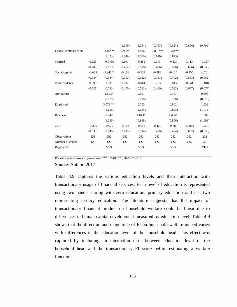
156

(1.349) (1.364) (0.767) (0.824) (0.866) (0.795)

Education*transaction -3.46*** 2.932* 1.694 -2.851*** -2.69*** - -

(1.323) (1.649) (1.500) (0.816) (0.873)

Married 0.325 -0.0438 0.101 -0.252 0.143 -0.220 0.113 -0.327

(0.780) (0.679) (0.477) (0.588) (0.496) (0.576) (0.676) (0.736)

Social capital -0.683 -1.240** -0.116 -0.537 -0.283 -0.615 -0.455 -0.781

(0.584) (0.544) (0.357) (0.522) (0.337) (0.442) (0.533) (0.582)

Own residence 0.093 1.081 0.202 -0.064 0.265 0.043 -0.041 -0.018

(0.721) (0.753) (0.470) (0.532) (0.460) (0.532) (0.647) (0.677)

Agriculture 1.553* 0.501 0.467 0.608

(0.879) (0.730) (0.720) (0.875)

Employed 3.079*** 0.755 0.862 1.552

(1.118) (1.034) (0.865) (1.072)

Business 0.249 1.643* 1.436* 1.382

(1.086) (0.938) (0.856) (1.098)

2016 -0.306 -0.626 -0.102 -0.613 -0.426 -0.783 -0.0981 -0.407

(0.630) (0.548) (0.400) (0.514) (0.408) (0.484) (0.632) (0.656)

Observations 252 252 252 252 252 252 252 252

Number of cohort 126 126 126 126 126 126 126 126

Region RE YES YES YES YES

Robust standard errors in parentheses *** p<0.01, ** p<0.05, * p<0.1

Source: Author, 2017

Table 4.9 captures the various education levels and their interaction with

transactionary usage of financial services. Each level of education is represented

using two panels staring with zero education, primary education and last two

representing tertiary education. The literature suggests that the impact of

transactionary financial product on household welfare could be linear due to

differences in human capital development measured by education level. Table 4.9

shows that the direction and magnitude of FI on household welfare indeed varies

with differences in the education level of the household head. This effect was

captured by including an interaction term between education level of the

household head and the transactionary FI score before estimating a welfare

function.

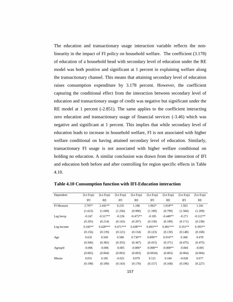
157

The education and transactionary usage interaction variable reflects the non-

linearity in the impact of FI policy on household welfare. The coefficient (3.178)

of education of a household head with secondary level of education under the RE

model was both positive and significant at 1 percent in explaining welfare along

the transactionary channel. This means that attaining secondary level of education

raises consumption expenditure by 3.178 percent. However, the coefficient

capturing the conditional effect from the interaction between secondary level of

education and transactionary usage of credit was negative but significant under the

RE model at 1 percent (-2.851). The same applies to the coefficient interacting

zero education and transactionary usage of financial services (-3.46) which was

negative and significant at 1 percent. This implies that while secondary level of

education leads to increase in household welfare, FI is not associated with higher

welfare conditional on having attained secondary level of education. Similarly,

transactionary FI usage is not associated with higher welfare conditional on

holding no education. A similar conclusion was drawn from the interaction of IFI

and education both before and after controlling for region specific effects in Table

4.10.

Table 4.10 Consumption function with IFI-Education interaction

Dependent (Ln Exp) (Ln Exp) (Ln Exp) (Ln Exp) (Ln Exp) (Ln Exp) (Ln Exp) (Ln Exp)

IFI RE IFI RE IFI RE IFI RE

FI Measure 2.797* 2.441** 0.235 1.186 1.962* 1.918** 1.503 1.341

(1.623) (1.049) (1.256) (0.990) (1.189) (0.799) (1.584) (1.209)

Lag lnexp -0.247 -0.517** -0.226 -0.475** -0.185 -0.449** -0.271 -0.512**

(0.205) (0.214) (0.143) (0.207) (0.158) (0.189) (0.171) (0.238)

Log income 0.345** 0.428*** 0.471*** 0.438*** 0.493*** 0.481*** 0.351** 0.395**

(0.156) (0.139) (0.121) (0.134) (0.123) (0.130) (0.148) (0.168)

Age 0.635 0.569 0.580 0.730** 0.899** 0.910** 0.368 0.478

(0.506) (0.382) (0.355) (0.367) (0.415) (0.371) (0.475) (0.475)

Agesqrd -0.006 -0.006 -0.005 -0.006* -0.008** -0.008** -0.004 -0.005

(0.005) (0.004) (0.003) (0.003) (0.0034) (0.003) (0.004) (0.004)

Hhsize 0.031 0.185 -0.021 0.079 0.121 0.184 -0.028 0.077

(0.198) (0.189) (0.143) (0.170) (0.157) (0.168) (0.196) (0.227)

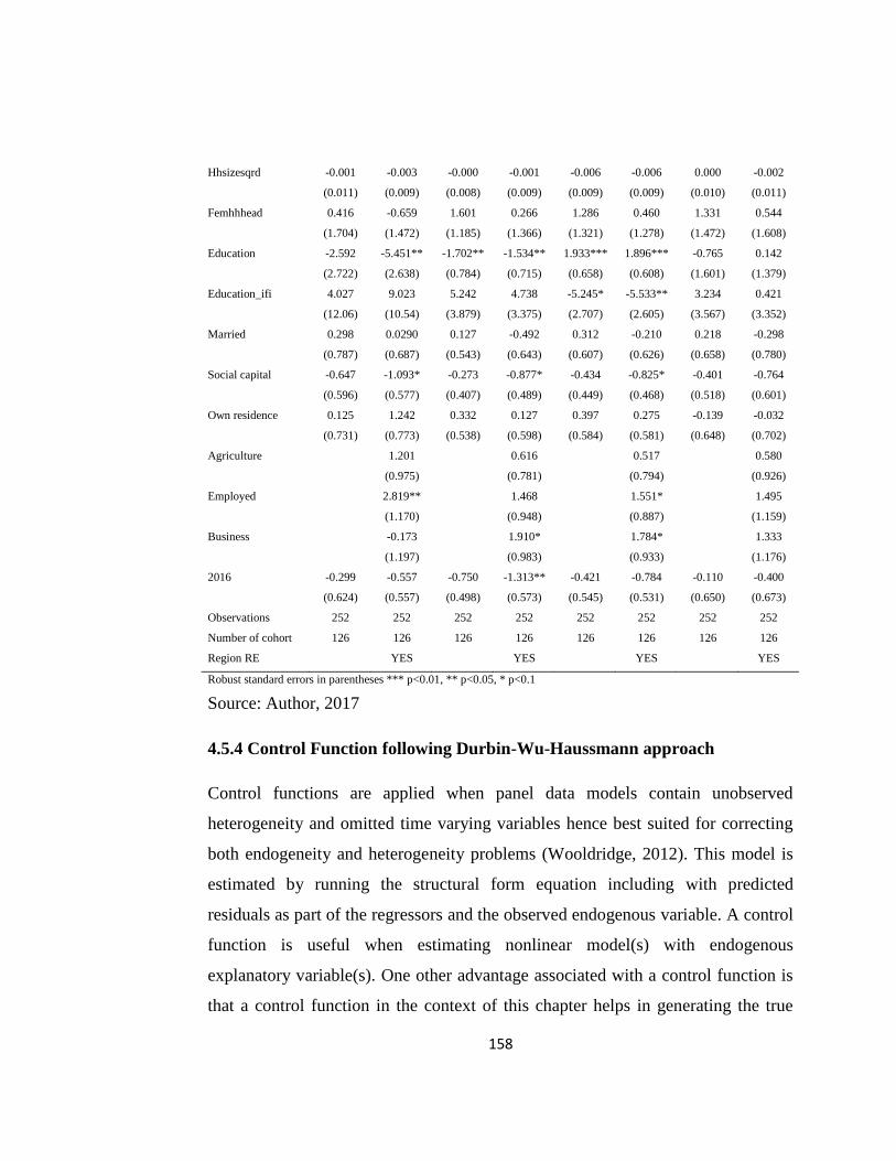
158

Hhsizesqrd -0.001 -0.003 -0.000 -0.001 -0.006 -0.006 0.000 -0.002

(0.011) (0.009) (0.008) (0.009) (0.009) (0.009) (0.010) (0.011)

Femhhhead 0.416 -0.659 1.601 0.266 1.286 0.460 1.331 0.544

(1.704) (1.472) (1.185) (1.366) (1.321) (1.278) (1.472) (1.608)

Education -2.592 -5.451** -1.702** -1.534** 1.933*** 1.896*** -0.765 0.142

(2.722) (2.638) (0.784) (0.715) (0.658) (0.608) (1.601) (1.379)

Education_ifi 4.027 9.023 5.242 4.738 -5.245* -5.533** 3.234 0.421

(12.06) (10.54) (3.879) (3.375) (2.707) (2.605) (3.567) (3.352)

Married 0.298 0.0290 0.127 -0.492 0.312 -0.210 0.218 -0.298

(0.787) (0.687) (0.543) (0.643) (0.607) (0.626) (0.658) (0.780)

Social capital -0.647 -1.093* -0.273 -0.877* -0.434 -0.825* -0.401 -0.764

(0.596) (0.577) (0.407) (0.489) (0.449) (0.468) (0.518) (0.601)

Own residence 0.125 1.242 0.332 0.127 0.397 0.275 -0.139 -0.032

(0.731) (0.773) (0.538) (0.598) (0.584) (0.581) (0.648) (0.702)

Agriculture 1.201 0.616 0.517 0.580

(0.975) (0.781) (0.794) (0.926)

Employed 2.819** 1.468 1.551* 1.495

(1.170) (0.948) (0.887) (1.159)

Business -0.173 1.910* 1.784* 1.333

(1.197) (0.983) (0.933) (1.176)

2016 -0.299 -0.557 -0.750 -1.313** -0.421 -0.784 -0.110 -0.400

(0.624) (0.557) (0.498) (0.573) (0.545) (0.531) (0.650) (0.673)

Observations 252 252 252 252 252 252 252 252

Number of cohort 126 126 126 126 126 126 126 126

Region RE YES YES YES YES

Robust standard errors in parentheses *** p<0.01, ** p<0.05, * p<0.1

Source: Author, 2017

4.5.4 Control Function following Durbin-Wu-Haussmann approach

Control functions are applied when panel data models contain unobserved

heterogeneity and omitted time varying variables hence best suited for correcting

both endogeneity and heterogeneity problems (Wooldridge, 2012). This model is

estimated by running the structural form equation including with predicted

residuals as part of the regressors and the observed endogenous variable. A control

function is useful when estimating nonlinear model(s) with endogenous

explanatory variable(s). One other advantage associated with a control function is

that a control function in the context of this chapter helps in generating the true

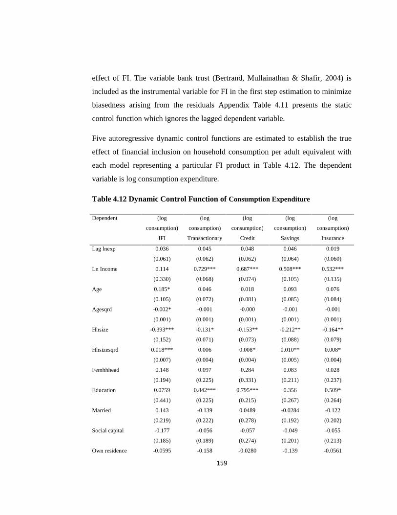
159

effect of FI. The variable bank trust (Bertrand, Mullainathan & Shafir, 2004) is

included as the instrumental variable for FI in the first step estimation to minimize

biasedness arising from the residuals Appendix Table 4.11 presents the static

control function which ignores the lagged dependent variable.

Five autoregressive dynamic control functions are estimated to establish the true

effect of financial inclusion on household consumption per adult equivalent with

each model representing a particular FI product in Table 4.12. The dependent

variable is log consumption expenditure.

Table 4.12 Dynamic Control Function of Consumption Expenditure

Dependent (log

consumption)

(log

consumption)

(log

consumption)

(log

consumption)

(log

consumption)

IFI Transactionary Credit Savings Insurance

Lag lnexp 0.036 0.045 0.048 0.046 0.019

(0.061) (0.062) (0.062) (0.064) (0.060)

Ln Income 0.114 0.729*** 0.687*** 0.508*** 0.532***

(0.330) (0.068) (0.074) (0.105) (0.135)

Age 0.185* 0.046 0.018 0.093 0.076

(0.105) (0.072) (0.081) (0.085) (0.084)

Agesqrd -0.002* -0.001 -0.000 -0.001 -0.001

(0.001) (0.001) (0.001) (0.001) (0.001)

Hhsize -0.393*** -0.131* -0.153** -0.212** -0.164**

(0.152) (0.071) (0.073) (0.088) (0.079)

Hhsizesqrd 0.018*** 0.006 0.008* 0.010** 0.008*

(0.007) (0.004) (0.004) (0.005) (0.004)

Femhhhead 0.148 0.097 0.284 0.083 0.028

(0.194) (0.225) (0.331) (0.211) (0.237)

Education 0.0759 0.842*** 0.795*** 0.356 0.509*

(0.441) (0.225) (0.215) (0.267) (0.264)

Married 0.143 -0.139 0.0489 -0.0284 -0.122

(0.219) (0.222) (0.278) (0.192) (0.202)

Social capital -0.177 -0.056 -0.057 -0.049 -0.055

(0.185) (0.189) (0.274) (0.201) (0.213)

Own residence -0.0595 -0.158 -0.0280 -0.139 -0.0561

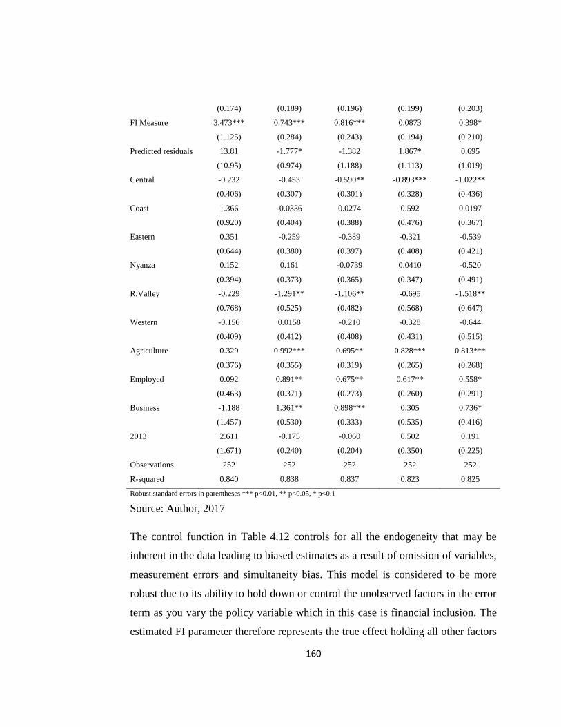
160

(0.174) (0.189) (0.196) (0.199) (0.203)

FI Measure 3.473*** 0.743*** 0.816*** 0.0873 0.398*

(1.125) (0.284) (0.243) (0.194) (0.210)

Predicted residuals 13.81 -1.777* -1.382 1.867* 0.695

(10.95) (0.974) (1.188) (1.113) (1.019)

Central -0.232 -0.453 -0.590** -0.893*** -1.022**

(0.406) (0.307) (0.301) (0.328) (0.436)

Coast 1.366 -0.0336 0.0274 0.592 0.0197

(0.920) (0.404) (0.388) (0.476) (0.367)

Eastern 0.351 -0.259 -0.389 -0.321 -0.539

(0.644) (0.380) (0.397) (0.408) (0.421)

Nyanza 0.152 0.161 -0.0739 0.0410 -0.520

(0.394) (0.373) (0.365) (0.347) (0.491)

R.Valley -0.229 -1.291** -1.106** -0.695 -1.518**

(0.768) (0.525) (0.482) (0.568) (0.647)

Western -0.156 0.0158 -0.210 -0.328 -0.644

(0.409) (0.412) (0.408) (0.431) (0.515)

Agriculture 0.329 0.992*** 0.695** 0.828*** 0.813***

(0.376) (0.355) (0.319) (0.265) (0.268)

Employed 0.092 0.891** 0.675** 0.617** 0.558*

(0.463) (0.371) (0.273) (0.260) (0.291)

Business -1.188 1.361** 0.898*** 0.305 0.736*

(1.457) (0.530) (0.333) (0.535) (0.416)

2013 2.611 -0.175 -0.060 0.502 0.191

(1.671) (0.240) (0.204) (0.350) (0.225)

Observations 252 252 252 252 252

R-squared 0.840 0.838 0.837 0.823 0.825

Robust standard errors in parentheses *** p<0.01, ** p<0.05, * p<0.1

Source: Author, 2017

The control function in Table 4.12 controls for all the endogeneity that may be

inherent in the data leading to biased estimates as a result of omission of variables,

measurement errors and simultaneity bias. This model is considered to be more

robust due to its ability to hold down or control the unobserved factors in the error

term as you vary the policy variable which in this case is financial inclusion. The

estimated FI parameter therefore represents the true effect holding all other factors

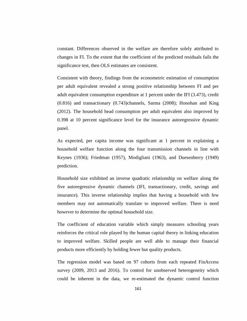
161

constant. Differences observed in the welfare are therefore solely attributed to

changes in FI. To the extent that the coefficient of the predicted residuals fails the

significance test, then OLS estimates are consistent.

Consistent with theory, findings from the econometric estimation of consumption

per adult equivalent revealed a strong positive relationship between FI and per

adult equivalent consumption expenditure at 1 percent under the IFI (3.473), credit

(0.816) and transactionary (0.743)channels, Sarma (2008); Honohan and King

(2012). The household head consumption per adult equivalent also improved by

0.398 at 10 percent significance level for the insurance autoregressive dynamic

panel.

As expected, per capita income was significant at 1 percent in explaining a

household welfare function along the four transmission channels in line with

Keynes (1936); Friedman (1957), Modigliani (1963), and Duesenberry (1949)

prediction.

Household size exhibited an inverse quadratic relationship on welfare along the

five autoregressive dynamic channels (IFI, transactionary, credit, savings and

insurance). This inverse relationship implies that having a household with few

members may not automatically translate to improved welfare. There is need

however to determine the optimal household size.

The coefficient of education variable which simply measures schooling years

reinforces the critical role played by the human capital theory in linking education

to improved welfare. Skilled people are well able to manage their financial

products more efficiently by holding fewer but quality products.

The regression model was based on 97 cohorts from each repeated FinAccess

survey (2009, 2013 and 2016). To control for unobserved heterogeneity which

could be inherent in the data, we re-estimated the dynamic control function

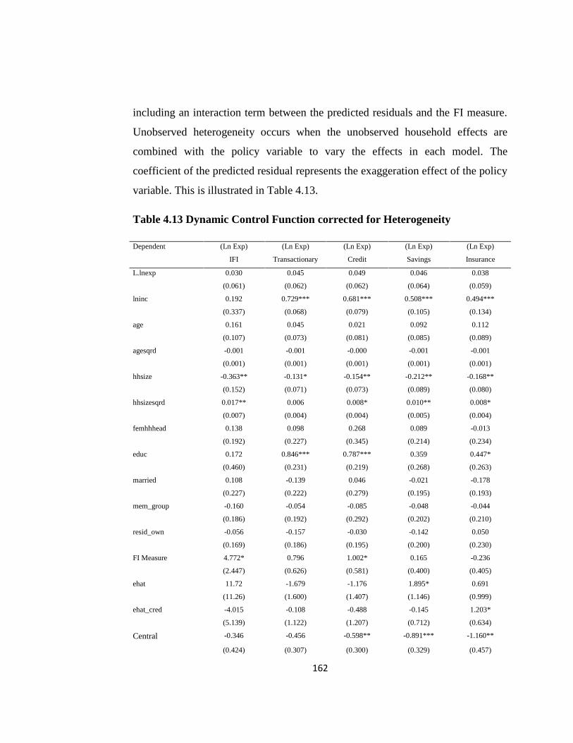
162

including an interaction term between the predicted residuals and the FI measure.

Unobserved heterogeneity occurs when the unobserved household effects are

combined with the policy variable to vary the effects in each model. The

coefficient of the predicted residual represents the exaggeration effect of the policy

variable. This is illustrated in Table 4.13.

Table 4.13 Dynamic Control Function corrected for Heterogeneity

Dependent (Ln Exp) (Ln Exp) (Ln Exp) (Ln Exp) (Ln Exp)

IFI Transactionary Credit Savings Insurance

L.lnexp 0.030 0.045 0.049 0.046 0.038

(0.061) (0.062) (0.062) (0.064) (0.059)

lninc 0.192 0.729*** 0.681*** 0.508*** 0.494***

(0.337) (0.068) (0.079) (0.105) (0.134)

age 0.161 0.045 0.021 0.092 0.112

(0.107) (0.073) (0.081) (0.085) (0.089)

agesqrd -0.001 -0.001 -0.000 -0.001 -0.001

(0.001) (0.001) (0.001) (0.001) (0.001)

hhsize -0.363** -0.131* -0.154** -0.212** -0.168**

(0.152) (0.071) (0.073) (0.089) (0.080)

hhsizesqrd 0.017** 0.006 0.008* 0.010** 0.008*

(0.007) (0.004) (0.004) (0.005) (0.004)

femhhhead 0.138 0.098 0.268 0.089 -0.013

(0.192) (0.227) (0.345) (0.214) (0.234)

educ 0.172 0.846*** 0.787*** 0.359 0.447*

(0.460) (0.231) (0.219) (0.268) (0.263)

married 0.108 -0.139 0.046 -0.021 -0.178

(0.227) (0.222) (0.279) (0.195) (0.193)

mem_group -0.160 -0.054 -0.085 -0.048 -0.044

(0.186) (0.192) (0.292) (0.202) (0.210)

resid_own -0.056 -0.157 -0.030 -0.142 0.050

(0.169) (0.186) (0.195) (0.200) (0.230)

FI Measure 4.772* 0.796 1.002* 0.165 -0.236

(2.447) (0.626) (0.581) (0.400) (0.405)

ehat 11.72 -1.679 -1.176 1.895* 0.691

(11.26) (1.600) (1.407) (1.146) (0.999)

ehat_cred -4.015 -0.108 -0.488 -0.145 1.203*

(5.139) (1.122) (1.207) (0.712) (0.634)

Central -0.346 -0.456 -0.598** -0.891*** -1.160**

(0.424) (0.307) (0.300) (0.329) (0.457)

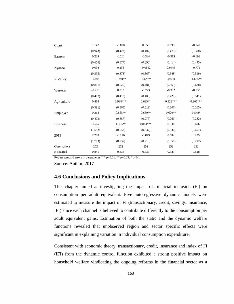
163

Coast 1.147 -0.028 0.053 0.595 -0.049

(0.943) (0.422) (0.407) (0.479) (0.378)

Eastern 0.205 -0.261 -0.384 -0.315 -0.698

(0.656) (0.377) (0.398) (0.414) (0.445)

Nyanza 0.094 0.158 -0.0842 0.0443 -0.771

(0.395) (0.373) (0.367) (0.348) (0.519)

R.Valley -0.405 -1.291** -1.125** -0.690 -1.675**

(0.801) (0.525) (0.481) (0.569) (0.678)

Western -0.213 0.013 -0.223 -0.332 -0.838

(0.407) (0.410) (0.406) (0.429) (0.541)

Agriculture 0.418 0.988*** 0.695** 0.828*** 0.905***

(0.391) (0.365) (0.319) (0.266) (0.265)

Employed 0.214 0.885** 0.660** 0.620** 0.548*

(0.473) (0.387) (0.277) (0.261) (0.282)

Business -0.757 1.355** 0.884*** 0.336 0.606

(1.552) (0.553) (0.332) (0.530) (0.407)

2013 2.290 -0.176 -0.049 0.502 0.225

(1.703) (0.237) (0.210) (0.350) (0.212)

Observations 252 252 252 252 252

R-squared 0.841 0.838 0.837 0.823 0.828

Robust standard errors in parentheses *** p<0.01, ** p<0.05, * p<0.1

Source: Author, 2017

4.6 Conclusions and Policy Implications

This chapter aimed at investigating the impact of financial inclusion (FI) on

consumption per adult equivalent. Five autoregressive dynamic models were

estimated to measure the impact of FI (transactionary, credit, savings, insurance,

IFI) since each channel is believed to contribute differently to the consumption per

adult equivalent gains. Estimation of both the static and the dynamic welfare

functions revealed that unobserved region and sector specific effects were

significant in explaining variation in individual consumption expenditure.

Consistent with economic theory, transactionary, credit, insurance and index of FI

(IFI) from the dynamic control function exhibited a strong positive impact on

household welfare vindicating the ongoing reforms in the financial sector as a

164

necessary tool for enhancing household welfare. Even though use of the lagged

dependent variable in pseudo panel estimation may not yield robust estimates due

to the use of aggregated data organized in cohorts, the technique is often

considered to be superior in the absence of longitudinal data for tracking

households over time.

Lastly, the conditional effect of FI from the interaction between education and FI

implies that while secondary level of education leads to increase in household

welfare, FI is not associated with higher welfare conditional on having attained

secondary level of education.

Given the significant impact of FI on consumption per adult equivalent, this

chapter recommends a bigger government involvement in ensuring that FI is

enhanced. Particular, the government should spearhead a campaign aimed at

lowering the transactionary costs to raise uptake.

165

Chapter Five: Impact of Financial Inclusion on

Vulnerability to Poverty

5.1 Introduction

Poverty reduction remains a key development challenge the world over despite

stepping up the campaign to eradicate poverty and hunger by 2015 under

Millennium Development Goals (MDG1). This is in spite of the many programs

rolled out to provide a roadmap on how to overcome poverty. Past research has

concentrated on demystifying headcount poverty and how best it can be overcome

with little or no attention being paid on its dynamic manifestation.

The dynamic structure of poverty draws a distinction between transient (entry or

exit) and chronic (re-entry) poverty. Lack of access to formal financial services by

the poor is often cited as a key constraint. The poverty question can only be

answered if a strong and vibrant financial system which facilitates transfer of

financial resources from the surplus units to the deficit units through financial

intermediation is established. Chithra (2006) asserts that FI brings the weak and

vulnerable population segment within the ambit of the formal financial system

often considered to be more organized.

Binswanger and Khandkher (1995) associate access to credit with the poor's ability

to smoothen consumption. Similar sentiments were echoed by World Bank (2013)

opining that universal access enhances access to a range of financial services to tap

opportunities and lower household vulnerability. This is also associated with the

poor's ability to improve their livelihoods and spur economic growth.

Collins, Murdoch, Rutherford, and Ruthven (2009) illustrate how poor households

manage their finances in their informal economies in order to mitigate against

transitory changes in their meager incomes. The yearlong financial diaries

166

collected in Bangladesh and India illustrate the model used by the poor in

countering poverty spells through savings symbolizing a very high demand for

financial services. The authors however challenged the use of headcount measure

of poverty due to the unpredictability and irregularity of income. Matul et al.

(2013) suggest that the uptake of insurance products is strikingly low due to

limited trust and liquidity constraints complicating efforts aimed at mitigating

vulnerability risks making it increasingly difficult for the poor to escape poverty.

Efforts to address global poverty appear to have paid off. World Bank (2015)

reported a decline in the population living on less than $ 1.90 a day in 2015 to a

forecast 9.6 percent of the global population. This could be attributed to the rapid

economic expansion and myriad intervention programs put in place over the years.

MDGs considered the number of persons living on less than 1.25 dollar a day as

the best measure of poverty (UN, 2000). This informed the need to reduce poverty

by half between 1990 and 2015 and World Banks campaign to reduce extreme

poverty to 3 percent by 2030.

Available evidence indicates that poverty in Sub-Saharan Africa declined from

56.5 to 48.5 percent for the period 1990 to 2010 (World Bank, 2011). Odhiambo

(2010) on the impact of financial development on poverty reduction in Kenya from

1968-2006 using a trivariate causality model based on co-integration and error

correction mechanism established a positive link between financial development

and poverty reduction. The study further established a unidirectional causality of

financial development on savings and a bidirectional causal relationship between

savings and poverty reduction.

Lack of access to financial services, adversely affect economic growth and poverty

alleviation by limiting the poor’s ability to mobilize savings and acquire assets for

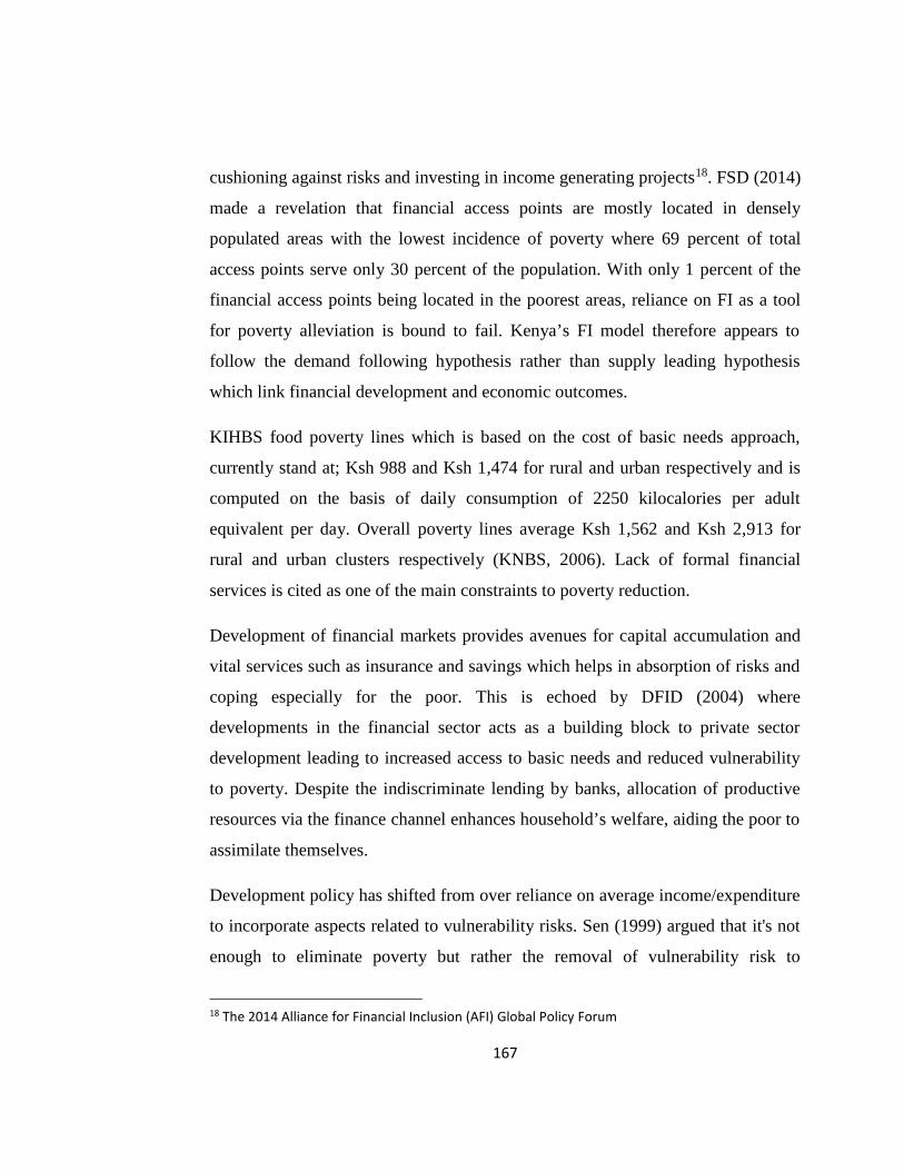
167

cushioning against risks and investing in income generating projects18. FSD (2014)

made a revelation that financial access points are mostly located in densely

populated areas with the lowest incidence of poverty where 69 percent of total

access points serve only 30 percent of the population. With only 1 percent of the

financial access points being located in the poorest areas, reliance on FI as a tool

for poverty alleviation is bound to fail. Kenya’s FI model therefore appears to

follow the demand following hypothesis rather than supply leading hypothesis

which link financial development and economic outcomes.

KIHBS food poverty lines which is based on the cost of basic needs approach,

currently stand at; Ksh 988 and Ksh 1,474 for rural and urban respectively and is

computed on the basis of daily consumption of 2250 kilocalories per adult

equivalent per day. Overall poverty lines average Ksh 1,562 and Ksh 2,913 for

rural and urban clusters respectively (KNBS, 2006). Lack of formal financial

services is cited as one of the main constraints to poverty reduction.

Development of financial markets provides avenues for capital accumulation and

vital services such as insurance and savings which helps in absorption of risks and

coping especially for the poor. This is echoed by DFID (2004) where

developments in the financial sector acts as a building block to private sector

development leading to increased access to basic needs and reduced vulnerability

to poverty. Despite the indiscriminate lending by banks, allocation of productive

resources via the finance channel enhances household’s welfare, aiding the poor to

assimilate themselves.

Development policy has shifted from over reliance on average income/expenditure

to incorporate aspects related to vulnerability risks. Sen (1999) argued that it's not

enough to eliminate poverty but rather the removal of vulnerability risk to

18 The 2014 Alliance for Financial Inclusion (AFI) Global Policy Forum

168

persistent and endemic deprivation. Chaudhuri (2002) argues that vulnerability

assessment must be rooted on explicit models of inter-temporal household

behaviour. The negative shocks faced by households however don't necessarily

lead to poverty since they can be mitigated against if early warning signs are

issued for policy intervention ex ante.

Coping mechanisms if well designed can also reduce the negative effects of

poverty ex post. As more and more people are pooled out of poverty, subsequent

surveys reveal that new ones enter the poverty trap making it appear like a zero

sum game which has only succeeded in maintaining poverty at a constant level.

But even with this cycle, the data has revealed that there is a significant proportion

that faces the risk of becoming poor in subsequent periods (vulnerable). This

creates the need to profile the vulnerable population for effective policy

interventions.

The broad objectives in this study revolved around the estimation and

determination of vulnerability as expected poverty in Kenya. This study is

centered on three specific research objectives derived from the broad objectives

namely:

1) To estimate the VEP for Kenya based on the 2009, 2013 and 2016

household survey data

2) To estimate the impact of FI on VEP in Kenya

3) To develop a poverty transition matrix using Kenya's household survey

data

An empirical study capturing the depth of vulnerability is critical in setting

different policy targets for the moderately and extremely vulnerable segments

since its mitigation is done ex ante based on future occurrences marking a sharp

departure from policies touching on poverty often mitigated ex post after it strikes.

169

In addition, a poverty transition matrix based on an empirical assessment helps in

explaining movements across the poverty line. An inclusive financial system is

one that goes beyond the usage of financial services to incorporate other aspects

related to welfare and vulnerability to poverty at both the national and county

levels. Use of repeated cross sectional data provides a more robust technique of

capturing the dynamic structure of poverty for policy.

5.2 Literature on Vulnerability to Poverty

The implications of FI on vulnerability to poverty are founded on a number of

theoretical linkages which include; the investment theory, human capital theory

and firm behaviour theory. Existing literature indicate that FI yields immense

benefits to the poor through elimination of barriers to access such as collateral

requirements and high borrowing costs. This increased access as explained by the

human capital theory in turn helps the populace invest in education which

ultimately boosts their payoffs. Firms also benefits from the reduction in cost of

capital as funds become readily available and at affordable rates. The firm

behaviour theory associates these benefits with increased production and more job

creation.

Whereas the strand of literature on poverty has been growing, empirical

examination using repeated cross sectional data remains scanty. This section

provides a summarized review of literature related to developments on

vulnerability assessment pioneered by Amemiya (1977). Alwang, Siegel and

Jorgensen (2001) describe vulnerability as a phenomenon characterized by

uncertain occurrences which require a forward looking approach to overcome. A

household’s ability to respond, time horizon and access to assets shape the manner

in which a household confronts vulnerability. Vulnerability studies help in

distinguishing the structurally poor from the resilient population who would

remain non vulnerable even in the absence of consumption vulnerability.

170

5.2.1 Theoretical Literature Review

The link between financial inclusion and poverty is motivated by the direct and the

indirect channels. The direct channel improves the plight of the poor through

broadened access to financial services while the indirect channel by Schumpeter

(1911) operates through the finance growth nexus to reduce poverty and income

inequality. Besides the direct and indirect theories studies on vulnerability to

poverty draws heavily from microeconomic theory and especially on decision

making under risk and uncertainty. This introduces indifference curves facing risk

averse, risk neutral and risk lovers as developed from the theory of expected

utility. A risk averse person's utility curve falls with variability in consumption

ceteris paribus. The certainty equivalence theorem on consumption fails due to

information asymmetry on individual’s utility functions from consumption. This is

also complicated by lack of longitudinal data in developing countries capturing

variability in individual consumption.

Theories on mobility assessment by Shorrocks (1978) and Ok (1999) with their

limited requirement of cardinally comparable utility functions offer important

insight on the measurement of vulnerability to poverty based on long term income

transition from one generation to another. This could include the shift from a poor

state to a non-poor state over time. However despite its wide acceptance, this

theory is criticized for laying much emphasis on historical patterns at the expense

of current or future patterns.

The issue of vulnerability as variability has also been cited in literature where the

link between historical shocks and future occurrences is associated with a

comparative analysis of consumption standard deviations and income variability.

The higher the margin by which the standard deviation of past consumption

changes, the more vulnerable the population. This however requires longitudinal

data with which also imposes a strong homogeneity assumption on the distribution

171

of consumption changes in the panels. Exposure to vulnerability is explained by

measures of dispersion in this framework. The main weakness in the use of

standard deviation to capture vulnerability is in the weighting of the risks where

both the downside and the upward risk are weighed the same.

Variability appears to hurt the poor more than it does to the non-poor. On the

contrary, the downside risk appears to rise for non-poor households when the

average consumption is declining. A more preferred measure is the coefficients of

variation though it can blow up for certain cells when some means tend to zero.

Besides giving odd results during times of persistent growth, the standard

deviation offers no accounting for persistence of downturns or negative serial

correlation.

Greenwood and Jovanovic (1990) developed a nonlinear model relating financial

development, income inequality and economic development. The theory posits that

broadened access to financial services benefits the rich at the early stages of

development increasing income inequality since the poor cannot afford the range

of financial services in the market. This income inequality however disappears as

more financial development is attained. This clearly shows that financial

development has to be intensified to ensure there are trickle down effects to the

underprivileged. This theory resembles Kuznets (1955) inverted U hypothesis

where income inequality widens at the early stages of development but falls as

more industrialization is achieved.

Galor and Zeira (1993) corroborates the inequality argument by stating that market

imperfections such as information asymmetry disadvantage the poor who lack

collateral, credit histories and connections to access financial services. Financial

development is therefore thought to be the solution to poverty by

disproportionately relaxing credit constraints and reducing income inequality for

the poor (Beck et al., 2004). Financial development reduces poverty through the

172

indirect channel by raising economic growth. This effect may also be transmitted

through changes in income distribution.

The trickledown effect theory also associates financial development and poverty

reduction. The theory suggests that economic growth reduces income inequality

through creation of economic opportunities for the poor (Todaro, 1997). Jalilian

and Kirkpatrick (2005) argued that one way of broadening access to financial

services among the poor is through elimination of market imperfections which lead

to market failures and high transactionary costs. Secondly the poor can be

encouraged to take advantage of credit and insurance services in the market to

build their asset base to improve their livelihoods.

5.3 Empirical Literature

5.3.1 Measuring Vulnerability to Poverty

Three main approaches have been put forth in the literature on the measurement of

vulnerability. Vulnerability in this context is analyzed as the probability of

remaining poor or falling into poverty in the future otherwise termed as

vulnerability as expected poverty (VEP) by Chaudhuri et al., (2002); Pritchett,

Suryahadi and Sumarto (2000); Chaudhuri, Jalan and Suryahadi (2002) and

Christiaensen and Subbarao (2005).

The other approaches cited in the literature comprise; vulnerability as expected

utility (VEU) by Ligon and Schechter (2003) and vulnerability as uninsured

exposure to risk (VER) by Amin, Rai, and Topa (2003); Dercon and Krishnan

(2000) and Glewwe and Hall (1998). Given that vulnerability studies dwell on the

future, they are usually motivated by theories touching on decision making under

risk and uncertainty. This informs why idiosyncratic shocks are included in the

estimation of vulnerability to poverty. These among other household

characteristics are what explain the vulnerability to poverty transition matrix. To

173

link FI and VEP, the study invokes a number of theories including; the human

capital theory, investment theory and firm behaviour theory.

The VEP approach according to Chaudhuri et al. (2002) defines vulnerability as

the probability of remaining poor or experiencing poverty in the near future given

one's socioeconomic characteristics. Vulnerability assessment poses challenges

since it's an unobservable phenomenon unlike poverty. Its assessment therefore

requires drawing some inferences about future outcomes usually captured as

probability of future income shortfall below the poverty line. This approach helps

estimate the probability of falling into or remaining poor in subsequent periods

using repeated survey data in the absence of long longitudinal data for dynamic

analysis especially in developing countries.

Studies on vulnerability assume that differences in vulnerability are attributed to

observable individual characteristics. Use of repeated cross sectional survey data

creates a panel dataset which if well utilized, the time series variation in

consumption expenditure can be used to explain individual risk profile in a given

period. This methodology makes use of two repeated surveys at a time to establish

the vulnerability status based on poverty trajectory. The VEP approach has

however come under criticism for assuming that cross section variance is a good

proxy of individual inter-temporal income variation (Ligon and Schecter, 2003).

The VEU approach which falls in the class of FGT measures defines vulnerability

as low expected utility (difference between the utility derived from a certainty

equivalent consumption level). It follows the certainty equivalence theorem by

choosing a threshold income level above which an individual is considered not to

be vulnerable (Ligon and Schecter, 2004). It also includes household individual

risks (idiosyncratic and covariate risk components). This approach has however

been criticized for basing vulnerability assessment to individual risk preferences

(Christiaensen and Subbarao, 2005). Critics also argue that the approach tends to

174

favour risky individuals who are identified by policy makers as highly vulnerable

while it may not be the case hence violating the equality axiom.

Vulnerability under the VER approach is considered to be the inability to

smoothen consumption over time in the presence of shocks (Dercon and Krishnan,

2000). This approach investigates the welfare loss from lack of effective risk

management tools hence backward oriented. Christiaensen and Subbarao (2005)

empirical work established serious shortcomings in this approach for failure to

bring out vulnerability among poor households where the fluctuations are low in

the lower tail of the distribution. They also argued that due to high probability of

adverse shocks attached to risky assets held by non-poor households, they stand a

high risk of been wrongly adjudged as vulnerable. Chaudhuri (2003) also

perceives all vulnerability measures pegged on consumption smoothing as

improper since they treat all shocks as symmetrical. This method is therefore

unsuitable for this study since the vulnerability to shocks isn't dependent on

individual or household consumption (Ligon and Schechter, 2003).

Morduch (1994) describe vulnerability as that point where the expected

consumption expenditure fall above the poverty line while the households are

stochastically under the poverty line. Heitzman et al. (2002) introduced a new

perspective of measuring vulnerability by classifying it as a risk chain comprising

of unexpected occurrences, risk management and outcomes such as loss of

welfare. Effective management of the unexpected occurrences (shocks) by

individuals and the government is what pools someone out of the vulnerability

state.

However the estimation follows Bourguignon and Goh (2004) whose analysis is

based on repeated cross sectional data. Despite the availability of cross sectional

data for VEP analysis, use of cross sectional variance to proxy inter-temporal

consumption expenditure variation has its own challenges. VER distinguishes

175

shocks facing households against those affecting the entire population. This

approach has faced stiff criticism for assuming that individuals have perfect

knowledge about their preferences yet their occurrence is a stochastic process

hence uncertain (Kanbur, 1987).

Cafiero and Vakis (2006) and Alwang, Siegel and Jorgenson (2001) argue that

vulnerability measures are not forward looking but are based on the past actions

such as welfare outcomes and shocks hence recommend use of simple basic

poverty line. This critique however cannot match the benefits of FGT class of

indices. The FGT related indices are preferred since they operate without

necessarily defining individual utility functions which can be difficult to map due

to varying preferences. This dynamic approach to poverty measurement which

introduces individual risks is forward looking and important for the development

agenda. This is especially so because poor people are more prone to risks and yet

their means of mitigating against such risks is limited.

Holzmann and Jorgensen (2000) recognizes the need to undertake vulnerability

assessments towards the formulation of ex-ante and ex-post strategies for

alleviation and prevention of poverty. This study employs a pseudo panel

estimation to generate a vulnerability line for Kenya for effective assessment of

the non-poor persons facing the risk of falling into poverty. The dynamic structure

of poverty is supported by Seok (2007) who established a state dependence of

poverty from one period to another. A poor person today is highly likely to be poor

in the next period.

A comprehensive analysis of welfare outcomes requires a mix of both the

traditional poverty measures and vulnerability assessment using modern estimation

techniques. If not mitigated against, shocks to the financial system may lead to

huge, irreversible losses in the absence of sufficient assets or insurance for

consumption smoothing (Jacoby and Skoufias, 1997). Similar sentiments were

176

echoed by Morduch, 1994 and Dercon, 2000 in relation to income risk, coping

strategies and safety nets. Existing literature associates vulnerability risks to

reduced adoption of appropriate technology. Carter, 1997; Morduch, 2002; Larson

and Plessman, 2002 contend that vulnerability risks leave poor households with

limited option of growing low risk but lower return crop varieties as opposed to

their rich counterparts who can apply high risk but efficient production technology

since they have a range of consumption smoothing options. Holzmann and

Jorgensen (2000) admit that failure to tackle the risks exposes vulnerable persons

to poverty.

Among the three approaches discussed, this study adapts the VEP approach by

(Chaudhuri et al., 2002) in analyzing vulnerability to poverty. The repeated cross

sectional surveys are considered to be rich in informing on the current poverty

status as well as the probability of falling into poverty in the next period. Although

Chaudhuri et al. (2002) argued that vulnerability assessment using a VEP approach

can be conducted even with a single cross section survey; this study employs three

waves of FinAccess survey to construct pseudo panels for vulnerability

assessment. This study emerges as the first to be carried out in Kenya focusing on

the effect of vulnerability to poverty using pseudo panel structure.

Pritchett et al. (2000) measure of vulnerability is expressed as the ratio between

the populations considered vulnerable based on a predefined threshold and the

proportion of the poor. A higher ratio signals a high incidence of vulnerability

while a lower ratio indicates that the existing vulnerability affects just a few

people. Each survey represents a cross section which forms the basis of evaluating

vulnerability in the next period based on a transition matrix.

The probability threshold to determine vulnerability line is arrived at based on the

probability of failing into poverty in the next period given a household

consumption per adult equivalent. Other developing countries like India consider

177

vulnerability to range between 1.25 and 2 times the national poverty line, National

Commission for Enterprises in the Unorganized Sector (NCEUS) (2007). Dang

and Lanjouw (2014) in line with Chaudhuri (2002) VEP approach define

vulnerability as the lower bound level of income for the non-vulnerable population

or the upper bound income level for the non-poor population facing the risk of

becoming poor.

This study follows the vulnerability line proposed by Dang and Lanjow (2014)

using two waves of cross sectional data which is limited to the non-poor

population who risk falling into poverty. This non parametric approach is

considered to be more appropriate as compared to the arbitrary scaling of poverty

lines by a given factor for the entire population which includes those already in

poverty. This approach has several advantages in that it’s able to classify the

vulnerable population along three groups; the poor, vulnerable and the middle

class often considered to be the engine that drives the economy. This chapter

borrows heavily from the work of Chaudhuri (2000; 2003) which presents a robust

parametric method of measuring vulnerability based on the head count measure of

poverty developed by Foster, Greer and Thorbecke (1984).

Karmanou and Morduch (2002) non parametric technique extends the headcount

based measure of vulnerability by defining it as the difference in the expected

value of a poverty (VEP) measure between the current and future values. The

analysis of cross sectional data established that vulnerability can be looked at as

the probability that a household will be poor (below poverty line) in the next

period if not currently poor or remain poor (Chaudhuri, 2002). Ligon and Schecter

(2002) define vulnerability as the sum of losses orchestrated by poverty and

exposure to risk is motivated by a utility function.

Whereas poverty is observable, vulnerability is not hence call for drawing of

inferences about future consumption patterns. Both VEP and VEU approaches rely

178

on the consumption variable often determined by individual characteristics. The

level of consumption is influence by idiosyncratic risk factors. Chaudhuri (2002)

approach posits that a person who is vulnerable today will be poor at time t + 1

unless there are transfers made to reduce poverty. Vulnerability as expected

poverty is founded on the premise that welfare as measured by future consumption

will be lower than the poverty line.

Literature on vulnerability to poverty appears to converge on the main

determinants. Many studies have adapted the VEP approach by Chaudhuri et al.

(2002) in carrying out empirical work. They include; Jha and Dang (2009); Kang

et al., (2011); Albert (2007); Kang (2014). McCullouch and Calandrino (2003);

Seok (2007) and Kang (2009) for example associate VEP to female headed

households, age, education and income fluctuations. Other determinants cited

included geographical locations where rural dwellers are considered to have a

higher probability of being poor in future especially in they are involved in

agriculture as a way of life (Diamond, 1999; McCullouch and Calandrino, 2003).

A more recent study on VEP by Kang (2014) established that the incidence of

poverty is higher among female headed households (39.8 percent) as compared to

15.5 percent for male headed households while the probability of falling below

poverty line in the next period stood at37.8 percent and 9.9 percent for female

headed and male headed households respectively. This probability of falling into

poverty or remaining poor in the next period is what raises concern among policy

makers (Quisumbing, 2002).

Kang (2015; 2014) on determinants of vulnerability to poverty in Korea

considered the characteristics of the household head; age, marital status, gender,

education and economic status using OLS estimation. Findings suggest that female

headed households, married household heads and high dependency burden had a

positive relation with household vulnerability to poverty. The relationship was

179

however negative among educated households and those with a higher net asset. A

high debt to income ratio also appeared to raise vulnerability to poverty risks.

Daressa and Muleta (2008) study on vulnerability to poverty in Ethiopia

established a negative relationship between the squared age variable and female

headed households. Increase in the age of a household head is associated with an

increase in human skills, experience and asset base leading to a fall in vulnerability

to poverty. The positive coefficient on the household size variable signals an

increase in vulnerability to poverty as more pressure builds up on the consumption

basket. The coefficient however changes sign after squaring the household size

variable. A fairly large family isn't as bad since it can act as a source of labour

manpower. Conversely, vulnerability to poverty fell with increase in literacy levels

which is associated with adoption of modern agricultural technologies. In addition,

asset ownership such as livestock, oxen and land significantly and negatively

influence vulnerability to poverty.

Bidani and Richter (2001) in a study on vulnerability in Thailand also found a

strong link between strong chronic poverty and low mean vulnerability on the rise

in poverty and vulnerability to poverty. The rural North East residents were

particularly found to have a higher probability of falling into poverty as compared

to urban Bangkok residents. Increase in education level also appeared to lower the

degree of vulnerability to poverty. Asset ownership among farmers yielded

interesting results where farmers with small land acreage appeared better off than

those with bigger land acreage.

On geographical location, Skoufias (2002) pointed that the degree of vulnerability

falls with urbanization. The author also cited dependency ratio as one of the

determinants of vulnerability to poverty. Households with smaller children are less

vulnerable as compared to families with older people due to the differences in the

amount of food intake. Female headed households and poorer households bore a

180

higher probability of falling or remaining poor in subsequent periods as compared

to male headed and richer households.

Dang and Raghbendra (2009) examined vulnerability as expected poverty in select

Central Asian countries concluded that vulnerability differs with geographical

location, and household characteristics. To be specific, vulnerability to poverty

was largely found to be a rural phenomenon in all countries studied. Increase in

household size led to a huge increase in vulnerability to poverty especially for

households with 5 members and above. The authors however obtained mixed

results for the relationship between gender of household head and vulnerability to

poverty. The contribution of higher education among household heads on

vulnerability was found to be negative. This implies that less educated household

heads are more vulnerable to poverty in comparison with highly educated

household heads.

The vulnerability rate also fell with both house and land ownership. Asset

ownership therefore appears to offer safety nets incase of economic shocks. The

positive relationship between household size and vulnerability to poverty was also

echoed by Christiaensen and Subbarao (2005). Other determinants of vulnerability

cited by Dang and Raghbendra (2009) include; ethnicity, dependency ratio, asset

base and transport system in use. Availability of public transport was found to

lower the vulnerability probability by increasing average consumption. The under

16 and over 60 year olds are considered vulnerable for holding lower expectations

about future consumption. Asset ownership is perceived to be a source of income

considered to be critical in raising future consumption.

Dercon and Krishnan (2004) on vulnerability to poverty among Ethiopian rural

households established a negative relationship between household asset base,

human capital, improved road network and increased urbanization on vulnerability

to poverty. Idiosyncratic shocks such as rainfall were also found to lower

181

vulnerability to poverty through increased consumption. Analysis of rural

households by Bigsten and Shimeles (2003) also cited age of the household age,

dependency ratio, education, and land ownership as some of the determinants of

vulnerability to poverty.

Jalan and Ravallion (1998) on vulnerability in China using panel data provided a

strong negative link between asset ownership and age on transient poverty.

Ownership of physical assets also appeared to lower chronic poverty though most

determinants of transient and chronic shocks differ. This was also echoed by

Haddad and Ahmed (2003). Years of schooling appear to have a bigger impact on

chronic poverty as compared to transient. The higher the dependency ratio as well

as increase in household size, the higher the vulnerability. Woolard and Klasen

(2004) cite dependency ratio, household size and female headed households, asset

base and education as some of the determinants of vulnerability to poverty.

The reviewed literature provides a close link between shocks in the economy,

responses and welfare outcomes. It also raises the need to extend measures of

poverty to cover vulnerability to poverty aspects. Poverty studies focus on a static

analysis while vulnerability captures a dynamic analysis of poverty. As Chaudhuri.

et al. (2002) rightly puts it, forward looking policy anti-poverty interventions that

lead to prevention of poverty rather than alleviation can only emanate from studies

on vulnerability to poverty. Chaudhuri. et al. (2002) and Christiaensen and

Subbarao (2005) VEP approach was identified as the most suitable for this chapter

in estimating vulnerability to poverty in Kenya using repeated cross sectional data

on financial access for the period 2009 to 2016. The VEP approach considers

vulnerability to poverty as an individual probability to fall or remain poor in

subsequent periods.

182

5.3.2 Financial Inclusion (FI) and Vulnerability as Expected Poverty

(VEP)

Literature on vulnerability to poverty dates back from early 1980's where a

monograph on "Poverty and Dynamics" (Sen, 1981) on landless agricultural

labourers were found to have a higher vulnerability risk as compared to the

landless sharecroppers despite their similarity in average standard of living due to

the 1943 Great Bengal Famine. In the 1990's the World Bank recognized the need

to disaggregate poverty further to capture both chronic and transient poverty

(World Bank, 1990). The 2000's saw the introduction of the theoretical modeling

of household behaviour under risk bringing in the debate on welfare variability.

This variability in welfare reflects a dynamic analysis based on consumption per

adult equivalent.

The link between financial inclusion and vulnerability to poverty is best explained

by modern development theories even though the relationship is characterized by

conflicting predictions. Modern development theories focus on the dynamism of

and persistence of growth and income inequalities especially under markets

characterized by information asymmetry. Galor and Zeira (1993) cite financial

market imperfections as the main reason behind poor investment in human capital

development despite its high marginal productivity. Efforts should be initiated to

reduce the financial market imperfections even though it’s often treated as being

exogenous. Banjeree and Newman (1993) argued that financial sector

development reduce market imperfections which in turn lower the degree of

inequality. Financial imperfections raise the degree of income inequality since the

financial system limits the flow of capital from the surplus to the deficit units.

Tackling information asymmetry raises financial sector development which in turn

promotes pro poor growth and poverty alleviation through creation of an enabling

environment for individual participation in financial and credit markets and overall

183

reduction in income inequality (Kaldor, 1966; Banjeree and Newman, 1993). On

the other hand, benefits associated with an improved financial system appear to be

more skewed towards the rich. This is reflected in the inverted U hypothesis which

then raises the question whether financial inclusion and development is pro poor or

it ends up widening the inequality gap between the rich and the poor.

A healthy financial system according to Rajan and Zingales (2003) introduces

competition which in turn promotes efficiency and improved livelihoods for the

poor. Financial development has immense economic benefits in the long run

leading to accelerated economic growth, reduction in inequalities and poverty.

Kuznet (1955; 1963) inverted U-curve however posits that inequality rises in the

early stages of development due to rapid expansion of financial services and

concentration among a few people, before starting to fall as benefits from the

development spread out.

The inverted U-shaped relationship between income inequality and financial sector

development is also supported by Greenwood and Jovanovic (1990) where

developments in the financial sector raise inequality at the initial stages of

development since only the few relatively wealthy persons have access to high

return investments, before starting to fall as more people join the formal financial

system to enjoy the benefits. Despite poverty falling at every stage of financial

development, the benefits towards the rich are more leading to more pronounced

inequality at the initial stages before it falls back as more development is achieved.

As new financial services such as credit facility are brought into the market, the

rich take advantage and borrow more to invest since they can raise the minimum

requirements demanded by financial service providers. The U-shaped theory

operate on the premise that financial intermediaries provide savers with higher

returns at lower risks, but that poor individuals due to their low marginal

propensity to save cannot initially afford to make use of these financial

184

intermediaries, leading to growing inequality. The theory however, assumes that

the initial surge in inequality is offset as more people and especially the poor gain

access to the financial markets. Expansion of the formal economy through

increased pool of financial services helps pull more people into the formal labour

market.

Jalilian and Kirkpatrick (2002) using OLS and Panel regressions supported the

effect of financial sector development towards the alleviation of poverty in low

income countries. Their study concluded that financial development has a direct

impact on poverty through enhanced access to financial services and an indirect

one through the growth of mean income.

Eswaran and Kotwal (1989) on implications of credit constraints in developed

economies established that persons with greater access to credit are better placed

to absorb shocks although the effect fizzle out as the capital markets develop

further to include everyone. This is especially so in countries where savings rates

are high rendering borrowing to smoothen consumption unnecessary. A risk averse

individual will therefore dissave or borrow when faced with transitory changes in

income or expenditure.

Jalan and Ravalion (1999) and Glewwe and Hall (1998) provided immense

contribution to the literature on measurement of vulnerability to poverty based on

consumption variability. The longitudinal approach to the analysis of vulnerability

is attributed to Townsend (1994) and Udry (1995) who pioneered panel estimation

of household consumption insurance against idiosyncratic risks. This was followed

by the likes of Dercon and Krishnan (2000) and Morduch (2005). Pritchet et al.

(2000) contends that even a two year panel suffices in measuring standard

deviation of consumption during vulnerability assessment.

Honohan (2007) employed OLS regression analysis to carry out a cross country

analysis of access to financial services for over 160 countries. Econometric

185

estimates indicate an association between access to finance by households and

reduced inequality (Gini coefficient). A 10 percent increase in access to financial

services led to a 0.6 percent point lower Gini coefficient. Countries with deep

financial systems were found to have low levels of absolute poverty at both US $ 1

and US $ 2 poverty line even though it ceases to be significant when mean income

per capita is included in multiple regressions. Financial depth measured in terms of

value of private sector credit to GDP ratio appears to have a significant impact on

poverty rather than mere access captured by percentage of households with an

account.

Morduch (1994) refinement decomposes poverty into two, that is, poverty as a

result of bad shocks and exit from the poverty trap as a result of a good shock.

This classification helps generate samples for the real non poor and the non poor

from the positive shocks. Coping strategies from the vulnerable population offers

important insights on how the plight of poverty can be overcome. Literature on

coping mechanisms and particularly on the efficacy of informal insurance have

been advanced by among others Dercon, 2001; Jalan and Ravallion, 1999; Amin et

al., 1999 and Morduch, 2002 in the measurement of vulnerability often associated

with imperfect risk sharing from variations in consumption.

Three factors accounting for vulnerability to poverty include; the pattern of

shocks, strength of coping mechanisms as well as structural and behavioral impact

of decline in consumption. Asset holding provides a possible alternative to

consumption when it comes to the computation of vulnerability. Asset holding is

seen to provide a good coping mechanism in the wake of adverse shocks. More

information is however required to inform on the distribution of shocks. World

Development Report 2000/2001 borrows from this approach considered to be a

close alternative to consumption given the limitation of panel data.

186

Chaudhuri (2000; 2003) considers poverty as an ex-post measure of a household’s

wellbeing or lack thereof. Otherwise stated, it’s the current state of deprivation,

lack of resources or capabilities to satisfy needs. Vulnerability which also proxies

poverty is an ex-ante measure of wellbeing which reflects future prospects of a

household rather than how well off a household currently is. It’s argued that where

there is no risk about uncertainty in future, vulnerability and poverty measures of

wellbeing are the same. Exposure to risk is the main determinant of vulnerability

and emanates from volatility in consumption (Chaudhuri, 2003). This forces

households to adopt mitigating strategies to smooth consumption to avoid

irreversible losses from sale of assets in the absence of insurance. Simple savings

interventions such as, the use of a lockbox has found to have promising welfare

impacts

As a stochastic phenomenon, current poverty differs from future expected poverty

raising the need to estimate vulnerability as expected poverty since a static

approach to wellbeing limits policy intervention. VEP highlights differences in ex-

ante poverty prevention and ex-post poverty alleviation interventions Chaudhuri

(2003). This measure of poverty is preferred for factoring in variations across

households exposure to risks as well as well as the built it asymmetry measure of

poverty which gives more weight to downside risks Exposure to risk and

uncertainty affect current wellbeing hence a central tenet of the basic theory of

human behaviour (Chaudhuri, 2000; 2003). The author cites limited productive

and financial assets as well as limited access to credit and risk management

instruments as some of the determinants of poverty and vulnerability

Browning and Lusardi (1995) highlights a number of determinants to vulnerability

including; wealth, income, future income expectations, income shocks. All these

variables are influenced by the macroeconomic, social and political environment

where they operate as well as individual characteristics both observable and

187

unobservable. Vulnerability to poverty studies helps answer questions like; who is

likely to be poor, how likely are they to be poor, how poor are they likely to be,

and why they are likely to be poor.

Karlan and Morduch (2009) posits that access to financial services holds the key to

poverty reduction and economic development. Poor households with limited

access to financial services are said to make costly decisions such as undertaking

the sale of valuable assets in response to economic shocks rather than taking

advantage of beneficial investments. Simple savings interventions such as, the use

of a lockbox has been found to give rise to promising welfare impacts. Besides,

improved technology and increased access to financial services have given rise to

new opportunities for information delivery, products, incentives and a push for a

more effective and informed decision making by individuals.

Burgess & Pande (2005) in their investigation of the impact of rural banks on

poverty in India following an instrumental variable technique argued that banks

prefer opening branches in richer areas. However, branch expansion into the rural

unbanked locations in India significantly reduced rural poverty though it left the

urban areas unaffected. This mainly occurred in the savings and credit channels

Mckenzie (2003) and Cunningham and Maloney (2000) challenged the role of

education as a major determinant of vulnerability to poverty. In their studies on

México, the authors established that less educated household heads appeared more

resilient to the 1982 debt crisis and the Tequilla Mexico crisis. Much of the

existing literature however tend to agree on the degree of vulnerability in rural

areas as high compared to that of the urban population (Gunther and Harttgen,

2009; Chaudhuri et al., 2002; Christiensen and Subbarao, 2005).

Using a pseudo panel approach on repeated cross sections, Christiaensen and

Subbarao (2005) sought to measure vulnerability from the 1994 and 1997 Welfare

Monitoring Surveys and rainfall data from secondary sources. Findings revealed a

188

39 percent probability of falling into poverty (vulnerability) for the rural

households in Kenya. Vulnerability to poverty was also found to be higher among

households residing in arid areas which record highly volatile rainfall patterns.

Contrary to expectations, ownership of livestock was found not to be significant in

protecting households against covariate shocks to consumption. Instead the study

recommended improved access to markets and increased participation in off farm

activities to mitigate against vulnerability to poverty.

Cunningham and Maloney (2000) evaluate vulnerability on the basis of exposure

to adverse shocks. Such an approach has its own challenges especially in

quantifying the shocks. Philip and Rayhan (2004) look at vulnerability as the

probability that a household become poor at least once in the next few years. Their

study concludes that poverty and vulnerability to poverty have a bi-directional

causality where each is a consequence of the other. Due to the complexity of

poverty and vulnerability, the study elevates the location factor which should

shape the poverty alleviation programs. Such programs should take into

consideration the peculiar features that exacerbate poverty and vulnerability in a

certain location.

Gender of the household head may also influence vulnerability to poverty.

Christiaensen and Boisvert (2000) found a lower vulnerability probability among

female headed households in Mali when compared to male headed households.

This outcome was also echoed by Jha and Dang (2008) in a study on Central Asia.

Pitt and Khandker (1998) in a study on 87 rural Bangladesh villages in 1991 found

credit to be a significant determinant of household expenditure, assets, children’s

schooling, and labour supply. Innovations like group based credit programs led to

significant influence on household spending, asset acquisition and children’s

schooling. Results showed that an estimated 5 per cent of households who

participated were pulled above the poverty line annually. Overall, the impact of

189

MFIs’ credit programmes is positive among the middle to upper income poor but

rather unclear to the very poor clients who require an innovative range of financial

products.

This outcome was supported by Zaman (2004) who looked at the impact of the

various microfinance programs in Bangladesh and concluded that microfinance

programs are reasonably successful at reaching the poor, and that access to

microcredit contributes to poverty reduction by reducing the poor's vulnerability.

He adds that microfinance helps reduce vulnerability through consumption

smoothing, emergency assistance during periods of acute natural disasters, and

female empowerment the latter enhancing a woman’s decision-making role, her

marital stability, and her control over resources and mobility.

Xu, Clarke and zou (2006) on finance and income inequality used data from 91

countries between 1960 and 1995 to test the link between financial sector

development and income inequality. Using credit to the private sector and claims

on the non-financial domestic sector by banks to proxy financial development,

they found a negative relationship between financial development and income

inequality signaling reduced inequality, even with minimal financial development.

Financial inclusion goes hand in hand with financial development.

Bittencourt (2010) in his examination of the impact financial sector development

on income inequality in Brazil in the 1980s and 1990s using panel time series

analysis established that access to financial services reduces income inequalities as

individuals insulate themselves against macroeconomic shocks emanating from

inflation. This impact is also attributed to earnings potential from credit. A

developed and vibrant financial sector therefore helps in alleviating inequalities

hence cushion the economy against unnecessary distortionary taxation.

Berthelemy and Varoudakis (1996) suggest that insufficient financial development

exposes a country to a persistent poverty trap which may raise the peoples’

190

vulnerability to poverty. They argue that, because of increasing returns to scale in

the financial sector, a vicious circle can be created, where low levels of financial

intermediation result in only a few market players. The lack of competition results

in high costs, leading to low real deposit rates and hence low savings, which in

turn limits the amount of financial intermediation. They argue that financial sector

underdevelopment can therefore be a serious obstacle to growth, even when a

country has established other conditions necessary for sustained economic

development.

AFI (2011; 2014) revealed that about one in ten adults in Kenya often go without

food. The international poverty line set at an average of US $ 2 a day is prone to

both upward and downward swings due to fluctuations in household income. The

authors cite other risks such as; loss of land, harvest, savings, prices fluctuations

among others. World Bank (2001) defines vulnerability as the resilience against

such shocks. A vulnerability line according to Pritchett et al. (2000) is defined as

that level of income below which individuals experience greater than even chance

of experiencing poverty in the near future.

Copestake (2007) suggests that FI provides a platform for reducing poverty

especially in the low income countries. Similar sentiments were echoed by

McGregor, 2007 who argued that poverty is a consequence of deprivation of a

range of resources due to vulnerability to shocks. Access to financial resources or

lack of it therefore presents a causal link between resource endowment and

vulnerability to poverty (Rutherford, 2000). Dercon (2001) conceptualizes

vulnerability to poverty by linking ownership of household assets and improved

welfare. Meaningful use of the asset can translate to improved welfare outcome

represented by consumption per adult equivalent. Identifying the degree of

vulnerability to poverty helps develop interventions that minimize the probability

of one becoming poor in the future.

191

Beck, et al. (2004) performed OLS and Instrumental Variable regressions of

changes of a country’s poverty and income inequality on the country’s average

level of financial development over that time. This methodology enabled them to

examine long run relationships between the different variables. To measure

financial development, they used the ratio of private credit to GDP. They used

developed and developing countries to examine income inequality, while they only

used developing countries to examine poverty. They found that countries with

higher ratios of private credit to GDP recorded a higher percentage reduction

income inequality and poverty. Beck et al. (2007) reaffirmed these findings in a

cross country analysis covering 245 observations where a robust relationship

linking the depth of financial intermediation, accelerated growth and faster

reduction in income inequality was established. This positive link between FI,

aggregate growth and individual welfare was reaffirmed again in Beck et al.

(2008) with a 30 percent reduction in poverty across countries in the wake of

financial sector development.

A reduction in financial market imperfections is associated with positive incentive

effects and reduction in transaction costs. Their findings suggest that financial

development helps raise incomes of the poorest quintile hence lowering income

inequality. 40 percent of increase in income growth is attributed to reduction in

income inequality while 60 percent is attributed to an increase in economic

growth. Similar sentiments were echoed in a recent publication by Park and

Mercado (2015) targeting 37 developing Asian economies who established that

financial inclusion is instrumental in reducing poverty and inequality in income.

Chibba (2009) on financial inclusion, poverty reduction and millennium

development goals (MDGs) claim that FI acts as a tool for providing incremental

and complementary solutions for poverty reduction. The study perceives FI in the

context of inclusive development as a means through which poverty and inequality

192

can be tackled to enhance the attainment of MDGs. Financial inclusion, poverty

reduction and MDGs nexus is said to be founded on four main pillars namely;

private sector development, financial literacy, microfinance and public sector

support. Given the immense role played by financial inclusion in private sector

development, the study claims that the traditionally shy commercial banks are now

developing financial services suited for low wage earners and the poor.

Fadun (2014) and Ayyagari (2013) on the role of financial inclusion and outreach

as a tool for poverty alleviation in Nigeria and India respectively established that a

reduction in the financially excluded persons helps in alleviating poverty and

redistribution of income. This is also echoed by Clarke, Xu and Zou (2006).

Collins, Morduch, Rutherford, and Ruthven (2009) in their analysis of the

portfolios of the poor using financial diaries interrogated balance sheets of

households, processes of cash flow and turnover, money management practices

and decision making processes. Based on the interview conducted on the

households twice monthly for two years the study concluded that the 2.5 billion

global poor populations is different and dynamic despite being homogenous. The

authors challenged the use of headcount measure of poverty citing unpredictability

and irregularity of income.

5. 4 Overview of Literature

Establishing the link between FI and vulnerability to poverty stands out as an

important undertaking aimed at improving people's livelihoods and especially the

underprivileged. Insufficient financial development is considered to be a key

catalyst of poverty which exposes households to even more suffering by exposing

them to poverty even in the following period. Enhanced access to financial

services pulls the adult population within the ambit of the formal financial system

which is considered to be safe, secure and more affordable. Focus on poverty by

researchers shifts focus from overreliance on headcount poverty considered to be

193

static by the policy makers. This helps in creating forward looking anti-poverty

policy interventions whose focus is poverty eradication rather than mere

alleviation.

Even though several approaches have been highlighted in the literature on the

measurement of vulnerability, use of the VEP approach is considered to be

superior due to its ability to explain poverty ex post. Other measures discussed

include vulnerability as expected utility (VEU) and vulnerability as uninsured

exposure to risk (VER). The approach helps in predicting the probability of falling

into the poverty trap in the following period. Access to financial services was

found to have a strong positive and consistent effect towards the reduction of VEP.

Access to credit services for example was found to be critical in countering

significant transitory changes in income. The need to generate Kenya's transition

matrix on households shift from one welfare state to another elevates the

importance of this study.

5.5 Construction of a vulnerability index

According to Chaudhuri et al., (2002), estimation of individual welfare standard

distribution to derive the probability of expected poverty requires estimates for

mean and variance of consumption drawn from pseudo panel data. Longitudinal

data helps generate the household inter-temporal variance of consumption.

Chaudhuri (2003) whose work follows Bourguignon, Goh and Kim’s (2004) mean

based approach considers the variance to be of an exponential type. Stochastic

properties of inter-temporal income (proxied by consumption expenditure)

variation (idiosyncratic shocks in assumption) are important in explaining

vulnerability to poverty. Vulnerability assessment is based on the estimation of

both the expected income and its variation over time.

Bourguignon, Goh and Kim’s (2004) estimation follows an autoregressive process

of order one (AR(1)) where current values of individual earnings are estimated

194

based on the immediately preceding household characteristics in line with the first

(mean) and second (variance) moments. Evolution of the mean and variance of

earnings within a cohort is considered to be sufficient in estimating the common

characteristics of individual earning process. Model parameters recovered from

pseudo-panels resonates well with those estimated directly from a true panel. The

persistence parameter of consumption shocks (basic consumption dynamic

parameter) from one period to the next recovered from repeated cross sectional

data (pseudo panel) are not significantly different from those recovered from a true

panel. However the measures of vulnerability are only similar in trends but not in

the point estimates. The only weakness is that variability in consumption may not

be the only source of vulnerability to poverty.

This study employs repeated cross sectional survey data to carry out a

vulnerability assessment. A vulnerability index is stochastically constructed by

first estimating a consumption function by ordinary least squares (OLS) method to

predict the consumption and derive the variance of consumption for each

household, make assumptions on the distribution of consumption such as normal

or exponential as well as the threshold of both poverty and vulnerability. OLS

yields asymptotically efficient parameters. This can be expressed as:

ln ...........................................................................................................(1)i i ic X e where ic is the per capita consumption expenditure which proxy income; iX a

vector of household characteristics explained by parameter ; ie is the

disturbance term capturing the idiosyncratic factors or shocks which influence per

capita household consumption assuming that that the economy is relatively stable

over time. In a linear model, the disturbance term is assumed to have zero mean

and constant variance iie X2, . This assumption may however fail to yield

efficient estimates due to heteroscedasticity from the unobserved individual

heterogeneity.

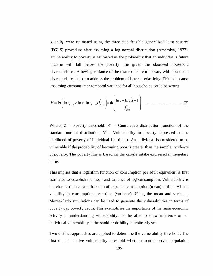
195

and were estimated using the three step feasible generalized least squares

(FGLS) procedure after assuming a log normal distribution (Amemiya, 1977).

Vulnerability to poverty is estimated as the probability that an individual's future

income will fall below the poverty line given the observed household

characteristics. Allowing variance of the disturbance term to vary with household

characteristics helps to address the problem of heteroscedasticity. This is because

assuming constant inter-temporal variance for all households could be wrong.

2, 1 , 1 1

1

ln ln , 1Pr ln ln | ln , ...........................................(2)i t i t jt

jt

z c tV c z c

Where; Z – Poverty threshold; - Cumulative distribution function of the

standard normal distribution; V – Vulnerability to poverty expressed as the

likelihood of poverty of individual i at time t. An individual is considered to be

vulnerable if the probability of becoming poor is greater than the sample incidence

of poverty. The poverty line is based on the calorie intake expressed in monetary

terms.

This implies that a logarithm function of consumption per adult equivalent is first

estimated to establish the mean and variance of log consumption. Vulnerability is

therefore estimated as a function of expected consumption (mean) at time t+1 and

volatility in consumption over time (variance). Using the mean and variance,

Monte-Carlo simulations can be used to generate the vulnerabilities in terms of

poverty gap poverty depth. This exemplifies the importance of the main economic

activity in understanding vulnerability. To be able to draw inference on an

individual vulnerability, a threshold probability is arbitrarily set.

Two distinct approaches are applied to determine the vulnerability threshold. The

first one is relative vulnerability threshold where current observed population

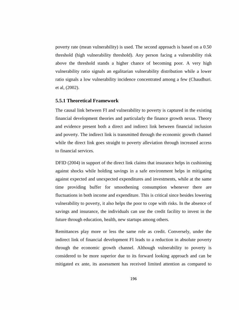
196

poverty rate (mean vulnerability) is used. The second approach is based on a 0.50

threshold (high vulnerability threshold). Any person facing a vulnerability risk

above the threshold stands a higher chance of becoming poor. A very high

vulnerability ratio signals an egalitarian vulnerability distribution while a lower

ratio signals a low vulnerability incidence concentrated among a few (Chaudhuri.

et al, (2002).

5.5.1 Theoretical Framework

The causal link between FI and vulnerability to poverty is captured in the existing

financial development theories and particularly the finance growth nexus. Theory

and evidence present both a direct and indirect link between financial inclusion

and poverty. The indirect link is transmitted through the economic growth channel

while the direct link goes straight to poverty alleviation through increased access

to financial services.

DFID (2004) in support of the direct link claims that insurance helps in cushioning

against shocks while holding savings in a safe environment helps in mitigating

against expected and unexpected expenditures and investments, while at the same

time providing buffer for smoothening consumption whenever there are

fluctuations in both income and expenditure. This is critical since besides lowering

vulnerability to poverty, it also helps the poor to cope with risks. In the absence of

savings and insurance, the individuals can use the credit facility to invest in the

future through education, health, new startups among others.

Remittances play more or less the same role as credit. Conversely, under the

indirect link of financial development FI leads to a reduction in absolute poverty

through the economic growth channel. Although vulnerability to poverty is

considered to be more superior due to its forward looking approach and can be

mitigated ex ante, its assessment has received limited attention as compared to

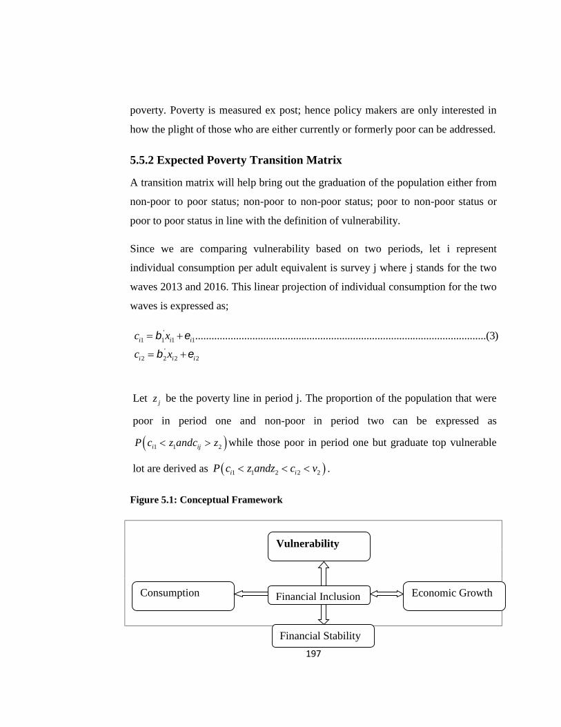
197

poverty. Poverty is measured ex post; hence policy makers are only interested in

how the plight of those who are either currently or formerly poor can be addressed.

5.5.2 Expected Poverty Transition Matrix

A transition matrix will help bring out the graduation of the population either from

non-poor to poor status; non-poor to non-poor status; poor to non-poor status or

poor to poor status in line with the definition of vulnerability.

Since we are comparing vulnerability based on two periods, let i represent

individual consumption per adult equivalent is survey j where j stands for the two

waves 2013 and 2016. This linear projection of individual consumption for the two

waves is expressed as;

'1 1 1 1

'2 2 2 2

...........................................................................................................(3)i i i

i i i

c x

c x

Let jz be the poverty line in period j. The proportion of the population that were

poor in period one and non-poor in period two can be expressed as

1 1 2i ijP c z andc z while those poor in period one but graduate top vulnerable

lot are derived as 1 1 2 2 2i iP c z andz c v .

Figure 5.1: Conceptual Framework

Financial Inclusion Economic Growth

Financial Stability

Vulnerability

Consumption

Expenditure/Assets

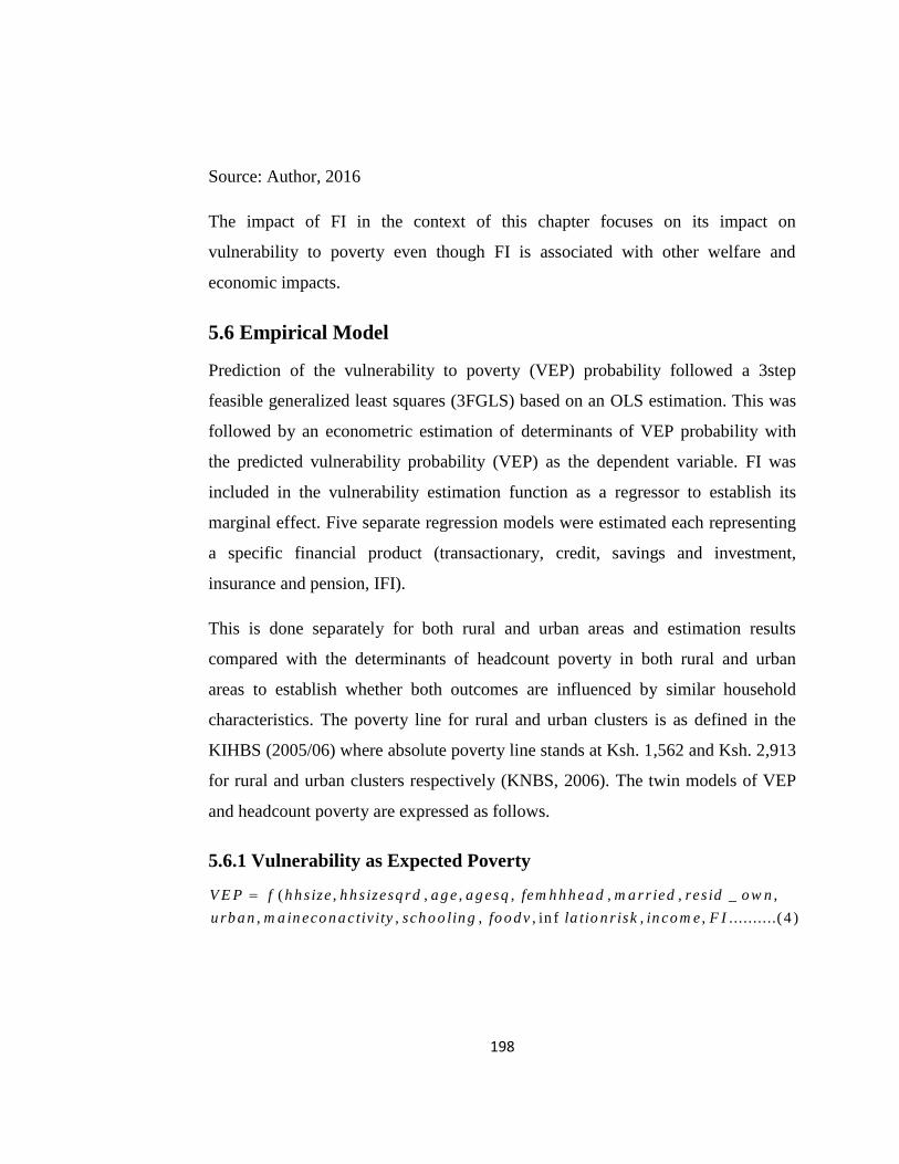
198

Source: Author, 2016

The impact of FI in the context of this chapter focuses on its impact on

vulnerability to poverty even though FI is associated with other welfare and

economic impacts.

5.6 Empirical Model

Prediction of the vulnerability to poverty (VEP) probability followed a 3step

feasible generalized least squares (3FGLS) based on an OLS estimation. This was

followed by an econometric estimation of determinants of VEP probability with

the predicted vulnerability probability (VEP) as the dependent variable. FI was

included in the vulnerability estimation function as a regressor to establish its

marginal effect. Five separate regression models were estimated each representing

a specific financial product (transactionary, credit, savings and investment,

insurance and pension, IFI).

This is done separately for both rural and urban areas and estimation results

compared with the determinants of headcount poverty in both rural and urban

areas to establish whether both outcomes are influenced by similar household

characteristics. The poverty line for rural and urban clusters is as defined in the

KIHBS (2005/06) where absolute poverty line stands at Ksh. 1,562 and Ksh. 2,913

for rural and urban clusters respectively (KNBS, 2006). The twin models of VEP

and headcount poverty are expressed as follows.

5.6.1 Vulnerability as Expected Poverty

( , , , , , , _ ,

, , , , in f , , ..........( 4 )

V E P f h h size h h sizesq rd a g e a g esq fem h h h ea d m a rried res id o w n

u rb a n m a in eco n a ctiv ity sch o o lin g fo o d v la tio n r isk in co m e F I

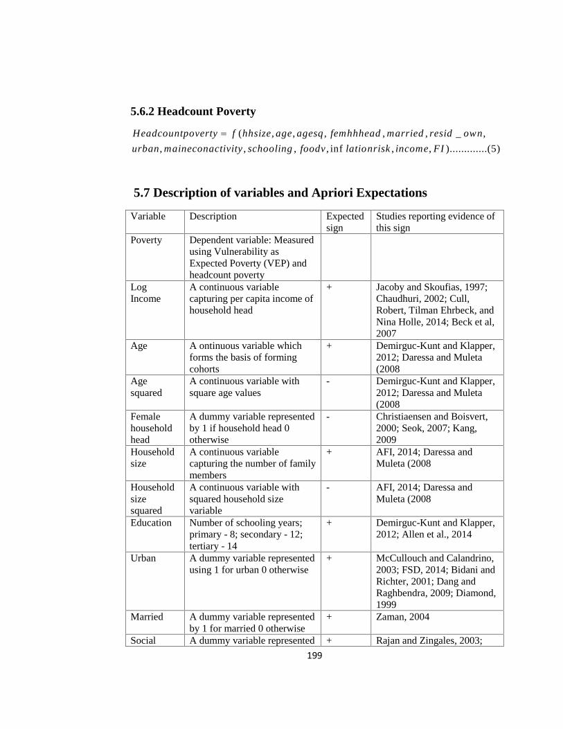
199

5.6.2 Headcount Poverty

( , , , , , _ ,

, , , , inf , , ).............(5)

Headcountpoverty f hhsize age agesq femhhhead married resid own

urban maineconactivity schooling foodv lationrisk income FI

5.7 Description of variables and Apriori Expectations

Variable Description Expectedsign

Studies reporting evidence ofthis sign

Poverty Dependent variable: Measuredusing Vulnerability asExpected Poverty (VEP) andheadcount poverty

LogIncome

A continuous variablecapturing per capita income ofhousehold head

+ Jacoby and Skoufias, 1997;Chaudhuri, 2002; Cull,Robert, Tilman Ehrbeck, andNina Holle, 2014; Beck et al,2007

Age A ontinuous variable whichforms the basis of formingcohorts

+ Demirguc-Kunt and Klapper,2012; Daressa and Muleta(2008

Agesquared

A continuous variable withsquare age values

- Demirguc-Kunt and Klapper,2012; Daressa and Muleta(2008

Femalehouseholdhead

A dummy variable representedby 1 if household head 0otherwise

- Christiaensen and Boisvert,2000; Seok, 2007; Kang,2009

Householdsize

A continuous variablecapturing the number of familymembers

+ AFI, 2014; Daressa andMuleta (2008

Householdsizesquared

A continuous variable withsquared household sizevariable

- AFI, 2014; Daressa andMuleta (2008

Education Number of schooling years;primary - 8; secondary - 12;tertiary - 14

+ Demirguc-Kunt and Klapper,2012; Allen et al., 2014

Urban A dummy variable representedusing 1 for urban 0 otherwise

+ McCullouch and Calandrino,2003; FSD, 2014; Bidani andRichter, 2001; Dang andRaghbendra, 2009; Diamond,1999

Married A dummy variable representedby 1 for married 0 otherwise

+ Zaman, 2004

Social A dummy variable represented + Rajan and Zingales, 2003;

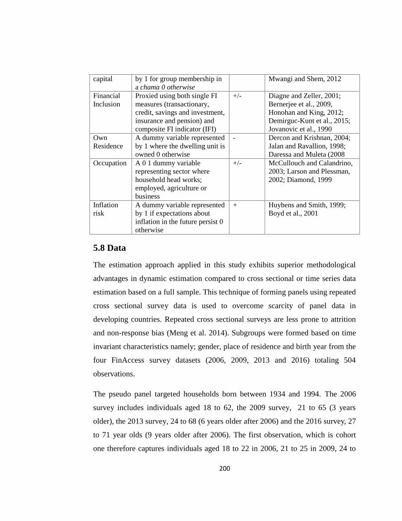
200

capital by 1 for group membership ina chama 0 otherwise

Mwangi and Shem, 2012

FinancialInclusion

Proxied using both single FImeasures (transactionary,credit, savings and investment,insurance and pension) andcomposite FI indicator (IFI)

+/- Diagne and Zeller, 2001;Bernerjee et al., 2009,Honohan and King, 2012;Demirguc-Kunt et al., 2015;Jovanovic et al., 1990

OwnResidence

A dummy variable representedby 1 where the dwelling unit isowned 0 otherwise

- Dercon and Krishnan, 2004;Jalan and Ravallion, 1998;Daressa and Muleta (2008

Occupation A 0 1 dummy variablerepresenting sector wherehousehold head works;employed, agriculture orbusiness

+/- McCullouch and Calandrino,2003; Larson and Plessman,2002; Diamond, 1999

Inflationrisk

A dummy variable representedby 1 if expectations aboutinflation in the future persist 0otherwise

+ Huybens and Smith, 1999;Boyd et al., 2001

5.8 Data

The estimation approach applied in this study exhibits superior methodological

advantages in dynamic estimation compared to cross sectional or time series data

estimation based on a full sample. This technique of forming panels using repeated

cross sectional survey data is used to overcome scarcity of panel data in

developing countries. Repeated cross sectional surveys are less prone to attrition

and non-response bias (Meng et al. 2014). Subgroups were formed based on time

invariant characteristics namely; gender, place of residence and birth year from the

four FinAccess survey datasets (2006, 2009, 2013 and 2016) totaling 504

observations.

The pseudo panel targeted households born between 1934 and 1994. The 2006

survey includes individuals aged 18 to 62, the 2009 survey, 21 to 65 (3 years

older), the 2013 survey, 24 to 68 (6 years older after 2006) and the 2016 survey, 27

to 71 year olds (9 years older after 2006). The first observation, which is cohort

one therefore captures individuals aged 18 to 22 in 2006, 21 to 25 in 2009, 24 to

201

28 in 2012 and 27 to 31 in 2016. This methodological framework by Deaton, 1986

was also used by Ackah et al. (2007) in Ghana. The short age bands may however

lead to fewer respondents in a cohort despite the large cross section dimension.

Large age cohort bands may also not be good since they reduce the cross section

dimension.

Gender variable is disaggregated to generate panels for males and females

respectively while the geographical aspect is captured by the seven regions (44

counties), formerly provinces with the exception of North Eastern region which

has 3 counties namely; Mandera, Wajir and Garissa for missing in the 2013 wave

due to logistical constraints. A key consideration in cohort analysis is the tradeoff

between the number of cohorts and number of observations for each cohort.

McKenzie (2004) posits that a large number of cohorts minimize errors associated

with small samples.

Estimation of Vulnerability as Expected Poverty was based on 126 cohorts

generated from the Fin Access survey data on Kenya collected in 2009, 2013 and

2016 by the Financial Sector Deepening (FSD) Kenya, in collaboration with the

Central Bank of Kenya and the Kenya National Bureau of Statistics (KNBS). The

results were compared with poverty estimates based on 5,233 observations from

the latest FinAccess survey data released in 2016. The datasets capture the

financial access landscape, usage of financial services by individuals in Kenya and

their socioeconomic status including their consumption expenditure. Pritchet et al.

(2000) contends that a two year panel is sufficient in measuring standard

deviations related to consumption expenditure in vulnerability assessments

justifying the use of the two year repeated survey data.

Since the analysis is based on repeated cross sections, a total of 378 cohorts have

been generated based on similarities in gender (2 cohorts whether male or female),

age (9 cohorts based on 5 year age bands) and location (7 cohorts comprising of

202

Kenya's old provincial structure excluding North Eastern Province). This pseudo

panel technique is considered to be more superior since it's the only way the

dynamic estimation of the variable of interest can be measured.

5.9 Discussion of Results

Policy formulation on the improvement of household/individual welfare in

developing countries has for a long time relied on poverty assessments based on a

headcount index. The sharp focus on this crude measure has however failed to

achieve the desired results but has only managed to alleviate poverty only

marginally. Those considered poor in the past have either remained poor or

transited to non-poor status. The same applies to the non-poor whose status has

either remained non poor or turned poor. This ex-post approach of measuring

individual welfare is considered to be subsidiary in policy formulation as

compared to the ex-ante measure described as being more futuristic.

A person’s probability of falling or remaining poor in the future is determined by

the nature of shocks whether transitory or permanent. Unlike poverty which is

observable through the headcount index, vulnerability to poverty is unobservable.

Several mechanisms exist on how to measure it. One main assumption in its

measurement is that differences in vulnerability among individuals are associated

with their observable characteristics. The empirical measure of vulnerability

estimated using the three step GLS estimation procedure by Amemiya (1977), is

compared to the observed measure of poverty and presented in a distribution table

on the entire population. This model estimation also helps in drawing prediction on

the direction of movement of poverty in subsequent periods among Kenyan

households.

5.9.1 Diagnostic Tests

203

Endogeneity in model estimation relating FI and poverty could be emanating from

omission of variables, measurement errors or simultaneity bias (Woldridge, 2012).

This endogeneity bias leads to wrong policy formulation hence the need to control

for it if it’s present. Conventionally, the Durbin Wu-Haussman test was conducted

by first running a FI model on the four transmission channels (transactionary,

credit, savings, insurance) as well as the aggregated FI channel (IFI). The residuals

for each FI channel are predicted and included in a reduced form equation as

regressors. Wooldridge (2012) suggests that failure to reject the null hypothesis

(exogeneity assumption) rules out the presence of endogeneity bias.

Choice of the approach to use in the construction of the vulnerability index is

informed by the assumptions made. VEP estimation follows a parametric

estimation approach (Chaudhuri, 2002) while Karmanou & Morduch (2002) uses

Monte Carlo simulations in a non-parametric approach. VEP estimation is founded

on the probability that household consumption level at time t+1 will lie below the

poverty line the main assumption being that cross sectional variation is a good

proxy for inter-temporal variation. The Monte Carlo technique entails a

bootstrapping of the empirical distribution of observable shocks and estimation

residuals. This technique was however not used since it assumes that shocks to

consumption experienced by different households are drawn from same

distribution creating heteroscedasticity for which it has no control.

The GMM estimation applied in this model fits a linear regression fits a linear

regression of vulnerability to poverty using bank trust as an instrumental variable

for FI. This estimation technique is considered to be more efficient as it yields the

smallest variance. Its therefore able to correct the variance covariance matrix for

heteroscedasticity and for autocorrelation. To allow for heteroscedasticity,

heteroscedastic robust standard errors were included. The autocorrelation test (AR

(1)) command failed because we are only dealing with a single period. However,

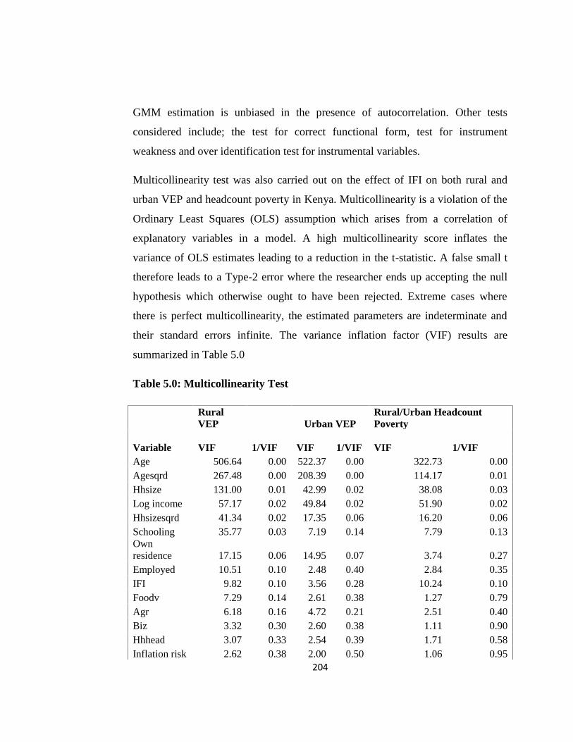
204

GMM estimation is unbiased in the presence of autocorrelation. Other tests

considered include; the test for correct functional form, test for instrument

weakness and over identification test for instrumental variables.

Multicollinearity test was also carried out on the effect of IFI on both rural and

urban VEP and headcount poverty in Kenya. Multicollinearity is a violation of the

Ordinary Least Squares (OLS) assumption which arises from a correlation of

explanatory variables in a model. A high multicollinearity score inflates the

variance of OLS estimates leading to a reduction in the t-statistic. A false small t

therefore leads to a Type-2 error where the researcher ends up accepting the null

hypothesis which otherwise ought to have been rejected. Extreme cases where

there is perfect multicollinearity, the estimated parameters are indeterminate and

their standard errors infinite. The variance inflation factor (VIF) results are

summarized in Table 5.0

Table 5.0: Multicollinearity Test

RuralVEP Urban VEP

Rural/Urban HeadcountPoverty

Variable VIF 1/VIF VIF 1/VIF VIF 1/VIFAge 506.64 0.00 522.37 0.00 322.73 0.00Agesqrd 267.48 0.00 208.39 0.00 114.17 0.01Hhsize 131.00 0.01 42.99 0.02 38.08 0.03Log income 57.17 0.02 49.84 0.02 51.90 0.02Hhsizesqrd 41.34 0.02 17.35 0.06 16.20 0.06Schooling 35.77 0.03 7.19 0.14 7.79 0.13Ownresidence 17.15 0.06 14.95 0.07 3.74 0.27Employed 10.51 0.10 2.48 0.40 2.84 0.35IFI 9.82 0.10 3.56 0.28 10.24 0.10Foodv 7.29 0.14 2.61 0.38 1.27 0.79Agr 6.18 0.16 4.72 0.21 2.51 0.40Biz 3.32 0.30 2.60 0.38 1.11 0.90Hhhead 3.07 0.33 2.54 0.39 1.71 0.58Inflation risk 2.62 0.38 2.00 0.50 1.06 0.95

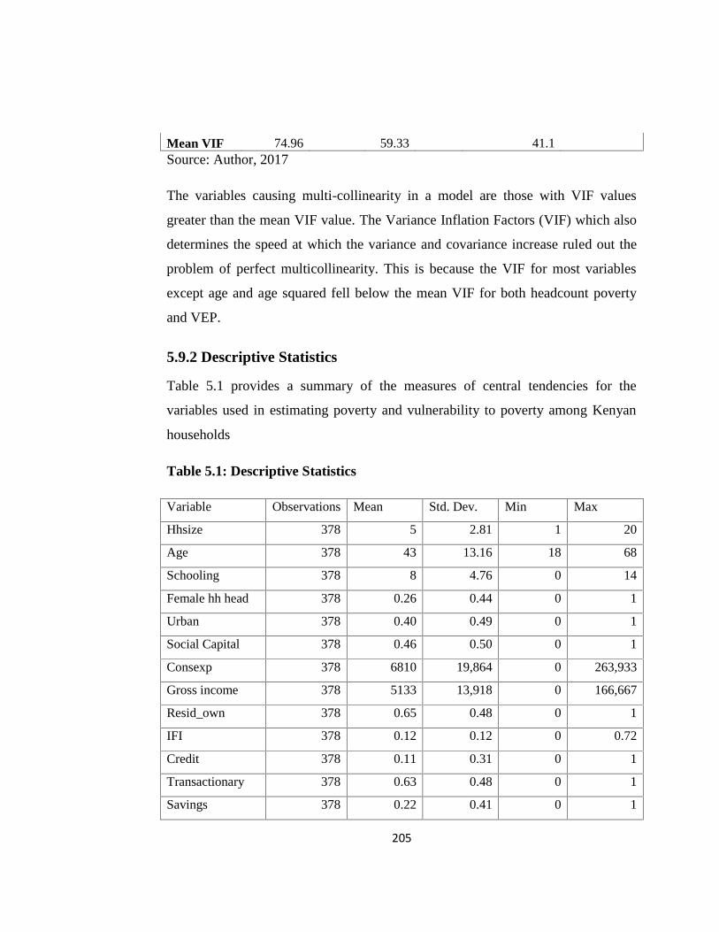
205

Mean VIF 74.96 59.33 41.1Source: Author, 2017

The variables causing multi-collinearity in a model are those with VIF values

greater than the mean VIF value. The Variance Inflation Factors (VIF) which also

determines the speed at which the variance and covariance increase ruled out the

problem of perfect multicollinearity. This is because the VIF for most variables

except age and age squared fell below the mean VIF for both headcount poverty

and VEP.

5.9.2 Descriptive Statistics

Table 5.1 provides a summary of the measures of central tendencies for the

variables used in estimating poverty and vulnerability to poverty among Kenyan

households

Table 5.1: Descriptive Statistics

Variable Observations Mean Std. Dev. Min Max

Hhsize 378 5 2.81 1 20

Age 378 43 13.16 18 68

Schooling 378 8 4.76 0 14

Female hh head 378 0.26 0.44 0 1

Urban 378 0.40 0.49 0 1

Social Capital 378 0.46 0.50 0 1

Consexp 378 6810 19,864 0 263,933

Gross income 378 5133 13,918 0 166,667

Resid_own 378 0.65 0.48 0 1

IFI 378 0.12 0.12 0 0.72

Credit 378 0.11 0.31 0 1

Transactionary 378 0.63 0.48 0 1

Savings 378 0.22 0.41 0 1

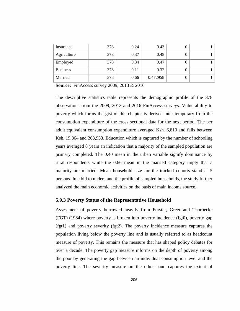
206

Insurance 378 0.24 0.43 0 1

Agriculture 378 0.37 0.48 0 1

Employed 378 0.34 0.47 0 1

Business 378 0.11 0.32 0 1

Married 378 0.66 0.472958 0 1

Source: FinAccess survey 2009, 2013 & 2016

The descriptive statistics table represents the demographic profile of the 378

observations from the 2009, 2013 and 2016 FinAccess surveys. Vulnerability to

poverty which forms the gist of this chapter is derived inter-temporary from the

consumption expenditure of the cross sectional data for the next period. The per

adult equivalent consumption expenditure averaged Ksh. 6,810 and falls between

Ksh. 19,864 and 263,933. Education which is captured by the number of schooling

years averaged 8 years an indication that a majority of the sampled population are

primary completed. The 0.40 mean in the urban variable signify dominance by

rural respondents while the 0.66 mean in the married category imply that a

majority are married. Mean household size for the tracked cohorts stand at 5

persons. In a bid to understand the profile of sampled households, the study further

analyzed the main economic activities on the basis of main income source..

5.9.3 Poverty Status of the Representative Household

Assessment of poverty borrowed heavily from Forster, Greer and Thorbecke

(FGT) (1984) where poverty is broken into poverty incidence (fgt0), poverty gap

(fgt1) and poverty severity (fgt2). The poverty incidence measure captures the

population living below the poverty line and is usually referred to as headcount

measure of poverty. This remains the measure that has shaped policy debates for

over a decade. The poverty gap measure informs on the depth of poverty among

the poor by generating the gap between an individual consumption level and the

poverty line. The severity measure on the other hand captures the extent of

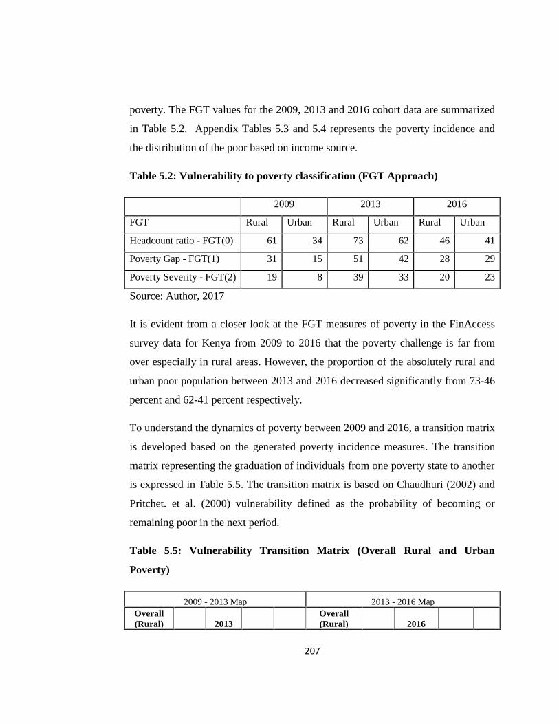
207

poverty. The FGT values for the 2009, 2013 and 2016 cohort data are summarized

in Table 5.2. Appendix Tables 5.3 and 5.4 represents the poverty incidence and

the distribution of the poor based on income source.

Table 5.2: Vulnerability to poverty classification (FGT Approach)

2009 2013 2016

FGT Rural Urban Rural Urban Rural Urban

Headcount ratio - FGT(0) 61 34 73 62 46 41

Poverty Gap - FGT(1) 31 15 51 42 28 29

Poverty Severity - FGT(2) 19 8 39 33 20 23

Source: Author, 2017

It is evident from a closer look at the FGT measures of poverty in the FinAccess

survey data for Kenya from 2009 to 2016 that the poverty challenge is far from

over especially in rural areas. However, the proportion of the absolutely rural and

urban poor population between 2013 and 2016 decreased significantly from 73-46

percent and 62-41 percent respectively.

To understand the dynamics of poverty between 2009 and 2016, a transition matrix

is developed based on the generated poverty incidence measures. The transition

matrix representing the graduation of individuals from one poverty state to another

is expressed in Table 5.5. The transition matrix is based on Chaudhuri (2002) and

Pritchet. et al. (2000) vulnerability defined as the probability of becoming or

remaining poor in the next period.

Table 5.5: Vulnerability Transition Matrix (Overall Rural and Urban

Poverty)

2009 - 2013 Map 2013 - 2016 MapOverall(Rural) 2013

Overall(Rural) 2016

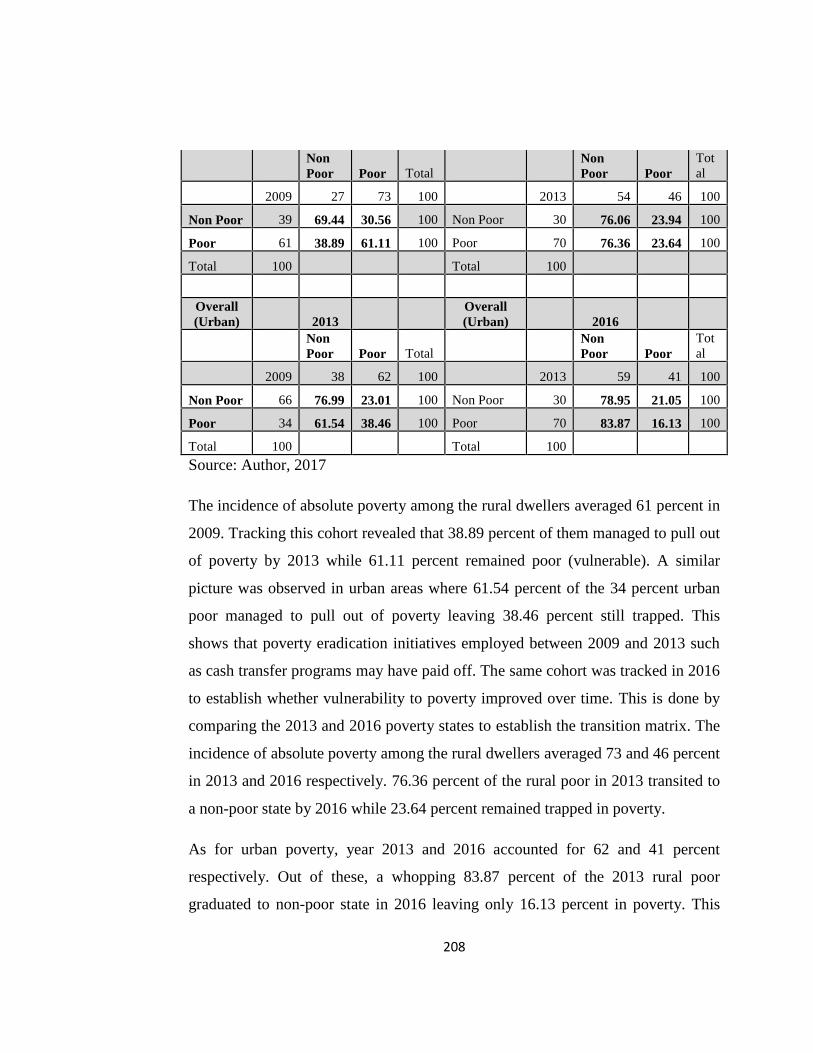
208

NonPoor Poor Total

NonPoor Poor

Total

2009 27 73 100 2013 54 46 100

Non Poor 39 69.44 30.56 100 Non Poor 30 76.06 23.94 100

Poor 61 38.89 61.11 100 Poor 70 76.36 23.64 100

Total 100 Total 100

Overall(Urban) 2013

Overall(Urban) 2016

NonPoor Poor Total

NonPoor Poor

Total

2009 38 62 100 2013 59 41 100

Non Poor 66 76.99 23.01 100 Non Poor 30 78.95 21.05 100

Poor 34 61.54 38.46 100 Poor 70 83.87 16.13 100

Total 100 Total 100

Source: Author, 2017

The incidence of absolute poverty among the rural dwellers averaged 61 percent in

2009. Tracking this cohort revealed that 38.89 percent of them managed to pull out

of poverty by 2013 while 61.11 percent remained poor (vulnerable). A similar

picture was observed in urban areas where 61.54 percent of the 34 percent urban

poor managed to pull out of poverty leaving 38.46 percent still trapped. This

shows that poverty eradication initiatives employed between 2009 and 2013 such

as cash transfer programs may have paid off. The same cohort was tracked in 2016

to establish whether vulnerability to poverty improved over time. This is done by

comparing the 2013 and 2016 poverty states to establish the transition matrix. The

incidence of absolute poverty among the rural dwellers averaged 73 and 46 percent

in 2013 and 2016 respectively. 76.36 percent of the rural poor in 2013 transited to

a non-poor state by 2016 while 23.64 percent remained trapped in poverty.

As for urban poverty, year 2013 and 2016 accounted for 62 and 41 percent

respectively. Out of these, a whopping 83.87 percent of the 2013 rural poor

graduated to non-poor state in 2016 leaving only 16.13 percent in poverty. This

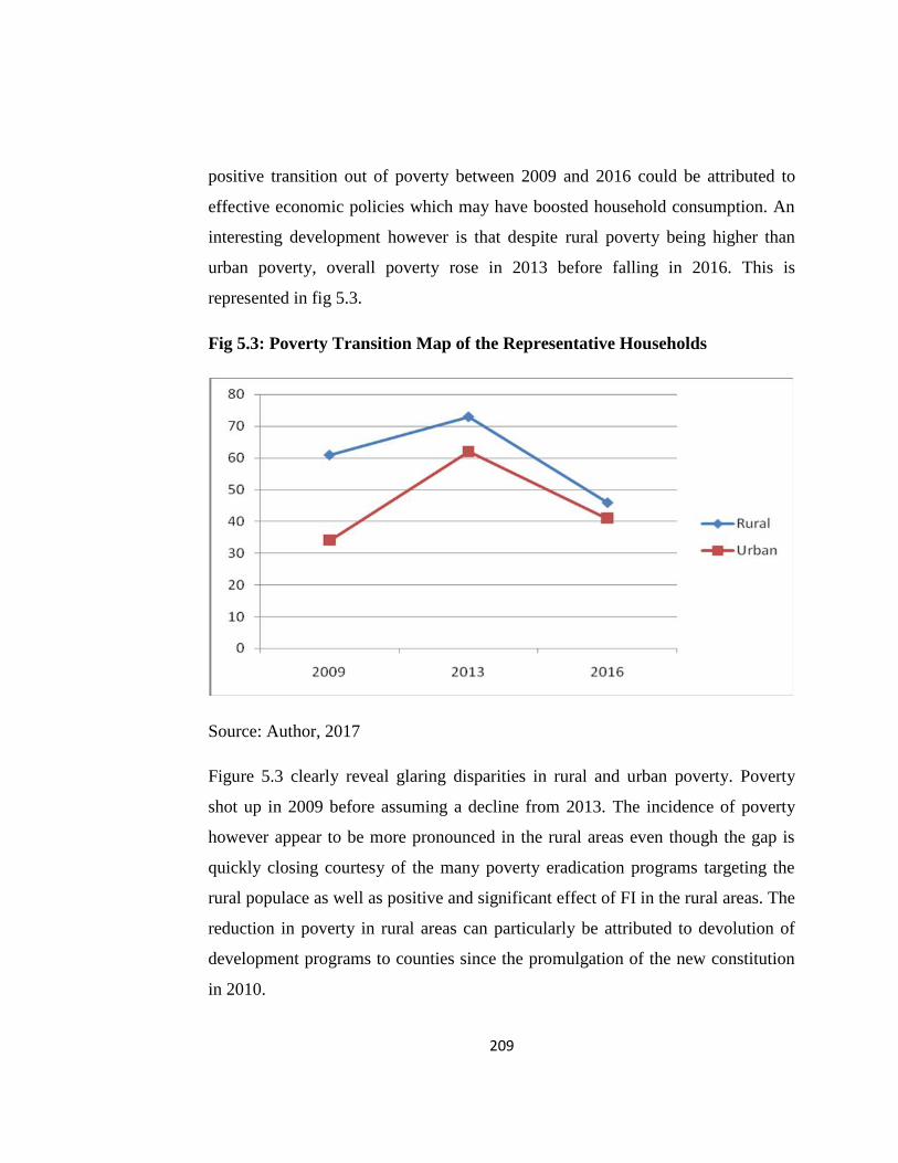
209

positive transition out of poverty between 2009 and 2016 could be attributed to

effective economic policies which may have boosted household consumption. An

interesting development however is that despite rural poverty being higher than

urban poverty, overall poverty rose in 2013 before falling in 2016. This is

represented in fig 5.3.

Fig 5.3: Poverty Transition Map of the Representative Households

Source: Author, 2017

Figure 5.3 clearly reveal glaring disparities in rural and urban poverty. Poverty

shot up in 2009 before assuming a decline from 2013. The incidence of poverty

however appear to be more pronounced in the rural areas even though the gap is

quickly closing courtesy of the many poverty eradication programs targeting the

rural populace as well as positive and significant effect of FI in the rural areas. The

reduction in poverty in rural areas can particularly be attributed to devolution of

development programs to counties since the promulgation of the new constitution

in 2010.

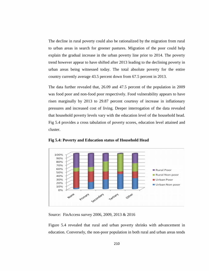
210

The decline in rural poverty could also be rationalized by the migration from rural

to urban areas in search for greener pastures. Migration of the poor could help

explain the gradual increase in the urban poverty line prior to 2014. The poverty

trend however appear to have shifted after 2013 leading to the declining poverty in

urban areas being witnessed today. The total absolute poverty for the entire

country currently average 43.5 percent down from 67.5 percent in 2013.

The data further revealed that, 26.09 and 47.5 percent of the population in 2009

was food poor and non-food poor respectively. Food vulnerability appears to have

risen marginally by 2013 to 29.87 percent courtesy of increase in inflationary

pressures and increased cost of living. Deeper interrogation of the data revealed

that household poverty levels vary with the education level of the household head.

Fig 5.4 provides a cross tabulation of poverty scores, education level attained and

cluster.

Fig 5.4: Poverty and Education status of Household Head

Source: FinAccess survey 2006, 2009, 2013 & 2016

Figure 5.4 revealed that rural and urban poverty shrinks with advancement in

education. Conversely, the non-poor population in both rural and urban areas tends

211

to rise with increase in education level attained. The incidence of poverty among

the tertiary education level holders averaged 13.63 and 0 percent for urban and

rural areas respectively while it stood at 91.67 and 78.26 percent for those with no

education in the urban and rural cluster respectively. Next is a mapping of the

incidence of poverty by region.

212

Fig 5.5: Poverty Incidence by Region

Source: Author, 2017

Figure 5.5 presents a geospatial mapping of poverty incidence in Kenya for year

2016 from the full sample. Appendix Table 5.6 illustrates the status of poverty and

consumption expenditure in 2016. The map revealed that indeed poverty varies

213

across the country with the highest incidence being reported in Western region

(62.28 percent followed by Nyanza (55.39 percent) and Rift Valley (48.34 percent)

in that order. Poverty was lowest in Nairobi region standing at 21.98 percent

followed by Central (32.22 percent) and Coast region (39.83 percent) in that order.

However, as mentioned earlier, aggregated figures often mask the true picture on

the ground hence the analysis at smaller economic units.

Given the dynamic nature of poverty, analysis of poverty at a point is likely to be

flawed leading to wrong inferences for policy. To address this problem, this

chapter tried to develop a poverty cycle based on repeated cross sections to

understand poverty trends of the representative household in the cohort data (This

information is drawn from Appendix Table 5.7 on regional poverty and

consumption expenditure cycle between 2009 and 2019.). The pie charts which

represent the incidence of poverty over the three repeated cross section surveys

have been superimposed on the poverty map to show the poverty trends by region.

Virtually all regions except Nairobi experienced acute poverty incidence in 2009

(blue shading). Poverty appear to have stagnated in 2013 but a marked

improvement in terms of poverty reduction is observable in Nyanza, Central and

Coast region by 2016 (green shading). Figure 5.7 illustrates the link between

poverty and FI in Kenya.

Fig 5.7: Geospatial Mapping of the IFI and Poverty using ArcGIS

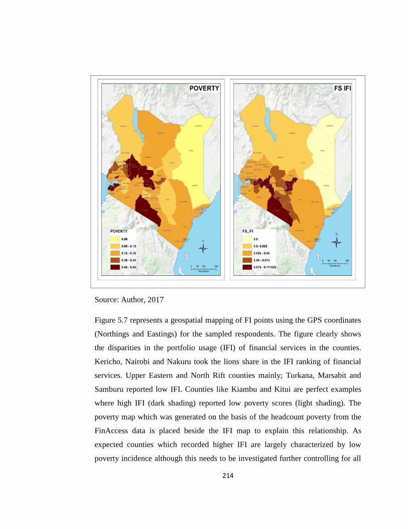
214

Source: Author, 2017

Figure 5.7 represents a geospatial mapping of FI points using the GPS coordinates

(Northings and Eastings) for the sampled respondents. The figure clearly shows

the disparities in the portfolio usage (IFI) of financial services in the counties.

Kericho, Nairobi and Nakuru took the lions share in the IFI ranking of financial

services. Upper Eastern and North Rift counties mainly; Turkana, Marsabit and

Samburu reported low IFI. Counties like Kiambu and Kitui are perfect examples

where high IFI (dark shading) reported low poverty scores (light shading). The

poverty map which was generated on the basis of the headcount poverty from the

FinAccess data is placed beside the IFI map to explain this relationship. As

expected counties which recorded higher IFI are largely characterized by low

poverty incidence although this needs to be investigated further controlling for all

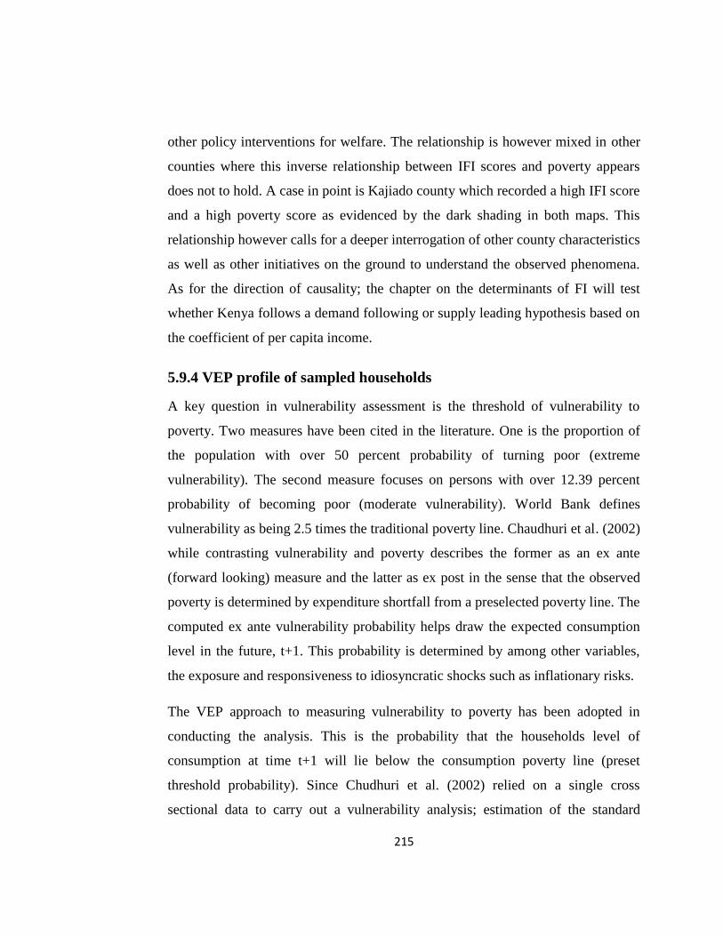
215

other policy interventions for welfare. The relationship is however mixed in other

counties where this inverse relationship between IFI scores and poverty appears

does not to hold. A case in point is Kajiado county which recorded a high IFI score

and a high poverty score as evidenced by the dark shading in both maps. This

relationship however calls for a deeper interrogation of other county characteristics

as well as other initiatives on the ground to understand the observed phenomena.

As for the direction of causality; the chapter on the determinants of FI will test

whether Kenya follows a demand following or supply leading hypothesis based on

the coefficient of per capita income.

5.9.4 VEP profile of sampled households

A key question in vulnerability assessment is the threshold of vulnerability to

poverty. Two measures have been cited in the literature. One is the proportion of

the population with over 50 percent probability of turning poor (extreme

vulnerability). The second measure focuses on persons with over 12.39 percent

probability of becoming poor (moderate vulnerability). World Bank defines

vulnerability as being 2.5 times the traditional poverty line. Chaudhuri et al. (2002)

while contrasting vulnerability and poverty describes the former as an ex ante

(forward looking) measure and the latter as ex post in the sense that the observed

poverty is determined by expenditure shortfall from a preselected poverty line. The

computed ex ante vulnerability probability helps draw the expected consumption

level in the future, t+1. This probability is determined by among other variables,

the exposure and responsiveness to idiosyncratic shocks such as inflationary risks.

The VEP approach to measuring vulnerability to poverty has been adopted in

conducting the analysis. This is the probability that the households level of

consumption at time t+1 will lie below the consumption poverty line (preset

threshold probability). Since Chudhuri et al. (2002) relied on a single cross

sectional data to carry out a vulnerability analysis; estimation of the standard

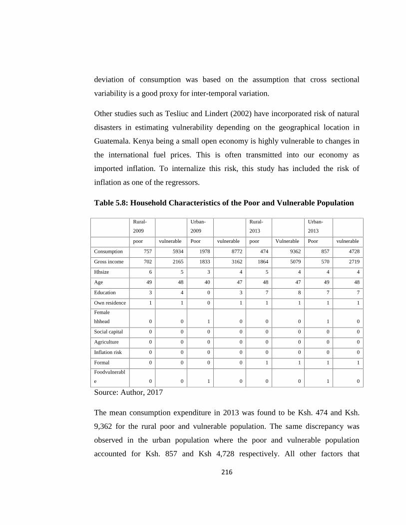
216

deviation of consumption was based on the assumption that cross sectional

variability is a good proxy for inter-temporal variation.

Other studies such as Tesliuc and Lindert (2002) have incorporated risk of natural

disasters in estimating vulnerability depending on the geographical location in

Guatemala. Kenya being a small open economy is highly vulnerable to changes in

the international fuel prices. This is often transmitted into our economy as

imported inflation. To internalize this risk, this study has included the risk of

inflation as one of the regressors.

Table 5.8: Household Characteristics of the Poor and Vulnerable Population

Rural-

2009

Urban-

2009

Rural-

2013

Urban-

2013

poor vulnerable Poor vulnerable poor Vulnerable Poor vulnerable

Consumption 757 5934 1978 8772 474 9362 857 4728

Gross income 702 2165 1833 3162 1864 5079 570 2719

Hhsize 6 5 3 4 5 4 4 4

Age 49 48 40 47 48 47 49 48

Education 3 4 0 3 7 8 7 7

Own residence 1 1 0 1 1 1 1 1

Female

hhhead 0 0 1 0 0 0 1 0

Social capital 0 0 0 0 0 0 0 0

Agriculture 0 0 0 0 0 0 0 0

Inflation risk 0 0 0 0 0 0 0 0

Formal 0 0 0 0 1 1 1 1

Foodvulnerabl

e 0 0 1 0 0 0 1 0

Source: Author, 2017

The mean consumption expenditure in 2013 was found to be Ksh. 474 and Ksh.

9,362 for the rural poor and vulnerable population. The same discrepancy was

observed in the urban population where the poor and vulnerable population

accounted for Ksh. 857 and Ksh 4,728 respectively. All other factors that

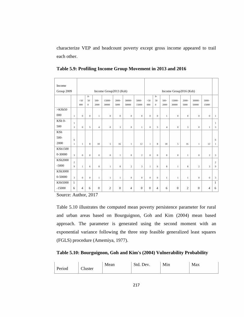
217

characterize VEP and headcount poverty except gross income appeared to trail

each other.

Table 5.9: Profiling Income Group Movement in 2013 and 2016

Income

Group 2009 Income Group2013 (Ksh) Income Group2016 (Ksh)

>50

000

0-

50

0

500-

2000

15000-

30000

2000-

5000

30000-

50000

5000-

15000

>50

000

0-

50

0

500-

2000

15000-

30000

2000-

5000

30000-

50000

5000-

15000

>KSh50

000 1 0 0 1 0 0 0 0 0 0 1 0 0 0 0 1

KSh 0-

5001

3 0 5 4 0 3 0 1 0 5 4 0 3 0 1

1

3

KSh

500-

20006

1 1 8 18 5 16 1 12 1 8 18 5 16 1 12

6

1

KSh1500

0-30000 3 0 0 0 0 1 0 2 0 0 0 0 1 0 2 3

KSh2000

-50002

9 1 6 8 1 8 2 3 1 6 8 1 8 2 3

2

9

KSh3000

0-50000 3 0 0 1 1 1 0 0 0 0 1 1 1 0 0 3

KSh5000

-15000

1

6 4 6 0 2 0 4 0 0 4 6 0 2 0 4

1

6

Source: Author, 2017

Table 5.10 illustrates the computed mean poverty persistence parameter for rural

and urban areas based on Bourguignon, Goh and Kim (2004) mean based

approach. The parameter is generated using the second moment with an

exponential variance following the three step feasible generalized least squares

(FGLS) procedure (Amemiya, 1977).

Table 5.10: Bourguignon, Goh and Kim's (2004) Vulnerability Probability

Period ClusterMean Std. Dev. Min Max

218

2013/16 Rural0.29 0.02 0.26 0.33

Urban0.31 0.03 0.27 0.43

Source: Author, 2017

The estimated probability of expenditure shortfall for the representative household

in future averaged 29 and 31 percent for the rural and urban clusters respectively

for the period 2013/16. This signals a tapering vulnerability risk between the rural

and urban areas going forward (Bourguignon, Goh and Kim, 2004). These results

are based on the three step FGLS where both the ex-ante mean and ex ante

variance are computed before an auxiliary regression of the squared residuals and

the regressors is carried out. Imposing a log normal distribution assumption helps

generate the first and second moment. The estimation assumes that the variance of

the disturbance term (inter-temporal variance of log consumption) is constant for

all households. Heteroscedasticity is corrected by allowing the variance of the

disturbance term to vary with household characteristics. Pritchett et al., (2000)

posit that vulnerability as expected poverty rises with the length of time horizon

since uncertainty rises more as you move into the distant future.

The instrumental variable GMM two step procedure was used to estimate a

logarithmic expenditure function with IFI as one of the regressors. Based on the

vulnerability risk in both rural and urban areas, there is need to interrogate the data

further to understand the characteristics of this vulnerable population. This is

analyzed econometrically in the next section.

5.9.4 Econometric estimation of Vulnerability

Chaudhuri (2000; 2003) defined vulnerability to poverty as the probability that the

population currently lying above the poverty line will fall below it in the next

period or those below will still fall below it in the next period based on the

consumption per adult equivalent indicator. Given this inter-temporal variation,

219

vulnerability as expected poverty (VEP) follows an autoregressive process of order

one (AR (1)) which in the context of this chapter focused on the population

considered to be absolutely poor both in 2013 and 2016. Morduch (1994) offered a

simplified definition of vulnerability to poverty as simply operating below the

poverty line though this is what is often termed as headcount poverty. The

vulnerability measure therefore nets out those people who were poor in 2009 but

were able to exit the poverty trap in 2013. Households found poor in two

subsequent surveys, say 2009 and 2013 or 2013 and 2016 form the vulnerable

population while the non-poor form the reference category.

Prior knowledge about looming vulnerability risks help households adopt

mitigation strategies early enough to minimize suffering. A variable capturing the

risk of going without food in future was included in the model to test household

preparedness in tackling such risks. Sen (1999) however posits that elimination of

poverty is not enough; instead, households should focus more on the elimination of

vulnerability risks which threaten plunging the household back to poverty due to

deprivation.

The coefficient of food vulnerability risk in explaining VEP was found to be

negative and significant at 10 percent. This shows that rural households are well

able to cushion themselves adequately once they are equipped with information on

the looming vulnerability risks. The risk of going sometimes or often without food

in the country dropped from a high of 59.1 percent in 2013 to around 41.9 percent

in 2016. This indicates that the war against vulnerability to poverty is being won.

To counter the shocks, 39.9 and 46.8 percent households in the rural areas and

urban areas used savings as the main coping strategy in rural and urban areas

respectively while 26.8 and 32.2 percent respectively embraced social capital from

their networks. Holzmann and Jorgensen (2000) argue that mitigating vulnerability

risks early enough helps in avoiding the poverty trap. Failure to mitigate leads to

220

huge, irreversible losses which exacerbates poverty especially where households

lack sufficient assets or insurance to smoothen consumption (Jacoby and Skoufias,

1997).

FSD (2016) report identified various shocks faced by households in the last two

years. The main shocks faced by households included; drought/famine (33.1

percent) followed by loss of property from fire or theft (14.8 percent) and death of

a relative (13.8 percent) in that order. To prove that risks faced in urban and rural

areas are different, urban households listed death of a relative as the main shock

they experienced in the past two years (24.1 percent) followed by loss of property

(19.6 percent) and increased cost of basic items (12.8 percent) in that order. The

high ranking of risk of property loss among urban households depict how much

value they attach to assets. This picture offer insights on the vulnerability risks

faced in the country.

Rural households may not be hit hard by inflationary pressure since most products

they consume are grown in the farms. This argument is also supported by their low

ranking of the risk of loss of income of the main income earner (3.9 percent).

Urban households are disadvantaged since despite earning slightly more, they have

to spend a huge chunk of their income on household expenses. The risk of loss of

the income of main wage earner in the past two years averaged (7.8 percent) and

indication that loss of income in the urban areas could have more serious

implications on welfare in urban areas as compared to rural areas.

In the list of coping strategies, asset disposal was not left behind with rural and

urban households recording 8.9 and 4.6 percent respectively. This explains why

savings and asset holding exhibits a positive impact on welfare. Hardly 5 percent

of households in either rural or urban areas cut back their expenses or borrowed

from banks to mitigate the risks. This explains why the uptake of credit remains

221

low (14 percent) in Kenya (FSD, 2016). Smoothing of consumption is therefore

done through other mechanisms such as liquidating assets.

While Christiaensen and Boisvert (2000) and Jha and Dang (2008) established

lower incidences of poverty among female headed households, findings from this

study suggest that female headed households run a higher risk of falling into

poverty as evidenced by the strong positive coefficient significant at 1 percent

confidence level. Findings from the VEP estimation support the work of Kang

(2014) who found poverty among female headed households to be higher than that

of male headed households.

Daressa and Muleta (2008) argued that increase in the age of household head

facilitates an increase in the stock of human capital, wealth of experience and asset

base which in turn yields a reduction in vulnerability to poverty. This study on its

part revealed that age of the household head despite having a negative relationship

with VEP was non-significant. However, age squared variable was found to be

positive signaling an increase in vulnerability as old age strikes. This could be

attributed to loss of wage income once households hit retirement age. Around this

time, households rely on accumulated savings to meet their day to day financial

obligations. This expenditure on consumption exposes them to vulnerability risks.

Increase in household size beyond a certain level piles pressure on household

income raising the probability of falling into poverty. Results from this analysis

however paint a different picture where the lower the family sizes the higher the

exposure risk to poverty. This raises a question on how small is small and how big

is big, even though the answer to this question falls outside the purview of this

study. This indicates that there is an optimal household size. Contrary to findings

by Mckenzie (2003) and Cunningham and Maloney (2000) on education where

less educated household heads bore a lower incidence of poverty, this study

222

established that rural poverty indeed falls with increase in schooling years. This

elevates the role of human capital development in improving household welfare.

Conventional vulnerability estimation considers two periods at a time. Such an

estimation that focuses on the dynamic transition brings out factors that

characterize vulnerability in the cohorts being tracked. The next subsection

discusses the determinants of VEP probability derived using the three step Feasible

Generalized Least Squares (FGLS) technique. Focus is mainly on the impact of FI

whose effect on VEP is compared with that of headcount poverty in both rural and

urban areas. This approach is considered to be robust due to its ability to inform on

how deviations from the mean will affect the predicted vulnerability probability.

The link between FI and vulnerability to poverty is well established by the

modern development theories. These theories are mainly concerned with

elimination of barriers to FI such as capital market imperfections. Table 5.12a

focuses on an econometric estimation of vulnerability as expected poverty (VEP)

in the rural areas for year 2013 while Table 5.12b targets the urban population

VEP in line with Chaudhuri (2002) and Christiaensen and Subbarao (2005)

framework. The main aim of this chapter was to bring out the role of FI and

establish whether vulnerability to poverty and headcount poverty are influenced by

similar characteristics. The estimation focused on household characteristics in

2013 and consumption expenditure in 2016 following the autoregressive process

of order 1 (AR (1)) applied in VEP estimation.

The reported results represent marginal effects (elasticities) as each regressor

changes by one unit from its mean. Since the prediction of the VEP probability is

founded on moment generating functions where mean and variance is determined

first, Bourguignon, Goh and Kim’s (2004) mean based approach considers the

variance to be of an exponential type. Appendix Tables 5.11a and 5.11b represents

the determinants of VEP for rural and urban households respectively before

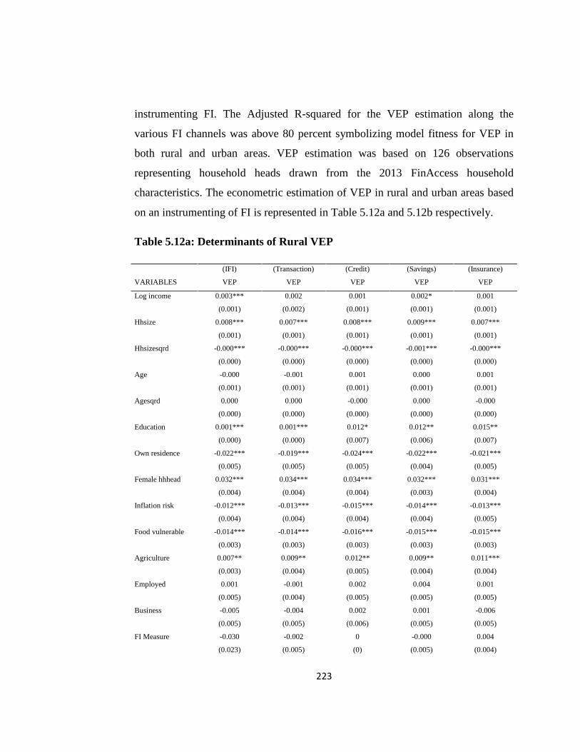
223

instrumenting FI. The Adjusted R-squared for the VEP estimation along the

various FI channels was above 80 percent symbolizing model fitness for VEP in

both rural and urban areas. VEP estimation was based on 126 observations

representing household heads drawn from the 2013 FinAccess household

characteristics. The econometric estimation of VEP in rural and urban areas based

on an instrumenting of FI is represented in Table 5.12a and 5.12b respectively.

Table 5.12a: Determinants of Rural VEP

(IFI) (Transaction) (Credit) (Savings) (Insurance)

VARIABLES VEP VEP VEP VEP VEP

Log income 0.003*** 0.002 0.001 0.002* 0.001

(0.001) (0.002) (0.001) (0.001) (0.001)

Hhsize 0.008*** 0.007*** 0.008*** 0.009*** 0.007***

(0.001) (0.001) (0.001) (0.001) (0.001)

Hhsizesqrd -0.000*** -0.000*** -0.000*** -0.001*** -0.000***

(0.000) (0.000) (0.000) (0.000) (0.000)

Age -0.000 -0.001 0.001 0.000 0.001

(0.001) (0.001) (0.001) (0.001) (0.001)

Agesqrd 0.000 0.000 -0.000 0.000 -0.000

(0.000) (0.000) (0.000) (0.000) (0.000)

Education 0.001*** 0.001*** 0.012* 0.012** 0.015**

(0.000) (0.000) (0.007) (0.006) (0.007)

Own residence -0.022*** -0.019*** -0.024*** -0.022*** -0.021***

(0.005) (0.005) (0.005) (0.004) (0.005)

Female hhhead 0.032*** 0.034*** 0.034*** 0.032*** 0.031***

(0.004) (0.004) (0.004) (0.003) (0.004)

Inflation risk -0.012*** -0.013*** -0.015*** -0.014*** -0.013***

(0.004) (0.004) (0.004) (0.004) (0.005)

Food vulnerable -0.014*** -0.014*** -0.016*** -0.015*** -0.015***

(0.003) (0.003) (0.003) (0.003) (0.003)

Agriculture 0.007** 0.009** 0.012** 0.009** 0.011***

(0.003) (0.004) (0.005) (0.004) (0.004)

Employed 0.001 -0.001 0.002 0.004 0.001

(0.005) (0.004) (0.005) (0.005) (0.005)

Business -0.005 -0.004 0.002 0.001 -0.006

(0.005) (0.005) (0.006) (0.005) (0.005)

FI Measure -0.030 -0.002 0 -0.000 0.004

(0.023) (0.005) (0) (0.005) (0.004)

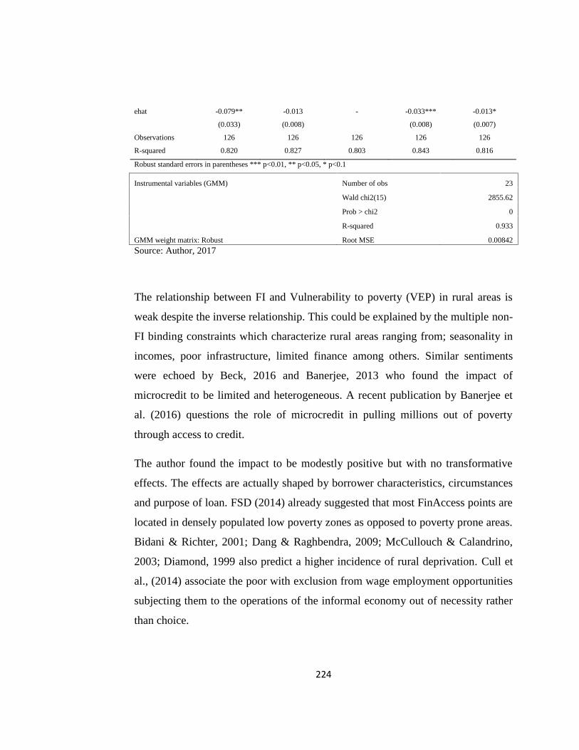
224

ehat -0.079** -0.013 - -0.033*** -0.013*

(0.033) (0.008) (0.008) (0.007)

Observations 126 126 126 126 126

R-squared 0.820 0.827 0.803 0.843 0.816

Robust standard errors in parentheses *** p<0.01, ** p<0.05, * p<0.1

Instrumental variables (GMM) Number of obs 23

Wald chi2(15) 2855.62

Prob > chi2 0

R-squared 0.933

GMM weight matrix: Robust Root MSE 0.00842

Source: Author, 2017

The relationship between FI and Vulnerability to poverty (VEP) in rural areas is

weak despite the inverse relationship. This could be explained by the multiple non-

FI binding constraints which characterize rural areas ranging from; seasonality in

incomes, poor infrastructure, limited finance among others. Similar sentiments

were echoed by Beck, 2016 and Banerjee, 2013 who found the impact of

microcredit to be limited and heterogeneous. A recent publication by Banerjee et

al. (2016) questions the role of microcredit in pulling millions out of poverty

through access to credit.

The author found the impact to be modestly positive but with no transformative

effects. The effects are actually shaped by borrower characteristics, circumstances

and purpose of loan. FSD (2014) already suggested that most FinAccess points are

located in densely populated low poverty zones as opposed to poverty prone areas.

Bidani & Richter, 2001; Dang & Raghbendra, 2009; McCullouch & Calandrino,

2003; Diamond, 1999 also predict a higher incidence of rural deprivation. Cull et

al., (2014) associate the poor with exclusion from wage employment opportunities

subjecting them to the operations of the informal economy out of necessity rather

than choice.

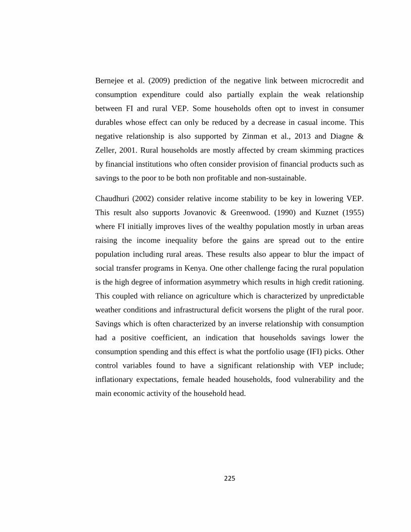
225

Bernejee et al. (2009) prediction of the negative link between microcredit and

consumption expenditure could also partially explain the weak relationship

between FI and rural VEP. Some households often opt to invest in consumer

durables whose effect can only be reduced by a decrease in casual income. This

negative relationship is also supported by Zinman et al., 2013 and Diagne &

Zeller, 2001. Rural households are mostly affected by cream skimming practices

by financial institutions who often consider provision of financial products such as

savings to the poor to be both non profitable and non-sustainable.

Chaudhuri (2002) consider relative income stability to be key in lowering VEP.

This result also supports Jovanovic & Greenwood. (1990) and Kuznet (1955)

where FI initially improves lives of the wealthy population mostly in urban areas

raising the income inequality before the gains are spread out to the entire

population including rural areas. These results also appear to blur the impact of

social transfer programs in Kenya. One other challenge facing the rural population

is the high degree of information asymmetry which results in high credit rationing.

This coupled with reliance on agriculture which is characterized by unpredictable

weather conditions and infrastructural deficit worsens the plight of the rural poor.

Savings which is often characterized by an inverse relationship with consumption

had a positive coefficient, an indication that households savings lower the

consumption spending and this effect is what the portfolio usage (IFI) picks. Other

control variables found to have a significant relationship with VEP include;

inflationary expectations, female headed households, food vulnerability and the

main economic activity of the household head.

226

Table 5.12b: Determinants of Urban VEP

(IFI) (Transaction) (Credit) (Savings) (Insurance)

Dependent Variable VEP VEP VEP VEP VEP

Log income -0.012*** -0.001 -0.007*** -0.007*** -0.009***

(0.002) (0.001) (0.002) (0.001) (0.002)

Hhsize -0.032*** -0.026*** -0.021*** -0.034*** -0.026***

(0.005) (0.0017) (0.005) (0.004) (0.007)

Hhsizesqrd 0.003*** 0.003*** 0.002*** 0.004*** 0.003***

(0.000) (0.000) (0.000) (0.000) (0.000)

Age -0.003** -0.001* -0.002 -0.001 -0.002

(0.001) (0.001) (0.002) (0.001) (0.002)

Agesqrd 0.000** 0.000*** 0.000 0.000 0.000

(0.000) (0.000) (0.000) (0.000) (0.000)

Education 0.002** 0.001* 0.022*** -0.009 0.018**

(0.001) (0.000) (0.008) (0.009) (0.008)

Own residence -0.021* -0.037*** -0.023** -0.005 -0.020

(0.012) (0.005) (0.011) (0.008) (0.014)

Female hhhead 0.024*** 0.040*** 0.018*** 0.020*** 0.025**

(0.005) (0.002) (0.007) (0.005) (0.010)

Inflation risk 0.005 -0.039*** 0.014 0.008 0.009

(0.005) (0.004) (0.010) (0.006) (0.009)

Food vulnerable -0.016** -0.021*** -0.031*** 0.000 -0.028***

(0.007) (0.002) (0.009) (0.006) (0.008)

Agriculture 0.022*** -0.015*** 0.014 0.004 0.001

(0.008) (0.005) (0.016) (0.007) (0.016)

Employed -0.002 -0.032*** -0.000 0.006 -0.011

(0.011) (0.004) (0.013) (0.006) (0.013)

Business 0.008 -0.011*** 0.004 0.015** -0.008

(0.008) (0.003) (0.011) (0.006) (0.014)

FI -0.103*** -0.069*** -0.002 0.004 -0.019

(0.037) (0.005) (0.012) (0.013) (0.017)

ehat 0.258*** 0.116*** - 0.059*** 0.033

(0.080) (0.010) (0.016) (0.029)

Observations 126 126 126 126 126

R-squared 0.933 0.988 0.867 0.944 0.878

Robust standard errors in parentheses *** p<0.01, ** p<0.05, * p<0.1

Instrumental variables (GMM) Number of obs 43

Wald chi2(15) 248.47

Prob > chi2 0

R-squared 0.8204

GMM weight matrix: Robust Root MSE 0.0076

227

Source: Author, 2017

Urban VEP appears to fall significantly with increase in transactionary and

portfolio usage of financial services hence supporting findings by Chaudhuri,

2002; Odhiambo, 2010 and Demirguc-Kunt et., al 2015. The same applies to per

capita income whose increase led to a significant reduction in the VEP among the

urban populace.

A comparison of factors that determine VEP and headcount poverty revealed

interesting results. The results challenged Chaudhuri (2002) argument that VEP

and headcount poverty are determined by similar characteristics. Given that most

policies focus more on the reduction of headcount poverty, the persistence in

poverty could be explained by the inability of policy to pick causes of VEP in both

rural and urban areas. Schooling, per capita income, asset ownership and FI appear

to shape both VEP and headcount poverty in a bigger way. The positive coefficient

of residence ownership in the rural headcount poverty shows that asset holding in

the rural areas could be a catalyst for a surge in poverty as households cut their

consumption to accumulate wealth.

Households ought to build their consumption first before resorting to investment is

assets. The difficulty in liquidating assets in rural areas particularly makes the

investment in assets not a reliable tool for the eradication of headcount poverty.

The government advocates for programs which ride on liquid assets to address

poverty. A case is in point is the governments cash transfer programs whose audit

report revealed that it's already bearing fruits in transforming the lives of the

vulnerable population in 21 sub-counties (GoK, 2014). Table 5.13a presents an

econometric estimation of the determinants of rural headcount poverty along the

various FI transmission channels based on the full sample data covering 5,233

observations in the 2016 FinAccess survey data.

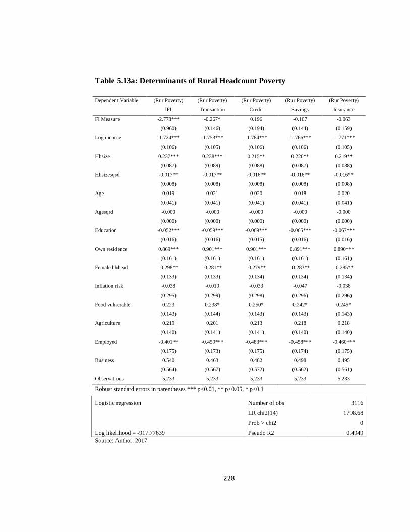
228

Table 5.13a: Determinants of Rural Headcount Poverty

Dependent Variable (Rur Poverty) (Rur Poverty) (Rur Poverty) (Rur Poverty) (Rur Poverty)

IFI Transaction Credit Savings Insurance

FI Measure -2.778*** -0.267* 0.196 -0.107 -0.063

(0.960) (0.146) (0.194) (0.144) (0.159)

Log income -1.724*** -1.753*** -1.784*** -1.766*** -1.771***

(0.106) (0.105) (0.106) (0.106) (0.105)

Hhsize 0.237*** 0.238*** 0.215** 0.220** 0.219**

(0.087) (0.089) (0.088) (0.087) (0.088)

Hhsizesqrd -0.017** -0.017** -0.016** -0.016** -0.016**

(0.008) (0.008) (0.008) (0.008) (0.008)

Age 0.019 0.021 0.020 0.018 0.020

(0.041) (0.041) (0.041) (0.041) (0.041)

Agesqrd -0.000 -0.000 -0.000 -0.000 -0.000

(0.000) (0.000) (0.000) (0.000) (0.000)

Education -0.052*** -0.059*** -0.069*** -0.065*** -0.067***

(0.016) (0.016) (0.015) (0.016) (0.016)

Own residence 0.869*** 0.901*** 0.901*** 0.891*** 0.890***

(0.161) (0.161) (0.161) (0.161) (0.161)

Female hhhead -0.298** -0.281** -0.279** -0.283** -0.285**

(0.133) (0.133) (0.134) (0.134) (0.134)

Inflation risk -0.038 -0.010 -0.033 -0.047 -0.038

(0.295) (0.299) (0.298) (0.296) (0.296)

Food vulnerable 0.223 0.238* 0.250* 0.242* 0.245*

(0.143) (0.144) (0.143) (0.143) (0.143)

Agriculture 0.219 0.201 0.213 0.218 0.218

(0.140) (0.141) (0.141) (0.140) (0.140)

Employed -0.401** -0.459*** -0.483*** -0.458*** -0.460***

(0.175) (0.173) (0.175) (0.174) (0.175)

Business 0.540 0.463 0.482 0.498 0.495

(0.564) (0.567) (0.572) (0.562) (0.561)

Observations 5,233 5,233 5,233 5,233 5,233

Robust standard errors in parentheses *** p<0.01, ** p<0.05, * p<0.1

Logistic regression Number of obs 3116

LR chi2(14) 1798.68

Prob > chi2 0

Log likelihood = -917.77639 Pseudo R2 0.4949Source: Author, 2017

229

Determinants of Rural poverty appear to vary with the household’s financial

product of choice. In line with Odhiambo N.M. (2010) and Jalilian and Kirkpatrick

(2002) prediction of the presence of an inverse relationship between financial

development and poverty, econometric estimation results established an inverse

relationship between transactionary and IFI usage on headcount poverty in rural

areas.

The impact of FI on headcount poverty in rural areas was found to be strong

especially for transactionary and portfolio usage (IFI) categories. The weak link

between insurance usage and poverty could be explained by the low uptake of FI

in rural areas since households main economic activity is agriculture which is

largely informal hence doesn’t attract statutory deductions like in the urban areas

where majority are formally employed. The positive coefficient for credit though

non-significant points to the weak relationship between extension of loan facilities

and welfare. This could be rationalized by the amount of credit rationing dominant

in rural areas. Female headed households also reported significantly lower poverty

than male headed households. This result supports Christiaensen & Boisvert

(2000).

Households whose main economic activity is full time employment reported lower

poverty incidence as compared to all other sectors including agriculture. The

results also support the role of education in lowering headcount poverty in rural

areas. Given that residence ownership in rural areas is almost universal, ownership

of residence has a nil effect on reduction in poverty. Homelessness in rural areas is

not an issue given that even rentals are not many. This however contradicts Dercon

& Krishnan (2004) and Jalan & Ravallion (1998) who found asset holding to have

a negative impact on poverty. What differs in the rural areas is actually the quality

of housing which could lead to varying impacts on headcount poverty. Table 5.13b

presents the estimation of the determinants of urban headcount poverty along the

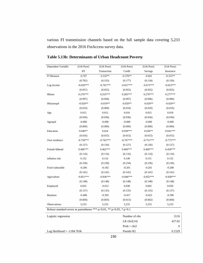
230

various FI transmission channels based on the full sample data covering 5,233

observations in the 2016 FinAccess survey data.

Table 5.13b: Determinants of Urban Headcount Poverty

Dependent Variable (Urb Poor) (Urb Poor) (Urb Poor) (Urb Poor) (Urb Poor)

IFI Transaction Credit Savings Insurance

FI Measure -0.707 0.332** -0.376** -0.041 -0.315**

(0.702) (0.153) (0.177) (0.134) (0.150)

Log income -0.659*** -0.701*** -0.657*** -0.673*** -0.653***

(0.057) (0.055) (0.055) (0.055) (0.055)

Hhsize 0.276*** 0.253*** 0.283*** 0.270*** 0.277***

(0.097) (0.094) (0.097) (0.096) (0.096)

Hhsizesqrd -0.020** -0.019** -0.020** -0.020** -0.020**

(0.010) (0.009) (0.010) (0.010) (0.010)

Age 0.015 0.015 0.016 0.015 0.018

(0.036) (0.036) (0.036) (0.036) (0.036)

Agesqrd -0.000 -0.000 -0.000 -0.000 -0.000

(0.000) (0.000) (0.000) (0.000) (0.000)

Education 0.040** 0.024 0.039*** 0.036** 0.041***

(0.016) (0.015) (0.015) (0.015) (0.015)

Own residence -0.759*** -0.762*** -0.767*** -0.751*** -0.775***

(0.127) (0.126) (0.127) (0.126) (0.127)

Female hhhead 0.466*** 0.462*** 0.469*** 0.469*** 0.450***

(0.116) (0.116) (0.116) (0.116) (0.116)

inflation risk 0.152 0.133 0.149 0.151 0.152

(0.236) (0.238) (0.234) (0.236) (0.236)

Food vulnerable -0.206 -0.192 -0.201 -0.201 -0.208

(0.141) (0.141) (0.141) (0.141) (0.141)

Agriculture -0.851*** -0.836*** -0.846*** -0.852*** -0.838***

(0.148) (0.148) (0.148) (0.148) (0.148)

Employed 0.022 -0.012 0.038 0.002 0.050

(0.137) (0.135) (0.135) (0.135) (0.137)

Business -0.408 -0.393 -0.417 -0.423 -0.396

(0.604) (0.603) (0.613) (0.602) (0.604)

Observations 5,233 5,233 5,233 5,233 5,233

Robust standard errors in parentheses *** p<0.01, ** p<0.05, * p<0.1

Logistic regression Number of obs 3116

LR chi2(14) 427.62

Prob > chi2 0

Log likelihood = -1184.7636 Pseudo R2 0.1529

231

Source: Author, 2017

Headcount poverty in urban areas appears to fall sharply with the increase in FI

and housing. FI and housing appear to be the main constraints facing urban

households. FI however affects the households differently depending on the

product with credit having a negative and significant impact. Access to a loan

facility by an urban household lowers their headcount poverty significantly by 3.6

percent and 3.17 percent for insurance uptake.

Transactionary financial product appears to have a positive effect on urban poverty

reduction. This could be rationalized by the high uptake of transactionary products

in urban areas leading to rapid diminishing returns in the form of an S-shaped

production as evidenced by Banerjee & Duflo (2007) where gains from the uptake

of transactionary products are high but decrease as more and more transactionary

products are taken up.

This probably signals the presence of an optimal transactionary product holding

which if exceeded becomes counterproductive as evidenced by the positive

coefficient. This positive coefficient could explain the weak link between the

portfolio usage (IFI) and urban poverty.

Credit uptake also leads to a reduction in poverty by around 3.6 percent. Contrary

to the rural areas where female headed households exhibited lower poverty

incidence, urban households headed by females reported higher poverty incidence

contradicting Christiaensen & Boisvert (2000). Residence ownership in urban

areas significantly led to a reduction in headcount poverty across all financial

product categories reinforcing Dercon & Krishnan (2004) and Jalan & Ravallion

(1998) findings. Increase in schooling years also appeared to have a nil effect on

urban poverty reduction. This could probably be explained by the high education

levels in urban areas.

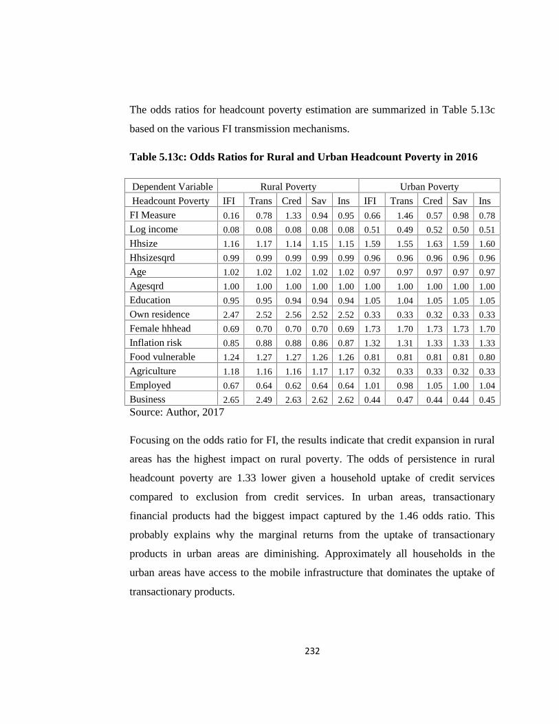
232

The odds ratios for headcount poverty estimation are summarized in Table 5.13c

based on the various FI transmission mechanisms.

Table 5.13c: Odds Ratios for Rural and Urban Headcount Poverty in 2016

Dependent Variable Rural Poverty Urban Poverty

Headcount Poverty IFI Trans Cred Sav Ins IFI Trans Cred Sav Ins

FI Measure 0.16 0.78 1.33 0.94 0.95 0.66 1.46 0.57 0.98 0.78

Log income 0.08 0.08 0.08 0.08 0.08 0.51 0.49 0.52 0.50 0.51

Hhsize 1.16 1.17 1.14 1.15 1.15 1.59 1.55 1.63 1.59 1.60

Hhsizesqrd 0.99 0.99 0.99 0.99 0.99 0.96 0.96 0.96 0.96 0.96

Age 1.02 1.02 1.02 1.02 1.02 0.97 0.97 0.97 0.97 0.97

Agesqrd 1.00 1.00 1.00 1.00 1.00 1.00 1.00 1.00 1.00 1.00

Education 0.95 0.95 0.94 0.94 0.94 1.05 1.04 1.05 1.05 1.05

Own residence 2.47 2.52 2.56 2.52 2.52 0.33 0.33 0.32 0.33 0.33

Female hhhead 0.69 0.70 0.70 0.70 0.69 1.73 1.70 1.73 1.73 1.70

Inflation risk 0.85 0.88 0.88 0.86 0.87 1.32 1.31 1.33 1.33 1.33

Food vulnerable 1.24 1.27 1.27 1.26 1.26 0.81 0.81 0.81 0.81 0.80

Agriculture 1.18 1.16 1.16 1.17 1.17 0.32 0.33 0.33 0.32 0.33

Employed 0.67 0.64 0.62 0.64 0.64 1.01 0.98 1.05 1.00 1.04

Business 2.65 2.49 2.63 2.62 2.62 0.44 0.47 0.44 0.44 0.45

Source: Author, 2017

Focusing on the odds ratio for FI, the results indicate that credit expansion in rural

areas has the highest impact on rural poverty. The odds of persistence in rural

headcount poverty are 1.33 lower given a household uptake of credit services

compared to exclusion from credit services. In urban areas, transactionary

financial products had the biggest impact captured by the 1.46 odds ratio. This

probably explains why the marginal returns from the uptake of transactionary

products in urban areas are diminishing. Approximately all households in the

urban areas have access to the mobile infrastructure that dominates the uptake of

transactionary products.

233

5.10 Conclusions and Policy Implications

The main objective of this chapter was to investigate the impact of financial

inclusion of VEP and headcount poverty. This was however preceded by a

construction of the VEP probability using Bourguignon, Goh and Kim (2004)

mean based approach for rural and urban areas. VEP was computed as the

probability that a household's consumption per adult equivalent at time t+1 would

fall below the poverty line while headcount poverty was computed as the

population living below the poverty line based on KIHBS 2005/06. Contrary to

Chaudhuri et al. (2002) who found a close relationship between determinants of

headcount poverty and VEP, this analysis found that headcount poverty and

vulnerability as expected poverty are independent concepts.

Policies geared towards eradication of poverty should factor in vulnerability

probability of the entire population. This outcome is elaborated by the poverty

transition matrix where 61.11 percent of the 61 percent found to be rural poor in

2009 remained poor in 2013 as compared to 38.89 percent who transited to non-

poor state. Poverty declined between 2013 and 2016 where 23.64 percent of the 70

percent 2013 rural poor remained poor compared to 76.36 percent who transited to

non-poor state. The picture is no different when it comes to the urban population

even though poverty incidence and vulnerability is lower. Persistence in poverty

for the 34 percent urban poor in 2009 averaged 38.46 percent. This shows that

61.54 percent of the 2009 urban poor population pulled out of the poverty. A more

significant reduction in the poor population was observed in 2016 where only

16.13 percent of the 70 percent poor population in 2013 remained poor. A

whopping 83.87 percent therefore managed to pull out of the poverty trap

successfully. An econometric estimation of the determinants of headcount poverty

and VEP on the cohort data established mixed results with FI having an inverse

relationship with both rural and urban VEP. Save for rural VEP, urban VEP, rural

and urban headcount poverty reported a significant relationship with FI implying

234

that rural households could be facing many other constraints other than financial

exclusion which limit their welfare change even with FI.

Asset holding was also found to have impacted positively on VEP among rural

households. This shows how rural households tradeoff consumption expenditure

with accumulation of illiquid assets like land and house ownership. This illiquid

state of assets makes the assets less useful in cushioning poor households against

short term liquidity risks. The relationship between residence ownership and VEP

is however negative in urban areas an indication that urban households are mainly

constrained by lack of credit and housing.

Given the pivotal role played by financial services in lowering ex-ante and ex-post

poverty, the government should encourage financial institutions to increase the

range of financial services at least cost to spread the gains. It was also found that

effectiveness of FI in rural areas could be curtailed by the many constraints faced

there. To this end, the government both at national and county levels should ensure

that the number of deprivations in rural areas is reduced by increasing funding

towards the development of other support infrastructure such as roads,

communication, quality housing among others.

In urban areas, housing and access to finance appear to be the main constraints.

The government should therefore ensure that it’s able to come up with low cost

housing and more competitive financial landscape to bring down the cost of

financial services. This way, poverty would be able to fall by a bigger margin.

Tackling VEP in rural areas therefore requires not just FI but a combination of FI

and other capabilities such as knowhow, infrastructural development among other

interventions. Continuous human capital development through education is critical

given the tendency of the educated to migrate to urban areas in search of greener

pastures.

235

Chapter Six: Summary, Conclusions and Policy

Recommendations

6.1 Conclusions

The study sought to investigate the dynamics of financial inclusion (FI) and its

impact on welfare in Kenya. The role of FI as a tool for enhanced welfare and

reduction in vulnerability to poverty cannot be overemphasized. The following

section details the conclusions and policy recommendations drawn from the study.

Firstly, the study developed both aggregated and single financial product usage

indicators to inform on the level and status of FI across the country. This was

followed by a stochastic dominance testing to establish which product dominates

financial markets and for which households. The measurement of single financial

product usage was based on the use of at least one form of transactionary financial

service. As for the portfolio usage, Sarma's (2008) was applied to aggregate

household financial product usage across all the four categories namely;

transactionary, credit, savings and investment, insurance and pension.

Secondly, a determination of drivers of FI was carried out from both the demand

and supply side. Determination of single product usage followed panel estimation.

Haussmann specification test was applied to test for the most suitable estimation

model and this led to the selection of fixed effects model estimation technique

since random effects model was found to be inefficient. The system GMM was

preferred due to its ability to incorporate lagged dependent variables as

instrumental variables and correct for Nickel bias often associated with FE

estimation (Woldridge, 2012). Thirdly, the developed measures of FI were

subjected to further estimation to establish how they impact on household

consumption per adult equivalent. This objective was aimed at unraveling welfare

236

differences from the use of varied financial instruments. A two-step GMM

estimation technique was applied to establish the impact of FI.

Given that FinAccess data is essentially cross sectional, the study developed

cohort panel to track households over time in line with Deaton (1985) technique

which estimates relationship between variables based on cohort means. Cohorts

are tracked in this case due to the difficulty of tracking same households in a true

panel especially in developing countries. Repeated cross sections generate

successive random samples of households from the cohorts since each household

is specifically a member of a single cohort which is tracked over time. Cohort

panel helps control for unobserved FE in almost a similar fashion as a true panel.

This approach was applied since pooled analysis of raw household data assumes

that households in repeated cross sections are independent leading to biased

estimates. The unobserved heterogeneity is assumed to originate from the different

geographical locations, survey year effects as well as the sector where the

household head works. The study therefore controls for the seven provinces;

Nairobi, Central, Eastern, Rift Valley, Nyanza, Coast and Western. The sectors

considered were Agriculture; non-Agriculture Employment and non-Agriculture

Business trading.

Lastly, the research was interested in establishing how FI feeds into the headcount

measure of poverty as well as vulnerability to poverty. One other overriding

objective was to develop a transition matrix based on the incidence of poverty

since 2006. The probability of VEP was predicted using the three step feasible

generalized least squares before subjecting the measure to an OLS estimation to

establish its determinants. The determinants of headcount poverty were compared

to the determinants of VEP to establish whether policy convergence in tackling the

twin challenges could be effective. All the chapters made use of the repeated

household survey data organized into 126 cohort panels. The ranking of FI was

237

however based on the county administrative structures. The maiden data was

gathered in 2006 to profile developments in the financial sector. Conclusions from

the entire report are summarized as follows.

6.2 Summary of Research Findings

This study reported some very interesting results with respect to FI and welfare

impacts. The microeconomic analysis of the impact of FI on welfare based on

pseudo panel estimation revealed that indeed FI is associated with immense

welfare benefits in terms of increased per adult equivalent consumption

expenditure, reduced headcount poverty and reduced vulnerability as expected

poverty (VEP). The marginal effects however differ by product with

transactionary, credit, insurance and a portfolio financial product usage leading to

huge positive welfare impacts.

The determinants of FI also vary with the product being examined even though per

capital income stood out buttressing the operation of the demand following

hypothesis among Kenyan households. The difference in the determinants of

poverty and VEP underscores the complex nature of improving household welfare

due to the independence of the two concepts. Policies aimed at eradicating poverty

should take into account the vulnerability probability of the population as well as

household characteristics. Policy formulation should also factor in both single

product and aggregated financial product usage indicators so as to bring about

targeted interventions.

Findings from this study are therefore instrumental in informing policy on factors

that can mitigate the adverse effects of vulnerability to poverty ex ante. An

inclusive financial system should therefore go beyond the usage of financial

services to incorporate other aspects related to welfare at both the national and

county levels. The following section summarizes the findings from the study based

on the research objectives.

238

6.2.1 Measures and Extent of FI in Kenya

Transactionary products in 2016 took the lion’s share (77.64 percent) in the

uptake of formal financial services followed by savings and investment

(32.43 percent), insurance (26.85 percent) and credit (14.62 percent) in that

order.

Uptake of financial services across the country displayed huge

geographical disparities with Kericho, Nairobi and Nakuru leading the

pack in the ranking of the index of financial inclusion (IFI). This could be

rationalized by the proximity of the urban population to financial access

channels.

Marsabit, Turkana and Samburu trailed all other counties by recording the

lowest IFI. In terms of regional government structure, of the seven regions

considered, Eastern region trailed while Nairobi region which is largely

urban populated was ranked highest in the usage of formal financial

services. A substitution effect from the traditional transactionary banking

products such as debit/ ATM cards, bank accounts among others to the

more flexible and readily accessible mobile money accounts was observed

leading to deeper financial markets.

Similarly, DTM and DTS savings seem to be encroaching the traditional

market for bank savings and investments. The same picture is reflected in

the use of credit products where uptake of bank loans is falling. However,

savings and credit usage has remained low since 2006 and more

particularly among the rural populace. Gender disparities in the uptake of

financial products since 2006 were also witnessed across the country where

the male gender appears to stochastically dominate financial product usage

along all the categories. This is also observed in the urban cluster which

dominates usage of the more flexible mobile financial products. Insurance

239

is dominated by NHIF and NSSF products which takes the lions share. In

all the categories of formal product usage, that is; transactionary, credit,

savings and insurance, tertiary education to a large extent appear to

stochastically dominate the other education levels.

6.2.2 Determinants of FI in Kenya

Demand Side

Social capital which is largely seen as a variable that can help to overcome

information asymmetry through group membership was found to have a

positive impact on the transactionary usage of finance. Group affiliation

enables members to gain access to various financial services from financial

institutions upon securing guarantors from the existing members.

Financial literacy which is critical in decision making was also found to

contribute positively on the uptake of credit and portfolio usage of finance.

It is expected that users of credit services will strive to understand more

about the implications of taking up the credit, repayment patterns, interest

charged among other considerations. This knowledge explains the negative

coefficient in the IFI and the credit transmission channels. It’s also

expected that a financially literate person will only go for those products

that yield maximum utility as opposed to hold several products with less

economic value. Education which builds on financial literacy was also

found to be significant in the uptake of IFI, transactionary, savings and

insurance products.

Trust in commercial banks was also found to be quite significant in

explaining IFI and transactionary usage of finance. The positive coefficient

indicates that choice of transactionary products as well as a portfolio

240

uptake of financial services is dependent on the trust bestowed on the

financial service providers.

The unobserved survey year effect in 2016 was found to be significant and

negative in determining the uptake of credit and insurance products but was

positive in the context of transactionary products. This implies that events

of 2016 had mixed impact on FI in Kenya.

The multiplier effect of per capita income and FI was positive and

significant at 1 percent in explaining all financial product categories except

transactionary financial products. This positive effect emphasizes the

critical role played by income per capita in enhancing FI as espoused by

the demand following hypothesis

The results also revealed that geographical location matters when it comes

to the uptake of financial services. From the seven regions considered in

the model, Households living in Central, Eastern, Nyanza and Rift Valley

had a lower probability of accessing transactionary products as compared

to their Nairobi counterparts. This could be explained by the nearness to

financial service providers in Nairobi as evidenced by the negative

coefficient for distance in the formal access strand.

A household’s main economic activity also influences the usage of

financial services. Households whose main economic activity was

agriculture were found to have a lower probability of accessing insurance

services most of which are designed for the formal employees.

The positive and significant coefficient of household size with respect to

IFI, credit and savings transmission channels associate increased usage of

financial services to rising household size. This would however need to be

investigated further to establish the optimal household size.

241

Supply side

The 2016 unobserved year specific effects had a negative impact on the

uptake of financial products from the other formal strand but a positive

impact on the formal strand. This clearly shows that the events of 2016

largely affected the formal strand and had no effect on the informal strand.

Per capita income had a positive impact on product usage from the other

formal access strand. This shows that the other formal strand is sensitive to

changes in the economy.

Increase in the distance to the nearest bank also lowered the demand for

financial services from both the formal and the formal other strand. This

shows that households are sensitive to the distance they have to cover to

get to the nearest financial service provider. This could also be rationalized

by the negative coefficient in the formal access channel taken up by

Central, Eastern, Nyanza and Rift Valley.

The important role played by the social capital in informal markets was

established by the 1 percent positive and significant coefficient. This

elevates the value of group membership seen as a critical factor considered

by informal financial service providers when designing their products. It’s

evident also that formal financial service provider is slowly embracing

social capital going by the 10 percent level of significance.

Households involved in agriculture appeared to prefer other formal

financial access channel

6.2.3 Impact of FI on Consumption Expenditure in Kenya

Estimation of both the static and the dynamic welfare functions revealed

that the unobservable survey year fixed effects as well as the region and

242

sector specific effects were instrumental in explaining variation in

individual welfare both at a point and over time.

Transactionary, credit, insurance and IFI were found to impact positively

and significantly on household welfare. Looked at from a single

measurement perspective, uptake of credit accounted for the highest impact

on consumer welfare. This result is consistent with the direct effect of FI

on welfare where FI impacts positively on welfare. The portfolio usage of

financial services (IFI) was also found to lead to huge welfare gains. This

shows that improvement of the entire financial system in critical in

enhancing household welfare.

The conditional effect from the interaction between education and FI

implies that while secondary level of education leads to increase in

household welfare, FI is not associated with higher welfare conditional on

having attained secondary level of education.

6.2.4 Impact of FI on VEP in Kenya

Contrary to Chaudhuri et al., (2002), findings suggest that VEP and

headcount poverty in Kenya are independent concepts. This is also

evidenced by the transition matrix which reveals persistence in the poverty

cycle over time. What this data is unable to establish however is the exact

number of years/months it takes for the effects of vulnerability to poverty

to fizzle out completely for the representative household in the cohort

given that the surveys are separated by three years. This could be informed

by high frequency data.

In terms of poverty transition, 61.11 percent of the 61 percent found to be

rural poor in 2009 remained poor in 2013 as compared to 38.89 percent

who transited to non-poor state. A slight improvement was observed in

243

2016 where only 23.64 percent of the 70 percent 2013 rural poor remained

poor compared to 76.36 percent who transited to non-poor state. The

picture is no different when it comes to the urban population even though

poverty incidence and vulnerability is lower. Persistence in urban poverty

fell by 38.34 in 2009 to 2013 and 16.13 percent between 2013 and 2016.

Part of this reduction is attributed to FI.

An econometric estimation of the impact of FI on VEP and headcount

poverty based on the cohort data found mixed results. While FI (credit,

savings, insurance and IFI) exhibited a negative and significant relationship

with urban VEP, transactionary financial product reported a positive

significant relationship with urban VEP symbolizing an S shaped

relationship which could be rationalized by diminishing marginal returns.

The relationship was also negative across all product categories in the rural

areas except insurance even though the relationship was weak. This inverse

relationship between FI and VEP confirms that policy makers can target FI

when designing policy interventions to improve welfare.

The demographic characteristics of a household head shape VEP

differently with asset ownership and household expectation about future

inflation having a negative impact on welfare. Rural household’s tradeoff

consumption expenditure for asset accumulation. Most of the assets held

are also highly illiquid to the point that they may not be useful in

cushioning poor households against short term liquidity risks. Development

of poverty reduction strategies should therefore consider various household

characteristics.

Expectations about future inflation and food vulnerability portrayed a

negative relationship to both VEP and poverty. This signifies the important

role that prior information on potential risks plays in preparing households

244

to face them. This also raises their ability to cushion against exposure to

idiosyncratic shocks. Female headed households were also found to face

higher headcount poverty in urban areas as compared to male headed

households but lower headcount poverty in rural areas.

6. 3 Contribution to existing knowledge

One of the main contributions from this study is pioneering a ranking of Kenyan

counties on the basis of their financial inclusivity. The study established that

financial inclusion varies across the country. This could be linked to peculiarities

in particular counties which also opens up a window for deeper interrogation to

understand the variance. The categorization of formal financial products along

transactionary, credit, savings and investment, insurance and pension offers an

exhaustive way of capturing access to a broad range of financial services in Kenya.

Secondly, the study established that the observed welfare differences vary with the

measure of financial inclusion adopted. The most effective transmission

mechanisms in improving welfare were found to be the transactionary and credit

channels. An inclusive financial system should go beyond the usage of financial

services to incorporate other aspects related to welfare at both the national and

county levels.

Thirdly, the study established that targeting poverty to improve household welfare

is limiting. Policy makers should consider both headcount and vulnerability as

expected poverty (VEP) which can only be analyzed inter-temporally.

Last but not least, the study contributed heavily methodologically by pioneering a

dynamic estimation of financial inclusion and welfare using repeated cross

sectional data organized in cohorts to form a pseudo panel. This methodology has

helped to overcome challenges associated with lack of longitudinal data in

developing countries for carrying out dynamic estimations.

245

Lastly, this thesis is founded on the most recent data on Kenya's financial

landscape from the demand side (FinAccess 2016, 2013, 2009 and 2006).

6.4: Recommendations for policy

Due to the establishment of the clear link between FI, welfare and vulnerability to

poverty, the study recognized the need to deepen targeted access to financial

services especially in low income zones which may not attract financial

institutions, increase human capital development through education and financial

literacy programs to supplement FI, improve the existing credit information

system, increase supply of basic services by the government and increase

economic activities towards employment creation which would lead to increase in

per capita income.

Increasing the range of formal financial products will lead to a more competitive

financial market leading to a reduction in transactionary costs. Financial inclusion

maps can help the government identify areas that lag behind in financial

development. Given that poverty is a multidimensional phenomenon, data on FI as

well as other economic variables can be superimposed on the poverty maps to help

tackle it.

The quality of schooling can be enhanced by improving the learning curriculum to

accommodate topics touching on financial literacy and resource management. In

addition, studies on the development of the index of FI to measure the

performance of the entire financial system should be intensified. This could help in

the development of an appropriate product weighting formulae to minimize

ambiguity in the generated IFI.

Lastly, there is need to develop insurance products for agriculture which is the

main economic activity in rural areas. Specific recommendations for each research

objective are specified as follows:

246

6.4.1 Measures and Extent of FI in Kenya

This chapter recommends that the government should encourage even distributions

of financial services to all counties to minimize the dominance by certain segments

of the population. With the low credit counts reported, the government through the

credit information sharing (CIS) Kenya should intensify the compilation of credit

reports by extending it to the agriculture sector which is the mainstay of our

country’s economy to ensure that the rural population mainly involved in

agriculture benefit from low cost credit products. In addition, more effort should

be put to ensure that DTMs and DTMs get the necessary support to increase their

market share in the supply of financial services. Lastly, proper measurement of FI

and barriers to it should be made a priority.

6.4.2 Determinants of FI in Kenya

This chapter recommends economic empowerment of masses through increased

economic activities by the government and private agencies which would raise per

capita income found to be significant in promoting FI. Secondly, human capital

development through education and financial literacy programs should be included

in school curriculum by the Ministry of Education given its positive and

significant impact.

In addition, mainstream financial service providers should factor in social capital

when designing credit products given its significant positive contribution in

driving access to financial services from the informal strand. Last but not least,

given that most rural households rely on agriculture for their survival, financial

service providers should be able to design products that meet the needs of this

population segment. This is mainly because a majority recorded a negative

coefficient with respect to the uptake of insurance services.

247

Lastly, transparency in the manner in which financial services are handled should

be enhanced in both formal and informal financial access channels given the

positive and significant coefficient reported for bank trust.

6.4.3 Impact of FI on Consumption Expenditure in Kenya

Given the significant impact of FI on consumption per adult equivalent, this

chapter recommends a bigger government involvement to ensure that FI is

enhanced. In particular, the government should spearhead a campaign aimed at

lowering transactionary costs to raise uptake of financial services.

Due to the significant impact of tertiary education on consumption expenditure,

the Ministry of Education should increase investment in higher learning

institutions to enhance human capital development. Lastly, the researchers should

give priority to studies relating FI to real sector outcomes. This is so because FI is

not an objective in itself, but only to the extent that it helps improve individual and

aggregate welfare.

The study also established that welfare differences vary with the transmission

channel. Given that the credit channel had the fastest transmission; policy makers

should pay more attention to the design of credit products and their distribution to

maximize gains.

6.4.4 Impact of FI on VEP in Kenya

Given the pivotal role played by financial services in lowering exante and expost

poverty, the government should encourage financial institutions to increase the

range of financial services at least cost to ensure the gains are spread out to the

larger population. It was also found that effectiveness of FI in rural areas could be

curtailed by the many constraints faced there. To this end, the government both at

national and county levels should ensure that the number of deprivations in rural

248

areas is reduced by increasing funding towards the development of other support

infrastructure such as roads, communication, quality housing among others.

In urban areas, housing and access to finance appear to be the main constraints.

The government should therefore ensure that it’s able to come up with low cost

housing and more competitive financial landscape to bring down the cost of

financial services. This way, poverty would be able to fall by a bigger margin.

Tackling VEP in rural areas therefore requires not just FI but a combination of FI

and other capabilities such as knowhow, infrastructural development among other

interventions. Continuous human capital development through education is critical

given the tendency of the educated to migrate to urban areas in search of greener

pastures.

6.5 Limitations of the study and suggestions for further studies

This study provided a detailed analysis of the usage of financial services in the

entire financial system and how they impact on household welfare. Whereas an

interrogation of the quality of financial services to examine the extent to which the

available range of financial products matches clients’ needs would have been more

informative, lack of the quality dimension in the data limits such an investigation.

Future researchers should now explore the quality dimension of financial access to

extend FI frontiers further. This should be accompanied by sectoral based

stochastic dominance tests to establish the effect of each financial product and its

distribution.

Lack of high frequency data also limits dynamic interrogation of vulnerability as

expected poverty. The government should increase funding for research and

development to guarantee high frequency data that can easily inform on the

transition path of vulnerability to poverty as well as draw forecasts and predictions

on household vulnerability probability. This should be done alongside studies on

249

alternative measures of welfare such as deprivation index to supplement use of per

adult equivalent consumption expenditure. Poverty being a multidimensional

aspect, there is need to investigate what other constraints face rural households by

rolling out studies touching on the state of the infrastructure which was missing in

this study to understand how they impact on FI.

Geospatial mapping of FI and welfare outcomes was a complicated process which

involved alot of cleaning of the GPS coordinates. Several observations had

missing GPS coordinates hence were dropped. The lack of consumption

expenditure data in 2006 also limited the inclusion of year 2006 survey in the

dynamic estimation of welfare. The survey year 2006 had used 25 matches to

symbolize the money held by an individual for expenditure in a month. This

measure of monthly expenditure was therefore incompatible with the money

metric measure used in 2009, 2013 and 2016 data.

Lastly, as much as the study would have wanted to map FI in all the 47 counties,

this was limited to 44 counties hence excluding the 3 counties in North Eastern

region (Mandera, Wajir and Garissa) which were not sampled in the 2013 survey

data due to logistical challenges hence information about their financial landscape

was missing.

250

References

Abdel-Magid, M. F. (1979). Toward a Better Understanding of the Role ofMeasurement in Accounting. The Accounting Review, 54, No. 2.

Acemoglu, D., & Robinson, J. A. (2001). A Theory of PoliticalTransitions. American Economic Review, 91(4), 938-963

Acemoglu, D., Ticchi, D., & Vindigni, A. (2011). Emergence And Persistence OfInefficient States. Journal of the European Economic Association, 9(2),177-208

Aduda, J. & Kalunda, E. (2012). Financial Inclusion and Financial Sector Stabilitywith reference to Kenya. Journal of Applied Finance and Banking, 2 (6),95-120

African Development Bank (2015). Financial Inclusion Initiative. Financial andTechnical Series. Africa Research Bulletin, 52(1)

Alliance for Financial Inclusion (2013). Putting Financial Inclusion on the GlobalMap. The 2013 Maya Declaration Progress Report. Bangkok.

Alter, A., & Yontcheva, B. (2015). Financial Inclusion and Development in theCEMAC. IMF Working Paper, No. 15(235), 1

Aghion, P., & Bolton, P. (1997). A Theory of Trickle-Down Growth andDevelopment. The Review of Economic Studies, 64(2), 151-172

Agrawal, A. (2008). The need for Financial Inclusion with an Indian perspective.Economic Research. IDBI Gilts Limited, Janmabhoomi Bhavan,Janmabhoomi Marg, Fort, Mumbai

Ahmed, S. (2003). Microcredit and Poverty New Realities and Issues. Journalof Bangladesh Studies, USA.

Akhavein, J., Frame, W. S., & White, L. J. (2005). The Diffusion of FinancialInnovations: An Examination of the Adoption of Small Business CreditScoring by Large Banking Organizations. The Journal of Business, 78(2),577- 596

251

Akudugu M.A. (2013). Determinants of financial inclusion in Western Africa:Insights from Ghana. Research Journal of Finance and Accounting 4(8)

Albert, J. R. (2007). Household Vulnerability to Income Poverty. Policy Note2007(5), Philippine Institute for Development Studies.

Allen, F., Demirguc-Kunt, A., Klapper, L., & Peria, M. S. (2012). TheFoundations of Financial Inclusion: Understanding Ownership and Useof Formal Accounts. Policy Research Working Papers

Allen, F., Carletti, E., Cull, R., Qian, J., Senbet, L., & Valenzuela, P. (2014). TheAfrican Financial Development and Financial Inclusion Gaps. PolicyResearch Working Papers, 7019

Alliance for Financial Inclusion (2011). The G20 Principles for InnovativeFinancial Inclusion: Bringing the Principles to Life. Case Studies Preparedon behalf of the Global Partnership for Financial Inclusion. Bangkok

Alliance for Financial Inclusion (2011). Measuring Financial Inclusion: Core Setof Financial Inclusion Indicators Report. Bangkok, Thailand

Alwang, J., Siegel, P.B., Jorgensen, S.L.(2001). Vulnerability : a view fromdifferent disciplines. Social Protection discussion paper series, 01(15).Washington, D.C. : The World Bank

Amemiya, T. (1977). The Maximum Likelihood and the Nonlinear Three- StageLeast Squares Estimator in the General Nonlinear SimultaneousEquation Model. Econometrica, 45(4), 955-968

Amidzic, G., Massara, A., & Mialou, A. (2014). Assessing Countries FinancialInclusion Standing: A New Composite Index. IMF WorkingPapers, 14(36), 1

Amin, S., Rai, A. S., & Topa, G. (2003). Does microcredit reach the poor andvulnerable? Evidence from northern Bangladesh. Journal of DevelopmentEconomics, 70(1), 59-82.

Ando, A. and Modigliani, F. (1963). The Life Cycle Hypothesis of Saving:Aggregate Implications and Tests. American Economic Review, 53(1), 55-84

252

Angelucci, M., Karlan, D. and Zinman. J. (2015). Microcredit Impacts: Evidencefrom a Randomized Microcredit Program Placement Experiment byCompartamos Banco: Dataset. American Economic Journal, 7(1), 151–182

Arellano, M., & Bond, S. (1991). Some Tests of Specification for Panel Data:Monte Carlo Evidence and an Application to Employment Equations. TheReview of Economic Studies, 58(2), 277-297

Arellano, M., & Bover, O. (1995). Another look at the instrumental variableestimation of error-components models. Journal of Econometrics, 68(1),29-51

Attanasio, O., Augsburg, B., Haas, R. D., Fitzsimons, E., & Harmgart, H. (2011).Group Lending or Individual Lending? Evidence from a Randomized FieldExperiment in Rural Mongolia. Working Paper, 11(20). London: Instituteof Fiscal Studies

Ayyagari, M., Beck, T., and Hoseini, M. (2013). Finance and Poverty: Evidencefrom India. CEPR Discussion Paper, 9497.

Bagehot, W. (1873). A General View Of Lombard Street. A Description of theMoney Market Lombard Street, 21-74

Banerjee, A., Karlan, D., & Zinman, J. (2015). Six Randomized Evaluations ofMicrocredit: Introduction and Further Steps. American Economic Journal:Applied Economics, 7(1), 1-21

Banerjee, A. V. (2013). Microcredit Under the Microscope: What Have WeLearned in the Past Two Decades, and What Do We Need toKnow? Annual Review of Economics, 5(1), 487-519

Banerjee, A., Duflo, E., Glennerster, R., & Kinnan, C. (2015). The Miracle ofMicrofinance? Evidence from a Randomized Evaluation. AmericanEconomic Journal: Applied Economics, 7(1), 22-53

Banerjee, A. V., & Duflo, E. (2007). The Economic Lives of the Poor. Journal ofEconomic Perspectives, 21(1), 141-167

Banerjee, A. V., & Newman, A. F. (1993). Occupational Choice and the Process ofDevelopment. Journal of Political Economy, 101(2), 274-298

253

Barro, R. J. (1990). The Stock Market and Investment. Review of FinancialStudies, 3(1), 115-131

Bauchet, J., Cristobal M., Laura S., Jeanette T., and Anna Y. (2011). LatestFindings from Randomized Evaluations of Microfinance. Access toFinance Forum, 2, Consultative Group to Assist the Poor (CGAP),Washington, DC

Bawa, V. S. (1982). Research Bibliography—Stochastic Dominance: A ResearchBibliography. Management Science, 28(6), 698-712

Bebczuk, R. (2008). Financial Inclusion in Latin America and the Caribbean:Review and Lessons. Working Paper, 68. UNLP and CEDLAS. InterAmerican Development Bank

Beck (2016). Financial Inclusion in Africa. Cass Business School, London

Beck, T., Degryse, H., & Kneer, C. (2014). Is more finance better? Disentanglingintermediation and size effects of financial systems. Journal of FinancialStability, 10, 50-64

Beck, T., Demirgüç-Kunt, A., & Levine, R. (2004). Finance, Inequality, andPoverty: Cross-Country Evidence. Policy Research Working Papers

Beck, T., Demirgüç-Kunt, A., & Maksimovic, V. (2005). Financial and LegalConstraints to Growth: Does Firm Size Matter? The Journal ofFinance, 60(1), 137-177

Beck, T., Demirgüç-Kunt, A., & Levine, R. (2007). Finance, inequality and thepoor. Journal of Economic Growth J Econ Growth, 12(1), 27-49

Lusinyan, L. (2005). Financial structure and economic growth: A cross-countrycomparison of banks, markets, and development, A. Demirgüç-Kunt and R.Levine (eds), The MIT Press, Cambridge, MA, 2001. Int. J. Fin. Econ.International Journal of Finance & Economics, 10(1), 91-92

Beck, T., Levine, R., & Levkov, A. (2010). Big Bad Banks? The Winners andLosers from Bank Deregulation in the United States. The Journal ofFinance, 65(5), 1637-1667

254

Bekaert, G., Harvey, C. R., & Lundblad, C. (2001). Emerging equity markets andeconomic development. Journal of Development Economics, 66(2), 465-504

Berthelemy, J. C., & Varoudakis, A. (1996). Economic Growth, ConvergenceClubs, And The Role Of Financial Development. Oxford EconomicPapers, 48(2), 300-328

Bertrand, M., Mullainathan, S., & Shafir, E. (2004). A Behavioral-EconomicsView of Poverty. American Economic Review, 94(2), 419-423

Bidani, B. and Richter, K. (2001). Household Vulnerability and the Asian Crisis:The Case of Thailand, World Bank

Bigsten, A., Kebede, B., Shimeles, A., & Taddesse, M. (2003). Growth andPoverty Reduction in Ethiopia: Evidence from Household PanelSurveys. World Development, 31(1), 87-106

Binswanger, H. P., & Khandker, S. R. (1995). The impact of formal financeon the rural economy of India. Journal of Development Studies, 32(2),234-262

Bittencourt, M. (2009). Financial development and inequality: Brazil 1985–1994. Economic Change and Restructuring, 43(2), 113-130

Baulch, B., & Hoddinott, J. (2000). Economic mobility and poverty dynamicsin developing countries. Journal of Development Studies, 36(6), 1-24

Bourguignon, F., Goh, C., & Kim, D. I. (2004). Estimating IndividualVulnerability to Poverty with Pseudo-Panel Data. Policy ResearchWorking Papers, 3375

Boyd, J. H., Levine, R., & Smith, B. D. (2001). The impact of inflation onfinancial sector performance. Journal of Monetary Economics, 47(2),221-248

Branson, W.H. (1989). Macroeconomic Theory and Policy 3rd ed, New York:Harper and Row

Browning, M. and Lusardi, A. (1996). Household Saving: Micro Theories andMicro Facts. Journal of Economic Literature, 34(4), 1797-1855

255

Brune, L., Giné, X., Goldberg, J., & Yang, D. (2016). Facilitating Savings forAgriculture: Field Experimental Evidence from Malawi. EconomicDevelopment and Cultural Change, 64(2), 187-220

Buera, F., Kaboski, J., & Shin, Y. (2012). The Macroeconomics of Microfinance.NBER Working Papers, 17905, National Bureau of Economic Research,Inc

Burges, R. and Pandes, R. (2005). Do Rural Banks matter? Evidence from theIndian Social Banking Experiment. The American Economic Review,95(3), 780-795

Burney, N. A., & Akmal, M. (1991). Food Demand In Pakistan: AnApplication Of The Extended Linear Expenditure System. Journal ofAgricultural Economics, 42(2), 185-195

Cafiero, C. and Vakis R. (2006). Risk and Vulnerability Considerations in PovertyAnalysis: Recent Advances and Future Directions. Social Protection Unit,Human Development Network. SP Discussion Paper 0610. The World

Bank, Washington, D.C.

Cámara, N., & David, T. (2015). Factors that matter for financial inclusion:Evidence from Peru.Aestimatio, 9(2015), 8-29

Campbell, N., & Thorndike, A. M. (1953). What is Science? Phys. Today PhysicsToday, 6(8), 18

Campero, A and Kaiser, K (2013). Access to Credit: Awareness and Use ofFormal and Informal Credit Institutions. Working paper, 2013(07).Bank of Mexico

Carter, M. (1997). Environment, Technology, and the Social Articulation ofRisk in West African Agriculture. Economic Development andCultural Change, 45(3), 557-590

Central Bank of Kenya, Kenya National Bureau of Statistics & Financial SectorDeepening Kenya (2016). FinAccess Household Survey. Nairobi, Kenya

Central Bank of Kenya, Kenya National Bureau of Statistics & Financial SectorDeepening Kenya (2013). FinAccess Household Survey. Nairobi, Kenya

256

Central Bank of Kenya, Kenya National Bureau of Statistics & Financial SectorDeepening Kenya (2009). The 2016 FinAccess Household Survey onfinancial inclusion. Nairobi, Kenya

Central Bank of Kenya, Kenya National Bureau of Statistics & Financial SectorDeepening Kenya (2006). The 2016 FinAccess Household Survey onfinancial inclusion. Nairobi, Kenya

Central Bank of Kenya (2013). Prudential Guidelines for Institutions Licensedunder Banking Act

Central Bank of Kenya (2015). Bank Supervision Annual Report. Kenya

Central Bank of Kenya (2014). Bank Supervision Annual Report. Kenya

Chakravarty, S. R., & Pal, R. (2013). Financial inclusion in India: Anaxiomatic approach. Journal of Policy Modeling, 35(5), 813-837

Chakrabarty, K.C., (2011). Financial Inclusion and Banks: Issues andPerspectives: Address delivered at the FICCI – UNDP Seminar on“Financial Inclusion: Partnership between Banks, MFIs andCommunities. New Delhi

Chaudhuri, S. (2000). Empirical methods for assessing household vulnerability topoverty. Department of Economics, Columbia University: New York

Chaudhuri, S. (2003). Assessing vulnerability to poverty: Concepts, empiricalmethods and illustrative examples. Department of Economics, ColumbiaUniversity: New York

Chaudhuri, S., Jalan, J. & Suryahadi, A. (2002). Assessing householdvulnerability to poverty from cross-sectional data: A methodology andestimates from Indonesia. Dept. of Economics, Columbia University,Discussion paper, No. 0102-52.

Chibba, M. (2009). Financial Inclusion, Poverty Reduction and the MillenniumDevelopment Goals. The European Journal of DevelopmentResearch, 21(2), 213-230

257

Chinn, M. D., & Ito, H. (2006). What matters for financial development? Capitalcontrols, institutions, and interactions. Journal of DevelopmentEconomics, 81(1), 163-192

Chithra, N., & Selvam, M. (2013). Determinants of Financial Inclusion: AnEmpirical Study on the Inter-State Variations in India. Available at SSRN2296096

Christensen, J. (2004). Domestic Debt Markets in Sub-Saharan Africa. IMFWorking Paper, No 04(46), 1

Christiaensen, L. J. (2005). Towards an Understanding of HouseholdVulnerability in Rural Kenya. Journal of African Economies, 14(4), 520-558

Christiaensen, L. & Boisvert, R.N. (2000). On measuring households foodvulnerability: Case evidence from northern Mali. Cornell University.Department of Agricultural and Managerial Economics, Working Paper,No. 2000–05.

Chuah, H.L. and Thai, V. (2004). Financial Development and Economic Growth:Evidence from Causality Tests for the GCC Countries, IMF WorkingPaper, No. 04.

Claessens, S. (2006). Access to Financial Services: A Review of the Issues andPublic Policy Objectives. The World Bank Research Observer, 21(2), 207-240

Clarke, G. R., Xu, L. C., & Zou, H. (2006). Finance and Income Inequality: WhatDo the Data Tell Us? Southern Economic Journal, 72(3), 578-596

Collins, D., Morduch, J., Rutherford, S. and Ruthven, O. (2009). Portfolios of thePoor: How the World's Poor Live on $2 a Day. Princeton, New Jersey:Princeton University Press. 320 pp. $29.95. ISBN 06-91141-48-7(HB). Journal of South Asian Development, 5(2), 306-309

Columbus, F.H. (2001). Politics and Economics of Latin America. NovaPublishers, Huntington. New York, 1, 64-66

Consultative Group to Assist the Poor (CGAP) & The World Bank Group. (2010).Financial Access 2010: The State of Financial Inclusion through the Crisis.

258

Copestake, J. (2007). Mainstreaming Microfinance: Social PerformanceManagement or Mission Drift? World Development, 35(10), 1721-1738

Crépon, B., Devoto, F., Duflo, E., & Pariente, W. (2014). Estimating the Impact ofMicrocredit on Those Who Take It Up: Evidence from a RandomizedExperiment in Morocco

Cull, R., Demirgüç-Kunt, A., & Morduch, J. (2013). Banks andMicrobanks. Journal of Financial Services Research , 46(1), 1-53

Cull, Robert, Tilman Ehrbeck, and Nina Holle. (2014). Financial Inclusion andDevelopment: Recent Impact Evidence. Focus Note 92. Washington, D.C.:CGAP

Cunningham, W. and W.F. Maloney (2000). Measuring vulnerability: Whosuffered in the 1995 Mexican crisis? World Bank: Washington DC

Daly, A. and Zachary S. (1978), Improved multiple choice models, in D.Hensher and M. Dalvi, eds., Determinants of Travel Choice, SaxonHouse, Sussex

Dang, H. H., & Lanjouw, P. F. (2014). Welfare Dynamics Measurement: TwoDefinitions of a Vulnerability Line and Their EmpiricalApplication. Policy Research Working Paper, No. 6944 Washington DC:The World Bank.

Dang, T. and Jha, R. (2009). Vulnerability to Poverty in select Central AsianCountries. The European Journal of Comparative Economics, 6(1), 17-50

Dargay, J.M. and Vythoulkas, P.C. (1999). Estimation of a dynamic car ownershipmodel: A pseudo-panel approach. Journal of Transport Economics andPolicy 33(3), 287–301.

David, R. (2006). How to Do xtabond2: An introduction to Difference and SystemGMM in Stata. Centre for Global Development, Working Paper No. 103

Davidson, R. (2006). Stochastic dominance. The new Palgrave dictionary ofEconomics. Second Edition. Eds. Steven N. Durlauf and Lawrence E.Blume. Palgrave Macmillan.

259

Davidson, R., & Duclos, J. (2000). Statistical Inference for Stochastic Dominanceand for the Measurement of Poverty and Inequality. Econometrica, 68(6),1435- 1464

Deaton (2001). Understanding Consumption. Clarendo Press, London, 40 -45

Deaton, A.S. (1992). Understanding Consumption, Oxford and New York: OxfordUniversity Press

Deaton, A. (1986). Chapter 30 Demand analysis. Handbook ofEconometrics, 1767- 1839

Deaton, A. (1985). Panel data from time series of cross-sections. Journal ofEconometrics, 30(1-2), 109-126

Deb, A. and Kubzansky, M. (2012). Bridging the Gap: The Business Case for

Financial Capability. Monitor Inclusive Markets

Demetriades, P. O., & Hussein, K. A. (1996). Does financial development causeeconomic growth? Time-series evidence from 16 countries. Journal ofDevelopment Economics, 51(2), 387-411

Demirguc-Kunt, A., Klapper, L., Singer, D., & Oudheusden, P. V. (2015). TheGlobal Findex Database 2014: Measuring Financial Inclusion around theWorld. Policy Research Working Paper, No. 7255, World Bank,Washington, DC

Demirgüç-Kunt, A., & Klapper, L. (2012). Financial Inclusion in Africa: AnOverview. Policy Research Working Paper, No. 6088. Washington, D.C.:World Bank

Demirguc-Kunt, A., & Klapper, L. (2012). Measuring Financial Inclusion: TheGlobal Findex Database. Policy Research Working Paper, No, 6025.Washington, D.C.: World Bank

Demirguc-Kunt, A., Klapper, L., & Singer, D. (2013). Financial Inclusion andLegal Discrimination against Women: Evidence from DevelopingCountries. Policy Research Working Paper, No. 6416. Washington,D.C.: World Bank

260

Demirgüç-Kunt, A. and R. Levine. (2007). Finance and Economic Opportunity,Brown University, mimeo.

Dercon, Stefan. (2000). Income Risk, Coping Strategies and Safety Nets.Background paper World Development Report 2000/01: Centre for theStudy of African Economies, Oxford University.

Dercon, S. (2001). Assessing vulnerability to poverty. DFID

Dercon, S. (2004). Growth and shocks: Evidence from rural Ethiopia. Journal ofDevelopment Economics, 74(2), 309-329

Dercon, S., & Krishnan, P. (2004). Food Aid and Informal Insurance. InsuranceAgainst Poverty, 305-329

Dercon, S., & Krishnan, P. (2000). Vulnerability, seasonality and poverty inEthiopia. Journal of Development Studies, 36(6), 25-53

Muleta, A., & Deressa, D. (2014). Female Headed Households and Poverty inRural Ethiopia. Science, Technology and Arts Research Journal, 3(1),152

DFID (2004). The importance of financial sector development for growth andpoverty reduction, Working Paper series, London, UK.

Dhrifi, A. (2013). A Revisit of the Growth Inequality Poverty Relationship:The Role of Institutional Quality. International Journal of Advances inManagement and Economics, 2(1), 94-102

Diagne A., and Zeller M. (2001). Access to credit and its impact on welfare inMalawi. Research Report No 116. Washington, D.C.: International FoodPolicy Research Institute.

Diamond, D. W., & Dybvig, P. H. (1983). Bank Runs, Deposit Insurance, andLiquidity. Journal of Political Economy, 91(3), 401-419

Diamond, D. W. (1984). Financial Intermediation and Delegated Monitoring. TheReview of Economic Studies, 51(3), 393-414

Do, Q., & Levchenko, A. A. (2004). Trade and Financial Development. PolicyResearch Working Paper, No. 3347.

261

Drummond, P., Wajid K., and Williams O. (eds.), (2014). The Quest for RegionalIntegration in the East African Community, Washington: InternationalMonetary Fund.

Duesenberry, J. (1948). Income-Consumption Relations and their Implications, inLloyd Metzler, editor, Income, Employment and Public Policy.

Dupas, P., & Robinson, J. (2013). Savings Constraints and MicroenterpriseDevelopment: Evidence from a Field Experiment in Kenya. AmericanEconomic Journal: Applied Economics, 5(1), 163-192

Easterly, W., & Levine, R. (2003). Tropics, germs, and crops: How endowmentsinfluence economic development. Journal of Monetary Economics, 50(1),3-39

Eswaran & Kotwal; (1990). Implications of Credit Constraints for Risk Behaviourin Less Developed Economies. Oxford Economic Papers, 42, 473-482

Eswaran, M., & Kotwal, A. (1989). Credit as insurance in agrarianeconomies. Journal of Development Economics, 31(1), 37-53

Fadun S.A (2014). Financial inclusion, tool for poverty alleviation and incomeredistribution in developing countries: Evidence from Nigeria. AcademicResearch International, 5(3)

Fama, E. F. (1970). Efficient Capital Markets: A Review of Theory and EmpiricalWork. The Journal of Finance, 25(2), 383-417

Fazzari, S. M., Hubbard, R. G., Petersen, B. C., Blinder, A. S., & Poterba, J. M.(1988). Financing Constraints and Corporate Investment. BrookingsPapers on Economic Activity, 1988(1), 141

Financial Sector Deepening (2011). Highlights from FSD’s strategy 2011-2015:Issue 06

Financial Sector Deepening Trust (2014). Supporting the development of inclusivefinancial markets. Annual Report

Financial Sector Deepening Trust (2015). Kenya's Financial Transformation in the21st Century

262

Foster, J., Greer, J., & Thorbecke, E. (1984). A Class of Decomposable PovertyMeasures. Econometrica, 52(3), 761

Friedman, M. (1957). A Theory of the Consumption Function. Princeton, NJ:Princeton Univerity Press

Galor, O., & Zeira, J. (1993). Income Distribution and Macroeconomics. TheReview of Economic Studies, 60(1), 35-52

Giné, X., & Townsend, R. M. (2004). Evaluation of financial liberalization: Ageneral equilibrium model with constrained occupation choice. Journalof Development Economics, 74(2), 269-307

Glewwe, P., & Hall, G. (1998). Are some groups more vulnerable tomacroeconomic shocks than others? Hypothesis tests based on paneldata from Peru. Journal of Development Economics, 56(1), 181-206

Global Partnership for Financial Inclusion (2011). Financial Inclusion Data:Assessing the landscape and country level target approaches. Discussionpaper, IFC, Washington, DC

Gough, I. and McGregor, J.A. (2007) Researching wellbeing: From concepts tomethodology. From Theory to Research Wellbeing in DevelopingCountries, 316-350

Government of Kenya (2004). The Economic Recovery Strategy for Wealth andEmployment Creation, 2003-2004.Government Printer, Nairobi

Government of Kenya, National Development Plan (2002 – 2008) EffectiveManagement for Sustainable Economic Growth and Poverty Reduction.Government Printer.

Government of Kenya (2007). Kenya Vision 2030, Nairobi: Ministry of Planningand National Development (available at www.vision2030.go.ke/).

Government of Kenya (1994). Welfare Monitoring Survey. Government Printers,Nairobi.

Government of Kenya (1965). African Socialism and its Application to Planningin Kenya. Sessional Paper No. 1. Government Printers, Nairobi.

263

Government of Kenya. Development Plans, various. Government Printers,Nairobi.

Greene W.H. Econometric Analysis, Second Edition, Macmillan, 2003. Chapter21.

Greenwood, J., & Jovanovic, B. (1990). Financial Development, Growth, and theDistribution of Income. Journal of Political Economy, 98(5 1), 1076-1107

Greenwood, J., Sanchez, J. M., & Wang, C. (2013). Quantifying the impact offinancial development on economic development. Review of EconomicDynamics, 16(1), 194-215

Greenwood, R., & Scharfstein, D. (2013). The Growth of Finance. Journal ofEconomic Perspectives,27(2), 3-28

Gupta, Anil (1986). Consumption Behaviour in India, Anmol Publications, Delhi

Gupta, K.L. (1987). Aggregate Savings, Financial Intermediation and InterestRate, Review of Economics and Statistics, 58(2), 303-311

Gurley, J. G., Shaw, E. S. (1955). Financial aspects of economic development.American Economic Review 45, 515-538

Günther, I., & Harttgen, K. (2009). Estimating Households Vulnerability toIdiosyncratic and Covariate Shocks: A Novel Method Applied inMadagascar. World Development, 37(7), 1222-1234

Haddad, L., & Ahmed, A. (2003). Chronic and Transitory Poverty: Evidencefrom Egypt, 1997–99. World Development, 31(1), 71-85

Hall (2001). Stochastic Implications of the Life-cycle permanent. IncomeHypothesis: Theory and Evidence. Journal of Political Economy. 2(3),10-4

Han, R., & Melecky, M. (2013). Financial Inclusion for Financial Stability: Accessto Bank Deposits and the Growth of Deposits in the Global FinancialCrisis. Policy Research Working Paper, No. 6577.

264

Hannig, A., & Jansen, S. (2010). Financial Inclusion and Financial Stability:Current Policy Issues. Working Paper, No. 259. Tokyo: AsianDevelopment Bank Institute

Hansen, L. P. (1982). Large Sample Properties of Generalized Method ofMoments Estimators. Econometrica, 50(4), 1029-1054

Hausman, J. A., & Taylor, W. E. (1981). Panel Data and UnobservableIndividual Effects. Econometrica,49(6), 1377-1398

Heitzmann, K., Canagarajah, R.S. & Siegel, P.B. (2002). Guidelines forassessing the sources of risks and vulnerability. Social ProtectionDiscussion Paper No. 0218. The World Bank, Washington.

Henry, P. B. (2000). Stock Market Liberalization, Economic Reform, andEmerging Market Equity Prices. The Journal of Finance, 55(2), 529-564

Jeong, H., & Townsend, R. M. (2007). Sources of TFP growth: Occupationalchoice and financial deepening. Economic Theory, 32(1), 179-221

Holzmann, R. and S. Jorgensen (2000). Social Risk Management: A ConceptualFramework for Social Protection and Beyond. Social Protection DiscussionPaper No. 0006. The World Bank: Washington, D.C.

Honohan, P. (2005). Banking Sector Crises And Inequality. Policy ResearchWorking Paper, No. 3659.

Honohan, P. (2006). Household Financial Assets In The Process ofDevelopment. Policy Research Working Paper, No. 3965.

Honohan, P. (2008). Cross-country variation in household access to financialservices. Journal of Banking & Finance, 32(11), 2493-2500

Honohan, Patrick and Michael King (2012). Cause and effect of financial access:Cross country evidence from the finscope surveys, in Robert Cull, AsliDemirguc-Kunt and Jonathan Morduch (eds) Banking the world:Empirical foundations of financial inclusion, MIT Press, 2012

265

Hoyos, C., X. Peña & D. Tuesta (2014). Determinants of financial inclusion inMexico based on the 2012 National Financial Inclusion Survey. WorkingPaper, No. 14(15).

Huang, Y. (2011). General Determinants of Financial Development. Determinantsof Financial Development, 10-63

Huybens, E., and B.D. Smith, (1999). Inflation, Financial Markets, and long-runreal activity. Journal of Monetary Economics, 43, 283-315.

Imai, K. S., Gaiha, R., & Kang, W. (2011). Vulnerability and poverty dynamics inVietnam. Applied Economics, 43(25), 3603-3618

International Monetary Fund (2012). Financial Access Survey, StatisticsDepartment

Jacoby, H. G., & Skoufias, E. (1997). Risk, Financial Markets, and HumanCapital in a Developing Country. The Review of Economic Studies, 64(3),311-335

Jain, L. R. and Tendulkar, S. D. (1973). Analysis of Occupational Differences inConsumer Expenditure Patterns in India, Sankhyd, 35(2), 239- 267.

Jaffee, D., & Levonian, M. (2001). The Structure of Banking Systems inDeveloped and Transition Economies. European FinancialManagement, 7(2), 161-181

Jalan, J., & Ravallion, M. (1999). Are the poor less well insured? Evidenceon vulnerability to income risk in rural China. Journal of DevelopmentEconomics, 58(1), 61-81

Jalilian, H., & Kirkpatrick, C. (2005). Does Financial DevelopmentContribute to Poverty Reduction? Journal of Development Studies, 41(4),636-656

Jalilian, H., & Kirkpatrick, C. (2002). Financial development and povertyreduction in developing countries. Int. J. Fin. Econ. International Journalof Finance & Economics, 7(2), 97-108

266

Jha, R., & Dang, T. (2009). Vulnerability to Poverty in select Central AsianCountries. The European Journal of Comparative Economics 6(1), 17-50.

Johnson, S., & Nino-Zarazua, M. (2011). Financial Access and Exclusion inKenya and Uganda. Journal of Development Studies, 47(3), 475-496

Kaboski, J. P., & Townsend, R. M. (2012). The Impact of Credit on VillageEconomies. American Economic Journal: Applied Economics, 4(2), 98-133

Kaldor, N. (1966). Causes of the Slow Rate of Economic Growth in the UnitedKingdom. Cambridge: Cambridge University Press

Kalunda (2014). Financial Inclusion Impact on Small Scale Tea Farmers in NyeriCounty, Kenya. World Journal of Social Sciences, 4(1), 130-139

Kamanou, G., & Morduch, J. (2004). Measuring Vulnerability toPoverty. Insurance Against Poverty, 155-175

Kannan, K., & Papola, T. (2007). Workers in the informal sector: Initiativesby India's National Commission for Enterprises in the Unorganized Sector(NCEUS). International Labour Review, 146(3-4), 321- 329

Kanbur, S. M. (1987). Measurement and Alleviation of Poverty: With anApplication to the Effects of Macroeconomic Adjustment. Staff Papers -International Monetary Fund, 34(1), 60-85

Kang, S. (2009). Implication for Anti-Poverty Policy Taking into AccountPersistence and Recurrence of Poverty. Economic DevelopmentResearch, 15(2), 263-286

Kang, W. (2015). An Investigation of the Determinants of HouseholdVulnerability and Poverty in Korea and the World Economy, 16(2), 223-251

Kang, W. (2014). The Analysis of Poverty Dynamics in Korea and PolicyImplication. KDI Policy Research Series 2014(08)

Karlan, D., & Morduch, J. (2010). Access to Finance. Handbook of DevelopmentEconomics Handbooks in Economics, 4703-4784

267

Karlan, D., & Zinman, J. (2009). Expanding Credit Access: Using RandomizedSupply Decisions to Estimate the Impacts. Review of FinancialStudies, 23(1), 433-464

Kempson, C. and Whyley, E. (1999b). Kept out or opted out? Understanding andcombating financial exclusion. Bristol, Policy Press. 21, 18-22

Kenya National Bureau of Statistics (KNBS) (2014). Demographic and HealthSurvey 2013-2014. Nairobi, Kenya

Kenya National Bureau of Statistics (KNBS) (2008). Demographic and HealthSurvey 2008-2009. Nairobi, Kenya

Kenya National Bureau of Statistics (KNBS) (2008). Well-Being in Kenya, asocio- economic profile. Nairobi, Kenya

Kenya National Bureau of Statistics (KNBS) (2006). Kenya Integrated HouseholdBudget Survey 2005-2006. Nairobi, Kenya

Keynes, J. M. (1937). Alternative Theories of the Rate of Interest. The EconomicJournal, 47(186), 241-252

Keynes, John Maynard (1936). The General Theory of Employment Interest andMoney. London Press: Macmillan.

King, R. G., & Levine, R. (1993). Finance and Growth: Schumpeter Might BeRight. The Quarterly Journal of Economics, 108(3), 717-737

Knight, J., Shi, L., & Quheng, D. (2010). Education and the Poverty Trap in RuralChina: Closing the Trap. Oxford Development Studies, 38(1), 1-24

Kuldeep Singh and Singh Kondan (2012). Financial Inclusion, Development andIts Determinants: An Empirical Evidence of Indian States. The AsianEconomic Review53 (1), 115-134.

Kuznets, S. (1955). Economic growth and income inequality. American EconomicReview, 45, 1-28.

Kuznets, S. (1963). Quantitative Aspects of the Economic Growth ofNations: VIII. Distribution of Income by Size. Economic Developmentand Cultural Change, 11(2, Part 2), 1-80

268

Lanjouw, P., & Ravallion, M. (1995). Poverty and Household Size. TheEconomic Journal, 105(433), 1415-1434

Larson, D., & Plessmann, F. (2002). Do Farmers Choose to Be Inefficient?Evidence from Bicol, Philippines. Policy Research Working Paper, No.2787, The World Bank, Washington D.C.

Levine, R. & Renelt, D. (1992). A Sensitivity Analysis of Cross-Country GrowthRegressions. The American Economic Review, 82(4), 942-963

Levine, R. (2004). Finance and Growth: Theory and Evidence. Working paper10766, National Bureau of Economic Research, Cambridge, MA.

Levine, Ross, (1997). Financial Development and Economic Growth: Views andAgenda. Journal of Economic Literature, 35, 688-726.

Levine, R. (2008). Finance And The Poor. Manchester School, 76, 1-13

Levine, R. (2005). Chapter 12 Finance and Growth: Theory andEvidence. Handbook of Economic Growth, 865-934

Levy, H. (1998). Stochastic dominance. Kluwer Academic Publishers,Norwell, MA.

Ligon, E. & Schechter, L. (2004). Evaluating Different Approaches toEstimating Vulnerability. Social Protection Discussion Paper Series,World Bank

Ligon, E., & Schechter, L. (2003). Measuring Vulnerability*. Economic JournalThe Economic Journal,113(486)

Lindbeck, A. and D. J. Snower (2001, Winter). Insiders and outsiders. Journal ofEconomic Perspectives 15 (1), 165–188

Lucas, R. E. (1988). On the mechanics of economic development. Journal ofMonetary Economics,22(1), 3-42

Mas-Colell, A., Whinston, M.D., and Green, J.R. (1995). Microeconomic Theory.Oxford University Press, New York Oxford.

269

Matul, M., Dalal, A., Bock, O. D., & Gelade, W. (2013). Microinsurance demand:Determinants and strategies. Enterprise Development andMicrofinance, 24(4), 311-327

Mayer, Colin and Sussman, Oren, (2001). The Assessment: Finance, Law, andEconomic Growth. Oxford Review of Economic Policy,17(4)

Mcculloch, N., & Calandrino, M. (2003). Vulnerability and Chronic Poverty inRural Sichuan. World Development, 31(3), 611-628

McFadden, D. (1978). Modeling the choice of residential location, in A. Kar-lquistet al. (ed.), Spatial interaction theory and residential location, North-Holland, Amsterdam, 75–96.

Mckenzie, D. J. (2004). Asymptotic theory for heterogeneous dynamic pseudo-panels. Journal of Econometrics, 120(2), 235-262

Mckenzie, D. J. (2003). How do Households Cope with Aggregate Shocks?Evidence from the Mexican Peso Crisis. World Development, 31(7), 1179-1199

Mckillop, D. G., & Wilson, J. O. (2007). Financial exclusion. Public Money andManagement, 27(1), 9-12

Mckinnon, R. I. (1974). Money and Capital in EconomicDevelopment. International Journal, 29(4), 649

Meng, Y., Brennan, A., Purshouse, R., Hill-Mcmanus, D., Angus, C., Holmes, J.,and Meier, P. S. (2014). Estimation of own and cross price elasticitiesof alcohol demand in the UK—A pseudo-panel approach using the LivingCosts and Food Survey 2001–2009. Journal of Health Economics, 34, 96-103

Merton, R. C. (1992). Financial Innovation And Economic Performance. Journalof Applied Corporate Finance, 4(4), 12-22

Merton, Robert C., and Zvi Bodie. (1995). A Conceptual Framework forAnalyzing the Financial Environment. Chap. 1 in The Global FinancialSystem: A Functional Perspective, edited by Dwight B. Crane et al.Cambridge: Harvard Business School Press

270

Merton, R. C., & Bodie, Z. (2005). Design Of Financial Systems: Towards ASynthesis Of Function And Structure. The World of Risk Management, 1-27

Mbiti, I., & Weil, D. N. (2013). The Home Economics of E-Money: Velocity,Cash Management, and Discount Rates of M-Pesa Users. AmericanEconomic Review, 103(3), 369-374

Milton Friedman (1957). Inflation : Causes and Consequences

Moffitt, R. (1993). Identification and estimation of dynamic models with atime series of repeated cross-sections. Journal of Econometrics, 59(1-2),99-123

Morduch, J. (2004). Consumption Smoothing Across Space: Testing Theoriesof Risk-Sharing in the ICRISAT Study Region of SouthIndia. Insurance Against Poverty, 38-56

Morduch, J. (1994). Poverty and Vulnerability. American EconomicReview,84(2)221-225

Morduch, J. (1999). The Microfinance Promise. Journal of EconomicLiterature, 37(4), 1569-1614

Morduch, J. (1995). Income Smoothing and Consumption Smoothing. Journal ofEconomic Perspectives, 9(3), 103-114

Moser, C. O. (1998). The asset vulnerability framework: Reassessing urbanpoverty reduction strategies. World Development, 26(1), 1-19

Mukherjee, S., & Benson, T. (2003). The Determinants of Poverty in Malawi,1998. World Development,31(2), 339-358

Murphy, B. P., Chakravarti, I. M., Laha, R. G., & Roy, J. (1968). Handbookof Methods of Applied Statistics. Vol. I: Techniques of Computation,Descriptive Methods and Statistical Inference. Applied Statistics, 17(3),293

Mwangi I.W and Shem A.O (2012). Social capital and access to credit in Kenya.American Journal of Social and Management Sciences, 2151-1559

271

National Commission for Enterprises in the Unorganized Sector (2007). Report onConditions of Work and Promotion of Livelihoods in the UnorganizedSector. New Delhi

Ncube Mthuli (2016). Digital Financial Services and Regulatory Policies inAfrica. AERC Senior Policy Seminar, Nairobi

Ndikumana, L. (2005). Financial development, financial structure, and domesticinvestment: International evidence. Journal of International Money andFinance, 24(4), 651-673

Nelson, R. and Phelps, E. (1966). Investment in human, technological diffusion,and economic growth, American Economic Review: Papers andProceedings, 61, 69–75.

Odhiambo, N. M. (2010). Is financial development a spur to poverty reduction?Kenya's experience. Journal of Economic Studies, 37(3), 343-353

Oxford Poverty and Human Development Initiative (OPHI) (2016). Kenya countrybriefing. Multidimensional Poverty Index Data Bank, OPHI. University ofOxford

Oxford Poverty and Human Development Initiative (OPHI) (2013). Kenya countrybriefing. Multidimensional Poverty Index Data Bank, OPHI. University ofOxford

Pagano, M. and P. Volpin (2001). The Political Economy of Finance. OxfordReview of Economic Policy, 17(4), 502-519.

Park, C., & Mercado, R. J. (2005). Financial Inclusion, Poverty, and IncomeInequality in Developing Asia. ADB Economics: Working Paper Series,No. 426

Patrick, H. T. (1966). Financial Development and Economic Growth inUnderdeveloped Countries. Economic Development and CulturalChange, 14(2), 174-189

Philip and Rayhan (2004). Vulnerability to Poverty: What are the causes andhow are they related? Term Paper for Inter-Disciplinary Course,International Doctoral Studies Program, Zef, Bonn.

272

Philippon, T. (2015). Has the US Finance Industry Become Less Efficient? On theTheory and Measurement of Financial Intermediation. American EconomicReview, 105(4), 1408-1438

Pitt, M., & Khandker, S. (1998). The impact of Group‐Based Credit Programson Poor Households in Bangladesh: Does the Gender of ParticipantsMatter? Journal of Political Economy, 106(5), 958-996

Porta, R. L., Lopez‐De‐Silanes, F., Shleifer, A., & Vishny, R. (1998). Lawand Finance. Journal of Political Economy, 106(6), 1113-1155

Porta, R. L., Lopez-De-Silanes, F., Shleifer, A., & Vishny, R. W. (1997). LegalDeterminants of External Finance. The Journal of Finance, 52(3), 1131-1150

Quartey, P. (2008). Financial Sector Development, Savings Mobilization andPoverty Reduction in Ghana. Financial Development, Institutions, Growthand Poverty Reduction, 87-119

Quisumbing, A. R. (2002). Consumption smoothing, vulnerability and povertyin rural Bangladesh. Draft paper. Washington, D. C: International FoodPolicy Research Institute (IFPRI).

Rajan, R., & Zingales, L. (1998). Financial Dependence and Growth. AmericanEconomic Review, 88(3), 559-586.

Rajan, R. G., & Zingales, L. (2003). The great reversals: The politics of financialdevelopment in the twentieth century. Journal of FinancialEconomics, 69(1), 5-50

Rau, N. (2004). Financial intermediation and access to finance in African countriessouth of Sahara. Reserve Bank of South Africa.

Ravallion, M. (1992). Poverty comparisons: a guide to concepts and methods(Washington DC, World Bank).

Ravallion, Martin, (1994). Poverty Comparisons, Chur, Swtizerland: HarwoodAcademic Press

273

Raza, S. H., Shahzadi, H., & Akram, M. (2014). Exploring the Determinants ofFinancial Development (Using Panel Data on Developed and DevelopingCountries). JFE Journal of Finance and Economics,2(5), 166-172

Robinson, J (1952). The Generalization of the General Theory, In: The Rate ofInterest and Other Essays, London: MacMillan Publishing Company: 67-142

Rochadi, S. Budi, 2010. Implementing Financial Inclusion Program In DevelopingCountry, Luncheon Address. The 2010 AFI Global Policy Forum, Bali, 27-29

Romer, P. M. (1986). Increasing Returns and Long-Run Growth. Journal ofPolitical Economy, 94(5), 1002-1037

Rutherford, M. (2000). Understanding Institutional Economics: 1918–1929. Journal of the History of Economic Thought JHET, 22(03), 277-308

Sachs, J. (2003). Institutions Don't Rule: Direct Effects of Geography on PerCapita Income. Cambridge MA, National Bureau of Economic Research,Working Paper No 9490.

Sarma, M., & Pais, J. (2010). Financial Inclusion and Development. Journal ofInternational Development J. Int. Dev., 23(5), 613-628

Sarma, M. (2008). Index of Financial Inclusion A Concept Note, ICRIER Workingpaper No. 215. Indian Council for Research in International EconomicRelations, New Delhi

Sarma, M. (2012). Index of Financial Inclusion. A measure of financial sectorinclusiveness. Berlin Working Papers on Money, Finance, Trade andDevelopment, Working Paper No. 07/2012

Satya R. Chakravarty and Rupayan Pal (2010). Measuring Financial Inclusion: AnAxiomatic Approach, Indira Gandhi Institute of Development Research.Working Paper, 2010(003)

Schrieder G & Sharma M (1999). Impact of microfinance on poverty reductionand social capital formation: A review and synthesis of empiricalevidence. Savings and development, 23(1), 67-93.

274

Schumpeter, J.A. (1934). Theory of Economic Development: An Inquiry Profits,Capital, Credit, Interest, and the Business Cycle, Havard UniversityPress: Cambridge, Mass.

Schumpeter, J.A. (1911). Theory of Economic Development, HavardUniversity Press.

Scott and Smith (2014). Financial Inclusion and Chronic Poverty. OverseasDevelopment Institute, London

Sen, A. (1981). Poverty and Famines: An Essay on Entitlement andDeprivation, Oxford: Clarendon Press.

Sen, A. (1999). A Plan for Asia's Growth, Asia Week, October 8, 25.

Seok, S.H., (2007). Testing for State Dependence Effects in PovertyDynamics. Social Security Study, 23(3), 79-99

Serrao, M. V., Sequeira, A. H., & Hans, B. V. (2012). Designing a Methodology toInvestigate Accessibility and Impact of Financial Inclusion

Shaw, E. S. (1973). Financial Deepening in Economic Development. OxfordUniversity Press, New York.

Shorrocks, A. F. (1983). Ranking Income Distributions. Economica, 50(197), 3-17

Shorrocks, A. (1978). Income inequality and income mobility. Journal ofEconomic Theory, 19(2), 376-393

Shubham Chaudhuri, (2003). Assessing vulnerability to poverty: concepts,empirical methods and illustrative examples Department of EconomicsColumbia University

Suryahadi, A., Sumarto, S., & Pritchett, L. (2000). Quantifying Vulnerabilityto Poverty: A Proposed Measure, Applied to Indonesia. PolicyResearch Working Papers

Silva, I. D. (2008). Micro‐level determinants of poverty reduction in Sri Lanka:A multivariate approach. International Journal of Social Economics, 35(3), 140-158

275

Skoufias E. (2002). Measuring Household Vulnerability to Risk. Someestimates from Russia. International Food Policy Research Institutes2033K Street NW, Washington DC.

Small, K. A., & Hsiao, C. (1985). Multinomial Logit SpecificationTests. International Economic Review,26(3), 619

Stern, N. (1989). The Economics of Development: A Survey. The EconomicJournal, 99(397), 597

Stevens, S. S. (1959). Measurement, Psychophysics and Utility in C. W.Churchman and P. Ratoosh (eds.), Measurement Definitions andTheories, John Wiley.

Stiglitz and Weiss (1981). Credit rationing in credit markets with imperfectinformation. American Economic Review, 71.

Stulz, R. M., & Williamson, R. (2003). Culture, openness, and finance. Journal ofFinancial Economics,70(3), 313-349

Stulz, R., & Williamson, R. (2001). Culture, Openness, and Finance University ofOhio mimeo.

Subbarao, K., & Christiaensen, L. J. (2004). Toward an Understanding ofHousehold Vulnerability in Rural Kenya. Policy Research WorkingPaper No. 3326. Washington D.C. World Bank Taylor, Lance (1984).

Structuralist macroeconomics: Applicable models for the third world. Journalof Macroeconomics, 6(1), 117

Tobin, J. (1965). Money and Economic Growth. Econometrica, 33(4), 671Todaro,M. (1997). Economic Development. Addison Wesley, Longman Ltd.,New York.

Townsend, R. M. (1994). Risk and Insurance in VillageIndia. Econometrica, 62(3), 539

Tuesta D., Sorensen G., Haring A., and Camara N. (2015). Financialinclusion and its determinants: the Argentine case. BBVA Working Paper15(03)

276

Udry C. (1995). Risk and Saving in N. Nigeria. The American Economic Review.85(5), 1287-1300.

Wijnbergen, S. V. (1983). Interest rate management in LDC's. Journal ofMonetary Economics, 12(3), 433-452

Wijnbergen, S. V. (1983). Credit policy, inflation and growth in a financiallyrepressed economy. Journal of Development Economics, 13(1-2), 45-65

UN General Assembly, United Nations Millennium Declaration, ResolutionAdopted by the General Assembly , 18 September 2000

Verbeek, M., (2008). Pseudo-panels and repeated cross-sections. In: Matyas,L.,Sevestre, P. (Eds.), The Econometrics of Panel Data. Springer-Verlag,Berlin, 369–383.

Verbeek, M., & Vella, F. (2005). Estimating dynamic models from repeatedcross- sections. Journal of Econometrics, 127(1), 83-102

Williams, H. C. (1977). On the formation of travel demand models andeconomic evaluation measures of user benefit. Environment andPlanning A, 9(3), 285-344

Woolard, I., & Klasen, S. (2005). Determinants of Income Mobility andHousehold Poverty Dynamics in South Africa. Journal of DevelopmentStudies, 41(5), 865-897

Woolcock, M. (2013). Social Inclusion: Its significance for Development Theory,Research and Policy, UNESCO. Paris

Wooldridge, J.M. (2010). Econometric Analysis of Cross Section and PanelData, 2nd Edition. Cambridge, MA: MIT Press

World Bank (1990c). Stabilization and Adjustment: Toward Accelerated Growth,Report No. 9047-KE. Washington, DC: World Bank, East AfricaDepartment.

World Bank (1990). World Development Report 1990: Poverty, New York:Oxford University Press.

277

World Bank (2000). World Development Report 2000/2001: AttackingPoverty, New York: Oxford University Press.

World Bank (2008). Finance for all?: policies and pitfalls in expanding access. TheInternational Bank for Reconstruction and Development. Washington D.C.

World Bank (2013). Financial Capabilities in Mexico. Results from the 2012national survey on financial behaviors, attitudes and knowledge. WorldBank.

World Bank (2014). Access to finance. An unfinished agenda. The InternationalBank for Reconstruction and Development. Washington D.C.

World Bank (2015). South Africa Economic Update. South Africa

World Bank (2015). Global Monitoring Report, 2015/2016

World Bank. (2015). World Development Report: Mind, Society, and Behavior:World Bank.

World Savings Bank Institute (2009). Beyond microcredit: the role of savingsbanks in microfinance. Experiences from Latin America, Africa and Asia,Perspectives 59.

World Savings Bank Institute (WSBI) & European Savings Banks Group (ESBG)(2011). Corporate Governance and Access to Finance, Perspectives 62.

Xu, L., Clarke, G., & Zou, H. (2003). Finance and Income Inequality: Test ofAlternative Theories. Policy Research Working Paper, No. 2984, 2984.

Yunus (2007). Annual Report 2007. Grameen Bank. Dhaka.

Zaman, H. (2004). Microfinance in Bangladesh: Growth, Achievements, andLessons. In Consultative Group to Assist the Poor. Scaling Up PovertyReduction: Case Studies in Microfinance. Global Learning Process forScaling Up Poverty Reduction Conference in Shanghai, Washington,DC, 25-27

Zeldes (2005). Consumption and Liquidity Constraints: An empiricalinvestigation. Journal of Political Economy, 2(3), 15-20.

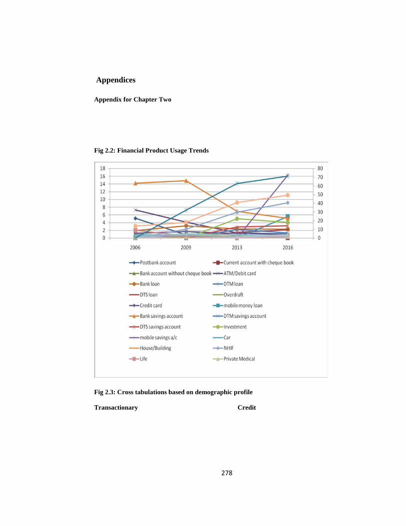
278

Appendices

Appendix for Chapter Two

Fig 2.2: Financial Product Usage Trends

Fig 2.3: Cross tabulations based on demographic profile

Transactionary Credit

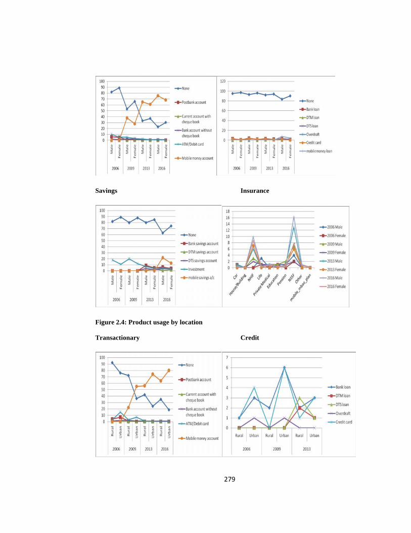
279

Savings Insurance

Figure 2.4: Product usage by location

Transactionary Credit

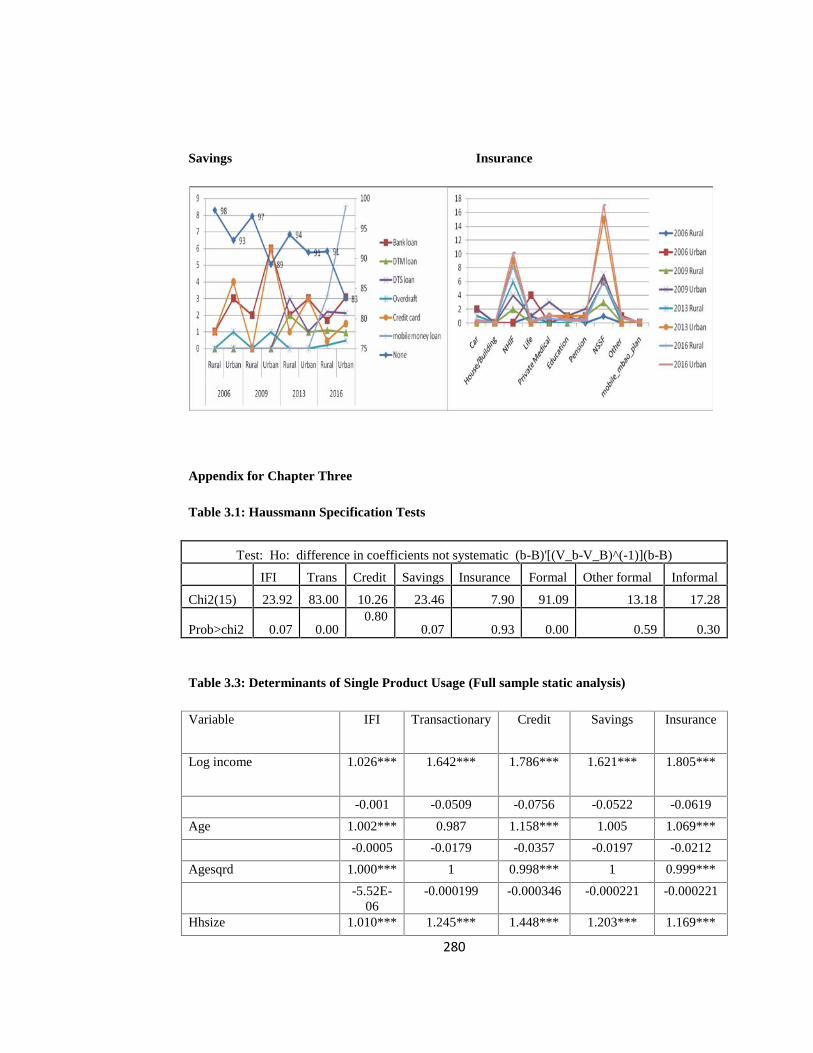
280

Savings Insurance

Appendix for Chapter Three

Table 3.1: Haussmann Specification Tests

Test: Ho: difference in coefficients not systematic (b-B)'[(V_b-V_B)^(-1)](b-B)

IFI Trans Credit Savings Insurance Formal Other formal Informal

Chi2(15) 23.92 83.00 10.26 23.46 7.90 91.09 13.18 17.28

Prob>chi2 0.07 0.000.80

0.07 0.93 0.00 0.59 0.30

Table 3.3: Determinants of Single Product Usage (Full sample static analysis)

Variable IFI Transactionary Credit Savings Insurance

Log income 1.026*** 1.642*** 1.786*** 1.621*** 1.805***

-0.001 -0.0509 -0.0756 -0.0522 -0.0619

Age 1.002*** 0.987 1.158*** 1.005 1.069***

-0.0005 -0.0179 -0.0357 -0.0197 -0.0212

Agesqrd 1.000*** 1 0.998*** 1 0.999***

-5.52E-06

-0.000199 -0.000346 -0.000221 -0.000221

Hhsize 1.010*** 1.245*** 1.448*** 1.203*** 1.169***

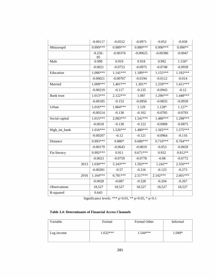
281

-0.00117 -0.0552 -0.0971 -0.052 -0.058

Hhsizesqrd 0.999*** 0.989*** 0.980*** 0.990*** 0.990**

-9.25E-05

-0.00376 -0.00625 -0.00386 -0.0047

Male 0.998 0.919 0.918 0.992 1.156*

-0.0021 -0.0753 -0.0975 -0.0748 -0.0939

Education 1.006*** 1.141*** 1.189*** 1.155*** 1.192***

-0.00021 -0.00767 -0.0194 -0.0112 -0.014

Married 1.009*** 1.401*** 1.301** 1.259*** 1.411***

-0.00219 -0.117 -0.135 -0.0943 -0.12

Bank trust 1.013*** 2.122*** 1.087 1.296*** 1.448***

-0.00185 -0.153 -0.0956 -0.0835 -0.0939

Urban 1.016*** 1.864*** 1.129 1.128* 1.127*

-0.00214 -0.138 -0.102 -0.0785 -0.0793

Social capital 1.015*** 2.083*** 1.541*** 1.480*** 1.298***

-0.0018 -0.138 -0.122 -0.0908 -0.0875

High_int_bank 1.016*** 1.526*** 1.480*** 1.565*** 1.575***

-0.00207 -0.12 -0.121 -0.0964 -0.116

Distance 0.993*** 0.880* 0.680*** 0.710*** 0.764***

-0.00179 -0.0643 -0.0819 -0.053 -0.0659

Fin literacy 0.992*** 0.911 0.671*** 0.932 0.812**

-0.0023 -0.0759 -0.0778 -0.08 -0.0772

2013 1.030*** 5.343*** 1.593*** 1.242** 2.550***

-0.00281 -0.57 -0.216 -0.123 -0.273

2016 1.164*** 6.781*** 2.517*** 2.142*** 2.601***

-0.0028 -0.687 -0.328 -0.204 -0.267

Observations 18,527 18,527 18,527 18,527 18,527

R-squared 0.643

Significance levels: *** p<0.01, ** p<0.05, * p<0.1

Table 3.4: Determinants of Financial Access Channels

Variable Formal Formal Other Informal

Log income 1.632*** 1.544*** 1.049*

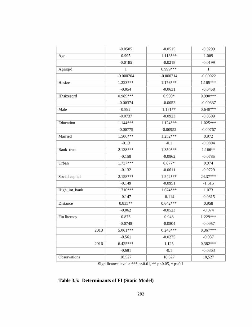
282

-0.0505 -0.0515 -0.0299

Age 0.995 1.118*** 1.009

-0.0185 -0.0218 -0.0199

Agesqrd 1 0.999*** 1

-0.000204 -0.000214 -0.00022

Hhsize 1.223*** 1.176*** 1.165***

-0.054 -0.0631 -0.0458

Hhsizesqrd 0.989*** 0.990* 0.990***

-0.00374 -0.0052 -0.00337

Male 0.892 1.171** 0.640***

-0.0737 -0.0923 -0.0509

Education 1.144*** 1.124*** 1.025***

-0.00775 -0.00952 -0.00767

Married 1.506*** 1.252*** 0.972

-0.13 -0.1 -0.0804

Bank trust 2.138*** 1.359*** 1.166**

-0.158 -0.0862 -0.0785

Urban 1.737*** 0.877* 0.974

-0.132 -0.0611 -0.0729

Social capital 2.158*** 1.542*** 24.37***

-0.149 -0.0951 -1.615

High_int_bank 1.710*** 1.674*** 1.073

-0.147 -0.114 -0.0815

Distance 0.835** 0.642*** 0.958

-0.062 -0.0523 -0.074

Fin literacy 0.875 0.948 1.229***

-0.0748 -0.0804 -0.0957

2013 5.061*** 0.243*** 0.367***

-0.561 -0.0275 -0.037

2016 6.425*** 1.125 0.382***

-0.681 -0.1 -0.0363

Observations 18,527 18,527 18,527

Significance levels: *** p<0.01, ** p<0.05, * p<0.1

Table 3.5: Determinants of FI (Static Model)

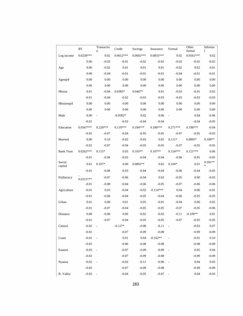
283

IFITransaction

Credit Savings Insurance FormalOtherformal

Informal

Log income 0.0238*** 0.02 0.0612*** 0.0692*** 0.0835*** 0.02 0.0561*** 0.02

0.00 -0.03 -0.01 -0.02 -0.02 -0.03 -0.02 -0.02

Age 0.00 -0.02 0.01 0.01 0.01 -0.02 0.02 0.01

0.00 -0.04 -0.01 -0.01 -0.01 -0.04 -0.01 -0.01

Agesqrd 0.00 0.00 0.00 0.00 0.00 0.00 0.00 0.00

0.00 0.00 0.00 0.00 0.00 0.00 0.00 0.00

Hhsize 0.01 -0.04 0.0385* 0.0467* 0.01 -0.03 -0.01 0.02

-0.01 -0.04 -0.02 -0.03 -0.03 -0.03 -0.03 -0.03

Hhsizesqrd 0.00 0.00 0.00 0.00 0.00 0.00 0.00 0.00

0.00 0.00 0.00 0.00 0.00 0.00 0.00 0.00

Male 0.00 - -0.0582* 0.02 0.06 - 0.04 -0.06

-0.01 -0.03 -0.04 -0.04 -0.04 -0.05

Education 0.0567*** 0.228*** 0.119*** 0.184*** 0.180*** 0.271*** 0.198*** -0.04

-0.01 -0.07 -0.04 -0.05 -0.05 -0.07 -0.05 -0.05

Married 0.00 0.10 -0.02 -0.03 0.02 0.111* 0.0895* 0.108**

-0.01 -0.07 -0.04 -0.05 -0.05 -0.07 -0.05 -0.05

Bank Trust 0.0262*** 0.115* 0.05 0.103** 0.107** 0.154*** 0.121*** 0.06

-0.01 -0.06 -0.03 -0.04 -0.04 -0.06 -0.05 -0.05

Socialcapital

0.01 0.107* 0.00 0.0891** 0.02 0.104* 0.010.591***

-0.01 -0.06 -0.03 -0.04 -0.04 -0.06 -0.04 -0.05

Finliteracy-0.0315***

-0.07 -0.06 -0.04 0.02 -0.05 0.00 -0.03

-0.01 -0.08 -0.04 -0.06 -0.05 -0.07 -0.06 -0.06

Agriculture -0.01 0.03 -0.04 -0.02 -0.114*** 0.04 0.06 -0.01

-0.01 -0.06 -0.04 -0.05 -0.04 -0.06 -0.05 -0.05

Urban 0.01 0.00 0.01 0.05 -0.01 -0.04 0.00 0.02

-0.01 -0.07 -0.04 -0.05 -0.05 -0.07 -0.05 -0.06

Distance 0.00 -0.06 0.00 -0.02 -0.03 -0.11 -0.109** 0.01

-0.01 -0.07 -0.04 -0.05 -0.05 -0.07 -0.05 -0.05

Central -0.02 - -0.127* -0.08 -0.11 - -0.03 0.07

-0.02 -0.07 -0.09 -0.08 -0.09 -0.09

Coast -0.01 - 0.01 0.04 -0.162** - -0.01 0.10

-0.02 -0.06 -0.08 -0.08 -0.08 -0.09

Eastern -0.03 - -0.07 -0.09 -0.09 - 0.05 0.04

-0.02 -0.07 -0.09 -0.08 -0.09 -0.09

Nyanza -0.02 - -0.02 -0.11 -0.06 - 0.04 0.05

-0.02 -0.07 -0.09 -0.08 -0.09 -0.09

R. Valley -0.02 - -0.04 -0.05 -0.07 - 0.04 -0.03

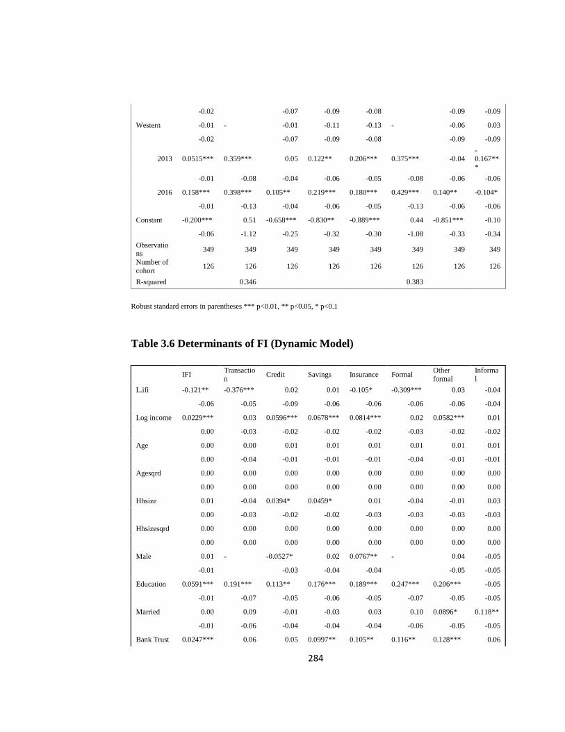
284

-0.02 -0.07 -0.09 -0.08 -0.09 -0.09

Western -0.01 - -0.01 -0.11 -0.13 - -0.06 0.03

-0.02 -0.07 -0.09 -0.08 -0.09 -0.09

2013 0.0515*** 0.359*** 0.05 0.122** 0.206*** 0.375*** -0.04-0.167***

-0.01 -0.08 -0.04 -0.06 -0.05 -0.08 -0.06 -0.06

2016 0.158*** 0.398*** 0.105** 0.219*** 0.180*** 0.429*** 0.140** -0.104*

-0.01 -0.13 -0.04 -0.06 -0.05 -0.13 -0.06 -0.06

Constant -0.200*** 0.51 -0.658*** -0.830** -0.889*** 0.44 -0.851*** -0.10

-0.06 -1.12 -0.25 -0.32 -0.30 -1.08 -0.33 -0.34

Observations

349 349 349 349 349 349 349 349

Number ofcohort

126 126 126 126 126 126 126 126

R-squared 0.346 0.383

Robust standard errors in parentheses *** p<0.01, ** p<0.05, * p<0.1

Table 3.6 Determinants of FI (Dynamic Model)

IFITransaction

Credit Savings Insurance FormalOtherformal

Informal

L.ifi -0.121** -0.376*** 0.02 0.01 -0.105* -0.309*** 0.03 -0.04

-0.06 -0.05 -0.09 -0.06 -0.06 -0.06 -0.06 -0.04

Log income 0.0229*** 0.03 0.0596*** 0.0678*** 0.0814*** 0.02 0.0582*** 0.01

0.00 -0.03 -0.02 -0.02 -0.02 -0.03 -0.02 -0.02

Age 0.00 0.00 0.01 0.01 0.01 0.01 0.01 0.01

0.00 -0.04 -0.01 -0.01 -0.01 -0.04 -0.01 -0.01

Agesqrd 0.00 0.00 0.00 0.00 0.00 0.00 0.00 0.00

0.00 0.00 0.00 0.00 0.00 0.00 0.00 0.00

Hhsize 0.01 -0.04 0.0394* 0.0459* 0.01 -0.04 -0.01 0.03

0.00 -0.03 -0.02 -0.02 -0.03 -0.03 -0.03 -0.03

Hhsizesqrd 0.00 0.00 0.00 0.00 0.00 0.00 0.00 0.00

0.00 0.00 0.00 0.00 0.00 0.00 0.00 0.00

Male 0.01 - -0.0527* 0.02 0.0767** - 0.04 -0.05

-0.01 -0.03 -0.04 -0.04 -0.05 -0.05

Education 0.0591*** 0.191*** 0.113** 0.176*** 0.189*** 0.247*** 0.206*** -0.05

-0.01 -0.07 -0.05 -0.06 -0.05 -0.07 -0.05 -0.05

Married 0.00 0.09 -0.01 -0.03 0.03 0.10 0.0896* 0.118**

-0.01 -0.06 -0.04 -0.04 -0.04 -0.06 -0.05 -0.05

Bank Trust 0.0247*** 0.06 0.05 0.0997** 0.105** 0.116** 0.128*** 0.06

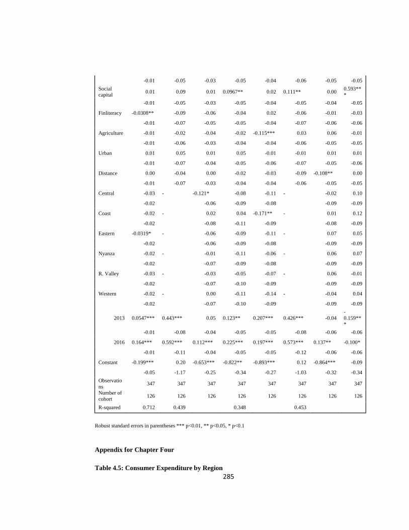
285

-0.01 -0.05 -0.03 -0.05 -0.04 -0.06 -0.05 -0.05

Socialcapital

0.01 0.09 0.01 0.0967** 0.02 0.111** 0.000.593***

-0.01 -0.05 -0.03 -0.05 -0.04 -0.05 -0.04 -0.05

Finliteracy -0.0308** -0.09 -0.06 -0.04 0.02 -0.06 -0.01 -0.03

-0.01 -0.07 -0.05 -0.05 -0.04 -0.07 -0.06 -0.06

Agriculture -0.01 -0.02 -0.04 -0.02 -0.115*** 0.03 0.06 -0.01

-0.01 -0.06 -0.03 -0.04 -0.04 -0.06 -0.05 -0.05

Urban 0.01 0.05 0.01 0.05 -0.01 -0.01 0.01 0.01

-0.01 -0.07 -0.04 -0.05 -0.06 -0.07 -0.05 -0.06

Distance 0.00 -0.04 0.00 -0.02 -0.03 -0.09 -0.108** 0.00

-0.01 -0.07 -0.03 -0.04 -0.04 -0.06 -0.05 -0.05

Central -0.03 - -0.121* -0.08 -0.11 - -0.02 0.10

-0.02 -0.06 -0.09 -0.08 -0.09 -0.09

Coast -0.02 - 0.02 0.04 -0.171** - 0.01 0.12

-0.02 -0.08 -0.11 -0.09 -0.08 -0.09

Eastern -0.0319* - -0.06 -0.09 -0.11 - 0.07 0.05

-0.02 -0.06 -0.09 -0.08 -0.09 -0.09

Nyanza -0.02 - -0.01 -0.11 -0.06 - 0.06 0.07

-0.02 -0.07 -0.09 -0.08 -0.09 -0.09

R. Valley -0.03 - -0.03 -0.05 -0.07 - 0.06 -0.01

-0.02 -0.07 -0.10 -0.09 -0.09 -0.09

Western -0.02 - 0.00 -0.11 -0.14 - -0.04 0.04

-0.02 -0.07 -0.10 -0.09 -0.09 -0.09

2013 0.0547*** 0.443*** 0.05 0.123** 0.207*** 0.426*** -0.04-0.159***

-0.01 -0.08 -0.04 -0.05 -0.05 -0.08 -0.06 -0.06

2016 0.164*** 0.592*** 0.112*** 0.225*** 0.197*** 0.573*** 0.137** -0.100*

-0.01 -0.11 -0.04 -0.05 -0.05 -0.12 -0.06 -0.06

Constant -0.199*** 0.20 -0.653*** -0.822** -0.893*** 0.12 -0.864*** -0.09

-0.05 -1.17 -0.25 -0.34 -0.27 -1.03 -0.32 -0.34

Observations

347 347 347 347 347 347 347 347

Number ofcohort

126 126 126 126 126 126 126 126

R-squared 0.712 0.439 0.348 0.453

Robust standard errors in parentheses *** p<0.01, ** p<0.05, * p<0.1

Appendix for Chapter Four

Table 4.5: Consumer Expenditure by Region

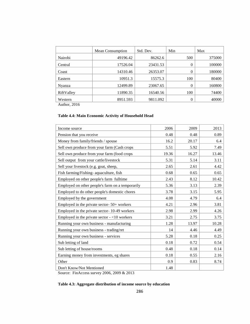
286

Mean Consumption Std. Dev. Min Max

Nairobi 49196.42 86262.6 500 375000

Central 17526.04 23431.53 0 100000

Coast 14310.46 26353.07 0 180000

Eastern 10951.3 15575.3 100 80400

Nyanza 12499.89 23067.65 0 160800

RiftValley 11890.35 16540.56 100 74400

Western 8951.593 9811.092 0 40000Author, 2016

Table 4.4: Main Economic Activity of Household Head

Income source 2006 2009 2013

Pension that you receive 0.48 0.48 0.89

Money from family/friends / spouse 16.2 20.17 6.4

Sell own produce from your farm (Cash crops 5.51 5.92 7.49

Sell own produce from your farm (food crops 19.36 16.27 13.46

Sell output from your cattle/livestock 5.31 5.14 3.11

Sell your livestock (e.g. goat, sheep, 2.65 2.61 4.42

Fish farming/Fishing- aquaculture, fish 0.68 0.65 0.65

Employed on other people's farm fulltime 2.43 8.12 10.42

Employed on other people's farm on a temporarily 5.36 3.13 2.39

Employed to do other people's domestic chores 3.78 3.15 5.95

Employed by the government 4.08 4.79 6.4

Employed in the private sector- 50+ workers 4.21 2.96 3.81

Employed in the private sector- 10-49 workers 2.98 2.99 4.26

Employed in the private sector - <10 workers 3.21 2.75 3.75

Running your own business - manufacturing 1.28 13.97 10.28

Running your own business - trading/ret 14 4.46 4.49

Running your own business - services 5.28 0.18 0.25

Sub letting of land 0.18 0.72 0.54

Sub letting of house/rooms 0.48 0.18 0.14

Earning money from investments, eg shares 0.18 0.55 2.16

Other 0.9 0.83 8.74

Don't Know/Not Mentioned 1.48Source: FinAccess survey 2006, 2009 & 2013

Table 4.3: Aggregate distribution of income source by education

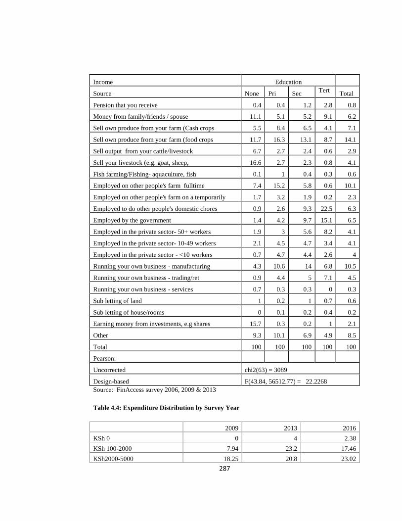
287

Income Education

Source None Pri Sec Tert Total

Pension that you receive 0.4 0.4 1.2 2.8 0.8

Money from family/friends / spouse 11.1 5.1 5.2 9.1 6.2

Sell own produce from your farm (Cash crops 5.5 8.4 6.5 4.1 7.1

Sell own produce from your farm (food crops 11.7 16.3 13.1 8.7 14.1

Sell output from your cattle/livestock 6.7 2.7 2.4 0.6 2.9

Sell your livestock (e.g. goat, sheep, 16.6 2.7 2.3 0.8 4.1

Fish farming/Fishing- aquaculture, fish 0.1 1 0.4 0.3 0.6

Employed on other people's farm fulltime 7.4 15.2 5.8 0.6 10.1

Employed on other people's farm on a temporarily 1.7 3.2 1.9 0.2 2.3

Employed to do other people's domestic chores 0.9 2.6 9.3 22.5 6.3

Employed by the government 1.4 4.2 9.7 15.1 6.5

Employed in the private sector- 50+ workers 1.9 3 5.6 8.2 4.1

Employed in the private sector- 10-49 workers 2.1 4.5 4.7 3.4 4.1

Employed in the private sector - <10 workers 0.7 4.7 4.4 2.6 4

Running your own business - manufacturing 4.3 10.6 14 6.8 10.5

Running your own business - trading/ret 0.9 4.4 5 7.1 4.5

Running your own business - services 0.7 0.3 0.3 0 0.3

Sub letting of land 1 0.2 1 0.7 0.6

Sub letting of house/rooms 0 0.1 0.2 0.4 0.2

Earning money from investments, e.g shares 15.7 0.3 0.2 1 2.1

Other 9.3 10.1 6.9 4.9 8.5

Total 100 100 100 100 100

Pearson:

Uncorrected chi2(63) = 3089

Design-based F(43.84, 56512.77) = 22.2268Source: FinAccess survey 2006, 2009 & 2013

Table 4.4: Expenditure Distribution by Survey Year

2009 2013 2016

KSh 0 0 4 2.38

KSh 100-2000 7.94 23.2 17.46

KSh2000-5000 18.25 20.8 23.02

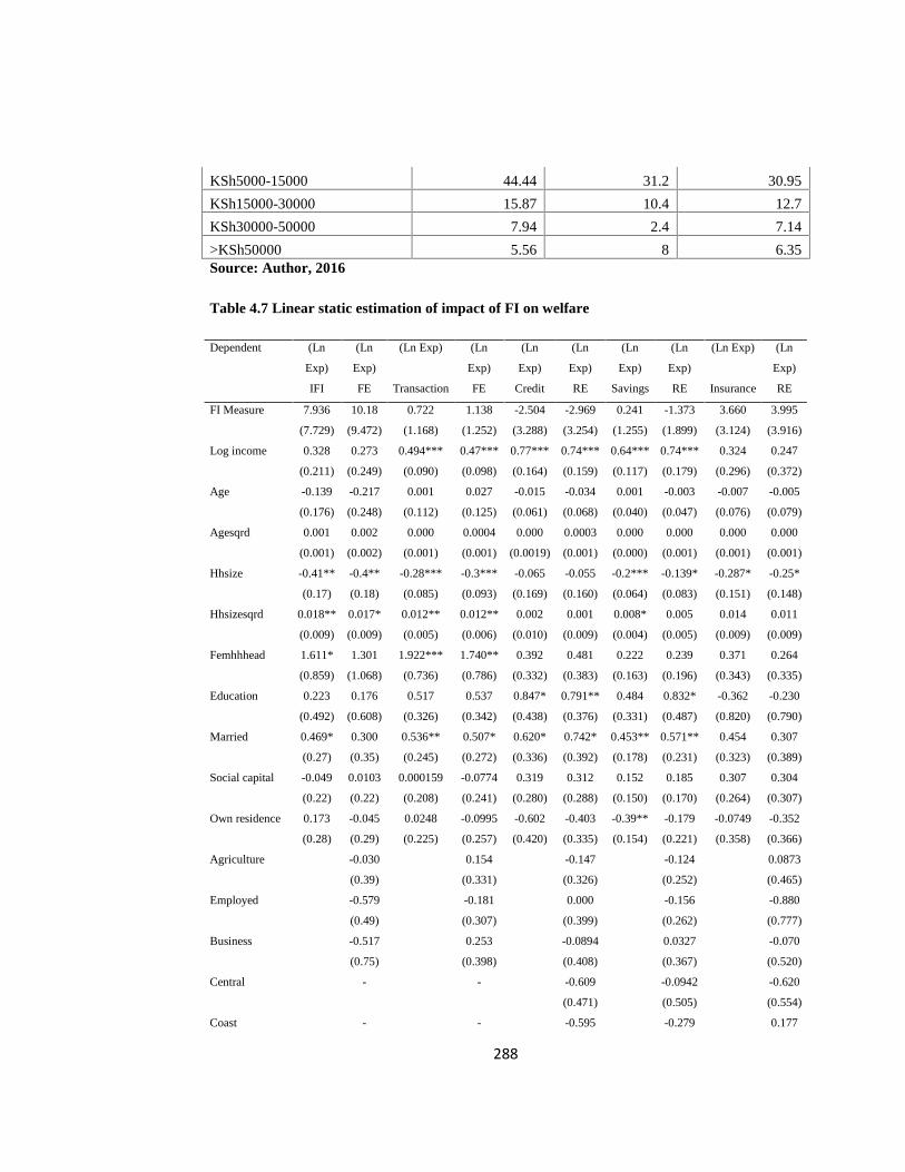
288

KSh5000-15000 44.44 31.2 30.95

KSh15000-30000 15.87 10.4 12.7

KSh30000-50000 7.94 2.4 7.14

>KSh50000 5.56 8 6.35Source: Author, 2016

Table 4.7 Linear static estimation of impact of FI on welfare

Dependent (Ln

Exp)

(Ln

Exp)

(Ln Exp) (Ln

Exp)

(Ln

Exp)

(Ln

Exp)

(Ln

Exp)

(Ln

Exp)

(Ln Exp) (Ln

Exp)

IFI FE Transaction FE Credit RE Savings RE Insurance RE

FI Measure 7.936 10.18 0.722 1.138 -2.504 -2.969 0.241 -1.373 3.660 3.995

(7.729) (9.472) (1.168) (1.252) (3.288) (3.254) (1.255) (1.899) (3.124) (3.916)

Log income 0.328 0.273 0.494*** 0.47*** 0.77*** 0.74*** 0.64*** 0.74*** 0.324 0.247

(0.211) (0.249) (0.090) (0.098) (0.164) (0.159) (0.117) (0.179) (0.296) (0.372)

Age -0.139 -0.217 0.001 0.027 -0.015 -0.034 0.001 -0.003 -0.007 -0.005

(0.176) (0.248) (0.112) (0.125) (0.061) (0.068) (0.040) (0.047) (0.076) (0.079)

Agesqrd 0.001 0.002 0.000 0.0004 0.000 0.0003 0.000 0.000 0.000 0.000

(0.001) (0.002) (0.001) (0.001) (0.0019) (0.001) (0.000) (0.001) (0.001) (0.001)

Hhsize -0.41** -0.4** -0.28*** -0.3*** -0.065 -0.055 -0.2*** -0.139* -0.287* -0.25*

(0.17) (0.18) (0.085) (0.093) (0.169) (0.160) (0.064) (0.083) (0.151) (0.148)

Hhsizesqrd 0.018** 0.017* 0.012** 0.012** 0.002 0.001 0.008* 0.005 0.014 0.011

(0.009) (0.009) (0.005) (0.006) (0.010) (0.009) (0.004) (0.005) (0.009) (0.009)

Femhhhead 1.611* 1.301 1.922*** 1.740** 0.392 0.481 0.222 0.239 0.371 0.264

(0.859) (1.068) (0.736) (0.786) (0.332) (0.383) (0.163) (0.196) (0.343) (0.335)

Education 0.223 0.176 0.517 0.537 0.847* 0.791** 0.484 0.832* -0.362 -0.230

(0.492) (0.608) (0.326) (0.342) (0.438) (0.376) (0.331) (0.487) (0.820) (0.790)

Married 0.469* 0.300 0.536** 0.507* 0.620* 0.742* 0.453** 0.571** 0.454 0.307

(0.27) (0.35) (0.245) (0.272) (0.336) (0.392) (0.178) (0.231) (0.323) (0.389)

Social capital -0.049 0.0103 0.000159 -0.0774 0.319 0.312 0.152 0.185 0.307 0.304

(0.22) (0.22) (0.208) (0.241) (0.280) (0.288) (0.150) (0.170) (0.264) (0.307)

Own residence 0.173 -0.045 0.0248 -0.0995 -0.602 -0.403 -0.39** -0.179 -0.0749 -0.352

(0.28) (0.29) (0.225) (0.257) (0.420) (0.335) (0.154) (0.221) (0.358) (0.366)

Agriculture -0.030 0.154 -0.147 -0.124 0.0873

(0.39) (0.331) (0.326) (0.252) (0.465)

Employed -0.579 -0.181 0.000 -0.156 -0.880

(0.49) (0.307) (0.399) (0.262) (0.777)

Business -0.517 0.253 -0.0894 0.0327 -0.070

(0.75) (0.398) (0.408) (0.367) (0.520)

Central - - -0.609 -0.0942 -0.620

(0.471) (0.505) (0.554)

Coast - - -0.595 -0.279 0.177

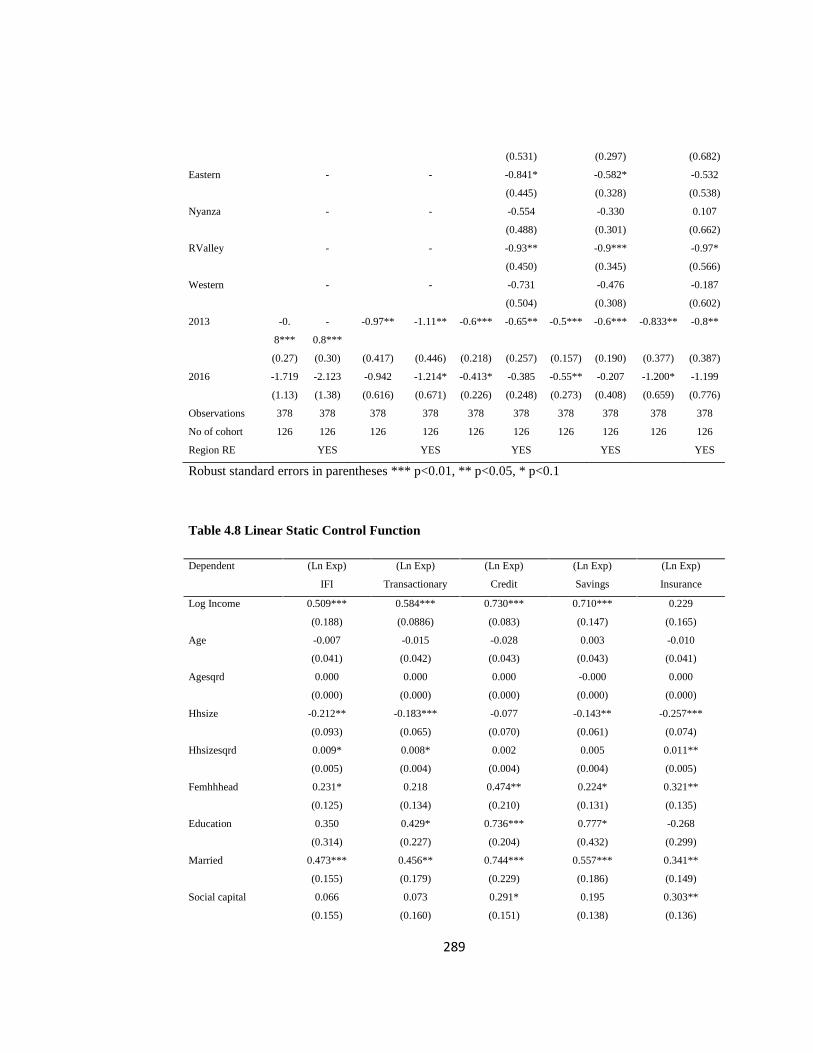
289

(0.531) (0.297) (0.682)

Eastern - - -0.841* -0.582* -0.532

(0.445) (0.328) (0.538)

Nyanza - - -0.554 -0.330 0.107

(0.488) (0.301) (0.662)

RValley - - -0.93** -0.9*** -0.97*

(0.450) (0.345) (0.566)

Western - - -0.731 -0.476 -0.187

(0.504) (0.308) (0.602)

2013 -0.

8***

-

0.8***

-0.97** -1.11** -0.6*** -0.65** -0.5*** -0.6*** -0.833** -0.8**

(0.27) (0.30) (0.417) (0.446) (0.218) (0.257) (0.157) (0.190) (0.377) (0.387)

2016 -1.719 -2.123 -0.942 -1.214* -0.413* -0.385 -0.55** -0.207 -1.200* -1.199

(1.13) (1.38) (0.616) (0.671) (0.226) (0.248) (0.273) (0.408) (0.659) (0.776)

Observations 378 378 378 378 378 378 378 378 378 378

No of cohort 126 126 126 126 126 126 126 126 126 126

Region RE YES YES YES YES YES

Robust standard errors in parentheses *** p<0.01, ** p<0.05, * p<0.1

Table 4.8 Linear Static Control Function

Dependent (Ln Exp) (Ln Exp) (Ln Exp) (Ln Exp) (Ln Exp)

IFI Transactionary Credit Savings Insurance

Log Income 0.509*** 0.584*** 0.730*** 0.710*** 0.229

(0.188) (0.0886) (0.083) (0.147) (0.165)

Age -0.007 -0.015 -0.028 0.003 -0.010

(0.041) (0.042) (0.043) (0.043) (0.041)

Agesqrd 0.000 0.000 0.000 -0.000 0.000

(0.000) (0.000) (0.000) (0.000) (0.000)

Hhsize -0.212** -0.183*** -0.077 -0.143** -0.257***

(0.093) (0.065) (0.070) (0.061) (0.074)

Hhsizesqrd 0.009* 0.008* 0.002 0.005 0.011**

(0.005) (0.004) (0.004) (0.004) (0.005)

Femhhhead 0.231* 0.218 0.474** 0.224* 0.321**

(0.125) (0.134) (0.210) (0.131) (0.135)

Education 0.350 0.429* 0.736*** 0.777* -0.268

(0.314) (0.227) (0.204) (0.432) (0.299)

Married 0.473*** 0.456** 0.744*** 0.557*** 0.341**

(0.155) (0.179) (0.229) (0.186) (0.149)

Social capital 0.066 0.073 0.291* 0.195 0.303**

(0.155) (0.160) (0.151) (0.138) (0.136)

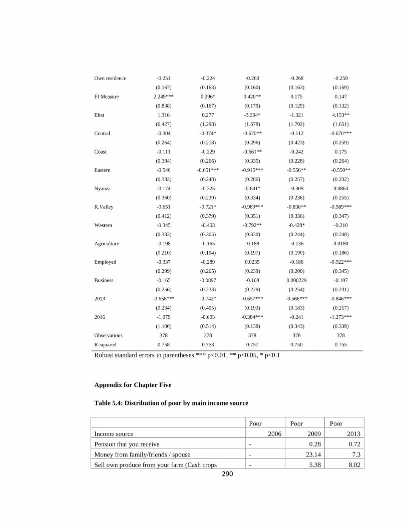
290

Own residence -0.251 -0.224 -0.260 -0.268 -0.259

(0.167) (0.163) (0.160) (0.163) (0.169)

FI Measure 2.249*** 0.296* 0.420** 0.175 0.147

(0.838) (0.167) (0.179) (0.129) (0.132)

Ehat 1.316 0.277 -3.204* -1.321 4.153**

(6.427) (1.298) (1.678) (1.702) (1.651)

Central -0.304 -0.374* -0.670** -0.112 -0.670***

(0.264) (0.218) (0.296) (0.423) (0.259)

Coast -0.111 -0.229 -0.661** -0.242 0.175

(0.384) (0.266) (0.335) (0.228) (0.264)

Eastern -0.546 -0.651*** -0.915*** -0.556** -0.550**

(0.333) (0.248) (0.286) (0.257) (0.232)

Nyanza -0.174 -0.325 -0.641* -0.309 0.0863

(0.360) (0.239) (0.334) (0.236) (0.255)

R.Valley -0.651 -0.721* -0.989*** -0.838** -0.989***

(0.412) (0.379) (0.351) (0.336) (0.347)

Western -0.345 -0.403 -0.792** -0.428* -0.210

(0.333) (0.305) (0.330) (0.244) (0.248)

Agriculture -0.198 -0.165 -0.188 -0.136 0.0180

(0.210) (0.194) (0.197) (0.190) (0.186)

Employed -0.337 -0.289 0.0235 -0.186 -0.922***

(0.299) (0.265) (0.239) (0.200) (0.345)

Business -0.165 -0.0897 -0.108 0.000229 -0.107

(0.256) (0.233) (0.229) (0.254) (0.231)

2013 -0.658*** -0.742* -0.657*** -0.566*** -0.846***

(0.234) (0.405) (0.193) (0.183) (0.217)

2016 -1.079 -0.693 -0.384*** -0.241 -1.273***

(1.100) (0.514) (0.138) (0.343) (0.339)

Observations 378 378 378 378 378

R-squared 0.758 0.753 0.757 0.750 0.755

Robust standard errors in parentheses *** p<0.01, ** p<0.05, * p<0.1

Appendix for Chapter Five

Table 5.4: Distribution of poor by main income source

Poor Poor Poor

Income source 2006 2009 2013

Pension that you receive - 0.28 0.72

Money from family/friends / spouse - 23.14 7.3

Sell own produce from your farm (Cash crops - 5.38 8.02

291

Sell own produce from your farm (food crops - 21.34 14.74

Sell output from your cattle/livestock - 5.61 3.33

Sell your livestock (e.g. goat, sheep, - 3.04 5.39

Fish farming/Fishing- aquaculture, fish - 0.46 0.69

Employed on other people's farm fulltime - 12.51 13.41

Employed on other people's farm on a temporarily - 4.09 2.69

Employed to do other people's domestic chores - 0.37 3.25

Employed by the government - 1.79 4.41

Employed in the private sector- 50+ workers - 1.15 2.78

Employed in the private sector- 10-49 workers - 2.21 4.3

Employed in the private sector - <10 workers - 2.39 3.64

Running your own business - manufacturing - 10.4 8.41

Running your own business - trading/ret - 3.59 3.69

Running your own business - services - 0.23 0.33

Sub letting of land - 0.28 0.36

Sub letting of house/rooms - 0.05 0.11

Earning money from investments, e.g shares - 0.97 3.22

Other 9.19Source: FinAccess survey 2006, 2009 & 2013

Table 5.3: Poverty Status and Cluster by education (2009-2016)

None Primary Secondary Tertiary Other

Urban Non poor 8.33 40.91 55.81 86.36 62.5

Poor 91.67 59.09 44.19 13.64 37.5

Rural Non poor 21.74 25.58 57.5 100 47.06

Poor 78.26 74.42 42.5 0 52.94Author, 2016

Table 5.6: Status of Poverty and Consumption expenditure in 2016

Cohort Means FULL Sample 2016

Region Consumption Expenditure Cohort Poor Consumption Expenditure Poor

Nairobi 12989.86 20 15633 21.98

Central 6947.62 53 6676 32.22

Coast 5401.175 58 7039 39.83

Eastern 2594.741 79 9937 42.2

Nyanza 3990.821 69 3896 55.39

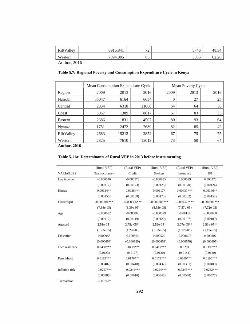
292

RiftValley 6915.841 72 5746 48.34

Western 7894.085 65 3806 62.28Author, 2016

Table 5.7: Regional Poverty and Consumption Expenditure Cycle in Kenya

Mean Consumption Expenditure Cycle Mean Poverty Cycle

Region 2009 2013 2016 2009 2013 2016

Nairobi 35047 6164 6654 0 27 25

Central 2334 6318 11068 64 64 36

Coast 5057 1389 8817 67 83 33

Eastern 2386 831 4507 80 93 64

Nyanza 1751 2472 7689 82 85 42

RiftValley 2683 15212 2852 67 75 75

Western 2825 7610 15013 73 50 64Author, 2016

Table 5.11a: Determinants of Rural VEP in 2013 before instrumenting

(Rural VEP) (Rural VEP) (Rural VEP) (Rural VEP) (Rural VEP)

VARIABLES Transactionary Credit Savings Insurance IFI

Log income -0.000546 -0.000578 -0.000885 0.000529 0.000270

(0.00117) (0.00123) (0.00128) (0.00120) (0.00124)

Hhsize 0.00334** 0.00364** 0.00317* 0.00431*** 0.00346**

(0.00156) (0.00168) (0.00170) (0.00152) (0.00152)

Hhsizesqrd -0.000304*** -0.000305*** -0.000286*** -0.000327*** -0.000300***

(7.98e-05) (8.39e-05) (8.55e-05) (7.57e-05) (7.72e-05)

Age -0.000632 -0.000860 -0.000599 -0.00118 -0.000688

(0.00112) (0.00119) (0.00120) (0.00107) (0.00109)

Agesqrd 2.51e-05* 2.75e-05** 2.52e-05* 3.07e-05** 2.51e-05**

(1.23e-05) (1.29e-05) (1.32e-05) (1.17e-05) (1.19e-05)

Education 0.000953 0.000504 0.000520 0.000607 0.000807

(0.000656) (0.000629) (0.000658) (0.000570) (0.000605)

Own residence 0.0400*** 0.0419*** 0.0417*** 0.0201 0.0398***

(0.0123) (0.0127) (0.0130) (0.0141) (0.0120)

Femhhhead 0.0183*** 0.0176*** 0.0173*** 0.0200*** 0.0190***

(0.00407) (0.00418) (0.00432) (0.00391) (0.00400)

Inflation risk -0.0257*** -0.0245*** -0.0254*** -0.0245*** -0.0232***

(0.00585) (0.00610) (0.00645) (0.00548) (0.00577)

Transaction -0.00763*

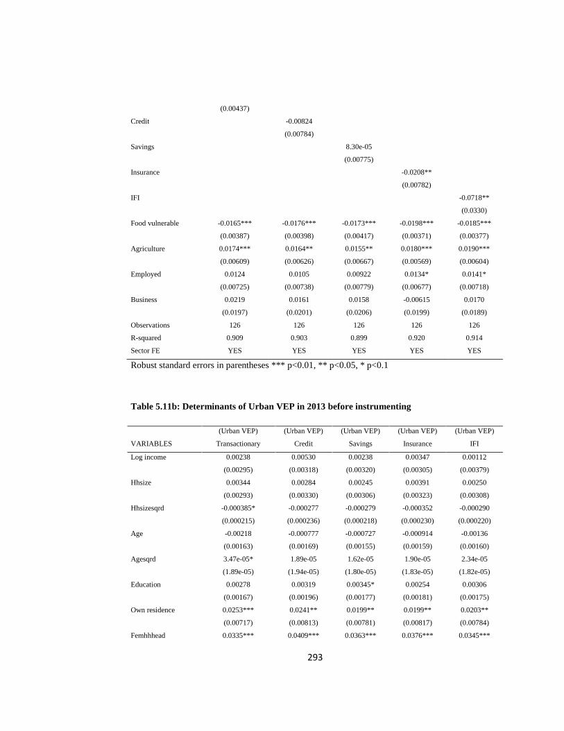
293

(0.00437)

Credit -0.00824

(0.00784)

Savings 8.30e-05

(0.00775)

Insurance -0.0208**

(0.00782)

IFI -0.0718**

(0.0330)

Food vulnerable -0.0165*** -0.0176*** -0.0173*** -0.0198*** -0.0185***

(0.00387) (0.00398) (0.00417) (0.00371) (0.00377)

Agriculture 0.0174*** 0.0164** 0.0155** 0.0180*** 0.0190***

(0.00609) (0.00626) (0.00667) (0.00569) (0.00604)

Employed 0.0124 0.0105 0.00922 0.0134* 0.0141*

(0.00725) (0.00738) (0.00779) (0.00677) (0.00718)

Business 0.0219 0.0161 0.0158 -0.00615 0.0170

(0.0197) (0.0201) (0.0206) (0.0199) (0.0189)

Observations 126 126 126 126 126

R-squared 0.909 0.903 0.899 0.920 0.914

Sector FE YES YES YES YES YES

Robust standard errors in parentheses *** p<0.01, ** p<0.05, * p<0.1

Table 5.11b: Determinants of Urban VEP in 2013 before instrumenting

(Urban VEP) (Urban VEP) (Urban VEP) (Urban VEP) (Urban VEP)

VARIABLES Transactionary Credit Savings Insurance IFI

Log income 0.00238 0.00530 0.00238 0.00347 0.00112

(0.00295) (0.00318) (0.00320) (0.00305) (0.00379)

Hhsize 0.00344 0.00284 0.00245 0.00391 0.00250

(0.00293) (0.00330) (0.00306) (0.00323) (0.00308)

Hhsizesqrd -0.000385* -0.000277 -0.000279 -0.000352 -0.000290

(0.000215) (0.000236) (0.000218) (0.000230) (0.000220)

Age -0.00218 -0.000777 -0.000727 -0.000914 -0.00136

(0.00163) (0.00169) (0.00155) (0.00159) (0.00160)

Agesqrd 3.47e-05* 1.89e-05 1.62e-05 1.90e-05 2.34e-05

(1.89e-05) (1.94e-05) (1.80e-05) (1.83e-05) (1.82e-05)

Education 0.00278 0.00319 0.00345* 0.00254 0.00306

(0.00167) (0.00196) (0.00177) (0.00181) (0.00175)

Own residence 0.0253*** 0.0241** 0.0199** 0.0199** 0.0203**

(0.00717) (0.00813) (0.00781) (0.00817) (0.00784)

Femhhhead 0.0335*** 0.0409*** 0.0363*** 0.0376*** 0.0345***

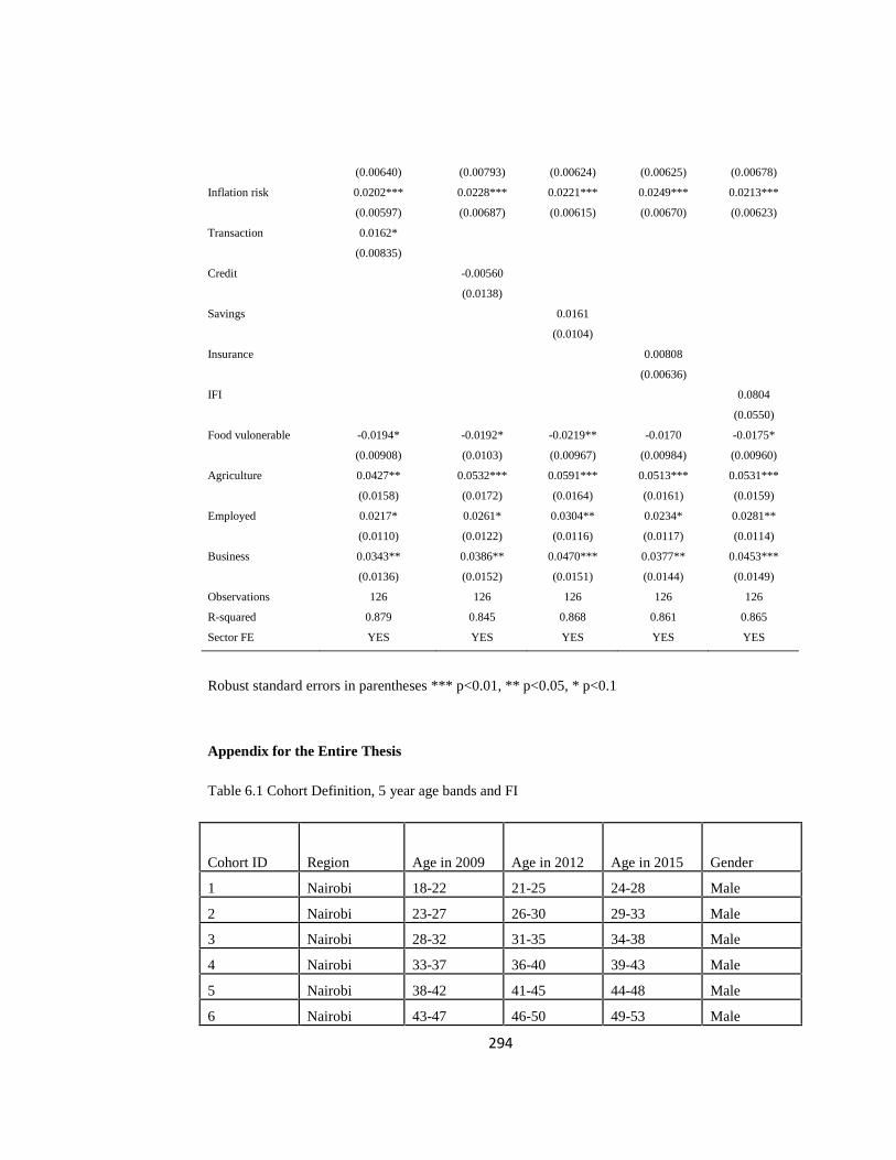
294

(0.00640) (0.00793) (0.00624) (0.00625) (0.00678)

Inflation risk 0.0202*** 0.0228*** 0.0221*** 0.0249*** 0.0213***

(0.00597) (0.00687) (0.00615) (0.00670) (0.00623)

Transaction 0.0162*

(0.00835)

Credit -0.00560

(0.0138)

Savings 0.0161

(0.0104)

Insurance 0.00808

(0.00636)

IFI 0.0804

(0.0550)

Food vulonerable -0.0194* -0.0192* -0.0219** -0.0170 -0.0175*

(0.00908) (0.0103) (0.00967) (0.00984) (0.00960)

Agriculture 0.0427** 0.0532*** 0.0591*** 0.0513*** 0.0531***

(0.0158) (0.0172) (0.0164) (0.0161) (0.0159)

Employed 0.0217* 0.0261* 0.0304** 0.0234* 0.0281**

(0.0110) (0.0122) (0.0116) (0.0117) (0.0114)

Business 0.0343** 0.0386** 0.0470*** 0.0377** 0.0453***

(0.0136) (0.0152) (0.0151) (0.0144) (0.0149)

Observations 126 126 126 126 126

R-squared 0.879 0.845 0.868 0.861 0.865

Sector FE YES YES YES YES YES

Robust standard errors in parentheses *** p<0.01, ** p<0.05, * p<0.1

Appendix for the Entire Thesis

Table 6.1 Cohort Definition, 5 year age bands and FI

Cohort ID Region Age in 2009 Age in 2012 Age in 2015 Gender

1 Nairobi 18-22 21-25 24-28 Male

2 Nairobi 23-27 26-30 29-33 Male

3 Nairobi 28-32 31-35 34-38 Male

4 Nairobi 33-37 36-40 39-43 Male

5 Nairobi 38-42 41-45 44-48 Male

6 Nairobi 43-47 46-50 49-53 Male

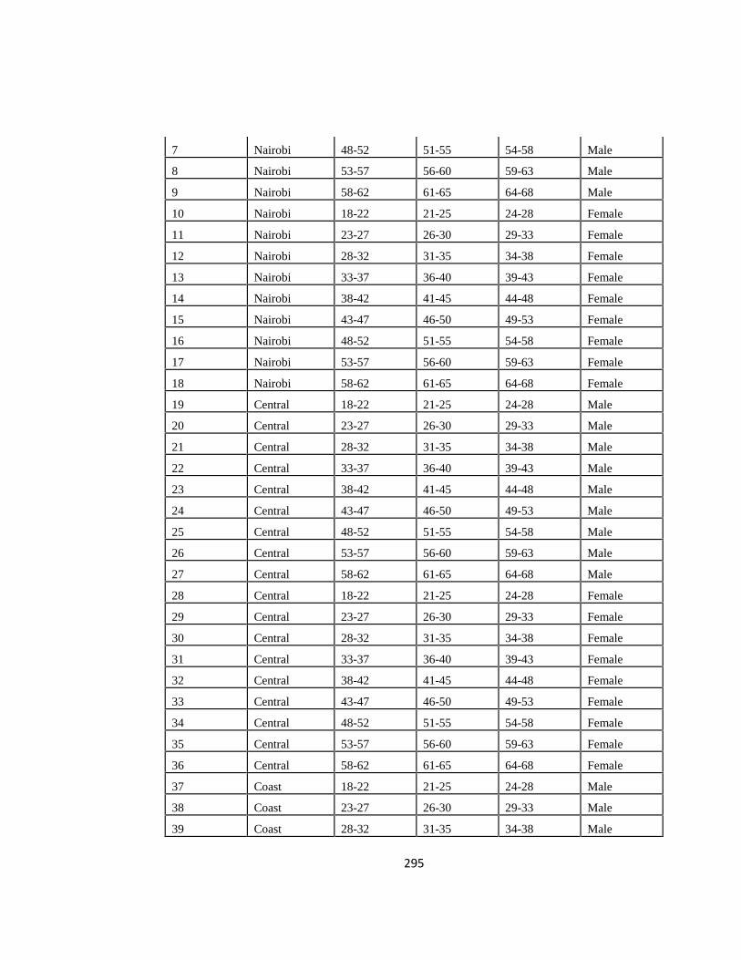
295

7 Nairobi 48-52 51-55 54-58 Male

8 Nairobi 53-57 56-60 59-63 Male

9 Nairobi 58-62 61-65 64-68 Male

10 Nairobi 18-22 21-25 24-28 Female

11 Nairobi 23-27 26-30 29-33 Female

12 Nairobi 28-32 31-35 34-38 Female

13 Nairobi 33-37 36-40 39-43 Female

14 Nairobi 38-42 41-45 44-48 Female

15 Nairobi 43-47 46-50 49-53 Female

16 Nairobi 48-52 51-55 54-58 Female

17 Nairobi 53-57 56-60 59-63 Female

18 Nairobi 58-62 61-65 64-68 Female

19 Central 18-22 21-25 24-28 Male

20 Central 23-27 26-30 29-33 Male

21 Central 28-32 31-35 34-38 Male

22 Central 33-37 36-40 39-43 Male

23 Central 38-42 41-45 44-48 Male

24 Central 43-47 46-50 49-53 Male

25 Central 48-52 51-55 54-58 Male

26 Central 53-57 56-60 59-63 Male

27 Central 58-62 61-65 64-68 Male

28 Central 18-22 21-25 24-28 Female

29 Central 23-27 26-30 29-33 Female

30 Central 28-32 31-35 34-38 Female

31 Central 33-37 36-40 39-43 Female

32 Central 38-42 41-45 44-48 Female

33 Central 43-47 46-50 49-53 Female

34 Central 48-52 51-55 54-58 Female

35 Central 53-57 56-60 59-63 Female

36 Central 58-62 61-65 64-68 Female

37 Coast 18-22 21-25 24-28 Male

38 Coast 23-27 26-30 29-33 Male

39 Coast 28-32 31-35 34-38 Male

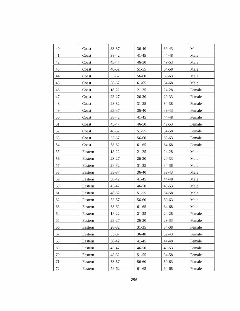
296

40 Coast 33-37 36-40 39-43 Male

41 Coast 38-42 41-45 44-48 Male

42 Coast 43-47 46-50 49-53 Male

43 Coast 48-52 51-55 54-58 Male

44 Coast 53-57 56-60 59-63 Male

45 Coast 58-62 61-65 64-68 Male

46 Coast 18-22 21-25 24-28 Female

47 Coast 23-27 26-30 29-33 Female

48 Coast 28-32 31-35 34-38 Female

49 Coast 33-37 36-40 39-43 Female

50 Coast 38-42 41-45 44-48 Female

51 Coast 43-47 46-50 49-53 Female

52 Coast 48-52 51-55 54-58 Female

53 Coast 53-57 56-60 59-63 Female

54 Coast 58-62 61-65 64-68 Female

55 Eastern 18-22 21-25 24-28 Male

56 Eastern 23-27 26-30 29-33 Male

57 Eastern 28-32 31-35 34-38 Male

58 Eastern 33-37 36-40 39-43 Male

59 Eastern 38-42 41-45 44-48 Male

60 Eastern 43-47 46-50 49-53 Male

61 Eastern 48-52 51-55 54-58 Male

62 Eastern 53-57 56-60 59-63 Male

63 Eastern 58-62 61-65 64-68 Male

64 Eastern 18-22 21-25 24-28 Female

65 Eastern 23-27 26-30 29-33 Female

66 Eastern 28-32 31-35 34-38 Female

67 Eastern 33-37 36-40 39-43 Female

68 Eastern 38-42 41-45 44-48 Female

69 Eastern 43-47 46-50 49-53 Female

70 Eastern 48-52 51-55 54-58 Female

71 Eastern 53-57 56-60 59-63 Female

72 Eastern 58-62 61-65 64-68 Female

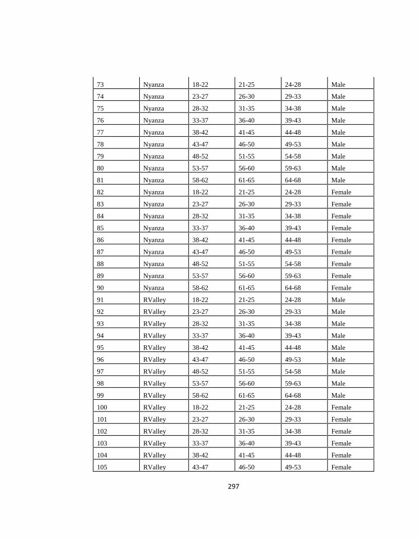
297

73 Nyanza 18-22 21-25 24-28 Male

74 Nyanza 23-27 26-30 29-33 Male

75 Nyanza 28-32 31-35 34-38 Male

76 Nyanza 33-37 36-40 39-43 Male

77 Nyanza 38-42 41-45 44-48 Male

78 Nyanza 43-47 46-50 49-53 Male

79 Nyanza 48-52 51-55 54-58 Male

80 Nyanza 53-57 56-60 59-63 Male

81 Nyanza 58-62 61-65 64-68 Male

82 Nyanza 18-22 21-25 24-28 Female

83 Nyanza 23-27 26-30 29-33 Female

84 Nyanza 28-32 31-35 34-38 Female

85 Nyanza 33-37 36-40 39-43 Female

86 Nyanza 38-42 41-45 44-48 Female

87 Nyanza 43-47 46-50 49-53 Female

88 Nyanza 48-52 51-55 54-58 Female

89 Nyanza 53-57 56-60 59-63 Female

90 Nyanza 58-62 61-65 64-68 Female

91 RValley 18-22 21-25 24-28 Male

92 RValley 23-27 26-30 29-33 Male

93 RValley 28-32 31-35 34-38 Male

94 RValley 33-37 36-40 39-43 Male

95 RValley 38-42 41-45 44-48 Male

96 RValley 43-47 46-50 49-53 Male

97 RValley 48-52 51-55 54-58 Male

98 RValley 53-57 56-60 59-63 Male

99 RValley 58-62 61-65 64-68 Male

100 RValley 18-22 21-25 24-28 Female

101 RValley 23-27 26-30 29-33 Female

102 RValley 28-32 31-35 34-38 Female

103 RValley 33-37 36-40 39-43 Female

104 RValley 38-42 41-45 44-48 Female

105 RValley 43-47 46-50 49-53 Female

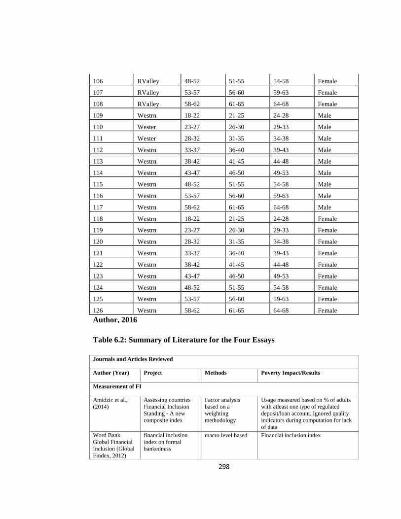
298

106 RValley 48-52 51-55 54-58 Female

107 RValley 53-57 56-60 59-63 Female

108 RValley 58-62 61-65 64-68 Female

109 Westrn 18-22 21-25 24-28 Male

110 Wester 23-27 26-30 29-33 Male

111 Wester 28-32 31-35 34-38 Male

112 Westrn 33-37 36-40 39-43 Male

113 Westrn 38-42 41-45 44-48 Male

114 Westrn 43-47 46-50 49-53 Male

115 Westrn 48-52 51-55 54-58 Male

116 Westrn 53-57 56-60 59-63 Male

117 Westrn 58-62 61-65 64-68 Male

118 Westrn 18-22 21-25 24-28 Female

119 Westrn 23-27 26-30 29-33 Female

120 Westrn 28-32 31-35 34-38 Female

121 Westrn 33-37 36-40 39-43 Female

122 Westrn 38-42 41-45 44-48 Female

123 Westrn 43-47 46-50 49-53 Female

124 Westrn 48-52 51-55 54-58 Female

125 Westrn 53-57 56-60 59-63 Female

126 Westrn 58-62 61-65 64-68 Female

Author, 2016

Table 6.2: Summary of Literature for the Four Essays

Journals and Articles Reviewed

Author (Year) Project Methods Poverty Impact/Results

Measurement of FI

Amidzic et al.,(2014)

Assessing countriesFinancial InclusionStanding - A newcomposite index

Factor analysisbased on aweightingmethodology

Usage measured based on % of adultswith atleast one type of regulateddeposit/loan account. Ignored qualityindicators during computation for lackof data

Word BankGlobal FinancialInclusion (GlobalFindex, 2012)

financial inclusionindex on formalbankedness

macro level based Financial inclusion index

299

Chakravarty &Pal (2010)

Measuring FinancialInclusion: AnAxiomatic Approach

Index of FinancialInclusion

The index was based on sixdimensions; geographic penetrationdemographic penetration; Depositaccounts per 1000 people; Creditaccount per 1000 people; Depositincome ratio and Credit income ratio.

Sarma (2008) Index of FinancialInclusion: threedimensional approachcapturingaccessibility,availability and usageof financial services

Index of FinancialInclusion

Accessibility is proxied using the bankpenetration. The number of bankbranches and ATMs measureavailability while the ratio of creditplus deposit to GDP measured usageThe method simply averages shortfallsof individual attainments from themaximum attainable values

Honohan (2008) Financial access in160 countries basedon household andinstitutional data

Index of FinancialInclusion

A non linear aggregation of loanproducts and transactionary depositaccounts from household surveysexhibit a high correlation with theusage of financial services.

Bawa (1982) Stochastic DominanceTesting

Kolmogorov-Smirnov (KS)dominance test

KS test provides a comparativeanalysis of two cumulative frequencydistributions at a time.

Demirguc-kunt etal., (2015)

Measuring FI aroundthe world usingGlobal FindexDatabase 2014

FI indices (over100) of savings,borrowing,payments and riskmanagement across140 economies

FI is centered on usage rather thanaccess. 62 percent adults globally enjoyholding an account in a bank or otherfinancial institution or with a mobilemoney provider up from 51 percent in2011.

Determinants of FI

Allen, Franklin,Elena Carletti,Robert Cull, JunQian, LemmaSenbet, andPatricioValenzuela(2014)

Africa financialdevelopment andfinancial inclusiongaps based on globalFindex data

OLS regression Population density as one of the mostimportant variables in Africa.Considerable barriers associated withinfrastructural handicaps have beenovercome by mobile banking.Measures categorized as; percentage ofadults with a formal account;percentage of adults with a formal loanand percentage of adults using mobilebanking.

Jalilian andKirkpatrick(2002)

Financial developmentand poverty reductionin developingeconomies for 42countries

Panel data methods Market failure and financial marketimperfections is the main cause ofpoverty. A unit change in financialdevelopment improves growthprospects of poor people in developingcountries by almost 0.4%

Honohan andMichael King inCull Robert,Demirguc-Kunt &Morduch (2013)

Cause and Effect ofFinancial Access inBanking the World:Empirical Foundationsof FI

Multivariate Probit Urban population, male gender,education, income, financial literacy,ownership of mobile phone and trust inbanks have a positive relationship withfinancial access

McGregor, 2007 Wellbeing inDeveloping Countries:From concepts to

Integrated wellbeingmodel based onoutcomes, structures

Wellbeing is considered as an interplaybetween; resources that a person is ableto command, what they are able to

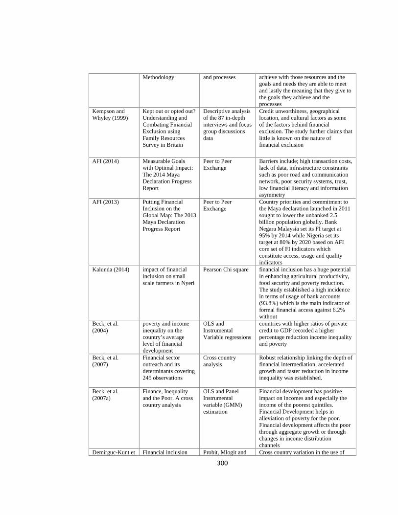
300

Methodology and processes achieve with those resources and thegoals and needs they are able to meetand lastly the meaning that they give tothe goals they achieve and theprocesses

Kempson andWhyley (1999)

Kept out or opted out?Understanding andCombating FinancialExclusion usingFamily ResourcesSurvey in Britain

Descriptive analysisof the 87 in-depthinterviews and focusgroup discussionsdata

Credit unworthiness, geographicallocation, and cultural factors as someof the factors behind financialexclusion. The study further claims thatlittle is known on the nature offinancial exclusion

AFI (2014) Measurable Goalswith Optimal Impact:The 2014 MayaDeclaration ProgressReport

Peer to PeerExchange

Barriers include; high transaction costs,lack of data, infrastructure constraintssuch as poor road and communicationnetwork, poor security systems, trust,low financial literacy and informationasymmetry

AFI (2013) Putting FinancialInclusion on theGlobal Map: The 2013Maya DeclarationProgress Report

Peer to PeerExchange

Country priorities and commitment tothe Maya declaration launched in 2011sought to lower the unbanked 2.5billion population globally. BankNegara Malaysia set its FI target at95% by 2014 while Nigeria set itstarget at 80% by 2020 based on AFIcore set of FI indicators whichconstitute access, usage and qualityindicators

Kalunda (2014) impact of financialinclusion on smallscale farmers in Nyeri

Pearson Chi square financial inclusion has a huge potentialin enhancing agricultural productivity,food security and poverty reduction.The study established a high incidencein terms of usage of bank accounts(93.8%) which is the main indicator offormal financial access against 6.2%without

Beck, et al.(2004)

poverty and incomeinequality on thecountry’s averagelevel of financialdevelopment

OLS andInstrumentalVariable regressions

countries with higher ratios of privatecredit to GDP recorded a higherpercentage reduction income inequalityand poverty

Beck, et al.(2007)

Financial sectoroutreach and itsdeterminants covering245 observations

Cross countryanalysis

Robust relationship linking the depth offinancial intermediation, acceleratedgrowth and faster reduction in incomeinequality was established.

Beck, et al.(2007a)

Finance, Inequalityand the Poor. A crosscountry analysis

OLS and PanelInstrumentalvariable (GMM)estimation

Financial development has positiveimpact on incomes and especially theincome of the poorest quintiles.Financial Development helps inalleviation of poverty for the poor.Financial development affects the poorthrough aggregate growth or throughchanges in income distributionchannels

Demirguc-Kunt et Financial inclusion Probit, Mlogit and Cross country variation in the use of

301

al., (2013) and legaldiscrimination againstwomen: Analysis ofthe Global Findex datacovering 98 countries

Ologit financial services is attributed to legaldiscrimination on women and gendernorms. Lack of systematic indicators offinancial inclusion is the maindrawback to the enhancement ofgender parity in the formal financialsystem

Demirguc-Kuntand Klapper,2012)

financial inclusion inAfrica using the 2012Global Findexcovering 148countries

Descriptive analysis The financial depth often measuredusing private sector credit to GDP ratioin 2010 revealed that sub SaharanAfrica assumes 24% compared to172% recorded for high incomecountries. The proportion of adultswith a formal account in the countrystood at 42% compared to 54% and80% for South Africa and Mauritiusrespectively. Main barriers include;cost, distance, documentation

Aduda & Kalunda(2012)

theoretical andempirical literature onthe impact of financialinclusion on financialstability in Kenya

Non analytical Emphasis on the four key measures offinancial inclusion namely; access,quality, usage and impact

Sarma and Pias(2011)

Cross country analysisof financial inclusionand developmentacross countries

OLS regression Low income groups, ethnic minorities,immigrants and the aged are leading infinancial exclusion but also argues thatthe rural poor located far away fromthe FSPs have a higher risk of beingexcluded. Index of FI positively linkedto income, adult literacy but inverselyrelated to income inequality and ruralpopulation

Agrawal, 2008). The need for financialinclusion with anIndian perspective

Descriptive analysis Barriers include; adult literacy,urbanization, infrastructure andespecially communicationdevelopment, distance, cost andidentity proof

Park and Mercado(2015)

Financial inclusion,poverty and incomeinequality in 37developing Asianeconomies

Impact assessmentfrom the regressionanalysis

financial inclusion lowers poverty andincome inequality. Barriers include; percapita income, rule of law anddemographic characteristics indeveloping countries

Hannig andJansen (2010)

Financial inclusionand financial stability

Descriptive analysis Greater financial inclusion presentsopportunities for enhancing financialstability. Need to narrow the gapbetween documentation thresholdrequired by banks and quality ofdocumentation prevalent among lowincome clients

Claessens (2006)in Morduch(1999) dimensionof access

Access to FinancialServices: A Review ofthe Issues and PublicPolicy

Comparativeanalysis

Availability, cost, range, type andquality of financial services can besummarized by the followingdimensions of access; reliability,convenience, continuity and flexibilityof financial services.

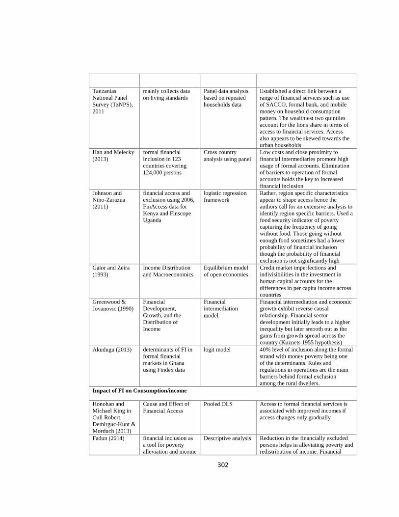
302

TanzaniasNational PanelSurvey (TzNPS),2011

mainly collects dataon living standards

Panel data analysisbased on repeatedhouseholds data

Established a direct link between arange of financial services such as useof SACCO, formal bank, and mobilemoney on household consumptionpattern. The wealthiest two quintilesaccount for the lions share in terms ofaccess to financial services. Accessalso appears to be skewed towards theurban households

Han and Melecky(2013)

formal financialinclusion in 123countries covering124,000 persons

Cross countryanalysis using panel

Low costs and close proximity tofinancial intermediaries promote highusage of formal accounts. Eliminationof barriers to operation of formalaccounts holds the key to increasedfinancial inclusion

Johnson andNino-Zarazua(2011)

financial access andexclusion using 2006,FinAccess data forKenya and FinscopeUganda

logistic regressionframework

Rather, region specific characteristicsappear to shape access hence theauthors call for an extensive analysis toidentify region specific barriers. Used afood security indicator of povertycapturing the frequency of goingwithout food. Those going withoutenough food sometimes had a lowerprobability of financial inclusionthough the probability of financialexclusion is not significantly high

Galor and Zeira(1993)

Income Distributionand Macroeconomics

Equilibrium modelof open economies

Credit market imperfections andindivisibilities in the investment inhuman capital accounts for thedifferences in per capita income acrosscountries

Greenwood &Jovanovic (1990)

FinancialDevelopment,Growth, and theDistribution ofIncome

Financialintermediationmodel

Financial intermediation and economicgrowth exhibit reverse causalrelationship. Financial sectordevelopment initially leads to a higherinequality but later smooth out as thegains from growth spread across thecountry (Kuznets 1955 hypothesis)

Akudugu (2013) determinants of FI informal financialmarkets in Ghanausing Findex data

logit model 40% level of inclusion along the formalstrand with money poverty being oneof the determinants. Rules andregulations in operations are the mainbarriers behind formal exclusionamong the rural dwellers.

Impact of FI on Consumption/income

Honohan andMichael King inCull Robert,Demirguc-Kunt &Morduch (2013)

Cause and Effect ofFinancial Access

Pooled OLS Access to formal financial services isassociated with improved incomes ifaccess changes only gradually

Fadun (2014) financial inclusion asa tool for povertyalleviation and income

Descriptive analysis Reduction in the financially excludedpersons helps in alleviating poverty andredistribution of income. Financial

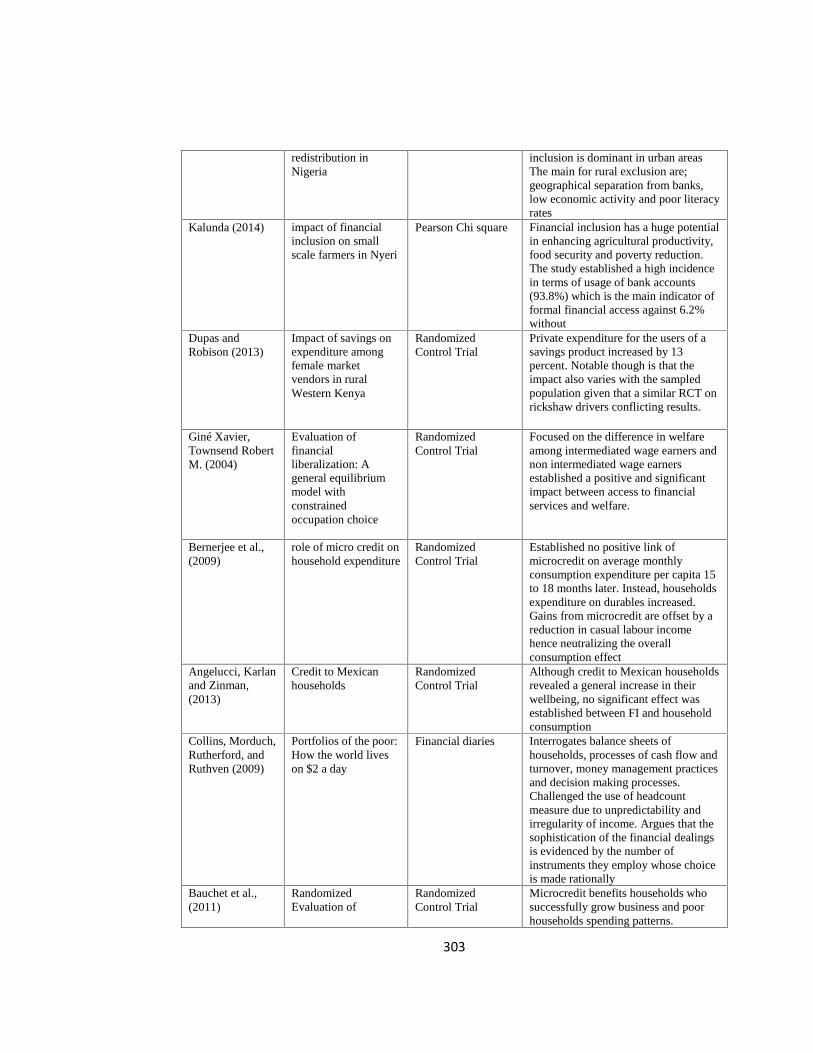
303

redistribution inNigeria

inclusion is dominant in urban areasThe main for rural exclusion are;geographical separation from banks,low economic activity and poor literacyrates

Kalunda (2014) impact of financialinclusion on smallscale farmers in Nyeri

Pearson Chi square Financial inclusion has a huge potentialin enhancing agricultural productivity,food security and poverty reduction.The study established a high incidencein terms of usage of bank accounts(93.8%) which is the main indicator offormal financial access against 6.2%without

Dupas andRobison (2013)

Impact of savings onexpenditure amongfemale marketvendors in ruralWestern Kenya

RandomizedControl Trial

Private expenditure for the users of asavings product increased by 13percent. Notable though is that theimpact also varies with the sampledpopulation given that a similar RCT onrickshaw drivers conflicting results.

Giné Xavier,Townsend RobertM. (2004)

Evaluation offinancialliberalization: Ageneral equilibriummodel withconstrainedoccupation choice

RandomizedControl Trial

Focused on the difference in welfareamong intermediated wage earners andnon intermediated wage earnersestablished a positive and significantimpact between access to financialservices and welfare.

Bernerjee et al.,(2009)

role of micro credit onhousehold expenditure

RandomizedControl Trial

Established no positive link ofmicrocredit on average monthlyconsumption expenditure per capita 15to 18 months later. Instead, householdsexpenditure on durables increased.Gains from microcredit are offset by areduction in casual labour incomehence neutralizing the overallconsumption effect

Angelucci, Karlanand Zinman,(2013)

Credit to Mexicanhouseholds

RandomizedControl Trial

Although credit to Mexican householdsrevealed a general increase in theirwellbeing, no significant effect wasestablished between FI and householdconsumption

Collins, Morduch,Rutherford, andRuthven (2009)

Portfolios of the poor:How the world liveson $2 a day

Financial diaries Interrogates balance sheets ofhouseholds, processes of cash flow andturnover, money management practicesand decision making processes.Challenged the use of headcountmeasure due to unpredictability andirregularity of income. Argues that thesophistication of the financial dealingsis evidenced by the number ofinstruments they employ whose choiceis made rationally

Bauchet et al.,(2011)

RandomizedEvaluation of

RandomizedControl Trial

Microcredit benefits households whosuccessfully grow business and poorhouseholds spending patterns.

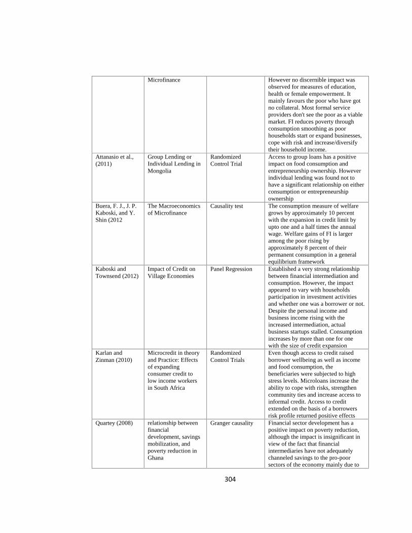
304

Microfinance However no discernible impact wasobserved for measures of education,health or female empowerment. Itmainly favours the poor who have gotno collateral. Most formal serviceproviders don't see the poor as a viablemarket. FI reduces poverty throughconsumption smoothing as poorhouseholds start or expand businesses,cope with risk and increase/diversifytheir household income.

Attanasio et al.,(2011)

Group Lending orIndividual Lending inMongolia

RandomizedControl Trial

Access to group loans has a positiveimpact on food consumption andentrepreneurship ownership. Howeverindividual lending was found not tohave a significant relationship on eitherconsumption or entrepreneurshipownership

Buera, F. J., J. P.Kaboski, and Y.Shin (2012

The Macroeconomicsof Microfinance

Causality test The consumption measure of welfaregrows by approximately 10 percentwith the expansion in credit limit byupto one and a half times the annualwage. Welfare gains of FI is largeramong the poor rising byapproximately 8 percent of theirpermanent consumption in a generalequilibrium framework

Kaboski andTownsend (2012)

Impact of Credit onVillage Economies

Panel Regression Established a very strong relationshipbetween financial intermediation andconsumption. However, the impactappeared to vary with householdsparticipation in investment activitiesand whether one was a borrower or not.Despite the personal income andbusiness income rising with theincreased intermediation, actualbusiness startups stalled. Consumptionincreases by more than one for onewith the size of credit expansion

Karlan andZinman (2010)

Microcredit in theoryand Practice: Effectsof expandingconsumer credit tolow income workersin South Africa

RandomizedControl Trials

Even though access to credit raisedborrower wellbeing as well as incomeand food consumption, thebeneficiaries were subjected to highstress levels. Microloans increase theability to cope with risks, strengthencommunity ties and increase access toinformal credit. Access to creditextended on the basis of a borrowersrisk profile returned positive effects

Quartey (2008) relationship betweenfinancialdevelopment, savingsmobilization, andpoverty reduction inGhana

Granger causality Financial sector development has apositive impact on poverty reduction,although the impact is insignificant inview of the fact that financialintermediaries have not adequatelychanneled savings to the pro-poorsectors of the economy mainly due to

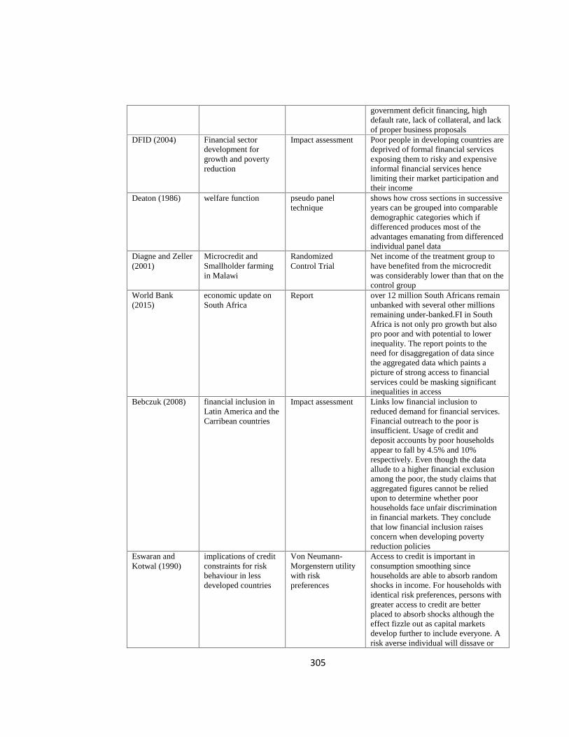
305

government deficit financing, highdefault rate, lack of collateral, and lackof proper business proposals

DFID (2004) Financial sectordevelopment forgrowth and povertyreduction

Impact assessment Poor people in developing countries aredeprived of formal financial servicesexposing them to risky and expensiveinformal financial services hencelimiting their market participation andtheir income

Deaton (1986) welfare function pseudo paneltechnique

shows how cross sections in successiveyears can be grouped into comparabledemographic categories which ifdifferenced produces most of theadvantages emanating from differencedindividual panel data

Diagne and Zeller(2001)

Microcredit andSmallholder farmingin Malawi

RandomizedControl Trial

Net income of the treatment group tohave benefited from the microcreditwas considerably lower than that on thecontrol group

World Bank(2015)

economic update onSouth Africa

Report over 12 million South Africans remainunbanked with several other millionsremaining under-banked.FI in SouthAfrica is not only pro growth but alsopro poor and with potential to lowerinequality. The report points to theneed for disaggregation of data sincethe aggregated data which paints apicture of strong access to financialservices could be masking significantinequalities in access

Bebczuk (2008) financial inclusion inLatin America and theCarribean countries

Impact assessment Links low financial inclusion toreduced demand for financial services.Financial outreach to the poor isinsufficient. Usage of credit anddeposit accounts by poor householdsappear to fall by 4.5% and 10%respectively. Even though the dataallude to a higher financial exclusionamong the poor, the study claims thataggregated figures cannot be reliedupon to determine whether poorhouseholds face unfair discriminationin financial markets. They concludethat low financial inclusion raisesconcern when developing povertyreduction policies

Eswaran andKotwal (1990)

implications of creditconstraints for riskbehaviour in lessdeveloped countries

Von Neumann-Morgenstern utilitywith riskpreferences

Access to credit is important inconsumption smoothing sincehouseholds are able to absorb randomshocks in income. For households withidentical risk preferences, persons withgreater access to credit are betterplaced to absorb shocks although theeffect fizzle out as capital marketsdevelop further to include everyone. Arisk averse individual will dissave or

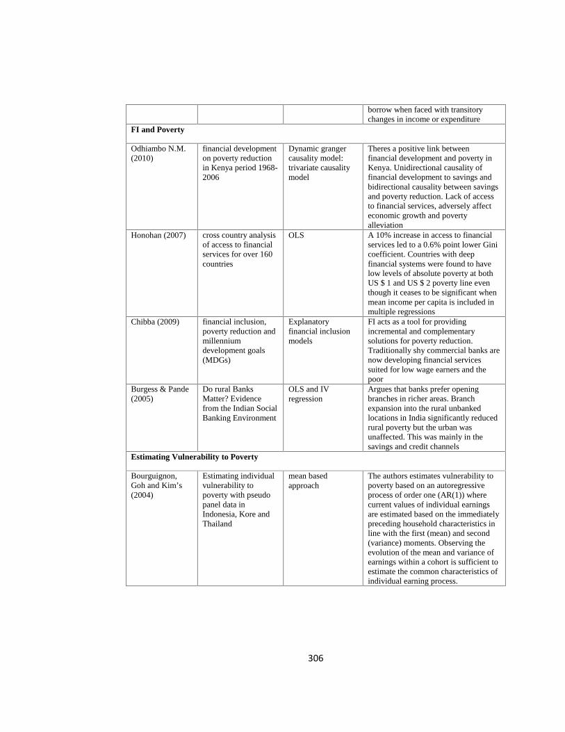
306

borrow when faced with transitorychanges in income or expenditure

FI and Poverty

Odhiambo N.M.(2010)

financial developmenton poverty reductionin Kenya period 1968-2006

Dynamic grangercausality model:trivariate causalitymodel

Theres a positive link betweenfinancial development and poverty inKenya. Unidirectional causality offinancial development to savings andbidirectional causality between savingsand poverty reduction. Lack of accessto financial services, adversely affecteconomic growth and povertyalleviation

Honohan (2007) cross country analysisof access to financialservices for over 160countries

OLS A 10% increase in access to financialservices led to a 0.6% point lower Ginicoefficient. Countries with deepfinancial systems were found to havelow levels of absolute poverty at bothUS $ 1 and US $ 2 poverty line eventhough it ceases to be significant whenmean income per capita is included inmultiple regressions

Chibba (2009) financial inclusion,poverty reduction andmillenniumdevelopment goals(MDGs)

Explanatoryfinancial inclusionmodels

FI acts as a tool for providingincremental and complementarysolutions for poverty reduction.Traditionally shy commercial banks arenow developing financial servicessuited for low wage earners and thepoor

Burgess & Pande(2005)

Do rural BanksMatter? Evidencefrom the Indian SocialBanking Environment

OLS and IVregression

Argues that banks prefer openingbranches in richer areas. Branchexpansion into the rural unbankedlocations in India significantly reducedrural poverty but the urban wasunaffected. This was mainly in thesavings and credit channels

Estimating Vulnerability to Poverty

Bourguignon,Goh and Kim’s(2004)

Estimating individualvulnerability topoverty with pseudopanel data inIndonesia, Kore andThailand

mean basedapproach

The authors estimates vulnerability topoverty based on an autoregressiveprocess of order one (AR(1)) wherecurrent values of individual earningsare estimated based on the immediatelypreceding household characteristics inline with the first (mean) and second(variance) moments. Observing theevolution of the mean and variance ofearnings within a cohort is sufficient toestimate the common characteristics ofindividual earning process.

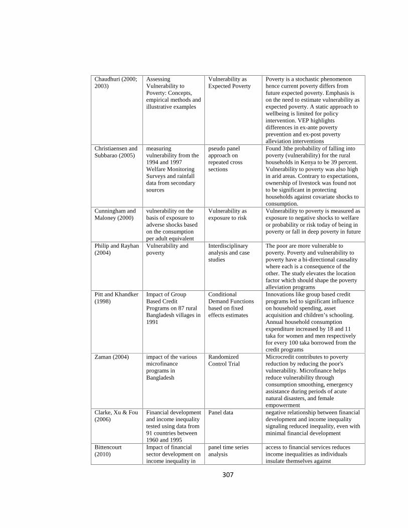
307

Chaudhuri (2000;2003)

AssessingVulnerability toPoverty: Concepts,empirical methods andillustrative examples

Vulnerability asExpected Poverty

Poverty is a stochastic phenomenonhence current poverty differs fromfuture expected poverty. Emphasis ison the need to estimate vulnerability asexpected poverty. A static approach towellbeing is limited for policyintervention. VEP highlightsdifferences in ex-ante povertyprevention and ex-post povertyalleviation interventions

Christiaensen andSubbarao (2005)

measuringvulnerability from the1994 and 1997Welfare MonitoringSurveys and rainfalldata from secondarysources

pseudo panelapproach onrepeated crosssections

Found 3the probability of falling intopoverty (vulnerability) for the ruralhouseholds in Kenya to be 39 percent.Vulnerability to poverty was also highin arid areas. Contrary to expectations,ownership of livestock was found notto be significant in protectinghouseholds against covariate shocks toconsumption.

Cunningham andMaloney (2000)

vulnerability on thebasis of exposure toadverse shocks basedon the consumptionper adult equivalent

Vulnerability asexposure to risk

Vulnerability to poverty is measured asexposure to negative shocks to welfareor probability or risk today of being inpoverty or fall in deep poverty in future

Philip and Rayhan(2004)

Vulnerability andpoverty

Interdisciplinaryanalysis and casestudies

The poor are more vulnerable topoverty. Poverty and vulnerability topoverty have a bi-directional causalitywhere each is a consequence of theother. The study elevates the locationfactor which should shape the povertyalleviation programs

Pitt and Khandker(1998)

Impact of GroupBased CreditPrograms on 87 ruralBangladesh villages in1991

ConditionalDemand Functionsbased on fixedeffects estimates

Innovations like group based creditprograms led to significant influenceon household spending, assetacquisition and children’s schooling.Annual household consumptionexpenditure increased by 18 and 11taka for women and men respectivelyfor every 100 taka borrowed from thecredit programs

Zaman (2004) impact of the variousmicrofinanceprograms inBangladesh

RandomizedControl Trial

Microcredit contributes to povertyreduction by reducing the poor'svulnerability. Microfinance helpsreduce vulnerability throughconsumption smoothing, emergencyassistance during periods of acutenatural disasters, and femaleempowerment

Clarke, Xu & Fou(2006)

Financial developmentand income inequalitytested using data from91 countries between1960 and 1995

Panel data negative relationship between financialdevelopment and income inequalitysignaling reduced inequality, even withminimal financial development

Bittencourt(2010)

Impact of financialsector development onincome inequality in

panel time seriesanalysis

access to financial services reducesincome inequalities as individualsinsulate themselves against

308

Brazil in the 1980sand 1990s

macroeconomic shocks emanatingfrom inflation

Berthelemy andVaroudakis(1996)

Policies of Economictakeoff

Growth Analysis Insufficient financial developmentexposes a country to a persistentpoverty trap which may raise thepeoples’ vulnerability to poverty