Embed Size (px)
Citation preview
ERAECMWF Re-Analysis
Project Report Series
1. ERA-15 Description
J. K. Gibson, P. Kållberg, S. Uppala,
A. Hernandez, A. Nomura, E. Serrano
European Centre forMedium-Range WeatherForecasts
Europäisches Zentrum fürmittelfristigeWettervorhersage
Centre européen pour les prévisions météorologique à moyen terme
(Version 2 - January 1999)

ECMWF Re-Analysis Project Report Series
i
ACKNOWLEDGEMENT
The ECMWF Re-Analysis (ERA) project would not have been possible without the active support and co-
operation of many agencies, bodies, and individuals.
In addition to the Council of the European Centre for Medium-range Weather Forecasts, practical support in
terms of finance, staffing, and/or the supply of data has been received from the following:
• University of California Lawrence Livermore National Laboratory
• The European Union
• Japan Meteorological Agency
• World Meteorological Organisation and World Climate Research Programme
• National Center for Atmospheric Research, Boulder, Colorado
• Cray Research Incorporated
• National Oceanic and Atmospheric Administration, National Centers for Environmental Predic-
tion, Washington
• United Kingdom Meteorological Office
• Center for Ocean, Land, and Atmosphere Studies, Maryland, USA.
• National Snow and Ice Data Center, University of Colorado
• National Meteorological Centre, Melbourne
Permission to use data supplied is gratefully acknowledged.
ERA production data have been subjected to validation through specially commissioned validation projects.
The advice and information provided by the ERA Validation Partners is gratefully acknowledged. Validation
Partners included:
• Max-Planck-Institut für Meteorologie, Hamburg, Germany
• Direction de la Météorologie Nationale, France
• Koninklijk Nederlands Meteorologisch Instituut
• Istituto per lo Studio della Metodologie, IMGA, Modena, Italy
• United Kingdom Meteorological Office
• University of Bologna, Italy
• Danish Meteorological Institute
The ERA project received advice from its External Advisory Group, whose members included:

ECMWF Re-Analysis Project Report Series
ii
Dr. J-C André, Météo France; Prof. Dr. Lennart Berngtsson, Max-Planck-Institut; Dr. D. Blaskovich, Cray
Research Incorporated; Dr. G. Boer, AES Canada; Dr. D. Carson, Hadley Centre, U.K.; Prof. W. L. Gates,
PCMDI, University of California; Prof. B. Hoskins, University of Reading, U.K.; R. Jenne, NCAR; Dr. E.
Kalnay, NMC Washington; Dr. R. Newson, WCRP, WMO; Dr. B. Orfila, European Climate Systems Net-
work; Prof. J. Shukla, University of Maryland; Dr. C. Schuurmans, KNMI; Dr. O. Talagrand, LMD, Paris;
Prof. S. Tibaldi, Bologna University; Dr. K. Trenberth, NCAR; Dr. W. Wergen, DWD.
The help and assistance given by ECMWF Staff, the other re-analysis groups throughout the world, and the
many other interested parties too numerous to mention by name are gratefully appreciated
ECMWF Re-Analysis Project Report Series
iii
ECMWF Re-Analysis Project Report Series
1. ERA-15 Description(Version 2 - May 1999)
Contents
1. Introduction ..................................................................... 3
2. Planning........................................................................... 42.1 Data Assimilation at ECMWF............................................... 42.2 Initial considerations ............................................................. 52.3 Work programme................................................................... 5
3. Input Data for the ECMWF Re-Analysis ........................ 73.1 Data sources........................................................................... 7
Satellite radiance data ...........................................................7Cloud track winds .................................................................9Other observations ..............................................................10
3.2 Data sources - forcing fields................................................ 113.3 Acquisition and preparation of data .................................... 12
Pre-processing of the CCR data..........................................12Pre-processing of NESDIS 1-b data ...................................13Pre-processing of other observations ..................................13Preparation of the forcing fields .........................................14
3.4 Conformity with other re-analysis projects ......................... 14
4. Experimentation ............................................................ 154.1 Vertical Resolution.............................................................. 154.2 Timeliness of first guess with respect to observations ........ 174.3 Orography............................................................................ 174.4 Soil....................................................................................... 184.5 Clouds.................................................................................. 18
5. The ECMWF Re-Analysis Data Assimilation Scheme. 215.1 One dimensional variational analysis (1D-Var) .................. 22
The 1D-Var method ............................................................22Bias corrections for 1D-Var................................................22The use of retrievals in the analysis ....................................23
5.2 The analysis ......................................................................... 23Monitoring, bias correction, and observation blacklists .....24
ECMWF Re-Analysis Project Report Series
iv
The analysis and quality control ......................................... 26The assumed observation errors ........................................ 26The assumed “First Guess” (FG) errors ............................ 27Objective optimum interpolation analysis.......................... 27Snow cover ......................................................................... 28Soil Moisture ...................................................................... 28The normal mode initialisation........................................... 28
5.3 The ECMWF global atmospheric model .............................29The model formulation ....................................................... 29The basic equations ............................................................ 29The resolution in time and space ........................................ 30The numerical formulation ................................................. 32Parametrization of physical processes................................ 33
6. Production ......................................................................406.1 Overview..............................................................................406.2 Production system design.....................................................416.3 Organising the observations.................................................426.4 Data assimilation..................................................................436.5 Adding results to the archive................................................456.6 Checking the archive files....................................................466.7 Production log ......................................................................466.8 Post-production log ..............................................................48
7. Re-Analysis Output........................................................517.1 Analysis and Forecast Fields................................................51
Daily data............................................................................ 51Monthly data....................................................................... 55
7.2 Data from ERA - observations and feedback.......................617.3 Other data .............................................................................617.4 Availability of ERA data......................................................61
8. Concluding Remarks......................................................62
References:........................................................................63
Bibliography:.....................................................................67
ECMWF Re-Analysis Project Report Series
v
ECMWF Re-Analysis Project Report Series
1. ERA-15 Description(Version 2 - May 1999)
List of Tables
Table 1 - Cloud cleared radiance data were used from the following satellites for theperiods indicated 8
Table 2 - Periods when ECMWF retrievals from NESDIS I-b data were used tosupplement gaps in CCR data. 9
Table 3 - Sea Surface Temperature used by the ECMWF Re-Analysis 12
Table 4 - Pressure of model levels when the surface pressure is 1015 hPa 31
Table 5 - Events from the Production Log. 47
Table 6 - Upper Air Parameters - daily archive 52
Table 7 - Surface and single level parameters - daily archive 53
Table 8 - Upper Air Parameters - monthly means and monthly “daily” means 55
Table 9 - Upper Air Parameters - variance and co-variance dats 56
Table 10 - Surface and single level parameters - monthly archive 58
Table 11 - Forecast accumulations - monthly mean data 60

ECMWF Re-Analysis Project Report Series
vi

ECMWF Re-Analysis Project Report Series
vii
ECMWF Re-Analysis Project Report Series
1. ERA-15 Description(Version 2 - May 1999)
List of Figures
Page 4 Figure 1 - Data assimilation using 6 hour cycles
Page 8 Figure 2 - Availability and use of cloud cleared radiance data.
Page 16 Figure 3 - Root mean square fit of radiosonde meridional winds to thefirst guess, 20˚N to 20˚S, for three weeks in January 1993. Full line 19levels, dashed line 31 levels
Page 16 Figure 4 - Root mean square fit of Northern Hemisphere (North of 20˚N)temperatures to the analyses, for three weeks in January 1993. Full line19 levels, dashed line 31 levels
Page 19 Figure 5 - Difference, in octas, between the annual mean total cloud cov-er from the prognostic and diagnostic cloud schemes. Blue colours indi-cate more clouds in the prognostic (ERA) scheme
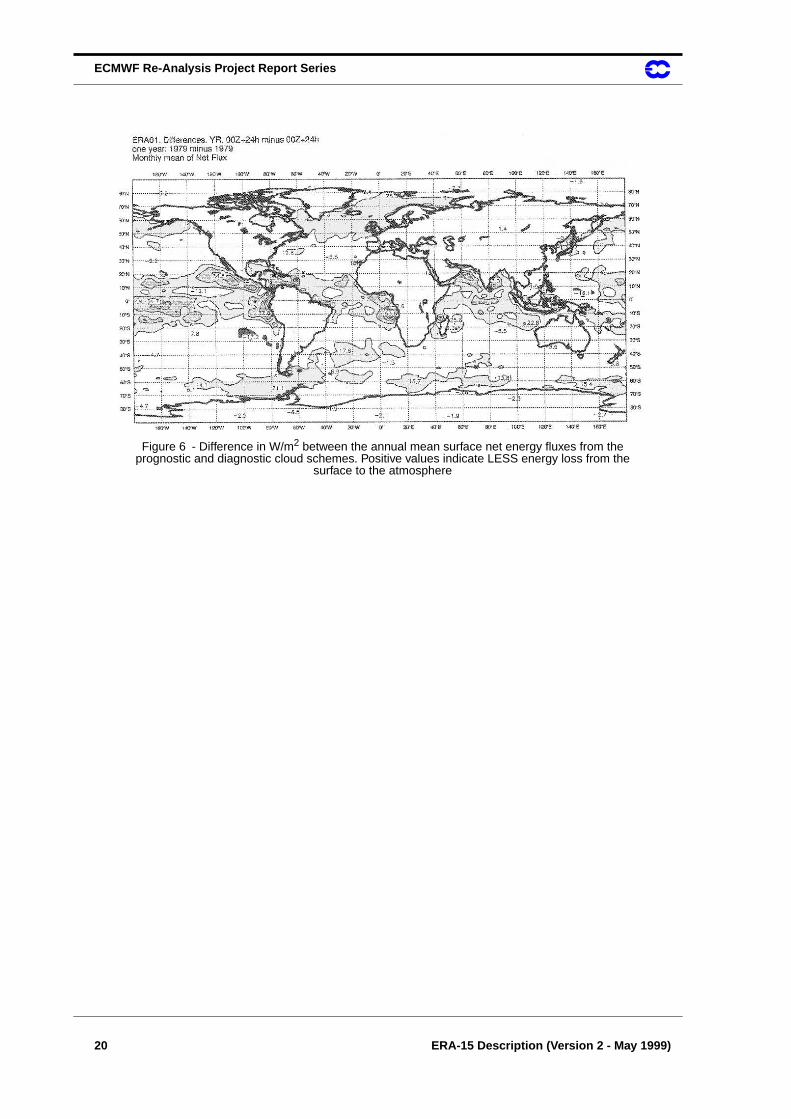
Page 20 Figure 6 - Difference in W/m2 between the annual mean surface net en-ergy fluxes from the prognostic and diagnostic cloud schemes. Positivevalues indicate LESS energy loss from the surface to the atmosphere
Page 24 Figure 7 - The use of TOVS retrievals in the ERA analyses
Page 25 Figure 8 - Difference information contained in “analysis feedback”.
Page 30 Figure 9 - The 31-level vertical resolution
Page 42 Figure 10 - principal concentrations of data associated with the mainprocessing components of ERA.
Page 44 Figure 11 - The main components of the ERA system.

ECMWF Re-Analysis Project Report Series
viii
ERA-15 Description (Version 2 - May 1999) 1
ERA-15Description
(Version 2 - May1999)

2 ERA-15 Description (Version 2 - May 1999)

ECMWF Re-Analysis Project Report Series
ERA-15 Description (Version 2 - May 1999) 3
ECMWF Re-Analysis Project Report Series
1. ERA-15 Description(Version 2 - May 1999)
J. K. Gibson, P. Kållberg, S. Uppala, A. Hernandez, A. Nomura, E. Serrano
1. Introduction
ECMWF began its operational activities in 1979. Since then the Centre's archive of analyses and forecasts
has become an important source of data for research. It is used extensively by the Centre's staff and by
scientists from all over the world for a wide variety of studies and applications. In recent years this archive
has been the basis for the ECMWF TOGA (Tropical Ocean Global Atmosphere) data set, providing analyses
of the global atmosphere for TOGA research.
Operational analyses, while providing a valuable resource for research, are affected by the major changes in
models, analysis technique, assimilation, and observation usage which are an essential product of research
and progress in an operational numerical weather prediction centre. They also can make use only of those
observations which become available within near real time. Many years ago Bengtsson and Shukla (1988)
expressed the idea that such considerations provide valid reasons for performing a consistent re-analysis of
atmospheric data. Typical research applications which could make good use of re-analyses include studies of
predictability, observing system performance, general circulation diagnostics, atmospheric low-frequency
variability, the global hydrological and energy cycle and coupled ocean-atmosphere modelling.
The first ECMWF Re-Analysis (ERA) project has produced a new, validated 15 year data set of assimilated
data for the period 1979 to 1993 (ERA-15). The project began in February 1993. The first phase of the work
required the acquisition and preparation of the observations and forcing fields. During the first year a
substantial programme of experimentation, closely co-ordinated with the Centre's Research and Operational
activities was completed. This enabled the scientific components of the re-analysis system to be defined, and
a strategy for production to be determined. At the same time work was progressing on the development of
both the production system and the internal validation tools. The final production system was adopted in
1994, and there followed a period of sustained production, monitoring and validation throughout 1995 and
the first nine months of 1996.
ECMWF Re-Analysis Project Report Series
4 ERA-15 Description (Version 2 - May 1999)
All data generated by the project likely to be of future value have been collected and preserved. These
include blacklist information, radiosonde bias correction tables, TOVS bias and calibration files, and the
record of which satellites have been used at different periods.
2. Planning
2.1 Data Assimilation at ECMWF
In many areas of the globe the density of available observations is far below that needed to support the
analysis with the required accuracy. In such areas a simple analysis would rely mainly on satellite based
observations: cloud cleared radiance data or retrieved temperature and humidity data from the NOAA
satellites, and cloud motion wind data from geostationary satellites.
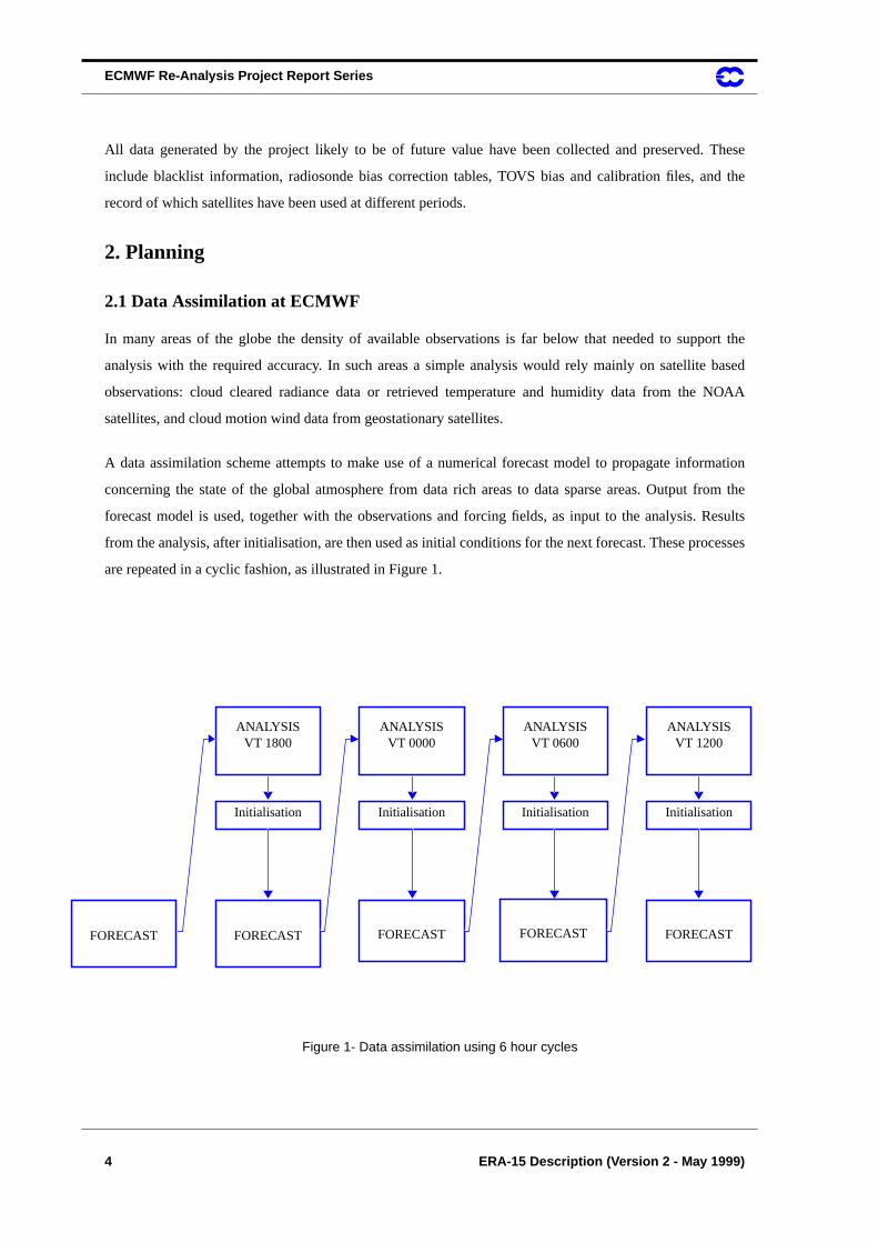
A data assimilation scheme attempts to make use of a numerical forecast model to propagate information
concerning the state of the global atmosphere from data rich areas to data sparse areas. Output from the
forecast model is used, together with the observations and forcing fields, as input to the analysis. Results
from the analysis, after initialisation, are then used as initial conditions for the next forecast. These processes
are repeated in a cyclic fashion, as illustrated in Figure 1.
Figure 1- Data assimilation using 6 hour cycles
ANALYSISVT 1800
ANALYSISVT 0000
ANALYSISVT 0600
ANALYSISVT 1200
FORECAST FORECAST FORECAST FORECAST
Initialisation Initialisation Initialisation Initialisation
FORECAST

ECMWF Re-Analysis Project Report Series
ERA-15 Description (Version 2 - May 1999) 5
Thus, continuous data assimilation over a long period is really equivalent to running the forecast model as a
global circulation model and relaxing towards the observations and forcing fields at six hourly intervals.
2.2 Initial considerations
If a data assimilation scheme of the type outlined above is to be used for re-analysis over a given period, the
following must be considered in some detail before the actual production work can be attempted:
• the observations and forcing fields to be used as input;
• the acquisition, preparation, and checking required with respect to these input data
• the exact composition of the assimilation system to be used;
• what data the production system should generate;
• how the production should be monitored and validated;
• what data should be archived;
• how end users can be given access to the data;
• what other deliverables, such as documentation and reports, the project should be required to
deliver.
To enable this to be done two advisory bodies were set up - an internal steering group, and an external
advisory board.
The external advisory group provided contact with the potential end-users of the re-analyses, and was of
particular assistance in helping to determine the archive policy. Members of this group also provided
valuable opinion with respect to many of the scientific choices which had to be made.
The internal steering group provided critical input to the initial planning, the decision making with respect to
the production system components, and the archive policy. Steering group meetings also provided the
essential discussion and exchange of information without which the excellent level of co-operation enjoyed
between the project staff and other groups within ECMWF would not have been possible.
2.3 Work programme
Early planning effort resulted in a work programme which required a number of objectives to be achieved.
It was decided to acquire a number of additions to the archive of observations accumulated from ECMWF’s
daily operations. The acquisition and preparation of these additional data would need to have been completed
for any particular year before re-analysis of that year could take place.

ECMWF Re-Analysis Project Report Series
6 ERA-15 Description (Version 2 - May 1999)
It was also necessary to acquire appropriate forcing fields in the form of sea surface temperatures (SST), and
sea-ice cover. The various candidate data sets would then need to be examined carefully so that a decision
could be made on which to use.
The re-analysis production was to be carried out with an invariant data assimilation system. There were a
number of decision which needed to be made with regard to the exact configuration of the analysis system,
and also of the forecast model. The resolution to be used both in the vertical and the horizontal would need to
be decided. Thus it was considered necessary to embark on a number of controlled experiments to assess the
various available options.
A production system capable of sustaining the required rate of re-analysis had to be designed and assembled.
It would need to include sufficient monitoring components to enable problems to be intercepted, and
reasonable confidence to be established with respect to the on-going generation of results. The system
needed to be checked out carefully to ensure that it performed correctly from both a scientific and technical
point of view. Optimization would be necessary to achieve the required production rate.
A validation programme, including the setting up of a number of external validation projects was envisaged
to ensure that the re-analysis results achieved the goal of the production of a validated set of data. The
following entered into contracts as external validation partners:
Max Plank Institut für Meteorologie, Hamburg, Germany (MPI);
Hadley Centre, Meteorological Office, Bracknell, U.K. (UKMO);
Météo-France, Toulouse, France (DMN);
Danish Meteorological Institute, Copenhagen, Denmark (DMI);
Royal Netherlands Meteorological Institute, De Bilt, Netherlands (KNMI);
Instituto per lo studio delle Metodologie Geofisiche Ambientali, CNR, Modena, Italy (IMGA);
Atmospheric Dynamics Group, University of Bologna Italy (ADGB).
During production it would thus be necessary to make results and information concerning progress available
to the validation teams. The precise data to be generated to form the results of the re-analysis had to be
specified, and the archive designed. As much archive construction as possible would need to be accom-
plished during the production, so as to minimise the residual tidy-up work necessary at the end of production.
To complete the project it would be highly desirable to produce a good set of documentation, and to organise
the observations, the forcing fields, and the information gained during the production in such a way that it
would be of maximum benefit to any future re-analysis.
ECMWF Re-Analysis Project Report Series
ERA-15 Description (Version 2 - May 1999) 7
3. Input Data for the ECMWF Re-Analysis
The data used for the re-analysis, their acquisition, and the work done to prepare them for the assimilation
system are described in this section.
3.1 Data sources
The ECMWF Archive contains all observational data acquired in real time from the World Meteorological
Organisation’s Global Telecommunications System (GTS) since the beginning of daily operations in 1979.
An archive of First GARP Global Experiment (FGGE) level II-b data was also on-site at ECMWF. To
provide a comprehensive set of input data for ERA data were acquired from a number of additional sources.
3.1.1 Satellite radiance data
The 250 km cloud cleared radiance (CCR) data were acquired from the World Data Centre at Ashville. These
data contains layer-mean virtual temperature for 15 standard layers, layer precipitable water content for 3
layers, cloud cleared brightness temperatures and various identification parameters.
The TIROS Operational Vertical Sounder (TOVS) measures multi-spectral radiances, which are related to
the temperature and humidity structure in the atmosphere. Since 1979 the National Environmental Satellite
Data Information Service (NESDIS) have routinely produced CCR data. The method followed is: first the
completely cloud free fields of view (spots) are identified and selected; next those spots which are partly
clear are processed to extract the radiances for the clear areas from the cloud-contaminated radiances; for the
remaining spots only microwave radiances can be used. The radiances after cloud clearing are thus identified
as clear, partly cloudy or cloudy. Until 10 June 1980 cloud clearing was done with the algorithm described
by Smith and Woolf (1976); for later data NESDIS used the method of McMillin and Dean (1982).
The quality of satellite retrievals varies considerably over the years. The causes of this variability are mainly
related to the processing of the raw data. Generally the same instruments, High-resolution Infra-red
Radiation Sounder (HIRS), Microwave Sounding Unit (MSU), and Stratospheric Sounding Unit (SSU) were
used with the same specifications on all satellites. There are some minor exceptions, notably with respect to
the channel 10 centre frequency for the HIRS unit on NOAA-11, but these are thought to have had little
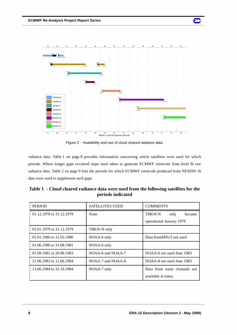
impact on the assimilations. Figure 2 illustrates the availability of data from the various NOAA satellites
throughout the ERA period.
The cloud cleared radiance archive provided an almost continuous source throughout the ERA period.
Unfortunately, however, there were a number of periods for which the archive was not complete. Where gaps
occurred for only a few analysis cycles production was allowed to continue without the use of cloud cleared
ECMWF Re-Analysis Project Report Series
8 ERA-15 Description (Version 2 - May 1999)
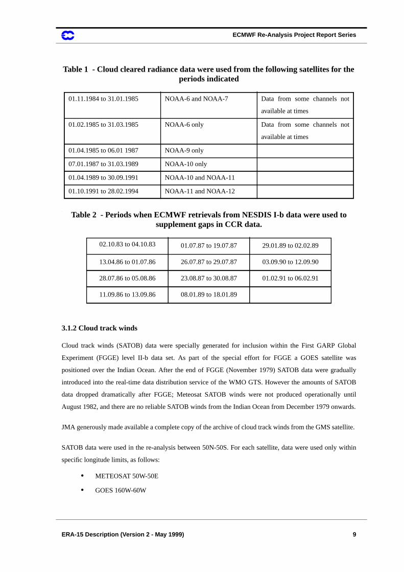
radiance data. Table 1 on page 8 provides information concerning which satellites were used for which
periods. Where longer gaps occurred steps were taken to generate ECMWF retrievals from level Ib raw
radiance data. Table 2 on page 9 lists the periods for which ECMWF retrievals produced from NESDIS 1b
data were used to supplement such gaps
.
Figure 2 - Availability and use of cloud cleared radiance data.
Table 1 - Cloud cleared radiance data were used from the following satellites for theperiods indicated
PERIOD SATELLITES USED COMMENTS
01.12.1978 to 31.12.1978 None TIROS-N only became
operational January 1979
01.01.1979 to 31.12.1979 TIROS-N only
01.01.1980 to 31.05.1980 NOAA-6 only Data fromMSU3 not used
01.06.1980 to 31.08.1981 NOAA-6 only
01.09.1981 to 20.06.1983 NOAA-6 and NOAA-7 NOAA-6 not used June 1983
21.06.1983 to 12.06.1984 NOAA-7 and NOAA-8 NOAA-8 not used June 1983
13.06.1984 to 31.10.1984 NOAA-7 only Data from some channels not
available at times
79 80 81 82 83 84 85 86 87 88 89 90 91 92 93
Black is used for passive periods
79 80 81 82 83 84 85 86 87 88 89 90 91 92 93
01 JAN 05 AUG
01 SEP 28 FEB
16 OCT
01 JAN 20 JUN
13 AUG
01 SEP 25 FEB
20 JUN
01 JUL 12 JUN
23 SEP
01 NOV 01 JUL
25 FEB 28 FEB
07 JAN
01 FEB 16 SEP
19 DEC
01 JAN
15 SEP
01 OCT
TIROS-N
NOAA-6
NOAA-7
NOAA-8
NOAA-9
NOAA-10
NOAA-11
NOAA-12
ECMWF Re-Analysis Project Report Series
ERA-15 Description (Version 2 - May 1999) 9
.
3.1.2 Cloud track winds
Cloud track winds (SATOB) data were specially generated for inclusion within the First GARP Global
Experiment (FGGE) level II-b data set. As part of the special effort for FGGE a GOES satellite was
positioned over the Indian Ocean. After the end of FGGE (November 1979) SATOB data were gradually
introduced into the real-time data distribution service of the WMO GTS. However the amounts of SATOB
data dropped dramatically after FGGE; Meteosat SATOB winds were not produced operationally until
August 1982, and there are no reliable SATOB winds from the Indian Ocean from December 1979 onwards.
JMA generously made available a complete copy of the archive of cloud track winds from the GMS satellite.
SATOB data were used in the re-analysis between 50N-50S. For each satellite, data were used only within
specific longitude limits, as follows:
• METEOSAT 50W-50E
• GOES 160W-60W
01.11.1984 to 31.01.1985 NOAA-6 and NOAA-7 Data from some channels not
available at times
01.02.1985 to 31.03.1985 NOAA-6 only Data from some channels not
available at times
01.04.1985 to 06.01 1987 NOAA-9 only
07.01.1987 to 31.03.1989 NOAA-10 only
01.04.1989 to 30.09.1991 NOAA-10 and NOAA-11
01.10.1991 to 28.02.1994 NOAA-11 and NOAA-12
Table 2 - Periods when ECMWF retrievals from NESDIS I-b data were used tosupplement gaps in CCR data.
02.10.83 to 04.10.83 01.07.87 to 19.07.87 29.01.89 to 02.02.89
13.04.86 to 01.07.86 26.07.87 to 29.07.87 03.09.90 to 12.09.90
28.07.86 to 05.08.86 23.08.87 to 30.08.87 01.02.91 to 06.02.91
11.09.86 to 13.09.86 08.01.89 to 18.01.89
Table 1 - Cloud cleared radiance data were used from the following satellites for theperiods indicated
ECMWF Re-Analysis Project Report Series
10 ERA-15 Description (Version 2 - May 1999)
• HIMAWARI 90E-170W
In addition the following restrictions were applied:
• METEOSAT:
• Not used over land between 50N and 35N.
• Not used over land between 35N and 20N when P > 500 hPa.
• Not used over land between 20S and 50S when P > 500 hPa.
• GOES:
• Not used between 50N and 20N when P < 700 hPa.
• Not used over land between 50N and 20N.
• Not used over land between 20S and 50S when P > 500 hPa.
• HIMAWARI:
• Not used between 50N and 20N when P < 700 hPa.
• Not used over land between 50N and 20N.
• Not used over land between 20S and 50S when P > 500 hPa.
• Not used between 20S and 50S when P < 700 hPa.
• INSAT:
• not used.
3.1.3 Other observations
The principal source of conventional observations has been the ECMWF real-time data collection from the
Meteorological Archive and Retrieval System (MARS). These data are acquired from two major nodes on
the World Meteorological Organisation's Global Telecommunications Network (WMO GTS). Little, if any
data are distributed within the GTS with a cut-off of more than 24 hours. Nevertheless up to three days
accumulation of data is allowed at ECMWF before they are added to the archive. ECMWF daily operations
began in 1979; in consequence it can be expected that these data may not be as complete for the early months
as for the majority of the period of interest. It should be noted that although the most important observational
data are exchanged globally via the GTS, there are differences with respect to regional and national data in
the availability of data from any one node.
For 1979 the principal source of observations was the First GARP Global Experiment (FGGE) level II-b data
set. During FGGE a considerable number of special observation were made, particularly in the tropics. There
was also an immense effort during FGGE to collect all observations made. In December 1979, after the

ECMWF Re-Analysis Project Report Series
ERA-15 Description (Version 2 - May 1999) 11
FGGE year, the number of radiosonde observations dropped significantly. In 1980, the first full year of
ECMWF operations, not all potentially available observations were being acquired. From 1981 the
radiosonde coverage increased, but was still below that potentially available. PILOT data amounts are fairly
constant during the period; in 1980 they are almost the only upper air data source (except CCR) over the
Indian Ocean.
Ship and buoy observations were augmented by adding data from the Comprehensive Ocean Atmosphere
Data Set (COADS) (Woodruff et al., 1993). Additionally, buoy data from the TOGA and SUBDUCTION
experiments were obtained.
The level II-b data from the Alpine Experiment were acquired from the University of Innsbrück. Data from
most other observing experiments were found to have been distributed via the GTS.
The Japan Meteorological Agency (JMA) archive was found to contain considerably more aircraft data over
the North Pacific than the MARS archive; it also included more radiosonde data from the immediate area
around Japan. These differences are likely to be due to the regional and national practices applied at different
GTS nodes. Appropriate sub-sets of this archive were kindly supplied by JMA to help rectify these
deficiencies.
Operational experience at ECMWF had established the importance of making use of the surface pressures
from the pseudo observations called “PAOBS” generated by the National Meteorological Centre at
Melbourne. The Australian Bureau of Meteorology kindly made available a copy of their PAOB archive.
It had been hoped to include dropsonde data for the TOGA COARE period, and also from the BASE
experiment. These data were acquired, but technical difficulties associated with their use within the ERA
assimilation system prevented their inclusion.
3.2 Data sources - forcing fields
The externally prescribed forcing of the re-analyses, in addition to the observations, comes from the sea
surface temperatures (SST) and the sea ice cover.
Sea ice cover, though potentially available from the sea surface temperature data sets, was derived separately
at ECMWF from SMMR and SSM/I data, using a scheme devised as part of the ERA project (Nomura,
1997).
For most of the re-analysis (November 1981 to February 1994) sea surface temperatures from the National
Centers for Environmental Prediction (NCEP) in Washington (Reynolds, 1994) were obtained. These are at a
ECMWF Re-Analysis Project Report Series
12 ERA-15 Description (Version 2 - May 1999)
1 degree resolution, and are available weekly. They were generated using an optimal interpolation technique,
and make use of satellite and in-situ data.
For the period before November 1981 the Meteorological Office 1 degree monthly Global sea-Ice and Sea
Surface Temperatures (GISST) version 1.1 (Parker et al., 1995) were acquired initially. However, at a later
date it was decided to re-run the whole of 1979 and part of 1980. It was also considered highly desirable to
use the same observations and forcing fields as the NCEP re-analysis for 1979. At the time of the re-run,
GISST version 2.2 (Rayner et al., 1996) was available and had been used by NCEP. The 1979 GISST sea
surface temperatures were thus acquired and used, while the re-run of 1980 made use of the original GISST
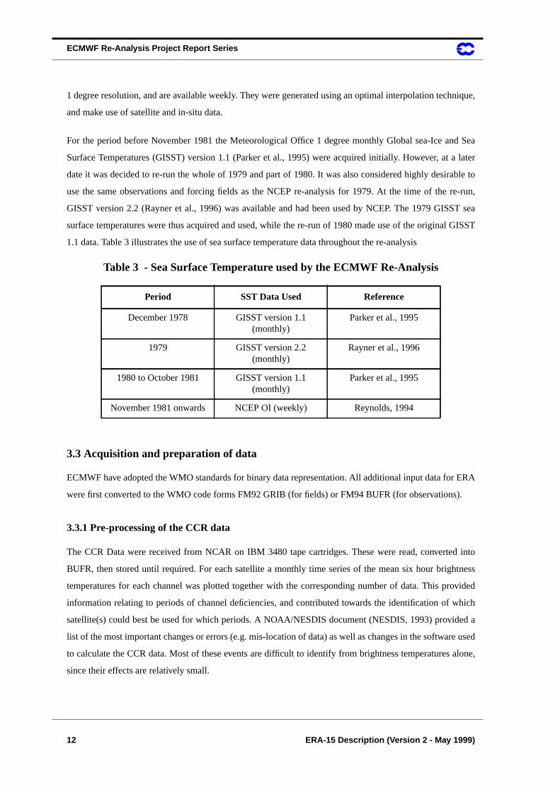
1.1 data. Table 3 illustrates the use of sea surface temperature data throughout the re-analysis
.
3.3 Acquisition and preparation of data
ECMWF have adopted the WMO standards for binary data representation. All additional input data for ERA
were first converted to the WMO code forms FM92 GRIB (for fields) or FM94 BUFR (for observations).
3.3.1 Pre-processing of the CCR data
The CCR Data were received from NCAR on IBM 3480 tape cartridges. These were read, converted into
BUFR, then stored until required. For each satellite a monthly time series of the mean six hour brightness
temperatures for each channel was plotted together with the corresponding number of data. This provided
information relating to periods of channel deficiencies, and contributed towards the identification of which
satellite(s) could best be used for which periods. A NOAA/NESDIS document (NESDIS, 1993) provided a
list of the most important changes or errors (e.g. mis-location of data) as well as changes in the software used
to calculate the CCR data. Most of these events are difficult to identify from brightness temperatures alone,
since their effects are relatively small.
Table 3 - Sea Surface Temperature used by the ECMWF Re-Analysis
Period SST Data Used Reference
December 1978 GISST version 1.1(monthly)
Parker et al., 1995
1979 GISST version 2.2(monthly)
Rayner et al., 1996
1980 to October 1981 GISST version 1.1(monthly)
Parker et al., 1995
November 1981 onwards NCEP OI (weekly) Reynolds, 1994
ECMWF Re-Analysis Project Report Series
ERA-15 Description (Version 2 - May 1999) 13
Occasionally there were miss-located soundings in the CCR data-set, especially during the first few days of a
year. As part of the quality control, the latitude and longitude of the soundings were checked and the wrong
locations corrected, using a set of orbital elements provided by NESDIS, and a diary of earth-location
problems was made.
3.3.2 Pre-processing of NESDIS 1-b data
A number of gaps were identified with respect to the 250 km cloud cleared radiance data; a system was
prepared, with the aid of the Satellite Data Section, to fill these gaps using the NESDIS I-b data.
First, orbits without either MSU or HIRS measurements were rejected, duplicated data eliminated, and the
files re-structured in a form convenient for further processing. These file were then stored until required by
the production suite.
During the production, 1-b data were pre-processed, ingested, and cloud cleared. The software to accomplish
this was adapted for use in the ERA system from the International TOVS Processing Package (ITPP4). The
cloud clearing module used the first guess forecast of the surface temperature in the tests for detection of
clear fields of view.
3.3.3 Pre-processing of other observations
Observations from MARS were extracted for periods well ahead of the ERA production. They were then
passed through a conversion programme to ensure that they could be read, and to convert old editions of
BUFR to the current edition. The converted data were categorized into conventional data, ships, buoys, and
satellite data. The ships and buoys were further categorized into those containing non-trivial identifiers and
those annotated simply “SHIP”. Resulting files were stored until required.
FGGE and ALPEX data were first converted from the FGGE II-b format to BUFR, then organized into files
and stored until required.
The additional observations received from JMA were converted into BUFR and stored. These data include
additional TEMP and AIREP data from the North Pacific, and a full set of GMS cloud winds. The GMS
cloud winds only became available after ERA production had reached 1981; they have been used from May
1981 onwards, and for the January to August 1980 re-run, but not for the period September 1980 to April
1981.

ECMWF Re-Analysis Project Report Series
14 ERA-15 Description (Version 2 - May 1999)
3.3.4 Preparation of the forcing fields
The SST data were interpolated from their original 1˚ x 1˚ resolution to the ERA Gaussian grid, and then
linearly in time to the actual analysis time. There is no separate field in ERA describing the sea-ice distri-
bution; instead it is defined as sea points with SST values below -1.8˚C. The sea-ice distribution is
determined from SMMR and SSM/I data, available on CD-ROM (NSIDC, 1992; NSIDC, 1993). Since an
ERA gridpoint is either land or sea, partial ice-cover is not possible. Sea areas where the SSMR-SSM/I data
indicate more than 55% ice cover are defined as sea-ice, other points as open water (Nomura, 1997). The
limit 55% was chosen based on comparisons between the satellite data and manual sea-ice analyses from
operational centres. The sea-ice areas in the original SST analyses included partially ice covered areas and
were found to be too large.
3.4 Conformity with other re-analysis projects
Since the National Centers for Environmental Prediction (NCEP), Washington, and NASA's Data Assimi-
lation Office (DAO) are also producing re-analyses it was considered desirable to have at least one year
during which each of the re-analysis projects would use the same input data. To this end a special effort was
made to enable each of the three centres to use an identical set of observations, sea surface temperatures, and
ice limits for 1979. ECMWF’s contribution to this effort was to make available the FGGE observations in
BUFR, and the sea-ice limits.
ECMWF Re-Analysis Project Report Series
ERA-15 Description (Version 2 - May 1999) 15
4. Experimentation
Before commencing the re-analysis, it was necessary to define the assimilation system to be used. Our goal
was to use a modern but proven data assimilation, not necessarily identical to the system being used for the
ECMWF operations at the time. Hence we selected ‘traditional’ optimum interpolation (OI) rather than the
newer variational analysis, which was under development at the centre at the time and implemented opera-
tionally in 1996. Also, to conserve resources, it was pre-determined that the re-analyses should be accom-
plished with a horizontal spectral resolution of T106, corresponding to a Gaussian grid resolution of 1.125
degrees or about 125 km.
Based on in house experience and advice from both the external advisory group and the steering group, a set
of parallel data assimilation and forecast experiments were carried out.
4.1 Vertical Resolution
The vertical resolution was examined in a three week experiment with two resolutions, 19 and 31 hybrid
levels, with the increased resolution concentrated in the free troposphere and lower stratosphere in the 31-
level version. The results showed that the fit of the first guess to the observations (OB-FG) was clearly better
with the higher resolution for both horizontal wind components of the TEMP/PILOT reports. In the northern
hemisphere (NH) this improvement was consistent from the mid-troposphere upwards, while in the tropics
the improvement was concentrated between 300hPa and 70 hPa. Figure 3 shows the 31-level improvement
in OB-FG for the meridional wind component between 20˚N and 20˚S. In the southern hemisphere (SH) the
differences were small and inconclusive due to the small amount of data in relation to the number of TOVS
profiles. Importantly, the improvement in the fit of the observed winds was retained through the initialisation.
The temperatures showed a similar behaviour, most pronounced around the tropopause where the 19-level
resolution was inadequate. This is seen for example in the fit of the analysis to the observations (OB-AN),
which depict how well the analysis is able to represent the TEMP soundings. In the Northern Hemisphere the
OB-AN root mean square “misfit” of the analyses to the soundings is reduced from almost 1.5K to just about
1.0K between 250hPa and 300hPa (figure 4). Zonal averages of the meridional wind over the three weeks
show that the 31 levels assimilation produced a 20% stronger Hadley cell outflow around 200hPa. The eddy
kinetic energy was about 2% more lively in the higher resolution.
Two sets of 21 10-day forecasts were also run. The differences were in general small, although we noted a
slight improvement in the NH 1000hPa scores from the higher resolution. In the SH the low resolution
forecasts were the better, which is interesting since, in these early tests, the TOVS data were handled
differently in the two hemispheres. In the NH radiances were used to produce physical retrievals with the

ECMWF Re-Analysis Project Report Series
16 ERA-15 Description (Version 2 - May 1999)
-.
Figure 3 - Root mean square fit of radiosonde meridional winds to the first guess, 20˚N to 20˚S, forthree weeks in January 1993. Full line 19 levels, dashed line 31 levels
.
Figure 4 - Root mean square fit of Northern Hemisphere (North of 20˚N) temperatures to theanalyses, for three weeks in January 1993. Full line 19 levels, dashed line 31 levels
RMS fits of analysis to Radiosondes
10
30
50
70
100
150
200
250
300
400
500
700
850
10003 4 5 6 7 8
Meriodonal wind (m/s)
Pre
ss
ure
(h
Pa
)
FGATL19
FGATL31
10
20
30
50
70
100
150
200
250
300
400
500
700
850
10000 1 2 3 4 5
Layer-mean temperature (K)
FGATL19
FGATL31
ECMWF Re-Analysis Project Report Series
ERA-15 Description (Version 2 - May 1999) 17
variational method (1D-Var), while in the SH the operational NESDIS retrievals were used. In the SH TOVS
data dominate since there are few radiosondes, and it is evident that the NESDIS profiles do not benefit from
the higher vertical model resolution. In the NH on the other hand the finer details added by the more
abundant TEMP data were described better with the higher resolution. Such details are also subsequently
retained better in the analysis through the variational use of the TOVS radiances.
4.2 Timeliness of first guess with respect to observations
The first O/I scheme introduced into ECMWF operations used 6 hour cycling, with a six hour forecast
providing the first guess conditions. Later, a method called First Guess at Appropriate Time (FGAT) was
introduced, and had been used for several years (Vasiljevic, 1990). In the FGAT approach the OB-FG
increments are calculated from first guess information based on 3-hour, 6-hour, and 9-hour forecasts. These
forecasts provided more timely first guess information with respect to the times of the observations, since the
observations included data for a 6-hour period centred on the analysis time.
The FGAT scheme is considerably more expensive both in terms of computing time and file handling. A
comparison with a NoFGAT assimilation was made in a three-week parallel analysis/forecast experiment.
FGAT was seen to give a marginally positive impact in the OB-FG data fit, primarily in the MSL pressure
near rapidly developing oceanic systems. These differences were however soon lost in the following
forecasts, and we could not detect a significant impact in any of the 21 individual 10-day forecasts run as part
of this experiment. In view of the considerable increase of the work load for FGAT, the NoFGAT method was
selected for ERA.
4.3 Orography
Sub-gridscale orographic effects such as stagnant air in mountain valleys were for a long time parametrized
at ECMWF by the use of an envelope orography, in which the gridpoint mean height was increased in
proportion to the sub-gridscale variance in the US Navy 10’ by 10’ database used to define the orography.
(Wallace et al., 1983). The envelope orography was however known to reduce the number of observations
used in mountainous areas, and it also had some negative effects on the medium-range forecasts. In a three-
week parallel experiment up to 10-15% more observations were accepted with mean orography at 1000hPa
and 925hPa, both SYNOP and perhaps more importantly, TEMP. In another assimilation experiment a new
parametrization of the effects of sub-gridscale orography which also includes a revised formulation of the
gravity wave drag was tested successfully in the re-analysis configuration. See Lott and Miller (1997) for a
description and evaluation of the formulation.

ECMWF Re-Analysis Project Report Series
18 ERA-15 Description (Version 2 - May 1999)
4.4 Soil
ECMWF had for many years used a two-level soil scheme with prescribed climatological temperature and
moisture in the lower layer. The use of a prescribed soil climatology has the obvious risk of forcing a re-
analysis towards its climate, which may be based on sparse information and may suffer from inconsistencies.
Hence the new four level self-contained soil parametrization scheme developed by Viterbo and Beljaars
(1995) for operational implementation was also selected for ERA and tested in a parallel assimilation
experiment, which for reasons explained below is somewhat obsolete and will not be described here.
4.5 Clouds
After the experimentation described above and several other tests which were of a more technical or, in view
of later developments obsolete, nature, the production began in earnest in December 1994, starting from
1979, the FGGE year. At this time the operational diagnostic cloud scheme (Slingo, 1987) had been selected
for ERA use.
After a few months of the initial production had been run our monitoring indicated that a surface temperature
warm bias, which was causing problems in the daily operations, was also apparent in the re-analyses. This
was attributed to problems in the cloud cover, particularly over mid-latitude land areas in springtime, where
unrealistic heating and drying was found to be due to too few clouds. As a quick remedy a very simple
nudging scheme was introduced in which the soil moisture was adjusted towards the near-ground
atmospheric humidity analyses (Viterbo, 1994, Viterbo, 1996, Mahfouf, 1991). Although the nudging
reduced the bias problem, the more fundamental problem of too few clouds was still apparent.
Meanwhile a new cloud scheme with prognostic equations for cloud water content and cloud fraction, but
without cloud advection, had approached maturity and had in tests been shown to yield more realistic clouds
(Tiedtke,1994 and Jakob,1995). The re-analysis was stopped when production had reached the end of 1979
and another set of parallel assimilations was run for July 1985 and January 1986 with a thoroughly revised
physics package. This, in addition to the prognostic cloud scheme and the soil moisture nudging, also
contained revisions to the oceanic albedo for short wave radiation bu Morcrette, and to the shallow
convection by Nordeng. The results of these tests were so encouraging that it was decided to go back and
restart the entire re-analysis from 1979 with the new physics.
The two complete 1979 assimilations are quite different, not only in the actual cloud amounts but also in
important derived quantities such as surface energy fluxes and precipitation. This sensitivity experiment
covering an entire year demonstrates the important fact that many aspects of a re-analysis are to a high
degree defined by the assimilating forecast model, and particularly by its physics. The difference between the
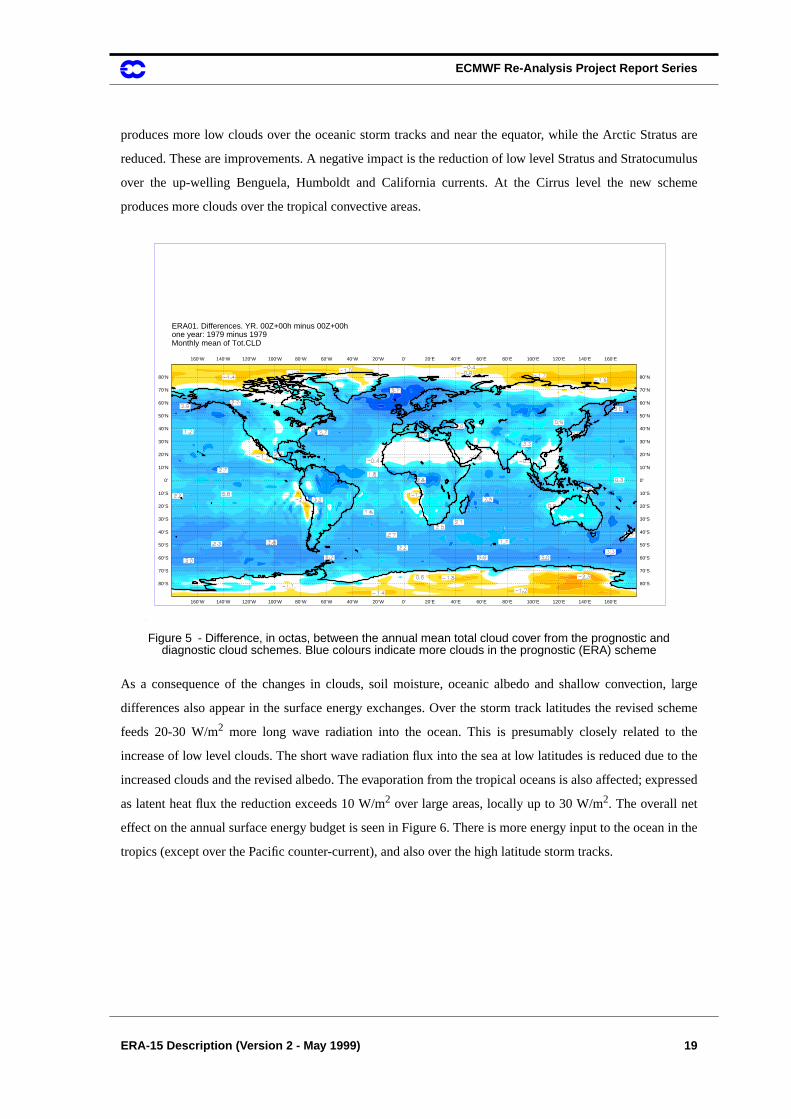
annual averages of the daily mean total cloud amounts are shown in Figure 5. The prognostic scheme
ECMWF Re-Analysis Project Report Series
ERA-15 Description (Version 2 - May 1999) 19
produces more low clouds over the oceanic storm tracks and near the equator, while the Arctic Stratus are
reduced. These are improvements. A negative impact is the reduction of low level Stratus and Stratocumulus
over the up-welling Benguela, Humboldt and California currents. At the Cirrus level the new scheme
produces more clouds over the tropical convective areas.
As a consequence of the changes in clouds, soil moisture, oceanic albedo and shallow convection, large
differences also appear in the surface energy exchanges. Over the storm track latitudes the revised scheme
feeds 20-30 W/m2 more long wave radiation into the ocean. This is presumably closely related to the
increase of low level clouds. The short wave radiation flux into the sea at low latitudes is reduced due to the
increased clouds and the revised albedo. The evaporation from the tropical oceans is also affected; expressed
as latent heat flux the reduction exceeds 10 W/m2 over large areas, locally up to 30 W/m2. The overall net
effect on the annual surface energy budget is seen in Figure 6. There is more energy input to the ocean in the
tropics (except over the Pacific counter-current), and also over the high latitude storm tracks.
.
Figure 5 - Difference, in octas, between the annual mean total cloud cover from the prognostic anddiagnostic cloud schemes. Blue colours indicate more clouds in the prognostic (ERA) scheme
80OS80OS
70OS 70OS
60OS60OS
50OS 50OS
40OS40OS
30OS 30OS
20OS20OS
10OS 10OS
0O0O
10ON 10ON
20ON20ON
30ON 30ON
40ON40ON
50ON 50ON
60ON60ON
70ON 70ON
80ON80ON
160OW
160OW 140OW
140OW 120OW
120OW 100OW
100OW 80OW
80OW 60OW
60OW 40OW
40OW 20OW
20OW 0O
0O 20OE
20OE 40OE
40OE 60OE
60OE 80OE
80OE 100OE
100OE 120OE
120OE 140OE
140OE 160OE
160OE
Monthly mean of Tot.CLDone year: 1979 minus 1979ERA01. Differences. YR. 00Z+00h minus 00Z+00h
ECMWF Re-Analysis Project Report Series
20 ERA-15 Description (Version 2 - May 1999)
.
Figure 6 - Difference in W/m2 between the annual mean surface net energy fluxes from theprognostic and diagnostic cloud schemes. Positive values indicate LESS energy loss from the
surface to the atmosphere
ECMWF Re-Analysis Project Report Series
ERA-15 Description (Version 2 - May 1999) 21
5. The ECMWF Re-Analysis Data Assimilation Scheme
From the experiences described in 4. above the following data assimilation system was selected and used for
the 15 years of re-analysis.
• Spectral T106 resolution with 31 vertical hybrid levels.
• Intermittent statistical (optimum interpolation) analysis with 6 hour cycling and noFGAT.
• One dimensional variational (1D-VAR) physical retrieval of TOVS cloud cleared radiances
below 100hPa, and NESDIS operational retrievals above. No TOVS data were used above
100hPa between 20˚N and 20˚S.
• Diabatic, non-linear normal mode initialisation, five vertical modes.
• The Integrated Forecast System (IFS) version of the ECMWF forecast model with 3-dimen-
sional semi-Lagrangian advection.
• Mean orography with a compatible parametrization of the effects of sub-grid scale orography.
• Prognostic soil temperature and soil moisture, with nudging of the moisture from boundary layer
atmospheric humidity analyses.
• Prognostic equations for cloud water and ice content and the cloud cover.
• ECMWF operational radiation parametrization with prescribed concentrations of aerosols, CO2
and O3, with O3 varying geographically and seasonally, the aerosols varying geographically and
vertically and the CO2 held constant.
• ECMWF operational planetary boundary layer parametrization.
The externally prescribed forcing of the re-analyses, in addition to the observations, comes from the ocean
surface temperatures (SST) and the ocean ice cover, and has been described in section 3.2 on page 11 above.
Apart from the horizontal resolution, the ERA assimilation system was identical to the ECMWF operational
system used between April 1995 and January 1996.
The principal components of the scheme are the one dimensional variational analysis of the cloud cleared
radiances, the optimal interpolation analysis, and the global atmospheric model. In the following some
aspects of these components as used in ERA are presented. Particular emphasis has been placed on aspects of
the system which do not accord strictly with the scientific documentation presented in ECMWF’s Research
Manuals (ECMWF, 1992). For in-depth descriptions of the components of the ECMWF data assimilation
and forecast the reader should consult the Research Manuals, and the bibliography provided (page 67).
ECMWF Re-Analysis Project Report Series
22 ERA-15 Description (Version 2 - May 1999)
5.1 One dimensional variational analysis (1D-Var)
A scheme developed by Eyre to make use of the raw TOVS radiances had been adapted at ECMWF to run on
cloud cleared radiances and is known as “one-dimensional variational analysis” or 1D-Var. Integral
components of the scheme include a radiative transfer model and a radiance bias monitoring and tuning
scheme. Within the 1D-Var process a comprehensive quality control is performed on the radiances (Eyre,
1989, 1992, 1993; Eyre et al. 1993).
In the re-analysis 1D-Var is applied globally, including the use of the three stratospheric channels of the SSU.
5.1.1 The 1D-Var method
The variational part is to find the atmospheric temperature and humidity structure (1D-Var retrieval) which
best fits the measured radiances. It is achieved by the minimization of the penalty function with respect to the
atmospheric state, which is the fit of the measured radiance vector to the atmospheric state vector in radiance
space (calculated by the radiative transfer model), to the background profile and to other information. The
method of Newtonian iteration is used to minimize the penalty function starting from the first guess as the
initial profile. If a sounding has not converged within 5 iterations it is rejected. TOVS channels used by the
1D-Var are: HIRS channels 1-7 and 10-15, MSU channels 2-4 and SSU channels 1-3 are used for “clear” and
“partly cloudy” soundings; HIRS channels 1-3, MSU channels 2-4 and SSU channels 1-3 are used for
“cloudy” soundings. A sounding is also rejected even if the minimization converges if the “measurement
cost” for any channel exceeds its threshold value. A sounding is rejected due to residual cloud contamination
if the measured-minus-forecast difference for HIRS 10 is below the threshold values over sea, over sea-ice
and over land. In the stability check, based on the results by Andersson, a number of retrievals with
suspected erroneous static stability are rejected (Andersson et al., 1991). Finally the accepted retrievals are
thinned to a spacing of about 250 km (Eyre et al., 1993).
An important contribution to the ERA humidity analysis is derived from the 1D-Var assimilation of the
radiance information contained in especially the “water vapour channels”, HIRS channels 10, 11, and 12
(McNally and Vesperini, 1996).
5.1.2 Bias corrections for 1D-Var
Eyre points out that for the effective implementation of 1D-Var it is necessary to apply a bias correction to
the CCR data (Eyre, 1992). The “measurements” (CCR data) have undergone calibration and preprocessing.
Any radiative transfer model has random and systematic errors. The systematic errors mainly result from the
errors in the spectroscopic data, on which the radiative models are based. Within the 1D-Var process the
radiative transfer model is applied to forecast model profiles. The differences between the measured and the
ECMWF Re-Analysis Project Report Series
ERA-15 Description (Version 2 - May 1999) 23
calculated brightness temperatures contain components from errors in the preprocessing of raw radiances,
the radiative transfer model and the forecast model. The magnitude of the bias is of the order of a typical
forecast error that the radiances try to correct; thus it has to be removed. Before 1D-Var retrievals are
“actively” produced from a new satellite, the 1D-Var processing is done in “passive” mode producing the
departure statistics without the final 1D-Var retrievals to allow the calculation of the initial biases. The
passive period is typically two to four weeks, and has guaranteed a smooth transition to new satellites.
As pointed out by Eyre it would be preferable to correct these errors at source, but since this is not possible a
practical strategy has been adopted (Eyre, 1992). Biases between measured brightness temperatures and
those calculated from the six hour forecast profiles are adjusted using corrections calculated from the
previous months biases close to a selection of reliable radiosonde stations in different parts of the world. The
bias corrections are determined for each channel and are then applied during the following month of assimi-
lation.
For quality control purposes the mean corrected and uncorrected measurement minus first guess departures
for each six hour period are plotted against time as a monthly “radgram” for each channel and satellite. Since
the first guess itself is independent of any changes in the CCR data, at least when a change is about to
happen, these graphs reveal satellite problems that have occurred during the previous month. Often NESDIS
has listed a change (e.g. a change in the water vapour attenuation coefficients), but it is only afterwards that it
can be seen whether or not this change has caused a significant problem in the data assimilation. In practice
full use of this information would require the bias tuning to be done separately during all the abnormal
periods, and those periods subsequently re-run with new coefficients.
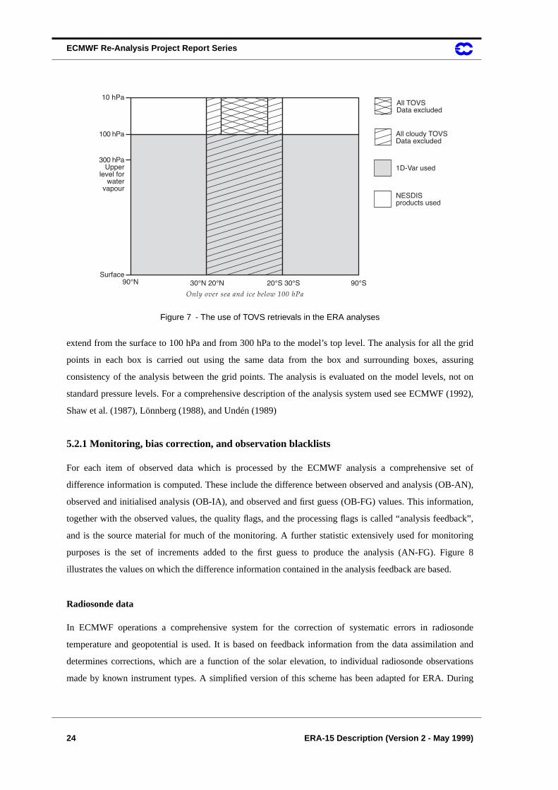
5.1.3 The use of retrievals in the analysis
In the Optimum Interpolation analysis the 1D-Var temperature retrievals are used globally below 100 hPa
over sea areas; they are not used over land. In the tropics only cloud free retrievals are used. The NESDIS
temperature retrievals are used above 100 hPa in the extra-tropical areas of both hemispheres. In the tropics
no retrievals are used above 100 hPa. Humidity retrievals are used below 300 hPa over sea areas, and are not
used over land. Figure 7 gives a diagrammatic picture indicating which kind of retrievals are used where. All
retrievals are subjected to further quality control within the OI analysis system, together with all other obser-
vations, before use.
5.2 The analysis
In contrast to some other analysis schemes, grid points are not analysed individually in the ECMWF system
but are grouped together, in “boxes” of variable horizontal size depending on the data density. The boxes
ECMWF Re-Analysis Project Report Series
24 ERA-15 Description (Version 2 - May 1999)
extend from the surface to 100 hPa and from 300 hPa to the model’s top level. The analysis for all the grid
points in each box is carried out using the same data from the box and surrounding boxes, assuring
consistency of the analysis between the grid points. The analysis is evaluated on the model levels, not on
standard pressure levels. For a comprehensive description of the analysis system used see ECMWF (1992),
Shaw et al. (1987), Lönnberg (1988), and Undén (1989)
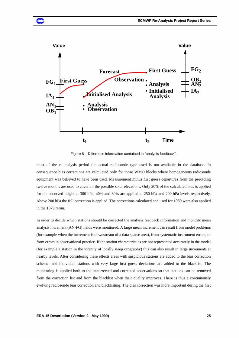
5.2.1 Monitoring, bias correction, and observation blacklists
For each item of observed data which is processed by the ECMWF analysis a comprehensive set of
difference information is computed. These include the difference between observed and analysis (OB-AN),
observed and initialised analysis (OB-IA), and observed and first guess (OB-FG) values. This information,
together with the observed values, the quality flags, and the processing flags is called “analysis feedback”,
and is the source material for much of the monitoring. A further statistic extensively used for monitoring
purposes is the set of increments added to the first guess to produce the analysis (AN-FG). Figure 8
illustrates the values on which the difference information contained in the analysis feedback are based.
Radiosonde data
In ECMWF operations a comprehensive system for the correction of systematic errors in radiosonde
temperature and geopotential is used. It is based on feedback information from the data assimilation and
determines corrections, which are a function of the solar elevation, to individual radiosonde observations
made by known instrument types. A simplified version of this scheme has been adapted for ERA. During
Figure 7 - The use of TOVS retrievals in the ERA analyses
ECMWF Re-Analysis Project Report Series
ERA-15 Description (Version 2 - May 1999) 25
most of the re-analysis period the actual radiosonde type used is not available in the database. In
consequence bias corrections are calculated only for those WMO blocks where homogeneous radiosonde
equipment was believed to have been used. Measurement minus first guess departures from the preceding
twelve months are used to cover all the possible solar elevations. Only 20% of the calculated bias is applied
for the observed height at 300 hPa; 40% and 80% are applied at 250 hPa and 200 hPa levels respectively.
Above 200 hPa the full correction is applied. The corrections calculated and used for 1980 were also applied
in the 1979 rerun.
In order to decide which stations should be corrected the analysis feedback information and monthly mean
analysis increment (AN-FG) fields were monitored. A large mean increment can result from model problems
(for example when the increment is downstream of a data sparse area), from systematic instrument errors, or
from errors in observational practice. If the station characteristics are not represented accurately in the model
(for example a station in the vicinity of locally steep orography) this can also result in large increments at
nearby levels. After considering these effects areas with suspicious stations are added to the bias correction
scheme, and individual stations with very large first guess deviations are added to the blacklist. The
monitoring is applied both to the uncorrected and corrected observations so that stations can be removed
from the correction list and from the blacklist when their quality improves. There is thus a continuously
evolving radiosonde bias correction and blacklisting. The bias correction was more important during the first
Figure 8 - Difference information contained in “analysis feedback”.
Time
Value
•
•
•
t1 t2
••
•Forecast First Guess
First GuessAnalysisInitialised
Initialised Analysis
AnalysisAN1
IA 1
FG1
• Observation
•Observation
OB1
Analysis
FG2
OB2AN2IA 2
Value
ECMWF Re-Analysis Project Report Series
26 ERA-15 Description (Version 2 - May 1999)
half of the re-analysis. Noticeable improvements in the quality of radiosondes later in the re-analysis period
resulted in a marked reduction in the corrections which needed to be applied.
Other observational data
Very few stations other than radiosonde stations were included within the blacklist. A notable exception is a
number of SYNOP stations near the Andes in Western South America, to the West of the Amazon basin. The
surface pressure data from these stations, coupled with their temperature and humidity data were found to
produce a spurious drying out of the surface moisture, due to deficiencies in the way they and the adjacent
steep orography were handled by the system. Blacklisting the surface pressure of a selection of these stations
was used as a crude “cure” for this problem.
5.2.2 The analysis and quality control
The analysis itself is used to perform quality control on the observations. During a first pass through the
analysis, the observed values are compared with each other and with the appropriate data from the 6 hour
forecast used as a first guess to generate a quality assessment of the data they contain, and to select the most
appropriate values for use within the analysis proper. Stations which report more than once during the 6 hour
period or appear in duplicate form are reduced in number, the observation closest to analysis time being
chosen. High density aircraft data and drifting buoy data are thinned where necessary. There are specific
checks for multi-level data. An observation which has been rejected in the early stages cannot be considered
in later checks. Observations accepted in the early checks can later have their quality re-assessed, and
possibly be rejected.
Data from TEMPs are normally only taken from 15 standard levels. If any are missing the nearest significant
level will be used. The heights to the significant levels have been computed during the hydrostatic check. If
there is a significant difference between a reported standard level and the re-computed one, the former will
be rejected and the latter used.
5.2.3 The assumed observation errors
In the ECMWF analysis system all observations of the same type are ascribed a typical error variance ,
computed from a long series of observations compared with analysis. Except for TEMPs, there is generally
no distinction between different platforms, all are assumed to be of equal quality.
The assumed typical wind errors are for SYNOP/SHIP: 3-4 m/s, DRIBU 5-6 m/s. TEMP and PILOT are
assumed to have a typical error of 2-3 m/s in the lower troposphere, compared to 3 m/s for AIREP and
σ0( )
σ0( )
ECMWF Re-Analysis Project Report Series
ERA-15 Description (Version 2 - May 1999) 27
SATOB. In the upper troposphere TEMP and PILOT are assumed to have errors around 3 m/s, AIREP 4 m/s
and SATOB 6 m/s.
The assumed typical height errors are for SYNOP 7 m (1 hPa), SHIP and DRIBU 14 m (2 hPa) and PAOB 32
m (4 hPa). For TEMP there are three quality classes, defined according to the monitoring statistics. The
typical 200 hPa geopotential error in the first group is 13 m, in the second 20 m and in the third 26 m.
Certain vertical error correlations are used to “spread out” the influence of, for example, an observation of an
AIREP in the vertical. Thus a wind report at 250 hPa is assumed to correlate 0.5 with the wind at 200 and
300 hPa, only 0.1 with 500 hPa and 100-150 hPa. In the same way a height observation at 500 hPa is
assumed to correlate around 0.5 with the height at 700 and 350 hPa.
5.2.4 The assumed “First Guess” (FG) errors
The assumed uncertainty of an observation is combined with the assumed uncertainty of the FG
, resulting in an estimate of the total uncertainty in the analysis. For the following FG 6 hours later this
uncertainty is increased by about 50%, a value roughly representative of a typical error growth over six
hours.
In the ERA analysis system, neither the analysis error nor the FG error are flow dependent. They depend to a
large extent on the typical data quality and coverage in the area, which in some areas may lead to occasional
misfits.
5.2.5 Objective optimum interpolation analysis
If is the extrapolated geopotential (or FG) and a single new observation, and are the assumed
errors, then the analysis takes the value
which means that when the observations are unreliable, is large and almost takes the value . Then
there is little impact on the FG. On the other hand, when the observations are assumed fairly accurate, is
small and almost takes the value . Then the observations will have a substantial impact on the analysis.
The ECMWF “Optimum Interpolation” (OI) analysis method is an extension of optimal interpolation
(Eliassen, 1995, and Gandin, 1963) to a multivariate three dimensional interpolation of deviations of obser-
vations from a forecast field (Lorenc, 1981). It is more correctly “statistical interpolation” since assumptions
σg( )
σ0( )σg( )
Zg Z0 σg σ0
Za
Za Zg Zo Zg–( )σg2 σo
2 σg2+( )⁄+=
σ0 Za Zg
σ0
Za Z0
ECMWF Re-Analysis Project Report Series
28 ERA-15 Description (Version 2 - May 1999)
made in using linear regression and error covariance when modelling the interpolation result in a process
which is not truly optimal.
5.2.6 Snow cover
The snow cover is initialized at every analysis time from a combination of two fields, snow fall and snow
depth, both analysed with a simple successive correction method. The snow fall analysis is based on station
snow fall data and the snow depth analysis on persistence, observed station snow depths and climatology.
Satellite-based snow cover estimates were not used in ERA. The amount of snowfall and snow depth obser-
vations vary considerably during the ERA years, there were for instance very few observations from central
Asia and Siberia before 1992.
It is important to point out that since the snow cover is analysed from observations, the water mass budget of
the hydrological cycle is not closed for the snow phase.
5.2.7 Soil Moisture
The soil moisture is initialized at each analysis time by a very simple nudging method based on the analysis
increments in the near surface atmospheric humidity. The vertically integrated soil moisture in the three
upper layers is corrected at each analysis time by a correction term proportional to the humidity analysis
increment (Viterbo and Courtier, 1995, Mahfouf,1991)
.
Where is the integrated soil moisture and q the near-ground atmospheric humidity. C is a constant and
the time step. Subscripts a and g stand for analysis and first guess respectively.
5.2.8 The normal mode initialisation
Though the wind and mass fields are balanced within the analysis “boxes”, on the larger scale and away from
the equator, minor imbalances still appear between the “boxes”. These imbalances set up fictitious, undesired
gravity waves. In the normal mode initialisation process the model suppresses these gravity waves. During
the process, the mass and wind fields become adjusted in such a way that no further undesired gravity waves
will appear.
A primary reason for initialisation is to improve the data assimilation. Unless initial, spurious waves in the
first guess forecast, especially in the surface pressure, are eliminated, they can lead to the rejection of good,
Θa Θg C∆t qa qg–( )+=
Θ t∆
ECMWF Re-Analysis Project Report Series
ERA-15 Description (Version 2 - May 1999) 29
and the acceptance of bad observations, and to a degraded estimation of the necessary increments to be
generated by the selected observations.
5.3 The ECMWF global atmospheric model
5.3.1 The model formulation
The model characteristics can be summarized by six basic physical equations, the resolution in time and
space and the way the numerical computations are carried out. A detailed documentation of the ECMWF
forecast model is under preparation, and will be available on the Internet. A description of the numerical
aspects and the semi-Lagrangian implementation can be found in Ritchie et al. (1995).
5.3.2 The basic equations
Of the six equations governing the ECMWF primitive equation atmospheric model, two are diagnostic and
tell us about the static relation between different parameters:
• The GAS LAW gives the relation between pressure, density and temperature,
• The HYDROSTATIC EQUATION shows the relationship between the density of the air and the
change of pressure with height,
The other four equations are prognostic and describe the changes with time of the horizontal wind
components, temperature and water vapour content of an air parcel, and of the surface pressure.
• The EQUATION OF CONTINUITY ensures that the mass is conserved and makes it possible to
determine the vertical velocity and change in the surface pressure.
• The EQUATION OF MOTION describes how changes in the wind are caused by the mass gradi-
ent, the Coriolis force and what the effects of friction are near the earth’s surface. The wind field
is described in the model by its vorticity and divergence, which are the forecast variables. The
west- and south-wind components are extracted at the post-processing stage
• The THERMODYNAMIC EQUATION expresses how a change in temperature is brought about
by adiabatic cooling or warming due to vertical displacement, latent heat release, radiation from
the sun, the air and the earth’s surface and frictional or turbulent processes (diffusion).
ECMWF Re-Analysis Project Report Series
30 ERA-15 Description (Version 2 - May 1999)
• The CONTINUITY EQUATION FOR MOISTURE assumes that the moisture content of an air
parcel is constant, except for losses due to precipitation and condensation or gains by evapora-
tion from clouds and rain or from the oceans and continents.
The hydrostatic assumption eliminates vertically propagating sound waves. Gravity waves, (and strictly
horizontal sound waves) are retained by the primitive equations. A proper treatment of the gravity waves is
essential for the adjustment processes between mass and wind.
5.3.3 The resolution in time and space
Temporal resolution:
The computational time step has to be chosen with care in order to avoid numerical instabilities and ensure
sufficient accuracy. The re-analysis system used a time step of 30 minutes.
Vertical resolution:
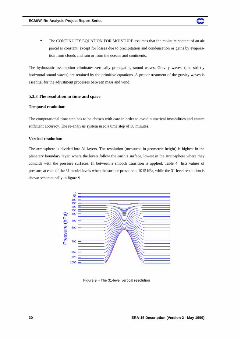
The atmosphere is divided into 31 layers. The resolution (measured in geometric height) is highest in the
planetary boundary layer, where the levels follow the earth’s surface, lowest in the stratosphere where they
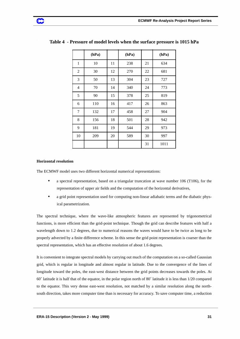
coincide with the pressure surfaces. In between a smooth transition is applied. Table 4 lists values of
pressure at each of the 31 model levels when the surface pressure is 1015 hPa, while the 31 level resolution is
shown schematically in figure 9.
Figure 9 - The 31-level vertical resolution
1000
925
850
700
500
400
300250200150100
1050
Pre
ssur
e (h
Pa)
ECMWF Re-Analysis Project Report Series
ERA-15 Description (Version 2 - May 1999) 31
.
Horizontal resolution
The ECMWF model uses two different horizontal numerical representations:
• a spectral representation, based on a triangular truncation at wave number 106 (T106), for the
representation of upper air fields and the computation of the horizontal derivatives,
• a grid point representation used for computing non-linear adiabatic terms and the diabatic phys-
ical parametrization.
The spectral technique, where the wave-like atmospheric features are represented by trigonometrical
functions, is more efficient than the grid-point technique. Though the grid can describe features with half a
wavelength down to 1.2 degrees, due to numerical reasons the waves would have to be twice as long to be
properly advected by a finite difference scheme. In this sense the grid point representation is coarser than the
spectral representation, which has an effective resolution of about 1.6 degrees.
It is convenient to integrate spectral models by carrying out much of the computation on a so-called Gaussian
grid, which is regular in longitude and almost regular in latitude. Due to the convergence of the lines of
longitude toward the poles, the east-west distance between the grid points decreases towards the poles. At
60˚ latitude it is half that of the equator, in the polar region north of 80˚ latitude it is less than 1/20 compared
to the equator. This very dense east-west resolution, not matched by a similar resolution along the north-
south direction, takes more computer time than is necessary for accuracy. To save computer time, a reduction
Table 4 - Pressure of model levels when the surface pressure is 1015 hPa
(hPa) (hPa) (hPa)
1 10 11 238 21 634
2 30 12 270 22 681
3 50 13 304 23 727
4 70 14 340 24 773
5 90 15 378 25 819
6 110 16 417 26 863
7 132 17 458 27 904
8 156 18 501 28 942
9 181 19 544 29 973
10 209 20 589 30 997
31 1011
ECMWF Re-Analysis Project Report Series
32 ERA-15 Description (Version 2 - May 1999)
of the Gaussian grid was introduced in 1991. The reduced Gaussian grid is defined as a step-wise reduction
of the number of grid points along a latitude line, to keep the east-west separation almost constant. Between
20N and 20S the grid is identical to a regular Gaussian longitude-latitude grid. By doing this the computa-
tional time has been reduced by about 25 to 30%.
5.3.4 The numerical formulation
The choice of a numerical scheme is the result of a compromise between the need to preserve numerical
accuracy, and the need to save computer time and speed up the forecast. When the operational T213L31
model was implemented in 1991, the traditional Eulerian scheme would have been too expensive, and a
semi-Lagrangian scheme was introduced to reduce the computer cost.
The basic difference between an Eulerian and a Lagrangian representation can be seen from the equation (in
one-dimensional space)
:
which in an Eulerian way expresses that the local changes in Q are due to the advection of Q by the wind U:
or in a Lagrangian way that Q is conserved for a given parcel
:
Whereas most Eulerian schemes require small time steps to avoid numerical instability, (the quantity Q must
not be advected by more than one grid length per time step), the Lagrangian scheme allows longer time steps,
where a limitation is the need to approximate curved trajectories by straight lines (or great circles on the
globe) during each time step.
Although it would be possible in theory to carry out predictions in a Lagrangian framework by following a
set of marked fluid parcels, in practice shear and stretching deformations tend to concentrate parcels inhomo-
geneously, so that it is difficult to maintain uniform resolution over the forecast region. A semi-Lagrangian
scheme is used to overcome this difficulty.
In this version, the grid points are stationary. At each time step the scheme computes a backward trajectory
from every grid point. The point reached defines where the air parcel was at the beginning of the time step.
dQdt-------
t∂∂Q
Ux∂
∂Q+ 0= =
t∂∂Q
U–x∂
∂Q=
dQdt------- 0=
ECMWF Re-Analysis Project Report Series
ERA-15 Description (Version 2 - May 1999) 33
The value of the variable in that point is then carried forward to the grid point, applying the various physical
processes.
5.3.5 Parametrization of physical processes
The primary purpose of the ECMWF model is medium-range weather forecasting, which has been defined as
the production of operational weather forecasts for the time-range 4-10 days. Although the purpose of the re-
analysis is different, using the same system has many benefits. Either goal requires very good descriptions of
the various physical processes that affect the weather development. A ten-day integration makes it absolutely
necessary to include effects with relatively long time scale, even as subtle as the evaporation by vegetation, in
order to handle the flow pattern more accurately. The different time scales and feed-back mechanisms
between the various processes makes the computations complex and expensive.
The mechanisms for these processes are mainly related to small scale disturbances in space and time, smaller
than the scales explicitly resolved by the model, from convective clouds down to molecular processes. The
effect that these sub-gridscale processes have on the larger scales can be computed only by parametrization,
i.e. formulating indirectly their overall effect in terms of known grid scale variables.
The Planetary Boundary Layer
The treatment of the planetary boundary layer (PBL), the lowest part of the troposphere, plays a fundamental
role for the whole atmosphere-earth system. It is through the surface exchanges of momentum, heat and
moisture that the atmosphere “feels” that it moves over a rough land surface or a wet smooth sea.
In the ECMWF model the lowest six levels are at around 30, 140, 340, 600, 900 and 1200 m above the model
surface. Even with this fairly high resolution the vertical gradients of temperature, wind, moisture etc. in the
PBL cannot be described very accurately, let alone the turbulent transports of momentum, heat and moisture.
For the estimation of these parameters the model uses the larger scale variables such as wind, temperature
and specific humidity, with the assumption that the transports are proportional to the vertical gradients. At
the earth’s surface, the turbulent transports of momentum, heat and moisture are computed as functions of
air-surface differences and surface characteristics. This approach is often referred to as first order turbulence
closure, in contrast to so called higher order schemes where the turbulence is predicted explicitly in one form
or another.
The surface
The model orography determines the relief of the lower model boundary, but other characteristics such as
vegetation, snow cover, sea ice distribution, albedo &c. strongly influence the surface processes in the model.
ECMWF Re-Analysis Project Report Series
34 ERA-15 Description (Version 2 - May 1999)
To have a realistic simulation of the boundary layer, the knowledge of such factors as the heat and moisture
content in the surface soil is essential. The degree to which convective clouds are created in the model
depends on the stored heat and moisture in the soil. Over land areas, snow depth, soil temperature and soil
wetness are forecast variables, calculated by a model of the soil with 4 layers at depths 7, 21, 72 and 189 cm.
Over the sea the surface temperatures are prescribed by external analyses
The orography
The ERA orography is given by a spectral T106 fitted version of the gridpoint averages (in the model
resolution) of a 1/6˚ x 1/6˚ reference field. This field is referred to as the ‘mean’ orography and is supple-
mented by four additional fields describing the height, orientation, anisotropy and slope of the sub-grid
orography. This allows a realistic representation of the mountain drag. An important part of the scheme is
that, depending on dynamical criteria, it can block the low level flow rather than make the air go over the
orography.
Compared to older versions of the orography parametrization, the ERA mean orography, together with the
physical parametrization, produces more realistic precipitation in mountainous regions; whereas in the older
versions the largest rainfall tended to fall on the tops of mountain ranges, it now falls on the slopes.
The land-sea mask
The model surface is logically divided into sea and land points. A grid point is defined as a land point if more
than 50% of the actual surface of the grid is land, calculated from the 1/6˚ x 1/6˚ reference field.
Sea surface temperature and sea-ice
The sea surface temperature (SST) used in ERA is taken from analyses produced externally, as described in
section 3.2 on page 11. The SST of ice-free water was kept constant during the 24-hour and 10-day forecasts.
There is no separate field in ERA describing the sea-ice distribution; instead it is defined as sea points with
SST values below -1.8˚C. The temperature at the surface of the ice is variable, according to a simple energy
balance/heat budget scheme. The distribution of sea and sea-ice points is kept constant during the forecast;
no freezing of the water or melting of the ice is allowed.
Albedo
A background yearly climate field is used, according to which the albedo is set to 0.55 over sea ice and 0.07
over open water. Over land the albedo has a minimum value of 0.07 and cannot exceed 0.80. The model is
able to alter it during the run according to changes in snow cover, but not to changes in vegetation.
ECMWF Re-Analysis Project Report Series
ERA-15 Description (Version 2 - May 1999) 35
The soil representation
The parametrization of the surface processes over land takes into account the distribution between bare land
and vegetation (based on geographical data) at each grid point. The soil is represented by a four-layer model
with layers at depths 7, 21, 72 and 189 cm. as described earlier. The soil hydrology is simulated in the same
four layers. A skin (or brightness) temperature, characteristic of a layer with no heat capacity at the soil-
atmosphere interface, represents the balance between radiative fluxes, sensible and latent heat fluxes and a
flux into the ground. Temperature in the four soil layers changes due to the combined effect of ground heat
flux and snow melting, where appropriate.
Snow cover
The thermal properties of snow covered ground depend only on the depth of the snow cover (actually the
amount of water in the snow). No considerations are made for the age of the snow, i.e. the model will treat
old dark snow as if it was white.
Soil moisture
The soil moisture is divided into skin and soil reservoirs. The skin reservoir (which mainly is moisture on
vegetation) evolves under the action of its own evaporation and its ability to collect dew and intercept precip-
itation. The soil reservoir takes into account contributions from precipitation and snow melt, as well as losses
due to deep penetration (gravity), evaporation over bare ground and root uptake by vegetation (i.e. to the
transpiration). Vegetation uptake takes place in the three upper layers, the root depth. The soil moisture
budget is not closed, excesses are removed as ‘run-off’ which has been extracted and is available as an ERA
product. The run-off contains three parts, surface run-off, deep penetration and excess over saturation in each
layer. The surface run-off is the difference between the throughfall (where throughfall = precipitation - inter-
ception on vegetation) and the infiltration into the soil. The deep penetration is the dominant component of
the run-off
Further climatological fields
The fraction of vegetation is specified in each grid point and used by the model to estimate the roughness and
the evaporation. This field does not vary with the seasons.
Gravity wave drag
When stably stratified air flow crosses a mountain ridge, gravity waves are excited in the flow. Depending on
the static stability and vertical wind shear, these gravity waves can propagate vertically until they have suffi-
ciently large amplitude to break. This process has a certain impact on the large scale flow; it makes it slightly
less zonal and contributes to the formation of blocking highs and cut-off lows. This physical process is incor-
ECMWF Re-Analysis Project Report Series
36 ERA-15 Description (Version 2 - May 1999)
porated into the model as the gravity wave drag (GWD) scheme. It represents the momentum transport due to
sub-grid gravity waves. Some of the wave drag occurs in the stratosphere, and there is also significant low-
level drag. The dependence on static stability and wind speed implies a maximum in winter and a minimum
in summer.
Radiation
In view of the importance of cloud-radiation interaction in both long and short term processes, ECMWF has
placed high emphasis on the treatment of the absorption and scattering by clouds of solar and terrestrial
radiation. About one fifth of the overall computational time in the forecast model is devoted to the radiation
scheme, as much as for the dynamics.
The radiation spectrum is divided into eight frequency bands: two in the short wave spectrum (direct and
diffuse radiation from the sun), and six in the long wave spectrum (from the earth and within the atmos-
phere). The upward and downward diffused radiation is computed for each of the eight spectral bands. The
parameters influencing the emission and absorption are pressure, moisture, cloud cover and cloud water
content. Assumed parameters are the ground albedo (modified according to the snow cover), the solar
constant and the concentration of CO2, O3 and aerosols. The solar constant has the value 1370 W/m2. The
carbon dioxide has a constant mass mixing ratio over the whole globe corresponding to a volume concen-
tration of 353 ppm(v). The ozone distribution depends on height, latitude, longitude and season, based on
analyses from the 1970’s.
The radiation scheme is designed to take the cloud-radiation interactions into account, in considerable detail.
It allows partial cloud cover in any layer of the model. For cloudy grid points, computations are made both
for clear and overcast conditions, and the total amount weighted together according to the forecast cloud
amount.
Convection
The convection schemes in the model (Tiedtke, 1989) fulfil five objectives:
• creation of cloud amount to be used by the radiation scheme,
• computation of precipitation,
• computation of vertical transport of moisture,
• computation of vertical momentum fluxes,
ECMWF Re-Analysis Project Report Series
ERA-15 Description (Version 2 - May 1999) 37
• computation of temperature changes in the atmosphere due to release of latent heat or cooling in
connection with evaporation.
In the general convection scheme, sub-grid vertical fluxes of mass, heat, water vapour and momentum are
computed at each model level with the help of a simple cloud model interacting with its environment. The
scheme is applied to penetrative convection, shallow convection and mid-level convection. They are mutually
exclusive, so only when the scheme fails to create cloud of one type, does it try the next.
Deep convection predominantly occurs in disturbed situations with a deep layer of conditional instability and
large-scale moisture convergence. The down draught mass flux is assumed proportional to the up draught
mass flux.
Shallow convection predominantly occurs in undisturbed flow, in the absence of large scale convergent flow.
For example trade wind cumuli under a subsidence inversion, convection occurring in the ridge region of
tropical easterly waves or day time convection over land. The moisture supply is from surface evaporation. It
does not normally produce precipitation.
Mid-level convection describes convective cells which originate at levels above the boundary layer. A well
known example is Altocumulus castellanus floccus. Less clearly visible, but frequent, are rain bands
connected to extra-tropical cyclones.
Clouds
There is no analysis of clouds, but the 6-hour first guess forecast clouds are carried forward to the next
analysis time. Although in general the forecast cloud cover gives useful information, the main purpose of the
cloud scheme is to provide input to the radiation computations.
In the ERA model the clouds are described by three prognostic parameters: the cloud fraction, the content of
cloud liquid water and cloud ice. The cloud scheme is unique in treating the main cloud-related processes in
a consistent way by forecasting both cloud fraction and cloud water/ice content with their own prognostic
equations. The cloud processes are strongly coupled to other parametrization processes. (Tiedtke, 1993;
Jakob, 1994)
Clouds are generated by large-scale ascent, cumulus convection, boundary layer turbulence and radiative
cooling. They are dissipated through evaporation due to large-scale descent, cumulus-induced subsidence,
radiative heating and turbulence at both cloud tops and sides, as through precipitation processes.
Convective clouds are computed in parallel with the convective scheme (see above). Moisture is carried
upward and condenses into liquid water/ice or “condensate”. This condensate will either fall out as precipi-
ECMWF Re-Analysis Project Report Series
38 ERA-15 Description (Version 2 - May 1999)
tation, be carried higher up in the cloud or be advected horizontally out of the cloud. In this latter case, and
only then, the scheme will use this part of the condensate to create stratiform and cirrus clouds (altocumulus
castellanus, anvils and other remains from convective processes).
Stratocumulus clouds are linked to the boundary layer moisture flux produced by the vertical diffusion
scheme.
Stratiform clouds (e.g. low level stratus and medium level nimbostratus types) are determined by the rate at
which the saturation specific humidity decreases due to upward vertical motion and radiative cooling.
Evaporation processes are accounted for in several ways: large-scale and cumulus-induced subsidence and
radiative heating, evaporation at the cloud sides due to turbulent processes and turbulent motion at the cloud
tops.
Precipitation processes take into account not only the local water/ice content, but also different precipitation
enhancement processes. The effect of evaporation of falling precipitation is also included.
The hydrological cycle
There are two precipitation generating mechanisms included in the ECMWF model, for convective and for
stratiform (frontal or dynamical) precipitation. The generated precipitation is affected by evaporation and
melting.
Convective precipitation: the condensation leading to precipitation is assumed to be liquid water or snow. No
ice crystals or liquid water are assumed to be stored in clouds or floating in the air as cloud particles. The
rain/snow partly moistens the atmospheric environment by detrainment, the rest falls out of the cloud as
precipitation.
Stratiform precipitation : precipitation both as water and ice crystals (snow) are considered, depending on
the temperature of the layer where condensation takes place. No condensation is stored as cloud drops or ice
crystals. The transition from ice to water is supposed to occur when the precipitation passes through layers
with temperatures warmer than +2˚C. Freezing water is not considered in the model except as snow.
Evaporation: it is assumed that precipitation falling from a saturated layer saturates the first layer
underneath before reaching the next layer below. This may substantially reduce the precipitation on the
ground. Evaporation of the precipitation is not assumed to take place within the cloud, only between the
cloud base and the ground. The layer below a precipitating, non-convective cloud is always almost saturated.
ECMWF Re-Analysis Project Report Series
ERA-15 Description (Version 2 - May 1999) 39
Melting: melting of falling snow occurs in a thin layer of a few hundreds of metres below the freezing level.
It is assumed the snow can melt in each layer whenever the temperature exceeds 2˚C. The melting is limited
not only by the snow amount, but also by keeping the induced cooling of the layer such that the temperature
of the layer after melting is not less than 2˚C.
The three cloud parameters, cloud liquid water content, cloud ice water content and cloud fraction are
extracted on the model levels and archived on the Gaussian grid. In addition there is an extraction of ‘low’,
‘middle’ and ‘high’ clouds, separated by the pressure levels 800 hPa and 450 hPa, these fields are also
available as a ‘more convenient’ summary of the detailed cloud fields.
Again it is important to stress that the global hydrological cycle cannot be closed in a data assimilation such
as ERA where the snow amount is adjusted each analysis cycle by observations (see section 5.2.6 on page
28).
ECMWF Re-Analysis Project Report Series
40 ERA-15 Description (Version 2 - May 1999)
6. Production
6.1 Overview
It was essential to develop a reliable production system capable of performing data assimilation at a very fast
rate. Using the combined experience of the Centre's Operations and Research Departments, the systems in
use were studied carefully, slimmed down where necessary, modified to exploit a data archive as opposed to
real-time data, and optimised for performance. This resulted in a prototype system capable of performing at
the required rate, which was further refined and completed while being used as the principal vehicle for the
initial ERA experimentation.
A period of experimentation then followed to determine the exact components of the data assimilation
system to be used for the full re-analysis. This has been described in some detail in section 4. on page 15.
Once production began, late in 1994, the scientific emphasis gradually moved from experimentation to
monitoring and validation. The external forcing fields were validated before the production started by means
of maps, averages and time series. Every effort was made to detect, as early as possible, potential problems
which would require further investigation. Where appropriate, production was halted and re-started from an
earlier date; in some cases production was allowed to continue, but the month or months concerned re-run at
a later time. The production monitoring made use of a set of quality control tools, whose output, usually in
the form of graphical information, was inspected continuously. All graphical and tabular monitoring results
were kept both as hard copies and as files. Diaries were kept of all special events and problems encountered.
Production and monitoring continued throughout 1995 and into 1996. During the second quarter of 1996 the
first pass through the full 15 years was completed. Monitoring enabled many errors which happened during
the production to be located and rectified; nevertheless two lengthy periods needed to be re-run. First, the
early production (to August 1980) was adversely affected by an error which significantly affected humidity
at upper levels. Secondly, all cloud track wind data (SATOB) except the GMS data were accidentally
excluded from June 1990 to October 1992, due to a change in their format within the ECMWF archive. A re-
run of the first period was particularly desirable, as it presented an opportunity to run the FGGE year with the
same observations and forcing fields as NCEP and DAO. Both re-runs were completed in September 1996.
The internal validation programme was augmented by the on-going work of the external validation projects
The continuous exchange of information between the ERA team and the validation partners proved to be
extremely useful. It has resulted in material being available to potential future users of the data which should
be of considerable assistance (ECMWF, 1997).
ECMWF Re-Analysis Project Report Series
ERA-15 Description (Version 2 - May 1999) 41
Close co-operation has also been established between the ERA team and the teams responsible for the NCEP
re-analysis, and the re-analysis performed by the DAO.
6.2 Production system design
The design of the production system exploited the cost effectiveness of two SGI servers to which were
attached a large amount of relatively inexpensive disk space, and attempted to optimise the locality of data to
appropriate compute servers taking particular account of the type of connectivity.
The ERA production system ran under the control of ECMWF's Supervisor Monitor Scheduler (SMS)
(Pesonen and Raoult, 1992). SMS enables computer “tasks” to be classified as belonging to “families” within
“suites”. Complex scheduling can then be performed according to attributes relating to events set by tasks,
task completion, family completion, and various other criteria. Tasks may be designated to run on any known
computer with a network connection to the computer on which the SMS is running. A graphical interface
provides monitoring information, enables manual changes to be made when required, and gives fast access to
task output, scripts, status information, and scheduling information. The use of SMS contributed greatly to
the smooth and efficient running of the ECMWF re-analysis system.
The ERA production system comprised a number of modules, each of which was scheduled as an
independent suite by the SMS. The various modules each addressed a specific part of the production for one
month. They included modules to:
• extract and organize observational data,
• perform data assimilation,
• archive results,
• check each archive file, and to
• generate monthly means and statistics.
Figure 10 shows the principal concentrations of data associated with the main processing components
together with their machine of residence. Data were moved from the Cray to the Silicon Graphics (SGI)
environment as soon after creation as possible, minimizing the amount of Cray disk space needed. Within the
SGI environment up to three months of observations and feedback, and up to two months of production fields
could be accommodated. Data were added to the ECMWF's MARS archive as monthly files at the end of
each month of production.
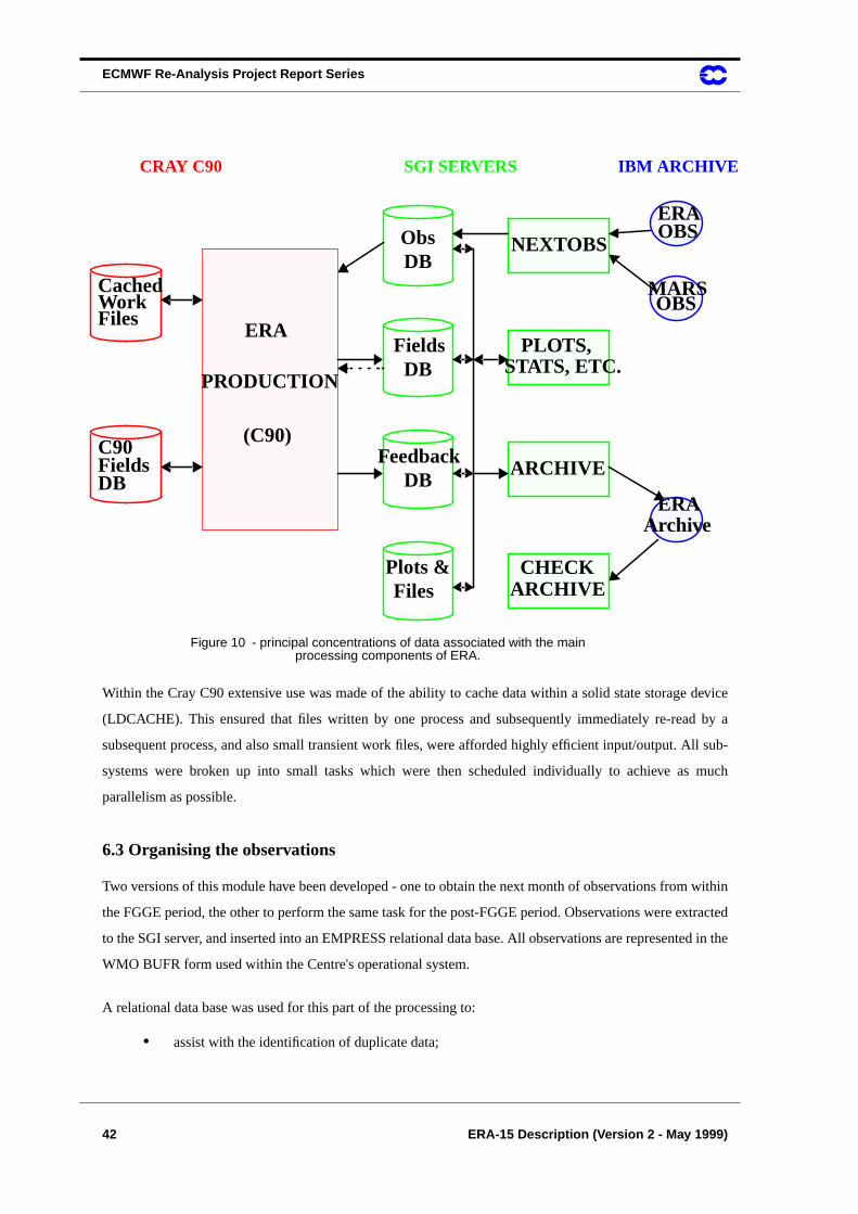
ECMWF Re-Analysis Project Report Series
42 ERA-15 Description (Version 2 - May 1999)
Within the Cray C90 extensive use was made of the ability to cache data within a solid state storage device
(LDCACHE). This ensured that files written by one process and subsequently immediately re-read by a
subsequent process, and also small transient work files, were afforded highly efficient input/output. All sub-
systems were broken up into small tasks which were then scheduled individually to achieve as much
parallelism as possible.
6.3 Organising the observations
Two versions of this module have been developed - one to obtain the next month of observations from within
the FGGE period, the other to perform the same task for the post-FGGE period. Observations were extracted
to the SGI server, and inserted into an EMPRESS relational data base. All observations are represented in the
WMO BUFR form used within the Centre's operational system.
A relational data base was used for this part of the processing to:
• assist with the identification of duplicate data;
ObsDB
FieldsDB
FeedbackDB
Plots &Files
OBSERA
MARSOBS
ERAArchive
ERA
PRODUCTION
(C90)
NEXTOBS
PLOTS,STATS, ETC.
ARCHIVE
CHECKARCHIVE
CachedWorkFiles
C90FieldsDB
Figure 10 - principal concentrations of data associated with the mainprocessing components of ERA.
CRAY C90 SGI SERVERS IBM ARCHIVE
ECMWF Re-Analysis Project Report Series
ERA-15 Description (Version 2 - May 1999) 43
• organize the data according to data type and data source;
• enable sub-sets of data to be defined and accessed quickly for investigative purposes.
EMPRESS was chosen because of its ability to represent data descriptive attributes in relational form while
representing the associated data in pure binary form as binary large objects (BLOBs).
Especially in the post-FGGE period it has been found essential to load the observations into the data base in
such a way as to ensure that the best version of each observation is retained, and other versions rejected. The
order followed was: PAOB; buoys from COADS (these all have sensible identification numbers); GMS cloud
winds; CCR; MARS conventional data, including ships; JMA TEMP and AIREP data; COADS ships; ships
from MARS without proper call signs; ships from COADS without proper call signs.
Later data did not over-write earlier data for an identical date/time/location/ID combination. For SHIP data,
the later data did not over-write earlier data for an identical date/time/location, with appropriate rounding of
the time and location attributes (for duplicate identification purposes) to mask differences due to data having
been encoded on different computers.
The MARS ships were given preference over COADS because they contain more data. The version of the
COADS data set used only contains the basic surface parameters.
Frequent problems were encountered with respect to buoy data between the hours of 21:00 and midnight. It
is suspected that, for many of these data, the date/time is in error by 24 hours. It has also been found that, in
most cases where such discrepancies were noted, there were ample data for the midnight analyses from the
buoys concerned between the hours of midnight and 03:00. In consequence no buoy data between the hours
of 21:00 and midnight were added to the observations data base. When all buoys had been added, a check
programme was run to produce monthly surface pressure profiles for each buoy, and to produce updates to
the buoy blacklist.
When all data had been added to the observations data base a count was made for each observation type and
each day. This was summarized within a monthly table, giving early warning of any deficiencies.
6.4 Data assimilation
Figure 11 describes the main components of the ERA data assimilation module.
.
Observations were extracted as required from the observations data base. They were then subjected to a final
modification process to ensure presentation to the assimilation system in an acceptable form. At this stage
the corrections from the TEMP bias correction scheme were applied.
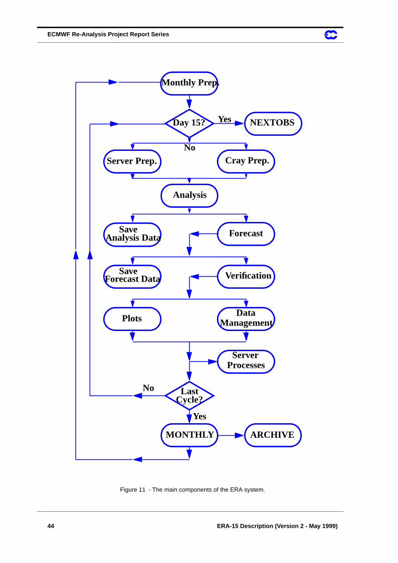
ECMWF Re-Analysis Project Report Series
44 ERA-15 Description (Version 2 - May 1999)
Figure 11 - The main components of the ERA system.
Monthly Prep.
Day 15? Yes
No
Yes
No LastCycle?
NEXTOBS
MONTHLY ARCHIVE
Server Prep. Cray Prep.
Analysis
ForecastSaveAnalysis Data
SaveForecast Data
Plots
Verification
DataManagement
ServerProcesses
ECMWF Re-Analysis Project Report Series
ERA-15 Description (Version 2 - May 1999) 45
Results in the form of analysis and forecast fields were stored initially for a short time within the CRAY C90
fields data base, to allow rapid access by subsequent CRAY C90 tasks. They were also inserted into an
EMPRESS data base on the SGI system soon after they had been produced, and accumulated for one month
before being added to the IBM based archive. At all stages the fields data were accessible using MARS; thus
the ERA system was fully re-startable from any data assimilation cycle within the month.
Analysis feedback statistics were moved to an SGI server as produced, and entered into an EMPRESS data
base of identical structure to that used for the observations.
When the 15th of each month was reached the module to organize the observations for two months ahead
was started; this enabled preparation of the observations to be completed well before they were needed, and
action to be taken in good time when problems were detected.
At the end of each month of production the bias corrections required for the 1D-VAR system were computed
from the accumulated statistics, and results for the current month added to the archive. Next, a search was
made for the file containing the required information to generate the next month's blacklist of suspect
stations. If this file existed, the blacklist was generated and the data assimilation module repeated for the next
month. If not, the system suspended itself awaiting manual recovery.
Special dumps of strategic files, libraries and binaries were made at the end of each month of production; this
enabled any month to be re-run, using starting conditions identical to those of the earlier production.
6.5 Adding results to the archive
The ECMWF Meteorological Archive and Retrieval System (MARS) is the basic system for the
management of the Centre's archives. MARS allows data to be described using a command language based
on attributes which approximate to a reasonable meteorological definition of the data. Some of these
attributes are universally obvious, such as parameter, level, time, step, and representation. Others are
somewhat less intuitive, but enable a precise description to be made concerning which of a number of
possible sub-sets of similar data are actually being defined. Thus attributes such as “expver” (experiment
version number), and “class” (operational, research, ERA) provide full facilities for the extension of MARS
not only for use with a project such as re-analysis, but also for the retention of many variants of the same data
- especially useful where parts of a re-analysis may need to be re-run.
It was decided to archive ERA fields as monthly files within the MARS system. This allows efficient retrieval
of long periods of data, and reduces the number of files to be accommodated. This is an important consider-
ation, as the file management system on which MARS depends operates more efficiently if the numbers of
files can be minimized. The MARS system provides the mapping between the described data (described in
ECMWF Re-Analysis Project Report Series
46 ERA-15 Description (Version 2 - May 1999)
Meteorological terms) and the physical data within physical files. It was also decided that all archive
processes would be initiated from the SGI servers. To support this a considerable amount of development of
the MARS system was required.
Within MARS a separate “class” has been added for ERA. This has enabled the MARS “expver” parameter
to be used to distinguish between different versions of re-analysis data which have been added to the archive.
It has also enabled checking and experimental runs to be made without prejudice to the main production
archive.
In addition to the archive of the analysis and forecast fields, data sets containing important job output,
selected post-script files, and files containing analysis feedback information are stored. An analysis of
satellite data processing for each previous month was performed, resulting in appropriate plots and statistics
which could be used carefully to monitor the performance of the 1D-Variational scheme. Tasks were also run
at the end of each production month to compute radiosonde bias corrections for the next month.
6.6 Checking the archive files
It was essential to verify that the fields which had been added to the archive at the level of the IBM could be
accessed. Since it would be too costly in terms of computer and disk space resources to retrieve and check
every individual field, selected fields from at least two dates within every archive file were checked. The
selected fields were retrieved, decoded, and summary information printed.
6.7 Production log
During the ERA production a considerable amount of monitoring was carried out in order to identify, and
where possible rectify deficiencies. A production log was kept in which all changes and events of note where
listed. Information concerning the use of satellite data, the various sources of observations, and the sea
surface temperature used has already been given in section 3. on page 7. Table 5 lists those events noted
during the production which may have a significant bearing on the re-analysis data.
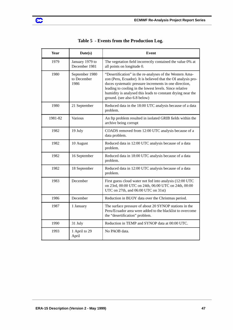
ECMWF Re-Analysis Project Report Series
ERA-15 Description (Version 2 - May 1999) 47
Table 5 - Events from the Production Log.
Year Date(s) Event
1979 January 1979 toDecember 1981
The vegetation field incorrectly contained the value 0% atall points on longitude 0.
1980 September 1980to December1986
“Desertification” in the re-analyses of the Western Ama-zon (Peru, Ecuador). It is believed that the OI analysis pro-duces systematic pressure increments in one direction,leading to cooling in the lowest levels. Since relativehumidity is analysed this leads to constant drying near theground. (see also 6.8 below)
1980 21 September Reduced data in the 18:00 UTC analysis because of a dataproblem.
1981-82 Various An ftp problem resulted in isolated GRIB fields within thearchive being corrupt
1982 19 July COADS removed from 12:00 UTC analysis because of adata problem.
1982 10 August Reduced data in 12:00 UTC analysis because of a dataproblem.
1982 16 September Reduced data in 18:00 UTC analysis because of a dataproblem.
1982 18 September Reduced data in 12:00 UTC analysis because of a dataproblem.
1983 December First guess cloud water not fed into analysis (12:00 UTCon 23rd, 00:00 UTC on 24th, 06:00 UTC on 24th, 00:00UTC on 27th, and 06:00 UTC on 31st)
1986 December Reduction in BUOY data over the Christmas period.
1987 1 January The surface pressure of about 20 SYNOP stations in thePeru/Ecuador area were added to the blacklist to overcomethe “desertification” problem.
1990 31 July Reduction in TEMP and SYNOP data at 00:00 UTC.
1993 1 April to 29April
No PAOB data.

ECMWF Re-Analysis Project Report Series
48 ERA-15 Description (Version 2 - May 1999)
6.8 Post-production log
After finalizing the ERA-15 production, the output analysis and short-range forecast fields (listed in section
7.) have been used extensively and evaluated both internally at ECMWF and externally by the scientific
community at large. During these activities some further problems and deficiencies have been uncovered.
The most serious are listed here; more details about many of them may be found in Report No. 2 “Aspects of
the Re-Analysed Climate” in this series of ECMWF Re-Analysis Project Reports.
• Surface temperature in extremely stable conditions.Primarily over the Antarctic Icesheet,
but also noticed over Greenland, the ERA-15 surface temperatures drop to unrealistically low
values, sometimes down to -90oC. In extremely stable conditions the vertical diffusion of heat in
the forecast model vanished almost entirely. Hence the surface temperature was determined
entirely by the radiative balance.
Throughout Due to a programming error in the forecast model, theentire ERA was run with very little regard to the latent heatof freezing/melting in the convection. The sensitivity ofthis error was evaluated in a one month parallel assimila-tion, and it was shown to impact the zonal mean tempera-ture in the ITCZ to some extent, at most by 0.2K around500mb. There was also a small impact on the precipitation,primarily as redistribution of local convective maxima inthe ITCZ. Since the bug was only discovered after severalyears of assimilation, and was not considered too serious,it was decided to complete ERA with the bug included, inorder not to introduce a discontinuity in the ITCZ ‘cli-mate’.
Throughout For surface data the main source of observations wereSYNOP reports exchanged over the WMO GTS. In theearly years many stations did not report snow depth.Where available, the analysis system used takes account ofreported snow depth. Thus in some areas the snow depthinformation within the re-analysis, especially for earlyyears, is largely model generated.
Throughout Three “sea points” in Lake Victoria have constant sea sur-face temperatures of about 17 deg. C. which is too low.This results in a local minimum in convective precipitationover the lake.
Throughout A spurious sea point within the Congo basin is seen to pro-duce surface energy fluxes more typical of tropical oceanthan neighbouring land points.
Table 5 - Events from the Production Log.
Year Date(s) Event
ECMWF Re-Analysis Project Report Series
ERA-15 Description (Version 2 - May 1999) 49
• Antarctic orography. The orography database used for ERA-15 had substantial errors in the
interior of Antarctica, locally exceeding one kilometre.
• Station height at Vostok.The WMO reported station height of Vostok (107oE, 78.5oS) had an
error of about 70 meters. This error was ‘too small’ to be discovered by the Quality Control pro-
cedures in the Optimum Interpolation (O/I) scheme in this otherwise completely data-void Ant-
arctic interior. Hence there is a fictitious low in the mean ERA-15 analyses reaching from the
surface at 600hPa a few 100hPa upwards. The mass and wind analyses should be used with
utmost care in that part of the world.
• Surface temperatures in boreal forests during spring.An unrealistically large value was used
for the albedo in high latitude regions covered by evergreen forests (taiga). As a consequence the
ERA-15 surface and 2-metre temperatures are unrealistically cold in the affected areas during
spring - still snow covered but with substantial solar radiation. Extremely, in parts of Siberia and
Canada, the 2-metre temperature may be down to 10oC too cold in April. There is also some
impact on temperatures in the lower free atmosphere, primarily below 850hPa.
• Non-representative island stations.In the O/I scheme, 10-metre winds from isolated island
stations were used. Due to local effects, these observations are not representative of the near-sur-
face wind fields over the surrounding sea. During the subsequent forecast phase of the data
assimilation, the wind speeds in the vicinity of these stations recover, causing spin-up effects in
the surface exchange processes. Primarily the evaporation and, consequently, the precipitation
are affected, mostly in the ITCZ, and worst in the western Pacific.
• The “Amazon” problem. After several years of assimilation, a serious error was discovered in
the soil temperatures and soil wetness in a small region in the western most equatorial Amazon
basin (west of 70oW). From September 1980 to the end of 1986, this area is too hot and too dry.
Due to the time limitations of the ERA project it was not possible to reprocess the full period
affected once the problem was discovered. The period before September 1980 was, however, re-
run for other reasons, and does contain the correction for this problem. The drying out was a
combined effect of the O/I scheme using relative humidity as its humidity variable, and the local
failure of the method used to compensate for the semi-diurnal tide in the observed surface pres-
sures in this low lying area very close to the high Andes. After blacklisting surface pressure
observations from the critical region, the soil and precipitation quickly recovered to realistic val-
ues, but the long term hydrology of the Amazon basin in ERA-15 is not correct. (see also table 5
in the previous section)
• Temperature and humidity biases in the tropics.In ERA-15 TOVS satellite cloud cleared
radiances (CCRs) from a long series of NOAA satellites were used in a one-dimensional varia-
tional approach. The method requires a minimization of the effects of drift and sudden changes
ECMWF Re-Analysis Project Report Series
50 ERA-15 Description (Version 2 - May 1999)
in the instrumental outputs. This is done by inter-calibration and bias correction of the IR and
microwave radiation from the radiometers. In spite of extensive monitoring, quality control and
bias correction, the ERA-15 analyses suffer from changes in the instrument behaviour. The
impact is seen as sudden ‘jumps’ in timeseries of the analyzed temperatures and humidities in
the lower troposphere, primarily at low latitudes. The worst instance is in November 1986 when
an unrealistically large scale warming and moistening of the ITCZ took place. Although these
jumps are believed not to affect the day-to-day synoptic developments in ERA-15 too badly -
they are for instance not noticeable in first guess comparisons with radiosondes - great care
should nevertheless be taken when attempting to use the reanalyses for studies of, for example,
long-term ‘climate’ trends.
ECMWF Re-Analysis Project Report Series
ERA-15 Description (Version 2 - May 1999) 51
7. Re-Analysis Output
7.1 Analysis and Forecast Fields
The WMO representation form FM92 GRIB is used to represent all analysis and forecast fields. In general,
ERA GRIB data are coded using ECMWF’s local version of GRIB code table 2 (version number 128), which
gives parameter names and units. An additional local version of GRIB code table 2 (version 160) is used for
some monthly, seasonal, yearly, and climatological parameters. Local version 160 was devised for ERA use,
and enables time normalised flux values, variances, and co-variances to be represented. When allocating
parameter numbers within table 160 a close correspondence with the numbering system of table 128 has
been maintained. Thus, with a few minor exceptions, code figures from table 160 refer to the same
parameters as code figures from table 128 (but with time normalised units for accumulated values). The
exceptions are with respect to a few originally unused entries in table 128 used for extra parameters in table
160, which have since been allocated to serve other needs within table 128.
7.1.1 Daily data
Primary data have been saved from each analysis, the four times daily 6 hour forecasts, and every six hourly
intervals from the twice-daily forecasts extended to 24 hours. Initialised analysis data are stored as time 0 of
the forecast data. Data from ten day forecasts based on ERA data have been saved at 12 hourly intervals
throughout the forecasts. The resulting archive contains data at the resolution and on the spatial grid of the
assimilation system for the 31 model levels (seeVertical resolution: on page 30), for 17 pressure levels
(1000, 925, 850, 775, 700, 600, 500, 400, 300, 250, 200, 150, 100, 70, 50, 30, and 10 hPa), and for surface
and single level parameters. In addition pressure level and single level data are available on a regular 2.5
degree latitude/longitude grid. Interpolation rfrom T106 spherical harmonics has been achieved by first
truncating to T47, then transforming to the 2.5 degree grid.
Table 6 gives details of the upper air parameters; these include the logarithm of surface pressure, which
although not strictly an “upper air” parameter is produced in spherical harmonics along with the model level
data, and is required to compute the pressures of the data points. The table indicates which parameters are
stored at model levels, and which are stored on pressure levels. The various horizontal representations are
indicated by sh (spherical harmonics), gg (Gaussian grid), and 2.5o (2.5 degree latitude/longitude grid).
Except where indicated, parameters are available from both the analyses and the forecasts.
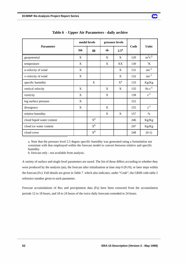
ECMWF Re-Analysis Project Report Series
52 ERA-15 Description (Version 2 - May 1999)
.
A variety of surface and single level parameters are saved. The list of these differs according to whether they
were produced by the analysis (an), the forecast after initialisation at time step 0 (Fc/0), or later steps within
the forecast (Fc). Full details are given in Table 7 which also indicates, under “Code”, the GRIB code table 2
reference number given to each parameter.
Forecast accumulations of flux and precipitation data (Fa) have been extracted from the accumulation
periods 12 to 18 hours, and 18 to 24 hours of the twice daily forecasts extended to 24 hours
Table 6 - Upper Air Parameters - daily archive
Parametermodel levels pressure levels
Code Unitslsh gg sh 2.5o
geopotential X X X 129 m2s-2
temperature X X XX 130 ˚K
u-velocity of wind X X 131 ms-1
v-velocity of wind X X 132 ms-1
specific humidity X Xa
a. Note that the pressure level 2.5 degree specific humidity was generated using a formulation notconsistant with that emplouyed within the forecast model to convert between relative and specifichumidity.
133 Kg/Kg
vertical velocity X X X 135 Pa s-1
vorticity X X 138 s-1
log surface pressure X 152
divergence X X 155 s-1
relative humidity X X 157 %
cloud liquid water content Xb
b. forecast only - not available from analysis.
246 Kg/Kg
cloud ice water content Xb 247 Kg/Kg
cloud cover Xb 248 (0-1)
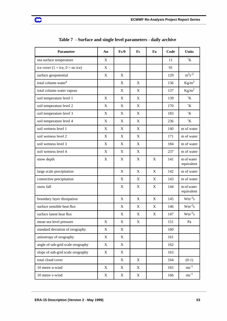
ECMWF Re-Analysis Project Report Series
ERA-15 Description (Version 2 - May 1999) 53
.
Table 7 - Surface and single level parameters - daily archive
Parameter An Fc/0 Fc Fa Code Units
sea surface temperature X 11 ˚K
ice cover (1 = ice, 0 = no ice) X 91
surface geopotential X X 129 m2s-2
total column watera X X 136 Kg/m2
total column water vapour X X 137 Kg/m2
soil temperature level 1 X X X 139 ˚K
soil temperature level 2 X X X 170 ˚K
soil temperature level 3 X X X 183 ˚K
soil temperature level 4 X X X 236 ˚K
soil wetness level 1 X X X 140 m of water
soil wetness level 2 X X X 171 m of water
soil wetness level 3 X X X 184 m of water
soil wetness level 4 X X X 237 m of water
snow depth X X X X 141 m of waterequivalent
large scale precipitation X X X 142 m of water
convective precipitation X X X 143 m of water
snow fall X X X 144 m of waterequivalent
boundary layer dissipation X X X 145 Wm-2s
surface sensible heat flux X X X 146 Wm-2s
surface latent heat flux X X X 147 Wm-2s
mean sea level pressure X X X 151 Pa
standard deviation of orography X X 160
anisotropy of orography X X 161
angle of sub-grid scale orography X X 162
slope of sub-grid scale orography X X 163
total cloud cover X X 164 (0-1)
10 metre u-wind X X X 165 ms-1
10 metre v-wind X X X 166 ms-1

ECMWF Re-Analysis Project Report Series
54 ERA-15 Description (Version 2 - May 1999)
2 metre temperature X X X 167 ˚K
2 metre dewpoint X X X 168 ˚K
surface solar radiation downwardb X X 169 Wm-2s
land/sea mask X X 172 (0,1)
surface roughness X X 173 m
albedo X X 174
surface thermal radiation downwardsb X X 175 Wm-2s
surface solar radiation X X 176 Wm-2s
surface thermal radiation X X 177 Wm-2s
top solar radiation X X 178 Wm-2s
top thermal radiation X X 179 Wm-2s
u-component of stress X X 180 Nm-2s
v-component of stress X X 181 Nm-2s
evaporation X X 182 m of water
convective cloud cover X X 185 (0-1)
low cloud cover X X 186 (0-1)
medium cloud cover X X 187 (0-1)
high cloud cover X X 188 (0-1)
latitudinal component of gravity wavestress
X X X 195 Nm-2s
meridional component of gravitywave stress
X X X 196 Nm-2s
gravity wave dissipation X X X 197 Wm-2s
skin reservoir content X X X 198 m of water
percentage of vegetation X X 199 %
runoff X X X 205 m of water
instantaneous X component of surfacestress
X X 229 Nm-2
Instantaneous Y component of sur-face stress
X X 230 Nm-2
instantaneous surface heat flux X X 231 Wm-2
Table 7 - Surface and single level parameters - daily archive
Parameter An Fc/0 Fc Fa Code Units
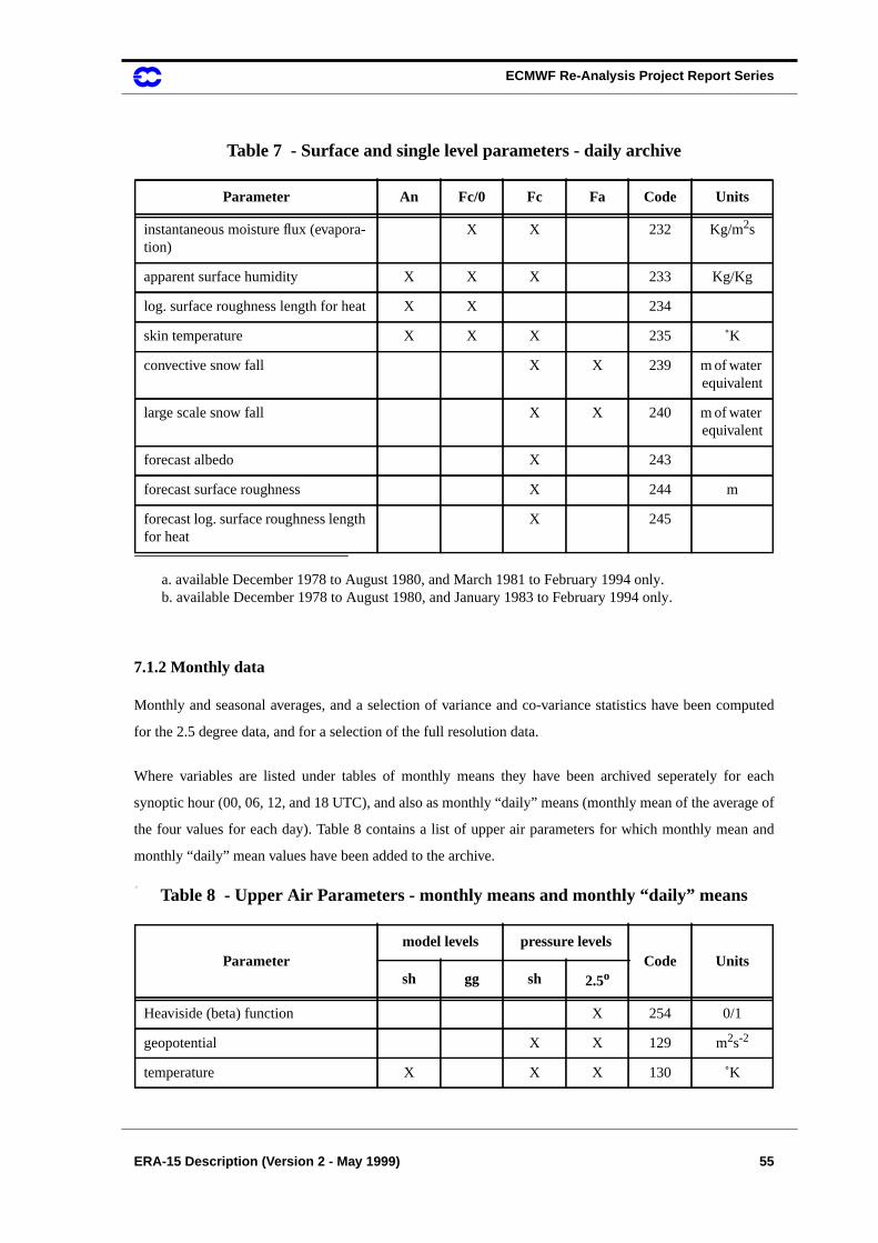
ECMWF Re-Analysis Project Report Series
ERA-15 Description (Version 2 - May 1999) 55
7.1.2 Monthly data
Monthly and seasonal averages, and a selection of variance and co-variance statistics have been computed
for the 2.5 degree data, and for a selection of the full resolution data.
Where variables are listed under tables of monthly means they have been archived seperately for each
synoptic hour (00, 06, 12, and 18 UTC), and also as monthly “daily” means (monthly mean of the average of
the four values for each day). Table 8 contains a list of upper air parameters for which monthly mean and
monthly “daily” mean values have been added to the archive.
.M
instantaneous moisture flux (evapora-tion)
X X 232 Kg/m2s
apparent surface humidity X X X 233 Kg/Kg
log. surface roughness length for heat X X 234
skin temperature X X X 235 ˚K
convective snow fall X X 239 m of waterequivalent
large scale snow fall X X 240 m of waterequivalent
forecast albedo X 243
forecast surface roughness X 244 m
forecast log. surface roughness lengthfor heat
X 245
a. available December 1978 to August 1980, and March 1981 to February 1994 only.b. available December 1978 to August 1980, and January 1983 to February 1994 only.
Table 8 - Upper Air Parameters - monthly means and monthly “daily” means
Parametermodel levels pressure levels
Code Unitssh gg sh 2.5o
Heaviside (beta) function X 254 0/1
geopotential X X 129 m2s-2
temperature X X X 130 ˚K
Table 7 - Surface and single level parameters - daily archive
Parameter An Fc/0 Fc Fa Code Units
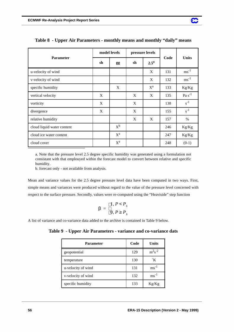
ECMWF Re-Analysis Project Report Series
56 ERA-15 Description (Version 2 - May 1999)
Mean and variance values for the 2.5 degree pressure level data have been computed in two ways. First,
simple means and variances were produced without regard to the value of the pressure level concerned with
respect to the surface pressure. Secondly, values were re-computed using the “Heaviside” step function
A list of variance and co-variance data added to the archive is contained in Table 9 below.
u-velocity of wind X 131 ms-1
v-velocity of wind X 132 ms-1
specific humidity X Xa 133 Kg/Kg
vertical velocity X X X 135 Pa s-1
vorticity X X 138 s-1
divergence X X 155 s-1
relative humidity X X 157 %
cloud liquid water content Xb 246 Kg/Kg
cloud ice water content Xa 247 Kg/Kg
cloud cover Xa 248 (0-1)
a. Note that the pressure level 2.5 degree specific humidity was generated using a formulation notconsistant with that emplouyed within the forecast model to convert between relative and specifichumidity.b. forecast only - not available from analysis.
Table 9 - Upper Air Parameters - variance and co-variance dats
Parameter Code Units
geopotential 129 m2s-2
temperature 130 ˚K
u-velocity of wind 131 ms-1
v-velocity of wind 132 ms-1
specific humidity 133 Kg/Kg
Table 8 - Upper Air Parameters - monthly means and monthly “daily” means
Parametermodel levels pressure levels
Code Unitssh gg sh 2.5o
β1 P Ps<,
0 P Ps≥,
=

ECMWF Re-Analysis Project Report Series
ERA-15 Description (Version 2 - May 1999) 57
For surface and single level parameters monthly values were created both for each model produced
parameter on an “as is” basis, and in a time normalised manner.
vertical velocity 135 Pa s-1
relative humidity 157 %
SD of geopotential 206 m2s-2
cov. temperature and geopotential 207 Km2s-2
SD of temperature 208 K
cov. sp. humidity and geopotential 209 m2s-2
cov. sp. humidity and temperature 210 K
SD of specific humidity 211 (0 - 1)
cov. u-wind and geopotential 212 m3s-3
cov. u-wind and temperature 213 Kms-1
cov. u-wind and specific humidity 214 ms-1
SD of u-velocity of wind 215 ms-1
cov. v-wind and geopotential 216 m3s-3
cov. v-wind and temperature 217 Kms-1
cov. v-wind and specific humidity 218 ms-1
cov. v-wind and u-wind 219 m2s-2
SD of v-velocity of wind 220 ms-1
cov. vertical velocity and geopotential 221 Pam2s-3
cov. vertical velocity and temperature 222 KPas-1
cov. vertical velocity and specifichumidity
223 Pas-1
cov. vertical velocity u-wind 224 Pams-2
cov. vertical velocity and v-wind 225 Pams-2
SD of vertical velocity 226 Pas-1
SD of relative humidity 227 %
Table 9 - Upper Air Parameters - variance and co-variance dats
Parameter Code Units
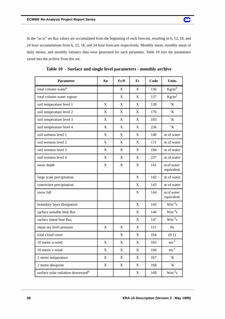
ECMWF Re-Analysis Project Report Series
58 ERA-15 Description (Version 2 - May 1999)
In the “as is” set flux values are accumulated from the beginning of each forecast, resulting in 6, 12, 18, and
24 hour accumulations from 6, 12, 18, and 24 hour forecasts respectively. Monthly mean, monthly mean of
daily means, and monthly variance data were generated for each parameter. Table 10 lists the parameters
saved into the archive from this set.
.
Table 10 - Surface and single level parameters - monthly archive
Parameter An Fc/0 Fc Code Units
total column watera X X 136 Kg/m2
total column water vapour X X 137 Kg/m2
soil temperature level 1 X X X 139 ˚K
soil temperature level 2 X X X 170 ˚K
soil temperature level 3 X X X 183 ˚K
soil temperature level 4 X X X 236 ˚K
soil wetness level 1 X X X 140 m of water
soil wetness level 2 X X X 171 m of water
soil wetness level 3 X X X 184 m of water
soil wetness level 4 X X X 237 m of water
snow depth X X X 141 m of waterequivalent
large scale precipitation X 142 m of water
convective precipitation X 143 m of water
snow fall X 144 m of waterequivalent
boundary layer dissipation X 145 Wm-2s
surface sensible heat flux X 146 Wm-2s
surface latent heat flux X 147 Wm-2s
mean sea level pressure X X X 151 Pa
total cloud cover X X 164 (0-1)
10 metre u-wind X X X 165 ms-1
10 metre v-wind X X X 166 ms-1
2 metre temperature X X X 167 ˚K
2 metre dewpoint X X X 168 ˚K
surface solar radiation downwardb X 169 Wm-2s
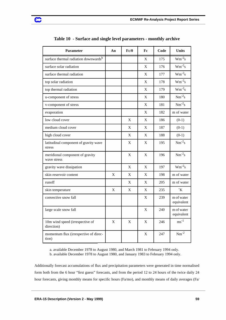
ECMWF Re-Analysis Project Report Series
ERA-15 Description (Version 2 - May 1999) 59
Additionally forecast accumulations of flux and precipitation parameters were generated in time normalised
form both from the 6 hour “first guess” forecasts, and from the period 12 to 24 hours of the twice daily 24
hour forecasts, giving monthly means for specific hours (Fa/mo), and monthly means of daily averages (Fa/
surface thermal radiation downwardsb X 175 Wm-2s
surface solar radiation X 176 Wm-2s
surface thermal radiation X 177 Wm-2s
top solar radiation X 178 Wm-2s
top thermal radiation X 179 Wm-2s
u-component of stress X 180 Nm-2s
v-component of stress X 181 Nm-2s
evaporation X 182 m of water
low cloud cover X X 186 (0-1)
medium cloud cover X X 187 (0-1)
high cloud cover X X 188 (0-1)
latitudinal component of gravity wavestress
X X 195 Nm-2s
meridional component of gravitywave stress
X X 196 Nm-2s
gravity wave dissipation X X 197 Wm-2s
skin reservoir content X X X 198 m of water
runoff X X 205 m of water
skin temperature X X X 235 ˚K
convective snow fall X 239 m of waterequivalent
large scale snow fall X 240 m of waterequivalent
10m wind speed (irrespective ofdirection)
X X X 246 ms-1
momentum flux (irrespective of direc-tion)
X 247 Nm-2
a. available December 1978 to August 1980, and March 1981 to February 1994 only.b. available December 1978 to August 1980, and January 1983 to February 1994 only.
Table 10 - Surface and single level parameters - monthly archive
Parameter An Fc/0 Fc Code Units
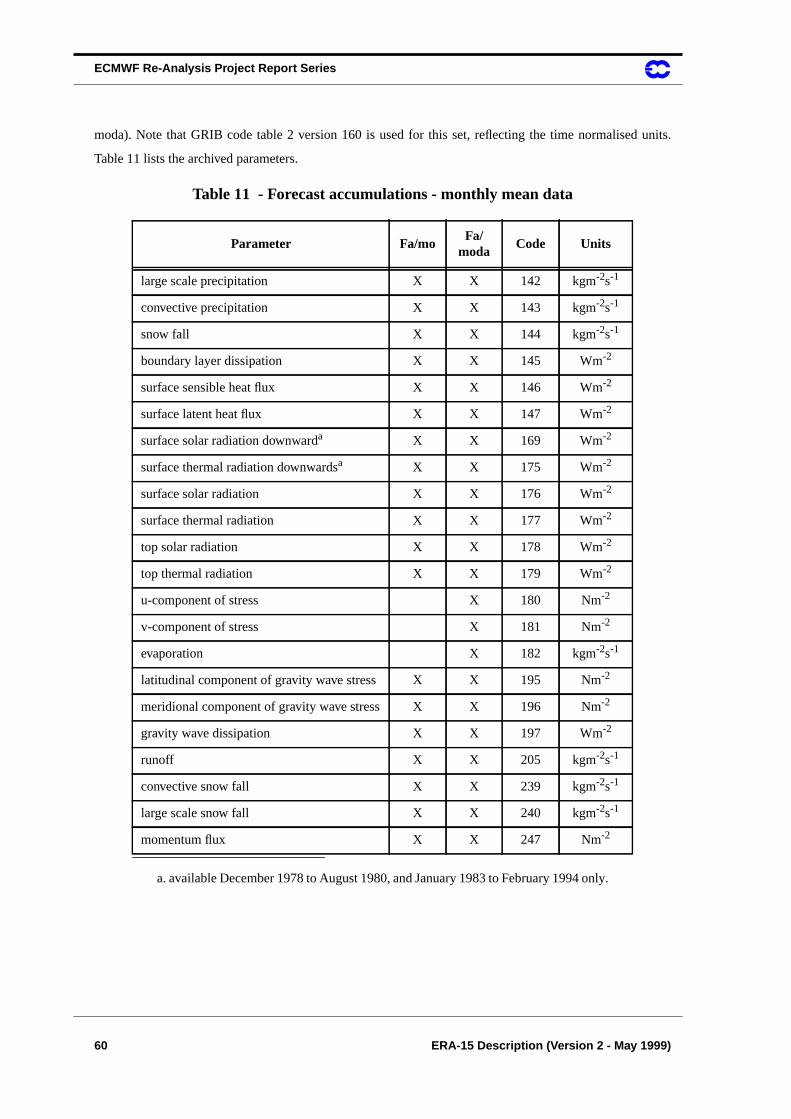
ECMWF Re-Analysis Project Report Series
60 ERA-15 Description (Version 2 - May 1999)
moda). Note that GRIB code table 2 version 160 is used for this set, reflecting the time normalised units.
Table 11 lists the archived parameters.
Table 11 - Forecast accumulations - monthly mean data
Parameter Fa/moFa/
modaCode Units
large scale precipitation X X 142 kgm-2s-1
convective precipitation X X 143 kgm-2s-1
snow fall X X 144 kgm-2s-1
boundary layer dissipation X X 145 Wm-2
surface sensible heat flux X X 146 Wm-2
surface latent heat flux X X 147 Wm-2
surface solar radiation downwarda
a. available December 1978 to August 1980, and January 1983 to February 1994 only.
X X 169 Wm-2
surface thermal radiation downwardsa X X 175 Wm-2
surface solar radiation X X 176 Wm-2
surface thermal radiation X X 177 Wm-2
top solar radiation X X 178 Wm-2
top thermal radiation X X 179 Wm-2
u-component of stress X 180 Nm-2
v-component of stress X 181 Nm-2
evaporation X 182 kgm-2s-1
latitudinal component of gravity wave stress X X 195 Nm-2
meridional component of gravity wave stress X X 196 Nm-2
gravity wave dissipation X X 197 Wm-2
runoff X X 205 kgm-2s-1
convective snow fall X X 239 kgm-2s-1
large scale snow fall X X 240 kgm-2s-1
momentum flux X X 247 Nm-2
ECMWF Re-Analysis Project Report Series
ERA-15 Description (Version 2 - May 1999) 61
7.2 Data from ERA - observations and feedback
The observed values presented to the analyses together with difference statistics with respect to the analyses,
the initialized analyses, and the 6 hour forecasts used as “first guess” have been stored. The difference
statistics contained within these data contain a wealth of information concerning the characteristics of the
data assimilation system, and of the observing system.
7.3 Other data
Throughout the ERA production all important job output for the various sub-systems of the production
system were collected into monthly files and added to the archives. Individual outputs for single jobs within
these files can be obtained where required, enabling investigations to be carried out into specific cases where
necessary.
As routine, a number of graphical plots were generated and stored on-line for monitoring purposes. These
include data coverage maps, analysis increments, and maps of selected parameters. At the end of each
production month these plot files were organised into a suitable form and added to the archive.
7.4 Availability of ERA data
Data from ERA are made available to research scientists throughout the world. The Data Services Unit at
ECMWF are able to extract and supply sub-sets of data to meet users' requirements, and will supply full
details on request. Enquiries should be addressed to:
Data Services,ECMWF,Shinfield Park,Reading, RG2 9AX,U.K.
or by e-mail to [email protected].
Additionally, selected data are available to the German academic community from the Max-Plank-Intstitut,
Hamburg; to the United Kingdom academic community through the British Atmospheric Data Centre,
Rutherford Appleton Laboratory, Didcot; to the UCAR community in the United States of America through
the National Center for Atmospheric Research; and to the Atmospheric Model Iintercomparison Project
(AMIP) community through the Program for Climate Model Diagnostics and Intercomparison (PCMDI),
University of California, Lawrence Livermore National Laboratory.
ECMWF Re-Analysis Project Report Series
62 ERA-15 Description (Version 2 - May 1999)
8. Concluding Remarks
The production of a completely consistent global re-analysis would require a consistent observing system
with respect both to the quantity and quality of observations. This requirement cannot be met in its entirety
from the historical record. In consequence, the ERA project has attempted to apply a consistent data assimi-
lation scheme to a reasonable sub-set of those data which are available, and to contributing components of
the observing system which have been reasonably consistent throughout the 15 year period.
Probably the most important contributing system is the cloud cleared radiance data set from the polar
orbiting satellites. Through the use of the 1D-Variational method a specific attempt has been made within the
ERA project to maximise the use of these data with respect both to the mass/wind analyses and the humidity
analyses.
The very considerable efforts made initially to ensure the selection of a suitably high quality assimilation
system led to a programme of research and experimentation which yielded much in terms of useful feedback
and development not only for ERA but also for ECMWF’s research and operations.
Data from ERA are already extensively used for research purposes within ECMWF, and have provided the
raw material for a number of interesting validation reports (ECMWF, 1997). They have been made available
to the ECMWF Member States through the Centre’s archives, to the AMIP community through PCMDI, to
the United States’ academic community through UCAR/NCAR, and to research workers elsewhere through
the ECMWF Data Services.
ECMWF Re-Analysis Project Report Series
ERA-15 Description (Version 2 - May 1999) 63
References:
Andersson, E., Hollingsworth, A., Kelly, G., Lonnberg, P., Pailleux, J. and Zhang, Z. 1991: Global observing
system experiments on operational statistical retrievals of satellite sounding data. Mon. Weather
Rev., 119, 1851-1864.
Bengtsson, L., Shukla, J., 1988: Integration of Space and In Situ Observations to Study Global Climate
Change. Bull. Amer. Meteorol. Soc., 69, 1130-1143.
ECMWF Data Assimilation, 1992: Research Manual 1 - ECMWF Data Assimilation Scheme - Scientific
Documentation - ECMWF Meteorol. Bull. M1.5/3.
ECMWF Forecast System, 1992: Research Manual 2 - ECMWF Forecast Model Documentation - Adiabatic
Part - ECMWF Meteorol. Bull. M1.6/3.
ECMWF Forecast System, 1992: Research Manual 3 - ECMWF Forecast Model Documentation - Physical
Parametrization - ECMWF Meteorol. Bull. M1.6/2.
Eliassen, A., 1954: Provisional report on calculation of spatial covariance and autocorrelation of the pressure
field. Inst. Weather and Climate Res., Acad. Sci. Oslo, Rept. No. 5.
Eyre, J. R. 1989: Inversion of cloudy satellite sounding radiances by nonlinear optimal estimation. Q. J. R.
Meteorol. Soc., 113, 1001-1037.
Eyre, J. R. 1991: A fast radiative transfer model for satellite sounding systems. ECMWF Technical Memo-
randum 176.
Eyre, J. R. 1992: A bias correction scheme for simulated TOVS brightness temperatures. ECMWF Technical
Memorandum 186.
Eyre, J. R., Kelly, G. A., McNally, A. P., and Anderson, E., 1992: Assimilation of TOVS radiance informa-
tion through one-dimensional variational analysis - ECMWF Technical Memorandum No. 187,
July 1992.
Eyre, J. R., Kelly, G. A., McNally, A. P., Andersson, E. and Persson, A. 1993: Assimilation of TOVS radi-
ance information through one-dimensional variational analysis. Q. J. R. Meteorol. Soc., 119,
1427-1463.
Gandin, L. S., 1963: Objective analysis of meteorological fields. Translated from Russian by Israeli Program
of Scientific Translations, 1965, 242pp.
ECMWF Re-Analysis Project Report Series
64 ERA-15 Description (Version 2 - May 1999)
Jakob, C., 1994: The Impact of the New Cloud Scheme on ECMWF’s Integrated Forecast System (IFS). Pro-
ceedings of ECMWF/GEWEX Workshop on Modelling, Validation and Assimilation of Clouds,
ECMWF, November 1994.
Lönnberg P., 1988: Developments in the ECMWF analysis system. ECMWF Seminar Proceedings - Data
assimilation and the use of satellite data. Vol. I, 75-119.
Lorenc A.C., 1981: A global three-dimensional multivariate statistical interpretation scheme. Mon. Weather
Rev., 109, 701-721.
Lott, F., and Miller, M. J., 1997: A new subgrid-scale orographic drag parametrization: Its formulation and
testing. Quart. J. Roy. Meteor. Society, 123, 101-127.
Mahfouf, J.F., 1991:Analysis of soil moisture from near surface parameters: A feasibility study. J. Appl.
Meteor., 30, 1534-1547.
McMillin, L. M., and Dean, C. 1982: Evaluation of a new operational technique for producing clear radi-
ances. J. Appl. Meteorol., 21, 1005-1014.
McNally, A. P., and Vesperini, M., 1996: Variational analysis of humidity information from TOVS radiances.
Q. J. R. Meteorol. Soc., 122, 1521-1544.
NESDIS, 1993: Polar Orbiter Archived TOVS Soundin Data Change and Problem Record, and TOVS Oper-
ational Processing/Changes. NOAA/NESDIS, personal communication.
Nomura A., 1997: Global Sea Ice Concentration Data Set for use with the ECMWF Re-Analysis System
ECMWF Project Report Series, 4. (previously issued as ECMWF Technical Report No. 76, March
1995.)
NSIDC, 1992: DMSP SSM/I Brightness Temperature and Sea Ice Concentration Grids for the Polar Regions
on CD-ROM. User’s Guide.
NSIDC, 1993: Nimbus-7 SMMR Polar Radiances and Arctic and Antarctic Sea Ice Concentrations on CD-
ROM. User’s Guide, Third Revised Edition.
Gaffen, D. J., 1993: WMO TD No. 541.
Parker, D. E., Folland C. K., Ward M. N., Jackson M., and Maskell K., 1995: Marine surface data for analysis
of climate fluctuations on interannual to century timescales. In D. G. Martinson, K. Bryan, M.
Ghil, M. M. Hall, T. R. Karl, E. S. Sarachik, S. Sorooshian, and L. D. Talley, editors, Natural Cli-
ECMWF Re-Analysis Project Report Series
ERA-15 Description (Version 2 - May 1999) 65
mate Variability on Decade-to-Century Time Scales, 241-250. National Academy Press, Washing-
ton, D.C.
Pesonen, O., and Raoult, B., 1992: SMS and CDP User Guide and Reference Manual, ECMWF.
Rayner, N. A., Horton E. B., Parker D. E., Folland C. K., and Hackett R. B., 1996: Version 2.2 of the Global
sea-ice and Sea Surface Temperature data set, 1903-1994. CRTN 74, September 1996, Hadley
Centre.
Reynolds, R. W. and Smith T. M., 1994: Improved Global Sea Surface Temperature Analysis Using Opti-
mum Interpolation. J. Climate, 7, 929-948.
Ritchie H., Temperton C., Simmons A.J., Hortal M., Davies T., Dent D., Hamrud M., 1995: Implementation
of the Semi-Lagrangian Method in a High Resolution Version of the ECMWF Forecast Model.
Mon. Weather Rev., 123, 489-514.
Shaw D.B., Lönnberg P., Hollingsworth A. and Undén P., 1987: Data assimilation: The 1984/85 revision of
the ECMWF mass and wind analysis. Q. J. R. Meteorol. Soc., 113, 533-566.
Slingo J.J., 1987: The development and verification of a cloud prediction scheme for the ECMWF model. Q.
J. R. Meteorol. Soc., 213, 899-927.
Smith, W. L., Woolf, H. M., 1976: The use of eigenvectors of statistical covariance matrices for interpreting
satellite sounding radiometer observations. J. Atmos. Sci., 33, 1127-1150.
Tiedtke M., 1989: A comprehensive massflux scheme for cumulus parametrization in large-scale models.
Mon. Weather Rev., 117, 1779-1800.
Tiedtke M, 1993: Representation of clouds in large-scale models. Mon. Weather Rev., 121, 3040-3061
Undén P., 1989: Tropical data assimilation and analysis of divergence. Mon.Weather Rev., 117, 2495-2517.
Vasiljevic, D., 1990; Use of First Guess at Appropriate Time. ECMWF Research Departments Memorandum
R2327/2591.
Viterbo, P., and Beljaars, A.C.M., 1995: An improved land surface parametrization scheme in the ECMWF
model and its validation. J. Clim., 8, 2716-2748.
Viterbo, P., and Courtier, P., 1995: The importance of soil water for medium-range weather forecasting.
Implications for data assimilation. International workshop of slowly varying components of pre-
ECMWF Re-Analysis Project Report Series
66 ERA-15 Description (Version 2 - May 1999)
dictable atmospheric motions, Beijing, China, 7-10 March 1995. PWPR Rep. Ser. No. 6, WMO/
TD No. 652, 121-130.
Viterbo, P., 1996: The representation of surface processes in general circulation models. Doctorial thesis,
ECMWF, 1-201.
Wallace J. M, Tibaldi S.,and Simmons A. J., 1983: Reduction of systematic forecast errors in the ECMWF
model through the introduction of an envelope orography. Q. J. R. Meteorol. Soc., 109, 683-717.
Woodruff, S.D., Lubker, S.J., Wolter, K., Worley, S.J., and Elms, J.D., 1993: Comprehensive Ocean-Atmos-
phere Data Set (COADS) Release 1a.: 1980-92. Earth System Monitor, 4, No. 1, 1-8.
ECMWF Re-Analysis Project Report Series
Bibliography 67
Bibliography:
ECMWF Re-Analysis Project Report Series
ECMWF, 1997: ECMWF Re-Analysis Validation Reports - Part 2. ECMWF Re-Analysis Project Report
Series,7 onwards, in preparation.
Gibson, J.K., Kållberg, P., Uppala, S., Nomura, A., Hernandez, A., Serrano, E., 1997: ERA Description.
ECMWF Re-Analysis Project Report Series,1.
Kållberg, P., 1997: Aspects of the Re-Analysed Climate. ECMWF Re-Analysis Project Report Series,2.
Nomura A., 1997: Global Sea Ice Concentration Data Set for use with the ECMWF Re-Analysis System
ECMWF Project Report Series,4. (previously issued as ECMWF Technical Report No. 76, March
1995.)
Serrano, E., 1997: Tropical Cyclones. ECMWF Re-Analysis Project Report Series,5.
Stendel, M., and Arpe, K., 1997: Evaluation of the Hydrological Cycle in Re-Analysis and Observations.
ECMWF Re-Analysis Validation Reports - Part 1. ECMWF Re-Analysis Project Report Series,6.
Uppala, S., 1997: Observing System Performance in ERA. ECMWF Re-Analysis Project Report Series,3.
ECMWF Re-Analysis data sources and forcing fields
Gaffen, D. J., 1993: WMO TD No. 541.
Nomura A., 1995: Global Sea Ice Concentration Data Set for use with the ECMWF Re-Analysis System.
ECMWF Technical Report No. 76, March 1995.
NSIDC, 1992: DMSP SSM/I Brightness Temperature and Sea Ice Concentration Grids for the Polar Regions
on CD-ROM. User’s Guide.
NSIDC, 1993: Nimbus-7 SMMR Polar Radiances and Arctic and Antarctic Sea Ice Concentrations on CD-
ROM. User’s Guide, Third Revised Edition.
Parker, D. E., Folland C. K., Ward M. N., Jackson M., and Maskell K., 1995: Marine surface data for analysis
of climate fluctuations on interannual to century timescales. In D. G. Martinson, K. Bryan, M.
Ghil, M. M. Hall, T. R. Karl, E. S. Sarachik, S. Sorooshian, and L. D. Talley, editors, Natural Cli-
ECMWF Re-Analysis Project Report Series
68 Bibliography
mate Variability on Decade-to-Century Time Scales, 241-250. National Academy Press, Washing-
ton, D.C.
Rayner, N. A., Horton E. B., Parker D. E., Folland C. K., and Hackett R. B., 1996: Version 2.2 of the Global
sea-ice and Sea Surface Temperature data set, 1903-1994. CRTN 74, September 1996, Hadley
Centre.
Reynolds, R. W. and Smith T. M., 1994: Improved Global Sea Surface Temperature Analysis Using Opti-
mum Interpolation. J. Climate,7, 929-948.
Woodruff, S.D., Lubker, S.J., Wolter, K., Worley, S.J., and Elms, J.D., 1993: Comprehensive Ocean-Atmos-
phere Data Set (COADS) Release 1a.: 1980-92. Earth System Monitor,4, No. 1, 1-8.
ECMWF Re-Analysis miscellaneous references
Boer, G.J, 1982. Diagnostic Equations in Isobaric Coordinates. Mon. Weather Rev.,110, 1801-1820.
Kållberg, P., and DelSol, F., 1986: Systematic Biases in Cloud-Track-Wind Data from Jet-Stream Regions. in
“Collection of Papers Presented at the WMO/IUGG Symposium, Tokyo, 4-8 August 1986”, Spe-
cial Volume of the J. Meteorol. Soc. of Japan, 91-106.
Pesonen, O., and Raoult, B., 1992: SMS and CDP User Guide and Reference Manual, ECMWF.
Randel, David L., Vonder Haar, T. H., Ringerud, M. A., Stephens, G. L., Greenwald, T. J., and Combs, C. L.,
1996: A new global water vapor dataset. Bull. Amer. Meteorol. Soc.,77, No.6 1233-1246
Uppala, S., 1996: Observational statistics on the performance of the ECMWF Re-Analysis system during the
period 1979-1983. Seventh Symposium on Global Change Studies, Amer. Meterol. Soc, 116-119.
Satellite data one dimensional variational system
Andersson, E., Hollingsworth, A., Kelly, G., Lonnberg, P., Pailleux, J. and Zhang, Z. 1991: Global observing
system experiments on operational statistical retrievals of satellite sounding data. Mon. Weather
Rev., 119, 1851-1864.
Eyre, J. R. 1989: Inversion of cloudy satellite sounding radiances by nonlinear optimal estimation. Q. J. R.
Meteorol. Soc.,113, 1001-1037.
ECMWF Re-Analysis Project Report Series
Bibliography 69
Eyre, J. R. 1991: A fast radiative transfer model for satellite sounding systems. ECMWF Technical Memo-
randum 176.
Eyre, J. R. 1992: A bias correction scheme for simulated TOVS brightness temperatures. ECMWF Technical
Memorandum 186.
Eyre, J. R., Kelly, G. A., McNally, A. P., and Anderson, E., 1992: Assimilation of TOVS radiance informa-
tion through one-dimensional variational analysis - ECMWF Technical Memorandum No. 187,
July 1992.
Eyre, J. R., Kelly, G. A., McNally, A. P., Andersson, E. and Persson, A. 1993: Assimilation of TOVS radi-
ance information through one-dimensional variational analysis. Q. J. R. Meteorol. Soc.,119,
1427-1463.
ITPP-5.0 User Guide, 1995 Cooperative Institute for Meteorological Satellite Studies (CIMSS), University
of Wisconsin-Madison..
McMillin, L. M., and Dean, C. 1982: Evaluation of a new operational technique for producing clear radi-
ances. J. Appl. Meteorol.,21, 1005-1014.
McNally, A. P., and Vesperini, M., 1996: Variational analysis of humidity information from TOVS radiances.
Q. J. R. Meteorol. Soc.,122, 1521-1544.
NESDIS, 1993: Polar Orbiter Archived TOVS Soundin Data Change and Problem Record, and TOVS Oper-
ational Processing/Changes. NOAA/NESDIS, personal communication.
Smith, W. L., Woolf, H. M., 1976: The use of eigenvectors of statistical covariance matrices for interpreting
satellite sounding radiometer observations. J. Atmos. Sci.,33, 1127-1150.
Smith, W. L., Woolf, H. M., Hayden, C. M., Wark, D. Q. and McMillin, L. M. 1979: The TIROS-N Opera-
tional Vertical Sounder. Bull. Amer. Meteorol. Soc.,60, 1177-1187.
Analysis system
Bengtsson L., Kanamitsu M., Kallberg P. and Uppala. S., 1982: FGGE 4-dimensional data assimilation at
ECMWF. Bull. Amer. Meteorol. Soc.,63, 29-43.
Bengtsson, L., Shukla, J., 1988: Integration of Space and In Situ Observations to Study Global Climate
Change. Bull. Amer. Meteorol. Soc.,69, 1130-1143.
ECMWF Re-Analysis Project Report Series
70 Bibliography
ECMWF Data Assimilation, 1992: Research Manual 1 - ECMWF Data Assimilation Scheme - Scientific
Documentation - ECMWF Meteorol. Bull. M1.5/3.
Eliassen, A., 1954: Provisional report on calculation of spatial covariance and autocorrelation of the pressure
field. Inst. Weather and Climate Res., Acad. Sci. Oslo, Rept. No. 5.
Gandin, L. S., 1963: Objective analysis of meteorological fields. Translated from Russian by Israeli Program
of Scientific Translations, 1965, 242pp.
Hollingsworth A., Lönnberg P., 1986: The statistical structure of short-range forecast errors as determined
from radiosonde data. Part I: The wind field. Tellus, 38A, 111-136.
Hollingsworth A., Shaw D.B., Lönnberg P., Illari L., Arpe K. and Simmons A.J., 1986: Monitoring of obser-
vation and analysis quality by a data assimilation system. Mon. Weather Rev.,114, 5, 861-879.
Lönnberg P., Hollingsworth A., 1986: The statistical structure of short-range forecast errors as determined
from radiosonde data. Part II: The covariance of heights and wind errors, Tellus 38A, 137-161.
Lönnberg P., 1988: Developments in the ECMWF analysis system. ECMWF Seminar Proceedings - Data
assimilation and the use of satellite data.Vol. I, 75-119.
Lorenc A.C., 1981: A global three-dimensional multivariate statistical interpretation scheme. Mon. Weather
Rev.,109, 701-721.
Schmetz, J., 1991 Further improvements of Cloud Motion Wind extraction techniques. Proceedings, Work-
shop on wind extraction from operational meteorological satellite data, Washington, D. C.,
EUMETSAT, NOAA and WMO.
Shaw D.B., Lönnberg P., Hollingsworth A. and Undén P., 1987: Data assimilation: The 1984/85 revision of
the ECMWF mass and wind analysis. Q. J. R. Meteorol. Soc.,113, 533-566.
Undén P., 1989: Tropical data assimilation and analysis of divergence. Mon.Weather Rev.,117, 2495-2517.
Vasiljevic, D., 1990; Use of First Guess at Appropriate Time. ECMWF Research Departments Memorandum
R2327/2591.
Normal Mode Initialisation
Machenhauer B., 1977: On the dynamics of gravity oscillations in a shallow water model, with application to
normal mode initialization. Beitr. Physics Atmos. 50, 259-271.

ECMWF Re-Analysis Project Report Series
Bibliography 71
Temperton C., Williamson D.L., 1981: Normal mode initialisation for a multivariate grid-point model: Part I
linear aspects. Mon. Weather Rev.,109, 720;743.
Temperton C., 1988: Implicit normal mode initialization. Mon. Weather Rev.,116, 1013-1031.
Wergen W., 1988: The diabatic ECMWF normal mode initialisation scheme. Beitr. Physics Atmosph.61,
274-304.
Williamson D.L., Temperton C., 1981: Normal mode initialisation for a multivariate grid-point model: Part II
nonlinear aspects. Mon. Weather Rev.,109, 744-757.
Prediction model
ECMWF Forecast System, 1992: Research Manual 2 - ECMWF Forecast Model Documentation - Adiabatic
Part - ECMWF Meteorol. Bull. M1.6/3.
ECMWF Forecast System, 1992: Research Manual 3 - ECMWF Forecast Model Documentation - Physical
Parametrization - ECMWF Meteorol. Bull. M1.6/2.
Geleyn J.F., Hollingsworth A., 1979: An economical analytical method for the computation of the interaction
between scattering and line absorption of radiation. Beitr. Phys. Atmos.,52, 1-16.
Geleyn J.F., Preuss H.J., 1983: A new data set of satellite-derived surface albedo values for operational use at
ECMWF. Arch. Meteorol. GeoPhysics Bioclim., Ser. A,32, 353-359.
Geleyn J.F., 1988: Interpolation of wind temperature and humidity values from model levels to the height of
measurements. Tellus, 40A, 347-351.
Hortal M., Simmons A., 1991: Use of reduced Gaussian grids in spectral models. Mon.WeatherRev.,119,
1057-1074.
Jakob, C., 1994: The Impact of the New Cloud Scheme on ECMWF’s Integrated Forecast System (IFS). Pro-
ceedings of ECMWF/GEWEX Workshop on Modelling, Validation and Assimilation of Clouds,
ECMWF, November 1994.
Jakob, C., and Rizzi, R., 1996: Evaluation of model OLR in cloudy regions using TOVS 1b data. ECMWF
Research Department Memorandum R60.1/CJ/138/PA.
Janssen P., Beljaars A., Simmons A., Viterbo P., 1992: On the determination of the surface stress in an atmos-
pheric model. Mon.Weather Rev.,120, 2977-2985.
ECMWF Re-Analysis Project Report Series
72 Bibliography
Jarraud M., Simmons A., Kanamitsu M., 1988: Sensitivity of medium-range weather forecasts to the use of
an envelope orography. Quart. J. Roy. Meteor. Society,114, 989-1025.
Lott, F., and Miller, M. J., 1997: A new subgrid-scale orographic drag parametrization: Its formulation and
testing. Quart. J. Roy. Meteor. Society,123, 101-127.
Louis J.-F., 1979: A parametric model of vertical eddy fluxes in the atmosphere. Boundary-layer Meteoro-
logical,17, 187-202.
Mahfouf, J.F., 1991:Analysis of soil moisture from near surface parameters: A feasibility study. J. Appl.
Meteor.,30, 1534-1547.
Miller M., Beljaars A., Palmer T., 1992: The sensitivity of the ECMWF model to the parametrization of
evaporation from the tropical oceans. J. Climate,5, 418-434.
Miller M., Palmer T., Swinbank R., 1989: Orographic gravity - wave drag: its parametrization and influence
in general circulation and numerical weather prediction model. Meteor. Atmos. Phys.,40, 84-109.
Morcrette J.-J., 1991: Radiation and cloud radiative properties in the European Centre For Medium-Range
Weather Forecasts forecasting system. J. Geoph. Res.,96, 9121-9132.
Morcrette J.-J., 1990: Impact of changes to the radiative transfer parametrization plus cloud optical proper-
ties in the ECMWF model. Mon.Weather Rev.,118, 847-873.
Ritchie H., Temperton C., Simmons A.J., Hortal M., Davies T., Dent D., Hamrud M., 1995: Implementation
of the Semi-Lagrangian Method in a High Resolution Version of the ECMWF Forecast Model.
Mon. Weather Rev.,123, 489-514.
Simmons A.J., Burridge D.M., Jarraud M., Girard C., Wergen W., 1989: The ECMWF medium-range pre-
diction models. Development of the numerical formulations and the impact of increased resolu-
tion. Meteorol. Atmos. Phys.,40, 28-60.
Simmons A.J., Dent D., 1989: The ECMWF multi-tasking weather prediction model. Computer Physics
Reports,11, 165-194.
Slingo J.J., 1987: The development and verification of a cloud prediction scheme for the ECMWF model. Q.
J. R. Meteorol. Soc.,213, 899-927.
Tiedtke M., 1984: The effect of penetrative cumulus convection on the large scale flow in the general circula-
tion model. Beitr. Physics Atmos.,57, 216-239.

ECMWF Re-Analysis Project Report Series
Bibliography 73
Tiedtke M., 1989: A comprehensive massflux scheme for cumulus parametrization in large-scale models.
Mon. Weather Rev.,117, 1779-1800.
Tiedtke M, 1993: Representation of clouds in large-scale models. Mon. Weather Rev.,121, 3040-3061
Viterbo, P., and Beljaars, A.C.M., 1995: An improved land surface parametrization scheme in the ECMWF
model and its validation. J. Clim.,8, 2716-2748.
Viterbo, P., and Courtier, P., 1995: The importance of soil water for medium-range weather forecasting.
Implications for data assimilation. International workshop of slowly varying components of pre-
dictable atmospheric motions, Beijing, China, 7-10 March 1995. PWPR Rep. Ser. No. 6, WMO/
TD No. 652, 121-130.
Viterbo, P., 1996: The representation of surface processes in general circulation models. Doctorial thesis,
ECMWF, 1-201.
Wallace J. M, Tibaldi S.,and Simmons A. J., 1983: Reduction of systematic forecast errors in the ECMWF
model through the introduction of an envelope orography. Q. J. R. Meteorol. Soc.,109, 683-717.
References relating to ECMWF Re-Analysis Validation Partners
Arpe, K., 1994: Estimation of Global Precipitation Using the ECMWF Analysis-Forecasting Scheme -
Remote Sensing Rev., Vol. II, 93-105.
Edwards, J. M. and Slingo, A., 1996: Studies With a Flexible New Radiation Code, I: Choosing a Configura-
tion for a Large-scale Model - Q. J. R. Meteorol. Soc.,122, 698-719.
Slingo, A. and Webb, M. J., 1992: Simulation of clear-sky outgoing longwave radiation over the ocean using
parameter simulation - Q. J. R. Meteorol. Soc.,118, 1117-1144.

ECMWF Re-Analysis Project Report Series
74 Bibliography