Econ 240C Lecture 18. 2 Review 2002 Final Ideas that are transcending p. 15 Economic Models of Time Series Symbolic Summary

Econ 240C

Lecture 18

2

Review

• 2002 Final

• Ideas that are transcending p. 15

• Economic Models of Time Series

• Symbolic Summary

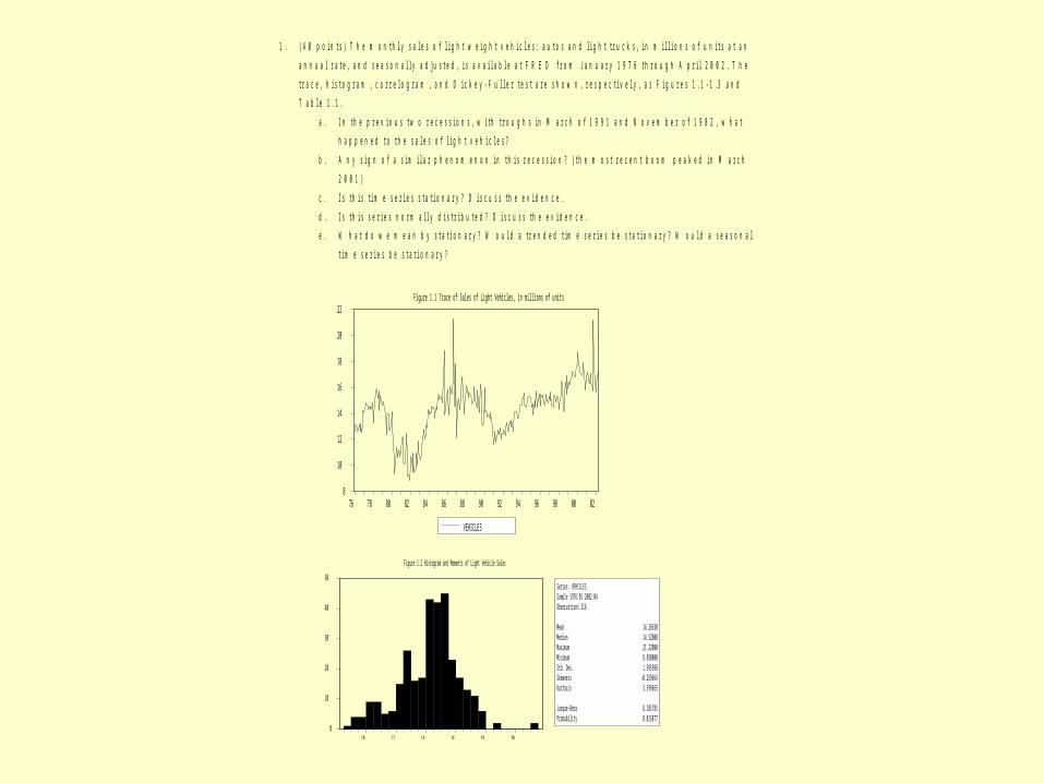
1 . ( 4 0 p o i n t s ) T h e m o n t h l y s a l e s o f l i g h t w e i g h t v e h i c l e s : a u t o s a n d l i g h t t r u c k s , i n m i l l i o n s o f u n i t s a t a n

a n n u a l r a t e , a n d s e a s o n a l l y a d j u s t e d , i s a v a i l a b l e a t F R E D f r o m J a n u a r y 1 9 7 6 t h r o u g h A p r i l 2 0 0 2 . T h e

t r a c e , h i s t o g r a m , c o r r e l o g r a m , a n d D i c k e y - F u l l e r t e s t a r e s h o w n , r e s p e c t i v e l y , a s F i g u r e s 1 . 1 - 1 . 3 a n d

T a b l e 1 . 1 .

a . I n t h e p r e v i o u s t w o r e c e s s i o n s , w i t h t r o u g h s i n M a r c h o f 1 9 9 1 a n d N o v e m b e r o f 1 9 8 2 , w h a t

h a p p e n e d t o t h e s a l e s o f l i g h t v e h i c l e s ?

b . A n y s i g n o f a s i m i l a r p h e n o m e n o n i n t h i s r e c e s s i o n ? ( t h e m o s t r e c e n t b o o m p e a k e d i n M a r c h

2 0 0 1 )

c . I s t h i s t i m e s e r i e s s t a t i o n a r y ? D i s c u s s t h e e v i d e n c e .

d . I s t h i s s e r i e s n o r m a l l y d i s t r i b u t e d ? D i s c u s s t h e e v i d e n c e .

e . W h a t d o w e m e a n b y s t a t i o n a r y ? W o u l d a t r e n d e d t i m e s e r i e s b e s t a t i o n a r y ? W o u l d a s e a s o n a l

t i m e s e r i e s b e s t a t i o n a r y ?

8

10

12

14

16

18

20

22

76 78 80 82 84 86 88 90 92 94 96 98 00 02

VEHICLES

Figure 1.1 Trace of Sales of Light Vehicles, in millions of units

0

10

20

30

40

50

10 12 14 16 18 20

Series: VEHICLESSample 1976:01 2002:04Observations 316

Mean 14.26630Median 14.52000Maximum 21.22000Minimum 8.850000Std. Dev. 1.995998Skewness -0.259664Kurtosis 3.599665

Jarque-Bera 8.285785Probability 0.015877

Figure 1.2 Histogram and Moments of Light Vehicle Sales

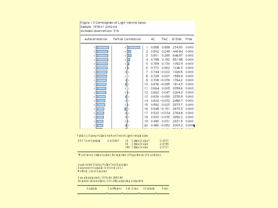
T a b l e 3 . 1 D i c k e y - F u l l e r U n i t R o o t T e s t o f L i g h t V e h i c l e S a l e s

A D F T e s t S t a t i s t ic - 2 . 4 2 3 8 6 7 1 % C r i t i c a l V a l u e * - 3 . 4 5 3 1 5 % C r i t i c a l V a l u e - 2 . 8 7 0 9 1 0 % C r i t i c a l V a l u e - 2 . 5 7 1 7

* M a c K i n n o n c r i t i c a l v a l u e s f o r r e j e c t i o n o f h y p o t h e s i s o f a u n i t r o o t .

A u g m e n t e d D i c k e y - F u l l e r T e s t E q u a t i o nD e p e n d e n t V a r i a b l e : D ( V E H I C L E S )M e t h o d : L e a s t S q u a r e s

S a m p l e ( a d j u s t e d ) : 1 9 7 6 : 0 4 2 0 0 2 : 0 4I n c l u d e d o b s e r v a t i o n s : 3 1 3 a f t e r a d j u s t i n g e n d p o i n t s

V a r i a b l e C o e f f i c i e n t S t d . E r r o r t - S t a t i s t i c P r o b .

V E H I C L E S ( - 1 ) - 0 . 0 6 8 6 0 6 0 . 0 2 8 3 0 4 - 2 . 4 2 3 8 6 7 0 . 0 1 5 9D ( V E H I C L E S ( - 1 ) ) - 0 . 3 6 2 9 9 3 0 . 0 5 6 2 2 5 - 6 . 4 5 6 0 7 5 0 . 0 0 0 0D ( V E H I C L E S ( - 2 ) ) - 0 . 2 9 6 1 3 0 0 . 0 5 4 4 6 4 - 5 . 4 3 7 1 6 4 0 . 0 0 0 0

C 0 . 9 9 9 9 4 8 0 . 4 0 6 9 4 9 2 . 4 5 7 1 8 1 0 . 0 1 4 6

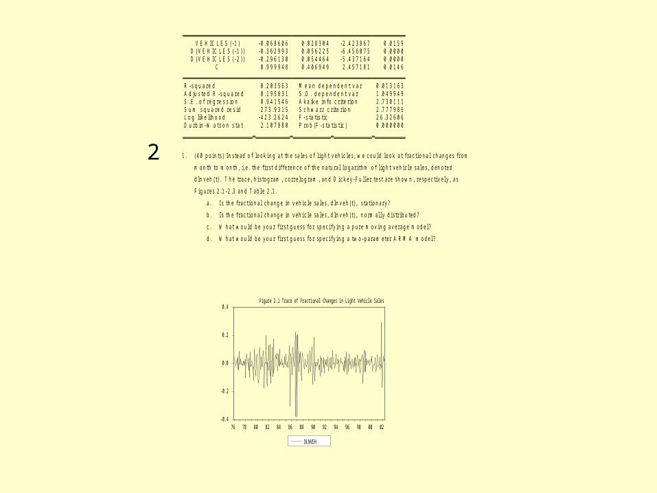
R - s q u a r e d 0 . 2 0 3 5 6 3 M e a n d e p e n d e n t v a r 0 . 0 1 3 1 6 3A d j u s t e d R - s q u a r e d 0 . 1 9 5 8 3 1 S . D . d e p e n d e n t v a r 1 . 0 4 9 9 4 9S . E . o f r e g r e s s i o n 0 . 9 4 1 5 4 6 A k a i k e i n f o c r i t e r i o n 2 . 7 3 0 1 1 1S u m s q u a r e d r e s i d 2 7 3 . 9 3 1 5 S c h w a r z c r i t e r i o n 2 . 7 7 7 9 8 6L o g l i k e l i h o o d - 4 2 3 . 2 6 2 4 F - s t a t i s t i c 2 6 . 3 2 6 0 6D u r b i n - W a t s o n s t a t 2 . 1 0 7 8 8 0 P r o b ( F - s t a t i s t i c ) 0 . 0 0 0 0 0 0

1 . ( 4 0 p o i n t s ) I n s t e a d o f l o o k i n g a t t h e s a l e s o f l i g h t v e h i c l e s , w e c o u l d l o o k a t f r a c t i o n a l c h a n g e s f r o m

m o n t h t o m o n t h , i . e . t h e f i r s t d i f f e r e n c e o f t h e n a t u r a l l o g a r i t h m o f l i g h t v e h i c l e s a l e s , d e n o t e d

d l n v e h ( t ) . T h e t r a c e , h i s t o g r a m , c o r r e l o g r a m , a n d D i c k e y - F u l l e r t e s t a r e s h o w n , r e s p e c t i v e l y , a s

F i g u r e s 2 . 1 - 2 . 3 a n d T a b l e 2 . 1 .

a . I s t h e f r a c t i o n a l c h a n g e i n v e h i c l e s a l e s , d l n v e h ( t ) , s t a t i o n a r y ?

b . I s t h e f r a c t i o n a l c h a n g e i n v e h i c l e s a l e s , d l n v e h ( t ) , n o r m a l l y d i s t r i b u t e d ?

c . W h a t w o u l d b e y o u r f i r s t g u e s s f o r s p e c i f y i n g a p u r e m o v i n g a v e r a g e m o d e l ?

d . W h a t w o u l d b e y o u r f i r s t g u e s s f o r s p e c i f y i n g a t w o - p a r a m e t e r A R M A m o d e l ?

-0.4

-0.2

0.0

0.2

0.4

76 78 80 82 84 86 88 90 92 94 96 98 00 02

DLNVEH

Figure 2.1 Trace of Fractional Changes in Light Vehicle Sales

2

0

2 0

4 0

6 0

8 0

- 0 . 4 - 0 . 3 - 0 . 2 - 0 . 1 0 . 0 0 . 1 0 . 2 0 . 3

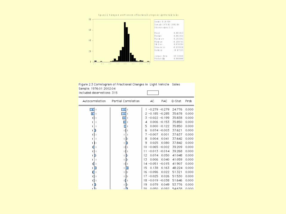
S e r i e s : D L N V E HS a m p l e 1 9 7 6 : 0 2 2 0 0 2 : 0 4

O b s e r v a t i o n s 3 1 5

M e a n 0 . 0 0 1 0 1 3M e d i a n 0 . 0 0 1 9 5 4

M a x i m u m 0 . 2 9 3 6 9 2

M i n i m u m - 0 . 3 8 0 7 4 5S t d . D e v . 0 . 0 7 0 2 8 4

S k e w n e s s - 0 . 8 3 8 8 2 0K u r t o s i s 1 0 . 0 7 5 3 5

J a r q u e - B e r a 6 9 3 . 9 8 4 8P r o b a b i l i t y 0 . 0 0 0 0 0 0

F i g u r e 2 . 2 H i s t o g r a m a n d M o m e n t s o f F r a c t i o n a l C a h n g e s i n L i g h t V e h i c l e S a l e s

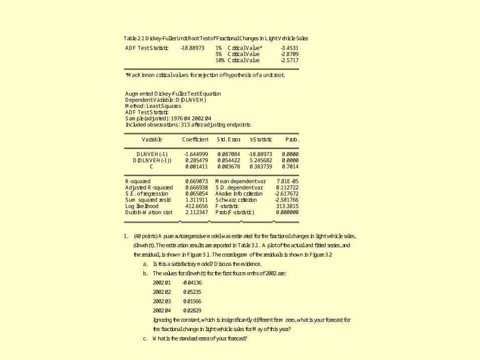
Table 2.1 Dickey-Fuller Unit Root Test of Fractional Changes in Light Vehicle Sales

ADF Test Statistic -18.88973 1% Critical Value* -3.4531 5% Critical Value -2.8709 10% Critical Value -2.5717

*MacKinnon critical values for rejection of hypothesis of a unit root.

Augmented Dickey-Fuller Test EquationDependent Variable: D(DLNVEH)Method: Least SquaresADF Test StatisticSample(adjusted): 1976:04 2002:04Included observations: 313 after adjusting endpoints

Variable Coefficient Std. Error t-Statistic Prob.

DLNVEH(-1) -1.644999 0.087084 -18.88973 0.0000D(DLNVEH(-1)) 0.285479 0.054422 5.245682 0.0000

C 0.001411 0.003678 0.383739 0.7014

R-squared 0.669073 Mean dependent var 7.81E-05Adjusted R-squared 0.666938 S.D. dependent var 0.112722S.E. of regression 0.065054 Akaike info criterion -2.617672Sum squared resid 1.311911 Schwarz criterion -2.581766Log likelihood 412.6656 F-statistic 313.3815Durbin-Watson stat 2.112347 Prob(F-statistic) 0.000000

1. (40 points) A pure autoregressive model was estimated for the fractional changes in light vehicle sales,

dlnveh(t). The estimation results are reported in Table 3.1. A plot of the actual and fitted series, and

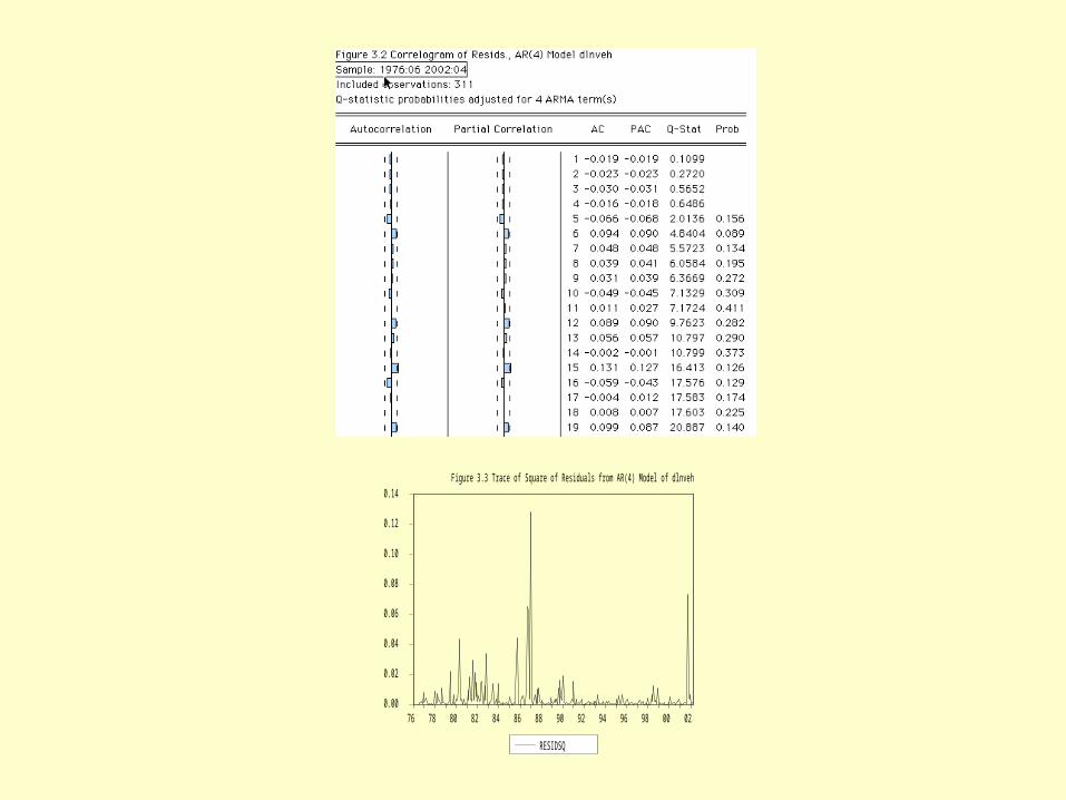
the residual, is shown in Figure 3.1. The correlogram of the residuals is shown in Figure 3.2

a. Is this a satisfactory model? Discuss the evidence.

b. The values for dlnveh(t) for the first four months of 2002 are:

2002:01 -0.04136

2002:02 0.05235

2002:03 0.01566

2002:04 0.02829

Ignoring the constant, which is insignificantly different from zero, what is your forecast for

the fractional change in light vehicle sales for May of this year?

c. What is the standard error of your forecast?

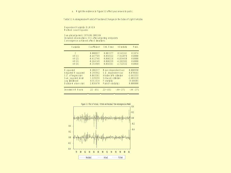
a . M i g h t t h e e v i d e n c e i n F i g u r e 3 . 3 a f f e c t y o u r a n s w e r t o p a r t c .

T a b l e 3 . 1 A u t o r e g r e s s i v e M o d e l o f F r a c t i o n a l C h a n g e s i n t h e S a l e s o f L i g h t V e h i c l e s

D e p e n d e n t V a r i a b l e : D L N V E HM e t h o d : L e a s t S q u a r e s

S a m p l e ( a d j u s t e d ) : 1 9 7 6 : 0 6 2 0 0 2 : 0 4I n c l u d e d o b s e r v a t i o n s : 3 1 1 a f t e r a d j u s t i n g e n d p o i n t sC o n v e r g e n c e a c h i e v e d a f t e r 3 i t e r a t i o n s

V a r i a b l e C o e f f i c i e n t S t d . E r r o r t - S t a t i s t i c P r o b .

C 0 . 0 0 0 8 5 7 0 . 0 0 1 5 7 7 0 . 5 4 3 2 4 1 0 . 5 8 7 4A R ( 1 ) - 0 . 4 4 7 7 6 9 0 . 0 5 6 5 2 2 - 7 . 9 2 2 0 7 8 0 . 0 0 0 0A R ( 2 ) - 0 . 4 1 2 7 4 6 0 . 0 6 0 2 1 6 - 6 . 8 5 4 4 5 0 0 . 0 0 0 0A R ( 3 ) - 0 . 2 6 4 1 4 9 0 . 0 6 0 2 5 9 - 4 . 3 8 3 5 8 3 0 . 0 0 0 0A R ( 4 ) - 0 . 1 5 3 9 8 9 0 . 0 5 6 5 6 1 - 2 . 7 2 2 5 3 2 0 . 0 0 6 8

R - s q u a r e d 0 . 2 0 6 3 1 7 M e a n d e p e n d e n t v a r 0 . 0 0 0 9 9 0A d j u s t e d R - s q u a r e d 0 . 1 9 5 9 4 2 S . D . d e p e n d e n t v a r 0 . 0 7 0 6 8 3S . E . o f r e g r e s s i o n 0 . 0 6 3 3 8 1 A k a i k e i n f o c r i t e r i o n - 2 . 6 6 3 3 5 3S u m s q u a r e d r e s i d 1 . 2 2 9 2 5 5 S c h w a r z c r i t e r i o n - 2 . 6 0 3 2 2 8L o g l i k e l i h o o d 4 1 9 . 1 5 1 4 F - s t a t i s t i c 1 9 . 8 8 6 0 5D u r b i n - W a t s o n s t a t 2 . 0 3 6 6 7 0 P r o b ( F - s t a t i s t i c ) 0 . 0 0 0 0 0 0

I n v e r t e d A R R o o t s . 2 2 - . 6 5 i . 2 2 + . 6 5 i - . 4 4 + . 3 7 i - . 4 4 - . 3 7 i

-0.4

-0.2

0.0

0.2

0.4

-0.4

-0.2

0.0

0.2

0.4

78 80 82 84 86 88 90 92 94 96 98 00 02

Residual Actual Fitted

Figure 3.1 Plot of Actual, Fitted and Residual from Autoregressive Model

0.00

0.02

0.04

0.06

0.08

0.10

0.12

0.14

76 78 80 82 84 86 88 90 92 94 96 98 00 02

RESIDSQ

Figure 3.3 Trace of Square of Residuals from AR(4) Model of dlnveh

1 . ( 4 0 p o i n t s ) A u t o s a n d l i g h t t r u c k s a r e a c o n s u m e r d u r a b l e a n d a r e l i k e l y t o b e a f f e c t e d b y t h e i n t e r e s t

r a t e i f c o n s u m e r s t a k e o u t a n a u t o l o a n . A s a n i n d i c a t o r o f t h e c o s t o f c r e d i t , t h e p r i m e l o a n r a t e f r o m

b a n k s i s a v a i l a b l e i n a m o n t h l y s e r i e s f r o m F R E D b e g i n n i n g i n J a n u a r y 1 9 4 9 . T h i s i n t e r e s t r a t e d a t a

f r o m J a n u a r y 1 9 7 6 i s c o m b i n e d w i t h t h e d a t a f o r l i g h t v e h i c l e s a l e s . T h e c h a n g e i n t h e p r i m e r a t e ,

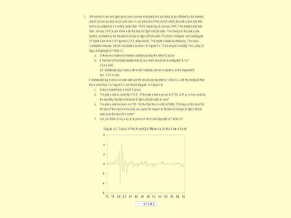
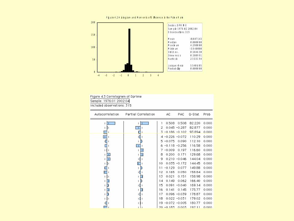
d p r i m e , i s r e l a t e d t o t h e f r a c t i o n a l c h a n g e i n l i g h t v e h i c l e s a l e s . T h e t r a c e , h i s t o g r a m a n d c o r r e l o g r a m

o f d p r i m e a r e s h o w n i n F i g u r e s 4 . 1 - 4 . 3 , r e s p e c t i v e l y . T h i s d p r i m e s e r i e s i s s t a t i o n a r y . T h e c r o s s -

c o r r e l a t i o n b e t w e e n d l n v e h a n d d p r i m e i s s h o w n i n F i g u r e 4 . 4 . T h e G r a n g e r C a u s a l i t y T e s t , u s i n g 1 2

l a g s , i s d i s p l a y e d i n T a b l e 4 . 1 .

a . I s t h e r e a n y e v i d e n c e o f e i t h e r v a r i a b l e c a u s i n g t h e o t h e r ? D i s c u s s .

b . W h a t k i n d o f b i v a r i a t e r e l a t i o n s h i p d o y o u t h i n k s h o u l d b e i n v e s t i g a t e d ? W h y ?

i N o m o d e l

i i A d i s t r i b u t e d l a g m o d e l , w i t h w h i c h v a r i a b l e , d l n v e h o r d p r i m e , a s t h e d e p e n d e n t ?

i i i A V A R m o d e l

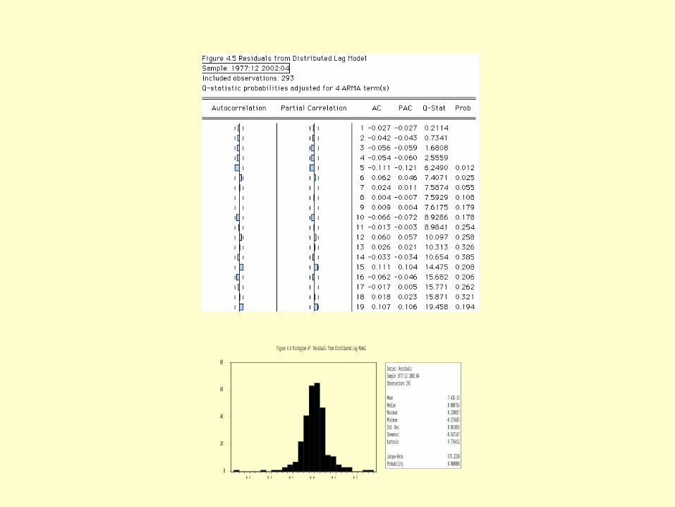
A d i s t r i b u t e d l a g m o d e l w a s e s t i m a t e d a n d t h e r e s u l t s a r e r e p o r t e d i n T a b l e 4 . 2 , w i t h t h e r e s i d u a l s f r o m

t h i s m o d e l s h o w n i n F i g u r e 4 . 5 , a n d t h e i r h i s t o g r a m i n F i g u r e 4 . 6 .

c . I s t h i s a s a t i s f a c t o r y m o d e l ? D i s c u s s .

d . T h e p r i m e r a t e i s c u r r e n t l y 4 . 7 5 % . I f t h e p r i m e r a t e w e n t u p t o 5 . 7 5 % i n M a y , w h a t w o u l d b e

t h e r e s u l t i n g f r a c t i o n a l i n c r e a s e i n l i g h t v e h i c l e s a l e s i n J u n e ?

e . T h e p r i m e r a t e h a s b e e n a t 4 . 7 5 % f o r t h e f i r s t f o u r m o n t h s o f 2 0 0 2 . I f i t s t a y s a t t h i s l e v e l f o r

t h e r e s t o f t h i s y e a r w h a t w o u l d y o u e x p e c t t o h a p p e n t o f r a c t i o n a l c h a n g e s i n l i g h t v e h i c l e

s a l e s o v e r t h e n e x t 1 8 m o n t h s ?

f . C a n y o u t h i n k o f a n y w a y t o i m p r o v e o n t h e m o d e l r e p o r t e d i n T a b l e 4 . 2 ?

-6

-4

-2

0

2

4

6

7 6 7 8 8 0 8 2 8 4 8 6 8 8 9 0 9 2 9 4 9 6 9 8 0 0 0 2

D P R I M E

F i g u re 4 . 1 T r a c e o f t h e M o n t h l y D i f f e re n c e i n t h e P r i m e R a t e

0

5 0

1 0 0

1 5 0

2 0 0

- 4 - 3 - 2 - 1 0 1 2 3 4

S e r ie s : D P R IM ES a m p le 1 9 7 6 :0 2 2 0 0 2 : 0 4O b s e r v a t io n s 3 1 5

M e a n - 0 .0 0 7 1 4 3M e d ia n 0 .0 0 0 0 0 0M a x im u m 4 .2 9 0 0 0 0M in im u m - 3 .9 4 0 0 0 0S t d . D e v . 0 .5 8 4 6 3 0S k e w n e s s 0 .3 8 0 9 9 1K u r to s is 2 3 .5 3 1 9 4

J a r q u e -B e ra 5 5 4 0 .6 0 5P r o b a b ili ty 0 .0 0 0 0 0 0

F ig u r e 4 . 2 H is t o g r a m a n d M o m e n t s o f D iff e r e n c e in th e P r im e R a te

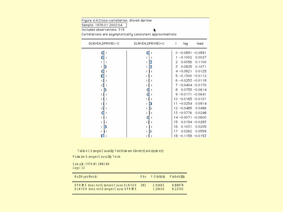
T a b l e 4 . 1 G r a n g e r C a u s a l i t y T e s t B e t w e e n d ln v e h ( t ) a n d d p r i m e ( t )

P a i r w is e G r a n g e r C a u s a l i t y T e s t s

S a m p le : 1 9 7 6 :0 1 2 0 0 2 :0 4L a g s : 1 2

N u ll H y p o th e s is : O b s F - S ta t i s t i c P r o b a b i l i t y

D P R IM E d o e s n o t G r a n g e r C a u s e D L N V E H 3 0 3 2 .9 4 8 6 5 0 .0 0 0 7 0 D L N V E H d o e s n o t G r a n g e r C a u s e D P R IM E 1 .2 8 6 3 4 0 .2 2 5 9 2

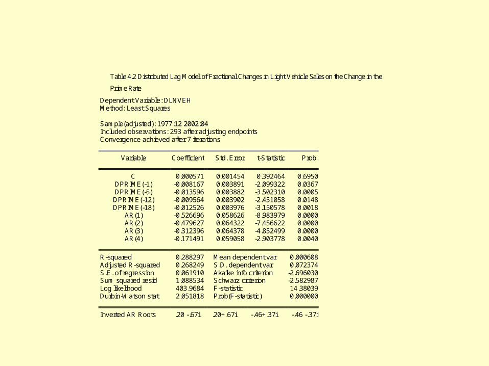
Table 4.2 Distributed Lag Model of Fractional Changes in Light Vehicle Sales on the Change in the

Prime Rate

Dependent Variable: DLNVEHMethod: Least Squares

Sample(adjusted): 1977:12 2002:04Included observations: 293 after adjusting endpointsConvergence achieved after 7 iterations

Variable Coefficient Std. Error t-Statistic Prob.

C 0.000571 0.001454 0.392464 0.6950DPRIME(-1) -0.008167 0.003891 -2.099322 0.0367DPRIME(-5) -0.013596 0.003882 -3.502310 0.0005DPRIME(-12) -0.009564 0.003902 -2.451058 0.0148DPRIME(-18) -0.012526 0.003976 -3.150578 0.0018

AR(1) -0.526696 0.058626 -8.983979 0.0000AR(2) -0.479627 0.064322 -7.456622 0.0000AR(3) -0.312396 0.064378 -4.852499 0.0000AR(4) -0.171491 0.059058 -2.903778 0.0040

R-squared 0.288297 Mean dependent var 0.000608Adjusted R-squared 0.268249 S.D. dependent var 0.072374S.E. of regression 0.061910 Akaike info criterion -2.696030Sum squared resid 1.088534 Schwarz criterion -2.582987Log likelihood 403.9684 F-statistic 14.38039Durbin-Watson stat 2.051818 Prob(F-statistic) 0.000000

Inverted AR Roots .20 -.67i .20+.67i -.46+.37i -.46 -.37i

0

20

40

60

80

-0.3 -0.2 -0.1 0.0 0.1 0.2

Series: ResidualsSample 1977:12 2002:04Observations 293

Mean 7.43E-15Median 0.000756Maximum 0.250037Minimum -0.373685Std. Dev. 0.061056Skewness -0.547147Kurtosis 9.776412


Figure 4.6 Histogram of Residuals from Distributed Lag Model

15

Review

• 2. Ideas That Are Transcending

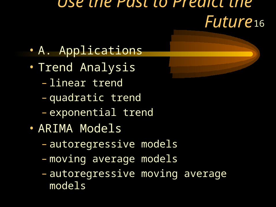
16Use the Past to Predict the Future

• A. Applications

• Trend Analysis– linear trend– quadratic trend– exponential trend

• ARIMA Models– autoregressive models– moving average models– autoregressive moving average models

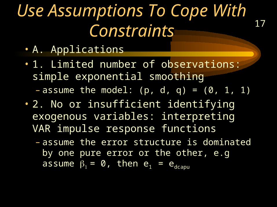
17Use Assumptions To Cope With

Constraints• A. Applications

• 1. Limited number of observations: simple exponential smoothing– assume the model: (p, d, q) = (0, 1, 1)

• 2. No or insufficient identifying exogenous variables: interpreting VAR impulse response functions– assume the error structure is dominated by one

pure error or the other, e.g assume = 0, then e1 = edcapu

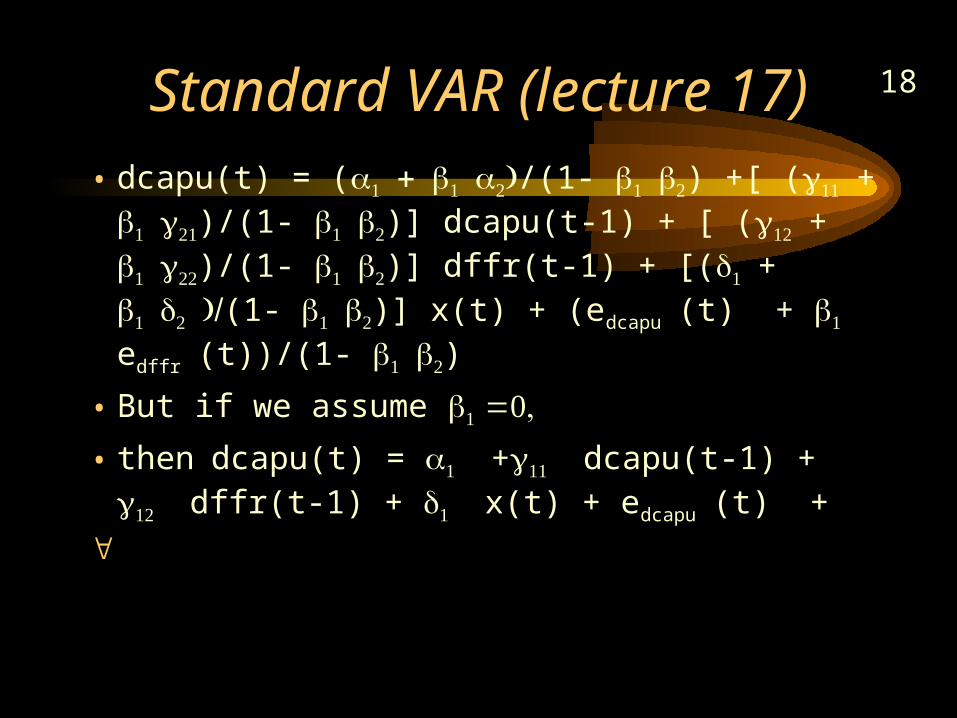
18Standard VAR (lecture 17)

• dcapu(t) = (/(1- ) +[ (+ )/(1- )] dcapu(t-1) + [ (+ )/(1- )] dffr(t-1) + [(+ (1- )] x(t) + (edcapu(t) + edffr(t))/(1- )

• But if we assume

• thendcapu(t) = + dcapu(t-1) + dffr(t-1) + x(t) + edcapu(t) +

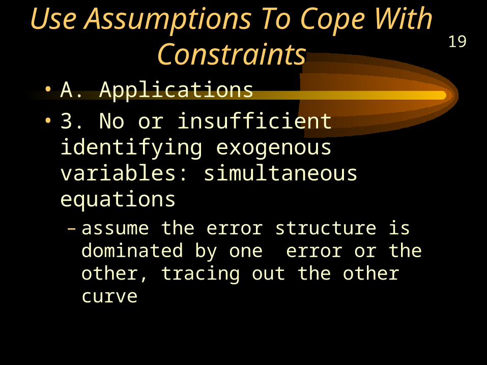
19Use Assumptions To Cope With

Constraints• A. Applications

• 3. No or insufficient identifying exogenous variables: simultaneous equations– assume the error structure is dominated by one

error or the other, tracing out the other curve

20

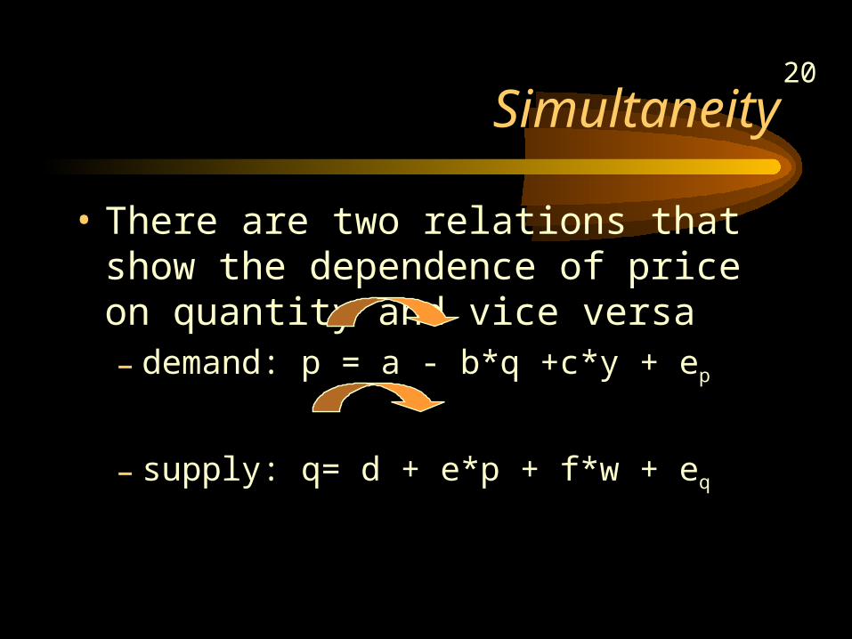
Simultaneity

• There are two relations that show the dependence of price on quantity and vice versa– demand: p = a - b*q +c*y + ep

– supply: q= d + e*p + f*w + eq

21

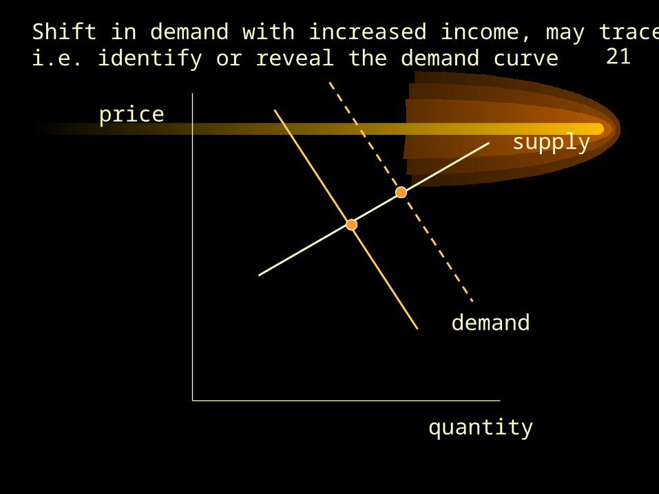
demand

price

quantity

Shift in demand with increased income, may trace outi.e. identify or reveal the demand curve

supply

22

Review

• 2. Ideas That Are Transcending

23

Reduce the unexplained sum of squares to increase the significance of

results• A. Applications

• 1. 2-way ANOVA: using randomized block design– example: minutes of rock music listened to on

the radio by teenagers Lecture 1 Notes, 240 C• we are interested in the variation from day to day

• to get better results, we control for variation across teenager

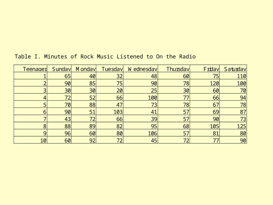
Table I. Minutes of Rock Music Listened to On the Radio

Teenager Sunday Monday Tuesday Wednesday Thursday Friday Saturday1 65 40 32 48 60 75 1102 90 85 75 90 78 120 1003 30 30 20 25 30 60 704 72 52 66 100 77 66 945 70 88 47 73 78 67 786 90 51 103 41 57 69 877 43 72 66 39 57 90 738 88 89 82 95 68 105 1259 96 60 80 106 57 81 80

10 60 92 72 45 72 77 90

Figure 1: Minutes of Rock Music Listened to Per Day

0

10

20

30

40

50

60

70

80

90

Sunday Monday Tuesday Wednesday Thursday Friday Saturday

Day of the Week

Min

ute

s

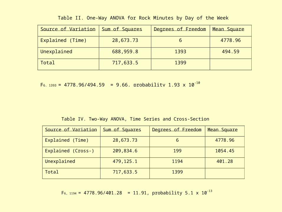
Table IV. Two-Way ANOVA, Time Series and Cross-Section

Source of Variation Sum of Squares Degrees of Freedom Mean Square

Explained (Time) 28,673.73 6 4778.96

Explained (Cross-) 209,834.6 199 1054.45

Unexplained 479,125.1 1194 401.28

Total 717,633.5 1399

F6, 1194 = 4778.96/401.28 = 11.91, probability 5.1 x 10-13

Table II. One-Way ANOVA for Rock Minutes by Day of the Week

Source of Variation Sum of Squares Degrees of Freedom Mean Square

Explained (Time) 28,673.73 6 4778.96

Unexplained 688,959.8 1393 494.59

Total 717,633.5 1399

F6, 1393 = 4778.96/494.59 = 9.66, probability 1.93 x 10-10

27



• 2. Distributed lag models: model dependence of y(t) on a distributed lag of x(t) and– model the residual using ARMA

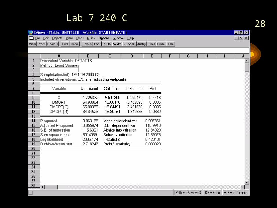
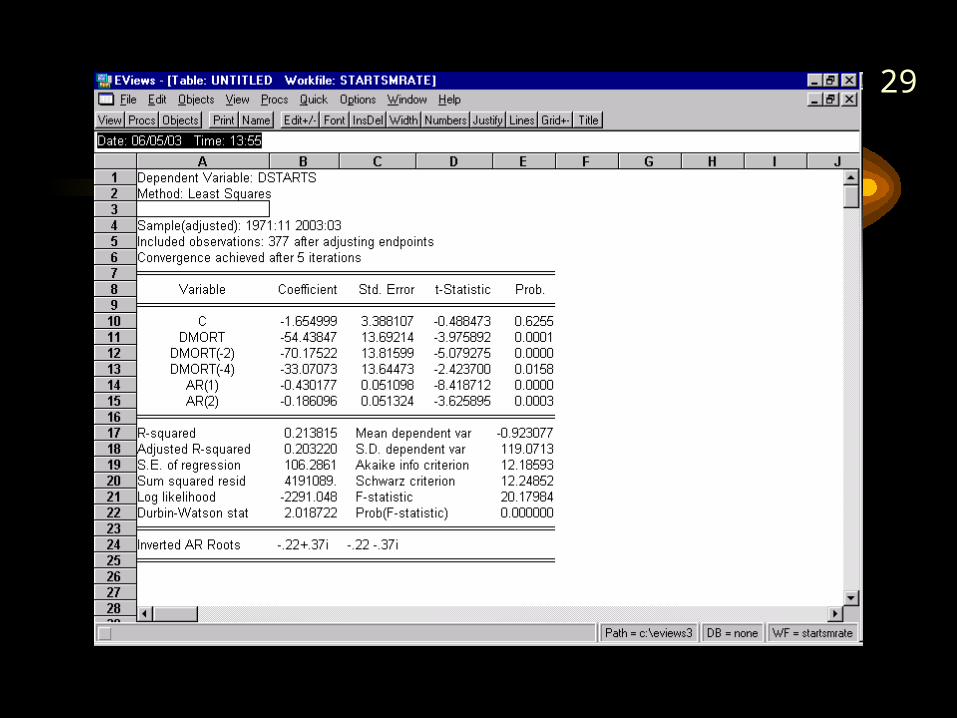
28Lab 7 240 C

29

30



• 3. Intervention Models: model known changes (policy, legal etc.) by using dummy variables, e.g. a step function or pulse function

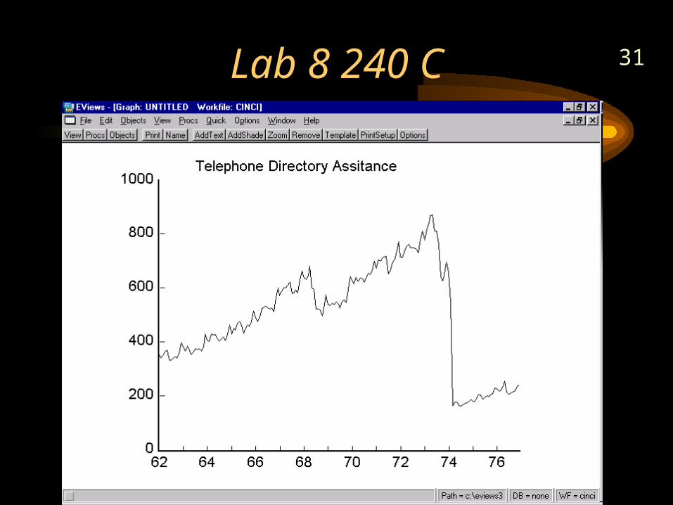
31Lab 8 240 C

32

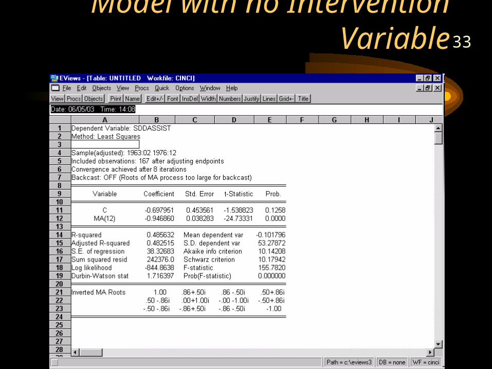
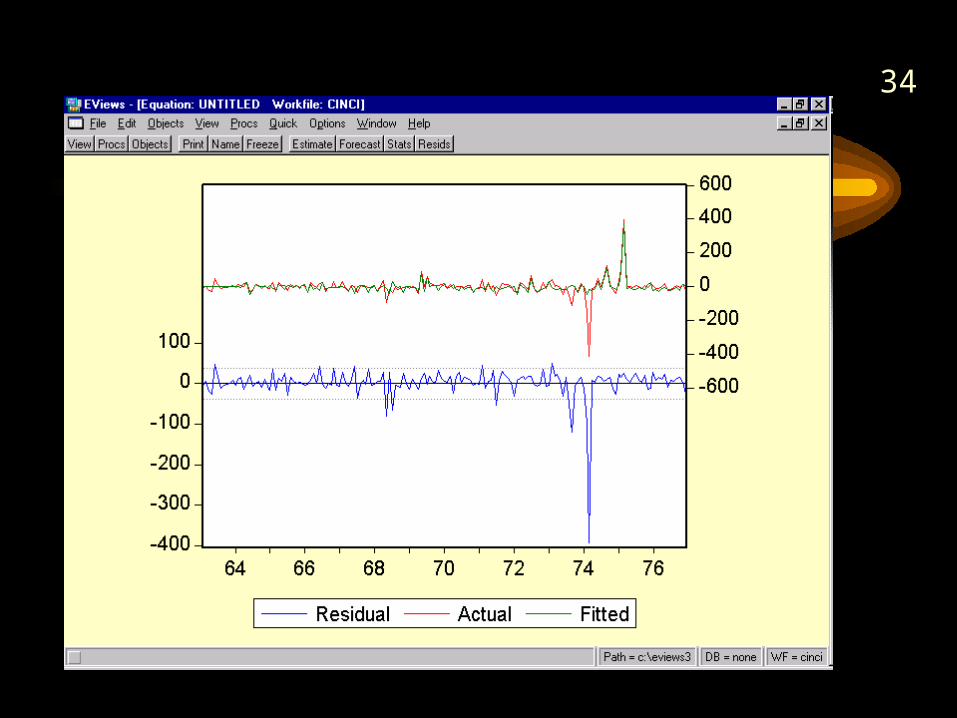
33Model with no Intervention Variable

34

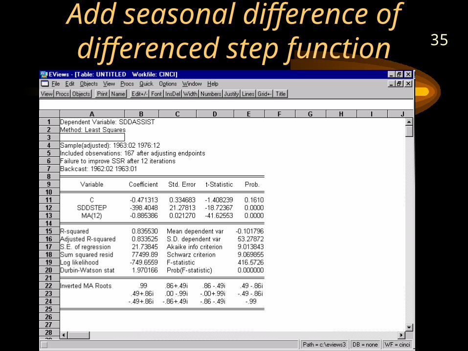
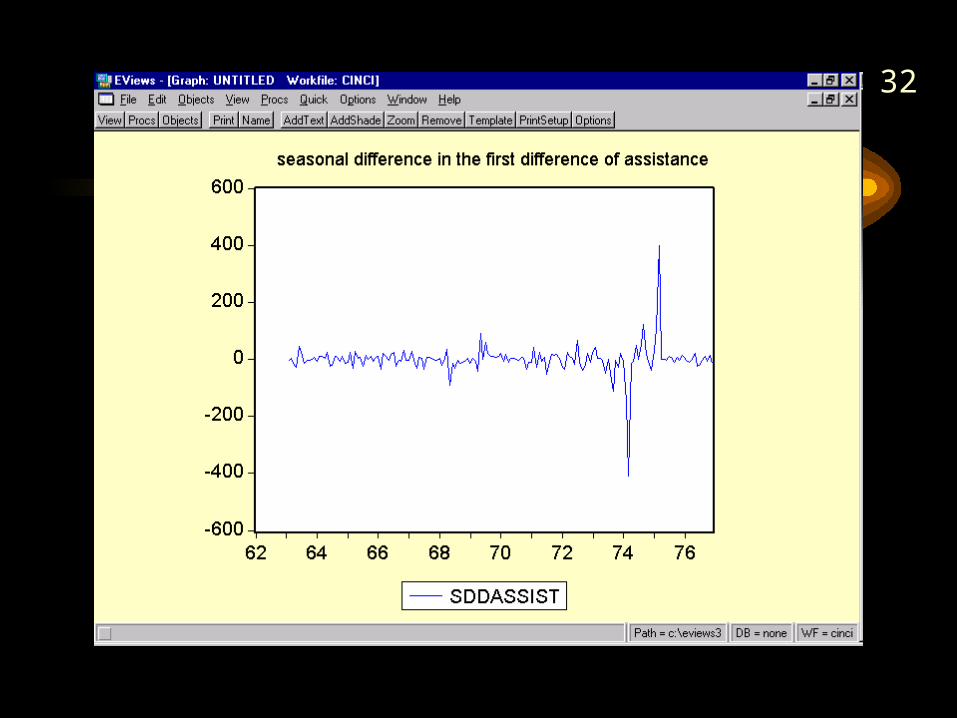
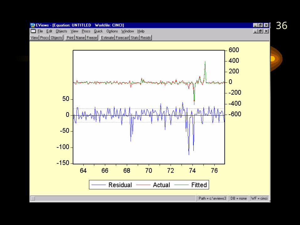
35Add seasonal difference of differenced step function

36

37

Review

• 2002 Final

• Ideas that are transcending



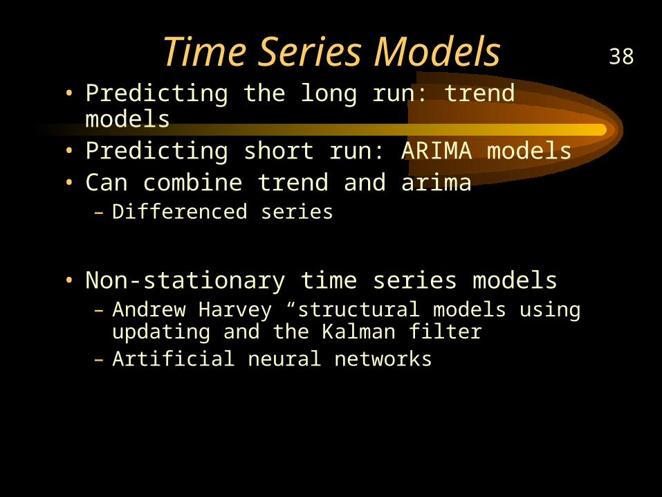
38Time Series Models• Predicting the long run: trend models• Predicting short run: ARIMA models• Can combine trend and arima

– Differenced series

• Non-stationary time series models– Andrew Harvey “structural models using updating and

the Kalman filter– Artificial neural networks

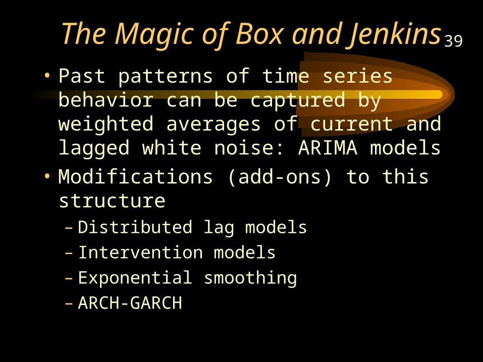
39The Magic of Box and Jenkins• Past patterns of time series behavior can be

captured by weighted averages of current and lagged white noise: ARIMA models

• Modifications (add-ons) to this structure– Distributed lag models– Intervention models– Exponential smoothing– ARCH-GARCH

40

Economic Models of Time Series

• Total return to Standard and Poors 500

41

Model One: Random Walks

• Last time we characterized the logarithm of total returns to the Standard and Poors 500 as trend plus a random walk.

• Ln S&P 500(t) = trend + random walk = a + b*t + RW(t)

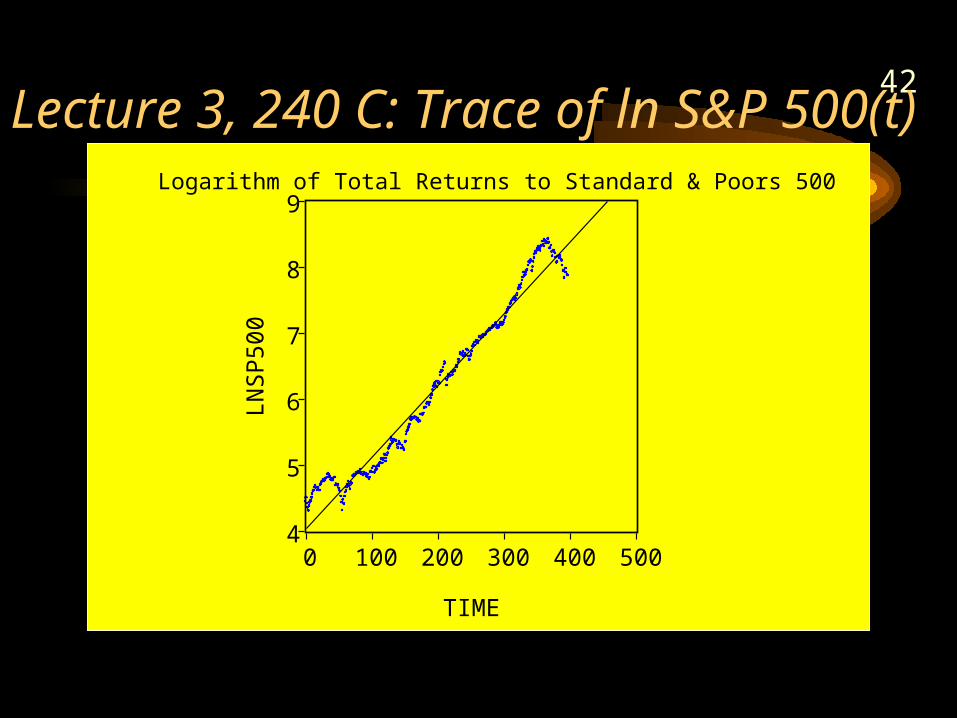
42Lecture 3, 240 C: Trace of ln S&P 500(t)

4

5

6

7

8

9

0 100 200 300 400 500

TIME

LN

SP50

0

Logarithm of Total Returns to Standard & Poors 500

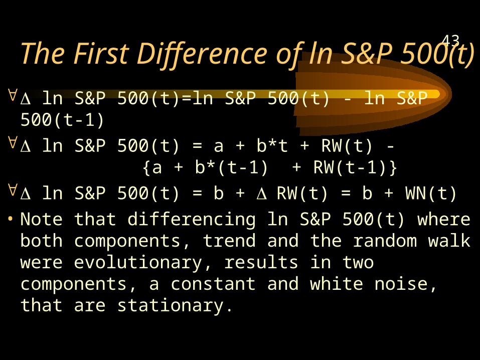
43The First Difference of ln S&P 500(t)

ln S&P 500(t)=ln S&P 500(t) - ln S&P 500(t-1) ln S&P 500(t) = a + b*t + RW(t) -

{a + b*(t-1) + RW(t-1)} ln S&P 500(t) = b + RW(t) = b + WN(t)

• Note that differencing ln S&P 500(t) where both components, trend and the random walk were evolutionary, results in two components, a constant and white noise, that are stationary.

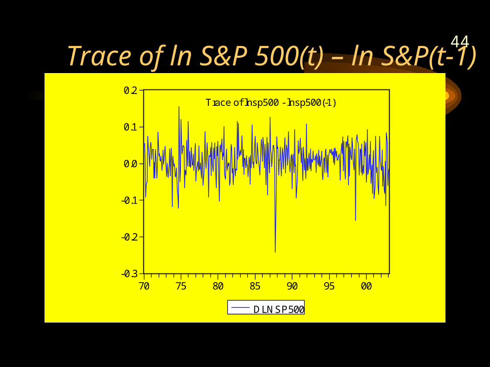
44Trace of ln S&P 500(t) – ln S&P(t-1)

-0.3

-0.2

-0.1

0.0

0.1

0.2

70 75 80 85 90 95 00

DLNSP500

Trace of lnsp500 - lnsp500(-1)

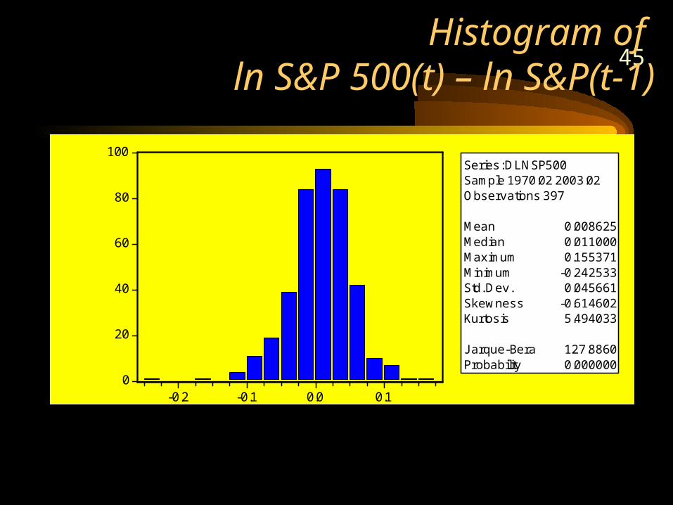
45Histogram of

ln S&P 500(t) – ln S&P(t-1)

0

20

40

60

80

100

-0.2 -0.1 0.0 0.1

Series: DLNSP500Sample 1970:02 2003:02Observations 397

Mean 0.008625Median 0.011000Maximum 0.155371Minimum -0.242533Std. Dev. 0.045661Skewness -0.614602Kurtosis 5.494033


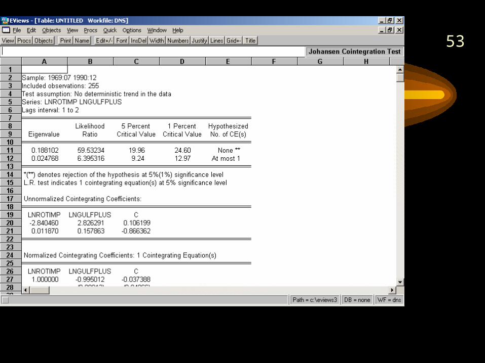
46Cointegration Example• The Law of One Price• Dark Northern Spring wheat

– Rotterdam import price, CIF, has a unit root– Gulf export price, fob, has a unit root– Freight rate ambiguous, has a unit root at 1%

level, not at the 5%

• Ln PR(t)/ln[PG(t) + F(t)] = diff(t)– Know cointegrating equation: – 1* ln PR(t) – 1* ln[PG(t) + F(t)] = diff(t)– So do a unit root test on diff, which should be

stationary; check with Johansen test

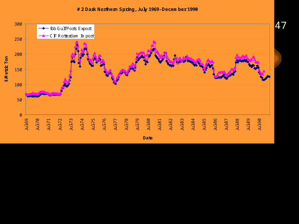
47

# 2 Dark Northern Spring, July 1969- December 1990

0

50

100

150

200

250

300Ju

l-6

9

Jul-

70

Jul-

71

Jul-

72

Jul-

73

Jul-

74

Jul-

75

Jul-

76

Jul-

77

Jul-

78

Jul-

79

Jul-

80

Jul-

81

Jul-

82

Jul-

83

Jul-

84

Jul-

85

Jul-

86

Jul-

87

Jul-

88

Jul-

89

Jul-

90

Date

$/M

etr

ic T

on

fob Gulf Ports Export

CIF Rotterdam Import

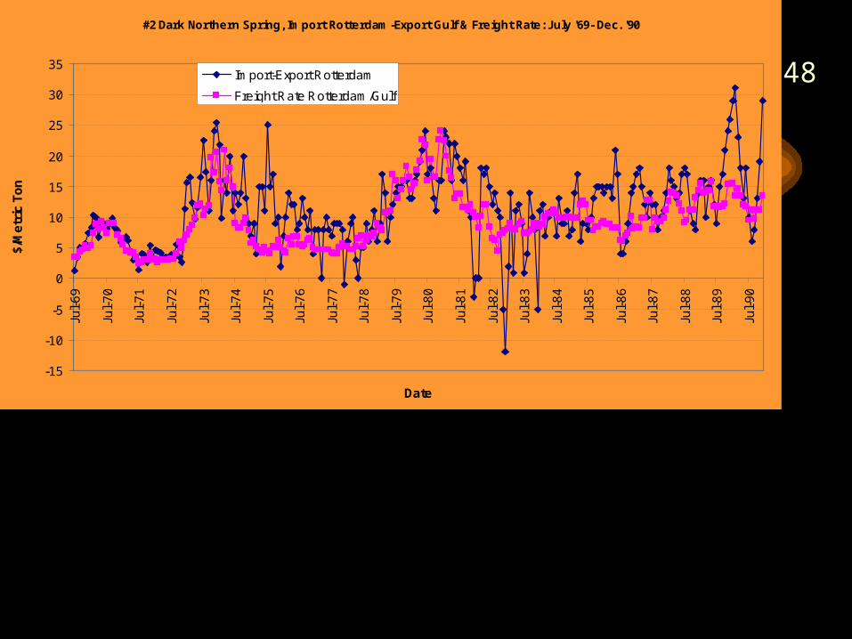
48

#2 Dark Northern Spring, Import Rotterdam-Export Gulf & Freight Rate: July '69- Dec. '90

-15

-10

-5

0

5

10

15

20

25

30

35Ju

l-6

9

Jul-

70

Jul-

71

Jul-

72

Jul-

73

Jul-

74

Jul-

75

Jul-

76

Jul-

77

Jul-

78

Jul-

79

Jul-

80

Jul-

81

Jul-

82

Jul-

83

Jul-

84

Jul-

85

Jul-

86

Jul-

87

Jul-

88

Jul-

89

Jul-

90

Date

$/M

etr

ic T

on

Import-Export Rotterdam

Freight Rate Rotterdam/Gulf

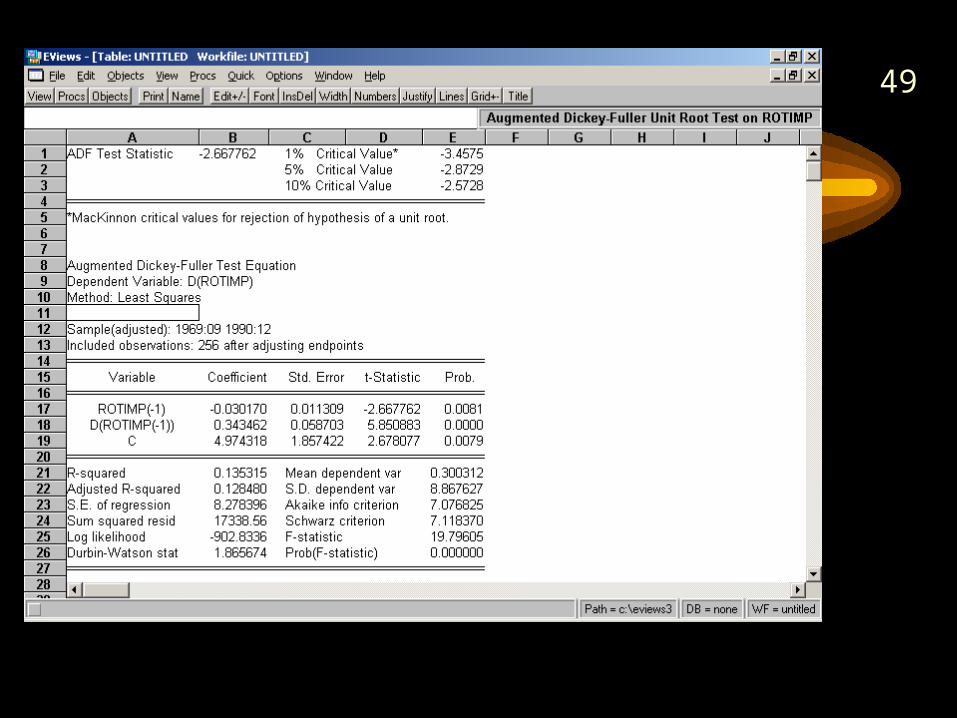
49

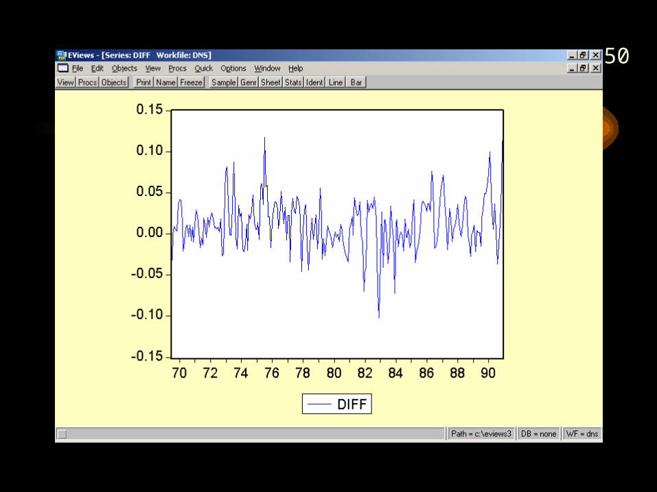
50

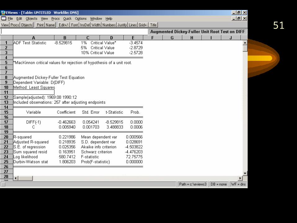
51

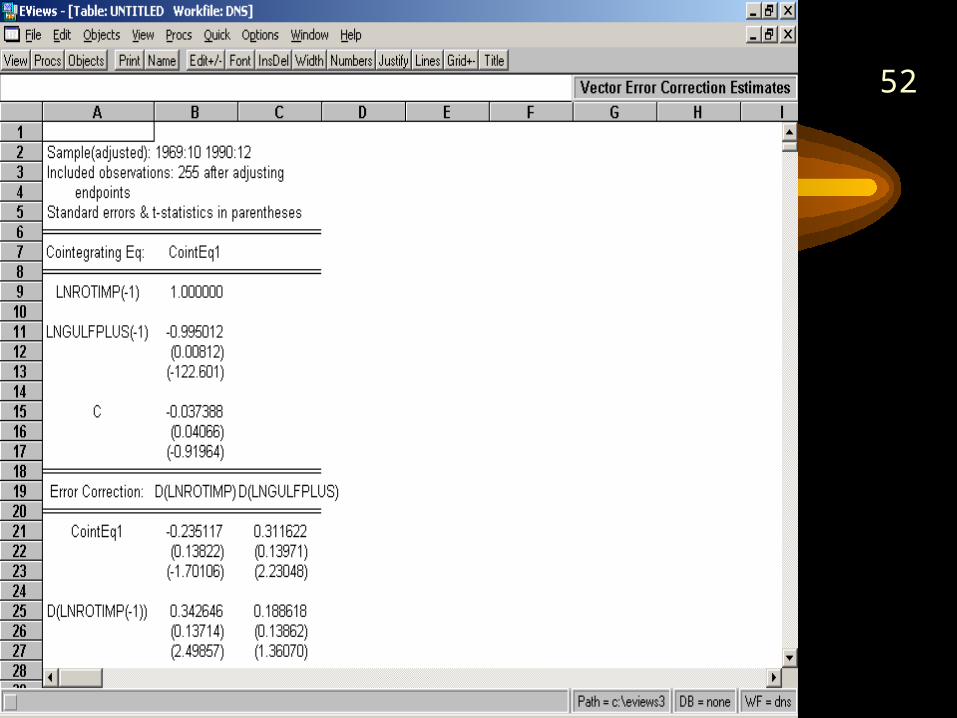
52

53

54

Review

• 2002 Final

• Ideas that are transcending



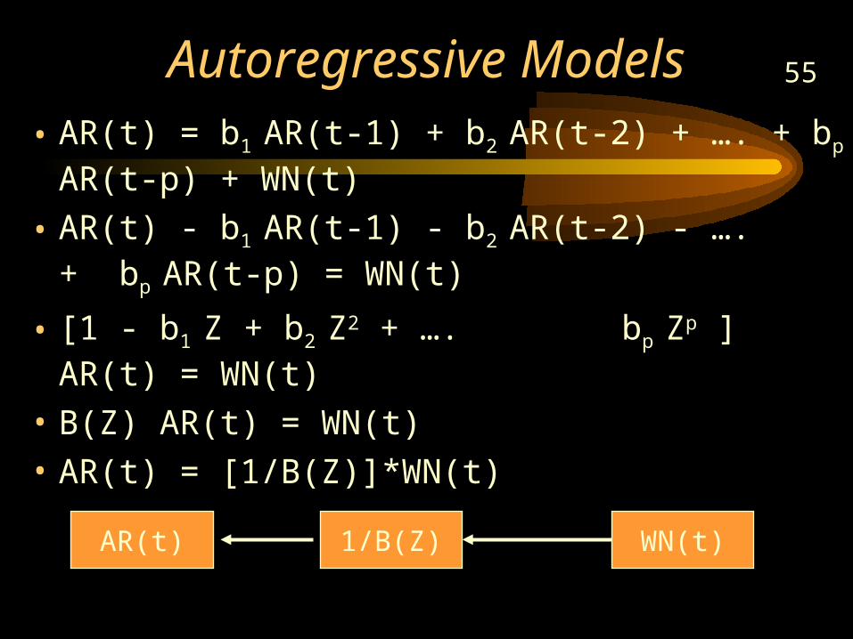
55Autoregressive Models• AR(t) = b1 AR(t-1) + b2 AR(t-2) + …. + bp AR(t-p)

+ WN(t)

• AR(t) - b1 AR(t-1) - b2 AR(t-2) - …. + bp AR(t-p) = WN(t)

• [1 - b1 Z + b2 Z2 + …. bp Zp ] AR(t) = WN(t)

• B(Z) AR(t) = WN(t)

• AR(t) = [1/B(Z)]*WN(t)

WN(t)1/B(Z)AR(t)

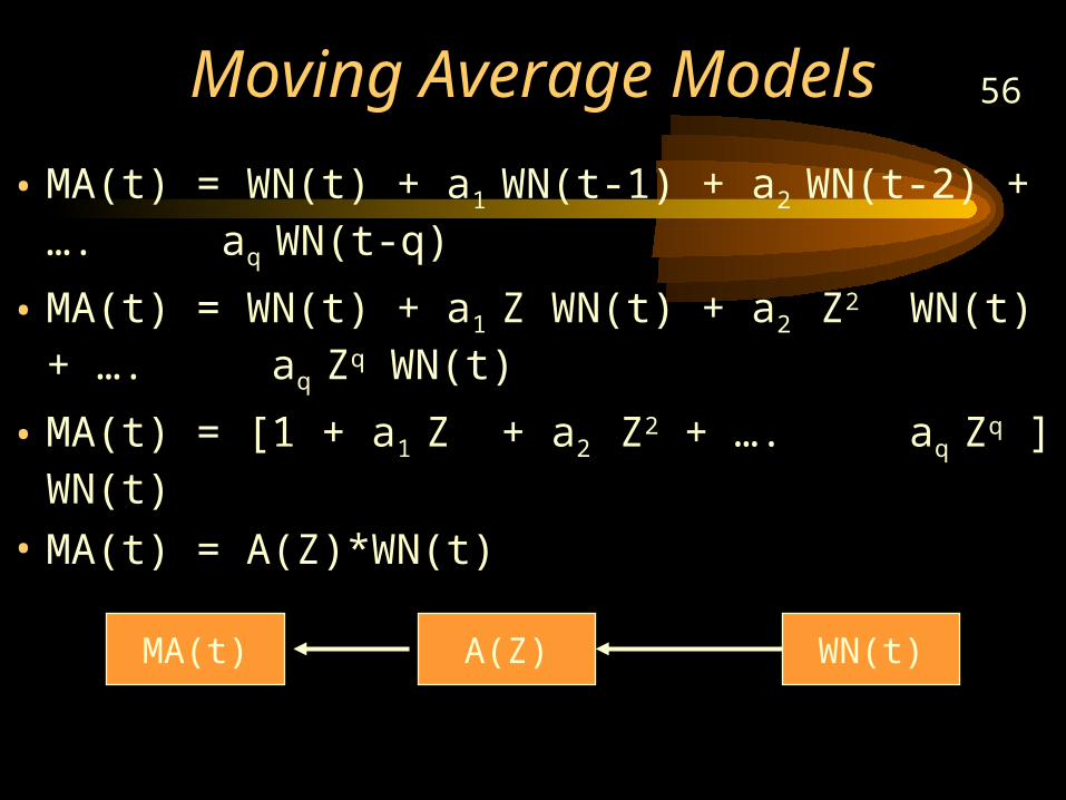
56Moving Average Models

• MA(t) = WN(t) + a1 WN(t-1) + a2 WN(t-2) + …. aq WN(t-q)

• MA(t) = WN(t) + a1 Z WN(t) + a2 Z2 WN(t) + …. aq Zq WN(t)

• MA(t) = [1 + a1 Z + a2 Z2 + …. aq Zq ] WN(t)

• MA(t) = A(Z)*WN(t)

WN(t)A(Z)MA(t)

57

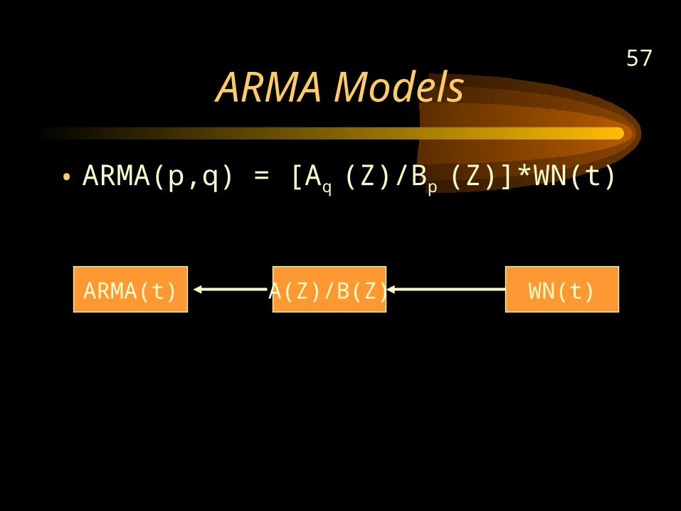
ARMA Models

• ARMA(p,q) = [Aq (Z)/Bp (Z)]*WN(t)

WN(t)A(Z)/B(Z)ARMA(t)

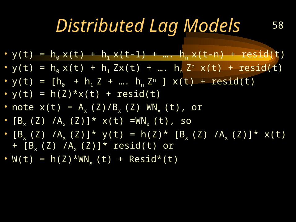
58Distributed Lag Models

• y(t) = h0 x(t) + h1 x(t-1) + …. hn x(t-n) + resid(t)• y(t) = h0 x(t) + h1 Zx(t) + …. hn Zn x(t) + resid(t)• y(t) = [h0 + h1 Z + …. hn Zn ] x(t) + resid(t)• y(t) = h(Z)*x(t) + resid(t)• note x(t) = Ax (Z)/Bx (Z) WNx (t), or• [Bx (Z) /Ax (Z)]* x(t) =WNx (t), so• [Bx (Z) /Ax (Z)]* y(t) = h(Z)* [Bx (Z) /Ax (Z)]* x(t) + [Bx (Z) /Ax

(Z)]* resid(t) or • W(t) = h(Z)*WNx (t) + Resid*(t)

59

Distributed Lag Models

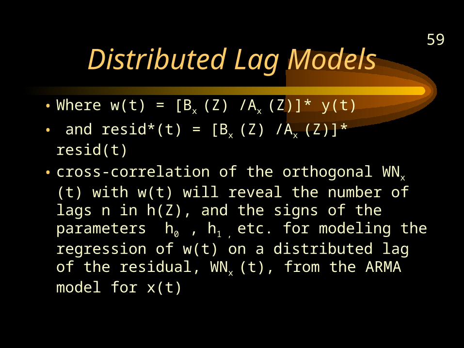
• Where w(t) = [Bx (Z) /Ax (Z)]* y(t)

• and resid*(t) = [Bx (Z) /Ax (Z)]* resid(t)

• cross-correlation of the orthogonal WNx (t) with w(t) will reveal the number of lags n in h(Z), and the signs of the parameters h0 , h1 , etc. for modeling the regression of w(t) on a distributed lag of the residual, WNx (t), from the ARMA model for x(t)

60

61

Economic Models of Time Series

• Interest Rate Parity

62

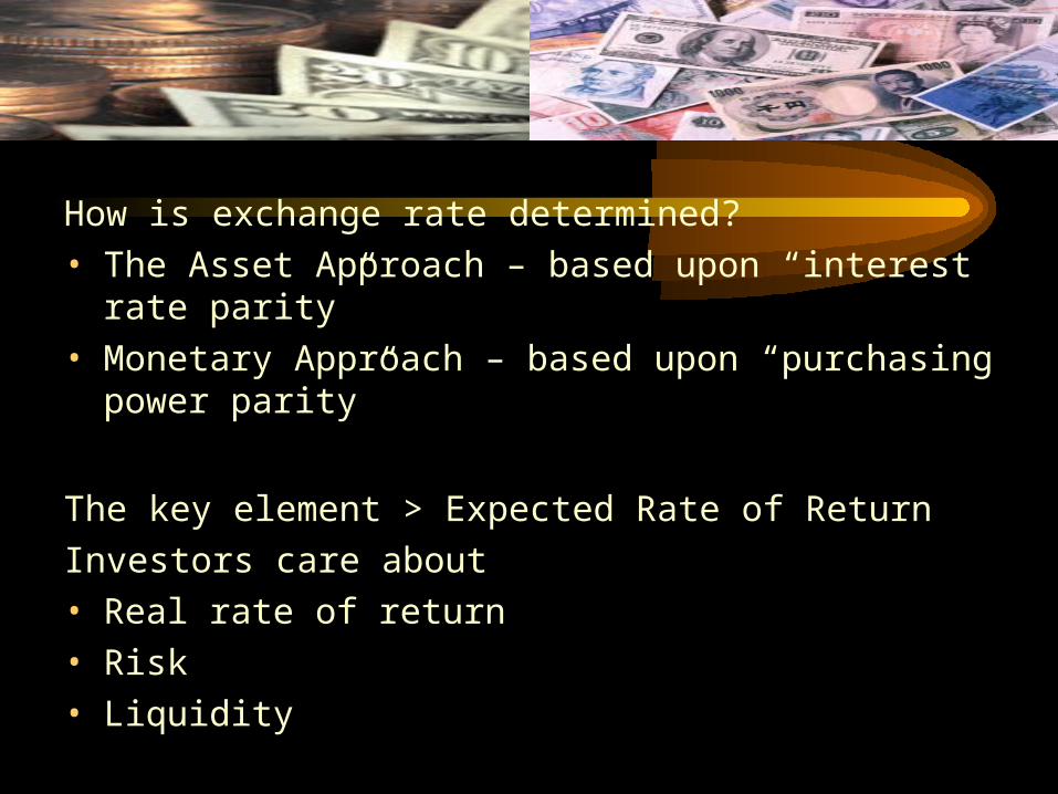
How is exchange rate determined?

• The Asset Approach – based upon “interest rate parity”

• Monetary Approach – based upon “purchasing power parity”

The key element > Expected Rate of Return

Investors care about

• Real rate of return

• Risk

• Liquidity

63

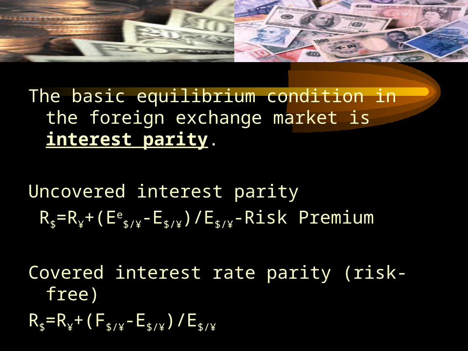
The basic equilibrium condition in the foreign exchange market is interest parity.

Uncovered interest parity

R$=R¥+(Ee$/¥-E$/¥)/E$/¥-Risk Premium

Covered interest rate parity (risk-free)

R$=R¥+(F$/¥-E$/¥)/E$/¥

64

0

5

10

15

20

25

1980 1985 1990 1995 2000 2005

Year

Prim

e Int

eres

t Rate

s (%

)

0

0.002

0.004

0.006

0.008

0.01

0.012

0.014

1980 1985 1990 1995 2000 2005

Year

Dolla

r per

Yen

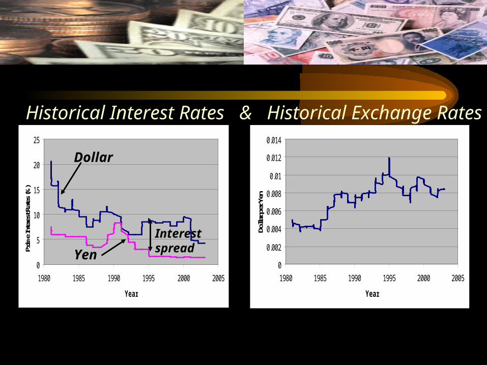
Historical Interest Rates & Historical Exchange Rates

Dollar

Yen

Interest spread

65

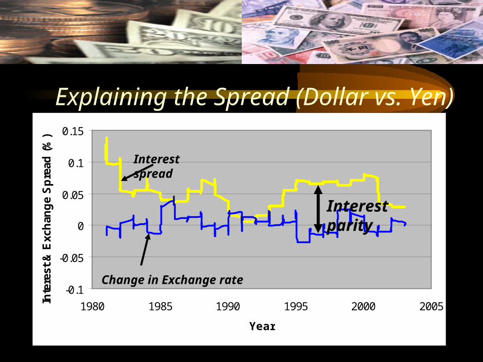
Explaining the Spread (Dollar vs. Yen)

-0.1

-0.05

0

0.05

0.1

0.15

1980 1985 1990 1995 2000 2005

Year

Inte

rest

& E

xch

ang

e S

pre

ad (

%)

Interest spread

Change in Exchange rate

Interest parity

Documents

Econ 240C Lecture 18. 2 Review 2002 Final Ideas that are transcending p. 15 Economic Models of Time Series Symbolic Summary