Graduate Theses and Dissertations Iowa State University Capstones, Theses andDissertations

2011

Economic analysis for transmission operation andplanningQun ZhouIowa State University

Follow this and additional works at: https://lib.dr.iastate.edu/etd

Part of the Electrical and Computer Engineering Commons

This Dissertation is brought to you for free and open access by the Iowa State University Capstones, Theses and Dissertations at Iowa State UniversityDigital Repository. It has been accepted for inclusion in Graduate Theses and Dissertations by an authorized administrator of Iowa State UniversityDigital Repository. For more information, please contact digirep@iastate.edu.

Recommended CitationZhou, Qun, "Economic analysis for transmission operation and planning" (2011). Graduate Theses and Dissertations. 12221.https://lib.dr.iastate.edu/etd/12221

Economic analysis for transmission operation and planning

by

Qun Zhou

A dissertation submitted to the graduate faculty

in partial fulfillment of the requirements for the degree of

DOCTOR OF PHILOSOPHY

Major: Electrical Engineering

Program of Study Committee: Chen-Ching Liu, Co-major Professor Leigh Tesfatsion, Co-major Professor

Venkataramana Ajjarapu William Meeker

Lizhi Wang

Iowa State University

Ames, Iowa

2011

Copyright © Qun Zhou, 2011. All rights reserved.

ii

TABLE OF CONTENTS

LIST OF FIGURES iv

LIST OF TABLES v

ABSTRACT vii

CHAPTER 1. INTRODUCTION 1

1.1 Motivation and Objectives 1

1.2 Literature Review 5

1.2.1 Short-Term Transmission Congestion Forecasting 5

1.2.2 Transmission Investment for Integrating Renewable Energy 6

1.3 Contributions of this Dissertation 8

1.4 Thesis Organization 10

CHAPTER 2. SHORT-TERM TRANSMISSION CONGESTION FORECASTING 12

2.1 Introduction 12

2.2 Basic Forecasting Problem Formulation 14

2.3 Basic Forecasting Algorithm Description 16

2.3.1 System Patterns and System Pattern Regions 16

2.3.2 Convex Hull Estimation of Historical SPRs 19

2.3.3 Basic Point Inclusion Test 22

2.3.4 Linear-Affine Mapping Procedure 23

2.4 Extension to Probabilistic Forecasting 25

2.4.1 Practical Data Availability Issues 25

2.4.2 Probabilistic Point Inclusion Test 27

2.4.3 Probabilistic Forecasting Algorithm 30

2.5 Five-Bus System: Basic Forecasting 31

2.5.1 Historical System Patterns and the Corresponding Sensitivity Matrices 32

2.5.2 Predicting System Pattern, Congestion and System Variables 33

2.6 NYISO Case Study: Probabilistic Forecasting 36

2.6.1 Case Study Overview 36

2.6.2 Implementation of Probabilistic Forecasting 37

2.6.3 Congestion Pattern Forecasts 39

2.6.4 Mean Forecasts for LMPs 40

iii

2.6.5 Interval Forecasts for Line Shadow Prices and LMPs 42

2.7 Extension to Cross-Scenario Forecasting 47

CHAPTER 3. TRANSMISSION INVESTMENT FOR INTEGRATING RENEWABLE ENERGY 49

3.1 Introduction 49

3.2 Nomenclature 50

3.3 Problem Formulation 51

3.3.1 Overview 51

3.3.2 Negotiation Process 52

3.3.3 Policy implications on RE subsidies 55

3.4 Negotiation: A Nash Bargaining Approach 55

3.4.1 Nash Bargaining 56

3.4.2 Bargaining on RE Interconnection: An Analytical Model 57

3.4.3 Bargaining on RE Interconnection: A Detailed Formulation 60

3.5 Implications on Renewable Subsidy Policy 63

3.5.1 Centralized Planning and Policy Implication 63

3.5.2 An Illustrative Example 64

3.5.3 Centralized Planning: A Detailed Formulation 68

3.6 Numerical Results 69

3.6.1 Garver’s Six-Bus Test Case 69

3.6.2 The Negotiated Solution with Renewable Energy Contract Price FP 72

3.6.3 The Negotiated Solution with Market-Based Price LMP 73

3.6.4 Centralized Transmission Planning 74

3.6.5 RE Subsidy Sensitivity Analysis 75

CHAPTER 4. CONCLUSION 79

4.1 Summary of the Dissertation 79

4.2 Future Work 81

APPENDIX. PROOF 82

BIBLIOGRAPHY 86

LIST OF PUBLICATIONS 94

iv

LIST OF FIGURES

Figure 1. Illustration of two system pattern regions (SPRs) in load space 19

Figure 2. Illustration of the QuickHull algorithm 21

Figure 3. Illustration of the basic point inclusion test for an SPR in a load plane 23

Figure 4. Convex hull estimates for SPRs can be biased 26

Figure 5. Two possible types of forecast error due to biased SPR estimates 27

Figure 6. 5-bus network 32

Figure 7. Predicted hourly power flow on line TL1 during day 363 35

Figure 8. Predicted LMP at bus 2 during day 363 35

Figure 9. Actual versus mean LMP forecasts for Zone Central on 01/31/2007 41

Figure 10. Actual versus mean LMP forecasts for Zone Central on 02/28/2007 41

Figure 11. Actual versus interval D-S line shadow price forecasts on 01/31/2007 43

Figure 12. Actual versus interval D-S line shadow price forecasts on 02/28/2007 44

Figure 13. Actual versus interval LMP forecasts for Zone Central on 01/31/2007 45

Figure 14. Actual versus interval LMP forecasts for Zone Central on 02/28/2007 46

Figure 15. Scenario-conditioned and cross-scenario forecasting 48

Figure 16. Negotiation between the RE-GenCo and the TransCo 54

Figure 17. Options for renewable generation and transmission investment 65

Figure 18. Garver’s six-bus test system 70

Figure 19. Transmission plan variation under SUB with contract price FP 76

Figure 20. Transmission plan variation under SUB with market-based price LMP 77

Figure 21. Payment rate variation under SUB with contract price FP 77

Figure 22 Payment rate variation under SUB with market-based price LMP 78

v

LIST OF TABLES

Table 1. Flags used for system patterns 17

Table 2. The four most frequent historical system patterns for the 5-bus system 32

Table 3. Sensitivity matrix and ordinate vector for system pattern S4 (partially shown) 34

Table 4. LMP and line congestion predictions under S3 34

Table 5. Four most frequent historical congestion patterns for 01/31/2007 38

Table 6. Forecasted congestion patterns versus the actual pattern on 01/31/2007 40

Table 7. RMSE and MAPE values for the twelve test days 42

Table 8. Loss function values as a measure of interval forecasting performance 46

Table 9. Generator and load data 70

Table 10. Wind unit data 70

Table 11. Transmission data 71

Table 12. Scenarios of wind speed in four subperiods 72

Table 13. Maximum possible output of wind energy 72

Table 14. Negotiated transmission investment decision YN 73

Table 15. Negotiated results of payment rate and attained utilities 73

Table 16. Negotiated transmission plan MNY and utility levels 74

Table 17. Centralized transmission investment decision Yc 75

Table 18. Social surplus under different investment decisions 75

vi

ACKNOWLEDGEMENTS

I would like to take this opportunity to express my deep and sincere gratitude to my

major professors, Dr. Chen-Ching Liu and Dr. Leigh Tesfatsion. I have been fortunate to

have Professor Liu as my advisor, who gave me the freedom to explore on my own and also

the guidance that leads me towards the correct research direction. His patience and

continuous support helped me accomplish this dissertation. I would also like to give my

sincere thanks to Professor Tesfatsion. I am deeply grateful to her for the discussions that

helped me sort out the technical details of my work. Besides being an inspiring advisor, she

is also an excellent mentor in life, where she always gives me valuable advice, and her

positive attitude has greatly influenced me in every aspect.

I am also grateful to my minor professor, Dr. William Meeker, for sharing his time to

discuss research with me and also providing strong support in my career development.

I am also thankful to Dr. Lizhi Wang and Dr. Ajjarapu Venkataramana for their

encouragement and valuable comments.

It is my pleasure to thank Dr. Ron Chu for the industry insights and enlightening

discussion in this research.

I would also want to thank my dear husband, Wei Sun, for being there all the time. I

am especially grateful to my parents, Chaoping Zhou and Suqin Wang, my sister and brother

for their unconditional support and encouragement in my endeavors.

The author acknowledges the financial support of Electric Power Research Center

(EPRC) at Iowa State University.

vii

ABSTRACT

Restructuring of the electric power industry has caused dramatic changes in the use of

transmission system. The increasing congestion conditions as well as the necessity of

integrating renewable energy introduce new challenges and uncertainties to transmission

operation and planning. Accurate short-term congestion forecasting facilitates market traders

in bidding and trading activities. Cost sharing and recovery issue is a major impediment for

long-term transmission investment to integrate renewable energy.

In this research, a new short-term forecasting algorithm is proposed for predicting

congestion, LMPs, and other power system variables based on the concept of system

patterns. The advantage of this algorithm relative to standard statistical forecasting methods

is that structural aspects underlying power market operations are exploited to reduce the

forecasting error. The advantage relative to previously proposed structural forecasting

methods is that data requirements are substantially reduced. Forecasting results based on a

NYISO case study demonstrate the feasibility and accuracy of the proposed algorithm.

Moreover, a negotiation methodology is developed to guide transmission investment

for integrating renewable energy. Built on Nash Bargaining theory, the negotiation of

investment plans and payment rate can proceed between renewable generation and

transmission companies for cost sharing and recovery. The proposed approach is applied to

Garver’s six bus system. The numerical results demonstrate fairness and efficiency of the

approach, and hence can be used as guidelines for renewable energy investors. The results

also shed light on policy-making of renewable energy subsidies.

1

CHAPTER 1. INTRODUCTION

1.1 Motivation and Objectives

The integration of electricity markets and renewable energy into electric power

systems continue to increase. Transmission operation and planning have become highly

challenging in the new environment.

This research is aimed to tackle two challenging issues in transmission system

operation and planning. Specifically, the first task is the development of a short-term

congestion and price forecasting tool to facilitate bidding and trading strategy development

for market participants. The proposed algorithm exploits both structural and statistical

aspects of wholesale power markets, and outperforms state-of-the-art forecasting tools.

The second task is concerned with a new methodology to guide renewable energy

generation and transmission companies on the negotiation of transmission investment cost

sharing and recovery. The proposed approach based on Nash Bargaining theory gives a fair

and efficient utility allocation in the negotiation process. The negotiation is further compared

with a centralized planning model to provide guidance for policy makers on establishing

appropriate renewable energy subsidies.

In many transmission regions, congestion in wholesale power markets is managed by

Locational Marginal Prices (LMPs), the pricing of power in accordance with the location and

timing of its power injection into or withdrawal from the transmission grid. Congestion and

LMP forecasts are highly important for decision-making by market operators and market

participants.

2

In short-term transmission operation, congestion occurs when the available

economical electricity has to be delivered to load “out-of-merit-order” due to transmission

limitations. Transmission congestion is detrimental to power system security. It also causes

LMP discrepancies between the constrained and unconstrained areas, which could lead to a

high congestion cost. Therefore, as a result of transmission congestion, high reliability risks

and electricity price risks are faced by system operators and market participants, respectively.

Congestion forecasting is critical to market operators as well as market participants

[1]. Congestion forecasting tools can be used for identification of potential congestive

conditions, detection of the exercise of market power, and scenario-conditioned planning.

Congestion forecasting also gives interpretable signals to electricity price behaviors, and can

be used to induce more accurate and reliable price forecasting which assists market

participants in making decisions for bidding and trading strategies. Therefore, accurate

forecasts of congestion and LMP also give advantages to market traders in bidding and

trading activities and long-term investment planning.1

In long-term system planning, major transmission projects are needed, in the United

States and beyond, to integrate renewable resources, primarily wind generation, located

mostly in remote areas. The delivery of renewable energy is important for meeting the

Renewable Portfolio Standards (RPS). As of February 2009, nearly 300,000MW of wind

projects were waiting to be connected to the grid [2]. One factor contributing to the backlog

1 For example, during an internship at Genscape, Inc., the author observed first-hand that the customers for Genscape’s LMP forecasting services were generation companies, load-serving entities, and utilities interested in developing daily market bidding strategies and improving their over-the-counter electricity trading.

3

is the difficulty in siting transmission lines due to local oppositions. For lines crossing

multiple states, additional difficulties arise in the permitting process due to different state

laws and regulations. However, the real issues are the uncertainties concerning who should

bear the transmission costs and how the transmission investments should be recovered. In

order to meet the RPS at the mandated date, these issues need to be resolved and

transmission projects need to be completed.

Transmission can be separated into three categories; regulated, generation

interconnection or merchant transmission. In general, the cost responsibility of the regulated

transmission for reliability, economic and operational performance purposes is assigned to

the loads benefiting from the investment via a regulated rate. The generation developers bear

transmission cost for interconnecting its proposed generation and a transmission developer

will be responsible for its merchant transmission project [3]. But the policy-driven

transmission to meet RPS is a new category in which cost responsibility has not been clearly

defined.

Currently, a RE developer has to pay the entire cost of the generation interconnection

transmission to the interconnected Transmission Owner through a Regional Transmission

Organization (RTO), such as PJM, ISO-New England, and New York ISO, prior to the in-

service date of the generator. As a result, the RE developer bears the whole risk of both

generation and transmission investments. This increases the cost to finance a RE project and

discourage the investment. On the contrary, the authors propose a market-based approach,

where the unavoidable risks and uncertainties due to renewable energy intermittency could

be shared by RE developers and transmission companies. The expected generation revenue

will be used to fund the RE and transmission projects.

4

In this dissertation, the interconnection of a RE project is accomplished by a

Merchant Transmission (MT) project and is coordinated between a RE Generation Company

(RE-GenCo) and a Transmission Company (TransCo). Furthermore, the recovery of their

investments is a result of a negotiation between the two entities using the expected generation

profit based on the market and generation performance. Hence, a RE-GenCo waiting to be

connected to the power grid can actively seek out a TransCo who is interested in investing in

new transmission lines if the compensation from the RE-GenCo is sufficiently attractive.

Negotiation then can proceed considering the uncertainties associated with outputs renewable

resources and electricity prices. An agreement is reached if satisfactory returns are achieved

for both companies.

The prerequisite for a successful settlement from the negotiation between a RE-

GenCo and a TransCo is the sufficient profit margins for both parties. However, it is possible

that the expected generation revenue may not be adequate to cover the generation and

transmission investments plus the profit margin. Under this situation, an incentive may be

required to assure the accomplishment of these investments. However, if an incentive is

needed, policy makers will have to deal with the questions, “What do the incentives look like

and what would be their optimal values?” Schumacher et al. [4] report that incentive could be

policy initiatives to promote transmission development. FERC also eases policies [5] for MT

developers to hold auction to attract and pre-subscribe some capacity to “anchor customers.”

Incentive can be monetary incentives such as Renewable Energy Certificates (RECs) that

need to be purchased by LSEs to meet the RPS [6], or energy subsidies such as Investment

Tax Credits (ITCs) and Production Tax Credits (PTCs). Using monetary incentives, RE-

GenCos could gain an additional revenue stream that facilitates the negotiation process.

5

1.2 Literature Review

1.2.1 Short-Term Transmission Congestion Forecastin g

Many studies have focused on electricity price forecasting. With only publicly

available information in hand, most applicable price forecasting tools are restricted to

statistical methods [1], [7]-[17]. For example, statistical methods are deployed to forecast the

hourly Ontario energy price on a basis of publicly available electricity market information [7].

Nogales’ research in [8] is a pioneering work in the application of time series models in

electricity price forecasting. ARIMA [9] and GARCH [10] are also used to predict electricity

price. Meanwhile, another branch in statistical forecasting has been developed based on

intelligent system techniques, among which neural network approaches are widely used in

load forecasting and extended to price forecasting as well. Shahidepour in [11] primarily

focuses on the application of Artificial Neural Network (ANN) in load and price forecasting.

Other neural network approaches [12]-[15] are also investigated in electricity price

forecasting. Structural models considering wholesale power market fundamentals have also

been attempted [19]-[20].

However, few studies have focused on congestion forecasting. Li [21] applies a

statistical model to predict line shadow prices. EPRI [22] has developed a congestion

forecasting model that uses sequential Monte Carlo simulation to produce a probabilistic load

flow. The EPRI model provides congestion probabilities for transmission lines of interests,

but it requires intensive data input to the load flow model.

Li and Bo [23]-[24] examine LMP variation in response to load variation, and they

predict the next binding constraint when load is increased. However, the authors also assume

6

that a particular system growth pattern exists and that load growth at each bus is proportional

to this pattern. Most U.S. wholesale power markets operating under LMP are geographically

large; hence, distributed loads do not necessarily exhibit proportional growth. Moreover, the

authors’ approach has not been applied in large-scale power systems where practical issues

of limited data availability need to be considered.

In our study [25], a piecewise linear-affine mapping between distributed loads and

DC-OPF system variable solutions was identified and applied to forecast congestion and

LMPs under the maintained assumption that complete historical information was available

regarding the marginality (or not) of generating units and the congestion (or not) of

transmission lines. This method is able to give an exact prediction result since it is derived

from the core structure of a wholesale power market. However, when applied to the actual

forecasting of large-scale wholesale power systems, data requirements become a problem.

The needed historical generation capacity data and line flow data are either publicly

unavailable on market operator websites or only available with some delay. Consequently,

the correct pattern of binding constraints corresponding to any possible future load point is

difficult to effectively identify, which in turn prevents the accurate forecasting of system

variables.

1.2.2 Transmission Investment for Integrating Renew able Energy

The transmission expansion planning problem has been addressed by a number of

researchers from technical point of view. Garces et.al proposed a bilevel approach for

transmission planners to minimize network cost while facilitating energy trading [26]. A

multi-objective framework is developed to handle different stakeholders’ interests [27], and

7

transmission planning models proposed in [28] and [29] take into account the demand

uncertainty. Transmission expansion methodologies regarding the uncertainty from large-

scale wind farms are presented in [30] and [31]. Sauma and Oren [32] provide an evaluation

method for different transmission investments based on equilibrium models with the

consideration of interactive generation firms.

These studies focus on solving optimal transmission investment decisions in

centralized approaches which are usually undertaken by centralized transmission planners or

regulatory bodies. The centralized planning is associated with a FERC approved rate method

for the transmission developers, typically the traditional utilities, to recover their costs of

investment. A number of rate methods have been examined in the literature. Typically, a

postage stamp rate is adopted to recover the fixed transmission cost [33]. Different usage-

based methods are also suggested and evaluated by Pan et. al [33]. The potential fairness

issue in usage-based methods is attempted to resolve using min-max fairness criteria [34]. In

addition to the rate structure, Galiana et.al proposed a cost allocation methodology based on

the principle of equivalent bilateral exchanges. The allocated cost responsibilities are then

used to set the rates for different LSEs. Finally, different allocation and rate setting

approaches are presented in [35]-[39].

Independent from the centralized planning performed by RTOs such as PJM, research

effort has been dedicated to explore market-based transmission planning models which can

be considered as decentralized approaches for transmission investment. Roh et al. [40]

proposed a coordinated transmission and generation planning model which incorporates the

characteristics from the centralized and decentralized models. RTO acts as a coordinator

rather than a decision maker by providing capacity signals to market participants who

8

independently decide the investment plans. Research has been conducted on merchant

transmission projects, a market-based transmission investment in the current US electricity

markets. Joskow and Tirole [41] examined performance attributes associated with merchant

transmission models with the consideration of several realistic attributes of electricity

markets and transmission networks. Salazar et al. [42] identified the most opportunistic time

to start a merchant transmission project from an investor point of view. In their continued

work [43], they proposed a market-based rate design for recovering merchant transmission

investment costs from policy makers’ point of view.

The transmission investment model in this dissertation differs from the previous work

in that the investment of a market-based transmission project is recovered via a negotiated

transmission rate from a RE-GenCo to a TransCo. Negotiation results are derived and

provide guidance for market participants in an actual negotiation process. Additionally, the

model can be used to develop renewable energy subsidies for policy makers to design market

incentives for promoting transmission investment and use of renewable energy resources.

1.3 Contributions of this Dissertation

Transmission is a critical component in power systems. Economic analysis of

transmission system is an important task to support the decision making in short-term

operation and planning. This dissertation is focused on the development of transmission

congestion forecasting tool and transmission investment model for integrating renewable

energy. The original contributions are summarized as follows:

1. A congestion forecasting tool based on convex hull techniques

9

The proposed forecasting algorithm is a novel use of convex hull techniques to enable

the short-term forecasting of congestion conditions, prices, and other system variables. The

convex hull algorithm and probabilistic inclusion test effectively predict congestion patterns

at various operating points. Compared with state-of-the-art structural forecasting models, this

new method significantly reduces the forecasting data requirement by using only publicly

available data but still achieves a high level of accuracy.

2. A novel concept of system patterns to enhance the forecasting accuracy

The forecasting algorithm proposes the new concept of system patterns as an effective

way to take generation and transmission capacity constraints into account. This concept

captures the core structure of wholesale power markets and hence permits more accurate

forecasting results. The new method exploiting the system pattern concept outperforms

traditional statistical forecasting models for large-scale power systems.

3. A negotiation methodology for renewable energy transmission investment based on

Nash Bargaining theory

The proposed transmission investment model based on Nash Bargaining approach

provides a decentralized methodology for integrating renewable energy. The negotiation

methodology takes into account electricity market uncertainties and the intermittent nature of

renewable energy. The negotiated results provide guidelines for renewable energy generation

and transmission companies in sharing and recovering integration and investment cost.

4. A new approach to evaluate renewable energy subsidy policy

The comparison between negotiation and centralized planning addresses the issue of

optimal subsidy policy to produce sufficient incentives for renewable energy investment. The

optimal subsidy policy can steer the negotiated solution to a centralized solution that

10

maximizes the social surplus. The results provide important guidance for policy makers to

establish proper renewable energy subsidies.

1.4 Thesis Organization

This research conducts an economic analysis for transmission operation and planning.

Specifically for short-term transmission operation, it is intended to provide a congestion and

price forecasting tool by analyzing the fundamentals of power markets. For long-term

transmission planning, a systematic negotiation methodology among market participants is

provided for renewable energy investment incorporating the stochastic nature of renewable

resources. The comparison between the negotiation model and centralized planning model is

a resource for decision support in policy making of renewable energy subsidies.

Chapter 2 presents a congestion forecasting tool based on the results of [44]. A new

short-run congestion forecasting algorithm is proposed based on the concept of system

patterns—combinations of status flags for transmission lines and generating units. It is shown

that the load space can be divided into convex sets within which system variables can be

expressed as linear-affine functions of loads. Congestion forecasting is then transformed into

the problem of identifying the correct system pattern. A convex hull algorithm is developed

to estimate the convex sets in the load space. A point inclusion test is used to identify the

possible system patterns and congestion conditions for a future operating point and a

corresponding “sensitivity matrix” is used to forecast LMPs and line shadow prices.

Forecasting results based on a NYISO case study demonstrate that the proposed forecasting

procedure is highly efficient.

11

Chapter 3 outlines the research on transmission investment to integrate renewable

energy. The negotiation process is analyzed for renewable energy interconnection between a

RE-GenCo and a TransCo. Nash Bargaining theory is adopted to determine the transmission

investment plans and RE-GenCo’s transmission payment. The negotiation methodology as

well as its results provides an alternative means to transmission planning for integrating

renewable energy. By modifying the included subsidies, the proposed negotiation approach

produces results (i.e. transmission plan and rate) mirroring those from a centralized planning

model in which the objective is to maximize the overall social surplus. The renewable energy

subsidies can be used as an adjusting parameter to steer the investment plan derived from the

negotiation towards an optimal plan. This result and comparison provide important guidance

to policy makers for determining appropriate renewable energy subsidies.

Chapter 4 provides conclusions and discusses the future research directions.

12

CHAPTER 2. SHORT-TERM TRANSMISSION CONGESTION

FORECASTING

2.1 Introduction

In this chapter, a new algorithm is developed for the short-term forecasting of system

variables in wholesale power systems with substantially reduced data requirements. This

algorithm permits the derivation of estimated probability distributions for congestion, LMPs,

and other DC-OPF system variable solutions in real-time markets and in forward markets

with hour-ahead, day-ahead and week-ahead time horizons, conditional on a given

commitment-and-line scenario that specifies a set of generating units committed for possible

dispatch and a set of transmission lines capable of supporting power flow. Moreover, given

suitable availability of historical data, this scenario-conditioned forecasting algorithm can be

generalized to a cross-scenario forecasting algorithm by the assignment of probabilities to

different commitment-and-line scenarios.

This new forecasting algorithm makes use of two supporting techniques in order to

substantially reduce the amount of required data relative to [25]. The first technique is a

method developed by Bemporad et al. [45] and Tøndel et al. [46] for dividing the parameter

space of a Quadratic-Linear Programming (QLP) problem into convex subsets such that,

within each convex subset, the optimal solution values can be expressed as linear-affine

functions of the parameters. A similar technique is applied in this study to a QLP DC-OPF

problem formulation to show that, conditional on any given commitment-and-line scenario,

the load space can be divided into convex subsets within which the optimal DC-OPF system

13

variable solutions are linear-affine functions of load. Each convex subset corresponds to a

unique system pattern, that is, a unique array of flags reflecting a particular pattern of binding

minimum or maximum capacity constraints for the committed generating units and available

transmission lines specified by the commitment-and-line scenario.

The second technique concerns convex hull determination. Given any collection of

points, computational geometry [47] provides algorithms to compute the corresponding

convex hull, i.e., the smallest convex set containing these points. Convex hull algorithms

have been gaining popularity in the areas of computer graphics, robotics, geographic

information systems and so forth. To date, however, they have not been applied in electricity

market forecasting. A convex hull algorithm is used in this study to estimate the convex

subsets of load space within which DC-OPF solutions are linear-affine functions of load

when incomplete historical data prevent their exact determination.

More precisely, the proposed forecasting algorithm generates short-term forecasts for

congestion, LMPs, and other power system variables as follows. Let L denote a vector of

loads at some possible future operating point corresponding to a particular commitment-and-

line scenario S. A convex hull method is first used to estimate the division of load space into

convex subsets (system pattern regions), each corresponding to a distinct historically-

observed system pattern of binding capacity constraints for the particular committed

generating units and available transmission lines specified under S. A probabilistic point

inclusion test is next used to calculate the probability that L is associated with each historical

system pattern, taking into account the imprecision with which the system pattern regions in

load space are estimated. The congestion conditions at L are then probabilistically forecasted

using the probability-weighted historical system patterns, and forecasts for LMPs and other

14

system variables at L are calculated using the linear-affine mapping between load and DC-

OPF system variable solutions that corresponds to each probability-weighted historical

system pattern.

2.2 Basic Forecasting Problem Formulation

In electricity markets, congestion occurs when the available economical electricity

has to be delivered to load “out-of-merit-order” due to transmission limitations. That is,

higher-cost generation needs to be dispatched in place of cheaper generation to meet this load

in order to avoid overload of transmission lines. In this case, the LMP levels at different

nodes separate from each other and from the unconstrained market-clearing price. Therefore,

congestion is a critical factor determining the formation of LMP levels.

However, congestion patterns are difficult to anticipate since they are related to the

network topology of power systems. Provided perfect information is available, such as

network data, load data, and generator bidding data, a market clearing model could be

utilized to obtain accurate forecasts of congestion conditions and prices. Nevertheless, two

issues arise for this direct forecasting method. First, most market traders do not have direct

access to the information that is needed to implement this method; they would have to

depend on data published by market operators. Second, the market operators, themselves,

would need a high degree of computational speed to carry out the required computations.

As a result, statistical tools have been developed that tackle these two forecasting

issues by modeling the statistical correlation between prices and explanatory factors. These

statistical tools lack explicit consideration for congestion, partly because no effective

approach has been developed to enable these tools to capture and express the effects of

15

congestion. Ignoring the effects of congestion makes the forecasted prices less reliable and

difficult to interpret at operating points with abnormal price behaviors.

Surely it is possible to glean some useful information about future possible

congestion conditions based on statistically forecasted LMPs. However, these intuitive

insights, based on forecasters’ experiences, cannot provide reliable congestion forecasts.

From a cause-and-effect point of view, congestion is the cause while LMP is the effect. One

cannot infer the cause (congestion) from the effect (LMP) since LMP is not solely driven by

congestion. In particular, statistical LMP forecasting tools do not take into account the

structural aspects of power markets that fundamentally drive the determination of LMPs:

namely, the fact that LMPs are derived as solutions to optimal power flow problems subject

to generation capacity and transmission line constraints.

As explained more carefully in Section 2.3.1, the novel concept of a “system pattern”

is used in this study to incorporate the structural generation capacity and transmission line

aspects that drive congestion outcomes. The forecasting of congestion at a possible future

operating point is thus transformed into a problem of estimating the correct system pattern at

this operating point. Moreover, the forecasting of prices and other system variables at this

operating point can subsequently be undertaken using the particular linear-affine mapping

between load and DC-OPF system variable solutions that is associated with this system

pattern.

This basic forecasting approach makes three simplifying assumptions. First, it is

assumed that the forecasting of system variables at possible future operating points can be

conditioned on a particular commitment-and-line scenario, that is, a particular generation

commitment (designation of generating units available for dispatch) and a particular network

16

topology (designation of available transmission lines). Second, it is assumed that a lossless

DC-OPF problem formulation is used for the determination of LMPs and other system

variables, implying in particular that the loss components of LMPs are neglected. Third, it is

assumed that generator supply-offer behaviors are relatively static in the forecasting

horizons.

2.3 Basic Forecasting Algorithm Description

2.3.1 System Patterns and System Pattern Regions

At any system operating point, the number of marginal generating units and binding

transmission constraints tends to be small compared to the number of nodes, transmission

lines, and generating units. For example, in the Midwest Independent System Operator

(MISO) region with 36,845 network buses and 5,575 generating units, the number of day-

ahead binding constraints is published daily and is typically observed to be less than 20 for

an hourly interval [48]. On the other hand, high-cost units such as gas and oil units are more

likely to become marginal units during peak hours, the number of which is modest.

Exploiting this important characteristic of power markets, the idea of a system pattern

is introduced consisting of a vector of flags indicating the marginal status of committed

generating units and the congestion status of available transmission lines at any given system

operating point; see Table 1. As long as the number of marginal generating units (labeled 0)

and the number of congested transmission lines (labeled -1 or 1) are relatively few in number,

the number of possible system patterns can be easily handled.

As noted in Section 2.2, the basic congestion forecasting problem can then be

transformed into a problem of estimating the correct system pattern for any given possible

17

future operating point. The congestion forecast is directly obtained once the system pattern is

estimated, since the status of transmission lines is part of the system pattern. Moreover, as

clarified below in Section 2.3.4, short-term forecasts for prices and other system variables at

the operating point can also be obtained making use of this estimated system pattern.

Table 1. Flags used for system patterns

Generating units Transmission lines

State Minimum

Capacity

Marginal

Unit

Maximum

Capacity

Negative

Congestion

No

Congestion

Positive

Congestion

Flag -1 0 1 -1 0 1

The proposition below provides the theoretical foundation for our proposed

forecasting approach. The proposition uses the concept of a convex polytope for an n-

dimensional Euclidean space Rn, i.e., a region in Rn determined as the intersection of finitely

many half-spaces in Rn.

Proposition 1: Suppose a standard DC-OPF formulation with fixed loads and

quadratic generator cost functions is used by a market operator to determine system variable

solutions. Then, conditional on any given commitment-and-line scenario S, the load space

can be covered by convex polytopes such that: (i) the interior of each convex polytope

corresponds to a unique system pattern; and (ii) within the interior of each convex polytope

the system variable solutions can be expressed as linear-affine functions of the vector of

distributed loads.

The proof of Proposition 1, originally derived in [44], is outlined in an appendix to

this dissertation. The proof starts with the derivation of inequality and equality constraints

constructed from the first-order KKT conditions for a DC-OPF problem conditional on a

18

particular commitment-and-line scenario S. The inequality constraints characterize convex

polytopes that cover the load space, where the interior of each convex polytope corresponds

to a unique system pattern. The convex polytopes constituting the covering of the load space

are referred to as System Pattern Regions (SPRs) for the fact that the interior of each convex

polytope is associated with a unique system pattern.

Within each SPR the equality constraints take the form of linear-affine equations with

constant coefficients that describe fixed linear-affine relationships between DC-OPF system

variable solutions and the vector of loads. The matrix of coefficients for these linear-affine

functions gives the rates of change with regard to real-power dispatch levels for generating

units and shadow prices for bus balance and line constraints when loads are perturbed within

the region. This matrix is referred to below as the sensitivity matrix for this SPR.

Figure 1 provides illustrative depictions of two SPRs, R1 and R2, together with their

associated linear-affine mappings, when the load space is composed of two-dimensional load

vectors L = (L1, L2). The symbol P denotes the vector of unit dispatch levels, and the symbol

Λ denotes the vector of dual variables. The mappings are characterized by sensitivity

matrices (K1, K2) and ordinate vectors (0

1K , 0

2K ) that are constant within each SPR, which

implies that the DC-OPF solutions for P and Λ can be expressed as fixed linear-affine

functions of the load vector L within each SPR.

19

01 1

PK L K

= + Λ

02 2

PK L K

= + Λ

Figure 1. Illustration of two system pattern regions (SPRs) in load space

2.3.2 Convex Hull Estimation of Historical SPRs

In practice, deriving the exact form of the SPRs is difficult due to limited access to

most of the required information. This required information includes supply offer data,

generating unit capacity data, and transmission limit data.

This lack of information can be overcome by applying a “convex hull algorithm” to

historical load data to estimate SPRs. The convex hull of a point set B is the smallest convex

set that contains all the points of B [49]. A convex hull algorithm is a computational method

for computing the convex hull of a set B.

Each historical load point corresponding to a particular commitment-and-line

scenario S can in principle be associated with a distinct system pattern based on

corresponding historical data regarding the marginal status of the committed generating units

and the congested status of the available transmission lines. The historical SPR

corresponding to each such historically identified system pattern can then be estimated by

20

deriving the convex hull of the collection of all historical load points that have been

associated with this system pattern.

This study makes use of the “QuickHull algorithm” to estimate historical SPRs

conditional on a given commitment-and-line scenario S. The QuickHull algorithm, developed

by Barber et al. [50], is an iterative procedure for determining all of the points constituting

the convex hull of a finite set B. At each step, points in B that are internal to the convex hull

of B, and hence not viable as vertices of the convex hull, are identified and eliminated from

further consideration. This process continues until no more such points can be found.

An illustrative application of the QuickHull algorithm for a finite planar set B is

presented in Figure 2. The set B is first partitioned into two subsets B1 and B2 by a line lr

connecting a left-most upper point l to a right-most lower point r, as depicted in in Figure

2(a). More precisely, the points in B with the smallest x value are first selected and, from

among these points, a point with a largest y value is chosen to be the left-most upper point l;

similarly for the right-most lower point r. For each subset B1 and B2, a point z in B that is

furthest from lr is determined and two additional lines are constructed, lzur from l to z and

zruur

from z to r; see Figure 2(b). By construction, points of B that lie strictly inside the

resulting triangle lzr are strictly interior to the convex hull of B and hence can be eliminated

from further consideration. The points on the triangle itself are possible vertex points for the

boundary of the convex hull of B.

21

Figure 2. Illustration of the QuickHull algorithm

To continue the recursion, the above procedure is repeated for the reduced subset

BRed of B resulting from this elimination. Specifically, two subsets and associated triangles

are formed as before for BRed and the points of BRed lying within the interiors of the

resulting triangles are eliminated. If a triangle ever degenerates to a line, then all the points

along the line lie on the boundary of the convex hull of B by construction. For example, in

Figure 2(c) the endpoints r and m of the line rm both lie on the boundary of the convex hull

of B.

This process of elimination continues until no additional points to be eliminated can

be found. Since B is finite, the process is guaranteed to stop in finitely many steps. All the

convex hull points for B (boundary and interior) can be determined recursively in this manner.

The complete convex hull for B is depicted in Figure 2(d). By construction, this convex hull

is a planar convex polytope.

The main advantage of the QuickHull algorithm relative to other such algorithms is

its ability to efficiently handle high-dimensional sets B by reducing computational

22

requirements [51]. The QuickHull algorithm has been widely used in scientific applications

and appears to be the algorithm of choice for higher-dimensional convex hull computing [52].

2.3.3 Basic Point Inclusion Test

Suppose the load space has been divided up into estimated SPRs whose interiors

correspond to distinct system patterns, conditional on a given commitment-and-line scenario

S. Consider, now, the task of forecasting congestion conditions at some future operating point

a short time into the future for which scenario S again obtains. The essence of this forecasting

problem is the detection of the correct SPR for this future operating point. If the correct SPR

can be detected, then congested conditions can be inferred directly from the corresponding

system pattern.

This detection is undertaken in this study by means of a “point inclusion test”. The

basic point inclusion test used in this study is illustrated in Figure 3 for an SPR in a load

plane. Recall that each SPR takes the form of a convex polytope, i.e., a region expressable as

the intersection of half-spaces; hence each SPR has flat faces with straight edges. Let the

normal vectors pointing towards the interior of the SPR be constructed for each edge of the

SPR. Now consider the depicted point P1, and let 1aP

uuur denote the vector directed from the

vertex a to the point P1. The dot product between 1aP

uuur and each normal vector of each

neighboring edge of a is greater than or equal to 0. If this is true for all vertices of the SPR,

the point P1 is judged to be on or inside the SPR. On the other hand, one can see that P2 is

outside the SPR since the dot product of 2aP

uuur and the normal vector for the neighboring edge

connecting a to b is negative.

23

Figure 3. Illustration of the basic point inclusion test for an SPR in a load plane

As will be seen in Section 2.4, practical data-availability issues prevent the use of the

basic point inclusion test for the exact determination of the SPR containing any possible

future load point L. However, given a suitable probabilistic extension of this basic point

inclusion test, the probability that any particular SPR contains L can be estimated.

2.3.4 Linear-Affine Mapping Procedure

Given sufficient generation and transmission information, each historical load point

can be associated with an SPR according to the status of the generating units and

transmission lines at the historical operating time. More precisely, given any commitment-

and-line scenario S, consider the collection of all historically observed load points obtaining

under S. Let this collection of historical load points be partitioned into subsets corresponding

to distinct system patterns for scenario S. For each load subset, use the QuickHull algorithm

to calculate its convex hull in load space. Each of these convex hulls then constitutes a

distinct estimated SPR for scenario S. In principal, any future load point corresponding to

scenario S can then be associated with one of these estimated SPRs by means of the basic

24

point inclusion test. This association permits the prediction of congestion, prices, and other

DC-OPF system variable solutions at this load point.

To see this more clearly, let hiY and hiL denote matrices consisting of all historically

observed DC-OPF system solution vectors and load vectors corresponding to a particular

system pattern i for a particular commitment-and-line scenario S. Let the SPR in load space

corresponding to this system pattern, denoted by Ri, be estimated by the convex hull REi of

the collection of all of the historically observed load vectors included inhiL .

By Proposition 1, the mapping between hiY and h

iL can be expressed in the linear-

affine form

0h hi i i iK LY K= + (1)

where Ki denotes the sensitivity matrix corresponding to Ri. Normally there will be

multiple historical operating points corresponding to any one SPR for a given commitment-

and-line scenario S. In this case Ordinary Least Squares (OLS) can be applied to (1) to

obtain estimates iK and 0ˆiK for iK and 0

iK , as follows:

( )0

1ˆ )

ˆ( )

(( )

T

T T hi

iT

i

TK

K

−

=

X X X Y (2)

where )[ ]( h T

iL=X 1 .

Now let fiL denote a possible load vector for a future operating time that has been

found to belong to the estimated SPR REi, as determined from a basic point inclusion test

applied to the collection of all historically estimated SPRs corresponding to scenario S. Then

the forecasted vector fiY of DC-OPF system variable solutions corresponding to fiL can be

calculated as

25

0ˆ ˆf f

i i i iK LY K= + (3)

The above linear-affine mapping procedure is modified in Section 2.4 to

accommodate some practical issues arising from data incompleteness.

2.4 Extension to Probabilistic Forecasting

Practical data availability issues arise for the implementation of the basic scenario-

conditioned forecasting algorithm outlined in Section 2.3. This section discusses how these

issues can be addressed by means of a probabilistic extension of this basic algorithm.

Throughout this discussion the analysis is assumed to be conditioned on a given

commitment-and-line scenario S.

2.4.1 Practical Data Availability Issues

The basic scenario-conditioned forecasting algorithm proposed in Section 2.3

assumes that historical data are available regarding binding constraints for all generating

units and for transmission lines on an hourly basis. In actuality, however, the marginal status

of generating units is either confidential or published with limitations. Moreover, the

theoretical load space cannot be fully reflected by the hourly historical load data which

represent several realizations and subsets of the complete load space.

Due to these data limitations, in practice the set A indexing hourly binding

constraints cannot be completely determined. Consequently, estimates obtained for the SPRs

could be biased. The two basic ways in which this bias could arise are illustrated in Figure 4

for a simple two-dimensional load space. Suppose the SPR corresponding to the true binding

constraint set A is given by RA (area 1) in Figure 4.

26

This true SPR RA can in principle be determined by applying the basic point inclusion

test to every possible future operating point. Suppose, however, that the practically estimated

binding constraint set AE1 is incomplete; for example, suppose AE1 only reflects the status of

the most frequently congested lines. Given complete historical load data, the estimated

convex hull RE1 (area 3) would then have to be larger than the true RA (area 1) because AE1 is

smaller (less restrictive) than the trueA . In fact, however, the actual estimated convex hull

must be based on available historical load data. Since the latter is only a subset of the full

load space, the result will be an actual estimated convex hull RE (area 2) that lies within RE1

(area 3). In short, incompleteness of A and incompleteness of the practical load space each

separately introduce bias in the estimate for RA, but in opposing directions.

Figure 4. Convex hull estimates for SPRs can be biased

What are the practical implications of this bias for our basic forecasting algorithm?

Two possible cases need to be handled, as illustrated in Figure 5.

Case A: Point r in Figure 5 lies in the interior of two different estimated SPRs,

namely, RE1 and RE2 corresponding to two distinct system patterns A1 and A2. The true SPRs

corresponding to A1 and A2 are denoted by the shaded regions RA1 and RA2, respectively. The

27

fact that the interiors of the true SPRs do not overlap follows from Proposition 1. However,

as explained above, overlap can occur for the interiors of estimated SPRs due to bias.

Case B: Point t in Figure 5 is actually in the true SPR RA2. However, point t cannot

be assigned to either of the estimated SPRs because the bias in these estimates has caused

point t to lie outside of both of them.

Figure 5. Two possible types of forecast error due to biased SPR estimates

2.4.2 Probabilistic Point Inclusion Test

To mitigate the issues arising from the two types of bias discussed in Section 2.4.1,

mean and interval forecasting can be performed for the DC-OPF system variable solutions

corresponding to any forecasted future load point Lf. This probabilistic forecasting can be

implemented by estimating the probability of each SPR conditional on Lf, which can be

characterized as a probabilistic point inclusion test.

More precisely, let Lf denote the forecasted load at a future operating point f, and let

Ri denote any particular SPR i. Let the collection of all historically identified SPRs be

denoted by Rh, and let CR denote the cardinality of Rh. Suppose the probability of occurrence

28

for any SPR not in Rh is zero. Then the probability that Ri has occurred, given that Lf has been

observed, can be expressed as:

( )( )

( | )|

( | ( ))h

i i

i

f

f

Ri

ii

f R P RP R

R P R

P LL

P L∈

=∑

(4)

In practice, the various terms in (4) have to be estimated. In this study it will be

assumed that the prior probability ( )iP R is an empirical prior estimated by the historical

frequency of Ri: namely, the number of times in the past that Ri has been observed to occur

divided by the total number of all past SPR observations.

The term ( )|fiP L R in (4) represents the probability of observing the load point Lf

given that the true SPR is Ri. Intuitively, this probability should be a decreasing function of

the distance between Lf and Ri. Therefore, this probability is estimated in this study as

follows:

( / )ˆ |(

1( )

1 / )h

f ii

iRi

TDP R

D T

DL

D

γ

γ

∈

−=

−∑ (5)

In (5) the term Di denotes the (Euclidean) distance between Lf and Ri, and TD denotes

the total distance calculated as the sum of the distances between Lf and each SPR in Rh. The

normalization parameter γ in (5) can be adjusted to obtain an appropriate conditional

probability measure, possibly by using historical data as training cases. A specification

0γ = results in a uniform conditional probability (5) for Lf: namely, 1 divided by the

cardinality CR of Rh. In this case (5) is independent of the distance measures Di.

Alternatively, a specification 1γ = implies the conditional probability (5) is derived from a

linear normalization, while 2γ = corresponds to a quadratic normalization. As will be shown

29

below, the quadratic normalization form of the conditional probability (5) results in good

forecasts for our NYISO case study.

Mean forecasts for the DC-OPF system variable solutions at the operating point f with

forecasted load point Lf can then be obtained using the estimated form for the conditional

probability assessments (4), denoted by fiP for short. Let f

iY denote the forecasted DC-OPF

system variable solution vector corresponding to any historical SPR Ri in Rh. The mean

forecast fY can then be calculated as

h

f f fi i

i R

PY Y∈

= ∑ (6)

A forecaster might also be interested in calculating upper and lower bounds for the

DC-OPF system variable solutions calculated with respect to the most likely SPRs. Let nmp

denote the forecaster’s desired cut-off number of most probable SPRs, and let MP represent

the subset of Rh that contains these nmp most probable SPRs. Then the upper bound UBf and

lower bound LBf for each forecasted DC-OPF system variable solution can be determined

over the set of SPRs in MP. As a measure of dispersion, the forecaster can further consider

the coverage probability CP, defined to be the summation of the probability assessments (4)

for the nmp most probable SPRs.

Finally, another alternative might be for the forecaster to consider mean forecasts

calculated using the nmp most probable SPRs, i.e. the subset MP of Rh. For example, a

forecaster could choose nmp=1, which would result in a point forecast for the DC-OPF

system variable solutions based on a single most likely SPR Ri in Rh as determined from the

estimated form of the conditional probability assessments (4).

30

2.4.3 Probabilistic Forecasting Algorithm

Taking into account the practical data issues addressed in Sections 2.4.1and 2.4.2, our

proposed probabilistic forecasting algorithm proceeds in four steps, as follows:

Step 1: Perform historical data processing to identify historical system patterns. Use

the QuickHull algorithm to estimate historical SPRs as convex hulls of historically observed

load points corresponding to distinct historical system patterns.

Step 2: For each historical SPR estimated in Step 1, a linear-affine mapping between

load vectors and DC-OPF system variable solution vectors is derived using historical load

and system variable data. The system variable solution vectors include real-power dispatch

levels and dual variables for nodal balance and transmission line constraints. The linear-

affine mapping is characterized by a sensitivity matrix and an ordinate vector.

Step 3: For any possible load point Lf in the near future for which system variable

forecasts are desired, a probabilistic point inclusion test is performed. More precisely, the

estimated form of the conditional probability distribution (4) is used to estimate the

probability that Lf lies in each of the historical SPRs identified in Step 1.

Step 4: The results from Steps 1-3 are used to generate probabilistic forecasts at the

future possible operating point Lf for generation capacity and transmission congestion

conditions (system patterns) as well as for DC-OPF system variable solutions for dispatch

levels and dual variables (including LMPs). For example, these probabilistic forecasts could

take the form of mean and interval forecasts, or they could be point forecasts based on a most

probable SPR.

31

2.5 Five-Bus System: Basic Forecasting

The input data file for the 5-bus test case included in the download of the AMES

Wholesale Power Market Test Bed [53] is used below to illustrate basic forecasting

algorithm outlined in Section 2.3. As depicted in Figure 6, this 5-bus test case has six

transmission lines (TL1-TL6), five generation units (G1-G5), and three load-serving entities

(LSE 1-LSE 3).

The AMES test bed implements a wholesale power market operating over a

transmission network with congestion managed by LMP [54]. Profit-seeking generation units

in AMES are able to learn over time how to report their supply offers based on their past

profit outcomes. In this study, however, it is assumed that each generation unit reports its true

cost and capacity attributes to the ISO each day for the day-ahead energy market.

The load data for our 5-bus case study are scaled-down time-varying loads derived

from load data available at the MISO website [55]. Using this load data, AMES was run for

365 simulated days in order to determine historical system patterns s. The sensitivity matrix

and ordinate vector for each of these patterns was then calculated. System pattern

determination and system variable prediction were carried out for various possible distributed

load patterns. These steps are explained more carefully in the following subsections.

32

Figure 6. 5-bus network

2.5.1 Historical System Patterns and the Correspond ing Sensitivity

Matrices

Nine system patterns were identified from the AMES output obtained from the 365

simulated days using a year of scaled-down MISO load data. The four most frequently

observed system patterns are displayed in Table 2.

Table 2. The four most frequent historical system patterns for the 5-bus system

Pattern G1 G2 G3 G4 G5 TL1 TL2 TL3 TL4 TL5 TL6 S1 1 0 -1 -1 0 0 0 0 0 0 0 S2 0 0 0 -1 0 1 0 0 0 0 0 S3 1 0 0 -1 0 1 0 0 0 0 0 S4 1 0 -1 -1 0 1 0 0 0 0 0

The sensitivity matrix and ordinate vector for each of the nine historical system

patterns were then estimated making use of actual system operating points observed for each

historical system pattern. To illustrate, we compute the sensitivity matrix and ordinate vector

for the dispatch level of generation unit G1 in system pattern S4. Specifically, using four

33

historically observed operating points t = 1,…,4 associated with system pattern S4, a set of

four linear equations was determined as follows:

1 4 1 4 1 4 1 41 11 1 12 2 13 3 14P P P PJ OP L J L J L= + + + (7)

4 4 42 2 41 11 1 12 2 13 3

2 214P P P PJ L J L J LP O= + + + (8)

4 4 43 3 41 11 1 12 2 13 3

3 314P P P PJ L J L J LP O= + + + (9)

4 4 44 4 41 11 1 12 2 13 3

4 414P P P PJ L J L J LP O= + + + (10)

Here 1tP denotes the dispatch level of G1 at operating point t and t

jL denotes the load

level of LSE j at operating point t. These four equations determine solution values for the

four unknown variables 411PJ , 4

12PJ , 4

13PJ and 4

1PO . The superscript “P4” represents the dispatch

level P in system pattern S4. The subscript “11” denotes the dispatch level of G1 with respect

to load level of LSE 1. The first three solution values determine one row of the block

matrix 4PJ , hence also one row of the sensitivity matrix 4J for system pattern S4. The last

solution value determines one element of 4PO , hence one element of the ordinate vector 4O

for system pattern S4. Other rows and elements can be similarly computed. The sensitivity

matrix and ordinate vector for S4 are partially shown in Table 3.

2.5.2 Predicting System Pattern, Congestion and Sys tem Variables

Now suppose that a certain distributed load pattern is forecasted for the near future.

For example, suppose the forecasted loads for buses 1 through 3 in a particular hour H are L1

= 245.50MW, L2 = 211.64MW, and L3 = 170.17MW. An iterative assume-check procedure

can then be undertaken to determine which system pattern corresponds to these forecasted

load conditions. Since complete information is available for prediction, the correct system

pattern can be found precisely. In this five bus case, the correct system pattern is found to be

34

S3. LMP and congestion predictions generated for these forecasted loads under system

pattern S3 are reported in Table 4, along with the actual LMPs and congestion resulting

under this load condition.

Table 3. Sensitivity matrix and ordinate vector for system pattern S4 (partially shown)

OLMP JLMP

23.83

3400.00

2729.20

994.43

52.79

− − −

−

0.02 0.03 0.01

8.74 7.12 2.35

7.02 5.72 1.89

2.59 2.09 0.71

0.17 0.15 0.05

− − −

OP JP

110

6679.66

0

0

6679.30

−

0 0 0

17.21 13.89 4.23

0 0 0

0 0 0

17.92 14.68 5.14

− − −

OF JF 250.00

601.57

5938.09

250.00

208.97

741.26

0 0 0

1.43 1.05 0.03

15.78 12.87 4.20

1.0 0 0

0.89 0.92 0.03

2.14 1.84 0.94

− − − − − −

− − − − − −

Table 4. LMP and line congestion predictions under S3

LMPS LMP1 LMP2 LMP3 LMP4 LMP5

Predicted 15.14 29.50 26.79 19.29 15.84

Actual 15.12 29.49 26.77 19.28 15.86

Congested lines Predicted: TL1 Actual: TL1

35

The proposed approach is also tested for the prediction of LMPs and line flows over

successive hours. Figure 7 and Figure 8 display the predicted and actual values for the power

flow on line TL1 and the LMP at bus 2 for all 24 hours of the simulated day 363. As seen,

the predicted values are nearly coincident with the actual values, differing only by small

computational round-off and truncation errors.

Figure 7. Predicted hourly power flow on line TL1 during day 363

Figure 8. Predicted LMP at bus 2 during day 363

36

2.6 NYISO Case Study: Probabilistic Forecasting

2.6.1 Case Study Overview

A case study using NYISO 2007 data is reported in this section for the probabilistic

scenario-conditioned forecasting algorithm presented in Section 2.4. NYISO has a footprint

covering 11 load zones [56]. Short-term zonal load forecasting data and binding constraints

data are available at the NYISO website [57].

This forecasting algorithm is applicable for power markets using either nodal or zonal

LMP pricing, since Proposition 1 does not rule out either form of pricing. However,

NYISO’s website [57] only posts daily zonal load data for its 11 load zones, which makes it

impossible to forecast prices down to each node. In addition, historical NYISO price data

reveal the similarity of LMPs within some of these 11 load zones, hence the negligibility of

inter-zonal congestion between these zones. For this reason, to reduce our computational

burden without any significant loss of information, we chose to reduce the original 11 load

zones for the NYISO to 8 load zones by combining Zone Millwood with Dunwoodie, and

Zone West and Genesee with Central.

The top 25 most frequently congested high-voltage transmission lines during 2007 for

the NYSIO day-ahead market are studied in [58]. The focus of our case study is on the five

most frequently congested high-voltage transmission lines during 2007, specifically,

DUNWODIE 345 SHORE RD 345 1 (D-S), CENTRAL EAST-VC (C-V), PLSNTVLY 345

LEEDS 345 1 (P-L), WEST CENTRAL (W-C), SPRNBRK 345 EGRDNCTR 345 1 (S-E).

Since the marginal status of generating units is not available from the NYISO, the

37

conditioning scenario for this empirical study is taken to be the availability of these five lines.

System patterns are thus equivalent to congestion patterns for these five lines.

Regarding time period, we selected 12 test days consisting of the last day of each

month in 2007. The 24 operating hours starting from 0:00 for each test day were treated as

future operating points. Forecasted load data at these hours were used to identify system

patterns and to generate system variable forecasts. These forecasted results were then

compared with actual realizations to evaluate the performance of our algorithm. Due to space

limitations, graphical illustrations are presented only for January 31st and February 28th;

numerical results for the last days of other months are given in tables.

All calculations for this case study were implemented using Matlab 7.8 on an Intel

Core 2 PC with 3.0GHz CPU. The computational time for each daily forecast was about 2

minutes.

2.6.2 Implementation of Probabilistic Forecasting

Historical price and load data were first processed to identify historical system

patterns and SPRs, which is Step 1 of our probabilistic forecasting algorithm. Sorted by

congestion patterns, about 19 to 30 historical system patterns (hence SPRs) were found for

each forecasted day. For example, the four most frequently observed congestion patterns for

January 31st are shown in Table 5. System patterns for other days are categorized similarly.

Step 2 of our algorithm was then carried out. Specifically, the sensitivity matrix and

ordinate vector for each historical SPR were estimated by ordinary least squares, making use

of the actual system operating points observed for each historical system pattern.

38

Table 5. Four most frequent historical congestion patterns for 01/31/2007

Pattern D-S C-V P-L S-C S-E

P1 1 0 0 0 0

P2 0 0 0 0 0

P3 1 1 0 0 0

P4 1 1 0 1 0

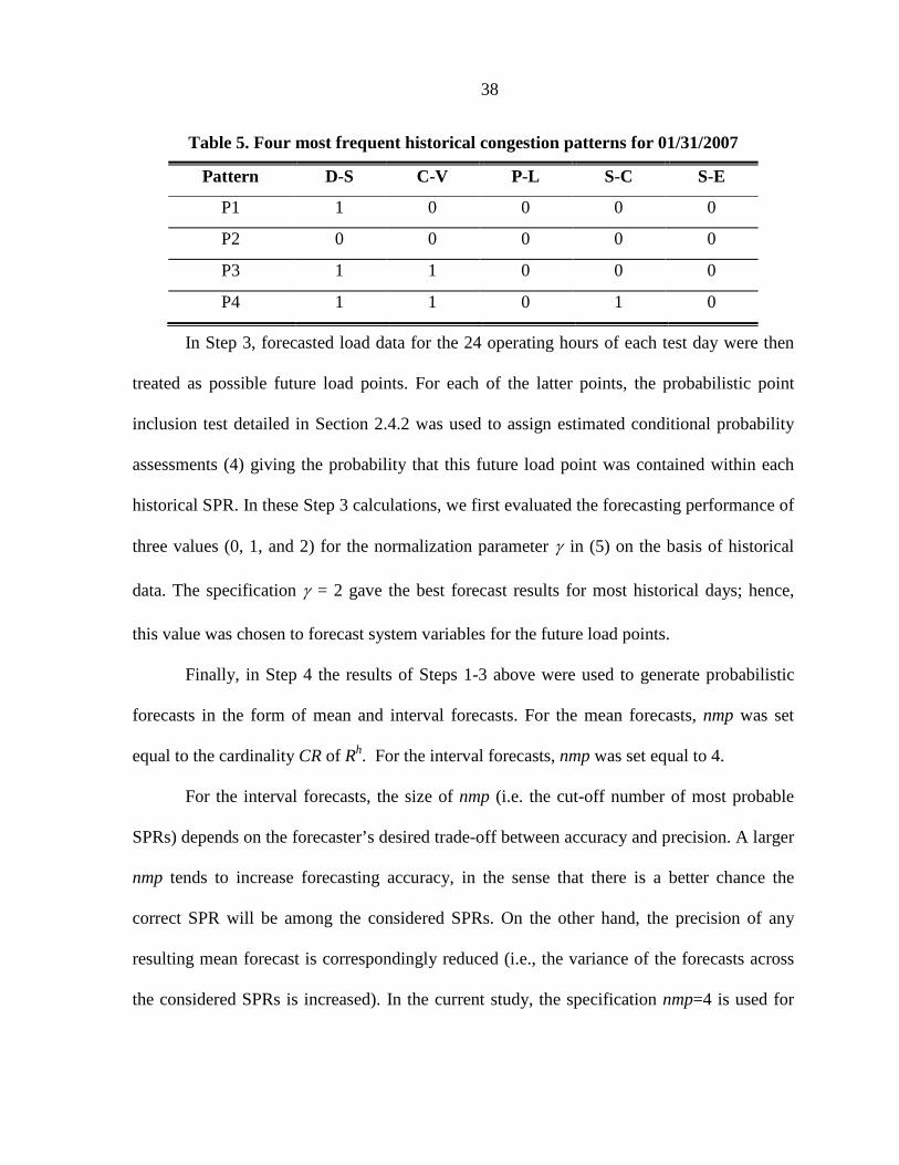
In Step 3, forecasted load data for the 24 operating hours of each test day were then

treated as possible future load points. For each of the latter points, the probabilistic point

inclusion test detailed in Section 2.4.2 was used to assign estimated conditional probability

assessments (4) giving the probability that this future load point was contained within each

historical SPR. In these Step 3 calculations, we first evaluated the forecasting performance of

three values (0, 1, and 2) for the normalization parameter γ in (5) on the basis of historical

data. The specification γ = 2 gave the best forecast results for most historical days; hence,

this value was chosen to forecast system variables for the future load points.

Finally, in Step 4 the results of Steps 1-3 above were used to generate probabilistic

forecasts in the form of mean and interval forecasts. For the mean forecasts, nmp was set

equal to the cardinality CR of Rh. For the interval forecasts, nmp was set equal to 4.

For the interval forecasts, the size of nmp (i.e. the cut-off number of most probable

SPRs) depends on the forecaster’s desired trade-off between accuracy and precision. A larger

nmp tends to increase forecasting accuracy, in the sense that there is a better chance the

correct SPR will be among the considered SPRs. On the other hand, the precision of any

resulting mean forecast is correspondingly reduced (i.e., the variance of the forecasts across

the considered SPRs is increased). In the current study, the specification nmp=4 is used for

39

interval forecasts because it results in good precision without significant loss of coverage

probability.

2.6.3 Congestion Pattern Forecasts

Table 6 reports the four most probable hourly congestion patterns, along with their

associated estimated conditional probabilities and coverage probability CP (based on nmp=4),

for every fifth hour of January 31st, 2007, starting from hour 0:00. Actual congestion patterns

corresponding to each reported hour are highlighted in gray. As seen, for the reported hours

the actual congestion pattern is always included among the forecasted congestion patterns

and has the highest estimated conditional probability. For future reference, note also that the

first entry of the actual congestion pattern, corresponding to transmission line D-S, is always

1. This indicates that D-S is frequently congested.

The multiple forecasted congestion patterns associated with each reported hour in

Table 6 represent several credible congestion scenarios that could occur in the future. If a

forecaster desires to derive one forecast for the future congestion pattern, an intuitively

reasonable option would be to select a forecasted congestion pattern that has the highest

associated conditional probability (4). As observed in Table 6, for the case study at hand this

approach would result in the correct prediction of the actual congestion pattern for each

reported hour. In general, however, more reliable forecasts for system conditions and DC-

OPF system variable solutions would be obtained by making fuller use of the conditional

probability assessments (4) to form mean forecasts and interval forecasts.

40

Table 6. Forecasted congestion patterns versus the actual pattern on 01/31/2007

Time Forecasted Probabilities CP Actual

0:00

1 0 0 0 0 0 0 0 0 0 1 1 0 0 0 1 1 0 1 0

0.3632 0.2411 0.2066 0.1432

0.9541 1 0 0 0 0

5:00

1 0 0 0 0 0 0 0 0 0 1 1 0 0 0 1 1 0 1 0

0.3451 0.2043 0.2418 0.1486

0.9398 1 0 0 0 0

10:00

1 0 0 0 0 0 0 -1 0 0 1 1 0 0 0 1 1 0 1 0

0.4237 0.0236 0.3654 0.1299

0.9426 1 0 0 0 0

15:00

1 0 0 0 0 0 0 -1 0 0 1 1 0 0 0 1 1 0 1 0

0.3661 0.0271 0.4243 0.1277

0.9452 1 1 0 0 0

20:00

1 0 0 0 0 0 0 0 0 0 1 1 0 0 0 1 1 0 1 0

0.4247 0.0244 0.3612 0.1332

0.9435 1 0 0 0 0

2.6.4 Mean Forecasts for LMPs

One of the benefits of congestion forecasting is to enable the more precise prediction

of LMPs for market operators and traders in their short-term decision making. Forecasted and

actual LMPs for Zone Central on Jan 31st and Feb 28th are shown in and Figure 9. Root Mean

Squared Error (RMSE) and Mean Absolute Percentage Error (MAPE) [11] are used as

measures of forecast accuracy:

242

1

1RMSE ( )

24actual forecast

i ii

LMP LMP=

= −∑ (11)

24

1

| |1MAPE

24

acutal forecast

i i

actuali i

LMP LMP

LMP=

−= ∑ (12)

41

0 5 10 15 20 2545

50

55

60

65

70

75

80

85

90

95

Time (h)

Zon

al L

MP

($/

MW

h)

ForecastedActual

Figure 9. Actual versus mean LMP forecasts for Zone Central on 01/31/2007

0 5 10 15 20 2540

50

60

70

80

90

Time (h)

Zon

al L

MP

($/

MW

h)

Forecasted Actual

Figure 10. Actual versus mean LMP forecasts for Zone Central on 02/28/2007

Table 7 reports the RMSE and MAPE obtained using our probabilistic forecasting

algorithm for each of our 12 test days. Corresponding forecast results obtained using a well-

known statistical model – the Generalized Autoregressive Conditional Heteroskedasticity

(GARCH) model [10]– are also shown for comparison. As seen, except for the slightly

smaller MAPE value attained in February using GARCH, our forecasting algorithm

outperforms GARCH in the sense that smaller RMSE and MAPE values are obtained.

42

Table 7. RMSE and MAPE values for the twelve test days

Day RMSE MAPE

Model Proposed Alg. GARCH Proposed Alg. GARCH

01/31/2007 5.026 8.689 0.0525 0.0902

02/28/2007 3.393 4.465 0.0472 0.0384

03/31/2007 4.029 7.094 0.0677 0.0727

04/30/2007 4.853 8.297 0.0535 0.1005

05/31/2007 7.401 14.741 0.0934 0.1198

06/30/2007 3.439 13.359 0.0679 0.1485

07/31/2007 3.941 11.623 0.0530 0.1082

08/31/2007 4.076 5.913 0.0671 0.0781

09/30/2007 3.249 6.636 0.0603 0.0862

10/31/2007 4.135 8.561 0.0638 0.1176

11/30/2007 6.476 7.208 0.0770 0.0855

12/31/2007 7.051 14.185 0.0903 0.1435

2.6.5 Interval Forecasts for Line Shadow Prices and LMPs

Interval forecasting is recommended over mean forecasting for line shadow prices. As

clarified below, interval forecasting is more informative than mean forecasting for line

shadow prices because the underlying attribute of interest (negative-direction, zero, or

positive-direction congestion) is measured by a discretely-valued indicator (-1, 0, or 1).

Hourly upper-bound and lower-bound interval forecasts for the line shadow prices on

line D-S on January 31st and Feb 28th are shown in Figure 11and Figure 12 along with actual

43

line shadow prices for comparison. As seen, the actual line shadow prices for most hours fall

within the forecasted intervals.

To better interpret these findings, consider the Table 6 results which forecast that line

D-S (the first congestion pattern entry) will be either congested or not during hour 20 with

varying probabilities. If congestion is forecasted, it is in the positive direction (+1); and,

from Figure 11, the line shadow price is estimated to be about $60/MWh. On the other hand,

if no congestion is forecasted (0), then from Figure 11 the line shadow price is estimated to

be $0/MWh.

One final point for interval forecasts for line shadow prices is important to note. For

lines for which no congestion occurs in any of the reported congestion patterns (e.g., line S-E

in Table 6), the corresponding upper and lower bounds for the forecasted line shadow price

interval will both be zero, indicating zero congestion.

0 5 10 15 20 250

10

20

30

40

50

60

70

Time (h)

Sha

dow

Pric

e ($

/MW

h)

ActualUpper BoundLower Bound

Figure 11. Actual versus interval D-S line shadow price forecasts on 01/31/2007

44

0 5 10 15 20 250

10

20

30

40

50

Time (h)

Sha

dow

Pric

e ($

/MW

h)

ActualUpper BoundLower Bound

Figure 12. Actual versus interval D-S line shadow price forecasts on 02/28/2007

Interval forecasts for Zone Central LMPs on January 31st and February 28th are shown

in Figure 13 and Figure 14 along with actual LMP values for comparison. For most hours the

actual LMP values fall within the upper and lower bounds of the forecasted intervals.

The interval forecasting performance for line shadow prices and zonal LMPs is

measured using the accuracy-informativeness tradeoff model developed in [59]. The

statistical loss function LOSS is defined to be

| |( )

y mln g

gLOSS δ

−+= (13)

In (13), y denotes the actual value, mdenotes the midpoint of the forecasted interval,

and ln(g) denotes the natural logarithm of the widthg of the forecasted interval. Also, δ

determines the tradeoff between accuracy (the first term) and informativeness (the second

term); in this case study δ is set to 1. Note that a smaller LOSS indicates better performance

for interval forecasting.

45

Table 8 gives the LOSS values for the interval forecasts obtained for line shadow

price and zonal LMPs using our probabilistic forecasting algorithm versus the forecasts

obtained using a statistical GARCH model. As seen, our probabilistic forecasting algorithm

results in uniformly lower LOSS values than GARCH, indicating a better forecasting

performance.

A possible explanation for this performance difference is that GARCH has difficulty

handling the volatility of line shadow prices, which can abruptly change from 0 to large non-

zero values. In contrast, our probabilistic forecasting algorithm captures the physical

meaning of these line shadow prices and this facilitates better forecasting.

0 5 10 15 20 2540

50

60

70

80

90

100

Time (h)

Zon

al L

MP

($/

MW

h)

ActualUpper BoundLower Bound

Figure 13. Actual versus interval LMP forecasts for Zone Central on 01/31/2007

46

0 5 10 15 20 2540

50

60

70

80

90

Time (h)

Zon

al L

MP

($/

MW

h)

ActualUpper BoundLower Bound

Figure 14. Actual versus interval LMP forecasts for Zone Central on 02/28/2007

Table 8. Loss function values as a measure of interval forecasting performance

Day Shadow Price Forecasting LMP Forecasting

Model Proposed Alg. GARCH Proposed Alg. GARCH

01/31/2007 3.824 4.063 2.896 4.196

02/28/2007 3.729 3.977 2.835 3.649

03/31/2007 3.236 3.672 2.574 3.633

04/30/2007 3.398 3.778 3.133 4.164

05/31/2007 3.493 4.187 3.421 4.032

06/30/2007 3.838 3.897 3.365 4.425

07/31/2007 2.726 3.350 2.839 4.892

08/31/2007 2.916 3.352 2.787 3.624

09/30/2007 3.140 3.567 2.245 3.965

10/31/2007 2.825 3.335 2.725 3.799

11/30/2007 3.256 3.738 3.088 3.537

12/31/2007 3.481 3.962 3.164 3.919

47

In this study we observed that, in some months (January, May, November, and

December), the peak-hour LMPs and line shadow prices were difficult to forecast with

precision. This phenomenon could possibly be due to changes in the generating unit

commitment pattern or in the transmission network topology over the forecast horizon. To

enhance peak-hour forecasting results, more careful collection of historical data might be

needed to ensure that these historical data correspond to the same commitment-and-line

scenario as the forecasted point. Alternatively, as discussed in the following Section 2.7, an

extended cross-scenario forecast study could be attempted.

2.7 Extension to Cross-Scenario Forecasting

To this point, the forecasting algorithm developed in this study has been conditioned

on a given commitment-and-line scenario S specifying a particular generating unit

commitment pattern and a particular transmission network topology. One interpretation of S

is that it represents anticipated conditions at a future operating point for which forecasts are

desired. Another interpretation of S is that it represents a possible future system contingency

(e.g., an N-1 outage scenario) under consideration in a contingency planning study.

A possibly useful extension of this algorithm would be to assign probabilities to

distinct scenarios, thus permitting the probabilistic cross-scenario blending of forecasts.

These scenarios could be characterized not only on the basis of system patterns, i.e.,

generating unit commitments and transmission network topology, but also on the basis of a

variety of other types of contingencies.

As illustrated in Figure 15, for any future operating point whose system conditions

need to be forecasted, the corresponding generating unit commitment, transmission network

48

topology, and other contingencies could be projected with some probabilities. In each of

these projected scenarios, our scenario-conditioned forecasting algorithm could be applied to

estimate congestion, LMPs, and other system variables. The final forecast for any system

variable of interest could then be the expected value of this system variable calculated across

all projected scenarios.

System Pattern

1System Pattern

2

Historical operating points

Scenario 1 Scenario 2

New forecasted point

P2P1

Figure 15. Scenario-conditioned and cross-scenario forecasting

49

CHAPTER 3. TRANSMISSION INVESTMENT FOR INTEGRATING

RENEWABLE ENERGY

3.1 Introduction

In this chapter, a method is proposed to support the negotiation process for renewable

energy integration between a Renewable Energy (RE) Generation Company (RE-GenCo) and

a Transmission Company (TransCo). The process begins with a prudent development of

transmission plans by the two companies, taking into consideration the intermittency of

renewable energy such as wind generation. Then the payment from the RE-GenCo to the

TransCo is negotiated. If the payment is low, the TransCo may not fully recover its

investment; if the payment is high, the RE-GenCo is not profitable. Hence the parties could

fail to reach an agreement. Note that this study can also be extended to include a LSE who

can contract to purchase a certain amount of renewable energy.

Nash Bargaining theory is applied to determine the transmission investment plans and

RE-GenCo’s transmission payment. The Nash bargaining solution gives a fair and efficient

utility allocation for the two companies. The negotiation methodology as well as its results

provides guidelines to transmission investors for integrating renewable energy under

uncertainties. The negotiation is then compared with a centralized planning model to evaluate

renewable energy subsides. The comparison shed light to policy makers on designing proper

renewable energy subsidies.

50

3.2 Nomenclature

Indices and sets:

n Index for buses

s Index for scenarios

t Index for subperiods

i Index for generators

j Index for loads

b Index for supply or bid blocks

k Index for transmission lines

o(k) Sending-end of transmission line k

r(k) Receiving-end of transmission line k

R Index for the bus where renewable generation will be invested

Ir Index for the renewable generator invested by the RE-GenCo

NΩ Set of all system buses

TΩ Set of all subperiods

SΩ Set of all scenarios GnΩ Set of generators at Bus n LnΩ Set of loads at Bus n biΩ Set of blocks of Generator i bjΩ Set of blocks of Load j

TGΩ Set of traditional generators

RGΩ Set of renewable generators

ETΩ Set of existing transmission lines

CTΩ Set of candidate transmission lines

GΩ Set of all system generators

LΩ Set of all system loads

Parameters:

51

tD Duration of subperiod t Gibλ Offer price of the bth block by the ith generator

Ljbλ Bid price of the bth block by the jth load

kICT Annualized investment cost of transmission line k

GibP Size of the bth block for the ith generator LjbP Size of the bth block for the jth load

RibtsP Size of the bth block for the ith renewable generator at subperiod t in

scenario s

kF Transmission capacity of line k

kx Transmission reactance of line k

SUB Parameter of renewable energy subsidies

RGIC Annualized investment cost of renewable generation

RGd Threat point of the RE-GenCo

Td Threat point of the TransCo

FP Renewable energy contract price ($/MWh) for RE-GenCo

Decision variables:

GibtsP Electricity produced by the bth block of ith generator at subperiod t in scenario s.

kY Electricity consumed by the bth block of jth load at subperiod t in scenario s.

λ Negotiated payment from the RE-GenCo to the TransCo.

ktsF Power flow of transmission line k at subperiod t in scenario s.

ntsLMP LMP of Bus n at subperiod t in scenario s.

3.3 Problem Formulation

3.3.1 Overview

This section describes the negotiation process between a RE-GenCo and a TransCo.

Assuming that a RE-GenCo has decided to invest in a RE project at a remote location, the

52

RE-GenCo can pay a construction company to build the interconnection transmission if, in

the business case, the RE-GenCo can demonstrate with certainty that the projected output and

the electricity price allows it to recover both the generation and transmission investments. In

this case, the RE-GenCo would assume all profit risks and uncertainties. However, due to the

intermittent nature of the generation output, the RE-GenCo may not want to do so. Instead,

the RE-GenCo may seek out a TransCo who is interested in investing in transmission, to bear

part of the risks. The risk transfer is consummated by the RE-GenCo paying the TransCo a

transmission rate, based on the projected generation performance and electricity prices, for

recovering the transmission investment. The payment, measured by a rate λ ($/MWh)

multiplied by dispatched renewable energy (MWh), necessitates a negotiation among two

parties.

To simplify the discussion, several assumptions are made. First, the utilities are

presented in annualized terms in the sense that the calculation is conducted for a typical year

with annualized cost components. Second, maintenance costs are not explicitly modeled

since an annualized maintenance cost can be included as part of the annual capital

investments. Third, a risk neutral attribute is assumed so that the RE-GenCo’s utility RGU and

the TransCo’s utility TU can be expressed as expected profits of the two participants. These

simplifications can be easily relaxed.

3.3.2 Negotiation Process

Two possible outcomes can be reached during a negotiation; an agreement is reached

or both parties walk away. For the first outcome, an agreement is reached if the RE-GenCo,

53

after paying the negotiated transmission rate, can recover its generation investment and, at

the same time, the TransCo can recover its transmission investment.

A bilateral contract signed with LSEs is assumed for the RE-GenCo to manage price

fluctuations in an electricity market. This assumption is valid since a number of electric

utilities have issued long-term (10+ years) power purchase agreements, according to [60].

Considering the projected generation output and a payment to the TransCo, the utility

function of the risk-neutral RE-GenCo given a set of future scenarios SΩ is defined by

[[ ] ]S

T

RGRG s t Rts ts

t

U E D FP SUB P Cλ∈Ω∈Ω

= + − −∑ (14)

where br rI r

RG b Gts I I btsb

C Pλ∈Ω

=∑ , representing production cost for the RE unit. Note that the

generation investment can be included in (14). However, it is, instead, used as the RE-

GenCo’s threat point, dRG.

If the RE-GenCo does not sign bilateral contracts with LSEs, it confronts an exposure

to market price uncertainties. The utility function (14) can be modified to a market-based

version MRGU , taking into account market-based electricity prices at its bus R (i.e. Locational

Marginal Prices (LMPs)).

[[ ] ]S

T

M RGRG s t Rts Rts ts

t

U E D LMP SUB P Cλ∈Ω∈Ω

= + − −∑ (15)

For the TransCo, if an agreement is achieved, the profit collected by the TransCo

from the RE-GenCo's payment with the subtraction of transmission investment can be

expressed as

[ ]S

CTT

T s t Rts k kt k

U E D P ICT Yλ∈Ω∈Ω ∈Ω

= −∑ ∑

(16)

54

In the alternative in which no agreement is reached, the transmission investment will

not occur. In this case, the failure to reach an agreement results in the RE-GenCo utility

function arriving at its threat point, RGd , which is set as the stranded RE generation

investment, RGIC . Likewise, if the TransCo receives no payment, the TransCo’s utility

function is settled at its threat point Td which equals 0.

With knowledge of the utility functions, threat points and projected market conditions,

a negotiation process is initiated on the transmission investment plan and the associated

transmission rate/payment. The process is depicted in Figure 16. While the two companies

negotiate, they anticipate the market operation whose results (LMPs, generation outputs and

transmission flows) in turn will affect their attained profit. Therefore, they tend to choose the

transmission plan and payment rate which benefit them most.

Foresee

Negotiation variables:

Negotiated rateTransmission plans

Operation variables:

LMPs

Generation outputs

Transmission flows

ISO market

operation

URG,UT,dRG,dT

Negotiation

Figure 16. Negotiation between the RE-GenCo and the TransCo

In the negotiation process, both the RE-GenCo and the TransCo take into

consideration the intermittent nature of the generation output, the planned transmission

capacity with its associated investment cost, and the electricity prices. Due to the complexity

55

and inter-relationship between the negotiated results and the transmission investment plan, it

entails a careful examination of negotiation methodology and solution, which is presented in

Section 3.4.

3.3.3 Policy implications on RE subsidies

Optimal transmission investment plans are aimed by policy makers to maximize

social surplus, but cannot be directly imposed on merchant transmission investment in a

competitive market environment. A possible approach to steer the negotiated transmission

investment plans towards the social optimal investment is to make use of the controllable RE

subsidy parameter SUB, an important component in both companies’ utility functions. With

everything else unchanged, the negotiated solution can be expressed as a non-linear function

of SUB. By adjusting this RE subsidy parameter, policy makers then can possibly alter the

negotiated solution to match the social optimal transmission investment plan.

The social optimal solution is derived from a centralized transmission planning. The

objective is to maximize social surplus (the operation surplus minus transmission investment

cost, subject to operation and planning constraints). Contrasting the negotiated solution with

the centralized solution, an optimal RE subsidy parameter can be obtained to provide

guidance to policy makers. The details of the model construction and comparison are

illustrated in Section 3.5.

3.4 Negotiation: A Nash Bargaining Approach

The result between the RE-GenCo and the TransCo in the negotiation process

described in Section 3.3 is solved by applying the Nash Bargaining theory. Specifically, a

56

two-player Nash Bargaining problem and its solution concept are applied to the negotiation

problem to derive the analytical model and detailed formulation.

3.4.1 Nash Bargaining

The research on two-person bargaining problems is initiated by Nash [61], [62]. In his

seminal work, the bargaining problem is defined when two players, who negotiate over a

utility possibility set U , with their threat points 1 2( , )d d d= , try to achieve a settlement

point 1 2( , )u u u= . Nash proved that for every bargaining problem( , )dU , there is a unique

solution 1 2( , ) ( ( , ), ( , )f d f d f d=U U U that satisfies the following four axioms.

• Axiom 1. Invariance to linear transformation: For any monotonic linear-affine

function H , it requires that ( ( ), ( )) ( ( , ))f H H d H f d=U U . This essentially needs the

solution be agnostic of any linear-affine transformations, i.e. shifting and scaling.

• Axiom 2. Symmetry: if 1 2d d= , 1 2( , )u u ∈U and 2 1( , )u u ∈U ,

then 1 2( , ) ( , )f d f d=U U . This indicates that the solution should provide equal gains from

the cooperation when the feasible utility set U is symmetric.

• Axiom 3. Independence of irrelevant alternatives: for two bargaining

problems ( , )dU and( , )d′U , if ( , )f d′ ∈U U , then ( ) ( , )f f d′=U U . It basically says that

the addition of irrelevant alternatives does not change the solution.

• Axiom 4. Pareto efficiency: if u and u′ are two utility points in a bargaining

problem ( , )dU andu u′ > , then ( , )f d u≠U . This axiom requires the pareto-optimality of

the bargaining solution.

57

The unique bargaining solution is then obtained by solving the following optimization

problem:

1 2 1 2

1 2

1 1 2 2( , ) ( , )

( , )

( , ) maximize ( )( )u u d d

u u

f d arg u d u d>

∈

= − −U

U

(17)

The objective is named Nash product, which is later extended in n-person bargaining

game [64]. The solution to this problem is referred to as Nash Bargaining Solution (NBS), an

important solution concept in game theory, has the properties of simplicity and robustness.

Empirical evidences to support NBS are indicated in experimental bargaining theory given in

reference [65].

3.4.2 Bargaining on RE Interconnection: An Analytic al Model

Suppose that a RE-GenCo has decided to build a RE generating unit at some remote

location, and financing of the capital 0($)C has been secured. The maximum available output

of the RE unit is denoted by( )r MW , a random variable with probability density function

(pdf) ( )g r and cumulative density function (cdf)( )G r , subject to the variability of the

renewable resource. The model also assumes production cost ($ / )RC MWh and renewable

energy subsidies ($ / )RS MWh are constant.

As discussed earlier, the RE-GenCo (denoted by subscript R in the formulation) seeks

out a TransCo (denoted by subscript T) to invest in transmission lines to interconnect the RE

project and to deliver its output to distance load centers. The per-unit cost to the TransCo for

the generation interconnection transmission is represented by ($ / )TC MWh . The price for the

renewable energy is represented by a fixed payment($ / )RD MWh . The two parties negotiate

58

and try to reach an agreement on the payment rate ($ / )MWhλ corresponding to the agreed

upon transmission capacity( )TF MW .

Note that the output for the RE generation RP is constrained by the lower value of the

maximum available output r and the transmission capacityTF , i.e.

( , )R TP min r F= (18)

Using these representations, the RE-GenCo’s utility is the expected profit (EPR),

·[ ]R R R R Ru EP D S C λ= + − − (19)

and the TransCo’s utility is given as

·T R T Tu EP F Cλ= − (20)

Note that their threat points are0( ,0)C .

Applying Nash bargaining theory, the decision variables λ and TF can be solved

by maximizing the Nash Production (NP)

, 0max [ ( , ) ] ( , )TF R T T TNP u F C u Fλ λ λ= − ⋅ (21)

The solution can be found if 0Ru > and 0Tu > .

Take the first order derivatives with respect to λ and TF ,

0[ ]R TT R

u uNPu u C

λ λ λ∂ ∂∂

= + −∂ ∂ ∂

(22)

0[ ]R TT R

T T T

u uNPu u C

F F F

∂ ∂∂= + −

∂ ∂ ∂ (23)

Note that REP in equations (19) and (20) is a function of TF due to (18),

( , )R r TEP E min r F= . When r>F T, min(r,FT)=FT; when r<=F T, min(r,FT)=r , the expectation

then is

59

0

0 0

0

0

· ( ) |

[1 ( )] ( )

[1 ( )] [ ( )] ( )

( ) ( ) ( )

( )

T

T

T T

T

T

R T T r F

F

T T

F F

T T

F

T T T T T

F

T

EP F Pr r F E

F G F rg r dr

F G F d rG r G r dr

F F G F F G F G r dr

G d

r

F r r

≤= > +

= − +

= − + −

= − + −

= −

∫

∫ ∫

∫

∫

(24)

From (24), the partial derivative of REP with respect to TF can be expressed as

1 ( )RT

T

EPG F

F

∂= −

∂ (25)

The partial derivative of Ru and Tu with respect to λ and TF can be obtained, i.e.,

/R Ru EPλ∂ ∂ = − (26)

/ [1 ( )] [ ]R T T R R Ru F G F D S C λ∂ ∂ = − × + − − (27)

/T Ru EPλ∂ ∂ = (28)

/ [1 ( )]T T T Tu F G F Cλ∂ ∂ = − × − (29)

Insert equations (26)-(29) into equations (22) and (23),

0[ ]r T R R

NPEP u EP u C

λ∂

= − × + −∂

(30)

0[1 ( )][ ] [[1 ( )] ][ ]T R R R T T T RT

NPG F D S C u G F C u C

Fλ λ

∂= − + − − × + − − −

∂

(31)

The solution can be found when the above two equations equal to 0. Then equation

(30) becomes

0[ ] 0R R TEP u C u− − = (32)

The expected RE output REP is normally positive, and hence (32) satisfies only when

0R Tu C u− = (33)

which is the logical outcome in which the utility is equally divided between the RE-GenCo

and the TransCo.

60

The relation between λ and TF can be derived by replacing Ru and Tu in (33) with (19)

and (20)

0[ ]R R R R R T TEP D S C C EP F Cλ λ+ − − − = − (34)

Re-expressing the equation, one obtains

0

2 2T TR R R

R

C F CD S C

EPλ

−+ −= − (35)

Similarly, set equation (31) equal to 0, replace 0Ru C− with Tu , and omit positiveTu .

Equation (31) can be rewritten as

[1 ( )][ ] 0T R R R TG F D S C C− + − − = (36)

TF then can be solved in the following explicit form

11 TT

R R R

CF G

D S C−

= − + − (37)

andλ can be found by replacing TF in (35) with (37).

It is observed the negotiated payment rate λ and invested transmission capacity

TF can be explicitly determined in this model with the consideration of the RE output

uncertainty. However, since the transmission investment is lumpy in nature, the transmission

plan is likely to consist of a set of discrete transmission candidates. Hence a more careful

examination of the negotiation process and a detailed formulation to handle the lumpy

investment are needed.

3.4.3 Bargaining on RE Interconnection: A Detailed Formulation

The bargaining process on RE interconnection is formulated as a bi-level

optimization problem. The Nash product is maximized in the upper level problem, while a set

61

of lower problems represents the market operations anticipated by the RE-GenCo and the

TransCo, for every hour t and scenario s.

The detailed formulation is given below, with the RE-GenCo's utility RGU and the

TransCo's utility TU denoted by (14) and (16). Suppose the negotiation is intended to connect

the RE unit Ir at Bus r, the bargaining problem is then formulated as:

[ ],

max ( , ) ( , , ) k

RG Rts RG T Rts kY

U P IC U P Yλ

λ λ− ×

(38)

Subject to

( , )RG Rts RGU P ICλ ≥ (39)

( , , ) 0T Rts kU P Yλ ≥ (40)

CT CTk R k

k k

M Y M Yλ∈Ω ∈Ω

− ≤ ≤∑ ∑ (41)

rbI r

GRts I bts

b

P P∈Ω

= ∑ (42)

where , ,Rts T SP t s∀ ∈Ω ∀ ∈Ω =

maxG L L b G b

ibts jbts n j i

L L G Gjb jbts ib ibts

P P j b i b

arg P Pλ λ∈Ω ∈Ω ∈Ω ∈Ω

−∑ ∑ ∑ ∑ (43)

Subject to

| ( ) | ( )

0, ( ),L bn j

Ljbts kts kts nts N

k o k n k r k nj b

P F F LMP n= =∈Ω ∈Ω

+ − = ∀ ∈Ω∑ ∑ ∑ ∑ (44)

0 , ,G G TG bibts ib iP P i b≤ ≤ ∀ ∈Ω ∀ ∈Ω (45)

0 , ,G G RG bibts ibts iP P i b≤ ≤ ∀ ∈Ω ∀ ∈Ω (46)

( ) ( )

1[ ], ET

kts o k ts r k tsk

F kX

δ δ= − ∀ ∈Ω (47)

, ETk kts kF F F k− ≤ ≤ ∀ ∈Ω (48)

( ) ( )

1(1 ) [ ] (1 ) , CT

k kts o k ts r k ts kk

Y M F Y M kX

δ δ− − ≤ − − ≤ − ∀ ∈Ω (49)

, CTk k kts k kY F F Y F k− ≤ ≤ ∀ ∈Ω (50)

62

The upper level problem, consisting of equations (38)-(40), reflects the requirement

in Nash bargaining problem. Inequality (41) is an additional constraint demanding zero

payment if no transmission line is invested. Equality (42) collects the total dispatched

renewable energy output from all offer blocks of the RE unit which is to be interconnected.

For each hour t and scenario s, a corresponding lower-level problem (43)-(50) reflects the

market operation with LMPs, dispatched generation output, and transmission flow. The

objective of the lower-level problems (43) is to maximize market operation net surplus.

Constraint (44) enforces real power balance at each bus. Constraints (45) and (46) impose

generation capacity limit on non-renewable and renewable generating units, respectively.

Note that the maximum available output for some RE unit i, GibtsP varies in hours and

scenarios, allowing for the variability of renewable resources.

Constraints (47)-(50) enforce transmission limits for existing and candidate

transmission lines. Regarding constraint (49), the constraint is active and M is set at 0 when

Yk = 1 or the investment decision is affirmative. However, if Yk = 0 or the investment

decision is negative, M is set to be a large number meaning that this constraint is not active

and therefore not considered.

This formulation could be modified to consider market-based renewable energy price

(LMPs) received by the RE-GenCo, if it does not enter into a bilateral contract. Its utility

function in objective function (38) can be replaced by , ),(MRG Rts RtsPU LMP λ given in equation

(15). The utility function is now determined by both the renewable energy production RtsP

and its market price RtsLMP .

63

3.5 Implications on Renewable Subsidy Policy

A centralized transmission planning model is described in this section that will

provide a benchmark of social optimal transmission investment, for contrasting the

negotiated transmission plans described in Section 3.4. Policy implications on renewable

energy subsidies will be derived by proposing an analytical model and a detailed formulation,

where renewable subsidies are used as a critical and adjustable parameter to steer the

negotiated solution towards a centralized solution.

3.5.1 Centralized Planning and Policy Implication

Suppose a centralized planner, who performs the traditional Integrated Resource

Planning function, decides to interconnect a RE unit by planning and investing in a new

transmission line. Considering the benefit BR ($/MWh) from the renewable energy, the

centralized planner needs to make a decision on the invested transmission capacity FT to

maximize social surplus:

maximize T

R R R R T TF

SS EP B EP C F C= × − × − (51)

The same notation in Section 3.4.2 is used in (51). Take the derivative of SS with

respect to FT and set it equal 0, i.e.,

[ ]RR R T

T T

dEPdSSB C C

dF dF= − − (52)

0 [1 ( )][ ]T R R TG F B C C= − − − (53)

FT in the centralized planning model can be solved explicitly as follows,

11 TT

R R

CF G

B C−

= − − (54)

64

Comparing the negotiated solution (37) with the centralized solution (54), the

adjustable parameter of renewable energy subsidies, SR can be utilized to steer the negotiated

solution towards the benchmark solution by equating (37) and (54),

R R R R RD S C B C+ − = − (55)

R R RS B D= − (56)

Equation (56) indicates that the optimal renewable energy subsidies should be set as

the difference between the benefit from the RE generation and the payment for purchasing

renewable energy. Of course, determining the benefit received is not a trivial task. In any

event, policy makers can use this result as guidance for renewable energy subsidy policy, and

establish a subsidy mechanism that provides merchant investors with sufficient market

incentives for achieving social optimal transmission investment plans.

3.5.2 An Illustrative Example

A simple example is presented to illustrate the principle of the negotiation model and

demonstrate the important role of policy in moving the bargaining solution to an idealistic

solution that is societal beneficial.

The bi-level negotiation process depicted in Section 3.4 is elaborated by means of the

payoff matrix. The solutions for the negotiation model, in the two situations with or without

renewable energy, are compared with that in the centralized model.

As shown in Figure 17, a RE-GenCo is going to make a decision on a wind farm

investment. The company has two options.

65

• Option [1]: Investing at location [1] with cost $2/MW, it will be able to

generate 19MWh wind energy at the price of $1/MWh, and pay a rate 1Rλ to

the TransCo for transmission investment cost recovery.

• Option [2]: Investing at location [2] with cost $2/MW, it will be able to

generate 13MWh wind energy at the price of $1/MWh, and pay a rate 2Rλ to

the TransCo for transmission investment cost recovery.

Similarly, the TransCo has two options as follows:

• Option (1): TransCo will build the transmission along path (1) with capacity

19MW; its investment cost is $10, and TransCo receives 1Rλ from the GenCo.

• Option (2): TransCo will build the transmission along path (2) with capacity

13MW; its investment cost is $4, and TransCo receives 2Rλ from the GenCo.

Figure 17. Options for renewable generation and transmission investment

66

Correspondingly, LSE will receive three different levels of benefit, depending on the

negotiation results of the RE-GenCo and the TransCo.

• Benefit (a): If both the GenCo and the TransCo choose [1] and (1), LSE will

have a utility level of $14.

• Benefit (b): If they choose [2] and (2), LSE will have a utility level of $10.

• Benefit (c): LSE will have 0 otherwise.

In the first case there is no renewable energy subsidy, the payoff matrix for the

GenCo and the TransCo then can be expressed as follows:

TransCo

(1) (2)

GenCo [1] 1 11 2 10, )(19 R Rλ λ× − − − (-2,-4) [2] (-1,-6) 2 21 1 , 4(13 )R Rλ λ× − − −

Their negotiated result is the solution to maximize the product of their utilities, for

example, 1 1 1 [19 1 2 ]x 0]m 1a [

R R Rλ λ λ× − − − . Therefore, the solutions are 1 13.5Rλ = , 2 8Rλ = .

The payoff matrix is then

TransCo

(1) (2)

GenCo [1] (3.5,3.5) (-2,-4) [2] (-1,-6) (4,4)

The payoff matrix for LSE is determined by the negotiated result of the GenCo and

the TransCo.

TransCo

(1) (2)

GenCo [1] 14 0 [2] 0 10

67

Following the analysis of Nash Bargaining theory, the GenCo and the TransCo will

choose the option ([2], (2)) which maximizes their utility levels since Nash Product of (4, 4)

is greater than (3.5, 3.5).

Nevertheless, considering the social surplus which now involves the utility level from

LSE besides the two negotiators, the social optimal investment plan should be settled at ([1],

(1)). Indeed, the total social surplus achieved by ([1], (1)), 3.5+3.5+14=21, clearly exceeds

the total social surplus by ([2], (2)), 4+4+10=18.

In this case, the negotiated result does not match the centralized investment plan.

Hence, the social surplus maximization is not achieved.

Now consider how subsidy can help to steer the negotiated result to a centralized

social optimal solution. Suppose the RE-GenCo is subsidized by $0.5/MWh. The revenue

stream of the RE-GenCo now includes this subsidy in addition to the original energy sale.

Note that this subsidy will not alter the optimal solution for the centralized model; rather, it

will only re-distribute the total social surplus.

However, the payoff matrix for the RE-GenCo and the TransCo has been changed:

TransCo

(1) (2)

GenCo [1] 1 1(19 191 2 0. ,5 10)R Rλ λ× − −+− × (-2,-4) [2] (-1,-6) 2 2(13 11 1 0.5, 43 )R Rλ λ+× − − × −

The two companies negotiate the payment rate under the different investment plans,

resulting in 1 18.25Rλ = or 2 11.25Rλ = .

The numerical representation of the matrix becomes

68

TransCo

(1) (2)

GenCo [1] (8.25,8.25) (-2,-4) [2] (-1,-6) (7.25,7.25)

Apparently, Option ([1], (1)) outperforms Option ([2], (2)) in terms of greater utility

levels for both companies. Therefore, ([1], (1)) becomes the new negotiated result in this

subsidy environment. The subsidy $0.5/MWh indeed plays a crucial role in steering the

negotiated solution to a centralized solution and successfully achieves social optimality.

3.5.3 Centralized Planning: A Detailed Formulation

The detailed formulation of the centralized planning model, which allows for

uncertainties and realistic constraints, is presented below.

, ,maximize [ ]

G L SL b b CTibts jbts k

T Gj i

L L G Gs t jb jbts ib ibts k k

P P Y t ij b b k

E D P P ICT Yλ λ∈Ω∈Ω ∈Ω∈Ω ∈Ω ∈Ω ∈Ω

− −∑ ∑ ∑ ∑ ∑ ∑ (57)

Subject to

, T St s∀ ∈Ω ∀ ∈Ω

(44)— (50)

The objective function is to maximize social surplus composed of operation surplus

minus the transmission investment cost. The operation constraints are identical with the ones

in the negotiated model as given in equations (44)-(50).

69

3.6 Numerical Results

3.6.1 Garver’s Six-Bus Test Case

The detailed formulation for the negotiation on RE interconnection is studied with

Garver's six-bus test case in Figure 18, which comprises six buses, six existing transmission

lines, three generating units, and five loads. The generator at Bus 6 is assumed to be a RE or

wind resource. In this study, transmission lines between Bus 6 and the grid are needed to

deliver the RE output to the load. The supply offer and demand bid data for the two

traditional generators and 5 loads are given in Table 9. The number and size of blocks vary

for each market participant.

A constant production cost is assumed for the wind generator WG3 at Bus 6 and its

cost and operation data are given in Table 10. The third column is its investment cost ICRG

that will be used as the RE-GenCo’s threat point in the negotiation process. The renewable

energy contract price FP is given in the fourth column. Prate denotes the nameplate capacity

of the wind unit. The maximum possible output Pmax is characterized by the non-linear

function between wind speed v and Prate with three parameters of WG3: cut-in, cut-out and

rated wind speed Vci, Vco and Vrate. The non-linear feature can be described by the following

[30]:

0 0

( ) / ( )

0

ci

rate ci rate ci ci ratemax

rate rate co

c

v v

P v V V V V v VP

P V v V

V o v

≤ < − − ≤ <

= ≤ ≤

<

(58)

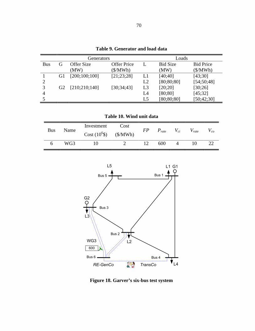
70

Table 9. Generator and load data

Generators Loads Bus G Offer Size

(MW) Offer Price ($/MWh)

L Bid Size (MW)

Bid Price ($/MWh)

1 G1 [200;100;100] [21;23;28] L1 [40;40] [43;30] 2 L2 [80;80;80] [54;50;48] 3 G2 [210;210;140] [30;34;43] L3 [20;20] [30;26] 4 L4 [80;80] [45;32] 5 L5 [80;80;80] [50;42;30]

Table 10. Wind unit data

Bus Name Investment

Cost (106$)

Cost

($/MWh) FP Prate Vci Vrate Vco

6 WG3 10 2 12 600 4 10 22

Bus 1

Bus 2

Bus 3

Bus 4

Bus 5

Bus 6

600

G1

G2

L1L5

L2

L4

L3

WG3

RE-GenCo TransCo

Figure 18. Garver’s six-bus test system

71

Table 11. Transmission data

Name From

Bus

To

Bus

Reactance

(Ω )

Limit

(MW)

Cost

(106$) Type

T1 1 2 0.4 250 - E(xisting)

T2 1 4 0.6 220 - E

T3 1 5 0.2 300 - E

T4 2 3 0.2 300 - E

T5 3 5 0.2 300 - E

T6 2 6 0.3 150 8.0 C(andidate)

T7 2 6 0.15 300 13 C

T8 3 6 0.4 150 9.2 C

T9 3 6 0.3 200 10 C

T10 4 6 0.3 200 11 C

Table 11 presents the data for the existing and candidate transmission lines. Five

transmission investment candidates (T6-T10) are proposed with the intent to connect Bus 6

to the grid. The pattern of transmission costs follows the economies of scale, e.g. building

one 300-MW line between Buses 2 and 6 is less expensive than building two 150MW lines

connecting these two buses.

To accommodate the variability from wind resource, three scenarios of wind speed

are constructed for four subperiods in a year, which are represented by four seasons with

equal time duration, i.e. 1·8760 2190

4h h= . The wind speed data in each scenario and

subperiod is given in

72

Table 12. Using the function (58), the maximum possible output of WG3 can be

calculated, and the result is shown in Table 13. Note that the wind unit normally generates

more renewable energy during the Fall and Winter season due to ample wind resources.

Table 12. Scenarios of wind speed in four subperiods

Scenario Spring Summer Fall Winter

S1=High wind 7 5 10 9

S2=Medium wind 5 5 8 9

S3=Low wind 2 1 5 8

Table 13. Maximum possible output of wind energy

Scenario Spring Summer Fall Winter

S1=High wind 300 100 600 500

S2=Medium wind 100 100 400 500

S3=Low wind 0 0 100 400

3.6.2 The Negotiated Solution with Renewable Energy Contract Price FP

All combinations of the 5 transmission candidates were examined and no negotiation

solution is reached without a subsidy. The renewable energy subsidy is then fixed at

SUB=$5/MWh and the negotiated solutions are examined using renewable energy contract

price FP. The negotiated transmission investment plan YN is reported in Table 14. The

negotiated payment λ and the attained utility levels for each party are given in Table 15.

73

Table 14. Negotiated transmission investment decision YN

Candidate Y6 Y7 Y8 Y9 Y10

Decision 0 1 0 0 0

Table 15. Negotiated results of payment rate and attained utilities

URG(106$) URG-ICRG(106$) UT(106$) λR ($/MWh)

10.54 0.54 0.54 8.43

It is observed that in the settlement, the RE-GenCo would like to pay the TransCo

$8.43/MWh for recovering the cost of transmission investment on candidate line 7. The value

of the 2nd and 3rd columns are identical, indicating the utility function for the RE-GenCo is

the same as the utility function for the TransCo (i.e. equal utility split) which verifies

equation (33) established in the analytical model for bargaining over transmission investment.

3.6.3 The Negotiated Solution with Market-Based Pri ce LMP

Although most renewable energy developers enter into bilateral contracts to secure a

fixed electricity price, they can also choose to receive LMPs in market settlement. In this

situation, its market-based utility function MRGU is used in the negotiation process. Using the

same subsidy parameter SUB at $5/MWh, the new investment transmission plan MNY and the

associated utility levels are shown in Table 16.

The market-based negotiation results show more transmission investments.

Specifically, the resulted plan suggests building 2 lines to Bus 2 and 1 line to bus 3, making

the wind generator bus an integral part of the system. Comparing Table 16 with Table 15, a

significantly higher utility and transmission rate are also attained. For example, UT is raised

from $0.54 million to $11.73 million and the negotiated rate is $18.88/MWh .The increases

74

are due primarily to higher generator revenues from LMPs than that obtained from contract

price FP.

Table 16. Negotiated transmission plan MNY and utility levels

Trans plan Y6 Y7 Y8 Y9 Y10

1 1 0 1 0

Utility

levels

MRGU M

RGU -ICRG UT λR

21.73 11.73 11.73 18.88

By investing in the 3 lines and transforming the generator bus into a system bus, the

RE generator output are not constrained in any scenarios. Hence, the energy price or LMP for

the RE generator output is always determined by the system marginal units and not by the

cheaper wind generator. As a result, the expected higher generator revenue due to higher

market-based price (LMP) allows the RE-GenCo to make higher profits and to pay for

additional transmission.

3.6.4 Centralized Transmission Planning

In Section 3.5.1, an optimal RE subsidy parameter SUB is explicitly obtained for

steering the negotiated solution on transmission investment to the social optimal solution.

This section will examine the possibility of adjusting RE subsidy parameter to achieve the

goal in a more comprehensive formulation.

As shown in Section 3.5.3, optimization problem (57) is solved for the centralized

solution targeting to maximize social surplus. The solution YC is then obtained in Table 17.

75

Table 17. Centralized transmission investment decision Yc

Candidate Y6 Y7 Y8 Y9 Y10

Decision 1 1 0 0 0

Compared to previous negotiated results, candidate line T6 and T7 are the 2 lines to

be invested by the centralized planning in order to maximize the social surplus. The achieved

social surpluses under different investment decisions are compared in Table 18. The

centralized planning gives the maximum social surplus, while the negotiated decision, when

the RE-GenCo is settled at market-based prices—LMPs, results in the lowest social surplus.

This is not surprising since the negotiation between the RE-GenCo and the TransCo is

focused on their profits from the investment decision and not on the overall social surplus. YN

gives low social surplus due to underinvestment in transmission lines (T7), and MNY results in

an even lower social surplus due to the overinvestment in transmission lines (T6, T7 and T9).

Table 18. Social surplus under different investment decisions

Decisions NY MNY CY

Social Surplus ($106) 137.96 136.38 142.55

3.6.5 RE Subsidy Sensitivity Analysis

This section is concerned with the possibility of adjusting the subsidies SUB to drive

the negotiated solution towards the maximum social surplus derived from the centralized

planning decision. The sensitivity analysis of SUB on transmission planning decisions and

negotiated payment rate are shown in Figure 19-Figure 21.

Note that the simulation result includes the use of negative values for SUB,

representing penalties rather than subsides for generating renewable energy. This negative

76

value can be used to model cost overrun, high financial charges on capital, or costs incurred

from project delay.

Figure 19 shows that there is no negotiated transmission plan when SUB is between

$-10/MWh and $5/MWh. When SUB is between $7/MWh and $41/MWh, the negotiated

result is [1 1 0 0 0], which is exactly the centralized plan and the maximum social surplus

solution. Beyond $42/MWh, even though the higher subsidies would afford more

transmission investments, the resultant social surplus is less than the case when the subsidy is

between $7/MWh to $41/MWh. This implies that, policy makers can always increase

subsidies to incentivize transmission investments to attain the maximum social surplus goal.

Nevertheless, excessive subsidies can lead to more transmission but not necessarily higher

overall social surplus.

Figure 19. Transmission plan variation under SUB with contract price FP

However, when RE-GenCo receives LMP instead of FP, Figure 20 shows that the

subsidy SUB has limitations to function as a controllable parameter for steering the

negotiated transmission investment decision to the social optimal solution. This implies that,

77

due to the LMP uncertainty, subsidies may help to reach an investment decision but may be

restricted for achieving social optimal investment plans.

Figure 20. Transmission plan variation under SUB with market-based price LMP

This observation is further demonstrated in Figure 21 and Figure 22 in which the

negotiated transmission rate increases piece-wise linearly with subsidies. Figure 21 also

shows step changing of Rλ when SUB alters the negotiated transmission plans. However,

Figure 22 exhibits only one-time step up of payment rate when subsidies are sufficient to

form an agreement in the negotiation. No more step changing but only linear changing of Rλ

is shown after the agreement, due to the limited controllability of subsidies.

Figure 21. Payment rate variation under SUB with contract price FP

78

Figure 22 Payment rate variation under SUB with market-based price LMP

Based on the observations, this case study leads to the following suggestions:

(1) The Nash Bargaining theory guides the negotiation process. The results show that

the RE-GenCo and the TransCo equally split utilities attained from renewable energy

investment. The Nash Bargaining solution renders a fair and efficient utility allocation

between the two companies.

(2) Subsidies are critical for RE-GenCos and TransCos to reach an investment

agreement during the proposed negotiation process. It can also steer the negotiated solution

to the centralized solution which achieves maximum social surplus when the electricity price

is fixed through renewable energy contracts.

(3) Due to market price uncertainties, the controllability of subsidies is limited when

RE-GenCos do not sign a renewable energy contract. This limitation needs to be recognized

in the design of subsidies.

79

CHAPTER 4. CONCLUSION

4.1 Summary of the Dissertation

This dissertation addresses the issues associated with the short-term transmission

operation and long-term transmission planning. A congestion forecasting algorithm is

developed to assist market operators and market participants in short-run decision making. In

long-term transmission planning, the issues of negotiation and policy making for integrating

renewable energy are investigated.

Short-term congestion forecasting is critical for both market traders and market

operators. Congestion forecasting helps to explain electricity price behaviors and facilitates

decision making of power market participants.

In Chapter 2, this dissertation proposes a basic scenario-conditioned forecasting

algorithm that permits the short-term forecasting of congestion, prices, and other power

system variables conditional on a given generating unit commitment pattern and transmission

network topology. This basic algorithm uses the novel concept of “system pattern” to permit

structural capacity constraints on generation and transmission to be taken into consideration

in the forecasting procedure.

To handle practical data-availability concerns, an extension of this basic algorithm is

then proposed in a probabilistic framework that can be implemented on the basis of publicly

available information. The accuracy of this probabilistic algorithm relative to a more

traditional GARCH statistical forecasting model is demonstrated with a NYISO case study.

A cross-scenario extension of this forecasting algorithm is proposed in which

probabilities are assigned to different scenarios. This permits forecasters to probabilistically

80

average forecasts across distinct scenarios, allowing the use of longer forecast horizons

and/or increasingly available historical data.

Chapter 3 is concerned with the issue of transmission investment to integrate

renewable energy. A negotiation methodology has been proposed between a renewable

energy developer and a transmission company for sharing renewable energy uncertainties

and market risks.

The rate or payment, which is paid by the RE developer to the TransCo for

transmission cost recovery, is established via a negotiation methodology based on Nash

Bargaining theory. Both the analytical and numerical solutions of the transmission plan and

payment are derived for the negotiation. The practicality of the proposed approach and the

Nash Bargaining solution provide important investment guidance to both generation and

transmission developers.

If the projected generation performance and market prices do not render an agreement,

a renewable energy subsidy may be needed to incentivize transmission projects to meet the

RPS requirement. The proposed approach can be used by policy makers to develop a proper

subsidy to RE developer for reaching an agreement in a negotiation.

The findings show that transmission investment plans and payment rate can be

effectively determined in the negotiation using the Nash bargaining approach. By comparing

the negotiation and the centralized planning model, an optimal subsidy policy can be

obtained to achieve maximum social surplus. It is also recognized that the controllability of

subsidies is limited due to electricity price uncertainties when RE-GenCos sign no renewable

energy contracts.

81

4.2 Future Work

The two approaches for transmission operation and planning are developed under

some assumptions. The future work can be aimed at more generalized and practical

approaches with realistic considerations.

In Chapter 2, the proposed algorithm is targeted for energy-only markets; future work

should consider the incorporation of ancillary services. Future work can also explore

additional factors, such as possible strategic supply offer behaviors by generators. Moreover,

alternative forms for the probabilistic point inclusion test, a key building block of the

proposed algorithm, will be systematically studied.

In Chapter 3, future work can consider the use of more realistic scenarios for handling

renewable energy uncertainties by exploiting more advanced scenario generation methods,

for example, a moment-matching method developed in [66]. Future work could also be the

extension of this approach to a multi-player negotiation that consists of multiple market

participants including LSEs, policy makers, additional RE and transmission developers.

Furthermore, the issue of asymmetric accessible information for different market participants

should be examined.

82

APPENDIX. PROOF

Consider a wholesale power market operating over a transmission grid with N buses.

Assume for simplicity that each bus i has one fixed load denoted by Li and one generator

with a real power level denoted by Pi. Suppose, also, that each generator i has a quadratic

total cost function with coefficients ia and ib . Finally, suppose the objective of the market

operator in each hour is to minimize the total system cost of meeting fixed load subject to an

injection-equals-load balance constraint, transmission line flow limits, and generator

operating capacity limits.

In particular, suppose the market operator attempts to achieve its objective in each

hour by using the following standard DC-OPF formulation that assumes a lossless

transmission system:

2

1

min [ ]N

i i i iP

i

a P b P=

+∑ (59)

1 1

. . 0 : N N

i ii i

s t P L λ= =

− =∑ ∑ (60)

j1

[ ] F : , for 1:N

ij i i ji

P L j Tβ µ+ +

=

− ≤ =∑ (61)

j1

[ ] F : , for 1:N

ij i i ji

P L j Tβ µ− −

=

− − ≤ =∑ (62)

: , for 1:U Ui i iP Cap i Nσ≤ = (63)

: , for 1:L Li i iP Cap i Nσ− ≤ − = (64)

In these equations, ijβ denotes the Generation Shift Factor (GSF) that measures the

impact of 1MW injection by generator i on transmission line j. Equality (60) represents the

system balance constraint ensuring total generation matches total load. The transmission line

83

flow limit constraints in two directions are expressed in (61) and (62). The last two

inequalities (63) and (64) express each generator’s upper and lower operating capacity limits.

Proposition 1: Consider the standard DC-OPF formulation with fixed loads and

quadratic generator cost functions described in (59) through (64). Suppose this standard

formulation is used by a market operator to determine system variable solutions. Then,

conditional on any given commitment-and-line scenario S, the load space can be covered by

convex polytopes such that: (i) the interior of each convex polytope corresponds to a unique

system pattern; and (ii) within the interior of each convex polytope the system variable

solutions can be expressed as linear-affine functions of the vector of distributed loads.

Proof Outline [44]: First note that the DC-OPF formulation can equivalently be

expressed in the following compact form:

1min

2T T

PP HP Pα+ (65)

1 1 1 1. . : s t G P W S L= + Λ (66)

and, for 2 : (1 2 2 ) i N T= + +

: i i i iG P W S L≤ + Λ (67)

The notation in this general QP problem is described in [44]. The KKT first-order

necessary conditions for (65)-(67) can then be expressed as follows:

0THP Gα+ + Λ = (68)

1 1 1 0G P W S L− − = (69)

and,for 2 : (1 2 2 ),i N T= + +

( ) 0i i i iG P W S LΛ − − = (70)

0iΛ ≥ (71)

84

0i i iG P W S L− − ≤ (72)

Let A denote the set of indices corresponding to the active (binding) equality and

inequality constraints for the DC-OPF problem. If the number of binding unit capacity

constraints and line limit constraints are denoted by R and M, respectively, then

Cardinality(A ) = 1+R+M. Let GA ,WA and SA represent the matrices corresponding to A .

Then, GA ,WA and SA have row dimension 1+R+M and column dimension N. Let ΛA denote

the multiplier vector corresponding toA . GivenA , equations (68)-(70)reduce to

0G P W S L− − =A A A (73)

( ) 0THP Gα+ + Λ =A A (74)

Tøndel [46] defines the linear independence constraint qualification (LICQ) for an

active set of constraints to be the assumption that these constraints are linearly independent.

For the problem at hand, LICQ holds if GA has full row rank. A generator that is at its upper

capacity limit cannot at the same time be at its lower limit, hence [1 0 · · · 0] and [−1 0 · · · 0]

never co-exist. Moreover, the GSF matrix included in GA has linearly independent rows.

Thus, rank(GA) = min[1+R+M, N]. It follows that GA has full row rank 1+R+M if

1 R M N+ + ≤ (75)

The regularity condition (75) requires that the number of binding constraints

[1+R+M] does not exceed the number of decision variables N, a necessary condition for the

existence of the DC-OPF problem solutions assumed to exist in Proposition 1. Consequently,

(75) automatically holds under the assumptions of Proposition 1.

11 1( )TG H G G H W S Lα−− − Λ = − + +

A A A A A A (76)

11 1 1 1( ) ( )T TP H H G G H G G H W S Lα α−− − − − = − + + +

A A A A A A (77)

( )11 10 ( ) , /1T

iG H G G H W S L iα

−− − ≤ − + + ∀ ∈ A A A A A A/ (78)

85

11 1 1 1( ) ( ) , /1T Ti i iW S L G H H G G H G G H W S L iα α

−− − − − + ≥ − + + + ∀ ∈ A A A A A A A/ (79)

Given the LICQ (75) and the diagonal form of the matrix H, 1( )TG H G−A A is

invertible. Equations (73) and (74) can then be used to derive explicit solutions for ΛA and

P as shown in equations (76) and (77). Note that these solutions are linear-affine functions of

the load vector L.

In summary, given a particular load vector L, explicit solutions have been derived for

P and ΛA as linear-affine functions of L. However, by construction, as long as the set A of

active constraints remains unchanged in a neighborhood of the load vectorL in the load space

L, the linear-affine form of these solutions remains optimal. Such a neighborhood is given by

the feasible region determined from (71) and (72). Substituting ΛA and P from equations

(76) and (77) into (71) and (72), one obtains inequalities (78) and (79). The load vectors L

satisfying the latter inequalities are the intersection of a finite number of half-spaces in the

load space, and hence they form a convex polytope in this load space.

86

BIBLIOGRAPHY

[1] G. Li, C. C. Liu, C. Mattson, and J. Lawarrée, “Day-ahead electricity price

forecasting in a grid environment,” IEEE Trans. Power Syst., vol. 22, no. 1, pp. 266-

274, Feb. 2007.

[2] (2009, Feb.) Green power superhighways. [Online]. Available:

http://seia.org/galleries/pdf/GreenPowerSuperhighways.pdf

[3] (2010, Mar.) A survey of transmission cost allocation issues, methods and practices.

[Online]. Available: http://pjm.com/documents/media /documents/reports/20100310-

transmission-allocation-cost-web.ashx

[4] A. Schumacher, A. Fink, and K. Porter, “Moving beyond paralysis: How states and

regions are creating innovative transmission projects,” National Renewable Energy

Laboratory, MA, Tech. Rep. NREL/SR-550- 46691, Oct. 2009.

[5] (2009, Mar.) FERC revises policies to ease financing of merchant transmission

projects. [Online]. Available: http://www.hunton.com/files/tbl_s10News/16070/

ferc_revises_policies 3.3.09.pdf

[6] C. B. Berendt, “A state-based approach to building a liquid national market for

renewable energy certificates: the REC-EX model,” The Electricity Journal, vol. 19,

issue 5, pp. 54-68, Jun 2006.

[7] H. Zareipour, C. A. Cañizares, K. Bhattacharya, and J. Thomson, “Application of

public-domain market information to forecast Ontario’s wholesale electricity prices,”

IEEE Trans. Power Syst., vol. 21, no. 4, pp. 1707-1717, Nov. 2006.

87

[8] F. Nogales, J. Contreras, A. Conejo, and R. Espinola, “Forecasting next-day

electricity prices by time series models,” IEEE Trans. Power Syst., vol. 17, no. 2, pp.

342–348, May 2002.

[9] J. Contreras, R. Espinola, F. J. Nogales, and A. J. Conejo, “ARIMA models to predict

next-day electricity prices,” IEEE Trans. Power Syst., vol. 18, no. 3, pp. 1014–1020,

Aug. 2003

[10] R. C. Garcia, J. Contreras, M. Akkeren, and J. B. C. Garcia, “A GARCH forecasting

model to predict day-ahead electricity prices,” IEEE Trans. Power Syst., vol. 20, no. 2,

pp. 867–874, May 2005.

[11] M. Shahidehpour, H. Yamin, and Z. Yi, Market Operations In Electric Power

Systems, Forecasting, Scheduling, and Risk Management. New York: Wiley-

Interscience, 2002.

[12] Y. Y. Hong and C. Y. Hsiao, "Locational marginal price forecasting in deregulated

electricity markets using artificial intelligence," IEE Proceedings-Generation

Transmission and Distribution, vol. 149, no. 5, pp. 621-626, Sept. 2002.

[13] N. Amjady, "Day-ahead price forecasting of electricity markets by a new fuzzy neural

network," IEEE Trans. Power Syst., vol. 21, no. 2, pp. 887-896, May 2006.

[14] Y.-Y. Hong and C.-F. Lee, “A neuro-fuzzy price forecasting approach in deregulated

electricity markets”, Electric Power Systems Research, vol. 7, pp. 3151–157, 2005.

[15] H. Y. Yamin, S. M. Shahidehpour, and Z. Li, “Adaptive short-term electricity price

forecasting using artificial neural networks in the restructured power markets,”

Electrical Power and Energy Systems, vol. 26, pp.571–581, Oct. 2004.

88

[16] F. Gao, X. Guan, X.-R. Cao, and A. Papalexopoulos, “Forecasting power market

clearing price and quantity using a neural network method,” Proc. IEEE Power

Engineering Society Summer Meeting, vol. 4, pp. 2183-2188, 2000.

[17] E. Ni and P. B. Luh, “Forecasting power market clearing price and its discrete PDF

using a Bayesian-based classification method,” Proc. IEEE Power Engineering

Society Winter Meeting, vol. 3, pp. 1518-1523, 2001.

[18] J.D. Nicolaisen, C. W. Richter, and G. B. Sheble, “Price signal analysis for

competitive electric generation companies,” Proc. Int. Conf. Electric Utility

Deregulation and Restructuring and Power Technologies DRPT, pp. 66-71, 2000.

[19] D. W. Bunn, “Forecasting loads and prices in competitive power markets,” Proc. of

the IEEE, vol. 88, no. 2, pp. 163-169, Feb. 2000.

[20] J. Bastian, J. Zhu, V. Banunarayanan, and R. Mukerji, “Forecasting energy prices in a

competitive market,” IEEE Computer Applications in Power, pp. 40-45, Jul. 1999.

[21] G. Li, C. C. Liu, and H. Salazar, “Forecasting transmission congestion using day-

ahead shadow prices,” Proceedings IEEE PSCE 2006, pp. 1705-1709, 2006.

[22] L. Min, S. T. Lee, P. Zhang, V. Rose and J. Cole, “Short-term probabilistic

transmission congestion forecasting,” Proceedings IEEE DPRT 2008, pp.764-770,

Nanjing, China, April 2008.

[23] R. Bo and F. Li, "Probabilistic LMP forecasting considering load uncertainty," IEEE

Trans. Power Syst., vol 24, no. 3, pp. 911-922, Aug. 2009.

[24] F. Li and R. Bo, "Congestion and price prediction under load variation," IEEE Trans.

Power Syst., vol. 24, no. 2, pp. 1279-1289, May 2009.

89

[25] Q. Zhou, L. Tesfatsion, and C. C. Liu, “Global sensitivity analysis for the short-term

prediction of system variables,” Proc. IEEE PES General Meeting 2010, Mpls, MN,

USA, July 26 - July 29, 2010.

[26] L. P. Garces, A. J. Conejo, R. Garcia-Bertrand, and R. Romero, “A bilevel approach

to transmission expansion planning within a market environment,” IEEE Trans.

Power Syst., vol. 24, no. 3, pp. 1513–1522, Aug. 2009.

[27] P. Maghouli, S. H. Hosseini, M. O. Buygi, and M. Shahidehpour, “A multi-objective

framework for transmission expansion planning in deregulated environments,” IEEE

Trans. Power Syst., vol. 24, no. 2, pp. 1051–1061, May 2009.

[28] S. de la Torre, A. J. Conejo, and J. Contreras, “Transmission expansion planning in

electricity markets,” IEEE Trans. Power Syst., vol. 23, no. 1, pp. 238–248, 2008.

[29] I. J. Silva, M. J. Rider, R. Romero, and C. A. F. Murari, “Transmission network

expansion planning considering uncertainty in demand,” IEEE Trans. Power Syst.,

vol. 21, no. 4, pp. 1565–1573, 2006.

[30] H. Yu, C. Y. Chung, K. P. Wong, and J. H. Zhang, “A chance constrained

transmission network expansion planning method with consideration of load and

wind farm uncertainties,” IEEE Trans. Power Syst., vol. 24, no. 3, pp. 1568–1576,

2009.

[31] R. Billinton and W. Wangdee, “Reliability-based transmission reinforcement

planning associated with large-scale wind farms,” IEEE Trans. Power Syst., vol. 22,

no. 1, pp. 34–41, 2007.

90

[32] E. Sauma and S. Oren, “Proactive planning and valuation of transmission investments

in restructured electricity markets,” Journal of Regulatory Economics, vol. 30, pp.

358–387, 2006.

[33] J. Pan, Y. Teklu, S. Rahman, and K. Jun, “Review of usage-based transmission cost

allocation methods under open access,” IEEE Trans. Power Syst., vol. 15, no. 4, pp.

1218–1224, 2000.

[34] A. R. Abhyankar, S. A. Soman, and S. A. Khaparde, “Min-max fairness criteria for

transmission fixed cost allocation,” IEEE Trans. Power Syst., vol. 22, no. 4, pp.

2094–2104, 2007.

[35] H. A. Gil, F. D. Galiana, and A. J. Conejo, “Multiarea transmission network cost

allocation,” IEEE Trans. Power Syst., vol. 20, no. 3, pp. 1293–1301, 2005.

[36] H. A. Gil, F. D. Galiana, and E. L. da Silva, “Nodal price control: a mechanism for

transmission network cost allocation,” IEEE Trans. Power Syst., vol. 21, no. 1, pp. 3–

10, 2006.

[37] P. R. Gribik, D. Shirmohammadi, J. S. Graves, and J. G. Kritikson, “Transmission

rights and transmission expansions,” IEEE Trans. Power Syst., vol. 20, no. 4, pp.728–

1737, 2005.

[38] W. Shang and O. Volij, “Transmission investment cost allocation within the

cooperative game framework,” in Proc. IEEE PES Power Systems Conf. and

Exposition PSCE ’06, 2006, pp. 1971–1977.

[39] F. J. Rubio-Oderiz and I. J. Perez-Arriaga, “Marginal pricing of transmission

services: a comparative analysis of network cost allocation methods,” IEEE Trans.

Power Syst., vol. 15, no. 1, pp. 448–454, 2000.

91

[40] J. H. Roh, M. Shahidehpour, and Y. Fu, “Market-based coordination of transmission

and generation capacity planning,” IEEE Trans. Power Syst., vol. 22, no. 4, pp. 1406–

1419, 2007.

[41] P. Joskow and J. Tirole, “Merchant transmission investment,” The Journal of

Industrial Economics, pp. 233–264, 2005.

[42] H. Salazar, C. C. Liu, and R. F. Chu, “Decision analysis of merchant transmission

investment by perpetual options theory,” IEEE Trans. Power Syst., vol. 22, no. 3, pp.

1194–1201, 2007.

[43] H. Salazar, C. C. Liu, and R. F. Chu, “Market-based rate design for recovering

merchant transmission investment,” IEEE Trans. Power Syst., vol. 25, no. 1, pp. 305–

312, 2010.

[44] Q. Zhou, L. Tesfatsion, and C. C. Liu, “Short-term congestion forecasting in

wholesale power markets”, IEEE Trans. Power Syst., to appear.

[45] A. Bemporad, M. Morari, V. Dua, and E. N. Pistikopoulos, “The explicit linear

quadratic regulator for constrained systems,” Automatica, vol. 38, pp. 3-20, 2002.

[46] P. Tøndel, T. A. Johansen, and A. Bemporad, “An algorithm for multi-parametric

quadratic programming and explicit MPC solutions,” Automatica, vol. 39, pp. 489-

497, 2003.

[47] M. Berg, M. Kreveld, M. Overmars, and O. Schwarzkopf, Computational Geometry:

Algorithms and Applications. Berlin, New York: Springer, 2000.

[48] MISO Fact Sheet. [Online]. Available: http://www.midwestiso.org/

[49] F. P. Preparata and M. I. Shamos, Computational Geometry: An Introduction. New

York: Springer-Verlag, 1985.

92

[50] C. B. Barber, D. P. Dobkin, and H. T. Huhdanpaa, “The Quickhull Algorithm for

Convex Hulls,” ACM Transactions on Mathematical Software, vol. 22, no. 4, pp.

469-483, Dec. 1996.

[51] Qhull. [Online]. Available: http://www.qhull.org/.

[52] S. S. Skiena, The Algorithm Design Manual. London, Springer, 2008.

[53] AMES Wholesale Power Market Test Bed: Homepage. [Online]. Available at

http://www.econ.iastate.edu/tesfatsi/AMESMarketHome.htm

[54] H. Li and L. Tesfatsion, “The AMES wholesale power market test bed:A

computational laboratory for research, teaching, and training,” Proc., IEEE Power

and Energy Society General Meeting, Calgary, Alberta, CA, July 26-30, 2009.

[55] MISO Website. [Online]. Available: http://www.midwestiso.org

[56] NYISO map. [Online]. Available:http://www.ferc.gov/images/marketoversight/mkt-

electric/regmaps/2007_ny_elect_map.gif

[57] NYISO Market Data. [Online]. Available: http://www.nyiso.com/public

/marketsoperations/market/data/pricingdata/index.jsp

[58] F. Rahimi. Market metrics for DOE congestion study: overview and

results.[Online].Available:http://www.congestion09.anl.gov/documents/docs/techws/

Rahimi.pdf

[59] I. Yaniv and D. P. Foster, “Graininess of judgment under uncertainty: an accuracy-

informativeness trade-off,” Journal of Experimental Psychology, General 124,

pp.424-432, 1995.

[60] R. Wiser and M. Bolinger, “Renewable energy RFPs: Solicitation response and wind

contract prices,” Lawrence Berkeley National Laboratory, 2005.

93

[61] J. F. Nash, “The bargaining problem,” Econometrica, vol. 18, no. 2, pp. 155–162,

1950. [Online]. Available: http://www.jstor.org/ stable/1907266

[62] J. Nash, “Two-person cooperative games,” Econometrica, vol. 21, no. 1, pp. 128–140,

1953.

[63] K. Binmore, A. Rubinstein, and A. Wolinsky, “The Nash bargaining solution in

economic modeling,” The RAND Journal of Economics, vol. 17, no. 2, pp. pp. 176–

188, 1986. [Online]. Available: http://www.jstor.org/stable/2555382

[64] L. Tesfatsion, “Games, goals, and bounded rationality,” Theory and Decision, vol. 17,

pp. 149–175, 1984.

[65] P. C. Roth and D. A. R. Gpa, “Bargaining experiments,” Handbook of Experimental

Economics. Princeton University Press, 1995, pp. 253–348

[66] Q. Zhou, L. Tesfatsion, and C. C. Liu, "Scenario generation for price forecasting in

restructured wholesale power markets", Proc. IEEE PES Power Systems Conf. and

Exposition PSCE ’09, Seattle, WA, March 15-18, 2009.

94

LIST OF PUBLICATIONS

Q. Zhou, L. Tesfatsion, and C. C. Liu, “Short-term congestion forecasting in wholesale

power markets,” IEEE Transactions on Power Systems, to appear.

Q. Zhou, L. Tesfatsion, C. C. Liu, and R. Chu, “A Nash Bargaining approach for

transmission investment to integrate renewable energy,” IEEE Transactions on Power

Systems, to be submitted.

Q. Zhou, L. Tesfatsion, and C. C. Liu, “Global sensitivity analysis for the short-term

prediction of system variables,” IEEE Power & Energy Society General Meeting 2010,

Minneapolis, Minnesota, July 2010.

Q. Zhou, L. Tesfatsion, and C. C. Liu, “Scenario generation for price forecasting in

restructured wholesale power markets,” IEEE Power Systems Conference & Exposition

2009, Seattle, WA, March 2009.

Q. Zhou, C. Mao, J. Lu, H. Liu, and H. Wang, “Digital simulation of power system

load,” Proceedings of the CSU-EPSA, vol. 20, no.3, Jun. 2008.