EEM332 Lecture Slides1 EEM332 Design of Experiments En. Mohd Nazri Mahmud MPhil (Cambridge, UK) BEng (Essex, UK) [email protected] Room 2.14 Ext. 6059

EEM332 Lecture Slides 1

EEM332Design of Experiments

En. Mohd Nazri Mahmud

MPhil (Cambridge, UK)

BEng (Essex, UK)

[email protected]

Room 2.14

Ext. 6059

mailto:[email protected]


Agenda

1. Statistical design of experiments2. Basic Statistical Concepts3. Simple Comparative Experiments4. Statistical Hypothesis5. The t-test


Experiment

Is it enough to focus on designing experiments only?

How about the analysis of the data collected during the experiments?


Statistical design of experiments

The process of planning the experiment so that appropriate data that can be analysed by statistical methods will be collected for the purpose of valid and objective conclusions to be made.

Three basic principles• Randomisation• Replication• Blocking

RandomisationThe allocation of the experimental material and the order in which the individual runs or trials of the experiments are to be performed are randomlydetermined.Assist in “averaging out” the effect of extraneous factors that may be presentUse random number generator


Statistical design of experiments

ReplicationAn independent repeat of each factor combination.2 important properties

• Allows experimenter to obtain an estimate of the experimental error• Allows experimenter to obtain a more precise estimate of the true mean response.

BlockingA design technique used to reduce or eliminate the variability due to nuisance factors.


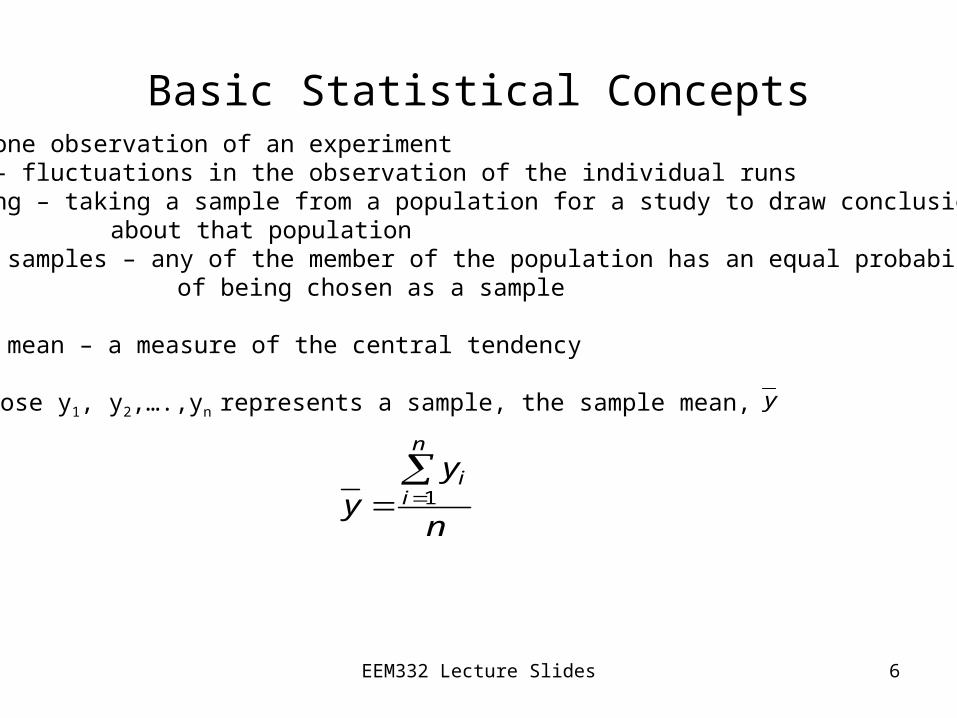
Basic Statistical ConceptsRun – one observation of an experimentNoise – fluctuations in the observation of the individual runsSampling – taking a sample from a population for a study to draw conclusions

about that populationRandom samples – any of the member of the population has an equal probability

of being chosen as a sample

Sample mean – a measure of the central tendency

Suppose y1, y2,….,yn represents a sample, the sample mean, y

n

yy

n

ii

1


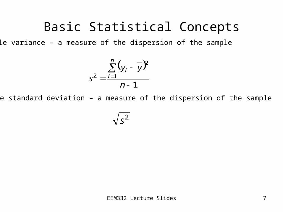
Basic Statistical ConceptsSample variance – a measure of the dispersion of the sample

1

1

2

2

n

yys

n

ii

Sample standard deviation – a measure of the dispersion of the sample

2s


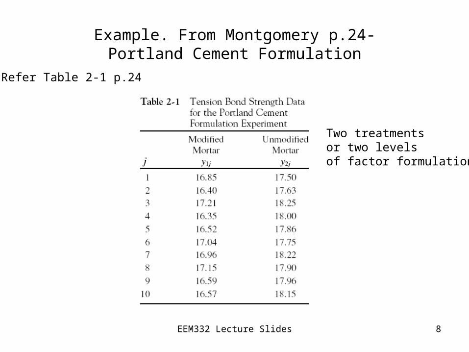
Example. From Montgomery p.24-Portland Cement Formulation

Refer Table 2-1 p.24

Two treatmentsor two levelsof factor formulations


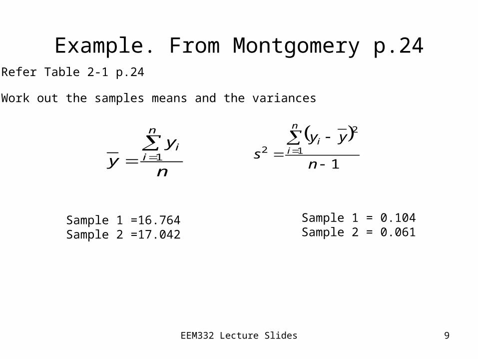
Example. From Montgomery p.24

n

yy

n

ii

1

Refer Table 2-1 p.24

Sample 1 =16.764 Sample 2 =17.042

Sample 1 = 0.104Sample 2 = 0.061

Work out the samples means and the variances

1

1

2

2

n

yys

n

ii


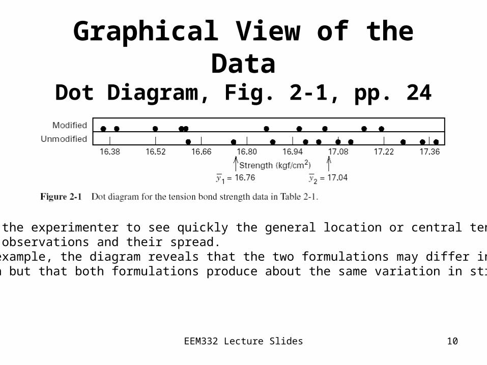
Graphical View of the DataDot Diagram, Fig. 2-1, pp. 24

Enables the experimenter to see quickly the general location or central tendency of the observations and their spread.In the example, the diagram reveals that the two formulations may differ in mean Strength but that both formulations produce about the same variation in strength.


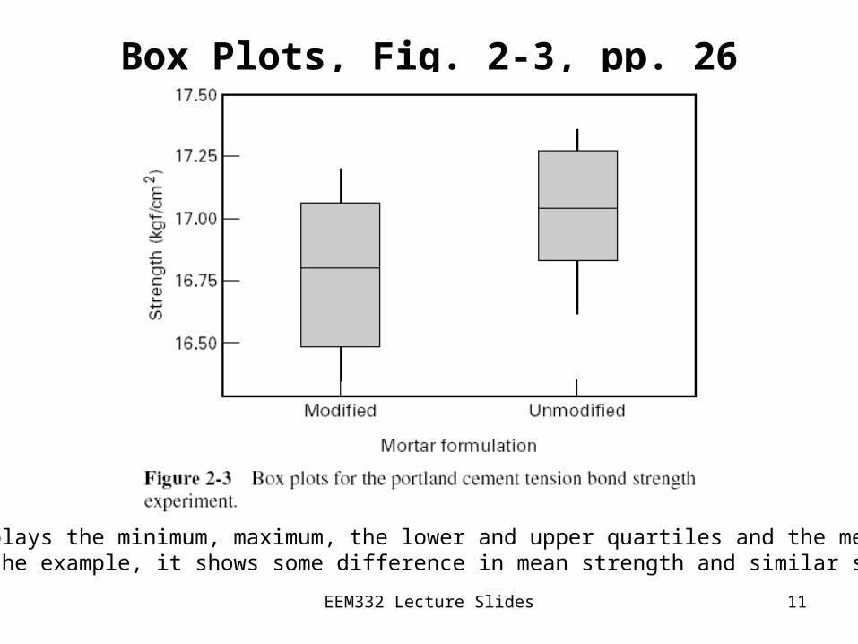
Box Plots, Fig. 2-3, pp. 26

Displays the minimum, maximum, the lower and upper quartiles and the median.In the example, it shows some difference in mean strength and similar spread.


Simple Comparative ExperimentsExperiments to compare 2 conditions ( or sometimes called treatments)

Example. P. 23 – an experiment to determine whether two different formulationsof a product give equivalent results.

Section 2.4-p. 34 discuss how the data from the simple comparative experiment can be analysed using Hypothesis testing procedures for comparing twotreatment means.


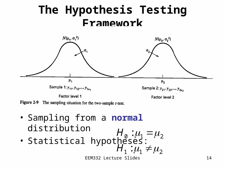
The Hypothesis Testing Framework

• Statistical hypothesis testing is a useful framework for many experimental situations

• Origins of the methodology date from the early 1900s

• We will use a procedure known as the two-sample t-test


The Hypothesis Testing Framework

• Sampling from a normal distribution• Statistical hypotheses:

0 1 2

1 1 2

:

:

H

H


Statistical HypothesisA statement either about the parameters of a probability distribution or the parameters of a model that reflects some conjecture about the problemsituation

Hypothesis Testing (or Significance Testing)A technique of statistical inference to assist experimenter in comparative

experiments and allows comparison to be made on objective terms, and with knowledge of the risks associated with reaching the wrong conclusion.

(Refer example. p. 24)- it is not obvious that the two samples really are different.One may be faced with the problem of making a definite decision with respect to an uncertain hypothesis which is known only through its observable consequences.


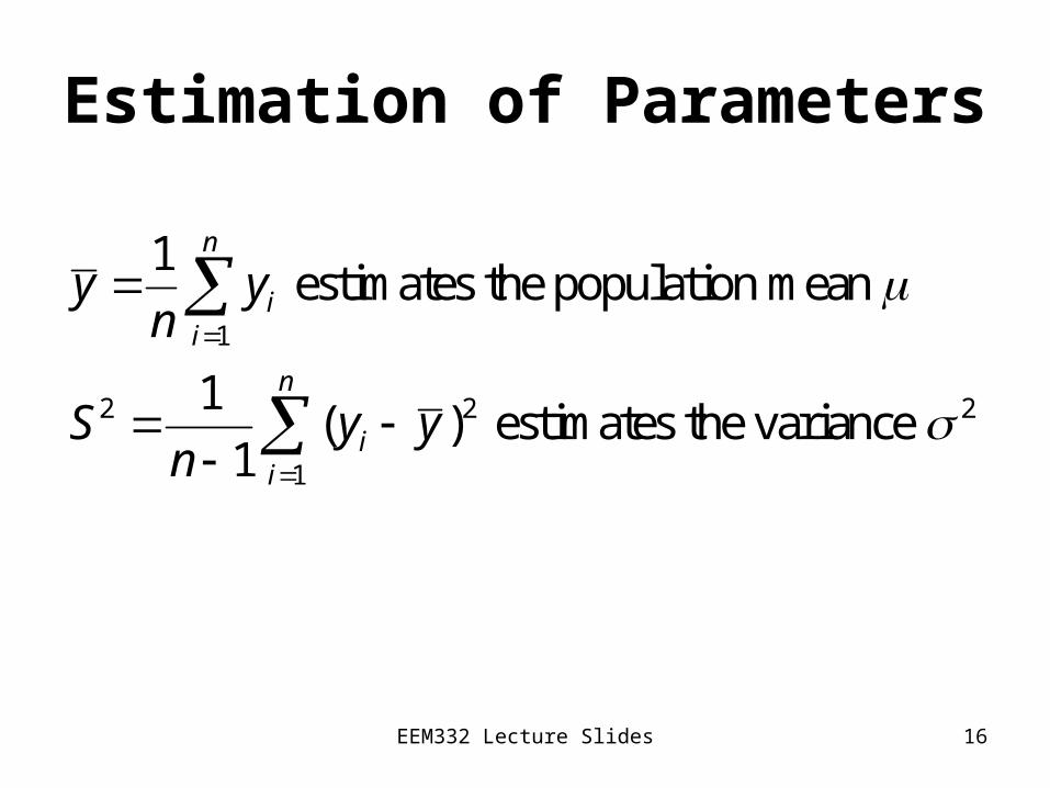
Estimation of Parameters

1

2 2 2

1

1 estimates the population mean

1( ) estimates the variance

1

n

ii

n

ii

y yn

S y yn


The t-TestA t test is any statistical hypothesis test for two groups in which the test statistic has a t distribution if the null hypothesis is true.

A test of the null hypothesis that the means of two normally distributed populations are equal.

Used for investigating the statistical significance of the difference between two sample means, and for confidence intervals for the difference between two population means.

Given two data sets, each characterized by its mean, standard deviation and number of data points, we can use some kind of t test to determine whether the means are distinct, provided that the underlying distributions can be assumed to be normal.

The t-distribution is a probability distribution that arises in the problem of estimating the mean of a normally distributed population when the sample size is small. (Refer to Montgomery p. 606)


The two sample t-TestTesting for a significant difference between two means

The t statistics compares two means to see if they are significantly different fromeach other (For the table of t-statistics see Table 2-3 page 47 and Table 2-4 page 48)

Used for investigating the statistical significance of the difference between two sample means, and for confidence intervals for the difference between two population means.

Example of two sample t-test p. 36-7


Degrees of freedom (df) is a measure of the number of independent pieces of information on which the precision of a parameter estimate is based. The degrees of freedom for an estimate equals the number of observations (values) minus the number of additional parameters estimated for that calculation.

Example. P. 36

As we have to estimate more parameters, the degrees of freedom available decreases.It can also be thought of as the number of observations (values) which are freely available to vary given the additional parameters estimated.It can be thought of two ways: in terms of sample size and in terms of dimensions and parameters.

For a single sample t-test, degrees of freedom are one less than the number of Observation (n-1).For a two sample t-test, degrees of freedom are one less than the number of observation in the first sample plus one less than the number of observation in the second sample ( n1-1 + n2-1) or (n1 + n2 -2).


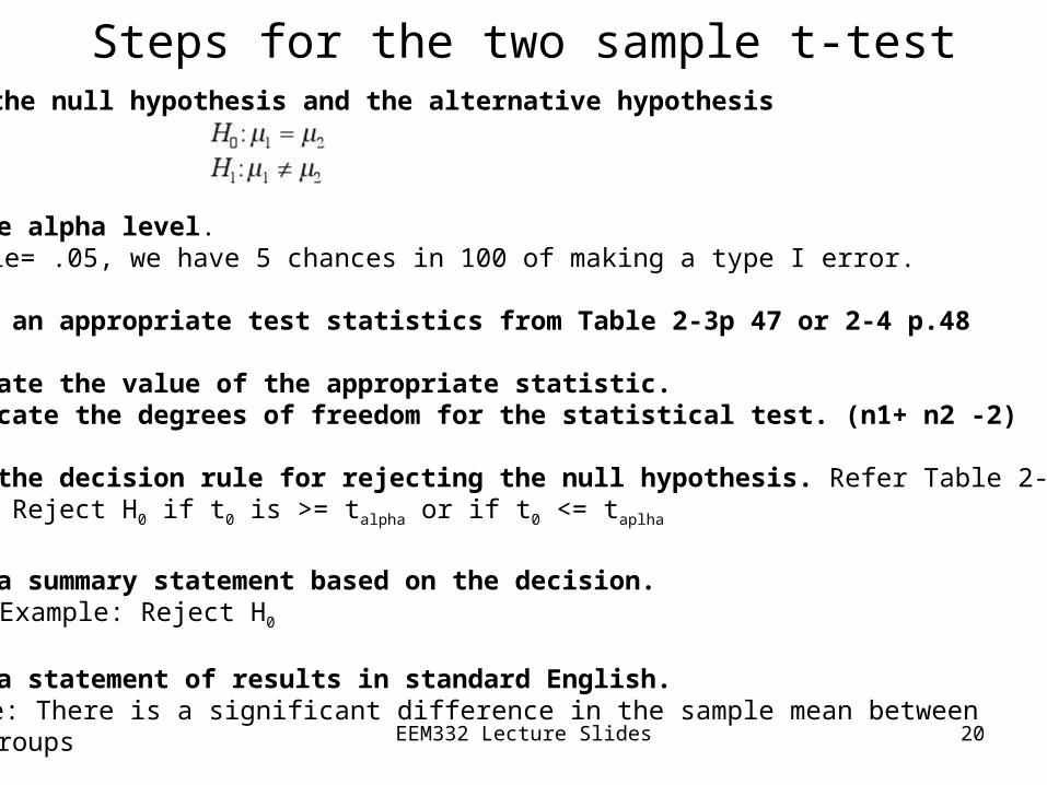
Steps for the two sample t-test1. State the null hypothesis and the alternative hypothesis

2. Set the alpha level. Example= .05, we have 5 chances in 100 of making a type I error.

3. Select an appropriate test statistics from Table 2-3p 47 or 2-4 p.48

4. Calculate the value of the appropriate statistic. Also indicate the degrees of freedom for the statistical test. (n1+ n2 -2)

5. Write the decision rule for rejecting the null hypothesis. Refer Table 2-3 / 2-4Example : Reject H0 if t0 is >= talpha or if t0 <= taplha

6. Write a summary statement based on the decision.Example: Reject H0

7. Write a statement of results in standard English.Example: There is a significant difference in the sample mean between

the two groups


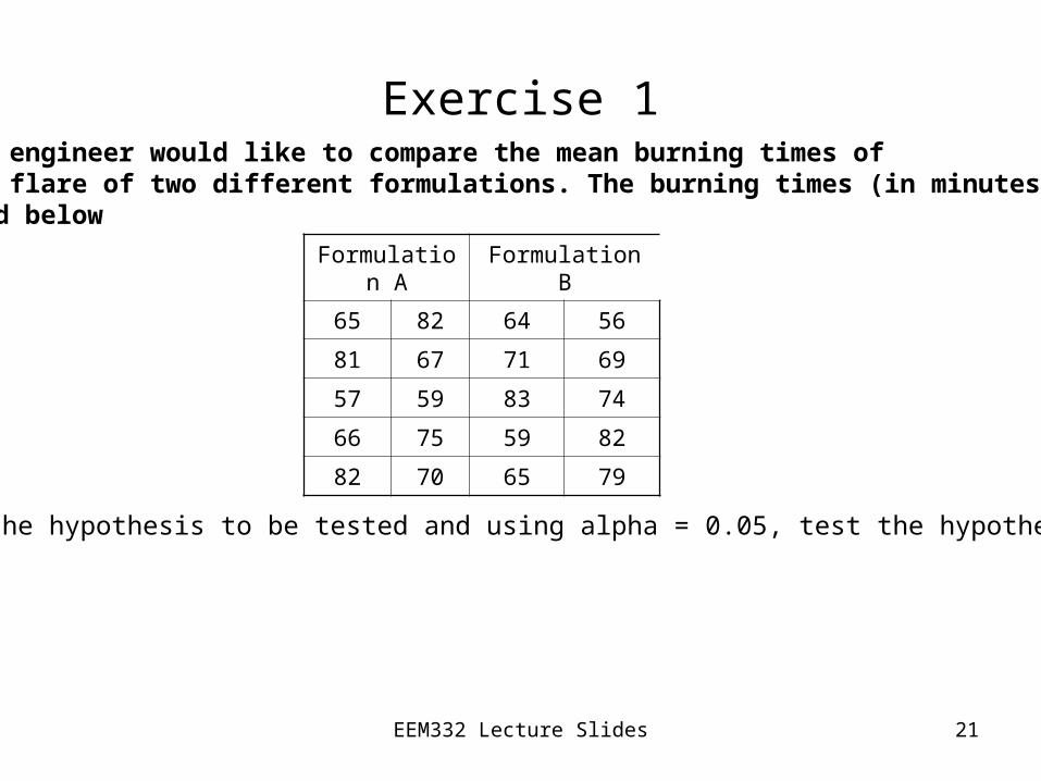
Exercise 1A design engineer would like to compare the mean burning times of chemical flare of two different formulations. The burning times (in minutes) aretabulated below

Formulation A Formulation B

65 82 64 56

81 67 71 69

57 59 83 74

66 75 59 82

82 70 65 79

State the hypothesis to be tested and using alpha = 0.05, test the hypotheses?


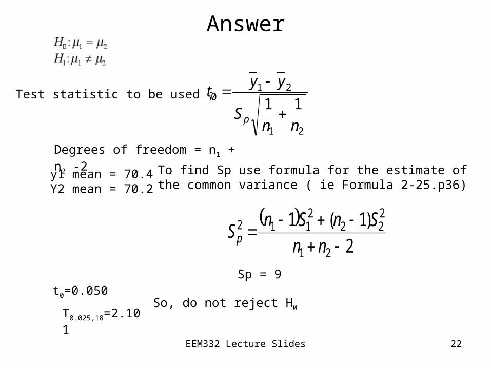
Answer

Test statistic to be used ;

21

210

11

nnS

yyt

p

Degrees of freedom = n1 + n2 -2

y1 mean = 70.4Y2 mean = 70.2

To find Sp use formula for the estimate of the common variance ( ie Formula 2-25.p36)

2

)1(1

21

222

2112

nn

SnSnS p

Sp = 9t0=0.050

T0.025,18=2.101So, do not reject H0


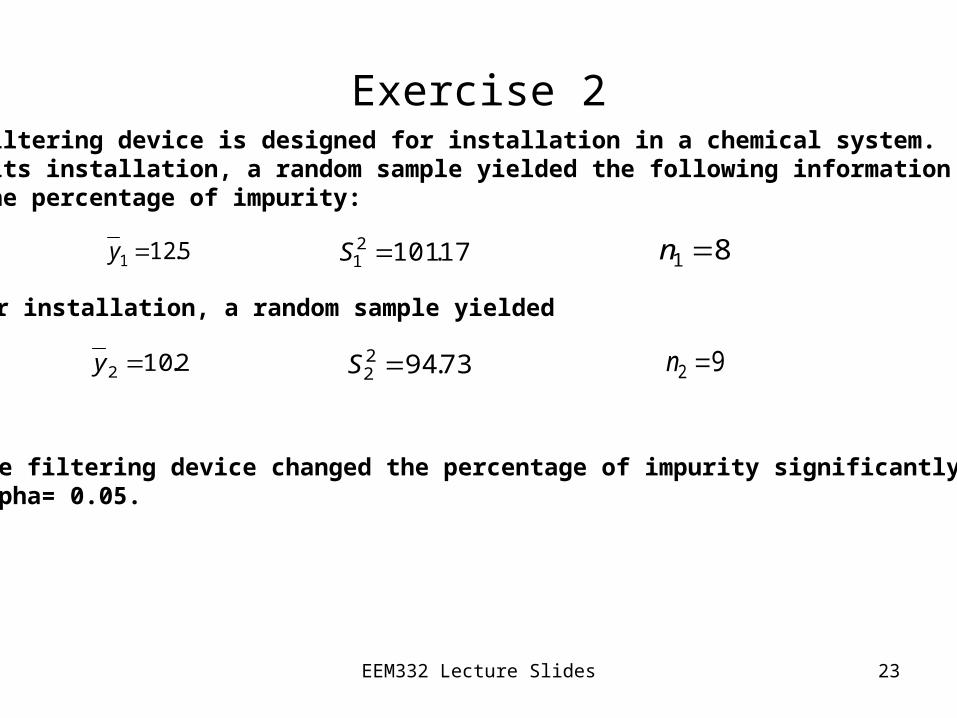
Exercise 2

2.102 y 73.9422 S

A new filtering device is designed for installation in a chemical system. Before its installation, a random sample yielded the following information about the percentage of impurity:

Has the filtering device changed the percentage of impurity significantly? Use alpha= 0.05.

5.121 y 17.10121 S 81 n

After installation, a random sample yielded

92 n


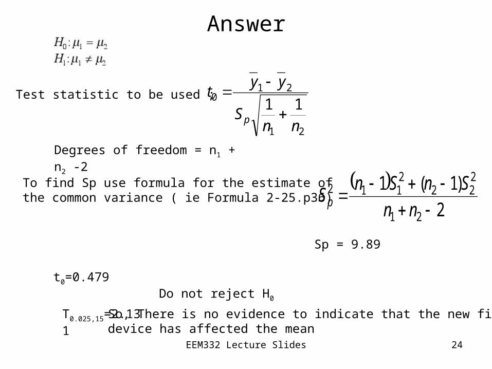
Answer

Test statistic to be used ;

21

210

11

nnS

yyt

p

Degrees of freedom = n1 + n2 -2

To find Sp use formula for the estimate of the common variance ( ie Formula 2-25.p36)

2

)1(1

21

222

2112

nn

SnSnS p

Sp = 9.89

t0=0.479

T0.025,15=2.131

Do not reject H0

So, There is no evidence to indicate that the new filtering device has affected the mean


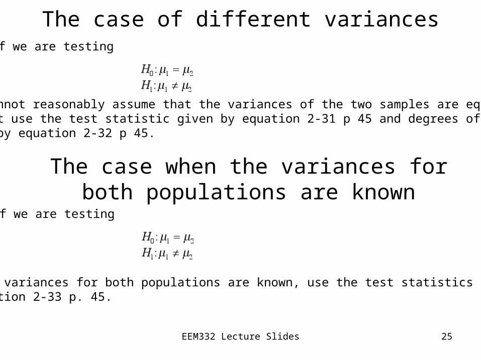
The case of different variancesIf we are testing

and cannot reasonably assume that the variances of the two samples are equal,We must use the test statistic given by equation 2-31 p 45 and degrees of freedom given by equation 2-32 p 45.

The case when the variances for both populations are known

If we are testing

and the variances for both populations are known, use the test statistics givenby equation 2-33 p. 45.


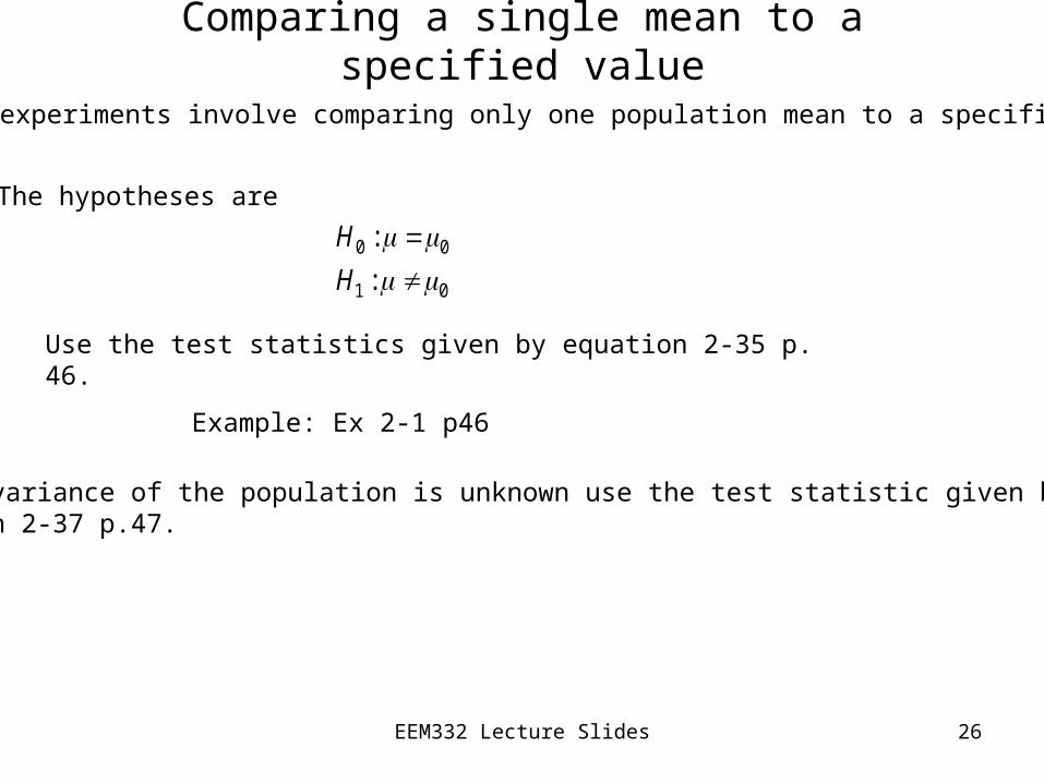
Comparing a single mean to a specified value

The hypotheses are

Some experiments involve comparing only one population mean to a specified value

Use the test statistics given by equation 2-35 p. 46.

00 : H

01 : H

Example: Ex 2-1 p46

If the variance of the population is unknown use the test statistic given byEquation 2-37 p.47.


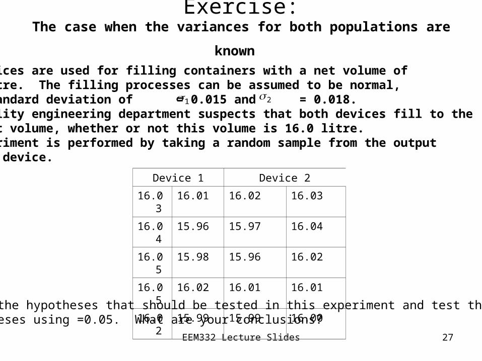
Exercise:The case when the variances for both populations are known

Two devices are used for filling containers with a net volume of 16.0 litre. The filling processes can be assumed to be normal, with standard deviation of = 0.015 and = 0.018. The quality engineering department suspects that both devices fill to the same net volume, whether or not this volume is 16.0 litre. An experiment is performed by taking a random sample from the output of each device.

Device 1 Device 2

16.03 16.01 16.02 16.03

16.04 15.96 15.97 16.04

16.05 15.98 15.96 16.02

16.05 16.02 16.01 16.01

16.02 15.99 15.99 16.00

State the hypotheses that should be tested in this experiment and test these hypotheses using =0.05. What are your conclusions?

1 2


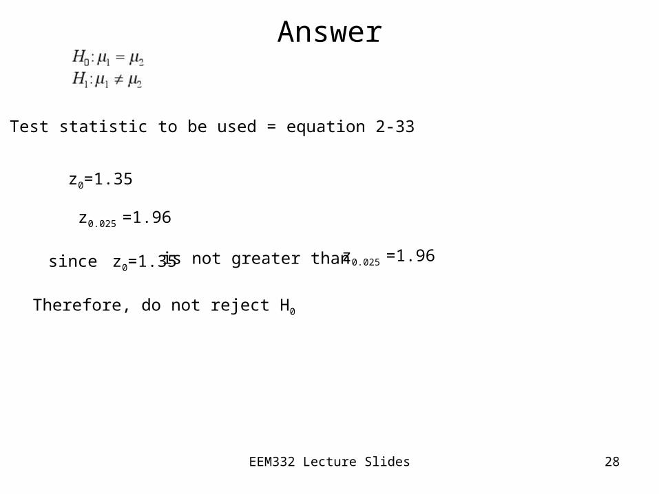
Answer

Test statistic to be used = equation 2-33

z0=1.35

z0.025 =1.96

Therefore, do not reject H0

since z0=1.35 is not greater than z0.025 =1.96


Confidence IntervalAn interval within which the value of the parameter or parameters in question would be expected to lie

Why ?

Hypothesis testing is useful but sometimes does not tell the entire story

It is often preferable to provide an interval within which the value of the parameteror parameters in question would be expected to lie.

In many engineering and industrial experiments, the experimenter already knowsThat the means differ, so they are more interested in a confidence interval on thedifference in means.


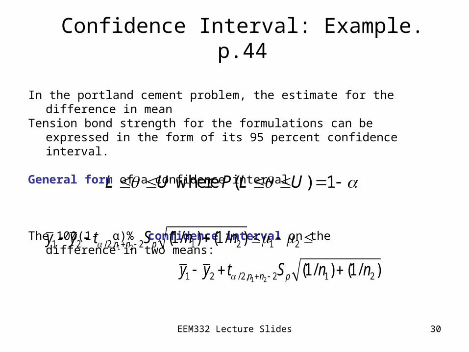
Confidence Interval: Example. p.44

where ( ) 1 L U P L U

In the portland cement problem, the estimate for the difference in meanTension bond strength for the formulations can be expressed in the form

of its 95 percent confidence interval.

General form of a confidence interval

The 100(1- α)% confidence interval on the difference in two means:

1 2

1 2

1 2 / 2, 2 1 2 1 2

1 2 / 2, 2 1 2

(1/ ) (1/ )

(1/ ) (1/ )

n n p

n n p

y y t S n n

y y t S n n


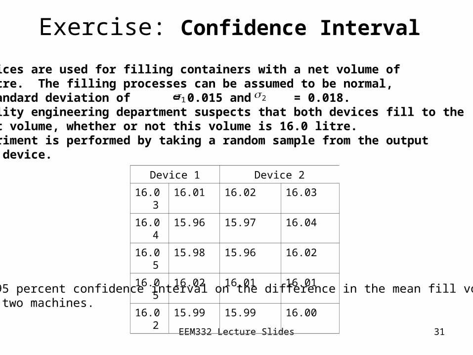
Exercise: Confidence Interval

Two devices are used for filling containers with a net volume of 16.0 litre. The filling processes can be assumed to be normal, with standard deviation of = 0.015 and = 0.018. The quality engineering department suspects that both devices fill to the same net volume, whether or not this volume is 16.0 litre. An experiment is performed by taking a random sample from the output of each device.

Device 1 Device 2

16.03 16.01 16.02 16.03

16.04 15.96 15.97 16.04

16.05 15.98 15.96 16.02

16.05 16.02 16.01 16.01

16.02 15.99 15.99 16.00

Find a 95 percent confidence interval on the difference in the mean fill volume for the two machines.

1 2


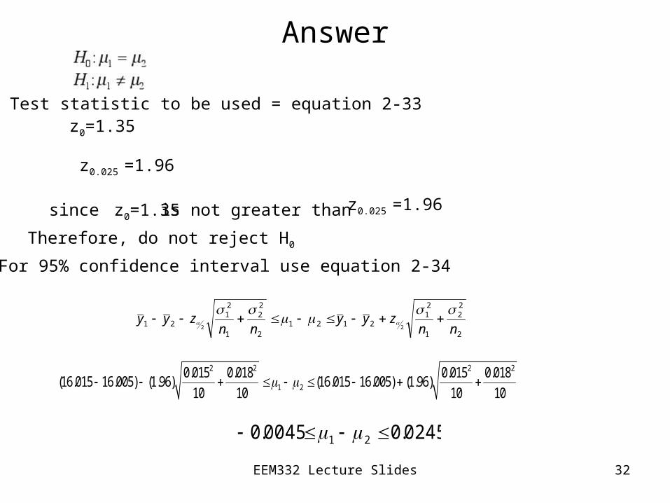
Answer

Test statistic to be used = equation 2-33z0=1.35

z0.025 =1.96

Therefore, do not reject H0

since z0=1.35 is not greater than z0.025 =1.96

For 95% confidence interval use equation 2-34

2

22

1

21

21212

22

1

21

21 22 nnzyy

nnzyy

2 2 2 2

1 2

0.015 0.018 0.015 0.018(16.015 16.005) (1.96) (16.015 16.005) (1.96)

10 10 10 10

0245.00045.0 21

Documents

EEM332 Lecture Slides1 EEM332 Design of Experiments En. Mohd Nazri Mahmud MPhil (Cambridge, UK) BEng (Essex, UK) [email protected] Room 2.14 Ext. 6059