Embed Size (px)
Citation preview

University of Central Florida University of Central Florida
STARS STARS
Electronic Theses and Dissertations, 2004-2019
2008
Effect Of Pressure Gradient And Wake On Endwall Film Cooling Effect Of Pressure Gradient And Wake On Endwall Film Cooling
Effectiveness Effectiveness
Sylvette Rodriguez University of Central Florida
Part of the Mechanical Engineering Commons
Find similar works at: https://stars.library.ucf.edu/etd
University of Central Florida Libraries http://library.ucf.edu
This Doctoral Dissertation (Open Access) is brought to you for free and open access by STARS. It has been accepted
for inclusion in Electronic Theses and Dissertations, 2004-2019 by an authorized administrator of STARS. For more
information, please contact [email protected].
STARS Citation STARS Citation Rodriguez, Sylvette, "Effect Of Pressure Gradient And Wake On Endwall Film Cooling Effectiveness" (2008). Electronic Theses and Dissertations, 2004-2019. 3703. https://stars.library.ucf.edu/etd/3703

EFFECT OF PRESSURE GRADIENT AND WAKE ON ENDWALL FILM COOLING EFFECTIVENESS
by
SYLVETTE RODRIGUEZ
B.S. University of Puerto Rico, 2000 M.S. University of Central Florida, 2005
A dissertation submitted in partial fulfillment of the requirements for the degree of Doctor of Philosophy
in the Department of Mechanical, Materials, and Aerospace Engineering in the College of Engineering and Computer Science
at the University of Central Florida Orlando, Florida
Fall Term
2008
Major Professor: Jayanta Kapat

ii
© 2008 Sylvette Rodriguez

iii
ABSTRACT
Endwall film cooling is a necessity in modern gas turbines for safe and reliable operation.
Performance of endwall film cooling is strongly influenced by the hot gas flow field, among
other factors. For example, aerodynamic design determines secondary flow vortices such as
passage vortices and corner vortices in the endwall region. Moreover blockage presented by the
leading edge of the airfoil subjects the incoming flow to a stagnating pressure gradient leading to
roll-up of the approaching boundary layer and horseshoe vortices. In addition, for a number of
heavy frame power generation gas turbines that use cannular combustors, the hot and turbulent
gases exiting from the combustor are delivered to the first stage vane through transition ducts.
Wakes induced by walls separating adjacent transition ducts located upstream of first row vanes
also influence the entering main gas flow field. Furthermore, as hot gas enters vane passages, it
accelerates around the vane airfoils. This flow acceleration causes significant streamline
curvature and impacts lateral spreading endwall coolant films. Thus endwall flow field,
especially those in utility gas turbines with cannular combustors, is quite complicated in the
presence of vortices, wakes and strong favorable pressure gradient with resulting flow
acceleration. These flow features can seriously impact film cooling performance and make
difficult the prediction of film cooling in endwall.
This study investigates endwall film cooling under the influence of pressure gradient
effects due to stagnation region of an axisymmetric airfoil and in mainstream favorable pressure
gradient. It also investigates the impact of wake on endwall film cooling near the stagnation
region of an airfoil. The investigation consists of experimental testing and numerical simulation.

iv
Endwall film cooling effectiveness is investigated near the stagnation region on an airfoil
by placing an axisymmetric airfoil downstream of a single row of inclined cylindrical holes. The
holes are inclined at 35° with a length-to-diameter ratio of 7.5 and pitch-to-diameter ratio of 3.
The ratio of leading edge radius to hole diameter and the ratio of maximum airfoil thickness to
hole diameter are 6 and 20 respectively. The distance of the leading edge of the airfoil is varied
along the streamwise direction to simulate the different film cooling rows preceding the leading
edge of the airfoil. Wake effects are induced by placing a rectangular plate upstream of the
injection point where the ratio of plate thickness to hole diameter is 6.4, and its distance is also
varied to investigate the impact of strong and mild wake on endwall film cooling effectiveness.
Blowing ratio ranged from 0.5 to 1.5.
Film cooling effectiveness is also investigated under the presence of mainstream pressure
gradient with converging main flow streamlines. The streamwise pressure distribution is
attained by placing side inserts into the mainstream. The results are presented for five holes of
staggered inclined cylindrical holes. The inclination angle is 30° and the tests were conducted at
two Reynolds number, 5000 and 8000.
Numerical analysis is employed to aid the understanding of the mainstream and coolant
flow interaction. The solution of the computational domain is performed using FLUENT
software package from Fluent, Inc. The use of second order schemes were used in this study to
provide the highest accuracy available. This study employed the Realizable κ-ε model with
enhance wall treatment for all its cases.

v
Endwall temperature distribution is measured using Temperature Sensitive Paint (TSP)
technique and film cooling effectiveness is calculated from the measurements and compared
against numerical predictions.
Results show that the characteristics of average film effectiveness near the stagnation
region do not change drastically. However, as the blowing ratio is increased jet to jet interaction
is enhanced due to higher jet spreading resulting in higher jet coverage. In the presence of wake,
mixing of the jet with the mainstream is enhanced particularly for low M. The velocity deficit
created by the wake forms a pair of vortices offset from the wake centerline. These vortices lift
the jet off the wall promoting the interaction of the jet with the mainstream resulting in a lower
effectiveness. The jet interaction with the mainstream causes the jet to lose its cooling
capabilities more rapidly which leads to a more sudden decay in film effectiveness. When film
is discharged into accelerating main flow with converging streamlines, row-to-row coolant flow
rate is not uniform leading to varying blowing ratios and cooling performance. Jet to jet
interaction is reduced and jet lift off is observed for rows with high blowing ratio resulting in
lower effectiveness.

vi
To my family, thank you for being a pillar of strength for me.

vii
ACKNOWLEDGMENTS
This work has been possible by the help and cooperation of many. To my advisor, Dr.
Jayanta Kapat, thank you for your support, dedication, and for all that I have learned from you.
Your passion and continued desire to rise above inspires many. I also thank my thesis
committee, Dr. Gordon, Dr Guha, Dr. Basu and in particular to Dr. Kassab, thank you for your
time and continuous support throughout the years.
It has been a privilege to work alongside the members of the investigation group at the
Center for Advanced Turbine and Energy Research (CATER): Quan, Vaidy, Chris, Humberto,
Anil, Stephanie and others. Your motivation and sense of teamwork is admirable.
To all my professors who contributed to my professional growth. To my friends,
colleagues, and to all who in one way or another have supported me and have taken part in this
dissertation, my sincerest gratitude.
There are no words that could possibly express the appreciation that I have for my family.
To my husband, Luis F., thank you for companionship through my late nights, for your
commitment to me in this journey and your continued words of comfort. To my parents, my
brother Benny and sister Mariel, whom have inspired me to supersede with your examples and
have taught me the value of education and the importance of following after my dreams.
Above all, my deepest gratitude is for my Lord Jesus, whom without any of this would
have meaning. May my whole life always bring glory and honor to Your name.

viii
TABLE OF CONTENTS
LIST OF FIGURES ....................................................................................................................... xi
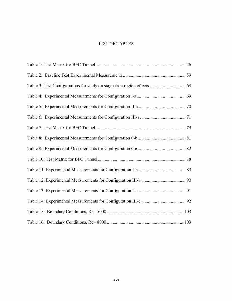
LIST OF TABLES....................................................................................................................... xvi
NOMENCLATURE ................................................................................................................... xvii
CHAPTER 1: INTRODUCTION................................................................................................... 1
CHAPTER 2: LITERATURE REVIEW........................................................................................ 8
Experimental Studies................................................................................................... 8
Computational Studies............................................................................................... 14
CHAPTER 3: METHODOLOGY ................................................................................................ 19
Experimental Methodology ........................................................................................ 19
BFC Wind Tunnel Details....................................................................................... 19
IFC Wind Tunnel Details ........................................................................................ 27
Temperature Sensitive Paint .................................................................................. 33
Computational Methodology ...................................................................................... 37
Computational Model ............................................................................................. 37
Grid and Mesh Generation..................................................................................... 39
Solution and Discretization..................................................................................... 39
Turbulence Model .................................................................................................. 40
Near-Wall Treatments ............................................................................................ 41

ix
Grid Independence................................................................................................. 43
Convergence.......................................................................................................... 43
Data Reduction of Experimental Data........................................................................ 44
Discharge Coefficient ............................................................................................. 44
Blowing Ratio and Momentum Flux........................................................................ 46
Film Cooling Effectiveness..................................................................................... 47
Uncertainty Analysis............................................................................................... 52
Data Reduction of Computational Data ..................................................................... 54
Film Cooling Effectiveness..................................................................................... 54
CHAPTER 4: RESULTS.............................................................................................................. 58
Baseline..................................................................................................................... 58
Experimental Details .............................................................................................. 58
CFD Details............................................................................................................ 58
Results and Discussion.......................................................................................... 61
Stagnation Region Effects ......................................................................................... 67
Experimental Details .............................................................................................. 68
Simulation Details .................................................................................................. 72
Results and Discussion.......................................................................................... 73
Wake Effects ............................................................................................................. 78
Experimental Details .............................................................................................. 79
Simulation Details .................................................................................................. 80
Results and Discussion.......................................................................................... 84

x
Stagnation Region and Wake effects......................................................................... 87
Experimental Details .............................................................................................. 88
Simulation Details .................................................................................................. 93
Results and Discussion.......................................................................................... 94
Film Coverage...................................................................................................... 101
Pressure Gradient.................................................................................................... 102
Experimental Details ............................................................................................ 103
Simulation Details ................................................................................................ 104
Results and Discussion........................................................................................ 105
Blowing Ratio Comparison ...................................................................................... 108
CHAPTER 5: CONCLUSIONS ................................................................................................. 112
REFERENCES ........................................................................................................................... 116

xi
LIST OF FIGURES
Figure 1: Gas temperature compared to allowable metal temperature ............................... 1
Figure 2: Damage to Nozzle Guide Vanes due to Excessive High Temperatures.............. 1
Figure 3: Development of Cooling Methods Techniques vs. Inlet Temperature .............. 2
Figure 4: Internal Cooling Passages on an Airfoil............................................................. 3
Figure 5: Different Film Cooling Methods (Eckert).......................................................... 3
Figure 6: Recovery Temperature vs. Adiabatic wall Temperature.................................... 4
Figure 7: Flow Model Proposed by Langston [2].............................................................. 5
Figure 8: Schematic of the Endwall Boundary Layers (Denton and Cumpsty) ................. 6
Figure 9: MS7001FA Gas Turbine and Representation of Region under Investigation..... 7
Figure 10: Schematic of the near hole flow field [7] ....................................................... 10
Figure 11: BFC Test Rig Schematic ................................................................................. 20
Figure 12: Location of thermocouples in BFC rig............................................................ 21
Figure 13: Scanivalve Calibration Curve.......................................................................... 22
Figure 14: Flow meters ..................................................................................................... 23
Figure 15: Acrylic test coupon.......................................................................................... 24
Figure 16: Leading Edge radius to Film Cooling Hole Pitch Ratio.................................. 25
Figure 17: Test Setup of Airfoil with Wake plate............................................................ 25
Figure 18: Test Configurations for study on BFC ............................................................ 26
Figure 19: Vertical section of the IFC tunnel ................................................................... 27
Figure 20: Horizontal section of the IFC tunnel ............................................................... 28

xii
Figure 21: Test Section Setup ........................................................................................... 31
Figure 22: Test Coupon .................................................................................................... 32
Figure 23: Alignment of inserts with film hole exits........................................................ 33
Figure 24: Emission spectrum of TSP (Liu, 2006) ........................................................... 34
Figure 25: Typical TSP setup and instrumentation (Liu, 2006) ....................................... 35
Figure 26: CCD camera and light source.......................................................................... 36
Figure 27: Spectrum of LED source (Liu, 2006).............................................................. 36
Figure 28: Computational Domain and Boundary Conditions Type (Configuration 0-a) 38
Figure 29: Inlet Total Pressure Profile.............................................................................. 38
Figure 30: Grid Independence Check ............................................................................... 43
Figure 31: Mach number distribution along the film hole rows ....................................... 45
Figure 32: Normal image of TSP...................................................................................... 48
Figure 33: Reference Image.............................................................................................. 49
Figure 34: Image of TSP showing coolant flow ............................................................... 50
Figure 35: TSP Calibration Curve .................................................................................... 50
Figure 36: Raw Temperature image from TSP................................................................. 51
Figure 37: Results of averaging effectiveness .................................................................. 52
Figure 38: Uncertainty distribution for film cooling effectiveness [29]........................... 53
Figure 39: Uncertainty in CD measurement [29] ............................................................. 53
Figure 40: FLUENT Local Temperature Data extracted for calculating effectiveness.... 55
Figure 41: Graphical User Interface to process Computational Data .............................. 56
Figure 42: Process flowchart of Data Reduction of Computational Data ........................ 57

xiii
Figure 43: Configuration 0-a CFD Grid .......................................................................... 60
Figure 44: CFD Domain and Boundary Conditions Type for Configuration 0-a............. 60
Figure 45: Data Comparison for M=0.5 .......................................................................... 61
Figure 46: Data Comparison for M=0.75 ........................................................................ 62
Figure 47: Comparison of Turbulence Models against Experimental Data .................... 63
Figure 48: Validation of Configuration 0-a ...................................................................... 64
Figure 49: Average Effectiveness for Configuration 0-a.................................................. 65
Figure 50: Local Temperature Distribution for Configuration 0-a................................... 65
Figure 51: Local Temperature Distribution for Configuration 0-a (Exp vs. CFD) .......... 65
Figure 52: Streamline Plot for Configuration 0-a (M=0.5) .............................................. 66
Figure 53: Streamline Plot for Configuration 0-a (M=1.5) .............................................. 67
Figure 54: Test Configurations for study on stagnation region effects ............................ 68
Figure 55: Stagnation Region Effects CFD Grid............................................................. 72
Figure 56: CFD Domain and Boundary Conditions Type for Configuration I and III-a. 73
Figure 57: Average Film Cooling Effectiveness for Configuration I-a........................... 74
Figure 58: Local Film Cooling Effectiveness for Configuration I-a (Exp. vs. CFD)....... 74
Figure 59: Average Film Cooling Effectiveness for Configuration I-b........................... 75
Figure 60: Local Film Cooling Effectiveness for Configuration I-b (Experimental) ....... 75
Figure 61: Average Film Cooling Effectiveness for Configuration I-c........................... 76
Figure 62: Local Film Cooling Effectiveness for Configuration I-c (Exp. vs. CFD)....... 76
Figure 63: Average Film Cooling Effectiveness (Configuration 0, I, and III-a) .............. 77
Figure 64: Streamline Plot for Configuration I-a (M=0.5 and 1.5) .................................. 77

xiv
Figure 65: Streamline Plot for Configuration I-c (M=0.5 and 1.5) .................................. 77
Figure 66: Test Configurations for study on wake effects................................................ 79
Figure 67: Wake effects CFD grid................................................................................... 83
Figure 68: CFD Domain and Boundary Condition Type for Configurations 0-b and c ... 83
Figure 69: Average film cooling effectiveness for Configuration 0-b ............................. 84
Figure 70: Average film cooling effectiveness for Configuration 0-c.............................. 85
Figure 71: Local Film Cooling Effectiveness for Configuration 0-b (M=0.5 and 1.5) .... 85
Figure 72: Average Film Effectiveness for Configurations 0-c (M=0.5 and 1.5) ............ 85
Figure 73: CFD Vector plot for varying x/D – Wake plate ............................................. 86
Figure 74: Streamline plots for Configuration 0-b ........................................................... 87
Figure 75: Streamline plots for Configuration 0-c............................................................ 87
Figure 76: Test Configurations for study on stagnation region and wake effects ............ 88
Figure 77: CFD Grid (Configuration III-c)...................................................................... 93
Figure 78: CFD Domain and Boundary Conditions Type ................................................ 94
Figure 79: Average Film Cooling Effectiveness for Configuration 1-b ........................... 95
Figure 80: Average Film Cooling Effectiveness for Configuration 1I-b.......................... 96
Figure 81: Average Film Cooling Effectiveness for Configuration 1II-b ........................ 96
Figure 82: Average Film Cooling Effectiveness for Configuration 1-c ........................... 97
Figure 83: Average Film Cooling Effectiveness for Configuration 1I-c.......................... 97
Figure 84: Average Film Cooling Effectiveness for Configuration 1II-c......................... 98
Figure 85: Local Film Cooling Effectiveness for Configuration 1-b ............................... 98
Figure 86: Local Film Cooling Effectiveness for Configuration II-b............................... 98

xv
Figure 87: Local Film Cooling Effectiveness for Configuration III-b ............................. 99
Figure 88: Local Film Cooling Effectiveness for Configuration 1-c................................ 99
Figure 89: Local Film Cooling Effectiveness for Configuration II-c ............................... 99
Figure 90: Local Film Cooling Effectiveness for Configuration III-c............................ 100
Figure 91: Streamline plots for Configuration I-b .......................................................... 100
Figure 92: Streamline plots for Configuration III-b ....................................................... 100
Figure 93: Streamline plots for Configuration I-c .......................................................... 101
Figure 94: Streamline plots for Configuration III-c........................................................ 101
Figure 95: Film Coverage ............................................................................................... 102
Figure 96: Pressure Gradient CFD Grid ........................................................................ 104
Figure 97: Pressure Gradient CFD Domain and Boundary Conditions Type ............... 105
Figure 98: Average Film Cooling Effectiveness (Re=5000 and 8000) .......................... 106
Figure 99: Temperature distribution at Re=5000 .......................................................... 107
Figure 100: Temperature distribution at Re=8000 ........................................................ 107
Figure 101: Streamline Plots (Re = 5000 and 8000) ..................................................... 108
Figure 102: Local Blowing Ratios for M = 0.5 ............................................................. 109
Figure 103: Local Blowing Ratios for M = 1.5 ............................................................. 110
Figure 104: Row by Row Blowing Ratio Variation (Re = 5000) ................................... 111
Figure 105: Row by Row Blowing Ratio Variation (Re = 8000) ................................... 111
xvi
LIST OF TABLES
Table 1: Test Matrix for BFC Tunnel ............................................................................... 26
Table 2: Baseline Test Experimental Measurements....................................................... 59
Table 3: Test Configurations for study on stagnation region effects................................ 68
Table 4: Experimental Measurements for Configuration I-a........................................... 69
Table 5: Experimental Measurements for Configuration II-a.......................................... 70
Table 6: Experimental Measurements for Configuration III-a ........................................ 71
Table 7: Test Matrix for BFC Tunnel ............................................................................... 79
Table 8: Experimental Measurements for Configuration 0-b .......................................... 81
Table 9: Experimental Measurements for Configuration 0-c .......................................... 82
Table 10: Test Matrix for BFC Tunnel ............................................................................. 88
Table 11: Experimental Measurements for Configuration I-b.......................................... 89
Table 12: Experimental Measurements for Configuration III-b ....................................... 90
Table 13: Experimental Measurements for Configuration I-c.......................................... 91
Table 14: Experimental Measurements for Configuration III-c ....................................... 92
Table 15: Boundary Conditions, Re= 5000 ................................................................... 103
Table 16: Boundary Conditions, Re= 8000 ................................................................... 103

xvii
NOMENCLATURE
A Area
a Actual
avg Average
aw Adiabatic wall
c Coolant
C Specific Heat
CD Discharge Coefficient
D diameter of hole inlet
f Film (Coolamt flow)
FCR Film Coverage Ratio, FCR=
h holes
I Momentum Flux ratio
K Acceleration Parameter, K= 2Ux
U∂
∂υ
L Length of hole
M Blowing ratio
m Main flow
•
m Mass Flow Rate
P Pressure
PI Pitch

xviii
Pr Prandtl Number
r Recovery
RKE Realizable κ-ε model
s Pitch
T Temperature
th theoretical
Tu Turbulence Intensity
U,V Velocity
w Wall
x Distance downstream of center of the hole
Greek Symbols
0 Stagnation value
∞ Mainstream condition
∞ Hole Inclination Angle
δ Boundary Layer Thickness
η Film cooling effectiveness
ρ Density

1
CHAPTER 1: INTRODUCTION
The gas turbine industry is continuously under demand to attain higher performance, longer
service life and lower emissions. The increasing demand to optimize gas turbines subjects hot
section components to more extreme operating conditions. The temperature of the gases entering
the turbine section is much greater than the allowable metal temperatures of the alloys used in
the turbine airfoils and endwall. Such high temperatures result on cracks, material deformation,
corrosion and fracture, as shown on Figure 2.
Figure 1: Gas temperature compared to allowable metal temperature (Cardwell, N. D., 2005 )
Figure 2: Damage to Nozzle Guide Vanes due to Excessive High Temperatures

2
The continuous effort to increase turbine efficiency has promoted the development and
sophistication of new material, thermal barriers and cooling methods. Different cooling methods
have been implemented to protect metal surfaces from hot gases; among them are film
impingement, ablation, transpiration and film cooling.
Figure 3: Development of Cooling Methods Techniques vs. Inlet Temperature (Clifford, 1985, AGARD CP 390; collected in Laskshminarayana, 1996)
In gas turbines air is drawn from the compressor and ejected via rows of holes located at
discrete locations on the airfoil and endwall to cool the surfaces. This process is called film
cooling. It consists of introducing a secondary flow into the boundary layer of the mainflow.
Film cooling not only protects the surface at the point of injection but also region downstream of
the injection point. The ejected coolant interacts with the external flow near the endwall and
generates aerodynamic and thermodynamic losses in the process. This reduces turbine stage
efficiency and the consumption of cooling air, which is detrimental to the overall cycle
efficiency. Over the recent years, existing cooling techniques are being optimized and new

3
endwall film cooling configurations are continuously explored. The data presented in Figure 5,
shows that film cooling is the most effective cooling methods among those developed in the
recent years.
Figure 4: Internal Cooling Passages on an Airfoil (Energy Efficient Engine (E3) NASA Report)
Figure 5: Different Film Cooling Methods (Eckert)
Endwall film cooling is determined among others by the inlet temperature distribution,
flow field and the state and thickness of the endwall boundary layer. The condition of the flow
entering the first stage vane is greatly affected by the hot and turbulent gases exiting from the
combustor. In order for this cooling technique to be effective, film cooling must provide
acceptable metal surface temperatures and reasonable temperature distribution over the endwall
to limit thermal stress as a result of large temperature gradients.

4
Goldstein [1] described that the convective heat transfer associated with film cooling is
determined by using a film heat transfer coefficient (hf), an adiabatic wall or film temperature
(Taw), where Tw is the local wall temperature:
( )awwf TThq −⋅= (Equation 1)
It is convenient to define a dimensionless adiabatic wall temperature, η, called film cooling
effectiveness. This dimensionless parameter is given by:
cr
awr
TTTT
−−
=η (Equation 2)
where Tr is the mainstream recovery temperature of the hot gas flow, and Tc is the stagnation
coolant temperature at the point of injection. The recovery temperature of the gas is calculated
by:
p
r CVTT⋅
⋅+= ∞ 2Pr
21
31
(Equation 3)
Tr is the surface temperature of an un-cooled insulated surface as shown in Figure 6.
Tr
Tc
Taw
T∞
T∞
Figure 6: Recovery Temperature vs. Adiabatic wall Temperature

5
Thus, the film cooling effectiveness varies from unity at the point of injection to zero where the
adiabatic wall temperature approaches the mainstream temperature due to mixing between the
coolant flow and the mainstream.
The flow near the endwall into which the coolant is being ejected can be inherently three-
dimensional. Due to the blockage presented by the leading edge of the airfoil, the incoming flow
is subjected to a stagnating pressure gradient. This causes the flow to undergo three-dimensional
separation and to roll up into a horseshoe vortex. Secondary flows make difficult the prediction
of the behavior of film cooling in the stagnation region. Moreover, the turning of the mainstream
flow within the vane passage together with airfoil curvature may produce a vane-to-vane
pressure gradient that generates a transverse component of flow within the endwall boundary
layer. The ejected coolant interacts with this three-dimensional flow. The flow can influence
coolant trajectories and to a smaller extend, the ejection of coolant has the potential of
influencing the three-dimensional flow.
Figure 7: Flow Model Proposed by Langston [2]

6
Figure 8: Schematic of the Endwall Boundary Layers (Denton and Cumpsty)
In most heavy frame power generation turbines, the hot and turbulent gases exiting from
the combustor are delivered to the first stage vane through transition ducts. Wakes induced by
the wall separating adjacent transition ducts located upstream of first row vanes, could also
influence the entering main gas flow field. The incoming flow field condition makes difficult
the prediction of the behavior of endwall film cooling near in the stagnation region as the film
approaches the turbine vane. Although thorough studies have been carried out on endwall film
cooling, the effect of the transition ducts on endwall film cooling near stagnation region is not
fully investigated.

7
Hot gases from combustor
Hot gases from combustor
Two adjacent transition pieces
Wall separating two transition pieces
Wake
High mainflow Mach number
Low mainflow Mach number
Stagnation point
Hot gases from combustor
Hot gases from combustor
Two adjacent transition pieces
Wall separating two transition pieces
Wake
High mainflow Mach number
Low mainflow Mach number
Stagnation point
Figure 9: MS7001FA Gas Turbine and Representation of Region under Investigation
The optimization of a cooling system has to be weighed against the increase in cycle
efficiency that can be achieved through higher turbine entry temperatures. Up to the present,
there are no correlations or experimental data available that characterize endwall film cooling
effectiveness near an airfoil’s stagnation region under the influence of wake induced by the
transition ducts and the pressure gradient induced by the incoming flow condition. This
dissertation presents the physics of flow mechanics responsible for determining downstream heat
transfer in the nearby region of the stagnation point of an axisymmetric airfoil, and under the
influence of pressure gradient and wake.

8
CHAPTER 2: LITERATURE REVIEW
Experimental Studies
Film cooling is a widely used method of cooling different components of aviation gas
turbines and power generation units. Film cooling enables turbines to operate at higher
temperatures than what the substrate super alloy can withstand. For decades, investigations on
film cooling techniques have been carried out for improving its performance to meet the ever
increasing turbine operating temperatures. In most gas turbine applications, the structural
loading at which its components are subjected does not allows a secondary flow to be injected
through slots; instead discrete holes are used to inject coolant into the mainstream.
Film cooling effectiveness depends on blowing ratio (M), momentum flux ratio (I),
mainstream turbulence intensity (Tu), length-to-diameter ratio (L/D), pitch-to-diameter ratio
(s/D), hole inclination angle (α), crossflow angle, displacement thickness of the mainstream
boundary layer -to-diameter ratio (δ/D), density ratio, and hole geometry. In the past years, there
have been several studies on film endwall film cooling where these important parameters have
been investigated. The blowing ratio and momentum flux ratio are defined as:
( )
( ) mm
cc
m
m
c
c
m
c
VV
AAV
AAV
Am
Am
M⋅⋅
=⋅⋅
⋅⋅
=
⎟⎟⎟
⎠
⎞
⎜⎜⎜
⎝
⎛
⎟⎟⎟
⎠
⎞
⎜⎜⎜
⎝
⎛
=•
•
ρρ
ρ
ρ
(Equation 4)

9
and
( )( )mm
cc
VV
I 2
2
⋅⋅
=ρρ
(Equation 5)
Nicklas [3] studied the effect of Mach number and blowing ratio on endwall heat transfer
and film-cooling effectiveness. Three rows of holes and a slot were investigated and found that
the interaction of coolant air and the secondary flow field greatly influenced heat transfer and
film effectiveness. It was observed that a decrease in intensity of the horseshoe vortex near the
endwall results in a reduction in heat transfer. Similarly, Zhang and Jaiswal [4] studied film
cooling effectiveness on a flat turbine nozzle endwall. It was reported that for low blowing
ratios, the secondary flows dominate over the momentum of the jet, resulting in a decrease in
effectiveness. On the contrary, at high blowing rates, the jet momentum overcomes the flow
field yielding to a higher effectiveness. According to Goldstein et al. [5], the low effectiveness
observed at low blowing ratios can be attributed to the jet spreading angle. He observed that for
low blowing ratios, the spreading of the jet does not vary significantly with the injection angle.
However, at a higher blowing ratio (M=1), the spreading angle increases at an injection of 90º
and decreases for blowing ratios greater than 1. This investigation was conducted on an
adiabatic flat plate for a row of holes inclined at 35º and 90º. Similarly, Eriksen and Goldstein
[6] studied the effect of blowing rates on heat transfer coefficient. They also found that for a 35º
row of film holes, high blowing rates increase heat transfer coefficient up to 27% for a blowing
ratio of two. This increase is attributed to the interaction between the jets and the mainstream,
resulting on an increase in the levels of turbulence. From these findings it can be inferred that

10
the spreading of the jets as described by Goldstein [5] enhances heat transfer and promotes
turbulence levels.
Figure 10: Schematic of the near hole flow field [7]
The exiting jet can produce a broad range of flow structures downstream of the injection
point. The jet as it exits is highly three-dimensional and contains flow features that are important
for the diffusion of the coolant fluid with the mainstream flow. At the point of injection the
coolant jet bends due to the inertial force of the mainstream flow and immediately starts to mix.
High blowing ratio can cause the coolant flow to lift off. The coolant flow penetrating into the
boundary layer can significantly reduce film cooling effectiveness. As depicted in Figure 10,
even at moderate blowing ratios a wake zone is formed in the lower part of the jet, downstream
of the film hole. This lowers the penetration velocity of jet allowing the freestream fluid to
penetrate more easily underneath of the core of the jet.
The difference of flow properties between the injected flow and mainstream as well as
the hole geometry also define the flow structure of the jet as it is injected into the mainstream.
The difference of flow properties between the injected flow and mainstream as well as
the hole geometry also define the flow structure of the jet as it is injected into the mainstream.

11
The effect of density ratio on film cooling effectiveness was studied by Sinha et al. [8] and
Pedersen et al. [9]. Sinha et al. [8] study was carried out for a single row of cylindrical holes
inclined at 35°. The density ratio ranged from 1.2 to 2.0. It was found that a decreased in
density ratio reduces significantly the spreading of the film cooling jet resulting in a reduction of
the laterally averaged effectiveness. Pedersen et al. [9] carried out an investigation for a single
row of holes inclined at 35°. Helium, carbon dioxide and refrigerant F-12 were used as coolant
flow injected into the mainstream. Thus, the density ratio varied from 0.75 to 4.17. Similarly,
this study reports that density ratio has a direct effect on film cooling effectiveness. This
investigation reports that an increase in density ratio increases film cooling effectiveness. The
influence of hole length-to-diameter ratio on film cooling with cylindrical holes was studied by
Lutum and Johnson [10]. The study was conducted on a row of cylindrical holes inclined at 35º
with varying length-to-diameter ratio (L/D = 1.75, 3.5, 5 and 7). It was determined that film
cooling effectiveness decreased with decreasing L/D. This is attributed to (1) undeveloped
character of the injected flow and (2) greater injection angle. Baldauf et al. [11] investigated the
effect of hole spacing. Their study shows that for pitch-to-diameter ratio of five or larger, the
lateral jet interaction is reduced significantly resulting on a decrease in effectiveness. For lower
s/D effectiveness is completely dominated by jet interaction at a blowing rate equal to 1.7. The
study results in a new correlation valid without any exception from the point of injection to the
region downstream, for all combinations of flow and geometry parameters for a row of film
holes in a flat plate.
Turbine inlet conditions in gas turbines generally consist of temperature and velocity
profiles that vary in the spanwise and pitchwise directions resulting from combustor exit

12
conditions. Pressure gradients in turbines can be attributed to two reasons: the inherent pressure
gradient from the turning of the flow and the pressure gradient resulting from the non-uniformity
of the incoming flow along the radial span of the airfoil passage. As a consequence, the leading
edge horseshoe vortex formed as the incoming boundary layer approached the stagnation region
of the vane separates into a pressure and suction side horseshoe vortex legs. As described by
Kost and Nicklas [12] the intensity of the horseshoe vortex is an important cause for the transport
of coolant from the endwall to the main flow. In this study it was recommended that in order to
prevent such an intensification of the horseshoe vortex, the distance from the injection point to
the leading edge should be increased.
Ammari et al. [13] studied the influence of mainstream acceleration on the heat transfer
coefficient for a single row of holes inclined at 35° in a flat plate. Two cases with two constant
acceleration parameters were analyzed in addition to the zero pressure gradient baseline case.
For the first case, K=1.96E-06 where as for the second case K=5.0E-6. In addition two species
were used as injected air, air and carbon dioxide yielding a density ratio of 1.0 and 1.52
respectively. The blowing ratio was also varied from 0.5 to 2.0. They found that heat transfer
coefficient increased as the acceleration increased. Also, it was reported that in the presence of
acceleration, the heat transfer coefficient was dependent of the density ratio, an increase in
density ratio lead to a decrease in heat transfer coefficient. The pressure gradient was achieved
by contouring the roof of the test section. In 1991, a similar film cooling effectiveness study was
carried out by Teekaram et al. [14]. They report effectiveness for a single row of cylindrical
holes on a flat plate inclined at 30º. Favorable and adverse pressure gradients are obtained by
contouring the wall opposite to the injection location. The study reports that a strong favorable

13
pressure gradient increases effectiveness. Lower effectiveness is measured in the presence of
adverse pressure gradient.
The literature contains some contradictory results about the influence of pressure gradient
on film cooling effectiveness. Kruse [15] reported film cooling effectiveness measurements for a
range of blowing ratios and pitch to diameter ratio. Three different injection angles were also
studied, 10°, 45° and 90°. The pressure gradient was achieved by using a flexible wall to
produce zero, favorable and adverse pressure gradient. The results of this paper show that
pressure gradient has a significant effect on film cooling effectiveness most noticeable at low
blowing ratios and small hole spacing. Adverse pressure gradient promotes jet lift off at
locations close to the injection point but results in an increase in the effectiveness farther
downstream. In the presence of favorable pressure gradient, the jet does not penetrate far into
the mainstream. At the exit of jet, the jet is flattened out due to the contraction of the mainflow
but the coolant does not mix well downstream of the injection point resulting in a lower film
cooling effectiveness. Similarly to Hay et al. [16], Kruse observed that the boundary layer
thickness seems not to have an effect on film cooling effectiveness. Similarly, Schmidt and
Bogard [17] studied the effect of pressure gradient on film cooling effectiveness. They
investigated a single row of cylindrical film cooling holes inclined at 35°. The top wall of the
test section was contoured to produce the desired pressure gradient. The investigation reported
that mainstream acceleration caused a faster decay in film cooling effectiveness, this is as a result
of an increase in turbulence and hence an increase in the rate at which the jets mix with the
mainstream. It was also reported a higher lateral averaged effectiveness near the injection region
for all blowing ratios. The effect of heat transfer coefficient under the influence of pressure

14
gradient was investigated by Hay et al., [18] [16]. In these papers they also investigate the
condition of the approaching boundary layer. The investigation was done for a single row of
film cooling holes inclined at 35 and 90°. It was reported that the condition of the boundary
layer has no significant effect on the heat transfer coefficient. In addition, for the same injection
angles, a contoured test section roof produced the effect of mild adverse, mild favorable and
strong favorable pressure gradient. It was reported that strong favorable pressure gradient
relaminarizes the boundary layer, resulting in a drastically reduction in the heat transfer
coefficient. It was concluded that the heat transfer coefficient is not sensitive to mild adverse
pressure gradient.
The studies presented for pressure gradient studied the effect of flow acceleration around
vane airfoils. This flow acceleration causes significant streamline curvature and impacts lateral
spreading endwall coolant films. This study focuses on endwall film cooling, which will impact
the spreading of the jet in the lateral direction.
Computational Studies
Researchers have also attempted to numerically predict film cooling performance. Over
the last years, different turbulence models have been developed in order to more accurately
predict the case of interest. Knost and Thole [19] presented results from a computational study
for two endwall film cooling hole patterns of the first stage nozzle guide vane. Computations
were performed for a pressure based incompressible flow for unstructured mesh. Reynolds
Average Navier Stokes (RANS) equations as well as the energy and turbulent equation were

15
solved using a second order discretization. The two equation turbulence model used was RNG
κ-ε model with non-equilibrium wall function. Their results show that the jet trajectory is highly
dependent on the local blowing ratio for the cooling holes. This study emphasizes the
importance of the presence of coolant leakage flow along the region where two turbine vanes are
mated. This coolant leakage flow provides cooling to the regions where the endwall film cooling
does not. Their findings are consistent with reported experimental data.
In 2000, Bernsdorf et al. [20] and Burdet et al. [7] reported experimental and computation
results for a single row of holes on a flat plate. The study simulated the effects of film cooling
row flow field on the pressure side of a turbine blade. In addition, two different cylindrical hole
injection angle were investigated. Blowing ratio was varied over a range typical of the film
cooling on a pressure side of a turbine blade. They used CFD code based on solving the
unsteady compressible RANS equation, MULT13. The solution method is based on an explicit,
finite volume, node based Ni-Lax-Wendroff time marching algorithm. This paper is relevant in
that it emphasizes the importance of accurately model the near hole region to capture the three
dimensional flow structure of the coolant jet. Another aspect of accurately defining the
numerical study is the wall treatment definition specified in the model. Walters and Leylek [21]
compared numerical results to experimental data for a single row of inclined holes. The length
to diameter ratio as well as the blowing ratio was varied. This study compared two layer wall
treatments versus wall functions. Their study generated unstructured mesh with wall treatment
values close to unity. The authors indicate that the combination of κ-ω with wall functions
seems to be the standard approach for such complex problems. However, this study reveals that
the use of two-layers wall treatment instead of wall functions significantly increases the

16
computational intensity of the simulation. From this investigation it was concluded that the two-
layers model is necessary in order to resolve the recirculating flow beneath the exiting jet. Far
field results from the two-layers model are almost equivalent to those predicted with wall
functions.
Standard κ-ε turbulence model is widely found in literature as a turbulence model of
choice for many researchers. Brittingham and Leylek [22] presented computational and
experimental results for a single row of holes inclined at 35º. Although, the film hole geometry
under investigation were variations of compound angle injection with shaped holes, the
computational methodology employed in this study could be of benefit to this investigation. In
this study they used multiblock, unstructured, pressure-correction code with multigrid and
underrelaxation type convergence acceleration. The two-equation turbulence model was
standard κ-ε. Near wall treatments were also employed. Their results are in good agreement
with the presented experimental data. Hassan and Yavuzkurt [23] recently published a paper
comparing four different two-equation turbulence models predictions on film cooling
performance. The models used are: standard k-e, RNG, realizable k-e and standard k-w, all
available in FLUENT, same modeling tool proposed in this work. In all four models, enhanced
wall treatments were used to resolve the flow near the solid boundaries. The computational
study simulated a single row of holes inclined at 30°. The mainstream domain was meshed using
a structured mesh whereas the other domain has a non-conformal (unstructured) mesh. This
study concluded that standard k-e model had the most consistent performance and the best
centerline effectiveness predictions among all turbulence models.

17
Other researchers have chosen κ-ω turbulence models as the model that better predicts
film cooling performance. Adami et al. [24] discusses the aerodynamic interaction between film
cooled blade and the periodic wake produced by a moving row of bars placed in a plane
upstream of the cascade. The CFD results are compared against the available experimental data.
They used spatial discretization based on a second order upwind TVD (Total Variation
Diminishing) finite element volume approach for hybrid unstructured grid. The turbulence
model employed was κ-ω by Wilcox. Their contribution is that the effect of wake does not
change the global flow field structure of the vane, but it affects more appreciably the local
features of the coolant mixing and separation beneath the ejecting holes. Kohli and Bogard [25]
in a recent publication, studied the performance of film cooling using airfoil contouring. This
study is a CFD based optimization study. For their simulation, a structured multiblock mesh was
used and κ-ω turbulence model. Both airfoil and film hole were meshed using a O-H grid
topology. The reported y+ values were of the order of one on no-slip boundaries.
Among the literature reviewed realizable κ-ε turbulence model has been reported to be
the best predictor of film cooling performance and endwall temperature distribution. Silieti et al.
[26] investigated film cooling effectiveness for a fan shaped hole using three different two-
equations turbulence models: realizable κ-ε, SST κ-ω and υ2-ƒ (V2F) models. Their study
presents a multiblock numerical grid. The fan shaped holes were meshed using different mesh
topologies: (1) hexahedral, (2) hybrid and (3) tetrahedral. Wall treatment values were in the
order of one or less. Little effect on the grid topology was observed. However, RKE turbulence
model best predicts centerline film cooling effectiveness among all other turbulence models
investigated.

18
Walters and Leylek [21] similarly modeled film cooling problems using multiblock
approach, unstructured mesh with a near wall treatment y+ value of the order of one. Proper
turbulence modeling is critical to accurately predict film cooling effectiveness. They reported
that realizable κ-ε model resulted in close agreement with the measured results. In this study,
film cooling holes were located on an airfoil.
Silieti et al. [27] studied film cooling effectiveness in a 3D gas turbine endwall with one
cylindrical hole inclined at 30º. Five different turbulence models were used: (1) standard κ-ε,
(2) RNG κ-ε, (3) realizable κ-ε, (4) standard κ-ω and (5) SST κ-ω model. The computational
work was set up using multiblock and all blocks in hexahedral mesh. Their findings were that
RKE performed better than all other models. This turbulence model was in closer agreement
with the predicted the surface temperature distribution.
Secondary flows typical in airfoil passages are the main contributors to heat transfer to
the airfoil endwall. Due to the blockage presented by the leading edge of the airfoil, the
incoming flow is subjected to a stagnating pressure gradient causing the flow to undergo three-
dimensional separation forcing the boundary layer to reorganize into a horseshoe vortex. The
airfoil leading edge region has grown in interest because it has been found that the horseshoe
vortices increase local endwall heat transfer significantly. Although some investigations have
been carried out to understand the complex three-dimensional flow in this region, the behavior of
the film cooling on this portion of the endwall is not fully understood. In the following section
attention will be given to the experimental set up, numerical approach and experimental and
numerical results.
19
CHAPTER 3: METHODOLOGY
This investigation was a combination of experimental testing and computational analysis.
Details of the test apparatus, data processing and computational analysis will be discussed in this
section.
Experimental Methodology
Tests were conducted in the Basic Film Cooling (BFC) rig and Impingement Film
Cooling (IFC) rig in the Engineering Field Lab facilities located on the main campus of the
University of Central Florida. The study on the nearby region of an stagnation region of an
airfoil and influence of wake on film effectiveness where carried out on the BFC rig. Pressure
gradient effects are therefore studied on the IFC rig.
BFC Wind Tunnel Details
Figure 11 shows the schematic diagram of the experimental apparatus. The apparatus
consists of a main flow supply, a secondary flow supply and associated measuring instruments.
The 15-kW blower supplies air at a rate of 4.719 m3/s, yielding a velocity of approximately 52
m/s at the test-section inlet. In this closed loop configuration, the work done by the fan heated up
the recirculated air to about 66°C (340 K) at the test section inlet over a period of about 3 hrs as
it reached steady state. The blower outlet was connected to a flow-conditioning module
consisting of a honeycomb, and three screens. The flow-conditioning module followed by a two-

20
dimensional nozzle is connected to the inlet of the test-section. The test-section was of 1.2 m
length, 0.53 m wide and 0.154 m height. Downstream of the test-section, a two-dimensional
diffuser with an area ratio of 3.5 and a total length of 2.1m serves to recover the pressure in the
tunnel. The test-section was made up of a 12.7- mm thick transparent Plexiglas plates, while and
the test coupon was made of the same material. Free stream turbulence intensity is less than 1%
at the test section.
Figure 11: BFC Test Rig Schematic
The secondary flow supply was nitrogen gas. Nitrogen gas is obtained from the boil off
of liquid nitrogen contained in dewars (large storage, vacuum insulated tanks) commonly at 1.62
MPa. Using a system of valves, and liquid nitrogen’s natural thermal instability, gas flow is
obtained at controllable rates. The temperature at which the gas exits the vessel depends on the
mass flow rate of the gas; the larger the amount being released, the colder the gas’ temperature.

21
If a large enough amount of gas is released continuously, the resulting outflow will be liquid.
Therefore, while running a test, in order to achieve nitrogen gas flow at a desired temperature,
the mass flow rate must be monitored. Nitrogen gas exits the tank through a main-flow control
valve and into an insulated 1.27 cm diameter copper pipe. The copper pipe runs an approximate
length of 7 meters before reaching a plenum.
Multiple instruments were used to capture the flow conditions of the mainstream and
coolant flow. Type E thermocouples were placed in multiple locations of the BFC rig and the
plenum in order to monitor and validate the temperature of the mainstream and the coolant while
the rig warmed up, and while TSP images were being captured. Figure 12 shows the location of
the thermocouples.
Figure 12: Location of thermocouples in BFC rig
The thermocouple in location 1 was used primarily to measure the mainstream
temperature. This temperature started at about 25 ºC and could reach up to 69 ºC in 2.5 hours.
The thermocouple in location 3 was also used to monitor the temperature of the mainstream, but
it always registered the same temperature of location 1, so it was seldom used. The thermocouple

22
in location 2 was used to monitor the recovery temperature of the test section floor. While the
mainstream could warm up in as little as two hours to 62ºC, location 2 took longer to catch up to
the mainstream temperature. The temperature reading takes approximately three and a half hours
to stabilize since the rig heats up very slowly. When steady state is reached in the rig, the
difference between the temperature registered on the floor of the test section and that of the
mainstream becomes about 1.5 ºC and remains quite steady throughout the test. The uncertainty
in measurements with these thermocouples is 1.0ºC.
Pressure measurements were made with pressure taps connected to a Scanivalve pressure
transducer. The range of the transducer is from -34.5 kPa to 34.5 kPa, and has a sensitivity of 6.9
Pa (0.001 psi). It is connected to the plenum through a pressure tap located on the side of the
plenum, and was used to monitor coolant static pressure. Other measurements involved the static
and dynamic pressure of the test section, performed regularly to assure tunnel stability and to
characterize the velocity profile at the injection point. Figure 13 shows the NIST-certified
calibration of the Scanivalve.
Figure 13: Scanivalve Calibration Curve

23
Flow measurements were made with two different thermal mass flow meters, high range
and low range to cover the entire range of testing, and keep the accuracy as high as possible. The
high range meter was a SIERRA 730 Series Accu-Mass thermal flow meter with a range of 0-
1100 L/min, a response time of 200 ms, and an accuracy of 1% of full scale. The low range flow
meter used was a McMillan 50K-14C, with a range of 0-500 SCFH, also with an accuracy of 1%
of full scale. During testing, it was ensured that the company-recommended tubing schemes were
followed. Tests were performed first with the low flow rate, for the lower pressure ratios, and
then with the high flow meter to cover the high pressure ratios.
Figure 14: Flow meters
The test coupon used in this investigation was machined in acrylic and consisted of 12
cylindrical holes inclined at 35º with a length to diameter (L/D) ratio of 7.5 and pitch to diameter
(P/D) ratio equal to 3. The test coupon is depicted in Figure 15.

24
Figure 15: Acrylic test coupon
An axisymmetric airfoil and rectangular plate was machined out of acrylic. During
testing, the airfoil was placed downstream of the injection point and it distance was varied to
simulate the different film cooling rows preceding the leading edge of the airfoil. As shown in
Figure 16, the leading edge radius-to-hole pitch ratio is 5. The airfoil position is varied along the
streamwise direction. This will provide data for a variety of closeness of the stagnation region to
the injection point.
Hot gases from the combustor pass through the transition pieces entering the first stage
vane. The adjoining walls of the transition pieces induce wake into this stage. In this study
wake is induced by using a rectangular acrylic plate, which is placed upstream of the injection
location. The wake plate is 0.5 inches thick and 5 inches long. Its trailing edge is rounded on

25
the corners to reflect the adjoining walls of the transition pieces. The wake plate location is also
varied to study the effect of the strength of the wake on film cooling effectiveness.
Figure 16: Leading Edge radius to Film Cooling Hole Pitch Ratio
Figure 17: Test Setup of Airfoil with Wake plate
Twelve different configurations were tested, including the baseline cases. Table 1 lists
the different configurations studied in this investigation. Schematic of these configurations are
also depicted in Figure 18.

26
0-a 0-b 0-c I-a II-a III-a I-b II-b III-b I-c II-c III-c
Figure 18: Test Configurations for study on BFC
Table 1: Test Matrix for BFC Tunnel
Nomenclature Distance from Airfoil to LE (x/d)
Distance from Wake Plate to LE
(x/d) 0-a - -
0-b - 12.7
0-c - 50.8
1-a 6.4 -
1I-a 12.7 -
1II-a 25.4 -
1-b 6.4 12.7
1I-b 12.7 12.7
1II-b 25.4 12.7
1-c 6.4 50.8
1I-c 12.7 50.8
1II-c 25.4 50.8

27
IFC Wind Tunnel Details
The IFC rig can be mainly divided into two sections, vertical section and the horizontal
section. The vertical section provided the secondary flow where as the horizontal section was
used as the crossflow or mainflow in this case. The fluid used in both the secondary flow and
mainflow was air. The secondary flow section is an open-loop duct where the air was supplied
by a compressor, and the mass flow rate entering the tunnel was controlled using a regulator. The
mainflow was supplied by a suction blower which has a rating of 645 CFM.
Figure 19: Vertical section of the IFC tunnel

28
Figure 20: Horizontal section of the IFC tunnel
The air supply for the impingement vertical duct is supplied by a compressor which is
connected to a tank in parallel that can hold up to 200 psi. The air from the compressor is passed
through a dehumidifier to remove the humidity of the air. This dehumidified air is stored in the
tank. The pipe line from the tank runs through an oil filter which is equipped with a carbon-
activated oil vapor separation filter to filter out the oil vapor from the air. This is necessary
because if the oil from the compressor enters the test section, it can cause a deposit on the
temperature sensitive paint (TSP) surface and can disturb the paint surface and have a direct
impact on the readings. A regulator is installed at the beginning of the piping for the tunnel right
after the oil filter. This enables us to set the required mass flow rate through the impingement
tunnel. The inlet mass flow rate at the regulator is measured using a Scanivalve inline venturi
meter. A pressure tap and a thermocouple are installed at the Scanivalve to calculate the mass
flow rate at those particular conditions.

29
The air after being set at the required mass flow rate conditions is then passed through an
18 KW Sylvania inline air heater which has the highest temperature rating of 1400ºF. The heater
is installed on the ground and can operate continuously for 5000 hrs or more. A thermocouple is
installed one inch after the exit of the heater, the other end of which is connected to the electric
heater feedthrough system. The two important factors for the heater are that the element wire
should not go above 1066 C for maximum heater life and there must be sufficient flow through
the heater so that the epoxy seal at the feed thorough does not become overheated. Since the
heater is controlled using a temperature controller, the response time of the thermocouple and
temperature controller become critical. The thermocouple should be an exposed junction style,
maximum wire diameter of 0.020”, and should be located within an inch of the heater exit and
should be located at/or slightly beyond the center of the pipe. The limiting factor for flow is the
ability to sense the air temperature. At low flow rates, the thermocouple response will lag far
behind the element temperature and there is a potential of overheating the element wire. The
overshoot in the element temperature will be more critical if the heater is being run near its
maximum temperature than if the heater is being run at relatively low temperatures. As an
estimate for thermocouple sensing, a minimum flow of 200 SCFH at lower temperatures and 400
SCFH at higher temperatures would work.
The entrance to the tunnel is of rectangular cross-section with a distributor, which is a
rectangular plate with holes so it can distribute the flow from the pipe throughout the rectangular
crossection. The flow is then made to pass through a diffuser for pressure recovery. Honeycombs
are set after the distributor for flow distribution and flow straightening. Then the hot air is made
to pass through a 3:1 contraction nozzle which is then connected to the plenum located above the

30
test section. The entire flow conditioning section is insulated and sealed at all the connections to
make sure there is no heat or mass loss through it.
Crossflow duct is the section where the target plate with film cooling holes is installed
on. The duct as seen in Figure 21 is installed with foam inserts on either side, to create the
streamwise pressure gradient. The bottom side of the duct is made of acrylic, so the TSP on the
other side of the target plate can be seen for the camera which is fixed underneath the duct.
Only one test configuration was studied. The test plate consisted 5 staggered rows of
holes inclined at 30º with a length to diameter (L/D) of 25 and pitch to diameter (P/D) of 8. The
test plate was made of Rohacell. Rohacell is polymethacrylimide (PMI-) rigid foam that is used
as a core material for sandwich constructions. It shows outstanding mechanical and thermal
properties. In comparison to all other foams, it offers the best ratio of weight and mechanical
properties as well as highest heat resistance. The WF 200 product is the hardest Rohacell
available in the market at the present instance. The main reason for the use of Rohacell in this
study is its thermal conductivity value which is as low as 3.3x10-02 Watts/m C.
31
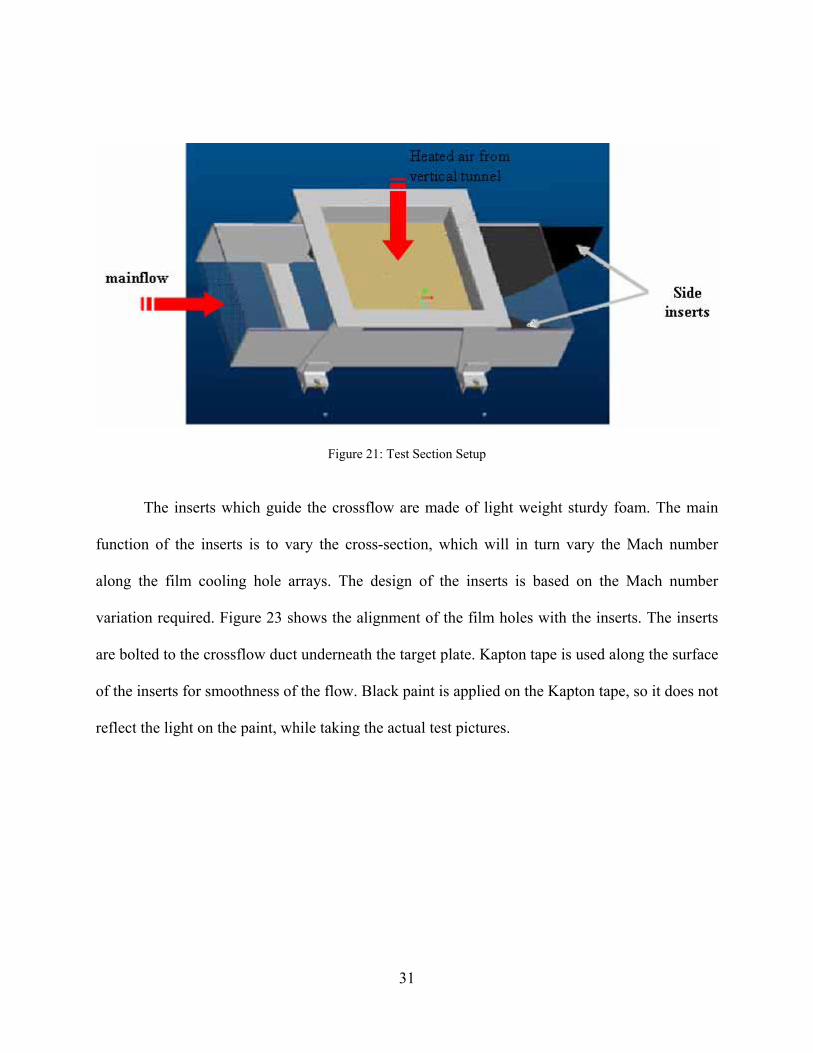
Figure 21: Test Section Setup
The inserts which guide the crossflow are made of light weight sturdy foam. The main
function of the inserts is to vary the cross-section, which will in turn vary the Mach number
along the film cooling hole arrays. The design of the inserts is based on the Mach number
variation required. Figure 23 shows the alignment of the film holes with the inserts. The inserts
are bolted to the crossflow duct underneath the target plate. Kapton tape is used along the surface
of the inserts for smoothness of the flow. Black paint is applied on the Kapton tape, so it does not
reflect the light on the paint, while taking the actual test pictures.

32
Figure 22: Test Coupon

33
Figure 23: Alignment of inserts with film hole exits
Temperature Sensitive Paint
Uni-coat Temperature Sensitive Paint, TSP, formulated by ISSI, is used in this study. The
effective temperature range is 0-100 ºC, beyond which the temperature sensitivity of TSP
becomes weaker. It is packaged in aerosol cans and can be applied easily with a spray. After it is
heat treated above 100 ºC for 30 minutes the temperature sensitivity of the paint is about 0.93ºC,
[28]. The TSP painted surface is smooth. The emission spectrum of TSP is shown in Figure 24.
An optical 590-nm long pass filter is also used on the camera to separate the excitation light and
emission light from the paint.

34
Figure 24: Emission spectrum of TSP (Liu, 2006)
TSP incorporates luminescent molecules in paint together with a transparent polymer
binder. Light of the proper wavelength is directed at the painted model to excite the luminescent
molecules. The sensor molecules become excited electronically to an elevated energy state. The
molecules undergo transition back to the ground state by several mechanisms, predominantly
radiative decay (luminescence). Sensor molecules emit luminescent light of a longer wavelength
than that of the excitation light. The appropriate filters can separate excitation light and
luminescent emission light, and the intensity of the luminescent light can be determined using a
photodetector. The excited energy state can also be deactivated by quenching processes. Through
two important photo-physical processes known as thermal- and oxygen-quenching, the
luminescent intensity of the paint emission is inversely proportional to local temperature. In
principle, a full spatial distribution of the surface temperature can be obtained by using the TSP
technique.

35
Figure 25: Typical TSP setup and instrumentation (Liu, 2006)
A high resolution 14-bit CCD (Charged Couple Device) camera was utilized for this
study. It is a PCO-1600 CCD camera, depicted in Figure 26, provided by the Cooke Corporation
with spatial resolution of 1200 by 1600 pixels. The image data is transferred via an IEEE 1394
(“firewire”) cable and firewire PCI card to a data collection PC. “CamWare” software provided
by Cooke Corp. is used in the Windows operating system to control initialization, exposure time
and image acquisition. The acquired image data are processed using MATLAB. The camera is
thermo-electrically cooled and has a high quantum efficiency at the paint emission wavelengths.
The choice and quality of the scientific-grade camera dictate the measurement accuracy.
LED-based illumination source (peak wavelength at 464 nm) was selected as the
excitation light for the TSP. The stability of the light source provided by ISSI is within 1% after
10 minute warm up. The CCD camera and excitation spectrum of LED is shown in Figure 26.

36
Figure 26: CCD camera and light source
Figure 27: Spectrum of LED source (Liu, 2006)

37
Computational Methodology
Computational Fluid Dynamics (CFD) plays an important role in the design of engine
components. In this study a comprehensive methodology was established and implemented to
consistently and more accurately predict film-cooling behavior. The common traits shared by all
computations documented in this work are described in detail in this section that follow; the
simulation specifics are documented in the appropriate sections.
Computational Model
In any computational simulation the accuracy of the results will depend strongly on the
application of a model to the problem at hand. The computational models match the
experimental test cases. Special attention is paid to the film hole region; due to the highly
complex recalculating nature of this area.
Due to the height of the wind tunnel used in these experiments, a symmetry condition
was applied at the top of the domain. A pressure profile was applied and it was adjusted
accordingly to match the boundary layer thickness at the location of the inlet plane. The velocity
was measured from experimental results and then it was used to estimate the inlet pressure
profile shown in Figure 29. A FORTRAN subroutine was then written to read this profile into
FLUENT and impose it as a boundary condition. An outlet pressure boundary condition was
applied far downstream from the jet injection site. At the plenum inlet, mass flow inlet
conditions were imposed.

38
Pressure Outlet • Static Pressure at the
exit
Pressure Inlet • from measured Velocity
and Turbulence )
Mass Flow Rate • Nitrogen modeled as “Air”
Symmetry Planes
Figure 28: Computational Domain and Boundary Conditions Type (Configuration 0-a)
0
5
10
15
20
25
30
101500 102000 102500 103000
Total Pressure (Pa)
y/D
Figure 29: Inlet Total Pressure Profile

39
Grid and Mesh Generation
A multi-block numerical grid was used in all cases to create a structured mesh. The grid
was created in Gambit from Fluent, Inc. The cells in the near-wall layers were stretched away
from the surfaces, and the first mesh point above the endwall was chosen such that the average is
of the order of unity. High cell concentration was placed where large flow/or temperature
gradients are expected.
After the grid generation phase is complete, the mesh is imported into FLUENT. The
flow is initialized according to the boundary conditions obtained from the experimental
conditions. Grid independence is established by increasing the number of cells in the grid and
performing test simulations until a negligible change in all field and surface results is
accomplished. For some cases, the maximum grid density was limited by the capabilities of the
computational resources.
Solution and Discretization
The solution of the computational domain is performed using FLUENT software package
from Fluent, Inc. The use of second order schemes were used in this study to provide the highest
accuracy available. Multigrid was used to decrease the CPU time required for each simulation.
The multigrid procedure solves the domain on varying levels of grid density smaller than the
original grid, thereby allowing information to propagate over the domain more quickly.
40
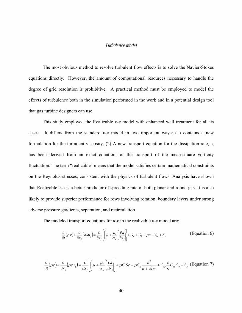
Turbulence Model
The most obvious method to resolve turbulent flow effects is to solve the Navier-Stokes
equations directly. However, the amount of computational resources necessary to handle the
degree of grid resolution is prohibitive. A practical method must be employed to model the
effects of turbulence both in the simulation performed in the work and in a potential design tool
that gas turbine designers can use.
This study employed the Realizable κ-ε model with enhanced wall treatment for all its
cases. It differs from the standard κ-ε model in two important ways: (1) contains a new
formulation for the turbulent viscosity. (2) A new transport equation for the dissipation rate, ε,
has been derived from an exact equation for the transport of the mean-square vorticity
fluctuation. The term “realizable" means that the model satisfies certain mathematical constraints
on the Reynolds stresses, consistent with the physics of turbulent flows. Analysis have shown
that Realizable κ-ε is a better predictor of spreading rate of both planar and round jets. It is also
likely to provide superior performance for rows involving rotation, boundary layers under strong
adverse pressure gradients, separation, and recirculation.
The modeled transport equations for κ-ε in the realizable κ-ε model are:
( ) ( ) κκκ
ρεκσµµρκρκ SYGG
xxu
xt Mbj
t
jj
j
+−−++⎥⎥⎦
⎤
⎢⎢⎣
⎡
∂∂
⎟⎟⎠
⎞⎜⎜⎝
⎛+
∂∂
=∂∂
+∂∂ (Equation 6)
( ) ( ) εεεκ κ
ευεκ
ερερεσµµρερε SGCCCSC
xxu
xt bj
t
jj
j
+++
−+⎥⎥⎦
⎤
⎢⎢⎣
⎡
∂∂
⎟⎟⎠
⎞⎜⎜⎝
⎛+
∂∂
=∂∂
+∂∂
31
2
21 (Equation 7)

41
where,
⎥⎦
⎤⎢⎣
⎡+
=5
,43.0max1 ηηC (Equation 8)
εκη S= (Equation 9)
ijih SSS 2= (Equation 10)
The coefficients were set as default by the software.
Near-Wall Treatments
Turbulent flows are significantly affected by the presence of walls. Obviously, the mean
velocity field is affected through the no-slip condition that has to be satisfied at the wall.
However, the turbulence is also changed by the presence of the wall in non-trivial ways. Very
close to the wall, viscous damping reduces the tangential velocity fluctuations, while kinematic
blocking reduces the normal fluctuations. Toward the outer part of the near wall region,
however, the turbulence is rapidly augmented by the production of turbulence kinetic energy due
to the large gradients in mean velocity.
The near-wall modeling significantly impacts the fidelity of numerical solutions, in as
much as walls are the main source of mean vorticity and turbulence. Therefore, accurate
representation of the flow in the near-wall region determines successful predictions of wall-
bounded turbulent flows.
Enhanced wall treatment is a near-wall modeling method that combines a two-layer
model with enhanced wall functions. If the near-wall mesh is fine enough to be able to resolve

42
the laminar sublayer (typically y+ ≈1), then the enhanced wall treatment will be identical to the
traditional two-layer zonal model (see below for details). However, the restriction that the near-
wall mesh must be sufficiently fine everywhere might impose too large a computational
requirement. Ideally, then, one would like to have a near-wall formulation that can be used with
coarse meshes (usually referred to as wall-function meshes) as well as fine meshes (low-
Reynolds-number meshes). In addition, excessive error should not be incurred for intermediate
meshes that are too fine for the near-wall cell centroid to lie in the fully turbulent region, but also
too coarse to properly resolve the sublayer.
To have a method that can extend its applicability throughout the near-wall region (i.e.,
laminar sublayer, buffer region, and fully-turbulent outer region) it is necessary to formulate the
law-of-the wall as a single wall law for the entire wall region. This is achieved by blending linear
(laminar) and logarithmic (turbulent) laws-of-the-wall. This approach allows the fully turbulent
law to be easily modified and extended to take into account other effects such as pressure
gradients or variable properties. The first layer of cells must have a cell center with falls in the
region measured by the y+, where y+ is defined as:
µ
ρ τ yuy =+ (Equation 11)
Building a grid to meet y+ requirements leads to some serious implications in reaching
grid independence and maintaining high quality grid. Near-wall approach is adequate for these
cases were the low Reynolds number effect is pervasive in the flow domain. All cases required a
near wall treatment that is valid in the viscosity-affected region and accordingly integrable all the
way to the wall.

43
Grid Independence
A grid independence check was carried out to determine the proper mesh size. The test
was carried out on the baseline case for that consisted of one cylindrical holes. The centerline
temperature was evaluated to determine if independence was achieved. Grid independence is
achieved when temperature variations from one grid size to another was minimal. For some
cases, the maximum grid density was limited by the capabilities of the computational resources.
250
300
350
400
0 10 20 30 40 50 60 70
x/D
T (K
)
620,570 cells
726,450 cells
898,720 cells
Figure 30: Grid Independence Check
Convergence
Convergence was determined with the following strict criteria: (1) Reduction of all
residuals of at least 4 orders of magnitude (2) Global mass and energy imbalance below 0.01%
and (3) Flow field and endwall surface temperature invariant with additional iterations.

44
Data Reduction of Experimental Data
Discharge Coefficient
In a orifice or other constriction, the ratio of the mass flow rate at the discharge end of the
orifice to that of an ideal orifice which expands an identical working fluid from the same initial
conditions to the same exit pressure is also known as discharge coefficient. In other words, the
discharge coefficient compares the amount of flow passing through an orifice to the theoretical
flow, based on the compressible flow equations for a specific area. The discharge coefficient
depends on the geometry of the constriction and flow conditions.
The amount of mass flow through the coupon at increasing pressure ratios was measured.
The tunnel has warmed up, the pressure in the plenum is increased at very small intervals and the
mass flow rate is taken for each pressure. For this test, the secondary flow supply was air.
Coolant temperature, static pressure and mainstream temperature are the main data taken for this
test. The tests were performed without the airfoil, wake plate or side inserts. Once the highest
pressure has been recorded, the tunnel can be stopped. Pressure and mass flow rate biases are
averaged between the beginning of the test and the end.
In the BFC rig, the discharge coefficient can be directly calculated using the following
equation:
⎥⎥⎥
⎦
⎤
⎢⎢⎢
⎣
⎡−⎟⎟
⎠
⎞⎜⎜⎝
⎛⋅
⋅−⋅
⎟⎟⎠
⎞⎜⎜⎝
⎛⋅⋅⋅
=−
⋅−
•
111
24
12
1
2k
k
stat
c
c
kk
c
statc
D
PP
TRkk
PP
PD
Nm
C
π
(Equation 12)

45
During these tests, the measured variables were: the volumetric flow rate, which was then
multiplied by the density to yield the mass flow rate, ma; Tc, the temperature of the coolant inside
the plenum; Pc the static pressure of the coolant inside the plenum; and Pstat, the main flow static
pressure, at the test section. Since the crossection of the test section is rectangular, no additional
pressure measurements of the mainstream were necessary. The remaining terms, N, κ, R, and D
were know constants, or obtained from tables.
On the other hand, in the IFC tunnel the pressure distribution along the inserts was
calculated by using the Mach number values, based on the area at the crossection of each hole
exit rows. Pressure distribution is then obtained by:
12
211
−−
⎟⎠⎞
⎜⎝⎛ ⋅
−+=
γγ
γ MPP
t
(Equation 13)
where P is the pressure, t indicates total conditions, γ is the specific heat ratio and M is the Mach
number.
Figure 31: Mach number distribution along the film hole rows

46
Using this pressure distribution along the inserts and using Bernoulli’s equations, the average
velocity at the exit of each row of holes were calculated.
consthgVP =⋅⋅+⋅⋅+ ρρ 2
21 (Equation 14)
Neglecting h and solving for velocity gives,
( )
ρ122 PPV −⋅
= (Equation 15)
The calculated velocity was then used to calculate the theoretical mass flow rate by:
hh NVAm ⋅⋅⋅=∗
ρ (Equation 16)
where Ah and Nh indicates the crossectional area of the hole and number of holes.
Actual mass flow rate is obtained from the mass flow rate reading and CD is calculated
by the ratio of the actual mass flow rate to the theoretical value.
•
•
=th
aD
m
mC (Equation 17)
Blowing Ratio and Momentum Flux
The blowing ratio, also called the mass flux ratio, is a dimensionless number used in film
cooling to quantify the ratio of the mass flow rate per unit area of the coolant to that of the
mainstream.

47
( )
( ) mm
cc
m
m
c
c
m
c
VV
AAV
AAV
Am
Am
M⋅⋅
=⋅⋅
⋅⋅
=
⎟⎟⎟
⎠
⎞
⎜⎜⎜
⎝
⎛
⎟⎟⎟
⎠
⎞
⎜⎜⎜
⎝
⎛
=•
•
ρρ
ρ
ρ
(Equation 18)
Given that,
hchc NVAcm ⋅⋅⋅=∗
ρ (Equation 19)
The blowing ratio can also be expressed as,
mm
hh
c
VNA
m
M⋅⋅
=⋅
•
ρ (Equation 20)
Another parameter that is often used is the momentum flux ratio. The momentum flux, I,
compares the kinetic energy of the coolant (per volume) versus that of the mainstream. The
momentum flux ratio is defined as:
( )( )mm
cc
VV
I 2
2
⋅⋅
=ρρ
(Equation 21)
Since the density ratio, DR, is kept nearly the momentum flux ratio can also be obtained by:
DRMI
2
= (Equation 22)
Film Cooling Effectiveness
Film cooling effectiveness (η) measurement is the main parameter used for comparison in
this study. As mentioned in Chapter 1 effectiveness is defined as:

48
cr
awr
TTTT
−−
=η (Equation 23)
However, obtaining the final plots of η requires a significant amount of data reduction. During
the test, three parameters are recorded: Tc – the coolant temperature, Taw – the adiabatic wall
temperature distribution downstream of the cooling holes, and Tr – the recovery temperature of
the test section. To analyze the TSP pictures, matrix handling software such as MATLAB is
used. The images are read into a matrix containing the intensity information over every pixel of
the TSP.
Figure 32: Normal image of TSP
Figure 32 shows an image of the TSP downstream of the coolant holes. This image was
taken under non-test conditions, without any LED lighting, and is used mainly for locating the
holes with respect to the edges of the paint layer. The coolant holes are very difficult to see under
testing conditions because they reflect back very little light. Figure 33 shows the same image, but
this time under LED lighting. If the TSP is at room conditions, and testing is ready to begin, then
this image becomes the reference image, and the intensity from any pixel becomes I(TR). The

49
LED light is kept on throughout the duration of the test. Neither the camera nor the LED light
may be moved, or the usage of the reference image will not be valid due to changes in lighting
conditions. Precautions must be taken to ensure that the data will not be polluted due to outside
lighting condition changes. For all tests and blowing ratios, images are taken in sets of four,
which are then averaged to filter out any fluctuations. For the reference image, the temperature
must be uniform, and known. Typical reference temperatures are around 25 ºC, or room
temperature.
Figure 33: Reference Image
The tunnel is allowed to warm up for over four hours. At that point another set of pictures
is picture is taken, named BR0, referring to zero blowing ratio. To obtain a flow image, first the
plenum must be kept at a constant pressure and temperature for approximately 8-10 minutes to
achieve the desired blowing ratio, and thus film cooling conditions over the paint. Once these
conditions are met, the set of images can be taken. Figure 34 shows TSP under cooling
conditions.

50
Figure 34: Image of TSP showing coolant flow
The process of taking images continues until all the blowing ratios are taken. Once this
has occurred, the testing ends and the images can be processed. Temperature is obtained as
follows: the ratio of emission intensity I(T) at any temperature T to the emission intensity I(TR)
at an unspecified reference temperature TR is,
( )( ) ),( R
R
TTfnTITIIR == (Equation 24)
Local ratios are then converted into temperature values. This is accomplished with the use of the
calibration curve of the paint. Figure 35 shows a typical calibration curve for TSP.
Figure 35: TSP Calibration Curve

51
The manipulation is done with software on a per-pixel level. Once the processing is done,
the intensity information yields temperatures. This is how the recovery temperature and the
adiabatic wall temperature distributions are obtained.
Figure 36: Raw Temperature image from TSP
The area captured by the CCD camera is significant in size, and does not provide the
resolution to calculate centerline effectiveness. Instead average effectiveness is calculated. To
calculate the span-wise-averaged cooling effectiveness, several physical factors are considered
such as edge effects, the number of cooling holes and the diameter of the holes. To discount edge
effects from influencing the temperature data, only holes close to the middle of the coupon center
are included in the averaging step.
The intensity data is reduced to pixel temperature data and local film cooling
effectiveness is calculated over the TSP surface. The data is then averaged in the spanwise
direction yielding an effectiveness distribution along the streamwise direction. The result of this
process is shown in Figure 37.

52
Figure 37: Results of averaging effectiveness
Uncertainty Analysis
The uncertainties reported were estimated following the procedure described by Kline
and McClintock (1953). The effectiveness as defined in the equation below is used to find the
derivatives in the uncertainty equation:
222
⎟⎟⎠
⎞⎜⎜⎝
⎛⋅⋅+⎟⎟
⎠
⎞⎜⎜⎝
⎛⋅+⎟⎟
⎠
⎞⎜⎜⎝
⎛⋅=
awrc Taw
Tr
Tc
n UdT
dUdTdU
dTdU ηηη (Equation 25)
In this case UTr and UTaw, the uncertainties in the recovery and adiabatic wall
temperatures are equal since both are obtained with TSP, which was calibrated with a
thermocouple. UTc is 1.0ºC, which is the uncertainty in the coolant temperature, as measured
with the plenum thermocouple set up. The values of Uη are evaluated at every point on the
effectiveness curve, and give the uncertainty band shown in Figure 38.

53
Figure 38: Uncertainty distribution for film cooling effectiveness [29]
The uncertainty in the discharge coefficient has been calculated similarly:
22
222
⎟⎟⎠
⎞⎜⎜⎝
⎛⋅+⎟
⎟⎠
⎞⎜⎜⎝
⎛⋅+
⎟⎟⎠
⎞⎜⎜⎝
⎛⋅+⎟⎟
⎠
⎞⎜⎜⎝
⎛⋅+⎟
⎠
⎞⎜⎝
⎛ ⋅
=
DDavg
tDavg
pDc
pDstat
mD
Dc
UCdD
dUC
dTd
UCdPd
UCdP
dUC
dmd
U (Equation 26)
This equation yields results that suggest the uncertainty at the lower pressure ratios is larger than
the uncertainty at the higher pressure ratios.
Figure 39: Uncertainty in CD measurement [29]

54
Considering both rigs, it can be summarized that the uncertainties of the measurements in
the present study are as follow: (1) Precision interval of TSP is found to be ±0.93°C with 95%
level of confidence [28] (2) The uncertainty in the effectiveness values was on an average less
than 3%, while the highest value was calculated to be less than 9%. (3) Uncertainty of CD values
ranges in the order of ± 9%, and ± 1% at the higher pressure ratios.
Data Reduction of Computational Data
Film Cooling Effectiveness
The average effectiveness was calculated using FLUENT predictions by exporting the
temperature data from the bottom adiabatic wall of the model. The data is the processed using a
code written in C++. The execution of the code consists of arranging the raw data by x, z and
corresponding temperature value. It then averages temperature and calculates average
effectiveness. A GUI (Graphical User Interface) was created to facilitate the process of the
simulation data. The process flowchart explains the details of the GUI and execution of the code.

55
Figure 40: FLUENT Local Temperature Data extracted for calculating effectiveness

56
Figure 41: Graphical User Interface to process Computational Data

57
Figure 42: Process flowchart of Data Reduction of Computational Data
Read input file and remove all negative x’s (x = 0 @ trailing edge of film holes)
Remove columns not needed (cellnumber, y-coordinate)
and reformat file to maintain digits of precision
List x’s and z’s unique values and
corresponding Temperature values.
Average temperature and calculate η
cr
wr
TTTT
−−
=η
CODE EXECUTION
DETAILS
Input file
Formatted file
Sorted data
Output data
Create input file by Outputting
temperature data from FLUENT
Initialize parameters (D, Tp, Tr, digits
of precision of input and output file)
Check “Create Bounded Eta” and
select corresponding streamline case
Is the Airfoil present?
Browse for input
file “Set input file”
Click “Run”
(execute code)
GUI EXECUTION
DETAILS
YES
NO

58
CHAPTER 4: RESULTS
Baseline
The baseline case consists the test coupon of a single row of cylindrical holes inclined at
35° with a L/D = 7.5 and a PI/D = 3. The test was conducted as described in Chapter 3. This
section describes the experimental readings and computational details specific to this
configuration.
Experimental Details
During these tests, the measured variables were the Tc, the temperature of the coolant
inside the plenum; Pc the static pressure of the coolant inside the plenum to match target mass
flow rate based on discharge coefficient test; and Pstat, the main flow static pressure, at the test
section. Tests were carried out for four blowing ratios, M=0.5, 0.75, 1.0, and 1.5. The test
conditions are described in Table 2.
CFD Details
The numerical model consisted of 726,450 cells. The cell topology is hexahedral and y+
was close to unity. As illustrated in Figure 44 the side and top walls were defined as symmetry
plane where as a pressure boundary condition was prescribed at the inlet and outlet of
mainstream. On the plenum, a mass flow inlet was specified. The numerical simulation was

59
carried out for the lowest and highest blowing ratios (M=0.5 and 1.5). The values used as
boundary conditions matched the experimental measurements.
Table 2: Baseline Test Experimental Measurements
Parameter Mainstream Conditions
Plenum Conditions
P static (Pa) 101118 -
Temperature (K) 337 260 M = 0.5
Mass flow rate (average per hole) - 8.49 x 10⁻⁵
P static (Pa) 101118 -
Temperature (K) 337 255 M = 0.75
Mass flow rate (average per hole) - 1.22 x 10⁻⁴
P static (Pa) 101118 -
Temperature (K) 337 255 M = 1.0
Mass flow rate (average per hole) - 1.63 x 10⁻⁴
P static (Pa) 101118 -
Temperature (K) 337 256 M = 1.5
Mass flow rate (average per hole) - 2.45 x 10⁻⁴

60
Figure 43: Configuration 0-a CFD Grid
Pressure Outlet • Static Pressure at the
exit
Pressure Inlet • from measured Velocity
and Turbulence )
Mass Flow Rate • Nitrogen modeled as “Air”
Symmetry Planes
Figure 44: CFD Domain and Boundary Conditions Type for Configuration 0-a

61
Results and Discussion
Average film cooling effectiveness for the baseline configuration was compared against
existing literature. The present data is compared with the data of Sinha et al. [8] and Lutum [10]
for two different blowing ratios. Figure 45 and Figure 46 show that the presented experimental
results correlate well with the results presented in the literature validating the procedure followed
to acquire the data for the present study.
Figure 45: Data Comparison for M=0.5

62
Figure 46: Data Comparison for M=0.75
The experimental data was also compared to the numerical predictions. Researchers have
used different turbulence models to predict average film cooling effectiveness yielding different
results. As discussed in Chapter 2, it is very common to use RKE or SKW model for modeling
film cooling. At the beginning of this study it was unknown which of the two models could be
use for the analysis that could better predict average effectiveness, therefore, both models were
employed and the results showed that based on our experimental data RKE better predicts film
cooling effectiveness. Figure 47 shows the comparison of the two turbulence models and
experimental data for M = 0.5. Film cooling effectiveness predictions for RSW model are valid
for x/d ≤10 where as for RKE model the predictions are valid up to x/d ≤ 25. Using the RKE
model, for x/d=50 the difference between the numerical predictions and experimental
measurements could be as high as 27%. The error calculated using the SKW model is estimate

63
to be as high as 30% for the same x/d. The numerical predictions of film cooling effectiveness
were also compared against Lutum [10]and Sinha [8] experimental data. The comparison shows
that RKE is also a better predictor of film cooling effectiveness. Literature has shown that SKW
may over predict the diffusion of jets, which explains the high effectiveness value at higher x/d.
For this reason, the numerical simulation used RKE model as a turbulence model for predicting
film cooling effectiveness.
0.00
0.05
0.10
0.15
0.20
0.25
0.30
0.35
0.40
0 10 20 30 40 50
x/D
η avg
Exp, M=0.5, I = 0.198
RKE, M=0.5, I=0.189
SKW, M=0.5, I=0.189
Figure 47: Comparison of Turbulence Models against Experimental Data

64
0.00
0.05
0.10
0.15
0.20
0.25
0.30
0.35
0.40
0 10 20 30 40 50
x/D
η avg
Exp, M=0.5, I = 0.198RKE, M=0.5, I=0.189SKW, M=0.5, I=0.189(Lutum L/D=3.5) M=0.52, I=0.24(Lutum L/D=7) M=0.5, I=0.24(Sinha L/D=1.75) M = 0.5, I = 0.208(Lutum L/D=1.75) M=.52, I=.208
Figure 48: Validation of Configuration 0-a
Figure 49 through Figure 51 shows average effectiveness for varying blowing ratio and
local effectiveness distribution for Configuration 0-a. The results show that for low blowing
ratio higher effectiveness occurs close to the injection point. For high blowing ratio
effectiveness decreases due to jet lift off. Jet to jet interaction is promoted as a result of an
increase of the blowing ratio. The interaction of the jet with the nearby jets and mainstream
enhances mixing resulting in a slight increase in effectiveness.

65
0.00
0.05
0.10
0.15
0.20
0.25
0.30
0 5 10 15 20 25 30 35 40 45 50
x/d
Effe
ctiv
enes
ess
M=0.5M=0.75M=1.0M=1.5
RKE, M = 0.5RKE, M = 1.5
Figure 49: Average Effectiveness for Configuration 0-a
M=0.5 M=0.75 M=1.5 M=1.0
Figure 50: Local Temperature Distribution for Configuration 0-a
Figure 51: Local Temperature Distribution for Configuration 0-a (Exp vs. CFD) M=0.5 M=1.5

66
The computational results agree with the experimental data. Streamline case shows that
for low blowing ratios, the jet remains close to the surface. The opposite is observed with the
higher blowing ratio case. Figure 53 shows the detachment of the flow as it enters the
mainstream. The flow later reattaches resulting in an increase in the average film effectiveness.
Sinha et al. [8] observed that the laterally averaged effectiveness is strongly dependent on
the lateral spreading of the cooling jet which increases laterally average effectiveness. Similarly,
Eriksen and Goldstein [6] observed that higher blowing ratios promote the interaction of the jets
with the adjacent jets and with the mainstream flow resulting in a higher effectiveness farther
downstream of the injection point. These findings are consistent with the results of the present
study. Higher effectiveness promotes jet interaction resulting in higher effectiveness when
reattachment of the jet occurs.
Figure 52: Streamline Plot for Configuration 0-a (M=0.5)

67
Figure 53: Streamline Plot for Configuration 0-a (M=1.5)
Stagnation Region Effects
A study on film cooling effectiveness was then carried out to understand the effect of the
closeness of the stagnation region of an airfoil. The configurations considered in this section are
configurations I-a, II-a and II-a. An axisymmetric airfoil is placed downstream of the injection
point and temperature distribution was obtained for various blowing ratios. This section
describes the experimental readings and computational details specific to these configurations.

68
I-a II-a III-a
Figure 54: Test Configurations for study on stagnation region effects
Table 3: Test Configurations for study on stagnation region effects
Nomenclature Distance from Airfoil to LE (x/d)
Distance from Wake Plate to LE
(x/d)
1-a 6.4 -
1I-a 12.7 -
1II-a 25.4 -
Experimental Details
During these tests, the measured variables were the Tc, the temperature of the coolant
inside the plenum; Pc the static pressure of the coolant inside the plenum; and Pstat, the main flow
static pressure, at the test section. Tests were carried out for four blowing ratios, M=0.5, 0.75,
1.0, and 1.5. The test conditions are listed in Tables 4-6.

69
Table 4: Experimental Measurements for Configuration I-a
Parameter Mainstream Conditions Plenum Conditions
P static (Pa) 101118 -
Temperature (K) 337 258 M = 0.5
Static Plenum Pressure (Pa) - 101338
P static (Pa) 101118 -
Temperature (K) 337 255 M = 0.75
Static Plenum Pressure (Pa) - 102069
P static (Pa) 101118 -
Temperature (K) 337 258 M = 1.0
Static Plenum Pressure (Pa) - 103241
P static (Pa) 101118 -
Temperature (K) 337 257 M = 1.5
Static Plenum Pressure (Pa) - 105448

70
Table 5: Experimental Measurements for Configuration II-a
Parameter Mainstream Conditions Plenum Conditions
P static (Pa) 101118 -
Temperature (K) 338 255 M = 0.5
Static Plenum Pressure (Pa) - 101345
P static (Pa) 101118 -
Temperature (K) 338 261 M = 0.75
Static Plenum Pressure (Pa) - 102090
P static (Pa) 101118 -
Temperature (K) 338 255 M = 1.0
Static Plenum Pressure (Pa) - 103234
P static (Pa) 101118 -
Temperature (K) 338 257 M = 1.5
Static Plenum Pressure (Pa) - 105441
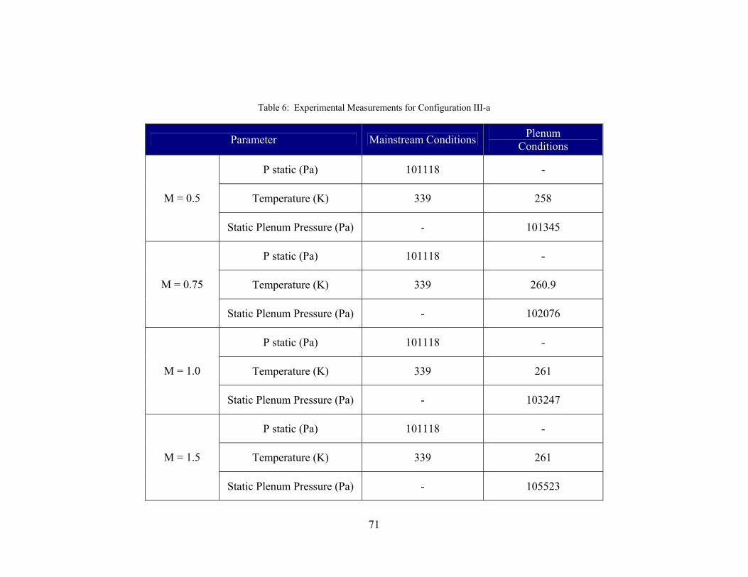
71
Table 6: Experimental Measurements for Configuration III-a
Parameter Mainstream Conditions Plenum Conditions
P static (Pa) 101118 -
Temperature (K) 339 258 M = 0.5
Static Plenum Pressure (Pa) - 101345
P static (Pa) 101118 -
Temperature (K) 339 260.9 M = 0.75
Static Plenum Pressure (Pa) - 102076
P static (Pa) 101118 -
Temperature (K) 339 261 M = 1.0
Static Plenum Pressure (Pa) - 103247
P static (Pa) 101118 -
Temperature (K) 339 261 M = 1.5
Static Plenum Pressure (Pa) - 105523
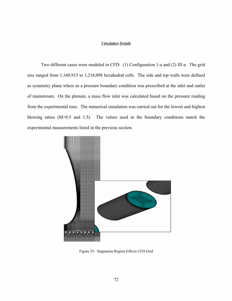
72
Simulation Details
Two different cases were modeled in CFD: (1) Configuration 1-a and (2) III-a. The grid
size ranged from 1,160,915 to 1,218,098 hexahedral cells. The side and top walls were defined
as symmetry plane where as a pressure boundary condition was prescribed at the inlet and outlet
of mainstream. On the plenum, a mass flow inlet was calculated based on the pressure reading
from the experimental runs. The numerical simulation was carried out for the lowest and highest
blowing ratios (M=0.5 and 1.5). The values used in the boundary conditions match the
experimental measurements listed in the previous section.
Figure 55: Stagnation Region Effects CFD Grid

73
Mass Flow Rate • Nitrogen modeled as “Air”
Pressure Outlet • Static Pressure at the exit
Symmetry Planes Pressure Inlet • from measured Velocity
and Turbulence )
Figure 56: CFD Domain and Boundary Conditions Type for Configuration I and III-a
Results and Discussion
The stagnation gradient created by the blockage presented by the leading edge of the
airfoil causes the flow to undergo three-dimensional separation. A detailed study on film
cooling effectiveness was then carried out to understand the effect of the stagnation gradient and
closeness of the stagnation region of an airfoil. Figure 57 through Figure 62 show effectiveness
measurements obtained for configuration I-a, II-a, III-a. The data shows that for low blowing
ratios effectiveness is higher specifically in the region close to the injection point. On the
contrary, higher effectiveness is observed at larger x/D.
At lower blowing ratios, jet spreading is minimal, making it necessary to implement
alternative means of endwall cooling in the region adjacent to the airfoil. The jet to jet
interaction is small and hence there is no spreading of the jet. This jet spreading is more evident

74
as the blowing ratio is increased. The local effectiveness results shown on Figures 58, 60, and 62
indicate that the lateral spreading of the jets as the blowing ratio is increased.
The stagnation gradient created by the blockage presented by the leading edge of the
airfoil causes the flow to undergo three-dimensional separation. The effect caused by the
stagnation region not only impacts effectiveness but film coverage. The results also reveal that
the area coverage significantly varies with the blowing ratio. This trend was observed for all
configurations.
Figure 57: Average Film Cooling Effectiveness for Configuration I-a
Figure 58: Local Film Cooling Effectiveness for Configuration I-a (Exp. vs. CFD)
0.00
0.05
0.10
0.15
0.20
0.25
0.30
0.35
0.40
0.45
0.50
0 10 20 30 40 50x/d
Effe
ctiv
enes
s
M = 0.5
M = 0.75
M = 1.0
M = 1.5
RKE, M = 0.5
RKE, M = 1.5
M = 0.5 M=1.5
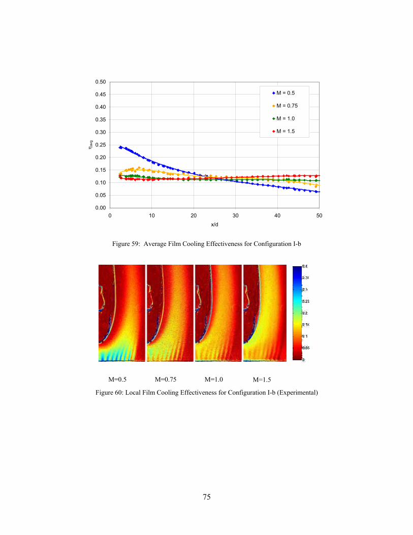
75
0.00
0.05
0.10
0.15
0.20
0.25
0.30
0.35
0.40
0.45
0.50
0 10 20 30 40 50x/d
η avg
M = 0.5
M = 0.75
M = 1.0
M = 1.5
Figure 59: Average Film Cooling Effectiveness for Configuration I-b
Figure 60: Local Film Cooling Effectiveness for Configuration I-b (Experimental)
M=0.5 M=0.75 M=1.0 M=1.5

76
0.00
0.05
0.10
0.15
0.20
0.25
0.30
0.35
0.40
0.45
0.50
0 10 20 30 40 50
x/d
η avg
M = 0.5
M = 0.75
M = 1.0
M = 1.5
RKE, M = 0.5
RKE, M = 1.5
Figure 61: Average Film Cooling Effectiveness for Configuration I-c
Figure 62: Local Film Cooling Effectiveness for Configuration I-c (Exp. vs. CFD)
M = 0.5 M = 1.5

77
0
0.05
0.1
0.15
0.2
0.25
0.3
0.35
0.4
0 5 10 15 20 25 30 35 40 45 50x/D
ηavg
0-a, M=0.5
0-a, M=1.5
I-a, M = 0.5
I-a, M = 1.5
I-c, M = 0.5
I-c, M = 1.5
Figure 63: Average Film Cooling Effectiveness (Configuration 0, I, and III-a)
Figure 64: Streamline Plot for Configuration I-a (M=0.5 and 1.5)
Figure 65: Streamline Plot for Configuration I-c (M=0.5 and 1.5)

78
From the streamline plots depicted in Figures 64 and 65 show that for M = 0.5 the film
remains close to the surface and flows around the airfoil. As the blowing ratio is increased, the
jet overcomes the mainstream effect and lifts off. This interaction with the mainstream increase
mixing in the region close to the stagnation point resulting in an increase in effectiveness. When
the airfoil is placed further downstream of the injection point (Configuration III-a) the coolant jet
does not face any interference flowing forward without having to be redirected. If the local
effectiveness pictures are observed, the leading edge of the airfoil is cooled better for higher
blowing ratios, this indicates that the momentum of the jet is able to overcome the pressure
gradient created by the presence of the airfoil. This is more evident in Figure 64 where the jet
streamlines are much closer to the airfoil for higher blowing ratios.
Wake Effects
The incoming flow characteristics have a direct effect on endwall film cooling
effectiveness. The wake generated by the adjoining walls of the transition pieces enhance
mixing of the jet with the mainstream. The cooling capability may quickly be lost preventing the
surfaces from being cooled adequately. To understand the effect of wake on film effectiveness,
a rectangular plate was placed upstream of the injection point. The distance was varied and
temperature distribution was obtained for various blowing ratios. This section describes the
experimental readings and computational details specific to these configurations.

79
0-b 0-c
Figure 66: Test Configurations for study on wake effects
Table 7: Test Matrix for BFC Tunnel
Nomenclature Distance from Airfoil to LE (x/d)
Distance from Wake Plate to LE
(x/d)
0-b - 12.7
0-c - 50.8
Experimental Details
Similarly to the other configurations, the measured variables were the Tc, the temperature
of the coolant inside the plenum; Pc the static pressure of the coolant inside the plenum; and Pstat,
the main flow static pressure, at the test section. Tests were carried out for four blowing ratios,
M=0.5, 0.75, 1.0, and 1.5. The test conditions are described in Tables 8 and 9.

80
Simulation Details
Two different cases were modeled in CFD: (1) Configuration 0-b and (2) 0-c. The grid
size ranged from 1,480,380 to 1,710,380 hexahedral cells. The side and top walls were defined
as symmetry plane where as a pressure boundary condition was prescribed at the inlet and outlet
of mainstream. On the plenum, a mass flow inlet was calculated based on the pressure reading
from the experimental runs. The numerical simulation was carried out for the lowest and highest
blowing ratios (M=0.5 and 1.5). The values used in the boundary conditions match the
experimental measurements listed in Tables 8 and 9.

81
Table 8: Experimental Measurements for Configuration 0-b
Parameter Mainstream Conditions
Plenum Conditions
P static (Pa) 101118 -
Temperature (K) 339 258 M = 0.5
Static Plenum Pressure (Pa) - 101344
P static (Pa) 101118 -
Temperature (K) 339 259 M = 0.75
Static Plenum Pressure (Pa) - 102009
P static (Pa) 101118 -
Temperature (K) 339 259 M = 1.0
Static Plenum Pressure (Pa) - 103096
P static (Pa) 101118 -
Temperature (K) 339 259 M = 1.5
Static Plenum Pressure (Pa) - 105078

82
Table 9: Experimental Measurements for Configuration 0-c
Parameter Mainstream Conditions
Plenum Conditions
P static (Pa) 101118 -
Temperature (K) 339 258 M = 0.5
Static Plenum Pressure (Pa) - 101346
P static (Pa) 101118 -
Temperature (K) 339 260 M = 0.75
Static Plenum Pressure (Pa) - 102019
P static (Pa) 101118 -
Temperature (K) 339 261 M = 1.0
Static Plenum Pressure (Pa) - 103098
P static (Pa) 101118 -
Temperature (K) 339 261 M = 1.5
Static Plenum Pressure (Pa) - 105083

83
Figure 67: Wake effects CFD grid
Figure 68: CFD Domain and Boundary Condition Type for Configurations 0-b and c
Mass Flow Rate • Nitrogen modeled as “Air”
Pressure Outlet • Static Pressure at the exit
Symmetry Planes
Pressure Inlet • from measured Velocity
and Turbulence )

84
Results and Discussion
In real engine conditions, endwall film cooling is also affected by the wake induced by
the adjacent walls of the transition pieces. Figures 69 and 70 plot average film cooling
effectiveness in the presence of wake for test configuration 0-b and 0-c. The presence of wake
promotes the mixing of the jet with the mainstream resulting in lower effectiveness. For the
cases where the wake plate is placed at x/D=-50.8 upstream of the injection point, the average
effectiveness is higher at small x/D. These figures show that for low blowing ratio, the presence
of wake increases effectiveness for low x/D. On the contrary, at high x/D effectiveness is higher
for the highest blowing ratio.
0.00
0.05
0.10
0.15
0.20
0.25
0.30
0.35
0.40
0 10 20 30 40 50 60
X/D
M = 0.5
M = 0.75
M = 1.0
M = 1.5
RKE, M=0.5
RKE, M=1.5
Figure 69: Average film cooling effectiveness for Configuration 0-b

85
0.00
0.05
0.10
0.15
0.20
0.25
0.30
0.35
0.40
0 10 20 30 40 50 60
X/D
h
M = 0.5
M = 0.75
M = 1.0
M = 1.5
RKE, M=0.5
RKE, M=1.5
Figure 70: Average film cooling effectiveness for Configuration 0-c
M = 0.5 M = 1.5
Figure 71: Local Film Cooling Effectiveness for Configuration 0-b (M=0.5 and 1.5)
Figure 72: Average Film Effectiveness for Configurations 0-c (M=0.5 and 1.5)
M=0.5 M=1.5

86
As shown in Figures 74 and 75 the numerical simulation aid in the understanding of the
vortex formation physics caused by the induced wake. The velocity deficit created by the wake
forms a pair of vortices offset from the wake centerline. These vortices lift the jet off the wall
promoting the interaction of the jet with the mainstream resulting in a lower effectiveness. The
jet interaction with the mainstream causes the jet to lose its cooling capabilities more rapidly
which leads to a more sudden decay in film effectiveness. Overall, an increase in the strength of
the wake results in a reduction of film effectiveness due to the interaction of the jet with the
mainstream flow. The simulation also shows that the wake plate causes the flow to separate
forming a recirculation region at the trailing edge of the plate. This recirculation pulls some of
the jet flow in the reverse direction. This means that a fraction of the flow is not utilized for the
purpose of cooling the region downstream of the injection point as it is intended by design.
(a) x/D=10 (b) x/D=20 (c) x/D=30
Figure 73: CFD Vector plot for varying x/D – Wake plate

87
Figure 74: Streamline plots for Configuration 0-b
Figure 75: Streamline plots for Configuration 0-c
Stagnation Region and Wake effects
Under real engine conditions, the effectiveness of the film has to be evaluated in the
presence of both the wake and pressure gradient effects. This section presents the results of the
study of combined effect of wake and stagnation region on film cooling effectiveness.
Experimental and computational results are presented herein.

88
I-b II-b III-b I-c II-c III-c
Figure 76: Test Configurations for study on stagnation region and wake effects
Table 10: Test Matrix for BFC Tunnel
Nomenclature Distance from Airfoil to LE (x/d)
Distance from Wake Plate to LE
(x/d) 1-b 6.4 12.7
1I-b 12.7 12.7
1II-b 25.4 12.7
1-c 6.4 50.8
1I-c 12.7 50.8
1II-c 25.4 50.8
Experimental Details
For configurations I-III-b and c, the measured variables were the Tc, the temperature of
the coolant inside the plenum; Pc the static pressure of the coolant inside the plenum; and Pstat,
the main flow static pressure, at the test section. Tests were carried out for four blowing ratios,
M=0.5, 0.75, 1.0, and 1.5. The test conditions were as followed:

89
Table 11: Experimental Measurements for Configuration I-b
Parameter Mainstream Conditions
Plenum Conditions
P static (Pa) 101118 -
Temperature (K) 339 257 M = 0.5
Static Plenum Pressure (Pa) - 101329
P static (Pa) 101118 -
Temperature (K) 339 255 M = 0.75
Static Plenum Pressure (Pa) - 102113
P static (Pa) 101118 -
Temperature (K) 339 260 M = 1.0
Static Plenum Pressure (Pa) - 103251
P static (Pa) 101118 -
Temperature (K) 339 256 M = 1.5
Static Plenum Pressure (Pa) - 105457

90
Table 12: Experimental Measurements for Configuration III-b
Parameter Mainstream Conditions
Plenum Conditions
P static (Pa) 101118 -
Temperature (K) 339 258 M = 0.5
Static Plenum Pressure (Pa) - 101332
P static (Pa) 101118 -
Temperature (K) 339 259 M = 0.75
Static Plenum Pressure (Pa) - 102058
P static (Pa) 101118 -
Temperature (K) 339 259 M = 1.0
Static Plenum Pressure (Pa) - 103073
P static (Pa) 101118 -
Temperature (K) 339 258 M = 1.5
Static Plenum Pressure (Pa) - 105104
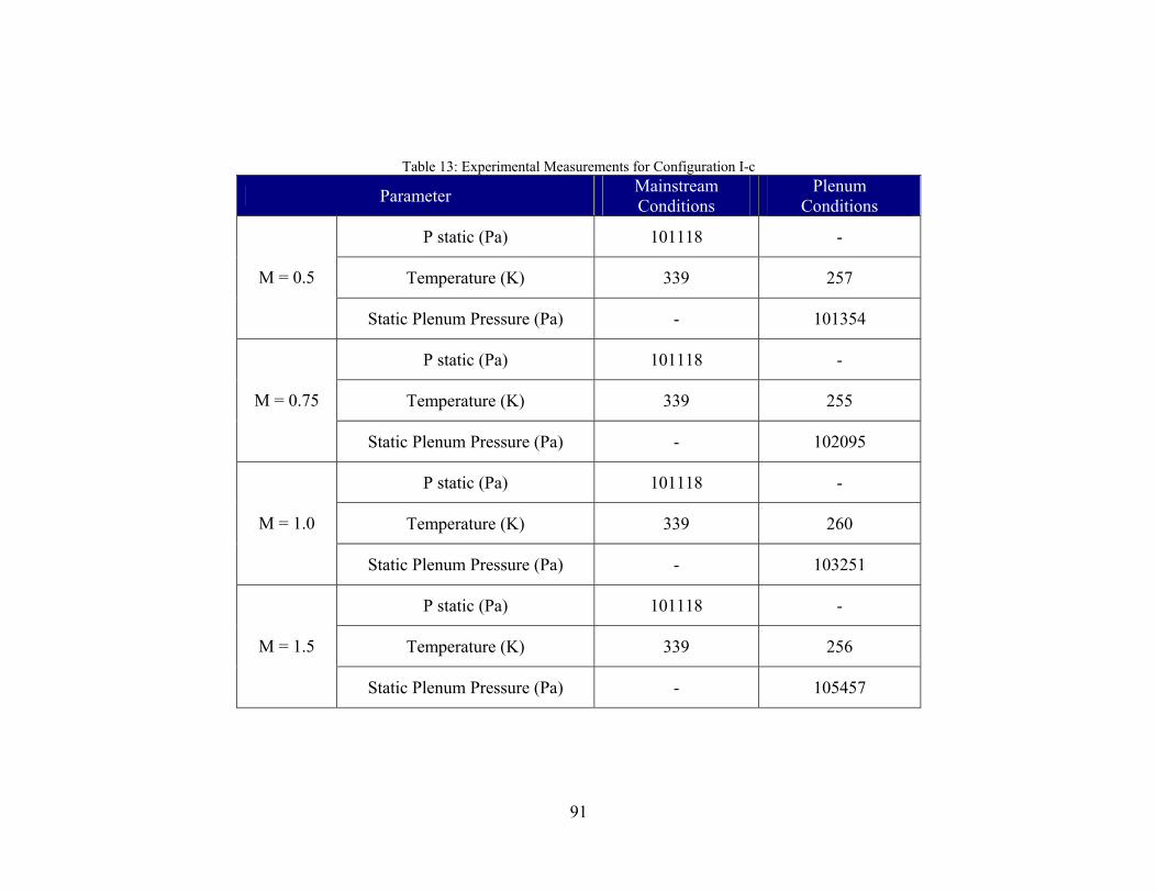
91
Table 13: Experimental Measurements for Configuration I-c
Parameter Mainstream Conditions
Plenum Conditions
P static (Pa) 101118 -
Temperature (K) 339 257 M = 0.5
Static Plenum Pressure (Pa) - 101354
P static (Pa) 101118 -
Temperature (K) 339 255 M = 0.75
Static Plenum Pressure (Pa) - 102095
P static (Pa) 101118 -
Temperature (K) 339 260 M = 1.0
Static Plenum Pressure (Pa) - 103251
P static (Pa) 101118 -
Temperature (K) 339 256 M = 1.5
Static Plenum Pressure (Pa) - 105457

92
Table 14: Experimental Measurements for Configuration III-c
Parameter Mainstream Conditions Plenum Conditions
P static (Pa) 101118 -
Temperature (K) 339 258 M = 0.5
Static Plenum Pressure (Pa) - 101347
P static (Pa) 101118 -
Temperature (K) 339 260.9 M = 0.75
Static Plenum Pressure (Pa) - 102078
P static (Pa) 101118 -
Temperature (K) 339 261 M = 1.0
Static Plenum Pressure (Pa) - 103247
P static (Pa) 101118 -
Temperature (K) 339 261 M = 1.5
Static Plenum Pressure (Pa) - 105523

93
Simulation Details
Configurations I-b, III-b, I-c and III-c were modeled. The fluid domains ranged from
1,351,265 to 1,513,265 hexahedral cells. The side and top walls were defined as symmetry plane
where as a pressure boundary condition was prescribed at the inlet and outlet of mainstream. On
the plenum, a mass flow inlet was calculated based on the pressure reading from the
experimental runs. The numerical simulation was carried out for the lowest and highest blowing
ratios (M=0.5 and 1.5). The values used in the boundary conditions match the experimental
measurements listed in the previous section
Figure 77: CFD Grid (Configuration III-c)

94
Figure 78: CFD Domain and Boundary Conditions Type
Results and Discussion
The results presented for these configurations show that the combination of wake and
stagnation region results in a decrease of average effectiveness. The presence of wake promotes
the mixing of the jet with the mainstream resulting in lower effectiveness. For the cases where
the wake plate is placed at x/D=-50.8 upstream of the injection point (Configurations I-c and III-
Mass Flow Rate • Nitrogen modeled as “Air”
Pressure Outlet • Static Pressure at the exit
Symmetry Planes
Pressure Inlet • from measured Velocity
and Turbulence )

95
c), the average effectiveness is higher at small x/D. At this location the wake effect is almost
negligible and effectiveness values approximate results to Configurations I-a and III-a.
As observed in Figure 91, the proximity of the wake plate results in a recirculation
upstream of the injection point. This recirculation region draws coolant air back preventing it
from flowing downstream. As the blowing ratio increases the jet has the momentum to
overcome these effects and less air is drawn backwards. The jet interaction with the mainstream
causes the jet to lose its cooling capabilities more rapidly which leads to a more sudden decay in
film effectiveness.
0.00
0.05
0.10
0.15
0.20
0.25
0.30
0.35
0.40
0.45
0.50
0 10 20 30 40 50x/d
η av
g
M = 0.5
M = 0.75
M = 1.0
M = 1.5
RKE, M = 0.5
RKE, M = 1.5
Figure 79: Average Film Cooling Effectiveness for Configuration 1-b

96
0.00
0.05
0.10
0.15
0.20
0.25
0.30
0.35
0.40
0.45
0.50
0 10 20 30 40 50 60
X/D
h av
g
M = 0.5
M = 0.75
M = 1.0
M = 1.5
Figure 80: Average Film Cooling Effectiveness for Configuration 1I-b
0.00
0.05
0.10
0.15
0.20
0.25
0.30
0.35
0.40
0.45
0.50
0 10 20 30 40 50x/d
η avg
M = 0.5
M = 0.75
M = 1.0
M = 1.5
RKE, M = 0.5
RKE, M = 1.5
Figure 81: Average Film Cooling Effectiveness for Configuration 1II-b

97
0.00
0.05
0.10
0.15
0.20
0.25
0.30
0.35
0.40
0.45
0.50
0 10 20 30 40 50
x/d
η av
g
M = 0.5
M = 0.75
M = 1.0
M = 1.5
RKE, M = 0.5
RKE, M = 1.5
Figure 82: Average Film Cooling Effectiveness for Configuration 1-c
0.00
0.05
0.10
0.15
0.20
0.25
0.30
0.35
0.40
0.45
0.50
0 10 20 30 40 50 60X/D
h av
g
M = 0.5M = 0.75M = 1.0M = 1.5
Figure 83: Average Film Cooling Effectiveness for Configuration 1I-c

98
0.00
0.05
0.10
0.15
0.20
0.25
0.30
0.35
0.40
0 10 20 30 40 50 60X/D
h
M = 0.5
M = 0.75
M = 1.0
M = 1.5
RKE, M=0.5
RKE, M=1.5
Figure 84: Average Film Cooling Effectiveness for Configuration 1II-c
M = 0.5 M = 1.5
Figure 85: Local Film Cooling Effectiveness for Configuration 1-b
M=0.5 M=0.75 M=1.0 M=1.5
Figure 86: Local Film Cooling Effectiveness for Configuration II-b

99
Figure 87: Local Film Cooling Effectiveness for Configuration III-b
M = 0.5 M = 1.5
Figure 88: Local Film Cooling Effectiveness for Configuration 1-c
M=0.5 M=0.75 M=1.0 M=1.5
Figure 89: Local Film Cooling Effectiveness for Configuration II-c
M=0.5 M=1.5

100
M=0.5 M=1.5
Figure 90: Local Film Cooling Effectiveness for Configuration III-c
The streamline plots presented in Figure 92 shows that the jets are practically undisturbed
when the wake plate is place farther upstream of the injection point. In cases where the wake
plate is closer to the injection point, jet flow is altered and mixed with the mainstream flow,
particularly for low blowing ratios.
Figure 91: Streamline plots for Configuration I-b
Figure 92: Streamline plots for Configuration III-b

101
Figure 93: Streamline plots for Configuration I-c
Figure 94: Streamline plots for Configuration III-c
Film Coverage
Higher blowing ratios promote the interaction of the jets with the adjacent jets and with
the mainstream flow resulting in a higher effectiveness farther downstream of the injection point.
Higher effectiveness promotes jet interaction resulting in higher effectiveness when reattachment
of the jet occurs.

102
Figure 95 shows that film coverage ratio (FCR) is higher at higher blowing ratios. This trend
was observed for all configurations. At lower blowing ratios, jet spreading is minimal, making it
necessary to implement alternative means of endwall cooling in the region adjacent to the airfoil.
The jet to jet interaction is small and hence there is no spreading of the jet. This jet spreading is
more evident as the blowing ratio is increased.
Configuration 0-a for all M
Figure 95: Film Coverage
Pressure Gradient
Film cooling effectiveness is also investigated under the presence of mainstream pressure
gradient with converging main flow streamlines. The streamwise pressure distribution is
attained by placing side inserts into the mainstream. The results are presented for five holes of
staggered inclined cylindrical holes. The inclination angle is 30° and the tests were conducted at
two Reynolds number, 5000 and 8000.

103
Experimental Details
Each row of film holes has different pressure ratios because of the inserts along the
mainstream. The measured variables were the measured variables were the Tc, the temperature of
the coolant inside the plenum and mainstream; Pp the static pressure inside the plenum; and Pstat,
the main flow static pressure at the test section.
Table 15: Boundary Conditions, Re= 5000
Parameter (ρU)α (ρU)f, avg Blowing Ratio
Row 1 25.09 74.36 2.96
Row 2 30.94 74.36 2.40
Row 3 40.13 74.36 1.85
Row 4 56.97 74.36 1.31
Re = 5000
Row 5 93.06 74.36 0.80
Temperature (K) 302 333
Table 16: Boundary Conditions, Re= 8000
Parameter (ρU)α (ρU)f Blowing Ratio
Row 1 25.09 131.65 2.96
Row 2 30.94 131.65 2.40
Row 3 40.13 131.65 1.85
Row 4 56.97 131.65 1.31
Re = 8000
Row 5 93.06 131.65 0.80
Temperature (K) 302 333

104
Simulation Details
Only one configuration was used for this study. The fluid domains contained 1,611,225
hexahedral cells. The side and top walls were defined as symmetry plane where as a pressure
boundary condition was prescribed at the outlet of mainstream. At the inlet of mainstream and
plenum, a mass flow inlet was calculated prescribed based on readings from the experimental
runs. The numerical simulation was carried out for Re=5000 and 8000. The values used in the
boundary conditions match the experimental measurements listed in Tables 15 and 16.
Figure 96: Pressure Gradient CFD Grid

105
Figure 97: Pressure Gradient CFD Domain and Boundary Conditions Type
Results and Discussion
The average jet Reynolds numbers of 5000 and 8000 are tested and averaged
effectiveness is plotted for these cases. Figure 98 shows the values plotted along the mainstream
for the 30o plate. Experimental data shows that for the first two rows M values is so high that
film supply that the jets lift off resulting in very poor coverage and film effectiveness is low.
Blowing ratio reduces for rows 3, 4 and 5 the blowing ratio (M) and it can be observed an
increase in η values. Similar trend can be observed in to Re=8000. In addition, the increase in
average effectiveness could also be attributed to reattachment of the jet at a higher x/D.
The numerical predictions as well as the experimental results report a decrease in
effectiveness prior to the following row of holes. This is more pronounced in the numerical
Inlet Mass Flow Rate • Air
Pressure Outlet • Static Pressure at the exit
Symmetry Planes
Inlet Mass Flow Rate

106
predictions. In part, the discrepancies could be attributed to the turbulence model employed for
jet entrainment under accelerating flow conditions. This wave-like behavior could be attributed
to the accelerating mainstream which reduces turbulence and constraints jet spreading in the
lateral direction. This reduction inhibits the jet to jet interaction and hence jet coverage is less.
The effect of mainstream pressure gradient also maintains the film longer. The variation in film
cooling effectiveness as a function of x/D is a parameter considered in endwall film cooling hole
configurations in order to provide uniform coverage to the metal surfaces.
0
0.05
0.1
0.15
0.2
0.25
0.3
0.35
0.4
0.45
0.5
0 5 10 15 20 25 30 35 40 45 50
x/D
η av
g
Exp Re=5000
CFD Re=5000
Exp Re=8000
CFD Re=8000
Figure 98: Average Film Cooling Effectiveness (Re=5000 and 8000)
The streamlines plots depicted in Figure 100 shows that in the case of higher Reynolds
number jet lift off is more evident. Similarly, for both cases, lift off occurs for the first few rows,
where blowing ratio is high.

107
Figure 99: Temperature distribution at Re=5000
Figure 100: Temperature distribution at Re=8000

108
Figure 101: Streamline Plots (Re = 5000 and 8000)
Blowing Ratio Comparison
Local flow field alter the behavior of the coolant flow and its interaction with the
mainstream. The trend observed on the numerical effectiveness predictions indicates that there is
a local in blowing ratios from hole to hole. The mainstream pressure variation due to the
presence of the airfoil, wake and side inserts impact the local characteristics of the flow field
resulting in a different blowing ratio that directly impact the behavior of the exiting jet. For low

109
blowing ratio cases, the data presented in Figure 102 and 103 shows that the blowing ratio
average value is higher than the target for configuration 1-b and 0-b. This configuration
corresponds to configurations where the wake plate is closer to the injection point. As discussed
by Adami et al. [24], wake affects the local features of the coolant mixing and separation of the
ejecting flow.
0.00
0.50
1.00
1.50
2.00
2.50
3.00
3.50
4.00
h1 h2 h3 h4 h5 h6 h7 h8
avera
ge
Hole Number
Blo
win
g R
atio
Configuration 0-aConfiguration 1-aConfiguration III-aConfiguration 0-bConfiguration 0-cConfiguration 1-bConfiguration III-bConfiguration I-cConfiguration III-c
0.00
0.50
1.00
1.50
2.00
2.50
3.00
3.50
4.00
h1 h2 h3 h4 h5 h6 h7 h8
avera
ge
Hole Number
Blo
win
g R
atio
Configuration 0-aConfiguration 1-aConfiguration III-aConfiguration 0-bConfiguration 0-cConfiguration 1-bConfiguration III-bConfiguration I-cConfiguration III-c
Figure 102: Local Blowing Ratios for M = 0.5
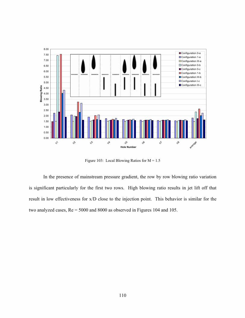
110
0.00
0.50
1.00
1.50
2.00
2.50
3.00
3.50
4.00
4.50
5.00
5.50
6.00
6.50
7.00
7.50
8.00
h1 h2 h3 h4 h5 h6 h7 h8
avera
ge
Hole Number
Blo
win
g R
atio
Configuration 0-aConfiguration 1-aConfiguration III-aConfiguration 0-bConfiguration 0-cConfiguration 1-bConfiguration III-bConfiguration I-cConfiguration III-c
Figure 103: Local Blowing Ratios for M = 1.5
In the presence of mainstream pressure gradient, the row by row blowing ratio variation
is significant particularly for the first two rows. High blowing ratio results in jet lift off that
result in low effectiveness for x/D close to the injection point. This behavior is similar for the
two analyzed cases, Re = 5000 and 8000 as observed in Figures 104 and 105.

111
0.00
0.50
1.00
1.50
2.00
2.50
3.00
3.50
4.00
1 2 3 4 5Row Number
Blo
win
g R
atio
Re = 5000-Actuals
Figure 104: Row by Row Blowing Ratio Variation (Re = 5000)
0.00
0.50
1.00
1.50
2.00
2.50
3.00
3.50
4.00
4.50
5.00
5.50
6.00
6.50
1 2 3 4 5Row Number
Blo
win
g R
atio
Re = 8000-Actuals
Figure 105: Row by Row Blowing Ratio Variation (Re = 8000)

112
CHAPTER 5: CONCLUSIONS
The gas turbine industry is continuously under demand to attain higher performance,
longer service life and lower emissions. The continuous effort to increase turbine efficiency has
promoted the development and sophistication of new material, thermal barriers and cooling
methods. Endwall film cooling is a necessity in modern gas turbines for safe and reliable
operation.
Performance of endwall film cooling is strongly influenced by among other factors the
hot gas flow field. Thus endwall flow field, especially those in utility gas turbines with cannular
combustors, is quite complicated in the presence of vortices, wakes and strong favorable pressure
gradient with resulting flow acceleration. These flow features can seriously impact film cooling
performance and make difficult the prediction of film cooling in endwall.
This study investigated endwall film cooling under the influence of pressure gradient
effects due to stagnation region of an axisymmetric airfoil and in mainstream favorable pressure
gradient. It also investigates the impact of wake on endwall film cooling near the stagnation
region of an airfoil. The investigation consisted of experimental testing and numerical
simulation. From the experimental results and numerical predictions the following conclusions
can be drawn:
For the Configuration 0-a, film cooling effectiveness is higher for lower blowing ratio at
low x/D. At high blowing ratio, the jet lifts off for low x/D, the jet later reattaches effectiveness
is increases. High blowing ratio promotes jet to jet interaction resulting in higher jet coverage
area.

113
The presence of an asymmetric airfoil did not change average effectiveness
characteristics drastically. Film effectiveness is higher for low x/D at low blowing ratios and at
higher x/D effectiveness is higher for high blowing ratios. However, film coverage is impacted
by the presence of the airfoil. It was observed that at low blowing ratio, the film flows around
the airfoil but is not able to provide coverage in the region adjacent to the airfoil. This may be
attributed to the low momentum flux and its inability to overcome the mainstream pressure
variations as well as a reduction in lateral spreading of the jet. At lower blowing ratios, jet
spreading is minimal, making it necessary to implement alternative means of endwall cooling in
the region adjacent to the airfoil.
Wake induced by placing a rectangular plate upstream of the injection point also has an
impact on endwall film cooling effectiveness. The cases on which the plate was placed far
upstream of the injection point (Configurations 0-c, I-c and III-c) did not affected film cooling
effectiveness. The flow was practically undisturbed by the presence of the wake plate. The
opposite was observed when the wake plate was close to the injection point (Configurations 0-b,
I-b and III-b). The presence of the bluff body formed a recirculation region downstream the
trailing edge of the plate drawing coolant flow upstream of the injection point into the
recirculation region. This flow intended to cool the region downstream of the holes is now being
mixed with the mainstream, loosing its cooling capabilities more rapidly. Turbulence created by
the wake, enhanced mixing of the jet flow with the mainstream resulting in a reduction of film
cooling effectiveness. The combination of wake and stagnation region reduced film effectiveness
furthermore, particularly for cases where the wake plate and airfoil were closest to the injection
point. (Configuration 1-b).

114
The effect of mainstream favorable pressure gradient on film cooling effectiveness was
also investigated. Multiple researchers have studied the effect of favorable pressure gradient on
airfoil vane cooling but endwall film cooling under accelerating conditions is not fully
understood. The numerical predictions as well as the experimental results report a wave-like
variation on film cooling effectiveness. This is more pronounced in the numerical analysis. In
part, the discrepancies could be attributed to the turbulence model employed for jet entrainment
under accelerating flow conditions. However, both results agree that the jet of the first rows of
holes lift off due to the variation of blowing ratios as a result of the mainstream pressure
distribution. This results in lower effectiveness which is then increased as x/D increases.
Several factors could be responsible of the flow behavior. The favorable pressure gradient
reduces mainstream turbulence and hence mixing of the jet is reduced leading to lower
effectiveness. In addition, it also inhibits lateral jet spreading which also impacts jet coverage.
Last, for the cases of stagnation region and wake effects, numerical analysis aid to the
understanding of the interaction of the flow with the mainstream. Flow visualization could serve
an additional tool to validate direction of the flow as it enters the mainstream. Also, the impact
of the shape of the wake plate trailing edge could also be varied to investigate if film
performance can be improved in the region downstream of the bluff body. Much more can be
done for the case of mainstream pressure gradient. This configuration can be modeled using
various turbulence models to determine which model better predicts film cooling effectiveness
under this mainflow conditions. In addition, shaped holes can also be tested and modeled to
emulate endwall film cooling hole configurations commonly used in the gas turbine industry. In
order for this cooling technique to be effective, film cooling must provide acceptable metal

115
surface temperatures and reasonable temperature distribution over the endwall to limit thermal
stress as a result of large temperature gradients. Better understanding of the behavior and
interaction of the jet flow with the mainstream could potentially impact endwall film hole
cooling patterns in order to increase endwall film effectiveness.

116
REFERENCES
1. Goldstein, R.J., et al., Film Cooling Following Injection Through Inclined Circular
Tubes. Israel Journal of Technology, 1970. 108(1-2): p. 145-154.
2. Ellis, S.J., D.G. Bogard, and M.E. Crawford, Effects of Streamwise Pressure Gradient on
the Suction Surface Boudary Layer of a Turbine Airfoil, in Mechanical Engineering.
1991, University of Texas: Austin.
3. Nicklas, M., Film-Cooled Turbine Endwall in a Transonic Flow Field: Part II---Heat
Transfer and Film-Cooling Effectiveness. Journal of Turbomachinery, 2001. 123(4): p.
720-729.
4. Zhang, L.J. and R.S. Jaiswal, Turbine Nozzle Endwall Film Cooling Study Using
Pressure-Sensitive Paint. Journal of Turbomachinery, 2001. 123(4): p. 730-738.
5. Goldstein, R.J., E.R. Eckert, and J.W. Ramsey, Film Cooling with Injection through
Holes: Adiabatic Wall Temperatures Downstream of a Circular Hole. Journal of
Engineering for Power, 1968: p. 384-395.
6. Eriksen, V.L. and R.J. Goldstein, Heat Transfer and Film Cooling Following Injection
Through Inclined Circular Tubes. Journal of Heat Mass Transfer, 1974: p. 239-245.
7. Burdet, A., R.S. Abhari, and M.G. Rose, Modeling of Film Cooling - Part II: Model for
Use in 3D CFD. ASME Turbo Expo, GT2005-68780, 2005.
8. Sinha, A.K., D.G. Bogard, and M.E. Crawford, Film-Cooling Effectiveness Downstream
of a Single Row of Holes With Variable Density Ratio. Journal of Turbomachinery, 1991.
113(3): p. 442-449.

117
9. Pedersen, D.R., E.R.G. Eckert, and R.J. Goldstein, Film Cooling with Large Density
Differences Between the Mainstream and the Secondary Fluid Measured by the Heat-
Mass Transfer Analogy. Journal of Turbomachinery, 1977. 99: p. 620-627.
10. Lutum, E. and B.V. Johnson, Influence of the Hole Length-to-Diameter Ratio on Film
Cooling With Cylindrical Holes. Journal of Turbomachinery, 1999. 121(2): p. 209-216.
11. Baldauf, S., et al., Correlation of Film-Cooling Effectiveness From Thermographic
Measurements at Enginelike Conditions. Journal of Turbomachinery, 2002. 124(4): p.
686-698.
12. Kost, F. and M. Nicklas, Film-Cooled Turbine Endwall in a Transonic Flow Field: Part
I---Aerodynamic Measurements. Journal of Turbomachinery, 2001. 123(4): p. 709-719.
13. Ammari, H.D., N. Hay, and D. Lampard, Effect of Acceleration on the Heat Transfer
Coefficient on a Film-Cooled Surface. Journal of Turbomachinery, 1991. 113(3): p. 464-
471.
14. Teekaram, A.J.H., C.J.P. Forth, and T.V. Jones, Film Cooling in the Presence of
Mainstream Pressure Gradients. Journal of Turbomachinery, 1991. 113(3): p. 484-492.
15. Kruse, H., Effects of Hole Geometry, Wall Curvature and Pressure Gradient on Film
Cooling Downstream of a Single Row. AGARD Conf Proc 390, 1985.
16. Hay, N., D. Lampard, and C.L. Saluja, Effects of the Condition of the Approach
Boundary Layer and of Mainstream Pressure Gradients on the Heat Transfer Coefficient
on Film-Cooled Surfaces. ASME J. Engineering for Gas Turbines and Power, vol. 107,
pp.99-104.
118
17. Schmidt, D.L. and D.G. Bogard, Pressure Gradient Effects on Film Cooling. ASME
Turbo Expo, 95-GT-18, 1995.
18. Hay, N., D. Lampard, and C.L. Saluja, Effects of Cooling Films on the Heat Transfer
Coefficient on a Flat Plate with Zero Mainstream Pressure Gradient. Journal of
Engineering for Gas Turbines and Power, 1985. 107: p. 105-110.
19. Knost, D.G. and K.A. Thole, Computational Predictions of Endwall Film-Cooling for a
First Stage Vane. ASME Turbo Expo, GT2003-38252, 2003.
20. Bernsdorf, S., M.G. Rose, and R.S. Abhari, Modelling of Film Cooling - Part I:
Experimental Study of Flow Structure. ASME Turbo Expo, GT2005-68783, 2005.
21. Walters, D.K. and J.H. Leylek, A Detailed Analysis of Film-Cooling Physics: Part I---
Streamwise Injection With Cylindrical Holes. Journal of Turbomachinery, 2000. 122(1):
p. 102-112.
22. Brittingham, R.A. and J.H. Leylek, A Detailed Analysis of Film Cooling Physics: Part
IV--- Compound-Angle Injection With Shaped Holes. Journal of Turbomachinery, 2000.
122(1): p. 133-145.
23. Hassan, J.S. and S. Yavuzkurt, Comparison of Tour Different Two-Equation Models of
Turbulence in Predicting Film Cooling Performance. ASME Turbo Expo, GT2006-
90860, 2006.
24. Adami, P., et al., Interaction Between Wake and Film Cooling Jets: Numerical Analysis.
ASME Turbo Expo, GT2004-53178, 2004.
25. Kholi, A. and D.G. Bogard, Improving Film Cooling Performance Using Airfoil
Contouring. ASME Turbo Expo, GT2006-90852, 2006.

119
26. Silieti, M., A.J. Kassab, and E. Divo, Film Cooling Effectiveness from a Single Scaled-
Up Fan-Shaped Hole a CFD Simulation of Adiabatic and Conjugate Heat Transfer
Models. ASME Turbo Expo, GT2005-68431, 2005.
27. Silieti, M., E. Divo, and A.J. Kassab, Numerical Investigation of Adiabatic and
Conjugate Film Cooling Effectiveness on a Single Cylindrical Film-Cooling Hole. ASME
International Mechanical Engineering Congress and R &D Expo, IMECE2004-62196,
2004.
28. Liu, Q., J. Kapat, and C.J. Douglass, Applicability of Temperature Sensitive Paints for
Measurement of Surface Temperature Distribution. ASME Turbo Expo, GT2003-38591,
2003.
29. Zuniga, H.A., et al., Discharge Coefficient and Effectiveness Measurement for Conical
Shaped Film Cooling Holes. ASME International Mechanical Engineering Congress and
R &D Expo, IMECE2005-81713, 2005.
30. Thompson, M.C., T. Leweke, and C.H.K. Williamson, The Physical Mechanism of
Transition in Bluff Body Wakes. Journal of Fluids and Structures, 2001. 15(3-4): p. 607-
616.
31. Knost, D.G. and K.A. Thole, Adiabatic Effectiveness Measurements of Endwall Film-
Cooling for a First-Stage Vane. Journal of Turbomachinery, 2005. 127(2): p. 297-305.
32. Kohli, A. and D.G. Bogard, Adiabatic Effectiveness, Thermal Fields, and Velocity Fields
for Film Cooling With Large Angle Injection. Journal of Turbomachinery, 1997. 119(2):
p. 352-358.

120
33. Friedrichs, S., H.P. Hodson, and W.N. Dawes, Aerodynamic Aspects of Endwall Film-
Cooling. Journal of Turbomachinery, 1997. 119(4): p. 786-793.
34. Sivrioglu, M., An Analysis of the Effects of Pressure Gradient and Streamline Curvature
on Film Cooling Effectiveness. Warme-und Stoffubertragung, 1991. 26(103-107).
35. Colban, W.F., K.A. Thole, and G. Zess, Combustor Turbine Interface Studies---Part 1:
Endwall Effectiveness Measurements. Journal of Turbomachinery, 2003. 125(2): p. 193-
202.
36. Colban, W.F., et al., Combustor Turbine Interface Studies---Part 2: Flow and Thermal
Field Measurements. Journal of Turbomachinery, 2003. 125(2): p. 203-209.
37. Harrison, K.L. and D.G. Bogard, Comparison of RANS Turbulence Models for Prediction
of Film Cooling Performance. ASME Turbo Expo, GT2008-51423, 2008.
38. Okita, Y. and C. Nakamata, Computational Predictions of Endwall Film Cooling for a
Turbine Nozzle Vane with an Asymmetric Countoured Passage. ASME Turbo Expo,
GT2008-50878, 208.
39. Chen, P.-H., Z.-M. Miao, and J.-W. Chen, Convective Transport Phenomena for
Stagnation Film Cooling. Heat Transfer in Gas Turbine, 1994. 300: p. 31-44.
40. Kline, S. and F. McClintock, Describing Uncertainties in a Single Sample Experiments.
Mechanical Engineering 75,, 1953: p. 3-8.
41. McGovern, K.T. and J.H. Leylek, A Detailed Analysis of Film Cooling Physics: Part II -
Compound - Angle Injection with Cylindrical Holes. Journal of Turbomachinery, 2000.
122: p. 113-121.

121
42. Hyams, D.G. and J.H. Leylek, A Detailed Analysis of Film Cooling Physics: Part III---
Streamwise Injection With Shaped Holes. Journal of Turbomachinery, 2000. 122(1): p.
122-132.
43. Leylek, J.H. and R.D. Zerkle, Discrete-Jet Film Cooling: A Comparison of
Computational Results With Experiments. Journal of Turbomachinery, 1994. 116(3): p.
358-368.
44. Friedrichs, S., H.P. Hodson, and W.N. Dawes, Distribution of Film Cooling Effectiveness
on a Turbine Endwall Measured Using the Ammonia and Diazo Technique. Journal of
Turbomachinery, 1996. 118: p. 613-621.
45. Praisner, T.J. and C.R. Smith, The Dynamics of the Horseshoe Vortex and Associated
Endwall Heat Transfer, Part 1 - Temporal Behavior. 2005.
46. Praisner, T.J. and C.R. Smith, The Dynamics of the Horseshoe Vortex and Associated
Endwall Heat Transfer, Part 2 - Time-Mean Results. aSME Turbo Expo, GT2005-69091,
2005.
47. Yavuzkurt, S. and M. Habte, Effect of Compuational Grid and Performance of Two-
Equation Models of Turbulence for Film Cooling Applications. ASME Turbo Expo,
GT2008-50153, 2008.
48. Mayhew, J.E., J.W. Baughn, and A.R. Byerley, The effect of freestream turbulence on
film cooling adiabatic effectiveness. International Journal of Heat and Fluid Flow, 2003.
24(5): p. 669-679.

122
49. Starke, A.R., R.A.W.M. Henkes, and M.J. Tummers, Effects of curvature and pressure
gradient on a turbulent near wake. Experimental Thermal and Fluid Science, 1999.
19(1): p. 49-56.
50. Marty, P., F. Michel, and P. Tochon, Experimental and numerical study of the heat
transfer along a blunt flat plate. International Journal of Heat and Mass Transfer, 2008.
51(1-2): p. 13-23.
51. Tummers, M.J., D.M. Passchier, and R.A.W.M. Henkes, Experimental investigation of an
adverse pressure gradient wake and comparison with calculations. Experimental
Thermal and Fluid Science, 1997. 14(1): p. 17-24.
52. Feng, Y., Z. Xiao-cheng, and D. Zhao-hui, Experimental Measurement and Numerical
Simulation for Flow Field and Film Cooling Effectiveness in Film-Cooled Turbine.
Journal of Hydrodynamics, 2006. 19(4): p. 459-466.
53. Tummers, M.J., D.M. Passchier, and P.G. Bakker, Experiments on the turbulent wake of
a flat plate in a strong adverse pressure gradient. International Journal of Heat and Fluid
Flow, 2007. 28(1): p. 145-160.
54. Brown, A. and C.L. Saluja, Film Cooling from a Single Hole and a Row of Holes of
Variable Pitch to Diameter Ratio. Journal of Heat Mass Transfer, 1979. 22: p. 525-533.
55. Lutum, E., et al., Film Cooling on a Convex Surface: Influence of External Pressure
Gradient and Mach number on Film Cooling Performance. Heat and Mass Transfer,
2001. 38.
56. Sundaram, N. and K.A. Thole, Film-Cooling Flowflieds with trenched Holes on an
Endwall. ASME Turbo Expo, GT2008-50149, 2008.

123
57. Kumaran, M. and S. Vengadesan, Flow Characteristics Behind Rectangular Cylinder
Placed Near a Wall. Numerical Heat Transfer, 2007. 52: p. 643-660.
58. Vino, G., et al., Flow structures in the near-wake of the Ahmed model. Journal of Fluids
and Structures, 2005. 20(5): p. 673-695.
59. Kang, M.B. and K.A. Thole, Flowfield Measurements in the Endwall Region of a Stator
Vane. Journal of Turbomachinery, 2000. 122(3): p. 458-466.
60. Thole, K.A. and D.G. Knost, Heat transfer and film-cooling for the endwall of a first
stage turbine vane. International Journal of Heat and Mass Transfer, 2005. 48(25-26): p.
5255-5269.
61. Kang, M.B., A. Kohli, and K.A. Thole, Heat Transfer and Flowfield Measurements in the
Leading Edge Region of a Stator Vane Endwall. Journal of Turbomachinery, 1999.
121(3): p. 558-568.
62. Friedrichs, S., H.P. Hodson, and W.N. Dawes, Heat Transfer Committee Best Paper of
1995 Award: Distribution of Film-Cooling Effectiveness on a Turbine Endwall Measured
Using the Ammonia and Diazo Technique. Journal of Turbomachinery, 1996. 118(4): p.
613-621.
63. Walters, D.K. and J.H. Leylek, Impact of Film-Cooling Jets on Turbine Aerodynamic
Losses. Journal of Turbomachinery, 2000. 122(3): p. 537-545.
64. Han, S. and R.J. Goldstein, Influence of Blade Leading Edge Geometry on Turbine
Endwall Heat (Mass) Transfer. ASME Turbo Expo, GT2005-68590, 2005.
65. Burd, S.W. and T.W. Simon, The Influence of Coolant Supply Geometry on Film Coolant
Exit Flow and Surface Adiabatic Effectiveness. 2006.

124
66. Burd, S.W., R.W. Kaszeta, and T.W. Simon, Measurements in Film Cooling Flows: Hole
L/D and Turbulence Intensity Effects. Journal of Turbomachinery, 1998. 120(4): p. 791-
798.
67. Burd, S.W. and T.W. Simon, Measurements of Discharge Coefficients in Film Cooling.
Journal of Turbomachinery, 1999. 121(2): p. 243-248.
68. Miao, J.-M. and C.-Y. Wu, Numerical approach to hole shape effect on film cooling
effectiveness over flat plate including internal impingement cooling chamber.
International Journal of Heat and Mass Transfer, 2006. 49(5-6): p. 919-938.
69. Meunier, P., S. Le Dizès, and T. Leweke, Physics of vortex merging. Comptes Rendus
Physique, 2005. 6(4-5): p. 431-450.
70. Ethridge, M.I., J.M. Cutbirth, and D.G. Bogard, Scaling of performance for varying
density ratio coolants on an airfoil with strong curvature and pressure gradient effects.
Journal of Turbomachinery, 2001. 123(2): p. 231-237.
71. Jubran, B.A., Shower Head Film Cooling Effectveness of a Symmetrical Turbine Blade
Model - Effect of Lateral Injection. JSME Thermal Engineering Summer Heat Transfer
Conference, HT2007-32081, 2007.
72. Tiedemann, M. and F. Kost, Some Aspects of Wake-Wake Interactions Regarding
Turbine Stator Clocking. Journal of Turbomachinery, 2001. 123(3): p. 526-533.
73. Leweke, T. and C.H.K. Williamson, Three-dimensional instabilities in wake transition.
European Journal of Mechanics - B/Fluids, 1998. 17(4): p. 571-586.
74. Harrison, K.L. and D.G. Bogard, Use of the Adiabatic Wall Temperature in Film Cooling
to Predict Wall Heat Flux and Temperature. ASME Turbo Expo, GT2008-51424, 2008.

125
75. Huang, R.F. and C.L. Lin, Velocity Field of a Bluff-Body Wake. Journal of Wind
Engineering and Industrial Aerodynamics, 2000. 85: p. 31-45.
76. Thompson, M.C., et al., Wake transition of two-dimensional cylinders and axisymmetric
bluff bodies. Journal of Fluids and Structures, 2006. 22(6-7): p. 793-806.
[30]
[12, 30-76]