Dissertations and Theses

5-2017

Extended Surface Heat Transfer Coefficients via Endwall Extended Surface Heat Transfer Coefficients via Endwall

Temperature Measurements Temperature Measurements

Yogesh Pai

Follow this and additional works at: https://commons.erau.edu/edt

Part of the Aerospace Engineering Commons

Scholarly Commons Citation Scholarly Commons Citation Pai, Yogesh, "Extended Surface Heat Transfer Coefficients via Endwall Temperature Measurements" (2017). Dissertations and Theses. 345. https://commons.erau.edu/edt/345

This Thesis - Open Access is brought to you for free and open access by Scholarly Commons. It has been accepted for inclusion in Dissertations and Theses by an authorized administrator of Scholarly Commons. For more information, please contact commons@erau.edu.

EXTENDED SURFACE HEAT TRANSFER COEFFICIENTS VIA ENDWALL

TEMPERATURE MEASUREMENTS

A Thesis

Submitted to the Faculty

of

Embry-Riddle Aeronautical University

by

Yogesh Pai

In Partial Fulfillment of the

Requirements for the Degree

of

Master of Science in Aerospace Engineering

May 2017

Embry-Riddle Aeronautical University

Daytona Beach, Florida

iii

ACKNOWLEDGMENTS

First and foremost, I would like to thank my committee members, Dr. Boetcher and

Dr. Leishman for their valuable insights, suggestions and for being so kind to me. The

entirety of this work has been possible due to my advisor Dr. Ricklick. Thank you for being

so patient & constantly pushing me to strive harder. You’ve raised the bar for my future

bosses and I can only wish that I can share half the rapport with them as I had with you. I

can’t begin to fathom the things you’ve done for me over the course of my Masters, you’ve

been nothing but inspirational. I will always recall your mantra during arduous times, “If

you knew what you were doing, it wouldn’t be called research”. I wouldn’t even be here if

not for my family. Thank you so much for always encouraging me to learn and giving me

the opportunity to do so. I consider myself really lucky to have you guys as my support-

system. I would like to thank my lab-mates; Royce, Anish, Bhushan, Yash, Sravan,

Stanrich & Bianca for their support and critique. Their knowledge and insight is a major

factor for the completion of my thesis. Also, I would like to make a special mention to

Kiran, Johnny, Gopika, Chef Sundar, Jitesh, Amey, Sampu, Uday, OG Sundar, Nishu,

Parth for all their support. I can’t imagine life without you guys. I’m also indebted to ERAU

for the infrastructure and financial support provided during my degree. I would have been

crazier if it hadn’t been for the active football community here in school. Daytona, you

may not be the world’s most famous beach but thanks for the awesome year-round sunny

weather and the amazingly friendly people. You made me feel right at home. I would like

to dedicate this work to my Ajja and Mauma, for I’ve not known a love truer than yours.

Thank you everyone for letting me be a part of something bigger. God bless you all

and God bless the United States of America.

iv

TABLE OF CONTENTS

SYMBOLS ........................................................................................................................ vii

ABBREVIATIONS ......................................................................................................... viii

ABSTRACT ....................................................................................................................... ix

1. Introduction ............................................................................................................... 10

1.1 Motivation-The Need for Gas Turbine Cooling ................................................. 10

1.2 Fundamentals of Heat Transfer & Extended Surfaces ...................................... 13

1.3 Turbine Blade Cooling Methods ........................................................................ 16

1.4 Pin-Fin Channel Flow Features .......................................................................... 20

1.5 Experimental Measurement Techniques ............................................................ 22

2. Literature Review...................................................................................................... 24

3. Problem Statement .................................................................................................... 35

4. Methodology ............................................................................................................. 37

4.1 Experimental Setup ............................................................................................ 37

4.2 Temperature Sensitive Paint ................................................................................... 42

4.2 Data Reduction........................................................................................................ 44

4.2 CFD- Setup and Boundary Conditions ................................................................... 48

5. Extended Surface Methodology ................................................................................ 51

5.1 Introduction to Extended Surface Analysis ............................................................ 51

5.2 Derivation of Analytical Solution ........................................................................... 54

6. Results & Discussion ................................................................................................ 56

6.1 Analytical Verification Results ............................................................................... 56

6.2 Computational Verification Results ........................................................................ 59

6.3 Experimental Verification Results .......................................................................... 59

6.3.1 Rig Validation- Intensity of Lights ................................................................. 60

6.3.2 Rig Validation- Heat Leakage Test ................................................................ 61

6.3.3 Rig Validation- Smooth Channel Test ............................................................ 62

6.3.4 Extended Surface Methodology Results-Comparison with Ames ................. 64

6.3.5 Channel Average Nusselt number Results ..................................................... 66

7. Conclusion ................................................................................................................ 70

REFERENCES ................................................................................................................. 72

v

LIST OF FIGURES

Figure 1-1. Brayton cycle ................................................................................................. 10

Figure 1-2 Turbine inlet temperature versus Power (Sautner et al., 1992) ....................... 11

Figure 1-3. Increase in turbine inlet temperature with various cooling methods over the

years. (Clifford, 1985)....................................................................................................... 12

Figure 1-4. Variety of Extended surfaces (Incropera & Dewitt, 2011) ............................ 15

Figure 1-5. Comparison of benefits of using extended surfaces with a flat surface. ........ 16

Figure 1-6. Blade cooling techniques (Han, 2004) ........................................................... 17

Figure 1-7. In-house pin-fin rig test section. ..................................................................... 18

Figure 1-8. Types of array arrangement: (a) Inline array (b) Staggered array (Siw et al.,

2012) ................................................................................................................................. 20

Figure 1-9. Flow features around a single cylinder. (Nguyen et al., 2012) ...................... 20

Figure 1-10. CFD simulation showcasing the flow features of a pin fin channel.

(Fernandes, 2015) ............................................................................................................. 21

Figure 2-1. Row averaged Nu for conducting and non-conducting pin arrays. (Metzger &

Haley, 1982) ...................................................................................................................... 26

Figure 2-2. Row averaged Sherwood numbers at pin surface & endwall for different

Reynold’s numbers. (Chyu, 1999) .................................................................................... 27

Figure 2-3. Midline Nu/Re0.5 distribution of different rows for Re=30,000 ................... 29

Figure 2-4. Endwall Nusselt number contour for Re=13,000 for different streamwise

spacings. (Lawson et al., 2011) ......................................................................................... 30

Figure 2-5. Circumferential Frossling number distribution for different Re for cylindrical

and oblong pins. (Kirsch et al., 2013) ............................................................................... 31

Figure 2-6. Cross section of pins tested. (Sahiti et el., 2006) ........................................... 31

Figure 2-7. Array averaged Nu as a function of Re for different shapes. ......................... 33

Figure 2-8. Array averaged Eu as a function of Re for different shapes. ......................... 33

Figure 2-9. Seal whisker and proposed bio-inspired cylinder. ......................................... 34

Figure 2-10. Alternate geometries considered for the study. (Pai et al., 2017) ................ 34

Figure 4-1. Experimental Setup. ....................................................................................... 37

Figure 4-2. Schematic of Flow Loop…………………………………………………….40

Figure 4-3. Non-dimensional distances………………………………………………….41

vi

Figure 4-3. Layout of the test section with boundary conditions. .................................... 40

Figure 4-4. Serpentine arrangement of Inconel strips in the test section. ......................... 40

Figure 4-5. Circuit Diagram of the entire setup. ............................................................... 41

Figure 4-6. Jablonksi Diagram (Bell. 2001) ..................................................................... 43

Figure 4-7. Typical TSP calibration curve (Fernandes, 2015).......................................... 43

Figure 4-8. (a) Reference image of higher intensity, known temperature. ....................... 44

Figure 4-9. Pressure drop versus mass flow rate for the venturi-flowmeter. .................... 46

Figure 4-10. Boundary Conditions for the CHT case. ...................................................... 49

Figure 5-1. 2D Model of an extended surface. ................................................................. 51

Figure 5-2. Analytical Solutions for different tip conditions. ........................................... 53

Figure 6-1. Verification of Analytical solution w/ standard solution for infinite fin. ...... 57

Figure 6-2. Temperature distribution along the pin height without IHG. ......................... 60

Figure 6-3. Temperature distribution along the pin height with IHG. .............................. 60

Figure 6-4. Intensity Stabilization over time .................................................................... 60

Figure 6-5. Schematic of Heat Leak Test arrangement .................................................... 61

Figure 6-6. Heat Leakage Test Results- Difference in temperature vs Heat flux supplied.

........................................................................................................................................... 62

Figure 6-7. Spanwise averaged smooth channel Nusselt number..................................... 63

Figure 6-8. Comparison of analytical solution with Ames for Re=3,000. ........................ 64

Figure 6-9. Comparison of analytical solution with Ames for Re=10,000. ...................... 65

Figure 6-10. Comparison of analytical solution with Ames for Re=30,000. .................... 66

Figure 6-11. Endwall Nusselt number contour Re=30,000……………………..……….69

Figure 6-12. Comparison of average Nusselt numbers with previous research. .............. 69

vii

SYMBOLS

Greek

η Isentropic efficiency

ρ Specific resistivity. (Ohm/m)

µ Dynamic viscocity. (Ns/m2)

θ Excess temperature function (K)

Ac Cross-sectional area (m2)

As Surface area(m2)

Bi Biot number

Cp Specific heat capacity

D Pin diameter (m)

f Darcy friction factor

Dh Hydraulic diameter (m)

h Heat transfer coefficient (W/m2K)

H Channel height (m)

I Current supplied. (A)

k Thermal conductivity of the pin (W/mK)

m Fin parameter (m)

�� Mass flow rate. (kg/s)

Nu Nusselt number

Nu0 Nusselt number for fully developed smooth channel flow

P Perimeter (m)

p Pressure (Pa)

Pr Prandtl number

Q Rate of heat transfer. (W)

q”lost Heat flux lost to the surrounding (W/m2)

q”supplied Heat flux supplied (W/m2)

𝑞𝑏"

Heat flux supplied to the base(W/m2)

viii

�� Internal heat generation(W/m3)

R Resistance of the strips. (Ohm)

Re Reynolds number

Tb Bulk temperature (K)

Ts Surface temperature (K)

T∞ Freestream temperature (K)

X Streamwise distance (m)

Y Spanwise distance (m)

ABBREVIATIONS

CFD Computational Fluid Dynamics

CAD Computer Aided Design

RANS Reynolds Averaged Navier Stokes

LES Large Eddy Simulation

DNS Direct Numerical Solution

STAR-CCM+ Simulation of Turbulence in Arbitrary Regions-Computational

Continuum Modeling

sCMOS Scientific Complementary Metal-Oxide Semiconductor

TSP Temperature Sensitive Paint

PSP Pressure Sensitive Paint

IHG Internal Heat Generation

CHT Conjugate Heat Transfer

LED Light Emitting Diode

ESM Extended Surface Methodology

TBC Thermal Barrier Coating

IR Infrared

PTML Propulsion Thermal Management Laboratory

PVC Poly-vinyl Chloride

SST Shear Stress Transport

UV Ultraviolet

AC Alternating Current

ix

ABSTRACT

Pai, Yogesh MSAE, Embry-Riddle Aeronautical University, May 2017. Extended Surface

Heat Transfer Coefficients via Endwall Temperature Measurements.

Short pins are used for internal cooling of the trailing edge in a gas turbine blade. A novel

method is described in this thesis which helps in simplifying the experimental process used

to obtain average heat transfer data on the pin surface, at the expense of additional post-

processing complexity. The method is based on a unique, analytical solution of the

longitudinal conduction equation with internal heat generation, allowing computation of

heat transfer rates via pin base temperature measurements via Temperature Sensitive Paint,

or similar non-intrusive methods. Verification of this method is done with comparisons to

the solution of infinite fins with internal heat generation, conjugate computational results,

and experimental data validated against the literature. Agreement within 8% of

experimental and 2% of numerical results confirm the suitability of the method.

10

1. Introduction

1.1 Motivation-The Need for Gas Turbine Cooling

Most passenger aircrafts operating today are powered by gas turbine engines. Gas

turbine engines are preferred for flight due to their high power-to-weight ratio as well as

their robustness and efficiency in delivering power. High power output at maximum

efficiency is one of the major requirements for engine manufacturers and designers as this

helps in reducing fuel usage and ultimately operating costs for airlines. The Brayton cycle

describes the working of a gas turbine engine as shown in Figure 1-1.

Figure 1-1. Brayton cycle

An ideal Brayton cycle consists of adiabatic compression in the compressor section

(1-2), constant pressure heat addition in the combustor (2-3) and the last step in the process,

expansion for energy extraction in the turbine section (3-4). The energy obtained from the

turbine drives the compressor in this process. In simpler words, freestream air is

11

compressed in the compressor section and introduced in the combustor where fuel is added

to this compressed air and ignited. This mixture of hot gas is then introduced into the

turbine section where the turbine blades extract energy.

The isentropic efficiency of a gas turbine engine is given by:

𝜂 = 1 −𝑇4

𝑇3 (1)

where T3 = Turbine Inlet Temperature

T4 = Turbine Exit Temperature

Thus, from the above equation we can see that an increase in turbine inlet

temperature results in an increase in the efficiency of a gas turbine engine. Figure 1-2 shows

the increase in engine power for various engines with a corresponding increase in turbine

inlet temperature.

Figure 1-2 Turbine inlet temperature versus Power (Sautner et al., 1992)

Thus, increasing the turbine inlet temperature not only increases the efficiency but

12

also the power output as shown in Figure 1-2. However, the turbine inlet temperature is

physically limited by the blade material limits. The hot blade component begins to weaken

at a lower temperature as compared to blade material melting point (Han, 2004). This

further limits the operating turbine inlet temperature with a view to promote component

life. Hence, to allow hot gas temperatures beyond these limits, modern gas turbine blade

components are either given thermal protective coatings, cooled or even both. Thermal

barrier coatings (TBC) are used to minimize the effect of thermal stresses induced and

reflect much of the radiant heat from the hot gases to prevent it from reaching the blade

material. In addition to this, TBC's must retain its protective properties for prolonged

service times and thermal cycles without failure (Clarke et al., 2012). TBCs are ceramics,

based on Zirconium Dioxide–Yttrium Oxide and produced by plasma spraying

(Muktinutalapati, 2011). Figure 1-3 shows the increase in turbine inlet temperature over

the years with the introduction of various cooling techniques.

Figure 1-3. Increase in turbine inlet temperature with various cooling methods over the

years. (Clifford, 1985)

13

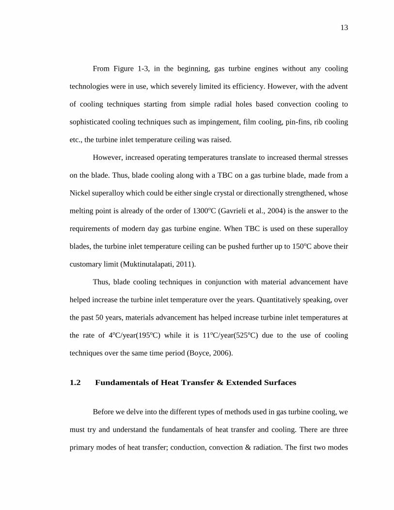
From Figure 1-3, in the beginning, gas turbine engines without any cooling

technologies were in use, which severely limited its efficiency. However, with the advent

of cooling techniques starting from simple radial holes based convection cooling to

sophisticated cooling techniques such as impingement, film cooling, pin-fins, rib cooling

etc., the turbine inlet temperature ceiling was raised.

However, increased operating temperatures translate to increased thermal stresses

on the blade. Thus, blade cooling along with a TBC on a gas turbine blade, made from a

Nickel superalloy which could be either single crystal or directionally strengthened, whose

melting point is already of the order of 1300oC (Gavrieli et al., 2004) is the answer to the

requirements of modern day gas turbine engine. When TBC is used on these superalloy

blades, the turbine inlet temperature ceiling can be pushed further up to 150oC above their

customary limit (Muktinutalapati, 2011).

Thus, blade cooling techniques in conjunction with material advancement have

helped increase the turbine inlet temperature over the years. Quantitatively speaking, over

the past 50 years, materials advancement has helped increase turbine inlet temperatures at

the rate of 4oC/year(195oC) while it is 11oC/year(525oC) due to the use of cooling

techniques over the same time period (Boyce, 2006).

1.2 Fundamentals of Heat Transfer & Extended Surfaces

Before we delve into the different types of methods used in gas turbine cooling, we

must try and understand the fundamentals of heat transfer and cooling. There are three

primary modes of heat transfer; conduction, convection & radiation. The first two modes

14

are discussed in detail here since the focus of this thesis primarily deals with these.

Conduction may be viewed as the transfer of energy from the more energetic to the

less energetic particles of a substance due to interactions between the particles. In simpler

words, it can be defined as the transfer of heat between the hot surface and the colder

surface, which are in physical contact with each other, because of the existing temperature

gradient between them. The rate of conduction heat transfer is given by Fourier’s Law:

𝑄𝑥 = −𝑘𝐴𝑐𝑑𝑇

𝑑𝑥 (2)

Here, Qx is the rate of heat transfer. k and Ac are the thermal conductivity and cross-

sectional area of the colder surface respectively while dT/dx is the temperature gradient in

the x direction. The negative sign indicates the direction of heat transfer leaving the hot

surface into the cooler surface.

Convection is described by Newton’s Law of Cooling which states that the rate of

heat lost from a body is proportional to difference in temperature between the hot body and

the surrounding fluid. In context, it is the rate of heat lost by the hot surface to the

surrounding cooler fluid.

𝑄 = ℎ𝐴𝑠∆𝑇 (3)

Here, Q is the rate of heat transfer, h is the convective heat transfer coefficient of

the cooler fluid, As is the surface area of the hot surface while ∆T is the temperature

difference between them. The heat transfer coefficient is dependent on conditions in the

boundary layer which is influenced by the hot surface geometry, the nature of the fluid

motion and a variety of thermodynamic and transport properties of the fluid.

From equation (2), for a given size of the body, we can increase the rate of heat

transfer due to conduction by using a material of higher thermal conductivity. From

15

equation (3), we can increase the rate of heat transfer due to convection either by increasing

the h and/or reducing the temperature of the cooler fluid, thereby increasing ∆T and/or

increasing the surface area (As) available for heat transfer. h can be increased by increasing

the fluid velocity. However, only increasing the fluid velocity is either insufficient to obtain

the desired heat transfer rate and often the costs associated in doing so involves increasing

the pumping power requirements which is unfeasible (Incropera & Dewitt, 2011).

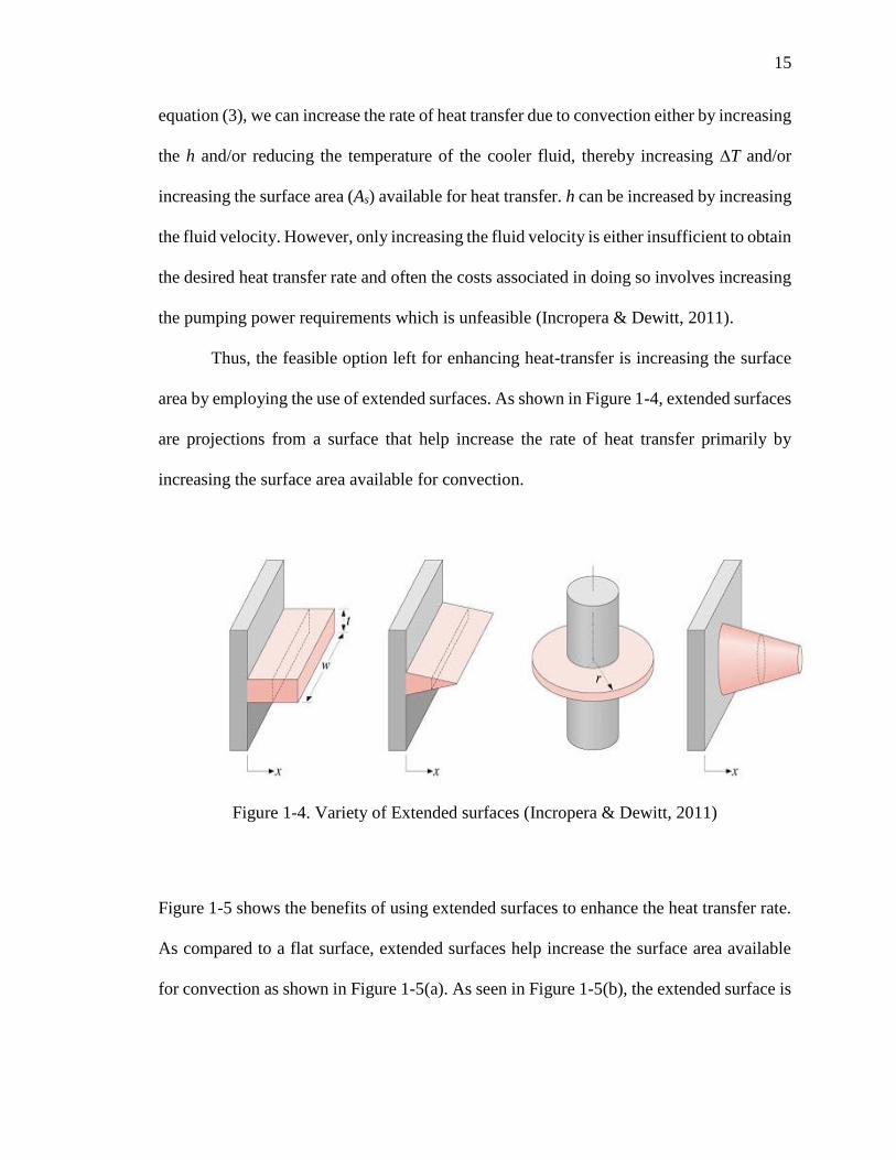
Thus, the feasible option left for enhancing heat-transfer is increasing the surface

area by employing the use of extended surfaces. As shown in Figure 1-4, extended surfaces

are projections from a surface that help increase the rate of heat transfer primarily by

increasing the surface area available for convection.

Figure 1-4. Variety of Extended surfaces (Incropera & Dewitt, 2011)

Figure 1-5 shows the benefits of using extended surfaces to enhance the heat transfer rate.

As compared to a flat surface, extended surfaces help increase the surface area available

for convection as shown in Figure 1-5(a). As seen in Figure 1-5(b), the extended surface is

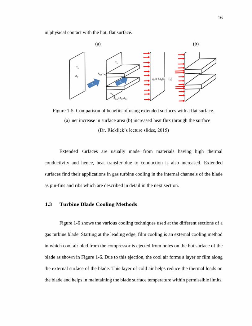
16

in physical contact with the hot, flat surface.

(a) (b)

Figure 1-5. Comparison of benefits of using extended surfaces with a flat surface.

(a) net increase in surface area (b) increased heat flux through the surface

(Dr. Ricklick’s lecture slides, 2015)

Extended surfaces are usually made from materials having high thermal

conductivity and hence, heat transfer due to conduction is also increased. Extended

surfaces find their applications in gas turbine cooling in the internal channels of the blade

as pin-fins and ribs which are described in detail in the next section.

1.3 Turbine Blade Cooling Methods

Figure 1-6 shows the various cooling techniques used at the different sections of a

gas turbine blade. Starting at the leading edge, film cooling is an external cooling method

in which cool air bled from the compressor is ejected from holes on the hot surface of the

blade as shown in Figure 1-6. Due to this ejection, the cool air forms a layer or film along

the external surface of the blade. This layer of cold air helps reduce the thermal loads on

the blade and helps in maintaining the blade surface temperature within permissible limits.

17

Figure 1-6. Blade cooling techniques (Han, 2004)

Impingement cooling is a type of internal cooling technique predominantly used

near the leading edge of the gas turbine blade. As the name suggests, multiple jets of

coolant ejected from internal holes impinge on the surface of the hot blade at the leading

edge and help enhance the heat transfer.

Rib-turbulated cooling is the use of ribs, which are protrusions placed commonly

on the two opposite walls of the internal channel of a gas turbine blade. These ribs act as

flow obstructers and help enhance mixing in the section in which they are placed. The

function of a rib is to trip the boundary layer of the incoming flow such that the flow

separates and then re-attaches after the rib, creating re-circulation zones which augment

the level of the turbulence in the channel and ultimately enhance heat transfer. Since it

disturbs only the near wall flow, the pressure drop in the channel is within acceptable limits.

(Han, 2004).

Pin-fin cooling is the use of a bank of extended surfaces at the short and narrow

18

trailing edge of the gas turbine blade. Like ribs, they help augment turbulence and mixing

in the internal channel for heat transfer enhancement of the hot endwalls of gas turbine

blade at the trailing edge. Figure 1-7 is an image of the in-house pin fin rig test section

showcasing several circular cylindrical pins.

Figure 1-7. In-house pin-fin rig test section.

Pin-fins could be of several different shapes but the most commonly preferred for

experimental investigation are circular cylindrical ones due to the ease of manufacturing.

(Ames et al., (2006,2007), Chyu et al (1999), VanFossen (1981), Metzger & Haley (1982),

Lawson et al., (2011)).

Figure 1-8 shows the two typical arrangements of arrays used in a pin-fin cooling

channel. It also shows the typical nomenclature used for the non-dimensional distances

between the pins in the streamwise (X/D) and spanwise (Y/D) direction. Distances are

19

usually normalized using the pin diameter (D). For an inline array, the rows are arranged

in such a way that pins of consecutive rows are right behind each other. For a staggered

array, the rows are alternatively arranged in such a manner that corresponding pins of any

given row lie behind in the gap of the pins in the previous rows. Experimental

investigations involving variation of parameters such as pin spacing, pin material, pin

dimensions are discussed in detail in the literature review section.

(a)

(b)

Figure 1-8. Types of array arrangement: (a) Inline array (b) Staggered array (Siw et al.,

2012)

The use of pin-fin cooling at the trailing edge is 3-fold; to act as flow turbulators,

to increase effective surface area and to provide structural support at the short and narrow

Flow Direction

X/D

Y/D

X/D

Y/D

20

trailing edge. The primary objective of this study deals with the experimentation involving

pin-fin channels and hence the next section describes some of the features of pin-fin

channel in detail.

1.4 Pin-Fin Channel Flow Features

Some of the main characteristics of an internal cooling channel with a pin-fin array are

regions of accelerated flows between the pins, stagnation flows, localized low and high

pressure regions, flow separation zones and the presence of horse-shoe vortices at the endwall

that contribute towards enhancing the rates of convective heat transfer (Ames (2006), Chyu

(1999), Metzger (1982)). Figure 1-9 highlights some of the flow features at the end-wall

caused due to flow obstruction by a single pin-fin.

Figure 1-9. Flow features around a single cylinder. (Nguyen et al., 2012)

The presence of the pin causes the cooling air to stagnate on the cylinder surface

21

facing the flow, accelerate around the sides before separating due to the adverse pressure

gradients (Celli, 1997). Figure 1-9 also shows the horse-shoe vortices formed at the endwall

as the cooling air is forced to flow around the cylinder. Presence of horse-shoe vortices are

not preferred from the aerodynamic point of view as they cause performance losses.

However, in a pin-fin channel, these vortices break up the boundary layer on the end walls

and produce high shear stress beneath it which results in high heat transfer from the end

walls (Chyu et al., 1999).

Figure 1-10 is an image of a computational simulation of flow in a pin-fin channel.

Clearly visible in this figure are the vortices created behind the pin due to flow separation

at the sides. The resulting unsteady shedding of vortex caused by separation results in the

chaotic mixing of cooling air on the back surface of the pin thereby driving heat transfer

rates in this region (Ames & Dvorak, 2006).

Figure 1-10. CFD simulation showcasing the flow features of a pin fin channel.

(Fernandes, 2015)

22

1.5 Experimental Measurement Techniques

Thermocouples, naphthalene sublimation, thermo-chromic liquid crystals, IR

cameras, temperature sensitive paint (TSP) are the different means of obtaining

temperature data from an experimental setup. TSP, thermo-chromic liquid crystals, IR

cameras are used to obtain high resolution, highly localized data of the entire test surface

whereas thermocouples are attached at discrete points of interest.

The naphthalene sublimation technique involves dipping the test object in liquid

naphthalene for one second, which after cooling forms very thin layer on the surface. After

coating, the test objects are stored in a tightly sealed plastic box for at least 15 hours so that

they attain thermal equilibrium with the surrounding air. Before the test run, each of the

components are weighed using a highly sensitive and accurate electronic balance. After the

heated test, the setup is individually weighed again and the difference in the weight yields

the amount of naphthalene that sublimated during the run. Using a mass transfer analogy,

the Nusselt number is obtained.

IR cameras measure the radiation emitted by the hot test surface. This radiation is

a function of not only the temperature but also of the emissivity and reflectance of the body.

The radiant energy is related to the temperature and the emissivity of an object as given by

the modified Stefan-Boltzmann law. Although the relationship is linear, the emissivity of

a body itself is dependent on the material, surface finish and viewing angle (Liu, 2007). If

the emissivity of the body is less than unity, the body reflects some of the radiation from

the surrounding objects as well leading to an error in temperature measurement. The IR

system comprises of an IR radiation detector, an optical system to concentrate the radiation

on the detector as well as a scanning mirror. The detector is usually cooled by liquid

23

nitrogen or Peltier cooler to minimize detector noise. Besides, the optical access window

needs to be of Germanium material since standard silica glass, acrylic and quartz are

opaque to infrared radiation (Liu, 2007).

Thermochromic liquid crystals are commonly used to qualitatively study heat

transfer characteristics and only recently have been used to quantify heat transfer co-

efficients (Uzol & Camci, 2005). There are certain organic compounds that act neither like

an isotropic liquid nor a non-isotropic crystalline solid but rather something in the middle

of both these phases. These compounds are referred to as liquid crystals or mesophases.

These liquid crystals react to changes in temperature, shear stress and electromagnetic

fields by emitting light of corresponding wavelength. This is due to the molecules of these

crystals stretch or contract depending on the change in temperature, shear stress and

electromagnetic fields. Shear stress sensitivity can be made insignificant by encapsulating

these crystals in a polymer while maintaining its temperature dependency. Although these

liquid crystals can be handled easily, to capture the color change, the background of the

test section must be painted completely black. One of the major disadvantages of using

TLC is that the calibration curve is sensitive to the viewing angle and the lighting and hence

can cause problems if used for quantitative applications (Liu, 2007).

Each of these temperature measurement techniques described here excluding TLC

involves machining of the test section or making arrangements extraneous to the

experimental setup. Also, the pin surface and endwall measurements need to be taken

separately. Thus, there is a need for a non-intrusive prediction of surface average heat

transfer coefficients which provide for faster turn-around times for the testing of different

geometries by reducing setup time and cost albeit at additional post processing complexity.

24

2. Literature Review

A significant amount of studies have been conducted with regards to pin-fin cooling

at the trailing edge of the turbine; experimentally as well as computationally. Some of the

earliest works included trying to correlate the heat transfer characteristics between long

tubes in cross flow heat exchangers and very short pins in plate-fin heat exchangers with

pin-fin channels in a turbine blade. The difference between the three cases being in the

height to diameter ratio (H/D). The pin-fins in an internal cooling channel of a gas turbine

blade have a H/D ratio between the other two applications. Armstrong and

Winstanley(1988) found that the interpolation between the two extreme cases did not

accurately predict the performance characteristics of pin-fins in a gas turbine blade. The

effect of conducting and non-conducting array of pins on surface average Nusselt number

was studied by Metzger & Haley (1982, 1984) and by VanFossen (1982). Investigations

were also done to obtain correlations for staggered and inline arrays by a host of

researchers. (Sparrow (1980,2004), VanFossen (1982), Metzger et al., (1982), Chyu

(1998)). Alternative pin geometries were compared against the baseline circular cylindrical

pins for their pressure loss benefits by Goldstein et al., (1994), Chyu (1996, 1998) and

Camci et al., (2005). Pin and row removal studies were also conducted to investigate the

pressure loss and heat transfer characteristics by Sparrow & Molki (1982) and recently by

Kirsch et al. (2014).

As the focus of research areas in regards to pin-fin cooling changed over the years,

so did the experimental measurement techniques. In the 1980’s, thermocouples were the

preferred method of acquiring temperature data (Metzger & Haley (1982), VanFossen

(1982, 1984) Sparrow (1980)). In the 1990’s, heat transfer characteristics of the pin surface

25

were studied via a mass transfer analogy using a naphthalene sublimation technique

(Goldstein et al., (1994), Chyu (1998,1999), Sparrow (1984). In the late 90’s and 2000’s,

non-intrusive techniques such as IR and TLC were used to acquire endwall and pin surface

data (Camci et al. (2005), Ames et al., (2007), Lawson et al. (2011), Kirsch et al., (2013)).

Some of these studies are reviewed in detail in the following section.

VanFossen (1981, 1984) investigated the effects of pin height and pin inclination

in a pin fin array. For his experiments, he utilized a staggered array of 4 rows but used two

different set of pins. The first set of pins had an H/D= 0.5 and X/D= 2 while the

configuration of the other set of pins was twice of this. Two separate arrays consisting of

wooden and copper pin arrays were used to isolate and study the contribution of endwall

and the pin surface individually. Only the endwalls were heated and maintained at a

constant temperature. Thermocouples were used to obtain temperature data. He found that

heat transfer coefficients on the pin surface were about 35% higher than the endwall.

Inclined pins were found to have the same heat transfer characteristics as compared to the

pins that are perpendicular to the endwall. Another study conducted by Brigham and

VanFossen (1984) concluded that short pin fins indicated lower levels of heat transfer

compared to longer pins of same design and that heat transfer augmentation is strongly

dependent on the H/D ratio.

In order to compare the effect of conducting and non-conducting pins in a pin-fin

channel experiment, Metzger & Haley (1982) used copper and balsa wood cylindrical pin-

fins for their experimentation. The H/D of the pins were 1 and the pins were placed in a

moderately dense manner (~XD=1.32-5). Both endwalls were heated and had foil heater

segments for each row, powered individually. The heat flux on each of these individual

26

segments were adjusted till an isothermal wall boundary condition was achieved that is the

temperature difference between all segments was negligible (± 0.1oC). Figure 2-1 is a plot

of row average Nusselt number for conducting and non-conducting pins at different

Reynold’s numbers.

Figure 2-1. Row averaged Nu for conducting and non-conducting pin arrays. (Metzger &

Haley, 1982)

Since this was a study to obtain row averaged Nusselt number, thermocouples were

used at each row to obtain temperature data. Additional thermocouples were attached to

account for failure. For each array configuration, pin type and flow rate, 2 power levels

were used, corresponding to segment temperatures approximately 6oC and 12oC above the

duct flow bulk temperature. Figure 2-1 shows that the difference in Nusselt number

between conducting and non-conducting pins is negligible for the low Reynold’s number

case. Similar to many other researchers, they observed heat transfer augmentation up to

row 3 and then a periodically fully-developed rate of augmentation till the last row.

27

Chyu et al., (1990, 1999) used a naphthalene sublimation technique to study the

individual heat transfer contributions from the pin as well as endwall using a mass transfer

analogy. This setup helped them to ensure that the entire wetted surface in a pin fin channel

was thermally active. He also noted that the variety of thermal boundary modelling used

by researchers for a pin-fin array did not influence the general trends of heat transfer as

significantly as the individual magnitudes due to bulk flow temperature variations.

The mass transfer co-efficient or the Sherwood number is analogous to the Nusselt

number in heat transfer. Chyu (1999) used aluminum pins and investigated both inline and

staggered arrays for Reynold's numbers of 7650, 16800 & 23100. A constant wall

temperature boundary condition was utilized at the endwall. Figure 2-2 shows the row

averaged Sherwood numbers at the pin surface and endwall for different Reynold’s

numbers. As we can see from Fig. 2-2, he concluded that the heat transfer coefficient on

the pin surface is higher than that on the uncovered end wall by approximately 10-20% as

compared to 30-40% obtained by VanFossen(1982)

Figure 2-2. Row averaged Sherwood numbers at pin surface & endwall for different

Reynold’s numbers. (Chyu, 1999)

Since the endwall represents about 80% of the wetted area, he believed that an

experimental approach focused solely on the endwall contribution is more representative

of the channel than the one focused solely on pins which the author believes grossly

28

undermines the influence of the pins on endwall heat transfer.

Uzol and Camci (2005) conducted a study to compare endwall heat transfer

enhancements and total pressure loss between circular, elliptical and a pin based on NACA

0024 airfoil. They had an H/D=1.5, S/D=X/D=2 for a staggered array of 2 rows of pins.

Their test section containing the pin-fin array and the heated section was placed 4 & 2 pin

diameters distance from the entrance respectively. They used a constant heat flux boundary

condition on the endwall, the pin was not heated. Endwall heat transfer data was obtained

by using liquid crystal thermography. A detailed description of liquid crystal thermography

can be found here (Wilberg et al., 2004). It was observed that the circular fin array had

27% higher Nusselt number as compared to the elliptical and the NACA shaped pins.

However, the total pressure loss in the circular channel was found to be 46.5% higher than

the elliptical fin and 59.5% higher than the NACA shaped pin. They also used a parameter

referred to as the specific friction loss in an internal channel which is the ratio of average

friction factor to the average Nusselt number for the channel to compare overall

performance of the pin shapes. The elliptical and the NACA fin had a lower specific friction

loss as compared to the circular ones due to the pressure loss benefits on the account of

delayed flow seperation.

Ames et al., (2006) studied the flow physics that is characteristic of a pin fin channel

by measuring turbulence intensity and acquiring pin-fin midline heat transfer and pressure

distribution around the pin for Reynolds numbers of 3000, 10,000 and 30,000 as shown in

Figure 2-3. Their Reynold’s number was based on the maximum velocity between the pins

and the pin diameter. They had a H/D=2, X/D=S/D= 2.5 which is comparable to the in-

house rig which is the primary reason for comparing the veracity of the results obtained

29

from this study to the work done by Ames et al. Hot-wire anemometry was used to measure

the fluid characteristics. They used a constant heat flux boundary condition on the pin

surface and had a heated entrance length to ensure that the flow is thermally developed

when it reaches the test section. Data was acquired from a single heated pin by placing it

in different rows, using 24 equally spaced thermocouples placed around the pin. They

found that heat transfer is the highest in the 3rd row due to highest effective velocity while

heat transfer augmentation due to turbulence is the highest in row 4.

Figure 2-3. Midline Nu/Re0.5 distribution of different rows for Re=30,000

(Ames, 2006)

Lawson et al., (2011) investigated the effect of spanwise and stream-wise spacing

on heat transfer augmentation and pressure loss in a low aspect ratio pin-fin channel and

Reynolds number ranging from 5000 to 30,000. Nusselt number contours of the endwall

were acquired by measuring temperature with an infrared (IR) camera through a Zinc

Selenide window which allowed for IR transmittance. A constant heat flux boundary

condition was maintained since both the endwalls were heated with the help of Inconel

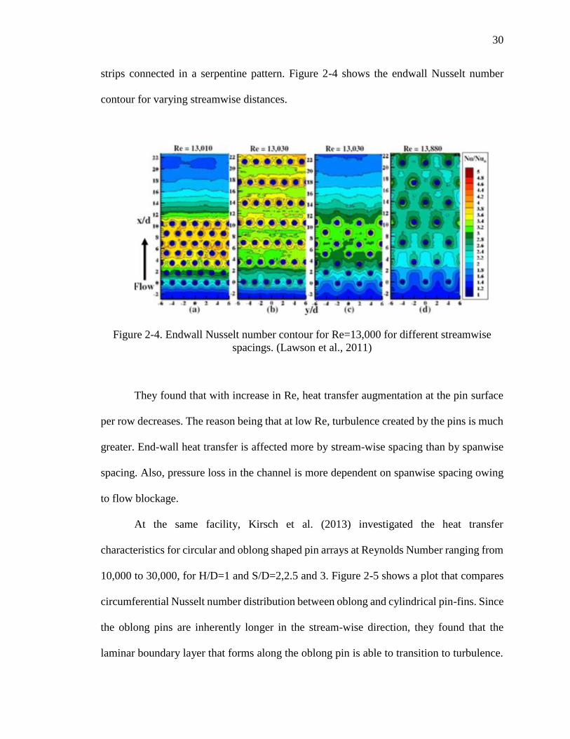
30

strips connected in a serpentine pattern. Figure 2-4 shows the endwall Nusselt number

contour for varying streamwise distances.

Figure 2-4. Endwall Nusselt number contour for Re=13,000 for different streamwise

spacings. (Lawson et al., 2011)

They found that with increase in Re, heat transfer augmentation at the pin surface

per row decreases. The reason being that at low Re, turbulence created by the pins is much

greater. End-wall heat transfer is affected more by stream-wise spacing than by spanwise

spacing. Also, pressure loss in the channel is more dependent on spanwise spacing owing

to flow blockage.

At the same facility, Kirsch et al. (2013) investigated the heat transfer

characteristics for circular and oblong shaped pin arrays at Reynolds Number ranging from

10,000 to 30,000, for H/D=1 and S/D=2,2.5 and 3. Figure 2-5 shows a plot that compares

circumferential Nusselt number distribution between oblong and cylindrical pin-fins. Since

the oblong pins are inherently longer in the stream-wise direction, they found that the

laminar boundary layer that forms along the oblong pin is able to transition to turbulence.

31

As a result, the heat transfer decreases until the point at which the transition to turbulence

occurs. A sharp increase in heat transfer can be seen at this point, which is very evident

from the secondary peak in the Nusselt number that can be seen in the above figure.

Figure 2-5. Circumferential Frossling number distribution for different Re for cylindrical

and oblong pins. (Kirsch et al., 2013)

Since the primary focus of this study is an experimental investigation, only a couple

of computational studies have been reviewed and discussed ahead. A computational study

comparing the heat transfer enhancement and pressure loss of different cross-sectional

shapes of pins was conducted by Sahiti et al (2006). Figure 2-shows the cross-sections of

the various shapes that were tested.

Figure 2-6. Cross section of pins tested. (Sahiti et el., 2006)

32

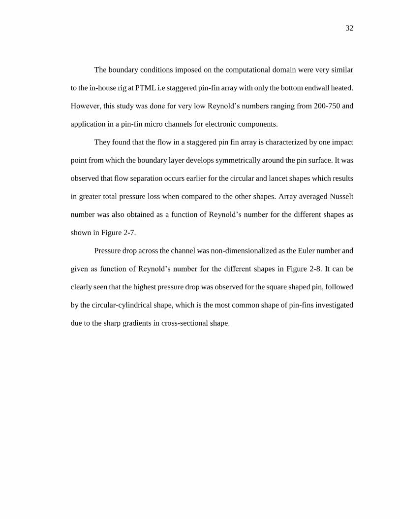
The boundary conditions imposed on the computational domain were very similar

to the in-house rig at PTML i.e staggered pin-fin array with only the bottom endwall heated.

However, this study was done for very low Reynold’s numbers ranging from 200-750 and

application in a pin-fin micro channels for electronic components.

They found that the flow in a staggered pin fin array is characterized by one impact

point from which the boundary layer develops symmetrically around the pin surface. It was

observed that flow separation occurs earlier for the circular and lancet shapes which results

in greater total pressure loss when compared to the other shapes. Array averaged Nusselt

number was also obtained as a function of Reynold’s number for the different shapes as

shown in Figure 2-7.

Pressure drop across the channel was non-dimensionalized as the Euler number and

given as function of Reynold’s number for the different shapes in Figure 2-8. It can be

clearly seen that the highest pressure drop was observed for the square shaped pin, followed

by the circular-cylindrical shape, which is the most common shape of pin-fins investigated

due to the sharp gradients in cross-sectional shape.

33

Figure 2-7. Array averaged Nu as a function of Re for different shapes.

(Sahiti et al., 2006)

Figure 2-8. Array averaged Eu as a function of Re for different shapes.

(Sahiti et al., 2006)

More recently, alternative pin geometries that are inspired by nature were also

investigated numerically by the author (Pai et al., 2017).

These designs were inspired by the shape of the harbor seal whisker as shown in

Figure 2-9. (NASA, 2014). The undulated shape of the whiskers results in reduced vortex

excitation and smaller, organized flow structures behind the whisker. (Hanke et al., 2010).

In its application to turbine blades, reduced aerodynamic loading and total pressure losses

have been observed (Shyam et al., 2015)

34

Figure 2-9. (a) Seal whisker (Hanke et al., 2010) and (b) Proposed bio-inspired cylinder.

(Pai et al., 2015).

Figure 2-10 shows the various alternate geometries considered for this study.

Figure 2-10. Alternate geometries considered for the study. (Pai et al., 2017)

The bio-cylinders analyzed in this study were adapted from models described in the

literature. The heat transfer and pressure loss characteristics were compared to baseline

circular and elliptical models for two Reynold's numbers. The BP2 geometry performed

better as compared to the circular baseline and other models in terms of heat transfer

enhancement by about 5% while EP1, the baseline elliptical model performed the best in

terms of thermal performance at constant pumping power. It should be noted that all the

alternative geometries (EP1, BP1, BP2, BP3) showcased significantly less pressure loss as

compared to the circular baseline case (CP1).

(a) (b)

35

3. Problem Statement

As we saw in the previous section, researchers have been using different thermal

boundary conditions when studying the thermal performance of pin-fin arrays. Since the

flow in an internal cooling channel of a gas turbine blade is turbulent, the heat transfer

characteristics are highly dependent on the fluid properties i.e. Reynold’s number and

Prandtl number and show very weak dependency on the thermal boundary condition

(Bejan, 2003). Each boundary condition arrangement has corresponding advantages as well

as ensuing complexity in the experimental setup. The reason for using different thermal

boundary conditions is to simplify the complicated experimental setup and as well as to

compensate for manufacturing limitations. In most of the experiments, either the pin is

heated or the endwall.

Since the flow-field in a pin-fin cooling channel is highly complex and non-

uniform, many thermocouples would need to be attached to obtain data from the entire test

surface. The use of thermocouples is accompanied by additional machining of holes on the

pin and endwalls. Often, additional thermocouples are attached in the event of failure of

the original thermocouple. Thus, for a pin-fin array, use of thermocouples is accompanied

by large setting up times due to the additional machining that is required. Internal heat

generation within the pin is required to maintain a sufficient temperature difference

between the pin surface and coolant, reducing experimental uncertainty.

Thus, certain simplifications can be made either on the experimental side or the

post-processing side for the ease and shorter turn-around times of testing. Validation tests

need to be done with well-established experiments. In terms of the design process,

experimental verification is the step following the elimination of the initial geometries

36

through numerical simulations. As we can see, there is a need for predicting average heat

transfer coefficients on the surface of a fin through non-intrusive techniques to reduce the

turnaround times associated with experimental setup.

The hypothesis of this study is that the base temperature of the pin can be used to

obtain accurate pin surface average heat transfer coefficients. The new method prescribed

in this thesis aims to simplify the setting up process at the cost of additional post-processing

complexity.

The 3 major objectives of this thesis are listed below:

1) Obtain analytical solution and validate with existing solution.

First, an analytical solution is obtained for the unique boundary conditions of the

in-house experimental setup. This solution is then validated by comparing it with

an existing solution for an infinite fin with internal heat generation Bejan (2003).

2) Verify numerically using CFD

The analytical solution is then verified numerically in STAR-CCM+ first by using

a prescribed pin surface heat transfer coefficient and for a second case of conjugate

heat transfer, both for a single pin in an internal channel.

3) Verify experimentally and compare with Ames' paper (2006)

After the analytical solution is verified analytically and numerically, the in-house

experimental setup is used to further establish confidence in the method by

comparing generated results to the results given by Ames (2006). This paper was

chosen to compare our results due to the similarity between experimental setups.

37

4. Methodology

4.1 Experimental Setup

The test section, shown in Figure 4-1, is manufactured from 2.54cm (1”) thick

optically clear acrylic. Figure 4-1 also shows the sCMOS camera used for recording TSP

emission, the TSP excitation LED lights along with the current source. The working of

TSP is detailed in the next section. Acrylic was chosen as it allows suitable optical access

for TSP measurements, as well as its insulation properties. The current pin-fin array

consists of 8 rows, having 7 full cylindrical, aluminum pins in each row arranged in a

staggered manner. The arrangement for this study was also used for previous investigations

by Fernandes (2015) and Prasad (2016).

Figure 4-1. Experimental Setup.

Figure 4-2 shows the schematic of the flow loop used for the experiments. The

centrifugal blower was operated in suction mode for all experiments. The flow was

controlled using gate valves. The venture flow meter gave the difference in pressure

38

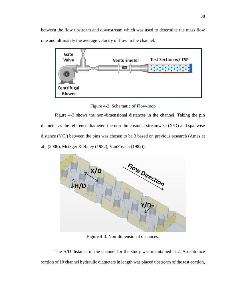
between the flow upstream and downstream which was used to determine the mass flow

rate and ultimately the average velocity of flow in the channel.

Figure 4-2. Schematic of Flow-loop

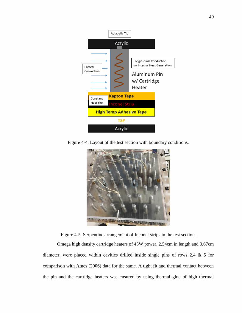
Figure 4-3 shows the non-dimensional distances in the channel. Taking the pin

diameter as the reference diameter, the non-dimensional streamwise (X/D) and spanwise

distance (Y/D) between the pins was chosen to be 3 based on previous research (Ames et

al., (2006), Metzger & Haley (1982), VanFossen (1982)).

The H/D distance of the channel for the study was maintained at 2. An entrance

section of 10 channel hydraulic diameters in length was placed upstream of the test-section,

H/D

Y/D

X/D

Figure 4-3. Non-dimensional distances.

39

and an exit section of 5 channel hydraulic diameters was placed downstream. From the exit

section, a transition duct was used to adapt the rectangular duct to circular PVC piping.

This PVC piping connected the tunnel to a centrifugal blower was in operation under

suction mode as seen in Figure 4-1 and Figure 4-2. Adiabatic inlet and outlet sections of

10 and 5 hydraulic diameters respectively, are attached just upstream and downstream of

the test section.

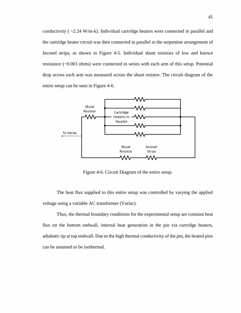
Figure 4-4 shows a cross sectional view of the layout in the test section with a single

pin. The thickness of the strips under the pin are exaggerated here for clarity. The pin is

held between the two acrylic endwalls and the pin tip is flush fit into a cavity machined on

the top endwall. The pins can be made of conducting (thermally active) or non-conducting

material. For this study, they were manufactured from aluminum. The size of the pin was

such that the Biot number was less than 1 and hence temperature distribution within the

pin was uniform. The inner side of the heated wall of the test section was painted with TSP.

Inconel strips were attached in series in a serpentine manner with the help of copper bus

bars at the ends using a high temperature adhesive tape to provide a constant heat flux

boundary at the wall as shown in Figure 4-4 for an investigation of a rib channel at the

same facility (Prasad, 2016). The width of the Inconel strips was equal to the diameter of

the pin placed on it (0.015m).

Kapton tape was used to prevent electrical contact wherever the pins were in contact

with the Inconel strips on the bottom endwall. The Kapton and adhesive tape are 0.03mm

and 0.02mm thick respectively, yielding a negligible temperature drop under normal

operating conditions (estimated to be < 0.1°C for a typical high heat flux case).

40

Figure 4-4. Layout of the test section with boundary conditions.

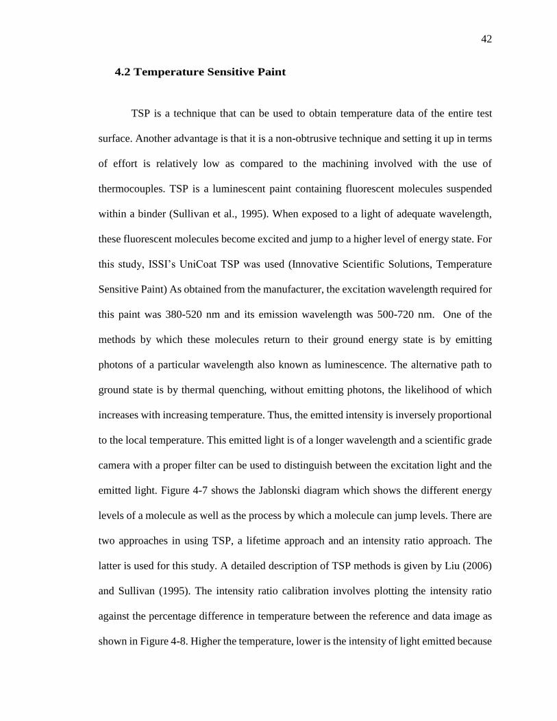
Figure 4-5. Serpentine arrangement of Inconel strips in the test section.

Omega high density cartridge heaters of 45W power, 2.54cm in length and 0.67cm

diameter, were placed within cavities drilled inside single pins of rows 2,4 & 5 for

comparison with Ames (2006) data for the same. A tight fit and thermal contact between

the pin and the cartridge heaters was ensured by using thermal glue of high thermal

41

conductivity ( ~2.24 W/m-k). Individual cartridge heaters were connected in parallel and

the cartridge heater circuit was then connected in parallel to the serpentine arrangement of

Inconel strips, as shown in Figure 4-5. Individual shunt resistors of low and known

resistance (~0.003 ohms) were connected in series with each arm of this setup. Potential

drop across each arm was measured across the shunt resistor. The circuit diagram of the

entire setup can be seen in Figure 4-6.

Figure 4-6. Circuit Diagram of the entire setup.

The heat flux supplied to this entire setup was controlled by varying the applied

voltage using a variable AC transformer (Variac).

Thus, the thermal boundary conditions for the experimental setup are constant heat

flux on the bottom endwall, internal heat generation in the pin via cartridge heaters,

adiabatic tip at top endwall. Due to the high thermal conductivity of the pin, the heated pins

can be assumed to be isothermal.

42

4.2 Temperature Sensitive Paint

TSP is a technique that can be used to obtain temperature data of the entire test

surface. Another advantage is that it is a non-obtrusive technique and setting it up in terms

of effort is relatively low as compared to the machining involved with the use of

thermocouples. TSP is a luminescent paint containing fluorescent molecules suspended

within a binder (Sullivan et al., 1995). When exposed to a light of adequate wavelength,

these fluorescent molecules become excited and jump to a higher level of energy state. For

this study, ISSI’s UniCoat TSP was used (Innovative Scientific Solutions, Temperature

Sensitive Paint) As obtained from the manufacturer, the excitation wavelength required for

this paint was 380-520 nm and its emission wavelength was 500-720 nm. One of the

methods by which these molecules return to their ground energy state is by emitting

photons of a particular wavelength also known as luminescence. The alternative path to

ground state is by thermal quenching, without emitting photons, the likelihood of which

increases with increasing temperature. Thus, the emitted intensity is inversely proportional

to the local temperature. This emitted light is of a longer wavelength and a scientific grade

camera with a proper filter can be used to distinguish between the excitation light and the

emitted light. Figure 4-7 shows the Jablonski diagram which shows the different energy

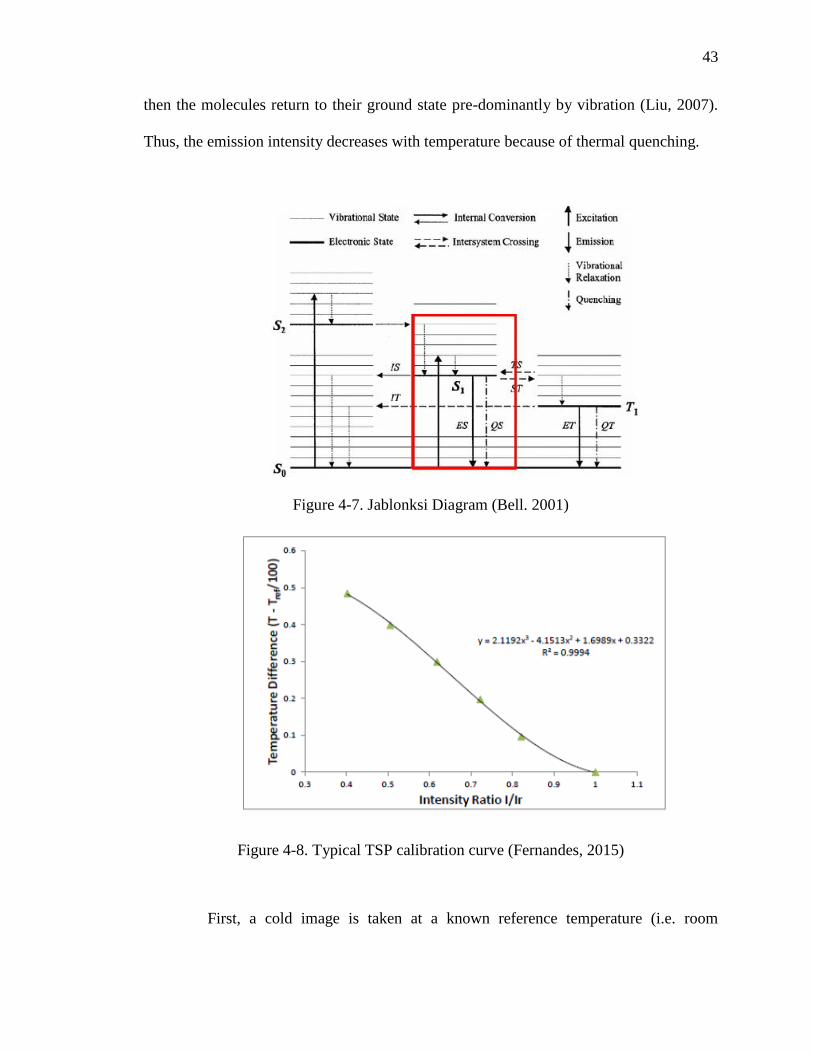
levels of a molecule as well as the process by which a molecule can jump levels. There are

two approaches in using TSP, a lifetime approach and an intensity ratio approach. The

latter is used for this study. A detailed description of TSP methods is given by Liu (2006)

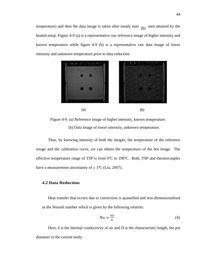
and Sullivan (1995). The intensity ratio calibration involves plotting the intensity ratio

against the percentage difference in temperature between the reference and data image as

shown in Figure 4-8. Higher the temperature, lower is the intensity of light emitted because

43

then the molecules return to their ground state pre-dominantly by vibration (Liu, 2007).

Thus, the emission intensity decreases with temperature because of thermal quenching.

Figure 4-7. Jablonksi Diagram (Bell. 2001)

Figure 4-8. Typical TSP calibration curve (Fernandes, 2015)

First, a cold image is taken at a known reference temperature (i.e. room

44

temperature) and then the data image is taken after steady state has been attained by the

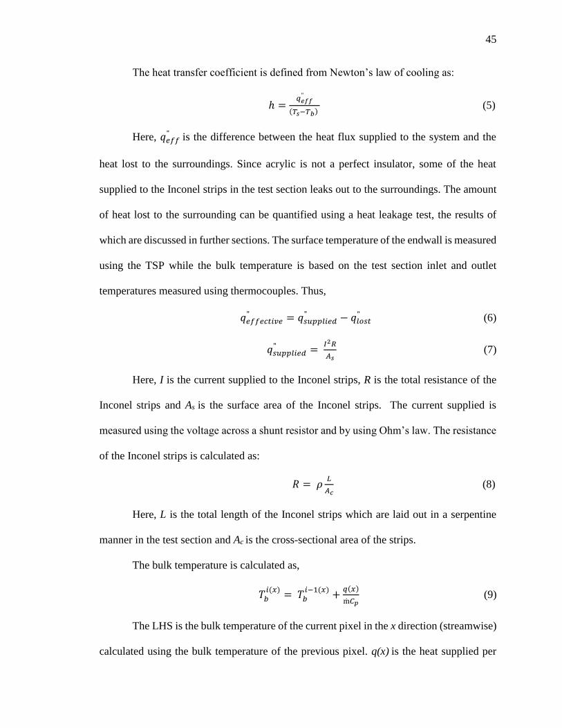
heated setup. Figure 4-9 (a) is a representative raw reference image of higher intensity and

known temperature while figure 4-9 (b) is a representative raw data image of lower

intensity and unknown temperature prior to data reduction.

Figure 4-9. (a) Reference image of higher intensity, known temperature.

(b) Data image of lower intensity, unknown temperature.

Thus, by knowing intensity of both the images, the temperature of the reference

image and the calibration curve, we can obtain the temperature of the hot image. The

effective temperature range of TSP is from 0ºC to 100ºC. Both, TSP and thermocouples

have a measurement uncertainty of ± 1ºC (Liu, 2007).

4.2 Data Reduction

Heat transfer that occurs due to convection is quantified and non-dimensionalised

as the Nusselt number which is given by the following relation:

𝑁𝑢 =ℎ𝐷

𝑘 (4)

Here, k is the thermal conductivity of air and D is the characteristic length, the pin

diameter in the current study.

(a)

(b)

(b)

45

The heat transfer coefficient is defined from Newton’s law of cooling as:

ℎ =𝑞𝑒𝑓𝑓

"

(𝑇𝑠−𝑇𝑏) (5)

Here, 𝑞𝑒𝑓𝑓" is the difference between the heat flux supplied to the system and the

heat lost to the surroundings. Since acrylic is not a perfect insulator, some of the heat

supplied to the Inconel strips in the test section leaks out to the surroundings. The amount

of heat lost to the surrounding can be quantified using a heat leakage test, the results of

which are discussed in further sections. The surface temperature of the endwall is measured

using the TSP while the bulk temperature is based on the test section inlet and outlet

temperatures measured using thermocouples. Thus,

𝑞𝑒𝑓𝑓𝑒𝑐𝑡𝑖𝑣𝑒" = 𝑞𝑠𝑢𝑝𝑝𝑙𝑖𝑒𝑑

" − 𝑞𝑙𝑜𝑠𝑡" (6)

𝑞𝑠𝑢𝑝𝑝𝑙𝑖𝑒𝑑" =

𝐼2𝑅

𝐴𝑠 (7)

Here, I is the current supplied to the Inconel strips, R is the total resistance of the

Inconel strips and As is the surface area of the Inconel strips. The current supplied is

measured using the voltage across a shunt resistor and by using Ohm’s law. The resistance

of the Inconel strips is calculated as:

𝑅 = 𝜌𝐿

𝐴𝑐 (8)

Here, L is the total length of the Inconel strips which are laid out in a serpentine

manner in the test section and Ac is the cross-sectional area of the strips.

The bulk temperature is calculated as,

𝑇𝑏𝑖(𝑥)

= 𝑇𝑏𝑖−1(𝑥)

+𝑞(𝑥)

m𝐶𝑝 (9)

The LHS is the bulk temperature of the current pixel in the x direction (streamwise)

calculated using the bulk temperature of the previous pixel. q(x) is the heat supplied per

46

pixel, �� is the mass flow rate into the channel while Cp is the specific heat capacity of the

air based on the mean bulk temperature.

Mass flow rate through the channel was obtained by a venturi flow-meter of

diameter ~3”. This was calculated using a calibration curve supplied by the manufacturer

as shown in Figure 4-10. The accuracy as stated by the manufacturer was ±1% (Preso

Venturi SSM user manual). The mass flow rate through the pipe was dependent on the

difference in pressure, the density and temperature of the inlet air.

Figure 4-10. Pressure drop versus mass flow rate for the venturi-flowmeter.

Using the mass flow rate obtained, the Reynolds number through the channel is

given by,

𝑅𝑒 =��𝐷

𝜇𝐴𝑐𝑒𝑓𝑓 (10)

D here is the pin diameter while Aceff is the effective cross-sectional area between

the pins. The effective cross-sectional area is the same one used by Ames (2006) that is the

47

difference between the open channel area and the frontal area of a single row of pins.

As mentioned earlier, measurement uncertainty of a thermocouple and TSP is ±

1ºC. From equation (5), for a constant wall heat flux and a temperature difference of 20ºC,

error in h is already around 10%. Previous investigations (Prasad, 2016) have also shown

the reduced uncertainty in Nusselt number for a higher temperature difference. Thus, we

need to ensure that the surface temperature is higher than the bulk flow temperature by at

least 20ºC to reduce our experimental uncertainty in determination of h. After repeated

tests, it has also been found that due to lateral conduction and high heat transfer rates

around the pin surface, pin temperatures cannot be raised adequately higher than bulk flow

temperatures. Hence, we need to raise the surface temperature of the pin through internal

heat generation via the use of cartridge heaters. This will be empirically proven in section

7.1. The heat generated by the cartridge heaters is assumed to be the internal heat generated

within the pin. Hence, the reference volume while calculating the internal heat generated

per unit volume is the pin volume. This is calculated as;

�� = 𝐼2𝑅𝐶ℎ

𝑉𝑝𝑖𝑛 (11)

Here, �� is the internal heat generated per unit volume for a single pin. I is the current

supplied to the individual cartridge heater. This is measured using the shunt resistor

connected in series to the cartridge heaters in parallel. Vpin is the volume of the cylindrical

pin. The current measured by the two shunt resistors (cartridge heaters in parallel + Inconel

strips) is added and verified with the total current supplied & obtained from the ammeter

of the Variac.

48

4.2 CFD- Setup and Boundary Conditions

A simple, single pin model was created in STAR-CCM+ to verify the analytical

solution numerically. It should be noted that the numerical simulation was run to verify the

underlying hypothesis of our analytical methodology and not to verify the accuracy of the

results obtained through simulation. The hypothesis being, the pin base temperature can be

used to obtain pin surface average Nusselt number. Hence, a mesh independence test was

not carried out.

As a first check to verify the analytical solution obtained in Section 5, a simulation

was run with a specified heat transfer coefficient on the surface of the solid aluminum pin.

The parameters used were the same as the one used in our experimental setup. A constant

heat transfer coefficient on the pin surface with a constant heat flux at the base, internal

heat generation within the pin and an adiabatic tip were the boundary conditions imposed

for this case. The purpose of this simulation was to examine the pin base temperature

obtained if all the assumptions made for the analytical solution were still valid. The second

step was to do a conjugate heat transfer (CHT) analysis on a single pin in an internal

channel having the same parameters as the 1st case. For the CHT case, we solve both the

conduction and convection equations simultaneously. The local velocities and transport

variables in this case are obtained by solving the Reynold’s Averaged Navier-Stokes

(RANS) equations. A detailed description of the Navier-Stokes equations can be found in

standard fluid mechanics reference books. The RANS approach models turbulence by

averaging the unsteadiness of the turbulence. Since we average the unsteadiness of the

turbulence, this method is not as resource intensive as DNS & LES. Equation (12) is the

RANS equation where the fluid properties, u and p are expressed as a sum of the mean and

49

fluctuating components.

𝜕(𝜌𝑢𝑖)

𝜕𝑥+

𝜕(𝜌𝑢𝑖𝑢𝑗+𝜌𝑢𝑖′𝑢𝑗

′ )

𝜕𝑥= −

𝜕��

𝜕𝑥+

𝛿

𝛿𝑥𝑗[µ (

𝛿𝑢𝑖

𝛿𝑥𝑗+

𝛿𝑢𝑗

𝛿𝑥𝑖)] (12)

The quantity 𝑢𝑖′𝑢𝑗

′ is known as the Reynolds stress tensor which is symmetric and

has six components. Thus, by decomposing the fluid properties into a sum of mean and

fluctuating values gives rise to additional unknown quantities with no new equations.

Hence, to close the system of equations, we include a few equations which are known as

turbulence model equations. Previous efforts (Fernandes et al, 2015) have shown that the

shear stress transport (SST) k-ω turbulence model yields the most accurate predictions of

pin-fin thermal performance, as compared against experimental results and hence is the

choice of turbulence model here. The two additional equations in this model which helps

us close the RANS equations are given by Equations (13) & (14) below,

𝜕𝑘

𝜕𝑡+ 𝑈𝑗

𝛿𝑘

𝛿𝑥𝑗= 𝜏𝑖𝑗

𝜕𝑈𝑖

𝜕𝑥𝑗− 𝛽∗𝑘𝜔 +

𝛿

𝛿𝑥𝑗[(𝜈 + 𝜎∗𝜈𝑇)

𝛿𝑘

𝛿𝑥𝑗] (13)

𝜕𝜔

𝜕𝑡+ 𝑈𝑗

𝛿𝜔

𝛿𝑥𝑗=

𝛼𝜔

𝑘𝜏𝑖𝑗

𝜕𝑈𝑖

𝜕𝑥𝑗− 𝛽𝜔2 +

𝛿

𝛿𝑥𝑗[(𝜈 + 𝜎𝜈𝑇)

𝛿𝜔

𝛿𝑥𝑗] (14)

Figure 4-11 shows the boundary conditions applied for the CHT case.

Figure 4-11. Boundary Conditions for the CHT case.

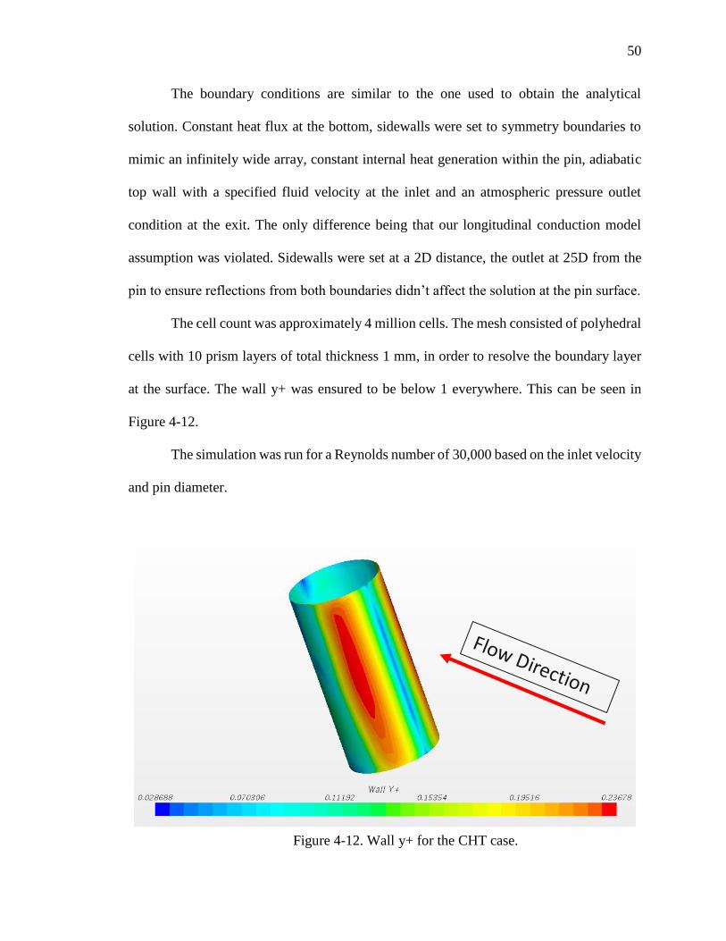
50

The boundary conditions are similar to the one used to obtain the analytical

solution. Constant heat flux at the bottom, sidewalls were set to symmetry boundaries to

mimic an infinitely wide array, constant internal heat generation within the pin, adiabatic

top wall with a specified fluid velocity at the inlet and an atmospheric pressure outlet

condition at the exit. The only difference being that our longitudinal conduction model

assumption was violated. Sidewalls were set at a 2D distance, the outlet at 25D from the

pin to ensure reflections from both boundaries didn’t affect the solution at the pin surface.

The cell count was approximately 4 million cells. The mesh consisted of polyhedral

cells with 10 prism layers of total thickness 1 mm, in order to resolve the boundary layer

at the surface. The wall y+ was ensured to be below 1 everywhere. This can be seen in

Figure 4-12.

The simulation was run for a Reynolds number of 30,000 based on the inlet velocity

and pin diameter.

Figure 4-12. Wall y+ for the CHT case.

51

5. Extended Surface Methodology (ESM)

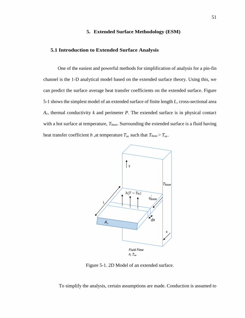
5.1 Introduction to Extended Surface Analysis

One of the easiest and powerful methods for simplification of analysis for a pin-fin

channel is the 1-D analytical model based on the extended surface theory. Using this, we

can predict the surface average heat transfer coefficients on the extended surface. Figure

5-1 shows the simplest model of an extended surface of finite length L, cross-sectional area

Ac, thermal conductivity k and perimeter P. The extended surface is in physical contact

with a hot surface at temperature, Tbase. Surrounding the extended surface is a fluid having

heat transfer coefficient h ,at temperature 𝑇∞ such that Tbase > 𝑇∞.

Figure 5-1. 2D Model of an extended surface.

To simplify the analysis, certain assumptions are made. Conduction is assumed to

52

be only in the longitudinal direction i.e. only along the fin length even though the

conduction is two dimensional. However, the conduction in the lateral direction is

negligible enough to be ignored. Other assumptions are steady state conditions, constant

thermal conductivity, negligible radiation, no heat generation within the pin and the heat

transfer co-efficient is uniform over the surface.

With these assumptions, by doing a simple energy balance over an elemental cut-

section of length dx & using equations (2) and (3), we obtain this general governing

equation for an extended surface,

𝑑2𝜃

𝑑𝑥2 − 𝑚2𝜃 = 0 (15)

where 𝑚 = √ℎ𝑃

𝑘𝐴𝑐 & 𝜃(𝑥) = 𝑇(𝑥) − 𝑇∞

m is known as the fin parameter and 𝜃 is the excess temperature function.

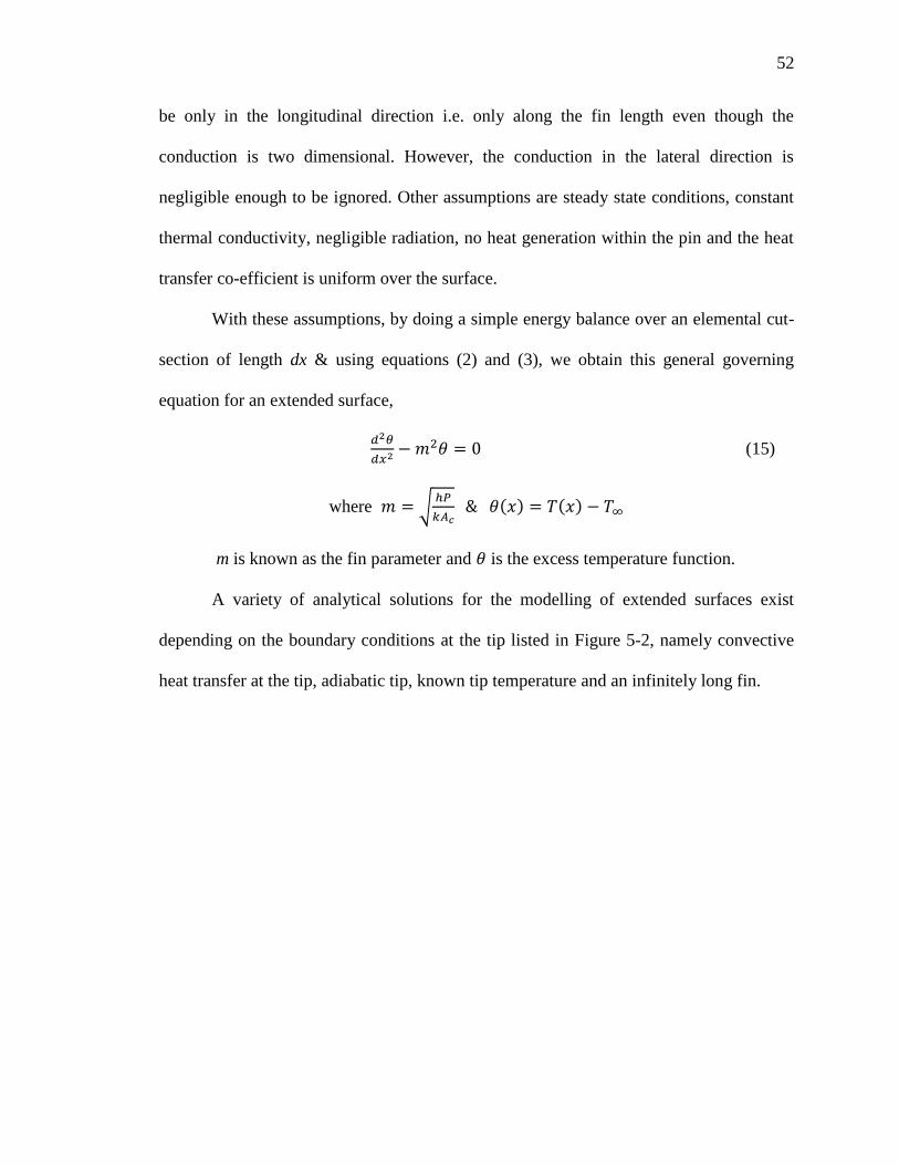
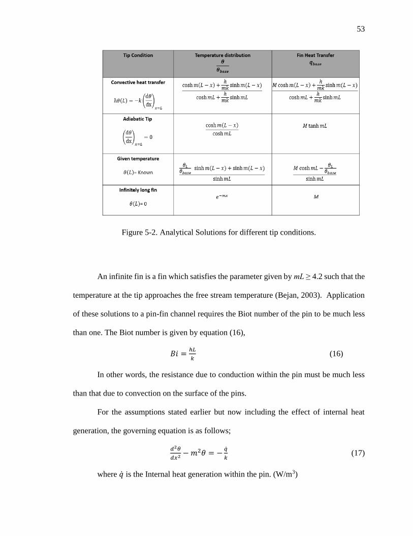
A variety of analytical solutions for the modelling of extended surfaces exist

depending on the boundary conditions at the tip listed in Figure 5-2, namely convective

heat transfer at the tip, adiabatic tip, known tip temperature and an infinitely long fin.

53

Figure 5-2. Analytical Solutions for different tip conditions.

An infinite fin is a fin which satisfies the parameter given by mL ≥ 4.2 such that the

temperature at the tip approaches the free stream temperature (Bejan, 2003). Application

of these solutions to a pin-fin channel requires the Biot number of the pin to be much less

than one. The Biot number is given by equation (16),

𝐵𝑖 =ℎ𝐿

𝑘 (16)

In other words, the resistance due to conduction within the pin must be much less

than that due to convection on the surface of the pins.

For the assumptions stated earlier but now including the effect of internal heat

generation, the governing equation is as follows;

𝑑2𝜃

𝑑𝑥2 − 𝑚2𝜃 = −��

𝑘 (17)

where �� is the Internal heat generation within the pin. (W/m3)

54

The solution (Bejan, 2003) for such a system is given for an infinitely fin as,

𝜃(𝑥) = 𝜃𝑏𝑒−𝑚𝑥 +��

𝑘𝑚2(1 − 𝑒−𝑚𝑥) (18)

In the next section, a solution for a finite length fin with internal heat generation is

derived which is representative of our experimental setup.

5.2 Derivation of Analytical Solution

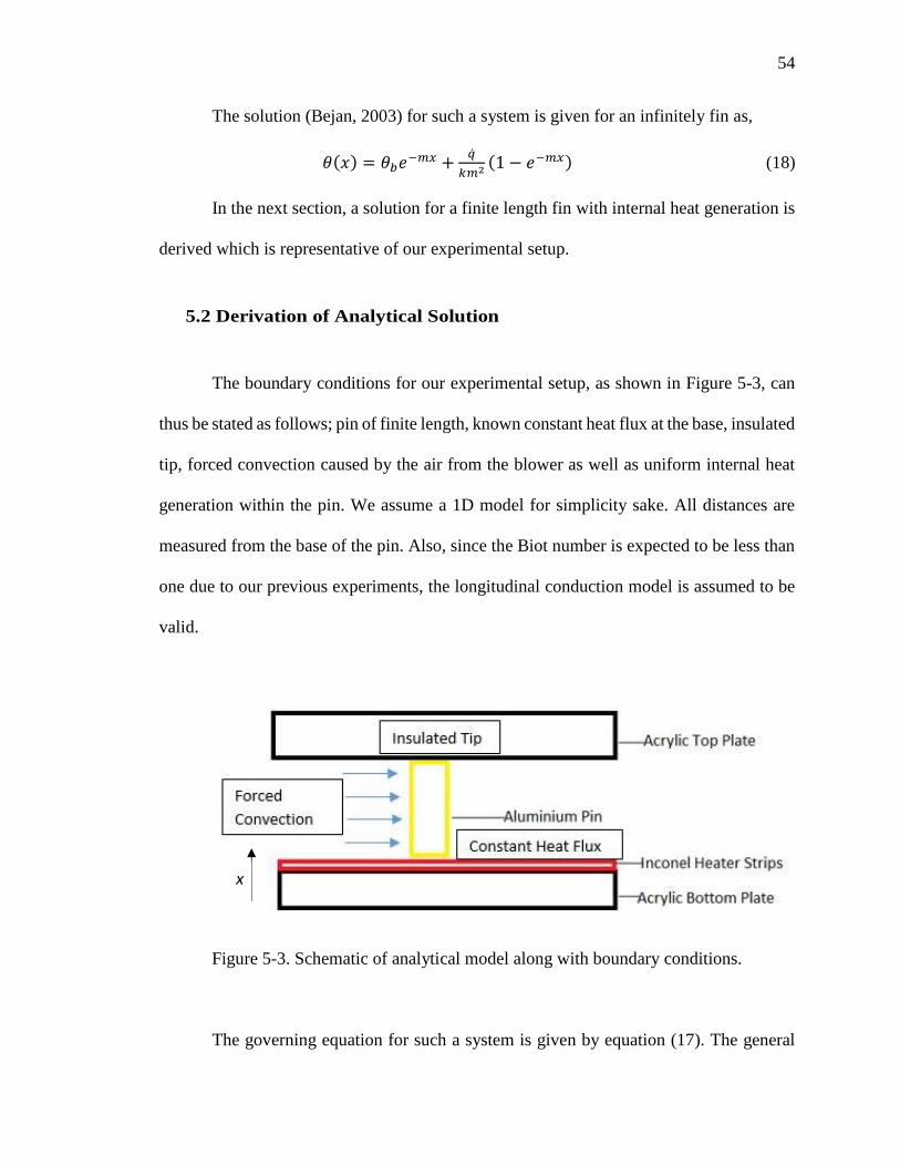
The boundary conditions for our experimental setup, as shown in Figure 5-3, can

thus be stated as follows; pin of finite length, known constant heat flux at the base, insulated

tip, forced convection caused by the air from the blower as well as uniform internal heat

generation within the pin. We assume a 1D model for simplicity sake. All distances are

measured from the base of the pin. Also, since the Biot number is expected to be less than

one due to our previous experiments, the longitudinal conduction model is assumed to be

valid.

Figure 5-3. Schematic of analytical model along with boundary conditions.

The governing equation for such a system is given by equation (17). The general

x

55

solution is obtained by solving the above equation using the Method of Annihilators;

𝜃(𝑥) = 𝑐1𝑒𝑚𝑥 + 𝑐2𝑒−𝑚𝑥 + 𝑐3 (19)

The boundary conditions can be expressed mathematically as;

@ 𝑥 = 0, − 𝑘𝑑𝜃

𝑑𝑥= 𝑞𝑏

" @ 𝑥 = 𝐿, 𝑑𝜃

𝑑𝑥= 0 (20)

Using the boundary conditions, we can solve for the constants and the solution for

such a system is obtained as:

𝜃(𝑥) =(𝑞𝑏

" .𝑒𝑚𝑥−2𝑚𝐿+𝑞𝑏" .𝑒−𝑚𝑥)

𝑘𝑚(1−𝑒−2𝑚𝐿)−

��

𝑘𝑚2 (21)

This gives us the temperature distribution along the length of the pin. Inversely,

using an iterative method and the known values of heat flux and temperature at the base,

we can calculate the surface average pin heat transfer co-efficient. The solution is later

verified against equation (18) in section 6.1

56

6. Results & Discussion

6.1 Analytical Verification Results

To verify the analytical solution obtained in section 5.2, it was compared to the

standard solution presented in heat transfer handbooks for a fin of infinite length with

similar boundary conditions.(Bejan, 2003) The solution for a fin of infinite length with

constant heat flux at the base is given by equation (18).

However, it should be noted that equation (18) is a solution for a pin of infinite length

and hence to compare with equation (21), the current model was implemented with the

condition mL ≥ 4.2 Table 1 lists the parameters used for the comparison between the two

solutions. These parameters are representative of our experimental setup.

Using the parameters listed in Table 6-1, taking the infinite length to be 0.3m , we

observe that our analytical solution matches that of Bejan’s exactly, as shown in Figure 6-

1.

Table 6-1. Pin parameters

Pin diameter (D) 0.015 m

Actual Pin height

0.03 m

Infinite Fin Approximation

height (L)

0.3 m

h 200 W/m2-K

k (aluminum) 205 W/m-K

T∞ 300 K

𝒒𝒃" 3200 W/m2

Bi 0.00297

�� 3.116 W/m3

57

Figure 6-1. Verification of Analytical solution w/ standard solution for infinite fin.

Using the parameters listed in Table 1, and taking the pin to be of finite length,

temperature distribution along the pin height was obtained with and without internal heat

generation as shown in Figure 6-2 & 6-3 . We can see that with internal heat generation,

the pin surface temperature is ~20ºC higher than the free-stream temperature, with a

variation of 0.3ºC from the base to the pin, due to the low Biot number.

Thus, as mentioned earlier internal heat generation is necessary in order to

sufficiently raise the pin surface temperatures above the freestream.

358.2

358.4

358.6

358.8

359

359.2

359.4

359.6

0 0.1 0.2 0.3

Tem

pe

ratu

re, K

Distance along pin height, m

Insulated Tip

Infinite Fin Approximation

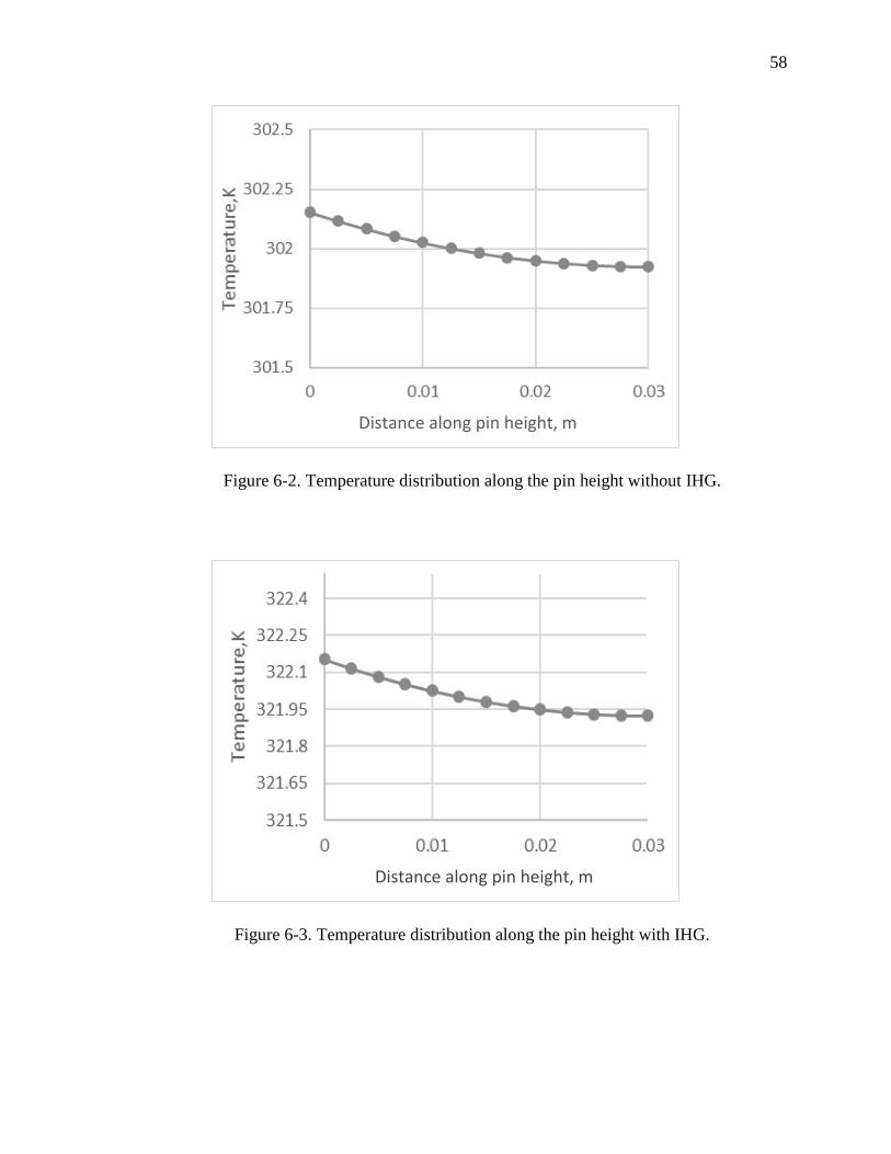
58

Figure 6-2. Temperature distribution along the pin height without IHG.

Figure 6-3. Temperature distribution along the pin height with IHG.

Distance along pin height, m

Distance along pin height, m

59

6.2 Computational Verification Results

First, the pin surface average Nusselt number was obtained from the simulation.

Second, the average base temperature of the pin as obtained from the simulation was input

into the non-linear equation (21) and solved iteratively using MATLAB® to obtain the

surface average heat transfer coefficient. This heat transfer coefficient was then non-

dimensionalised as the Nusselt number and compared with the value obtained from the

simulation. The initial guess for the non-linear equation was obtained from the theoretical

fin parameter based on previous experimentation i.e values in Table 1. It was found that

the solution was not dependent on the initial guess for the non-linear equation since

MATLAB® uses a Trust-region Dogleg method (MathWorks Documentation, MATLAB

2015b, 2015). More information on this method can be found in the user document.

As we can see from Table 6-2, the pin surface averaged Nusselt number obtained

from our analytical methodology is in close agreement with the value obtained via CFD.

6.3 Experimental Verification Results

After the numerical verification was completed, the analytical methodology was

tested on a full-scale pin-fin channel. The setup of this entire rig is explained in an earlier

section. However, before running tests to prove our underlying hypothesis, certain tests

Table 6-2. Comparison with CFD

Case Surface Average Nu %

Error CFD ESM

Prescribed Nu 103 103.18 0.1748

CHT 102.99 101.08 1.8545

dfasf

60

were done to establish confidence in the results obtained from our measurement techniques.

6.3.1 Rig Validation- Intensity of Lights

One of the earliest tests done to validate our experimental setup was the intensity

of lights test. As mentioned earlier, temperatures are determined from TSP using the

intensity ratio of the reference and data image. The accuracy of the intensity captured is

dependent on the stability of the light intensity emitted by the light source, UV light in this

case. Readings would be consistent only if there is minimal fluctuation of intensity. Hence,

it is very important to know the time taken by the light to reach a stable intensity. The point

of this test was to establish a suitable “warm-up” time for the UV lights to reduce

uncertainty.

Figure 6-4 shows the intensity stabilization over time for one such test.

Figure 6-4. Intensity Stabilization over time

The UV light is shone upon a white paper such that it is uniformly illuminated. The

48600

48800

49000

49200

49400

49600

49800

50000

50200

50400

0 10 20 30 40 50 60

INTE

NSI

TY

TIME ELAPSED (MIN)

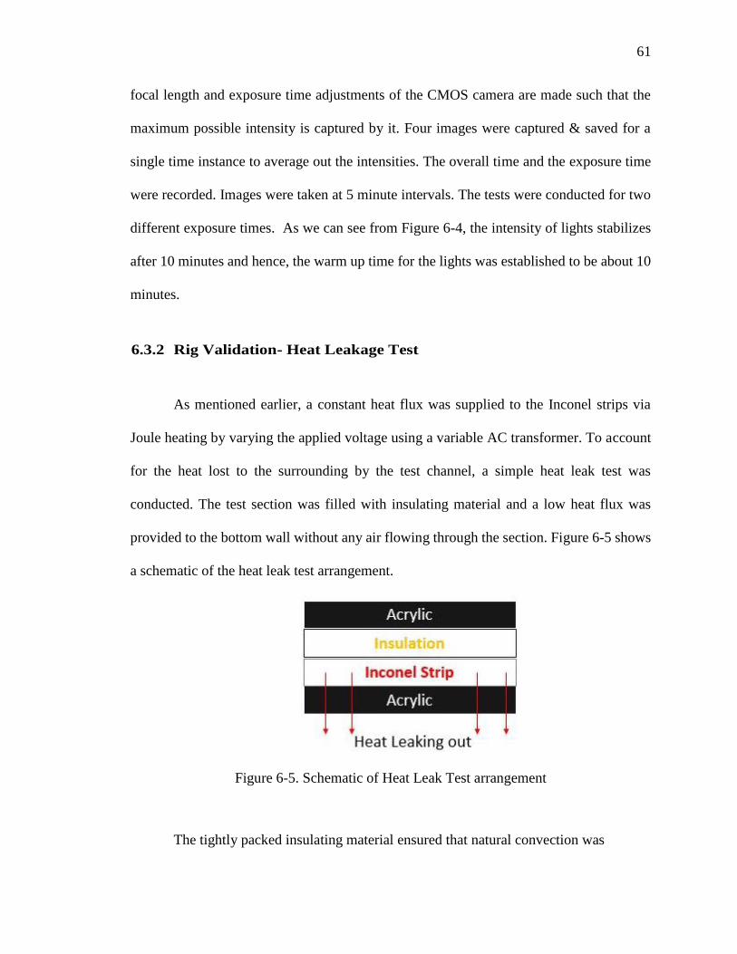
61

focal length and exposure time adjustments of the CMOS camera are made such that the

maximum possible intensity is captured by it. Four images were captured & saved for a

single time instance to average out the intensities. The overall time and the exposure time

were recorded. Images were taken at 5 minute intervals. The tests were conducted for two

different exposure times. As we can see from Figure 6-4, the intensity of lights stabilizes

after 10 minutes and hence, the warm up time for the lights was established to be about 10

minutes.

6.3.2 Rig Validation- Heat Leakage Test

As mentioned earlier, a constant heat flux was supplied to the Inconel strips via

Joule heating by varying the applied voltage using a variable AC transformer. To account

for the heat lost to the surrounding by the test channel, a simple heat leak test was

conducted. The test section was filled with insulating material and a low heat flux was

provided to the bottom wall without any air flowing through the section. Figure 6-5 shows

a schematic of the heat leak test arrangement.

Figure 6-5. Schematic of Heat Leak Test arrangement

The tightly packed insulating material ensured that natural convection was

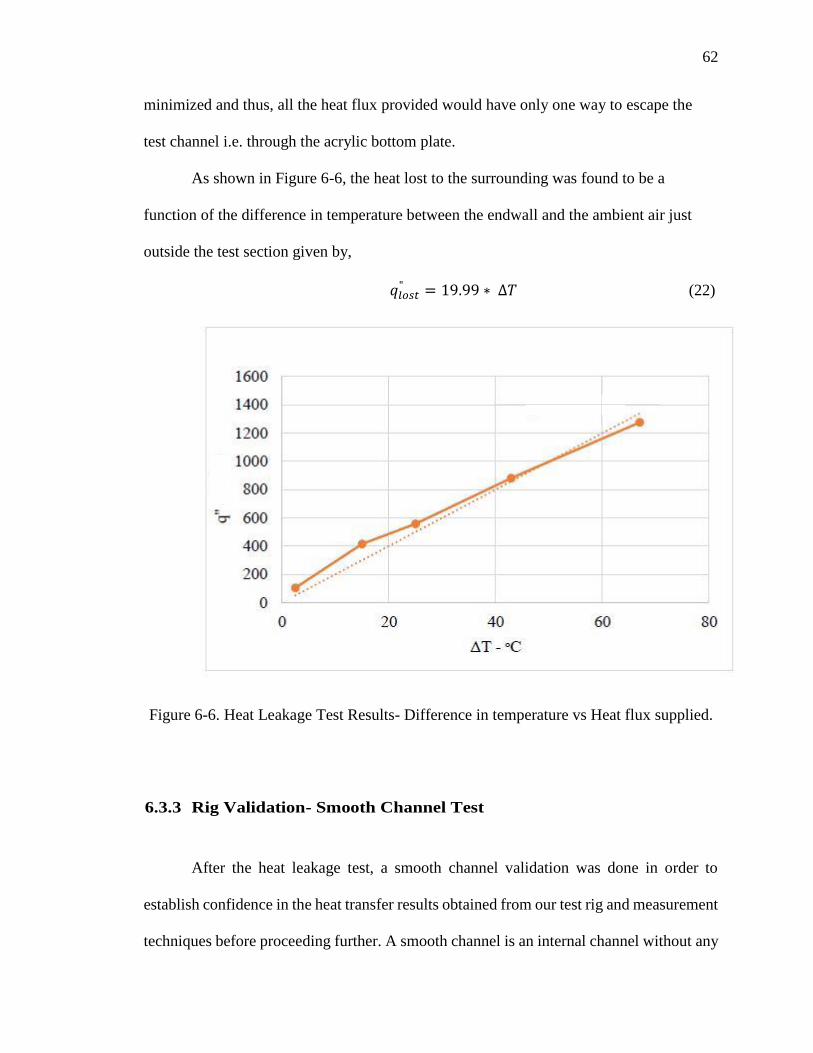
62

minimized and thus, all the heat flux provided would have only one way to escape the

test channel i.e. through the acrylic bottom plate.

As shown in Figure 6-6, the heat lost to the surrounding was found to be a

function of the difference in temperature between the endwall and the ambient air just

outside the test section given by,

𝑞𝑙𝑜𝑠𝑡" = 19.99 ∗ ∆𝑇 (22)

Figure 6-6. Heat Leakage Test Results- Difference in temperature vs Heat flux supplied.

6.3.3 Rig Validation- Smooth Channel Test

After the heat leakage test, a smooth channel validation was done in order to

establish confidence in the heat transfer results obtained from our test rig and measurement

techniques before proceeding further. A smooth channel is an internal channel without any

63

flow turbulators that help enhance heat transfer. The spanwise averaged Nusselt Number

for the smooth channel was compared to Gnielinski’s correlation for Nusselt number in a

smooth channel with fully developed flow for a Reynold’s number of 12,500 (Bejan, 2003)

as shown in Figure 6-7.

Since heating begins at the start of the test section, the impact of thermal

development of the flow is seen up to approximately at an X/D of 15. After this point, the

experimental spanwise average is in agreement with Gnielinski’s correlation given by

equation (20), well within ±12% of Gnielinski’s (1976) experimental uncertainty.

𝑁𝑢 =(

𝑓

8)(𝑅𝑒−1000)𝑃𝑟

1+12.7(𝑓

8)

0.5(𝑃𝑟

23−1)

(23)

where f is the Darcy friction factor given by,

𝑓 = (0.79 ln(𝑅𝑒) − 1.64)−2 (24)

Figure 6-7. Spanwise averaged smooth channel Nusselt number.

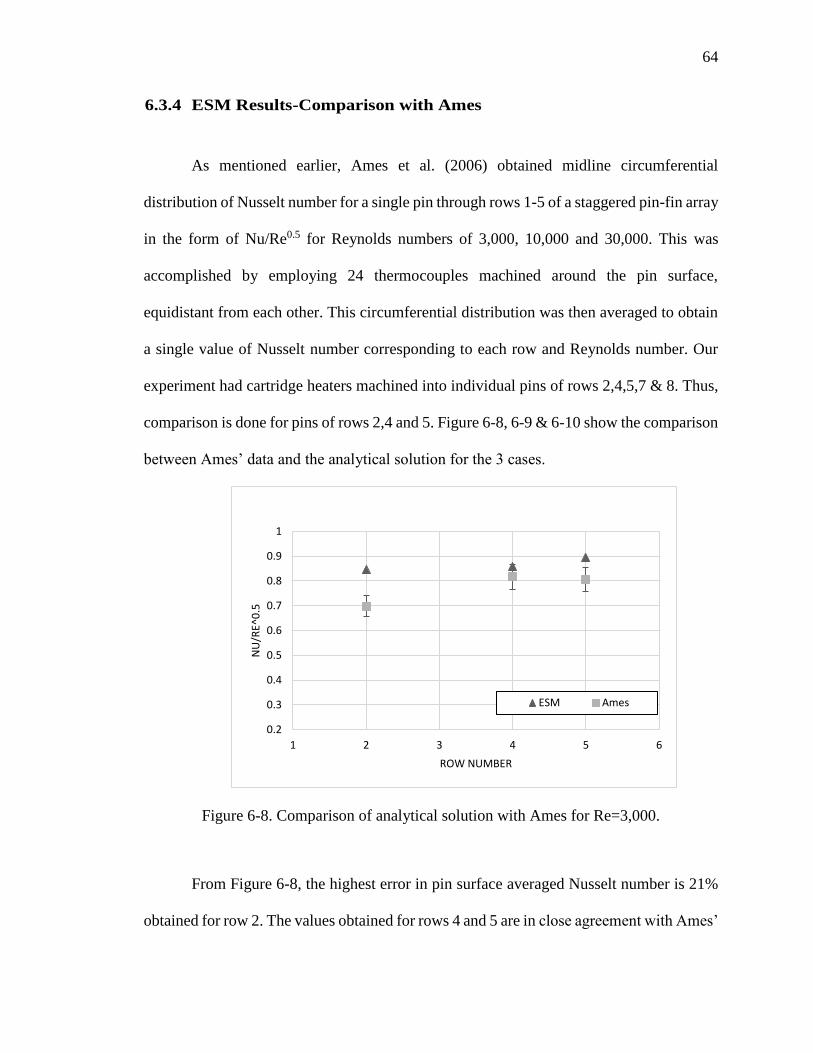
64

6.3.4 ESM Results-Comparison with Ames

As mentioned earlier, Ames et al. (2006) obtained midline circumferential

distribution of Nusselt number for a single pin through rows 1-5 of a staggered pin-fin array

in the form of Nu/Re0.5 for Reynolds numbers of 3,000, 10,000 and 30,000. This was

accomplished by employing 24 thermocouples machined around the pin surface,

equidistant from each other. This circumferential distribution was then averaged to obtain

a single value of Nusselt number corresponding to each row and Reynolds number. Our

experiment had cartridge heaters machined into individual pins of rows 2,4,5,7 & 8. Thus,

comparison is done for pins of rows 2,4 and 5. Figure 6-8, 6-9 & 6-10 show the comparison

between Ames’ data and the analytical solution for the 3 cases.

Figure 6-8. Comparison of analytical solution with Ames for Re=3,000.

From Figure 6-8, the highest error in pin surface averaged Nusselt number is 21%

obtained for row 2. The values obtained for rows 4 and 5 are in close agreement with Ames’

0.2

0.3

0.4

0.5

0.6

0.7

0.8

0.9

1

1 2 3 4 5 6

NU

/RE^

0.5

ROW NUMBER

ESM Ames

65

data having an error of ~8% on an average.

Figure 6-9. Comparison of analytical solution with Ames for Re=10,000.

Again, in Figure 6-9, we see that relatively, the highest error in surface averaged

Nusselt number is for row 2 as compared to Ames’ data. The percentage error for row 4 &

5 are 12% and 20% respectively.

Similar to the previous two Reynolds number cases, for Re=30,000, the highest

error in the surface averaged Nusselt number is observed for row 2, while row 4 and row

5 are in close agreement (~8%) with Ames’ experimental data, as can be seen in Figure 6-

10.

It is fairly evident from figures 6-8, 6-9 and 6-10 that the analytical solution has the

highest disagreement in row 2 for all Reynolds numbers. One of the possible reasons for

this discrepancy could be that Ames’ has a heated test entrance length, because of which

his flow is fully developed hydro-dynamically as well as thermally. Our experimental setup

does not have a heated entrance length and hence is not thermally full developed until the

0.2

0.3

0.4

0.5

0.6

0.7

0.8

0.9

1

1.1

1 2 3 4 5 6

NU

/RE^

0.5

ROW NUMBER

ESM Ames

66

second row.

Figure 6-10. Comparison of analytical solution with Ames for Re=30,000.

6.3.5 Channel Average Nusselt number Results

The channel average Nusselt number is an average of both, pins and endwall

values. Hence, endwall Nusselt numbers were also obtained for the three test cases.

Then, the pins and endwall Nusselt numbers were averaged into a single value to

obtain an average Nusselt number for the entire endwall and another for the pins.

Figure 6-11 is a raw image of the endwall Nusselt number contour for the

Reynold’s number of 30,000. The arrows indicate the regions of data that have

been ignored while calculating the average endwall Nusselt number. These are

regions of the through bolt washers, regions where the strips have peeled off

because of delamination as well as the areas between the strips which are unheated.

After repeated heated tests, the acrylic test section was found to warp in size. Since

0.2

0.3

0.4

0.5

0.6

0.7

0.8

0.9

1

1.1

1 2 3 4 5 6

NU

/RE^

0.5

ROW NUMBER

ESM Ames

67

the acrylic test section and the aluminum pins were machined to have a tight fit,

warping of the test section created a gap, forcing the pins to lose contact with the

Inconel strips. The through bolt and washer arrangement ensured physical contact

between the pin and the strips. The smearing of data around the pin locations are a

result of lateral conduction along the strips. These areas are ignored for this study

but for future investigations, these can be corrected for. Areas under the pin

represent the heat transfer that occurs due to the fin effect and hence have been

ignored. Encircled in the same figure, in rows 2,4,5,7 & 8 are the pins with cartridge

heaters machined in them. These are the pins used to compare the surface average

Nusselt numbers obtained from the analytical methodology with Ames et al. (2006).

The region within the dotted lines is the region considered for the averaging of

endwall Nusselt number.

Figure 6-11. Endwall Nusselt number contour for Re=30,000.

68

Figure 6-12 is a plot of various average Nusselt numbers for the different Reynold’s

number cases that were run, compared to some of the previous work done by researchers.

(Ames et al. (2007), Metzger et al. (1982), van Fossen(1982)) From this figure, it becomes

clear that the pin surface Nusselt numbers are higher than the endwall by 40% which is

consistent with previous findings (Chyu(1999), VanFossen(1981), Al Dabagh and

Andrews (1992)). It should be noted that pin average Nusselt number shown in the above

figure is an average of the three pins’ surface average Nusselt number that were obtained

using the analytical methodology in the previous section. The pin surface data from the

other rows were not considered while calculating this average since the pin surface data

was not collected at those rows. The author believes including that data would drive the

pin Nusselt number average lower than what they are currently. The experimental pin

average Nusselt number for the 3 Reynold’s number cases were compared to the correlation

given by VanFossen, 1981. Except for the Reynold’s number case of 30,000, the average

pin surface Nusselt number is higher than the value obtained by VanFossen for reasons

discussed earlier. The highest difference is found for the lowest Reynold’s number case.

Since the endwall has a much greater area as compared to the pin surface in totality,

it would be unfair to compare the channel average by simply taking an arithmetic average

of the average value of the two. The channel average Nusselt number data presented here

is thus an area weighted average, weighing in the contribution of the pin and endwall based

on corresponding area. From figure 6-11, we can see that the area weighted channel average

of the Nusselt number is in close agreement with both Ames’ and Metzger’s data. On an

average, the percentage difference was about 5% and 9% with Ames’s and Metzger’s

channel average Nusselt numbers. The highest difference with Ames’s data was observed

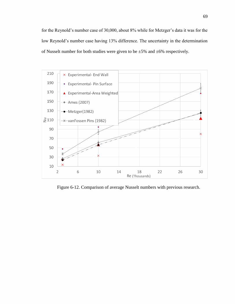
69

for the Reynold’s number case of 30,000, about 8% while for Metzger’s data it was for the

low Reynold’s number case having 13% difference. The uncertainty in the determination

of Nusselt number for both studies were given to be ±5% and ±6% respectively.

Figure 6-12. Comparison of average Nusselt numbers with previous research.

70

7. Conclusion

The purpose of this study was to provide a new methodology to obtain pin surface

average heat transfer coefficients in pin fin cooling experimentation by using non-intrusive

techniques such as TSP. This methodology was verified analytically, numerically as well

as experimentally. The hypothesis was that the base temperature of the pin can be used to

predict surface average heat transfer coefficients of the pins. The base temperature at the

pin was determined using TSP. This helps in reducing setting up times and complexity of

the experimentation at the cost of additional post processing efforts.

1. An analytical solution was obtained to do the same for the boundary conditions

common to pin fin cooling experimentation as well as the in-house experimental rig. The

analytical solution with a few minor modifications was verified after comparison with a

standard solution listed in heat transfer reference books. The need for raising the pin surface

temperature using internal heat generation via the use of cartridge heaters was also shown

by the analytical solution.

2. A conceptual validation of the method using CFD was also undertaken. Two

cases were run, first a conduction only case and second, a CHT case. Nusselt numbers

obtained using this analytical method were found to be within 2% of the simulation results.

3. For experimental validation, a study conducted by Ames et al, was chosen for

comparison. The reason being their experimental setup was similar to in house

experimental setup. Pin surface average Nusselt numbers were compared for pins from

71

rows 2,4 & 5 for Reynold’s numbers of 3,000, 10,000 & 30,000. The highest error on an

average was found to be for row 2 for all Reynold’s numbers of about 25%. This could be

attributed to the fact that the in house experimental rig did not have a heated entrance length

contrary to Ames’ experiment. Nusselt numbers for row 4 and row 5 on an average, for all

Reynold’s numbers, showed an error of 8% and 12% respectively.

4. Endwall Nusselt numbers were also studied. The pin surface heat transfer

coefficient was found to be 40% higher than endwall heat transfer coefficient. Area

weighted, channel average Nusselt number versus Reynold’s number was also compared

and found to be in close agreement with correlations given previously by various

researchers.

Thus, using just the endwall temperature measurements, Nusselt numbers were

obtained for both the endwall as well as the pin surface. This aids in faster turn-around

times of testing different pin geometries for gas turbine cooling.

Some of the recommendations to further this investigation is the use of rheostats

for individual power control to the cartridge heaters, including the correction of lateral

conduction along the Inconel strips which results in faux high heat transfer rates around

the pin base and a detailed uncertainty estimation of the ESM itself.

72

REFERENCES

Ames, F. E., Dvorak, L. A., & Morrow, M. J. (2004, January). Turbulent augmentation of

internal convection over pins in staggered pin fin arrays. In ASME Turbo Expo

2004: Power for Land, Sea, and Air (pp. 787-796). American Society of

Mechanical Engineers.

Ames, F. E., & Dvorak, L. A. (2006, January). The influence of reynolds number and row

position on surface pressure distributions in staggered pin fin arrays. In ASME

Turbo Expo 2006: Power for Land, Sea, and Air (pp. 149-159). American Society

of Mechanical Engineers.

Ames, F. E., & Dvorak, L. A. (2006). Turbulent transport in pin fin arrays: experimental

data and predictions. Journal of turbomachinery, 128(1), 71-81.

Ames FE, Nordquist CA, Klennert LA. Endwall Heat Transfer Measurements in a

Staggered Pin Fin Array With an Adiabatic Pin. ASME. Turbo Expo: Power for

Land, Sea, and Air, Volume 4: Turbo Expo 2007, Parts A and B ():423-432.

doi:10.1115/GT2007-27432

Armstrong JJ, Winstanley DD. A Review of Staggered Array Pin Fin Heat Transfer for

Turbine Cooling Applications. ASME. J. Turbomach. 1988;110(1):94-103.

doi:10.1115/1.3262173.

Baughn JW, Ireland PT, Jones TV, Saniei NN. A Comparison of the Transient and Heated-

Coating Methods for the Measurement of Local Heat Transfer Coefficients on a Pin

Fin. ASME. Turbo Expo: Power for Land, Sea, and Air, Volume 4: Heat Transfer;

Electric Power; Industrial and Cogeneration ():V004T09A031. doi:10.1115/88-

GT-180.

Bejan, A., & Kraus, A. D. (2003). Heat transfer handbook (Vol. 1). John Wiley & Sons.

Bell, James, Schairer, E., Hand, L., Mehta, R. (2001). “Surface Preassure Measurements

Using Luminescent Coatings”. Journal of Fluid Mechanics, 33, pp 155-206.

Bernard L. Koff, “Gas Turbine Technology Evolution: A Designer’s Perspective”, Turbo

Vision, Inc., Palm Beach Gardens, Florida, 2004.

Brigham, B. A., & Van Fossen, G. J. (1984). Length to diameter ratio and row number

effects in short pin fin heat transfer. ASME, Transactions, Journal of Engineering

for Gas Turbines and Power (ISSN 0022-0825), 106, 241-245.

Boyce M. P. (2006), Gas Turbine Engineering Handbook, 3rd Edition.

Chang, S. W., Yang, T. L., Huang, C. C., & Chiang, K. F. (2008). Endwall heat transfer

73

and pressure drop in rectangular channels with attached and detached circular pin-

fin array. International Journal of Heat and Mass Transfer, 51(21), 5247-5259.

Chyu MK, Hsing YC, Natarajan VV. Convective Heat Transfer of Cubic Fin Arrays in a

Narrow Channel. ASME. Turbo Expo: Power for Land, Sea, and Air, Volume 4:

Heat Transfer; Electric Power; Industrial and Cogeneration ():V004T09A020.

doi:10.1115/96-GT-201.

Chyu MK, Hsing YC, Shih TP, Natarajan VV. Heat Transfer Contributions of Pins and

Endwall in Pin-Fin Arrays: Effects of Thermal Boundary Condition Modeling.

ASME. Turbo Expo: Power for Land, Sea, and Air, Volume 4: Heat Transfer;

Electric Power; Industrial and Cogeneration ():V004T09A037. doi:10.1115/98-

GT-175.

Chyu, M. K., Hsing, Y. C., Shih, T. P., & Natarajan, V. (1999). Heat transfer contributions

of pins and endwall in pin-fin arrays: effects of thermal boundary condition

modeling. Journal of Turbomachinery, 121(2), 257-263.

Clarke, D. R., Oechsner, M., & Padture, N. P. (2012). Thermal-barrier coatings for more

efficient gas-turbine engines. MRS bulletin, 37(10), 891-898.

Clifford, R. J. (1985, September). Rotating heat transfer investigations on a multi-pass

cooling geometry. In In AGARD Heat Transfer and Cooling in Gas Turbines 12 p

(SEE N86-29823 21-07).

Dabagh A, Andrews GE. Pin-Fin Heat Transfer: Contribution of the Wall and the Pin to

the Overall Heat Transfer. ASME. Turbo Expo: Power for Land, Sea, and Air,

Volume 4: Heat Transfer; Electric Power; Industrial and Cogeneration

():V004T09A022. doi:10.1115/92-GT-242.

Downs, J. P., and Landis, K. K., “Turbine Cooling Systems Design - Past, Present and

Future”, Jupiter, FL: Florida Turbine Technologies, Inc., 2009

Fernandes, R. (2016). Investigation of Pin Fin Cooling Channels for Applications in Gas

Turbines.

Fernandes, R., Ricklick, M., and Pai, Y., 2015, “CFD Benchmarking of Heat Transfer and

Pressure Drop Predictions in a Pin Fin Channel.” 51st AIAA/SAE/ASEE Joint

Propulsion Conference, AIAA Propulsion and Energy Forum, (AIAA 2015-3736)

Gavrieli, K., Salim, N. Yanez, A. (2004) Jet Engine, A Historical Introduction

http://cs.stanford.edu/people/eroberts/courses/ww2/projects/jetairplanes/

how.html

Gnielinski, V. (1976). New equations for heat and mass-transfer in turbulent pipe and

channel flow. International chemical engineering, 16(2), 359-368.

74

Goldstein, R. J., Jabbari, M. Y., & Chen, S. B. (1994). Convective mass transfer and

pressure loss characteristics of staggered short pin-fin arrays. International Journal

of Heat and Mass Transfer, 37, 149-160.

Han, J. C. (2004). Recent studies in turbine blade cooling. International Journal of

Rotating Machinery, 10(6), 443-457.

Han, J. C., Dutta, S., & Ekkad, S. (2012). Gas turbine heat transfer and cooling technology.

CRC Press.

Hanke, W., Witte, M., Miersch, L., Brede, M., Oeffner, J., Michael, M., & Dehnhardt, G.

(2010). Harbor seal vibrissa morphology suppresses vortex-induced vibrations. The

Journal of experimental biology, 213(15), 2665-2672.

Hwang, J. J., & Lui, C. C. (2002). Measurement of endwall heat transfer and pressure drop

in a pin-fin wedge duct. International Journal of Heat and Mass Transfer, 45(4),

877-889.

Incropera, F. P., & De Witt, D. P. (1985). Fundamentals of heat and mass transfer.

Kirsch KL, Ostanek JK, Thole KA, Kaufman E. Row Removal Heat Transfer Study for

Pin Fin Arrays. ASME. Turbo Expo: Power for Land, Sea, and Air, Volume 5A:

Heat Transfer ():V05AT12A006. doi:10.1115/GT2014-25348..

Lawson, Seth A., Alan A. Thrift, Karen A. Thole, and Atul Kohli. 2011. "Heat transfer

from multiple row arrays of low aspect ratio pin fins." International Journal of Heat

and Mass Transfer 54, (17): 4099-4109

Lei, Z. (2005). Effect of RANS turbulence models on computation of vortical flow over

wing-body configuration. Transactions of the Japan Society for Aeronautical and

Space Sciences, 48(161), 152-160.

Liu, Quan, Kapat, J, “Study of Heat Transfer Characteristics of Impinging Air Jet Using

Pressure and Temperature Sensitive Luminescent Paint”, UCF Dissertation, May

2006.

Liu, T., Campbell, B., Sullivan, J. (1995). “Accuracy of TSP for heat transfer

measurements”. AIAA 95-2042.

MathWorks Documentation, MATLAB 2015b (2015) http://www.mathworks.com/

help/signal/ref/butter.html

Meher-Homji, C. B., Zachary, J., & Bromley, A. F. (2010, October). Gas Turbine Fuels-

System Design, Combustion and Operability. In Proceedings of the 39th

75

Turbomachinery Symposium, George R. Brown Convention Center, Houston,

Texas (pp. 4-7).

Metzger DE, Haley SW. Heat Transfer Experiments and Flow Visualization for Arrays of

Short Pin Fins. ASME. Turbo Expo: Power for Land, Sea, and Air, Volume 4: Heat

Transfer; Electric Power ():V004T09A007. doi:10.1115/82-GT-138.

Morris, W. D., & Chang, S. W. (1997). An experimental study of heat transfer in a

simulated turbine blade cooling passage. International Journal of Heat and Mass

Transfer, 40(15), 3703-3716.

Muktinutalapati, N. R. (2011). Materials for Gas Turbines-An Overview. INTECH Open

Access Publisher.

Nguyen, T. D., & Harmand, S. (2013). Heat transfer and vortical structures around a

rotating cylinder with a spanwise disk and low-velocity crossflow. International

Journal of Heat and Mass Transfer, 64, 1014-1030.

Pai, Y., Prasad, A., Fernandes, R., Ricklick, M., (2017). Bio-Inspired Cylinders for

Enhanced Heat Transfer in Internal Cooling of Gas Turbines, AIAA Propulsion &

Energy Forum,2017, Atlanta, GA.

Peles, Y., Koşar, A., Mishra, C., Kuo, C. J., & Schneider, B. (2005). Forced convective

heat transfer across a pin fin micro heat sink. International Journal of Heat and

Mass Transfer, 48(17), 3615-3627.

Prasad, A., & Ricklick, M. A. (2017). A Detailed Uncertainty Analysis of Heat Transfer

Experiments using Temperature Sensitive Paint. In 55th AIAA Aerospace Sciences

Meeting (p. 1283).

Ricklick, M. A., & Carpenter, C. (2014). Comparison of Heat Transfer Prediction for

Various Turbulence Models in a Pin Fin Channel. 50th AIAA/ASME/SAE/ASEE

Joint Propulsion Conference, AIAA Propulsion and Energy Forum, (AIAA 2014-

3838)

Sahiti, N., Lemouedda, A., Stojkovic, D., Durst, F., & Franz, E. (2006). Performance

comparison of pin fin in-duct flow arrays with various pin cross-sections. Applied

Thermal Engineering, 26(11), 1176-1192.

Sautner, M., Clouser, S., Han, J.C., 1992. “Determination of Surface Heat Transfer and

Film Cooling Effectiveness in Unsteady Wake Flow Conditions.” AGARD

Conference Proceedings 527, pp. 6-1 to 6-12.

Shyam, V., Ameri, A., Poinsatte, P., Thurman, D., Wroblewski, A., & Snyder, C. (2015,

June). Application of Pinniped Vibrissae to Aeropropulsion. In ASME Turbo Expo

2015: Turbine Technical Conference and Exposition (pp. V02AT38A023-

V02AT38A023). American Society of Mechanical Engineers.

76

Siw, S. C., Chyu, M. K., Shih, T. I. P., & Alvin, M. A. (2012). Effects of pin detached

space on heat transfer and pin-fin arrays. Journal of Heat Transfer, 134(8), 081902.

Sparrow, E. M., Ramsey, J. W., & Altemani, C. A. C. (1980). Experiments on in-line pin

fin arrays and performance comparisons with staggered arrays. ASME J. Heat

Transfer, 102(1), 44-50.

Sparrow, E. M., & Molki, M. (1982). Effect of a missing cylinder on heat transfer and fluid

flow in an array of cylinders in cross-flow. International journal of heat and mass

transfer, 25(4), 449-456.

Sparrow, E. M., Stahl, T. J., and Traub, P., 1984, Heat Transfer Adjacent to the Attached

End of a Cylinder in Crossflow," International Journal of Heat and Mass Transfer,

Vol. 27, pp. 233-242.

Sparrow, E. M., Abraham, J. P., & Tong, J. C. (2004). Archival correlations for average

heat transfer coefficients for non-circular and circular cylinders and for spheres in

cross-flow. International Journal of Heat and Mass Transfer, 47(24), 5285-5296.

Uzol, O., & Camci, C. (2005). Heat transfer, pressure loss and flow field measurements

downstream of staggered two-row circular and elliptical pin fin arrays. Journal of

heat transfer, 127(5), 458-471.

VanFossen, G. J. (1982). Heat-transfer coefficients for staggered arrays of short pin fins.

Journal of Engineering for Power, 104(2), 268-274.

Wiberg, R., & Lior, N. (2004). Errors in thermochromic liquid crystal thermometry.

Review of scientific instruments, 75(9), 2985-2994.

Zukauskas, A., & Ziugzda, J. (1985). Heat transfer of a cylinder in crossflow.Washington,

DC, Hemisphere Publishing Corp., 1985, 219 p. Translation., 1