Effective Inventory Management with GP and · Achieving Effective Inventory Management with Dynamics GP and RockySoft. Achieving Effective Inventory Management 2 Introduction Distributors

Jon Schreibfeder

Effective Inventory Management, Inc.

Achieving Effective Inventory Management with Dynamics GP and RockySoft

Achieving Effective Inventory Management 2

Introduction Distributors make money by selling inventory. But many, if not most distributors experience “challenges” in managing what is probably their largest investment. They have excess inventory of some items while experiencing stock outs of other items. The mission of Effective Inventory Management, Inc. (EIM) is to help organizations achieve the goal of effective inventory management:

“Effective inventory management allows a distributor to meet or exceed customers’ expectations of product availability with the amount of each item that will maximize the distributor’s net profits.”

The first part of the goal involves meeting your customers’ expectations. The second part discusses finding the amount of inventory, required to meet these expectations, which will result in the best return on the amount of money you have invested in these products. The two parts of the overall goal of effective inventory management are not contradictory. In fact, they compliment each other. The superior set of features included in RockySoft’s Inventory Management Suite enhances Microsoft Dynamics Great Plains software to provide you with a “state of the art” inventory management tool set. A methodical, comprehensive plan of best practice policies and procedures along with this software will lead to success and reduce the “heartburn” associated with an inventory that is out of control. Wouldn’t be nice to make the following statements you may have heard in your office or warehouse a thing of the past?

• “We aren’t stocking the products our customers expect us to have immediately available.” • “Why are we constantly out of stock of the products asked for most often?” • “There’s too much dead stock in our warehouse!” • “Our turnover is much lower than most other distributors in our industry. What are we doing

wrong?” • “We work very hard. Why aren’t we making money?”

With this guide we want to help you:

• Increase the profitability of your company • Provide outstanding service to your customers • Work smarter, not harder • Enjoy working in a well run organization


Develop Your Approved Stock List When you stock a product you are making a commitment: a commitment to have the item available in reasonable quantities for immediate delivery when your customers want them. Every distributor should have an approved stock list for each warehouse or site that maintains inventory. This list contains the products the distributor has committed to stock in that specific location. This commitment does not necessarily mean that some of the item is always on the shelf. For example, seasonal products may be in stock for only part of the year. Or, you may reorder one piece of a slow-moving item when you sell the one piece in stock. But stocked products should normally be in your warehouse when your customers want them. In most cases not all material in a distributor’s warehouse is on the approved stock list. Some of it may be unwanted “stuff”. Here are some ways unwanted stuff can find its way into a warehouse:

• Left over quantities of non-stock products. For example a customer orders ten pieces of a special order item and your buyer must order a case of 24 pieces. The customer buys the ten pieces but the remaining 14 pieces land up on a shelf in your warehouse

• Customer cancellations or returns of non-stock items • A customer stops buying products stocked specifically for them • Left over quantities of discontinued products • Left over quantities of new stock items that did not achieve the anticipated sales volume

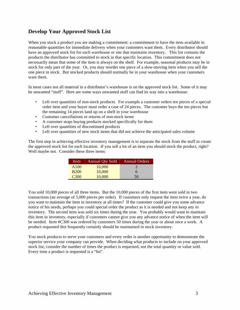
The first step in achieving effective inventory management is to separate the stock from the stuff to create the approved stock list for each location. If you sell a lot of an item you should stock the product, right? Well maybe not. Consider these three items:

Item Annual Qty Sold Annual Orders A100 10,000 2 B200 10,000 6 C300 10,000 50

You sold 10,000 pieces of all three items. But the 10,000 pieces of the first item were sold in two transactions (an average of 5,000 pieces per order). If customers only request the item twice a year, do you want to maintain the item in inventory at all times? If the customer could give you some advance notice of his needs, perhaps you could special order the product as it is needed and not keep any in inventory. The second item was sold six times during the year. You probably would want to maintain this item in inventory, especially if customers cannot give you any advance notice of when the item will be needed. Item #C300 was ordered by customers 50 times during the year or about once a week. A product requested this frequently certainly should be maintained in stock inventory. You stock products to serve your customers and every order is another opportunity to demonstrate the superior service your company can provide. When deciding what products to include on your approved stock list, consider the number of times the product is requested, not the total quantity or value sold. Every time a product is requested is a “hit”.


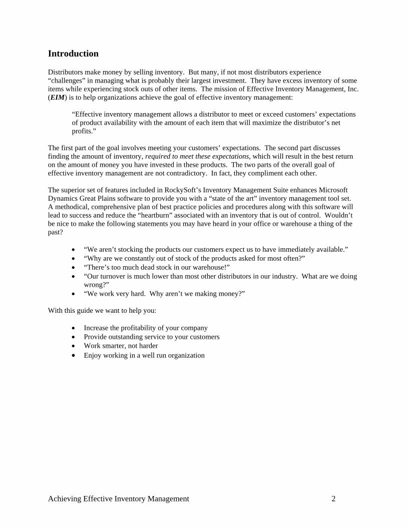
An effective way to separate the stock from stuff is to use a tool that will automatically rank and order products. Look at the following snapshot of RockySoft’s Economic Order Manager. Parts are ranked by the cumulative hits:

It is not unusual for 10% - 13% of a distributor’s inventory items to account for 80% of total annual hits and for 50% or more of products to have less than five hits a year. It’s a good idea to implement as part of corporate policy a minimum number of annual “hits” for an item to automatically remain on the approved stock list. Some industrial distributors question whether a product with fewer than four annual hits should be stocked while food distributors generally look for at least 12 annual hits for an item to remain in stock inventory. Please note that we are not recommending the removal of all products with a low number of hits from stock inventory. We just want to be sure that you have a good reason for stocking each of these low usage products:

• The item is an emergency repair part that contributes to the your reputation as a reliable supplier • It is necessary to stock this item to support the sale of other more profitable items • The item has a high profit margin that outweighs the cost of carrying inventory for a lengthy

period of time. Note that RockySoft has the capability to combine several criteria in the item ranking process. For example, you can assign a higher rank to an item with five hits that has a 60% gross margin than a product with the same number of hits with a 15% gross margin.

When Should the Stock of a Product Be Replenished? It’s a hot day in August. The sales manager of CE Distribution bursts into the buyer’s office and screams, “We’re out of #B240 switches again. Get some in here right away!” The buyer waited until the #B240 switches were out of stock before beginning the replenishment process. Unfortunately, it takes a week after a purchase order is placed for a shipment of #B240 switches to arrive


from the vendor. That means that CE Distribution will be out of stock for the next seven days and won’t be able to fill customer orders for the product. Most distributors agree, at least in principle, that waiting until an item is out of stock is not the best time to begin the replenishment process for the product. But unfortunately, too many buyers decide which vendor line will be ordered next by skimming through a pile of sales tickets that contain backordered items. There has to be a better way. In a perfect world, the replenishment shipment of a product would always arrive just as the last piece of the product was removed from the shelf to fill a customer order. Even though the world isn’t perfect, this concept can help us determine when a product should be ordered. Let’s look at the example again. It takes seven days to receive a shipment of #B240 switches from the vendor. If a replenishment order of the #B240 switches is placed when a seven day supply is still on the shelf, the replacement shipment should arrive on the day the last piece in stock is sold. We will avoid a stock out situation. To determine this quantity, we need to examine two variables: expected upcoming usage for the product (also known as the demand forecast) and the projected lead time. The demand forecast is defined as the quantity of a stocked item we predict will be sold or otherwise consumed in an upcoming month. The prediction of the amount of time it takes to get a new shipment of a product from the supplier is called the projected lead time. To avoid running out of stock, we must order the item when we have enough stock to fulfill anticipated demand during the projected lead time. This is a quantity equal to:

Anticipated Demand/Day ∗ Projected Lead Time Will the anticipated demand per day of an item correspond to the actual quantity sold or otherwise used in the upcoming month? Probably not. Nor will shipments from the supplier always arrive in a time period equal to the projected lead time. This is a prediction of the quantity of the product that will be sold or otherwise used during the time we think it will take to replenish stock. Now imagine this situation. You stock a popular item, the #S256 die blaster. In fact, you sell an average of two die blasters a day. Your supplier, the Die Blaster Company of America, is usually a reliable supplier and your projected lead time for the product is seven days. So, if you sell an average of two units per day, and it takes seven days to replenish your stock, you should reorder the die blasters when there are 14 pieces left on the shelf. But, what if one day during the lead time you sell four die blasters? Or, the truck carrying your shipment is delayed by a freak snowstorm outside of Buffalo? What will happen? You’ll probably run out of stock. What will your customers’ reaction be when you explain that either they ordered too much of the product, or the shipment was delayed? They won’t be happy. They count on you being a reliable supplier. Remember that part of the goal of effective inventory management is to “meet or exceed your customers’ expectations of product availability.” For this reason, it is often wise to add an “insurance” quantity to the formula that determines when to reorder an item. We call this insurance the “safety stock.” Safety stock provides protection against greater than normal demand or delivery delays during the time it takes to order and receive a replenishment shipment. So, we want to order a product as soon as its “Replenishment Position” (On-Hand - Committed on Customers Orders + Currently On Order From a Supplier) drops below an amount equal to:

(Anticipated Demand/Day x Projected Lead Time) + Safety Stock


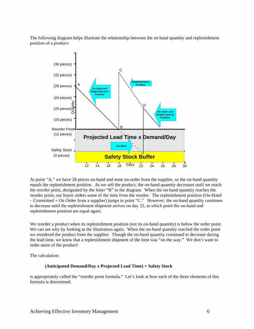
The following diagram helps illustrate the relationship between the on hand quantity and replenishment position of a product:

Qua

ntity

Days

Safety Stock

Reorder Point

12 14 16 18 22 24 26 28 30

(4 pieces)

(12 pieces) Projected Lead Time x Demand/Day

Safety Stock Buffer

On Hand andReplenishment

Position

ReplenishmentPosition

On Hand andReplenishment

Position

On Hand

A

B

C

D

(16 pieces)

(20 pieces)

(24 pieces)

(28 pieces)

(32 pieces)

(36 pieces)

At point “A,” we have 28 pieces on-hand and none on-order from the supplier, so the on-hand quantity equals the replenishment position. As we sell the product, the on-hand quantity decreases until we reach the reorder point, designated by the letter “B” in the diagram. When the on-hand quantity reaches the reorder point, our buyer orders some of the item from the vendor. The replenishment position (On-Hand – Committed + On Order from a supplier) jumps to point “C.” However, the on-hand quantity continues to decrease until the replenishment shipment arrives on day 22, at which point the on-hand and replenishment position are equal again.

We reorder a product when its replenishment position (not its on-hand quantity) is below the order point. We can see why by looking at the illustration again. When the on-hand quantity reached the order point we reordered the product from the supplier. Though the on-hand quantity continued to decrease during the lead time, we knew that a replenishment shipment of the item was “on the way.” We don’t want to order more of the product! The calculation:

(Anticipated Demand/Day x Projected Lead Time) + Safety Stock

is appropriately called the “reorder point formula.” Let’s look at how each of the three elements of this formula is determined.


Anticipated Demand You’re obviously in trouble if you don’t have the inventory your customers expect you to have. And, if you’ve bought too much of an item, your money is tied up and can’t be invested in the other products that allow you to take advantage of new sales opportunities. Many systems will forecast future demand of a product with a simple average of past usage. Often this is the average of the usage recorded over the past six months. This works pretty well if an item has fairly consistent usage. For example, consider this item’s usage history:

Jul Jun May Apr Mar Feb Jan Dec

Usage ? 80 154 90 145 133 100 78

An average of the usage recorded over the past six months (January – June) would equal 117 pieces [(100 + 133 + 145+ 90 + 154 + 80) ÷ 6 = 117]. But what happens if an item is experiencing increasing or decreasing sales? Consider another product’s usage history:

Jul Jun May Apr Mar Feb Jan Dec

Usage ? 154 145 133 100 90 80 78

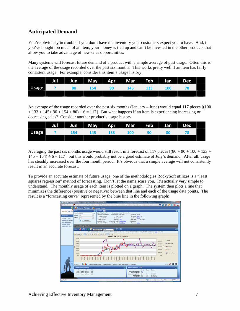
Averaging the past six months usage would still result in a forecast of 117 pieces [(80 + 90 + 100 + 133 + 145 + 154) ÷ 6 = 117], but this would probably not be a good estimate of July’s demand. After all, usage has steadily increased over the four month period. It’s obvious that a simple average will not consistently result in an accurate forecast. To provide an accurate estimate of future usage, one of the methodologies RockySoft utilizes is a “least squares regression” method of forecasting. Don’t let the name scare you. It’s actually very simple to understand. The monthly usage of each item is plotted on a graph. The system then plots a line that minimizes the difference (positive or negative) between that line and each of the usage data points. The result is a “forecasting curve” represented by the blue line in the following graph:


Note that the curve did not respond to the occasional spikes in usage. This is because the user identified specific events which resulted in these abnormal temporary increases in demand. The gray bar at the bottom of the graph identifies the occurrence of these events.

The curve is continued to predict usage in upcoming months. If usage has been increasing over the last several months, the curve (and the resulting forecast of future demand) will reflect this increase. On the other hand if usage has been decreasing over the last several months, future forecasts will mirror the lower usage of the product. RockySoft’s forecasting curve is intelligent and will identify other usage trends as well including:

• Seasonal usage patterns where the forecast should be based on usage in the upcoming months, last year, adjusted for the difference in volume between this year and last year.

• Reoccuring “blips” in usage. For example, a product might have large usage quantities every

second or third month. RockySoft will adjust the forecast month by month, predicting high sales one month and low sales in another month. This is a much better solution than “smoothing” the high and low months into a “middle ground” forecast produced by many computer systems. In the large usage months, this system’s middle ground forecast will be far less than actual usage. In the months with small sales a middle ground forecast will far exceed actual usage. It’s true that in dealing with item with recurring blips in usage, middle ground forecasts are consistent. They are nearly always wrong!

Collaborative Forecasting There is an old saying, “what you sold in the past is a good indication of what you will sell in the future”. But forecasting future demand solely on past usage history is like predicting weather from a windowless room only using a stack of old newspapers. Sure there is plenty of data available, but wouldn’t the forecaster get better information if he/she contacted other nearby weather stations, looked at current satellite data, or perhaps even opened a window? Collaborative forecasting is the process of obtaining information that will affect future usage of stocked products that is not reflected in past usage. Sources of this information include:

• Salespeople. Are they gaining or losing customers? How will these changes affect usage? • Customers. Is the usage of particular products going to be significantly affected by changes in a

customer’s production schedule or marketing plan? • The Market Environment. Is there an upcoming event that will affect usage of specific

products?


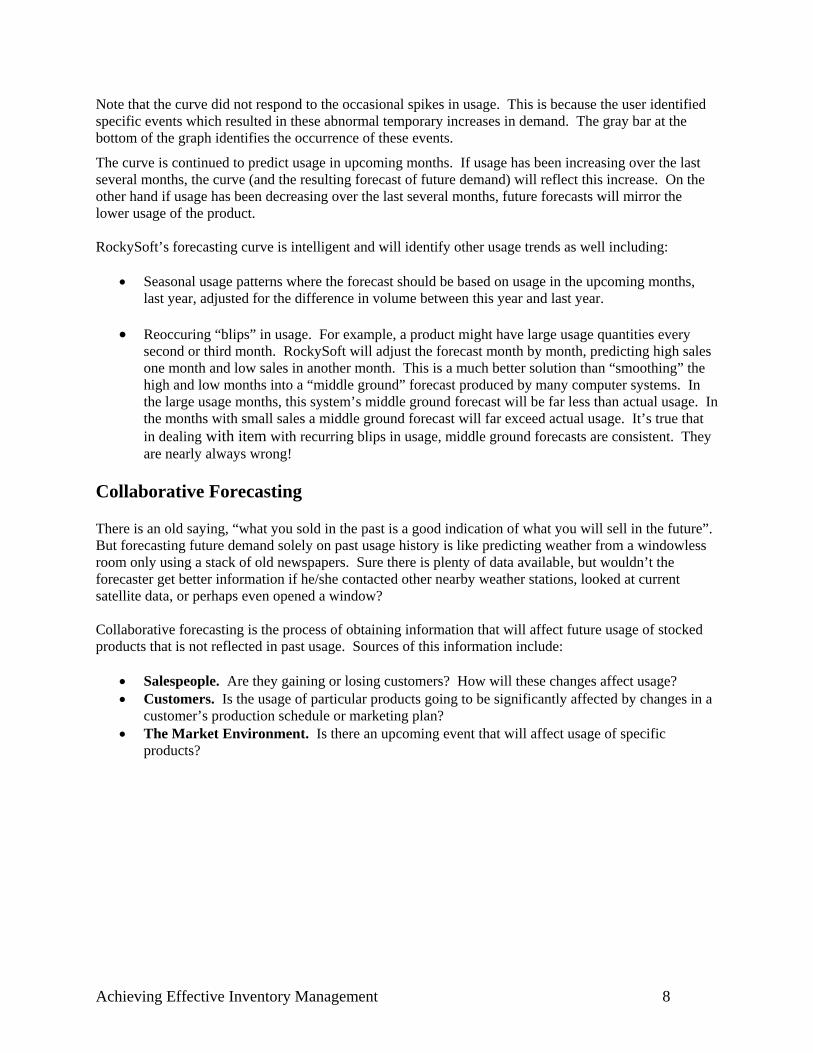
RockySoft’s forecasting tools allow a user to enter a quantity that reflects the effect of collaborative information. This can be either a positive or negative amount. The system will also report the accuracy of these predictions over time. This encourages salespeople and customers to put more thought into the information they provide. The total demand for an upcoming month is equal to the results of the forecast demand formula (with or without a trend factor) and the optional collaborative quantity.

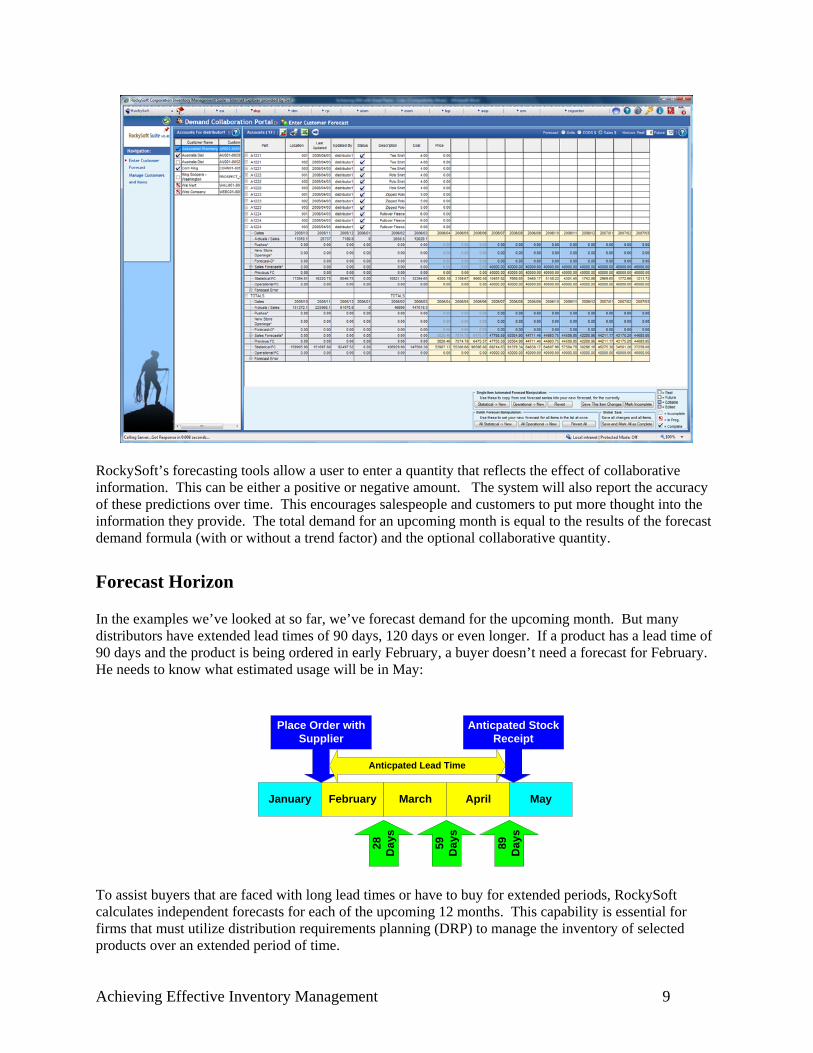
Forecast Horizon In the examples we’ve looked at so far, we’ve forecast demand for the upcoming month. But many distributors have extended lead times of 90 days, 120 days or even longer. If a product has a lead time of 90 days and the product is being ordered in early February, a buyer doesn’t need a forecast for February. He needs to know what estimated usage will be in May:

January February March April May

Place Order withSupplier

Anticpated Lead Time

Anticpated StockReceipt

28 Day

s

59 Day

s

89 Day

s

To assist buyers that are faced with long lead times or have to buy for extended periods, RockySoft calculates independent forecasts for each of the upcoming 12 months. This capability is essential for firms that must utilize distribution requirements planning (DRP) to manage the inventory of selected products over an extended period of time.


Projected Lead Time The second component of the reorder point formula is the projected lead time:

Reorder Point = (Anticipated Demand/Day ∗ Projected Lead Time) + Safety Stock The projected lead time is the amount of time (in days) we estimate it will take to replenish our stock of an item from the normal source of supply. Previously, we found that we can use previous usage as a guide to future demand of a product. The same concept is applicable to the projected lead time. That is, recent lead times for a product are often a good indicator of how long it will take to get the item from the supplier if we were to order it today. Lead times should be maintained separately for each item in each warehouse. Why?

• Even though several products are obtained from the same vendor, their lead times can be very different. A popular product in the line may always be available from the vendor’s shelf stock, while a slower moving item may have a lead time of several weeks, or even several months!

• A distributor may stock the same item in several warehouses. But each site may obtain the product from a different source. And, even if the same vendor supplies the item to all of the branches, the time it takes to get the item to each warehouse may be different.

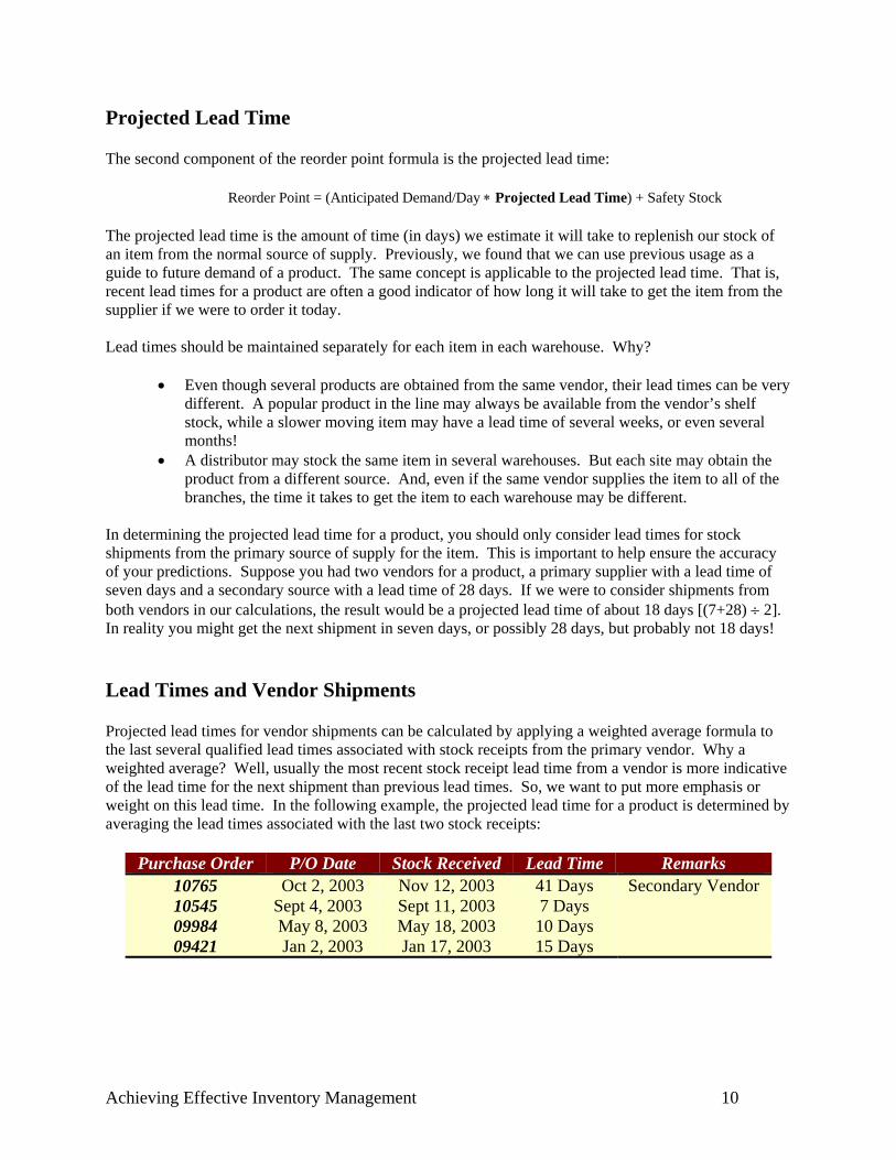
In determining the projected lead time for a product, you should only consider lead times for stock shipments from the primary source of supply for the item. This is important to help ensure the accuracy of your predictions. Suppose you had two vendors for a product, a primary supplier with a lead time of seven days and a secondary source with a lead time of 28 days. If we were to consider shipments from both vendors in our calculations, the result would be a projected lead time of about 18 days [(7+28) ÷ 2]. In reality you might get the next shipment in seven days, or possibly 28 days, but probably not 18 days! Lead Times and Vendor Shipments Projected lead times for vendor shipments can be calculated by applying a weighted average formula to the last several qualified lead times associated with stock receipts from the primary vendor. Why a weighted average? Well, usually the most recent stock receipt lead time from a vendor is more indicative of the lead time for the next shipment than previous lead times. So, we want to put more emphasis or weight on this lead time. In the following example, the projected lead time for a product is determined by averaging the lead times associated with the last two stock receipts:

Purchase Order P/O Date Stock Received Lead Time Remarks 10765 Oct 2, 2003 Nov 12, 2003 41 Days Secondary Vendor 10545 Sept 4, 2003 Sept 11, 2003 7 Days 09984 May 8, 2003 May 18, 2003 10 Days 09421 Jan 2, 2003 Jan 17, 2003 15 Days


The weight placed on the most recent qualified lead time is twice the weight placed on the previous lead time:

Purchase Order Lead Time Weight Extension 10545 7 Days 2 14 Days 09984 10 Days 1 10 Days Total 3 24 Days

24 Days ÷ 3 = 8 Days

The projected lead time is eight days. Notice that neither the lead time associated with the shipment from the secondary vendor or the old lead time from January is included in the calculation. In determining how many stock receipts to use in calculating a projected lead time, keep in mind that you don’t receive a product as often as you sell it. Think of one of your most popular products. It may be sold every day; but it is probably received, at most, once or twice a month. In fact, you may have a six to twelve month supply of over half of your stocked items. That means that these products are received from the vendor only once or twice a year. A lot of things can occur over extended periods of time that will affect the lead time for an item. For example:

• Your vendor can add or shut down production lines • Freight carriers can use different routes • The availability of the raw materials needed to make the product may change

Even the most recent lead times may not be a good indication of your anticipated lead time for the next shipment:

• The vendor may experience a seasonal fluctuation in demand, so his lead time performance is always bad in December. In December, you are using historic lead time information from October and November, so your projected lead time is too short. But in January you are using historic lead time information from December and as a result your projected lead time is too long.

• The vendor may be having a temporary process problem. For example one of his machines

breaks down which affects the production of three products you have on order with him. What is the probability that the next time you order these parts the machine will still be broken?

• The vendor’s raw materials shipments have been delayed., Your system will automatically

increase the lead time and therefore launch a new set of orders for these finished items, thus asking the vendor for more product just at the time when he can not get enough parts to build even the existing orders.

It is not surprising that many distributors manually maintain lead times based on the longest “normal” lead time for the product. For example, if an item’s lead time ranges from seven to 21 days, the lead time is manually set to 21 days. When determining an item’s lead keep in mind the four “components” of this parameter:

• The time it takes you to place an order once you realize it is needed • The time it takes the vendor to process your order and ship the material • The transportation time to get the material to your warehouse


• The time necessary to receive the material and prepare it for use or sale

Actual Projected Lead Times for vendor purchase orders are maintained in the PO Lead Time cell in the Replenishment Values tab of Inventory Sites Maintenance:

Safety Stock The last component of the reorder point formula is safety stock:

Reorder Point = (Anticipated Demand/Day ∗ Projected Lead Time) + Safety Stock Safety stock provides you with protection against running out of stock during the time it takes to replenish inventory. Why is this protection necessary?

• Demand is a prediction based on past history, trend factor(s), and/or known future usage of a product. The item’s actual usage will probably be a little more or a little less. Safety stock is needed for those occasions when actual usage exceeds forecasted demand. It is “insurance” to help ensure that you can fulfill customer requests for a product.

• The projected lead time is also a prediction, usually based on the lead times from the last

several stock receipts. Sometimes the actual lead time will be greater than what was projected. Safety stock provides protection from stock outs when the time it takes to receive a replenishment shipment exceeds the projected lead time.


The following diagrams illustrate how safety stock is used:

Qua

ntity

Days

Safety Stock

Reorder Point

2 4 6 8 12 14 16 18 20

(4 pieces)

(12 pieces)

A

Projected Lead Time = 8 Days Demand = 1 piece/day

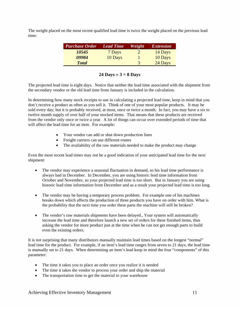
On Order With Vendor = 0 The dotted line in the graph represents the available quantity (On- Hand - Committed) of the item. A replenishment order is placed on the first of the month as the available quantity available reaches the reorder point [“A” in the graph]. In this example, there is none of the product currently on incoming replenishment orders. Therefore, at point “A,” the item’s available quantity equals its replenishment position. The actual usage of eight pieces during the lead time is consistent with demand. The shipment arrives on the 9th of the month. As the stock receipt is processed, the available quantity on the shelf is equal to the safety stock quantity. The protection provided by the safety stock was not needed. The product again reaches the order point on the 11th of the following month [“B” in the following graph]:

Qua

ntity

Days

Safety Stcok

Reorder Point

12 14 16 18 22 24 26 28 30

(4 pieces)

(12 pieces)

B

C

Projected Lead Time = 8 Days Demand = 1 piece/day

On Order With Vendor = 0


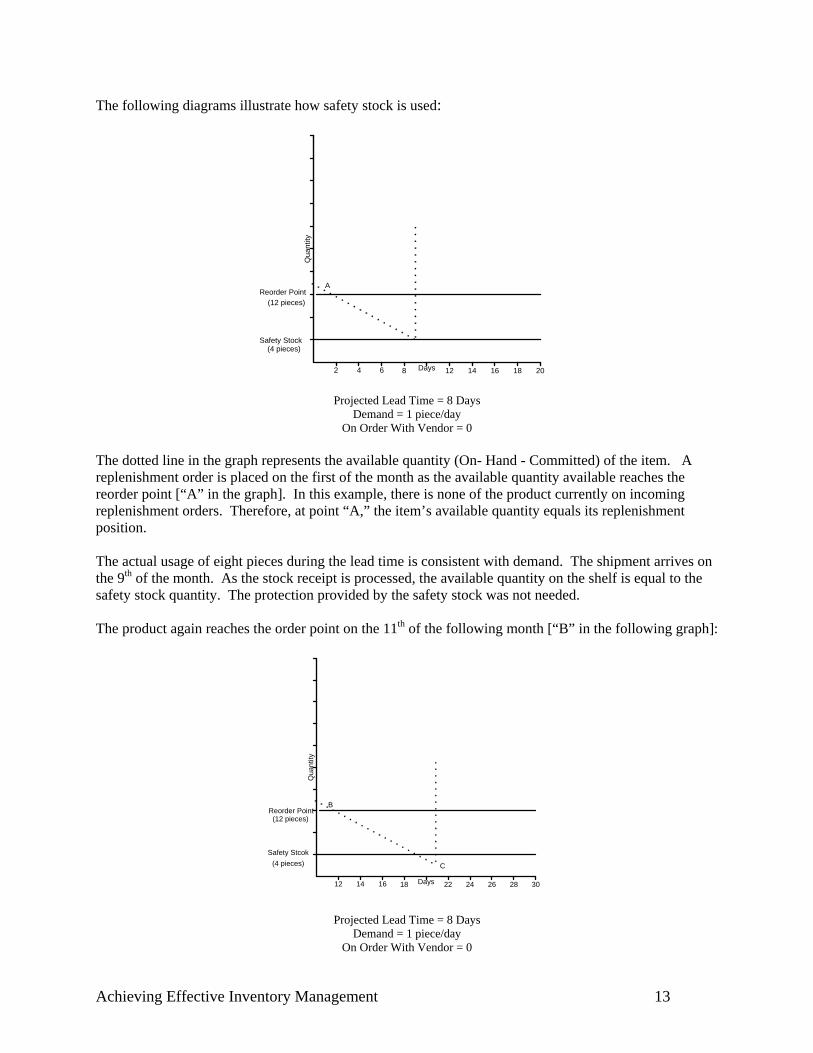
Another order is placed with the supplier. But the vendor is temporarily experiencing manufacturing problems and the shipment arrives two days late [“C” in the graph]. If it weren’t for the safety stock, we would have run out of the product. Shortly after the shipment arrives, a customer orders 10 pieces of the product. You experience more than a week’s usage in just one day. The available quantity falls to “D” in the following graph. A replenishment order is issued that day, but the available quantity is already below the reorder point.

Qua

ntity

Days

Safety Stock

Rerder Point

12 14 16 18 22 24 26 28 30

(4 pieces)

(12 pieces)

B

C

D

E

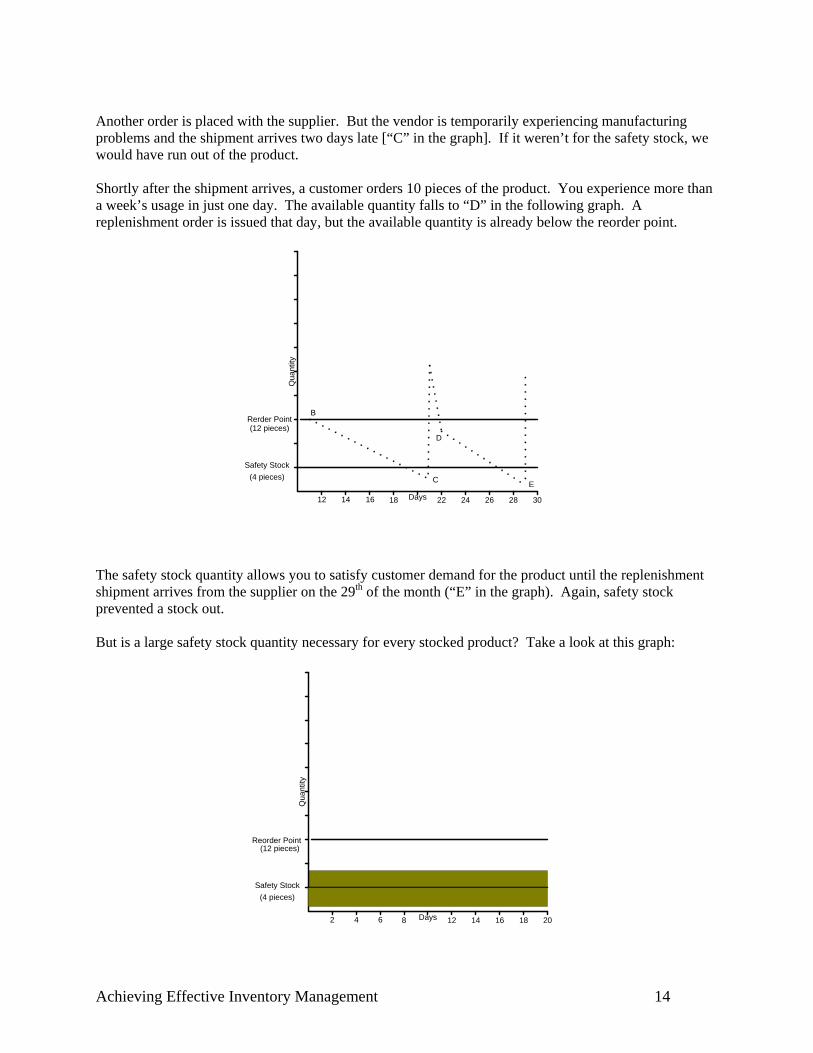
The safety stock quantity allows you to satisfy customer demand for the product until the replenishment shipment arrives from the supplier on the 29th of the month (“E” in the graph). Again, safety stock prevented a stock out. But is a large safety stock quantity necessary for every stocked product? Take a look at this graph:

Qua

ntity

Days

Safety Stock

Reorder Point

2 4 6 8 12 14 16 18 20

(4 pieces)

(12 pieces)


When a replenishment shipment arrives, the available quantity is usually somewhere in the shaded area of the graph. Notice that the safety stock quantity is in the middle of the shaded area. About half the time you will use some, or all of the safety stock before the replenishment shipment arrives. The other stock receipts will arrive before you use any of the safety stock. On average, the full safety stock quantity is always on the shelf when the replenishment shipment arrives. It is, on average, “non-moving” inventory. A distributor puts inventory in her warehouse to sell it to customers. Profits from these sales are necessary to pay the distributor’s expenses and provide a return on her investment. With this thought in mind, it seems as though it would not be a good idea for a distributor to intentionally have non-moving inventory in stock. On the other hand, keep in mind the goal of effective inventory management:

“Effective inventory management allows a distributor to meet or exceed customers’ expectations of product availability with the amount of each item that will maximize the distributor’s net profits.”

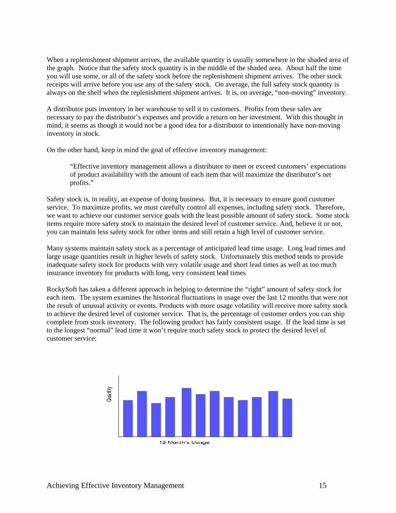
Safety stock is, in reality, an expense of doing business. But, it is necessary to ensure good customer service. To maximize profits, we must carefully control all expenses, including safety stock. Therefore, we want to achieve our customer service goals with the least possible amount of safety stock. Some stock items require more safety stock to maintain the desired level of customer service. And, believe it or not, you can maintain less safety stock for other items and still retain a high level of customer service. Many systems maintain safety stock as a percentage of anticipated lead time usage. Long lead times and large usage quantities result in higher levels of safety stock. Unfortunately this method tends to provide inadequate safety stock for products with very volatile usage and short lead times as well as too much insurance inventory for products with long, very consistent lead times RockySoft has taken a different approach in helping to determine the “right” amount of safety stock for each item. The system examines the historical fluctuations in usage over the last 12 months that were not the result of unusual activity or events. Products with more usage volatility will receive more safety stock to achieve the desired level of customer service. That is, the percentage of customer orders you can ship complete from stock inventory. The following product has fairly consistent usage. If the lead time is set to the longest “normal” lead time it won’t require much safety stock to protect the desired level of customer service:


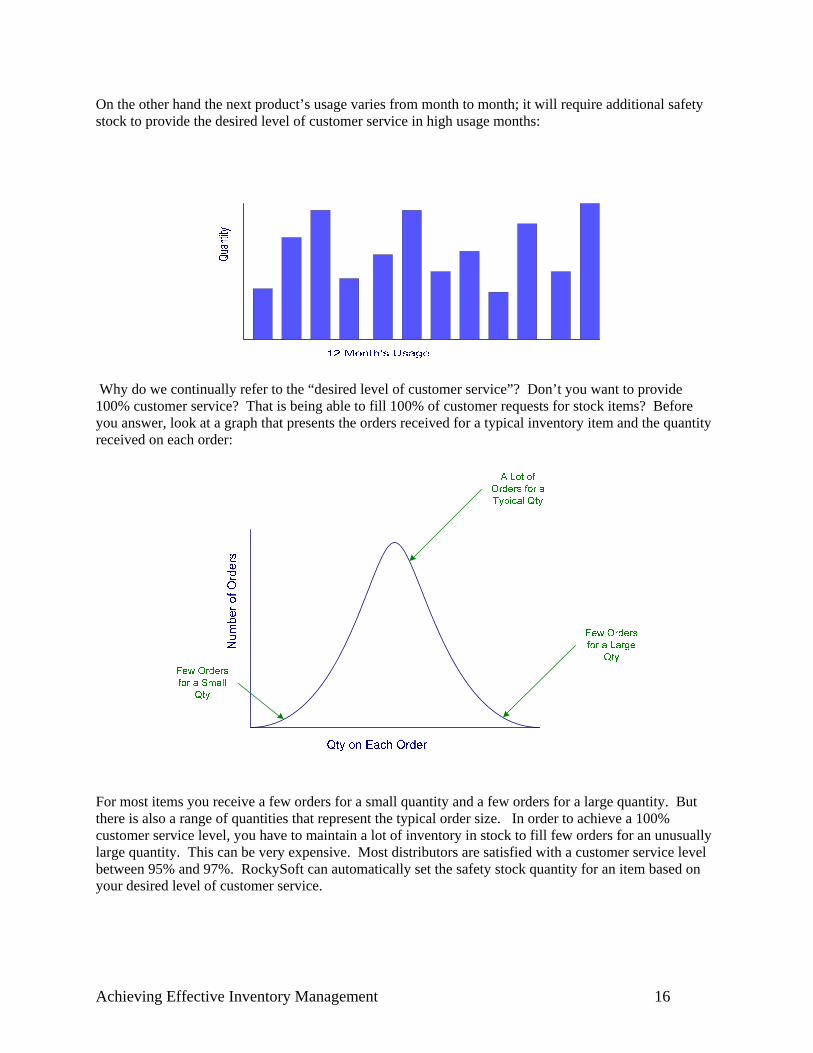
On the other hand the next product’s usage varies from month to month; it will require additional safety stock to provide the desired level of customer service in high usage months:

Why do we continually refer to the “desired level of customer service”? Don’t you want to provide 100% customer service? That is being able to fill 100% of customer requests for stock items? Before you answer, look at a graph that presents the orders received for a typical inventory item and the quantity received on each order:

For most items you receive a few orders for a small quantity and a few orders for a large quantity. But there is also a range of quantities that represent the typical order size. In order to achieve a 100% customer service level, you have to maintain a lot of inventory in stock to fill few orders for an unusually large quantity. This can be very expensive. Most distributors are satisfied with a customer service level between 95% and 97%. RockySoft can automatically set the safety stock quantity for an item based on your desired level of customer service.


The Review Cycle and the Line Point To avoid a possible stockout, a product should be ordered as soon as its replenishment position (On-Hand - Committed + On Order) falls below its reorder point. Unfortunately vendors usually do not accept purchase orders that just contain one product. Even if they do, the terms they offer for a small order probably prevent you from competitively selling the item. In order to meet the supplier’s terms and buy “at the right price”, you must often order a target amount of the vendor’s products. This target amount can be expressed in:

• Units. A total number of pieces need to be ordered. For example, if you order 1,000 pieces of 10 different items, you have achieved a 10,000 unit order target.

• An Amount. Many vendors will require an order target of “x” dollars, (based on your replacement cost for the material purchased)

• Weight. A target order weighing “x” pounds. • Volume. This refers to the “space” filled by the merchandise ordered. It is a common

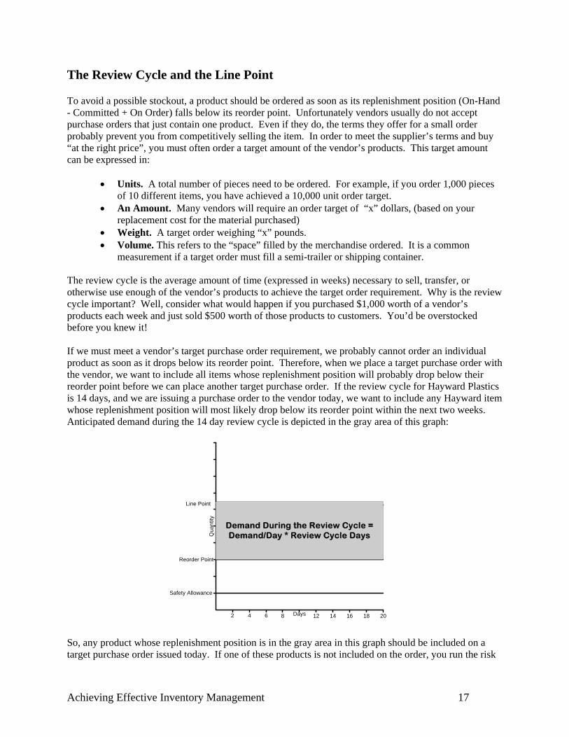
measurement if a target order must fill a semi-trailer or shipping container. The review cycle is the average amount of time (expressed in weeks) necessary to sell, transfer, or otherwise use enough of the vendor’s products to achieve the target order requirement. Why is the review cycle important? Well, consider what would happen if you purchased $1,000 worth of a vendor’s products each week and just sold $500 worth of those products to customers. You’d be overstocked before you knew it! If we must meet a vendor’s target purchase order requirement, we probably cannot order an individual product as soon as it drops below its reorder point. Therefore, when we place a target purchase order with the vendor, we want to include all items whose replenishment position will probably drop below their reorder point before we can place another target purchase order. If the review cycle for Hayward Plastics is 14 days, and we are issuing a purchase order to the vendor today, we want to include any Hayward item whose replenishment position will most likely drop below its reorder point within the next two weeks. Anticipated demand during the 14 day review cycle is depicted in the gray area of this graph:

Qua

ntity

Days

Safety Allowance

Reorder Point

2 4 6 8 12 14 16 18 20

Demand During the Review Cycle =Demand/Day * Review Cycle Days

Line Point

So, any product whose replenishment position is in the gray area in this graph should be included on a target purchase order issued today. If one of these products is not included on the order, you run the risk


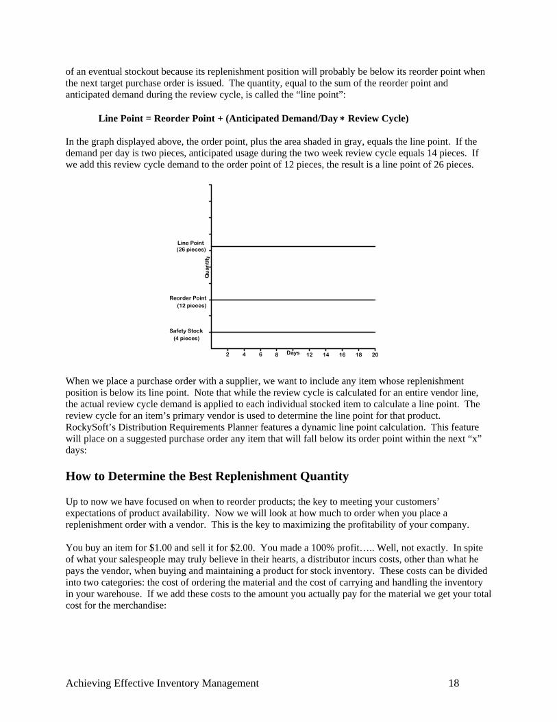
of an eventual stockout because its replenishment position will probably be below its reorder point when the next target purchase order is issued. The quantity, equal to the sum of the reorder point and anticipated demand during the review cycle, is called the “line point”: Line Point = Reorder Point + (Anticipated Demand/Day ∗ Review Cycle) In the graph displayed above, the order point, plus the area shaded in gray, equals the line point. If the demand per day is two pieces, anticipated usage during the two week review cycle equals 14 pieces. If we add this review cycle demand to the order point of 12 pieces, the result is a line point of 26 pieces.

Qu

an

tity

Days

Safety Stock

Reorder Point

2 4 6 8 12 14 16 18 20

(4 pieces)

(12 pieces)

Line Point (26 pieces)

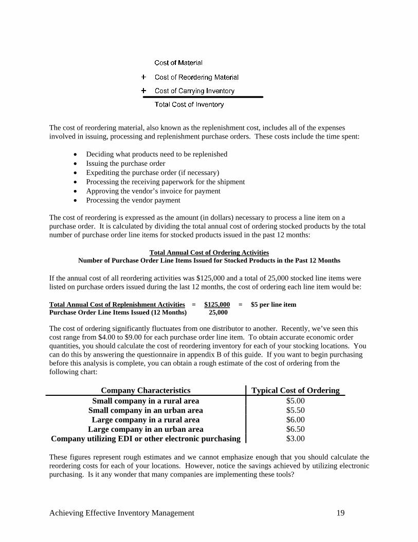
When we place a purchase order with a supplier, we want to include any item whose replenishment position is below its line point. Note that while the review cycle is calculated for an entire vendor line, the actual review cycle demand is applied to each individual stocked item to calculate a line point. The review cycle for an item’s primary vendor is used to determine the line point for that product. RockySoft’s Distribution Requirements Planner features a dynamic line point calculation. This feature will place on a suggested purchase order any item that will fall below its order point within the next “x” days: How to Determine the Best Replenishment Quantity Up to now we have focused on when to reorder products; the key to meeting your customers’ expectations of product availability. Now we will look at how much to order when you place a replenishment order with a vendor. This is the key to maximizing the profitability of your company. You buy an item for $1.00 and sell it for $2.00. You made a 100% profit….. Well, not exactly. In spite of what your salespeople may truly believe in their hearts, a distributor incurs costs, other than what he pays the vendor, when buying and maintaining a product for stock inventory. These costs can be divided into two categories: the cost of ordering the material and the cost of carrying and handling the inventory in your warehouse. If we add these costs to the amount you actually pay for the material we get your total cost for the merchandise:


The cost of reordering material, also known as the replenishment cost, includes all of the expenses involved in issuing, processing and replenishment purchase orders. These costs include the time spent:

• Deciding what products need to be replenished • Issuing the purchase order • Expediting the purchase order (if necessary) • Processing the receiving paperwork for the shipment • Approving the vendor’s invoice for payment • Processing the vendor payment

The cost of reordering is expressed as the amount (in dollars) necessary to process a line item on a purchase order. It is calculated by dividing the total annual cost of ordering stocked products by the total number of purchase order line items for stocked products issued in the past 12 months:

Total Annual Cost of Ordering Activities Number of Purchase Order Line Items Issued for Stocked Products in the Past 12 Months

If the annual cost of all reordering activities was $125,000 and a total of 25,000 stocked line items were listed on purchase orders issued during the last 12 months, the cost of ordering each line item would be: Total Annual Cost of Replenishment Activities = $125,000 = $5 per line item Purchase Order Line Items Issued (12 Months) 25,000 The cost of ordering significantly fluctuates from one distributor to another. Recently, we’ve seen this cost range from $4.00 to $9.00 for each purchase order line item. To obtain accurate economic order quantities, you should calculate the cost of reordering inventory for each of your stocking locations. You can do this by answering the questionnaire in appendix B of this guide. If you want to begin purchasing before this analysis is complete, you can obtain a rough estimate of the cost of ordering from the following chart:

Company Characteristics Typical Cost of Ordering Small company in a rural area $5.00

Small company in an urban area $5.50 Large company in a rural area $6.00

Large company in an urban area $6.50 Company utilizing EDI or other electronic purchasing $3.00 These figures represent rough estimates and we cannot emphasize enough that you should calculate the reordering costs for each of your locations. However, notice the savings achieved by utilizing electronic purchasing. Is it any wonder that many companies are implementing these tools?


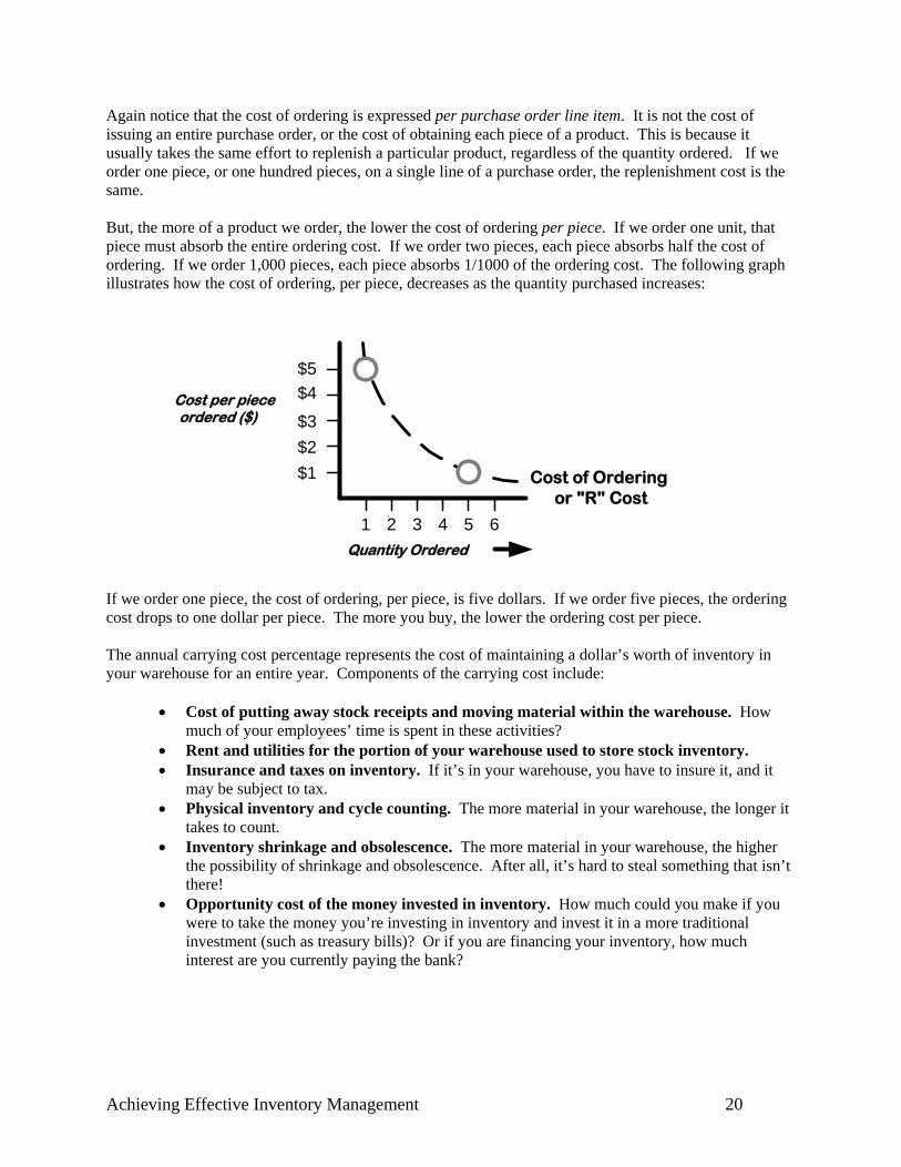
Again notice that the cost of ordering is expressed per purchase order line item. It is not the cost of issuing an entire purchase order, or the cost of obtaining each piece of a product. This is because it usually takes the same effort to replenish a particular product, regardless of the quantity ordered. If we order one piece, or one hundred pieces, on a single line of a purchase order, the replenishment cost is the same. But, the more of a product we order, the lower the cost of ordering per piece. If we order one unit, that piece must absorb the entire ordering cost. If we order two pieces, each piece absorbs half the cost of ordering. If we order 1,000 pieces, each piece absorbs 1/1000 of the ordering cost. The following graph illustrates how the cost of ordering, per piece, decreases as the quantity purchased increases:

Cost of Ordering or "R" Cost

Cost per pieceordered ($)

Quantity Ordered

$5

1

$4$3$2$1

2 3 4 5 6

If we order one piece, the cost of ordering, per piece, is five dollars. If we order five pieces, the ordering cost drops to one dollar per piece. The more you buy, the lower the ordering cost per piece. The annual carrying cost percentage represents the cost of maintaining a dollar’s worth of inventory in your warehouse for an entire year. Components of the carrying cost include:

• Cost of putting away stock receipts and moving material within the warehouse. How much of your employees’ time is spent in these activities?

• Rent and utilities for the portion of your warehouse used to store stock inventory. • Insurance and taxes on inventory. If it’s in your warehouse, you have to insure it, and it

may be subject to tax. • Physical inventory and cycle counting. The more material in your warehouse, the longer it

takes to count. • Inventory shrinkage and obsolescence. The more material in your warehouse, the higher

the possibility of shrinkage and obsolescence. After all, it’s hard to steal something that isn’t there!

• Opportunity cost of the money invested in inventory. How much could you make if you were to take the money you’re investing in inventory and invest it in a more traditional investment (such as treasury bills)? Or if you are financing your inventory, how much interest are you currently paying the bank?


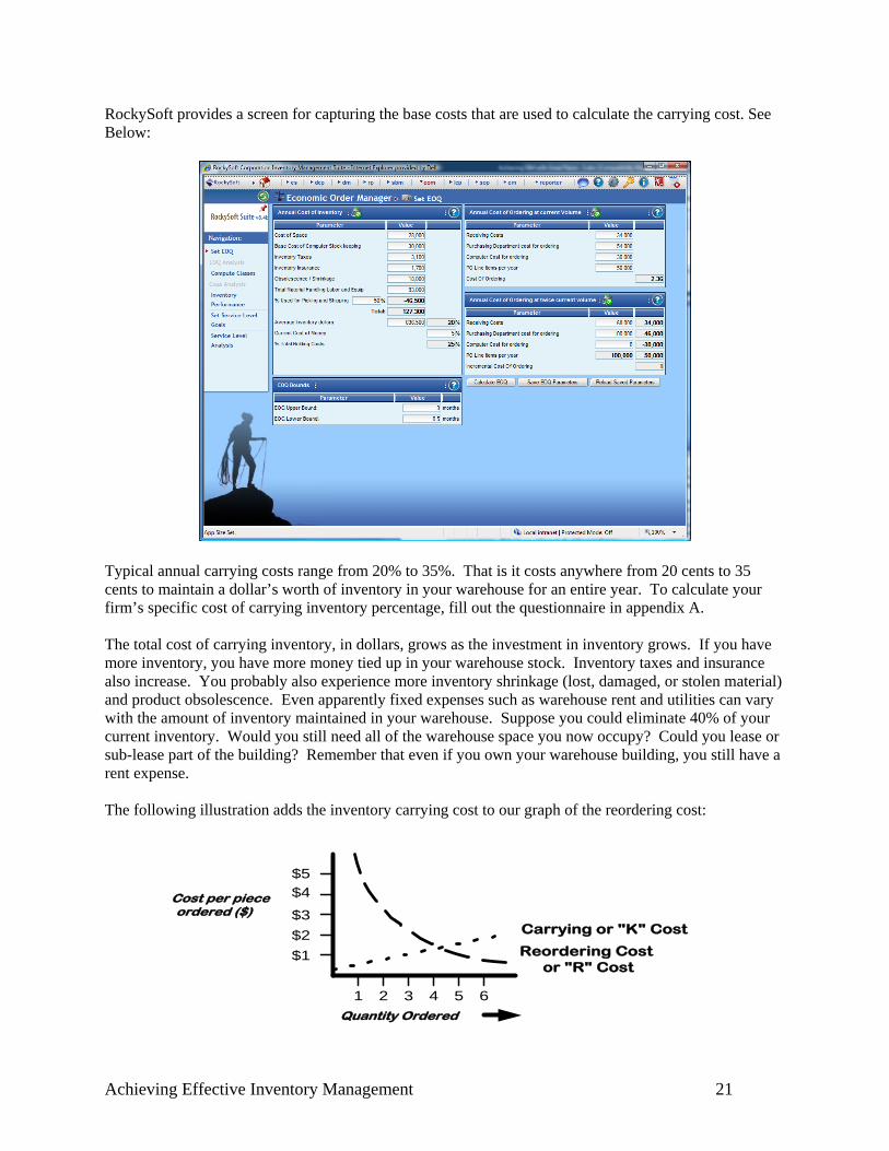
RockySoft provides a screen for capturing the base costs that are used to calculate the carrying cost. See Below:

Typical annual carrying costs range from 20% to 35%. That is it costs anywhere from 20 cents to 35 cents to maintain a dollar’s worth of inventory in your warehouse for an entire year. To calculate your firm’s specific cost of carrying inventory percentage, fill out the questionnaire in appendix A. The total cost of carrying inventory, in dollars, grows as the investment in inventory grows. If you have more inventory, you have more money tied up in your warehouse stock. Inventory taxes and insurance also increase. You probably also experience more inventory shrinkage (lost, damaged, or stolen material) and product obsolescence. Even apparently fixed expenses such as warehouse rent and utilities can vary with the amount of inventory maintained in your warehouse. Suppose you could eliminate 40% of your current inventory. Would you still need all of the warehouse space you now occupy? Could you lease or sub-lease part of the building? Remember that even if you own your warehouse building, you still have a rent expense. The following illustration adds the inventory carrying cost to our graph of the reordering cost:

Reordering Cost or "R" Cost


Quantity Ordered

$5

1

$4

$3$2$1

2 3 4 5 6

Carrying or "K" Cost


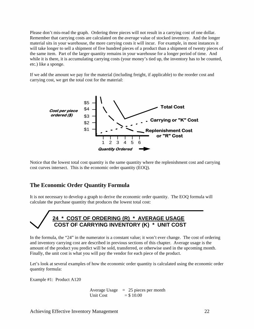
Please don’t mis-read the graph. Ordering three pieces will not result in a carrying cost of one dollar. Remember that carrying costs are calculated on the average value of stocked inventory. And the longer material sits in your warehouse, the more carrying costs it will incur. For example, in most instances it will take longer to sell a shipment of five hundred pieces of a product than a shipment of twenty pieces of the same item. Part of the larger quantity remains in your warehouse for a longer period of time. And while it is there, it is accumulating carrying costs (your money’s tied up, the inventory has to be counted, etc.) like a sponge. If we add the amount we pay for the material (including freight, if applicable) to the reorder cost and carrying cost, we get the total cost for the material:

Replenishment Cost or "R" Cost


Quantity Ordered

$5

1

$4$3$2$1

2 3 4 5 6

Carrying or "K" Cost

Total Cost

Notice that the lowest total cost quantity is the same quantity where the replenishment cost and carrying cost curves intersect. This is the economic order quantity (EOQ). The Economic Order Quantity Formula It is not necessary to develop a graph to derive the economic order quantity. The EOQ formula will calculate the purchase quantity that produces the lowest total cost:

24 * COST OF ORDERING (R) * AVERAGE USAGE COST OF CARRYING INVENTORY (K) * UNIT COST

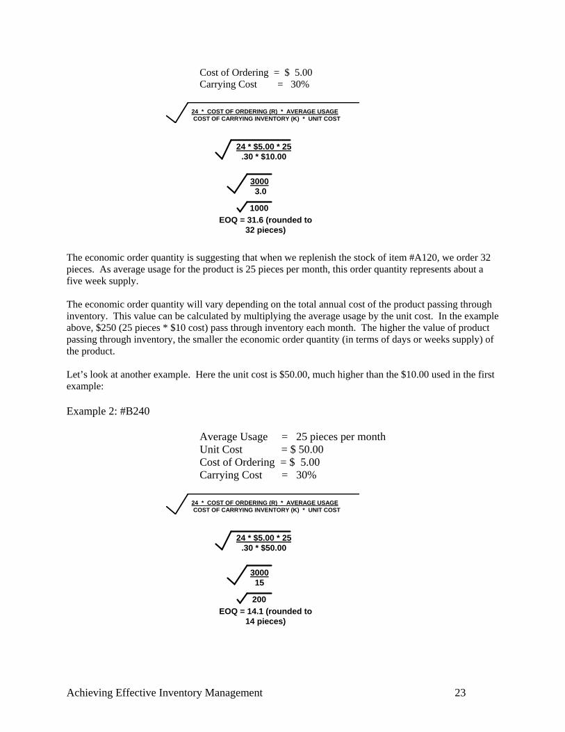
In the formula, the “24” in the numerator is a constant value; it won’t ever change. The cost of ordering and inventory carrying cost are described in previous sections of this chapter. Average usage is the amount of the product you predict will be sold, transferred, or otherwise used in the upcoming month. Finally, the unit cost is what you will pay the vendor for each piece of the product. Let’s look at several examples of how the economic order quantity is calculated using the economic order quantity formula: Example #1: Product A120

Average Usage = 25 pieces per month Unit Cost = $ 10.00


Cost of Ordering = $ 5.00 Carrying Cost = 30%


24 * $5.00 * 25

.30 * $10.00

3000 3.0

1000EOQ = 31.6 (rounded to

32 pieces) The economic order quantity is suggesting that when we replenish the stock of item #A120, we order 32 pieces. As average usage for the product is 25 pieces per month, this order quantity represents about a five week supply. The economic order quantity will vary depending on the total annual cost of the product passing through inventory. This value can be calculated by multiplying the average usage by the unit cost. In the example above, $250 (25 pieces * $10 cost) pass through inventory each month. The higher the value of product passing through inventory, the smaller the economic order quantity (in terms of days or weeks supply) of the product. Let’s look at another example. Here the unit cost is $50.00, much higher than the $10.00 used in the first example: Example 2: #B240

Average Usage = 25 pieces per month Unit Cost = $ 50.00 Cost of Ordering = $ 5.00 Carrying Cost = 30%


24 * $5.00 * 25

.30 * $50.00

3000 15

200EOQ = 14.1 (rounded to

14 pieces)


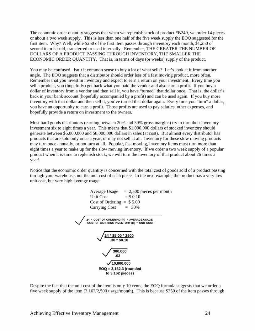
The economic order quantity suggests that when we replenish stock of product #B240, we order 14 pieces or about a two week supply. This is less than one half of the five week supply the EOQ suggested for the first item. Why? Well, while $250 of the first item passes through inventory each month, $1,250 of second item is sold, transferred or used internally. Remember, THE GREATER THE NUMBER OF DOLLARS OF A PRODUCT PASSING THROUGH INVENTORY, THE SMALLER THE ECONOMIC ORDER QUANTITY. That is, in terms of days (or weeks) supply of the product. You may be confused. Isn’t it common sense to buy a lot of what sells? Let’s look at it from another angle. The EOQ suggests that a distributor should order less of a fast moving product, more often. Remember that you invest in inventory and expect to earn a return on your investment. Every time you sell a product, you (hopefully) get back what you paid the vendor and also earn a profit. If you buy a dollar of inventory from a vendor and then sell it, you have “turned” that dollar once. That is, the dollar’s back in your bank account (hopefully accompanied by a profit) and can be used again. If you buy more inventory with that dollar and then sell it, you’ve turned that dollar again. Every time you “turn” a dollar, you have an opportunity to earn a profit. Those profits are used to pay salaries, other expenses, and hopefully provide a return on investment to the owners. Most hard goods distributors (earning between 20% and 30% gross margins) try to turn their inventory investment six to eight times a year. This means that $1,000,000 dollars of stocked inventory should generate between $6,000,000 and $8,000,000 dollars in sales (at cost). But almost every distributor has products that are sold only once a year, or may not sell at all. Inventory for these slow moving products may turn once annually, or not turn at all. Popular, fast moving, inventory items must turn more than eight times a year to make up for the slow moving inventory. If we order a two week supply of a popular product when it is time to replenish stock, we will turn the inventory of that product about 26 times a year! Notice that the economic order quantity is concerned with the total cost of goods sold of a product passing through your warehouse, not the unit cost of each piece. In the next example, the product has a very low unit cost, but very high average usage:

Average Usage = 2,500 pieces per month Unit Cost = $ 0.10 Cost of Ordering = $ 5.00 Carrying Cost = 30%


24 * $5.00 * 2500

.30 * $0.10

300,000 .03

10,000,000EOQ = 3,162.3 (rounded

to 3,162 pieces) Despite the fact that the unit cost of the item is only 10 cents, the EOQ formula suggests that we order a five week supply of the item (3,162/2,500 usage/month). This is because $250 of the item passes through


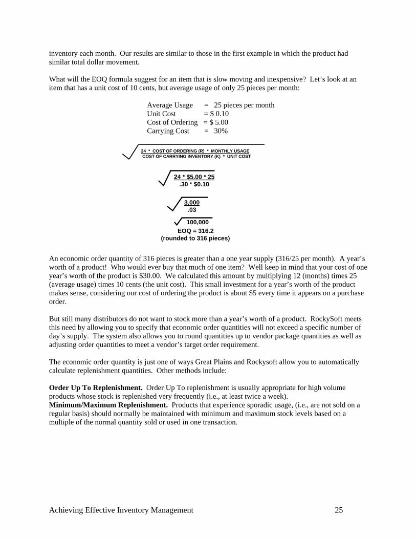
inventory each month. Our results are similar to those in the first example in which the product had similar total dollar movement. What will the EOQ formula suggest for an item that is slow moving and inexpensive? Let’s look at an item that has a unit cost of 10 cents, but average usage of only 25 pieces per month:

Average Usage = 25 pieces per month Unit Cost = $ 0.10 Cost of Ordering = $ 5.00 Carrying Cost = 30%

24 * COST OF ORDERING (R) * MONTHLY USAGECOST OF CARRYING INVENTORY (K) * UNIT COST

24 * $5.00 * 25

.30 * $0.10

3,000 .03

100,000EOQ = 316.2

(rounded to 316 pieces)

An economic order quantity of 316 pieces is greater than a one year supply (316/25 per month). A year’s worth of a product! Who would ever buy that much of one item? Well keep in mind that your cost of one year’s worth of the product is $30.00. We calculated this amount by multiplying 12 (months) times 25 (average usage) times 10 cents (the unit cost). This small investment for a year’s worth of the product makes sense, considering our cost of ordering the product is about $5 every time it appears on a purchase order. But still many distributors do not want to stock more than a year’s worth of a product. RockySoft meets this need by allowing you to specify that economic order quantities will not exceed a specific number of day’s supply. The system also allows you to round quantities up to vendor package quantities as well as adjusting order quantities to meet a vendor’s target order requirement. The economic order quantity is just one of ways Great Plains and Rockysoft allow you to automatically calculate replenishment quantities. Other methods include: Order Up To Replenishment. Order Up To replenishment is usually appropriate for high volume products whose stock is replenished very frequently (i.e., at least twice a week). Minimum/Maximum Replenishment. Products that experience sporadic usage, (i.e., are not sold on a regular basis) should normally be maintained with minimum and maximum stock levels based on a multiple of the normal quantity sold or used in one transaction.


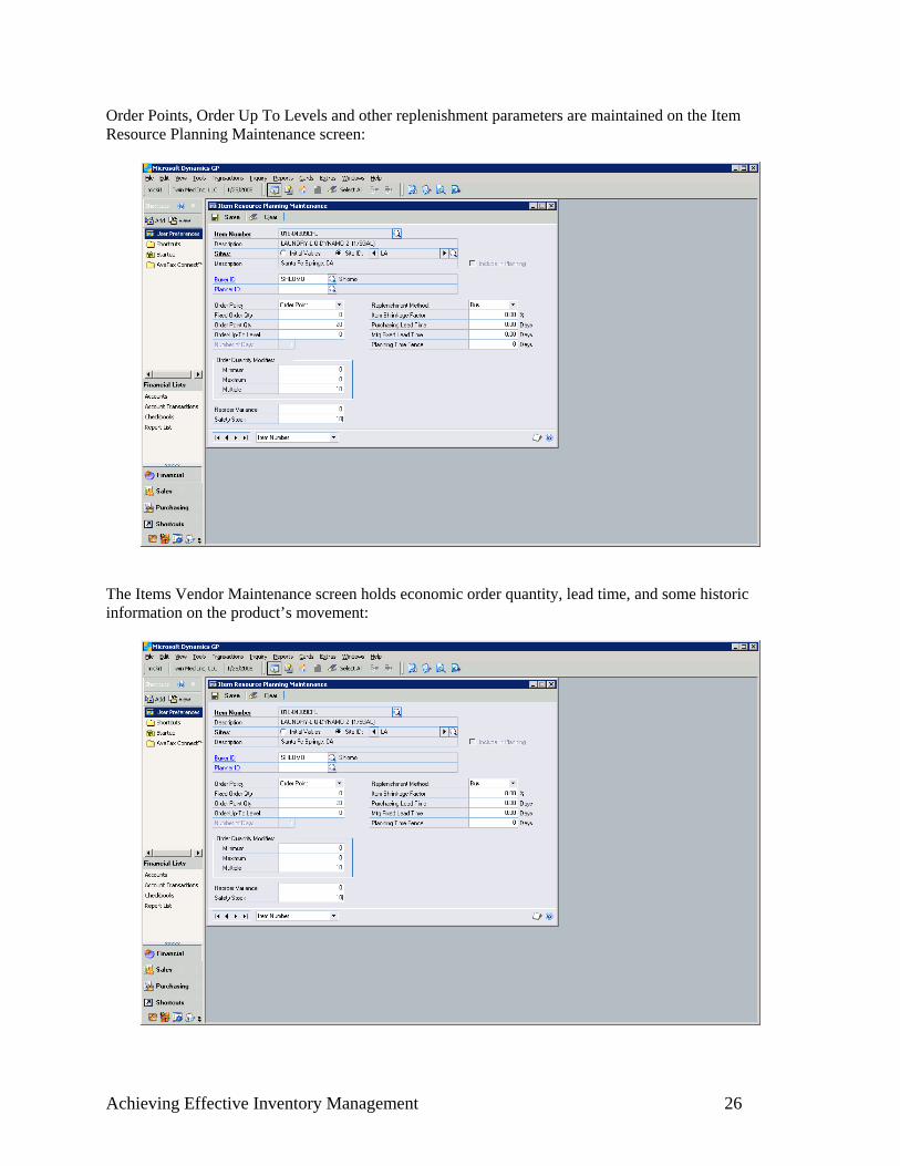
Order Points, Order Up To Levels and other replenishment parameters are maintained on the Item Resource Planning Maintenance screen:

The Items Vendor Maintenance screen holds economic order quantity, lead time, and some historic information on the product’s movement:


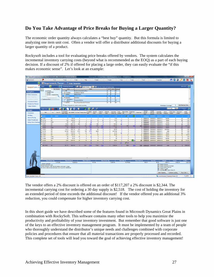
Do You Take Advantage of Price Breaks for Buying a Larger Quantity? The economic order quantity always calculates a “best buy” quantity. But this formula is limited to analyzing one item unit cost. Often a vendor will offer a distributor additional discounts for buying a larger quantity of a product. Rockysoft includes a tool for evaluating price breaks offered by vendors. The system calculates the incremental inventory carrying costs (beyond what is recommended as the EOQ) as a part of each buying decision. If a discount of 2% if offered for placing a large order, they can easily evaluate the “if this makes economic sense”. Let’s look at an example:

The vendor offers a 2% discount is offered on an order of $117,207 a 2% discount is $2,344. The incremental carrying cost for ordering a 30 day supply is $2,518. The cost of holding the inventory for an extended period of time exceeds the additional discount! If the vendor offered you an additional 3% reduction, you could compensate for higher inventory carrying cost. In this short guide we have described some of the features found in Microsoft Dynamics Great Plains in combination with RockySoft. This software contains many other tools to help you maximize the productivity and profitability of your inventory investment. But remember that good software is just one of the keys to an effective inventory management program. It must be implemented by a team of people who thoroughly understand the distributor’s unique needs and challenges combined with corporate policies and procedures that ensure that all material transactions are properly processed and recorded. This complete set of tools will lead you toward the goal of achieving effective inventory management!

Documents

Effective Inventory Management with GP and · Achieving Effective Inventory Management with Dynamics GP and RockySoft. Achieving Effective Inventory Management 2 Introduction Distributors