Effects of Correlated Shadowing: Connectivity, Localization, and RF

Tomography

Neal Patwari and Piyush Agrawal

Sensing and Processing Across Networks Lab

ECE Department, University of Utah, Salt Lake City, USA

[npatwari, pagrawal]@ece.utah.edu

Abstract

Unlike current models for radio channel shadowing in-

dicate, real-world shadowing losses on different links in a

network are not independent. The correlations have both

detrimental and beneficial impacts on sensor, ad hoc, and

mesh networks. First, the probability of network connec-

tivity reduces when link shadowing correlations are consid-

ered. Next, the variance bounds for sensor self-localization

change, and provide the insight that algorithms must infer

localization information from link correlations in order to

avoid significant degradation from correlated shadowing.

Finally, a major benefit is that shadowing correlations be-

tween links enable the tomographic imaging of an environ-

ment from pairwise RSS measurements. This paper applies

measurement-based models, and measurements themselves,

to analyze and to verify both the benefits and drawbacks of

correlated link shadowing.

1. Introduction

This paper addresses the effects of an accurate radio

layer model on multi-hop wireless network performance

analysis. In particular, we apply a path loss model which

connects link shadowing losses to the physical environment

in which the network operates. Because nearby links are of-

ten affected by the same shadowers in the environment, link

losses can be correlated. The new probability model for

path loss improves the accuracy of analysis of the effects of

the physical layer in multi-hop networks. In this paper, we

quantify the effects of correlated shadowing in three topics:

network connectivity (Section 3), sensor received signal-

strength (RSS)-based localization bounds (Section 4), and

radio tomographic imaging (RTI) (Section 5). This quan-

tification uses simulation and analysis using a proposed link

shadowing model, and experimental measurements.

Each section introduces its topic in more detail, but in

short, existing i.i.d. link fading models overestimate net-

work connectivity and do not permit complete analysis of

RSS self-localization lower bounds on variance. Further,

the same effect which causes correlated shadowing also en-

ables the imaging of environments using link measurements

of RSS, which may lead to the development of whole-

building imaging sensor networks for security applications

or for emergency use by fire-fighters and police.

This paper presents the first broad study of the effects

of link fading correlations on sensor, ad hoc, and mesh net-

work performance. We first, in this section, discuss existing

path loss and fading models for multi-hop networks, and

give intuitions as to why they are not adequate. Section 2

provides an overview of the correlated link fading model

used in this paper, the network shadowing (NeSh) model,

which was reported in [2]. The lack of a validated model

has prevented past research from quantifying link correla-

tion effects. Sections 3 through 5 present the effects of the

model in the three areas mentioned above, and Section 6

concludes and discusses open research topics.

1.1. Path Loss and Fading

The path loss on a link has three contributions: (1)Large-

scale path loss due to distance; (2)Shadowing loss due to

obstructions; and (3)Non-shadowing loss due to multipath

(a.k.a. small-scale or frequency selective fading). Given this

delineation, we denote Pi,j as the measured received power

at node j transmitted by node i,

Pi,j = P (di,j) − Zi,j , (1)

Zi,j = Xi,j + Yi,j , (2)

where di,j is the distance between nodes i and j, P (d) is

the ensemble mean dBm received power at distance d, Xi,j

is the dB shadowing loss, and Yi,j is the non-shadow fading

loss in dB. We refer to Zi,j as the total fading loss. Ensem-

ble mean received power at distance d is given by [9],

P (d) = PT − Π0 − 10np log10

d

∆0, (3)

where PT is the transmitted power in dBm, np is the path

loss exponent, and Π0 is the loss experienced at a short ref-

erence distance ∆0 from the transmitter antenna.

1.2. Existing Models

The literature commonly considers two fading models.

The first is that fading is insignificant, i.e., Zi,j = 0 for

all links (i, j). This is commonly referred to as the cir-

cular coverage model, because links in all directions will

be disconnected deterministically for d such that P (d) ex-

ceeds a threshold. Very significant analytical results have

been derived using the circular coverage model regarding

connectivity (as reviewed in [14]) and capacity [8], to note

two example applications. The circular coverage model is a

common assumption in published research [13].

The second model is that fading Zi,j is random, indepen-

dent and identically distributed on each link. We refer to

this as the i.i.d. link fading model, and it is used in analysis

of many wireless networks, and has been used in published

analysis and simulation of multi-hop networks [10, 3].

1

2

3

4

Figure 1. Three links with a common node.

In reality, neither model accurately represents the radio

channel for multi-hop networks. While coverage area is cer-

tainly not circular, it generally has some continuous shape.

The i.i.d. link fading model does not have any spatial mem-

ory, so there is no sense of coverage area. For example,

consider nodes which can communicate with node 1 in Fig-

ure 1. Node 2 may be disconnected while node 3 is con-

nected, or vice versa, regardless of how close nodes 2 and 3

are to each other. Also, the fading on links (1,3) and (1,4)

are independent, even though objects which attenuate link

(1,3) probably also attenuate link (1,4). These disconnects

between the i.i.d. link fading model and reality motivate the

application of a model with link shadowing correlation. Per-

haps the best motivation is that link shadowing correlations

have been experimentally observed in measured sensor net-

works [2], yet their impacts have not yet been studied.

2. Network Shadowing Model

In order to develop analysis and simulations which con-

sider correlated link shadowing, we must apply a statisti-

cal model which has been verified using measurements. In

mobile radio networks, the model of Gudmundson [7] is

used to model shadow fading correlations for a mobile link

with a common base station. However, this model is un-

able to model correlations between links with no common

endpoints, as are common in ad hoc networks.

In this paper, we apply the network shadowing (NeSh)

model of [2]. To model the experimentally observed char-

acteristic of correlated link shadowing, the network shad-

owing (NeSh) model first models the environment in which

the network operates. It then considers shadowing losses to

be a function of that environment, which has the effect of

correlating losses on geographically proximate links.

The shadowing caused by an environment is quantified in

an underlying spatial loss field p(x). The NeSh model as-

sumes that p(x) is an isotropic wide-sense stationary Gaus-

sian random field with zero mean and exponentially decay-

ing spatial correlation. Specifically,

E [p(xi)p(xj)] = Rp(di,j) =σ2

X

δe−

di,jδ (4)

where di,j = ‖xj − xi‖ is the Euclidian distance between

xi and xj , δ is a space constant and σ2X is the variance of

Xi,j .

Next, the NeSh model formulates the shadowing on link

a = (i, j) as a normalized integral of the p(x) over the line

between link endpoints xi and xj ,

Xa ,1

d1/2i,j

∫ xj

xi

p(y)dy. (5)

Single Link Properties: The NeSh model agrees with two

important empirically-observed link shadowing properties:

Prop-I The variance of link shadowing is approxi-

mately constant with path length [9],[21].

Prop-II Shadowing losses are Gaussian [21],[18].

The model in (5) can be seen to have Prop-II, since Xa is

a scaled integral of a Gaussian random process. To show

Prop-I, we note that E[Xa] = 0, and

Var [Xa] =1

di,j

∫ xj

xi

∫ xj

xi

Rp(||β − α||)dαT dβ. (6)

Using (4) as the model for spatial covariance,

Var [Xa] = σ2X

[

1 − δ

di,j

(

1 − e−di,j/δ)

]

. (7)

When di,j >> δ, the NeSh model has Prop-I,

Var [Xa] ≈ σ2X . (8)

Joint Link Properties: Given two links a, b ∈ Z2, both Xa

and Xb are functions of the same shadowing field p(x), thus

the model (5) introduces correlation between them. The co-

variance between Xa and Xb is,

Cov (Xa, Xb) =σ2

X/δ

d1/2i,j d

1/2l,m

∫ xj

xi

∫ xm

xl

e−||β−α||

δ dαT dβ

(9)

The covariance (9) is computed by numerical integration,

using code available on [1].

2.1. Non-Shadow Fading

As given in (1), received power Pi,j consists of losses

due both to shadow fading Xi,j and non-shadow fading Yi,j .

The NeSh model assumes that {Yi,j}i,j are independent.

Nodes in ad hoc, sensor, and mesh networks are typically

separated by many wavelengths, and small-scale fading cor-

relation is approximately zero at such distances [5]. Further,

the NeSh model assumes that small scale fading is indepen-

dent of shadow fading.

In particular, Yi,j is modeled as Gaussian (in dB) with

zero mean and variance σ2Y . While small scale fading

for narrowband fading channels is typically modeled as

Rayleigh, Rician, or other non-Gaussian distribution, the

NeSh model assumes that nodes have a wideband receiver

which effectively averages narrowband fading losses across

frequencies in its bandwidth. As an average of small-scale

fading losses at many frequencies, Yi,j , by a central limit

argument, is approximately Gaussian.

2.2. Joint Link Received Power Model

On a single link a = (i, j), total fading loss Za = Xa +Ya. Since Xa and Ya are independent and Gaussian (in dB),

total fading Za is also Gaussian with variance

σ2dB , Var [Za] ≈ σ2

X + σ2Y . (10)

Furthermore, we consider the joint model for the total

fading on all links in the network. Let a1, . . . , aK for ak =(ik, jk) be an enumeration of the K unique measured links

in the network. A unique link ak must have both that ak 6=al for all l 6= k and that the reciprocal link is not included,

i.e., (jk, ik) 6= al for all l. The vector RSS on all links is

P = [Pa1, . . . , PaK

].

The vector P is multivariate Gaussian, and thus it is com-

pletely specified by its mean and covariance. We define vec-

tor P as the mean of P, which is given by

P = [P (da1), . . . , P (daK

)], (11)

where P (dak) = P (dik ,jk

) is given in (3). Next, denoting

C to be the covariance matrix of P,

Ck,l = σ2Y Ik,l + Cov (Xak

, Xal) (12)

where Ik,l = 1 if k = l and 0 otherwise, and Cov (Xa, Xb)is given in (9).

2.3. Research Evidence

The NeSh model was tested in a measurement campaign

in [2] which measured fifteen realizations of indoor wire-

less sensor networks. Each realization was measured in

a randomly-altered environment. Following the measure-

ments, the losses on each ‘link geometry’, that is, the rel-

ative positioning of two links, were used to calculate a co-

variance between the shadowing on two links. The model

explained 80.4% of the measured covariances on the tested

link geometries.

Both current i.i.d. link fading models and the NeSh

model require two parameters, σ2dB and np [21]. The NeSh

model requires two additional parameters, σ2X and δ. In [2],

these are reported to be σ2X/σ2

dB = 0.29 and δ = 0.21 m.

These measured parameters in all of the following analysis

and simulation.

2.4. Model Limitations

We note that the NeSh model has limitations. First, it is

a purely statistical model, not a solution to the electromag-

netic wave propagation equation. To simulate a network

deployed in a known place with known obstructions, one

could use ray-tracing to determine loss on each link with

high accuracy. The NeSh model is valuable only for simu-

lations of random deployments.

Second, the model in [2] was tested for 2-D, not 3-D

deployments. Although not tested, the model is applica-

ble to 3-D; one could apply 3-D coordinates in (4) and (5).

For example, in forest deployments with sensors at different

heights in trees, the NeSh model could be applied. How-

ever, varying terrain may be difficult to properly model us-

ing NeSh, since hills and mountains are typically orders of

magnitude larger than other obstructions – a single space

constant δ in (4) may not suffice.

Thirdly, we would expect to see no NeSh model im-

provement (but no degradation) in environments without

obstructions (e.g., empty parking lots) or with extremely

small obstructions compared to the path lengths. For ex-

ample, a completely flat and homogeneous forested envi-

ronment with link lengths of kilometers, would see shad-

owing, but few links would cross the same trees. In this

case, δ/di,j → 0 and link covariances would also be zero.

Finally, the NeSh model in (5) integrates loss along a

line-of-sight (LOS) path between transmitter and receiver.

The NeSh model only indirectly incorporates non-LOS

paths in the model for shadowing loss. If an LOS path

is strongly shadowed, the model effectively assumes that

NLOS signals typically arrive with lower power as well

(due to additional scattering or reflection to go around the

obstruction). The normalization by 1/d1/2i,j in (5) also helps

to diminish the impact of the LOS path as the path length in-

creases (since longer paths tend to have higher NLOS con-

tributions [17]). For longer links, the normalization term de-

creases the emphasis of the total loss on any one part of the

environment. The NeSh model is statistical, so it relies on

typical links having such a correlation between NLOS and

LOS contributions. However, in strongly reflective environ-

ments, e.g., inside an airplane, such an assumption may not

be valid, and the NeSh model should not be used.

The model described in this paper is not perfect for all

cases, but it does provide a means to incorporate link cor-

relations into network simulation and analysis, which we

attempt in the following sections.

3. Network Connectivity

It is typically of critical importance to ensure that a

multi-hop wireless network is connected. A network can

be represented as a graph G = (V , E) with vertices V as the

set of all nodes, and a set of directional edges E contain-

ing each transmitter/receiver pair which can communicate.

A network is connected if there exists a path between each

pair of vertices in its graph. If a network is not connected,

it may fail to perform as intended, lacking the capability to

transfer data from one part of a network to another. If nodes

are mobile, a temporary disconnectivity introduces latency

until reconnection. If nodes are stationary, for example in

a sensor network, a non-connected network requires a hu-

man administrator to go back to repair the sensor network,

possibly by moving existing nodes or deploying additional

nodes. Since non-connectivity is a major failure, networks

are ideally over-provisioned or deployed densely in order to

ensure a high probability of connectivity.

In this section, we study the connectivity of particular

networks via simulation using both i.i.d. link shadowing and

correlated shadowing models. We show that network con-

nectivity in the i.i.d. link shadowing model is overly opti-

mistic. This bias is most severe in robust networks designed

to ensure reliable connectivity.

3.1. Related Research

Certainly, the vast majority of connectivity research as-

sumes the circular coverage model [13], which allows quick

results with relatively simple analysis. Recent work has ex-

panded connectivity analysis by using the i.i.d. log-normal

shadowing model. For example, Hekmat and Van Mieghem

[10] and Bettstetter and Hartmann [3] studied connectivity

in ad hoc networks using the i.i.d. log-normal shadowing

model. The model leads in those works to a result that the

increase in the variance of shadow fading in the channel also

increases the connectivity of the network for the same den-

sity of nodes [3]. The results presented in this section show

that these connectivity gains are overstated by the use of an

i.i.d. link fading model.

3.2. Methods

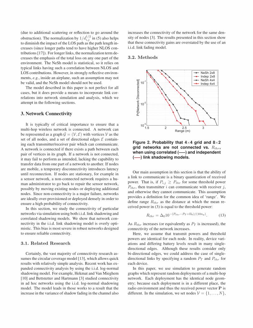
Figure 2. Probability that 4×4 grid and 8×2grid networks are not connected vs. Rthr,

when using correlated (—–) and independent

(—–) link shadowing models.

Our main assumption in this section is that the ability of

a link to communicate is a binary quantization of received

power. That is, if Pi,j ≥ Pthr for some threshold power

Pthr, then transmitter i can communicate with receiver j,

and otherwise they cannot communicate. This assumption

provides a definition for the common idea of ‘range’. We

define range Rthr as the distance at which the mean re-

ceived power in (3) is equal to the threshold power:

Rthr = ∆010−(Pthr−PT +Π0)/(10np). (13)

As Rthr increases (or equivalently as PT is increased), the

connectivity of the network increases.

Here, we assume that transmit powers and threshold

powers are identical for each node. In reality, device vari-

ations and differing battery levels result in many single-

directional edges. Although these results consider only

bi-directional edges, we could address the case of single-

directional links by specifying a random PT and Pthr for

each device.

In this paper, we use simulation to generate random

graphs which represent random deployments of a multi-hop

network. Each deployment has the identical node geom-

etry; because each deployment is in a different place, the

radio environment and thus the received power vector P is

different. In the simulation, we set nodes V = {1, . . . , N},

select particular coordinates (xi, yi) for all i ∈ V , and then

perform many independent trials. In each trial we

1. Generate P from a multivariate Gaussian distribution

with mean P from (11) and covariance C from (12).

2. Define the set of edges E = {a : Pa ≥ Pthr}.

3. Determine whether or not the graph G is connected.

3.3. Results

For simulations, we must set model parameters. We have

chosen σdB = 7.0, np = 3.0, and ∆0 = 1 m; and the mea-

sured parameters of δ = 0.21 m and σX/σdB = 0.29 from

[2]. In our study, we vary Rthr, or equivalently because of

(13), vary (PT − Π0 − Pthr). This allows us to study the

effects of increasing ‘range’ however that increased range

is achieved.

We first consider a sensor network of N = 16 nodes

deployed regularly in a 4 by 4 grid, in a 4 m by 4 m area

(so that the nodes are spaced each 1.333 m). We run 105

trials at each value of range Rthr between 1.1 m and 2.5

m. Figure 2 shows the simulated probability of the network

being disconnected, in both i.i.d. link fading and correlated

link fading models.

Next we consider the same N = 16 nodes deployed in a

long rectangle, in a 2 by 8 grid, in a 1.5 m by 10.5 m area

(so that nodes are spaced each 1.5 m). This deployment has

approximately the same area (16 m2 vs. 15.75 m2 here) and

thus the same node density. The longer deployment simu-

lates a sensor network used, for example, in a security sys-

tem to monitor a border. We run 105 trials at each value of

range Rthr between 1.8 m and 3.4 m, and Figure 2 displays

the probabilities of non-connectivity in both fading models.

3.4. Discussion

For reliable deployments, e.g., with Rthr = 2.2 m in the

square example, the probability of the network being dis-

connected is 4.1 × 10−3 under the i.i.d. link fading model

and 9.5× 10−3 under the correlated link shadowing model.

The increase of 230% for the correlated model represents a

significant increase in the risk of network non-connectivity.

In the rectangular example, for Rthr = 3.0 m, the probabil-

ity of non-connectivity rises 380% from 1.6 × 10−3 under

the i.i.d. link fading model to 6.1 × 10−3 under the corre-

lated link shadowing model. We observe that narrow de-

ployment areas magnify the negative effects of link correla-

tion on network connectivity. The results also indicate that

as the overall reliability is increased, the over-estimation of

connectivity in the i.i.d. link fading model will be increas-

ingly severe.

4. Sensor Self-Localization

Lower bounds on sensor self-location estimation have

been derived in past research order to provide insight into

the effects of system design choices [15, 20, 22, 4, 18]. For

example, if the lowest possible localization variance using

nodes capable of one measurement modality is too high for

the application requirements, a system designer can decide

on an alternate measurement modality. As another exam-

ple, if an implemented estimator achieves a location vari-

ance close to the bound, a designer knows that more effort

on estimator design will not improve accuracy significantly

further.

However, localization bounds reported in the literature

have been derived assuming that measurements on different

links are independent. If measurements are correlated, such

a lower bound would not in fact be rigorous, i.e., the derived

lower bound on variance may in fact be higher or lower. In

this section, we present the Cramer-Rao bound (CRB) for

localization variance when measurements of signal strength

are correlated as given by the NeSh model. The CRB is a

lower bound on the variance of any unbiased estimator. It

is particularly valuable because it does not depend on the

algorithm implemented.

4.1. Derivation

To derive the Cramer-Rao bound, we assume that coor-

dinates to be estimated, θ, are unknown, where

θ = [x1, . . . , xn, y1, . . . , yn]T ,

where xi = [xi, yi]T is the coordinate of node i. Here, we

assume that some devices, nodes n+1, . . . , N have a priori

known coordinate, and thus do not need to be estimated.

Let xi and yi be unbiased estimators of xi and yi. The

CRB provides that the trace of the covariance of the ith lo-

cation estimate, which we call the location estimation vari-

ance bound, satisfies

σ2i , tr {covθ(xi, yi)} = Varθ [xi] + Varθ [yi]

≥[

F−1]

i,i+

[

F−1]

n+i,n+i(14)

The Fisher information matrix F for this case is [12],

F = Fµ + FC (15)

[Fµ]m,n =

[

∂P

∂θm

]T

C−1

[

∂P

∂θn

]

[FC ]m,n =1

2tr

[

C−1 ∂C

∂θmC−1 ∂C

∂θn

]

The derivatives ∂P∂θi

depend on whether the ith parameter is

an x or y coordinate of a node, and are given in [19] to be:

∂P(dak)

∂xm=

−α(xm − xjk)/d2

m,jk, if m = ik

−α(xm − xik)/d2

m,ik, if m = jk

0, otherwise

∂P(dak)

∂ym=

−α(ym − yjk)/d2

m,jk, if m = ik

−α(ym − yik)/d2

m,ik, if m = jk

0, otherwise

where α =10np

log 10 and distance d2m,jk

= ‖xm − xjk‖2.

4.2. Discussion of Fisher Information Terms

We refer to Fµ as the mean term and FC as the covari-

ance term of the Fisher information matrix in (15). As the

names imply, the mean and covariance terms quantify the

information present in the mean and the covariance of the

RSS measurements in the network, respectively.

RSS measurements are informative in the mean because

the ensemble average RSS measurement in (3) is a func-

tion of distance. In CRB analysis under the i.i.d. link fading

model, C = σ2dBI for identity matrix I . Under the NeSh

model, the information in the mean term is reduced by the

non-diagonal covariance matrix C. This will be shown nu-

merically in Section 4.3.

In contrast, the covariance term provides additional in-

formation about the coordinates due to the correlations

found in the link RSS measurements. In effect, relation-

ships between fading loss measurements on pairs of links in

the network will indicate something about the relative ge-

ometry of those links. For example, if two links (i, j) and

(i, k) both have very high losses Zi,j and Zi,k, it may in-

dicate that nodes j and k are in the same relative direction

from node i. In analyses which use the i.i.d. link fading

model, FC = 0, and thus no information is gained from the

relationships between measurements on pairs of links.

The calculation of { ∂C∂θk

}k is complicated by the size of

matrix C and the fact that we require 2n different partial

derivatives. We calculate ∂C∂θk

using a finite difference ap-

proximation. Writing the covariance matrix as C(θ) to ex-

plicitly show it as a function of the coordinates θ,

∂C

∂θk≈ C(θ + ǫek) − C(θ)

ǫ,

where ek is the vector of all zeros except for a 1 in the kth

position, and ǫ is a small positive constant, in this case, we

use ǫ = 10−2 m.

4.3. CRB Comparison in Example Net-works

To evaluate the relative effect of correlation in the path

loss model, we define the relative increase in the standard

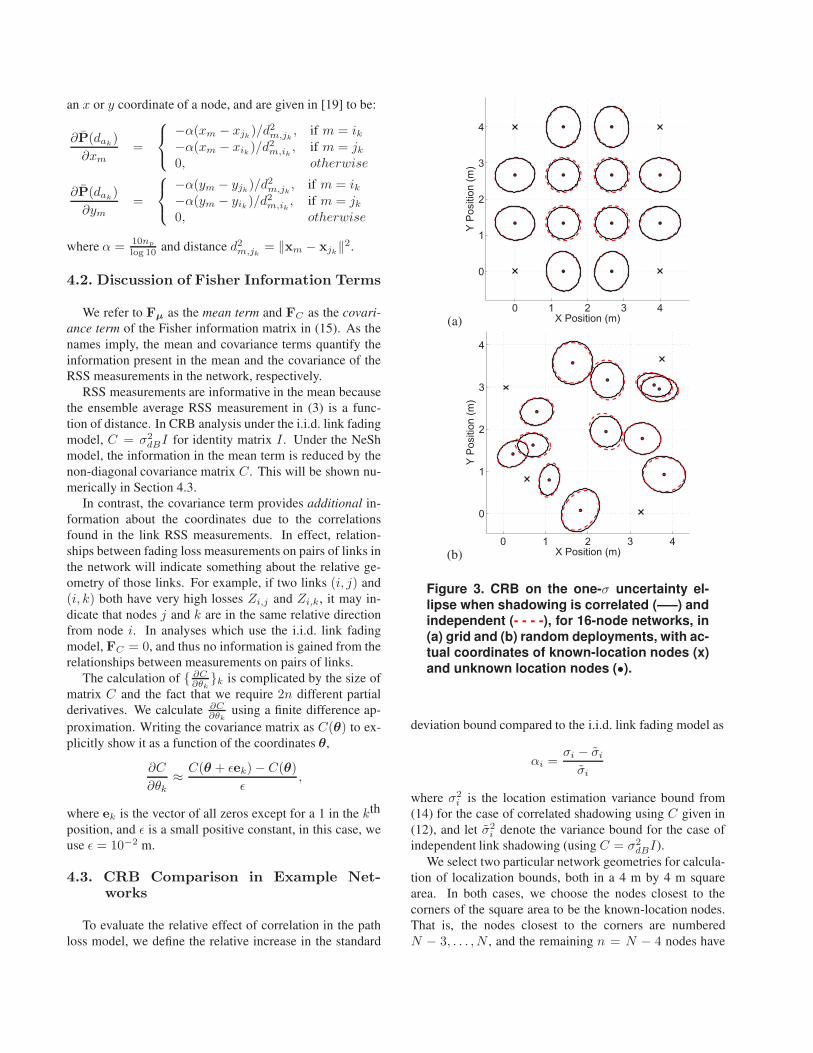
(a)

(b)

Figure 3. CRB on the one-σ uncertainty el-

lipse when shadowing is correlated (—–) andindependent (- - - -), for 16-node networks, in

(a) grid and (b) random deployments, with ac-tual coordinates of known-location nodes (x)

and unknown location nodes (•).

deviation bound compared to the i.i.d. link fading model as

αi =σi − σi

σi

where σ2i is the location estimation variance bound from

(14) for the case of correlated shadowing using C given in

(12), and let σ2i denote the variance bound for the case of

independent link shadowing (using C = σ2dBI).

We select two particular network geometries for calcula-

tion of localization bounds, both in a 4 m by 4 m square

area. In both cases, we choose the nodes closest to the

corners of the square area to be the known-location nodes.

That is, the nodes closest to the corners are numbered

N − 3, . . . , N , and the remaining n = N − 4 nodes have

no prior coordinate knowledge.

First, we deploy nodes in a 4 by 4 square grid within the

4 m by 4 m area. Nodes are separated by 1.333 m, N = 16,

and n = 12. We calculate the CRB in both i.i.d. and cor-

related link fading models from (14). Figure 3(a) shows

the actual location and bound on 1-σ covariance ellipse of

each node i = 1 . . . 12. The 1-σ covariance ellipse is a use-

ful visual representation of the magnitude and direction of

variation of a node’s coordinate estimate. The locations of

the reference nodes are also shown. For i = 1 . . . 12, the

values αi are in the range of -0.09 to 0.02, with an average

of -0.024. This means that on average, the standard devia-

tion bound, when shadow fading correlations are taken into

account, decreases by 2.4%.

Next, we generate a random deployment by selecting

coordinates independently from a uniform distribution on

[0m, 4m]2. The actual node locations and the calculated

CRB on 1-σ covariance ellipse for each node are shown in

Figure 3(b). For i = 1 . . . 12, the values αi are in the range

of -0.13 to 0.03, with an average of -0.045. The average

standard deviation bound decreases by 4.5%. In general,

for random deployments, the decrease in standard deviation

bound is more significant than the grid deployment.

4.4. Discussion and Investigation of Results

These decreases in the bound may be unexpected, be-

cause it is counterintuitive that correlation may improve

localization. We might expect that increased link correla-

tion effectively increases the ‘noise’ level since measure-

ments with additional nodes cannot be used as effectively to

‘average-out’ fading error. For example, in Figure 1, if an

obstruction attenuates both links (1,3) and (1,4), then both

link measurements would tend to push nodes 3 and 4 further

from node 1. If link measurements were i.i.d., there would

be a lower chance of both link measurements (1,3) and (1,4)

‘agreeing’ nodes 3 and 4 should be further from node 1.

To investigate further, we momentarily ignore the co-

variance term FC and focus solely on the mean term Fµ

in (15). This mean term of the Fisher information matrix

should support our above intuition about correlation acting

to increase the effective noise level. So, momentarily set-

ting FC = 0 in (15), we calculate the bound using F = Fµ.

We call this the NeSh model-based mean term-only bound.

We calculate this NeSh model-based mean term-only

bound for the same deployment geometries studied previ-

ously in Figure 3. In this case, we compare the 1-σ co-

variance ellipses of the NeSh model-based mean term-only

bound and of the i.i.d. link fading CRB in Figure 4. The

results show clearly that using only the information in the

mean term, the lower bound increases when taking into ac-

count link correlations. For the grid deployment in Figure

4(a), the values αi are in the range of 0.03 to 0.11, with an

average of 0.080. This means that on average, when we ig-

nore the information in the covariance term of the Fisher in-

formation, the lower bound on standard deviation increases

by 8.0%. For the random deployment in Figure 4(b), the

same lower bound increases an average of 13.8%. In gen-

eral random deployments show a more significant increase

in lower bound when considering the mean term-only.

This further investigation demonstrates two things:

1. The intuition that link correlations negatively impact

localization is true, when estimators only consider the

localization information contained in the mean rela-

tionship between received power and distance in (3).

2. The use of the information contained in the correla-

tions between links’ fading measurements can com-

pensate for the information loss in the mean term, and

in fact can reduce localization variances lower than

previously thought possible.

These results indicate that estimators which consider

correlations between link measurements when estimating

node locations will aid the effort to achieve the lowest pos-

sible variance. Some localization algorithms have applied

statistical learning techniques which explicitly attempt to

learn correlations in RSS measurements from training data

and then use them to classify or estimate node location

[6, 16]. Other algorithms may be readily adapted to con-

sider link correlations, for example, belief propagation net-

work approaches such as in [11]. However, evaluation of

these methods to compare algorithm performance vs. the

new bound is beyond the scope of this paper. Future work

in RSS-based localization algorithms must investigate ap-

proaches to infer location information from link fading cor-

relations.

5. Radio Tomographic Imaging

The mechanism which causes correlated link shadowing

is detrimental to network connectivity and can be detrimen-

tal to sensor self-localization, as discussed in the past two

sections. However, there is a benefit gained from the exis-

tence of correlated link shadowing, as we discuss in this sec-

tion. Simultaneous imaging through whole buildings would

improve security systems and could save lives in emergency

situations. For example, if fire-fighters knew where peo-

ple were within a building, they could more accurately di-

rect rescue operations, and monitor emergency personnel in

building.

If link shadowing is a function of the attenuating prop-

erties of the environment in between the transmitter and re-

ceiver, then link shadowing measurements can be used to in-

fer those properties. Consider the 20-node network shown

in Figure 5. An attenuating object in the building would

(a)

(b)

Figure 4. NeSh model ‘mean term-only’

bound (—–) and CRB using the i.i.d. link fad-ing model (- - - -) on localization one-σ uncer-

tainty ellipses, for the same (a) grid and (b)random deployments in Figure 3.

tend to increase shadowing loss on multiple links which

cross over that object. The inverse perspective on this prob-

lem is that high shadowing loss on multiple, intersecting

links can be used to infer the location of that attenuating

object. By analogy to the medical usage of electromagnetic

waves for imaging, we call this method radio tomographic

imaging (RTI).

Related work in radar imaging measures scattering,

and this imaging method uses transmission. These two

wave propagation mechanisms have fundamentally differ-

ent properties [23, Section 1.10]. In scattering, a wave hits

an object and effectively retransmits waves in other direc-

tions. The scattered wave measured at the radar device has

power on the order of 1/d4 (in free space). In transmission,

a wave passes through an object and continues in one direc-

5 7

18 19 20 2114 15 16 17

1

2

3

4

5 6 7 8 9 10 11 12 13

Figure 5. Nodes measure shadowing on links

covering a building area. Radio tomographic

imaging (RTI) algorithms image the area’stransmission properties.

tion. The transmitted wave loses power due to transmission

but arrives at a distant receiver with power on the order of

1/d2 (again, in free space). In cluttered environments, both

exponents will increase. One fundamental benefit of trans-

mission is that the signal range is approximately the square

of that of scattering.

Note that imaging requires correlated shadowing. If link

shadowing is independent between links, then there is no

chance of being able to image the location of the obstruc-

tions in the environment.

Finally, there are certainly many tomographic imaging

algorithms, as they have been explored in the literature for

multiple purposes over the course of the past decades. The

RF tomographic imaging problem introduces physical vari-

ations which require special consideration. As such, we

don’t claim to present an optimal image estimation algo-

rithm, only one reasonable attempt.

5.1. Motion Imaging Algorithm

The imaging algorithm proceeds as follows. To compute

an image of the motion in the building at time n,

1. Difference: Find the link path loss difference, νi,j =P avg

i,j − Pi,j where P avgi,j is the past history average

received power for link (i, j). Denote ν as a vector of

all {νi,j}i,j as in (16).

2. Inverse: Find the weighted least-squared (WLS) error

solution for the (pixelated) attenuation field p. The

WLS estimator is given by p = Πν, where Π is the

projection matrix given in (19).

3. Contrast: Convert the real-valued attenuation estimate

p into a image vector p with values in the range [0, 1]using the transformation in (20).

These three steps are detailed and justified below.

5.2. Difference

When we image motion, we are not interested in the

static attenuation caused by the environment. This static

attenuation can be calculated initially, assuming that the

nodes are deployed and measuring link losses prior to any

motion in the environment. Alternatively, if there is quite a

bit of motion during the initial setup, we would expect that

an average of path losses measured during a long segment

of random motion would reduce the effects of each partic-

ular motion. In that case, a system might use a running

average of the link losses over a long history to estimate the

static attenuation. In any of these cases, we refer to P avgi,j as

the average past history received power on link (i, j). The

loss difference νi,j = P avgi,j − Pi,j quantifies the current

additional loss on link (i, j). Additional loss on this link

should be explained by high additional attenuation in the

field p(x). As done in Section 2.2, we list unique measured

links as ak = (ik, jk) for k = 1, . . . , K where K is the total

number of measured links, and then define

ν = [νi1,j1 , . . . , νiK ,jK]T (16)

5.3. Inverse

Next, we solve for the pixelated additional loss field,

p = [p(y1), . . . , p(yM )]T

where yi is the center coordinate of the ith pixel. The vector

p is the change in attenuation at each pixel of the measured

area. We assume that p is correlated as given in (4).

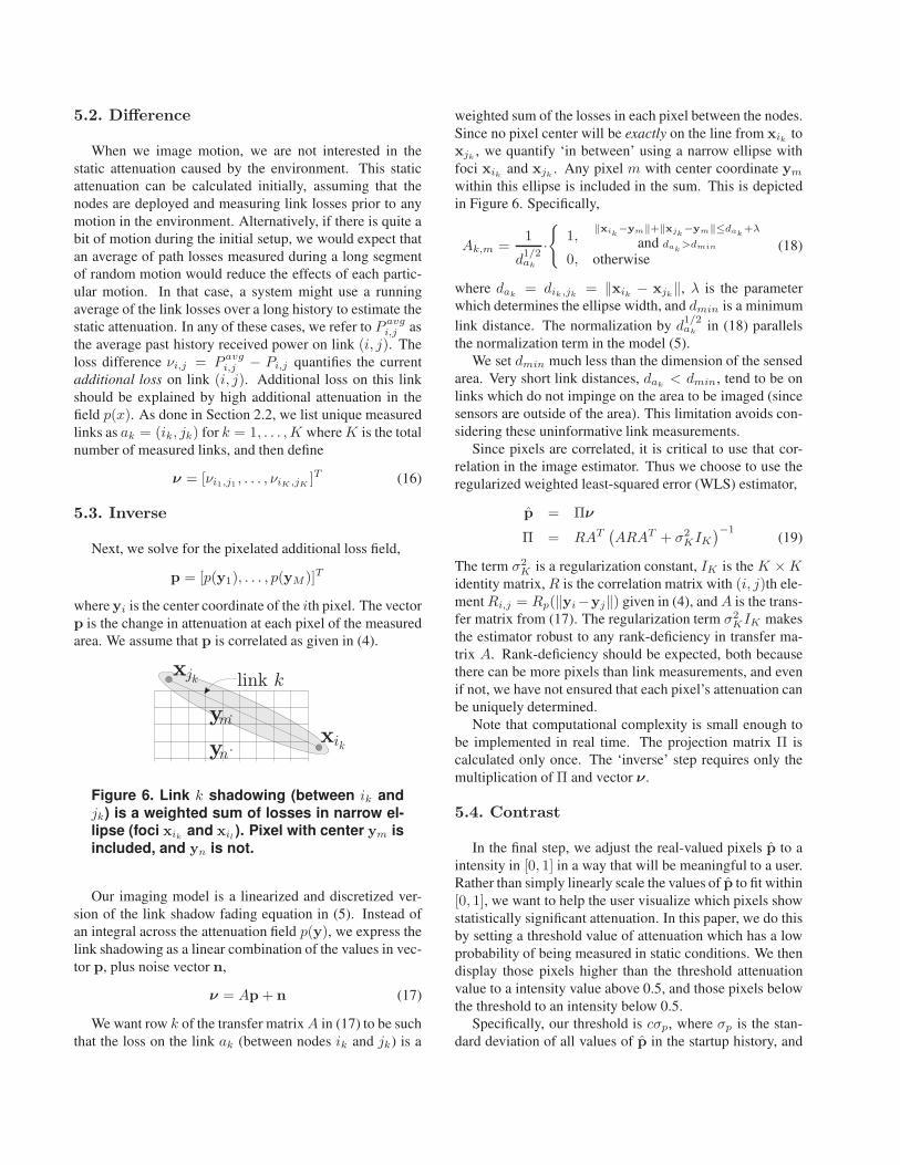
xik

xjk

y

y

m

n

link k

Figure 6. Link k shadowing (between ik and

jk) is a weighted sum of losses in narrow el-lipse (foci xik

and xil). Pixel with center ym is

included, and yn is not.

Our imaging model is a linearized and discretized ver-

sion of the link shadow fading equation in (5). Instead of

an integral across the attenuation field p(y), we express the

link shadowing as a linear combination of the values in vec-

tor p, plus noise vector n,

ν = Ap + n (17)

We want row k of the transfer matrix A in (17) to be such

that the loss on the link ak (between nodes ik and jk) is a

weighted sum of the losses in each pixel between the nodes.

Since no pixel center will be exactly on the line from xikto

xjk, we quantify ‘in between’ using a narrow ellipse with

foci xikand xjk

. Any pixel m with center coordinate ym

within this ellipse is included in the sum. This is depicted

in Figure 6. Specifically,

Ak,m =1

d1/2ak

·{

1,‖xik

−ym‖+‖xjk−ym‖≤dak

+λ

and dak>dmin

0, otherwise(18)

where dak= dik,jk

= ‖xik− xjk

‖, λ is the parameter

which determines the ellipse width, and dmin is a minimum

link distance. The normalization by d1/2ak in (18) parallels

the normalization term in the model (5).

We set dmin much less than the dimension of the sensed

area. Very short link distances, dak< dmin, tend to be on

links which do not impinge on the area to be imaged (since

sensors are outside of the area). This limitation avoids con-

sidering these uninformative link measurements.

Since pixels are correlated, it is critical to use that cor-

relation in the image estimator. Thus we choose to use the

regularized weighted least-squared error (WLS) estimator,

p = Πν

Π = RAT(

ARAT + σ2KIK

)−1(19)

The term σ2K is a regularization constant, IK is the K × K

identity matrix, R is the correlation matrix with (i, j)th ele-

ment Ri,j = Rp(‖yi−yj‖) given in (4), and A is the trans-

fer matrix from (17). The regularization term σ2KIK makes

the estimator robust to any rank-deficiency in transfer ma-

trix A. Rank-deficiency should be expected, both because

there can be more pixels than link measurements, and even

if not, we have not ensured that each pixel’s attenuation can

be uniquely determined.

Note that computational complexity is small enough to

be implemented in real time. The projection matrix Π is

calculated only once. The ‘inverse’ step requires only the

multiplication of Π and vector ν.

5.4. Contrast

In the final step, we adjust the real-valued pixels p to a

intensity in [0, 1] in a way that will be meaningful to a user.

Rather than simply linearly scale the values of p to fit within

[0, 1], we want to help the user visualize which pixels show

statistically significant attenuation. In this paper, we do this

by setting a threshold value of attenuation which has a low

probability of being measured in static conditions. We then

display those pixels higher than the threshold attenuation

value to a intensity value above 0.5, and those pixels below

the threshold to an intensity below 0.5.

Specifically, our threshold is cσp, where σp is the stan-

dard deviation of all values of p in the startup history, and

Table 1. Motion Experiment Timeline19:00:08-19:01:02 Open door, walk to, then stand in,

SW corner.

19:01:03-19:02:02 Walk to, then stand in, SE corner.

19:02:03-19:03:08 Walk to, then stand in, NE corner.

19:03:09-19:04:03 Walk to, then stand in, NW corner.

19:04:04 Exit room.

c is a positive constant. Since link losses ν are zero-mean

multivariate Gaussian (in dB) and p is a linear combina-

tion of ν, pixel values p will also be zero-mean and Gaus-

sian. Thus the false alarm probability, i.e., that p(yi) > cσp

when the environment is static, is approximately Q (c),

where Q (·) is the complementary CDF of a standard nor-

mal random variable, Q (x) = 12

[

1 − erf(x/√

2)]

. For ex-

ample, in the experiment described in Section 5.5, we use

c = 2.8, which makes the false alarm probability approxi-

mately 0.25%.

We also want to scale pixel values so that an intensity of

1 indicates the highest pixel value. We do this by using the

following (nonlinear) scaling function:

p = 1 − Q

(

p − cσp

a

)

(20)

where we choose a scaling constant a based on the maxi-

mum value of p, which we denote pmax = max p,

a = max [ǫa, (pmax − cσp)/b] (21)

where ǫa and b are predetermined positive constants. We

must ensure that a > 0 so that (20) does not have a

divide-by-zero, and thus (21) assigns it a minimum of ǫa.

The result of (21) is to ensure that when some pixels have

p(yi) > cσp, that the maximum attenuation in the image

is always displayed with intensity value of Q (b). For ex-

ample, we use b = 5 in Section 5.5, so that this maximum

intensity is very close to 1.

5.5. Experiment

We use an unoccupied 5m by 5m room in the Warnock

Engineering Building on the University of Utah campus.

All walls are interior walls, and mica2 sensors are placed

outside of the room, about 0.5m from each wall, as shown

in Figure 7(f). Admittedly, an empty room is a friendly en-

vironment for RTI, and future tests must verify that RTI can

work properly in average cluttered building environments.

Each sensor runs a TinyOS program to record the RSS

and id number from any messages received from its neigh-

bors. It also transmits (at 915 MHz), each half second, a

message containing its id and the (id, RSS) measurement

pairs which it recorded in the past half second. A laptop

Table 2. RTI Experiment SettingsVariable Name Description

Experiment Description

N = 20 Number of sensors

K = 190 Number of links measured

M = 121 Number of pixels

P avgi,j Average Pi,j prior to 19:00:08

σp Std. dev. of pixel values p prior to

19:00:08

Channel Model Parameters from [2]

δ = 0.21m Attenuation field correlation distanceσ2

X

σ2

dB

= 0.29 Shadowing variance ratio

RTI Algorithm Parameters

λ = 0.2m Ellipse ‘width’ parameter

dmin = 2m Minimum link length

σ2K = 3 Regularization constant

c = 2.8 # of σp for contrast threshold

b = 5 Maximum contrast parameter

ǫa = 0.1 Minimum contrast scale factor

connected to a listening node records and time-stamps all

packets transmitted by the sensors. The laptop is also con-

nected to a video camera which records time-stamped im-

ages from within the room so that the nature of activity is

known at each second.

To reduce missing data (due to interference), we average

the two measurements over time on a link (i, j) and the two

reciprocal channel measurements on link (j, i). Thus, each

second, there is one measurement for the bi-directional link

between nodes i and j, Pi,j . If there were no measurements

to average, we set Pi,j = P avgi,j .

The sensors are turned on and left running for about

40 minutes. This is the ‘startup period’ used to initialize

{P avgi,j }i,j and σp. Beginning at time 19:00:08, as detailed

in Table 1, a person walks into the room, walks to and

then stands in each corner, each for one minute, and finally

leaves the room.

We follow the algorithm steps outlined above to calculate

the image intensity vector p each second, using the con-

stants listed in Table 2 and display images. In Figure 7(a-e),

images recorded exactly one minute apart are shown. The

first four images are those at 19:00:23, 19:01:23, 19:02:23,

and 19:03:23, within 20 seconds after the movement to the

SE, SW, NW, and NE corners, respectively. The final image

shown in Figure 7(e) is taken at 19:04:23, about 20 seconds

after the person left the room.

5.6. Discussion

From Figure 7, we note positive results and opportunities

for future improvement. The results show that the extra at-

(a) (b) (f)

N

SW

Sensor

StoppingPosition

Door

WalkingPath

Key SENE

NW

SW

(c) (d) (e)

Figure 7. Radio tomographic images for times and person locations (a) 19:02:23 in NE corner, (b)

19:01:23 in SE corner, (c) 19:03:23 in NW corner, (d) 19:00:23 in SW corner, and (e) 19:04:23 whenperson was out of room. In (f) is an area map with diagram of the experiment.

tenuation caused by a person in a room can be both detected

and located. When no motion exists, images are almost al-

ways empty, with p ≈ 0. While a person is stationary in

the room, there is noticeable change, and the darkest pixels

indicate the general location of that extra attenuation. Fi-

nally, Figure 7 does not show calculated images during a

person’s movement, but we note that: (1) the image clearly

displays that motion exists with multiple dark pixels, but (2)

the image does not accurately locate that motion. We sup-

pose that since the sensors, as programmed, do not measure

the link losses simultaneously, the differences are enough to

confuse the result.

Further research is still warranted. Figure 7(a) shows

pixels with medium intensity at locations other than the SE

corner of the room. Periodically, such random effects are

seen in the images calculated while a person was stationary.

These undesired effects may be caused by multipath fading,

since a person acts not only as an attenuator, but also as a

reflector and scatterer. These effects may be smaller in mag-

nitude than the LOS effects, but because the RSS measure-

ments are narrowband and subject to narrowband fading,

there can be significant loss difference in other links besides

those crossing the pixel where the person is standing. We

believe both wideband RSS measurements and more exten-

sive time-averaging will be useful to reduce these effects.

Finally, we used relatively large pixels in this implemen-

tation, each 0.25 m2 in area. This is influenced by the fact

that with 20 sensors there are 190 link measurements, and

with the given pixel size, we have 121 pixels in the image.

We expect that we will require more link measurements

than pixels in order to reduce the ‘noise’ effects caused by

narrowband fading. Moreover, we can’t expect RF-based

tomography to have the same resolution as x-ray tomog-

raphy - the wavelength at 900 MHz is 33 cm, which is a

limiting factor for RTI.

Note that the number of links will likely increase at the

same rate as the number of pixels as the area size increases.

If sensors are deployed with constant ∆x spacing between

them around the perimeter of a square area with side length

L, both the number of pixels and the number of links in-

crease as O(

L2)

. Thus we can expect constant resolution

as we apply RTI to larger areas.

6. Conclusion

This paper demonstrates quantitative effects of the real-

world phenomenon of correlated shadowing on links, in

connectivity, localization, and in radio tomographic imag-

ing. The results indicate that: (1) reliable connectivity will

be much more difficult than predicted by i.i.d. link models,

(2) RSS-based localization algorithms must use link corre-

lations in coordinate estimation to reduce variance, and (3)

link correlations can be used to infer the location of motion

in an environment.

Generally, the three topics only touch the surface of the

effects on sensor networks. For example, while connectiv-

ity was considered, coverage was not, yet coverage and con-

nectivity are closely related [24]. Sensors deployed to lis-

ten for RF signals would have their coverage area affected

by shadowing correlation. Moreover, if the propagation in

other media, such as sound and light, are similarly corre-

lated by obstructions in the environment, then acoustic and

video sensor networks would have coverage areas affected

by correlation. Further, exposure problems, such as find-

ing the minimal exposure path, will be affected. Finally,

the choice of physical layer model will affect analysis of

network capacity, cooperative communication schemes, and

energy consumption. Analysis can be improved by applying

more accurate shadowing models such as the NeSh model

applied in this paper.

Future research must also test and verify the NeSh model

in different environments, at different frequencies, and at

different network densities, in order to verify the model and

to provide measured σ2X and δ for common cases of multi-

hop network deployments.

Acknowledgements

The authors wish to thank Steven S. King for his aid in

conducting the measurement experiments in Section 5.

References

[1] Sensing and Processing Across Networks (SPAN) Lab web-

site. http://span.ece.utah.edu.

[2] P. Agrawal and N. Patwari. Correlated link shadow fading

in multi-hop wireless networks. IEEE Trans. Wire-

less Commun. Submitted Nov. 2007, [Online]

http://span.ece.utah.edu/pmwiki/pmwiki.

php?n=Main.Archives.

[3] C. Bettstetter and C. Hartmann. Connectivity of wireless

multihop networks in a shadow fading environment. Wirel.

Netw., 11(5):571–579, 2005.

[4] A. Catovic and Z. Sahinoglu. The Cramer-Rao bounds

of hybrid TOA/RSS and TDOA/RSS location estimation

schemes. IEEE Commun. Lett., 8(10):626–628, Oct. 2004.

[5] G. D. Durgin. Space-Time Wireless Channels. Prentice Hall

PTR, 2002.

[6] B. Ferris, D. Hahnel, and D. Fox. Gaussian processes for

signal strength-based location estimation. In Proc. Robotics

Science and Systems, 2006.

[7] M. Gudmundson. Correlation model for shadow fading in

mobile radio systems. IEE Electronics Letters, 27(23):2145

– 2146, 7 Nov. 1991.

[8] P. Gupta and P. R. Kumar. The capacity of wireless net-

works. IEEE Trans. Info. Theory, 46(2):388–404, Mar.

2000.

[9] H. Hashemi. The indoor radio propagation channel.

Proc. IEEE, 81(7):943–968, July 1993.

[10] R. Hekmat and P. V. Mieghem. Connectivity in wireless ad-

hoc networks with a log-normal radio model. Springer Mo-

bile Networks and Applications, 11:351–360, April 2006.

[11] A. T. Ihler, J. W. Fisher III, and R. L. Moses. Nonparametric

belief propagation for self-calibration in sensor networks. In

IEEE ICASSP 2004, volume 3, pages 861–864, May 2004.

[12] S. M. Kay. Fundamentals of Statistical Signal Processing.

Prentice Hall, New Jersey, 1993.

[13] D. Kotz, C. Newport, and C. Elliott. The mistaken axioms of

wireless-network research. Technical Report TR2003-467,

Dept. of Computer Science, Dartmouth College, July 2003.

[14] B. Krishnamachari. Networking Wireless Sensors. Cam-

bridge University Press, Cambridge UK, 2005.

[15] R. L. Moses, D. Krishnamurthy, and R. Patterson. An

auto-calibration method for unattended ground sensors. In

ICASSP, volume 3, pages 2941–2944, May 2002.

[16] X. Nguyen, M. I. Jordan, and B. Sinopoli. A kernel-based

learning approach to ad hoc sensor network localization.

ACM Trans. Sen. Netw., 1(1):134–152, 2005.

[17] K. Pahlavan, P. Krishnamurthy, and J. Beneat. Wideband

radio propagation modeling for indoor geolocation applica-

tions. IEEE Comm. Magazine, 36:60–65, April 1998.

[18] N. Patwari, J. Ash, S. Kyperountas, R. M. Moses, A. O.

Hero III, and N. S. Correal. Locating the nodes: Cooper-

ative localization in wireless sensor networks. IEEE Signal

Process., 22(4):54–69, July 2005.

[19] N. Patwari and A. O. Hero III. Signal strength localization

bounds in ad hoc & sensor networks when transmit powers

are random. In Fourth IEEE Workshop on Sensor Array and

Multichannel Processing (SAM’06), July 2006.

[20] N. Patwari, A. O. Hero III, M. Perkins, N. Correal, and R. J.

O’Dea. Relative location estimation in wireless sensor net-

works. IEEE Trans. Signal Process., 51(8):2137–2148, Aug.

2003.

[21] T. S. Rappaport. Wireless Communications: Principles and

Practice. Prentice-Hall Inc., New Jersey, 1996.

[22] A. Savvides, W. Garber, S. Adlakha, R. Moses, and M. B.

Srivastava. On the error characteristics of multihop node

localization in ad-hoc sensor netwoks. In 2nd Intl. Workshop

on Inform. Proc. in Sensor Networks, April 2003.

[23] W. L. Stutzman and G. A. Theile. Antenna Theory and De-

sign. John Wiley & Sons, 1981.

[24] H. Zhang and J. C. Hou. Maintaining sensing coverage and

connectivity in large sensor networks. Ad Hoc & Sensor

Wireless Networks (Old City), 1:89–124, March 2005.