Eindhoven University of Technology

MASTER

Improving the promotion forecast accuracy at Coca-Cola enterprises

Kock, J.

Award date:2012

DisclaimerThis document contains a student thesis (bachelor's or master's), as authored by a student at Eindhoven University of Technology. Studenttheses are made available in the TU/e repository upon obtaining the required degree. The grade received is not published on the documentas presented in the repository. The required complexity or quality of research of student theses may vary by program, and the requiredminimum study period may vary in duration.

General rightsCopyright and moral rights for the publications made accessible in the public portal are retained by the authors and/or other copyright ownersand it is a condition of accessing publications that users recognise and abide by the legal requirements associated with these rights.

• Users may download and print one copy of any publication from the public portal for the purpose of private study or research. • You may not further distribute the material or use it for any profit-making activity or commercial gain

Take down policyIf you believe that this document breaches copyright please contact us providing details, and we will remove access to the work immediatelyand investigate your claim.

Download date: 14. Jun. 2018

Eindhoven, June 2012

Bachelor of Engineering in Logistics and Transport Management

Student identity number 0726072

in partial fulfilment of the requirements for the degree of

Master of Science

in Operations Management and Logistics

Supervisors TU/e: Prof.dr. A.G. (Ton) de Kok, OPAC dr.ir. R.M. (Remco) Dijkman, IS

Supervisor Coca-Cola Enterprises BV: E. (Edward) van Stiphout Supervisor EyeOn BV: A. (André) Vriens

Improving the Promotion Forecast Accuracy at Coca-Cola Enterprises

by J. (Jasper) Kock

2

TUE. School of Industrial Engineering. Series Master Theses Operations Management and Logistics Subject headings: sales forecasting, promotions, data mining, consumer goods

3

Abstract This master thesis describes the construction of a statistical promotion forecasting model for Coca-Cola Enterprises. The main technique used for the analysis is linear regression, but the resulting accuracy is compared with three data mining algorithms to see what method performs best. The data mining algorithms outperformed the linear regression by just a few percent, which is not enough to counter the loss in understandability. The linear regression model is based on the relative increase in consumer sales, which is then translated with a separate retailer model into the sell-out sales forecast of Coca-Cola. A third model takes the cannibalization into account, and all three models are combined in a promo database and forecasting tool. The consumer sales model is an improvement compared to the current forecasting performance, but the retailer model performs less good. Therefore, the main recommendation of this research is to improve the retailer model, for instance by using data mining as tool.

4

Management summary This research is performed at Coca-Cola Enterprises (CCE) and is directed at the process of forecasting promotions. The relevance of improving the promotion execution is quite large nowadays, with increasing promotional pressure (volume sold in promotion, relative to the total volume) and increased competition in a declining economy. All these trends will of course influence the decision making process at retailers and manufacturers, and will generate a higher need for more structured, more detailed and more reliable data about promotions. Coca-Cola Enterprises has also spotted this trend and has therefore issued a project to increase promotional accuracy and improve the promotion process.

Problem introduction Next to an ever increasing promotion pressure, also market conditions have been changing rapidly the last few years: retailers fought price wars, which lowered margins, while the economy is cooling down, resulting in lower turnovers. It is important then to accurately forecast the sales during promotions, so to be able to benefit from the (temporary) increase in sales.

One of the main drivers for CCE to initiate this project is the new promotion strategy which has been introduced in 2011, and has to be fine-tuned for 2012 to optimize the promotional mix. For better insight, the promotion planning process has to be understood, as well as the main drivers of promotion effectiveness (in terms of marketing). Finally, volume expectations should be met, to allocate the budget in the most effective way.

Another main issue related to forecasting is the concept of forward-buying, and its distribution over the different promotion weeks. Retailers will start buying one or two weeks prior to the actual promotion week, stocking their warehouses, but the volumes and distribution of the forward-buying process differ between retailers and products. Since the forecast accuracy is measured per week, this means that forecasting the distribution among the promotion weeks is of high importance to be able to forecast correctly on a weekly bases.

From the context above, the following problem formulation can be constituted:

CCE does not know the main (effects of the) drivers of promotion effectiveness. Besides, CCE does not have insight in the volume distribution across the promotion weeks.

A good understanding of the promotion drivers and volume distribution will result in less over- or under forecasting, which in turn will result in less out of stocks (OOS) or overstocking in the warehouses. The problem context and problem formulation therefore results into the following research question:

What drivers of promotion forecasting accuracy have a significant effect at Coca Cola Enterprises and how can this knowledge help CCE to improve their forecast accuracy?

The project will ultimately result in the following deliverables:

• Expansion of the current literature on promotional forecasting techniques; • Determination of correlation between promotional drivers and volume & timing of

promotions;

5

• Set up of a statistical (regression) analysis ; • Evaluation and integration of the model in the existing demand planning process; • Development of documentation & training (material) for the users of the decision support

model;

Which has resulted in the following scope for this project.:

• Dutch retail market • “Home” channel (supermarket retailers) • Data of 2010 - 2012 • All products (±260)

Design The main intervention is based on a linear regression analysis, but also a comparison is made with three data mining algorithms. The dependent variable in both cases is the natural log transformed relative lift in relation to the baseline, called the Lift Factor (LF). The model is based at the consumer level, which will later be translated to an ex-factory forecast, which takes the pre-loading of the retailer into account.

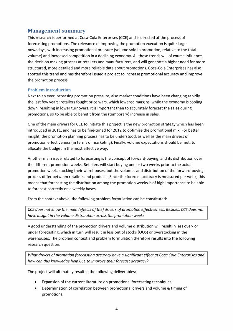
The independent variables that will be tested are selected in a session with the stakeholders at CCE, but the final set of variables that are tested are summarized in Table 1.

Variable Measurement level Gondola End Yes, No Euroweken Yes, No Hamsterweken Yes, No Packaging Pouch, Can, Bottle Sub(brand) Aquarius, Burn, Capri-Sun, Chaudfontaine, Coca-Cola, Dr. Pepper, Fanta,

Fernandes, Monster, Schweppes, Sprite Brandpromo Yes, No Leaflet Front, Mid, Back, No Leaflet Holiday Carnival, Eastern, Christmas, Queensday, Ascension, Pentecost, no holiday Retailer AH, C1000, Jumbo, Super de Boer, Linders, Coop, Deen, Hoogvliet, Plus, Spar,

Vomar WC soccer Yes, No Premiums Yes, No Instore Yes, No Casepack size 1, 4, 5, 6, 9, 10, Other Price off % Table 1 Independent variables considered in the final models. Bold variables are the control variables for dummies (for brand this depends on the model)

The training sample consists of all the promotion from 2010-2011, while the test set will be based on the promotions from the first quarter of 2012.

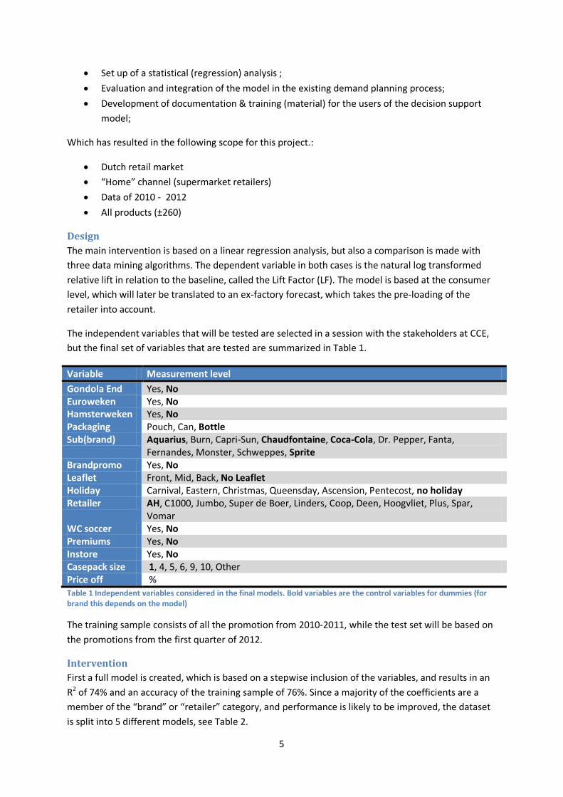
Intervention First a full model is created, which is based on a stepwise inclusion of the variables, and results in an R2 of 74% and an accuracy of the training sample of 76%. Since a majority of the coefficients are a member of the “brand” or “retailer” category, and performance is likely to be improved, the dataset is split into 5 different models, see Table 2.

6

Model # Model name SKU’s included in model Baseline 1 Coke Coke CC regular 2 Fanta/Sprite Fanta, sprite Sprite 3 High LF Chaudfontaine, Schweppes Chaudfontaine 4 Other Aquarius, Burn, Capri-Sun, Dr

Pepper, Fernandes, Monster Aquarius

5 In-out In-out articles CC regular Table 2 Overview of the five models

Since model five consists of the products which are only sold during promotion, their baseline is close to zero and a LF therefore cannot be calculated. As solution, these articles are forecasted on the relative sales compared to the baseline of a related product.

Training sample Test sample Model Model name Accuracy

shop floor # cases Accuracy

shop floor Accuracy Model

Accuracy DP

# cases

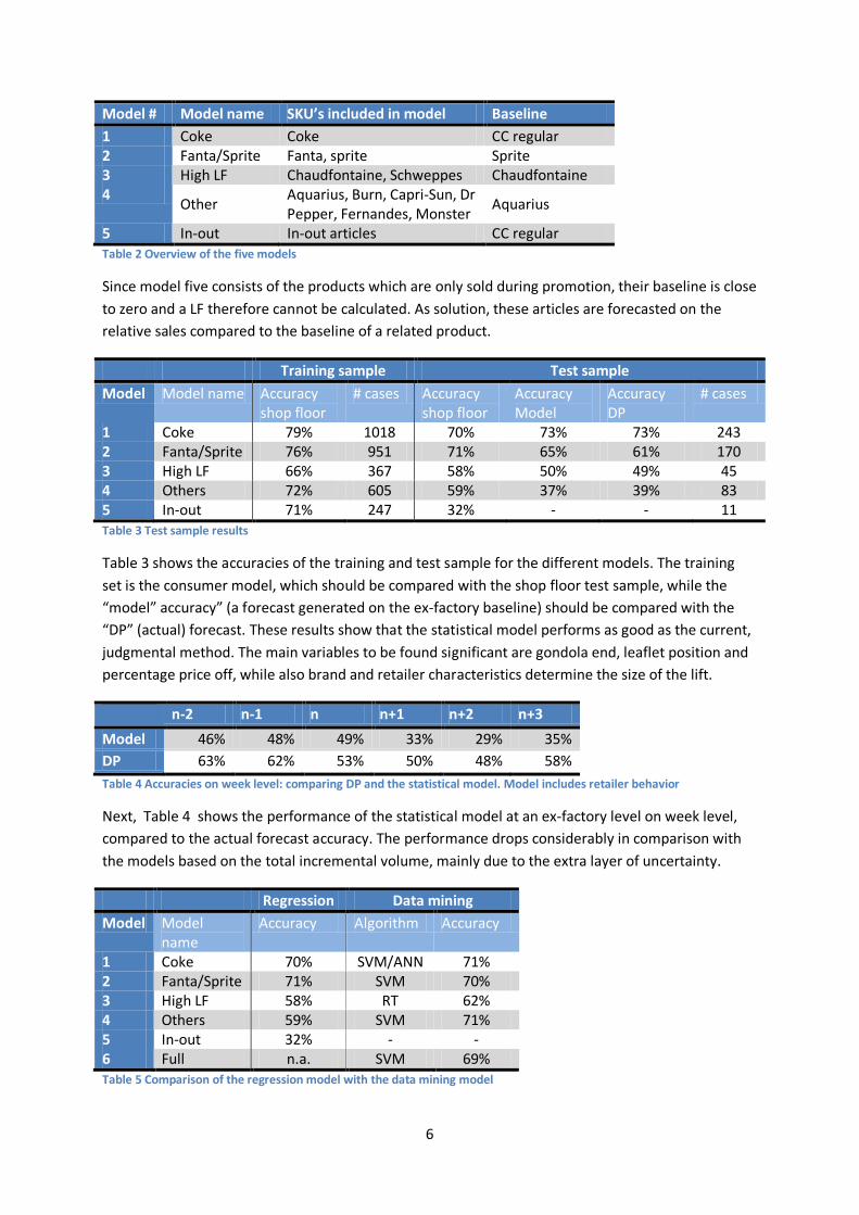
1 Coke 79% 1018 70% 73% 73% 243 2 Fanta/Sprite 76% 951 71% 65% 61% 170 3 High LF 66% 367 58% 50% 49% 45 4 Others 72% 605 59% 37% 39% 83 5 In-out 71% 247 32% - - 11 Table 3 Test sample results

Table 3 shows the accuracies of the training and test sample for the different models. The training set is the consumer model, which should be compared with the shop floor test sample, while the “model” accuracy” (a forecast generated on the ex-factory baseline) should be compared with the “DP” (actual) forecast. These results show that the statistical model performs as good as the current, judgmental method. The main variables to be found significant are gondola end, leaflet position and percentage price off, while also brand and retailer characteristics determine the size of the lift.

n-2 n-1 n n+1 n+2 n+3 Model 46% 48% 49% 33% 29% 35% DP 63% 62% 53% 50% 48% 58% Table 4 Accuracies on week level: comparing DP and the statistical model. Model includes retailer behavior

Next, Table 4 shows the performance of the statistical model at an ex-factory level on week level, compared to the actual forecast accuracy. The performance drops considerably in comparison with the models based on the total incremental volume, mainly due to the extra layer of uncertainty.

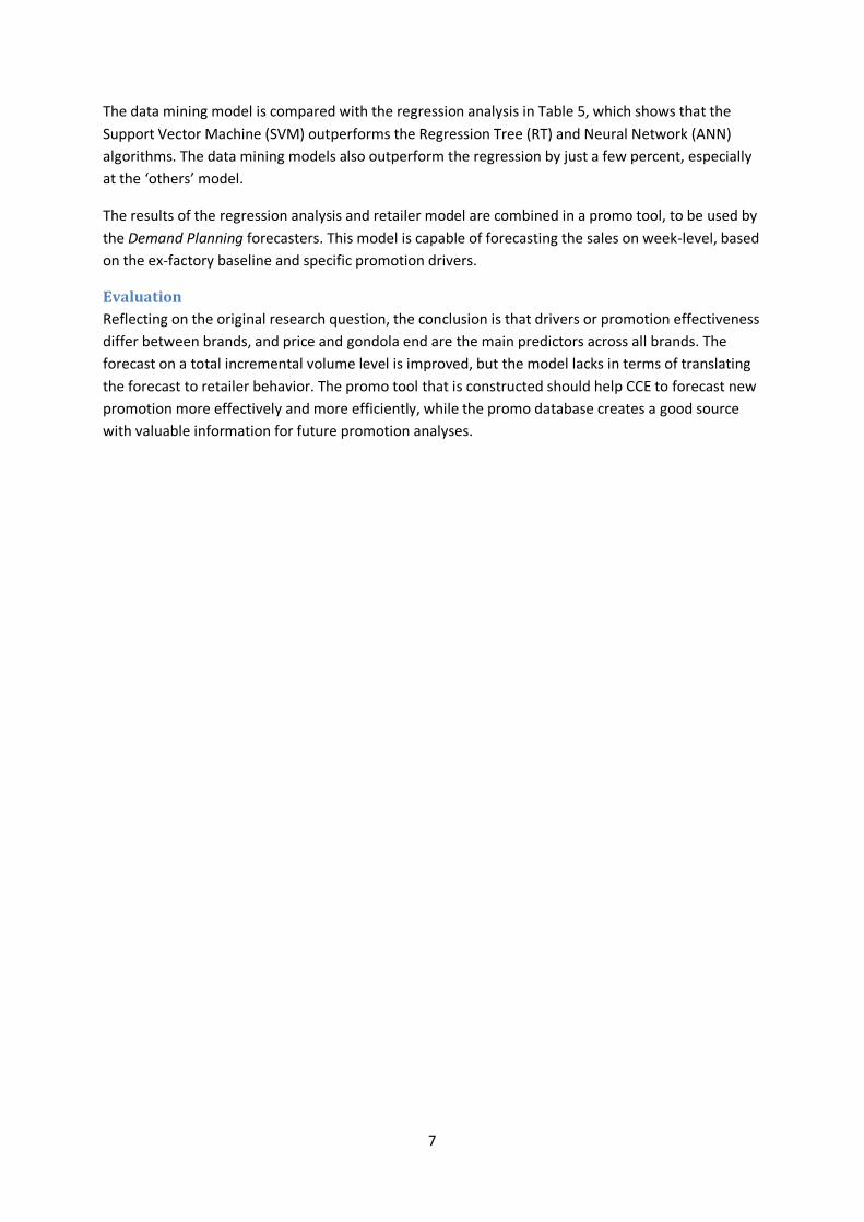
Regression Data mining Model Model

name Accuracy Algorithm Accuracy

1 Coke 70% SVM/ANN 71% 2 Fanta/Sprite 71% SVM 70% 3 High LF 58% RT 62% 4 Others 59% SVM 71% 5 In-out 32% - - 6 Full n.a. SVM 69% Table 5 Comparison of the regression model with the data mining model

7

The data mining model is compared with the regression analysis in Table 5, which shows that the Support Vector Machine (SVM) outperforms the Regression Tree (RT) and Neural Network (ANN) algorithms. The data mining models also outperform the regression by just a few percent, especially at the ‘others’ model.

The results of the regression analysis and retailer model are combined in a promo tool, to be used by the Demand Planning forecasters. This model is capable of forecasting the sales on week-level, based on the ex-factory baseline and specific promotion drivers.

Evaluation Reflecting on the original research question, the conclusion is that drivers or promotion effectiveness differ between brands, and price and gondola end are the main predictors across all brands. The forecast on a total incremental volume level is improved, but the model lacks in terms of translating the forecast to retailer behavior. The promo tool that is constructed should help CCE to forecast new promotion more effectively and more efficiently, while the promo database creates a good source with valuable information for future promotion analyses.

8

Preface This master thesis is the result of the final part of my study Industrial Engineering and Management at the Eindhoven University of Technology. This project was executed at Coca-Cola Enterprises BV in Rotterdam, The Netherlands from February 2012 to the end of June 2012.

I would like to grab the opportunity to express my gratitude towards a few people who have helped me during this project. First of all Edward van Stiphout for his knowledge of CCE’s promotion forecasting and his supervision during the past few months; next I would like to thank André Vriens for his supervision from EyeOn and his business insights regarding promotion forecasting. I would also like to thank my co-workers at Demand Planning for their support, help and having a good time; I hope their new promo tool and models will help them forecast even better! Last but not least, I want to extend my gratitude towards Ton de Kok and Remco Dijkman from the TU/e for their theoretical (and practical) knowledge and supervision.

Jasper Kock Rotterdam, June 2012

9

Contents Abstract ..........................................................................................................................................3

Management summary ...................................................................................................................4

Preface ...........................................................................................................................................8

Contents .............................................................................................................................................9

Part 1: Project definition .................................................................................................................. 11

1. Introduction .......................................................................................................................... 12

1.1 Company description ..................................................................................................... 12

1.2 Overview literature ........................................................................................................ 13

1.3 Structure of the report................................................................................................... 14

2. Problem Definition and Research Question ........................................................................... 15

2.1 Project Context .............................................................................................................. 15

2.2 Research question ......................................................................................................... 16

2.3 Assignment and deliverables ......................................................................................... 16

2.4 Scope ............................................................................................................................. 17

2.5 Project Approach ........................................................................................................... 17

Part 2: Diagnosis............................................................................................................................... 18

3. Current situation ................................................................................................................... 19

3.1 Current process ............................................................................................................. 19

3.2 Current performance ..................................................................................................... 19

4. Problem diagnosis ................................................................................................................. 21

Part 3: Design ................................................................................................................................... 23

5. Dependent and independent variables .................................................................................. 24

5.1 Dependent variable ....................................................................................................... 24

5.2 Independent variables ................................................................................................... 26

6. Retailer model ....................................................................................................................... 28

7. Data analysis ......................................................................................................................... 30

8. Assumptions.......................................................................................................................... 32

Part 4: Intervention .......................................................................................................................... 33

9. Regression model .................................................................................................................. 34

9.1 Full model ...................................................................................................................... 34

9.2 Alterations made to the full model ................................................................................ 34

9.3 Results of the linear regression analysis ......................................................................... 36

10

9.4 Validation ...................................................................................................................... 39

10. Adaption of regression model ............................................................................................ 41

10.1 Cannibalization .............................................................................................................. 41

10.2 From consumer to retailer model .................................................................................. 42

11. Data mining model ............................................................................................................ 44

11.1 Short introduction to Data Mining ................................................................................. 44

11.2 Implementation ............................................................................................................. 44

11.3 Results ........................................................................................................................... 45

11.4 Comparison with regression .......................................................................................... 45

12. Promo tool and process ..................................................................................................... 46

12.1 Requirements ................................................................................................................ 46

12.2 Result ............................................................................................................................ 46

12.3 New process .................................................................................................................. 47

Part 5: Evaluation ............................................................................................................................. 49

13. Conclusions and recommendations ................................................................................... 50

13.1 Conclusions ................................................................................................................... 50

13.2 Recommendations ......................................................................................................... 52

References .................................................................................................................................... 54

Appendices ................................................................................................................................... 57

Appendix I – Current process..................................................................................................... 58

Appendix II – Cause and Effect diagram ..................................................................................... 59

Appendix III – Coefficients full model ........................................................................................ 60

Appendix IV – Linear Regression Assumptions ........................................................................... 62

Appendix V - Linear regression results ....................................................................................... 64

Appendix VI – Cannibalization results ........................................................................................ 72

Appendix VII – Retailer models .................................................................................................. 74

Appendix VIII– Regression tree .................................................................................................. 76

Appendix IX – Promo Tool ......................................................................................................... 77

Appendix X – Promo tool table-layout ....................................................................................... 79

11

Part 1: Project definition

(1) Problem definition

(2) Diagnosis

(3) Design (4) Intervention

(5) Evaluation

12

1. Introduction ‘New price-war supermarkets’ heads news bulletin Nu.nl (2011) at November 14th 2011. Because of lower turnovers, supermarkets in the Netherlands prepare for yet another price-war says Paul Moers from the marketing company PM.SMS. One of the main weapons supermarkets are going to use is (price) promotions, which brings promotional pressure even to a higher level for manufacturers. According to Paul Moers, the average promotional pressure (volume sold in promotion, relative to the total volume) was just under 17% in 2011, but will be increasing in 2012!

This will of course influence the decision making process at retailers and manufacturers, and will generate a higher need for more structured, more detailed and more reliable data about promotions. Coca-Cola Enterprises has also spotted this trend and has therefore issued a project to increase promotional accuracy and improve the promotion process.

This document will describe the process and outcome of this project, which concerns the final phase of the master thesis project in the field of Operations Management and Logistics. It was conducted under supervision of the faculty of Technology Management at the Eindhoven University of Technology and regards a project executed within Coca Cola Enterprises (CCE), in collaboration with EyeOn, a planning and forecast Consultancy Company.

The goal of this project is twofold. At the academic level, the project aims at contributing to the scientific literature regarding promotion forecasting at manufacturers. The practical goal of the project is to improve the forecast process and forecast accuracy at Coca Cola Enterprises.

1.1 Company description

CCE Coca-Cola Enterprises (CCE) is a public company not to be confused with the ‘The Coca-Cola Company’ (TCCC). TCCC is the owner of the brand Coca-Cola and is responsible for commercial marketing and produces the syrup used in the bottling process; CCE is one of the main bottlers of TCCC worldwide, but also owns the distribution rights for other related products. While CCE’s headquarters are in the USA, its activities span the Benelux, France, Great Britain, Sweden and Norway. The Benelux business unit employs approximately 3,500 people in 11 locations, including four major production plants. At the Rotterdam Dutch Headquarters, approximately 300 employees work in primarily marketing &, sales. CCE is the number one beverage supplier in the Benelux. The three coke flavors are responsible for about two-thirds of sales; a further 30% comes from other sparkling drinks, while 5% comes from waters. The Netherlands have one of the lowest per capita consumption rates in the world – its consumers each drink around 147 servings of The Coca-Cola Company’s products every year, compared to 340 in Belgium.

CCE divides its customers based on “at home” sales and “out-of-home” sales. The former comprises of the main retail stores, of which Albert Heijn, Jumbo, C1000 and retailers combined in the purchasing organization SuperUnie are the main clients. The latter comprises of catering, liquor stores, beverage wholesalers and purchasing organizations for bars, restaurants, etc.

13

Eyeon EyeOn is a specialized consultancy firm that supports multi-site companies in implementing excellent planning and control processes in order to improve their business performance. To remain innovative, EyeOn is continuously involved in various research projects in close cooperation with Tilburg University, Erasmus University Rotterdam and Eindhoven University.

EyeOn’s expertise constitutes to the fields of Integrated Business Planning, Demand Planning, Supply Planning and Financial Planning.

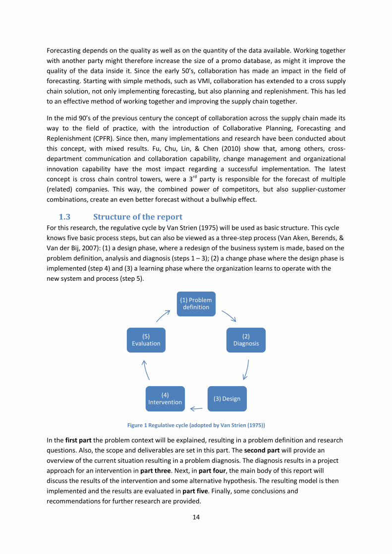
1.2 Overview literature In this paragraph the relevant literature for the research field of this master thesis will be summarized, based on the literature study by Kock (2012).

There are three reasons for companies to use promotions: 1) to generate market share; 2) to reduce inventory for members in the supply chain; 3) to generate short term profit. Research suggests that promotions do not generate a long term effect (Srinivasan, Pauwels, Hanssens, & Dekimpe, 2004), but promotions are mainly used to counter competitive promotions, causing a vicious cycle and eventually a prisoners dilemma (Blattberg & Neslin, 1990). Forecasting these promotions requires a collection of independent variables such as price reduction, TV or leaflet to predict the increase or absolute sales for that specific week. Main techniques used are judgmental, statistical and data mining models. Statistical models come in many forms, where multiple linear regression is the main technique used for these kinds of studies. Data mining and linear regression models generate the best results, while the latter is mainly used in real life applications. Both have their pros and cons; data mining can generate results that are not expected a priori, which is also the main drawback since the main drivers cannot always be explained businesswise. The results of linear regression are easy to explain to layman, and can easily be implemented into a tool, but needs lots of (dummy) variables to take all information into account, therefore potentially creating multicollinearity (see appendix IV).

Data mining can be used as a predictive tool for forecasting promotions, especially in a non-linear context. Different researchers have gained good results with different techniques; most of them outperformed the standard statistical models (Aburto & Weber, 2007, Ali, Sayin, Van Woensel, & Fransoo, 2009, Chang & Wang, 2006, Delen, Walker, & Kadam, 2005). One of the advantages of data mining is its ability to find patterns in seemingly random sets of data. The different algorithms are based on complex mathematical models, but are fairly easily to implement in model building with the help of different software packages. One of the main drawbacks of data mining in general is that it finds patterns in data, regardless if this pattern makes any sense businesswise (Delen et al., 2005). Another drawback is that apart from regression trees, the models use a black box approach: data is inputted and returned, but what the model does is not easy to explain. Therefore, all conclusions should be regarded with even more care than one would do with statistical models.

Judgmental adjustment is a technique that might improve the forecast that statistical models generate, for example when the judge has contextual information available that is not present in the model, or when the model has excess room for improvement. Researchers have found mixed results in terms of forecast accuracy improvement.

14

Forecasting depends on the quality as well as on the quantity of the data available. Working together with another party might therefore increase the size of a promo database, as might it improve the quality of the data inside it. Since the early 50’s, collaboration has made an impact in the field of forecasting. Starting with simple methods, such as VMI, collaboration has extended to a cross supply chain solution, not only implementing forecasting, but also planning and replenishment. This has led to an effective method of working together and improving the supply chain together.

In the mid 90’s of the previous century the concept of collaboration across the supply chain made its way to the field of practice, with the introduction of Collaborative Planning, Forecasting and Replenishment (CPFR). Since then, many implementations and research have been conducted about this concept, with mixed results. Fu, Chu, Lin, & Chen (2010) show that, among others, cross-department communication and collaboration capability, change management and organizational innovation capability have the most impact regarding a successful implementation. The latest concept is cross chain control towers, were a 3rd party is responsible for the forecast of multiple (related) companies. This way, the combined power of competitors, but also supplier-customer combinations, create an even better forecast without a bullwhip effect.

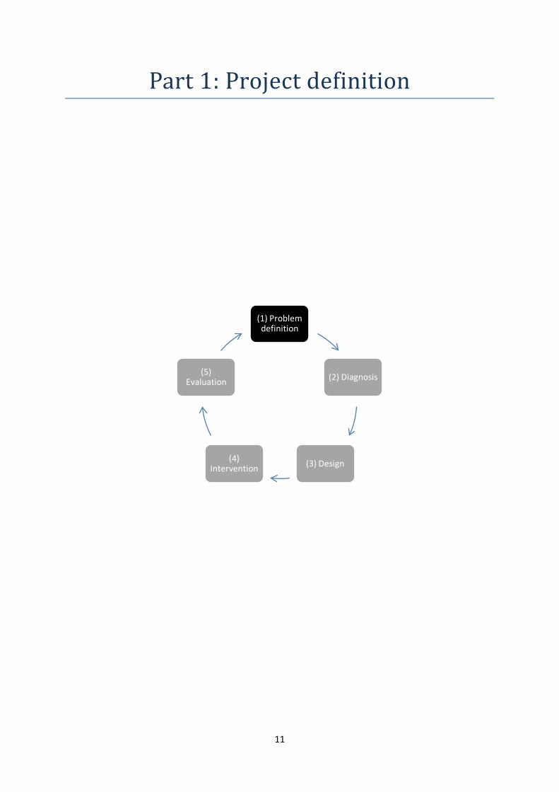
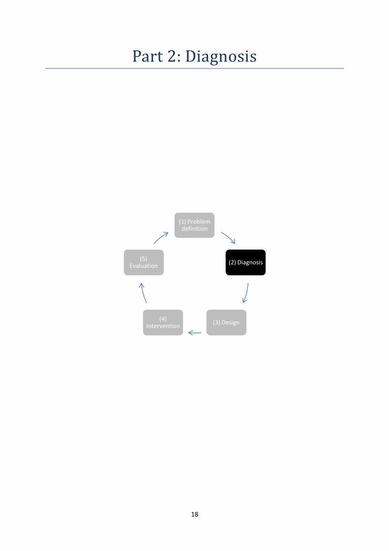
1.3 Structure of the report For this research, the regulative cycle by Van Strien (1975) will be used as basic structure. This cycle knows five basic process steps, but can also be viewed as a three-step process (Van Aken, Berends, & Van der Bij, 2007): (1) a design phase, where a redesign of the business system is made, based on the problem definition, analysis and diagnosis (steps 1 – 3); (2) a change phase where the design phase is implemented (step 4) and (3) a learning phase where the organization learns to operate with the new system and process (step 5).

Figure 1 Regulative cycle (adopted by Van Strien (1975))

In the first part the problem context will be explained, resulting in a problem definition and research questions. Also, the scope and deliverables are set in this part. The second part will provide an overview of the current situation resulting in a problem diagnosis. The diagnosis results in a project approach for an intervention in part three. Next, in part four, the main body of this report will discuss the results of the intervention and some alternative hypothesis. The resulting model is then implemented and the results are evaluated in part five. Finally, some conclusions and recommendations for further research are provided.

(1) Problem definition

(2) Diagnosis

(3) Design (4) Intervention

(5) Evaluation

15

2. Problem Definition and Research Question This chapter will cover the problem at hand in a project context in paragraph 2.1, resulting in the research question in paragraph 2.2. Next the main deliverables for CCE will be stated in paragraph 2.3. Paragraph 2.4 will form the scope of this project, and finally paragraph 2.5 will end with the project approach.

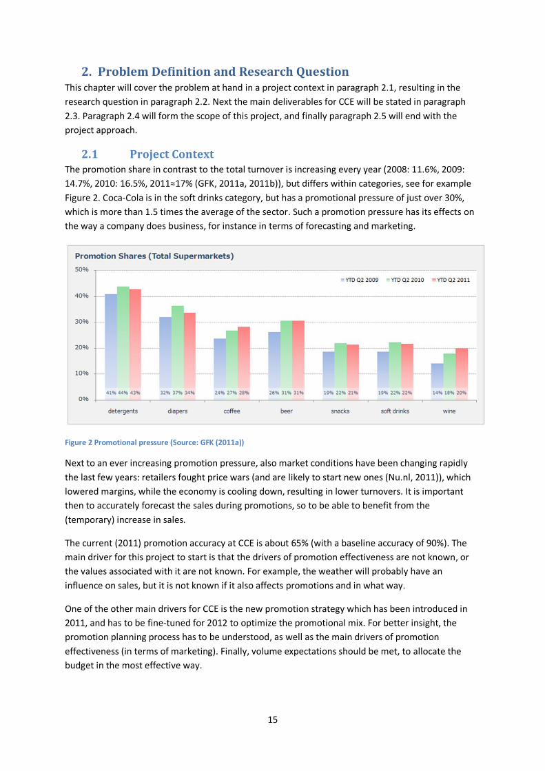
2.1 Project Context The promotion share in contrast to the total turnover is increasing every year (2008: 11.6%, 2009: 14.7%, 2010: 16.5%, 2011≈17% (GFK, 2011a, 2011b)), but differs within categories, see for example Figure 2. Coca-Cola is in the soft drinks category, but has a promotional pressure of just over 30%, which is more than 1.5 times the average of the sector. Such a promotion pressure has its effects on the way a company does business, for instance in terms of forecasting and marketing.

Figure 2 Promotional pressure (Source: GFK (2011a))

Next to an ever increasing promotion pressure, also market conditions have been changing rapidly the last few years: retailers fought price wars (and are likely to start new ones (Nu.nl, 2011)), which lowered margins, while the economy is cooling down, resulting in lower turnovers. It is important then to accurately forecast the sales during promotions, so to be able to benefit from the (temporary) increase in sales.

The current (2011) promotion accuracy at CCE is about 65% (with a baseline accuracy of 90%). The main driver for this project to start is that the drivers of promotion effectiveness are not known, or the values associated with it are not known. For example, the weather will probably have an influence on sales, but it is not known if it also affects promotions and in what way.

One of the other main drivers for CCE is the new promotion strategy which has been introduced in 2011, and has to be fine-tuned for 2012 to optimize the promotional mix. For better insight, the promotion planning process has to be understood, as well as the main drivers of promotion effectiveness (in terms of marketing). Finally, volume expectations should be met, to allocate the budget in the most effective way.

16

Another main issue related to forecasting is the concept of forward-buying, and its distribution over the different promotion weeks. Retailers will start buying one or two weeks prior to the actual promotion week, stocking their warehouses, but the volumes and distribution of the forward-buying process differ between retailers and products. Since the forecast accuracy is measured per week, this means that forecasting the distribution among the promotion weeks is of high importance to be able to forecast correctly on a weekly bases.

From the context above, the following problem formulation can be constituted:

CCE does not know the main (effects of the) drivers of promotion effectiveness. Besides, CCE does not have insight in the volume distribution across the promotion weeks.

2.2 Research question A good understanding of the promotion drivers and volume distribution will result in less over- or under forecasting, which in turn will result in less out of stocks (OOS) or overstocking in the warehouses. OOS are of a main concern, not only for CCE, but also for the retailers. Coca-Cola is namely the 3rd strongest brand in the Netherlands and the strongest brand to be found in the supermarket (Velthuis, Kruk, & Dekker, 2011), which means Coca-Cola is a brand that drives customers to the retailers. Being out of stock is therefore unacceptable, see for example the problems during the SAP-implementation in early 2007 (Distrifood, 2007).

The problem context and problem formulation therefore results into the following research question:

What drivers of promotion forecasting accuracy have a significant effect at Coca Cola Enterprises and how can this knowledge help CCE to improve their forecast accuracy?

The sales forecasts also influence other processes and accuracy’s besides that of the Demand Planning department. The main question can therefore be broken down in two sub questions about the effects on other departments and processes.

How can CCE improve on the general understanding on promotion tactics and drivers? After a promotion has been forecasted and carried out, the results can be used to forecast new promotions, but they can also be used to evaluate the promotion effectiveness. The marketing department already uses a promotion evaluation tool, but do not really have insight in all the drivers that explain a successful promotion. With the help of the analysis on promotion drivers, the marketing department can improve on their understanding.

How can CCE improve the financial situation and distribution of funds? Since forecasting is the base for the monthly gap closing and weekly Monday sales target meetings, a good forecast can have an effect on the distribution of funds. When the forecasts for a specific product lag behind target, CCE can for example decide to offer extra promotional sales to boost sales. A good forecast could also improve the general financial situation, for example by allowing a lower safety stock or shorter lead times.

2.3 Assignment and deliverables The project will ultimately result in the following deliverables:

• Expansion of the current literature on promotional forecasting techniques;

17

• Determination of correlation between promotional drivers and volume & timing of promotions;

• Set up of a statistical (regression) analysis ; • Evaluation and integration of the model in the existing demand planning process; • Development of documentation & training (material) for the users of the decision support

model;

2.4 Scope The research will be conducted at the Dutch office of CCE. The market structure of the Netherlands in terms of soft drinks is quite different than that of our neighbours (e.g. Dutch drink more coffee and tea), and data is only available and applicable to Holland, therefore the scope will be limited to the Dutch retail market. To narrow it even more down, only the supermarket/retail channel (home channel) will be analyzed due to the fragmentation of sales in the out-of-home channel.

Due to data-availability and data-accuracy, the temporal constraint lies on data between 2010 and 2012. More data points generally produces more significant results, but considering changing market conditions, data from a longer time span might not result in better forecasts for the future. The 2010-2011 period will be used as test sample, while the (first quarter of) 2012 data will be used as validation set.

The full product catalogue from the home-channel will be analyzed on SKU-level, containing Coca Cola, Fanta, Fernandes, Capri-Sun, Aquarius and many others in all different forms and packages. In total this constitutes to 264 different SKU’s. The scope of the research can be summarized as follows:

• Dutch retail market • “Home” channel (supermarket retailers) • Data of 2010 - 2012 • All products (±260)

2.5 Project Approach This report will continue with the diagnosis, which is used to describe the current situation and problem diagnosis, based on interviews with relevant stakeholders at CCE. Next, the design part will declare all relevant decisions that are made during the project, such as what variables are used in the intervention and what steps have been taken in the intervention. The intervention part will describe the results of the regression analysis, and further adoptions of the resulting models. Also, a comparison is made with a data mining model. Next, a new process is proposed, along with a promo forecasting tool. The next part, the evaluation, will compare the results of the model with the current method and will give an overview of the testing results of the model in combination with the tool.

18

Part 2: Diagnosis

(1) Problem definition

(2) Diagnosis

(3) Design (4) Intervention

(5) Evaluation

19

3. Current situation This chapter will describe the current situation at CCE. The current process is described in paragraph 3.1, while the current performance is described in paragraph 3.2.

3.1 Current process The current forecasting process is based on five layers of information (see Appendix I), namely the retailer, Account Management, Demand Planning, Customer Service and the factory.

The promotion process starts every year with the development of a promotion strategy by the National Account Managers. The strategy will state where the focus of the next year will be on, and therefore which products are likely to be put on promotion. This strategy is converted each quarter to a promotion calendar, which in term is communicated to all retailers. The promotion calendar is a tool which states what promotions CCE would like to have in what weeks. The retailer will then propose a calendar based on the CCE calendar, but with alterations made to accommodate promotions of competitors. This process should be completed before the start of each quarter. The Account Managers then put together all the promotions and communicate this to Demand Planning, together with an initial judgemental forecast. Also, the discount data is communicated to Customer Service, who enter it in the ERP-system, so that the retailers automatically receive their discount on ordering.

Demand Planning then makes a forecast based on information from previous years and promotion parameters, such as gondola end, leaflet and TV. Next, DP communicates the forecast to the Account Managers, who can give their opinion and suggest alterations based on commercial information. In the next few weeks, whenever something may change (i.e. a change in weeks, or products), the forecast is updated subsequently, ultimately resulting in a final forecast.

Two weeks prior to the promotion, Albert Heijn, C1000 and Plus communicate their pre-loading volumes to CCE, after which Demand Management can make a final forecast based on “real” demand data. This could also mean that volume is shifted between SKU’s, for example from 4-packs to single bottles. As a basic rule, the forecast made by CCE is used as base, which means that when AH or C1000 communicates a higher volume for the pre-loading week (n-1), the forecast for the next week (n) will be lowered such that the total volume equals the initial forecast,

This final forecast is put into the ERP-system, where the production planners from the factory can use this to make a production schedule. The volumes are also communicated to Customer Service and Master Data, for budgetary and financial overviews.

3.2 Current performance The current performance is measured by the Mean Absolute Percentage Error (MAPE):

𝑀𝐴𝑃𝐸 = �|𝐴𝑐𝑡𝑢𝑎𝑙𝑠𝑖 − 𝐹𝑜𝑟𝑒𝑐𝑎𝑠𝑡𝑖 |

𝐴𝑐𝑡𝑢𝑎𝑙𝑠𝑖

𝑁

𝑖=1

∗ 100

In 2011, the MAPE of the Home channel differed between 72% and 23%, with a cumulative MAPE of 35% at the end of 2011, compared to 50% at early 2011.

20

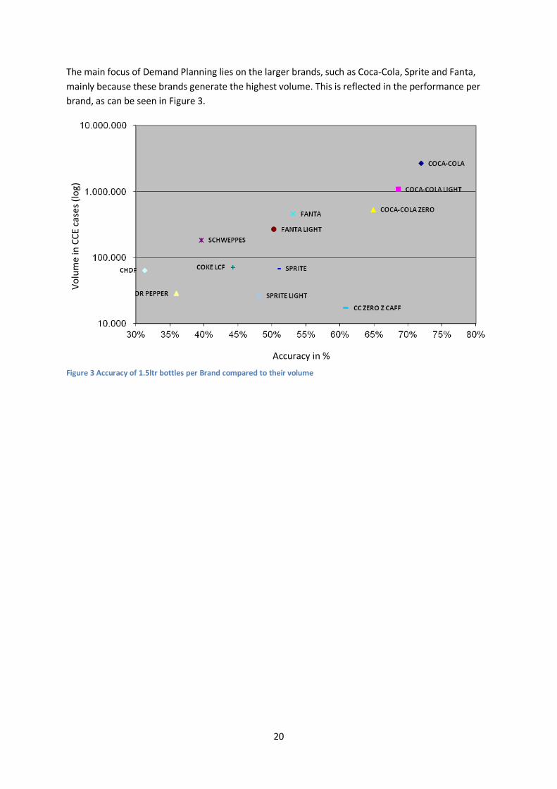
The main focus of Demand Planning lies on the larger brands, such as Coca-Cola, Sprite and Fanta, mainly because these brands generate the highest volume. This is reflected in the performance per brand, as can be seen in Figure 3.

Figure 3 Accuracy of 1.5ltr bottles per Brand compared to their volume

Accuracy in %

Volu

me

in C

CE ca

ses (

log)

21

4. Problem diagnosis An overview of all relevant factors concerning the difficulties of promotion forecasting is gathered from interviews with CCE-stakeholders. All these factors are summarized in a (preliminary) cause-and-effect diagram, see appendix II.

Data availability Most of the important data is only available from a short time window: major sales and promotion data since the introduction of a new ERP-system in late 2008, and consumer data (Nielsen) only dates back three years. Next to this, promotions are a special type of event, where 30% of sales do not lead to 30% of data points due to the uplift factor. This in turn may lead to few data points available for reference, especially for slow movers (with few promotions).

Data is also spread over multiple departments and when shared, is presented in non-standardized excel-sheets where the data has to be extracted from. Moreover, this data does not always have to be accurate due to changes in promotions by retailers or sales.

Finally, present forecasts are based on retailer-demand, while this is an indirect measure for the final consumer sales. The bullwhip-effect may play a significant role in the conversion from consumer sales to retail sales and demand may be shifted in time, called pre-loading.

Retailer influence There is always one leader in a supply chain who has the most power to decide or implement changes. In many cases this is the retailer, since they have a direct influence on the end-client (Hogarth-Scott & Parkinson, 1993). In the CCE case, the manufacturer also has a strong position, but ultimately it is the retailer who decides on promotions in his store, which can result in a lack of information when promotions are changed on the way. Also, most retailers do not share information across the supply chain, which could result in unforeseen spikes in demand.

Retailers are also known for their forward buying behaviour in the weeks before the promotion (have enough stock to be able to meet demand), as well as their tendency to fill their warehouses with low-cost promotion goods for further use. The latter is countered by only offering a price reduction on scanner data, but still many retailers do not want, or are able, to comply to this.

Promotion process standards The current process to forecast promotions is standardized by habit. There are some agreements and files to be send periodically from one department to another, but no official process has been written down or agreed on.

This may have its effect on the promotion forecasting, for example when not-standard events occur (e.g. a change in a promotion), this is not structurally dealt with. Also, there are multiple people and departments involved, who can add and change information, which in turn may result in long throughput times.

Promotion strategy execution The ’The Coca-Cola Company’ and marketing departments within CCE determine a promotion strategy each year, which focuses on a specific brand or target group. This strategy is then evaluated, after which it will be used as input for the strategy for next year.

22

It is therefore important to execute this strategy well, and to communicate the strategy internally and to the retailers, since retailers will have their own strategy, and account managers might have their own ideas about promotions as well.

23

Part 3: Design

(1) Problem definition

(2) Diagnosis

(3) Design (4) Intervention

(5) Evaluation

24

5. Dependent and independent variables This chapter will provide an overview of the dependent and independent variables and their calculations. Paragraph 5.1 will give an overview of the dependent variable, while paragraph 5.2 will go more into detail to what other variables can be used to make a good prediction

5.1 Dependent variable The dependent variable is not as clear cut as one might expect upfront. Since the sales during promotion is to be forecasted, the absolute sales during promotion (Van Heerde, Leeflang, & Wittink, 2002) would seem a logical choice. The absolute sales however, are dependent on the type and size of a product, therefore creating potentially large differences between promotions, such as small cans of Burn Energy versus 6-packs 1.5L Coca-Cola. Therefore, the natural log of the absolute volume is sometimes used (Cooper, Baron, Levy, Swisher, & Gogos, 1999), to meet the requirements of a linear relationship more closely. This does however not take other variables, such as the retailer into account, which might weaken the predictions, since larger retailers generate larger volumes, simply by having more stores. The absolute increase in sales with respect to the baseline (De Schrijver, 2009) or the relative (normal log of the) Lift Factor (LF) compared to the base line (Loo, Woensel, & others, 2006, M. J. T. Van der Poel, 2010, De Schrijver, 2009) might therefore better predict promotional volume.

At first, multiple dependent variables will be tested to see which generates the best result, but since the LF seems the more logical choice, our attention is directed to this variable.

Source of data Since the model will be used from a manufacturing point of view, the sellout to the retailer should be the variable to predict. The sellout data, however, also incorporates retailer behavior, such as bad forecasts, pre-loading, stocking and safety. To be able to make a genuine forecast, one should go downstream to the end customer. This data, the scan-data at the various retailer outlets, is available from various marketing bureaus, such as Nielsen and GfK. For this project, Nielsen is chosen as main supplier, since CCE already has a contract with them.

The actual sellout data to the retailer is available from the ERP-system at CCE, which incorporates a statistical baseline, actual sales and the forecasts generated by Demand Planning.

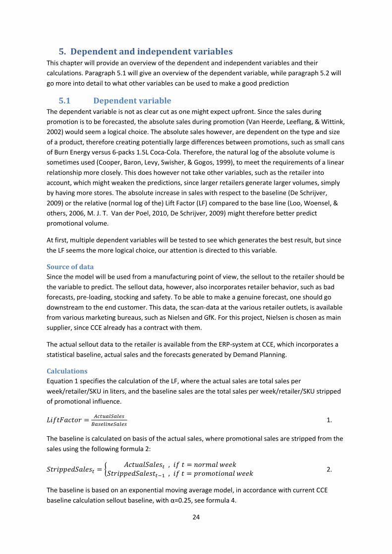
Calculations Equation 1 specifies the calculation of the LF, where the actual sales are total sales per week/retailer/SKU in liters, and the baseline sales are the total sales per week/retailer/SKU stripped of promotional influence.

𝐿𝑖𝑓𝑡𝐹𝑎𝑐𝑡𝑜𝑟 = 𝐴𝑐𝑡𝑢𝑎𝑙𝑆𝑎𝑙𝑒𝑠𝐵𝑎𝑠𝑒𝑙𝑖𝑛𝑒𝑆𝑎𝑙𝑒𝑠

1.

The baseline is calculated on basis of the actual sales, where promotional sales are stripped from the sales using the following formula 2:

𝑆𝑡𝑟𝑖𝑝𝑝𝑒𝑑𝑆𝑎𝑙𝑒𝑠𝑡 = � 𝐴𝑐𝑡𝑢𝑎𝑙𝑆𝑎𝑙𝑒𝑠𝑡 , 𝑖𝑓 𝑡 = 𝑛𝑜𝑟𝑚𝑎𝑙 𝑤𝑒𝑒𝑘𝑆𝑡𝑟𝑖𝑝𝑝𝑒𝑑𝑆𝑎𝑙𝑒𝑠𝑡𝑡−1 , 𝑖𝑓 𝑡 = 𝑝𝑟𝑜𝑚𝑜𝑡𝑖𝑜𝑛𝑎𝑙 𝑤𝑒𝑒𝑘

� 2.

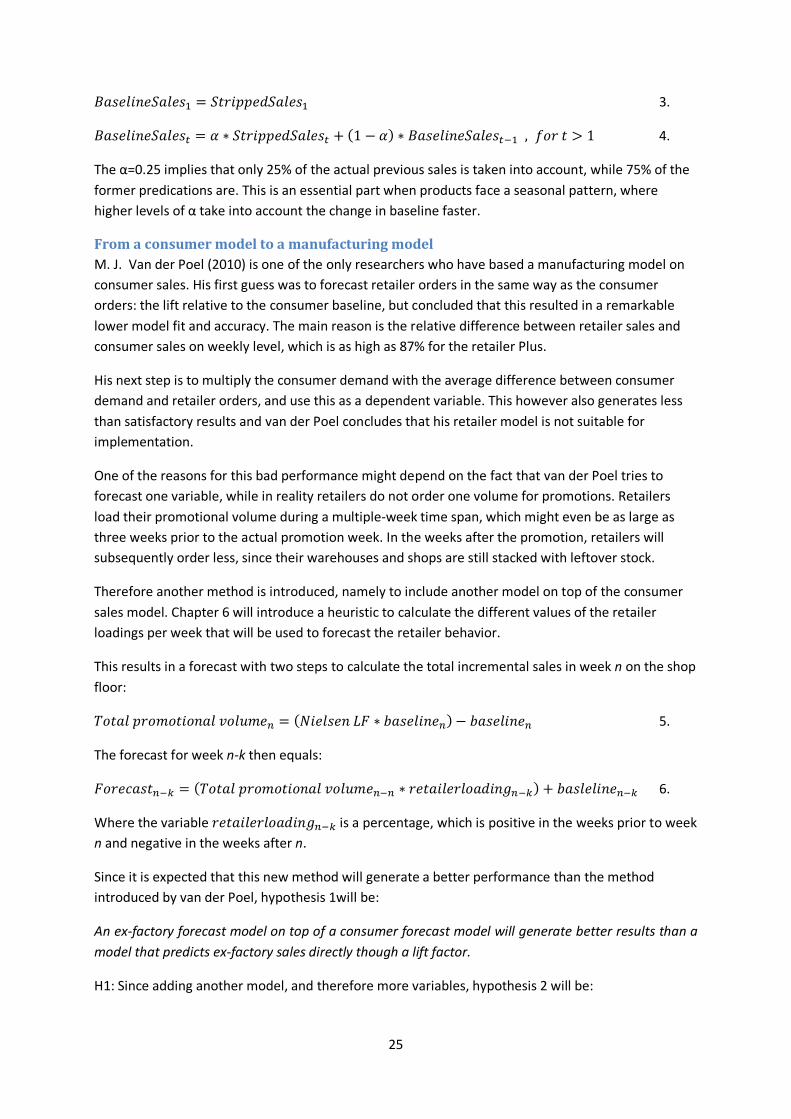
The baseline is based on an exponential moving average model, in accordance with current CCE baseline calculation sellout baseline, with α=0.25, see formula 4.

25

𝐵𝑎𝑠𝑒𝑙𝑖𝑛𝑒𝑆𝑎𝑙𝑒𝑠1 = 𝑆𝑡𝑟𝑖𝑝𝑝𝑒𝑑𝑆𝑎𝑙𝑒𝑠1 3.

𝐵𝑎𝑠𝑒𝑙𝑖𝑛𝑒𝑆𝑎𝑙𝑒𝑠𝑡 = 𝛼 ∗ 𝑆𝑡𝑟𝑖𝑝𝑝𝑒𝑑𝑆𝑎𝑙𝑒𝑠𝑡 + (1 − 𝛼) ∗ 𝐵𝑎𝑠𝑒𝑙𝑖𝑛𝑒𝑆𝑎𝑙𝑒𝑠𝑡−1 , 𝑓𝑜𝑟 𝑡 > 1 4.

The α=0.25 implies that only 25% of the actual previous sales is taken into account, while 75% of the former predications are. This is an essential part when products face a seasonal pattern, where higher levels of α take into account the change in baseline faster.

From a consumer model to a manufacturing model M. J. Van der Poel (2010) is one of the only researchers who have based a manufacturing model on consumer sales. His first guess was to forecast retailer orders in the same way as the consumer orders: the lift relative to the consumer baseline, but concluded that this resulted in a remarkable lower model fit and accuracy. The main reason is the relative difference between retailer sales and consumer sales on weekly level, which is as high as 87% for the retailer Plus.

His next step is to multiply the consumer demand with the average difference between consumer demand and retailer orders, and use this as a dependent variable. This however also generates less than satisfactory results and van der Poel concludes that his retailer model is not suitable for implementation.

One of the reasons for this bad performance might depend on the fact that van der Poel tries to forecast one variable, while in reality retailers do not order one volume for promotions. Retailers load their promotional volume during a multiple-week time span, which might even be as large as three weeks prior to the actual promotion week. In the weeks after the promotion, retailers will subsequently order less, since their warehouses and shops are still stacked with leftover stock.

Therefore another method is introduced, namely to include another model on top of the consumer sales model. Chapter 6 will introduce a heuristic to calculate the different values of the retailer loadings per week that will be used to forecast the retailer behavior.

This results in a forecast with two steps to calculate the total incremental sales in week n on the shop floor:

𝑇𝑜𝑡𝑎𝑙 𝑝𝑟𝑜𝑚𝑜𝑡𝑖𝑜𝑛𝑎𝑙 𝑣𝑜𝑙𝑢𝑚𝑒𝑛 = (𝑁𝑖𝑒𝑙𝑠𝑒𝑛 𝐿𝐹 ∗ 𝑏𝑎𝑠𝑒𝑙𝑖𝑛𝑒𝑛)− 𝑏𝑎𝑠𝑒𝑙𝑖𝑛𝑒𝑛 5.

The forecast for week n-k then equals:

𝐹𝑜𝑟𝑒𝑐𝑎𝑠𝑡𝑛−𝑘 = (𝑇𝑜𝑡𝑎𝑙 𝑝𝑟𝑜𝑚𝑜𝑡𝑖𝑜𝑛𝑎𝑙 𝑣𝑜𝑙𝑢𝑚𝑒𝑛−𝑛 ∗ 𝑟𝑒𝑡𝑎𝑖𝑙𝑒𝑟𝑙𝑜𝑎𝑑𝑖𝑛𝑔𝑛−𝑘) + 𝑏𝑎𝑠𝑙𝑒𝑙𝑖𝑛𝑒𝑛−𝑘 6.

Where the variable 𝑟𝑒𝑡𝑎𝑖𝑙𝑒𝑟𝑙𝑜𝑎𝑑𝑖𝑛𝑔𝑛−𝑘 is a percentage, which is positive in the weeks prior to week n and negative in the weeks after n.

Since it is expected that this new method will generate a better performance than the method introduced by van der Poel, hypothesis 1will be:

An ex-factory forecast model on top of a consumer forecast model will generate better results than a model that predicts ex-factory sales directly though a lift factor.

H1: Since adding another model, and therefore more variables, hypothesis 2 will be:

26

H2: Including an ex-factory model on top of a consumer sales model will lower the overall forecast accuracy

5.2 Independent variables A priori it is expected that temperature, price and time between promotions have the largest influence, together with the variation of ordering behaviour of the retailer and the promo execution of the retailer. Since the latter cannot be measured, this is not taken into account. The ordering behavior of the retailer is modeled using a separate model, on top of the consumer sales model.

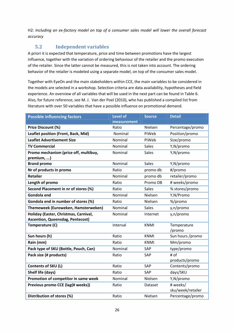
Together with EyeOn and the main stakeholders within CCE, the main variables to be considered in the models are selected in a workshop. Selection criteria are data availability, hypotheses and field experience. An overview of all variables that will be used in the next part can be found in Table 6. Also, for future reference, see M. J. Van der Poel (2010), who has published a compiled list from literature with over 50 variables that have a possible influence on promotional demand.

Possible influencing factors Level of measurement

Source Detail

Price Discount (%) Ratio Nielsen Percentage/promo Leaflet position (Front, Back, Mid) Nominal PiWeb Position/promo Leaflet Advertisement Size Nominal PiWeb Size/promo TV Commercial Nominal Sales Y,N/promo Promo mechanism (price off, multibuy, premium, ...)

Nominal Sales Y,N/promo

Brand promo Nominal Sales Y,N/promo Nr of products in promo Ratio promo db #/promo Retailer Nominal promo db retailer/promo Length of promo Ratio Promo DB # weeks/promo Second Placement in nr of stores (%) Ratio Sales % stores/promo Gondola end Nominal Nielsen Y,N/Promo Gondola end in number of stores (%) Ratio Nielsen %/promo Themeweek (Euroweken, Hamsterweken) Nominal Sales y,n/promo Holiday (Easter, Christmas, Carnival, Ascention, Queensdag, Pentecost)

Nominal Internet y,n/promo

Temperature (C) Interval KNMI Temperature /promo

Sun hours (h) Ratio KNMI Sun hours /promo Rain (mm) Ratio KNMI Mm/promo Pack type of SKU (Bottle, Pouch, Can) Nominal SAP type/promo Pack size (# products) Ratio SAP # of

products/promo Contents of SKU (L) Ratio SAP Contents/promo Shelf life (days) Ratio SAP days/SKU Promotion of competitor in same week Nominal Nielsen Y,N/promo Previous promo CCE (lag(# weeks)) Ratio Dataset # weeks/

sku/week/retailer Distribution of stores (%) Ratio Nielsen Percentage/promo

27

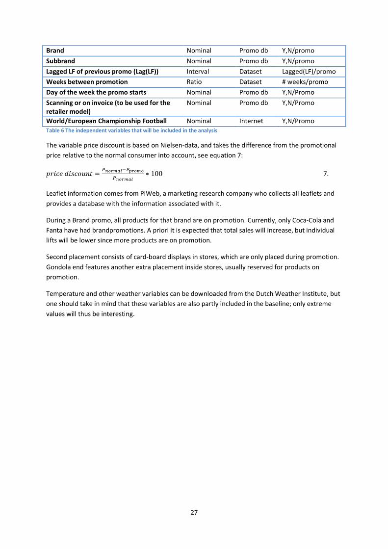
Brand Nominal Promo db Y,N/promo Subbrand Nominal Promo db Y,N/promo Lagged LF of previous promo (Lag(LF)) Interval Dataset Lagged(LF)/promo Weeks between promotion Ratio Dataset # weeks/promo Day of the week the promo starts Nominal Promo db Y,N/Promo Scanning or on invoice (to be used for the retailer model)

Nominal Promo db Y,N/Promo

World/European Championship Football Nominal Internet Y,N/Promo Table 6 The independent variables that will be included in the analysis

The variable price discount is based on Nielsen-data, and takes the difference from the promotional price relative to the normal consumer into account, see equation 7:

𝑝𝑟𝑖𝑐𝑒 𝑑𝑖𝑠𝑐𝑜𝑢𝑛𝑡 = 𝑃𝑛𝑜𝑟𝑚𝑎𝑙−𝑃𝑝𝑟𝑜𝑚𝑜

𝑃𝑛𝑜𝑟𝑚𝑎𝑙∗ 100 7.

Leaflet information comes from PiWeb, a marketing research company who collects all leaflets and provides a database with the information associated with it.

During a Brand promo, all products for that brand are on promotion. Currently, only Coca-Cola and Fanta have had brandpromotions. A priori it is expected that total sales will increase, but individual lifts will be lower since more products are on promotion.

Second placement consists of card-board displays in stores, which are only placed during promotion. Gondola end features another extra placement inside stores, usually reserved for products on promotion.

Temperature and other weather variables can be downloaded from the Dutch Weather Institute, but one should take in mind that these variables are also partly included in the baseline; only extreme values will thus be interesting.

28

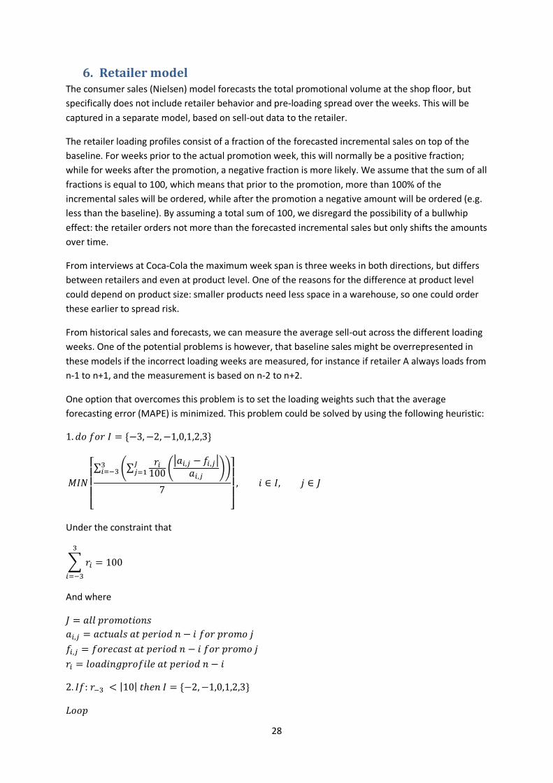
6. Retailer model The consumer sales (Nielsen) model forecasts the total promotional volume at the shop floor, but specifically does not include retailer behavior and pre-loading spread over the weeks. This will be captured in a separate model, based on sell-out data to the retailer.

The retailer loading profiles consist of a fraction of the forecasted incremental sales on top of the baseline. For weeks prior to the actual promotion week, this will normally be a positive fraction; while for weeks after the promotion, a negative fraction is more likely. We assume that the sum of all fractions is equal to 100, which means that prior to the promotion, more than 100% of the incremental sales will be ordered, while after the promotion a negative amount will be ordered (e.g. less than the baseline). By assuming a total sum of 100, we disregard the possibility of a bullwhip effect: the retailer orders not more than the forecasted incremental sales but only shifts the amounts over time.

From interviews at Coca-Cola the maximum week span is three weeks in both directions, but differs between retailers and even at product level. One of the reasons for the difference at product level could depend on product size: smaller products need less space in a warehouse, so one could order these earlier to spread risk.

From historical sales and forecasts, we can measure the average sell-out across the different loading weeks. One of the potential problems is however, that baseline sales might be overrepresented in these models if the incorrect loading weeks are measured, for instance if retailer A always loads from n-1 to n+1, and the measurement is based on n-2 to n+2.

One option that overcomes this problem is to set the loading weights such that the average forecasting error (MAPE) is minimized. This problem could be solved by using the following heuristic:

1.𝑑𝑜 𝑓𝑜𝑟 𝐼 = {−3,−2,−1,0,1,2,3}

𝑀𝐼𝑁

⎣⎢⎢⎢⎡∑ �∑ 𝑟𝑖

100 ��𝑎𝑖,𝑗 − 𝑓𝑖,𝑗�

𝑎𝑖,𝑗�𝐽

𝑗=1 �3𝑖=−3

7⎦⎥⎥⎥⎤

, 𝑖 ∈ 𝐼, 𝑗 ∈ 𝐽

Under the constraint that

� 𝑟𝑖 = 1003

𝑖=−3

And where

𝐽 = 𝑎𝑙𝑙 𝑝𝑟𝑜𝑚𝑜𝑡𝑖𝑜𝑛𝑠 𝑎𝑖,𝑗 = 𝑎𝑐𝑡𝑢𝑎𝑙𝑠 𝑎𝑡 𝑝𝑒𝑟𝑖𝑜𝑑 𝑛 − 𝑖 𝑓𝑜𝑟 𝑝𝑟𝑜𝑚𝑜 𝑗 𝑓𝑖,𝑗 = 𝑓𝑜𝑟𝑒𝑐𝑎𝑠𝑡 𝑎𝑡 𝑝𝑒𝑟𝑖𝑜𝑑 𝑛 − 𝑖 𝑓𝑜𝑟 𝑝𝑟𝑜𝑚𝑜 𝑗 𝑟𝑖 = 𝑙𝑜𝑎𝑑𝑖𝑛𝑔𝑝𝑟𝑜𝑓𝑖𝑙𝑒 𝑎𝑡 𝑝𝑒𝑟𝑖𝑜𝑑 𝑛 − 𝑖

2. 𝐼𝑓: 𝑟−3 < |10| 𝑡ℎ𝑒𝑛 𝐼 = {−2,−1,0,1,2,3}

𝐿𝑜𝑜𝑝

29

𝐸𝑙𝑠𝑒𝑖𝑓: 𝑟3 < |10| 𝑡ℎ𝑒𝑛 𝐼 = {−3,−2,−1,0,1,2}

𝐿𝑜𝑜𝑝

𝐸𝑙𝑠𝑒: 𝐸𝑁𝐷

Following this heuristic for a subset of J, the optimal spread over the weeks including the percentages should be calculated.

30

7. Data analysis A first look at the available data might reveal how the data is structured, and if some transformations need to take place.

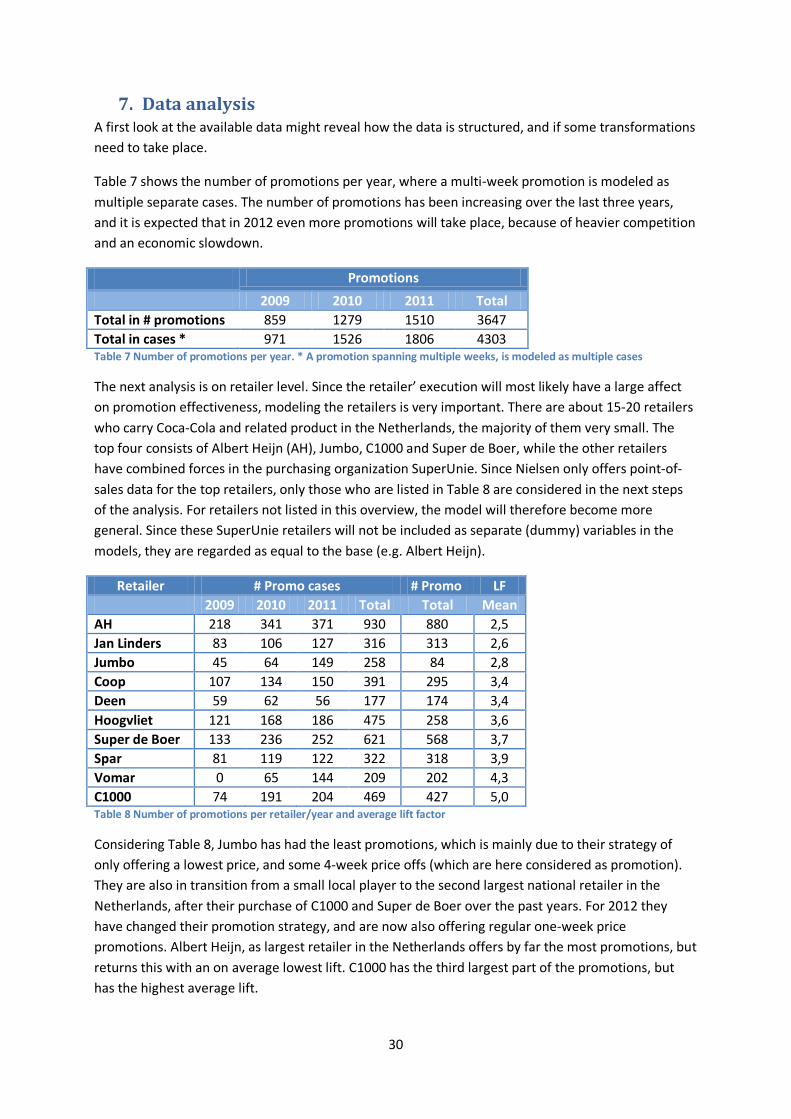
Table 7 shows the number of promotions per year, where a multi-week promotion is modeled as multiple separate cases. The number of promotions has been increasing over the last three years, and it is expected that in 2012 even more promotions will take place, because of heavier competition and an economic slowdown.

Promotions 2009 2010 2011 Total Total in # promotions 859 1279 1510 3647 Total in cases * 971 1526 1806 4303 Table 7 Number of promotions per year. * A promotion spanning multiple weeks, is modeled as multiple cases

The next analysis is on retailer level. Since the retailer’ execution will most likely have a large affect on promotion effectiveness, modeling the retailers is very important. There are about 15-20 retailers who carry Coca-Cola and related product in the Netherlands, the majority of them very small. The top four consists of Albert Heijn (AH), Jumbo, C1000 and Super de Boer, while the other retailers have combined forces in the purchasing organization SuperUnie. Since Nielsen only offers point-of-sales data for the top retailers, only those who are listed in Table 8 are considered in the next steps of the analysis. For retailers not listed in this overview, the model will therefore become more general. Since these SuperUnie retailers will not be included as separate (dummy) variables in the models, they are regarded as equal to the base (e.g. Albert Heijn).

Retailer # Promo cases # Promo LF 2009 2010 2011 Total Total Mean AH 218 341 371 930 880 2,5 Jan Linders 83 106 127 316 313 2,6 Jumbo 45 64 149 258 84 2,8 Coop 107 134 150 391 295 3,4 Deen 59 62 56 177 174 3,4 Hoogvliet 121 168 186 475 258 3,6 Super de Boer 133 236 252 621 568 3,7 Spar 81 119 122 322 318 3,9 Vomar 0 65 144 209 202 4,3 C1000 74 191 204 469 427 5,0 Table 8 Number of promotions per retailer/year and average lift factor

Considering Table 8, Jumbo has had the least promotions, which is mainly due to their strategy of only offering a lowest price, and some 4-week price offs (which are here considered as promotion). They are also in transition from a small local player to the second largest national retailer in the Netherlands, after their purchase of C1000 and Super de Boer over the past years. For 2012 they have changed their promotion strategy, and are now also offering regular one-week price promotions. Albert Heijn, as largest retailer in the Netherlands offers by far the most promotions, but returns this with an on average lowest lift. C1000 has the third largest part of the promotions, but has the highest average lift.

31

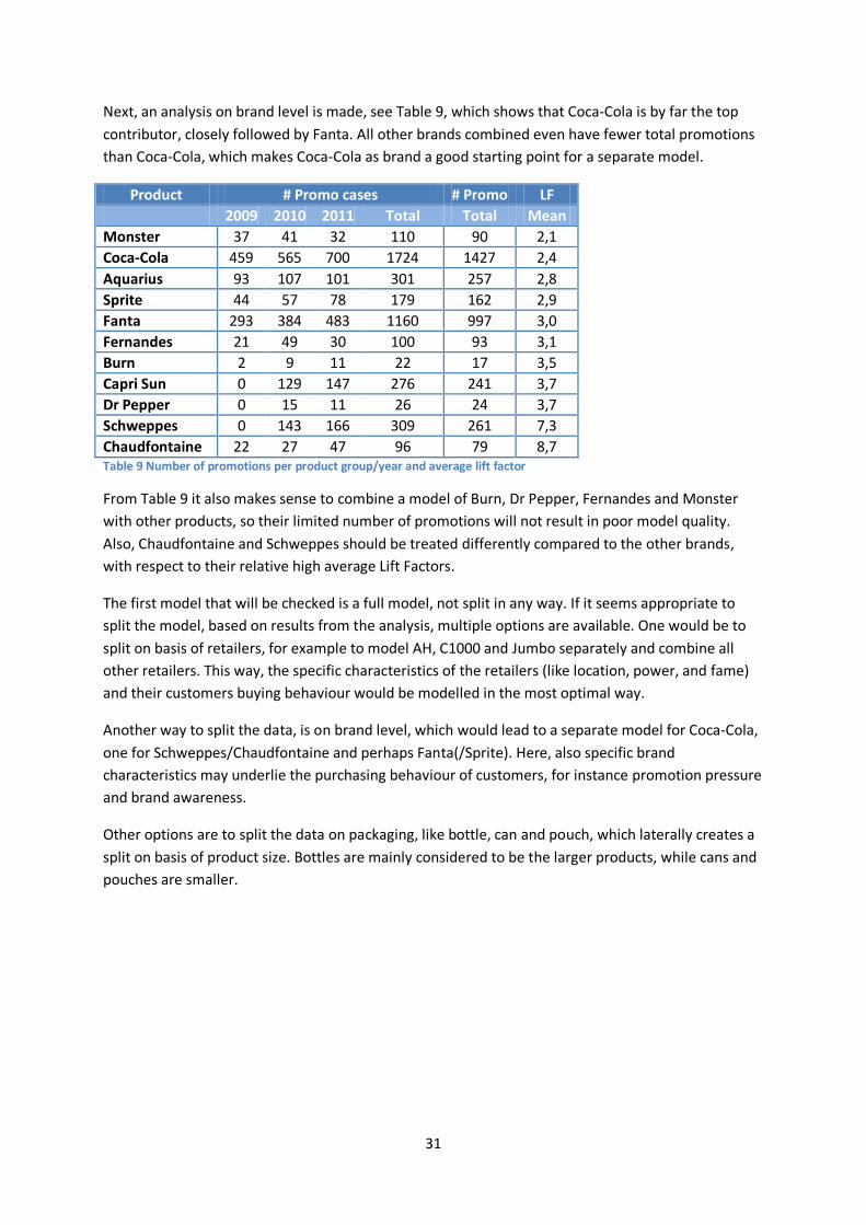
Next, an analysis on brand level is made, see Table 9, which shows that Coca-Cola is by far the top contributor, closely followed by Fanta. All other brands combined even have fewer total promotions than Coca-Cola, which makes Coca-Cola as brand a good starting point for a separate model.

Product # Promo cases # Promo LF 2009 2010 2011 Total Total Mean Monster 37 41 32 110 90 2,1 Coca-Cola 459 565 700 1724 1427 2,4 Aquarius 93 107 101 301 257 2,8 Sprite 44 57 78 179 162 2,9 Fanta 293 384 483 1160 997 3,0 Fernandes 21 49 30 100 93 3,1 Burn 2 9 11 22 17 3,5 Capri Sun 0 129 147 276 241 3,7 Dr Pepper 0 15 11 26 24 3,7 Schweppes 0 143 166 309 261 7,3 Chaudfontaine 22 27 47 96 79 8,7 Table 9 Number of promotions per product group/year and average lift factor

From Table 9 it also makes sense to combine a model of Burn, Dr Pepper, Fernandes and Monster with other products, so their limited number of promotions will not result in poor model quality. Also, Chaudfontaine and Schweppes should be treated differently compared to the other brands, with respect to their relative high average Lift Factors.

The first model that will be checked is a full model, not split in any way. If it seems appropriate to split the model, based on results from the analysis, multiple options are available. One would be to split on basis of retailers, for example to model AH, C1000 and Jumbo separately and combine all other retailers. This way, the specific characteristics of the retailers (like location, power, and fame) and their customers buying behaviour would be modelled in the most optimal way.

Another way to split the data, is on brand level, which would lead to a separate model for Coca-Cola, one for Schweppes/Chaudfontaine and perhaps Fanta(/Sprite). Here, also specific brand characteristics may underlie the purchasing behaviour of customers, for instance promotion pressure and brand awareness.

Other options are to split the data on packaging, like bottle, can and pouch, which laterally creates a split on basis of product size. Bottles are mainly considered to be the larger products, while cans and pouches are smaller.

32

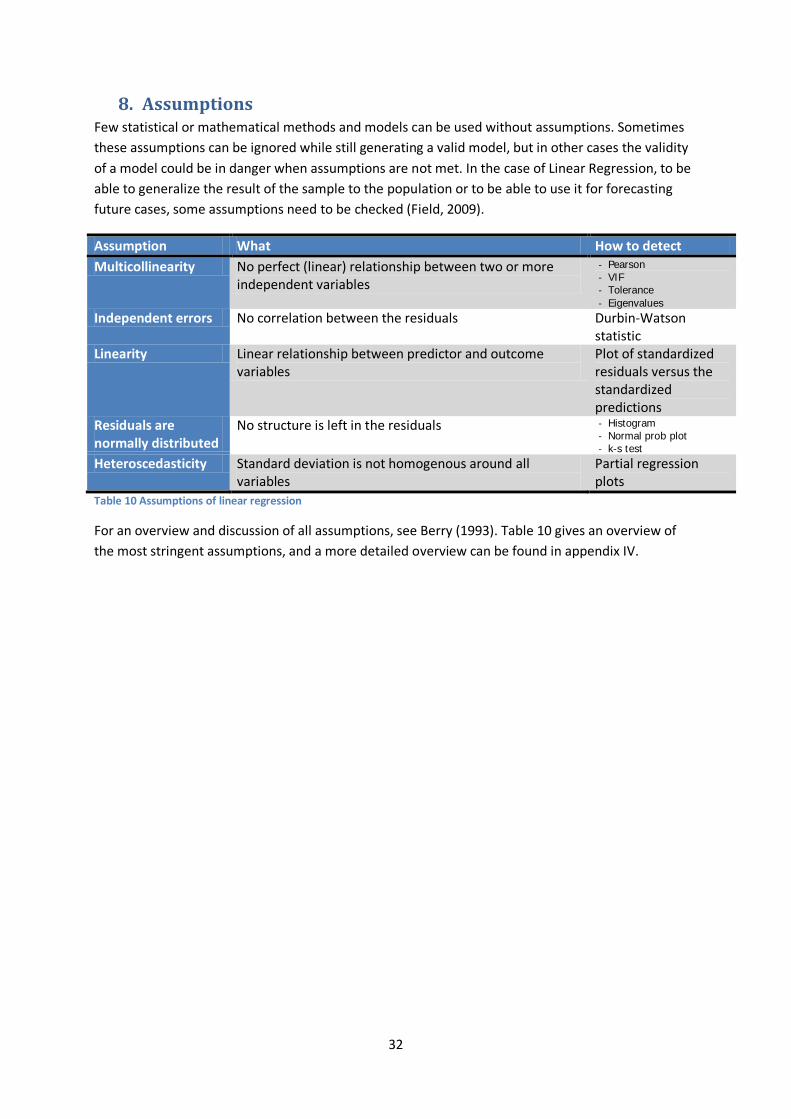
8. Assumptions Few statistical or mathematical methods and models can be used without assumptions. Sometimes these assumptions can be ignored while still generating a valid model, but in other cases the validity of a model could be in danger when assumptions are not met. In the case of Linear Regression, to be able to generalize the result of the sample to the population or to be able to use it for forecasting future cases, some assumptions need to be checked (Field, 2009).

Assumption What How to detect Multicollinearity No perfect (linear) relationship between two or more

independent variables - Pearson - VIF - Tolerance - Eigenvalues

Independent errors No correlation between the residuals Durbin-Watson statistic

Linearity Linear relationship between predictor and outcome variables

Plot of standardized residuals versus the standardized predictions

Residuals are normally distributed

No structure is left in the residuals - Histogram - Normal prob plot - k-s test

Heteroscedasticity Standard deviation is not homogenous around all variables

Partial regression plots

Table 10 Assumptions of linear regression

For an overview and discussion of all assumptions, see Berry (1993). Table 10 gives an overview of the most stringent assumptions, and a more detailed overview can be found in appendix IV.

33

Part 4: Intervention

(1) Problem definition

(2) Diagnosis

(3) Design (4) Intervention

(5) Evaluation

34

9. Regression model This chapter will describe the main analysis, which is based on a linear regression model. The analysis will start with the full model in paragraph 9.1, after which paragraph Error! Reference source not found. will explain which alterations are made to the full model to reach the results in paragraph 9.3. Finally, paragraph 9.4 will provide the results of the validation analysis on the test data set.

9.1 Full model The full model incorporates all variables that are collected and uses a stepwise inclusion of the variables in the regression model. The dependent variable is the natural log transformed Lift Factor, and the training sample consists of the 2010 and 2011 data. The model results in an R2 of 74% and an accuracy of the training sample of 76%. The resulting coefficients can be found in appendix III, and below the most interesting ones are explained in more detail.

The variables with the highest Beta are ‘Fanta’ and ‘Schweppes’, after which ‘Gondola end’ takes up third place. Interestingly, the coefficient of the lagged LF of the previous promotion is positive, which is strange, because a higher lift would imply more stock at the customers to be left when the next promotion hits. However, the factor ‘time’ is not taken into account, which could mean that promotions which are not promoted frequently (and thus receive a higher lift) are measured by this variable.

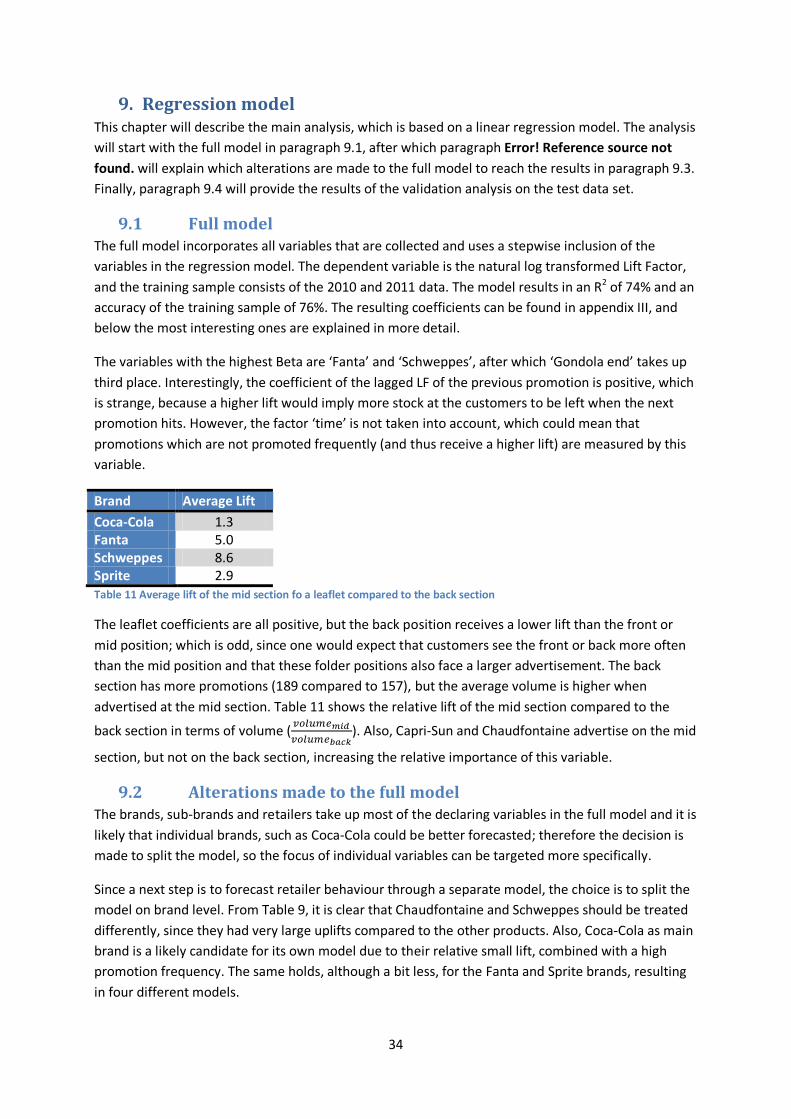
Brand Average Lift Coca-Cola 1.3 Fanta 5.0 Schweppes 8.6 Sprite 2.9 Table 11 Average lift of the mid section fo a leaflet compared to the back section

The leaflet coefficients are all positive, but the back position receives a lower lift than the front or mid position; which is odd, since one would expect that customers see the front or back more often than the mid position and that these folder positions also face a larger advertisement. The back section has more promotions (189 compared to 157), but the average volume is higher when advertised at the mid section. Table 11 shows the relative lift of the mid section compared to the

back section in terms of volume ( 𝑣𝑜𝑙𝑢𝑚𝑒𝑚𝑖𝑑𝑣𝑜𝑙𝑢𝑚𝑒𝑏𝑎𝑐𝑘

). Also, Capri-Sun and Chaudfontaine advertise on the mid

section, but not on the back section, increasing the relative importance of this variable.

9.2 Alterations made to the full model The brands, sub-brands and retailers take up most of the declaring variables in the full model and it is likely that individual brands, such as Coca-Cola could be better forecasted; therefore the decision is made to split the model, so the focus of individual variables can be targeted more specifically.

Since a next step is to forecast retailer behaviour through a separate model, the choice is to split the model on brand level. From Table 9, it is clear that Chaudfontaine and Schweppes should be treated differently, since they had very large uplifts compared to the other products. Also, Coca-Cola as main brand is a likely candidate for its own model due to their relative small lift, combined with a high promotion frequency. The same holds, although a bit less, for the Fanta and Sprite brands, resulting in four different models.

35

One extra model is created however, to account for the specific promotion-items; for instance the Coca-Cola 6-pack, which are not sold regularly, but only during promotion. Since these products have no baseline, it is not possible to calculate a LF. One solution would be to use the absolute volume, or other values as discussed in paragraph 5.1, but we have chosen to model these promo-items (also called in-out items) relative to the baseline of a related product. For instance, we assume the 6-pack Coke to be closely related to the 4-pack Coke, since also cannibalization effects occur when the 6-pack is on promotion.

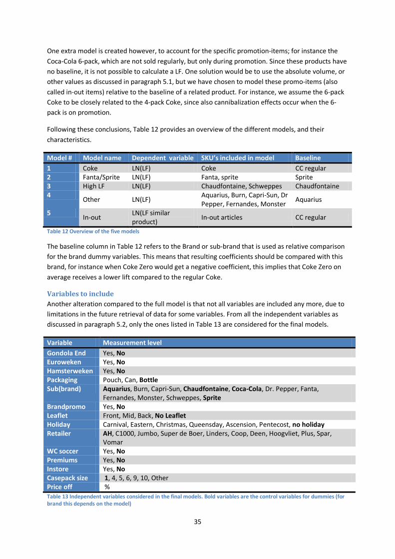
Following these conclusions, Table 12 provides an overview of the different models, and their characteristics.

Model # Model name Dependent variable SKU’s included in model Baseline 1 Coke LN(LF) Coke CC regular 2 Fanta/Sprite LN(LF) Fanta, sprite Sprite 3 High LF LN(LF) Chaudfontaine, Schweppes Chaudfontaine 4 Other LN(LF) Aquarius, Burn, Capri-Sun, Dr

Pepper, Fernandes, Monster Aquarius

5 In-out LN(LF similar product) In-out articles CC regular

Table 12 Overview of the five models

The baseline column in Table 12 refers to the Brand or sub-brand that is used as relative comparison for the brand dummy variables. This means that resulting coefficients should be compared with this brand, for instance when Coke Zero would get a negative coefficient, this implies that Coke Zero on average receives a lower lift compared to the regular Coke.

Variables to include Another alteration compared to the full model is that not all variables are included any more, due to limitations in the future retrieval of data for some variables. From all the independent variables as discussed in paragraph 5.2, only the ones listed in Table 13 are considered for the final models.

Variable Measurement level Gondola End Yes, No Euroweken Yes, No Hamsterweken Yes, No Packaging Pouch, Can, Bottle Sub(brand) Aquarius, Burn, Capri-Sun, Chaudfontaine, Coca-Cola, Dr. Pepper, Fanta,

Fernandes, Monster, Schweppes, Sprite Brandpromo Yes, No Leaflet Front, Mid, Back, No Leaflet Holiday Carnival, Eastern, Christmas, Queensday, Ascension, Pentecost, no holiday Retailer AH, C1000, Jumbo, Super de Boer, Linders, Coop, Deen, Hoogvliet, Plus, Spar,

Vomar WC soccer Yes, No Premiums Yes, No Instore Yes, No Casepack size 1, 4, 5, 6, 9, 10, Other Price off % Table 13 Independent variables considered in the final models. Bold variables are the control variables for dummies (for brand this depends on the model)

36

The variable ‘gondola end distribution’ is changed in a ‘yes/no’ variable, since the account managers do not know this information up front. The variable ‘main distribution’ cannot be measured as well, so are temperature variables. The variable ‘lag(LF)’ is based on the Nielsen LF, which is only available after the promotion has taken place, so this one is discarded as well.

From LF to Ln(LF) Businesswise the untransformed LF provides better insight in how drivers influence volumes, since the model coefficients say exactly how much the lift will change when a variable is added. However, statistical reasons might vouch for a transformation of the LF, since this might improve the model due to the linear relationship between the independent and dependent variables (which is an underlying assumption for regression analysis). In the full model, first the untransformed LF was selected as dependent variable, but subsequently this resulted in Normal Probability Plots with a horizontal, instead of a linear line, therefore violating the assumption of normality. Therefore, the natural log transformed LF is used in the results obtained in the full model as described in the previous paragraph, which also resulted in better accuracies. Because of these results, the natural log (ln) transformed Lift Factor will be used for the next models as well. This will make it harder to interpret the resulting coefficients, but for a implementation in a real life tool, this makes no difference, since the mathematics will take place in the background.

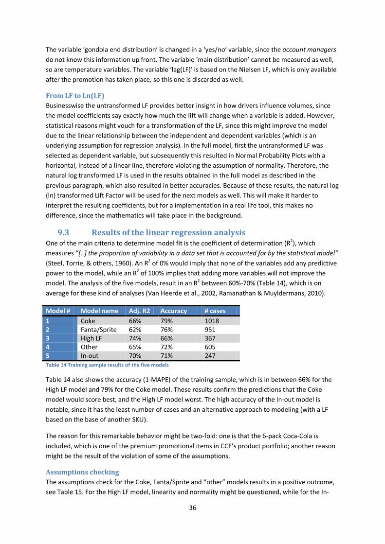
9.3 Results of the linear regression analysis One of the main criteria to determine model fit is the coefficient of determination (R2), which measures “[..] the proportion of variability in a data set that is accounted for by the statistical model” (Steel, Torrie, & others, 1960). An R2 of 0% would imply that none of the variables add any predictive power to the model, while an R2 of 100% implies that adding more variables will not improve the model. The analysis of the five models, result in an R2 between 60%-70% (Table 14), which is on average for these kind of analyses (Van Heerde et al., 2002, Ramanathan & Muyldermans, 2010).

Model # Model name Adj. R2 Accuracy # cases 1 Coke 66% 79% 1018 2 Fanta/Sprite 62% 76% 951 3 High LF 74% 66% 367 4 Other 65% 72% 605 5 In-out 70% 71% 247 Table 14 Training sample results of the five models

Table 14 also shows the accuracy (1-MAPE) of the training sample, which is in between 66% for the High LF model and 79% for the Coke model. These results confirm the predictions that the Coke model would score best, and the High LF model worst. The high accuracy of the in-out model is notable, since it has the least number of cases and an alternative approach to modeling (with a LF based on the base of another SKU).

The reason for this remarkable behavior might be two-fold: one is that the 6-pack Coca-Cola is included, which is one of the premium promotional items in CCE’s product portfolio; another reason might be the result of the violation of some of the assumptions.

Assumptions checking The assumptions check for the Coke, Fanta/Sprite and “other” models results in a positive outcome, see Table 15. For the High LF model, linearity and normality might be questioned, while for the In-

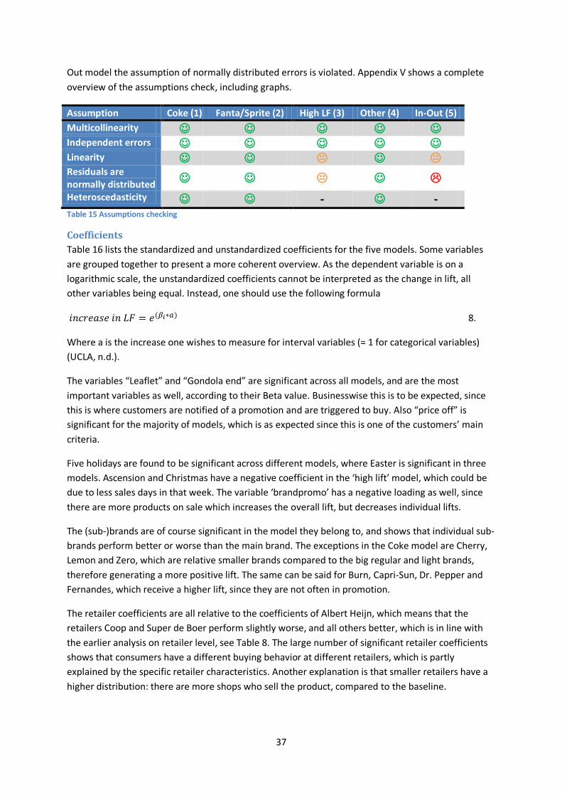
37

Out model the assumption of normally distributed errors is violated. Appendix V shows a complete overview of the assumptions check, including graphs.

Assumption Coke (1) Fanta/Sprite (2) High LF (3) Other (4) In-Out (5) Multicollinearity Independent errors Linearity Residuals are normally distributed Heteroscedasticity - - Table 15 Assumptions checking

Coefficients Table 16 lists the standardized and unstandardized coefficients for the five models. Some variables are grouped together to present a more coherent overview. As the dependent variable is on a logarithmic scale, the unstandardized coefficients cannot be interpreted as the change in lift, all other variables being equal. Instead, one should use the following formula

𝑖𝑛𝑐𝑟𝑒𝑎𝑠𝑒 𝑖𝑛 𝐿𝐹 = 𝑒(𝛽𝑖∗𝑎) 8.

Where a is the increase one wishes to measure for interval variables (= 1 for categorical variables) (UCLA, n.d.).

The variables “Leaflet” and “Gondola end” are significant across all models, and are the most important variables as well, according to their Beta value. Businesswise this is to be expected, since this is where customers are notified of a promotion and are triggered to buy. Also “price off” is significant for the majority of models, which is as expected since this is one of the customers’ main criteria.

Five holidays are found to be significant across different models, where Easter is significant in three models. Ascension and Christmas have a negative coefficient in the ‘high lift’ model, which could be due to less sales days in that week. The variable ‘brandpromo’ has a negative loading as well, since there are more products on sale which increases the overall lift, but decreases individual lifts.

The (sub-)brands are of course significant in the model they belong to, and shows that individual sub-brands perform better or worse than the main brand. The exceptions in the Coke model are Cherry, Lemon and Zero, which are relative smaller brands compared to the big regular and light brands, therefore generating a more positive lift. The same can be said for Burn, Capri-Sun, Dr. Pepper and Fernandes, which receive a higher lift, since they are not often in promotion.

The retailer coefficients are all relative to the coefficients of Albert Heijn, which means that the retailers Coop and Super de Boer perform slightly worse, and all others better, which is in line with the earlier analysis on retailer level, see Table 8. The large number of significant retailer coefficients shows that consumers have a different buying behavior at different retailers, which is partly explained by the specific retailer characteristics. Another explanation is that smaller retailers have a higher distribution: there are more shops who sell the product, compared to the baseline.

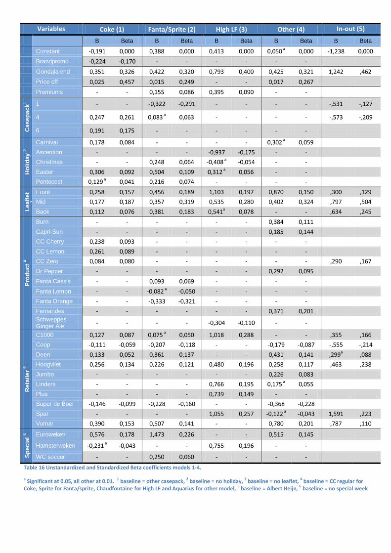
Variables Coke (1) Fanta/Sprite (2) High LF (3) Other (4) In-out (5)

B Beta B Beta B Beta B Beta B Beta

Constant -0,191 0,000 0,388 0,000 0,413 0,000 0,050 a 0,000 -1,238 0,000 Brandpromo -0,224 -0,170 - - - - - - Gondala end 0,351 0,326 0,422 0,320 0,793 0,400 0,425 0,321 1,242 ,462 Price off 0,025 0,457 0,015 0,249 - - 0,017 0,267 Premiums - - 0,155 0,086 0,395 0,090 - -

Cas

epac

k1 1 - - -0,322 -0,291 - - - - -,531 -,127

4 0,247 0,261 0,083 a 0,063 - - - - -,573 -,209

6 0,191 0,175 - - - - - -

Hol

iday

2

Carnival 0,178 0,084 - - - - 0,302 a 0,059 Ascention - - - - -0,937 -0,175 - - Christmas - - 0,248 0,064 -0,408 a -0,054 - - Easter 0,306 0,092 0,504 0,109 0,312 a 0,056 - - Pentecost 0,129 a 0,041 0,216 0,074 - - - -

Leaf

let

3

Front 0,258 0,157 0,456 0,189 1,103 0,197 0,870 0,150 ,300 ,129 Mid 0,177 0,187 0,357 0,319 0,535 0,280 0,402 0,324 ,797 ,504 Back 0,112 0,076 0,381 0,183 0,541a 0,078 - - ,634 ,245

Prod

uct 4

Burn - - - - - - 0,384 0,111 Capri-Sun - - - - - - 0,185 0,144 CC Cherry 0,238 0,093 - - - - - - CC Lemon 0,261 0,089 - - - - - - CC Zero 0,084 0,080 - - - - - - ,290 ,167 Dr Pepper - - - - - - 0,292 0,095 Fanta Cassis - - 0,093 0,069 - - - - Fanta Lemon - - -0,082 a -0,050 - - - - Fanta Orange - - -0,333 -0,321 - - - - Fernandes - - - - - - 0,371 0,201 Schweppes Ginger Ale - - - - -0,304 -0,110 - -

Ret

aile

r 5

C1000 0,127 0,087 0,075 a 0,050 1,018 0,288 - - ,355 ,166 Coop -0,111 -0,059 -0,207 -0,118 - - -0,179 -0,087 -,555 -,214 Deen 0,133 0,052 0,361 0,137 - - 0,431 0,141 ,299a ,088 Hoogvliet 0,256 0,134 0,226 0,121 0,480 0,196 0,258 0,117 ,463 ,238 Jumbo - - - - - - 0,226 0,083 Linders - - - - 0,766 0,195 0,175 a 0,055 Plus - - - - 0,739 0,149 - - Super de Boer -0,146 -0,099 -0,228 -0,160 - - -0,368 -0,228 Spar - - - - 1,055 0,257 -0,122 a -0,043 1,591 ,223 Vomar 0,390 0,153 0,507 0,141 - - 0,780 0,201 ,787 ,110

Spec

ial 6 Euroweken 0,576 0,178 1,473 0,226 - - 0,515 0,145

Hamsterweken -0,231 a -0,043 - - 0,755 0,196 - -

WC soccer - - 0,250 0,060 - - - - Table 16 Unstandardized and Standardized Beta coefficients models 1-4.

a Significant at 0.05, all other at 0.01. 1 baseline = other casepack, 2 baseline = no holiday, 3 baseline = no leaflet, 4 baseline = CC regular for Coke, Sprite for Fanta/sprite, Chaudfontaine for High LF and Aquarius for other model, 5 baseline = Albert Heijn, 6 baseline = no special week

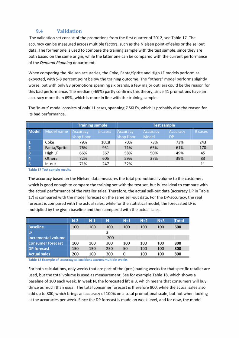
9.4 Validation The validation set consist of the promotions from the first quarter of 2012, see Table 17. The accuracy can be measured across multiple factors, such as the Nielsen point-of-sales or the sellout data. The former one is used to compare the training sample with the test sample, since they are both based on the same origin, while the latter one can be compared with the current performance of the Demand Planning department.

When comparing the Nielsen accuracies, the Coke, Fanta/Sprite and High LF models perform as expected, with 5-8 percent point below the training outcome. The “others” model performs slightly worse, but with only 83 promotions spanning six brands, a few major outliers could be the reason for this bad performance. The median (=69%) partly confirms this theory, since 41 promotions have an accuracy more than 69%, which is more in line with the training sample.

The ‘in-out’ model consists of only 11 cases, spanning 7 SKU’s, which is probably also the reason for its bad performance.

Training sample Test sample Model Model name Accuracy

shop floor # cases Accuracy

shop floor Accuracy Model

Accuracy DP

# cases

1 Coke 79% 1018 70% 73% 73% 243 2 Fanta/Sprite 76% 951 71% 65% 61% 170 3 High LF 66% 367 58% 50% 49% 45 4 Others 72% 605 59% 37% 39% 83 5 In-out 71% 247 32% - - 11 Table 17 Test sample results

The accuracy based on the Nielsen data measures the total promotional volume to the customer, which is good enough to compare the training set with the test set, but is less ideal to compare with the actual performance of the retailer sales. Therefore, the actual sell-out data (accuracy DP in Table 17) is compared with the model forecast on the same sell-out data. For the DP-accuracy, the real forecast is compared with the actual sales, while for the statistical model, the forecasted LF is multiplied by the given baseline and then compared with the actual sales.

N-2 N-1 N N+1 N+2 N+3 Total Baseline 100 100 100 100 100 100 600 LF 3 Incremental volume 200 Consumer forecast 100 100 300 100 100 100 800 DP forecast 150 150 250 50 100 100 800 Actual sales 200 100 300 0 100 100 800 Table 18 Example of accuracy calcualtions accross multiple weeks

For both calculations, only weeks that are part of the (pre-)loading weeks for that specific retailer are used, but the total volume is used as measurement. See for example Table 18, which shows a baseline of 100 each week. In week N, the forecasted lift is 3, which means that consumers will buy thrice as much than usual. The total consumer forecast is therefore 800, while the actual sales also add up to 800, which brings an accuracy of 100% on a total promotional scale, but not when looking at the accuracies per week. Since the DP forecast is made on week level, and for now, the model

40

forecast is not, we compare the two models on total promotional level, which in the example of Table 18 would be both equal to 100%.

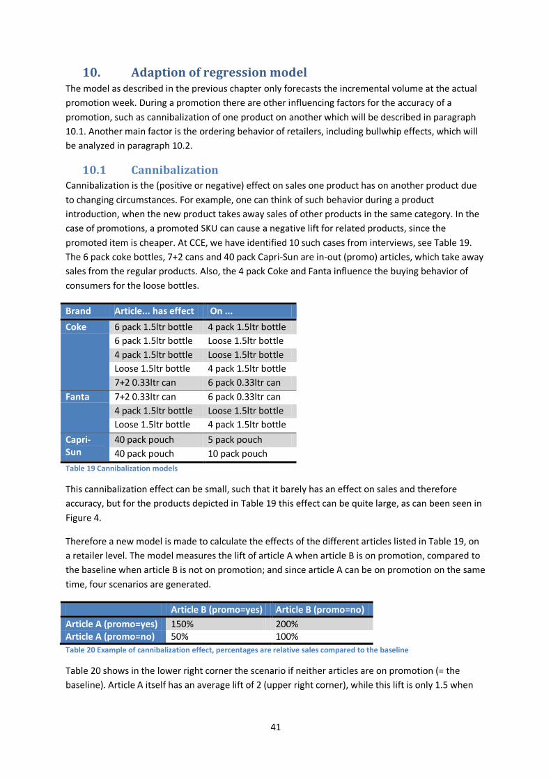
41

10. Adaption of regression model The model as described in the previous chapter only forecasts the incremental volume at the actual promotion week. During a promotion there are other influencing factors for the accuracy of a promotion, such as cannibalization of one product on another which will be described in paragraph 10.1. Another main factor is the ordering behavior of retailers, including bullwhip effects, which will be analyzed in paragraph 10.2.

10.1 Cannibalization Cannibalization is the (positive or negative) effect on sales one product has on another product due to changing circumstances. For example, one can think of such behavior during a product introduction, when the new product takes away sales of other products in the same category. In the case of promotions, a promoted SKU can cause a negative lift for related products, since the promoted item is cheaper. At CCE, we have identified 10 such cases from interviews, see Table 19. The 6 pack coke bottles, 7+2 cans and 40 pack Capri-Sun are in-out (promo) articles, which take away sales from the regular products. Also, the 4 pack Coke and Fanta influence the buying behavior of consumers for the loose bottles.

Brand Article... has effect On ... Coke 6 pack 1.5ltr bottle 4 pack 1.5ltr bottle

6 pack 1.5ltr bottle Loose 1.5ltr bottle 4 pack 1.5ltr bottle Loose 1.5ltr bottle Loose 1.5ltr bottle 4 pack 1.5ltr bottle 7+2 0.33ltr can 6 pack 0.33ltr can

Fanta 7+2 0.33ltr can 6 pack 0.33ltr can 4 pack 1.5ltr bottle Loose 1.5ltr bottle Loose 1.5ltr bottle 4 pack 1.5ltr bottle

Capri-Sun

40 pack pouch 5 pack pouch 40 pack pouch 10 pack pouch

Table 19 Cannibalization models

This cannibalization effect can be small, such that it barely has an effect on sales and therefore accuracy, but for the products depicted in Table 19 this effect can be quite large, as can been seen in Figure 4.

Therefore a new model is made to calculate the effects of the different articles listed in Table 19, on a retailer level. The model measures the lift of article A when article B is on promotion, compared to the baseline when article B is not on promotion; and since article A can be on promotion on the same time, four scenarios are generated.

Article B (promo=yes) Article B (promo=no) Article A (promo=yes) 150% 200% Article A (promo=no) 50% 100% Table 20 Example of cannibalization effect, percentages are relative sales compared to the baseline

Table 20 shows in the lower right corner the scenario if neither articles are on promotion (= the baseline). Article A itself has an average lift of 2 (upper right corner), while this lift is only 1.5 when

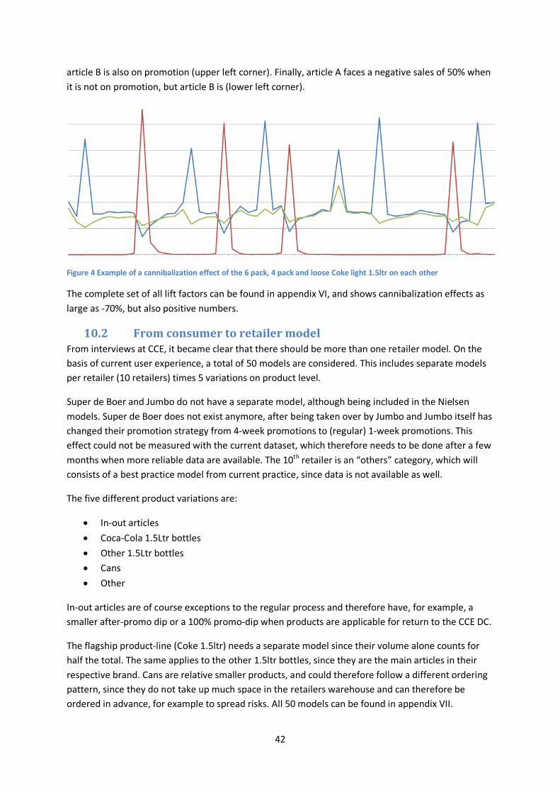
42

article B is also on promotion (upper left corner). Finally, article A faces a negative sales of 50% when it is not on promotion, but article B is (lower left corner).

Figure 4 Example of a cannibalization effect of the 6 pack, 4 pack and loose Coke light 1.5ltr on each other

The complete set of all lift factors can be found in appendix VI, and shows cannibalization effects as large as -70%, but also positive numbers.

10.2 From consumer to retailer model From interviews at CCE, it became clear that there should be more than one retailer model. On the basis of current user experience, a total of 50 models are considered. This includes separate models per retailer (10 retailers) times 5 variations on product level.

Super de Boer and Jumbo do not have a separate model, although being included in the Nielsen models. Super de Boer does not exist anymore, after being taken over by Jumbo and Jumbo itself has changed their promotion strategy from 4-week promotions to (regular) 1-week promotions. This effect could not be measured with the current dataset, which therefore needs to be done after a few months when more reliable data are available. The 10th retailer is an “others” category, which will consists of a best practice model from current practice, since data is not available as well.

The five different product variations are:

• In-out articles • Coca-Cola 1.5Ltr bottles • Other 1.5Ltr bottles • Cans • Other

In-out articles are of course exceptions to the regular process and therefore have, for example, a smaller after-promo dip or a 100% promo-dip when products are applicable for return to the CCE DC.

The flagship product-line (Coke 1.5ltr) needs a separate model since their volume alone counts for half the total. The same applies to the other 1.5ltr bottles, since they are the main articles in their respective brand. Cans are relative smaller products, and could therefore follow a different ordering pattern, since they do not take up much space in the retailers warehouse and can therefore be ordered in advance, for example to spread risks. All 50 models can be found in appendix VII.

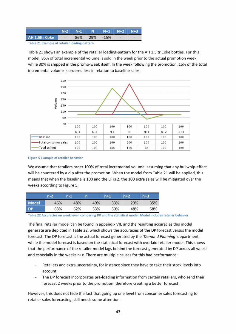
43

N-2 N-1 N N+1 N+2 N+3 AH 1.5ltr Coke - 86% 29% -15% - - Table 21 Example of retailer loading-pattern

Table 21 shows an example of the retailer loading-pattern for the AH 1.5ltr Coke bottles. For this model, 85% of total incremental volume is sold in the week prior to the actual promotion week, while 30% is shipped in the promo-week itself. In the week following the promotion, 15% of the total incremental volume is ordered less in relation to baseline sales.

Figure 5 Example of retailer bahavior

We assume that retailers order 100% of total incremental volume, assuming that any bullwhip-effect will be countered by a dip after the promotion. When the model from Table 21 will be applied, this means that when the baseline is 100 and the LF is 2, the 100 extra sales will be mitigated over the weeks according to Figure 5.

n-2 n-1 n n+1 n+2 n+3 Model 46% 48% 49% 33% 29% 35% DP 63% 62% 53% 50% 48% 58% Table 22 Accuracies on week level: comparing DP and the statistical model. Model includes retailer behavior

The final retailer model can be found in appendix VII, and the resulting accuracies this model generate are depicted in Table 22, which shows the accuracies of the DP forecast versus the model forecast. The DP forecast is the actual forecast generated by the ‘Demand Planning’ department, while the model forecast is based on the statistical forecast with overlaid retailer model. This shows that the performance of the retailer model lags behind the forecast generated by DP across all weeks and especially in the weeks n+x. There are multiple causes for this bad performance:

- Retailers add extra uncertainty, for instance since they have to take their stock levels into account;

- The DP forecast incorporates pre-loading information from certain retailers, who send their forecast 2 weeks prior to the promotion, therefore creating a better forecast;

However, this does not hide the fact that going up one level from consumer sales forecasting to retailer sales forecasting, still needs some attention.

44

11. Data mining model Computers have become more powerful over the last few years, resulting in the possibility to make use of data analysis on large sets of data. These techniques, referred to as ‘data mining’ have proven themselves to be able to result in good models, therefore a data mining model is constructed as reference to the linear regression model. We will test multiple algorithms, an Artificial Neural Network (ANN), a Regression Tree and a Support Vector Machine (SVM), to see if they generate different results. Paragraph 11.1 will start with a short description of data mining and the different techniques, while paragraph 11.2 gives an overview of how this is implemented in the CCE-case. Paragraph 11.3 shows the results generated by the data mining models, and paragraph 11.4 makes a comparison with the linear regression results.

11.1 Short introduction to Data Mining Data mining has its origin in the early 20th century, with the emergence of computer science. Since data sets grew larger in size and complexity, manual data-analysis became harder and harder, such that new techniques were needed. Neural networks became available in the 1950’s, while decision trees made their way to computer science in the 1960’s and support vector machines in the 1990’s. Applying these (and many other) methods to data with the intention of uncovering hidden patterns, is called data mining (Kantardzic, 2011).

Data mining can be used to make predictions, based on a set of preliminary data, which is basically the same as Linear Regression. One of the main differences however is that data mining is not based on an underlying theoretical model that should be predicted, but just aims to find patterns in (random) data. The advantage being that patterns not thought of upfront can thus be modeled (if the data is available), but the opposite being that some patterns may not make sense businesswise.

For more information about the different data mining techniques, see (Kock, 2012) and (M. J. A. Berry & Linoff, 2004).

11.2 Implementation One of the advantages of Data Mining is its ability to find patterns in data that cannot be found with other tools, since there is no underlying assumption of a specific (non)-linear relationship, which is for example the case with linear regression. Including all available variables would therefore probably yield in a good forecast, but to provide a good comparison with the linear regression models, only the variables included in the regression model are included in the data mining model as well (see Table 13). A full model will be generated, since data mining models should “create” separate models themselves, but for a true comparison, also the four models from the regression analysis (Coke, Fanta/Sprite, High LF and Others) will be tested. Since the ‘in-out’ model lacks enough data points in the test sample, it is excluded from the analysis.

As a training set, 2010-2011 will be used, while the first quarter of 2012 will be used as test sample. The software used is “Knime”, which has a graphical interface and allows for the open source Weka-algorithms (Hall et al., 2009) to be includes; these provide all of the most used algorithms currently available, including algorithms that are capable of analyzing nominal variables.

For the SVM model, the standard Weka SVM node (Shevade, Keerthi, Bhattacharyya, & Murthy, 2000) used with standard settings; for the Regression Tree the Weka M5P algorithm (Boser, Guyon, & Vapnik, 1992) is selected, mainly because of its capability to include nominal variables. The

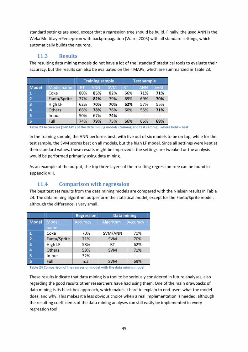
45

standard settings are used, except that a regression tree should be build. Finally, the used ANN is the Weka MultiLayerPerceptron with backpropagation (Ware, 2005) with all standard settings, which automatically builds the neurons.

11.3 Results The resulting data mining models do not have a lot of the ‘standard’ statistical tools to evaluate their accuracy, but the results can also be evaluated on their MAPE, which are summarized in Table 23.

Training sample Test sample Model Model name RT ANN SVM RT ANN SVM 1 Coke 80% 85% 82% 66% 71% 71% 2 Fanta/Sprite 77% 82% 79% 69% 69% 70% 3 High LF 62% 70% 70% 62% 57% 55% 4 Others 68% 78% 76% 60% 55% 71% 5 In-out 50% 67% 74% - - - 6 Full 74% 79% 75% 66% 66% 69% Table 23 Accuracies (1-MAPE) of the data mining models (training and test sample); where bold = best

In the training sample, the ANN performs best, with five out of six models to be on top, while for the test sample, the SVM scores best on all models, but the high LF model. Since all settings were kept at their standard values, these results might be improved if the settings are tweaked or the analysis would be performed primarily using data mining.

As an example of the output, the top three layers of the resulting regression tree can be found in appendix VIII.

11.4 Comparison with regression The best test set results from the data mining models are compared with the Nielsen results in Table 24. The data mining algorithm outperform the statistical model, except for the Fanta/Sprite model, although the difference is very small.

Regression Data mining Model Model

name Accuracy Algorithm Accuracy

1 Coke 70% SVM/ANN 71% 2 Fanta/Sprite 71% SVM 70% 3 High LF 58% RT 62% 4 Others 59% SVM 71% 5 In-out 32% - - 6 Full n.a. SVM 69% Table 24 Comparison of the regression model with the data mining model

These results indicate that data mining is a tool to be seriously considered in future analyses, also regarding the good results other researchers have had using them. One of the main drawbacks of data mining is its black box approach, which makes it hard to explain to end-users what the model does, and why. This makes it a less obvious choice when a real implementation is needed, although the resulting coefficients of the data mining analyses can still easily be implemented in every regression tool.

46

12. Promo tool and process A statistical model alone would not improve CCE’s forecast, therefore a tool that implements the model is proposed in this chapter. Paragraph 13.1 will describe the requirements of the tool, after which paragraph 13.2 will provide some details of the actual tool. Finally, paragraph 12.3 discusses the new process to forecast the promotions.

12.1 Requirements The tool should be able to use the output of the statistical model to generate a forecast. This constitutes to the following functional requirements:

• The tool should be easy to work with • The tool should be based on input by the Account Managers • The tool should convert this input with the LF from the statistical model into a new forecast • The tool should take the retailer behavior into account • The tool should be able to predict when another SKU is cannibalized • The tool should output this in such a way that it is easily interpretable • It should be easy to export the resulting forecast to the ERP-environment • It should be possible to update the LF-model and retailer-model on a regular basis • Previous promotions, with their corresponding actual sales, LF and accuracy’s should be

present in the model to be used as reference for future forecasts • The tool should be constructed on a software platform already available at CCE

Since the requirements indicate that a database would really improve the tool over a spreadsheet-program, the obvious choice would be to implement the tool in the current ERP-environment. But since this would require specific information, access, time and money this is taken out of scope for this project. One of the main software packages used for databases is MS Access, and since the future users of the tool know how to use this, it is selected as software to build the tool.

12.2 Result Since promotions are an important aspect of the processes at CCE, other departments also have projects running to improve their efficiency. One of these projects originates at the financial level, with a goal to counter price differences and keep the promotion budget in control. This project was set up during the course of this master thesis and one of its results was the creation of a promo database where the Account Managers would input the promotions using a strict protocol. Since the input from Account Management is the same as what is required for Demand Planning, both projects were combined into one project.

One of the results of the cooperation is that at the input screen, new variables are attached according to the needs of Demand Planning, such as TV, Gondola end, premiums, etc. These variables can then be used as input in the statistical model to generate a forecast.

The promotion database is a shared Access DB, with all promotions and their corresponding variables. For Demand Planning a separate module is made, which links to the central DB and uses other input to form the forecast. The tool is constructed on three levels

1. Promotion overview, which shows all promotions currently ‘open’;

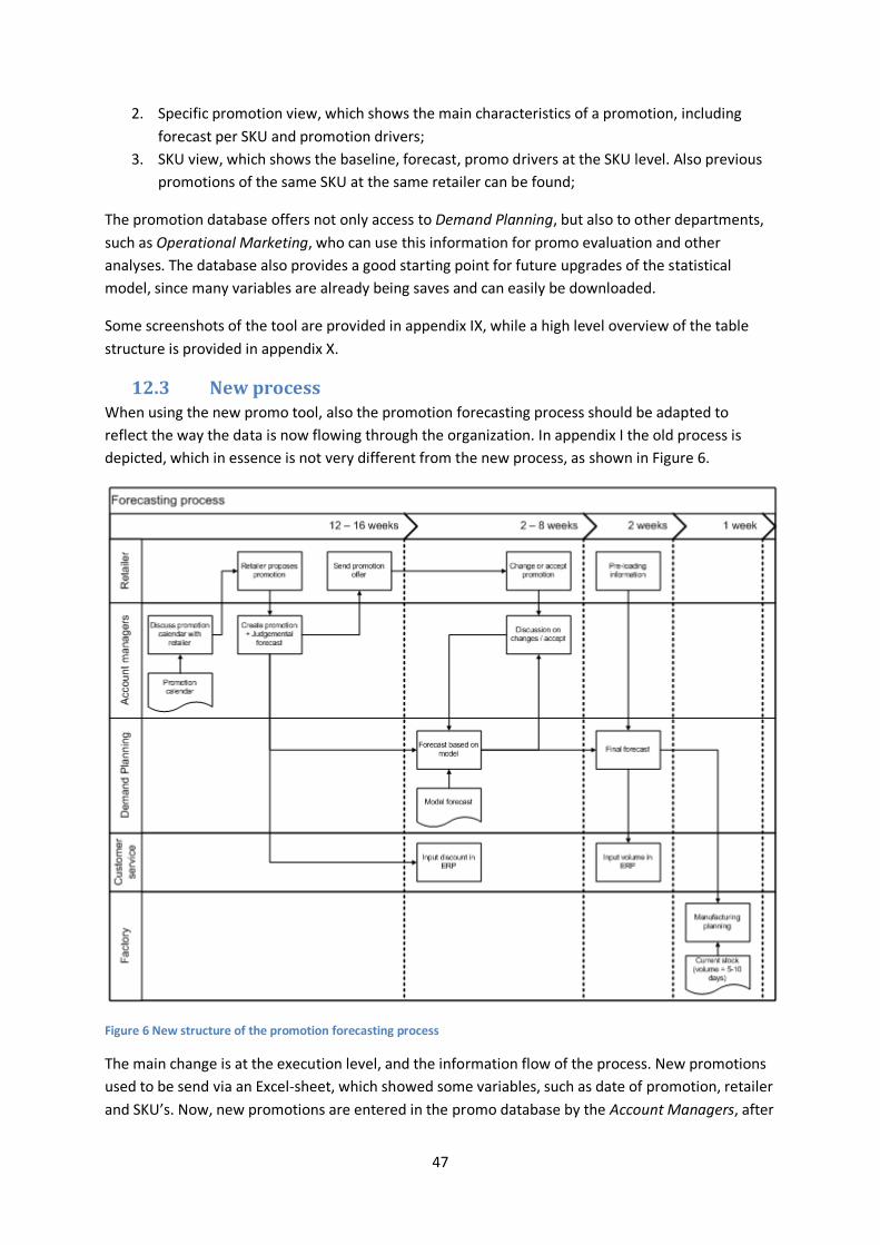
47

2. Specific promotion view, which shows the main characteristics of a promotion, including forecast per SKU and promotion drivers;

3. SKU view, which shows the baseline, forecast, promo drivers at the SKU level. Also previous promotions of the same SKU at the same retailer can be found;

The promotion database offers not only access to Demand Planning, but also to other departments, such as Operational Marketing, who can use this information for promo evaluation and other analyses. The database also provides a good starting point for future upgrades of the statistical model, since many variables are already being saves and can easily be downloaded.

Some screenshots of the tool are provided in appendix IX, while a high level overview of the table structure is provided in appendix X.

12.3 New process When using the new promo tool, also the promotion forecasting process should be adapted to reflect the way the data is now flowing through the organization. In appendix I the old process is depicted, which in essence is not very different from the new process, as shown in Figure 6.

Figure 6 New structure of the promotion forecasting process

The main change is at the execution level, and the information flow of the process. New promotions used to be send via an Excel-sheet, which showed some variables, such as date of promotion, retailer and SKU’s. Now, new promotions are entered in the promo database by the Account Managers, after

48

which the retailer receives a standard format with the proposal, Master Data receives the price rebate to be linked to that specific retailer during a specified time and Demand Planning instantaneously receives the promotion details on which the forecast can be automatically generated.

Changes in promotions used to be followed by the creation of a new Excel-sheet, even if the change was not notably influencing the forecasted volume, since this was required for the other departments. In the new tool, all changes are visible to the user instantaneously, and can be filtered to only reflect changes that affect the forecast.

The main change for the Demand Planning is that they can now use the new tool to forecast the promotions, instead of using Excel-sheets with information about historical promotions. The forecast can be copy/pasted into the ERP-environment, instead of manually typed from paper sheets, and the forecast generated by the statistical model is proposed automatically.

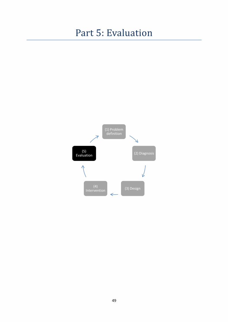
49

Part 5: Evaluation

(1) Problem definition

(2) Diagnosis

(3) Design (4) Intervention

(5) Evaluation

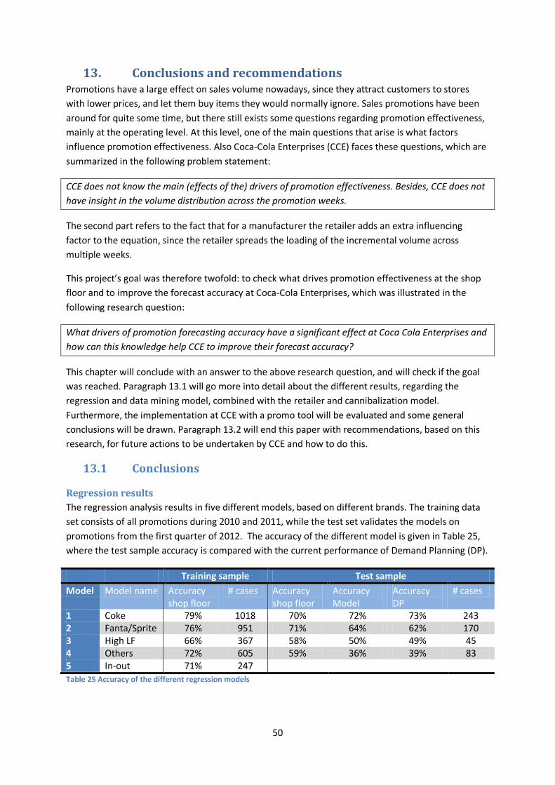
50

13. Conclusions and recommendations Promotions have a large effect on sales volume nowadays, since they attract customers to stores with lower prices, and let them buy items they would normally ignore. Sales promotions have been around for quite some time, but there still exists some questions regarding promotion effectiveness, mainly at the operating level. At this level, one of the main questions that arise is what factors influence promotion effectiveness. Also Coca-Cola Enterprises (CCE) faces these questions, which are summarized in the following problem statement:

CCE does not know the main (effects of the) drivers of promotion effectiveness. Besides, CCE does not have insight in the volume distribution across the promotion weeks.

The second part refers to the fact that for a manufacturer the retailer adds an extra influencing factor to the equation, since the retailer spreads the loading of the incremental volume across multiple weeks.

This project’s goal was therefore twofold: to check what drives promotion effectiveness at the shop floor and to improve the forecast accuracy at Coca-Cola Enterprises, which was illustrated in the following research question:

What drivers of promotion forecasting accuracy have a significant effect at Coca Cola Enterprises and how can this knowledge help CCE to improve their forecast accuracy?

This chapter will conclude with an answer to the above research question, and will check if the goal was reached. Paragraph 13.1 will go more into detail about the different results, regarding the regression and data mining model, combined with the retailer and cannibalization model. Furthermore, the implementation at CCE with a promo tool will be evaluated and some general conclusions will be drawn. Paragraph 13.2 will end this paper with recommendations, based on this research, for future actions to be undertaken by CCE and how to do this.

13.1 Conclusions

Regression results The regression analysis results in five different models, based on different brands. The training data set consists of all promotions during 2010 and 2011, while the test set validates the models on promotions from the first quarter of 2012. The accuracy of the different model is given in Table 25, where the test sample accuracy is compared with the current performance of Demand Planning (DP).

Training sample Test sample Model Model name Accuracy

shop floor # cases Accuracy

shop floor Accuracy Model

Accuracy DP

# cases

1 Coke 79% 1018 70% 72% 73% 243 2 Fanta/Sprite 76% 951 71% 64% 62% 170 3 High LF 66% 367 58% 50% 49% 45 4 Others 72% 605 59% 36% 39% 83 5 In-out 71% 247 Table 25 Accuracy of the different regression models

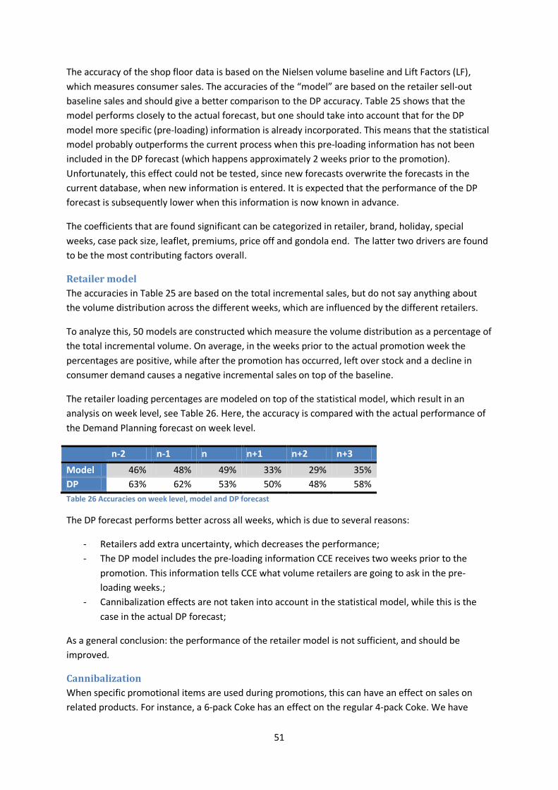
51

The accuracy of the shop floor data is based on the Nielsen volume baseline and Lift Factors (LF), which measures consumer sales. The accuracies of the “model” are based on the retailer sell-out baseline sales and should give a better comparison to the DP accuracy. Table 25 shows that the model performs closely to the actual forecast, but one should take into account that for the DP model more specific (pre-loading) information is already incorporated. This means that the statistical model probably outperforms the current process when this pre-loading information has not been included in the DP forecast (which happens approximately 2 weeks prior to the promotion). Unfortunately, this effect could not be tested, since new forecasts overwrite the forecasts in the current database, when new information is entered. It is expected that the performance of the DP forecast is subsequently lower when this information is now known in advance.

The coefficients that are found significant can be categorized in retailer, brand, holiday, special weeks, case pack size, leaflet, premiums, price off and gondola end. The latter two drivers are found to be the most contributing factors overall.

Retailer model The accuracies in Table 25 are based on the total incremental sales, but do not say anything about the volume distribution across the different weeks, which are influenced by the different retailers.

To analyze this, 50 models are constructed which measure the volume distribution as a percentage of the total incremental volume. On average, in the weeks prior to the actual promotion week the percentages are positive, while after the promotion has occurred, left over stock and a decline in consumer demand causes a negative incremental sales on top of the baseline.

The retailer loading percentages are modeled on top of the statistical model, which result in an analysis on week level, see Table 26. Here, the accuracy is compared with the actual performance of the Demand Planning forecast on week level.

n-2 n-1 n n+1 n+2 n+3 Model 46% 48% 49% 33% 29% 35% DP 63% 62% 53% 50% 48% 58% Table 26 Accuracies on week level, model and DP forecast

The DP forecast performs better across all weeks, which is due to several reasons:

- Retailers add extra uncertainty, which decreases the performance; - The DP model includes the pre-loading information CCE receives two weeks prior to the

promotion. This information tells CCE what volume retailers are going to ask in the pre-loading weeks.;

- Cannibalization effects are not taken into account in the statistical model, while this is the case in the actual DP forecast;

As a general conclusion: the performance of the retailer model is not sufficient, and should be improved.

Cannibalization When specific promotional items are used during promotions, this can have an effect on sales on related products. For instance, a 6-pack Coke has an effect on the regular 4-pack Coke. We have

52

analyzed all the relations which CCE found significant earlier, and modeled the cannibalization effect as a negative (or positive) percentage on top of the total sales during the loading-weeks.

Data mining The data mining models’ accuracy proved to be performing closely to the linear regression results, which is interesting since less time was actually spent tweaking the data mining models; the “others” model even outperformed the regression model by about 10-percent points.

The Support Vector Machine algorithm seems to perform best, compared to the Regression Tree and Neural Network, but has as drawback that it is also the least intuitive algorithm in terms of how it works and how the output should be interpreted, making it less likely to be implemented in a real lift environment.

Promo tool The promotion tool is based on a cross-departmental promotion database that has been developed by CCE as a separate project, but with input from Demand Planning and this research. The database input is generated by the Account Managers, who enter new promotions with specific promotional driver information, such as gondola end, leaflets, TV and premiums. This data is then transferred to other departments, such as Master Data, who adjust prices for the customers, and Demand Management to forecast sales.

The promo drivers set by the account managers are used by the new promo tool to forecast the incremental volume across the different loading weeks, based on the statistical models generated. DP users can adjust the forecast generated by the model, and view previous promotion of the same SKU at the same retailer with the corresponding performance in terms of accuracy.

General conclusions Reflecting on the original research question, “What drivers of promotion forecasting accuracy have a significant effect at Coca Cola Enterprises and how can this knowledge help CCE to improve their forecast accuracy?”, the conclusion is that drivers or promotion effectiveness differ between brands, and price and gondola end are the main predictors across all brands. The forecast on a total incremental volume level is improved, but the model lacks in terms of translating the forecast to retailer behavior. The promo tool that is constructed should help CCE to forecast new promotion more effectively and more efficiently, while the promo database creates a good source with valuable information for future promotion analyses.

13.2 Recommendations This project can be seen as one further step in the right direction of excellent promo forecasting, however, there are many more steps to be taken.

Data Mining One of these steps could be to try data mining as the main analysis tool for a future statistical model, since the analysis in this report has generated good results. One of the most interesting opportunities could be to use the data mining to combine a consumer model and a retailer model into one. For instance, such a model could make use of multiple layers in an Artificial Neural Network to separate consumer and retailer sales, or generate new branches in a Regression Tree for the retailer model.

53

Future statistical models Future statistical models should base the forecast on SAP-data and combine that with the Nielsen data, instead of combining SAP to Nielsen. This way, all relevant exceptions, such as multiple SAP-numbers for one EAN number (for instance when there are multiple trade packages) are captured, instead of modeling them afterwards. The new promo database is the first step in the right direction, since the majority of data is available there, and thus would prove an excellent base to start with.

One should keep in mind that statistical analysis depends on historical data, which is used to forecast the future. If the future does not reflect the past any more, statistical models are not capable of changing their behavior, which is for example reflected in the way the retailer Jumbo has changed his promotion strategy from 4-week price-off to a 1-week promotion. Not only should Demand Planning keep the underlying statistical model in mind, but they should also trigger the Account Managers if they change their promotion strategy.

Promo tool For the promo tool to be really up-to-date and working seamless with the current process, an interface should be made between the MS Access Promo DB tool and the SAP DB. In the ideal situation, real time data should be subtracted from SAP (the actual and baseline sales), so the tool always depends on the latest accurate data. Next, the forecast should be imported in SAP when the user clicks on the forecast button in the Access tool. This makes the forecasting process more efficient and makes sure the data is less prone to errors or inconsistencies.

Finally, the data that is available in the promo tool and database can be extended to other departments, or used even more by the current users. Extensions could be for example:

- Commercial promotion evaluation (profit management) - Actual sales overview on consumer and ex-factory level; with comparisons between the two - Target evaluations for Account Managers (budget) and Demand Planning (accuracy)

Evaluation To constantly improve the performance, a weekly or monthly top 10-outlier analysis should be performed to see where the model does not fit the actual situation. This would provide CCE with an overview of the specific articles that need special attention, and creates vital input to be used in future upgrading of the statistical model.

54

References Aburto, L. & Weber, R. (2007). Improved supply chain management based on hybrid demand

forecasts. Applied Soft Computing, 7(1), 136 - 144. doi:10.1016/j.asoc.2005.06.001

Van Aken, J. E., Berends, H. & Van der Bij, H. (2007). Problem-solving in organizations: a methodological handbook for business students. Cambridge Univ Pr.

Ali, Ö. G., Sayin, S., Van Woensel, T. & Fransoo, J. (2009). SKU demand forecasting in the presence of promotions. Expert Systems with Applications, 36(10), 12340-12348. Elsevier.

Barnett, V. (1978). The study of outliers: purpose and model. Applied Statistics, 242-250. JSTOR.

Berry, M. J. A. & Linoff, G. S. (2004). Data Mining Techniques for Marketing, Sales and Customer Relationship Managament.

Berry, W. D. (1993). Understanding regression assumptions. Sage Publications, Inc.

Blattberg, R. C. & Neslin, S. A. (1990). Sales promotion: Concepts, methods, and strategies. Prentice Hall Englewood Cliffs, NJ.

Boser, B. E., Guyon, I. M. & Vapnik, V. N. (1992). A training algorithm for optimal margin classifiers. Proceedings of the fifth annual workshop on Computational learning theory, 144-152.

Chang, P. C. & Wang, Y. W. (2006). Fuzzy Delphi and back-propagation model for sales forecasting in PCB industry. Expert systems with applications, 30(4), 715-726. Elsevier.

Cooper, L. G., Baron, P., Levy, W., Swisher, M. & Gogos, P. (1999). PromoCastTM: A new forecasting method for promotion planning. Marketing Science, 301-316. JSTOR.

Delen, D., Walker, G. & Kadam, A. (2005). Predicting breast cancer survivability: a comparison of three data mining methods. Artificial Intelligence in Medicine, 34(2), 113 - 127. doi:10.1016/j.artmed.2004.07.002

Distrifood. (2007). Coca-Cola vreest lege schappen in supers. http://www.distrifood.nl/web/Nieuws/Fabrikanten/Fabrikanten-artikel/125681/CocaCola-vreest-lege-schappen-in-supers.htm.

Durbin, J. & Watson, G. S. (1951). Testing for serial correlation in least squares regression. II. Biometrika, 38(1/2), 159-177. JSTOR.

55

Field, A. P. (2009). Discovering statistics using SPSS. SAGE publications Ltd.

Fu, H.-P., Chu, K.-K., Lin, S.-W. & Chen, C.-R. (2010). A STUDY ON FACTORS FOR RETAILERS IMPLEMENTING CPFR - A FUZZY AHP ANALYSIS. JOURNAL OF SYSTEMS SCIENCE AND SYSTEMS ENGINEERING. TIERGARTENSTRASSE 17, D-69121 HEIDELBERG, GERMANY: SPRINGER HEIDELBERG. doi:10.1007/s11518-010-5136-8

GFK. (2011). GFK Jaarcongres ’Sell me more: promoties, het paard van Troje?

GFK. (2011). GfK Jaarcongres 2011: Brand Survival.

Hall, M., Frank, E., Holmes, G., Pfahringer, B., Reutemann, P. & Witten, I. H. (2009). The WEKA data mining software: an update. ACM SIGKDD Explorations Newsletter, 11(1), 10-18. ACM.

Van Heerde, H. J., Leeflang, P. S. H. & Wittink, D. R. (2002). How promotions work: SCAN* PRO-based evolutionary model building. Schmalenbach business review, 54(3), 198-220.

Hogarth-Scott, S. & Parkinson, S. T. (1993). Retailer-Supplier Relationships in the Food Channel: A Supplier Perspective. International Journal of Retail & Distribution Management, 21(8). MCB UP Ltd.

Hutcheson, G. & Sofroniou, N. (1999). The multivariate social scientist: Introductory statistics using generalized linear models. Sage Publications Ltd.

Kantardzic, M. (2011). Data mining: concepts, models, methods, and algorithms. Wiley-IEEE Press.

Kock, J. (2012). Literature Study, Improving the Promotion Forecast at Coca-Cola.

Loo, M., Woensel, T. T. & others. (2006). Out-of-Stock reductie van actieartikelen, Model voor vraagvoorspelling en logistieke aansturing van actieartikelen bij Schuitema/C1000. Technische Universiteit Eindhoven.

Myers, R. H. (1990). Classical and modern regression with applications (Vol. 488). Duxbury Press Belmont, California.

Nu.nl. (2011). Nieuwe prijzenoorlog supermarkten ’ . http://www.nu.nl/economie/2667783/nieuwe-prijzenoorlog-supermarkten.html.

56

Van der Poel, M. J. (2010). A Literature study at promotion forecasting in the Fast Moving Consumer Good sector.

Van der Poel, M. J. T. (2010). Improving the promotion forecasting accuracy at Unilever Netherlands.

Ramanathan, U. & Muyldermans, L. (2010). Identifying the underlying structure of demand during promotions: A structural equation modelling approach. Expert Systems with Applications. Elsevier.

De Schrijver, B. (2009). Forecasting for promotion items at Metro Cash & Carry Netherlands.

Shevade, S. K., Keerthi, S., Bhattacharyya, C. & Murthy, K. R. K. (2000). Improvements to the SMO algorithm for SVM regression. Neural Networks, IEEE Transactions on, 11(5), 1188-1193. IEEE.

Srinivasan, S., Pauwels, K., Hanssens, D. M. & Dekimpe, M. G. (2004). Do promotions benefit manufacturers, retailers, or both? Management Science, 617-629. JSTOR.

Steel, R. G. D., Torrie, J. H. & others. (1960). Principles and procedures of statistics. Principles and procedures of statistics. McGraw-Hill Book Company, Inc., New York, Toronto, London.

Van Strien, P. J. (1975). Naar een methodologie van het praktijkdenken in de sociale wetenschappen. Nederlands tijdschrift voor de Psychologie, 30(7), 601-619.

UCLA. (n.d.). How do I interpret a regression model when some variables are log transformed? Retrieved from http://www.ats.ucla.edu/stat/mult_pkg/faq/general/log_transformed_regression.htm

Velthuis, B., Kruk, J. & Dekker, K. (2011). BrandBattle: De sterkste merken van Nederland.

Ware, M. (2005). Implementation of multilayer perceptron backpropagation (2005).

57

Appendices Appendix I – Current process 54

Appendix II – Cause and Effect diagram 55

Appendix III – Coefficients full model 56

Appendix IV – Linear Regression Assumptions 58

Appendix V - Linear regression results 60

Appendix VI – Cannibalization results 68

Appendix VII – Retailer models 70

Appendix VIII– Regression tree 72

Appendix IX – Promo Tool 73

Appendix X – Promo tool table-layout 75

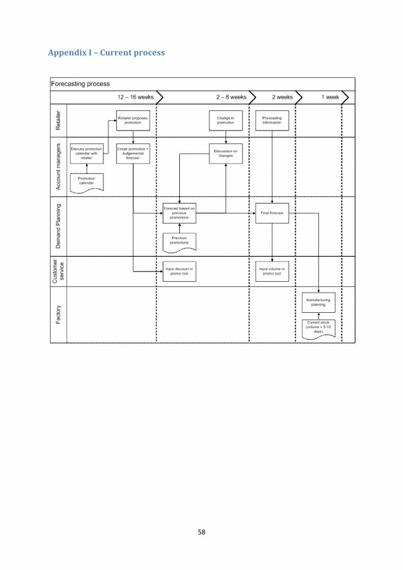
58

Appendix I – Current process

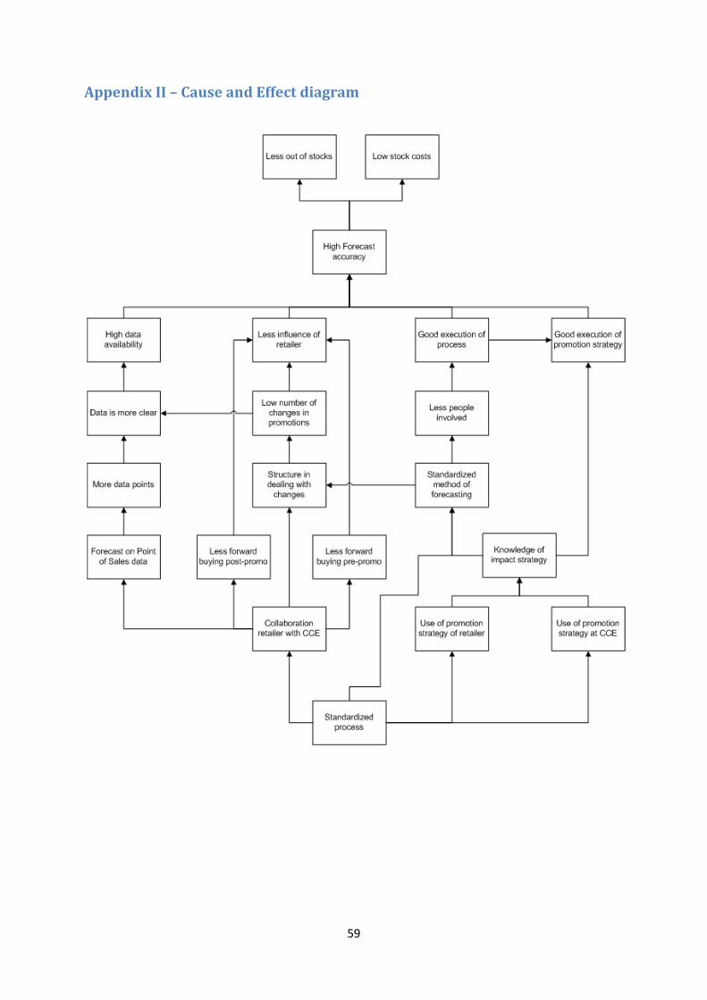
59

Appendix II – Cause and Effect diagram

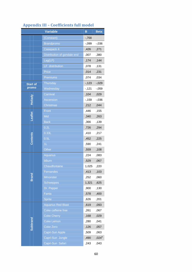
60

Appendix III – Coefficients full model Variable B Beta

(Constant) -,700

Brandpromo -,099 -,036

Casepack 4 ,426 ,271

Distribution of gondale end ,007 ,380

Lag(LF) ,174 ,144

LF distribution ,078 ,131

Price ,014 ,231

Premiums ,074 ,034

Start of promo

Thursday -,123 -,029

Wednesday -,121 -,059

Hol

iady

Carnival ,104 ,029

Ascension -,159 -,036

Christmas ,212 ,044

Leaf

let Front ,446 ,155

Mid ,340 ,263

Back ,366 ,139

Con

tent

s

0.2L ,726 ,294

0.33L ,410 ,217

0.5L ,452 ,225

1L ,590 ,241

Other ,559 ,108

Bra

nd

Aquarius ,224 ,083

bBurn ,529 ,067

Chaudfontaine 1,025 ,220

Fernandes ,413 ,103

Mmonster ,252 ,060

Schweppes 1,321 ,625

Dr. Pepper ,900 ,130

Fanta ,578 ,400

Sprite ,626 ,201

Subb

rand

Aquarius Red Blast ,619 ,093

Coke caffeine free ,261 ,067

Coke Cherry ,168 ,029

Coke Lemon ,280 ,041

Coke Zero ,126 ,057

Capri-Sun Apple ,509 ,063

Capri-Sun Jungle ,490 ,024a

Capri-Sun Safari ,243 ,043

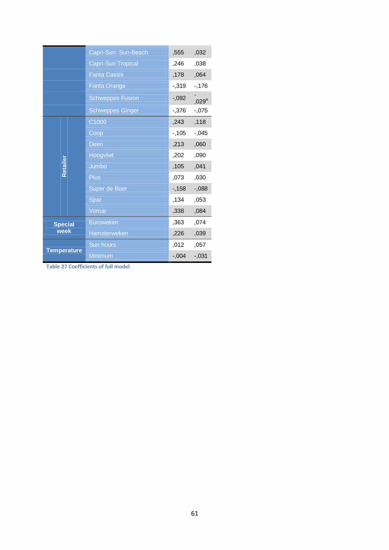
61

Capri-Sun Sun-Beach ,555 ,032

Capri-Sun Tropical ,246 ,038

Fanta Cassis ,178 ,064

Fanta Orange -,319 -,176

Schweppes Fusion -,092 -,029a

Schweppes Ginger -,376 -,075

Ret

aile

r

C1000 ,243 ,118

Coop -,105 -,045

Deen ,213 ,060

Hoogvliet ,202 ,090

Jumbo ,105 ,041

Plus ,073 ,030

Super de Boer -,158 -,088

Spar ,134 ,053

Vomar ,338 ,084

Special week

Euroweken ,363 ,074

Hamsterweken ,226 ,039

Temperature Sun hours ,012 ,057

Minimum -,004 -,031

Table 27 Coefficients of full model

62

Appendix IV – Linear Regression Assumptions

Multicollinearity When two or more predictor variables both measure the same underlying structure, these variables will be correlated: when one increases, the other will increase (with the same value) as well. This causes a potential problem for linear regression, where we want to predict the influence of each individual factor, potentially causing an over- or underestimations of variables and a lower model fit. Therefore we want no perfect linear relationship, also called multicollinearity, which can be tested by multiple measures. The Pearson correlation is the standard one-tail correlation coefficient and should be below 0.9 or 0.8 for obvious reasons. The variance inflation factor (VIF) can indicate a more subtle form of multicollinearity, and it is suggested by Myers (1990) that the VIF should be below 10 or on average below 1 for a model to be not biased.

A third measure that can be checked is the variance proportion distribution over the different variables. For every predictor, we want the variance proportion to be distributed across different so called eigenvalues (=the size of the distribution of a variable). For a more detailed explanation, see Hutcheson & Sofroniou (1999).

Cross-validity Cross-validity is the main reason to check for assumptions. One of the main indicators for cross-validity is Stein’s adjust R2, which is given in the following equation.

𝐴𝑑𝑗𝑢𝑠𝑡𝑒𝑑 𝑅2 = 1− ��𝑛 − 1

𝑛 − 𝑘 − 1� �

𝑛 − 2𝑛 − 𝑘 − 2

� �𝑛 + 1𝑛

�� (1 − 𝑅2)

If this value is close to the original R2, one can conclude that the model is also usable for predicting a different sample of the same population.

Independent errors Since the original predictors should not be correlated, we also want the residuals to be uncorrelated. This assumption can be tested with the Durbin-Watson test, and the outcome should be as close to 2 as possible. On a general note, all values between 1 and 3 are OK, but this depends on sample size and the number of predictors, see for a more detailed overview Durbin & Watson (1951). Also looking at randomness in a studentized residuals versus standardized predictions plot could reveal independent errors.

Outliers Although we have identified outliers in the previous chapter, we can double check this in the residuals. From the notion that in a normally distributed sample 95% of all standardized residuals should be within ±2 and 99% within ±2,5, this provides an indication if there are more cases in the periphery than should be, for example, a standardized residual larger than 3 could be a cause of concern (Field, 2009).

To go more in detail, we could check Cook’s distance (which measures the influence of one case on the whole model), which should be smaller than 1, or the centered leverage value (which measures the influence of the observed value of the outcome variable over the predicted variable) which should be within 2x or 3x the average leverage (k+1/n). As a final check, the Mahalanobis distance

63

(the distance of one case to the mean of the predictor variable) could be measured. Barnett (1978) has produced a table of cut-off values based on sample size and the number of predictors.

Linearity Since we are using linear regression, the assumption is that the relationship between the predictor and outcome variables is linear. This can be tested by plotting the standardized residuals versus the standardized predictions. This plot should look like a random array or dots evenly dispersed around zero. Also the partial plots of all predictor variables should look like a random cloud.

Residuals are normally distributed One of the assumptions is that the residuals, and not the predictors, need to be normally distributed with a mean of 0. This can be checked by looking at the histogram of the residuals, which should look like the classic bell shape, or by checking the normal probability plot, which plots the expected cumulative probability on the observed cumulative probability. This latter plot should form a straight line from {0,0} to {1,1}. A final test is the Kolmorgorov-Smirnov or Shapiro-Wilk test, which measures if the sample is different from a normal distribution. There are however some drawbacks to these tests, so results should be used with caution (Field, 2009).

Heteroscedasticity Heteroscedasticity implies that variance is unequal at different levels of a predictor variable. For example, the spread around the mean LF of a promotion at Albert Heijn is different from a promotion at C1000. This can be verified in the same way as linearity, by looking at the partial plots, together with the plots of the standardized residuals versus the standardized predictions and the studentized residuals versus the standardized predictions.

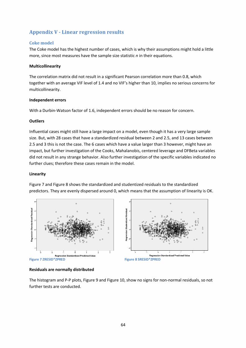
64

Appendix V - Linear regression results

Coke model The Coke model has the highest number of cases, which is why their assumptions might hold a little more, since most measures have the sample size statistic n in their equations.

Multicollinearity

The correlation matrix did not result in a significant Pearson correlation more than 0.8, which together with an average VIF level of 1.4 and no VIF’s higher than 10, implies no serious concerns for multicollinearity.

Independent errors

With a Durbin-Watson factor of 1.6, independent errors should be no reason for concern.

Outliers

Influential cases might still have a large impact on a model, even though it has a very large sample size. But, with 28 cases that have a standardized residual between 2 and 2.5, and 13 cases between 2.5 and 3 this is not the case. The 6 cases which have a value larger than 3 however, might have an impact, but further investigation of the Cooks, Mahalanobis, centered leverage and DFBeta variables did not result in any strange behavior. Also further investigation of the specific variables indicated no further clues; therefore these cases remain in the model.

Linearity

Figure 7 and Figure 8 shows the standardized and studentized residuals to the standardized predictors. They are evenly dispersed around 0, which means that the assumption of linearity is OK.

Figure 7 ZRESID*ZPRED

Figure 8 SRESID*ZPRED

Residuals are normally distributed

The histogram and P-P plots, Figure 9 and Figure 10, show no signs for non-normal residuals, so not further tests are conducted.

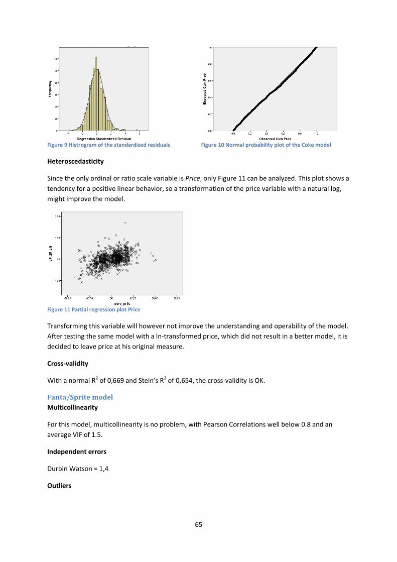
65

Figure 9 Histrogram of the standardized residuals

Figure 10 Normal probability plot of the Coke model

Heteroscedasticity

Since the only ordinal or ratio scale variable is Price, only Figure 11 can be analyzed. This plot shows a tendency for a positive linear behavior, so a transformation of the price variable with a natural log, might improve the model.

Figure 11 Partial regression plot Price

Transforming this variable will however not improve the understanding and operability of the model. After testing the same model with a ln-transformed price, which did not result in a better model, it is decided to leave price at his original measure.

Cross-validity

With a normal R2 of 0,669 and Stein’s R2 of 0,654, the cross-validity is OK.

Fanta/Sprite model Multicollinearity

For this model, multicollinearity is no problem, with Pearson Correlations well below 0.8 and an average VIF of 1.5.

Independent errors

Durbin Watson = 1,4

Outliers

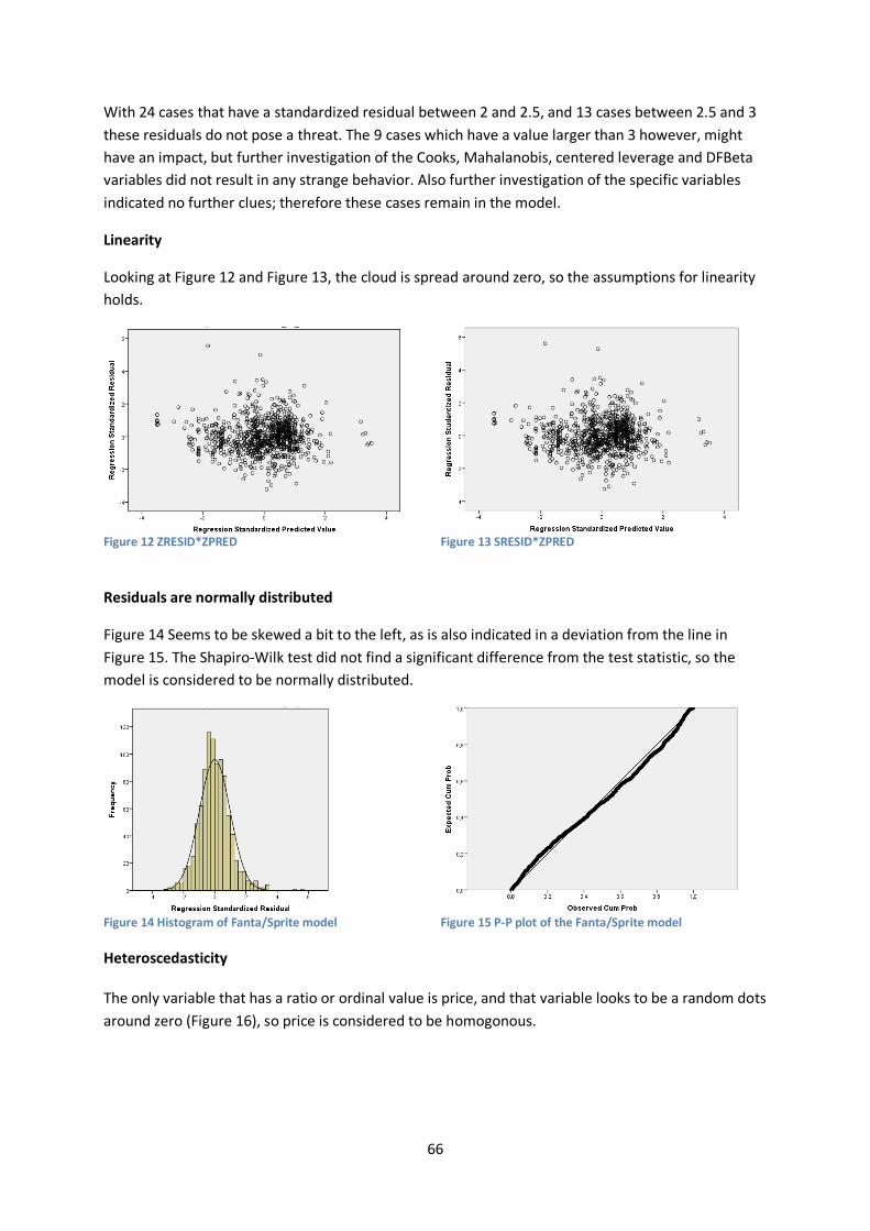
66

With 24 cases that have a standardized residual between 2 and 2.5, and 13 cases between 2.5 and 3 these residuals do not pose a threat. The 9 cases which have a value larger than 3 however, might have an impact, but further investigation of the Cooks, Mahalanobis, centered leverage and DFBeta variables did not result in any strange behavior. Also further investigation of the specific variables indicated no further clues; therefore these cases remain in the model.

Linearity

Looking at Figure 12 and Figure 13, the cloud is spread around zero, so the assumptions for linearity holds.

Figure 12 ZRESID*ZPRED

Figure 13 SRESID*ZPRED

Residuals are normally distributed

Figure 14 Seems to be skewed a bit to the left, as is also indicated in a deviation from the line in Figure 15. The Shapiro-Wilk test did not find a significant difference from the test statistic, so the model is considered to be normally distributed.

Figure 14 Histogram of Fanta/Sprite model

Figure 15 P-P plot of the Fanta/Sprite model

Heteroscedasticity

The only variable that has a ratio or ordinal value is price, and that variable looks to be a random dots around zero (Figure 16), so price is considered to be homogonous.

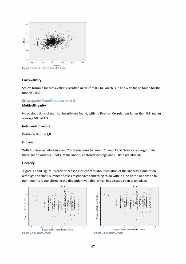
67

Figure 16 Partial regression plot Price

Cross-validity

Stein’s formula for cross-validity resulted in an R2 of 0,614, which is in line with the R2 found for the model: 0,632 Schweppes/Chaudfontaine model Multicollinearity

No obvious signs of multicollinaerity are found, with no Pearson Correlations larger than 0.8 and an average VIF of 1.3

Independent errors

Durbin Watson = 1,8

Outliers

With 16 cases in between 2 and 2.5, three cases between 2.5 and 3 and three cases larger than , there are no outliers. Cooks, Mahalanobis, centered leverage and DFBeta are also OK.

Linearity

Figure 17 and Figure 18 provide reasons for concern about violation of the linearity assumption, although the small number of cases might have something to do with it. One of the options to fix non-linearity is transforming the dependent variable, which has already been taken place.

Figure 17 ZRESID*ZPRED

Figure 18 SRESID*ZPRED

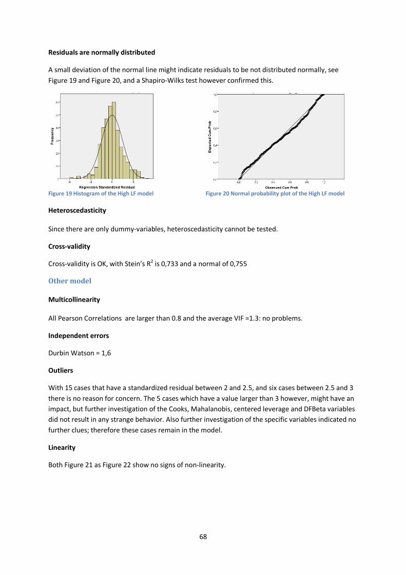
68

Residuals are normally distributed

A small deviation of the normal line might indicate residuals to be not distributed normally, see Figure 19 and Figure 20, and a Shapiro-Wilks test however confirmed this.

Figure 19 Histogram of the High LF model

Figure 20 Normal probability plot of the High LF model

Heteroscedasticity

Since there are only dummy-variables, heteroscedasticity cannot be tested.

Cross-validity

Cross-validity is OK, with Stein’s R2 is 0,733 and a normal of 0,755

Other model

Multicollinearity

All Pearson Correlations are larger than 0.8 and the average VIF =1.3: no problems.

Independent errors

Durbin Watson = 1,6

Outliers

With 15 cases that have a standardized residual between 2 and 2.5, and six cases between 2.5 and 3 there is no reason for concern. The 5 cases which have a value larger than 3 however, might have an impact, but further investigation of the Cooks, Mahalanobis, centered leverage and DFBeta variables did not result in any strange behavior. Also further investigation of the specific variables indicated no further clues; therefore these cases remain in the model.

Linearity

Both Figure 21 as Figure 22 show no signs of non-linearity.

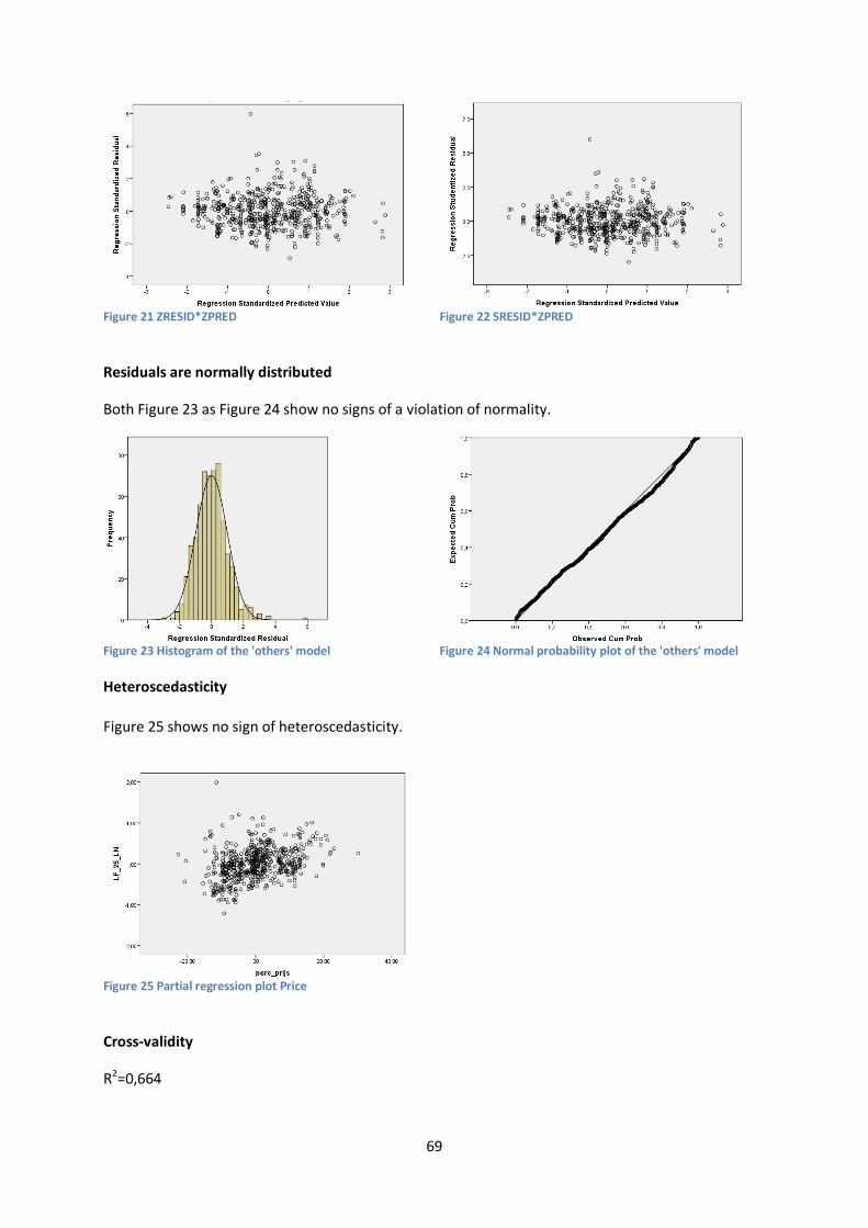
69

Figure 21 ZRESID*ZPRED

Figure 22 SRESID*ZPRED

Residuals are normally distributed

Both Figure 23 as Figure 24 show no signs of a violation of normality.

Figure 23 Histogram of the 'others' model

Figure 24 Normal probability plot of the 'others' model

Heteroscedasticity

Figure 25 shows no sign of heteroscedasticity.

Figure 25 Partial regression plot Price

Cross-validity

R2=0,664

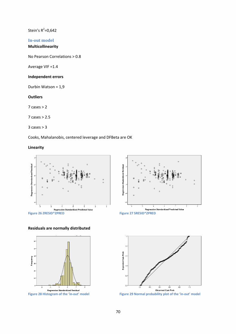
70

Stein’s R2=0,642

In-out model Multicollinearity

No Pearson Correlations > 0.8

Average VIF =1.4

Independent errors

Durbin Watson = 1,9

Outliers

7 cases > 2

7 cases > 2.5

3 cases > 3

Cooks, Mahalanobis, centered leverage and DFBeta are OK

Linearity

Figure 26 ZRESID*ZPRED

Figure 27 SRESID*ZPRED

Residuals are normally distributed

Figure 28 Histogram of the ‘in-out’ model

Figure 29 Normal probability plot of the ‘in-out’ model

71

The histogram, Figure 28, shows some sign of normality, but the normal probability plot, Figure 29, shows a strong deviation from the linear line. Therefore other tests are conducted, Kolmogorov-Smirnov and Shapiro-Wilks. Both test the null-hypothesis that a random sample is equal to a known statistical distribution (in our case a normal distribution). Our tests result in a significance of 0.000, therefore the null-hypothesis cannot be rejected and the conclusion is that there is strong evidence for a non-normally distribution of errors.

Cross-validity

R2=0,717

Stein’s R2=0,683

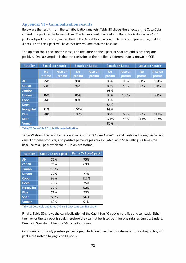
72

Appendix VI – Cannibalization results Below are the results from the cannibalization analysis. Table 28 shows the effects of the Coca-Cola six and four pack on the loose bottles. The tables should be read as follows: for instance cell(AH;6 pack on 4 pack no promo) means that at the Albert Heijn, when the 6 pack is on promotion, and the 4 pack is not, the 4 pack will have 35% less volume than the baseline.

The uplift of the 4 pack on the loose, and the loose on the 4 pack at Spar are odd, since they are positive. One assumption is that the execution at the retailer is different than is known at CCE.

Retailer 6 pack on 4 pack 6 pack on Loose 4 pack on Loose Loose on 4 pack

No

promo Also on promo

No promo

Also on promo

No promo

Also on promo

No promo

Also on promo

AH 65% 90% 98% 95% 91% 104% C1000 53% 96% 80% 45% 30% 91% Jumbo 98% Linders 36% 86% 93% 100% 91% Coop 66% 89% 93% Deen 84% Hoogvliet 51% 101% 93% Plus 60% 100% 86% 68% 88% 110% Spar 171% 44% 116% 102% Vomar 85% Table 28 Coca-Cola 1.5Ltr bottle cannibalization

Table 29 shows the cannibalization effects of the 7+2 cans Coca-Cola and Fanta on the regular 6-pack cans. For these products, also positive percentages are calculated, with Spar selling 3.4 times the baseline of a 6 pack when the 7+2 is on promotion.

Retailer Coke 7+2 on 6 pack Fanta 7+2 on 6 pack

AH 72% 75% C1000 76% 63% Jumbo 115% - Linders 72% 77% Coop 92% 113% Deen 78% 75% Hoogvliet 79% 92% Plus 77% 59% Spar 220% 342% Vomar 62% 91% Table 29 Coca-Cola and Fanta 7+2 on 6 pack cans cannibalization

Finally, Table 30 shows the cannibalization of the Capri-Sun 40 pack on the five and ten pack. Either the five, or the ten pack is sold, therefore they cannot be listed both for one retailer. Jumbo, Linders, Deen and Spar do not feature 50 packs Capri-Sun.

Capri-Sun returns only positive percentages, which could be due to customers not wanting to buy 40 packs, but instead buying 5 or 10 packs.

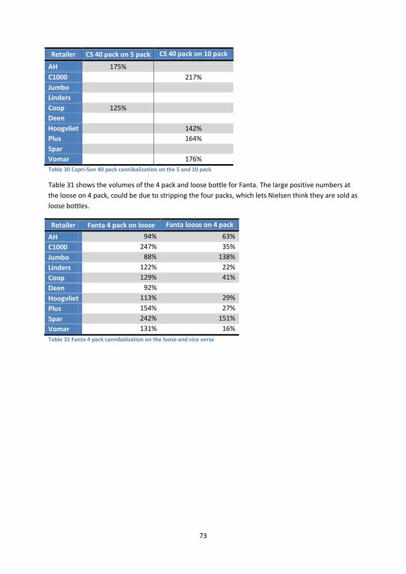
73

Retailer CS 40 pack on 5 pack CS 40 pack on 10 pack

AH 175% C1000 217% Jumbo Linders Coop 125% Deen Hoogvliet 142% Plus 164% Spar Vomar 176% Table 30 Capri-Sun 40 pack cannibalization on the 5 and 10 pack

Table 31 shows the volumes of the 4 pack and loose bottle for Fanta. The large positive numbers at the loose on 4 pack, could be due to stripping the four packs, which lets Nielsen think they are sold as loose bottles.

Retailer Fanta 4 pack on loose Fanta loose on 4 pack

AH 94% 63% C1000 247% 35% Jumbo 88% 138% Linders 122% 22% Coop 129% 41% Deen 92% Hoogvliet 113% 29% Plus 154% 27% Spar 242% 151% Vomar 131% 16% Table 31 Fanta 4 pack cannibalization on the loose and vice versa

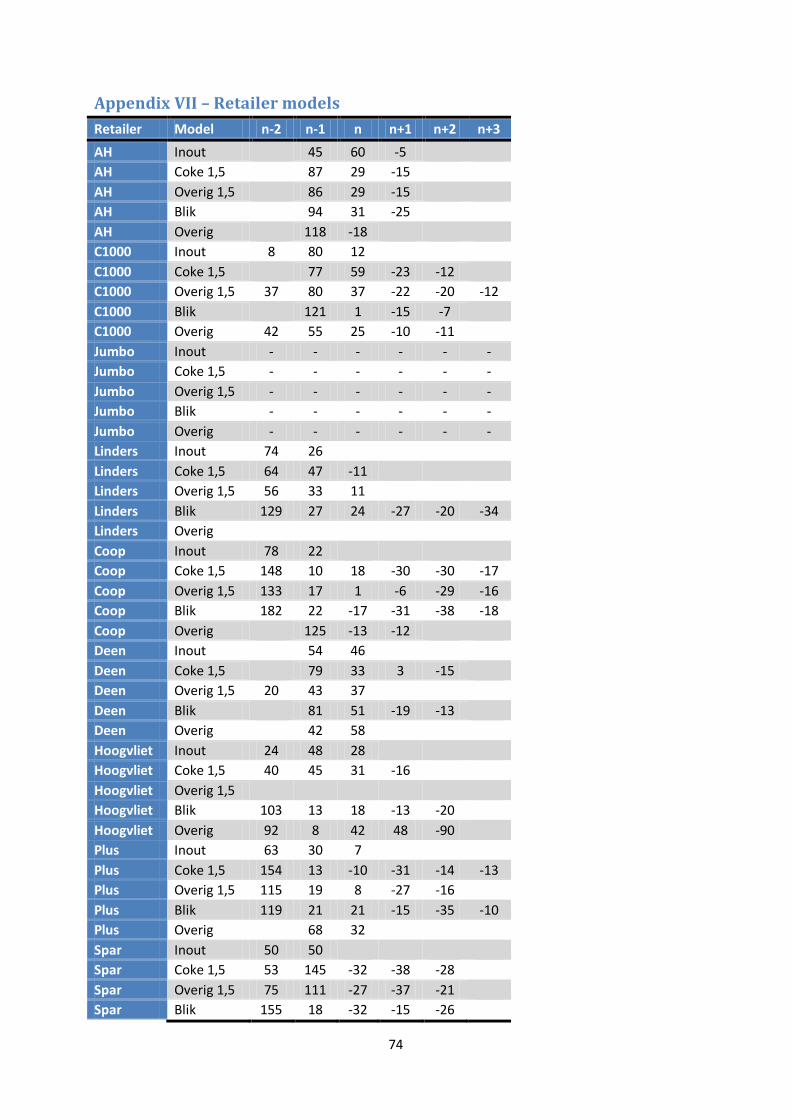
74

Appendix VII – Retailer models Retailer Model n-2 n-1 n n+1 n+2 n+3 AH Inout 45 60 -5 AH Coke 1,5 87 29 -15 AH Overig 1,5 86 29 -15 AH Blik 94 31 -25 AH Overig 118 -18 C1000 Inout 8 80 12 C1000 Coke 1,5 77 59 -23 -12 C1000 Overig 1,5 37 80 37 -22 -20 -12 C1000 Blik 121 1 -15 -7 C1000 Overig 42 55 25 -10 -11 Jumbo Inout - - - - - - Jumbo Coke 1,5 - - - - - - Jumbo Overig 1,5 - - - - - - Jumbo Blik - - - - - - Jumbo Overig - - - - - - Linders Inout 74 26 Linders Coke 1,5 64 47 -11 Linders Overig 1,5 56 33 11 Linders Blik 129 27 24 -27 -20 -34 Linders Overig Coop Inout 78 22 Coop Coke 1,5 148 10 18 -30 -30 -17 Coop Overig 1,5 133 17 1 -6 -29 -16 Coop Blik 182 22 -17 -31 -38 -18 Coop Overig 125 -13 -12 Deen Inout 54 46 Deen Coke 1,5 79 33 3 -15 Deen Overig 1,5 20 43 37 Deen Blik 81 51 -19 -13 Deen Overig 42 58 Hoogvliet Inout 24 48 28 Hoogvliet Coke 1,5 40 45 31 -16 Hoogvliet Overig 1,5 Hoogvliet Blik 103 13 18 -13 -20 Hoogvliet Overig 92 8 42 48 -90 Plus Inout 63 30 7 Plus Coke 1,5 154 13 -10 -31 -14 -13 Plus Overig 1,5 115 19 8 -27 -16 Plus Blik 119 21 21 -15 -35 -10 Plus Overig 68 32 Spar Inout 50 50 Spar Coke 1,5 53 145 -32 -38 -28 Spar Overig 1,5 75 111 -27 -37 -21 Spar Blik 155 18 -32 -15 -26

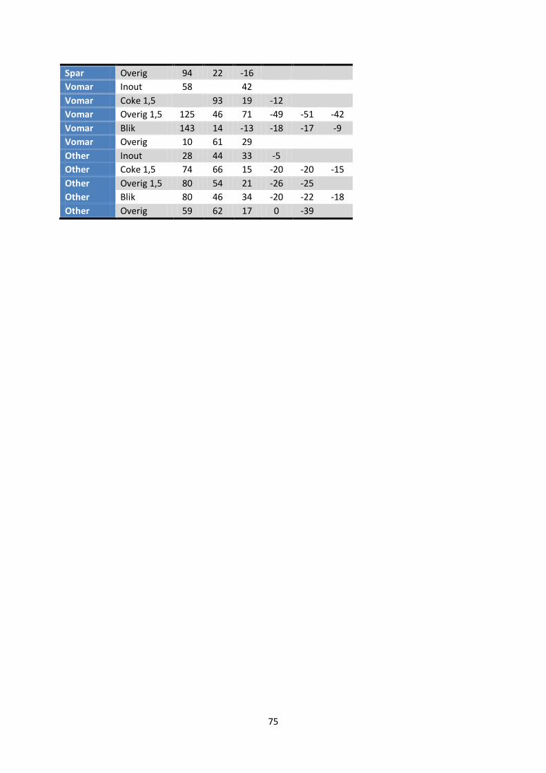
75

Spar Overig 94 22 -16 Vomar Inout 58 42 Vomar Coke 1,5 93 19 -12 Vomar Overig 1,5 125 46 71 -49 -51 -42 Vomar Blik 143 14 -13 -18 -17 -9 Vomar Overig 10 61 29 Other Inout 28 44 33 -5 Other Coke 1,5 74 66 15 -20 -20 -15 Other Overig 1,5 80 54 21 -26 -25 Other Blik 80 46 34 -20 -22 -18 Other Overig 59 62 17 0 -39

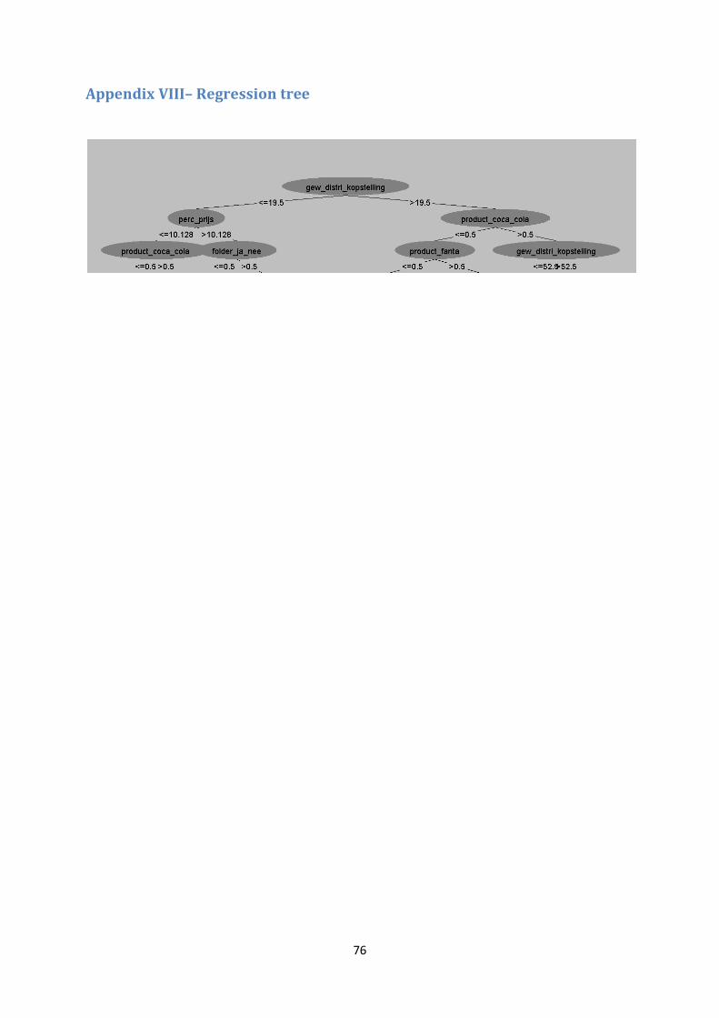
76

Appendix VIII– Regression tree

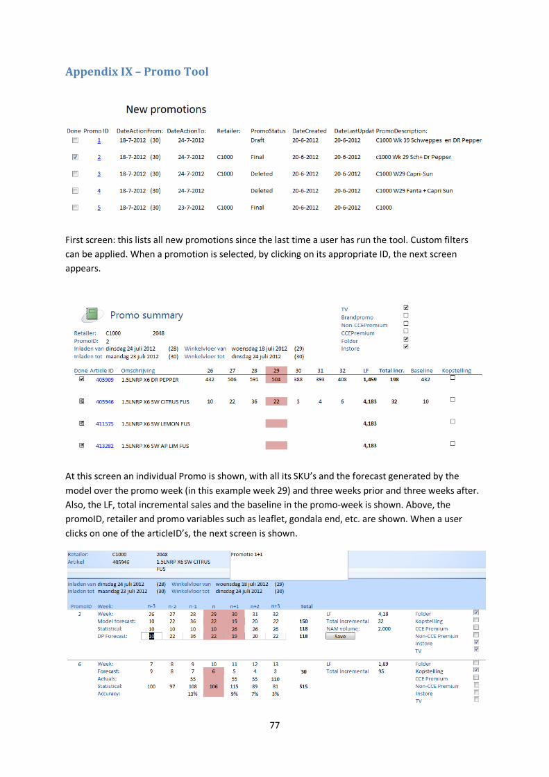
77

Appendix IX – Promo Tool

First screen: this lists all new promotions since the last time a user has run the tool. Custom filters can be applied. When a promotion is selected, by clicking on its appropriate ID, the next screen appears.

At this screen an individual Promo is shown, with all its SKU’s and the forecast generated by the model over the promo week (in this example week 29) and three weeks prior and three weeks after. Also, the LF, total incremental sales and the baseline in the promo-week is shown. Above, the promoID, retailer and promo variables such as leaflet, gondala end, etc. are shown. When a user clicks on one of the articleID’s, the next screen is shown.

78

Here, the top promotion (with ID=2) is to be forecasted, while the promotion with ID=6 already has already been completed and therefore already has actual sales associated with it. The tool shows for the promotion to forecast the forecast suggested by the statistical model, the statistical baseline and promo variables. In the lowest row, called DP Forecast, the model forecast is shown but can be altered by the user. When the “send-button” is hit, the forecast is saved and can be used to export to SAP.

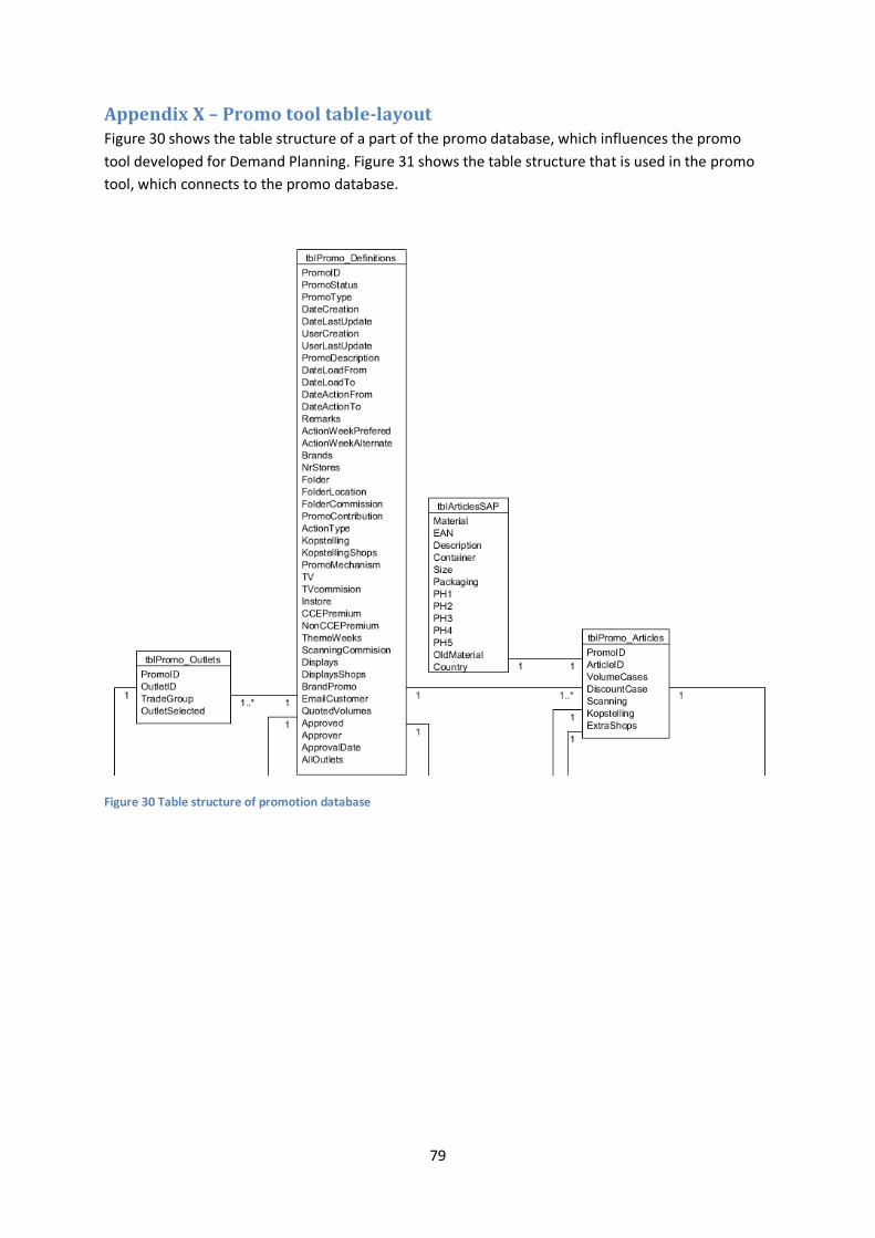
79

Appendix X – Promo tool table-layout Figure 30 shows the table structure of a part of the promo database, which influences the promo tool developed for Demand Planning. Figure 31 shows the table structure that is used in the promo tool, which connects to the promo database.

Figure 30 Table structure of promotion database

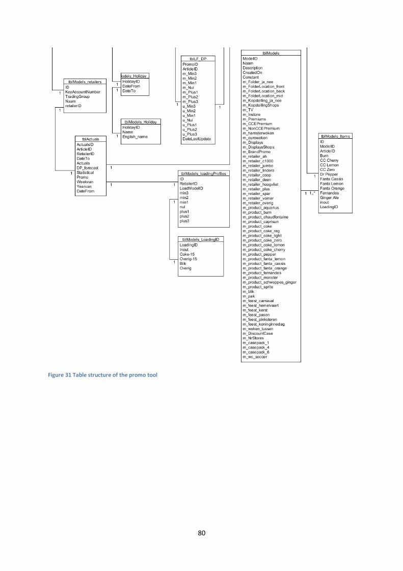
80

Figure 31 Table structure of the promo tool