Electrical Power and Energy Systems 64 (2015) 542–550

Contents lists available at ScienceDirect

Electrical Power and Energy Systems

journal homepage: www.elsevier .com/locate / i jepes

Stochastic simulation of power systems with integrated intermittentrenewable resources

http://dx.doi.org/10.1016/j.ijepes.2014.07.0490142-0615/� 2014 Elsevier Ltd. All rights reserved.

⇑ Corresponding author.E-mail addresses: degeilh1@illinois.edu (Y. Degeilh), gross@illinois.edu

(G. Gross).

Yannick Degeilh, George Gross ⇑University of Illinois at Urbana–Champaign, 4052 Electrical and Computer Engineering Building, 306 North Wright Street, Urbana, IL 61801, USA

a r t i c l e i n f o

Article history:Received 21 March 2014Received in revised form 12 July 2014Accepted 16 July 2014Available online 15 August 2014

Keywords:Monte Carlo/stochastic simulationTransmission-constrained day-aheadmarketsProduction costingReliabilityEmissionsRenewable resource integration

a b s t r a c t

We report on the development of a comprehensive, stochastic simulation methodology that provides thecapability to quantify the impacts of integrated renewable resources on the power system economics,emissions and reliability variable effects over longer periods with the various sources of uncertaintyexplicitly represented. We model the uncertainty in the demands, the available capacity of conventionalgeneration resources and the time-varying, intermittent renewable resources, with their temporal andspatial correlations, as discrete-time random processes. We deploy Monte Carlo simulation techniquesto systematically sample these random processes and emulate the side-by-side power system and trans-mission-constrained day-ahead market operations. We construct the market outcome sample paths foruse in the approximation of the expected values of the various metrics of interest. Our efforts to addressthe implementational aspects of the methodology so as to ensure computational tractability for large-scale systems over longer periods include the use of representative simulation periods, parallelizationand variance reduction techniques. Applications of the approach include planning and investment studiesand the formulation and analysis of policy. We illustrate the capabilities and effectiveness of the simula-tion approach on representative study cases on a modified WECC 240-bus system. The results providevaluable insights into the impacts of deepening penetration of wind resources.

� 2014 Elsevier Ltd. All rights reserved.

Introduction

The deepening penetration of intermittent renewable resourcespresents major challenges in power system planning and opera-tions in light of their highly time-varying nature and their associ-ated geographical and climatological sources of uncertainty.Indeed, unlike conventional resource outputs, wind and solarresource outputs cannot be controlled by the operator except tobe curtailed. The high variability in wind speeds and insolationpatterns, both temporal and spatial, results at times in intermittentwind and solar resource outputs [1]. A consequence is that thewind and solar outputs do not necessarily track the load patternand thus cannot always contribute to serve the peak loads. Thereare also concerns about ‘‘spilling’’ of wind energy at night due tothe insufficient load demand and the physical impossibility to shutdown the base-loaded conventional units for short periods. Whilemorning and mid-day solar power outputs are aligned with theloads, their quick decline after sunset occurs when the loads arestill high. Both wind and solar resources therefore impose addi-

tional requirements on the conventional units to effectively man-age the variability/intermittency and uncertainty effects. Furtherissues arise from the fact that the wind speed and insolation pat-terns show various degrees of spatial correlation, resulting inhighly variable nodal power injections which may lead, at times,to congestion. These complications illustrate the critical need toappropriately represent the temporal and spatial correlations ofthe wind and solar resource outputs in the assessment of thepower system performance. Such need implies that the variousrenewable resource outputs, as well as the demands and conven-tional generation available capacities, must be modeled by randomprocesses (r.p.s) so as to capture the impacts of their variabilityacross time and space. These requirements drive the need for acomprehensive simulation tool that can effectively quantify theexpected economic, reliability and emission variable effects ofpower system with integrated renewable resources.

The conventional probabilistic simulation approach [2] and itsextensions [3,4] cannot adequately provide the needed level ofdetail due to its inability to represent chronological phenomenasuch as the grid operations and their impacts on the day-aheadmarket (DAM) outcomes, as well as the time-dependent natureand temporal correlations of the demands and supply resources,particularly the renewable resources. A distinctly different

Y. Degeilh, G. Gross / Electrical Power and Energy Systems 64 (2015) 542–550 543

approach, which may be used to represent the uncertain DAM out-comes with the capability to explicitly represent the grid con-straints, is the probabilistic optimal power flow (P-OPF), [5,6].One drawback of the P-OPF approach, however, is that it requiresa number of significant simplifying assumptions to render theproblem into a solvable form. For instance, the representation ofthe power system evolution over time, including the temporal cor-relations among the system variables, requires the formulation of amulti-period P-OPF, whose tractability is questionable even for asmall number of periods. Many renewable integration studies inthe literature report the use of the Monte Carlo simulation to rep-resent the power system and its sources of uncertainty. Most focusexclusively on the probabilistic modeling of a single renewableresource, generally, wind [7,8]. We are not aware of a comprehen-sive approach which integrates under a single umbrella the varioussources of uncertainty that impact power system operations acrosstime. In this paper, we report on the development of a comprehen-sive analytical framework and general Monte Carlo simulationapproach with the capability to assess, over longer duration peri-ods, the impacts on power grid variable effects of the variabledemands, renewable generation outputs and conventionalresource available capacities. While our approach can easily beadapted to incorporate various stochastic models, including thosebased on copulas, statistical transforms for multivariate depen-dence such as principal component analysis, time-series synthesisusing many variants of ARMA-type schemes, numerical weatherprediction methods, historical time-series re-sampling and hind-cast [9–13], our objective is to construct a practical scheme basedon models that require no calibration nor the use of complex trans-forms, unlike the various models just mentioned. As such, we con-struct appropriate stochastic models to capture the time-varyingand uncertain behavior of multi-site renewable power outputs,with the cross-correlations between the sites and time correlationsexplicitly accounted for and to incorporate into a comprehensivestochastic simulation framework. Our approach, while relativelyeasy to implement, can handle any type of renewable output prob-ability distribution, including non parametric distributions, as werequire no assumptions on the shape of their joint cumulative dis-tribution functions (j.c.d.f.s). The implementation, in fact, ensuresthe computational tractability of the approach for realistic sizedpower systems.

In the analytic framework, we represent the demands andsupply resource outputs as discrete-time r.p.s. In particular, wemodel the multi-site wind (solar) power outputs over time asa discrete-time r.p. whose j.c.d.f. explicitly incorporates the spa-tial and temporal correlations among the wind (solar) poweroutputs at all the sites for all periods of interest. For concrete-ness, we assume that the power system described in this paperoperates in a market environment. Our approach uses an hour asthe smallest indecomposable unit of time and uses the realiza-tions of the r.p.s at these subperiods. In addition, a snapshot rep-resentation of the grid is used to represent the impacts of thetransmission constraints on the hourly day-ahead markets(DAMs) outcomes. Our Monte Carlo simulation methodology usessystematic sampling mechanisms to generate the realizations ofthe various r.p.s and to construct the so-called sample paths(s.p.s) [14, p. 97]. We note that such s.p.s embody the correla-tions among the constituent random variables (r.v.s) of ther.p.s. We use the s.p.s of the demand, multi-site renewable out-put and generator available capacity r.p.s as inputs into the emu-lation of the transmission-constrained hourly DAMs. Wecompute the market clearing results of the transmission-con-strained hourly DAMs using the solution of the linearized opti-mal power flow (OPF) typically used in the ISO markets [15, p.534]. The outcomes of the DAMs are used to construct the s.p.sof the so-called market outcome r.p.s. Clearly, these s.p.s capture

the correlations among the various market outcomes. We usethe hourly realizations that constitute these s.p.s to computethe metrics of interest used to assess the performance of thepower system and associated markets. These metrics includethe hourly expected locational marginal prices (LMPs), revenuesof the generators, total payments made by buyers in the DAMs,congestion rents, the system-wide CO2 emissions, as well asthe reliability indices LOLP and EUE. We note that these metricsare computed by explicitly accounting for the deliverability ofthe electricity. The methodology is also able to capture the sea-sonal effects in demands and renewable outputs, the impacts ofmaintenance scheduling and the ramifications of new policy ini-tiatives. There is a broad range of applications of the simulationmethodology to operations, resource planning studies, produc-tion costing issues, investment analysis, transmission utilization,reliability analysis, environmental assessments, policy formula-tion and to answer quantitatively various what-if questions. Wealso discuss the various implementational steps, such as parallel-ization, variance reduction and deployment of representativeweeks, we used to improve the computational tractability ofthe proposed approach.

The paper contains four additional sections. In Section ‘The pro-posed simulation framework’, we describe the overall structure ofthe simulation approach by formally introducing the time frame inwhich the simulations are performed and the general Monte Carloprocedure. We also discuss in detail the modeling of the input r.p.s,the sampling schemes used to generate their s.p.s, and the mappingof these s.p.s into outcome s.p.s via the OPF solutions. In Section‘Implementational aspects’, we discuss the steps implemented toimprove the computational tractability of the approach. In Section‘Illustrative studies’, we illustrate the capabilities of the approachwith two representative case studies that focus on the impacts ofdeepening wind penetration and the substitutability of conven-tional resources by wind resources. We conclude with a summaryin Section ‘Conclusion’ together with directions for future work.

The proposed simulation framework

The proposed simulation approach emulates the side-by-sidepower system operations and transmission-constrained markets,with the objective to evaluate, on average, the variable effects ofthe power system with integrated renewable resources. In this sec-tion, we describe the overall Monte Carlo procedure, including itstime frame and the generation of the market outcome s.p.s fromwhich we compute the power system metrics of performance.

The simulation is carried out for the specified study period T .We decompose T into non-overlapping simulation periods T i’ssuch that T ¼

SiT i. We define each simulation period T i in such

a way that the system resource mix and unit commitment, thetransmission grid, the operating policies, the market structureand the seasonality effects remain unchanged over its duration.While there are many possible choices for a simulation period,we specify each simulation period to be of one-week duration. Thischoice captures the load patterns over the week and week-enddays, and is able to incorporate the maintenance schedules. Wefurther decompose each simulation period into subperiods, wherea subperiod is the smallest indecomposable unit of time repre-sented in the simulation. We assume that each variable is constantover the entire duration of a subperiod. The simulation, as such,ignores any phenomenon whose time scale is smaller than a sub-period. We choose to use subperiods of one hour duration as anacceptable compromise between the level of detail needed for arealistic representation of the power system and market opera-tions and the computational tractability of the simulation. The sub-period selection is particularly appropriate as many existing DAMsare cleared on an hourly basis. We denote by h the index of the

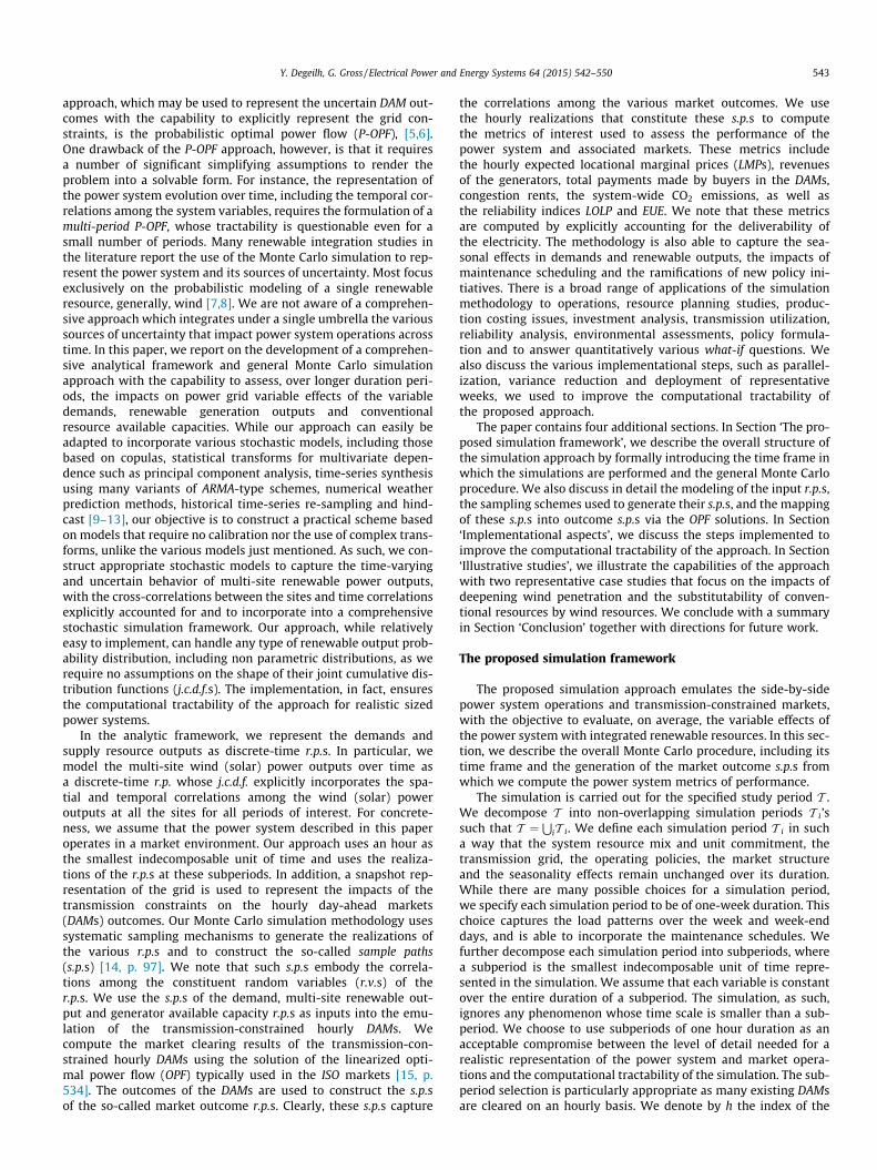
Fig. 1. Conceptual structure of the approach.

544 Y. Degeilh, G. Gross / Electrical Power and Energy Systems 64 (2015) 542–550

subperiods in a simulation period T i such thatT i ¼ h : h ¼ 1; . . . ;168f g. 1

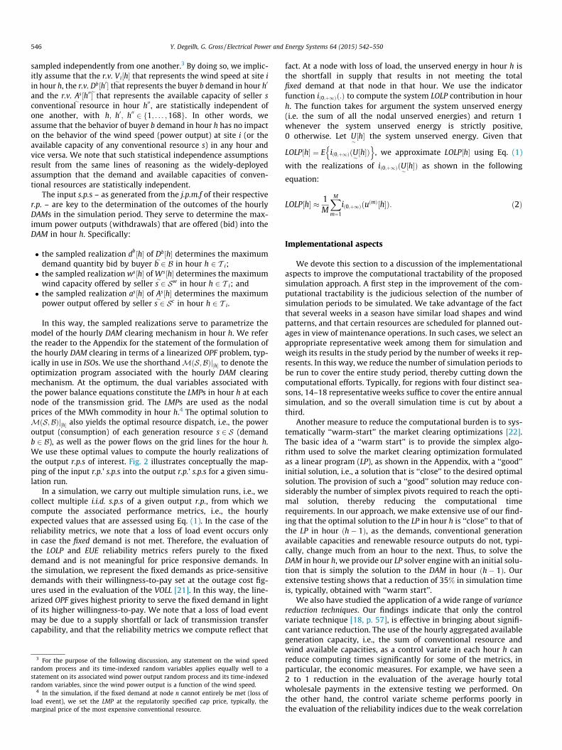
The simulation emulates the side-by-side power system opera-tions and transmission-constrained market. Specifically, in eachsimulation period, we emulate the sequence of the 168 hourlyDAM clearings where the market outcomes determine the contri-butions to the performance metrics of interest. We use the hourlydiscretized time axis in the construction of all the models and eval-uate the metrics on an hourly basis. The modeling of the highlyvariable demands, multi-site renewable power outputs and con-ventional generator available capacities, all of which are uncertainand participate in the hourly DAMs, is in terms of discrete-timer.p.s which are collections of r.v.s indexed by the 168 hours ofthe simulation period. These input r.p.s are mapped by the DAMclearing mechanism into the output discrete-time r.p.s, alsoindexed by the 168 hours of the simulation period, that representthe market outcomes. We provide a conceptual representation ofsuch a mapping in Fig. 1. We make use of Monte Carlo simulationtechniques in the simulation approach to evaluate the performancemetrics. Such procedure is formally described in what follows.

We denote by X�½h� : h ¼ 1; . . . ;168

n oa r.p. defined over 168

hours. We denote by fx½h� : h¼ 1; . . . ;168g ¼ x½1�;x½2�; . . . ;x½168�f ga collection of time-indexed realizations – also known as a

sample path (s.p.) – of the r.p. X�½h� : h ¼ 1; . . . ;168

n o[14, p. 97]. Note

that a s.p. captures the time-dependencies of the individualrealizations x½h� in a manner that is consistent with the correlationsthat exist among the r.v.s X

�½h�; h ¼ 1; . . . ;168. Our simulation

approach makes use of the so-called independent Monte Carlo[16, p. 10], and requires the construction of multiple independentand identically distributed (i.i.d.) s.p.s for each output r.p. to evaluatethe performance metrics. Note that in this context, the phrase‘‘i.i.d. s.p.s’’ has the sense that the s.p.s constitute the realizations ofindependent identically distributed r.p.s. A simulation run is thebasic process through which we construct a s.p. for each of theoutput r.p.s. It consists of sampling each one of the input r.p. j.c.d.f.s– or joint probability mass functions (j.p.m.f.s) depending on ther.p. model – in order to generate the s.p.s whose hourly realizationsare used as inputs in the corresponding hourly DAMs. The s.p.sof the input r.p.s are mapped into s.p.s of the output r.p.s via themodel of the market clearing mechanism for each hourly DAM ofthe simulation period. Thus, a s.p. for each output r.p. is obtainedfrom the series of 168 cleared DAMs.

We carry out multiple simulation runs in order to create theoutput s.p.s from which we estimate the performance metrics foreach market outcome of interest. We select our performance met-rics to be the expected values of the time-indexed r.v.s making upthe output r.p.s of interest.2 Let M be the number of simulation runs;

1 We point out that the proposed approach is sufficiently general to be applicableto other time scales.

2 Other metrics may be defined along similar lines. It is also possible toapproximate the output r.p. j.c.d.f.s.

we estimate, for an output r.p. Y�½h� : h ¼ 1; . . . ;168

n o, the hourly

sample mean point estimate �y½h� of each r.v. Y�½h�; h ¼ 1; . . . ;168:

y�½h� ¼ 1

M

XM

j¼1

yðjÞ½h� ð1Þ

where yðjÞ½h� is the realization of r.v. Y�ðjÞ½h� in simulation run j (note

that the Y�ðjÞ½h�’s are i.i.d.). The number of simulation runs M depends

on the statistical reliability requirements specified for the estima-tion of the desired expected values. We define the statistical reli-

ability of the hourly sample mean estimator Y�½h� ¼ 1

M

PMj¼1Y�ðjÞ½h� to

be the length of the 100ð1� aÞ% confidence interval with0 < a < 1 for the true mean lY

�½h� of r.v. Y

�½h� [17, p. 82, p. 451].

According to the Central Limit Theorem, the sample mean estimatorY�½h� is approximately normally distributed for large M [18, p. 78].

Thus, we can establish that lY�½h� lies in the interval

Y�½h� � z 1�a=2ð Þ

rY�½h�ffiffiffiMp ; Y

�½h� þ z 1�a=2ð Þ

rY�½h�ffiffiffiMp

h iwith a 100ð1� aÞ% probabil-

ity, where rY�½h� is the standard deviation of r.v. Y

�½h�, and

z1�a=2 ¼ U�1ð1� aÞ, with U�1 the inverse of the cumulative distribu-tion function (c.d.f.) of the standard normal distribution Nð0;1Þ.Note that the length of the confidence interval is a function inffiffiffiffiffi

Mp �1

. While it is possible to select M so as to set the confidenceinterval length and achieve the desired statistical reliability, in prac-

tice, a function inffiffiffiffiffiMp �1

decays very slowly for large M; beyond acertain value of M, the improvement in statistical reliability is gen-erally too small to warrant the extra computing-time needed to per-form additional simulation runs.

We discuss the stochastic models and sampling procedures forthe input r.p.s. For concreteness, the only renewable resource weconsider in the rest of our analysis is wind.

Let B the set of buyers in the hourly DAMs. For simplicity andclarity in the notation, we assume that each buyer b 2 B submitsa demand bid for a load located at one node and one node only.From the outset, we wish to capture the spatial and temporal cor-relations among the various buyer demands. Now, given that thecleared demands, as observed from historical load data, are sea-sonal and have a weekly cycle, we assume that, in each week ofthe same season, the buyer demands over a week period can be

modeled by the discrete-time r.p. D�½h� : h ¼ 1; . . . ;168

� �, where

D�½h� ¼ D

�1½h�; . . . ;D

�jBj½h�

h iyand y denotes the transpose. Such a r.p.

is the collection of time-indexed random vectors D�½h� for

h ¼ 1; . . . ;168, with each random vector D�½h� in hour h containing

the ordered collection of the buyer demand r.v.s for each buyerb 2 B. Such representation explicitly accounts for the correlationsacross buyer and time that exist among the hourly demandsD�

b½h� of each buyer b 2 B. For clarity, we may represent all the

jointly distributed r.v.s D�

b½h�, 8b 2 B; h ¼ 1; . . . ;168 making up

the buyer demand r.p. in the following array:

D�

1½1� D�

1½2� . . . D�

1½168�

D�

2½1� D�

2½2� . . . D�

2½168�

..

. ... . .

. ...

D�jBj½1� D

�jBj½2� . . . D

�jBj½168�

2666666664

3777777775

Y. Degeilh, G. Gross / Electrical Power and Energy Systems 64 (2015) 542–550 545

We now describe how to construct and sample, in practice, thediscrete-time r.p. of the (hourly) buyer demands over a week. Wegather weeks of simultaneously-measured hourly buyer demandsfrom a seasonally disaggregated historical database so as to cap-ture the cross-dependencies among the buyer demands acrossmultiple time periods. We use these data to construct the samplespace X

D�½h�: h¼1;...;168

n o of the buyer demand r.p. Note that each

weekly set of simultaneously-measured hourly buyer demands

constitutes a s.p. of D�½h� : h ¼ 1; . . . ;168

� �and as such, contains

realizations of each r.v. D�

b½h�; h ¼ 1; . . . ;168; b 2 B. We assume

the equi-probability of each one of the s.p.s retrieved from the his-

torical data to approximate the j.p.m.f. of D�½h� : h ¼ 1; . . . ;168

� �.

We proceed to discuss the sampling procedure of such j.p.m.f.The method is the multidimensional case of the proceduredescribed in [18, p. 139], to generate a realization from a (discrete)r.v. ‘‘empirical’’ c.d.f. The procedure entails drawing one of the his-torical s.p.s making up the sample space X

D�½h�: h¼1;...;168

n o with prob-

ability one over the total number of s.p.s making up said samplespace. The selected sample-path contains hourly realizations

db½h�; h ¼ 1; . . . ;168; b 2 B that are consistent with the correla-tions existing among the D

�b½h�; b 2 B; h ¼ 1; . . . ;168, r.v.s making

up the buyer demand r.p. Another way to restate this statementis to say that, since every historical s.p. has the cross-dependencyinformation relating the hourly buyer demands embedded in it,so does the selected s.p.

We apply an analogous approach to the stochastic modeling ofthe multi-site hourly wind speeds. We denote a wind farm locationby index i 2 I . For simplicity in the notation, we assume that eachwind farm is a distinct seller in the hourly DAMs. We define a one-to-one and onto mapping between each wind farm location i andits seller s 2 Sw in the market, where Sw is the collection of thejSwj ¼ jIj sellers at the nodes where the farms are located. Weassume that each wind speed at each farm location is uniformfor the entire farm. Furthermore, we assume that the wind speedsare seasonal and have a daily cycle. In a similar manner as with thehourly buyer demands, we seek to capture the spatial and tempo-ral correlations of the wind speed r.v.s V

� i½h� across locations i 2 Iand hours of the day h ¼ 1; . . . ;24. Thus, we represent the multi-site hourly wind speeds by the discrete-time r.p.

V�½h� : h ¼ 1; . . . ;24

� �, where V

�½h� ¼ V

�1½h�; . . . ;V� jIj½h�

h iy. We note

that, similarly as for the buyer demand r.p., the multi-site windspeed r.p. is the collection of time-indexed random vectors V

�½h�

for h ¼ 1; . . . ;24, with each random vector V�½h� in hour h contain-

ing the ordered collection of the wind speed r.v.s at the multiplesites represented in set I . The construction and sampling proce-dures of such a discrete-time r.p. closely follow those of the buyerdemand r.p. As such, a s.p. of the multi-site wind speed r.p. is a col-lection of hourly wind speed realizations at all the sites. Such a col-lection of hourly wind speeds is representative of the wind speedpatterns at the multiple sites and so captures the existing crossdependencies. In the specific case of the multi-site wind speedr.p. however, we need to generate 7 daily s.p.s in order to constructthe s.p. for the 7� 24 hours in a week. Let us denote by v ðjÞ the jths.p. independently drawn from the j.p.m.f. of

V�½h� : h ¼ 1; . . . ;24

� �. We sample and collect 7 independent s.p.s

from the j.p.m.f. of V�½h� : h ¼ 1; . . . ;24

� �to obtain the s.p. for the

week v ð1Þ;v ð2Þ; . . . v ð7Þn o

. Note that v ðjÞ does not necessarily have

to represent the multi-site wind speeds of day j; it can representany arbitrary day in the week. However, for simplicity in the nota-

tion, we make it represent day j. Under this notation, v ðjÞi ½h� denotesthe wind speed at wind farm i 2 I in hour h of day j.

At this stage, we may convert the s.p. wind speeds into their cor-responding power outputs. To do so, we make use of the wind farmcharacteristic power curves, using the procedure described inappropriate detail in [4]. As such, the power output of a particularwind farm is a piece-wise polynomial function of its wind speed.Note that by converting all the s.p.s making up the sample space

of V�½h� : h ¼ 1; . . . ;24

� �, we obtain the corresponding multi-site

wind power output r.p. W�½h� : h ¼ 1; . . . ;24

� �in a straightfor-

ward manner. Now, exploiting the one-to-one and onto mappingthat relates a wind farm location i 2 I to its seller s 2 Sw, we

may denote by wðjÞi ½h� ¼ ðwsÞðjÞ½h� the wind farm power output that

is obtained from the conversion of v ðjÞi ½h�. For convenience in therest of the paper however, and to reflect the fact that we have con-structed a multi-site wind power output s.p. for the week, we dropthe dependency on exponent j and express h in terms of a weekhour, so that ws½h� denotes the wind power output of sellers 2 Sw in hour h of the week.

We introduce a simplifying assumption for the set Sc of marketparticipants who sell the outputs of the conventional generationresources: similarly as for the buyer demands, seller s 2 Sc offersthe output of only one conventional resource. As such, we shallindex each conventional generation resource by s 2 Sc . We modeleach conventional resource as a multi-state unit with two or morestates – outaged, various partially derated capacities and fullcapacity. We assume that each conventional resource is statisti-cally independent of any other generation resource. As such, ifA�

s½t� designates the available capacity of seller s unit at time t, then

A�

s½t� and A�

s0 ½t�, with s – s0; s; s0 2 Sc , are statistically independent.

We use a discrete-event driven Markov Process model with theappropriate stochastic event-times distributions to represent theunderlying r.p. governing the available capacity of each conven-tional resource. We assume statistically independent exponen-tially-distributed r.v.s. to represent the transition times betweenthe states. Such model allows us to explicitly represent the periodsduring which a conventional unit might be up, down, or running atderated capacities in the simulation.

In light of the statistical independence assumption, we con-struct individual s.p.s for each conventional resource. The method-ology for simulating the available capacity of a conventionalresource over time is well documented in the literature, and canbe found under the names of next-event method, state duration sam-pling, or simply sequential simulation [19]. The procedure consistsof simulating the sequence of available capacity states throughwhich the conventional resource passes over time. We do so bysampling the appropriate transition-time exponential distributionas the conventional resource transitions from a state of the dis-crete-event driven Markov Process model to another [20, p. 59].In terms of our approach, the state of seller s resource, i.e., itsavailable capacity, is hence determined (after rounding thesampled transition-time to the nearest hour if necessary) for eachhour h of the week. The collection of hourly realizationsas½1�; as½2�; . . . ; as½168�f g constitutes a week-long s.p. of seller s

resource available capacity.We note that the random process-based models for the buyer

demands, multi-site wind speeds (power outputs) and conven-tional generation resource available capacities are built and

546 Y. Degeilh, G. Gross / Electrical Power and Energy Systems 64 (2015) 542–550

sampled independently from one another.3 By doing so, we implic-itly assume that the r.v. V

� i½h� that represents the wind speed at site iin hour h, the r.v. D

�b½h0� that represents the buyer b demand in hour h0

and the r.v. A�

s½h00� that represents the available capacity of seller sconventional resource in hour h00, are statistically independent ofone another, with h; h0; h00 2 f1; . . . ;168g. In other words, weassume that the behavior of buyer b demand in hour h has no impacton the behavior of the wind speed (power output) at site i (or theavailable capacity of any conventional resource s) in any hour andvice versa. We note that such statistical independence assumptionsresult from the same lines of reasoning as the widely-deployedassumption that the demand and available capacities of conven-tional resources are statistically independent.

The input s.p.s – as generated from the j.p.m.f of their respectiver.p. – are key to the determination of the outcomes of the hourlyDAMs in the simulation period. They serve to determine the max-imum power outputs (withdrawals) that are offered (bid) into theDAM in hour h. Specifically:

� the sampled realization db½h� of D�

b½h� determines the maximumdemand quantity bid by buyer b 2 B in hour h 2 T i;� the sampled realization ws½h� of W

�s½h� determines the maximum

wind capacity offered by seller s 2 Sw in hour h 2 T i; and� the sampled realization as½h� of A

�s½h� determines the maximum

power output offered by seller s 2 Sc in hour h 2 T i.

In this way, the sampled realizations serve to parametrize themodel of the hourly DAM clearing mechanism in hour h. We referthe reader to the Appendix for the statement of the formulation ofthe hourly DAM clearing in terms of a linearized OPF problem, typ-ically in use in ISOs. We use the shorthandMðS;BÞj½h� to denote theoptimization program associated with the hourly DAM clearingmechanism. At the optimum, the dual variables associated withthe power balance equations constitute the LMPs in hour h at eachnode of the transmission grid. The LMPs are used as the nodalprices of the MWh commodity in hour h.4 The optimal solution toMðS;BÞj½h� also yields the optimal resource dispatch, i.e., the poweroutput (consumption) of each generation resource s 2 S (demandb 2 B), as well as the power flows on the grid lines for the hour h.We use these optimal values to compute the hourly realizations ofthe output r.p.s of interest. Fig. 2 illustrates conceptually the map-ping of the input r.p.’ s.p.s into the output r.p.’ s.p.s for a given simu-lation run.

In a simulation, we carry out multiple simulation runs, i.e., wecollect multiple i.i.d. s.p.s of a given output r.p., from which wecompute the associated performance metrics, i.e., the hourlyexpected values that are assessed using Eq. (1). In the case of thereliability metrics, we note that a loss of load event occurs onlyin case the fixed demand is not met. Therefore, the evaluation ofthe LOLP and EUE reliability metrics refers purely to the fixeddemand and is not meaningful for price responsive demands. Inthe simulation, we represent the fixed demands as price-sensitivedemands with their willingness-to-pay set at the outage cost fig-ures used in the evaluation of the VOLL [21]. In this way, the line-arized OPF gives highest priority to serve the fixed demand in lightof its higher willingness-to-pay. We note that a loss of load eventmay be due to a supply shortfall or lack of transmission transfercapability, and that the reliability metrics we compute reflect that

3 For the purpose of the following discussion, any statement on the wind speedrandom process and its time-indexed random variables applies equally well to astatement on its associated wind power output random process and its time-indexedrandom variables, since the wind power output is a function of the wind speed.

4 In the simulation, if the fixed demand at node n cannot entirely be met (loss ofload event), we set the LMP at the regulatorily specified cap price, typically, themarginal price of the most expensive conventional resource.

fact. At a node with loss of load, the unserved energy in hour h isthe shortfall in supply that results in not meeting the totalfixed demand at that node in that hour. We use the indicatorfunction ið0;þ1Þð:Þ to compute the system LOLP contribution in hourh. The function takes for argument the system unserved energy(i.e. the sum of all the nodal unserved energies) and return 1whenever the system unserved energy is strictly positive,0 otherwise. Let U

�½h� the system unserved energy. Given that

LOLP½h� ¼ E ið0;þ1ÞðU�½h�Þn o

, we approximate LOLP½h� using Eq. (1)

with the realizations of ið0;þ1ÞðU� ½h�Þ as shown in the following

equation:

LOLP½h� � 1M

XM

m¼1

ið0;þ1ÞðuðmÞ½h�Þ: ð2Þ

Implementational aspects

We devote this section to a discussion of the implementationalaspects to improve the computational tractability of the proposedsimulation approach. A first step in the improvement of the com-putational tractability is the judicious selection of the number ofsimulation periods to be simulated. We take advantage of the factthat several weeks in a season have similar load shapes and windpatterns, and that certain resources are scheduled for planned out-ages in view of maintenance operations. In such cases, we select anappropriate representative week among them for simulation andweigh its results in the study period by the number of weeks it rep-resents. In this way, we reduce the number of simulation periods tobe run to cover the entire study period, thereby cutting down thecomputational efforts. Typically, for regions with four distinct sea-sons, 14–18 representative weeks suffice to cover the entire annualsimulation, and so the overall simulation time is cut by about athird.

Another measure to reduce the computational burden is to sys-tematically ‘‘warm-start’’ the market clearing optimizations [22].The basic idea of a ‘‘warm start’’ is to provide the simplex algo-rithm used to solve the market clearing optimization formulatedas a linear program (LP), as shown in the Appendix, with a ‘‘good’’initial solution, i.e., a solution that is ‘‘close’’ to the desired optimalsolution. The provision of such a ‘‘good’’ solution may reduce con-siderably the number of simplex pivots required to reach the opti-mal solution, thereby reducing the computational timerequirements. In our approach, we make extensive use of our find-ing that the optimal solution to the LP in hour h is ‘‘close’’ to that ofthe LP in hour ðh� 1Þ, as the demands, conventional generationavailable capacities and renewable resource outputs do not, typi-cally, change much from an hour to the next. Thus, to solve theDAM in hour h, we provide our LP solver engine with an initial solu-tion that is simply the solution to the DAM in hour ðh� 1Þ. Ourextensive testing shows that a reduction of 35% in simulation timeis, typically, obtained with ‘‘warm start’’.

We also have studied the application of a wide range of variancereduction techniques. Our findings indicate that only the controlvariate technique [18, p. 57], is effective in bringing about signifi-cant variance reduction. The use of the hourly aggregated availablegeneration capacity, i.e., the sum of conventional resource andwind available capacities, as a control variate in each hour h canreduce computing times significantly for some of the metrics, inparticular, the economic measures. For example, we have seen a2 to 1 reduction in the evaluation of the average hourly totalwholesale payments in the extensive testing we performed. Onthe other hand, the control variate scheme performs poorly inthe evaluation of the reliability indices due to the weak correlation

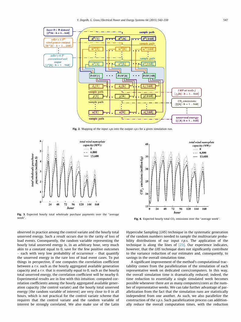
Fig. 2. Mapping of the input s.ps into the output s.p.s for a given simulation run.

Fig. 3. Expected hourly total wholesale purchase payments over the ‘‘averageweek’’. Fig. 4. Expected hourly total CO2 emissions over the ‘‘average week’’.

Y. Degeilh, G. Gross / Electrical Power and Energy Systems 64 (2015) 542–550 547

observed in practice among the control variate and the hourly totalunserved energy. Such a result occurs due to the rarity of loss ofload events. Consequently, the random variable representing thehourly total unserved energy is, in an arbitrary hour, very muchakin to a constant equal to 0, save for the few positive outcomes– each with very low probability of occurrence – that quantifythe unserved energy in the rare loss of load event cases. To putthings in perspective, if one computes the correlation coefficientbetween a r.v. such as the hourly aggregated available generationcapacity and a r.v. that is essentially equal to 0, such as the hourlytotal unserved energy, the correlation coefficient will be nearby 0.Experimental results are in line with this intuition: computed cor-relation coefficients among the hourly aggregated available gener-ation capacity (the control variate) and the hourly total unservedenergy (the random variable of interest) are very close to 0 in allhours, which is not practical for the control variate scheme thatrequires that the control variate and the random variable ofinterest be strongly correlated. We also make use of the Latin

Hypercube Sampling (LHS) technique in the systematic generationof the random numbers needed to sample the multivariate proba-bility distributions of our input r.p.s. The application of thetechnique is along the lines of [23]. Our experience indicates,however, that the LHS technique does not significantly contributeto the variance reduction of our estimates and, consequently, tosavings in the overall simulation time.

A significant improvement of the method’s computational trac-tability comes from the parallelization of the simulation of eachrepresentative week on dedicated cores/computers. In this way,the overall simulation time is dramatically reduced; indeed, thetime reduction to essentially a single simulated week becomespossible whenever there are as many computers/cores as the num-ber of representative weeks. We can take further advantage of par-allelization from the fact that the simulation runs are statisticallyindependent from one another. As such, we also parallelize theconstruction of the s.p.s. Such parallelization process can addition-ally reduce the overall computation times, with the reduction

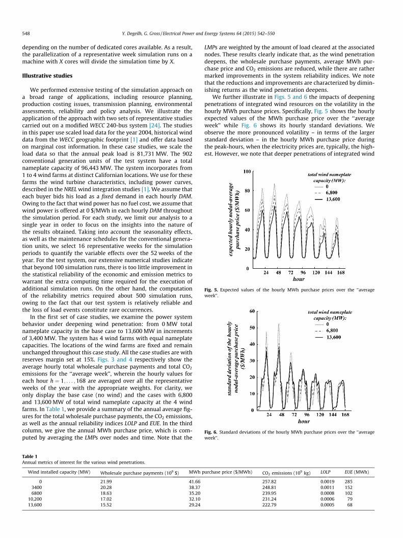
Fig. 5. Expected values of the hourly MWh purchase prices over the ‘‘averageweek’’.

Fig. 6. Standard deviations of the hourly MWh purchase prices over the ‘‘averageweek’’.

548 Y. Degeilh, G. Gross / Electrical Power and Energy Systems 64 (2015) 542–550

depending on the number of dedicated cores available. As a result,the parallelization of a representative week simulation runs on amachine with X cores will divide the simulation time by X.

Illustrative studies

We performed extensive testing of the simulation approach ona broad range of applications, including resource planning,production costing issues, transmission planning, environmentalassessments, reliability and policy analysis. We illustrate theapplication of the approach with two sets of representative studiescarried out on a modified WECC 240-bus system [24]. The studiesin this paper use scaled load data for the year 2004, historical winddata from the WECC geographic footprint [1] and offer data basedon marginal cost information. In these case studies, we scale theload data so that the annual peak load is 81,731 MW. The 902conventional generation units of the test system have a totalnameplate capacity of 96,443 MW. The system incorporates from1 to 4 wind farms at distinct Californian locations. We use for thesefarms the wind turbine characteristics, including power curves,described in the NREL wind integration studies [1]. We assume thateach buyer bids his load as a fixed demand in each hourly DAM.Owing to the fact that wind power has no fuel cost, we assume thatwind power is offered at 0 $/MWh in each hourly DAM throughoutthe simulation period. For each study, we limit our analysis to asingle year in order to focus on the insights into the nature ofthe results obtained. Taking into account the seasonality effects,as well as the maintenance schedules for the conventional genera-tion units, we select 16 representative weeks for the simulationperiods to quantify the variable effects over the 52 weeks of theyear. For the test system, our extensive numerical studies indicatethat beyond 100 simulation runs, there is too little improvement inthe statistical reliability of the economic and emission metrics towarrant the extra computing time required for the execution ofadditional simulation runs. On the other hand, the computationof the reliability metrics required about 500 simulation runs,owing to the fact that our test system is relatively reliable andthe loss of load events constitute rare occurrences.

In the first set of case studies, we examine the power systembehavior under deepening wind penetration: from 0 MW totalnameplate capacity in the base case to 13,600 MW in incrementsof 3,400 MW. The system has 4 wind farms with equal nameplatecapacities. The locations of the wind farms are fixed and remainunchanged throughout this case study. All the case studies are withreserves margin set at 15%. Figs. 3 and 4 respectively show theaverage hourly total wholesale purchase payments and total CO2

emissions for the ‘‘average week’’, wherein the hourly values foreach hour h ¼ 1; . . . ;168 are averaged over all the representativeweeks of the year with the appropriate weights. For clarity, weonly display the base case (no wind) and the cases with 6,800and 13,600 MW of total wind nameplate capacity at the 4 windfarms. In Table 1, we provide a summary of the annual average fig-ures for the total wholesale purchase payments, the CO2 emissions,as well as the annual reliability indices LOLP and EUE. In the thirdcolumn, we give the annual MWh purchase price, which is com-puted by averaging the LMPs over nodes and time. Note that the

Table 1Annual metrics of interest for the various wind penetrations.

Wind installed capacity (MW) Wholesale purchase payments (109 $) MWh p

0 21.99 41.663400 20.28 38.376800 18.63 35.20

10,200 17.02 32.1013,600 15.52 29.24

LMPs are weighted by the amount of load cleared at the associatednodes. These results clearly indicate that, as the wind penetrationdeepens, the wholesale purchase payments, average MWh pur-chase price and CO2 emissions are reduced, while there are rathermarked improvements in the system reliability indices. We notethat the reductions and improvements are characterized by dimin-ishing returns as the wind penetration deepens.

We further illustrate in Figs. 5 and 6 the impacts of deepeningpenetrations of integrated wind resources on the volatility in thehourly MWh purchase prices. Specifically, Fig. 5 shows the hourlyexpected values of the MWh purchase price over the ‘‘averageweek’’ while Fig. 6 shows its hourly standard deviations. Weobserve the more pronounced volatility – in terms of the largerstandard deviation – in the hourly MWh purchase price duringthe peak-hours, when the electricity prices are, typically, the high-est. However, we note that deeper penetrations of integrated wind

urchase price ($/MWh) CO2 emissions (109 kg) LOLP EUE (MWh)

257.82 0.0019 285248.81 0.0011 152239.95 0.0008 102231.24 0.0006 79222.79 0.0005 68

Fig. 7. Hourly LOLP contributions over the ‘‘average week’’.

Y. Degeilh, G. Gross / Electrical Power and Energy Systems 64 (2015) 542–550 549

resources tend to exacerbate such volatility also on the days withlower peak loads, on the Thursday–Sunday period, but tend toreduce the volatility in the hours with the highest loads in theMonday–Wednesday period. An analysis of these results suggeststhat wind generation contributes to avert scarcity events in thehours of the week with the highest loads. The plot in Fig. 7 illus-trates such phenomenon. The fewer scarcity events imply reducedoccurrences of price spikes. As a result, the volatility in the MWhpurchase prices at the peak load hours is reduced. On the otherhand, wind generation tends to induce increased volatility in theelectricity prices during the peak hours of the less-heavily-loadeddays. In such cases, the variability of the wind outputs tends tochange the set of generators that contribute to the determinationof the LMPs in each simulation run. Due to these changes, theresulting LMPs have higher volatility.

In the second set of case studies, we investigate to what extentwind resources may substitute for conventional resources frompurely a system reliability perspective. The base case has noinstalled wind capacity and uses 15% reserves margin to evaluatethe system reliability. In the other sensitivity cases, the conven-tional resource mix is supplemented by the same 4 wind farmsconsidered in the second set of case study with the 13,600 MWtotal nameplate capacity. We examine the impacts of retiring con-ventional resource capacity, thus leading to lowered reserves mar-gin levels (we consider that the reserves margin is provided by theconventional resources only). Fig. 8 shows the LOLP and EUE as afunction of the retired conventional capacity and resulting reservesmargins after installation of the 13,600 MW of wind capacity, withthe dashed line showing the associated reliability index for thebase case with no wind and the 15% reserves margin. The

Fig. 8. Annual LOLP and EUE vers

simulation results indicate that the 13,600 MW of installed windcapacity – about 16.6% of the annual peak load 81,731 MW – cansubstitute for about 4% of the weekly peak loads, on average overthe year, in terms of retired conventional generation capacity, thatis about 3,000 MW. In other words, from purely a system reliabilityperspective, wind resources constitute rather poor substitutes forconventional resources, since 13,600 MW of wind power name-plate capacity can substitute for only 22% of the conventionalresource capacity on an annual basis.

Conclusion

In this paper, we present the comprehensive, stochastic simula-tion framework we developed to emulate the side-by-side behav-ior of power system and market operations over longer-termperiods. Our approach makes detailed use of discrete-time r.p.s inthe adaptation of Monte Carlo simulation techniques. As such,the framework can explicitly represent various sources of uncer-tainty in the demands, the available capacity of conventional gen-eration resources and the time-varying, intermittent renewableresources, with their temporal and spatial correlations. In addition,the simulation methodology represents the impacts of the networkconstraints on the market outcomes. In this way, the simulationapproach is able to quantify the impacts of integrated renewableresources on power system economics, reliability and emissions.The stochastic simulation approach has a broad range of applica-tions in planning, operational analysis, policy formulation andanalysis and to provide quantitative assessments of various whatif case studies.

The representative results we present from the extensive stud-ies performed effectively demonstrate the strong capabilities of thesimulation approach. The results of these studies on a modifiedWECC 240-bus system, making use of scaled load data and histor-ical wind data in the WECC geographic footprint clearly indicatethat the integration of deepening levels of wind resources to apreexisting system may effectively drive the total wholesalepurchase payments and CO2 emissions down, as well as improvesystem reliability. There are, however, diminishing returns onthese benefits as higher penetrations of wind power are achieved.Wind generation is also shown to exacerbate (reduce) the volatilityin electricity prices in hours when the system is moderately(heavily) loaded. Simulation results indicate that, from a puresystem reliability perspective, the wind resources constitute afairly poor substitute for conventional resources.

Future work includes taking advantage of the tool design to gaininsights into the integration of other intermittent, time-varyingresources, such as solar, active demand response resources and

us system reserves margins.

550 Y. Degeilh, G. Gross / Electrical Power and Energy Systems 64 (2015) 542–550

utility-scale storage units into the grid. Another topic of consider-able interest is the analysis of the impacts of intermittent resourceintegration on ramping capability requirements.

Acknowledgements

Research performed was supported in part by the NationalScience Foundation under grant NSF ECCS-0925754 ‘‘ManagingIntermittency in Planning and Operations of Power’’, PSERC, theU.S. Department of Energy for ‘‘The Future Grid to EnableSustainable Energy Systems’’ and Stanford University GCEP.

Appendix: Hourly DAM clearing model

We provide a model for the hourly DAM clearing mechanism.We make use of the lossless DC power flows to model the grid[15, p. 534], as is the practice in today’s ISO-run markets. We fur-ther assume that the sellers (buyers) submit piecewise linear offer(bid) functions, which we denote by csð�Þ for seller s 2 S ¼ Sc SSw

(bbð�Þ for buyer b 2 B). Under these assumptions, the proposed OPFis a linear program.

Let N ¼ fn : n ¼ 0;1; . . . ; ðN � 1Þg be the set of network buseswith bus 0 being the slack bus, and L ¼ fl ¼ 1; . . . ; Lg the set oftransmission lines. Let matrices A, Bd and B designate the reducedbranch to node incidence, the branch susceptance and the reducednodal susceptance matrices, respectively. We denote by b0 the col-umn vector of the augmented susceptance matrix corresponding tothe slack node and by h the vector of voltage phase angles at thejN j � 1 buses other than the slack bus. We denote by f ¼ Bd A h

the vector of line flows, f M and f m the vectors of transmission line

ratings in each flow direction. We specify ðjsÞm to be the minimumcapacity of seller s 2 Sc conventional resource. We also define theconventional generation (wind farm generation) power injectionat node n in hour h as pc

n½h� ¼P

s2Sc at node ngs½h�pw

n ¼P

s2Sw at node ngs½h�� �

, where gs½h� is the output of seller s gen-eration resource in hour h. The power consumption due to loadsat node n in hour h is similarly denoted bypd

n½h� ¼P

b2B at node n‘b½h�, where ‘b½h� is the cleared demand of

buyer b in hour h. We use kn½h� to denote the dual variable associ-ated with the power balance equation at bus n in hour h. The lin-earized OPF in hour h 2 T i is formulated as:

max‘b ½h�;gs ½h�

Xb2B

bbð‘b½h�Þ �Xs2S

csðgs½h�Þ !

ðA:1aÞ

subject to

pc½h� þ pw½h�� �

� pd½h� ¼ Bh½h� $ k½h� ðA:1bÞ

pc0½h� þ pw

0 ½h�� �

� pd0½h� ¼ by0h½h� $ k0½h� ðA:1cÞ

� f m6 BdAh½h� 6 f M ðA:1dÞ

0 6 ‘b½h� 6 db½h�; 8b 2 B ðA:1eÞðjsÞm 6 gs½h� 6 as½h�; 8s 2 Sc ðA:1fÞ0 6 gs½h� 6 ws½h�; 8s 2 Sw: ðA:1gÞ

References

[1] GE Energy. Western wind and solar integration study. NREL, tech rep; 2010.<http://www.nrel.gov/docs/fy10osti/47434.pdf>.

[2] Balériaux H, Jamoulle E, De Guertechin F Linard. Simulation de l’exploitationd’un parc de machines thermiques de production d’electricite couples a desstations de pompage. RevueE (edition SRBE) 1967;5(7):3–24.

[3] Zhang Y, Chowdhury A. Reliability assessment of wind integration in operatingand planning of generation systems. In: Proceedings of the IEEE PES generalmeeting, Calgary; July 26–30 2009. p. 1–7.

[4] Maisonneuve N, Gross G. A production simulation tool for systems withintegrated wind energy resources. IEEE Trans Power Syst 2011;26(4):2285–92.

[5] Verbic G, Canizares C. Probabilistic optimal power flow in electricity marketsbased on a two-point estimate method. IEEE Trans Power Syst2006;21(4):1883–93. Nov.

[6] Madrigal M, Ponnambalam K, Quintana V. Probabilistic optimal power flow. In:IEEE Canadian conference on electrical and computer engineering, vol. 1; 1998.p. 385–8.

[7] Anderson C, Cardell J. The impact of wind energy on generator dispatch profilesand carbon dioxide production. In: 45th Hawaii international conference onsystem science (HICSS), Maui; January 04–07, 2012. p. 2020–6.

[8] Vallee F, Lobry J, Deblecker O. System reliability assessment method for windpower integration. IEEE Trans Power Syst 2008;23(3):1288–97.

[9] Haghi H, Bina M, Golkar M. Nonlinear modeling of temporal wind powervariations. IEEE Trans Sustain Energy 2013;4(4):838–48.

[10] Burke D, O’Malley M. A study of principal component analysis applied tospatially distributed wind power. IEEE Trans Power Syst 2011;26(4):2084–92.

[11] Tastu J, Pinson P, Madsen H. Space–time scenarios of wind power generationproduced using a gaussian copula with parametrized precision matrix.Technical University of Denmark, tech rep; 2013. <http://orbit.dtu.dk/fedora/objects/orbit:122325/datastreams/file_f6e2279f-5894-4d85-a4dd-e351e6048fda/content>.

[12] Chen N, Qian Z, Nabney I, Meng X. Wind power forecasts using gaussianprocesses and numerical weather prediction. IEEE Trans Power Syst2013;PP(99):1–10.

[13] Rajagopalan B, Lall U, Tarboton D, Bowles D. Multivariate nonparametricresampling scheme for generation of daily weather variables. Stoch HydrolHydraul 1997;11:65–93.

[14] Hajek B. Notes for ECE 534 – an exploration of random processes forengineers. Univ. of Illinois at Urbana–Champaign; 2009.

[15] Wood A, Wollenberg B. Power generation, operation and control. NY: JohnWiley and Sons, Inc.; 1996.

[16] Fishman G. A first course in Monte Carlo. Duxbury; 2006.[17] Kleijnen J. Statistical techniques in simulation – Parts 1 and 2. New

York: Marcel Dekker, Inc.; 1974.[18] Bratley P, Fox BL, Schrage LE. A guide to simulation. New York: Springer-

Verlag; 1983.[19] Ubeda J, Allan R. Sequential simulation applied to composite system reliability

evaluation. IEE Proc Part C: Gener Transm Distrib 1992;139(2):81–6.[20] Asmussen S, Glynn P. Stochastic simulation: algorithms and analysis. Springer;

2007.[21] Silva V. Value of flexibility in systems with large wind penetration. Ph.D.

dissertation, Imperial College London; 2010. <http://tel.archives-ouvertes.fr/docs/00/72/43/58/PDF/VSilva_PhDAllChapters_v9_-_unlinked_-_test.pdf>.

[22] Stott B, Hobson E. Power system security control calculations using linearprogramming. IEEE Trans Power Ap Syst 1978;PAS-97(5):1713–31.

[23] Kowli A, Gross G. Quantifying the variable effects of systems with demandresponse resources. In: Proceedings of the IREP symposium – bulk powersystem dynamics and control, Buzios; August 01–06, 2010.

[24] Price J, Goodin J. Reduced network modeling of WECC as a market designprototype. In: Proceedings of the IEEE PES general meeting, Detroit; July 24–28, 2011. p. 1–6.