Electrorotation of a viscous droplet in a uniform direct currentelectric field

by

Hui He

B.A., Wuhan University; Wuhan, Hubei, China, 2009

M.S., Brown University; Providence, RI, USA, 2011

A dissertation submitted in partial fulfillment of the

requirements for the degree of Doctor of Philosophy

in Physics Department at Brown University

PROVIDENCE, RHODE ISLAND

May 2014

c© Copyright 2014 by Hui He

This dissertation by Hui He is accepted in its present form

by Physics Department as satisfying the

dissertation requirement for the degree of Doctor of Philosophy.

Date

Petia M. Vlahovska, Ph.D., Advisor

Recommended to the Graduate Council

Date

Thomas Powers, Ph.D., Reader

Date

Jay Tang, Ph.D., Reader

Approved by the Graduate Council

Date

Peter Weber, Dean of the Graduate School

iii

Acknowledgements

I would like to express my sincere gratitude to my research advisor, Prof. Petia Vlahovska, who

continuously supports my PhD study and research. Her patience of answering my questions,

her insistence on high standard with my research, her understanding and encouragement at my

moments of frustration with research and life have given me an unforgettable and fruitful graduate

school experience. This prepares me well for my next life endeavor.

I also want to thank the rest of my prelim and thesis committee, Prof. Thomas Powers and

Prof. Jay Tang, for their time, insightful comments and guiding me through the defense process.

Besides, I want to thank Lane McConnell from Northwestern University, who has been helping

me to develop the numerical codes and Paul Salipante for the contribution on experimental data.

Also, thanks to the previous and current group members, Marc Shapiro, Kela Lushi, Malika

Ouriemi, for the great accompany and various kinds of assistance.

Last but not the least, I want to thank my parents, Longfu He and Zhaoju Ge, who have been

supportive of my education and understanding on my life choices. Also, my elder sister, Cong He,

who mentors me like a teacher, supports me as a family, and understands me like a friend.

iv

Hui He hui_he@brown.edu 1-401-440-4319

EDUCATION 2009-2014 Ph.D. in Physics Brown University, Providence, RI, USA

• Thesis entitled “Electrorotation of a droplet in a uniform DC electric field”, which studies both analytically and numerically the experimentally observed nonaxisymmetric droplet Electrohydrodynamics.

2009-2011 Master in Physics Brown University, Providence, RI, USA 2005-2009 Bachelor of Science in Physics (Major) Wuhan University, Wuhan, Hubei, China

• Physics Base Class • Graduation project “Study of Surface Diffusion Problems by the NEB method”, where two

surface diffusion problems were analyzed using Matlab simulation approach 2005-2009 Bachelor of Science in Finance (Minor) Wuhan University, Wuhan, Hubei, China

PUBLICATIONS 2013 H.He, P.F. Salipante, P.M. Vlahovska, “Electrorotation of a viscous droplet in a uniform direct current electric field”, Physics of Fluids, 25 (2013) 032106 2009 H. He, M.Y. Xie, Y. Ding, X.F. Yu, “Synthesis of Fe3O4@LaF3:Ce,Tb nanocomposite with bright fluorescence and strong magnetism”, Applied Surface Science, 225 (2009) 4623 2009 M. Y. Xie, L. Yu, H. He, X.F. Yu, “Synthesis of highly fluorescent LaF3:Ln3+/LaF3 core/shell nanocrystal by a surfactant-free aqueous solution route”, Journal of Solid State Chemistry, 182 (2009) 597

RESEARCH EXPERIENCE 2010-2014 School of Engineering Brown University, Providence, RI, USA

• Concentration on theoretical and computational Fluid Mechanics • Talk entitled “Electrorotation of a droplet in a uniform electric field” at 66th Annual Meeting

of the APS Division of Fluid Dynamics Summer 2010 Division of Applied Math, Brown University, Providence, RI, USA

• Conducted research on computational simulation of red blood cell flow using C++ 2007-2009 Key Laboratory of Acoustic and Photonic Materials and Devices of Ministry of Education Wuhan University, Wuhan, Hubei, China

• Synthesized various rare-earth nanomaterials and characterized their optical properties

TEACHING EXPERIENCE Fall 2009&2010 PHYS-0050, Physics Department, Brown University, Providence, RI

• Foundations of Mechanics (Undergraduate) Spring 2010 PHYS-0070, Physics Department, Brown University, Providence, RI

• Analytical Mechanics (Undergraduate)

SKILLS

• Programming: Matlab, Fortran, Mathematica and C++ • Language: Fluent English, Native Mandarin

v

Abstract of “Electrorotation of a viscous droplet in a uniform direct current electric field” by HuiHe, Ph.D., Brown University, May 2014

We study both analytically and numerically the experimentally observed nonaxisymmetric droplet

deformation and orientation in a uniform DC electric field. The theoretical model shows that a

rotational flow is induced about the droplet above a threshold electric field. As a result, drop shape

becomes a general ellipsoid with major axis obliquely oriented to the applied field direction. The

small deformation analytical theory is in excellent agreement with the experimental data for high

viscosity drops. The numerical simulation for large distortion using boundary integral method has

been validated by the 2D analytical theory (Feng (2002)).

vi

Contents

1 INTRODUCTION 1

2 PROBLEM FORMULATION 102.1 Introduction and physical picture . . . . . . . . . . . . . . . . . . . . . . . . . . . 102.2 Electric field governing equations and boundary conditions . . . . . . . . . . . . . 152.3 Velocity field governing equations and boundary conditions . . . . . . . . . . . . . 182.4 Drop shape evolution . . . . . . . . . . . . . . . . . . . . . . . . . . . . . . . . . 192.5 Stress balance . . . . . . . . . . . . . . . . . . . . . . . . . . . . . . . . . . . . . 202.6 Nondimensionalization . . . . . . . . . . . . . . . . . . . . . . . . . . . . . . . . 22

3 LEADING ORDER ANALYTICAL SOLUTION IN 3D 273.1 Introduction . . . . . . . . . . . . . . . . . . . . . . . . . . . . . . . . . . . . . . 273.2 General spherical harmonics formation . . . . . . . . . . . . . . . . . . . . . . . . 30

3.2.1 Electric field and electric tractions . . . . . . . . . . . . . . . . . . . . . . 303.2.2 Velocity field and viscous tractions . . . . . . . . . . . . . . . . . . . . . . 323.2.3 Drop shape . . . . . . . . . . . . . . . . . . . . . . . . . . . . . . . . . . 33

3.3 Solution to the Taylor problem without charge convection . . . . . . . . . . . . . 343.3.1 Electric field . . . . . . . . . . . . . . . . . . . . . . . . . . . . . . . . . . 343.3.2 Velocity field . . . . . . . . . . . . . . . . . . . . . . . . . . . . . . . . . 353.3.3 Drop deformation . . . . . . . . . . . . . . . . . . . . . . . . . . . . . . . 37

3.4 Solution to Electrorotation problem with charge convection . . . . . . . . . . . . . 383.4.1 Electric field . . . . . . . . . . . . . . . . . . . . . . . . . . . . . . . . . . 393.4.2 Velocity field . . . . . . . . . . . . . . . . . . . . . . . . . . . . . . . . . 403.4.3 Drop deformation . . . . . . . . . . . . . . . . . . . . . . . . . . . . . . . 413.4.4 Drop tilt angle . . . . . . . . . . . . . . . . . . . . . . . . . . . . . . . . . 43

3.5 Discussion and comparison with the experiment . . . . . . . . . . . . . . . . . . . 443.5.1 Drop tilt angle . . . . . . . . . . . . . . . . . . . . . . . . . . . . . . . . . 443.5.2 Drop deformation . . . . . . . . . . . . . . . . . . . . . . . . . . . . . . . 49

4 BOUNDARY INTEGRAL FORMULATION IN 2D 564.1 Introduction . . . . . . . . . . . . . . . . . . . . . . . . . . . . . . . . . . . . . . 564.2 Electric field boundary integral equations . . . . . . . . . . . . . . . . . . . . . . 57

vi

4.2.1 Free-space Green’s function . . . . . . . . . . . . . . . . . . . . . . . . . 574.2.2 Boundary integral equation for a point in the bulk . . . . . . . . . . . . . . 584.2.3 Boundary integral equation for an interfacial point . . . . . . . . . . . . . . 60

4.3 Velocity field boundary integral equations . . . . . . . . . . . . . . . . . . . . . . 654.3.1 Free-space Green’s function . . . . . . . . . . . . . . . . . . . . . . . . . 654.3.2 Boundary integral equation for a point in the bulk . . . . . . . . . . . . . . 664.3.3 Boundary integral equation for an interfacial point . . . . . . . . . . . . . . 69

5 NUMERICAL SCHEME AND RESULTS 745.1 Introduction . . . . . . . . . . . . . . . . . . . . . . . . . . . . . . . . . . . . . . 745.2 Shape representation . . . . . . . . . . . . . . . . . . . . . . . . . . . . . . . . . 77

5.2.1 Spectral representation . . . . . . . . . . . . . . . . . . . . . . . . . . . . 775.2.2 Updating and remeshing the shape . . . . . . . . . . . . . . . . . . . . . . 785.2.3 Curvature and unit normal vector . . . . . . . . . . . . . . . . . . . . . . . 785.2.4 Error test . . . . . . . . . . . . . . . . . . . . . . . . . . . . . . . . . . . 79

5.3 Numerical scheme for the electric field . . . . . . . . . . . . . . . . . . . . . . . . 835.3.1 Matrix representation . . . . . . . . . . . . . . . . . . . . . . . . . . . . . 835.3.2 Dealing with singularity of the Green’s function . . . . . . . . . . . . . . . 885.3.3 Error test . . . . . . . . . . . . . . . . . . . . . . . . . . . . . . . . . . . 90

5.4 Numerical scheme for the velocity field . . . . . . . . . . . . . . . . . . . . . . . 955.4.1 Matrix representation . . . . . . . . . . . . . . . . . . . . . . . . . . . . . 955.4.2 Dealing with singularity of the stokeslet and its associated stress tensor . . 965.4.3 Error test . . . . . . . . . . . . . . . . . . . . . . . . . . . . . . . . . . . 98

5.5 Results . . . . . . . . . . . . . . . . . . . . . . . . . . . . . . . . . . . . . . . . . 99

6 CONCLUSION AND OUTLOOK 102

A Maxwell-Wagner time scale 104

B Quincke rotation 106

C Scalar and vector spherical harmonics 108

D Fundamental solution sets of velocity fields 109

E 2D leading-order solution for drops with electrorotation 111

vii

List of Tables

viii

List of Figures

1.1 Morphological states of emulsions in a static condition [12]. External electric field is applied to thevertical direction: (a) formation of chain-like morphology in emulsion at E = 0.9kV/mm, whenthe continuous phase is more conducting than the dispersed drops; (b) formation of elongated liquidcolumnar columnar morphology at E = 0.5kV/mm, when the continuous phase is less conductingthan the dispersed drops. . . . . . . . . . . . . . . . . . . . . . . . . . . . . . . . . . 2

1.2 Electrospray diagram depicting the Taylor cone. . . . . . . . . . . . . . . . . . . . . . . . 21.3 Streamlines of a drop suspended in another kind of fluid from Ref. [32]. The numbers are values of

ψ/Aa2. a is the radius of the drop and A is the maximum velocity. . . . . . . . . . . . . . . 31.4 (a) The computational result of deformation D versus the square of electric field E2 for the case of

a castor oil drop in silicon oil from Feng and Scott (1996) [8]. Solid line is the computational result;dashed line is the asymptotic theory [32]; the squares are experimental data. (b) The deformationparameter DT in Ref. [8] is defined as DT = zmax−rmax

zmax+rmax. zmax is the maximum distance between

the drop surface and the centre of mass of the drop along the direction of the applied electric fieldand rmax is that in the direction perpendicular to the applied electric field . . . . . . . . . . . 5

1.5 Drop breakup process [17]: (a) when the drop is much more conducting than the surrounding fluidsand drop viscosity is very low; (b) when the drop is only more conducting than the surroundingfluids by one order of magnitude and there is no viscosity contrast. inset: details of the discretizationin the simulation . . . . . . . . . . . . . . . . . . . . . . . . . . . . . . . . . . . . . 6

1.6 Circulation and rotating flow patterns inside the silicon oil drop with radius r = 1.3mm when (a)electric field E = 2.86kV/cm and (b) E = 3.54kV/cm from Ref. [11]. The circulation androtating flow patterns are schematically illustrated in (c) and (d), respectively. . . . . . . . . . . 7

1.7 Unsteady drop behavior in a uniform DC electric field from Ref. [27]. (a) viscosity insideviscosity outside = 1, electric

field strength E = 9.9kV/cm, drop radius a = 1.8mm. (b) viscosity insideviscosity outside = 14, E = 9.7kV/cm,

a = 3.0mm. . . . . . . . . . . . . . . . . . . . . . . . . . . . . . . . . . . . . . . . 8

2.1 Illustration of the problem formulation . . . . . . . . . . . . . . . . . . . . . . . . . . . 112.2 Surface charge distribution and direction of surface electric tractions for a drop with (a) charge

relaxation inside is slower than outside; (b) charge relaxation is faster inside than outside. . . . . 122.3 Droplet with faster conduction in outside fluid deforms to an oblate and axisymmetrical straining

flow appears. . . . . . . . . . . . . . . . . . . . . . . . . . . . . . . . . . . . . . . 132.4 Unfavorable dipole configuration forms and results in rotation when the electric field is beyond a

critical value. The rotation can be either clockwise or counterclockwise depending on the initialperturbation. . . . . . . . . . . . . . . . . . . . . . . . . . . . . . . . . . . . . . . . 14

2.5 Sketches illustrating drop shape and flow streamlines in a uniform direct current electric field withincreasing strength: (a) The drop is spherical without electric field; (b) Pure straining flow andaxisymmetric oblate deformation under weak electric fields; (c) A rotational flow appears and thedrop is tilted under strong electric field. . . . . . . . . . . . . . . . . . . . . . . . . . . 14

ix

2.6 Charge flow for an infinitely thin column V with top surface S2 and bottom surface S1. The surfaceenclosed S0 has charge density Q with normal unit vector n and velocity us. The conductivity andelectric field inside and outside are σin/out and Ein/out respectively. . . . . . . . . . . . . . . 16

3.1 (a) The drop tilt angle φ0 is the angle between the major axis of the drop and x axis; (b) The dipoletilt angle β is the angle between the dipole and the electric field. . . . . . . . . . . . . . . . . 44

3.2 Comparison of the 3D theoretical drop tilt angle (solid line), theoretical dipole tilt angle (dashedline), 2D theoretical drop tilt angle (dash dot line) for drop radius 0.9mm, experimental (squares)drop tilt angle for viscosity ratio λ = 14 and drop radius a) 0.9mm; b) 1.05mm; c) 1.85mm, d)2.45mm. P = 0.56, R = 0.027, EQ = 0.27kV/cm . . . . . . . . . . . . . . . . . . . . . 45

3.3 Representation of two possible oblate drop orientation with respect to the observer from Ref. [26].The arrows denote rotational flow direction. A rotation axis parallel to the observation directionprovides a clear view of the oblique orientation (left), while a rotation axis perpendicular to theview axis obscures the oblique orientation (right). . . . . . . . . . . . . . . . . . . . . . . 46

3.4 Comparison of the 3D theoretical drop tilt angle (solid line), experimental drop tilt angle (solid dots)and shifted experimental drop tilt angle (circles) under a) viscosity ratio 1.4; b) and viscosity ratio0.14 for drop radius r = 0.9mm, P = 0.56, R = 0.027, EQ = 0.27kV/cm . . . . . . . . . . 47

3.5 Comparison of the theoretical drop tilt angle under viscosity ratio 14 (solid line), viscosity ratio1.4 (dash-dot line) and viscosity ratio 0.14 (dashed line) for drop radius 0.9mm. Other physicalparameters are same as Figure 3.4. . . . . . . . . . . . . . . . . . . . . . . . . . . . . . 49

3.6 a) Evolution of drop tilt angle upon application of electric field for a drop with radius 0.9mm andviscosity ratio λ = 14. E/EQ = 1.5, i.e., Cael = 1.54 (solid line), E/EQ = 2.0, i.e., Cael = 2.74

(dash-dot line), E/EQ = 2.5, i.e., Cael = 4.29 (dashed line)E/EQ = 1.5, i.e., Cael = 1.54 (solidline),E/EQ = 2.0, i.e., Cael = 2.74 (dash-dot line),E/EQ = 2.5, i.e., Cael = 4.29 (dashed line).b) Evolution of the tilt angle upon application of electric field for a drop with radius 0.9mm andcapillary number Cael = 2.74. viscosity ratio λ = 1 (solid line), λ = 5 (dash-dot line), λ = 14

(dashed line). R = 0.027, P = 0.56. . . . . . . . . . . . . . . . . . . . . . . . . . . . 503.7 Illustration of the definition for the drop deformation D = (L − B)/(L + B): L is the length and

B is the breadth; r+ and r− corresponds to the longest and the shortest radii. respectively . . . . 503.8 Comparison of the 3D theoretical drop deformation (solid line), 2D theoretical drop deformation

(dashed line) and experimental result (squares) under viscosity ratio 14 for drop radius a) 0.9mm;b) 1.05mm; c) 1.85mm, d) 2.45mm. Other physical parameters same as Figure 3.4. . . . . . . 52

3.9 Illustration of the fluid circulation limitation effect on drop deformation. . . . . . . . . . . . . 533.10 Comparison of the 3D theoretical deformation with viscosity ratio λ = 14 for drop radius 0.9mm

(solid line), 1.05mm (dash-dot line), 1.85mm (dashed line) and 2.45mm (dotted line). All otherphysical parameters same as Figure 3.4. . . . . . . . . . . . . . . . . . . . . . . . . . . 53

3.11 Comparison of the 2D and 3D theoretical deformation for viscosity ratio 14 (solid line), viscosityratio 5 (dash-dot line) and viscosity ratio 1 (dashed line) for a drop with radius 0.9mm and otherphysical parameters same as Figure 3.4. . . . . . . . . . . . . . . . . . . . . . . . . . . 54

3.12 a) Evolution of the drop shape upon application of electric field for a drop with radius 0.9mm andcapillary number Cael = 2.74, viscosity ratio λ = 1 (solid line), λ = 5 (dash-dot line), λ = 14

(dashed line). R = 0.027, P = 0.56. b) Evolution of the drop shape upon application of electricfield for a drop with radius 0.9mm and viscosity ratio λ = 14. E/EQ = 1.5, i.e., Cael = 1.54

(solid line), E/EQ = 2.0, i.e., Cael = 2.74 (dash-dot line), E/EQ = 2.5, i.e., Cael = 4.29

(dashed line). . . . . . . . . . . . . . . . . . . . . . . . . . . . . . . . . . . . . . . 55

4.1 Illustration of the observation point ξ, source point x and their distance r . . . . . . . . . . . 58

x

4.2 The inner domain Ωin and outer domain Ωout are separated by the interface Γ. The outer domain isunbounded, so Γ∞ is theoretical. The normal unit vector n is defined as pointing from the surfaceinto the outer domain. . . . . . . . . . . . . . . . . . . . . . . . . . . . . . . . . . . . 61

4.3 (a) Boundary decomposition for calculating the inside electric potential at the singularity point ξ;(b) Boundary decomposition for calculating the outside electric potential at the singularity point ξ 62

5.1 The process diagram of the iterative approach. . . . . . . . . . . . . . . . . . . . . . . . 755.2 The ellipse x2

m2 + y2

n2 = 1 with major axis m and minor axis n . . . . . . . . . . . . . . . . 805.3 Plot of the absolute error of the numerical normal vector components (a) nx and (b) ny by the

spectral method versus the inverse of interpolation points n = 72, 144, 288 for a sphere (solid line);an ellipse with k = n

m = 0.5(dash-dot line); an ellipse with k = 2.5(dashed line). . . . . . . . 825.4 Plot of the absolute error for the second order derivatives (a) xss and (b) yss by the spectral method

versus the inverse of interpolation points n = 72, 144, 288 for a sphere (solid line); an ellipse withk = 0.5 (dash-dot line); an ellipse with k = 2.5 (dashed line). . . . . . . . . . . . . . . . . . 84

5.5 Plot of the relative error of the numerical curvature by the spectral method versus the inverse ofinterpolation points n = 72, 144, 288 for a sphere (solid line); an ellipse with k = 0.5 (dash-dotline); an ellipse with k = 2.5 (dashed line). . . . . . . . . . . . . . . . . . . . . . . . . . 85

5.6 A solid sphere of radius a vexposed to the electric field . . . . . . . . . . . . . . . . . . . . 915.7 Plot of the absolute error of (a) the normal inside electric field En

in; (b) the tangential inside electricfield Et

in; (c) the normal outside electric field Enout; (d) the tangential outside electric field Et

out

versus the inverse of the interpolation points n = 72, 144, 288. Solid line is for the ellipse with ratiok = 2.5; dash-dot line for k = 1.0 and dashed line for k = 0.5. . . . . . . . . . . . . . . . . 94

5.8 (a) Evolution of the drop deformation D under Capillary number Cael = 0.68. (b) The dropdeforms to an oblate (dashed line) from a circle (solid line).The dimensionless time interval isdt = 0.01; total time steps is 2000; 72 interpolation points. Other parameters include P = 0.5,R = 0.01, λ = 1. . . . . . . . . . . . . . . . . . . . . . . . . . . . . . . . . . . . . . 99

5.9 (a) Evolution of the drop deformation D under Capillary number Cael = 0.68. (b) The dropdeforms to an oblate (dashed line) from a circle (solid line).The dimensionless time interval isdt = 0.01; total time steps is 2000; 72 interpolation points. Other parameters include P = 0.5,R = 0.8, λ = 1. . . . . . . . . . . . . . . . . . . . . . . . . . . . . . . . . . . . . . 100

5.10 Comparison with Feng’s 2D theory: (a) the numerical deformation D versus electric Capillarynumber Cael. Parameters are adopted from Feng’s paper [7]: R = 0.01, P = 0.5, λ = 1, dropradius r = 1mm. Code is stable for (b) very deformed oblate and starts to be unstable when thedrop starts to show the sign of (c) breakup. . . . . . . . . . . . . . . . . . . . . . . . . . 100

A.1 Dielectric sphere of radius a with dielectric constant εin and conductivity σin suspended in anotherfluid with εout and σout. The whole system is subjected to a uniform electric field of magnitude E0. 105

xi

CHAPTER ONE

INTRODUCTION

Electrohydroydnamics (EHD) studies the dynamics of fluids in an electric field. On one side, it can

be viewed as fluid dynamics involving electric field forces. On the other side, it can be regarded as

electrodynamics with an extra influence from the moving fluid on the electric field. The interplay

between the flow and the electric field contributes to the complexity of EHD.

EHD plays an important role in various industrial and technical applications. For example, it

is used in the petroleum industry to demulsify water-in-crude oil emulsions [25]. The reason is

that when two water drops approach each other, they are separated by a thin film. The application

of an electric field could destabilize the thin film and therefore promote the coalescence of the

drops. When the drops aggregate to fluid column and further become a big mass of water, they

would either sediment or float up to be separate from the oil. Coalescence of dispersed drops in an

emulsion under external electric field [12] is shown in Figure 1.1.

Another application is electrospray. When a small volume of conductive fluid is exposed to

an electric field, the liquid forms the shape of a cone, which is known as the Taylor Cone shown

in Figure 1.2. When the electric field reaches a critical value, the tip of the Taylor Cone emits

1

(a) (b)

Figure 1.1: Morphological states of emulsions in a static condition [12]. External electric field is applied to thevertical direction: (a) formation of chain-like morphology in emulsion at E = 0.9kV/mm, when the continuousphase is more conducting than the dispersed drops; (b) formation of elongated liquid columnar columnar morphologyat E = 0.5kV/mm, when the continuous phase is less conducting than the dispersed drops.

E

Figure 1.2: Electrospray diagram depicting the Taylor cone.

a jet of fluid. This is the beginning of the electrospraying process. Other applications include

ink jet printing [5], electrohydrodynamic pumps [39], utilizing electric field to induce mixing in

microfluidics and etc.

To obtain fundamental understanding of the microstructural evolution in those processes, a lot

of work was done to study the behavior for an isolated drop exposed to an electric field. Before

1960, the main focus was on perfect conducting or perfect dielectric fluid, such as, a perfect

2

Figure 1.3: Streamlines of a drop suspended in another kind of fluid from Ref. [32]. The numbers are values ofψ/Aa2. a is the radius of the drop and A is the maximum velocity.

insulating drop immersed in a perfect insulating fluid or a highly conducting drop in a perfect

insulating fluid. For both of these two cases, the fluid remain motionless and the drop adopts

the shape of a prolate ellipsoid at equilibrium, where the axis of symmetry is the direction of the

imposed electric field [21, 10, 23]. Since the fluids are at rest at equilibrium, this phenomenon is

referred to as electrohydrostatics.

Surprisingly, Allen and Mason (1962) observed oblate deformation in experiments of a silicone

oil droplet immersed in oxidized castor oil. These fluids are both poorly conducting or leaky

dielectric liquid [2] and it was correctly pointed out by Konski and Harris that the oblate shape

could result from the finite conductivity in both fluids [22]. G.I. Taylor recognized the importance

of tangential electric stresses on the interface of two leaky dielectric fluids and thus proposed the

well-known leaky dielectric model [32, 20, 29]. In his model, tangential electric stress drags the

fluid into motion. As a result, toroidal circulation pattern is formed inside of the droplet and the

flow is axisymmetrical as shown in Figure 1.3. In the limit of Stokes flow and small perturbation,

3

Taylor derived the physical criterion for discriminating prolate and oblate deformations, which

depends upon the ratio of dielectric constant, viscosity, and conductivity of fluids inside and outside

of the drop. It was shown that the droplet is possible to remain spherical under critical parameter

values. The Taylor model will be reviewed in greater details in Section 3.1.

Taylor’s model qualitatively explains most of the observations, however, careful experiments

by Vizika and Saville (1992) [35] found quantitative discrepancy between experiments and theory:

(a) For drops deformed into prolate ellipsoids in a steady field, the deformation is 1.02 to 1.6 times

the theoretically predicted values; (b) For drops deformed into oblate ellipsoids in a steady field,

the deformation is slightly smaller than the theoretical prediction. This prompted further research

aimed at improving the theory by removing some of restrictions in the original model.

One limitation of Taylor’s model is the neglection of charge convection effects. In reality, the

electric charges are convected by the moving fluid, which could influence the electric field. The

significance of the charge convection effect is usually measured in terms of the electric Reynolds

number, Reel, defined as,

Reel =charge convection time due to flow mobility

charge relaxation time due to ohmic conduction(1.1)

In Taylor’s model, Reel is assumed to be small enough so that charge convection could be

neglected. However, qualitative discussion on charge convections has been repeatedly brought

up [35, 33, 8] and quantitative investigation for finite electric Reynolds number was in demand.

Feng (1998) [6] consequently incorporated the charge convection and studied the behavior of a

drop at finite electric Reynolds number. According to his computational results, charge convection

reduces the intensity of electrohydrodynamic flow. Oblate drop associated with a pole-to-equator

flow are less deformed when charge convection taken into account, while the deformation of prolate

4

x

y

rmax

zmax E

(a) (b)

DT =zmax − rmaxzmax + rmax

DT

Figure 1.4: (a) The computational result of deformation D versus the square of electric field E2 for the case of acastor oil drop in silicon oil from Feng and Scott (1996) [8]. Solid line is the computational result; dashed line is theasymptotic theory [32]; the squares are experimental data. (b) The deformation parameter DT in Ref. [8] is defined asDT = zmax−rmax

zmax+rmax. zmax is the maximum distance between the drop surface and the centre of mass of the drop along

the direction of the applied electric field and rmax is that in the direction perpendicular to the applied electric field

drop with an equator-to-pole flow is enhanced. This suggests a source of discrepancy between

experiments and Taylor’s model.

Another limitation of the conventional analytical solutions is the assumption of small drop

deformation. Numerical techniques, which do not require a closed form solution, can study

large deformation [3, 17, 8, 6]. Feng and Scott (1996) [8] utilized the Galerkin finite element

method. Their computational result recovered the asymptotic solutions of Taylor (1966) under

the conditions of creeping flow, small deformation and small Reynolds number, but differed

significantly when the drop deformation becomes noticeable. In the parameter space of the drop

deformationDT versus the square of the dimensionless electric fieldE2, linear relationship appears

under weak electric fields. The definition of the deformation parameter DT is illustrated in Figure

1.4 (b). At stronger fields, the solution branch folds back at the turning point to lower values

of the field strength, implying unsteady status beyond a critical electric field Ec. The nonlinear

relationship between DT and E2 explained part of discrepancies between the experiment and

5

Figure 1.5: Drop breakup process [17]: (a) when the drop is much more conducting than the surrounding fluids anddrop viscosity is very low; (b) when the drop is only more conducting than the surrounding fluids by one order ofmagnitude and there is no viscosity contrast. inset: details of the discretization in the simulation

asymptotic theory, because deformation reached the nonlinear region in many experiments while

the experimental data were compared with the asymptotic linear theory. Comparing to Taylor’s

analytical solution, numerical work of Feng and Scott (1996) gives a more complete picture for

the problem of a neutrally buoyant leaky dielectric drop in an immiscible leaky dielectric fluid

subjected to an electric field.

Another computational approach is the boundary integral method used by lac and Homsy

(2007) [17] as formulated by Sherwood (1998) [31]. Different from Sherwood’s work, which

only considered the prolate drop case and restricted to a narrow interval of dielectric constant and

conductivity, Lac and Homsy (2007) studied a broader range of these parameters. In particular,

unstable regions and various break-up modes are identified. Figure 1.5 (a) and (b) from Ref. [17]

show the dynamic process of drop breakup when the drop is much more conducting and only more

conducting by one order of magnitude than the suspension medium. The instability is characterized

by appearance of fast evolving fingers at the drop tips.

Most of those previous work on EHD [32, 1, 17] focused on weak electric field. Recently,

interesting phenomena such as rotation under strong electric field has been reported [26, 13, 11,

6

Figure 1.6: Circulation and rotating flow patterns inside the silicon oil drop with radius r = 1.3mm when (a) electricfield E = 2.86kV/cm and (b) E = 3.54kV/cm from Ref. [11]. The circulation and rotating flow patterns areschematically illustrated in (c) and (d), respectively.

28]. The rotation of a dielectric solid sphere immersed in a slightly conducting liquid subject

to a uniform strong electric field was first observed over 100 years ago and known as Quincke

rotation [9, 18, 34]. Mathematical model of Quincke rotation is given in Appendix B. For the

case of a droplet, rotational flow occurs under strong electric field. This is called "electrorotation".

Krause and Chandratreya (1998) [15] showed that the rotational flow can suppress the deformation,

especially perpendicular to the applied field direction. Ha and Yang (2000) [11] experimentally

studied the behavior of less conducting silicon oil droplet suspended in more conducting castor

oil under uniform DC electric field. As shown in Figure 1.6, silicon oil droplet was seeded with

aluminum power and clearly showed the toroidal circulations predicted by Taylor’s model under

weak field in their experiment. When the electric field gets stronger, a rotational flow arises, but

the symmetric axis of the droplet remains steadily oblique from the electric field direction. To

clarify these effects, Salipante and Vlahovska (2010) [26] systematically measured the tilt angle

and deformation over a broad range of drop sizes, viscosity ratios and electric field strengths.

7

Figure 1.7: Unsteady drop behavior in a uniform DC electric field from Ref. [27]. (a) viscosity insideviscosity outside = 1, electric field

strength E = 9.9kV/cm, drop radius a = 1.8mm. (b) viscosity insideviscosity outside = 14, E = 9.7kV/cm, a = 3.0mm.

Summary on their experimental results are given in Section 3.1.

Under even stronger electric field, Salipante and Vlahovska (2013) [27] showed a neutrally

leaky dielectric drop initially deforms to an ellipsoid and then exhibits unsteady motions. When

the drop viscosity is high, the ellipsoid tumbles and randomly reverses its direction of rotation as in

Figure 1.7 (b). When the drop viscosity is low, it undergoes additional deformation while rotating

as in Figure 1.7 (a).

Motivated by the observed nonaxisymmetric drop deformation and orientation in a uniform

electric DC electric field, we aim to build a theoretical model including charge convection to

explain the experimental data from Salipante and Vlahovska (2010) [26]. Although Feng (2002)

[7] has investigated on this topic analytically under small deformation, his model is limited to

two-dimensional analysis. Moreover, the model predicts viscosity independent deformation, which

is at odds with the strong viscosity effect found in the experiments [26]. Therefore, we will develop

a three-dimensional analytical model in this thesis. To explore the unsteady dynamics and large

distortion under even stronger electric field observed by Sanlipante and Vlahovska (2013) [27], we

are pursuing a numerical solution utilizing the boundary integral method based on Lac and Homsy

(2007) [17] and McConnell, Miksis and Vlhavoska [19]. The numerical model starts with two

8

dimension. Following is the outline of this thesis.

Chapter 2 introduces the physical system and formulates the governing equations along with

the boundary conditions for the electric field and the flow field. Also, important parameters such

as electric Reynolds number, rotational Reynolds number, electric capillary number and various

time scales are discussed.

Chapter 3 first summarizes the solution for Taylor’s problem in the framework of spherical

harmonics and then expands to give a leading-order perturbative solution in three dimension taking

into account charge convection and electrorotation. Comparison with the experimental data shows

that the theoretical model works best for small drop size and high viscosity ratio. The deformation

is very sensitive to viscosity ratio and weakly dependent on drop size once rotation starts.

Chapter 4 builds up the general boundary integration formulation for the electric field and the

flow field via the Green’s function. The handling singularity points of the singularity points in the

free space Green’s kernels is discussed.

Chapter 5 describes the simulation process and gives the numerical scheme for the shape

representation, the electric field and velocity field. Error test for the shape representation is done

by comparing the numerical normal vector and curvature for an ellipse. Error test for the electric

field is completed through the comparison of the numerical electric field at the beginning with

the theoretical electric field around a undeformed ellipse. Shape evolution and steady state shapes

are studied numerically. Finally, the numerical deformation under various Capillary number is

compared with Feng’s 2D theory [7].

Chapter 6 summarizes our analytical and numerical work and proposes future work direction.

9

CHAPTER TWO

PROBLEM FORMULATION

2.1 Introduction and physical picture

The specific system under our investigation is a neutrally buoyant drop with radius a, viscosity

ηin, conductivity σin and dielectric constant εin, suspended in a different fluid with viscosity ηout,

conductivity σout and dielectric constant εout, as shown in Figure 2.1. The whole system is exposed

to a uniform electric field in y direction with magnitude E0,

E∞ = E0y (2.1)

The electric stress in this system could be found by the Maxwell stress tensor,

Tel = ε(EE− 1

2E2) (2.2)

which accounts for the electric stresses due to both free charges and polarization [20, 8]. On the

boundary, the mismatch of stress tensor leads to a jump of the electric force. The tangential electric

10

x

y rs =1+ f (θ,ϕ )

εin,σ in,ηin

εout,σ out,ηout

a

Chapter 2

Problem Formulation

Consider a neutrally buoyant drop with radius a, viscosity in, conductivity in and

dielectric constant in, suspended in a fluid with viscosity out, conductivity out and

dielectric constant out. The whole system is exposed to a uniform electric field with

magnitude E0,

(2.1) E1 = E0y

The mismatch of electric properties inside and outside the droplet leads to a jump of

the electric field on the surface. When both of the fluids are ideal insulating dielectrics,

no free charges accumulate on the interface. When one of the fluids is weakly conduct-

ing, the electric field is always perpendicular to the interface. Because electric stress is

the consequence of the electric field acting on surface charges, there is either no elec-

tric stress or only normal electric stress for those two cases. The normal electric stress

could be balanced by the surface tension. Therefore, at steady state, the droplet adopts

the shape of a prolate ellipsoid and the fluids are motionless.

When both of the fluids are weakly conducting (leaky dielectric), things become

more complicated. Surface charges distribution depends on the difference of the charge

relaxation time of the fluids. If the charge relaxation inside the drop is slower than flu-

ids outside, the interface charge is dominated by charges brought from the surrounding

fluids. On the other side, if the charge relaxation inside the drop is faster, the interface

9

Figure 2.1: Illustration of the problem formulation

force is very important because it incurs fluid motion. The magnitude of the net tangential electric

force density is a product of the free charge density on the surface and the tangential electric field

strength. The derivation is given in Section 2.5.

When both fluids are ideally insulating, no free surface charge exists. Obviously, there is no

tangential electric traction. When one of the fluids is perfectly conducting, the electric field is

always perpendicular to the interface. There is only normal electric stress, which could be offset

by the Laplace stress due to surface tension. Therefore, at steady state, the droplet adopts the shape

of a prolate ellipsoid and the fluids are motionless.

When both fluids are weakly conducting (leaky dielectric), things become more complicated.

Positive charges move along the direction of the electric field, while negative charges move

oppositely. The mismatch of electric properties of the leaky dielectric fluids inside and outside the

droplet may lead to accumulation of free charges on the surface. The final configuration depends

on the relative charge relaxation time inside and outside of the drop. If the charge relaxation inside

the drop is slower than fluid outside, the interface charge is dominated by charges brought from the

11

E

(a) (b)

Figure 2.2: Surface charge distribution and direction of surface electric tractions for a drop with (a) charge relaxationinside is slower than outside; (b) charge relaxation is faster inside than outside.

surrounding fluid. On the other side, if the charge relaxation inside the drop is faster, the interface

charge is dominated by the charges from inside fluid. The tangential electric field acting on the

surface charge produces tangential electric stress. When charge conduction is faster outside than

inside, tangential electric stresses point from poles to the equator, as in Figure 2.2 (a). A drop with

faster interior conduction has equator-to-pole tangential electric stresses, as in Figure 2.2 (b).

Under a weak electric field, tangential electric stress drags the fluid into motion.

Axisymmetrical straining flow appears. For the case of faster conduction outside, the droplet

deforms into an oblate shape. The direction of the straining flow and drop shape are shown in

Figure 2.3. Under the assumption of no charge convection, the leaky dielectric model quantified

the straining flow and the deformation of the droplet [32].

Under strong electric field, electrorotation appears in the case shown in Figure 2.2 (a). The

reason is that the separation of positive and negative charges produces a drop dipole opposite to

the electric field direction as shown in Figure 2.4, which is an unstable orientation. When the

electric field reaches a critical strength, a perturbation could create an electric torque. For a rigid

12

E

Figure 2.3: Droplet with faster conduction in outside fluid deforms to an oblate and axisymmetrical straining flowappears.

sphere, the torque leads to physical rotation of the particle known as Quincke rotation [9]. On one

side, the rotation of the particle convects the surface charge, which tries to flip the dipole. On the

other side, the surrounding fluid recharges the surface, which prevents the dipole from completely

flipping over. The equilibrium reaches when charge convection rate due to rotation is equal to

the charge conduction rate. Under this situation, the dipole has a stable tilt angle. The constant

electric torque results in continuous object spinning. The critical electric field and angular velocity

of Quincke rotation is given in the Appendix B. In the case of a droplet, straining flow exists in

addition to the rotational flow. The staining flow deforms the droplet into an ellipsoid with the

major axis steadily tilted with respect to the direction of the electric field. Salipone and Valhovska

[26] experimentally showed the dipole direction may not aligned with the drop major axis.

To summarize, the whole physical mechanism is illustrated in Figure 2.5. In this chapter, we

will formulate the governing equations and boundary conditions for the electric field and flow field,

taking into account the charge convection and electrorotation. Dimension analysis is done at the

end.

13

P P

w

β

E

Figure 2.4: Unfavorable dipole configuration forms and results in rotation when the electric field is beyond a criticalvalue. The rotation can be either clockwise or counterclockwise depending on the initial perturbation.

E

(a) (b) (c)

Figure 2.5: Sketches illustrating drop shape and flow streamlines in a uniform direct current electric field withincreasing strength: (a) The drop is spherical without electric field; (b) Pure straining flow and axisymmetric oblatedeformation under weak electric fields; (c) A rotational flow appears and the drop is tilted under strong electric field.

14

2.2 Electric field governing equations and boundary conditions

The electric field E is irrotational and the electric potential satisfies the Laplace equation,

∇× E = 0, ∇2ψ = 0 (2.3)

The boundary conditions placed on the electric field are,

(a) The electric potential is finite everywhere, we have,

Ein is finite, at r → 0 (2.4)

(b) Far from the droplet, the electric field tends to be unperturbed and equal to the imposed

electric field,

Eout → E∞, at r →∞ (2.5)

(c) The tangential electric field is continuous on the interface,

n× (Ein − Eout) = 0 (2.6)

where, n is the unit normal vector of the interface.

(d) The normal component of the electric displacement field experiences a jump by an amount

15

Infinite small h n

S0

S1

S2

Q

σ in,Εin

σ out,Εout

uS

q q q

q q

q q q

q q

Figure 2.6: Charge flow for an infinitely thin column V with top surface S2 and bottom surface S1. The surfaceenclosed S0 has charge density Q with normal unit vector n and velocity us. The conductivity and electric field insideand outside are σin/out and Ein/out respectively.

proportional to the free surface charge density, Q,

Q = n · (εoutEout − εinEin) (2.7)

(e) The current conservation condition around the interface requires,

n · (σinEin − σoutEout) = ∇t · (uQ) +∂Q

∂t(2.8)

where ∇t is the surface gradient operator and u is the interfacial velocity. This is where the flow

field comes to influence the electric field in our model. The left hand side of (2.8) indicates the

conduction current. The right hand side represents the convection current due to fluid motion.

The derivation is based on the charge continuity equation on the interface. Thinking about the

charge mass conservation in a control volume V enclosing the surface S0 with bottom surface S1,

S2 and infinitely small height h as shown in Figure 2.6. The changing rate of the charge in V equals

to the the difference between charge inflow and outflow. Using q to indicate the charge density at

16

any space point, then,

S

J · ndS = − ∂

∂t

y

V

qdV (2.9)

Because the volume V has an infinitely small height, the total charges in the volume V is

related to the surface charge density Q,

RHS = −∂Q∂tS0 (2.10)

The charge flow, or current, could be decomposed to the conduction current and the convection

current. The conduction current is due to the drift of electrons under electric field, which satisfies

Ohm’s law,

Jcond = σE (2.11)

Therefore, the total conduction current on the boundary surface is,

S

Jcond · ndS =x

side surface

Jcond · ndS︸ ︷︷ ︸

=0,h→0

+x

bottom surface S1

Jcond · ndS +x

top surface S2

Jcond · ndS

=n · (JoutS2 − JinS1) = n · (σoutEout − σinEin)S0

(2.12)

The convection current results from the motion of ions with velocity u,

Jconv = qu (2.13)

Applying the divergence theorem, the total convection current on the surface could be related to

17

the convection current in the volume V ,

S

Jconv · ndS =y

V

∇ · JconvdV = ∇t · (Qu)S0, h→ 0 (2.14)

Therefore, the left hand side of the continuity equation (2.9) becomes,

LHS =

S

J · ndS =

S

Jcond · ndS +

S

Jconv · ndS

= n · (σoutEout − σinEin)S0 +∇t · (Qu)S0

(2.15)

Eliminating the constant area term S0 on both sides of the continuity equation, we achieve the

current conservation equation,

n · (σoutEout − σinEin) +∇t · (uQ) = −∂Q∂t

(2.16)

At steady state, the local time derivative of surface charge density should disappear, i.e. ∂Q∂t

= 0,

and therefore we obtain the current conservation condition for our problem.

2.3 Velocity field governing equations and boundary conditions

Fluids in this study are assumed to be incompressible and the flow is in the limit of stokes region,

meaning the inertial forces are much smaller compared with viscous forces [16]. The steady

velocity field therefore satisfies the Stokes equation and continuity equation,

ηα∇2uα = ∇pα, ∇ · uα = 0, where α = in, out (2.17)

18

with pα and uα denoting the pressure and fluid velocity, respectively.

Because there is no imposed flow, the fluid becomes static far from the droplet,

uout → 0, at r →∞ (2.18)

To guarantee no molecules pass through the interface, the velocities on the surface approaching

from inside and outside have to be equal,

uin = uout, on the surface (2.19)

2.4 Drop shape evolution

Suppose that the shape equation of the droplet is F (x, y, z, t), which is always equal to zero. Then

the unit normal vector n is related to the shape function by,

n =∇F|∇F | (2.20)

Now, since F is a scalar function which is always equal to zero at any point on the fluid interface,

its material time derivative following any point on the interface is equal to zero,

DF

Dt=∂F

∂t+ u · ∇F = 0, on the surface (2.21)

where ∂F∂t

represents the change of F with time at a fixed location.

In a reference with the drop center at r = 0 with initial radius a, we can use rs = a(1 +

19

+f(t, θ, ϕ)) to represent the drop interface, where f is the deviation of the drop shape from a

sphere. Then F = r− rs represents the shape function. Now substituting the expression of F into

(2.21) for an initially unit spherical drop, we obtain the shape evolution equation,

∂f

∂t= u · (r−∇f), at r = rs (2.22)

2.5 Stress balance

Due to the discontinuity of electric and viscous properties, there is a "jump" in both the electric

and hydrodynamic stresses on the surface. The net stress is given by the difference of the stress

inside and outside,

n · [Tel] = n · (Telout −Tel

in) (2.23)

n · [Thd] = n · (Thdout −Thd

in ) (2.24)

where, [ ] denotes the jump and hd and el indicate hydrodynamic part and electric part, respectively.

The hydrodynamic stress tensor is calculated by [16],

T hdα,ij = −pδij + ηα(∂ui∂xj

+∂uj∂xi

), where α = in, out (2.25)

The electric stress tensor is given by the Maxwell stress tensor [8, 20],

T elα,ij = εα(EiEj − E2δij/2), where α = in, out (2.26)

20

where, δij is the Kronecker Delta function. Then, the net normal direction electric stress is,

(n · [Tel])n = [T elnn] = T elout,nn − T elin,nn

= εout(E2out,n −

1

2(E2

out,n + E2out,t))− εin(E2

in,n −1

2(E2

in,n + E2in,t))

=1

2εout(E

2out,n − E2

out,t)−1

2εin(E2

in,n − E2in,t)

(2.27)

And the net tangential direction electric stress is,

(n · [Tel])t = [T elnt] = T elout,nt − T elin,nt

= εoutEout,nEout,t − εinEin,nEin,t

= Et(εoutEout,n − εinEin,n) = EtQ

(2.28)

where, we have used the continuous tangential electric field condition (2.36) and the normal

direction electric field boundary condition (2.7). This equation mathematically explains why

nonzero surface free charge density and tangential electric field strength give rise to tangential

electric stress.

To avoid acceleration, the net electric stress, net viscous stress and the Laplace stress due to

surface tension balance at equilibrium on the drop surface,

n · ([Thd] + [Tel]) = γ(∇ · n)n, on the surface (2.29)

where γ refers to the surface tension and ∇ · n is the mean curvature H . If the drop shape is

spherical, i.e., ∇H = 2a, then the right hand side of the stress balance equation is a constant.

However, if the net pressure on the left hand side changes as a function of position on the surface,

then the drop has to deform to a shape where the interface curvature ∇ · n varies in precisely the

same as the left hand side. So this stress balance condition determines the final shape of the drop.

21

2.6 Nondimensionalization

Because the droplet is suspended in an unbounded medium, the natural length scale Lc here

is the initial radius of the droplet a. The imposed electric field strength E0 can be used as

the characteristic electric field strength, and the viscosity in the suspending liquid ηout as the

characteristic viscosity. Then the characteristic charge density Qc should be εoutE0 by (2.7), the

characteristic hydrodynamic tensor T hdc = ηoutuca

according to (2.43), and the characteristic electric

stress T elc = εoutE20 by the Maxwell stress tensor (2.44). Here, uc is the characteristic velocity.

Because of the stress balance condition, the characteristic electric stress and characteristic viscous

stress should be equal and therefore, we could find the magnitude of the characteristic velocity,

T elc = T hdc ⇒ εoutE20 =

ηoutucLc

⇒ uc =aεoutE

20

ηout(2.30)

Before displaying the scaled equations, it’s convenient to introduce the conductivity ratio R of

fluids inside and outside the drop, the dielectric constant ratio P and the viscosity ratio λ,

R =σinσout

, P =εinεout

, λ =ηinηout

(2.31)

Also, the electric Reynolds number Reel, electric Capillary number Cael and rotational Reynolds

number are,

Reel =ε2outE

20

σoutηout(1 + λ), Cael =

εoutE20a

γ, Rew =

ηout(1 + λ)w

εoutE20

(2.32)

whose physical meaning will be discussed later.

22

Now with these introduced parameters, we change all the dimensional governing equations and

boundary conditions to their dimensionless forms and summarize as below,

Electric field governing equation:

∇× E = 0 (2.33)

Electric field boundary conditions:

Ein is finite, at r → 0 (2.34)

Eout → E∞, at r →∞ (2.35)

n× (Ein − Eout) = 0 (2.36)

n · (REin − Eout) = Reel∇t · (uQ), at r = rs (2.37)

Q = n · (Eout − PEin), at r = rs (2.38)

Velocity field governing equation:

∇2uα = ∇pα, ∇ · uα = 0, where α = in, out (2.39)

Velocity field boundary conditions:

uout → 0, at r →∞ (2.40)

uin = uout, at r = rs (2.41)

Stress balance conditions:

n · ([Thd] + [Tel]) = Ca−1el (∇ · n)n, at r = rs (2.42)

T hdα,ij = −pδij + λαα(∂jui + ∂iuj), where α = in, out, λin = λ, λout = 1 (2.43)

T elα,ij = Sα(EiEj − EiEjδij/2), where α = in, out, Sin = P, Sout = 1 (2.44)

Shape evolution equation:

∂f

∂t= u · (r−∇f) (2.45)

23

To explore more about the physical meaning behind these dimensionless parameters, we can

start from understanding the time scales. When there is an imposed electric field, ions in the

fluids move. The charge relaxation time scale could be found by the normal direction electric field

boundary condition and Ohm’s law,

Qctc

= Jc = σE0

Qc = εE0

⇒ tc =εασα, where α = in, out (2.46)

As to the case of a leaky dielectric drop immersed in a leaky fluid fluid, the net charge accumulation

rate is determined from both charge relaxation time inside tinc and outside toutc . tinc < toutc means the

conduction in the drop fluid is faster than the suspending liquid. As a result, the interface charge

distribution is dominated by charges from inside fluid as shown in Figure 2.2 (b) and the drop

dipole is aligned with the electric field. On the opposite, tinc > toutc represents the conduction in the

suspending liquid is faster than inside fluid. Henceforth, charges in the suspending liquid dominate

the interface charge distribution as in Figure 2.2 (a). The drop dipole is reversed and the drop

deforms to be oblate. The rate of the charge accumulating on the interface and dipole formation

in the three-dimensional problem are characterized by the Maxwell-Wagner polarization timescale

given in Appendix A,

tMW =εout + 2εinσout + 2σin

(2.47)

With the accumulation of charges on the boundary, an electric force arises and its tangential

component drags the interface into motion. This resulting hydrodynamic flow deforms the droplet

on a time scale related to the inverse shear rate imposed by the electric shear stresses,

[T el] ∼ [T hd]⇒ tehd =ηout(1 + λ)

εoutE20

(2.48)

24

The importance of the charge convection is quantified by the electric Reynolds number, which

compares the charge relaxation time to the charge convection time due to flow motion,

Reel =tctehd

(2.49)

In the presence of electrorotation, an additional time scale appears. The importance of

rotational flow is characterized by the ratio of the straining flow time scale tehd and the rotational

flow time scale tw = 1/w,

Rew =tehdtw

= tehdw (2.50)

where w is the rotational rate. If rotational time scale tw is much shorter than the deformation time

scale tehd, meaning the rotational Reynolds number Rew is big and rotational flow is strong, drop

deformation is limited.

The surface tension γ plays the role of a restoring force for a deformed droplet. Then the time

scale for a deformed drop to relax to its equilibrium spherical shape is given by,

γ(∇ · n) ∼ [T hd]⇒ tγ =ηouta(1 + λ)

γ(2.51)

The ratio of the deforming time scale tehd and the distorting time scale tγ , defined as the electric

capillary number Cael, characterizes the magnitude of drop deformation,

Cael =tehdtγ

=εoutE

20a

γ(2.52)

This interpretation is also consistent with the dimensionless stress balance condition (2.42). For

Cael 1, very small deviation from a spherical shape can result in sufficient variation in the term

25

Ca−1el ∇ · n to match with the net electric and viscous stress. On the other side, when Cael 1,

pressure variation has to be offered by large deformation of the drop shape for large variation

in the curvature term. However, Cael is not a reliable parameter to decide the drop deformation

magnitude when electrorotation appears. Because the suppressing effect is influential under strong

rotational flow, a big Cael system could still have small drop deformation under this case.

26

CHAPTER THREE

LEADING ORDER ANALYTICAL

SOLUTION IN 3D

3.1 Introduction

In the system of a charge-free leaky dielectric droplet immersed in another leaky dielectric fluid

subject to external electric field, the electric field induces hydrodynamic flow. In return, the

hydrodynamic flow convects charges and influences the electric field. Taylor’s classical leaky

dielectric model (1966) [32] ignores the second effect by assuming very small electric Reynolds

number, i.e. Reel 0, which measures the importance of charge convection. In his model, the

distribution of potential around a drop in another fluid is assumed to be the same as that which

would exist in a static state. The electric stress is then computed without information from the

flow field. The velocity field is derived from the balance of the surface tension, electric stress and

viscous stress. It was found that the flow is axisymmetrically aligned with the electric field. The

drop adopts a prolate or an oblate spheroidal shape depending on the viscosity, conductivity, and

dielectric constant of fluids inside and outside the drop. To a leading order, the deformation of a

27

drop in 3D is described by [7],

DT =9Cael

16(2 +R)2(1− 2P +R2 +

3(R− P )(3λ+ 2)

5(1 + λ)) (3.1)

The deformation DT is defined in the x− y plane, same as in Figure 1.4 (b).

Under strong fields, a nonaxisymmetrical rotational flow appears when the conduction outside

is faster than inside, i.e. R < P . For a solid sphere, it is referred to as Quincke rotation. According

to the mathematical model given in Appendix B, the rotational rate and critical electric field in 3D

are,

ωQ =1

τmw

√E2

E2c

− 1

EQ =

√2ηoutσout(2 +R)2

3ε2out(P −R)

(3.2)

which are size independent.

Salipante and Vlahovska [26] systematically measured the critical electric field, the drop tilt

angle, rotational rate and drop deformation. Their results showed that the threshold field strength

is well approximated by the Quincke rotation criterion (3.2) for small and high viscous drops. But

unlike Quincke rotation, drop size affects electrorotation.

In their experiments of a silicon oil drop suspended in castor oil, outside charge relaxation

time scale, tc,out = εoutσout

, is in the order of 1 second. The rotational flow time scale, tw = 1/w,

is also about 1 second. For high viscosity ratio λ, the straining flow time scale, tehd = ηouta(1+λ)

εoutE20

,

approximates to 10 seconds. The restoring time scale due to surface tension, tγ = ηouta(1+λ)γ

,

is about 1 second. Therefore, the electric capillary number, Cael = tγtehd

, is in the order of 0.1,

28

which implies that the restoring force due to surface tension is about 10 times stronger than the

distorting force coming from the straining flow. So the drop undergoes small deformation. The

rotational Reynolds number, Rew = tehdtw

, is in the order of 10. This indicates that the rotational

flow dominates the straining flow.

The goal of this chapter is to give a theoretical explanation to the experimentally observed

nonaxisymmetric droplet deformation and orientation in a uniform DC electric field by Salipante

and Vlahovska (2010) [26]. Our model is based on Taylor’s classical leaky dielectric model [32],

but includes the charge convection effect. Because of the small deformation, we could look for a

leading order perturbative solution around a sphere. Since the straining flow is much weaker than

the rotational flow, the charge convection could be assumed to solely come from the rotational

flow. Small drop size a and high viscosity ratio λ, which are necessary to make Cael small and

Rew big, are preconditions of our small deformation analytical model.

The two dimensional solution of this model for drops with electrorotation has been derived by

Feng (2002) [7]. The result is too complicated to list here and will be given in Appendix E. The

first-order drop deformation of cases without electrorotation is,

DT,2D =εinaE

20

γ

R(R + 1) + 1− 3S

3S(1 +R)2cos(2φ) (3.3)

which is viscosity independent. Here, we will pursue a three dimensional solution to explain the

strong viscosity effect found in the experiments.

Due to the spherical symmetry, the problem will be solved in the framework of spherical

harmonics. This formalism allows the deviation of very compact solutions, which include charge

convection [36, 30] or higher order perturbation [38, 13]. Definitions of spherical harmonics Yjm

and the vector spherical harmonics yjmq are given in Appendix C. The general spherical harmonics

29

representations for variables of interest will be developed in section 3.2.

In section 3.3, we recover the solution for Taylor’s model [32] without charge convection under

weak fields. In section 3.4, a three dimensional leading order solution for the electrorotation

problem under strong fields is given. In section 3.5, the theoretical result and experiment data

for tilt angle and deformation are compared.

3.2 General spherical harmonics formation

3.2.1 Electric field and electric tractions

In spherical harmonics, the dimensionless external electric potential is,

ψ∞ = −y = g∞r(Y11 + Y1−1), g∞ = i

√2π

3(3.4)

The j = 1 symmetry in the applied uniform electric field (3.4) implies j = 1 symmetry in perturbed

electric field under spherical geometry.

The general solution of the electric potential that satisfies the Laplace equation is,

ψ = −g∞∞∑

j=0

m=j∑

m=−j(gjmr

j + ejmr−j−1)Yjm(θ, φ) (3.5)

where, ejm and gjm are constant coefficients that determine the electric field strength. Einstein’s

summation rule will be applied over repeat indices for following expressions.

30

To satisfy the far field condition (2.35), the electric potential outside should only include the

decaying spherical harmonics with j = 1 symmetry,

ψout = ψ∞ − g∞e1mr−2Y1m (3.6)

To be finite at the drop center requested by (2.34), i.e., r → 0, the inside electric potential is

solely composed of the growing spherical harmonics with j = 1 symmetry,

ψin = −g∞g1mrY1m (3.7)

By the relationship between the electric field and electric potential E = −∇ψ, the electric field

inside and outside in spherical harmonics form are found to be,

Eout = E∞ + g∞(√

2y1m0 − 2y1m2)r−3

Ein = g∞g1m(√

2y1m0 + y1m2)

(3.8)

where, the dimensionless external electric field is,

E∞ = y = g∞∇[r(Y11 + Y1−1)]

= g∞(y1m2 +√

2y1m0)

(3.9)

The electric tractions exerted on the surface follow from the Maxwell stress tensor (2.44),

τ el = [(r · Eout)Eout −1

2Eout · Eoutr]− P [(r · Ein)Ein −

1

2Ein · Einr] (3.10)

31

An electric field with j = 1 symmetry generates electric tractions with j = 0, 1 and 2. The

isotropic part j = 0 is balanced by the hydrostatic pressure. The position-dependent stress j = 2

is responsible for drop deformation. The j = 1 component is the torque and only exists under

electrorotation. So the form of electric tractions in spherical harmonics reduces to,

τ el = τ el2m0y2m0 + τ el2m2y2m2 + τ el101y101, m = 0,±2 (3.11)

where, the coefficients τjmq in general expressions are found by (3.10),

τ el101 =√

3π2

(e11 − e1−1)

τ el2±22 =√

π30

(−2 + (2− 5e1±1)e1±1 + 2P (1 + e1±1)2)

τ el202 = 13

√π5(−2 + e1−1(1− 5e11) + e11 + 2P (1 + e1−1)(1 + e11))

τ el200 =√

π30

(−2 + e11 + 2P (1 + e1−1)(1 + e11) + e1−1(1 + 4e11))

τ el2±20 =√

π5(1 + e1±1 + 2e2

1±1 + P (1 + e1±1)2)

(3.12)

3.2.2 Velocity field and viscous tractions

The velocity fields uout and uin that satisfy the Stokes equations and continuity equation (2.39)

could be expanded on the basis sets for solutions of the Stokes equations, i.e., u±jmq, listed in

Appendix D,

uout(r) =∑

jmq

cjmqv−jmq(r), uin(r) =

∑

jmq

cjmqv+jmq(r) (3.13)

where,∑

jmq

=∞∑

j=1

j∑

m=−j

2∑

q=0

(3.14)

32

cjmq are coefficients that determine the velocity strength. On a sphere with r = 1, the basis sets

for solutions of the Stokes equation v±jmq are simply yjmq.

The viscous traction τ exerting on a sphere with a normal vector r is r ·T and may be expanded

in vector spherical harmonics,

τ = r ·T = τjmqyjmq (3.15)

where the viscous traction coefficients τjmq are linearly related to the velocity field coefficients

cjmq,

τ outjm0

τ outjm1

τ outjm2

=

−(2j + 1) 0 3√

jj+1

0 −(2 + j) 0

3√

jj+1

0 −4+3j+2j2

j+1

·

cjm0

cjm1

cjm2

(3.16)

τ injm0

τ injm1

τ injm2

=

2j + 1 0 −3√

j+1j

0 j − 1 0

−3√

j+1j

0 3+j+2j2

j

·

cjm0

cjm1

cjm2

(3.17)

3.2.3 Drop shape

The deviation of the shape from a sphere could be expanded in spherical harmonics as,

f(t, θ, φ) =∑

j≥2

j∑

m=−jfjm(t)Yjm(θ, φ) (3.18)

At leading order, the uniform electric field only generates ellipsoidal deformation, which is

characterized by the second order spherical harmonics, i.e., j = 2. Therefore, the deviation of

33

the drop shape takes the form,

f = (f20Y20 + f22Y22 + f2−2Y2−2)

=3

4

√5

π(f20(−1

3+ cos2 θ) +

√2

3(f ′22 cos 2φ− f ′′22 sin 2φ) sin2 θ)

(3.19)

where f2,±2 = f ′22 ± if ′′22.

3.3 Solution to the Taylor problem without charge convection

For the following, the superscript T is used to indicate solutions for the Taylor problem.

3.3.1 Electric field

In Taylor’s model, the influence of the flow field on electric field is ignored. Therefore, the electric

field coefficients eT1m and gT1m are determined independent of the flow field. With the general

spherical harmonics formation of the electric field (3.8), the current conservation condition (2.37)

when Reel = 0 gives,

RgT1m + 2eT1m − 1 = 0 (3.20)

and the continuous tangential electric field boundary condition (2.36) shows,

gT1m − eT1m − 1 = 0 (3.21)

34

The two equations (3.20) and (3.21) yield the solutions for the electric field strength,

gT1m =3

2 +R, eT1m =

1−R2 +R

(3.22)

The induced surface charge could be derived from the electric displacement field condition

(2.38),

QT (θ, φ) =3(R− P )

2(R + 2)sinφ cos θ (3.23)

Substituting the electric field coefficients e1m and g1m into the general expression of the electric

tractions (3.12), we find the electric tractions for the Taylor problem,

τ el,T220 = τ el,T2−20 = 32τ el,T200 = −9π(R−P )

5(R+2)2

τ el,T222 = τ el,T2−22 = 32τ el,T202 = −3

√3π10

R2−2P+1(R+2)2

(3.24)

3.3.2 Velocity field

The velocity field is determined from the stress balance condition (2.42), which has one radial

component in spherical harmonics form,

τ el,Tjm2 + τ out,Tjm2 − λτ in,Tjm2 = Ca−1el (j2 + j − 2)fjm (3.25)

and one tangential component,

τ el,Tjm0 + τ out,Tjm0 − λτ in,Tjm0 = 0 (3.26)

35

The electric tractions τ el,Tjmq is known from (3.24). Substituting the generals expressions of

viscous tractions expressions τ in,Tjmq ((3.17)) and τ out,Tjmq ((3.16)), we transform the stress balance

conditions (3.26) and (3.25) in terms of the velocity field coefficients cjmq,

√32(2 + 3λ)cT2m0 − (6 + 13

2λ)cT2m2 − 4Ca−1

el fT2m + τ el,T2m2 = 0

−5(1 + λ)cT2m0 +√

32(2 + 3λ)cT2m2 + τ el,T2m0 = 0

(3.27)

Notice all terms with j 6= 2 disappear because the electric traction (3.11) and the deformation

(3.19) expressions only involve j = 2 modes. To have a clearer physical view of the velocity field

coefficients, we rearrange the terms in (3.27) to obtain,

cT2m0 = CT2m0 − Ca−1

el DT20(λ)fT2m

cT2m2 = CT2m2 − Ca−1

el DT22(λ)fT2m

(3.28)

where,

CT2m0 =

(12 + 13λ)τ el,T2m0 +√

6(2 + 3λ)τ el,T2m2

(3 + 2λ)(16 + 19λ)

CT2m2 =

10(1 + λ)τ el,T2m2 +√

6(2 + 3λ)τ el,T2m0

(3 + 2λ)(16 + 19λ)

DT20(λ) =

4√

6(2 + 3λ)

(3 + 2λ)(16 + 19λ)

DT22(λ) =

40(1 + λ)

(3 + 2λ)(16 + 19λ)

(3.29)

The velocity coefficients, CT2m0 and CT

2m2, describe the leading order velocity field, which is

generated by the imposed electric field. The components, Ca−1el D

T20(λ)fT2m and Ca−1

el DT22(λ)fT2m,

represent the flow driven by capillary stresses, i.e., relaxation of the deformed drop back to the

equilibrium spherical shape.

36

3.3.3 Drop deformation

The evolution of the drop shape is derived from the kinematic condition (2.45), i.e., ∂f∂t

= u · (r−

∇f), on the surface. With the general spherical harmonics expression for the deviation (3.19), the

evolution equation becomes,

∂fT2m∂t

Y2m = u · r︸︷︷︸first order

−u · ∇fT2mY2m︸ ︷︷ ︸second order

(3.30)

The electric field generates the straining flow, which then acts to deform the drop. Therefore,

the term u · ∇fT2m is second order. Substituting the general spherical harmonics expression of

the velocity field around a lightly deformed sphere with r = 1, i.e., u · r = cT2m2Y2m, the shape

evolution equation in leading order requires,

∂fT2m∂t

= cT2m2 = CT2m2 − Ca−1

el DT22(λ)fT2m, (see (3.28)) (3.31)

The inhomogeneous term CT2m2 represents drop shape distortion by the straining flow. The second

term, proportional to the inverse of electric Capillary number, describes the relaxation of the drop

shape due to surface tension.

The equilibrium condition of the static drop shape, i.e.,∂fT2m

∂t= 0, yields the solution for drop

deformation at steady state,

fT20 =

√2

3fT22′ = −

3Cael4(2 +R)2

√π

5(1− 2P +R2 +

3(R− P )(3λ+ 2)

5(1 + λ)) (3.32)

37

To compare with Taylor’s deformation solution, we check the deviation in x−y plane, i.e. θ = π/2,

fT =3

4

√5

π(−1

3fT20 +

√2

3(fT ′22 cos 2φ− fT ′′22 sin 2φ))

=9Cael

16(2 +R)2(1− 2P +R2 +

3(R− P )(3λ+ 2)

5(1 + λ))(− cos 2φ− 1

3) (3.33)

which gives the result for drop deformation,

DT =9Cael

16(2 +R)2(1− 2P +R2 +

3(R− P )(3λ+ 2)

5(1 + λ)) (3.34)

This recovers Taylor’s solution of deformation (3.1).

3.4 Solution to Electrorotation problem with charge convection

To explain experimental data about electorotation under the condition of Rew 1 by Salipante

and Vlahovska (2010) [26], the charge convection is assumed to be dominated by the rotational

flow. Because the vector spherical harmonics yjmq with q = 1 represent the solenoidal component

of a vector velocity field tangential to a surface, the rotational surface velocity responsible for

charge convection on a unit sphere r = 1 in spherical harmonics could be written as,

c101y101 = ω(2i

√π

3)y101 (3.35)

where the angular velocity ω will be determined as a part of the solution. The coefficient 2i√

π3

is

extracted for simplifying calculations below.

38

3.4.1 Electric field

Because charge convection is taken into account and the velocity field influences the electric field,

the electric field solution depends on the rotational flow. With the induced surface charge density

represented as,

Q =1∑

m=−1

Q1mY1m (3.36)

the current conservation condition (2.37) gives one relationship between the electric field and the

surface charge density coefficients Q1m,

i

√2π

3(|m| − 2e1m −Rg1m) = imReelωQ1m (3.37)

where we used the recouping property of harmonics,

∇ · (Yjmy101) = −mYjm√

3

8π

The electric displacement field boundary condition (2.38) shows the second relationship

between the electric field and the surface charge density coefficients,

Q1m = i

√2π

3(1− 2e1m − Pg1m) (3.38)

The two relationships (3.37) and (3.38) present the electric field solutions as functions of the

39

rotational rate w,

e1m = −1 +3(i+mReelω)

2i+ 2mReelω +mReelωP + iR

g1m =3(i+mReelω)

2i+ 2mReelω +mReelωP + iR

(3.39)

The electric tractions follow from the general expression (3.12),

τ el101 = −3i√

6π(R− P )Reelω

(2 +R)2 + (2 + P )2Re2elω

2

τ el200 = −6

√3π

10

(R− P )Reelω

(2 +R)2 + (2 + P )2Re2elω

2

τ el2±20 = ±9

√π

5

(R− P )(1∓Reelω)

(2 +R∓ i(2 + P )Reelω)2

τ el202 = −3

√π

5

1 +R2 − 2P + (P − 1)2Re2elω

2

(2 +R)2 + (2 + P )2Re2elω

2

τ el2±22 = −3

√3π

10

1 +R2 − 2P ∓ i(1− 2P +RP )Reelω − (P − 1)2Re2elω

2

(2 +R∓ i(2 + P )Reelω)2

(3.40)

where, τ el101 represents the electric torque, τ el2m0 tangential stresses and τ el2m2 electric pressure.

3.4.2 Velocity field

Similar to the Taylor problem, the velocity field is determined form the stress balance condition.

However, except the radial component q = 2 (3.25) and the tangential component q = 0 (3.26),

we would have an extra decoupled rotational component corresponding to q = 1,

τ eljm1 + τ outjm1 − λτ injm1 = 0 (3.41)

40

which in terms of velocity field coefficients is,

3c1m1 + τ el1m1 = 0 (3.42)

This rotational stress balance component gives us the solution of the angular velocity,

c101 =τel101

3

c101y101 = i2ω√

π3y101

⇒ω =1

Reeltmw

√−1 + (

E0

EQ)2

(3.43)

where tmw = σin+2σoutεin+2εout

is the three-dimensional Maxwell-Wagner time and EQ =√

2ηoutσout(2+R)2

3ε2out(P−R)

the threshold electric field for electrorotation to happen. This implies the leading order solution

for angular velocity is exactly the Quincke result for a rigid sphere (3.2).

Just as in the Taylor problem, the radial component of the stress balance condition (3.25) and

the tangential component (3.26) give the straining flow (3.28) the same formation as in Taylor

problem (3.28). But the solution differs because the electric field tractions have changed in this

case.

3.4.3 Drop deformation

At Rew & 1, the total velocity in the presence of electrorotation happens is composed of a

rotational component and a straining component, i.e., u = ustrain + urot. The straining flow

is inversely related to the viscosity ratio, i.e., ustrain ∼ 1/λ, according to (3.29), while the

41

rotational flow is independent of λ in accordance with (3.43). Therefore, at high viscosity ratio,

the rotational velocity is leading order and the straining flow is next order. Substituting the general

spherical harmonics expression for the deviation f (3.19), we obtain the evolution equation (2.45)

in spherical harmonics,

∂f2m

∂tY2m = (ustrain + urot) · (r−∇f2mY2m)

= ustrain · r︸ ︷︷ ︸first order

−ustrain · ∇(f2mY2m)︸ ︷︷ ︸second order

+urot · r︸ ︷︷ ︸=0

−urot · ∇(f2mY2m)︸ ︷︷ ︸first order

(3.44)

The third term urot · r disappears because the rotational flow corresponds to the solenoidal

component q = 1, which is tangential to the surface. The multiplication of the first order straining

flow and the first order deformation makes ustrain · ∇(f2mY2m) second order. For a leading order

solution, the evolution equation (3.44) gives us,

∂f2m

∂t= c2m2 + iωmf2m

= C2m2 − Ca−1el D22(λ)f2m + iwmf2m, (see (3.28))

(3.45)

where, we have used uhdr = c2m2Y2m and recoupling property of spherical harmonics,

y101yjm0 = −√

3

8π

m√j(j + 1)

Yjm

⇒ urot∇(f2mY2m) = ω(2i

√π

3)y101f2my2m0 = −iωmf2mY2m

(3.46)

Unlike the Taylor problem, where the leading order drop deformation has only contributions from

distorting force due to straining flow, i.e., C2m2, and restoring force due to surface tension, i.e.,

Ca−1el D22(λ)f2m, the drop deformation in this problem is influenced by rotational flow as well

indicated by the third term in (3.45) [36].

42

With the initial condition of spherical drop shape, i.e., f2m(t = 0) = 0, the solution for the

time dependent differential equation (3.45) is found to be,

f2m(t) = C2m2(iwm− Ca−1el D22(λ))−1[e(iwm−Ca−1

el D22(λ))t − 1], m = 0,±2 (3.47)

The drop deformation at steady status is found through the condition of zero local time

derivative, i.e., ∂f2m∂t

= 0,

f20 = −CaelC202

D22(λ)

f ′22 =iCaelC222

2(2Caelω − iD22(λ))− iCaelC2−22

2(2Caelω + iD22(λ))

f ′′22 =CaelC222

2(2Caelω − iD22(λ))+

CaelC2−22

2(2Caelω + iD22(λ))

(3.48)

3.4.4 Drop tilt angle

The tilt angle φ0 is defined in the x− y plane between the drop major axis and the x axis as shown

in Figure 3.1 (a). It corresponds to the point where the deformation is the biggest, i.e., Df(φ0)Dφ0

= 0,

which gives,

φ0 = −1

2arctan(

f ′′22

f ′22

) (3.49)

A tilt angle of zero corresponds to the Taylor result without rotation.

43

P

w

β

E

(b) (a)

ϕ0

x

y

Figure 3.1: (a) The drop tilt angle φ0 is the angle between the major axis of the drop and x axis; (b) The dipole tiltangle β is the angle between the dipole and the electric field.

3.5 Discussion and comparison with the experiment

3.5.1 Drop tilt angle

In the Ref. [26] by Salipante and Vlahovska (2010), the drop tilt angle and deformation of droplet

under different electric strength were measured. The dipole tilt angle,

β = arctan(1

tmww) = arctan[(

E20

E2Q

− 1)−1/2] (3.50)

was used as an approximation for theoretical comparison. Differences between the drop tilt angle

and dipole tilt angle is illustrated in Figure 3.1.

Figure 3.2 plots our 3D theoretical drop tilt angle, the 2D theoretical drop tilt angle (E.6),

experimental drop tilt angle versus the electric field for various drop sizes under a high viscosity

ratio condition of λ = 14. Below the critical electric field, it’s the Taylor solution. Rotation

44

0 0.5 1 1.5 2 2.5 30

10

20

30

40

50

60

70

80

90

E0/E

Q

deg

ree

droplet tilt angleFeng 2D tilt angledipole tilt angleoriginal experiment

(a) λ = 14, r = 0.9mm

0 0.5 1 1.5 2 2.5 30

10

20

30

40

50

60

70

80

90

E0/E

Q

deg

ree

droplet tilt angleFeng 2D tilt angledipole tilt angleoriginal experiment

(b) λ = 14, r = 1.05mm

0 0.5 1 1.5 2 2.5 30

10

20

30

40

50

60

70

80

90

E0/E

Q

deg

ree

droplet tilt angleFeng 2D tilt angledipole tilt angleoriginal experiment

(c) λ = 14, r = 1.85mm

0 0.5 1 1.5 2 2.5 30

10

20

30

40

50

60

70

80

90

E0/E

Q

deg

ree

droplet tilt angleFeng 2D tilt angledipole tilt angleoriginal experiment

(d) λ = 14, r = 2.45mm

Figure 3.2: Comparison of the 3D theoretical drop tilt angle (solid line), theoretical dipole tilt angle (dashed line), 2Dtheoretical drop tilt angle (dash dot line) for drop radius 0.9mm, experimental (squares) drop tilt angle for viscosityratio λ = 14 and drop radius a) 0.9mm; b) 1.05mm; c) 1.85mm, d) 2.45mm. P = 0.56, R = 0.027, EQ =0.27kV/cm

45

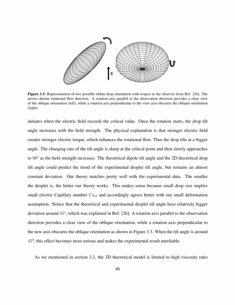
Figure 3.3: Representation of two possible oblate drop orientation with respect to the observer from Ref. [26]. Thearrows denote rotational flow direction. A rotation axis parallel to the observation direction provides a clear viewof the oblique orientation (left), while a rotation axis perpendicular to the view axis obscures the oblique orientation(right).

initiates when the electric field exceeds the critical value. Once the rotation starts, the drop tilt

angle increases with the field strength. The physical explanation is that stronger electric field

creates stronger electric torque, which enhances the rotational flow. Thus the drop tilts at a bigger

angle. The changing rate of the tilt angle is sharp at the critical point and then slowly approaches

to 90o as the field strength increases. The theoretical dipole tilt angle and the 2D theoretical drop

tilt angle could predict the trend of the experimental droplet tilt angle, but remains an almost

constant deviation. Our theory matches pretty well with the experimental data. The smaller

the droplet is, the better our theory works. This makes sense because small drop size implies

small electric Capillary number Cael and accordingly agrees better with our small deformation

assumption. Notice that the theoretical and experimental droplet tilt angle have relatively bigger

deviation around 45o, which was explained in Ref. [26]: A rotation axis parallel to the observation

direction provides a clear view of the oblique orientation, while a rotation axis perpendicular to

the new axis obscures the oblique orientation as shown in Figure 3.3. When the tilt angle is around

450, this effect becomes most serious and makes the experimental result unreliable.

As we mentioned in section 3.1, the 3D theoretical model is limited to high viscosity ratio

46

0 0.5 1 1.5 2 2.5 30

10

20

30

40

50

60

70

80

90

E0/E

Q

deg

ree

droplet tilt angleoriginal experimentshifted experiment

(a) λ = 1.4

0 0.5 1 1.5 2 2.5 30

10

20

30

40

50

60

70

80

90

E0/E

Q

deg

ree

droplet tilt angleoriginal experimentshifted experiment

(b) λ = 0.14

Figure 3.4: Comparison of the 3D theoretical drop tilt angle (solid line), experimental drop tilt angle (solid dots) andshifted experimental drop tilt angle (circles) under a) viscosity ratio 1.4; b) and viscosity ratio 0.14 for drop radiusr = 0.9mm, P = 0.56, R = 0.027, EQ = 0.27kV/cm

47

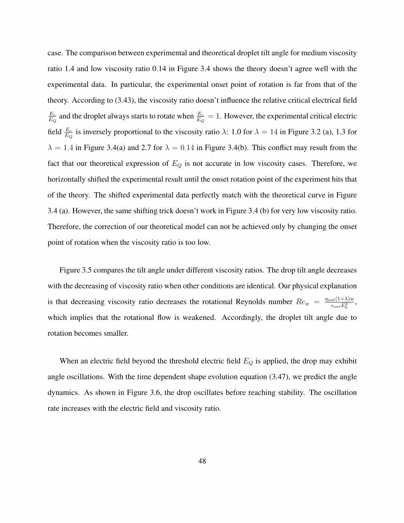
case. The comparison between experimental and theoretical droplet tilt angle for medium viscosity

ratio 1.4 and low viscosity ratio 0.14 in Figure 3.4 shows the theory doesn’t agree well with the

experimental data. In particular, the experimental onset point of rotation is far from that of the

theory. According to (3.43), the viscosity ratio doesn’t influence the relative critical electrical field

EcEQ

and the droplet always starts to rotate when EcEQ

= 1. However, the experimental critical electric

field EcEQ

is inversely proportional to the viscosity ratio λ: 1.0 for λ = 14 in Figure 3.2 (a), 1.3 for

λ = 1.4 in Figure 3.4(a) and 2.7 for λ = 0.14 in Figure 3.4(b). This conflict may result from the

fact that our theoretical expression of EQ is not accurate in low viscosity cases. Therefore, we

horizontally shifted the experimental result until the onset rotation point of the experiment hits that

of the theory. The shifted experimental data perfectly match with the theoretical curve in Figure

3.4 (a). However, the same shifting trick doesn’t work in Figure 3.4 (b) for very low viscosity ratio.

Therefore, the correction of our theoretical model can not be achieved only by changing the onset

point of rotation when the viscosity ratio is too low.

Figure 3.5 compares the tilt angle under different viscosity ratios. The drop tilt angle decreases

with the decreasing of viscosity ratio when other conditions are identical. Our physical explanation

is that decreasing viscosity ratio decreases the rotational Reynolds number Rew = ηout(1+λ)w

εoutE20

,

which implies that the rotational flow is weakened. Accordingly, the droplet tilt angle due to

rotation becomes smaller.

When an electric field beyond the threshold electric field EQ is applied, the drop may exhibit

angle oscillations. With the time dependent shape evolution equation (3.47), we predict the angle

dynamics. As shown in Figure 3.6, the drop oscillates before reaching stability. The oscillation

rate increases with the electric field and viscosity ratio.

48

0 0.5 1 1.5 2 2.5 30

10

20

30

40

50

60

70

80

90

E0/E

Q

tilt

an

gle

, deg

ree

λ=14λ=1.4λ=0.14

Figure 3.5: Comparison of the theoretical drop tilt angle under viscosity ratio 14 (solid line), viscosity ratio 1.4(dash-dot line) and viscosity ratio 0.14 (dashed line) for drop radius 0.9mm. Other physical parameters are same asFigure 3.4.

3.5.2 Drop deformation

The drop deformation D for the electrorotation problem is defined as,

D =L−BL+B

(3.51)

where L = 2r+ is the drop length and B = 2r− is the breadth as shown in Figure 3.7. According

to (3.19), the longest radius r+ and shortest r− in the x-y plane correspond to,

r± = 1 +3

4

√5

π(−1

3f20 ±

√2

3(f ′22 cos 2φ0 − f ′′22 sin 2φ0)) (3.52)

Note that this definition is different from the one introduced by Taylor (see Figure 1.4 (b)), where

zmax and rmax are the drop axes parallel and perpendicular to the electric field. The new definition

49

0 100 200 300 400 5000

20

40

60

80

100

t/tehd

An

gle

, deg

ree

Ca=1.54Ca=2.74Ca=4.29

0 100 200 300 400 5000

10

20

30

40

50

60

70

80

90

t/tehd

An

gle

, deg

ree

λ=1λ=5λ=14

Figure 3.6: a) Evolution of drop tilt angle upon application of electric field for a drop with radius 0.9mm andviscosity ratio λ = 14. E/EQ = 1.5, i.e., Cael = 1.54 (solid line), E/EQ = 2.0, i.e., Cael = 2.74 (dash-dotline), E/EQ = 2.5, i.e., Cael = 4.29 (dashed line) E/EQ = 1.5, i.e., Cael = 1.54 (solid line), E/EQ = 2.0,i.e., Cael = 2.74 (dash-dot line), E/EQ = 2.5, i.e., Cael = 4.29 (dashed line). b) Evolution of the tilt angle uponapplication of electric field for a drop with radius 0.9mm and capillary number Cael = 2.74. viscosity ratio λ = 1(solid line), λ = 5 (dash-dot line), λ = 14 (dashed line). R = 0.027, P = 0.56.

x

y

r−

r+

B L

ϕ0

Figure 3.7: Illustration of the definition for the drop deformation D = (L − B)/(L + B): L is the length and B isthe breadth; r+ and r− corresponds to the longest and the shortest radii. respectively

50

makes more sense in the electrorotation problem, because the droplet tilts and the major/minor

axises are not always parallel or perpendicular to the electric field direction. D is negative for

oblate deformation while positive for prolate deformation under Taylor’s definition. With our

definition, D stays positive.

Figure 3.8 compares the experimental and theoretical deformation for various drop sizes. The

theoretical prediction works better for smaller droplet below a critical electric field, because it

matches better with the small deformation model precondition explained in section 3.1. Before

rotation starts, drop deformation is given by the classical Taylor result (3.1). The deformation

increases with the drop size, because the distorting straining flow is relatively stronger which can

be seen from the bigger electric capillary number. However, beyond the critical electric field,

the deformation decreases with the electric field. The explanation is that elongation produced by

straining flow within one period of rotation is convected towards the compression axis (see Figure

3.9 (a)) by the rotational component of the flow (see Figure 3.9 (b)), so fluid circulation inside the

drop could limit drop deformation.

Figure 3.10 shows the relationship between deformation and drop sizes. Beyond the critical

electric field, the deformation is weakly dependent on the drop size. This is because drop

deformation is limited by the strong rotation, whose rate is size-independent and not the surface

tension, which scales as the capillary number involving the size.

A great advantage of our model over the 2D theory is its dependence on viscosity ratio. Figure

3.11 compares the drop deformation for various viscosity ratios. Once the electrorotation initiates,

drop behavior becomes very sensitive to the viscosity ratio. The reason is that when viscosity

ratio increases, the rotational flow associated with the limitation effect is stronger compared to

the straining flow according to the rotational Reynolds number Rew (2.50). As a result, when the

51

0 0.5 1 1.5 2 2.5 30

0.02

0.04

0.06

0.08

0.1

0.12

0.14

0.16

0.18

E0/E

Q

Def

orm

atio

n

3D theory drop deformationFeng 2D theoryexperimental drop deformation

(a) λ = 14, r = 0.9mm

0 0.5 1 1.5 2 2.5 30

0.05

0.1

0.15

0.2

E0/E

Q

Def

orm

atio

n

3D theory drop deformationFeng 2D theoryexperimental drop deformation

(b) λ = 14, r = 1.05mm

0 0.5 1 1.5 2 2.5 30

0.05

0.1

0.15

0.2

0.25

0.3

0.35

E0/E

Q

Def

orm

atio

n

3D theory drop deformationFeng 2D theoryexperimental drop deformation

(c) λ = 14, r = 1.85mm

0 0.5 1 1.5 2 2.5 30

0.05

0.1

0.15

0.2

0.25

0.3

0.35

0.4

0.45

E0/E

Q

Def

orm

atio

n

3D theory drop deformationFeng 2D theoryexperimental drop deformation

(d) λ = 14, r = 2.45mm

Figure 3.8: Comparison of the 3D theoretical drop deformation (solid line), 2D theoretical drop deformation (dashedline) and experimental result (squares) under viscosity ratio 14 for drop radius a) 0.9mm; b) 1.05mm; c) 1.85mm, d)2.45mm. Other physical parameters same as Figure 3.4.

52

Elongation axis

Compression axis

E

(a) (b)

Figure 3.9: Illustration of the fluid circulation limitation effect on drop deformation.

0 1 2 30

0.05

0.1

0.15

0.2

0.25

0.3

0.35

E0/E

Q

Def

orm

atio

n

r=0.9mmr=1.05mmr=1.85mmr=2.45mm

Figure 3.10: Comparison of the 3D theoretical deformation with viscosity ratio λ = 14 for drop radius 0.9mm (solidline), 1.05mm (dash-dot line), 1.85mm (dashed line) and 2.45mm (dotted line). All other physical parameters same asFigure 3.4.

53

0 0.5 1 1.5 2 2.5 30

0.02

0.04

0.06

0.08

0.1

0.12

0.14

0.16

0.18

E0/E

Q

Def

orm

atio

n

λ=14λ=5λ=1Feng D

Figure 3.11: Comparison of the 2D and 3D theoretical deformation for viscosity ratio 14 (solid line), viscosity ratio5 (dash-dot line) and viscosity ratio 1 (dashed line) for a drop with radius 0.9mm and other physical parameters sameas Figure 3.4.

viscosity ratio is high, i.e., λ = 14, the suppressing effect is strong and deformation decreases

with increasing electric field beyond the critical electric field. In contrast, for low viscosity ratio,

i.e., λ = 1, the suppressing effect is weak and deformation could continue to increase with the

increasing electric field. The deformation of Feng’s 2D theory is irrelevant to the viscosity ratio

and fails to catch this trend.

Before reaching stability, the drop shape exhibits damped oscillations, as predicted by the time

dependent shape evolution equation (3.47). The decaying time scale is controlled by the surface

tension. Figure 3.12 shows the decaying time increases as the electric field and viscosity ratio

increase.

54

0 100 200 300 400 5000

0.02

0.04

0.06

0.08

0.1

0.12

0.14

0.16

t/tehd

Deformation

λ=1λ=5λ=14

(b)

0 100 200 300 400 5000

0.01

0.02

0.03

0.04

0.05

0.06

t/tehd

Deformation

Ca=1.54Ca=2.74Ca=4.29

(a)

Figure 3.12: a) Evolution of the drop shape upon application of electric field for a drop with radius 0.9mm andcapillary number Cael = 2.74, viscosity ratio λ = 1 (solid line), λ = 5 (dash-dot line), λ = 14 (dashed line).R = 0.027, P = 0.56. b) Evolution of the drop shape upon application of electric field for a drop with radius 0.9mmand viscosity ratio λ = 14. E/EQ = 1.5, i.e., Cael = 1.54 (solid line), E/EQ = 2.0, i.e., Cael = 2.74 (dash-dotline), E/EQ = 2.5, i.e., Cael = 4.29 (dashed line).

55

CHAPTER FOUR

BOUNDARY INTEGRAL

FORMULATION IN 2D

4.1 Introduction

The damped oscillations before reaching stability in the small deformation analytical model shown

in section 3.5 could not explain the continuous tumbling and oscillation observed by Salipante

and Vlahovska (2013) [27], which was mentioned in Chapter 1. This leads us to extend our

study beyond the leading order approximation and to the region of very strong electric fields.

The interplay between electric field and fluid motion makes the problem nonlinear without a

closed-form solution, so we turn to numerical methods. The plan is to start from two dimensions.

Boundary integral method [24] allows a parameter of interest, such as the electric field or the

velocity, at a given instant of time to be computed only from variables on the boundary. Therefore,

with this method, the simulation domain reduces from infinite 2D space down to finite 1D interface,

which decreases the computation cost.

56

The boundary integral method satisfies exactly the condition of vanishing perturbation

(quiescent fluid and uniform electric field) far from the drop. In contrast, some numerical methods

need to truncate the outer domain. For example, Feng and Scott (1996) [8] truncated their domain

at a distance of ten drop radii around the drop while using finite element method for simulation.

The truncation effects could be neglected in a studying range of relatively small deformation.

However, when the drop deforms a lot, this might be a serious issue.

The boundary integral method has been successfully used for simulation in various droplet

EHD problems: axisymmetric deformation and stability of a viscous drop (Lac and Homsy, 2007)

[17], drop breakup (Sherwood, 1988) [31], deformation and interaction of drop pairs (Baygents,

Rivette and Stone, 1998) [3], vesicle electrohydrodynamics in DC electric field (McConnell,

Miksis and Vlahovska, 2013) [19]. In this chapter, we are going to build the 2D boundary

integral formulation for both the electric field and the velocity field in preparation for numerical

implementation in Chapter 5.

4.2 Electric field boundary integral equations

4.2.1 Free-space Green’s function

The free space Green’s function corresponding to the electric potential of a point charge problem

is,

∇2G(x, ξ) = −δ(x− ξ) (4.1)

57

+ 1

2vi() =

Z1

4Gijfjds +

Z p.v 1

4Tijk(x, )vjnkds (14)

n · (REin Eout) = Reelrs · (usQ), at r = rs (15)

Q = n · (Eout PEin) (16)

Gij(x, ) = ij ln r +xixj

r2(17)

Tijk(x, ) = 4xixj xk

r4(18)

r = |x| and x = x

2

+ 1

2vi() =

Z1

4Gijfjds +

Z p.v 1

4Tijk(x, )vjnkds (14)

n · (REin Eout) = Reelrs · (usQ), at r = rs (15)

Q = n · (Eout PEin) (16)

Gij(x, ) = ij ln r +xixj

r2(17)

Tijk(x, ) = 4xixj xk

r4(18)

r = |x| and x = x

2

x

y

x

s ζ r

Figure 4.1: Illustration of the observation point ξ, source point x and their distance r

where the derivative is done with respect to x. By Fourier transformation, it’s easy to find the two

dimensional solution,

G(x, ξ) = − 1

2πln r (4.2)

where r = |x − ξ| is the distance between the source point x and the observation point ξ as

illustrated in Figure 4.1.

4.2.2 Boundary integral equation for a point in the bulk

The general boundary integral equation for the electric potential, ψ, of a space point in a domain

Ω enclosed by the boundary ∂Ω is based on the Green’s identity,

x

Ω

(w∇2ψ − ψ∇2w)dA =

∫

∂Ω

(w∇ψ − ψ∇w) · nds (4.3)

58

where w is any scalar. This is derived by multiplying the test scalar w over the Laplacian of the

electric potential and then integrating over the domain Ω,

x

Ω

w∇2ψdA =x

Ω

w∇ · ∇ψdA

=x

Ω

∇ · (w∇ψ)dA−x

Ω

∇w · ∇ψdA

=x

Ω

∇ · (w∇ψ)dA− (x

Ω

∇ · (w∇ψ)dA−x

Ω

ψ∇2wdA)

=x

Ω

ψ∇2wdA+

∫

∂Ω

(w∇ψ − ψ∇w) · nds

(4.4)

In the derivation, we have used integration by parts and the divergence theorem, i.e.,s∇·FdA =

∫F · nds, for a vector field F.

Green’s identity holds in general and connects the integration over a 2D space with the

integration over its boundary. To apply it to our specific drop problem, we replace the general

scalar w with the 2D Green’s function G(x, ξ) and consider the electric field at a point inside the

drop, ξ ∈ Ωin, enclosed by the interface Γ as shown in Figure 4.2, then,

x

Ωin

(G∇2ψin − ψin∇2G)dA =

∫

Γ

(G∇ψin − ψin∇G)] · nds, ξ ∈ Ωin (4.5)

Now substituting ∇2ψin = 0 and ∇2G(x, ξ) = −δ(x − ξ) to the left hand side of equation (4.5),

we obtain the general integral equation for the electric potential at a point in the drop,

ψin(ξ) =

∫

Γ

(G∇ψin − ψin∇G)] · nds, ξ ∈ Ωin (4.6)

Similarly, we could apply Green’s identity (4.3) to the perturbative electric potential, ψout, at

59

a space point belonging to the outside domain, i.e., ξ ∈ Ωout. This time the boundary has two

components, Γ and Γ∞, as shown in Figure 4.2. Since the perturbation at infinity disappears, the

integrals of perturbative electric potential along Γ∞ are zero. The outside perturbative electric

potential satisfies,

ψout(ξ) =−∫

Γ

(G∇ψout − ψout∇G)] · nds+

∫

Γ∞(G∇ψout − ψout∇G)] · nds

︸ ︷︷ ︸=0

=−∫

Γ

(G∇ψout − ψout∇G)] · nds, ξ ∈ Ωout

(4.7)

The negative sign on the right side of equation (4.7) results from the fact that the normal vector n

is defined to be pointing inside with respect to the outer domain.

Note that both the actual electric potential inside and outside are composed of two components.

One is contributed by the applied electric field, ψ∞in/out, and the other is perturbation, ψin/out,

ψin = ψin + ψ∞in , ψout = ψout + ψ∞out (4.8)

Here, we only separate the sources for the outside electric potential. The reason is that the

integration about ψ∞out on the boundary Γ∞ does not disappear, which is different from the case of

ψout. On the other side, the interior domain has only one boundary, Γ, so the boundary integration

equation (4.6) applies to ψin, ψ∞in and their sum ψin.

4.2.3 Boundary integral equation for an interfacial point

For a space point at the interface, i.e., ξ ∈ Γ, there is a singularity problem existing in the Green’s

function when the source point approaches to the observation point, i.e., x→ ξ. To overcome this

60

Ωout

Ωin

Γ Γ∞

n

Figure 4.2: The inner domain Ωin and outer domain Ωout are separated by the interface Γ. The outer domain isunbounded, so Γ∞ is theoretical. The normal unit vector n is defined as pointing from the surface into the outerdomain.

issue, we replace the boundary near the singularity point with a small semicircle centered at ξ of

radius ε. Let’s denote the new boundary as Γ′ and the semicircle Γε as shown in Figure 4.3 (a).

Then the original boundary Γ is the difference between the two boundaries as ε→ 0,

Γ = limε→0

(Γ′ − Γε) (4.9)

Now the singularity point ξ at the old boundary Γ is enclosed by the new boundary Γ′,

equation(4.6) could be applied, then,

ψin(ξ) = limε→0

∫

Γ′(G∇ψin − ψin∇G)] · nds

=

∫

Γ

(G∇ψin − ψin∇G)] · nds+ limε→0

∫

Γε

(G∇ψin − ψin∇G)] · nds

=

∫

Γ

(G∇ψin − ψin∇G)] · nds+1

2ψin(ξ), ξ ∈ Γ

(4.10)

61

Γ '

Γε

ξx

θ = π

θ = 0

ε

Γ '

Γεξ

x

θ = π

θ = 0

ε

(b) (a)

Figure 4.3: (a) Boundary decomposition for calculating the inside electric potential at the singularity point ξ; (b)Boundary decomposition for calculating the outside electric potential at the singularity point ξ

where we have used,

limε→0

∫

Γε

(G∇ψin − ψin∇G)] · nds

= limε→0

∫ π

0

(− 1

2πln r∇ψin + ψin

r

2πr2)] · nε · εdθ

= limε→0

∫ π

0

− 1

2πε ln ε∇ψin · nεdθ + lim

ε→0

∫ π

0

(ψinε

2πε2ε)dθ =

1

2ψin(ξ)

(4.11)

Rearranging the terms in (4.10), we obtain the boundary integral equation for the inside electric

potential of an interfacial point,

1

2ψin(ξ ∈ Γ) =

∫

Γ

(G∇ψin − ψin∇G)] · nds, ξ ∈ Γ (4.12)

Similarly, we can derive the boundary integral equation for the outside perturbative electric

potential of an interfacial point with a new boundary as shown in Figure 4.3 (b),

1

2ψout(ξ ∈ Γ) = −

∫

Γ

(G∇ψout − ψout∇G)] · nds ξ ∈ Γ (4.13)

62

For the outside electric potential due to the applied field, we could use the condition of the

continuous electric potential and obtain,

1

2ψ∞out(ξ) =

1

2ψ∞in (ξ) =

∫

Γ

(G∇ψ∞in − ψ∞in∇G)] · nds =

∫

Γ

(G∇ψ∞out − ψ∞out∇G)] · nds, ξ ∈ Γ

(4.14)

Combining the two equations, (4.13) and (4.14), we arrive at the boundary integral formulation

for the actual outside electric potential at the interface,

1

2ψout(ξ) = −

∫

Γ

(G∇ψout − ψout∇G) · nds+ ψ∞out(ξ), ξ ∈ Γ (4.15)

where we have used the following derivation,

1

2ψout(ξ) =

1

2(ψout(ξ) + ψ∞out(ξ))

=−∫

Γ

(G∇ψout − ψout∇G)] · nds+

∫

Γ

(G∇ψ∞out − ψ∞out∇G)] · nds

=−∫

Γ

(G∇(ψout + ψ∞out)− (ψout + ψ∞out)∇G)] · nds+ 2

∫

Γ

(G∇ψ∞out − ψ∞out∇G)] · nds

=−∫

Γ

(G∇ψout − ψout∇G) · nds+ ψ∞out(ξ), ξ ∈ Γ

(4.16)

To make these equations accessible to our boundary conditions, we add the two boundary

integral equations (4.12) and (4.15) and acquire,

1

2(ψin(ξ)+ψout(ξ)) = ψ∞out(ξ)+

∫

Γ

(G(x, ξ)(∇ψin−∇ψout)+(ψin−ψout)∇G(x, ξ))·nds, ξ ∈ Γ

(4.17)

For getting the boundary integral equation of the electric field at an interfacial point, we take

the gradient with respect to ξ on both side of the above equation and use the relationship between

63

electric field and electric potential E = −∇ψ,

1

2(Eout(ξ) + Ein(ξ))

=E∞(ξ) +

∫

Γ

∇ξG(x, ξ)(Eout · n− Ein · n)ds+

∫

Γ

(ψin − ψout)︸ ︷︷ ︸=0

∇ξ∇G(x, ξ)ds

=E∞(ξ) +1

2π

∫

Γ

r

r2(Eout · n− Ein · n)ds, ξ ∈ Γ

(4.18)

where, the continuous electric potential boundary condition ψin = ψout was applied.

For numerical implementation, we multiply by n(ξ) both sides of the equation to establish the

boundary integral equation of the normal electric field and by the tangential unit vector t(ξ) for

that of the tangential electric field,

E∞(ξ) · n(ξ) +1

2π

∫

Γ

r(s) · n(ξ)

r(s)2(En

out(s)− Enin(s))ds =

1

2(En

out(ξ) + Enin(ξ)) (4.19)

E∞(ξ) · t(ξ) +1

2π

∫

Γ

r(s) · t(ξ)

r(s)2(En

out(s)− Enin(s))ds =

1

2(Et

out(ξ) + Etin(ξ)) = Et(ξ), ξ ∈ Γ

(4.20)

where, s refers to the arclength. For the computation, we first calculate the normal direction electric

field based on equation (4.19) via the current conservation condition (2.37) and the surface charge

density expression (2.38). Et is then found by (4.20) with normal electric field values as inputs.

Details of this numerical process are given in section 5.3.1.

64

4.3 Velocity field boundary integral equations

4.3.1 Free-space Green’s function

According to the Ref. [24] by C. Pozrikidis, the related free space Green’s function problem for

the hydrodynamic flow corresponds to the single point force problem,

∇ · τ = −δ(x− ξ)e, ∇ · u = 0 (4.21)

where, the derivative is about the parameter x. e is the unit directional vector, u the velocity, and

τ the stress tensor.

The solutions for the velocity and corresponding stress tensor in two dimensions are,

ui(x) =1

4πλαGij(u, ξ)ej, τij(x) =

1

4πTijk(x, ξ)ek (4.22)

where, i, j, k represent x, y components, Gij the stokeslet,

Gij(x, ξ) = −δij ln r +xixjr2

(4.23)

and Tijk,

Tijk(x, ξ) = −4xixjxkr4

(4.24)

Space indicators r = |x| and x = x− ξ are shown in Figure 4.1.

65

4.3.2 Boundary integral equation for a point in the bulk

The boundary integral equation for the velocity field at a point ξ in a domain Ω enclosed by the

boundary ∂Ω is built based on the following identity,

x

Ω

(u · ∇ · τ − u · ∇ · τ)dA =x

Ω

∇ · (u · τ − u · τ )dA =

∫

∂Ω

(u · τ − u · τ ) · nds (4.25)

or in its component form,

x

Ω

(ui∂

∂xjτij(u)− ui

∂

∂xjτij(u))dA =

x

Ω

(∂

∂xj(τij(u)ui)−

∂

∂xj(τij(u)ui))dA (4.26)

=

∫

∂Ω

(τij(u)uinj − τij(u)uinj)ds (4.27)

where τ is an arbitrary stress tensor that corresponds to the velocity u and pressure p, and τ an

arbitrary stress tensor relates to the velocity u and pressure p, i.e.,

τij(u) = −δijp+ µ(∂uj∂xi

+∂ui∂xj

), τij(u) = −δij p+ µ(∂uj∂xi

+∂ui∂xj

) (4.28)

Both of the two cases have the same viscosity µ.

The equality (4.27) is a result of the divergence theorem. The derivation of the equality (4.26)

66

involves the following steps,

∂

∂xj(τij(u)ui) =

∂

∂xj(−δijuip+ µui(

∂uj∂xi

+∂ui∂xj

))

=∂

∂xj(−ujp+ µui(

∂uj∂xi

+∂ui∂xj

))

=− p ∂uj∂xj︸︷︷︸

=∇·u=0

−uj∂p

∂xj+ µ

∂ui∂xj

(∂uj∂xi

+∂ui∂xj

) + µui(∂

∂xi(∂uj∂xj

)

︸ ︷︷ ︸=∇·u=0

+∂2ui∂x2

j

)

=− uj∂p

∂xj+ µ

∂ui∂xj

(∂uj∂xi

+∂ui∂xj

) + µui(∇2ui)

=− uj∂p

∂xj+

1

2µ∂ui∂xj

(∂uj∂xi

+∂ui∂xj

) +1

2µ∂uj∂xi

(∂ui∂xj

+∂uj∂xi

) + µui(∇2ui) (exchange the indices i and j)

=ui(µ∇2ui −∂p

∂xi) +

1

2µ(∂ui∂xj

+∂uj∂xi

)(∂uj∂xi

+∂uj∂xi

)

=ui∂

∂xjτij(u) +

1

2µ(∂ui∂xj

+∂uj∂xi

)(∂uj∂xi

+∂uj∂xi

)

(4.29)

and similarly,

∂

∂xj(τij(u)ui) =

∂

∂xjτij(u)uidA+

1

2µ(∂ui∂xj

+∂uj∂xi

)(∂uj∂xi

+∂uj∂xi

)dA (4.30)

The integration over the difference of the equations (4.29) and (4.30) yields,

x

Ω

(∂

∂xj(τij(u)ui)−

∂

∂xj(τij(u)ui))dA =

x

Ω

(ui∂

∂xjτij(u)− ui

∂

∂xjτij(u))dA (4.31)

The identity (4.25) holds in general. To apply it to our problem, we assume the velocity u,

pressure p and stress tensor τ are solutions for the Stokes equation, while the other sets u, p, τ

67

satisfy the point force problem (4.21). The boundary integral expression (4.27) becomes,

∫

∂Ω

(τij(u)uinj − τij(u)uinj)ds (∗)

=

∫

∂Ω

(1

4πµGij(x, ξ)σij(u)njej −

1

4πTijk(x, ξ)uinjek)ds

=

∫

∂Ω

(1

4πµGij(x, ξ)fiej −

1

4πTijk(x, ξ)uinjek)ds

=

∫

∂Ω

(1

4πµGij(x, ξ)fjei −

1

4πTijk(x, ξ)ujnkei)ds (∗∗)

(4.32)

where, fj is the jth component force exerting on the boundary from the enclosed domain and

relates to the stress tensor by fj = τjknk. In step (∗), we substituted solutions of the point force

problem, i.e., ui(x) = 14πµ

Gij(x, ξ)ej and τij(u) = 14πTijk(x, ξ)ek. In step (∗∗), the indices i, j, k

are exchanged by virtue of the symmetry in Gij and Tijk.

Substituting∇ · τ = 0 and∇ · τ = −δ(x− ξ)e, the integration expression (4.26) over the 2D

domain could be reduced to the velocity at a single point,

x

Ω

(ui∂

∂xjτij(u)− ui

∂

∂xjτij(u)) =

x

Ω

uiδij(x− ξ)eidA =

ui(ξ)ei, ξ ∈ Ω

0, ξ 6∈ Ω

(4.33)

Finally, with (4.32) and (4.33), we arrive at,

ui(ξ) =1

4πµ

∫

∂Ω

Gij(x, ξ)fjds−1

4π

∫

∂Ω

Tijk(x, ξ)ujnkds, ξ ∈ Ω (4.34)

0 =1

4πµ

∫

∂Ω

Gij(x, ξ)fjds−1

4π

∫

∂Ω

Tijk(x, ξ)ujnkds, ξ 6∈ Ω (4.35)

This general boundary integral equation relates the velocity of the fluid at a given point ξ with

the integrals around the boundary of the domain. The first line integral is called the single layer

68

potential of the force density fj and the second integral is referred to as the double layer potential

of uj .

4.3.3 Boundary integral equation for an interfacial point

Similarly to the way we deal with the electric field, to obtain the boundary integral equation for the

velocity of a point at the interface, we have to treat the inside and outside velocity at the interface

separately. Again, the domain and boundary are denoted the same as in Figure 4.2. And we

decompose the actual inside and outside velocity into two components, uin/out which vanishes at

infinity and u∞in/out attributed to the imposed flow,

uin = uin + u∞in, uout = uout + u∞out (4.36)

Similar decomposition applies to the viscous force, fin/out,

fin = fin + f∞in , fout = fout + f∞out (4.37)

The velocity is continuous across the interface, but the mismatch of viscosity of the inner and outer

domain leads to discontinuity of the viscous stresses inside and outside. Accordingly,

∆f∞ = f∞out − f∞in , ∆f = fout − fin, ∆f = fout − fin (4.38)

Since the viscous stress tensor is proportional to the viscosity, the jump of the force, ∆f∞, due to

the imposed flow satisfies,

f∞in = λf∞out, ∆f∞ = (1− λ)f∞out =1− λλ

f∞in (4.39)

69

Consider the limit of a point approaching the interface from the outer domain, i.e., ξ ∈ Ωout ∩

ξ → Γ, the integration of variables over the inner domain according to (4.35) is,

0 =1

4πλ

∫

Γ

Gij(x, ξ)f∞in,jds−1

4π

∫

Γ

Tijk(x, ξ)u∞in,jnkds

=1

4π(1− λ)

∫

Γ

Gij(x, ξ)∆f∞ds− 1

4π

∫

Γ

Tijk(x, ξ)u∞j nkds

(4.40)

where, we have plugged in (4.39) and used the boundary condition of continuous velocity, i.e.

u∞in,j = u∞out,j = u∞j , because ξ is almost at the interface.

Similarly, applying (4.35) to the perturbative velocity at ξ and integrating over the inside

domain, we obtain,

0 =1

4πλ

∫

Γ

Gij(x, ξ)fin,jds−1

4π

∫

Γ

Tijk(x, ξ)ujnkds (4.41)

To utilize the boundary force condition, we apply (4.34) to the perturbative velocity at ξ but

integrate over the outer domain,

uout,i(ξ) =− 1

4π

∫

Γ

Gij(x, ξ)fout,jds+1

4π

∫

Γ

Tijk(x, ξ)uout,jnkds

+1

4π

∫

Γ∞Gij(x, ξ)fout,jds−

1

4π

∫

Γ∞Tijk(x, ξ)uout,jnkds

︸ ︷︷ ︸=0

=− 1

4π

∫

Γ

Gij(x, ξ)fout,jds+1

4π

∫

Γ

Tijk(x, ξ)ujnkds

(4.42)

where the integrals of perturbative variables, fout,j and uout,j , disappear because the influence of

the drop surface at infinity is trivial.

Multiplying λ on both side of (4.41) and then being subtracted from (4.42), we arrive at the

70

boundary integral equation for the outside perturbative velocity of a point approaching to the

interface infinitely from the outer domain,

uout,i(ξ) = − 1

4π

∫

Γ

Gij(x, ξ)∆fjds+1− λ

4π

∫

Γ

Tijk(x, ξ)ujnkds, ξ ∈ Ωout ∩ ξ → Γ (4.43)

The combination of (4.40) and (4.43) gives the boundary integral equation for the actual outside

velocity at ξ,

uouti (ξ) = − 1

4π

∫

Γ

Gij(∆fj + ∆f∞j )ds+1− λ

4π

∫

Γ

Tijk(x, ξ)ujnkds

⇒uouti (ξ) = u∞i (ξ)− 1

4π

∫

Γ

Gij∆fjds+1− λ

4π

∫

Γ

Tijk(x, ξ)ujnkds, ξ ∈ Ωout ∩ ξ → Γ

(4.44)

For a space point right at the interface, i.e., ξ ∈ Γ, there are singularity issues existing in both

the single kernel integration and double kernel integration as the source point approaching to the

observation point. To proceed for a boundary integral equation of an interfacial point, we apply the

similar trick as for the electric potential and replace the nearby boundary with a small semicircle

centered at ξ with radius ε as in Figure 4.3 (b). Then the boundary Γ is the difference between the

new boundary Γ′ and the semicircle Γε as ε→ 0,

Γ = limε→0

(Γ′ − Γε) (4.45)

Since the interfacial point, ξ ∈ Γ, is enclosed by and approaches to the new boundary, Γ′.

71

Therefore, we could apply equation (4.44) and have,

uouti (ξ) =u∞0 (ξ)− limε→0

1

4π

∫

Γ′Gij∆fjds+ lim

ε→0

1− λ4π

∫

Γ′Tijk(x, ξ)ujnkds)

=u∞0 (ξ)− 1

4π

∫

Γ

Gij∆fjds+1− λ

4π

∫

Γ

Tijk(x, ξ)ujnkds

− limε→0

1

4π

∫

Γε

Gij∆fjds+ limε→0

1− λ4π

∫

Γε

Tijk(x, ξ)ujnkds

(4.46)

The forth term disappears because,

limε→0

1

4π

∫

Γε

Gij∆fjds = limε→0

1

4π

∫ 2π

π

(−δij ln r +xixjr2

)∆fjεdθ

= limε→0

1

4π

∫ 2π

π

(−δij ln ε+xixjε2

)∆fjεdθ = 0 (xixj ∼ ε2) (4.47)

The fifth term becomes,

limε→0

1− λ4π

∫

Γε

Tijk(x, ξ)ujnkds = limε→0

1− λ4π

∫

Γε

(−4xixjxkr4

)ujnkds

=− 1− λπ

limε→0

∫ 2π

π

xixjxkε4

ujxkεεdθ (n =

x

ε)

=− 1− λπε2

uj(ξ) limε→0

∫ 2π

π

xixjdθ (x2k = ε2, uj(x)→ uj(ξ))

=− 1− λπε2

uj1

2πε2δij (∗)

=1− λ

2ui(ξ)

(4.48)

At step (∗), we used∫ 2π

πxixjdθ = 1

2πε2δij , which can be seen by making x1 = ε cos θ, x2 = ε cos θ

and integrating separately on x1x1, x1x2 and x2x2.

Substituting (4.47) and (4.48) into (4.46) , we find the boundary integral equation for a point ξ

72

right at the interface,

λ+ 1

2ui(ξ) = u∞0 (ξ)− 1

4π

∫Gij∆fjds+

1− λ4π

∫Tijk(x, ξ)ujnkds, ξ ∈ Γ (4.49)

Because there is no imposed flow in our problem, u∞0 (ξ) disappears. Therefore,

λ+ 1

2ui(ξ) = − 1

4π

∫Gij∆fjds+

1− λ4π

∫Tijk(x, ξ)ujnkds, ξ ∈ Γ (4.50)

73

CHAPTER FIVE

NUMERICAL SCHEME AND RESULTS

5.1 Introduction

With the boundary integral formulation established in Chapter 4, the task is left to implementation.

The electric fields are computed by,

E∞(ξ) · n(ξ) +1

2π

∫r(s) · n(ξ)

r(s)2(En

out(s)− Enin(s))ds =

1

2(En

out(ξ) + Enin(ξ))

E∞(ξ) · t(ξ) +1

2π

∫r(s) · t(ξ)

r(s)2(En

out(s)− Enin(s))ds = Et(ξ)

R(Enin − En

out) = Reel∇t · (uQ)

Q = Enout − PEn

in

(5.1)

which are based on information of the interface position and the velocity. The boundary integral

equation (4.50) for the velocity field,

λ+ 1

2ui(ξ) = − 1

4π

∫Gij∆fjds+

1− λ4π

∫Tijk(x, ξ)ujnkds (5.2)

74

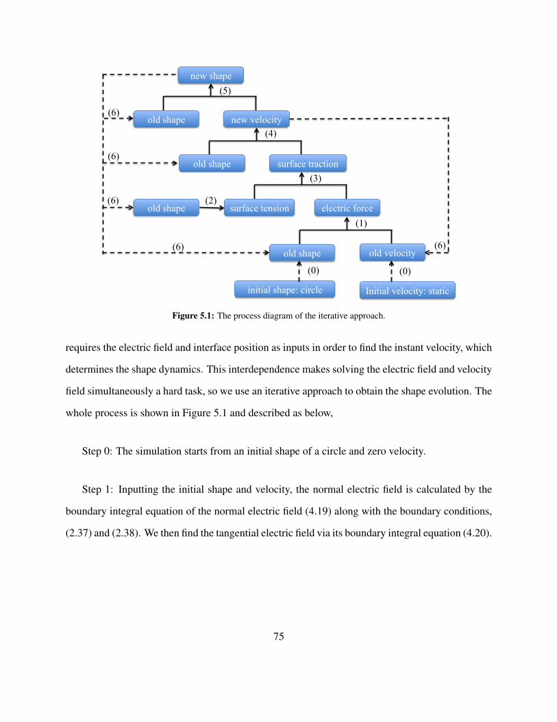
new shape

old shape new velocity

old shape surface traction

surface tension electric force

old velocity old shape

old shape

(5)

(1)

(3)

(4)

(2)

(6)

(6)

(6)

(6) (6)

initial shape: circle Initial velocity: static

(0) (0)

Figure 5.1: The process diagram of the iterative approach.

requires the electric field and interface position as inputs in order to find the instant velocity, which

determines the shape dynamics. This interdependence makes solving the electric field and velocity

field simultaneously a hard task, so we use an iterative approach to obtain the shape evolution. The

whole process is shown in Figure 5.1 and described as below,

Step 0: The simulation starts from an initial shape of a circle and zero velocity.

Step 1: Inputting the initial shape and velocity, the normal electric field is calculated by the

boundary integral equation of the normal electric field (4.19) along with the boundary conditions,

(2.37) and (2.38). We then find the tangential electric field via its boundary integral equation (4.20).

75

The value of the normal and tangential electric force follow from equations (2.27) and (2.28),

(n · [Tel])n =1

2εout(E

2out,n − E2

out,t)−1

2εin(E2

in,n − E2in,t)

(n · [Tel])t = EtQ

(5.3)

The numerical scheme for the electric field is given in section 5.3.

Step2: From the old shape information, the curvature H is found, which determines the

dimensionless surface tension, i.e., Ca−1el Hn. The numerical process of obtaining the mean

curvature from the shape information is described in section 5.2.3.

Step3: With the surface tension calculated in step 2 and the electric force obtained in step 1,

the surface traction is found by the stress balance condition ((2.42)),

∆f = Ca−1el Hn− n · [Tel] (5.4)

Step 4: Using the boundary integral equation for the velocity field (4.50), we compute the new

velocity from the old shape and the surface traction from step 3 as inputs. Details of the numerical

scheme for the velocity field is shown in section 5.4.

Step 5: The new shape is computed based on the previous shape and the new velocity. This

step is elaborated in section 5.2.2.

Step 6: The old shape and velocity are updated with new ones. The simulation cycle continues.

The implementation of the boundary integral equations for the velocity and electric field mainly

encounter two challenges: integration and singularity. To realize integration numerically, we

76

equally discretize the interface to N points with respect to the arclength. The parameters such

as the electric field strength, electric field force, velocity on the surface are represented in the

vector form composed of the corresponding parameter at each point. Then integration over the

interface is naturally realized by matrix multiplication. The singularity of the free-space Green’s

kernels will be handled analytically first.

In section 5.2, we introduce the shape representation including discretization, shape updating

techniques etc. Details about the matrix representation and singularity removal for the electric field

and velocity field boundary integral equations are given in section 5.3 and section 5.4, respectively.

At the end in section 5.4, the computational results under various Capillary number are validated

by Feng’s 2D theory.

5.2 Shape representation

5.2.1 Spectral representation

The drop interface is represented by the spectral method, x(s) =∑k=∞

k=−∞ x(k)φ(s) , where φ(s)

is a complete basis and s is a parameter. Here for our 2D problem with N discretized points, we

choose the Fourier expansions e−iks to be φ(s) and arclength to be s. Therefore,

x(s) =

k=N/2−1∑

k=−N/2x(k)e−iks (5.5)

For uniformly distributed points, the coefficients x(k) can be computed by Fast Fourier

Transformation.

77

This spectral representation allows us to easily calculate the first derivative and second

derivative,

xs(s) =

k=N/2−1∑

k=−N/2(−ik)x(k)e−iks, xss(s) =

k=N/2−1∑

k=−N/2(−ik)2x(k)e−iks (5.6)

which will be used later to determine curvature and normal vector of the surface.

5.2.2 Updating and remeshing the shape

To update the shape of the drop, we use the Runge-Kutta Method to achieve a second order

accuracy. Runge-Kutta method is a single-step method, however, with multiple stages per step.

For each time step n, we first compute the velocity un+1/2 at the midpoint of the time interval ∆t

and then obtain the position at the end of that step using the midpoint velocity,

xn+1 = xn + un+1/2∆t (5.7)

After the updating, we remesh the surface by dividing the points equally again with cubic spline

interpolation in order to use Fast Fourier Transformation to calculate the coefficients x(k) in the

spectral representation.

5.2.3 Curvature and unit normal vector

The dimensionless capillary stress is Ca−1Hn, which is dependent on the curvatureH and the unit

normal vector n. The purpose in this part is to express the curvature as a function of the derivatives

78

of the position with respect to the arclength s, so that it can be found once the position x(s) is

known.

The curvature measures the rate at which a space curve r(t) = (x, y) changes direction. Its

magnitude equals to the changing rate of the unit tangential vector t with respect to the arclength,

H = |dtds| = |ts| = |rss| = |(xss, yss)| =

√x2ss + y2

ss (5.8)

where we have used the definition for a unit tangential vector,

t =rs|rs|

|rs| = |dr

ds| = | tds

ds| = 1

⇒ t = rs = (xs, ys) (5.9)

From the perpendicular relationship between the unit normal and tangential vectors, i.e., n· t =

0, it’s easy to obtain the expression of n for numerical computation,

n = (ys,−xs) (5.10)

5.2.4 Error test

To validate the shape representation by the spectral method, we tested the accuracy of the

numerically computed normal vector and curvature of an ellipse, x2

m2 + y2

n2 = 1, which is depicted

in Figure 5.2. The ratio of the minor and major axes for the ellipse is defined as k = nm

. k = 1.0

corresponds to a circle. The further the ratio k is away from one, the more deviated the ellipse is

from a circle.

79

-m m

-n

n x2

m2 +y2

n2=1 (mcosθ, nsinθ )

x

y

θ

Figure 5.2: The ellipse x2

m2 + y2

n2 = 1 with major axis m and minor axis n

Theoretical unit normal vector and curvature of an ellipse

The parameterized space curve of an ellipse could be represented as r(θ) = (m cos θ, n sin θ). So

the unit tangential vector is,

t(θ) =r′(θ)

|r′(θ)| =(−m sin θ, n cos θ)

|(−m sin θ, n cos θ)| = (− sin θ√

sin2 θ + k2 cos2 θ,

k cos θ√sin2 θ + k2 cos2 θ

) (5.11)

The unit normal vector n is perpendicular to the tangential vector, i.e., n(θ) · t(θ) = 0.

Therefore,

n(θ) = (k cos θ√

sin2 θ + k2 cos2 θ,

sin θ√sin2 θ + k2 cos2 θ

) (5.12)

80

According to the curvature function (5.8), the theoretical curvature of the ellipse is,

H = |d2r(θ)

ds2| = | d

ds(dr(θ)

ds)| = |dt(θ)/dθ

ds/dθ|

=|(− k2 cos θ

m(sin2 θ + k2 cos2 θ)2,− k sin θ

m(sin2 θ + k2 cos2 θ)2)|

=k

m(sin2 θ + k2 cos2 θ)1.5

(5.13)

where, we have used the first derivative of the unit tangential vector with respect to the parameter

θ,

dt(θ)

dθ=d

dθ(

− sin θ√sin2 θ + k2 cos2 θ

,k cos θ√

sin2 θ + k2 cos2 θ)

=(− k2 cos θ

(sin2 θ + k2 cos2 θ)1.5,− k sin θ

(sin2 θ + k2 cos2 θ)1.5)

(5.14)

and the first derivative of the arclength s with respect to the parameter θ,

s =

∫ θ

0

|r′(u)|du =

∫ θ

0

√m2 sin2 u+ n2 cos2 udu

⇒ ds

dθ=

√m2 sin2 θ + n2 cos2 θ = m

√sin2 θ + k2 cos2 θ

(5.15)

Accuracy of the numerical unit normal vector of an ellipse

Here, the numerical unit normal vector computed by (5.10) is compared with the theoretical normal

vector indicated in (5.12). Figure 5.3 gives the relationship between the biggest absolute error for

the normal vector components, nx and ny, among all discretized points and the number of total

interpolating points. Note that the absolute error was used instead of the relative error, because

the theoretical unit normal vector components might be zero at some points. When k = 0.5 and

k = 2.5, the error largely decreases with increasing interpolating points, which could be identified

81

−2.6 −2.4 −2.2 −2 −1.8−16

−14

−12

−10

−8

−6

−4

log10

(1/n)

log

10(a

bsol

ute

erro

r of

nx)

k = 2.5k = 1.0k = 0.5

(a)

−2.6 −2.4 −2.2 −2 −1.8−16

−14

−12

−10

−8

−6

−4

log10

(1/n)

log

10(a

bsol

ute

erro

r of

ny)

k = 2.5k = 1.0k = 0.5

(b)

Figure 5.3: Plot of the absolute error of the numerical normal vector components (a) nx and (b) ny by the spectralmethod versus the inverse of interpolation points n = 72, 144, 288 for a sphere (solid line); an ellipse with k = n

m =0.5(dash-dot line); an ellipse with k = 2.5(dashed line).

as the discretization error. For the case of a circle, k = 1, the spectral method already gives a very

small error of the order 10−14 even when the total number of interpolation points is as few as 72.

Therefore, the main contributor for the total error of a circle should be the roundoff error, which is

not necessarily decreasing as more interpolation points are used. The generally small order of the

error and the right trend of the error as a function of the number of interpolation points prove the

high accuracy of the spectral method on first order derivatives.

82

Accuracy of the numerical curvature for an ellipse

To test the accuracy of the numerical curvature for an ellipse, H =√x2ss + y2

ss. We first compare

each of its two components, xss and yss, with their theoretical values from equation (5.13). Figure

5.4 shows the absolute errors of the two second order derivatives. The general trend is very similar

to the first order derivative. The discretization error decreases when more interpolation points were

used for the case of k = 0.5 and k = 2.5. The roundoff error dominates in the case of a circle,

i.e., k = 1. For the same k and number of interpolation points, the absolute error of the second

order derivatives is generally 1000 times higher than the first order derivatives. For example, when

k = 2.5 and n = 288, the absolute error for nx is on the order of 10−7, while the absolute error

for xss is on the order of 10−4. The low absolute errors and systematic agreement with first order

errors validate the implementation of the spectral method for second order derivatives.

Figure 5.5 shows the relative error of the numerical curvature versus the number of total

interpolation points. The small errors of the curvature for very "deformed" shapes such as k = 2.5

and k = 0.5 proves that the numerical values of surface tension in our simulation are reliable.

5.3 Numerical scheme for the electric field

5.3.1 Matrix representation

The numerical scheme for the boundary integral equation of the normal direction electric field

(4.19) is,

(1

2πF− 1

2I)En

out − (1

2πF +

1

2I)En

in = −En∞ (5.16)

83

−2.6 −2.4 −2.2 −2 −1.8−12

−10

−8

−6

−4

−2

0

log10

(1/n)

log

10(a

bsol

ute

erro

r of

xss

)

k = 2.5k = 1.0k = 0.5

(a)

−2.6 −2.4 −2.2 −2 −1.8−12

−10

−8

−6

−4

−2

0

log10

(1/n)

log

10(a

bsol

ute

erro

r of

yss

)

k = 2.5k = 1.0k = 0.5

(b)

Figure 5.4: Plot of the absolute error for the second order derivatives (a) xss and (b) yss by the spectral method versusthe inverse of interpolation points n = 72, 144, 288 for a sphere (solid line); an ellipse with k = 0.5 (dash-dot line); anellipse with k = 2.5 (dashed line).

84

−2.6 −2.4 −2.2 −2 −1.8−12

−10

−8

−6

−4

−2

log10

(1/n)

log

10(r

elat

ive

erro

r of

cur

vatu

re)

k = 2.5k = 1.0k = 0.5

Figure 5.5: Plot of the relative error of the numerical curvature by the spectral method versus the inverse ofinterpolation points n = 72, 144, 288 for a sphere (solid line); an ellipse with k = 0.5 (dash-dot line); an ellipsewith k = 2.5 (dashed line).

85

where all the bold parameters represent matrices or vectors. I is a N × N identity matrix. Enin,

Enout and En

∞ are N × 1 vectors composed of the normal direction inside, outside and external

electric field at each interfacial point. F is the N × N matrix form of r(s)·n(ξ)r2(s)

ds with the element

Flm =(xl−xm)nxl+(yl−ym)nyl

(xl−xm)2+(yl−ym)2ds, where the subscripts l,m indicate the lth and mth points, (x, y) the

2D position, ds the arclength interval, (nx, ny) the normal vector.

To establish the numerical scheme for the electric field boundary conditions, Q = n · (Eout −

PEin) and n · (REin − Eout) = Reel∇t · (uQ), we first combine them into one equation,

(REnin − En

out) = ∇t · (uQ)

=Reel · ((ut)sQ+ utQs +QunH) (∗)

=Reel(Dut + unH)(Enout − PEn

in) +ReelutD(Enout − PEn

in)

=Reel(Dut + unH + utD)Enout − PReel(Dut + unH + utD)En

in

(5.17)

where D represents first order derivative with respect to the arclength. The derivation for step (*)

is as below,

∇s · (usQ) = ∇s · (uttQ) +∇s · (unnQ)

=∂(utQ)

∂s+Qun∇s · n + n · ∇s(unQ)

=∂(utQ)

∂s+QunH = (ut)sQ+ utQs +QunH

(5.18)

Now the normal direction electric field boundary condition (5.17) in the matrix form is,

(M + I)Enout − (PM +RI)En

in = 0 (5.19)

where we have defined a N × N matrix M = Reel(Dut + Hun + utD) with D a N × N

86

dimensional first order derivative operator, ut and un both N × 1 dimensional vectors composed

of the corresponding normal and tangential vector components at each point, H a N ×N diagonal

matrix composed of the mean curvature as the diagonal elements.

With the matrix form of the normal direction electric field governing equation (5.16) and

boundary condition (5.19), we can write a 2N × 2N block matrix system to solve the normal

electrical field numerically,

( 12πF− 1

2I) −( 1

2πF + 1

2I)

(M + I) −(PM +RI)

×

Eno

Eni

=

−En

∞

0

(5.20)

which yields for the solutions,

Eno

Eni

=

( 12πF− 1

2I) −( 1

2πF + 1

2I)

(M + I) −(PM +RI)

−1

×

−En

∞

0

(5.21)

After solving the normal electric field, the tangential electric field follow from the following

matrix representation derived from the boundary integral equation (4.20),

Et = Et∞ +

1

2πFT(En

out − Enin) (5.22)

where, FTij =(xi−xj)txi+(yi−yj)tyi

(xi−xj)2+(yi−yj)2 ds.

87

5.3.2 Dealing with singularity of the Green’s function

Note that both matrices F and FT in (5.21) and (5.22) include singularity points when the

source point (x(s), y(s)) approaches to the observation point x(s0), y(s0). These singularities

are introduced by the Green’s function. The singularity in F can be removed by L’Hopital’s rule,

lims→s0

Fss0 = lims→s0

[x(s0)− x(s)]ys(s0)− [y(s0)− y(s)]xs(s0)

[x(s0)− x(s)]2 + [y(s0)− y(s)]2=

0

0

= lims→s0

1

2

−xs(s)ys(s0) + ys(s)xs(s0)

[x(s)− x(s0)]xs(s) + [y(s)− y(s0)]ys(s)=

0

0

=1

2

−xss(s)ys(s0) + yss(s)xs(s0)

x2s(s) + y2

s(s) = 1

=1

2[−xss(s0)ys(s0) + yss(s0)xs(s0)] (5.23)

where we have substituted the expression for the normal vector x component, i.e., nx = ys, and y

component, i.e., ny = −xs.

L’Hopital’s rule does not apply at the singularity point in FT, but the singularity could be

removed in the context of integration by the following procedure,

FT(Eno − En

i ) , FTf =

∫r(s) · t(s)r(s)2

f(s)ds

=

∫r(s) · t(s) + sin[π(s− s0)]/π

r2(s)f(s)ds−

∫sin[π(s− s0)]

πr2(s)f(s)ds

=

∫r(s) · t(s) + sin[π(s− s0)]/π

r2(s)f(s)ds−

∫sin[π(s− s0)]

πr2(s)[f(s)− f(s0)]ds

−∫

sin[π(s− s0)]

πr2(s)f(s0)ds

(5.24)

88

For the first term at s = s0, we can use the L’Hopital’s rule,

lims→s0

r(s) · t(s) + sin[π(s− s0)]/π

r(s)2

= lims→s0

[x(s0)− x(s)]xs(s0) + [y(s0)− y(s)]ys(s0) + sin[π(s− s0)]/π

[x(s)− x(s0)]2 + [y(s)− y(s0)]2=

0

0

= lims→s0

1

2

−xs(s)xs(s0)− ys(s)ys(s0) + cos[π(s− s0)]

[x(s)− x(s0)]xs(s) + [y(s)− y(s0)]ys(s)=

0

0

= lims→s0

1

2

−xss(s)xs(s0)− yss(s)ys(s0)− π sin[π(s− s0)]

[x(s)− x(s0)]xss(s) + [y(s)− y(s0)]yss(s) + x2s(s) + y2

s(s)

= −1

2[xs(s0)xss(s0) + ys(s0)yss(s0)] (5.25)

For the second term, at s = s0, we have f(s) − f(s0) = 0. Therefore, this term disappears at

the singularity point.

For the third term, we can draw a small semicircle with radius ε around the singularity point

similar as in Figure 4.3 (a), then,

lims→s0

sin[π(s− s0)]

πr2(s)f(s0) = lim

ε→0

∫ s0+ε

s0−ε

sin[π(s− s0)]

πr2(s)f(s0)ds

=f(s0) limε→0

∫ s0+ε

s0−ε

sin[π(s− s0)]

πε2ds = f(s0) lim

ε→0

∫ π

0

sin[π(εθ − ε)]πε2

εdθ

=f(s0) limε→0

∫ π

0

ε(θ − 1)

ε2εdθ = f(s0)(

1

2π2 − π)

(5.26)

Substituting (5.25) and (5.26) into (5.24), we obtain,

FTf =

∫

s 6=s0

r(s) · t(s)r(s)2

f(s)ds− (1

2(xsxss + ysyss) + (

1

2π2 − π))f(s0) (5.27)

89

Therefore, FT could be implemented as below,

FTij/ds =

(xi−xj)tx+(yi−yj)ty(xi−xj)2+(yi−yj)2 , i 6= j

−12(xsxss + ysyss)− (1

2π2 − π), i = j

(5.28)

5.3.3 Error test

To validate the numerical scheme for the electric field (5.21) , we could compare the numerical

electric field at t = 0 before the drop deformation starts and hydrodynamic flow arises with the

theoretical electric field around a undeformed ellipse in 2D.

Theoretical electric field around a undeformed ellipse in two dimensions

For a undeformed ellipse, x2

m2 + y2

n2 = 1, the theoretical electric field on the surface is [40],

Enin =

Enout

R=E0(m+ n)

Rm+ n

m sin θ√m2 sin2 θ + n2 cos2 θ

Etin = Et

out =E0(m+ n)

Rm+ n

n cos θ√m2 sin2 θ + n2 cos2 θ

(5.29)

Because the derivation for (5.29) is more tedious, here we derive the theoretical electric field for a

undeformed circle, which is similar to the derivation for an ellipse but easier to show.

Assume a undeformed circle of radius a exposed to the electric field with magnitude E0 as

shown in Figure 5.6, the potential in the bulk satisfies the Laplace equation,

∇2φ = 0 (5.30)

90

E

a

r

Θ

Figure 5.6: A solid sphere of radius a vexposed to the electric field

whose general solution in 2D is,

φ(r, θ) = A ln r +K +∞∑

n=1

rn(An sin(nθ) +Bn cos(nθ)) +∞∑

n=1

r−n(Cn sin(nθ) +Dn cos(nθ))

(5.31)

Here, A, K, An, Bn, Cn, Dn are all constant coefficients and (r, θ) is the polar coordinates.

At r = 0, the potential is finite, therefore, all the terms include r−n and ln r should disappear.

The inside potential adopts the form,

φin(r, θ) = Kin +∞∑

n=1

rn(An sin(nθ) +Bn cos(nθ)) (5.32)

At infinity, perturbation is ignored, the potential approaches to−E0r cos θ. The outside electric

91

potential should have the form,

φout(r, θ) = Kout − E0r cos θ +∞∑

n=1

r−n(Cn sin(nθ) +Dn cos(nθ)) (5.33)

On the surface r = a, it has the boundary condition of continuous potential and current

conservation,

φin(a, 0) = φout(a, 0), σout∂φout∂r

= σin∂φin∂r

(5.34)

Substituting the general form of the inside and outside potential into the two boundary

conditions, we have,

Kin +∞∑

n=1

an(An sin(nθ) +Bn cos(nθ)) = Kout − E0a cos θ +∞∑

n=1

a−n(Cn sin(nθ) +Dn cos(nθ))

σin

∞∑

n=1

nan−1(An sin(nθ) +Bn cos(nθ)) = −σout[E0 cos θ +∞∑

n=1

na−(n+1)(Cn sin(nθ) +Dn cos(nθ)]

(5.35)

To satisfy the relationship in (5.35), it is required that the coefficients satisfy,

An = Cn = 0, Bn = Dn = 0, n 6= 1

B1 = − 2E0

R+1, D1 = R−1

R+1a2E0

(5.36)

With these coefficients, the potential inside and outside are found to be,

φin(r, θ) = − 2E0

R + 1r cos θ, φout(r, θ) = −[r +

1−R1 +R

a2

r]E0 cos θ (5.37)

92

By E = −∇φ, the electric field is found to be,

Enin(r, θ) = −∂φin

∂r=

2E0

R + 1cos θ, En

out(r, θ) = −∂φout∂r

= (1− 1−R1 +R

a2

r2)E0 cos θ

Etin(r, θ) = −∂φin

r∂θ= − 2E0

R + 1sin θ, Et

out(r, θ) = −∂φoutr∂θ

= −(1 +1−R1 +R

a2

r2)E0 sin θ

(5.38)

Accuracy of normal and tangential electric field around a undeformed ellipse

As shown in Figure 5.7, the absolute error of the numerical normal electric field inside and outside

around an ellipse are both as low as 10−12 with 288 interpolation points. For the more deformed

ellipse k = 2.5 and k = 0.5, the logarithm error decreases linearly with the increasing interpolation

points, which could be identified as the discretization error. For the circle, the total error is already

very small for interpolation points as few as 72 and thus dominated by the roundoff error, which is

independent of number of total interpolation points. The absolute error of the numerical tangential

electric field is greatly increased compared to the numerical normal electric field. The added error

is quite likely introduced from the singularity point in the matrix FT included in (5.22). The

tangential electric field error linearly decreases with the number of total interpolation points. The

accuracy of the electric field could be improved, but at relatively expensive computational cost.

93

−2.6 −2.4 −2.2 −2 −1.8−15

−10

−5

0

log10

(1/n)

log

10(a

bsol

ute

erro

r of

Einn

)

k = 2.5k = 1.0k = 0.5

(a)

−2.6 −2.4 −2.2 −2 −1.8−2.5

−2

−1.5

−1

−0.5

log10

(1/n)

log

10(a

bsol

ute

erro

r of

Et in

)

k = 2.5k = 1.0k = 0.5

(b)

−2.6 −2.4 −2.2 −2 −1.8−15

−10

−5

log10

(1/n)

log

10(a

bsol

ute

erro

r of

Eou

tn

)

k = 2.5k = 1.0k = 0.5

(c)

−2.6 −2.4 −2.2 −2 −1.8−2.5

−2

−1.5

−1

−0.5

log10

(1/n)

log

10(a

bsol

ute

erro

r of

Et ou

t)

k = 2.5k = 1.0k = 0.5

(d)

Figure 5.7: Plot of the absolute error of (a) the normal inside electric field Enin; (b) the tangential inside electric field

Etin; (c) the normal outside electric field En

out; (d) the tangential outside electric field Etout versus the inverse of the

interpolation points n = 72, 144, 288. Solid line is for the ellipse with ratio k = 2.5; dash-dot line for k = 1.0 anddashed line for k = 0.5.

94

5.4 Numerical scheme for the velocity field

5.4.1 Matrix representation

Substituting the stress balance condition ∆f = Ca−1Hn − [Tel] · n in the boundary integral

equation for the velocity field (4.50), we find

1 + λ

2v(ξ)i = − 1

4π

∫Gij(

H

Caeln− [Tel] · n)ds+

1− λ4π

∫Tijk(x, ξ)vjnkds (5.39)

Its corresponding matrix form is,

1 + λ

2

vx

vy

=

Sxx Sxy

Syx Syy

(− 1

4πCael×

HNx

HNy

+

1

4π

fex

fey

)

+1− λ

4

TNxx TNxy

TNyx TNyy

×

vx

vy

(5.40)

where vx and vy are both N × 1 vectors composed of the x and y direction velocity at each point,

HNx and HNy both N × 1 vectors corresponding to the product of mean curvature and normal

vector components (Hnx and Hny), fex and fey both N × 1 vectors indicating x and y component

electric force density. Also, we have defined the following 2N × 2N matrices,

S = Gijds, TN = Tijknkds (5.41)

Note that we were working in the normal and tangential coordinate for computing the electric

field, but change into the x − y coordinate heres for a clearer expression of S and TN. The two

95

coordinates is related by the normal and tangential vectors.

Rearranging the terms, the matrix form (5.40) gives us the numerical scheme for updating the

velocity, vx

vy

= (DL)−1

Sxx Sxy

Syx Syy

(− 1

4πCael×

Hx

Hy

+

1

4π

fex

fey

) (5.42)

where,

DL =1 + λ

2I− 1− λ

4πTN (5.43)

5.4.2 Dealing with singularity of the stokeslet and its associated stress tensor

As the source point s approaches the observation point s0 on the surface, singularity appear in

both the stokeslet Gij and its associated stress tensor Tijk. Therefore, the implementation of the

corresponding matrix S and DL encounter singularity issues. For the stokeslet Gij = −δij ln r +

xixjr2

, the second term xixjr2

has a removable singularity at s = s0 via L’Hopital’s rule. Using i = 1

represents the x component and j = 2 the y component, then,

lims→s0

x1x2

r2= lim

s→s0

[x(s)− x(s0)][y(s)− y(s0)]

[x(s)− x(s0)]2 + [y(s)− y(s0)]2=

0

0

= lims→s0

xs(s)[y(s)− y(s0)] + ys(s)[x(s)− x(s0)]

2xs(s)[x(s)− x(s0)] + 2ys(s)[y(s)− y(s0)]=

0

0

= lims→s0

xss(s)[y(s)− y(s0)] + 2xs(s)ys(s) + yss(s)[x(s)− x(s0)]

2xss(s)[x(s)− x(s0)] + 2xs(s)xs(s) + 2yss(s)[y(s)− y(s0)] + 2ys(s)ys(s)

=xs(s0)ys(s0)

x2s(s0) + y2

s(s0)= xs(s0)ys(s0)

(5.44)

Similarly, we could derive,

lims→s0

x1x1

r2= x2

s(s0), lims→s0

x2x2

r2= y2

s(s0) (5.45)

96

For the first term in the stokeslet −δij ln r, the L’Hopital’s rule doesn’t work. We consider the

singularity in the context of integration,

−∫ 1

0

δij ln r∆fj(s)ds =

∫ 1

0

(−δij1

2ln r2)∆fj(s)ds

=−∫ 1

0

δij1

2ln

π2r2

sin2 π(s− s0)∆fj(s)ds−

∫ 1

0

δij(∆fj(s)−∆fj(s0))1

2ln[

sin2 π(s− s0)

π2]ds

− δij∆fj(s0)

∫ 1

0

1

2ln[

sin2 π(s− s0)

π2]

︸ ︷︷ ︸=0

ds

=− lims→s0

δij1

2ln

π2r2

sin2 π(s− s0)︸ ︷︷ ︸(∗)=0

∆fj(s)ds− lims→s0

δij (∆fj(s)−∆fj(s0))︸ ︷︷ ︸=0

1

2ln[

sin2 π(s− s0)

π2]ds

−∫ 1

0,s 6=s0δij

1

2ln

π2r2

sin2 π(s− s0)∆fj(s)ds−

∫ 1

0,s 6=s0δij(∆fj(s)−∆fj(s0))

1

2ln[

sin2 π(s− s0)

π2]ds

=−∫ 1

0,s 6=s0δij ln r∆fj(s)ds+ δij∆fj(s0)

∫ 1

0,s 6=s0

1

2ln[

sin2 π(s− s0)

π2]ds

(5.46)

where, the (*) term could be proved to be equal to 0 by L’ Hopital’s rule,

lims→s0

lnπ2r2

sin2 π(s− s0)= ln lim

s→s0

π2r2

sin2 π(s− s0)= ln

0

0

= ln lims→s0

2π2(s− s0)

2π sinπ(s− s0) cosπ(s− s0)= ln

0

0

= ln lims→s0

1

cos(s− s0)= ln 1 = 0

(5.47)

Equation (5.46) implies that for the numerical computation, we could define ln r =

−∫ 1

0,s 6=s012

ln[ sin2 π(s−s0)π2 ]ds at s = s0.

97

To summarize, the stokeslet Gij could be implemented as,

Gij =

−δij ln r +xixjr2, s 6= s0

δij∫ 1

0,s 6=s012

ln[ sin2 π(s−s0)π2 ]ds+ (xi)s(s0)(xj)s(s0), s = s0

(5.48)

The singularity in the stress tensor Tijk is integrally removable. From (4.48), we know that∫ L

0

−4xixj xkr4

nk(s)ds = 2πvi(s0) for a circle. Therefore,

∫ 1

0

Tijkvj(s)nk(s)ds =

∫ 1

0

−4xixjxkr4

vj(s)nk(s)ds

=

∫ 1

0

−4xixjxkr4

(vj(s)− vj(s0))nk(s)ds+ vj(s0)

∫ 1

0

−4xixjxkr4

nk(s)ds

≈∫ 1

0

−4xixjxkr4

(vj(s)− vj(s0))nk(s)ds− 2πvi(s0)

(5.49)

The last step approximation sign ≈ is due to the deviation from a circle. So the stresslet could be

implemented as,

Tijk =

−4xixj xkr4

, s 6= s0

−2π, s = s0

(5.50)

5.4.3 Error test

At equilibrium, the surface normal velocity should vanish and the deformation becomes stable.

Figure 5.8 shows the deformation evolution under a big electric Capillary number Cael = 0.68,

R = 0.01 and P = 0.5. The dimensionless time step is dt = 0.01. After 2000 steps, the

deformation approaches the limit of 0.18. The drop evolves from a circle to a stable oblate, which

agrees with the prediction we described in section 2.6 for cases R < P .

98

0 5 10 15 200

0.05

0.1

0.15

0.2

time t

defo

rmat

ion

D

−0.2 −0.1 0 0.1 0.2−0.2

−0.15

−0.1

−0.05

0

0.05

0.1

0.15

0.2

x

y

Figure 5.8: (a) Evolution of the drop deformation D under Capillary number Cael = 0.68. (b) The drop deforms toan oblate (dashed line) from a circle (solid line).The dimensionless time interval is dt = 0.01; total time steps is 2000;72 interpolation points. Other parameters include P = 0.5, R = 0.01, λ = 1.

Figure 5.9 shows the deformation evolution under the same big Capillary number Ca = 0.68,

R = 0.8 and P = 0.5. The dimensionless time interval is dt = 0.01. After 2000 steps, the

deformation reaches the limit of 0.065. The drop becomes an prolate from a circle, which agrees

with the prediction for cases of R > P .

5.5 Results

To validate our result, we start from the no viscosity contrast case, λ = 1, and without charge

convection, Reel = 0. The numerical deformation is compared to the theoretical 2D deformation

from Feng’s model [7] for various electric Capillary numbers, which is depicted in Figure 5.10.

The deformation is defined the same way as in (3.51).

99

0 5 10 15 200

0.02

0.04

0.06

0.08

time t

defo

rmat

ion

D

−0.2 −0.1 0 0.1 0.2−0.2

−0.1

0

0.1

0.2

x

y

Figure 5.9: (a) Evolution of the drop deformation D under Capillary number Cael = 0.68. (b) The drop deforms toan oblate (dashed line) from a circle (solid line).The dimensionless time interval is dt = 0.01; total time steps is 2000;72 interpolation points. Other parameters include P = 0.5, R = 0.8, λ = 1.

(a)

79

0 0.2 0.4 0.6 0.80

0.02

0.04

0.06

0.08

0.1

0.12

0.14

0.16

Ca

D

OurDFengD

Figure 6.1: Comparison with Feng’s 2D theory: the numerical deformation D versus Capillary numberCa. Parameters are adopted from Feng’s paper [35]: R = 0.01, P = 0.5, = 1, drop radius r = 1mm.

the sign of breakup as seen in Figure

(b)

(c)

Cael

Figure 5.10: Comparison with Feng’s 2D theory: (a) the numerical deformation D versus electric Capillary numberCael. Parameters are adopted from Feng’s paper [7]: R = 0.01, P = 0.5, λ = 1, drop radius r = 1mm. Code isstable for (b) very deformed oblate and starts to be unstable when the drop starts to show the sign of (c) breakup.

100

We adopted the parameters from Ref. [7], where R < P , so the droplet is supposed to be

deformed to an oblate shape. For small Capillary number below 0.2, the numerical deformation is

inseparable from the 2D theory. The deviation from the leading order theory starts around Capillary

number 0.2 and gradually increases as the Capillary number gets bigger.

Our simulation starts to be unstable beyond Capillary number 0.64, where the drop starts to

show the sign of breakup as seen in the Figure 5.10 (c) according to the 2D theoretical model.

This prevents us from investigating interesting dynamics under a bigger Capillary number. One

potential reason is that the equally distributed interpolation points does not give sufficient accuracy

for the concave area like in Figure 5.10 (c). On one side, the accuracy of the boundary integral

method declines when the boundary includes sharp corners. And it might be improved when more

boundary elements are distributed around regions with strong variation [24]. On the other side,

equal distribution is required to utilize the Fast Fourier Transformation to compute accurate first

order and second order derivatives of the positions. This problem is hoped to be solved for future

research.

101

CHAPTER SIX

CONCLUSION AND OUTLOOK

In this thesis, we investigated the electrorotation of a droplet in a uniform electric field analytically

and numerically. For small deformations, a 3D analytical model was built up, which takes into

account the charge convection dominated by the rotational flow. In particular, our theory captures

the limitation effects of fluid circulation on drop deformation. The results show that beyond the

critical electric field, drop deformation is insensitive to drop size but very sensitive to the viscosity

ratio, which is a big advantage over the 2D theory with viscosity ratio independence. The evolution

equation shows that the drop shape can exhibit damped oscillations while approaching steady

state. The leading order analytical solutions agree quantitatively well with the experiment for

very viscous and small size drops. However, the agreement for drops with lower viscosity is only

qualitative because of the non-negligible charge convection from the straining component of the

electrohydrodynamic flow.

For large deformations, we adopted the boundary integral equation and established the

numerical scheme for 2D. As a preliminary result, the 2D numerical deformation has been

validated by Feng’s 2D analytical theory [7]. Without viscosity contrast, the simulations extend

beyond the small deformation region and reache electric Capillary number as high as 0.68. For

102

bigger electric capillary number, the numerical method becomes unstable. Several methods that

we have tried to stabilize the codes all failed. These include increasing the interpolation points to

as many as 288, decreasing the time interval to as low as 10−5, and adding an arbitrary velocity

tangential to the surface to maintain a proper distribution of the points [4]. Future research direction

for improving the code stability could start from trying unequal distributed points. The extension

from 2D to 3D might encounter some difficulties, but it’s an important work in a sense that a 3D

model is more realistic.

103

APPENDIX A

Maxwell-Wagner time scale

The transient response of an ohmic dielectric sphere to a suddenly applied electric field provides

physical insight concerning the Maxwell-Wagner charge relaxation mechanism [14].

Consider a spherical particle of radius a with dielectric constant εin and conductivity σin

suspended in another kind of fluid with dielectric constant εout and conductivity σout. Assume

that a uniform electric field in the z direction is turned on suddenly,

E(t) = E0g(t)z (A.1)

where g(t) is the unit step function. Similar to the derivation in section 3.3.1, the potential outside

ψout and inside ψin the sphere should take the following form to satisfy the Laplace equation and

the far field condition,

ψout = −E0g(t)r cos θ +A(t) cos θ

r2, ψin = −B(t)r cos θ (A.2)

The boundary conditions (2.6), (2.7) and (2.8) without convection current apply here as well.

104

P

w

E0

x

y

z

a εin,σin

εout,σout

Θ r

Figure A.1: Dielectric sphere of radius a with dielectric constant εin and conductivity σin suspended in another fluidwith εout and σout. The whole system is subjected to a uniform electric field of magnitude E0.

Substituting the expression of Ein/out = −∇ψin/out into the boundary conditions, we obtain,

a−3A(t) +B(t) = E0g(t)

2a−3A(t) cos θ − σinσout

B(t) cos θ +1

σout

∂Q

∂t= −E0g(t) cos θ

Q = [−2a−3A(t)εout + εinB(t)− E0εoutg(t)] cos θ

(A.3)

This yields the solution for A(t),

A(t) =σin − σoutσin + 2σout

E0(1− e−t/τMW ) +εin − εoutεin + εout

E0e−t/τMW (A.4)

Therefore, the effective moment is,

Peff = 4πεoutA(t) = 4πεout[σin − σoutσin + 2σout

E0(1− e−t/τMW ) +εin − εoutεin + εout

E0e−t/τMW ] (A.5)

which implies that the Maxwell-Wagner time scale τMW is the relaxation time scale associated

with the accumulation of free charge Q at the surface of the sphere.

105

APPENDIX B

Quincke rotation

When a solid sphere immersed in a leaky dielectric liquid subjected in a uniform z direction electric

field same as in Figure A.1, the Quincke rotation appears above a threshold electric field when the

charge relaxation inside the object is slower than that of liquid outside the object, i.e., tc,out < tc,in

[34]. The rotation happens because an initial perturbation deviates the dipole from its original

unfavorable orientation and creates a non-zero electric torque,

Tel = Peff × E0 (B.1)

where Peff and E0 stand for the effective dipole moment of the sphere and the external electric

field, respectively. At the same time, the viscous forces generate friction to restrain rotation, which

is proportional to the rotational rate. The corresponding viscous torque is given by,

Tη = −8πa3ηoutwQx (B.2)

At steady state, the conservation of angular momentum yields the equation of momentum,

IdwQdt

x = Tel + Tη (B.3)

106

where I is the inertial of momentum and wQ the angular velocity.

Under a rotating coordinate system at rest with respect to the sphere, the electric field E0 and

effective dipole moment Peff satisfy,

E0 = Re[E0(z− iy)e−iwQt], Peff = Re[4πa3εoutε∗in − ε∗out

ε∗in + 2ε∗out

E0(z− iy)e−iwQt] (B.4)

where the complex dielectric constants are ε∗in/out = εin/out − iσin/outwQ.

Therefore, the electric torque follows from (B.1),

Tel = 6πεouta3E2

0

R(P −R)

(2 + P )(R + 2)

Ω

1 + Ω2x (B.5)

where we have defined the dimensionless angular velocity Ω = wQτMW .

The equation of motion (B.3) could be casted into an ordinary differential equation by

substituting (B.5) and (B.2),dΩ

dt= AΩ(

B

Ω2 + 1− 1) (B.6)

where,

A =8πa3ηoutwQ

I, B =

E20

E2Q

, E2Q =

2σoutηoutP (R + 2)2

3εoutεin(P −R)(B.7)

The ODE has the solutions,

Ω =

0, (B > 1)

0 (unstable solution), ±√B − 1 (stable solutions), (B > 1)

(B.8)

where ± reflects two possible rotational directions.

107

APPENDIX C

Scalar and vector spherical harmonics

The normalized spherical scalar harmonics are defined as [37],

Yjm(θ, φ) = [2j + 1

4π

(j −m)!

(j +m)!](−1)mPm

j (cos θ)eimφ (C.1)

where (r, θ, φ) are the spherical coordinates and Pmj (cos θ) the Legendre polynomials.

The vector spherical harmonics are defined as,

yjm0 = [j(j + 1)]−1/2r∇ΩYjm, yjm1 = −ir× yjm0, yjm2 = rYjm (C.2)

where r = rr

and ∇Ω denotes the angular part of the gradient operator. yjm0 and yjm1 are

tangential, while yjm2 is normal to a sphere.

Some of the spherical harmonics we have used in the calculations are,

Y1,0 =1

2

√1

π, Y1,±1 = ±1

2

√3

2πsin θe±iφ

Y2,0(θ, φ) =1

4

√5

π(3 cos2 θ − 1), Y2,±2(θ, φ) =

1

4

√15

2πe±2iφ sin2 θ

(C.3)

108

APPENDIX D

Fundamental solution sets of velocity fields

The expressions for the fundamental sets of velocity field u±jmq(r, θ, φ) that satisfy the Stokes

equation are [37],

u−jm0 =1

2r−j(2− j + jr−2)yjm0 +

1

2r−j[j(j + 1)]1/2(1− r−2)yjm2

u−jm1 = r−j−1yjm1

u−jm2 =1

2r−j(2− j)( j

1 + j)1/2(1− r−2)yjm0 +

1

2r−j(j + (2− j)r−2)yjm2

(D.1)

u+jm0 =

1

2rj−1[−(j + 1) + (j + 3)r2]yjm0 −

1

2rj−1[j(j + 1)]1/2(1− r2)yjm2

u+jm1 = rjyjm1

u+jm2 =

1

2rj−1(3 + j)(

j + 1

j)1/2(1− r2)yjm0 +

1

2rj−1[j + 3− (j + 1)r2]yjm2

(D.2)

On a sphere r = 1 these fundamental solutions reduce to,

u±jmq = yjmq (D.3)

109

Therefore, u±jm0 and u±jm1 are tangential, and u±jm2 is normal to a sphere. In general, a vector

velocity field which is tangential to a surface with normal n can be viewed as the sum of an

irrotational component and a solenoidal component

n · (∇s × virr) = 0

∇s · vsol = 0

(D.4)

Checking the definition of the vector spherical harmonics, it’s obvious that the irrotational

component is identified by the q = 0 vector spherical harmonic, and the solenoidal corresponds to

the q = 1 vector spherical harmonic on a sphere.

110

APPENDIX E

2D leading-order solution for drops with

electrorotation

For drops with electrorotation taking into account charge convection dominated by rotational flow,

the electric potential ψin/out and velocity field vin/out take the forms [7],

ψout = −Ω ln r + (1− 1

r2)(B2 cos 2θ + β2 sin 2θ)

ψin =Ω

2(1− r2) + (r4 − r2)(B2 cos 2θ + β2 sin 2θ)

(E.1)

and,

vout = −Er cos θ +E

r(ξ1 cos θ + Ξ1 sin θ)

vin = −Er(1− ξ1) cos θ − Ξ1 sin θ

(E.2)

111

where,

ξ1 =−[ ˆRe2

el(1− P )(1 +R) + (1 + P )(1−R)]

(P + 1)(1 +R)(1 + ˆRe2el)

Ξ1 =−2 ˆReel(P −R)

(P + 1)(1 +R)(1 + ˆRe2el)

(E.3)

and,

B2 =(1 +R)2

4|P −R| [(P + 1)ξ1 − 1]Ξ1

β2 =(1 +R)2

8|P −R| [1− P + 2Pξ1 − (P + 1)(ξ21 − Ξ2

1)]

(E.4)

with the dimensionless angular velocity,

Ω =1

Reel

√2(P −R)(1 +R)(1 + λ)PReel

|P −R|λ(1 + P )− 1

ˆReel = ReelΩ

(E.5)

The expressions for leading-order drop deformation D2D and drop tilt angle θ2 are described

by,

D2D = α2

√1 + tan2 2θ2, θ2 =

1

2arctan(A2/α2) (E.6)

where,

α2 =εinaE

20

12γP[3(1− P ) + 6Pξ1 + (1− 3P )(ξ2

1 − Ξ21)]

A2 =εinaE

20

6γP[3P + (1− 3P )ξ1]Ξ1

(E.7)

112

Bibliography

[1] O. O. Ajayi. A note on taylor’s electrohydrodynamic theory. Proc. R. Soc. Lond.,364:499–507, 1978.

[2] Allan and Mason. Particle behavior in shear and electric fields.1. deformation and burst offluid drops. Proc. Royal Soc. A, 267:45–61, 1962.

[3] J. C. Baygents, N. J. Rivette, and H. A. Stone. Electrohydrodynamic deformation andinteraction of drop pairs. J. Fluid. Mech., 368:359–375, 1998.

[4] Ivan Bazhlekov. Non-singular boundary-integral method for deformable drops in viscousflows. 2003.

[5] P. Dutta D. Byun, V. D. Nguyen and H. C. Park. A hybrid inkjet printer utilizingelectrohydrodynamic jetting and piezoelectric actuation. Japanese Journal of AppliedPhysics, 49:060216, 2010.

[6] J. Q. Feng. Electrohydrodynamic behavior of a drop subjected to a steady uniform electricfield at finite electric reynolds number. Proc. Royal Soc. A, 455:2245–2269, 1999.

[7] J. Q. Feng. A 2d electrohydrodynamic model for electrorotation of fluid drops. J. Coll. Int.Sci., 246:112–121, 2002.

[8] J. Q. Feng and T. C. Scott. A computational analysis of electrohydrodynamics of a leakydielectric drop in an electric field. J. Fluid. Mech., 311:289–326, 1996.

[9] Quincke G. Ueber rotation em im constanten electrischen felde. Ann. Phys. Chem.,59:417–86, 1896.

[10] C. G. Garton and Z. Krasucki. Bubbles in insulating liquids: Stability in an electric field.Proc. Roy. Soc. Lond., 280:211–226, 1964.

[11] J. W. Ha and S. M. Yang. Electrohydrodynamics and electrorotation of a drop with fluid lessconductive than that of the ambient fluid. Phys. Fluids, 12:764–772, 2000.

[12] J. W. Ha and S. M. Yang. Rheological responses of oil-in-oil emulsions in an electric field.J. Rheol., 44:235–256, 2000.

[13] H. He, P. F. Salipante, and P. M. Vlahovska. Electrorotation of a viscous droplet in a uniformdirect current electric field. Phys. Fluids, 25:032106, 2013.

113

[14] Thomas B. Jones. Electromechanics of particles. Cambridge University Press, 1995.

[15] S. Krause and P. Chandratreya. Electrorotation of deformable fluid droplets. J. Coll. Int. Sci.,206:10–18, 1998.

[16] Pijush K. Kundu and Ira M. Cohen. Fluid mechanics. 4th edition.

[17] E. Lac and G. M. Homsy. Axisymmetric deformation and stability of a viscous drop in asteady electric field. J. Fluid. Mech, 590:239–264, 2007.

[18] E. Lemaire, L. Lobry, and N. and Pannacci. Viscosity of an electro-rheological suspensionwith internal rotations. J. Rheology, 52:769–783, 2008.

[19] L. C. McConnell, M. J. Miksis, and P. M. Vlahovska. Vesicle electrohydrodynamics in dcelectric fields. IMA Journal of Applied Mathematics, 2013.

[20] J. R. Melcher and G. I. Taylor. Electrohydrodynamics - a review of role of interfacial shearstress. Annu. Rev. Fluid Mech., 1:111–146, 1969.

[21] C. T. O’Konski and R. L. Gunther. Verification of the free energy equation for electricallypolarized droplets. J. Colloid Sci., 10:563–570, 1955.

[22] C. T. O’Konski and F. E. Harris. Electric free energy and the deformation of droplets inelectrically conducting systems. J. Phys. Chem, 61:1172–1174, 1957.

[23] C. T. O’Konski and H. C. Thacher. The distortion of aerosol droplets by an electric field. J.Phys. Chem, 57:955–958, 1953.

[24] C. Pozrikidis. Boundary integral and singularity methods for linearized viscous flow.Cambridge University Press, 1992.

[25] K. J. Ptasinski and P. J. A. M. Kerkhof. Electric field driven separations: Phenomena andapplications. Sep. Sci. Technol, 27:995, 1992.

[26] P. F. Salipante and P. M. Vlahovska. Electrohydrodynamics of drops in strong uniform dcelectric field. Phys. Fluids, 22:11210, 2010.

[27] P. F. Salipante and P. M. Vlahovska. Electrohydrodynamics of drops in strong uniform dcelectric field. Physical Review E, 88:043003, 2013.

[28] H. Sato, N. Kaji, T. Mochizuki, and Y. H. Mori. Behavior of oblately deformed dropletsin an immiscible dielectric liquid under a steady and uniform electric field. Phys. Fluids,18:127101, 2006.

[29] D. A. Saville. Electrohydrodynamics: The taylor-melcher leaky dielectric model. Annu.Rev.Fluid Mech., 29:27–64, 1997.

[30] J. Schwalbe, P.M. Vlahovska, and M. Miksis. Vesicle electrohydrodynamics. Phys. Rev. E,83:046309, 2011.

114

[31] J. D. Sherwood. Breakup of fluid droplets in electric and magnetic fields. J. Fluid Mech.,188:133–146, 1988.

[32] G. I. Taylor. Studies in electrohydrodynamics. i. circulation produced in a drop by an electricfield. Proc. Royal Soc. A, 291:159–166, 1966.

[33] S. Torza, R.G. Cox, and S.G. Mason. Electrohydrodynamic deformation and burst of liquiddrops. Phil. Trans. Royal Soc. A, 269:295–319, 1971.

[34] I. Turcu. Electric field induced rotation of spheres. J. Phys. A: Math. Gen., 20:3301–3307,1987.

[35] O. Vizika and D. A. Saville. The electrohydrodynamic deformation of drops suspended inliquids in steady and oscillatory electric fields. J. Fluid Mech., 239:1–21, 1992.

[36] P. M. Vlahovska. On the rheology of a dilute emulsion in a uniform electric field. J. FluidMech., 670:481–503, 2011.

[37] P. M. Vlahovska and R. S. Gracia. Dynamics of a viscous vesicle in linear flows. Phys. Rev.E, 75:016313, 2007.

[38] P.M. Vlahovska, J. Blawzdziewicz, and M. Loewenberg. Small-deformation theory for asurfactant-covered drop in linear flows. J. Fluid Mech, 624:293–337, 2009.

[39] J.S. Yagoobi. Electrohydrodynamic pumping of dielectric liquids. Journal of Electrostatics,63:861–869, 2005.

[40] K. W. Yu and P. M. Hui. Effective dielectric response of nonlinear composites. PhysicalReview B, 47:21, 1992.

115