ELEN602 Lecture 3

• Review of last lecture

– layering, IP architecture

• Data Transmission

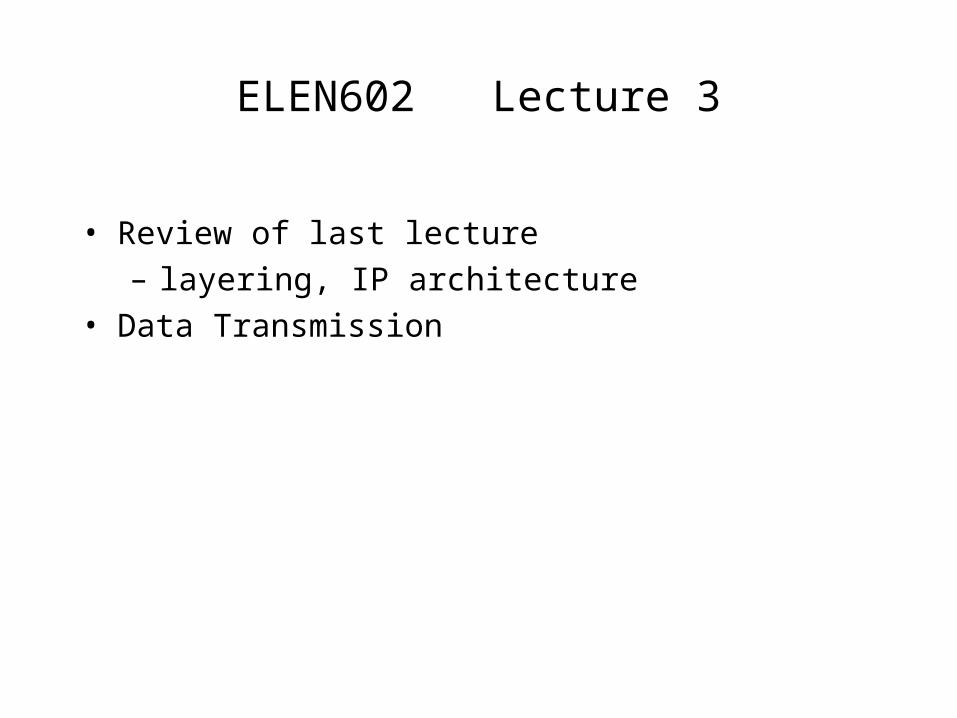
Receiver

Communication channel

Transmitter

Abstract View of Data Transmission

Communication Channel Properties:

-- Bandwidth

-- Transmission and Propagation Delay

-- Jitter

-- Loss/Error rates

-- Buffering

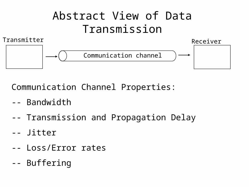
(a) Analog transmission: all details must be reproduced accurately

Sent

Sent

Received

Received

• e.g digital telephone, CD Audio

(b) Digital transmission: only discrete levels need to be reproduced

• e.g. AM, FM, TV transmission

Analog vs. Digital Transmission

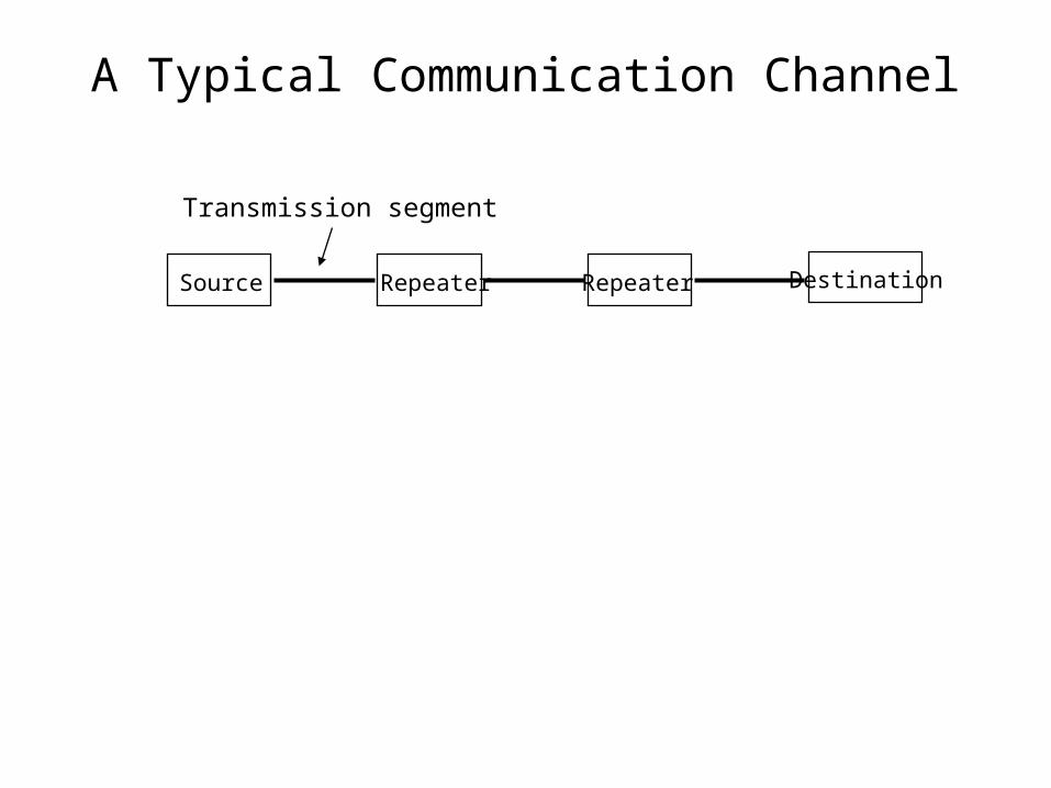
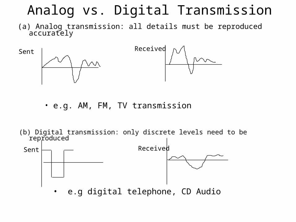
Source Repeater DestinationRepeater

Transmission segment

A Typical Communication Channel

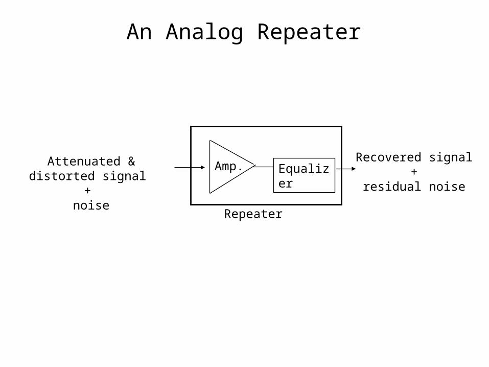
Attenuated & distorted signal +

noise

EqualizerRecovered signal

+residual noise

Repeater

Amp.

An Analog Repeater

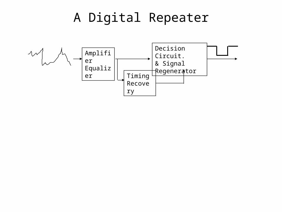
AmplifierEqualizer

TimingRecovery

Decision Circuit.& SignalRegenerator

A Digital Repeater

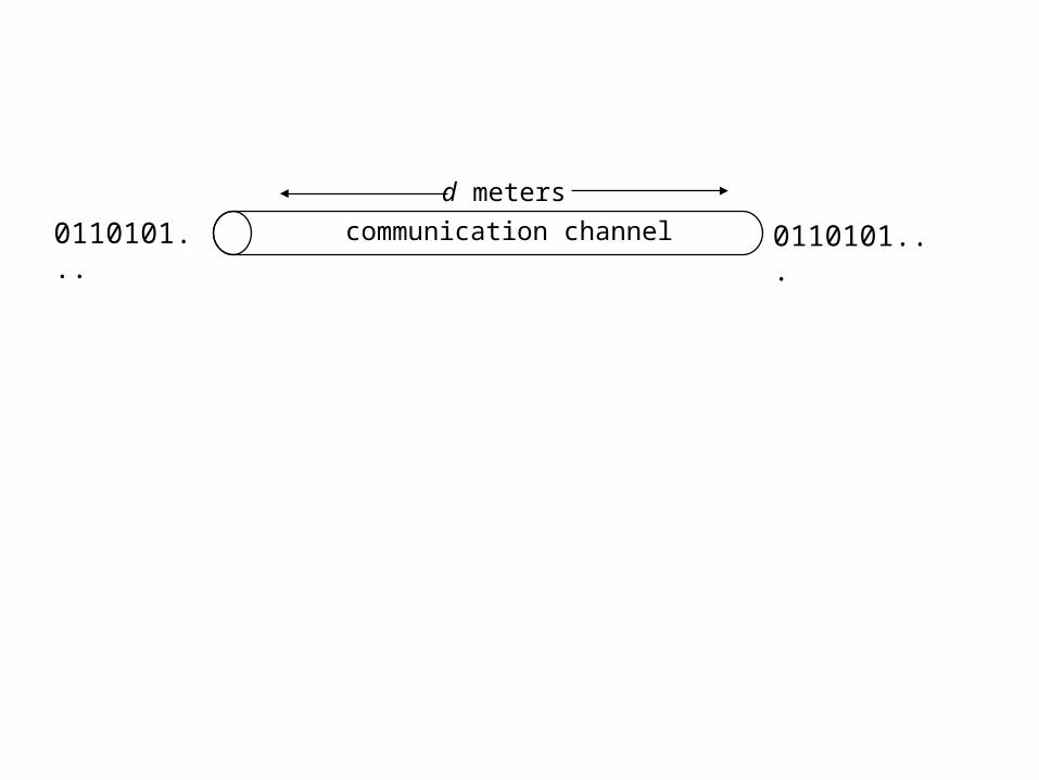
communication channel

d meters

0110101... 0110101...

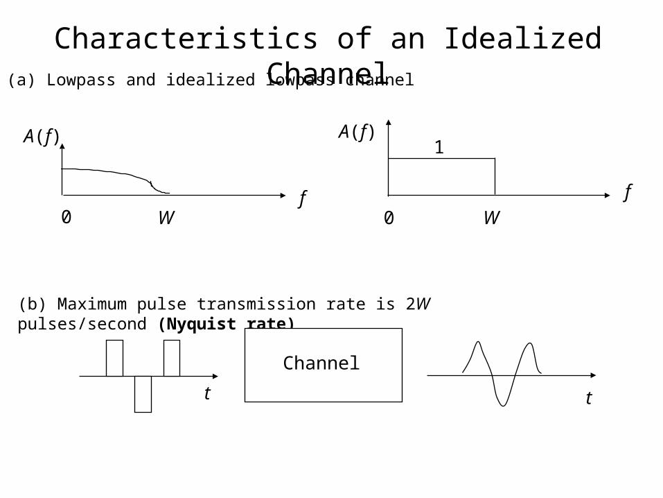
f0 W

A(f)

(a) Lowpass and idealized lowpass channel

(b) Maximum pulse transmission rate is 2W pulses/second (Nyquist rate)

0 W

f

A(f)1

Channel

tt

Characteristics of an Idealized Channel

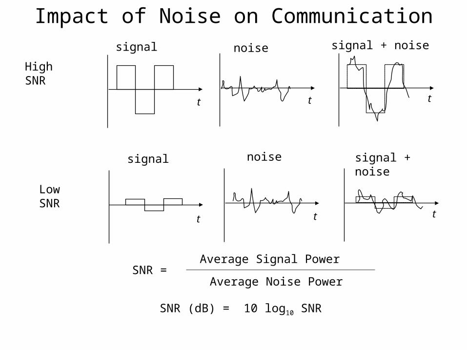
signal noise signal + noise

signal noise signal + noise

HighSNR

LowSNR

SNR = Average Signal Power

Average Noise Power

SNR (dB) = 10 log10 SNR

t t t

t t t

Impact of Noise on Communication

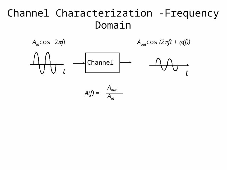
Channel

t t

Aincos 2ft Aoutcos (2ft + (f))

Aout

AinA(f) =

Channel Characterization -Frequency Domain

f

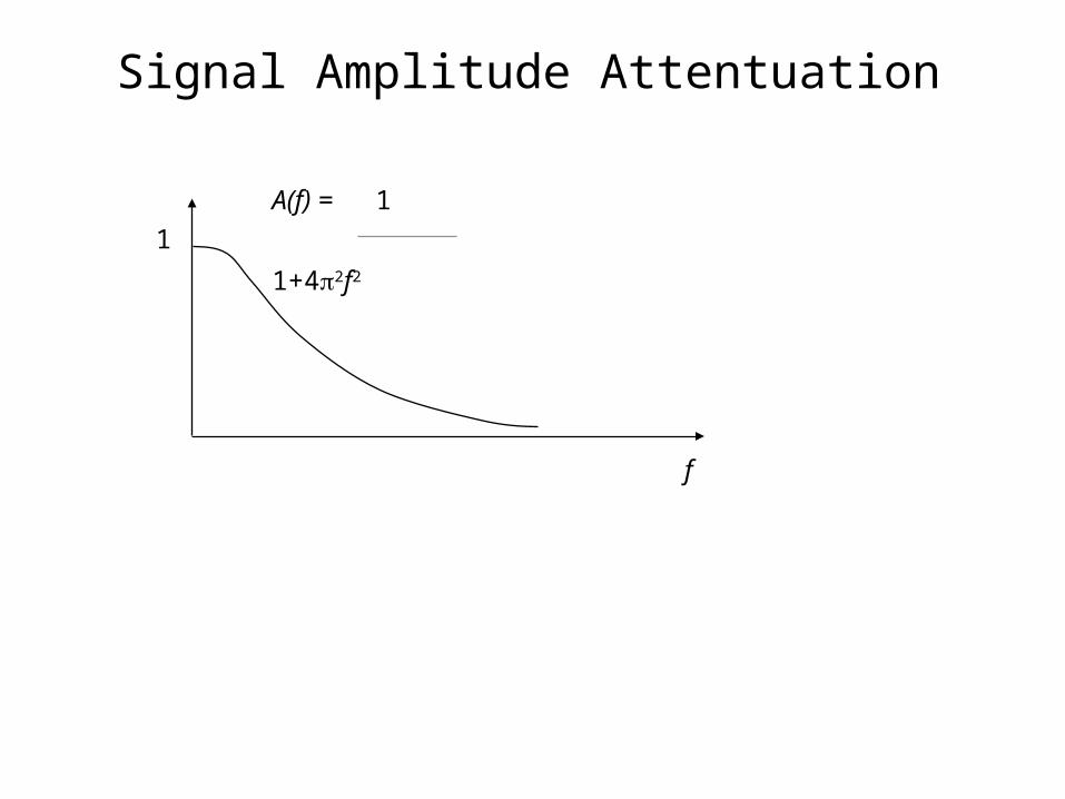
1A(f) = 1

1+42f2

Signal Amplitude Attentuation

f

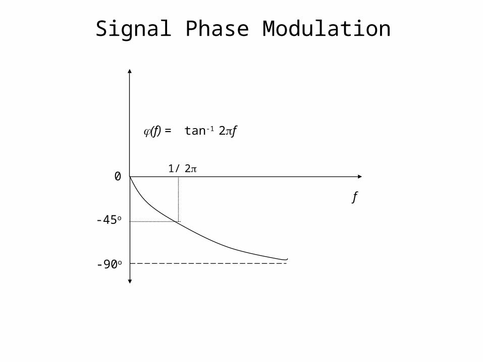
0

(f) = tan-1 2f

-45o

-90o

1/ 2

Signal Phase Modulation

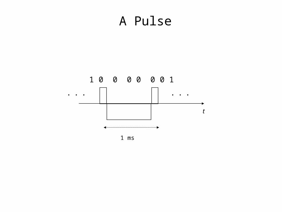
1 0 0 0 0 0 0 1

. . . . . .

t

1 ms

A Pulse

- 1 . 5

- 1

- 0 . 5

0

0 . 5

1

1 . 5

0

0.125 0.2

5

0.375 0.5

0.625 0.7

5

0.875

1

- 1 . 5

- 1

- 0 . 5

0

0 . 5

1

1 . 5

0

0.125 0.2

5

0.375 0.5

0.625 0.7

5

0.875

1

- 1 . 5

- 1

- 0 . 5

0

0 . 5

1

1 . 5

0

0.125 0.2

5

0.375 0.5

0.625 0.7

5

0.875

1

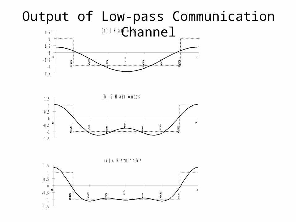
( b ) 2 H a r m o n i c s

( c ) 4 H a r m o n i c s

( a ) 1 H a r m o n i c

Output of Low-pass Communication Channel

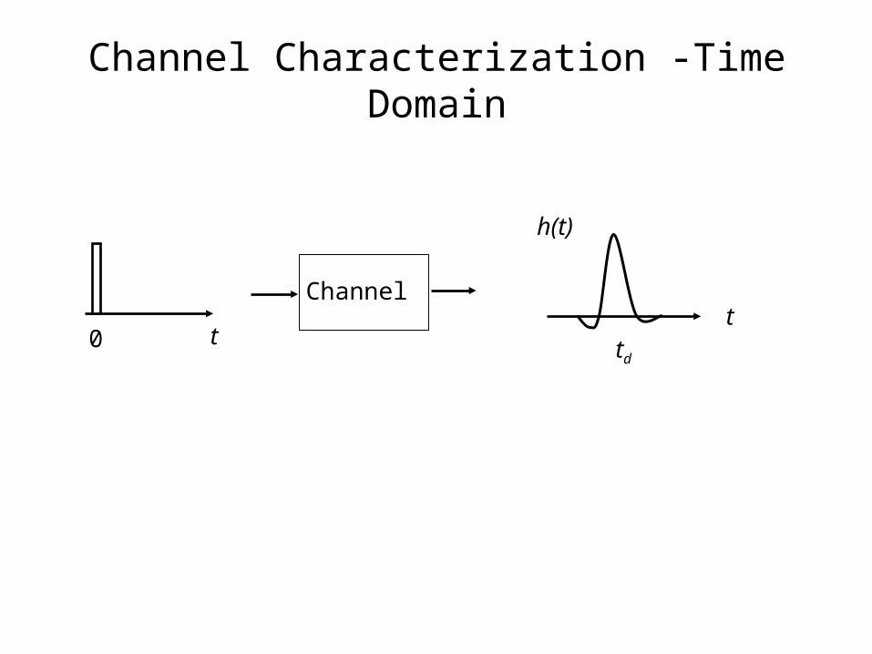
Channel

t0t

h(t)

td

Channel Characterization -Time Domain

-0.4

-0.2

0

0.2

0.4

0.6

0.8

1

1.2

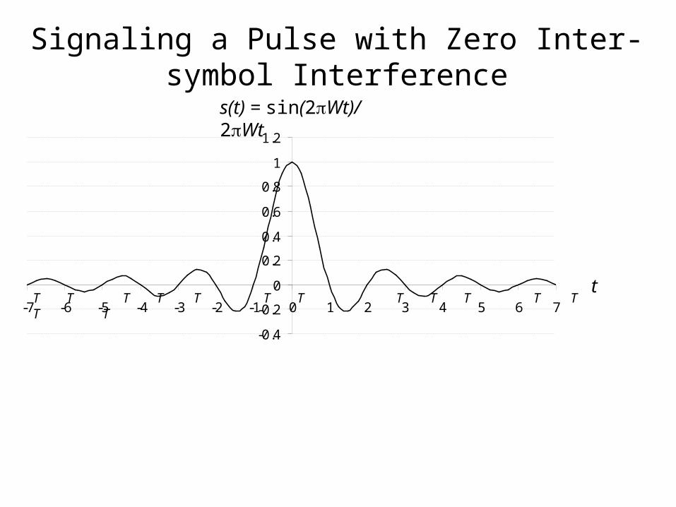
-7 -6 -5 -4 -3 -2 -1 0 1 2 3 4 5 6 7t

s(t) = sin(2Wt)/ 2Wt

T T T T T T T T T T T T T T

Signaling a Pulse with Zero Inter-symbol Interference

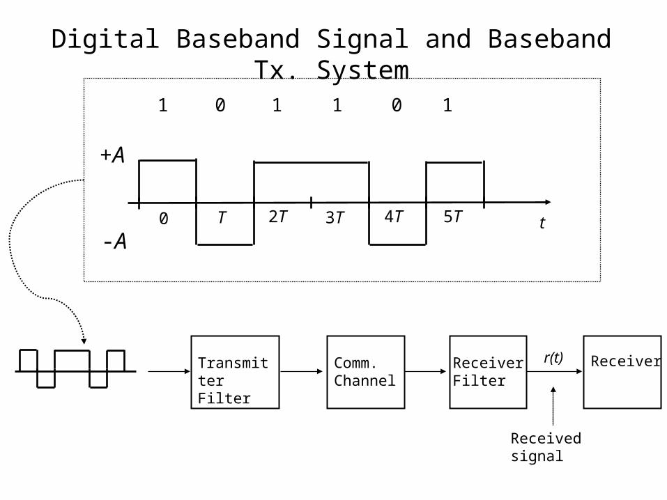
+A

-A0 T 2T 3T 4T 5T

1 1 1 10 0

Transmitter Filter

Comm. Channel

Receiver Filter

Receiverr(t)

Received signal

t

Digital Baseband Signal and Baseband Tx. System

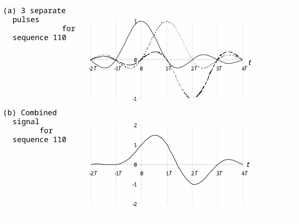
-2

-1

0

1

2

-2 -1 0 1 2 3 4

-1

0

1

-2 -1 0 1 2 3 4

(a) 3 separate pulses for sequence 110

(b) Combined signal for sequence 110

t

tT T T T TT

T T T T TT

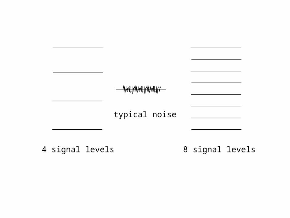
4 signal levels 8 signal levels

typical noise

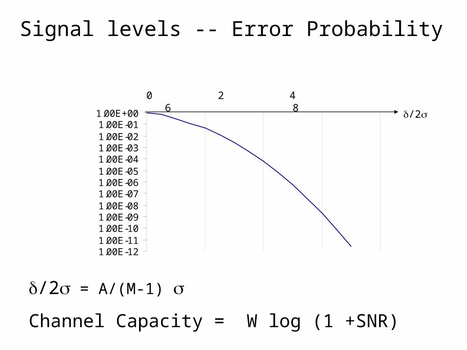
1.00E-121.00E-111.00E-101.00E-091.00E-081.00E-071.00E-061.00E-051.00E-041.00E-031.00E-021.00E-011.00E+00

0 2 4 6 8 /2

Signal levels -- Error Probability

/2 = A/(M-1)

Channel Capacity = W log (1 +SNR)

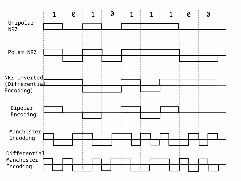
1 0 1 0 1 1 0 01UnipolarNRZ

NRZ-Inverted(DifferentialEncoding)

BipolarEncoding

ManchesterEncoding

DifferentialManchesterEncoding

Polar NRZ

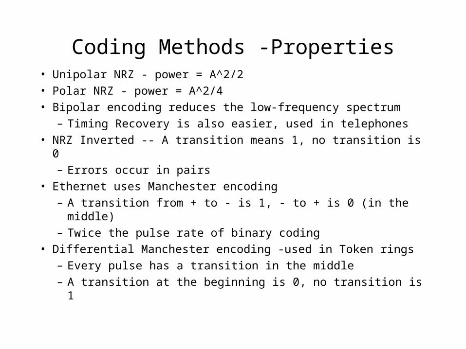
Coding Methods -Properties• Unipolar NRZ - power = A^2/2• Polar NRZ - power = A^2/4• Bipolar encoding reduces the low-frequency spectrum

– Timing Recovery is also easier, used in telephones• NRZ Inverted -- A transition means 1, no transition is 0

– Errors occur in pairs• Ethernet uses Manchester encoding

– A transition from + to - is 1, - to + is 0 (in the middle)– Twice the pulse rate of binary coding

• Differential Manchester encoding -used in Token rings– Every pulse has a transition in the middle– A transition at the beginning is 0, no transition is 1

-0.2

0

0.2

0.4

0.6

0.8

1

1.2

0

0.2

0.4

0.6

0.8 1

1.2

1.4

1.6

1.8 2

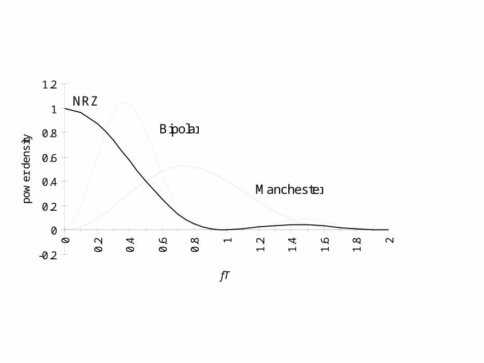
fT

pow

er d

ensi

ty

NRZ

Bipolar

Manchester

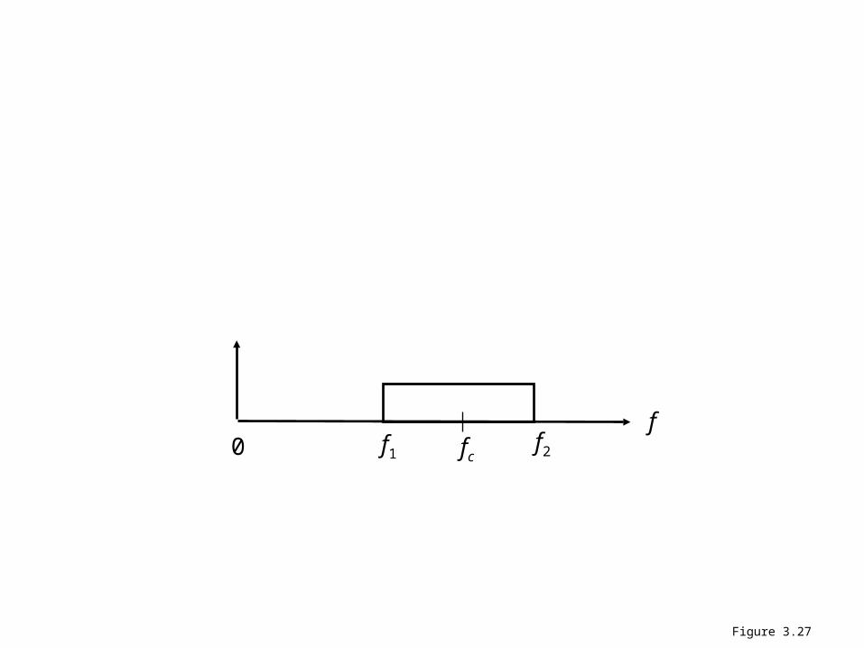
f f2 f1 fc0

Figure 3.27

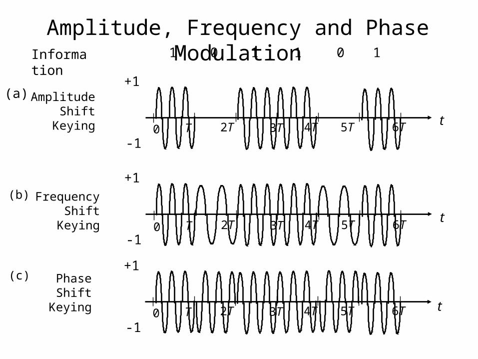
Information

1 1 1 10 0

+1

-10 T 2T 3T 4T 5T 6T

AmplitudeShift

Keying

+1

-1

FrequencyShift

Keying

+1

-1

PhaseShift

Keying

(a)

(b)

(c)

0 T 2T 3T 4T 5T 6T

0 T 2T 3T 4T 5T 6T

t

t

t

Amplitude, Frequency and Phase Modulation

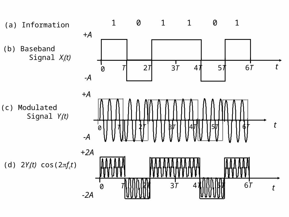
1 1 1 10 0(a) Information

(d) 2Yi(t) cos(2fct)

+2A

-2A

+A

-A

(c) Modulated Signal Yi(t)

0 T 2T 3T 4T 5T 6T

+A

-A

(b) Baseband Signal Xi(t)

0 2T 3T 6T

0 T 2T 3T 4T 5T 6T

T 4T 5T

t

t

t

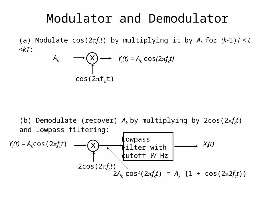
(a) Modulate cos(2fct) by multiplying it by Ak for (k-1)T < t <kT:

Ak x

cos(2fct)

Yi(t) = Ak cos(2fct)

(b) Demodulate (recover) Ak by multiplying by 2cos(2fct) and lowpass filtering:

x

2cos(2fct)2Ak cos2(2fct) = Ak {1 + cos(2fct)}

LowpassFilter withcutoff W Hz

Xi(t)Yi(t) = Akcos(2fct)

Modulator and Demodulator

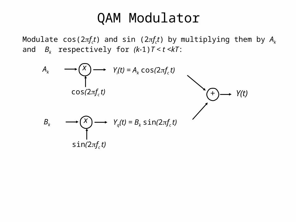
Akx

cos(2fc t)

Yi(t) = Ak cos(2fc t)

Bkx

sin(2fc t)

Yq(t) = Bk sin(2fc t)

+ Y(t)

Modulate cos(2fct) and sin (2fct) by multiplying them by Ak and Bk respectively for (k-1)T < t <kT:

QAM Modulator

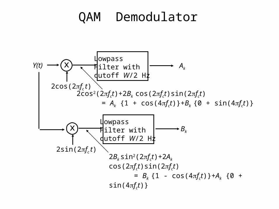
Y(t) x

2cos(2fc t)2cos2(2fct)+2Bk cos(2fct)sin(2fct) = Ak {1 + cos(4fct)}+Bk {0 + sin(4fct)}

LowpassFilter withcutoff W/2 Hz

Ak

x

2sin(2fc t)2Bk sin2(2fct)+2Ak cos(2fct)sin(2fct) = Bk {1 - cos(4fct)}+Ak {0 + sin(4fct)}

LowpassFilter withcutoff W/2 Hz

Bk

QAM Demodulator

Ak

Bk

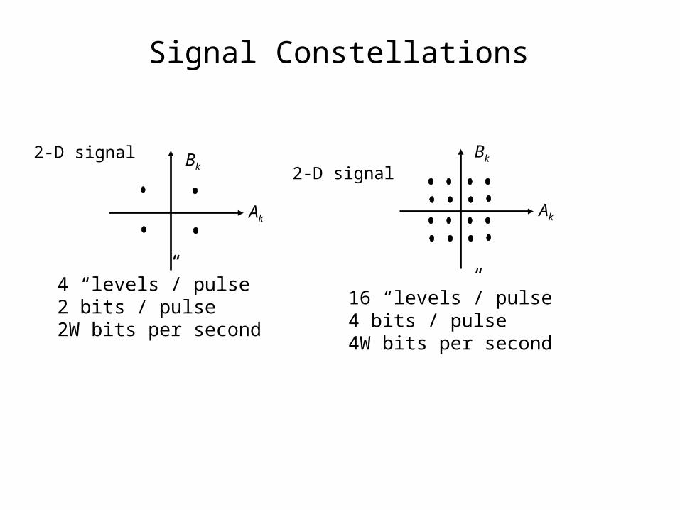
16 “levels”/ pulse4 bits / pulse4W bits per second

Ak

Bk

4 “levels”/ pulse2 bits / pulse2W bits per second

2-D signal2-D signal

Signal Constellations

Ak

Bk

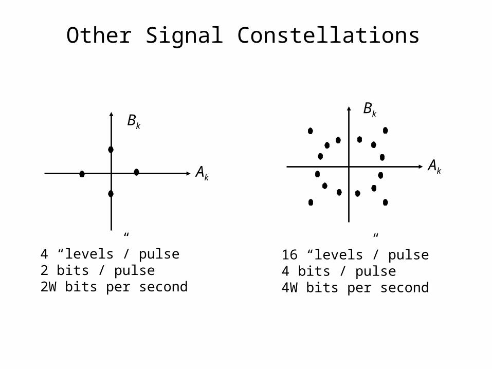
4 “levels”/ pulse2 bits / pulse2W bits per second

Ak

Bk

16 “levels”/ pulse4 bits / pulse4W bits per second

Other Signal Constellations

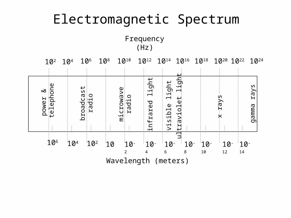
102 104 106 108 1010 1012 1014 1016 1018 1020 1022 1024

Frequency (Hz)

Wavelength (meters)

106 104 102 10 10-2 10-4 10-6 10-8 10-10 10-12 10-14

pow

er &

tele

phon

e

broa

dcas

tra

dio

mic

row

ave

radi

o

infr

ared

ligh

t

visi

ble

ligh

t

ultr

avio

let l

ight

x ra

ys

gam

ma

rays

Electromagnetic Spectrum

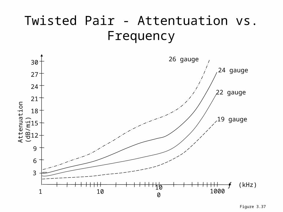
Att

enua

tion

(dB

/mi)

f (kHz)

19 gauge

22 gauge

24 gauge

26 gauge

6

12

3

9

15

18

21

24

27

30

1 10 100 1000

Figure 3.37

Twisted Pair - Attentuation vs. Frequency

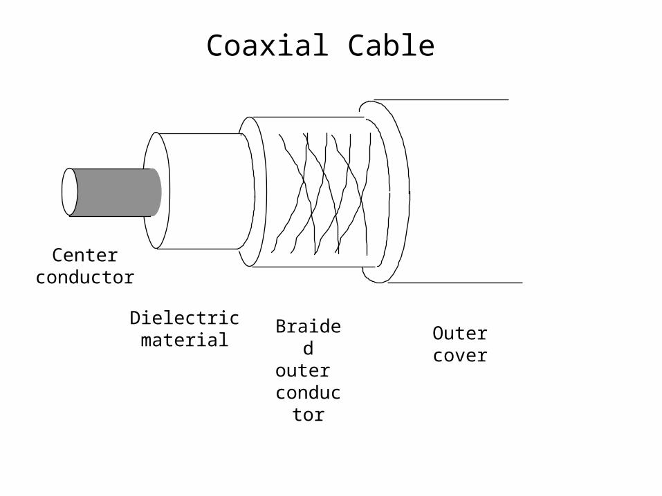
Centerconductor

Dielectricmaterial

Braidedouter

conductor

Outercover

Coaxial Cable

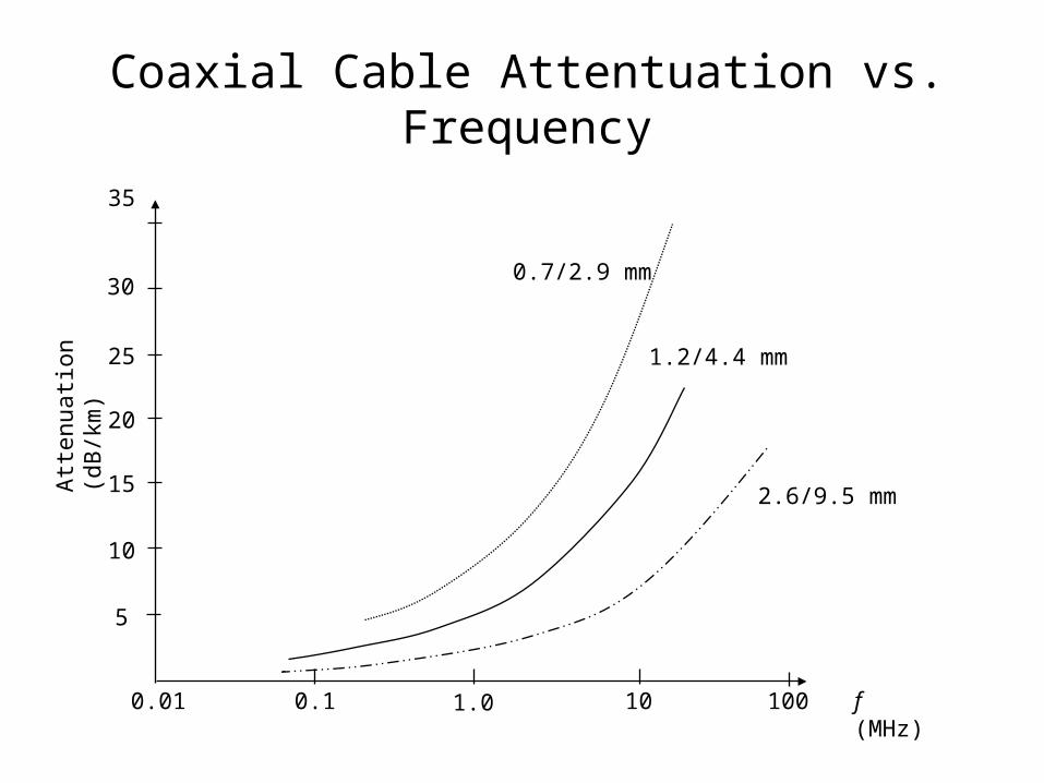
35

30

10

25

20

5

15Att

enua

tion

(dB

/km

)

0.01 0.1 1.0 10 100 f (MHz)

2.6/9.5 mm

1.2/4.4 mm

0.7/2.9 mm

Coaxial Cable Attentuation vs. Frequency

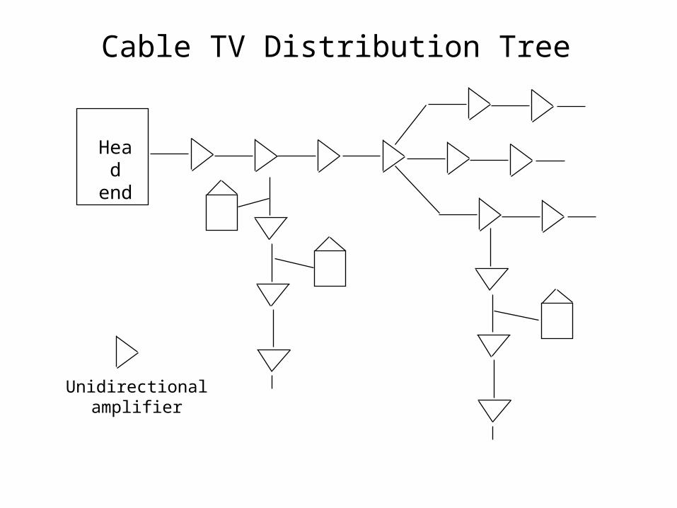
Head

end

Unidirectionalamplifier

Cable TV Distribution Tree

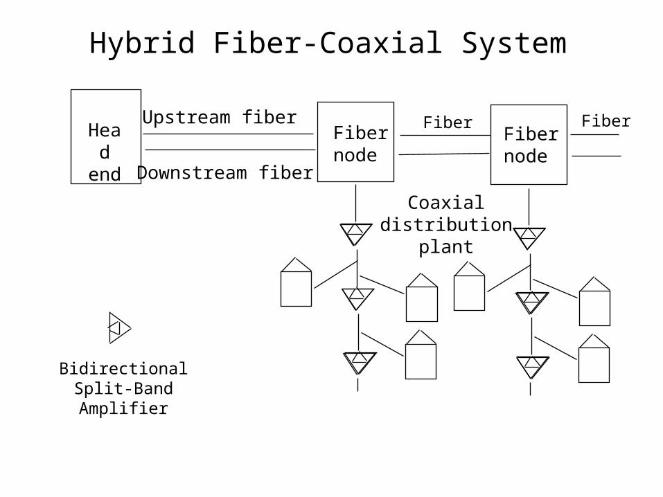
Head

end

Upstream fiber

Downstream fiber

Fibernode

Coaxialdistribution

plant

Fibernode

BidirectionalSplit-BandAmplifier

Fiber Fiber

Hybrid Fiber-Coaxial System

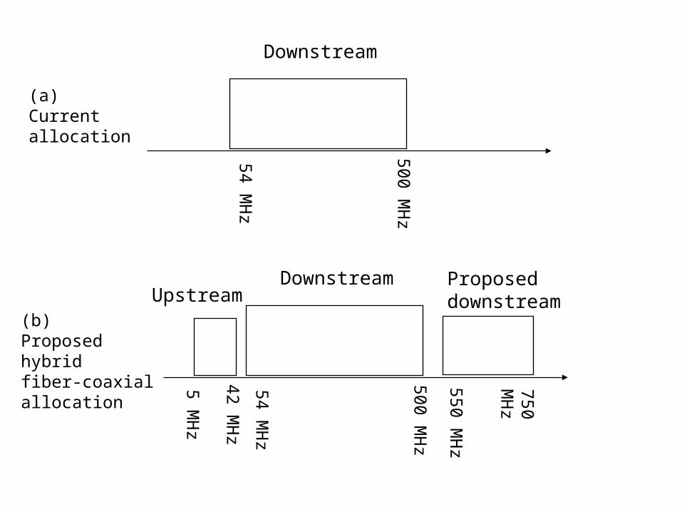
Downstream

54 MH

z

500 MH

zUpstream

Downstream

5 MH

z

42 MH

z

54 MH

z

500 MH

z

550 MH

z

750 MH

z

(a)Currentallocation

(b) Proposedhybridfiber-coaxialallocation

Proposed downstream

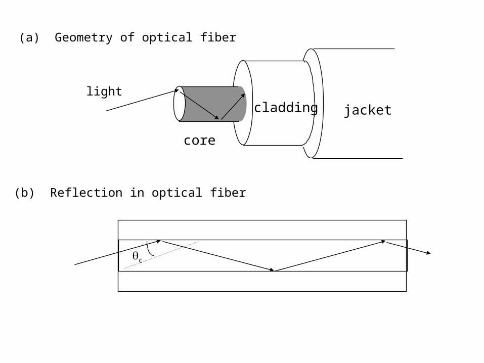
core

cladding jacket

light

c

(a) Geometry of optical fiber

(b) Reflection in optical fiber

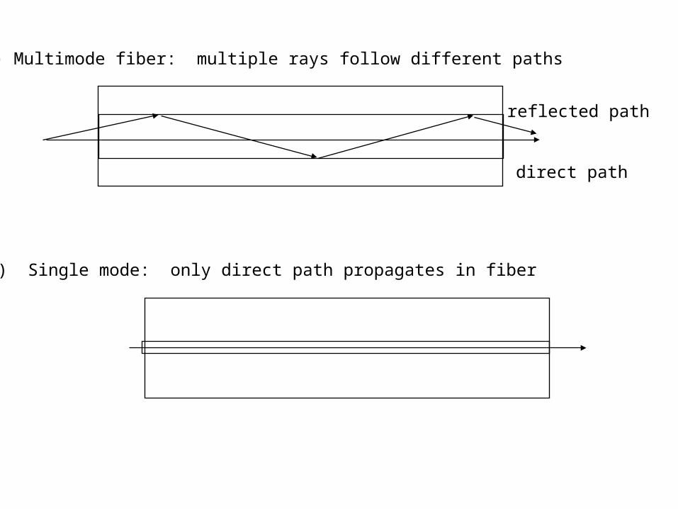
(a) Multimode fiber: multiple rays follow different paths

(b) Single mode: only direct path propagates in fiber

direct path

reflected path

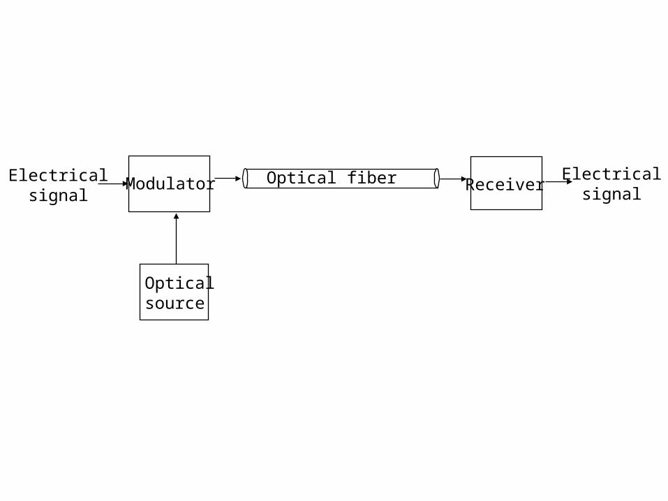
Optical fiber

Opticalsource

ModulatorElectricalsignal

ReceiverElectrical

signal

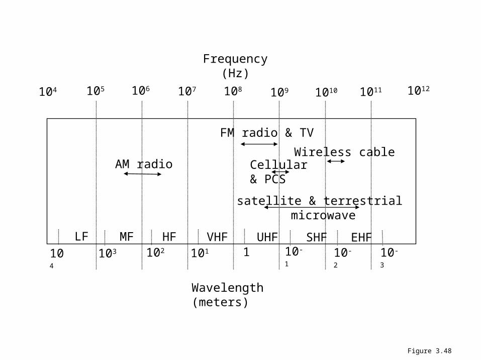
104 106 107 108 109 1010 1011 1012

Frequency (Hz)

Wavelength (meters)

103 102 101 1 10-1 10-2 10-3

105

satellite & terrestrial microwave

AM radio

FM radio & TV

LF MF HF VHF UHF SHF EHF104

Cellular& PCS

Wireless cable

Figure 3.48