EMI in an RQZ: the need for buffer zones

Carol Wilson, CSIRO Research ConsultantRFI2010, Groningen

Outline of presentation

Introduction – purpose of EMI buffer zone analysis

Prediction method components• Interference thresholds• Emission levels• Characterisation of EMI activities• Prediction of attenuation

Examples of analysis

Results of buffer zone analysis

Close

Introduction – EMI buffer zones

Intentional radio transmitters narrowband signals variety of mitigation techniques (including avoidance)

Noise from electrical equipment, machinery broadband interference harder to mitigate

Need to define buffer zones around human activity to avoid EMI in design of SKA array configuration

Challenges due to SKA requirements

• Frequency – 70 MHz to 25.25 GHz – large compared to most current telescopes

• Physical extent of telescope (large number of separate stations over a large geographic extent)

• Rigorous demands of radioastronomy

• Time frame (current -> ~2020 -> 50 years or more)

SKA three zone approach

Core (2.5 km radius, 50% of array) with highest levels of protection (aim for ITU-R RA.769-2 continuum).

Intermediate (<180 km radius, 25% of array) with protection relaxed by 15 dB from continuum thresholds.

Remote (> 180 km, 25% of array) with protection relaxed by further 25 dB (corresponds to VLBI levels).

Core site chosen in a remote location

Intermediate and remote sites to be chosen based on RFI, UV coverage, geophysics, logistics, etc

Buffer zones for separation from EMI needed for intermediate and remote sites

Components of prediction model

Emission level – radioastronomy threshold = attenuation required

Model expected usage patterns of equipmentUse propagation model to find distance at which

attenuation is exceeded

• Thresholds established by ITU-R Study Group 7• Emissions – use published EMC/EMI standards• Model of usage patterns - estimated• Attenuation – need propagation model(s)

Defining radio quietness

ITU Recommendation RA.769-2• Harmful interference levels assuming reception into 0 dBi sidelobe• Values for continuum, spectral line and VLBI observations• Continuum observation values used as basic protection levels for SKA core

Frequencyf

(MHz)

Assumed bandwidth f

(kHz)

Threshold interference levels

Input power PH

(dBW)

Pfd SH  f

(dB(W/m2))

Spectral pfd SH

(dB(W/(m2 Hz)))

(7) (8) (9)

151.525325.3

408.05611

1 413.51 6652 6954 995

10 65015 37522 35523 800

2.956.63.96

27101010

10050

290400

–199–201–203–202–205–207–207–207–202–202–195–195

–194–189–189–185–180–181–177–171–160–156–146–147

–259–258–255–253–255–251–247–241–240–233–231–233

(7) Power level at the input of the receiver considered harmful to high sensitivity observations, PH. This is expressed as the interference level which introduces an error of not more than 10% in the measurement of P.

(8) pfd in a spectral line channel needed to produce a power level of PH in the receiving system with an isotropic receiving antenna.

(9) Spectral pfd needed to produce a power level PH in the receiving system with an isotropic receiving antenna.

Interference thresholds

Interference threshold levels from Recommendation ITU-R RA.769-2

-300

-280

-260

-240

-220

-200

-180

-160

10 100 1000 10000 100000

Frequency (MHz)

Sp

ec

tra

l p

fd (

dB

(W/(

m2

Hz)

))

Continuum

Continuum +15

Line

VLBI

Emission standards

Interference power as a function of frequency from:• Road vehicles – CISPR standard 12:2005. • Railways – European EN 50121-2: 2006. • Household appliances and tools – CISPR standard 14-

1:2003. • Arc welders – CISPR standard 11:2004. • Power lines - Australian standard AS/NZS 2344:1997.

Frequency dependence:• Roads: increasing to 400 MHz, then constant• Rail: decreasing with frequency• Appliances/tools: increasing to 300 MHz, assumed

constant beyond

Categories

Farmsteads/individual dwellings = 7 appliances, 4 power tools and 1 vehicle.

Towns – n x dwellings, assumption that 1/3 of households are “active” at any time.

Roads – minor (small number of vehicles per day) and major (multiple vehicles for a substantial part of the day)

Rail – lightly used (4 trains a day) and heavy (continuous use)

Mines – based on town analysis for similar activity

Power lines – range of voltages

Propagation models

Some propagation models use specific terrain

For buffer zones, generic models needed

ITU-R Recommendation P.1546-3 used for EMI buffers

Inputs: frequency, terminal heights, time percentage, type of path (land, sea, mixed)

• Interference source height: 2 metres (except power lines)• Telescope height: 1 metre < 300 MHz, 15 metres > 300 MHz

Model used iteratively to find distance for required loss

Attenuation increases as function of frequency

Attenuation decreases with higher antenna heights (discontinuity at 300 MHz due to telescope height)

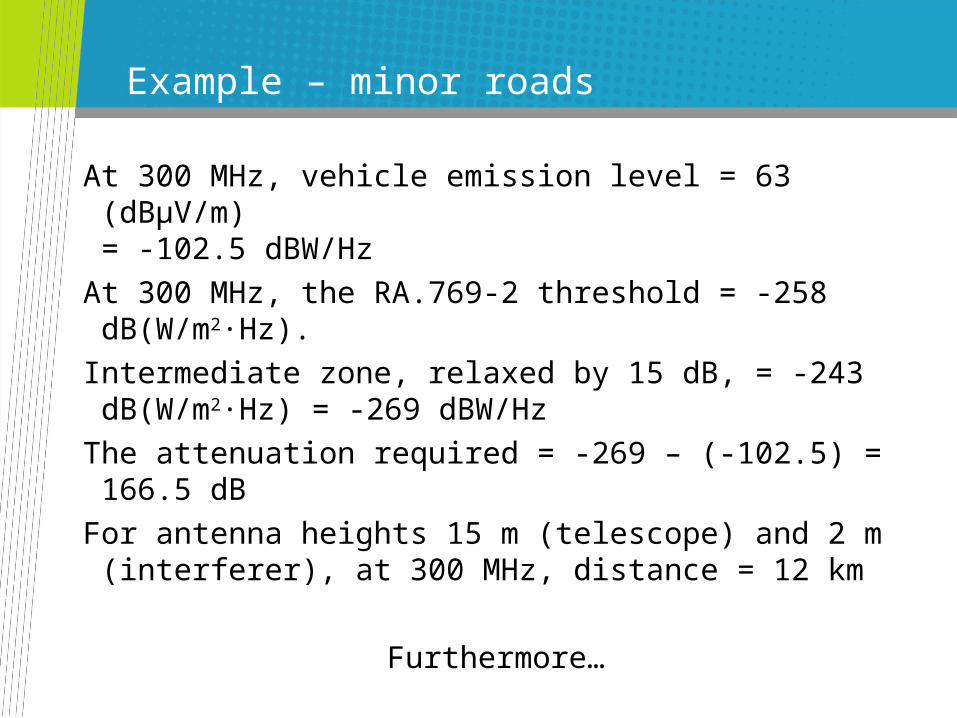
Example – minor roads

At 300 MHz, vehicle emission level = 63 (dBμV/m) = -102.5 dBW/Hz

At 300 MHz, the RA.769-2 threshold = -258 dB(W/m2·Hz).

Intermediate zone, relaxed by 15 dB, = -243 dB(W/m2·Hz) = -269 dBW/Hz

The attenuation required = -269 – (-102.5) = 166.5 dB

For antenna heights 15 m (telescope) and 2 m (interferer), at 300 MHz, distance = 12 km

Furthermore…

Example – minor roads (continued)

Allow 10 vehicles per day within 12 km for 5% of day.

0.05*24*60 = 72 minutes or 7.2 minutes per vehicle

At 100 km/hr, vehicle travels 12 km in 7.2 minutes

Relax limit to 10.5 km as shown

Repeat at other frequencies

12 km

10.5 km12 km

Example – minor roads (continued)

Buffer zone for minor roads

0.0

2.0

4.0

6.0

8.0

10.0

12.0

14.0

0 100 200 300 400 500 600 700 800 900 1000

Frequency (MHz)

Bu

ffer

zo

ne

dis

tan

ce (

km)

Low antenna below 300 MHz

15 m antenna

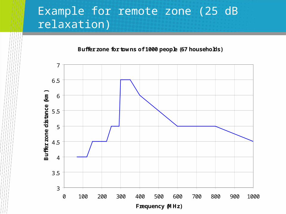
Buffer zone for towns of 1000 people (67 households)

3

3.5

4

4.5

5

5.5

6

6.5

7

0 100 200 300 400 500 600 700 800 900 1000

Frequency (MHz)

Bu

ffer

zo

ne

dis

tan

ce (

km)

Example for remote zone (25 dB relaxation)

Buffer zones for intermediate and remote stations

Intermediate Remote

Minor roads 10.5 km 3 km

Major roads 33.5 6.5

Local rail 10.5 3.5

Heavy rail 30.5 5.5

Farms 13.5 3

Towns: 100 people

21 5

1000 people 27 6.5

5000 people 31 7

10000 people 37.5 8.5

Power lines Up to 8 km Up to 1.5 km

Conclusions

• Core of SKA to be protected primarily by remote location

• Buffer zones around human activity have been defined for the intermediate and remote stations of the SKA

• The methodology for calculation can be applied to other scenarios (e.g. intermediate traffic roads)

• EMI buffer zones will be part of analysis in optimising the SKA array configuration

Contact UsPhone: 1300 363 400 or +61 3 9545 2176

Email: enquiries@csiro.au Web: www.csiro.au

Thank you!

Questions?

Carol Wilson, Research Consultantcarol.wilson@csiro.au