-i-

Energy Use in California Wholesale Water Operations: Development and Application of a General Energy Post-Processor for California Water

Management Models

By

MATTHEW EARL BATES B.S. (California State University, Long Beach) 2006

THESIS

Submitted in partial satisfaction of the requirements for the degree of

MASTER OF SCIENCE

in

Civil and Environmental Engineering

in the

OFFICE OF GRADUATE STUDIES

of the

UNIVERSITY OF CALIFORNIA

DAVIS

Approved:

_____________________________________ Jay R. Lund, Chair

_____________________________________ Frank J. Loge

_____________________________________ William E. Fleenor

Committee in Charge

2010

-ii-

Abstract

This thesis explores the effects of future water and social conditions on energy consumption in the major pumping and generation facilities of California’s interconnected water-delivery system, with particular emphasis on the federally-owned Central Valley Project, California-owned State Water Project, and the large locally-owned systems in Southern California. Anticipated population growth, technological advancement, climatic changes, urban water conservation, and restrictions of through-Delta pumping will together affect the energy used for water operations and alter statewide water deliveries in complex ways that are often opposing and difficult to predict. Flow modeling with detailed statewide water models is necessary, and the CALVIN economic-engineering optimization model of California’s interconnected water-delivery system is used to model eight future water-supply scenarios. Model results detail potential water-delivery patterns for the year 2050, but do not explicitly show the energy impacts of the modeled water operations. Energy analysis of flow results is accomplished with the UC Davis General Energy Post-Processor, a new tool for California water models that generalizes previous efforts at energy modeling and extends embedded-energy analysis to additional models and scenarios. Energy-intensity data come from existing energy post-processors for CalSim II and a recent embedded-energy-in-water study prepared by GEI Consultants and Navigant Consulting for the California Public Utilities Commission. Differences in energy consumption are assessed between modeled scenarios and comparisons are made between data sources, with implications for future water and energy planning strategies and future modeling efforts. Results suggest that the effects of climate warming on water-delivery energy use could be relatively minimal, that the effects of a 50% reduction in Delta exports can be largely offset by 30% urban water conservation, and that a 30% conservation in urban water use can produce energy savings of over 40%, from the base case. Results also show that refining estimates of future Delta export and urban water conservation levels is necessary to increase confidence in energy-related planning and investment. Sensitivity analyses suggest that the compared energy-intensity data are highly interchangeable and using data combined from multiple sources is preferable to include more facilities without skewing results.

-iii-

Acknowledgements

Special thanks to the Public Interest Energy Research (PIER) program of the California Energy Commission for funding this study and to Guido Franco, as project manager, for coordinating and including this work as a PIER project.

Special thanks also to my major professor Dr. Jay Lund, for his guidance, mentorship, and many helpful suggestions, and to committee members Dr. Frank Lodge and Dr. William Fleenor for their contributions to improve this effort. I appreciate the willingness of Brian Van Lienden (CH2M Hill) to share and discuss the CalSim II energy post-processors, and an early discussion with Bill Bennett (GEI Consultants) regarding the preliminary energy-intensity findings of his team.

I am especially grateful to Dr. Josué Medellín-Azuara, Rachel Ragatz, and Christina Connell for their work in developing the CALVIN model runs, and to Sachi De Souza for her modeling assistance. I have thoroughly enjoyed the companionship of my peers, Nathan Burly, David Rheinheimer, Partrick Ji, Kaveh Madani, and the other member of our research group, and am indebted to the generations of CALVINists that have gone before me.

-iv-

Table of Contents

1. Introduction ............................................................................................................................. 1

1.1. Objectives and Scope of Study ......................................................................................... 2

1.2. Background on Water and Energy in California ............................................................... 2

1.2.1. Water and Energy Policy .......................................................................................... 2

1.2.2. Water and Energy Relationships .............................................................................. 4

1.3. Existing Models of California Water-Energy Relationships .............................................. 5

1.3.1. LongTermGen and SWP_Power Energy Post-Processors for CalSim II .................... 5

1.3.2. GEI/Navigant Water-Energy Model ......................................................................... 6

1.3.3. CALVIN Water Management Model ........................................................................ 6

2. Energy Use Estimation ............................................................................................................. 7

2.1. Estimation Methods ......................................................................................................... 7

2.2. General Energy Post-Processor ........................................................................................ 8

2.3. Energy Intensity Data for California Pumping and Generation Facilities ........................ 8

2.4. Post-Processor Application to Water Management Models ......................................... 11

3. Future Water Supply Scenarios for California ........................................................................ 14

3.1. Year 2050 Levels of Development and Urban Water Demands .................................... 14

3.2. Historical and Altered Climates ..................................................................................... 15

3.3. Urban Water Conservation ............................................................................................ 16

3.4. Reductions in Through-Delta Pumping .......................................................................... 17

3.5. Summary of Future Water Supply Scenarios for California ........................................... 19

4. Results and Discussion ........................................................................................................... 19

4.1. Energy Use Results for Water-Supply Scenarios ............................................................ 19

4.2. Sensitivity of Energy-Use Results to Data Source and Water Project ............................ 23

4.3. Discussion and Comparision of the General Energy Post-Processor vs. Existing

Water-Energy Analysis Software ................................................................................... 26

5. Limitations ............................................................................................................................. 29

6. Extensions .............................................................................................................................. 30

7. Conclusions ............................................................................................................................ 31

8. References ............................................................................................................................. 33

1

1. Introduction Few things are more important to California’s economy and citizenry than sustainable water and energy systems. California’s water supply and water demands have a fundamental geographic imbalance, with the most precipitation falling in northern mountainous regions, where the snow-pack also lies, and most population and agricultural areas occupying the more arid southern Central Valley, coastal regions, and southern desert. In response, California has gone to great lengths to transport water from where it originates to where it is desired. California’s state, federal and local water projects annually transfer over twenty million acre-feet of water many miles to satisfy these demands, though this conveyance comes with significant energy and economic costs (DWR 2009a, CEC 2005).

Transporting large volumes of water over long distances, especially in a state with significant topography, requires pumping facilities that consume large amounts of energy. The State Water Project (SWP), which operates many of these pumping facilities, is the largest single user of energy in all of California (CEC 2005). In total, about nineteen percent of the state’s energy consumption is tied to water use. While most of this is by end-users of water, principally for in-home water heating, about five percent of California’s electricity is used to treat and transport surface water in the statewide water conveyance network (CEC 2005; GEI 2010). Future changes to the quantity and sources of water transferred throughout the state are expected to alter past energy use patterns, and special tools are needed to assess the energy impacts of changes in the waterscape. Predicting future needs is difficult in an unsteady environment. Climate change, population growth, and operational uncertainties complicate matters and generally make resources scarcer. Water conservation helps counterbalance the effects of other forces on the system, and can help maintain overall water and energy supply reliability. Multiple scenarios of future water demands and supplies can be modeled with statewide water models to predict the scope of future water operations. Using knowledge of the relationship between water pumping and energy consumption, the results of modeled scenarios can be compared and analyzed to assess likely net energy use under each water delivery scenario.

This work introduces an improved energy post-processor for California water management models. This post-processor uses flow results from an external water model to calculate corresponding energy use under various scenarios. A history of interest in water and energy in California is discussed, including a synopsis of three related models. General post-processor methods and software development are also discussed, and application is considered to the flow networks of two prominent water management models. Data and sources for energy-intensities are given and compared, and the implications of data differences are explored. Lastly, the energy post-processor is applied to the results of a modeled suite of water supply scenarios covering a range of water demand, climate change, water conservation, and water availability futures for California, with energy use for the state, federal, and largest local water projects forecasted and compared between scenarios.

2

1.1. Objectives and Scope of Study

This study has three primary objectives, each of which advances our quantitative capacity or understanding of embedded energy in California water. The first objective is to create a simple, versatile, and thorough tool for calculating the energy impacts of water operations. Several existing works address this in various forms, but a generic tool allowing separated energy-intensity data to be used with flow results from multiple water-model networks and simulation scenarios is needed. The UC Davis General Energy Post-Processor developed in this study accomplishes these goals and addresses many limitations of preceding works.

With its generalized format, the scope of the energy post-processor is essentially limited only by data availability. As improved energy-intensity and water-model network data are developed, this energy post-processor can be applied far beyond the scope of the initial analysis undertaken in this study.

The second objective of this study is to compare energy intensities between data sources and to synthesize these findings into a set of default energy-intensity data for the post-processor. Insights can be gained by identifying local and systematic differences between sources, with implications for ongoing water management studies that rely on these data.

The scope of the default data analyzed and supplied with the post-processor includes thirty-three pumping and eight in-conduit generation facilities (some facilities are aggregates of several distinct locations; only thirty-one of the pumping facilities can be associated with CALVIN links) in the state, federal, and local water projects for which energy intensities are known and distinct network links on one of the major California water models can be identified.

The third objective of this study is to use the post-processor and default data to perform energy analysis on a suite of model runs outlining possible water-supply futures for California. The results of this analysis improve our understanding of the magnitude and distribution of water-delivery energy demands that can be expected in the future.

The scope of this energy analysis of water supply futures includes eight CALVIN runs covering a variety of climate change, system operation, water availability, and water conservation assumptions.

1.2. Background on Water and Energy in California

1.2.1. Water and Energy Policy

Water and energy supplies have both been subject to shortage in recent California history and maintaining resource supply reliability is a topic of great planning and political interest. Ongoing political discussions and growing scientific uncertainties regarding our environmental future have built considerable interest in the nexus of interactions between water and energy. As home to large industrial, high-tech, and agricultural sectors, and with the largest population of any state, disruptions in either water or energy services are extremely costly (e.g. E3 2005; LaCommare and Eto 2004; Lineweber and McNulty 2001; Wade et al. 1991; EDAW Inc. 2008; M.Cubed 2008).

3

The 2001-2002 California energy crisis is a prime example of energy disruptions becoming the focus of great public attention. With a newly deregulated power industry, uncertain political oversight, high energy demands, low resource availability, and internal policy problems, the power market was unable to reasonably match supply with demand and became subject to manipulation by profiteering producers and resellers. Energy prices skyrocketed ten-fold, costing the state billions of dollars in direct costs, and rolling blackouts and brownouts became common, contributing to indirect costs that were even greater. The total costs of this supply unreliability are still being paid today (Joskow 2001). With anticipated population growth of up to seventy-five percent by the year 2050, demand for energy will increase in the future. Optimally managing California energy supplies will remain important for decades to come (Landis and Reilly 2002, US Census Bureau 2010).

Water delivery, too, has faced significant service-reliability challenges. Wholesale water deliveries from the State Water Project and the Central Valley Project (CVP) have been subject to oversubscription and continual shortages due to misalignments between historical water contracts, increasing urban and agricultural demands, and actual water availability (LAO 2009). Projected SWP water allocations for 2010, for example, were initially limited to a mere five percent of contracted amounts and subsequently increased to a maximum of only fifty percent of contracted amounts (DWR 2009c; DWR 2010b). Though early water supply projections for 2010 were abnormally low, it is now rare for CVP and SWP contractors to receive the full amount of their requested water deliveries.

The main hub of California’s water supply network, the Sacramento-San Joaquin Delta (the Delta), is both a legally-protected tidal estuary and the system interchange for about 15 percent of California’s water deliveries to approximately 25 million Californians and 750,000 acres of irrigated land (DWR 2007, 2009a, 2009b). Recent scientific studies are raising concerns that the effects of climate change, continued environmental degradation, and natural disasters may soon render the Delta temporarily or permanently unavailable for continued use as a key segment of California’s water supply network (DWR 2007; Mount and Twiss 2005; Lund et at. 2010; Fleenor et al. 2008; URS 2009c; Zetland 2010; Miller et al. 2003; Hayhoe et al. 2004). Though the California water supply system is highly constrained in its current form, export shortages are expected to become more dramatic in the future.

Partly in response to past and anticipated resource shortages, recent political action in California is addressing the makeup and reliability of future water and energy supplies. California Assembly Bill 32, signed into law in 2006, is landmark legislation requiring a 25 percent reduction in per-capita greenhouse gas emissions by the year 2020 (Office of the Governor 2006). Major steps in achieving this goal, as outlined in the state’s Climate Change Scoping Plan, include energy conservation and energy efficiency measures to reduce both current greenhouse gas emissions and future energy demands (CARB 2008).

Other current legislation (i.e. Assembly Bill 2514, which has until September 30, 2010 to be signed into law) is laying a foundation for the mandatory development of new energy storage facilities to regulate load, increase the state’s ability to deal with surges in demand, and increase overall efficiency in the energy supply system (Legislative Counsel 2010). Improvements in energy efficiency have been mandated to be California’s first priority for meeting future energy demands and, between 1975 and 2006, singlehandedly increased the state’s economy by 3 percent and saved over $56 billion (CPUC 2006). California continues to show a sustained interest in energy efficiency and the reliability of energy supplies.

4

Recent political action has also addressed future water supply reliability. Senate Bill 7, signed into law in November 2009, requires that California achieve a 20 percent reduction in urban per-capita water use by the end of year 2020 and requires agricultural water suppliers to implement water efficiency measures, quantity-based pricing, and standardized reporting of deliveries (Legislative Counsel 2009b). Entities that fail to meet the provisions of the bill will be ineligible for all state water grants and loans, which should motivate most affected agencies.

Recognizing the dangers to the Delta and its significance to water supply reliability, Senate Bill 1, also of the 2009 session, establishes legally co-equal goals of protecting the environment in the Delta and ensuring continued water supply reliability. Through a newly created Delta Stewardship Counsel, the state is actively pursuing scientific and political options to navigate these goals (Legislative Counsel 2009a).

These examples of recent legislative action regarding the future of energy and water in California—in the context of pressing budgetary challenges and a severe recession—illustrate the central role these issues hold in California’s political landscape.

1.2.2. Water and Energy Relationships

Recent scientific studies have sought to quantify the specific relationships between water and energy supplies in California, with the goal of better informing the policy decisions surrounding these two resources. Periodic updates to the California Water Plan (e.g. DWR 2009a) provide an up-to-date overview of statewide water operations and project trends for the future. Similarly, periodic Integrated Energy Policy Reports and updates (e.g. CEC 2007) give an overview of the current status of California energy resources and project energy trends for the future. These documents provide the factual basis from which other analyses extrapolate, and both contain special sections addressing interactions with other resources.

As early as the 1970s, energy use was being estimated for farm irrigation in California (Rawlins 1977), in the context of maximizing crop production per unit input. Detailed, modern estimates of agricultural-water energy use are given in Burt et al. (2003), which examines energy used in conveying wholesale water to irrigation districts, district-level surface and groundwater pumping, and farm-level groundwater and booster pumping, all in the context of agricultural-to-urban water transfers, groundwater banking, irrigation efficiency, desalination, pump fuel choices, climate change, and policy shifts.

Wilkinson (2000) lays a foundation for agricultural and urban water-energy modeling by identifying key water-energy relationships in California, deriving a methodology for calculating the energy embodied in water transfers, developing an energy calculation tool, and presenting a list of policy implications and potential efficiency improvements. The California Energy Commission has recently refined these relationships, added new energy-intensity data, identified additional policy conclusions and areas for efficiency gains, and projected water and energy trends for the future (CEC 2005). Remaining uncertainties and key areas for future research are identified in a roadmap for water and wastewater energy efficiency jointly published by the California Energy Commission and the American Water Works Association Research Foundation (Means et al. 2004). Based on these reports, total water-energy analysis should also include the effects of powerplant generation, building cooling, water transport and deliveries, household end use and water heating, water and wastewater treatment, desalination, groundwater pumping, and similar energy uses for urban water deliveries.

5

Cohen et al. (2004), motivated by environmental concerns, focus these water-energy relationships on the need to improve overall efficiency through additional water conservation and more-careful planning for the full life-cycle costs of water and energy resource development. Example life-cycles analyses for alternative water supply sources have been performed by Stokes and Horvath (2006), for two case studies in Northern and Southern California. Gleick (1994) and Lofman et al. (2002) give good, concise overviews of the relevant water-energy relationships at play in California and elsewhere.

The relationships between water and energy are complex and water and energy supplies will remain scarce and valuable in California’s future. The types of modeling and analysis outlined in this study can help identify and predict the interactions between these two resources in an uncertain world, and inform the policy decisions that will shape our future.

1.3. Existing Models of California Water-Energy Relationships

This study has benefited significantly from several contemporary water and energy models. While these models have been effective for their intended purposes, they collectively lead to the need for a new energy post-processor that combines individual strengths in a generic and flexible way. The energy post-processor introduced in this thesis draws specifically from the models described below for energy-intensity data, but departs from their approach towards network representation, scenario specification, and software design. An overview of additional water-energy models can be found in (Marsh and Sharma 2006).

1.3.1. LongTermGen and SWP_Power Energy Post-Processors for CalSim II

LongTermGen, the first major energy post-processor for California water, was developed by Surface Water Resources Inc. for the Western Area Power Administration (WAPA) and the U.S. Bureau of Reclamation in the early 2000’s. LongTermGen works exclusively with the California Department of Water Resources (DWR) CalSim II model, and contains energy-related data for dozens of pumping and generation facilities in the federally-owned Central Valley Project. Originally designed for the energy industry, the post-processor contains detailed facility-level data for energy planning and projection. Representation is includes for energy-intensity factors and functions, transmission losses between the facility and the substation, quantity and capacities for pumps and turbines, on/off peak energy ratios, and an energy adjustment factor, all of which can vary monthly. The post-processor was developed in Microsoft Excel and includes significant Visual Basic code to guide the calculations (WAPA 2004).

Based on the success of the LongTermGen, the Department of Water Resources commissioned the SWP_Power post-processor to mirror this analysis for the California-owned State Water Project. Since 2004, both of these CalSim II energy post-processors have been a part of the Common Model Package used by state and federal agencies for CALFED surface storage investigations (e.g. DWR 2010a; Van Lienden et al. 2007) and similar analyses by public agencies, engineering firms, and water districts, to support local water-planning and environmental studies (e.g. USBR 2009; HDR 2007; Jones & Stokes 2003; EDWPA 2008). The primary result of an SWP_Power or LongTermGen energy analysis of a CalSim II run is a time series of energy data for each of facilities included in these post-processors.

6

CalSim II, the water model used by LongTermGen and SWP_Power, is a detailed water model focused primarily on California’s state and federal water projects, with a cursory representation of the largest local projects. Though it allocates deliveries with a linear-programming algorithm, CalSim II is generally employed as a simulation model, having water deliveries determined by priority-based contractual and water right rules and operating patterns that closely resemble current management policies.

The CalSim II model network includes many hundreds of links and nodes representing individual reservoirs, pumping and generation facilities, river and canal reaches, groundwater pumping and infiltration locations, water sources and sinks, inflows, outflows, demand areas, and other notable facilities throughout the state. It is a mass-balance model, strictly concerned with the movement of water to satisfy priority-based operations, and does not explicitly model hydrologic or hydraulic phenomenon. To analyze the effects of various hydrologic, hydraulic, and social conditions, the model is run with different parameters, boundary conditions, and operating rules. CalSim II is a complex model that tends to requires several hours of run time to produce flow results for each link in the network.

1.3.2. GEI/Navigant Water-Energy Model

A separate embedded energy in water study is currently being conducted by GEI Consultants and Navigant Consulting for the California Public Utilities Commission (CPUC). This study analyzes recent water delivery and energy use data to empirically estimate energy intensity at selected California pumping and generation facilities. When available, detailed facility-level operations data were consulted to estimate energy intensities. Based on findings regarding the energy currently embodied in wholesale water deliveries, the study makes broad projections for water and energy use in 2020 and 2030.

The GEI/Navigant team is developing a custom water-energy spreadsheet model to accompany their study. This model has a user-friendly web interface and covers a broad segment of California’s interconnected water delivery system, including water-delivery and energy use representations of nine water wholesalers (including the state, federal, and many local projects), groundwater pumping, local surface-water supplies, recycled water, and desalination sources (GEI 2010). Their water supply model operates at a broad spatial scale, representing statewide demands as aggregated into ten point-source hydrologic regions. Because the data and relationships are aggregated into simple equation-based relationships, the spreadsheet model produces results instantaneously and does not use either a simulation or optimization engine to allocate flows on a per-time-step basis. Given this simplicity, the GEI/Navigant spreadsheet model can quickly be adjusted to simulate changes in supply, demand, and infrastructure, and includes easy-to-use text boxes and buttons to fine-tune these values.

1.3.3. CALVIN Water Management Model

The California Value Integrated Network (CALVIN) is a statewide water management model developed by researchers at the University of California – Davis that implicitly models energy use through cost-based economic-engineering analysis of California water deliveries. Like CalSim II, CALVIN is a highly detailed and geographically extensive water model with several hundred links and nodes representing individual facilities throughout the state. The CALVIN network includes a variety of local water projects, municipalities, agricultural demands, and water sources in California’s interconnected water system, in addition to the state and federal water projects. CALVIN is currently the most detailed and extensive water-delivery model for

7

California, covering approximately 92 percent of the total population and 88 percent of the all irrigated land in the state (Draper et al. 2003). CALVIN has been widely applied for many climate change, water market, Delta management, dam removal, conjunctive use, and water conservation applications (e.g. Tanaka et al. 2006; Connell 2009; Lund et al. 2010; Medellín-Azuara et al. 2008; Ragatz 2010; Zhu et al. 2005; Tanaka and Lund 2003; Null and Lund 2006; Lund et al. 2003; Jenkins et al. 2007).

While the scope of the CALVIN network is similar to that of CalSim II, CALVIN takes a unique approach towards allocating water to satisfy demands. While water allocations in comparable models are governed by operational and contractual rules, CALVIN water allocations are governed by economic functions and an optimization engine that seek to minimize the total cost of shortage and water operations, statewide. Energy use is implicitly modeled in CALVIN though complex cost functions that account for the cost of pumping, the benefit hydropower, and the cost of other factors associated with water conveyance throughout the state (Draper et al. 2003).

2. Energy Use Estimation

2.1. Estimation Methods

The amount of energy used to pump water or produced through hydroelectric generation is estimated from fundamental facility properties and records of water delivery. In this analysis, flow refers to the volume of water passing through a pumping or generating facility in a fixed period of time. Flow is measured from source to destination and is always considered a positive quantity. Typical units of flow are cubic-feet (cf), acre-feet (AF), and thousand acre-feet (KAF or TAF) per unit of time. (An acre-foot is the volume of water needed to flood an acre of land to a depth of one foot). For this study, flow is analyzed in units of KAF/month.

Energy intensity is a facility property that refers to the amount of energy required to pass a fixed volume of water through a facility. Facilities with higher energy intensities use more energy to pass the same volume of water than do facilities with lower energy intensities. Energy intensity is positive for pumping facilities, indicating energy use, and negative for generating facilities, indicating energy production. Energy intensities can be either observed or calculated, and are generally fairly constant for a given facility, over time. Small variations in energy intensity arise from differences in pump efficiencies at different levels of flow, fluctuations in pumping head, and differences in seasonal water operations. For most facilities included in this study, energy intensity is represented as a constant average value, though facilities subject to greater variations in energy intensity are represented through functions of the water level in associated reservoirs. In general, energy intensity could also be represented as a function of time, flow, or any other measure.

The energy used at a facility is estimated by multiplying flow by energy intensity (Equation 1). In this analysis, pumping facilities have positive energy use and generating facilities have negative energy use. In most cases, the energy calculated at each facility is expected to be less than the total energy needed at, or more than the total energy delivered to, the nearest substation on the electrical grid, due to losses in electricity transmission. Typical units for energy, at the scale examined in this analysis, are kilowatt-hours (kWh), megawatt-hours (MWh), and gigawatt-hours (GWh).

8

energy-use = flow x energy intensity (1)

2.2. General Energy Post-Processor

A main purpose of this project is to create a simple, versatile, thorough, and extensible tool for calculating the energy impacts of water operations. Wherever possible, the post-processor design is generic, to allow for types of facilities and uses not currently known or not included by default. While default data are supplied, they are currently limited to energy consumption by pumping facilities and energy production at recovery generation facilities. However, the structure of the post-processor is flexible-enough to accommodate other sources of energy use (e.g. water and wastewater treatment, desalination, groundwater pumping, water recycling etc.). Flexibility is also available regarding the associated water models. While currently linked to the CALVIN and CalSim II networks by default, network information for other models can be added in columns designated for this purpose. Several post-processing options allow for customization of the energy calculations. A few clicks can differentiate the resulting analysis based on chosen water project, facility type, water model network, or energy-intensity data source.

The post-processor is developed in Microsoft Excel to make the calculations and underlying logic transparent to the user, using Visual Basic code used to guide the calculations. The post-processor is divided into several topical sheets for input, internal data (“default data”), and results. On the introductory sheet, the user is presented with a series of textboxes outlining the purpose of the tool, the technical steps required to calculate energy results, and a series of options to guide the calculations. A time-stamped version number identifies any updates to the post-processor that may be forthcoming. A list of network-link pathnames aids in retrieving relevant DSS flow results from the water models.

The calculation options on the introductory page significantly expand the usefulness of this tool, and the option-boxes are entirely flexible. Default option text is supplied with the post-processor to match the known data, but can be modified by the user at any time. The Visual Basic code and macros that guide these calculations are generic and search the internal data for all energy intensities, network links, water project names, or facility types that contain the text in the option boxes. In some cases (i.e. selecting energy-intensity data source), a preferential order can be established with a comma separated list. Instead of skipping facilities that do not have data from the preferred source, alternate sources can be listed (if no alternate sources are listed, only facilities from the chosen source will be included in the results). This makes the post-processor nearly infinitely extendable, with the potential to be useful for settings far removed from the original energy analysis. A copy of the General Energy Post-Processor can be freely obtained from the author or the chair of this thesis committee.

2.3. Energy Intensity Data for California Pumping and Generation Facilities

The scope of facilities included with the General Energy Post-Processor and used in this study is limited to pumping and recovery generation facilities directly tied to water deliveries. Hydropower facilities upstream of the Delta are generally not affected by the parameters altered in the eight water-supply scenarios of this study (e.g. urban water conservation, reduced

9

Delta exports) and are thus excluded. Energy intensity data (Table2) come from pumping and recovery generation facilities included in the LongTermGen and SWP_Power post-processors, as supplied by Brian Van Lienden in November, 2009 (Brian Van Lienden, Engineer, CH2M Hill, pers. comm.) and included in the draft GEI/Navigant embedded energy in water study released by the Public Utilities Commission in May, 2010 (GEI 2010).

The energy intensities in LongTermGen and SWP_Power lack suitable documentation but appear to come from both empirical data and analytically calculations based on pump/turbine design and water lift/head. CVP energy intensities for LongTermGen were originally provided by the Western Area Power Authority, and SWP energy intensities for SWP_Power were originally provided by the State Operations Control Office (CH2M Hill 2009). Though dates of development, people involved, and the underlying data are unavailable, these tools will likely remain relevant due to their regular use for planning and analysis by the State of California.

The undocumented and somewhat-analytical approach of SWP_Power and LongTermGen can be contrasted with the purely empirical and well-documented approach of the GEI/Navigant study. By comparing historical monthly water deliveries with historical monthly energy generation and consumption, this study empirically calculates the average energy intensity of each represented facility. Their data come predominantly from existing public documents and utility records provided by system operators. The quality of all source data has been checked, and only reasonable data are included in their average energy intensities. Though not used in this analysis, an error range and minimum and maximum values also are listed for most facilities.

Due to gaps in overlap between the two data sources, direct comparisons of approach are limited to just half of the total facilities included in the General Energy Post-Processor. In total, the GEI/Navigant study contains data for one generation and nine pumping facilities not included by DWR, most of which are on the south coast or in Southern California. DWR contains data for eights pumping stations not included by GEI, most of which are in Northern or Central California. Between the two sources, data are available for a total of forty-one facilities (Table2).

All available energy-intensity data from LongTermGen, SWP_Power, and the GEI/Navigant study are included with the General Energy Post Processor and available for analysis. Data from each of these sources can be used exclusively, combined with other data sources in a preferential order, or combined on a case-by-case basis.

For each facility, a single energy-intensity is selected as the “default datum” in the General Energy Post Processor. These selections follow the author’s best judgment of the most accurate energy intensities for each facility, and vary by source. Where energy intensity is available from only one source, that source is used for the default datum. When two data sources are available, GEI/Navigant data are generally preferred for their empirical and verifiable nature. An exception is made for facilities modeled by LongTermGen and SWP_Power with functions instead of as values. Energy-intensity functions are necessary for facilities that experience wide fluctuations in head based on changing water levels in an associated reservoir. For example, energy intensity at the William R. Gianelli pumping/generation plant, which is extremely variable and which has a GEI error range of up to forty-five percent, is modeled by DWR as a function of the storage level in San Luis Reservoir, reducing a major source of uncertainty. Wherever

10

available, energy intensity functions from the DWR post-processors are preferred (CH2M Hill 2009; GEI 2010).

In most cases, the included energy intensities correspond to physical facilities on a one-to-one basis. Notable exceptions are the aggregated pumping facilities in the Colorado River Aqueduct (CRA) and the aggregated recovery generation facilities belonging to the Metropolitan Water District of Southern California (MWD). These groups of facilities are combined out of necessity, due to a lack of detail in energy intensity measurements and/or model representation. The Colorado River Aqueduct has five pumping stations: Whitsett, Gene, Iron Mountain, Eagle Mountain, and Julian Hinds, all of which GEI aggregates to a single energy-intensity of 1,976.1 kWh/AF. This is not anticipated to affect the general accuracy of the results, as all water traversing the aqueduct must pass through each of the five facilities (GEI 2010).

The Metropolitan Water District of Southern California has sixteen recovery hydropower facilities which are aggregated in this study. Each of these facilities receives water from the CRA, the SWP, or from combined SWP+CRA sources. GEI (2010) aggregates these facilities with three energy intensities, grouped by water source. Due to CALVIN’s lack of a detailed network representation within Central MWD and due to the scattered locations of these facilities, the three aggregated GEI intensities have been further combined to produce a single energy intensity for all MWD deliveries. As annual MWD deliveries from the SWP and CRA are of approximately equal magnitude (481,000 – 1,502,00 AF/year vs. 720,100 – 1,299,200 AF/year, respectively), an arithmetic mean, weighted by nameplate capacity, is employed for this final aggregation (Table 1; GEI 2010; MWD 2010).

Table 1. Individual MWD hydropower facilities, aggregated by weighted average for application to the CALVIN water model network used in this study (nameplate capacity from MWD 2010; energy intensity from GEI 2010).

MWD Generation Facility Nameplate

Capacity (MWh) Water

Source Energy Intensity

(kWh/AF) Foothill Feeder -9.0 SWP -216 Greg Avenue -1.0 SWP -216 San Dimas -9.9 SWP -216 Etiwanda -23.9 SWP -216 Sepulveda Canyon -8.5 SWP -216 Venice -10.1 SWP -216 Perris -7.9 SWP -216 Yorba Linda -5.1 SWP+CRA -39 Rio Hondo -1.9 SWP+CRA -39 Valley View -4.1 SWP+CRA -39 Coyote Creek -3.1 SWP+CRA -39 Diamond Valley Lake (Wadsworth) -29.7 SWP+CRA -39 Red Mountain, San Diego pipeline #5 -5.9 SWP+CRA -39 Lake Mathews -4.9 CRA -56 Corona -2.9 CRA -56 Temescal -2.9 CRA -56 Capacity-Weighted Arithmetic Mean -135.5

11

2.4. Post-Processor Application to Water Management Models

To be useful for analysis, the energy-intensity data in the General Energy Post-Processor must be associated with the network links of water models producing relevant flow results. Prior water-energy studies in this domain have used either the GEI/Navigant water-energy model (i.e. GEI 2010) or the LongTermGen and SWP_Power energy post-processors for CalSim II (e.g. DWR 2010a, USBR 2009, HDR 2007, Jones & Stokes 2003, and EDWPA 2008). The GEI/Navigant model does not produce detailed flow results and is not very extensible, and thus is suitable for incorporation in the General Energy Post-Processor as a source of energy data, but not as a water model. Instead, network link data for CalSim II and CALVIN are included.

Correlating energy-intensity with network links is straightforward between LongTermGen and SWP_Power and CalSim II. These post-processors have been used with CalSim II previously and already contain all relevant network information. Matching these facilities to CALVIN involves referencing the CALVIN schematic and database and general inquiries about facility location. In most cases this is straightforward, but the final matches presented in the General Energy Post-Processor (Table2) still rely on the author’s best judgment. A similar approach is used to match the GEI/Navigant energy data to the model networks of both CALVIN and CalSim II.

The General Energy Post-Processor extends water-energy analysis to CALVIN. Like both CalSim II and the GEI/Navigant model, CALVIN is a large-scale model operating on long time steps at the statewide level. Like CalSim II, but unlike the GEI/Navigant model, CALVIN can support long-range policy and planning efforts, and has been used in studies projecting results over the course of the next century. Like CalSim II, CALVIN flow results are separate from the energy post-processing and require extra effort to export/import data and change scenarios, unlike the GEI/Navigant model which processes both water and energy data in the same system. Also like CalSim II, CALVIN takes significant training to fully understand and requires a considerable amount of run-time to produce flow results in each scenario; California’s water system is complex, after all. The GEI/Navigant model takes no special training to run and can quickly shift between a fixed number of pre-formulated scenarios.

CALVIN is unique in California as a statewide optimization water-management model. With the goal of minimizing the total statewide costs of water shortages and operations, CALVIN incorporates a portfolio of integrated water management activities to explore scenarios that are physically possible and which would be optimal if the business-as-usual water delivery rules could be relaxed. As an optimization model, it shows the most economically efficient allocation and operation of water, considering all the costs associated with water delivery and shortage – costs which are neglected by the GEI/Navigant and CalSim II models seeking to mimic existing operating rules. While energy costs are implicit in CALVIN solutions and not easily separable for water-energy analysis, they do dictate the flow of water through the network. As such, CALVIN seems especially appropriate to use for the energy post-processing of flow results.

12

Table2. Pumping and generation facilities included in the General Energy Post-Processor (negative energy intensities represent energy generation; default data sources represent the author’s estimate of best data available; DWR energy intensities and most CalSim II links courtesy of Brian Van Lienden, Engineer, CH2M Hill; GEI energy intensities from GEI 2010; CALVIN links from database version O03I05 and schematic version 05/20/2009; additional CalSim II links from schematic version 7/23/2009).

Facility Name

Water Project

DWR Energy

Intensity (kWh/AF)

GEI Energy

Intensity (kWh/AF)

Default Data

Source

CALVIN Link(s)

CalSim II Link(s)

Red Bluff1 CVP 12.0 -- DWR D77-C11 + HSU2D77-C62

D171 + C1712

Corning CVP 190.0 -- DWR HSU2D77-C6 D171 Tehama-Colusa Relift

CVP 43.2 -- DWR D77-C11 C171

Folsom3,4 CVP (function) -- DWR -- D8

Folsom Storage

CVP -- -- N/A SR-8 S8

Barker Slough SWP -- 184.5 GEI D55-C22 C402B Cordelia SWP -- 368.7 GEI C22-T14NAPA C402B Contra Costa CVP 164.8 -- DWR CC1 PMP-C70 D408 South Bay SWP 797.0 843.2 GEI SoBayPMP-D891 D801 Del Valle SWP 72.0 73.3 GEI DVallePMP-SR-15 D811

Banks SWP

297.0 284.7 GEI Banks PMP-D801 D419_SWP

CVP D419_CVP Jones CVP 237.5 232.7 GEI Tracy PMP-D701 D418 DMC Intertie4 CVP 42.3 -- DWR -- C700A

O’Neill CVP 59.2 59.5 GEI ONeillPMP-D814 C702 – C7052

O’Neill CVP -35.0 -32.2 GEI ONeillPWP-D712 C705 – C7022

Gianelli5 SWP

(function) 338.1 DWR GianPMP-SR-12

D805 – C122

CVP D703 – C112

Gianelli5 SWP

(-function) -217.1

DWR GianelPWP-D816

C12 – D8052

CVP -233.8 C11 – D7032

San Luis Storage

CVP -- -- N/A SR-12 S11 + S12 + S132

San Felipe5 CVP (function) 240.0 DWR SR-12-D714 D11

San Luis Relift CVP 93.5 -- DWR D816-D818 C832 + C8082

Delta CVP 0.5 -- DWR D712-D722 C705

13

Mendota Relift

Dos Amigos SWP

137.9 135.6 GEI DAmigoPMP-D744 C825

CVP C834 + D419_CVC2

Las Perillas SWP 77.0 77.0 GEI LPerilPMP-BadgerPMP

D850

Badger Hill SWP 200.0 198.8 GEI BadgerPMP-D847 C866 Devil’s Den SWP -- 723.2 GEI D847-D848 C867 Bluestone SWP -- 737.0 GEI D847-D848 C867 Polonia Pass SWP -- 715.7 GEI D847-D848 C867 Buena Vista SWP 242.0 244.8 GEI BuenaPMP-D860 C860 Teerink SWP 295.0 267.8 GEI WheelrPMP-D862A C862 Chrisman SWP 639.0 623.8 GEI ChrismPMP-D862B C864 Edmonston SWP 2,236.0 2,280.8 GEI EdmonsPMP-C103 C865 Alamo SWP -105 -116.6 GEI Alamo PWP-D868 C876 Oso SWP 280.0 273.0 GEI OSO PMP-D884 C890 Warne SWP -573.0 -584.1 GEI Warne PWP-SR-28 C892 Castaic6 SWP (-function) -963.2 DWR Cast PWP-D887 C893 Pyramid Lake Storage

SWP -- -- N/A SR-28 S28

Castaic Lake Storage

SWP -- -- N/A SR-29 S29

Pearblossom SWP 703.0 682.9 GEI PB PMP-C124 C880 Mojave Siphon

SWP -95.0 -77.4 GEI Mojave PWP-SR-25 C882

Devil’s Canyon

SWP -1,113.0 -1,210.9 GEI Devils PWP-C129 C25

Greenspot SWP -- 556.1 GEI C129-C138 -- Crafton Hills SWP -- 594.1 GEI C129-C138 -- Cherry Valley SWP -- 378.8 GEI C129-C138 -- Colorado River Aqueduct7

Local -- 1,976.10 GEI JuliaH PMP-C136 --

Central MWD7

Local -- -135.3 GEI D876-C161 + D888-C161 + C139-C1612

--

1. Pumping only necessary September – May. 2. A combination of links is required to accurately represent this facility on this network. 3. Energy intensity is a function of Folsom Reservoir storage levels. 5. Facility not represented by CALVIN and not included in subsequent analysis. 6. Energy intensity is a function of San Luis Reservoir storage levels. 7. Energy intensity is a function of Pyramid Lake and Castaic Lake storage levels. 8. Energy intensity aggregated from several facilities.

14

3. Future Water Supply Scenarios for California This analysis compares the energy impacts of eight future water-supply scenarios for California. These scenarios assume year 2050 levels of development (population, land use, etc.) and cover a range of conditions exploring historical and altered climates, zero and thirty percent urban water conservation, and zero, fifty, and one-hundred percent reductions in water exports through the Delta. Flow results for each scenario are estimated with CALVIN, and energy use is assessed with the new UC Davis General Energy Post-Processor, with energy-intensity data from LongTermGen, SWP_Power, and the GEI/Navigant study.

3.1. Year 2050 Levels of Development and Urban Water Demands

Year 2050 levels of development (Table 3) are derived in the California Urban Water Demands for Year 2050 report to the Public Interest Energy Research program of the California Energy Commission (Jenkins et al. 2007). This report anticipates year 2050 CALVIN urban water demands, as related to previous CALVIN studies and based on relevant per-capita water use and population projections from recent studies by the Department of Water Resources (1998) and Landis and Reilly (2002).

In this high-growth scenario, 2050 levels of development assume a California population of 65.1 million people, with the greatest changes anticipated in the Central Valley and areas of Southern California (Landis and Reilly 2002). Year 2050 per-capita water use of 221 gallons per day is based DWR (1998) projections of 2020 per-capita water use and assumed insignificant changes in overall population density (Landis and Reilly 2002). Total 2050 urban water demands are estimated by multiplying the 2050 projected population by 2050 projected per-capita water use. This leads to total urban water demand of 13.3 million acre-feet per year for the fraction of the population living in communities represented by CALVIN (54.0 of 65.1 million people; Jenkins et al. 2007).

Urban populations in CALVIN are represented in forty-one extended municipal areas. Thirty of these municipal areas have economically represented urban water demands, with value functions that allow for tradeoffs between scarcity cost and water deliveries. The remaining eleven municipal areas are small communities in the Central Valley with fixed water use quantities, not allowing for scarcity trade-offs. These community populations and water demands are small enough that all water is considered unavailable for economically-driven reallocation. Based on population and per-capita water-use projections and estimates of monthly water use patterns, residential price elasticities, current retail water prices, sector-specific (e.g. residential, commercial, industrial) water use breakdowns, industrial water production values, and total-cost-of-shortage functions (“penalty functions”) are developed by Jenkins et al. (2007) following Jenkins et al. (2001, Appendices B-1 and B-2; 2003) and Lund et al. (2003, Appendix B), for each municipal area.

Along with population growth and changes in levels of demand, scientific advancement is expected to favor new technologies. The year-2050 cost of desalination in CALVIN has been revised from the previous value of $1,400 per acre-foot in 1995 dollars (Tanaka et al. 2008; Fryer 2010) to $1,100 per-acre foot in 1995 dollars, assuming improved desalination technology. The cost of water reuse has been left at $1,000 per acre-foot in 1995 dollars (Tanaka et al. 2008). Adjusting for inflation with the Engineering News-Record twenty-city-average construction-cost

15

index, a multiplier of 1.59 is used to convert to old and new desalination values of $2,226 and $1,750, respectively, and a wastewater reuse value of $1,590, in 2010 dollars (Grogan 2010).

Table 3. Year-2050 projections for statewide populations and levels of development, costs in year 2010 dollars (Jenkins et al. 2007; Tanaka et al. 2008; Grogan 2010)

2050 Projections Population of California 65,106,855 Population in CALVIN 54,040,726 CALVIN Water Demands (MAF/yr) 13.346 Average Per-Capita Use (GPD) 221 Cost of desalination ($2010/AF) $1,750 Cost of water reuse ($2010/AF) $1,590

3.2. Historical and Altered Climates

Two climate change scenarios are presented for the year 2050: a base case scenario derived from the historical climate record and warm-dry scenario based on the Intergovernmental Panel on Climate Change (IPPC) A2 emissions scenario for high population growth and fragmented technological advancement (Nakicenovic et al. 2000), often considered as a worse-case of the frequently modeled scenarios for climate change (e.g. Maurer 2007). The hydrologic inflows in the historical climate have been vetted in previous CALVIN studies (e.g. Tanaka et al. 2006; Null and Lund 2006; Medellin et al 2008), and the warm-dry scenario inflows were recently translated for CALVIN input by Connell (2009). Connell also developed a warm-wet CALVIN hydrology, based on warm-dry scenario temperatures and hydrologic timing coupled with historical hydrologic precipitation and runoff volumes. This scenario is not included in the present analysis as the flow results and total scarcity costs were shown to be only marginally greater than those expected under the historical scenario (Connell 2009). The two scenarios presented for analysis in this study bracket high and low values in the range of climates likely to be observed in California by the year 2050 (Connell 2009; Ragatz 2010).

The historical climate hydrology is based on 72 years of recent hydrologic record (October 1921 – September 1993), and includes time-series of values for stream inflows, groundwater inflows and reservoir evaporation, which are used to derive urban and agricultural return flows and groundwater-surface water interactions. These records come from established surface- and groundwater models for California and cover the vast majority of water traversing the state (Draper et al. 2003; Jenkins et al. 2001; Zhu et al. 2005; Medellin et al. 2008).

The warm-dry climate hydrology is developed from the results of the National Oceanic and Atmospheric Administration (NOAA) Global Fluid Dynamics Laboratory (GFDL) climate model CM2.1. GFDL CM2.1 simulates long-term climate-change effects and seasonal fluctuations in atmospheric and oceanic conditions for the IPPC A2 emissions scenario for a thirty-year period centered about the year 2085 (Delworth et al. 2006). These results were downscaled for California to generate local projections of streamflow and groundwater fluxes over the simulation period (Maurer 2007; Maurer and Duffy 2005) using bias correction and spatial downscaling methods (Maurer and Hidalgo 2008). The downscaled results for California show an ultimate 4.5oC increase in temperature and variable decreases in precipitation across the state (Cayan et al. 2008B).

16

3.3. Urban Water Conservation

Two scenarios are presented for the level of urban water conservation expected by the year 2050: a base-case scenario that continues current water-demand trends and an aggressive scenario that cuts urban water demands by 30 percent. These two scenarios probably bracket the low and high values of water conservation likely by the year 2050, the latter of which represents a shift in policy beyond current goals. Industrial water use is considered generally efficient not subjected to additional water conservation in these scenarios.

In the CALVIN network, urban water conservation is applied to 41 nodes representing residential

and commercial municipal areas, 30 of which have economically-represented demands and 11

of which have fixed demands (Table 4; Jenkins et al. 2007). Where large cities have a separate

node for industrial water-use (14, in total), no additional water conservation is applied. In

addition, several links were added to connect local inflows with regional outflows and sinks, to

dispose of the excess water introduced in some water conservation scenarios. For additional

details related to water conservation in CALVIN, see Ragatz (2010).

Table 4. Municipal areas with 2050 urban water conservation (Jenkins et al. 2007; Jenkins et al. 2001; Howitt et al. 2001; Ragatz 2010)

Municipal Areas Included in Category

Urban areas with economically represented residential and commercial water demands (with 30% water conservation)

Redding, Oroville and Yuba City, Greater Sacramento, Napa and Solano Counties, Contra Costa Water District, Galt, Stockton, East Bay Cities, Greater San Francisco, Santa Clara Valley and Alameda Country, Modesto and Manteca, San Luis Obispo and Santa Barbara, Fresno and Clovis, Turlock and Ceres, Madera and Merced, Sanger, Selma, Reedley, Dinuba, Visalia and Tulare, Delano and Wasco, Bakersfield, Blythe and Needles, Mohave and Surrounding Areas, Antelope Valley Area, Castaic Lake Water Agency Cities, Ventura County, Los Angeles and Orange Counties, San Bernardino Valley, Riverside County, Coachella Valley, San Diego County, El Centro and Surrounding Areas

Urban areas with fixed residential and commercial water demands (with 30% water conservation)

Small agricultural communities referenced in the Central Valley Production Model (CVPM) and Statewide Agricultural Production Model (SWAP) Regions 2, 3, 4, 5, 6, 9, 10, 14, 15, 19, and 21

Urban areas with economically represented industrial water demands ( no new water conservation)

Greater Sacramento, Contra Costa Water District, Napa and Solano Counties, Santa Clara Valley and Alameda Country, Stockton, Greater San Francisco, Ventura County, Fresno and Clovis, Bakersfield, Los Angeles and Orange Counties, Riverside County, San Bernardino Valley, San Diego County

17

Residential and commercial economically-represented demand reductions are implemented to effectively shrink each area’s total-cost-of-shortage function (penalty function) without changing its overall shape. Demand reductions, for these nodes, are achieved through a thirty-percent cut in the volume of water demanded and a corresponding thirty-percent cut of the most expensive uses contributing to the total cost of shortage. This approach optimistically sets a high bound for urban water conservation by year 2050. Fixed urban demand nodes with no economic representation, usually smaller communities in the Central Valley, have their volume of water demanded cut by a flat thirty percent (Ragatz 2010).

3.4. Reductions in Through-Delta Pumping

The Delta is a major hub of California water and contains some of the most important pumping infrastructure in the state. From here, Northern California water is diverted to urban and agricultural users in the San Francisco Bay Area, Central Valley, Coastal Regions, and Southern California. These water exports have contributed to the significant alteration of the ecology of the estuary (Nichols et al. 1986), and have recently been increasingly targeted by environmental groups and public figures seeking to restore native fish populations. It is widely acknowledged that ecosystems in the Delta are deteriorating to federally-actionable levels and that politically-feasible solutions are scarce (Lund et al. 2010; Zetland 2010). The particular decline in delta smelt populations recently led Federal District Court Judge Oliver W. Wanger to rule against continued Delta pumping, in December 2007, citing the Endangered Species Act’s protection of the endangered fish. The effects of Wanger-decision reductions are estimated at twenty-two to thirty percent, for the average water year (DWR 2007), and the availability of future pumping for Delta exports is has become less certain (Lund et al. 2010).

The effects of climate change are expected to further complicate management of the Delta. With anticipated increases in sea level over the coming century (e.g. Cayan et al. 2008a; Heberger et al. 2009), the relationship between water operations and tidal mixing in the Delta will continue to change. The results are likely to create a more saline environment less suitable for beneficial use (Fleenor et al. 2008). Farmers and water agencies that currently operate Delta pumps to minimize costs will reduce or end water extractions when salinity levels are high and treatment more expensive. If salinity levels permanently increase, the amount of time when useful and cost-effective water is available for Delta exports will be limited.

With dozens of islands supported by poorly-founded levees, and subsided below mean sea level, the risk of future flooding is high (Suddeth et al. 2010). As the sea level rises, the hydraulic pressure gradient acting against the levees of subsided Delta islands will grow greater and greater (URS 2009b; Mount and Twiss 2005). With an expected shift in the magnitude and timing of hydrologic events, bringing more variable meteorology and less precipitation retained as snowpack, the risk of flooding from storm events is also expected to increase (URS 2009b; Anderson et al. 2008; Miller et al. 2003; Hayhoe et al. 2004). Lastly, as more time elapses without a major earthquake, the risk of a high-magnitude seismic event – with widespread levee failure – becomes exceedingly likely in the future (Mount and Twiss 2005; URS 2009b). Working

18

together, these forces contribute to substantially increased risks of widespread Delta flooding by the year 2050 (URS 2009a, 2009b, Mount and Twiss 2005, Suddeth et al. 2010).

The relevant danger in each of these cases is that catastrophic island failure could render the Delta unusable for water operations for several months or years at a time. Depending on conditions when islands flood, large quantities of sea water may be pulled into the upper estuary to fill these newly flooded volumes. Even if the carefully maintained North-South and East-West water conveyance and pumping facilities remain physically intact, the increased salinity from the tremendous influx of sea water could dramatically reduce or eliminate export capability (Fleenor et al. 2008; URS 2009a; Mount and Twiss 2005). Future water supply scenarios must be prepared to deal with a statewide water-supply system that cannot reliably sustain historical levels of Delta pumping.

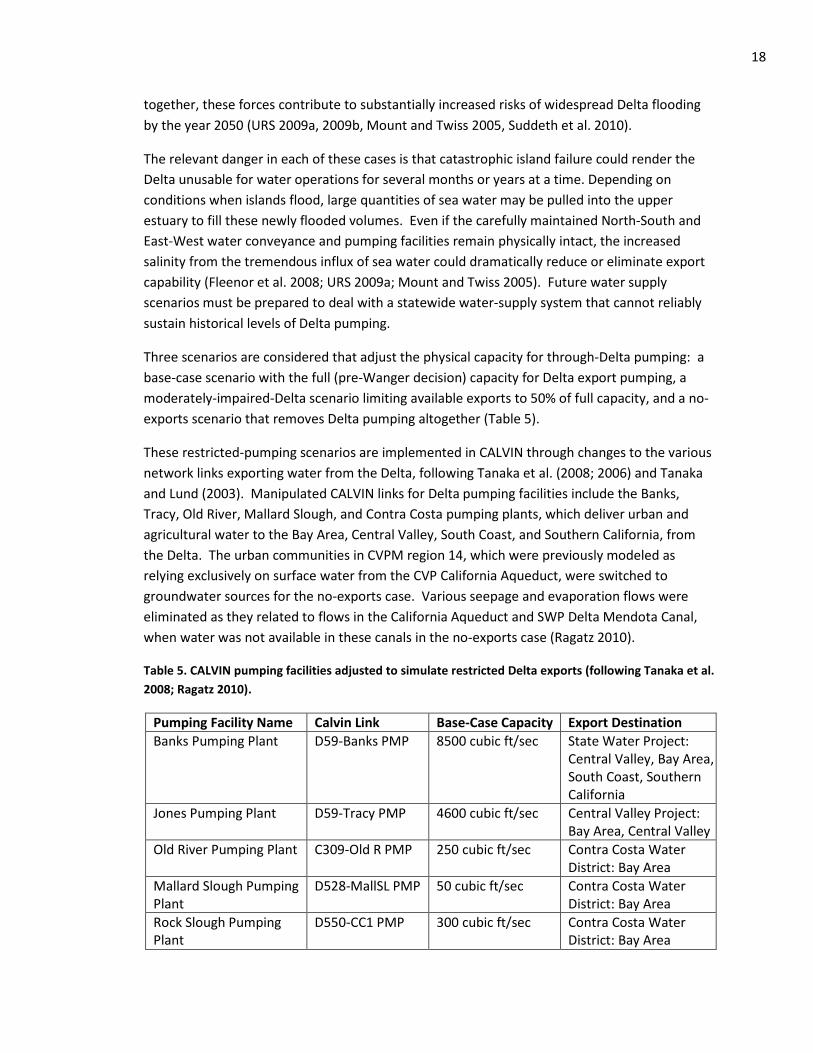
Three scenarios are considered that adjust the physical capacity for through-Delta pumping: a base-case scenario with the full (pre-Wanger decision) capacity for Delta export pumping, a moderately-impaired-Delta scenario limiting available exports to 50% of full capacity, and a no-exports scenario that removes Delta pumping altogether (Table 5).

These restricted-pumping scenarios are implemented in CALVIN through changes to the various network links exporting water from the Delta, following Tanaka et al. (2008; 2006) and Tanaka and Lund (2003). Manipulated CALVIN links for Delta pumping facilities include the Banks, Tracy, Old River, Mallard Slough, and Contra Costa pumping plants, which deliver urban and agricultural water to the Bay Area, Central Valley, South Coast, and Southern California, from the Delta. The urban communities in CVPM region 14, which were previously modeled as relying exclusively on surface water from the CVP California Aqueduct, were switched to groundwater sources for the no-exports case. Various seepage and evaporation flows were eliminated as they related to flows in the California Aqueduct and SWP Delta Mendota Canal, when water was not available in these canals in the no-exports case (Ragatz 2010).

Table 5. CALVIN pumping facilities adjusted to simulate restricted Delta exports (following Tanaka et al. 2008; Ragatz 2010).

Pumping Facility Name Calvin Link Base-Case Capacity Export Destination Banks Pumping Plant D59-Banks PMP 8500 cubic ft/sec

State Water Project: Central Valley, Bay Area, South Coast, Southern California

Jones Pumping Plant D59-Tracy PMP 4600 cubic ft/sec Central Valley Project: Bay Area, Central Valley

Old River Pumping Plant C309-Old R PMP 250 cubic ft/sec Contra Costa Water District: Bay Area

Mallard Slough Pumping Plant

D528-MallSL PMP 50 cubic ft/sec Contra Costa Water District: Bay Area

Rock Slough Pumping Plant

D550-CC1 PMP 300 cubic ft/sec Contra Costa Water District: Bay Area

19

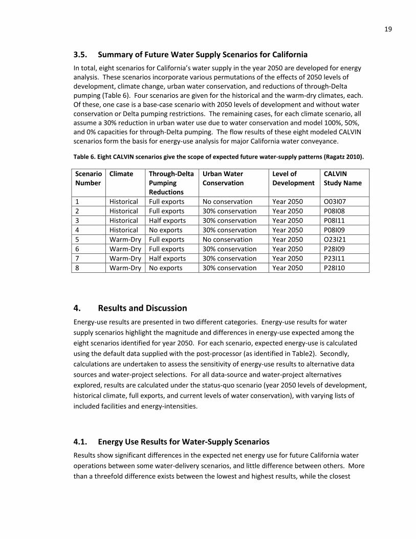
3.5. Summary of Future Water Supply Scenarios for California

In total, eight scenarios for California’s water supply in the year 2050 are developed for energy analysis. These scenarios incorporate various permutations of the effects of 2050 levels of development, climate change, urban water conservation, and reductions of through-Delta pumping (Table 6). Four scenarios are given for the historical and the warm-dry climates, each. Of these, one case is a base-case scenario with 2050 levels of development and without water conservation or Delta pumping restrictions. The remaining cases, for each climate scenario, all assume a 30% reduction in urban water use due to water conservation and model 100%, 50%, and 0% capacities for through-Delta pumping. The flow results of these eight modeled CALVIN scenarios form the basis for energy-use analysis for major California water conveyance.

Table 6. Eight CALVIN scenarios give the scope of expected future water-supply patterns (Ragatz 2010).

Scenario Number

Climate Through-Delta Pumping Reductions

Urban Water Conservation

Level of Development

CALVIN Study Name

1 Historical Full exports No conservation Year 2050 O03I07 2 Historical Full exports 30% conservation Year 2050 P08I08 3 Historical Half exports 30% conservation Year 2050 P08I11 4 Historical No exports 30% conservation Year 2050 P08I09 5 Warm-Dry Full exports No conservation Year 2050 O23I21 6 Warm-Dry Full exports 30% conservation Year 2050 P28I09 7 Warm-Dry Half exports 30% conservation Year 2050 P23I11 8 Warm-Dry No exports 30% conservation Year 2050 P28I10

4. Results and Discussion Energy-use results are presented in two different categories. Energy-use results for water supply scenarios highlight the magnitude and differences in energy-use expected among the eight scenarios identified for year 2050. For each scenario, expected energy-use is calculated using the default data supplied with the post-processor (as identified in Table2). Secondly, calculations are undertaken to assess the sensitivity of energy-use results to alternative data sources and water-project selections. For all data-source and water-project alternatives explored, results are calculated under the status-quo scenario (year 2050 levels of development, historical climate, full exports, and current levels of water conservation), with varying lists of included facilities and energy-intensities.

4.1. Energy Use Results for Water-Supply Scenarios

Results show significant differences in the expected net energy use for future California water operations between some water-delivery scenarios, and little difference between others. More than a threefold difference exists between the lowest and highest results, while the closest

20

results are within one percent of each other. Average expected net-energy use ranges from 3,810 to 13,896 GWh/year, depending on climate and levels of Delta exports and urban water conservation. Energy use is highest in scenarios with full Delta exports and no water conservation, and lowest in scenarios with no Delta exports and thirty-percent conservation (Table 7). However, these calculations for major California water conveyance do not include the relevant energy use by desalination, water recycling, groundwater pumping and other water and wastewater treatment facilities. Nor do they include the energy consumed by end-users of water, the largest contributors to water-related energy consumption.

Calculated net energy-use includes the energy expenditures for pumping operations and the energy gains from in-conduit recovery hydropower generation. The magnitude of energy used for major conveyance pumping ranges from an average of 3,958 to 16,672 GWh/year, across scenarios. Average in-conduit recovery generation ranges from 148 to 2,776 GWh/year, across scenarios, and varies from four to seventeen percent as a fraction of pumping. Recovery generation experiences more fluctuation between scenarios than does pumping, having an almost twentyfold difference between its lowest and highest projections, as opposed to pumping’s fourfold difference.

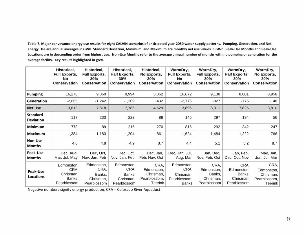
21

Table 7. Major conveyance energy use results for eight CALVIN scenarios of anticipated year-2050 water-supply patterns. Pumping, Generation, and Net Energy Use are annual averages in GWh. Standard Deviation, Minimum, and Maximum are monthly net use values in GWh. Peak-Use Months and Peak-Use Locations are in descending order from highest use. Non-Use Months refer to the average annual number of months with no pumping or generation for the average facility. Key results highlighted in grey.

Historical, Full Exports,

No Conservation

Historical, Full Exports,

30% Conservation

Historical, Half Exports,

30% Conservation

Historical, No Exports,

30% Conservation

WarmDry, Full Exports,

No Conservation

WarmDry, Full Exports,

30% Conservation

WarmDry, Half Exports,

30% Conservation

WarmDry, No Exports,

30% Conservation

Pumping 16,278 9,060 8,994 5,062 16,672 9,138 8,601 3,958

Generation -2,665 -1,242 -1,209 -432 -2,776 -827 -775 -148

Net Use 13,613 7,818 7,785 4,629 13,896 8,311 7,826 3,810

Standard Deviation

117 233 222 88 145 297 194 56

Minimum 778 89 216 270 816 292 342 247

Maximum 1,384 1,183 1,204 861 1,624 1,484 1,222 766

Non-Use Months

4.6 4.8 4.9 8.7 4.4 5.1 5.2 8.7

Peak-Use Months

Dec, Aug, Mar, Jul, May

Dec, Oct, Nov, Jan, Feb

Dec, Oct, Nov, Jan, Feb

Dec, Jan, Feb, Nov, Oct

Dec, Jan, Jul, Aug, Mar

Jan, Dec, Nov, Feb, Oct

Jan, Feb, Dec, Oct, Nov

May, Jan, Jun, Jul, Mar

Peak-Use Locations

Edmonston, CRA,

Chrisman, Banks,

Pearblossom

Edmonston, CRA,

Banks, Chrisman,

Pearblossom

Edmonston, CRA,

Banks, Chrisman,

Pearblossom

CRA, Edmonston,

Chrisman, Pearblossom,

Teerink

Edmonston, CRA,

Chrisman, Pearblossom,

Banks

CRA, Edmonston,

Banks, Chrisman,

Pearblossom

CRA, Edmonston,

Banks, Chrisman,

Pearblossom

CRA, Edmonston,

Chrisman, Pearblossom,

Teerink Negative numbers signify energy production, CRA = Colorado River Aqueduct

22

In general, net energy use is expected to be less in scenarios featuring reduced exports and/or thirty-percent water conservation than in the year-2050 base case (Figure 1). The only exception is under a warm-dry climate, where net energy use is expected to significantly decrease from the base case with no exports, but slightly increase from the base case with full or half exports. A slight shift in peak-energy-use location is also predicted, favoring the Colorado River Aqueduct over the State Water Project in scenarios with a warm-dry climate or no Delta exports (Table 7), with a maximum decrease of over 4,500 GWh/year in net energy use at the Edmonston pumping plant and full use of the Colorado River Aqueduct, in the worst-case scenario. This corresponds well with the reductions to SWP export capacity for the A2 scenario modeled by Anderson et al. (2008).

0

2,000

4,000

6,000

8,000

10,000

12,000

14,000

16,000

Full ExportsNo Conservation

Full Exports 30% Conservation

Half Exports30% Conservation

No Exports 30% Conservation

Avg

erag

e A

nnua

l Ene

rgy

Use

(GW

h)

Scenario

Historical Climate

Warm-Dry Climate

Figure 1. Water-delivery-energy-use results for year 2050, organized by climate scenario.

Comparison of results that differ by only one criterion (Table 8) gives insights into how additional information on each criterion might reduce uncertainties in estimated future energy use. Agreement is best between scenarios of different climate types but identical Delta export and urban water conservation levels, with an average difference of just two percent. Scenarios with different levels of urban water conservation but identical climate and export levels show more variability, with an average difference in major conveyance energy use of forty-one percent. Scenarios of the same climate and water conservation types but differing export levels show an average difference of forty-seven percent between low and high major conveyance energy-use values, though the difference between full and half Delta exports, with year 2050 levels of development and 30-percent urban water conservation, is small.

23

Table 8. Relative differences in annual net energy use between scenarios that differ on only one criterion, averaged across all scenarios sharing that difference. Key results highlighted in grey.

Historical -> Warm Dry Climate

Zero -> 30% New Conservation

Full -> Half Delta Exports

Half -> No Delta Exports

Full -> No Delta Exports

4% increase with full or half exports

41% decrease 3% decrease 46% decrease 47% decrease 18% decrease with

no exports

(2% overall average decrease)

4.2. Sensitivity of Energy-Use Results to Data Source and Water Project

Five scenarios are explored comparing the effects of data source on calculated energy-use. The base case in this comparison is the year-2050 projection with a historical climate, full Delta exports, and no additional urban water conservation, as calculated with the General Energy Post-Processor default data (the author’s interpretation of the best data for each facility). The four additional comparisons explore the same water-use scenario (i.e. using the same CALVIN flow results), but calculate energy-use using: DWR data as a first preference and GEI data when unavailable, GEI data when as a first preference and DWR data unavailable, DWR data exclusively and omitting all other facilities, and GEI data exclusively and omitting all other facilities.

The results of this comparison show a high degree of uniformity among scenarios calculated with the three combined data sources (Default data, DWR first, and GEI first), which include the same forty-one facilities and range from 13,613 to 13,886 GWh/year (Table 10). Somewhat surprisingly, both DWR-first and GEI-first calculations produce slightly higher energy-use estimates than their combined default-data estimate. Estimates using only DWR data (covering thirty-one facilities) and GEI-only data (covering thirty-three facilities) are lower than in the base case, though not to the same degree. In absolute terms, DWR-only results are twenty-three percent lower than in the base case while GEI-only results are just one percent lower than in the base case. When scaled to the fraction of facilities included, the DWR-only results are just two percent higher than the base case and the GEI-only results are twenty-two percent higher than the base case (Table 9). This difference is attributed to the DWR data having a mix of facilities similar to those in the default data and to the GEI data being more heavily weighted towards the large, energy-intensive facilities of the Coastal Branch of the SWP, East Branch Extension of the SWP and Colorado River Aqueduct, and excluding facilities with relatively low energy intensities.

24

Table 9. Percent differences from the default-data base case, by data source. Key results highlighted in grey.

DWR first GEI first DWR only GEI only Difference from

base case 2% increase 1% increase 23% decrease 1% decrease

Number of Facilities Included1 41 41 31 33

Difference from base case when

scaled to fraction of facilities included

-- -- 2% increase 22% increase

1. Pumping and generation counted separately.

25

Table 10. Sensitivity of energy-use results to data source and project scope. Results are calculated based on identical input data (CALVIN flow results for the historical climate, full Delta exports, no new urban water conservation scenario) using different combinations of energy-intensity data. Scenarios to the left of the break vary data sources but calculate energy use for all included facilities, scenarios to the right of the break all use the default data but vary included facilities by water project. Pumping, Generation, and Net Energy Use are annual averages in GWh. Standard Deviation, Minimum, and Maximum are monthly net use values in GWh. Peak-Use Months and Peak-Use Locations are in descending order from highest use. Non-Use Months refer to the average annual number of months with no pumping or generation for the average facility. Key results highlighted in grey.

Default Data DWR first GEI first DWR only GEI only SWP only CVP only

Pumping 16,278 16,394 16,549 12,791 16,123 12,547 2,598

Generation -2,665 -2,507 -2,749 -2,316 -2,710 -2,455 -19

Net Use 13,613 13,886 13,800 10,475 13,413 10,093 2,580

No. of facilities

41 41 41 31 33 27 16

Standard Deviation

117 119 107 105 100 84 77

Minimum 778 790 788 590 782 587 28

Maximum 1,384 1,407 1,476 1,107 1,448 1,099 369

Non-Use Months

5 5 5 3 4 3 1

Peak-Use Months

Dec, Aug, Mar, Jul, May

Dec, Aug, Mar, Jul, May

Dec, Aug, Jul, Mar, May

Dec, Mar, Aug, Jul, Jun

Dec, Aug, Jul, Mar, May

Dec, Aug, Oct, Jul, Mar

Aug, Mar, Jul, Jun, May

Peak-Use Locations

Edmonston, Colorado River

Aqueduct, Chrisman,

Banks, Pearblossom

Edmonston, Colorado River

Aqueduct, Chrisman,

Banks, Pearblossom

Edmonston, Colorado River

Aqueduct, Chrisman,

Banks, Pearblossom

Edmonston, Chrisman,

Banks, Pearblossom,

Teerink

Edmonston, Colorado River

Aqueduct, Chrisman,

Banks, Pearblossom

Edmonston, Chrisman,

Banks, Pearblossom,

Teerink

Banks, Dos Amigos (CVP),

San Luis Relift, Jones,

Tehama-Colusa Relift

26

The results can also be looked at for differences in energy use between individual water projects. For this analysis, base case results are calculated with default data from the year-2050 historical climate, full Delta exports, and no new urban conservation scenario, for all facilities for which the General Energy Post Processor has data in the CVP, SWP, and Local water projects. Two additional results are calculated with the same input scenario and energy-intensity data, but limited to facilities in only the CVP and in only the SWP (Table 10). Due to their lesser role in major California water conveyance, local facilities are not included in this comparison. Comparisons show that both the CVP and SWP significantly underestimate base-case energy use, both in absolute terms and as a fraction of included facilities (Table 11). This is attributed to the higher-than-average energy intensity of the omitted Colorado River Aqueduct, which singlehandedly raises energy use estimates by an average 2,575 GWh/year in the base case, and to the CVP and SWP both having a mix of facilities dissimilar to those in the default data.

Table 11. Percent differences from the default-data base case, by water project.

SWP only CVP only Difference from

base case 26% decrease 81% decrease

Number of Facilities Included1 27 16

Difference from base case when

scaled to fraction of facilities included

13% increase 51% decrease

1. Pumping and generation counted separately; some facilities used jointly by both SWP and CVP.

4.3. Discussion and Comparision of the General Energy Post-Processor vs. Existing Water-Energy Analysis Software

The UC Davis General Energy Post-Processor introduced in this thesis combines useful elements from several previous works, including the recent GEI/Navigant model and study and the LongTermGen and SWP_Power energy post-processors for CalSim II. It is generic and modular in form, promotes many types of analyses, and is easily adaptable for future studies. With separate databases for energy intensity, water-model network, and facility-level data, each linked through runtime parameter selection and user-defined keywords, the scope of water-energy modeling and analysis is broadened to many additional models and scenarios.

By default, model-network data are included in the General Energy Post-Processor for the CALVIN and CalSim II water models. Like LongTermGen and SWP_Power, the General Energy Post-Processor is envisioned to be most useful for energy analysis with large, detailed water management models. Regardless, networks links for other water models (e.g. local models, the GEI/Navigant model) can easily be added. An option, populated from a customizable list, is presented for the user to select which water-model network or networks to employ in calculating energy-use results. The ability to switch between networks and to incorporate flow from multiple networks and models is not available in any alternative energy post-processors for

27

California water models. The CalSim II energy post-processors are expected to require a moderate degree of adjustment to be useful with other model networks (including the anticipated CALSIM III), and the GEI/Navigant model is not anticipated to be useful with any network beyond its own coarse system representation.

One strength of the GEI/Navigant model is its empirical and traceable approach towards energy-intensity. These empirical data are generally expected to produce the most accurate energy-use results, especially for flow patterns that are reasonably similar to the recent operations from which these data were derived. This approach is contrasted with the more opaque and somewhat analytical approach of LongTermGen and SWP_Power. The UC Davis energy post-processor incorporates data each of these sources and is poised to incorporate additional data that becomes available in the future. An option exists to select facility energy intensities on a case-by-case basis, through general source preferences, or from one exclusive data source. This ability is unavailable in prior California water-energy tools and enables a new type of sensitivity analysis, where the energy impacts of flow results can be compared between energy-intensity data sources. Both the GEI and DWR tools include a several additional energy intensities and facilities that are beyond the wholesale-water-supply scope of this study (e.g. local deliveries, upstream hydropower).

The GEI/Navigant model is relatively well documented, with a brief user’s manual and an accompanying report with appendices detailing energy-intensity development and general model design. The UC Davis energy post-processor is also well documented, containing comments and notes for each represented energy intensity, facility, and network link, often detailing source documents, areas for further investigation, contact people, revision notes, and geo-referenced data. The relative lack of documentation in the CalSim II post-processors is understandable given their history as internal tools for WAPA, DWR, and other public agencies, and has not proved to be a barrier to their use by external parties (e.g. USBR 2009; HDR 2007; Jones & Stokes 2003; EDWPA 2008).

As with existing energy post-processors, runtime is negligible for the UC Davis post-processor. The total analysis time is predominantly a function of water model selection and the amount of time necessary to prepare and run each scenario. Total analysis time will be longer with the General Energy Post-Processor, LongTermGen, and SWP_Power than with the GEI/Navigant tool, which couples water modeling with energy post-processing and requires no export/import of flow results. Total analysis time is expected to be slightly shorter with the General Energy Post-Processor than with LongTermGen and SWP_Power, which require input data to be imported in a very specific format. These differences imply that the GEI/Navigant model is easiest to use, but least flexible, that the UC Davis and CalSim II post-processors have similar ease of use, and that the UC Davis post-processor has the greatest flexibility.

LongTermGen and SWP_Power model several physical facility characteristics than are not included with the GEI/Navigant or UC Davis post-processors, including information on the number of units at each facility, facility capacities, expected transmission losses to the nearest substation, percent of on-peak and off-peak operation, etc. This makes these tools especially relevant for studies interested in the facility-level details of expected energy use and deliveries, whereas the other post-processors are most useful to assess the comparative differences between scenarios. The CalSim II post-processors also explicitly include a flow capacity check, which the GEI/Navigant disregards and UC Davis tools assumes is dealt with by the associated water model (e.g. directly in CALVIN or CalSim II).

28

One major strength of the CalSim II post-processors is their flexibility in representing energy-intensity at each facility. In these tools, energy intensity is most often represented as a fixed average annual value, but is occasionally represented as a fixed monthly value or as an algebraic function of other parameters. This is useful for capturing nuances in time-dependent energy-intensity fluctuations (e.g. at the Red Bluff Research Pumping Plant) or when energy intensity is associated with variable head (e.g. at the San Luis-Gianelli plant), and is represented in pre-defined Visual Basic functions hidden from the user. The UC Davis energy post-processor includes these energy intensity functions with native Excel equations, though Visual Basic functions can also be easily added. This is not available in the GEI/Navigant model. Depending on the application, each of the tools compared in this analysis has relative advantages and disadvantages (Table 12).

Table 12. Comparison of the relative strengths and weaknesses of each of the water-energy analysis tools mentioned in this study. Best tool(s) in each category highlighted in grey.

GEI/Navigant

model

LongTermGen and

SWP_Power

UC Davis General Energy Post-Processor

Overall description: Quick & easy, but limited

Detailed, but unintuitive

Moderate and flexible

Ease of use 1st 3rd 2nd Level of facility detail 3rd 1st 2nd

Flexibility within current scope 3rd 2nd 1st Extensibility to different scopes and

new types of analysis 3rd 2nd 1st

Level of documentation 1st 3rd 2nd Ease of incorporating new data 2nd 3rd 1st

Transparency of calculations to the end user 1st 2nd 1st

Total time required for analysis 1st 3rd 2nd Strong history of prior use -- 1st -- Can rapidly switch between

scenarios and/or options 1st 3rd 2nd

Automatically graphs results 1st 2nd -- Ease of expansion to new model

networks (e.g. CalSim III) 3rd 2nd 1st

Can combine flow results from multiple water models -- -- 1st

Number of facilities relevant to wholesale water deliveries 33 31 41

Number of additional facilities not relevant to wholesale water

deliveries 31 11 0

Number of facilities with energy intensities from multiple sources 0 0 23

Number of energy intensity functions [total / relevant] 0/0 16/5 5/5

1. Facilities mentioned without energy intensities not included.

29

5. Limitations Several important limitations should be kept in mind with the water-energy analysis undertaken in this study. As with any modeling project, the flow scenarios modeled with CALVIN are subject to boundary conditions and limiting assumptions, as discussed in detail in Jenkins et al. (2001; 2004). The quality of the energy analysis of these flow results is also limited by the energy-intensity data available for each facility, as described in GEI (2010) and somewhat described in CH2M-Hill (2009). Unfortunately, documentation for the energy-intensity data in the LongTermGen and SWP_Power is somewhat sparse and scattered (for example, some data comments are available only from within the Visual Basic code, others are missing altogether), though detailed energy-intensity functions are included where prudent. For GEI data, only average energy intensities are reported, with an accompanying error range and low/high values. Though more detailed historical operations data was collected by the GEI/Navigant team to produce these average intensities, this data has not be released and no apparent attempt was made to convert it to energy-intensity functions for facilities with significant variability.

In terms of project scope, this analysis has been limited to pumping and recovery-generation facilities associated with California wholesale water deliveries. Though present, this scope does not include the energy benefits of hydropower facilities upstream of the Delta or the additional energy use associated with local-scale water treatment, deliveries, end use, and disposal. The scope is also limited to surface-water energy use, as detailed energy-intensity data are generally unavailable for groundwater pumping.

Some degree of accuracy is necessarily also lost in mapping known energy intensities to modeled network links. With large-scale models like CALVIN and CalSim II, the best available link for a given facility may not include the effects of minor upstream diversions and local inflows. For cases where the water model reasonably covers the location of an included facility, identifying the proper link can still be difficult if the facility is not noted on the model schematic (as was often found in both CALVIN and CalSim II), if the model network logically splits flows that occupy the same physical pipeline (e.g. CalSim II flows through the Gianelli facility are split into separate links for the CVP, SWP, and Environmental Water Account), or if the actual facility location is difficult to correlate with any particular model link (e.g. various re-lift pumping may or may not be located before or after some aggregated diversion in the model). Moreover, not all facilities can be mapped to the model network at all. For example, links for the relatively small Folsom pumping plant and proposed DMC Intertie cannot be found in the CALVIN schematic, and links for the relatively large facilities of the SWP East Branch Extension, Colorado River Aqueduct, and Central MWD cannot be found in the traditional schematic for CalSim II. In cases with lingering uncertainties, detailed notes have been included for that facility in the General Energy Post-Processor, and the most reasonable match is made based on the author’s best judgment.

30

6. Extensions Several improvements remain to be made in future versions of the UC Davis General Energy Post-Processor to better the quality of the user’s experience and to improve the general usefulness of the tool (for example, to automatically summarize and graph results).

The post-processor currently incorporates energy intensities as point values or as functions of other time series. Though the underlying flow/energy-use data (e.g. from GEI 2009) have not been made available, more precise definitions of energy intensity can be specified through piecewise-linear curves of values/functions specified through time or for different levels of flow. Examples where this would be useful include the Red Bluff Research pumping plant, which has a fixed energy intensity but only operate for part of the year, or facilities like the Banks and Tracy pumping plants that have significant operational overheads that affect plant efficiency as a function of flow.

The post-processor currently relies on flow and energy input data being verified by the user to be in compatible units. In this analysis, energy intensity is specified in kWh/AF and flow in KAF/month, producing energy-use results in MWh/month which are converted to GWh/month for graphical and tabular display. The post-processor could be made more useful by including functions to convert between units of flow and energy and by applying these functions automatically to the input data and results.

The default data included with the post-processor are limited to the pumping and recovery generation facilities within the scope of the present study. To be made more widely useful, data for additional hydropower and energy-use facilities can also be added.

The post-processor currently includes network data for CALVIN, CalSim II, and a blank space for one additional network. To support analysis with many different networks without needing to constantly switch between spreadsheets, additional spaces can be added. Once available, network links should also be added for CalSim III.

A compromise must be made between a tool’s extensibility/generality and the intricate depth to which it can be applied to specific problems. The General Energy Post-Processor is a highly extensible and general tool that can easily be applied to many types of problems and which contains data sufficient to perform a variety of comparative analyses. It does not, however, mimic the level of detail found in LongTermGen and SWP_Power. For analyses that include transmission losses, number of pumping/generating units, unit capacities, facility capacities, on- and off-peak percentages of energy use, and which are useful for operational planning, additional default data will need to be compiled and tradeoffs will need to be made as routines added that limit the scope of the tool but streamline special-purpose calculations.

31

7. Conclusions The above analysis leads to several conclusions, some relevant for policy and planning purposes, and some highlighting the salience and role different data/sources have for future modeling efforts. The results are organized accordingly, below.

Implications for water and energy planning and policy:

We may not need to worry much about the impacts of climate change on water-delivery energy use when planning for the net energy use associated with major water conveyance in California’s water network (assuming the system is allowed to operate as freely as in CALVIN). Some scenarios show a slight increase in expected energy use with a warm-dry climate, but never of more than six percent. One scenario even shows a decrease in net energy use under a warm-dry vs. historical climate.

With thirty-percent water conservation, the loss of fully half of current Delta exports bears little effect on net conveyance energy use. This is perhaps the most salient conclusion that can be drawn from the energy-use projections for the future water supply scenarios shown in Figure 1. This also implies that water conservation could be discussed as one response to anticipated levee failure and pumping restrictions in the Delta.

We can be almost assured to have sufficient energy supplies to continue delivering water in the future, even in the face of climate change, reduced Delta exports, and/or increased urban water conservation. Results for only one of the seven perturbed scenarios predict energy-use higher than in the year-2050 base case, by only two percent. Planning energy investment solely around anticipated population growth (i.e. by continuing current per-capita investment trends) will likely be sufficient to ensure energy availability for major water conveyance in the future.

Reducing our uncertainty regarding future scenarios can have big payoffs. Model results show energy-use scenarios that differ by over 350%. Pinpointing which groups of scenarios are most likely can focus our assessment of future water and energy needs, boost our confidence in future water and energy investment, and potentially realize substantial cost savings over year-2050 base case projections.

The value of additional information seems greatest for urban water conservation, next important for Delta export levels, and least important for climate change. This conclusion is based on greater percent differences in net energy use between scenarios differing in each of these dimensions, respectively (Table 8). This is promising because reducing uncertainty regarding future water conservation can largely be accomplished through political processes (e.g. by analyzing past conservation goals, by legislating penalties for not meeting future goals, by rewarding early adoption, etc), and reducing uncertainty for Delta export levels can be partially accomplished by political processes (e.g. by clarifying the scope of the Endangered Species Act, by constructing isolated conveyance channels) that do not contain the level raw physical uncertainty that surrounds climate change.

32

If thirty-percent urban-water conservation can be implemented, a conveyance energy savings of over forty percent can be realized. This may be a promising way to free-up energy resources without increasing water shortages.

With a shift in peak-use facilities towards the Colorado River Aqueduct with climate change or a total loss of Delta exports, in-conduit generation there will likely remain cost effective in the future. This conclusion, based results in Table 7, also implies that in-conduit generation in the SWP may become less cost effective in the future but that hydropower facilities in Central MWD will also likely hold their value.

Choosing between data sources for modeling and decision making:

It does not matter whether energy-use calculations predominantly use GEI or DWR data. Total energy use is similar in all cases modeling the full forty-one represented facilities, regardless of whether the energy-use estimates always prefer DWR over GEI data, always prefer GEI over DWR data, or use some rational decision process to prefer a combination of the two. This result does not hold for cases using only DWR or only GEI data to model a subset of the forty-one facilities. Even though energy intensities for individual facilities can be quite different between data sources, the overall average differences are quite small.

Using GEI-only data can provide a good approximation of total base-case energy use, but using DWR-only data can provide a good approximation of average base-case per-facility energy use. These conclusions hold true even though nearly ¼ of the total number of facilities are missing from each of these sources. Regardless, using combined DWR-GEI energy-intensity data is preferred to include more facilities in the analysis without skewing either total or average net energy use.

Neither CVP-only nor SWP-only results are a good approximation for the operations of the system as a whole. This is true both in absolute terms or when scaled to the fraction of facilities included.

The General Energy Post-Processor is a useful tool for the energy post-processing of flow results. It currently contains water-energy data for CALVIN and CalSim II, and can easily be extended to CalSim III and other water models. Energy intensities can also be added for water treatment, desalination, groundwater pumping, water recycling and other energy costs associated with modeled flow though specific network links.

33

8. References Anderson J, Chung F, Anderson M, Brekke L, Easton D, Ejeta M, Peterson R, Snyder R. 2008.

Progress on incorporating climate change into management of California's water resources. Climatic Change 87(Suppl1):S91-S108.

Burt C, Howes D, Wilson G. 2003. California agricultural water electrical energy requirements, final report. Prepared for California Energy Commission, PIER Program. Irrigation and Training Research Center, California Polytechnic State University, San Luis Obispo, California. CEC-400-2005-002-AT1. 154 p. Available from: http://www.energy.ca.gov/2005publications/CEC-400-2005-002/CEC-400-2005-002-AT1.PDF

Cayan DR, Bromirski PD, Hayhoe K, Tyree M, Dettinger MD, Flick RE. 2008A. Climate change projections of sea level extremes along the California coast. Climatic Change 87(Suppl 1):S57-S73.

Cayan DR, Maurer EP, Dettinger MD, Tyree M, Hayhoe K. 2008B. Climate change scenarios for the California region. Climatic Change 87(Suppl 1):S21-S42.

[CEC] California Energy Commission. 2005. California’s water-energy relationship. California Energy Commission, Sacramento, California. CEC-700-2005-011-SF. 180 p.

[CEC] California Energy Commission. 2007. Integrated energy policy report. California Energy Commission, Sacramento, California. CEC-100-2007-008-CMF. 250 p.

CH2M Hill. 2009. Project Use Computational Descriptions. Documents provided with LongTermGen and SWP_Power post-processors for CalSim II. Available from Brian Van Lienden, CH2M Hill.

Cohen R, Nelson B, Wolff G. 2004. Energy down the drain—the hidden costs of California’s water supply. Natural Resources Defense Council and the Pacific Institute. Natural Resources Defense Council Publications Dept, New York, New York. 85 p. Available from: http://www.nrdc.org/water/conservation/edrain/contents.asp

Connell CR. 2009. Bring the heat, but hope for rain: adapting to climate warming for California. MS Thesis. 48 p. Available from the University of California, Davis, Davis, California.

[CPUC] California Public Utilities Commission, California Energy Commission. 2006. Energy Efficiency: California’s Highest-Priority Resource. California Public Utilities Commission, San Francisco, California. 8 p. Available from: ftp://ftp.cpuc.ca.gov/Egy_Efficiency/CalCleanEng-English-Aug2006.pdf

Delworth TL, Broccoli AJ, Rosati A, Stouffer RJ, Balaji V, Beesley JA, Cooke WF, Dixon KW, Dunne J, Dunne KA, Durachta JW, Findell KL, Ginoux P, Gnanadesikan A, Gordon CT, Griffies SM, Gudgel R, Harrison MJ, Held IM, Hemler RS, Horowitz LW, Klein SA, Knutson TR, Kushner PJ, Langenhorst AR, Lee HC, Lin SJ, Lu J, Malyshev SL, Milly PCD, Ramaswamy V, Russell J, Schwarzkopf MD, Shevliakova E, Sirutis JJ, Spelman MJ, Stern WF, Winton M, Wittenberg AT, Wyman B, Zeng F, Zhang R. 2006. GFDL's CM2 global coupled climate models. Part I: formulation and simulation characteristics. Journal of Climate 19(5):643-674.

Draper AJ, Jenkins MW, Kirby KW, Lund JR, Howitt RE. 2003. Economic-engineering optimization for California water management. Journal of Water Resources Planning and Management 129(3):155-164.

34

[DWR] California Department of Water Resources. 1998. California water plan update, bulletin 160-98. State of California, Department of Water Resources, Sacramento, California. Available from: http://www.waterplan.water.ca.gov/previous/b160-98/TOC.cfm

[DWR] California Department of Water Resources. 2007. DWR Releases Water Delivery Impact Estimates Following Wanger Decision. State of California, Department of Water Resources, Sacramento, California. 2 p. Available from: http://www.water.ca.gov/news/newsreleases/122407wanger.pdf

[DWR] California Department of Water Resources. 2009a. California water plan update – highlights, Bulletin 160-09. State of California, Department of Water Resources, Sacramento, California. 32 p. Available from: http://www.waterplan.water.ca.gov/cwpu2009/index.cfm

[DWR] California Department of Water Resources. 2009b. California water plan update – Volume 3 Regional Reports: Sacramento—San Joaquin Delta, Bulletin 160-09. State of California, Department of Water Resources, Sacramento, California. 70 p. Available from: http://www.waterplan.water.ca.gov/cwpu2009/index.cfm

[DWR] California Department of Water Resources. 2009c. 2010 State Water Project initial allocation, notice to contractors 09-09. State of California, Department of Water Resources, Sacramento, California. 2 p. Available from: http://wwwdwr.water.ca.gov/swpao/deliveries.cfm

[DWR] California Department of Water Resources. 2010a. Development of common model package. State of California, Department of Water Resources, Sacramento, California. Available from: http://www.water.ca.gov/storage/common_assumptions/cmpackages_index.cfm

[DWR] California Department of Water Resources. 2010b. 2010 State Water Project allocation increase to 50 Percent, notice to contractors 10-11. State of California, Department of Water Resources, Sacramento, California. p. Available from: http://wwwdwr.water.ca.gov/swpao/deliveries.cfm

EDAW Inc. 2008. Cost of Water Shortage. Memo to East Bay Municipal Utility District dated March 14, 2008. EDAW Inc, San Francisco, California. 6 p. Available from: http://www.ebmud.com/sites/default/files/pdfs/Cost%20of%20Water%20Shortage.pdf

[EDWPA] El Dorado Water & Power Authority. 2008. Notice of preparation, El Dorado Water & Power Authority, supplemental water rights project. 12 p. Available from: http://www.edcgov.us/waterandpower/water_power_pdf/EDWPA_FINAL_NOP_October_24_2008.pdf

[E3] Energy and Environmental Economics, Inc. 2005. The cost of wildlife-caused power outages to California’s economy. Prepared for California Energy Commission, PIER Program. CEC-500-2005-030. 29 p. Available from: http://www.energy.ca.gov/pier/project_reports/CEC-500-2005-030.html

Fleenor WE, Hanak E, Lund JR, Mount JR. 2008. Delta hydrodynamics and water salinity with future conditions. In Lund J, Hanak E, Fleenor W, Bennett W, Howitt R, Mount J, Moyle P. Comparing futures for the Sacramento-San Joaquin Delta. Public Policy Institute of California. 51 p. Available from: http://www.ppic.org/main/publication.asp?i=810

Fryer J. 2010. An investigation of the marginal cost of seawater desalination in California. Residents for Responsible Desalination, Huntington Beach, California. 25 p.

35

[GEI] GEI Consultants and Navigant Consulting. 2010. Embedded energy in water studies, study 1: statewide and regional water-energy relationship – draft final report. Prepared for California Public Utilities Commission, Energy Division. 155 p. Available from: http://www.energydataweb.com/cpuc/home.aspx

Gleick PH. 1994. Water and energy. Annual Review of Energy and the Environment 19:267-299.

Grogan T. 2010. How to use ENR’s cost indexes. Engineering News-Record 264(10):60.

Hayhoe K, Cayan D, Field CB, Frumhoff PC, Maurer EP, Miller NL, Moser SC, Schneider SH, Cahill KN, Cleland EE, Dale L, Drapek R, Hanemann RM, Kalkstein LS, Lenihan J, Lunch CK, Neilson RP, Sheridan SC, Verville JH. 2004. Emissions pathways, climate change, and impacts on California. Proceedings of the National Academy of Sciences of the United States of America 101(34):12422-12427.

HDR. 2007. Draft environmental report/environmental impact statement for the Proposed Lower Yuba River Accord, appendix d, modeling technical memorandum. Prepared for California Department of Water Resources, Yuba County Water Agency, and U.S. Department of Interior, Bureau of Reclamation. 108 p. Available from: http://www.usbr.gov/mp/nepa/nepa_projdetails.cfm?Project_ID=2549

Heberger M, Cooley H, Herrera P, Gleick PH, Moore E. The impacts of sea-level rise on the California coast. Prepared for California Energy Commission, California Climate Change Center. CEC-500-2009-024-F. 115 p. Available from: http://pacinst.org/reports/sea_level_rise/report.pdf

Howitt RE, Ward KB, Msangi SM. 2001. Statewide water and agricultural production model, appendix A. In Jenkins MW, Draper AJ, Lund JR, Howitt RE, Tanaka SK, Ritzema R, Marques GF, Msangi SM, Newlin BD, Van Lienden BJ, Davis MD, Ward KB. 2001. Improving California Water Management: Optimizing Value and Flexibility. Prepared for CALFED Bay-Delta Program. University of California Davis, Davis, California. 11 p. Available from: http://cee.engr.ucdavis.edu/faculty/lund/CALVIN/Report2/

Jenkins MW, Draper AJ, Lund JR, Howitt RE, Tanaka SK, Ritzema R, Marques GF, Msangi SM, Newlin BD, Van Lienden BJ, Davis MD, Ward KB. 2001. Improving California water management: optimizing value and flexibility. Prepared for CALFED Bay-Delta Program. University of California Davis, Davis, California. 150 p. Available from: http://cee.engr.ucdavis.edu/faculty/lund/CALVIN/Report2/

Jenkins MW, Lund JR, Howitt RE. 2003. Using economic loss functions to value urban water scarcity in California. Journal of the American Water Works Association 95(2):58-70.

Jenkins MW, Medellín-Azuara J, Lund JR. 2007. California urban water demands for year 2050. Prepared for California Energy Commission, PIER Program. CEC-500-2005-195. 19 p.

Jones & Stokes. 2003. Freeport Regional Water Project, volume 3, modeling technical appendix to the draft environmental impact report/environmental impact statement. Prepared for Freeport Regional Water Authority and U.S. Department of Interior, Bureau of Reclamation. 1146 p. Available from: http://www.freeportproject.org/nodes/project/draft_eir_eis_v3.php

Joskow PL. 2001. California’s electricity cricis. Oxford Review of Economic Policy 17(3):365-388.

36

LaCommare KH, Eto JH. 2004. Understanding the cost of power interruptions to U.S. electricity consumers. Lawrence Berkeley National Laboratory, Environmental Energy Technologies Division. 70 p. Available from: http://certs.lbl.gov/pdf/55718.pdf

Landis JD, Reilly M. 2002. How we will grow: baseline projections of California’s urban footprint through the year 2100. Institute of Urban and Regional Development, University of California Berkeley, Berkeley, California. 114 p. Available from: http://escholarship.org/uc/item/8ff3q0ns

[LAO]Legislative Analyst Office. 2009. Water rights: issues and perspectives. Prepared for California Senate Natural Resources and Water Committee. 12 p. Available from: http://www.lao.ca.gov/laoapp/PubDetails.aspx?id=1959

Legislative Counsel. 2010. Assembly bill number 2514, introduced. Legislative Counsel, State of California, Sacramento, California. 17 p. Available from: http://www.leginfo.ca.gov/pub/09-10/bill/asm/ab_2501-2550/ab_2514_bill_20100219_introduced.pdf

Legislative Counsel. 2009a. Senate bill number 1, chaptered. Legislative Counsel, State of California, Sacramento, California. 39 p. Available from: http://www.leginfo.ca.gov/pub/09-10/bill/sen/sb_0001-0050/sbx7_1_bill_20091112_chaptered.pdf

Legislative Counsel. 2009b. Senate bill number 7, chaptered. Legislative Counsel, State of California, Sacramento, California. 25 p. Available from: http://www.leginfo.ca.gov/pub/09-10/bill/sen/sb_0001-0050/sbx7_7_bill_20091110_chaptered.pdf

Lineweber D, McNulty S. 2001. The cost of power disturbances to industrial & digital economy companies. Prepared for Consortium for Electric Infrastructure to Support a Digital Society, an initiative by EPRI and the Electricity Innovation Institute. EPRI reference # 1006274. Primen, Madison, Wisconsin. 105 p. Available from: http://www.epri-intelligrid.com/intelligrid/docs/Cost_of_Power_Disturbances_to_Industrial_and_Digital_Technology_Companies.pdf

Lofman D, Petersen M, Bower A. 2002. Water, energy and environment nexus: the California experience. International Journal of Water Resources Development 18(1):73-85.

Lund JR, Howitt RE, Jenkins MW, Zhu T, Tanaka SK, Pulido M, Tauber M, Ritzema R, Ferriera I. 2003. Climate warming and California’s water future. Prepared for California Energy Commission. University of California Davis, Davis, California. 86 p. Available from: http://cee.engr.ucdavis.edu/faculty/lund/CALVIN/ReportCEC/

Lund JR, Hanak E, Fleenor WE, Bennett WA, Howitt RE, Mount JF, Moyle PB. 2010 Comparing Futures for the Sacramento-San Joaquin Delta, University of California Press, Berkeley, California. 256 p.

M.Cubed. 2008. Addendum to Shortage Cost TM [Technical Memo]. Memo to East Bay Municipal Utility District dated February 6, 2008. M.Cubed, Oakland, California. 10 p. Available from: http://www.ebmud.com/sites/default/files/pdfs/Cost%20of%20Water%20Shortage%20Addendum.pdf

Marsh D, Sharma D. 2006. Water-energy nexus: a review of existing models. 1st Australian Young Water Professionals Conference, The University of New South Wales, Sydney. 6 p. Available from: http://www.cwwt.unsw.edu.au/ywp2006/papers/YWP%202.2.pdf

37

Maurer EP. 2007. Uncertainty in hydrologic impacts of climate change in the Sierra Nevada, California, under two emissions scenarios. Climatic Change 82(3-4):309-325.

Maurer EP, Duffy PB. 2005. Uncertainty in projections of streamflow changes due to climate change in California. Geophysical Research Letters 32(3):1-5.

Maurer EP, Hidalgo HG. 2008. Utility of daily vs. monthly large-scale climate data: an intercomparison of two statistical downscaling methods. Hydrology and Earth System Science 12(2):551-563.

Means E III. 2004. Water and wastewater industry energy efficiency: a research roadmap. Prepared for American Water Works Association Research Foundation and California Energy Commission. American Water Works Association Research Foundation, Denver, Colorado. CEC-500-2004-901. 129 p. Available from: http://www.energy.ca.gov/2004publications/CEC-500-2004-901/CEC-500-2004-901.PDF

Medellín-Azuara J, Harou JJ, Olivares MA, Madani K, Lund JR, Howitt RE, Tanaka SK, Jenkins MW, Zhu T. 2008. Adaptability and adaptations of California’s water supply system to dry climate warming. Climatic Change 87(Supplement 1):S75-S90.

Miller NL, Bashford KE, Strem E. 2003. Potential impacts of climate change on California hydrology. Journal of the American Water Resources Association 39(4):771-784.

Nakicenovic N, Alcamo J, Davis G, de Bries B, Fenhann J, Gaffin S, Gregory K, Grubler A, Jung TY, Kram T, La Rovere EL, Michaelis L, Shunsuke M, Tsuneyuki M, Pepper W, Pitcher H, Schlesinger M, Shukla P, Smith S, Swart R, van Rooijen S, Victor N, Dadi Z. 2000. Special report on emissions scenarios, Intergovernmental Panel on Climate Change. Cambridge University Press, Port Chester, New York. 612 p. Available from: http://www.grida.no/publications/other/ipcc_sr/?src=/climate/ipcc/emission/

Nichols FH, Cloern JE, Luoma SN, Peterson DH. 1986. The modification of an estuary. Science 231(4738): 567-573.

Null SE, Lund JR. 2006. Reassembling Hetch Hetchy: water supply without O'Shaughnessy Dam. Journal of the American Water Resources Association 42(2):395-408.

Office of the Governor. 2006. Gov. Schwarzenegger Signs Landmark Legislation to Reduce Greenhouse Gas Emissions. Press release GAAS:684:06 dated Sept 27, 2006. Available from: http://gov.ca.gov/index.php?/press-release/4111/

Ragatz R. 2010. Forks in the road: how water conservation and varying Delta exports affect California’s water supply in the face of climate change. MS Thesis. Available from the University of California, Davis, Davis, California.

Rawlins SL. 1977. Irrigation and the energy economics of water management for hydrologic basins. In Lockeretz W. Agriculture and energy: proceedings of a conference, Washington University, St. Louis, Missouri, June 17-19, 1976. Academic Press, San Francisco, California. p. 131-147

Stokes J, Horvath A. 2006. Life cycle energy assessment of alternative water supply systems. International Journal of Life Cycle Assessment 11(5):335-343.

Suddeth RJ, Mount J, Lund JR. 2010. Levee decisions and sustainability for the Sacramento-San Joaquin Delta. San Francisco Estuary and Watershed Science 8(2). 24 p. Available from: http://escholarship.org/uc/item/9wr5j84g

38

Tanaka SK, Lund JR. 2003. Effects of increased delta exports on Sacramento valleys economy and water management. Journal of the American Water Resources Association 39(6):1509-1519.

Tanaka SK, Zhu T, Lund JR, Howitt RE, Jenkins MW, Pulido-Velazquez MA, Tauber M, Ritzema RS, Ferreira IC. 2006. Climate warming and water management adaptation for California. Climatic Change 76(3–4):361-387.

Tanaka SK, Connell CR, Madani K, Lund JR, Hanak E, Medellín-Azuara J. 2008. The economic costs and adaptations for alternative Delta regulations, technical appendix F. In Lund J, Hanak E, Fleenor W, Bennett W, Howitt R, Mount J, Moyle P. Comparing futures for the Sacramento-San Joaquin Delta. San Francisco (CA): Public Policy Institute of California. 70 p. Available from: http://www.ppic.org/main/publication.asp?i=810\

[URS] URS Corporation, J.R. Benjamin and Associates. 2009a. Section 11, salinity impacts. In Delta risk management strategy (DRMS) phase 1 final risk analysis report. Prepared for California Department of Water Resources. 24 p. Available from: http://www.water.ca.gov/floodmgmt/dsmo/sab/drmsp/phase1_information.cfm

[URS] URS Corporation, J.R. Benjamin and Associates. 2009b. Section 14, risk analysis for future years. In Delta risk management strategy (DRMS) phase 1 final risk analysis report. Prepared for California Department of Water Resources. 42 p. Available from: http://www.water.ca.gov/floodmgmt/dsmo/sab/drmsp/phase1_information.cfm

[USBR] U.S. Bureau of Reclamation, Mid-Pacific Region. 2009. San Joaquin River restoration program water year 2010 interim flows project environmental assessment/initial study, appendix g, modeling. xx p. Available from: http://www.usbr.gov/mp/nepa/nepa_projdetails.cfm?Project_ID=3612

US Census Bureau. California QuickFacts from the US Census Bureau, 2009 population estimate. US Census Bureau. Available from: http://quickfacts.census.gov/qfd/states/06000.html

Wade WW, Hewitt JA, Nussbaum MT. 1991. Cost of industrial water shortages. Prepared for California Urban Water Agencies. Spectrum Economics Inc, San Francisco, California. 215 p. Available from: http://www.cuwa.org/publications.html

[WAPA] Western Area Power Administration. 2004. CVP power resources report (Green Book 2004). 78 p. Available from: http://www.wapa.gov/sn/marketing/docs/Scheduling/FinalGreenbook2004.pdf

Van Lienden B, Leaf R. 2007. Development of Common Assumptions Common Model Package for the CALFED Surface Storage Investigations. Presentation to California Water and Environmental Modeling Forum. Available from: http://www.cwemf.org/Asilomar/CommonAssumptionsBVanlienCWEMF2007.ppt

Zetland D. 2010. A Broken Hub Will Not Wheel: Water Reallocation in California. Journal of Contemporary Water Research & Education 144:18-28.

Zhu TJ, Jenkins MW, Lund JR. 2005. Estimated impacts of climate warming on California water availability under twelve future climate scenarios. Journal of the American Water Resources Association 41(5):1027-1038.