Engineering Fracture Mechanics - University of Michiganveeras/papers/39.pdf · S. Panwar et al./Engineering Fracture Mechanics 162 (2016) 290–308 291. which reduces the stiffness

Engineering Fracture Mechanics 162 (2016) 290–308

Contents lists available at ScienceDirect

Engineering Fracture Mechanics

journal homepage: www.elsevier .com/locate /engfracmech

Modeling fatigue failure using the variational multiscalemethod

http://dx.doi.org/10.1016/j.engfracmech.2016.05.0210013-7944/� 2016 Elsevier Ltd. All rights reserved.

⇑ Corresponding author.E-mail address: [email protected] (V. Sundararaghavan).URL: http://umich.edu/~veeras (V. Sundararaghavan).

Shardul Panwar, Shang Sun, Veera Sundararaghavan ⇑Department of Aerospace Engineering, University of Michigan, Ann Arbor, MI 48105, USA

a r t i c l e i n f o a b s t r a c t

Article history:Received 27 January 2016Received in revised form 26 May 2016Accepted 31 May 2016Available online 2 June 2016

Keywords:Variational Multi-Scale MethodFatigueCohesive zone modelCrack propagation

In this paper, we study fatigue failure using the variational multiscale method (VMM). Inthe VMM, displacement jumps are represented using finite elements with specially con-structed discontinuous shape functions. These elements are progressively added alongthe crack path during fatigue failure. The stiffness of these elements changes non-linearlyin response to the accumulation of damage during cyclic loading. The evolution law forstiffness is represented as a function of traction and the number of loading cycles sincethe initial onset of failure. Numerical examples illustrate the use of this new methodologyfor modeling macroscopic crack growth under Mode I loading as well as microscopic crackgrowth under mixed mode loading within the elastic regime. We find that the discontinu-ous elements can consistently predict the Mode I stress intensity factor (SIF) and the micro-structurally short crack growth paths, and that the computed Paris law for steady crackgrowth is controlled primarily by two parameters in the decohesion law.

� 2016 Elsevier Ltd. All rights reserved.

1. Introduction

Numerically, solving a boundary value problem with a crack or multiple cracks inside the domain is not a trivial task,because, these new boundaries (or surfaces) are originally not part of a domain and emerge only as the domain boundariesare loaded. In the context of the finite element method (FEM), the framework of the Galerkin based traditional FEMs are notparticularly suited to solve this type of problem. This is due to limitations such as spurious mesh-related length scales [1,2]and the requirement that the mesh be aligned relative to the strain localization band [3,4], which has kinematics similar tothat of the crack boundaries. In recent years, however, a whole new class of finite element methods have emerged that cansolve the problem of new boundaries emerging inside a domain without experiencing any of the limitations of traditionalFEMs. Depending upon how these new boundaries are embedded in the finite element framework, these methods arebroadly classified into two families, node enrichment FEM (e.g. X-FEM) and elemental enrichment FEM (e.g. E-FEM).Between these two families, Oliver et al. [5] showed that, under similar conditions, X-FEM is more computationally expen-sive. Therefore, E-FEM would be a favorable option for problems requiring more computational time. One such problem isfatigue failure, in which crack growth can occur over millions of cycles, so computational solutions are very expensive (interms of computing time).

http://crossmark.crossref.org/dialog/?doi=10.1016/j.engfracmech.2016.05.021&domain=pdf

http://dx.doi.org/10.1016/j.engfracmech.2016.05.021

mailto:[email protected]

<xml_chg_old>http://umich.edu/veeras</xml_chg_old><xml_chg_new>http://umich.edu/~veeras</xml_chg_new>

http://dx.doi.org/10.1016/j.engfracmech.2016.05.021

http://www.sciencedirect.com/science/journal/00137944

http://www.elsevier.com/locate/engfracmech

Nomenclature

a; b cohesive fatigue parameters�r; r0 coarse-scale and fine-scale residual�u; �w continuous coarse-scale displacement fieldsCc crack surfacesut discontinuous displacement fieldr; e stress, strainf body forceG;H cracked element out-normal and crack face normal directionN;B;d standard finite element shape function, shape function gradient, and displacement field nodal valuesn;m normal and tangential directionsT external tractionu0;w0 discontinuous fine-scale displacement fieldsu;w displacement field and variation of displacement fieldD;R applied displacement and load ratioC;Hn;Hm material elastic stiffness, Mode-I cohesive stiffness, and Mode-II cohesive stiffnessX domainJ j-integralKI;KIc Mode-I stress intensity factor and Mode-I critical stress intensity factorm;C Paris curve constantsNf number of loading cycles experienced by material point since the onset of failureTgbc critical grain boundary fracture stress

Tcrss critical resolved shear stressW;Cij strain energy density and HCP material elastic constants

S. Panwar et al. / Engineering Fracture Mechanics 162 (2016) 290–308 291

In this paper, we use a type of E-FEM introduced by Hughes [6] and referred to as the variational multiscale method(VMM) by Garikipati [7]. VMM uses a multiscale interpolation scheme to embed cracks into the continuum domain (repre-senting discontinuities using a Heaviside function). The main advantage of the multiscale interpolation scheme over the par-tition of unity interpolation scheme (used in X-FEM) is the local-to-element nature of the discontinuous displacement field.This means that the additional degree of freedom needed to represent the discontinuity will be condensed out at the elementlevel, thereby leaving the sparsity pattern of the global problem untouched. This is why the computational cost of multiscaleinterpolation based VMM (E-FEM) is less than the partition of unity interpolation based X-FEM and why the former is moresuitable for fatigue problems.

Modeling any crack growth problem requires a correct physical representation of the mechanics of the crack tip. Classi-cally, this is done using Linear Elastic Fracture Mechanics (LEFM), which is based on Griffith’s [8] energy-based and Irwin’s[9] stress-intensity-factor based theories of crack propagation. Elasticity theory produces stress singularity at the crack tip. Inreal materials, however, the stresses in front of the crack tip are nonlinear and have finite values. To address this problem,Dugdale [10] and Barenblatt [11] independently developed Cohesive Zone Model (CZM) theory. Willis [12] showed that theCZM is equivalent to Griffith’s [8] energy balance concept when the size of the cohesive zone is small compared to the size ofthe crack and the specimen geometry. Later, Hillerborg et al. [13] introduced the concept of the CZMwithin the framework ofthe finite element method. Around the same time, Bazant and Oh [14] introduced the crack band model, which localizes theprocess zone in a single element. However, this model in the framework of finite element analysis often exhibits mesh ori-entation bias, meaning that the orientation of the crack band depends on the orientation of the mesh discretization [15]. TheCZM, however, regards the fracture process as a gradual separation between the material surfaces, and this separation isresisted by the cohesive tractions. It also defines the stress at the crack tip using a progressive material degradation law. Thislaw, called the Traction–Separation law, specifies a relationship between the crack surface traction and the crack surface sep-aration. For monotonic fracture problems, Xu and Needleman [16] developed a simple form of the CZM to incorporate rever-sible behavior. In this model, the interfaces heal when brought back into contact after separation. Camacho and Ortiz [17]developed a model in which the unloading and reloading process is reversible. However, during this unloading and reloadingevent, there is no energy dissipation; thus, this model is not suitable for cyclic loading. De-Andres et al. [18] extended thislinear loading and unloading cohesive model to analyze fatigue crack growth in a aluminum shaft. In this model, the damageparameter is adjusted explicitly as the number of loading cycles increases, without any dependence on the damage processoccurring within a loading cycle. This results in the lack of predictability of the fatigue crack growthmodel. Nguyen et al. [19]developed a one-parameter cohesive model that takes into account the irreversible behavior of failure process and theloading–unloading hysteresis. Inspired by this and similar cohesive models [20,21], Maiti and Geubelle [22] developed atwo-parameter cohesive model that takes into account all the nonlinear effects associated with failure mechanisms. In theirmodel, once a crack forms, the interface begins to accumulate irreversible damage during the loading part of each cycle,

292 S. Panwar et al. / Engineering Fracture Mechanics 162 (2016) 290–308

which reduces the stiffness of the interface. During unloading, the model response is linear, but with a lower slope comparedto the previous loading cycle. Maiti and Geubelle [22] used this cohesive model in the framework of the standard finite ele-ment method and referred to it as the cohesive/volumetric finite element method (CVFE). However, the use of zero-volumeelements or interface elements in the standard finite element framework makes the method subject to the numerical dis-cretization scheme. To solve this issue, we combine the cohesive model developed by Maiti and Geubelle [22] with theVMM. The coupling of a cohesive zone model with the VMM has been demonstrated by Rudraraju et al. [23]. They used asimple linear CZM inside the framework of the VMM to successfully demonstrate crack propagation in laminated fiberreinforced composites and showed experimental comparisons. However, the VMM has not yet been utilized in problemsinvolving cyclic loading. In this paper, we employ a cyclic cohesive zone model, referred to as the fatigue CZM, proposedby Maiti and Geubelle [22] along with the variational multiscale method to predict the steady state crack growth rate intwo-dimension.

Using cohesive theory to accurately predict any failure process requires proper calibration of the cohesive model param-eters. One approach is to fit the cohesive parameters to one or more experiment(s) and then use those fitted parameters topredict other experimental results. Using this approach, uniaxial tensile tests can be used to determine the cohesive param-eters for Mode I fracture [24]. Another approach is to determine these parameters from a lower-scale calculation [25,26]. Incase of fatigue failure, Maiti and Geubelle [22] followed the first approach and fitted cohesive parameters to the macro-scaleParis law.

Thus, the objectives of this paper are: (1) to successfully demonstrate the coupling of the fatigue cohesive model with thevariational multiscale method, (2) to correctly predict the macro-scale Mode I stress intensity factor, (3) to correlate theexperimental micro-structurally short crack path with the VMM crack path, (4) to introduce an approach for calibratingthe fatigue cohesive law parameters from the macro experiments, and (5) to show that different steady-state crack growthrates (or Paris laws) can be simulated by different cohesive parameters that control the loading stiffness of the fatigue CZM.

The present paper is divided into three sections. Section 2 gives a brief description of the variational multiscale method.Section 3 describes the cohesive model used for modeling fatigue failure. In Section 4, we present our numerical results forfatigue failure using different representative two-dimensional problems.

2. The Variational Multi-Scale Method (VMM)

The presence of cracks in a continuum domain necessitates a discontinuous representation of the displacement field. Anumerical treatment of such discontinuities and the resultant singular strain field was done in the work of Temam andStrang [27], which was on the space BD(X) (of functions of bounded deformation). This idea was later used to develop anumerical framework for the problem of strong discontinuities due to strain localization by Simo et al. [28], Simo and Oliver[29], and Armero and Garikipati [1]. Later, this approach was adopted by Garikipati [7] to embed micro-mechanical surfacelaws into a macroscopic continuum formulation in a multiscale setting. The mathematical model of this variational multi-scale method is briefly described in Section 2.1.

2.1. A mathematical model of the variational multiscale method

The crack surface (Cc) in a continuous domain (X) is shown in Fig. 1. The standard weak form of the balance of linearmomentum over the domain (X) is given by
Z
X$sw : rdV ¼

ZXw � f dV þ

Z@Xt

w � T dS ð2:1Þ

where r is the stress, w is an admissible displacement variation, $sw is the symmetric gradient of the variation, T is theexternal traction and f is the body force. The displacement fields (u and variation w) can be decomposed into continuouscoarse-scale (�u; �w) and discontinuous fine-scale (u0;w0) components. Such a decomposition is possible because of therequirement that the fine-scale fields u0 and w0 must vanish outside the fine-scale subdomain X0. In crack propagation prob-lems, the fine-scale field (u0) represents the discontinuity.

u ¼ �uþ u0 ð2:2Þw ¼ �wþw0 ð2:3Þ

�u 2 S ¼ fv jv ¼ g on @Xug

�w 2 �m ¼ fvjv ¼ 0 on @Xug

u0 2 S0 ¼ fv jv ¼ 0 on X n intðX0Þg

w0 2 m0 ¼ fv jv ¼ 0 on X n intðX0Þg

Fig. 1. 2-Dimensional representation of a crack opening sut and the crack surface Cc .


where S � BDðXÞ; m � H1ðXÞ, S ¼ �S � S0, and m ¼ �m � m0. �m and m0 are chosen to be linearly independent. More concisely, thechoice of space S at the elemental level can be represented using linear polynomials, while space S0 contains non-nodal sup-ported functions (e.g. discontinuities) that are independent from S.

Using this additive decomposition, the weak form (2.1) can be separated into two equations, one involving only thecoarse-scale variation �w, and another involving only the fine-scale variation w0.
Z
X$s �w : rdV ¼

ZX

�w � f dV þZCh

�w � T dS ð2:4Þ

ZX$sw0 : rdV ¼

ZXw0 � f dV þ

ZCh

w0 � T dS ð2:5Þ

Eq. (2.5) can be simplified by using integration by parts and variational arguments to [7]:
ZCcw0r � ndS ¼
ZCcw0 � Tc dS ð2:6Þ

where Tc is the external traction on the crack faces.

2.2. The micro-mechanical surface law

The micro-mechanics of crack growth (Fig. 2) can be explained by a traction–separation law. This traction–separation lawis inserted into the continuum formulation through Eq. (2.6). The traction Tc is decomposed into two components (for 2-Dproblems), one normal to the crack face Tc

n

� �and another tangent to the crack face Tc

m

� �.

Tc ¼ Tcnnþ Tc

mm ð2:7Þ

The fine scale-field u0, which is composed of a displacement discontinuity sut, can be similarly decomposed into itscomponents sunt (opening) and sumt (shear) along the n and m directions respectively.

sut ¼ suntnþ sumtm ð2:8Þ

Using the above two Eqs. (2.7) and (2.8), the micro-mechanical cohesive law (discussed in Section 4) can be utilized byspecifying the relationship between traction components and discontinuous displacement components in both the normaland tangential directions. For the case of monotonic loading, a simple surface traction law is used, given by [30]:

Tcn ¼ Tc

n0 �Hnsunt; Tcm ¼ Tc

m0 �Hmsumt ð2:9Þ

where Tcn0 and Hn are the Mode I critical opening traction and Mode I softening modulus, respectively, and Tc

m0 and Hm arethe Mode II critical opening traction and Mode II softening modulus, respectively. In Section 3, we modify the surface tractionlaw to account for cyclic irreversibility.

Fig. 2. Micro-structural domain X0 and crack surface Cc , along with crack directions normal n and tangent m.


2.3. Finite-dimensional formulation (2-dimensional)

In a finite-dimensional setting, the domain X can be divided into a number of connected non-overlapping elements such

that X ¼ [nel1 Xh

e , where nel represents the number of elements in the finite domain. The fine-scale displacement u0 can bewritten in terms of local interpolation functions as:

u0e ¼ MTcsute ð2:10Þ

where sute is the elemental value of the fine-scale displacement discontinuity. MTc is a multiscale shape function given by

MTc ¼ N � HTc ð2:11Þ
where N is the usual linear shape function for triangular elements, and HTc is the Heaviside function, which is used to intro-duce a discontinuity within the sub domain Cc. This construction ensures thatMTc ¼ 0 on X n intðX0Þ. The construction of thismultiscale shape functionMTc in two-dimensions is shown in Fig. 3. In the weak form,MTc comes into the system of equationas $MTc through the expression for $u0.
$u0 ¼ $MTc sut ð2:12Þ
where
sut ¼ sutxsuty

" #; rMTc ¼ 1

hi G � dCcH;

G ¼nix 00 ni

y

niy ni

x

264

375; and H ¼

nx 00 ny

ny nx

264

375

G and H are the matrix representations of a crack element’s out-normal and a crack face’s normal directions, respectively. hi

is the element length.The expressions for strain and stress are given by [23],

e ¼ Bdþ G � dTcHð Þsut ð2:13Þ

r ¼ C : Bdþ Gsutð Þ ð2:14Þ
where B is the standard matrix form of the shape function gradient, d is the nodal value of the coarse-scale displacement, andC is the elastic stiffness matrix. Substituting these expressions into the weak form Eqs. (2.4) and (2.6), the resulting coarse-scale and fine-scale equations are respectively given by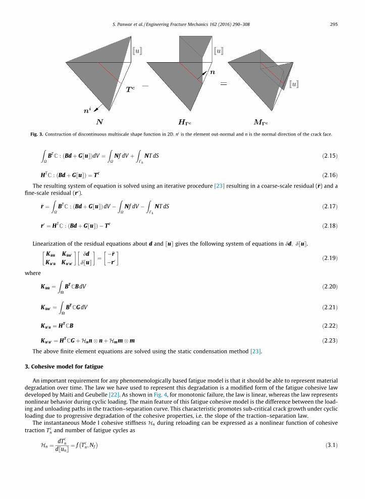

Fig. 3. Construction of discontinuous multiscale shape function in 2D. ni is the element out-normal and n is the normal direction of the crack face.


ZXBT

C : ðBdþ GsutÞdV ¼ZXNf dV þ

ZCh

NT dS ð2:15Þ

HTC : ðBdþ GsutÞ ¼ Tc ð2:16Þ

The resulting system of equation is solved using an iterative procedure [23] resulting in a coarse-scale residual (�r) and afine-scale residual (r0).

�r ¼ZXBT

C : ðBdþ GsutÞdV �ZXNf dV �

ZCh

NT dS ð2:17Þ

r0 ¼ HTC : ðBdþ GsutÞ � Tc ð2:18Þ

Linearization of the residual equations about d and sut gives the following system of equations in dd; dsut.

K �u�u K �uu0

Ku0�u Ku0u0

� �dddsut

� �¼ ��r

�r0

� �ð2:19Þ

where

K �u�u ¼ZXBT

CBdV ð2:20Þ

K �uu0 ¼ZXBT

CGdV ð2:21Þ

Ku0 �u ¼ HTCB ð2:22Þ

Ku0u0 ¼ HTCG þHnn� nþHmm�m ð2:23Þ

The above finite element equations are solved using the static condensation method [23].

3. Cohesive model for fatigue

An important requirement for any phenomenologically based fatigue model is that it should be able to represent materialdegradation over time. The law we have used to represent this degradation is a modified form of the fatigue cohesive lawdeveloped by Maiti and Geubelle [22]. As shown in Fig. 4, for monotonic failure, the law is linear, whereas the law representsnonlinear behavior during cyclic loading. The main feature of this fatigue cohesive model is the difference between the load-ing and unloading paths in the traction–separation curve. This characteristic promotes sub-critical crack growth under cyclicloading due to progressive degradation of the cohesive properties, i.e. the slope of the traction–separation law.

The instantaneous Mode I cohesive stiffness Hn during reloading can be expressed as a nonlinear function of cohesivetraction Tc

n and number of fatigue cycles as

Hn ¼ dTcn

dsunt¼ f Tc

n;Nf

� � ð3:1Þ

Fig. 4. Subcritical vs. critical failure. Tcn0 and sunct are Mode I critical opening traction and displacement, respectively.


where Nf denotes the number of loading cycles experienced by a material point since the onset of failure, Tcn denotes the

normal component of traction on the crack face and sunt is the normal component of the displacement discontinuity onthe crack face. A similar expression can be written for Mode II failure. A two-parameter power law relationship can be usedto model the rate of decay of the cohesive stiffness Hn.

Hn ¼ f Tcn;Nf

� � ¼ �cðNf ÞTcn ð3:2Þ

where

c ¼ 1aN�b

f ð3:3Þ

Here a and b are cohesive parameters that are related to the degradation of the cohesive strength. The cohesive parameter ahas the dimension of length while b denotes the history dependence of the failure process. Both of these parameters accountfor the unloading–reloading hysteresis. The inclusion of this hysteresis may, in the phenomenological sense, account for thedissipative mechanism arising from reverse yielding upon unloading. Reverse yielding upon unloading may occur when thecrack growth happens as a result of alternating crystallographic slip [31]. This dissipative mechanism can also be caused as aresult of repeated rubbing of asperities, which may cause steady weakening of the cohesive surfaces. A simple phenomeno-logical model that incorporates this assumption has been built by relating the cohesive stiffness to the number of loadingcycles through a power law relationship (3.2). The above evolution law can be expressed in terms of the rate of change ofthe cohesive stiffness Hn as

_Hn ¼ � 1aN

�bf Hn

_sunt _sunt P 0

0 _sunt < 0

(ð3:4Þ

The second equation states that there is no change in cohesive stiffness during unloading cycle. Eq. (3.4) can be convertedfrom the temporal to the spatial domain and, using a 1st order finite difference approximation, can be written as

Hðiþ1Þn ¼ HðiÞ

n 1� 1aN�b

f suntðiþ1Þ � sunt

ðiÞ� ��

ð3:5Þ

for _sunt P 0, superscripts (i + 1) and (i) denote the adjacent load steps in a loading cycle. Thus, the traction–separation curveslope (Hn) is progressively degraded as the number of loading cycles increases.

There are four independent fatigue cohesive model parameters that have to be calibrated. Fracture strength Tcn0

� �, area

under the traction–separation curve, and critical displacement ðsunctÞ are three monotonic cohesive model parameters, ofwhich only two are independent. For fatigue fracture, material parameters a and b are the additional two parameters thathave to be calibrated. We can calibrate the first two monotonic cohesive model parameters by setting Tc

n0 equal to the frac-ture strength of the elastic material and the area under the traction–separation curve equal to the Mode I fracture toughnessGc

I of the elastic material. The cohesive parameters a and b are calibrated from macro-scale experiments. The procedure forcalibrating these two parameters is described in next section.

4. Results and discussions

In this section, examples are shown using this combined method (the VMM with the CZM) called the VariationalMultiscale Cohesive Method (VMCM). These examples cover different concepts within fracture mechanics and are presentedto show the capability of this method. Results are provided for the macroscopic stress intensity factor, the micro-structurally


short crack path, and fatigue crack growth. The later example is used to show that, by varying parameters a and b, fatiguecrack growth curves of different materials can be predicted and inversely cohesive parameters a and b can also be calibratedfrom macro experiments. These examples demonstrate the capability of this method to model failure in materials at themacro-level as well as at the micro-level.

The objectivity of this method with respect to numerical discretization has already been demonstrated by Rudraraju et al.[23]. Unless otherwise noted, the material used is an epoxy [22] with E = 3.9 GPa, m ¼ 0:4, and Mode I fracture toughnessGIc ¼ 88:97 J=m2. The Mode I critical opening traction Tc

n0 is taken to be 50 MPa, while the material parameters a and bare taken to be 5 lm and 0.5, respectively. In all numerical simulations, the length of the elements in front of the cracktip is defined to be smaller than p

8E

ð1�m2ÞGIcravg

[22] so that the fracture process is accurately captured in this region. Here,

ravg Tcn0

2

� �is the average stress in the cohesive zone. To concentrate more on the accuracy and benefits of this method,

we present only the local Mode I simulation. Mode II and Mixed-Mode simulation can quite easily be carried out usingthis method. An in-house C++ based code has been developed to produce data for all the examples presented in this section.To solve the nonlinear equations that arise from the finite element formulations, a Newton–Raphson iterative schemeis used.

4.1. Comparison of the linear elastic stress intensity factor and the J-integral stress intensity factor

A comparison between the theoretical stress intensity factor and the numerical stress intensity factor is important todetermine the accuracy of the stress field surrounding the crack using the VMM approach. This serves as a basic verificationof the numerical method. The theoretical Mode I stress intensity factor (SIF) is calculated from a linear elastic fracturemechanics (LEFM) solution, while the numerical SIF is calculated using the J-integral method [32]. The SIF from linear elasticfracture mechanics is given by [33]

KI ¼ rffiffiffiffiffiffipa

p1:12� 0:23a=bþ 10:6ða=bÞ2

n�21:7ða=bÞ3 þ 30:4ða=bÞ4

oð4:1Þ

where r is the applied stress, b is the height of the specimen and a is the crack length. The J-integral SIF is calculated alongthe contour C surrounding the boundary of a cohesive zone as shown in Fig. 5; this is given by Eq. (4.2).

J ¼ZC

Wdy� Ti@ui

@xds

� ð4:2Þ

where W is the strain energy density, Ti is the ith component of the traction vector perpendicular to C in the outward direc-tion, ui is the ith component of the displacement vector, and ds is an arc length element along contour C. For plane strainconditions, the following relation is given by Rice [32]

KI ¼ JEð1� m2Þ

� �1=2ð4:3Þ

The LEFM requirement of small scale yielding imposes the condition that the cohesive zone size should be much less thanthe crack length (q < a) in order for the stress field outside the cohesive zone to be nearly the same as the K-dominant stressfield. Thus, the cohesive zone size maintains a constant value of q � 0:08 mm, which is smaller than the initial crack lengtha ¼ 0:1 mm.

The simulation parameters for calculating the J-integral from the FEM domain are the same as those used in the previoussection.

As can be seen in Fig. 6, the numerically computed values for the SIF using the J-integral method are close to the SIF valuespredicted by LEFM. The small discrepancy between the two results can be attributed to the size of the cohesive zone, sincethe LEFM solution is valid only for small-scale yielding. Thus, using the VMCM, we can accurately capture the stress fieldsurrounding the crack.

xy

σσ Γ

T

dsρ

2h

b

Fig. 5. J-integral path taken around the cohesive zone, b = 1 mm (cohesive zone length q � 0:08 mm).

Fig. 6. Comparison between LEFM SIF and J-integral SIF.


4.2. Micro-structurally short surface crack propagation

The subject of micro-structurally short crack growth is used to show the ability of the VMCM to model two-dimensionalmicro-structural failure. Micro-structurally short crack growth refers to crack growth inside a grain (called trans-granularfracture) or at the grain boundaries (called inter-granular fracture). In this section, we show numerical simulation of crackgrowth across multiple grains where the crack could be a mixture of inter-granular and trans-granular fracture. In trans-granular fracture, the crack can follow either the slip planes or a plane lying in-between the slip planes.

The material model we use in our simulation is a hexagonal closed packed (HCP) Mg alloy, WE43, with five elastic con-stants and two lattice constants, as shown below,

C11 ¼ 58 GPa; C12 ¼ 25 GPa; C13 ¼ 20:8 GPa;

C33 ¼ 61:2 GPa; C55 ¼ 16:6 GPa:

c ¼ 5:21 Å; a ¼ 3:21 Å

The material orientation data for individual grains are obtained from electron backscatter diffraction (EBSD) mapping (seeFig. 7), and the crack growth path image is obtained from scanning electron microscopy (SEM) of the WE43 surface [34].Using the grain orientations (Euler–Bunge angles), elastic constants for individual grains are transformed from the crystalframe to the global simulation frame. These transformed 3-D elastic constants are converted to 2-D using plane stressassumptions. This way, the VMM is combined with 2-D crystal elasticity to model micro-structurally short crack growth.The mathematical formulations are similar to those described in Section 2, where the micro-structural domain containsthe grain boundaries and C in Eq. (2.13) is the transformed 2-D elastic anisotropic stiffness matrix.

The HCP Mg has, in total, 18 slip systems, 3 basal hai , 3 prismatic hai, 6 pyramidal hai, and 6 pyramidal hc þ ai slip sys-tems. In pure Mg, the primary slip plane is the basal plane, but when Mg is alloyed with different materials, other slip planesbecome active. In the case of WE43, the crack growth mostly occurs along the basal and the pyramidal hai planes [34]. Tomodel a surface crack propagation problem using plane stress assumptions we use slip lines inside the grains. The slip linesare the intersections of the slip planes (basal and pyramidal hai) and the simulation plane. For our simulation, we use 1 basalslip line and 3 pyramidal hai slip lines for simplicity. The crystal parameters for these 2 slip lines are taken from Choi et al.[35] and are shown below,

Tbasalcrss ¼ 25 MPa; Tpyramidal

crss ¼ 68 MPa

Tgbc ¼ 83 MPa; Tgb cross

c ¼ 100 MPa

Fig. 7. EBSD image with orientation data of a Mg WE43 experimental specimen [34].


Tcrss above corresponds to the critical resolved shear stress or the fracture strength of the slip plane, Tgbc represents the

grain boundary strength, and Tgb crossc is the increased grain boundary strength. The grain boundaries act as micro-

structural barriers to short crack propagation, the strength of which varies with the crystallographic orientation relationship.The higher the tilt and twist mis-orientation angles between adjacent slip bands the more effective the grain boundaries areas barriers to the transmission of slip into the adjacent grains. This also holds true for the crack growth from one grain to

another grain across a grain boundary, and this increased grain boundary strength is labeled here as Tgb crossc . A constant value

of Tgb crossc is used to concentrate more on the varied applications of the VMCM. The crack growth along the slip lines is char-

acterized as Mode II fracture, while the crack growth along the grain boundary is Mode I fracture.In this simulation, there are six cohesive traction–separation laws to account for 1 basal slip crack (Mode II), 3 pyramidal

slips crack (Mode II), 1 grain boundary cracking (Mode I), and 1 grain boundary crossing. For all these laws, we use a criticalsliding/opening displacement value of 0:1 lm.

For a tension test, in a elastic material, the crack on the macroscopic level will grow perpendicular to the direction of themaximum principal stress. However, at the microscopic level, the cracks can only grow along certain planes within a grain.These planes are the slip planes, and for a MgWE43 alloy, the crack grows predominantly along the basal plane and the pyra-midal plane [34]. Thus, to model this crack path, we developed a crack tracking algorithm that takes into account all of thesepaths. At the crack tip, the algorithm searches through all the favorable lines (i.e. 1 basal and 3 pyramidal planes within agrain or 1 basal, 3 pyramidal, and 1 grain boundary at the grain boundary) that meet the fracture criteria and selects the linewhose normal is closest to the maximum principal stress direction. This way, the crack grows along the slip lines and/oralong the grain boundaries.

The finite element mesh for this model is created using a real micro-structural image. The model domain consists of 82grains with different orientations as shown in the color1 plot (Fig. 7). The grain edges of this real micro-structure are gen-erated using ImageJ [36], and then the OOF [37] program is used to generate a finite element mesh from these edges. Thesteps outlined above are shown in Fig. 8. The size of the micro-notch in Fig. 8(c) is similar to the size of experimentalmicro-notch.

The boundary conditions for this simulation are applied so as to match the experimental boundary conditions. In theexperiment, the specimen is loaded in tension along the RD direction [34]. To produce similar loads on our model bound-aries, we apply tensile loads on the left and right boundaries of Fig. 8(c), while loads from Poisson’s effect (m ¼ 0:27) areapplied on the top and bottom boundaries. The loading is applied until the micro-structural crack reaches the domainboundary.

In Fig. 9, we show the comparison between the experimental crack path and our numerical crack path. Fig. 9(b) is a super-position of the EBSD image with the numerical crack path. This figure also contains basal slip lines to show that the crack

1 For interpretation of color in ‘Fig. 7’, the reader is referred to the web version of this article.

Fig. 8. FE mesh generated from a real micro-structure image, RD – Rolled direction, TD – Transverse direction. (a) EBSD image [34]. (b) Grains edgesgenerated from ImageJ [36]. (c) FE mesh generated from OOF [37] with colors shown only for distinguishing different grains. (For interpretation of thereferences to color in this figure legend, the reader is referred to the web version of this article.)


growth inside a grain closely follows these slip lines. On comparing these two figures (Fig. 9(a) and (b)), we see that the crackpath predicted using the VMCM method is close to the experimental crack path even when using a coarse mesh. The differ-

ences between these two crack paths are due to our assumptions of constant grain boundary strength Tgbc

� �and plane stress

and due to the use of a constant Tgb crossc value for all grain boundaries. These parameters need to be more carefully calibrated

for the alloy from lower-scale simulations and/or experiments so that the crack path can be better reproduced. The shortfatigue crack growth can also be modeled using the VMCM. However, for each cohesive law, there are two additional param-eters a and b that have to be calibrated, along with the above-mentioned parameters. The fatigue parameters a and b are

Fig. 9. Comparison of experimental crack path and numerical crack path. (a) Experimental crack image – SEM crack image superimposed on EBSD image[34]. (b) VMCM crack path (shown in dark red) superimposed on EBSD image with basal slip lines shown in each grain. (For interpretation of the referencesto color in this figure legend, the reader is referred to the web version of this article.)


linked to each slip system. Thus, experimental fatigue crack growth rates for each individual slip system are needed tocalibrate these two parameters. The crack growth rates for each slip system can be measured through method, such asbenchmarking [38] or striations.

4.3. ‘Local’ Mode I fatigue crack growth

For fatigue crack growth, we have again considered the SENT specimen (Fig. 5). The crack evolution is considered to be‘local’ Mode I, which implies that, in the direction of crack path, there is no shear stress, and the Mode II fracture toughness iszero. In Fig. 5, the left boundary of the specimen has no displacement in the x-direction, and the bottom left corner of thespecimen has zero displacement in the y-direction. Fatigue tests of specimens are carried out under displacement-controlled tension loading (Fig. 10). The shape of the applied displacement does not affect the fatigue behavior, as the ratedependence of the material is ignored. The maximum displacement Dmax is taken to be 0.009b, the initial crack length is

a0 ¼ 0:1b, and the amplitude ratio R rmaxrmin

� �is 0.

Fig. 11 shows the evolution of traction–separation for a point on the cohesive zone. In the finite element model, this is thethird element in the crack path. We can clearly see the dissipation between the loading–unloading cycles in this element. The

Fig. 10. Variation of applied displacement D with time.

Fig. 11. Evolution of traction–separation curve for a point on the cohesive zone.


dotted line in this figure is the monotonic failure line and is shown to indicate the sub-critical nature of the fatigue cracks.The nonlinear nature of the maximum crack opening traction per cycle can also be clearly seen in this figure.

Fig. 12 shows rxx distribution snapshots taken at different cycles. The crack has propagated � 0:3 times the total width ofthe specimen after 2200 cycles. After this cycle,

KI ¼ 22 MPaffiffiffiffiffiffiffiffiffimm

p ð� KIc ¼ 22:21 MPaffiffiffiffiffiffiffiffiffimm

p Þ ð4:4Þ

and the crack propagates rapidly, indicating the final failure (KIc is monotonic fracture toughness) is as predicted by the LEFMsolution.

As can be inferred from the above statement, the curve of the crack path versus the number of loading cycles (Fig. 13)should be asymptotic. This is the expected behavior of the fatigue crack growth in the case of a SENT specimen. To getthe Paris curve, we need the applied stress intensity factor. The applied stress intensity factor (KI) is calculated using theJ-integral method [32]. The details of KI calculation are given in Section 4.1. By differentiating the crack length with respectto the number of loading cycles (Fig. 13), we can calculate the crack growth rate (da=dN) and plot it versus the change instress intensity factor (DKI). This curve represents the steady state crack growth rate (Fig. 14). The curve captures the finalfailure quite well as indicated by Eq. (4.4). The slope of this curve (Fig. 14) is m = 2.5 and the intercept C � 10�07 mm/cycle.

4.4. Effect of parameters a and b on the Paris curve

In this section, we do a parametric study on the effect of cohesive parameters a and b on the crack growth rate and theParis curve. Fig. 15 plots crack tip advancement versus the number of loading cycles for three different values of a, whileb ¼ 0:2 is kept constant. As can be seen in this figure, the crack growth rate decreases as a increases. For a ¼ 2 lm, the crackadvances nearly 0.4 times the width of the specimen in 80 cycles, whereas, for a ¼ 5 lm, the crack takes around 240 cycles toadvance the same distance. Differentiating the crack length with respect to the number of cycles, we can plot (Fig. 16) thecrack growth rate (da=dN) versus the change in stress intensity factor (DKI). Thus, for different values of a, we get Pariscurves with different intercepts (C ¼ 1� 10�06 to 3� 10�06 mm/cycle). Thus, for the same stress intensity factor we canget different crack growth rates and by changing a we can change these rates.

In Fig. 17, the plot of crack length versus number of cycles for different b-values is shown. For different values of b (0.1,0.3, and 0.5), the crack growth rate changes, and by differentiating these curves we get different Paris curves (Fig. 18) with

Fig. 12. rxx stress (MPa) distribution for ‘local’ Mode I fatigue crack growth. (a) Stress distribution at the end of the first cycle. (b) Stress distribution at theend of 2200 cycles (cracked elements have been removed from the plot).

Fig. 13. Fatigue crack growth in SENT specimen versus the number of loading cycles.


different slopes (m ¼ 2:5 to 3:3;C � 10�07 mm/cycle). Thus, by changing these two parameters, one can obtain Paris curvesfor different materials.

This procedure is followed with polystyrene [39], which has E = 3.1 GPa, m ¼ 0:35, and Mode I fracture toughnessGIc ¼ 1164:52 J=m2. The Mode I critical opening traction Tc

n0 is taken to be equal to the craze stress, 38 MPa [39]. Theparameters a and b are calibrated from the experimental data [40], and the parameters are found to be in the range of

Fig. 14. Paris curve, a ¼ 5 lm and b ¼ 0:5.

Fig. 15. Effect of a parameter on crack propagation (b ¼ 0:2).


Fig. 16. Paris curves for different values of a (b = 0.2).

Fig. 17. Effect of b parameter on crack propagation (a ¼ 5 lm).


0.03–0.05 mm and 0:5, respectively (Fig. 19). The simulations were run on 150 mm � 50 mm � 3 mm SENT specimens withan initial crack length of a0 ¼ 20 mm [39].

Future work will involve microscopic interpretation of a and b using localized grain-to grain crack growth ratemeasurements.

Fig. 18. Paris curves for different values of b (a = 5 lm).

Fig. 19. a and b parameters calibrated for polystyrene [39].


5. Conclusion

Modeling fatigue failure is valuable for predictive modeling of component life and ensuring structural integrity in aero-space structures. In this paper, the variational multiscale method (VMM) is used to model fatigue crack propagation for thefirst time. In this approach, a discontinuous displacement field is added to elements that exceed the critical values of normal


or tangential traction during loading. This additional degree of freedom is represented within the cracked element using aspecial discontinuous shape function, which ensures that the displacement jump is localized to that particular element. Thefinite element formulation and code implementation details are presented. Compared to traditional cohesive zone modelingapproaches, this method does not require the use of any special interface elements in the micro-structure. This method isshown to produce accurate stress field near the crack tip. A micro-structurally short crack growth simulation is performedalong with an experimental comparison to demonstrate the accuracy of this method in predicting microscopic crack pathsand Mixed-Mode failure. A two-parameter phenomenological fatigue cohesive law is incorporated into the VMM via a trac-tion continuity equation. The relationship between the phenomenological model parameters and the slope and intercept ofthe Paris curve are shown. We have shown that different Paris curves can be simulated by varying the parameters in thecohesive law. As an example, we have performed a comparison between our fatigue model and published experimental data.Future work will focus on developing a micro-mechanical interpretation of these parameters and their calibration withexperimental data.

Acknowledgments

The authors would like to acknowledge Professor John Allison, Professor J. Wayne Jones, and their graduate student JacobAdams, of Material Science Engineering Department at the University of Michigan, Ann Arbor for providing the experimentaldata. The computations have been carried out as part of research supported by the U.S. Department of Energy, Office of BasicEnergy Sciences, Division of Materials Sciences and Engineering under Award No. DE-SC0008637 that funds the PRedictiveIntegrated Structural Materials Science (PRISMS) Center at the University of Michigan.

References

[1] Armero F, Garikipati K. An analysis of strong discontinuities in multiplicative finite strain plasticity and their relation with the numerical simulation ofstrain localization in solids. Int J Solids Struct 1996;33(20–22):2863–85.

[2] Bazant Z. Mechanics of distributed cracking. Appl Mech Rev 1986;39:675–705.[3] Larsson R, Runesson K, Ottosen NS. Discontinuous displacement approximation for capturing plastic localization. Int J Numer Methods Eng

1993;36:2087–105.[4] Ramakrishnan N, Okada H, Atluri SN. On shear band formation: II. Simulation using finite element method. Int J Plasticity 1994;10(5):521–34.[5] Oliver J, Huespe AE, Sanchez PJ. A comparative study on finite elements for capturing strong discontinuities: E-FEM vs X-FEM. Comput Methods Appl

Mech Eng 2006;195:4732–52.[6] Hughes TJR. Multiscale phenomena: Greens functions, the Dirichlet-to Neumann formulation, subgrid scale models, bubbles and the origins of

stabilized methods. Comput Methods Appl Mech Eng 1995;127:387–401.[7] Garikipati K. A variational multiscale method to embed micromechanical surface laws in the macromechanical continuum formulation. Comput Model

Eng Sci 2002;3:175–84.[8] Griffith AA. The phenomena of rupture and flow in solids. Philos Trans Roy Soc Lond A 1921;221:163–98.[9] Irwin G. Analysis of stresses and strains near the end of a crack traversing a plate. J Appl Mech 1957;24:361–4.[10] Dugdale DS. Yielding of steel sheets containing slits. Int J Mech Phys Solids 1960;8(2):100–4.[11] Barenblatt G. The mathematical theory of equilibrium cracks in brittle fracture. Adv Appl Mech 1962;7:55–129.[12] Willis JR. A comparison of the fracture criteria of Griffith and Barenblatt. J Mech Phys Solids 1967;15(3):151–62.[13] Hillerborg A, Modeer M, Petersson PE. Analysis of crack formation and crack growth in concrete by means of fracture mechanics and finite elements.

Cem Concr Res 1976;6(6):773–81.[14] Bazant ZP, Oh B. Crack band theory for fracture of concrete. Mater Struct 1983;16:155–77.[15] Rots J, Nauta P, Kuster G, Blaauwendraad J. Smeared crack approach and fracture localization in concrete, vol. 30. Delft: Delft University of Technology;

1985.[16] Xu XP, Needleman A. Numerical simulations of fast crack-growth in brittle solids. J Mech Phys Solids 1994;42(9):1397–434.[17] Camacho GT, Ortiz M. Computational modeling of impact damage in brittle materials. Int J Solids Struct 1996;33(20–22):2899–938.[18] de Andres A, Perez J, Ortiz M. Elastoplastic finite element analysis of three-dimensional fatigue crack growth in aluminum shafts subjected to axial

loading. Int J Solids Struct 1999;36:2175–320.[19] Nguyen O, Repetto E, Ortiz M, Radovitzky R. A cohesive model for fatigue crack growth. Int J Fract 2001;110:351–69.[20] Roe K, Siegmund T. An irreversible cohesive zone model for interface fatigue crack growth simulation. Eng Fract Mech 2003;70:209–32.[21] Yang B, Mall S, Ravi-Chandar K. A cohesive model for fatigue crack growth in quasibrittle materials. Int J Solids Struct 2001;38:3927–44.[22] Maiti S, Geubelle PH. A cohesive model for fatigue failure of polymers. Eng Fract Mech 2005;72:691–708.[23] Rudraraju S, Salvi A, Garikipati K, Waas AM. Predictions of crack propagation using a variational multiscale approach and its application to fracture in

laminated fiber reinforced composites. Compos Struct 2012;94:3336–46.[24] Rocco C, Guinea GV, Planas J, Elices M. Review of the splitting-test standards from a fracture mechanics point of view. Cem Concr Res 2001;31:73–82.[25] Yamakov V, Saether, Phillips D, Glaessgen E. Molecular-dynamics simulation-based cohesive zone representation of inter-granular fracture processes

in aluminum. J Mech Phys Solids 2006;54:1899–928.[26] He M, Li S. An embedded atom hyperelastic constitutive model and multiscale cohesive finite element method. Comput Mech 2012;49(3):337–55.[27] Temam R, Strang G. Functions of bounded deformation. Arch Ration Mech Anal 1980;75:7–21.[28] Simo JC, Oliver J, Armero F. An analysis of strong discontinuities induced by strain-softening in rate-independent inelastic solids. Comput Mech

1993;12:277–96.[29] Simo JC, Oliver J. A new approach to the analysis and simulation of strain softening in solids 1994:25–39.[30] Sundararaghavan V, Sun S. Modeling crack propagation in polycrystalline alloys using a variational multiscale cohesive method. 2nd World congress

on integrated computational materials and engineering, vol. 36. Hoboken (NJ, USA): John Wiley and Sons, Inc; 2013.[31] Kanninen M, Popelar C. Advanced fracture mechanics. Oxford: Oxford University Press; 1985.[32] Rice JR. A path independent integral and the approximate analysis of strain concentration by notches and cracks. J Appl Mech 1968;35:379.[33] Perez N. Fracture mechanics. Kluwer Academic Publisher; 2004.[34] Allison J, Jones JW. Personal communication. Ann Arbor: Material Science and Engineering Department at University of Michigan; 2015.[35] Choi S-H, Kim D, Park S, You B. Simulation of stress concentration in mg alloys using the crystal plasticity finite element method. Acta Mater 2010;58

(1):320–9.[36] National Institute of Health. ImageJ: image processing and analysis in Java. <http://imagej.nih.gov/ij/index.html>.

http://refhub.elsevier.com/S0013-7944(16)30253-3/h0005















































http://imagej.nih.gov/ij/index.html


[37] National Institute of Standards and Technology (U.S. Department of Commerce). OOF: finite element analysis of microstructures. <http://www.ctcms.nist.gov/oof/>.

[38] McBagonluri F, Akpan E, Mercer C, Shen W, Soboyejo W. An investigation of the effects of microstructure on dwell fatigue crack growth in Ti-6242.Mater Sci Eng: A 2005;405(1):111–34.

[39] Marshall G, Culver L, Williams J. Fracture phenomena in polystyrene. Int J Fract 1973;9(3):295–309.[40] Skibo M, Hertzberg R, Manson J. Fatigue fracture processes in polystyrene. J Mater Sci 1976;11(3):479–90.

http://www.ctcms.nist.gov/oof/

http://www.ctcms.nist.gov/oof/





Documents

Engineering Fracture Mechanics - University of Michiganveeras/papers/39.pdf · S. Panwar et al./Engineering Fracture Mechanics 162 (2016) 290–308 291. which reduces the stiffness