Embed Size (px)
Citation preview

ENGINEERING MEASUREMENT: Ch-2
Yan Naing Aye
November 29, 2010
1 Static Characteristics
Oideal = KI + a (1)
K =Omax −Omin
Imax − Imin
(2)
a = Omin −KImin (3)
With non− linearity, O (I) = KI + a+N (I) (4)
Maximum non− linearity =N
Omax −Omin
× 100% (5)
Sensitivity = K +dN (I)
dI(6)
Generalized model,
O (I) = (K +KMIM) I + (a+KIII) +N (I) (7)
Maximum hysteresis =H
Omax −Omin
× 100% (8)
Resolution =∆IR
Imax − Imin
× 100% (9)
Error band,
P (O) =
1
2hif Oideal − h ≤ O ≤ Oideal + h
0 if O > Oideal + h0 if O < Oideal − h
(10)
1

Figure 1: Block diagram
Normal distribution,
P (x) =1
σ√
2πe−
(x−x)2
2σ2 (11)
Single element,
Mean output, O =(K +KM IM
)I +
(a+KI II
)+N
(I)
(12)
Standard deviation, σO =
√(∂O
∂I
)2
σ2I +
(∂O
∂IM
)2
σ2IM
+
(∂O
∂II
)2
σ2II
(13)
Batch of elements,
O =(K + KM IM
)I +
(a+ KI II
)+N
(I)
(14)
σ2O =
(∂O
∂I
)2
σ2I +
(∂O
∂IM
)2
σ2IM
+
(∂O
∂II
)2
σ2II
+
(∂O
∂K
)2
σ2K
+
(∂O
∂KM
)2
σ2KM
+
(∂O
∂KI
)2
σ2KI
+
(∂O
∂a
)2
σ2a (15)
Repeatability test,
O =1
N
N∑k=1
Ok (16)
σO =
√√√√ 1
N
N∑k=1
(Ok − O
)2(17)
2

∆O =∂O
∂I∆I +
∂O
∂IM∆IM +
∂O
∂II∆II (18)
1.1 Example 1 ***
A thermocouple’s e.m.f (µV ) is represented by: E = 40T + 0.04T 2, where T C isthe junction temp. Use T = 0 and 100 for Imin and Imax. What are the
1. ideal straight line intercept and
2. the non-linearity at 50C?
#Solution
Imin = 0CImax = 100COmin = 40T + 0.04T 2 = 0µVOmax = 40T + 0.04T 2 = 40× 100 + 0.04× 1002 = 4400µV
K =Omax −Omin
Imax − Imin
=4400− 0
100− 0
= 44µV C−1
a = Omin −KImin
= 0µV
Oideal = KI + a
Eideal = 44T + 0
Eideal = 44T
E (50C) = 40T + 0.04T 2
= 40× 50 + 0.04× 502
= 2100µV
3

Eideal (50C) = 44T
= 44× 50
= 2200µV
Non-linearity,
N (50C) = E − Eideal
= 2100− 2200
= −100µV
4

2 Problems
2.1 Pr 2.1
According to wikipedia,
Melting point for zinc:419.5CBoiling point for zinc:907CMelting point for silver:961.78CBoiling point for silver:2162C
E (100C) = 645µVE (420C) = 3375µVE (838.7C) = 9149µV (calculated from answers, may be it is for silver alloy)E (T C) = a1T + a2T
2 + a3T3
After substitution,
a1 (100) + a2 (100)2 + a3 (100)3 = 645
a1 (420) + a2 (420)2 + a3 (420)3 = 3375
a1 (838.7) + a2 (838.7)2 + a3 (838.7)3 = 9149
102a1 + 104a2 + 106a3 = 645
420a1 + 1.764× 10⁵a2 + 7.4× 10⁷a3 = 3375
838.7a1 + 7.034× 10⁵a2 + 5.9× 10⁸a3 = 9149
Solve simultaneous linear equations with three unknowns: 1
a1 = 6.06µV C−1
a2 = 3.61× 10⁻³µV C−2
a3 = 2.59× 10⁻⁶µV C−3
1For Casio fx-991MS and similar calculators
• Enter equation mode and choose 3 unknowns : mode,mode,mode, 1, 3
• Input data (key in number) and then press =
• As soon as you input a value for the final coefficient, one of the solutions appears.
• Press down arrow key to view other solutions.
• Pressing AC key at this point returns to the coefficient input screen.
5

2.2 Pr 2.2
R (θ) = αeβθ
R (273.15) = 9kΩ
R (373.15) = 0.5kΩ
αeβ
273.15 = 9000
αeβ
373.15 = 500
e(β
273.15− β
373.15) =9000
500
β
(1
273.15− 1
373
)= ln (18)
β = 2946K
R (θ) = αeβθ
R (273.15) = 9kΩ
αe2946
273.15 = 9000Ω
α = 0.1863Ω
R (θ) = αeβθ
R (25 + 273.15) = 0.1863e2946
298.15
R (298.15) = 3643Ω
= 3.64kΩ
2.3 Pr 2.3 ***
(a)
Imin = 0cmImax = 3cmOmin = 0mVOmax = 58mV
6

K =Omax −Omin
Imax − Imin
=58− 0
3− 0
=58
3mV cm−1
a = Omin −KImin
= 0mV
Oideal = KI + a
=58
3I
Table 1: Ideal output and non-linearity
I 0.0 0.5 1.0 1.5 2.0 2.5 3.0O 0.0 16.5 32.0 44.0 51.5 55.5 58.0
Oideal 0.0 9.66 19.33 29.0 38.6 48.33 58.0N(I) 0.0 6.84 12.67 15.0 12.9 7.17 0.0
From table, N = 15mV
Maximum non-linearity as a % of f.s.d =N
Omax −Omin× 100%
=15
58− 0× 100%
= 25.9%
(b) To find KI , set I = Imin = 0When Vs changes from 0.5V to 0.6V , output did not change.∆II = 0.6− 0.5 = 0.1V∆O = 0
KI =∆O
∆II= 0
7

To find KM , calculate modified K for new IM .At Vs = 0.6V ,
Knew =Omax −Omin
Imax − Imin
=74− 0
3− 0
=74
3mV cm−1
IM = 0.6− 0.5 = 0.1V ,
Knew = K +KMIM74
3=
58
3+KM × 0.1
KM = 53.33mV cm−1V −1
(c)K = 58
3 = 19.33mV cm−1
2.4 Pr 2.4
Table 2: Liquid level sensor calibration results and hysteresis
Level h (cm) 0.0 1.5 3.0 4.5 6.0 7.5 9.0 10.5 12.0 13.5 15.0O ↑ (V ) 0.00 0.35 1.42 2.40 3.43 4.35 5.61 6.50 7.77 8.85 10.2O ↓ (V ) 0.14 1.25 2.32 3.55 4.43 5.70 6.78 7.80 8.87 9.65 10.2
Hysteresis (V ) 0.14 0.90 0.90 1.15 1.00 1.35 1.17 1.30 1.10 0.80 0.00
Maximum hysteresis as a % of f.s.d =H
Omax −Omin× 100%
=1.35
10.2− 0× 100%
= 13.245%
8

2.5 Pr 2.5 ***
Table 3: Probability density for each interval
Interval N P = N35
p(O) = P0.5
207.0− 207.4 1 1/35 0.0571207.5− 207.9 3 3/35 0.1714208.0− 208.4 9 9/35 0.5143208.5− 208.9 12 12/35 0.6857209.0− 209.4 7 7/35 0.4000209.5− 209.9 2 2/35 0.1143210.0− 210.4 1 1/35 0.0571
(a)
Figure 2: Histogram of probability density values
9
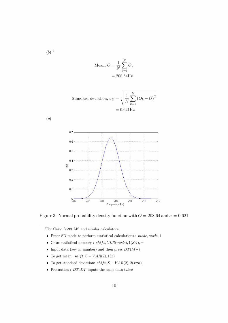
(b) 2
Mean, O =1
N
N∑k=1
Ok
= 208.64Hz
Standard deviation, σO =
√√√√ 1
N
N∑k=1
(Ok − O
)2= 0.621Hz
(c)
Figure 3: Normal probability density function with O = 208.64 and σ = 0.621
2For Casio fx-991MS and similar calculators
• Enter SD mode to perform statistical calculations : mode,mode, 1
• Clear statistical memory : shift, CLR(mode), 1(Scl),=
• Input data (key in number) and then press DT (M+)
• To get mean: shift, S − V AR(2), 1(x)
• To get standard deviation: shift, S − V AR(2), 2(xσn)
• Precaution : DT,DT inputs the same data twice
10
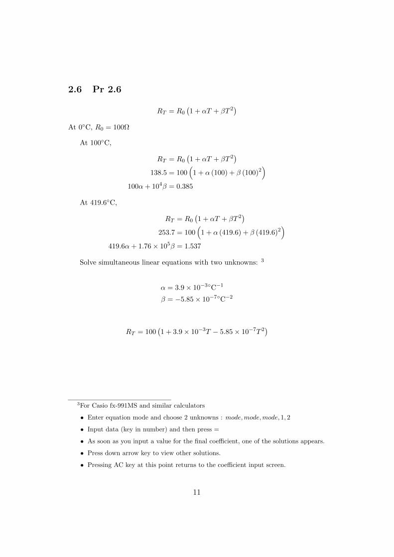
2.6 Pr 2.6
RT = R0
(1 + αT + βT 2
)At 0C, R0 = 100Ω
At 100C,
RT = R0
(1 + αT + βT 2
)138.5 = 100
(1 + α (100) + β (100)2
)100α+ 104β = 0.385
At 419.6C,
RT = R0
(1 + αT + βT 2
)253.7 = 100
(1 + α (419.6) + β (419.6)2
)419.6α+ 1.76× 10⁵β = 1.537
Solve simultaneous linear equations with two unknowns: 3
α = 3.9× 10⁻³C−1
β = −5.85× 10⁻⁷C−2
RT = 100(1 + 3.9× 10⁻³T − 5.85× 10⁻⁷T 2
)
3For Casio fx-991MS and similar calculators
• Enter equation mode and choose 2 unknowns : mode,mode,mode, 1, 2
• Input data (key in number) and then press =
• As soon as you input a value for the final coefficient, one of the solutions appears.
• Press down arrow key to view other solutions.
• Pressing AC key at this point returns to the coefficient input screen.
11

2.7 Pr 2.7 ***
(a)
K =Omax −Omin
Imax − Imin
=20− 4
10− 0
= 1.6mAbarg−1
a = Omin −KImin
= 4− 0
= 4mA
Output at I = 0 changes only when temperature changes. Therefore, temper-ature is interfering input.
To find KI , set I = Imin = 0∆II = 25− 20 = 5C∆O = 6− 4 = 2mA
KI =∆O
∆II
=2
5= 0.4mAC−1
To find KM , calculate modified K for new IM .At Vs = 12V ,
Knew =Omax −Omin
Imax − Imin
=28− 4
10− 0
= 2.4mAbarg−1
Vs is modifying input, IM = 12− 10 = 2V ,
Knew = K +KMIM
2.4 = 1.6 +KM × 2
KM = 0.4mAbarg−1V −1
12

(b) Generalized model,
O (I) = (K +KMIM ) I + (a+KIII)
= (1.6 + 0.4IM ) I + (4 + 0.4II)
For I = 5barg,IM = 12− 10 = 2V , and II = 25− 20 = 5C,
O (I) = (1.6 + 0.4IM ) I + (4 + 0.4II)
= (1.6 + 0.4× 2) 5 + (4 + 0.4× 5)
= 18mA
2.8 Pr 2.8
Omin = 1VOmax = 5VImin = 0NImax = 2× 10⁵N
K =Omax −Omin
Imax − Imin
=5− 1
2× 105
= 2× 10⁻⁵V N−1
a = Omin −KImin
= 1− 0
= 1V
O = KI + a
= 2× 10⁻⁵I + 1V
2.9 Pr 2.9
Omin = 4mAOmax = 20mAImin = 0PaImax = 2× 10⁴Pa
13

K =Omax −Omin
Imax − Imin
=20− 4
2× 104
= 8× 10⁻⁴mAPa−1
a = Omin −KImin
= 4− 0
= 4mA
O = KI + a
= 8× 10⁻⁴I + 4 mA
2.10 Pr 2.10
Omin = 0VOmax = 5VImin = 0barImax = 10barO (4) = 2.2V
K =Omax −Omin
Imax − Imin
=5− 0
10− 0
= 0.5V bar−1
a = Omin −KImin
= 0− 0
= 0V
Oideal = KI + a
= 0.5I
Oideal (4) = o.5× 4
= 2V
14
Non-linearity = Omeasured −Oideal
= 2.2− 2
= 0.2V
Non-linearity as a % of f.s.d =N
Omax −Omin× 100%
=0.2
5− 0
= 4%
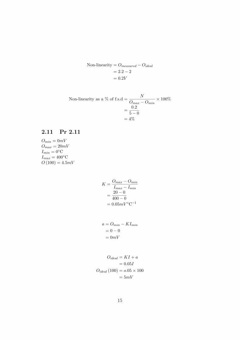
2.11 Pr 2.11
Omin = 0mVOmax = 20mVImin = 0CImax = 400CO (100) = 4.5mV
K =Omax −Omin
Imax − Imin
=20− 0
400− 0
= 0.05mV C−1
a = Omin −KImin
= 0− 0
= 0mV
Oideal = KI + a
= 0.05I
Oideal (100) = o.05× 100
= 5mV
15

Non-linearity = Omeasured −Oideal
= 4.5− 5
= −0.5mV
Non-linearity as a % of f.s.d =N
Omax −Omin× 100%
=−0.5
20− 0
= −2.5%
2.12 Pr 2.12
K =Omax −Omin
Imax − Imin
=27388− 0
500− 0
= 54.776µV C−1
a = Omin −KImin
= 0− 0
= 0µV
(a)
Oideal = KI + a
= 54.776I
(b) At 100C,
Oideal (100) = 54.776× 100
= 5477.6µV
Non-linearity = Omeasured −Oideal
= 5268− 5477.6
= −209.6µV
16

Non-linearity as a % of f.s.d =N
Omax −Omin× 100%
=−209.6
27388− 0
= −0.77%
At 300C,
Oideal (300) = 54.776× 300
= 16432.8µV
Non-linearity = Omeasured −Oideal
= 16325− 16432.8
= −107.8µV
Non-linearity as a % of f.s.d =N
Omax −Omin× 100%
=−107.8
27388− 0
= −0.4%
2.13 Pr 2.13
At standard temperature of 20C,
K =Omax −Omin
Imax − Imin
=5− 0
104 − 0
= 5× 10⁻⁴V N−1
a = Omin −KImin
= 0− 0
= 0V
To find KI , set I = Imin = 0. When ∆II = 30− 20 = 10C, ∆O = 0V .
KI =∆O
∆II= 0
17

To find KM , calculate modified K for IM = 30− 20 = 10C. At temperatureof 30C,
Knew =Omax −Omin
Imax − Imin
=5.5− 0
104 − 0
= 5.5× 10⁻⁴V N−1
Knew = K +KMIM
5.5× 10⁻⁴ − 5× 10−4 = KM × 10
KM = 5× 10⁻⁶V N−1C−1
2.14 Pr 2.14
At standard temperature of 20C,
K =Omax −Omin
Imax − Imin
=5− 1
∆I
=4
∆I
To find KI , set I = Imin. When ∆II = 30−20 = 10C, ∆O = 1.2−1 = 0.2V .
KI =∆O
∆II
=0.2
10= 0.02V C−1
To find KM , calculate modified K for IM = 30− 20 = 10C. At temperatureof 30C,
Knew =Omax −Omin
Imax − Imin
=5.2− 1.2
∆I
=4
∆I
Knew = K +KMIM4
∆I− 4
∆I= KM × 10
KM = 0
18

2.15 Pr 2.15
At standard temperature of 20C,
K =Omax −Omin
Imax − Imin
=20− 4
104 − 0
= 1.6× 10⁻³mAPa−1
To find KI , set I = Imin. When ∆II = 30−20 = 10C, ∆O = 4.2−4 = 0.2mA.
KI =∆O
∆II
=0.2
10= 0.02mAC−1
To find KM , calculate modified K for IM = 30− 20 = 10C. At temperatureof 30C,
Knew =Omax −Omin
Imax − Imin
=20.8− 4.2
104 − 0
= 1.66× 10⁻³mAPa−1
Knew = K +KMIM
1.66× 10⁻³ − 1.6× 10−3 = KM × 10
KM = 6× 10⁻⁶mAPa−1C−1
2.16 Pr 2.16
Input range= 0 to 5V
(a) 8 bit binaryNumber of levels= 28 = 256Range= 0 to 255
Resolution =5− 0
255= 0.0196V
19

Resolution as a % of f.s.d =0.0196
5× 100%
= 0.392%
(b) 16 bit binaryNumber of levels= 216 = 65536Range= 0 to 65535
Resolution =5− 0
65535= 76.3µV
Resolution as a % of f.s.d =76.3× 10⁻⁶
5× 100%
= 0.00153%
2.17 Pr 2.17
Output range = 0 to 10VO(3) ↓=3.05VO(3) ↑=2.95V
Hysteresis = 3.05− 2.95
= 0.1V
Hysteresis as a % of f.s.d =H
Omax −Omin× 100%
=0.1
10− 0× 100%
= 1%
20

3 Old Questions
3.1 2009-3
(a)
At standard temperature, T = 20C Imin = 0Omin =100Imax = 10−5
Omax = 101
K =Omax −Omin
Imax − Imin
=101− 100
10−5 − 0
= 105Ω
a = Omin −KImin
= 100− 0
= 100Ω
Oideal = KI + a
= 105I + 100
To find KI , set I = Imin = 0When T changes from 20C to 30C, output did not change.∆II = 30− 20 = 10C∆O = 100− 100 = 0
KI =∆O
∆II= 0ΩC−1
To find KM , calculate modified K for new IM .At T = 30C,
Knew =Omax −Omin
Imax − Imin
=102− 100
10−5 − 0
= 2× 10⁵Ω
21

IM = 30− 20 = 10C,
Knew = K +KMIM
2× 105 = 105 +KM × 10
KM = 104ΩC−1
Since characteristics are linear, N(I) = 0
O = KI + a+N(I) +KMIMI +KIII
= 105I + 100 + 0 + 104IMI + 0
= 105I + 104IMI + 100
For input strain, I = 5× 10⁻⁶ at T = 25CIM = 25− 20 = 5C
O(5× 10⁻⁶
)= 105I + 104IMI + 100
= 105 × 5× 10−6 + 104 × 5× 5× 10−6 + 100
= 100.75Ω
(b)
Figure 4: Characteristics of a thermocouple
• T1 is the input temperature to be measured.
• Sensitivity K is 52.17.
• Non-linearity is −13.43() + . . .
22

• Interfering input is T2C reference temperature.
• The interfering coupling constant, KI , is −38.74
• The output is e.m.f , E in microvolts.
• All the T junctions add the two inputs entering the junction to produce anoutput.
3.2 2008-5
At standard supply voltage, Vs = 1VImin = 0cmImax = 10cmy = x2
Omin = I2min
= 0mV
Omax = I2max
= 100mV
(a)
K =Omax −Omin
Imax − Imin
=100− 0
10− 0
= 10mV cm−1
a = Omin −KImin
= 0− 0
= 0mV
Oideal = KI + a
= 10I
Oideal (5) = 10× 5
= 50mV
23

O = I2
O (5) = 52
= 25mV
Non-linearity at 5cm, N(5) = O(5)−Oideal(5) = 25− 50 = −25mV
Non-linearity as a % of f.s.d =N
Omax −Omin× 100%
=−25
100− 0× 100%
= −25%
(b) To find KI , set I = Imin = 0At Vs = 1.1V ,Omin = 1.1 × 02 = 0mV When Vs changes from 1V to 1.1V ,
output did not change.∆II = 1.1− 1 = 0.1V∆O = 0− 0 = 0
KI =∆O
∆II= 0mV V −1
To find KM , calculate modified K for new IM .At Vs = 1.1V ,Omax = 1.1I2
max = 1.1× 100 = 110mV
Knew =Omax −Omin
Imax − Imin
=110− 0
10− 0
= 11mV cm−1
IM = 1.1− 1 = 0.1V ,
Knew = K +KMIM
11 = 10 +KM × 0.1
KM = 10mV cm−1V −1
24
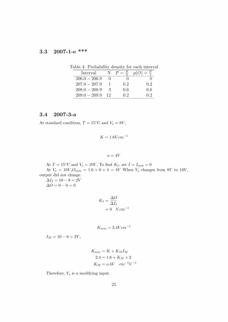
3.3 2007-1-e ***
Table 4: Probability density for each interval
Interval N P = N5
p(O) = P1
206.0− 206.9 0 0 0207.0− 207.9 1 0.2 0.2208.0− 208.9 3 0.6 0.6209.0− 209.9 12 0.2 0.2
3.4 2007-3-a
At standard condition, T = 15C and Vs = 8V ,
K = 1.6V cm−1
a = 4V
At T = 15C and Vs = 10V , To find KI , set I = Imin = 0At Vs = 10V ,Omin = 1.6 × 0 + 4 = 4V When Vs changes from 8V to 10V ,
output did not change.∆II = 10− 8 = 2V∆O = 0− 0 = 0
KI =∆O
∆II= 0 V cm−1
Knew = 2.4V cm−1
IM = 10− 8 = 2V ,
Knew = K +KMIM
2.4 = 1.6 +KM × 2
KM = o.4V cm−1V −1
Therefore, Vs is a modifying input.
25

At T = 20C and Vs = 8V , To find KI , set I = Imin = 0At T = 20C,Omin = 1.6 × 0 + 6 = 6V When T changes from 15C to 20C,
output has changed.∆II = 20.15 = 5C∆O = 6− 4 = 2V
KI =∆O
∆II
=2
5= 0.4 V C−1
Knew = 1.6V cm−1
IM = 20.15 = 5C
Knew = K +KMIM
1.6 = 1.6 +KM × 5
KM = oV cm−1C−1
Therefore, T is a interfering input.Since equations are linear equations, N(I) = 0
O = KI + a+N(I) +KMIMI +KIII
= 1.6I + 4 + 0 + o.4IMI + 0.4II
At T = 20C and Vs = 10V
I = 5cmIM = 10− 8 = 2VII = 20− 15 = 5C
O = 1.6I + 4 + 0 + o.4IMI + 0.4II
= 1.6× 5 + 4 + 0.4× 2× 5 + 0.4× 5
= 18V
26

3.5 2006-3
(a) To determine interfering input,
• Imin is entered
• Sensor is hold under standard condition
• The environmental input to be tested is changed by a known amount, ∆II
• It is an interfering input if a resulting output, ∆O, appears
• An interfering input raises the input-output characteristic line vertically onthe graph and maintains the gradient to be constant
• Then KI = ∆O∆II
(b)
At standard supply voltage, Vs = 10VImin = 0barOmin = 0mAO = ITherefore, K = 1mAbar−1 and a = 0mA
To find KI , set I = Imin = 0At Vs = 12V ,Omin = I + 1 = 1mA When Vs changes from 10V to 12V ,∆II = 12− 10 = 2V∆O = 1− 0 = 1
KI =∆O
∆II
=1
2= 0.5mA V −1
There is no modifying input, KM = 0Since equations are linear equations, N(I) = 0
O = KI + a+N(I) +KIII
= 1× I + 0 + 0 + o.5II
= I + 0.5II
When I = 5bar and II = 11− 10 = 1V
27

O = I + 0.5II
= 5 + 0.5× 1
= 5.5mA
(c) It should be assumed that s=0.
I = T1 = 0CK = 52.17N(I) = −13.43T1 + 3.319× 10⁻²T 2
1
KI = −38.74II = T2 = 1Ca = 0
O(I) = KI + a+N(I) +KIII
E(T1) = 52.17T1 + 0− 13.43T1 + 3.319× 10⁻²T 21 + 2.071× 10⁻⁴T 3
1 − 2.195× 10⁻⁶T 41 − 38.74T2
= −38.74µV
3.6 2005-4
(d) Since input-output graph is linear, N(I) = 0.At T = 20C and Vs = 10V
K =Omax −Omin
Imax − Imin
=20− 4
10− 0
= 1.6mA bar−1
a = Omin −KImin
= 4− 1.6× 0
= 4mA
At T = 20C and Vs = 12V ,When Vs changes from 10V to 12V , Omin doesn’t change. That is why, Vs is
not an interfering input.
Knew =Omax −Omin
Imax − Imin
=28− 4
10− 0
= 2.4mA bar−1
28

IM = 12− 10 = 2V
Knew = K +KMIM
2.4 = 1.6 +KM × 2
KM = 0.4mA bar−1V −1
Vs is modifying input.At T = 25C and Vs = 10V ,When T changes from 20C to 25C,∆O = 8− 4 = 4mA ∆II = 25− 20 = 5C
KI =∆O
∆II
=4
5= 0.8mA bar−1
That is why, T is an interfering input.
Knew =Omax −Omin
Imax − Imin
=24− 8
10− 0
= 1.6mA bar−1
IM = 25− 20 = 5C
Knew = K +KMIM
1.6 = 1.6 +KM × 5
KM = 0mA bar−1V −1
T is not a modifying input.(e)
I = 4barIM = 10− 10 = 0VII = 23− 20 = 3C
O = (K +KMIM )I + (a+KIII) +N(I)
= (1.6 + 0.4× 0)4 + (4 + 0.8× 3) + 0
= 12.8mA
29

3.7 2004-4-c
(c)
K =Omax −Omin
Imax − Imin
=2− 0
2− 0
= 1mA MPa−1
a = Omin−KImin
= 0− 0
= 0mA
Oideal(I) = KI + a
= I
O(I) ↑ = 0.5I2
O(1MPa) ↑ = 0.5mA
General equation when there is no interfering and modifying inputs,
O(I) ↓ = (K +KMIM )I + (a+KIII) +N(I)
= KI + a+N(I)
= I − 0.5I2 + I
= 2I − 0.5I2
O(1MPa) ↓ = 2− 0.5
= 1.5mA
Hysteresis = O(I) ↓ −O(I) ↑= 1.5− 0.5
= 1mA
30