Embed Size (px)
Citation preview
University of KentuckyUKnowledge
Theses and Dissertations--Civil Engineering Civil Engineering
2016
ENHANCING THE STRENGTHPROPERTIES OF FLY ASH BY ADDINGWASTE PRODUCTSAlfred J. SusiloUniversity of Kentucky, [email protected] Object Identifier: http://dx.doi.org/10.13023/ETD.2016.388
Right click to open a feedback form in a new tab to let us know how this document benefits you.
This Doctoral Dissertation is brought to you for free and open access by the Civil Engineering at UKnowledge. It has been accepted for inclusion inTheses and Dissertations--Civil Engineering by an authorized administrator of UKnowledge. For more information, please [email protected].
Recommended CitationSusilo, Alfred J., "ENHANCING THE STRENGTH PROPERTIES OF FLY ASH BY ADDING WASTE PRODUCTS" (2016).Theses and Dissertations--Civil Engineering. 44.https://uknowledge.uky.edu/ce_etds/44

STUDENT AGREEMENT:
I represent that my thesis or dissertation and abstract are my original work. Proper attribution has beengiven to all outside sources. I understand that I am solely responsible for obtaining any needed copyrightpermissions. I have obtained needed written permission statement(s) from the owner(s) of each third-party copyrighted matter to be included in my work, allowing electronic distribution (if such use is notpermitted by the fair use doctrine) which will be submitted to UKnowledge as Additional File.
I hereby grant to The University of Kentucky and its agents the irrevocable, non-exclusive, and royalty-free license to archive and make accessible my work in whole or in part in all forms of media, now orhereafter known. I agree that the document mentioned above may be made available immediately forworldwide access unless an embargo applies.
I retain all other ownership rights to the copyright of my work. I also retain the right to use in futureworks (such as articles or books) all or part of my work. I understand that I am free to register thecopyright to my work.
REVIEW, APPROVAL AND ACCEPTANCE
The document mentioned above has been reviewed and accepted by the student’s advisor, on behalf ofthe advisory committee, and by the Director of Graduate Studies (DGS), on behalf of the program; weverify that this is the final, approved version of the student’s thesis including all changes required by theadvisory committee. The undersigned agree to abide by the statements above.
Alfred J. Susilo, Student
Dr.. Michael E. Kalinski, Major Professor
Dr. Yi-Tin Wang, Director of Graduate Studies
1 ENHANCING THE STRENGTH PROPERTIES OF FLY ASH BY ADDING
WASTE PRODUCTS
DISSERTATION
A dissertation submitted in partial fulfillment of the requirements for the degree of Doctor of Philosophy in the
College of Engineering at the University of Kentucky
By
Alfred Jonathan Susilo Lexington, Kentucky
Director: Dr. Michael E. Kalinski, Ph.D., P.E, Professor of Civil Engineering
Lexington, Kentucky
2016
Copyright © Alfred Jonathan Susilo 2016
ABSTRACT OF DISSERTATION
ENHANCING THE STRENGTH PROPERTIES OF FLY ASH BY ADDING WASTE PRODUCTS
For this study, the main material to be investigated is Class F fly ash that
originates from the combustion of Appalachian coal. Alone, fly ash exhibits poor
strength properties and is susceptible to liquefaction when subject to dynamic loading.
This research is focused on investigating the effect of adding materials that would
otherwise be considered as waste products to the fly ash. Materials to be considered
include crumb rubber, shredded carpet and shredded paper. The benefits from this
research are twofold. First, provide a method to stabilize fly ash. For large masses of fly
ash such as those found at power plants and landfills, improved strength of the fly ash
will make the mass safer and more reliable with respect to stability. Second, provide a
use for waste materials that would otherwise be stockpiled or disposed of in landfills at
a significant cost, which in turn will minimize the environmental impact. Using this
approach, materials will be added to fly ash rather than using fly ash as an additive,
which will increase the rate of fly ash usage and more directly address the issue the
large volumes of fly ash that are being produced today.
To perform this research, representative samples of Class F fly ash were tested
to characterize the physical properties of the materials. Later, this Class F fly ash was
mixed with specific percentage of three waste materials to evaluate the behavior and
performance of the fly ash admixture. Using these reconstituted specimens, a suite of
laboratory tests to assess the static and cyclic strength properties of each specimen was
performed, as well as the dynamic properties of the specimens. The expectations were
to develop correlations between mixture ratios and the various measured properties,
and to identify mixture ratios that will optimize the strength characteristics of the
specimens.
In the end, crumb rubber was found to be the best additive to improve the
properties of Class F fly ash compared to the other waste materials used. This
conclusion can be used by power plant facilities to increase the safety factor against
liquefaction at their impoundment facilities.
KEYWORDS: Liquefaction, Class F fly ash, crumb rubber, shredded carpet, shredded
paper, reconstituted specimens
Alfred J. Susilo
July 12, 2016
iii
ENHANCING THE STRENGTH PROPERTIES OF FLY ASH BY ADDING WASTE
PRODUCTS
By
Alfred Jonathan Susilo
Dr. Michael E. Kalinski
Director of Dissertation
Dr. Yi-Tin Wang
Director of Graduate Studies
July 21, 2016

iv
To my parents

iii
2 ACKNOWLEDGEMENTS
I would like to thank Dr. Michael E. Kalinski for his willingness of becoming my
advisor, believing in me, orientating me to such an interesting research topic and also
for his time, guidance, support, relentless effort and patience during my research. He is
a very good advisor and I wish I could spend more time with him during my Ph.D.
research.
I would like to express my gratitude for my committee members; L. Sebastian
Bryson, Ph.D., P.E., Kyle A. Perry, Ph.D., Gabriel B. Dadi, Ph.D., P.E., LEED AP and John
Silva-Castro, Ph.D. for their support, guidance, time, efforts and valuable information
for this dissertation. I would also like to thank Braden Lusk, Ph.D. for agreeing to serve
as external reviewer for my research.
I would like to extend my thanks to all the professors, staffs, and fellow graduate
students in University of Kentucky for their support, assistance and mostly for their
friendship. They help create a very welcoming and comfortable situation during my stay
in Lexington, Kentucky.
I would like to express my appreciation to all personal in Geotechnical
Consulting and Testing Systems LLC (GCTS) for their support, time and relentless effort
during my research.

iv
Finally, I want to thank my family especially my parents for their support,
encouragement, and patience during my study which contributes to the completion of
this dissertation.
v
3 TABLE OF CONTENTS
Acknowledgements ....................................................................................................... .iii
List of Tables ................................................................................................................. .ix
List of Figures………………………………………………………………………………………………….……………..x
Chapter 1 …………………..………………………………………………………………………………………………….1
1 Introduction ......................................................................................................... 1
1.1 Research Background ...........................................................................................1
1.2 History of Incidents at Fly Ash Impoundments ...................................................20
1.3 Other Research Related to Fly Ash .....................................................................26
1.4 Gaps in the Current State of Knowledge .............................................................30
1.5 Research Objectives ...........................................................................................31
1.6 Research Limitations ..........................................................................................32
1.7 Dissertation Outline ...........................................................................................33
Chapter 2…………………………………………………………..……………………………………………..….………35
2. Waste Materials Used in This Study ...................................................................35
2.1 Fly Ash ...............................................................................................................35
2.2 Crumb Rubber ....................................................................................................39
2.3 Shredded Carpet ................................................................................................43
2.4 Shredded Paper .................................................................................................47
vi
Chapter 3 .......................................................................................................................49
3. Description of Laboratory Test Method ..............................................................49
3.1 Laboratory Testing of Mechanical Properties .....................................................49
3.1.1 Index Properties .......................................................................................49
3.1.2 Grain Size Distribution ..............................................................................50
3.1.3 Shear Modulus and Damping Ratio (Strain-Controlled Cyclic Loading) ......51
3.2 Chemical Properties of the Materials .................................................................55
3.3 Cyclic Triaxial Testing .........................................................................................56
Chapter 4 .......................................................................................................................66
4. Typical Results from Laboratory Testing .............................................................66
4.1 Introduction .......................................................................................................66
4.2 Static Tests .........................................................................................................66
4.3 Dynamic Tests ....................................................................................................73
4.3.1 Development of Modulus Reduction Curves .............................................73
4.3.2 Cyclic Triaxial Testing ................................................................................79
Chapter 5 .......................................................................................................................90
5. Interpretation of Test Results .............................................................................90
5.1 Overview............................................................................................................90
5.2 Specific Gravity ..................................................................................................90
5.3 Grain Size Distribution........................................................................................92
5.4 Plotting of Data to Identify Optimum Blends ......................................................97
vii
5.5 Identify Optimum Blends of Fly Ash and Other Waste Materials ...................... 115
Chapter 6 ..................................................................................................................... 124
6. Conclusion and Recommendations .................................................................. 124
6.1 Findings of the Study ........................................................................................ 124
6.2 Recommendations for Practitioners ................................................................. 140
6.3 Future Research ............................................................................................... 153
APPENDIX A ................................................................................................................. 155
A. Cyclic Triaxial Test Results ................................................................................ 155
APPENDIX B ................................................................................................................. 254
B. Cyclic Triaxial Testing Procedure ...................................................................... 254
B.1 Cyclic Triaxial Testing System .......................................................................... 254
B.1.1 Resilient Modulus Test System (Pressure Board) .................................... 255
B.1.2 Cyclic Triaxial Machine ............................................................................ 256
B.2 Reconstitute Test Specimen ............................................................................. 259
B.3 Sealing the Chamber of Cyclic Triaxial Machine ................................................ 262
B.4 Filling the Triaxial Chamber with Liquid ............................................................ 265
B.5 Flooding and Saturating the Specimen ............................................................. 271
B.6 Consolidation Process ...................................................................................... 274
B.7 Applying Load-controlled Loading .................................................................... 274
B.8 Emptying the Chamber .................................................................................... 275
APPENDIX C ................................................................................................................. 277

viii
C. Cyclic Triaxial Testing Spreadsheet ................................................................... 277
REFERENCES ................................................................................................................ 281
VITA ............................................................................................................................. 290
ix
4 LIST OF TABLES
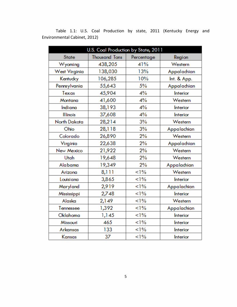
Table 1.1: U.S. Coal Production by state, 2011 (Kentucky Energy and Environmental
Cabinet, 2012) .................................................................................................................. 5
Table 1.2: Location of 26 facilities with a total of 44-coal-fired power plant waste sites,
or coal ash ponds, identified with a high-hazard rating by the EPA (U.S. Environmental
Protection Agency, 2009)................................................................................................ 12
Table 2.1: Typical composition of fly ash (FHWA, 1999) .................................................. 35
Table 2.2: Statistics of tire recycling and disposal in the U.S (Rubber Manufacturers
Association, 2003) .......................................................................................................... 43
Table 3.1: Chemical Requirements for Fly Ash Classification (ASTM C 618) ..................... 55
Table 3.2: Specimen preparation check list for cyclic traixial testing (ASTM D5311) ........ 58
Table 4.1: Specific gravity of selected samples used in this study .................................... 68
Table 4.2: Properties of fly ash specimens used to develop modulus reduction curves ... 76
Table 4.3: Various ratios of fly ash specimens and results data from different tests ....... 80
Table 5.1: Specific gravity results for specimens tested .................................................. 91
Table 5.2: Grain size distribution of Class F fly ash used in this study ............................. 94
Table 5.3: Weight of specimens ...................................................................................... 99
Table 5.4: Specimen test results to find optimum combination .................................... 100
Table 5.5: Specimen information and test result of Class F Fly ash and selected
composition.................................................................................................................. 105
Table 5.6: Specimen information and results of all specimens tested ........................... 122
Table 6.1: Cyclic Resistance Ratio (CRR) and Factor of safety (FS) ................................. 135
Table 6.2: Factor of Safety for all zones in predicted peak ground acceleration (PGA), on
hard rock from a magnitude-7.5 earthquake in the New Madrid Seismic Zone ............. 146
Table 6.3: Matrix comparison from each waste material .............................................. 151
x
LIST OF FIGURES
Figure 1.1: U.S. Coal Production, 2011 (Kentucky Energy and Environmental Cabinet,
2012) ................................................................................................................................ 4
Figure 1.2: Wet disposal method ...................................................................................... 7
Figure 1.3: Dry disposal method ....................................................................................... 7
Figure 1.4: Wet disposal storage pond in Ohio Power Plant .............................................. 8
Figure 1.5: Dry disposal storage in a coal ash landfill......................................................... 8
Figure 1.6: Location of 26 facilities with a total of 44-coal-fired power plant waste sites,
or coal ash ponds, identified with a high-hazard rating by the EPA (U.S. Environmental
Protection Agency, 2009)................................................................................................ 11
Figure 1.7: Groundwater monitoring well ....................................................................... 15
Figure 1.8: TVA’s Johnsonville power plant impoundment (Southern Alliance for Clean
Energy, 2013) ................................................................................................................. 16
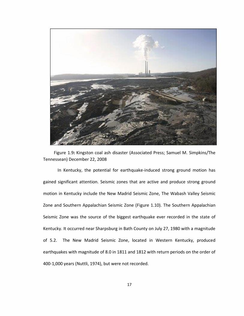
Figure 1.9: Kingston coal ash disaster (Associated Press; Samuel M. Simpkins/The
Tennessean) December 22, 2008 .................................................................................... 17
Figure 1.10: Topographic map showing earthquakes greater than magnitude 2.5 (circles)
in Southeastern US from 1962 – 2012 (Alabama Earthquakes, 2016) .............................. 18
Figure 1.11: Coal producing counties in Kentucky, 2014 (Kentucky Transportation
Cabinet, 2015) ................................................................................................................ 19
Figure 1.12: Fly ash impoundment at the DPL Power Plant after an accident .................. 21
Figure 1.13: Slope failure occurred as a result of fly ash flow at the DPL Power Plant .... 21
Figure 1.14: Movement of fly ash at the DPL impoundment ........................................... 22
Figure 1.15: Trackhoe engulfed in fly ash at the DPL impoundment after a fly ash failure
caused by liquefaction .................................................................................................... 22
Figure 1.16: Side picture of Trackhoe covered with fly ash caused by fly ash failure at the
DPL impoundment .......................................................................................................... 23
xi
Figure 1.17: Portion of a fly ash flow failure in an impoundment at the DPL power plant 23
Figure 1.18: Kingston Plant coal ash retention pond two years before the December
2008 failure (EPA, 2009) ................................................................................................. 24
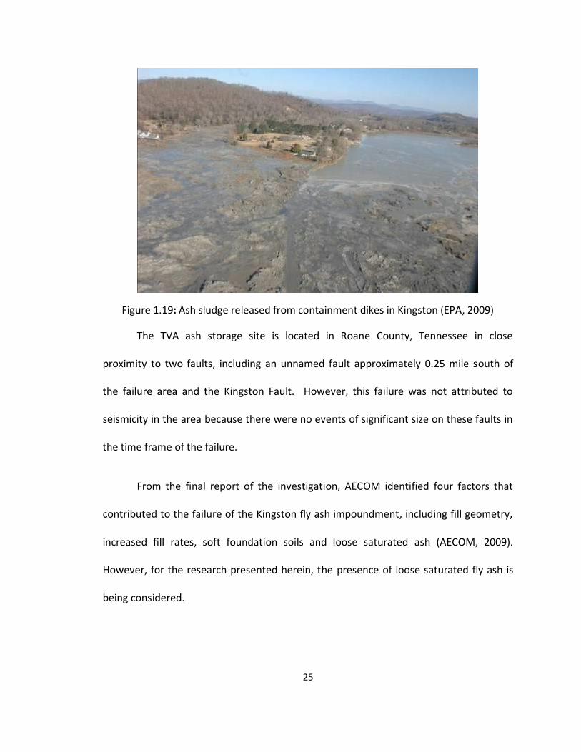
Figure 1.19: Ash sludge released from containment dikes in Kingston (EPA, 2009) ......... 25
Figure 2.1: Typical gradation curve for fly ash (after Kalinski and Hippley, 2005) ............ 36
Figure 2.2: The gradation curves separating liquefiable and nonliquefiable soils
(Tsuchida, 1970) ............................................................................................................. 37
Figure 2.3: Crumb Rubber ............................................................................................... 40
Figure 2.4: Landfill of used tires (Hudson, CO: World's Largest Tire Dump) (Leather, 2010)41
Figure 2.5: Carpet Shredder machinery........................................................................... 44
Figure 2.6: Shredded carpet ............................................................................................ 45
Figure 2.7: Shredded carpet after hand shredding .......................................................... 45
Figure 2.8: Used carpet Landfills ..................................................................................... 46
Figure 2.9: Shredded Paper............................................................................................. 48
Figure 3.1: Examples of Acceptable and Unacceptable Sinusoidal Loading Wave Forms
For Cyclic Triaxial Load Control Tests (ASTM D3999). ...................................................... 53
Figure 3.2: Deviator stress versus time at 2 psi ............................................................... 54
Figure 3.3: Axial strain versus time at 5 psi ..................................................................... 54
Figure 3.4: Class F Fly ash used in this research............................................................... 56
Figure 3.5: Schematic Illustration of pore pressure data derived from cyclic triaxial
testing ............................................................................................................................ 59
Figure 3.6: Schematic Illustration of Identification of liquefaction from cyclic triaxial test61
Figure 3.7: Correlation between equivalent uniform cyclic stress ratio and SPT (N1)60 –
Value for events of magnitude M ≈7.5 for varying fines contents, (Youd, et al, 2001). .... 64
Figure 4.1: Grain size distribution of Class F fly ash used in this study ............................. 69
xii
Figure 4.2: The X-Ray diffraction (XRD) machine used in this study ................................. 71
Figure 4.3: Sample holder for the X-Ray diffraction (XRD) test ........................................ 72
Figure 4.4: Chemical composition of typical Class F fly ash used in this study ................. 72
Figure 4.5: Schematic illustration of a hysteresis loop from cyclic triaxial testing (ASTM
D3999). ........................................................................................................................... 74
Figure 4.6: Shear modulus versus cyclic shear strain graph ............................................. 77
Figure 4.7: Damping ratio versus cyclic shear strain graph .............................................. 78
Figure 4.8: 80% Fly ash Class F and 20 % shredded paper ............................................... 81
Figure 4.9: Storage pond failure at a power plant in Ohio ............................................... 82
Figure 4.10: Height of impoundment facilities failure at a power plant in Ohio ............... 82
Figure 4.11: Schematic Illustration of axial Strain versus number of cycle graph ............. 83
Figure 4.12: Schematic Illustration deviator stress versus number of cycle graph .......... 85
Figure 4.13: Schematic Illustration of excess pore pressure versus number of cycles
graph .............................................................................................................................. 86
Figure 4.14: Schematic Illustration of excess pore pressure ratio versus normalized
number of cycles graph .................................................................................................. 86
Figure 4.15: Schematic Illustration of deviator stress versus axial strain graph ............... 88
Figure 4.16: Schematic Illustration of excess pore pressure ratio and axial strain versus
number of cycles graph .................................................................................................. 89
Figure 5.1: Liquefaction susceptibility based on Chinese criteria ..................................... 93
Figure 5.2: Tsuchida (1970) Vs. Grain size distribution of Class F fly ash used in this study95
Figure 5.3: Liquefaction susceptibility based on Seed et al. (2003) .................................. 96
Figure 5.4: Liquefaction susceptibility based on Bray & Sancio (2004) ............................ 97
Figure 5.5: Number of cycles to liquefy versus percentage graph by dry weight (Fly ash
Class F and Shredded carpet) at CSR = 0.30................................................................... 100
xiii
Figure 5.6: Number of cycles to liquefy versus percentage graph by dry weight (Fly ash
Class F and Crumb rubber) at CSR = 0.30 ...................................................................... 101
Figure 5.7: Number of cycles to liquefy versus percentage graph by dry weight (Fly ash
Class F and Shredded paper) at CSR = 0.30 ................................................................... 101
Figure 5.8: Test result of Class F Fly ash and selected composition ............................... 106
Figure 5.9: ru versus N/NL graph of 100% Class F fly ash (A), 5% carpet fiber (B), 10%
crumb rubber (C) and 10% shredded paper (D) at 0.15 CSR .......................................... 108
Figure 5.10: ru versus N/NL graph of 100% Class F fly ash, 5% carpet fiber, 10% crumb
rubber and 10% shredded paper at 0.15 CSR ................................................................ 109
Figure 5.11: ru versus N/NL graph of 100% Class F fly ash (A), 5% carpet fiber (B), 10%
crumb rubber (C) and 10% shredded paper (D) at 0.30 CSR .......................................... 110
Figure 5.12: ru versus N/NL graph of 100% Class F fly ash, 5% carpet fiber, 10% crumb
rubber and 10% shredded paper at 0.30 CSR ................................................................ 111
Figure 5.13: ru versus N/NL graph of 100% Class F fly ash (A), 5% carpet fiber (B), 10%
crumb rubber (C) and 10% shredded paper (D) at 0.50 CSR .......................................... 112
Figure 5.14: ru versus N/NL graph of 100% Class F fly ash, 5% carpet fiber, 10% crumb
rubber and 10% shredded paper at 0.50 CSR ................................................................ 113
Figure 5.15: Number of cycles to liquefaction versus percentage of waste material by
volume at optimum blend using 0.30 CSR ..................................................................... 115
Figure 5.16: Schematic Illustration of axial strain graph shows specimen in extension and
compression at the same time during testing ............................................................... 116
Figure 5.17: Schematic Illustration of axial strain graph shows specimen was in extension
compare to compression .............................................................................................. 117
Figure 5.18: Schematic Illustration of deviator stress versus axial strain graph shows
specimen contraction and extension at the same time ................................................. 118
Figure 5.19: Schematic Illustration of deviator stress versus axial strain graph shows
specimen in extension .................................................................................................. 119
Figure 5.20: Schematic Illustration of ru versus N/NL graph showing rapid early increase
in pore pressure ........................................................................................................... 120
xiv
Figure 5.21: Schematic Illustration of ru versus N/NL graph showing a steady rate of pore
pressure increase ......................................................................................................... 120
Figure 5.22: Cyclic stress ratio (CSR) Versus Number of cycles (N) of all specimen tested
graph ............................................................................................................................ 123
Figure 6.1: Comparison between the normalized shear modulus (G/Gmax) of fly ash
samples used in this study and the relationships suggested by Vucetic and Dobry (1991)
for clay with PI=0, Darendeli (2001) PI=0 and Ishibashi and Zhang (1993) for non-plastic
soils. ............................................................................................................................. 127
Figure 6.2: Three families of shear modulus reduction and damping ratio curves,
developed by Vucetic & Dobry (1991) ........................................................................... 128
Figure 6.3: Influence of effective confining pressure on modulus reduction curves: (a)
Non-plastic soil and (b) Plastic soil (Ishibashi and Zhang, 1993) .................................... 129
Figure 6.4: Prediction curves of increasing normalised shear modulus and decreasing
damping ratio with increasing confining pressure (Darendeli,2001). ............................. 130
Figure 6.5: Comparison between the normalized shear modulus (G/Gmax) of fly ash
samples used in this study and the relationships suggested by Vucetic and Dobry (1991)
for clay with PI=0 and PI=200. ....................................................................................... 131
Figure 6.6: Comparison between the damping ratio of fly ash samples used in this study
and the relationships suggested by Vucetic and Dobry (1991) for clay with PI=0 and
PI=200. ......................................................................................................................... 132
Figure 6.7: Comparison between the damping ratio of fly ash samples used in this study
and the relationships suggested by Vucetic and Dobry (1991) for clay with PI=0 and
Darendeli (2001) PI=0. .................................................................................................. 133
Figure 6.8: Hysteresis loop of 100% Class F fly ash (A), 5% carpet fiber (B), 10% crumb
rubber (C) and 10% shredded paper (D) at 0.15 CSR ..................................................... 136
Figure 6.9: Hysteresis loop of 100% Class F fly ash (A), 5% carpet fiber (B), 10% crumb
rubber (C) and 10% shredded paper (D) at 0.30 CSR ..................................................... 137
Figure 6.10: Hysteresis loop of 100% Class F fly ash (A), 5% carpet fiber (B), 10% crumb
rubber (C) and 10% shredded paper (D) at 0.50 CSR ..................................................... 138
xv
Figure 6.11: Hysteresis loop of 100% Class F fly ash (A), 20% carpet fiber (B), 20% crumb
rubber (C) and 20% shredded paper (D) at 0.30 CSR ..................................................... 139
Figure 6.12: Cyclic resistance ratio (CRR) Vs. Number of cycles (N) for all specimens
tested ........................................................................................................................... 144
Figure 6.13: Information to calculate factor of safety (SF) for all zone in predicted peak
ground acceleration (PGA), on hard rock from a magnitude-7.5 earthquake in the New
Madrid Seismic Zone .................................................................................................... 145
Figure 6.14: Predicted peak ground acceleration (PGA), on hard rock from a magnitude-
7.5 earthquake in the New Madrid Seismic Zone .......................................................... 147
Figure 6.15: Comparison of Published CRR Weighting Factors ...................................... 148
1
Chapter 1
1 INTRODUCTION
1.1 Research Background
During the 2000s, the United States experienced a rapid increase in the amount
of fly ash produced from coal power plants as well as the number of fly ash storage
ponds and impoundment facilities. When coal is burned, roughly 10% of the coal
remains as ash. Coal ash is comprised of several types of ash including fly ash, bottom
ash, and boiler slag.
Bottom ash and fly ash are produced at rates of 12-20% by weight of the original
coal (Chen et al., 1991) when coal is burned to produce steam for electricity generation.
Bottom ash unlike fly ash, is the ash remaining in the bottom of a coal-fired boiler after
combustion, while the flue gas carries fly ash as residue of the burnt coal, which is
collected using electrostatic precipitators (ESP). This residue, called fly ash, is generally
considered to be an industrial waste. Bottom ash is too heavy to rise so it settles at the
bottom of the boiler as a relatively coarse, gritty material in contrast to fly ash which
consists of very fine particles.
In 2008, the American Coal Ash Association (ACAA) estimated that 136 million
tons of coal combustion products (CCP) were produced in the United States, with fly ash
comprising 72 million tons. In contrast, only 64 million tons of fly ash were produced in
2004 (American Coal Ash Association, 2012).
2
Right et al. (1998) reported that only 20% of the ash by-products are recycled
while 80% are landfilled at the power plant site. The total cost of managing coal
combustion waste ranged from $2.20 to $34.14 per metric ton in 1988 (U.S.
Environmental Protection Agency, 1988) and this cost will continue to rise in the future.
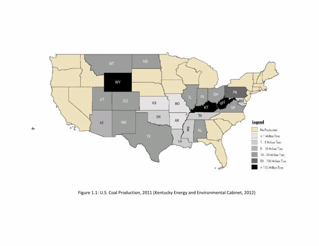
In the Commonwealth of Kentucky, which was the third highest coal producer in
the United States during 2011 (Figure 1.1.), coal mining was by far the largest source of
energy production which contributed to the economy, trade, and investments of
Kentucky. In the same year, coal production in the United States increased to 1.09
billion tons and the state of Kentucky contributed to 10% of the production (Table 1.1).
This increase was accompanied by an increase in the number of disposal facilities.
With the increase of ash production, the biggest challenge for disposal ponds is
to provide sufficient capacity and maintain overall stability. To accommodate the
problem, many options are available, including:
1. Construction of new facilities, which pose a significant cost;
2. Expansion of existing facilities, which require stabilization of larger masses of fly
ash;
3. Construction of containment spill berms, which may pose a significant cost; and
4. Installation of treatment facilities and application of dry placement methods,
which may be expensive but allow fly ash to be placed in larger embankments.

3
Although action was issued by the United States Mine Safety and Health
Administration (MSHA) and the Kentucky Office of Mine Safety and Licensing (KOMSL)
to provide safety and health standard regulation for coal mining wastes, these
regulations do not explicitly provide guidance for treating, handling and storage of coal
combustion byproducts such as fly ash.
4
Figure 1.1: U.S. Coal Production, 2011 (Kentucky Energy and Environmental Cabinet, 2012)
5
Table 1.1: U.S. Coal Production by state, 2011 (Kentucky Energy and
Environmental Cabinet, 2012)
6
Approximately 71.1 million tons of CCP were produced at coal power plants in
the United States in 2005 (American Coal Ash Association, 2008). This number has
steadily increased and 136 million tons were produced in 2008 by 460 power plants.
Approximately 43% of fly ash produced was reused and the remaining fly ash was
landfilled at a significant cost (American Coal Ash Association, 2008) as described in
Chapter 5. Ash from coal combustion is the second largest stream of industrial waste in
the United States at approximately 130 million tons produced per year (Southern
Alliance for Clean Energy, 2013), but is less strictly controlled than municipal solid
waste.
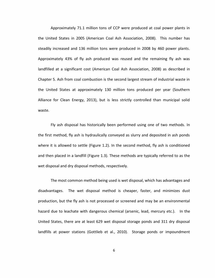
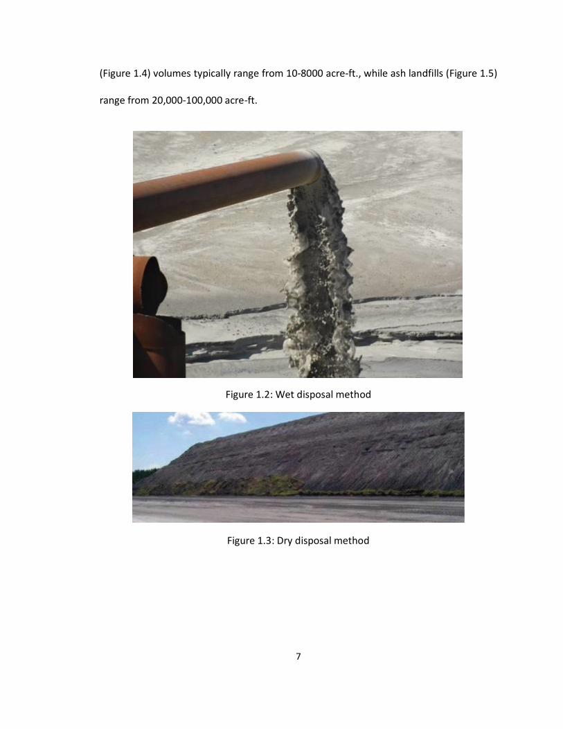
Fly ash disposal has historically been performed using one of two methods. In
the first method, fly ash is hydraulically conveyed as slurry and deposited in ash ponds
where it is allowed to settle (Figure 1.2). In the second method, fly ash is conditioned
and then placed in a landfill (Figure 1.3). These methods are typically referred to as the
wet disposal and dry disposal methods, respectively.
The most common method being used is wet disposal, which has advantages and
disadvantages. The wet disposal method is cheaper, faster, and minimizes dust
production, but the fly ash is not processed or screened and may be an environmental
hazard due to leachate with dangerous chemical (arsenic, lead, mercury etc.). In the
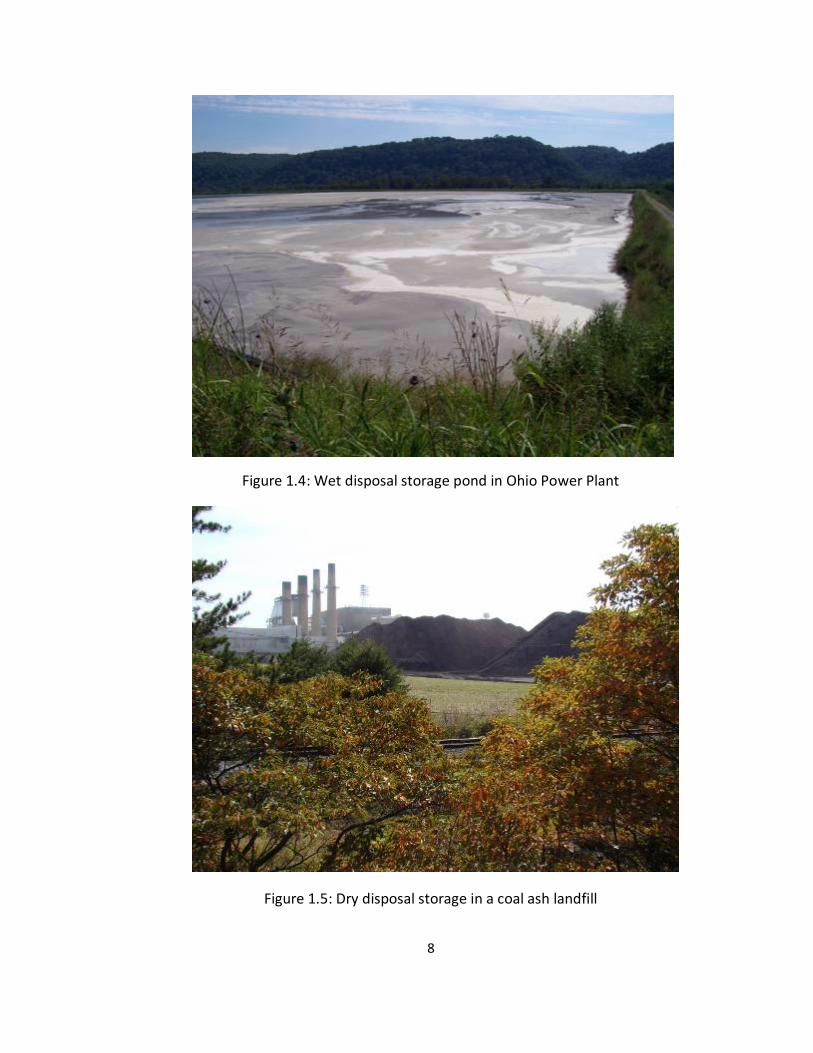
United States, there are at least 629 wet disposal storage ponds and 311 dry disposal
landfills at power stations (Gottlieb et al., 2010). Storage ponds or impoundment
7
(Figure 1.4) volumes typically range from 10-8000 acre-ft., while ash landfills (Figure 1.5)
range from 20,000-100,000 acre-ft.
Figure 1.2: Wet disposal method
Figure 1.3: Dry disposal method
8
Figure 1.4: Wet disposal storage pond in Ohio Power Plant
Figure 1.5: Dry disposal storage in a coal ash landfill
9
The generation of soaring volumes of coal combustion products combined with
rising environmental restrictions and increasing landfilling costs have become major
concerns for utilities. Garlisch (2010) stated that fly ash is the ash that rises up and is
trapped by the stack filters. About 74% of the ash generated is fly ash. Pollution from fly
ash dumps significantly increases both cancer and noncancerous health risks and
degrades water quality in groundwater supplies. The United States derives over half its
electricity from coal fired power plants. There are up to 1,300 impoundments
nationwide including wet ash ponds and dry landfill at power stations, offsite dry
landfills and inactive dumps. Some states have recently started requiring liners for new
impoundments scheduled to be built, while stack filtration devices such as scrubbers
reduce fly ash emissions by around 95%, thus leaving about 5% of the fly ash produced
to be released into the atmosphere.
With time, many existing dry disposal landfills will be closed. These closed
landfills, if abandoned without any treatment, or if a fly ash fill is emplaced in low lying
or swampy terrain, will generate leachate. The leachate may flow downward into the
ground water and impact water quality if the leachate is not properly managed. Ghosh
& Subbarao (1998) presented the concentrations of metals in leachate samples from fly
ash landfills analyzed by an atomic absorption spectrophotometer for the metals, Cd, Cr,
Cu, Fe, Mg, Ni, Pb, and Zn. The lowest of the permissible limits for primary drinking
water quality standards for the World Health Organization (WHO, 1984) and U.S EPA
10
(1988) and for the guidelines for Canadian Drinking Water Quality (Health Canada,
1979), considered as the allowable limits, were often exceeded.
Furthermore, leachate generated by Class F fly ash (the type found in Kentucky)
also can caused problems. Since Class F fly ash has a lower lime content compared to
Class C fly ash, it also has a higher hydraulic conductivity compare to Class C, so leachate
can flow more freely through Class F fly ash. The typical hydraulic conductivity for Class
F fly ash is around 1.0 x 10⁻⁵ cm/s.
Leachate can be minimized by using covers, liners and leachate collection and
removal systems. To illustrate how leachate can endanger wildlife, there was one
catastrophic event that happened at Belews Lake in North Carolina, which killed 19 of
the 22 species of fish in the lake and remains a problem over a decade later (Lemly,
2001).
Fly ash ponds are used to store ash generated from coal combustion at power
plants. To dispose of the ash, a power plant usually constructs their own fly ash ponds.
Each pond has a suitable capacity and site limitations. To monitor the condition of each
pond, the Federal National Pollutant Discharge Elimination System (NPDES) regulates
and permits guidelines that each facility should follow, and yearly inspection is used to
assure the stability of fly ash ponds and minimize loss of property and casualties from
pond failure.
11
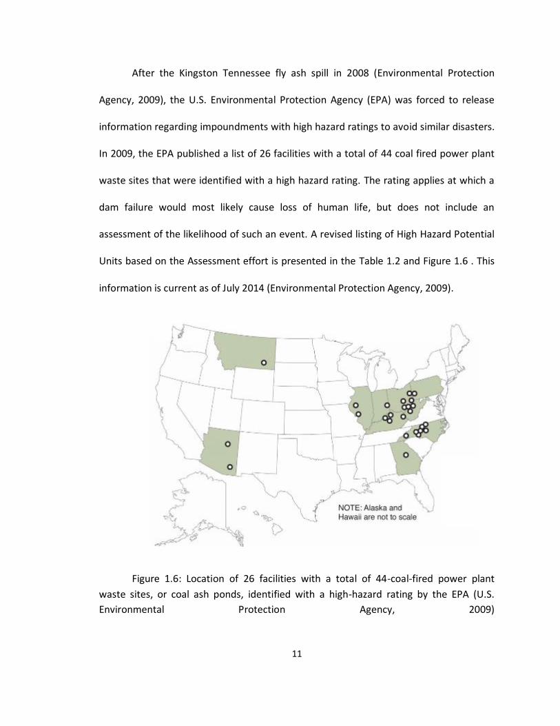
After the Kingston Tennessee fly ash spill in 2008 (Environmental Protection
Agency, 2009), the U.S. Environmental Protection Agency (EPA) was forced to release
information regarding impoundments with high hazard ratings to avoid similar disasters.
In 2009, the EPA published a list of 26 facilities with a total of 44 coal fired power plant
waste sites that were identified with a high hazard rating. The rating applies at which a
dam failure would most likely cause loss of human life, but does not include an
assessment of the likelihood of such an event. A revised listing of High Hazard Potential
Units based on the Assessment effort is presented in the Table 1.2 and Figure 1.6 . This
information is current as of July 2014 (Environmental Protection Agency, 2009).
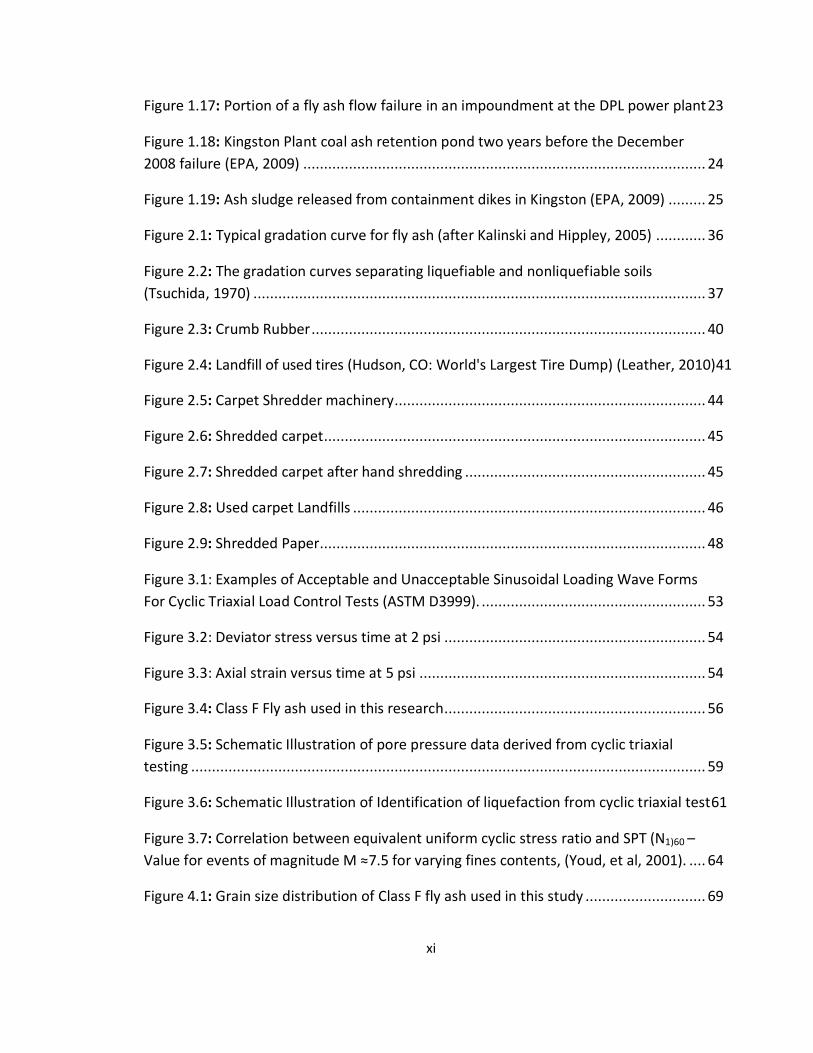
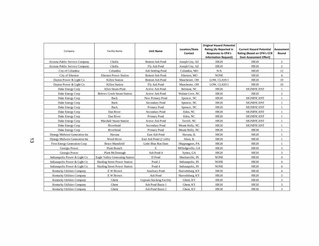
Figure 1.6: Location of 26 facilities with a total of 44-coal-fired power plant
waste sites, or coal ash ponds, identified with a high-hazard rating by the EPA (U.S.
Environmental Protection Agency, 2009)
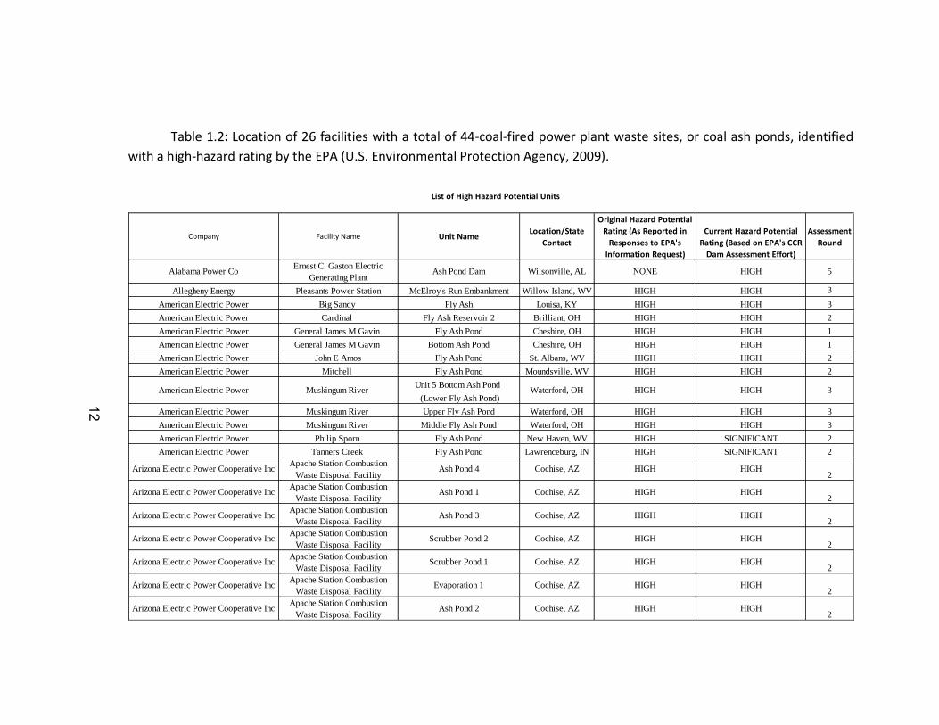
12
Table 1.2: Location of 26 facilities with a total of 44-coal-fired power plant waste sites, or coal ash ponds, identified
with a high-hazard rating by the EPA (U.S. Environmental Protection Agency, 2009).
Original Hazard Potential
Rating (As Reported in Current Hazard Potential Assessment
Responses to EPA's Rating (Based on EPA's CCR Round
Information Request) Dam Assessment Effort)
Ernest C. Gaston Electric
Generating Plant
Allegheny Energy Pleasants Power Station McElroy's Run Embankment Willow Island, WV HIGH HIGH 3
American Electric Power Big Sandy Fly Ash Louisa, KY HIGH HIGH 3
American Electric Power Cardinal Fly Ash Reservoir 2 Brilliant, OH HIGH HIGH 2
American Electric Power General James M Gavin Fly Ash Pond Cheshire, OH HIGH HIGH 1
American Electric Power General James M Gavin Bottom Ash Pond Cheshire, OH HIGH HIGH 1
American Electric Power John E Amos Fly Ash Pond St. Albans, WV HIGH HIGH 2
American Electric Power Mitchell Fly Ash Pond Moundsville, WV HIGH HIGH 2
Unit 5 Bottom Ash Pond
(Lower Fly Ash Pond)
American Electric Power Muskingum River Upper Fly Ash Pond Waterford, OH HIGH HIGH 3
American Electric Power Muskingum River Middle Fly Ash Pond Waterford, OH HIGH HIGH 3
American Electric Power Philip Sporn Fly Ash Pond New Haven, WV HIGH SIGNIFICANT 2
American Electric Power Tanners Creek Fly Ash Pond Lawrenceburg, IN HIGH SIGNIFICANT 2
Apache Station Combustion
Waste Disposal Facility
Apache Station Combustion
Waste Disposal Facility
Apache Station Combustion
Waste Disposal Facility
Apache Station Combustion
Waste Disposal Facility
Apache Station Combustion
Waste Disposal Facility
Apache Station Combustion
Waste Disposal Facility
Apache Station Combustion
Waste Disposal Facility
Alabama Power Co
Facility NameCompany
List of High Hazard Potential Units
Muskingum River American Electric Power HIGH HIGH 3
Unit NameLocation/State
Contact
HIGH HIGH2
HIGH HIGH2
HIGH HIGH2
HIGH HIGH2
HIGH HIGH2
NONE HIGH 5
HIGH HIGH2
HIGH HIGH2
Evaporation 1
Scrubber Pond 1
Scrubber Pond 2
Ash Pond 3
Ash Pond 1
Arizona Electric Power Cooperative Inc
Arizona Electric Power Cooperative Inc
Arizona Electric Power Cooperative Inc
Cochise, AZ
Cochise, AZ
Cochise, AZ
Cochise, AZ
Cochise, AZ
Cochise, AZAsh Pond 2
Arizona Electric Power Cooperative Inc Ash Pond 4 Cochise, AZ
Arizona Electric Power Cooperative Inc
Arizona Electric Power Cooperative Inc
Arizona Electric Power Cooperative Inc
Wilsonville, ALAsh Pond Dam
Waterford, OH
12
13
Original Hazard Potential
Rating (As Reported in Current Hazard Potential Assessment
Responses to EPA's Rating (Based on EPA's CCR Round
Information Request) Dam Assessment Effort)
Arizona Public Service Company Cholla Bottom Ash Pond Joseph City, AZ HIGH HIGH 2
Arizona Public Service Company Cholla Fly Ash Pond Joseph City, AZ HIGH HIGH 2
City of Columbia Columbia Ash Settling Pond Columbia, MO N/A HIGH 12
City of Sikeston Sikeston Power Station Bottom Ash Pond Sikeston, MO NONE HIGH 4
Dayton Power & Light Co Killen Station Bottom Ash Pond Manchester, OH LOW, CLASS I HIGH 10
Dayton Power & Light Co Killen Station Fly Ash Pond Manchester, OH LOW, CLASS I HIGH 10
Duke Energy Corp Allen Steam Plant Active Ash Pond Belmont, NC HIGH SIGNIFICANT 1
Duke Energy Corp Belews Creek Steam Station Active Ash Pond Walnut Cove, NC HIGH HIGH 2
Duke Energy Corp Buck New Primary Pond Spencer, NC HIGH SIGNIFICANT 1
Duke Energy Corp Buck Secondary Pond Spencer, NC HIGH SIGNIFICANT 1
Duke Energy Corp Buck Primary Pond Spencer, NC HIGH SIGNIFICANT 1
Duke Energy Corp Dan River Secondary Pond Eden, NC HIGH SIGNIFICANT 1
Duke Energy Corp Dan River Primary Pond Eden, NC HIGH SIGNIFICANT 1
Duke Energy Corp Marshall Steam Station Active Ash Pond Terrell, NC HIGH SIGNIFICANT 1
Duke Energy Corp Riverbend Secondary Pond Mount Holly, NC HIGH SIGNIFICANT 1
Duke Energy Corp Riverbend Primary Pond Mount Holly, NC HIGH HIGH 1
Dynegy Midwest Generation Inc Havana East Ash Pond Havana, IL HIGH HIGH 1
Dynegy Midwest Generation Inc Wood River East Ash Pond (2 cells) Alton, IL HIGH HIGH 1
First Energy Generation Corp Bruce Mansfield Little Blue Run Dam Shippingport, PA HIGH HIGH 1
Georgia Power Plant Branch E Milledgeville, GA HIGH HIGH 3
Georgia Power Plant McDonough Ash Pond 4 Symra, GA HIGH HIGH 3
Indianapolis Power & Light Co Eagle Valley Generating Station D Pond Martinsville, IN NONE HIGH 4
Indianapolis Power & Light Co Harding Street Power Station Pond 2 Indianapolis, IN NONE HIGH 4
Indianapolis Power & Light Co Harding Street Power Station Pond 4 Indianapolis, IN NONE HIGH 4
Kentucky Utilities Company E W Brown Auxiliary Pond Harrodsburg, KY HIGH HIGH 4
Kentucky Utilities Company E W Brown Ash Pond Harrodsburg, KY HIGH HIGH 3
Kentucky Utilities Company Ghent Gypsum Stacking Facility Ghent, KY HIGH HIGH 3
Kentucky Utilities Company Ghent Ash Pond Basin 1 Ghent, KY HIGH HIGH 3
Kentucky Utilities Company Ghent Ash Pond Basin 2 Ghent, KY HIGH HIGH 3
Company Facility Name Unit NameLocation/State
Contact
13
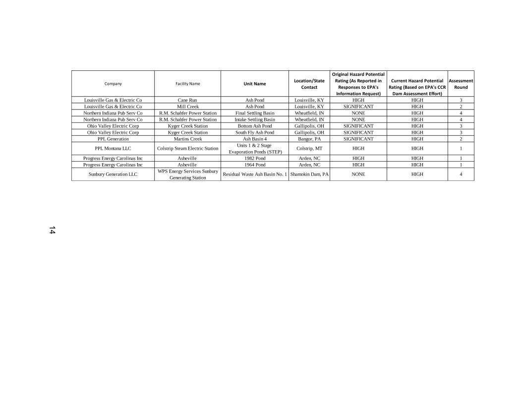
14
Original Hazard Potential
Rating (As Reported in Current Hazard Potential Assessment
Responses to EPA's Rating (Based on EPA's CCR Round
Information Request) Dam Assessment Effort)
Louisville Gas & Electric Co Cane Run Ash Pond Louisville, KY HIGH HIGH 3
Louisville Gas & Electric Co Mill Creek Ash Pond Louisville, KY SIGNIFICANT HIGH 2
Northern Indiana Pub Serv Co R.M. Schahfer Power Station Final Settling Basin Wheatfield, IN NONE HIGH 4
Northern Indiana Pub Serv Co R.M. Schahfer Power Station Intake Settling Basin Wheatfield, IN NONE HIGH 4
Ohio Valley Electric Corp Kyger Creek Station Bottom Ash Pond Gallipolis, OH SIGNIFICANT HIGH 3
Ohio Valley Electric Corp Kyger Creek Station South Fly Ash Pond Gallipolis, OH SIGNIFICANT HIGH 3
PPL Generation Martins Creek Ash Basin 4 Bangor, PA SIGNIFICANT HIGH 2
Units 1 & 2 Stage
Evaporation Ponds (STEP)
Progress Energy Carolinas Inc Asheville 1982 Pond Arden, NC HIGH HIGH 1
Progress Energy Carolinas Inc Asheville 1964 Pond Arden, NC HIGH HIGH 1
WPS Energy Services Sunbury
Generating Station
Location/StateCompany Facility Name Unit Name
Contact
PPL Montana LLC Colstrip Steam Electric Station Colstrip, MT HIGH HIGH
Sunbury Generation LLC NONE HIGH 4
1
Shamokin Dam, PAResidual Waste Ash Basin No. 1
14
15
Due to sludge release incidents, the EPA formally requested that electric utilities
that have surface impoundments or similar units provide information about the
structural integrity of their units and give more attention regarding this concern. In this
case, structural integrity of storages pond can be affected by any movement such as
earthquakes, blasting, machinery vibrations, etc.
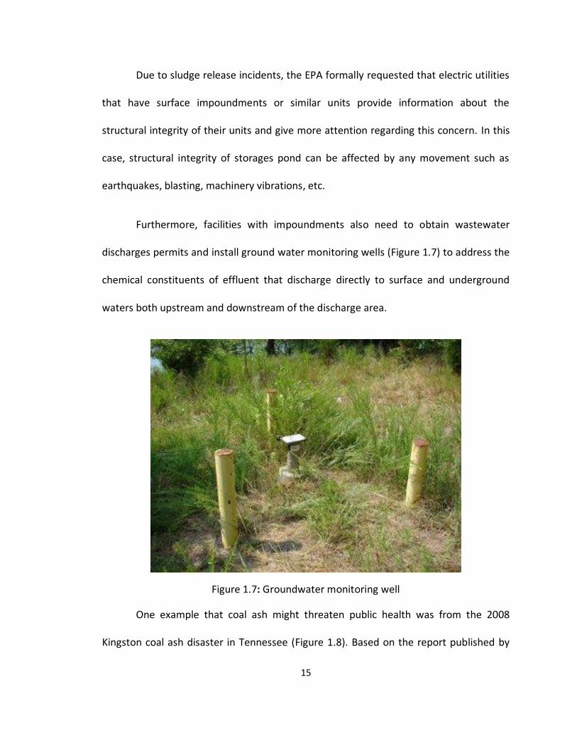
Furthermore, facilities with impoundments also need to obtain wastewater
discharges permits and install ground water monitoring wells (Figure 1.7) to address the
chemical constituents of effluent that discharge directly to surface and underground
waters both upstream and downstream of the discharge area.
Figure 1.7: Groundwater monitoring well
One example that coal ash might threaten public health was from the 2008
Kingston coal ash disaster in Tennessee (Figure 1.8). Based on the report published by
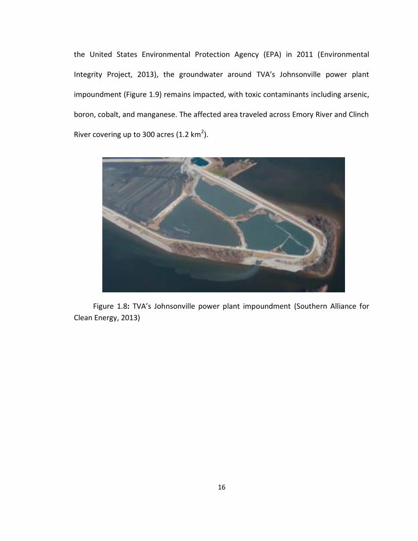
16
the United States Environmental Protection Agency (EPA) in 2011 (Environmental
Integrity Project, 2013), the groundwater around TVA’s Johnsonville power plant
impoundment (Figure 1.9) remains impacted, with toxic contaminants including arsenic,
boron, cobalt, and manganese. The affected area traveled across Emory River and Clinch
River covering up to 300 acres (1.2 km2).
Figure 1.8: TVA’s Johnsonville power plant impoundment (Southern Alliance for
Clean Energy, 2013)
17
Figure 1.9: Kingston coal ash disaster (Associated Press; Samuel M. Simpkins/The
Tennessean) December 22, 2008
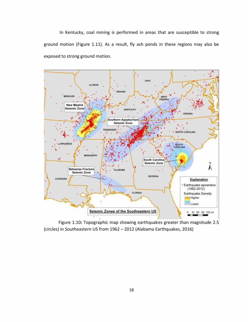
In Kentucky, the potential for earthquake-induced strong ground motion has
gained significant attention. Seismic zones that are active and produce strong ground
motion in Kentucky include the New Madrid Seismic Zone, The Wabash Valley Seismic
Zone and Southern Appalachian Seismic Zone (Figure 1.10). The Southern Appalachian
Seismic Zone was the source of the biggest earthquake ever recorded in the state of
Kentucky. It occurred near Sharpsburg in Bath County on July 27, 1980 with a magnitude
of 5.2. The New Madrid Seismic Zone, located in Western Kentucky, produced
earthquakes with magnitude of 8.0 in 1811 and 1812 with return periods on the order of
400-1,000 years (Nuttli, 1974), but were not recorded.
18
In Kentucky, coal mining is performed in areas that are susceptible to strong
ground motion (Figure 1.11). As a result, fly ash ponds in these regions may also be
exposed to strong ground motion.
Figure 1.10: Topographic map showing earthquakes greater than magnitude 2.5
(circles) in Southeastern US from 1962 – 2012 (Alabama Earthquakes, 2016)
19
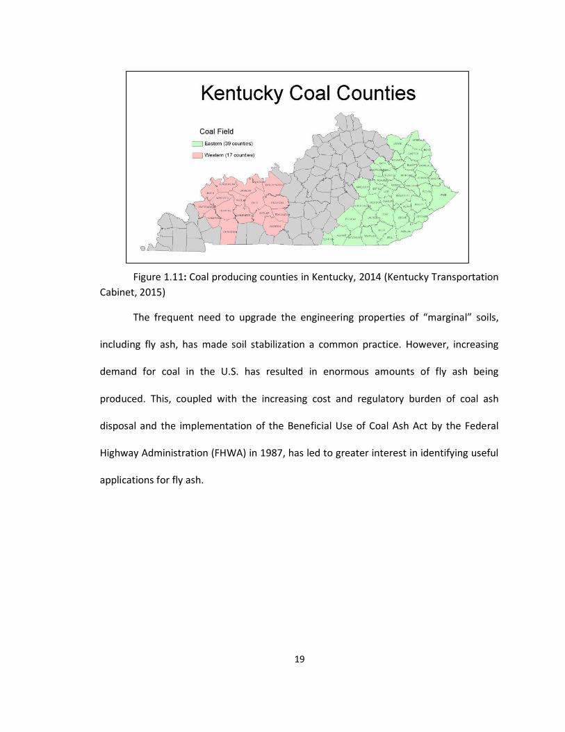
Figure 1.11: Coal producing counties in Kentucky, 2014 (Kentucky Transportation
Cabinet, 2015)
The frequent need to upgrade the engineering properties of “marginal” soils,
including fly ash, has made soil stabilization a common practice. However, increasing
demand for coal in the U.S. has resulted in enormous amounts of fly ash being
produced. This, coupled with the increasing cost and regulatory burden of coal ash
disposal and the implementation of the Beneficial Use of Coal Ash Act by the Federal
Highway Administration (FHWA) in 1987, has led to greater interest in identifying useful
applications for fly ash.
20
1.2 History of Incidents at Fly Ash Impoundments
In the past, many fly ash impoundments were built with the assumption that fly
ash is resistant to liquefaction. Recently, this assumption has come into question due to
many accidents which have also resulted in some fatalities. One of the more significant
factors leading to ground failure during earthquakes is the liquefaction of loose to
medium-dense sands below the water table (Seed and Harder, 1990), but cohesionless
fine-grained material like fly ash is also susceptible to liquefaction. During shaking, the
ash tends to densify. The water in the pores cannot escape quickly enough, so excess
pore pressure develops. In turn, effective stress decreases. Ash depends on the effective
stress between the grains to mobilize shear strength. Therefore, the increasing pore
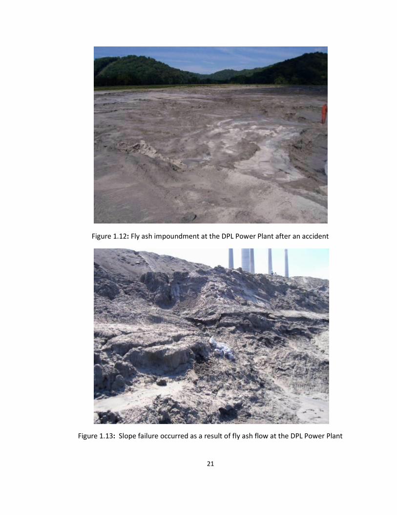
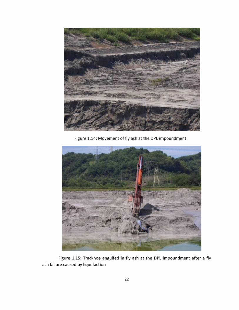
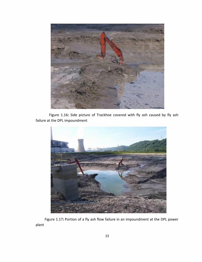
water pressure leads to strength loss. The example illustrated in Figure 1.12-Figure 1.17
is from the Dayton Power and Light (DPL) power plant in Maysville, Ohio where a mass
of hydraulically placed fly ash failed due to dynamic loading in (vibrations) from
machinery, which induced liquefaction in the material and a flow failure that engaged
several dozen acres of the impoundment and resulted in one fatality.
21
Figure 1.12: Fly ash impoundment at the DPL Power Plant after an accident
Figure 1.13: Slope failure occurred as a result of fly ash flow at the DPL Power Plant
22
Figure 1.14: Movement of fly ash at the DPL impoundment
Figure 1.15: Trackhoe engulfed in fly ash at the DPL impoundment after a fly
ash failure caused by liquefaction
23
Figure 1.16: Side picture of Trackhoe covered with fly ash caused by fly ash
failure at the DPL impoundment
Figure 1.17: Portion of a fly ash flow failure in an impoundment at the DPL power
plant
24
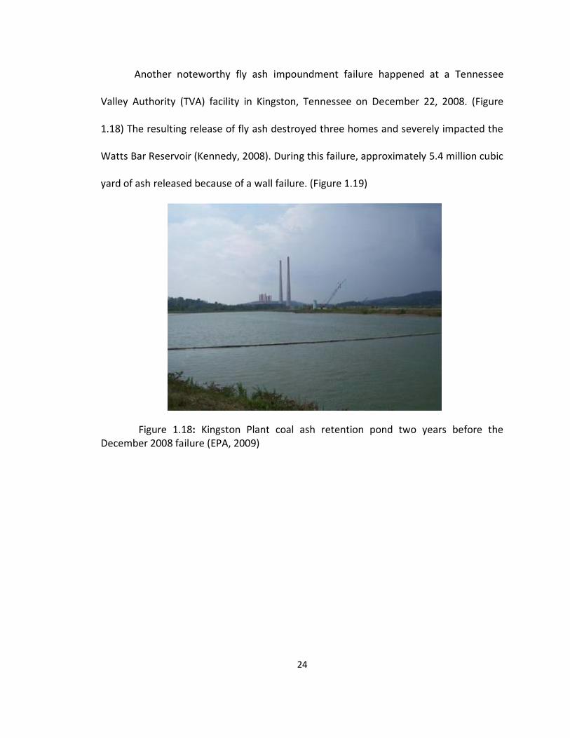
Another noteworthy fly ash impoundment failure happened at a Tennessee
Valley Authority (TVA) facility in Kingston, Tennessee on December 22, 2008. (Figure
1.18) The resulting release of fly ash destroyed three homes and severely impacted the
Watts Bar Reservoir (Kennedy, 2008). During this failure, approximately 5.4 million cubic
yard of ash released because of a wall failure. (Figure 1.19)
Figure 1.18: Kingston Plant coal ash retention pond two years before the December 2008 failure (EPA, 2009)
25
Figure 1.19: Ash sludge released from containment dikes in Kingston (EPA, 2009)
The TVA ash storage site is located in Roane County, Tennessee in close
proximity to two faults, including an unnamed fault approximately 0.25 mile south of
the failure area and the Kingston Fault. However, this failure was not attributed to
seismicity in the area because there were no events of significant size on these faults in
the time frame of the failure.
From the final report of the investigation, AECOM identified four factors that
contributed to the failure of the Kingston fly ash impoundment, including fill geometry,
increased fill rates, soft foundation soils and loose saturated ash (AECOM, 2009).
However, for the research presented herein, the presence of loose saturated fly ash is
being considered.
26
The Kingston incident raised concerns within the electric power industry and the
general public regarding the geotechnical behavior of coal combustion products (CCP)
and their engineering properties. Therefore, it has become of great interest amongst
members of the geotechnical engineering community serving the utility industry to
establish whether or not there is potential for CCR to liquefy at a site under certain
credible loading conditions such as blasting and vibrations from machinery.
1.3 Other Research Related to Fly Ash
The following section contains a brief review of related research where the
dynamic and cyclic behavior of fly ash was investigated. Although a large amount of
literature exists on the cyclic resistance of sands, silts, and clays, less has been done to
determine the liquefaction potential of fly ash. The test programs had varying objectives
and correlation between tests is limited. However, common behavioral patterns and
properties are identified. Much of the available literature on stabilizing fly ash
embankments is based upon test results from university research projects, industry
sources and private engineering firms.
There are many factors related to failure of fly ash embankments. Those factors
include ash type, ash solubility, degree of compaction, overconsolidation ratio, moisture
content, and position relative to the groundwater table. Some attempts have been
made to predict the behavior of coal ash using the Cone Penetration Test (CPT) and
Standard Penetration Test (SPT). However, correlations between cyclic resistance and
CPT or SPT may not be reliable. Cunningham et al. (1977) suggested that in loose
27
conditions ash may liquefy during CPT and SPT testing, which may lead to misleading
results. According to Leonards and Bailey (1982) the behavior of compacted ash cannot
be inferred from SPT or CPT largely because these tests do not adequately sense the
effect of pre-stressing due to compaction.
Zand et al. (2007) and Zand et al. (2008) investigated the liquefaction, post
liquefaction and settlement behaviors of fly ash by performing cyclic triaxial tests on fly
ash samples at different densities, confining stresses and cyclic stress ratios using the
standard cyclic triaxial test method (ASTM D5311). Results from their investigation
showed that the shear strength of fly ash is closely related to dry unit weight. The
consolidation rate of fly ash was measured using conventional oedomenter
consolidation testing to investigate the long-term settlement behavior of Class F fly ash.
In addition, a considerable amount of research has been conducted to study
different techniques such as vacuum dewatering, electro-osmosis consolidation,
vibrocompaction, stone-sand columns, blasting compaction, lime stabilization and fiber
mix stabilization to improve the density, stiffness and bearing capacity of fly ash. Kumar
et al. (2006) investigated the effect of polypropylene fibers to stabilize fly ash
embankments. According to this, randomly distributed discrete fibers can be used to
improve shear strength, CBR value and modulus of subgrade reaction of fly ash
embankments. The tests were performed on unreinforced soil-fly ash and reinforced
soil-fly ash systems. The reinforcement was varied from 0% to 2% by weight of the soil
and fly ash, with the aspect ratio of 90. Triaxial test results indicate that fiber aspect
28
ratio (l/d) or fiber length divided by its diameter significantly affects the magnitude of
both the critical confining stress, and the strength of soil-fiber composite.
Many researchers have attempted to evaluate the behavior of adding fiber into
fly ash as a means to reduce cost of construction and encourage sustainable
development. Choudhary et al. (2011) analyzed the shear strength of fiber reinforced fly
ash. The material of added fiber used is polyethylene (synthetic) with fiber contents of
0.25, 0.50 and 1.0 % by mass of dry fly ash. The results show that the stiffness of fly ash
increases with increasing fiber content, with improvements in elastic modulus, shear
strength, cohesion and friction angle.
Puppala et al. (2001) conducted tests on expansive soil stabilization using recycled
waste materials. Both fly ash and polypropylene fiber, the typical fiber found in carpet,
were mixed with expansive soils. The test result shows that both materials increased
strength and decreased shrinkage strains of the soils. The waste materials reduce the
volume change of expansive soil during saturated and dried conditions.
Mohan et. al. (2012) used natural fiber such as coconut fiber mixed with fly ash
and concrete. Four different coconut fibers percentages of 0.15, 0.30, 0.45 and 0.60%
were used. The results show that the addition of coconut fiber increased the strain at
which the material failed. Fly ash is classified as low plasticity silt (ML). The
improvement in unconfined compressive strength is believed to be due to skin friction
between the fibers and fly ash. When the specimen is loaded axially, the fly ash are
29
believed to apply confining pressure on the fibers, and in this process they get stretched
with mobilization of tensile force. The tensile force T varies with the orientation of the
fibers within the specimen (Kumar and Singh, 2010).
Boominathan and Hari (2002) concluded that at low confining pressure, randomly
distributed geosynthetic fiber/mesh reinforcement provides a higher rate of
improvement in liquefaction resistance of fly ash. Addition of randomly distributed
mesh and fiber elements increases significantly the liquefaction resistance of fly ash at
low relative densities. Randomly distributed mesh elements (the ratio of longest to the
shortest side) should be near 1.0 to better arrest liquefaction when compared with
randomly distributed fiber elements because the mesh elements provide better
interlocking of the fly ash and also provide faster dissipation of pore pressure along the
sample length. The optimum percentage of fiber/mesh content is found to be 2% to
resist liquefaction. The gain in liquefaction resistance of fly ash due to mesh/fiber
reinforcements is more pronounced at lower confining pressures and hence reinforcing
fly ash with mesh/fiber elements is a better choice among available ground
improvement techniques to improve liquefaction resistance of fly ash.
In agreement, Kumar et al. (2006) presented the effect of inclusion of
polypropylene fibres in fly ash. The percentage increase in CBR value is higher at lower
percentages of fiber content, where 0.5% fibre content is seen to be the optimum.
30
Kulkarni (2003) investigated the effect of filler-fiber on the compressive strength
of fly ash and short-fiber epoxy composited (reinforced epoxy layers). The results show
that the decrease in density can be attributed to the tendency of fibers to bunch. The
properties of such composites are greatly influenced by shape, size, and distribution of
the reinforcing phase in addition to their chemical composition and volume fraction.
Viswanathan et al. (1997) used fly ash as an admixture to stabilize subgrade soils.
The reactions involved in the stabilization of soils with fly ash admixtures are
categorized as short term (immediate) and long term reactions. The short term reaction
in clays is the exchange of cations on the surface of the clay particles which results in a
decrease in its plasticity index (PI). However, in cohesionless coarse grained soils, the
admixture serves as “micro aggregate” resulting in an increase in the maximum dry
density. The long term reactions are pozzolonic and occur over a period of weeks or
months. Pozzolonic reactions result in the formation of cementious products such as
calcium silicate hydrate and calcium aluminate hydrate which increases the strength,
stability and durability of soil.
1.4 Gaps in the Current State of Knowledge
From the previous section, the mechanics of liquefaction in fly ash are now well
understood and the potential for occurrence can be estimated and avoided with a
reasonable degree of confidence. Although a large amount of literature exists on the
cyclic resistance of fly ash and fly ash admixtures especially with fibers (Kaniraj et al,
2003); none has been done to determine the liquefaction potential of fly ash admixtures
31
with waste products. To address this subject an experimental program along with an
analytical study was conducted to evaluate the effect of adding waste products such as
crumb rubber, shredded carpet and shredded paper; to enhance the strength properties
of fly ash.
A secondary objective of this research is to identify an alternate method to
recycle used tires and shredded carpet, materials that would otherwise be considered as
waste products.
In order to address this concern, cyclic triaxial testing combined with analytical
analyses were conducted to evaluate the liquefaction potential of reconstituted fly ash
specimens to depict the material in the impoundment facilities and to evaluate the
strength properties of the material. Based on this, we can investigate the effect of waste
products on fly ash liquefaction.
Although a large amount of conducted research already provides methods to
stabilize fly ash, none calculate the costs to implement the method in the actual field
and shows comparison matrix costs between methods. This calculation is very
substantial especially if impoundment facilities want to select the most appropriate
method to solve the problem with fly ash stability.
1.5 Research Objectives
This study will focus on utilizing cyclic triaxial testing to collect information such
as deviator stress, axial deformation and excess pore pressure from every specimen
32
tested. This recorded information will be used to make hysteresis loop and develop
cyclic resistance ratio (CRR). Using this information the expectations of this research
were as follows:
1) A method would be identified to stabilize fly ash in storage ponds with
respect to static stability.
2) A method would be identified to re-task waste products such as crumb
rubber, shredded carpet, and shredded paper to reduce waste stream.
3) Methods will be developed to analyze the liquefaction resistance of fly
ash admixtures against dynamic loading from earthquakes and vibrations
4) A cost matrix would be developed to quantify the benefit of using waste
products as addictives to provide justification for the method.
1.6 Research Limitations
Time limitations, number of waste products, cyclic stress ratio (CSR), the amount
of specimens tested, laboratory testing equipment and specimen ratio or composition;
mentioned are the limitations applied for this research.
Time limitation affected the number of specimen tested and how long one
specimen gets tested. Pore pressure parameter B-value, according to ASTM D5311,
sample is considered saturated if B-value is greater than 95%. To accommodate this
requirement, minimum of 2 days to a maximum of 1 week were needed to establish
saturation, resulted in limited number of specimens tested
33
Byproduct of tires, shredded carpet and paper, previously mentioned were the
only waste products used for this research. The selected materials were in high
consideration that will help to enhance the strength properties of fly ash.
Initially, the cyclic stress ratio (CSR) used ranged from 0.30 to 0.80, but changed
to 0.15 - 0.50. The changed was made because specimens tested at cyclic stress ratio
higher than 0.50, gave a small number of cycles to liquefaction (Less than 4). These
results show that all specimens with different composition and waste materials showed
same behavior at cyclic stress ratio higher than 0.50. After decreasing the CSR, the
number of cycles to liquefaction ranged from 2 cycles to more than 100 cycles.
The testing equipment used on this research was cyclic strength testing
instrument and it is adequate to see the effect and analyze the results for each
specimens.
Finally, specimen composition contains Class F fly ash with waste material up to a
maximum of 20% by dry weight. This limit of up to 20% waste material was used because
the amount of waste products more than the maximum limit tends to occupy more
volume than fly ash and also to maintain fly ash as the primary material and not
secondary material or filler.
1.7 Dissertation Outline
In Chapter 2, the physical properties of fly ash and also other materials
considered to be used in this research are explained. Physical properties to be explained
34
include specific gravity and grain size distribution. Also in this chapter, current uses and
disposal method of fly ash, crumb rubber, shredded carpet and paper are explained
briefly.
Chapter 3 is used to explain and describe triaxial testing, including basic
information about the machine, how the instrument works, the assumptions used, input
parameters, and expected output.
Chapter 4 results of the physical and chemical properties of selected material for
this research. This chapter also will briefly explain how to run the laboratory testing
such as specific gravity, grain size distribution and strain-controlled cyclic triaxial testing.
Further, chemical composition of fly ash specimen from the X-Ray diffraction (XRD) test
is discussed.
In chapter 5, the typical results from geotechnical and cyclic triaxial testing are
presented. These results including specific gravity, grain size distribution curve and plots
generate from cyclic triaxial testing.
Finally, chapter 6 provides the conclusions obtained from the research. Several
recommendations for further research are also included in this chapter.
35
Chapter 2
2. WASTE MATERIALS USED IN THIS STUDY
2.1 Fly Ash
The American Society for Testing and Materials (ASTM) standard C618 identifies
two classes of fly ash. Class C fly ash is derived from the combustion of younger lignite
or sub bituminous coal. It generally contains more than 20% of quicklime (CaO) and is
self-cementing when mixed with water. Class F fly ash is derived from the combustion
of older anthracite or bituminous coal. It contains less quicklime and is not self-
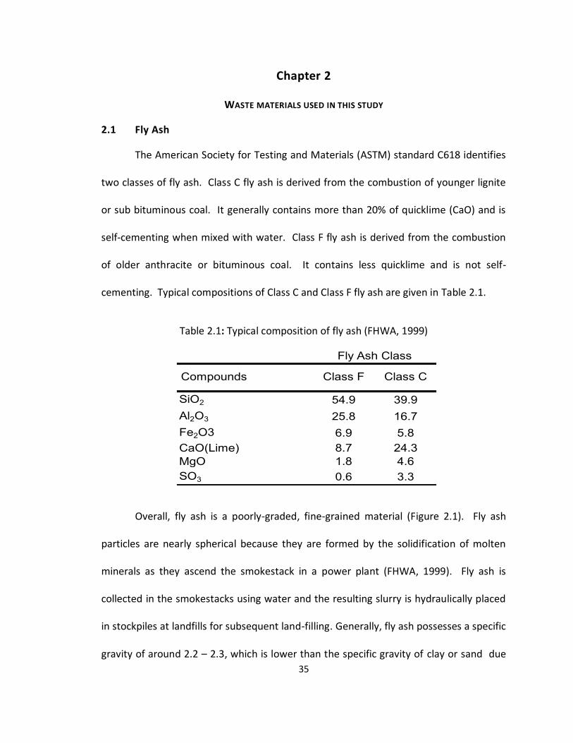
cementing. Typical compositions of Class C and Class F fly ash are given in Table 2.1.
Table 2.1: Typical composition of fly ash (FHWA, 1999)
SiO2 54.9 39.9
Al2O3 25.8 16.7
Fe2O3 6.9 5.8
CaO(Lime) 8.7 24.3
MgO 1.8 4.6
SO3 0.6 3.3
Compounds Class F Class C
Fly Ash Class
Overall, fly ash is a poorly-graded, fine-grained material (Figure 2.1). Fly ash
particles are nearly spherical because they are formed by the solidification of molten
minerals as they ascend the smokestack in a power plant (FHWA, 1999). Fly ash is
collected in the smokestacks using water and the resulting slurry is hydraulically placed
in stockpiles at landfills for subsequent land-filling. Generally, fly ash possesses a specific
gravity of around 2.2 – 2.3, which is lower than the specific gravity of clay or sand due
36
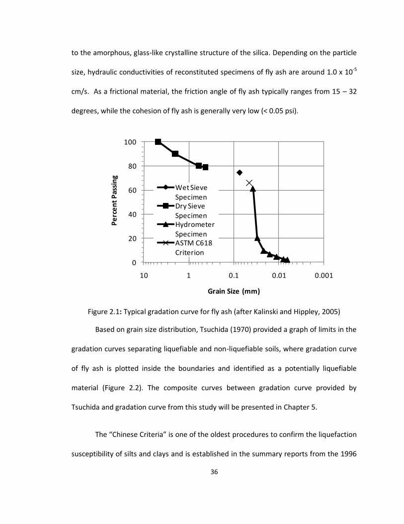
to the amorphous, glass-like crystalline structure of the silica. Depending on the particle
size, hydraulic conductivities of reconstituted specimens of fly ash are around 1.0 x 10⁻⁵
cm/s. As a frictional material, the friction angle of fly ash typically ranges from 15 – 32
degrees, while the cohesion of fly ash is generally very low (< 0.05 psi).
0
20
40
60
80
100
0.0010.010.1110
Pe
rce
nt
Pas
sin
g
Grain Size (mm)
Wet Sieve SpecimenDry Sieve SpecimenHydrometer SpecimenASTM C618 Criterion
Figure 2.1: Typical gradation curve for fly ash (after Kalinski and Hippley, 2005)
Based on grain size distribution, Tsuchida (1970) provided a graph of limits in the
gradation curves separating liquefiable and non-liquefiable soils, where gradation curve
of fly ash is plotted inside the boundaries and identified as a potentially liquefiable
material (Figure 2.2). The composite curves between gradation curve provided by
Tsuchida and gradation curve from this study will be presented in Chapter 5.
The “Chinese Criteria” is one of the oldest procedures to confirm the liquefaction
susceptibility of silts and clays and is established in the summary reports from the 1996
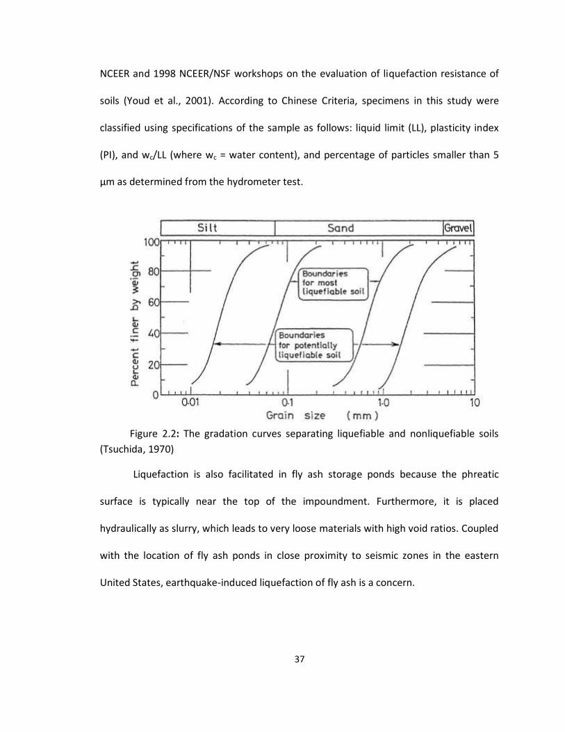
37
NCEER and 1998 NCEER/NSF workshops on the evaluation of liquefaction resistance of
soils (Youd et al., 2001). According to Chinese Criteria, specimens in this study were
classified using specifications of the sample as follows: liquid limit (LL), plasticity index
(PI), and wc/LL (where wc = water content), and percentage of particles smaller than 5
μm as determined from the hydrometer test.
Figure 2.2: The gradation curves separating liquefiable and nonliquefiable soils
(Tsuchida, 1970)
Liquefaction is also facilitated in fly ash storage ponds because the phreatic
surface is typically near the top of the impoundment. Furthermore, it is placed
hydraulically as slurry, which leads to very loose materials with high void ratios. Coupled
with the location of fly ash ponds in close proximity to seismic zones in the eastern
United States, earthquake-induced liquefaction of fly ash is a concern.
38
Class C fly ash contains greater than 20% quicklime and is self-cementing similar
to portland cement. Products derived from Class C fly ash have been used as concrete
admixtures, brick additives, and for soil stabilization (ACI 2010). Class F fly ash, on the
other hand, is not used as a cementing agent, but is sometimes used as an additive to
concrete to improve flowability. With the addition of a cementing agent such as
quicklime or portland cement, fly ash is sometimes used as a fill material.
Nevertheless the reuse of fly ash is not widespread, and most fly ash produced at
power plants is ultimately placed in landfills. However, there are some novel uses for fly
ash being discovered. For instance, The Recycle Material Resource Center (RMRC)
provides an option to use fly ash as a fill material to help reclaim coal strip mines
(Recycle Material Resource Center, 2012). This method is a breakthrough to utilize
unused fly ash. The ash used in this method should be dewatered to an optimum
moisture content before use.
Disposal of large amounts of waste materials such as fly ash is a significant
problem in the United States and worldwide from both an economic and an
environmental perspective. Fly ash is designated as a special waste because of the large
volumes, and because it is generally considered less hazardous than municipal solid
waste (MSW). Special wastes often have separate, less restrictive requirements for
landfills. In addition to the technical and site restrictions imposed by The Resource
Conservation and Recovery Act (RCRA), other economic and political conditions also
affect the landfilling of MSW and special wastes. Considerations such as cost of land,
39
proximity to waste stream sources, and proximity to existing infrastructure also play a
role in decisions regarding how and where to place the waste.
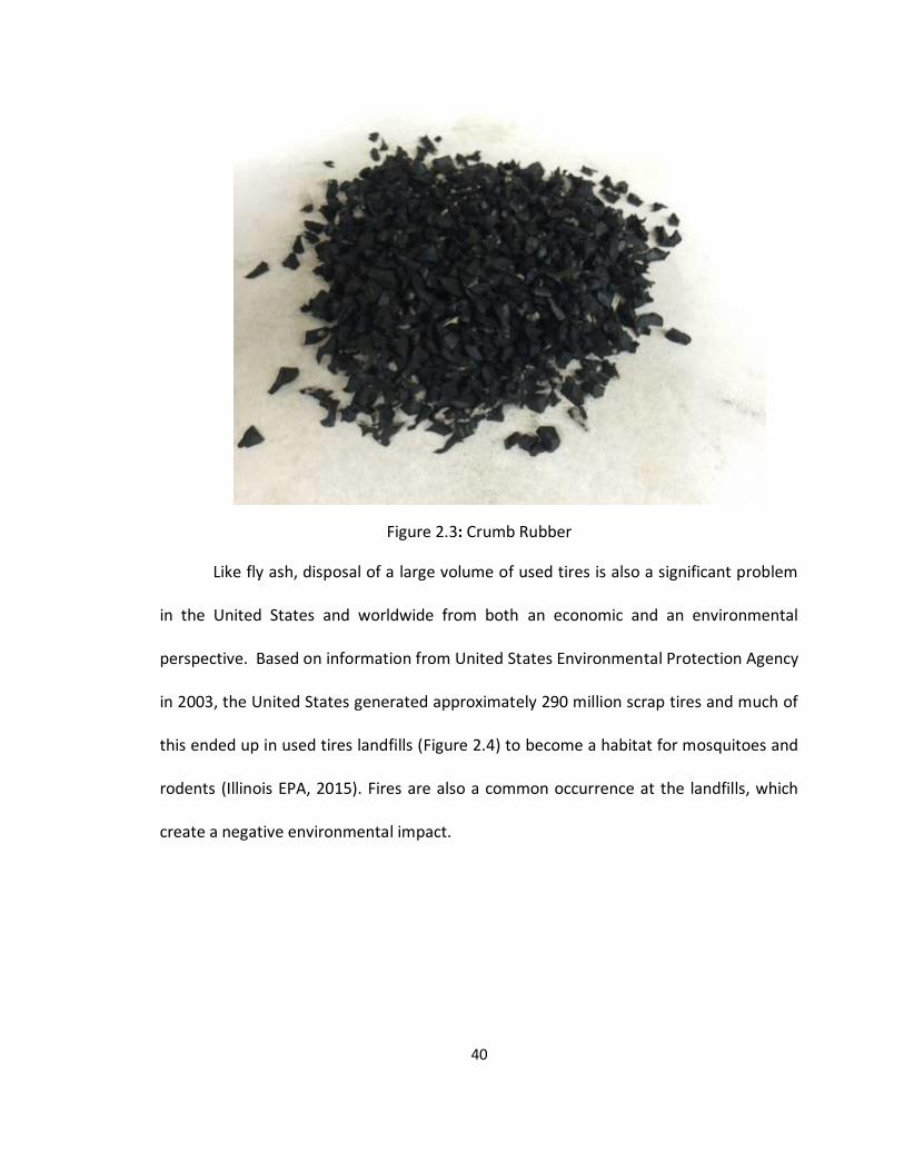
2.2 Crumb Rubber
Tires in the form of crumb rubber were used in this study as an additive to fly ash.
Crumb rubber particle size (Figure 2.3) typically range from gravel-sized to sand-sized.
The size of crumb rubber used in this research was 0.20 – 0.25 in. in width and 0.100 -
0.125 in. in thickness with a specific gravity of approximately 1.1. This size was chosen
because it is easy to find and many companies sell recycled tires in this size, meaning
that companies have capability to cut tires into this size and also to accommodate the
minimum size require for cyclic triaxial testing.
Crumb rubber is commonly used as an additive for rubberized asphalt concrete,
is used in clothing, and is considered as safe ground cover for playgrounds and
schoolyards. In Missouri, shredded waste tires have been used as fill material for road
subgrades (Engstrom and Lamb, 2003).
40
Figure 2.3: Crumb Rubber
Like fly ash, disposal of a large volume of used tires is also a significant problem
in the United States and worldwide from both an economic and an environmental
perspective. Based on information from United States Environmental Protection Agency
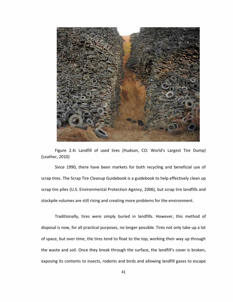
in 2003, the United States generated approximately 290 million scrap tires and much of
this ended up in used tires landfills (Figure 2.4) to become a habitat for mosquitoes and
rodents (Illinois EPA, 2015). Fires are also a common occurrence at the landfills, which
create a negative environmental impact.
41
Figure 2.4: Landfill of used tires (Hudson, CO: World's Largest Tire Dump)
(Leather, 2010)
Since 1990, there have been markets for both recycling and beneficial use of
scrap tires. The Scrap Tire Cleanup Guidebook is a guidebook to help effectively clean up
scrap tire piles (U.S. Environmental Protection Agency, 2006), but scrap tire landfills and
stockpile volumes are still rising and creating more problems for the environment.
Traditionally, tires were simply buried in landfills. However, this method of
disposal is now, for all practical purposes, no longer possible. Tires not only take up a lot
of space, but over time, the tires tend to float to the top, working their way up through
the waste and soil. Once they break through the surface, the landfill’s cover is broken,
exposing its contents to insects, rodents and birds and allowing landfill gases to escape
42
(South Central Iowa Solid Waste Agency, 2016). The oil and ash created during fires can
also cause leaching problems. Therefore, for both practical and environmental reasons,
most municipalities in the United States no longer permit the inclusion of tires in regular
landfills. Landfills dedicated to shredded tires (monofills) are an effort to dispose of
tires, rather than recycle them. While monofilling could potentially reduce some of the
environmental problems of mixing tires with other landfill materials, it requires
substantial expenditures for land, shredding and handling. It is also unlikely that
monofilled tires will be reclaimed at a later date for fuel or any other worthwhile
purpose. This is not a current practice, but rather one under consideration in a number
of locations including Ohio and North Carolina. With tires being banned from landfills,
undisposed waste volume has increased rapidly (Yang et al., 2002).
According to the EPA, most recycled tires are used as fuel (scrap tires and used
oil are being converted to energy sources through the tire liquefaction process (Siuru,
1993) while the rest are used as ground rubber and other rubber-modified or rubber-
based products such as rubberized asphalt. Although most tires are already recycled and
used to create byproducts, there are still 265 millions of tires in stockpiles as
summarized in Table 2.2.
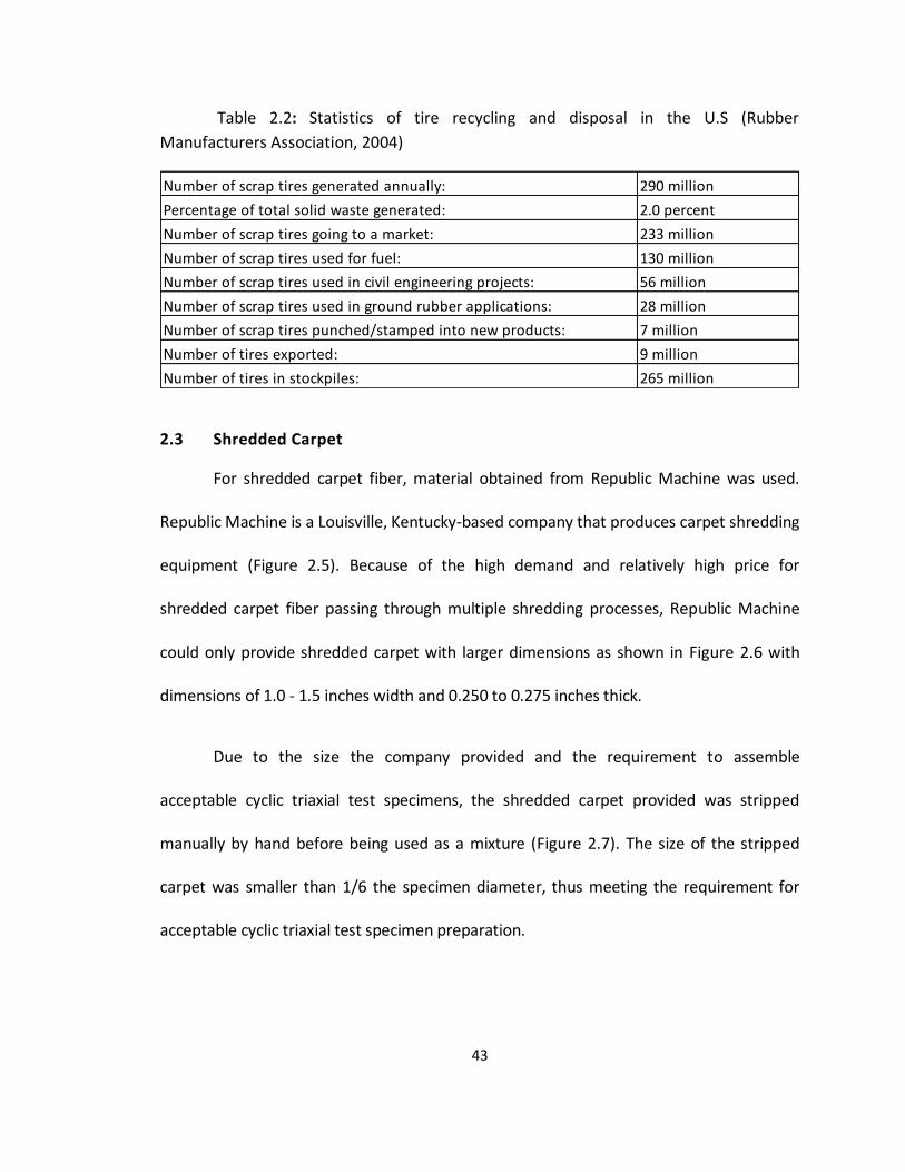
43
Table 2.2: Statistics of tire recycling and disposal in the U.S (Rubber
Manufacturers Association, 2004)
Number of scrap tires generated annually: 290 million
Percentage of total solid waste generated: 2.0 percent
Number of scrap tires going to a market: 233 million
Number of scrap tires used for fuel: 130 million
Number of scrap tires used in civil engineering projects: 56 million
Number of scrap tires used in ground rubber applications: 28 million
Number of scrap tires punched/stamped into new products: 7 million
Number of tires exported: 9 million
Number of tires in stockpiles: 265 million
2.3 Shredded Carpet
For shredded carpet fiber, material obtained from Republic Machine was used.
Republic Machine is a Louisville, Kentucky-based company that produces carpet shredding
equipment (Figure 2.5). Because of the high demand and relatively high price for
shredded carpet fiber passing through multiple shredding processes, Republic Machine
could only provide shredded carpet with larger dimensions as shown in Figure 2.6 with
dimensions of 1.0 - 1.5 inches width and 0.250 to 0.275 inches thick.
Due to the size the company provided and the requirement to assemble
acceptable cyclic triaxial test specimens, the shredded carpet provided was stripped
manually by hand before being used as a mixture (Figure 2.7). The size of the stripped
carpet was smaller than 1/6 the specimen diameter, thus meeting the requirement for
acceptable cyclic triaxial test specimen preparation.
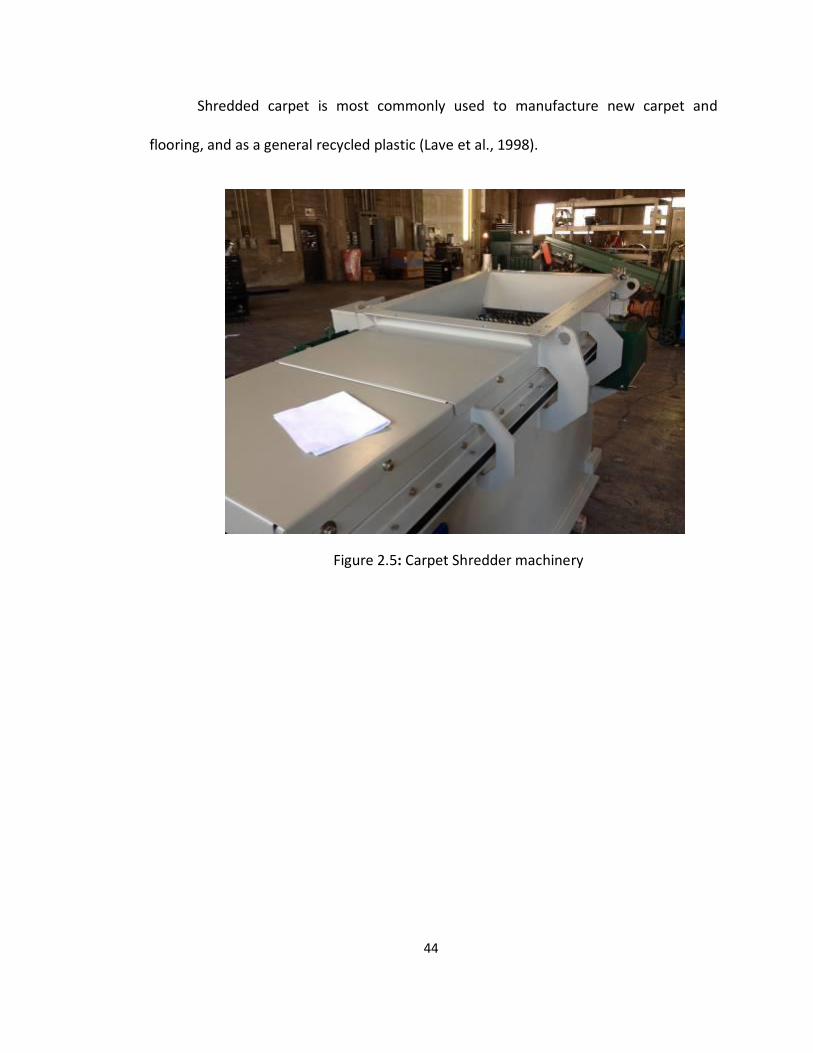
44
Shredded carpet is most commonly used to manufacture new carpet and
flooring, and as a general recycled plastic (Lave et al., 1998).
Figure 2.5: Carpet Shredder machinery
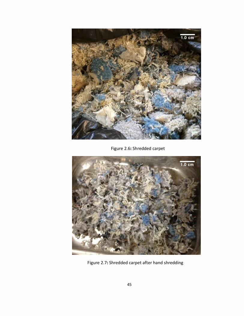
45
Figure 2.6: Shredded carpet
Figure 2.7: Shredded carpet after hand shredding
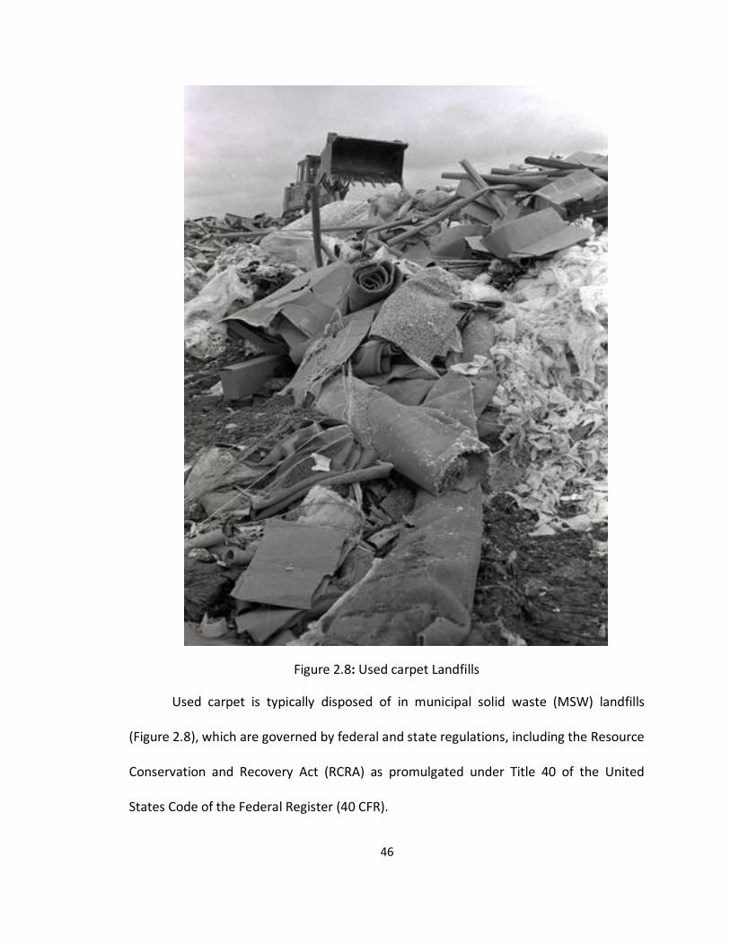
46
Figure 2.8: Used carpet Landfills
Used carpet is typically disposed of in municipal solid waste (MSW) landfills
(Figure 2.8), which are governed by federal and state regulations, including the Resource
Conservation and Recovery Act (RCRA) as promulgated under Title 40 of the United
States Code of the Federal Register (40 CFR).
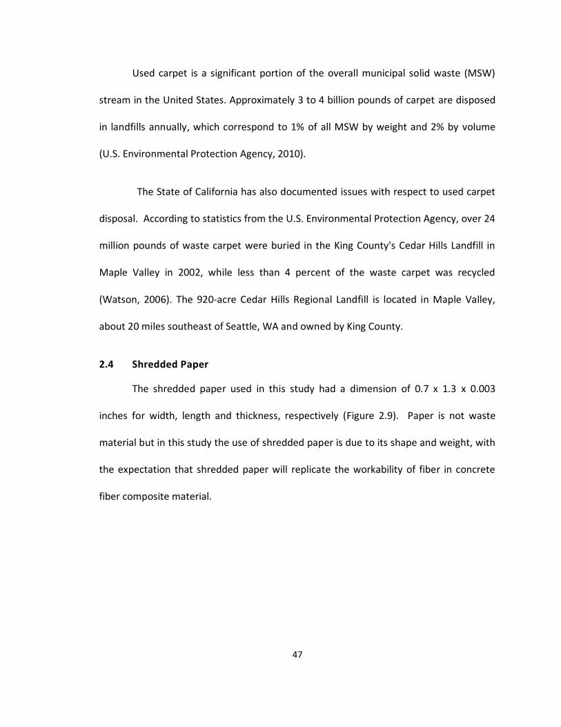
47
Used carpet is a significant portion of the overall municipal solid waste (MSW)
stream in the United States. Approximately 3 to 4 billion pounds of carpet are disposed
in landfills annually, which correspond to 1% of all MSW by weight and 2% by volume
(U.S. Environmental Protection Agency, 2010).
The State of California has also documented issues with respect to used carpet
disposal. According to statistics from the U.S. Environmental Protection Agency, over 24
million pounds of waste carpet were buried in the King County's Cedar Hills Landfill in
Maple Valley in 2002, while less than 4 percent of the waste carpet was recycled
(Watson, 2006). The 920-acre Cedar Hills Regional Landfill is located in Maple Valley,
about 20 miles southeast of Seattle, WA and owned by King County.
2.4 Shredded Paper
The shredded paper used in this study had a dimension of 0.7 x 1.3 x 0.003
inches for width, length and thickness, respectively (Figure 2.9). Paper is not waste
material but in this study the use of shredded paper is due to its shape and weight, with
the expectation that shredded paper will replicate the workability of fiber in concrete
fiber composite material.
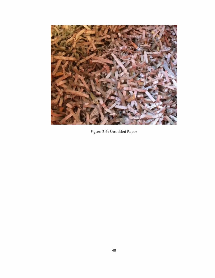
48
Figure 2.9: Shredded Paper
49
Chapter 3
3. DESCRIPTION OF LABORATORY TEST METHOD
3.1 Laboratory Testing of Mechanical Properties
3.1.1 Index Properties
The properties obtained from the experiments included index properties and
strength properties. All experiments were performed according to American Society of
Testing Materials (ASTM) standards. All samples were tested immediately after
preparation and therefore time effects were not considered in the entire study. Test
methods used include specific gravity, grain size distribution and modulus and damping
properties using the cyclic triaxial apparatus. Because Class F fly ash is non-plastic,
Atterberg limits were not determined.
First, specific gravity of soil solids, Gs, is the mass density of the mineral solids in
soil normalized relative to the mass density of water (Kalinski, 2011). Alternatively, it
can be viewed as the mass of a given volume of soil solids normalized relative to the
mass of an equivalent volume of water at a temperature of 20 degrees Celsius.
To prepare the samples, ASTM D854 (Standard Test Method for Specific Gravity
of Soils) was used. To get the appropriate result, the entire sample de-aired for at least
24 hours although according to ASTM D854, oven-dried specimens only need 2 to 4
hours of applied vacuum for adequate de-airing. Extra vacuumed time was used
because according to the ASTM standard the minimum vacuum source should be 12.8
psi. The vacuum source available in our laboratory was less than 12.8 psi so alonger
50
vacuum time was used, in this study a 24 hours vacuum time was used. The water used
is distilled water and the oven temperature is at 110 degree Celsius per the ASTM
standard.
In this study, there were four (4) different compositions (Class F fly ash, Class F
fly ash with shredded carpet, Class F fly ash with crumb rubber and Class F fly ash with
shredded paper) with a total of ten (10) samples tested. To prepare the specimen, fly
ash and waste materials were combined in a given ratio (Table 4.3) and mixed using a
mixer until they were completely blended together. The samples were then oven dried
at a temperature of 110 0C. The apparatus used for this test included a flask bottle,
squeeze bottle, plastic funnel, scale, spoon and tin container. The testing procedure to
determine the specific gravity was in accordance with the ASTM D854 standard.
Fly ash specimens for this research were Class F specimen from the combustion
of Appalachian coal in Kentucky specifically from Dayton Power Light (DPL) power plant
in Maysville, Ohio. From earlier investigations, test results had shown that this type of
fly ash has a specific gravity of around 2.20.
3.1.2 Grain Size Distribution
Grain size distribution testing (dry sieving) was performed in accordance with
ASTM standard D422. The sieves used were #4, #10, #20, #40, #60, #140, and #200.
Grain size refers to the size of an opening in a square mesh through which a grain will
51
pass. Because fly ash consists of fines particle typically smaller than 0.075 mm, the
hydrometer test was also performed to complete the gradation curve.
In this study, the liquefaction susceptibility of fly ash material was investigated
by using the available liquefaction criteria such as Chinese criteria, Tsuchida (1970),
Seed et al. (2003) and Bray & Sancio (2004), results were used to confirm whether fly
ash is susceptible to liquefaction according to mechanical properties and gradation
curve. The test results are presented in Chapter 5.
3.1.3 Shear Modulus and Damping Ratio (Strain-Controlled Cyclic Loading)
The dynamic and cyclic properties were tested (shear modulus and material
damping) using the cyclic triaxial apparatus per the ASTM D3999 standard. To find these
properties, fly ash specimens were tested using strain-controlled cyclic loading. The
relative importance of parameters affecting shear modulus and damping has been
documented by, Hardin & Drnevich (1972) and others.
For soil and rock, the outcome from this test is to quantify the response of
specimens to strong ground motion. The outcome properties of tested specimens from
this test are shear modulus (G), material damping (D), and shear strain (γ). Typically, as
strain increases, damping ratio increases while shear modulus decreases. The plots of
modulus reduction curves for Class F fly ash used in this study are shown in Chapter 4.
In this test, specimens of Class F fly ash were reconstituted. The basic properties
of specimen used for this test are shown in Chapter 4. Specimen preparation and input
52
data for this test is identical to the cyclic triaxial method (ASTM D5311) but the
amplitude of cyclic load much smaller than used in liquefaction assessment. By applying
small cyclic deviator stress which maintains axial strain from passing elastic limit but
enough to trigger measureable response from the specimen, the recording information
from this test transmitted through pore pressure transducer and deformation gauge
during shearing phase.
The test starts with 2 psi cyclic loading and proceeds by gradually increasing the
deviator stress until 5 psi cyclic load. The test stopped at 0.01% shear strain as stated in
the standard. The ASTM D3999 standard states the test result is valid if no disturbance
such as noise induced by the equipment occurs during testing. Figure 3.1 shows the
acceptable and non-acceptable deviator stress for this test according to the standard
and Figure 3.2 shown the typical deviator stress applied to the specimen during this test
and its acceptable range.
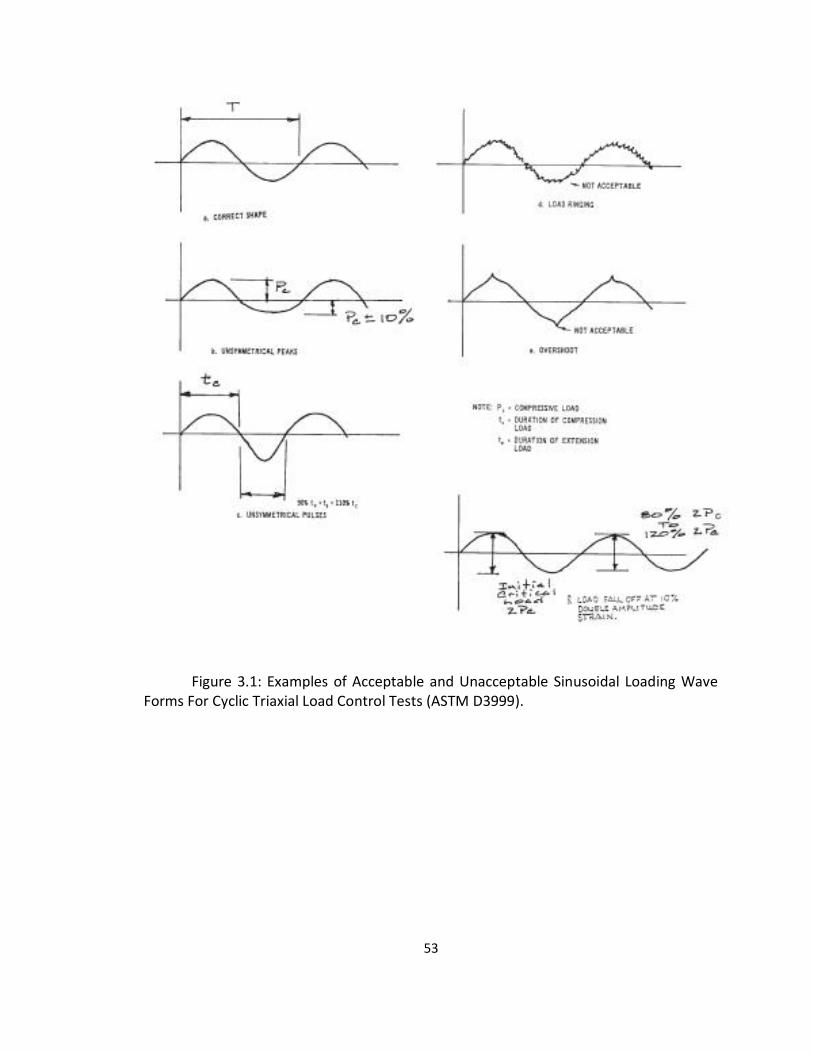
53
Figure 3.1: Examples of Acceptable and Unacceptable Sinusoidal Loading Wave Forms For Cyclic Triaxial Load Control Tests (ASTM D3999).
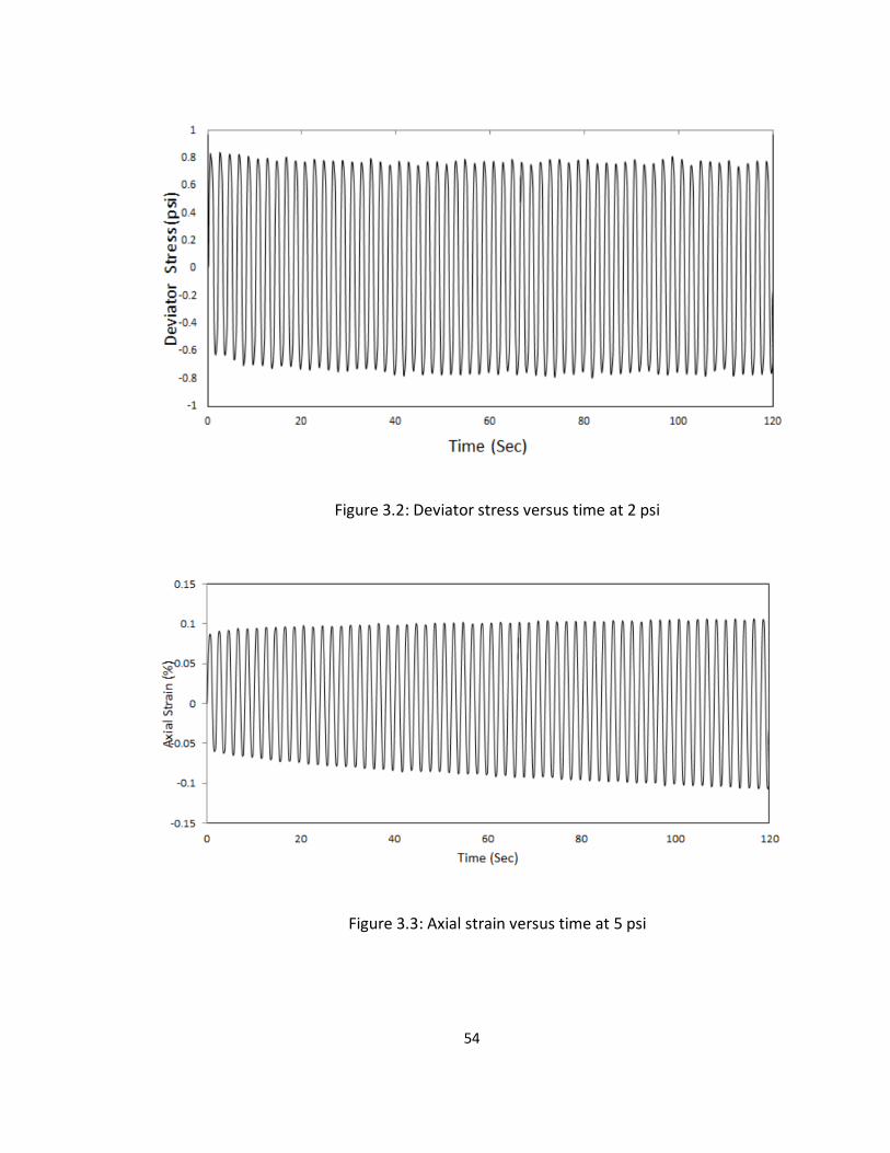
54
Figure 3.2: Deviator stress versus time at 2 psi
Figure 3.3: Axial strain versus time at 5 psi
55
Figure 3.3 shows the deformation of a specimen tested at 5 psi indicating that
the specimen experienced deformation in the elastic region or recoverable range, so no
permanent deformation occurred and it is acceptable according to the standard.
3.2 CHEMICAL PROPERTIES OF THE MATERIALS
Most of the coal used in Appalachian power plants is bituminous coal mined
from local deposits, although significant anthracite deposits exist. According to ASTM
C618, the SiO2 +AL2O3+FE2O3 content must be greater than 70% and the SO3 content
must be greater than 5% for the fly ash to be considered Class F (Table 3.1). Class F fly
ash is also characterized by a low CaO content (less than 20%) and is not considered
self-cementing like Class C fly ash.
Table 3.1: Chemical Requirements for Fly Ash Classification (ASTM C 618)
Properties Fly Ash Class
Class F Class C
Silicon dioxide (SiO2) plus aluminum oxide (Al2O3) plus iron 70.0 50.0
oxide (Fe2O3), min, %
Sulfur trioxide (SO3), max, % 5.0 5.0
Moisture Content, max, % 3.0 3.0
Loss on ignition, max, % 6.0 6.0
CaO Content, % < 20.0 > 20.0
Fly ash used on this research was Class F (Figure 3.4). Class F fly ash contains less
than 20% lime (CaO) while Class C fly ash generally contains more than 20% lime (CaO).
With that characteristic Class C fly ash hardens when exposed to water.
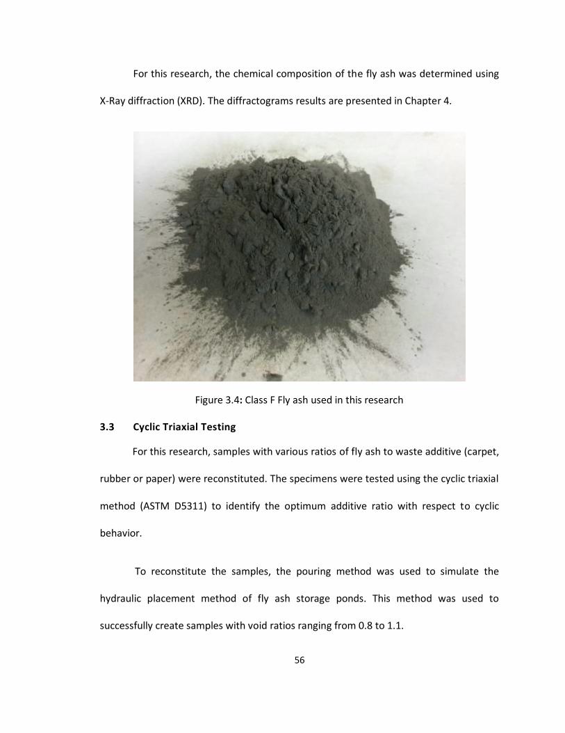
56
For this research, the chemical composition of the fly ash was determined using
X-Ray diffraction (XRD). The diffractograms results are presented in Chapter 4.
Figure 3.4: Class F Fly ash used in this research
3.3 Cyclic Triaxial Testing
For this research, samples with various ratios of fly ash to waste additive (carpet,
rubber or paper) were reconstituted. The specimens were tested using the cyclic triaxial
method (ASTM D5311) to identify the optimum additive ratio with respect to cyclic
behavior.
To reconstitute the samples, the pouring method was used to simulate the
hydraulic placement method of fly ash storage ponds. This method was used to
successfully create samples with void ratios ranging from 0.8 to 1.1.
57
Cyclic triaxial tests (ASTM D5311) were conducted under undrained conditions to
simulate undrained field conditions during earthquake or other cyclic loading on
impoundment facilities such as vibrations from machinery. Cyclic triaxial strength tests
are destructive. Failure may be defined on the basis of the number of stress cycles
required to reach a limiting strain or a pore pressure ratio of unity.
Cyclic strength depends upon many factors, including density, confining
pressure, applied cyclic shear stress, stress history, grain structure, age of soil deposit,
specimen preparation procedure, frequency, uniformity, and shape of the cyclic wave
form. Thus, close attention must be given to testing details and equipment.
Cyclic triaxial testing was performed using a SBEL triaxial testing system in the
University of Kentucky (UK) laboratory, which was modified in 2009 by GCTS Testing
Systems Company to perform cyclic triaxial testing. Cyclic triaxial testing was performed
on reconstituted specimens based on the ASTM Standard Test Method for Load
Controlled Cyclic Triaxial Strength of Soil (D 5311). Table 3.2 shows the specimen
preparation checklist based on the ASTM D5311 test standard. This list should be
satisfied to validate the result from the test.
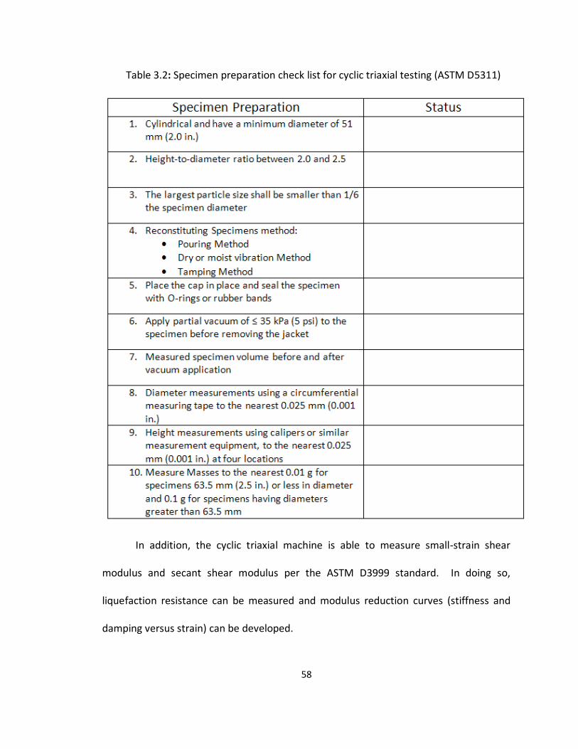
58
Table 3.2: Specimen preparation check list for cyclic triaxial testing (ASTM D5311)
In addition, the cyclic triaxial machine is able to measure small-strain shear
modulus and secant shear modulus per the ASTM D3999 standard. In doing so,
liquefaction resistance can be measured and modulus reduction curves (stiffness and
damping versus strain) can be developed.
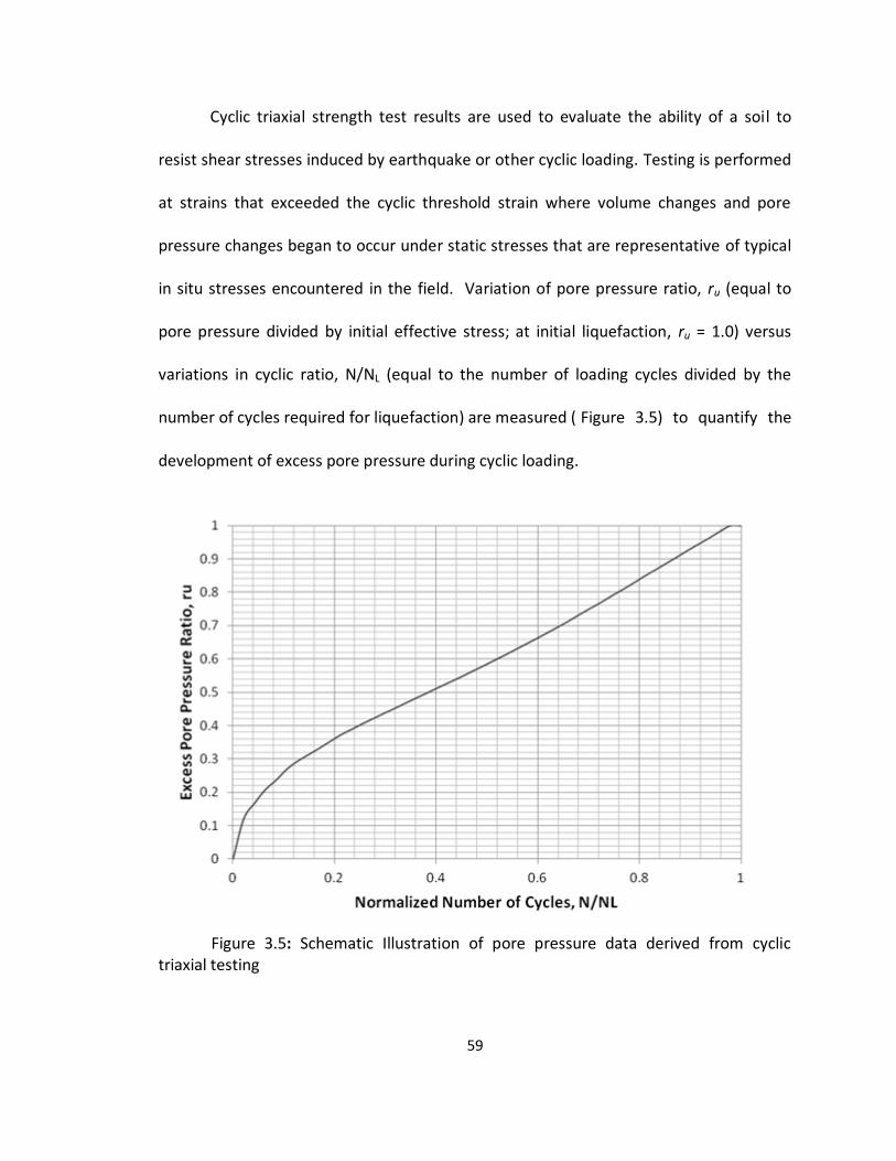
59
Cyclic triaxial strength test results are used to evaluate the ability of a soil to
resist shear stresses induced by earthquake or other cyclic loading. Testing is performed
at strains that exceeded the cyclic threshold strain where volume changes and pore
pressure changes began to occur under static stresses that are representative of typical
in situ stresses encountered in the field. Variation of pore pressure ratio, ru (equal to
pore pressure divided by initial effective stress; at initial liquefaction, ru = 1.0) versus
variations in cyclic ratio, N/NL (equal to the number of loading cycles divided by the
number of cycles required for liquefaction) are measured ( Figure 3.5) to quantify the
development of excess pore pressure during cyclic loading.
Figure 3.5: Schematic Illustration of pore pressure data derived from cyclic triaxial testing

60
Liquefaction is defined as the transformation of a granular material from a solid
to a liquefied state as a consequence of increased pore-water pressure and reduced
effective stress (Marcuson, 1978). Increased pore-water pressure is induced by the
tendency of granular materials to compact when subjected to cyclic shear deformations.
The change of state occurs most readily in loose to moderately dense granular soils with
poor drainage, such as silty sands or sands and gravels capped by or containing seams of
impermeable sediment.
In loose materials, the softening is also accompanied by a loss of shear strength
that may lead to large shear deformations or even flow failure under moderate to high
shear stresses, such as beneath a foundation or sloping ground. Loose soils also compact
during liquefaction and reconsolidation, leading to ground settlement.
Sand boils may also erupt as excess pore water pressures dissipates. Calculation,
or estimation, of two variables is required for evaluation of liquefaction resistance of
soils: (1) the seismic loading on a soil layer, expressed in terms of cyclic stress ratio
(CSR); and (2) the capacity of the soil to resist liquefaction, expressed in terms of cyclic
resistance ratio (CRR).
Liquefaction is identified as the point where the pore pressure ratio reaches
unity and a dramatic increase in the axial deformation occurs, as seen in Figure 3.6.
Note for the plots, compression corresponds to positive stresses and strains, while
extension corresponds to negative stresses and strains.
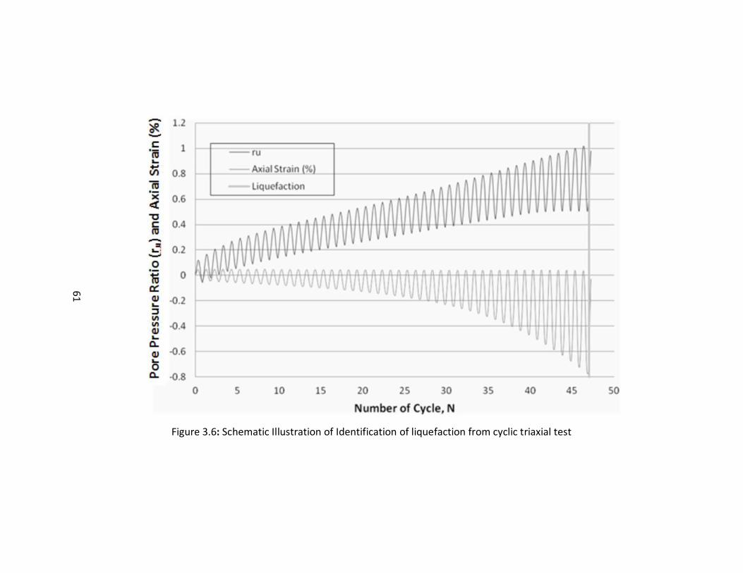
61
Figure 3.6: Schematic Illustration of Identification of liquefaction from cyclic triaxial test
61
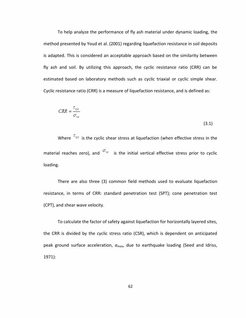
62
To help analyze the performance of fly ash material under dynamic loading, the
method presented by Youd et al. (2001) regarding liquefaction resistance in soil deposits
is adapted. This is considered an acceptable approach based on the similarity between
fly ash and soil. By utilizing this approach, the cyclic resistance ratio (CRR) can be
estimated based on laboratory methods such as cyclic triaxial or cyclic simple shear.
Cyclic resistance ratio (CRR) is a measure of liquefaction resistance, and is defined as:
(3.1)
Where is the cyclic shear stress at liquefaction (when effective stress in the
material reaches zero), and is the initial vertical effective stress prior to cyclic
loading.
There are also three (3) common field methods used to evaluate liquefaction
resistance, in terms of CRR: standard penetration test (SPT); cone penetration test
(CPT), and shear wave velocity.
To calculate the factor of safety against liquefaction for horizontally layered sites,
the CRR is divided by the cyclic stress ratio (CSR), which is dependent on anticipated
peak ground surface acceleration, amax, due to earthquake loading (Seed and Idriss,
1971):
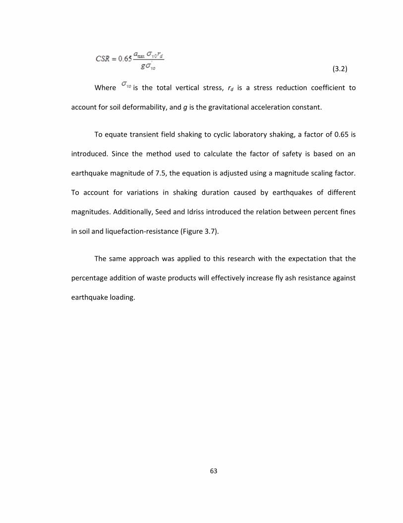
63
(3.2)
Where is the total vertical stress, rd is a stress reduction coefficient to
account for soil deformability, and g is the gravitational acceleration constant.
To equate transient field shaking to cyclic laboratory shaking, a factor of 0.65 is
introduced. Since the method used to calculate the factor of safety is based on an
earthquake magnitude of 7.5, the equation is adjusted using a magnitude scaling factor.
To account for variations in shaking duration caused by earthquakes of different
magnitudes. Additionally, Seed and Idriss introduced the relation between percent fines
in soil and liquefaction-resistance (Figure 3.7).
The same approach was applied to this research with the expectation that the
percentage addition of waste products will effectively increase fly ash resistance against
earthquake loading.

64
Figure 3.7: Correlation between equivalent uniform cyclic stress ratio and SPT
(N1)60 – Value for events of magnitude M ≈7.5 for varying fines contents, (Youd, et al,
2001).
Based on Youd, et al., (2001), correlation between equivalent uniform cyclic
stress ratio (CSR) and Standard Penetration Test (SPT) for Magnitude (M) = 7.5 for
varying fines contents, with adjustments at low cyclic stress ratio as recommended by
the National Center for Earthquake Engineering Research (NCEER) working group.

65
In this study, using CSR values of 0.15, 0.30 and 0.50 already cover low to high
CSR and using 0.50 CSR as a maximum limit for this research is appropriate because CSR
greater than 0.50 would normally result in the liquefaction of the specimens with very
low number of cycles and it will be very difficult to compare.
66
Chapter 4
4. TYPICAL RESULTS FROM LABORATORY TESTING
4.1 Introduction
In this chapter, selected representative results from this study are presented.
The results will be separated in two sections. In the beginning, the mechanical and
chemical properties of Class F fly ash and waste materials are summarized. Next, shows
the dynamic properties of Class F fly ash from cyclic shear strain and used to find the
relationship between the shear modulus and the damping ratio versus cyclic shear
strain.
4.2 Static Tests
This section shows the results of specific gravity, grain size distribution, and XRD-
testing. First, specific gravity is presented. These properties are important because they
are used as input data to run cyclic triaxial testing.
The waste materials used in this study have lower specific gravity than Class F fly
ash and when used as additives decreased specific gravity of the fly ash sample. The
average of specific gravity results were used as an input data for cyclic triaxial testing
with the assumption that specimen combination tested govern and also used to
determine the confining pressure during testing.
67
There are ten (10) samples in this study, three (3) for specimens of Class F fly
ash, two (2) for 10% rubber, three (3) for 5% carpet fiber and two (2) for 10% paper. As
shown in Table 4.1, the results for specific gravity testing range from 2.02 to 2.19. The
result shows agreement that fly ash particles are cenosphere or hollow particles made
largely of silica and alumina. The prior characteristics (i.e. hollow, spherical particles and
uniform gradation) in turn explain the lower compacted densities of fly ash relative to
conventional earth fill compacted to the same effort.
Next static tests, including grain size distribution, were run to get the results of
representative samples prepared and tested using mechanical sieve and hydrometer.
Figure 4.1 shows the combined results of Class F fly ash from mechanical sieve and
hydrometer. The gradation curve will be used to determine liquefiable potential of Class
F fly ash using Tsuchida (1971), “Chinese Criteria”, Seed et al. (2003), and Bray & Sancio
(2004). The discussion will be explained in Chapter 5.
.
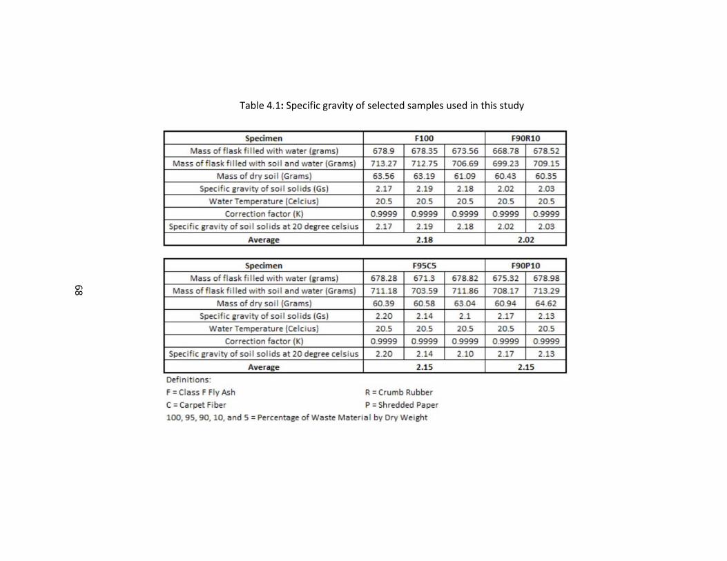
68
Table 4.1: Specific gravity of selected samples used in this study
68
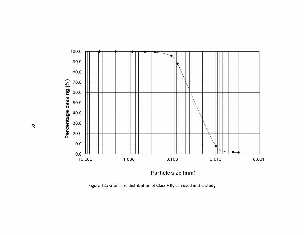
69
Figure 4.1: Grain size distribution of Class F fly ash used in this study
69
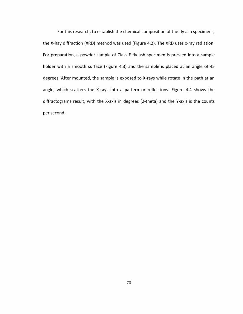
70
For this research, to establish the chemical composition of the fly ash specimens,
the X-Ray diffraction (XRD) method was used (Figure 4.2). The XRD uses x-ray radiation.
For preparation, a powder sample of Class F fly ash specimen is pressed into a sample
holder with a smooth surface (Figure 4.3) and the sample is placed at an angle of 45
degrees. After mounted, the sample is exposed to X-rays while rotate in the path at an
angle, which scatters the X-rays into a pattern or reflections. Figure 4.4 shows the
diffractograms result, with the X-axis in degrees (2-theta) and the Y-axis is the counts
per second.
71
Figure 4.2: The X-Ray diffraction (XRD) machine used in this study
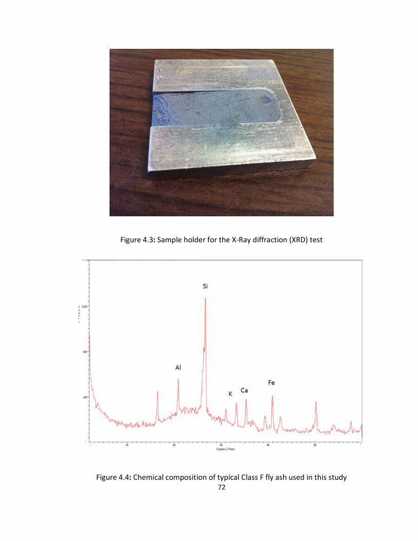
72
Figure 4.3: Sample holder for the X-Ray diffraction (XRD) test
Figure 4.4: Chemical composition of typical Class F fly ash used in this study
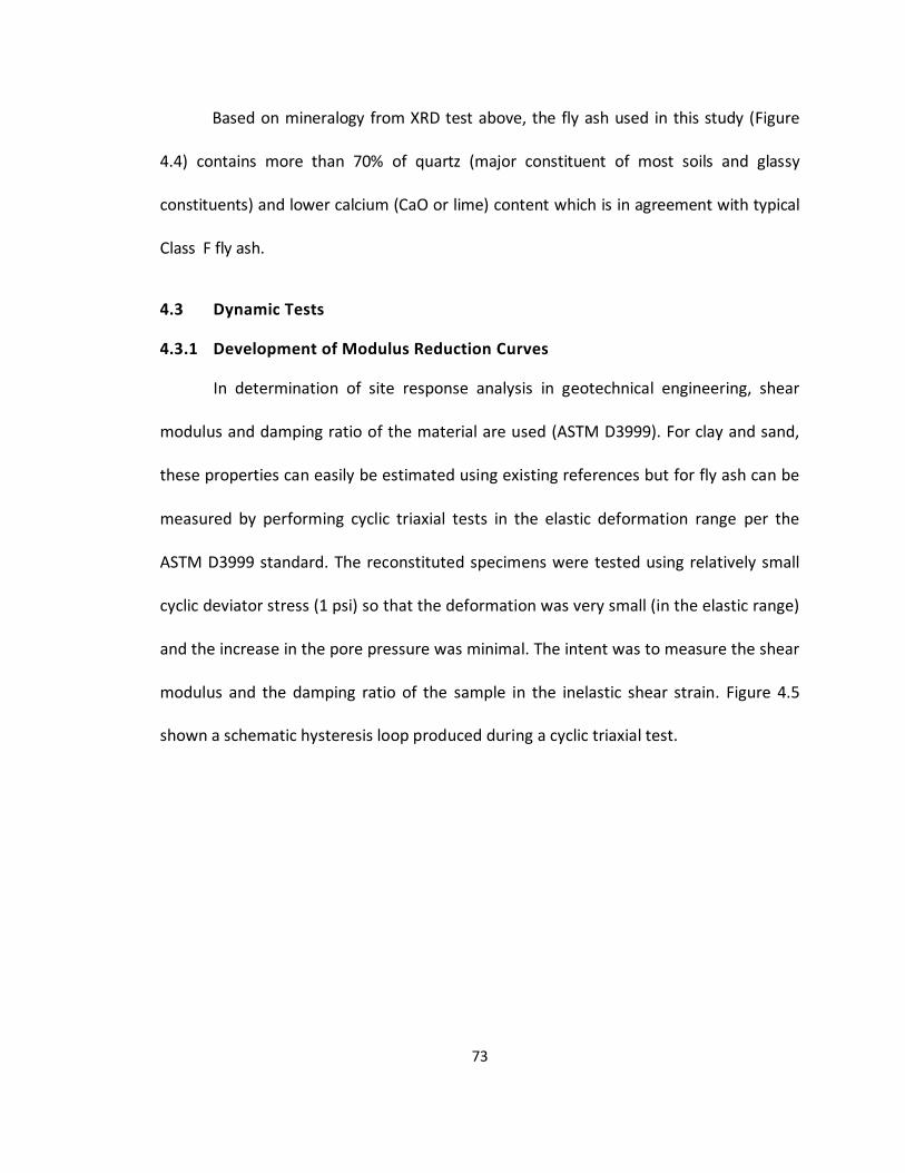
73
Based on mineralogy from XRD test above, the fly ash used in this study (Figure
4.4) contains more than 70% of quartz (major constituent of most soils and glassy
constituents) and lower calcium (CaO or lime) content which is in agreement with typical
Class F fly ash.
4.3 Dynamic Tests
4.3.1 Development of Modulus Reduction Curves
In determination of site response analysis in geotechnical engineering, shear
modulus and damping ratio of the material are used (ASTM D3999). For clay and sand,
these properties can easily be estimated using existing references but for fly ash can be
measured by performing cyclic triaxial tests in the elastic deformation range per the
ASTM D3999 standard. The reconstituted specimens were tested using relatively small
cyclic deviator stress (1 psi) so that the deformation was very small (in the elastic range)
and the increase in the pore pressure was minimal. The intent was to measure the shear
modulus and the damping ratio of the sample in the inelastic shear strain. Figure 4.5
shown a schematic hysteresis loop produced during a cyclic triaxial test.
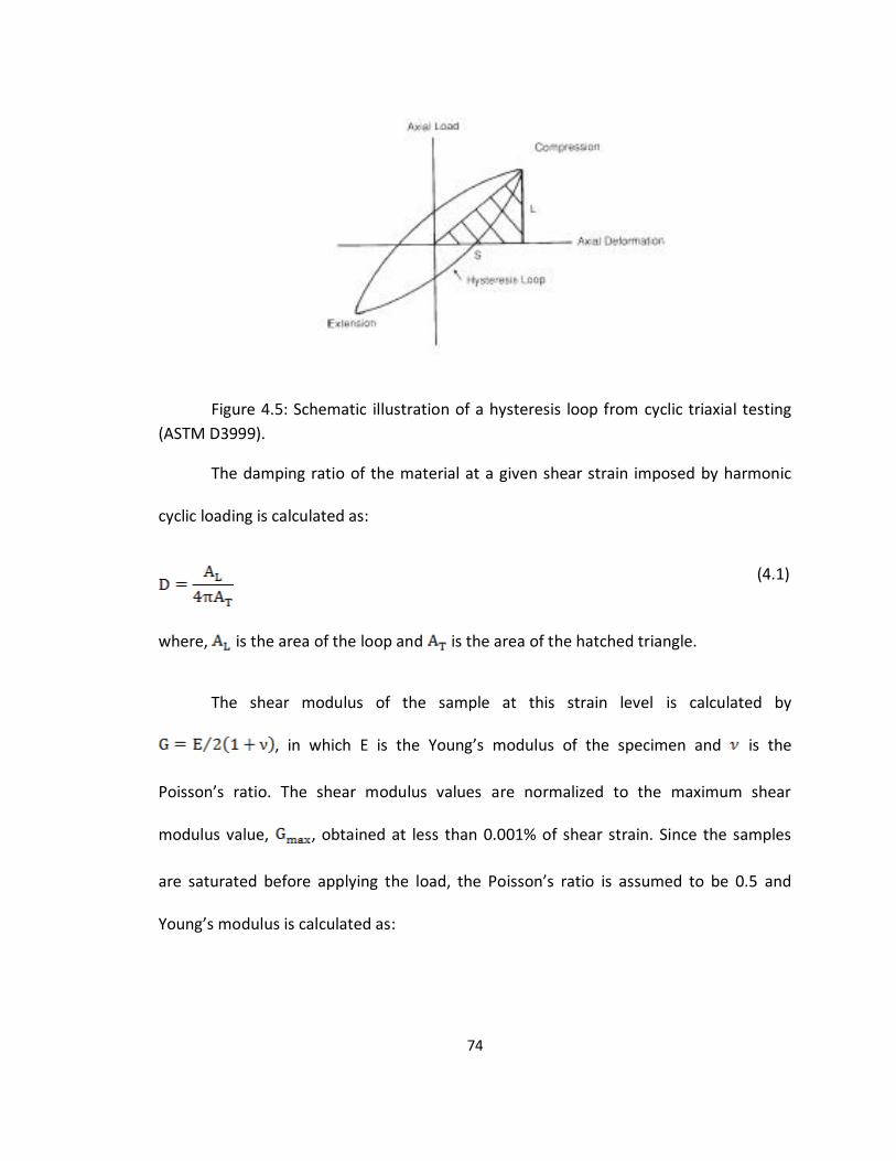
74
Figure 4.5: Schematic illustration of a hysteresis loop from cyclic triaxial testing
(ASTM D3999).
The damping ratio of the material at a given shear strain imposed by harmonic
cyclic loading is calculated as:
(4.1)
where, is the area of the loop and is the area of the hatched triangle.
The shear modulus of the sample at this strain level is calculated by
, in which E is the Young’s modulus of the specimen and is the
Poisson’s ratio. The shear modulus values are normalized to the maximum shear
modulus value, , obtained at less than 0.001% of shear strain. Since the samples
are saturated before applying the load, the Poisson’s ratio is assumed to be 0.5 and
Young’s modulus is calculated as:
75
where is the double amplitude load, is the double amplitude deformation, is
the height of the specimen after consolidation and is the area of the specimen after
consolidation.
The imposed shear strain in this loop is calculated by using:
(4.3)
where , single amplitude axial strain, is found by using , where
is the double amplitude axial strain and is calculated by . Additional
validation is performed by checking if the specimen experienced shear strains that
exceeded the recommended value of 0.01% per the ASTM D3999 standard.
It should be noted that the results for shear modulus and damping ratio versus
cyclic strain ratio of Class F fly ash used in this study are best fit lines as shown in Figure
4.6 and Figure 4.7. However, it is emphasized that the number of tests in this study were
limited and the measurement of small strains were not highly accurate. Table 4.2 shows
the properties of Class F fly ash specimens used to generate the modulus reduction
curves developed in this study.
(4.2)
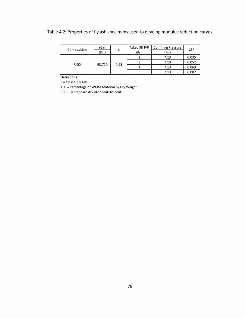
76
Table 4.2: Properties of fly ash specimens used to develop modulus reduction curves
γSat Asked SD P-P Confining Pressure
(Pcf) (Psi) (Psi)
2 7.13 0.035
3 7.13 0.052
4 7.13 0.069
5 7.13 0.087
Definitions:
F = Class F Fly Ash
100 = Percentage of Waste Material by Dry Weight
SD P-P = Standard deviator peak-to-peak
Composition e CSR
F100 93.710 0.95
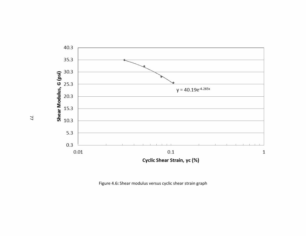
77
Figure 4.6: Shear modulus versus cyclic shear strain graph
77
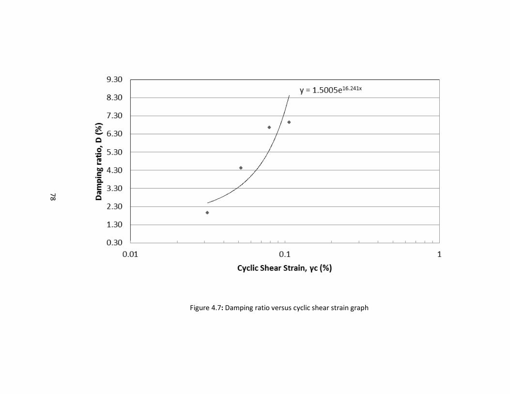
78
Figure 4.7: Damping ratio versus cyclic shear strain graph
78
79
4.3.2 Cyclic Triaxial Testing (ASTM D5311)
This test is commonly used to measure the variation of pore pressure and strain
potential of saturated soils. For this test, there are 11 different combinations with the
compositions of waste materials range from 1.5 – 20.0% as shown in Table 4.3.
To refer to each individual sample based on percentage of dry weight of waste
material, a code system was used using alphabetical characters and number. For
example, a specimen with a combination of Class F fly ash and crumb rubber with a
composition of 90% fly ash and 10% crumb rubber was named F90R10 (F = Class F fly
ash, R = Crumb rubber and 90 and 10 is the amount of dry weight used). The same code
also applied to carpet fiber and shredded paper using code of C and P, respectively.
The specimen compositions reported in this research are based on dry weight.
The maximum amount of 20% ratio was used as a maximum value to maintain fly ash as
the primary material. The decision was based on specimen dimensions, especially for
carpet and paper, where a ratio higher than 20% tended to occupy more space and
make the primary material (fly ash) behave more like a filler. Figure 4.8 shows how 20%
shredded paper combination makes fly ash behave as filler to the paper.
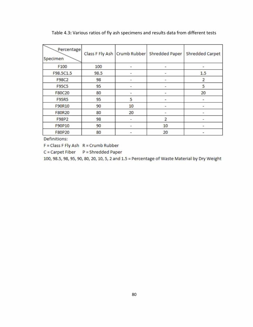
80
Table 4.3: Various ratios of fly ash specimens and results data from different tests
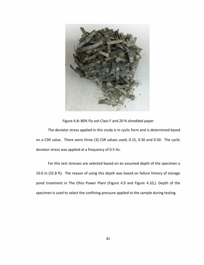
81
Figure 4.8: 80% Fly ash Class F and 20 % shredded paper
The deviator stress applied in this study is in cyclic form and is determined based
on a CSR value. There were three (3) CSR values used; 0.15, 0.30 and 0.50. The cyclic
deviator stress was applied at a frequency of 0.5 Hz.
For this test stresses are selected based on an assumed depth of the specimen a
10.0 m (32.8 ft). The reason of using this depth was based on failure history of storage
pond treatment in The Ohio Power Plant (Figure 4.9 and Figure 4.10,). Depth of the
specimen is used to select the confining pressure applied to the sample during testing.
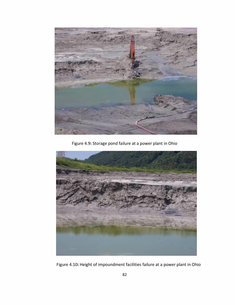
82
Figure 4.9: Storage pond failure at a power plant in Ohio
Figure 4.10: Height of impoundment facilities failure at a power plant in Ohio
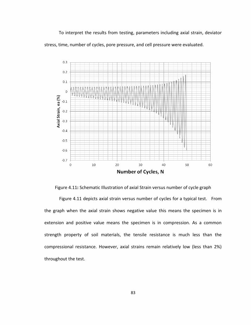
83
To interpret the results from testing, parameters including axial strain, deviator
stress, time, number of cycles, pore pressure, and cell pressure were evaluated.
Figure 4.11: Schematic Illustration of axial Strain versus number of cycle graph
Figure 4.11 depicts axial strain versus number of cycles for a typical test. From
the graph when the axial strain shows negative value this means the specimen is in
extension and positive value means the specimen is in compression. As a common
strength property of soil materials, the tensile resistance is much less than the
compressional resistance. However, axial strains remain relatively low (less than 2%)
throughout the test.
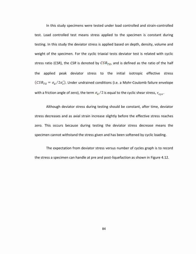
84
In this study specimens were tested under load controlled and strain-controlled
test. Load controlled test means stress applied to the specimen is constant during
testing. In this study the deviator stress is applied based on depth, density, volume and
weight of the specimen. For the cyclic triaxial tests deviator test is related with cyclic
stress ratio (CSR), the CSR is denoted by , and is defined as the ratio of the half
the applied peak deviator stress to the initial isotropic effective stress
. Under undrained conditions (i.e. a Mohr-Coulomb failure envelope
with a friction angle of zero), the term is equal to the cyclic shear stress, .
Although deviator stress during testing should be constant, after time, deviator
stress decreases and as axial strain increase slightly before the effective stress reaches
zero. This occurs because during testing the deviator stress decrease means the
specimen cannot withstand the stress given and has been softened by cyclic loading.
The expectation from deviator stress versus number of cycles graph is to record
the stress a specimen can handle at pre and post-liquefaction as shown in Figure 4.12.
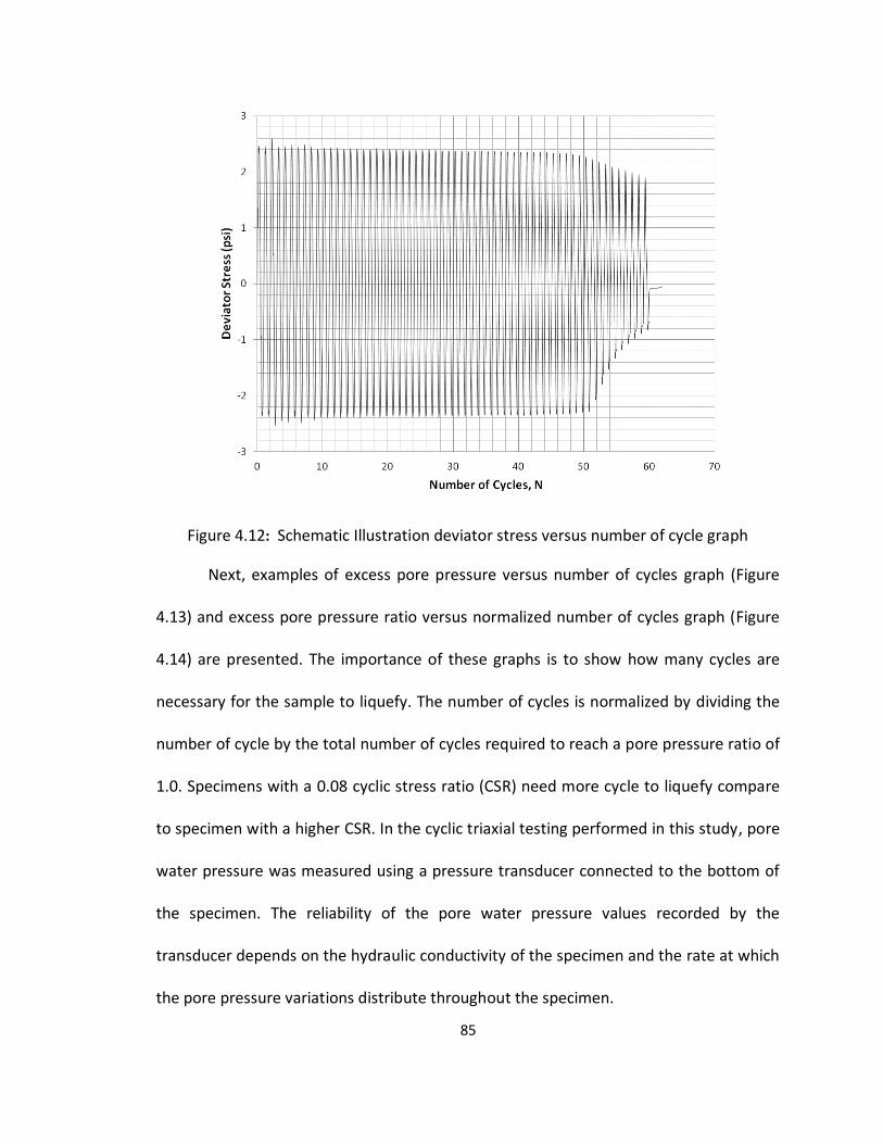
85
Figure 4.12: Schematic Illustration deviator stress versus number of cycle graph
Next, examples of excess pore pressure versus number of cycles graph (Figure
4.13) and excess pore pressure ratio versus normalized number of cycles graph (Figure
4.14) are presented. The importance of these graphs is to show how many cycles are
necessary for the sample to liquefy. The number of cycles is normalized by dividing the
number of cycle by the total number of cycles required to reach a pore pressure ratio of
1.0. Specimens with a 0.08 cyclic stress ratio (CSR) need more cycle to liquefy compare
to specimen with a higher CSR. In the cyclic triaxial testing performed in this study, pore
water pressure was measured using a pressure transducer connected to the bottom of
the specimen. The reliability of the pore water pressure values recorded by the
transducer depends on the hydraulic conductivity of the specimen and the rate at which
the pore pressure variations distribute throughout the specimen.
86
Figure 4.13: Schematic Illustration of excess pore pressure versus number of
cycles graph
Figure 4.14: Schematic Illustration of excess pore pressure ratio versus normalized number of cycles graph
87
The graph of excess pore pressure versus number of cycles is also used to
investigate how waste material will affect the number of cycles. Comparison tables and
graphs are presented in Chapter 5.
Finally, peak-to-peak deviator stress versus axial strain is evaluated (Figure 4.15).
The hysteresis loops shown in the beginning specimen still have higher stiffness and the
loops are relatively steep. As the test progresses, the loops flatten as the specimen
softens. The hysteresis loops also shows the change in length during testing. Initially,
the samples shorten and lengthen at equal amounts. However, this condition only
stands while the specimens have higher stiffness before excess pore pressure
developed. Afterward, shortening exceeds extension. The loop also becomes broader as
the specimen experience higher strain levels.
Before the test end, the loops begin to exhibit a banana-like shape which is
indicative of strain hardening. At this stage, the sample begins to dilate. This
strengthening effect enhances the ability of fly ash to hold higher stresses at the post-
liquefaction condition.
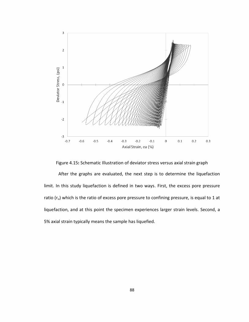
88
Figure 4.15: Schematic Illustration of deviator stress versus axial strain graph
After the graphs are evaluated, the next step is to determine the liquefaction
limit. In this study liquefaction is defined in two ways. First, the excess pore pressure
ratio (ru) which is the ratio of excess pore pressure to confining pressure, is equal to 1 at
liquefaction, and at this point the specimen experiences larger strain levels. Second, a
5% axial strain typically means the sample has liquefied.
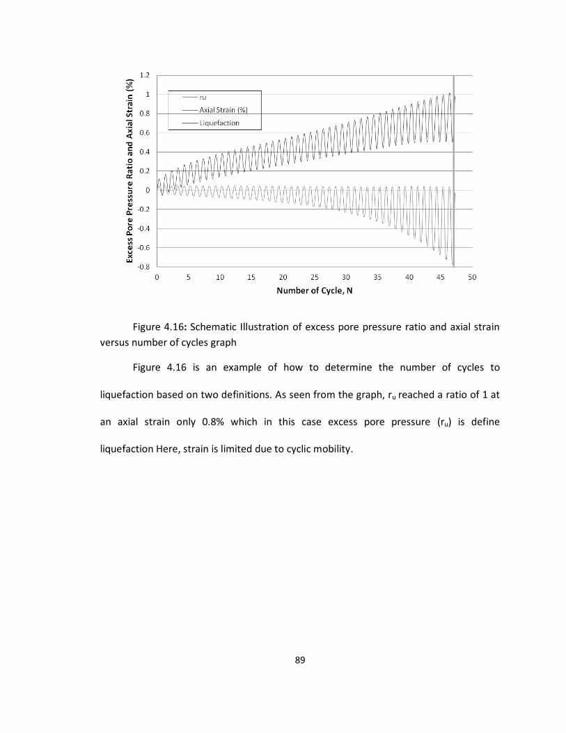
89
Figure 4.16: Schematic Illustration of excess pore pressure ratio and axial strain
versus number of cycles graph
Figure 4.16 is an example of how to determine the number of cycles to
liquefaction based on two definitions. As seen from the graph, ru reached a ratio of 1 at
an axial strain only 0.8% which in this case excess pore pressure (ru) is define
liquefaction Here, strain is limited due to cyclic mobility.
90
Chapter 5
5. INTERPRETATION OF TEST RESULTS
5.1 Overview
In this chapter, the analysis of mechanical properties and cyclic triaxial test
results performed on fly ash and waste materials is addressed. The correlation between
measured parameters with results from other research is explained. Samples were
reconstituted following the ASTM D5311 procedure using the pouring method. The
reconstituted specimens were created to represent specimens created using the field
method of wet dumping. The fly ash samples are usually normally consolidated due to
the dumping method. They have been constantly loaded and the overburdened stress
has never been removed. In the lab, the samples were tested in the cyclic triaxial
chamber as normally consolidated samples.
5.2 Specific Gravity
As shown in Table 5.1, specific gravity ranged from 2.02 to 2.19. One explanation
for this lower average specific gravity is the fact that a high proportion of fly ash
particles are cenospheres (hollow particles) made largely of silica and alumina which,
partially explains the lower compacted densities of fly ash relative to conventional earth
fill compacted to the same effort.
For cyclic triaxial input data, the value of specific gravity used was based on the
average of the specific composition. The assumption used for specific gravity was the
combination of fly ash with one additional material that used the same value although
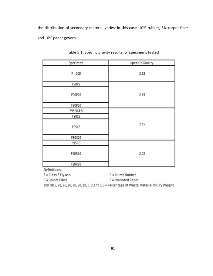
91
the distribution of secondary material varies; in this case, 10% rubber, 5% carpet fiber
and 10% paper govern.
Table 5.1: Specific gravity results for specimens tested
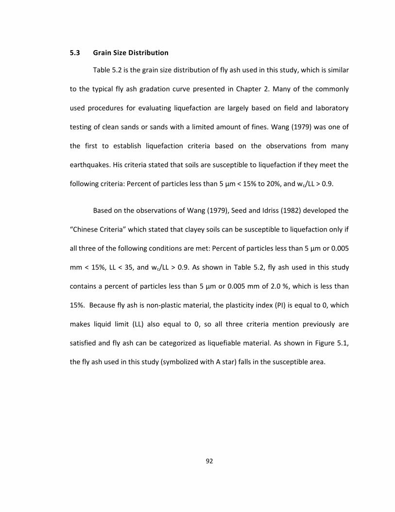
92
5.3 Grain Size Distribution
Table 5.2 is the grain size distribution of fly ash used in this study, which is similar
to the typical fly ash gradation curve presented in Chapter 2. Many of the commonly
used procedures for evaluating liquefaction are largely based on field and laboratory
testing of clean sands or sands with a limited amount of fines. Wang (1979) was one of
the first to establish liquefaction criteria based on the observations from many
earthquakes. His criteria stated that soils are susceptible to liquefaction if they meet the
following criteria: Percent of particles less than 5 μm < 15% to 20%, and wc/LL > 0.9.
Based on the observations of Wang (1979), Seed and Idriss (1982) developed the
“Chinese Criteria” which stated that clayey soils can be susceptible to liquefaction only if
all three of the following conditions are met: Percent of particles less than 5 μm or 0.005
mm < 15%, LL < 35, and wc/LL > 0.9. As shown in Table 5.2, fly ash used in this study
contains a percent of particles less than 5 μm or 0.005 mm of 2.0 %, which is less than
15%. Because fly ash is non-plastic material, the plasticity index (PI) is equal to 0, which
makes liquid limit (LL) also equal to 0, so all three criteria mention previously are
satisfied and fly ash can be categorized as liquefiable material. As shown in Figure 5.1,
the fly ash used in this study (symbolized with A star) falls in the susceptible area.
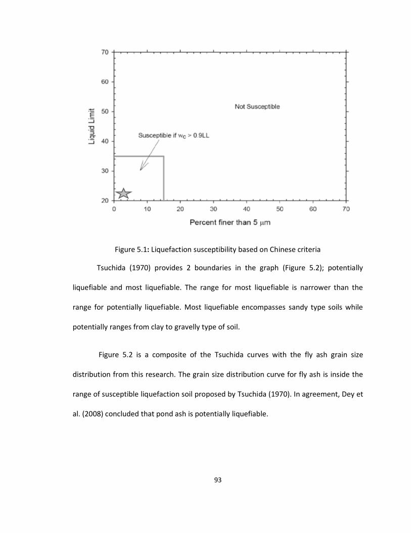
93
Figure 5.1: Liquefaction susceptibility based on Chinese criteria
Tsuchida (1970) provides 2 boundaries in the graph (Figure 5.2); potentially
liquefiable and most liquefiable. The range for most liquefiable is narrower than the
range for potentially liquefiable. Most liquefiable encompasses sandy type soils while
potentially ranges from clay to gravelly type of soil.
Figure 5.2 is a composite of the Tsuchida curves with the fly ash grain size
distribution from this research. The grain size distribution curve for fly ash is inside the
range of susceptible liquefaction soil proposed by Tsuchida (1970). In agreement, Dey et
al. (2008) concluded that pond ash is potentially liquefiable.
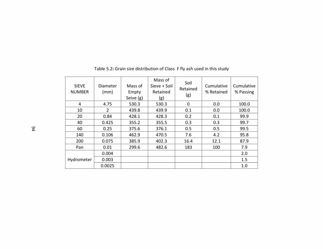
94
Table 5.2: Grain size distribution of Class F fly ash used in this study
SIEVE NUMBER
Diameter (mm)
Mass of Empty
Seive (g)
Mass of Sieve + Soil Retained
(g)
Soil Retained
(g)
Cumulative % Retained
Cumulative % Passing
4 4.75 530.3 530.3 0 0.0 100.0
10 2 439.8 439.9 0.1 0.0 100.0
20 0.84 428.1 428.3 0.2 0.1 99.9
40 0.425 355.2 355.5 0.3 0.3 99.7
60 0.25 375.6 376.1 0.5 0.5 99.5
140 0.106 462.9 470.5 7.6 4.2 95.8
200 0.075 385.9 402.3 16.4 12.1 87.9
Pan 0.01 299.6 482.6 183 100 7.9
Hydrometer
0.004 2.0
0.003 1.5
0.0025 1.0
94
95
Figure 5.2: Tsuchida (1970) Vs. Grain size distribution of Class F fly ash used in this study
95
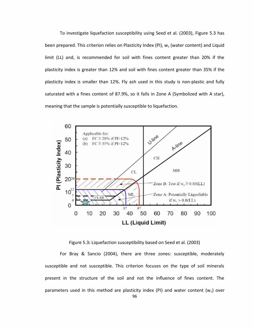
96
To investigate liquefaction susceptibility using Seed et al. (2003), Figure 5.3 has
been prepared. This criterion relies on Plasticity Index (PI), wc (water content) and Liquid
limit (LL) and, is recommended for soil with fines content greater than 20% if the
plasticity index is greater than 12% and soil with fines content greater than 35% if the
plasticity index is smaller than 12%. Fly ash used in this study is non-plastic and fully
saturated with a fines content of 87.9%, so it falls in Zone A (Symbolized with A star),
meaning that the sample is potentially susceptible to liquefaction.
Figure 5.3: Liquefaction susceptibility based on Seed et al. (2003)
For Bray & Sancio (2004), there are three zones: susceptible, moderately
susceptible and not susceptible. This criterion focuses on the type of soil minerals
present in the structure of the soil and not the influence of fines content. The
parameters used in this method are plasticity index (PI) and water content (wc) over
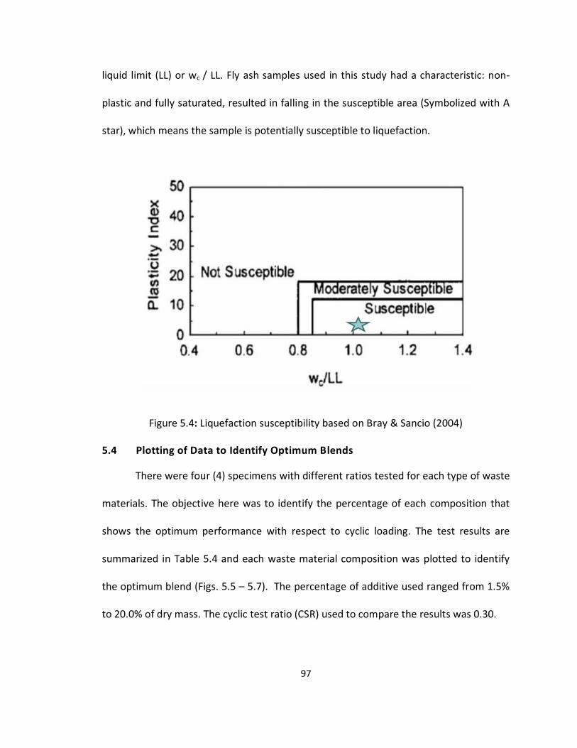
97
liquid limit (LL) or wc / LL. Fly ash samples used in this study had a characteristic: non-
plastic and fully saturated, resulted in falling in the susceptible area (Symbolized with A
star), which means the sample is potentially susceptible to liquefaction.
Figure 5.4: Liquefaction susceptibility based on Bray & Sancio (2004)
5.4 Plotting of Data to Identify Optimum Blends
There were four (4) specimens with different ratios tested for each type of waste
materials. The objective here was to identify the percentage of each composition that
shows the optimum performance with respect to cyclic loading. The test results are
summarized in Table 5.4 and each waste material composition was plotted to identify
the optimum blend (Figs. 5.5 – 5.7). The percentage of additive used ranged from 1.5%
to 20.0% of dry mass. The cyclic test ratio (CSR) used to compare the results was 0.30.
98
For carpet fiber, a ratio above 5% of dry weight generates a specimen whose
behavior is dominated by the additional material (carpet fiber) instead of the fly ash.
The reason is the weight of carpet fiber. The mold used in this study has maximum
diameter of 2.8 in and according to the ASTM D5311, a height-to-diameter ratio for the
sample tested is 2.0 – 2.5 is desired. For this study the target ratio was 2.0 which made
the height and diameter of all specimens tested relatively the same. Specimens of fly
ash and carpet fiber had the lowest weight compared to others at the same percentage
of dry weight as shown in Table 5.3. Because the fly ash and carpet fiber specimens had
the lowest weight means shredded carpet used more space inside the mold.
Nevertheless, 20% carpet fiber test was conducted to maintain fairness in comparison at
the same maximum percentage for all waste materials. Due to the difficulties during
mixing and to maintain fly ash as primary material, no specimens were tested above 20
percent content.
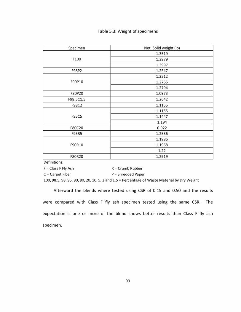
99
Table 5.3: Weight of specimens
Specimen Net. Solid weight (lb)
1.3519
1.3879
1.3997
F98P2 1.2547
1.2312
1.2765
1.2794
F80P20 1.0973
F98.5C1.5 1.2642
F98C2 1.1155
1.1155
1.1447
1.194
F80C20 0.922
F95R5 1.2536
1.1986
1.1968
1.22
F80R20 1.2919
Definitions:
F = Class F Fly Ash R = Crumb Rubber
C = Carpet Fiber P = Shredded Paper
100, 98.5, 98, 95, 90, 80, 20, 10, 5, 2 and 1.5 = Percentage of Waste Material by Dry Weight
F100
F90P10
F95C5
F90R10
Afterward the blends where tested using CSR of 0.15 and 0.50 and the results
were compared with Class F fly ash specimen tested using the same CSR. The
expectation is one or more of the blend shows better results than Class F fly ash
specimen.

100
Table 5.4: Specimen test results to find optimum combination
Void Ratio
e
F100C0 0.30 0.96 26
F98.5C1.5 0.28 1.19 5
F95C5 0.30 1.37 8
F80C20 0.28 1.5 7
F100C0 0.30 0.96 26
F95R5 0.30 0.98 4
F90R10 0.30 1.09 11
F80R20 0.30 0.89 7
F100C0 0.30 0.96 26
F98P2 0.30 1.04 4
F90P10 0.30 1.06 7
F80P20 0.30 1.26 7
Definitions:
F = Class F Fly Ash R = Crumb Rubber
C = Carpet Fiber P = Shredded Paper
100, 98.5, 98, 95, 90, 80, 20, 10, 5, 2 and 1.5 = Percentage of Waste Material by Dry Weight
Class F Fly Ash & Shredded paper
Specimen Compositon CSR N cycles
Class F Fly Ash & Shredded carpet
Class F Fly Ash & Crumb Rubber
Figure 5.5: Number of cycles to liquefy versus percentage graph by dry weight
(Fly ash Class F and Shredded carpet) at CSR = 0.30
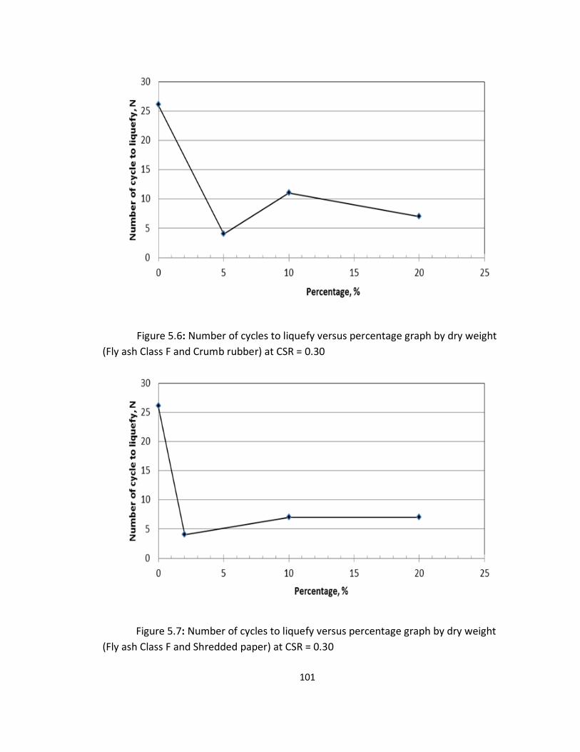
101
Figure 5.6: Number of cycles to liquefy versus percentage graph by dry weight
(Fly ash Class F and Crumb rubber) at CSR = 0.30
Figure 5.7: Number of cycles to liquefy versus percentage graph by dry weight
(Fly ash Class F and Shredded paper) at CSR = 0.30
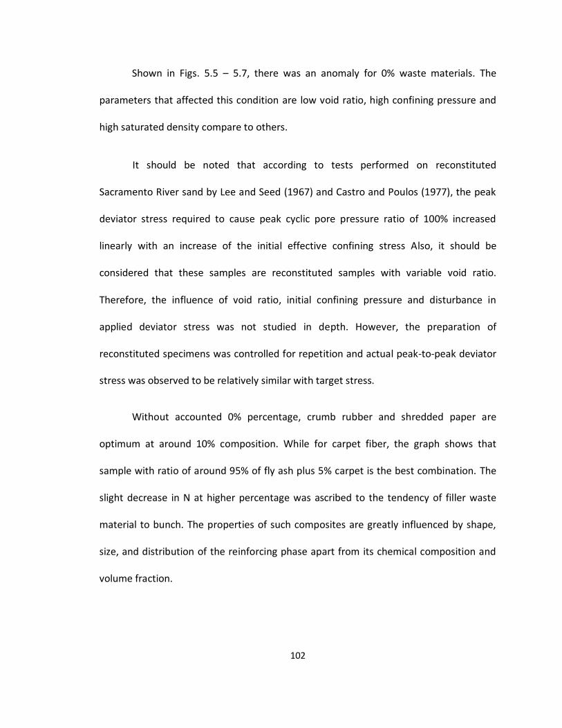
102
Shown in Figs. 5.5 – 5.7, there was an anomaly for 0% waste materials. The
parameters that affected this condition are low void ratio, high confining pressure and
high saturated density compare to others.
It should be noted that according to tests performed on reconstituted
Sacramento River sand by Lee and Seed (1967) and Castro and Poulos (1977), the peak
deviator stress required to cause peak cyclic pore pressure ratio of 100% increased
linearly with an increase of the initial effective confining stress Also, it should be
considered that these samples are reconstituted samples with variable void ratio.
Therefore, the influence of void ratio, initial confining pressure and disturbance in
applied deviator stress was not studied in depth. However, the preparation of
reconstituted specimens was controlled for repetition and actual peak-to-peak deviator
stress was observed to be relatively similar with target stress.
Without accounted 0% percentage, crumb rubber and shredded paper are
optimum at around 10% composition. While for carpet fiber, the graph shows that
sample with ratio of around 95% of fly ash plus 5% carpet is the best combination. The
slight decrease in N at higher percentage was ascribed to the tendency of filler waste
material to bunch. The properties of such composites are greatly influenced by shape,
size, and distribution of the reinforcing phase apart from its chemical composition and
volume fraction.
103
Therefore, percentage of around 10% may be taken as the optimum for
shredded paper and crumb rubber. While for carpet fiber, a 5% composition was
optimum.
Table 5.5 shows the summarized results of specimen comparison at optimum
blend by dry weight. As shown, void ratio are varies from 0.96 to 1.46; in comparison,
field in-situ void ratio for 12 meter ash deposit is 0.54-1.10 (Gandhi et al., 1997). Void
ratio is a key indicator of the tendency of a soil to undergo volume change during
drained shear and this volume change can be either contractive or dilative. As confining
pressure increased, however, the behavior of the fly ash specimen started to exhibit
contractive characteristics.
This study is load-controlled, so deviator stress during testing should be
constant. Input data for deviator stresses were calculated from CSR values of 0.15, 0.30
and 0.50, but the machine might not be able to apply the input stresses as instructed.
Based on the standard deviator or stresses executed by the machine, back calculation is
needed to find the actual CSR values. Actual CSR can be calculated by adding maximum
value of deviator stress and absolute value of minimum deviator stress for each tested
specimen divided by 4.
Summarized results from Table 5.5 were also plotted in Figure 5.8. To illustrate
the observed trend, linear trend lines were fitted to each dataset to extend the curves.
104
It shows at CSR higher than 0.4, the number of cycle for mixed specimens is 4. It means
at this CSR number of cycle to liquefy and the strength properties do not increase.
Next, at a CSR around 0.30 the effect of waste materials has still not improved
the fly ash properties. Finally, an effect of waste material is found at around 0.15 CSR
with a combination of 90% fly ash with 10% rubber where the number of cycles to
liquefy is higher than 100% Class F fly ash.
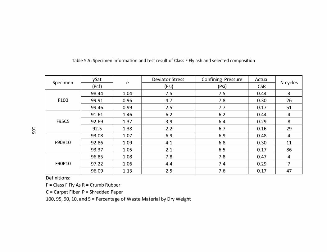
105
Table 5.5: Specimen information and test result of Class F Fly ash and selected composition
γSat Deviator Stress Confining Pressure Actual
(Pcf) (Psi) (Psi) CSR
98.44 1.04 7.5 7.5 0.44 3
99.91 0.96 4.7 7.8 0.30 26
99.46 0.99 2.5 7.7 0.17 51
91.61 1.46 6.2 6.2 0.44 4
92.69 1.37 3.9 6.4 0.29 8
92.5 1.38 2.2 6.7 0.16 29
93.08 1.07 6.9 6.9 0.48 4
92.86 1.09 4.1 6.8 0.30 11
93.37 1.05 2.1 6.5 0.17 86
96.85 1.08 7.8 7.8 0.47 4
97.22 1.06 4.4 7.4 0.29 7
96.09 1.13 2.5 7.6 0.17 47
Definitions:
F = Class F Fly AshR = Crumb Rubber
C = Carpet Fiber P = Shredded Paper
100, 95, 90, 10, and 5 = Percentage of Waste Material by Dry Weight
F90P10
Specimen e N cycles
F100
F95C5
F90R10
105
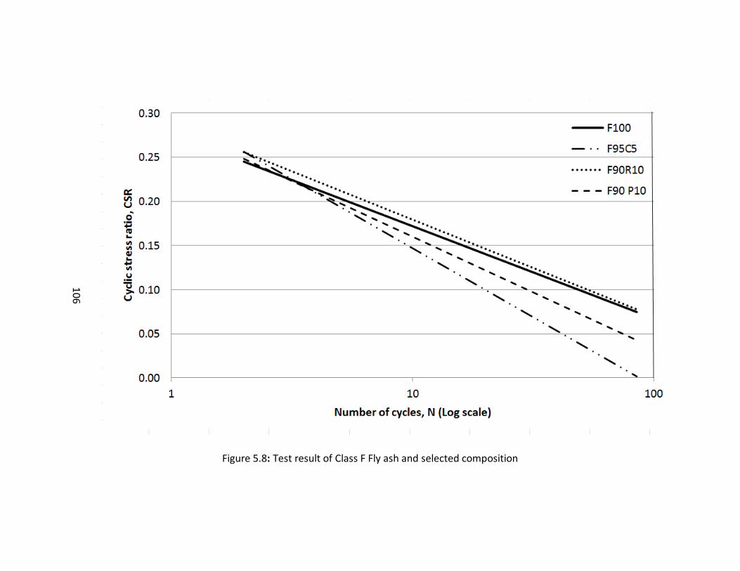
106
Figure 5.8: Test result of Class F Fly ash and selected composition
106
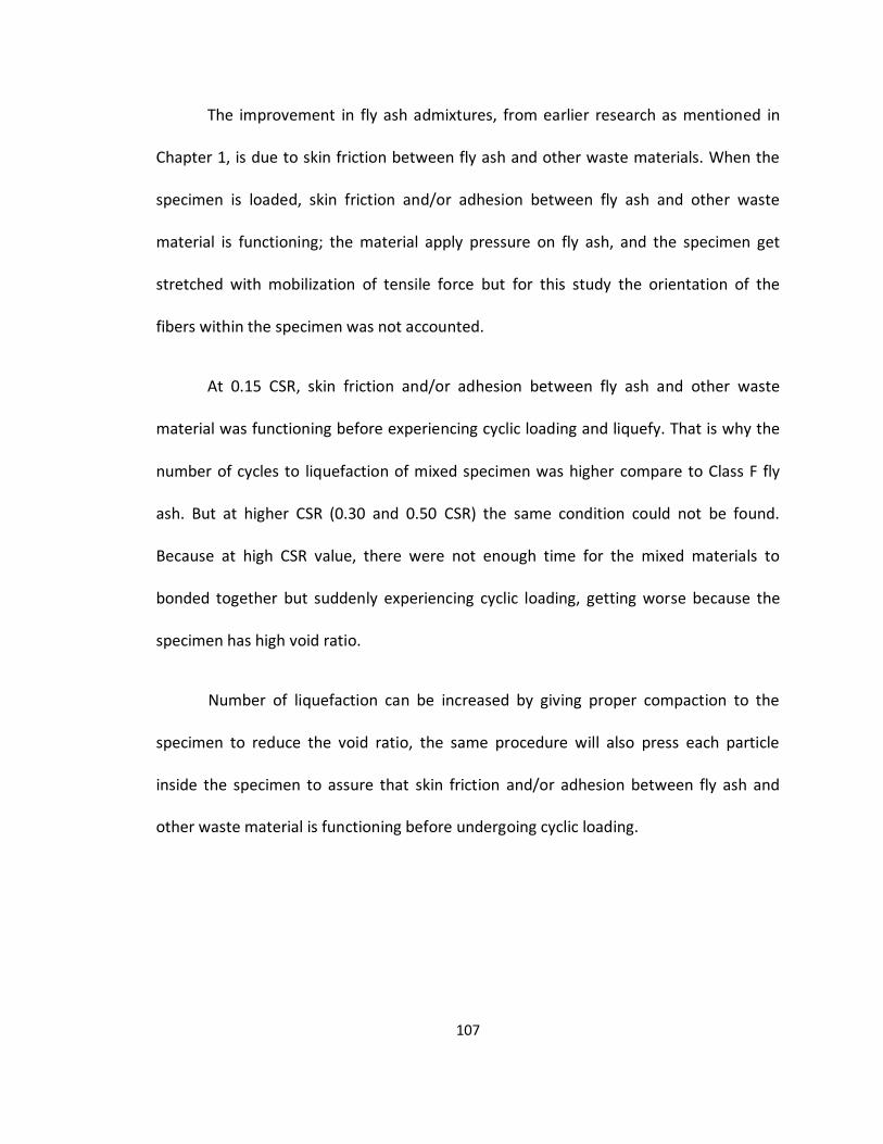
107
The improvement in fly ash admixtures, from earlier research as mentioned in
Chapter 1, is due to skin friction between fly ash and other waste materials. When the
specimen is loaded, skin friction and/or adhesion between fly ash and other waste
material is functioning; the material apply pressure on fly ash, and the specimen get
stretched with mobilization of tensile force but for this study the orientation of the
fibers within the specimen was not accounted.
At 0.15 CSR, skin friction and/or adhesion between fly ash and other waste
material was functioning before experiencing cyclic loading and liquefy. That is why the
number of cycles to liquefaction of mixed specimen was higher compare to Class F fly
ash. But at higher CSR (0.30 and 0.50 CSR) the same condition could not be found.
Because at high CSR value, there were not enough time for the mixed materials to
bonded together but suddenly experiencing cyclic loading, getting worse because the
specimen has high void ratio.
Number of liquefaction can be increased by giving proper compaction to the
specimen to reduce the void ratio, the same procedure will also press each particle
inside the specimen to assure that skin friction and/or adhesion between fly ash and
other waste material is functioning before undergoing cyclic loading.
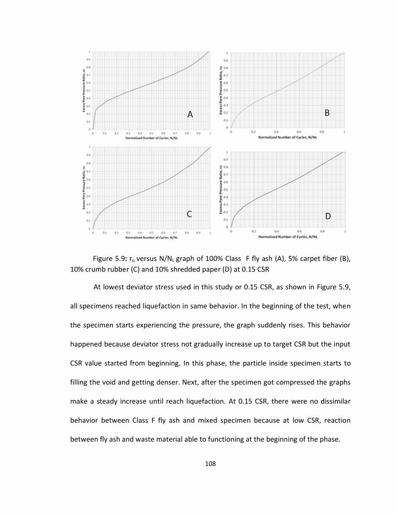
108
Figure 5.9: ru versus N/NL graph of 100% Class F fly ash (A), 5% carpet fiber (B),
10% crumb rubber (C) and 10% shredded paper (D) at 0.15 CSR
At lowest deviator stress used in this study or 0.15 CSR, as shown in Figure 5.9,
all specimens reached liquefaction in same behavior. In the beginning of the test, when
the specimen starts experiencing the pressure, the graph suddenly rises. This behavior
happened because deviator stress not gradually increase up to target CSR but the input
CSR value started from beginning. In this phase, the particle inside specimen starts to
filling the void and getting denser. Next, after the specimen got compressed the graphs
make a steady increase until reach liquefaction. At 0.15 CSR, there were no dissimilar
behavior between Class F fly ash and mixed specimen because at low CSR, reaction
between fly ash and waste material able to functioning at the beginning of the phase.
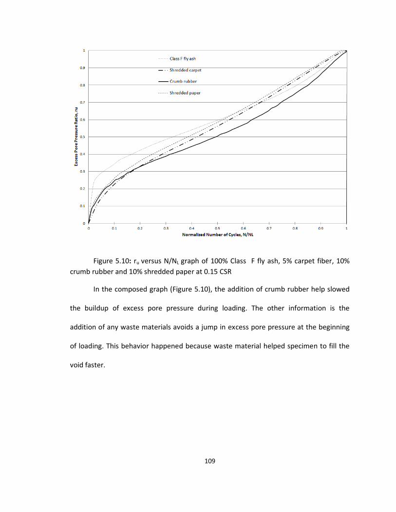
109
Figure 5.10: ru versus N/NL graph of 100% Class F fly ash, 5% carpet fiber, 10%
crumb rubber and 10% shredded paper at 0.15 CSR
In the composed graph (Figure 5.10), the addition of crumb rubber help slowed
the buildup of excess pore pressure during loading. The other information is the
addition of any waste materials avoids a jump in excess pore pressure at the beginning
of loading. This behavior happened because waste material helped specimen to fill the
void faster.
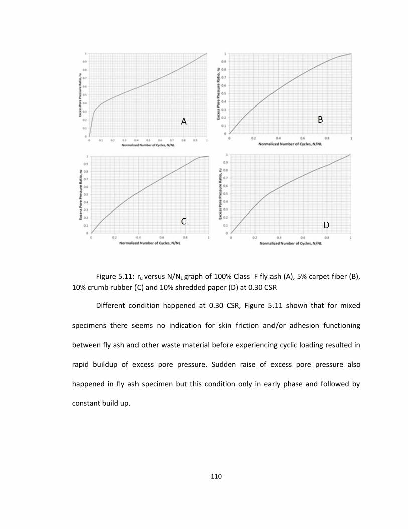
110
Figure 5.11: ru versus N/NL graph of 100% Class F fly ash (A), 5% carpet fiber (B),
10% crumb rubber (C) and 10% shredded paper (D) at 0.30 CSR
Different condition happened at 0.30 CSR, Figure 5.11 shown that for mixed
specimens there seems no indication for skin friction and/or adhesion functioning
between fly ash and other waste material before experiencing cyclic loading resulted in
rapid buildup of excess pore pressure. Sudden raise of excess pore pressure also
happened in fly ash specimen but this condition only in early phase and followed by
constant build up.
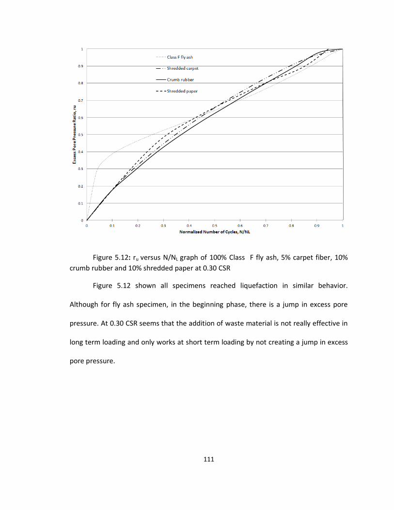
111
Figure 5.12: ru versus N/NL graph of 100% Class F fly ash, 5% carpet fiber, 10%
crumb rubber and 10% shredded paper at 0.30 CSR
Figure 5.12 shown all specimens reached liquefaction in similar behavior.
Although for fly ash specimen, in the beginning phase, there is a jump in excess pore
pressure. At 0.30 CSR seems that the addition of waste material is not really effective in
long term loading and only works at short term loading by not creating a jump in excess
pore pressure.
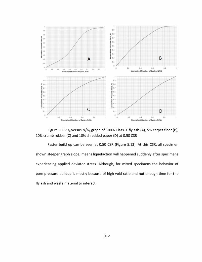
112
Figure 5.13: ru versus N/NL graph of 100% Class F fly ash (A), 5% carpet fiber (B),
10% crumb rubber (C) and 10% shredded paper (D) at 0.50 CSR
Faster build up can be seen at 0.50 CSR (Figure 5.13). At this CSR, all specimen
shown steeper graph slope, means liquefaction will happened suddenly after specimens
experiencing applied deviator stress. Although, for mixed specimens the behavior of
pore pressure buildup is mostly because of high void ratio and not enough time for the
fly ash and waste material to interact.
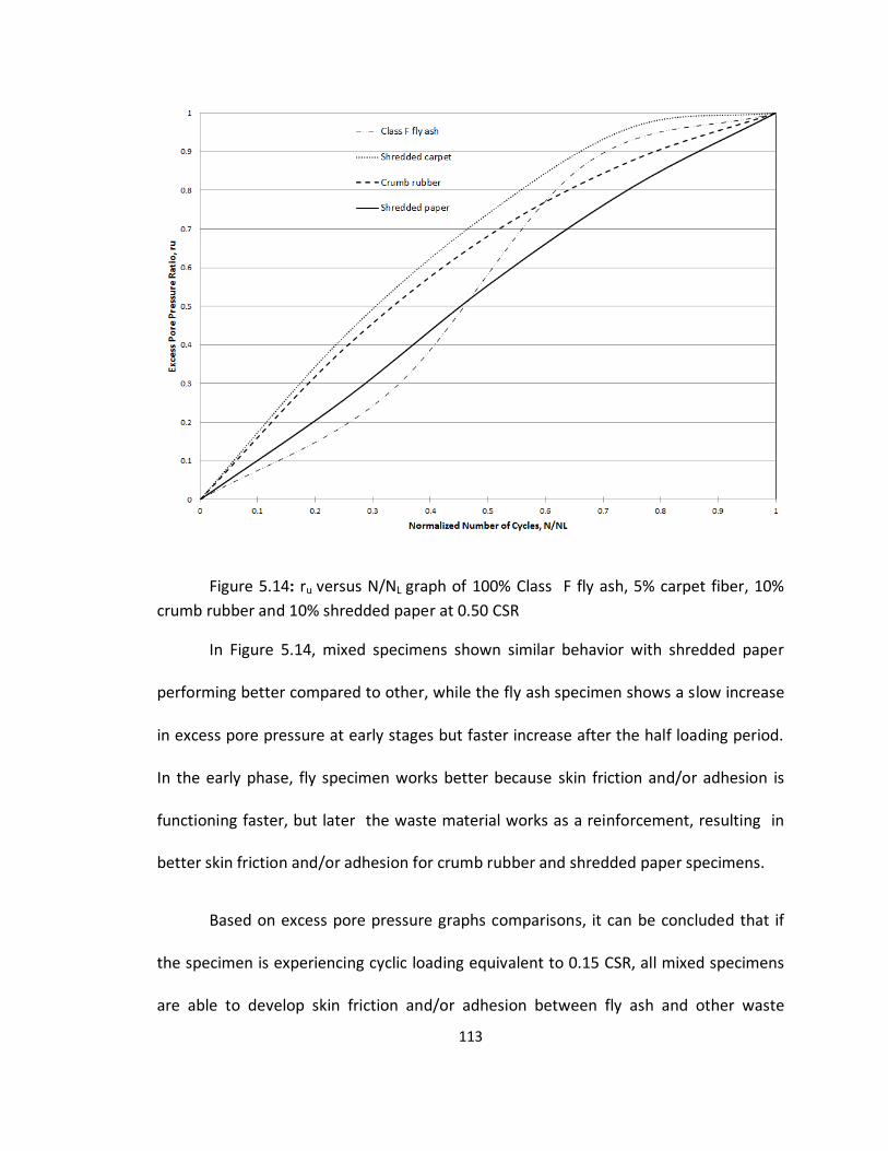
113
Figure 5.14: ru versus N/NL graph of 100% Class F fly ash, 5% carpet fiber, 10%
crumb rubber and 10% shredded paper at 0.50 CSR
In Figure 5.14, mixed specimens shown similar behavior with shredded paper
performing better compared to other, while the fly ash specimen shows a slow increase
in excess pore pressure at early stages but faster increase after the half loading period.
In the early phase, fly specimen works better because skin friction and/or adhesion is
functioning faster, but later the waste material works as a reinforcement, resulting in
better skin friction and/or adhesion for crumb rubber and shredded paper specimens.
Based on excess pore pressure graphs comparisons, it can be concluded that if
the specimen is experiencing cyclic loading equivalent to 0.15 CSR, all mixed specimens
are able to develop skin friction and/or adhesion between fly ash and other waste
114
material during testing, especially crumb rubber specimen resulting in higher number of
liquefaction compare to other combination. Meanwhile, at higher cyclic loading (0.30
and 0.50 CSR), skin friction and/or adhesion between fly ash and other waste material
were not able to perform properly, resulting in lower number of cycles to liquefaction
for mixed specimens compare to fly ash specimen.
Besides investigating each specimen according to dry weight, evaluating
specimens based on volume is also necessary to find the effect of the number of cycles
to liquefaction.
The information from Figure 5.15 is shredded paper starts to affect mixed
specimens at 3% until it reached optimum at 15%, so it is useless to add more shredded
carpet in specimen above 15% because number of cycles for liquefaction will not
increase. Meanwhile for crumb rubber, the optimum of this waste material is at 21%.
Similar performance is also shown by shredded carpet, which reached optimum at 38%.
For crumb rubber and shredded carpet adding waste material more than the optimum
percentage will decrease the number of cycles to liquefaction.
Lastly, based on volume comparison, shredded carpet, crumb rubber and
shredded paper optimum at 38%, 21% and 15%, respectively.
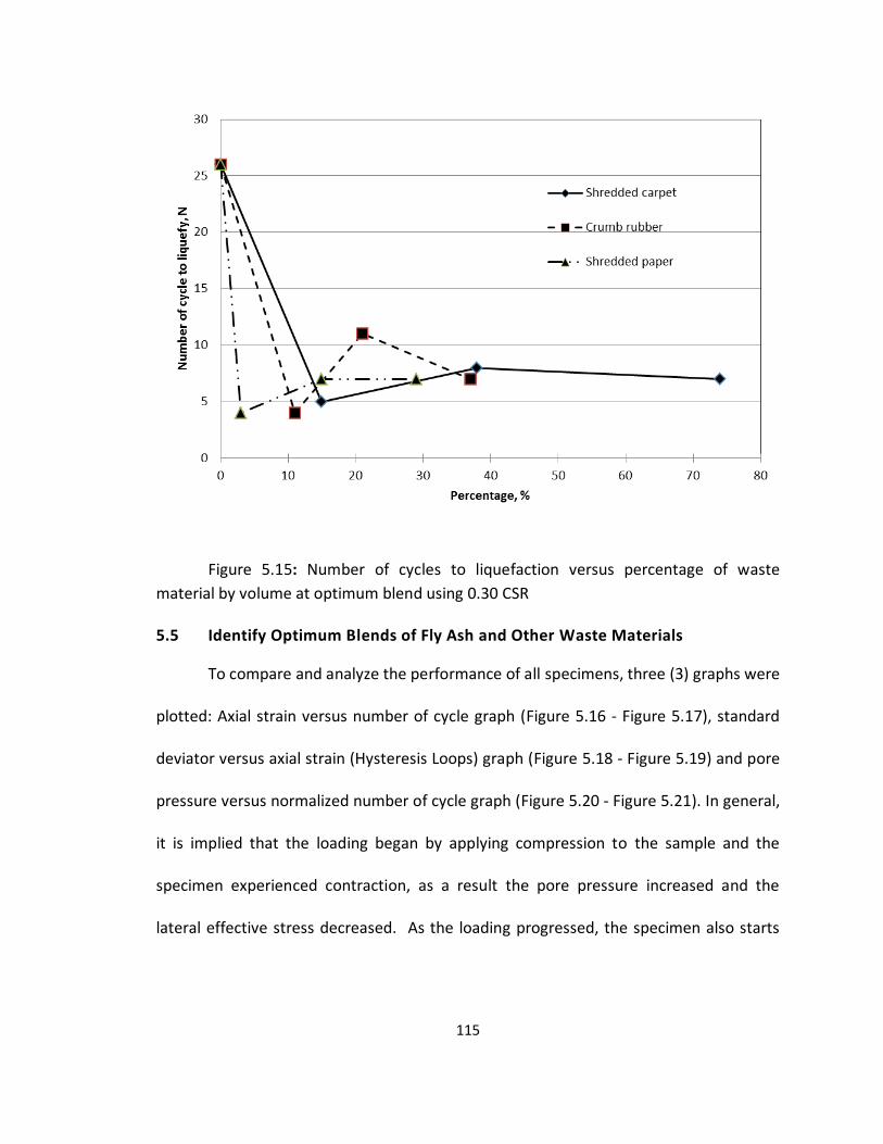
115
Figure 5.15: Number of cycles to liquefaction versus percentage of waste
material by volume at optimum blend using 0.30 CSR
5.5 Identify Optimum Blends of Fly Ash and Other Waste Materials
To compare and analyze the performance of all specimens, three (3) graphs were
plotted: Axial strain versus number of cycle graph (Figure 5.16 - Figure 5.17), standard
deviator versus axial strain (Hysteresis Loops) graph (Figure 5.18 - Figure 5.19) and pore
pressure versus normalized number of cycle graph (Figure 5.20 - Figure 5.21). In general,
it is implied that the loading began by applying compression to the sample and the
specimen experienced contraction, as a result the pore pressure increased and the
lateral effective stress decreased. As the loading progressed, the specimen also starts
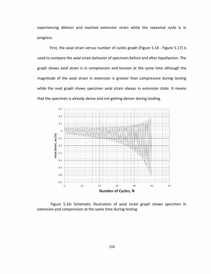
116
experiencing dilation and reached extension strain while the repeated cycle is in
progress.
First, the axial strain versus number of cycles graph (Figure 5.16 - Figure 5.17) is
used to compare the axial strain behavior of specimen before and after liquefaction. The
graph shows axial strain is in compression and tension at the same time although the
magnitude of the axial strain in extension is greater than compressive during testing
while the next graph shows specimen axial strain always in extension state. It means
that the specimen is already dense and not getting denser during loading.
Figure 5.16: Schematic Illustration of axial strain graph shows specimen in extension and compression at the same time during testing
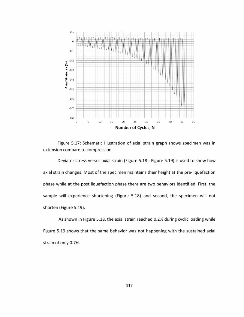
117
Figure 5.17: Schematic Illustration of axial strain graph shows specimen was in
extension compare to compression
Deviator stress versus axial strain (Figure 5.18 - Figure 5.19) is used to show how
axial strain changes. Most of the specimen maintains their height at the pre-liquefaction
phase while at the post liquefaction phase there are two behaviors identified. First, the
sample will experience shortening (Figure 5.18) and second, the specimen will not
shorten (Figure 5.19).
As shown in Figure 5.18, the axial strain reached 0.2% during cyclic loading while
Figure 5.19 shows that the same behavior was not happening with the sustained axial
strain of only 0.7%.
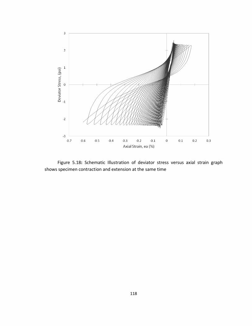
118
Figure 5.18: Schematic Illustration of deviator stress versus axial strain graph
shows specimen contraction and extension at the same time
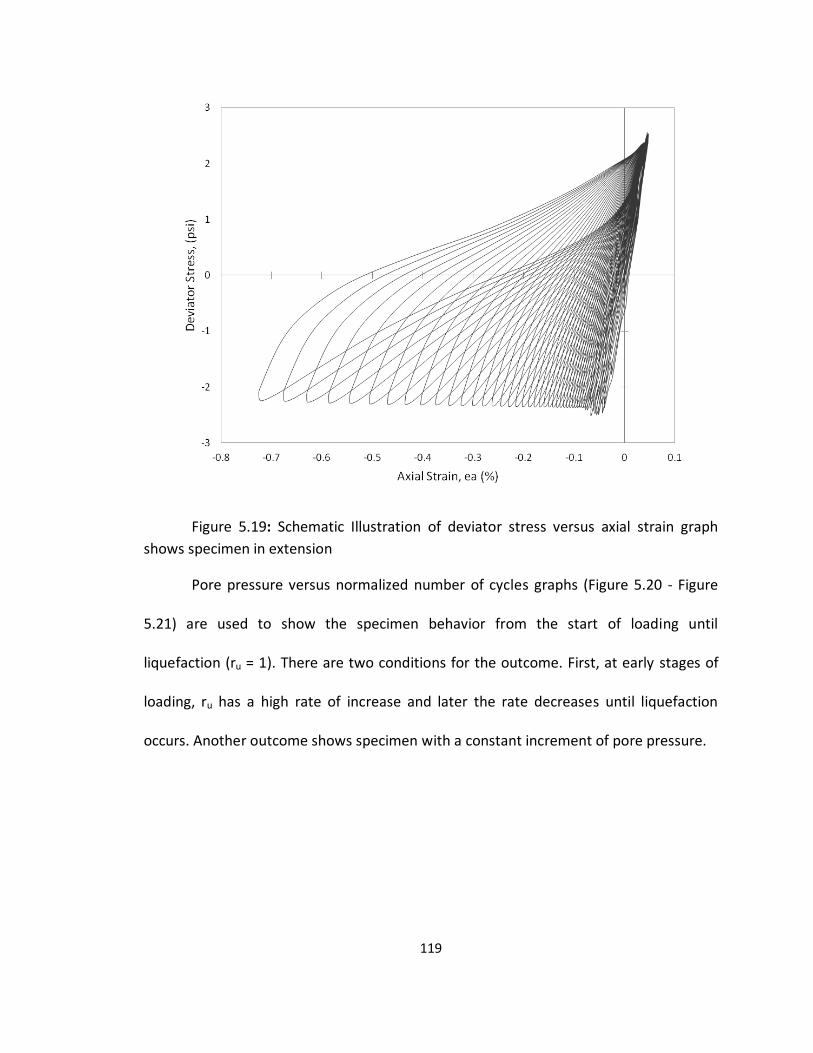
119
Figure 5.19: Schematic Illustration of deviator stress versus axial strain graph
shows specimen in extension
Pore pressure versus normalized number of cycles graphs (Figure 5.20 - Figure
5.21) are used to show the specimen behavior from the start of loading until
liquefaction (ru = 1). There are two conditions for the outcome. First, at early stages of
loading, ru has a high rate of increase and later the rate decreases until liquefaction
occurs. Another outcome shows specimen with a constant increment of pore pressure.
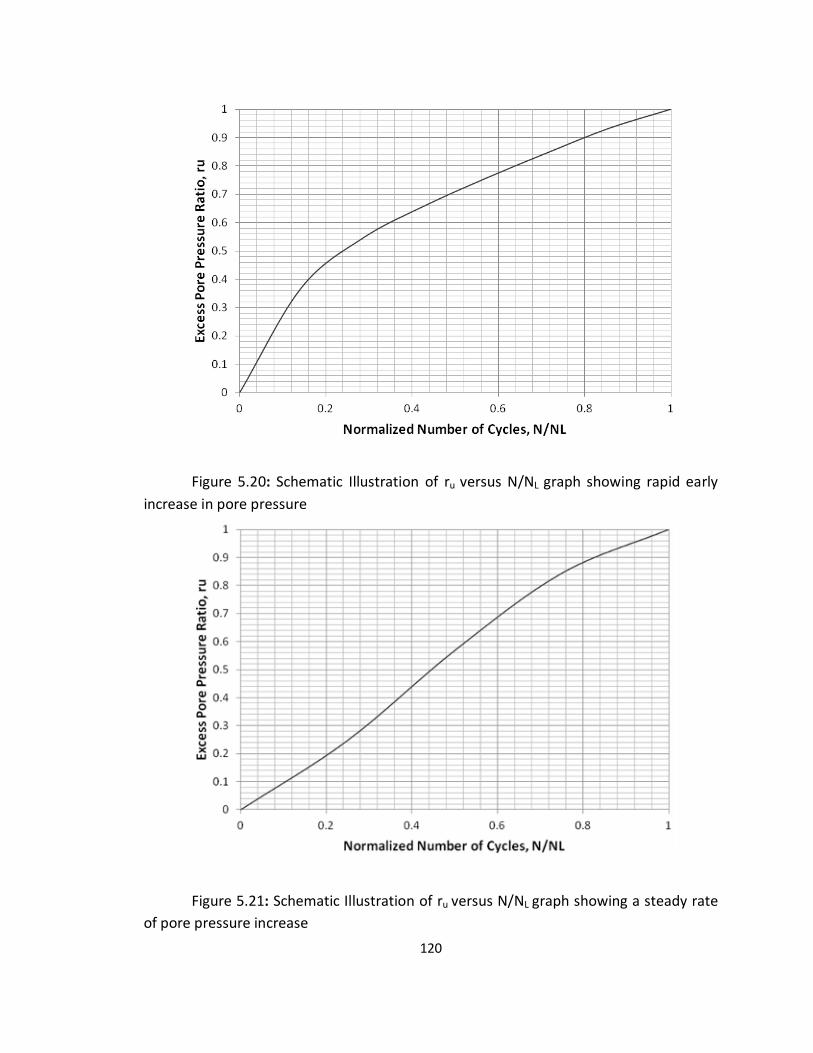
120
Figure 5.20: Schematic Illustration of ru versus N/NL graph showing rapid early
increase in pore pressure
Figure 5.21: Schematic Illustration of ru versus N/NL graph showing a steady rate
of pore pressure increase
121
For fly ash specimen, it is apparent that at the beginning and near the end of
cycles, pore pressure accumulates faster but this condition is non-existent for specimen
with waste material; pore pressure increase seems more evenly.
There is sudden buildup of pore pressure fly ash and this behavior is opposite to
the behavior of sand. This behavior is due to the uniform particle size of fly ash, which
permits rapid propagation of pore water pressure through the specimen.
The results from each specimen are summarized and plotted in Table 5.6 and
Figure 5.22. To illustrate the observed trend, a power function trend line is fitted to
each dataset. The distribution of the data is roughly following the power function trend
line; although a scatter is observed as it appears from Figure 5.22. As shown from Table
5.6, the number of cycle from each specimen was influenced by density, void ratio,
confining pressure and cyclic stress ratio.
In general, the results of Class F fly ash with crumb rubber works better by
showing more number of cycles compare to 100% Fly ash at 0.15 CSR.
122
122
Table 5.6: Specimen information and results of all specimens tested
γSat Confining Pressure Actual
(Pcf) (Psi) CSR
98.44 1.04 7.5 0.44 3
99.91 0.96 7.8 0.30 26
99.46 0.99 7.7 0.17 51
F98.5C1.5 95.18 1.19 6.9 0.27 5
92.83 1.36 6.4 0.46 4
93.78 1.29 6.6 0.30 6
91.61 1.46 6.2 0.44 4
92.69 1.37 6.4 0.29 8
92.5 1.38 6.7 0.16 29
93.17 1.07 6.9 0.37 2
94.48 0.98 7.2 0.29 4
93.08 1.07 6.9 0.48 4
92.86 1.09 6.8 0.30 11
93.37 1.05 6.5 0.17 86
F80R20 95.99 0.89 7.5 0.29 7
F98P2 97.5 1.04 7.4 0.28 4
96.85 1.08 7.8 0.47 4
97.22 1.06 7.4 0.29 7
96.09 1.13 7.6 0.17 47
F80P20 94.17 1.26 6.7 0.29 7
Definitions:
F = Class F Fly Ash R = Crumb Rubber
C = Carpet Fiber P = Shredded Paper
100, 98.5, 98, 95, 90, 80, 20, 10, 5, 2 and 1.5 = Percentage of Waste Material by Dry Weight
N cycles
F100
F98C2
F95C5
F95R5
F90R10
F90P10
Composition e
123
Figure 5.22: Cyclic stress ratio (CSR) Versus Number of cycles (N) of all specimen tested graph
123
124
Chapter 6
6. CONCLUSION AND RECOMMENDATIONS
6.1 Findings of the Study
In this section, the analysis of laboratory tests results performed on Class F fly
ash and other waste material is addressed. Also the correlation between the laboratory
measured parameters is discussed.
Using the cyclic shear test as described in ASTM D3999, the test results show
that the maximum shear modulus of the specimens is 38.99 psi. Using the same
information, normalized shear modulus reduction curves and damping ratio curves were
generated and compared with other research (Figure 6.1 and Figure 6.7). Based on
research conducted by Guoxi et al. (1985), it is found that the dynamic shear moduli
increase as confining pressure increases and decrease as void ratio increases. In
agreement, the material used in this study have high void ratio, which results in low
shear modulus. Therefore, it may be concluded that fly ash is one kind of material which
possess high void ratio and low shear modulus. Void ratio varies from 1.08 – 1.61.
The samples from this study responded with the lowest values of shear modulus
and demonstrated the softest response. However, as the trend suggests, at lower shear
strains higher values of shear modulus could be expected. The softer response of the
specimen is related to the lower in-situ confining stress. Due to the lower confinement
and looser structure, the Young’s modulus of the sample was lower which resulted in
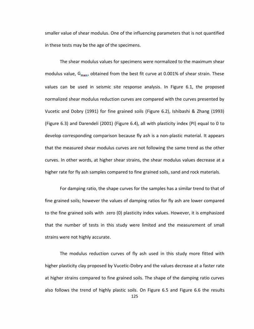
125
smaller value of shear modulus. One of the influencing parameters that is not quantified
in these tests may be the age of the specimens.
The shear modulus values for specimens were normalized to the maximum shear
modulus value, , obtained from the best fit curve at 0.001% of shear strain. These
values can be used in seismic site response analysis. In Figure 6.1, the proposed
normalized shear modulus reduction curves are compared with the curves presented by
Vucetic and Dobry (1991) for fine grained soils (Figure 6.2), Ishibashi & Zhang (1993)
(Figure 6.3) and Darendeli (2001) (Figure 6.4), all with plasticity index (PI) equal to 0 to
develop corresponding comparison because fly ash is a non-plastic material. It appears
that the measured shear modulus curves are not following the same trend as the other
curves. In other words, at higher shear strains, the shear modulus values decrease at a
higher rate for fly ash samples compared to fine grained soils, sand and rock materials.
For damping ratio, the shape curves for the samples has a similar trend to that of
fine grained soils; however the values of damping ratios for fly ash are lower compared
to the fine grained soils with zero (0) plasticity index values. However, it is emphasized
that the number of tests in this study were limited and the measurement of small
strains were not highly accurate.
The modulus reduction curves of fly ash used in this study more fitted with
higher plasticity clay proposed by Vucetic-Dobry and the values decrease at a faster rate
at higher strains compared to fine grained soils. The shape of the damping ratio curves
also follows the trend of highly plastic soils. On Figure 6.5 and Figure 6.6 the results

126
from Class F fly ash used in this study are superimposed with curves proposed by
Vucetic-Dobry for clay with plasticity index (PI) equal to 0 and 200.
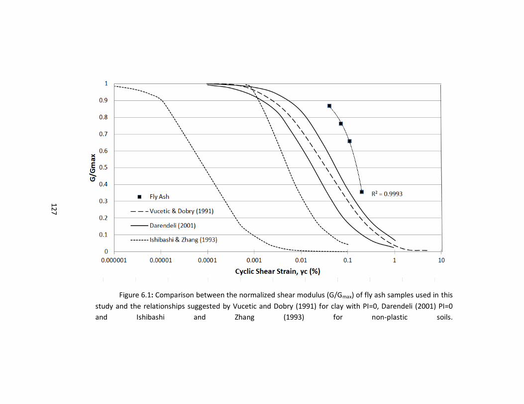
127
Figure 6.1: Comparison between the normalized shear modulus (G/Gmax) of fly ash samples used in this
study and the relationships suggested by Vucetic and Dobry (1991) for clay with PI=0, Darendeli (2001) PI=0
and Ishibashi and Zhang (1993) for non-plastic soils.
127
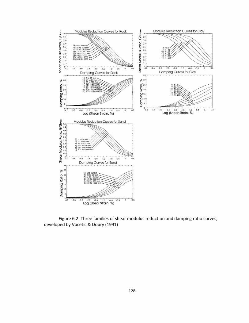
128
Figure 6.2: Three families of shear modulus reduction and damping ratio curves, developed by Vucetic & Dobry (1991)
129
Figure 6.3: Influence of effective confining pressure on modulus reduction curves: (a) Non-plastic soil and (b) Plastic soil (Ishibashi and Zhang, 1993)
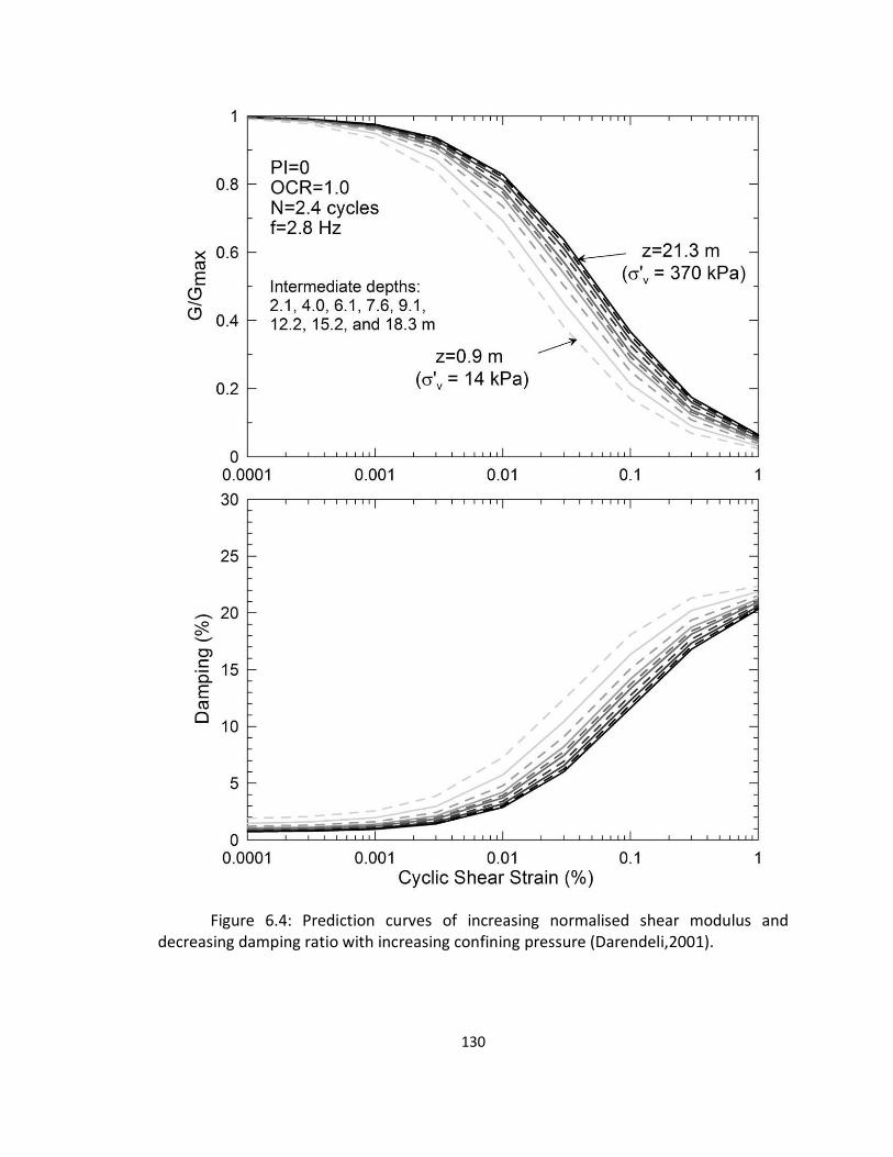
130
Figure 6.4: Prediction curves of increasing normalised shear modulus and decreasing damping ratio with increasing confining pressure (Darendeli,2001).
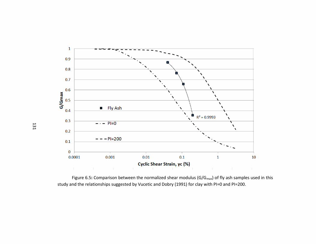
131
Figure 6.5: Comparison between the normalized shear modulus (G/Gmax) of fly ash samples used in this
study and the relationships suggested by Vucetic and Dobry (1991) for clay with PI=0 and PI=200.
131
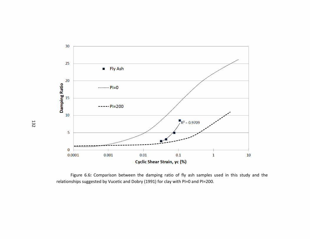
132
Figure 6.6: Comparison between the damping ratio of fly ash samples used in this study and the
relationships suggested by Vucetic and Dobry (1991) for clay with PI=0 and PI=200.
132
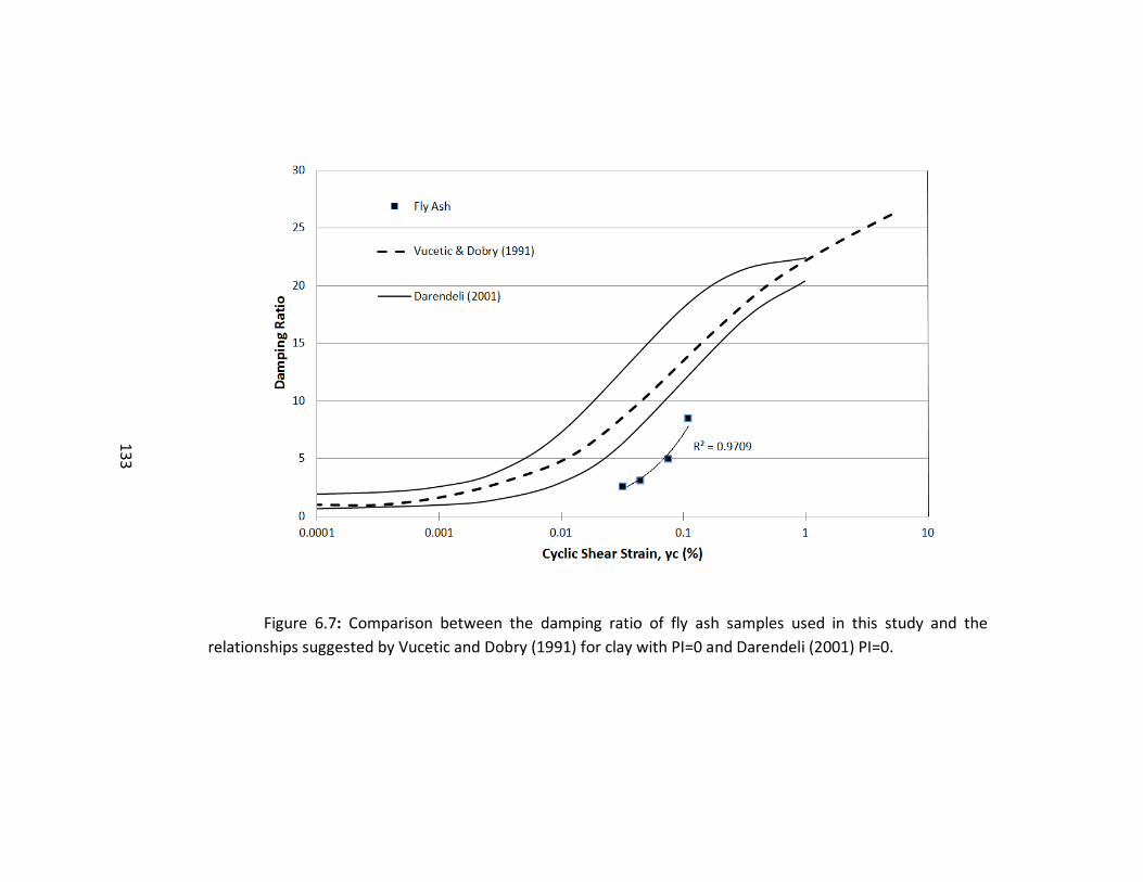
133
Figure 6.7: Comparison between the damping ratio of fly ash samples used in this study and the
relationships suggested by Vucetic and Dobry (1991) for clay with PI=0 and Darendeli (2001) PI=0.
133
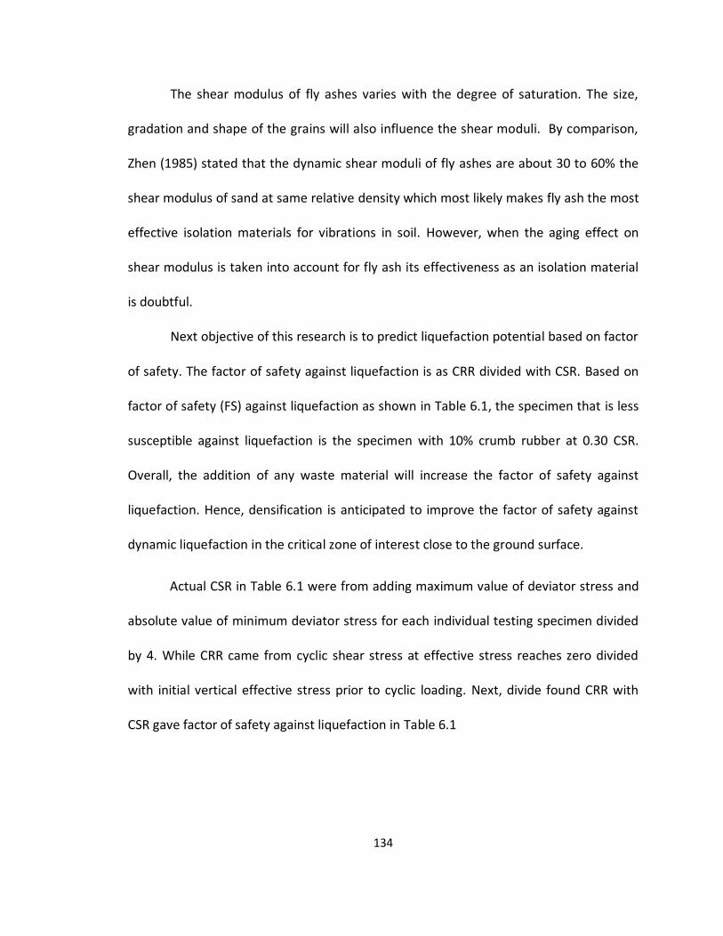
134
The shear modulus of fly ashes varies with the degree of saturation. The size,
gradation and shape of the grains will also influence the shear moduli. By comparison,
Zhen (1985) stated that the dynamic shear moduli of fly ashes are about 30 to 60% the
shear modulus of sand at same relative density which most likely makes fly ash the most
effective isolation materials for vibrations in soil. However, when the aging effect on
shear modulus is taken into account for fly ash its effectiveness as an isolation material
is doubtful.
Next objective of this research is to predict liquefaction potential based on factor
of safety. The factor of safety against liquefaction is as CRR divided with CSR. Based on
factor of safety (FS) against liquefaction as shown in Table 6.1, the specimen that is less
susceptible against liquefaction is the specimen with 10% crumb rubber at 0.30 CSR.
Overall, the addition of any waste material will increase the factor of safety against
liquefaction. Hence, densification is anticipated to improve the factor of safety against
dynamic liquefaction in the critical zone of interest close to the ground surface.
Actual CSR in Table 6.1 were from adding maximum value of deviator stress and
absolute value of minimum deviator stress for each individual testing specimen divided
by 4. While CRR came from cyclic shear stress at effective stress reaches zero divided
with initial vertical effective stress prior to cyclic loading. Next, divide found CRR with
CSR gave factor of safety against liquefaction in Table 6.1
135
Table 6.1: Cyclic Resistance Ratio (CRR) and Factor of safety (FS) for typical scenarios
Actual FS
CSR Liquefaction
0.44 0.04 0.18
0.30 0.20 1.33
0.17 0.09 1.04
F98.5C1.5 0.27 0.24 1.79
F98C2 0.46 0.22 0.96
0.44 0.27 1.20
0.29 0.28 1.96
0.16 0.14 1.74
F80C20 0.27 0.22 1.60
F95R5 0.29 0.06 0.44
0.48 0.43 1.76
0.30 0.29 1.99
0.17 0.10 1.18
F80R20 0.29 0.10 0.69
F98P2 0.28 0.27 1.90
0.47 0.46 1.96
0.29 0.19 1.28
0.17 0.14 1.66
F80P20 0.29 0.22 1.52
Definitions:
F = Class F Fly Ash R = Crumb Rubber
C = Carpet Fiber P = Shredded Paper
100, 98.5, 98, 95, 90, 80, 20, 10, 5, 2 and 1.5 = Percentage of Waste Material by Dry Weight
F90P10
CRRSpecimen
F100
F95C5
F90R10
The parameters that low factors of safety were void ratio, confining pressure,
saturated density, overconsolidation ratio, and age of the specimens. These parameters
were not accounted to adjust the factor of safety. In general, the addition of the waste
materials enhanced fly ash performance against cyclic loading and increases the factor
of safety against liquefaction.
Better understanding of how waste materials enhanced fly ash performance
against cyclic loading can be seen by comparing hysteresis loop. Material combinations
used were optimum percentage by dry weight at 0.15, 0.30 and 0.50 CSR.
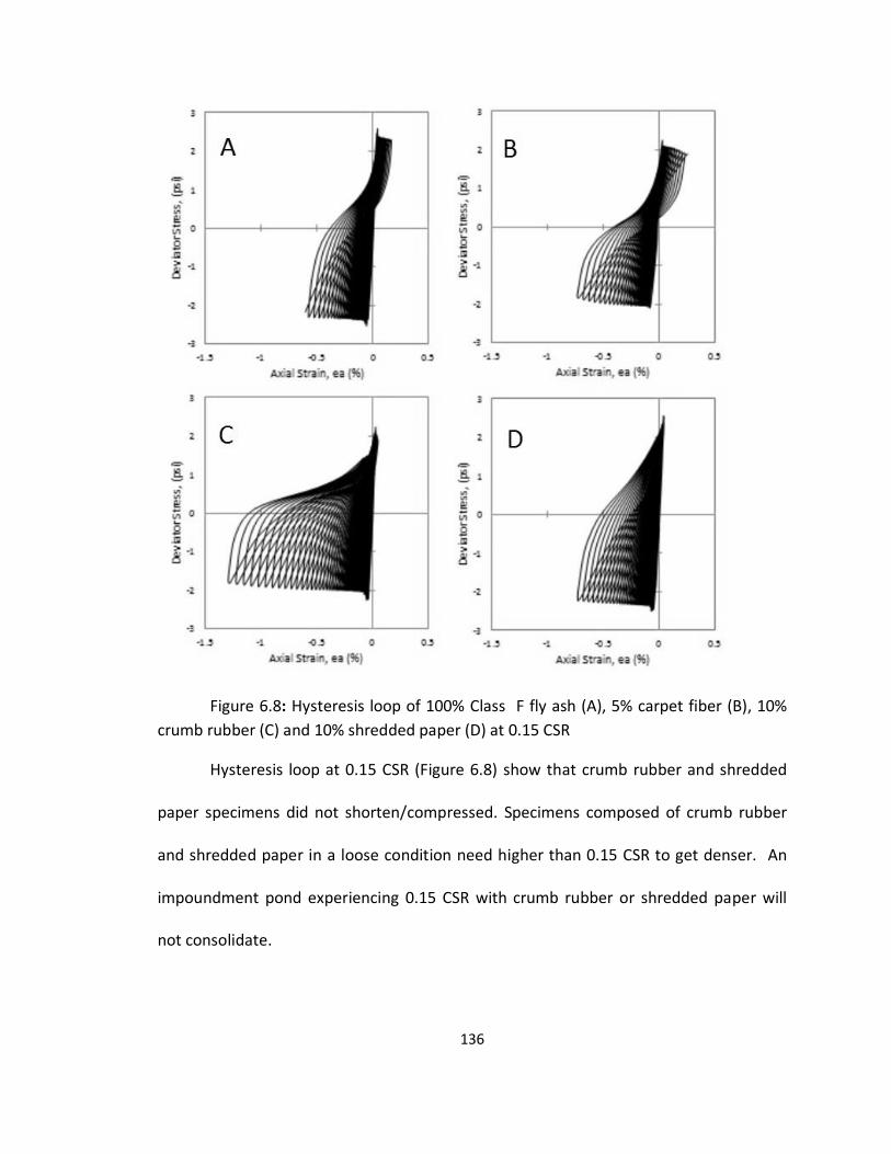
136
Figure 6.8: Hysteresis loop of 100% Class F fly ash (A), 5% carpet fiber (B), 10%
crumb rubber (C) and 10% shredded paper (D) at 0.15 CSR
Hysteresis loop at 0.15 CSR (Figure 6.8) show that crumb rubber and shredded
paper specimens did not shorten/compressed. Specimens composed of crumb rubber
and shredded paper in a loose condition need higher than 0.15 CSR to get denser. An
impoundment pond experiencing 0.15 CSR with crumb rubber or shredded paper will
not consolidate.
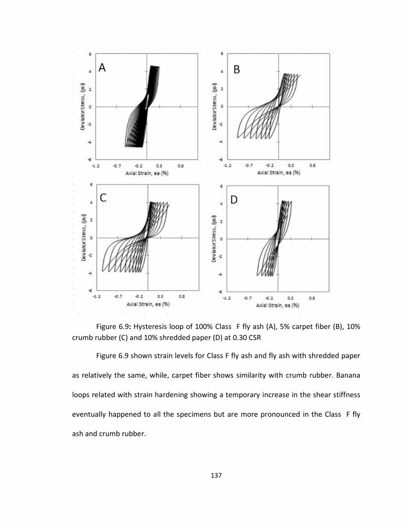
137
Figure 6.9: Hysteresis loop of 100% Class F fly ash (A), 5% carpet fiber (B), 10%
crumb rubber (C) and 10% shredded paper (D) at 0.30 CSR
Figure 6.9 shown strain levels for Class F fly ash and fly ash with shredded paper
as relatively the same, while, carpet fiber shows similarity with crumb rubber. Banana
loops related with strain hardening showing a temporary increase in the shear stiffness
eventually happened to all the specimens but are more pronounced in the Class F fly
ash and crumb rubber.
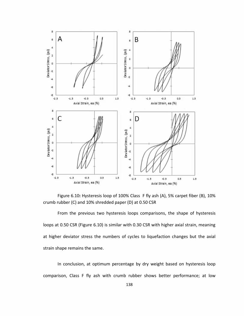
138
Figure 6.10: Hysteresis loop of 100% Class F fly ash (A), 5% carpet fiber (B), 10%
crumb rubber (C) and 10% shredded paper (D) at 0.50 CSR
From the previous two hysteresis loops comparisons, the shape of hysteresis
loops at 0.50 CSR (Figure 6.10) is similar with 0.30 CSR with higher axial strain, meaning
at higher deviator stress the numbers of cycles to liquefaction changes but the axial
strain shape remains the same.
In conclusion, at optimum percentage by dry weight based on hysteresis loop
comparison, Class F fly ash with crumb rubber shows better performance; at low
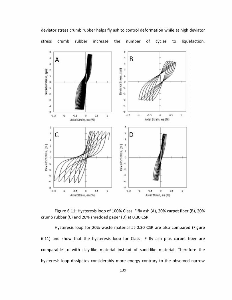
139
deviator stress crumb rubber helps fly ash to control deformation while at high deviator
stress crumb rubber increase the number of cycles to liquefaction.
Figure 6.11: Hysteresis loop of 100% Class F fly ash (A), 20% carpet fiber (B), 20%
crumb rubber (C) and 20% shredded paper (D) at 0.30 CSR
Hysteresis loop for 20% waste material at 0.30 CSR are also compared (Figure
6.11) and show that the hysteresis loop for Class F fly ash plus carpet fiber are
comparable to with clay-like material instead of sand-like material. Therefore the
hysteresis loop dissipates considerably more energy contrary to the observed narrow
140
loops typical to the sand-like materials. By increasing carpet fiber content, the loops
become broader and thus it can be considered a clay-like behavior with cyclic mobility.
Summarizing the results, compositions of Class F fly ash with waste materials
such as shredded carpet, shredded paper and crumb rubber that give optimum
enhancement ranges from 5 to 10% by dry weight and 15 to 38% by volume.
6.2 Recommendations for Practitioners
Gray and Lin (1972) stated that fly ash has advantages when used in mass-fills.
Properly compacted and stabilized fly ash is as durable as conventional compacted earth
fill. Compacted fly ashes have been reported to exhibit age hardening behavior, i.e., a
time-dependent increase in strength after compaction. Age hardening behavior or
pozzolonic properties has been correlated with the presence of free lime in the fly ash.
Fly ash which have been lagooned prior to compaction does not exhibit as much age
hardening.
In addition, Gray and Lin (1972) describe the effect of degree of saturation on
the compressibility of compacted fly ash; the partially saturated fly ash was considerably
less compressible, in the case of fully saturated samples, a large proportion of total
volume decrease occurs during the primary consolidation phase. Primary consolidation
occurs very rapidly and in the usual field situation would not be as important as
secondary compression in explaining or accounting for long term settlement.
141
Due to scarcity of land around power plants, one option for increasing the
capacity of an ash pond is by raising its height. In this study, the expectation is to
increase the useful capacity of storage pond by increasing the fly ash embankment.
In many places the total height of the deposit is higher than 30 m. The ash
deposit placed in slurry form has a very low density and leads to problems such as
liquefaction during earthquakes, poor bearing capacity, large settlement, etc.
Considerable research has been conducted to improve the density of ash by different
techniques such as vacuum dewatering, electro osmosis, vibro-compaction, stone
columns, blasting, etc. (Gandhi, et al, 1999).
This study provides an option to increase the capacity of fly ash ponds by
increasing the earthen dikes of an existing pond. When a fly ash material is stable then it
can be placed in higher dikes. As shown on Table 6.1, any composition of waste material
increases the factor of safety and Class F fly ash with 10% crumb rubber shows the
highest safety factor of 1.99 which is adequate enough to withstand stress that is
applied.
To help practitioners predict factors of safety against liquefaction, this study
provide equations to approximate cyclic resistance ratio (CRR) using cyclic stress ratio
(CSR). There are equations for each waste material (Class F fly ash, shredded carpet,
crumb rubber and shredded paper) that are recommended to be used if the addition of
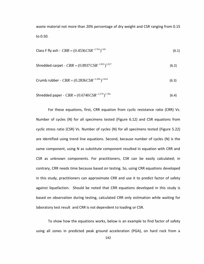
142
waste material not more than 20% percentage of dry weight and CSR ranging from 0.15
to 0.50.
Class F fly ash - 69.1763.2 )4536.0( CSRCRR (6.1)
Shredded carpet - 627.1855.1 )8937.0( CSRCRR (6.2)
Crumb rubber - 024.2306.3 )2836.0( CSRCRR (6.3)
Shredded paper - 784.1379.2 )6740.0( CSRCRR (6.4)
For these equations, first, CRR equation from cyclic resistance ratio (CRR) Vs.
Number of cycles (N) for all specimens tested (Figure 6.12) and CSR equations from
cyclic stress ratio (CSR) Vs. Number of cycles (N) for all specimens tested (Figure 5.22)
are identified using trend line equations. Second, because number of cycles (N) is the
same component, using N as substitute component resulted in equation with CRR and
CSR as unknown components. For practitioners, CSR can be easily calculated; in
contrary, CRR needs time because based on testing. So, using CRR equations developed
in this study, practitioners can approximate CRR and use it to predict factor of safety
against liquefaction. Should be noted that CRR equations developed in this study is
based on observation during testing, calculated CRR only estimation while waiting for
laboratory test result and CRR is not dependent to loading or CSR.
To show how the equations works, below is an example to find factor of safety
using all zones in predicted peak ground acceleration (PGA), on hard rock from a

143
magnitude 7.5 earthquake in the New Madrid Seismic Zone (Figure 6.14) and predict the
factor of safety using CRR from equations. The procedure for this example is shown in
Figure 6.13. To find CSR in this example, αmax value is based from Figure 6.14 and γsat
value is the average from tested specimen. The calculated CSR value will be used as an
input for equation to get CRR and find factor of safety against liquefaction. The result for
all zones is shown in Table 6.2.
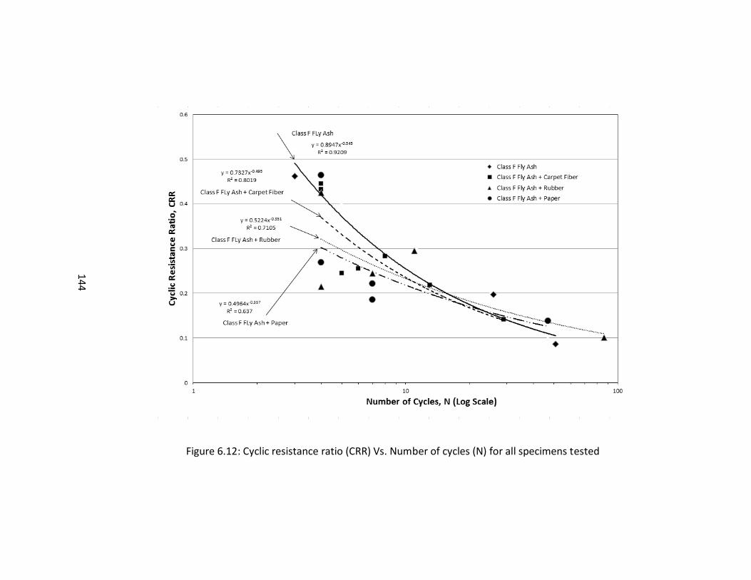
144
Figure 6.12: Cyclic resistance ratio (CRR) Vs. Number of cycles (N) for all specimens tested
144
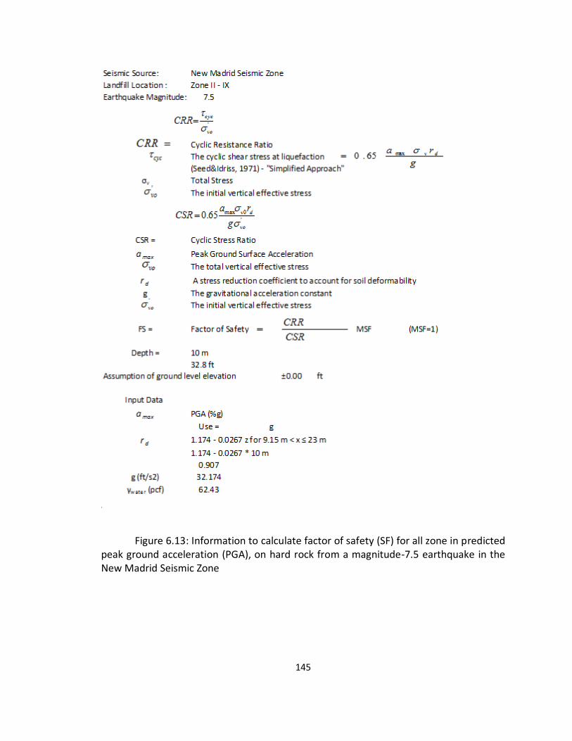
145
Figure 6.13: Information to calculate factor of safety (SF) for all zone in predicted peak ground acceleration (PGA), on hard rock from a magnitude-7.5 earthquake in the New Madrid Seismic Zone
146
Table 6.2: Factor of Safety for all zones in predicted peak ground acceleration (PGA), on hard rock from a magnitude-7.5 earthquake in the New Madrid Seismic Zone
Material = Class F fly ash
Perceived αmax γsat σv
shaking (g) (pcf) (psf) (psf) (psf)
Violent 1.24 1352.50 1.12 0.97 0.87
Severe 0.65 708.97 0.59 2.38 4.05
Very strong 0.34 370.85 0.31 5.82 18.96
strong 0.18 196.33 0.16 14.01 86.24
Moderate 0.092 100.35 0.08 35.42 426.46
Light 0.039 42.54 0.04 115.91 3292.48
Weak 0.014 15.27 0.01 477.30 37769.41
Not felt 0.0017 1.85 0.00 8786.23 5725718.00
CRR
1208.35
FS
99.27 3256.06
CSR'
vo cyc
Material = Class F fly ash + Shredded Carpet
Perceived αmax γsat σv
shaking (g) (pcf) (psf) (psf) (psf)
Violent 1.24 1352.50 1.12 1.39 1.24
Severe 0.65 708.97 0.59 2.52 4.30
Very strong 0.34 370.85 0.31 4.60 14.99
strong 0.18 196.33 0.16 8.30 51.07
Moderate 0.092 100.35 0.08 15.46 186.21
Light 0.039 42.54 0.04 34.28 973.72
Weak 0.014 15.27 0.01 88.65 7015.36
Not felt 0.0017 1.85 0.00 626.61 408339.72
CSR CRR FS
92.66 3039.25 991.54
'
vo cyc
Material = Class F fly ash + Crumb rubber
Perceived αmax γsat σv
shaking (g) (pcf) (psf) (psf) (psf)
Violent 1.24 1352.50 1.12 0.89 0.80
Severe 0.65 708.97 0.59 2.60 4.44
Very strong 0.34 370.85 0.31 7.60 24.75
strong 0.18 196.33 0.16 21.73 133.76
Moderate 0.092 100.35 0.08 65.91 793.65
Light 0.039 42.54 0.04 272.30 7735.09
Weak 0.014 15.27 0.01 1480.93 117187.73
Not felt 0.0017 1.85 0.00 48322.71 31490448.19
FS
93.96 3081.89 1034.18
CSR CRR'
vo cyc
Material = Class F fly ash + Shredded paper
Perceived αmax γsat σv
shaking (g) (pcf) (psf) (psf) (psf)
Violent 1.24 1352.50 1.12 1.28 1.14
Severe 0.65 708.97 0.59 2.76 4.71
Very strong 0.34 370.85 0.31 5.97 19.45
strong 0.18 196.33 0.16 12.72 78.29
Moderate 0.092 100.35 0.08 28.26 340.32
Light 0.039 42.54 0.04 78.44 2228.28
Weak 0.014 15.27 0.01 265.34 20997.08
Not felt 0.0017 1.85 0.00 3258.45 2123431.36
96.37 3160.94 1113.23
CSR CRR FS'
vo cyc
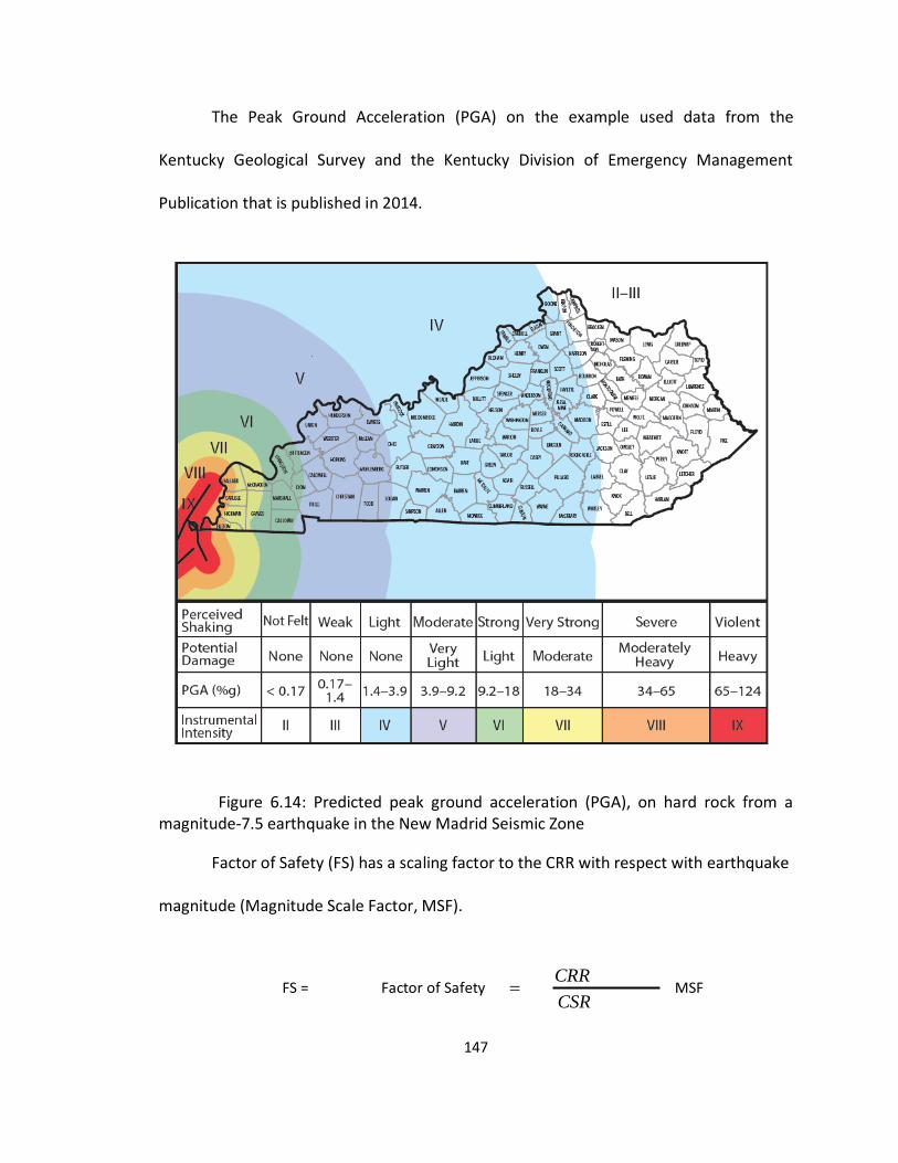
147
The Peak Ground Acceleration (PGA) on the example used data from the
Kentucky Geological Survey and the Kentucky Division of Emergency Management
Publication that is published in 2014.
Figure 6.14: Predicted peak ground acceleration (PGA), on hard rock from a magnitude-7.5 earthquake in the New Madrid Seismic Zone
Factor of Safety (FS) has a scaling factor to the CRR with respect with earthquake
magnitude (Magnitude Scale Factor, MSF).
FS = Factor of Safety MSF
'
vo
CSR
CRR
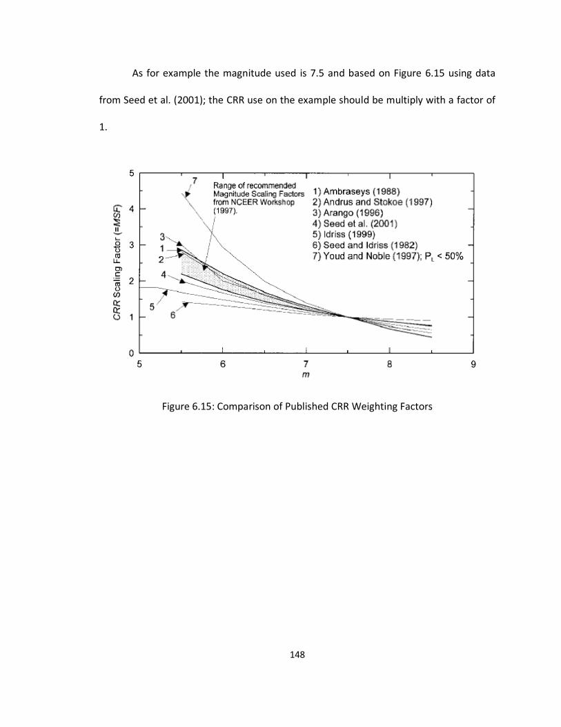
148
As for example the magnitude used is 7.5 and based on Figure 6.15 using data
from Seed et al. (2001); the CRR use on the example should be multiply with a factor of
1.
Figure 6.15: Comparison of Published CRR Weighting Factors
149
From the example above, it shows that all impoundment facilities at location
Zone VIII is not at risk for liquefaction from New Madrid Seismic Zone. On the other
hand, for impoundment facilities located in Zone IX with PGA of 34-65 %g, two
specimens have lower factor of safety than 1, as can be seen in Table 6.2.
Using the information above, it is apparent that the effect of waste materials
affecting factor of safety against liquefaction. As shown, without any addition of waste
material, fly ash composition at zone IX has safety factor less than 1.
The result above also implies that specimen with waste material might withstand
vibration from machinery used on impoundment facilities. Today, many storage ponds
use back hoes to compact and denser fly ash layer, this mechanism can be replaced by
vibrating the pond to get better and more stable conditions with the help of adding
waste material to the existing fly ash layer. At the same time, the same materials also
increase the safety of storage ponds while machinery is at work in order to make sure
that a vibration generated by the machinery will not disrupt the stability of storage
pond.
From an economical perspective, the compacted dry density of fly ash is typically
in the range of 70 pcf to 80 pcf (Gray and Lin, 1972) which is well below most
conventional fill materials such as clay (Around 110 pcf) and sand (Around 100 pcf)
which gives an economical advantage. For example, 1 ton of compacted fly ash
represents a greater volume than 1 ton of conventional earth fill. This is an advantage if
150
the fill or embankment must be placed on ground of low bearing capacity or where long
term settlement is possible.
The cost of siting and preparing new areas for landfills rises every year, these
existing impoundment locations are being considered for construction landfills. Before
the impoundments can be used for this purpose, the stability of the impounded material
must be determined.
Business and cost-effectiveness prospects can be appreciated in the long-term.
In the beginning, money allocation to purchase shredder machinery in the facilities
might be expensive but as time lapses the facilities will benefit from companies who
utilize their impoundment facilities to dump used tires, carpet and paper. This usage will
generate income for the company. In conclusion, these facilities will have 2 benefits;
improved the stability of impoundment facilities and earned income.
To illustrate, a cost matrix comparison between adding crumb rubber, shredded
carpet and paper is presented in Table 6.3. The condition for this comparison used a
typical impoundment facilities dimensions with 10% additional waste materials by
volume, material in impoundment facilities is in loose condition, but the price to buy
shredder for waste material and fees to open and maintain ash impoundment facilities
as stated in USEPA regulations are not in consideration.

151
Table 6.3: Matrix comparison from each waste material
Where:
The impoundment dimensions are 10 acre-ft. with 32.8 ft. depth and a total
volume of 14,287,680 sq. ft.
The density of tire shreds = 30 lb/ft3 (Office of Research, Development, and
Technology, Office of Safety, RDT, 2012)
The density of carpet = 6 lb/ft3 (Assistant Secretary for Housing Federal Housing
Commissioner, 1993)
The density of paper = 43 lb/ft3
The price for dumping a passenger car tire = $0.50 per tire with average weight of
passenger tires as scrap are 20 pounds (Department of Ecology state of Washington,
2010)
The price for dumping carpet = 5 cents per pound
The price for dumping paper = 0.5 cents per 50 pound
Typical shredder machine price = $175,000 - $475,000
152
Not under consideration: loss of fly ash volume in impoundment, legal fees, permit
fees and other regulations (including tribal issues) such as wastewater collection,
storage or treatment system permit and an NPDES permit (U.S. EPA, 2016)
As mentioned in Chapter 1, the total cost of managing coal combustion waste
ranged from $2.20 to $34.14 per metric ton in 1988 (USEPA, 1988) and depends on the
distance from power plant to the impoundment. With the money that power plants
receive from opening their impoundment facilities to waste material the overhead cost
might be reduced. From Table 6.3, 90% of fly ash is 12,858,912 sq. ft. and if converted to
weight using a density of 70 pcf will give 450,062 ton. This amount of fly ash will cost
power plants ranging from $990,136 to $15,365,114 to impound it and with the addition
of waste material on their impoundment facilities this cost will decrease.
In conclusion, a number of factors affect disposal costs. The lowest cost occurs
when a disposal site is located near the power plant and the material being disposed
can be easily handled. If the material can be piped, rather than trucked, costs are
usually lower. In these types of situations, cost may be as low as $3.00 to $5.00 per
ton. In other areas, when distance is far away and the material must be handled several
times due to its moisture content or volume, costs could range from $20.00 to $40.00 a
ton. In some areas, the costs are even higher. If new sites are required and extensive
permitting processes take place, the total cost of the facility may be increased, resulting
in higher disposal costs over time.
153
Confidently with the results shown on this research, it can be implemented as an
alternative to stabilize fly ash inside any treatment ponds, use fly ash admixtures as
material for impoundments dikes and enhance liquefaction resistance against dynamic
loading from earthquake while also reducing waste stream volumes
Finally, although fly ash is a liquefiable material nevertheless, it possesses some
hidden potential such as durability, sustainability enhancements, safety enhancements
reduction in pollutants and cost effectiveness/economic benefits.
6.3 Future Research
Many aspects can be modified, changed and improved to make this research
better. One way to improve this research is to increase the size of sample specimen; this
might generate a more precise result to represent in-situ condition.
Low permeability decreases the probability of extensive ground water
percolation and the consequent in danger of soluble material being leached out of the
fill. Low permeability, on the other hand, also means a high degree runoff or higher
dikes; therefore precautions to prevent erosion of side slopes should be taken. The next
step is to have a series of slope stability testing of compacted Class F fly ash and fly ash
mixtures to find the factor of safety so it can be implemented on the field.
For future research, the variation in dimensions, specification and compositions
of waste materials might be in considered for testing. Adding waste materials beside
154
crumb rubber, shredded carpet and shredded paper, with other waste material might
proof to also enhance the strength properties of fly ash.
Materials that originate from construction and demolition (C & D) waste might
also be in consideration. Construction and demolition materials can be collected from
construction, renovation and demolition of any structures. This material consists of
concrete, wood, metal, brick, glass, etc. Similar to other waste materials, C & D
materials also get placed in landfills and experience the same problematic situation with
the other waste materials. One of the options to reduce the waste is by reusing and
recycling.
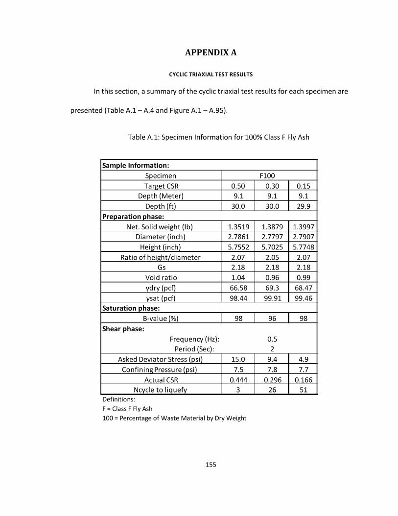
155
APPENDIX A
A. CYCLIC TRIAXIAL TEST RESULTS
In this section, a summary of the cyclic triaxial test results for each specimen are
presented (Table A.1 – A.4 and Figure A.1 – A.95).
Table A.1: Specimen Information for 100% Class F Fly Ash
Definitions:
F = Class F Fly Ash
100 = Percentage of Waste Material by Dry Weight
Sample Information:
0.50 0.30 0.15
9.1 9.1 9.1
30.0 30.0 29.9
Preparation phase:
1.3519 1.3879 1.3997
2.7861 2.7797 2.7907
5.7552 5.7025 5.7748
2.07 2.05 2.07
2.18 2.18 2.18
1.04 0.96 0.99
66.58 69.3 68.47
98.44 99.91 99.46
Saturation phase:
98 96 98
Shear phase:
0.5
2
15.0 9.4 4.9
7.5 7.8 7.7
0.444 0.296 0.166
3 26 51
Confining Pressure (psi)
Actual CSR
Ncycle to liquefy
γsat (pcf)
B-value (%)
Frequency (Hz):
Period (Sec):
Asked Deviator Stress (psi)
Height (inch)
Ratio of height/diameter
Gs
Void ratio
γdry (pcf)
Target CSR
Depth (Meter)
Depth (ft)
Net. Solid weight (lb)
Diameter (inch)
Specimen F100
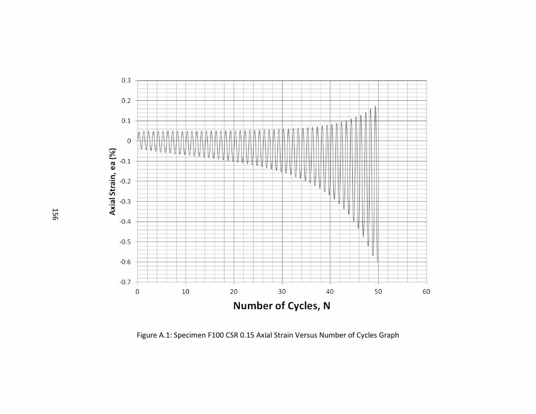
156
156
Figure A.1: Specimen F100 CSR 0.15 Axial Strain Versus Number of Cycles Graph
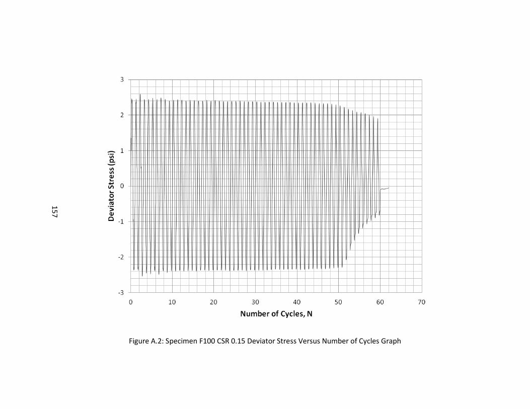
157
157
Figure A.2: Specimen F100 CSR 0.15 Deviator Stress Versus Number of Cycles Graph
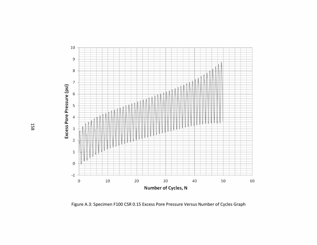
158
158
Figure A.3: Specimen F100 CSR 0.15 Excess Pore Pressure Versus Number of Cycles Graph
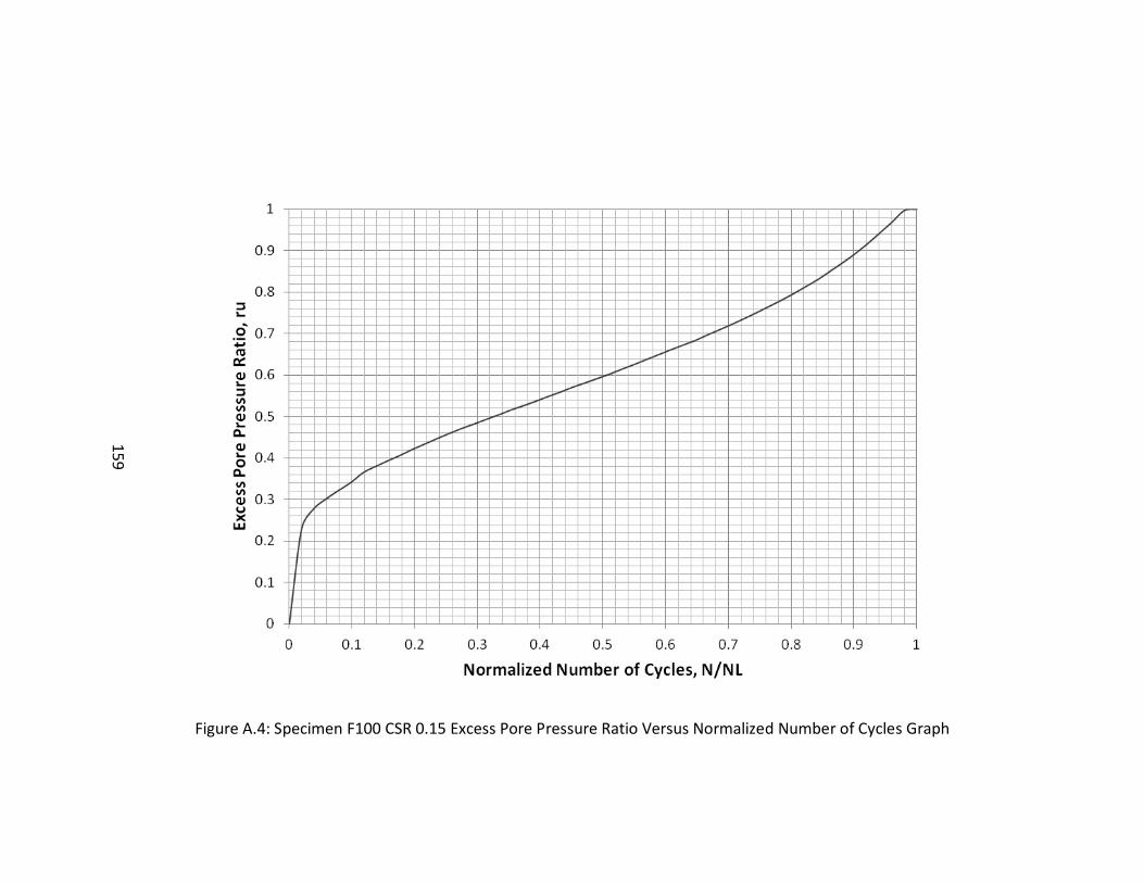
159
159
Figure A.4: Specimen F100 CSR 0.15 Excess Pore Pressure Ratio Versus Normalized Number of Cycles Graph
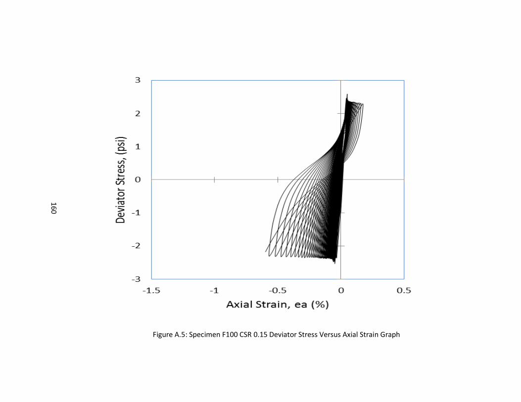
160
160
Figure A.5: Specimen F100 CSR 0.15 Deviator Stress Versus Axial Strain Graph
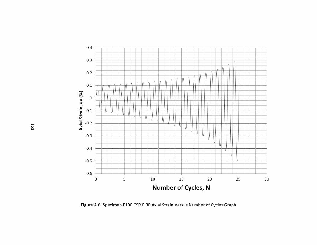
161
161
Figure A.6: Specimen F100 CSR 0.30 Axial Strain Versus Number of Cycles Graph
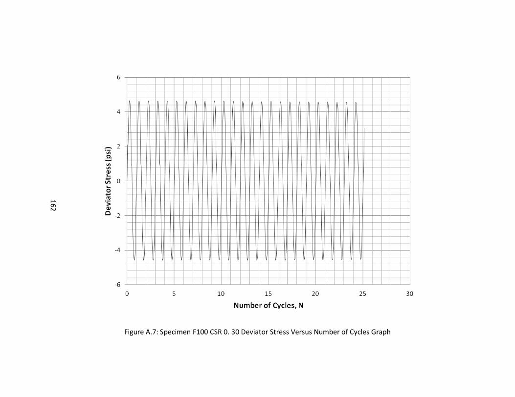
162
162
Figure A.7: Specimen F100 CSR 0. 30 Deviator Stress Versus Number of Cycles Graph
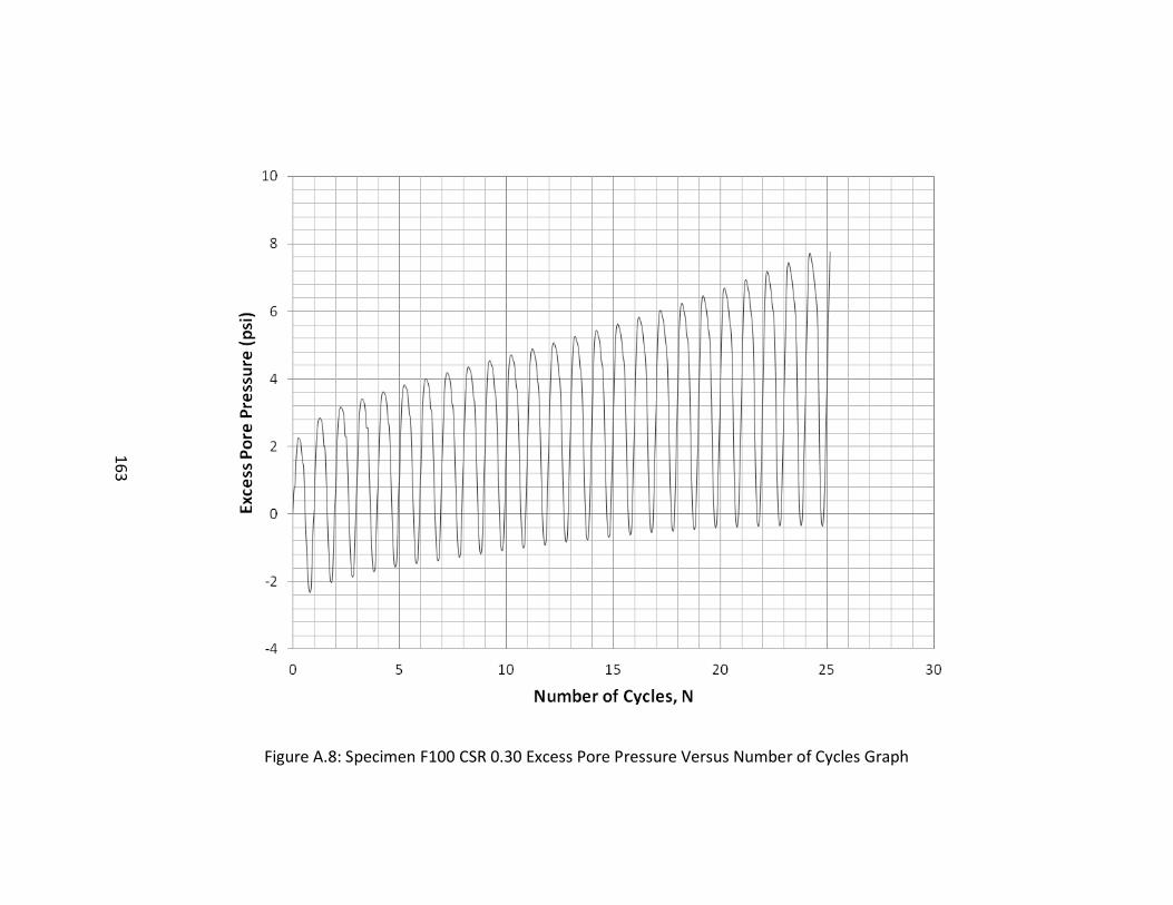
163
163
Figure A.8: Specimen F100 CSR 0.30 Excess Pore Pressure Versus Number of Cycles Graph
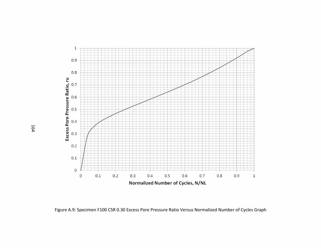
164
164
Figure A.9: Specimen F100 CSR 0.30 Excess Pore Pressure Ratio Versus Normalized Number of Cycles Graph
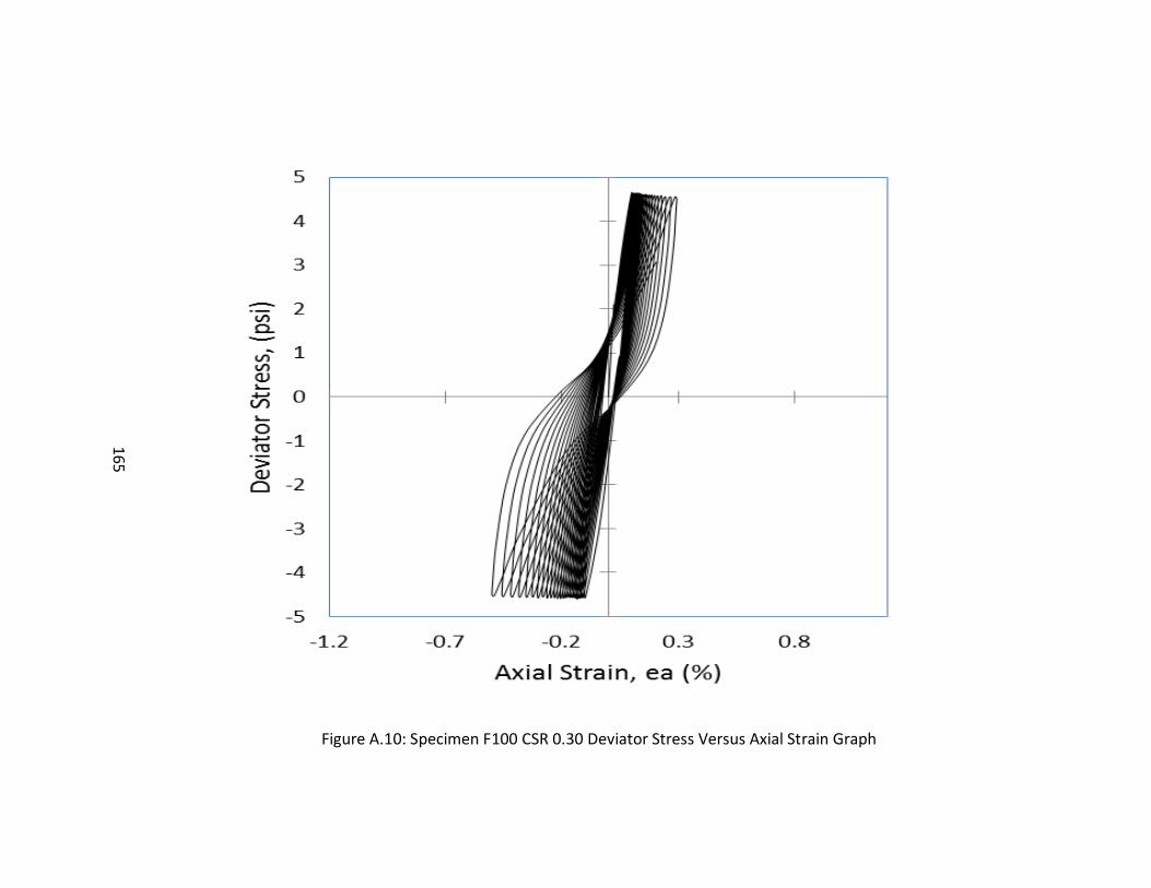
165
165
Figure A.10: Specimen F100 CSR 0.30 Deviator Stress Versus Axial Strain Graph
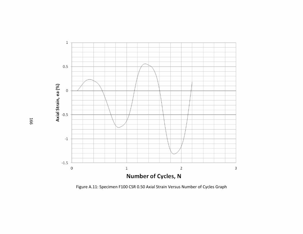
166
166
Figure A.11: Specimen F100 CSR 0.50 Axial Strain Versus Number of Cycles Graph
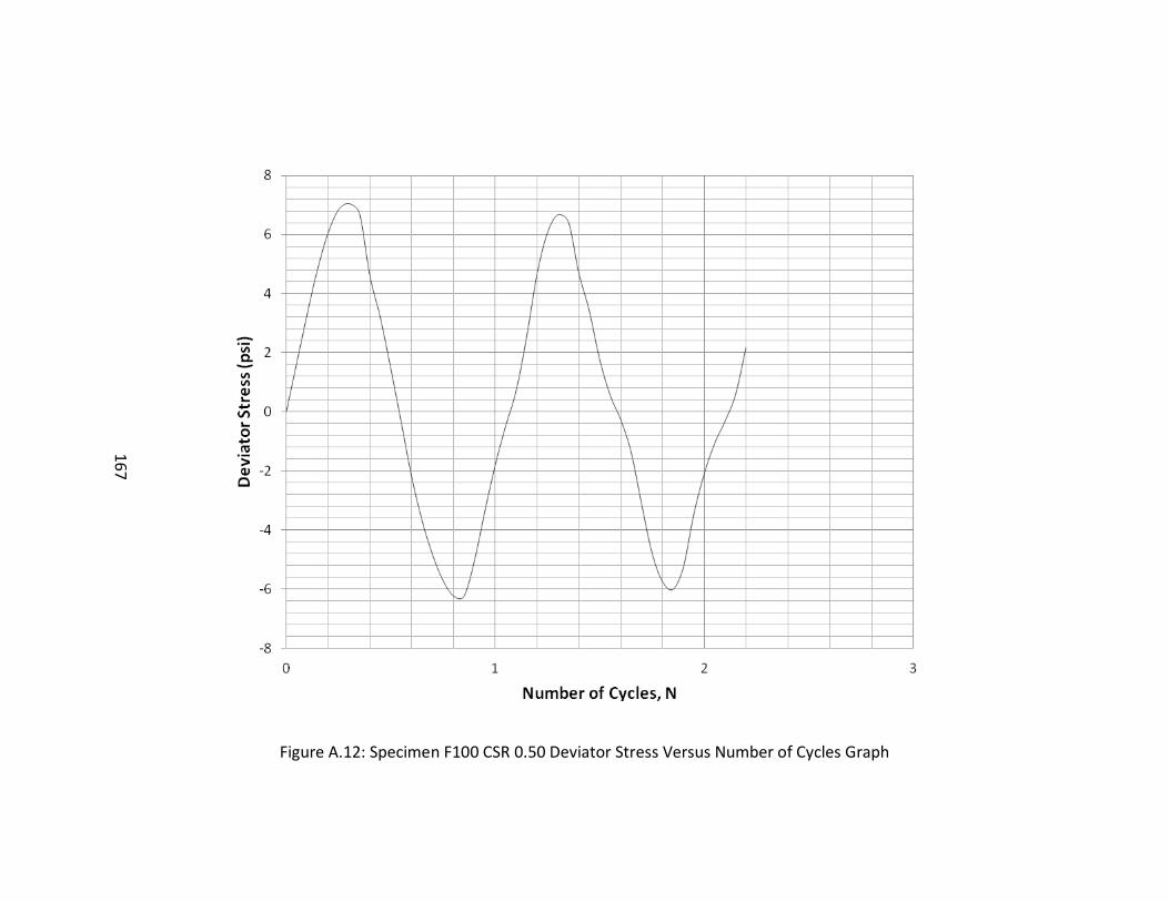
167
167
Figure A.12: Specimen F100 CSR 0.50 Deviator Stress Versus Number of Cycles Graph
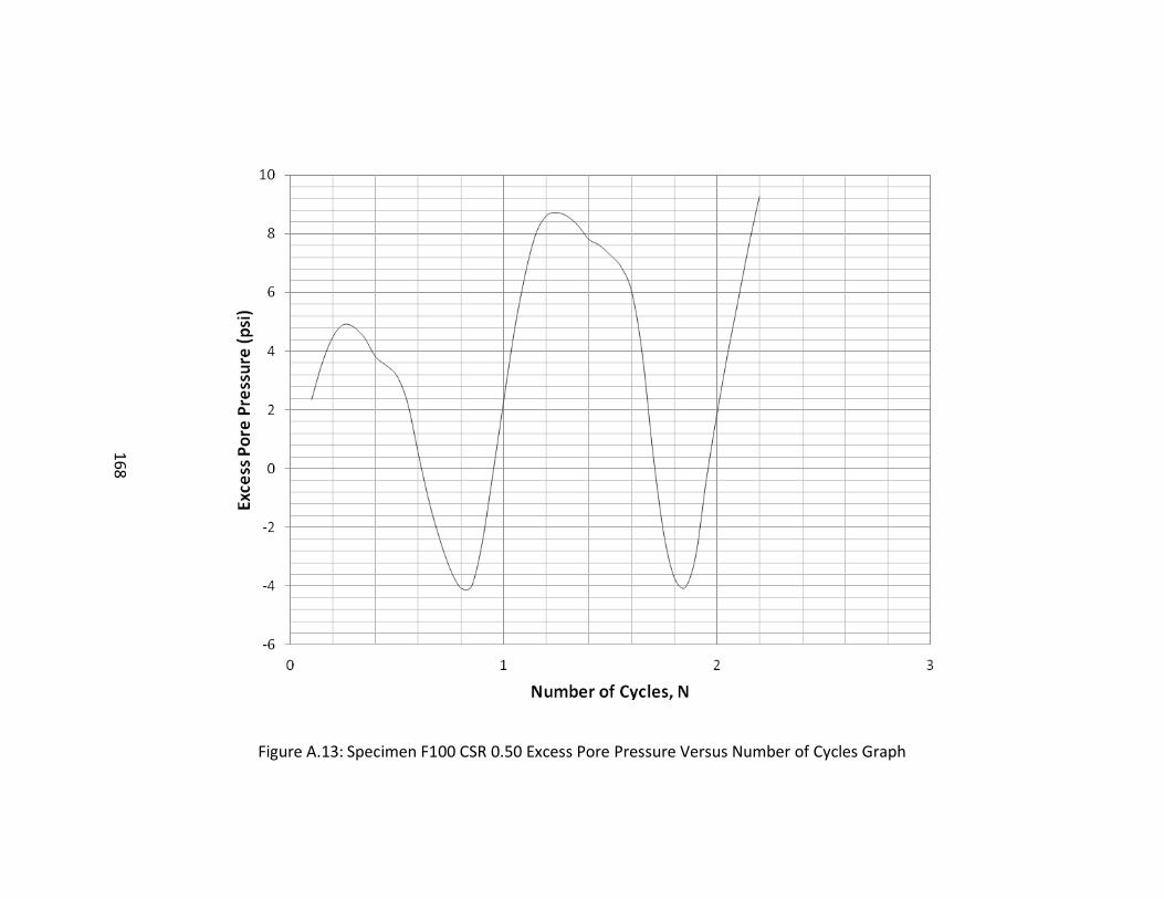
168
168
Figure A.13: Specimen F100 CSR 0.50 Excess Pore Pressure Versus Number of Cycles Graph
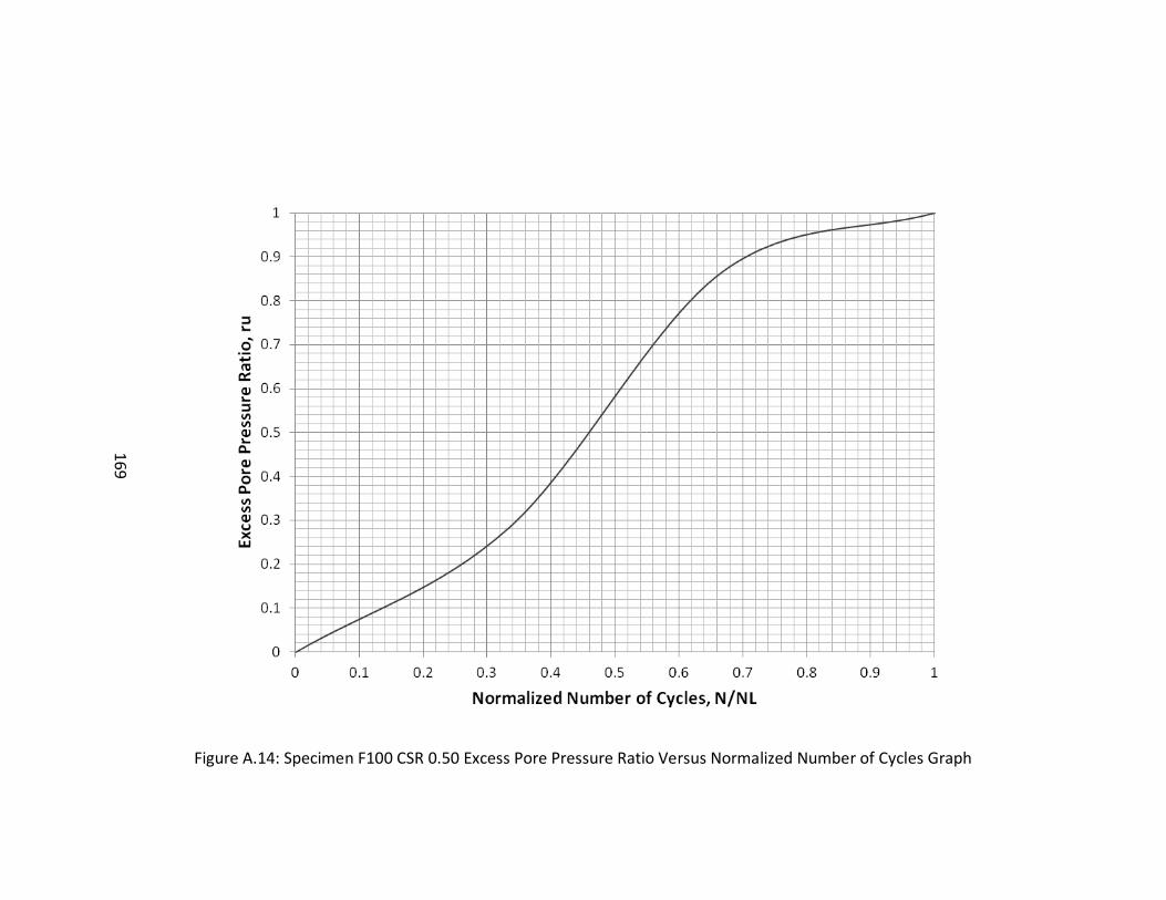
169
169
Figure A.14: Specimen F100 CSR 0.50 Excess Pore Pressure Ratio Versus Normalized Number of Cycles Graph
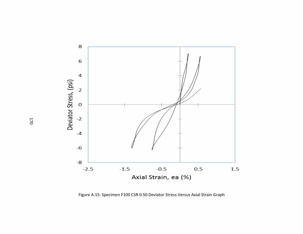
170
170
Figure A.15: Specimen F100 CSR 0.50 Deviator Stress Versus Axial Strain Graph
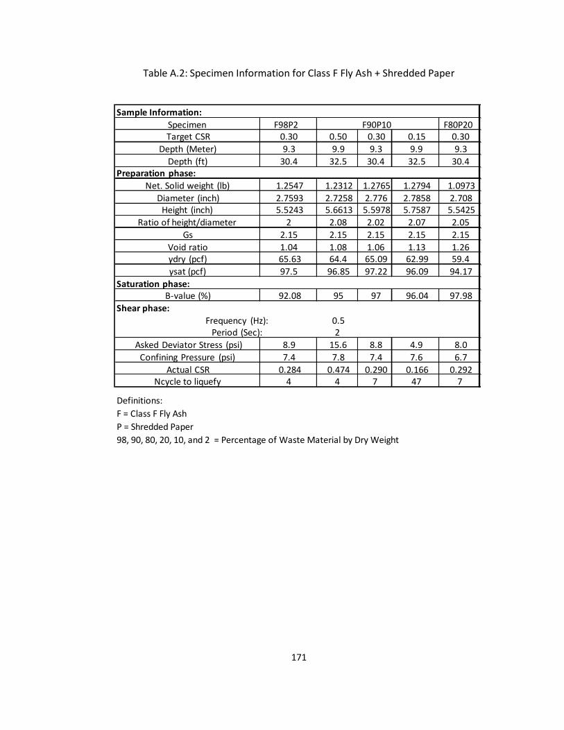
171
Table A.2: Specimen Information for Class F Fly Ash + Shredded Paper
Definitions:
F = Class F Fly Ash
P = Shredded Paper
98, 90, 80, 20, 10, and 2 = Percentage of Waste Material by Dry Weight
Sample Information:
F98P2 F80P200.30 0.50 0.30 0.15 0.30
9.3 9.9 9.3 9.9 9.3
30.4 32.5 30.4 32.5 30.4Preparation phase:
1.2547 1.2312 1.2765 1.2794 1.0973
2.7593 2.7258 2.776 2.7858 2.7085.5243 5.6613 5.5978 5.7587 5.5425
2 2.08 2.02 2.07 2.05
2.15 2.15 2.15 2.15 2.15
1.04 1.08 1.06 1.13 1.2665.63 64.4 65.09 62.99 59.4
97.5 96.85 97.22 96.09 94.17
Saturation phase:92.08 95 97 96.04 97.98
Shear phase:
0.52
8.9 15.6 8.8 4.9 8.0
7.4 7.8 7.4 7.6 6.7
0.284 0.474 0.290 0.166 0.2924 4 7 47 7
Confining Pressure (psi)
Actual CSRNcycle to liquefy
F90P10
γsat (pcf)
B-value (%)
Frequency (Hz):Period (Sec):
Asked Deviator Stress (psi)
Height (inch)
Ratio of height/diameter
Gs
Void ratioγdry (pcf)
Target CSR
Depth (Meter)
Depth (ft)
Net. Solid weight (lb)
Diameter (inch)
Specimen
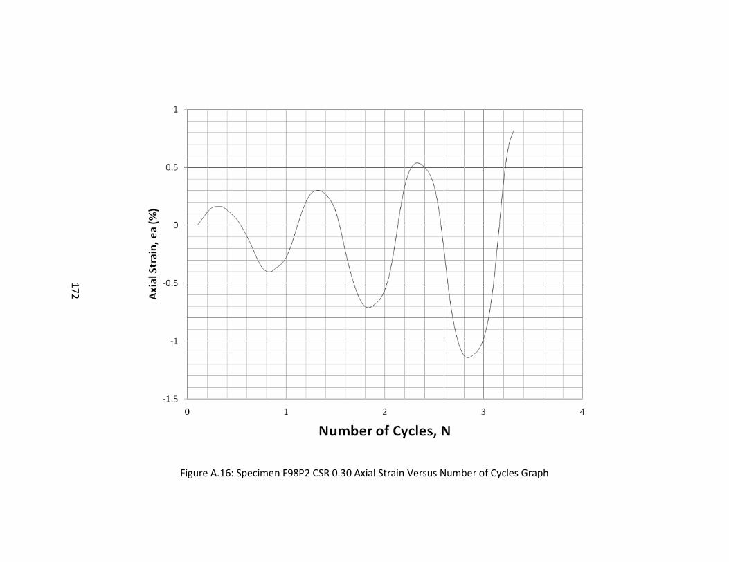
172
Figure A.16: Specimen F98P2 CSR 0.30 Axial Strain Versus Number of Cycles Graph
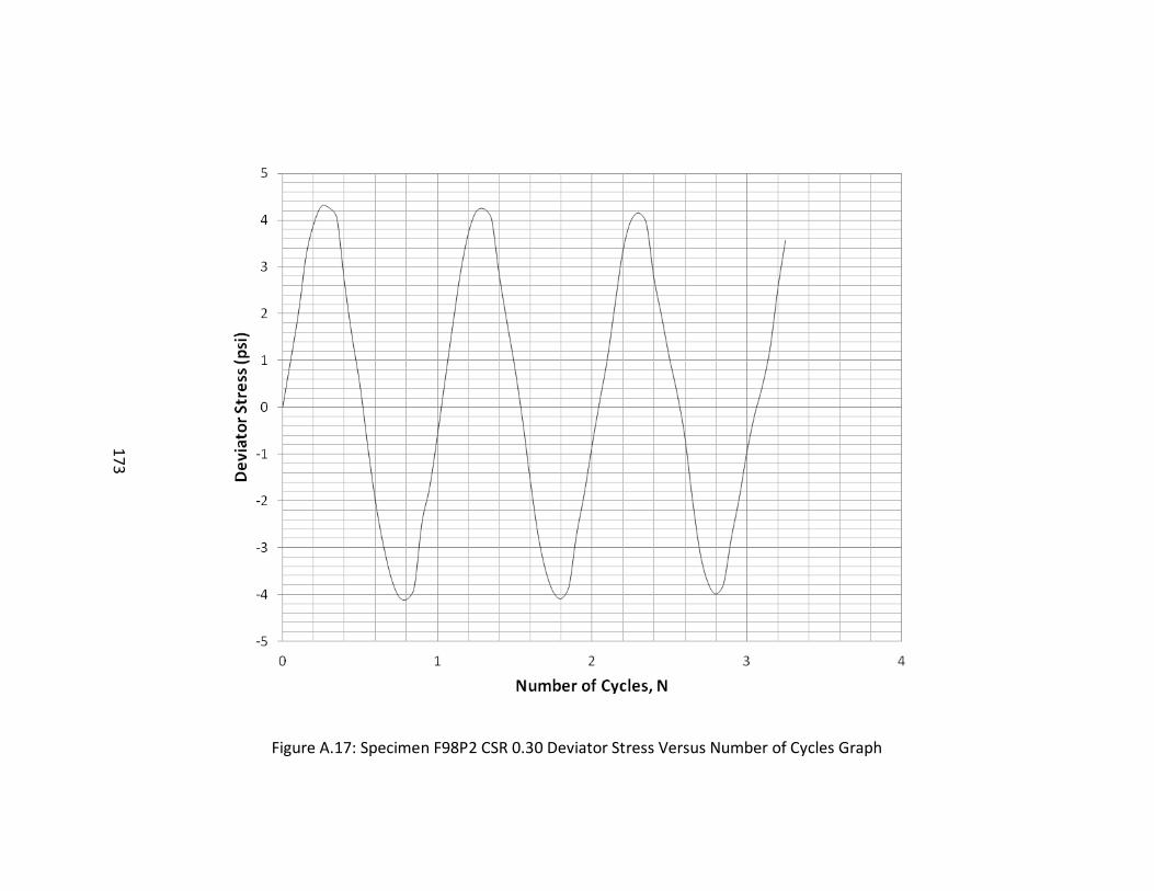
173
Figure A.17: Specimen F98P2 CSR 0.30 Deviator Stress Versus Number of Cycles Graph
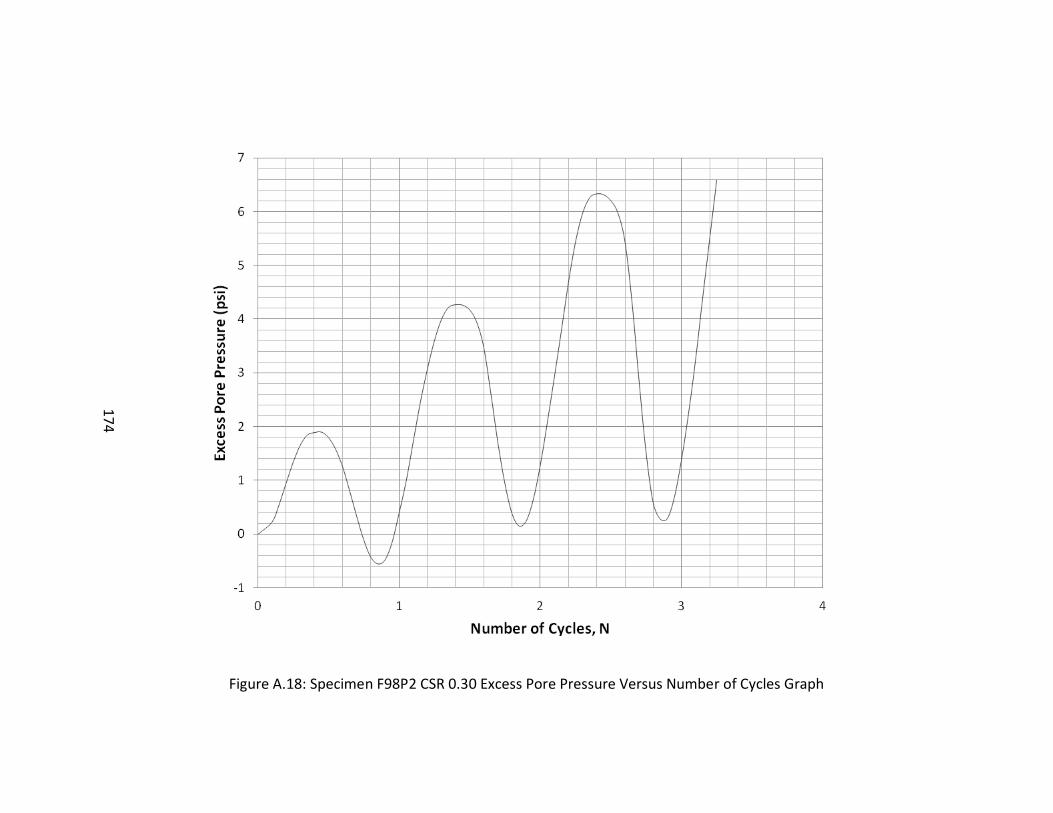
174
Figure A.18: Specimen F98P2 CSR 0.30 Excess Pore Pressure Versus Number of Cycles Graph
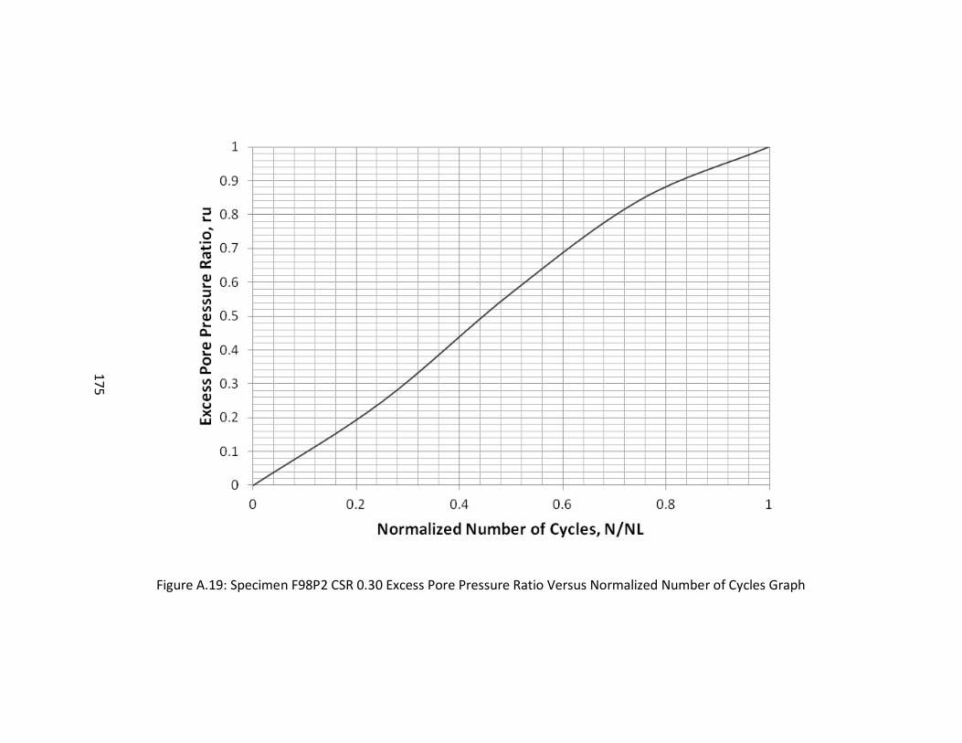
175
Figure A.19: Specimen F98P2 CSR 0.30 Excess Pore Pressure Ratio Versus Normalized Number of Cycles Graph
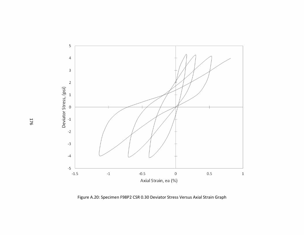
176
Figure A.20: Specimen F98P2 CSR 0.30 Deviator Stress Versus Axial Strain Graph
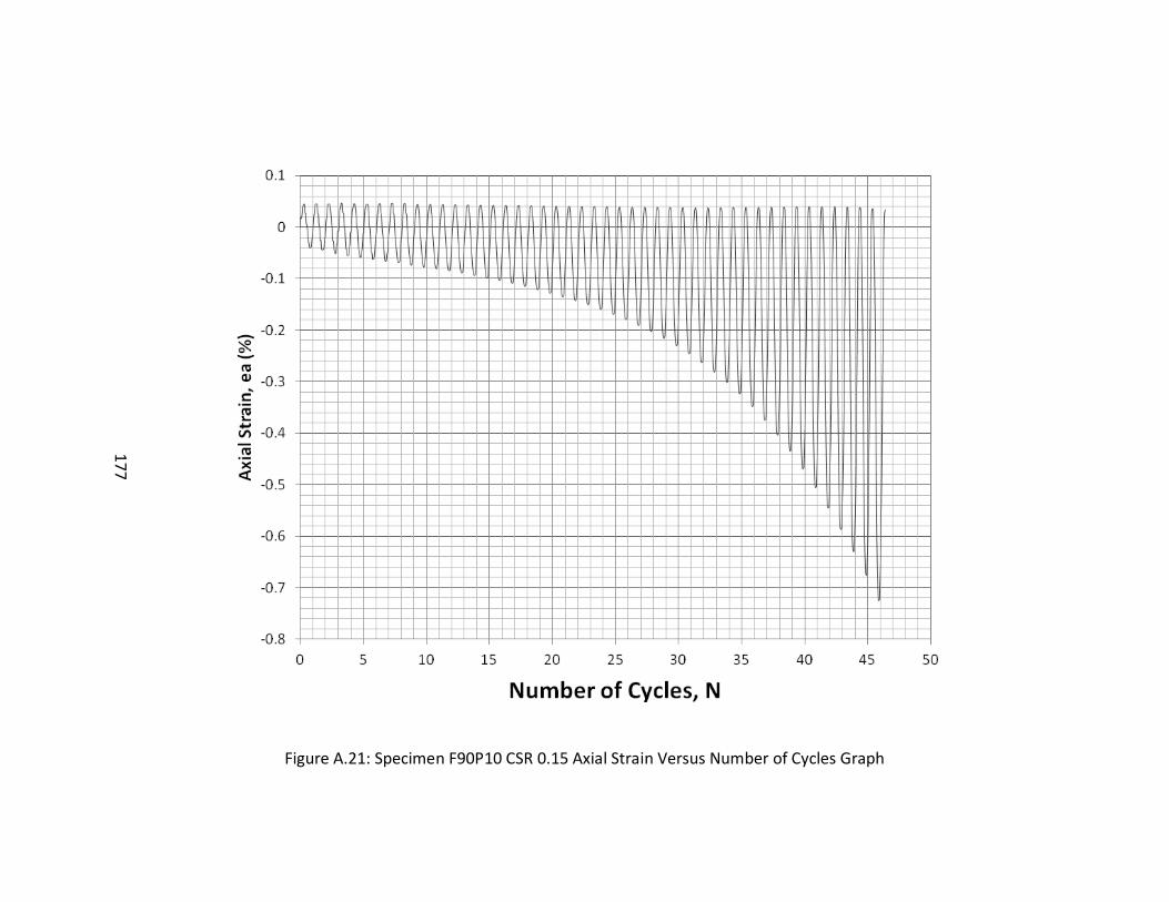
177
Figure A.21: Specimen F90P10 CSR 0.15 Axial Strain Versus Number of Cycles Graph
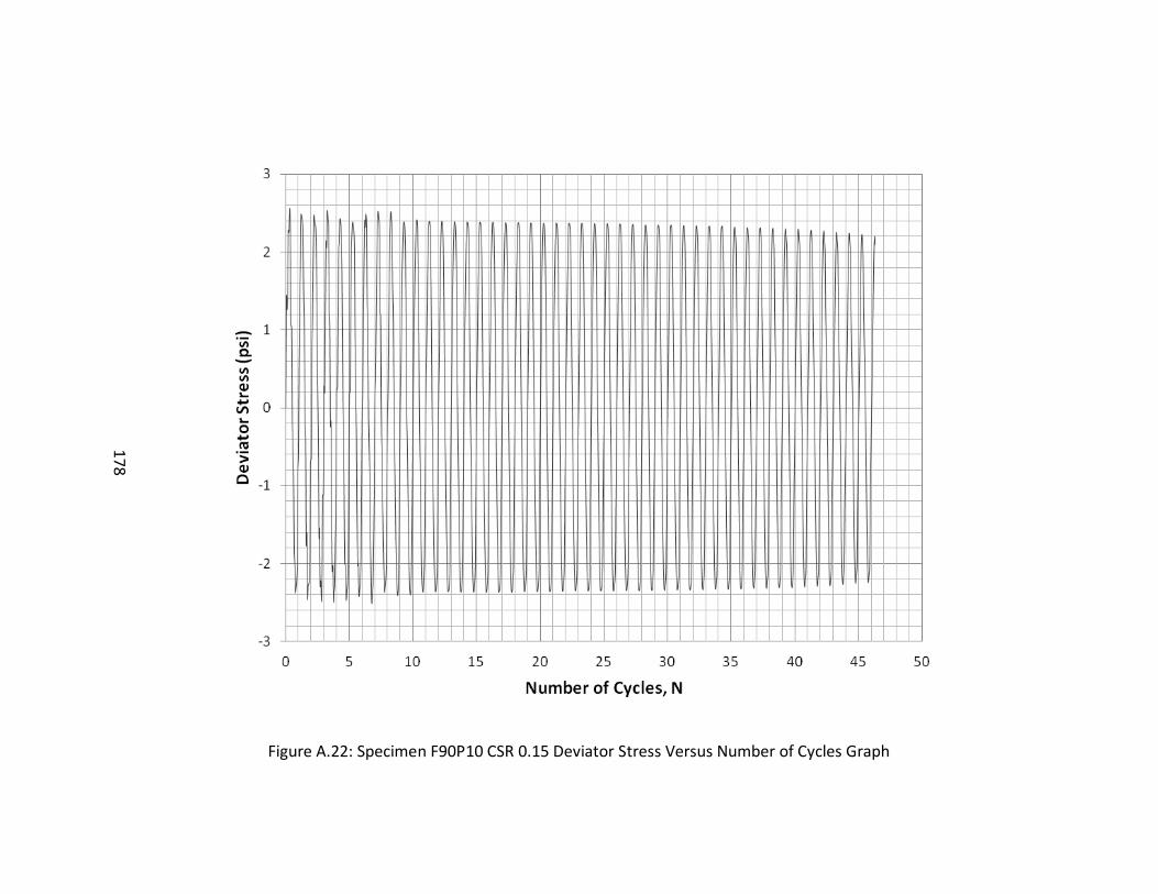
178
Figure A.22: Specimen F90P10 CSR 0.15 Deviator Stress Versus Number of Cycles Graph
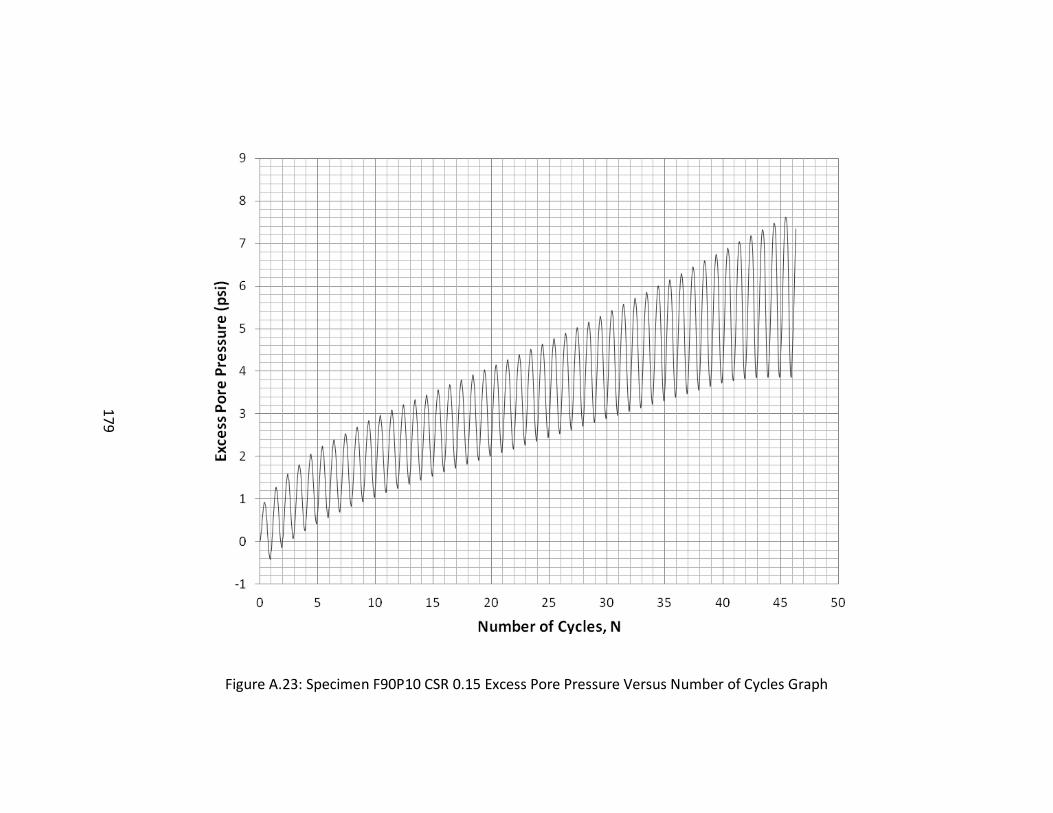
179
Figure A.23: Specimen F90P10 CSR 0.15 Excess Pore Pressure Versus Number of Cycles Graph
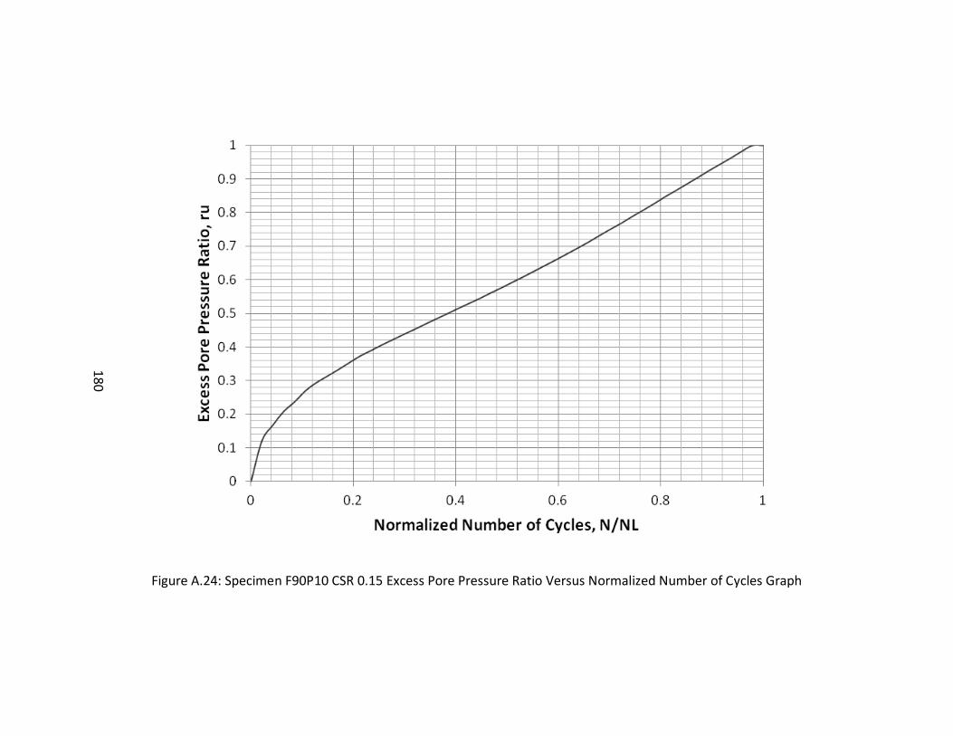
180
Figure A.24: Specimen F90P10 CSR 0.15 Excess Pore Pressure Ratio Versus Normalized Number of Cycles Graph
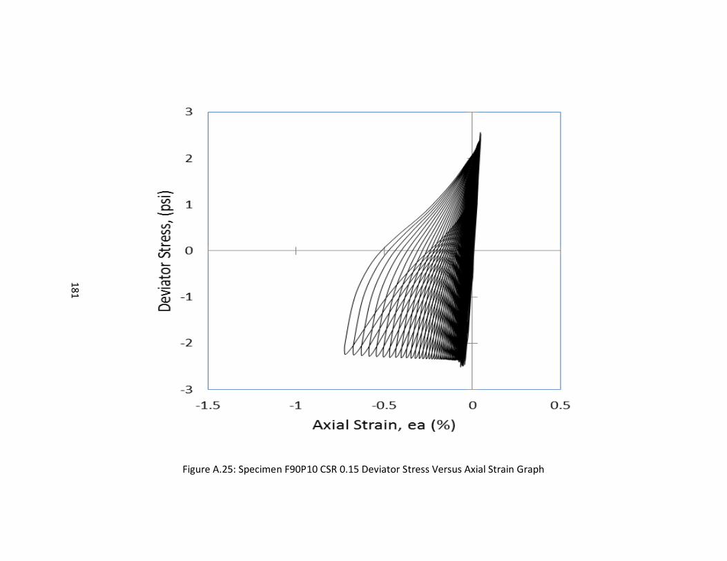
181
Figure A.25: Specimen F90P10 CSR 0.15 Deviator Stress Versus Axial Strain Graph
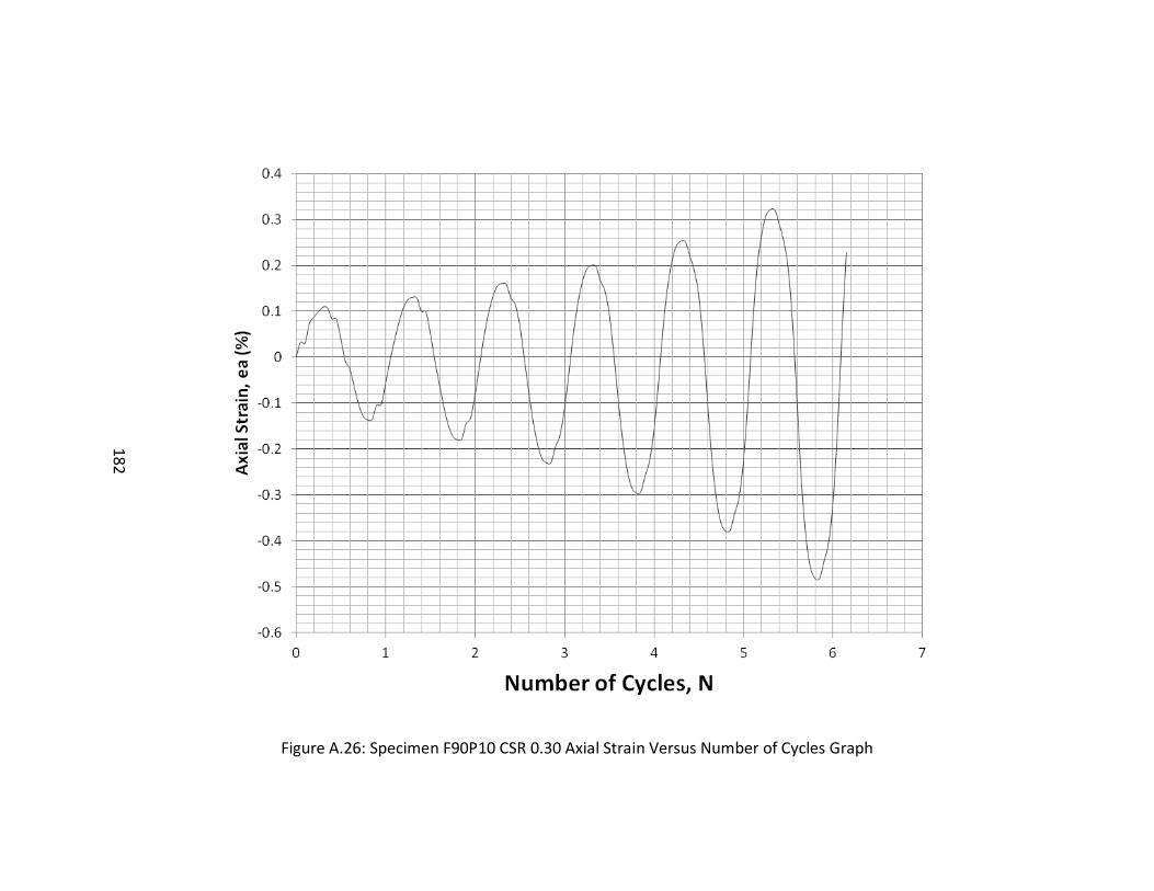
182
Figure A.26: Specimen F90P10 CSR 0.30 Axial Strain Versus Number of Cycles Graph
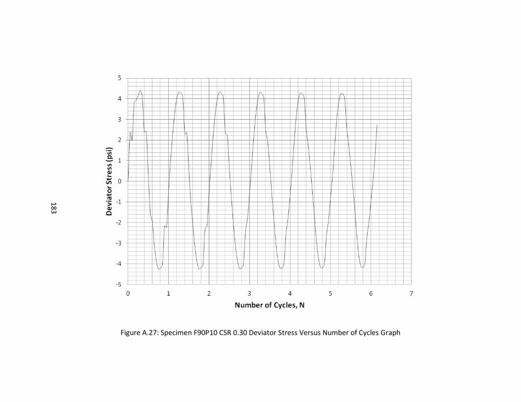
183
Figure A.27: Specimen F90P10 CSR 0.30 Deviator Stress Versus Number of Cycles Graph
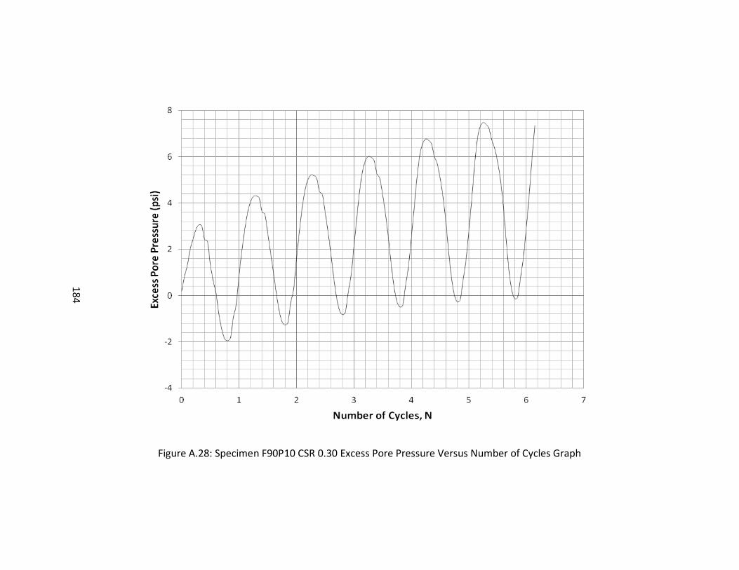
184
Figure A.28: Specimen F90P10 CSR 0.30 Excess Pore Pressure Versus Number of Cycles Graph
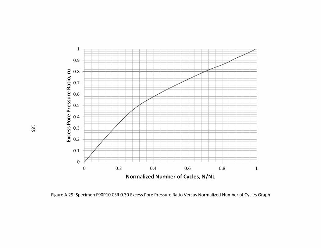
185
Figure A.29: Specimen F90P10 CSR 0.30 Excess Pore Pressure Ratio Versus Normalized Number of Cycles Graph
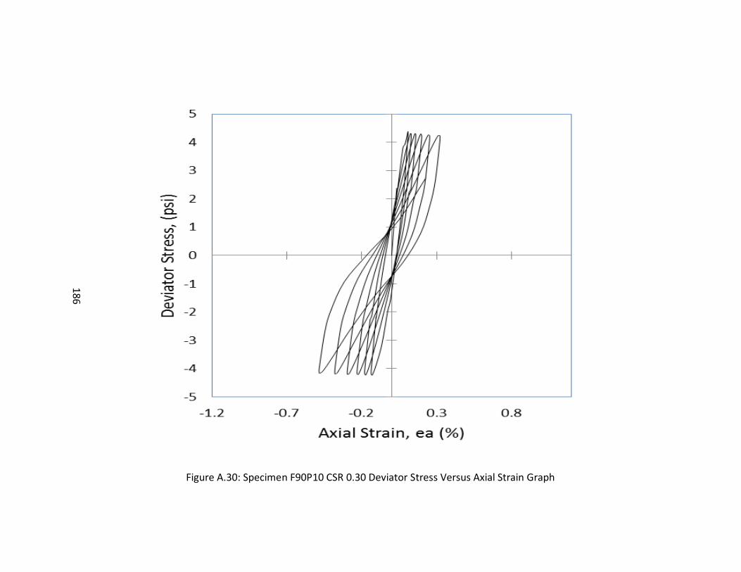
186
Figure A.30: Specimen F90P10 CSR 0.30 Deviator Stress Versus Axial Strain Graph

187
Figure A.31: Specimen F90P10 CSR 0.50 Axial Strain Versus Number of Cycles Graph
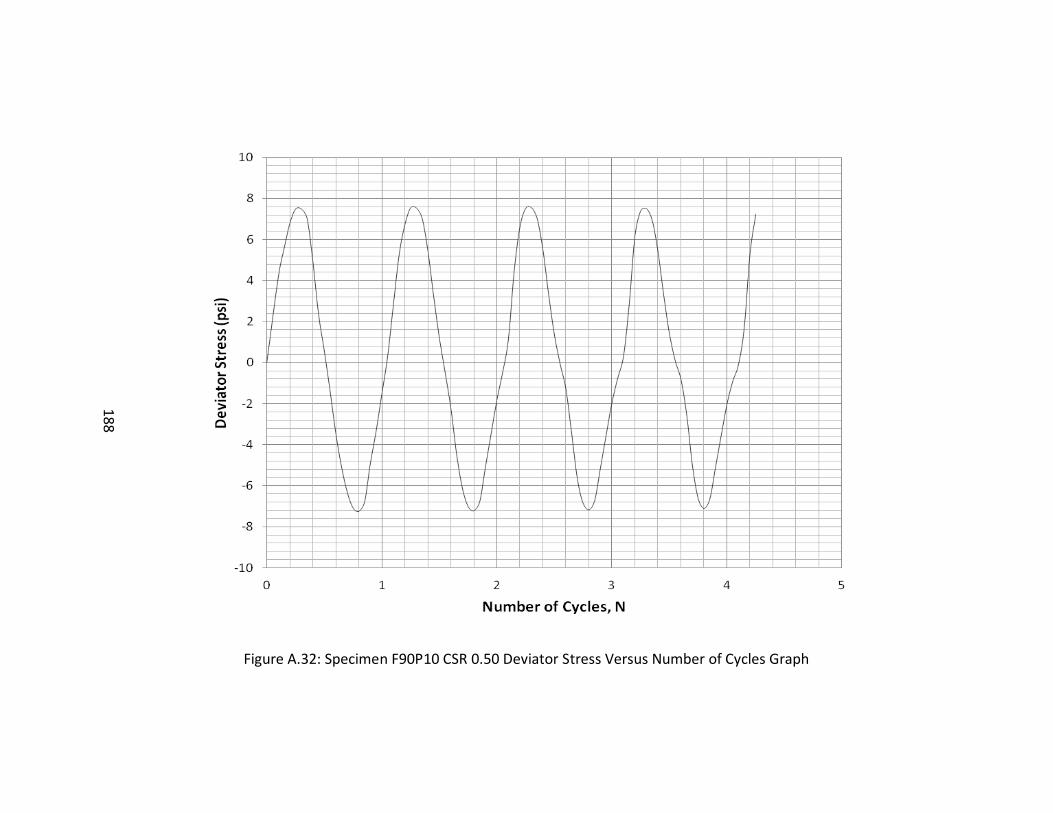
188
Figure A.32: Specimen F90P10 CSR 0.50 Deviator Stress Versus Number of Cycles Graph
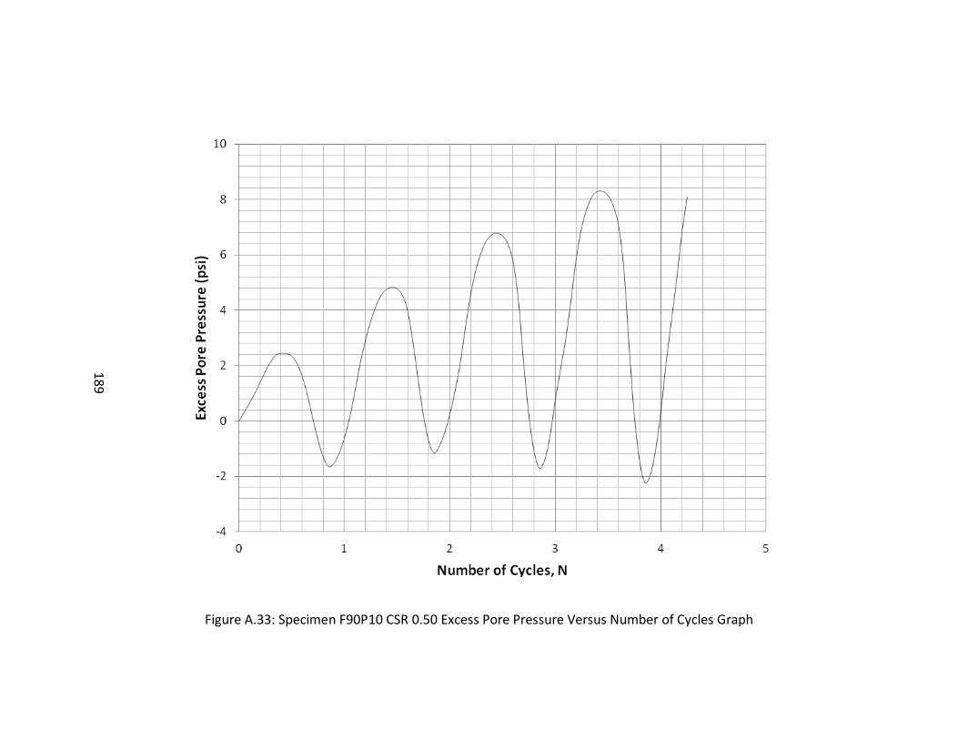
189
Figure A.33: Specimen F90P10 CSR 0.50 Excess Pore Pressure Versus Number of Cycles Graph
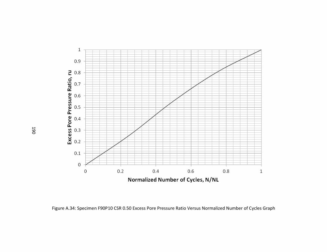
190
Figure A.34: Specimen F90P10 CSR 0.50 Excess Pore Pressure Ratio Versus Normalized Number of Cycles Graph
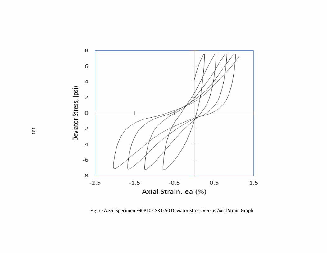
191
Figure A.35: Specimen F90P10 CSR 0.50 Deviator Stress Versus Axial Strain Graph
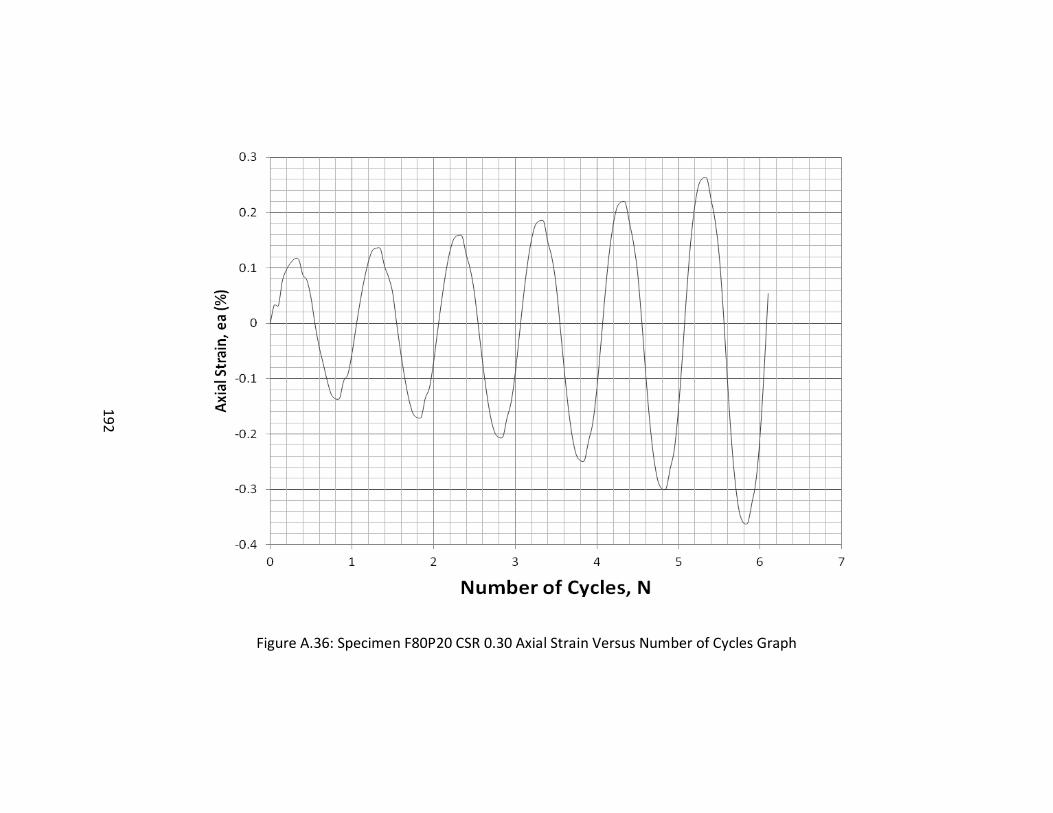
192
Figure A.36: Specimen F80P20 CSR 0.30 Axial Strain Versus Number of Cycles Graph

193
Figure A.37: Specimen F80P20 CSR 0.30 Deviator Stress Versus Number of Cycles Graph
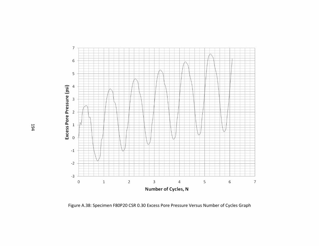
194
Figure A.38: Specimen F80P20 CSR 0.30 Excess Pore Pressure Versus Number of Cycles Graph
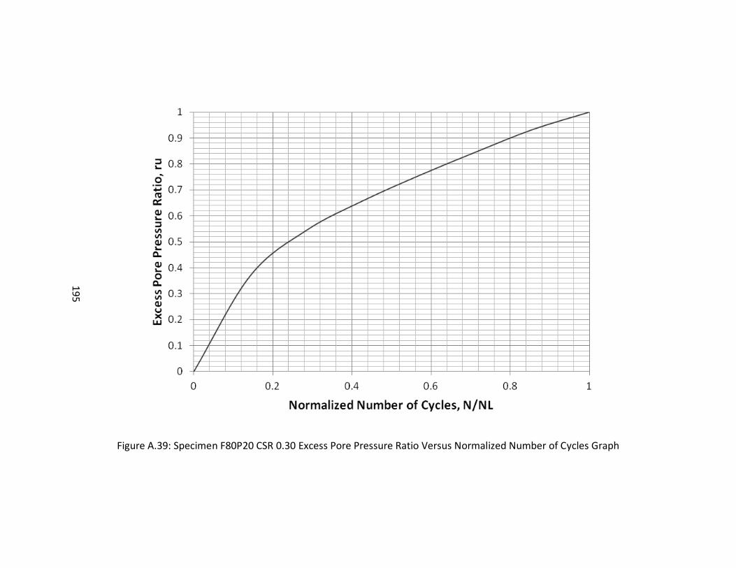
195
Figure A.39: Specimen F80P20 CSR 0.30 Excess Pore Pressure Ratio Versus Normalized Number of Cycles Graph
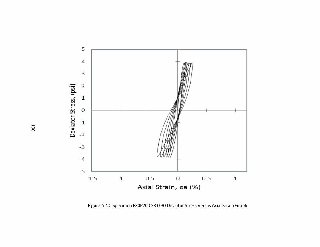
196
Figure A.40: Specimen F80P20 CSR 0.30 Deviator Stress Versus Axial Strain Graph
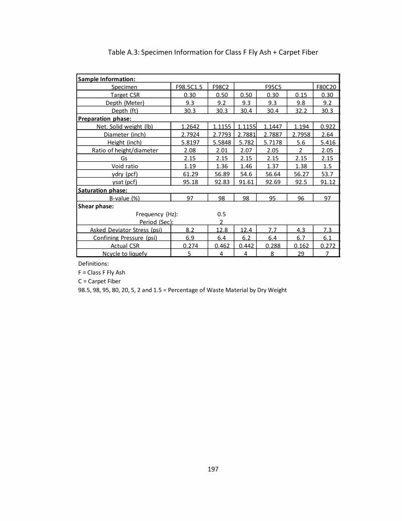
197
Table A.3: Specimen Information for Class F Fly Ash + Carpet Fiber
Definitions:
F = Class F Fly Ash
C = Carpet Fiber
98.5, 98, 95, 80, 20, 5, 2 and 1.5 = Percentage of Waste Material by Dry Weight
Sample Information:F98.5C1.5 F98C2 F80C20
0.30 0.50 0.50 0.30 0.15 0.309.3 9.2 9.3 9.3 9.8 9.2
30.3 30.3 30.4 30.4 32.2 30.3Preparation phase:
1.2642 1.1155 1.1155 1.1447 1.194 0.9222.7924 2.7793 2.7881 2.7887 2.7958 2.645.8197 5.5848 5.782 5.7178 5.6 5.4162.08 2.01 2.07 2.05 2 2.052.15 2.15 2.15 2.15 2.15 2.151.19 1.36 1.46 1.37 1.38 1.561.29 56.89 54.6 56.64 56.27 53.795.18 92.83 91.61 92.69 92.5 91.12
Saturation phase:97 98 98 95 96 97
Shear phase:0.52
8.2 12.8 12.4 7.7 4.3 7.36.9 6.4 6.2 6.4 6.7 6.1
0.274 0.462 0.442 0.288 0.162 0.2725 4 4 8 29 7
Confining Pressure (psi)Actual CSR
Ncycle to liquefy
γsat (pcf)
B-value (%)
Frequency (Hz):Period (Sec):
Asked Deviator Stress (psi)
Height (inch)Ratio of height/diameter
GsVoid ratioγdry (pcf)
Target CSRDepth (Meter)
Depth (ft)
Net. Solid weight (lb)Diameter (inch)
Specimen F95C5

198
Figure A.41: Specimen F98.5C1.5 CSR 0.30 Axial Strain Versus Number of Cycles Graph
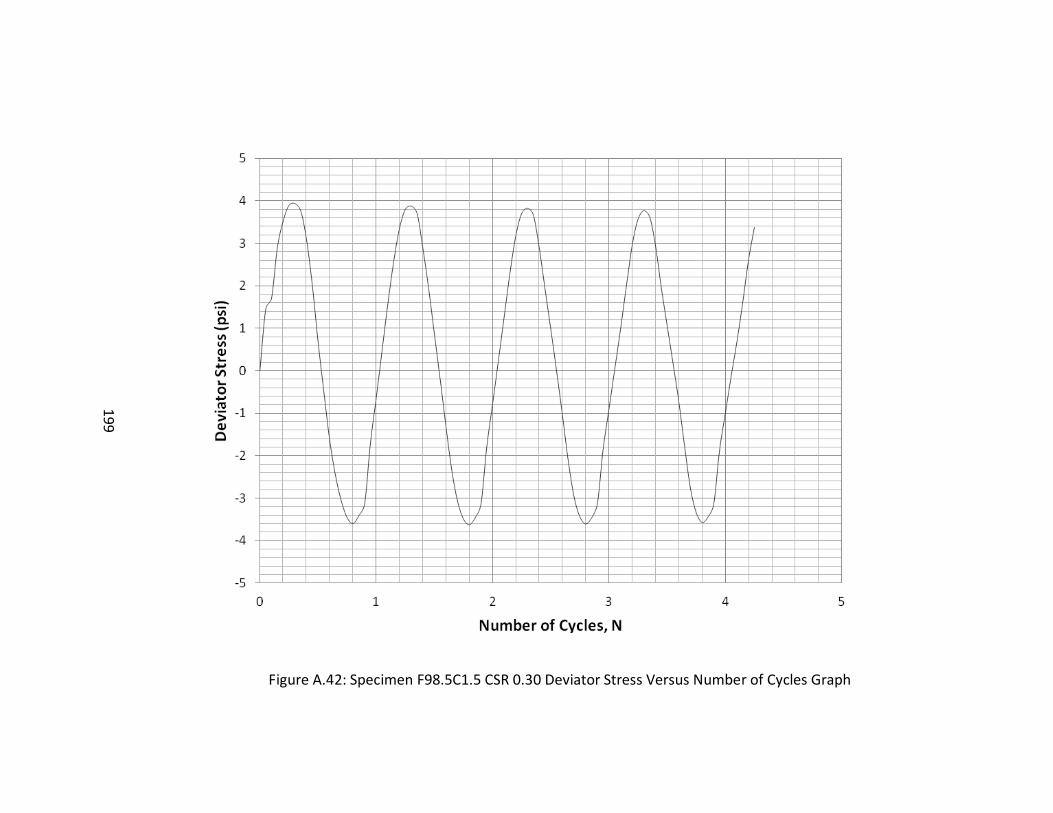
199
Figure A.42: Specimen F98.5C1.5 CSR 0.30 Deviator Stress Versus Number of Cycles Graph
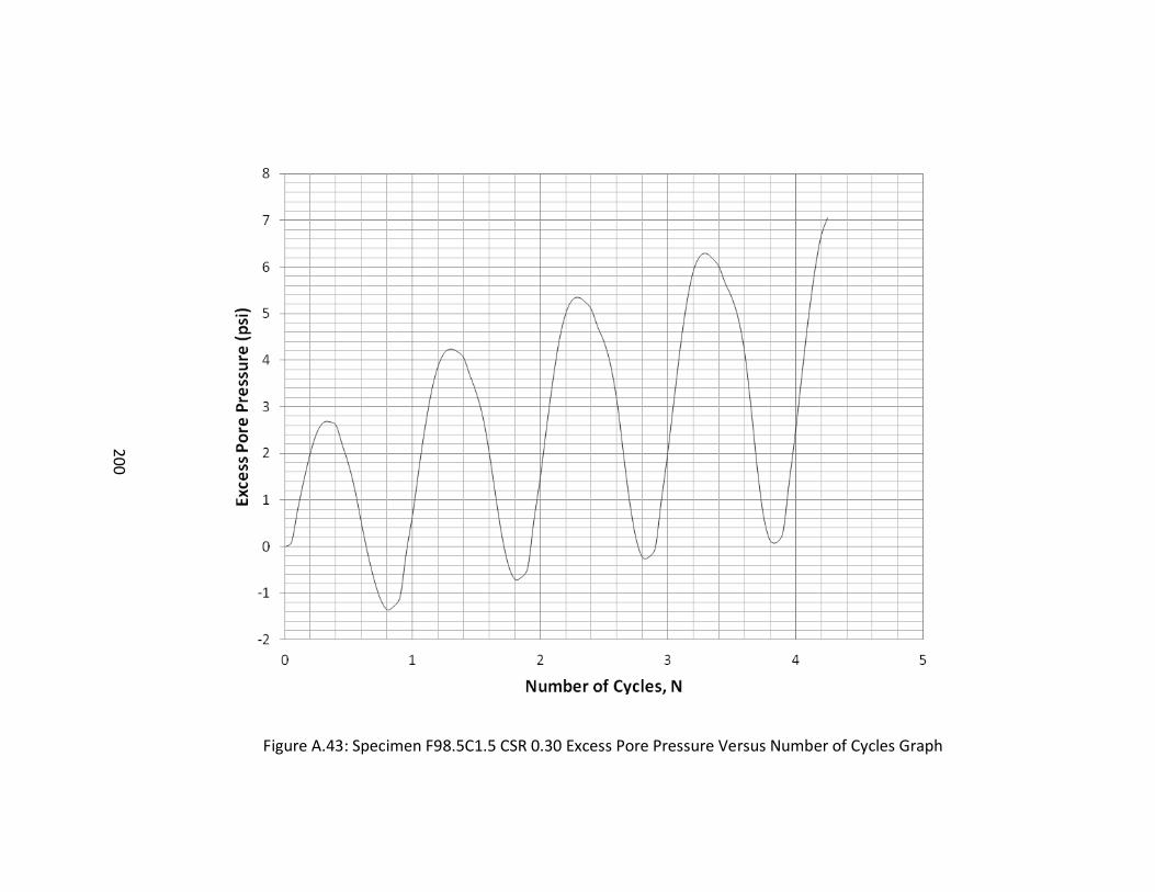
200
Figure A.43: Specimen F98.5C1.5 CSR 0.30 Excess Pore Pressure Versus Number of Cycles Graph
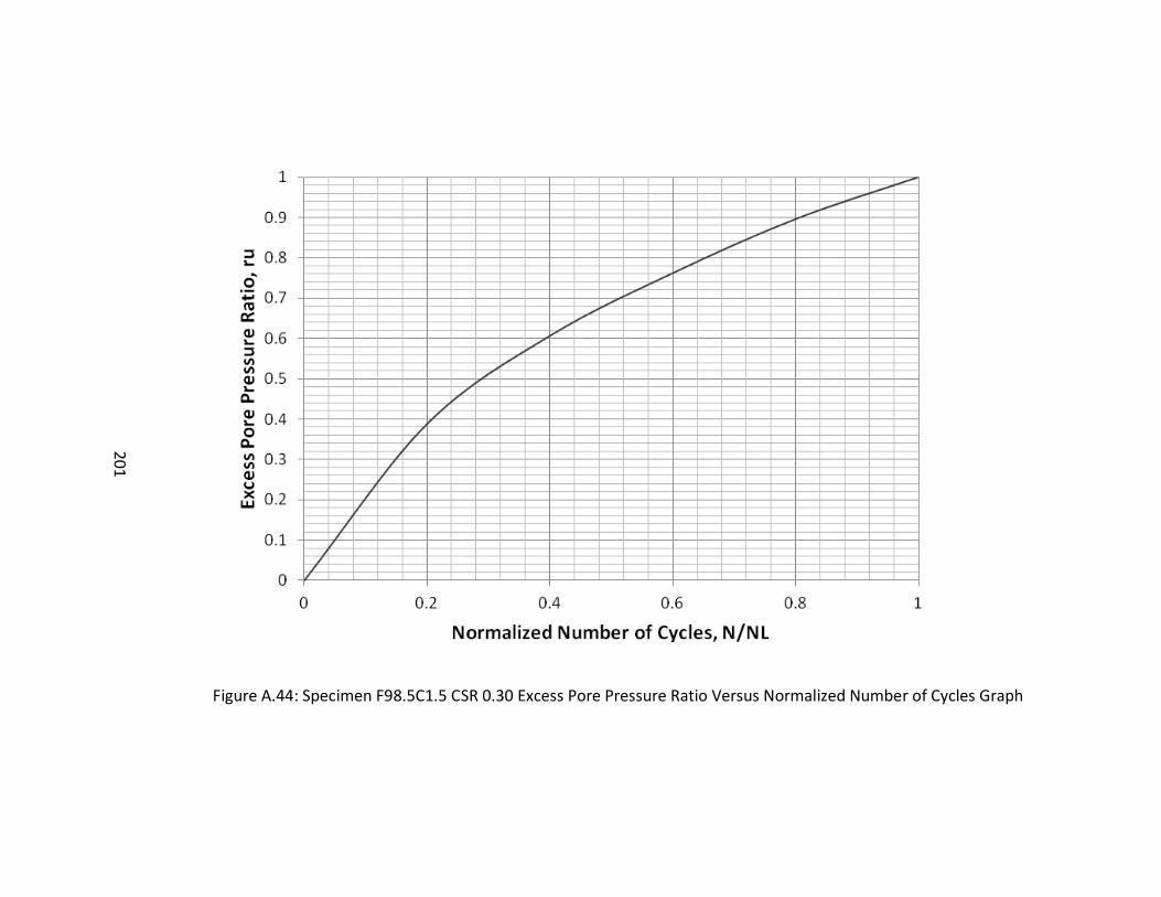
201
Figure A.44: Specimen F98.5C1.5 CSR 0.30 Excess Pore Pressure Ratio Versus Normalized Number of Cycles Graph
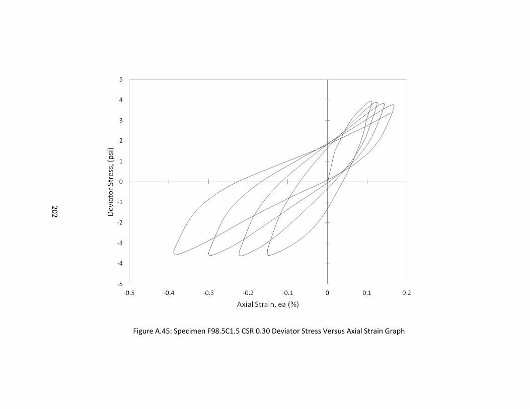
202
Figure A.45: Specimen F98.5C1.5 CSR 0.30 Deviator Stress Versus Axial Strain Graph
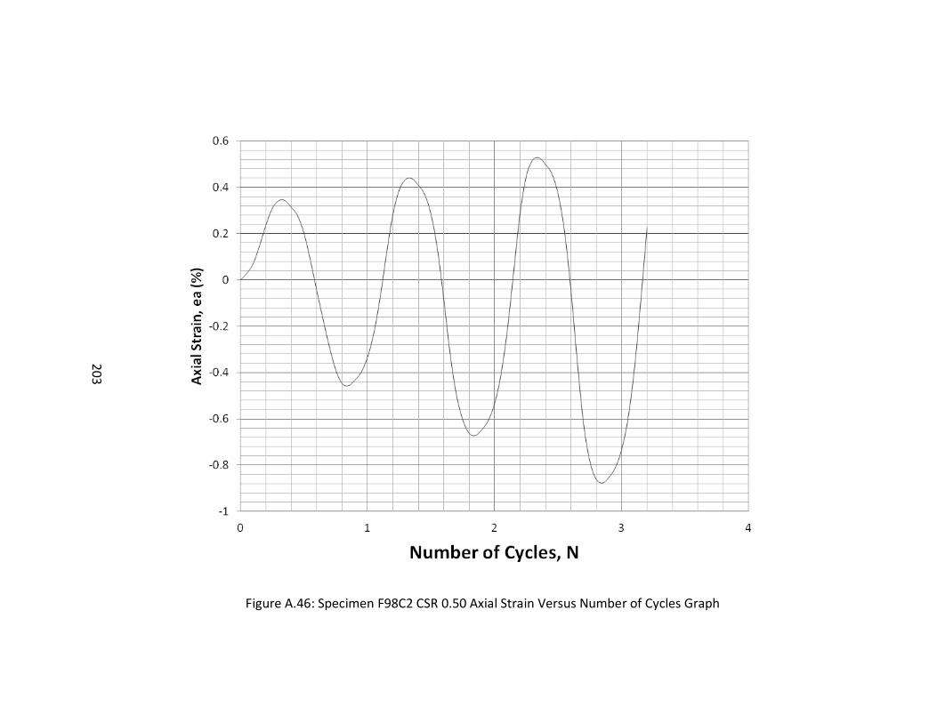
203
Figure A.46: Specimen F98C2 CSR 0.50 Axial Strain Versus Number of Cycles Graph
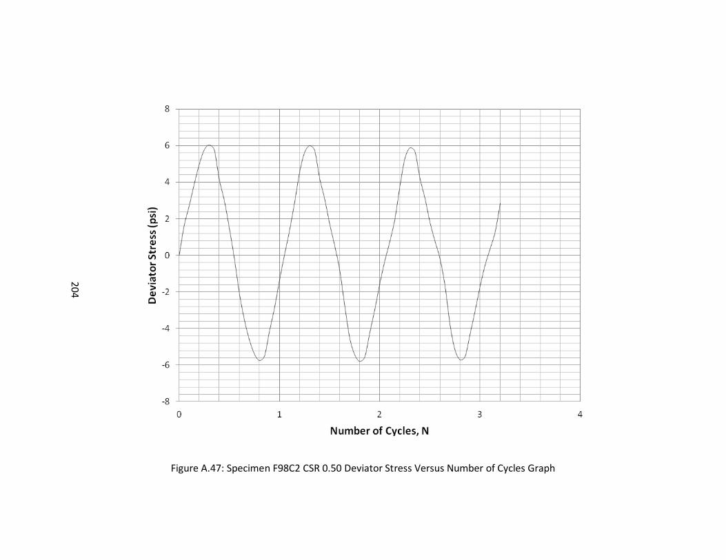
204
Figure A.47: Specimen F98C2 CSR 0.50 Deviator Stress Versus Number of Cycles Graph
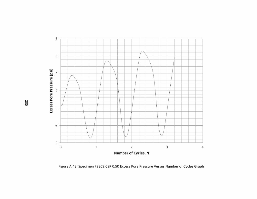
205
Figure A.48: Specimen F98C2 CSR 0.50 Excess Pore Pressure Versus Number of Cycles Graph

206
Figure A.49: Specimen F98C2 CSR 0.50 Excess Pore Pressure Ratio Versus Normalized Number of Cycles Graph
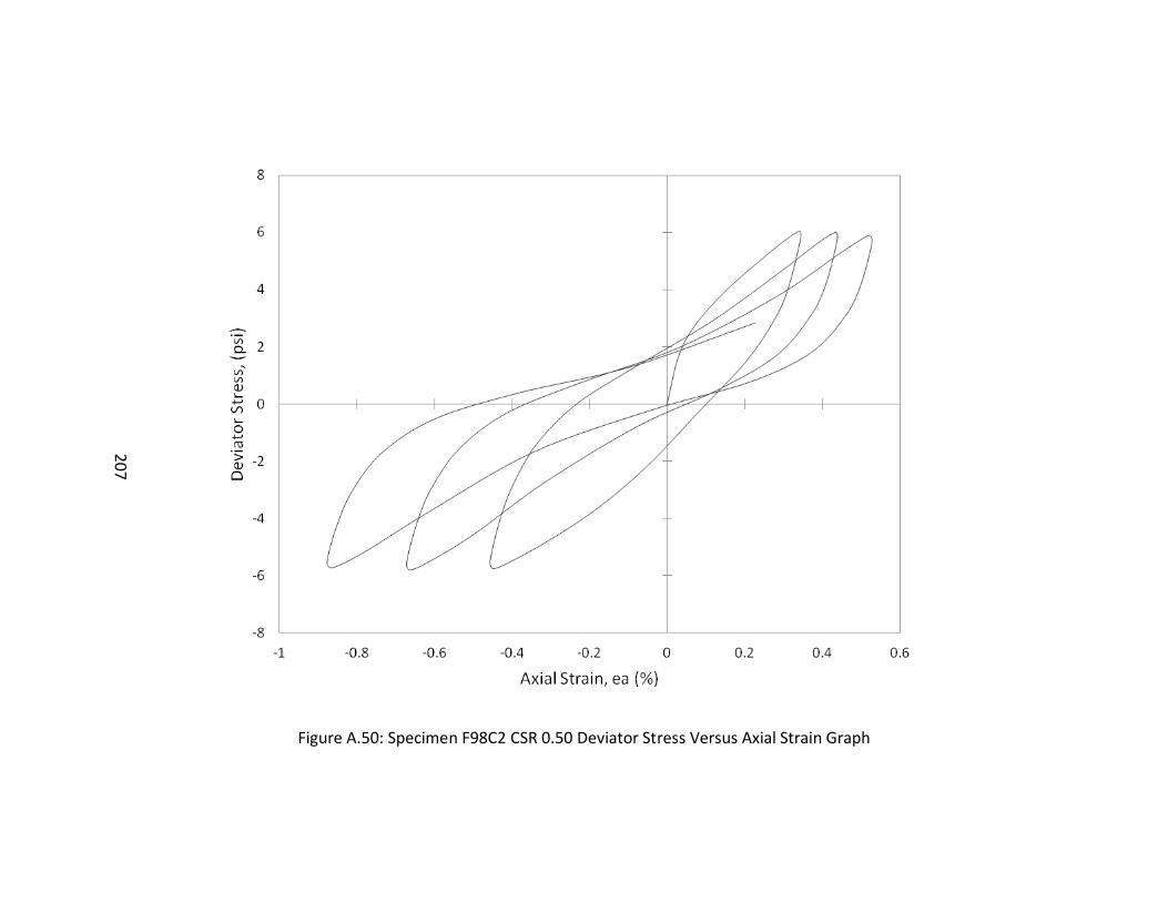
207
Figure A.50: Specimen F98C2 CSR 0.50 Deviator Stress Versus Axial Strain Graph
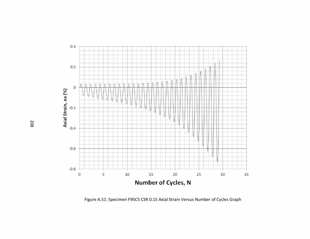
208
Figure A.51: Specimen F95C5 CSR 0.15 Axial Strain Versus Number of Cycles Graph
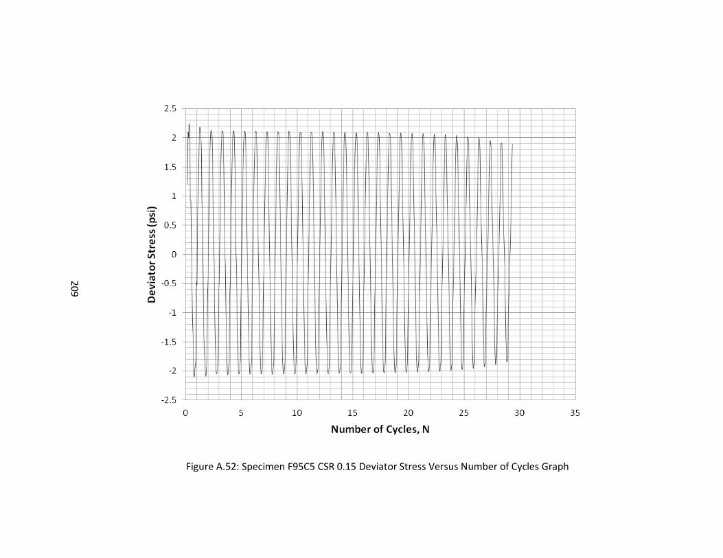
209
Figure A.52: Specimen F95C5 CSR 0.15 Deviator Stress Versus Number of Cycles Graph
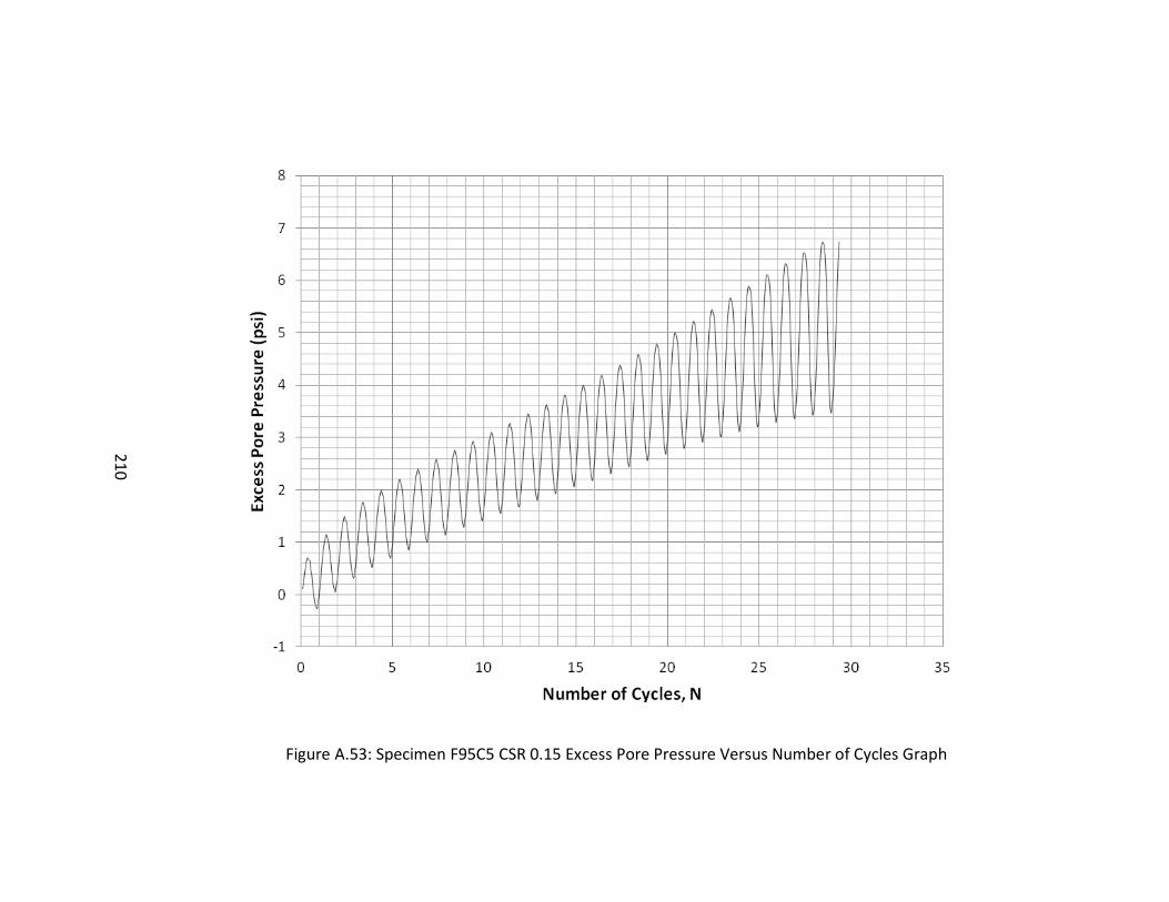
210
Figure A.53: Specimen F95C5 CSR 0.15 Excess Pore Pressure Versus Number of Cycles Graph
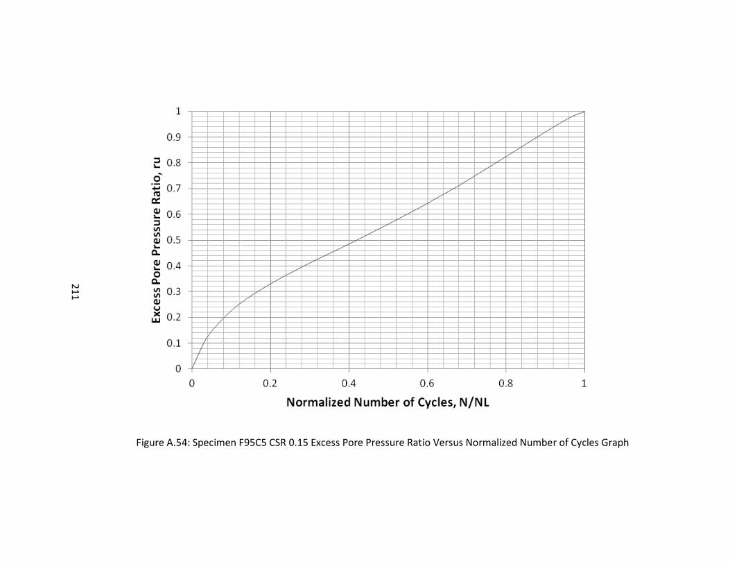
211
Figure A.54: Specimen F95C5 CSR 0.15 Excess Pore Pressure Ratio Versus Normalized Number of Cycles Graph
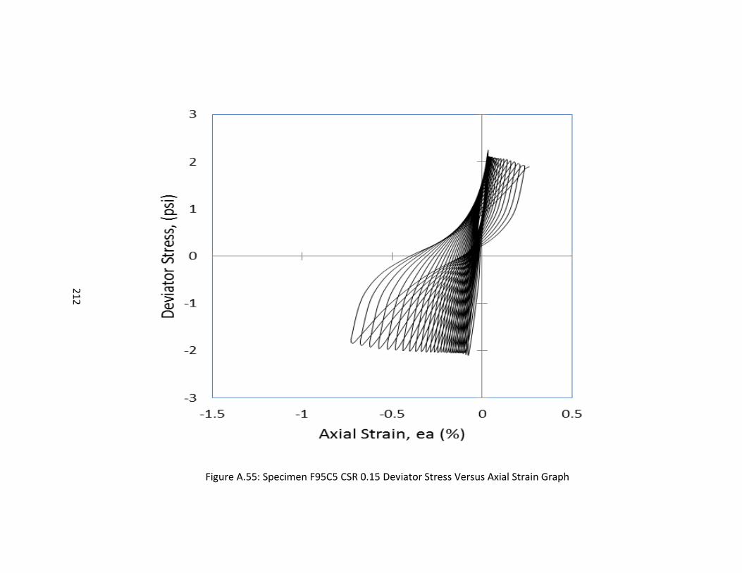
212
Figure A.55: Specimen F95C5 CSR 0.15 Deviator Stress Versus Axial Strain Graph
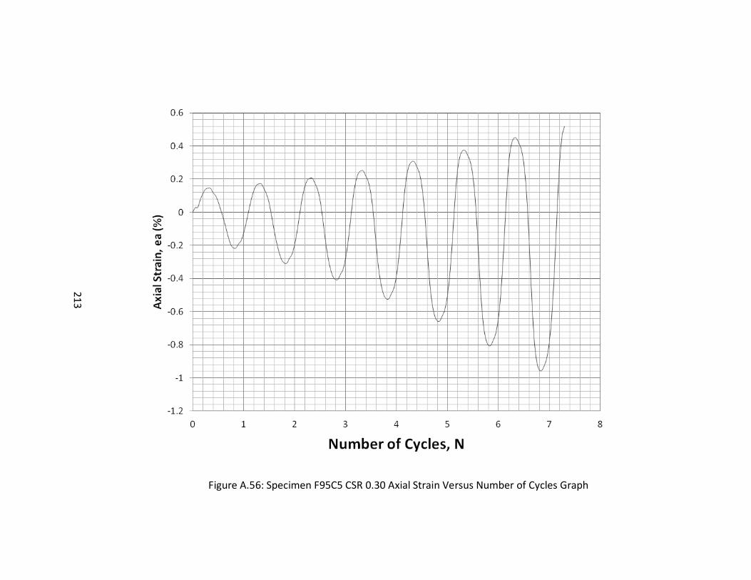
213
Figure A.56: Specimen F95C5 CSR 0.30 Axial Strain Versus Number of Cycles Graph
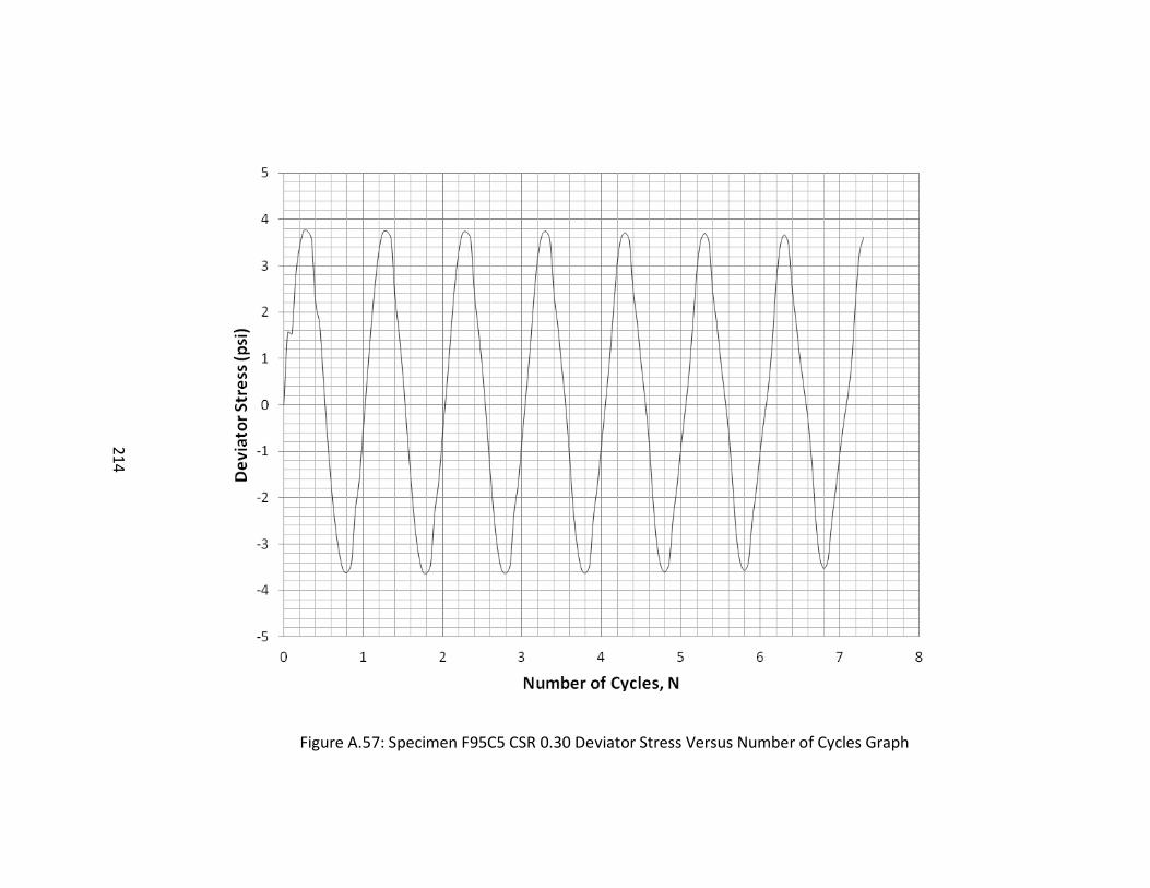
214
Figure A.57: Specimen F95C5 CSR 0.30 Deviator Stress Versus Number of Cycles Graph
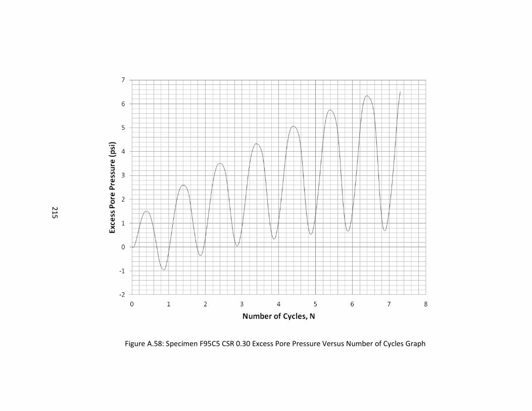
215
Figure A.58: Specimen F95C5 CSR 0.30 Excess Pore Pressure Versus Number of Cycles Graph
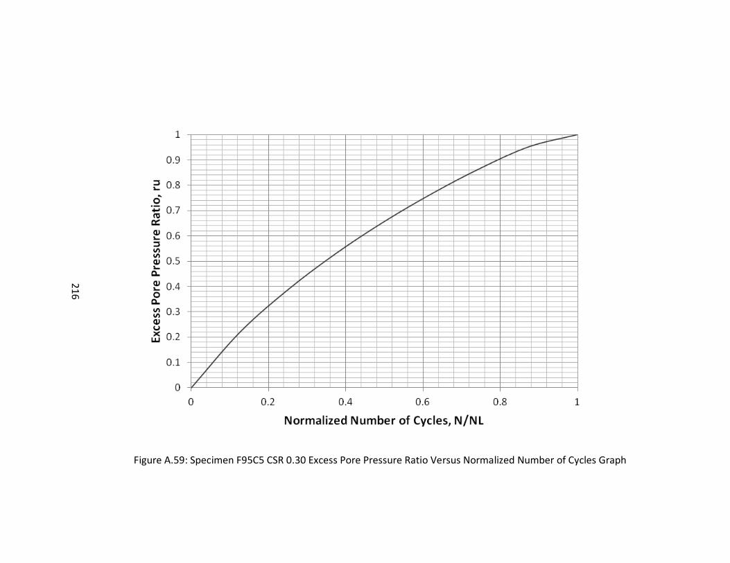
216
Figure A.59: Specimen F95C5 CSR 0.30 Excess Pore Pressure Ratio Versus Normalized Number of Cycles Graph
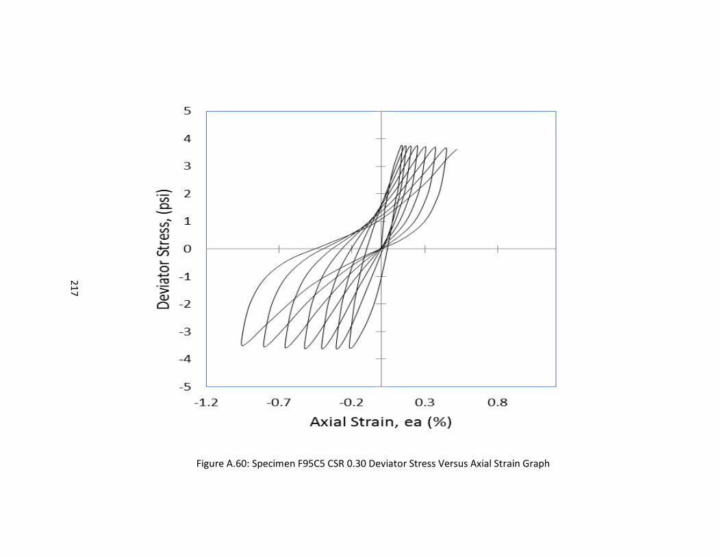
217
Figure A.60: Specimen F95C5 CSR 0.30 Deviator Stress Versus Axial Strain Graph
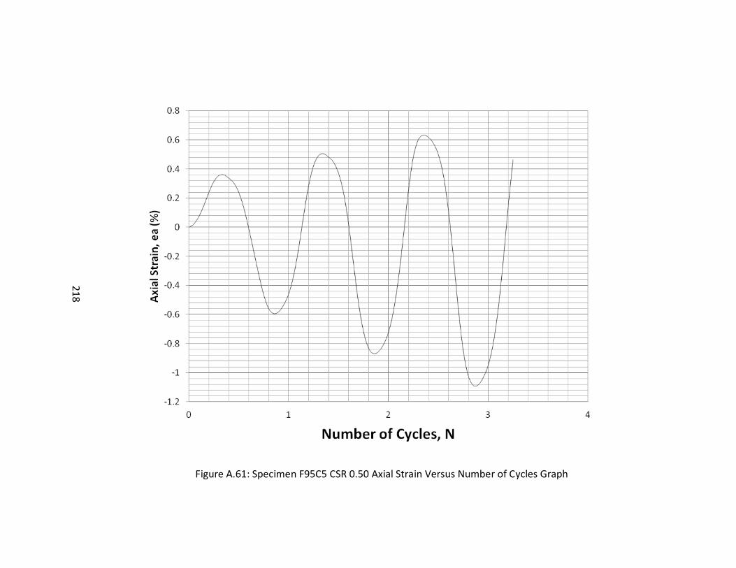
218
Figure A.61: Specimen F95C5 CSR 0.50 Axial Strain Versus Number of Cycles Graph
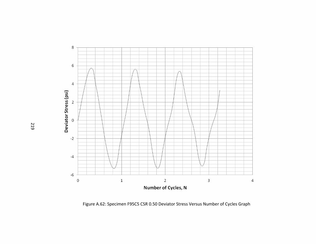
219
Figure A.62: Specimen F95C5 CSR 0.50 Deviator Stress Versus Number of Cycles Graph
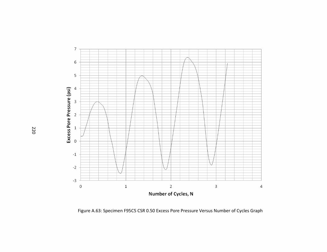
220
Figure A.63: Specimen F95C5 CSR 0.50 Excess Pore Pressure Versus Number of Cycles Graph
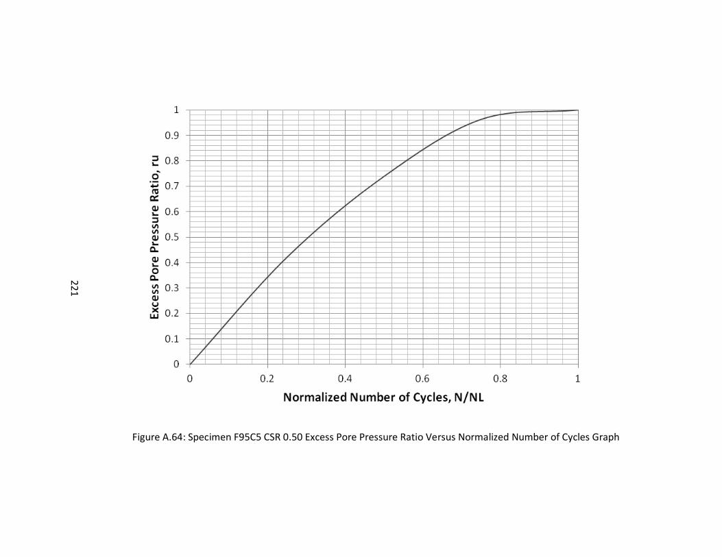
221
Figure A.64: Specimen F95C5 CSR 0.50 Excess Pore Pressure Ratio Versus Normalized Number of Cycles Graph
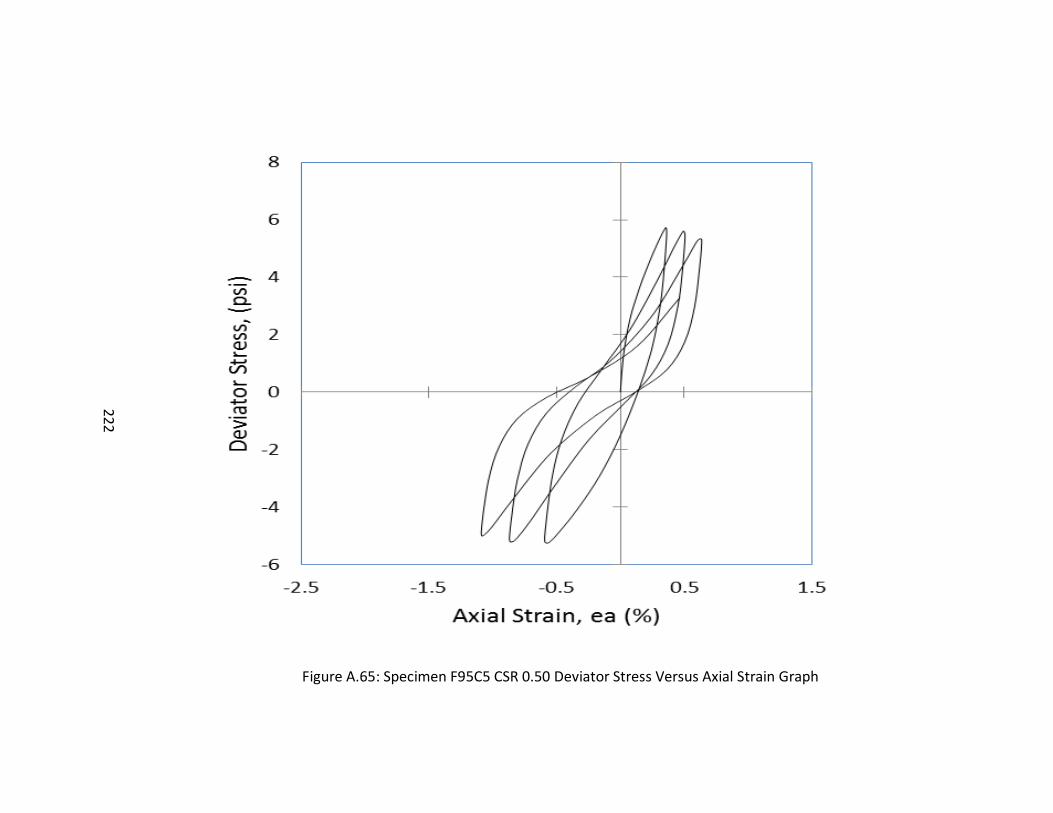
222
Figure A.65: Specimen F95C5 CSR 0.50 Deviator Stress Versus Axial Strain Graph

223
Figure A.66: Specimen F80C20 CSR 0.30 Axial Strain Versus Number of Cycles Graph
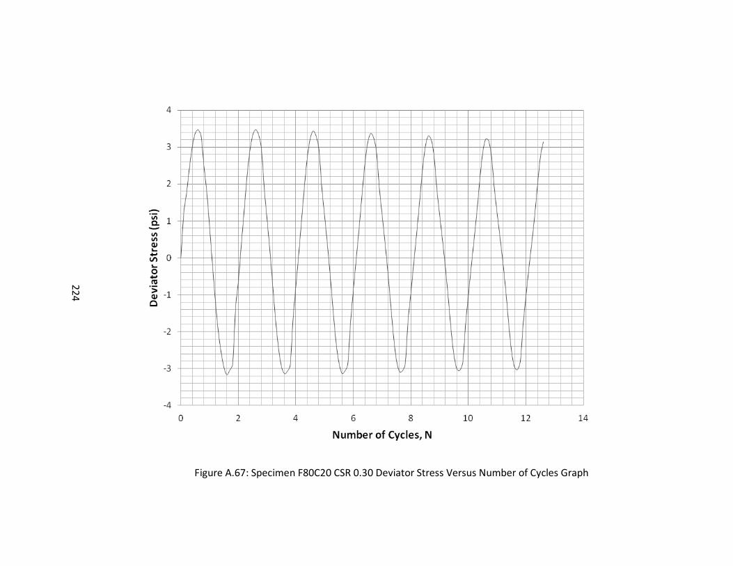
224
Figure A.67: Specimen F80C20 CSR 0.30 Deviator Stress Versus Number of Cycles Graph
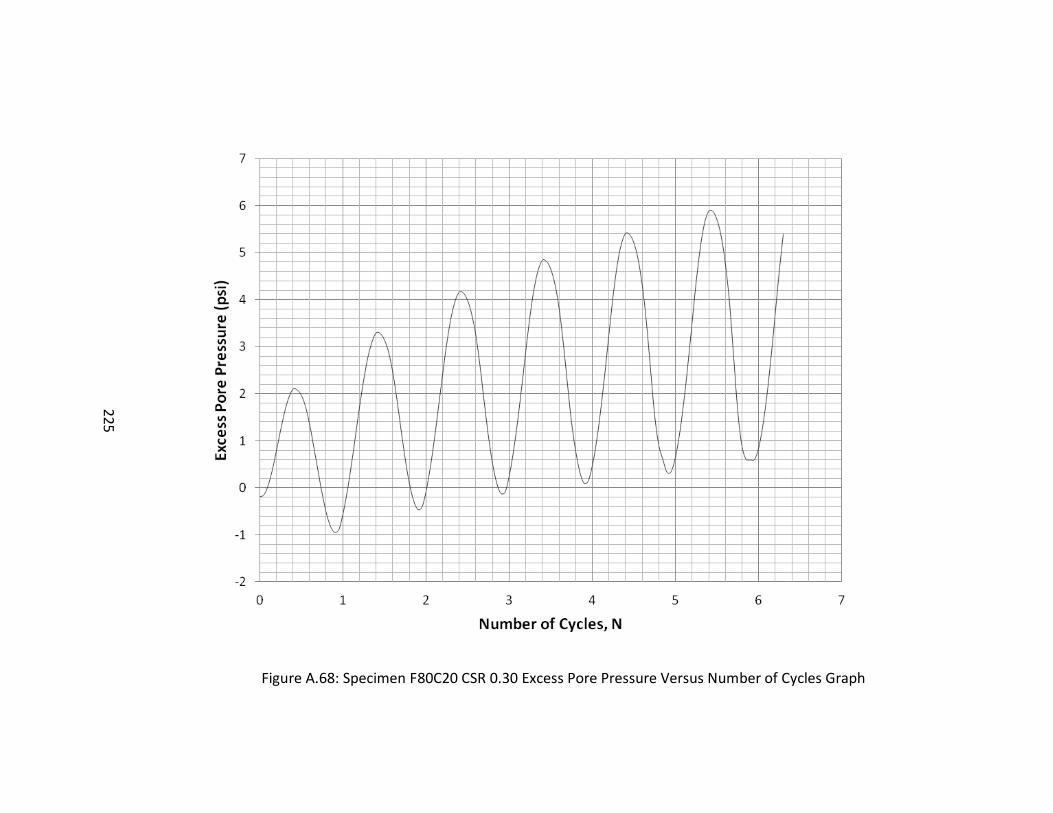
225
Figure A.68: Specimen F80C20 CSR 0.30 Excess Pore Pressure Versus Number of Cycles Graph
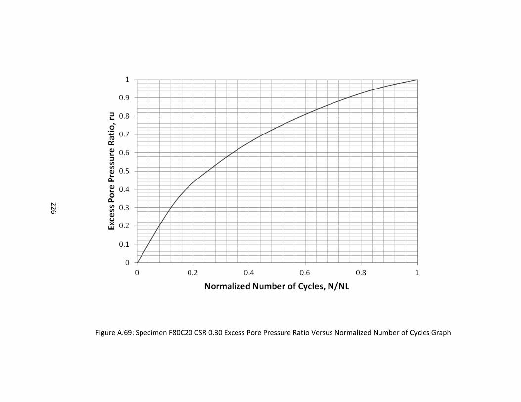
226
Figure A.69: Specimen F80C20 CSR 0.30 Excess Pore Pressure Ratio Versus Normalized Number of Cycles Graph
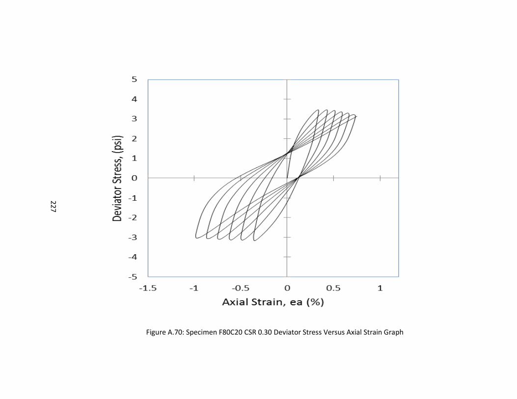
227
Figure A.70: Specimen F80C20 CSR 0.30 Deviator Stress Versus Axial Strain Graph
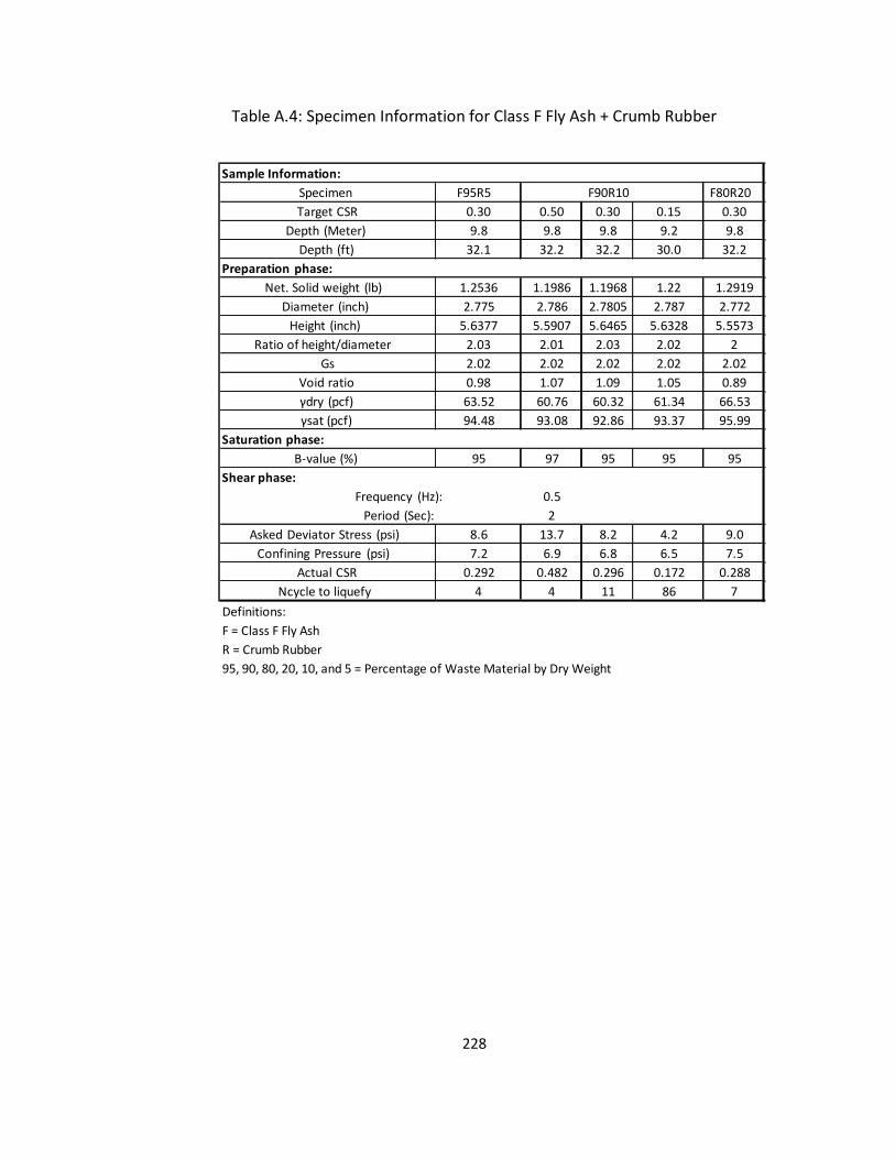
228
Table A.4: Specimen Information for Class F Fly Ash + Crumb Rubber
Definitions:
F = Class F Fly Ash
R = Crumb Rubber
95, 90, 80, 20, 10, and 5 = Percentage of Waste Material by Dry Weight
Sample Information:
F95R5 F80R20
0.30 0.50 0.30 0.15 0.30
9.8 9.8 9.8 9.2 9.8
32.1 32.2 32.2 30.0 32.2
Preparation phase:
1.2536 1.1986 1.1968 1.22 1.2919
2.775 2.786 2.7805 2.787 2.772
5.6377 5.5907 5.6465 5.6328 5.5573
2.03 2.01 2.03 2.02 2
2.02 2.02 2.02 2.02 2.02
0.98 1.07 1.09 1.05 0.89
63.52 60.76 60.32 61.34 66.53
94.48 93.08 92.86 93.37 95.99
Saturation phase:
95 97 95 95 95
Shear phase:
0.5
2
8.6 13.7 8.2 4.2 9.0
7.2 6.9 6.8 6.5 7.5
0.292 0.482 0.296 0.172 0.288
4 4 11 86 7
Confining Pressure (psi)
Actual CSR
Ncycle to liquefy
F90R10
γsat (pcf)
B-value (%)
Frequency (Hz):
Period (Sec):
Asked Deviator Stress (psi)
Height (inch)
Ratio of height/diameter
Gs
Void ratio
γdry (pcf)
Target CSR
Depth (Meter)
Depth (ft)
Net. Solid weight (lb)
Diameter (inch)
Specimen
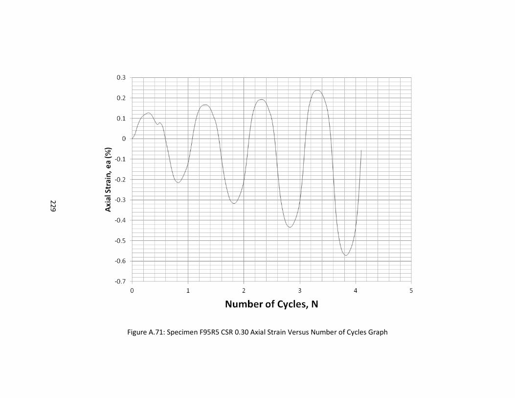
229
Figure A.71: Specimen F95R5 CSR 0.30 Axial Strain Versus Number of Cycles Graph
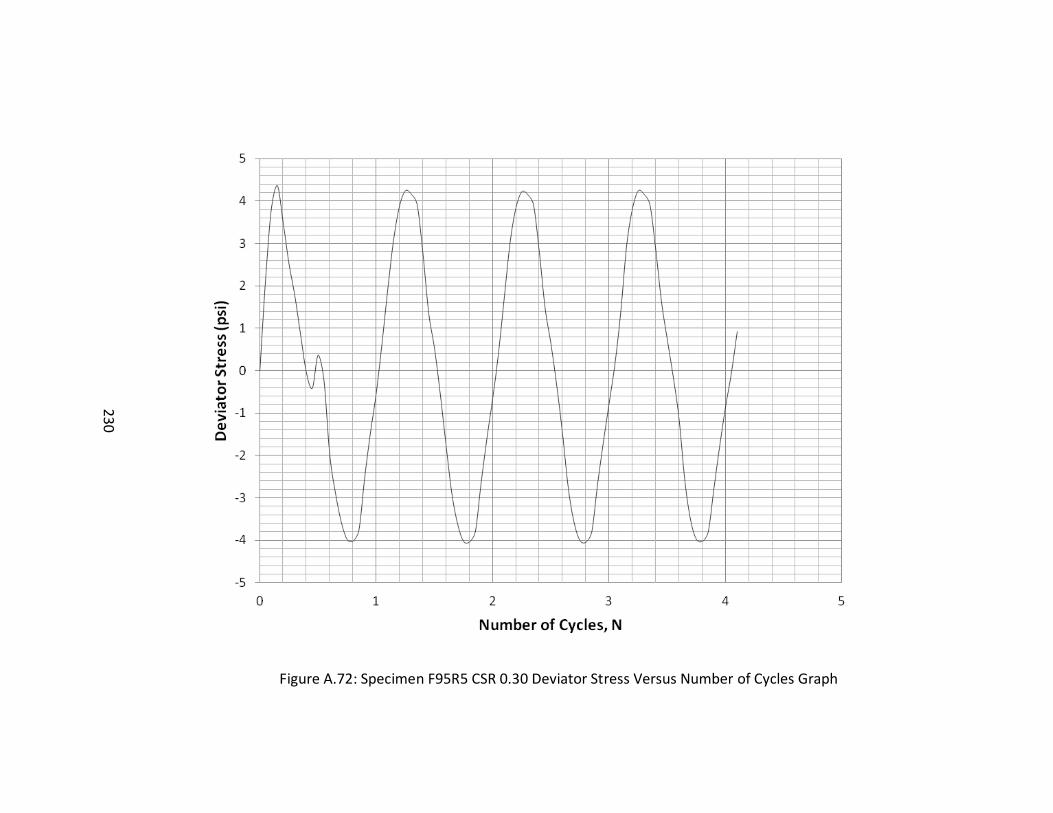
230
Figure A.72: Specimen F95R5 CSR 0.30 Deviator Stress Versus Number of Cycles Graph
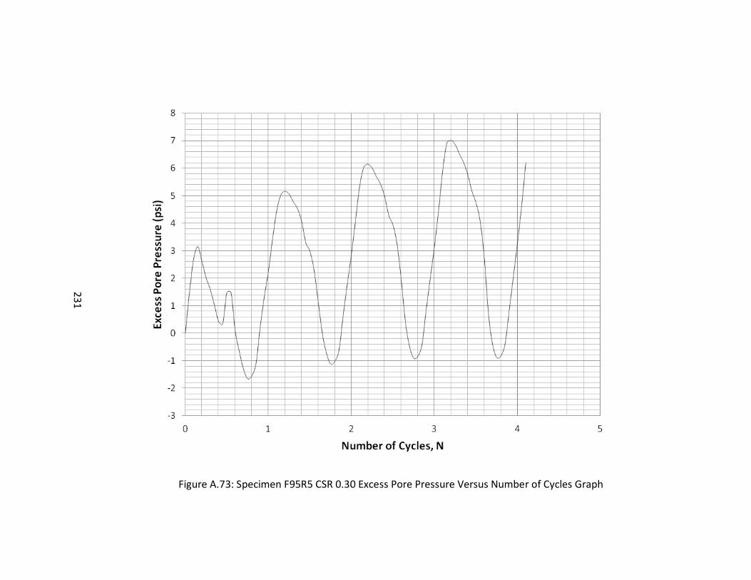
231
Figure A.73: Specimen F95R5 CSR 0.30 Excess Pore Pressure Versus Number of Cycles Graph
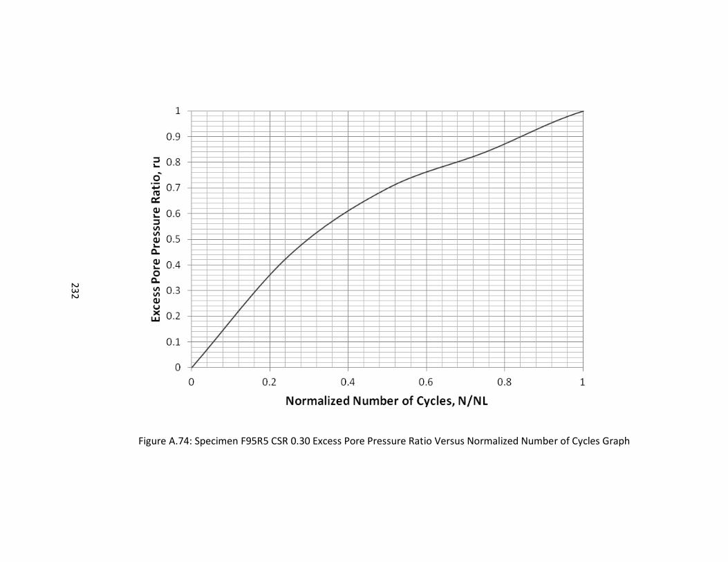
232
Figure A.74: Specimen F95R5 CSR 0.30 Excess Pore Pressure Ratio Versus Normalized Number of Cycles Graph
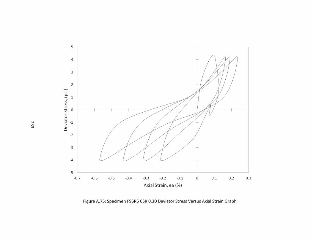
233
Figure A.75: Specimen F95R5 CSR 0.30 Deviator Stress Versus Axial Strain Graph
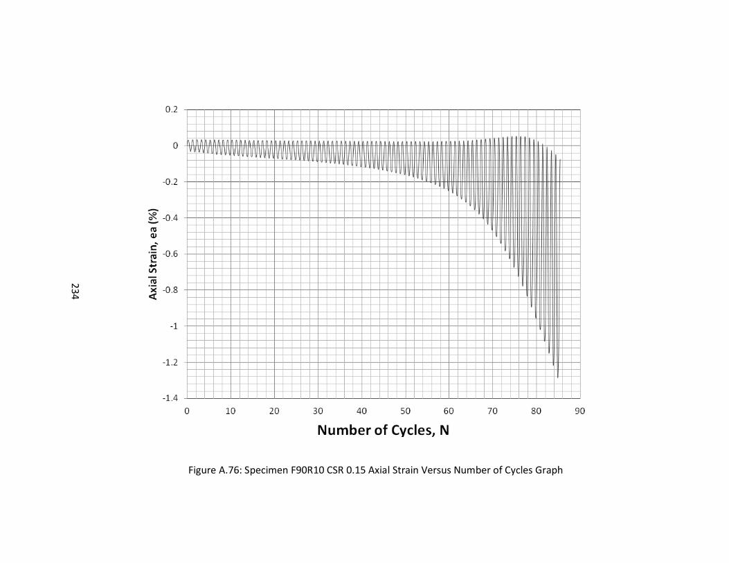
234
Figure A.76: Specimen F90R10 CSR 0.15 Axial Strain Versus Number of Cycles Graph
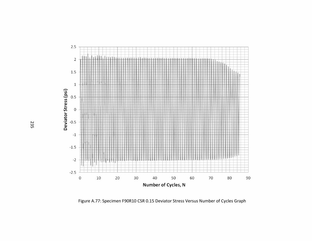
235
Figure A.77: Specimen F90R10 CSR 0.15 Deviator Stress Versus Number of Cycles Graph
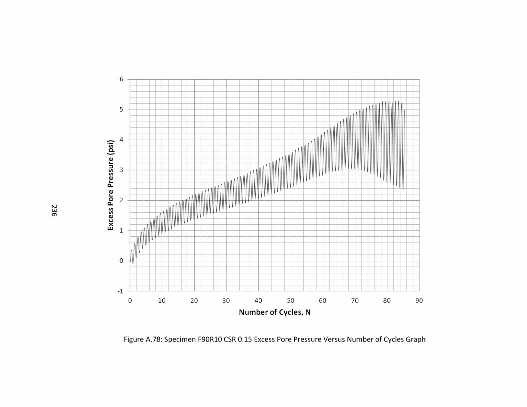
236
Figure A.78: Specimen F90R10 CSR 0.15 Excess Pore Pressure Versus Number of Cycles Graph
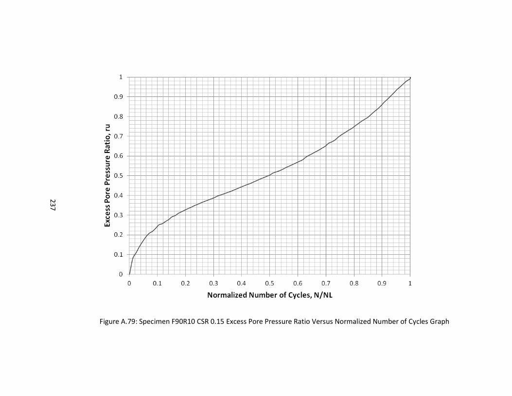
237
Figure A.79: Specimen F90R10 CSR 0.15 Excess Pore Pressure Ratio Versus Normalized Number of Cycles Graph
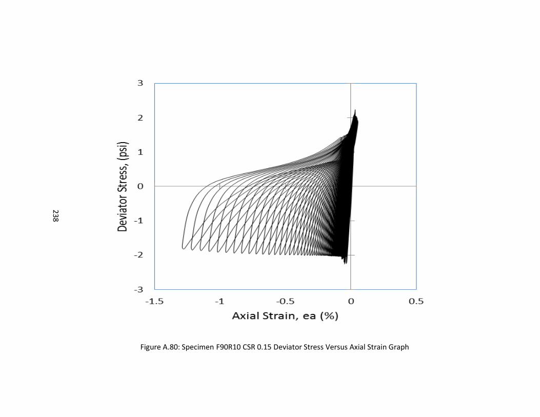
238
Figure A.80: Specimen F90R10 CSR 0.15 Deviator Stress Versus Axial Strain Graph
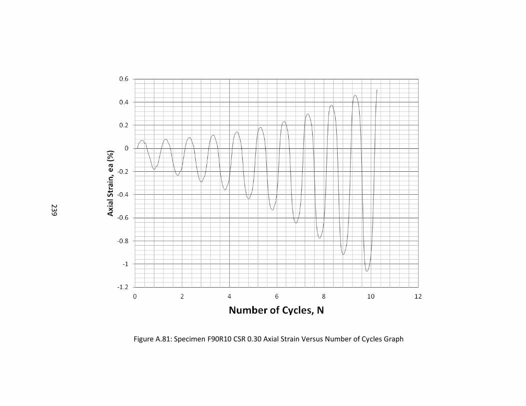
239
Figure A.81: Specimen F90R10 CSR 0.30 Axial Strain Versus Number of Cycles Graph

240
Figure A.82: Specimen F90R10 CSR 0.30 Deviator Stress Versus Number of Cycles Graph
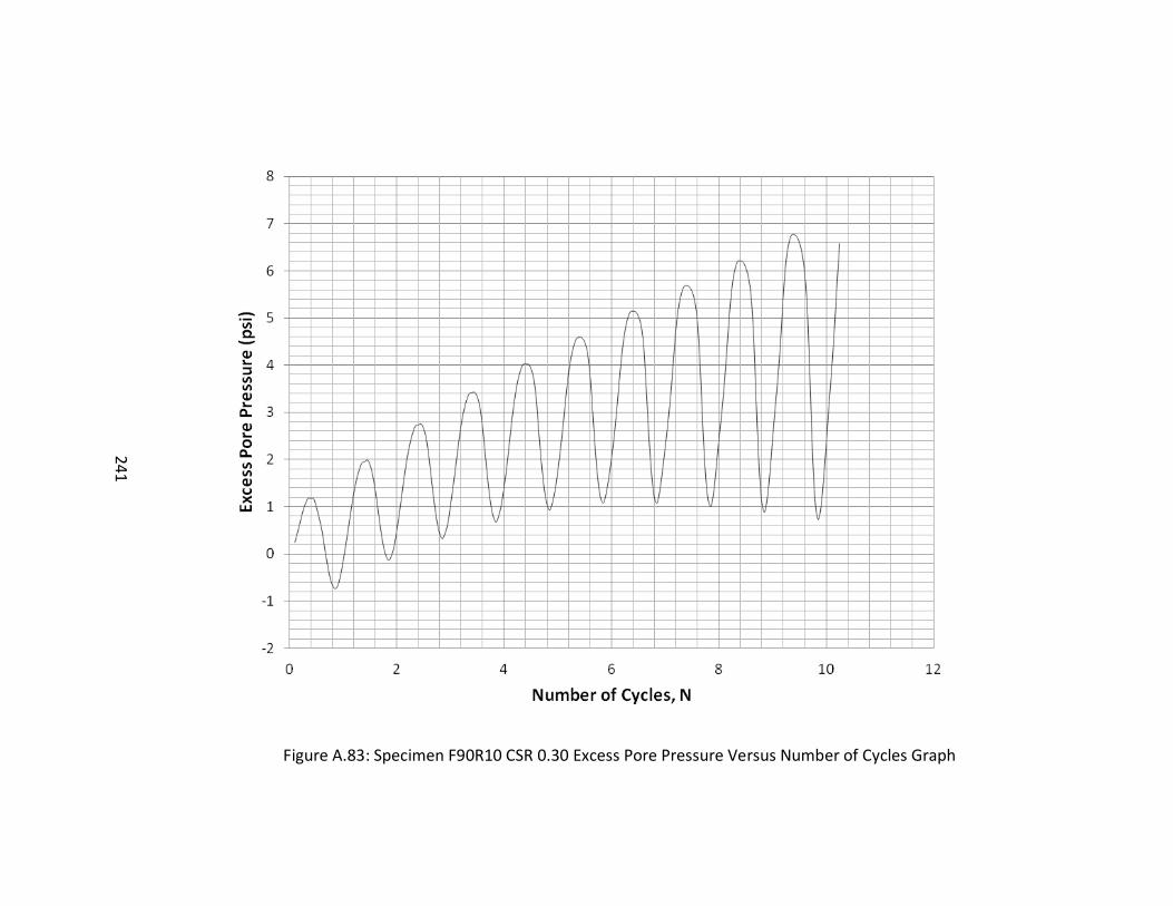
241
Figure A.83: Specimen F90R10 CSR 0.30 Excess Pore Pressure Versus Number of Cycles Graph
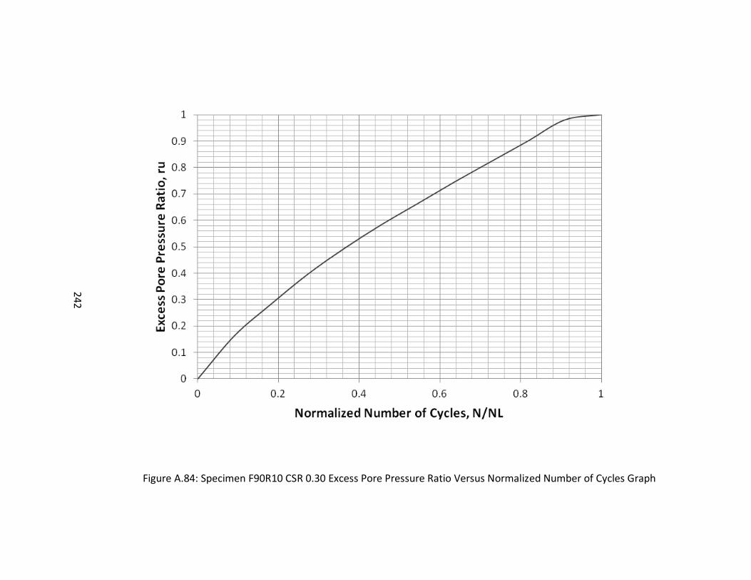
242
Figure A.84: Specimen F90R10 CSR 0.30 Excess Pore Pressure Ratio Versus Normalized Number of Cycles Graph
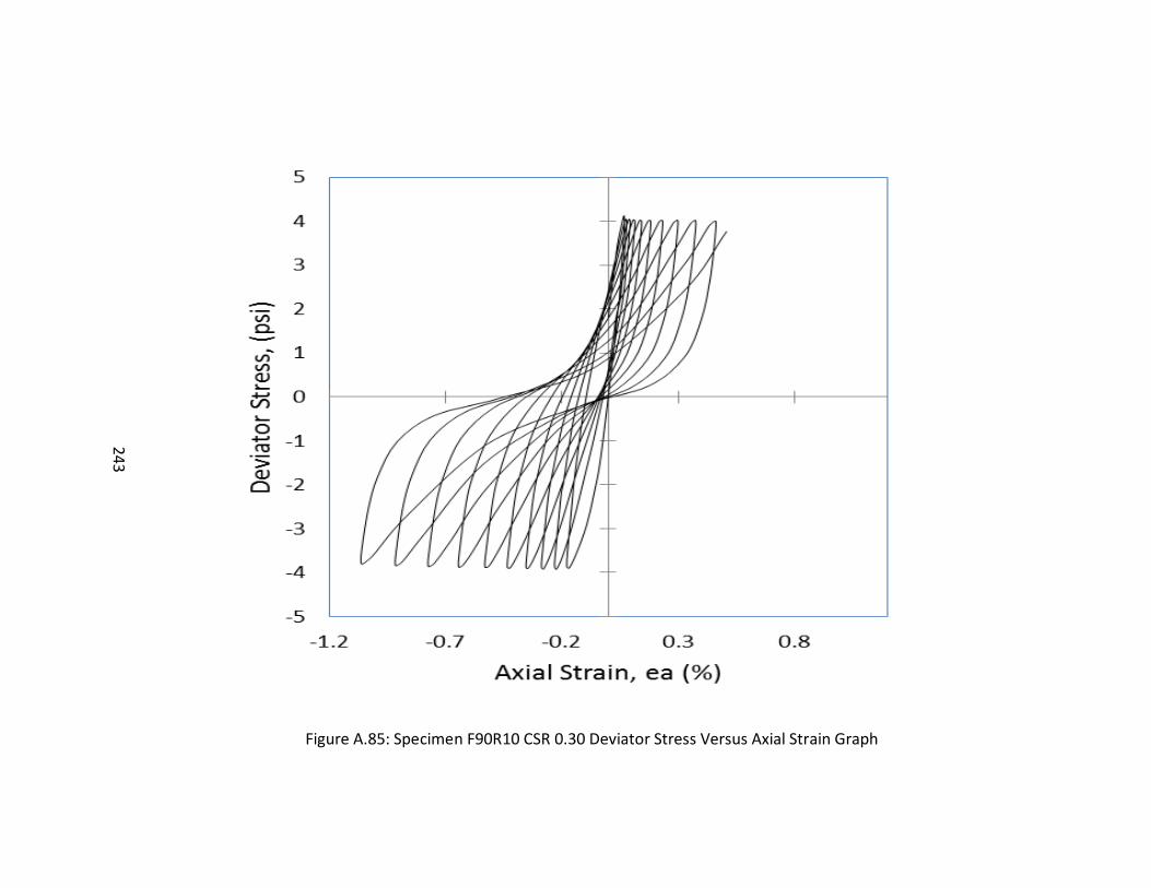
243
Figure A.85: Specimen F90R10 CSR 0.30 Deviator Stress Versus Axial Strain Graph

244
Figure A.86: Specimen F90R10 CSR 0.50 Axial Strain Versus Number of Cycles Graph

245
Figure A.87: Specimen F90R10 CSR 0.50 Deviator Stress Versus Number of Cycles Graph
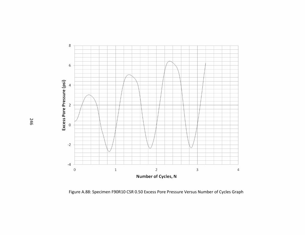
246
Figure A.88: Specimen F90R10 CSR 0.50 Excess Pore Pressure Versus Number of Cycles Graph
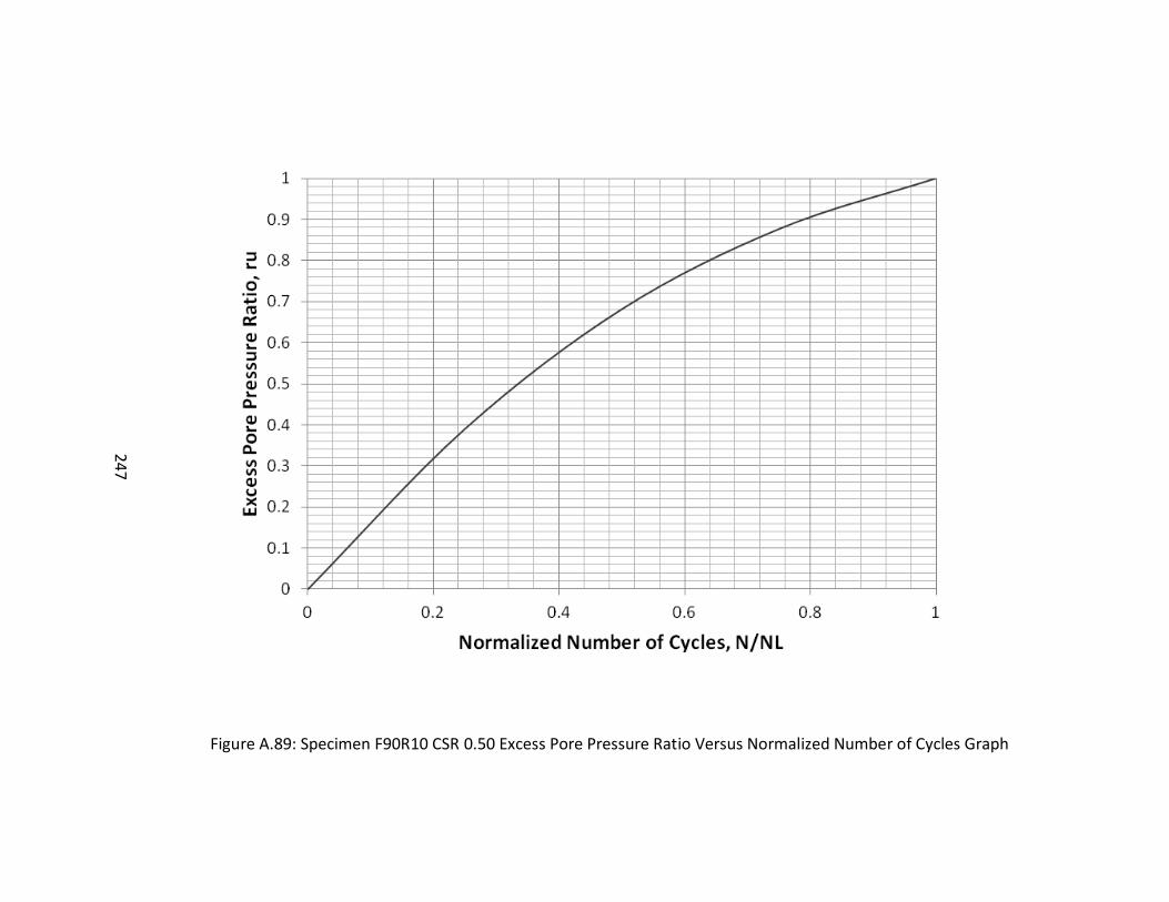
247
Figure A.89: Specimen F90R10 CSR 0.50 Excess Pore Pressure Ratio Versus Normalized Number of Cycles Graph
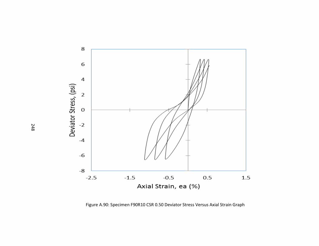
248
Figure A.90: Specimen F90R10 CSR 0.50 Deviator Stress Versus Axial Strain Graph
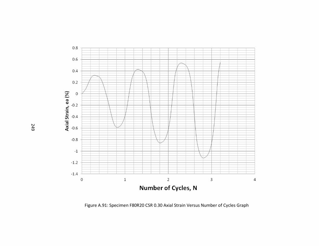
249
Figure A.91: Specimen F80R20 CSR 0.30 Axial Strain Versus Number of Cycles Graph
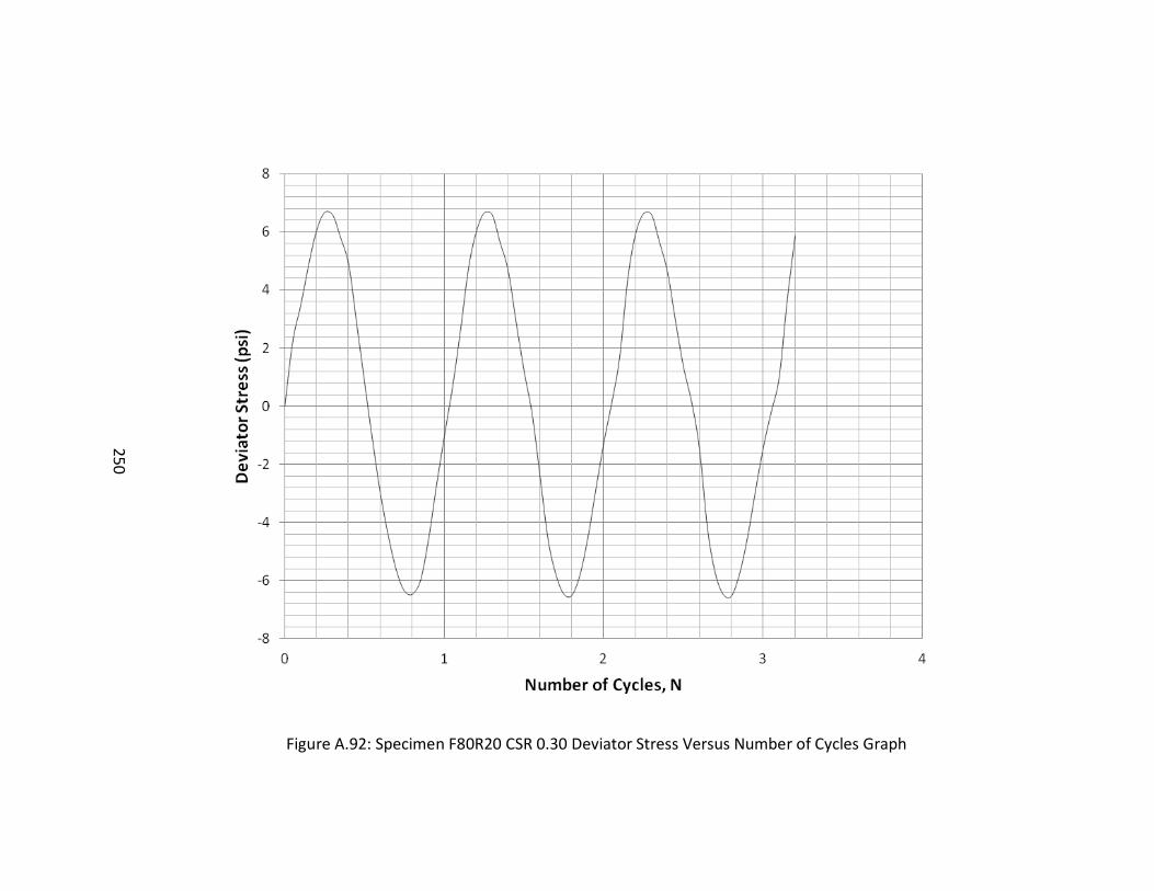
250
Figure A.92: Specimen F80R20 CSR 0.30 Deviator Stress Versus Number of Cycles Graph
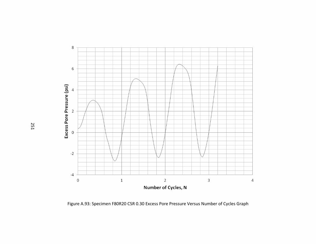
251
Figure A.93: Specimen F80R20 CSR 0.30 Excess Pore Pressure Versus Number of Cycles Graph
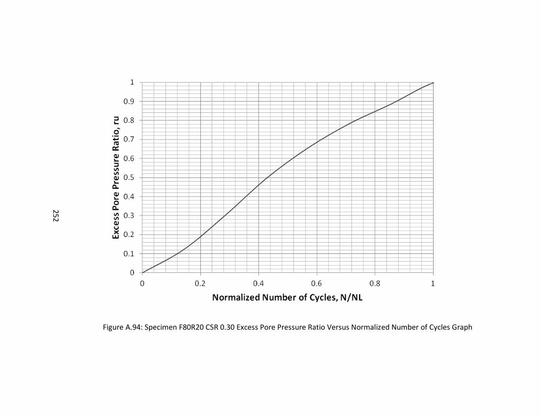
252
Figure A.94: Specimen F80R20 CSR 0.30 Excess Pore Pressure Ratio Versus Normalized Number of Cycles Graph
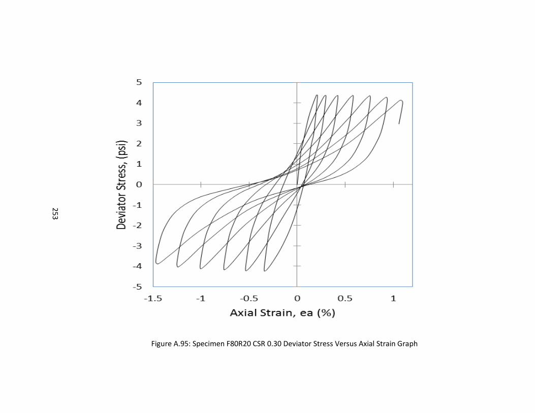
253
Figure A.95: Specimen F80R20 CSR 0.30 Deviator Stress Versus Axial Strain Graph
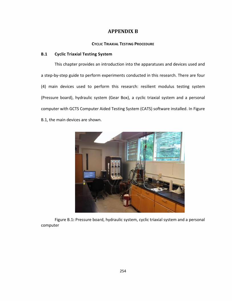
254
APPENDIX B
B. CYCLIC TRIAXIAL TESTING PROCEDURE
B.1 Cyclic Triaxial Testing System
This chapter provides an introduction into the apparatuses and devices used and
a step-by-step guide to perform experiments conducted in this research. There are four
(4) main devices used to perform this research: resilient modulus testing system
(Pressure board), hydraulic system (Gear Box), a cyclic triaxial system and a personal
computer with GCTS Computer Aided Testing System (CATS) software installed. In Figure
B.1, the main devices are shown.
Figure B.1: Pressure board, hydraulic system, cyclic triaxial system and a personal computer
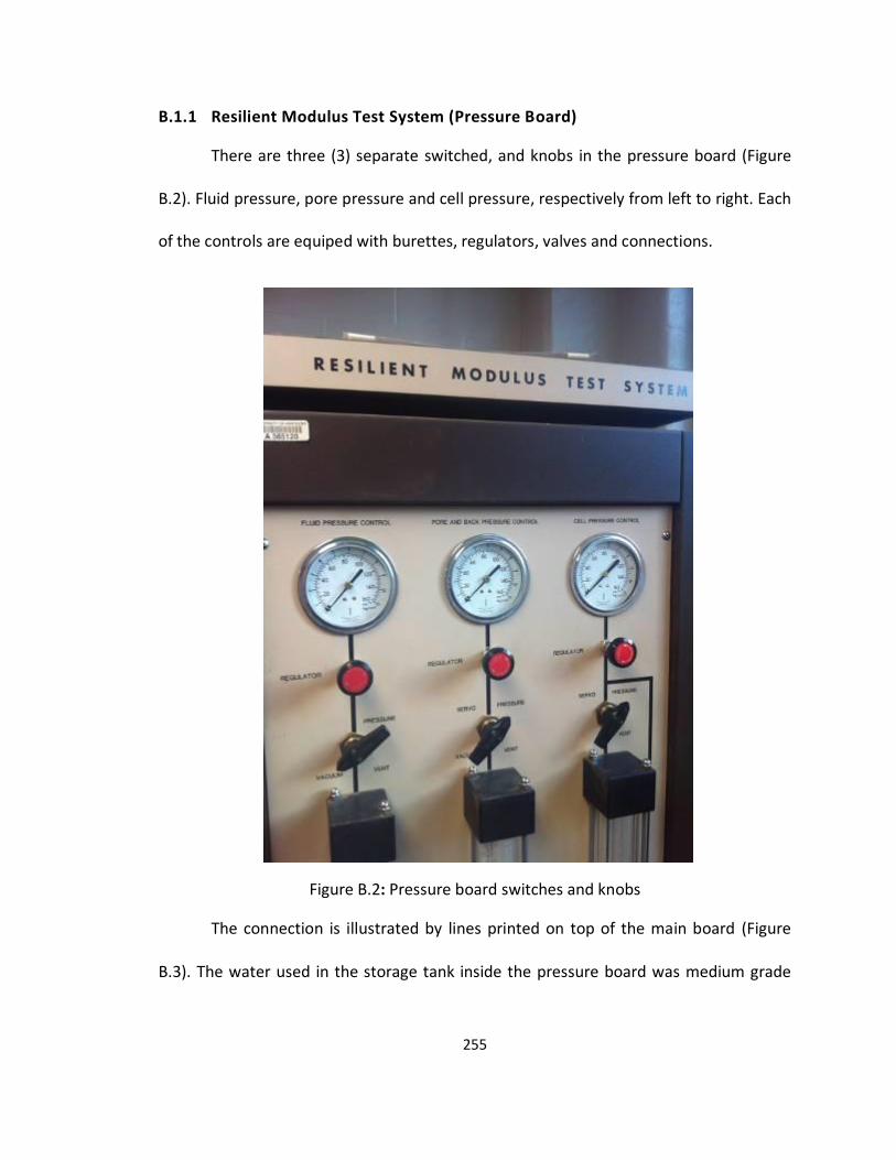
255
B.1.1 Resilient Modulus Test System (Pressure Board)
There are three (3) separate switched, and knobs in the pressure board (Figure
B.2). Fluid pressure, pore pressure and cell pressure, respectively from left to right. Each
of the controls are equiped with burettes, regulators, valves and connections.
Figure B.2: Pressure board switches and knobs
The connection is illustrated by lines printed on top of the main board (Figure
B.3). The water used in the storage tank inside the pressure board was medium grade
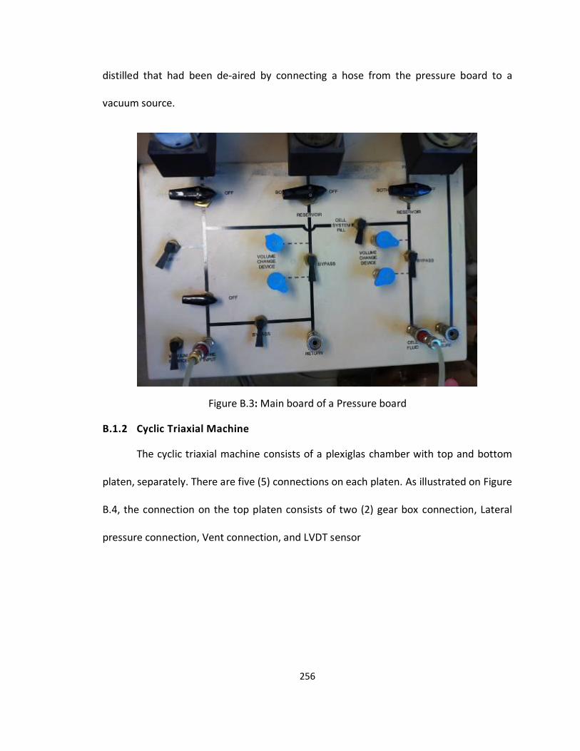
256
distilled that had been de-aired by connecting a hose from the pressure board to a
vacuum source.
Figure B.3: Main board of a Pressure board
B.1.2 Cyclic Triaxial Machine
The cyclic triaxial machine consists of a plexiglas chamber with top and bottom
platen, separately. There are five (5) connections on each platen. As illustrated on Figure
B.4, the connection on the top platen consists of two (2) gear box connection, Lateral
pressure connection, Vent connection, and LVDT sensor
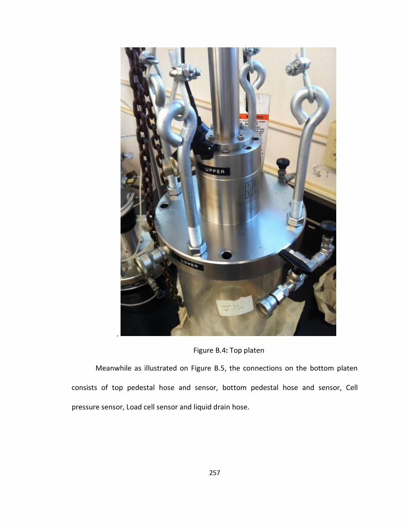
257
.
Figure B.4: Top platen
Meanwhile as illustrated on Figure B.5, the connections on the bottom platen
consists of top pedestal hose and sensor, bottom pedestal hose and sensor, Cell
pressure sensor, Load cell sensor and liquid drain hose.
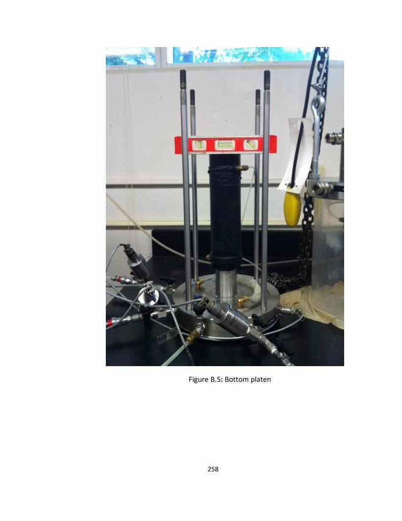
258
Figure B.5: Bottom platen
259
B.2 Reconstitute Test Specimen
Because fly ash has lower specific gravity compare to soils, a delicate handling
of reconstituting material should be applied to avoid the specimen from collapsing. To
help reconstitute the specimen, the tools needed are the following:
1. Split mold with 2.8 inch in diameter
2. Four (4) 2.8 inch rubber O-ring
3. 2.8 inch neoprene membrane
4. Two (2) porous stone
5. Two (2) filter paper
6. Scale
7. Ruler
8. Caliper
9. 7/16” wrench
10. 1/4” diameter tube
11. 1/8” diameter tube
12. Vacuum water trap (Figure B.6)
13. Plastic funnel
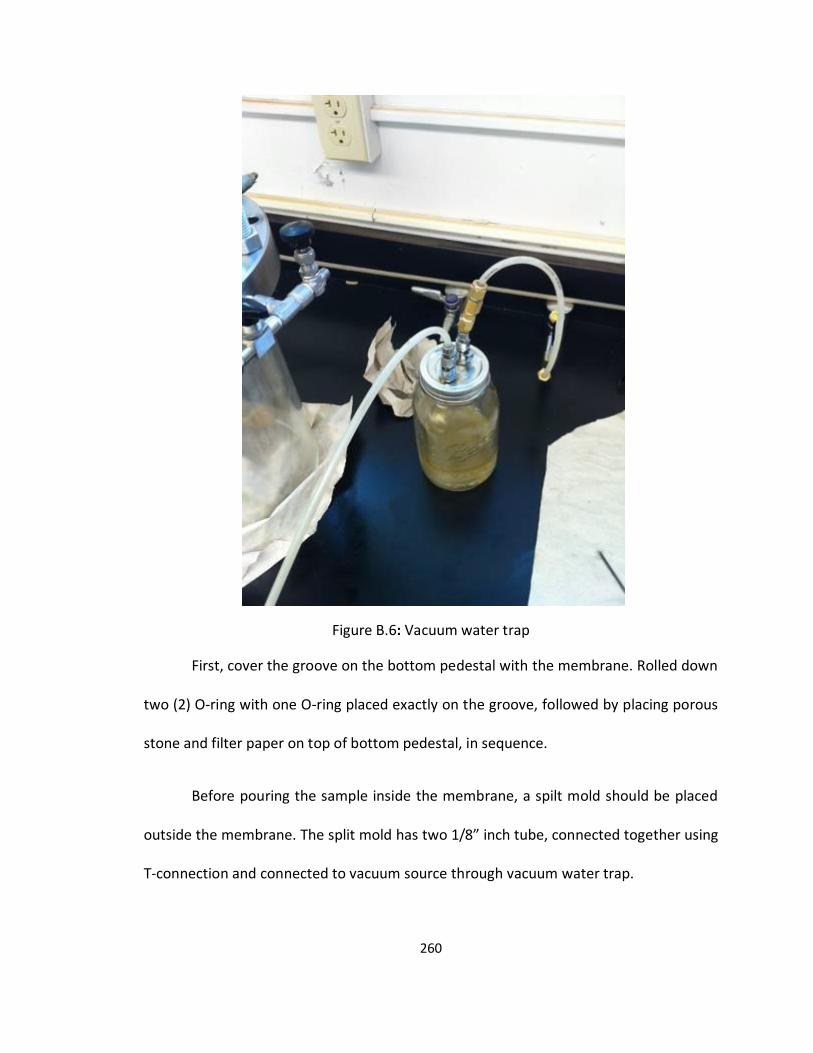
260
Figure B.6: Vacuum water trap
First, cover the groove on the bottom pedestal with the membrane. Rolled down
two (2) O-ring with one O-ring placed exactly on the groove, followed by placing porous
stone and filter paper on top of bottom pedestal, in sequence.
Before pouring the sample inside the membrane, a spilt mold should be placed
outside the membrane. The split mold has two 1/8” inch tube, connected together using
T-connection and connected to vacuum source through vacuum water trap.
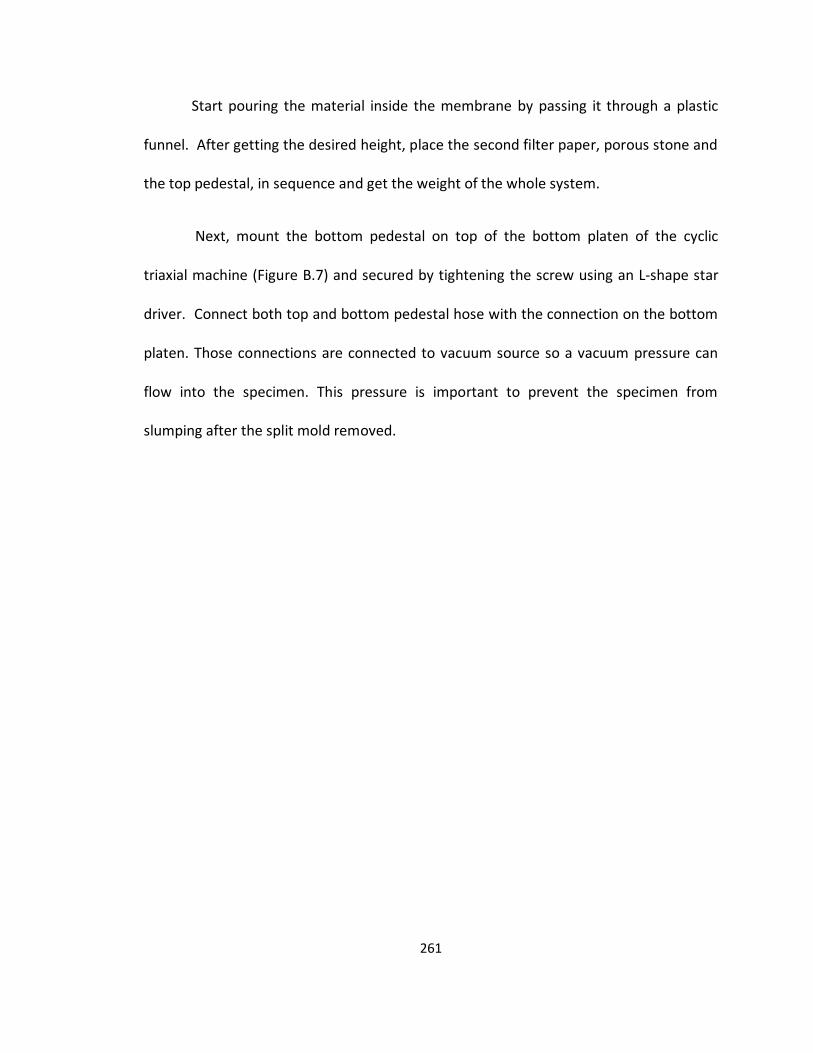
261
Start pouring the material inside the membrane by passing it through a plastic
funnel. After getting the desired height, place the second filter paper, porous stone and
the top pedestal, in sequence and get the weight of the whole system.
Next, mount the bottom pedestal on top of the bottom platen of the cyclic
triaxial machine (Figure B.7) and secured by tightening the screw using an L-shape star
driver. Connect both top and bottom pedestal hose with the connection on the bottom
platen. Those connections are connected to vacuum source so a vacuum pressure can
flow into the specimen. This pressure is important to prevent the specimen from
slumping after the split mold removed.
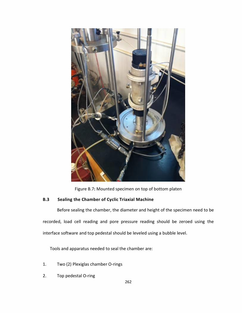
262
Figure B.7: Mounted specimen on top of bottom platen
B.3 Sealing the Chamber of Cyclic Triaxial Machine
Before sealing the chamber, the diameter and height of the specimen need to be
recorded, load cell reading and pore pressure reading should be zeroed using the
interface software and top pedestal should be leveled using a bubble level.
Tools and apparatus needed to seal the chamber are:
1. Two (2) Plexiglas chamber O-rings
2. Top pedestal O-ring
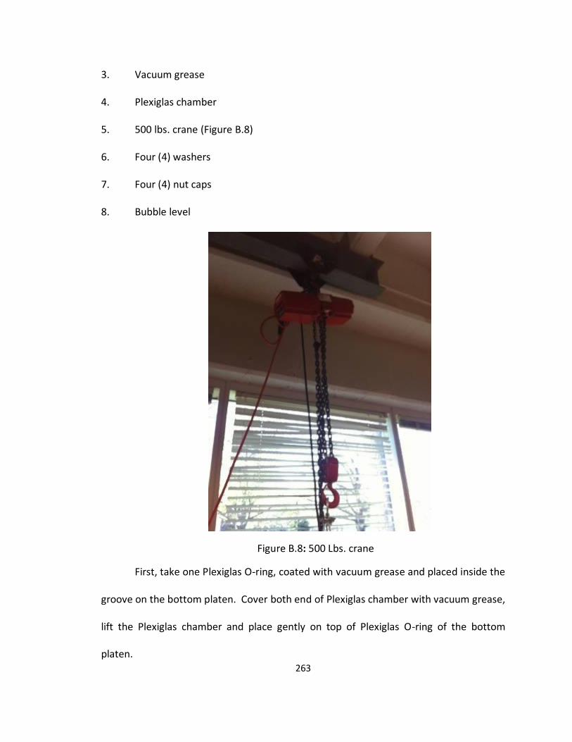
263
3. Vacuum grease
4. Plexiglas chamber
5. 500 lbs. crane (Figure B.8)
6. Four (4) washers
7. Four (4) nut caps
8. Bubble level
Figure B.8: 500 Lbs. crane
First, take one Plexiglas O-ring, coated with vacuum grease and placed inside the
groove on the bottom platen. Cover both end of Plexiglas chamber with vacuum grease,
lift the Plexiglas chamber and place gently on top of Plexiglas O-ring of the bottom
platen.
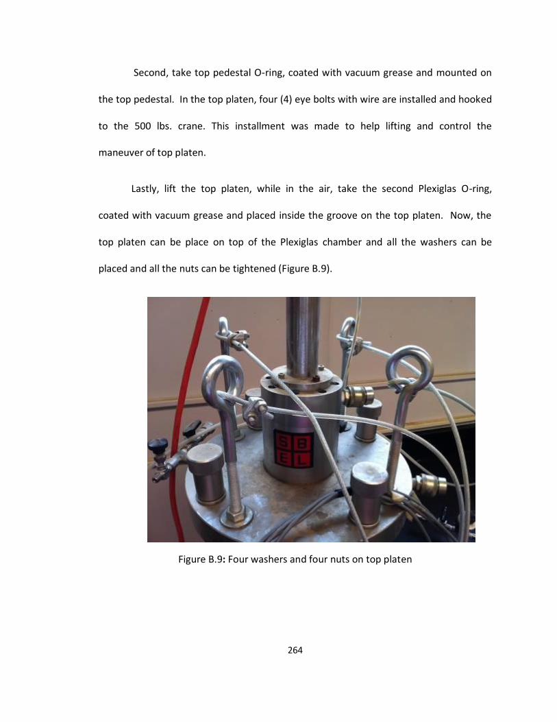
264
Second, take top pedestal O-ring, coated with vacuum grease and mounted on
the top pedestal. In the top platen, four (4) eye bolts with wire are installed and hooked
to the 500 lbs. crane. This installment was made to help lifting and control the
maneuver of top platen.
Lastly, lift the top platen, while in the air, take the second Plexiglas O-ring,
coated with vacuum grease and placed inside the groove on the top platen. Now, the
top platen can be place on top of the Plexiglas chamber and all the washers can be
placed and all the nuts can be tightened (Figure B.9).
Figure B.9: Four washers and four nuts on top platen
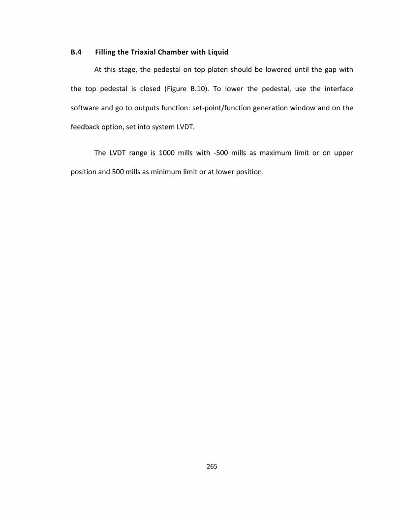
265
B.4 Filling the Triaxial Chamber with Liquid
At this stage, the pedestal on top platen should be lowered until the gap with
the top pedestal is closed (Figure B.10). To lower the pedestal, use the interface
software and go to outputs function: set-point/function generation window and on the
feedback option, set into system LVDT.
The LVDT range is 1000 mills with -500 mills as maximum limit or on upper
position and 500 mills as minimum limit or at lower position.
266
Figure B.10: Lowering pedestal of top platen to close the gap with top pedestal
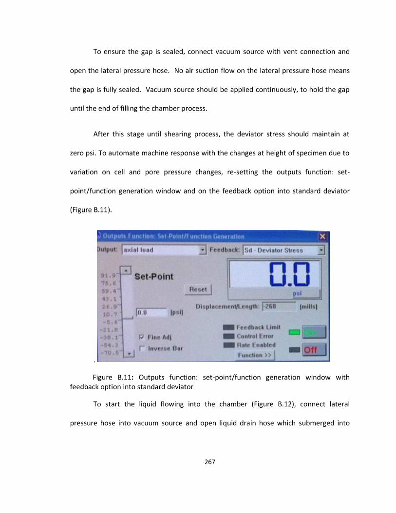
267
To ensure the gap is sealed, connect vacuum source with vent connection and
open the lateral pressure hose. No air suction flow on the lateral pressure hose means
the gap is fully sealed. Vacuum source should be applied continuously, to hold the gap
until the end of filling the chamber process.
After this stage until shearing process, the deviator stress should maintain at
zero psi. To automate machine response with the changes at height of specimen due to
variation on cell and pore pressure changes, re-setting the outputs function: set-
point/function generation window and on the feedback option into standard deviator
(Figure B.11).
.
Figure B.11: Outputs function: set-point/function generation window with feedback option into standard deviator
To start the liquid flowing into the chamber (Figure B.12), connect lateral
pressure hose into vacuum source and open liquid drain hose which submerged into
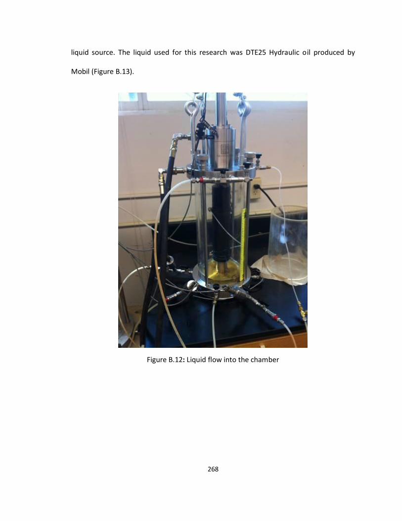
268
liquid source. The liquid used for this research was DTE25 Hydraulic oil produced by
Mobil (Figure B.13).
Figure B.12: Liquid flow into the chamber
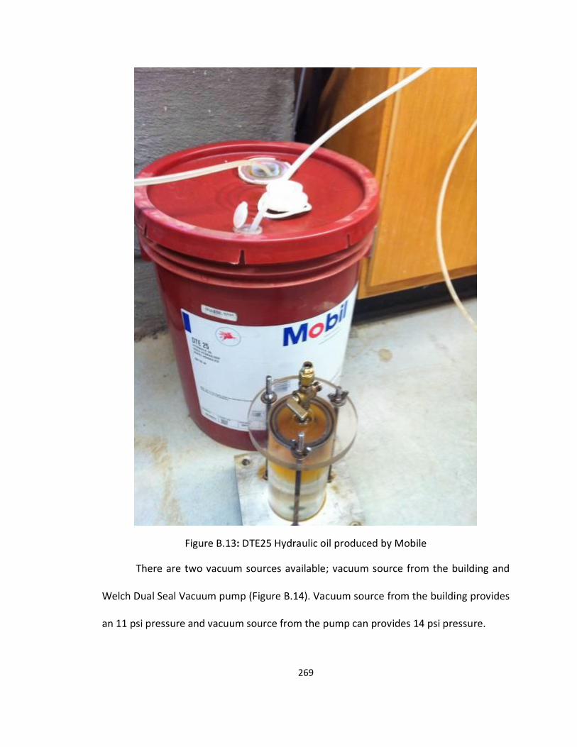
269
Figure B.13: DTE25 Hydraulic oil produced by Mobile
There are two vacuum sources available; vacuum source from the building and
Welch Dual Seal Vacuum pump (Figure B.14). Vacuum source from the building provides
an 11 psi pressure and vacuum source from the pump can provides 14 psi pressure.
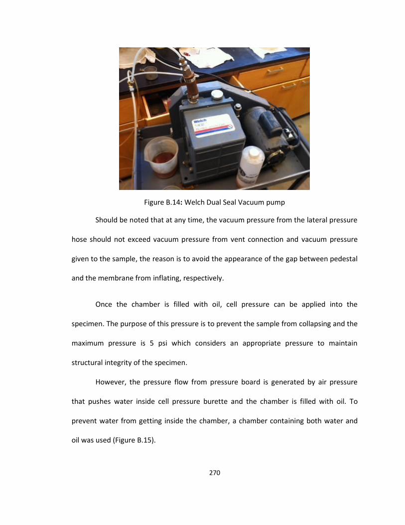
270
Figure B.14: Welch Dual Seal Vacuum pump
Should be noted that at any time, the vacuum pressure from the lateral pressure
hose should not exceed vacuum pressure from vent connection and vacuum pressure
given to the sample, the reason is to avoid the appearance of the gap between pedestal
and the membrane from inflating, respectively.
Once the chamber is filled with oil, cell pressure can be applied into the
specimen. The purpose of this pressure is to prevent the sample from collapsing and the
maximum pressure is 5 psi which considers an appropriate pressure to maintain
structural integrity of the specimen.
However, the pressure flow from pressure board is generated by air pressure
that pushes water inside cell pressure burette and the chamber is filled with oil. To
prevent water from getting inside the chamber, a chamber containing both water and
oil was used (Figure B.15).
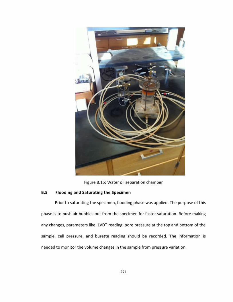
271
Figure B.15: Water oil separation chamber
B.5 Flooding and Saturating the Specimen
Prior to saturating the specimen, flooding phase was applied. The purpose of this
phase is to push air bubbles out from the specimen for faster saturation. Before making
any changes, parameters like: LVDT reading, pore pressure at the top and bottom of the
sample, cell pressure, and burette reading should be recorded. The information is
needed to monitor the volume changes in the sample from pressure variation.
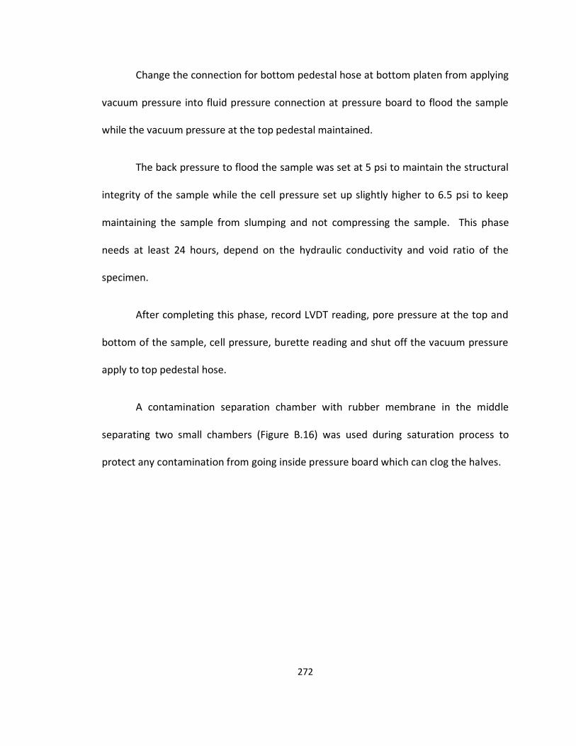
272
Change the connection for bottom pedestal hose at bottom platen from applying
vacuum pressure into fluid pressure connection at pressure board to flood the sample
while the vacuum pressure at the top pedestal maintained.
The back pressure to flood the sample was set at 5 psi to maintain the structural
integrity of the sample while the cell pressure set up slightly higher to 6.5 psi to keep
maintaining the sample from slumping and not compressing the sample. This phase
needs at least 24 hours, depend on the hydraulic conductivity and void ratio of the
specimen.
After completing this phase, record LVDT reading, pore pressure at the top and
bottom of the sample, cell pressure, burette reading and shut off the vacuum pressure
apply to top pedestal hose.
A contamination separation chamber with rubber membrane in the middle
separating two small chambers (Figure B.16) was used during saturation process to
protect any contamination from going inside pressure board which can clog the halves.
273
Figure B.16: Contamination separation chamber
During this phase, the remaining air bubble will dissipate and the sample will
start the saturation process. At this stage, the cell pressure should always be higher (+/-
1.5 psi) than pore pressure to avoid stress disturbance. To measure the saturation level,
the Skempton’s parameter (B) can be measured by following the guidelines
recommended by ASTM D5311.
274
Saturation was determined by measuring the B-value. Once a specimen reached a
B-Value of 95% or higher the cyclic triaxial test was performed. However, if the B-value
did not reach this criterion within two days, the specimen was tested due to time
constraints.
B.6 Consolidation Process
After achieving the minimum requirements for B-value, the consolidation phase
can be executed. During the consolidation process, the specimen is allowed to drain.
This process can be done by increasing the cell pressure to the desired confining
pressure which is related to the in-situ effective stress of the sample. By increasing cell
pressure and maintaining pore pressure, water inside the specimen will start flowing out
which means consolidation process happened.
B.7 Applying Load-controlled Loading
After completing the consolidation process, cyclic load-controlled loading could
be started. The applied pressure was determined in the form of cyclic stress ratio (CSR)
and input as deviator stress in psi unit.
The specimen experienced a cyclic loading at frequency of 0.5 Hz or equivalent
to a period of 2 seconds, and CSR ranged from 0.08 – 0.25. During the test, no drainage
was allowed from the specimen.
275
This phase was set up to run for 120 – 300 seconds, depending on the CSR value,
with lower CSR needing more time was needed and vice versa. Before starting the
phase, shut off both pore pressure connections.
B.8 EMPTYING THE CHAMBER
The last phase is emptying the chamber and setting the machine in normal
conditions to prepare for the next specimen. To drain the oil, connect lateral pressure
connection with pressure source and open the drain hose.
Before unplugging all the connections and turning off the machine, make sure
that the LVDT reading is back to original position or minus (-) 500, to assure that the
next specimen will have enough space between the pedestals.
Remove and clean the specimen from bottom pedestal and put the end
connection into both hoses to make sure that all the water will not drain during
handling. Remove the specimen from neoprene membrane and measure the weight
(Figure B.17) before putting inside the oven for moisture content measurement.
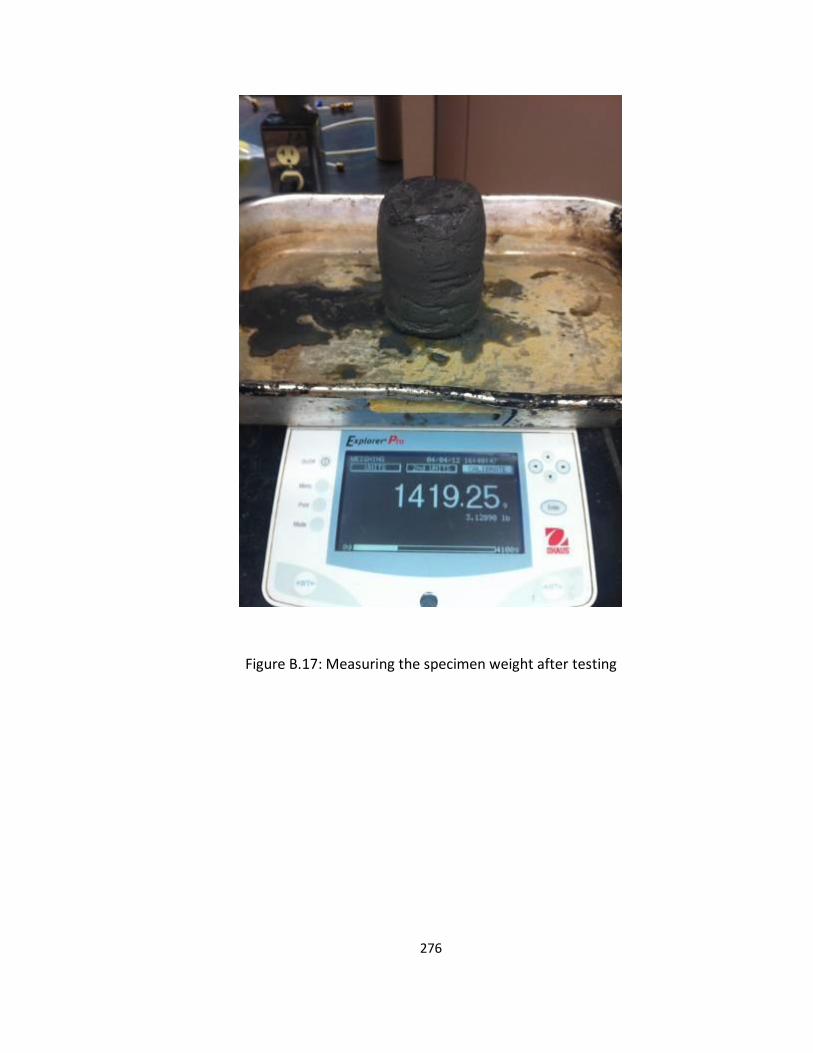
276
Figure B.17: Measuring the specimen weight after testing
277
APPENDIX C
C. CYCLIC TRIAXIAL TESTING SPREADSHEET
In this section, the spreadsheet to record all the information starting from
specimen preparation until shear phase for cyclic triaxial testing are presented (Table
C.1 – C.3).
To record all the reading during cyclic triaxial test, a spreadsheet was created to
help organize and calculate all information needed for each specimen. The spreadsheet
was used from the beginning of the test, to record the dimensions of sample, until the
last phase to record the oven-dried weight of sample for moisture content
measurement.
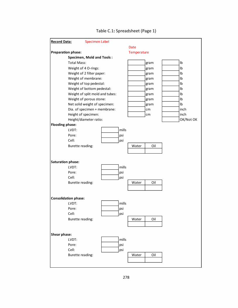
278
Table C.1: Spreadsheet (Page 1)
Record Data: Specimen Label
Date
Preparation phase: Temperature
Specimen, Mold and Tools :
Total Mass: gram lb
Weight of 4 O-rings: gram lb
Weight of 2 filter paper: gram lb
Weight of membrane: gram lb
Weight of top pedestal: gram lb
Weight of bottom pedestal: gram lb
Weight of split mold and tubes: gram lb
Weight of porous stone: gram lb
Net solid weight of specimen: gram lb
Dia. of specimen + membrane: cm inch
Height of specimen: cm inch
Height/diameter ratio: OK/Not OK
Flooding phase:
LVDT: mills
Pore: psi
Cell: psi
Burette reading: Water Oil
Saturation phase:
LVDT: mills
Pore: psi
Cell: psi
Burette reading: Water Oil
Consolidation phase:
LVDT: mills
Pore: psi
Cell: psi
Burette reading: Water Oil
Shear phase:
LVDT: mills
Pore: psi
Cell: psi
Burette reading: Water Oil
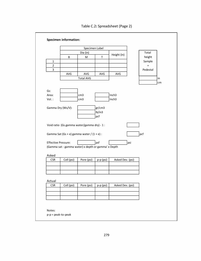
279
Table C.2: Spreadsheet (Page 2)
Specimen information:
Total
B M T height
1 Sample
2 +
3 Pedestal
AVG AVG AVG AVG
in
cm
Gs:
Area: cm3 Inch3
Vol. : cm3 Inch3
Gamma Dry (Ws/V): gr/cm3
lb/in3
pcf
Void ratio (Gs.gamma water/gamma dry) - 1 :
Gamma Sat (Gs + e) gamma water / (1 + e) : pcf
Effective Pressure: psf psi
(Gamma sat - gamma water) x depth or gamma' x Depth
AskedCSR Cell (psi) Pore (psi) p-p (psi)
Actual CSR Cell (psi) Pore (psi) p-p (psi)
Notes:
p-p = peak-to-peak
Asked Dev. (psi)
Asked Dev. (psi)
Specimen Label
Dia (in)Height (in)
Total AVG
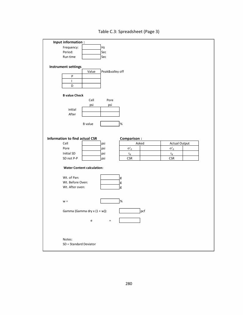
280
Table C.3: Spreadsheet (Page 3)
Input information :
Frequency: Hz
Period: Sec
Run time Sec
Instrument settingsValue Peak&valley off
P
I
D
B value Check
Cell Pore
psi psi
initial
After
B value %
Information to find actual CSR Comparison :Cell psi
Pore psi '0 '0
Initial SD psi d d
SD not P-P psi CSR CSR
Water Content calculation:
Wt. of Pan: g
Wt. Before Oven: g
Wt. After oven: g
w = %
Gamma (Gamma dry x (1 + w)): pcf
e =
Notes:
SD = Standard Deviator
Asked Actual Output
281
REFERENCES
AECOM Technology Corporation (AECOM). (2009). Root Cause Analysis of TVA
Kingston Dredge Pond Failure on December 22, 2008.
Alabama Earthquakes. (2016). Retrieved June 20, 2016, from
http://gsa.state.al.us/gsa/geologichazards/Quakes_AL.htm
American Coal Ash Association (ACAA). (2008). 2008 Coal Combustion Product
(CCP) Production and use survey report. Retrieved from http://www.acaa-
usa.org/Portals/9/Files/PDFs/2008_ACAA_CCP_Survey_Report_FINAL_100509.p
df
American Coal Ash Association (ACAA). (2012). 1966-2012 Fly Ash Production
and use charts. Retrieved from http://www.acaa-
usa.org/Portals/9/Files/PDFs/1966-2012_FlyAsh_Prod_and_Use_Charts.pdf
American Coal Ash Association (ACAA). (2012). “Frequently Asked Questions”.
Retrieved September 8, 2014, from
http://acaa.affiniscape.com/displaycommon.cfm?an=1&subarticlenbr=5
American Concrete Institute (ACI). (2010). "Fly ash Contribution to Sustainable
Conrete Construction." ACI-American Concrete Institute. ACI, 21 March 2010.
Web. 27 Aug 2010.
<http://www.concrete.org/education/Webcasts/FlyAshIndex.html>.
Associated Press; Samuel M. Simpkins/The Tennessean Retrieved from
http://www.usatoday.com/story/news/nation/2013/12/22/coal-ash-
spill/4143995/
Assistant Secretary for Housing Federal Housing Commissioner. (1993). HUD
Building Product Standards and Certification Program for Carpet. Tech. no. 44d.
N.p.: Department of Housing and Urban Development, 1993. Print.
ASTM C 618 Specification for Coal Fly Ash and Raw or Calcined Natural Pozzolan
for Use as a Mineral Admixture in Portland Cement Concrete
282
ASTM D422 - 63(2007) Standard Test Method for Particle-Size Analysis of Soils.
American Society for Testing and Materials, Annual Book of ASTM Standards.
Vol. 04.08.
ASTM D854 - 10 Standard Test Methods for Specific Gravity of Soil Solids by
Water Pycnometer. American Society for Testing and Materials, Annual Book of
ASTM Standards. Vol. 04.08.
ASTM D2216 - 10 Standard Test Methods for Laboratory Determination of Water
(Moisture) Content of Soil and Rock by Mass. American Society for Testing and
Materials, Annual Book of ASTM Standards. Vol. 04.08.
ASTM D3999 - 11 Standard Test Methods for the Determination of the Modulus
and Damping Properties of Soils Using the Cyclic Triaxial Apparatus. American
Society for Testing and Materials, Annual Book of ASTM Standards. Vol. 04.08.
ASTM D5311 - 11 Standard Test Method for Load Controlled Cyclic Triaxial
Strength of Soil. American Society for Testing and Materials, Annual Book of
ASTM Standards. Vol. 04.08.
Boominathan, A., & Hari, S. (2002). Liquefaction strength of fly ash reinforced
with randomly distributed fibers. Soil Dynamics and Earthquake Engineering,
1027-1033.
Bray, J. D., Sancio, R. B., Riemer, M. F., and Durgunoglu, T. (2004). “Liquefaction
susceptibility of fine-grained soils.” Proc., 11th Int. Conf. on Soil Dynamics and
Earthquake Engineering and 3rd Int. Conf. on Earthquake Geotechnical
Engineering, D. Doolin et al., eds., Stallion Press, Singapore, 655–662.
Castro, G. and Poulos, S. J. (1977). “Factors affecting liquefaction and cyclic
mobility.” Journal of the Geotechnical Engineering Division, Proceedings of the
ASCE, 103(6), 501-516.
Chen, Y., A. Gottesman, T. Aviad, and Y. Inbar. (1991). “The Use of Bottom-Ash
Coal-Cinder Amended with Compost as a Container Medium in Horticulture,”
Acta Horticulturae 294: 173-I 8 1, 1991.
Choudary, A., Jha, J., & Gill, K. (2011). Shear strength characteristics of fiber
reinforced fly ash.
283
Cunningham, J. A., Lukas, R. G., and Andreson, T. C. (1977). “Improvement of Fly
Ash and Stage—A Case Study,” Proceedings, Conference on Geotechnical Practice
for Disposal of Solid Waste Materials, American Society of Civil Engineers, Ann
Arbor, MI, 1977, pp. 227–245.
Darendeli, M. (2001). “Development of a new family of normalized modulus
reduction and material damping curves.” Ph.D. Thesis, Dept. of Civil Eng., Univ. of
Texas, Austin.
Department of Ecology state of Washington "Waste Tires." Washington State
Department of Ecology, 04 Apr. 2010. Retrieved from
http://www.ecy.wa.gov/programs/swfa/tires/.
Dey, Ashim, & Gandhi, S.R. (2008). Evaluation of liquefaction potential of pond
ash. Geotechnical Engineering for Disaster Mitigation and Rehabilitation, Science
Press Beijing and Springer-Verlag GmbH Berlin Heidelberg
Engstrom, G. and R. Lamb. (2003). Using shredded waste tires as a lightweight fill
material for road subgrades: a summary report. Minnesota Department of
Transportation, Physical Research & Geotechnical Engineering Sections,
Materials Research & Engineering. RMA. 2004b. U.S. scrap tire markets: 2003
edition. Rubber Manufacturers Association, Washington, DC.
Environmental Integrity Project. (2013). TVA’s Toxic Legacy: Groundwater
Contaminated by Tennessee Valley Authority Coal Ash.
Environmental Protection Agency (EPA). (2009). Fact Sheet: Coal Combustion
Residues (CCR) - Surface Impoundments with High Hazard Potential Ratings, June
2009
Federal Highway Administration (FHWA). (1999). "Fly ash facts for Highway
Engineers." 3rd. 1. Washington, D.C.
Gandhi, S., Dey, A., & Selvam, S. (1999). Densification of Pond Ash by Blasting.
Journal of Geotechnical and Geoenvironmental Engineering, 125(10), 889-889.
Retrieved September 8, 2014.
Gandhi, S. R., Raju, V.S., and Vinal Kumar. (1997). “Densificationof deposited ash
slurry.” Proc., 13th Int. Conf. on solid waste technol. And Mgmt., Vol. 1, 4C, 1-8.
284
Garlisch, Nick. (2010). “Coal ash disposal” Retrieved from
http://www.kentlaw.edu/faculty/fbosselman/classes/energyF10/Nick%20Garlisc
h.ppt
Ghosh, A., & Subbarao, C. (1998). Hydraulic Conductivity and Leachate
Characteristics of Stabilized Fly Ash. JOURNAL OF ENVIRONMENTAL
ENGINEERING, 812-812.
Gottlieb, B., Gilbert, S., & Evans, L. (2010). Coal Ash the Toxic Threat to Our
Health and Environment. . Retrieved from http://www.psr.org/assets/pdfs/coal-
ash.pdf
Gray, D.H. and Lin, Y.K., (1972). Engineering properties of compacted fly ash.
Journal of Soil Mechanics and Foundation Engineering, ASCE, 98 (4), 361–380.
Guoxi, Zeng, Yaozhang, Gu, Jianping, Wu. (1985). Dynamic shear modulus of fly
ash. Chinese Jounal of Geotechnical Engineering;1985-05
Hardin, B. O. & Drnevich, V. P. (1972). “Shear modulus and damping in soils:
Design equations and curves.” Journal of Soil Mechanics and Foundations
Division, ASCE. 98(7): 667-692.
Health Canada. (1979). Guidelines for Canadian Drinking Water Quality -
Hardness. Ottawa, Canada: Health Canada.
Illinois Environmental Protection Agency (Illinois EPA). (2016). Used Tire Facts
and Information. Retrieved June 20, 2016, from
http://www.epa.illinois.gov/topics/waste-management/waste-disposal/used-
res/facts/index
Ishibashi, I. & Zhang, X. (1993) “Unified dynamic shear moduli and damping
ratios of sand and clay”. Soils and Foundations 33(1): 182-191.
Kalinski, M. E., and Hippley, B. T., (2005). “The Effect of Water Content and
Cement Content on the Strength of Portland Cement-Stabilized Compacted Fly
Ash,” Fuel, Elsevier, Vol. 84, No. 14-15, pp. 1812-1819.
Kalinski, M. (2011). Soil mechanics: Lab manual: 2nd edition (Revised/Expanded
ed.). Hoboken, NJ: Wiley.
285
Kaniraj, Shenbaga, and V Gayathri. "Geotechnical behavior of fly ash mixed with
randomly oriented fiber inclusions." Geotechnical behavior of fly ash mixed with
randomly oriented fiber inclusions 21.3 (2003): 123-149. Web. 27 Aug 2010.
<http://www.sciencedirect.com/science?_ob=ArticleURL&_udi=B6V3D-840TMK-
1&_user=16764&_coverDate=06%2F30%2F2003&_rdoc=1&_fmt=high&_orig=se
arch&_sort=d&_docanchor=&view=c&_searchStrId=1213993607&_rerunOrigin=
google&_acct=C000001898&_version=1&_urlVersion=0&_userid=16764&md5=c
cd25cd0a9630c4977009ce01072eff5>.
Kennedy, Chloe. "TVA ash pond breach: Resident says area has 'changed forever'."
knoxvillebiz.com. 23 Dec 2008. Knoxville Daily News, Web.
<http://www.knoxnews.com/news/2008/dec/23/tva-ash-pond-breach-resident-
says-area-has-changed/>, 14 Jun (2009).
Kentucky Energy and Environmental Cabinet. (2012). Kentucky Coal Facts - 12th
Edition.
Kentucky transportation cabinet. (2015). 2015 Kentucky statewide rail plan, April
2015
Kulkarni, S. (2003). Effect of filler-fiber interactions on compressive strength of
fly ash and short-fiber epoxy composites. Journal of Applied Polymer Science, 87,
836-841.
Kumar, Praveen, Mehndiratta, H C, Chandranarayana, S, & Singh, S P. (2006).
Effect of randomly distributed fibers on flyash embankments. Vol. 86, November
2005.
Kumar, P., & Singh, S. (2010). Fiber-Reinforced Fly Ash Subbases in Rural Roads.
Journal of Transportation Engineering, 134(4), 171-180.
Lave L, Conway-Schempf N, Harvey J, Hart D, Bzee T and MacCracken C (1998).
Recycling postconsumer nylon carpet: a case study of the economics and
engineering issues associated with recycling post-consumer goods. J Ind Ecol 2:
117-126.
Leather, T. (2010). Seas of Rubber: The Truth About Tire Recycling. Retrieved
August 25, 2016, from http://recyclenation.com/2010/06/sea-rubber-truth-tire-
recycling
286
Lee, K. L. and Seed, H. B. (1967). “Cyclic stress conditions causing liquefaction of
sand.” Journal of the Soil Mechanics and Foundations Division, Proceedings of the
ASCE, 93(1), pp. 47-70.
Lemly, A. (2001). Symptoms and implications of selenium toxicity in fish: The
Belews Lake case example. Aquatic Toxicology, 39-49.
Leonards GA, Bailey B. (1982). Pulverized coal ash as structural fill. J Geotech Eng
108(GT4):517–531
Marcuson,W. F., III. (1978). ‘‘Definition of terms related to liquefaction.’’ J.
Geotech. Engrg. Div., ASCE, 104(9), 1197–1200.
Mohan, K.S.R., P. Jayabalan and A. Rajaraman, (2012). Properties of fly ash based
coconut fiber composite. Am. J. Eng. Applied Sci., 5: 29-34.
Nuttli, Otto W. (1974). Earthquake Information Bulletin. Volume 6.Number 2
(March-April 1974)
Office of Research, Development, and Technology, Office of Safety, RDT. (2012).
User Guidelines for Waste and Byproduct Materials in Pavement Construction.
Publication. no. FHWA-RD-97-148, U.S. Department of Transportation Federal
Highway Administration..
Puppala, A., Hoyos, L., Viyanant, C., & Musenda, C. (2001). Fiber and Fly Ash
Stabilization Methods to Treat Soft Expansive Soils. Soft Ground Technology, 112,
Pg. 136-145.
Recycle Material Resource Center (RMRC). (2012). Coal Bottom Ash/Boiler Slag -
Material Description. Retrieved from http://rmrc.wisc.edu/ug-mat-coal-bottom-
ashboiler-slag/
Right, R.J., Kemper, W.D., Millner, P.D., Power, J.F., Krocak, R.F., (1998).
Agricultural uses of municipal, animal and industrial byproducts. USDA-ARS,
Conversation Research Report. No. 44
Rubber manufacturers association (RMA). (2004). U.S. Scrap tire markets 2003
edition. Retrieved from https://rma.org/sites/default/files/US_STMarkets2003-
final.pdf
287
Seed, H. B., and Idriss, I. M., (1971), Simplified Procedure for Evaluating Soil
Liquefaction Potential, Journal of the Soil Mechanics and Foundations Division,
Proceedings of the ASCE, Vol. 97, No. SM9, pp. 1249-1273.
Seed, H. B., and Idriss, I. M. (1982). ‘‘Ground motions and soil liquefaction during
earthquakes.’’ Earthquake Engineering Research Institute Monograph, Oakland,
Calif.
Seed, R. B., and Harder, L. F., (1990), SPT-Based Analysis of Cyclic Pore Pressure
Generation and Undrained Residual Strength,. Proceedings of the H. Bolton Seed
Memorial Symposium, University of California, Berkeley, Vol. 2, pp. 351-376.
Seed et al. (2003). Seed, R B., Cetin, K.O., Moss, R.E.S., Kammerer, A., Wu, J.,
Pestana, J., Riemer, M., Sancio, R.B., Bray, J.D., Kayen, R.E., & Faris, A. 2003.
Recent advances in soil liquefaction engineering: a unified and consistent
framework. Keynote presentation, 26th Annual ASCE Los Angeles Geotechnical
Spring Seminar, Long Beach, CA.
Siuru, William D., (1993), Waste/energy: Turning tires and oil into alternative
fuel, Retrieved from
http://waste360.com/mag/waste_wasteenergy_turning_tires
Southern Alliance for Clean Energy. (2013). Coal Ash Storage Methods. Retrieved
from http://www.southeastcoalash.org/?page_id=78
South Central Iowa Solid Waste Agency (SCISWA). (2016). Retrieved June 20,
2016, from http://www.sciswa.org/services/recycling/specialitem/tires.html
Tsuchida, H., (1970). "Prediction and Countermeasure Against the Liquefaction in
Sand Deposits," Abstract of the Seminar in the Port and Harbor Research
Institute (in Japanese).
U.S. Environmental Protection Agency (U.S. EPA). (1988). Wastes from the
combustion of coal by electric utility power plants. USEPA Washington, DC.
EPA/530-SW-88-002
U.S. Environmental Protection Agency (U.S. EPA). (2010). Identifying Greener
Carpet. Retrieved June 20, 2016, from
https://www.epa.gov/greenerproducts/identifying-greener-carpet
288
U.S. Environmental Protection Agency (U.S. EPA), (2016). Frequent Questions
about Applicability of Other Regulations and Implementing the Final Rule
Regulating the Disposal of Coal Combustion Residuals (CCR). (2016, June 7).
Retrieved August 25, 2016, from https://www.epa.gov/coalash/frequent-
questions-about-applicability-other-regulations-and-implementing-final-rule
Viswanathan, R., Saylak, D., & Estakhri, C. (1997). Stabilization of Subgrade Soils
Using Fly Ash
Vucetic, M. and Dobry, R. (1991). ”Effect of Soil Plasticity on Cyclic Response.”
Journal of Geotechnical Engineering, 117(1), 89–107.
Wang W. (1979). “Some findings in soil liquefaction.” Water Conservancy and
Hydroelectric Power Scientific Research Institute, Beijing, China.
Watson, T. (2006). The benefits of green carpeting, in any color. The Seattle
Times.
World health organization (WHO), (1984). Guidelines for Drinking-water Quality,
volume 1 & 2.
Yang, S., Lohnes, R. A., and Kjartanson, B. H., (2002). “Mechanical Properties of
Shredded Tires,” Geotechnical Testing Journal, GTJODJ, Vol. 25, No. 1, March
2002, pp. 44–52.
Youd, T. L., Idriss, I. M., Andrus, R. D., Arango, I., Castro, G., Christian, J. T., Dobry,
R., Finn, W. D. L., Harder, L. F., Hynes, M. E., Ishihara, K., Koester, J. P., Liao, S. C.,
Marcuson, W. F., Martin, G. R., Mitchell, J. K., Moriwaki, Y., Power, M. S.,
Robertson, P. K., Seed, R. B., and Stokoe, K. H., (2001), Liquefaction Resistance of
Soils: Summary Report from the 1996 NCEER and 1998 NCEER/NSF Workshops
on Evaluation of Liquefaction Resistance of Soils, Journal of Geotechnical and
Geoenvironmental Engineering, American Society of Civil Engineers, Vol. 127, No.
10, pp. 817-833.
Zand, B., Tu, W., Amaya, P., Wolfe, W., & Butalia, T. (2008). An experimental
investigation on liquafaction potential and post-liquefaction shear strength of
impounded flya ash. FUEL, 88, 1160-1166.
289
Zand, Behrad, Wei Tu, Pedro J. Amaya, William E. Wolfe, and Tarunjit Butalia.
(2007). "Evaluation of liquefaction potential of impounded fly ash." World of Coal
Ash.
Zhen, G.X., Gu, R.Z. and Wu, J.P. (1985). "Dynamic Shear Moduli of Flyashes",
Chinese Journal of Geotechnical Engineering, Vol. 7, No. 5.
290
VITA
Alfred Jonathan Susilo was born in Jakarta, Indonesia. He graduated from
Tarumanagara University, Jakarta, Indonesia in 2005 with Bachelor Degree in Civil
Engineering. During his senior year, he worked as an assistant for surveying laboratory.
After working as a full-time engineer for Consulting Engineering Company in Indonesia
for Two (2) Years, he continued his study at McNeese State University (University of
Louisiana System) in Lake Charles, LA from 2007 to 2009, and also worked as Graduate
Assistant for Surveying and Soil Mechanics laboratories. The following year after earned
his Master Degree in Civil Engineering, he continued his study at University of Kentucky,
Lexington, KY and during his research he also employed as an instructor for the
Undergraduate Soil Mechanics Laboratory
July 21, 2016