Embed Size (px)
Citation preview

23 11
Article 19.1.7Journal of Integer Sequences, Vol. 22 (2019),2
3
6
1
47
Enumerating Multiplex Juggling Patterns
Steve ButlerDepartment of Mathematics
Iowa State UniversityAmes, IA 50011
Jeongyoon Choi, Kimyung Kim, and Kyuhyeok SeoGyeonggi Science High School for the Gifted
Gyeonggi ProvinceRepublic of Korea
Abstract
A classic problem in the mathematics of juggling is to give a basic enumeration ofthe number of juggling patterns. This has been solved in the case when at most oneball is caught/thrown at a time, with the simplest proof being due to Ehrenborg andReaddy by the use of cards.
We introduce a new set of cards that can be used to count multiplex jugglingpatterns (when multiple balls can be caught/thrown at a time). This set of cardsmodels the correct behavior and avoids the problems of ambiguity; on the other handthe cards are no longer independent. By use of the transfer matrix method combinedwith the cards we enumerate multiplex juggling patterns with exactly b balls and handcapacity κ, and include data for κ = 2, 3, and establish some combinatorial propertiesof the cards.
1 Introduction
While mathematics and juggling have existed independently for thousands of years, it hasonly been in the last thirty years that the mathematics of juggling has become a subject
1
in its own right (for a general introduction see Polster [5]). Several different approaches fordescribing juggling patterns have been used. The best-known method is siteswap which givesinformation what to do with the ball that is in your hand at the given moment, in particularhow “high” you should throw the ball (see [1, 5]). For theoretical and enumeration purposesa more useful method is to describe patterns by the use of cards. This was first introduced inthe work of Ehrenborg and Readdy [4] (see also Stadler [7]), and modified by Butler, Chung,Cummings and Graham [2].
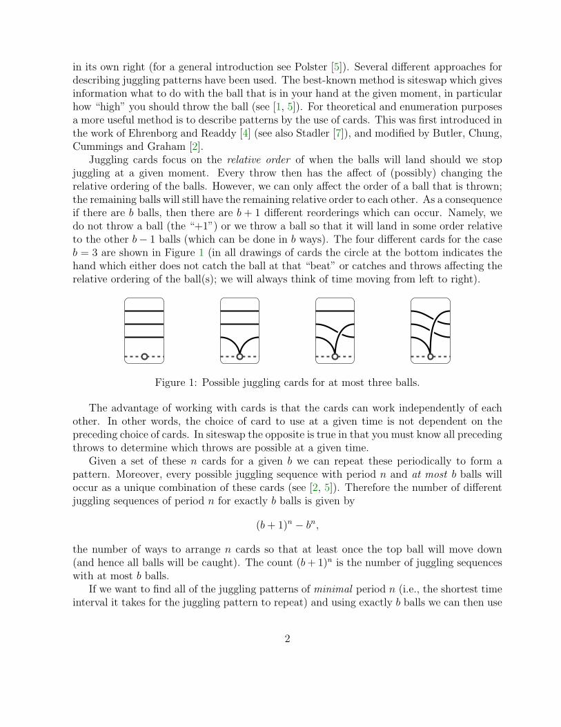
Juggling cards focus on the relative order of when the balls will land should we stopjuggling at a given moment. Every throw then has the affect of (possibly) changing therelative ordering of the balls. However, we can only affect the order of a ball that is thrown;the remaining balls will still have the remaining relative order to each other. As a consequenceif there are b balls, then there are b + 1 different reorderings which can occur. Namely, wedo not throw a ball (the “+1”) or we throw a ball so that it will land in some order relativeto the other b− 1 balls (which can be done in b ways). The four different cards for the caseb = 3 are shown in Figure 1 (in all drawings of cards the circle at the bottom indicates thehand which either does not catch the ball at that “beat” or catches and throws affecting therelative ordering of the ball(s); we will always think of time moving from left to right).
Figure 1: Possible juggling cards for at most three balls.
The advantage of working with cards is that the cards can work independently of eachother. In other words, the choice of card to use at a given time is not dependent on thepreceding choice of cards. In siteswap the opposite is true in that you must know all precedingthrows to determine which throws are possible at a given time.
Given a set of these n cards for a given b we can repeat these periodically to form apattern. Moreover, every possible juggling sequence with period n and at most b balls willoccur as a unique combination of these cards (see [2, 5]). Therefore the number of differentjuggling sequences of period n for exactly b balls is given by
(b+ 1)n − bn,
the number of ways to arrange n cards so that at least once the top ball will move down(and hence all balls will be caught). The count (b+ 1)n is the number of juggling sequenceswith at most b balls.
If we want to find all of the juggling patterns of minimal period n (i.e., the shortest timeinterval it takes for the juggling pattern to repeat) and using exactly b balls we can then use
2

Mobius inversion and divide out by the period to get
1
n
∑
d|n
µ(nd)((b+ 1)d − bd
),
where µ is the Mobius function (see [1]). We will revisit this with more detail in Section 5.(We differentiate a juggling sequence from a juggling pattern by noting that a jugglingpattern is not time dependent, i.e., if we shift time by 1 unit it is still the same pattern, butit might not be the same sequence.)
For as long as there has been interest in the mathematics of juggling, there has beeninterest in extending results to multiplex juggling (where more than one ball is allowed to becaught at a time). In Ehrenborg and Readdy [4] they produced possible cards for multiplexjuggling. For these cards, multiple balls could come down at a given time and would thenbe redistributed appropriately. While these cards can describe every juggling pattern thereis the problem that uniqueness is lost (see Figure 2 for an example of two consecutive cardsdescribing the same pattern but using different cards; note these cards are mirrored fromthe form of the cards given in Ehrenborg and Readdy [4]). So these do not form a bijectionwith the number of juggling sequences.
Figure 2: Ambiguity arising from using cards of Ehrenborg and Readdy [4].
One approach is to distinguish the balls which come down. This is what was done inButler, Chung, Cummings, and Graham [2], an example of such a card is shown in Figure 3.This avoids ambiguity that might arise but does not accurately reflect multiplex jugglingin practice. Rather this reflects passing patterns with multiple jugglers involved, and eachjuggler catching one ball (in particular the different points that come down correspond tothe different jugglers).
Figure 3: An example of a card used in Butler, Chung, Cummings, and Graham [2].
In this paper we will propose a new type of card which can be used for multiplex juggling.It avoids the ambiguity problem of Ehrenborg and Readdy and also avoids the modeling
3

problem of Butler, Chung, Cummings, and Graham. However it does come at the cost ofhaving a card being dependent on the previous card which came before. In Section 2 wewill introduce these cards, and in Section 3 we show how to use matrices associated witha weighted graph to count the number of periodic card sequences of length n. We thencount the number of juggling sequences and the number of juggling patterns in Section 4and Section 5. In Section 6 we will consider what happens when we limit the number ofballs which can be thrown. We will give some concluding remarks in Section 7, including adiscussion of counting crossing numbers.
We will also see that the objects generated in the process of deriving our count seemto have independent combinatorial interest. Moreover, while our main goal has been toenumerate juggling patterns, the cards themselves might be useful for the exploration ofother combinatorial aspects of juggling.
Finally, we note that while there has some been interest in counting multiplex jugglingpatterns, prior to this paper there has been little success. Butler and Graham [3] made themost progress but their focus was on counting closed walks in a state graph and were notable to efficiently enumerate all juggling patterns.
2 Cards for multiplex juggling
The way that cards describe juggling patterns is through understanding the relative orderof their landing times. The ambiguity that appeared in Figure 2 comes from the fact thattwo balls are landing together but still being kept separate in the ordering. Since they areseparate we could order them in two ways but that does not affect the pattern. This suggeststhe following simple fix: tracks in the cards no longer represent individual balls, but rathergroups of balls which will land together. So now either the “lowest” group does not land, orthe lowest group lands and the balls get thrown so that they are placed in a new track(s)and/or added to an existing track(s).
Before each throw we will have a composition (or ordered partition) of the number ofballs b on the left of the card. We will call this the arrival composition, i.e., (q1, q2, . . . , qk)which corresponds to the statement that were we to stop juggling we would first have q1 ballsland together at some point; then q2 balls land together some time later; and so on untilfinally qk balls land together at the end. (Note that we do not claim that they will land onetime step apart from each other; cards are keeping track of relative ordering of when thingsland and not the absolute times that they will land.)
After each throw we will have another composition of b on the right of the card. We willcall this the departure composition, i.e., (r1, r2, . . . , rℓ). The number of parts in the arrivaland departure compositions need not be the same, but we must have ℓ ≥ k − 1. If thebottom track of balls land, then the card indicates how the q1 balls get redistributed to thedeparture composition. Examples of these cards are shown in Figure 4 where the first cardcorresponds to going from (2, 1, 1) back to (2, 1, 1) and the second corresponds to going from(2, 2, 1) to (1, 2, 2).
4
2
1
1
2
1
1
2
2
1
1
2
2
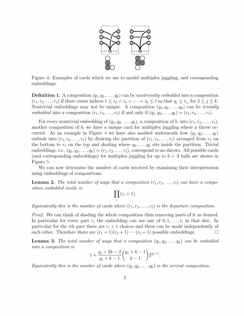
Figure 4: Examples of cards which we use to model multiplex juggling, and correspondingembeddings.
Definition 1. A composition (q1, q2, . . . , qk) can be nontrivially embedded into a composition(r1, r2, . . . , rℓ) if there exists indices 1 ≤ i2 < i3 < · · · < ik ≤ ℓ so that qj ≤ rij for 2 ≤ j ≤ k.Nontrivial embeddings may not be unique. A composition (q1, q2, . . . , qk) can be trivially
embedded into a composition (r1, r2, . . . , rℓ) if and only if (q1, q2, . . . , qk) = (r1, r2, . . . , rℓ).
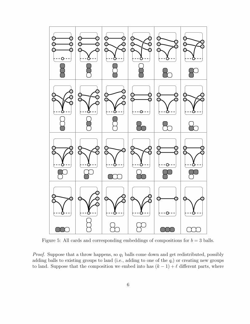
For every nontrivial embedding of (q1, q2, . . . , qk), a composition of b, into (r1, r2, . . . , rℓ),another composition of b, we have a unique card for multiplex juggling where a throw oc-curred. As an example in Figure 4 we have also marked underneath how (q1, q2, . . . , qk)embeds into (r1, r2, . . . , rℓ) by drawing the partition of (r1, r2, . . . , rℓ) arranged from r1 onthe bottom to rℓ on the top and shading where q2, . . . , qk sits inside the partition. Trivialembeddings, i.e., (q1, q2, . . . , qk) = (r1, r2, . . . , rℓ), correspond to no throws. All possible cards(and corresponding embeddings) for multiplex juggling for up to b = 3 balls are shown inFigure 5.
We can now determine the number of cards involved by examining their interpretationusing embeddings of compositions.
Lemma 2. The total number of ways that a composition (r1, r2, . . . , rℓ) can have a compo-
sition embedded inside is ∏
i
(ri + 1).
Equivalently this is the number of cards where (r1, r2, . . . , rℓ) is the departure composition.
Proof. We can think of shading the whole composition then removing parts of it as desired.In particular for every part ri the embedding can use any of 0, 1, . . . , ri in that slot. Inparticular for the ith part there are ri + 1 choices and these can be made independently ofeach other. Therefore there are (r1 + 1)(r2 + 1) · · · (rℓ + 1) possible embeddings.
Lemma 3. The total number of ways that a composition (q1, q2, . . . , qk) can be embedded
into a composition is
1 +q1 + 2k − 2
q1 + k − 1
(q1 + k − 1
k − 1
)2q1−1.
Equivalently this is the number of cards where (q1, q2, . . . , qk) is the arrival composition.
5
1
1
1
1
1
1
1
1
1
1
1
1
1
1
1
1
1
1
1
1
1
1
1
1
1
1
1
2
1
1
1
1
2
1
2
1
1
1
1
2
1
1
1
1
2
1
1
1
1
2
1
2
1
2
1
2
1
2
1
2
1
2
1
1
2
2
1
1
2
2
1
3
1
2
2
1
1
2
1
2
1
2
1
2
1
2
3 3
1
1
1 3
2
1
3
1
2
3 3 3 3
Figure 5: All cards and corresponding embeddings of compositions for b = 3 balls.
Proof. Suppose that a throw happens, so q1 balls come down and get redistributed, possiblyadding balls to existing groups to land (i.e., adding to one of the qi) or creating new groupsto land. Suppose that the composition we embed into has (k − 1) + ℓ different parts, where
6

0 ≤ ℓ ≤ q1. This can happen in
(k − 1 + ℓ
ℓ
)(k + q1 − 2
q1 − ℓ
)=
ℓ+ k − 1
q1 + k − 1
(q1ℓ
)(q1 + k − 1
k − 1
)
different ways. The(k−1+ℓ
ℓ
)divides the parts as coming from an existing part (e.g., qi) or
being newly created. For the ℓ new parts we first need to get a contribution of 1 comingfrom q1 leaving q1 − ℓ available to distribute among the k − 1 + ℓ different parts arbitrarilywhich can be done in
(k+q1−2q1−ℓ
)ways. Finally, we can perform some simple manipulation of
binomial coefficients.Putting this together we have that the total number of ways that (q1, q2, . . . , qk) can be
embedded into another composition by a throw is
q1∑
ℓ=0
ℓ+ k − 1
q1 + k − 1
(q1ℓ
)(q1 + k − 1
k − 1
)=
1
q1 + k − 1
(q1 + k − 1
k − 1
) q1∑
ℓ=0
(ℓ+ k − 1)
(q1ℓ
)
=1
q1 + k − 1
(q1 + k − 1
k − 1
)( q1∑
ℓ=0
ℓ
(q1ℓ
)+
q1∑
ℓ=0
(k − 1)
(q1ℓ
))
=1
q1 + k − 1
(q1 + k − 1
k − 1
)(q12
q1−1 + (k − 1)2q1)
=q1 + 2k − 2
q1 + k − 1
(q1 + k − 1
k − 1
)2q1−1.
Combining this with the “+1” from the trivial embedding and the result follows.
We can now determine the total number of cards, or equivalently the total number ofembeddings possible. Starting with b = 0 the numbers are
1, 2, 7, 24, 82, 280, 956, 3264, 11144, 38048, 129904, 443520, 1514272, . . . .
This is sequence A003480 in the OEIS [6] which is initiated with a0 = 1, a1 = 2 and a2 = 7and for b ≥ 3 we have ab = 4ab−1 − 2ab−2.
Theorem 4. If ab is the number of possible cards used for describing multiplex juggling with
b balls, then a1 = 2, a2 = 7, and for b ≥ 3 we have ab = 4ab−1 − 2ab−2.
Proof. Verification of a1 and a2 can be done by examining Figure 5, so it remains to establishthe recursion. We can count the number of cards by breaking our count up according to thedeparture composition using Lemma 2. In particular we have
ab =∑
(r1,r2,...)∈Rb
∏
i≥1
(ri + 1), (1)
7
where Rb are all of the compositions of b.We now further break up this count by combining the compositions according to the size
of the first part which can be anything from 1 to b. So we have
ab =b∑
j=1
( ∑
(j,r2,...)∈Rb
(j + 1)∏
i≥2
(ri + 1)
)
=b∑
j=1
(j + 1)
( ∑
(r2,...)∈Rb−j
∏
i≥2
(ri + 1)
)
=b∑
j=1
(j + 1)ab−j,
where in the last step we note that we have the form of (1).To finish we have
ab − 2ab−1 + ab−2 =b∑
j=1
(j + 1)ab−j − 2b−1∑
j=1
(j + 1)ab−1−j +b−2∑
j=1
(j + 1)ab−2−j
=b∑
k=1
(k + 1)ab−k − 2b∑
k=2
kab−k +b∑
k=3
(k − 1)ab−k
= 2ab−1 − ab−2.
Here we reindex the three sums to be consistent and then note that all but the first twoterms will drop out. Rearranging we conclude ab = 4ab−1 − 2ab−2, as desired.
3 Combining cards by taking walks in a graph
The advantage to using cards in order to describe juggling patterns was the ability to have thecurrent card be chosen independently of all other cards. With these new cards for multiplexjuggling we now have to be careful in that the choice of our current card is dependent onthe previous card. Namely, the departure composition of the previous card must match thearrival composition of the current card. Moreover if we are forming a pattern with period nwe need to make sure that our last card will also be consistent with our first card (so thatwe can repeat the pattern).
To help achieve this we will construct a directed multi-graph Gb by letting the verticesof Gb be the compositions of b; and for each card we add a directed edge from the arrivalcomposition to the departure composition.
Observation 5. There is a one-to-one correspondence between periodic sequences using ncards and closed walks of length n in the graph. In particular, to count the number ofperiodic sequences using n cards it suffices to count the number of closed walks of length n.
8

This follows by noting that each card is an edge and if two cards are used sequentially thenthe edges also occur sequentially in the graph, giving the correspondence between sequencesof consecutive cards and walks in the graph. Moreover the fact that we can repeat thepattern periodically indicates that we must return to the same composition that we startedwith, so the walk is closed.
We now can use the transfer matrix method (see Stanley [8, Ch. 4.7]).
Theorem 6 (Transfer matrix method). Given a directed multi-graph G let A be the matrix
with rows and columns indexed by the vertices with Auv equal to the number of directed arcs
from u → v. Then tr(An) equals the number of closed walks of length n in the graph.
Let Ab be the matrix associated with the graph Gb. We have A0 = (1), A1 = (2),
A2 =(2)
(1, 1)
(2 11 3
), A3 =
(3)(2, 1)(1, 2)
(1, 1, 1)
2 1 1 11 3 2 31 1 2 00 1 1 4
,
and
A4 =
(4)(3, 1)(1, 3)
(2, 1, 1)(2, 2)
(1, 2, 1)(1, 1, 2)
(1, 1, 1, 1)
2 1 1 1 1 1 1 11 3 2 3 2 3 3 41 1 2 0 0 0 0 00 1 1 4 1 3 3 61 1 1 1 3 1 1 00 1 0 2 1 2 0 00 0 1 0 1 1 3 00 0 0 1 0 1 1 5
,
where on the left we have marked the compositions that correspond to the vertex. Forreference we also give the graphs G0, G1, G2, G3 in Figure 6.
∅
1
(1)
2 (1, 1)
(2)
3
2
11
(3) (1, 2)
(1, 1, 1)(2, 1)
2
3
2
4
1
1
1 1 1 1
3
1
2
1
G0 G1 G2 G3
Figure 6: The graphs G0, G1, G2 and G3.
9
We note that Lemma 2 can be used to determine the column sums of Ab, while Lemma 3can be used to determine the row sums of Ab. Using Theorem 6 we also get the sum of allentries of the matrix.
4 Counting multiplex juggling sequences
We can combine Observation 5 together with Theorem 6 to find the number of periodicsequences of n cards. For each sequence of cards we will get a multiplex juggling sequence.This is done by following the balls thrown in the diagram formed by placing the cardssequentially to see how many time steps in the future each ball will land. Conversely, givena juggling sequence we can determine a set of cards used by determining which groups ofballs will land together after every throw and consistently choose the same composition forballs not involved.
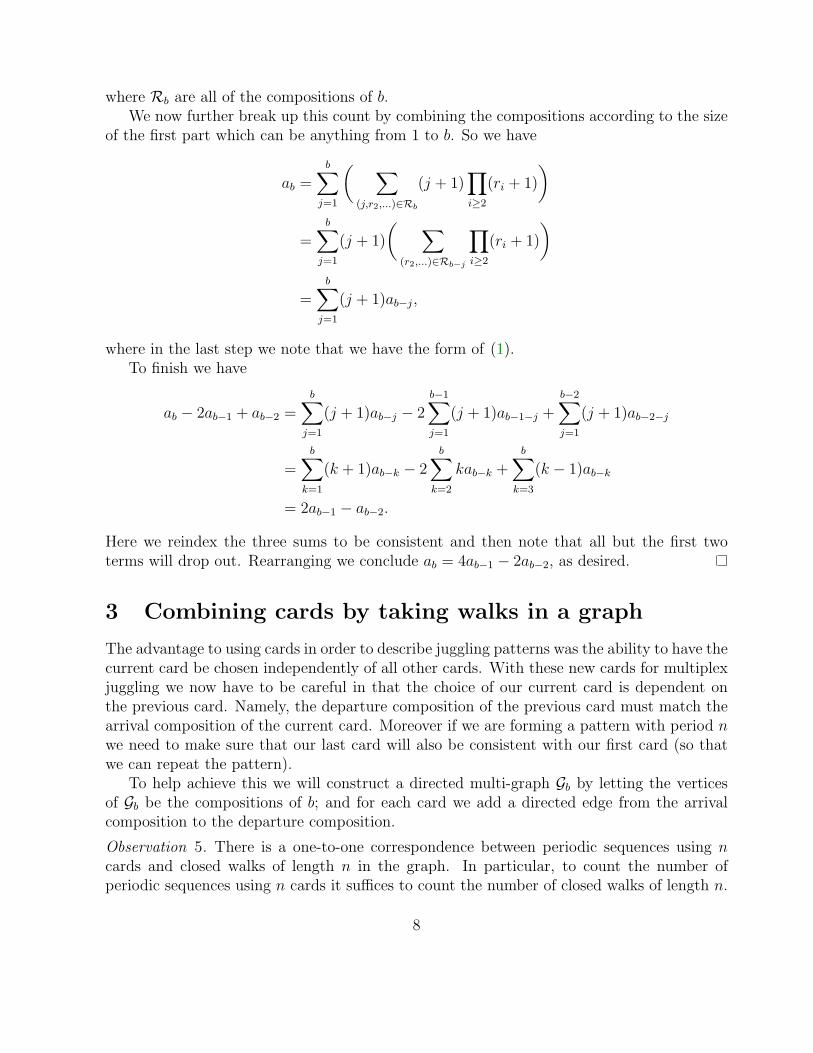
For a given juggling sequence there can be multiple ways in which it can be representedusing the cards. (This is different than the case where at most one ball was caught at a time.)The problem lies in what happens with balls that are never used. For instance in Figure 7we see two distinct sets of three cards which correspond to the same juggling sequence, thedifference between them being the tracks in the unused balls.
1
1
2
1
3
1
1 1
1
3
2
1
1
1 1
1
1
2 1
2
1
1
2
2
1
3
2 2
3
2
1
2 2
1
2 1
2
2
Figure 7: Two distinct sets of three cards with the same juggling sequence.
Note that for juggling where at most one ball is caught the unused balls all have thesame behavior, in our language they would correspond to lying in tracks with capacity 1 atthe top. So to count the number of juggling sequences we take the difference of the ways toplace n cards with b tracks, (b + 1)n, and the ways to place n cards with b − 1 tracks, bn,(which is in bijection with the number of ways to place n cards with b tracks and the toptrack is never used). This gives (b + 1)n − bn. We will do something similar with our cardsthat we are using for multiplex juggling.
Theorem 7. Let jsb(n) be the number of multiplex juggling sequences using exactly b balls
and with period n. Then
jsb(n) = tr(Anb )−
b−1∑
i=0
tr(Ani ).
Proof. We proceed by induction on b. For the base case of b = 0 there is one card (theempty card) and so for any length n there is exactly one way to position these cards. SinceA0 = (1) we have tr(An
0 ) = 1 establishing the base case.
10

Now assume that it works up through b− 1 and consider the case for b. First we observe
tr(Anb ) = jsb(n) +
b−1∑
i=0
2b−i−1jsi(n).
This follows by noting that for every juggling sequence which uses exactly i balls we can finda sequence of cards corresponding to the compositions of i. We can now add b − i balls tothe top of each card as long as we do it consistently across the different cards. Moreover thenumber of different options we have to place the b−i balls equals the number of compositionsof b− i which is 2b−i−1.
Rearranging and using our induction hypothesis we have
jsb(n) = tr(Anb )−
b−1∑
i=0
2b−i−1jsi(n)
= tr(Anb )−
b−1∑
i=0
2b−i−1
(tr(An
i )−i−1∑
j=0
tr(Anj )
)
= tr(Anb )−
b−1∑
i=0
tr(Ani )
(2b−i−1 −
b−i−2∑
k=0
2k)
= tr(Anb )−
b−1∑
i=0
tr(Ani ),
establishing the result.
5 Counting multiplex juggling patterns
To go from counting juggling sequences of period n to counting juggling patterns of minimalperiod n we want to do two things. First we want to remove any pattern that has shorterperiod (suppose d divides n, then any periodic sequence of cards of length d can be repeatedn/d times to make a periodic sequence of cards of length n). Second we want to divide outby n since in juggling patterns there is no set start time.
For the first issue we can use Mobius inversion (see [8]). Namely we note that if msb(n)is the number of juggling sequences with b balls and minimal period n, then
jsb(n) =∑
d|n
msb(d).
So if we let µ(nd) be the Mobius function it follows
msb(n) =∑
d|n
µ(nd)jsb(d).
11

With this in hand we can now divide out by the rotational symmetry of the starting pointand determine the number of juggling patterns with b balls and period n which we denotejpb(n). Combining the above with Theorem 7 we get the following.
Theorem 8. The number of multiplex juggling patterns with b balls and minimal period n is
jpb(n) =1
n
∑
d|n
µ(nd)
(tr(Ad
b)−b−1∑
i=0
tr(Adi )
).
In Table 1 we give the number of minimal period juggling patterns for b = 2, 3, 4, 5 andperiod at most 15.
b = 2 b = 3 b = 4 b = 5
n = 1 2 3 5 7n = 2 4 12 32 77n = 3 13 63 261 964n = 4 37 310 2089 12086n = 5 118 1618 17449 156975n = 6 356 8434 147807 2077448n = 7 1142 45142 1276577 27976399n = 8 3620 243998 11169023 381752857n = 9 11744 1336644 98872035 5267354817n = 10 38275 7392117 883717142 73358245986n = 11 126234 41247234 7964898829 1029873201879n = 12 418735 231856131 72305691686 14559160765380n = 13 1399610 1311820110 660528998007 207076019661773n = 14 4702499 7464002451 6067348742573 2961063646029819n = 15 15883190 42679372930 56002661734041 42542385162393167
Table 1: The number of multiplex juggling patterns of minimal period n using b balls.
As a special case of Theorem 8 we have
jpb(1) = tr(Ab)−b−1∑
i=0
tr(Ai). (2)
We can also compute the number of period one multiplex juggling patterns directly.
Theorem 9. We have jpb(1) = p(b), where p(b) is the number of partitions of b.
Proof. In order for a card to produce a valid multiplex juggling sequence of period one withb balls we must have the arrival and departure compositions of the card be equal. That is(q1, q2, . . . , qk) = (r1, r2, . . . , rk). Further we must have that when the q1 balls get distributed
12

some ball gets placed into the top group. This second requirement will force qk to “embed”into rk−1 (otherwise it would have to embed into rk but the placement of at least one moreball in the top group then results in qk 6= rk). In particular this then forces, in turn, qito embed in ri−1 for i = 2, . . . , k. This is only possible if q1 ≥ q2 ≥ · · · ≥ qk. Thereforeour composition on the sides of the card have the unique ordering from largest to smallestelement (e.g., it corresponds to a partition).
Conversely, if we start with a partition we can create a card as above by placing thepartition on the sides of the card from largest to smallest; then all but the bottom groupwill shift down by one while the bottom group will then drop down and redistribute to filldifferences as needed. An example of this is shown in Figure 8 for the partition (3, 3, 2, 2).
2
2
3
3
2
2
3
3
Figure 8: Forming a period one juggling sequence from the partition (3, 3, 2, 2).
Theorem 10. Let p(b) denote the number of partitions of b. Then
tr(Ab) = p(b) +b−1∑
i=0
2b−i−1p(i).
Proof. Updating equation (2) using Theorem 9 we have
p(b) = tr(Ab)−b−1∑
i=0
tr(Ai).
We now proceed by induction. We have tr(A0) = 1 = p(0) (note that the sum will be emptyand not contribute), establishing the base case. Now suppose that we have established theresult up through b− 1 and consider the case for b. We have
tr(Ab) = p(b) +b−1∑
i=0
tr(Ai)
= p(b) + p(b− 1) + 2b−2∑
i=0
tr(Ai)
= p(b) + p(b− 1) + 2p(b− 2) + 22b−3∑
i=0
tr(Ai)
13

= · · ·
= p(b) + p(b− 1) + 2p(b− 2) + 22p(b− 3) + · · ·+ 2b−1p(0)
= p(b) +b−1∑
i=0
2b−i−1p(i),
establishing the result.
Using this we get that the trace of Ab starting with b = 0 is
1, 2, 5, 11, 24, 50, 104, 212, 431, 870, 1752, 3518, 7057, 14138, 28310, 56661, . . . .
This is sequence A090764 in the OEIS [6]. The recurrence that we have derived is a variantof that given in the OEIS. We now give a different variation establishing that this is thesame sequence as given in the OEIS.
Theorem 11. Let P(b) be the set of partitions of b, and for a partition q let o(q) denote the
number of 1s in the partition. Then
tr(Ab) =∑
q∈P(b)
2o(q).
Proof. We proceed by induction on b. The result is easily checked for small cases, so nowassume it works up through b− 1. Then we have the following.
∑
q∈Pb
2o(q) =∑
q∈Pb
o(q)=0
2o(q) +∑
q∈Pb
o(q)>0
2o(q)
=∑
q∈Pb
o(q)=0
1 + 2∑
q∈Pb−1
2o(q)
=(p(b)− p(b− 1)
)+ 2 tr(Ab−1)
=(p(b)− p(b− 1)
)+ 2
(p(b− 1) +
b−2∑
i=0
2b−i−2p(i)
)
= p(b) +b−1∑
i=0
2b−i−1p(i)
= tr(Ab).
We first divide up our partitions on whether we include a 1; then we note that there arep(b) − p(b − 1) partitions that do not include a 1 and p(b − 1) partitions that do include a1 (i.e., taking a partition with b − 1 we can append a 1 to get a partition of b which doesinclude a 1). We apply the induction hypothesis, and then apply Theorem 10 once, clean upour sum, and finally apply Theorem 10 a second time.
14

6 Juggling patterns with hand capacity
One of our basic assumptions that we have employed is that we can catch and throw anynumber of balls at any given step. From a practical standpoint jugglers usually limit them-selves to catching and throwing at most two or three balls at a time. The approach outlinedabove works just as well when we introduce a capacity constraint into how many balls canland at a given time, or equivalently how many balls can be thrown at a given time.
To do this we let Ab,κ be the principal submatrix of Ab by taking all rows and columnsindexed by compositions with all parts of size at most κ. (Since no arrival composition canhave q1 ≥ κ it follows that any valid juggling sequence can be formed by cards with all partsof size at most κ.)
Theorem 12. Let jsb,κ(n) be the number of multiplex juggling sequences using exactly bballs, with period n and all throws involve at most κ balls. Then
jsb,κ(n) = tr(Anb,κ)−
b−1∑
i=max{0,b−κ}
tr(Ani,κ). (3)
Let jpb,κ(n) be the number of multiplex juggling patterns using exactly b balls, with minimal
period n and all throws involve at most κ balls. Then
jpb,κ(n) =1
n
∑
d|n
µ(nd)
(tr(Ad
b,κ)−b−1∑
i=max{0,b−κ}
tr(Adi,κ)
). (4)
Before beginning the proof, observe if κ = 1, then this reduces to the case of jugglingwhere at most one ball can be caught at a time (i.e., Ab,1 = (b+1)); and if κ = ∞ then thisis equivalent to what we have already done.
Proof. We note that (4) follows from (3) by applying Mobius inversion. So it suffices toestablish (3).
We proceed by induction on b. For the base case of b = 0 there is one card (the emptycard) and the capacity places no restriction on its use, and so for any length there is exactlyone way to position these cards. Since tr(An
0 ) = 1 this establishes the base case.Let ri,κ be the number of compositions of i with each part at most κ. By grouping based
on the first part (which has size between 1 and κ) we have
ri,κ =
min{κ,i}∑
j=1
ri−j,κ, (5)
the min{κ, i} coming from noting that we cannot have compositions with negative parts andso we need to handle the case of small i.
15

Now assume that we have established the result up through b− 1 and consider the casefor b. First we observe
tr(Anb,κ) = jsb,κ(n) +
b−1∑
i=0
rb−i,κjsi,κ(n).
This follows by noting that for every juggling sequence which uses exactly i balls we canfind a sequence of cards which uses exactly i balls. We can now add b− i balls to the top ofeach card as long as we do it consistently across the different cards. Moreover the number ofdifferent options we have to place the b− i balls equals the number of compositions of b− iwith each part at most κ which is rb−i,κ.
We have
jsb,κ(n) = tr(Anb,κ)−
b−1∑
i=0
rb−i,κjsi,κ(n)
= tr(Anb,κ)−
b−1∑
i=0
rb−i,κ
(tr(An
i,κ)−i−1∑
j=max{0,i−κ}
tr(Anj,κ)
)(6)
= tr(Anb,κ)−
b−1∑
i=0
tr(Ani,κ)
(rb−i,κ −
b−i−1∑
j=max{0,b−i−κ}
rj,κ
)(7)
= tr(Anb,κ)−
b−1∑
i=max{0,b−κ}
tr(Ani,κ).
The equality in (6) uses the induction hypothesis and the equality in (7) is due to rearrangingthe terms. Finally we observe that (5) indicates that almost all of the terms will cancel,except for the first few initial terms which can easily be checked to be one, establishing theresult.
For reference we have produced the number of multiplex juggling patterns for κ = 2 inTable 2 and for κ = 3 in Table 3.
We note that we can ask similar questions about the sum of the entries in Ab,κ as wellas the row and column sums as we did with Ab (i.e., Lemma 2, Lemma 3 and Theorem 4).However the counts are less clear, and have not appeared in the OEIS. As an example if wecount the total number of cards when κ = 2 we get the following numbers, starting withb = 0:
1, 2, 7, 17, 41, 91, 195, 403, 812, 1601, 3102, 5922, 11165, 20824, 38477, . . . .
These numbers do appear to satisfy a relatively simple relationship. In particular throughb = 25 these numbers agree with the following conjecture.
16

κ = 2 b = 2 b = 3 b = 4 b = 5
n = 1 2 2 3 3n = 2 4 9 18 30n = 3 13 47 134 314n = 4 37 224 950 3140n = 5 118 1118 6938 31886n = 6 356 5522 50751 324909n = 7 1142 27910 376402 3341566n = 8 3620 141946 2813824 34605634n = 9 11744 730544 21219536 360849352n = 10 38275 3790391 161190485 3785776259n = 11 126234 19827570 1232724798 39941119938n = 12 418735 104422007 9483975303 423549648963n = 13 1399610 553339258 73360425430 4512516867634n = 14 4702499 2947940371 570219618745 48282551418859n = 15 15883190 15780565950 4451677886746 518633980103198
Table 2: The number of multiplex juggling patterns of period n using b balls with capacityκ = 2.
κ = 3 b = 2 b = 3 b = 4 b = 5
n = 1 2 3 4 5n = 2 4 12 28 58n = 3 13 63 231 713n = 4 37 310 1840 8591n = 5 118 1618 15168 106073n = 6 356 8434 126258 1325570n = 7 1142 45142 1069002 16789985n = 8 3620 243998 9154845 214916096n = 9 11744 1336644 79252442 2776778019n = 10 38275 7392117 692290928 36167946945n = 11 126234 41247234 6095630354 474470288650n = 12 418735 231856131 54045188641 6263882726811n = 13 1399610 1311820110 482108239540 83162406390939n = 14 4702499 7464002451 4323812672665 1109678347266127n = 15 15883190 42679372930 38963338572980 14873888879020290
Table 3: The number of multiplex juggling patterns of period n using b balls with capacityκ = 3.
17

Conjecture 13. Let a(2)b be the number of cards for multiplex juggling with b balls and
where each track has capacity at most κ = 2. Then
∑
b≥0
a(2)b xb =
1− x+ x2 + x3
(1− x− x2)3.
7 Conclusion
By modifying the cards used for juggling, namely allowing a subset of the balls to be groupedtogether, we have found a method that works for enumerating multiplex juggling patterns.There are still a few questions that remain, particularly in understanding what happenswhen we limit the number of balls that can be caught at any given time.
Ehrenborg and Readdy [4] introduced cards for juggling and used them to study a q-analog of juggling by counting crossings. It is easy to count crossings on each card and thenone simply adds up the crossings over all cards used to count the crossings of the pattern.We note that the matrices used here can be easily adapted to this situation. Namely foreach card we count crossings (making sure to count multiplicity when balls move in groups),and then weight the card (and hence edge in the graph) by qk where k is the numberof crossings. Finally we can form matrices Ab(q) where we add up the weights of cardsconnecting compositions. As an example we have
A3(q) =
(3)(2, 1)(1, 2)
(1, 1, 1)
2 1 1 11 q + 2 q + 1 q2 + q + 11 q 2 00 1 q q2 + q + 2
.
We note that Theorem 7 and Theorem 12 can be easily modified to count the number ofjuggling patterns with minimal period based on the number of crossings.
An applied mathematical juggler might also want to add the constraint that whenevermultiple balls are thrown that no two balls get thrown to the same height. Our method canbe readily adopted to this situation by simply removing any card which has two balls movedto the same track, which leads to modified graphs Gb, and also modified matrices, Ab. Forexample we have
A2 =(2)
(1, 1)
(1 11 3
), and A3 =
(3)(2, 1)(1, 2)
(1, 1, 1)
1 0 0 10 2 1 31 1 2 00 1 1 4
.
The matrices Ab might also have independent interest. Let us consider the characteristicpolynomial of Ab. If we let Pb := Pb(x) = det(xI−Ab), then we have the following factoriza-tion (here the fi are all polynomials and the Pb are found my multiplying the corresponding
18

polynomials in the row together).
P0 = f 10
P1 = f 11
P2 = f 12
P3 = f 10 f 1
3
P4 = f 20 f 1
1 f 14
P5 = f 50 f 2
1 f 12 f 1
5
P6 = f 90 f 5
1 f 22 f 1
3 f 16
P7 = f 190 f 9
1 f 52 f 2
3 f 14 f 1
7
P8 = f 370 f 19
1 f 92 f 5
3 f 24 f 1
5 f 18
P9 = f 740 f 37
2 f 192 f 9
3 f 54 f 2
5 f 16 f 1
9
P10 = f 1480 f 74
1 f 372 f 19
3 f 94 f 5
5 f 26 f 1
7 f 110
P11 = f 2960 f 148
1 f 742 f 37
3 f 194 f 9
5 f 56 f 2
7 f 18 f 1
11
P12 = f 5910 f 296
1 f 1482 f 74
3 f 374 f 19
5 f 96 f 5
7 f 28 f 1
9 f 112
P13 = f 11830 f 591
1 f 2962 f 148
3 f 744 f 37
5 f 196 f 9
7 f 58 f 2
9 f 110 f 1
13
The polynomials fi are given by the following (the number on the right indicates the largestroot of the polynomial).
f0(x) = x− 1 1.000 . . .f1(x) = x− 2 2.000 . . .f2(x) = x2 − 5x+ 5 3.618 . . .f3(x) = x3 − 10x2 + 27x− 20 6.124 . . .f4(x) = x5 − 20x4 + 135x3 − 396x2 + 518x− 245 9.884 . . .f5(x) = x7 − 36x6 + · · · − 25·5·72 15.382 . . .f6(x) = x11 − 65x10 + · · · − 25·32·52·73 23.255 . . .f7(x) = x15 − 110x14 + · · · − 211·32·53·74 34.332 . . .f8(x) = x22 − 185x21 + · · ·+ 210·34·54·76·112 49.689 . . .f9(x) = x30 − 300x29 + · · ·+ 221·35·56·78·112 70.702 . . .f10(x) = x42 − 481x41 + · · ·+ 221·39·58·712·113·132 99.127 . . .f11(x) = x56 − 752x55 + · · ·+ 238·312·511·716·114·132 137.190 . . .f12(x) = x77 − 1165x76 + · · · − 242·317·516·722·119·133 187.694 . . .f13(x) = x101 − 1770x100 + · · · − 270·323·521·729·1111·134 254.151 . . .
These polynomials are important as they give the eigenvalues of the matrices which inturn determine the rate of growth of the number of juggling sequences. It should be notedthat f1, . . . , f13 are all irreducible.
There are several interesting things that are appearing in the characteristic polynomials.
• The sequence of the exponents of fi in the Pj seem to follow
1, 0, 0, 1, 2, 5, 9, 19, 37, 74, 148, 296, 591, 1183, . . . .
19

This appears to be the sequence A178841 in the OEIS [6] which counts the number ofpure inverting compositions of n.
• The degree of the polynomials fi follow
1, 1, 2, 3, 5, 7, 11, 15, 22, 30, 42, 56, 77, 101, . . . .
This appears to be the sequence A000041 in the OEIS [6] which counts the number ofpartitions of n.
• The second coefficients of the polynomials fi follow
1, 2, 5, 10, 20, 36, 65, 110, 185, 300, 481, 752, 1165, 1770, . . . .
This appears to be the sequence A000712 in the OEIS [6] which counts the number ofpartitions of n into parts of 2 kinds.
We have no explanations for any of these phenomena, but given the nature of how thematrix is formed, we believe this is more than coincidence.
We look forward to more research being done into these cards, into multiplex jugglingpatterns, and into the matrices Ab.
8 Acknowledgment
The authors thank a referee for extensive useful suggestions on an earlier draft of this paper.
References
[1] J. Buhler, D. Eisenbud, R. Graham, and C. Wright, Juggling drops and descents, Amer.
Math. Monthly 101 (1994), 507–519.
[2] S. Butler, F. Chung, J. Cummings, and R. Graham, Juggling card sequences, J. Comb.
8 (2017), 507–539.
[3] S. Butler and R. Graham, Enumerating (multiplex) juggling sequences, Ann. Comb. 13
(2010), 413–424.
[4] R. Ehrenborg and M. Readdy, Juggling applications to q-analogues, Discrete Math. 157
(1996), 107–125.
[5] B. Polster, The Mathematics of Juggling, Springer, 2000.
[6] N. J. A. Sloane, The On-Line Encyclopedia of Integer Sequences, http://oeis.org.
[7] J. Stadler, Juggling and vector compositions, Discrete Math. 258 (2002), 179–191.
20

[8] R. Stanley, Enumerative Combinatorics, Volume I, second edition, Cambridge, 2012.
2000 Mathematics Subject Classification: Primary 05A15; Secondary 00A08.Keywords: juggling, transfer matrix method, composition, partition.
(Concerned with sequences A000041, A000712, A003480, A090764, and A178841.)
Received March 13 2017; revised versions received March 2 2018; January 30 2019; January31 2019. Published in Journal of Integer Sequences, February 2 2019.
Return to Journal of Integer Sequences home page.
21