1

EPIC Modeling System Guide

Water, Salt & Energy Management Problems

Daene C. McKinney

and

Andrey G. Savitsky

June 2001 (Revised August 2001)

i

Contents ACKNOWLEDGEMENTS ..........................................................................................................1

INTRODUCTION .........................................................................................................................2 1. EPIC MODELING SYSTEM..................................................................................................2

1.1. Introduction and Example ...............................................................................................2 1.1.1. Aral Sea Basin River and Irrigation System ..........................................................2 1.1.2. Central Asia Energy System ..................................................................................3

1.2. Modeling Network ............................................................................................................4

1.3. Optimization Criteria .......................................................................................................4 1.3.1. Water Task .............................................................................................................4 1.3.2. Water and Salinity Task .........................................................................................6 1.3.3. Water and Energy Task ..........................................................................................6

1.4. Constraints ........................................................................................................................7 1.4.1. Water Task .............................................................................................................7 1.4.2. Water and Salinity Task .........................................................................................8 1.4.3. Water and Energy Task ..........................................................................................9

2. USING THE EPIC MODELING SYSTEM.........................................................................12 2.1. Main Module ...................................................................................................................12

2.2. Water Task ......................................................................................................................13 2.2.1. Working Directory ...............................................................................................13 2.2.2. Network Creator ...................................................................................................13 2.2.3. Network_Directions .............................................................................................18 2.2.4. Node Listing.........................................................................................................20 2.2.5. "Time Steps".........................................................................................................22 2.2.6. Data Input .............................................................................................................23 2.2.7. Lake Morphology.................................................................................................32 2.2.8. Objective Weights ................................................................................................34 2.2.9. Internal Database..................................................................................................35 2.2.10. Constraints..........................................................................................................37 2.2.11. Build Model........................................................................................................40 2.2.11. Solve Model .......................................................................................................41 2.2.12. Display Results...................................................................................................42 2.2.13. Additional Capabilities.......................................................................................43

2.3. Water – Salt Task ...........................................................................................................44 2.3.1. Introduction ..........................................................................................................44 2.3.2. Internal Database..................................................................................................44 2.3.3. Constraints............................................................................................................46 2.3.4. Build Model..........................................................................................................48 2.3.5. Solve Model .........................................................................................................49

ii

2.3.6. Display Results.....................................................................................................50 2.4. Water – Energy Task......................................................................................................51

2.4.1. Introduction ..........................................................................................................51 2.4.2. Objective Weights ................................................................................................51 2.4.3. Constraints............................................................................................................54 2.4.4. Build Model..........................................................................................................56 2.4.5. Solve Model .........................................................................................................57 2.4.6. Display Results.....................................................................................................58

REFERENCES ............................................................................................................................59

1

ACKNOWLEDGEMENTS

An early version of the work reported here was developed with financial support provided by the United States Agency for International Development (USAID) under contract Contract No. PCE-I-00-96-00002-00, Task Order No. 813, Environmental Policies and Institutions for Central Asia. That work included the inputs of the many people who participated in the Working Group on Modleing as reported in the report edited by McKinney and Kenshimov (2000). Recent support to Dr. Savitsky for this work was provided by a Contemporary Issues Fellowhip from the International Research and Exchange (IREX) Program. The authors are thankful for the strong contributions to this work by Alexie Zyryanov and Elena Antipova of Kyrgyzenergo in Bishkek, Kyrgyzstan. The comments, observations and encouragement of Alex Meeraus of the GAMS Development Corporation are greatly appreciated.

2

INTRODUCTION

The modeling system is designed by Daene McKinney and Andrey Savitsky based on previous work with Central Asian water and energy specialists (see acknowledgements). The program system is intended for automatically creating and solving General Algebraic Modeling System (GAMS) models dealing with river basin management and associated energy distribution. The Guide is organized as follows: • In the first chapter, an example is described for which a GAMS model is created and an

optimization calculations performed for operation of a river network and associated energy distribution.

• After that, we describe the modules of the program system that prepare information for each block of the GAMS model that can solve the example problem.

• Further, we consider operation of each module incorporated in the program system and describe the structure of all output files formed in the process of their execution. The description of modules is given in the sequence they should be executed when a GAMS file is created.

1. EPIC MODELING SYSTEM

1.1. Introduction and Example As a example, we calculate optimal management of water in the Aral Sea Basin rivers, Syr Darya and Amu Darya, and the distribution of the associated energy in the Central Asia Energy System. Diagrams of the water and energy parts of the model are shown in Figures 1 and 2. 1.1.1. Aral Sea Basin River and Irrigation System The water part of the model includes the following: • Reservoirs:

Uchkurgan, Andijan, Kayrakum, Charvak, Chardara, Shamaldisai, Tashkumur, Kurpsai, Toktogul, Tyuyamuyun, Nurek;

• Sources of water supply: River inflow: Naryn, Karadarya , Chirchik , Ugam, Vahsh, Pandj, Surhandarya,

Kashkadarya, and Kafirnigan rivers; Side inflow: Toktogul to Uchkurgan, Andijan to Uchtepa, before Akdjar,

Kajrakum to Chardara, Chirchik, before Aral Sea;

3

Return flow to: Kayrakum, and Chardara reservoirs; Precipitation on: Andijan; Kayrakum, Charvak, and Chardara reservoirs

• Water users: Syr Darya: On reaches Toktogul to Uchkurgan and Andijan to Uchtepa

including BFK, Podvodiash canal, before Akdjar, from Kayrakum reservoir, from reaches Kajrakum to Chardara, from Chirchik, Kizylkum canal, and reaches Chardara to Aral Sea.

Amu Darya: Lenina canal, Petniakarna, Tashaka, and Urgencharna canals,

Klichbai, Kipchakbozsu, and Gumabajska canals, Right canal and Kizketken canal, Sovetjab, Octyabrana, and Pataarna canals, Pumping intake, Dashhouz, Right and left canals in Tuyamuyun system, Drinking canal, Karshi canal, Amu Buhara canal, Karakum canal, and Upper users on Amudarya.

Losses: Infiltration and evaporation from rivers and lakes

The main water resources of the region (the rivers Syr Darya and Amu Darya) originate in the upstream countries of Kyrgyzstan and Tajikistan, and then flow toward the Aral Sea. The Syr Darya basin is highly regulated by the Toktogul multi-year storage reservoir, and also by the Kayrakum, Chardara, Andijan and Charvak seasonal reservoirs. The Amu Darya basin is not so highly regulated as the Syr Darya, with only one major reservoir, Nurek, and one re-regulation reservoir, Tuyamuyun. The reservoirs of both basins were designed to operate in an integrated fashion based on growing season irrigation water demands. 1.1.2. Central Asia Energy System The energy part of the model includes the following: • Energy generation:

Design plants Aggregate of hydro- and thermal- power generating plants (HPP

and TPP) for all 5 Central Asian countries whose loads are calculated by the model;

Off-design plants Aggregate of off-design plants (those that operate at almost

constant output in all time periods) for all 5 Central Asian countries whose loads are specified and remain unchanged in all calculations;

• Energy consumers: Five energy consumers, the internal demands of each Central

Asian country; and

4

• Energy transmission: Regional energy transfers to and from the Central Asian Electricity Pool (CAEP) and the balance of electricity and the balance of electricity in an aggregated representation of the grid.

The energy producers and users are connected through a simplified representation of the Central Asian Electricity Pool (CAEP), a power grid covering four Central Asian republics (Uzbekistan, Tajikistan, Kyrgyzstan, and Turkmenistan) and South Kazakhstan, comprised of 29 thermal power plants (TPP) and 48 hydropower plants (HPP) with a total installed capacity of 25,122 MW (McKinney and Kenshimov, 2000). The modeling scheme of the water system is shown in Figure 1 and the energy system in Figure 2. The two systems are linked through the hydropower plants. According to the user’s needs, the system can be solved as a:

• Water management task; • Water and salt management task; or • Water and energy management task.

1.2. Modeling Network

A river system is formally separated into two groups of mathematical objects:

1. Those objects - called “nodes”- that change the quantity and quality of water according to physical laws; and

2. Those objects - called “arcs” - that transfer characteristics of water quality and quantity between groups of nodes.

The water transfer variable for an arc usually includes the index of the initial (from node) and final (to node) nodes to which it is connected. This representation results in an inefficient use of computer memory. The EPIC Program uses an approach in which the water transfer variable is associated with arcs rather than nodes. In turn, these arcs have a description of connections (nodes) isolated from the main calculation process, thus separating the initial and final nodes. For details of this representation, please see McKinney and Kenshimov (2000, Chapt. 3, Sec. 3.3.2.2). 1.3. Optimization Criteria 1.3.1. Water Task For the water part, the optimization criterion is similar to that in the BVO "Syr Darya" model (McKinney and Kenshimov, 2000). The basic requirements of the water part of the model, when applied to the Aral Sea basin rivers (Syr Darya and Amu Darya), are to provide for optimal regulation of transboundary water resources of the basin rivers under various conditions. This can be formulated as follows:

5

• Calculate the water balance at the model nodes and at the international borders for a

specified planning period; • Satisfy, to the extent possible, the water needs of basin countries during the planning

period or season (non-vegetation, vegetation); • Follow any set operation regimes of the basin reservoirs according to the technical

requirements and rules of their operation, and with provision for all reservoirs to fulfill their functions;

• Satisfy, to the extent possible, requirements for flow to the Aral Sea and pre-Aral Region, approved by the ICWC for the water year and for the season; and

• Satisfy, to the extent possible, requirements for sanitary releases for parts of the rivers and their main tributaries for certain periods of time, first of all – for the vegetation period; and

• Calculate average monthly releases from the reservoirs containing hydropower plants for use by UDC Energia for planning and correction of water and power balances, and power regimes of the CAEP.

The main criterion is to minimize deficits of water delivery to all users

(1)

where

water demanded by user i in period t (million m3);

water delivered to user i in period t (million m3); F group of technological components; and c1 weight (dimensionless and very large relative to c2- c5).

The technological components of the objective function greatly simplify and accelerate the calculations. These should be used with priorities (weights) many orders of magnitude less than the priorities of the main task of delivering demanded water to users. Ignoring the technological components may sometimes lead to solutions that are optimal, but unacceptable in practice. Small priorities applied to these components do not greatly affect the solution, which will remain close to optimal.

F = (2)

(1) (2) (3) (4) where

6

electricity of HPP j in period t (million kWh);

electricity demand of HPP j in period t (million kWh);

capacity of reservoir j (million.m3); T index of last time step; Σi number of nodes in the river network; Σt number of time steps; Σh number of HPPs; Σ v number of reservoirs; vg reservoirs with HPPs; and c2-c6 weights (dimensionless and very small relative to c1).

(1) Solution Stability: This component is used only in especially high-water years or when calculating river reaches with considerable unused water volumes. Available “extra” water should be delivered to the river mouth (delta). However, it is not considered important when the delta gets it, but its quality is important. Therefore, sometimes an irregular water release along the river channel can occur and this should be prevented. (2) Water Storage at End of Modeling Period: Sometimes it is necessary to solve problems related to water storage for the next vegetation period. In this case a fixed value for storage at the end of the modeled period can be assigned, and an incompatible solution may be found. Certainly, after several calculation experiments the maximum water storage may be defined which can be reserved for the next period. It is simpler, however, to assign a priority to this technological component and let the model determine the bound for the maximum water storage in reservoirs with only a single calculation experiment. (3) Meeting Energy Demands: This component can be deleted from the objective function without any detriment to the solution. (4) Constraint Compatibility: This component is the sum of squares of all sources of water flowing or consumed in the system for the calculation period. We assign a negative weight to this component. The role of this component is as follows: under an optimal solution it will equal zero. However, if constraints and requirements of the solution exclude the possibility of a solution, then instead of an emergency stop while solving a problem, the user will obtain a solution, in which virtual users consume any water surpluses, and a virtual source makes up any deficit. 1.3.2. Water and Salinity Task The optimization criteria for the Water and Salinity Task are the same as for the Water Task, since salinity is included only as a constraint in the model and not as an objective. 1.3.3. Water and Energy Task

7

The optimization criterion in the water-energy task is to minimize the cost of providing the internal energy demands of the Central Asian Republic's while taking into account reservoir operation in the electricity generation or irrigation modes. This criterion is embodied in the objective function as minimization of electricity production costs for thermal and hydroelectric plants and the squared differences between modeled energy delivery and demand

(3)

where electricity production cost for TPP j with owner i ($/million kWh);

electricity production of TPP j with owner i in period t (million kWh);

electricity production cost for HPP j with owner i ($/million kWh);

electricity production of HPP j with owner i in period t (million kWh);

cost for electricity transfer to/from CAEP by owner i in period t ($/million kWh);

electricity transfer to/from CAEP by owner i in period t (million kWh);

cost for electricity deficit of user i in period t ($/million kWh);

electricity consumed by user i in period t (million kWh); and

electricity demanded by user i in period t (million kWh)

1.4. Constraints 1.4.1. Water Task The water part of the model is a sequential arrangement of the reservoirs and HPPs of the Naryn-Syr Darya Cascade and the Amu Darya basin with lateral inflows and water diversions. For every reservoir j, water balances in time period t are calculated as: (4)

where

volume of water in reservoir j at time t (million m3);

release from reservoir j in period t (million m3);

inflow to reservoir j in period t (million m3);

average area of reservoir j over time t (million m2); and

8

evaporation from reservoir j in period t (m). For simple nodes, hydropower stations, distributing nodes, and control nodes, we have for each node j of this type and for each time period t, we have (5)

where is the source or user located for simple nodes (million.m3). For water users, we calculate return flow from provided (6)

where Rj is the return flow ratio for node j (dimensionless). Flow from water source nodes is represented as

(7)

where

known hydrograph of flow from the source j (million.m3);

return flow from the users to node j (million.m3); and user subset of water users connected with the given flow source.

1.4.2. Water and Salinity Task For every reservoir j, salt balances in time period t are calculated as: (8)

(9)

(10) where

salt content in the reservoir at the time t (thousand.tons);

9

average mineralization in reservoir j at initial time (g/L);

salt outflow from node j in period t (thousand tons); and

salt inflow to node j in period t (thousand tons). For simple nodes, hydropower stations, distributing nodes, and control nodes, we have for each node j of this type and for each time period t, we have

(11)

For water users, we calculate the salt content of the return flow from (12) where is the mineralization of return water from user j in period t (g/L). Salt coming from water source nodes is represented as (13)

where

mineralization of water in the source j (g/L); and

mineralization of return waters from the user u (g/L). 1.4.3. Water and Energy Task The power generation at HPP j is calculated according to the following equation: (14) where

power generated by HPP j with owner i in period time t (kW);

flow through HPP j with owner i in period time t (m3/sec);

effective head on HPP j with owner i in period time t (m); and

efficiency of HPP j.

10

The output of electric energy from HPP j is calculated as:

(15)

where

electricity of HPP j with owner i in period t (million kWh); and

number of seconds in the period t All entities of the energy part of the model are connected by one equation: the total output of all generating plants is equal to the internal consumption and balance of transfers to/from the CAEP

(16)

The connection between the water part and the energy part of the model is

(17)

where G is the set of all HPPs in the model.

11

Figure 1. The Aral Sea basin river network.

12

Figure 2. The Central Asian energy system schematic.

2. USING THE EPIC MODELING SYSTEM 2.1. Main Module Execution of the EPIC Program software is carried out through the program main.exe. In Figure 3 the window presented at start-up of main.exe is shown. The main function of this module is the activation of other modules in the software package. The menu bar at the top of the screen contains a number of items that call the various modules of the software system. The right most menu item is the call to help. It consists of:

• Information on the purpose and use of the module; • Information on the authors and origin of the module; and • The structure of the complex of programs in the software system.

Below we consider each subitem of the main menu.

13

Figure 3. View of Main screen of EPIC Program. 2.2. Water Task This menu item controls the modules that: 1) create model networks for river basins, 2) create the data base and GAMS model for modeling water flow in a river basin, 3) execute the water task model, and 4) display the results. The model which is created uses the objective function shown in Eq. 1 and the general constraints shown in Eq. 3. 2.2.1. Working Directory Selecting “Working Directory” from the “Water” menu item (see Figure 4) allows you to select the directory in which the program will work, that is, the directory in which all files will be found or stored. After selecting this menu item, a window appears from which you can select your working directory (see Figure 5). At the bottom of the window you can see the path to the working directory that was chosen last time. The default path is the directory in which the EPIC program is located. Select (or navigate to) the working directory from the subdirectories present on the on the left part of the window. Once the directory has been chosen, you should press the "Create Path" button. After this, the choice will be shown in the top part of all windows of the EPIC Program to remind you of the working directory you are using. Creating a path to the working directory automatically creates the file "location.in" in the main directory. This file has one line containing the path to the working directory. In the right part of the window of the module, you can delete, transfer, copy, or rename any of the displayed files. 2.2.2. Network Creator This item allows the user to create networks representing river systems of any configuration and complexity. Upon selecting the menu item “Network Creation” the window shown in Figure 6 will appear. In this window two menu items are available to the user: "File" and "Help". Choosing "Help" will display information on the use of the given module in a special information window.

14

Figure 4. View of “Main” screen when selecting from the “Water” menu.

Figure 5. View of “Working Directory” selection window. Selecting “Open” from the "File" menu the user can find and load in system memory a file named "klav.out" or create a new file. The search directory is the current working directory

15

selected previously. If the file “klav.out” does not exist, it will be created by this module. In addition, all previously created files are kept in backup copies with file extensions "bak". After opening an existing, or creating a new, “klav.out” file the user receives access to a window for construction of the network. By pressing the left mouse button, moving it, and then releasing it, the user forms a line connecting two nodes of a network. If this action fails it means that the user may have pressed the right key instead of left. In that case, the ability to create the network is restored by pressing the button "return". To delete an existing node, select the node and press the “DELETE” button, the initial node, together with all arcs to which it is connected, will be removed from the network.

Figure 6. View of “Network Creator” window. If you place the mouse on one of the nodes, information about that node will be displayed at the bottom of the window: 1) the name of the node, and 2) the number of its owner. On the right-hand side of the window are radio-buttons for designating the owner and type of a node. Also on the right part of the window are two buttons: "Update" and "Return". By placing the mouse on a node and pressing of the right button, the user actually fixes the choice of that node and can determine the type of node, its owner, and its name by pressing the appropriate radio-buttons and filling in the information about the name of the node. After filling in the name of a node and pressing the appropriate button for the type and owner of the node, press the "Update" button and

16

all entered information will be associated with the node in the network. If, instead, you press "Return", all entered information or changes will be ignored. Frequently, you might press the right mouse button when the cursor is not on any node, then you can not create a new arc. To return to the normal data entry mode, press the "Return" button. If the pointer of the mouse is not located on a node, the information window will display the word "empty" and the total number of nodes entered in the network is displayed. Once you are finished designing your network close the window and return to the “main” program. If new information about the network have been entered, the user will receive a reminder to save the changes. The result of executing the “Network Creation” module is the creation or updating of the file "klav.out", a file with a strictly regulated structure and format. An example of the file "klav.out" is given below. In the file “klav.out”, the first fifteen lines are comments which are not used by any of the programs, but the user can make any marks or additional comments here. The first nine columns of the following lines contain information about the connections (arcs) in the network. The first column is the serial number of the arc. Each arc is a line on the network. The second and third columns are the x and y graphical coordinates of the beginning (from) node of the arc. The fourth and fifth columns are the x and y coordinates of the ending (to) node of the arc. The sixth and seventh columns are integers representing the types of the beginning and ending nodes of the arc. The eighth and ninth columns are integers representing the owners of the initial and final nodes of the arc. The textual information located at the end of each line consists of two parts subdivided by a special symbols: 1) the first part = > ___ <, and 2) the second part > ______ < =. The first part contains the external name of the initial node and the second part contains the external name of final node. The external names can be up to 44 letters. The absence of letters is replaced by symbols "_". The user can edit the “klav.out” file by other means (e.g., text editor) besides the given module. When creating the “klav.out” file, the program makes a first rough check of correctness of the network. Arcs with identical initial and final nodes are deleted, leaving only one arc. Also, nodes which are too close together are deleted. The network must contain certain types of nodes (simple, control, source, mouth and user), whereas, others are unessential (reservoirs, losses, time lag). The EPIC Program provides for calculation of power generation by reservoirs when they release water through turbines (see Eq’s. 4 and 5). Power generation is calculated only on arcs where the first node is a reservoir and the second node is a control point. If there are no arcs where the first node is a reservoir and the second node is a control point, power generation is not calculated.

17

File “klav.out” ________________________________________ types: simple 1 ³ owners: Uzb 1 supply 2 ³ Kir 2 lakes 3 ³ Kaz 3 intake 4 ³ Tad 4 mouth 5 ³ Tur 5 contrl 6 ³ losses 7 ³ T_LAG. 8 ³ _______________________________________ ________________________________________________________ connections types owners ________________________________________________________ N x y x y 1 2 1 2 name1 (second in this way >) ³ name2 ________________________________________________________ 1 169 191 199 216 3 6 1 1 => UCHKURGAN_reservoire_______________________ <> Release from NARIN_kascades_of_reservoires_ <= 2 147 163 169 191 6 3 1 1 => control point after SHAMALDISAJ reservoire <> UCHKURGAN_reservoire_______________________ <= 3 199 216 237 224 6 1 1 1 => Release from NARIN_kascades_of_reservoires_ <> Point for side inflow Toktogul_Uchkurgan___ <= 4 242 159 237 224 2 1 1 1 => Side inflow on reaches Toktogul Uchkurgan__ <> Point for side inflow Toktogul_Uchkurgan___ <= 5 237 224 267 218 1 6 1 1 => Point for side inflow Toktogul_Uchkurgan___ <> Release from Toktogul+side inflow__________ <= 6 267 218 299 218 6 1 1 1 => Release from Toktogul+side inflow__________ <> Points for losses Toktogul_Uchkurgan_______ <= 7 299 218 235 253 1 4 1 1 => Points for losses Toktogul_Uchkurgan_______ <> River losses in reaches Toktogul Uchkurgan_ <= 8 299 218 333 210 1 6 1 1 => Points for losses Toktogul_Uchkurgan_______ <> Uchkurgan_gp_______________________________ <= 9 333 210 361 197 6 1 1 1 => Uchkurgan_gp_______________________________ <> Intake point from Toktugul-Uchkurgan_______ <= 10 361 197 299 263 1 4 1 1 => Intake point from Toktugul-Uchkurgan_______ <> Intake on reaches Toktogul Uchkurgan_______ <= 11 361 197 388 189 1 6 1 2 => Intake point from Toktugul-Uchkurgan_______ <> Uchkurgan_gydropost________________________ <= 12 388 189 417 173 6 1 2 2 => Uchkurgan_gydropost________________________ <> Uchkurgan+ g.p._Uchtepa____________________ <= 13 445 169 417 173 6 1 2 2 => Uchtepa____________________________________ <> Uchkurgan+ g.p._Uchtepa____________________ <= 14 479 181 445 169 1 6 2 2 => Point for evaporation computation_________ <> Uchtepa____________________________________ <= 15 479 181 545 249 1 4 2 2 => Point for evaporation computation_________ <> Evaporation from river_____________________ <= 16 519 179 479 181 1 1 2 2 => Intake point inside reaches Andijan Uchtepa <> Point for evaporation computation_________ <= 17 519 179 585 239 1 4 2 2 => Intake point inside reaches Andijan Uchtepa <> Intake on Andijan Uchtepa reaches_BFK______ <= 18 551 163 519 179 6 1 2 2 => Karabagish+inside inflow (Andijan Uchtepa)_ <> Intake point inside reaches Andijan Uchtepa <= 19 585 155 551 163 1 6 2 2 => Karabagish+inside inflow (Andijan Uchtepa)_ <> Karabagish+inside inflow (Andijan Uchtepa)_ <= 20 545 77 585 155 2 1 2 2 => Inside inflow (Andijan Uchtepa)____________ <> Karabagish+inside inflow (Andijan Uchtepa)_ <= 21 615 131 585 155 6 1 2 2 => Karabagish_________________________________ <> Karabagish+inside inflow (Andijan Uchtepa)_ <= 22 653 107 615 131 1 6 2 2 => Intake point for POVODJASH-kanal___________ <> Karabagish_________________________________ <= 23 653 107 637 159 1 4 2 2 => Intake point for POVODJASH-kanal___________ <> Podvodiash-kanal___________________________ <= 24 685 83 653 107 6 1 2 2 => Release from Andijan reservoir_____________ <> Intake point for POVODJASH-kanal___________ <= 25 725 67 685 83 3 6 2 2 => ANDIJAN_reservoir__________________________ <> Release from Andijan reservoir_____________ <= 26 725 67 705 125 3 4 2 2 => ANDIJAN_reservoir__________________________ <> Losses from Andijan lake___________________ <= 27 693 15 725 67 2 3 2 2 => Pricipitation on Andijan reservoir_________ <> ANDIJAN_reservoir__________________________ <= 28 779 23 725 67 2 3 2 2 => Inflow to Andijan reservoir________________ <> ANDIJAN_reservoir__________________________ <= 29 417 173 399 217 1 1 2 2 => Uchkurgan+ g.p._Uchtepa____________________ <> Point for inside inflow before Akdjar______ <= 30 453 221 399 217 2 1 2 2 => inside inflow before Akdjar________________ <> Point for inside inflow before Akdjar______ <= 31 399 217 385 253 1 6 2 2 => Point for inside inflow before Akdjar______ <> KAL point for observation__________________ <= 32 385 253 383 291 6 1 2 2 => KAL point for observation__________________ <> Intake point before Akdjar_________________ <= 33 383 291 329 329 1 4 2 2 => Intake point before Akdjar_________________ <> Intake before Akdjar______________________ <= 34 383 291 407 329 1 1 2 2 => Intake point before Akdjar_________________ <> Point for evaporation on river surfaces____ <= 35 407 329 361 373 1 4 2 2 => Point for evaporation on river surfaces____ <> Evaporation from river surfaces____________ <= 36 407 329 449 359 1 6 2 2 => Point for evaporation on river surfaces____ <> Akdjar point_______________________________ <= 37 449 359 503 369 6 3 2 3 => Akdjar point_______________________________ <> KAJRAKUM_reservoir_________________________ <=

18

Table 2 shows the types of nodes and corresponding symbols used for the internal names of nodes. Full internal names (index + number of the node of a specific type in the network) are assigned to nodes in the module “Data Entry”.

Table 2. Internal Indices of Various Node Types.

Types of Nodes Index Simple K Inflow I Reservoir V Water Diversion U River Mouth R Control Point C Losses P Lag Time T

2.2.3. Network_Directions This module allows the user to modify the network representation of the river system created in the “Network Creation” module: • Changing the configuration of the network by modifying structural connections in it. • Changing the direction of flow on arcs between nodes. The overall objective of the module is to provide an opportunity to change the flow direction on the arcs connecting initial and final nodes. Also, this module can be used to change the locations of initial and final nodes while not changing any information about the nodes. In Figure 7 the working window of the module with the network loaded in it is shown. Two menu items are accessible to the user: "File" and "Help". The choice "Help" will provide the user with information about opportunities and rules of use of the module. The choice "File" gives the user an opportunity to locate and load the file "klav.out". The search directory is working directory. However, the user can take a "klav.out" file from any directory. After loading the “klav.out” file the user receives access to a window containing the network. Moving the mouse to one of the nodes causes information about the node to be displayed in windows at the bottom the screen: internal name of the node, its serial number, and the number of its owner. Changing the Configuration of a Network To change configuration of a network you should: 1. Point to a node; 2. Press the left mouse button;

19

3. While pressing the left mouse button drag the node to the new position; and 4. Release the mouse button at the moment when the node is in the new position. Changing Flow Direction of Arcs Between Nodes On each arc connecting nodes are small rectangles. Also, each arc has a small arrowhead indicating the direction of flow along that arc. To change the flow direction of an arc, you should: 1. Point to the middle of the arc that connects nodes; and 2. Press the left mouse button The prior direction of the arc will reverse.

Figure 7. View of “Network Directions” window.

During the execution of this module, a file is written containing the changes and coinciding with the initial “klav.out” file both in name and structure. The user can write this file over the initial “klav.out” or save it in any convenient place. In case there was any change of the information about the network the user receives a reminder to save the changes.

20

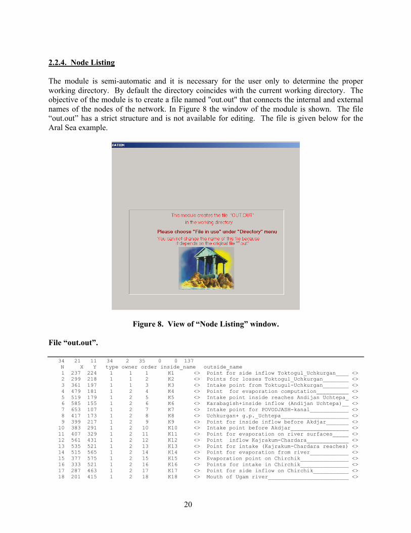
2.2.4. Node Listing The module is semi-automatic and it is necessary for the user only to determine the proper working directory. By default the directory coincides with the current working directory. The objective of the module is to create a file named "out.out" that connects the internal and external names of the nodes of the network. In Figure 8 the window of the module is shown. The file “out.out” has a strict structure and is not available for editing. The file is given below for the Aral Sea example.

Figure 8. View of “Node Listing” window.

File “out.out”. 34 21 11 34 2 35 0 0 137 N X Y type owner order inside_name outside_name 1 237 224 1 1 1 K1 <> Point for side inflow Toktogul_Uchkurgan____ <> 2 299 218 1 1 2 K2 <> Points for losses Toktogul_Uchkurgan________ <> 3 361 197 1 1 3 K3 <> Intake point from Toktugul-Uchkurgan________ <> 4 479 181 1 2 4 K4 <> Point for evaporation computation__________ <> 5 519 179 1 2 5 K5 <> Intake point inside reaches Andijan Uchtepa_ <> 6 585 155 1 2 6 K6 <> Karabagish+inside inflow (Andijan Uchtepa)__ <> 7 653 107 1 2 7 K7 <> Intake point for POVODJASH-kanal____________ <> 8 417 173 1 2 8 K8 <> Uchkurgan+ g.p._Uchtepa_____________________ <> 9 399 217 1 2 9 K9 <> Point for inside inflow before Akdjar_______ <> 10 383 291 1 2 10 K10 <> Intake point before Akdjar__________________ <> 11 407 329 1 2 11 K11 <> Point for evaporation on river surfaces_____ <> 12 561 431 1 2 12 K12 <> Point inflow Kajrakum-Chardara_____________ <> 13 535 521 1 2 13 K13 <> Point for intake (Kajrakum-Chardara reaches) <> 14 515 565 1 2 14 K14 <> Point for evaporation from river____________ <> 15 377 575 1 2 15 K15 <> Evaporation point on Chirchik_______________ <> 16 333 521 1 2 16 K16 <> Points for intake in Chirchik_______________ <> 17 287 463 1 2 17 K17 <> Point for side inflow on Chirchik___________ <> 18 201 415 1 2 18 K18 <> Mouth of Ugam river_________________________ <>

21

19 517 771 1 4 19 K19 <> Point for side inflow computation___________ <> 20 537 815 1 4 20 K20 <> point for intake before ARAL_SEA____________ <> 21 547 904 1 4 21 K21 <> point for losses before ARAL________________ <> 22 547 996 1 4 22 K22 <> Point for evaporation computation___________ <> 23 763 900 1 2 23 K23 <> point_for intake____________________________ <> 24 750 620 1 2 24 K24 <> FIRST-POINT-after TUJAMUIN reservoire______ <> 25 740 664 1 2 25 K25 <> point for Petniakarna_intake________________ <> 26 736 750 1 2 26 K26 <> point for intake computation________________ <> 27 758 826 1 2 27 K27 <> point for intakes_on Amudarja river_________ <> 28 621 1014 1 2 28 K28 <> lower_distribution points___________________ <> 29 727 355 1 5 29 K29 <> main_distribution_point_on_Amudaria ________ <> 30 747 314 1 2 30 K30 <> intake point for upper_user on Amudarja_____ <> 31 783 268 1 1 31 K31 <> Surhandaria_inflow__________________________ <> 32 827 222 1 2 32 K32 <> Kashakadarja_inflow_________________________ <> 33 875 184 1 3 33 K33 <> Kafirnigan_inflow___________________________ <> 34 907 146 1 3 34 K34 <> Begining of Amudarja river__________________ <> 35 242 159 2 1 1 I1 <> Side inflow on reaches Toktogul Uchkurgan___ <> 36 545 77 2 2 2 I2 <> Inside inflow (Andijan Uchtepa)_____________ <> 37 693 15 2 2 3 I3 <> Pricipitation on Andijan reservoir__________ <> 38 779 23 2 2 4 I4 <> Inflow to Andijan reservoir_________________ <> 39 453 221 2 2 5 I5 <> inside inflow before Akdjar_________________ <> 40 487 309 2 3 6 I6 <> Return water to KAJRAKUM_reservoir__________ <> 41 553 317 2 3 7 I7 <> Precipitation to KAJRAKUM_reservoir_________ <> 42 587 371 2 2 8 I8 <> Inside inflow on reaches Kajrakum-Chardara__ <>

The first line of the file “out.out” contains the information on the number of units of a particular type: simple, sources, reservoirs, users, river mouths, control, loss, time lag, total number of nodes in the network. The lines after the first line each contain information about a certain node in the network. By column, these are, for each node: serial number, x and y coordinates, type, owner, serial number, internal name, and, after the dividing marks " < > ", external name. The “Node Listing” module creates one more text file that is a derivative of the "out.out" file and contains a list of reservoirs in the network. The file, "lakes.lst", for our example is listed in Table 3. File “lakes.lst”.

11 169 191 UCHKURGAN_reservoir_______________________ 725 67 ANDIJAN_reservoir_________________________ 503 369 KAYRAKUM_reservoir________________________ 139 357 CHARVAK reservoir_________________________ 449 707 CHARDARA_rezervoir________________________ 133 128 SHAMALDISAI_reservoir_____________________ 133 63 TASHKUMYR_reservoir___________ __________ 197 35 KURPSAI_reservoir_________________________ 293 39 TOHTOGUL__________________________________ 738 538 TYUYAMUYUN_main_reservoir_________________ 917 64 NUREK_reservoir___________________________

The number of reservoirs in the circuit is specified in the first line and their external names are given on the remaining lines. The “Node Listing” module automatically determines the number of owners in the network and records this information in the file "how_many.own". It consists of one line, for our example: 5 owners in your system

22

2.2.5. "Time Steps"

The module “Time Steps” determines the size and number of time intervals to be applied in model. Also, the user can specify the intensity of evaporation (in meters) from a water surface in each time step. Up to 36 time intervals of four types (month, decade, day, hour) can be specified in the module. The developers can increase the number of time intervals up to at least 100. The user has the opportunity to determine how many days are present in each of the chosen intervals. For example, months can have lengths of 28, 29, 30, and 31 days, decades can have lengths of 8, 9, 10, 11 days. Moreover, the account can begin with an incomplete decade or month. In Figure 9 the window of the “Time Steps” module is shown. As before, two choices are available to the user, "File" and "Help". In mode "Help" the user receives some information on using module. In model "File" the user can load the file "steps.in" from any directory. If this file does not exist, the user may create it with the module.

Figure 9. View of “Time Steps” window.

The user is presented with two tables containing numbers. The left table is for editing all the values of time step and evaporation. The right table contains the information accepted by the

23

user as correct. For moving the updated information from the working table to the permanent file there is a "transfer" button. An example of the “steps.in” file is given in Table 5.

File “lakes.lst”. 12 1 1 30 -0.000100 2 30 0.000200 3 30 0.000200 4 30 0.000400 5 30 0.000500 6 30 0.000500 7 30 0.000700 8 30 0.000300 9 30 0.000200 10 30 0.000200 11 30 0.000100 12 30 -0.000100

The first column is the serial number of a time interval. The second column is the number of subintervals in one interval (here days in one month). The third column is the evaporation in meters for a time interval. The minus sign characterizes precipitation - which is considered negative evaporation. 2.2.6. Data Input The objective of the “Data Input” module is the creation and subsequent editing of data related to the flow of water through the elements of the network. As shown in Figure 10, the menu items "File" and "Help" are available to the user. In the "Help" mode the user can read the help information about the module. In the "File" mode, the user can load files "steps.in", "klav.out", "out.out" from the working directory. If the files do not exist or they do not have the correct format, the user will receive an error message. The “Data Input” module operates only if the input files mentioned above have the correct formats. If the initial files are found and loaded, then the module searches for the files: "Supply.in", "user.in", "lakes.in", "mouth.in", "lagtime.in", and "losses.in". If they are not found, they are created and filled with default data. A window with the image of the network is visible to the user. Each of type of node of the network has its own tabular display of information appropriate to its function. In Figure 10 the working panel after loading the network of the Aral Sea basin is displayed with the Naryn river shown. Small windows at the bottom and right of the screen provides information to the user: 1) the internal serial number of the node (5), the external name (inside inflow before Akdjar _____________), internal name (I5), Owner (2), type of node (Supply), and type of time period (month). Scrolling allows the entire network to be viewed.

24

Figure 10. View of “Data Input” window with information about a source displayed. The mouse cursor is used to highlight nodes. If the user presses the right mouse button, that node is frozen and the tables located in the right part of the screen may be used to enter data. Each table is in strict conformity with a type of node. An example table is shown in Figure 10. If the "*.in" files mentioned above exist, then the tables are filled in with the information from those files. Otherwise, the table is filled in with default information. The user can change any of the data values. After filling the table the user can press one of the buttons: "Update", or "Return". The "Update" button updates the information in the table from the working memory to a more permanent file. The "Return" button ignores all new information in the table leaving the previous information. Upon finishing, the user has created or updated the files: "supply.in", "user.in", "lakes.in", "mouth.in", "lagtime.in", and "losses.in". In the upper right-hand corner of the working panel there are two radio-buttons "runoff" and "storage". These buttons allow the user to determine the units of water flow to a user, from a source, or at the mouth. By pressing the appropriate button, the user can enter the data in m3/sec or in million m3/time step. Let's consider now items in the tables of input on units of different types: 1. "Demand" - first column on the right in Figure 11 - is the requirement for water by a user, the second column – is the salinity of return flow from this user. In the first line of the additional

25

table are the coefficients to calculate return flow (Wreturn) from use of the water (Winflow) by the formula Wreturn = A* Winflow + B The second line of the table is not used at the present time.

Figure 11. View of “Data Input” window with information about a user displayed. 2. "Source" - first column on the right in Figure 10 - contains the flow of water in the units shown at the top of the table, in the second column is the salinity of this water. 3. "Mouth" – first column contains the required flow of water. The sign of the numbers is important: a negative sign indicates the undesirability of receiving water in this location (e.g., Arnasai Depression); a positive sign indicates the usefulness of water (e.g., Aral Sea). 4. "Loss" uses four cells: only the first two are important and they contain L and A. These allow calculation of losses Wlosses through a site where the flow of water is Winflow by the formula Wlosses = L * A * Winflow

26

5. "Time lag" uses four cells: only the first two are important and they contain V and L. These allow calculation of flow delay by the formula M = L / V / Time

where M - Parameter L - Length of a site (m) V - Velocity (m/sec) Time - interval (sec) Woutflow, t = (1-M) * Winflow, t + M * Winflow, t-1 The time delay for return flow is one time interval. If reaches exist with longer delay times then a series of time delay nodes can be used on an extended reach of the river. 6. "Reservoir" nodes have fourteen cells (see Figure 12)

Start V - storage volume at the beginning of the modeling period Start S - salinity of water at the beginning of the modeling period Emax - maximum generation of a hydropower plant Emin - minimum generation of a hydropower plant A - coefficients calculated in the module "Morphology" described below B - coefficients calculated in the module "Morphology" described below H0 - level at which volume of water in reservoir will be equal to zero

V = A (H-H0)B

where V – volume, and H – water elevation

- Spare field

A1, A2, A3

- coefficients in the generation efficiency - turbine flow (Winflow) function

ε = A1 * Winflow2 + A2*Winflow + A3

B1, B2,B3

- coefficients in the tailrace elevation (Hnb) - turbineflow (Winflow) function

Hnb = B1 * Winflow2 + B2*Winflow + B3

For the elementary accounts it is enough to enter the first line (initial storage volume) and second cell (initial salinity). The other factors are brought in only to account for energy production.

27

The default values for A1, A2, B1, B2 are zero, A3 equal to 1, B3 equal to H0; if evaporation is ignored, then A = 0, B = 1, H0 = 1.

Figure 12. View of “Data Input” window with information about Toktogul reservoir displayed.

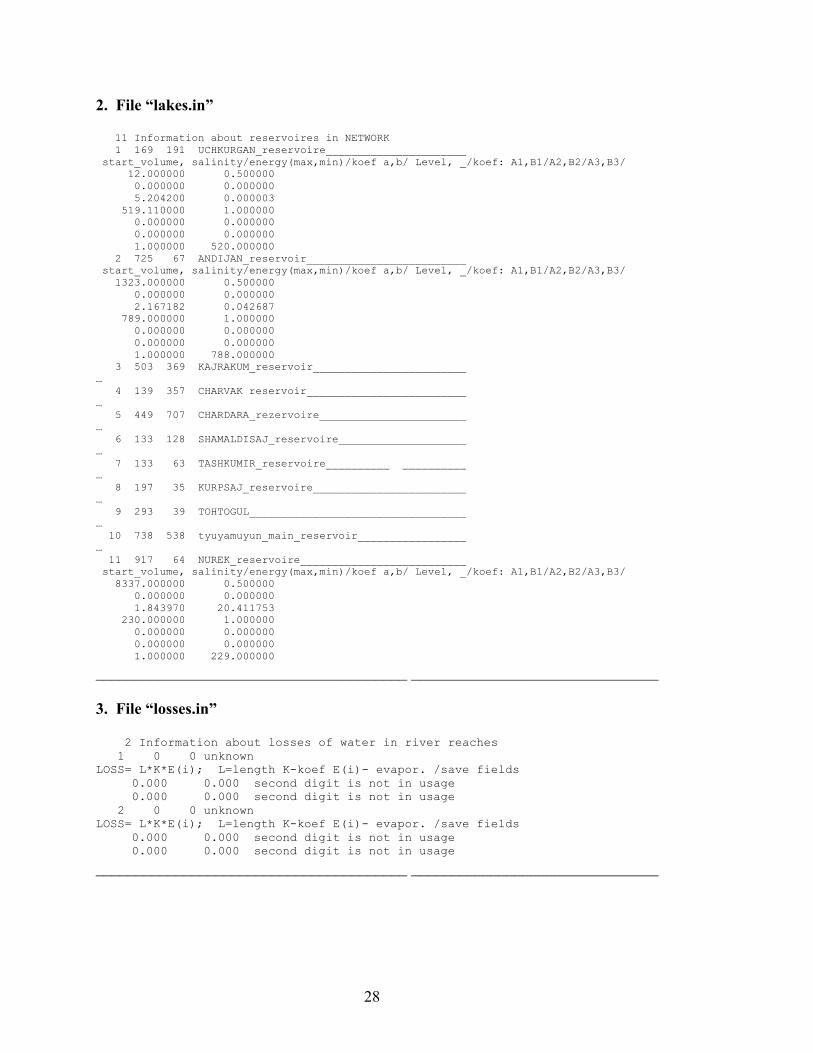
The resulting structure of the files created or edited in the “Data Input” module are presented in abbreviated form below. The full example data files can be found in the data set on the software distribution diskette(s). 1. File “lagtime.in” 2 Information time lag in river reaches 1 0 0 unknown L=length(km) V-velosity(m/sec) /save fields 0.000 0.000 second digit is not in usage 0.000 0.000 second digit is not in usage 2 0 0 unknown L=length(km) V-velosity(m/sec) /save fields 0.000 0.000 second digit is not in usage 0.000 0.000 second digit is not in usage

_______________________________________ _______________________________

28

2. File “lakes.in” 11 Information about reservoires in NETWORK 1 169 191 UCHKURGAN_reservoire______________________ start_volume, salinity/energy(max,min)/koef a,b/ Level, _/koef: A1,B1/A2,B2/A3,B3/ 12.000000 0.500000 0.000000 0.000000 5.204200 0.000003 519.110000 1.000000 0.000000 0.000000 0.000000 0.000000 1.000000 520.000000 2 725 67 ANDIJAN_reservoir_________________________ start_volume, salinity/energy(max,min)/koef a,b/ Level, _/koef: A1,B1/A2,B2/A3,B3/ 1323.000000 0.500000 0.000000 0.000000 2.167182 0.042687 789.000000 1.000000 0.000000 0.000000 0.000000 0.000000 1.000000 788.000000 3 503 369 KAJRAKUM_reservoir________________________ … 4 139 357 CHARVAK reservoir_________________________ … 5 449 707 CHARDARA_rezervoire_______________________ … 6 133 128 SHAMALDISAJ_reservoire____________________ … 7 133 63 TASHKUMIR_reservoire__________ __________ … 8 197 35 KURPSAJ_reservoire________________________ … 9 293 39 TOHTOGUL__________________________________ … 10 738 538 tyuyamuyun_main_reservoir_________________ … 11 917 64 NUREK_reservoire__________________________ start_volume, salinity/energy(max,min)/koef a,b/ Level, _/koef: A1,B1/A2,B2/A3,B3/ 8337.000000 0.500000 0.000000 0.000000 1.843970 20.411753 230.000000 1.000000 0.000000 0.000000 0.000000 0.000000 1.000000 229.000000 _______________________________________ _______________________________ 3. File “losses.in” 2 Information about losses of water in river reaches 1 0 0 unknown LOSS= L*K*E(i); L=length K-koef E(i)- evapor. /save fields 0.000 0.000 second digit is not in usage 0.000 0.000 second digit is not in usage 2 0 0 unknown LOSS= L*K*E(i); L=length K-koef E(i)- evapor. /save fields 0.000 0.000 second digit is not in usage 0.000 0.000 second digit is not in usage

_______________________________________ _______________________________

29

4. File “mouth.in” 2 Information about water which can move in mouths 1 557 687 Release to Arnasaj________________________ 1 4 (storage > -1) (runoff > 1) ;1-hour,2-day,3-decade,4-month -1.000 … 2 535 1096 ARAL_SEA__________________________________ 1 4 (storage > -1) (runoff > 1) ;1-hour,2-day,3-decade,4-month 0.000 …

_______________________________________ _______________________________ 5. File “supply.in” 21 Information about water supplies and salinity of water 1 242 159 Side inflow on reaches Toktogul Uchkurgan_ 1 4 (storage > -1) (runoff > 1) ;1-hour,2-day,3-decade,4-month 1.000 0.800 2.000 0.800 3.000 0.800 4.000 0.800 5.000 0.800 79.700 0.800 114.700 0.800 101.700 0.800 67.800 0.800 43.100 0.800 31.000 0.800 2.000 0.800 2 545 77 Inside inflow (Andijan Uchtepa)___________ 1 4 (storage > -1) (runoff > 1) ;1-hour,2-day,3-decade,4-month 76.000 0.800 127.000 0.800 143.000 0.800 135.000 0.800 235.000 0.800 235.000 0.800 256.000 0.800 221.000 0.800 103.000 0.800 129.000 0.800 120.000 0.800 130.000 0.800 3 693 15 Pricipitation on Andijan reservoir________ … 4 779 23 Inflow to Andijan reservoir_______________ … 5 453 221 inside inflow before Akdjar_______________ … 6 487 309 Return water to KAJRAKUM_reservoir________ … 7 553 317 Precipitation to KAJRAKUM_reservoir_______ … 8 587 371 Inside inflow on reaches Kajrakum-Chardara … 9 265 393 Side inflow on Chirchik___________________ … 10 99 403 Ugam river________________________________ … 11 93 267 Precipitation on surface in CHARVAK_reserv

30

… 12 63 297 CHARVAK_rezervoire_inflow_________________ … 13 333 683 Return water to CHARDARA reservoire_______ … 14 351 721 Precipitation in CHARDARA_reservoire______ … 15 443 823 Side inflow before Aral_sea_______________ … 16 333 27 inflow in TOHTOGUL________________________ … 17 735 198 Surhandaria_river_________________________ … 18 761 162 kashkadaria_river_________________________ … 19 803 128 kafirnigan_river__________________________ … 20 811 58 Vahsh_river_______________________________ … 21 1061 128 Pandj_river_______________________________ …

_______________________________________ _______________________________ 6. File “users.in” 34 Information about water user,salinity of return water and return koefficients a and b 1 235 253 River losses in reaches Toktogul Uchkurgan 1 4 (storage > -1) (runoff > 1) ;1-hour,2-day,3-decade,4-month 1 0.000 0.000 2 1.000 0.000 3 2.000 0.000 4 2.000 0.000 5 3.000 0.000 6 3.000 0.000 7 4.000 0.000 8 3.000 0.000 9 0.000 0.000 10 0.000 0.000 11 0.000 0.000 12 0.000 0.000 return koefficients in formulae Wreturn = Wintakw*A + B 37 0.000 0.000 first digit is A, second not in use 38 0.000 0.000 first digit is B, second not in use 2 299 263 Intake on reaches Toktogul Uchkurgan______ 1 4 (storage > -1) (runoff > 1) ;1-hour,2-day,3-decade,4-month 1 28.800 0.000 2 54.700 0.000 3 96.600 0.000 4 192.000 0.000 5 189.000 0.000 6 281.000 0.000 7 322.000 0.000 8 258.000 0.000 9 116.000 0.000 10 66.200 0.000 11 56.100 0.000 12 5.400 0.000 return koefficients in formulae Wreturn = Wintakw*A + B 37 0.000 0.000 first digit is A, second not in use 38 0.000 0.000 first digit is B, second not in use 3 545 249 Evaporation from river____________________

31

… 4 585 239 Intake on Andijan Uchtepa reaches_BFK_____ 1 4 (storage > -1) (runoff > 1) ;1-hour,2-day,3-decade,4-month 1 41.000 0.000 2 76.000 0.000 3 120.000 0.000 4 99.000 0.000 5 125.000 0.000 6 109.000 0.000 7 111.000 0.000 8 109.000 0.000 9 87.000 0.000 10 91.000 0.000 11 88.000 0.000 12 80.000 0.000 return koefficients in formulae Wreturn = Wintakw*A + B 37 0.000 0.000 first digit is A, second not in use 38 0.000 0.000 first digit is B, second not in use 5 637 159 Podvodiash-kanal__________________________ … 6 705 125 Losses from Andijan lake__________________ … 7 329 329 Intake before Akdjar_____________________ … 8 361 373 Evaporation from river surfaces___________ … 9 465 451 Intake from KAJRAKUM_reservoir____________ … 10 511 457 Losses from KAJRAKUM reservoir____________ … 11 569 547 Intake on reaches Kajrakum-Chardara reache … 12 553 593 Evaporation from river surface____________ … 13 359 627 Evaporation from _Chirchik_______________ … 14 311 575 Intake from Chirchik______________________ … 15 207 351 Losses from CHARVAK_rezervoire___________ … 16 559 735 Intake to Kizilkum kanal__________________ … 17 413 779 Losses in CHARDARA_reservoir______________ … 18 473 865 Intake before ARAL_SEA____________________ … 19 487 948 River losses before Aral__________________ … 20 493 1016 Evaporation losses before Aral____________ … 21 785 988 LENINA_CHANAL_____________________________ … 22 816 738 PETNIAKARNA_TASHSAKA_URGENCHARNA__________ … 23 824 796 KLICHBAJ_KIPCHAKBOZSU_GUMABAJSAKA_________ … 24 686 890 RIGHTCHANAL_KIZKETKEN_____________________ … 25 842 876 SOVETJAB_OKTJABRARNA_PAHTAARNA____________ … 26 645 1052 PUMPING_INTAKE+infiltration losses________ … 27 862 516 DASHHOUZ__________________________________

32

… 28 638 592 RIGHT_CHANAL_IN TUJAMUIN SYSTEMS__________ … 29 832 564 LEFT_CANAL_IN TUJAMUIN_SYSTEM_____________ … 30 690 624 DRINK-KANAL_______________________________ … 31 669 421 karshi_kanal______________________________ … 32 639 361 amu_buhara_kanal__________________________ … 33 787 417 karakum_kanal_____________________________ … 34 643 273 Upper user on Amudarja____________________ …

_______________________________________ _______________________________ Notice, that at the top of each of the files comment lines are available for use. The first number in the first line shows the number of nodes of the given type in the river system. Other lines, beginning with the second, repeat for each node in the given group. The first figure in the second line is the serial number of the given node in the group of nodes of the given type. The second and third numbers of the second line show the coordinates of the node in the graphic representation of the network. Further, there is an external name of the node, considerably simplifying editing the files with other text editors. In the third line (second for each node of a given type) are figures (runoff or storage) and a time interval. 2.2.7. Lake Morphology The “Lake Morphology” module estimates the reservoir morphological coefficients already mentioned in the previous section in the description of input for reservoirs. When the module is selected from the “Water” menu, the user is presented with the window shown in Figure 13. If files containing information about the morphological data do not exist, they are created anew by default. The user can change the data in the tables (at the lower left-hand corner in Figure 13) simultaneously viewing how the changes are reflected in the diagrams above. On each of the diagrams, two curves are given: first is the tabulated data, second is the function determined by the method of the least squares. The module is very sensitive to changes in the data, and consequently, it is recommended that only small changes be made. Also, it is necessary to use a rule, that as you move down in the table levels and volumes increase. The names of reservoirs are read from the file "lakes.lst" described above, shown in a special window from which the user can choose a reservoir. In the top part of the window are information on all factors regarding the reservoirs. After the user is satisfied with the degree of concurrence of the curves with the data points on each of the diagrams, the user can use one of two buttons: "Save and Exit" or "Save for Usage". In the first case, all the files created by the user are written to the file "lakes.vol". In the second case, the data are written to the file "lakes.in", which was described above.

33

The given module can be used once to estimate the factors or it may not be used at all if the user knows the morphological factors from other sources and to enters them in the file "lakes.in" using the module "Data Input".

Figure 13. View of “Lake Morphology” window with information about Toktogul reservoir displayed.

The file “lakes.vol” is shown below. For a complete listing of this file, please see the data set on the distribution diskette(s). File “lakes.vol” 1 169 191 > reservoir_n5 below(Tohtogul)______________ < 2.2437671026 0.6010715230 535.00 <= a, b, ho 1.2437671026 1.3486645096 0.5543209459 1.7883387753 ______________________________________ I N I VOLUME I LEVEL I AREA I calculation by koeff. I I W I L I S I W(L) S(L) S(W) 1 0.000 536.000 0.000 0.601 1.349 0.00 2 4.000 537.000 4.000 2.847 3.194 3.86 3 9.000 538.000 5.000 7.071 5.288 6.05 4 16.000 539.000 6.999 13.484 7.564 8.32 5 22.000 540.000 5.999 22.246 9.983 9.92 6 24.000 541.000 2.000 33.490 12.524 10.41 7 26.000 542.000 2.000 47.329 15.171 10.88 8 27.000 543.000 1.000 63.863 17.912 11.11 9 31.000 544.000 4.000 83.181 20.738 12.00 10 33.000 545.000 2.000 105.364 23.641 12.42

34

11 35.000 546.000 2.000 130.487 26.617 12.83 12 37.000 547.000 2.000 158.620 29.659 13.24 13 40.000 548.000 3.000 189.826 32.763 13.82 14 42.000 549.000 2.000 224.166 35.927 14.20 15 45.000 550.000 3.000 261.698 39.146 14.75 16 48.000 551.000 3.000 302.476 42.418 15.29 17 50.000 552.000 2.000 346.551 45.740 15.64 18 52.000 553.000 2.000 393.972 49.110 15.98 19 55.000 554.000 3.000 444.786 52.526 16.49 20 58.000 555.000 3.000 499.039 55.986 16.98 ______________________________________ - - 2 725 67 > Andijan reservoir_________________________ < … 3 503 369 > Kajrakum reservoir________________________ < … 4 139 357 > Charvak reservoir_________________________ < … 5 449 707 > Chardara_lake_____________________________ < … 6 133 128 > reservoire n4 (after tohtogul)____________ < … 7 133 63 > reservoire_n3_(after tohtogul) __________ < … 8 197 35 > reservoire n2 after Toktogul______________ < … 9 293 39 > TOHTOGUL__________________________________ < … 10 738 538 > tyuyamuyun_main_reservoir_________________ < … 11 917 64 > Nurek_reservoir___________________________ < …

In the first line, the first number is the serial number of the reservoir and then its external name, facilitating editing by text editors. Three morphological factors with subsequent comments follow. The factors for calculation of the area - volume relationship for the reservoir are given. The table requires 20 lines for each reservoir, and the first three columns are the most important: serial number, volume, elevation, and area data followed by sample calculations from the functions using the fitted parameters so that the user can, once again, estimate the degree of approximation of the data by the function. Pay careful attention to the fact that the zero level must be less than any of levels in the table. In a case there are problems working with the module it is necessary to remove the file "lakes.vol" from the working directory and to recreate it. Problems can arise due to the high sensitivity of the approximating function to the estimated parameters. 2.2.8. Objective Weights The objective function of the water management model is comprised of five components, each of which can be examined as a separate individual task. These components are described in detail in McKinney and Kenshimov (2000, Chapter 3). The purpose of the “Objective Weights” module is to assign the priority (weight) for each of the individual tasks in the objective function. At start of the module there is a working window and the user can assign the priorities of the tasks using the five cells in the window, see Figure 14. On the right there is a comment on use of the module. The user can load the available information by opening the file "digits.in" as shown in the following table.

35

File “digits.in”

* USERS OUTPUT FILLING ENERGY STABILITY * 1000.00 0.00 0.00 0.00 60.00 P1= 1000.00 ; P2= 0.00 ; P3= 0.00 ; P4= 0.00 ; P5= 60.00 ;

Figure 14. View of “Objective Weights” window with information about assigned priorities of the objective function components.

The file is created according to the rules of the GAMS compiler and consequently its editing is recommended only through the editor of priorities in the "Objective Weights" module. Mark "*" - means that all given line is perceived by the compiler as a comment. See the tutorial of McKinney and Savitsky (2000) for detailed information on creating GAMS files and models. The "Objective Weights" module uses only the two first lines of the file and the other five lines are ignored. That is, any changes made in lines 3-8 will be ignored by the "Objective Weights" module, and when storing the file, lines 3-8 will be generated from the information in the first two lines. When conducting numerical experiments, the user can directly change lines 3-8 in a text editor and GAMS will use them. This can accelerate work. By setting a zero weight for a particular task, the user can exclude the given task from consideration by GAMS. 2.2.9. Internal Database The window for the “Internal Database” module is shown in Figure 15, in which two buttons are accessible to the user and on the right are given rules on use of the module. The button "Exit" leaves the module without making any actions. The button "Execution" creates the internal database of restrictions precisely coordinated with the network. Initially, the database is empty and contains fields in which constrains under the water management task are entered. These

36

constraints may be to limit volumes of water in reservoirs and flows of water in channels or rivers in the network. It is recommended to execute this module only once during creation of a model, as any earlier database will deleted and overwritten by a new one. A fragment of the internal database is given below.

Figure 15. View of “Internal Database” window.

File “limitall”

34 21 11 34 2 35 0 0 136 136 3 1 1 169 191 V1 < reservoir_n5below(Tohtogul)_______________ 3 1 1 169 191 V1 < reservoir_n5below(Tohtogul)_______________ ______________volume for lakes_________ ____________________________________________________________ time lower upper fixed usage 1 - in use step limit limit limit in model 0 - not use ____________________________________________________________ m1 0.000 20000.000 12.000 0 0 1 m2 0.000 20000.000 12.000 0 0 1 m3 0.000 20000.000 12.000 0 0 1 m4 0.000 20000.000 12.000 0 0 1 m5 0.000 20000.000 12.000 0 0 1 m6 0.000 20000.000 12.000 0 0 1 m7 0.000 20000.000 12.000 0 0 1 m8 0.000 20000.000 12.000 0 0 1 m9 0.000 20000.000 12.000 0 0 1 m10 0.000 20000.000 12.000 0 0 1 m11 0.000 20000.000 12.000 0 0 1 m12 0.000 20000.000 12.000 0 0 1 ____________________________________________________________ 3 2 2 725 67 V2 < Andijanreservoir__________________________ … C1 < controlpointbeforereservoiren5___

37

3 1 1 169 191 V1 < reservoir_n5below(Tohtogul)_________ ___ storage on connection between first and second knots____ ____________________________________________________________ time lower upper fixed usage 1 - in use step limit limit limit in model 0 - not use ____________________________________________________________ m1 0.000 1000.000 0.000 0 0 0 m2 0.000 1000.000 0.000 0 0 0 m3 0.000 1000.000 0.000 0 0 0 m4 0.000 1000.000 0.000 0 0 0 m5 0.000 1000.000 0.000 0 0 0 m6 0.000 1000.000 0.000 0 0 0 m7 0.000 1000.000 0.000 0 0 0 m8 0.000 1000.000 0.000 0 0 0 m9 0.000 1000.000 0.000 0 0 0 m10 0.000 1000.000 0.000 0 0 0 m11 0.000 1000.000 0.000 0 0 0 m12 0.000 1000.000 0.000 0 0 0 ____________________________________________________________ 6 1 1 199 216 C2 < ReleasefromToktogulreservoir______ … I1 < SideinflowonreachesToktogulUchku

The first line contains the information on the number of nodes of the given type and number of arcs in the network. Following this are tables for each reservoir of the working circuit. All constraints are given in the table. It is possible to limit the flow from above (upper bound), from below (lower bound) or set flow to a fixed value for a time interval. It is possible to use or not use constraints in your model. In the given fragment of an internal database shown above there are restrictions on volumes in reservoirs which will be used in model. 2.2.10. Constraints This module allows the user to create the database of constraints (restrictions) for the water management task, and to use them in a GAMS model. Figure 16 shows the window of the module when you are entering constraints for a particular reservoir. Using the “File” menu, the user must load the internal database file "limitall" from the working directory. After loading the file the working panel will display the network of the river system, in which each type of node is represented by a special graphic symbol. On arcs connecting nodes appear dark blue rectangles, which turn yellow when the cursor is on them. Sometimes the frame will appear red, meaning that previous restrictions were defined there. Highlighting a rectangle on an arc causes the appearance of information at the bottom of the screen: serial number, name (internal and external), owner and type of node for both the beginning and ending node of an arc. For reservoirs, the initial and final nodes coincide. In the bottom right corner of the window is shown the information on type and quantity of time intervals in the model. Using the module, you can specify the upper, lower or fixed limits for any of the arcs in any time interval. Once numerical data for a constraint is entered, the user can choose to include the

38

constraint in the model by pressing the "In use" checkbox above the cell for entered data. Once the constraint is entered in the database, black vertical lines will be displayed on three graphic panels in the top part of the window. The black vertical lines indicate the time interval in which constraints (upper, lower, or fixed) are active. Below this, you can see a graph of the constraints for the node or arc. Simultaneously with that, around the rectangle on the arc a red box will appear. This shows that for the given arc there is a constraint. Otherwise, rectangles remain yellow. If you enter a constraint for one item and one time interval, you can distribute the constraint to all time intervals by pressing the "Use in all time steps" button. This action will instantly cause the corresponding red strip at the top of the graphic to turn black. The user can cancel constraints in all time steps by using the "Don’t use in all time steps" button. The corresponding black strips in the graphic menu will become red. The user can use different units for constraints, e.g., runoff in m3/sec or storage in million m3/time interval. Next to the input cells for constraint data are coefficient windows that multiply or divide according to the "Multiply" and "Divide" buttons. However, in the internal database, information are stored only in million m3/time interval. To select an arc about which to enter constraints, the user must choose the arc with the cursor and press the right mouse button, freezing the cursor. Then constraints for that arc can be entered. To return control of the system to the network panel, the user must press the left mouse button.

39

Figure 16. View of “Constraints” window with information about Toktogul reservoir displayed.

When finished entering constraints, the user should save the information using the “Save” item uner the “File” menu. This creates or updates the file of model constraints "cnstr". This file is written according to the rules of the GAMS language. An example of such a “cnstr” file is given below. File “cnstr”

vol.lo('V9','m1') = 13555.00; Toktogul vol.up('V9','m1') = 13555.00; vol.lo('V9','m2') = 5500.00; vol.up('V9','m2') = 19500.00; vol.lo('V9','m3') = 5500.00; vol.up('V9','m3') = 19500.00; vol.lo('V9','m4') = 5500.00; vol.up('V9','m4') = 19500.00; vol.lo('V9','m5') = 5500.00; vol.up('V9','m5') = 19500.00; vol.lo('V9','m6') = 5500.00; vol.up('V9','m6') = 19500.00; vol.lo('V9','m7') = 5500.00; vol.up('V9','m7') = 19500.00; vol.lo('V9','m8') = 5500.00; vol.up('V9','m8') = 19500.00; vol.lo('V9','m9') = 5500.00; vol.up('V9','m9') = 19500.00; vol.lo('V9','m10') = 5500.00; vol.up('V9','m10') = 19500.00; vol.lo('V9','m11') = 5500.00; vol.up('V9','m11') = 19500.00; vol.lo('V9','m12') = 14882.00; vol.up('V9','m12') = 19500.00; … flow.up('R1_V5','m1') = 1000.00; Chardara - Arnasai flow.up('R1_V5','m2') = 1000.00; flow.up('R1_V5','m3') = 1000.00; flow.fx('R1_V5','m4') = 0.00; flow.fx('R1_V5','m5') = 0.00; flow.fx('R1_V5','m6') = 0.00; flow.fx('R1_V5','m7') = 0.00; flow.fx('R1_V5','m8') = 0.00; flow.fx('R1_V5','m9') = 0.00; flow.fx('R1_V5','m10') = 0.00; flow.fx('R1_V5','m11') = 0.00; flow.up('R1_V5','m12') = 1000.00; flow.up('C20_V5','m1') = 1000.20; Chardara – Sry Darya flow.up('C20_V5','m2') = 1000.20; flow.up('C20_V5','m3') = 1000.20; flow.up('C20_V5','m11') = 1000.20; flow.up('C20_V5','m12') = 1000.20;

We remind the reader, that for reservoirs the constraints are on storage volumes, and on arcs they are on flow volumes.

40

2.2.11. Build Model This module generates the mathematical model using the GAMS language. In Figure 17 the module window is shown. The model consists of a group of files one of which is the main file "riv_new.gms". It is comprised of the following files, which GAMS will include as part of the model: "cnstr", and "digits.in". The module searches for these files in the current working directory.

Figure 17. View of “Build Model” window.

Three buttons are accessible to the user in the window: “Input”, “Equations” and “All Model”. The “Input” button creates the main file "riv_new.gms", which contains the information on the structure of the river network and the initial data. The “Equations” button creates the file "equation". The “All Model” button create both files: "riv_new.gms " and "equation" in one step. This division is very useful as it enables the user to carry out numerical experiments changing only a part of the model through a text editor. The “Exit” button on the right allows the user to leave the module. Information is displayed on the number of each type of node in the network and the sufficiency or insufficiency of the information for construction of the model. Two information windows on the right show the user the condition of model construction. Information about the presence of gross errors in the files is presented as necessary. The software was used to create a model of the Amu Darya and Syr Darya Rivers in Central Asia. The authors note that the system models river systems in which all reservoirs have only only a single capacity. On the Amu Darya river there is a reservoir consisting of four capacities. We have not included this feature of the Amu Darya river in the software since the this is the only instance of such multi-capacity reservoirs known to the authors and the software is intended

41

for wide uses. However, the task of solving the problem of management of a multi-capacity reservoirs is can be solved by GAMS (see McKinney and Savitsky, 2000), 2.2.11. Solve Model The model is comprised of four interacting and isolated files that contain the text of the model of optimal water management (files “riv_new.gms”, “equation”, “digits.in”, and “cnstr”). The model is written according to the rules of the GAMS language. The first part defines all parameters and initial data that determine a specific calculation problem (the riv_new.gms file). The second part is actually the universal part of the model including equations (the equation file). The third part is a file with information about priorities in the optimization objective (the digits.in file). The fourth part is a file of the constraints imposed on variables (the cnstr file). After the model has been created, the compiler GAMS can work with it. If GAMS is installed on your C disk in a directory named c:\GAMS, then the menu item “solve” can call GAMS to solve for the optimum of the model. When installing GAMS on your computer it is necessary to specify the path to the directory containing the GAMS compiler and in this case realization of GAMS calculations will be always accessible through the main menu. Optimization Calculations of the GAMS Model To start the GAMS compiler you should select the “Solve model” item from the “Water” menu. The GAMS riv_new.gms command line is formed and executed. Messages of the GAMS compiler will appear in a DOS window and the user should watch for the appearance of the label OPTIMAL SOLUTION FOUND which means that the water balance for the entire river network is satisfied precisely and an optimal solution has been found in full accordance with the system of priorities and constraints. After solution of the model three files are created: "riv_new.lst" This is the normal GAMS listing file, and it contains information about the

work of the GAMS compiler; "river.new" This file contains the values of all variables in the model in tabular form

and with necessary comments; and "demo.new" This contains the variable values for graphic display. The user has access to first two files through the appropriate items of the main menu. Common messages of the GAMS compiler “INFEASIBLE SOLUTION” – more often this message appears in a problem where mutually exclusive constraints are placed on decision variables. For example, if the user fixes a release from a reservoir equal to 100 m3/s and specifies that flow to a downstream node should not be more than 99 m3/s, he will surly receive this message. The only means to avoid this message is to turn off all constraints on water flows simultaneously and then sequentially turn them on, recalculating the model.

42

“BADLY BOUND” – this message appears results from uncoordinated initial storage volume in a reservoir and upper and lower bounds. For example, initial storage of a reservoir might have been set to 100 million m3 and the lower bound is 200 million m3. This situation will assure the appearance of the message. “TOO MANY ITERATIONS” – this message can easily be corrected by replicating several times the line in the file “equation” that contains the word SOLVE. 2.2.12. Display Results The “Display Results” module does not create any files, and it does not make any calculation. Its purpose is graphic representation of the model solution in graphic and tabular form. In Figure 18 the working window of the module is shown. On the left side of the window is the river network. On the right side are a graphical panel and a tabular panel. By selecting any arc in the network the user can see the solution results in the two right panels. In Figure 18, the solution for Toktogul reservoir is shown and in Figure 19, the solution for Kayrakum reservoir is shown. Figure 19 shows clearly the upper and lower constraints on the reservoir storage volume.

Figure 18. “Display Results” module with Toktogul reservoir solution displayed.

43

Figure 19. “Display Results” module with Kayrakum reservoir solution displayed. 2.2.13. Additional Capabilities Form creation Creates a file of the solution information in the form usually used by workers of water organizations. This component can be organized for special purposes by the authors. Translation of Results into Other Languages The GAMS compiler works only with letters of the Latin alphabet, and that causes problems of readability of output forms when they are desired in other alphabets, e.g., Cyrillic. In addition, internal names given by the program system to nodes of the calculated scheme impede the reading and interpretation of results. To solve this problem, we created the module of the translator of results.

44

2.3. Water – Salt Task 2.3.1. Introduction This task is to determine the optimum water management of a river basin considering the salinity of waters. Mineralization of water is calculated but it does not enter into the objective function and consequently the decision is actually wholly determined in by the water task, except to the extent that constraints restrict the development of saline waters in the river. However, salinity of water is accounted for fully and in case constraints are placed on water salinity the solution will be found which complies with the given restrictions. Proceeding from this, the upper or lower constraints on salinity are accessible to the user. In the menu the “Main” module the item "Water - Salt" is accessible to the user (see Figure 20). Under this menu are located the various operations necessary to solve the water – salinity task.

Figure 20. View of “Main” screen when selecting from the “Water - Salt” menu.

2.3.2. Internal Database The window for the “Internal Database” module is shown in Figure 21, in which two buttons are accessible to the user and on the right are given rules on use of the module. The button "Exit" leaves the module without making any actions. The button "Execution" creates the internal database of restrictions precisely coordinated with the network. Initially, the database is empty and contains fields in which constrains under the water management task are entered. These constraints may be to limit salinity at various points along the river network. It is recommended to execute this module only once during creation of a model, as any earlier database will deleted and overwritten by a new one. A fragment of the internal database file “limitals” is given below.

45

Figure 21. View of “Internal Database” window.

File “limitals” 1 1 1 1 1 1 1 1 7 7 3 1 1 258 69 (type of unit, number, accessory(belonging), coordinate) V1 < (internal name and in network and an external name) Unknown _________________________________ < > 3 1 1 258 69 (type of unit, number, accessory(belonging), coordinate) V1 < Unknown _________________________________ < > ______________ MINERALIZATION for lakes ________ (kind of restrictions) _______________________________________ _____________________ Time lower upper fixed Usage 1 - in use Step limit limit limit in model 0 - not use _______________________________________ _____________________ M1 10.000 20.000 0.000 1 0 0 M2 0.000 20.000 11.000 0 0 1 M3 0.000 20.000 0.000 0 0 0 … … … … … … … … Is similar M35 0.000 20.000 0.000 0 0 0 M36 0.000 20.000 0.000 0 0 0 _______________________________________ _____________________ 2 1 1 304 37 information about I1 < initial unit Supply _______________________________ and his(its) name 3 1 1 258 69 information about V1 < final unit Unknown __________________________ and his(its) name ___ Storage on connection between first and second knots ____ _______________________________________ _____________________ Time lower upper fixed Usage 1 - in use Step limit limit limit in model 0 - not use _______________________________________ _____________________ M1 0 10 0 0 0 0

46

M2 0 10 0 0 0 0 M3 0 10 0 0 0 0 … … … … … … … … Is similar M36 0 10 0 0 0 0 _______________________________________ _____________________

The first line contains the information on the number of nodes of the given type and number of arcs in the network. Following this are tables for each reservoir of the working circuit. All constraints are given in the table. It is possible to limit the flow from above (upper bound), from below (lower bound) or set flow to a fixed value for a time interval. It is possible to use or not use constraints in your model. In the given fragment of an internal database shown above there are restrictions on volumes in reservoirs that will be used in model. 2.3.3. Constraints This module allows the user to create the database of constraints (restrictions) for the water – salinity management task, and to use them in a GAMS model. Figure 22 shows the window of the module when you are entering constraints for a particular reservoir. Using the “File” menu, the user must load the internal database file "limitals" from the working directory. After loading the file the working panel will display the network of the river system, in which each type of node is represented by a special graphic symbol. On arcs connecting nodes appear dark blue rectangles, which turn yellow when the cursor is on them. Sometimes the frame will appear red, meaning that previous restrictions were defined there. Highlighting a rectangle on an arc causes the appearance of information at the bottom of the screen: serial number, name (internal and external), owner and type of node for both the beginning and ending node of an arc. For reservoirs, the initial and final nodes coincide. In the bottom right corner of the window is shown the information on type and quantity of time intervals in the model. Using the module, you can specify the upper, lower or fixed limits for any of the arcs in any time interval. Once numerical data for a constraint is entered, the user can choose to include the constraint in the model by pressing the "In use" checkbox above the cell for entered data. Once the constraint is entered in the database, black vertical lines will be displayed on three graphic panels in the top part of the window. The black vertical lines indicate the time interval in which constraints (upper, lower, or fixed) are active. Below this, you can see a graph of the constraints for the node or arc. Simultaneously with that, around the rectangle on the arc a red box will appear. This shows that for the given arc there is a constraint. Otherwise, rectangles remain yellow. If you enter a constraint for one item and one time interval, you can distribute the constraint to all time intervals by pressing the "Use in all time steps" button. This action will instantly cause the corresponding red strip at the top of the graphic to turn black. The user can cancel constraints in all time steps by using the "Don’t use in all time steps" button. The corresponding black strips in the graphic menu will become red. The user can use different units for constraints, e.g., runoff in m3/sec or storage in million m3/time interval. Next to the input cells for constraint data are coefficient windows that multiply or divide according to the "Multiply" and "Divide" buttons. However, in the internal database, information are stored only in million m3/time interval. To select an arc about which to enter constraints, the user must choose the arc with the cursor and press the right mouse button, freezing the cursor. Then

47

constraints for that arc can be entered. Salinity constraints are entered in g/L. To return control of the system to the network panel, the user must press the left mouse button.

Figure 22. View of “Constraints” window for salinity constaints.

When finished entering constraints, the user should save the information using the “Save” item uner the “File” menu. This creates or updates the file of model constraints "cnstr". This file is written according to the rules of the GAMS language. An example of such a “cnstr_s” file is given below. File “cnstr_s”

Knot_s.lo('V1','m1') = 1.00; for a reservoir V1 and time m1 the bottom limit 1 Knot_s.lo('V1','m2') = 1.00; for a reservoir V1 and time m2 the bottom limit 1 Knot_s.fx('V1','m12') = 10.0; for a reservoir V1 and time m12 is fixed 10 * _________________________________ S_flow.lo('V1_c1','m1') = 2.00; for connection V1_c1 and time m1 the bottom limit 2 S_flow.up('V1_c1','m2') = 20.0; for connection V1_c1 and time m1 the bottom limit 20 S_flow.lo('V1_c1','m12') = 2.00; for connection V1_c1 and time m1 the bottom limit 2

Adding constraints on salinity to a model requires much patience and step-by-step work, so as to not destroy the opportunity to receive an optimal solution. We suggest that the user add

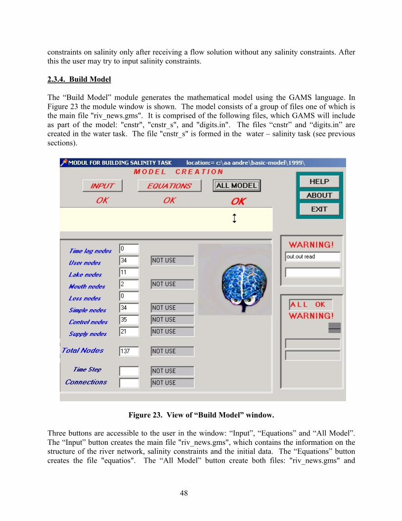
48

constraints on salinity only after receiving a flow solution without any salinity constraints. After this the user may try to input salinity constraints. 2.3.4. Build Model The “Build Model” module generates the mathematical model using the GAMS language. In Figure 23 the module window is shown. The model consists of a group of files one of which is the main file "riv_news.gms". It is comprised of the following files, which GAMS will include as part of the model: "cnstr", "cnstr_s", and "digits.in". The files “cnstr” and “digits.in” are created in the water task. The file "cnstr_s" is formed in the water – salinity task (see previous sections).

Figure 23. View of “Build Model” window.

Three buttons are accessible to the user in the window: “Input”, “Equations” and “All Model”. The “Input” button creates the main file "riv_news.gms", which contains the information on the structure of the river network, salinity constraints and the initial data. The “Equations” button creates the file "equatios". The “All Model” button create both files: "riv_news.gms" and

49

"equatios" in one step. This division is very useful as it enables the user to carry out numerical experiments changing only a part of the model through a text editor. The “Exit” button on the right allows the user to leave the module. Information is displayed on the number of each type of node in the network and the sufficiency or insufficiency of the information for construction of the model. Two information windows on the right show the user the condition of model construction. Information about the presence of gross errors in the files is presented as necessary. The software was used to create a model of the Amu darya and Syr Darya rivers including both water flow and salt movement. 2.3.5. Solve Model This model incorporates four interacting and isolated files that contain the text of the model of optimal water and energy management. The model is written according to the rules of the GAMS language. The first part defines all parameters and initial data that determine a specific calculation problem (the riv_news.gms file). The second part is actually the universal part of the model including equations (the equatios file). The third part consists of files with information about priorities in the optimization objective (the digits.in file). The fourth part consists of files of the constraints imposed on variables (the cnstr and cnstr_s files). After the model has been created, the compiler GAMS can work with it. If GAMS is installed on a C-disk within a directory c:\GAMS then through the main menu it can be called to solve for the optimum of the model. Optimization Calculations of the GAMS Model To start the GAMS compiler you should select the “Solve model” item from the “Water - Salt” menu. The GAMS riv_news.gms command line is formed and executed. Messages of the GAMS compiler will appear in a DOS window and the user should watch for the appearance of the label OPTIMAL SOLUTION FOUND which means that the water and salt balances for the river network are satisfied precisely and an optimal solution has been found in full accordance with the system of priorities. After solution of the model three files are created: "riv_news.lst" This is the normal GAMS listing file, and it contains information about the

work of the GAMS compiler; "rivers.new" This file contains the values of all variables in the model in tabular form

and with necessary comments; and "demo.new" This contains the water system variable values for graphic display. "demo_s.new" This contains the values of the salinity variables for graphic display. The user has access to first two files through the appropriate items of the main menu.

50

2.3.6. Display Results The “Display Results” module does not create any files, and it does not make any calculation. Its purpose is graphic representation of the model solution by simultaneous graphic and tabular representation. In Figure 24 the working window of the module is shown. On the left side of the window is the energy system. On the right side are a graphical panel and a tabular panel. By selecting any rectangle in the system network the user can see the results in these two panels. In Figure 24, the solution for Kyrgyz export of energy into the Central Asia Energy System during the vegetation period is shown. Figure 25 shows the solution for Uzbek import of energy from the Central Asia Energy System during the vegetation period.

Figure 24. View of “Display Results” window with solution for river system with salinity constraints showing salinity of water leaving Chardara reservoir (hypothetical calculation).

51

2.4. Water – Energy Task 2.4.1. Introduction This task is to determine the optimum management of the water regime in a river basin taking account of energy, separately, for each owner of energy generation assets in the energy system. In addition to hydropower stations, the production of energy by each owner is possible by their own managed thermal stations and by small stations that operate at almost constant output. The operation of hydropower plants is determined in coordination with the water portion of the modeling system. All energy generation asset owners are united in a uniform network or grid, making possible the transfer of energy from one user to another. Each country is considered to be an energy-user. The task exists in two modes: 1) an energy system where each owner is a user and receives the energy generated on its own assets; and 2) water and energy accounts of each country are split and energy can be exported and imported as needed. The second mode is recommended in cases where complexities of accounting exist in the first mode.

Figure 25. View of “Main” screen when selecting from the “Water - Energy” menu.

In the menu the “Main” module the item "Water - Energy" is accessible to the user (see Figure 25). Under this menu are located the various operations necessary to solve the water – energy task. 2.4.2. Objective Weights The “Objective Weights” module is activated by selecting that menu item from the “Water - Energy” menu (see Figure 25). The “Objective Weights” module window is shown in Figure 26.

52

In this window, the user has access to a button for choosing the owner of energy systems. The list of owners is given at the bottom of the panel:

Owner 1 = Kyrgyzstan Owner 2 = Uzbekistan Owner 3 = Tajikistan Owner 4 = Kazakhstan Owner 5 = Turkmenistan

This list shows the owners for Central Asia, but it can be modified for other regions.

Figure 26. View of “Objective Weights” screen.

The user can load previously defined information on energy demand and energy prices by selecting the “Open” command from the “File” menu and opening the file “money.in”. If this file has been created before, it can be updated here. If the file does not exist, or the user does not want to use the available information, default values can be used.

53

Once the “money.in” file has been loaded, the user may select an owner and enter or modify that user’s demand for energy in million kWh per time interval. The number of time intervals is taken from the file "steps.in" defined earlier. Under the area labeled “Objective Weights”, the user can enter information on the cost of manufacturing one unit of energy in:

• Non-calculated stations; • Thermal stations; • Hydroelectric power stations; • Transfer of energy from the regional energy system connected to other users; and • Damages from deficit of energy for user.

All of the information should be entered for each energy user. Once all the information has been entered the user may select “Save” from the “File” menu and save the new “money.in” file. The file “demand.in” is also updated with the information on energy demands. The command "Exit" in the “File” menu allows leaving the module without saving any changes. File "demand.in"

* 1694.00 user energy demand in time_step= 1 for owner 1 * 1412.00 user energy demand in time_step= 2 for owner 1 * 1383.00 user energy demand in time_step= 3 for owner 1 * 897.00 user energy demand in time_step= 4 for owner 1 * 647.00 user energy demand in time_step= 5 for owner 1 * 543.00 user energy demand in time_step= 6 for owner 1 * 560.00 user energy demand in time_step= 7 for owner 1 * 556.00 user energy demand in time_step= 8 for owner 1 * 540.00 user energy demand in time_step= 9 for owner 1 * 758.00 user energy demand in time_step= 10 for owner 1 * 1140.00 user energy demand in time_step= 11 for owner 1 * 1576.00 user energy demand in time_step= 12 for owner 1 … * 7000.00 user energy demand in time_step= 36 for owner 5 potr('owner1','A1owner1','m1')= 1694.00 ; potr('owner1','A1owner1','m2')= 1412.00 ; potr('owner1','A1owner1','m3')= 1383.00 ; potr('owner1','A1owner1','m4')= 897.00 ; potr('owner1','A1owner1','m5')= 647.00 ; potr('owner1','A1owner1','m6')= 543.00 ; potr('owner1','A1owner1','m7')= 560.00 ; potr('owner1','A1owner1','m8')= 556.00 ; potr('owner1','A1owner1','m9')= 540.00 ; potr('owner1','A1owner1','m10')= 758.00 ; potr('owner1','A1owner1','m11')= 1140.00 ; potr('owner1','A1owner1','m12')= 1576.00 ; … potr('owner5','A1owner5','m12')= 829.90 ; *______your system has 5 owners

The file consists of two parts: 1) an internal database of energy demand used in the interface program.

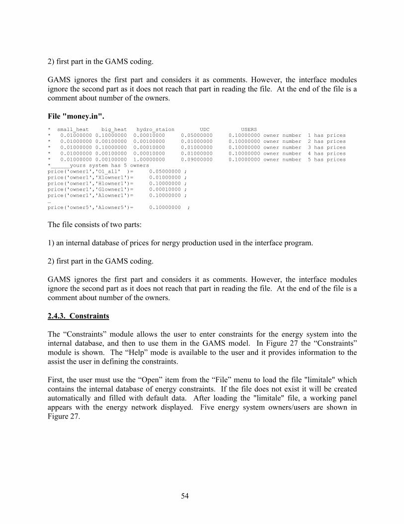
54

2) first part in the GAMS coding. GAMS ignores the first part and considers it as comments. However, the interface modules ignore the second part as it does not reach that part in reading the file. At the end of the file is a comment about number of the owners. File "money.in". * small_heat big_heat hydro_staion UDC USERS * 0.01000000 0.10000000 0.00010000 0.05000000 0.10000000 owner number 1 has prices * 0.01000000 0.00100000 0.00100000 0.01000000 0.10000000 owner number 2 has prices * 0.01000000 0.10000000 0.00010000 0.01000000 0.10000000 owner number 3 has prices * 0.01000000 0.00100000 0.00010000 0.01000000 0.10000000 owner number 4 has prices * 0.01000000 0.00100000 1.00000000 0.09000000 0.10000000 owner number 5 has prices *______yours system has 5 owners price('owner1','O1_all' )= 0.05000000 ; price('owner1','X1owner1')= 0.01000000 ; price('owner1','H1owner1')= 0.10000000 ; price('owner1','G1owner1')= 0.00010000 ; price('owner1','A1owner1')= 0.10000000 ; … price('owner5','A1owner5')= 0.10000000 ;

The file consists of two parts: 1) an internal database of prices for nergy production used in the interface program. 2) first part in the GAMS coding. GAMS ignores the first part and considers it as comments. However, the interface modules ignore the second part as it does not reach that part in reading the file. At the end of the file is a comment about number of the owners. 2.4.3. Constraints The “Constraints” module allows the user to enter constraints for the energy system into the internal database, and then to use them in the GAMS model. In Figure 27 the “Constraints” module is shown. The “Help” mode is available to the user and it provides information to the assist the user in defining the constraints. First, the user must use the “Open” item from the “File” menu to load the file "limitale" which contains the internal database of energy constraints. If the file does not exist it will be created automatically and filled with default data. After loading the "limitale" file, a working panel appears with the energy network displayed. Five energy system owners/users are shown in Figure 27.

55

Figure 27. “Constraints” module with information about the Central Asia energy system.

Blue rectangles with crosses are visible on lines connecting the objects of the energy system. These rectangles turn solid yellow when the cursor is over them. If the rectangle frame is yellow, then constraints were defined earlier and saved in the internal database. When the cursor is placed over an item, the information window at the bottom of the screen displays: external and internal names, owner, and type of station or user. In the right panel of the window, the user can enter upper, lower, or fixed limits for energy production, use or transfer in any time interval. After entering the constraint, it must be activated by pressing the check window "In use". Activating the constraint causes the constraint to be displayed in the graphic stripes at the top of the panel. Simultaneously, a yellow rectangle appears around the station on the energy system display, indicating that for at least one time interval there is a constraint for that station that will be used in the model. If a constraint is entered for one item and one time interval, the user can distribute the constraint to all time intervals by pressing the "Use in all time steps" button. This action will instantly cause the corresponding red strip at the top of the graphic to turn black. The user can cancel constraints in all time steps by using the "Don’t use in all time steps" button. The corresponding black strips in the graphic menu will become red.

56

The created or updated constraints must be saved in the file "cnstr_e" which is automatically created according to the rules of GAMS. An example of a fragment of the “cnstr_e” file is given below. File “cnstr_e”

* You can see below constrains in energy system E.fx ('owner1', 'X1owner1', 'm1') = 1.00; E.fx ('owner1', 'X1owner1', 'm2') = 1.00; E.fx ('owner1', 'X1owner1', 'm3') = 1.00; E.fx ('owner1', 'X1owner1', 'm4') = 1.00; E.fx ('owner1', 'X1owner1', 'm5') = 1.00; E.fx ('owner1', 'X1owner1', 'm6') = 1.00; E.fx ('owner1', 'X1owner1', 'm7') = 1.00; E.fx ('owner1', 'X1owner1', 'm8') = 1.00; E.fx ('owner1', 'X1owner1', 'm9') = 1.00; …

2.4.4. Build Model The “Build Model” module generates the mathematical model using the GAMS language. In Figure 28 the module window is shown. The model consists of a group of files one of which is the main file "riv_newe.gms". It is comprised of the following files, which GAMS will include as part of the model: "cnstr", "cnstr_e", "digits.in", “demand.in”, and "money.in". The files “cnstr” and “digits.in” are created in the water task. The files "cnstr_e", “demand.in”, and "money.in" are formed in the water – energy task (see previous sections).

Figure 28. View of “Build Model” window.

Three buttons are accessible to the user in the window: “Input”, “Equations” and “All Model”. The “Input” button creates the main file "riv_newe.gms", which contains the information on the structure of the river network, energy system and the initial data. The “Equations” button creates

57

the file "equatioe". The “All Model” button create both files: "riv_newe.gms " and "equatioe" in one step. This division is very useful as it enables the user to carry out numerical experiments changing only a part of the model through a text editor. The “Exit” button on the right allows the user to leave the module. Information is displayed on the number of each type of node in the network and the sufficiency or insufficiency of the information for construction of the model. Two information windows on the right show the user the condition of model construction. Information about the presence of gross errors in the files is presented as necessary. The software was used to create a model of the Amu Darya and Syr Darya Rivers and the Central Asia Energy System. 2.4.5. Solve Model This model incorporates four interacting and isolated files that contain the text of the model of optimal water and energy management. The model is written according to the rules of the GAMS language. The first part defines all parameters and initial data that determine a specific calculation problem (the riv_newe.gms file). The second part is actually the universal part of the model including equations (the equatioe file). The third part are files with information about priorities in the optimization objective (the digits.in and money.in files). The fourth part consists of files of the constraints imposed on variables (the cnstr and cnstr_e files). After the model has been created, the compiler GAMS can work with it. If GAMS is installed on a C-disk within a directory c:\GAMS then through the main menu it can be called to solve for the optimum of the model. Besides the model can be solved and way, independent of the main managing program. When installing GAMS on your computer it is necessary to specify the path to the directory containing the GAMS compiler and in this case realization of GAMS calculations will be always accessible through the main menu. Optimization Calculations of the GAMS Model To start the GAMS compiler you should select the “Solve model” item from the “Water - Energy” menu. The GAMS riv_newe.gms command line is formed and executed. Messages of the GAMS compiler will appear in a DOS window and the user should watch for the appearance of the label OPTIMAL SOLUTION FOUND which means that the water and energy balances for the river network and energy system are satisfied precisely and an optimal solution has been found in full accordance with the system of priorities. After solution of the model three files are created: "riv_newe.lst" This is the normal GAMS listing file, and it contains information about the

work of the GAMS compiler; "rivere.new" This file contains the values of all variables in the model in tabular form

and with necessary comments; and "demo.new" This contains the water system variable values for graphic display.

58

"demo_e.new" This contains the energy system variable values for graphic display. The user has access to first two files through the appropriate items of the main menu. 2.4.6. Display Results The “Display Results” module does not create any files, and it does not make any calculation. Its purpose is graphic representation of the model solution by simultaneous graphic and tabular representation. In Figure 29 the working window of the module is shown. On the left side of the window is the energy system. On the right side are a graphical panel and a tabular panel. By selecting any rectangle in the system network the user can see the results in these two panels. In Figure 29, the solution for Kyrgyz export of energy into the Central Asia Energy System during the vegetation period is shown. Figure 30 shows the solution for Uzbek import of energy from the Central Asia Energy System during the vegetation period.

Figure 29. View of “Display Results” window with solution for energy system displayed showing export of energy from Kyrgyzsstan to Central Asia Energy System in vegetation

period.

59

Figure 30. View of “Display Results” window with solution for energy system displayed showing import of energy to Uzbekistan from the Central Asia Energy System in

vegetation period.

REFERENCES

Antipova, E., A. Zyryanov, D. McKinney, A. Savitsky, Optimization of Syr Darya Water and Energy Uses, submitted to Water International, 2001. Brooke A., D. Kendrick, and A. Meeraus. 1998, GAMS: A User’s Guide, GAMS Development Corporation, Washington, DC.

McKinney, D.C. and A.K. Kenshimov (eds.), Optimization of the Use of Water and Energy Resources in the Syrdarya Basin Under Current Conditions, Technical Report, US Agency for International Development, Environmental Policies and Institutions for Central Asia (EPIC) Program, Almaty, Kazakstan, 2000. (http://www.ce.utexas.edu/prof/mckinney/papers/aral/00-06-W/EPIC-00-06-W.htm)

60

McKinney, D.C., and A. G. Savitsky., GAMS Tutorial for Water and Energy Management, Technical Report, Center for Research in Water Resources, The University of Texas at Austin, 2001 (http://www.ce.utexas.edu/prof/mckinney/ce385d/papers/GAMS-Tutorial.pdf)