Equation Chapter 1 Section 1

Design of ZnS/ZnSe Gradient-Index Lenses in the Mid-Wave Infrared and Design,

Fabrication, and Thermal Metrology of Polymer Radial Gradient-Index Lenses

by

James Anthony Corsetti

Submitted in Partial Fulfillment of the

Requirements for the Degree

Doctor of Philosophy

Supervised by Professor Duncan T. Moore

The Institute of Optics

Arts, Sciences, and Engineering

Edmund A. Hajim School of Engineering and Applied Sciences

University of Rochester

Rochester, New York

2017

ii

Dedication

This thesis is dedicated to my parents. I would not be where I am now without your

love and support.

iii

Table of Contents

Biographical Sketch .......................................................................................................... vii

Acknowledgments.............................................................................................................. ix

Abstract…........ ................................................................................................................. xii

Contributors and Funding Sources................................................................................... xiv

List of Tables… ................................................................................................................ xv

List of Figures.. ................................................................................................................ xvi

Chapter 1. Introduction to GRIN materials ................................................................. 1

Motivation ............................................................................................................ 1

Definition of GRIN Shape.................................................................................... 1

1.2.1 Axial GRIN ................................................................................................... 2

1.2.2 Radial GRIN ................................................................................................. 3

1.2.3 Spherical GRIN ............................................................................................. 4

GRIN Materials .................................................................................................... 5

1.3.1 Glass .............................................................................................................. 6

1.3.2 ZnS/ZnSe GRINs .......................................................................................... 6

1.3.3 Polymers ....................................................................................................... 7

Thermal Modeling ................................................................................................ 8

Thermal Metrology ............................................................................................ 10

Objective of Thesis............................................................................................. 12

Chapter 2. GRIN ZnS/ZnSe Design Studies ............................................................. 16

Background ........................................................................................................ 16

Color Correction using GRIN Materials ............................................................ 17

Design Study ...................................................................................................... 21

2.3.1 Spectral Considerations .............................................................................. 21

2.3.2 Material Selection ....................................................................................... 22

Singlet Studies .................................................................................................... 24

iv

2.4.1 Specifications .............................................................................................. 24

2.4.2 Homogeneous Designs................................................................................ 24

2.4.3 ZnS/ZnSe GRIN Design ............................................................................. 25

2.4.4 Weight Analysis .......................................................................................... 27

2.4.5 Alternative GRIN Material Designs ........................................................... 28

Objective lens studies ......................................................................................... 32

2.5.1 Background ................................................................................................. 32

2.5.2 System Specifications ................................................................................. 32

2.5.3 Design summary ......................................................................................... 33

2.5.4 Homogeneous and GRIN Comparison ....................................................... 34

Zoom lens designs .............................................................................................. 36

2.6.1 Preliminary Zoom Design ........................................................................... 36

2.6.2 5X Zoom Design ......................................................................................... 46

Conclusions ........................................................................................................ 54

Chapter 3. Copolymer GRIN Designs ...................................................................... 56

Introduction ........................................................................................................ 56

PMMA/polystyrene pairing................................................................................ 57

Color correction.................................................................................................. 59

Zoom designs ..................................................................................................... 61

3.4.1 2x zoom designs .......................................................................................... 62

3.4.2 GRIN Chromatic Macro ............................................................................. 65

10x zoom designs ............................................................................................... 69

Conclusions and future work ............................................................................. 73

Chapter 4. Fabrication of copolymer GRIN elements .............................................. 75

Background ........................................................................................................ 75

Rochester process ............................................................................................... 76

4.2.1 Monomer preparation.................................................................................. 76

4.2.2 Copolymerization ........................................................................................ 76

4.2.3 Initial samples ............................................................................................. 79

v

4.2.4 Results ......................................................................................................... 81

2x zoom design using manufactured profile ...................................................... 85

Conclusions and future work ............................................................................. 88

Chapter 5. Athermalization of radial GRIN polymers .............................................. 90

Introduction ........................................................................................................ 90

Thermal Effects – Homogeneous ....................................................................... 91

Thermal effects - radial GRINs .......................................................................... 92

Athermalization .................................................................................................. 95

Polymers ............................................................................................................. 96

Validation and description of model .................................................................. 97

PMMA/polystyrene GRIN study ....................................................................... 99

Analytic modeling ............................................................................................ 102

Numerical modeling ......................................................................................... 104

Conclusions and future work ........................................................................ 107

Chapter 6. Thermal Interferometry ......................................................................... 109

Introduction ...................................................................................................... 109

Discussion of Instrument .................................................................................. 111

6.2.1 Previous Generation .................................................................................. 111

6.2.2 Updated System ........................................................................................ 112

Interferometric Measurements ......................................................................... 117

6.3.1 Beam Paths................................................................................................ 117

6.3.2 Data Acquisition ....................................................................................... 119

6.3.3 Athermalization of the test arm ................................................................. 122

Results .............................................................................................................. 124

6.4.1 Thermal measurement considerations ....................................................... 124

6.4.2 Steel Sample measurement ....................................................................... 125

6.4.3 ZrO2 Measurements .................................................................................. 127

6.4.4 CaF2 Measurement .................................................................................... 128

6.4.5 Zerodur Measurements ............................................................................. 130

vi

6.4.6 Sapphire measurement .............................................................................. 132

Polymer Measurements .................................................................................... 133

Conclusions and future work ........................................................................... 138

Chapter 7. Conclusions ........................................................................................... 139

Concluding remarks ......................................................................................... 139

Suggestions for future work ............................................................................. 142

References.….. … ........................................................................................................... 146

Appendix A. Lens listing for 5x MWIR zoom lens – homogeneous .......................... 153

Appendix B. Lens listing for 5x MWIR zoom lens – GRIN ...................................... 157

Appendix C. Lens listing for 2x visible zoom lens – homogeneous .......................... 160

Appendix D. Lens listing for 2x visible zoom lens – GRIN (optimized profile) ....... 163

Appendix E. CODEV® GRIN Chromatic macro........................................................ 166

Appendix F. Lens listing for 10x visible zoom lens – homogeneous ........................ 173

Appendix G. Lens listing for 10x visible zoom lens – GRIN ..................................... 176

Appendix H. Lens listing for 2x visible zoom lens – GRIN (JC018 profile) ............. 180

Appendix I. MATLAB code for identifying athermalized radial GRIN lenses ........ 183

Appendix J. MATLAB finite-element model (FEA) for modeling effect of temperature on radial GRIN elements ............................................................................ 186

Appendix K. Spectral data for thermal interferometer fused silica beamsplitter ........ 191

Appendix L. Thermal interferometer: data acquisition code (MATLAB) ................. 192

Appendix M. Thermal interferometer: data analysis code (MATLAB) ...................... 201

Appendix N. CTE and dn/dT for JC022 samples ....................................................... 216

vii

Biographical Sketch

James Anthony Corsetti was born in Rochester, New York and graduated from

Pittsford Sutherland High School in 2006. Thereafter, he attended the University of

Rochester in Rochester, New York. He graduated in 2010 with a Bachelor of Science

degree in optics. He received a Master of Science degree in optics in 2013. He pursued

research in gradient-index optics and optical design and metrology under the supervision

of Professor Duncan T. Moore.

List of Publications:

James A. Corsetti, William E. Green, Jonathan D. Ellis, Greg R. Schmidt, and Duncan T. Moore. “Simultaneous interferometric measurement of linear coefficient of thermal expansion and temperature-dependent refractive index coefficient of optical materials.” Appl. Opt. 55(29), 8145-8152 (2016) Rebecca E. Berman, James A. Corsetti, Keija Fang, Eryn Fennig, Peter McCarthy, Greg R. Schmidt, Anthony J. Visconti, Daniel J. L. Williams, Anthony J. Yee, Yang Zhao, Julie Bentley, Duncan T. Moore, and Craig Olson. “Optical design study of a VIS-SWIR 3X zoom lens,” Proc. SPIE 9580, Zoom Lenses V, 95800D (September 3, 2015); James A. Corsetti, Greg R. Schmidt, and Duncan T. Moore. “Axial and Lateral Color Correction in Zoom Lenses Utilizing Gradient-Index Copolymer Elements,” Proc. SPIE 9293, International Optical Design Conference 2014, 92930Y (Dec. 17, 2014). James A. Corsetti, Greg R. Schmidt, and D. T. Moore, "Axial and Lateral Color Correction in Zoom Lenses Utilizing Gradient-Index Copolymer Elements," in Classical

Optics 2014, OSA Technical Digest (online) (Optical Society of America, 2014), paper IW2A.2. James A. Corsetti, Greg R. Schmidt, and Duncan T. Moore. “Design and characterization of a copolymer radial gradient index zoom lens,” Proc. SPIE 9193, Novel Optical Systems Design and Optimization XVII, 91930U (Sep. 12, 2014). James A. Corsetti, Anthony J. Visconti, Kejia Fang, James A. Corsetti, Peter McCarthy, Greg R. Schmidt, and Duncan T. Moore. "Design, fabrication, and metrology of polymer

viii

gradient-index lenses for high-performance eyepieces", Proc. SPIE 8841, Current Developments in Lens Design and Optical Engineering XIV, 88411G (Sep. 28 2013). Anthony J. Visconti, James A. Corsetti, Kejia Fang, Peter McCarthy, Greg R. Schmidt, and Duncan T. Moore. "Eyepiece designs with radial and spherical polymer gradient-index optical elements", Opt. Eng. 52(11), 112102 (Aug. 2, 2013). Anthony J. Visconti, Kejia Fang, James A. Corsetti, Peter McCarthy, Greg R. Schmidt, and Duncan T. Moore. "Design and fabrication of a polymer gradient-index optical element for a high-performance eyepiece", Opt. Eng. 52(11), 112107 (Aug. 2, 2013). James A. Corsetti and Duncan T. Moore. "Color correction in the infrared using gradient-index materials", Opt. Eng. 52(11), 112109 (Jul 30, 2013). James A. Corsetti, Leo R. Gardner, and Duncan T. Moore. "Athermalization of polymer radial gradient-index singlets", Opt. Eng. 52(11), 112104 (Jul 25, 2013). James A. Corsetti and Duncan T. Moore, "Design of a ZnS/ZnSe Radial Gradient-Index Objective Lens in the Mid-Wave Infrared," Imaging and Applied Optics, ITu2E.3, (June 25, 2013). Peter McCarthy, James Corsetti, Duncan T. Moore, and Greg R. Schmidt. “Application of a Multiple Cavity Fabry-Perot Interferometer for Measuring the Thermal Expansion and Temperature Dependence of Refractive Index in New Gradient-Index Materials.” Optical Fabrication and Testing (OFT) Optical Testing II, OTu2D, (June 25, 2012).

ix

Acknowledgments

Thank you to all of the people that have helped me over the years:

To Duncan Moore, for giving me a chance to join your research group and for all

of your guidance and technical insights over the years. Thank you for being a great mentor

and teaching me so much about optical engineering and especially lens design. Thanks to

you, I am soon to begin my post-school career in optical design taking with me many of

the lessons I have learned from you during design group over the years.

To the members of my thesis committee: Jonathan Ellis, Julie Bentley, Thomas

Brown, and John Lambropoulos for all of your guidance and support of my research.

To the Defense Advanced Research Projects Agency (DARPA) for funding my

research throughout graduate school (Contract HR0011-10-C-0111).

To the members of the GRIN group, especially everyone who was a part of the M-

GRIN program with me and helped me to complete my thesis: Anthony Yee, Yang Zhao,

Eryn Fennig, Oscar Ta, Ben Feifke, and Ed White.

To Evelyn Sheffer and Lynn Doescher for always being willing to help and never

forgetting anyone’s birthday.

To Peter McCarthy and Kejia Fang for your technical advice and assistance and for

making the laboratory full of laughter.

A special thanks to Greg Schmidt for always having a smile and open door, as well

as an answer for every optics question I ever asked. I really appreciate all of the time you

spent teaching me about everything from polymer chemistry to interferometry to the

benefits of mantis shrimp.

x

To the department staff for all of their help and support over the years, especially

Gayle Thompson, Noelene Votens, Kari Brick, Gina Kern, Lori Russell, Betsy Benedict,

and Lissa Cotter.

To Per Adamson, for always being willing to help me in the laboratory and giving

illuminating advice on lasers, lenses, and love.

To James Zavislan for the many conversations and for being my mentor during my

undergraduate studies and for helping me to always keep things in perspective.

To all of the friends I have made over the years in the department, including the

lunch table: Daniel Sidor, Coby Reimers, Eric Schiesser, Kyle Fuerschbach, and Dustin

Shipp, as well as the Baloneks (Hillary, Robert, and Greg but not Dan…just kidding Dan,

you too).

To Bill Green for your friendship and for the many hours we spent with our heads

jammed inside of the environmental chamber. I appreciate all of the time and effort you

put in for me and all of the jokes and stories and trips to Harry G’s and Dogtown.

To Daniel Savage, for your friendship and help and sense of humor since we began

in the department. I cannot believe it has been ten years since we were starry-eyed freshmen

tracing rays in ITS.

To Brandon Zimmerman, for your friendship and advice and for teaching me the

lasers course with Dan a few days before the prelim. A special thanks for setting Margaret

and I up together.

To Michael Kaiman for your friendship and rounds one through infinity. Here is to

many more great times and laugh-until-we-cry conversations and experiences.

xi

To Aaron Bauer and Anthony Visconti for being great housemates and better

friends and for all the days of jokes, playing nerd cards, football, WWE, swearing at

CODEV®, and hiking volcanoes that made graduate school so much more enjoyable.

To my family, for their love and guidance.

To my grandparents, Lillian and Anthony Provazza and Florence and Amato

Corsetti, for the love and support you have always given me.

To my brother Matthew and sister Julia for always knowing how to make me laugh

and keeping me sane. I love you and thank you for both being my best friends.

To my parents, Sandra and Jim, without whom I would never have been able to

finish this work. I am blessed to have you both as parents and will strive to bring up your

future grandchildren with the same amount of love and patience you have always shown

to me and my siblings. Words cannot express my gratitude, I love you both.

To my amazing fiancé Margaret, for always believing in me when I did not. Thank

you for your unwavering love and support each and every day through this journey. I hope

that I can now do as wonderful a job for you as you complete your thesis as you did for me

during mine. I cannot wait to begin our life together. Te amo por siempre mi amor!!!

xii

Abstract

Gradient-index (GRIN) materials are ones for which the index of refraction varies

as a function of spatial coordinate within an optical element. The radial GRIN is a specific

instance where the isoindicial surfaces, or surface of constant index of refraction, exist as

concentric cylinders centered upon the optical axis. The variation of the index of refraction

as a function of lens aperture yields a second source of optical power in the element with

the first coming from the lens’ surface curvatures. This fact, coupled with the chromatic

variation of the GRIN profile, provides the optical designer with additional degrees of

freedom as compared to a traditional homogeneous lens, most notably in the pursuit of

correcting chromatic aberration. This thesis explores a number of topics related to the

design, manufacture, and testing of radial GRIN elements.

Such elements are used in a series of design studies, the first on the application of

the crystalline ZnS/ZnSe GRIN material to the mid-wave infrared (MWIR) waveband

between 3 and 5 μm and the second to a copolymer GRIN of polymethyl methacrylate

(PMMA) and polystyrene over the visible spectrum. In both cases, GRIN singlets are seen

to act as achromats over their respective wavebands. A series of zoom lens design studies

are presented in which the GRIN designs consistently offer superior color correction and

imaging performance over homogeneous designs of the same number of elements.

Efforts to fabricate the PMMA/polystyrene radial GRIN are presented. For this

purpose, a centrifugal force method is employed whereby both MMA and styrene monomer

are rapidly rotated in a temperature-controlled environment. As copolymerization occurs,

the spinning of the sample causes the isoindicial surfaces to take on a cylindrical shape.

xiii

Process challenges including monomer-to-polymer volume reduction and haze are both

presented along with a discussion of the fabricated radial samples. A profile manufactured

in this way is modeled as part of the aforementioned zoom lens studies in CODEV® to

determine the sensitivity of the design space to the GRIN profile shape.

When designing any optical system, it is important to know how that system will

behave with a change in temperature. In order to answer that, two key material parameters

are defined: (1) the coefficient of thermal expansion (CTE) which dictates how much a

material expands or contracts with a temperature change and (2) the temperature-dependent

refractive index (dn/dT) which determines how the index of refraction changes. A series of

computer models are presented for the purpose of determining how a radial GRIN element

is affected by a given temperature change. Analogous to it being possible to achromatize a

single radial GRIN element, modeling work shows that it is also possible to athermalize

such an element.

Finally, an interferometric system is presented for the purpose of measuring both

the CTE and dn/dT of a sample simultaneously. The system operates by tracking changes

in optical path difference between the sample and background as a function of temperature

in order to carry out these measurements. Results on a number of samples including steel,

ZrO2, CaF2, Zerodur, Sapphire, and a series of PMMA/polystyrene copolymers are

presented.

xiv

Contributors and Funding Sources

The work was supported by a dissertation committee consisting of Professors

Duncan Moore (advisor), Julie Bentley, and Thomas Brown of The Institute of Optics, and

Professors Jonathan Ellis and John Lambropoulos of the Department of Mechanical

Engineering at the University of Rochester.

The work in this thesis was supported by funding from the Defense Advanced

Research Projects Agency (DARPA) Manufacturable Gradient-Index (M-GRIN) program

(Contract HR0011-10-C-0111).

The design and modeling work in this thesis was made possible with a student

license of CODEV® provided by Synopsys®.

The GRIN design work carried out in this thesis was done with the use of linear

composition model created by Dr. Peter McCarthy.

In Chapter 4, the centrifugal system for fabricating the radial GRIN samples was

put together by Dr. Greg Schmidt. In the same chapter, the Mach-Zehnder interferometer

used to measure those samples was assembled by Dr. Peter McCarthy.

In Chapter 6, the mechanical design of the thermal interferometer test arm,

beamsplitter mount, and support frame was done in conjunction with Dr. Jonathan Ellis

and Bill Green who also assisted in the assembly. The index of refraction measurements of

sample JC022 in the same chapter were carried out with the assistance of Dr. Anthony

Visconti.

xv

List of Tables

Table 2-1: Abbe numbers of GRIN materials over three infrared wavebands. ................ 20

Table 2-2: Comparison of the required element focal length and Δn values for various

GRIN materials in the MWIR for a system focal length of 50 mm (f/2) as calculated from

base and GRIN Abbe numbers of each material. The Δn values marked with a star

indicate that they are not physically realizable for the system specifications while

unmarked values are realizable. ........................................................................................ 29

Table 2-3: Homogeneous and GRIN Petzval-like objective designs ................................ 34

Table 2-4: 3x zoom lens design specifications ................................................................. 37

Table 2-5: Specification comparison between NEOS and GRIN 5x zoom lenses. .......... 48

Table 3-1: First order specifications of 2x zoom design ................................................... 62

Table 3-2: First order specifications of 10x zoom design ................................................. 70

Table 4-1: Summary of calculation of required monomer volumes for sample JC018

layers ................................................................................................................................. 82

Table 5-1: Material data for polymers used in thermal modeling studies. ....................... 97

Table 5-2: Effect of +40°C temperature change on EFL for five lenses in athermalization

study ................................................................................................................................ 103

Table 6-1: Summary of JC022 samples .......................................................................... 134

xvi

List of Figures

Figure 1-1: Illustration of isoindicial surfaces for both an (a) axial and (b) radial GRIN.

Colors designate surfaces of constant index of refraction. ................................................. 3

Figure 1-2: Illustration of isoindicial surfaces for a spherical GRIN. ................................ 5

Figure 1-3: CTE measured as a function of temperature for a number of optical materials.

Figure adapted from [30] ................................................................................................. 10

Figure 1-4: (a) Illustration of the calculation of transverse ray aberration plots. (b)

Example of a transverse ray aberration plot showing transverse error as a function of

normalized pupil coordinate, both in the y-direction. This particular plot indicates the

presence of axial color. ..................................................................................................... 13

Figure 2-1: Atmospheric transmittance of the electromagnetic spectrum.

Figure adapted from [52]. ................................................................................................. 22

Figure 2-2: “Glass map” for a number of MWIR materials. Homogeneous materials are

shown as solid markers while GRIN materials are line markers. ..................................... 23

Figure 2-3: On-axis MTF performance comparison between homogeneous designs and

ZnS/ZnSe GRIN singlet. ................................................................................................... 25

Figure 2-4: Comparison of performance between the aspheric ZnSe singlet (top) and the

GRIN singlet (bottom). The transverse ray plots are shown in units of mm. Note change

in scale of transverse ray plots. ......................................................................................... 27

xvii

Figure 2-5: On-axis MTF performance comparison between ZnS/ZnSe GRIN singlet of

different weights. ZnS/ZnSe (1) is 12.9g, ZnS/ZnSe (2) is 7.2g and ZnS/ZnSe (3) is 3.9g.

........................................................................................................................................... 28

Figure 2-6: Comparison of MTF performance between three MWIR GRIN singlets. ..... 30

Figure 2-7: Comparison of performance between three MWIR GRIN singlets From top to

bottom: ZnS/ZnSe, IG3/IG4, and IG2/IG3. ...................................................................... 31

Figure 2-8: Radial GRIN profiles for three MWIR GRIN singlets From top to bottom:

IG3/IG4 (Δn ~ 0.13), IG2/IG3(Δn ~ 0.13), and ZnS/ZnSe (Δn ~ 0.10) ........................... 31

Figure 2-9: (Left) Si-Si aspheric homogeneous design (middle) ZnS/ZnSe-Si GRIN

design (right) Si-Ge-Si homogeneous design. , scale of ±60 μm ..................................... 36

Figure 2-10: First order element layout for three zoom positions. From top to bottom:

EFL = 150 mm, 100 mm, and 50 mm. .............................................................................. 39

Figure 2-11: 3x zoom homogeneous lens drawing. From top to bottom: EFL = 150 mm,

100 mm, and 50 mm. ........................................................................................................ 40

Figure 2-12: 3x zoom homogeneous MTF plots. From left to right: EFL = 150 mm,

100 mm, and 50 mm. ........................................................................................................ 41

Figure 2-13: 3x zoom homogeneous transverse ray plots, scale of ±50 μm. From left to

right: EFL = 150 mm, 100 mm, and 50 mm. .................................................................... 41

Figure 2-14: Second lens located within surface sag of first lens for certain zoom

positions before adding user-defined constraints. ............................................................. 42

Figure 2-15: 3x zoom homogeneous aspheric MTF plots. From left to right: EFL =

150 mm, 100 mm, and 50 mm. ......................................................................................... 42

xviii

Figure 2-16: 3x zoom homogeneous aspheric transverse ray plots, scale of ±50 μm. From

left to right: EFL = 150 mm, 100 mm, and 50 mm. .......................................................... 43

Figure 2-17: 3x zoom GRIN lens drawing (first and third elements are GRIN). From top

to bottom: EFL = 150 mm, 100 mm, and 50 mm. ............................................................ 44

Figure 2-18: 3x zoom GRIN MTF plots. From left to right: EFL = 150 mm, 100 mm, and

50 mm. .............................................................................................................................. 45

Figure 2-19: 3x zoom GRIN transverse ray plots. From left to right: EFL = 150 mm,

100 mm, and 50 mm. Note change in scale (now ±25 μm) compared to homogenous

designs............................................................................................................................... 46

Figure 2-20: 5x zoom homogenous lens drawing. From top to bottom: EFL = 250 mm,

100 mm, and 50 mm. ........................................................................................................ 49

Figure 2-21: 5x zoom homogenous lens MTF plots. From left to right: EFL = 250 mm,

100 mm, and 50 mm. ........................................................................................................ 50

Figure 2-22: 5x zoom homogenous lens transverse ray plots, scale of ±50 μm. From left

to right: EFL = 250 mm, 100 mm, and 50 mm. ................................................................ 50

Figure 2-23: 5x zoom GRIN lens drawing. From top to bottom: EFL = 250 mm, 100 mm,

and 50 mm......................................................................................................................... 51

Figure 2-24: 5x zoom GRIN lens MTF plots. From left to right: EFL = 250 mm, 100 mm,

and 50 mm......................................................................................................................... 52

Figure 2-25: 5x zoom GRIN lens transverse ray plots, scale of ±50 μm. From left to right:

EFL = 250 mm, 100 mm, and 50 mm. .............................................................................. 52

Figure 2-26: 5x GRIN zoom lens at 100 mm focal length zoom position ........................ 52

xix

Figure 2-27: Index profiles for the three radial GRIN elements in system (λ = 4µm)

plotted as a function of normalized radial coordinate (0 is the center of the lens) ........... 54

Figure 3-1: Dispersion plots of PMMA and PSTY .......................................................... 59

Figure 3-2: Lens drawings and ray aberration plots for singlet/doublet study. ................ 60

Figure 3-3: 2x zoom design lens layout ............................................................................ 63

Figure 3-4: Index profile of 2x zoom GRIN element ....................................................... 63

Figure 3-5: Ray aberration plots for 2x zoom design ....................................................... 64

Figure 3-6: MTF curves for 2x zoom design .................................................................... 65

Figure 3-7: N10 plotted as a function of chromatic coefficient for 2X zoom GRIN design

........................................................................................................................................... 68

Figure 3-8: Lateral color for both individual lens groups and system for both

homogeneous (left) and GRIN (right) 2x zoom designs (units of mm). ........................... 69

Figure 3-9: 10x zoom design lens layout .......................................................................... 70

Figure 3-10: Index profile of 10x zoom GRIN elements .................................................. 71

Figure 3-11: Ray aberration plots for 2x zoom design ..................................................... 72

Figure 3-12: MTF curves for 10x zoom designs .............................................................. 73

Figure 4-1: Layout of centrifugal radial GRIN setup (figure credit: Greg R. Schmidt) ... 78

Figure 4-2: Photograph of centrifugal radial GRIN setup ................................................ 78

Figure 4-3: Examples of radial GRIN samples: (a) a radial GRIN rod that is underfilled

leaving a central air pocket shown with a ruler for scale, (b) a radial GRIN rod with a

visible interface, and (c) a fully-filled radial GRIN rod. Both (b) and (c) are 14.4 mm in

diameter............................................................................................................................. 79

xx

Figure 4-4: Examples of fabricated radial GRIN samples. The left column shows the

interferograms of two approximately 0.6 mm-thick sections of samples and the right

column shows the index profiles through the center. ....................................................... 81

Figure 4-5: Illustration of copolymer layering process ..................................................... 82

Figure 4-6: GRIN profiles of various sections of radial sample JC018 ............................ 84

Figure 4-7: (a) Images and (b) CODEV® model of sample JC018. The sample has a

diameter of 14.4 mm ......................................................................................................... 85

Figure 4-8: (a) Meaured index profile and sixth-order fit for slice 2 of sample JC018. The

grayed-out area indicates the region greater than the aperture of the lens designed with

the fitted profile. (b) Comparison of GRIN profile shapes for 2X zoom lens design

between designed lens and fit of JC018, slice 2 profile. Note the change in aperture size

of the element between the two designs. .......................................................................... 86

Figure 4-9: Difference in index of refraction between the sixth-order fit to the

interferometrically-measured index profile data and the data itself. The accuracy of the

interferometric index measurements is ±2x10-5. ............................................................... 86

Figure 4-10: Ray aberration plots for homogeneous and both GRIN designs (fabricated

profile vs. designed profile) evaluated at the extreme zoom positions. ............................ 88

Figure 5-1: Effect of temperature increase on (a) a homogenous window and (b) a Wood

lens for materials with positive CTEs. Note that curvatures are induced in the radial

GRIN element. .................................................................................................................. 93

xxi

Figure 5-2: Output from MATLAB athermalization model for radials GRINs composed

of DAP (on axis) and CR-39®. The solid black curve indicates athermalized solutions.

The dashed line indicates afocal lenses. ........................................................................... 99

Figure 5-3: Output from MATLAB athermalization model for radials GRIN lenses of

5 mm thickness, 10 mm diameter and a ΔT of +40°C. (a) Lenses composed of pure

polystyrene on axis and varying amounts of PMMA at the periphery. (b) Lenses

composed of pure PMMA on axis and varying amounts of polystyrene at the periphery.

......................................................................................................................................... 100

Figure 5-4: A zoomed in version of Figure 5-3b to see the singlets of interest to be

compared for degree of athermalization. The five white dots indicate the five lenses of

the same nominal focal length (50 mm) chosen for the design study. ............................ 101

Figure 5-5: Effect of thickness change on athermalized GRIN singlet solution space. All

plots are pure PMMA on axis and varying amounts of polystyrene at the periphery

(between 0 and 100% polystyrene). All lenses are biconvex with c1 = -c2 varying between

0 and 0.05 mm-1. ............................................................................................................. 102

Figure 5-6: Illustration of differential element model of lens......................................... 105

Figure 5-7: Effect of CTE discrepancy on surface deformation fit. Only using the c

coefficient in the fit for the HIRITM/DAP material pair results in a relatively large fitting

error. By introducing the k coefficient into the fitting algorithm, this error can be brought

down to a level consistent with that achieved fitting the PMMA/polystyrene pair to only

the curvature c. ................................................................................................................ 106

xxii

Figure 6-1. Photograph of the thermal interferometer setup. Note meter stick on chamber for

scale. ................................................................................................................................ 115

Figure 6-2: Model of the Twyman-Green interfereometer system as designed and built.

The system is designed to measure over a 2” aperture. The reference arm is located

outside of the chamber whereas the test arm enters the chamber through a port in the top

of the chamber. Only the test arm is subjected to the change in temperature. The

reference arm remains at the temperature of the room. The sample under test sits directly

upon the test mirror inside of the environmental chamber. ............................................ 117

Figure 6-3. Side view of the beam paths within interferometer. The sample is shown resting upon

the test mirror. The three different OPDs can be used to compute CTE and dn/dT from

background fluctuations. .................................................................................................... 118

Figure 6-4: Pixel intensity as a function of applied voltage from the piezo controller .. 120

Figure 6-5: Comparison between generated phase maps using different numbers of steps

in phase-shifting algorithm. Each column shows the results for a specific number of

steps. The top row shows the generated phase map and the bottom row a horizontal

cutthrough of the wrapped phase data as indicated in the 2D phase map. ...................... 121

Figure 6-6. (a) Coated CaF2 sample resting on mirror. The region bounded by the dashed-line

rectangle indicates (b) the associated computed wrapped phase map. .................................... 121

Figure 6-7. Photograph of the interferometer test arm inside the thermal chamber. The lengths of

the invar and aluminum rods were chosen to minimize the drift of the sample location as a

function of temperature. ..................................................................................................... 123

xxiii

Figure 6-8. Plots of the change in optical path difference as a function of temperature for two

measurements of background fringes. The differences in materials (invar versus aluminum and

steel) comprising the test arm make the background motion less sensitive to thermal fluctuations.

......................................................................................................................................... 124

Figure 6-9. Measured change in thickness of 20 mm-thick steel gauge block for ΔT = 20°C with

the difference between the fit and measured data plotted on the secondary axis. The measured

CTE for this gauge block was 10.65 x10-6/°C at 20°C. ......................................................... 126

Figure 6-10. Measurement of 20 mm-thick steel gauge block CTE along with the reference data

from the manufacturer and previously reported Okaji data[33]. Note that the samples measured

by Okaji are 100 mm-thick. ................................................................................................ 127

Figure 6-11: Steel (left) and ZrO2 (right) samples .......................................................... 128

Figure 6-12: Measurement of CTE of ZrO2 sample in five degree increments .............. 128

Figure 6-13. Comparison of CaF2 CTE measurements between Rochester and literature values

[110, 111]. ........................................................................................................................ 129

Figure 6-14. Comparison of CaF2 dn/dT measurements between Rochester and literature values

[110-112]. Note that Corning’s dn/dT measurement was carried out at 656 nm rather than

632.8 nm. .......................................................................................................................... 130

Figure 6-15: Comparison of Zerodur® CTE measurements between Rochester and

literature values from Schott. .......................................................................................... 131

Figure 6-16: Comparison of Zerodur® dn/dT measurements between Rochester and

literature values from Schott. No error bars were given in the literature. Note that the

Schott data is measured at a wavelength of λ = 656.3 nm .............................................. 132

xxiv

Figure 6-17: Results of measurement of CTE (left) and dn/dT (right) of sapphire sample.

......................................................................................................................................... 133

Figure 6-18: Index of refraction (λ=532 nm) and time to volume reduction as a function

of composition for PMMA/polystyrene copolymers. ..................................................... 135

Figure 6-19: CTE and dn/dT as a function of composition for PMMA/polystyrene

copolymers. The parameters are calculated over the full range between 5 and 35°C. The

solid red lines indicate the range of reported values for homogeneous PMMA and

polystyrene ...................................................................................................................... 137

1

Chapter 1. Introduction to GRIN materials

Motivation

In engineering, packaging represents a major hurdle to overcome in the design and

fabrication of a product. Constraints on both physical dimensions and weight are key

concerns that must be addressed. The field of optics is no different in this regard as there

is a constant push for systems to be smaller and lighter whether they be the camera lens in

a smart phone or the mirrors forming the optical train of a space telescope. For this reason,

it is of interest to further technologies that enable optical systems and devices to be made

more compactly while maintaining or improving overall performance. The aim of this

thesis is to explore the potential of one such technology: gradient-index (GRIN) optics [1].

Traditionally, optical systems are composed of a number of homogeneous elements

in which the individual index of refraction of each element is constant in space for a single

wavelength. By allowing the index of single elements to vary as a function of position,

new degrees of freedom are introduced into the design process. Through the use of such

optical elements, imaging performance can be improved while system size and weight may

be decreased. These materials for which the index of refraction varies as a function of

spatial coordinate are called GRIN materials.

Definition of GRIN Shape

GRIN elements are traditionally defined by a number of factors, chief among them

the profile shape and element material. While the index profile of a GRIN element can

theoretically take on any three-dimensional shape, there are a number of profile shapes that

2

are much more common and therefore warrant further discussion. The profile shapes are

defined using the element’s isoindicial surfaces. Isoindicial surfaces are physical surfaces

or contours within the lens that have a constant index of refraction. The added degrees of

freedom in the design process afforded by GRIN elements are useful for both

monochromatic and polychromatic aberration correction. This fact has prompted the

inclusion of GRIN elements in the design of a number of optical systems [2-9].

1.2.1 Axial GRIN

The simplest profile shape is that of the axial GRIN where the isoindicial surfaces

are planes perpendicular to the optical axis as shown in Figure 1-1. This profile can be

designed to perform an equivalent role to that of an asphere by correcting spherical

aberration [10]. To illustrate this, one can think of under-corrected spherical aberration as

being an excess of optical path at the periphery of a lens that causes the rays traversing the

edge of the lens to focus before paraxial focus. An asphere corrects this aberration by

shaping the surface geometry to reduce the physical thickness at the edge of the lens. As

optical path is the product of physical distance and index of refraction, it is also valid to do

the correction by instead reducing the index of refraction at the periphery. An axial GRIN

profile is defined to do exactly that within the surface sag of the element. Having the

isoindicial surfaces extend past the limits of the surface sag and into the bulk of the lens

does not help correct the spherical aberration (since all rays traveling through the lens

experience the same index profile, regardless of aperture position at that point) but can

occur due to manufacturing limitations.

3

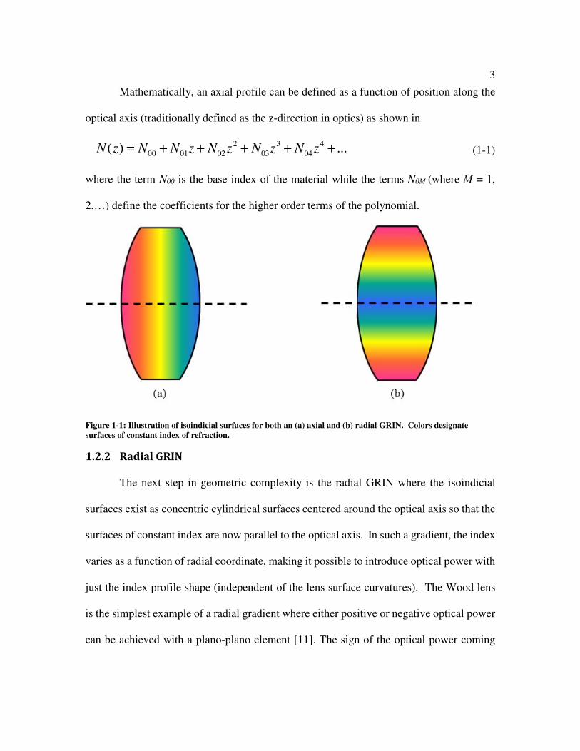
Mathematically, an axial profile can be defined as a function of position along the

optical axis (traditionally defined as the z-direction in optics) as shown in

2 3 4

00 01 02 03 04( ) ...N z N N z N z N z N z= + + + + + (1-1)

where the term N00 is the base index of the material while the terms N0M (where M = 1,

2,…) define the coefficients for the higher order terms of the polynomial.

Figure 1-1: Illustration of isoindicial surfaces for both an (a) axial and (b) radial GRIN. Colors designate

surfaces of constant index of refraction.

1.2.2 Radial GRIN

The next step in geometric complexity is the radial GRIN where the isoindicial

surfaces exist as concentric cylindrical surfaces centered around the optical axis so that the

surfaces of constant index are now parallel to the optical axis. In such a gradient, the index

varies as a function of radial coordinate, making it possible to introduce optical power with

just the index profile shape (independent of the lens surface curvatures). The Wood lens

is the simplest example of a radial gradient where either positive or negative optical power

can be achieved with a plano-plano element [11]. The sign of the optical power coming

4

from the GRIN profile depends on the orientation of the gradient. A positive gradient

describes when the index is higher along the optical axis and then decreases towards the

periphery while the opposite is true of a negative profile. This is analogous to a positive-

power homogeneous lens having greater thickness and therefore greater optical path at the

center of the lens than at its edge. A radial gradient is defined mathematically by

2 4 6 800 10 20 30 40( ) ...N r N N r N r N r N r= + + + + + (1-2)

where N is the index of refraction at some point r, the radial distance measured outwards

from the optical axis (so that r = 0 corresponds to being along the optical axis) while NM0

are the various index coefficients forming the index profile polynomial. It should be noted

that unlike the axial GRIN, the variation of the profile with the aperture location causes the

GRIN element to contribute to the chromatic behavior of the lens as well [12]. The majority

of the work carried out in this thesis is centered upon the design, fabrication, and metrology

of radial GRIN elements and as such this geometry is discussed in much greater detail in

subsequent chapters.

1.2.3 Spherical GRIN

For spherical gradients, the isoindicial surfaces are concentric spheres centered

upon a point P, which is located somewhere along the optical axis as shown in Figure 1-2.

Point P is defined as being located a distance rG from the vertex of the first surface of the

lens. The value of rG is free to take on any value, including ones so that the curvature of

the GRIN profile matches the curvature of one of the lens surfaces, which can make

manufacturing the elements easier if they are coined. The spherical GRIN is defined

mathematically using a combination of both Equation 1-3 and Equation 1-4.

5 2 3 4

0 1 2 3 4( ) ...N N N N N Nρ ρ ρ ρ ρ= + + + + + (1-3)

222 )( Grzyx −++=ρ (1-4)

Because the index varies both axially and radially, a spherical GRIN can be thought

of as a combination of both an axial and a radial GRIN profile. Both the Maxwell fisheye

and Luneberg lenses are specific instances of the spherical GRIN, with both being ball

lenses that have symmetric index profiles (so that point P is located in the center of the

lens). Each is capable of perfect geometric imaging for certain conjugates; however, optical

applications are limited as the object and/or image are located on the surface of or within

the element [13]. Extensive work has been carried out by Visconti et al. on the design,

fabrication, and testing of spherical GRIN elements where point P is located outside of the

lens for use within an eyepiece design [14].

Figure 1-2: Illustration of isoindicial surfaces for a spherical GRIN.

GRIN Materials

It is possible to form a GRIN element from a variety of materials using different

processes. Depending upon the waveband of interest, a number of options are available

6

from the ultraviolet, through the visible, and into the infrared. This section provides a

summary of a number of these materials.

1.3.1 Glass

Much research has been devoted to the pursuit of glass GRIN elements that transmit in

the visible [15-17]. Ion-exchange is a commonly used technique to make GRIN glass where

a piece of homogeneous glass is submerged into a liquid salt bath. The diffusion process

occurs where the free ions within the bath exchange with those of the glass. Thus the

chemical composition of the glass piece is altered from the outside in as the ions penetrate

further into the center of the material. If the glass is a cylindrical shape, this process can

yield a radial GRIN element. This diffusion process is traditionally a long one for elements

of large diameters (greater than 20 mm), requiring times on the order of multiple weeks or

months to yield a desired profile. The time required to yield a quadratic profile scales with

the square of the diameter of the lens blank, limiting the practicality of this method to

smaller-diameter elements; however, the time can be reduced with proper modifications to

process controls such as temperature and salt bath composition as demonstrated by

Visconti et al. [18].

1.3.2 ZnS/ZnSe GRINs

Chemical vapor deposition (CVD) is a process whereby chemical reactions are

controlled within a chamber to cause thin layers of a material to be deposited, layer by

layer, upon a substrate. Homogeneous zinc sulfide (ZnS) and zinc selenide (ZnSe) are both

crystalline materials that can be grown through CVD. Both of these materials have a very

wide band of transmission from 0.43 to 14 μm for ZnS and from 0.55 to 17 μm ZnSe

7

respectively [19]. This very large waveband of transmission makes both of these materials

very intriguing from the perspective of optical design. It has been demonstrated that a

GRIN from the pairing of ZnS and ZnSe can be grown using CVD [20]. Because the gases

that are used in the CVD process are highly toxic, pursuit of the fabrication process for the

ZnS/ZnSe GRIN has never occurred at the University of Rochester. This material pairing

does exhibit some unique chromatic properties, namely a negative Abbe number in the

mid-wave infrared (MWIR) which makes it of special interest from a color-correction

standpoint [21]. The ramifications of this fact are explored in much greater detail in

Chapter 2, which describes a series of designs using this material pairing over the band

between 3 and 5 μm. Other MWIR-transmitting GRIN materials include the ceramics

aluminum oxynitride (ALON®) and spinel along with a number of chalcogenide glasses

such as the Schott ‘IRG’ materials [22, 23].

1.3.3 Polymers

Polymers offer an opportunity for optical designs of reduced cost and weight when

compared with other homogeneous and GRIN materials [9, 22, 24-26]. Optical polymers

are typically formed from liquid monomers in a process caused polymerization. In this

process, a catalyst is introduced to cause a chemical reaction among the individual

monomer molecules which then form long molecular chains and become a solid polymer.

By allowing two miscible monomers to come into contact, diffusion between the two

monomers can take place. As polymerization occurs, a copolymer of the two materials is

formed, resulting in the formation of a GRIN profile. The catalyst used to fuel the reaction

is typically either heat introduced through a controlled water or air system or light, often

8

ultraviolet, in a process known as photopolymerization [27]. Depending on the shape,

orientation, and motion of the vessel used to hold the monomers being copolymerized, it

is possible to form a copolymer GRIN element of the axial, radial, or spherical geometry.

The processes used to generate each of these geometries are discussed in greater detail in

this thesis with a special emphasis placed on the radial geometry, the focus of the design

and metrology studies carried out in this work.

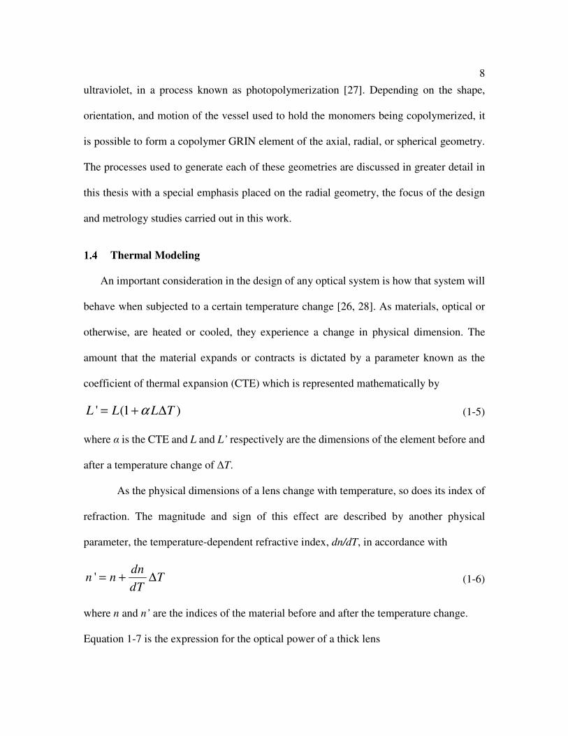
Thermal Modeling

An important consideration in the design of any optical system is how that system will

behave when subjected to a certain temperature change [26, 28]. As materials, optical or

otherwise, are heated or cooled, they experience a change in physical dimension. The

amount that the material expands or contracts is dictated by a parameter known as the

coefficient of thermal expansion (CTE) which is represented mathematically by

' (1 )L L L Tα= + ∆ (1-5)

where α is the CTE and L and L’ respectively are the dimensions of the element before and

after a temperature change of ΔT.

As the physical dimensions of a lens change with temperature, so does its index of

refraction. The magnitude and sign of this effect are described by another physical

parameter, the temperature-dependent refractive index, dn/dT, in accordance with

'dn

n n TdT

= + ∆ (1-6)

where n and n’ are the indices of the material before and after the temperature change.

Equation 1-7 is the expression for the optical power of a thick lens

9 2

1 21 2

( 1)( 1)( )lens

n c c tn c c

nϕ

−= − − + (1-7)

where c1 and c2 are the curvatures of the lens while t is its thickness. The change in the

curvature of a lens surface is given by

'1

cc

Tα=

+ ∆ (1-8)

where c and c’ are the curvatures of the lens before and after the temperature change. From

Equation 1-7 in conjunction with Equation 1-5, 1-6, and 1-8, one can see how a lens

changing temperature affects its optical power. The vast majority of materials have a

positive-signed CTE, meaning that for a temperature increase (positive ΔT) the thickness

of the element increases, increasing the value of φlens while the values for the curvature

decrease, decreasing the value of φlens. While some materials do have negative dn/dT

values, most have positive values. The power of a lens is directly related to its index of

refraction and as such, the change to φlens from an index change due to temperature can be

of either sign, being dependent on the signs of both dn/dT and ΔT.

Up to this point in this manuscript, only the effect of temperature upon

homogeneous elements has been discussed. Thermal considerations are of equal, if not

greater concern, to GRIN systems as the variation of the material composition throughout

the element means that both CTE and dn/dT vary as a function of position. In Chapter 5

the possibility of designing a radial GRIN lens such that the contributions to the optical

power coming from changes to lens geometry and index profile counteract one another for

10

a certain temperature change, maintaining the nominal focal length of the element and

therefore athermalizing the lens is discussed [26, 29].

Thermal Metrology

As mentioned in the previous section, both CTE and dn/dT are key parameters for

describing the effects of temperature on an optical element. Before any such analysis can

be carried out, one must have a means to measure these values. It should be noted that often

both CTE and dn/dT are quoted as a single value; however, this is misleading as both of

these parameters vary with the temperature of reference. Figure 1-3 shows an example of

this, displaying the CTE for a number of optical materials as a function of temperature [30].

From the data it is apparent that the CTE on a single material can vary dramatically

depending on the temperature range it is measured over.

Figure 1-3: CTE measured as a function of temperature for a number of optical materials.

Figure adapted from [30]

11

CTE is traditionally measured mechanically through the use of a dilatometer [31].

To do this, a sample is placed in physical contact with the measuring instrument. As the

sample is heated and expands, it pushes against a probe which is able to record or determine

displacement as a function of applied temperature. One example is the capacitance

dilatometer where the sample is placed between two plates that together form a capacitor.

As the sample changes size with temperature, the distance between the plates does as well.

This change in the measured capacitance can be converted to a measurement of the

thickness change of the sample with temperature.

Traditionally, dn/dT is determined using a refractometer that is capable of

measuring absolute index of refraction. By measuring the absolute index of a sample at a

series of temperatures, dn/dT is calculated by taking the derivative of the measured data

with respect to temperature.

It is possible to measure CTE and dn/dT optically using interferometry [32-36]. A

means to measure both of these parameters optically and simultaneously is desirable for

three reasons: (1) increased accuracy from using a known wavelength of light as the

measuring scale, (2) avoidance of needing to contact both surfaces of a sample with the

instrument, and (3) reduced measurement time and complexity by carrying out both

measurements simultaneously. For this purpose a thermal interferometer is built, capable

of measuring both CTE and dn/dT simultaneously and with each arm of the interferometer

subject to different environmental conditions [37]. At the time of writing this thesis, this is

the first such interferometer of its kind. A number of other interferometric systems exist

but many measure only CTE or dn/dT alone. Of those that do measure both parameters

12

simultaneously, the vast majority do so under vacuum and using a Fabry-Perot or other

configuration so that both reference and test arms of the interferometer are exposed to the

same environment which simplifies the measurement process but increases the cost.

Chapter 6 of this thesis describes the design, construction, and capabilities of this system

in much greater detail along with a discussion of the aforementioned other systems.

Objective of Thesis

The overall purpose of this thesis is to explore a number of topics related to the

design, fabrication, and metrology of radial GRIN elements. The first objective of the work

is to illustrate a GRIN element’s ability to improve the imaging performance of a lens

system with special emphasis placed on the correction of chromatic aberration in different

wavebands using different materials. This is presented in a series of design studies on (1)

the ZnS/ZnSe GRIN over the mid-wave infrared spectrum between 3 and 5 μm and (2) a

copolymer formed between polymethyl methacrylate (PMMA) and polystyrene that

transmits over the visible. These design studies are discussed in Chapter 2 and Chapter 3

respectively.

One goal of this thesis is to present the great potential of materials with negative

GRIN Abbe numbers to improve imaging performance. The majority of this thesis

concentrates on copolymer GRIN materials, namely the PMMA/polystyrene GRIN which

has a positive Abbe number over the visible spectrum. Negative GRIN Abbe numbers in

copolymers are possible over this waveband using theoretical material pairings. A non-

copolymer material known to have a negative GRIN Abbe number: the ZnS/ZnSe GRIN

13

is chosen to illustrate the benefits of this type of material for achromatization in a series of

design studies carried out over the mid-wave infrared.

Transverse ray aberration plots are used throughout the thesis as a metric for

determining a lens’ imaging performance and diagnosing whether certain aberrations,

namely axial and/or lateral color, are present in the lens system. As depicted in Figure 1-4,

such plots show transverse ray error (the distance between where a real and an ideal ray

will intersect the image plane, labeled εy in the y direction) as a function of normalized

pupil coordinate ρy, the x-axis of the plot. Separate plots are necessary for each field point

and in the sagittal (x-z) and tangential (y-z) planes of the lens.

Figure 1-4: (a) Illustration of the calculation of transverse ray aberration plots. (b) Example of a transverse ray

aberration plot showing transverse error as a function of normalized pupil coordinate, both in the y-direction.

This particular plot indicates the presence of axial color.

A GRIN’s ability to correct color is founded on the fact that a single radial GRIN

element contains a second source of optical power and chromatic dispersion (in addition to

that which comes from the base index of refraction). As such, a GRIN element contains

additional degrees of freedom as compared to a homogenous singlet and can be shown to

correct axial color in a manner approaching that achieved by a traditional achromatic

doublet. The observations taken from studies of simple homogeneous and GRIN singlets

14

and doublets are extended to more complex designs with a special emphasis placed on that

of zoom lens systems. Monochromatic zoom lens designs have been explored in the past

[38, 39]. When originally published, the zoom lens studies in this thesis were the first of

their kind into the use of both materials in their respective full wavebands. The application

of GRIN elements to polychromatic zoom lens designs has since been explored in greater

detail [40, 41]. One purpose of this thesis is to demonstrate the potential of these radial

GRIN elements to improve the imaging performance of such zoom lens systems. A

software tool to assist in this analysis was developed in CODEV® optical design software

to quantify the contributions to both axial and lateral color coming from the GRIN

elements.

The second objective of this thesis is to present a series of experiments to generate

these radial GRIN elements in the laboratory. Because the gases necessary to grow layers

of ZnS and ZnSe are toxic, no attempts are made to fabricate that material at the University

of Rochester. An apparatus for making PMMA/polystyrene GRIN elements is used that

applies a centrifugal force to a continuously-rotating mixture of the two monomers. The

fast rotation causes the monomers to separate according to their relative densities but still

diffuse into one another during the copolymerization process to generate a radial GRIN

profile. Difficulties experienced during these experiments keeping the center of the final

samples clear due to the issue of the volume reduction of the material within the monomer

chamber as the liquid monomer because a solid copolymer are discussed in Chapter 4.

The third objective of this thesis is to demonstrate the potential to athermalize a

radial GRIN singlet by taking advantage of the additional degrees of freedom that also

15

make it possible to achcromatize such a singlet under different circumstances. A series of

algorithms are presented that make it possible to identify such solutions so that they may

be further modeled in CODEV® or other ray-trace software. Additional algorithms are

presented to act as a basic finite-element model that treats a GRIN element as a stack of

differential rectangles. As a temperature change is applied, the effect on each element is

calculated and combined to determine more accurately the resulting change in lens

geometry and index profile than is possible analytically. This is discussed in greater detail

in Chapter 5.

The fourth and final objective of the thesis is to demonstrate the ability of the

thermal interferometer to simultaneously measure both the CTE and dn/dT of a given

homogeneous or GRIN sample. Explanations are presented concerning the theory behind

the measurement along with a discussion of the methodology used to prepare the sample

and then acquire and analyze the data. The interferometer design is based on the goals of

reducing both the cost of the instrument itself as well as time required to make a

measurement by being able to determine both thermal parameters from a single run.

Measurements have been carried out between approximately -40 and +50 °C. A discussion

of the design, operation, and results of the system are presented in Chapter 6.

16

Chapter 2. GRIN ZnS/ZnSe Design Studies

Background

Gradient-index (GRIN) materials are ones for which the index of refraction varies

as a function of position within the optical element [42]. The added degrees of freedom in

the design process afforded by GRIN elements are useful for both monochromatic and

polychromatic aberration correction. As discussed in Chapter 1, the particular effect of a

GRIN in an optical system is largely dependent upon the shape of the index profile with

the three most common GRIN geometries being: axial, where the isoindicial surfaces

(contours of constant index) are planes perpendicular to the optical axis, (2) radial, where

the isoindicial surfaces are concentric cylindrical surfaces centered around the optical axis

so that the contours of constant index are now parallel to the optical axis, and (3) spherical,

where the isoindicial surfaces are concentric spheres centered upon some point along the

optical axis. Axial GRINs perform a role largely analogous to an asphere and are capable

of correcting multiple orders of spherical aberration [10]. Radial and spherical GRIN lenses

have a second source of optical power coming directly from the index profile. The simplest

example of this effect is the Wood lens: a plano-plano element that is capable of forming

an image with a radial GRIN profile [11]. Radial GRINs are defined mathematically by

2 4 600 10 20 30( ) ...N r N N r N r N r= + + + + (2.1)

where r is the distance measured outward from the optical axis. By allowing the quadratic

radial GRIN term to vary, a second source of refracting power is added to the lens system,

theoretically creating a doublet in a single element. Given a lens with a radial GRIN profile

17

of the form shown in Equation 2.1 and a positive value of N10, the total optical power,

including surface curvatures and index profile, can be calculated by

200 1 2 10 00 00 1 2

00

sinh( )(N 1)( ) cosh( ) [2 ( 1) ]GRIN

tc c t N N N c c

N

αϕ α

α= − − − − − (2.2)

10

00

2N

Nα = (2.3)

where N00 and N10 are the base and quadratic coefficients of the radial GRIN index profile,

c1 and c2 are the curvatures of the first and second surfaces of the lens, and t is the thickness

of the element [43]. If N10 is instead negative, the cosh and sinh functions in Equation 2.2

are replaced with the cos and sin functions respectively. Approximating Equation 2.2, an

expression for the power of just the GRIN profile (ignoring the contributions of the surface

curvatures so that c1 = c2 = 0) is given by

102GRIN N tϕ = − (2.4)

assuming the thickness (t) of the element to be relatively thin [44]. This work concentrates

on the application of the radial geometry to color correction; however, achromatization

using GRIN elements is also possible using the spherical geometry as shown in recent work

[45].

Color Correction using GRIN Materials

Dispersion is a property inherent to all refractive optical materials whereby the

index of refraction of that material varies as a function of wavelength. This fact is the cause

of chromatic aberrations in polychromatic optical systems. All-reflective designs do not

suffer from chromatic aberrations; however, many such systems are designed with an

18

obscuration leading to a significant degradation of imaging performance at the mid-spatial

frequencies [46]. Axial color is the aberration causing best focus to vary as a function of

wavelength. The standard solution to correct axial color is to replace a homogeneous

singlet with a doublet composed of two different materials with different Abbe numbers, a

value that dictates how dispersive an optical material is. In doing so, the differing

dispersions of the two materials are able to balance one another in order to bring two

wavelengths to the same focus. The textbook example of such an achromat in the visible

spectrum is to combine a positive-power element composed of a crown glass (low

dispersion) such as BK7 with a negative-power element composed of a flint glass (high

dispersion) such as SF2. For a wavelength band of 3 to 5 µm, an achromatic doublet can

be formed with silicon and germanium [47]. In order to determine the powers of each

element necessary to correct axial color based on first order optical properties, one must

solve a pair of equations:

1 2 systemϕ ϕ ϕ+ = and (2.5)

1 2

1 2

0ϕ ϕ

ν ν+ = (2.6)

where φ is optical power, ν is the Abbe number, and the subscripts 1 and 2 denote the first

and second lenses composing the doublet. The Abbe number of a homogenous material is

defined for a particular waveband using

1mid

short long

n

n nν

−=

− (2.7)

19

where nshort, nmid, and nlong are the indices of the material at the extremes and center of the

spectral range. In order to minimize the optical power required of each individual element

when correcting color, the ratio of the two Abbe numbers should be as large as possible.

In order to correct secondary axial color, three wavelengths are brought to the same focus.

This requires definition of an additional property known as the partial dispersion (P) of a

material. The partial dispersion is defined according to

mid long

short long

n nP

n n

−=

−. (2.8)

A method for determining the paraxial contributions to both axial and lateral color

for radial GRIN elements is present in the literature [48]. As the index profile of a radial

GRIN element provides a second source of optical power to a lens, it also provides a second

Abbe number, making color correction possible with a single optical element (discussed in

further detail in subsection “ZnS/ZnSe GRIN Design”) [49]. There are a number of

material combinations available that are capable of forming a GRIN profile in the infrared

between 1 and 5 µm, although not all of them have been manufactured at this time. These

include those from the ceramic aluminum oxynitride (ALON®)[50] as well as

combinations of both zinc sulfide (ZnS) and zinc selenide (ZnSe)[20] and the Schott

chalcogenide ‘IG’ glasses.

While the methodology of picking materials for color correction as well as

Equations 2.5 and 2.6 hold true for GRIN materials as well as homogeneous ones, there

are different equations to define the Abbe number and partial dispersion of a GRIN

20

material. Equation 2.9 and Equation 2.10 define the GRIN Abbe number and partial

dispersion

midGRIN

short long

n

n nυ

∆=

∆ − ∆ (2.9)

mid long

GRIN

short long

n nP

n n

∆ −∆=

∆ − ∆ (2.10)

where each of the three Δn terms correspond to the difference in index of refraction

between the two homogeneous materials composing the gradient at a given wavelength.

As in the case when dealing with homogeneous elements, when correcting primary color

the difference in Abbe number between the two materials should be as large as possible in

order to minimize individual element power. The Abbe numbers for a number of infrared

GRIN materials are shown for the waveband from 1 to 5 µm, 1 to 3 µm, and 3 to 5 µm in

Table 2-1.

Table 2-1: Abbe numbers of GRIN materials over three infrared wavebands.

Material ν (1 to 5µm) ν (1 to 3µm) ν (3 to 5µm)

ALON® 8.1 50.9 9.4

ZnS/ZnSe 14.0 11.6 -63.1

IG2/IG3 2.8 3.0 71.8

IG2/IG6 6.2 6.7 96.0

IG2/IG4 6.9 7.3 188.1

IG4/IG6 5.8 6.4 73.5

IG4/IG3 2.0 2.2 52.5

IG6/IG3 0.2 0.2 8.0

21

It is possible for materials which transmit over a wide waveband to act as crown

glasses in one portion of the spectrum and as flint glasses in another. A common example

of this is germanium, which is much more dispersive between 1 and 5 µm than it is between

8 and 12 µm. From Table 2-1, it is apparent that such behavior can be exhibited by GRIN

materials in the infrared as between 1 and 3 µm, ALON® is much less dispersive than it is

between 3 and 5 µm, while the opposite is true of the majority of the GRIN chalcogenides.

Of particular interest is ZnS/ZnSe, which has a negative Abbe number between 3 and 5µm.

This GRIN material has been used in the design of infrared systems [51]. This work

explores the potential of this material to color correct over this particular waveband.

Design Study

2.3.1 Spectral Considerations

The mid-wave infrared (MWIR) is the spectral band between 3 and 5 µm. As shown

in Figure 2-1 this region sits between the short-wave infrared (SWIR) and long-wave

infrared (LWIR) in the electromagnetic spectrum and is bound on either side by spectral

bands of very high absorption due to atmospheric gas/water vapor which make imaging

over those wavelength ranges very difficult [52]. The MWIR waveband is a source of

interest for both military and non-military application. Achromatization studies have

already been carried out over this waveband using homogeneous materials [47].

22

Figure 2-1: Atmospheric transmittance of the electromagnetic spectrum. Figure adapted from [52].

2.3.2 Material Selection

Figure 2-2 shows a plot of Abbe number versus refractive index for a number of

infrared materials. As mentioned before, a high-performance MWIR achromat is formed

from silicon and germanium. The reason for this is clearly illustrated in Figure 2-2 where

one can see the large discrepancy in Abbe number between the two materials. Both silicon

and germanium have much larger indices of refraction than their visible glass counterparts,

which is somewhat common of infrared materials as seen in Figure 2-2, and often very

beneficial in the design process.

Tra

nsm

itta

nce

[%

]

Wavelength [µm]

23

Figure 2-2: “Glass map” for a number of MWIR materials. Homogeneous materials are shown as solid markers

while GRIN materials are line markers.

From Figure 2-2, the largest difference between a homogeneous and GRIN Abbe

number is seen to be between ZnSe and the ZnS/ZnSe GRIN, suggesting this material

would be very useful for color correction. Homogeneous ZnS and ZnSe elements have

already been used as part of achromatized infrared systems [53]. Additionally, the fact that

the gradient’s Abbe number is negative allows the optical power of both the base material

(the curvatures) and the gradient to be positive while satisfying Equations 2.5 and 2.6.

GRIN materials, along with diffractive optics, are one of the only means available to

achieve a negative Abbe number. As mentioned previously, a lens with a positive-power

gradient has a lower index of refraction at the edge of the element than at the center. This

is useful from the perspective of aberration correction as such a GRIN profile assist in the

24

correction of the undercorrected spherical aberration inherent to the base homogeneous

element.

Singlet Studies

2.4.1 Specifications

Beginning with single elements, this design study is performed using a full field of

view (FFOV) of 1° over the entire MWIR spectrum between 3 and 5 µm. System

specifications also include an entrance pupil diameter (EPD) of 25 mm and an effective

focal length (EFL) of 50 mm (yielding an f/2 lens). It is in faster systems that the real

benefit of GRIN becomes most apparent. At higher f/#’s, diffraction-limited performance

is comparatively easier to achieve and the use of GRIN does not yield as significant of

performance improvement over the homogeneous. All designs are carried out using

CODEV® optical design software.

2.4.2 Homogeneous Designs

To compare with the GRIN ZnS/ZnSe singlet, homogeneous lenses of both

materials are designed. With its higher index of refraction and lower dispersion, the ZnSe

singlets always yield superior performance to that of the ZnS singlets and so the ZnS

designs are not shown. Homogeneous singlets of both silicon and germanium are also

designed. Silicon yields better performance than germanium which yields better

performance than ZnSe; however, these designs are not included as the intent is to directly

compare the GRIN lens to the homogeneous materials that compose it. For both ZnS and

ZnSe, the limiting aberrations are third order spherical aberration and primary axial color.

To counteract the effect of spherical aberration, the fourth and sixth order aspheric terms

25

on the front surface of the element are allowed to vary, yielding a lens dominated by axial

color. A silicon and germanium air-spaced doublet is also designed in order to compare the

GRIN performance to the homogeneous doublet standard for achromats in the MWIR.

Figure 2-3 shows the on-axis MTF performance comparison between the homogeneous

ZnSe lenses and the ZnS/ZnSe GRIN lens (the design of which is discussed in the following

section).

Figure 2-3: On-axis MTF performance comparison between homogeneous designs and ZnS/ZnSe

GRIN singlet.

2.4.3 ZnS/ZnSe GRIN Design

All GRIN designs in this study are carried out using a model which forces the index

coefficients to vary within the refractive index bounds and according to the actual

dispersions of the real materials [54]. The imaging performance of the lens is optimized,

allowing both the element’s surface curvatures and defocus, along with the N00, N10, N20

and N30 coefficients of the radial GRIN index polynomial, to vary. The axial performance

of the final design is shown in Figure 2-3 along with the three aforementioned

0

0.2

0.4

0.6

0.8

1

0 30 60 90 120 150

Mo

du

lati

on

Spatial Frequency [cycles/mm]

Diffraction Limit

Si-Ge Doublet

ZnS/ZnSe GRIN

Aspheric ZnSe

ZnSe

26

homogeneous designs. It is apparent that the imaging performance has improved

dramatically from the aspheric singlet, yielding nearly diffraction-limited performance

with a single element. Most notably, Figure 2-4 shows that the addition of the GRIN profile

has acted to largely correct the axial color which is the limiting aberration of the aspheric

singlet. Now the lens is limited by a combination of spherochromatism and secondary

spectrum. While it is clear that the air-spaced doublet yields the best performance of the

designs, it is notable that the GRIN design is able to achieve nearly the same MTF

specifications with only a single element. Cutting down on element count is always

desirable in optical design in order to reduce both system weight and packaging size as

well as material cost (this is especially true in the infrared where materials such as

germanium are more expensive that standard BK7). Adding an asphere to the GRIN singlet

acts to correct some of the higher order spherical aberration but does not offer significant

improvement to the imaging performance.

27

Figure 2-4: Comparison of performance between the aspheric ZnSe singlet (top) and the GRIN singlet (bottom).

The transverse ray plots are shown in units of mm. Note change in scale of transverse ray plots.

2.4.4 Weight Analysis

Given Equation 2.4, in order for the GRIN profile to maintain a constant effective

focal length as the lens is made thinner, the magnitude of the coefficient N10 and therefore

the total change in index of refraction between the center and periphery of the lens (Δn)

must increase. To a certain degree, as long as the increased required Δn is consistent with

the real material bounds, the lens can be made thinner and therefore lighter without

sacrificing imaging performance. This is demonstrated by varying the center thickness of

the ZnS/ZnSe singlet between 2 and 5 mm and continually reoptimizing the imaging

performance, yielding designs of 12.9 g, 7.2 g, and 3.9 g. Figure 2-5 shows the MTF for

each of these singlets compared to that of the silicon and germanium doublet. Note that the

28

7.2 g design offers only a slight degradation in MTF performance when compared to the

12.9 g design; however, MTF performance drops off significantly for the 3.9 g design.

Though not included in the Figure 2-5, further decreasing the weight of the single element

GRIN design further degrades the MTF performance while increasing the weight beyond

12.9 g does not offer a significant improvement in imaging performance. The 7.2 g GRIN

design offers a 31% weight reduction when compared with the homogeneous doublet.

Figure 2-5: On-axis MTF performance comparison between ZnS/ZnSe GRIN singlet of different weights.

ZnS/ZnSe (1) is 12.9g, ZnS/ZnSe (2) is 7.2g and ZnS/ZnSe (3) is 3.9g.

2.4.5 Alternative GRIN Material Designs

To be thorough in the analysis, other GRIN materials are explored for their ability

to color correct over the MWIR. Table 2-2 shows the Abbe numbers for both the base

material and GRIN profile for each of these material combinations, as well as the required

focal lengths of each necessary to satisfy Equations 2.5 and 2.6 for a system focal length

of 50 mm. The final two columns of the table display the calculated Δn necessary for an

element thickness of 5 mm, as well as the maximum Δn allowed by that GRIN material at

0

0.2

0.4

0.6

0.8

1

0 30 60 90 120 150

Mod

ula

tion

Spatial Frequency [cycles/mm]

Diffraction Limit

Si-Ge Doublet

ZnS/ZnSe (1)

ZnS/ZnSe (2)

ZnS/ZnSe (3)

29

a wavelength of 4 µm. From the table, it is apparent that the very short individual focal

lengths required of some of these GRIN materials for MWIR color correction make using

those materials infeasible for this design study. In addition to this, the necessary values of

Δn for the majority of the materials are inconsistent with the real index bounds of the two

materials comprising that GRIN pairing using the assumed thickness of 5 mm. Thus in this

case, high imaging performance cannot be expected from those GRIN materials even when

allowing the element thickness to be much greater than 5 mm as correcting spherical

aberration and primary color require opposite-signed GRIN profiles. For this second part

of the design study, the three best physically realizable GRIN material candidates (based

on requiring the longest element focal lengths) are explored. In order from best to worst

these are: the ZnS/ZnSe combination discussed in the previous section, the IG3/IG4

chalcogenide glass combination, and finally the IG2/IG3 combination.

Table 2-2: Comparison of the required element focal length and Δn values for various GRIN materials in the

MWIR for a system focal length of 50 mm (f/2) as calculated from base and GRIN Abbe numbers of each

material. The Δn values marked with a star indicate that they are not physically realizable for the system

specifications while unmarked values are realizable.

Material νbase νGRIN fbase [mm] fGRIN [mm] Δn |Δnmax| ALON® 8 9 -5 5 -3.16* 0.03 IG2/IG3 195 72 32 -86 0.18 0.29 IG2/IG4 195 188 2 -2 7.97* 0.11 IG2/IG6 195 96 25 -52 0.30* 0.28 IG3/IG4 195 53 37 -136 0.12 0.18 IG3/IG6 168 8 48 -1007 0.02* 0.01 IG4/IG6 195 74 31 -83 0.19* 0.17

ZnS/ZnSe 178 -63 68 191 -0.08 0.18

The two chalcogenide GRIN designs use the same linear composition model

described in the previous section for the ZnS/ZnSe GRIN. Again, the GRIN profile is

allowed to vary to give the best performance possible. The on-axis MTF plots for each

30

design are shown in Figure 2-6. The best results of the three are attained with the ZnS/ZnSe

GRIN, followed by the IG3/IG4 pair, and the worst with the IG2/IG3 combination. These

findings are consistent with the calculated focal length data presented in Table 2-2. The

chalcogenide GRINs are limited by axial color and higher order spherical aberration as the

GRIN profile is of the opposite sign as it was with the ZnS/ZnSe GRIN. Note that only the

ZnS/ZnSe GRIN corrects axial color over the MWIR as is evident from the transverse ray

aberration plots shown in Figure 2-7. A comparison in GRIN profile between the three

designs is presented in Figure 2-8. The ZnS/ZnSe GRIN is positive in sign so the profile is

consistently working towards correcting both spherical aberration and axial color

simultaneously, while the negative profiles of the chalcogenides enhance undercorrected

spherical aberration.

Figure 2-6: Comparison of MTF performance between three MWIR GRIN singlets.

0

0.2

0.4

0.6

0.8

1

0 30 60 90 120 150

Mod

ula

tion

Spatial Frequency [cycles/mm]

Diffraction Limit

Si-Ge Doublet

ZnS/ZnSe GRIN

IG3/IG4

IG2/IG3

31

Figure 2-7: Comparison of performance between three MWIR GRIN singlets From top to bottom: ZnS/ZnSe,

IG3/IG4, and IG2/IG3.

Figure 2-8: Radial GRIN profiles for three MWIR GRIN singlets From top to bottom: IG3/IG4 (Δn ~ 0.13),

IG2/IG3(Δn ~ 0.13), and ZnS/ZnSe (Δn ~ 0.10)

32

Objective lens studies

2.5.1 Background

The previous section demonstrated the potential of the ZnS/ZnSe GRIN material

for color correction. It is interesting to investigate the effect of this material on a more

complicated optical system. Traditionally, in the visible spectrum, the Petzval lens

describes a high performance objective configuration of relatively fast speed and narrow

field of view, limited by astigmatism [55]. In their most simple form, Petzval designs are

composed of two positive-power element groups spaced apart from one another by a large

distance. If the lens is composed of only two elements, both of them must be positive power

and the system suffers heavily from axial color. The abnormal dispersive properties of the

ZnS/ZnSe GRIN provide a unique opportunity for designing Petzval-like objectives over

the MWIR.

2.5.2 System Specifications

All designs are specified to be f/2 with an effective focal length (EFL) of 100 mm

(yielding an entrance pupil diameter of 50 mm) [56]. The lens system is designed to be

compatible with the FLIR SC8300 indium antimonide (InSb) infrared detector, which is

sensitive over the waveband of interest (λ = 3-5 μm) [57]. The diagonal dimension of this

detector is 21.8 mm. For the assumed EFL of 100 mm, an image plane of this size

corresponds to a half field of view (HFOV) of 6.22° (for an object located at infinity.) All

designs are carried out in CODE V® using five field points (0, 40, 70, 85, and 100% of the

HFOV) and five wavelengths (λ = 3.0, 3.5, 4.0, 4.5, and 5.0 μm). Field weighting is allowed

33

to vary between designs in order to achieve the best imaging performance while the five

wavelengths are equally weighted during optimization. Distortion is held to be 2% or less.

In order to minimize the required diameter of individual lens elements, the aperture

stop is constrained to be located at the first surface of the first lens element. This is

consistent with the standard Petzval configuration [55]. The majority of infrared imaging

systems contain a thin window for the purpose of protecting the detector array [58]. To

simulate this, all designs are modeled with a 0.5 mm thick window of germanium placed

2 mm in front of the image plane. The clearance between the final lens element and the

protective window is constrained to be greater than 5 mm. Finally, the overall system

length (from the vertex of the first lens surface to the detector plane) is held to be less than

150 mm.

2.5.3 Design summary

For this study, designs of two and three elements are carried out using the

specifications quoted in the previous section. In addition to the GRIN designs,

homogeneous designs with and without aspheres are included in the study. Each design is

optimized for best imaging performance. When appropriate, the CODE V® Glass Expert is

used in order to find the best infrared material combination possible. Optimizing in this

way yields solutions composed mainly of silicon and germanium due to these materials’

very high indices. The FLIR detector used in this study has a pixel pitch of 14 μm. This

corresponds to a Nyquist frequency of approximately 36 line pairs per millimeter (lp/mm).

For each design, the contrast values of the worst-performing field point are tabulated from

the modulation transfer function (MTF) plots the software generates. Table 2-3 summarizes

34

these results with the MTF plot evaluated at 9, 18, 27, and 36 lp/mm (25, 50, 75, and 100%

of the Nyquist frequency, respectively) for each design. Aspheric surfaces are allowed in

some of the designs shown in Table 2-3. Specifically, designs with a ‘yes’ in the ‘aspheric

surfaces’ column are allowed one aspheric surface to be placed at the best location available

for that particular design. The final row of the table displays the diffraction-limited MTF

contrast values for each spatial frequency of interest.

Table 2-3: Homogeneous and GRIN Petzval-like objective designs

Elements Aspheres GRINs 9 lp/mm 18 lp/mm 27 lp/mm 36 lp/mm

2 No 0 0.508 0.134 0.077 0.053

2 Yes 0 0.695 0.400 0.248 0.165

2 No 1 0.864 0.697 0.546 0.405

2 No 2 0.878 0.733 0.600 0.487

3 No 0 0.894 0.783 0.677 0.576

3 Yes 0 0.895 0.782 0.673 0.571

Diffraction Limit 0.908 0.817 0.727 0.639

2.5.4 Homogeneous and GRIN Comparison

From Table 2-3 it is apparent that the two-element homogeneous system has the

worst imaging performance of any of the designs shown, as one would expect. In this case,

the best design is found to be formed from two silicon elements. Approaching the Nyquist

frequency, the imaging performance becomes very poor and the system is limited by a

combination of axial color and spherical aberration on axis. To reduce spherical aberration,

an aspheric surface is added with best performance achieved by placing it on the front

surface of the first silicon element. The design is now limited purely by axial color as seen

in Figure 2-9 which shows the lens drawings and transverse ray plots for this and other

designs of interest. (Note that for figure clarity, these evaluations are shown for three field

35

points.) By removing the aspheric surface and introducing a third element into the system,

the first silicon element is split into a silicon-germanium air-spaced doublet as shown in

Figure 2-9. The negative germanium element is useful for helping to correct axial color

and improves the performance to nearly-diffraction-limited levels. Adding an aspheric

surface to the three-element system provides a significant boost in the axial performance

of the lens but only moderate improvement in the off-axis performance.

For comparison, the design space is explored using the ZnS/ZnSe GRIN material.

For a two-element configuration, the ZnS/ZnSe GRIN yields better results as the front

element of the system than as the back element. From Table 2-3, it is clear that a two-

element GRIN/homogeneous (silicon) configuration yields significantly improved results

over the aspheric two-element homogeneous configuration. From Figure 2-9, it is apparent

that replacing the homogeneous element with a GRIN one drastically improves axial color

and therefore imaging performance. It should be noted that the silicon-germanium-silicon

design is still superior to ZnS/ZnSe-silicon design from a performance standpoint which is

consistent with the finding of the ZnS/ZnSe singlet study [21]. Going one step forward and

replacing the remaining silicon element with a second GRIN one provides a minor increase

in improvement that would unlikely justify the increased difficulty in fabrication over a

homogeneous lens.

36

Figure 2-9: (Left) Si-Si aspheric homogeneous design (middle) ZnS/ZnSe-Si GRIN design (right) Si-Ge-Si

homogeneous design. , scale of ±60 μm

Zoom lens designs

2.6.1 Preliminary Zoom Design

From here, the ZnS/ZnSe GRIN material is applied to the design of a zoom lens

[59]. Some work has been carried out on the application of GRIN elements to zoom lens

designs; however very little work has carried out in particular on the MWIR spectrum. A

material with a negative GRIN Abbe number is a new design feauture as applied to the

design space of zoom lenses over the MWIR. A number of homogenous infrared zoom

lenses have been designed over the last few decades [60]. For this zoom lens study, the

lens is designed to be compatible with an f/4 FLIR Photon HRC camera [61]. This is a 640

x 512 InSb detector with a pixel pitch of 15 µm that is sensitive in the MWIR. This detector

needs to be cooled and as such the camera core includes a Dewar enclosure in addition to

JAC 03-Mar-13

MWIR Petzval 2E Aspheric.seq

RAY ABERRATIONS ( MILLIMETERS )

5000.0000 NM

4000.0000 NM

3000.0000 NM

-0.06

0.06

-0.06

0.06

0.00 RELATIVE

FIELD HEIGHT

( 0.000 )O

-0.06

0.06

-0.06

0.06

0.70 RELATIVE

FIELD HEIGHT

( 4.354 )O

-0.06

0.06

-0.06

0.06

TANGENTIAL 1.00 RELATIVE SAGITTAL

FIELD HEIGHT

( 6.220 )O

JAC 03-Mar-13

MWIR Petzval 1 GRIN.seq

RAY ABERRATIONS ( MILLIMETERS )

5000.0000 NM

4000.0000 NM

3000.0000 NM

-0.06

0.06

-0.06

0.06

0.00 RELATIVE

FIELD HEIGHT

( 0.000 )O

-0.06

0.06

-0.06

0.06

0.70 RELATIVE

FIELD HEIGHT

( 4.354 )O

-0.06

0.06

-0.06

0.06

TANGENTIAL 1.00 RELATIVE SAGITTAL

FIELD HEIGHT

( 6.220 )O

JAC 03-Mar-13

MWIR Petzval 3E Homogeneous.seq

RAY ABERRATIONS ( MILLIMETERS )

5000.0000 NM

4000.0000 NM

3000.0000 NM

-0.06

0.06

-0.06

0.06

0.00 RELATIVE

FIELD HEIGHT

( 0.000 )O

-0.06

0.06

-0.06

0.06

0.70 RELATIVE

FIELD HEIGHT

( 4.354 )O

-0.06

0.06

-0.06

0.06

TANGENTIAL 1.00 RELATIVE SAGITTAL

FIELD HEIGHT

( 6.220 )O

MWIR Petzval 3E Homogeneous.seq JAC 03-Mar-13

18.00 MM

MWIR Petzval 2E Aspheric.seq JAC 03-Mar-13

18.00 MM

MWIR Petzval 1 GRIN.seq JAC 03-Mar-13

18.00 MM

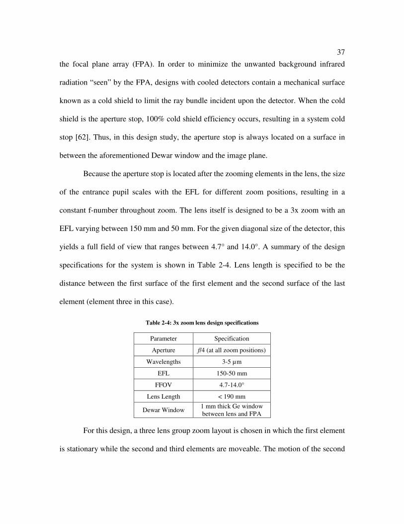
37

the focal plane array (FPA). In order to minimize the unwanted background infrared

radiation “seen” by the FPA, designs with cooled detectors contain a mechanical surface

known as a cold shield to limit the ray bundle incident upon the detector. When the cold

shield is the aperture stop, 100% cold shield efficiency occurs, resulting in a system cold

stop [62]. Thus, in this design study, the aperture stop is always located on a surface in

between the aforementioned Dewar window and the image plane.

Because the aperture stop is located after the zooming elements in the lens, the size

of the entrance pupil scales with the EFL for different zoom positions, resulting in a

constant f-number throughout zoom. The lens itself is designed to be a 3x zoom with an

EFL varying between 150 mm and 50 mm. For the given diagonal size of the detector, this

yields a full field of view that ranges between 4.7° and 14.0°. A summary of the design

specifications for the system is shown in Table 2-4. Lens length is specified to be the

distance between the first surface of the first element and the second surface of the last

element (element three in this case).

Table 2-4: 3x zoom lens design specifications

Parameter Specification

Aperture f/4 (at all zoom positions)

Wavelengths 3-5 µm

EFL 150-50 mm

FFOV 4.7-14.0°

Lens Length < 190 mm

Dewar Window 1 mm thick Ge window between lens and FPA

For this design, a three lens group zoom layout is chosen in which the first element

is stationary while the second and third elements are moveable. The motion of the second

38

lens is responsible for changing the focal length while the third lens moves maintain the

image position to be constant. By having two moving lens groups in a zoom system it is

possible to leave the image plane stationary over a number of zoom positions. Following

the method on three-element zoom lenses laid out in Warren J. Smith’s Modern Optical

Engineering, a first order solution to the design was carried out using

1 2

1( )A

R

R s sϕ

−=

+ , (2.11)

( 1)B A Rϕ ϕ= − + , (2.12)

( 1)( )3 1

AC

R R

R

ϕϕ

+ +Φ=

− , (2.13)

1

( 1)( 1)A

Rs

Rϕ

−=

+ , (2.14)

12

ss

R= and (2.15)

3 1'

( 1)R

lR R

−=

Φ + (2.16)

where φA, φB, and φC, are the individual powers of the first, second, and third lens elements

respectively, Φ is the power of the system at the “minimal shift” position (EFL = 100 mm),

R is the square root of the system magnification (3 in this case so R = 1.732), s1 and s2 are

the distances between the first and second and second and third lenses respectively, and l’

is the distance from the third lens to the image plane [63]. In this way, a thin lens solution

was generated for three zoom positions (EFL = 150 mm, 100 mm, and 50 mm) using

CODE V®’s zoom functionality as shown in Figure 2-10.

39

Figure 2-10: First order element layout for three zoom positions. From top to bottom: EFL =

150 mm, 100 mm, and 50 mm.

At this point, the design is carried out monochromatically (λ = 4 µm) using all

germanium elements (chosen for its very high refractive index). Note that the fourth

element is the Dewar window and that the aperture stop is located between the window and

the FPA in order to simulate the aforementioned cold stop. The system is held constant at

f/4 for all three zoom positions. From here, the distances between the first and second

lenses, the second and third lenses, and the third lens and the image plane, along with the

surface curvatures of the three lenses are optimized for best imaging performance holding

only EFL at each zoom position and an overall system length as constraints.

After creating the desired first-order lens layout, it is necessary to add thickness to

each element while moving the aperture stop farther away from the Dewar window. Also

at this point, the waveband is redefined to be the full 3-5 µm, prompting the need for

40

material variation within the design in order to correct chromatic aberrations. While it can

be possible to get away with designing using only germanium elements between 8 and

12 µm, the same is not true between 3 and 5 µm where the material is much more

dispersive. Using a combination of direct material variation and the CODE V® Glass

Expert, the best three-element homogeneous design using only spherical surfaces is found

to be silicon-germanium-silicon. The lens drawing is shown in Figure 2-11 along with the

MTF and transverse ray plots in Figure 2-12 and Figure 2-13 respectively. The MTF plots

are evaluated out to 33 cycles/mm, corresponding to the Nyquist frequency of the detector.

Figure 2-11: 3x zoom homogeneous lens drawing. From top to bottom: EFL = 150 mm, 100 mm,

and 50 mm.

41

Figure 2-12: 3x zoom homogeneous MTF plots. From left to right: EFL = 150 mm, 100 mm, and 50 mm.

Figure 2-13: 3x zoom homogeneous transverse ray plots, scale of ±50 μm. From left to right:

EFL = 150 mm, 100 mm, and 50 mm.

From the transverse ray plots, it is apparent that the system suffers from a number

of residual aberrations, most notably under-corrected spherical aberration on axis and

lateral color off axis. The inclusion of aspheric surfaces has become a common method of

correcting spherical aberration, especially for designs operating in the infrared since many

of the materials may be diamond turned. To that end, the lens is further optimized by

allowing each of the three elements to have one aspheric surface. It should be noted that at

this point in the design process, the second lens travels within the surface sag of the first

lens for certain zoom positions as shown in Figure 2-14. User-defined constraints are

written in CODE V® to prevent this from happing.

1.0

0.9

0.8

0.7

0.6

0.5

0.4

0.3

0.2

0.1

MODULATION

3.0 6.0 9.0 12.0 15.0 18.0 21.0 24.0 27.0 30.0 33.0

SPATIAL FREQUENCY (CYCLES/MM)

EFL = 150mm

DIFFRACTION MTF

JAC 28-May-13POSITION 1

DIFFRACTION LIMIT

AXIS

T

R0.7 FIELD ( )1.64O

T

R1.0 FIELD ( )2.35O

WAVELENGTH WEIGHT

5000.0 NM 1

4000.0 NM 1

3000.0 NM 1

DEFOCUSING 0.000001.0

0.9

0.8

0.7

0.6

0.5

0.4

0.3

0.2

0.1

MODULATION

3.0 6.0 9.0 12.0 15.0 18.0 21.0 24.0 27.0 30.0 33.0

SPATIAL FREQUENCY (CYCLES/MM)

EFL = 100mm

DIFFRACTION MTF

JAC 28-May-13POSITION 2

DIFFRACTION LIMIT

AXIS

T

R0.7 FIELD ( )2.45O

T

R1.0 FIELD ( )3.52O

WAVELENGTH WEIGHT

5000.0 NM 1

4000.0 NM 1

3000.0 NM 1

DEFOCUSING 0.000001.0

0.9

0.8

0.7

0.6

0.5

0.4

0.3

0.2

0.1

MODULATION

3.0 6.0 9.0 12.0 15.0 18.0 21.0 24.0 27.0 30.0 33.0

SPATIAL FREQUENCY (CYCLES/MM)

EFL = 50mm

DIFFRACTION MTF

JAC 28-May-13POSITION 3

DIFFRACTION LIMIT

AXIS

T

R0.7 FIELD ( )4.90O

T

R1.0 FIELD ( )7.01O

WAVELENGTH WEIGHT

5000.0 NM 1

4000.0 NM 1

3000.0 NM 1

DEFOCUSING 0.00000

JAC 28-May-13

EFL = 150mm

RAY ABERRATIONS ( MILLIMETERS )

5000.0000 NM

4000.0000 NM

3000.0000 NM

POSITION 1

-0.05

0.05

-0.05

0.05

0.00 RELATIVE

FIELD HEIGHT

( 0.000 )O

-0.05

0.05

-0.05

0.05

0.70 RELATIVE

FIELD HEIGHT

( 1.645 )O

-0.05

0.05

-0.05

0.05

TANGENTIAL 1.00 RELATIVE SAGITTAL

FIELD HEIGHT

( 2.347 )O

JAC 28-May-13

EFL = 100mm

RAY ABERRATIONS ( MILLIMETERS )

5000.0000 NM

4000.0000 NM

3000.0000 NM

POSITION 2

-0.05

0.05

-0.05

0.05

0.00 RELATIVE

FIELD HEIGHT

( 0.000 )O

-0.05

0.05

-0.05

0.05

0.70 RELATIVE

FIELD HEIGHT

( 2.450 )O

-0.05

0.05

-0.05

0.05

TANGENTIAL 1.00 RELATIVE SAGITTAL

FIELD HEIGHT

( 3.518 )O

JAC 28-May-13

EFL = 50mm

RAY ABERRATIONS ( MILLIMETERS )

5000.0000 NM

4000.0000 NM

3000.0000 NM

POSITION 3

-0.05

0.05

-0.05

0.05

0.00 RELATIVE

FIELD HEIGHT

( 0.000 )O

-0.05

0.05

-0.05

0.05

0.70 RELATIVE

FIELD HEIGHT

( 4.900 )O

-0.05

0.05

-0.05

0.05

TANGENTIAL 1.00 RELATIVE SAGITTAL

FIELD HEIGHT

( 7.009 )O

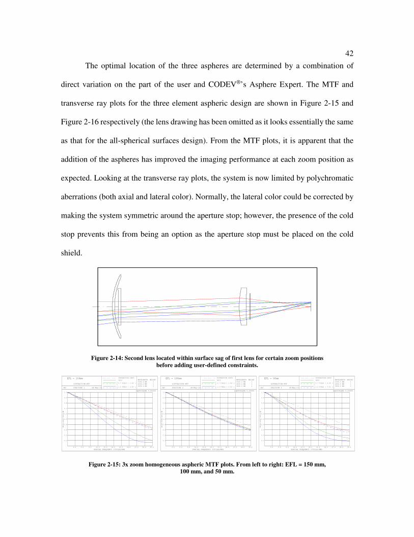
42

The optimal location of the three aspheres are determined by a combination of

direct variation on the part of the user and CODEV®’s Asphere Expert. The MTF and

transverse ray plots for the three element aspheric design are shown in Figure 2-15 and

Figure 2-16 respectively (the lens drawing has been omitted as it looks essentially the same

as that for the all-spherical surfaces design). From the MTF plots, it is apparent that the

addition of the aspheres has improved the imaging performance at each zoom position as

expected. Looking at the transverse ray plots, the system is now limited by polychromatic

aberrations (both axial and lateral color). Normally, the lateral color could be corrected by

making the system symmetric around the aperture stop; however, the presence of the cold

stop prevents this from being an option as the aperture stop must be placed on the cold

shield.

Figure 2-14: Second lens located within surface sag of first lens for certain zoom positions

before adding user-defined constraints.

Figure 2-15: 3x zoom homogeneous aspheric MTF plots. From left to right: EFL = 150 mm,

100 mm, and 50 mm.

1.0

0.9

0.8

0.7

0.6

0.5

0.4

0.3

0.2

0.1

MODULATION

3.0 6.0 9.0 12.0 15.0 18.0 21.0 24.0 27.0 30.0 33.0

SPATIAL FREQUENCY (CYCLES/MM)

EFL = 150mm

DIFFRACTION MTF

JAC 28-May-13POSITION 1

DIFFRACTION LIMIT

AXIS

T

R0.7 FIELD ( )1.64O

T

R1.0 FIELD ( )2.35O

WAVELENGTH WEIGHT

5000.0 NM 1

4000.0 NM 1

3000.0 NM 1

DEFOCUSING 0.000001.0

0.9

0.8

0.7

0.6

0.5

0.4

0.3

0.2

0.1

MODULATION

3.0 6.0 9.0 12.0 15.0 18.0 21.0 24.0 27.0 30.0 33.0

SPATIAL FREQUENCY (CYCLES/MM)

EFL = 100mm

DIFFRACTION MTF

JAC 28-May-13POSITION 2

DIFFRACTION LIMIT

AXIS

T

R0.7 FIELD ( )2.45O

T

R1.0 FIELD ( )3.52O

WAVELENGTH WEIGHT

5000.0 NM 1

4000.0 NM 1

3000.0 NM 1

DEFOCUSING 0.000001.0

0.9

0.8

0.7

0.6

0.5

0.4

0.3

0.2

0.1

MODULATION

3.0 6.0 9.0 12.0 15.0 18.0 21.0 24.0 27.0 30.0 33.0

SPATIAL FREQUENCY (CYCLES/MM)

EFL = 50mm

DIFFRACTION MTF

JAC 28-May-13POSITION 3

DIFFRACTION LIMIT

AXIS

T

R0.7 FIELD ( )4.90O

T

R1.0 FIELD ( )7.01O

WAVELENGTH WEIGHT

5000.0 NM 1

4000.0 NM 1

3000.0 NM 1

DEFOCUSING 0.00000

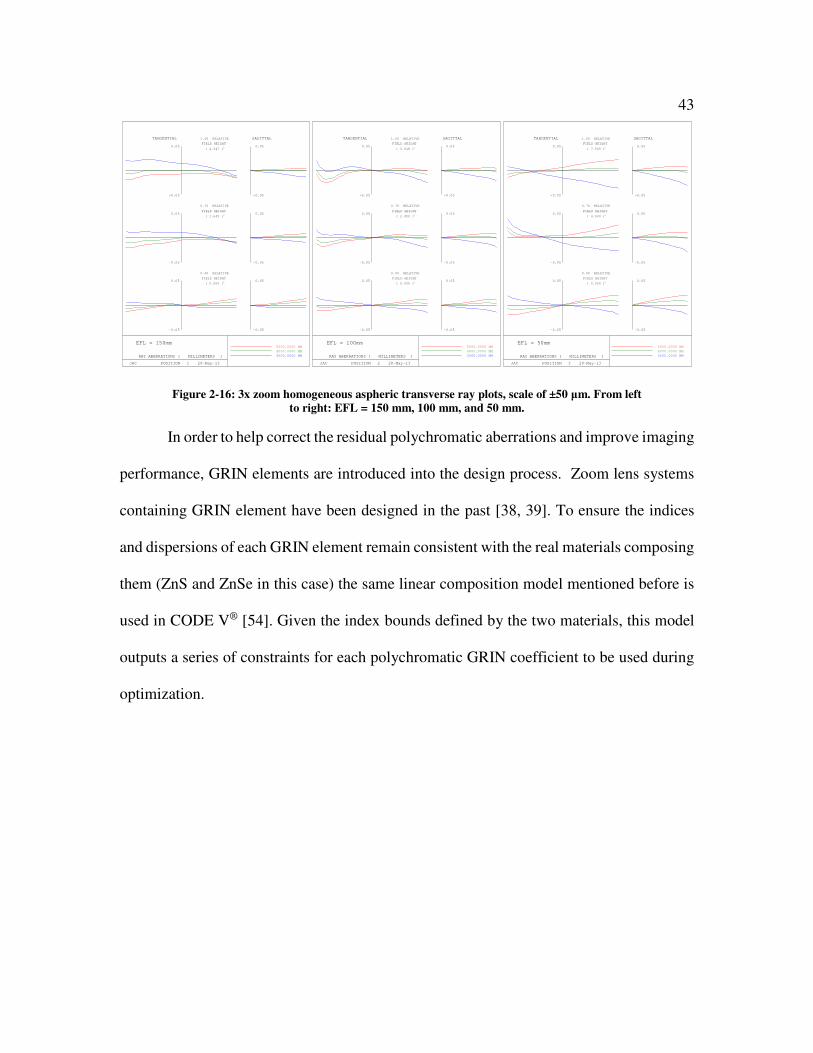
43

Figure 2-16: 3x zoom homogeneous aspheric transverse ray plots, scale of ±50 μm. From left

to right: EFL = 150 mm, 100 mm, and 50 mm.

In order to help correct the residual polychromatic aberrations and improve imaging

performance, GRIN elements are introduced into the design process. Zoom lens systems

containing GRIN element have been designed in the past [38, 39]. To ensure the indices

and dispersions of each GRIN element remain consistent with the real materials composing

them (ZnS and ZnSe in this case) the same linear composition model mentioned before is

used in CODE V® [54]. Given the index bounds defined by the two materials, this model

outputs a series of constraints for each polychromatic GRIN coefficient to be used during

optimization.

JAC 28-May-13

EFL = 150mm

RAY ABERRATIONS ( MILLIMETERS )

5000.0000 NM

4000.0000 NM

3000.0000 NM

POSITION 1

-0.05

0.05

-0.05

0.05

0.00 RELATIVE

FIELD HEIGHT

( 0.000 )O

-0.05

0.05

-0.05

0.05

0.70 RELATIVE

FIELD HEIGHT

( 1.645 )O

-0.05

0.05

-0.05

0.05

TANGENTIAL 1.00 RELATIVE SAGITTAL

FIELD HEIGHT

( 2.347 )O

JAC 28-May-13

EFL = 100mm

RAY ABERRATIONS ( MILLIMETERS )

5000.0000 NM

4000.0000 NM

3000.0000 NM

POSITION 2

-0.05

0.05

-0.05

0.05

0.00 RELATIVE

FIELD HEIGHT

( 0.000 )O

-0.05

0.05

-0.05

0.05

0.70 RELATIVE

FIELD HEIGHT

( 2.450 )O

-0.05

0.05

-0.05

0.05

TANGENTIAL 1.00 RELATIVE SAGITTAL

FIELD HEIGHT

( 3.518 )O

JAC 28-May-13

EFL = 50mm

RAY ABERRATIONS ( MILLIMETERS )

5000.0000 NM

4000.0000 NM

3000.0000 NM

POSITION 3

-0.05

0.05

-0.05

0.05

0.00 RELATIVE

FIELD HEIGHT

( 0.000 )O

-0.05

0.05

-0.05

0.05

0.70 RELATIVE

FIELD HEIGHT

( 4.900 )O

-0.05

0.05

-0.05

0.05

TANGENTIAL 1.00 RELATIVE SAGITTAL

FIELD HEIGHT

( 7.009 )O

44

Figure 2-17: 3x zoom GRIN lens drawing (first and third elements are GRIN). From top to

bottom: EFL = 150 mm, 100 mm, and 50 mm.

Design studies show that a significant increase in imaging performance both on and

off-axis is achievable with the introduction of one or more GRIN elements. A promising

design is found by allowing both the first and third elements to be ZnS/ZnSe GRIN lenses

while placing an asphere on the first surface of the second element (silicon). The layout of

this lens is shown in Figure 2-17. In this case, both GRIN elements are ZnSe on axis with

the first GRIN element (lens 1) having a total change of index between center and periphery

(Δn) of 0.081 while the second GRIN element (lens 3) has a Δn of about 0.048 (for the

reference wavelength of 4 µm). The maximum Δn possible for this material combination

is 0.18.

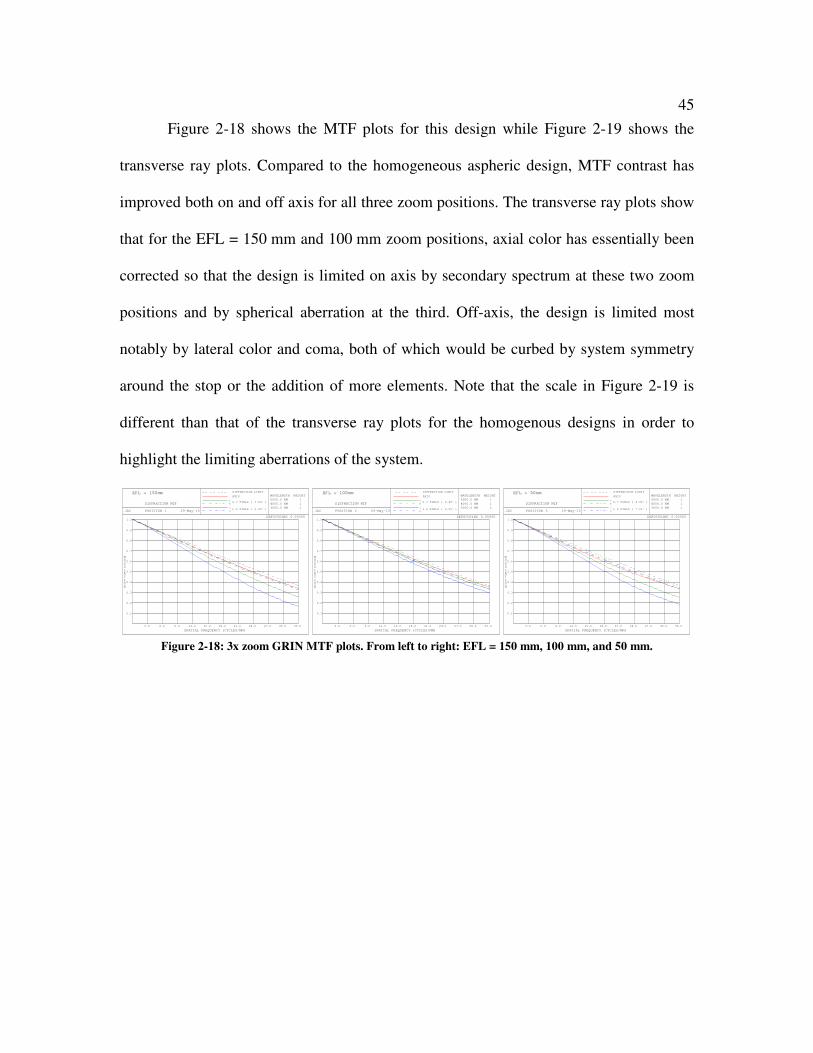
45

Figure 2-18 shows the MTF plots for this design while Figure 2-19 shows the

transverse ray plots. Compared to the homogeneous aspheric design, MTF contrast has

improved both on and off axis for all three zoom positions. The transverse ray plots show

that for the EFL = 150 mm and 100 mm zoom positions, axial color has essentially been

corrected so that the design is limited on axis by secondary spectrum at these two zoom

positions and by spherical aberration at the third. Off-axis, the design is limited most

notably by lateral color and coma, both of which would be curbed by system symmetry

around the stop or the addition of more elements. Note that the scale in Figure 2-19 is

different than that of the transverse ray plots for the homogenous designs in order to

highlight the limiting aberrations of the system.

Figure 2-18: 3x zoom GRIN MTF plots. From left to right: EFL = 150 mm, 100 mm, and 50 mm.

1.0

0.9

0.8

0.7

0.6

0.5

0.4

0.3

0.2

0.1

MODULATION

3.0 6.0 9.0 12.0 15.0 18.0 21.0 24.0 27.0 30.0 33.0

SPATIAL FREQUENCY (CYCLES/MM)

EFL = 150mm

DIFFRACTION MTF

JAC 29-May-13POSITION 1

DIFFRACTION LIMIT

AXIS

T

R0.7 FIELD ( )1.64O

T

R1.0 FIELD ( )2.35O

WAVELENGTH WEIGHT

5000.0 NM 1

4000.0 NM 1

3000.0 NM 1

DEFOCUSING 0.000001.0

0.9

0.8

0.7

0.6

0.5

0.4

0.3

0.2

0.1

MODULATION

3.0 6.0 9.0 12.0 15.0 18.0 21.0 24.0 27.0 30.0 33.0

SPATIAL FREQUENCY (CYCLES/MM)

EFL = 100mm

DIFFRACTION MTF

JAC 29-May-13POSITION 2

DIFFRACTION LIMIT

AXIS

T

R0.7 FIELD ( )2.45O

T

R1.0 FIELD ( )3.52O

WAVELENGTH WEIGHT

5000.0 NM 1

4000.0 NM 1

3000.0 NM 1

DEFOCUSING 0.000001.0

0.9

0.8

0.7

0.6

0.5

0.4

0.3

0.2

0.1

MODULATION

3.0 6.0 9.0 12.0 15.0 18.0 21.0 24.0 27.0 30.0 33.0

SPATIAL FREQUENCY (CYCLES/MM)

EFL = 50mm

DIFFRACTION MTF

JAC 29-May-13POSITION 3

DIFFRACTION LIMIT

AXIS

T

R0.7 FIELD ( )4.90O

T

R1.0 FIELD ( )7.01O

WAVELENGTH WEIGHT

5000.0 NM 1

4000.0 NM 1

3000.0 NM 1

DEFOCUSING 0.00000

46

Figure 2-19: 3x zoom GRIN transverse ray plots. From left to right: EFL = 150 mm, 100 mm,

and 50 mm. Note change in scale (now ±25 μm) compared to homogenous designs.

2.6.2 5X Zoom Design

While the preliminary design study demonstrates the usefulness of the ZnS/ZnSe

GRIN in zoom systems operating over the MWIR, it is interesting to see how a GRIN

system compares as the difficulty of the design increases. For this purpose, the designer

attempts to use the specifications of a 5x MWIR zoom lens available from New England

Optical Systems, Inc. (NEOS) as a goal [64]. The NEOS system is designed to be

compatible with a 256 x 256 sensor with a pixel pitch of 30 µm as compared to the 640 x

512 (15 µm pixel pitch) format being used for the GRIN lens study. Both lenses are

designed to have a 5x zoom with an EFL varying between 250 mm and 50 mm. Because

the detector size is different in each case while the focal lengths remain constant, the field

of view will be slightly different for the two systems with the GRIN system able to subtend

a greater field of view due to the image size being bigger. The field of view in each case is

determined by

tanh f θ= (2.17)

JAC 29-May-13

EFL = 150mm

RAY ABERRATIONS ( MILLIMETERS )

5000.0000 NM

4000.0000 NM

3000.0000 NM

POSITION 1

-0.025

0.025

-0.025

0.025

0.00 RELATIVE

FIELD HEIGHT

( 0.000 )O

-0.025

0.025

-0.025

0.025

0.70 RELATIVE

FIELD HEIGHT

( 1.645 )O

-0.025

0.025

-0.025

0.025

TANGENTIAL 1.00 RELATIVE SAGITTAL

FIELD HEIGHT

( 2.347 )O

JAC 29-May-13

EFL = 100mm

RAY ABERRATIONS ( MILLIMETERS )

5000.0000 NM

4000.0000 NM

3000.0000 NM

POSITION 2

-0.025

0.025

-0.025

0.025

0.00 RELATIVE

FIELD HEIGHT

( 0.000 )O

-0.025

0.025

-0.025

0.025

0.70 RELATIVE

FIELD HEIGHT

( 2.450 )O

-0.025

0.025

-0.025

0.025

TANGENTIAL 1.00 RELATIVE SAGITTAL

FIELD HEIGHT

( 3.518 )O

JAC 29-May-13

EFL = 50mm

RAY ABERRATIONS ( MILLIMETERS )

5000.0000 NM

4000.0000 NM

3000.0000 NM

POSITION 3

-0.025

0.025

-0.025

0.025

0.00 RELATIVE

FIELD HEIGHT

( 0.000 )O

-0.025

0.025

-0.025

0.025

0.70 RELATIVE

FIELD HEIGHT

( 4.900 )O

-0.025

0.025

-0.025

0.025

TANGENTIAL 1.00 RELATIVE SAGITTAL

FIELD HEIGHT

( 7.009 )O

47

where h is the half-diagonal of the detector, f is the EFL, and θ is the half-field of view. It

is assumed that the image size on the detector is a constant through zoom positions. While

the NEOS system is specified to be f/4, it is unclear if this is for only the 50 mm EFL or

for every zoom position (as is the case with the GRIN design as discussed earlier). If the

aperture stop is located at the cold shield for the NEOS design as well, the system is f/4 at

every zoom position. Information on the NEOS lens packaging constraints, Dewar

window, distortion, and imaging performance are unavailable online but are shown in

Table 2-5 for the GRIN lens along with a summary of the other system specifications for

each design. The GRIN design is specified to meet at least 40% contrast at every field point

at every zoom position at 23 cycles/mm (70% of the Nyquist frequency). The lens is also

specified to be significantly shorter in length than the 3x zoom system to make it more

compact. Because the aperture stop is located in the back of the system, the front element

of the system is generally very large, prompting the addition of a constraint on the

maximum allowable lens diameter as well.

The 3x design discussed in the previous section is used as a starting point for this

design. The addition of a fourth (stationary) element group is necessary to proceed forward

with the design using the increased zoom ratio. The NEOS design is specified to be dual

field so that it can operate in either narrow or wide field of view mode. The GRIN designs

are carried out at three zoom positions (EFL = 50 mm, 100 mm, and 250 mm) to add a

medium field of view zoom capability.

48 Table 2-5: Specification comparison between NEOS and GRIN 5x zoom lenses.

Parameter NEOS Design GRIN Design

Aperture f/4 f/4 (at all zoom positions)

Wavelengths 3-5 µm 3-5 µm

EFL 250-50 mm 250-50 mm

Detector Format 256 x 256 640 x 512

Pixel Pitch 30 µm 15 µm

Nyquist Frequency 17 cycles/mm 33 cycles/mm

Detector Diagonal 10.9 mm 12.3 mm

FFOV 2.5-12.4° 2.8-14.0°

Lens Length Unavailable < 135 mm

Lens Diameter Unavailable < 85 mm

Dewar Window Unavailable 1 mm thick Ge window between lens

and FPA

Performance Unavailable MTF > 40% for all field points at

23 cycles/mm (70% Nyquist frequency)

Distortion Unavailable < 2.5%

Both homogeneous and GRIN designs are carried out for the 5x system in tandem

in order to determine the optimal locations for the GRIN elements in the system and to

evaluate their effect on improving imaging performance. The design is capped to have a

maximum of six elements with less than 2.5% distortion. Both CODEV®’s Asphere Expert

and Glass Expert are used in the design process. A drawing of the three zoom positions for

the best homogeneous design is shown in Figure 2-20. Even with one aspheric surface

allowed on each of the six homogeneous elements, it is not possible to reach the MTF

specifications shown in Table 2-5 for the given system configuration. From Figure 2-21, it

is apparent that at the two extreme zoom positions, namely the narrow field of view zoom,

the MTF curves are not close to the required 40% contrast at 23 cycles/mm for every field

point. Even by weighting these zoom positions more heavily in the optimization process

the performance requirement could not be met. The transverse ray plots for the

49

homogenous design are shown in Figure 2-22. From these, it is apparent that the system is

again limited by both axial and lateral color as the aspheric homogeneous 3x design is in

the previous section. This is encouraging as the potential for GRIN elements in the system

is investigated.

Figure 2-20: 5x zoom homogenous lens drawing. From top to bottom: EFL = 250 mm, 100 mm, and

50 mm.

25.00 MM

25.00 MM

25.00 MM

50

Figure 2-21: 5x zoom homogenous lens MTF plots. From left to right: EFL = 250 mm, 100 mm, and 50 mm.

Figure 2-22: 5x zoom homogenous lens transverse ray plots, scale of ±50 μm. From left to

right: EFL = 250 mm, 100 mm, and 50 mm.

Transitioning from a homogeneous to a GRIN design, the front element of the

system is first changed from silicon to the ZnS/ZnSe GRIN. Optimization from here shows

a significant improvement in imaging performance as the GRIN profile assists in the

correction of the polychromatic aberrations. From here, additional GRIN elements are

added to improve system performance while the materials of the remaining homogenous

elements along with the locations of the aspheric surfaces are systematically varied in an

iterative process to determine the optimal design configuration. Figure 2-23 shows a

drawing of the GRIN system at the three zoom positions while Figure 2-24 and Figure 2-25

show the MTF plots and transverse ray plots respectively for this lens. As is the case for

1.0

0.9

0.8

0.7

0.6

0.5

0.4

0.3

0.2

0.1

MODULATION

2.0 4.0 6.0 8.0 10.0 12.0 14.0 16.0 18.0 20.0 22.0

SPATIAL FREQUENCY (CYCLES/MM)

EFL = 250mm

DIFFRACTION MTF

JAC 06-Jun-13POSITION 1

DIFFRACTION LIMIT

AXIS

T

R0.7 FIELD ( )0.99 O

T

R1.0 FIELD ( )1.41 O

WAVELENGTH WEIGHT

5000.0 NM 1

4000.0 NM 1

3000.0 NM 1

DEFOCUSING 0.000001.0

0.9

0.8

0.7

0.6

0.5

0.4

0.3

0.2

0.1

MODULATION

2.0 4.0 6.0 8.0 10.0 12.0 14.0 16.0 18.0 20.0 22.0

SPATIAL FREQUENCY (CYCLES/MM)

EFL = 100mm

DIFFRACTION MTF

JAC 06-Jun-13POSITION 2

DIFFRACTION LIMIT

AXIS

T

R0.7 FIELD ( )2.46O

T

R1.0 FIELD ( )3.52O

WAVELENGTH WEIGHT

5000.0 NM 1

4000.0 NM 1

3000.0 NM 1

DEFOCUSING 0.000001.0

0.9

0.8

0.7

0.6

0.5

0.4

0.3

0.2

0.1

MODULATION

2.0 4.0 6.0 8.0 10.0 12.0 14.0 16.0 18.0 20.0 22.0

SPATIAL FREQUENCY (CYCLES/MM)

EFL = 50mm

DIFFRACTION MTF

JAC 06-Jun-13POSITION 3

DIFFRACTION LIMIT

AXIS

T

R0.7 FIELD ( )4.90O

T

R1.0 FIELD ( )7.01O

WAVELENGTH WEIGHT

5000.0 NM 1

4000.0 NM 1

3000.0 NM 1

DEFOCUSING 0.00000

JAC 06-Jun-13

EFL = 250mm

RAY ABERRATIONS ( MILLIMETERS )

5000.0000 NM

4000.0000 NM

3000.0000 NM

POSITION 1

-0.05

0.05

-0.05

0.05

0.00 RELATIVE

FIELD HEIGHT

( 0.000 )O

-0.05

0.05

-0.05

0.05

0.70 RELATIVE

FIELD HEIGHT

( 0.986 )O

-0.05

0.05

-0.05

0.05

TANGENTIAL 1.00 RELATIVE SAGITTAL

FIELD HEIGHT

( 1.409 )O

JAC 06-Jun-13

EFL = 100mm

RAY ABERRATIONS ( MILLIMETERS )

5000.0000 NM

4000.0000 NM

3000.0000 NM

POSITION 2

-0.05

0.05

-0.05

0.05

0.00 RELATIVE

FIELD HEIGHT

( 0.000 )O

-0.05

0.05

-0.05

0.05

0.70 RELATIVE

FIELD HEIGHT

( 2.462 )O

-0.05

0.05

-0.05

0.05

TANGENTIAL 1.00 RELATIVE SAGITTAL

FIELD HEIGHT

( 3.518 )O

JAC 06-Jun-13

EFL = 50mm

RAY ABERRATIONS ( MILLIMETERS )

5000.0000 NM

4000.0000 NM

3000.0000 NM

POSITION 3

-0.05

0.05

-0.05

0.05

0.00 RELATIVE

FIELD HEIGHT

( 0.000 )O

-0.05

0.05

-0.05

0.05

0.70 RELATIVE

FIELD HEIGHT

( 4.900 )O

-0.05

0.05

-0.05

0.05

TANGENTIAL 1.00 RELATIVE SAGITTAL

FIELD HEIGHT

( 7.009 )O

51

the homogeneous design, the MTF plots for the GRIN lens are evaluated out to

23 cycles/mm. From Figure 2-24 it is apparent that the GRIN design achieves the

performance requirement of 40% contrast at all fields at 23 cycles/mm. Of particular

interest is the comparison of the two sets of ray aberration curves between the homogenous

and GRIN designs (Figure 2-22 and Figure 2-25). Both sets of plots are shown on the same

scale to highlight the performance improvement achieved by adding the GRIN elements.

It is worth noting that while the homogeneous design is limited heavily by primary lateral

color, this aberration is largely corrected in the GRIN system where the transverse ray plots

show secondary lateral color instead.

Figure 2-23: 5x zoom GRIN lens drawing. From top to bottom: EFL = 250 mm, 100 mm, and

50 mm.

25.00 MM

25.00 MM

25.00 MM

52

Figure 2-24: 5x zoom GRIN lens MTF plots. From left to right: EFL = 250 mm, 100 mm, and 50 mm.

Figure 2-25: 5x zoom GRIN lens transverse ray plots, scale of ±50 μm. From left to right: EFL

= 250 mm, 100 mm, and 50 mm.

Figure 2-26: 5x GRIN zoom lens at 100 mm focal length zoom position

1.0

0.9

0.8

0.7

0.6

0.5

0.4

0.3

0.2

0.1

MODULATION

2.0 4.0 6.0 8.0 10.0 12.0 14.0 16.0 18.0 20.0 22.0

SPATIAL FREQUENCY (CYCLES/MM)

EFL = 250mm

DIFFRACTION MTF

JAC 07-Jun-13POSITION 1

DIFFRACTION LIMIT

AXIS

T

R0.7 FIELD ( )0.99 O

T

R1.0 FIELD ( )1.41 O

WAVELENGTH WEIGHT

5000.0 NM 1

4000.0 NM 1

3000.0 NM 1

DEFOCUSING 0.000001.0

0.9

0.8

0.7

0.6

0.5

0.4

0.3

0.2

0.1

MODULATION

2.0 4.0 6.0 8.0 10.0 12.0 14.0 16.0 18.0 20.0 22.0

SPATIAL FREQUENCY (CYCLES/MM)

EFL = 100mm

DIFFRACTION MTF

JAC 07-Jun-13POSITION 2

DIFFRACTION LIMIT

AXIS

T

R0.7 FIELD ( )2.46O

T

R1.0 FIELD ( )3.52O

WAVELENGTH WEIGHT

5000.0 NM 1

4000.0 NM 1

3000.0 NM 1

DEFOCUSING 0.000001.0

0.9

0.8

0.7

0.6

0.5

0.4

0.3

0.2

0.1

MODULATION

2.0 4.0 6.0 8.0 10.0 12.0 14.0 16.0 18.0 20.0 22.0

SPATIAL FREQUENCY (CYCLES/MM)

EFL = 50mm

DIFFRACTION MTF

JAC 07-Jun-13POSITION 3

DIFFRACTION LIMIT

AXIS

T

R0.7 FIELD ( )4.90 O

T

R1.0 FIELD ( )7.01 O

WAVELENGTH WEIGHT

5000.0 NM 1

4000.0 NM 1

3000.0 NM 1

DEFOCUSING 0.00000

JAC 07-Jun-13

EFL = 250mm

RAY ABERRATIONS ( MILLIMETERS )

5000.0000 NM

4000.0000 NM

3000.0000 NM

POSITION 1

-0.05

0.05

-0.05

0.05

0.00 RELATIVE

FIELD HEIGHT

( 0.000 )O

-0.05

0.05

-0.05

0.05

0.70 RELATIVE

FIELD HEIGHT

( 0.986 )O

-0.05

0.05

-0.05

0.05

TANGENTIAL 1.00 RELATIVE SAGITTAL

FIELD HEIGHT

( 1.409 )O

JAC 07-Jun-13

EFL = 100mm

RAY ABERRATIONS ( MILLIMETERS )

5000.0000 NM

4000.0000 NM

3000.0000 NM

POSITION 2

-0.05

0.05

-0.05

0.05

0.00 RELATIVE

FIELD HEIGHT

( 0.000 )O

-0.05

0.05

-0.05

0.05

0.70 RELATIVE

FIELD HEIGHT

( 2.462 )O

-0.05

0.05

-0.05

0.05

TANGENTIAL 1.00 RELATIVE SAGITTAL

FIELD HEIGHT

( 3.518 )O

JAC 07-Jun-13

EFL = 50mm

RAY ABERRATIONS ( MILLIMETERS )

5000.0000 NM

4000.0000 NM

3000.0000 NM

POSITION 3

-0.05

0.05

-0.05

0.05

0.00 RELATIVE

FIELD HEIGHT

( 0.000 )O

-0.05

0.05

-0.05

0.05

0.70 RELATIVE

FIELD HEIGHT

( 4.900 )O

-0.05

0.05

-0.05

0.05

TANGENTIAL 1.00 RELATIVE SAGITTAL

FIELD HEIGHT

( 7.009 )O

53

Counting elements from the left to the right in Figure 2-26, lenses 1, 4, and 6 are

all ZnS/ZnSe GRIN. Optimization trials determined these locations to be the best

candidates for the GRIN profiles. Figure 2-27 shows plots of each of these three GRIN

profiles as a function of normalized aperture coordinate. The dotted lines indicate the index

bounds of homogenous ZnS and ZnSe at λ = 4 µm. Note that elements 1 and 4 have positive

optical power from both the surface curvatures as well as from the GRIN profile, while the

opposite is true of element 6 which has negative power coming from both sources. This

consistency in the signs of the power coming from each is the result of the negative Abbe

number of the GRIN profile. The trend is consistent with Equation 2-5 and Equation 2-6

which imply that when designing an achromat, the powers of both the surface curvatures

and GRIN profile may be the same sign as long as their Abbe numbers are of opposite sign.

The fact that CODE V® appears to be using the GRIN profile to achromatize single

elements within this design is consistent with a fundamental principle of zoom lens design,

namely that each lens groups should be individually achromatized (as opposed to balancing

system aberrations between lens groups) in order to yield high performance at each zoom

position [65].

54

Figure 2-27: Index profiles for the three radial GRIN elements in system (λ = 4µm) plotted as

a function of normalized radial coordinate (0 is the center of the lens)

There are a total of two aspheric surfaces in the system, one on the front surface of

lens 2 and one on the back surface of lens 5. While the design is only shown at the axial,

70% and full field point in this manuscript, it is checked at a number of intermediate field

points to ensure it meets performance specifications throughout the full field. All

specifications in Table 2-5 are met for the final GRIN design. CODEV® lens listings for

both the homogeneous and GRIN 5x zoom lenses are shown in 0 and Appendix B.

Conclusions

The ZnS/ZnSe GRIN has unique dispersion properties, a negative Abbe number, in

the MWIR that makes it an especially interesting material for the optical engineer designing

over this waveband. It is possible to both correct axial color and attain very high quality

imaging using only a single GRIN element. This work demonstrates the benefits of

2.25

2.30

2.35

2.40

2.45

0 0.2 0.4 0.6 0.8 1

Ref

ract

ive

Ind

ex

Normalized Lens Radius

Lens 1 Lens 4 Lens 6

55

ZnS/ZnSe GRIN elements in zoom systems operating over the MWIR. For a fixed element

count, GRIN aspheric designs are shown to offer superior imaging performance when

compared with homogeneous aspheric designs.

For the future it would be interesting to reattempt the design of the 5x system using

a different first order zoom layout. This design used the 3x system as a starting point and

resulted in a four element group layout with the first and third groups being positive power

and the second and fourth groups being negative power. Beginning the design with an

alternative power layout such as positive-negative-positive-positive or positive-negative-

negative-positive would likely result in different design forms than the one shown in this

paper and it would be useful to compare homogenous versus GRIN system performance

for each power combination.

It would also be worthwhile to explore the application of GRIN elements to more

complicated lenses with larger zoom ratios as there are a number of MWIR commercial

products having zoom ratios of 10x. Finally, there is a growing push towards developing

dual-band systems that are capable of imaging over multiple wavebands. It is interesting

to investigate how the addition of ZnS/Znse as well as other GRIN elements affect dual-

band mid/short wave infrared and mid/long wave infrared imagers.

56

Chapter 3. Copolymer GRIN Designs

Introduction

As mentioned in the introduction of this thesis, it is possible to form a GRIN profile

in a copolymer element. Polymers offer an opportunity for optical designs of reduced cost

and weight when compared with other homogeneous and GRIN materials. By allowing

two miscible monomers to come into contact, diffusion between the two monomers can

take place. As polymerization occurs, a copolymer of the two materials is formed, resulting

in the formation of a GRIN profile. Ohtsuka and Koike have performed extensive research

on a variety of copolymer GRIN systems, stemming mostly from the application of the

copolymers to GRIN fibers [24, 66, 67]. This group has also designed and fabricated much

larger radial polymer GRIN elements for the purpose of improving the human visual

system as elements for both eyeglasses and contacts lenses [68, 69]. Although the majority

of this work has concentrated on the radial geometry, Koike has worked on systems of both

the axial and spherical geometries [13, 70, 71].

Baer has pioneered a method of fabricating polymer GRIN elements from a

combination of polymethyl methacrylate (PMMA) and SAN17 by first forming sub

quarter-wavelength thick layers of the homogeneous materials and then combining them

in different ratios to form bulk material that has a refractive index dictated by the relative

composition of the two polymers [25]. Depending on the desired gradient-index profile,

individual layers of these various stock bulk materials are stacked and then thermoformed

at increased temperature and pressure in order to form a GRIN lens blank that can be coined

and diamond-turned into a lens.

57

In the Moore group at the University of Rochester, various studies have been

carried out on a variety of GRIN copolymer materials in a number of geometries. Gardner

investigated the application of the partial polymerization process for fabricating

combinations of DAP, HIRITM, and CR-39® in the radial geometry [26].

Prepolymerization essentially refers to the process of partially polymerizing a sample so

that the monomers begin to form long molecular chains but the full polymerization is not

completed. The net effect of this is to form a preform that can hold a desired shape

(cylindrical in the case of the radial) with a higher viscosity than the pure liquid monomer.

Once the preform is created, it is exposed to a second monomer or blend of monomers in

order to initiate material diffusion and generate an index profile. In order to simulate the

physiology of the insect eye, Schmidt modeled and fabricated tapered GRIN elements from

a variety of polymers through partial polymerization [72]. Photopolymerization is an

alternative means of fabricating GRIN polymer elements that uses light to catalyze the

chemical reaction [27].

PMMA/polystyrene pairing

Extensive work has been carried out regarding the copolymer formed between

(PMMA) and polystyrene. Both PMMA and polystyrene are desirable for use as they are

relatively cheap and readily available. Visconti has demonstrated the potential of this

material combination to greatly improve field aberrations and imaging performance in a

series of eyepiece studies [9]. While both radial and spherical geometry elements were

determined to be useful in the design process, the spherical geometry was chosen for further

pursuit due to greater maturity of the manufacturing process. Fang demonstrated the ability

58

to fabricate high optical quality axial-geometry GRIN rods in glass test tubes from PMMA

and polystyrene through a diffusion copolymerization process [73]. From there, these axial

geometry GRIN preforms were measured for index change and thermoformed to achieve

the desired profile slope [74]. From there, they were compressed in a spherical mold to

curve the planar isoindicial surfaces and yield a spherical GRIN. Efforts to generate radial-

geometry GRIN elements are discussed later in this chapter.

Note that the mathematics and color correction theory on radial GRIN elements

discussed in the previous chapter hold equally true for this material as for the ZnS/ZnSe

pairing As discussed before, the variation of the composition between two materials has an

Abbe number due to the refractive index changing throughout the material which makes it

possible for a GRIN singlet to act as a homogeneous doublet in an optical design [75].

Figure 3-1 displays the dispersion plots for both PMMA and polystyrene. This data is

measured on a Pulfrich refractometer and is used to calculate the base Abbe numbers of

each material as well as their GRIN Abbe number using Equation 2-7 and Equation 2-9

respectively. For the GRIN calculation, each Δnλ term corresponds to the difference in

index between PMMA and polystyrene at a given wavelength as shown in Figure 3-1. With

an Abbe number of 9, the GRIN profile is much more dispersive than either of the

homogeneous polymers that compose it (the Abbe numbers of PMMA and polystyrene are

57 and 30, respectively). Having two widely-spaced Abbe numbers is desirable from an

aberration and color-correction standpoint as it reduces the individual optical powers

required of each lens in the doublet. Thus, forming an imaging lens from this GRIN

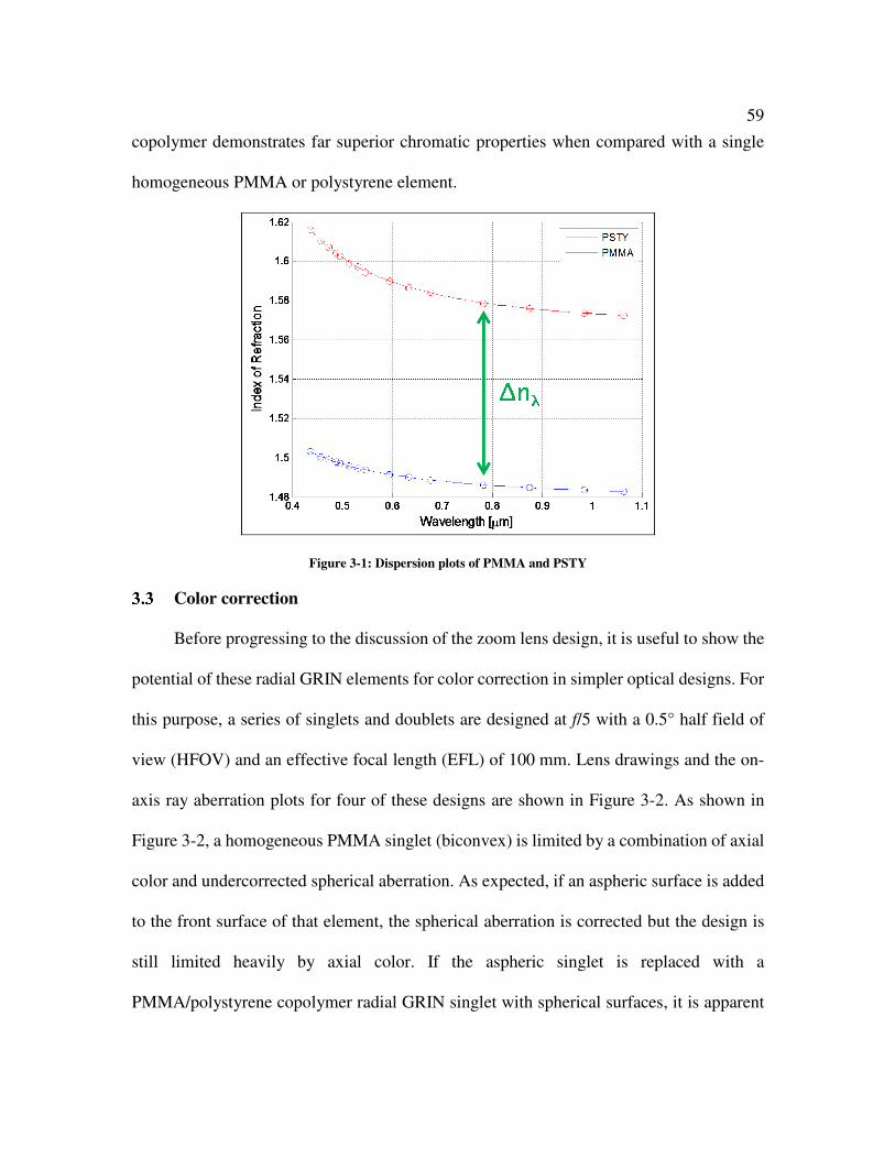
59

copolymer demonstrates far superior chromatic properties when compared with a single

homogeneous PMMA or polystyrene element.

Figure 3-1: Dispersion plots of PMMA and PSTY

Color correction

Before progressing to the discussion of the zoom lens design, it is useful to show the

potential of these radial GRIN elements for color correction in simpler optical designs. For

this purpose, a series of singlets and doublets are designed at f/5 with a 0.5° half field of

view (HFOV) and an effective focal length (EFL) of 100 mm. Lens drawings and the on-

axis ray aberration plots for four of these designs are shown in Figure 3-2. As shown in

Figure 3-2, a homogeneous PMMA singlet (biconvex) is limited by a combination of axial

color and undercorrected spherical aberration. As expected, if an aspheric surface is added

to the front surface of that element, the spherical aberration is corrected but the design is

still limited heavily by axial color. If the aspheric singlet is replaced with a

PMMA/polystyrene copolymer radial GRIN singlet with spherical surfaces, it is apparent

60

that the imaging performance is vastly improved as the design is no longer limited by axial

color but rather by a combination of secondary spectrum and spherochromatism. Compared

to the standard BK7/SF2 homogeneous doublet pair, the GRIN singlet is inferior in terms

of performance; however, it is a vast improvement over either of the homogeneous singlets

and it is important to remember that in this case, a single copolymer element is being

compared to two glass elements.

Figure 3-2: Lens drawings and ray aberration plots for singlet/doublet study.

It is interesting to note how well the design results match the achromatic doublet

equations for a radial GRIN element. This particular GRIN element shown in Figure 3-2

has a thickness of t = 7.57 mm, first and second surface radii of curvature of R1 = 50.06 mm

and R2 = -219.72 mm respectively, base index of 1.5339 at a wavelength of 587.6 nm

(42.4% PMMA and 57.6% polystyrene), and quadratic index coefficient (from

Equation 1.2) of N10 = 0.000202 mm-2. Using the radii and refractive index in Equation 2.2,

the homogeneous contribution to the optical power is found to be φhom = 0.0131 mm-1.

61

Using the thickness and N10 term in Equation 2.4, the GRIN contribution to the optical

power is calculated to be φGRIN = -0.0031 mm-1. Note that the powers are of opposite sign

as is expected in traditional achromat theory when dealing with two positive-Abbe number

materials. Substituting these values into Equation 2.5, the system power is found to be

0.01 mm-1 which is consistent with the 100 mm focal length of the lens while substituting

them into Equation 2.6 (with a homogeneous Abbe number of 38.1 and a GRIN Abbe

number of 9.1) yields a sum of 3.2 x10-6 mm-1, very close to the expected value of zero for

a color-correcting doublet.

Zoom designs

Recent design studies including the one discussed in the previous chapter have

shown that GRIN elements are very useful for color correction in a variety of wavebands

including the visible, the dual band visible/short-wave infrared, and the mid-wave infrared.

Although a few GRIN zoom systems have been designed in the past, polychromatic designs

utilizing real materials have been very limited to this point [38, 39, 59]. It is the aim of this

thesis to see how much of a performance improvement these GRIN elements can offer to

homogeneous zoom system largely limited by chromatic aberrations. The copolymer

GRIN is used in the design of a pair of zoom lens “families” which varied in zoom ratio as

well as in the number of moving groups within the lens from family to family. In all cases,

GRIN designs are compared to homogeneous designs for a fixed total element count. All

designs are carried out using McCarthy’s aforementioned linear composition model in

CODEV® optical design software [76].

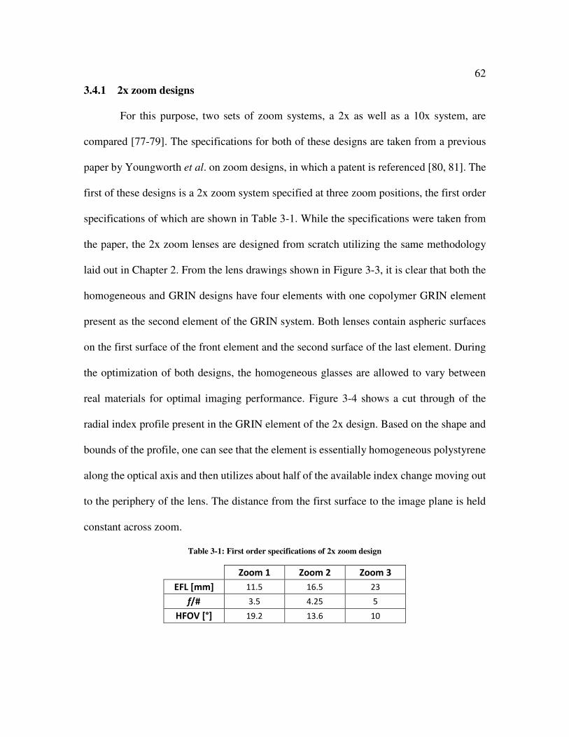
62

3.4.1 2x zoom designs

For this purpose, two sets of zoom systems, a 2x as well as a 10x system, are

compared [77-79]. The specifications for both of these designs are taken from a previous

paper by Youngworth et al. on zoom designs, in which a patent is referenced [80, 81]. The

first of these designs is a 2x zoom system specified at three zoom positions, the first order

specifications of which are shown in Table 3-1. While the specifications were taken from

the paper, the 2x zoom lenses are designed from scratch utilizing the same methodology

laid out in Chapter 2. From the lens drawings shown in Figure 3-3, it is clear that both the

homogeneous and GRIN designs have four elements with one copolymer GRIN element

present as the second element of the GRIN system. Both lenses contain aspheric surfaces

on the first surface of the front element and the second surface of the last element. During

the optimization of both designs, the homogeneous glasses are allowed to vary between

real materials for optimal imaging performance. Figure 3-4 shows a cut through of the

radial index profile present in the GRIN element of the 2x design. Based on the shape and

bounds of the profile, one can see that the element is essentially homogeneous polystyrene

along the optical axis and then utilizes about half of the available index change moving out

to the periphery of the lens. The distance from the first surface to the image plane is held

constant across zoom.

Table 3-1: First order specifications of 2x zoom design

Zoom 1 Zoom 2 Zoom 3

EFL [mm] 11.5 16.5 23

f/# 3.5 4.25 5

HFOV [°] 19.2 13.6 10

63

Figure 3-3: 2x zoom design lens layout

Figure 3-4: Index profile of 2x zoom GRIN element

1.48

1.50

1.52

1.54

1.56

1.58

1.60

-6 -4 -2 0 2 4 6

Lens Radius [mm]

Refr

acti

ve Index [λ=

58

7nm

]

PMMA

PSTY

64

Figure 3-5: Ray aberration plots for 2x zoom design

In order to evaluate system performance improvements in going from the

homogeneous to the GRIN design, Figure 3-5 shows the ray aberration plots across zoom

for the 2x zoom system on a scale of ±25 µm. From these plots it is apparent that the GRIN

design yields an improvement in polychromatic performance, namely by helping to reduce

the significant amount of lateral color very prominent in the extreme zoom positions of the

system. This improvement in chromatic behavior is due to the high dispersion of the GRIN

+25�m

-25�m

+25�m

-25�m

Tangential Sagittalhhhh = 1= 1= 1= 1

+25�m

-25�m

+25�m

-25�m

hhhh = 0= 0= 0= 0

+25�m

-25�m

+25�m

-25�m

Tangential Sagittalhhhh = 1= 1= 1= 1

+25�m

-25�m

+25�m

-25�m

hhhh = 0= 0= 0= 0

+25�m

-25�m

+25�m

-25�m

Tangential Sagittalhhhh = 1= 1= 1= 1

+25�m

-25�m

+25�m

-25�m

hhhh = 0= 0= 0= 0

+25�m

-25�m

+25�m

-25�m

Tangential Sagittalhhhh = 1= 1= 1= 1

+25�m

-25�m

+25�m

-25�m

hhhh = 0= 0= 0= 0

+25�m

-25�m

+25�m

-25�m

Tangential Sagittalhhhh = 1= 1= 1= 1

+25�m

-25�m

+25�m

-25�m

hhhh = 0= 0= 0= 0

+25�m

-25�m

+25�m

-25�m

Tangential Sagittalhhhh = 1= 1= 1= 1

+25�m

-25�m

+25�m

-25�m

hhhh = 0= 0= 0= 0

656.2725 NM656.3nm

Zoom

3:

Homogeneous GRINZoom

2:

Zoom

1:

656.2725 NM

587.5618 NM587.6nm486.1nm

587.5618 NM

486.1327 NM

587.6nm486.1nm

65

material. Figure 3-6 shows a comparison in modulation transfer function (MTF) curves

across zoom for the same 2x designs. These plots show the same performance improvement

in ray aberration curves for the two extreme zoom positions going from the homogeneous

to the GRIN design. CODEV® lens listings for both the homogeneous and GRIN 2x zoom

lenses are shown in Appendix C and Appendix D respectively.

Figure 3-6: MTF curves for 2x zoom design

3.4.2 GRIN Chromatic Macro

While ray aberration plots like those shown in Figure 3-5 are useful for looking at

the aberrations of a final optical system, they are not useful on either a surface-by-surface

0

0.2

0.4

0.6

0.8

1

0 10 20 30 40 50Cycles [mm-1]

Diff. Limit

F1: 0.0°

F2: 7.7° (T)

F2: 7.7° (S)

F3: 13.4° (T)

F3: 13.4° (S)

F4: 16.3° (T)

F4: 16.3° (S)

F5: 19.2° (T)

F5: 19.2° (S)

0

0.2

0.4

0.6

0.8

1

0 10 20 30 40 50Cycles [mm-1]

Diff. Limit

F1: 0.0°

F2: 5.5° (T)

F2: 5.5° (S)

F3: 9.5° (T)

F3: 9.5° (S)

F4: 11.6° (T)

F4: 11.6° (S)

F5: 13.6° (T)

F5: 13.6° (S)

0

0.2

0.4

0.6

0.8

1

0 10 20 30 40 50Cycles [mm-1]

Diff. Limit

F1: 0.0°

F2: 3.9° (T)

F2: 3.9° (S)

F3: 6.9° (T)

F3: 6.9° (S)

F4: 8.4° (T)

F4: 8.4° (S)

F5: 9.9° (T)

F5: 9.9° (S)

0

0.2

0.4

0.6

0.8

1

0 10 20 30 40 50Cycles [mm-1]

Diff. Limit

F1: 0.0°

F2: 7.7° (T)

F2: 7.7° (S)

F3: 13.4° (T)

F3: 13.4° (S)

F4: 16.3° (T)

F4: 16.3° (S)

F5: 19.2° (T)

F5: 19.2° (S)

0

0.2

0.4

0.6

0.8

1

0 10 20 30 40 50Cycles [mm-1]

Diff. Limit

F1: 0.0°

F2: 5.5° (T)

F2: 5.5° (S)

F3: 9.5° (T)

F3: 9.5° (S)

F4: 11.6° (T)

F4: 11.6° (S)

F5: 13.6° (T)

F5: 13.6° (S)

0

0.2

0.4

0.6

0.8

1

0 10 20 30 40 50Cycles [mm-1]

Diff. Limit

F1: 0.0°

F2: 3.9° (T)

F2: 3.9° (S)

F3: 6.9° (T)

F3: 6.9° (S)

F4: 8.4° (T)

F4: 8.4° (S)

F5: 9.9° (T)

F5: 9.9° (S)

Zoom

3:

Homogeneous GRIN

Zoom

2:

Zoom

1:

66

or an element-by-element basis for determining where in a system specific aberrations are

originating from. Seidel sums are a series of equations commonly used to tabulate the

contributions to third order and chromatic aberrations for each surface in an optical system,

making them a very useful tool for assessing where in a lens there is the most amount of a

certain aberration or where the balancing between aberrations is taking place. On its own,

CODEV® can calculate the Seidel sums for the third order surface contributions to the

aberrations as well as the transfer contributions to those aberrations which are the result of

the GRIN profile; however, it only does so for the monochromatic aberrations.

In order to calculate the contributions to both axial and lateral color for a radial

GRIN element, a macro is written in CODEV® based on a paper where the authors lay out

the methodology to calculate the polychromatic aberration contributions for GRIN

elements using Buchdahl notation [12]. The macro is included in Appendix E. While the

majority of the calculations are based on simple ray-trace values readily available from

CODEV® or other softwares, the definition of one specific parameter related to the GRIN

profile dispersion, ν11, warrants a more in-depth explanation.

When working with the Buchdahl model, the index of refraction is defined

according to

(3.1)

where Sharma defines n00λ0, ν01, and ν02 as the Buchdahl dispersion coefficients of the

optical material while ωλ is referred to as the chromatic coefficient and expressed

mathematically according to Equation 3.2

20 00 0 01 02( ) ...n nλ λ λ λω ν ω ν ω= + + +

67

0

0

( )

1 2.5( )

λ λω

λ λ

−=

+ − (3.2)

where λ is the wavelength (in micrometers) for which the chromatic coordinate is being

calculated and λ0 is defined by the user but taken to be the middle (reference) wavelength

(in microns). Thus the chromatic coefficient ω for wavelength λ0 is 0.

Based on the work of Moore and Sands, one can use Buchdahl notation to express

the index distribution for a radial GRIN as [82, 83]

20 1( , ) ( ) ( ) ...n r n n rλ λ λω ω ω= + + , (3.3)

where n0 and n1 are defined according to

20 00 0 01 02( ) ...n nλ λ λ λω ν ω ν ω= + + + (3.4)

21 10 0 11 12( ) ...n nλ λ λ λω ν ω ν ω= + + + (3.5)

where n0 and n1 are equivalent to the terms N00 and N10 from the standard equation for a

radial GRIN profile, specifically the base and quadratic coefficients. Given that fact, one

can determine v11 numerically by plotting the N10 values that CODEV® has optimized the

GRIN element to as a function of ωλ and finding the slope. Figure 3-7 shows an example

of this for the 2x zoom GRIN lens discussed in the previous section, with each N10 value

corresponding to a specific wavelength and therefore chromatic coordinate. In this case,

the relationship between N10 and ω is very linear and so it is sufficient to truncate

Equation 3.5 at only two terms though this may not always be the case. Sharma notes that

neglecting this second-order effect result in a loss of accuracy of less than 1% and considers

it a fair approximation [84].

68

Figure 3-7: N10 plotted as a function of chromatic coefficient for 2X zoom GRIN design

Using the aforementioned macro, the contributions to lateral color are calculated

across zoom for first the second element (the location of the GRIN element) and then for

the overall system for both the homogeneous and GRIN 2x zoom designs. The results of

these calculations for the second element and the system are summarized in Figure 3-8

(units of mm) along with those for the other lens groups that move together through zoom.

Note that the first group is just element one, the second group is just element two, and

group three is both elements three and four. Comparison of the plots show that at the

extreme zoom positions, lateral color is reduced in element two in going from a

homogeneous to a GRIN lens. Looking specifically at zoom position 1, the lateral color

has been reduced by a full order of magnitude with very significant decreases in the lateral

color at both of the other two zoom positions as well. The data shown in Figure 3-8 reflects

the improvements in system lateral color observed in the ray aberration plots from Figure

3-5. Again, the two extreme zoom positions show significant reduction of this aberration

while there is a minor degradation at the middle zoom although this is offset by the

69

improvements in imaging quality made at zoom 1 and zoom 3. Additionally, the GRIN

design has a better balance of the lateral chromatic aberration over the different zoom

positions and within groups.

Figure 3-8: Lateral color for both individual lens groups and system for both homogeneous (left) and GRIN

(right) 2x zoom designs (units of mm).

10x zoom designs

The second design is a 10x zoom system, the specifications of which are taken from

the same paper as the 2x designs [10, 77-79]. In this case, a patent lens from that paper is

used as the starting point [11]. The first order specifications for this system are shown in

Table 3-2. Figure 3-9 shows the lens layout of both the homogeneous and GRIN designs.

Each of these designs contain a total of nine elements with three moving groups. The

distance from the vertex of the first surface of the first element to the image plane is held

constant between zoom positions and distortion is constrained to be less than 3%. There

are two GRIN elements in this lens system as indicated in Figure 3-9 (elements six and

nine in the drawing) with plots of the GRIN profiles as a function of lens aperture shown

in Figure 3-10. From the figure it is apparent that both GRIN elements are utilizing the full

70

change in index available to them, an immediate sign that the GRIN profile is making a

significant difference in lens performance.

Table 3-2: First order specifications of 10x zoom design

Zoom 1 Zoom 2 Zoom 3

EFL [mm] 10 31 98

f/# 2 3.5 5

HFOV [°] 26.6 9.2 2.9

Figure 3-9: 10x zoom design lens layout

71

Figure 3-10: Index profile of 10x zoom GRIN elements

Figure 3-11 shows the ray aberration plots for the 10x zoom system on a scale of

±40 µm. From the figure it is clear that the homogeneous design is heavily limited by

chromatic aberration across the zoom range. At the short focal length zoom position the

design is limited by axial color while at the middle zoom position it is limited by lateral

color and at the final zoom position, it is limited by both axial and lateral color. Looking

at the corresponding GRIN design, each polychromatic aberration has been largely

corrected across zoom due to the presence of the two GRIN elements. Figure 3-12 shows

the MTF plots for both the homogeneous and GRIN systems across the zoom range. From

the plots, it is apparent that the addition of the GRIN elements has made the imaging

performance of the lens much more uniform across zoom with the performance vastly

improved at both the short and long focal length zoom positions. This enhancement is

largely due to the improved correction of both axial and lateral color in the GRIN system

over the homogenous as seen in Figure 3-11. As a reminder, the GRIN Abbe number of

1.48

1.5

1.52

1.54

1.56

1.58

1.6

-15 -10 -5 0 5 10 15

Ind

ex

of

Re

fra

ctio

n

Lens 6 Lens 9

Lens Radius [mm]

Refr

acti

ve In

dex [λ=

58

7nm

]

PMMA

PSTY

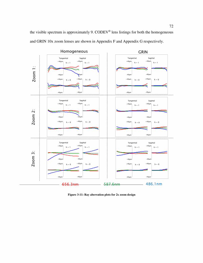
72

the visible spectrum is approximately 9. CODEV® lens listings for both the homogeneous

and GRIN 10x zoom lenses are shown in Appendix F and Appendix G respectively.

Figure 3-11: Ray aberration plots for 2x zoom design

Tangential Sagittal

h = 1 h = 1

-40�m

+40�m

-40�m

+40�m

h = 0 h = 0

-40�m

+40�m

-40�m

+40�m

Tangential Sagittal

h = 1 h = 1

-40�m

+40�m

-40�m

+40�m

h = 0 h = 0

-40�m

+40�m

-40�m

+40�m

Tangential Sagittal

h = 1 h = 1

-40�m

+40�m

-40�m

+40�m

h = 0 h = 0

-40�m

+40�m

-40�m

+40�m

Tangential Sagittal

h = 1 h = 1

-40�m

+40�m

-40�m

+40�m

h = 0 h = 0

-40�m

+40�m

-40�m

+40�m

Tangential Sagittal

h = 1 h = 1

-40�m

+40�m

-40�m

+40�m

h = 0 h = 0

-40�m

+40�m

-40�m

+40�m

Tangential Sagittal

h = 1 h = 1

-40�m

+40�m

-40�m

+40�m

h = 0 h = 0

-40�m

+40�m

-40�m

+40�m

656.2725 NM656.3nm

Zoom

3:

Homogeneous GRIN

Zoom

2:

Zoom

1:

656.2725 NM

587.5618 NM587.6nm486.1nm

587.5618 NM

486.1327 NM

587.6nm486.1nm

73

Figure 3-12: MTF curves for 10x zoom designs

Conclusions and future work

A series of design studies have been discussed utilizing a copolymer

PMMA/polystyrene radial GRIN. A number of simple homogeneous and GRIN singlets

and doublet designs were first compared to demonstrate the material’s ability to correct

color over the visible spectrum using a single element. This same type of element was then

applied to much more complex systems, first a 2x zoom lens followed by a 10x zoom lens.

In both cases the GRIN design was observed to have improved imaging performance over

its homogeneous counterpart of the same number of elements, largely due to the

improvements in the correction of color. A macro was written in CODEV® and MATLAB

0

0.2

0.4

0.6

0.8

1

0 20 40 60 80 100Cycles [mm-1]

Diff. Limit

F1: 0.0°

F2: 10.6° (T)

F2: 10.6° (S)

F3: 18.6° (T)

F3: 18.6° (S)

F4: 22.6° (T)

F4: 22.6° (S)

F5: 26.6° (T)

F5: 26.6° (S)

0

0.2

0.4

0.6

0.8

1

0 20 40 60 80 100Cycles [mm-1]

Diff. Limit

F1: 0.0°

F2: 3.7° (T)

F2: 3.7° (S)

F3: 6.5° (T)

F3: 6.5° (S)

F4: 7.8° (T)

F4: 7.8° (S)

F5: 9.2° (T)

F5: 9.2° (S)

0

0.2

0.4

0.6

0.8

1

0 20 40 60 80 100Cycles [mm-1]

Diff. Limit

F1: 0.0°

F2: 1.2° (T)

F2: 1.2° (S)

F3: 2.0° (T)

F3: 2.0° (S)

F4: 2.5° (T)

F4: 2.5° (S)

F5: 2.9° (T)

F5: 2.9° (S)

0

0.2

0.4

0.6

0.8

1

0 20 40 60 80 100Cycles [mm-1]

Diff. Limit

F1: 0.0°

F2: 5.5° (T)

F2: 5.5° (S)

F3: 9.5° (T)

F3: 9.5° (S)

F4: 11.6° (T)

F4: 11.6° (S)

F5: 13.6° (T)

F5: 13.6° (S)

0

0.2

0.4

0.6

0.8

1

0 20 40 60 80 100Cycles [mm-1]

Diff. Limit

F1: 0.0°

F2: 5.5° (T)

F2: 5.5° (S)

F3: 9.5° (T)

F3: 9.5° (S)

F4: 11.6° (T)

F4: 11.6° (S)

F5: 13.6° (T)

F5: 13.6° (S)

0

0.2

0.4

0.6

0.8

1

0 20 40 60 80 100Cycles [mm-1]

Diff. Limit

F1: 0.0°

F2: 5.5° (T)

F2: 5.5° (S)

F3: 9.5° (T)

F3: 9.5° (S)

F4: 11.6° (T)

F4: 11.6° (S)

F5: 13.6° (T)

F5: 13.6° (S)

Zoom

3:

Homogeneous GRIN

Zoom

2:

Zoom

1:

74

for evaluating the surface and element contributions to both axial and lateral color for radial

GRIN elements utilizing Buchdahl notation. Results from this further support the GRIN

lens’ role in correcting color in individual elements and the design as a whole.

Going forward, it would be of interest to carry out further design studies utilizing

this material pairing with applications to more complicated systems. This could include

higher zoom ratios, greater fields of view, faster speeds, etc., all in an effort to further map

out the space of GRIN design and determine in what forms this specific GRIN copolymer

as well as GRIN materials in general improve performance. There are a number of other

miscible optical copolymers pairings that have been explored in the past and it would be

of great use to apply some of these to the design forms laid out in this chapter as well as

others to determine what pairing gives the highest-performance.

75

Chapter 4. Fabrication of copolymer GRIN elements

Background

Based on the results of the previous chapter, the potential for copolymer radial

GRIN elements to improve the imaging performance of a lens system is apparent. Attempts

to fabricate such elements in the laboratory are pursued using the polymerization process

first discussed in Section 1.3.3. As mentioned in Section 3.1, numerous methods for

copolymerization exist. The processes of both prepolymerization and photopolymerization

can be used to generate both positive and negative-signed gradients; however, they provide

limited maximum achievable index changes and are not compatible with many polymer

combinations. Because of these reasons, an alternative process is pursued: the centrifugal

force method.

In an attempt to achieve higher index changes, this thesis concentrates on the

fabrication of polymer radial GRIN elements through the use of centrifugal forces, based

on the methodology demonstrated by a number of other groups. Most simply, this process

involves rotating a vessel containing various monomers at 2,000 rpm during the fabrication

process so that as copolymerization occurs, diffusion between those monomers results in

an element with cylindrical isoindicial surfaces: a radial GRIN. Im has demonstrated index

changes between 0.002 and 0.015 in GRIN optical fibers formed from a PMMA and

polystyrene copolymer [85]. Cho has been able to use photopolymerization on the

monomers MMA and 2,2,3,3-tetrafluoropropyl methacrylate (TFPMA) to fabricate GRIN

76

rods [86]. Duijnhoven has been able to copolymerize 5 mm-diameter rods of MMA and

TFPMA to have an index change of up to 0.009 [87].

Rochester process

4.2.1 Monomer preparation

Initial attempts at sample fabrication are carried out without first filtering either of

the two monomers before copolymerization. These samples are found to be very hazy.

Based on this and the results of Fang and Schmidt, all subsequent samples are fabricated

using filtered monomer in order to remove any substances and impurities that would inhibit

the reactions [73]. To do this, the monomer is placed in a glass funnel above a glass tube

filled with fine cotton, molecular sieve, and Al2O3 powder. Over time, the monomer drips

through the filtration tube and into a clean glass beaker below. The unfiltered styrene

monomer has a yellowish hue which is not observed in the filtered styrene monomer.

During polymerization, a liquid monomer shrinks in size as it becomes a solid

polymer in a process known as volume reduction. A set of experiments in which test tubes

of liquid monomer were photographed once every five minutes during polymerization over

time determined that MMA monomer reduces to 81% of its initial volume after

polymerization to PMMA with that same metric being 87% going from styrene to

polystyrene.

4.2.2 Copolymerization

The Rochester process involves filling a temperature-controlled spinning monomer

chamber with varying amounts of two or more monomers to control the index profile. The

GRIN rod fills from the outside to the inside as the material pumped first into the spinning

77

chamber settles first to the outside of the chamber. Because MMA is heavier than styrene,

GRIN elements of that material pairing fabricated in this manner have more PMMA on the

outside of the aperture and more polystyrene on the inside. As a result of that, only

positive-power profiles are created in this way since PMMA has a lower refractive index

than polystyrene. Using a different combination of miscible polymers such as PMMA and

poly(benzyl methacrylate), a negative-signed GRIN profile may be fabricated as well.

A schematic of such a system is shown in Figure 4-1. In this system, two monomers

are stored in separate syringes and then pumped through both a passive mixing chamber

and a pre-heating chamber as controlled by a computer. As the monomers are stored cold,

this is meant to ensure that the liquid matches the required temperature of the reaction as it

enters the chamber. Based on the desired final index profile, the computer is used to dictate

the relative fill rates of the two monomers into the actual spinning chamber where

copolymerization occurs. The chamber is rotated at 2,000 rpm by a lathe while

continuously-circulating heated water falls onto the rotating chamber in order to hold it at

a set temperature during copolymerization. Figure 4-2 shows a photograph of the system

with one end of the monomer test tube mounted in the lathe. During the fabrication process,

the other side of monomer test tube is secured inside of a rotary bearing meant for

additional stability. The feed needle is carefully inserted into the spinning cap of the test

tube to drip in monomer. For clarity, the top of the water chamber is not shown. After being

copolymerized, the samples, now solid, are removed from the lathe while still within the

test tube and placed inside of a convection oven for post-cure. This process is meant to

finalize the reaction by using up any residual initiator molecules left in the samples. The

78

samples are heated from 65 °C to 95 °C over the course of five hours, held at 95 °C for one

hour and then brought down to 25 °C over an additional ten hours. Once the post-cure is

complete, the samples are separated from the test tube by carefully breaking and removing

the glass surrounding the now-solid copolymer.

Figure 4-1: Layout of centrifugal radial GRIN setup (figure credit: Greg R. Schmidt)

Figure 4-2: Photograph of centrifugal radial GRIN setup

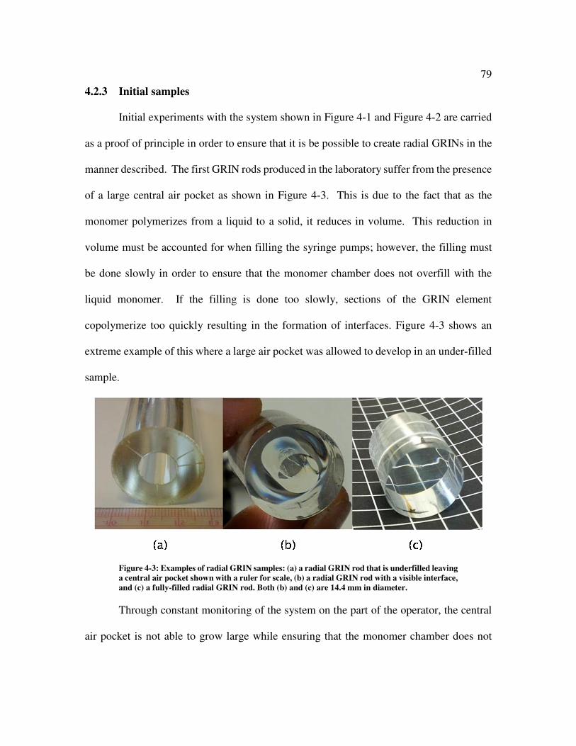
79

4.2.3 Initial samples

Initial experiments with the system shown in Figure 4-1 and Figure 4-2 are carried

as a proof of principle in order to ensure that it is be possible to create radial GRINs in the

manner described. The first GRIN rods produced in the laboratory suffer from the presence

of a large central air pocket as shown in Figure 4-3. This is due to the fact that as the

monomer polymerizes from a liquid to a solid, it reduces in volume. This reduction in

volume must be accounted for when filling the syringe pumps; however, the filling must

be done slowly in order to ensure that the monomer chamber does not overfill with the

liquid monomer. If the filling is done too slowly, sections of the GRIN element

copolymerize too quickly resulting in the formation of interfaces. Figure 4-3 shows an

extreme example of this where a large air pocket was allowed to develop in an under-filled

sample.

Figure 4-3: Examples of radial GRIN samples: (a) a radial GRIN rod that is underfilled leaving

a central air pocket shown with a ruler for scale, (b) a radial GRIN rod with a visible interface,

and (c) a fully-filled radial GRIN rod. Both (b) and (c) are 14.4 mm in diameter.

Through constant monitoring of the system on the part of the operator, the central

air pocket is not able to grow large while ensuring that the monomer chamber does not

80

overflow. An example of a fully filled radial sample produced in this way with no interfaces

is shown in Figure 4-3. A typical experiment begins with a fill rate between 20 and

25 μL/min and ended with one below 1 μL/min.

Once a radial sample is produced, it is necessary to measure the index profile. For

this purpose, sections that are roughly 0.6 mm-thick are cut from the GRIN rod

perpendicular to the isoindicial surfaces and the section is placed in one arm of a phase-

shifting Mach-Zehnder interferometer for measurement. Single-pass interferometers like

Mach-Zehnders are often preferable for measuring GRIN profiles as the index change can

result in a large number of interference fringes that are difficult to resolve using a double-

pass interferometer. Double-pass interferometers are also undesirable as ray registration

errors can occur from having to transmit back through the GRIN material. Sample

measurements yield interferograms like those shown in Figure 4-4 with all measurements

carried out at a wavelength of 632.8 nm. The index profiles shown in Figure 4-4 are

measured from left to right through the center of each radial sample.

Note that alone, the Mach-Zehnder interferometer provides only relative index data

so that one only knows the relative change in index across the aperture. A measurement

from a refractometer or other instrument capable of measuring absolute index of refraction

is required to fully quantify the GRIN profile. Note that the samples produced from this

process are not truly radial GRIN elements but rather tapered gradients due to the index

having an axial-direction dependence. In this thesis, sections from these samples are

approximated to radial GRIN lenses. Tapered gradients are explored in detail by

Schmidt [72].

81

Figure 4-4: Examples of fabricated radial GRIN samples. The left column shows the

interferograms of two approximately 0.6 mm-thick sections of samples and the right column

shows the index profiles through the center.

4.2.4 Results

To reduce setup complexity, an alternative method of combining the monomers is

adopted in the fabrication process whereby MMA and styrene are premixed in varying

ratios and then pumped together from one single syringe into the spinning chamber. In

experiments, either three or four ratios are pumped in order to create one sample. For this

sample, three ratios of monomers are pumped into the spinning test tube. These are (in

order of pumping) (1) 75/25, (2) 50/50, and (3) 25/75% PMMA/polystyrene by volume of

each polymer. This is illustrated in Figure 4-5 and summarized in Table 4-1. The volumes

of each ratio are chosen so that the distance between the outer and inner diameter of each

calculated copolymer layer are close to one another. The calculated outer (r1) and inner

(r2) radii for each layer are also summarized in Table 4-1 along with the calculated total

solid copolymer volume of each layer and the corresponding calculated liquid monomer

82

volumes for both MMA and styrene. The inner diameter of the test tube used for JC018 is

14.4 cm while the length is 11 cm.

Figure 4-5: Illustration of copolymer layering process

Table 4-1: Summary of calculation of required monomer volumes for sample JC018 layers

Layer Thickness r1 r2 PMMA Polystyrene Copolymer

volume MMA

volume Styrene volume

Unit cm cm cm -- -- mL mL mL

1 0.25 0.72 0.47 0.75 0.25 10.28 9.54 2.95

2 0.25 0.47 0.22 0.50 0.50 5.96 3.69 3.43

3 0.22 0.22 0 0.25 0.75 1.67 0.52 1.44

Samples JC016 and JC017 were both carried out with the same layering recipe as

JC018; however, both suffered from process issues that were adjusted for JC018. JC016

was the last sample attempted using unfiltered monomer and the resulting haze in the

sample prompted the switch to using filtered monomer for all future samples as stated in

Section 4.2.1. Additionally, the final sample had a central hole (like that observed in Figure

4-3) in approximately one-third of the length of the sample. This is because even though

the test tube was completely filled when last observed, further volume reduction occurred

as the reaction finished. Because of this, both JC017 and JC018 were periodically

monitored by the operator during the filling of layer 2 and constantly monitored during the

83

filling of layer 3 to prevent a hole from appearing at any point once the test tube was first

filled with monomer. An additional volume of the layer 3 monomer mixture was pumped

into the test tube (between 0.5 and 1 mL) during this process.

After the post-cure, JC017 was found to have a series of air bubbles throughout its

length that were not present when the sample was removed from the lathe. This means that

the copolymerization reaction was not complete and that there was still a large number of

monomer molecules present in the sample. As a result of this, JC018 was given

significantly more time to copolymerize in the lathe setup than its predecessors. Each

sample run began at 60 °C and ended at 67 °C. Both JC016 and JC017 were polymerized

for an additional 20 hours after reaching 67 °C while that number was extended to 58 hours

for JC018.

Figure 4-6 shows an example of the profile measurements at various points in

sample (JC018). These profiles (namely slices 2 and 3) are much more quadratic and

therefore much more beneficial for imaging applications than those shown in Figure 4-4.

It is apparent from Figure 4-6 that there is a large axial component to these GRIN profiles

over the full length of the sample. This is due to the fact that the while spinning, the test

tube is tilted upwards so that the monomer may more easily enter the chamber and remain

there during the polymerization process.

84

Figure 4-6: GRIN profiles of various sections of radial sample JC018

Figure 4-7 shows photographs and a CODE V® model of one section of sample

JC018. To see how well the fabricated lenses are described by the design software, the back

focal length (BFL) of sample JC018 is measured and compared against the quantity

calculated by a CODE V® model. Rather than modeling the single element with the profile

varying axially and radially, the lens is modeled first with just the radial profile of slice 1

and then the profile of just slice 2, yielding calculated BFLs of 26.7 mm and 25.8 mm,

respectively. Direct measurements of this quantity is 26.6 ± 1.2 mm. The uncertainty is

the standard deviation of these measurements.

85

Figure 4-7: (a) Images and (b) CODEV® model of sample JC018. The sample has a diameter of 14.4 mm

2x zoom design using manufactured profile

As shown earlier, the 2x GRIN zoom design shown in Figure 3-3 contains a

positive-powered index profile, the sign of which is consistent with the aforementioned

centrifugal method. Figure 4-8 shows the optimized index profile of that element at a

wavelength of 632.8 nm. A question arose as to how sensitive this particular design form

is to the shape and depth of the index profile. The main issue is whether or not this non-

optimal index profile still provides improvements to image quality, most notably working

towards correcting the lateral color across the zoom range. To explore this, the measured

index profile of sample JC018, slice 2 is modeled in MATLAB. From here, the profile is

fitted to a sixth-order polynomial. The results of this curve fit are shown in Figure 4-8. The

fit is only carried out over the aperture of the modeled element as calculated by CODEV®

with the actual GRIN rod being of a larger diameter. The darkened areas of the plot indicate

the unused region of the manufactured GRIN rod larger than the diameter of the modeled

86

element. The difference in index of refraction between the sixth-order fit to the

interferometrically-measured index profile data and the data itself is shown in Figure 4-9.

Figure 4-8: (a) Meaured index profile and sixth-order fit for slice 2 of sample JC018. The grayed-out area

indicates the region greater than the aperture of the lens designed with the fitted profile. (b) Comparison of

GRIN profile shapes for 2X zoom lens design between designed lens and fit of JC018, slice 2 profile. Note the

change in aperture size of the element between the two designs.

-4 -3 -2 -1 0 1 2 3 4-6

-4

-2

0

2

4

6

Radius [mm]

Ind

ex o

f re

fra

ctio

n d

iffe

ren

ce

( x

10

-4)

Figure 4-9: Difference in index of refraction between the sixth-order fit to the interferometrically-measured

index profile data and the data itself. The accuracy of the interferometric index measurements is ±2x10-5.

While the relative index profile of the element is measured interferometrically, it is

necessary to perform an absolute index measurement somewhere on the sample to gain a

valid reference point for the GRIN profile. This is done using a Metricon 2010/M prism

-6 -4 -2 0 2 4 61.48

1.5

1.52

1.54

1.56

1.58

1.6

Radius [mm]In

de

x o

f re

fra

ctio

n (

λ =

632

.8n

m)

2x Design Profile

Fit to Fabricated Profile

-8 -6 -4 -2 0 2 4 6 80

0.005

0.01

0.015

0.02

0.025

0.03

Radius [mm]

∆n (

λ =

63

2.8

nm

)

Measured

ax6 + bx4 + cx2 + d fit

(a) (b)

PMMA

Polystyrene

87

coupler system at the edge of the sample. After calibration, this instrument has an absolute

index accuracy of ±0.0002.The fit to the measured index profile of sample JC018, slice 2

is shown in Figure 4-8 alongside the optimized profile. Looking at both profiles on the

same plot, one can see that the optimized profile is significantly steeper than the measured

one, while also trending heavily towards the higher index (greater amount of polystyrene)

side of the GRIN.

Using the 2x zoom design file as a starting point from section 3.4.1, the fit to the

measured index profile is entered into CODEV® and not allowed to vary. From there,

optimization trials are carried out allowing the thicknesses and curvatures of the elements

to vary around the frozen GRIN profile in order to recover imaging performance. The

performance results of this are shown by the aberration plots contained in Figure 4-10. This

figure compares these plots for three designs: (1) homogeneous, (2) GRIN (fabricated

profile), and (3) GRIN (designed profile) with all evaluated at the extreme zoom positions.

Generally in zoom lens systems (and reflected in both Figure 3-5 and Figure 3-11) the

shortest and longest effective focal length configurations exhibit the worst imaging

performance with the aberrations being better controlled for the intermediate zoom

configurations. Because of this fact and for figure clarity, the middle zoom position shown

in Figure 3-5 and Figure 3-11 is omitted from Figure 4-10.

It is important to note that while the GRIN design with the measured profile does

offer significantly better performance than its homogeneous counterpart, its performance

is not quite as good as that of the design using the optimized index profile. However, this

indicates that a GRIN design does not need to have the optimal profile in place in order to

88

benefit from the GRIN element’s chromatic properties. Note especially that the benefits

for lateral color correction of both GRIN designs over the homogeneous system for the

EFL = 23 mm zoom position are very similar. The optimized profile yields superior

imaging performance for the other extreme zoom position but, again, the measured profile

is a significant improvement over the homogenous. The CODEV® lens listings for GRIN

5x zoom lens with the JC018 profile is shown in Appendix H.

Figure 4-10: Ray aberration plots for homogeneous and both GRIN designs (fabricated profile vs. designed

profile) evaluated at the extreme zoom positions.

Conclusions and future work

A centrifugal-force method is presented for the purpose of manufacturing

copolymer PMMA/polystyrene radial GRIN elements. Liquid MMA and styrene monomer

89

is copolymerized in a test tube rotating at approximately 2000 rpm in order to accomplish

this. A procedure for monomer filtering and preparation, layering, and system operation is

presented along with a discussion of the manufactured samples. Note that although many

issues are resolved, a number still exist including residual haze in the sample (greatly

reduced from the first samples) stemming from the issue of volume reduction causing

liquid monomer to come in contact with largely-copolymerized material at the center of

the sample in the final steps of the manufacturing process. Sample JC018 is presented in

detail with photographs of the element along with index profile measurements showcasing

a desirable quadratic shape in some regions of the sample. One such profile is applied to

the 2x zoom copolymer lens design presented in Chapter 3 to partially determine how

sensitive a GRIN design’s ability to correct color is to a given optimal profile shape. As

desired and expected, the imaging performance for the lens with the manufactured profile

is better than that of the homogenous lens but not as good as the lens with the optimal index

profile.

Going forward it would be useful to manufacture a monomer chamber that is

capable of shrinking in size as the copolymerization process occurs in an attempt to

compensate for the sample reducing in size. It is expected this would reduce the amount of

haze by halting the aforementioned issue of the liquid monomer contacting largely-

copolymerized material. At the same time, it would be useful to refine the process to

achieve larger index changes and to reduce the tilt angle of the lathe to reduce the axial

component of the index profile. It would also be of interest to attempt fabrication of some

of the same miscible polymer combinations discussed in the future work of Chapter 3.

90

Chapter 5. Athermalization of radial GRIN polymers

Introduction

A fundamental concern in the design of any optical system is the issue of how that

system is affected by a change in temperature. Traditionally, athermalized systems are

specifically designed so that an increase or decrease in temperature has a minimal effect

upon the optical performance. In practice, one or more of three processes are employed in

order to achieve athermalization and avoid performance degradation: (1) allowing

individual lenses/lens groups or the sensor to move, (2) mounting the lenses using specific

materials and dimensions to cause favorable airspace changes, and (3) using the thermal

properties of optical elements to compensate for focus change [88]. These last two methods

are a passive, rather than active, means of athermalizing a lens. If a system is composed of

only a single homogeneous element, it is not possible to use differing optical and/or

mechanical materials to compensate for one another and the image plane must be translated

to recover imaging performance as the temperature is changed. Largely analogous to the

process of achromatizing a lens (correcting primary axial color), athermalizing a system

requires at least two elements of different homogeneous materials.

As discussed in the previous chapters on optical design, utilizing GRIN materials

introduces new degrees of freedom into the design process. These allow for improved

aberration correction and therefore imaging performance while making it possible to

replace a number of homogeneous lenses with fewer GRIN lenses in order to reduce system

size and weight [89]. At least two homogeneous elements are required either to athermalize

or to achromatize a lens system of a given focal length [90]. Because the index is varying

91

across the lens aperture, both radial and spherical GRIN lenses have optical power due to

the index profile, in addition to the ray bending due to the lens surfaces. Thus, it is possible

for a single GRIN element to replace a homogeneous doublet under certain circumstances,

one of which, as mentioned in earlier chapters, is color correction. The ability to

achromatize a single GRIN lens begs the question of whether or not it would be possible

to athermalize a single GRIN lens as well [26]. It should be noted that the work carried out

in this thesis applies only to monochromatic systems undergoing a uniform temperature

change.

Thermal Effects – Homogeneous

Two material parameters must be defined in order to understand how an optical

system is affected by temperature: (1) the linear coefficient of thermal expansion (CTE)

and (2) the temperature-dependent index of refraction (dn/dT). The CTE is a measure of

how much a material changes in dimension with a change in temperature (a positive CTE

corresponds to a dimensional expansion with an increase in temperature and vice versa)

while the dn/dT dictates how the index of refraction changes with a change in temperature

(a positive dn/dT value implies the index of refraction increases when the temperature is

increased and vice versa). Note that a discussion of how both of these quantities are

measured is presented in the following chapter. The changes in the axial thickness and

semi-diameter of a lens are calculated using

' (1 )t t Tα= + ⋅∆ (5.1)

0 0' (1 )r r Tα= + ⋅ ∆ (5.2)

92

where t’ and r0’ are the new thickness and semi-diameter respectively, t and r0 are the initial

thickness and semi-diameter respectively, ΔT is the change in temperature, and α is the

CTE [26].

For a positive CTE, the lens expands both radially and axially with an increase in

temperature, the net effect of which is to decrease the magnitude of the surface curvature.

For a given temperature change, the change in surface curvature is given by

'1

cc

Tα=

+ ∆ (5.3)

where c’ is the new surface curvature and c is the initial surface curvature. The change in

the index of refraction of a material is described by

00 00'dn

N N TdT

= + ∆

(5.4)

where N’00 is the index of refraction of a homogeneous material after a temperature change

while N00 is the initial index of refraction.

Thermal effects - radial GRINs

Due to their relative mathematical simplicity when compared with spherical

GRINS, radial GRINs are chosen as the focus of this athermalization study. In such a

gradient, the index varies as a function of radial coordinate, making it possible to introduce

optical power with just the index profile shape (independent of the lens surface curvatures).

The Wood lens is the simplest example of a radial gradient, where either positive or

negative optical power can be achieved with a plano-plano element depending on the sign

of the gradient (a positive gradient describes when the index is higher along the optical axis

93

and then falls off towards the periphery while the opposite is true of a negative profile)

[91]. The index of refraction of a radial gradient is defined mathematically by

2 400 10 20( ) ...N r N N r N r= + + + (5.5)

where N is index of refraction for a given r (the distance measured outward from the optical

axis) and Nx0 are the index polynomial coefficients for a radial GRIN profile.

Figure 5-1: Effect of temperature increase on (a) a homogenous window and (b) a Wood lens for materials with

positive CTEs. Note that curvatures are induced in the radial GRIN element.

As a GRIN material’s composition changes as a function of spatial coordinate, so

do CTE and dn/dT. In the case of the Wood lens, the CTE varies across the aperture of the

lens so that a temperature change induces curvatures in nominally-planar surfaces.

Assuming the values to all be positive, if the CTE along the optical axis is greater than the

CTE at the periphery of the lens, this curvature is positive (and vice versa). This fact is

shown in Figure 5-1 which illustrates the effect of temperature on the surface curvatures of

both a homogenous and radial GRIN window (Wood lens). Note that the homogenous lens

expands in both directions but remains a window. This effect on the surface curvatures is

94

also inherent to radial GRIN lenses with non-planar surfaces. Additionally, the fact that

dn/dT is a spatially-varying parameter in a GRIN element must also be taken into account.

This chapter assumes that the material composition is varying quadratically

between the optical axis (quantities designated by a subscript a) and the edge of the lens

(quantities designated by a subscript b). This means that the GRIN profile is described by

only the first two terms of the Equation 5.5 above (N20 and all higher order coefficients are

equal to 0). The change in the surface curvature of the lens is given by

20

2

(1 ) ( )'

(1 )

a b a

a

t Tc T

rc

T

α α α

α

∆+ ∆ − −

=+ ∆

(5.6)

where c’ is the curvature of the lens after a change in temperature and r0 is the semi-

diameter of the lens. Note that for a homogenous lens, the equation reduces to Equation 5.3.

The quadratic index coefficient (N10) is given by

10 20

b an nN

r

−= (5.7)

where na is the index at the center of the lens, nb is the index at the periphery of the lens.

Note that Equation 5.4 is still used to calculate the new base index of the profile. The

change in the quadratic coefficient of the index profile is given by

10 22

0

( )'

11 ( ( ))

3

b ab a

a b a

dn dnn n T

dT dTN

T rα α α

− + − ∆

=

+ + − ∆

(5.8)

95

where N’10 is the quadratic term after a change in temperature. Note that in Equation 5.8,

the denominator is equal to the square of the expanded radius lens after the temperature

change [26].

Athermalization

A radial GRIN element has two contributions to the overall optical power of the

singlet, with the first being that of the surface curvatures and the second being that of the

index profile. It is possible to design GRIN singlets so that as the temperature changes, the

change in optical power due to surface curvatures is opposite in sign to that of the index

profile so that the net change in the focal length of the lens is as close to zero as possible.

Equations 4.9a, 4.9b, 4.10, and 4.11 are used to determine the optical power of a radial

GRIN singlet

200

1 2 00 1 200

( 1) sinh( )( )( 1)cosh( ) sinh( )

N kc c N k b k cc t

N kφ

−= + − − − (5.9a)

200

1 2 00 1 200

( 1) sin( )( )( 1)cos( ) sin( )

N kc c N k b k cc t

N kφ

−= + − − − (5.9b)

00

btk

N= (5.10)

00 102b N N= (5.11)

where c1 and c2 are the curvatures of the first and second surfaces of the lens respectively

[43]. Equation 5.9a is used if N10 > 0 and Equation 5.9b is used if N10 < 0. If N10 = 0, both

equations for φ reduce to that for the power a homogeneous lens. Note that these equations

(and all equations in this chapter) are defined so that a positive curvature value always

96

refers to a convex surface (on either surface). Using Equation 5.9a and Equation 5.9b for

φ, one can calculate the nominal optical power of a GRIN lens. For a given ΔT, one can

then determine the changes in the lens geometry and index profile using the equations

outlined in the previous section before finding the new optical power of the lens. The goal

is to find singlets where the difference in the optical power of the lens before and after the

temperature change is minimized.

Polymers

Thus far, this work has been focused on radial GRINs formed from a combination

of the optical polymers PMMA and polystyrene. Typically, polymers exhibit values of

CTE and dn/dT that are between one and two orders of magnitude greater than those of

optical glasses. For this reason, homogeneous plastic optical elements are much more

susceptible to a reduction in performance as a result of thermal effects than are most

homogeneous glass elements. To first order, the change in focal length of a lens (Δf) with

temperature is given by

/1 L H

dn dTf f T

nα α

∆ =− ∆ − +

− (5.12)

where f is the nominal focal length of the lens, αL, is the CTE of the lens material, and αH

is the CTE of the housing. Using Equation 5.12 and ignoring the contribution from the

housing (so that αH = 0) a BK7 singlet with a nominal focal length of 50 mm exhibits a

change in focal length of single microns over a temperature change of ΔT = +40°C [62].

Over the same temperature change, a polymer singlet of that same focal length has a focal

length change on the order of hundreds of microns. Table 5-1 summarizes the important

97

material parameters for these two polymers that were used in the athermalization model

found in literature [92].

Table 5-1: Material data for polymers used in thermal modeling studies.

Polymer Refractive Index [nD]

CTE [x10-5 / °C]

dn/dT [x10-5 / °C]

PMMA 1.4917 6.5 -8.5

Polystyrene 1.5903 6.3 -12.0

CR-39® 1.5016 10.38 -18.4

HIRITM 1.5594 13.51 -22.3

DAP 1.5728 8.29 -16.1

Validation and description of model

Initial studies into the possibility of athermalizing polymer GRIN lenses were done

by Leo Gardner in the late 1980s using three materials: CR-39®, HIRITM, and DAP (diallyl

phthalate) [26]. The relevant material parameters are summarized in Table 5-1 along with

those of PMMA and polystyrene. This first GRIN athermalization analysis by Gardner was

carried out using the method of double graphing [93]. New MATLAB code was written to

successfully reproduce Gardner’s double graphing plots used in the initial design studies

[26]. Because double graphing is a time consuming process, new code was written using

MATLAB, following the mathematical steps laid out in the previous section of this chapter.

This new model has been shown to find not only the same athermalized solutions the

double graphing method had, but many more and in only a small fraction of the time.

Before proceeding with the analysis of the PMMA/polystyrene GRIN pair, it was necessary

to confirm the MATLAB model with Gardner’s previous results regarding the other three

polymers.

98

The contour plots output from the model show nominal total optical power for a

series of possible singlets as a function of both lens geometry (the x-axis) and GRIN profile

(the y-axis). An example is shown in Figure 5-2, displaying the MATLAB model output

for a lens that is 25 mm thick and 10 mm in diameter with pure DAP along the optical axis

of the lens and a GRIN profile that varies quadratically between 0% and 100% CR-39® at

the periphery. In MATLAB, each lens is modeled so that it is 100% of one material on axis

(DAP in Figure 5-2) while ranging between 0% and 100% of the second material (CR-39®)

at the periphery of the lens, thus forming the GRIN profile. If the y-axis of the contour plot

(the concentration of CR-39®) equals 0, the lens is homogeneous DAP and no GRIN profile

exists. If the y-axis is instead equal to 1, the lens is varying quadratically between pure

DAP along the optical axis and pure CR-39® at the edge of the lens. Due to the large number

of input parameters available in this model, lenses are modeled as either equi-convex or

equi-concave for simplicity so that a negative c1 value yields an equi-concave lens while a

positive c1 value yields an equi-convex lens as shown in Figure 5-2. A c1 value of 0

corresponds to a plano-plano element and therefore a Wood lens.

The contours of the plot represent the nominal optical power of a GRIN lens for a

given surface curvature and index profile combination as calculated using Equation 9a and

Equation 9b. The model also computes the new optical power of that same singlet after a

specified change in temperature (in the case of Figure 5-2, this is an increase of 40°C).

After the user sets a threshold acceptable change between these two values of power

(0.005% in the case of Figure 5-2), the model identifies potentially-athermalized solutions

with black marks. Those lenses which are afocal (yielding a net optical power of 0) have

99

been identified with a dashed line in Figure 5-2. In Figure 5-2, the white dot designates the

combination of surface curvature and index profile that result in an athermalized solution

for this material pair as found by Gardner using the method of double graphing. The white

dot, Gardner’s solution, is shown to overlap right in the middle of the athermalized solution

space, showing agreement between the two methods. Testing the MATLAB model with

other material combinations of CR-39®, HIRITM, and DAP shows agreement between the

two methods.

Figure 5-2: Output from MATLAB athermalization model for radials GRINs composed of DAP (on axis) and

CR-39®. The solid black curve indicates athermalized solutions. The dashed line indicates afocal lenses.

PMMA/polystyrene GRIN study

With the model validated, it is further applied to the PMMA/polystyrene GRIN

combination. Figure 5-3 shows the MATLAB output for this material combination given a

lens thickness of 5 mm, lens diameter of 10 mm, and ΔT of +40°C. Figure 5-3a shows the

output for the case when there is pure polystyrene at the center of the lens and a variable

100

amount of PMMA at the periphery, while the opposite is true of Figure 5-3b. The black

line indicates the solution space of lenses identified as athermalized by the model (note that

the criteria for the model to identify an athermalized lens in this case is for the optical

power of the lens to change by less than 0.005%). Note that the in each case, the

athermalized singlet solutions correspond to lenses where the power coming from the

surface curvatures is opposite that of the GRIN profile. For example, in Figure 5-3a, the

GRIN profile is always of positive-signed optical power since the refractive index of

polystyrene (at the center of the lens) is higher than of PMMA (at the edge of the lens). At

the same time, the solutions only exist when the surface curvatures are contributing

negative optical power to the lens. The opposite is the case of Figure 5-3b.

Figure 5-3: Output from MATLAB athermalization model for radials GRIN lenses of 5 mm thickness, 10 mm

diameter and a ΔT of +40°C. (a) Lenses composed of pure polystyrene on axis and varying amounts of PMMA at

the periphery. (b) Lenses composed of pure PMMA on axis and varying amounts of polystyrene at the

periphery.

From here, it is necessary to determine if the model is correctly identifying

athermalized lenses. Figure 5-4 indicates five singlets of the same nominal effective focal

length (50 mm) chosen for a design comparison. Note that Figure 5-4 uses the same system

parameters as those detailed at the beginning of this section for Figure 5-3 but with different

101

axis limits in order to show the region of interest to the design study. In Figure 5-4, lens 1

is an athermalized singlet while the other four lenses are not. Of note is that lens 5 is a

homogeneous PMMA element. The model suggests that lenses which are closer to the

black curve experience a smaller change in EFL than those which are farther away from it.

Based on this, in Figure 5-4, one would expect lens 1 to have the least change in EFL with

a change in temperature while lens 5 would be expected to have the largest change.

Figure 5-4: A zoomed in version of Figure 5-3b to see the singlets of interest to be compared for degree of

athermalization. The five white dots indicate the five lenses of the same nominal focal length (50 mm) chosen for

the design study.

Figure 5-5 shows a series of athermalized lens solution spaces corresponding to the

same parameters as those discussed in the previous example and shown in Figure 5-4. All

lenses are biconvex with c1 = -c2 varying between 0 and 0.05 mm-1 while the lenses are

pure PMMA on axis with varying amounts of polystyrene at the periphery (between 0 and

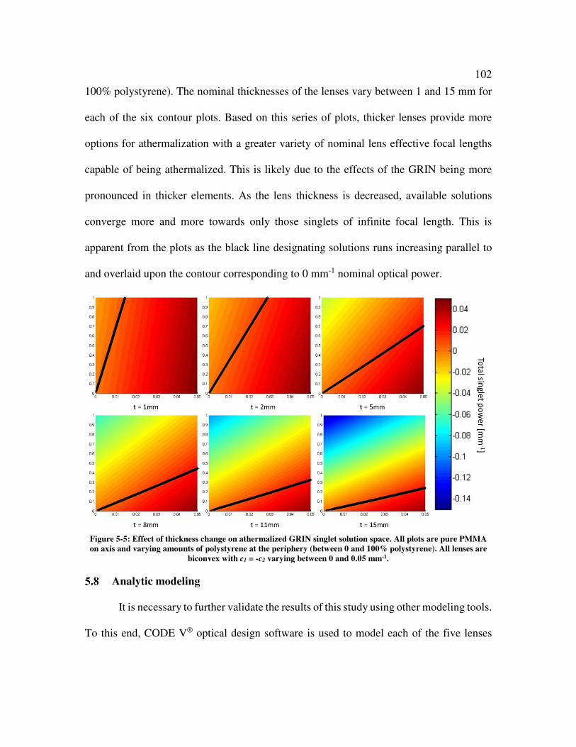
102

100% polystyrene). The nominal thicknesses of the lenses vary between 1 and 15 mm for

each of the six contour plots. Based on this series of plots, thicker lenses provide more

options for athermalization with a greater variety of nominal lens effective focal lengths

capable of being athermalized. This is likely due to the effects of the GRIN being more

pronounced in thicker elements. As the lens thickness is decreased, available solutions

converge more and more towards only those singlets of infinite focal length. This is

apparent from the plots as the black line designating solutions runs increasing parallel to

and overlaid upon the contour corresponding to 0 mm-1 nominal optical power.

Figure 5-5: Effect of thickness change on athermalized GRIN singlet solution space. All plots are pure PMMA

on axis and varying amounts of polystyrene at the periphery (between 0 and 100% polystyrene). All lenses are

biconvex with c1 = -c2 varying between 0 and 0.05 mm-1.

Analytic modeling

It is necessary to further validate the results of this study using other modeling tools.

To this end, CODE V® optical design software is used to model each of the five lenses

103

before and after the temperature increase. Changes to the lens geometry and index profile

are calculated using the methods discussed earlier in this work. Once the specifications for

each lens are entered into CODE V®, it is possible to monitor the change in a number of

performance metrics over the +40°C temperature change. Because EFL is the only

parameter being directly controlled by the model, other metrics are not analyzed in this

study. The effective focal length values calculated by CODE V® are found to match those

values calculated by the MATLAB model.

The results of this study are summarized in Table 5-2 which tabulates both the

nominal and final EFLs of each of the five lenses. Note that the final column of the table

displays the percent change in EFL after the temperature increase. From Table 5-2, it is

apparent that the lens identified as athermalized by the model has exhibited a change in

EFL of less than one micron while the homogeneous lens 5 (predicted to be the least

athermalized of the group) has had an increase in EFL of almost one half-millimeter. This

is consistent with what is expected as the extra degrees of freedom inherent to the GRIN

singlet better enable it to maintain constant optical power over a temperature change than

a homogeneous element. Table 5-2 also confirms the predicted trend that lenses which are

farther away from the athermalized curve will exhibit a greater change in EFL for a given

change in temperature. The MATLAB code used in this section is available in Appendix I.

Table 5-2: Effect of +40°C temperature change on EFL for five lenses in athermalization study

Lens Nominal

EFL [mm] Final EFL

[mm] Change

[%]

1 50.000 50.000 0.000

2 50.000 50.117 0.234

3 50.000 50.235 0.470

104

4 50.000 50.354 0.708

5 50.000 50.475 0.950

Numerical modeling

While the first-order analysis of the system is useful, it is not a complete model.

The equations laid out in this paper only apply to quadratic radial GRIN profiles and cannot

account for aspheric surfaces on the GRIN lens. In order to address more complicated radial

GRIN systems, a numerical model is developed in MATLAB which treats a GRIN lens as

a series of differential rectangular elements stacked up parallel to the isoindicial surfaces.

One can think of this as a relatively simple finite element model. Each of these differential

rectangles is modeled as a homogeneous element, the summed effect of which accounts for

the overall change in the lens with a change in temperature as shown in Figure 5-6.

Equation 5.1 and Equation 5.2 are used to calculate the change in the axial and radial

thickness of an individual element respectively, while Equation 5.4 is used to calculate the

change in refractive index of an element. Once the changes in geometry and index are

calculated for each of the individual elements (1,000 are used for the studies in this chapter)

the surface sag departure can be fit to an arbitrary number of aspheric coefficients using

Equation 5.13 (the equation for the sag departure of an aspheric surface)

24 6 8

4 6 82 2( ) ...

1 1 (1 )

csz s A s A s A s

k c s= + + + +

+ − + (5.13)

where z is the sag departure of the surface for a given radial distance s away from the

optical axis, c is the curvature of the surface, k is the conic constant, and An are the nth order

aspheric coefficients [94].

105

Figure 5-6: Illustration of differential element model of lens.

It is not always sufficient to model the change in lens geometry as a simple change

in surface curvature as in Equation 5.6. Just as a temperature change can induce surface

curvatures in a nominally plano-plano Wood lens, the differential CTE across the aperture

of a radial GRIN element can cause the surface to take on an aspheric shape, rather than a

purely spherical one. While the previous method is limited to describing only purely

quadratic radial GRIN profiles (the first two terms of Equation 5.5), using the numerical

model, the index profile can be fit to an arbitrary number of coefficients of the index

polynomial. Equation 5.5 is often truncated in this regard at the sixth-order term (N30) to

be consistent with CODE V®’s default radial GRIN definition. For quadratic profiles, the

lens thickness, diameter, surface curvatures, and index profile change in accordance with

the analytic method described in the previous section.

As a general rule, the need to model an optical surface with aspheric coefficients

increases as surface curvature increases and as the magnitude of the change in temperature

increases. As one would expect, an optical surface departs more from a sphere post-

temperature change as the discrepancy between the CTEs of the two materials increases.

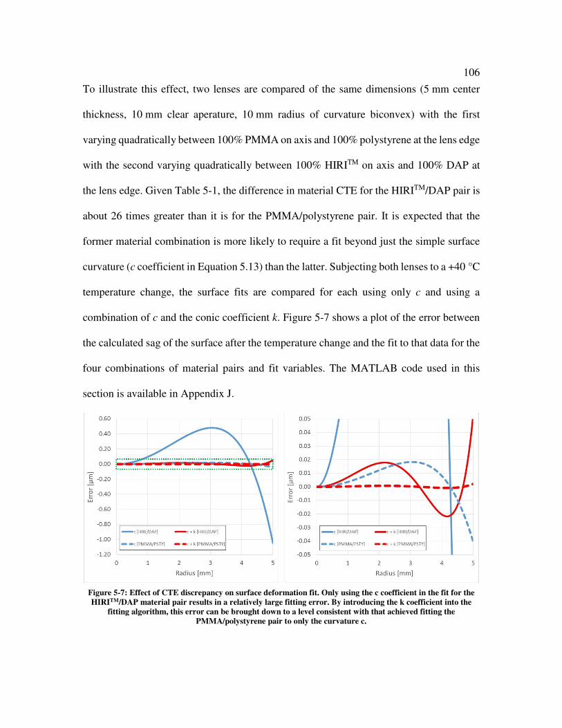
106

To illustrate this effect, two lenses are compared of the same dimensions (5 mm center

thickness, 10 mm clear aperature, 10 mm radius of curvature biconvex) with the first

varying quadratically between 100% PMMA on axis and 100% polystyrene at the lens edge

with the second varying quadratically between 100% HIRITM on axis and 100% DAP at

the lens edge. Given Table 5-1, the difference in material CTE for the HIRITM/DAP pair is

about 26 times greater than it is for the PMMA/polystyrene pair. It is expected that the

former material combination is more likely to require a fit beyond just the simple surface

curvature (c coefficient in Equation 5.13) than the latter. Subjecting both lenses to a +40 °C

temperature change, the surface fits are compared for each using only c and using a

combination of c and the conic coefficient k. Figure 5-7 shows a plot of the error between

the calculated sag of the surface after the temperature change and the fit to that data for the

four combinations of material pairs and fit variables. The MATLAB code used in this

section is available in Appendix J.

Figure 5-7: Effect of CTE discrepancy on surface deformation fit. Only using the c coefficient in the fit for the

HIRITM/DAP material pair results in a relatively large fitting error. By introducing the k coefficient into the

fitting algorithm, this error can be brought down to a level consistent with that achieved fitting the

PMMA/polystyrene pair to only the curvature c.

107

Because the CTE’s of PMMA and polystyrene are so close to one another, it is

likely sufficient in most applications to model the surface deformation as simple change in

radius of curvature. In the case of the HIRITM/DAP; however, the difference between the

calculated and fitted surface deformation is on the order of a micron at the edge of the lens.

It is only by introducing the conic coefficient into the fitting algorithm that the error drops

down to the order of tens of nanometers. While useful in certain applications, Equation

5.13 may not always be the best choice to fit surface deformation to depending on the shape

of the GRIN profile being modeled and it is useful to explore alternatives in the future for

radial and other GRIN geometries.

Conclusions and future work

The spatially-varying refractive index profile of a GRIN singlet makes it possible

to maintain a constant EFL over a change in temperature. Work is successfully carried out

to reproduce the first-order results of a previous student and extend the space of possible

solutions. A preliminary first-order design study comparing an athermalized polymer

GRIN lens to a number of other singlets of the same EFL validates the MATLAB model’s

ability to identify athermalized GRIN lenses. This work in the study of thermal effects on

GRIN systems shows potential for the possibility of athermalizing a single optical element.

A second model is also developed to more accurately model the effects of temperature on

radial GRIN lenses. Unlike the first-order model, this simplified finite element model is

able to treat elements with radial GRIN profile terms higher than only the quadratic term

and also elements with aspheric surfaces.

108

Practically speaking, when manufacturing polymer radial GRIN lenses such as

those discussed in this paper, it is necessary to account for the method of mounting in the

design process as the type of material used in the housing affects how the EFL changes

with temperature. Additionally, the method of mounting may cause stress in the element

so that the stress-induced birefringence of the element must also be monitored if such

elements are to be used as part of a real optical system.

109

Chapter 6. Thermal Interferometry

Introduction

An important consideration in the design of any optical system is how that system

behaves when subjected to a temperature change. As the temperature of an optical system

is increased or decreased, both its physical dimensions as well as its index of refraction

change according to that material’s linear coefficient of thermal expansion (CTE) and

temperature-dependent refractive index coefficient (dn/dT) respectively. The dimensional

change due to the CTE, α, is

( )1' ,TL L α+ ∆= (6.1)

where L’ is the dimensional size after a change in temperature ΔT while L is the

dimensional size for ΔT = 0 From Equation 6.1, the additional length of the sample (ΔL) is

given by

.L L Tα∆ = ∆ (6.2)

The vast majority of materials have CTEs that are positive in sign such that an

increase in temperature corresponds to an increase in sample length. Most metals have CTE

values between 10 and 20 parts per million per degree Celsius (x10-6/°C) while most

plastics are about an order of magnitude greater [28]. NBK7, a standard crown optical

glass, has a nominal CTE of about 7.1 x10-6/°C while Zerodur®, a glass ceramic

characterized by its very low expansion, has a nominal CTE of 0 x10-6/°C between 0 and

50 °C [95]. It should be noted that although CTE is often quoted as a single number, the

dimensional change is not completely linear with temperature for most materials, meaning

110

the value of the instantaneous CTE is different over different temperatures ranges for the

same material.

The refractive index of a material after a temperature change is

0'00 0 ,

dnN T

dN

T

= + ∆

(6.3)

where N00 is the initial index of refraction, corresponding to ΔT = 0 [96]. Values of dn/dT vary

significantly from material to material in both magnitude as well as in sign. Most optical glasses

have dn/dT values between 0.1 and 5 x10-6/°C and are found to be either positive or negative in

sign while optical polymers such as PMMA or polystyrene are orders of magnitude greater with

dn/dT on the order of -60 to -100 x10-6/°C [92]. Just as the base index of refraction of an optical

material varies with wavelength, dn/dT values do as well. To fully characterize the behavior of the

index of refraction of an optical material, dn/dT must be measured for a number of wavelengths

and over different temperature ranges. In this paper, an instrument is presented for the purpose of

measuring both CTE and dn/dT.

Interferometric techniques for measuring CTE and dn/dT have previously been published.

A number of interferometer geometries have been reported for the purpose of measuring CTE

including the Fizeau, Michelson, and Fabry-Perot among others [34]. Okaji, et al. report

measurements on the CTE of steel and ceramic gauge blocks over the temperature range between

-10 and +60°C [33]. Kuriyama, et al. later developed a ring interferometer system and compared

their measurements of the same samples’ CTE values against those measured by Okaji [97]. The

Ultra Precision Interferometer has been developed by Schödel, et al. to measure CTE down to 7 K

(-266.15°C) using three different stabilized lasers (λ = 780, 633, and 532 nm) [35]. This system has

111

since been used to measure silicon carbide ceramics, silicon nitride ceramics, and single crystal

silicon between 7 K and 300 K [98]. Dupouy, et al. measured the dn/dT of fused silica between 25

and 70°C using a Fabry-Perot interferometer [99].

It is possible to interferometrically measure both the CTE and dn/dT of a sample

simultaneously. Measurements of both thermal quantities for Nd:YAG laser rods as well as for

YAG laser rods have been reported [100, 101]. With both groups using a Fabry-Perot

configuration, Jewell, et al. measured CTE and dn/dT of vitreous silica and heavy-metal fluoride

glass samples between 25 and 100°C while Kazasidis and Wittrock measured both quantities for

both praseodymium-doped yttrium lithium fluoride (Pr:YLF) crystals and fused silica between 20

and 80°C [102, 103]. It should be noted that the vast majority of these systems that measure both

properties simultaneously do so with both arms of the interferometer in the same environmental

conditions and often in vacuum to avoid the issue of the index of air changing with temperature.

This chapter explores a method of interferometrically measuring CTE and dn/dT simultaneously

with the two arms of the interferometer in different environments.

Discussion of Instrument

6.2.1 Previous Generation

To measure both the CTE and dn/dT of an optical material, an interferometric technique is

employed with one arm of an interferometer extending into an environmental chamber capable of

cycling temperature. The sample to be measured is located inside of the environmental chamber.

During measurement, the temperature is changed.

The previous generation of this technique at the University of Rochester was designed and

built by McLaughlin, et al. using a Fabry-Perot interferometer [32]. The system was used to make

112

measurements of both homogeneous and gradient-index (GRIN) samples at a single wavelength

(λ = 632.8 nm). Specifically, it was used to validate the results of a model meant to determine the

thermal properties of GRIN glass [104]. It should be noted that for a Fabry-Perot system, cavity

finesse is an issue as only certain wavelengths are supported by the etalon. As the work was

conducted in the 1980s before CCD and CMOS detectors were cheaply available, a galvonometer

scanning system was used with a photodiode to make measurements of the full aperture of the

sample.

In 2012, McCarthy, et al. rebuilt the system using the original Fabry-Perot cavity used by

McLaughlin but included a CCD array to simultaneously image the full region of interest [36]. This

version of the interferometer placed the Fabry-Perot inside a convection oven with a window in the

door. Collimated light was sent through a beamsplitter and into the chamber where it was reflected

90° by a fold mirror into the Fabry-Perot etalon containing the sample under test. One issue with

using this interferometer configuration is that because the fold mirror was inside the chamber, it

was subjected to dimensional changes as the temperature was varied, resulting in a time-varying

image shift on the detector. This is detrimental because GRIN optics require the fringes to be

recorded from the same spatial location. For this reason, it was necessary to design the system to

have no fold mirror within the environmental chamber going forward. Additionally, the new

system was designed so that the piezo controller of the reference arm would not be located within

the chamber, great reducing any environmental effects on its motion.

6.2.2 Updated System

For the next-generation system, it is desired for the interferometer to have the ability to

make measurements at multiple wavelengths between the visible and mid-wave infrared (MWIR).

113

This eliminates a Fabry-Perot configuration because the finesse changes with wavelength or

requires prohibitively-expensive coatings for the cavity surfaces. Thus, a Twyman-Green

configuration is chosen for the next-generation interferometer due to the aforementioned finesse

issue as well as because of the significantly-decreased component cost for building the

interferometer. The system is designed to have easily-swappable optical components (windows,

imaging optics, etc.) to make taking measurements in different wavebands easier. In the visible,

both a HeNe laser and an Ar+ laser are coupled into the interferometer, allowing measurements at

a series of four wavelengths: 457, 488, 514.5 and 632.8 nm. To enable measurement of samples in

the MWIR, a λ = 3.39 μm HeNe laser is integrated into the system. When measuring in the MWIR,

it is necessary to switch out the lenses, windows, and beamsplitter for optics composed of CaF2 that

transmit at the desired wavelength. While all measurements reported in this thesis are carried out

at a wavelength of 632.8 nm, the system is capable of making measurements at these other

wavelengths to quantify the dispersion of dn/dT for a material and will be the subject of future

work.

The original desire for this instrument is to be able to make measurements between -40 and

+80°C; however, the actual range is limited due to decreased fringe stability at temperatures greater

than about +40°C and less than 0°C. For measurement, an Espec BTX-475 environmental chamber

is being used that is capable of cycling between -70 and +180°C. The main disadvantage for the

Twyman-Green configuration as compared to the Fabry-Perot is that the test and reference arms

are subjected to different environments (while the Fabry-Perot cavity had previously been entirely

located within the thermal environment). While the reference arm of the interferometer is in

ambient room temperature, the test arm is located within the environmental chamber. Because of

114

this, vibrations from the environmental chamber and air index fluctuations are detrimental to the

stability of the fringes being observed if not properly addressed.

To reduce vibrations, the optics are mounted above the chamber on a breadboard. This

breadboard is supported by four vibration-isolating feet that are mounted on a metal frame built

around the chamber. The metal frame and breadboard do not contact the environmental chamber

anywhere to minimize the coupling of vibrations into the test arm. Figure 6-1 shows a photograph

of the system as it exists in the laboratory. Note the aforementioned support frame surrounding the

chamber which in turn supports the vibration-isolating feet that support the breadboard.

Atop the breadboard are mounted the two HeNe lasers next to one another while the Ar+

laser sits on a separate shelf. The vibrations generated by the Ar+ laser’s cooling fan make it

impractical to mount it on the breadboard, which, in turn, makes it difficult to direct the beam to

the rest of the optics through free space. For that reason and to ease alignment between

wavelengths, both the Ar+ and visible HeNe lasers are fiber coupled to the same output through a

two-color combiner. Using a color-correcting doublet, the spatially-filtered and diverging beam is

then collimated. Through a series of fold/flip mirrors the visible HeNe beam is also coaligned to

the MWIR HeNe beam through free space. This makes it easier to align the MWIR beam. As

mentioned before, the collimating lens and all subsequent refractive optics must be switched for

CaF2 elements when measuring at this wavelength. For measurements at all wavelengths, once the

beam is collimated, it is then directed through two fold mirrors that send the beam down through a

hole in the breadboard.

115

Figure 6-1. Photograph of the thermal interferometer setup. Note meter stick on chamber for scale.

A four inch–diameter plate beamsplitter (fused silica for the visible and CaF2 for the

MWIR) is mounted directly underneath the hole in the breadboard. The beamsplitter mount is

attached to holes in the underside of the breadboard. Careful attention is paid to ensure that the

underside of the beamsplitter mount does not come in contact with the top of the chamber to avoid

the vibration-coupling issue. The reflection from the beamsplitter forms the reference arm of the

interferometer, parallel to the floor in the room. The fused silica beamsplitter was coated by

AccuCoat Inc. in Rochester, NY. The coatings for this beamsplitter are shown in Appendix K. The

reference mirror is mounted upon a piezo stage on the underside of the breadboard. This enables

phase-shifting during measurements. The beam that is transmitted downward through the

116

beamsplitter and into the chamber forms the test arm of the interferometer, perpendicular to the

floor in the room. In order to thermally-isolate the environments of the room and the chamber from

one another, a series of anti-reflection-coated windows are mounted within the mechanics of the

test arm (to be discussed in greater detail in a later section, along with the sample under test). The

windows are mounted inside of removable lens tubes that can be switched in and out depending on

the waveband of interest. For the visible, six 3 mm-thick float glass windows are used while for the

MWIR, three 6 mm-thick CaF2 windows are used. Different windows are used because of the

antireflection coatings. For the visible, the windows are specified to have an average reflectance of

less than 0.5% between 425 and 700 nm. Finally, the test mirror is mounted below the windows

inside of the chamber and parallel to the floor. The sample sits directly atop the test mirror.

A rail is mounted to the underside of the breadboard using a pair of magnetic bases and

right-angle mounts. This rail holds the imaging lenses as well as the visible detector: a Point Grey

Flea3 CMOS camera. The inclusion of the rail greatly eases the process of attempting to align the

imaging optics in the space between the breadboard and chamber. While the rail is also used to

carry the MWIR imaging optics, the MWIR detector, a FLIR a6700sc, is too large to be mounted

to the rail and must be mounted using a right-angle mount attached to the breadboard itself. Figure

6-2 shows a computer model of the interferometer to illustrate the location of the input collimated

beam, beamsplitter, reference arm, test arm, and imaging optics in relation to one another and the

Espec environmental chamber. Again, note that the reference and test arms are subjected to

different environmental conditions.

117

Figure 6-2: Model of the Twyman-Green interfereometer system as designed and built. The system is designed

to measure over a 2” aperture. The reference arm is located outside of the chamber whereas the test arm enters

the chamber through a port in the top of the chamber. Only the test arm is subjected to the change in

temperature. The reference arm remains at the temperature of the room. The sample under test sits directly

upon the test mirror inside of the environmental chamber.

Interferometric Measurements

6.3.1 Beam Paths

Because optical path length is the product of physical distance and index of refraction, a

method must be used whereby the user can distinguish the contribution of each to the optical path

difference (OPD) as the temperature is cycled. To make thermal measurements of a material using

this instrument, either two or three different sets of interferograms are analyzed concurrently. This

number is dependent upon the type of sample being measured with two sets of fringes being

necessary to measure the CTE of a reflective sample while three are required to measure both the

118

CTE and dn/dT of a transmissive sample. These three possible beam paths are denoted by OPDx

and are illustrated in Figure 6-3.

Figure 6-3. Side view of the beam paths within interferometer. The sample is shown resting upon the test mirror. The three

different OPDs can be used to compute CTE and dn/dT from background fluctuations.

OPD1 is the difference in optical path between just the reference mirror and the test mirror,

often referred to as the “background.” OPD2 is the difference in optical path between the reference

mirror and the top of the sample. For a reflective sample this is readily accomplished; however for

a transmissive sample, a coating of some kind must be applied to the sample to make a region of

the sample’s aperture reflective. This is accomplished by coating half of the aperture with

approximately 50 nm of gold using a Denton sputter coater. OPD3 is the difference in optical path

between the reference mirror and the test mirror but having traveled through the sample as well.

These are represented by

( ) ( ) ( )1 2 ,air

T nO PD T z T= (6.4)

( ) ( ) ( ) ( )( )2 2 , a n da irT n T z T LP TO D = − (6.5)

( ) ( ) ( ) ( )( ) ( ) ( )3 2 2 ,sa i rT n T z T L T n T TO P D L= − + (6.6)

where z is the physical distance between the test mirror and some height above the sample, L is the

thickness of the sample, nair is the index of refraction of the air, and ns is the index of refraction of

the sample. All of these variables are a function of temperature, T. All of these interferograms are

119

recorded simultaneously by imaging the collimated beam onto the CMOS detector. Because the

phase is tracked as a function of spatial coordinate, this technique can be used to see how CTE and

dn/dT vary across the aperture of a GRIN material. Often for an interferometric measurement, the

user is interested in observed OPD across a sample. For this instrument, the metric of interest is the

change in those OPDs as a function of time. The change in observed OPDx over time is denoted as

dOPDx.

6.3.2 Data Acquisition

To measure the thermal characteristics of a sample, both surfaces must be polished so that

the sample is optically flat with minimal wedge between surfaces. Before being placed inside of

the instrument, the samples and mirror are thoroughly cleaned to ensure better contact between

sample and mirror. In the current instrument, samples up to approximately 20 mm thick and 35 mm

in diameter can be measured. To accomplish phase-shifting in this interferometer, the reference

mirror is mounted on a Thorlabs NFL5DP20S piezo stage with a TPZ001 T-cube controller unit.

Phase maps are generated using the least-squares algorithm [105]. This method requires that the

piezo stage move through a full 2π cycle while images of the fringes are periodically recorded and

used to calculate the individual phase map. Calibration of the driving voltage required to achieve a

single cycle is carried out by recording the intensity of a series of pixels as the voltage is ramped

through a number of cycles. Figure 6-4 shows an example of this process with pixel intensity

plotted as a function of applied voltage from the piezo controller. The blue squares are the measured

data while the red dotted line is the sinusoidal fit to that measured data. The black circles in the plot

show the voltage values required to carry out the algorithm, in this case 25.

120

Figure 6-4: Pixel intensity as a function of applied voltage from the piezo controller

Twenty-five steps are found to give the best mixture of speed of acquisition and accuracy. This

high number of steps is due to the vibration of the fringes observed in the system. Figure 6-5 shows

a comparison between phase maps generated using a varying number of phase steps. The four-step

algorithm is a common choice in literature, while an 11-step algorithm is used by McCarthy in the

fabrication of a number of Mach-Zehnder interferometers; however, these algorithms are not

sufficient for the thermal interferometer due to fringe stability [106]. This is apparent in Figure 6-5,

showing each full two dimensional phase map alongside a horizontal cut through of the data. The

wrapped phase data for the 25-step algorithm is significantly smoother than that of either the 4 or

11-step algorithms and is very similar to that of a 250-step algorithm plotted for reference.

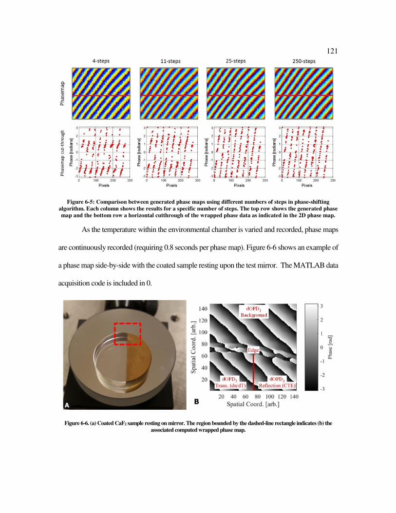
121

Figure 6-5: Comparison between generated phase maps using different numbers of steps in phase-shifting

algorithm. Each column shows the results for a specific number of steps. The top row shows the generated phase

map and the bottom row a horizontal cutthrough of the wrapped phase data as indicated in the 2D phase map.

As the temperature within the environmental chamber is varied and recorded, phase maps

are continuously recorded (requiring 0.8 seconds per phase map). Figure 6-6 shows an example of

a phase map side-by-side with the coated sample resting upon the test mirror. The MATLAB data

acquisition code is included in 0.

Figure 6-6. (a) Coated CaF2 sample resting on mirror. The region bounded by the dashed-line rectangle indicates (b) the

associated computed wrapped phase map.

122

After temperature cycling is complete, the phase maps are unwrapped as a function of time

and therefore temperature. By unwrapping the three regions of interest, the change in piston for

OPD1, OPD2, and OPD3 is determined. It is necessary to compare the relative amounts of phase

accumulated by each of the three beam paths to determine the CTE and dn/dT of the material.

6.3.3 Athermalization of the test arm

Just as the optical sample being measured expands or contracts in accordance with its CTE,

so does the housing of the optical windows (shown in Figure 6-2) that connects the beamsplitter

to the test mirror. Because of this, the height of the test mirror changes with temperature. This

change in the height of the test mirror affects the measurements of all three beam paths’ change in

piston, as all three are affected by a global change in height of the test mirror. The change in height

of the test mirror, along with changes to the index of air within the chamber contribute a change in

optical path to OPD1. This change in the optical path difference is designated as dOPD1. In addition

to this, the index of refraction of the windows within the test arm changes as well in accordance

with the dn/dT of the windows. Minimizing the effects of these contributions is necessary to

increase the accuracy of this instrument. It should be noted that dOPD1 is also affected by the

changing index of air and changing physical length of the interferometer’s reference arm; however,

since this arm is outside of the chamber and shielded from temperature changes with insulation,

this effect should be minimal compared to that on the test arm.

This issue is more commonly known as thermal drift and is common to the majority of

opto-mechanical designs. A standard method of correcting this issue is passive athermalization

where sets of rods or spacers of different lengths and materials are integrated into the system

housing [107]. Their differing lengths and CTEs are meant to counteract one another to compensate

123

for the image plane shifting with temperature. In this system, there are two sets of three rods

forming the mount of the test mirror: longer rods of low-CTE invar to form the forward direction

of the thermal circuit and shorter rods of higher-CTE aluminum to form the backward direction of

the thermal circuit. The mount for the test mirror rests on three adjustable stainless-steel screws, the

presence of which allows the user to change the amount of material in the backward direction of

the thermal circuit in the pursuit of locating the height of the test mirror for minimal change with

temperature. Figure 6-7 shows an image of the test arm extended down into the environmental

chamber.

Figure 6-7. Photograph of the interferometer test arm inside the thermal chamber. The lengths of the invar and aluminum

rods were chosen to minimize the drift of the sample location as a function of temperature.

It is important to note that all of the materials that compose the test arm must be

incorporated into the thermal drift model. Data for the CTE of the materials and the index of air as

a function of temperature are estimated based on NIST values [108, 109]. Figure 6-8 shows two

124

measurements of the change in optical path length of the background (dOPD1) as a function of

temperature. It should be noted that each measurement is relative to its starting measurement (at

the colder temperature) which is set to be 0 μm. These optical path length changes take place over

the course of about 10-12 hours and are readily trackable.

Figure 6-8. Plots of the change in optical path difference as a function of temperature for two measurements of background

fringes. The differences in materials (invar versus aluminum and steel) comprising the test arm make the background motion

less sensitive to thermal fluctuations.

Results

6.4.1 Thermal measurement considerations

The environmental chamber introduces a noisy environment for the instrument from both

vibrations and thermal currents. As mentioned above, the optical instrument is mechanically

decoupled from the environmental chamber with a set of pneumatic active vibration isolating feet.

Further strategies are also implemented to mitigate vibrations, such as identifying the sources of

excitation, investigating the system's natural frequencies, and passively damping the test arm.

Vibrations are mainly an issue when making measurements below 0°C as the chamber’s fan and

compressor make generating high-quality phase maps difficult. Ultimately, for these lower

temperature ranges, the best method is to adopt a measurement procedure which allows for the

125

chamber to be turned off during data collection. When the chamber is operating colder than

ambient, thermal currents are not an issue as the cold air remains inside the chamber. At elevated

temperatures, the hot air inside the chamber tends to rise out of the hole in the chamber. Special

attention is required to direct this turbulent air away from the instrument's optical path.

6.4.2 Steel Sample measurement

Several optical-grade samples are coated for use in the thermal interferometer including

steel, ZrO2, CaF2, sapphire, and Zerodur®; however, currently the only certified samples for their

thermal characteristics are a set of Mitutoyo steel and ZrO2 gauge blocks ranging in thickness from

1.2 mm to 20 mm. The steel gauge blocks are certified to be Grade 00 according to ASME B89.1.9-

2002 and are also NIST-traceable. The steel gauge blocks are all certified to have a CTE value of

10.8±0.5 x10-6/°C at a temperature of 20°C. As a preliminary measurement using the

interferometer, the 20 mm-thick steel gauge block is measured between 10 and 30°C (for a ΔT of

20°C). The changes in piston of the two paths of note in this case (dOPD1 and dOPD2) are tracked

throughout the measurement. These are used together along with the measured air temperature

within the chamber to determine the change in thickness of the steel sample.

It should be noted that the accuracy of the CTE measurement is directly related to the

accuracy of the measurement of the sample’s initial thickness. An n-percent error in measuring the

initial sample thickness will yield roughly an n-percent error in calculated CTE. Initial sample

thickness is measured using a micrometer accurate to ±1 μm. This contribution to the error is thus

very small for a 20 mm sample, in this case being approximately 0.005%.

The results of the steel measurement are shown in Figure 6-9 where the measured change

in thickness is plotted as a function of temperature along with the linear fit to the data. This linear

126

fit is used to calculate the CTE of the material over the indicated temperature range. By utilizing a

rearranged Equation 6-2 to solve for α, L is the nominal thickness of the sample being measured

(20 mm) while the term ΔL/ΔT can be taken to be the slope of the linear fit to the data shown in

Figure 6-9. Using this, the linear CTE is found to be 10.65 x10-6/°C at 20°C which is well within

the error bars specified by the manufacturer at 20°C. This methodology is used in all cases to extract

CTE and dn/dT values from measured data. The MATLAB data analysis code is included in

Appendix M. The maximum deviation between the measured data and the linear fit is 47 nm while

the average value of the deviation is 11 nm.

Figure 6-9. Measured change in thickness of 20 mm-thick steel gauge block for ΔT = 20°C with the difference between the fit

and measured data plotted on the secondary axis. The measured CTE for this gauge block was 10.65 x10-6/°C at 20°C.

Figure 6-10 shows the results of a measurement of the steel gauge block over a larger

temperature range. In this case, the CTE is calculated and plotted over a series of ten-degree

increments. These data represent a single measurement run of the sample. The maximum value of

the error bars is ±0.1 x10-6/°C. This plot also shows Mitutoyo’s measurement of the nominal value

of the CTE along with the associated measurement error bars. Finally, Figure 6-10 displays the

results of Okaji’s measurements of four 100 mm-thick Mitutoyo steel gauge blocks.

127

The largest source of error in a single measurement comes from variation between the

tracked dOPD1 and dOPD2 paths by different pixels on the detector. For this measurement, that

value is ±0.09 x10-6/°C. Also of note is that a thermal gradient exists within the chamber between

the top and bottom of the sample. Temperature is measured using a 12-channel Omega

RDXL12SD with a measurement resolution of 0.1˚C. For the 20 mm-thick steel sample this

difference in temperature is measured as high as 0.7˚C. Hardware improvements have reduced this

discrepancy to less than 0.1˚C over the course of a measurement. Comparing a measurement of

this same steel sample where the maximum thermal gradient is reduced from 0.7 to 0.1˚C

corresponds to a reduction in the measurement error bars (calculated purely due to this temperature

gradient) from ±0.25 to ±0.05 x10-6/°C.

Figure 6-10. Measurement of 20 mm-thick steel gauge block CTE along with the reference data from the manufacturer and

previously reported Okaji data[33]. Note that the samples measured by Okaji are 100 mm-thick.

6.4.3 ZrO2 Measurements

Zirconium dioxide (ZrO2) or zircon, is a ceramic noted for its high mechanical

strength and fracture toughness. An 18 mm-thick Mitutoyo gauge block of this material

has been acquired for CTE measurement. The gauge block is certified to have a CTE value of

9.3±0.5 x10-6/°C at a temperature of 20 °C. It appears white as shown in Figure 6-11 alongside

128

a steel gauge block. It should be noted that the thermal interferometer is still capable of

measuring the CTE of this sample, despite the ZrO2 sample’s reduced reflectance as

compared to the steel samples. Figure 6-12 shows the results of measuring and calculating

the CTE of this sample in five degree increments. The measurement shows agreement with

the CTE certification.

Figure 6-11: Steel (left) and ZrO2 (right) samples

Figure 6-12: Measurement of CTE of ZrO2 sample in five degree increments

6.4.4 CaF2 Measurement

The interferometer is used to measure a CaF2 sample as well. Figure 6-13 and Figure 6-14

show the measurements of the CTE and the dn/dT of the sample respectively. Overlaid upon the

129

CTE results are those of Cardinali, et al. as well as Corning [110, 111]. Figure 6-14 shows the

results from these same sources for dn/dT with additional results from NASA’s Cryogenic High-

Accuracy Refraction Measuring System (CHARMS) system [112]. It should be noted that for

dn/dT, Corning’s measurements are carried out at a wavelength of 656 nm, not 632.8 nm. The

plotted data is the result of five separate measurements of the sample. Uncertainty is based on the

variation between measurements rather than the uncertainty of any one trial. For the CTE

measurement, the maximum uncertainty is ±0.4 x10-6/°C while for dn/dT the maximum

uncertainty is ±0.9 x10-6/°C.

Figure 6-13. Comparison of CaF2 CTE measurements between Rochester and literature values [110, 111].

130

Figure 6-14. Comparison of CaF2 dn/dT measurements between Rochester and literature values [110-112]. Note that

Corning’s dn/dT measurement was carried out at 656 nm rather than 632.8 nm.

6.4.5 Zerodur Measurements

Invented by Schott in 1968, Zerodur® is a glass ceramic valued for its near-zero CTE over

a wide temperature range. This property makes it very attractive in the fabrication of space-based

telescope systems among other applications requiring minimal change with temperature. A

25.4 mm-diameter, 14.1 mm-thick cylindrical Zerodur® sample having λ/20 surface flatness is

measured. The vendor states its CTE to be 0±0.1 x10-6/°C which is consistent with Schott’s listing

of Zerodur® Expansion Class 2 between 0 and +50 °C [113]. Figure 6-15 and Figure 6-16

respectively show the results of measuring the CTE and dn/dT of the Zerodur® sample

between -10 and +60 °C. In both cases the data is plotted against that reported by Schott. The

plotted data is the result of ten separate measurements of the sample. As for the CaF2 measurement,

uncertainty is based on the variation between measurements. For the CTE measurement, the

maximum uncertainty is ±0.3 x10-6/°C while for dn/dT the maximum uncertainty is ±0.4 x10-6/°C.

The red dotted lines in Figure 6-15 indicate the bounds of uncertainty in the measurement of the

131

CTE of Expansion Class 2 Zerodur®. These bounds are consistent with the results of other groups.

Figure 6-16 shows data reported by Schott on the dn/dT of the material. No error bars are reported.

Note that the Schott measurement is carried out at a wavelength of 656.3 nm. The Rochester CTE

data appears to show a bias of approximately -0.1 x10-6/°C in the measurement range between 0

and 50°C. It is possible this bias exists in all aforementioned instrument measurements but is not

easily observable from the samples above since the quoted error bars are so much greater.

Additionally, the nominal CTE values are much greater than 0 x10-6/°C, yielding a significant

distinction between dOPD1 and dOPD2 and increasing the signal to noise ratio in the measurement.

Figure 6-15: Comparison of Zerodur® CTE measurements between Rochester and literature values from

Schott.

132

Figure 6-16: Comparison of Zerodur® dn/dT measurements between Rochester and literature values from

Schott. No error bars were given in the literature. Note that the Schott data is measured at a wavelength of

λ = 656.3 nm

6.4.6 Sapphire measurement

A 5 mm-thick, 25.4 mm-diameter sapphire window (Thorlabs WG31050) is

acquired and coated with gold for the purpose of measurement. The CTE of the sample is

reported by the vendor to be 5.3 x10-6/°C [114]. Neither error bars nor a range of

temperatures of measurement is reported. The same reference stating the CTE also quotes

a dn/dT value of 13.1 x10-6/°C; however, this value is for a reference wavelength of

546 nm. After direct correspondence, the vendor’s best estimate of the dn/dT of the

material at the measurement wavelength of 632.8 nm is quoted as 12.6 x10-6/°C. The

results of measuring the CTE and dn/dT of the sapphire sample are shown in Figure 6-17

over the range between 10 and 40 °C with individual measurements between 10 and 20°C,

20 and 25°C, and 28 and 40°C.

133

Figure 6-17: Results of measurement of CTE (left) and dn/dT (right) of sapphire sample.

Polymer Measurements

In the previous chapter, a model to determine how a radial GRIN element behaves

with a temperature change was developed. As mentioned, it was assumed in this model that

both the CTE and dn/dT of the element vary linearly with material composition. In order

to validate this assumption, a series of copolymer samples of varying ratios of PMMA and

polystyrene were fabricated and measured in the thermal interferometer. This series of 11

total samples is named JC022-X where X ranges between one and eleven.

The eleven samples of JC022 are copolymerized following the monomer

preparation method laid out by Fang and Schmidt in fabricating axial GRIN profiles [73].

Both the MMA and styrene liquid monomer volumes are separately filtered in order to

remove any substances and impurities that would inhibit the reactions. During

polymerization, a liquid monomer shrinks in size as it becomes a solid polymer in a process

known as volume reduction. A set of experiments in which test tubes of liquid monomer

are photographed once every five minutes during polymerization over time determines that

MMA monomer reduces to 81% of its initial volume after polymerization to PMMA with

134

that same metric being 87% going from styrene to polystyrene. The two monomers are

measured out in quantities so that each of the eleven final samples are of a set ratio of

PMMA and polystyrene by volume in increments of 10 % and have a final volume of

approximately 10 mL. This is summarized in Table 6-1. This shows the calculated solid

volumes of both PMMA and polystyrene necessary for each sample. These values are used

to calculate the volumes of liquid MMA and styrene mixed together for each sample.

Table 6-1: Summary of JC022 samples

JC022-X Fraction

polystyrene Volume PMMA

Volume polystyrene

Polymer Volume

Volume MMA

Volume styrene

Monomer volume

1 0 10.02 0.00 10.02 12.40 0.00 12.40

2 0.1 8.97 1.00 9.97 11.10 1.15 12.25

3 0.2 8.00 2.00 10.00 9.90 2.30 12.20

4 0.3 7.03 3.01 10.04 8.70 3.46 12.16

5 0.4 5.98 3.99 9.97 7.40 4.58 11.98

6 0.5 5.01 5.01 10.02 6.20 5.76 11.96

7 0.6 4.04 6.06 10.10 5.00 6.97 11.97

8 0.7 2.99 6.98 9.97 3.70 8.02 11.72

9 0.8 2.02 8.08 10.10 2.50 9.29 11.79

10 0.9 0.97 8.73 9.70 1.20 10.03 11.23

11 1 0.00 10.00 10.00 0.00 11.49 11.49

Each samples’ monomer quantities are measured and mixed in separate test tubes.

The samples are copolymerized in the 14.4 mm inner diameter test tubes in a water bath

held at a constant temperature of 60 °C. Due to limited space, the samples are polymerized

in two batches with the odd-numbered ones first followed by the even-numbered samples

about 52 hours later. The time to copolymerization is measured by analyzing a series of

photographs taken once every five minutes. The results are summarized on the secondary

axis of Figure 6-18. Note that the results are largely linear with composition until the 90%

135

polystyrene sample (JC022-10). It is of interest for future work to fabricate a series of

samples between JC022-10 and 11 in composition and investigate each of their

copolymerization times.

After being copolymerized, the samples, now solid, are placed inside of a

convection oven for post-cure. This process is meant to finalize the reaction by using up

any residual initiator molecules left in the samples. From here, the samples are removed

from the glass test tubes sectioned using an Isomert saw and polished by hand. The index

of refraction of each sample is measured at a wavelength of 532 nm using a Pulfrich

refractometer as shown in Figure 6-18. The index at this wavelength is shown to be linear

with composition. Each of the eleven samples is measured ten times on the refractometer

with the standard deviation of each set taken to be the measurement error for that sample

with values ranging between 0.00015 and 0.00077.

Figure 6-18: Index of refraction (λ=532 nm) and time to volume reduction as a function of composition for

PMMA/polystyrene copolymers.

136

It is determined that the available hand polisher is insufficient for polishing the

copolymer samples to the surface figure and wedge for measurement in the thermal

interferometer. As such, they are sectioned to discs between 2.7 and 2.8 mm-thick and sent

to Syntec Optics in Rochester, NY to be diamond turned to a final thickness of 2.5 mm

with 5 μm parallelism, 2 fringes of surface figure, and between 70 and 100 Å surface

roughness. Once returned, the samples are given the gold coating mentioned in the

discussion of previous samples at the University of Rochester’s Nanosystems Center.

With their smaller diameters (14.4 mm), the samples are measured in pairs in the

thermal interferometer. The temperature of the chamber is programmed to ramp between

2.5 and 37.5°C linearly over the course of 13 hours. For these measurements, it is found

that at temperatures outside of this range, the fringes are unstable. At the lower

temperatures, the chamber’s compressor became active causing the fringes to shake and

leading to errors in the generated phase maps. The increased magnitude of fringe vibration

and thermal gradient introduced in the test arm while measuring at higher temperatures

also resulted in errors in the calculated phase maps.

The results of measuring all eleven samples over the full temperature range of 5 to

35 °C are shown in Figure 6-19 where both the measured CTE and the measured dn/dT are

plotted as a function of copolymer composition. Note that each data point is a separate

measurement of the same sample with the 0, 0.1, 0.4, 0.6, and 0.9 polystyrene samples each

having multiple measurements in an attempt to illustrate the repeatability of these particular

high-value CTE and dn/dT measurements. In Appendix N, the data for the two parameters

137

as calculated over four different temperature ranges: between 5 and 15 °C, 15 and 25 °C,

25 and 35 °C, and finally the full 5 and 35 °C is summarized.

Figure 6-19: CTE and dn/dT as a function of composition for PMMA/polystyrene copolymers. The parameters

are calculated over the full range between 5 and 35°C. The solid red lines indicate the range of reported values

for homogeneous PMMA and polystyrene

Reported measurements of the CTE and dn/dT of both PMMA and polystyrene and

polymers in general vary dramatically between references. The CTE of PMMA are

reported to be between 50 and 90 x10-6/°C while that of polystyrene between 50 and

80 x10-6/°C with the majority of reports for both polymers between 60 and 75 x10-6/°C [92,

115-117]. The dn/dT of PMMA is reported to be between -85 and -105 x10-6/°C while that

of polystyrene is between -104 and -140 x10-6/°C. Measurements of both parameters using

the thermal interferometer fall within this reported range. These bounds are indicated in

Figure 6-19 for each of the two parameters and for each of the two homogenous polymers

with solid red lines.

138

Conclusions and future work

An interferometer has been developed for the purpose of simultaneously measuring both the

CTE and dn/dT of optical materials. It has been demonstrated that these measurements can be

carried out using an interferometer where each arm is subjected to a different environment and

without the need to pull vacuum on the sample. In this regard, this interferometer is believed to be

the first of its kind. Preliminary measurements on the CTE and dn/dT of a number of samples show

agreement with literature values made by manufacturers and other research institutions. It would

be of use to extend this system to the measurement of additional materials in order to better quantify

its range of operation and accuracy.

139

Chapter 7. Conclusions

Concluding remarks

The addition of gradient-index (GRIN) materials offers an opportunity to

significantly improve the optical performance of a lens system. Specifically, this thesis

focuses on GRIN elements of the radial geometry in which the isoindicial surfaces, the

surfaces of constant index of refraction, exist as a series of cylinders centered upon the

optical axis. For such an element, the index of refraction varies as a function of the semi-

aperture which in turn affects the chromatic properties of the lens. The GRIN profile

provides a second source of optical power to the lens with the first coming from the surface

curvatures. In addition to this, the profile variation with wavelength yields a second Abbe

number in a single element. These facts underlie the potential for a single radial GRIN

element to behave as a traditional homogeneous doublet by correcting chromatic

aberration.

The possibility to fabricate GRIN elements from a variety of materials including

optical and infrared chalcogenide glasses, ceramics, crystals, and polymers has been

discussed. Chapter 2 focused on the pairing of ZnS and ZnSe. The gases used in the

manufacturing process for this material are highly toxic and so the fabrication of this GRIN

has never been attempted at the University of Rochester. As a result, research efforts were

restricted to a series of design studies over the mid-wave infrared (MWIR) from 3-5 μm.

This range is of particular interest as over it, the GRIN Abbe number has a negative value.

Negative Abbe numbers have been shown to be useful in lens design as they can eliminate

the need for negative-powered elements under certain circumstances. Additionally, the

140

same-sign profile shape that works towards correcting color also works towards correcting

undercorrected spherical aberration. The ZnS/ZnSe GRIN was used in a series of design

studies comparing homogeneous and GRIN designs for simple singlets and doublets,

Petzval-like objective lenses, and finally, 3 and 5x zoom lenses. In all cases the GRIN

design showed significant imaging performance improvement over a homogeneous lens of

the same number of elements.

Chapter 3 catalogued a second series of design studies utilizing a material that could

be manufactured at the University of Rochester: a copolymer formed between polymethyl

methacrylate (PMMA) and polystyrene. The GRIN Abbe number is very dispersive over

this waveband with an Abbe number of approximately 9. Studies into singlet and doublet

designs and 2 and 10x zoom lens designs again show that the GRIN designs consistently

shows superior performance over their homogenous counterparts of the same number of

elements. Because CODEV® optical design software was unable to tabulate the Seidel

contributions to either axial or lateral color for GRIN materials as is, a macro was written

to perform these calculations using Buchdahl notation. Results supported the radial GRIN’s

ability to correct chromatic aberration.

Chapter 4 described attempts to manufacture the PMMA/polystyrene radial GRIN

material described in the previous chapter. Efforts were carried out using a centrifugal-

force method whereby both MMA and styrene monomer were copolymerized in a test tube

rotated at approximately 2000 rpm. The fabrication procedure as well as process challenges

such as monomer-to-polymer volume reduction and sample haze were described along with

the results of successfully-generated samples. The chapter concluded with a return to the

141

optical designs of Chapter 3 as a sixth-order profile manufactured in the laboratory was

applied to the 2x copolymer design. The study showed that while the manufactured profile

did not yield imaging performance as good as that of the optimized profile, it was better

than that of the analogous homogeneous design, largely because of the observed

corrections to chromatic aberrations.

The ability of a radial GRIN singlet to be achromatized raised the question of

whether or not it was possible to design such an element to instead be athermalized. This

issue was explored in Chapter 5, which introduces the reader to two material parameters:

the coefficient of thermal expansion (CTE) and temperature-dependent refractive index

(dn/dT). Respectively, these dictate how the geometry and index of refraction of an optical

element change with temperature. To expand the solution space first explored by a previous

student, a first-order model programmed in MATLAB was described for the purpose of

identifying athermalized radial GRIN singlets with spherical surfaces and quadratic

profiles. From here, a more advanced finite-element-like model was developed, capable of

treating higher-order radial profiles and more complete surface shapes such as aspheres.

The model showed that a radial GRIN element with nominally-spherical surfaces and a

large discrepancy in CTE as a function of space can become non-spherical with a change

in temperature.

Chapter 6 described the design, construction, and operation of an interferometer for

the purpose of simultaneous measurement both CTE and dn/dT. A discussion of other

institutions’ efforts to measure either or both of these parameters interferometrically was

presented. The Rochester instrument was a Twyman-Green interferometer with the test

142

arm extended into an environmental chamber and the piezo stage-mounted reference arm

outside of the chamber. By tracking the change in piston with temperature for the three

regions of interest (reflection off of the test mirror, reflection off of the top of the sample

under test, and reflection off of the test mirror after having transmitted through the samples)

one can calculate both CTE and dn/dT. The system was used to measure these parameters

as a function of temperature for a number of materials including steel, ZrO2, CaF2,

sapphire, Zerodur, and different PMMA and polystyrene copolymers. Results agreed with

those published in literature.

Suggestions for future work

Based on the promising results of the design studies, future work should be carried

out to apply both the ZnS/ZnSe and PMMA/polystyrene GRIN materials to additional

design forms. Of special note are traditional design forms limited by chromatic aberration

such as the zoom lens systems discussed in this thesis as well as certain eyepiece designs

such as those explored by Visconti et al. [40]. It is useful to more fully map out such

solution spaces, determining what degree of performance improvement can be gained as

compared to homogeneous designs of an equivalent element count. Specifically for the

zoom lens designs, it is of interest to expand the design studies to forms of higher zoom

ratios. Finally, it would be useful to investigate how such systems perform over an

expanded wavelength range as simultaneous imaging over multiple wavebands (the dual-

band mid-wave/long-wave infrared for example) becomes more prevalent.

Further research should be pursued on the optimal methods of manufacturing both

of these GRIN materials. As mentioned before, safety issues prevented any on-site attempts

143

at fabricating a ZnS/ZnSe GRIN element. The design studies in Chapter 2 indicate that

there is great benefit to be gained from such a material for a company or other institution

with the infrastructure necessary to create one. Even the highest-quality

PMMA/polystyrene radial GRIN samples manufactured in the laboratory still suffer from

readily-observable haze. Although steps were taken to mitigate this specific effect, this is

believed to still be the result of the volume reduction process as the incoming monomer

still comes into contact with largely-copolymerized material at the feed end of the test tube.

This could potentially be curbed by designing a deformable monomer chamber in such a

way so that as the liquid volume does solidify and shrink, the encapsulating vessel does as

well to compensate, preventing the need to ever add additional monomer. This could

perhaps be accomplished with a plunger that is able to slide further into the test tube as it

rotates while still maintaining a tight seal on the monomer within. Successful attempts to

manufacture profiles with greater index changes and specifically tuned to the requirements

of a given optical design would make these materials much more viable from a commercial

standpoint.

It would be of great use to fully validate the thermal model of radial GRIN elements.

To do this, one could manufacture a series of copolymer elements and fully characterize

their surface shapes, thicknesses, and index profiles. From here, one could test each

interferometrically as a function of temperature to determine how the focal length or other

parameters each change and determine if those results match those predicted by MATLAB

and CODEV®. Such work could be carried out by modifying the existing thermal

144

interferometer for measuring CTE and dn/dT by replacing the flat test mirror with an

element matched to the nominal power of the lens under test.

Research using the current system for measuring both CTE and dn/dT could be

carried out by applying its use to additional samples of interest. Of particular use would be

to attain some samples with certified measurements of both CTE and dn/dT in order to

cross–check the accuracy of the instrument with the results of another system. As is, only

the CTE measurements for the steel and ZrO2 gauge blocks contained any certification (and

those are only at a single temperature). The range of measurable temperatures using this

instrument is limited, with measurements lower than approximately +5 °C suffering from

the issue of the chamber compressor switching on leading to numerous discontinuities in

the data. At temperatures higher than approximately 40 °C, the thermal gradient within the

test arm of the system again led to sometimes unreliable data. To address this, a second

system built by Bill Green is being pursued, designed to heat and cool a much smaller

volume for the test arm and using a temperature unit much less prone to vibration than the

Espec chamber. In general, the signal-to-noise ratio of the system would be improved by

again pursing a Fabry-Perot design which has much more stable fringes as the test and

reference arms are not subjected to differing environments. Measuring in vacuum would

also improve the accuracy significantly by eliminating the issue of needing to account for

the temperature and therefore index of refraction of the air at the sample plane in the final

calculations.

Note that the change in the refractive index of a material with temperature is also

dependent on the stress on that sample. This is represented mathematically by

145

'dn dn d

n n TdT d dT

σ

σ

= +∆ +

(7.1)

where σ is the stress on the sample under test. Measurements of dn/dT taken with the

current thermal interferometer ignore the effect of stress on the sample being tested. Thus,

the quantity actually being measured is that shown in the brackets in Equation 7.1. Future

work should include a method to decouple these effects from one another to isolate

measurement of the dn/dT term from the second term related to the stress. Additionally,

the hysteresis of measurements of both CTE and dn/dT should be quantified for the

copolymer materials.

146

References

1. Moore, D.T., Gradient-index optics: a review. Applied Optics, 1980. 19(7): p. 1035-1038.

2. Forer, J.D., et al., Gradient-index eyepiece design. Applied Optics, 1983. 22(3): p. 407-412.

3. Atkinson, L.G., et al., Gradient-index wide-angle photographic objective design. Applied Optics, 1984. 23(11): p. 1735-1741.

4. Atkinson, L.G., et al., Design of a gradient-index photographic objective. Applied Optics, 1982. 21(6): p. 993-998.

5. Goldenberg, J.F., J.J. Miceli, and D.T. Moore, Photocopy reduction arrays: design

and analysis. Applied Optics, 1985. 24(24): p. 4288-4296. 6. Kindred, D.S. and D.T. Moore, Design, fabrication, and testing of a gradient-index

binocular objective. Applied Optics, 1988. 27(3): p. 492-495. 7. Bowen, J.P., et al., Radial gradient-index eyepiece design. Applied Optics, 1988.

27(15): p. 3170-3176. 8. Rouke, J.L., et al., Design of three-element night-vision goggle objectives. Applied

Optics, 1998. 37(4): p. 622-626. 9. Visconti, A.J., et al., Eyepiece designs with radial and spherical polymer gradient-

index optical elements. Optical Engineering, 2013. 52(11): p. 112102-112102. 10. Sands, P.J., Inhomogeneous Lenses, IV. Aberrations of Lenses with Axial Index

Distributions. Journal of the Optical Society of America, 1971. 61(8): p. 1086-1091.

11. Wood, R.W., Refraction of Light, in Physical Optics. 1905, Macmillan: New York. p. 71-77.

12. Sands, P.J., Inhomogeneous Lenses, V. Chromatic Paraxial Aberrations of Lenses

with Axial or Cylindrical Index Distributions. Journal of the Optical Society of America, 1971. 61(11): p. 1495-1500.

13. Koike, Y., Y. Sumi, and Y. Ohtsuka, Spherical gradient-index sphere lens. Applied Optics, 1986. 25(19): p. 3356-3363.

14. Visconti, A.J., et al. All-Plastic High-Performance Eyepiece Design Utilizing a

Spherical Gradient-Index Lens. in Classical Optics 2014. 2014. Kohala Coast, Hawaii: Optical Society of America.

15. Ohmi, S., et al., Gradient-index rod lens made by a double ion-exchange process. Applied Optics, 1988. 27(3): p. 496-499.

16. Kindred, D.S., J.L. Bentley, and D.T. Moore, Axial and radial gradient-index

titania flint glasses. Applied Optics, 1990. 29(28): p. 4036-4041. 17. Houde-Walter, S.N. and D.T. Moore, Gradient-index profile control by field-

assisted ion exchange in glass. Applied Optics, 1985. 24(24): p. 4326-4333. 18. Visconti, A.J., D.T. Moore, and J.L. Bentley. Large Diameter Radial Gradient-

Index Lenses Fabricated by Ion Exchange. in Imaging and Applied Optics

Technical Papers. 2012. Monterey, California: Optical Society of America.

147

19. The Correct Material for Infrared (IR) Applications.; https://www.edmundoptics.com/resources/application-notes/optics/the-correct-material-for-infrared-applications/.

20. Pickering, M.A., R.L. Taylor, and D.T. Moore, Gradient infrared optical material

prepared by a chemical vapor deposition process. Appl. Opt., 1986. 25(19): p. 3364-3372.

21. Corsetti, J.A., P. McCarthy, and D.T. Moore, Color correction in the infrared using

gradient-index materials. Optical Engineering, 2013. 52(11): p. 112109-112109. 22. Moore, D.T. New Gradient-index Materials and Designs with Polymers, Glass and

ALON. in Imaging and Applied Optics Technical Papers. 2012. Monterey, California: Optical Society of America.

23. Bornstein, A., et al. Development Of IR Graded Index Elements. 1987. 24. Koike, Y., et al., Gradient-Index Polymer Materials and Their Optical Devices.

Polymer Engineering and Science, 1989. 29(17): p. 1200-1204. 25. Ji, S., et al., Polymeric nanolayered gradient refractive index lenses: technology

review and introduction of spherical gradient refractive index ball lenses. Optical Engineering, 2013. 52(11): p. 112105-112105.

26. Gardner, L.R., Studies in Gradient Index Polymer Materials, in The Institute of

Optics. PhD thesis. 1989, University of Rochester: Rochester. 27. Ye, C. and R.R. McLeod, GRIN lens and lens array fabrication with diffusion-

driven photopolymer. Optics Letters, 2008. 33(22): p. 2575-2577. 28. Doyle, K.B., V.L. Genberg, and G.J. Michels, Optothermal Analysis Methods, in

Integrated Optomechanical Analysis. 2012, SPIE Press: Bellingham, WA. 29. Corsetti, J.A., et al., Athermalization of polymer radial gradient-index singlets.

Optical Engineering, 2013. 52(11): p. 112104-112104. 30. Burge, J.H., T. Peper, and S.F. Jacobs, Thermal Expansion of Borosilicate Glass,

Zerodur, Zerodur M, and Uncer amized Zerodur at Low Temperatures. Applied Optics, 1999. 38(34): p. 7161-7162.

31. Lement, B.S., C.S. Roberts, and B.L. Averbach, Determination of Small Thermal

Expansion Coefficients by a Micrometric Dilatometer Method. Review of Scientific Instruments, 1951. 22(3).

32. McLaughlin, P.O. and D.T. Moore, Measurement of the differential thermal

expansion and temperature dependence of refractive index in gradient-index glass. Applied Optics, 1985. 24(24): p. 4334-4341.

33. Okaji, M., N. Yamada, and H. Moriyama, Ultra-precise thermal expansion

measurements of ceramic and steel gauge blocks with an interferometric

dilatometer. Metrologia, 2000. 37(2): p. 165. 34. James, J.D., et al., A review of measurement techniques for the thermal expansion

coefficient of metals and alloys at elevated temperatures. Measurement Science and Technology, 2001. 12(3): p. R1.

35. Schödel, R., et al., A new Ultra Precision Interferometer for absolute length

measurements down to cryogenic temperatures. Measurement Science and Technology, 2012. 23(9): p. 094004.

148

36. McCarthy, P., et al. Application of a Multiple Cavity Fabry-Perot Interferometer

for Measuring the Thermal Expansion and Temperature Dependence of Refractive

Index in New Gradient-Index Materials. in Imaging and Applied Optics Technical

Papers. 2012. Monterey, California: Optical Society of America. 37. Corsetti, J.A., et al., Simultaneous interferometric measurement of linear

coefficient of thermal expansion and temperature-dependent refractive index

coefficient of optical materials. Applied Optics, 2016. 55(29): p. 8145-8152. 38. Tsuchida, H., et al., Design of zoom lens systems that use gradient-index materials.

Applied Optics, 1992. 31(13): p. 2279-2283. 39. Deguchi, M., D.T. Moore, and D.S. Kindred. Zoom lens design using gradient-

index lenses. in Image Acquisition and Scientific Imaging Systems. 1994. Proc. SPIE.

40. Berman, R., et al. Optical design study of a VIS-SWIR 3X zoom lens. 2015. 41. Zhao, Y., et al. Chromatic correction for a VIS-SWIR zoom lens using optical

glasses. 2015. 42. Moore, D.T., Gradient-index optics: a review. Appl. Opt., 1980. 19(7): p. 1035-

1038. 43. Sands, P.J., Inhomogeneous Lenses, III. Paraxial Optics. J. Opt. Soc. Am., 1971.

61(7): p. 879-885. 44. Atkinson, L.G., et al., Design of a gradient-index photographic objective. Appl.

Opt., 1982. 21(6): p. 993-998. 45. Flynn, R.A., et al., Achromatic GRIN singlet lens design. Opt. Express, 2013. 21(4):

p. 4970-4978. 46. Wang, M., F. Châteauneuf, and C. Proulx. Optical designs of compact multichannel

and all-reflective system for infrared imaging. in Infrared Technology and

Applications XXXVII. 2011. Orlando, Florida, USA: Proc. SPIE 8012. 47. McDowell, M.W. and H.W. Klee, Achromatization in the 3 to 5μm spectral region

withvisible light transmitting materials. Optical Engineering, 1984. 23(2): p. 187-192.

48. Bociort, F., Chromatic paraxial aberration coefficients for radial gradient-index

lenses. J. Opt. Soc. Am. A, 1996. 13(6): p. 1277-1284. 49. Sands, P.J., Inhomogeneous Lenses, V. Chromatic Paraxial Aberrations of Lenses

with Axial or Cylindrical Index Distributions. J. Opt. Soc. Am., 1971. 61(11): p. 1495-1500.

50. Savage, L. The Birth - and Growth - of Glass Ceramics. Photonics Spectra, 2011. 51. Howard, J.W. and D.P. Ryan-Howard, Optical design of thermal imaging systems

utilizing gradient -index optical materials. Optical Engineering, 1985. 24(2): p. 263-266.

52. Mann, A., System Considerations, in Infrared Optics and Zoom Lenses. 2009, SPIE Press: Bellingham, Washington. p. 3-4.

53. Lidwell, M.O. Achromatism of lenses for thermal IR. in Optical Systems

Engineering IV. 1984. Cambridge: Proc. SPIE 518. 54. McCarthy, P. and D.T. Moore. Optical Design with Gradient-Index Elements

Constrained to Real Material Properties. 2012. Optical Society of America.

149

55. Smith, W.J., The Petzval Lens; Head-up Display Lenses, in Modern Lens Design. 2005, McGraw-Hill: New York.

56. Smith, G.H., Ultraviolet and Infrared Lenses, in Camera Lenses: From Box

Camera to Digital 2006, SPIE Press: Bellingham WA. 57. FLIR Systems, FLIR SC8000 HD Series. 2013;

http://www.flir.com/thermography/americas/us/view/?id=45674&collectionid=530&col=45863

58. Smith, W.J., Infrared and Ultraviolet Systems, in Modern Lens Design. 2005, McGraw-Hill: New York.

59. Corsetti, J.A. and D.T. Moore. Design of a ZnS/ZnSe Radial Gradient-Index

Objective Lens in the Mid-Wave Infrared. in Imaging and Applied Optics. 2013. Arlington, Virginia: Optical Society of America.

60. Mann, A., Refractive Infrared Zoom Lenses, in Infrared Optics and Zoom Lenses. 2009, SPIE Press: Bellingham, WA. p. 55-110.

61. FLIR Systems, I., Photon HRC. 2013. 62. Riedl, M.J., Thermal Effects, in Optical Design Fundamentals for Infrared Systems.

2001, SPIE Press: Bellingham, WA. p. 138-139. 63. Smith, W.J., Basic Optical Devices, in Modern Optical Engineering, R. Fishcher

and W.J. Smith, Editors. 1990, McGraw-Hill: New York. p. 275-277. 64. Systems, N.E.O., MWIR 50/250mm DFOV, F/4.0. 2013. 65. Smith, W.J., Zoom Lenses, in Modern Lens Design. 2005, McGraw-Hill: New

York. p. 543-545. 66. Koike, Y., et al., Graded-index plastic optical fiber composed of methyl

methacrylate and vinyl phenylacetate copolymers. Applied Optics, 1990. 29(18): p. 2686-2691.

67. Ishigure, T., E. Nihei, and Y. Koike, Graded-index polymer optical fiber for high-

speed data communication. Applied Optics, 1994. 33(19): p. 4261-4266. 68. Wu, S.P., E. Nihei, and Y. Koike, Large radial graded-index polymer. Applied

Optics, 1996. 35(1): p. 28-32. 69. Koike, Y., et al., Gradient-index contact lens. Applied Optics, 1995. 34(22): p.

4669-4673. 70. Koike, Y., H. Hidaka, and Y. Ohtsuka, Plastic axial gradient-index lens. Applied

Optics, 1985. 24(24): p. 4321-4325. 71. Koike, Y., et al., Spherical gradient-index polymer lens with low spherical

aberration. Applied Optics, 1994. 33(16): p. 3394-3400. 72. Schmidt, G.R., Polymer Tapered Gradient Index Lenses. PhD Thesis. 2009,

University of Rochester. 73. Fang, K., Design, Fabrication and Characterization of Polymer Gradient-Index

(GRIN) Material. PhD thesis. 2016, University of Rochester. 74. Visconti, A.J., et al., Design and fabrication of a polymer gradient-index optical

element for a high-performance eyepiece. Optical Engineering, 2013. 52(11): p. 112107-112107.

75. Bociort, F., Chromatic paraxial aberration coefficients for radial gradient-index

lenses. Journal of the Optical Society of America A, 1996. 13(6): p. 1277-1284.

150

76. McCarthy, P. and D.T. Moore. Optical Design with Gradient-Index Elements

Constrained to Real Material Properties. in Imaging and Applied Optics Technical

Papers. 2012. Monterey, California: Optical Society of America. 77. Corsetti, J.A., G.R. Schmidt, and D.T. Moore. Design and characterization of a

copolymer radial gradient index zoom lens. 2014. 78. Corsetti, J.A., G.R. Schmidt, and D.T. Moore. Axial and lateral color correction in

zoom lenses utilizing gradient-index copolymer elements. 2014. 79. Corsetti, J.A., G.R. Schmidt, and D.T. Moore. Axial and Lateral Color Correction

in Zoom Lenses Utilizing Gradient-Index Copolymer Elements. in Classical Optics

2014. 2014. Kohala Coast, Hawaii: Optical Society of America. 80. Youngworth, R.N., E.I. Betensky, and W.T. Plummer. The AWMC metric for zoom

lens assessment. 2012. 81. Nagaoka, T., Zoom lens system. 1999: United States. 82. Moore, D.T., Design of Singlets with Continuously Varying Indices of Refraction.

Journal of the Optical Society of America, 1971. 61(7): p. 886-894. 83. Moore, D.T. and P.J. Sands, Third-Order Aberrations of Inhomogeneous Lenses

with Cylindrical Index Distributions. Journal of the Optical Society of America, 1971. 61(9): p. 1195-1201.

84. Krishna, K.S.R. and A. Sharma, Chromatic aberrations of radial gradient-index

lenses. I. Theory. Applied Optics, 1996. 35(7): p. 1032-1036. 85. Im, S.H., et al., Fabrication of a graded-index polymer optical fiber preform

without a cavity by inclusion of an additional monomer under a centrifugal force

field. Applied Optics, 2002. 41(10): p. 1858-1863. 86. Cho, H., et al., Commercial scale fabrication method for fabricating a gradient

refractive-index rod: overcoming volume shrinkage and chemical restrictions. Applied Optics, 2006. 45(28): p. 7239-7247.

87. van Duijnhoven, F.G.H. and C.W.M. Bastiaansen, Monomers and polymers in a

centrifugal field: a new method to produce refractive-index gradients in polymers. Applied Optics, 1999. 38(6): p. 1008-1014.

88. Rogers, P.J. and M. Roberts, Thermal Compensation Techniques, in Handbook of

Optics, Volume I: Fundamentals, Techniques, and Design, M. Bass, Editor. 1995, McGraw-Hill, Inc.: United States. p. 39.7-39.13.

89. Bowen, J.P., et al., Radial gradient-index eyepiece design. Appl. Opt., 1988. 27(15): p. 3170-3176.

90. Smith, W.J., The Basics of Lens Design, in Modern Optical Engineering. 2008, The McGraw-Hill Companies, Inc.: United States. p. 430.

91. Wood, R.W., Refraction of Light in Physical Optics. 1905, Macmillan: New York. p. 71-77.

92. The Handbook of Plastic Optics. 2 ed. 1983, Cincinatti: U.S. Precision Lens. 93. Kingslake, R., Design of a Spherically Corrected Achromat, in Lens Design

Fundamentals. 1978, Academic Press: New York. p. 125. 94. Malacara, D. and D.T. Moore, Prisms and Refractive Optical Components, in

Handbook of Optical Engineering, D. Malacara and B.J. Thompson, Editors. 2001, Marcel Dekker, Inc.: New York. p. 143.

151

95. Thermal Expansion of Zerodur. http://www.us.schott.com/advanced_optics/english/download/schott-zerodur-cte-classes-may-2013-us.pdf.

96. Jamieson, T.H., Thermal Effects In Optical Systems. Optical Engineering, 1981. 20(2): p. 202156-202156-.

97. Kuriyama, Y., et al., Development of a New Interferometric Measurement System

for Determining the Main Characteristics of Gauge Blocks. CIRP Annals - Manufacturing Technology, 2006. 55(1): p. 563-566.

98. Middelmann, T., A. Walkov, and R. Schödel. State-of-the-art cryogenic CTE

measurements of ultra-low thermal expansion materials. 2015. 99. Dupouy, P.-E., et al., Interferometric measurement of the temperature dependence

of an index of refraction: application to fused silica. Applied Optics, 2010. 49(4): p. 678-682.

100. Foster, J.D. and L.M. Osterink, Index of Refraction and Expansion Thermal

Coefficients of Nd:YAG. Applied Optics, 1968. 7(12): p. 2428-2429. 101. Fan, T.Y. and J.L. Daneu, Thermal coefficients of the optical path length and

refractive index in YAG. Applied Optics, 1998. 37(9): p. 1635-1637. 102. Kazasidis, O.S. and U. Wittrock, Interferometric measurement of the temperature

coefficient of the refractive index dn/dT and the coefficient of thermal expansion of

Pr:YLF laser crystals. Optics Express, 2014. 22(25): p. 30683-30696. 103. Jewell, J.M., C. Askins, and I.D. Aggarwal, Interferometric method for concurrent

measurement of thermo-optic and thermal expansion coefficients. Applied Optics, 1991. 30(25): p. 3656-3660.

104. McLaughlin, P.O. and D.T. Moore, Models for the thermal expansion coefficient

and temperature coefficient of the refractive index in gradient-index glass. Applied Optics, 1985. 24(24): p. 4342-4348.

105. Schreiber, H. and J.H. Bruning, Phase Shifting Interferometry, in Optical Shop

Testing, D. Malacara, Editor. 2007, John Wiley & Sons, Inc.: Hoboken, NJ. 106. McCarthy, P., Gradient-Index Materials, Design, and Metrology for Broadband

Imaging Applications. PhD Thesis. 2015, University of Rochester. 107. Rogers, P.J. and M. Roberts, Thermal compensation techniques, in Handbook of

Optics: Fundamentals, Techniques, and Design, M. Bass, Editor. 1995, McGraw-Hill, Inc.: USA. p. 7-16.

108. NIST Material Measurement Laboratory. Cryogenics Technologies Group:

Material Properties. http://cryogenics.nist.gov/MPropsMAY/material%20properties.htm.

109. Stone, J.A. and J.H. Zimmerman. Index of Refraction of Air. Available from: http://emtoolbox.nist.gov/Wavelength/Documentation.asp.

110. Corning Specialty Materials. Corning® Calcium Fluoride (CaF2) - Code 9575. 2014; http://www.corning.com/media/worldwide/global/documents/Calcium%20Fluoride%20PI%20Sheet%20September%202014.pdf.

111. Cardinali, V., et al., Determination of the thermo-optic coefficient dn/dT of

ytterbium doped ceramics (Sc 2 O 3, Y 2 O 3, Lu 2 O 3, YAG), crystals (YAG, CaF

152

2) and neodymium doped phosphate glass at cryogenic temperature. Optical Materials, 2012. 34(6): p. 990-994.

112. Leviton, D.B., et al. Temperature-dependent refractive index measurements of

CaF2, Suprasil 3001, and S-FTM16 for the Euclid near-infrared spectrometer and

photometer. 2015. 113. Zerodur Zero Expansion Glass Ceramic.

http://www.us.schott.com/d/advanced_optics/d0384fa7-d94d-4247-9810-29790623a47e/1.0/schott_zerodur_katalog_july_2011_us.pdf.

114. Optical Substrates: Sapphire. https://www.thorlabs.us/newgrouppage9.cfm?objectgroup_id=6973&tabname=Sapphire.

115. Thermal Properties. http://www.m-ep.co.jp/en/pdf/product/iupi_nova/physicality_04.pdf.

116. Properties of Optical Plastic Materials. http://www.plasticoptics.com/optical-plastic-materials.html.

117. Plastic Optics: Specifying Injection-Molded Polymer Optics. https://www.photonics.com/EDU/Handbook.aspx?AID=25487.

153

Appendix A. Lens listing for 5x MWIR zoom lens – homogeneous

EFL = 250mm

RDY THI RMD GLA CCY THC GLC

> OBJ: INFINITY INFINITY 100 100

1: 97.18989 6.000000 SILICON_SPECIAL 0 0

SLB: "grin1"

ASP:

K : 0.000000 KC : 100

CUF: 0.000000 CCF: 100

A :-.120788E-08 B :-.264738E-11 C :0.539877E-14 D :-.338892E-17

AC : 0 BC : 0 CC : 0 DC : 0

E :0.691409E-21 F :0.000000E+00 G :0.000000E+00 H :0.000000E+00

EC : 0 FC : 100 GC : 100 HC : 100

J :0.000000E+00

JC : 100

2: 121.80919 91.462979 0 0

3: 82.33401 5.000000 ZNS_SPECIAL 0 0

SLB: "e2"

4: 107.81032 1.235962 0 0

SPS QBF:

SCO/SCC

NRADIUS: 1.1835E+01 QB4: -2.8476E-01 QB6: -3.7952E-03

SCC C1: 0 SCC C3: 0 SCC C4: 0

QB8: 3.2673E-04 QB10: -9.8174E-04 QB12: -2.6453E-04

SCC C5: 0 SCC C6: 0 SCC C7: 0

QB14: 8.6756E-05

SCC C8: 0

ITR: FST

5: 119.71664 5.000000 GAAS_SPECIAL 0 0

SLB: "e3"

6: 46.33757 1.368567 0 0

SPS QBF:

SCO/SCC

NRADIUS: 1.0408E+01 QB4: 1.2765E-01 QB6: 3.2191E-03

SCC C1: 0 SCC C3: 0 SCC C4: 0

QB8: -9.7989E-05 QB10: 4.0243E-04 QB12: 9.4134E-05

SCC C5: 0 SCC C6: 0 SCC C7: 0

QB14: -1.5842E-05

SCC C8: 0

ITR: FST

7: 102.17313 3.000000 SILICON_SPECIAL 0 0

SLB: "grin4"

8: -806.85860 0.500634 0 0

SPS QBF:

SCO/SCC

NRADIUS: 1.7864E+01 QB4: 1.1990E-01 QB6: 2.6241E-02

SCC C1: 0 SCC C3: 0 SCC C4: 0

QB8: 1.6706E-03 QB10: -4.4422E-03 QB12: 4.1446E-03

SCC C5: 0 SCC C6: 0 SCC C7: 0

QB14: -2.6244E-03

SCC C8: 0

ITR: FST

154

9: 102.42023 6.984505 GAAS_SPECIAL 0 0

SLB: "e5"

10: 81.12093 2.545050 0 0

SPS QBF:

SCO/SCC

NRADIUS: 1.3684E+01 QB4: -1.1509E-01 QB6: -7.8829E-03

SCC C1: 0 SCC C3: 0 SCC C4: 0

QB8: 2.8088E-03 QB10: -1.3981E-03 QB12: 1.1912E-03

SCC C5: 0 SCC C6: 0 SCC C7: 0

QB14: 2.9247E-04

SCC C8: 0

ITR: FST

11: -58.03628 3.000000 BAF2_SPECIAL 0 0

SLB: "grin6"

SPS QBF:

SCO/SCC

NRADIUS: 1.3884E+01 QB4: 3.6366E-01 QB6: -1.2946E-01

SCC C1: 0 SCC C3: 0 SCC C4: 0

QB8: 8.9654E-03 QB10: 3.3594E-02 QB12: -2.4106E-02

SCC C5: 0 SCC C6: 0 SCC C7: 0

QB14: 7.3885E-03

SCC C8: 0

ITR: FST

12: -278.86647 3.000000 0 0

13: INFINITY 1.000000 GERMMW_SPECIAL 100 100

SLB: "dewar"

14: INFINITY 3.000000 100 0

STO: INFINITY 67.372289 100 PIM

IMG: INFINITY -0.070865 100 0

SPECIFICATION DATA

FNO 4.00000

DIM MM

WL 5000.00 4000.00 3000.00

REF 2

WTW 1 1 1

INI JAC

XAN 0.00000 0.00000 0.00000

YAN 0.00000 0.98595 1.40850

WTF 1.00000 1.00000 1.00000

VUX 0.00000 0.00091 0.00189

VLX 0.00000 0.00091 0.00189

VUY 0.00000 -0.00785 -0.00993

VLY 0.00000 0.01428 0.02747

POL N

PRIVATE CATALOG

PWL 5000.00 4000.00 3000.00

'grin1' 2.429527 2.433159 2.437579

GRC 0

URN 0.050000

URN C10 -0.6471E-04 -0.6402E-04 -0.6370E-04

GRC 0

URN C20 -0.7057E-08 -0.6981E-08 -0.6946E-08

GRC 0

URN C30 -0.1668E-11 -0.1650E-11 -0.1642E-11

GRC 0

155 'grin4' 2.396547 2.400530 2.405116

GRC 0

URN 0.050000

URN C10 -0.3722E-03 -0.3683E-03 -0.3664E-03

GRC 0

URN C20 -0.3417E-06 -0.3381E-06 -0.3364E-06

GRC 0

URN C30 -0.5509E-08 -0.5450E-08 -0.5423E-08

GRC 0

'grin6' 2.408828 2.412681 2.417204

GRC 0

URN 0.050000

URN C10 0.2352E-03 0.2327E-03 0.2315E-03

GRC 0

URN C20 -0.1020E-06 -0.1010E-06 -0.1004E-06

GRC 0

URN C30 -0.1162E-09 -0.1149E-09 -0.1144E-09

GRC 0

REFRACTIVE INDICES

GLASS CODE 5000.00 4000.00 3000.00

GERMMW_SPECIAL 4.015388 4.024610 4.044976

ZNS_SPECIAL 2.246097 2.251784 2.257187

GAAS_SPECIAL 3.301061 3.306776 3.316400

BAF2_SPECIAL 1.451022 1.456694 1.461146

SILICON_SPECIA 3.422272 3.425406 3.432338

SOLVES

PIM

No pickups defined in system

ZOOM DATA

ZOOM TITLE

POS 1 "EFL = 250mm"

POS 2 "EFL = 100mm"

POS 3 "EFL = 50mm"

POS 1 POS 2 POS 3

YAN F1 0.00000 0.00000 0.00000

YAN F2 0.98595 2.46228 4.90000

YAN F3 1.40850 3.51755 7.00877

WTF F2 1.00000 1.00000 1.00000

WTF F3 1.00000 1.00000 1.00000

VUY F1 -0.7940E-11 0.2947E-10 0.1029E-10

VLY F1 -0.7940E-11 0.2947E-10 0.1029E-10

VUY F2 -0.00785 -0.00134 0.00901

VLY F2 0.01428 0.02404 0.03194

VUY F3 -0.00993 0.00404 0.02514

VLY F3 0.02747 0.03666 0.05655

VUX F1 -0.7940E-11 0.1000E-09 0.1029E-10

VLX F1 -0.7940E-11 0.1000E-09 0.1029E-10

VUX F2 0.00091 0.00367 0.00675

VLX F2 0.00091 0.00367 0.00675

VUX F3 0.00189 0.00755 0.01401

VLX F3 0.00189 0.00755 0.01401

RSL DEF DEF DEF

156 THI S2 91.46298 40.14283 13.15711

THC S2 0 0 0

THI S6 1.36857 42.85671 78.26508

THC S6 0 0 0

THI S10 2.54505 12.37706 3.95440

THC S10 0 0 0

POS 1 POS 2 POS 3

INFINITE CONJUGATES

EFL 249.9978 99.9906 50.0046

BFL 67.3723 67.6088 67.3520

FFL -491.6330 26.3777 50.3676

FNO 4.0000 4.0000 4.0000

IMG DIS 67.3014 67.3014 67.3014

OAL 133.0977 133.0977 133.0977

PARAXIAL IMAGE

HT 6.1469 6.1464 6.1476

ANG 1.4085 3.5175 7.0088

ENTRANCE PUPIL

DIA 62.4994 24.9976 12.5011

THI 436.0316 174.2596 87.4929

EXIT PUPIL

DIA 16.8431 16.9022 16.8380

THI 0.0000 0.0000 0.0000

STO DIA 16.9989 17.0327 16.9615

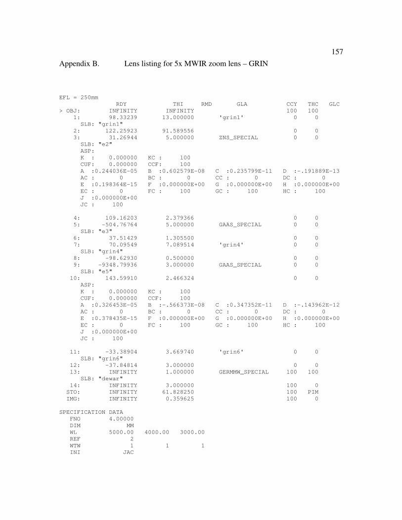
157

Appendix B. Lens listing for 5x MWIR zoom lens – GRIN

EFL = 250mm

RDY THI RMD GLA CCY THC GLC

> OBJ: INFINITY INFINITY 100 100

1: 98.33239 13.000000 'grin1' 0 0

SLB: "grin1"

2: 122.25923 91.589556 0 0

3: 31.26944 5.000000 ZNS_SPECIAL 0 0

SLB: "e2"

ASP:

K : 0.000000 KC : 100

CUF: 0.000000 CCF: 100

A :0.244036E-05 B :0.602579E-08 C :0.235799E-11 D :-.191889E-13

AC : 0 BC : 0 CC : 0 DC : 0

E :0.198364E-15 F :0.000000E+00 G :0.000000E+00 H :0.000000E+00

EC : 0 FC : 100 GC : 100 HC : 100

J :0.000000E+00

JC : 100

4: 109.16203 2.379366 0 0

5: -504.76764 5.000000 GAAS_SPECIAL 0 0

SLB: "e3"

6: 37.51429 1.305500 0 0

7: 70.09549 7.089514 'grin4' 0 0

SLB: "grin4"

8: -98.62930 0.500000 0 0

9: -9348.79936 3.000000 GAAS_SPECIAL 0 0

SLB: "e5"

10: 143.59910 2.466324 0 0

ASP:

K : 0.000000 KC : 100

CUF: 0.000000 CCF: 100

A :0.326453E-05 B :-.566373E-08 C :0.347352E-11 D :-.143962E-12

AC : 0 BC : 0 CC : 0 DC : 0

E :0.378435E-15 F :0.000000E+00 G :0.000000E+00 H :0.000000E+00

EC : 0 FC : 100 GC : 100 HC : 100

J :0.000000E+00

JC : 100

11: -33.38904 3.669740 'grin6' 0 0

SLB: "grin6"

12: -37.84814 3.000000 0 0

13: INFINITY 1.000000 GERMMW_SPECIAL 100 100

SLB: "dewar"

14: INFINITY 3.000000 100 0

STO: INFINITY 61.828250 100 PIM

IMG: INFINITY 0.359625 100 0

SPECIFICATION DATA

FNO 4.00000

DIM MM

WL 5000.00 4000.00 3000.00

REF 2

WTW 1 1 1

INI JAC

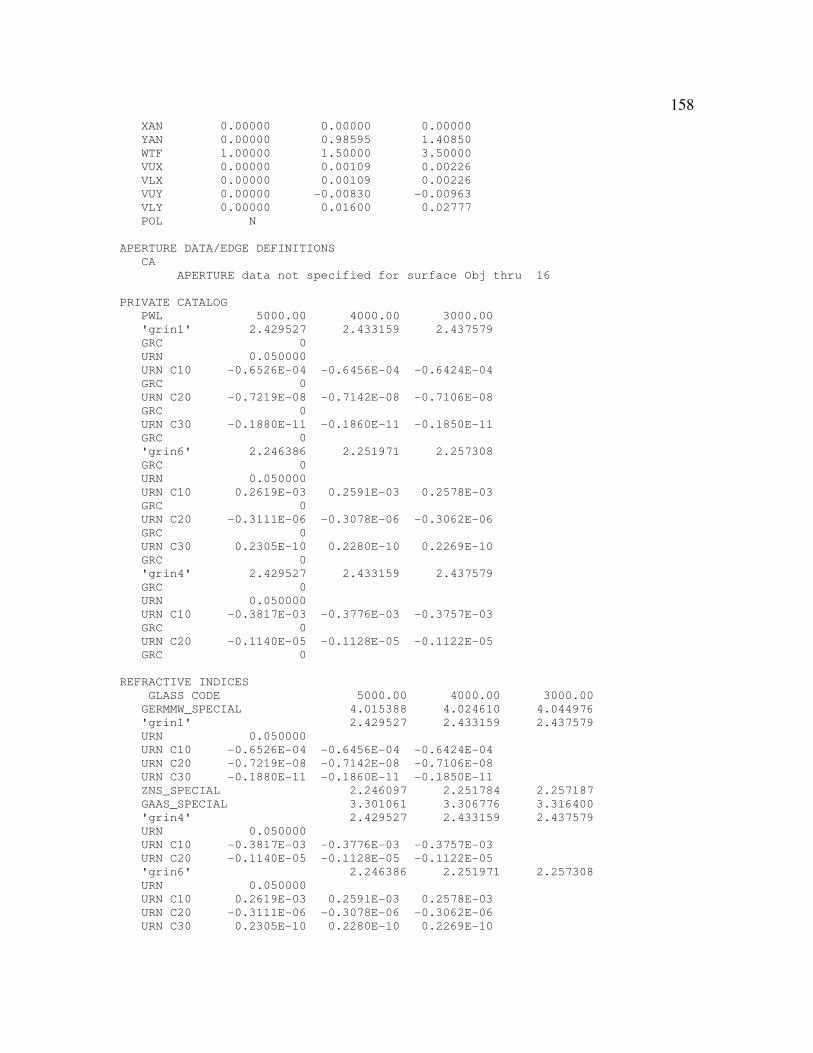
158 XAN 0.00000 0.00000 0.00000

YAN 0.00000 0.98595 1.40850

WTF 1.00000 1.50000 3.50000

VUX 0.00000 0.00109 0.00226

VLX 0.00000 0.00109 0.00226

VUY 0.00000 -0.00830 -0.00963

VLY 0.00000 0.01600 0.02777

POL N

APERTURE DATA/EDGE DEFINITIONS

CA

APERTURE data not specified for surface Obj thru 16

PRIVATE CATALOG

PWL 5000.00 4000.00 3000.00

'grin1' 2.429527 2.433159 2.437579

GRC 0

URN 0.050000

URN C10 -0.6526E-04 -0.6456E-04 -0.6424E-04

GRC 0

URN C20 -0.7219E-08 -0.7142E-08 -0.7106E-08

GRC 0

URN C30 -0.1880E-11 -0.1860E-11 -0.1850E-11

GRC 0

'grin6' 2.246386 2.251971 2.257308

GRC 0

URN 0.050000

URN C10 0.2619E-03 0.2591E-03 0.2578E-03

GRC 0

URN C20 -0.3111E-06 -0.3078E-06 -0.3062E-06

GRC 0

URN C30 0.2305E-10 0.2280E-10 0.2269E-10

GRC 0

'grin4' 2.429527 2.433159 2.437579

GRC 0

URN 0.050000

URN C10 -0.3817E-03 -0.3776E-03 -0.3757E-03

GRC 0

URN C20 -0.1140E-05 -0.1128E-05 -0.1122E-05

GRC 0

REFRACTIVE INDICES

GLASS CODE 5000.00 4000.00 3000.00

GERMMW_SPECIAL 4.015388 4.024610 4.044976

'grin1' 2.429527 2.433159 2.437579

URN 0.050000

URN C10 -0.6526E-04 -0.6456E-04 -0.6424E-04

URN C20 -0.7219E-08 -0.7142E-08 -0.7106E-08

URN C30 -0.1880E-11 -0.1860E-11 -0.1850E-11

ZNS_SPECIAL 2.246097 2.251784 2.257187

GAAS_SPECIAL 3.301061 3.306776 3.316400

'grin4' 2.429527 2.433159 2.437579

URN 0.050000

URN C10 -0.3817E-03 -0.3776E-03 -0.3757E-03

URN C20 -0.1140E-05 -0.1128E-05 -0.1122E-05

'grin6' 2.246386 2.251971 2.257308

URN 0.050000

URN C10 0.2619E-03 0.2591E-03 0.2578E-03

URN C20 -0.3111E-06 -0.3078E-06 -0.3062E-06

URN C30 0.2305E-10 0.2280E-10 0.2269E-10

159

SOLVES

PIM

No pickups defined in system

ZOOM DATA

ZOOM TITLE

POS 1 "EFL = 250mm"

POS 2 "EFL = 100mm"

POS 3 "EFL = 50mm"

POS 1 POS 2 POS 3

YAN F1 0.00000 0.00000 0.00000

YAN F2 0.98595 2.46228 4.90000

YAN F3 1.40850 3.51755 7.00877

WTF F2 1.50000 1.00000 1.00000

WTF F3 3.50000 1.00000 2.00000

VUY F1 0.3423E-11 0.2170E-11 0.1813E-12

VLY F1 0.3423E-11 0.2170E-11 0.1813E-12

VUY F2 -0.00830 0.00178 0.01486

VLY F2 0.01600 0.02606 0.03869

VUY F3 -0.00963 0.01108 0.03692

VLY F3 0.02777 0.03659 0.06274

VUX F1 0.3423E-11 0.2170E-11 0.1813E-12

VLX F1 0.3423E-11 0.2170E-11 0.1813E-12

VUX F2 0.00109 0.00475 0.00879

VLX F2 0.00109 0.00475 0.00879

VUX F3 0.00226 0.00967 0.01825

VLX F3 0.00226 0.00967 0.01825

RSL DEF DEF DEF

THI S2 91.58956 40.04167 13.21533

THC S2 0 0 0

THI S6 1.30550 43.11110 77.81068

THC S6 0 0 0

THI S10 2.46632 12.20861 4.33537

THC S10 0 0 0

POS 1 POS 2 POS 3

INFINITE CONJUGATES

EFL 250.0000 100.0000 50.0000

BFL 61.8282 62.2433 62.2544

FFL -506.0601 60.6080 78.6423

FNO 4.0000 4.0000 4.0000

IMG DIS 62.1879 62.1879 62.1879

OAL 142.0000 142.0000 142.0000

PARAXIAL IMAGE

HT 6.1470 6.1470 6.1470

ANG 1.4085 3.5175 7.0088

ENTRANCE PUPIL

DIA 62.5000 25.0000 12.5000

THI 504.8046 221.2678 118.8001

EXIT PUPIL

DIA 15.4571 15.5608 15.5636

THI 0.0000 0.0000 0.0000

STO DIA 15.6243 15.6931 15.6809

160

Appendix C. Lens listing for 2x visible zoom lens – homogeneous

EFL = 11.5mm

RDY THI RMD GLA CCY THC GLC

> OBJ: INFINITY INFINITY 100 100

1: 28.23444 2.049231 NFK5_SCHOTT 0 0

SLB: "e1"

ASP:

K : 0.000000 KC : 100

CUF: 0.000000 CCF: 100

A :0.753363E-05 B :-.333147E-07 C :0.517518E-09 D :0.000000E+00

AC : 0 BC : 0 CC : 0 DC : 100

2: 19.60967 5.582847 0 0

3: -16.01143 2.014817 NFK5_SCHOTT 0 0

SLB: "e2"

4: -190.36272 20.211631 0 0

STO: INFINITY 0.100000 100 0

6: 6.64250 3.800000 NLAF3_SCHOTT 0 0

SLB: "e3"

7: -10.81224 0.100000 0 0

8: -10.21423 2.861179 SF10_SCHOTT 0 0

SLB: "e4"

9: 13.00755 13.280294 0 0

ASP:

K : 0.000000 KC : 100

CUF: 0.000000 CCF: 100

A :0.128935E-02 B :0.337402E-04 C :0.244789E-05 D :0.000000E+00

AC : 0 BC : 0 CC : 0 DC : 100

IMG: INFINITY 0.000000 100 100

SPECIFICATION DATA

EPD 3.28570

DIM MM

WL 656.27 587.56 486.13

REF 2

WTW 1 1 1

XAN 0.00000 0.00000 0.00000 0.00000 0.00000

YAN 0.00000 7.67200 13.42600 16.30300 19.18000

WTF 1.00000 1.00000 1.00000 1.00000 1.00000

VUX 0.00000 0.00511 0.01651 0.02498 0.03537

VLX 0.00000 0.00511 0.01651 0.02498 0.03537

VUY 0.00000 0.01058 0.04101 0.06522 0.09590

VLY 0.00000 0.02114 0.06352 0.09426 0.13153

POL N

PRIVATE CATALOG

PWL 656.27 587.56 486.13

'grin2' 1.540205 1.545253 1.555441

GRC 0

URN 0.050000

URN C10 -0.1653E-02 -0.1704E-02 -0.1839E-02

GRC 0

URN C20 0.1659E-04 0.1710E-04 0.1846E-04

GRC 0

161 URN C30 -0.4476E-07 -0.4613E-07 -0.4981E-07

GRC 0

'grin4' 1.487957 1.491402 1.497298

GRC 0

URN 0.050000

URN C10 0.3734E-02 0.3848E-02 0.4155E-02

GRC 0

URN C20 0.1907E-04 0.1966E-04 0.2122E-04

GRC 0

URN C30 -0.1984E-05 -0.2044E-05 -0.2207E-05

GRC 0

REFRACTIVE INDICES

GLASS CODE 656.27 587.56 486.13

NFK5_SCHOTT 1.485345 1.487490 1.492269

NLAF3_SCHOTT 1.712522 1.716998 1.727471

SF10_SCHOTT 1.720848 1.728250 1.746481

No solves defined in system

No pickups defined in system

ZOOM DATA

ZOOM TITLE

POS 1 "EFL = 11.5mm"

POS 2 "EFL = 16.5mm"

POS 3 "EFL = 23mm"

POS 1 POS 2 POS 3

EPD 3.28570 3.88235 4.60000

YAN F2 7.67200 5.45200 3.94800

YAN F3 13.42600 9.54100 6.90900

YAN F4 16.30300 11.58550 8.38950

YAN F5 19.18000 13.63000 9.87000

VUY F1 0.2487E-12 0.2706E-11 0.5369E-11

VLY F1 0.2487E-12 0.2706E-11 0.5369E-11

VUY F2 0.01058 -0.00045 -0.00018

VLY F2 0.02114 0.00096 -0.00247

VUY F3 0.04101 -0.00063 -0.00233

VLY F3 0.06352 0.00361 -0.00564

VUY F4 0.06522 -0.00023 -0.00403

VLY F4 0.09426 0.00530 -0.00766

VUY F5 0.09590 0.00062 -0.00609

VLY F5 0.13153 0.00640 -0.01007

VUX F1 0.2487E-12 0.2706E-11 0.5369E-11

VLX F1 0.2487E-12 0.2706E-11 0.5369E-11

VUX F2 0.00511 0.1402E-04 -0.00047

VLX F2 0.00511 0.1402E-04 -0.00047

VUX F3 0.01651 0.00028 -0.00141

VLX F3 0.01651 0.00028 -0.00141

VUX F4 0.02498 0.00060 -0.00204

VLX F4 0.02498 0.00060 -0.00204

VUX F5 0.03537 0.00102 -0.00277

VLX F5 0.03537 0.00102 -0.00277

THI S2 5.58285 14.45327 17.62899

THC S2 0 0 0

THI S4 20.21163 8.56197 1.85497

162 THC S4 0 0 0

THI S9 13.28029 16.05953 19.59081

THC S9 0 0 0

POS 1 POS 2 POS 3

INFINITE CONJUGATES

EFL 11.5000 16.5000 23.0000

BFL 13.3077 16.0958 19.5621

FFL 10.9788 7.4394 -2.9496

FNO 3.5000 4.2500 5.0000

IMG DIS 13.2803 16.0595 19.5908

OAL 36.7197 33.9405 30.4092

PARAXIAL IMAGE

HT 4.0002 4.0009 4.0017

ANG 19.1800 13.6300 9.8700

ENTRANCE PUPIL

DIA 3.2857 3.8824 4.6000

THI 18.9531 21.4928 20.2126

EXIT PUPIL

DIA 4.7384 4.5582 4.5678

THI -3.2768 -3.2768 -3.2768

STO DIA 5.8521 5.6337 5.6488

163

Appendix D. Lens listing for 2x visible zoom lens – GRIN (optimized profile)

EFL = 11.5mm

RDY THI RMD GLA CCY THC GLC

> OBJ: INFINITY INFINITY 100 100

1: 153.05250 2.002688 NFK5_SCHOTT 0 0

SLB: "e1"

ASP:

K : 0.000000 KC : 100

CUF: 0.000000 CCF: 100

A :0.678809E-05 B :-.189994E-06 C :0.269889E-08 D :0.000000E+00

AC : 0 BC : 0 CC : 0 DC : 100

2: 28.83212 5.692019 0 0

3: -15.13370 2.332800 'grin2' 0 0

SLB: "grin2"

4: -117.97471 18.443687 0 0

STO: INFINITY 0.100000 100 0

6: 7.36119 3.270308 NLAK34_SCHOTT 0 0

SLB: "e3"

7: -15.26454 0.100000 0 0

8: -14.86794 3.800000 SF10_SCHOTT 0 0

SLB: "e4"

9: 15.61568 14.258498 0 0

ASP:

K : 0.000000 KC : 100

CUF: 0.000000 CCF: 100

A :0.967162E-03 B :0.246100E-04 C :0.101656E-05 D :0.000000E+00

AC : 0 BC : 0 CC : 0 DC : 100

IMG: INFINITY 0.000000 100 100

SPECIFICATION DATA

EPD 3.28570

DIM MM

WL 656.27 587.56 486.13

REF 2

WTW 1 1 1

XAN 0.00000 0.00000 0.00000 0.00000 0.00000

YAN 0.00000 7.67200 13.42600 16.30300 19.18000

WTF 1.00000 1.00000 1.00000 1.00000 1.00000

VUX 0.00000 0.00447 0.01490 0.02270 0.03199

VLX 0.00000 0.00447 0.01490 0.02270 0.03199

VUY 0.00000 0.00997 0.03622 0.05717 0.08287

VLY 0.00000 0.01935 0.06054 0.08742 0.11445

POL N

PRIVATE CATALOG

PWL 656.27 587.56 486.13

'grin2' 1.585265 1.591695 1.605584

GRC 0

URN 0.050000

URN C10 -0.2122E-02 -0.2187E-02 -0.2361E-02

GRC 0

URN C20 0.2187E-04 0.2254E-04 0.2433E-04

164 GRC 0

URN C30 -0.9741E-07 -0.1004E-06 -0.1084E-06

GRC 0

'grin4' 1.487957 1.491402 1.497298

GRC 0

URN 0.050000

URN C10 0.3734E-02 0.3848E-02 0.4155E-02

GRC 0

URN C20 0.1907E-04 0.1966E-04 0.2122E-04

GRC 0

URN C30 -0.1984E-05 -0.2044E-05 -0.2207E-05

GRC 0

REFRACTIVE INDICES

GLASS CODE 656.27 587.56 486.13

'grin2' 1.585265 1.591695 1.605584

URN 0.050000

URN C10 -0.2122E-02 -0.2187E-02 -0.2361E-02

URN C20 0.2187E-04 0.2254E-04 0.2433E-04

URN C30 -0.9741E-07 -0.1004E-06 -0.1084E-06

SF10_SCHOTT 1.720848 1.728250 1.746481

NFK5_SCHOTT 1.485345 1.487490 1.492269

NLAK34_SCHOTT 1.725090 1.729160 1.738469

No solves defined in system

No pickups defined in system

ZOOM DATA

ZOOM TITLE

POS 1 "EFL = 11.5mm"

POS 2 "EFL = 16.5mm"

POS 3 "EFL = 23mm"

POS 1 POS 2 POS 3

EPD 3.28570 3.88235 4.60000

YAN F2 7.67200 5.45200 3.94800

YAN F3 13.42600 9.54100 6.90900

YAN F4 16.30300 11.58550 8.38950

YAN F5 19.18000 13.63000 9.87000

VUY F1 -0.5433E-12 0.7268E-11 0.1783E-10

VLY F1 -0.5433E-12 0.7268E-11 0.1783E-10

VUY F2 0.00997 0.00113 0.00087

VLY F2 0.01935 0.00274 -0.00067

VUY F3 0.03622 0.00382 0.00124

VLY F3 0.06054 0.00911 -0.00050

VUY F4 0.05717 0.00628 0.00135

VLY F4 0.08742 0.01260 -0.00024

VUY F5 0.08287 0.00968 0.00146

VLY F5 0.11445 0.01407 -0.3744E-04

VUX F1 -0.5433E-12 0.7268E-11 0.1783E-10

VLX F1 -0.5433E-12 0.7268E-11 0.1783E-10

VUX F2 0.00447 0.00051 -0.2014E-04

VLX F2 0.00447 0.00051 -0.2014E-04

VUX F3 0.01490 0.00185 -0.1440E-04

VLX F3 0.01490 0.00185 -0.1440E-04

VUX F4 0.02270 0.00294 0.2143E-04

165 VLX F4 0.02270 0.00294 0.2143E-04

VUX F5 0.03199 0.00425 0.9015E-04

VLX F5 0.03199 0.00425 0.9015E-04

THI S2 5.69202 14.44287 16.71420

THC S2 0 0 0

THI S4 18.44369 6.38527 0.10000

THC S4 0 0 0

THI S9 14.25850 17.56606 21.58000

THC S9 0 0 0

POS 1 POS 2 POS 3

INFINITE CONJUGATES

EFL 11.5000 16.5000 23.0000

BFL 14.3105 17.6435 21.6265

FFL 9.1246 4.9032 -4.9621

FNO 3.5000 4.2500 5.0000

IMG DIS 14.2585 17.5661 21.5800

OAL 35.7415 32.4339 28.4200

PARAXIAL IMAGE

HT 4.0002 4.0009 4.0017

ANG 19.1800 13.6300 9.8700

ENTRANCE PUPIL

DIA 3.2857 3.8824 4.6000

THI 16.5254 17.7436 16.0420

EXIT PUPIL

DIA 5.1056 4.9888 5.0371

THI -3.5591 -3.5591 -3.5591

STO DIA 6.1108 5.9791 6.0431

166

Appendix E. CODEV® GRIN Chromatic macro

Instructions for running macro:

Ax_lat_GRIN_CODEV.seq manual (CODEV)

This document describes the operation of the CODE V sequence file ax_lat_GRIN_CODEV.seq. Note that all of the mathematics in the code are derived from: K. Siva Rama Krishna and Anurag Sharma, "Chromatic aberrations of radial gradient-index lenses. I. Theory," Appl. Opt. 35, 1032-1036 (1996). Please refer to that paper for more information on specific equations and definitions.

As of the writing of this document, CODEV® does not offer a means to calculate the polychromatic aberration coefficients of GRIN systems. This CODEV® macro provides a means to determine the axial and lateral color contributions from a quadratic radial GRIN element. Running ax_lat_GRIN_CODEV.seq on a GRIN surface in CODEV® calculates the third-order surface contributions to those aberrations (matching the values calculated by CODEV®’s built-in third-order aberration coefficient calculations (THO) in addition to the GRIN coefficients. To operate the macro, open ax_lat_GRIN_CODEV.seq in CODEV®. As shown in Figure A-1 this prompts user selection of both the surface number of the GRIN element as well as the zoom position (default to 1 if the system is not zoomed). Figure A-2 shows results from an example calculation, displaying axial and lateral color contributions for each surface and the GRIN as well as their sums. The constant ν11 is also displayed (discussed in Chapter 3).

Figure A-1: Dialog screen prompting user selection of surface number and zoom position

167

Figure A-2: Example output from chromatic macro

.seq file for GRIN Chromatic macro

!**********************************************************************

****

! Macro PLOTGRIN_polychrom

!

! Plots gradient index profile as a function of position at every

wavelength

!

! Usage:

! in PLOTGRIN surf# [type of GRIN]

!

!

! History: 2014_01_28 JAC Create

! Code was derived from: K. Siva Rama Krishna and Anurag Sharma,

"Chromatic aberrations of radial gradient-index lenses. I. Theory,"

Appl. Opt. 35, 1032-1036 (1996)

! See paper for more information

!**********************************************************************

****

! arg0 "Macro to plot gradient index profile as a function of

position."

!

! arg1 name "Surface number of GRIN element"

! arg1 type num

! arg1 default 1

! arg1 help "Surface number of GRIN material."

168 !

! arg2 name "Zoom Position"

! arg2 type num

! arg2 default 1

! arg2 help "Zoom position to plot."

!

!**********************************************************************

****

! Global variables

gbl num ^error ! Error flag for image evaluation

gbl str ^format ! format of value

gbl num ^ymax ! Maximum value on y-axis

gbl num ^ymin ! Minimum value on y-axis

! Local variables

lcl num ^surfnum

lcl num ^aray_y

lcl num ^lam_red

lcl num ^lam_green

lcl num ^lam_blue

lcl num ^w_red

lcl num ^w_blue

lcl num ^n_red_i

lcl num ^n_green_i

lcl num ^n_blue_i

lcl num ^V_i

lcl num ^v01_i

lcl num ^n_red_o

lcl num ^n_green_o

lcl num ^n_blue_o

lcl num ^V_o

lcl num ^v01_o

lcl num ^fa1

lcl num ^fa1_st

lcl num ^del_v_n

lcl num ^mu

lcl num ^ax

lcl num ^lat

lcl num ^C10

lcl num ^thi

lcl num ^alp

lcl num ^S

lcl num ^C

lcl num ^e

lcl num ^g0

lcl num ^g1

lcl num ^g2

lcl num ^v11

lcl num ^psi1

169 lcl num ^fa2

lcl num ^fa2_st

lcl num ^n10

lcl num ^ax_G

lcl num ^lat_G

! Buchdahl Coefficients

^lam_red == (wl w1)/1000

^lam_green == (wl w2)/1000

^lam_blue == (wl w3)/1000

^w_red == (^lam_red - ^lam_green)/(1+2.5*(^lam_red-^lam_green))

^w_blue == (^lam_blue - ^lam_green)/(1+2.5*(^lam_blue-^lam_green))

ver n

^surfnum == #1

^zoomnum == #2

! Define V and v01 for incident media

^n_red_i == (index(^surfnum-1,^zoomnum,1,1,0,0,0))

^n_green_i == (index(^surfnum-1,^zoomnum,2,1,0,0,0))

^n_blue_i == (index(^surfnum-1,^zoomnum,3,1,0,0,0))

if ^n_green_i = 1

^V_i == 0

^v01_i == 0

else

^V_i == (^n_green_i-1)/(^n_blue_i-^n_red_i)

^v01_i == (^n_green_i-1)/(^V_i*(^w_blue-^w_red))

end if

! Define V and v01 for refracting media

^n_red_o == (index(^surfnum,^zoomnum,1,1,0,0,0))

^n_green_o == (index(^surfnum,^zoomnum,2,1,0,0,0))

^n_blue_o == (index(^surfnum,^zoomnum,3,1,0,0,0))

if ^n_green_o = 1

^V_o == 0

^v01_o == 0

else

^V_o == (^n_green_o-1)/(^n_blue_o-^n_red_o)

^v01_o == (^n_green_o-1)/(^V_o*(^w_blue-^w_red))

end if

! Define V and v01 for third media

^n_red_3 == (index(^surfnum+1,^zoomnum,1,1,0,0,0))

^n_green_3 == (index(^surfnum+1,^zoomnum,2,1,0,0,0))

^n_blue_3 == (index(^surfnum+1,^zoomnum,3,1,0,0,0))

if ^n_green_3 = 1

^V_3 == 0

^v01_3 == 0

else

^V_3 == (^n_green_3-1)/(^n_blue_3-^n_red_3)

^v01_3 == (^n_green_3-1)/(^V_3*(^w_blue-^w_red))

end if

!!!!!!!!!!!!!!!!!!!!!!!!!!!!!!!!!!!!!!!!!!!!!!!!!!!!!!!!!!!!!!!!

! Calculate change in v01/n00 for a surface

170 ^del_v_n == (^v01_o/^n_green_o) - (^v01_i/^n_green_i)

! Begin surface contribution calculation

^fa1 == ^n_green_i*(hmy z^zoomnum s^surfnum)*(imy z^zoomnum

s^surfnum)*^del_v_n/^n_green_i

^fa1_st == ^n_green_i*(hmy z^zoomnum s^surfnum)*(icy z^zoomnum

s^surfnum)*^del_v_n/^n_green_i

! Calculate surface coefficients

^mu == -1/(umy si z^zoomnum)

^ax == ^mu*^fa1*(^w_blue-^w_red)

^lat == ^mu*^fa1_st*(^w_blue-^w_red)

wri "Surface axial S1"

eva(-^ax)

wri "Surface lateral S1"

eva(-^lat)

!!!!!!!!!!!!!!!!!!!!!!!!!!!!!!!!!!!!!!!!!!!!!!!!!!!!!!!!!!!!!!!!

! Calculate change in v01/n00 for a surface

^del_v_n_S2 == (^v01_3/^n_green_3) - (^v01_o/^n_green_o)

! Begin surface contribution calculation

^faS2 == ^n_green_o*(hmy z^zoomnum s^surfnum+1)*(imy z^zoomnum

s^surfnum+1)*^del_v_n_S2/^n_green_o

^faS2_st == ^n_green_o*(hmy z^zoomnum s^surfnum+1)*(icy z^zoomnum

s^surfnum+1)*^del_v_n_S2/^n_green_o

! Calculate surface coefficients

^mu == -1/(umy si z^zoomnum)

^ax_S2 == ^mu*^faS2*(^w_blue-^w_red)

^lat_S2 == ^mu*^faS2_st*(^w_blue-^w_red)

wri "Surface axial S2"

eva(-^ax_S2)

wri "Surface lateral S2"

eva(-^lat_S2)

!!!!!!!!!!!!!!!!!!!!!!!!!!!!!!!!!!!!!!!!!!!!!!!!!!!!!!!!!!!!!!!!

! End surface contribution calculation

! Begin tranfer contribution calculation

^n_green_axis == (index(^surfnum,^zoomnum,2,1,0,0,0))

^n_green_per == (index(^surfnum,^zoomnum,2,1,0,(hmy s^surfnum),0))

if ^n_green_axis - ^n_green_per = 0

^ax_G == ^mu*^fa2*(^w_blue-^w_red)

^lat_G == ^mu*^fa2_st*(^w_blue-^w_red)

else

171

^C10 == (GRN s^surfnum C10 w2 z^zoomnum)

^thi == (thi s^surfnum z^zoomnum)

^e == 2.718281828459046

!eva(^n_green_o)

^alp == sqrt(absf(2*^C10/^n_green_o))

!eva(^alp)

if ^C10 < 0

^C == cosf(^alp*^thi)

^S == sinf(^alp*^thi)/^alp

else if ^C10 > 0

^C == (^e**(^alp*^thi)+^e**(-^alp*^thi))/(2) !cosh

^S == (^e**(^alp*^thi)-^e**(-^alp*^thi))/(2*^alp) !sinh

else

^C == 1

^S == 0

end if

!eva(^C)

!eva(^S)

^g0 == 0.5*(^thi+^C*^S)

^g1 == ^S*^S

^g2 == (^thi - ^C*^S)/(2*^alp*^alp)

!eva(^g0)

!eva(^g1)

!eva(^g2)

^v11red == ((GRN s^surfnum C10 w1 z^zoomnum) - ^C10)/^w_red

^v11blue == ((GRN s^surfnum C10 w3 z^zoomnum) - ^C10)/^w_blue

!eva((^v11red+^v11blue)/2)

wri "v11"

^n10 == ^C10

^v11 == 0.00122889

!-0.00075901

eva(^v11)

!0.00132333

! 0.00028848

!-0.00075263

^psi1 == (^v11/^n10 - ^v01_o/^n_green_o)

!eva(^v01_o)

!wri "psi"

!eva(^psi1)

^fa2 == 2*^n10*^psi1*(^g0*(hmy z^zoomnum s^surfnum)*(hmy z^zoomnum

s^surfnum) + ^g1*(hmy z^zoomnum s^surfnum)*(umy z^zoomnum

s^surfnum+1)+^g2*(umy z^zoomnum s^surfnum+1)*(umy z^zoomnum

s^surfnum+1))

172 ^fa2_st == 2*^n10*^psi1*(^g0*(hmy z^zoomnum s^surfnum)*(hcy z^zoomnum

s^surfnum) + 0.5*^g1*((hmy z^zoomnum s^surfnum)*(ucy z^zoomnum

s^surfnum+1)+(hcy z^zoomnum s^surfnum)*(umy z^zoomnum s^surfnum+1)) +

^g2*(umy z^zoomnum s^surfnum+1)*(ucy z^zoomnum s^surfnum+1))

! Calculate GRIN coefficients

^mu == -1/(umy si z^zoomnum)

^ax_G == ^mu*^fa2*(^w_blue-^w_red)

^lat_G == ^mu*^fa2_st*(^w_blue-^w_red)

!eva(^fa2_st)

end if

wri "GRIN axial"

eva(^ax_G)

wri "GRIN lateral"

eva(^lat_G)

wri "Sum Axial"

eva(-^ax-^ax_S2+^ax_G)

wri "Sum Lat"

eva(-^lat-^lat_S2+^lat_G)

!wri "lF - lC"

!eva((^ax+^ax_S2-^ax_G)/(umy si z^zoomnum))

out y

173

Appendix F. Lens listing for 10x visible zoom lens – homogeneous

10x zoom, efl = 10mm

RDY THI RMD GLA CCY THC GLC

> OBJ: INFINITY INFINITY 100 100

1: 129.03733 3.000000 LLAH86_OHARA 0 0

SLB: "e1"

2: 64.13707 14.279409 SFPM2_OHARA 0 0

SLB: "e2"

3: -1037.40199 0.100000 0 0

4: 55.14020 8.371468 SFPM2_OHARA 0 0

SLB: "e3"

5: 126.73446 1.534938 0 0

6: 55.54215 2.500000 SFPM2_OHARA 0 0

SLB: "e4"

7: 15.74071 10.613936 0 0

8: -85.35226 1.000000 SFPM2_OHARA 0 0

SLB: "e45"

9: 24.24077 3.286086 0 0

10: 26.51113 3.240675 SLAL14_OHARA 0 0

SLB: "e5"

11: 84.38352 0.100000 0 0

12: 43.30257 67.331911 0 0

STO: INFINITY 0.100000 0 0

14: 27.73773 3.579720 SLAM3_OHARA 0 0

SLB: "e6"

ASP:

K : 0.000000 KC : 100

CUF: 0.000000 CCF: 100

A :-.783204E-04 B :-.195374E-07 C :-.502482E-08 D :0.000000E+00

AC : 0 BC : 0 CC : 0 DC : 100

15: -76.61738 3.272434 0 0

16: 26.50625 4.000000 SFPL53_OHARA 0 0

SLB: "e7"

17: -14.69303 1.938504 0 0

ASP:

K : 0.000000 KC : 100

CUF: 0.000000 CCF: 100

A :0.656149E-04 B :-.642356E-06 C :0.348083E-08 D :0.000000E+00

AC : 0 BC : 0 CC : 0 DC : 100

18: 19.35413 2.000000 SNPH2_OHARA 0 0

SLB: "e8"

ASP:

K : 0.000000 KC : 100

CUF: 0.000000 CCF: 100

A :0.499616E-05 B :0.801935E-07 C :-.364761E-08 D :0.000000E+00

AC : 0 BC : 0 CC : 0 DC : 100

19: 8.43398 15.750919 0 0

IMG: INFINITY 0.000000 100 100

SPECIFICATION DATA

EPD 5.00000

DIM MM

174 WL 656.27 587.56 486.13

REF 2

WTW 1 1 1

INI JAC

XAN 0.00000 0.00000 0.00000 0.00000 0.00000

YAN 0.00000 10.62600 18.59550 22.58025 26.56500

WTF 1.00000 1.00000 1.00000 1.00000 1.00000

VUX 0.00000 -0.00813 -0.02855 -0.04680 -0.07498

VLX 0.00000 -0.00813 -0.02855 -0.04680 -0.07498

VUY 0.00000 -0.03563 -0.11726 -0.19954 -0.34871

VLY 0.00000 -0.01609 -0.08467 -0.16298 -0.31624

POL N

PRIVATE CATALOG

PWL 656.27 587.56 486.13

'LV1' 1.844688 1.855040 1.880644

'LV2' 1.568498 1.570980 1.576506

'LV4' 1.455586 1.457200 1.460648

'LV6' 1.617322 1.620320 1.627108

'LV8' 1.695976 1.699790 1.708578

'LV10' 1.831307 1.842810 1.871441

'LV13' 1.568498 1.570980 1.576506

'LV14' 1.760862 1.766510 1.779977

'LV16' 1.568498 1.570980 1.576506

'LV18' 1.881698 1.888140 1.903476

'LV19' 1.602360 1.605200 1.611602

'LV21' 1.881698 1.888140 1.903476

'LV23' 1.515772 1.518250 1.523851

'grin5' 1.585273 1.591704 1.605594

GRC 0

URN 0.050000

URN C10 -0.8267E-03 -0.8521E-03 -0.9200E-03

GRC 0

URN C20 0.1732E-05 0.1785E-05 0.1928E-05

GRC 0

URN C30 -0.3209E-08 -0.3308E-08 -0.3571E-08

GRC 0

REFRACTIVE INDICES

GLASS CODE 656.27 587.56 486.13

SFPM2_OHARA 1.592555 1.595220 1.601342

LLAH86_OHARA 1.894221 1.902699 1.923335

SFPL53_OHARA 1.437333 1.438750 1.441954

SLAM3_OHARA 1.712528 1.717004 1.727488

SLAL14_OHARA 1.692974 1.696797 1.705521

SNPH2_OHARA 1.909158 1.922860 1.957994

No solves defined in system

No pickups defined in system

ZOOM DATA

ZOOM TITLE

POS 1 "10x zoom, efl = 10mm"

POS 2 "10x zoom, efl = 31mm"

POS 3 "10x zoom, efl = 98mm"

POS 1 POS 2 POS 3

175

EPD 5.00000 8.78130 19.66740

YAN F2 10.62600 3.69600 1.16440

YAN F3 18.59550 6.46800 2.03770

YAN F4 22.58025 7.85400 2.47435

YAN F5 26.56500 9.24000 2.91100

VUY F1 -0.1679E-12 0.7616E-11 -0.5662E-13

VLY F1 -0.1679E-12 0.7616E-11 -0.5662E-13

VUY F2 -0.03563 -0.00037 0.00739

VLY F2 -0.01609 0.00800 0.01010

VUY F3 -0.11726 0.00657 0.02455

VLY F3 -0.08467 0.02235 0.03510

VUY F4 -0.19954 0.01442 0.03825

VLY F4 -0.16298 0.03465 0.05550

VUY F5 -0.34871 0.02703 0.05642

VLY F5 -0.31624 0.05243 0.08204

VUX F1 -0.1679E-12 0.7616E-11 -0.5662E-13

VLX F1 -0.1679E-12 0.7616E-11 -0.5662E-13

VUX F2 -0.00813 0.00122 0.00276

VLX F2 -0.00813 0.00122 0.00276

VUX F3 -0.02855 0.00427 0.00908

VLX F3 -0.02855 0.00427 0.00908

VUX F4 -0.04680 0.00689 0.01403

VLX F4 -0.04680 0.00689 0.01403

VUX F5 -0.07498 0.01059 0.02042

VLX F5 -0.07498 0.01059 0.02042

THI S5 1.53494 40.36849 66.70971

THC S5 0 0 0

THI S12 67.33191 28.28023 3.15415

THC S12 0 0 0

THI S15 3.27243 2.74754 3.20177

THC S15 0 0 0

THI S17 1.93850 2.68153 1.01216

THC S17 0 0 0

POS 1 POS 2 POS 3

INFINITE CONJUGATES

EFL 10.0000 30.7345 98.3354

BFL 15.6816 15.7465 15.7032

FFL 53.4676 164.8288 135.8490

FNO 2.0000 3.5000 4.9999

IMG DIS 15.7509 15.7509 15.7509

OAL 130.2491 130.2491 130.2491

PARAXIAL IMAGE

HT 5.0000 4.9999 5.0004

ANG 26.5650 9.2400 2.9110

ENTRANCE PUPIL

DIA 5.0000 8.7813 19.6674

THI 57.7767 205.6110 557.7873

EXIT PUPIL

DIA 11.6033 6.6178 4.5836

THI -7.5250 -7.4158 -7.2145

STO DIA 14.4723 8.4359 5.5315

176

Appendix G. Lens listing for 10x visible zoom lens – GRIN

10x zoom, efl = 10mm

RDY THI RMD GLA CCY THC GLC

> OBJ: INFINITY INFINITY 100 100

1: 135.23819 3.000000 SLAH60_OHARA 0 0

SLB: "e1"

2: 49.60673 13.735028 SFPM2_OHARA 0 0

SLB: "e2"

3: -6547.29652 0.100000 0 0

4: 47.26300 8.273132 SFPM2_OHARA 0 0

SLB: "e3"

5: 119.88085 3.533455 0 0

6: 47.65881 2.500000 SLAH66_OHARA 0 0

SLB: "e4"

7: 15.76844 8.306959 0 0

8: -72.40898 1.000000 SLAL12_OHARA 0 0

SLB: "e45"

9: 42.74914 0.835482 0 0

10: 30.81078 5.478774 'grin5' 0 0

SLB: "grin5"

11: 51.50148 0.100000 0 0

12: 43.30257 63.254510 0 0

STO: INFINITY 0.100000 0 0

14: 24.36804 3.493146 LBSL7_OHARA 0 0

SLB: "e6"

ASP:

K : 0.000000 KC : 100

CUF: 0.000000 CCF: 100

A :-.649574E-04 B :-.128590E-06 C :-.264636E-08 D :0.000000E+00

AC : 0 BC : 0 CC : 0 DC : 100

15: 95.43450 3.688683 0 0

16: 29.43545 4.000000 SFPM2_OHARA 0 0

SLB: "e7"

17: -23.86616 0.100000 0 0

ASP:

K : 0.000000 KC : 100

CUF: 0.000000 CCF: 100

A :0.789774E-05 B :-.287763E-06 C :0.127466E-08 D :0.000000E+00

AC : 0 BC : 0 CC : 0 DC : 100

18: 15.32186 4.577121 'grin8' 0 0

SLB: "grin8"

19: 9.99106 19.923709 0 0

IMG: INFINITY 0.000000 100 100

SPECIFICATION DATA

EPD 5.00000

DIM MM

WL 656.27 587.56 486.13

REF 2

WTW 1 1 1

INI JAC

XAN 0.00000 0.00000 0.00000 0.00000 0.00000

YAN 0.00000 10.62600 18.59550 22.58025 26.56500

177 WTF 1.00000 1.00000 1.00000 1.00000 1.00000

VUX 0.00000 -0.00736 -0.02575 -0.04147 -0.06357

VLX 0.00000 -0.00736 -0.02575 -0.04147 -0.06357

VUY 0.00000 -0.03181 -0.10167 -0.16644 -0.26656

VLY 0.00000 -0.01502 -0.07630 -0.13647 -0.22966

POL N

PRIVATE CATALOG

PWL 656.27 587.56 486.13

'LV1' 1.844688 1.855040 1.880644

'LV2' 1.568498 1.570980 1.576506

'LV4' 1.455586 1.457200 1.460648

'LV6' 1.617322 1.620320 1.627108

'LV8' 1.695976 1.699790 1.708578

'LV10' 1.831307 1.842810 1.871441

'LV13' 1.568498 1.570980 1.576506

'LV14' 1.760862 1.766510 1.779977

'LV16' 1.568498 1.570980 1.576506

'LV18' 1.881698 1.888140 1.903476

'LV19' 1.602360 1.605200 1.611602

'LV21' 1.881698 1.888140 1.903476

'LV23' 1.515772 1.518250 1.523851

'grin5' 1.585273 1.591704 1.605594

GRC 0

URN 0.050000

URN C10 -0.4979E-03 -0.5132E-03 -0.5541E-03

GRC 0

URN C20 -0.3724E-06 -0.3838E-06 -0.4144E-06

GRC 0

URN C30 -0.1136E-08 -0.1170E-08 -0.1264E-08

GRC 0

'grin8' 1.487957 1.491402 1.497298

GRC 0

URN 0.050000

URN C10 0.1299E-02 0.1339E-02 0.1446E-02

GRC 0

URN C20 0.1181E-05 0.1217E-05 0.1314E-05

GRC 0

URN C30 0.6002E-07 0.6186E-07 0.6679E-07

GRC 0

REFRACTIVE INDICES

GLASS CODE 656.27 587.56 486.13

SFPM2_OHARA 1.592555 1.595220 1.601342

'grin5' 1.585273 1.591704 1.605594

URN 0.050000

URN C10 -0.4979E-03 -0.5132E-03 -0.5541E-03

URN C20 -0.3724E-06 -0.3838E-06 -0.4144E-06

URN C30 -0.1136E-08 -0.1170E-08 -0.1264E-08

SLAH60_OHARA 1.827376 1.834000 1.849819

'grin8' 1.487957 1.491402 1.497298

URN 0.050000

URN C10 0.1299E-02 0.1339E-02 0.1446E-02

URN C20 0.1181E-05 0.1217E-05 0.1314E-05

URN C30 0.6002E-07 0.6186E-07 0.6679E-07

SLAH66_OHARA 1.767798 1.772499 1.783373

SLAL12_OHARA 1.674188 1.677900 1.686438

LBSL7_OHARA 1.513846 1.516330 1.521905

No solves defined in system

178

No pickups defined in system

ZOOM DATA

ZOOM TITLE

POS 1 "10x zoom, efl = 10mm"

POS 2 "10x zoom, efl = 31mm"

POS 3 "10x zoom, efl = 98mm"

POS 1 POS 2 POS 3

EPD 5.00000 8.78130 19.66740

YAN F2 10.62600 3.69600 1.16440

YAN F3 18.59550 6.46800 2.03770

YAN F4 22.58025 7.85400 2.47435

YAN F5 26.56500 9.24000 2.91100

VUY F1 0.1887E-12 0.1574E-10 0.5389E-11

VLY F1 0.1887E-12 0.1574E-10 0.5389E-11

VUY F2 -0.03181 0.00948 0.00615

VLY F2 -0.01502 0.01815 0.00887

VUY F3 -0.10167 0.03739 0.02040

VLY F3 -0.07630 0.05374 0.02725

VUY F4 -0.16644 0.06003 0.03097

VLY F4 -0.13647 0.08086 0.04084

VUY F5 -0.26656 0.08973 0.04412

VLY F5 -0.22966 0.11543 0.05758

VUX F1 0.1887E-12 0.1574E-10 0.5389E-11

VLX F1 0.1887E-12 0.1574E-10 0.5389E-11

VUX F2 -0.00736 0.00455 0.00245

VLX F2 -0.00736 0.00455 0.00245

VUX F3 -0.02575 0.01455 0.00768

VLX F3 -0.02575 0.01455 0.00768

VUX F4 -0.04147 0.02210 0.01150

VLX F4 -0.04147 0.02210 0.01150

VUX F5 -0.06357 0.03161 0.01621

VLX F5 -0.06357 0.03161 0.01621

THI S5 3.53346 38.93481 63.01677

THC S5 0 0 0

THI S12 63.25451 27.48391 0.41973

THC S12 0 0 0

THI S15 3.68868 2.24555 6.21845

THC S15 0 0 0

THI S17 0.10000 1.91238 0.92170

THC S17 0 0 0

POS 1 POS 2 POS 3

INFINITE CONJUGATES

EFL 10.0000 30.7348 98.3371

BFL 19.8896 19.9404 19.8712

FFL 53.1145 151.3719 101.8769

FNO 2.0000 3.5000 5.0000

IMG DIS 19.9237 19.9237 19.9237

OAL 126.0763 126.0763 126.0763

PARAXIAL IMAGE

HT 5.0000 5.0000 5.0005

ANG 26.5650 9.2400 2.9110

ENTRANCE PUPIL

DIA 5.0000 8.7813 19.6674

179 THI 56.4828 183.6983 397.3378

EXIT PUPIL

DIA 14.8445 8.3490 6.5458

THI -9.7994 -9.2812 -12.8580

STO DIA 15.0078 9.0403 6.1634

180

Appendix H. Lens listing for 2x visible zoom lens – GRIN (JC018 profile)

EFL = 11.5mm

RDY THI RMD GLA CCY THC GLC

> OBJ: INFINITY INFINITY 100 100

1: 22.79060 4.500000 NFK58_SCHOTT 0 0

SLB: "e1"

ASP:

K : 0.000000 KC : 100

CUF: 0.000000 CCF: 100

A :0.408898E-04 B :-.147288E-06 C :0.964058E-08 D :0.000000E+00

AC : 0 BC : 0 CC : 0 DC : 100

2: 8.95852 2.845927 0 0

3: -7.81877 3.310076 'grin44' 0 0

SLB: "grin2"

4: -16.63999 11.891328 0 0

STO: INFINITY 0.100000 100 0

6: 6.45838 4.244140 NSSK5_SCHOTT 0 0

SLB: "e3"

7: -10.14381 0.100000 0 0

8: -9.92368 2.562845 SF4_SCHOTT 0 0

SLB: "e4"

9: 28.82713 15.175441 0 0

ASP:

K : 0.000000 KC : 100

CUF: 0.000000 CCF: 100

A :0.115479E-02 B :0.195470E-04 C :0.244596E-05 D :0.000000E+00

AC : 0 BC : 0 CC : 0 DC : 100

IMG: INFINITY 0.000000 100 100

SPECIFICATION DATA

EPD 3.28570

DIM MM

WL 656.27 587.56 486.13

REF 2

WTW 1 1 1

XAN 0.00000 0.00000

YAN 0.00000 19.18000

WTF 1.00000 1.00000

VUX 0.00000 0.01526

VLX 0.00000 0.01526

VUY 0.00000 0.04201

VLY 0.00000 0.08325

POL N

PRIVATE CATALOG

PWL 656.27 587.56 486.13

'grin2' 1.612950 1.615235 1.633133

GRC 0

URN 0.050000

URN C10 -0.1835E-02 -0.1941E-02 -0.2076E-02

GRC 0

URN C20 0.3809E-05 0.6447E-05 0.6500E-05

GRC 0

URN C30 -0.9934E-06 -0.9796E-06 -0.9871E-06

GRC 0

'grin4' 1.487914 1.491360 1.497256

181 GRC 0

URN 0.050000

URN C10 0.3733E-02 0.3848E-02 0.4154E-02

GRC 0

URN C20 0.1906E-04 0.1964E-04 0.2121E-04

GRC 0

URN C30 -0.1984E-05 -0.2045E-05 -0.2208E-05

GRC 0

'grin78' 1.543635 1.548788 1.559258

GRC 100

URN 0.050000

URN C10 -0.5846E-03 -0.6026E-03 -0.6506E-03

GRC 100

URN C20 -0.1197E-04 -0.1234E-04 -0.1332E-04

GRC 100

URN C30 0.2873E-06 0.2961E-06 0.3197E-06

GRC 100

'grin44' 1.543542 1.548692 1.559154

GRC 100

URN 0.050000

URN C10 -0.5846E-03 -0.6026E-03 -0.6506E-03

GRC 100

URN C20 -0.1197E-04 -0.1234E-04 -0.1332E-04

GRC 100

URN C30 0.2873E-06 0.2961E-06 0.3197E-06

GRC 100

REFRACTIVE INDICES

GLASS CODE 656.27 587.56 486.13

'grin44' 1.543542 1.548692 1.559154

URN 0.050000

URN C10 -0.5846E-03 -0.6026E-03 -0.6506E-03

URN C20 -0.1197E-04 -0.1234E-04 -0.1332E-04

URN C30 0.2873E-06 0.2961E-06 0.3197E-06

NSSK5_SCHOTT 1.654554 1.658440 1.667494

SF4_SCHOTT 1.747298 1.755201 1.774681

NFK58_SCHOTT 1.454462 1.456000 1.459479

No solves defined in system

No pickups defined in system

ZOOM DATA

ZOOM TITLE

POS 1 "EFL = 11.5mm"

POS 2 "EFL = 16.5mm"

POS 3 "EFL = 23mm"

POS 1 POS 2 POS 3

EPD 3.28570 3.88235 4.60000

YAN F2 19.18000 13.63000 9.87000

VUY F1 0.4498E-11 0.1914E-10 -0.1616E-12

VLY F1 0.4498E-11 0.1914E-10 -0.1616E-12

VUY F2 0.04201 -0.00943 0.00400

VLY F2 0.08325 -0.01952 -0.01084

VUX F1 0.4498E-11 0.1914E-10 -0.1616E-12

VLX F1 0.4498E-11 0.1914E-10 -0.1616E-12

182 VUX F2 0.01526 -0.00444 -0.00123

VLX F2 0.01526 -0.00444 -0.00123

THI S2 2.84593 6.61588 5.49026

THC S2 0 0 0

THI S4 11.89133 4.12639 0.77794

THC S4 0 0 0

THI S9 15.17544 19.17043 23.64450

THC S9 0 0 0

POS 1 POS 2 POS 3

INFINITE CONJUGATES

EFL 11.5000 16.5000 23.0000

BFL 15.2222 19.2474 23.6728

FFL 6.1991 1.0795 -8.7233

FNO 3.5000 4.2500 5.0000

IMG DIS 15.1754 19.1704 23.6445

OAL 29.5543 25.5593 21.0853

PARAXIAL IMAGE

HT 4.0002 4.0009 4.0017

ANG 19.1800 13.6300 9.8700

ENTRANCE PUPIL

DIA 3.2857 3.8824 4.6000

THI 13.1851 12.9392 10.5965

EXIT PUPIL

DIA 5.4087 5.4014 5.4763

THI -3.7085 -3.7085 -3.7085

STO DIA 6.1572 6.1780 6.2720

183

Appendix I. MATLAB code for identifying athermalized radial GRIN lenses

clear all

close all

clc

tic;

% % Material 1 - PMMA - Pete

% n2_i = 1.4917; % base index

% dndT_2 = -13.4e-5; % dn/dT

% CTE_2 = 8.98e-5; % CTE

% % Material 2 - PS - KJah

% n1_i = 1.5903; % base index

% dndT_1 = -12e-5; % dn/dT

% CTE_1 = 5e-5; % CTE

% Material Specifications

% % Material 1 - CR-39

% n2_i = 1.5016; % base index

% dndT_2 = -18.4e-5; % dn/dT

% CTE_2 = 10.38e-5; % CTE

% % Material 2 - DAP

% n1_i = 1.5728; % base index

% dndT_1 = -16.1e-5; % dn/dT

% CTE_1 = 8.29e-5; % CTE

% Material 2 - PMMA -Leo

n1_i = 1.4917; % base index

dndT_1 = -8.5e-5; % dn/dT

CTE_1 = 6.5e-5; % CTE

% Material 1 - PS -Leo

n2_i = 1.5903; % base index

dndT_2 = -12e-5; % dn/dT

CTE_2 = 6.3e-5; % CTE

% %Materal HIRI

% n2_i = 1.5594; % base index

% dndT_2 = -22.3e-5; % dn/dT

% CTE_2 = 13.51e-5; % CTE

% System/lens specifications

r = 5; % lens radius

W = 5; % thickness

dT = 40; % change in temperature

inc = 1001; % vector increment

c_i_1 = linspace(0.01,0.05,inc);

c_sca = 1;

c_i_2 = c_sca.*c_i_1;

% GRIN calculation

comp_a = 1; % Percent of material a along the axis

comp_b = linspace(0,0.8,inc); % Definition of range of composition

profiles for periphery

[c_i_1 comp_b] = meshgrid(c_i_1,comp_b);

n_a = comp_a.*n1_i + (1 - comp_a).*n2_i; % Index at optical axis

184 n_b = (1 - comp_b).*n1_i + comp_b.*n2_i; % Index at edge of lens

dn = n_b - n_a; % Full change in index

% Calculation of constants at initial temperature

n10 = (n_b - n_a)./(r.^2);

n00 = n_a;

b = sqrt(abs(2.*n00.*n10));

k = b.*W./n00;

% Calculation

W_p = W.*(1 + CTE_1.*dT);

N00_p = n_a + dndT_1.*dT;

CTE_a = comp_a.*CTE_1 + (1 - comp_a).*CTE_2;

CTE_b = (1 - comp_b).*CTE_1 + comp_b.*CTE_2;

dCTE = CTE_b - CTE_a;

c_p_1 = ((c_i_1.*(1 + CTE_a.*dT))-(dCTE.*W.*dT./(r.*r)))./((1 +

CTE_a.*dT).^2); % assumes

c_p_2 = ((c_sca.*c_i_1.*(1 + CTE_a.*dT))-(dCTE.*W.*dT./(r.*r)))./((1 +

CTE_a.*dT).^2);

dndT_a = comp_a.*dndT_1 + (1 - comp_a).*dndT_2;

dndT_b = (1 - comp_b).*dndT_1 + comp_b.*dndT_2;

d_dndT = dndT_b - dndT_a;

% r = (1 + CTE_a.*dT).*r + dT

N10_p = (r.^-2).*(dn + d_dndT.*dT)./((1 + (CTE_a + dCTE./3).*dT).^2);

C1_p = c_p_1;

C2_p = -c_p_2;

b_p = sqrt(abs(2.*N00_p.*N10_p));

k_p = b_p.*W_p./N00_p;

phiG_i_pos = (c_i_1 + c_sca.*c_i_1).*(n00 - 1).*cosh(k) - b.*sinh(k) +

c_i_1.*(-c_sca.*c_i_1).*W.*(n00 - 1).*(n00 - 1).*sinh(k)./(k.*n00);

phiG_i_neg = (c_i_1 + c_sca.*c_i_1).*(n00 - 1).*cos(k) + b.*sin(k) +

c_i_1.*(-c_sca.*c_i_1).*W.*(n00 - 1).*(n00 - 1).*sin(k)./(k.*n00);

phiG_i_0 = (n00 - 1).*(c_i_1 + c_sca.*c_i_1 -

W.*c_i_1.*c_sca.*c_i_1.*(n00 - 1)./n00);

for xx = 1:size(n10,1);

if n10(xx,1) > 0

phiG_i(xx,:) = phiG_i_pos(xx,:);

elseif n10(xx,1) < 0

phiG_i(xx,:) = phiG_i_neg(xx,:);

else

phiG_i(xx,:) = phiG_i_0(xx,:);

end

end

phiG_f_pos = (C1_p - C2_p).*(N00_p - 1).*cosh(k_p) - b_p.*sinh(k_p) +

C1_p.*C2_p.*W_p.*(N00_p - 1).*(N00_p - 1).*sinh(k_p)./(k_p.*N00_p);

phiG_f_neg = (C1_p - C2_p).*(N00_p - 1).*cos(k_p) + b_p.*sin(k_p) +

C1_p.*C2_p.*W_p.*(N00_p - 1).*(N00_p - 1).*sin(k_p)./(k_p.*N00_p);

phiG_f_0 = (N00_p - 1).*(c_p_1 + c_sca.*c_p_1 -

W.*c_p_1.*c_sca.*c_p_1.*(N00_p - 1)./N00_p);

for yy = 1:size(N10_p,1);

if N10_p(yy,1) > 0

185 phiG_f(yy,:) = phiG_f_pos(yy,:);

elseif N10_p(yy,1) < 0

phiG_f(yy,:) = phiG_f_neg(yy,:);

else

phiG_f(yy,:) = phiG_f_0(yy,:);

end

end

% Find athermalized solutions

dphi = (phiG_f - phiG_i)./phiG_i;

phiG_i;

a = abs(dphi) <= .00005;

a = single(a);

a(a==0) = NaN;

% plot3(c_i_1,comp_b,a,'ko')

% Numerically find curvatures and GRIN profile of athermalized

solutions

format long

power = 0.02;

Q = abs(phiG_i - power) <= .00000000001;

Q = single(Q);

Q(Q==0) = NaN;

[row col] = find(Q==1);

for ijk = 1:length(row)

% check(ijk) = phiG_i(row(ijk),col(ijk));

yy = c_i_1';

C1 = yy(col(ijk))

row(ijk);

GRIN = comp_b(row(ijk))

end

% % % % % % % % % % % % % % % % % % % % % % % % % % % % %

figure(8)

hold on

plot3(c_i_1,comp_b,a,'k*')

plot3(c_i_1,comp_b,Q,'mo')

surf(c_i_1,comp_b,phiG_i)

ath_c = [0.02069038, 0.027251987, 0.03382204, 0.040384416, 0.046954];

ath_g = [0, 0.16386995, 0.3285438, 0.49362015, 0.659476];

% size(ath_c)

% size(ath_g)

plot3(ath_c,ath_g,[1,1,1,1,1],'o')

% set(gca,'zlim',[30 35])

% plot3(-.0138,0.45,1,'go') % CR-39/DAP solution

% plot3(.0093,0.5,1,'go') % DAP/CR-39 solution

shading interp

colorbar

% caxis([-.08 .08])

view(2)

toc;

% xlabel('Curvatures')

% ylabel('Composition of Mat. 2 at Edge')

% title('Base Power (\phi)')

186

Appendix J. MATLAB finite-element model (FEA) for modeling effect of temperature on radial GRIN elements

close all

clear all

clc

% Material 2 - PMMA - Precision Lens

n_PMMA = 1.4917; % base index

dndT_PMMA = -8.5e-5; % dn/dT

CTE_PMMA = 6.5e-5; % CTE

% Material 1 - PS - Precision Lens

n_PS = 1.5903; % base index

dndT_PS = -12e-5; % dn/dT

CTE_PS = 6.3e-5; % CTE

% % Material PS (nd) Greg

% n_PS = 1.591704087;

% dndT_PS = -12e-5; % dn/dT

% CTE_PS = 6.3e-5; % CTE

% % Material PMMA (nd) Greg

% n_PMMA = 1.491402003;

% dndT_PMMA = -12.5e-5; % dn/dT

% CTE_PMMA = 6.5e-5; % CTE

% 1.517214 1.50

% % Material BK7

% n_PS = 1.518522;

% dndT_PS = 15e-5; % dn/dT

% CTE_PS = 4.2e-6; % CTE

% % Material PMMA (nd) Greg

% n_PMMA = 1.51852200001;

% dndT_PMMA = 15e-5; % dn/dT

% CTE_PMMA = 4.2e-6; % CTE

% Material HIRI

n_PMMA = 1.5594;

dndT_PMMA = -22.3e-5; % dn/dT

CTE_PMMA = 13.51e-5; % CTE

% Material DAP

n_PS = 1.5728;

dndT_PS = -16.1e-5; % dn/dT

CTE_PS = 8.29e-5; % CTE

R1 = 10;%1./0.027251987; % Radius of curvature of surface 1

R2 = -10;%-1./0.027251987; % Radius of curvature of surface 2

CT = 5; % Center thickness of lens

CA = 10; % Clear aperture of lens

inc = 1001; % Increment for numerical calculations (should be an odd number)

mid = ceil(inc./2); % Defines the index of the middle of the inc vector

r = linspace(-CA./2,CA./2,inc); % radial coordinate, make sure it starts at r =

0 by making inc odd

dT = 40; % Change in temperature for thermal analysis

% Lines below calculate surface curvatures based on ROCs from above and

% surface sag departures referenced from the vertex of that lens surface

% (NB: sag is positive for a convex surface and vice versa)

187 C1 = 1./R1;

C2 = -1./R2;

Sag_S1 = (C1).*(r.^2)./(1 + sqrt(1 - (C1.*r).^2));

Sag_S2 = (C2).*(r.^2)./(1 + sqrt(1 - (C2.*r).^2));

figure(1)

plot(r,Sag_S1)

xlabel('r [mm])')

ylabel('Sag [mm]')

title('Nominal Sag')

% % % % % % % % % % % % % % % % % % % % % % % % % % % % % % % % % % %

% This calculates half-slices of axial thickness of the lens as a function

% of distance from the axis

CT_S1 = CT./2 - Sag_S1;

CT_S2 = CT./2 - Sag_S2;

% The commands below plot the nominal lens shape

figure(2)

hold on

plot3(-CT_S1,r,linspace(1,1,inc)) % Surface 1

plot3(CT_S2,r,linspace(1,1,inc)) % Surface 2

plot3(linspace(-

CT_S1(inc),CT_S2(inc),inc),linspace(r(inc),r(inc),inc),linspace(1,1,inc)) % Top

of lens

plot3(linspace(-

CT_S1(1),CT_S2(1),inc),linspace(r(1),r(1),inc),linspace(1,1,inc)) % Bottom of

lens

ylim([-12 12])

axis equal

hold off

view(2)

xlabel('z [mm])')

ylabel('y [mm]')

title('Nominal Lens')

% % % % % % % % % % % % % % % % % % % % % % % % % % % % % % % % % % % % %

% Here we define the material composition polynomial for our radial GRIN.

% Eq: n(r) = N00 + N10(r^2) + N20(r^4) + N30(r^6)

% This can be done in a number of ways. Below we assume a quadratic profile

% varying between some composition of PS on axis and some composition at

% the edge of the lens.

f_PS_a = 0;%0.78750833; % fraction of PS along optical axis

f_PS_e = 1;%0.16386995;%;0.6816;%0.85492616; % fraction of PS at lens' edge

N00 = n_PS.*f_PS_a + n_PMMA.*(1 - f_PS_a);

N10 = ((n_PS.*f_PS_e + n_PMMA.*(1 - f_PS_e))-(n_PS.*f_PS_a + n_PMMA.*(1 -

f_PS_a)))./((CA./2).^2);

% N10 = 0;

% N20 = ((n_PS.*f_PS_e + n_PMMA.*(1 - f_PS_e))-(n_PS.*f_PS_a + n_PMMA.*(1 -

f_PS_a)))./((CA./2).^4);

N20 = 0;

% N30 = ((n_PS.*f_PS_e + n_PMMA.*(1 - f_PS_e))-(n_PS.*f_PS_a + n_PMMA.*(1 -

f_PS_a)))./((CA./2).^6);

N30 = 0;

n = N00 + N10.*(r.^2) + N20.*(r.^4) + N30.*(r.^6); % Defines index polynomial

Q = (n - n_PMMA)./(n_PS - n_PMMA); % Defines concentration polynomial

CTE = Q.*CTE_PS + (1 - Q).*CTE_PMMA; % Defines CTE polynomial

188 dndT = Q.*dndT_PS + (1 - Q).*dndT_PMMA; % Defines dn/dT polynomial

CA_inc = CA./inc; % defines thickness of rectangular elements in radial

direction

CA_inc_p = CA_inc.*(1 + CTE.*dT);

CA_p = sum(CA_inc_p);

disp(['EPD = ' num2str(CA_p)])

r_p = linspace(-CA_p./2,CA_p./2,inc);

n_p = n + dndT.*dT;

x1 = r_p;

y1 = n_p;

format long

B0 = [N00 N10]; %

fh = @(B,x1) B(1) + B(2).*x1.^2;

ahat=nlinfit(x1,y1,fh,B0);

% B0 = ahat; B0(length(B0) + 1) = N20;

% fh = @(B,x1) B(1) + B(2).*x1.^2 + B(3).*x1.^4;

% ahat=nlinfit(x1,y1,fh,B0);

%

% B0 = ahat; B0(length(B0) + 1) = N30;

% fh = @(B,x1) B(1) + B(2).*x1.^2 + B(3).*x1.^4 + B(4).*x1.^6;

% ahat=nlinfit(x1,y1,fh,B0);

ahat

figure(3)

% plot(r,n)

hold on

% plot(r_p,n_p,'r')

% plot(r_p,fh(ahat,x1),'g')

plot(r_p,fh(ahat,x1)-n_p)

xlabel('r [mm]')

ylabel('n')

title('Index Polynomials')

% legend('Nominal','\Delta T','Fit')

% legend('\Delta T','Fit')

hold off

% Calculate the new surface curvature using Leo's thesis equation (p38)

% R_p = (((1+CTE00.*dT).^2)./(C1.*(1+CTE00.*dT)-0.5.*CT.*dT.*CTE10))^-1;

% % % % % % % % % % % % % % % % % % % % % % % % % % % % % % % % % % % % %

% return

% This is the new center thickness of the lens after the temperature change

CT_F = CT.*(1 + CTE(mid).*dT);

disp(['CT = ' num2str(CT_F)])

% This calculates half-slices of axial thickness of the lens as a function

% of distance from the axis for the lens post temperature change

CT_S1_F = CT_S1.*(1 + CTE.*dT);

CT_S2_F = CT_S2.*(1 + CTE.*dT);

figure(4)

x = r_p;

y = (CT_S1_F(mid) - CT_S1_F); % Calculates the sag of the post-temp change lens

plot(r,y - Sag_S1) % Plots the difference in sag from post-temp to nominal

xlabel('r [mm])')

ylabel('\DeltaSag')

title('\DeltaSag = Sag(\DeltaT) - Sag(T0)')

% % % % % % % % % % % % % % % % % % % % % % % % % % % % % % % % % % % % % %

189 % Below we fit the sag of the post-temp change lens (y) using the sag

% equation starting with just the surface curvature and then iteratively

% adding one aspheric term per step. You use the nominal surface curvature

% as the first guess for the curve fitting and then the results of one step

% as the guesses for the next step

% Fit with sag equation up to surface curvature (C)

A0 = C1; %

fh = @(A,x) A(1).*x.^2./(1 + sqrt(1 - A(1).^2.*x.^2));

bhat=nlinfit(x,y,fh,A0);

% % % % % % % Fit with sag equation up to conic coefficient (k)

% A0 = bhat; A0(length(A0) + 1) = 0;

% fh = @(A,x) A(1).*x.^2./(1 + sqrt(1 - (1 + A(2)).*A(1).^2.*x.^2));

% bhat = nlinfit(x,y,fh,A0);

% % % %

% % % % % % % Fit with sag equation up to 4th order aspheric coefficient (A)

% A0 = bhat; A0(length(A0) + 1) = 0;

% fh = @(A,x) A(1).*x.^2./(1 + sqrt(1 - (1 + A(2)).*A(1).^2.*x.^2)) +

A(3).*x.^4;

% bhat = nlinfit(x,y,fh,A0);

% %

% % % Fit with sag equation up to 6th order aspheric coefficient (B)

% A0 = bhat; A0(length(A0) + 1) = 0;

% fh = @(A,x) A(1).*x.^2./(1 + sqrt(1 - (1 + A(2)).*A(1).^2.*x.^2)) +

A(3).*x.^4 + A(4).*x.^6;

% bhat = nlinfit(x,y,fh,A0);

% %

% % % Fit with sag equation up to 8th order aspheric coefficient (C)

% A0 = bhat; A0(length(A0) + 1) = 0;

% fh = @(A,x) A(1).*x.^2./(1 + sqrt(1 - (1 + A(2)).*A(1).^2.*x.^2)) +

A(3).*x.^4 + A(4).*x.^6 + A(5).*x.^8;

% bhat = nlinfit(x,y,fh,A0);

% %

% % % Fit with sag equation up to 10th order aspheric coefficient (D)

% A0 = bhat; A0(length(A0) + 1) = 0;

% fh = @(A,x) A(1).*x.^2./(1 + sqrt(1 - (1 + A(2)).*A(1).^2.*x.^2)) +

A(3).*x.^4 + A(4).*x.^6 + A(5).*x.^8 + A(6).*x.^10;

% bhat = nlinfit(x,y,fh,A0);

% %

% % % Fit with sag equation up to 12th order aspheric coefficient (E)

% A0 = bhat; A0(length(A0) + 1) = 0;

% fh = @(A,x) A(1).*x.^2./(1 + sqrt(1 - (1 + A(2)).*A(1).^2.*x.^2)) +

A(3).*x.^4 + A(4).*x.^6 + A(5).*x.^8 + A(6).*x.^10 + A(7).*x.^12;

% bhat = nlinfit(x,y,fh,A0);

% %

% % % Fit with sag equation up to 14th order aspheric coefficient (F)

% A0 = bhat; A0(length(A0) + 1) = 0;

% fh = @(A,x) A(1).*x.^2./(1 + sqrt(1 - (1 + A(2)).*A(1).^2.*x.^2)) +

A(3).*x.^4 + A(4).*x.^6 + A(5).*x.^8 + A(6).*x.^10 + A(7).*x.^12 + A(8).*x.^14;

% bhat = nlinfit(x,y,fh,A0);

% %

% % % Fit with sag equation up to 16th order aspheric coefficient (G)

% A0 = bhat; A0(length(A0) + 1) = 0;

% fh = @(A,x) A(1).*x.^2./(1 + sqrt(1 - (1 + A(2)).*A(1).^2.*x.^2)) +

A(3).*x.^4 + A(4).*x.^6 + A(5).*x.^8 + A(6).*x.^10 + A(7).*x.^12 + A(8).*x.^14

+ A(9).*x.^16;

% bhat = nlinfit(x,y,fh,A0);

% %

% % % Fit with sag equation up to 18th order aspheric coefficient (H)

190 % A0 = bhat; A0(length(A0) + 1) = 0;

% fh = @(A,x) A(1).*x.^2./(1 + sqrt(1 - (1 + A(2)).*A(1).^2.*x.^2)) +

A(3).*x.^4 + A(4).*x.^6 + A(5).*x.^8 + A(6).*x.^10 + A(7).*x.^12 + A(8).*x.^14

+ A(9).*x.^16 + A(10).*x.^18;

% bhat = nlinfit(x,y,fh,A0);

% %

% % % Fit with sag equation up to 20th order aspheric coefficient (I)

% A0 = bhat; A0(length(A0) + 1) = 0;

% fh = @(A,x) A(1).*x.^2./(1 + sqrt(1 - (1 + A(2)).*A(1).^2.*x.^2)) +

A(3).*x.^4 + A(4).*x.^6 + A(5).*x.^8 + A(6).*x.^10 + A(7).*x.^12 + A(8).*x.^14

+ A(9).*x.^16 + A(10).*x.^18 + A(11).*x.^20;

% bhat = nlinfit(x,y,fh,A0);

bhat

% close all

% % % % % % % % % % % % % % % % % % % % % % % % % % % % % % % % % % %

% Below we plot (post temp change) the sag of the surface as calculated

% numerically by the model and also as fit to the aspheric sag equation

figure(5)

subplot(2,1,1)

hold on

plot(x,y,'g')%,'markersize',5,'color',[0,0,0]);

max(y)

xf = linspace(x(1), x(length(x)),inc);

% max(xf)

% min(xf)

plot(xf,fh(bhat,xf),'linewidth',1,'color',[1,0,0]);

hold off

xlabel('r [mm])')

ylabel('Sag [mm]')

legend('Raw Sag Data','Sag Equation Fit','location','Best')

% Here the error between the numerical model and the fit is plotted

subplot(2,1,2)

hold on

plot(r,y - fh(bhat,xf))

plot(r,0,'k')

xlabel('r [mm])')

ylabel('Raw - Fit')

title('Error in fit')

vv = (bhat(1))^-1

close all

figure(6)

hold on

err = y - fh(bhat,xf);

plot(r_p,err)

oo = err(inc);

plot(r_p,0,'k')

xlabel('r [mm])')

ylabel('Raw - Fit')

title('Error in fit')

figure(7)

hold on

xlim([min(r) max(r)])

plot(r,n)

plot(r,linspace(n_PMMA,n_PMMA,inc),'k')

plot(r,linspace(n_PS,n_PS,inc),'k')

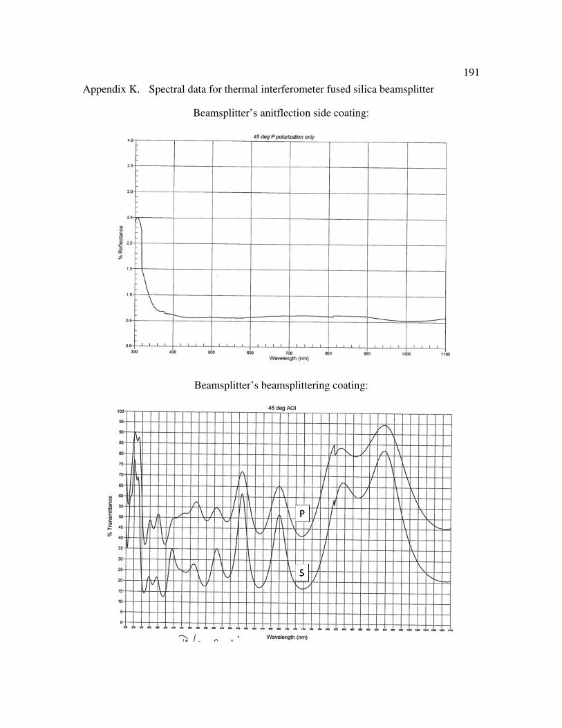
191

Appendix K. Spectral data for thermal interferometer fused silica beamsplitter

Beamsplitter’s anitflection side coating:

Beamsplitter’s beamsplittering coating:

192

Appendix L. Thermal interferometer: data acquisition code (MATLAB)

This is the main set of code is used to acquire phase maps. Note that InitCamera, InitState, and DefineRegion are separate subfunctions also included in this Appendix.

%% Initial Setup % % This code will initialize the camera as well as the piezo stage.

If % the piezo stage does not turn on and crashes matlab instead, try % unplugging and replugging in the power cable clear all addpath(genpath('cC:\Data\ThermalInterferometerToolbox')) % This setting determines the kind of test. A value of 1 will ask for % information about the corrsponding region. FlagReflect = 0; FlagTransmit = 0; FlagGRIN = 0; % Do you want to look at the wedge in the sample? FlagWedge = 0;

%Important information about the test and sample waveLength = .6328; %microns pressure = 1000.*98.9259776400000; %pascals relativeHumidity = 26.5; %percent thickNess = 5000; %micronsc inDexSample = 1.4935; %Sample index at ambient temperature wavenumber = 2*pi/waveLength;

%Start up the camera! [src vidobj] = InitCamera(30);

%Start up the Stage! htrans = InitStage;

%% Crop the region that is being watched by the camera! % A figure will appear, drag and right click to select the region you

would % like to record interferograms for.

vidobj.ROIPosition = DefineRegion(vidobj,2); %% Single shot - Code to get phase shift data in first place (move

piezo, take pics) % This code records intensity values of an averaged region of the

camera. % This should trace out a sine wave for an applied linear voltage. This % data will be used in the calibration the instrument. pause(1) tic clear vlt_stps V_app V_ramp clbrtn_frms

for vlt_stps = 1:201; % Number of voltage

193 vlt_stps V_app = 4+.05.*vlt_stps./2; % applied voltage per step V_ramp(vlt_stps) = V_app; % generate voltage ramp htrans.SetVoltOutput(0,V_app); pause(.02) clbrtn_frms(:,:,vlt_stps) = getsnapshot(vidobj); end toc

%% Plot acquired linescan of a single pixel intensity vs. applied

voltage % % This code will give us our calibration of the piezo stage to ramp

voltage % through a single period. This is necessary for the least-squares

phase % shifting algorithm we are using (Malacara). This code takes the

intensity % values from the previous section of code, plots them, then fits them

to a % sine wave, and finally designates a series of voltage values (with

black % circles) for stepping as we carry out the phase shifting algorithm.

Note % that these voltage values should span a single period of the sine

wave.

clear abc pxl_R pxl_C pxl_int amp1 shftd_pxl_int; % clbrtn_frms = double(clbrtn_frms); pxl_R = 100; pxl_C = 100; sqr_sz = 2; for abc = 1:length(V_ramp); pxl_int(abc) =

mean(mean(clbrtn_frms(pxl_R:pxl_R+sqr_sz,pxl_C:pxl_C+sqr_sz,abc))); end;

amp1 = 0.5.*(max(pxl_int) - min(pxl_int)); shftd_pxl_int = pxl_int - amp1 - min(pxl_int);

close(figure(3)) % figure(3) % plot(V_ramp,shftd_pxl_int,'r.') grid on

% close(figure(4));figure(4); hold on; box on; xx_data = V_ramp; yy_data=shftd_pxl_int; % plot(xx_data, yy_data, '.b')

d = xx_data; Irrad = yy_data; dmax = d(find(Irrad == max(Irrad),1,'first'));

194

Ifft=ifft(Irrad-mean(Irrad)); fftmax = find(abs(Ifft(1:fix(length(d)/2))) ==

max(abs(Ifft(1:fix(length(d)/2)))),1,'first'); dfx=(1/abs(d(2)-d(1)))/length(d); fxguess = dfx*(fftmax-1)*2*pi; phiguess = -fxguess*dmax;

AA = amp1; BB = fxguess; CC = phiguess; DD = 0; plot(xx_data, AA .* cos(BB .* xx_data + CC) + DD, '-g') % <-- Adjust

these title('Manual Fit')

% Now feed the starting point to Matlab myfit = fittype('a*cos(b*x+c)+d', 'independent', 'x', 'dependent',

'y'); myopt = fitoptions('Method', 'NonlinearLeastSquares'); myopt.StartPoint = [AA BB CC DD]; % <-- Numbers from Line 9 [f, g] = fit(xx_data', yy_data', myfit, myopt); yfit = f.a .* cos(f.b .* xx_data + f.c) + f.d;

% Plot James' data and the regression result close(figure(12));figure(12) hold on; box on plot(xx_data, yy_data, '.b') plot(xx_data, yfit, '-r') title('Matlab Fit')

V_fit = linspace(xx_data(1),xx_data(length(xx_data)),10001); yy_fit = f.a .* cos(f.b .* V_fit + f.c) + f.d; [ee V_max] = max(yy_fit(1:round(length(yy_fit)./2))); V1 = V_fit(V_max); V2 = V1 + 2.*pi./f.b; hold on; box on; num_st =4; % plot(linspace(V1,V2,num_st),linspace(0,0,num_st),'go') % yyfit = f.a .* cos(f.b .* linspace(V1,V2,num_st) + f.c) + f.d; PSramp = linspace(V1,V2,num_st+1); PSramp = PSramp(2:num_st+1); plot(PSramp,f.a .* cos(f.b .* PSramp + f.c) + f.d,'ko') % max(PSramp)-min(PSramp) % % % V2-V1 grid on PSramp(end)-PSramp(1)

%% Acquire phasemaps % % cThis code carries out the phase shifting algorithm by first moving

the % piezo stage to the first specified value in the vector 'PSramp',

captures

195 % a snapshot of the interferogram, saves it within the matrix 'snap',

then % moves the piezo stage to the second value within PSramp, captures a % second image, etc. until the matrix 'csnap' is a 3D matrix with the % dimensions of the camera aperature x the number of steps speficied by % 'num_st' in the previous section of code (25 seems to work well).

Once % 'snap' is completed, the interferograms can be processed to generate

a % phasemap (variable 'phasetemp') using the Malacara algorithm. The % phasemaps can be calculated during a data run or afterwards from the % 'snap' matrics. Both options are available in this code. To only

capture % a series of interferograms (only the 'snap' matricses), use lines

191-195 % and comment out 198-215. To generate phasemaps use lines 198-215 and % comment out 191-195 clear allfrm_allstp snap FS = stoploop; xyz = 0; while ~FS.Stop() % tic %_1 Name the count for the phase map xyz = xyz + 1; if xyz < 10; cnt = ['00000' num2str(xyz)]; elseif (xyz > 9) && (xyz < 100) cnt = ['0000' num2str(xyz)]; elseif (xyz > 99) && (xyz < 1000) cnt = ['000' num2str(xyz)]; elseif (xyz > 999) && (xyz < 10000) cnt = ['00' num2str(xyz)]; elseif (xyz > 9999) && (xyz < 100000) cnt = ['0' num2str(xyz)]; else cnt = num2str(xyz); end

clk = clock; % seco = num2str(clk(6)./60); tmstmp = [cnt '_' num2str(clk(4)) 'h' num2str(clk(5)) 'm_'

num2str(clk(2)) '_' num2str(clk(3)) '_' num2str(clk(1))]; %_1 %%%%%%%%%%%%%%%%%%%%%%%%%%%%% xyz % frng_snp = getsnapshot(vidobj); % save([cnt '_snap'],'frng_snp','-v7.3') %_2 Main code for ijk = 1:length(PSramp) % Number of voltage steps htrans.SetVoltOutput(0,PSramp(ijk)); pause(.03) % for lmn = 1 % number of images you are averaging % onefrm_stp = getsnapshot(vidobj); % store a single frame % allfrm_stp(:,:,lmn)=onefrm_stp; % Frames to be averaged

196 % clear onefrm_stp % end % avfrm_stp=mean(allfrm_stp,3); snap(:,:,ijk) = getsnapshot(vidobj); % clear avfrm_stp end % % %

% % % % % % % % % % % % % % % % % % % % % % % % % % % % % % % % % % % % % % % % % % % % % % % % % % % % % % Code for saving snapshots % % % % % % % % % % % % % % % % % % % % % % % % % % % % % % % % % % % % % % save(tmstmp,'snap','-v7.3') % % % % % % % % % % % % % % % % % % % % % % % % % % % % % % % % %

% % % % % % % % % % % % % % % % % % % % % % % % % % % % % % % % % % % % Code for makeing phasemaps, variable 'phasetemp' % % % % % % % % % % % % % % % % % % % % % % % % % % % % % % % % % % del = (1:length(PSramp)).*2.*pi./(length(PSramp)); I = double(snap);%(:,:,1:PSramp); N = 0; D = 0; for qrs = 1:(length(del)) N = N - I(:,:,qrs).*sin(del(qrs)); N=double(N); D = D + I(:,:,qrs).*cos(del(qrs)); D=double(D); end phasetemp = atan2(N,D);

save(tmstmp,'phasetemp','-v7.3') % % % % % % % % % % % % % % % % % % % % % % % % % % % % % % % % % % % % % % % % % % % % % % % % % % % % % % % % % % % % % % % % % %

%

pause(.05) end

%% % % Code for examining a generated phasemaps. This will plot whatever

is % saved as variable 'phasetemp'. It will show an image of the phasemaps

as % well as both wrapped and unwrapped spatial cutthroughs of the

variable in % both the horizontal and vertical directions. These cuttrhoughs can be % specified by the user using commands hcut and vcut (lines 236-237) close(figure(3)) figure(3) subplot(2,4,[1:2 5:6]) % surf(phasetemp_fft) imagesc(phasetemp)

197 % ylim([0 550]) view(2) shading interp colorbar hold on vcut = 125; hcut = 50;%55; line([vcut vcut],[0 size(phasetemp,1)],[4 4],'LineWidth',1,'Color','k') line([0 size(phasetemp,2)],[hcut hcut],[4 4],'LineWidth',1,'Color','k') axis equal

subplot(2,4,3) plot((phasetemp(:,vcut)),'k.') title('Vertical') grid on xlim([0 size(phasetemp,1)]) subplot(2,4,7) plot((phasetemp(hcut,:)),'k.') title('Horizontal') grid on xlim([0 size(phasetemp,2)])

subplot(2,4,4) v_unwrap = unwrap(phasetemp(:,vcut)'); vymin = 1; vymax = size(phasetemp,1); vxdata = vymin:vymax; vydata = v_unwrap(vymin:vymax)./(2.*pi); myfit = fittype('a*x+b', 'independent', 'x', 'dependent', 'y'); myopt = fitoptions('Method', 'NonlinearLeastSquares'); myopt.StartPoint = [-1 20]; % [f, g] = fit(vxdata', vydata', myfit, myopt); plot(vxdata,vydata,'r.');hold

on;plot(vxdata,f.a.*vxdata+f.b,'LineWidth',2) xlabel('Pixel') ylabel('Fringes') grid on title('Vertical') xlim([0 10+size(phasetemp,1)])

subplot(2,4,8) h_unwrap = unwrap(phasetemp(hcut,:)); hymin = 1; hymax = size(phasetemp,2); hxdata = hymin:hymax; hydata = h_unwrap(hymin:hymax)./(2.*pi); myfit = fittype('a*x+b', 'independent', 'x', 'dependent', 'y'); myopt = fitoptions('Method', 'NonlinearLeastSquares'); myopt.StartPoint = [-1 20]; % [f, g] = fit(hxdata', hydata', myfit, myopt); plot(hxdata,hydata,'r.');hold

on;plot(hxdata,f.a.*hxdata+f.b,'LineWidth',2) xlabel('Pixel') ylabel('Fringes') grid on title('Horizontal') xlim([0 10+size(phasetemp,2)])

198

Function InitCamera:

function [src vidobj] = InitCamera(framerate,exposuretime) %%%%%%%%%%%%%%%%%%%%%%%%%%%%%%%%%%%%%%%%%%%%% % InitCamera v .1 Jan/14/2016 % Bill Green, James Corsetti % Description: Starts up the CMOS sensor used for capturing phasemaps

% src - a structure that contains video settings such as frame rate, % exposure time, etc.

% vidobj - a structure that references the video feed

% framerate - provided in FPS. This script will provide a default if

not % specified

% exposuretime - prodivded in seconds. A default is provided if not

specified. % This script will terminate if the exposure time is longer than the

time between frames. imaqreset

if nargin < 2, exposuretime = []; end if nargin < 1, framerate = []; end

% supply default parameters if isempty(framerate), framerate = 30; end if isempty(exposuretime), exposuretime = .015736; end

if exist('vidobj') delete(vidobj) clear vidobj end

vidobj=videoinput('pointgrey', 1, 'F7_Raw8_640x512_Mode1'); viewport = preview(vidobj); vidobj.ReturnedColorspace='grayscale'; src = getselectedsource(vidobj); vidobj.ROIPosition = [0 0 640 512];

disp('Please wait 10 seconds...')

pause(2) src.ExposureMode = 'Manual'; pause(2) maxfps = 120; src.FrameRatePercentageMode = 'Manual';

199 src.FrameRatePercentage = 100*framerate/maxfps; pause(2) src.GainMode = 'Manual'; pause(2) src.ShutterMode = 'Manual'; if exposuretime > 1/framerate exposuretime = 1/(1.1*framerate); disp('Exposure time exceeds time inbetween frames, shutterspeed

changed accordingly') end src.Shutter = exposuretime; pause(2) disp('Camera Initialized Successfully')

Function InitCamera:

function htrans = InitStage %%%%%%%%%%%%%%%%%%%%%%%%%%%%%%%%%%%%%%%%%%%%% % InitStage v .1 Jan/11/2016 % Bill Green, James Corsetti % Description: Starts up the Thorlabs piezometric stage

% htrans - a handle for the stage, used to set the voltage

disp('Initializing Piezometric stage...') close(figure(2)) fig = figure(2); % Define figure for stage control activex GUI % set(fig,'Position',[200 200 1100 400]);

htrans = actxcontrol('MGPIEZO.MGPiezoCtrl.1',[0 0 549 400],fig);%

Define control for translation stage set(htrans,'HWSerialNum',81834010);% Determine the serial number of the

translation stage driver htrans.StartCtrl;% Start control disp('Phase Shifting Stage Initialized Successfully.')

200

Function DefineRegion:

function [cropCoords] = DefineRegion(image,imagetype) %%%%%%%%%%%%%%%%%%%%%%%%%%%%%%%%%%%%%%%%%%%%% % DefineRegion v .1 Jan/15/2016 % Bill Green, James Corsetti % Description: Grabs a screenshot from the camera, and allows you % to interactively select a region to subsample.

% image - The image that will be looked at in order to crop a region.

This can % either be the handle for the video feed, or a static image of the

phase % map. Designate this with the imagetype flag.

% imagetype - a flag that gets a screenshot differently depending on % whether you are pulling from a static image or the video feed. % imagetype = 1, use a static screenshot % imagetype = 2, use the video feed

% cropCoords - vector containing the information about the cropped % region: [xorigin yorigin width height]

switch imagetype case 1 imagetocrop = image;

case 2 imagetocrop = getsnapshot(image); end

fig = figure; [sampleRegion,cropCoords] = imcrop(imagetocrop); %imshow(sampleRegion); %crop = 'This is the region you have selected'; cropCoords = floor(cropCoords); close(fig) %j = text(.1*cropCoords(3),.1*cropCoords(4), crop,

'FontSize',14,'Color','r');

201

Appendix M. Thermal interferometer: data analysis code (MATLAB)

% Code for analyzing CTE and dn/dT clear timetab TAtab Ptab RHtab nairtab TStab timetab = excel_3_30_2017(:,1); Ptab = 1000.*98.9259776400000; RHtab = 26.5; TAtab = excel_3_30_2017(:,2); % air temperature TStab = (excel_3_30_2017(:,3) + excel_3_30_2017(:,4) +

excel_3_30_2017(:,5))./3; % sample temp nairtab = air_index_calc(TAtab,Ptab,RHtab,.6328); k = 2*pi/.6328; %% % Plot air and sample temp. vs time close(figure(154));figure(154) plot(excel_3_30_2017(:,1),TAtab,'m--') grid on; hold on plot(excel_3_30_2017(:,1),excel_3_30_2017(:,3),'r') plot(excel_3_30_2017(:,1),excel_3_30_2017(:,4),'g') plot(excel_3_30_2017(:,1),excel_3_30_2017(:,5),'b') plot(excel_3_30_2017(:,1),TStab,'k')

%% % Store all phasemaps in folder as variable D clear D vv fileloc = 'I:\2017_03_30_Syntec_5_&_7_p5_to35ramp_13hrs\PhaseMaps'; D = dir(fileloc); [vv,idx] = sort([D.datenum]); %% % Mark pixels in different regions to extract wrapped phase as a

function % of count close(figure(32)) figure(32); imagesc(phasetemp(:,:)); colorbar colormap summer axis equal hold on MKs = 6;

bg_ww_sft = 200; bg_ww = what_bg_pxls; ref_ww = what_ref_pxls; trans_ww = what_trans_pxls; regi4_ww = 1; reg55_ww =1;

% % % % % % % % % % % % % % % % % % Background region

202 % % % % % % % % % % % % % % % % % clear rows_bg cols_bg X_bg Y_bg X_bg_R Y_bg_R bg_cnt bg_pts

rows_bg=[50:5:130]; cols_bg=[132:5:192]'; [X_bg, Y_bg] = meshgrid(rows_bg,cols_bg); X_bg_R = reshape(X_bg,length(rows_bg)*length(cols_bg),1); Y_bg_R = reshape(Y_bg,length(rows_bg)*length(cols_bg),1);

for bg_cnt = 1:length(rows_bg)*length(cols_bg); bg_pts(bg_cnt,1) = X_bg_R(bg_cnt); bg_pts(bg_cnt,2) = Y_bg_R(bg_cnt); end

for bg_cnt2 = 1:size(bg_pts,1)

plot(bg_pts(bg_cnt2,2),bg_pts(bg_cnt2,1),'ro','MarkerSize',MKs,'MarkerE

dgeColor','k','MarkerFaceColor',[0 bg_cnt2./size(bg_pts,1) 0]) end

plot(bg_pts(bg_ww,2),bg_pts(bg_ww,1),'ro','MarkerSize',MKs,'MarkerEdgeC

olor','k','MarkerFaceColor',[1 0 0])

bg = [mean(bg_pts(bg_ww,1)) mean(bg_pts(bg_ww,2))];

text(bg(2)+5,bg(1),'BG') plot(bg(2),bg(1),'kx') plot(bg(2),bg(1),'ko')

% % % % % % % % % % % % % % % % % % % % % % % % % Reflection region (CTE of sample 1) % % % % % % % % % % % % % % % % % % % % % clear ref rows_ref cols_ref X_ref Y_ref X_ref_R Y_ref_R ref_cnt ref_pts

hold on rows_ref=[20:5:70]; cols_ref=[25:5:95]'; [X_ref, Y_ref] = meshgrid(rows_ref,cols_ref); X_ref_R = reshape(X_ref,length(rows_ref)*length(cols_ref),1); Y_ref_R = reshape(Y_ref,length(rows_ref)*length(cols_ref),1);

for ref_cnt = 1:length(rows_ref)*length(cols_ref); ref_pts(ref_cnt,1) = X_ref_R(ref_cnt); ref_pts(ref_cnt,2) = Y_ref_R(ref_cnt); end

for ref_cnt2 = 1:size(ref_pts,1)

203

plot(ref_pts(ref_cnt2,2),ref_pts(ref_cnt2,1),'ro','MarkerSize',MKs,'Mar

kerEdgeColor','k','MarkerFaceColor',[ref_cnt2./size(ref_pts,1) 0 1]) end

plot(ref_pts(ref_ww,2),ref_pts(ref_ww,1),'ro','MarkerSize',MKs,'MarkerE

dgeColor','k','MarkerFaceColor',[1 0 0]) ref = [mean(ref_pts(ref_ww,1)) mean(ref_pts(ref_ww,2))]; text(ref(2)+5,ref(1),'ref') plot(ref(2),ref(1),'kx') plot(ref(2),ref(1),'ko')

% % % % % % % % % % % % % % % % % % % % Transmission region (dn/dT of sample 1) % % % % % % % % % % % % % % % % % % % clear trans rows_trans cols_trans X_trans Y_trans X_trans_R Y_trans_R

trans_cnt trans_pts

hold on rows_trans=[92:5:142]; cols_trans=[25:5:95]'; [X_trans, Y_trans] = meshgrid(rows_trans,cols_trans); X_trans_R = reshape(X_trans,length(rows_trans)*length(cols_trans),1); Y_trans_R = reshape(Y_trans,length(rows_trans)*length(cols_trans),1);

for trans_cnt = 1:length(rows_trans)*length(cols_trans); trans_pts(trans_cnt,1) = X_trans_R(trans_cnt); trans_pts(trans_cnt,2) = Y_trans_R(trans_cnt); end

for trans_cnt2 = 1:size(trans_pts,1)

plot(trans_pts(trans_cnt2,2),trans_pts(trans_cnt2,1),'ro','MarkerSize',

MKs,'MarkerEdgeColor','k','MarkerFaceColor',[1-

trans_cnt2./size(trans_pts,1) 1-trans_cnt2./size(trans_pts,1) 1-

trans_cnt2./size(trans_pts,1)]) end

plot(trans_pts(trans_ww,2),trans_pts(trans_ww,1),'ro','MarkerSize',MKs,

'MarkerEdgeColor','k','MarkerFaceColor',[1 0 0]) trans = [mean(trans_pts(trans_ww,1)) mean(trans_pts(trans_ww,2))]; text(trans(2)+5,trans(1),'trans') plot(trans(2),trans(1),'kx') plot(trans(2),trans(1),'ko')

xlabel('Pixels') ylabel('Pixels')

% % % % % % % % % % % % % % % % % % % % % % % region 4 region (CTE of sample 2)

204 % % % % % % % % % % % % % % % % % % % % % % clear regi4 rows_regi4 cols_regi4 X_regi4 Y_regi4 X_regi4_R Y_regi4_R

regi4_cnt regi4_pts

hold on rows_regi4=[20:5:70]; cols_regi4=[230:5:300]'; [X_regi4, Y_regi4] = meshgrid(rows_regi4,cols_regi4); X_regi4_R = reshape(X_regi4,length(rows_regi4)*length(cols_regi4),1); Y_regi4_R = reshape(Y_regi4,length(rows_regi4)*length(cols_regi4),1);

for regi4_cnt = 1:length(rows_regi4)*length(cols_regi4); regi4_pts(regi4_cnt,1) = X_regi4_R(regi4_cnt); regi4_pts(regi4_cnt,2) = Y_regi4_R(regi4_cnt); end

for regi4_cnt2 = 1:size(regi4_pts,1)

plot(regi4_pts(regi4_cnt2,2),regi4_pts(regi4_cnt2,1),'ro','MarkerSize',

MKs,'MarkerEdgeColor','k','MarkerFaceColor',[0 0

regi4_cnt2./size(regi4_pts,1)]) end

plot(regi4_pts(regi4_ww,2),regi4_pts(regi4_ww,1),'ro','MarkerSize',MKs,

'MarkerEdgeColor','k','MarkerFaceColor',[1 0 0]) regi4 = [regi4_pts(regi4_ww,1) regi4_pts(regi4_ww,2)]; text(regi4(2)+5,regi4(1),'SS') plot(regi4(2),regi4(1),'kx') plot(regi4(2),regi4(1),'ko')

xlabel('Pixels') ylabel('Pixels')

% % % % % % % % % % % % % % % % % % % % % % reg55mission region (dn/dT of sample 2) % % % % % % % % % % % % % % % % % % % % % clear reg55 rows_reg55 cols_reg55 X_reg55 Y_reg55 X_reg55_R Y_reg55_R

reg55_cnt reg55_pts

hold on rows_reg55=[92:5:142]; cols_reg55=[230:5:300]'; [X_reg55, Y_reg55] = meshgrid(rows_reg55,cols_reg55); X_reg55_R = reshape(X_reg55,length(rows_reg55)*length(cols_reg55),1); Y_reg55_R = reshape(Y_reg55,length(rows_reg55)*length(cols_reg55),1);

for reg55_cnt = 1:length(rows_reg55)*length(cols_reg55); reg55_pts(reg55_cnt,1) = X_reg55_R(reg55_cnt); reg55_pts(reg55_cnt,2) = Y_reg55_R(reg55_cnt); end

205 for reg55_cnt2 = 1:size(reg55_pts,1)

plot(reg55_pts(reg55_cnt2,2),reg55_pts(reg55_cnt2,1),'ro','MarkerSize',

MKs,'MarkerEdgeColor','k','MarkerFaceColor',[1-

reg55_cnt2./size(reg55_pts,1) 1-reg55_cnt2./size(reg55_pts,1) 1-

reg55_cnt2./size(reg55_pts,1)]) end

plot(reg55_pts(reg55_ww,2),reg55_pts(reg55_ww,1),'ro','MarkerSize',MKs,

'MarkerEdgeColor','k','MarkerFaceColor',[1 0 0]) reg55 = [reg55_pts(reg55_ww,1) reg55_pts(reg55_ww,2)]; text(reg55(2)+5,reg55(1),'reg55') plot(reg55(2),reg55(1),'kx') plot(reg55(2),reg55(1),'ko')

xlabel('Pixels') ylabel('Pixels')

%%%%%%%%%%%%%%%%%%%%%%%%%%%%%%%%%

% Background for fitting tilt clear backgroundrows backgroundcols backgroundrows = 60:120; backgroundcols = 132:192; line([backgroundcols(1)

backgroundcols(length(backgroundcols))],[backgroundrows(1)

backgroundrows(1)],'Color',[1 1 1],'LineWidth',2.5) line([backgroundcols(1)

backgroundcols(length(backgroundcols))],[backgroundrows(length(backgrou

ndrows)) backgroundrows(length(backgroundrows))],'Color',[1 1

1],'LineWidth',2.5) line([backgroundcols(1) backgroundcols(1)],[backgroundrows(1)

backgroundrows(length(backgroundrows))],'Color',[1 1

1],'LineWidth',2.5) line([backgroundcols(length(backgroundcols))

backgroundcols(length(backgroundcols))],[backgroundrows(1)

backgroundrows(length(backgroundrows))],'Color',[1 1

1],'LineWidth',2.5)

%% clear time TAmeas TSmeas RHmeas nair refphase bgphase transphase

regi4phase xtilt ytilt %% clear bgphase_unfil bgphase_fft refphase_unfil refphase_fft

transphase_unfil transphase_fft %% % f1 and f2 are the bounds of the phasemaps f1 =3; f2 =70403; tic for frame = f1:1:f2; frame PM = D(frame).name;

206 load(PM); clear phasetemp_unfil phasetemp_fft phasetemp_combo

% The 3 sections below extract different information from system and

should % be run separately from f1 to f2

% % % % This code calculates time, nair, temp as a function of phasemap % 1 time(frame-f1+1) = D(frame).datenum; % 1 TAmeas(frame-f1+1) = interp1(timetab,TAtab,time(frame-

f1+1));%,'cubic','extrap'); % 1 TSmeas(frame-f1+1) = interp1(timetab,TStab,time(frame-

f1+1));%,'cubic','extrap'); % 1 RHmeas(frame-f1+1) = RHtab; % 1 nair(frame-f1+1) = interp1(timetab,nairtab,time(frame-

f1+1));%,'cubic','extrap'); % % % %

% % % % This code is used to fit background tilt % 2 b = puma_ho(phasetemp(backgroundrows,backgroundcols),2); % 2 % Fit 2-D tilt to background data % 2 [x1,y1] = meshgrid(backgroundcols,backgroundrows); % 2 model_function0 = @(vars,r) vars(3) + vars(1)*r(:,1) +

vars(2)*r(:,2); % fit background tilt to a plane % 2 guess = [(b(round(size(b,1)/2),end)-

b(round(size(b,1)/2),1))/(backgroundcols(end)-backgroundcols(1))

(b(end,round(size(b,2)/2))-

b(1,round(size(b,2)/2)))/(backgroundrows(end)-backgroundrows(1))

mean(mean(b))]; % guess is taking endpoints and finding slope % 2 [varfit1,resid,J,Sigma] = nlinfit([x1(:)

y1(:)],b(:),model_function0,guess,statset('TolFun',1e-30,'TolX',1e-

20,'MaxIter',1000)); % 2 xtilt(frame-f1+1) = varfit1(1);%/(2*nair(frame-f1+1)*k); %

putting the tilt into units of waves % 2 ytilt(frame-f1+1) = varfit1(2);%/(2*nair(frame-f1+1)*k); % % % %

% % % % Extract wrapped phase vs. pixel for each region of interest % 3 for bgcnt = 1:size(bg_pts,1); % 3 bgphase(frame-

f1+1,bgcnt)=phasetemp(bg_pts(bgcnt,1),bg_pts(bgcnt,2)); % 3 end % 3 % 3 for refcnt = 1:size(ref_pts,1); % 3 refphase(frame-

f1+1,refcnt)=phasetemp(ref_pts(refcnt,1),ref_pts(refcnt,2)); % 3 end % 3 % 3 for transcnt = 1:size(trans_pts,1); % 3 transphase(frame-

f1+1,transcnt)=phasetemp(trans_pts(transcnt,1),trans_pts(transcnt,2)); % 3 end % 3

207 % 3 for regi4cnt = 1:size(regi4_pts,1); % 3 regi4phase(frame-

f1+1,regi4cnt)=phasetemp(regi4_pts(regi4cnt,1),regi4_pts(regi4cnt,2)); % 3 end % 3 % 3 for reg55cnt = 1:size(reg55_pts,1); % 3 reg55phase(frame-

f1+1,reg55cnt)=phasetemp(reg55_pts(reg55cnt,1),reg55_pts(reg55cnt,2)); % 3 end % % % %

end toc %% % scale tilt by wavenumber xtilt=(xtilt_interp./(2.*nair.*k)); ytilt=(ytilt_interp./(2.*nair.*k)); disp('done') %% % fit tilt of every tenth phasemap with spline. That gives an x and y

tilt % for each phasemap xtilt_interp =

interp1(1:10:70401,xtilt(1:10:70401),1:1:70401,'spline'); ytilt_interp =

interp1(1:10:70401,ytilt(1:10:70401),1:1:70401,'spline'); figure;plot(xtilt_interp,'b.'); hold on; plot(1:10:70401,xtilt,'ro') figure;plot(ytilt_interp,'b.'); hold on; plot(1:10:70401,ytilt,'ro')

%% % This code unwraps bgphase, refphase, transphase and stores them as % variables: bgphaseuw_shft, refphaseuw_shft, and transphaseuw_shft

% Unwrap background phase clear bgphaseuw bguw_cnt bgphaseuw = zeros(size(bgphase,1),size(bgphase,2)); for bguw_cnt = 1:size(bgphase,2); bgphaseuw(:,bguw_cnt) = unwrap(bgphase(:,bguw_cnt)); % plot(bgphaseuw(:,bguw_cnt),'Color',[0 1 0]);%%[0

bguw_cnt./size(bg_pts,1) 0]) % hold on end

% Unwrap reflection phase clear refphaseuw refuw_cnt refphaseuw = zeros(size(refphase,1),size(refphase,2)); for refuw_cnt = 1:size(refphase,2); refphaseuw(:,refuw_cnt) = unwrap(refphase(:,refuw_cnt));

208 % plot(refphaseuw(:,refuw_cnt),'Color',[1 0

1])%[refuw_cnt./size(ref_pts,1) 0 1]) % hold on end

% Unwrap transmission phase clear transphaseuw transuw_cnt transphaseuw = zeros(size(transphase,1),size(transphase,2)); for transuw_cnt = 1:size(transphase,2); transphaseuw(:,transuw_cnt) = unwrap(transphase(:,transuw_cnt)); % plot(transphaseuw(:,transuw_cnt),'Color',[0 0 0]);%[1-

transuw_cnt./size(trans_pts,1) 1-transuw_cnt./size(trans_pts,1) 1-

transuw_cnt./size(trans_pts,1)]) % hold on end

% Shifted background phase clear bgphaseuw_shft close(figure(40)) figure(40) subplot(2,2,1) shft = 1; aaa = shft; bbb = 72000;

clear bgphaseuw_shft bgphaseuw_shft = zeros(size(bgphaseuw,1),size(bgphaseuw,2)); for bguw_shft_cnt = 1:size(bgphaseuw,2); bgphaseuw_shft(:,bguw_shft_cnt) = bgphaseuw(:,bguw_shft_cnt)-

bgphaseuw(shft,bguw_shft_cnt); plot(bgphaseuw_shft(:,bguw_shft_cnt),'Color',[0

bguw_shft_cnt./size(bgphaseuw,2) 0]) hold on end plot(mean(bgphaseuw_shft,2),'k','LineWidth',2.5) grid on xlabel('Count,time') ylabel('Fringes') xlim([aaa bbb])

% Shifted reference region clear refphaseuw_shft subplot(2,2,2) clear refphaseuw_shft refphaseuw_shft = zeros(size(refphaseuw,1),size(refphaseuw,2)); for refuw_shft_cnt = 1:size(refphaseuw,2); refphaseuw_shft(:,refuw_shft_cnt) = refphaseuw(:,refuw_shft_cnt)-

refphaseuw(shft,refuw_shft_cnt);

plot(refphaseuw_shft(:,refuw_shft_cnt),'Color',[refuw_shft_cnt./size(re

fphaseuw,2) 0 1]) hold on end

209 grid on plot(mean(refphaseuw_shft,2),'k','LineWidth',2.5) xlabel('Count,time') ylabel('Fringes') xlim([aaa bbb])

% Shifted transmission region clear transphaseuw_shft subplot(2,2,3) clear transphaseuw_shft transphaseuw_shft = zeros(size(transphaseuw,1),size(transphaseuw,2)); for transuw_shft_cnt = 1:size(transphaseuw,2); transphaseuw_shft(:,transuw_shft_cnt) =

transphaseuw(:,transuw_shft_cnt)-transphaseuw(shft,transuw_shft_cnt); plot(transphaseuw_shft(:,transuw_shft_cnt),'Color',[1-

transuw_shft_cnt./size(transphaseuw,2) 1-

transuw_shft_cnt./size(transphaseuw,2) 1-

transuw_shft_cnt./size(transphaseuw,2)]) hold on end grid on xlabel('Count,time') ylabel('Fringes') xlim([aaa bbb]) clear bgphaseuw refphaseuw transphaseuw

%% % Checkderiv code. This identifies the "best behaved" pixels in terms

of % discontinuities in the unwrapped phase and stores those values as % what_bg_pxls, what_ref_pxls, and what_trans_pxls to be used in code

above % when speficying pixels of interest close(figure(57));figure(57); clear what_bg_pxls bg_diff_cnt chk_bg_diff_met chk_bg_diff clear what_ref_pxls ref_diff_cnt chk_ref_diff_met chk_ref_diff clear what_trans_pxls trans_diff_cnt chk_trans_diff_met chk_trans_diff

thrsh_bg=3.0138; thrsh_ref=3.081;%2.752;%2.96; thrsh_trans=2.98;%2.416; stopshft = 53870;%40000; ofst = 1;%11500;

subplot(3,1,1) bg_diff_cnt = 1; for pixels = 1:size(bg_pts,1); chk_bg_diff =

sort(abs(diff(bgphaseuw_shft(shft+ofst:stopshft,pixels))),'descend'); chk_bg_diff_met(pixels) = mean(chk_bg_diff(1:6)); if chk_bg_diff_met(pixels) < thrsh_bg what_bg_pxls(bg_diff_cnt) = pixels; bg_diff_cnt = bg_diff_cnt+1;

210 end clear chk_bg_diff end plot(chk_bg_diff_met,'go') hold on plot(what_bg_pxls,chk_bg_diff_met(what_bg_pxls),'gx') plot(what_bg_pxls,chk_bg_diff_met(what_bg_pxls),'ko')

subplot(3,1,2) ref_diff_cnt = 1; for pixels = 1:size(ref_pts,1); chk_ref_diff =

sort(abs(diff(refphaseuw_shft(shft+ofst:stopshft,pixels))),'descend'); chk_ref_diff_met(pixels) = mean(chk_ref_diff(1:6)); if chk_ref_diff_met(pixels) < thrsh_ref what_ref_pxls(ref_diff_cnt) = pixels; ref_diff_cnt = ref_diff_cnt+1; end clear chk_ref_diff end plot(chk_ref_diff_met,'mo') hold on plot(what_ref_pxls,chk_ref_diff_met(what_ref_pxls),'mx') plot(what_ref_pxls,chk_ref_diff_met(what_ref_pxls),'ko')

subplot(3,1,3) trans_diff_cnt = 1; for pixels = 1:size(trans_pts,1); chk_trans_diff =

sort(diff(transphaseuw_shft(shft:stopshft,pixels)),'descend'); chk_trans_diff_met(pixels) = mean(chk_trans_diff(1:6)); if chk_trans_diff_met(pixels) < thrsh_trans what_trans_pxls(trans_diff_cnt) = pixels; trans_diff_cnt = trans_diff_cnt+1; end clear chk_trans_diff end plot(chk_trans_diff_met,'ko') hold on plot(what_trans_pxls,chk_trans_diff_met(what_trans_pxls),'rx') plot(what_trans_pxls,chk_trans_diff_met(what_trans_pxls),'ro')

%% % The following section of code calculates the CTE and dn/dT of the

sample

clear startframe endframe % these values are defined earlier in the code. The unwrapped phase

values % of each region bgphaseuw1 = mean(bgphaseuw_shft(:,bg_ww),2); refphaseuw1 = mean(refphaseuw_shft(:,ref_ww),2); transphaseuw1 = mean(transphaseuw_shft(:,trans_ww),2);

211

dOPD1 = (bgphaseuw1)./k; dOPD2 = (refphaseuw1)./k; dOPD3 = (transphaseuw1)./k;

close(figure(54));figure(54);plot(dOPD1,'g');hold

on;plot(dOPD2,'m');plot(dOPD3,'k');grid on close(figure(55));figure(55);plot(TSmeas,dOPD1,'g');hold

on;plot(TSmeas,dOPD2,'m');grid on;plot(TSmeas,dOPD3,'k');grid on xlabel('Temp') ylabel('Change in OPD ({\mu}m)'); legend('Background','Sample','Transmission')

startframe=shft; endframe = length(TSmeas); dOPD1_bnd = dOPD1(startframe:endframe)'; dOPD2_bnd = dOPD2(startframe:endframe)'; dOPD3_bnd = dOPD3(startframe:endframe)';

nair_bnd = nair(startframe:endframe); xtilt_bnd = xtilt(startframe:endframe); ytilt_bnd = ytilt(startframe:endframe); TAmeas_bnd = TAmeas(startframe:endframe); TSmeas_bnd = TSmeas(startframe:endframe); time_bnd = time(startframe:endframe);

% base thickness (in microns) and index of sample t0=2495; n0=1.52869493454192;

% calculated thickness and index of the sample over time tsamp = (nair_bnd(1).*t0 + 0.5.*(dOPD1_bnd-dOPD2_bnd) -

1.*((nair_bnd(1).*xtilt_bnd(1) - nair_bnd.*xtilt_bnd).*(ref(2)-bg(2)) +

(nair_bnd(1).*ytilt_bnd(1) - nair_bnd.*ytilt_bnd).*(ref(1)-

bg(1))))./nair_bnd; nsamp = (n0.*t0 + .5.*(dOPD3_bnd-dOPD2_bnd) + 1.*((nair_bnd.*xtilt_bnd

- nair_bnd(1).*xtilt_bnd(1)).*(ref(2) - trans(2)) +

(nair_bnd.*ytilt_bnd - nair_bnd(1).*ytilt_bnd(1)).*(ref(1) -

trans(1))))./tsamp;

% The following code is used find the change in both thickness and % index and then to fix discontinuities in the data dt = tsamp - tsamp(1); dtA=931;dtB=923;dt(dtA:length(dt))=dt(dtA:length(dt))-(dt(dtA)-

dt(dtB)); dtA=1161;dtB=1151;dt(dtA:length(dt))=dt(dtA:length(dt))-(dt(dtA)-

dt(dtB)); dtA=1432;dtB=1421;dt(dtA:length(dt))=dt(dtA:length(dt))-(dt(dtA)-

dt(dtB));

dn = nsamp - nsamp(1);

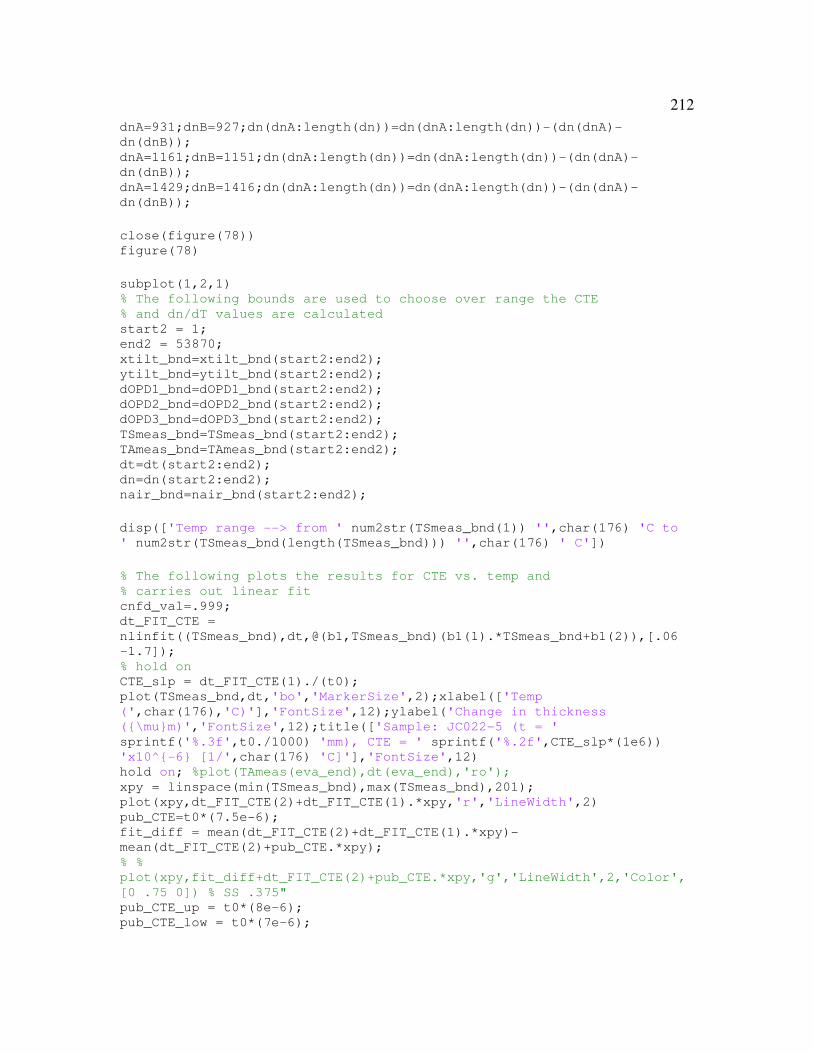
212 dnA=931;dnB=927;dn(dnA:length(dn))=dn(dnA:length(dn))-(dn(dnA)-

dn(dnB)); dnA=1161;dnB=1151;dn(dnA:length(dn))=dn(dnA:length(dn))-(dn(dnA)-

dn(dnB)); dnA=1429;dnB=1416;dn(dnA:length(dn))=dn(dnA:length(dn))-(dn(dnA)-

dn(dnB));

close(figure(78)) figure(78)

subplot(1,2,1) % The following bounds are used to choose over range the CTE % and dn/dT values are calculated start2 = 1; end2 = 53870; xtilt_bnd=xtilt_bnd(start2:end2); ytilt_bnd=ytilt_bnd(start2:end2); dOPD1_bnd=dOPD1_bnd(start2:end2); dOPD2_bnd=dOPD2_bnd(start2:end2); dOPD3_bnd=dOPD3_bnd(start2:end2); TSmeas_bnd=TSmeas_bnd(start2:end2); TAmeas_bnd=TAmeas_bnd(start2:end2); dt=dt(start2:end2); dn=dn(start2:end2); nair_bnd=nair_bnd(start2:end2);

disp(['Temp range --> from ' num2str(TSmeas_bnd(1)) '',char(176) 'C to

' num2str(TSmeas_bnd(length(TSmeas_bnd))) '',char(176) ' C'])

% The following plots the results for CTE vs. temp and % carries out linear fit cnfd_val=.999; dt_FIT_CTE =

nlinfit((TSmeas_bnd),dt,@(b1,TSmeas_bnd)(b1(1).*TSmeas_bnd+b1(2)),[.06

-1.7]); % hold on CTE_slp = dt_FIT_CTE(1)./(t0); plot(TSmeas_bnd,dt,'bo','MarkerSize',2);xlabel(['Temp

(',char(176),'C)'],'FontSize',12);ylabel('Change in thickness

({\mu}m)','FontSize',12);title(['Sample: JC022-5 (t = '

sprintf('%.3f',t0./1000) 'mm), CTE = ' sprintf('%.2f',CTE_slp*(1e6))

'x10^{-6} [1/',char(176) 'C]'],'FontSize',12) hold on; %plot(TAmeas(eva_end),dt(eva_end),'ro'); xpy = linspace(min(TSmeas_bnd),max(TSmeas_bnd),201);

plot(xpy,dt_FIT_CTE(2)+dt_FIT_CTE(1).*xpy,'r','LineWidth',2) pub_CTE=t0*(7.5e-6); fit_diff = mean(dt_FIT_CTE(2)+dt_FIT_CTE(1).*xpy)-

mean(dt_FIT_CTE(2)+pub_CTE.*xpy); % %

plot(xpy,fit_diff+dt_FIT_CTE(2)+pub_CTE.*xpy,'g','LineWidth',2,'Color',

[0 .75 0]) % SS .375" pub_CTE_up = t0*(8e-6); pub_CTE_low = t0*(7e-6);

213 fit_diff1 = mean(dt_FIT_CTE(2)+dt_FIT_CTE(1).*xpy)-

mean(dt_FIT_CTE(2)+pub_CTE_up.*xpy); % % plot(xpy,fit_diff1+dt_FIT_CTE(2)+pub_CTE_up.*xpy,'g--

','LineWidth',2,'Color',[0 .75 0]) % SS .375" fit_diff1 = mean(dt_FIT_CTE(2)+dt_FIT_CTE(1).*xpy)-

mean(dt_FIT_CTE(2)+pub_CTE_low.*xpy); % % plot(xpy,fit_diff1+dt_FIT_CTE(2)+pub_CTE_low.*xpy,'g--

','LineWidth',2,'Color',[0 .75 0]) % SS .375" fitresult = fit(TSmeas_bnd',dt','poly1'); ci = confint(fitresult,cnfd_val); disp(['dL/dT CTE of JC022-5 = ' sprintf('%.3f',CTE_slp*(1e6)) 'x10^{-6}

[1/',char(176) 'C]'])% '']) % disp(['Error of CTE of JC022-5 = ' sprintf('%.2f',(CTE_slp-

ci(1,1)./t0)*(1e6)) 'x10^{-6} [1/',char(176) 'C]']) legend('Measured','Linear Fit');%,'Published') % xlim([-40 20]) grid on % ylim([-1 3]) CTE_delta=(1./t0).*((dt(end)-dt(1))./(TSmeas_bnd(end)-TSmeas_bnd(1))); disp(['DL/DT CTE of JC022-5 = ' sprintf('%.3f',CTE_delta*(1e6)) 'x10^{-

6} [1/',char(176) 'C]'])% ''])

% The following plots the results for dn/dT vs. temp and % carries out linear fit nsamp=n0; subplot(1,2,2) nsamp_FIT_dndT =

nlinfit((TSmeas_bnd),dn,@(b2,TSmeas_bnd)(b2(1).*TSmeas_bnd+b2(2)),[.06

-1.7]); dndT_slp = nsamp_FIT_dndT(1); plot(TSmeas_bnd,dn,'bo','MarkerSize',2);xlabel(['Temp

(',char(176),'C)'],'FontSize',12);ylabel('Change in index of

refraction','FontSize',12);title(['Sample: JC022-5 (n ='

sprintf('%.3f',n0) '), dn/dT = ' sprintf('%.2f',dndT_slp*(1e6))

'x10^{-6} [1/',char(176) 'C]'],'FontSize',12) hold on; %plot(TAmeas(eva_end),dt(eva_end),'ro'); xpy = linspace(min(TSmeas_bnd),max(TSmeas_bnd),201);

plot(xpy,nsamp_FIT_dndT(2)+nsamp_FIT_dndT(1).*xpy,'r','LineWidth',2) pub_dndT=14.3e-6; fit_diff = mean(nsamp_FIT_dndT(2)+nsamp_FIT_dndT(1).*xpy)-

mean(nsamp_FIT_dndT(2)+pub_dndT.*xpy); % %

plot(xpy,fit_diff+nsamp_FIT_dndT(2)+pub_dndT.*xpy,'g','LineWidth',2,'Co

lor',[0 .75 0]) % SS .375" pub_dndT_up = 14.8e-6; pub_dndT_low = 13.8e-6; fit_diff1 = mean(nsamp_FIT_dndT(2)+nsamp_FIT_dndT(1).*xpy)-

mean(nsamp_FIT_dndT(2)+pub_dndT_up.*xpy); % % plot(xpy,fit_diff1+nsamp_FIT_dndT(2)+pub_dndT_up.*xpy,'g--

','LineWidth',2,'Color',[0 .75 0]) % SS .375" fit_diff1 = mean(nsamp_FIT_dndT(2)+nsamp_FIT_dndT(1).*xpy)-

mean(nsamp_FIT_dndT(2)+pub_dndT_low.*xpy);

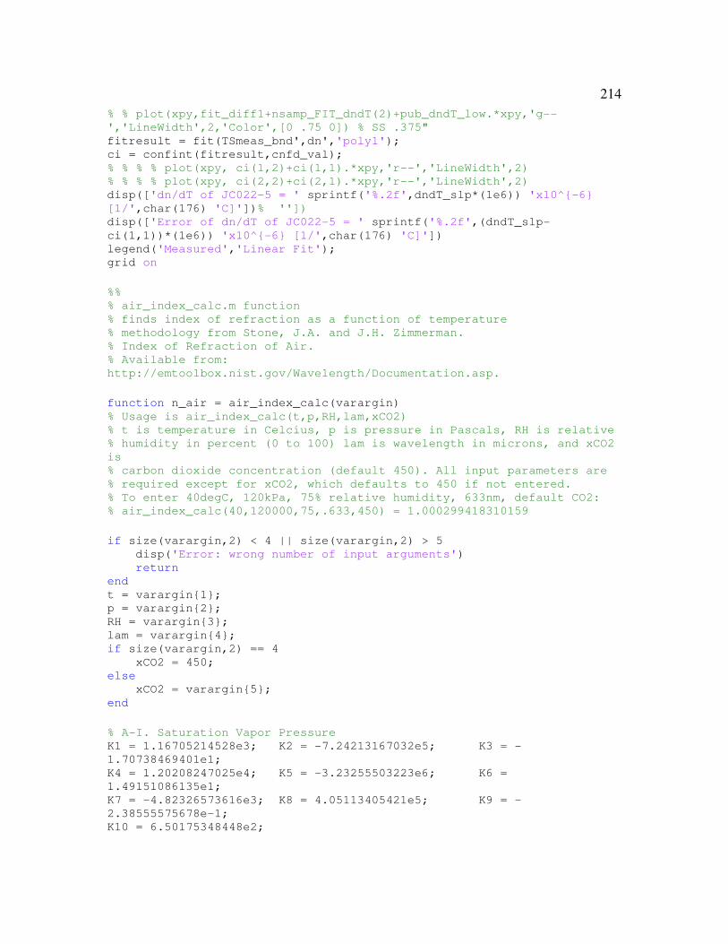
214 % % plot(xpy,fit_diff1+nsamp_FIT_dndT(2)+pub_dndT_low.*xpy,'g--

','LineWidth',2,'Color',[0 .75 0]) % SS .375" fitresult = fit(TSmeas_bnd',dn','poly1'); ci = confint(fitresult,cnfd_val); % % % % plot(xpy, ci(1,2)+ci(1,1).*xpy,'r--','LineWidth',2) % % % % plot(xpy, ci(2,2)+ci(2,1).*xpy,'r--','LineWidth',2) disp(['dn/dT of JC022-5 = ' sprintf('%.2f',dndT_slp*(1e6)) 'x10^{-6}

[1/',char(176) 'C]'])% '']) disp(['Error of dn/dT of JC022-5 = ' sprintf('%.2f',(dndT_slp-

ci(1,1))*(1e6)) 'x10^{-6} [1/',char(176) 'C]']) legend('Measured','Linear Fit'); grid on

%% % air_index_calc.m function % finds index of refraction as a function of temperature % methodology from Stone, J.A. and J.H. Zimmerman. % Index of Refraction of Air. % Available from:

http://emtoolbox.nist.gov/Wavelength/Documentation.asp.

function n_air = air_index_calc(varargin) % Usage is air_index_calc(t,p,RH,lam,xCO2) % t is temperature in Celcius, p is pressure in Pascals, RH is relative % humidity in percent (0 to 100) lam is wavelength in microns, and xCO2

is % carbon dioxide concentration (default 450). All input parameters are % required except for xCO2, which defaults to 450 if not entered. % To enter 40degC, 120kPa, 75% relative humidity, 633nm, default CO2: % air_index_calc(40,120000,75,.633,450) = 1.000299418310159

if size(varargin,2) < 4 || size(varargin,2) > 5 disp('Error: wrong number of input arguments') return end t = varargin{1}; p = varargin{2}; RH = varargin{3}; lam = varargin{4}; if size(varargin,2) == 4 xCO2 = 450; else xCO2 = varargin{5}; end

% A-I. Saturation Vapor Pressure K1 = 1.16705214528e3; K2 = -7.24213167032e5; K3 = -

1.70738469401e1; K4 = 1.20208247025e4; K5 = -3.23255503223e6; K6 =

1.49151086135e1; K7 = -4.82326573616e3; K8 = 4.05113405421e5; K9 = -

2.38555575678e-1; K10 = 6.50175348448e2;

215 T = t + 273.15; Q = T + K9./(T - K10); A = Q.^2 + K1.*Q + K2; B = K3.*(Q.^2) + K4.*Q + K5; C = K6.*(Q.^2) + K7.*Q + K8; X = -B + sqrt(B.^2 -4.*A.*C); psv = (10.^6).*((2.*C./X).^4);

% A-II. Determining Humidity alpha = 1.00062; beta = 3.14e-8; gamma = 5.60e-7; f = alpha + beta.*p + gamma.*t.*t; % enhancement factor f xv = (RH./100).*f.*psv./p; % xv is mole fraction

% A-III. Ciddor Calculation of Index of Refraction % part b w0 = 295.235; w1 = 2.6422; w2 = -0.03238; w3 = 0.004028; k0 = 238.0185; k1 = 5792105; k2 = 57.362; k3 = 167917; a0 = 1.58123e-6; a1 = -2.9331e-8; a2 = 1.1043e-10; b0 = 5.707e-6; b1 = -2.051e-8; c0 = 1.9898e-4; c1 = -2.376e-6; d = 1.83e-11; e = -0.765e-8; pR1 = 101325; TR1 = 288.15; Za = 0.9995922115; pvs = 0.00985938; R = 8.314472; Mv = 0.018015; % part c S = lam.^-2; % part d ras = (10^-8).*((k1./(k0 - S)) + (k3/(k2 - S))); rvs = (1.022e-8).*(w0 + w1.*S + w2.*S.*S + w3.*S.*S.*S); % part e Ma = 0.0289635 + (1.2011e-8).*(xCO2 - 400); raxs = ras.*(1 + (5.34e-7).*(xCO2 - 450)); % part f T = t + 273.15; Zm = 1 - (p./T).*((a0 + a1.*t + a2.*t.*t + (b0 + b1.*t).*xv + (c0 +

c1.*t).*xv.*xv)) + (d + e.*xv.*xv).*((p./T).^2); paxs = pR1.*Ma./(Za.*R.*TR1); pv = xv.*p.*Mv./(Zm.*R.*T); pa = (1 - xv).*p.*Ma./(Zm.*R.*T); % part g (index of refraction) n_air = 1 + (pa./paxs).*raxs + (pv./pvs).*rvs;

216

Appendix N. CTE and dn/dT for JC022 samples