Equivalent Numerical Model for Honeycomb Subjected to High Speed Impact

Thesis by

Simon Amine

Department of Mechanical Engineering Mc Gill University Montreal, Canada

June 2005

A Thesis submitted to McGill University in partial fulfillment of the requirements for the degree of

Master of Engineering

© Simon Amine, 2005

1+1 Library and Archives Canada

Bibliothèque et Archives Canada

Published Heritage Branch

Direction du Patrimoine de l'édition

395 Wellington Street Ottawa ON K1A ON4 Canada

395, rue Wellington Ottawa ON K1A ON4 Canada

NOTICE: The author has granted a non­exclusive license allowing Library and Archives Canada to reproduce, publish, archive, preserve, conserve, communicate to the public by telecommunication or on the Internet, loan, distribute and sell theses worldwide, for commercial or non­commercial purposes, in microform, paper, electronic and/or any other formats.

The author retains copyright ownership and moral rights in this thesis. Neither the thesis nor substantial extracts from it may be printed or otherwise reproduced without the author's permission.

ln compliance with the Canadian Privacy Act some supporting forms may have been removed from this thesis.

While these forms may be included in the document page cou nt, their removal does not represent any loss of content from the thesis.

• •• Canada

AVIS:

Your file Votre référence ISBN: 978-0-494-22628-5 Our file Notre référence ISBN: 978-0-494-22628-5

L'auteur a accordé une licence non exclusive permettant à la Bibliothèque et Archives Canada de reproduire, publier, archiver, sauvegarder, conserver, transmettre au public par télécommunication ou par l'Internet, prêter, distribuer et vendre des thèses partout dans le monde, à des fins commerciales ou autres, sur support microforme, papier, électronique et/ou autres formats.

L'auteur conserve la propriété du droit d'auteur et des droits moraux qui protège cette thèse. Ni la thèse ni des extraits substantiels de celle-ci ne doivent être imprimés ou autrement reproduits sans son autorisation.

Conformément à la loi canadienne sur la protection de la vie privée, quelques formulaires secondaires ont été enlevés de cette thèse.

Bien que ces formulaires aient inclus dans la pagination, il n'y aura aucun contenu manquant.

Abstract

Due to their high specific strength and stiffness, honeycomb sandwich structures are used

in impact-resistance applications. Their structural efficiency depends to a great extent on

the lightweight core separating the face sheets and providing overall high stiffness.

Detailed finite element modeling of the penetration of honeycombs by a projectile can be

fairly complex, and computationally expensive as shown in the first part of this study. A

computationally efficient axisymmetric equivalent numerical homogeneous model for

Aluminum 5052-H19 1/8in - O.OOlin hexagonal honeycomb subjected to high speed

impacts in the range of 60 mis to 140 mis is then developed. An equation-of-state model

for porous media is used for the equivalent honeycomb medium. A Taguchi

optimization, based on four unknown porous material parameters, is carried out. With

the optimal set, the equivalent model can accurately predict perforation velocities for

different impact conditions. The methodology for the optimization is explained and can

be used for any velocity range. The product of this work is a computationally efficient

numerical model that requires less than 8% of the time needed to numerically analyze

honeycombs in detail.

1

Résumé

Distinguées par leur haute rigidité et résistance, les structures sandwich en nid d'abeille

sont utilisées dans les applications de résistance à l'impact. Leur efficacité structurale est

une fonction directe de celle de leur légère âme, qui sépare les deux semelles du

sandwich, fournissant une haute résistance totale. La modélisation détaillée par éléments

finis de la perforation du nid d'abeille par un projectile peut être assez complexe et

coûteuse en temps de calcul tel que montré dans la première partie de cette étude. Un

modèle numérique homogène et axisymétrique offrant efficacement un comportement

équivalent en impact à grande vitesse (60-140m/s) à celui du nid d'abeille hexagonal

aluminium de type 5052-H19 l/8po - O.OOIpo est développé. Une formulation en

équation d'état des milieux poreux est utilisée pour représenter le comportement du

milieu équivalent du nid d'abeille. Une optimisation de Taguchi, mettant en évidence

l'effet de quatre paramètres liés au matériau sur le comportement du modèle est

effectuée. Avec le jeu de paramètres optimal trouvé, le modèle équivalent peut

précisément prédire les vitesses de perforation pour différents cas d'impact. La

méthodologie d'optimisation est expliquée et pourra être utilisée pour n'importe quelle

marge de vitesse. Le résultat de cette étude est un modèle de calcul numérique efficace

qui exige moins que 8% du temps nécessaire pour l'analyse numérique détaillée des nids

d'abeille.

ii

Acknowledgements

1 wish to thank my academic advisor, Professor James A. Nemes, who has continually

been a source of inspiration. His insight and generous support throughout the various

stages of this research work will always be appreciated.

Many thanks to:

• Dr. Abbas Milani and Ms. Christine EI-Lahham for their help with the Taguchi optimizations;

• Dr. Faycal Ben Yahia who was always willing to discuss the topie of finite element analysis and for reviewing the abstract translation;

• Mrs. Marika Asimakopulos for proof reading the final draft of this thesis.

Finally, a special "thank you" goes to my uncle Pierre and his family for always being

there for me with unconditionallove, caring and support, and to my parents and brother,

whose prayers and love have always accompanied me.

iii

Table of Contents

Abstract

Résumé

Acknowledgements

Table of Contents

List of Figures

List of Tables

List of Symbols

CHAPTER 1: INTRODUCTION, RESEARCH OBJECTIVES, AND PREVIOUS WORK

1.1 Introduction

1.2 Treatment of Impact Problems and Research Objectives

1.3 Literature Review 1.3.1 Experimental studies 1.3.2 Analytical studies

1.3.2.1 Elastic behaviour and equivalent properties 1.3.2.2 Plastic behaviour and penetration

1.3.3 Numerical analysis of honeycombs

1.4 Outline of Thesis

CHAPTER 2: MATHEMATICAL MODELS

2.1 Material Modeling 2.1.1 The Johnson-Cook constitutive model 2.1.2 Equation of state and the P - Cl model

2.2 Failure Modeling 2.2.1 The Johnson-Cook damage model

2.3 Optimization method: The Taguchi Approach 2.3.1 Finding the optimal set 2.3.2 The predictive equation 2.3.3 Analysis of variance (ANDV A)

CHAPTER 3: DETAILED HONEYCOMB MODELING

3.1 Model Description

1

11

iii

IV

vi

V111

x

1

6

8 8

10 11 12 13

15

16 17 20

27 27

29 30 30 31

33

iv

3.1.1 Geometry and boundary conditions 3.1.2 Mesh sensitivity and energy balance 3.1.3 Contact and interactions 3.1.4 Material and damage modeling

3.2 Results and Discussion

CHAPTER 4: EQUIVALENT HONEYCOMB MODELING

4.1 Model Description 4.1.1 Geometry and boundary conditions 4.1.2 Mesh sensitivity and energy balance 4.1.3 Contact and interactions 4.1.4 Material modeling

4.2 Parameters Sensitivity Study

CHAPTER 5: THE TAGUCHI OPTIMIZATION

5.1 Utility Function

5.2 Convention al Taguchi Optimization 5.2.1 Factor plots 5.2.2 Predictive equation and additivity of the method 5.2.3 Analysis of variance

5.3 The Taguchi Experiments 5.3.1 Initial array optimization 5.3.2 Refined array optimization

5.4 Discussion

5.5 Model Validation

5.6 Computational Efficiency

CHAPTER 6: CONCLUSIONS, RECOMMENDATIONS, AND FUTURE WORK

6.1 Conclusions

6.2 Recommendations

6.3 Future Work

Reference List

33 37 40 42

44

48 48 49 52 52

54

60

61 62 63 64

64 64 67

71

74

79

80

81

82

83

v

List of Figures

Figure 1.1- (a) Two-dimensional schematic of a typical sandwich structure, and (b) photo of an all Aluminum honeycomb sandwich structure 2

Figure 1.2 - Honeycomb cell c1usters 3

Figure 1.3 - Schematic showing the effects of increasing impact velocity for sub-ballistic impacts (adapted from Johnson et al., 1981) 5

Figure 1.4 - Sequence of penetration for impacts above the ballistic limit (adapted from Johnson et al., 1981) 5

Figure 1.5 - Characteristic stress-strain curve for metallic honeycomb un der uniaxial out-of-plane compression (adapted from Mohr and Doyoyo, 2004) 8

Figure 2.1 - Descriptive P - a elastic and plastic curves for the compaction of ductile porous mate rial (adapted from Hibbitt, Karlsson and Sorensen, Inc. ABAQUS/Explicit User's Manual) 23

Figure 3.1- Two dimensional quarter model view of the honeycomb c1uster showing symmetry, boundary conditions and spherical impactor 34

Figure 3.2 - A uniform mesh of 10 elements per honeycomb cell edge 36

Figure 3.3 - Impact configurations of honeycomb cells 36

Figure 3.4 - Three-dimensional geometric model of a 5-cell honeycomb c1uster with spherical impactor 37

Figure 3.5 - Mesh convergence plot on perforation velo city for 100m/s impact 38

Figure 3.6 - Energy balance of the model 40

Figure 3.7 - Impact vs. perforation velo city for different coefficients of friction 42

Figure 3.8 - Impact vs. perforation velocity from experimental and numerical results 45

Figure 3.9 - Equivalent plastic strain fringes shown at 0.75xlO-4 seconds after ~~ ~

Figure 3.10 - Equivalent plastic strain fringes shown at 1.75xlO-4 seconds after impact 46

VI

Figure 3.11- Equivalent plastic strain fringes shown at 2.50xl0-4 seconds after ~~ ~

Figure 3.12 - Equivalent plastic strain fringes shown at 3.50xlO-4 seconds after ~~ ~

Figure 4.1 - Geometry of the equivalent axisymmetric porous model 49

Figure 4.2 - Mesh convergence using the 80 mis impact velocity 50

Figure 4.3 - Sensitivity of perforation velo city on the plastic limit p s 58

Figure 4.4 - Sensitivity of perforation velo city on the speed of sound in virgin porous medium ce 58

Figure 4.5 - Sensitivity of perforation velo city on the porosity of the unloaded virgin porous material no 59

Figure 4.6 - Sensitivity of perforation velocity on the cutoff failure stress (J' f 59

Figure 5.1- Factor plots of average U responses from initial optimization results 66

Figure 5.2 - Factor plots of average U responses from refined optimization results 69

Figure 5.3 - Validation with experimental results for a 6.35 mm diameter spherical impactor 75

Figure 5.4 - Validation with experimental results for a 3.556 mm diameter spherical impactor 76

Figure 5.5 - Validation with experimental results for a 6.35 mm diameter, 19.05 mm long cylindrical impactor 77

vii

List of Tables

Table 2.1- Specified material properties for the P - a porous model 26

Table 3.1 - Effect of honeycomb c1uster size on penetration and computation time 35

Table 3.2 - Effect of mesh density on the perforation velocity 38

Table 3.3 - Effect of coefficient of friction on the penetration of honeycomb 41

Table 3.4 - Elastie and Johnson-Cook parameters for Aluminum 2024-T351 42

Table 3.5 - Johnson-Cook damage parameters for Aluminum 2024-T351 43

Table 4.1 - Material properties for Aluminum 5052-H19 1/8in - O.OOlin honeycomb as used in the P - a model 53

Table 4.2 - Initial variations of parameters 54

Table 4.3 - Effect of variation of parameters on the perforation velo city 57

Table 5.1- L-9 orthogonal array 62

Table 5.2 - Factor level variation for initial optimization 65

Table 5.3 - Perforation velocities and utility function responses of orthogonal array experiments for initial optimization 65

Table 5.4 - Average utility function response for each factor level in the initial optimization 66

Table 5.5 - Sum of squares of U responses for each factor from ANOVA and corresponding contributions 67

Table 5.6 - Factor level variation for refined optimization 67

Table 5.7 - Perforation velocities and utility function responses of the orthogonal array experiments for refined optimization 68

Table 5.8 - Average U response for each factor level in the refined optimization 69

Table 5.9 - Sum of squares for each factor from ANOVA and corresponding contribution to U response 69

V111

Table 5.10 - Optimal sets and factor contributions 72

Table 5.11- Optimization with single objective functions 73

Table 5.12 - Comparison between single and multi-objective optimization 73

Table 5.13 - Results of simulations (perforation velocity and penetration depth) carried out in low velocity regime to determine the ballistic limit of honeycomb 74

Table 5.14 - Experimental and simulation perforation velocities with a 3.556 mm diameter spherical impactor 76

Table 5.15 - Experimental and simulation perforation velocities with a 6.35 mm diameter, 19.05 mm long cylindrical impactor 77

Table 5.16 - Mean radii of damaged are as as given by the detailed and equivalent models 78

Table 5.17 - Computation time of detailed and equivalent model for different impacts velocities 79

IX

List of Symbols

A

D

di (i = 1-5)

Ekinetic

G

h

m

n

n p

P

Pe

Yield stress material parameter in the Johnson-Cook plasticity model

Distension function in the elastic regime

Distension function in the plastic regime

Strain hardening parameter in the Johnson-Cook plasticity model

Strain rate hardening parameter in the Johnson-Cook plasticity model

Specifie heat at constant pressure

Reference speed of sound in the solid mate rial

Reference speed of sound in the virgin porous material

Speed of sound in the solid material of which the porous medium is made

Cumulative damage parameter

Johnson-Cook damage parameters

Kinetic energy

Specifie energy

Total mechanical energy

Elastic shear modulus

Distension function used in the P - a model

Isentropic or elastic bulk modulus

Thermal softening exponent in the Johnson-Cook plasticity model

Number of experiments for each level of a factor A

Strain hardening exponent in the Johnson-Cook plasticity model

Porosity

Number of levels for factor A

Initial porosity

Pressure

Elastic limit

x

ss

~nst

U

U

U dissipated

U predicted

v

Wexternal

~nternal

y

Ypredicted

Z

a

a min

Pressure function in the plastic regime

Plastic limit

Slope of Us -Up curve

Sum of squares

Deviatoric stress tensor

Homologous temperature

Instantaneous tempe rature

Transition tempe rature

Melting tempe rature

Utility function

Total average utility function

Energy dissipated by friction

Particle velocity

Predicted utility function

Shock velo city

Perforation velo city

External work

InternaI energy

Average response for a given level of a factor

Total average response of experiments

Response of the ith row in the orthogonal array

Predicted response

Deviation in perforation ve10city

Distension

Distension at elastic limit

Minimum distension

Xl

fJ

v

P

Po

ŒJi =1-3)

Initial distension of the virgin porous material

Volumetrie thermal expansion coefficient

Kronecker Delta

Equivalent strain to fracture

Deviatoric strain tensor

Equivalent plastic strain

Equivalent plastic strain rate

Material parameter characterizing the onset of strain rate dependence

Grüneisen ratio

Variable relating the current and reference densities in the P - a model

Poisson's ratio (isotropie model)

Density

Reference density of the solid material

Density of the solid mate rial from which the porous medium is made

Von Mises equivalent stress

Total stress tensor

Hydrostatic cutoff failure stress

Hydrostatic mean stress

Yield stress

Pirst, second and third principal stresses

xii

CHAPTER 1

INTRODUCTION, RESEARCH OBJECTIVES, AND LITERATURE REVIEW

1.1 Introduction

Great attention has been given to sandwich structures in recent years due to their

structural importance and relative low weight in the offshore, marine, aerospace and

transportation industries. These structures serve a variety of systems ranging from skis to

jet engine nacelles and liners. A few more examples are helicopter rotor blades, ship

hulls and train fronts. Other examples lie in the transportation safety of hazardous

mate rials, containing nuc1ear reactor vessels and the design of lightweight body armors.

Sandwich structures are inhomogeneous and anisotropie in nature and are thus considered

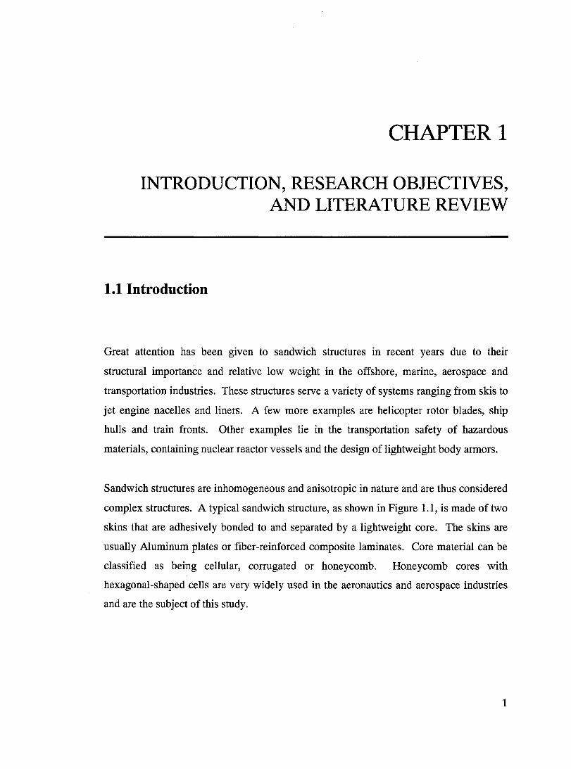
complex structures. A typical sandwich structure, as shown in Figure 1.1, is made of two

skins that are adhesively bonded to and separated by a lightweight core. The skins are

usually Aluminum plates or fiber-reinforced composite laminates. Core material can be

c1assified as being cellular, corrugated or honeycomb. Honeycomb cores with

hexagonal-shaped cells are very widely used in the aeronautics and aerospace industries

and are the subject of this study.

1

Facesheet

;AiI

1IIIIIIIIIIIIIIIIIIglllll[>~~~:;'

Facesheet Honeycomb core

(a) (b)

Figure 1.1- (a) Two-dimensional schematic of a typical sandwich structure, and (b) photo of an aIl Aluminum honeycomb sandwich structure

In general, honeycombs are used to improve the strength-to-weight ratio of structures and

to absorb energy. Sandwich structures with honeycomb cores have high specifie strength

and stiffness, which makes them promising for impact-resistance applications. Their

structural efficiency depends to a great extent on the lightweight core separating the face

sheets and providing high stiffness. The core also offers weight savings without

compromising performance. In fact, it enhances energy absorption. Goldsmith and

Louie (1995) state that the geometric features and mechanical properties of the core play

an important role in depicting the loading capacity and energy absorption capability of

sandwich structures. Hoo Fatt et al. (2000) explain that the core mainly ensures that a

higher bending rigidity of the skins is maintained - acting like the web in a structural 1-

beam - while the skins, being relatively stronger and stiffer, carry most of the impact

load. The bending rigidity of the structure is directly proportional to the thickness of the

core. However, the maximum thickness is often dictated by the core's shear failure.

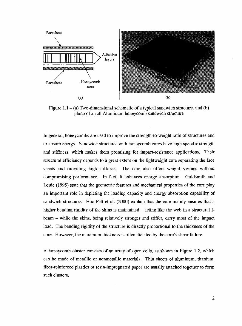
A honeycomb c1uster consists of an array of open ceIls, as shown in Figure 1.2, which

can be made of metallic or nonmetallic materials. Thin sheets of aluminum, titanium,

fiber-reinforced plastics or resin-impregnated paper are usuaIly attached together to form

such c1usters.

2

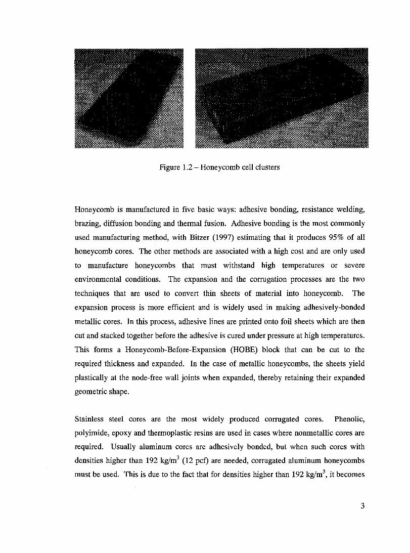
Figure 1.2 - Honeycomb cell c1usters

Honeycomb is manufactured in five basic ways: adhesive bonding, resistance wei ding,

brazing, diffusion bonding and thermal fusion. Adhesive bonding is the most commonly

used manufacturing method, with Bitzer (1997) estimating that it pro duces 95% of aIl

honeycomb cores. The other methods are associated with a high cost and are only used

to manufacture honeycombs that must withstand high temperatures or severe

environmental conditions. The expansion and the corrugation processes are the two

techniques that are used to convert thin sheets of material into honeycomb. The

expansion process is more efficient and is widely used in making adhesively-bonded

metallic cores. In this process, adhesive lines are printed onto foil sheets which are then

cut and stacked together before the adhesive is cured under pressure at high temperatures.

This forms a Honeycomb-Before-Expansion (HOBE) block that can be cut to the

required thickness and expanded. In the case of metallic honeycombs, the sheets yield

plastically at the node-free wall joints when expanded, thereby retaining their expanded

geometric shape.

Stainless steel cores are the most widely produced corrugated cores. Phenolic,

polyimide, epoxy and thermoplastic resins are used in cases where nonmetallic cores are

required. Usually aluminum cores are adhesively bonded, but when such cores with

densities higher than 192 kg/m3 (12 pct) are needed, corrugated aluminum honeycombs

must be used. This is due to the fact that for densities higher than 192 kg/m3, it becomes

3

impossible to successfully expand the ROBE block because the force required for the

expansion would be too great for the adhered nodes to hold together.

Basic honeycomb cell shapes are the hexagon, square and flex-core. A few variations of

these configurations are the over-expanded, under-expanded and reinforced

configurations. By varying the cell geometry, density and mechanical properties of

honeycombs, different combinations of curvature can be produced as was shown by

Evans (1991). The hexagon cell is by far the most common adhesively-bonded

honeycomb and the most widely used cell shape.

Sandwich structures are commonly subjected to severe impacts, such as those from

runway and space debris, hailstones and birds. This can result in partial penetration or

complete perforation of a structure. A kinetic energy penetration event is one in which

the projectile uses its energy of motion to push its way through a target. Backman and

Goldsmith (1978) define penetration as the entrance of a missile into a target without

completing its passage through it. At the end of penetration, the projectile remains

embedded in the target and forms a cavity therein. Perforation on the other hand results

in the projectile completely piercing the target and exiting from the other end.

The probabilistic ballistic limit is the velo city at which the projectile will perforate the

target 50% of the time. Johnson el al. (1981) classified impacts as being below or above

the ballistic limit. Zukas el al. (1982) explain that as impact occurs, compressive stress

waves are immediately generated and propagated in the projectile and target. For sub­

ballistic impacts, these waves move at the speed of sound in the material. Figure 1.3

shows that as the impact velocity increases, more mushrooming and embedding into the

target occurs.

4

Increasing impact velocity

PRE-IMPACT MUSHROOMING

BUCKLING EMBEDDING

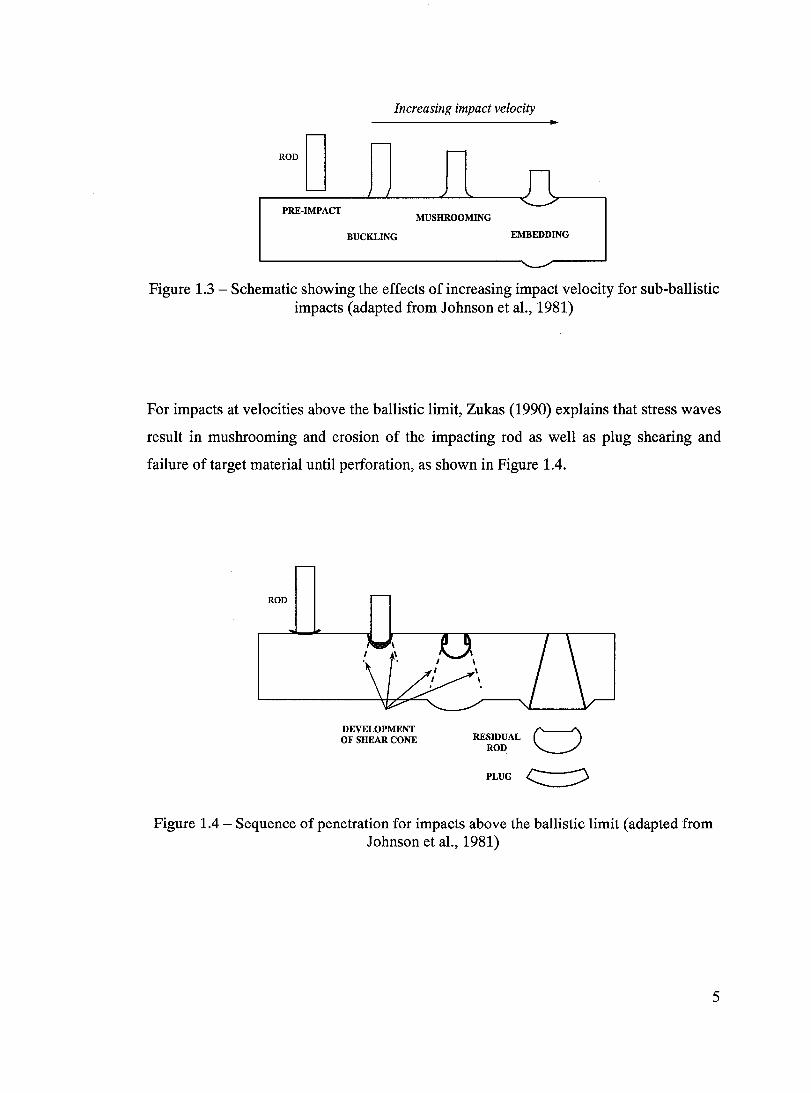
Figure 1.3 - Schematic showing the effects of increasing impact velocity for sub-ballistic impacts (adapted from Johnson et al., 1981)

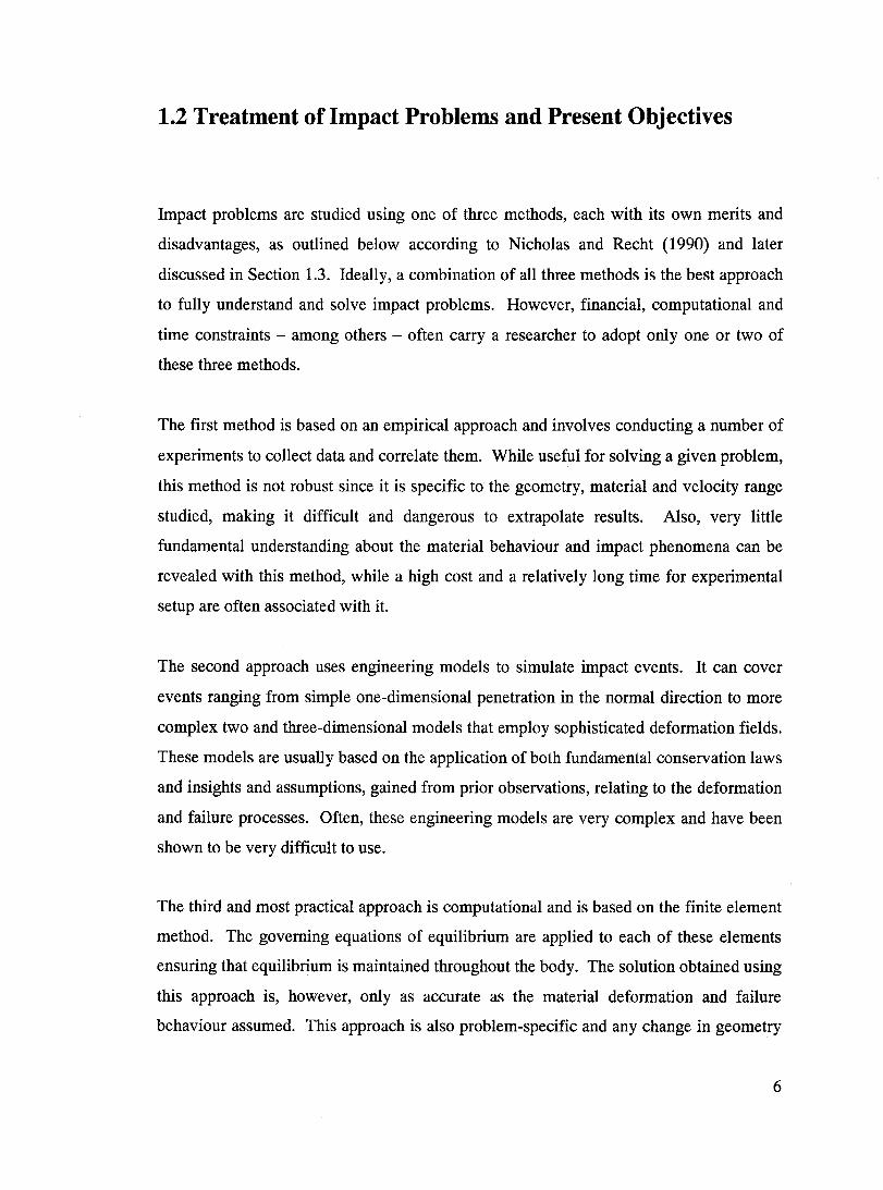
For impacts at velocities above the ballistic limit, Zukas (1990) explains that stress waves

result in mushrooming and erosion of the impacting rod as weIl as plug shearing and

failure of target material until perforation, as shown in Figure lA.

ROD

DEVELOPMENT OF SHEAR CONE RESIDUAL r-----'I

ROD '---./

PLUG ~

Figure 1.4 - Sequence of penetration for impacts above the ballistic limit (adapted from Johnson et al., 1981)

5

1.2 Treatment of Impact Problems and Present Objectives

Impact problems are studied using one of three methods, each with its own merits and

disadvantages, as outlined below according to Nicholas and Recht (1990) and later

discussed in Section 1.3. Ideally, a combination of all three methods is the best approach

to fully understand and solve impact problems. However, financial, computational and

time constraints - among others - often carry a researcher to adopt only one or two of

these three methods.

The first method is based on an empirical approach and involves conducting a number of

experiments to collect data and correlate them. While useful for solving a given problem,

this method is not robust since it is specific to the geometry, material and velocity range

studied, making it difficult and dangerous to extrapolate results. Also, very little

fundamental understanding about the material behaviour and impact phenomena can be

revealed with this method, while a high cost and a relatively long time for experimental

setup are often associated with it.

The second approach uses engineering models to simulate impact events. It can coyer

events ranging from simple one-dimensional penetration in the normal direction to more

complex two and three-dimensional models that employ sophisticated deformation fields.

These models are usually based on the application of both fundamental conservation laws

and insights and assumptions, gained from prior observations, relating to the deformation

and failure processes. Often, these engineering models are very complex and have been

shown to be very difficult to use.

The third and most practical approach is computational and is based on the finite element

method. The governing equations of equilibrium are applied to each of these elements

ensuring that equilibrium is maintained throughout the body. The solution obtained using

this approach is, however, only as accurate as the material deformation and failure

behaviour assumed. This approach is also problem-specific and any change in geometry

6

or input variables requires carrying out new simulations and interpreting new results.

However, de formation, stress and strain fields, and failure can be accurately captured

providing a more fundamental understanding of the behaviour of a structure. In cases

where analyses can be focused to study only specific areas or phenomena, the

computational time cost is bearable and remains relatively small compared to that

associated with experimental procedures. However, when the behaviour of large

honeycomb structures needs to be studied, detailed modeling of the honeycomb core will

increase the degrees of freedom of the finite element model resulting in a high

computational cost. This can be impractical and computationally un justifiable for

scientists and engineers wanting to study and optimize a large number of structures.

Hence, efficient numerical models based on equivalent homogeneous properties are

needed for modeling honeycomb cores.

The objective of this study is to develop a computationally efficient equivalent numerical

homogeneous model for Aluminum 5052-H19 1/8in - O.OOlin hexagonal honeycomb

subjected to high-speed impacts in the range of 60 mis to 140 rn/s. The model could be

used to predict perforation velocities and estimate the ballistic limit of honeycombs.

This objective is achieved by means of:

• Detailed modeling of Aluminum 5052-H19 1/8in - O.OOlin subject to ballistic

impact using finite element analysis,

• Development of a homogeneous finite element model based on the Equation of

State (EOS) model available in the commercial finite element code

ABAQUS/Explicit (Hibbitt, Karlsson and Sorensen, Inc. ABAQUSlExplicit

User's Manual),

• Optimization of the EOS model using the Taguchi approach and Analysis of

Variance (ANOVA) to accurate1y predict perforation velocities for a specifie

honeycomb-impactor configuration, and

• Validation of the EOS equivalent model using several honeycomb-impactor

configurations.

7

1.3 Literature Review

1.3.1 Experimental studies

Standard test methods, such as the ones outlined in ASTM C273-61, can be used to

determine in-plane shear properties of sandwich construction core materials. However,

these methods cannot be used when loading and boundary conditions differ from the ones

outlined in such methods. A number of researchers have experimentally studied the

behaviour of aluminum honeycomb when subjected to severe impact. Sorne of these

studies account for the interaction between the impactor and the honeycomb. Others

focused primarily on the global dynamic crushing of bare honeycomb.

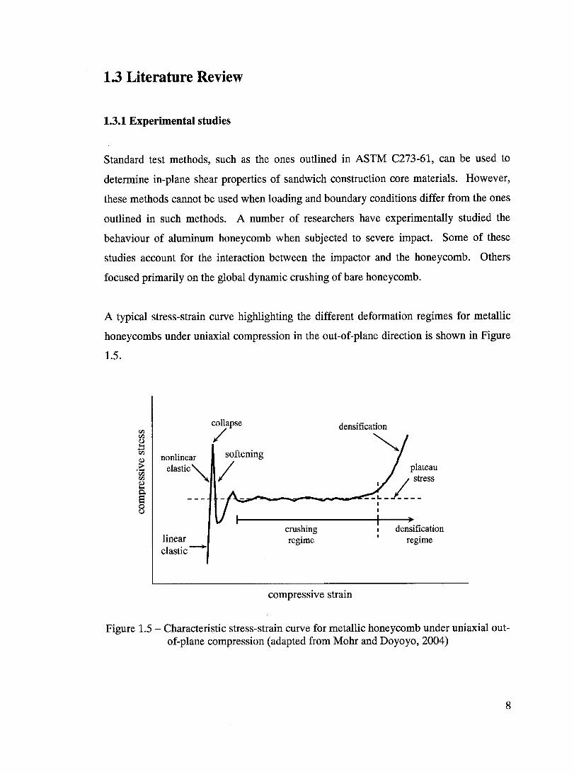
A typical stress-strain curve highlighting the different deformation regimes for metallic

honeycombs under uniaxial compression in the out-of-plane direction is shown in Figure

1.5.

nonlinear elastic",

linear e1astic-

collapse

/ softening

1

densification

~

crushing regime

compressive strain

plateau

)

densification regime

Figure 1.5 - Characteristic stress-strain curve for metallic honeycomb under uniaxial out­of-plane compression (adapted from Mohr and Doyoyo, 2004)

8

Goldsmith and Louie (1995) used a pneumatic gun in an experimental setup to determine

the ballistie limit of aluminum honeycomb. They tested four different honeycomb

configurations varying in cell size and wall thickness, which were impacted at different

velocities ranging from 30 mis to 183 mis with spherical and blunt-faced cylindrieal

projectiles having different sizes. Perforation velocities were recorded and plotted

against initial impact velocities and the ballistic limits of honeycombs for specifie

impact-honeycomb configurations were also determined. Energies absorbed during

penetration were computed from impact and exit velocities for ballistic tests, and from

statieally determined force-displacement histories in the case of static tests.

Wu and Jiang (1997) studied six different types of cellular honeycombs that were loaded

axially under quasi-static and dynamic conditions. For the impact tests, the velo city

histories were recorded using a laser-Doppler anemometer and a method was developed

to extract force and displacement histories from the measurements. This measuring and

extraction method proved to be an ideal non-contact measurement technique in this study.

An increase of up to 74% in the crush strength was found when specimens were loaded

dynamieally when compared to quasi-static loading. This increase was also found to be

proportional to the impact velo city. Wu and Jiang reported that manufacturer data sheets

greatly underestimate the crush strength of honeycombs.

Goldsmith et al. (1997) carried out an experimental investigation on the perforation

characteristies of cellular sandwich plates and their individual components using the

same pneumatic gun they had used in earlier studies. Initial projectile velocities ranged

from 17 mis to 380 mis for aIl targets. The honeycomb sheets had a higher ballistic limit

and produced different damage patterns than did the cellular cores with curved walls.

This was attributed to the flexibility of individual cells. For the configurations tested, the

sandwich plates exhibited the same ballistic limit regardless of core type or cell size since

the piercing of the facesheets is the primary mechanism in resisting perforation of the

sandwich plates.

9

Baker et al. (1998) conducted quasi-static and dynamic tests on thick-walled aluminum

and stainless steel fixed honeycomb specimens. They noted from the quasi-static tests

that specimen size had an effect on the deformation mode. Using circular recesses in the

upper and lower loading plates, the edge effects were altered to obtain the desired

deformation and failure mode of localized buckling of the cell walls. Further constraint

techniques were developed so that the stress-deformation characteristics of the specimen

are not changed from those for an infinite slab. Adequate constraints were applied to

honeycombs in the dynamic tests, which employed a high-pressure gas gun, made of a

barrel, impact chamber, backstop and a high-pressure furnishing system. These tests

consisted of striking honeycombs with projectiles. From the force-time history applied to

the specimen - as recorded by a strain gage force transducer - and the compression-time

and stress deformation functions, the energy absorption properties of the specimen are

determined. AIso, it was found that strain rates have a direct effect on the response of

honeycombs.

Zhao and Gary (1998) presented a new application of the Split Hopkinson Pressure Bar

(SHPB) to test the crushing behaviour of honeycomb under impact loading. From

pressure versus crush percent age plots of in-plane and out-of-plane crushing of

honeycombs, they report that their test method provides more accurate results than the

experimental testing techniques presented above. The improvement in accuracy is

attributed to the use of viscoelastic bars and a generalized two-strain measurement

method.

1.3.2 Analytical studies

There is considerable literature on analytical models developed for predicting the elastic

deformation of rnetallic honeycornbs under different loading conditions. Sorne

researchers have studied the in-plane response in order to gain understanding of the

mechanical response of metal foams, as was done by Okumara et al. (2002). Fewer

models exist for large deformation plastic behaviour and out-of-plane deformation of

honeycombs.

10

1.3.2.1 Elastic behaviour and equivalent properties

Based on the energy theorems used by Argyris (1955), Kelsey et al. (1958) applied the

unit displacement and unit load methods, along with appropriate simplifying assumptions

for the stress and strain fields, to obtain simple expressions for the upper and lower limits

to the equivalent transverse shear modulus of honeycomb sandwich core. The theory is

correlated with results from three-point bending tests carried out on sandwich beams and

shows good agreement.

Gibson and Ashby (1997) used a mechanics of materials approach to determine the in­

plane mechanical properties (linear and nonlinear elastic and plastic) of honeycombs.

They calculated four independent in-plane properties, namely the moduli of elasticity in

both in-plane directions, the in-plane shear modulus and Poisson's ratio, as weIl as the

elastic and plastic collapse stresses of the honeycomb and showed how these properties

depend on cell shape and density. Five additional moduli are needed to completely

describe the linear-elastic out-of-plane behaviour of honeycomb. Masters and Evans

(1996) developed a theoretical model for predicting the elastic constants of honeycombs

based on cell deformation by flexure, stretching and hinging. They show how the

properties can be tailored by varying the relative magnitudes of the force constants in

their model for the different deformation mechanisms. These force constants also

determine the degree of anisotropy of the honeycombs. For regular hexagons, it is shown

that the properties can be isotropic.

The homogenization the ory is often used for structures or media that are made of a large

number of periodic substructures. In such media, repeating substructures are considered

basic cells. In this theory, the equivalent mate rial properties of a periodic medium can be

obtained from the homogenization of a basic repeating cell. Shi and Tong (1995) used

this approach to study the influence of honeycomb geometry on the equivalent transverse

shear stiffness of honeycomb sandwich plates. Using the two-scale method of

homogenization for periodic media on a two-dimensional basic ceIl, they presented an

analytical first order solution for the equivalent transverse shear modulus of honeycomb

structures.

11

Xu and Qiao (2002) extended the adaptation of the homogenization theory to include

transverse shear deformation the ory for honeycomb sandwiches. In their work, the

solutions of formulated periodic homogenization functions lead to analytical formulae of

homogenized elastic stiffness of honeycomb sandwiches. These solutions also

demonstrated the significance of skin effect on honeycomb computations, which is often

neglected. Skin effect - or thickness effect by Becker (1998) - is the effect posed by the

constraints of two skin faces on the local deformation mechanism of a heterogeneous

core of a sandwich structure. By this effect, the stiffness properties of the core become

sensitive to the ratio of core thickness to unit cell size.

1.3.2.2 Plastic behaviour and penetration

Mohr and Doyoyo (2004) developed a phenomenological, orthotropic rate-independent

constitutive model for large out-of-plane plastic deformation of metallic honeycombs in

the crushing and densification regimes. This model was based on experimental

observations in a monolithic hexagonal honeycomb, whereby the direction of

macroscopic plastic flow during crushing under combined out-of-plane loading was

found to be coaxial with the direction of the compressive principal stress. Their model

was incorporated into a commercial finite element code and was successfully utilized to

simulate the behaviour of hexagonal aluminum honeycomb under biaxial loading

conditions.

Hoo Fatt et al. (2000) developed a three-stage analytical model for the perforation of

aluminum sandwich structures impacted by spherical and blunt-faced cylindrical

projectiles. Geometrical features and material properties of the top facesheet, honeycomb

core and bottom facesheet, as weIl as the mass and impact velo city of the blunt impactor

are used as inputs in this model. Residual velocities from one stage of penetration to the

next were found using energy balances. The model also ca1culates the plastic work

dissipated after each penetration stage, the total fracture and debonding work, the

dynamic crush and shear strength of honeycomb core for the impact velocity considered

and the extent of radial deformation and transverse deflection of the top facesheet at the

end of its perforation stage. This model relies on the perforation velocities of bare

12

honeycombs, which were obtained from experimental data presented by Goldsmith and

Louie (1995). A correction factor is used to reduce this velocity in order to account for

the fact that the honeycomb had already been crushed in the perforation stage of the top

facesheet. The ballistic limits of aluminum sandwich structures that were calculated by

this analytical model fell within 5% of the ballistic limits obtained from experimental

tests by Goldsmith et al. (1997).

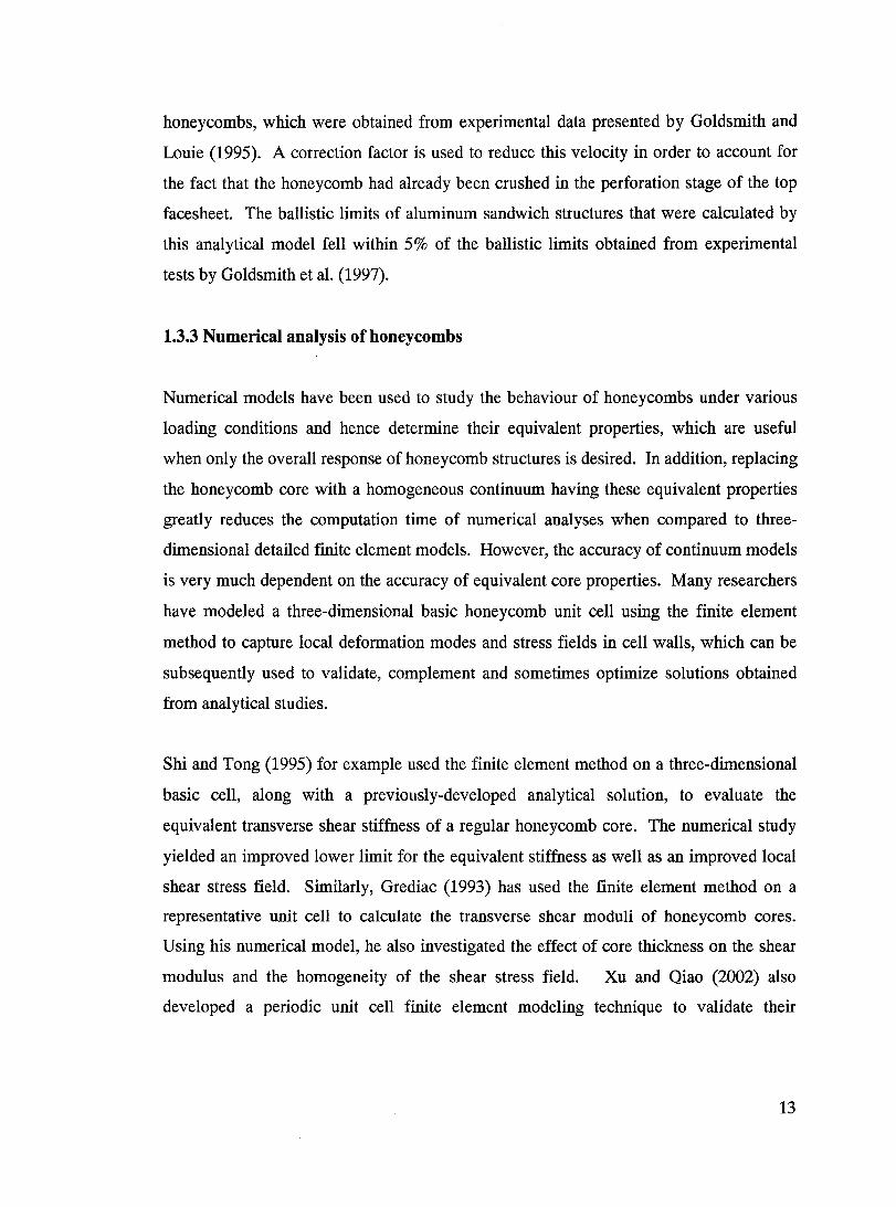
1.3.3 Numerical analysis of honeycombs

Numerical models have been used to study the behaviour of honeycombs under various

loading conditions and hence determine their equivalent properties, which are use fuI

when only the overall response of honeycomb structures is desired. In addition, replacing

the honeycomb core with a homogeneous continuum having these equivalent properties

greatly reduces the computation time of numerical analyses when compared to three­

dimensional detailed finite element models. However, the accuracy of continuum models

is very much dependent on the accuracy of equivalent core properties. Many researchers

have modeled a three-dimensional basic honeycomb unit cell using the finite element

method to capture local deformation modes and stress fields in cell walls, which can be

subsequently used to validate, complement and sometimes optimize solutions obtained

from analytical studies.

Shi and Tong (1995) for example used the finite element method on a three-dimensional

basic cell, along with a previously-developed analytical solution, to evaluate the

equivalent transverse shear stiffness of a regular honeycomb core. The numerical study

yielded an improved lower limit for the equivalent stiffness as weIl as an improved local

shear stress field. Similarly, Grediac (1993) has used the finite element method on a

representative unit cell to calculate the transverse shear moduli of honeycomb cores.

Using his numerical model, he also investigated the effect of core thickness on the shear

modulus and the homogeneity of the shear stress field. Xu and Qiao (2002) also

developed a periodic unit cell finite element modeling technique to validate their

13

analytical homogenization approach - as discussed in Section 1.3.2 - and complement it

with skin rigidity.

Guo and Gibson (1999) developed a finite element model of a two-dimensional regular

honeycomb cell cluster to study the effect of defects consisting of missing cells on

Young's moduli, the elastic buckling and the plastic collapse strength. They looked at

the elastic buckling strength and the plastic collapse strength of honeycombs with defects

and normalized them by the strength of intact honeycombs. They found that the

respective ratios decreased directly with the ratio of minimum net cross-sectional area to

the intact cross-sectional area, although this decrease was less rapid in the case of the

plastic collapse strength. Separate defects interact to reduce the elastic buckling strength.

At a separation of about 10 cells, separate defects act independently. It was also reported

that the separation distance has little effect on Young's modulus or the plastic collapse

strength of honeycombs. It was also found that the localization strain decreased with

increasing ratios of honeycomb cell wall thickness to cell wall edge length.

Ruan et al. (2003) studied the in-plane dynamic crushing of aluminum honeycombs by

modeling a cluster of honeycomb cells using the finite element method. They assessed

the effect of cell wall thickness and impact velocity on the de formation mode and plateau

stress of honeycombs. They found that oblique "X" shaped, transitional "V" shaped and

vertical localized "1" shaped bands characterized the deformation modes as the impact

velocity increased. A power law relating the plateau stresses to the cell wall thickness for

a given velo city showed good correlation. The plateau stresses in both in-plane

directions increase with increasing impact velocity according to a square law above a

certain velo city .

Nguyen et al. (2005) have developed Sandmesh, an explicit finite element-based

simulation tool, to predict damage within sandwich structures subjected to low velo city

impacts. In this tool, the honeycomb and the sandwich facesheets are modeled using

shell elements, following a detailed modeling approach that is often associated with high

computational cost. Mass scaling is integrated within Sandmesh in order to reduce the

14

computation time. However, computational accuracy is affected by mass scaling. This

tool was validated with results of experiments of honeycomb sandwich panels tested for

impact resistance and damage. For low velocity impact, this tool provides excellent

correlation with the force-time histories and is capable of predicting the size and depth of

permanent indentation.

1.4 Outline of Thesis

Chapter 2 will present the mathematical models on which the numerical analyses and

Taguchi optimization are based. The detailed honeycomb model is then described in

Chapter 3 and its results are presented and discussed. Chapter 4 describes the equivalent

EOS finite element model and highlights the effects of the parameters that are used in the

Taguchi optimization on the perforation velocity. In Chapter 5, the objective function for

the optimization is presented. An initial and a refined optimizations are presented and

discussed. The equivalent model using the optimal set of parameters for prediction of

perforation velocities is then validated using experimental results. A comparison of

computational cost between the detailed and equivalent model is also presented. Chapter

6 concludes this study and recommends future work that can be carried out to extend the

usefulness of the equivalent model.

15

CHAPTER2

MATHEMATICAL MODELS

In order to simulate structures in impact events, both the behaviour of mate rials and the

manifestation of failure need to be characterized. By virtue of the finite element method,

simulations or virtual experiments can be carried out providing useful data to better

understand the mechanics of a structure. However, numerical simulations require the use

of material and failure models, whereby the results are only as accurate as the assumed

models. Material models rely on a number of properties, which are usually obtained from

controlled physical experiments. It can be very difficult to set up - impossible in sorne

cases - and costl y to run such experiments, leaving a researcher with the sole option of

studying the effect of important properties by conducting parametric studies using

computer simulations. In this work, the Design of Experiment (DOE) approach and the

Taguchi method of optimization (as explained in section 2.3) are used to assess the

effects of four parameters in a porous mate rial model, and to optimize these parameters in

order to find equivalent properties for modeling the high speed penetration of

honeycombs.

2.1 Material Modeling

Characterization of material behaviour under high strain rates is important in order to

accurately model structures under severe impact conditions. Similar to the stress-strain

16

response, damage modeling and failure mode determination are important. Modeling of

complex impact events using c1osed-form analytical solutions has proven to be elusive,

sometimes impossible. Such problems are better handled by approximate solutions and

numerical analyses using finite element codes where well-established mate rial and

damage models are implemented.

2.1.1 The Johnson-Cook constitutive model

Metals exhibit elastic and plastic behaviour depending on the amount and rate of

deformation they undergo. Elastic behaviour of metals is usually described by Hooke's

law whereby the stress and strain in the material are linearly related by the modulus of

elasticity up to the onset of yielding. In the case of uniaxial tension, the elastic limit can

be defined as the maximum load that can be applied to a specimen without causing

permanent deformation. When a material is subject to many different combinations of

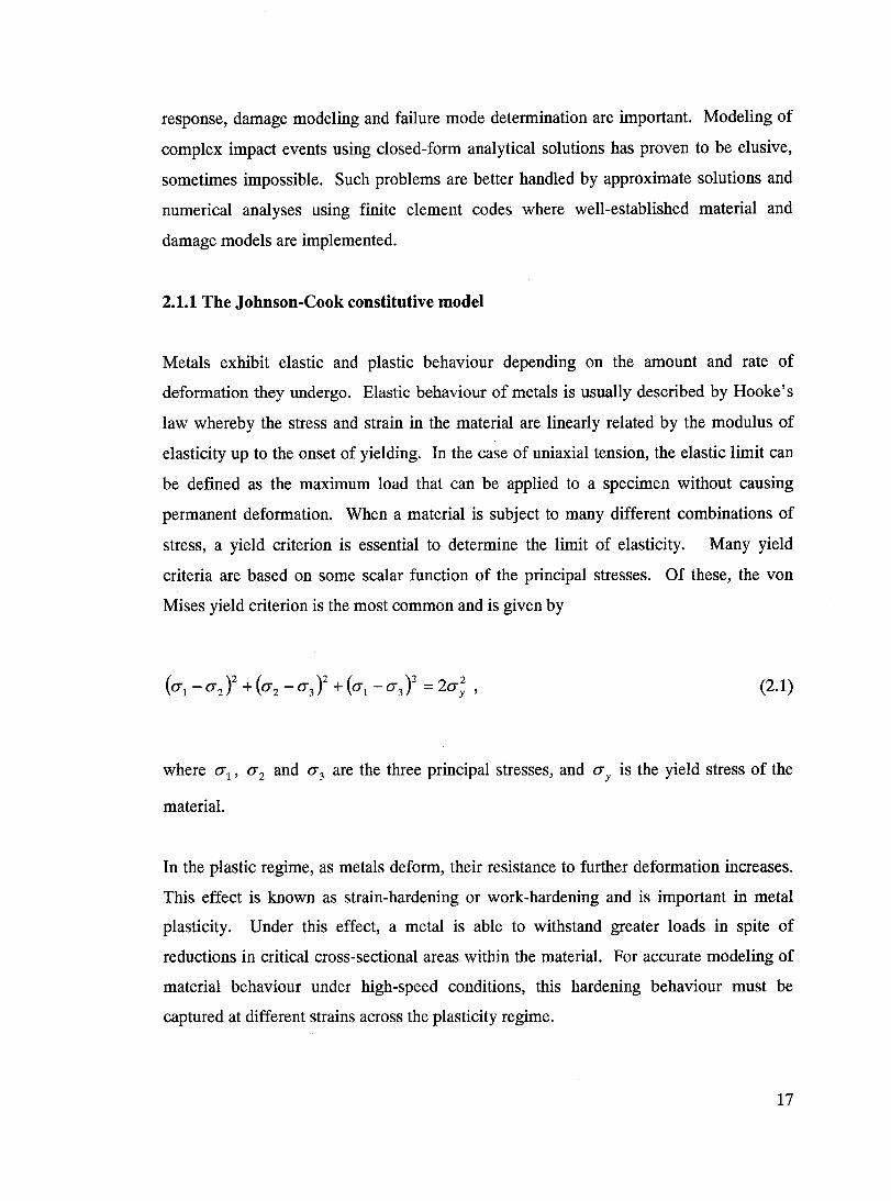
stress, a yield criterion is essential to determine the limit of elasticity. Many yield

criteria are based on sorne scalar function of the principal stresses. Of these, the von

Mises yield criterion is the most common and is given by

(2.1)

where (j l' (j 2 and (j 3 are the three principal stresses, and (j y is the yield stress of the

material.

In the plastic regime, as metals deform, their resistance to further deformation increases.

This effect is known as strain-hardening or work-hardening and is important in metal

plasticity. Vnder this effect, a metal is able to withstand greater loads in spite of

reductions in critical cross-sectional areas within the material. For accurate modeling of

material behaviour under high-speed conditions, this hardening behaviour must be

captured at different strains across the plasticity regime.

17

Impact events involving metallic materials result in a temperature rise during deformation

due to adiabatic heating. As a metal undergoes plastic work, heat is generated,

consequently affecting the deformation mode. Shearing due to adiabatic heating is a

deformation mode that is unique to high strain rates of deformation in metals and can

cause shear failure. It is considered to be an important failure mode. Woodward (1990)

reports that on the order of 95 % of the work done by plastic flow is converted to heat

while Meyers (1994) states this fraction is 90% for most metals. This heat, if prevented

from conducting (i.e. adiabatic condition), will raise the temperature of the metallic

sample causing thermal softening. In a real situation, sorne of the heat flows while the

remaining fraction causes sorne increase in metal temperature. In the case of those

metals where the rate of thermal softening is greater than the rate of work hardening,

most of the deformation takes place in the softened regions, thus producing adiabatic

shear bands. In metals with low thermal conductivity, little heat is conducted and thermal

softening effects are maximized. Adiabatic conditions are also a characteristic of high

speed impact loading since deformation occurs over a very short time period resulting in

high strain rates.

Woodward (1990) outlines a practical example showing how shearing due to adiabatic

heating affects deformation by considering sharp conical and flat-faced objects impacting

a metallic target. As they penetrate a body, sharp objects push material to the side. This

is in contrast to flat-faced penetrators that push material out, thus producing a plug, as

was shown in Figure 1.4. If shear bands exist as deformation is taking place, a metallic

plug can be produced in the case of penetration by sharp conical objects.

In modeling, it is thus important to consider the effect of temperature and strain rate on

the flow stress. Plasticity models that are suitable for high strain rate deformation not

only capture the instantaneous values of strain but also the strain rate and temperature

effects on the deformation. Such a model was proposed by Johnson and Cook (1983,

1985) and is given by

18

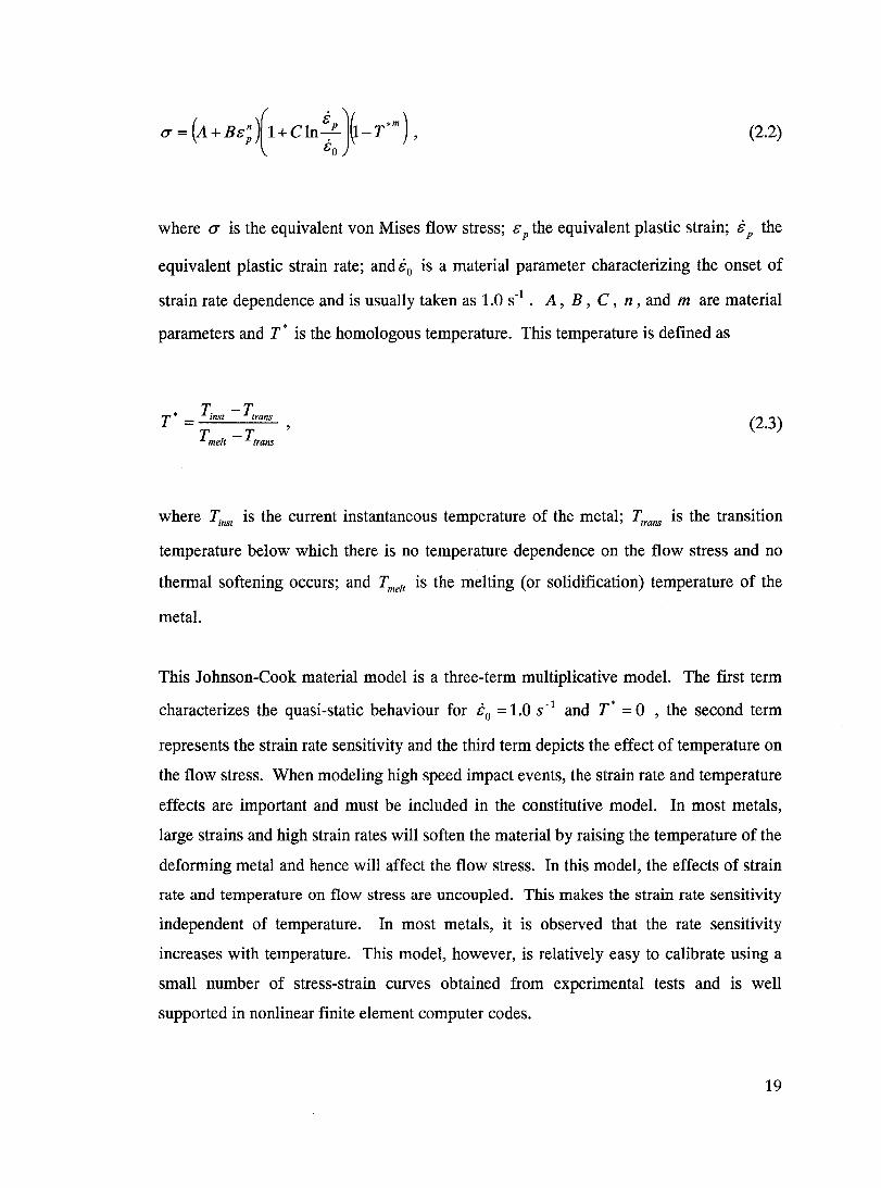
(2.2)

where a is the equivalent von Mises flow stress; & p the equivalent plastic strain; i p the

equivalent plastic strain rate; and io is a material parameter characterizing the onset of

strain rate dependence and is usually taken as 1.0 S-l. A, B, C, n, and mare mate rial

parameters and T * is the homologous temperature. This tempe rature is defined as

T * = T;nst - r;rans

T melt - T trans

(2.3)

where T inst is the current instantaneous temperature of the metal; Ttrans is the transition

tempe rature below which there is no temperature dependence on the flow stress and no

thermal softening occurs; and T melt is the melting (or solidification) temperature of the

metal.

This Johnson-Cook material model is a three-term multiplicative model. The first term

characterizes the quasi-static behaviour for io = 1.0 S-l and T* = 0 , the second term

represents the strain rate sensitivity and the third term depicts the effect of tempe rature on

the flow stress. When modeling high speed impact events, the strain rate and temperature

effects are important and must be included in the constitutive model. In most metals,

large strains and high strain rates will soften the material by raising the tempe rature of the

deforming metal and hence will affect the flow stress. In this model, the effects of strain

rate and temperature on flow stress are uncoupled. This makes the strain rate sensitivity

independent of temperature. In most metals, it is observed that the rate sensitivity

increases with temperature. This model, however, is relatively easy to calibrate using a

small number of stress-strain curves obtained from experimental tests and is weIl

supported in nonlinear finite element computer codes.

19

2.1.2 Equation of state and the P - a mode}

Herrmann (1969) proposed a phenomenological constitutive relation for the dynamic

compaction of ductile porous materials. His work gives a detailed description of the

irreversible compaction behaviour at low pressures and predicts the correct

thermodynamic behavior, by means of a Hugoniot description, at high pressures for the

fully compacted solid material. Shear strength effects were considered secondary in his

work and hence were neglected. The constitutive relation is suitable to solve stress wave

propagation problems for numerical solution methods. Carroll and HoIt (1972) suggested

modifications to the P - a model by Herrmann. Their modifications were made in the

relationship between the pressure in a porous material and the average matrix pressure.

Wardlaw et al. (1996) implemented the P - a equation of state in the DYSMAS code.

Equations of state are used in the ABAQUSlExplicit finite element code and provide a

hydrodynamie material model in whieh the material's volumetrie strength is determined.

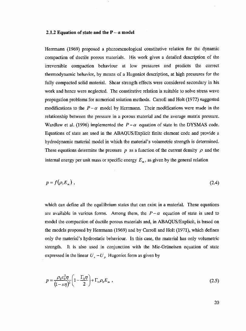
These equations determine the pressure p as a function of the current density p and the

internaI energy per unit mass or specifie energy E m , as given by the general relation

p= f{p,EJ, (2.4)

which can define aIl the equilibrium states that can exist in a material. These equations

are available in various forms. Among them, the P - a equation of state is used to

model the compaction of ductile porous materials and, in ABAQUSlExplicit, is based on

the models proposed by Herrmann (1969) and by Carroll and Holt (1971), which defines

only the material's hydrostatie behaviour. In this case, the material has only volumetrie

strength. It is also used in conjunction with the Mie-Grüneisen equation of state

expressed in the linear Us - U p Hugoniot form as given by

(2.5)

20

where Po is the reference density of the solid material; and Co the reference speed of

sound in the solid material. The term Poc~ is equivalent to the elastic bulk modulus at

small nominal strains.

s is the slope of the linear relationship between the linear shock velocity, Us, and the

partic1e velocity, U p according to

(2.6)

17 is a variable defined as

(2.7)

The GfÜneisen ratio, r o' is calculated according to the thermodynamic relationship

(2.8)

where Cp is the specific heat at constant pressure; Ko is the isentropic bulk modulus; f3

is the volumetrie thermal expansion coefficient and Po is the reference density.

Assuming an adiabatic and isothermal condition, equation (2.4) reduces to

p = f(p) , (2.9)

21

since the term containing the specific energy Emin equation (2.5) is eliminated.

It is convenient to introduce a scalar variable a, referred to as "distension", which allows

the distinction between the volume change due to material compression and that due to

pore collapse. a is defined as the ratio of the density of the sol id material from which

the porous medium is made, Ps' to porous material density, p, both evaluated at the

same temperature and pressure, as given by

a= Ps . P

(2.10)

a = 1 then corresponds to the state of the porous material being fully compacted to the

solid phase. The distension a is related to the porosity n by p

a-1 (2.11) n =

P a

Expressing a as a function of pressure p, equation (2.9) becomes the general P - a

equation of state for a specific porous material given by

(2.12)

The P - a model is an isotropie and homogenous model based on the assumption that aIl

the pores are uniformly dispersed throughout the porous medium. Both the elastic and

plastic compaction behaviours of a ductile porous medium, as given by the P - a model,

are shown in Figure 2.1.

22

a

2 a min

________ L ____________ _

1 1 1

1-+------~------------------~=-;---~

o Pe Ps P

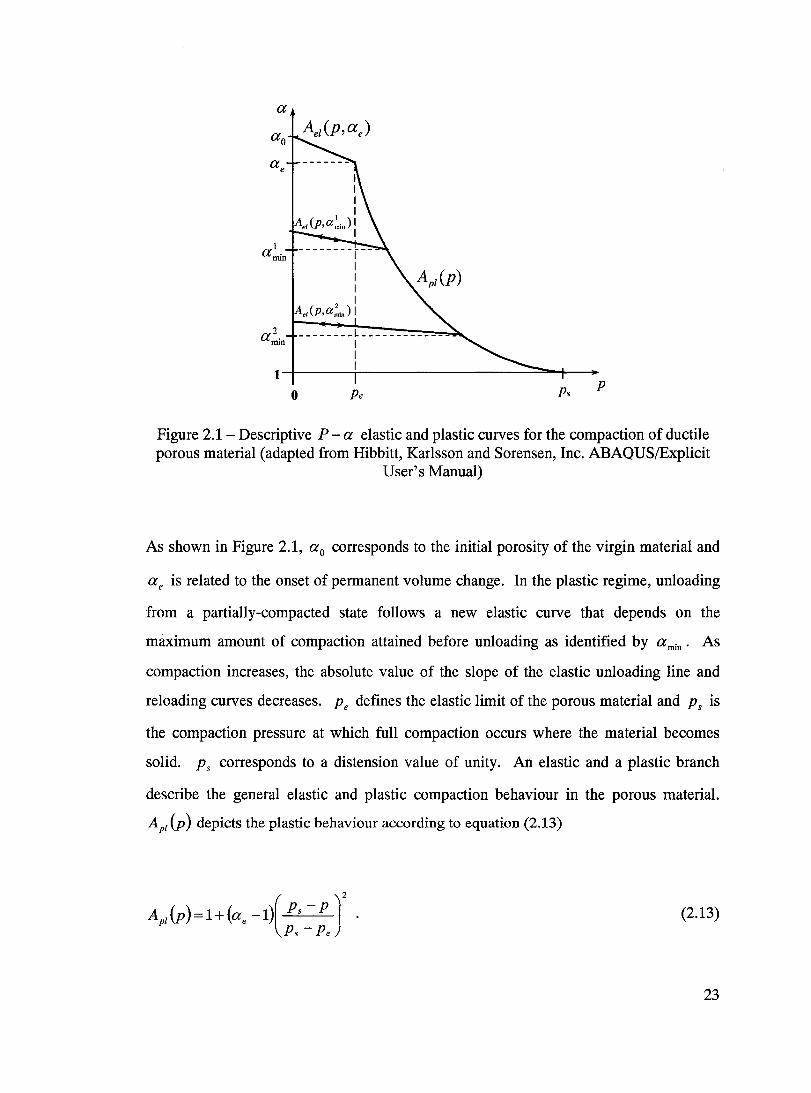
Figure 2.1 - Descriptive P - a elastic and plastic curves for the compaction of ductile porous material (adapted from Hibbitt, Karlsson and Sorensen, Inc. ABAQUSlExplicit

User's Manual)

As shown in Figure 2.1, ao corresponds to the initial porosity of the virgin material and

a e is related to the onset of permanent volume change. In the plastic regime, unloading

from a partially-compacted state follows a new elastic curve that depends on the

maximum amount of compaction attained before unloading as identified by a min • As

compaction increases, the absolu te value of the slope of the elastic unloading line and

reloading curves decreases. P e defines the elastic limit of the porous material and p s is

the compaction pressure at which full compaction occurs where the material becomes

solid. Ps corresponds to a distension value of unity. An elastic and a plastic branch

describe the general elastic and plastic compaction behaviour in the porous material.

Apl (p) depicts the plastic behaviour according to equation (2.13)

(2.13)

23

Ael (p, a min) characterizes the elastic unloading and reloading from partiall y -compacted

states and was originally proposed by Herrmann (1969) as the differential equation

(2.14)

where Ko is the elastic bulk modulus of the solid material at small nominal strains and

h(a) is given by

(2.15)

where Cs and ce are the reference sound speed in the solid material from which the

porous medium is made and the sound speed of the virgin porous material respectively.

From the work of Wardlaw et al. (1996), equation (2.14) for the elastic curve can be

simplified and replaced by the linear relation

(2.16)

where Ppl is the inverse of A pl (P) in equation (2.13) and is given by

(2.17)

24

The initial compression of the porous material is elastic and a plastic deformation regime

follows. Herrmann (1969) discussed that for an initially highly porous material, the

elastic compression should be due to elastic buckling of cell walls and the onset of

permanent volume change should correspond to the onset of plastic deformation of the

walls. On the other hand, for a material where the initial distension is close to unit y, little

change in a will occur in the e1astic compression phase since this phase will be

manifested in volume compression of cell walls. This effect is due to the confinement of

the surrounding material. Consequently, the onset of plastic flow would require higher

pressures. By virtue of irreversible compaction - as expected in a porous ductile material

- unloading is elastic without plastic reopening of the voids. Reloading would occur

elastically following the same unloading line up to the onset of plastic flow.

The total stress tensor, ()ij' can be divided into a volumetrie component (responsible for

change in volume of material but not shape) and a deviatoric stress component

(representing the shear stresses leading to deformation and change of shape) and is given

by

(2.18)

where Sij and the product () mbij are the deviatoric and volumetrie stress tensors

respectively. b ij is the Kronecker Delta and () m represents the hydrostatic mean stress

which is related to the pressure p calculated in the P - a model by the simple relation

(2.19)

The deviatoric behaviour of the material can be defined in ABAQUS/Explicit using a

simple linear isotropie deviatoric model given by

25

(2.20)

where G is the elastie shear modulus and Gij is the deviatorie strain tensor.

The volumetrie and deviatorie responses are uneoupled in this work where the volumetrie

response is governed by the P - a model.

In ABAQUSlExplicit, the list of properties that need to be specified for a porous medium

modeled using the P - a model is shown in Table 2.1.

Table 2.1 - Specified material properties for the P - a porous model

Po Reference density of solid mate rial

Co Reference speed of sound in the solid mate rial

s Slope of the Us - U p linear relationship

10 Grüneisen ratio

no Reference porosity: porosity of the unloaded virgin porous material

ce Reference speed of sound in the virgin porous material

Pe Elastie limit: eompaetion pressure required to initiate plastic behavior

Ps Plastic limit: eompaetion pressure at whieh aIl pores are erushed

G Shear modulus

26

2.2 Failure Modeling

In a general context, failure is related to loss of function. In metallic materials, it can

involve fracture, rupture or separation of mate rial. Failure is one of the most important

aspects of dynamic material characterization and a well-defined criterion must be used in

modeling failure for a specific engineering application.

Nicholas and Rajendran (1990) explain that damage models range in degree of

sophistication as well as in type. One type considers the evolution of the damage process

in the microstructure of the material. Such models are based on the nucleation and

growth of damage and are fairly complex. However, they follow the evolution of damage

that leads to physical failure quite accurately. On the other hand, other types of failure

models do not describe any microphysical phenomenon but model damage as an

accumulation of a macroscopic property such as strain or energy. These models assume

that failure occurs when a well-defined damage parameter reaches a critical value, with

the condition that material strength and stiffness before failure is not affected by the

damage.

Dynamic failure may strongly depend on the strain rate, stress state and loading history.

In damage models, the damage parameter may be accumulated with respect to time, thus

providing a cumulative measure of the damage. Sophistication in such models lies in the

fact that the damage parameter can also be a function of other variables such as

tempe rature, stress state and pressure.

2.2.1 The Johnson-Cook damage model

The Johnson-Cook damage model is widely used in finite element codes due to its

usefulness and dependence on a small number of parameters. In 1985, Johnson and Cook

introduced a damage model that is capable of accounting for the loading history by using

the concept of cumulative damage in the calculation of a damage parameter. Their

27

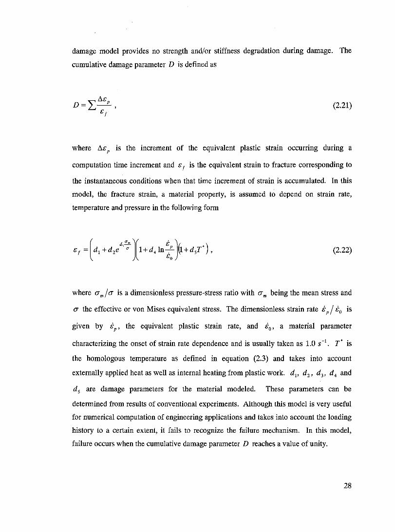
damage model provides no strength and/or stiffness degradation during damage. The

cumulative damage parameter D is defined as

(2.21)

where /1& p is the increment of the equivalent plastic strain occurring during a

computation time increment and & f is the equivalent strain to fracture corresponding to

the instantaneous conditions when that time increment of strain is accumulated. In this

model, the fracture strain, a mate rial property, is assumed to depend on strain rate,

temperature and pressure in the following form

(2.22)

where am / a is a dimensionless pressure-stress ratio with am being the mean stress and

a the effective or von Mises equivalent stress. The dimensionless strain rate & p / &0 is

given by & p' the equivalent plastic strain rate, and &0' a material parameter

characterizing the onset of strain rate dependence and is usually taken as 1.0 S-l. T* is

the homologous temperature as defined in equation (2.3) and takes into account

externally applied heat as well as internaI heating from plastic work. dp d 2 , d 3 , d 4 and

ds are damage parameters for the material modeled. These parameters can be

determined from results of conventional experiments. Although this model is very useful

for numerical computation of engineering applications and takes into account the loading

history to a certain extent, it fails to recognize the failure mechanism. In this model,

failure occurs when the cumulative damage parameter D reaches a value of unity.

28

2.3 Optimization Method: The Taguchi Approach

Parametric studies are often used in computer and physical experiments ta determine an

optimal set of physical parameters for a given response variable. Without the benefit of

an orderly approach, the parameters can be varied indefinitely and result in an

unnecessarily large number of experiments ta be carried out. This can be detrimental ta

the efficiency of the method used and time consuming in searching for an optimal

solution.

Ta reduce the number of necessary experiments, the effect of each parameter (or factor)

can be studied individually by isolating it in the design space as discussed in Fowlkes and

Creveling (1995). This is sometimes done by varying only the factor of interest and

keeping aIl other factors fixed. This method, however, is time consuming and requires

carrying out a large number of experiments depending on the sensitivity of each factor.

More systematically, the number of levels (or fixed values) of each factor can be

determined and a set of experiments can be carried out ta caver the entire factorial space

defined by aIl factors and their respective levels. The latter is based on the design of

experiments (DOE) method and is a very useful statistical method that can greatly reduce

the time needed ta design and study experiments. For example, an experiment involving

four different factors, each having three levels of variation, will result in conducting a

total of 34 or 81 (full factorial) experiments. An efficient and systematic DOE method

that is often used ta avoid full factorial designs, while still providing a reliable basis for

optimization, is the orthogonal array method. One main application of this method is the

planning of balanced experiments.

The rows of the array represent the specific sets of factor levels ta be performed (i.e. the

experiments), while the columns correspond ta the different factors who se effects are

being studied. Since the same number of runs is assigned ta each level of a column in an

orthogonal array, the set of experiments based on such an array is a balanced design set.

Such a set spans the experimental space uniformly where each factor-Ievel combination

29

occurs the same number of times across the experimental space and no factor is given

more importance than another.

2.3.1 Finding the optimal set

Based on the response values that are found from running the specific experiments

defined by the orthogonal array, an optimal solution can be found. This is done using

what is referred to as factor plots in the Taguchi DOE approach.

Factor plots show data points of response versus level of each factor in the optimization

se arch space. The responses corresponding to one level of a factor are averaged. The

average responses of all factor levels are used in factor plots. From these plots, the set of

levels of each factor giving the optimal solution can be found. This is explained further

by means of an example in Chapter 5. The optimal set of levels does not usually belong

to the original set of experiments defined by the orthogonal array.

There is a number of underlying assumptions and checks that are associated with the

Taguchi method. The comparison of average responses in factor plots is based on the

assumption that no significant interactions exist between factors. This assumption stems

from the definition of orthogonality and mainly ensures that the effect of one factor level

on the response is minimally dependent on the level of other factors. The validity of the

interaction assumption can be checked using interaction plots which also employ the

average response of factor levels.

It is important to note that in using physical experiments, the DOE method accounts for

noise factors. In this work, computer experiments are used, hence the response value for

a given input set is considered free of noise since repeats of a test are identical.

2.3.2 The predictive equation

As explained in the previous section, the Taguchi approach provides the optimal set of

factor levels. It can also be of interest to know the response of a combination of factor

30

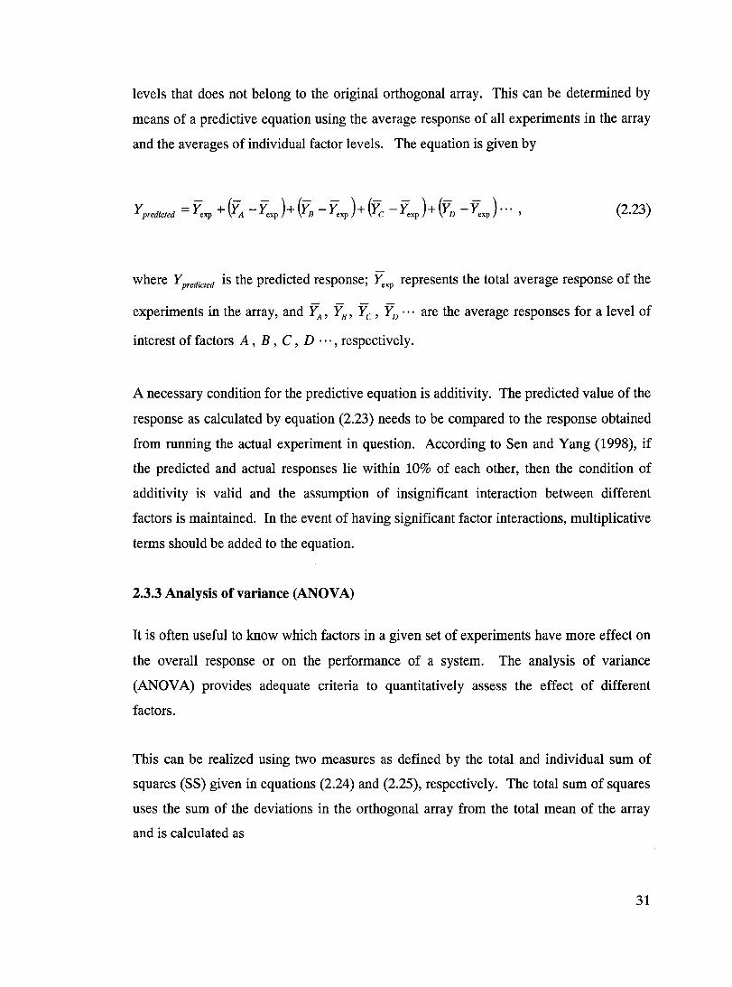
levels that does not belong to the original orthogonal array. This can be determined by

means of a predictive equation using the average response of all experiments in the array

and the averages of individual factor levels. The equation is given by

(2.23)

where Ypredicted is the predicted response; ~xp represents the total average response of the

experiments in the array, and ~, ~, Yc ' YD ••• are the average responses for a level of

interest of factors A, B, C, D "', respectively.

A necessary condition for the predictive equation is additivity. The predicted value of the

response as calculated by equation (2.23) needs to be compared to the response obtained

from running the actual experiment in question. According to Sen and Yang (1998), if

the predicted and actual responses lie within 10% of each other, then the condition of

additivity is valid and the assumption of insignificant interaction between different

factors is maintained. In the event of having significant factor interactions, multiplicative

terms should be added to the equation.

2.3.3 Analysis of variance (ANOV A)

It is often useful to know which factors in a given set of experiments have more effect on

the overall response or on the performance of a system. The analysis of variance

(ANDV A) provides adequate criteria to quantitatively assess the effect of different

factors.

This can be realized using two measures as defined by the total and individual sum of

squares (SS) given in equations (2.24) and (2.25), respectively. The total sum of squares

uses the sum of the deviations in the orthogonal array from the total mean of the array

and is calculated as

31

~( -)2 TotalSS = L..J 1'; - ~xp , (2.24) i=l

where Y; is the response of the ith row in the orthogonal array (i.e. response of an

experiment); ~xP is the mean response of aIl the experiments in the array and n is the

number of experiments.

Similarly, the sum of squares of each factor is calculated. This calculation is shown, for

instance, for factor A in equation (2.25) as

SS A = l m A (~i - ~xp)2 , (2.25) i=l

where YAi is the mean response of factor A for a given level; m is the number of

experiments for each level of factor A and nAis the number of levels of factor A.

The percent contribution of each factor on the overall response is determined by the ratio

of the individual sum of squares of a factor to the total sum of squares as given by

equation (2.26) for factor A as

% contribution of A = SS A xl 00 . TotalSS

(2.26)

The greater the effect of a factor, the greater is its contribution. By studying the

contributions, the experimental space can be refined by eliminating factors with relatively

low contributions and by placing more emphasis on significant factors in subsequent

investigations.

32

CHAPTER3

DETAILED HONEYCOMB MODELING

The numerical simulation of the penetration of bare honeycomb by a projectile is

undertaken using the general-purpose nonlinear finite element analysis program

ABAQUS/Explicit Version 6.4. A three-dimensional detailed modeling approach is

followed whereby a honeycomb cluster is fully modeled. The detailed model is described

and its results are presented and compared to experiments by Goldsmith and Louie

(1995).

3.1 Mode) Description

The modeling of the penetration of a rigid sphere through a cluster of honeycomb cells is

discussed in the following sections including geometry, boundary conditions, mesh

sensitivity, contact interactions, and material and damage.

3.1.1 Geometry and boundary conditions

The cell cluster considered in this work is made up of a number of regular hexagonal

cells having the same geometric features as Aluminum 5052-H19 l/8in - O.OOlin

honeycomb. This specific configuration is modeled so that correlation with experimental

results by Goldsmith and Louie (1995) can be made. AlI cells have a fixed size of 3.175

33

mm (0.125 in) and are 19.05 mm long while the impactor is 6.35 mm (0.25 in) in

diameter. AlI cell walls have the same thickness of 0.0254 mm (0.001 in). This differs

from real honeycombs where adhesively-bonded walls are twice as thick as other walls

by virtue of the expansion process used in the adhesive bonding manufacturing technique

(as explained in Section 1.1).

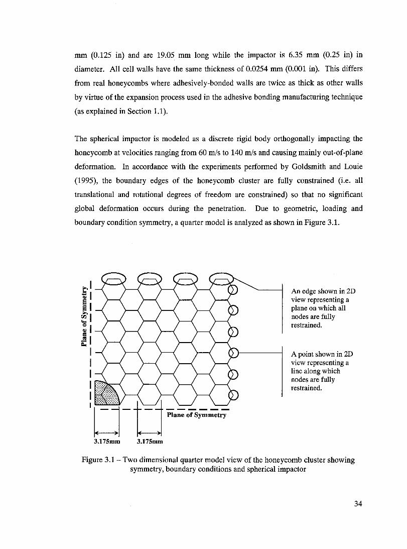
The spherical impactor is modeled as a dis crete rigid body orthogonally impacting the

honeycomb at velocities ranging from 60 mis to 140 mis and causing mainly out-of-plane

deformation. In accordance with the experiments performed by Goldsmith and Louie

(1995), the boundary edges of the honeycomb cluster are fully constrained (i.e. aIl

translational and rotational degrees of freedom are constrained) so that no significant

global deformation occurs during the penetration. Due to geometric, loading and

boundary condition symmetry, a quarter model is analyzed as shown in Figure 3.1.

3.175mm 3.175mm

An edge shown in 2D view representing a plane on which all nodes are fully restrained.

A point shown in 2D view representing a line along which nodes are fully restrained.

Figure 3.1- Two dimensional quarter model view of the honeycomb cluster showing symmetry, boundary conditions and spherical impactor

34

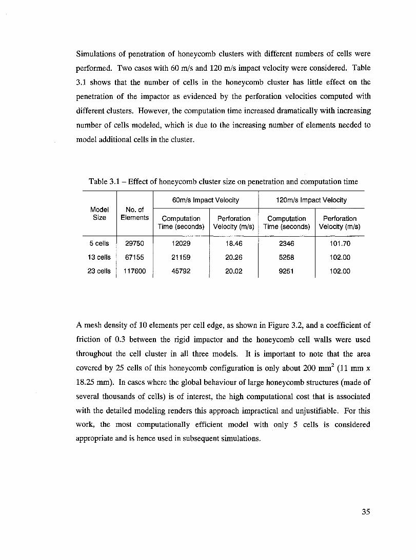
Simulations of penetration of honeycomb clusters with different numbers of cells were

performed. Two cases with 60 mis and 120 mis impact velocity were considered. Table

3.1 shows that the number of cells in the honeycomb cluster has little effect on the

penetration of the impactor as evidenced by the perforation velocities computed with

different clusters. However, the computation time increased dramatically with increasing

number of cells modeled, which is due to the increasing number of elements needed to

model additional cells in the cluster.

Table 3.1- Effect of honeycomb cluster size on penetration and computation time

60m/s Impact Velocity 120m/s Impact Velocity

Model No. of Size Elements Computation Perforation Computation Perforation

Time (seconds) Velocity (mis) Time (seconds) Velocity (mis)

5 cells 29750 12029 18.46 2346 101.70

13 cells 67155 21159 20.26 5258 102.00

23 cells 117600 45792 20.02 9251 102.00

A mesh density of 10 elements per cell edge, as shown in Figure 3.2, and a coefficient of

friction of 0.3 between the rigid impactor and the honeycomb cell walls were used

throughout the cell cluster in all three models. It is important to note that the area

covered by 25 cells of this honeycomb configuration is only about 200 mm2 (11 mm x

18.25 mm). In cases where the global behaviour of large honeycomb structures (made of

several thousands of cells) is of interest, the high computational cost that is associated

with the detailed modeling renders this approach impractical and un justifiable. For this

work, the most computationally efficient mode! with only 5 cells is considered

appropriate and is hence used in subsequent simulations.

35

Figure 3.2 - A uniform mesh of 10 elements per honeycomb cell edge

Although the honeycomb cluster is a geometrically periodic medium, the location of

impact could occur according to three different configurations as shown in Figure 3.3,

thus affecting the deformation mode of cell walls and subsequently resulting in different

perforation velocities.

Configuration 1 Impactor over cell

Configuration 2 Impactor over edge

Configuration 3 Impactor over corner

Figure 3.3 - Impact configurations of honeycomb cells

Only the first impact configuration is modeled where the centre of a cell is aligned with

the centre of the rigid spherical impactor. The diameter of the spherical impactor is twice

the honeycomb cell size to allow for the correlation between numerical and experimental

results from a number of tests by Goldsmith and Louie (1995). The final 5-cell three­

dimensional model is shown in perspective view in Figure 3.4.

36

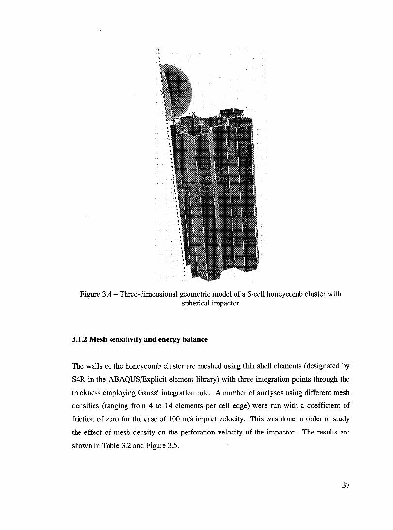
Figure 3.4 - Three-dimensional geometric model of a 5-cell honeycomb c1uster with spherical impactor

3.1.2 Mesh sensitivity and energy balance

The walls of the honeycomb c1uster are meshed using thin shell elements (designated by

S4R in the ABAQUSlExplicit element library) with three integration points through the

thickness employing Gauss' integration rule. A number of analyses using different mesh

densities (ranging from 4 to 14 elements per cell edge) were run with a coefficient of

friction of zero for the case of 100 mis impact velocity. This was done in order to study

the effect of mesh density on the perforation velocity of the impactor. The results are

shown in Table 3.2 and Figure 3.5.

37

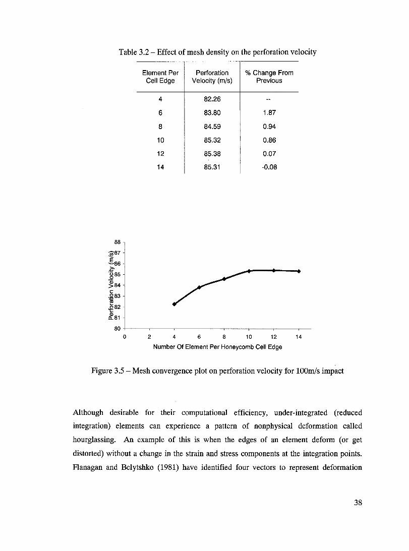
Table 3.2 - Effect of mesh density on the perforation velocity

88

~87

S86 ~ g85

~84 c: ~83 .g82 ~81

Element Per Cel! Edge

4

6

8

10

12

14

Perforation % Change From Velocity (mis) Previous

82.26

83.80 1.87

84.59 0.94

85.32 0.86

85.38 0.07

85.31 -0.08

80+---~~--~----~----~----,---~----~--

o 2 4 6 8 10 12 14

Number Of Element Per Honeycomb Cell Edge

Figure 3.5 - Mesh convergence plot on perforation velocity for lOOm/s impact

Although desirable for their computational efficiency, under-integrated (reduced

integration) elements can experience a pattern of nonphysical deformation called

hourglassing. An example of this is when the edges of an element deform (or get

distorted) without a change in the strain and stress components at the integration points.

Flanagan and Belytshko (1981) have identified four vectors to represent deformation

38

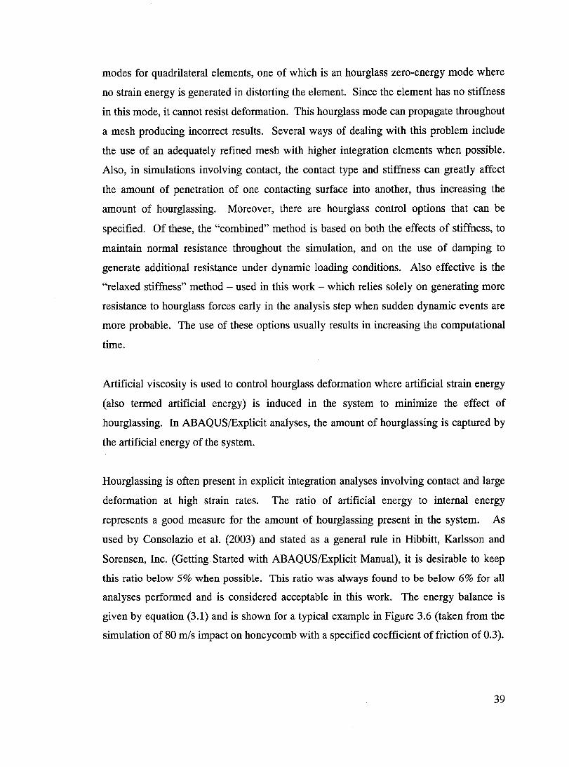
modes for quadrilateral elements, one of which is an hourglass zero-energy mode where

no strain energy is generated in distorting the element. Since the element has no stiffness

in this mode, it cannot resist deformation. This hourglass mode can propagate throughout

a mesh producing incorrect results. Several ways of dealing with this problem inc1ude

the use of an adequately refined mesh with higher integration elements when possible.

AIso, in simulations involving contact, the contact type and stiffness can greatly affect

the amount of penetration of one contacting surface into another, thus increasing the

amount of hourglassing. Moreover, there are hourglass control options that can be

specified. Of these, the "combined" method is based on both the effects of stiffness, to

maintain normal resistance throughout the simulation, and on the use of damping to

generate additional resistance under dynamic loading conditions. Aiso effective is the

"relaxed stiffness" method - used in this work - which relies solely on generating more

resistance to hourglass forces early in the analysis step when sudden dynamic events are

more probable. The use of these options usually results in increasing the computational

time.

Artificial viscosity is used to control hourglass deformation where artificial strain energy

(also termed artificial energy) is induced in the system to minimize the effect of

hourglassing. In ABAQUSlExplicit analyses, the amount of hourglassing is captured by

the artificial energy of the system.

Hourglassing is often present in explicit integration analyses involving contact and large

deformation at high strain rates. The ratio of artificial energy to internaI energy

represents a good measure for the amount of hourglassing present in the system. As

used by Consolazio et al. (2003) and stated as a general rule in Hibbitt, Karlsson and

Sorensen, Inc. (Getting Started with ABAQUSlExplicit Manual), it is desirable to keep

this ratio below 5% when possible. This ratio was always found to be below 6% for all

analyses performed and is considered acceptable in this work. The energy balance is

given by equation (3.1) and is shown for a typical ex ample in Figure 3.6 (taken from the

simulation of 80 mis impact on honeycomb with a specified coefficient of friction of 0.3).

39

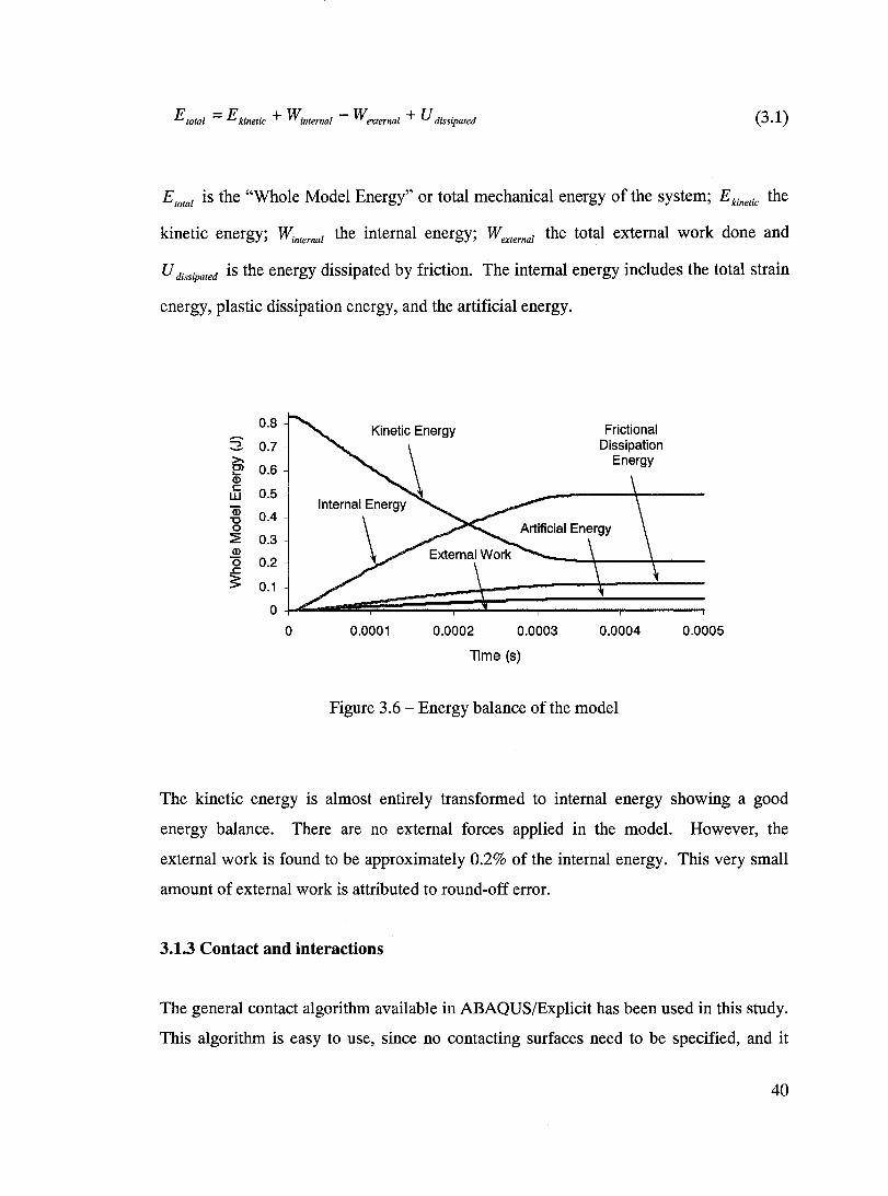
E total = E kinetic + Winternal - Wexternal + U dissipated (3.1)

Etotal is the "Whole Model Energy" or total mechanical energy of the system; E kinetic the

kinetic energy; W;nternal the internaI energy; Wexternal the total external work done and

U dissipated is the energy dissipated by friction. The internaI energy includes the total strain

energy, plastic dissipation energy, and the artificial energy.

0.8 -2- 0.7 >-C> 0.6 "-Cl) c: 0.5 UJ ID 0.4 "0 0

::2: 0.3 Cl)

ëi .c: 0.2

:s: 0.1

0

0 0.0001 0.0002 0.0003

lime (s)

Frictional Dissipation

Energy

0.0004

Figure 3.6 - Energy balance of the model

0.0005

The kinetic energy is almost entirely transformed to internaI energy showing a good

energy balance. There are no external forces applied in the model. However, the

external work is found to be approximately 0.2% of the internaI energy. This very small

amount of external work is attributed to round-off error.

3.1.3 Contact and interactions

The general contact algorithm available in ABAQUS/Explicit has been used in this study.

This algorithm is easy to use, since no contacting surfaces need to be specifie d, and it

40

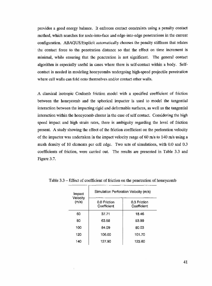
provides a good energy balance. It enforces contact constraints using a penalty contact

method, which searches for node-into-face and edge-into-edge penetrations in the current

configuration. ABAQUSlExplicit automatically chooses the penalty stiffness that relates

the contact force to the penetration distance so that the effect on time increment is

minimal, while ensuring that the penetration is not significant. The general contact

algorithm is especially useful in cases where there is self-contact within a body. Self­

contact is needed in modeling honeycombs undergoing high-speed projectile penetration

where cell walls can fold onto themselves and/or contact other walls.

A c1assical isotropic Coulomb friction model with a specified coefficient of friction

between the honeycomb and the spherical impactor is used to model the tangential

interaction between the impacting rigid and deformable surfaces, as well as the tangential

interaction within the honeycomb c1uster in the case of self contact. Considering the high

speed impact and high strain rates, there is ambiguity regarding the level of friction

present. A study showing the effect of the friction coefficient on the perforation velo city

of the impactor was undertaken in the impact velocity range of 60 mis to 140 mis using a

mesh density of 10 elements per cell edge. Two sets of simulations, with 0.0 and 0.3

coefficients of friction, were carried out. The results are presented in Table 3.3 and

Figure 3.7.

Table 3.3 - Effect of coefficient of friction on the penetration of honeycomb

Impact Simulation Perforation Velocity (mis)

Velocity (mis) 0.0 Friction 0.3 Friction

Coefficient Coefficient

60 37.71 18.46

80 63.58 53.99

100 84.09 80.03

120 106.00 101.70

140 127.90 123.60

41

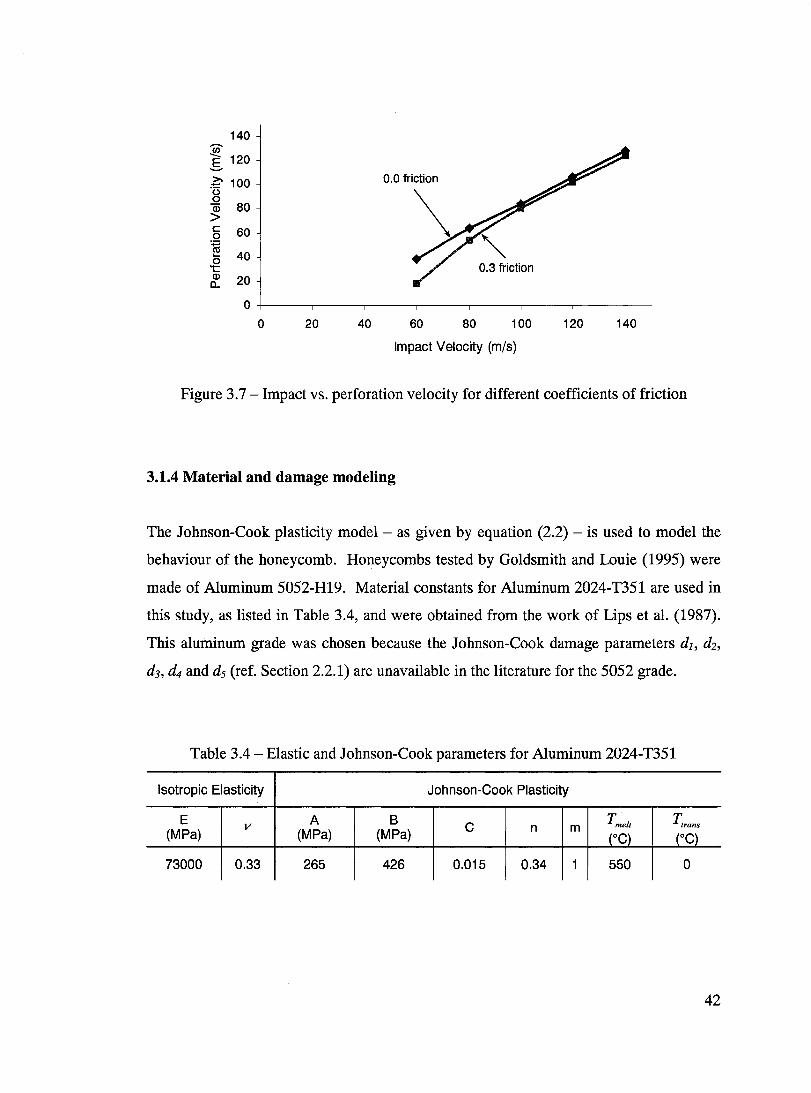
140 -~ 120 .s ~ 100 0.0 friction u 0 ID 80 > c: 60 0 '1ij

40 .... 0 't: 0.3 friction Q) 20 a..

0

0 20 40 60 80 100 120 140

Impact Veloeity (mis)

Figure 3.7 - Impact vs. perforation velo city for different coefficients of friction

3.1.4 Material and damage modeling

The Johnson-Cook plasticity model - as given by equation (2.2) - is used to model the

behaviour of the honeycomb. Honeycombs tested by Goldsmith and Louie (1995) were

made of Aluminum 5052-HI9. Material constants for Aluminum 2024-T351 are used in

this study, as listed in Table 3.4, and were obtained from the work of Lips et al. (1987).

This aluminum grade was chosen because the Johnson-Cook damage parameters dl, d2,

d3, d4 and d5 (ref. Section 2.2.1) are unavailable in the literature for the 5052 grade.

Table 3.4 - Elastic and Johnson-Cook parameters for Aluminum 2024-T351

Isotropie Elastieity Johnson-Cook Plasticity

E v A B C

Tme1t ~rans (MPa) (Mpa) (MPa) n m

(OC) (OC)

73000 0.33 265 426 0.015 0.34 1 550 0

42

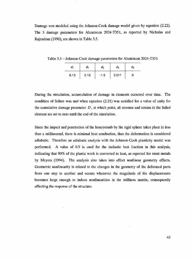
Damage was modeled using the Johnson-Cook damage model given by equation (2.22).

The 5 damage parameters for Aluminum 2024-T351, as reported by Nicholas and

Rajendran (1990), are shown in Table 3.5.

Table 3.5 - Johnson-Cook damage parameters for Aluminum 2024-T351

d1 d2 d3 d4 ds

0.13 0.13 -1.5 0.011 0

During the simulation, accumulation of damage in elements occurred over time. The

condition of failure was met when equation (2.21) was satisfied for a value of unit y for

the cumulative damage parameter D, at which point, aIl stresses and strains in the failed

element are set to zero until the end of the simulation.

Since the impact and penetration of the honeycomb by the rigid sphere takes place in less

than a millisecond, there is minimal heat conduction, thus the deformation is considered

adiabatie. Therefore an adiabatic analysis with the Johnson-Cook plasticity model was

performed. A value of 0.9 is used for the inelastic heat fraction in this analysis,

indicating that 90% of the plastic work is converted to heat, as reported for most metals

by Meyers (1994). The analysis also takes into effect nonlinear geometry effeets.

Geometrie nonlinearity is related to the changes in the geometry of the deformed parts

from one step to another and occurs whenever the magnitude of the displacements

becomes large enough to induce nonlinearities in the stiffness matrix, consequently

affecting the response of the structure.

43

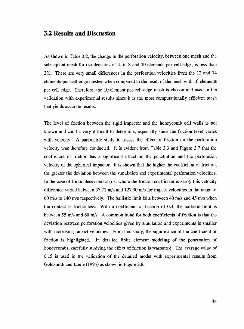
3.2 Results and Discussion

As shown in Table 3.2, the change in the perforation velo city, between one mesh and the

subsequent mesh for the densities of 4, 6, 8 and 10 elements per cell edge, is less than

2%. There are very small differences in the perforation velocities from the 12 and 14

elements-per-cell-edge meshes when compared to the result of the mesh with 10 elements

per cell edge. Therefore, the lO-element-per-cell-edge mesh is chosen and used in the

validation with experimental results since it is the most computationally efficient mesh

that yields accurate results.

The level of friction between the rigid impactor and the honeycomb cell walls is not

known and can be very difficult to determine, especially since the friction level varies

with velocity. A parame tric study to assess the effect of friction on the perforation

velocity was therefore conducted. It is evident from Table 3.3 and Figure 3.7 that the

coefficient of friction has a significant effect on the penetration and the perforation

velocity of the spherical impactor. It is shown that the higher the coefficient of friction,

the greater the deviation between the simulation and experimental perforation velocities.

In the case of frictionless contact (i.e. where the friction coefficient is zero), this velo city

difference varied between 37.71 mis and 127.90 mis for impact velocities in the range of

60 mis to 140 mis respectively. The ballistic limit falls between 40 mis and 45 mis when

the contact is frictionless. With a coefficient of friction of 0.3, the ballistic limit is

between 55 mis and 60 mis. A common trend for both coefficients of friction is that the

deviation between perforation velocities given by simulation and experiments is smaller

with increasing impact velocities. From this study, the significance of the coefficient of

friction is highlighted. In detailed finite element modeling of the penetration of

honeycombs, carefully studying the effect of friction is warranted. The average value of

0.15 is used in the validation of the detailed model with experimental results from

Goldsmith and Louie (1995) as shown in Figure 3.8.

44

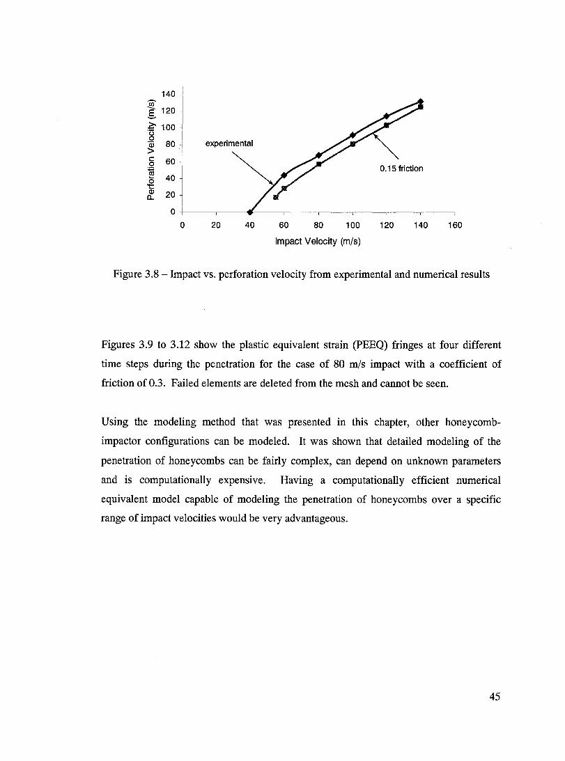
140 Ci) E 120 ---:È' 100 (.) o ~ 80

c 60 0

~ 40 0

't CI) 20 Il...

0

0 20 40 60 80 100 120 140 160

Impact Velocity (mis)

Figure 3.8 - Impact vs. perforation velocity from experimental and numerical results

Figures 3.9 to 3.12 show the plastic equivalent strain (PEEQ) fringes at four different

time steps during the penetration for the case of 80 mis impact with a coefficient of

friction of 0.3. Failed elements are deleted from the mesh and cannot be seen.

Using the modeling method that was presented in this chapter, other honeycomb­

impactor configurations can be modeled. It was shown that detailed modeling of the

penetration of honeycombs can be fairly complex, can depend on unknown parameters

and is computationally expensive. Having a computationally efficient numerical

equivalent model capable of modeling the penetration of honeycombs over a specifie

range of impact velocities would be very advantageous.

45

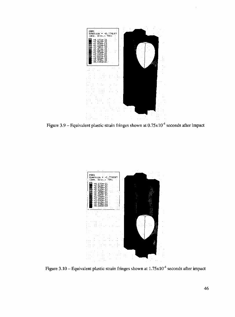
PEEQ fraction = -0.774597 (Ave. Crit.: 75'<)

+4. 173e-01 +3.BZ6e-01 +3.476e-01 +3.130,,-01 +Z.782e-01 +2.434e-01 +2.067e-01 +1. 73ge-01 +1.391e-01 +1.043e-01 +6.956e-OZ +3. 476e-OZ +O.OOOe+OO

Figure 3.9 - Equivalent plastic strain fringes shown at O.75xlO-4 seconds after impact

PEEQ fraction = -0.774597 (Ave. Crit.: 75%)

+4.173,,-01 +3.8Z6e-01 +3. 478e-01 +3.130,,-01 +2.782e-01 +Z.434e-01 +2.0B7e-01 +1.73ge-01 +1. 391e-01 +1.043e-01 +6.956e-02 +3. 47Be-OZ +O.OOOe+OO

Figure 3.10 - Equivalent plastic strain fringes shown at 1.75xlO-4 seconds after impact

46

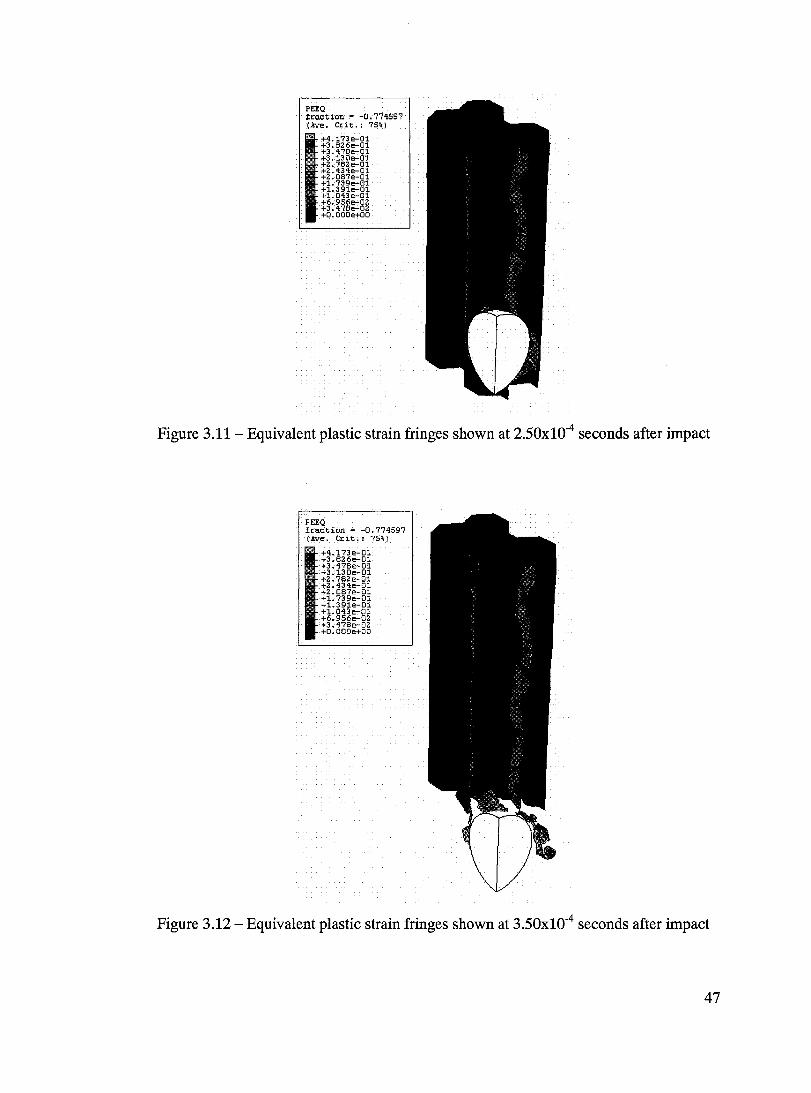
PEEQ fraction = -0.774597 (Ave. Crit.: 75%)

+4.173e-Ol +3. 6e-Ol +3. -01 +3. -01 +2. 01 +2. 01 +2. e-Ol +1. 73ge-Ol +1. 391e-Ol +1.043e-Ol +6.9S6e-02 +3. 478,,-OZ +O.OOOe+OO

Figure 3.11- Equivalent plastic strain fringes shown at 2.50xlQ-4 seconds after impact

PEEQ fraction = -0.774597 (Ave. Crit.: 75%)

+4.173e-Ol +3.8Z6e-Ol +3. 478e-Ol +3.130e-Ol +2.78Ze-Ol +2. 434e-Ol +2.087e-Ol +1.73ge-Ol +1.391e-Ol +1. 043e-Ol +6.956e-02 +3. 478e-02 +O.OOOe+OO

Figure 3.12 - Equivalent plastic strain fringes shown at 3.50x10-4 seconds after impact

47

CHAPTER4

EQUIVALENT HONEYCOMB MODELING

Using the P - a porous model that is described in Section 2.1.2, a two-dimensional

continuous isotropic axisymmetric numerical model for the penetration of honeycombs

by a projectile is developed. This model is based on four undetermined parameters and is

optimized to accurately predict perforation velocities of projectiles. An optimal set of

mate rial parameters is found from the Taguchi optimization method as will be presented

in Chapter 5.

4.1 Model Description

4.1.1 Geometry and boundary conditions

A rectangular sectional area, having a width of 22.225 mm and a height of 19.05 mm, is

used in the axisymmetric model. The width is chosen such that the ratio of target edge

size to impactor radius is 7. Meguid et al. (1999) suggest in their work on the

axisymmetric modeling of shot peening that this ratio should be a minimum of 5. The

height corresponds to the thickness of the honeycomb cluster (i.e. the height of each ceIl).

The spherical impactor is modeled axisymmetrically with a diameter of 6.35 mm.

Geometry, dimensions and boundary conditions of the equivalent model are shown in

48

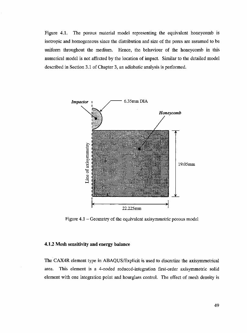
Figure 4.1. The porous material model representing the equivalent honeycomb is

isotropic and homogeneous since the distribution and size of the pores are assumed to be

uniform throughout the medium. Hence, the behaviour of the honeycomb in this

numerical model is not affected by the location of impact. Similar to the detailed model

described in Section 3.1 of Chapter 3, an adiabatic analysis is performed.

~- 6.35mm DIA

19.05mm

22.225mm

Figure 4.1- Geometry of the equivalent axisymmetric porous model

4.1.2 Mesh sensitivity and energy balance

The CAX4R element type in ABAQUSlExplicit is used to discretize the axisymmetrical

area. This element is a 4-noded reduced-integration first-order axisymmetric solid

element with one integration point and hourglass control. The effect of mesh density is

49

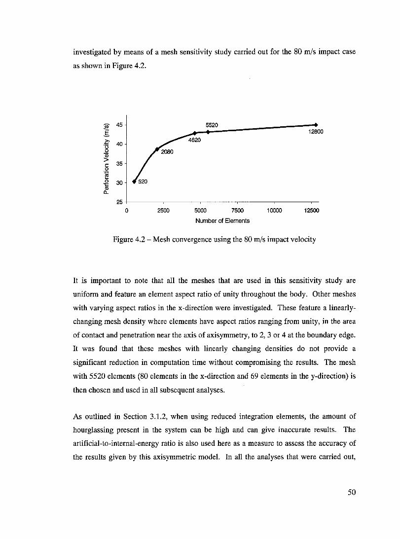
investigated by means of a mesh sensitivity study carried out for the 80 mis impact case

as shown in Figure 4.2.

~ 45 5520

.s 12800

>- 40 -"u 0

CD > 35 c: 0

~ 0 30 't: ID a..

25 0 2500 5000 7500 10000 12500

Number of Elements

Figure 4.2 - Mesh convergence using the 80 mis impact velo city

It is important to note that aIl the meshes that are used in this sensitivity study are

uniform and feature an element aspect ratio of unit y throughout the body. Other meshes

with varying aspect ratios in the x-direction were investigated. These feature a linearly­

changing mesh density where elements have aspect ratios ranging from unit y , in the area

of contact and penetration near the axis ofaxisymmetry , to 2, 3 or 4 at the boundary edge.

It was found that these meshes with linearly changing densities do not provide a

significant reduction in computation time without compromising the results. The mesh

with 5520 elements (80 elements in the x-direction and 69 elements in the y-direction) is

then chosen and used in aIl subsequent analyses.

As outlined in Section 3.1.2, when using reduced integration elements, the amount of

hourglassing present in the system can be high and can give inaccurate results. The

artificial-to-internal-energy ratio is also used here as a measure to assess the accuracy of

the results given by this axisymmetric model. In aIl the analyses that were carried out,

50

this energy ratio was found to vary between 25% and 30%. Attempts to reduce the high

amount of artificial energy in the system by mesh refinement, varying contact stiffness

parameters and using different hourglass control options proved unsuccessful. It was

finalIy speculated that the large amount of artificial energy is due to the instantaneous

failure model used. To test this hypothesis, two simulations - one without failure and

another with failure (aIl el se being the same) - were carried out and compared for the

case of 5 mis impact.

The tensile failure model that is used is based on the hydrostatic stress given by

1 am =-traceaij ,

3 (4.1)

where (J' m is the hydrostatic stress and (J'ij is the total stress tensor.

In this model, damage is not accumulated and failure occurs abruptly when the

hydrostatic stress, (J' m' exceeds the specified value of hydrostatic cutoff failure stress (J' f .

It was found that the artificial-to-internal-energy ratio was 2% in the analysis without

failure compared to 26% in the analysis with failure. This can be explained by the fact

that as elements fail abruptly, ABAQUSlExplicit induces artificial energy in the system

in the form of damping when necessary in order to keep the explicit integration scheme

stable. Further studies should be carried out in the future to reduce the energy ratio.

These studies should include the investigation of other failure models that can be used

with the P - a porous model. The results given by this axisymmetric model are hence

accepted as an approximate solution and will be used in the Taguchi optimization in

Chapter 5.

51

4.1.3 Contact and interactions

Contact between the equivalent medium and the rigid sphere is modeled using the contact

pair option available in ABAQUSlExplicit. The kinematic contact algorithm is specified

and associated with this option to enforce contact. This predictor/corrector algorithm

advances the kinematic state of the model to a predicted configuration without

considering the contact conditions. In this configuration, the slave nodes that penetrate

the mas ter surface are determined. The resisting force that is required to oppose

penetration is then ca1culated using the depth of penetration of each slave node, the mass

associated with the node, and the time increment. A corrected configuration, in which

the contact constraints are enforced, is then determined and subsequently used. The

general contact algorithm (described in Section 3.1.3) was not used because there is no

need to account for self-contact within the equivalent honeycomb medium.

Similar to the detailed model, the Coulomb friction model with a coefficient of friction of

0.1 is used. This coefficient does not represent true friction between the rigid impactor

and the deformable equivalent body and cannot be found from experimental tests or other

numerical studies. It was arbitrarily chosen (close to the 0.15 value used in the detailed

model) to represent a certain level of friction between the penetrating rigid impactor and

the equivalent honeycomb model.

4.1.4 Material modeling

A number of mate rial properties are specified for the P - a model, as outlined in section

2.1.2, to define the volumetric and deviatoric behaviour of the porous material. These

properties are listed for Aluminum 5052-H19 1/8in - O.OOlin honeycomb in Table 4.1.

52

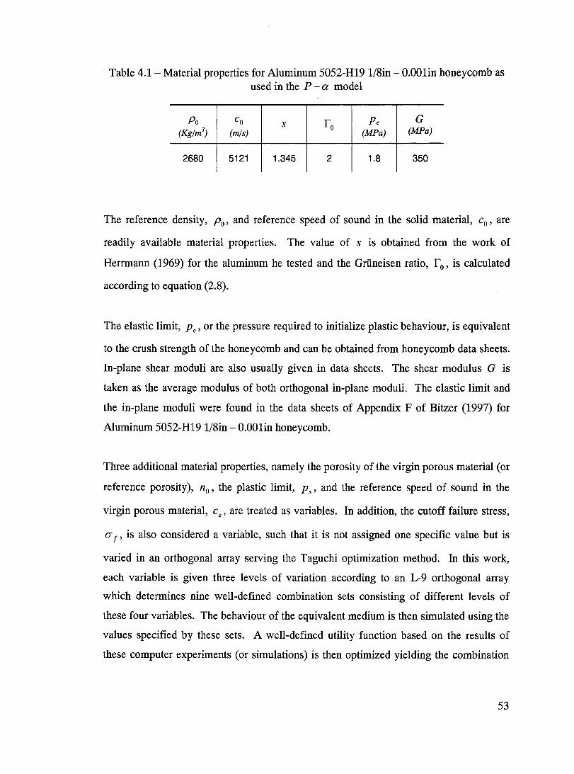
Table 4.1- Material properties for Aluminum 5052-H191/8in - O.OOlin honeycomb as used in the P - a model

Po Co s ro Pe G (Kglm3

) (mis) (MPa) (MPa)

2680 5121 1.345 2 1.8 350

The reference density, Po, and reference speed of sound in the solid material, co' are

readily available material properties. The value of s is obtained from the work of

Herrmann (1969) for the aluminum he tested and the Grüneisen ratio, r o ' is calculated

according to equation (2.8).

The elastic limit, Pe' or the pressure required to initialize plastic behaviour, is equivalent

to the crush strength of the honeycomb and can be obtained from honeycomb data sheets.

In-plane shear moduli are also usually given in data sheets. The shear modulus G is

taken as the average modulus of both orthogonal in-plane moduli. The elastic limit and

the in-plane moduli were found in the data sheets of Appendix Fof Bitzer (1997) for

Aluminum 5052-H191/8in - O.OOlin honeycomb.

Three additional material properties, namely the porosity of the virgin porous material (or

reference porosity), no, the plastic limit, Ps' and the reference speed of sound in the

virgin porous material, Ce' are treated as variables. In addition, the cutoff failure stress,

(J' f' is also considered a variable, such that it is not assigned one specifie value but is

varied in an orthogonal array serving the Taguchi optimization method. In this work,

each variable is given three levels of variation according to an L-9 orthogonal array

which determines nine well-defined combination sets consisting of different levels of

these four variables. The behaviour of the equivalent medium is then simulated using the

values specified by these sets. A well-defined utility function based on the results of

these computer experiments (or simulations) is then optimized yielding the combination

53

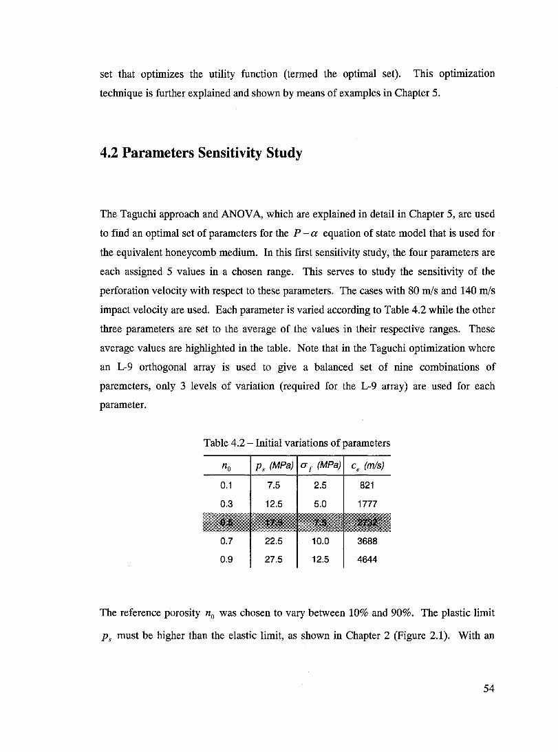
set that optimizes the utility function (termed the optimal set). This optimization

technique is further explained and shown by means of examples in Chapter 5.

4.2 Parameters Sensitivity Study

The Taguchi approach and ANDV A, which are explained in detail in Chapter 5, are used

to find an optimal set of parameters for the P - a equation of state model that is used for .

the equivalent honeycomb medium. In this first sensitivity study, the four parameters are

each assigned 5 values in a chosen range. This serves to study the sensitivity of the

perforation velo city with respect to these parameters. The cases with 80 mis and 140 mis

impact velo city are used. Each parameter is varied according to Table 4.2 while the other

three parameters are set to the average of the values in their respective ranges. These

average values are highlighted in the table. Note that in the Taguchi optimization where

an L-9 orthogonal array is used to give a balanced set of nine combinations of

paremeters, only 3 levels of variation (required for the L-9 array) are used for each

parameter.

Table 4.2 - Initial variations of parameters

no

0.1

0.3

0.7

0.9

Ps (MPa)

7.5

12.5

22.5

27.5

a f (Mpa)

2.5

5.0

10.0

12.5

ce (mis)

821

1777

3688

4644

The reference porosity no was chosen to vary between 10% and 90%. The plastic limit

Ps must be higher than the elastic limit, as shown in Chapter 2 (Figure 2.1). With an

54

elastic limit of 1.8 MPa for the honeycomb configuration studied, a lower plastic limit of

7.5 MPa was chosen significantly higher than the elastic limit. The plastic limit was

allowed to vary up to 27.5 MPa in increments of 5.0 MPa. The lower limit of the cutoff

failure stress is chosen as 2.5 MPa, and varied up to 12.5 MPa as shown in Table 4.2.

Running a number of simulations with different upper limits of the cutoff stress, this 12.5

MPa limit was chosen to ensure that perforation of the projectile occurs for the 80 mis

impact velocity case. The speed of sound in the virgin porous material was assumed to

be related linearly to the initial value of porosity no. In this linear relationship, it was

assumed that the speed of sound in air corresponds to a 100% porous material and the

speed of sound in solid aluminum corresponding to a zero percent porous medium. This

assumption does not violate the condition stated for the Taguchi optimization method

where no significant interactions should exist between factors (ref. Section 2.3.1).

Having one of the factors as a function of another represents the presence of colinearity

(not interactions) between factors. Moreover, the reverse order of the speeds of sound

with respect to porosity was used as a check in a Taguchi L-9 orthogonal array. It was

found that reversing the order of factors does not change the optimal solution.

The initial parameter variation study was conducted for impact velocities of 80 mis and

140 mis. The resulting perforation velocities for each combination of parameters

simulated are recorded in Table 4.3. The variations in perforation velocities differ

significantly in sorne cases. For example, considering the 80 mis impact velocity

simulation, the effects of both the initial porosity and the failure stress are significant (i.e.

the difference in the perforation velo city between the cases with the lower and upper

range values is 41.45 mis and 40.20 mis respectively) for the same values of plastic limit

Ps (17.5 MPa) and speed of sound in the virgin porous material ce (2722 mis). By

ca1culating the same difference in perforation velocity, it can be shown that the effect of

the plastic limit is clearly negligible while the speed of sound in the virgin porous

material can be considered relatively important. Also, it is of interest to note that the

perforation velo city would be more sensitive to the plastic limit, failure stress and speed

of sound parameters in the lower velocity range, as evidenced by having more variation

for the cases involving 80 mis impacts.

55

The purpose of this study is to assess the sensitivity of each parameter individually.

When conducting an optimization to find the optimal set of parameters for correlation

with experimental results, it can be expected that the initial porosity and failure stress

parameters have more effect on the perforation velocity than the plastic limit and the

speed of sound in the virgin porous mate rial and hence will have a more significant

contribution to the results. This is also shown in Figures 4.3 and 4.4 where the graphs of

perforation velocity against the Ps and Ce parameters do not show significant variations

as plotted on the same perforation velo city scale. This is in contrast to the steeper plots

shown in Figures 4.5 and 4.6 for the po rosit y and failure cutoff stress, respectively.

56

Table 4.3 - Effect of variation of parameters on the perforation velo city

Ps (MPa)

(Yr (MPa)

Ce

(mis) Perforation Velocity (mIs)

80 mIs Impact 140 mIs Impact

12.59 53.09

18.78 60.16

25.69 72.86

37.36 92.05

54.04 111.20

80 mIs Impact 140 mIs Impact

25.27 74.29

26.89 74.69

25.69 72.86

23.99 73.77

27.09 73.59

80 mIs Impact 140 mIs Impact

45.19 83.62

39.11 79.80

25.69 72.86

14.15 67.72

4.99 58.47

80 mIs Impact 140 mIs Impact

9.28 68.83

27.44 72.61

25.69 72.86

23.92 73.01

31.23 77.16

57

120 .-.. ~ S 100 140 mis impact ~ '13 80 0 ID • • • ./ • > 60 c: 0 80 mis impact

~ 40 .g Q) 20 a.. • L. • • ..

0

0 5 10 15 20 25 30

Plastic Limit (MPa)

Figure 4.3 - Sensitivity of perforation velo city on the plastic limit p s

120 ~ S 100 140 mis impact

.~ u 80 0

~ 60 • • ./ • ..

c: 0

~ 40 .... 0 't Q) 20 a..

80 mis impact

/ • .. • 0

0 1000 2000 3000 4000

Speed of Sound in Virgin Porous Medium (mis)

Figure 4.4 - Sensitivity of perforation velocity on the speed of sound in virgin porous

medium ce

58

120 ~ g 100 ~ 'u 80 o

~ 60 c 0

~ 40 .... 0 't:

20 Q) D-

O

0

: 80m/Sjmpact~ . 1

0.2 0.4 0.6 0.8

Porosity (Dimensionless)

Figure 4.5 - Sensitivity of perforation velo city on the porosity of the unloaded virgin porous mate rial no

120 ~ g 100 ~

III-'u 80 0 ID > 60 c 0

• --. 140 mis impact

.~ 80 mis impact

~ 40 .... 0 't:

20 Q) D-

o 0.0 2.0 4.0 6.0 8.0 10.0 12.0

Cutoff Failure Stress (MPa)

Figure 4.6 - Sensitivity of perforation velocity on the cutoff failure stress (J' f

59

CHAPTERS

THE TAGUCHI OPTIMIZATION

The optimization of the parameters in the P - a mate rial model that is used in the

equivalent axisymmetric modeling of honeycombs is presented in this chapter. The set of

parameters (no, p s' CFf' Ce) forms the basis for this optimization by means of an objective

function using the conventional Taguchi method. The equivalent optimal model is

validated using published experimental results by Goldsmith and Louie (1995). The

computational efficiency of the model, in terms of the time required for computations, is

then assessed and compared to that of the detailed honeycomb model of Chapter 3.

5.1 Utility Function

The objective of this study is to optimize the equivalent numerical model for the accurate

prediction of perforation velocities of bare Aluminum 5052-H19 1/8in - O.OOlin

hexagonal honeycomb when subjected to impacts in the range of 60 m/s to 140 rn/s. The

optimization is based on the parameter set (no, p s' CF f ' ce) and is carried out for more than

one data point, namely for impact velocities of 60, 80, 100, 120 and 140 rn/s. This

constitutes a multiple-criteria problem where each velocity case can be considered as a

single criterion. By introducing a utility function, multiple-criteria problems can be

converted into and treated as single-criterion problems. For this work, the utility function

60

is defined as the sum of Z values at different velocities, where Z is the absolute value of

the difference in perforation velocities between experimental and simulation results, as

depicted in equation (5.1).

U = Z60 (no,ps'Ci f ,cJ+ Z80 (no, Ps'Ci f ,cJ+ Z100 (no,ps,Ci f ,cJ ... ... + Z120 (no,ps,Ci f ,cJ+ Z140 (no,ps,Ci f ,cJ

where

Z 1 V exp V sim 1 i = perforation - perforation i

and

no E (nO-l' nO-2' nO-3)

Ps E (PS-PPS-2,PS-3)

Ci f E(Cif-pCif-2,Cif-3)

ce E (Ce-l'Ce-2,Ce-3)

(5.1)

In order to minimize the utility function U , the Taguchi optimization method is used to

find the optimal set of parameters (no, P s' Ci f ' ce) that yield the smallest deviation

between simulation and experimental results. Since the exact relationship between these

four parameters and the perforation velo city given by the finite element method is not

known (i.e. the finite element method acts as a "black box" to give data points), the

optimization is discrete and yields onl y a local minimum.

5.2 Conventional Taguchi Optimization

The four material parameters discussed in Chapter 4 - termed 'factors' in the Taguchi

optimization - are each assigned three levels of variation according to an L-9 orthogonal

array as shown in Table 5.1, where the numbers '1', '2' and '3' denote three different

levels (or values) a factor. It is shown that each factor appears an equal number of times

61

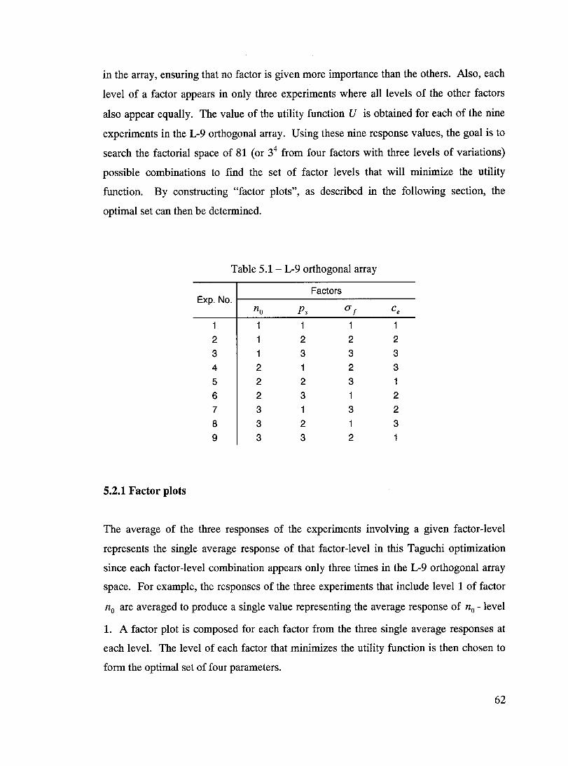
in the array, ensuring that no factor is given more importance than the others. Also, each

level of a factor appears in only three experiments where aIl levels of the other factors

also appear equaIly. The value of the utility function U is obtained for each of the nine

experiments in the L-9 orthogonal array. Using these nine response values, the goal is to

search the factorial space of 81 (or 34 from four factors with three levels of variations)

possible combinations to find the set of factor levels that will minimize the utility

function. By constructing "factor plots", as described in the following section, the

optimal set can then be determined.

5.2.1 Factor plots

The average of the three responses of the experiments involving a given factor-Ievel

represents the single average response of that factor-Ievel in this Taguchi optimization

since each factor-Ievel combination appears only three times in the L-9 orthogonal array

space. For example, the responses of the three experiments that include level 1 of factor

no are averaged to pro duce a single value representing the average response of no - level

1. A factor plot is composed for each factor from the three single average responses at

each level. The level of each factor that minimizes the utility function is then chosen to

form the optimal set of four parameters.

62

5.2.2 Prediction equation and additivity of the method

In the case where the optimal set is not one of the nine combinations tested (Le. it belongs

to the other 72 of 81 possible factorial experiments), which is often the case, the utility

function response for this optimal set can be ca1culated using equation (2.23). This

equation is rewritten as equation (5.2) for this optimization and can be used to find the

response of any of the 81 possible combinations.

(5.2)

where U predicted is the predicted response of the utility function for a specifie set of factor­

levels; U is the average U response from all nine experiments in the array and U no '

U ps ' U (J' f and U Ce are the average responses from aIl experiments involving the desired

levelof no, Ps' a f and ce' respectively.

As discussed in Section 2.3.2, for the prediction equation to accurately predict the

response of a specifie combination set of factor-Ievels, no interactions should exist

between factors. A simple check for the presence of interactions is done by assessing the

additivity assumption where the response of the optimal solution given by the prediction

equation is compared to the response given by the corresponding experiment (or

simulation). If the two responses are within 10% of each other (according to Sen and

Yang, 1998), then the additivity of the method holds true and hence the assumption of

insignificant interactions between factors is valid. The discrepancies between actual and

predicted responses can sometimes be the result of the deviation from linearity of the

predictive model used. As long as there are no multiplicative terms, the assumption of

additivity is valid given no significant interactions between factors.

63

5.2.3 Analysis of variance

Since the numerical model is used as a black box to give the perforation velocities that

are used in the optimization, it would be beneficial to know the effect of each factor on

the results. The contribution of each factor to the utility function response value is

assessed using the analysis of variances (ANOVA). This analysis is carried out on the

average response of each factor-Ievel. The total sum of squares and the sum of squares of

responses of each factor are ca1culated according to equations (2.24) and (2.25). The

ratio of these two sums given by (2.26), determines the percent contribution of each

factor to the overall response value.

5.3 The Taguchi Experiments

Two Taguchi optimizations are carried out. The first optimization is based on an "initial"

L-9 orthogonal array that spans the range of initial porosity of 10% to 90%. The second

optimization utilizes an array with the same percentage of variation for all four factors

and is centered about the optimal solution given by the first optimization. The

contributions of each factor to the results in each optimization are assessed and

compared. Single objective-criterion studies are also carried out using each velo city

separately.

5.3.1 Initial array optimization

The initial L-9 orthogonal array spans a relatively wide range of the four factors. Three

levels of variation for each factor are considered according to equation (5.1) as shown in

Table 5.2. The initial porosity no covers the range of 10% to 90%. The range of (J f is

chosen such that the projectile perforates the equivalent medium for the case with the

smallest impact velocity (60m/s) and with the lowest level of initial porosity (10%). The

64

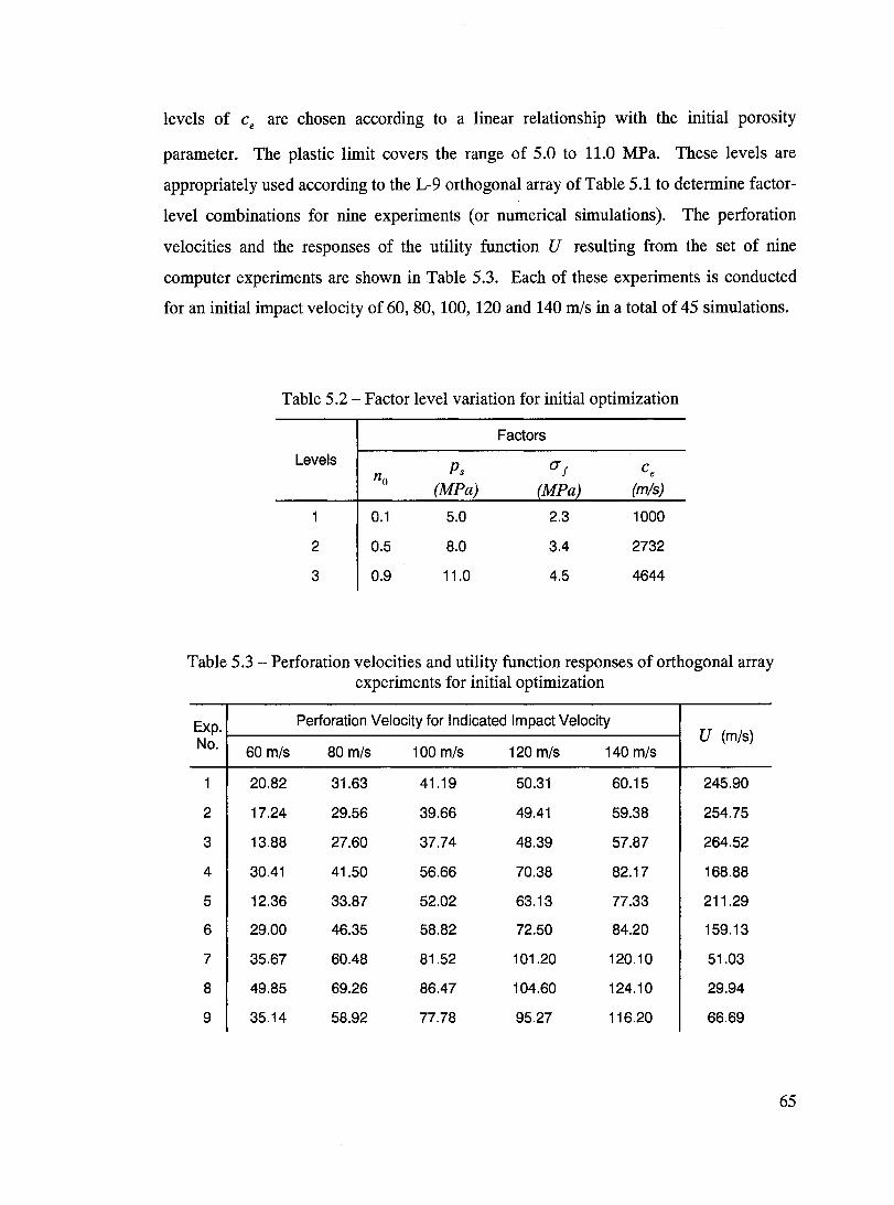
levels of Ce are chosen according to a linear relationship with the initial porosity

parameter. The plastic limit covers the range of 5.0 to 11.0 MPa. These levels are

appropriately used according to the L-9 orthogonal array of Table 5.1 to determine factor­

level combinations for nine experiments (or numerical simulations). The perforation

velocities and the responses of the utility function U resulting from the set of nine

computer experiments are shown in Table 5.3. Each of these experiments is conducted

for an initial impact velo city of 60,80, 100, 120 and 140 mis in a total of 45 simulations.

Table 5.2 - Factor level variation for initial optimization

Factors

Levels Ps CY f ce no (MPa) (MPa) (mis)

0.1 5.0 2.3 1000

2 0.5 8.0 3.4 2732

3 0.9 11.0 4.5 4644

Table 5.3 - Perforation velocities and utility function responses of orthogonal array experiments for initial optimization

Exp. Perforation Velocity for Indicated Impact Velocity

No. U (mis) 60 mis 80 mis 100 mis 120 mis 140 mis

20.82 31.63 41.19 50.31 60.15 245.90

2 17.24 29.56 39.66 49.41 59.38 254.75

3 13.88 27.60 37.74 48.39 57.87 264.52

4 30.41 41.50 56.66 70.38 82.17 168.88

5 12.36 33.87 52.02 63.13 77.33 211.29

6 29.00 46.35 58.82 72.50 84.20 159.13

7 35.67 60.48 81.52 101.20 120.10 51.03

8 49.85 69.26 86.47 104.60 124.10 29.94

9 35.14 58.92 77.78 95.27 116.20 66.69

65

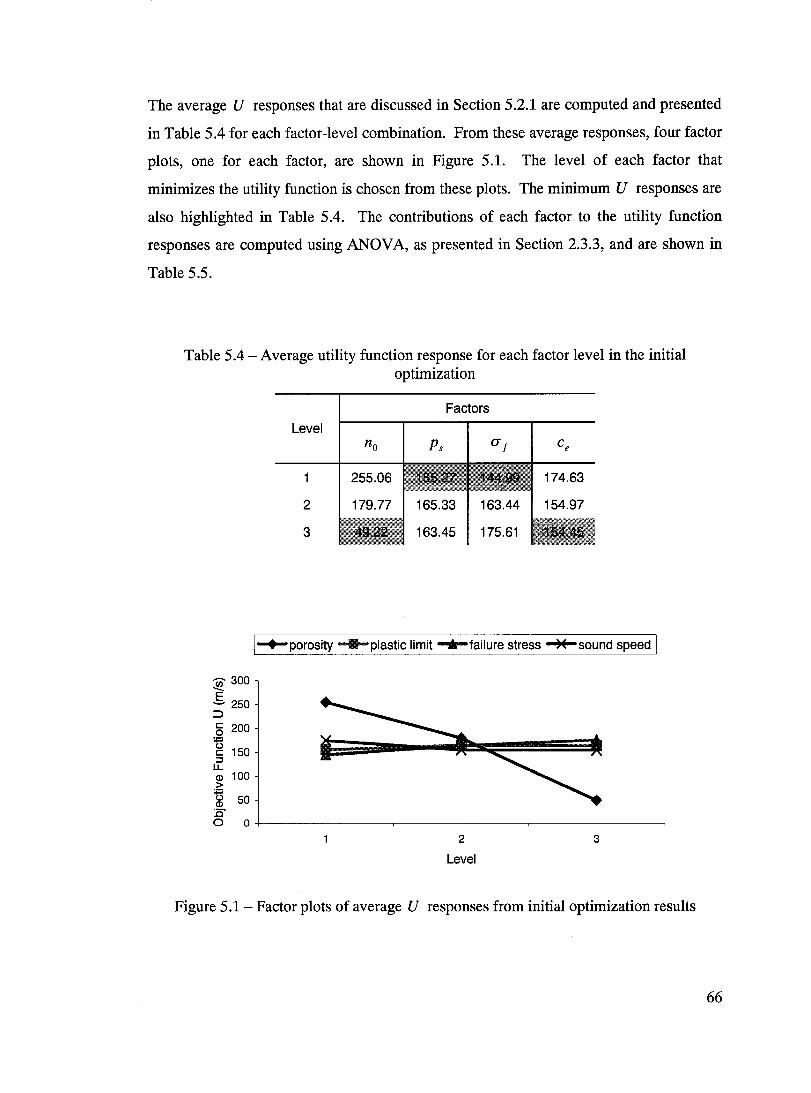
The average U responses that are discussed in Section 5.2.1 are computed and presented

in Table 5.4 for each factor-Ievel combination. From these average responses, four factor

plots, one for each factor, are shown in Figure 5.1. The level of each factor that

minimizes the utility function is chosen from these plots. The minimum U responses are

also highlighted in Table 5.4. The contributions of each factor to the utility function

responses are computed using ANOVA, as presented in Section 2.3.3, and are shown in

Table 5.5.

Table 5.4 - Average utility function response for each factor lev el in the initial optimization

:ê:' 300

S 250 ::> § 200

U c 150 ::::J u. Q) 100 > U 50 Q)

:0

Level

2

3

Factors

!-+-porosity -plastic limit ....... failure stress --*-sound speed!

o o+---------------~------------~--------------~

2

Level

3

Figure 5.1 - Factor plots of average U responses from initial optimization results

66

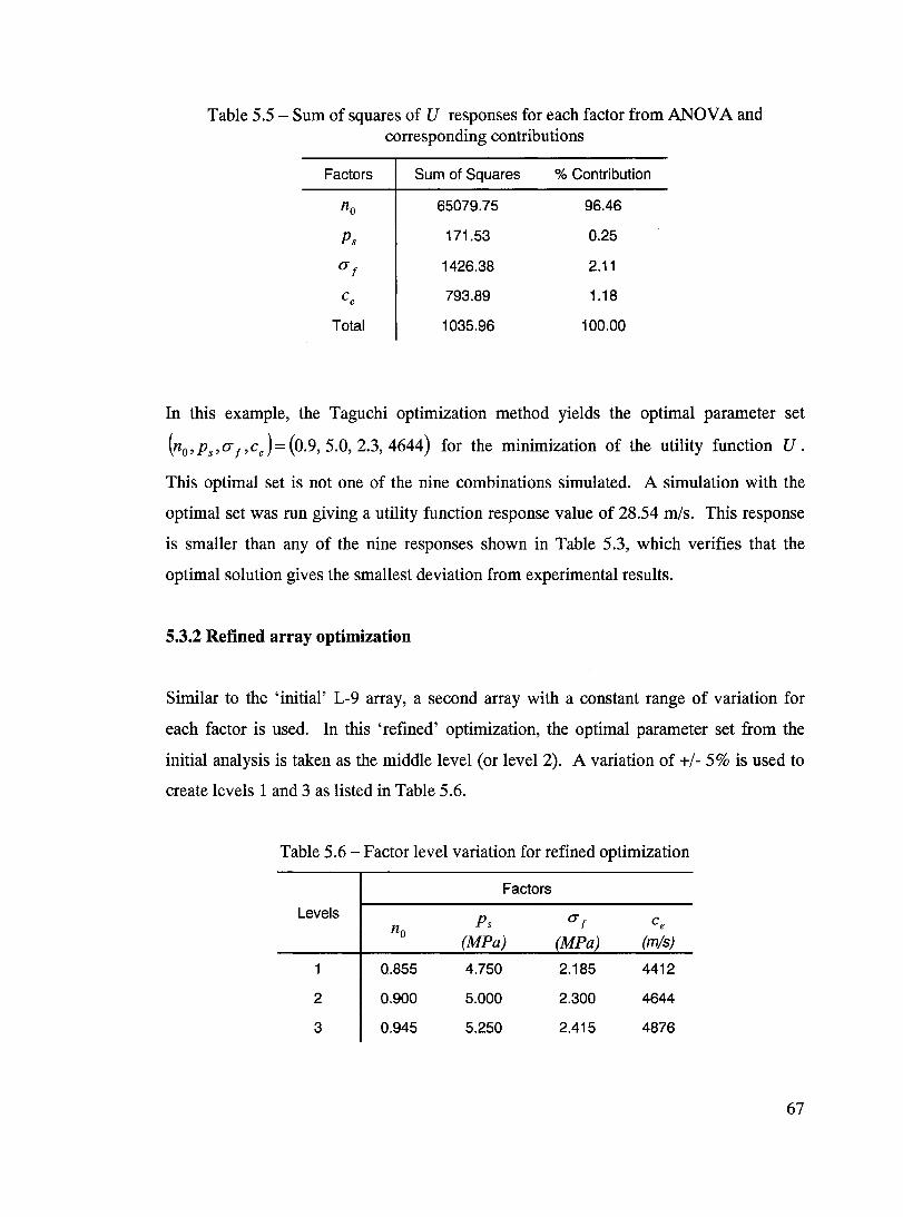
Table 5.5 - Sum of squares of U responses for each factor from ANOV A and corresponding contributions

Factors Sum of Squares % Contribution

no 65079.75 96.46

Ps 171.53 0.25

Ut 1426.38 2.11

ce 793.89 1.18

Total 1035.96 100.00

In this example, the Taguchi optimization method yields the optimal parameter set

(no,ps,ut ,cJ=(0.9, 5.0, 2.3, 4644) for the minimization of the utility function U.

This optimal set is not one of the nine combinations simulated. A simulation with the

optimal set was ron giving a utility function response value of 28.54 rn/s. This response

is smaller than any of the nine responses shown in Table 5.3, which verifies that the

optimal solution gives the smallest deviation from experimental results.

5.3.2 Refined array optimization

Similar to the 'initial' L-9 array, a second array with a constant range of variation for

each factor is used. In this 'refined' optimization, the optimal parameter set from the

initial analysis is taken as the middle level (or level 2). A variation of +/- 5% is used to

create levels 1 and 3 as listed in Table 5.6.

Table 5.6 - Factor level variation for refined optimization

Factors

Levels Ps Ut ce no (MPa) (MPa) (mis)

0.855 4.750 2.185 4412

2 0.900 5.000 2.300 4644

3 0.945 5.250 2.415 4876

67

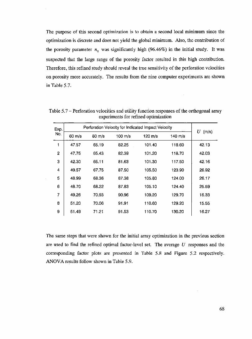
The purpose of this second optimization is to obtain a second local minimum since the

optimization is discrete and does not yield the global minimum. Also, the contribution of

the porosity parameter no was significantly high (96.46%) in the initial study. It was

suspected that the large range of the porosity factor resulted in this high contribution.

Therefore, this refined study should reveal the true sensitivity of the perforation velocities

on porosity more accurately. The results from the nine computer experiments are shown

in Table 5.7.

Table 5.7 - Perforation velocities and utility function responses of the orthogonal array experiments for refined optimization

Exp. Perforation Velocity for Indicated Impact Velocity U (mis) No. 60 mis 80 mis 100 mis 120 mis 140 mis

47.57 65.19 82.25 101.40 118.60 42.13

2 47.75 65.43 82.39 101.20 118.70 42.03

3 42.30 65.11 81.63 101.30 117.50 42.16

4 49.57 67.75 87.50 105.50 123.90 26.92

5 48.99 68.36 87.38 105.80 124.00 26.17

6 48.70 68.22 87.83 105.10 124.40 25.59

7 49.26 70.93 90.96 109.20 129.70 16.33

8 51.20 70.06 91.91 110.60 129.20 15.55

9 51.49 71.21 91.53 110.70 130.20 16.27

The same steps that were shown for the initial array optimization in the previous section

are used to find the refined optimal factor-Ievel set. The average U responses and the

corresponding factor plots are presented in Table 5.8 and Figure 5.2 respectively.

ANOVA results follow shown in Table 5.9.

68

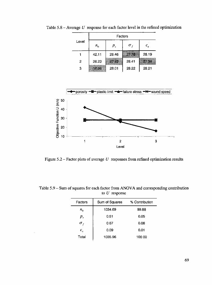
Table 5.8 - Average U response for each factor level in the refined optimization

~ 50 g :::l 40 c: o

g 30 ::J LL ID

~ 20 ID

Level

2

3

Factors

Ps

!-+-porosity _plastic limit .......... failure stress ~sound speed!

g 10+--------------,--------------~------------_, 2

Level

3

Figure 5.2 - Factor plots of average U responses from refined optimization results

Table 5.9 - Sum of squares for each factor from ANOVA and corresponding contribution to U response

Factors Sum of Squares % Contribution

no 1034.69 99.88

Ps 0.51 0.05

0"[ 0.67 0.06

ce 0.09 0.01

Total 1035.96 100.00

69

The optimal set (nO,ps,o-f,cJ=(0.945, 5.0,2.185,4644), corresponding to the set of

factor-Ievels (3, 2,1, 2), is found from the refined optimization. Again, this set does not

belong to the nine combination sets tested. However, a computer experiment was carried

out using this optimal set giving a value of 15.76 mis for the utility function U. The

refined study yields a sm aIler local minimum, when compared to 28.54 mis from the

initial study, thus presenting a closer fit to the experimental results for the velocity range

studied.

Equation (5.2) predicts a utility function response U of 15.32 mis for the refined optimal

set found. When compared to the response for the computer experiment (15.76 mis), the

difference between the two responses is only 2.77% (less than 10%), thus validating the

additivity assumption.

From this refined optimization, where the ranges of variation of aIl four factors are the

same (i.e. there is a 10% variation in aIl factors), a more clear indication of the

importance of each factor and its individu al contribution to the results can be revealed.

The contribution of the initial porosity to the optimal solution is 99.88%. This shows that

the initial po rosit y is a very important parameter that mainly controls the penetration in

the equivalent honeycomb model. The contributions of the plastic limit and the sound of

speed in the virgin porous material are very small. This was expected from Figures 4.3

and 4.4 where the plots of perforation velocities against Ps and ce were relatively flat.

The cutoff failure stress parameter 0- f did not have a significant contribution in both the

initial and refined optimizations because its chosen range is relatively narrow. In the

chosen range, the plots of variation in Figure 4.6 are reiatively flat aiso. It is important to

note that this narrow range of 0- f was necessarily chosen in order to always have

projectile perforation in any of the nine experiments, specifically the ones involving a

10% porous medium.

70

5.4 Discussion

The utility function response that is associated with the optimal solution in both initial

and refined studies was found to be 28.54 mis and 15.76 mis respectively. This decrease

in the value of U reflects the fact that the refined optimization study yields a second

local minimum. Further refinements can be carried out until convergence of the optimal

response is achieved. It is not necessary to do so in this work since the current solution is

deemed acceptable.

The relatively high porosity contribution (99.88%) from the refined study shows that over

the range of impact velocities 60 mis to 140 mis, the porosity is the most sensitive factor.

It was initially thought that the high contribution of porosity in the initial study (96.46%)

was due to the wide range of variation in porosity (0.1 to 0.9). The refined optimization

dearly shows that the utility function is highly sensitive to porosity. The optimal factor­

levels and corresponding contributions from both studies are summarized in Table 5.10.

Only the contribution of the porosity parameter has increased from the initial to the

refined study. Also, in both studies, the highest level of porosity was found to be the

optimal level indicating that in the velocity range of 60 to 140 mis, the utility function

response U is highly sensitive to porosity. The optimal solution for the plastic limit and

speed of sound in the virgin porous mate rial did not change. This finding is in

accordance with the factor plots of Ps and ce being nearly horizontallines. The change

in the optimal value of the failure stress (J" f (from 2.3 MPa to 2.185 MPa) is due to a

change from 28.41 mis to 27.76 mis in the average U response values of the levels of

(J" t' as was shown in Table 5.8.

71

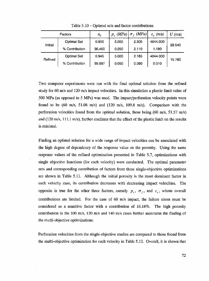
Table 5.10 - Optimal sets and factor contributions

Factors no Ps (MPa) Ut (MPa) ce (mis) U (mis)

Optimal Set 0.900 5.000 2.300 4644.000 Initial 28.540

% Contribution 96.460 0.250 2.110 1.180

Optimal Set 0.945 5.000 2.185 4644.000 Refined 15.760

% Contribution 99.887 0.050 0.060 0.010

Two computer experiments were run with the final optimal solution from the refined

study for 60 mis and 120 mis impact velocities. In this simulation a plastic limit value of

500 MPa (as opposed to 5 MPa) was used. The impact/perforation velocity points were

found to be (60 mis, 51.08 mis) and (120 mis, 109.8 mis). Comparison with the

perforation velocities found from the optimal solution, those being (60 mis, 51.57 mis)

and (120 mis, 111.1 mis), further confirms that the effect of the plastic limit on the results

is minimal.

Finding an optimal solution for a wide range of impact velocities can be associated with

the high degree of dependency of the response value on the porosity. Using the same

response values of the refined optimization presented in Table 5.7, optimizations with

single objective functions (for each velocity) were conducted. The optimal parameter

sets and corresponding contribution of factors from these single-objective optimizations

are shown in Table 5.11. Although the initial porosity is the most dominant factor in

each velocity case, its contribution decreases with decreasing impact velocities. The

opposite is true for the other three factors, namely Ps' Ut' and ce' whose overall

contributions are limited. For the case of 60 mis impact, the failure stress must be

considered as a sensitive factor with a contribution of 16.18%. The high porosity

contribution in the 100 mis, 120 mis and 140 mis cases further ascertains the finding of

the mutli-objective optimizations.

Perforation velocities from the single-objective studies are compared to those found from

the multi-objective optimization for each velocity in Table 5.12. Overall, it is shown that

72

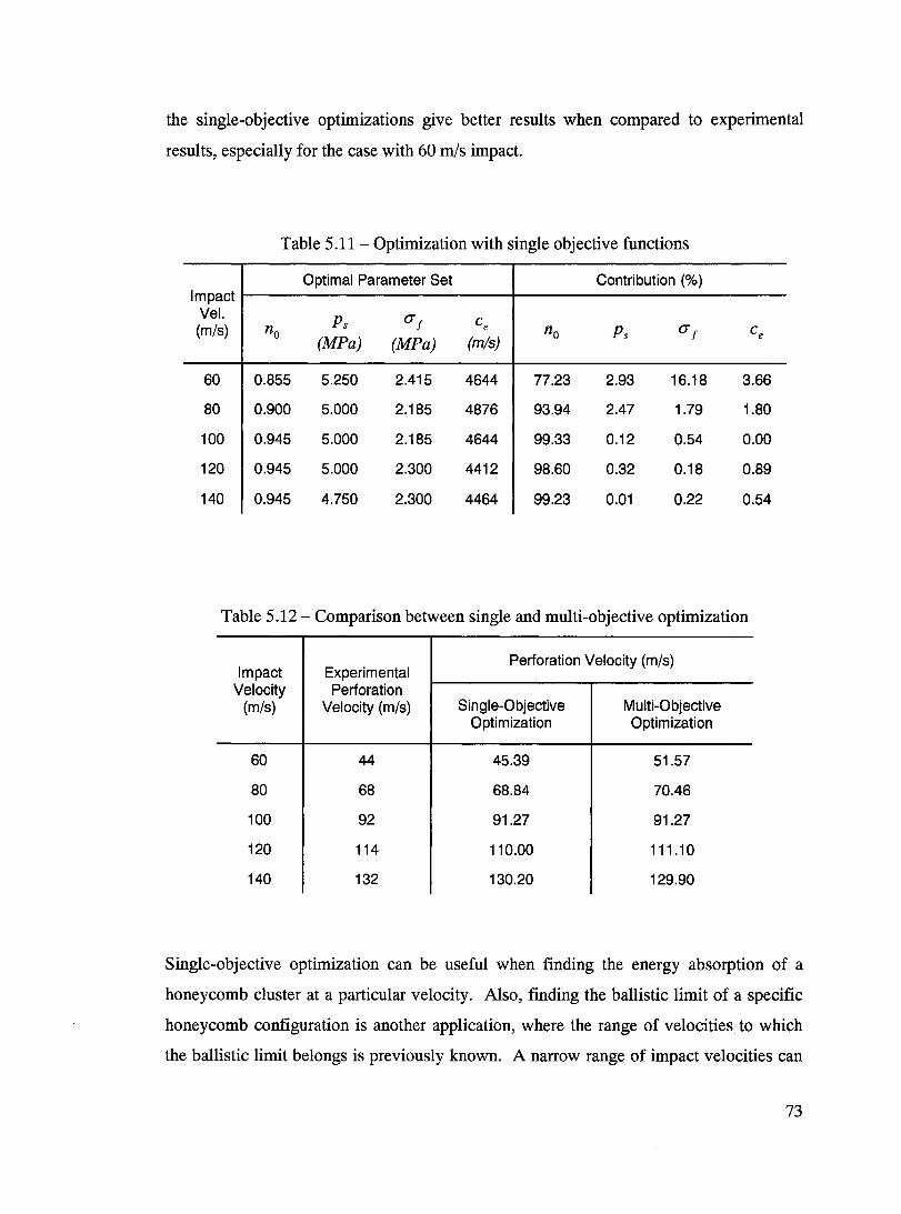
the single-objective optimizations give better results when compared to experimental

results, especially for the case with 60 mis impact.

Table 5.12 - Comparison between single and multi-objective optimization

Impact Experimental Perforation Velocity (mIs)

Velocity Perforation (mIs) Velocity (mIs) Single-Objective Multi-Objective

Optimization Optimization

60 44 45.39 51.57

80 68 68.84 70.46

100 92 91.27 91.27

120 114 110.00 111.10

140 132 130.20 129.90

Single-objective optimization can be useful when finding the energy absorption of a

honeycomb c1uster at a particular velocity. Also, finding the ballistic limit of a specifie

honeycomb configuration is another application, where the range of velocities to which

the ballistic limit belongs is previously known. A narrow range of impact velocities can

73

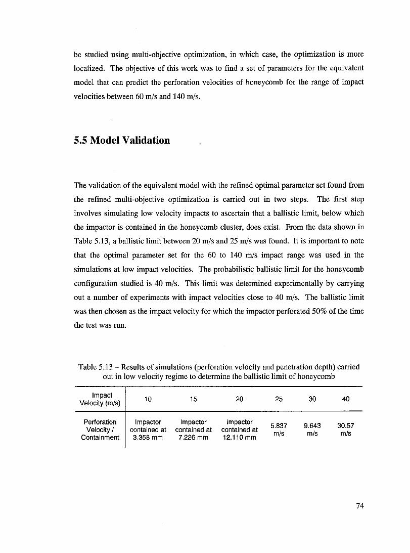
be studied using multi-objective optimization, in which case, the optimization is more

localized. The objective of this work was to find a set of parameters for the equivalent

model that can predict the perforation velocities of honeycomb for the range of impact

velocities between 60 mis and 140 mis.

5.5 Model Validation

The validation of the equivalent model with the refined optimal parame ter set found from

the refined multi-objective optimization is carried out in two steps. The first step

involves simulating low velocity impacts to ascertain that a ballistic limit, below which

the impactor is contained in the honeycomb cluster, do es exist. From the data shown in

Table 5.13, a ballistic limit between 20 mis and 25 mis was found. It is important to note

that the optimal parameter set for the 60 to 140 mis impact range was used in the

simulations at low impact velocities. The probabilistic ballistic limit for the honeycomb

configuration studied is 40 mis. This limit was determined experimentally by carrying

out a number of experiments with impact velocities close to 40 mis. The ballistic limit

was then chosen as the impact velocity for which the impactor perforated 50% of the time

the test was ron.

Table 5.13 - Results of simulations (perforation velo city and penetration depth) carried out in low velocity regime to determine the ballistic limit of honeycomb

Impact 10 15 20 25 30 40

Velocity (mis)

Perforation Impactor Impactor Impactor 5.837 9.643 30.57

Velocity 1 contained at contained at contained at mis mis mis Containment 3.358 mm 7.226 mm 12.110 mm

74

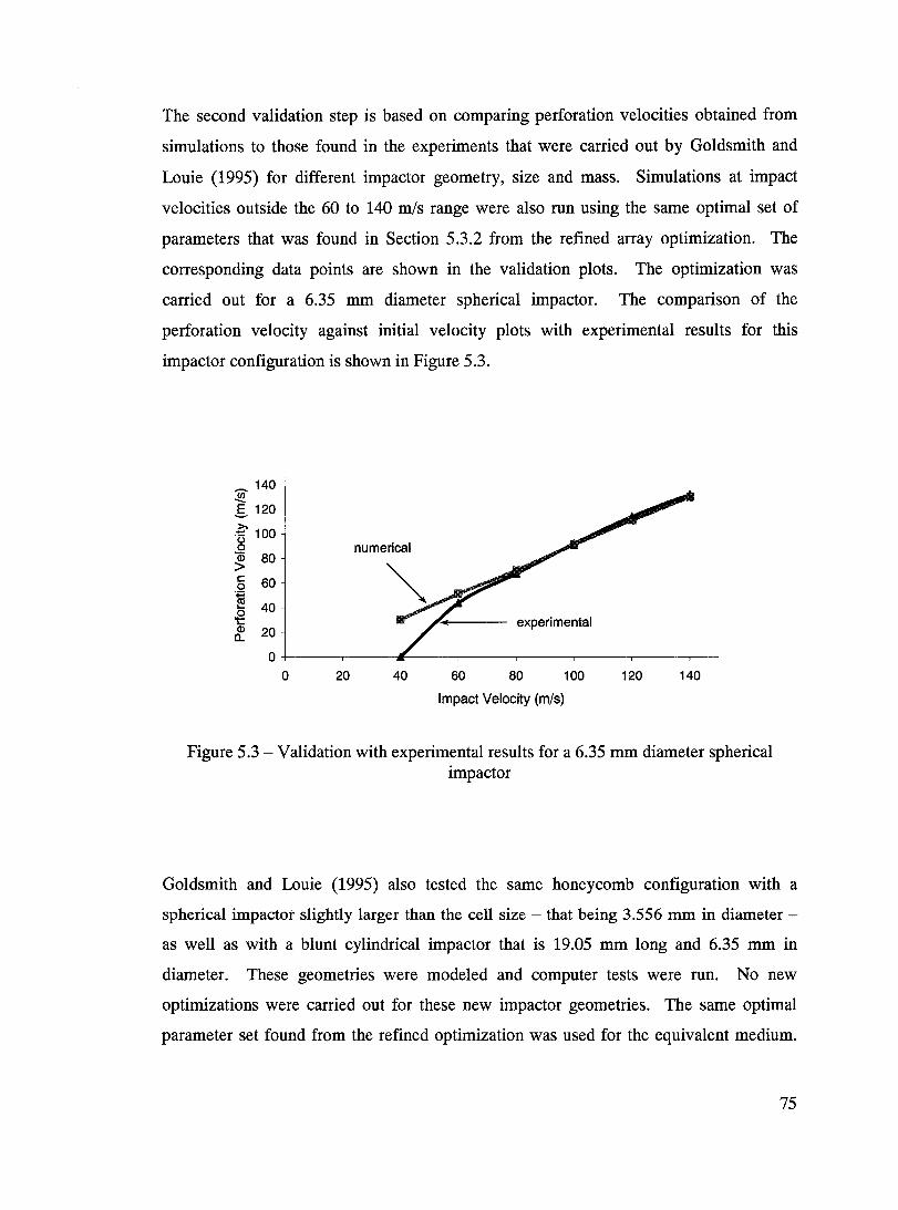
The second validation step is based on comparing perforation velocities obtained from

simulations to those found in the experiments that were carried out by Goldsmith and

Louie (1995) for different impactor geometry, size and mass. Simulations at impact

velocities outside the 60 to 140 mis range were also ron using the same optimal set of

parameters that was found in Section 5.3.2 from the refined array optimization. The

corresponding data points are shown in the validation plots. The optimization was

carried out for a 6.35 mm diameter spherical impactor. The comparison of the

perforation velocity against initial velo city plots with experimental results for this

impactor configuration is shown in Figure 5.3.

___ 140 .!!? É- 120

.-5' 100 0

Q5 80 > numerical

c: 60 0

~ 40 .... .g

ID 20 Cl.

experimental

0 0 20 40 60 80 100 120 140

Impact Velocity (mis)

Figure 5.3 - Validation with experimental results for a 6.35 mm diameter spherical impactor

Goldsmith and Louie (1995) also tested the same honeycomb configuration with a

spherical impactor slightly larger than the cell size - that being 3.556 mm in diameter -

as weIl as with a blunt cylindrical impactor that is 19.05 mm long and 6.35 mm in

diameter. These geometries were modeled and computer tests were ron. No new

optimizations were carried out for these new impactor geometries. The same optimal

parameter set found from the refined optimization was used for the equivalent medium.

75

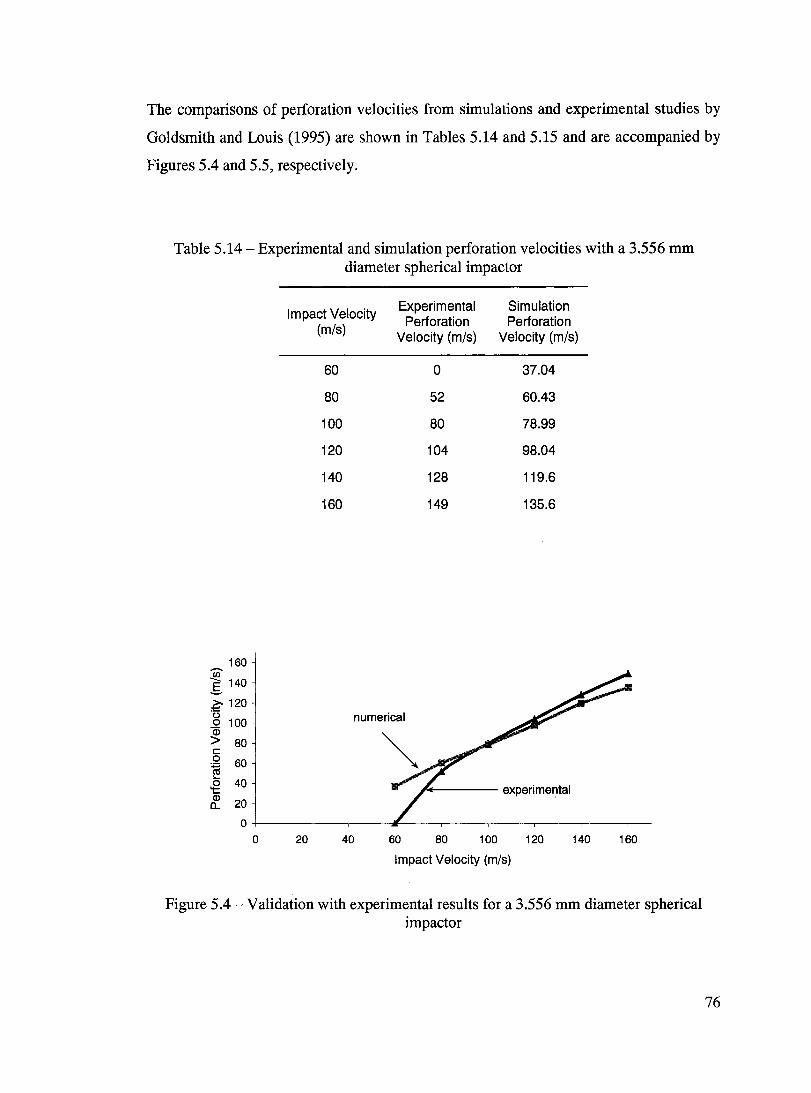
The comparisons of perforation velocities from simulations and experimental studies by

Goldsmith and Louis (1995) are shown in Tables 5.14 and 5.15 and are accompanied by

Figures 5.4 and 5.5, respectively.

Table 5.14 - Experimental and simulation perforation velocities with a 3.556 mm diameter spherical impactor

Impact Velocity Experimental Simulation Perforation Perforation

(mis) Velocity (mis) Velocity (mis)

60 0 37.04

80 52 60.43

100 80 78.99

120 104 98.04

140 128 119.6

160 149 135.6

160 Ul g 140

~ 120 'u 0 100 ID

numerical

> 80 c: 0 60 ~ L.

40 0 't: Q)

20 Il.

~--- experimel')tal

0

0 20 40 60 80 100 120 140 160

Impact Velocity (mis)

Figure 5.4 - Validation with experimental results for a 3.556 mm diameter spherical impactor

76

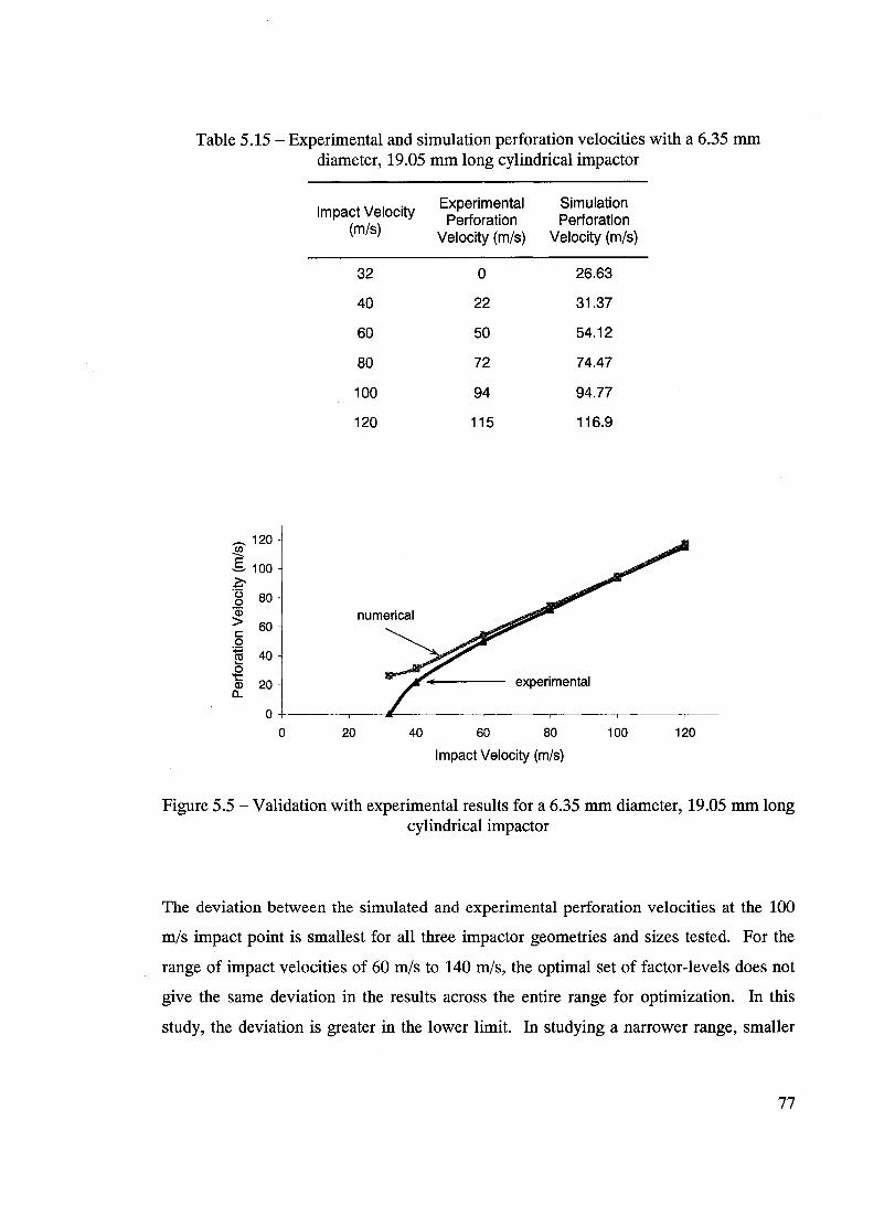
Table 5.15 - Experimental and simulation perforation velocities with a 6.35 mm diameter, 19.05 mm long cylindrical impactor

_ 120 ~ S 100 ~ .g 80

~ c: 60 o ~ 40 .g (J) 20 0..

Impact Velocity (mis)

32

40

60

80

100

120

numerical

Experimental Simulation Perforation Perforation

Velocity (mis) Velocity (mis)

0 26.63

22 31.37

50 54.12

72 74.47

94 94.77

115 116.9

experimental

o+------,--~~,-----_,------,_----_,------,_---

o 20 40 60 80 100 120

Impact Velocity (mis)

Figure 5.5 - Validation with experimental results for a 6.35 mm diameter, 19.05 mm long cylindrical impactor

The deviation between the simulated and experimental perforation velocities at the 100

mis impact point is smallest for all three impactor geometries and sizes tested. For the

range of impact velocities of 60 mis to 140 mis, the optimal set of factor-Ievels does not

give the same deviation in the results across the entire range for optimization. In this

study, the deviation is greater in the lower limit. In studying a narrower range, smaller

77

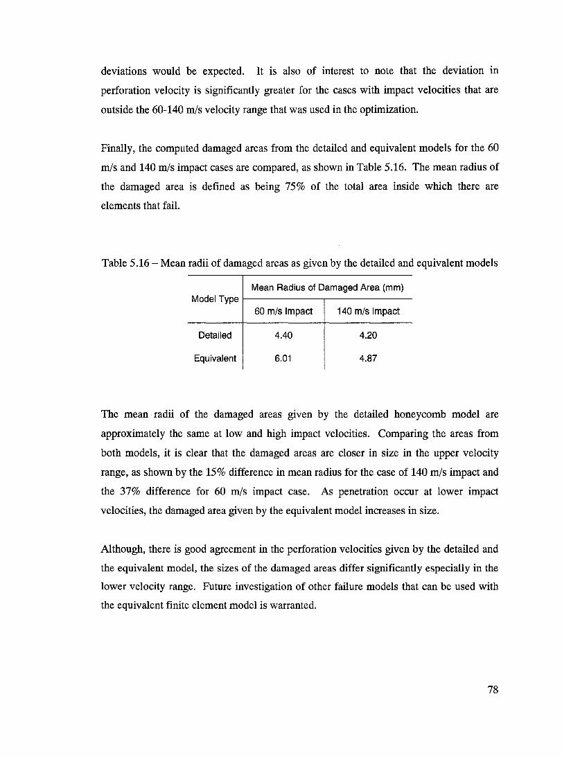
deviations would be expected. It is also of interest to note that the deviation in

perforation velo city is significantly greater for the cases with impact velocities that are

outside the 60-140 mis velocity range that was used in the optimization.

Finally, the computed damaged areas from the detailed and equivalent models for the 60

mis and 140 mis impact cases are compared, as shown in Table 5.16. The mean radius of

the damaged area is defined as being 75% of the total area inside which there are

elements that fail.

Table 5.16 - Mean radii of damaged are as as given by the detailed and equivalent models

Mean Radius of Damaged Area (mm) Model Type 1----------,--------

Detailed

Equivalent

60 mis Impact

4.40

6.01

140 mis Impact

4.20

4.87

The mean radii of the damaged areas given by the detailed honeycomb model are

approximately the same at low and high impact velocities. Comparing the areas from

both models, it is clear that the damaged areas are closer in size in the upper velocity

range, as shown by the 15% difference in mean radius for the case of 140 mis impact and

the 37% difference for 60 mis impact case. As penetration occur at lower impact

velocities, the damaged area given by the equivalent model increases in size.

Although, there is good agreement in the perforation velocities given by the detailed and

the equivalent model, the sizes of the damaged areas differ significantly especially in the

lower velocity range. Future investigation of other failure models that can be used with

the equivalent finite element model is warranted.

78

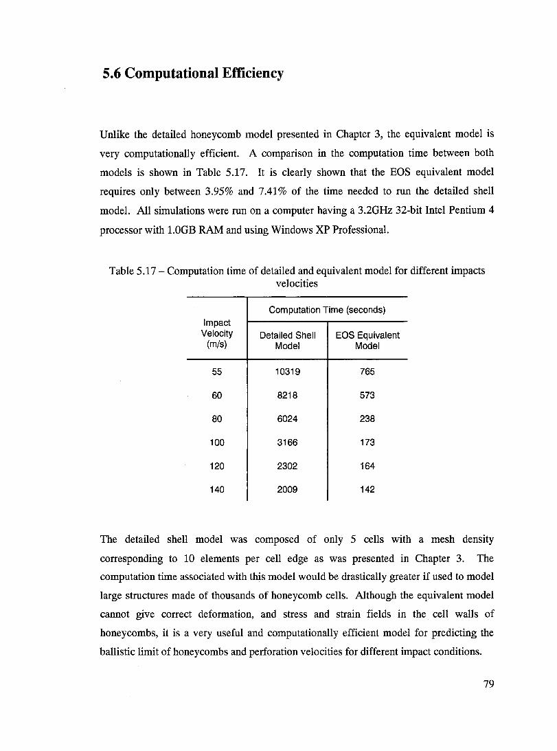
5.6 Computational Efficiency

Unlike the detailed honeycomb model presented in Chapter 3, the equivalent model is

very computationally efficient. A comparison in the computation time between both

models is shown in Table 5.17. It is clearly shown that the EOS equivalent model

requires only between 3.95% and 7.41% of the time needed to ron the detailed shell

model. AlI simulations were ron on a computer having a 3.2GHz 32-bit Intel Pentium 4

processor with 1.0GB RAM and using Windows XP Professional.

Table 5.17 - Computation time of detailed and equivalent model for different impacts velocities

Computation Time (seconds)

Impact Velocity Detailed Shell EOS Equivalent

(mis) Model Model

55 10319 765

60 8218 573

80 6024 238

100 3166 173

120 2302 164

140 2009 142

The detailed shell model was composed of only 5 cells with a mesh density

corresponding to 10 elements per cell edge as was presented in Chapter 3. The

computation time associated with this model would be drastically greater if used to model

large structures made of thousands of honeycomb cells. Although the equivalent model

cannot give correct deformation, and stress and strain fields in the cell walls of

honeycombs, it is a very useful and computationally efficient model for predicting the

ballistic limit of honeycombs and perforation velocities for different impact conditions.

79

CHAPTER6

CONCLUSIONS, RECCOMENDATIONS, AND FUTURE WORK

6.1 Conclusions

The finite element detailed modeling of Aluminum 5052-H19 1/8in - O.OOlin

honeycombs was undertaken. An efficient equivalent model for the prediction of the

ballistic limit and perforation velocities at different impact velocities in the range of 60

mis to 140 mis has been developed. From this work, it can be conc1uded that:

• The detailed three-dimensional modeling of honeycombs is very

computationally expensive due to the large number of elements that are

needed for the modeling of each cell. This high computational cost rend ers

this modeling approach impractical and sometimes un justifiable when

modeling large structures involving thousands of cells.

• Using an equation of state (EOS) model for porous materials, a finite element

model was developed for the prediction of perforation velocities of bare

honeycombs. This model is based on a number of parameters that are found

through the Taguchi optimization for specifie honeycomb configurations.

80

• The optimization of the equivalent model for the honeycomb configuration

studied was done for the range of 60 mis to 140 mis impact velocities. While

this optimization was carried out using one specific impactor geometry and

size, the same honeycomb model can be used with other impactor

configurations and gives good correlation with experimental results.

• The equivalent model is very computationally efficient requiring on average

6% of the time needed to run a corresponding simulation with the detailed

model.

• The same optimization approach can be followed to model other honeycomb

configurations. In the absence of experimental results, which formed the basis

for the optimization in this work, the results from the detailed modeling

approach for one impactor configuration can be used. The equivalent model

can then be used to predict perforation velo city of other impactor types.

• Over a wide range of impact velocities, deviations between the actual and

equivalent model results are expected. However, the optimization can be

focused on any specific range of impact velocities. It would be suspected that

less deviations are expected with narrower ranges.

6.2 Recommendations

Although they give relatively accurate results, both the detailed and the equivalent model

are not robust. While the optimization of the equivalent model yields different optimal

parameters in different impact velo city ranges and for different honeycombs, the detailed

model relies on the unknown level of friction between the impactor and the honeycomb

cell walls. Care must be taken in using the detailed modeling approach that was

presented in Chapter 3. The effect of friction on the penetration of specific honeycomb

81

configurations should be assessed before accepting the model results and using them in

the optimization of the equivalent model when experimental results are not available.

6.3 Future work

The results of the axisymmetric model were accepted as an approximate solution due to

the high ratio of artificial-to-internal energy. Further studies must be carried out to

reduce this energy ratio. These studies should inc1ude the investigation of other failure

models that can be used with the P - a porous equivalent model.

Other honeycomb configurations with varying cell wall thickness and size, and c1uster

thickness can be studied. The equivalent model's optimal parameters found for these

studies can then be carefully analyzed to find a relationship (or trend) between the

honeycomb' s geometric features and the optimal parameters of the corresponding

equivalent model. Also, the location of impact in the case of real honeycombs has a

significant effect on the penetration, the ballistic limit and the perforation velocities. By

modeling the three impact configurations presented in Chapter 3 for the same honeycomb

type, a trend can also be found from the equivalent optimal parameters. Such trends can

be used to assess the validity of the equivalent model for other honeycomb

configurations.

82

Reference List

Argyris, J.H. 1955, 'Energy theorems and structural analysis' ,Aircraft Engineering, vol. 27, no. 315,pp. 145-158.

Backman, M.E., Goldsmith, W. 1978, 'The mechanics of penetration ofprojectiles into targets', International Journal of Engineering Science, vol. 16, no. 1, pp. 1-99.

Baker, W.E., Togami, T.C., Weydert, lC. 1998, 'Static and dynamic properties ofhigh­density metal honeycombs', International Journal of Impact Engineering, vol. 21, no. 3, pp. 149-163.

Becker W. 1998, 'In-plane stiffnesses of a honeycomb core including the thickness effect' ,Archive of Applied Mechanics, vol. 68, no. 5, pp. 334-341.

Bitzer, T. 1997, Honeycomb Technology: Ma terials, Design, Manufacturing, Applications and Testing, Chapman & Hall, London.

Carroll, M., Holt, A.C. 1972, 'Suggested modification of the P-a model for porous materials', Journal of Applied Physics, vol. 43, no. 2, pp. 759-761.

Consolazio, G.R., Chung, J.H., Gurley, K.R. 2003, 'Impact simulation and full scale crash testing of a low profile concrete work zone barrier', Computers and Structures, vol. 81, no. 13, pp. 1359-1374.

Evans K.E. 1991, 'The design of doubly curved sandwich panels with honeycomb cores', Composite Structures, vol. 17, no. 2, pp. 95-111.

Flanagan, D.P., Belytschko, T. 1981, 'A uniform strain hexahedron and quadrilateral with orthogonal hourglass control', International Journal for Numerical Methods in Engineering, vol. 17, no. 5, pp. 679-706.

Fowlkes, W.Y., Creveling, C.M. 1995, Engineering Methods for Robust Product Design: Using Taguchi Methods in Technology and Product Development, Addison- Wesley, Reading, Massachusetts.

Gibson, L.J., Ashby, M.F. 1997, Cellular Solids: Structure and Properties, 2nd edn, Cambridge University Press, Cambridge.

83

Goldsmith, W., Louie, D.L. 1995, 'Axial perforation of aluminum honeycombs by projectiles', International Journal of Solids and Structures, vol. 32, no. 8-9, pp. 1017-1046.

Goldsmith, W., Wang, G., Li, K., Crane, D. 1997, 'Perforation of cellular sandwich plates', International Journal ofImpact Engineering, vol. 19, no. 5-6, pp. 361-379.

Grediac, M. 1993, 'A finite element study of the transverse shear in honeycomb cores', International Journal of Solids and Structures, vol. 30, no. 13, pp. 1777-1788.

Guo, X.E., Gibson, L.J. 1999, 'Behavior of intact and damaged honeycombs: a finite element study', International Journal of Mechanical Sciences, vol. 41, no. 1, pp. 85-105.

Herrmann, W. 1969, 'Constitutive equation for the dynamic compaction of ductile porous materials', Journal of Applied Physics, vol. 40, no.6, pp. 2490-2499.

Hibbitt, Karlsson and Sorensen, Inc. ABAQUS/Explicit User's Manual, Version 6.4, 2002.

Hibbitt, Karlsson and Sorensen, Inc. Getting Started with ABAQUS/Explicit Manual, Version 6.4, 2002.

Hoo Fatt, M.S., Park, K.S. 2000, 'Perforation of honeycomb sandwich plates by projectiles', Composites Part A: Applied Science and Manufacturing, vol. 31, no. 8, pp. 889-899.

Johnson G.R., Cook W.H. 1983, 'A Constitutive model and data for metals subjected to large strains, high strain rates and high temperatures,' in Proceedings of the Seventh International Symposium on Ballistics, The Hague, Netherlands, pp. 541-547.

Johnson, G.R., Cook, W.H. 1985, 'Fracture characteristics of three metals subjected to various strains, strain rates, temperatures and pressures', Engineering Fracture Mechanics, vol. 21, no. 1, pp. 31-48.

Johnson, W., Sengupta, A.K., Ghosh, S.K., Reid, S.R. 1981, 'Mechanics of high speed impact at normal incidence between plasticine rods and plates', Journal of the Mechanics and Physics of Solids, vol. 29, no. 5-6, pp. 413-445.

84

Kelsey, S., Gellatly, RA., Clark, B.w. 1958, 'The shear modulus of foil honeycomb cores', Aircraft Engineering, vol. 30, no. 356, pp. 294-302.

Lips, H.R., Weisshaupt, Niemeyer, T.W. 1987, 'Dynamic behavior and properties of heavy metals - experimental approach to separation of parameters in the Johnson-Cook model', in Proceedings of the Tenth International Symposium on Ballistics, San Diego, California, vol. 2.

Masters, I.G., Evans, K.E. 1996, 'Models for the elastic deformation of honeycombs', Composite Structures, vol. 35, no. 4, pp. 403-422.

Meguid, S.A., Shagal, G, Stranart, J.C., Daly, J. 1999, 'Three-dimensional dynamic finite element analysis of shot-peening induced residual stresses', Finite Elements in Analysis and Design, vol. 31, no. 3, pp. 179-191.

Meyers, M.A. 1994, Dynamic Behavior of Ma terials, Wiley, New York.

Mohr, D., Doyoyo, M. 2004, 'Large plastic deformation of metallic honeycomb: orthotropic rate-independent constitutive model', International Journal of Solids and Structures, vol. 41, no. 16-17, pp. 4435-4456.

Nguyen, M.Q., Jacombs, S.S., Thomson, RS., Hachenberg, D., Scott, M.L. 2005, 'Simulation of impact on sandwich structures', Composite Structures, vol. 67, no. 2, SPEC.ISS., pp. 217-227.

Nicholas, T., Rajendran, A.M. 1990, 'Material characterization at high strain rates', in High Velocity Impact Dynamics, edited by Jonas A. Zukas, Wiley, New York, pp. 127-296.

Nicholas, T., Recht, RF. 1990, 'Introduction to impact phenomena', in High Velocity Impact Dynamics, edited by Jonas A. Zukas, Wiley, New York, pp. 1-63.

Okumara, D., Ohno, N., Noguchi H. 2002, 'Post-buckling analysis of elastic honeycombs subject to in-plane biaxial compression', International Journal of Solids and Structures, vol. 39, no. 13-14, pp. 3487-3503.

Ruan, D., Lu, G., Wang, B., Yu, T.X. 2003, 'In-plane dynamic crushing of honeycombs -a finite element study', International Journal of Impact Engineering, vol. 28, no. 2, pp. 161-182.

85

Sen, P., Yang, J.B. 1998, Multiple Criteria Decision Support in Engineering Design, Springer, New York.

Shi, G., Tong, P. 1995, 'Equivalent transverse shear stiffness of honeycomb cores', International Journal ofSolids and Structures, vol. 32, no. 10, pp. 1383-1393.

Wardlaw, A.B., McKeown R., Chen, H. 1996, 'Implementation and application of the p­a equation of state in the DYSMAS code', Naval Surface Warfare Center, Dahlgren Division, Report Number: NSWCDD(fR-95/107.

Woodward, R.L. 1990, 'Materials failure at high strain rates', in High Velocity Impact Dynamics, edited by Jonas A. Zukas, Wiley, New York, pp. 65-125.

Wu, E., Jiang, W-S. 1997, 'Axial crush ofmetallic honeycombs, International Journal of Impact Engineering, vol. 19, no. 5-6, pp. 439-456.

Xu, X.F., Qiao, P. 2002, 'Homogenized elastic properties of honeycomb sandwich with skin effect', International Journal of Solids and Structures, vol. 39, no. 8, pp. 2153-2188.

Zhao, H., Gary, G. 1998, 'Crushing behaviour of aluminum honeycombs under impact loading', International Journal of Impact Engineering, vol. 21, no. 10, pp. 827-836.

Zukas, J.A. 1990, 'Introduction to penetration mechanics', in High Velocity Impact Dynamics, edited by Jonas A. Zukas, Wiley, New York, pp. 297-319.

Zukas, J.A., Nicholas, T., Swift, H., Greszczuk, L., Curran, D.R. 1982, Impact Dynamics, Wiley, New York.

86