Embed Size (px)
Citation preview

ERG for a Yukawa Theory in 3 Dimensions
Hidenori SONODAPhysics Department, Kobe University, Japan
14 September 2010 at ERG2010
AbstractWe consider a theory of N Majorana fermions and a real scalar in
the 3 dimensional Euclid space. We construct the RG flow of threeparameters using ERG. We look for a non-trivial fixed point by loopexpansions. For N = 1, we compare the critical exponents with thoseof the Wess-Zumino model at the fixed point. We need to improvethe numerical accuracy, perhaps, by going to 2-loop.
– Typeset by FoilTEX –
1
Plan of the talk
1. Spinors in D = 3
2. A Yukawa model in R3
3. ERG formalism (a quick review)
4. RG flow for the Yukawa model
5. 1-loop results
6. Comparison with the Wess-Zumino model
7. Summary and conclusions
H. Sonoda

2
Spinors in D = 3
1. Minkowski space
(a) We can choose the gamma matrices pure imaginary:
γ0 = σy, γ1 = iσx, γ2 = iσz satisfy {γµ , γν} = 2ηµν12
(b) A Lorentz transformation transforms a two-component spinor ψ as
ψ −→ Aψ where A ∈ SL(2, R) real!
Its complex conjugate ψ ≡ ψ†γ0 transforms as
ψ −→ ψA−1
H. Sonoda

3
(c) Given ψ = 1√2(u+ iv), where u, v are Majorana (real) spinors,
ψ (iγµ∂µ −m)︸ ︷︷ ︸real
ψ =1
2
(u(iγµ∂µ −m)u+ v(iγµ∂µ −m)v
)
where u ≡ uTσy transforms as u→ uA−1. (σyATσy = A−1)
(d) Parity{ψ(x, y, t) −→ −iγ1ψ(−x, y, t) = σxψ(−x, y, t)ψ(x, y, t) −→ ψ(−x, y, t)iγ1 = ψ(−x, y, t)(−)σx
forbids the mass term ψψ.
H. Sonoda
4
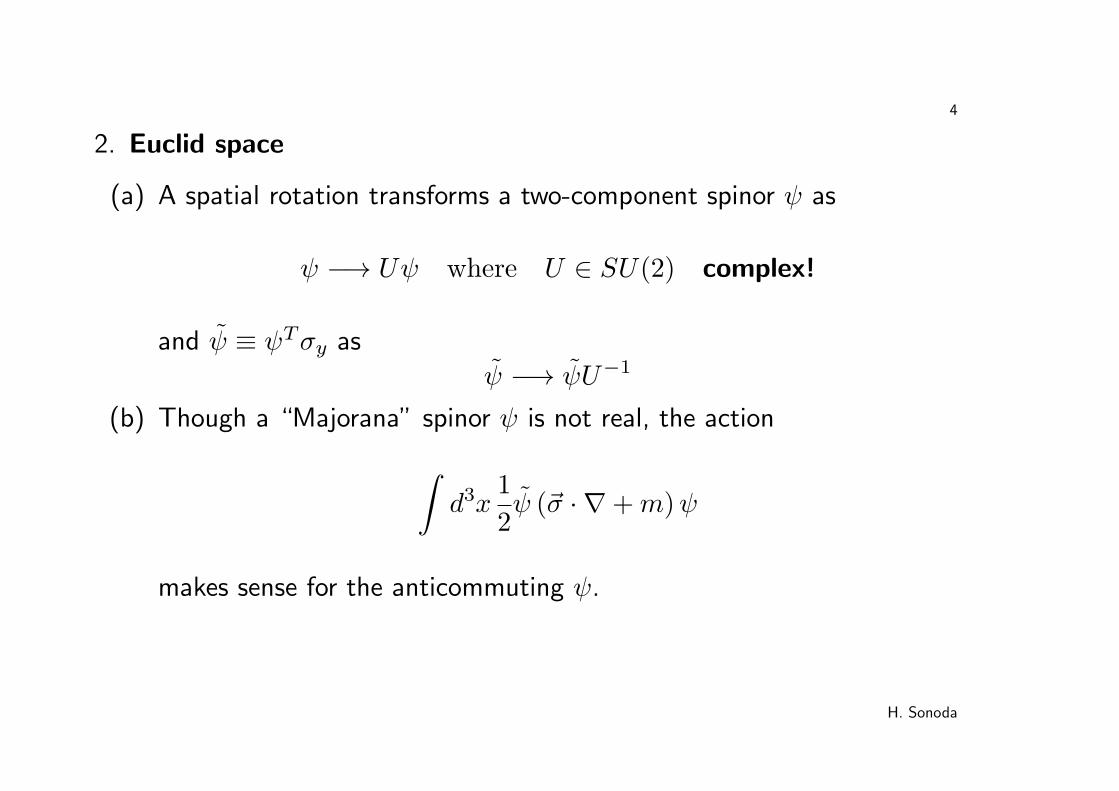
2. Euclid space
(a) A spatial rotation transforms a two-component spinor ψ as
ψ −→ Uψ where U ∈ SU(2) complex!
and ψ ≡ ψTσy as
ψ −→ ψU−1
(b) Though a “Majorana” spinor ψ is not real, the action∫d3x
1
2ψ (~σ · ∇+m)ψ
makes sense for the anticommuting ψ.
H. Sonoda

5
(c) Parity {ψ(x, y, z) −→ σyψ(x,−y, z)ψ(x, y, z) −→ ψ(x,−y, z)(−)σy
forbids the mass term ψψ.
(d) Parity’ — Parity & π-rotation around the y-axis gives{ψ(x, y, z)−→ iψ(−x,−y,−z)ψ(x, y, z)−→ iψ(−x,−y,−z)
H. Sonoda

6
A Yukawa model in R3
1. The classical lagrangian
L =1
2(∇φ)2 + 1
2
N∑I=1
χI~σ · ∇χI +1
2m2φ2 +
λ
4!φ4 + g φ
1
2
N∑I=1
χIχI
where φ is a real scalar, and χI (I = 1, · · · , N) are “Majorana” spinors.
2. three dimensionful parameters — [m2] = 2, [λ] = 1, [g] = 1/2
3. A fermion mass term is forbidden by the Z2 invariance (parity):{φ(~x) −→ −φ(−~x)χI(~x) −→ iχI(−~x)
H. Sonoda
7
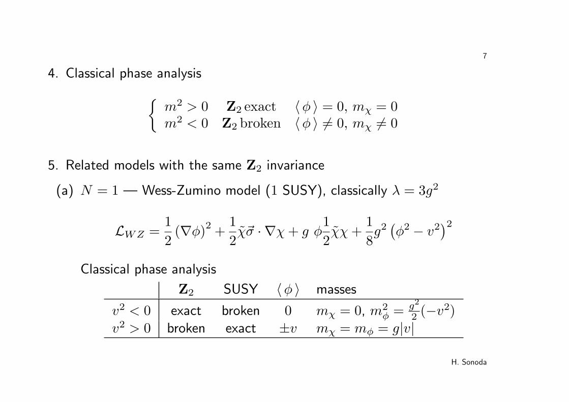
4. Classical phase analysis{m2 > 0 Z2 exact 〈φ 〉 = 0, mχ = 0m2 < 0 Z2 broken 〈φ 〉 6= 0, mχ 6= 0
5. Related models with the same Z2 invariance
(a) N = 1 — Wess-Zumino model (1 SUSY), classically λ = 3g2
LWZ =1
2(∇φ)2 + 1
2χ~σ · ∇χ+ g φ
1
2χχ+
1
8g2(φ2 − v2
)2Classical phase analysis
Z2 SUSY 〈φ 〉 masses
v2 < 0 exact broken 0 mχ = 0, m2φ = g2
2 (−v2)
v2 > 0 broken exact ±v mχ = mφ = g|v|
H. Sonoda

8
(b) N ≥ 2 — Gross-Neveu model with O(N) invariance
LGN =1
2
∑I
χI~σ · ∇χI −g02N
(1
2
∑I
χIχI
)2
Expectation
Z2
⟨∑I12χIχI
⟩mχ
g0 > g0,cr exact 0 = 0g0 < g0,cr broken 6= 0 6= 0
O(N) unbroken
H. Sonoda
9
6. We wish to do two things:
(a) construct the RG flow of m2, λ, g for the Yukawa model,(b) find a non-trivial fixed point and obtain the critical exponents there.
7. The non-trivial fixed point is accessible from the gaussian fixed point.
⇓
Perturbation theory is applicable.
8. Motivated by works by Wipf, Synatschke-Czerwonka, Braun, ... on SUSYmodels in 1 & 2 dimensions.
9. Talks on related subjects by Wipf, Synatschke-Czerwonka, Scherer.
H. Sonoda

10
Gaussianf.p.
Wilson-Fisherf.p.
mg
(m , , g )*λ*2*
2
Z exact2
Z broken2
Gross-Neveu λ
Wess-Zumino
0,crg
g fixed
mcr(g)
m2
RG flows for the Yukawa theorywith N Majorna fermions
N>1
N=12
g0
H. Sonoda

11
ERG formalism (a quick review)
1. Wilson action with a momentum cutoff Λ
SΛ = −1
2
∫p
p2
K(pΛ
)φ(p)φ(−p) + SI,Λ
K(x)
x20
1
1
2. the ERG differential equation by J. Polchinski (1983)
−Λ∂
∂ΛSI,Λ =
1
2
∫p
∆(p/Λ)
p2
{δSI,Λ
δφ(−p)δSI,Λ
δφ(p)+
δ2SI,Λ
δφ(−p)δφ(p)
}H. Sonoda
12
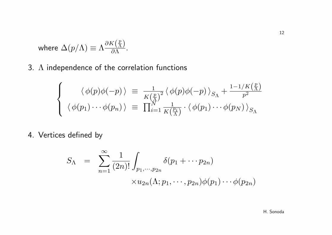
where ∆(p/Λ) ≡ Λ∂K( p
Λ)∂Λ .
3. Λ independence of the correlation functions〈φ(p)φ(−p) 〉 ≡ 1
K( pΛ)
2 〈φ(p)φ(−p) 〉SΛ+
1−1/K( pΛ)
p2
〈φ(p1) · · ·φ(pn) 〉 ≡∏N
i=11
K(piΛ )· 〈φ(p1) · · ·φ(pN) 〉SΛ
4. Vertices defined by
SΛ =
∞∑n=1
1
(2n)!
∫p1,···,p2n
δ(p1 + · · · p2n)
×u2n(Λ; p1, · · · , p2n)φ(p1) · · ·φ(p2n)
H. Sonoda

13
5. SΛ determined uniquely by the ERG diff eq & two sets of conditions:one at Λ = µ, another at Λ → ∞.
(a) conditions at Λ = µ introduce m2 and λ:u2(µ; 0, 0) = −m2
∂∂p2u2(µ; p,−p)
∣∣∣p2=0
= −1
u4(µ; 0, · · · , 0) = −λ
(b) asymptotic conditions for Λ → ∞ for renormalizabilityu2(Λ; p,−p)
Λ→∞−→ linear in p2
u4(Λ; p1, · · · , p4)Λ→∞−→ independent of pi
u2n≥6(Λ; p1, · · · , p2n)Λ→∞−→ 0
This guarantees that the flow starts from the gaussian fixed point.
H. Sonoda

14
6. µ dependence
−µ∂SΛ
∂µ= βOλ + βmOm + γN
whereOm ≡ −∂m2SΛ
Oλ ≡ −∂λSΛ
N ≡ −∫p
[φ(p)
δSΛδφ(p) +
K( pΛ)(1−K( p
Λ))p2
{δSΛδφ(p)
δSΛδφ(−p) +
δ2SΛδφ(p)δφ(−p)
}]N counts φ:
〈N φ(p1) · · ·φ(pn) 〉 = n 〈φ(p1) · · ·φ(pn) 〉
RG equation(−µ ∂
∂µ+ β∂λ + βm∂m2
)〈φ(p1) · · ·φ(pn) 〉 = nγ 〈φ(p1) · · ·φ(pn) 〉
H. Sonoda

15
7. dimensional analysis(Λ
∂
∂Λ+ µ
∂
∂µ+ 2m
2∂m2 + λ∂λ
)SΛ =
∫p
(pi
∂φ(p)
∂pi
+5
2φ(p)
)δSΛ
δφ(p)
8. Combining the ERG diff eq, µ dependence, and dimensional analysis, weobtain{
(λ+ β)∂λ + (2m2 + βm)∂m2
}S(m2, λ)
=
∫p
[{pi∂φ(p)
∂pi+
(5
2− γ +
∆(p/µ)
K(p/µ)
)φ(p)
}δS
δφ(p)
+∆(p/µ)− 2γK(1−K)
p21
2
{δS
δφ(p)
δS
δφ(−p)+
δ2S
δφ(p)δφ(−p)
}]
where we have set Λ = µ (fixed).
H. Sonoda

16
9. RG flow in the parameter space{ddtm
2 = 2m2 + βm(m2, λ)ddtλ = λ+ β(m2, λ)
10. Scaling formula⟨φ(p1e
∆t) · · ·φ(pne∆t)⟩m2e2∆t(1+∆t·βm) , λe∆t(1+∆t·β)
= e∆t{3+n(−52+γ)} · 〈φ(p1) · · ·φ(pn) 〉m2,λ
11. Universality — The dependence on the choice of K is absorbed intothe parameters m2, λ. Hence, the critical exponents are universal.
H. Sonoda

17
RG flow for the Yukawa model
1. RG flow ddtm
2 = 2m2 + βm(m2, λ, g)ddtλ = λ+ βλ(λ, g)ddtg = 1
2g + βg(λ, g)
2. A fixed point (m2∗, λ∗, g∗) is determined by
2m2∗ + βm(m2∗, λ∗, g∗) = 0λ∗ + βλ(λ
∗, g∗) = 012g
∗ + βg(λ∗, g∗) = 0
H. Sonoda

18
3. yE = 1ν determined by the linearized RG equation at the fixed point:
d
dt
(m2 −m2∗) = yE
(m2 −m2∗)
Hence,
yE = 2 +∂
∂m2βm
∣∣∣m2∗,λ∗,g∗
4. The anomalous dimensions γ∗φ, γ∗χ determined by
γ∗φ = γφ(λ∗, g∗), γ∗χ = γχ(λ
∗, g∗)
5. parametrization and normalization determined through the lowmomentum expansions of the vertices
H. Sonoda

19
∂
∂m2
∂
∂p2
φ
p
p
p
p
I J
I J
∣∣∣p2=m2=0∣∣∣p2=m2=0∣∣∣p2=m2=0∣∣∣m2=0∣∣∣pi=m2=0∣∣∣∣∣pi=m2=0
= 0
= −1
= −1
= −i~p · ~σδIJ +O(p2)
= − g√NδIJ
= −λ
H. Sonoda

20
6. The beta functions are computed from the RG equation
−µ ∂∂µSΛ = βλ (−∂λSΛ) + βg (−∂gSΛ) + βmOm + γφNφ + γχNχ
where Om ' −∂m2SΛ since we have incorporated m2 in the scalarpropagator.
Om = −∂m2SΛ
−∫q
K(1−K)
(q2 +m2)21
2
{δSΛ
δφ(q)
δSΛ
δφ(−q)+
δ2SΛ
δφ(q)δφ(−q)
}
H. Sonoda

21
1-loop results
1. 1-loop calculations give
βm =1
2λµ
∫q
∆
q2− 2
g2
Nµ
∫q
∆(1 − K)
q2
−m2
[1
2
λ
µ
∫q
∆
q4+ 2
g2
Nµ
∫q
∆
q4
{1
3(1 − K) +
1
6(∆ + ∆)
}]
βλ = −3λ2
µ
∫q
∆(1 − K)
q4+ 24
g4
Nµ
∫q
∆(1 − K)3
q4
−4λg2
Nµ
∫q
∆
q4
{1
3(1 − k) +
1
6(∆ + ∆)
}
βg = −gg2
Nµ
[3
∫q
∆(1 − K)2
q4+
∫q
∆(1 − K)
q4
H. Sonoda

22
+
∫q
∆
q4
{1
3(1 − K) +
1
6(∆ + ∆)
}]
where ∆(q) ≡ −2q2 ddq2
∆(q) =(−2q2 d
dq2
)2K(q).
The anomalous dimensions are given by
γφ =g2
µ
∫q
1
q4(1 − K)
(5
6∆ +
1
6∆
)
γχ =g2
Nµ
1
2
∫q
1
q4∆(1 − K)
H. Sonoda

23
2. Choice of K with one parameter a for optimization
K(q) =
1 if 0 < q2 < a2
1−q2
1−a2if a2 < q2 < 1
0 if 1 < q2
K(q)
q0
1
a2 12
Two limits: {Litim a2 = 0Wegner-Houghton a2 = 1
H. Sonoda
24
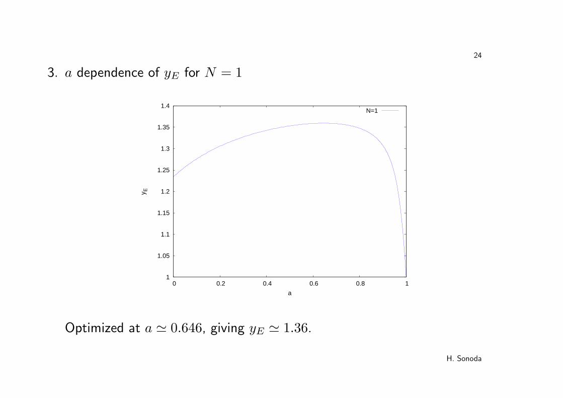
3. a dependence of yE for N = 1
1
1.05
1.1
1.15
1.2
1.25
1.3
1.35
1.4
0 0.2 0.4 0.6 0.8 1
y E
a
N=1
Optimized at a ' 0.646, giving yE ' 1.36.
H. Sonoda

25
4. γ∗φ = γ∗χ is expected from SUSY, but
0
0.05
0.1
0.15
0.2
0.25
0.3
0.35
0.4
0.45
0.5
0 0.2 0.4 0.6 0.8 1
a
gamma-phigamma-chi
γ∗φ ' 0.170, γ∗χ ' 0.056 at a = 0.646
H. Sonoda

26
5. N dependence
yEN→∞−→ 1 γ∗φ
N→∞−→ 1
2γ∗χ
N→∞−→ 0
0.95
1
1.05
1.1
1.15
1.2
1.25
1.3
1.35
1.4
0 0.2 0.4 0.6 0.8 1
y E
a
N=1N=10
N=100
0.1
0.15
0.2
0.25
0.3
0.35
0.4
0.45
0.5
0 0.2 0.4 0.6 0.8 1
gam
ma-
phi
a
N=1N=10
N=100
0
0.01
0.02
0.03
0.04
0.05
0.06
0.07
0 0.2 0.4 0.6 0.8 1
gam
ma-
chi
a
N=1N=10
N=100
The large N limits are independent of a.
The above results agree with the large N limit of the Gross-Neveu model.
H. Sonoda
27
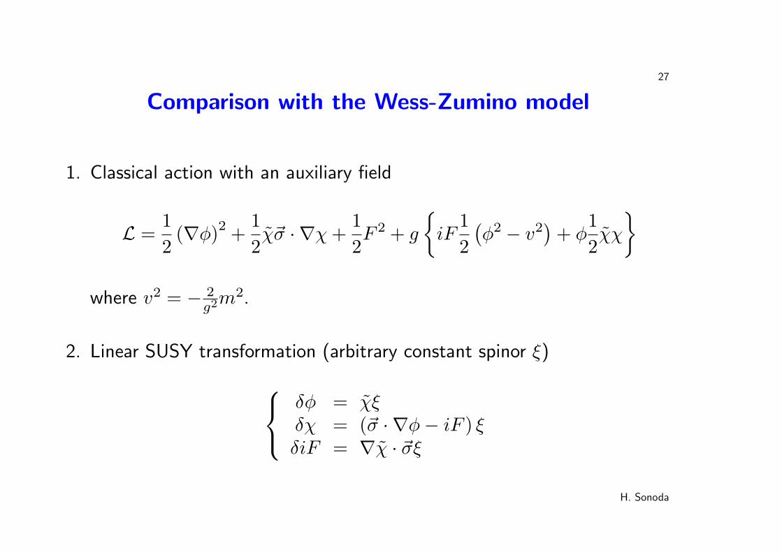
Comparison with the Wess-Zumino model
1. Classical action with an auxiliary field
L =1
2(∇φ)2 + 1
2χ~σ · ∇χ+
1
2F 2 + g
{iF
1
2
(φ2 − v2
)+ φ
1
2χχ
}
where v2 = − 2g2m2.
2. Linear SUSY transformation (arbitrary constant spinor ξ) δφ = χξδχ = (~σ · ∇φ− iF ) ξδiF = ∇χ · ~σξ
H. Sonoda

28
3. The supersymmetric φiF + 12χχ is forbidden by the Z2 φ(~x) −→ −φ(−~x)χ(~x) −→ iχ(−~x)F (~x) −→ F (−~x)
4. R-invarianceg → −g, φ→ −φ, F → −F
5. ERG is consistent with the linear SUSY.
6. RG equation
−µ ∂∂µSΛ = βg (−∂gSΛ) + βv2 (−∂v2SΛ) + γN
H. Sonoda
29
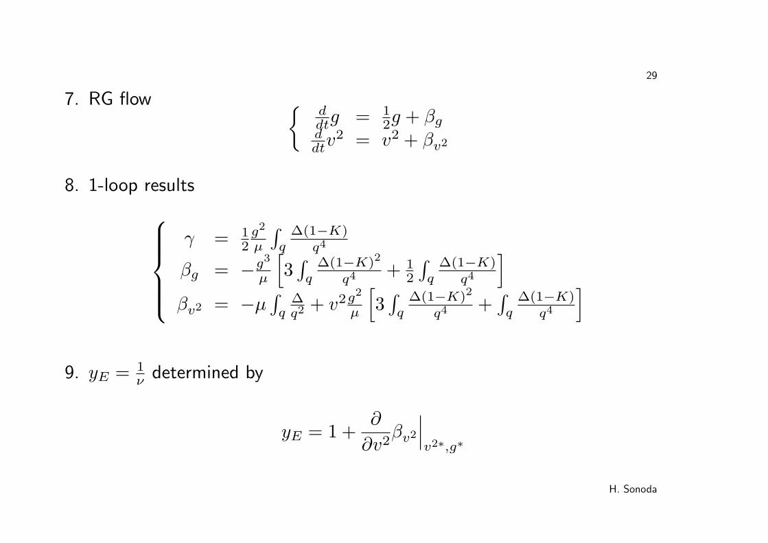
7. RG flow {ddtg = 1
2g + βgddtv
2 = v2 + βv2
8. 1-loop resultsγ = 1
2g2
µ
∫q∆(1−K)
q4
βg = −g3
µ
[3∫q∆(1−K)2
q4+ 1
2
∫q∆(1−K)
q4
]βv2 = −µ
∫q∆q2
+ v2g2
µ
[3∫q∆(1−K)2
q4+∫q∆(1−K)
q4
]
9. yE = 1ν determined by
yE = 1 +∂
∂v2βv2∣∣∣v2∗,g∗
H. Sonoda
30
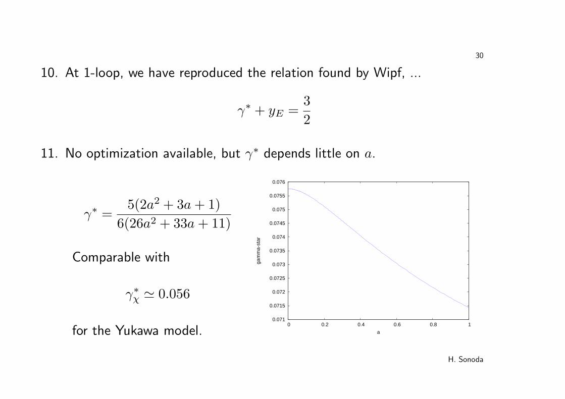
10. At 1-loop, we have reproduced the relation found by Wipf, ...
γ∗ + yE =3
2
11. No optimization available, but γ∗ depends little on a.
γ∗ =5(2a2 + 3a+ 1)
6(26a2 + 33a+ 11)
Comparable with
γ∗χ ' 0.056
for the Yukawa model. 0.071
0.0715
0.072
0.0725
0.073
0.0735
0.074
0.0745
0.075
0.0755
0.076
0 0.2 0.4 0.6 0.8 1
gam
ma-
star
a
H. Sonoda
31
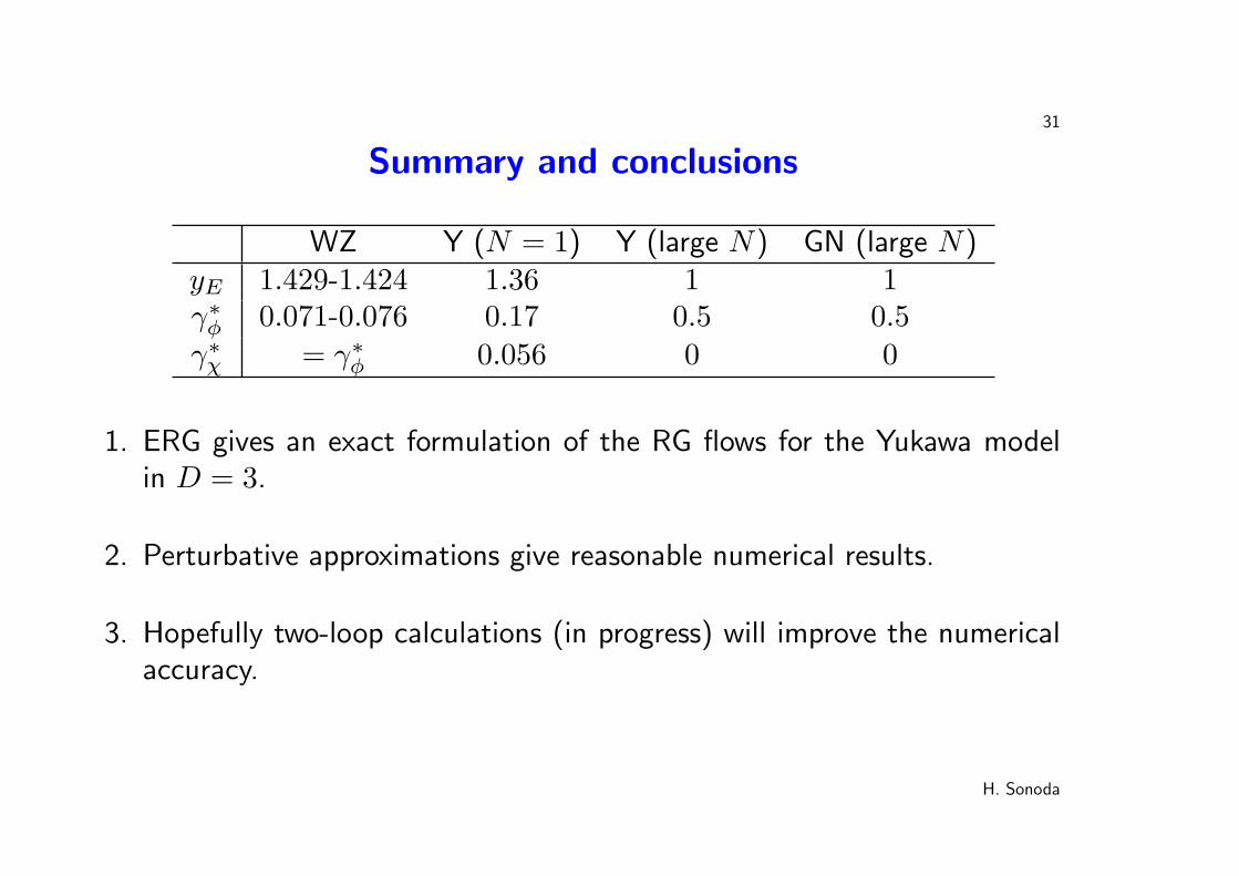
Summary and conclusions
WZ Y (N = 1) Y (large N) GN (large N)yE 1.429-1.424 1.36 1 1γ∗φ 0.071-0.076 0.17 0.5 0.5
γ∗χ = γ∗φ 0.056 0 0
1. ERG gives an exact formulation of the RG flows for the Yukawa modelin D = 3.
2. Perturbative approximations give reasonable numerical results.
3. Hopefully two-loop calculations (in progress) will improve the numericalaccuracy.
H. Sonoda