norges teknisk-naturvitenskapelige

universitet

Error estimates in inverse design of photoniccrystals

by

Larisa Beilina, Marte P. Hatlo, Harald E. Krogstad

preprint

numerics no. 8/2007

norwegian university of

science and technology

trondheim, norway

This report has URLhttp://www.math.ntnu.no/preprint/numerics/2007/N8-2007.pdf

Address: Department of Mathematical Sciences, Norwegian University of Science andTechnology, N-7491 Trondheim, Norway.

Error estimates in inverse design of

photonic crystals

Larisa Beilina, Marte P. Hatlo, Harald E. Krogstad

September 14, 2007

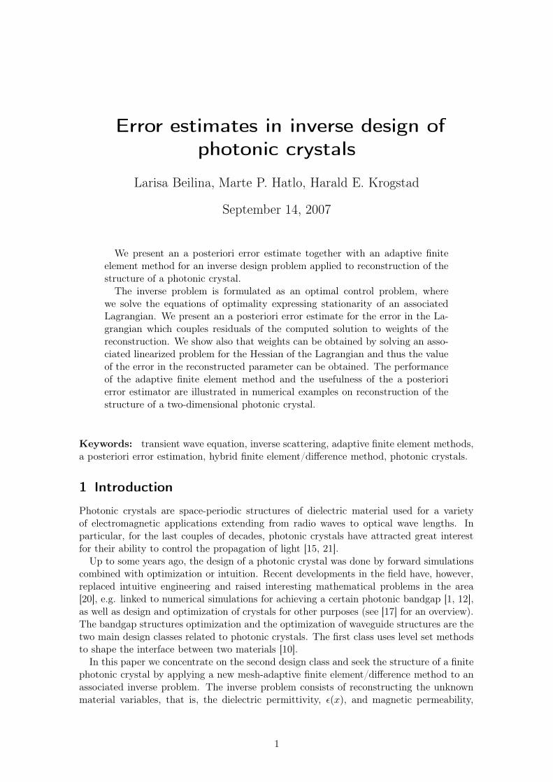
We present an a posteriori error estimate together with an adaptive finiteelement method for an inverse design problem applied to reconstruction of thestructure of a photonic crystal.

The inverse problem is formulated as an optimal control problem, wherewe solve the equations of optimality expressing stationarity of an associatedLagrangian. We present an a posteriori error estimate for the error in the La-grangian which couples residuals of the computed solution to weights of thereconstruction. We show also that weights can be obtained by solving an asso-ciated linearized problem for the Hessian of the Lagrangian and thus the valueof the error in the reconstructed parameter can be obtained. The performanceof the adaptive finite element method and the usefulness of the a posteriorierror estimator are illustrated in numerical examples on reconstruction of thestructure of a two-dimensional photonic crystal.

Keywords: transient wave equation, inverse scattering, adaptive finite element methods,a posteriori error estimation, hybrid finite element/difference method, photonic crystals.

1 Introduction

Photonic crystals are space-periodic structures of dielectric material used for a varietyof electromagnetic applications extending from radio waves to optical wave lengths. Inparticular, for the last couples of decades, photonic crystals have attracted great interestfor their ability to control the propagation of light [15, 21].

Up to some years ago, the design of a photonic crystal was done by forward simulationscombined with optimization or intuition. Recent developments in the field have, however,replaced intuitive engineering and raised interesting mathematical problems in the area[20], e.g. linked to numerical simulations for achieving a certain photonic bandgap [1, 12],as well as design and optimization of crystals for other purposes (see [17] for an overview).The bandgap structures optimization and the optimization of waveguide structures are thetwo main design classes related to photonic crystals. The first class uses level set methodsto shape the interface between two materials [10].

In this paper we concentrate on the second design class and seek the structure of a finitephotonic crystal by applying a new mesh-adaptive finite element/difference method to anassociated inverse problem. The inverse problem consists of reconstructing the unknownmaterial variables, that is, the dielectric permittivity, ε(x), and magnetic permeability,

1

µ(x), from measured wave scattering data on parts of the surface of the crystal, given thewave input on other parts. By solving the wave equation with the same input, the materialvariables are in principle obtained by fitting the computed to the measured data. Theproblem is formulated as finding a stationary point of a Lagrangian, involving the forwardwave equation (the state equation), the backward wave equation (the adjoint equation),and an equation expressing that the gradient with respect to the parameters vanishes. Theoptimum is found in an iterative process solving for each step the forward and backwardwave equations and updating the material coefficients.

We present a new mesh-adaptive method for the inverse problem, developed in [5],that is based on a specially constructed "goal-oriented" a posteriori error estimate whichcouples residuals of the computed solution to weights in the reconstruction reflecting thesensitivity of the reconstruction obtained by solving an associated linearized problem forthe Hessian of the Lagrangian. The derivation follows the main approach to adaptive errorcontrol in computational differential equations presented in [14, 3] and references therein.

Finally, numerical experiments on the reconstruction of the structure of a two-dimensionalphotonic crystal show the possibilities in computational inverse scattering using the adap-tive error control.

2 Mathematical model

We will restrict ourselves to the propagation of light in a mixed dielectric medium in abounded domain Ω ⊂ R

d, d = 2, 3 with boundary Γ, governed by Maxwell’s equations:

∂D

∂t−∇×H = −J, in Ω × (0, T ),

∂B

∂t+ ∇×E = 0, in Ω × (0, T ), (2.1)

∇ ·D = ρ, in Ω × (0, T ),

∇ ·B = 0, in Ω × (0, T ).

Here E(x, t) and H(x, t) are the electric and magnetic fields, whereas D(x, t) and B(x, t)are the electric and magnetic inductions, respectively. We assume that the dielectric per-mittivity, ε(x), and magnetic permeability, µ(x), are scalars, so that D = εE and B = µH.The material variables as well as the current density, J , and charge density, ρ, are assumedto be piecewise smooth.

By eliminating B and D from (2.1) we obtain two independent second order systems ofpartial differential equations

ε∂2E

∂t2+ ∇× (µ−1∇×E) = −

∂J

∂t,

µ∂2H

∂t2+ ∇× (ε−1∇×H) = ∇× (ε−1J), (2.2)

which may be solved imposing appropriate initial and boundary conditions.For simplicity, we restrict ourselves to formulation of the problem in terms of E(x, t)

and assume that J = 0 and ρ = 0. Taking into account the vector identity ∇×∇× V =∇(∇ · V ) −4V , we then obtain

ε∂2E

∂t2−∇ · (

1

µ∇E) = 0, in Ω × (0, T ). (2.3)

A similar system of equations is valid for H. Thus, the electric and magnetic fields inisotropic medium satisfy wave equations with a wave speed c(x) = 1/

√

ε(x)µ(x).We consider the equation (2.3) in the domain Ω representing the photonic crystal. Let

Γ1 ⊂ Γ and Γ2 = Γ\ Γ1. Assume that an impulse v1 is initialized at the boundary Γ1 andpropagated during time (0, t1] into Ω.

The forward problem consists of solving (2.3) with the following initial and boundaryconditions:

E(·, 0) = 0,∂E

∂t(·, 0) = 0, in Ω,

∂nE∣

∣

Γ1

= v1, on Γ1 × (0, t1],

∂nE∣

∣

Γ1

= 0, on Γ1 × (t1, T ),

∂nE∣

∣

Γ2

= 0, on Γ2 × (0, T ).

(2.4)

Our goal is to solve the inverse problem for (2.3) and (2.4), or to find the material param-eters ε(x) and µ(x) from knowledge of data at a finite set of observation points on Γ. Thedata are generated in experiments where impulses are emitted from Γ1, backscattered bymaterial inhomogeneities, and recorded again on parts of the boundary Γ.

In real applications the data are generated by emitting waves on the surface of theinvestigated object and are then recorded on parts of the surface of the object. In thispaper, data are generated by computing the forward problem (2.3)-(2.4) with given valuesof the parameters, and the corresponding solution was recorded at parts of the boundary.The coefficients are then “forgotten” and the goal is to reconstruct the coefficients fromcomputed boundary data.

3 A hybrid finite element/difference method

To solve equation (2.3)-(2.4) we use a hybrid FEM/FDM method developed in [9]. Themethod is obtained by using continuous space-time piecewise linear finite elements on apartially structured mesh in space. The computational space domain Ω is decomposed intoa finite element domain ΩFEM with an unstructured mesh and a finite difference domainΩFDM with a structured mesh, with typically ΩFEM covering only a small part of the Ω. InΩFDM we use quadrilateral elements in R2 and hexahedra in R3. In ΩFEM we use a finiteelement mesh Kh = K with elements K consisting of triangles in R2 and tetrahedrain R3. We associate with Kh a mesh function h = h(x) representing the diameter of theelement K containing x. For the time discretization we let Jk = J be a partition of thetime interval I = (0, T ) into time intervals J = (tk−1, tk] of uniform length τ = tk − tk−1.

We define the following L2 inner product and norm

((p, q)) =

∫ T

0

∫

Ωpq dx dt, ‖p‖2 = ((p, p)).

We further use the notation Dv = ∂v∂t

.To formulate the finite element method for (2.3)-(2.4) we introduce the finite element

3

trial space W vh and test space W λ

h defined by :

W v1 := v ∈ H1(Ω × J) : v(·, 0) = 0, ∂nv|Γ1

= v1, ∂nv|Γ2= 0,

W v2 := v ∈ H1(Ω × J) : v(·, 0) = 0, ∂nv|Γ = 0,

W λ := λ ∈ H1(Ω × J) : λ(·, T ) = 0, ∂nλ|Γ = 0,

W vh := v ∈W v

1 ∪W v2 : v|K×J ∈ P1(K) × P1(J),∀K ∈ Kh,∀J ∈ Jk,

W λh := λ ∈W λ : λ|K×J ∈ P1(K) × P1(J),∀K ∈ Kh,∀J ∈ Jk,

where P1(K) and P1(J) are the set of linear functions on K and J , respectively.The finite element method for (2.3)-(2.4) now reads: Find Eh ∈W v

h such that ∀λ ∈W λh ,

−((εDEh, Dλ)) + ((1

µ∇Eh,∇λ)) = ((

1

µv1, λ))(0,t1 ]×Γ1

. (3.0)

Here, the initial condition DE(·, 0) = 0 is imposed in weak form through the variationalformulation.

Expanding E in terms of the standard continuous piecewise linear functions ϕi(x) inspace and ψi(t) in time and substituting this into (3.0), we obtain the following system oflinear equations:

M(Ek+1 − 2Ek + Ek−1) = −τ2

K(1

6E

k−1 +2

3E

k +1

6E

k+1), k = 1, ..., N − 1, (3.1)

with initial conditions :E(·, 0) = DE(·, 0) = 0. (3.2)

Here, M is the mass matrix in space, K is the stiffness matrix, k = 1, 2, 3 . . . denotes thetime level, E is the unknown discrete field values of E, and τ is the time step. The explicitformulas for the entries in (3.1) at each element e are given as

M ei,j = (εϕi, ϕj)e,

Kei,j = (

1

µ∇ϕi,∇ϕj)e.

(3.3)

To obtain an explicit scheme we approximate M with the lumped mass matrix ML, where

approximate values of the mass integrals are obtained by using a quadrature rule, see[16, 11]. By multiplying (3.1) with (ML)−1 and replacing the terms 1

6Ek−1 + 2

3Ek + 1

6Ek+1

by Ek, we obtain an efficient explicit formulation:

Ek+1 = 2Ek − τ2(ML)−1

KEk −E

k−1 k = 1, ..., N − 1. (3.4)

In order to keep the same accuracy for the mass-lumped scheme as for the classical scheme(without mass-lumping), we use Gauss-Lobato quadrature rule which is exact for P1 ele-ments. On a regular mesh, the mass lumping using Gauss-Lobato quadrature rule for P1

elements provides a second order FDM approximation, or coincides with the FEM approx-imation. This is particularly important in our case since we are using a hybrid FEM/FDMmethod.

4 The inverse problem

We formulate the inverse problem for (2.3)-(2.4) as follows: given the function ∂nE =v1 on Γ1 × (0, t1] determine the coefficients ε(x), µ(x) for x ∈ Ω which minimizes the

quantity

J(E, ε, µ) =1

2

∫ T

0

∫

Ω(E − E)2δobs dxdt

+1

2γ1

∫

Ω(ε− ε0)

2 dx+1

2γ2

∫

Ω(µ− µ0)

2 dx.

(4.1)

Here E is the observed data at a finite set of observation points xobs, E satisfies (2.3)-(2.4)and thus depends on ε, µ. Moreover δobs =

∑

δ(xobs) is a sum of delta-functions δ(xobs)corresponding to the observation points, γi,i=1,2, are regularization parameters, and ε0, µ0

are initial guess values for parameters to be reconstructed. Choosing the regularizationparameters can be done iteratively in the computations and is discussed in Section 10.

To solve this minimization problem, we introduce the Lagrangian

L(u) = J(E, ε, µ) − ((εDE,Dλ)) + ((1

µ∇E,∇λ)) − ((

1

µv1, λ))(0,t1 ]×Γ1

, (4.2)

where u = (E, λ, ε, µ), and search for a stationary point with respect to u satisfying for allu = (E, λ, ε, µ)

L′(u; u) = 0, (4.3)

where L′ is the gradient of L. The equation (4.3) expresses that for all u,

L′λ(u; λ) = −((εDλ,DE)) + ((

1

µ∇E,∇λ)) − ((

2

µv1, λ))(0,t1 ]×Γ1

= 0,

L′E(u; E) = ((E − E, E))δobs

− ((εDλ,DE)) + ((1

µ∇λ,∇E)) = 0,

L′ε(u; ε) = −((DEDλ, ε)) + γ1(ε− ε0, ε) = 0,

L′µ(u; µ) = −((

1

µ2∇λ∇E, µ)) + ((

1

µ2v1λ, µ))(0,t1 ]×Γ1

+ γ2(µ− µ0, µ) = 0.

(4.4)

The first equation in (4.4) is a weak form of the state equation (2.4), the second equationis a weak form of the adjoint state equation,

ε∂2λ

∂t2−∇ · (

1

µ∇λ) = −(E − E)δobs, x ∈ Ω, 0 < t < T,

∂nλ = 0 on Γ × (0, T ),

λ(·, T ) = Dλ(·, T ) = 0 in Ω,

(4.5)

and the last two equations expresses stationarity with respect to the parameters ε, µ.

5 A finite element method for inverse problem

To formulate a finite element method for (4.3) we introduce the finite element space Vh ofpiecewise constants for the coefficients ε(x), µ(x), defined by :

Vh := v ∈ L2(Ω) : v ∈ P0(K),∀K ∈ Kh.

Recalling the definition of W vh related to the state E and W λ

h for the costate λ, anddefining Uh = W v

h ×W λh × Vh × Vh, we formulate the finite element method for (4.3) as:

Find uh ∈ Uh, such thatL′(uh; u) = 0 ∀u ∈ Uh. (5.1)

5

6 An a posteriori error estimate for the Lagrangian

We follow [7] to present the main steps in the proof of an a posteriori error estimate forthe Lagrangian. We start by writing an equation for the error e in the Lagrangian as

e = L(v) − L(vh) =

∫ 1

0

d

dεL(vε+ (1 − ε)vh)dε

=

∫ 1

0L′(vε+ (1 − ε)vh; v − vh)dε = L′(vh; v − vh) +R,

(6.1)

where R denotes a (small) second order term. For full details of the arguments we refer to[2] and [14].

Using the Galerkin orthogonality (4.3), the splitting

v − vh = (v − vIh) + (vI

h − vh) (6.2)

where vIh denotes an interpolant of v, and neglecting the term R, we get the following error

representation:e ≈ L′(vh; v − vI

h). (6.3)

For full details of the derivation of an a posteriori error estimate for the Lagrangianfor the time-dependent scalar wave equation, we refer to [4, 6, 7]. The main steps of thederivation are: estimation of v− vI

h in terms of derivatives of v, the mesh parameter h andtime step τ . Then the derivative of v is estimated by the corresponding derivatives of vh.The concrete form of the a posteriori error estimate (6.3) for the error in Lagrangian (4.2)is:

∣

∣e∣

∣ ≤ ((RE1, σλ))(0,t1 ]×Γ1

+ ((RE2, σλ)) + ((RE3

, σλ))

+ ((Rλ1, σE)) + ((Rλ2

, σE)) + ((Rλ3, σE))

+ ((Rε1 , σε)) + (Rε2 , σε)

+ ((Rµ1, σµ)) + ((Rµ2

, σµ))(0,t1 ]×Γ1+ (Rµ3

, σµ),

(6.4)

where the residuals are defined by

RE1=

2

µh|v1|, RE2

= maxS⊂∂K

1

µhh−1

k

∣

∣

[

∂sEh

]∣

∣, RE3= εhτ

−1∣

∣

[

∂Eht

]∣

∣,

Rλ1= |Eh − E|δobs

, Rλ2= max

S⊂∂K

1

µhh−1

k

∣

∣

[

∂sλh

]∣

∣, Rλ3= εhτ

−1∣

∣

[

∂λht

]∣

∣,

Rε1 = |Dλh| · |DEh|, Rε2 = γ1|εh − ε0|,

Rµ1=

1

µ2h

|∇λh| · |∇Eh|, Rµ2=

1

µ2h

|v1| · |λh|, Rµ3= γ2|µh − µ0|,

and the interpolation errors are

σλ = Cτ

∣

∣

∣

∣

[

∂λh

∂t

]∣

∣

∣

∣

+ Ch

∣

∣

∣

∣

[

∂λh

∂n

]∣

∣

∣

∣

,

σE = Cτ

∣

∣

∣

∣

[

∂Eh

∂t

]∣

∣

∣

∣

+ Ch

∣

∣

∣

∣

[

∂Eh

∂n

]∣

∣

∣

∣

,

σε = C∣

∣[εh]∣

∣,

σµ = C∣

∣[µh]∣

∣.

Here, [v] denotes the maximum of the modulus of the jump on element K (or time intervalJ) of the v across a face ofK (or boundary node of J), [∂sv] denotes the maximum modulus

of a jump in the normal derivative of v across a side K, [∂tv] is the maximum modulus ofthe jump of the time derivative of v across a boundary node of J , C is the interpolationconstant of moderate size.

7 A posteriori error estimation for parameter identification

Following [8] we present more general a posteriori error estimation to estimate error in thereconstructed parameter. We first note that

L′(u; u) − L′(uh; u) =

∫ 1

0

d

dεL′(uε+ (1 − ε)uh; u)dε

=

∫ 1

0L′′(uε+ (1 − ε)uh;u− uh, u)dε

= L′′(uh;u− uh, u) +R,

where R is a second order remainder and L′′(uh; ·, ·) is the Hessian of the Lagrangian.Since L′(u; u) = 0 and using the Galerkin orthogonality (5.1) with a splitting u − uh =(u − uI

h) + (uIh − uh) where uI

h ∈ Uh denotes an interpolant of u, we get the followingequation:

−L′′(uh;u− uh, u) = L′(uh; u) +R = L′(uh; u− uIh) +R. (7.1)

Estimate of the error in the parameter identification involve solution to the dual problem

−L′′(uh;u− uh, u) = (ψ, u − uh), (7.2)

where ψ is a given data. Comparing (7.1) with (7.2) and neglecting term R in (7.1) we getthe analog of an a posteriori error estimate for Lagrangian

(ψ, u− uh) ≈ L′(uh; u− uIh), (7.3)

where u is replaced by u. From this estimate we observe that the form of the error for aparameter identification is similar to the error in the Lagrangian with u replaced by u inweights.

We can choose u = u− uh in (7.2) and the dual problem can be written as:

−L′′(uh; u, u) = (ψ, u). (7.4)

We conclude that for appropriate choice of ψ as data in the dual problem and solvingapproximately of (7.4) for u we can get values of the error for u.

8 The Hessian of the Lagrangian

Now we present the Hessian of the Lagrangian for the problem (2.3)-(2.4). The corre-sponding Lagrangian for (2.3)-(2.4) in the case µ = 1 is

L(u) = J(E, ε) − ((εDE,Dλ)) + ((∇E,∇λ)) − ((v1, λ))(0,t1 ]×Γ1, (8.1)

where u = (E, λ, ε). The Hessian of the Lagrangian (8.1) then takes the following form:

L′′(u; u, u) = L′′E(u; u, E) + L′′

λ(u; u, λ) + L′′ε (u; u, ε), (8.2)

7

where

L′′E(u; u, E) = −((εDλ,DE)) + ((∇E,∇λ)) + ((E, E))δobs

− ((DEDλ, ε)),

L′′λ(u; u, λ) = −((εDE,Dλ)) + ((∇λ,∇E)) − ((v1, λ))(0,t1 ]×Γ1

− ((DEDλ, ε)),

L′′ε (u; u, ε) = −((DEDλ, ε)) − ((DλDE, ε)) + γ1(ε, ε).

Here we used the boundary conditions ∂nλ = ∂nλ = ∂nλ = 0 and ∂nE = ∂nE = ∂nE =v1|(0,t1 ]×Γ1

. Then the dual problem (7.4) takes the following strong form:

ε∂2λ

∂t2−∇ · (∇λ) + Eδobs

+ ε∂2λ

∂t2= ψ1,

ε∂2E

∂t2−∇ · (

1

ε∇E) + ε

∂2E

∂t2− v1|(0,t1 ]×Γ1

= ψ2,

−

∫ T

0DλDEdt−

∫ T

0DλDEdt+ γ1ε = ψ3

(8.3)

with initial and boundary conditions. Our goal is to solve the system (8.3) with alreadyknown approximation to the final solution u, computed using adaptive algorithm in Section9, and find u = (E, λ, ε). We assume that the solution of the adjoint problem, λ, and ∇λwill be small, and we can neglect all the terms involving λ to get the following approximatedproblem:

ε∂2λ

∂t2−∇ · (∇λ) + Eδobs

= ψ1,

ε∂2E

∂t2−∇ · (∇E) + ε

∂2E

∂t2− v1|(0,t1]×Γ1

= ψ2,

−

∫ T

0DλDEdt+ γ1ε = ψ3.

(8.4)

As already mentioned in [8], the stability properties of this system is an open problem.To solve the problem (8.4) we use the iterative algorithm described in [8], with already

computed approximation to u (values uh = (Eh, λh, εh), obtained in an adaptive algorithmin Section 9), and with initial guess u = um,m = 0. From the last equation in (8.4) wecan update ε as the iterative procedure

εm+1 = εm + α(ψ3 +

∫ T

0DλmDEhdt− γ1ε

m), (8.5)

where α > 0 is the step length in the iterative procedure. Next, we solve the secondequation in (8.4) to find E, and finally, the first equation to find λ. We stop computationswhen ||εm+1 − εm|| < eps, where eps > 0 is a tolerance, otherwise, we choose εm = εm+1

and return to the iterative procedure (8.5).

9 An adaptive algorithm for solution of the inverse problem

To improve the reconstruction and achieve better convergence in the computed parameterε (µ = 1), we use the following adaptive algorithm:

0. Choose an initial mesh Kh and an initial time partition J0 of the time interval (0, T ).Starting from initial guess of the parameter ε0, compute a sequence of εn in thefollowing steps:

1. Compute the solution En of the forward problem (2.3)-(2.4) on Kh and Jk withε = ε(n).

2. Compute the solution λn of the adjoint problem (4.5) on Kh and Jk.

3. Update the parameter ε on Kh and Jk using the quasi-Newton method

εn+1 = εn + αnHngn, (9.1)

where Hn is an approximate Hessian, computed using the usual BFGS update for-mula for the Hessian, see [18]. Next, gn is the gradient of the Lagrangian (4.2) withrespect to the parameter ε:

gn = −

∫ T

0DλnDEndt+ γ1(ε

n − ε0), (9.2)

and α is the step length in the parameter upgrade computed using an one-dimensionalsearch algorithm [19].

4. Stop if the gradient gn < tol; if not, set n = n+ 1 and go to step 5.

5. Compute an a posteriori error estimate (6.4) and refine all elements where |e| > tol.Here tol is a tolerance chosen by the user.

6. Construct a new mesh Kh and a new time partition Jk. Return to step 1 and performall steps of the optimization algorithm on a new mesh.

As we see from (6.4), the error in the Lagrangian consists of space-time integrals of dif-ferent residuals multiplied by the interpolation errors. Thus, to estimate the error in theLagrangian we need to compute the approximated values of (Eh, λh, εh) together withresiduals and interpolation errors. Since the residuals Rε1 , Rε2 dominate we neglect com-putations of all the other residuals in the a posteriori error estimator and compute the aposteriori error in step 5 of the adaptive algorithm as

(Rε1 +Rε2)σε > tol. (9.3)

In the current work, the refinement is based on the residuals, since they already give goodindications of where to refine the mesh. The interpolation errors and thus exact value of thecomputational error in the already reconstructed parameter can be obtained by computingthe Hessian of the Lagrangian using the iterative procedure in Section 8.

We should note that the regularization parameter should be small and not disturb thereconstruction by too much regularization. The value of γ will depend on the actual valuesof the reconstructed parameter ε.

10 Numerical Results

In this section we present several numerical examples to show performance of the adaptivehybrid method and the usefulness of the a posteriori error estimator (6.4).

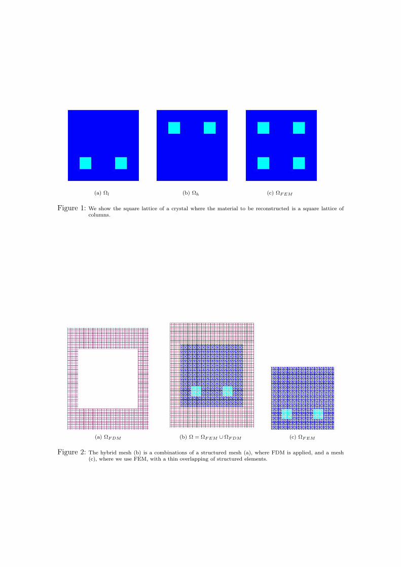
The computational domain in all our tests Ω = ΩFEM ∪ΩFDM is set as Ω = [−4.0, 4.0]×[−5.0, 5.0], which is split into a finite element domain ΩFEM = [−3.0, 3.0]× [−3.0, 3.0] withan unstructured mesh and a surrounding domain ΩFDM with a structured mesh, see Fig. 2.The space mesh in ΩFEM consists of triangles and in ΩFDM of squares, with mesh size in theoverlapping regions h = 0.25 and h = 0.125, in Example 1 and Example 2, correspondingly.

9

(a) Ωl (b) Ωh (c) ΩFEM

Figure 1: We show the square lattice of a crystal where the material to be reconstructed is a square lattice ofcolumns.

(a) ΩFDM (b) Ω = ΩFEM ∪ ΩFDM (c) ΩFEM

Figure 2: The hybrid mesh (b) is a combinations of a structured mesh (a), where FDM is applied, and a mesh(c), where we use FEM, with a thin overlapping of structured elements.

opt.it. 625 nodes 809 nodes 1263 nodes 2225 nodes1 0.0118349 0.0108764 0.0108764 0.0104762 0.0095824 0.00987447 0.00965067 0.009540413 0.00822312 0.00709372 0.00558728 0.007699984 0.00748565 0.00318215 0.00273809 0.003130695 0.00619674 0.002914346 0.005284747 0.004714198 0.00354939

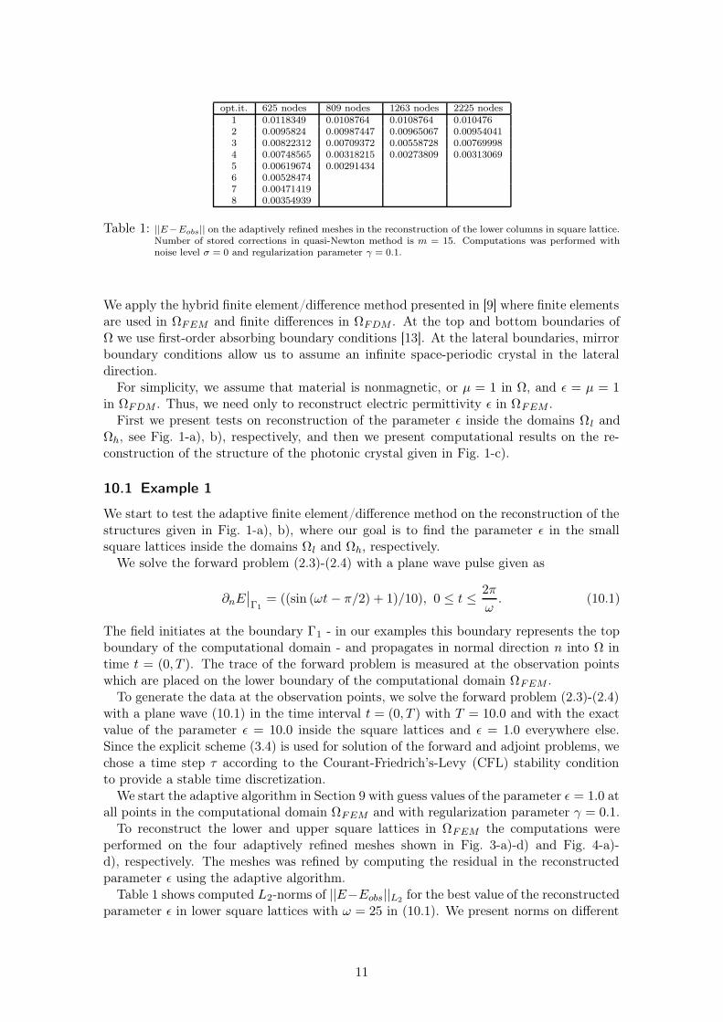
Table 1: ||E−Eobs|| on the adaptively refined meshes in the reconstruction of the lower columns in square lattice.Number of stored corrections in quasi-Newton method is m = 15. Computations was performed withnoise level σ = 0 and regularization parameter γ = 0.1.

We apply the hybrid finite element/difference method presented in [9] where finite elementsare used in ΩFEM and finite differences in ΩFDM . At the top and bottom boundaries ofΩ we use first-order absorbing boundary conditions [13]. At the lateral boundaries, mirrorboundary conditions allow us to assume an infinite space-periodic crystal in the lateraldirection.

For simplicity, we assume that material is nonmagnetic, or µ = 1 in Ω, and ε = µ = 1in ΩFDM . Thus, we need only to reconstruct electric permittivity ε in ΩFEM .

First we present tests on reconstruction of the parameter ε inside the domains Ωl andΩh, see Fig. 1-a), b), respectively, and then we present computational results on the re-construction of the structure of the photonic crystal given in Fig. 1-c).

10.1 Example 1

We start to test the adaptive finite element/difference method on the reconstruction of thestructures given in Fig. 1-a), b), where our goal is to find the parameter ε in the smallsquare lattices inside the domains Ωl and Ωh, respectively.

We solve the forward problem (2.3)-(2.4) with a plane wave pulse given as

∂nE∣

∣

Γ1

= ((sin (ωt− π/2) + 1)/10), 0 ≤ t ≤2π

ω. (10.1)

The field initiates at the boundary Γ1 - in our examples this boundary represents the topboundary of the computational domain - and propagates in normal direction n into Ω intime t = (0, T ). The trace of the forward problem is measured at the observation pointswhich are placed on the lower boundary of the computational domain ΩFEM .

To generate the data at the observation points, we solve the forward problem (2.3)-(2.4)with a plane wave (10.1) in the time interval t = (0, T ) with T = 10.0 and with the exactvalue of the parameter ε = 10.0 inside the square lattices and ε = 1.0 everywhere else.Since the explicit scheme (3.4) is used for solution of the forward and adjoint problems, wechose a time step τ according to the Courant-Friedrich’s-Levy (CFL) stability conditionto provide a stable time discretization.

We start the adaptive algorithm in Section 9 with guess values of the parameter ε = 1.0 atall points in the computational domain ΩFEM and with regularization parameter γ = 0.1.

To reconstruct the lower and upper square lattices in ΩFEM the computations wereperformed on the four adaptively refined meshes shown in Fig. 3-a)-d) and Fig. 4-a)-d), respectively. The meshes was refined by computing the residual in the reconstructedparameter ε using the adaptive algorithm.

Table 1 shows computed L2-norms of ||E−Eobs||L2for the best value of the reconstructed

parameter ε in lower square lattices with ω = 25 in (10.1). We present norms on different

11

a) 625 nodes b) 809 nodes c) 1263 nodes d) 2225 nodes1152 elements 1520 elements 2428 elements 4352 elements

e) 8 Q.N. it. f) 4 Q.N. it. g) 5 Q.N. it. h) 6 Q.N.it.625 nodes 809 nodes 1263 nodes 2225 nodes

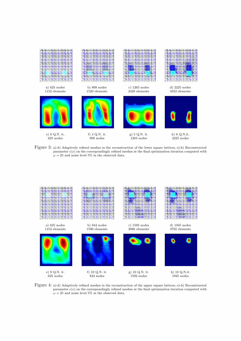
Figure 3: a)-d) Adaptively refined meshes in the reconstruction of the lower square lattices; e)-h) Reconstructedparameter ε(x) on the correspondingly refined meshes at the final optimization iteration computed withω = 25 and noise level 5% in the observed data.

a) 625 nodes b) 844 nodes c) 1592 nodes d) 1945 nodes1152 elements 1590 elements 3086 elements 3792 elements

e) 9 Q.N. it. f) 10 Q.N. it. g) 10 Q.N. it. h) 10 Q.N.it.625 nodes 844 nodes 1592 nodes 1945 nodes

Figure 4: a)-d) Adaptively refined meshes in the reconstruction of the upper square lattices; e)-h) Reconstructedparameter ε(x) on the correspondingly refined meshes at the final optimization iteration computed withω = 25 and noise level 5% in the observed data.

σ, γ 10−5 10−4 10−3 10−2 10−1

0 0.00630036 0.00630536 0.00475773 0.0046071 0.003130691 0.00650122 0.00642409 0.00489691 0.00425432 0.003171473 0.00671315 0.00644934 0.00572624 0.00427946 0.003179555 0.0068622 0.00661597 0.00639352 0.00428971 0.003187037 0.00731985 0.00598225 0.00631647 0.00462458 0.0031228110 0.00672832 0.00618862 0.00673036 0.00467998 0.0033115220 0.00702925 0.00696454 0.00640261 0.00448304 0.0037926

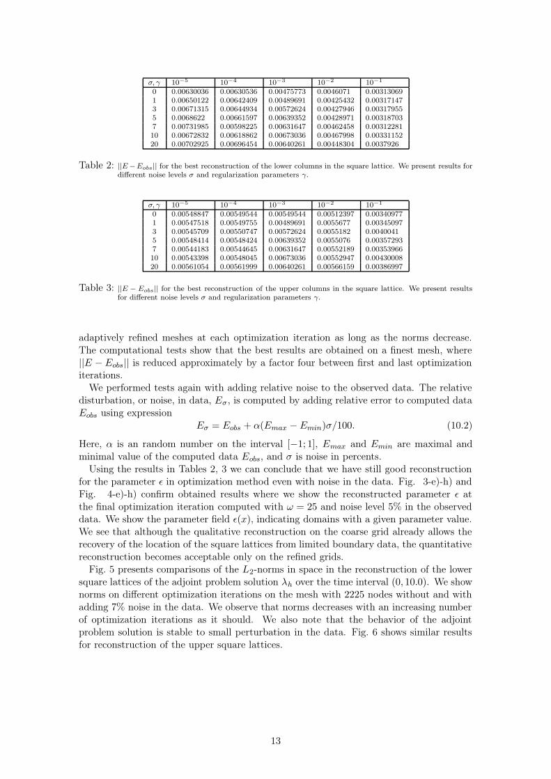
Table 2: ||E −Eobs|| for the best reconstruction of the lower columns in the square lattice. We present results fordifferent noise levels σ and regularization parameters γ.

σ, γ 10−5 10−4 10−3 10−2 10−1

0 0.00548847 0.00549544 0.00549544 0.00512397 0.003409771 0.00547518 0.00549755 0.00489691 0.0055677 0.003450973 0.00545709 0.00550747 0.00572624 0.0055182 0.00400415 0.00548414 0.00548424 0.00639352 0.0055076 0.003572937 0.00544183 0.00544645 0.00631647 0.00552189 0.0035396610 0.00543398 0.00548045 0.00673036 0.00552947 0.0043000820 0.00561054 0.00561999 0.00640261 0.00566159 0.00386997

Table 3: ||E − Eobs|| for the best reconstruction of the upper columns in the square lattice. We present resultsfor different noise levels σ and regularization parameters γ.

adaptively refined meshes at each optimization iteration as long as the norms decrease.The computational tests show that the best results are obtained on a finest mesh, where||E − Eobs|| is reduced approximately by a factor four between first and last optimizationiterations.

We performed tests again with adding relative noise to the observed data. The relativedisturbation, or noise, in data, Eσ, is computed by adding relative error to computed dataEobs using expression

Eσ = Eobs + α(Emax −Emin)σ/100. (10.2)

Here, α is an random number on the interval [−1; 1], Emax and Emin are maximal andminimal value of the computed data Eobs, and σ is noise in percents.

Using the results in Tables 2, 3 we can conclude that we have still good reconstructionfor the parameter ε in optimization method even with noise in the data. Fig. 3-e)-h) andFig. 4-e)-h) confirm obtained results where we show the reconstructed parameter ε atthe final optimization iteration computed with ω = 25 and noise level 5% in the observeddata. We show the parameter field ε(x), indicating domains with a given parameter value.We see that although the qualitative reconstruction on the coarse grid already allows therecovery of the location of the square lattices from limited boundary data, the quantitativereconstruction becomes acceptable only on the refined grids.

Fig. 5 presents comparisons of the L2-norms in space in the reconstruction of the lowersquare lattices of the adjoint problem solution λh over the time interval (0, 10.0). We shownorms on different optimization iterations on the mesh with 2225 nodes without and withadding 7% noise in the data. We observe that norms decreases with an increasing numberof optimization iterations as it should. We also note that the behavior of the adjointproblem solution is stable to small perturbation in the data. Fig. 6 shows similar resultsfor reconstruction of the upper square lattices.

13

0 100 200 300 400 500 600 700 800 900 1000−2.5

−2

−1.5

−1

−0.5

0

0.5

1

1.5

2x 10

−3

1 opt.it.6 opt.it.9 opt.it

0 100 200 300 400 500 600 700 800 900 1000−2.5

−2

−1.5

−1

−0.5

0

0.5

1

1.5

2x 10

−3

1 opt.it.6 opt.it.9 opt.it

noise σ = 7% noise σ = 0%

Figure 5: L2-norms in space of the adjoint problem solution λh in reconstruction of the lower columns in squarelattice on different optimization iterations. Here the x-axis denotes time steps on (0, 10.0).

0 100 200 300 400 500 600 700 800 900 1000−1.5

−1

−0.5

0

0.5

1

1.5

2x 10

−3

||λh||

1 opt.it.6.opt.it10 opt.it.

0 100 200 300 400 500 600 700 800 900 1000−2

−1.5

−1

−0.5

0

0.5

1

1.5

2x 10

−3

||λh||

1 opt.it5 opt.it.8 opt.it9 opt.it.

noise σ = 7% noise σ = 0%

Figure 6: L2-norms in space of the adjoint problem solution λh in the reconstruction of the upper columns in thesquare lattice on different optimization iterations. Here the x-axis denotes time steps on (0, 10.0).

a) 6082 elements b) 8806 elements c) 10854 elements d) 18346 elements

e) 6082 elements f) 8806 elements g) 10854 elements h) 18346 elements

i) 6082 elements j) 8806 elements k) 10854 elements l) 18346 elements

Figure 7: a)-d) Adaptively refined meshes ; e)-h) Reconstructed parameter ε(x), indicating domains with a givenparameter value: red color corresponds to the maximum parameter value on the corresponding meshes,and blue color - to the minimum.

10.2 Example 2

Now we seek to reconstruct the structure of the two-dimensional photonic crystal givenin Fig. 1-c). The electric field initiates at the top boundary of the computational domainΩFDM and consists of a plane wave E given as in (10.1) - and propagates in normaldirection n into Ω in time t = (0, 12.0) with ω = 6.

First we performed tests when the trace of the forward problem is measured at theobservation points only on the lower boundary, and then - tests when the reflected traceis also measured on the lower and top boundaries of the computational domain ΩFEM .

To achieve better results in the reconstruction, we performed tests letting the incomingwave from the top boundary of ΩFDM be equal to the reflected non-plane measured wavefrom the lower boundary ΩFDM . Thus, to generate the data at the observation points,first we solve the forward problem (2.3)-(2.4) with a plane wave (10.1) in the time intervalt = (0, T ) with the exact value of the parameter ε = 4.0 inside the square lattices andε = 1.0 everywhere else, and values of the solution of the forward problem are registeredat the lower boundary of the ΩFDM . Then, using these registered values at the lowerboundary, a non-plane wave is initialized in the time interval t = (T, 2T ). Again, a timestep τ is chosen according to CFL stability condition.

10.2.1 Test1

First we performed tests when the trace of the incoming wave was measured at the obser-vation points at the lower boundary of ΩFEM in time (0, T ), and then at the observationpoints at the top boundary in time (T, 2T ).

15

1 2 3 4 5 60.02

0.04

0.06

0.08

0.1

0.12

0.14

0.16

6082 elements, σ=08806 elements, σ=010854 elements, σ=018346 elements, σ=06082 elements, σ=18806 elements, σ=110854 elements, σ=118346 elements, σ=16082 elements, σ=38806 elements, σ=310854 elements, σ=318346 elements, σ=310854 elements, σ=518346 elements, σ=5

Figure 8: ||E − Eobs|| on adaptively refined meshes. Computations was performed with noise level σ = 0, 1, 3and 5% and with regularization parameter γ = 0.01. Here the x-axis denotes number of optimizationiterations.

1 2 3 4 5 6 7 8 9 10 110

0.05

0.1

0.15

0.2

0.25

6082 elements, σ=08806 elements, σ=010854 elements, σ=018346 elements, σ=010854 elements, σ=718346 elements, σ=710854 elements, σ=1018346 elements, σ=10

Figure 9: ||E − Eobs|| on adaptively refined meshes. Computations was performed with noise level σ = 0, 7 and10% and with regularization parameter γ = 0.01. Here the x-axis denotes number of optimizationiterations.

1 2 3 4 5 6 7 80.02

0.04

0.06

0.08

0.1

0.12

0.14

6082 elements, γ=0.16082 elements, γ=0.016082 elements, γ=0.0016082 elements, γ=0.00018806 elements, γ=0.18806 elements, γ=0.018806 elements, γ=0.0018806 elements, γ=0.000110854 elements, γ=0.110854 elements, γ=0.0110854 elements, γ=0.00110854 elements, γ=0.000118346 elements, γ=0.118346 elements, γ=0.0118346 elements, γ=0.00118346 elements, γ=0.0001

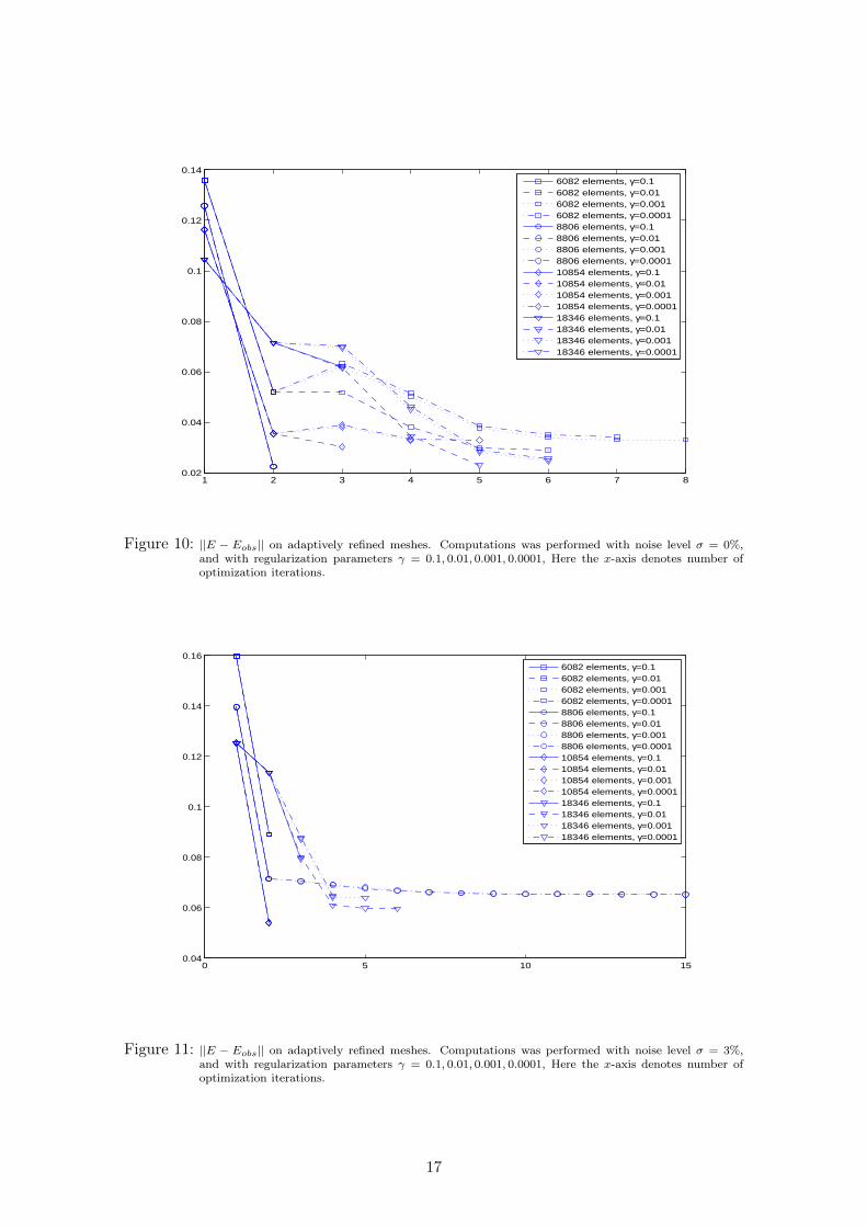
Figure 10: ||E − Eobs|| on adaptively refined meshes. Computations was performed with noise level σ = 0%,and with regularization parameters γ = 0.1, 0.01, 0.001, 0.0001, Here the x-axis denotes number ofoptimization iterations.

0 5 10 150.04

0.06

0.08

0.1

0.12

0.14

0.16

6082 elements, γ=0.16082 elements, γ=0.016082 elements, γ=0.0016082 elements, γ=0.00018806 elements, γ=0.18806 elements, γ=0.018806 elements, γ=0.0018806 elements, γ=0.000110854 elements, γ=0.110854 elements, γ=0.0110854 elements, γ=0.00110854 elements, γ=0.000118346 elements, γ=0.118346 elements, γ=0.0118346 elements, γ=0.00118346 elements, γ=0.0001

Figure 11: ||E − Eobs|| on adaptively refined meshes. Computations was performed with noise level σ = 3%,and with regularization parameters γ = 0.1, 0.01, 0.001, 0.0001, Here the x-axis denotes number ofoptimization iterations.

17

1 2 3 4 5 6 7 8 9 100.02

0.04

0.06

0.08

0.1

0.12

0.14

6082 elements, σ=08806 elements, σ=010854 elements, σ=018346 elements, σ=06082 elements, σ=18806 elements, σ=110854 elements. σ=118346 elements, σ=16082 elements, σ=38806 elements, σ=310854 elements, σ=318346 elements, σ=36082 elements, σ=58806 elements, σ=510854 elements, σ=518346 elements, σ=5

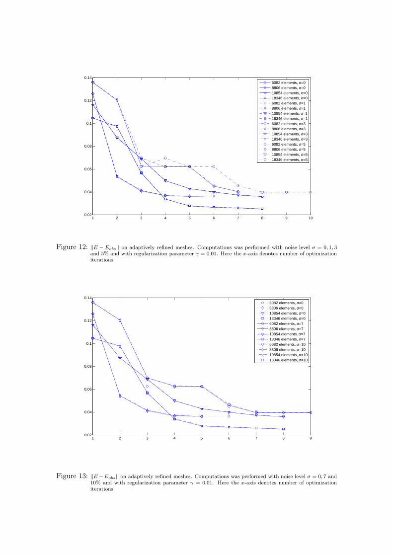
Figure 12: ||E − Eobs|| on adaptively refined meshes. Computations was performed with noise level σ = 0, 1, 3and 5% and with regularization parameter γ = 0.01. Here the x-axis denotes number of optimizationiterations.

1 2 3 4 5 6 7 8 90.02

0.04

0.06

0.08

0.1

0.12

0.14

6082 elements, σ=08806 elements, σ=010854 elements, σ=018346 elements, σ=06082 elements, σ=78806 elements, σ=710854 elements. σ=718346 elements, σ=76082 elements, σ=108806 elements, σ=1010854 elements, σ=1018346 elements, σ=10

Figure 13: ||E −Eobs|| on adaptively refined meshes. Computations was performed with noise level σ = 0, 7 and10% and with regularization parameter γ = 0.01. Here the x-axis denotes number of optimizationiterations.

1 2 3 4 5 6 7 80

0.02

0.04

0.06

0.08

0.1

0.12

0.14

0.16

6082 elements, γ=0.16082 elements, γ=0.016082 elements, γ=0.0016082 elements, γ=0.00018806 elements, γ=0.18806 elements, γ=0.018806 elements, γ=0.0018806 elements, γ=0.000110854 elements, γ=0.110854 elements, γ=0.0110854 elements, γ=0.00110854 elements, γ=0.000118346 elements, γ=0.118346 elements, γ=0.0118346 elements, γ=0.00118346 elements, γ=0.0001

Figure 14: ||E − Eobs|| on adaptively refined meshes. We show computational results with noise level σ = 1%and with regularization parameters γ = 0.1, 0.01, 0.001, 0.0001. Here the x-axis denotes number ofoptimization iterations.

1 2 3 4 5 60.02

0.04

0.06

0.08

0.1

0.12

0.14

6082 elements8806 elements10854 elements18346 elements

1 2 3 4 5 6 7 80.02

0.04

0.06

0.08

0.1

0.12

0.14

6082 elements8806 elements10854 elements18346 elements

a) b)

Figure 15: ||E − Eobs|| on adaptively refined meshes. We show computations: on a) with noise level σ =0% and with regularization parameter γ = 0.01 for Test 1; on b) with noise level σ = 1% andwith regularization parameter γ = 0.01 for Test 2. Here the x-axis denotes number of optimizationiterations.

19

In Fig. 8-9 we present a comparison of the computed L2-norms of ||E−Eobs||L2depending

on the relative noise σ on different adaptively refined meshes while the norms decrease.Relative noise σ in the data is computed using the expression (10.2). From these resultswe conclude that the reconstruction is stable with small values of the noise (see Fig. 8),and unstable with adding more than 5% noise to the data (Fig. 9).

In Fig. 10-11 we show a comparison of the computed L2-norms of ||E−Eobs||L2depending

on the different regularization parameters γ. We see that we obtain the smallest value ofthe difference ||E−Eobs||L2

with regularization parameter γ = 0.01 while choosing γ = 0.1is too large and involve too much regularization. The computational tests show that thebest results are obtained on the finest mesh, where ||E − Eobs|| is reduced approximatelyby a factor seven between first and last optimization iterations. Fig. 7-e)-h) shows thecorresponding to Fig. 15-a) reconstructed parameter field ε(x) at the final optimizationiteration indicating domains with a given parameter value.

10.2.2 Test2

Tests, described in this section, was performed when the reflected trace of the incomingwave was also measured at the observation points on the lower and top boundaries of thecomputational domain ΩFEM . Thus, we have twice more information at the observationpoints then in the previous test, and thus, we expect to get more quantitative reconstructionof the photonic crystal.

In Fig. 12-13 we present comparison of the computed L2-norms of ||E − Eobs||L2de-

pending on the relative noise σ on different adaptively refined meshes while the normsdecrease. Relative noise σ in data is computed using expression (10.2). From these resultswe conclude that the reconstruction is stable even with adding 10% noise to the data ontwo, three and four times refined meshes.

In Fig. 14 we show a comparison of the computed L2-norms of ||E−Eobs||L2depending on

the different regularization parameters γ. We see that the smallest value of the difference||E −Eobs||L2

we obtain with regularization parameter γ = 0.01 while choosing γ = 0.1 isagain too large and involve too much regularization. The computational tests show thatthe best results are obtained on the finest mesh, where ||E−Eobs|| is reduced approximatelyby a factor seven between first and last optimization iterations, see Fig. 15-b). Fig. 7-i)-l) shows the corresponding to Fig. 15-b) reconstructed parameter field ε(x) at the finaloptimization iteration indicating domains with a given parameter value.

11 Conclusions and Remarks

We have devised an explicit, adaptive hybrid FEM/FDM method which can be applied tothe reconstruction of the structure of the two-dimensional photonic crystal. The method ishybrid in the sense that different numerical methods, finite elements and finite differences,are used in different parts of the computational domain. The adaptivity is based on aposteriori error estimates for the associated Lagrangian in the form of space-time integralsof residuals multiplied by dual weights. We illustrated their usefulness for adaptive errorcontrol on an inverse scattering problem for recovering electric permittivity from boundarymeasured data.

References

[1] L. Sanchis A.Håkansson, J.S. Dehesa. Inverse design of photonic crystal devices. IEEEJournal on selected areas in communications, 23 (7):1365 – 1371, 2005.

[2] R. Becker. Adaptive finite elements for optimal control problems. Habilitationsschrift,2001.

[3] R. Becker and R. Rannacher. An optimal control approach to a posteriori errorestimation in finite element methods. Acta Numerica, Cambridge University Press,pages 1–225, 2001.

[4] L. Beilina. Adaptive FEM method for an inverse scattering problem. J. InverseProblems and Information Technologies, 1, 2-nd issue, 2003.

[5] L. Beilina. Adaptive finite element/difference methods for time-dependent inverse scat-tering problems. PhD thesis, Department of Computational Mathematics, ChalmersUniversity of Technology, 2003.

[6] L. Beilina and C. Clason. An adaptive hybrid fem/fdm method for an inverse scat-tering problem in scanning acoustic microscopy. J. SIAM Sci.Comp., 28(1), 2006.

[7] L. Beilina and C. Johnson. A Hybrid FEM/FDM method for an Inverse ScatteringProblem. In Numerical Mathematics and Advanced Applications - ENUMATH 2001.Springer-Verlag, 2001.

[8] L. Beilina and C. Johnson. A posteriori error estimation in computational inversescattering. J. Mathematical models and methods in applied sciences, 15(1):23–37,2005.

[9] L. Beilina, K. Samuelsson, and K. Åhlander. Efficiency of a hybrid method for thewave equation. In International Conference on Finite Element Methods, Gakuto In-ternational Series Mathematical Sciences and Applications. Gakkotosho CO.,LTD,2001.

[10] Eli Yablonovitch Chiu Yen Kao, Stanley Osher. Maximizing band gaps in two-dimensional photonic crystals by using level set methods. Applied Physics B: Lasersand Optics, 81:235 – 244, 2005.

[11] G. C. Cohen. Higher Order numerical methods for transient wave equations. SpringerVerlag, 2002.

[12] D.C.Dobson. An efficient method for band structure calculations in 2d photonic crys-tals. JCP, 149:363 – 376, 1999.

[13] B. Engquist and A. Majda. Absorbing boundary conditions for the numerical simu-lation of waves. Math. Comp., 31:629–651, 1977.

[14] K. Eriksson, D. Estep, and C. Johnson. Computational Differential Equations. Stu-dentlitteratur, Lund, 1996.

[15] Joshua N. Winn John D. Joannopoulos, Robert D. Meade. Photonic Crystals: Moldingthe Flow of Light. Princeton Unviersity Press, 1995.

21

[16] P. Joly. Variational methods for time-dependent wave propagation problems. LectureNotes in Computational Science and Engineering, Springer, 2003.

[17] E. Yablonovitch M. Burger, S. Osher. Inverse problem techniques for the design ofphotonic crystals. IEICE Transactions on Electronics, 87:258 – 265, 2004.

[18] J. Nocedal. Updating quasi-newton matrices with limited storage. J. Mathematicalof Comp., 35, N.151:773–782, 1991.

[19] O. Pironneau. Optimal shape design for elliptic systems. Springer Verlag, Berlin, 1984.

[20] P.Kuchment. The mathematics of photonic crystals. SIAM Mathematical Modelingin Optical Science, pages 207 – 272, 2001.

[21] E. Yablonovitch. Photonic crystals: Semiconductors of light. Scientific American,285, N. 6:47–55, 2001.