Embed Size (px)
Citation preview

norges teknisk-naturvitenskapelige
universitet
Error estimates in inverse electromagneticscattering
by
Larisa Beilina, Marte P. Hatlo, Harald E. Krogstad
preprint
numerics no. 10/2007
norwegian university of
science and technology
trondheim, norway
This report has URLhttp://www.math.ntnu.no/preprint/numerics/2007/N10-2007.pdf
Address: Department of Mathematical Sciences, Norwegian University of Science andTechnology, N-7491 Trondheim, Norway.


Error estimates in inverse
electromagnetic scattering
Larisa Beilina, Marte P. Hatlo, Harald E. Krogstad
December 19, 2007
In this paper we derive an a posteriori error estimate and present two differentadaptive algorithms for an inverse electromagnetic scattering problem.
The inverse problem is formulated as an optimal control problem, where wesolve equations expressing stationarity of an associated Lagrangian. The aposteriori error estimate for the Lagrangian couples residuals of the computedsolution to weights of the reconstruction. We show that the weights can beobtained by solving an associated linearized problem for the Hessian of theLagrangian, which is used in the second algorithm, while in the first algorithmwe compute only the residuals. The performance of the adaptive finite elementmethod and the usefulness of the a posteriori error estimate are illustrated innumerical examples.
1 Introduction
We apply the mesh-adaptive method, developed in [3], to an inverse electromagenticscattering problem. The method is based on an a posteriori error estimate which couplesresiduals of the computed solution to weights in the reconstruction. The new elementin the present work is the introduction of absorbing and mirror boundary conditions inthe formulation of the forward problem. Thus, the a posteriori error estimate for theinverse problem is also new. The derivation of the a posteriori estimate for the errorin the Lagrangian follows the main approach to adaptive error control in computationaldifferential equations, presented in [2, 7] and references therein.
The inverse problem consists of reconstructing the unknown material variable, that is,the dielectric permittivity, ε(x), from data measured on parts of the surface of the givendomain, given the wave input on other parts. By solving the wave equation with the sameinput, the material variables are in principle obtained by fitting the computed solutionto the measured data. The problem is formulated as finding a stationary point of theLagrangian, involving the forward wave equation (the state equation), the backward waveequation (the adjoint equation), and an equation expressing that the gradient with respectto the parameter vanishes. The optimum is found in an iterative process solving the forwardand backward wave equations and updating the material coefficient for each step.
We present two different adaptive algorithms to solve the inverse problem. In the firstalgorithm, the space-mesh adaptivity is based only on the computation of the residuals,since they already give us enough information. The second algorithm is extended to includecomputations of the weights. To compute the weights, we propose to solve a linerizedproblem for the Hessian of the Lagrangian.
1

Finally, numerical experiments where a periodic structure is reconstructed, show thepossibilities of using adaptive error control in computational inverse scattering.
2 Mathematical model
We shall restrict ourselves to the propagation of light in a mixed dielectric medium in abounded domain Ω ⊂ R
d, d = 2, 3, with boundary Γ, governed by Maxwell’s equations:
∂D
∂t−∇×H = −J, in Ω× (0, T ],
∂B
∂t+∇×E = 0, in Ω× (0, T ], (1)
∇ ·D = ρ, in Ω× (0, T ],
∇ ·B = 0, in Ω× (0, T ].
Here E(x, t) and H(x, t) are the electric and magnetic fields, whereas D(x, t) and B(x, t)are the electric and magnetic inductions, respectively. We assume that the dielectric per-mittivity, ε(x), is scalar and that the material is non-magnetic, so that µ(x) = 1. ThenD = εE and B = H. The current density, J , and charge density, ρ, are both assumed tobe zero.
By eliminating B andD from (1) we obtain two independent partial differential equations
ε∂2E
∂t2+∇× (∇×E) = 0,
∂2H
∂t2+∇× (ε−1∇×H) = 0,
(2)
which may be solved imposing appropriate initial and boundary conditions.For simplicity, we only consider the problem in terms of E(x, t). Taking into account
the vector identity ∇×∇× V = ∇(∇ · V )−4V , we obtain
ε∂2E
∂t2−∇ · (∇E) = 0, in Ω× (0, T ]. (3)
A similar equation is valid for H.Let Γ1∪Γ2 ⊂ Γ and Γ3 = Γ\ Γ1∪Γ2, and consider the forward problem consisting of (3)
and the following initial and boundary conditions (Here and below, we denote Dv = ∂v∂t
)
E(·, 0) = 0,∂E
∂t(·, 0) = 0, in Ω,
∂nE∣∣Γ1
= v1, on Γ1 × (0, t1],
∂nE∣∣Γ1
= DE, on Γ1 × (t1, T ],
∂nE∣∣Γ2
= DE, on Γ2 × (0, T ],
∂nE∣∣Γ3
= 0, on Γ3 × (0, T ],
(4)
Here v1 is a pulse emitted from Γ1, which propagates into Ω until t = t1. We use firstorder absorbing boundary conditions, given in [6], on Γ1 × (t1, T ] and Γ2 × (0, T ]. At thelateral boundaries Γ3 we use mirror boundary conditions.

Our goal is to solve the inverse problem for (3) and (4), or to find the material parameterε(x) from data at a finite set of observation points on Γ. The data are generated in exper-iments where pulses are emitted from Γ1, backscattered by the material inhomogenities,and recorded on parts of the boundary Γ.
In this paper, data are generated by computing the forward problem (3) and (4) forgiven values of the parameters, and saving the solution on parts of the boundary. Thecoefficients are then “forgotten” and the goal is to reconstruct the coefficients from thecomputed boundary data.
3 A hybrid finite element/difference method
To solve equation (3)-(4) we use a hybrid FEM/FDM method developed in [5]. Themethod uses continuous, piecewise linear finite elements in space and time on a partiallystructured mesh in space. The computational space domain Ω is decomposed into a finiteelement domain ΩFEM, with an unstructured mesh, and a finite difference domain ΩFDM,with a structured mesh. Typically, ΩFEM covers only a small part of Ω. In ΩFDM we usequadrilateral elements in R
2 and hexahedra in R3. In ΩFEM we use a finite element mesh
Kh = K with elements K consisting of triangles in R2 and tetrahedra in R
3. Let usassociate with Kh a mesh function hK = diam(K), ∀x ∈ K, representing the diameter ofthe element K. For the time discretization, let Jk = J be a partition of the time intervalI = (0, T ] into time intervals J = (tk−1, tk] of uniform length τ = tk − tk−1.
We define the following L2 inner products and norm
(p, q) =
∫
Ωpq dx, ((p, q)) =
∫
Ω
∫ T
0pq dt dx, ‖p‖2 = ((p, p)).
We introduce the finite element trial space W vh defined by :
W vh := v ∈W v
1 ∪W v2 : v|K×J ∈ P1(K)× P1(J),∀K ∈ Kh,∀J ∈ Jk,
where
W v1 := v ∈ H1(Ω× J) : v(·, 0) = 0, ∂nv|Γ1
= v1, ∂nv|Γ2= Dv, ∂nv|Γ3
= 0,W v
2 := v ∈ H1(Ω× J) : v(·, 0) = 0, ∂nv|Γ1= ∂nv|Γ2
= Dv, ∂nv|Γ3= 0.
Here P1(K) and P1(J) are the set of linear functions on K and J , respectively.Furthermore, the finite element space W λ
h for the costate λ, is defined by:
W λh := λ ∈W λ
1 ∪W λ2 : λ|K×J ∈ P1(K)× P1(J),∀K ∈ Kh,∀J ∈ Jk,
where
W λ1 : = λ ∈ H1(Ω× J) : λ(·, T ) = 0, ∂nλ|Γ1
= ∂nλ|Γ3= 0, ∂nλ|Γ2
= Dλ,W λ
2 : = λ ∈ H1(Ω× J) : λ(·, T ) = 0, ∂nλ|Γ1= ∂nλ|Γ2
= Dλ, ∂nλ|Γ3= 0.
The finite element method for (3)-(4) now reads: Find Eh ∈W vh such that ∀λ ∈W λ
h ,
− ((εDEh, Dλ)) + ((∇Eh,∇λ))
− ((DEh, λ))(t1 ,T ]×Γ1− ((DEh, λ))(0,T ]×Γ2
= ((v1, λ))(0,t1 ]×Γ1.
(5)
Here, the initial condition DE(0) = 0 is imposed in weak form through the variationalformulation.
Expanding E and λ in terms of the standard continuous piecewise linear functions ϕi(x)in space and ψi(t) in time, and substituting this into (5), we obtain an explit scheme forsolving (5), see for example [3] where a similar system is obtained for an acoustic waveequation with homogenous boundary conditions.
3

4 The inverse problem
We formulate the inverse problem for (3) and (4) as follows: given the function ∂nE =v1 on Γ1 × (0, t1], determine the coefficient ε(x) for x ∈ Ω, which minimizes the quantity
J(E, ε) =1
2
∫ T
0
∫
Ω(E − E)2δobs dxdt+
1
2γ
∫
Ω(ε− ε0)2 dx. (6)
Here E is the data observed at a finite set of points xobs, E satisfies (3) and (4) and thusdepends on ε. Moreover, δobs =
∑δ(x− xobs) is a sum of delta-functions corresponding to
the observation points, γ is a regularization parameter, and ε0 is the initial guess value forthe parameter we want to reconstruct.
To solve this minimization problem, we introduce the Lagrangian
L(u) = J(E, ε) − ((εDE,Dλ)) + ((∇E,∇λ)) − ((DE,λ))(t1 ,T ]×Γ1
− ((DE,λ))(0,T ]×Γ2− ((v1, λ))(0,t1 ]×Γ1
,(7)
where u = (E, λ, ε), and search for a stationary point with respect to u, satisfying for allu = (E, λ, ε)
L′(u; u) = 0, (8)
where L′ is the gradient of L. Equation (8) expresses that for all u,
∂L(u)
∂λ(λ) =− ((εDλ,DE)) + ((∇E,∇λ))− ((DE, λ))(t1 ,T ]×Γ1
− ((DE, λ))(0,T ]×Γ2− ((2v1, λ))(0,t1 ]×Γ1
= 0,
∂L(u)
∂E(E) =((E − E, E))δobs
− ((εDλ,DE)) + ((∇λ,∇E))
+ ((Dλ, E))[0,T )×Γ1+ ((Dλ, E))[0,T )×Γ2
= 0,
∂L(u)
∂ε(ε) =− ((DλDE, ε)) + γ(ε− ε0, ε) = 0.
(9)
The first equation in (9) is a weak form of the state equation (3) and (4), the secondequation is a weak form of the adjoint state equation,
ε∂2λ
∂t2−∇ · (∇λ) = −(E − E)δobs, x ∈ Ω, 0 ≤ t < T,
∂nλ = 0 on Γ1 × [0, t1),
∂nλ = Dλ on Γ1 × [0, T ),
∂nλ = Dλ on Γ2 × [0, T ),
∂nλ = 0 on Γ3 × [0, T ),
λ(·, T ) = Dλ(·, T ) = 0 in Ω,
(10)
and the last equation expresses stationarity with respect to the parameter ε.
5 A finite element method for inverse problem
To formulate a finite element method for (8) we introduce the finite element space Vh ofpiecewise constants for the coefficient ε(x), defined by :
Vh := v ∈ L2(Ω) : v ∈ P0(K),∀K ∈ Kh.

Recalling the definitions of W vh and W λ
h , related to the state E and the costate λ, anddefining Uh = W v
h ×W λh × Vh, we formulate the finite element method for (8) as: Find
uh ∈ Uh, such thatL′(uh; u) = 0, ∀u ∈ Uh. (11)
6 An a posteriori error estimate for the Lagrangian
Theorem 6.1. Let L(u) = L(E, λ, ε) be the Lagrangian as defined in (7), and let L(uh) =L(Eh, λh, εh) be the approximation of L(u). Then the following representation holds forthe error e = L(u)− L(uh):
∣∣e∣∣ ≤ ((RE1
, σλ))(0,t1 ]×Γ1+ ((RE2
, σλ)) + ((RE3, σλ))
+ ((RE4, σλ))(t1 ,T ]×Γ1
+ ((RE5, σλ))(0,T ]×Γ2
+ ((Rλ1, σE))δobs
+ ((Rλ2, σE)) + ((Rλ3
, σE))
+ ((Rλ4, σE))(0,T ]×Γ1
+ ((Rλ5, σE))(0,T ]×Γ2
+ ((Rε1 , σε)) + (Rε2 , σε),
(12)
where the residuals are defined by
RE1= 2|v1|, RE2
= maxS⊂∂K
h−1K
∣∣[∂sEh
]∣∣,
RE3= εhτ
−1∣∣[∂tEh
]∣∣, RE4= RE5
= |DEh|,Rλ1
= |Eh − E|, Rλ2= max
S⊂∂Kh−1
K
∣∣[∂sλh
]∣∣,
Rλ3= εhτ
−1∣∣[∂tλh
]∣∣, Rλ4= Rλ5
= |Dλh|,Rε1 = |Dλh| · |DEh|, Rε2 = γ|εh − ε0|,
and the interpolation errors are
σλ = Cτ |[Dλh]|+ ChK |[∂nλh]| ,σE = Cτ |[DEh]|+ ChK |[∂nEh]| ,σε = C
∣∣[εh]∣∣,
Here, [v] denotes the maximum of the modulus of a jump of v across the face of anelement K (or the boundary node of a time interval J), ∂sv denotes the normal derivativeof v across a side of K, ∂nv denotes the derivative of v in the outward normal of an elementK, [∂tv] is the maximum modulus of the jump of the time derivative of v across a boundarynode of J , C is interpolation constants of moderate size.
Proof. Throughout the proof, let C denote different constants of a moderate size.As in [1], we use the fundamental theorem of calucus to write
e = L(v)− L(vh)
=
∫ 1
0
d
dsL(vh + s(v − vh))ds
=
∫ 1
0L′(vh + s(v − vh); v − vh)ds
= L′(vh; v − vh) +R,
5
where R denotes a second order term. For full details of the arguments we refer to [1] and[7].
Neglecting the term R, and using the Galerkin orthogonality (11) with the splitting
v − vh = (v − vIh) + (vI
h − vh), (13)
where vIh denotes an interpolant of v, leads to the following error representation:
e ≈ L′(vh; v − vIh) = I1 + I2 + I3. (14)
Here
I1 =−((εhDEh, D(λ− λI
h)))
+((∇Eh,∇(λ− λI
h)))−((
2v1, λ− λIh
))(0,t1 ]×Γ1
−((DEh, λ− λI
h
))(t1 ,T ]×Γ1
−((DEh, λ− λI
h
))(0,T ]×Γ2
,
I2 =((Eh − E, E −EI
h
))δobs
−((εhDλh, D(E −EI
h)))
+((∇λh,∇(E −EI
h)))
+((Dλh, E −EI
h
))(0,T ]×Γ1
+((Dλh, E −EI
h
))(0,T ]×Γ2
,
I3 =−((DλhDEh, ε− εIh
))+ γ(εh − ε0, ε− εIh
),
To estimate I1, we integrate by parts in the first and second terms to obtain:∣∣I1
∣∣ =∣∣((εhD2Eh, λ− λI
h
))−((4Eh, λ− λI
h
))
−((
2v1, λ− λIh
))(0,t1 ]×Γ1
−((DEh, λ− λI
h
))(t1,T ]×Γ1
−((DEh, λ− λI
h
))(0,T ]×Γ2
−∑
k
∫
Ωεh[DEh(tk)
](λ− λI
h)(tk) dx
+∑
K
∫ T
0
∫
∂K
∂nEh(λ− λIh) dsdt
∣∣,
(15)
Here,[DEh(tk)
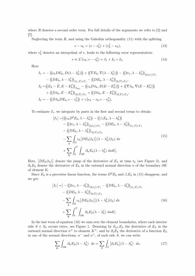
]denote the jump of the derivative of Eh at time tk (see Figure 2), and
∂nEh denote the derivative of Eh in the outward normal direction n of the boundary ∂Kof element K.
Since Eh is a piecewise linear function, the terms D2Eh and 4Eh in (15) disappear, andwe get:
∣∣I1
∣∣ =∣∣−((
2v1, λ− λIh
))(0,t1]×Γ1
−((DEh, λ− λI
h
))(t1,T ]×Γ1
−((DEh, λ− λI
h
))(0,T ]×Γ2
−∑
k
∫
Ωεh[DEh(tk)
](λ− λI
h)(tk) dx
+∑
K
∫ T
0
∫
∂K
∂nEh(λ− λIh) dsdt
∣∣.
(16)
In the last term of equation (16) we sum over the element boundaries, where each interiorside S ∈ Sh occurs twice, see Figure 1. Denoting by ∂n±Eh the derivative of Eh in theoutward normal direction n± to element K±, and by ∂sEh the derivative of a function Eh
in one of the normal directions, n− and n+, of each side S, we can write∑
K
∫
∂K
∂nEh(λ− λIh) ds =
∑
S
∫
S
[∂sEh
](λ− λI
h) ds, (17)

n−
∂K+
∂K−
S
K−
S
n+
K+
Figure 1: Two neighbouring elements K+ and K−, their boundaries, ∂K+ and ∂K−, andthe interior side S.
where the jump[∂sEh
]is defined as
[∂sEh] = maxS∈∂K
∂n+Eh, ∂n−Eh.
We distribute each jump equally to the two sharing elements and return to a sum of theelement edges ∂K :
∑
S
∫
S
[∂sEh] (λ− λIh) ds =
∑
K
1
2
∫
∂K
[∂sEh
](λ− λI
h) ds. (18)
We multiply and divide by hK , formally set dx = hKds and replace the integrals overthe element boundaries ∂K by integrals over the elements K, to get:
∣∣∣∣∣∑
K
1
2h−1
K
∫
∂K
[∂sEh
](λ− λI
h) hK ds
∣∣∣∣∣
≤ C∫
ΩmaxS⊂∂K
h−1K
∣∣[∂sEh
]∣∣∣∣λ− λIh
∣∣ dx,(19)
where[∂sEh
]∣∣K
= maxS⊂∂K
[∂sEh
]∣∣S.
In a similar way we can estimate the jump in time in (16) by multiplying and dividingby τ :
∣∣∣∣∣∑
k
∫
Ωεh [DEh(tk)] (λ− λI
h)(tk) dx
∣∣∣∣∣
≤∑
k
∫
Ωεhτ−1∣∣ [DEh(tk)]
∣∣∣∣(λ− λIh)(tk)
∣∣ τdx
≤C∑
k
∫
Jk
∫
Ωεhτ−1∣∣[∂tkEh
]∣∣∣∣λ− λIh
∣∣ dxdt
=C((εhτ−1∣∣[∂tEh
]∣∣,∣∣(λ− λI
h)∣∣ )).
(20)
Here, we have defined [∂tkEh] as the greatest of the two jumps on the interval (tk, tk+1]:
[∂tkEh] = maxk
([DEh(tk)] , [DEh(tk+1)]) ,
[∂tEh] = [∂tkEh] on Jk.
7

f−(tk)
ttk−1 tk+1J− J+
tk
[
f(tk)]
[
f(tk+1)]
[
f(tk−1)]
f+(tk)
Figure 2: The jump of a function f on the time mesth.
where [DEh(tk)] = DE+h (tk)−DE−h (tk). The time jumps are illustrated in Figure 2.
We substitute the expressions (19) and (20) in (16), to get:∣∣I1
∣∣ ≤((
2∣∣v1
∣∣,∣∣λ− λI
h
∣∣))(0,t1]×Γ1
−((∣∣DEh
∣∣,∣∣λ− λI
h
∣∣))(t1 ,T ]×Γ1
−((∣∣DEh
∣∣,∣∣λ− λI
h
∣∣))(0,T ]×Γ2
+ C((
maxS⊂∂K
h−1K
∣∣[∂sEh
]∣∣,∣∣λ− λI
h
∣∣ ))
+ C((εhτ−1∣∣[∂tEh
]∣∣,∣∣λ− λI
h
∣∣ )).
Next, we use the following standard interpolation estimate
|λ− λIh| ≤ C(τ2|D2λ|+ h2
K |D2xλ|), (21)
where we approximate the second derivative in time as
D2λ =∂2λ
∂t2=∂(Dλ)
∂t≈(Dλ)+ −
(Dλ)−
τ=
[Dλh
]
τ.
Here (·)+ and (·)− reperesents values on two neighbouring intervals J+ and J−, see Figure2. In the same way we approximate the second derivative in space:
D2xλ ≈
[∂nλh
]
h.
Substituting both expressions above in (21), we obtain∣∣λ− λI
h
∣∣ ≤ C(τ∣∣[Dλh
]∣∣+ hK
∣∣[∂nλh
]∣∣) (22)
and the estimate for I1 reduces to∣∣I1
∣∣ ≤C((
2∣∣v1
∣∣, τ∣∣[Dλh
]∣∣+ hK
∣∣[∂nλh
]∣∣))(0,t1]×Γ1
−C((∣∣DEh
∣∣, τ∣∣[Dλh
]∣∣+ hK
∣∣[∂nλh
]∣∣))(t1,T ]×Γ1
−C((∣∣DEh
∣∣, τ∣∣[Dλh
]∣∣+ hK
∣∣[∂nλh
]∣∣))(0,T ]×Γ2
+C((
maxS⊂∂K
h−1k
∣∣[∂sEh
]∣∣, τ∣∣[Dλh
]∣∣+ hK
∣∣[∂nλh
]∣∣))
+C((εhτ−1∣∣[∂tEh
]∣∣, τ∣∣[Dλh
]∣∣+ hK
∣∣[∂nλh
]∣∣)).

We estimate I2 similarly as I1. First, we integrate by parts to obtain∣∣I2
∣∣ ≤∣∣((Eh − E, E −EI
h
))δobs
+((εhD
2λh, E −EIh
))
−((4λh, E −EI
h
))+((Dλh, E −EI
h
))(0,T ]×Γ1
+((Dλh, E −EI
h
))(0,T ]×Γ2
∣∣
+ C((
maxS⊂∂K
h−1K
∣∣[∂sλh
]∣∣,∣∣E −EI
h
∣∣ ))
+ C((εhτ−1∣∣[∂tλh
]∣∣,∣∣E −EI
h
∣∣ )).Since λh is piecewice linear, the terms with 4λh and D2λh will disappear:
∣∣I2
∣∣ ≤((∣∣Eh − E
∣∣,∣∣E −EI
h
∣∣))δobs
+((∣∣Dλh
∣∣,∣∣E −EI
h
∣∣))(0,T ]×Γ1
+((∣∣Dλh
∣∣,∣∣E −EI
h
∣∣))(0,T ]×Γ2
+ C((
maxS⊂∂K
h−1K
∣∣[∂sλh
]∣∣,∣∣E −EI
h
∣∣))
+ C((εhτ−1∣∣[∂tλh
]∣∣,∣∣E −EI
h
∣∣)).Next, we use the same kind of interpolation estimate for |E −E I
h| as we found for |λ− λIh|
in equation (22), to get:∣∣I2
∣∣ ≤C((∣∣Eh − E
∣∣, τ∣∣ [DEh]
∣∣+ hK
∣∣ [∂nEh]∣∣))
δobs
+C((∣∣Dλh
∣∣, τ∣∣ [DEh]
∣∣+ hK
∣∣ [∂nEh]∣∣))
(0,T ]×Γ1
+C((∣∣Dλh
∣∣, τ∣∣ [DEh]
∣∣+ hK
∣∣ [∂nEh]∣∣))
(0,T ]×Γ2
+C((
maxS⊂∂K
h−1K
∣∣[∂sλh
]∣∣, τ∣∣ [DEh]
∣∣+ hK
∣∣ [∂nEh]∣∣))
+C((εhτ−1∣∣[∂tλh
]∣∣, τ∣∣ [DEh]
∣∣+ hK
∣∣ [∂nEh]∣∣)).
To estimate I3 we use the following approximation estimate for ε− εIh:
|ε− εIh| ≤ ChKDxε ≤ ChK
∣∣∣∣[εh]
hK
∣∣∣∣ ≤ C|[εh]|,
and we end up with∣∣I3
∣∣ ≤((|Dλh| |DEh| ,
∣∣[εh]∣∣ ))+ γ(
∣∣εh − ε0∣∣,∣∣[εh]
∣∣ ),
which complets the proof.
7 A posteriori error estimation for parameter identification
Following [4] we present a more general a posteriori estimate for the error in the recon-structed parameter. We first note that
L′(u; u)− L′(uh; u) =
∫ 1
0
d
dsL′(us+ (1− s)uh; u)ds
=
∫ 1
0L′′(us+ (1− s)uh;u− uh, u)ds
= L′′(uh;u− uh, u) +R,
9

where R is a second order remainder and L′′(uh; ·, ·) is the Hessian of the Lagrangian. SinceL′(u; u) = 0, we get
−L′′(uh;u− uh, u) = L′(uh; u) +R.
Next, we can use the Galerkin orthogonality (11) with the splitting u − uh = (u − uIh) +
(uIh − uh), where uI
h ∈ Uh denotes an interpolant of u, to get the following equation
−L′′(uh;u− uh, u) = L′(uh; u− uIh) +R. (23)
In our case the dual problem is defined as
−L′′(uh;u− uh, u) = (ψ, u − uh), (24)
where ψ is a given data. Neglecting the term R in (23), and comparing (23) with (24), weget
(ψ, u− uh) ≈ L′(uh; u− uIh). (25)
From this estimate we observe that the form of the error for a parameter identification issimilar to the error in the Lagrangian, if the weight u is replaced by u.
We can choose u− uh = u in (24) and the dual problem can be written as
−L′′(uh; u, u) = (ψ, u). (26)
We conclude that for an appropriate choice of the data, ψ, in the dual problem, we cansolve (26) approximately for u and thus get values of the error for u.
8 The Hessian of the Lagrangian
In Section 7 we presented an a posteriori error estimate for identification of the parameter.In this section we derive an approximation of the strong form of the dual problem (26),which can be used to calculate the weights for the problem (3)-(4).
The Hessian of the Lagrangian (7) takes the following form
L′′(u; u, u) = L′′E(u; u, E) + L′′λ(u; u, λ) + L′′ε (u; u, ε), (27)
where
L′′E(u; u, E) = −((εDλ,DE)) + ((∇E,∇λ)) + ((E, E))δobs− ((DEDλ, ε))
− ((DE, λ))[0,T )×Γ1− ((DE, λ))[0,T )×Γ2
,
L′′λ(u; u, λ) = −((εDE,Dλ)) + ((∇λ,∇E))− ((v1, λ))(0,t1 ]×Γ1− ((DEDλ, ε))
− ((Dλ, E))(t1 ,T ]×Γ1− ((Dλ, E))(0,T ]×Γ2
,
L′′ε (u; u, ε) = −((DEDλ, ε))− ((DλDE, ε)) + γ(ε, ε).
Here we have used the boundary conditions ∂nλ = Dλ, ∂nλ = Dλ, ∂nλ = Dλ on Γ1 ∪Γ2 × [0, T ), and ∂nE = ∂nE = ∂nE = v1|(0,t1 ]×Γ1
, ∂nE = DE, ∂nE = DE, ∂nE = DE onΓ1 × (t1, T ] and Γ2 × (0, T ], respectively.
Then the dual problem (26) takes the following strong form
ε∂2λ
∂t2−∇ · (∇λ) + Eδobs
+ ε∂2λ
∂t2−Dλ(t1,T )×Γ1
−Dλ(0,T )×Γ2= ψ1,
ε∂2E
∂t2−∇ · (1
ε∇E) + ε
∂2E
∂t2− v1|(0,t1 ]×Γ1
−DE(t1 ,T )×Γ1−DE(0,T )×Γ2
= ψ2,
−∫ T
0DλDEdt−
∫ T
0DλDEdt+ γ1ε = ψ3,
(28)

with initial and boundary conditions. Our goal is to solve the system (28) with an alreadyknown approximation to the final solution u, computed using the adaptive Algorithm 2 inSection 9, and find u = (E, λ, ε). We assume that the solution of the adjoint problem, λ,will be small after the final optimization iteration, and we can neglect all terms involvingλ to get the following approximated problem
ε∂2λ
∂t2−∇ · (∇λ) + Eδobs
−Dλ(t1,T )×Γ1−Dλ(0,T )×Γ2
= ψ1,
ε∂2E
∂t2−∇ · (∇E) + ε
∂2E
∂t2− v1|(0,t1]×Γ1
−DE(t1,T )×Γ1−DE(0,T )×Γ2
= ψ2,
−∫ T
0DλDEdt+ γε = ψ3.
(29)
As already mentioned in [4], the stability properties of this system is an open problem.
9 Adaptive algorithms for the inverse problem
In this section we present two different adaptive algorithms for solution of the inverseproblem presented in Section 4. In Algorithm 1, the refinement is based on computions ofthe residuals for the parameter, since they already give a good indication where to refinethe mesh. The interpolation errors, and thus the exact value of the computational error inthe reconstructed parameter, can be obtained by computing the Hessian of the Lagrangianusing equation (29) as shown in Algorithm 2.
As we see from (12), the error in the Lagrangian consists of integrals in space and time ofthe different residuals multiplied by the interpolation errors. Thus, to estimate the error inthe Lagrangian we need to compute the approximated values of (Eh, λh, εh) together withresiduals and interpolation errors. Since we want to control the error in the reconstructedparameter, εh, we limit the computations to Rε1 and Rε2 , and neglect to compute the otherresiduals in the a posteriori estimate (12). The a posteriori error in step 5 of Algorithm 1is thus calculated as
e(x) ≈∫ T
0Rα1
(x, t) dt+Rα2(x) . (30)
9.1 Algorithm 1
0. Choose an initial mesh Kh and an initial time partition J0 of the time interval (0, T ].Start with an initial guess ε0, and compute the sequence of εn in the following steps:
1. Compute the solution En of the forward problem (3)-(4) on Kh and Jk, with ε(x) =ε(n).
2. Compute the solution λn of the adjoint problem (10) on Kh and Jk.
3. Update the parameter ε on Kh and Jk using the quasi-Newton method
εn+1 = εn + αnHngn,
where Hn is an approximate Hessian, computed using the usual BFGS update for-mula for the Hessian, see [8]. Furthermore, gn is the gradient of the Lagrangian (7)
11

with respect to the parameter ε,
gn = −∫ T
0DλnDEndt+ γ(εn − ε0), (31)
where α is the step length in the parameter upgrade computed using an one-dimensionalsearch algorithm [9].
4. Stop computing ε if the gradient gn < η; if not set n = n+ 1 and go to step 1. Here,η is the tolerance in the quasi-Newton update.
5. Compute the residuals, Rε1 , Rε2 and refine the mesh in all points where
∫ T
0Rα1
(x, t) dt+Rα2(x) < tol (32)
is violated. Here tol is a tolerance chosen by the user.
6. Construct a new mesh Kh and a new time partition Jk. Return to step 1 and performall the steps of the optimization algorithm on the new mesh.
9.2 Algorithm 2
0. Choose an initial mesh Kh and an initial time partition J0 of the time interval (0, T ].Start with an initial guess ε0, and compute a sequence of εn in the following steps:
1. Compute the solution En of the forward problem (3)-(4) on Kh and Jk with ε(x) =ε(n).
2. Compute the solution λn of the adjoint problem (10) on Kh and Jk.
3. Update the parameter ε on Kh and Jk using the quasi-Newton method
εn+1 = εn + αnHngn,
where Hn is an approximate Hessian, and gn is the gradient of the Lagrangian (7)with respect to the parameter ε, as in equation (31).
4. Stop if the gradient gn < η; if not, set n = n + 1 and go to step 1. Here, η is thetolerance in the quasi-Newton update.
5. Compute the residuals, Rε1 and Rε2 , in (25).
6. Compute the weight σε in the a posteriori error estimate, (25), by solving equation(29), using the following iterative procedure:
6.1. From the last equation in (29), update ε as
εm+1 = εm + α(ψ3 +
∫ T
0DλmDEhdt− γεm), (33)
where α > 0 is the step length.
6.2. Solve the second equation in (29) and find E.
6.3. Solve the first equation in (29) and find λ.
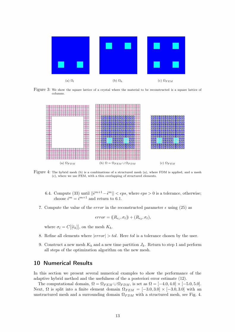
(a) Ωl (b) Ωh (c) ΩFEM
Figure 3: We show the square lattice of a crystal where the material to be reconstructed is a square lattice ofcolumns.
(a) ΩFDM (b) Ω = ΩFEM ∪ ΩFDM (c) ΩFEM
Figure 4: The hybrid mesh (b) is a combinations of a structured mesh (a), where FDM is applied, and a mesh(c), where we use FEM, with a thin overlapping of structured elements.
6.4. Compute (33) until ||εm+1− εm|| < eps, where eps > 0 is a tolerance, otherwise;choose εm = εm+1 and return to 6.1.
7. Compute the value of the error in the reconstructed parameter ε using (25) as
error = ((Rε1 , σε)) + (Rε2 , σε),
where σε = C∣∣[εh]
∣∣, on the mesh Kh.
8. Refine all elements where |error| > tol. Here tol is a tolerance chosen by the user.
9. Construct a new mesh Kh and a new time partition Jk. Return to step 1 and performall steps of the optimization algorithm on the new mesh.
10 Numerical Results
In this section we present several numerical examples to show the performance of theadaptive hybrid method and the usefulness of the a posteriori error estimate (12).
The computational domain, Ω = ΩFEM ∪ ΩFDM , is set as Ω = [−4.0, 4.0] × [−5.0, 5.0].Next, Ω is split into a finite element domain ΩFEM = [−3.0, 3.0] × [−3.0, 3.0] with anunstructured mesh and a surrounding domain ΩFDM with a structured mesh, see Fig. 4.
13

opt.it. 625 nodes 809 nodes 1263 nodes 2225 nodes1 0.0118349 0.0108764 0.0108764 0.0104762 0.0095824 0.00987447 0.00965067 0.009540413 0.00822312 0.00709372 0.00558728 0.007699984 0.00748565 0.00318215 0.00273809 0.003130695 0.00619674 0.002914346 0.005284747 0.004714198 0.00354939
Table 1: ||E − Eobs||L2 on the four adaptively refined meshes in the reconstruction of the lower squares. Thenumber of stored corrections in the quasi-Newton method is m = 15. The computations was performedwith noise level σ = 0 and regularization parameter γ = 0.1.
Between ΩFEM and ΩFDM there is a thin overlap. The space mesh consists of trianglesin ΩFEM , and squares in ΩFDM . In ΩFDM and the overlapping region, the mesh size ish = 0.25 and h = 0.125, in Example 1 and Example 2, respectively. We apply the hybridfinite element/difference method presented in [5] where finite elements are used in ΩFEM
and finite differences in ΩFDM . At the top and bottom boundaries of Ω we use first-orderabsorbing boundary conditions [6]. At the lateral boundaries, mirror boundary conditionsallow us to assume an infinite space-periodic structure in the lateral direction.
For simplicity, we assume that ε = 1 in ΩFDM . Thus, we only need to reconstruct theelectric permittivity ε in ΩFEM .
First, we present tests where we reconstruct the parameter ε inside the domains Ωl andΩh, see Fig. 3-a), b), respectively. Then we present results from the reconstruction of thestructure given in Fig. 3-c).
10.1 Example 1
We start to test the adaptive finite element/difference method on the reconstruction ofthe structures given in Fig. 3a) and 3 b), where our goal is to find the parameter ε in thedomains Ωl and Ωh, respectively.
To generate data at the observation points, we solve the forward problem (3)-(4) with aplane wave pulse given as
∂nE∣∣Γ1
= ((sin (ωt− π/2) + 1)/10), 0 ≤ t ≤ 2π
ω= t1. (34)
The field initiates at the boundary Γ1, in our examples this boundary represents the topboundary of the computational domain, and propagates in normal direction n into Ω.Thetrace of the forward problem is measured at the observation points, placed on the lowerboundary of the computational domain ΩFEM . On Γ1 × (t1, T ] and Γ2 × (0, T ] we usefirst order absorbing boundary conditions, [6]. Here, T = 10.0 and the exact value of theparameter is ε = 4.0 inside the square lattices and ε = 1.0 everywhere else. Since anexplicit scheme, [3], is used to solve the forward and adjoint problems, we choose a timestep τ according to the Courant-Friedrich’s-Levy (CFL) stability condition to provide astable time discretization.
We start Algorithm 1 in Section 9 with initial guess for the parameter being ε = 1.0 atall points in the computational domain ΩFEM and with regularization parameter γ = 0.1.
To reconstruct the lower and upper squares in ΩFEM , computations were performedon the four adaptively refined meshes shown in Fig. 5-a)-d) and Fig. 6-a)-d), respectively.The meshes was refined by computing the residual in the reconstructed parameter ε usingAlgorithm 1.

a) 625 nodes b) 809 nodes c) 1263 nodes d) 2225 nodes1152 elements 1520 elements 2428 elements 4352 elements
e) 8 Q.N. it. f) 4 Q.N. it. g) 5 Q.N. it. h) 6 Q.N.it.625 nodes 809 nodes 1263 nodes 2225 nodes
Figure 5: a)-d) Adaptively refined meshes in the reconstruction of the lower square lattices; e)-h) Reconstructedparameter ε(x) on the correspondingly refined meshes at the final optimization iteration computed withω = 25 and noise level 5% in the observed data.
a) 625 nodes b) 844 nodes c) 1592 nodes d) 1945 nodes1152 elements 1590 elements 3086 elements 3792 elements
e) 9 Q.N. it. f) 10 Q.N. it. g) 10 Q.N. it. h) 10 Q.N.it.625 nodes 844 nodes 1592 nodes 1945 nodes
Figure 6: a)-d) Adaptively refined meshes in the reconstruction of the upper square lattices; e)-h) Reconstructedparameter ε(x) on the correspondingly refined meshes at the final optimization iteration computed withω = 25 and noise level 5% in the observed data.
15

σ, γ 10−5 10−4 10−3 10−2 10−1
0 0.00630036 0.00630536 0.00475773 0.0046071 0.003130691 0.00650122 0.00642409 0.00489691 0.00425432 0.003171473 0.00671315 0.00644934 0.00572624 0.00427946 0.003179555 0.0068622 0.00661597 0.00639352 0.00428971 0.003187037 0.00731985 0.00598225 0.00631647 0.00462458 0.0031228110 0.00672832 0.00618862 0.00673036 0.00467998 0.0033115220 0.00702925 0.00696454 0.00640261 0.00448304 0.0037926
Table 2: ||E−Eobs||L2 for the best reconstruction of the lower squares. We present results for the different noiselevels σ and regularization parameters γ.
σ, γ 10−5 10−4 10−3 10−2 10−1
0 0.00548847 0.00549544 0.00549544 0.00512397 0.003409771 0.00547518 0.00549755 0.00489691 0.0055677 0.003450973 0.00545709 0.00550747 0.00572624 0.0055182 0.00400415 0.00548414 0.00548424 0.00639352 0.0055076 0.003572937 0.00544183 0.00544645 0.00631647 0.00552189 0.0035396610 0.00543398 0.00548045 0.00673036 0.00552947 0.0043000820 0.00561054 0.00561999 0.00640261 0.00566159 0.00386997
Table 3: ||E−Eobs||L2 for the best reconstruction of the upper squares. We present results for the different noiselevels σ and regularization parameters γ.
Table 1 shows the computed L2-norms of E − Eobs for the best reconstruction of theparameter ε in the lower squares, with ω = 25 in (34). We present the norms on thedifferent adaptively refined meshes at each optimization iteration as long as the normsdecrease. The computational tests show that the best results are obtained on the finestmesh, where ||E − Eobs||L2 is reduced by approximately a factor of four between the firstand last optimization iterations.
We performed the tests again, adding relative noise to the observed data. The data withrelative disturbation, or noise, Eσ, is computed by adding a relative error to the computeddata Eobs using the expression
Eσ = Eobs + α(Emax −Emin)σ/100. (35)
Here, α is a random number on the interval [−1; 1], Emax and Emin are the maximal andminimal values of the computed data Eobs, and σ is the noise in percents.
Using the results in Tables 2 and 3 we can conclude that we still have a good reconstruc-tion of the parameter ε, whene noise is added. These results are confirmed in Fig. 5-e)-h)and Fig. 6-e)-h) where we show the parameter field ε(x), at the final optimization itera-tion, computed with ω = 25 and noise level 5% in the observed data. We see that althoughthe qualitative reconstruction on the coarse grid already allows the recovery of the locationof the squares from the limited boundary data, the quantitative reconstruction becomesacceptable only on the refined grids.
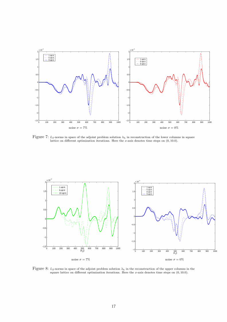
Fig. 7 presents the different L2-norms in space of the reconstruction of the lower squaresof the adjoint problem solution λh over the time interval (0, 10.0]. We show the norms inthe different optimization iterations on the mesh with 2225 nodes without and with adding7% noise in the data. We observe that the norms decreases with an increasing number ofoptimization iterations as it should. We also note that the behavior of the adjoint problemsolution is stable to small perturbations in the data. Fig. 8 shows the similar results forthe reconstruction of the upper squares.
0 100 200 300 400 500 600 700 800 900 1000−2.5
−2
−1.5
−1
−0.5
0
0.5
1
1.5
2x 10
−3
1 opt.it.6 opt.it.9 opt.it
0 100 200 300 400 500 600 700 800 900 1000−2.5
−2
−1.5
−1
−0.5
0
0.5
1
1.5
2x 10
−3
1 opt.it.6 opt.it.9 opt.it
noise σ = 7% noise σ = 0%
Figure 7: L2-norms in space of the adjoint problem solution λh in reconstruction of the lower columns in squarelattice on different optimization iterations. Here the x-axis denotes time steps on (0, 10.0).
0 100 200 300 400 500 600 700 800 900 1000−1.5
−1
−0.5
0
0.5
1
1.5
2x 10
−3
||λh||
1 opt.it.6.opt.it10 opt.it.
0 100 200 300 400 500 600 700 800 900 1000−2
−1.5
−1
−0.5
0
0.5
1
1.5
2x 10
−3
||λh||
1 opt.it5 opt.it.8 opt.it9 opt.it.
noise σ = 7% noise σ = 0%
Figure 8: L2-norms in space of the adjoint problem solution λh in the reconstruction of the upper columns in thesquare lattice on different optimization iterations. Here the x-axis denotes time steps on (0, 10.0).
17

a) 6082 elements b) 8806 elements c) 10854 elements d) 18346 elements
e) 6082 elements f) 8806 elements g) 10854 elements h) 18346 elementsαmax = 1.8804 αmax = 2.2325 αmax = 2.1135 αmax = 2.7559
i) 6082 elements j) 8806 elements k) 10854 elements l) 18346 elementsαmax = 1.7045 αmax = 1.8998 αmax = 1.8966 αmax = 4.0
Figure 9: a)-d) Adaptively refined meshes ; Reconstructed parameter ε(x), indicating domains with a given pa-rameter value: e)-h) in Test 1, i)-l) in Test 2. Here, red color corresponds to the maximum parametervalue on the corresponding meshes, and blue color - to the minimum.
10.2 Example 2
Now we seek to reconstruct the structure of the two-dimensional crystal given in Fig. 3-c).The electric field (34) initiates at the top boundary of the computational domain ΩFDM
and propagates in normal direction n into Ω, with ω = 6. As in Example 1, we use firstorder boundary conditions on Γ1 × (t1, T ] and Γ2 × (0, T ].
First we performed tests where the trace of the forward problem is measured at ob-servation points only on the lower boundary, and then, tests where the reflected trace ismeasured both on the lower and top boundaries of the computational domain ΩFEM .
To achieve better results in the reconstruction, we performed tests letting the incomingwave from the top boundary of ΩFDM be equal to the reflected non-plane wave measuredon the lower boundary of ΩFDM . Thus, to generate data at the observation points, wefirst solve the forward problem (3)-(4) with a plane wave (34) in the time interval t =(0, T ] with the exact value of the parameter being ε = 4.0 inside the square lattices andε = 1.0 everywhere else, and registered the values of the solution of the forward problemat the lower boundary of ΩFDM . Then, using these registered values, a non-plane waveis initialized, starting at t = T and ending at t = 2T . Again, a time step τ is chosenaccording to CFL stability condition.

1 2 3 4 5 60.02
0.04
0.06
0.08
0.1
0.12
0.14
0.16
6082 elements, σ=08806 elements, σ=010854 elements, σ=018346 elements, σ=06082 elements, σ=18806 elements, σ=110854 elements, σ=118346 elements, σ=16082 elements, σ=38806 elements, σ=310854 elements, σ=318346 elements, σ=310854 elements, σ=518346 elements, σ=5
Figure 10: ||E − Eobs|| on adaptively refined meshes. Computations was performed with noise level σ = 0, 1, 3and 5% and with regularization parameter γ = 0.01. Here the x-axis denotes number of optimizationiterations.
1 2 3 4 5 6 7 8 9 10 110
0.05
0.1
0.15
0.2
0.25
6082 elements, σ=08806 elements, σ=010854 elements, σ=018346 elements, σ=010854 elements, σ=718346 elements, σ=710854 elements, σ=1018346 elements, σ=10
Figure 11: ||E−Eobs|| on adaptively refined meshes. Computations was performed with noise level σ = 0, 7 and10% and with regularization parameter γ = 0.01. Here the x-axis denotes number of optimizationiterations.
19

1 2 3 4 5 6 7 80.02
0.04
0.06
0.08
0.1
0.12
0.14
6082 elements, γ=0.18806 elements, γ=0.110854 elements, γ=0.118346 elements, γ=0.16082 elements, γ=0.018806 elements, γ=0.0110854 elements, γ=0.0118346 elements, γ=0.016082 elements, γ=0.0018806 elements, γ=0.00110854 elements, γ=0.00118346 elements, γ=0.0016082 elements, γ=0.00018806 elements, γ=0.000110854 elements, γ=0.000118346 elements, γ=0.0001
Figure 12: ||E − Eobs|| on adaptively refined meshes. Computations was performed with noise level σ = 0%,and with regularization parameters γ = 0.1, 0.01, 0.001, 0.0001, Here the x-axis denotes number ofoptimization iterations.
0 5 10 150.04
0.06
0.08
0.1
0.12
0.14
0.16
6082 elements, γ=0.18806 elements, γ=0.110854 elements, γ=0.118346 elements, γ=0.16082 elements, γ=0.018806 elements, γ=0.0110854 elements, γ=0.0118346 elements, γ=0.016082 elements, γ=0.0018806 elements, γ=0.00110854 elements, γ=0.00118346 elements, γ=0.0016082 elements, γ=0.00018806 elements, γ=0.000110854 elements, γ=0.000118346 elements, γ=0.0001
Figure 13: ||E − Eobs|| on adaptively refined meshes. Computations was performed with noise level σ = 3%,and with regularization parameters γ = 0.1, 0.01, 0.001, 0.0001, Here the x-axis denotes number ofoptimization iterations.
1 2 3 4 5 6 7 8 9 100.02
0.04
0.06
0.08
0.1
0.12
0.14
6082 elements, σ=08806 elements, σ=010854 elements, σ=018346 elements, σ=06082 elements, σ=18806 elements, σ=110854 elements. σ=118346 elements, σ=16082 elements, σ=38806 elements, σ=310854 elements, σ=318346 elements, σ=36082 elements, σ=58806 elements, σ=510854 elements, σ=518346 elements, σ=5
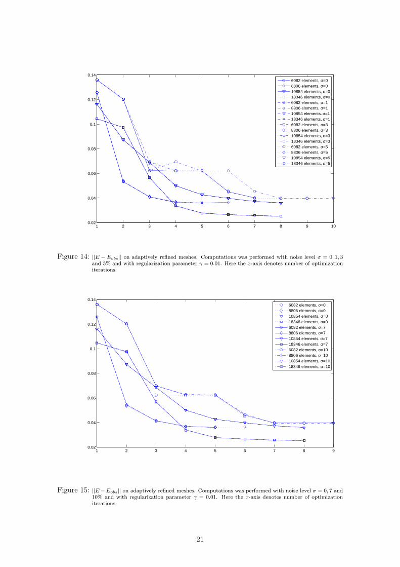
Figure 14: ||E − Eobs|| on adaptively refined meshes. Computations was performed with noise level σ = 0, 1, 3and 5% and with regularization parameter γ = 0.01. Here the x-axis denotes number of optimizationiterations.
1 2 3 4 5 6 7 8 90.02
0.04
0.06
0.08
0.1
0.12
0.14
6082 elements, σ=08806 elements, σ=010854 elements, σ=018346 elements, σ=06082 elements, σ=78806 elements, σ=710854 elements. σ=718346 elements, σ=76082 elements, σ=108806 elements, σ=1010854 elements, σ=1018346 elements, σ=10
Figure 15: ||E−Eobs|| on adaptively refined meshes. Computations was performed with noise level σ = 0, 7 and10% and with regularization parameter γ = 0.01. Here the x-axis denotes number of optimizationiterations.
21

1 2 3 4 5 6 7 80
0.02
0.04
0.06
0.08
0.1
0.12
0.14
0.16
6082 elements, γ=0.16082 elements, γ=0.016082 elements, γ=0.0016082 elements, γ=0.00018806 elements, γ=0.18806 elements, γ=0.018806 elements, γ=0.0018806 elements, γ=0.000110854 elements, γ=0.110854 elements, γ=0.0110854 elements, γ=0.00110854 elements, γ=0.000118346 elements, γ=0.118346 elements, γ=0.0118346 elements, γ=0.00118346 elements, γ=0.0001
Figure 16: ||E − Eobs|| on adaptively refined meshes. We show computational results with noise level σ = 1%and with regularization parameters γ = 0.1, 0.01, 0.001, 0.0001. Here the x-axis denotes number ofoptimization iterations.
1 2 3 4 5 60.02
0.04
0.06
0.08
0.1
0.12
0.14
6082 elements8806 elements10854 elements18346 elements
1 2 3 4 5 6 7 80.02
0.04
0.06
0.08
0.1
0.12
0.14
6082 elements8806 elements10854 elements18346 elements
a) b)
Figure 17: ||E − Eobs|| on adaptively refined meshes. We show computations: on a) with noise level σ =0% and with regularization parameter γ = 0.01 for Test 1; on b) with noise level σ = 1% andwith regularization parameter γ = 0.01 for Test 2. Here the x-axis denotes number of optimizationiterations.

10.2.1 Test1
First we performed the tests where the trace of the incoming wave was measured at theobservation points at the lower boundary of ΩFEM in the time interval (0, T ], and then atthe observation points at the top boundary in the time interval (T, 2T ].
In Fig. 10-11 we present a comparison of the computed L2-norms, ||E − Eobs||L2, de-
pending on the relative noise σ on the different adaptively refined meshes. The normsare plotted as long as they decrease. The relative noise σ in the data is computed usingexpression (35). From these results we conclude that the reconstruction is stable withsmall values of the noise (see Fig. 10), and unstable when adding more than 5% noise tothe data (Fig. 11).
In Fig. 12-13 we show a comparison of the computed L2-norms, ||E−Eobs||L2, depending
on the different regularization parameters γ. We see that we obtain the smallest value of||E − Eobs||L2
with the regularization parameter γ = 0.01, while choosing γ = 0.1 is toolarge and involve too much regularization. The computational tests show that the bestresults are obtained on the finest mesh, where ||E−Eobs||L2 is reduced by approximately afactor of seven between the first and last optimization iterations. Fig. 9-e)-h) correspondto Fig. 17-a) and show the reconstructed parameter field ε(x) at the final optimizationiteration.
10.2.2 Test2
The tests described in this section, was performed by measuring the trace of the incomingwave at the observation points on both the lower and upper boundaries of the computa-tional domain ΩFEM . Thus, we have twice as much information than in the previous test,and we expect to get a more quantitative reconstruction of the structure.
In Fig. 14-15 we present a comparison of the computed L2-norms, ||E − Eobs||L2, de-
pending on the relative noise σ on the different adaptively refined meshes. The normsare plotted as long as they decrease. The relative noise, σ, in the data is computed usingexpression (35). From these results we conclude that the reconstruction is stable on thetwo, three and four times refined meshes, even when 10% noise is added to the data.
In Fig. 16 we show a comparison of the computed L2-norms, ||E−Eobs||L2, depending on
the different regularization parameters γ. We see that the smallest value of ||E −Eobs||L2
is obtained with regularization parameter γ = 0.01, while γ = 0.1 is again too large andinvolve too much regularization. The computational tests show that the best results areobtained on the finest mesh, where ||E − Eobs||L2 is reduced by approximately a factorof seven between the first and last optimization iterations, see Fig. 17-b). Fig. 9-i)-l)correspond to Fig. 17-b), and show the reconstructed parameter field ε(x) at the finaloptimization iteration.
11 Conclusions and Remarks
We have devised an explicit, adaptive hybrid FEM/FDM method for inverse electromag-netic scattering. The method is hybrid in the sense that different numerical methods, finiteelements and finite differences, are used in different parts of the computational domain.We derived an a posteriori estimate for the error in the Lagrangian in the case when wehave first order absorbing [6] and mirror boundary conditions in the formulation of theforward problem. The adaptivity is based on a posteriori error estimates for the associ-ated Lagrangian in the form of space-time integrals of the residuals multiplied by the dualweights. In future work we plan to determine the error in the reconstructed parameter
23

numerically, by solving an associated problem for the Hessian of the Lagrangian. We il-lustrated the usefulness of the adaptive error control on an inverse scattering problem forrecovering the electric permittivity from boundary measured data.

References
[1] R. Becker. Adaptive finite elements for optimal control problems. Habilitationsschrift,2001.
[2] R. Becker and R. Rannacher. An optimal control approach to a posteriori error esti-mation in finite element methods. Acta Numerica, Cambridge University Press, pages1–225, 2001.
[3] L. Beilina. Adaptive finite element/difference methods for time-dependent inverse scat-tering problems. PhD thesis, Department of Computational Mathematics, ChalmersUniversity of Technology, 2003.
[4] L. Beilina and C. Johnson. A posteriori error estimation in computational inversescattering. J. Mathematical models and methods in applied sciences, 15(1):23–37, 2005.
[5] L. Beilina, K. Samuelsson, and K. Åhlander. Efficiency of a hybrid method for thewave equation. In International Conference on Finite Element Methods, Gakuto Inter-national Series Mathematical Sciences and Applications. Gakkotosho CO.,LTD, 2001.
[6] B. Engquist and A. Majda. Absorbing boundary conditions for the numerical simulationof waves. Math. Comp., 31:629–651, 1977.
[7] K. Eriksson, D. Estep, and C. Johnson. Computational Differential Equations. Stu-dentlitteratur, Lund, 1996.
[8] J. Nocedal. Updating quasi-newton matrices with limited storage. J. Mathematical ofComp., 35, N.151:773–782, 1991.
[9] O. Pironneau. Optimal shape design for elliptic systems. Springer Verlag, Berlin, 1984.
25