Embed Size (px)
Citation preview
T H E F I E L D A N A L Y Z E R P R I M E R
T H I R D E D I T I O N
Anders HeijlVincent Michael Patella
Anders HeijlVincent Michael Patella
Essential PerimetryEssential Perimetry
HEIJL &
PATELLA
ESSENTIA
L PER
IMETR
Y TH
E FIELD A
NA
LYZ
ER P
RIM
ER
ISBN 0-9721560-0-3
P/N 54000

The Field Analyzer Primer
Essential Perimetry

The Field Analyzer Primer
Essential Perimetry
T H I R D E D I T I O N
Anders Heijl, MD PhD
Professor and Chairman
Dept of Ophthalmology
Malmö University Hospital
Malmö, Sweden
Vincent Michael Patella, OD
Vice President, Clinical Affairs
Carl Zeiss Meditec Inc.
Dublin, California
Carl Zeiss Meditec Inc.
5160 Hacienda Drive
Dublin, California 94568
925.557.4100
Toll-Free 877.486.7473
Carl Zeiss Meditec AG
Goeschwitzer Strasse 51-52
D-07745 Jena, Germany
Copyright © 2002 Carl Zeiss Meditec Inc.
ISBN 0-9721560-0-3
P/N 54000
Rev. A
August 2002
All rights reserved. No part of this book may be
reproduced or transmitted in any form by any means,
electronic, mechanical, photocopying, recording, or
otherwise, without the prior written permission of
the publisher. For information, contact
Carl Zeiss Meditec.
Editor: Mary Jean Haley
Design: Seventeenth Street Studios
Illustrations: Johan Heijl
Index: Rachel Rice
Contents
v
Foreword, vii
Preface, ix
Introduction: How to Use This Primer, 1
Chapter 1. The Essentials of Perimetry 3
What is Automated Static Perimetry?
When is Perimetry Called For?
What are We Looking For?
Selecting a Test
Interpreting the Results
Chapter 2. Basic Principles of Perimetry 14
Normal and Abnormal Visual Fields
Applications of Perimetric Findings
Computerized Static Perimetry
Issues in Instrument Design
Threshold Testing Strategies
The Perimetrist and the Patient
Preparing the Patient for Testing
Chapter 3. Ordering a Test 25
Choosing a Test Pattern
Choosing a Stimulus Size
Choosing a Test Strategy
Following Glaucomatous Field Loss
Exceptions
SWAP
Testing for Disability, Drivers’ Licenses,
Blepharoplasty, Chloroquine
Chapter 4. STATPAC 44
The Single Field Analysis
Test Reliability Parameters
Analyzing a Series of Tests
Other Printouts
Comparing Older Results with SITA
Chapter 5. Glaucomatous Visual Field Loss 70
Anatomy and Glaucomatous Visual Field Defects
Characteristics of Glaucomatous Field Loss
Diagnosing Glaucomatous Field Loss
Following Glaucomatous Field Loss
Chapter 6. Neurological Visual Field Loss 90
Optic Nerve Disease
Lesions of the Optic Chiasm
Post-Chiasmal Lesions
Chapter 7. Visual Field Loss in Retinal Diseases 114
Chapter 8. Common Patterns of Artifactual Test Results 123
The Untrained Patient and Perimetric Learning
Droopy Lids
Correction Lens Artifacts
The Cloverleaf Field
The “Trigger-Happy” Field
Sudden and False Change
Chapter 9. The Hardware 144
The Bowl
The Optical System
The Central Processor
The Patient Interface
Literature Cited, 148
Index, 157
vi c o n t e n t s
Foreword
vii
the development of perimetry
from manual kinetic methods to the present state of
highly sophisticated automated perimetry, I found it a
particular pleasure to read this excellent textbook. Visual
acuity and visual field share the prize for the most impor-
tant visual functions. Because it measures visual function
outside the fovea, perimetry is essential for diagnosing
and treating glaucoma — as the authors point out — and
it is often useful for retinal and neurological disease. As
with every diagnostic technique, understanding the
background, possibilities, and limitations of perimetry is
vital. This book offers an excellent overview of these
aspects of the technique.
Although both the examination and the evaluation of
perimetric test results have been computerized, the inves-
tigator still needs to interpret the results. It is as an aid to
such interpretation that the authors have written this
book with special emphasis on the Humphrey Field Ana-
lyzer. After describing the essentials and basic principles
of perimetry, the authors discuss the most important
recent changes: faster examination techniques and better
interpretation. These improved techniques have made
automated perimetry into a highly efficient procedure
that can be easily repeated. Because of the inherent vari-
ation of this and every other method, repetition is vital.
Baseline field condition should be based upon a number
of repeated examinations and, similarly, establishing pro-
gression requires a series of examinations. The fast exam-
ination technique makes all this possible and practical, as
well as improving reliability.
All this is explained eloquently and clearly by the
authors, who are among the world’s top experts in the
field. The text is lavishly illustrated, an invaluable feature
in a book on perimetry. The three major subdivisions,
glaucoma, neurological and retinal disease, are well
treated with, of course, special emphasis on glaucoma —
the one disease where we could not do without perime-
try. In any technique artifacts may appear. It is important
to be aware of the artifactual possibilities of perimetry
and to differentiate them from true defects. The conse-
quences of this differentiation are highly important, and
the authors explain them clearly.
This textbook illustrates both the ripeness of the tech-
nique and the capabilities of the authors to explain it in
clear language. Perimetry will continue to be one of the
two essential visual function tests. Nowadays it has been
developed to a stage where it can be used routinely and
repeatedly by every professional and for almost every
patient. Essential Perimetry by Anders Heijl and Vincent
Michael Patella is highly recommended and with great
delight.
—Professor Erik L. Greve
Graveland, The Netherlands
viii f o r e w o r d
Preface
ix
was just gaining acceptance
sixteen years ago when the first edition of this primer was
published. That text emphasized technical and psy-
chophysical topics and contemplated a wide spectrum of
possible testing options. Today, automated perimetry has
become more standardized, and Essential Perimetry
reflects the consensus that has developed by concentrat-
ing on the specific procedures that, over the years, have
been incorporated into the standard of care.
In order to keep the book short and easily approached,
we have of necessity condensed complex ideas in ways
that we hope will be useful to practicing doctors and tech-
nicians. Condensation and summarization require that
judgments be made based upon our own opinions and
clinical experience. For this reason we have also cited the
primary references whenever possible, so that the inter-
ested reader may review the original reports and form his
or her own conclusions.
On a more personal note, this third edition celebrates
twenty years of close collaboration between the authors in
the development of automated perimetry. We wish to
thank our editor, Mary Jean Haley, without whose guid-
ance this text would not exist. And we would like to rec-
ognize the long-term members of the Swedish perimetry
development team: Boel Bengtsson, Peter Åsman, Jonny
Olsson, and Buck Cunningham. Thanks also go to Melissa
Allison, who supported the project through all its ups and
downs, and to Mandy Ambrecht and Cindy Metrose.
—Anders Heijl, MD, PhD
—Vincent Michael Patella, OD
x p r e f a c e
xi t h e e s s e n t i a l s o f p e r i m e t r y
xii e s s e n t i a l p e r i m e t r y
Introduction
How to Use This Primer
1
as an introduction to and
primer on clinical perimetry, particularly computerized
perimetry using the Humphrey® Field Analyzer. It is not
meant to replace classical textbooks on the subject, but
rather is intended as a brief overview for the ophthalmic
resident and as a reference on current Humphrey
perimetry for the busy ophthalmic practitioner.
Because of its purpose, this primer does not follow the
outline of most textbooks. For example, the bare essen-
tials of present-day practical perimetry are covered in a
very condensed form in just a few pages in Chapter 1.
The doctor who only has time for absolutely basic
information may choose just to read Chapter 1 and to
refer to the other chapters only on subjects of special
interest. A more interested reader, or a resident or new
practitioner, may choose to begin with Chapter 1 and
then read the rest of the book in order to understand not
only how to use perimetry but also why.

1The Essentials of Perimetry
3
a quick outline of essential
perimetric facts. The topics presented here are treated
more fully in later chapters.
What is Automated Static Perimetry?
Automated static perimetry is the most important clini-
cal tool for measuring visual function outside the fovea.
Threshold testing involves precise quantification of
visual sensitivity, while suprathreshold testing is used
mainly to establish whether visual function is within the
normal range.
When is Perimetry Called For?
Perimetry is essential in glaucoma management. It is fre-
quently useful in diagnosing and managing neurological
diseases, and it has a role in the diagnosis and treatment
of many retinal diseases. Perimetry is also used to certify
visual function in patients with vision disabilities.
G L A U C O M APerimetry is fundamental in diagnosing and managing
glaucoma. Test results that reproducibly demonstrate
field loss are the most conclusive and concrete means of
establishing a diagnosis of chronic open-angle glaucoma.
The best currently available method of following the pro-
gression of the disease is repeated visual field testing.
Imaging the optic disk or retinal nerve fiber layer is also
important, but it cannot replace perimetry in evaluating
glaucoma patients.
N E U R O L O G I C A L D I S E A S EQuantitative visual field testing is of great value in diag-
nosing and managing neurological disease, but methods
other than quantitative perimetry, such as confrontation
tests, are also sometimes used. When it comes to manag-
ing neurological disease, field testing is not as crucial a
technique as it is in glaucoma management; neuroimag-
ing can often replace perimetry.
R E T I N A L D I S E A S EVisual field testing has a role in diagnosing and treating
many retinal diseases, but direct observation of the fun-
dus through ophthalmoscopy is usually of greater value
in retinal diagnosis. Perimetry then becomes one of
many ancillary tests. In the work-up of retinal diseases,
testing in the area outside the central 30 degrees plays a
somewhat larger role than it does in diagnosing or fol-
lowing glaucoma or neurological disease.
Visual field testing does provide a means for follow-
ing the functional influence of many retinal diseases.
Here the role may sometimes resemble that of field test-
ing in low vision management and visual rehabilitation.
4 e s s e n t i a l p e r i m e t r y
What are We Looking For?
G L A U C O M AT O U S V I S U A L F I E L D L O S S Glaucomatous visual field loss usually occurs first in the
so-called Bjerrum areas of the upper and lower hemi-
fields. These two areas curve around the macula, extend-
ing upward and downward from the blind spot toward
the nasal field in two arcs. Early glaucomatous field
defects most often take the form of relative scotomas, or
small regions of decreased sensitivity. Defects in the nasal
field are particularly common, and sensitivity differences
across the horizontal meridian are often used diagnosti-
cally, particularly in the nasal hemifield (see figures 5-7,
5-8, and 5-9 in Chapter 5). Perimetric testing of glaucoma
patients is seldom done outside the central 30 degree
field because only a small percentage of glaucomatous
defects occurs in the peripheral field alone.
Considerable test-retest variability is a hallmark of
glaucomatous visual field loss; variable reduction of sen-
sitivity occurring in the same area, but not at exactly the
same test point locations, commonly precedes definite
glaucomatous field defects. Although an overall reduc-
tion in sensitivity is frequently seen in combination with
localized loss, homogeneous reduction of sensitivity
alone is almost never seen in glaucoma. It occurs regu-
larly in eyes with media opacities or miosis.
N E U R O L O G I C A L V I S U A L F I E L D L O S S Most neurological field defects are hemianopic, that is,
part of the defect respects the vertical meridian through
the point of fixation. As with glaucoma, the great major-
ity of defects start in the central 30 degrees of the visual
field (see figures in Chapter 6).
R E T I N A L V I S U A L F I E L D L O S S Perimetry is used to test for a large variety of field defects
caused by retinal disease. Such defects are often deep,
5 t h e e s s e n t i a l s o f p e r i m e t r y
have steep borders, and frequently are highly repro-
ducible (figures 7-1 and 7-3).
Selecting a Test
Static computerized perimetric tests are defined in
terms of the locations tested and the algorithm used to
measure the sensitivity at each test point. It is important
for the clinician to choose one standard test and use it for
most field testing. This facilitates developing an in-depth
understanding of the test results and ensures test-to-
test comparability of results, both for a given patient
and among patients.
Standard automated perimetry is usually performed
with one of four similar threshold measuring tests: 30-2
or 24-2 SITA Standard™, or 30-2 or 24-2 SITA Fast™. We
recommend that the clinician select one of these tests to
use as the default test in almost every case. All are high-
efficiency threshold tests that concentrate on the central
field where evidence of most diseases is to be found. They
differ in their test point patterns and in the test algo-
rithms used to perform the threshold measurements.
The 30-2 pattern comprises 76 test point locations
covering the central 30 degree field with a grid of points
6 degrees apart. The 24-2 test point pattern includes 54
test points covering the central field out to 24 degrees,
except nasally where it extends to 30 degrees. It is identi-
cal to the 30-2 pattern except that most of the outermost
ring of stimuli has been removed (fig. 3-1).
SITA Standard is a testing algorithm that offers very
high accuracy and a relatively short test time (four to eight
minutes per eye, depending on the test point pattern used
and the status of the patient’s eye). SITA Fast is a very fast
threshold test (two to six minutes per eye) with a diag-
nostic sensitivity similar to that of the Full Threshold test.
Threshold testing is always a good choice, and in oph-
thalmic clinical settings it is almost always to be pre-
ferred to suprathreshold screening tests. Threshold
6 e s s e n t i a l p e r i m e t r y
It is importantfor the clinician
to choose onestandard test
and use itfor most
field testing.
testing can detect the earliest visual field changes and is
the standard of care for following patients who have
established field loss.
P E R I M E T R I C F O L L O W - U PIt is usually most suitable to follow a patient over time
using the same SITA test that was used for diagnosis.
The same test strategy, that is SITA Standard or SITA
Fast, should be used every time. One very important rea-
son for this is that perimetric test results are affected by
visual fatigue and, as a result, tests of different durations
have different normal threshold values. It is more
informative to compare a series of fields obtained from
the same eye in clinical follow-up if the same algorithm
has been used for all tests.
P E R I P H E R A L F I E L D T E S T I N G Computerized testing of the area outside the central
thirty degrees is rarely performed for diagnostic pur-
poses. The Humphrey perimeter does have, however,
complete facilities for both suprathreshold and threshold
testing in the peripheral field. Because variability is much
larger in the peripheral than in the central visual field,
suprathreshold perimetry may be considerably more
helpful there than it is in the central 30 degree field.
Peripheral suprathreshold testing is frequently used
to certify visual function in drivers and to establish the
level of visual disability for insurance purposes. Note
that the goal in such certification testing is quite distinct
from medical diagnosis, in that the former is done with
very bright stimuli in order to rule out blindness, while
the latter uses more refined methods with the goal of
detecting subtle changes.
Several models of the Humphrey perimeter can also
perform kinetic testing. This feature is more valuable in
the peripheral than in the central field, and its use is
largely confined to tests for disability or driving.
7 t h e e s s e n t i a l s o f p e r i m e t r y
O T H E R T E S T SAlthough the clinician can choose to use a single default
test for over 95% of all field testing in most clinical settings,
other tests are sometimes called for. Short wavelength
automated perimetry (SWAP), also known as blue-yellow
perimetry, can detect glaucomatous visual field loss at ear-
lier stages than standard white-on-white perimetry (John-
son et al. 1993b; Sample et al. 1993; Polo et al. 2000).When
the macula area is the only area of interest, the SITA Stan-
dard or SITA Fast 10-2 tests are to be preferred (fig. 3-4).
In eyes seriously damaged by advanced glaucoma, it may
be necessary to concentrate all testing in a remaining cen-
tral island of the field by shifting to the 10-2 pattern, or to
change to a larger stimulus (see Chapter 3).
The Humphrey perimeter offers a selection of spe-
cific, non-standard functional tests that are sometimes
needed for legal purposes. These tests and their uses may
differ from country to country.
Interpreting the Results
STATPAC™ analysis is automatically applied to the
results of standard Humphrey threshold tests, either to
identify visual fields that fall outside the normal range,
or to identify patients whose vision continues to deteri-
orate. The description below identifies important fea-
tures of the Humphrey Field Analyzer test result
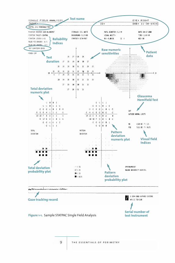
printouts (fig. 1-1). A detailed guide to interpreting
these results is presented in Chapter 4.
D E M O G R A P H I C S A N D T E S T I N G C O N D I T I O N S The patient’s name, identification number, and date of
birth are presented at the top of the printout, along with
the date and time of testing, visual acuity, pupil size, and
eye tested. On some models, the pupil size is measured
and recorded automatically. The printout also shows the
test pattern and test strategy used, the test duration, stim-
ulus size, and the background brightness.
8 e s s e n t i a l p e r i m e t r y
9 t h e e s s e n t i a l s o f p e r i m e t r y
Figure 1-1. Sample STATPAC Single Field Analysis
Test name
Raw numeric sensitivities
Glaucoma Hemifield Test
Visual fieldindices
Pattern deviationnumeric plot
Pattern deviation probability plot
Serial number oftest instrument
Total deviation numeric plot
Total deviation probability plot
Gaze tracking record
Patientdata
Test
duration
Reliability
indices }
An explanation of the reliability indices and other
information shown at the top of the printout is found in
Chapter 4.
D I A G N O S I N G F I E L D L O S STotal Deviation Probability Plots: The total deviation
plots are helpful as diagnostic tools because they high-
light areas of the visual field that fall outside the normal
range, after correcting for the patient’s age. Measured
visual field defects are expressed in terms of the percent-
age of normal subjects that could be expected to have
such a sensitivity. A p< 2% probability symbol, for
instance, indicates that fewer than 2% of normal subjects
would be expected to have such a low sensitivity.
Pattern Deviation Probability Plots: The pattern devi-
ation plots may be thought of as highlighting the local-
ized loss typical in glaucoma or other diseases while
filtering out generalized loss. They flag areas that deviate
significantly from normal, after first correcting for any
overall change in the height of the hill of vision, which is
usually the result of cataract or a small pupil.
Numerical Printouts: Although the numerical print-
outs cannot be rapidly and intuitively interpreted, it can
sometimes be rewarding to study them because they
show the actual measured threshold values upon which
all the other analyses and printouts are based. Decibel
values correlating to the total and pattern deviation
probability plots are shown on the Single Field Analysis
printout described in Chapter 4. While most users find
the probability plots much more informative, these
decibel defect values can sometimes provide further
useful detail.
Grayscale Printouts: These old favorites seem to give an
immediate and easily comprehensible picture of meas-
ured visual field sensitivity, at least in moderate to severe
visual field loss. Significant but shallow field loss may be
10 e s s e n t i a l p e r i m e t r y
unrecognizable in grayscale printouts, however, while
common and non-significant midperipheral reductions
of sensitivity may be overemphasized. For this reason,
one should focus on the probability plots rather than on
the grayscale printouts. The grayscale printout is useful in
highlighting common artifactual field loss such as that
caused by trial lens defects and false positive responses.
Glaucoma Hemifield Test (GHT): The GHT is an expert
system that analyzes test results by comparing local
defects in zones of the upper field with those found in
mirror image zones in the lower hemifield. The GHT
detects glaucomatous visual field loss with both high
sensitivity and high specificity and expresses its analysis
in plain language.
Visual Field Indices: Mean deviation (MD) and pattern
standard deviation (PSD) are not intended for diagnosis,
but they can be helpful in follow-up and also in scientific
studies for dividing groups of eyes into stages of a dis-
ease. Levels of significance are shown next to MD and
PSD values that fall outside the normal range.
F O L L O W - U PPerimetric results in abnormal fields may show consider-
able test-retest variability.When following chronic disease,
a series of fields is usually required in order to be sure that
true visual field changes have occurred. Determining the
stability of abnormal visual fields over time is clinically
important. Identifying progressive loss as early as possible
may be challenging and require some experience.
The glaucoma change probability plots discussed in
Chapter 4 differentiate between random test-retest fluc-
tuations and significant changes in glaucomatous fields.
Alternatively, a series of fields may be qualitatively ana-
lyzed for change using an Overview printout or using
regression analysis of MD.
11 t h e e s s e n t i a l s o f p e r i m e t r y
C O M M O N I N T E R P R E T AT I O N P I T F A L L S Several common, typical patterns of artifactual test
results are worth recognizing. These include fields from
eyes with partial ptosis or prominent eyebrows, fields
with correction lens or lens holder artifacts, fields from
patients with large numbers of false positive errors
(“trigger-happy” fields), and so-called cloverleaf fields.
Patients without previous experience of automated
perimetry sometimes produce seemingly abnormal
results characterized by concentric contraction or mid-
peripheral reduction of sensitivity. These and other fea-
tures of the test results are discussed more fully in
Chapter 8.
12 e s s e n t i a l p e r i m e t r y
13 t h e e s s e n t i a l s o f p e r i m e t r y
In order to interpret visual field test results the user must master and under-
stand many of the topics summarized in this chapter and covered in more
detail in the balance of this book. The following steps are offered as a rough
outline of how to proceed in general when trying to judge whether or not a
visual field test result is normal. Judging whether or not a series of tests repre-
sents medical stability is a more complex matter.
GENERAL GUIDELINES TO INTERPRETING HUMPHREY VISUAL FIELD TEST RESULTS
1. Are the results within the
normal range?
If the disease under consideration is
glaucoma, is the GHT normal or out-
side normal limits?
Are there patterns of loss on the
probability plots, especially the pat-
tern deviation probability plot, that
are clearly outside normal limits?
2. If the results are not within the
normal range, are they definitive?
Patterns of loss that are clearly con-
sistent with other findings have
increased credibility. These include
the following:
Clear nasal step or arcuate sco-
toma correlating well with optic
nerve head observations
Clear hemianopia
Loss clearly correlating with oph-
thalmoscopic findings
Loss clearly correlating with the
clinical history
Patterns of loss that are not well
defined, or that are not supported
by other observations, may require
retesting or further evaluation
3. Are there any red flags that sug-
gest the test results should be
reconsidered?
Signs of excessive false positive
responses, trial lens defects, or
other artifact, as outlined in
Chapter 8
False positive rate of 15% or higher
Fixation losses exceeding 20%
2Basic Principles of Perimetry
14
is most effective when
the user is familiar with the basic principles underlying
its operation and use.
Normal and Abnormal Visual Fields
The normal field of vision extends more than 90 degrees
temporally, 60 degrees nasally and superiorly, and about
70 degrees inferiorly, but most diagnostic visual field
testing concentrates on the area within 30 degrees of fix-
ation.Visual sensitivity is greatest at the very center of the
field and decreases toward the periphery. The visual field
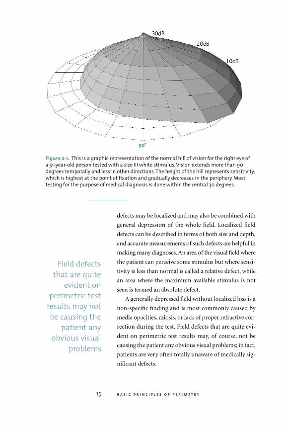
is commonly represented as a hill, or island of vision (fig.
2-1). The height of the normal hill of vision varies with
age, the general level of ambient light, stimulus size, and
stimulus duration.
Field defects characteristic of certain diseases will be
discussed later. For the moment it should simply be said
that a field defect is any statistically and clinically signif-
icant departure from the normal hill of vision. Field
defects may be localized and may also be combined with
general depression of the whole field. Localized field
defects can be described in terms of both size and depth,
and accurate measurements of such defects are helpful in
making many diagnoses. An area of the visual field where
the patient can perceive some stimulus but where sensi-
tivity is less than normal is called a relative defect, while
an area where the maximum available stimulus is not
seen is termed an absolute defect.
A generally depressed field without localized loss is a
non-specific finding and is most commonly caused by
media opacities, miosis, or lack of proper refractive cor-
rection during the test. Field defects that are quite evi-
dent on perimetric test results may, of course, not be
causing the patient any obvious visual problems; in fact,
patients are very often totally unaware of medically sig-
nificant defects.
15 b a s i c p r i n c i p l e s o f p e r i m e t r y
Figure 2-1. This is a graphic representation of the normal hill of vision for the right eye of
a 51-year-old person tested with a size III white stimulus. Vision extends more than 90
degrees temporally and less in other directions. The height of the hill represents sensitivity,
which is highest at the point of fixation and gradually decreases in the periphery. Most
testing for the purpose of medical diagnosis is done within the central 30 degrees.
90°
Field defectsthat are quite
evident on perimetric test
results may notbe causing the
patient anyobvious visual
problems.
Applications of Perimetric Findings
This book primarily addresses the application of perime-
try to diagnostic decision making. The goal of perimetry
in such cases is to obtain information important to the
decision at hand, and perimetric testing is directed
toward those portions of the visual field that are most
likely to be informative about the presence or stability of
a particular disease. Such examinations generally involve
careful measurement of threshold sensitivity at various
locations in the field in order to identify subtle changes.
Perimetry may also be used to determine the extent of
remaining visual function for insurance purposes or in
order for the patient to qualify for a driver’s license. In
such instances, subtle defects are often ignored, as they
are unlikely to affect visual performance. Most com-
monly, these examinations are performed by presenting
a very bright stimulus throughout the tested area—a
stimulus that would not be missed unless there is rather
profound loss of vision.
Computerized Static Perimetry
Computerized static perimetry has been the clinical
standard of care for at least fifteen years. Before that,
kinetic perimetry was usually performed using the
Goldmann manual perimeter. Over the years a number
of researchers have reported computerized static
perimetry to be superior to various methods of expertly
performed kinetic perimetry (Lynn 1969; Heijl 1976;
Katz et al. 1995).
Computerized threshold static perimetry involves
determining the dimmest stimulus that can be seen at a
number of pre-determined test point locations. Static
perimetry was performed manually long before com-
puters were widely available, but because of the complex-
ity of the technique and the difficulty of keeping track of
16 e s s e n t i a l p e r i m e t r y
multiple patient responses, the method was used mainly
in research settings. Computerization made it possible to
automate complex thresholding algorithms and to keep
track of patient responses at all of the points under exam-
ination. Improvements in computer processor speed later
facilitated the automation of increasingly complex—and
increasingly efficient—methods of data acquisition, such
as SITA, and data analysis that previously had been
impractical in clinical care.
Another important benefit of computerization is that
it allowed testing to be standardized, which has greatly
improved test comparability between clinics and around
the world. Indeed, standardization in perimetry now is so
highly valued that most clinics and hospitals have stan-
dardized on Humphrey perimetry and on a narrow range
of tests—usually 30-2 or 24-2 SITA threshold tests.
Issues in Instrument Design
A basic perimeter might be characterized as an instru-
ment that can present a stimulus of known size and
brightness against a known background for a known
amount of time in a known location in the visual field.
Efficient visual field testing can be achieved only if each
of these factors and others are carefully chosen.
S T I M U L U S S I Z E A N D I N T E N S I T YThe Humphrey perimeter uses projected stimuli. The
standard white stimuli can be varied in intensity over a
range of 5.1 log units (51 decibels) between 0.08 and
10,000 apostilbs (asb). The decibel (dB) value refers to
retinal sensitivity, rather than to stimulus intensity, with
0 dB corresponding to the maximum brightness that
the perimeter can produce (10,000 asb) and 51 dB to
0.08 asb (fig. 2-2). In standardized testing with a size III
white stimulus, the dimmest stimulus that can be seen
foveally by a young, well-trained observer is at most
17 b a s i c p r i n c i p l e s o f p e r i m e t r y
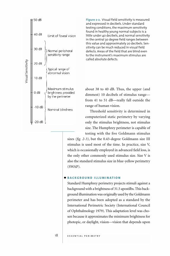
about 38 to 40 dB. Thus, the upper (and
dimmest) 10 decibels of stimulus range—
from 41 to 51 dB—really fall outside the
range of human vision.
Threshold sensitivity is determined in
computerized static perimetry by varying
only the stimulus brightness, not stimulus
size. The Humphrey perimeter is capable of
testing with the five Goldmann stimulus
sizes (fig. 2-3), but the 0.43-degree Goldmann size III
stimulus is used most of the time. In practice, size V,
which is occasionally employed in advanced field loss, is
the only other commonly used stimulus size. Size V is
also the standard stimulus size in blue-yellow perimetry
(SWAP).
B A C K G R O U N D I L L U M I N AT I O NStandard Humphrey perimetry projects stimuli against a
background with a brightness of 31.5 apostilbs. This back-
ground illumination was originally used by the Goldmann
perimeter and has been adopted as a standard by the
International Perimetric Society (International Council
of Ophthalmology 1979). This adaptation level was cho-
sen because it approximates the minimum brightness for
photopic, or daylight, vision—vision that depends upon
18 e s s e n t i a l p e r i m e t r y
Vis
ua
l S
en
siti
vit
y
Figure 2-2. Visual field sensitivity is measured
and expressed in decibels. Under standard
testing conditions, the maximum sensitivity
found in healthy young normal subjects is a
little under 40 decibels, and normal sensitivity
in the central 30 degree field ranges between
this value and approximately 20 decibels. Sen-
sitivity can be much reduced in visual field
defects. Areas of the field that are blind even
to the instrument’s maximum stimulus are
called absolute defects.
IV
V
III
Typical
blind
spot
size
Blind spot check
stimuli,
sizes I through V
III
retinal cone function rather than on rods. The advantage
of testing the photopic visual system is that visibility
depends more on object contrast than on absolute bright-
ness as it does in rod vision. Small changes in pupil size or
clarity of media have little effect on test results, and small
irregularities in background brightness can be remedied
by commensurate adjustments in stimulus brightness to
keep stimulus contrast at the desired level.
S T I M U L U S D U R AT I O N Stimulus duration significantly affects the visibility of
stimuli when they last only a very short time. Thus, a stim-
ulus lasting 0.002 seconds is roughly twice as visible as
one lasting only 0.001 second. On the other hand, it is just
as easy to see a spot that is shown for one second as it is to
see one that is shown for three seconds. The principle of
temporal summation holds that for very short durations,
the visibility of a stimulus increases with duration; when
19 b a s i c p r i n c i p l e s o f p e r i m e t r y
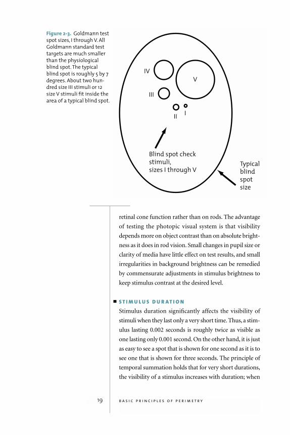
Figure 2-3. Goldmann test
spot sizes, I through V. All
Goldmann standard test
targets are much smaller
than the physiological
blind spot. The typical
blind spot is roughly 5 by 7
degrees. About two hun-
dred size III stimuli or 12
size V stimuli fit inside the
area of a typical blind spot.
a stimulus lasts more than about 0.5 seconds, on the other
hand, its visibility is basically independent of duration
(Lynn 1969; Aulhorn and Harms 1972).
The Humphrey perimeter uses a stimulus duration of
200 milliseconds (ms), which is long enough for visibil-
ity to be little affected by small variations in duration, but
still shorter than the latency for voluntary eye move-
ments (about 250 ms). As a result, the patient does not
have time to see a stimulus in the peripheral visual field
and look toward it (International Council of Ophthal-
mology 1979).
S T I M U L U S L O C AT I O N A N D F I X AT I O N M O N I T O R I N GIn order to map visual field sensitivity accurately it is nec-
essary to know where on the retina each stimulus is pre-
sented. It is not difficult to calibrate where the instrument
itself shows the stimulus, but knowing where the patient
is looking at the moment of stimulus presentation can be
complex. Fortunately, most patients fixate with rather
high precision, and the problem of proper stimulus loca-
tion has primarily become one of identifying those few
patients whose gaze is so unsteady that they should be re-
instructed on proper fixation technique.
The original Humphrey perimeter and one of the
current models rely upon the Heijl-Krakau blind spot
monitoring technique rather than a gaze tracker. This
method provides an index of the quality of patient fixa-
tion during an examination by periodically presenting
stimuli in the blind spot. Positive responses indicate poor
fixation. Because the normal blind spot is about six
degrees in diameter, fixation shifts of half of that
amount—about three to four degrees—can be detected.
One disadvantage of this method is that fixation checks
add to the test time and therefore can be made only occa-
sionally during the test.
The gaze tracker on recent models of the Humphrey
perimeter measures gaze direction with a precision of
20 e s s e n t i a l p e r i m e t r y
In order to mapvisual field sensitivity
accurately it isnecessary to
know where onthe retina each
stimulus is presented.
about one degree and records a measurement each time
a stimulus is presented. The gaze tracking results are
shown on the video screen during testing and are printed
at the bottom of the test results printout. On the gaze
printout, lines extending upward indicate the amount
of gaze error at each stimulus presentation, with full scale
indicating gaze errors of 10 degrees or more. Lines
extending downward indicate that the instrument was
unsuccessful in measuring gaze direction during that
particular stimulus presentation. (See Chapter 4 for fur-
ther discussion.)
Threshold Testing Strategies
The objective of static threshold perimetry is to deter-
mine the minimum stimulus that can be seen at each
tested location. Such findings are always subject to some
variability because patients make mistakes and because
the visual system itself is subject to certain variabilities.
Successful strategies balance time efficiency with provi-
sions to counteract such errors.
All Humphrey strategies start testing at a single loca-
tion in each quadrant of the visual field. If a stimulus is
seen, subsequent stimuli at that location are dimmed one
step at a time—usually by 3 or 4 decibels—until they are
no longer seen. Conversely, if the initial stimulus is not
seen, then subsequent presentations are made brighter in
steps until the patient presses the response button. Some
strategies repeat this process for confirmation of the find-
ing, either using the same step size, or perhaps a smaller
step, such as 2 dB. Testing is then expanded to other test
point locations, until threshold sensitivities have been
determined throughout the tested area.
In the early days of automated perimetry, threshold
testing frequently took twenty minutes or more per eye
because the test strategies were not very efficient. Effi-
ciency was soon improved by using test results at a meas-
ured point to determine the initial stimulus brightness at
21 b a s i c p r i n c i p l e s o f p e r i m e t r y
adjacent points, and by measuring patient reaction times
in order to make small adjustments to the pace of the test.
Even with these improvements, testing times averaged 15
minutes and were sometimes as long as 20 minutes.
The more recent SITA methods take advantage of
new mathematical techniques to achieve dramatic reduc-
tions in testing time without sacrificing accuracy. First,
the patented SITA strategies are based on a complex
model of the visual field that allows for more accurate
choices of the initial stimulus brightness and more com-
plete use of all available information when calculating
threshold sensitivity. New mathematical modeling also
allows SITA to make much more complete use of
response time information, resulting in a test pace that is
almost completely determined by the patient instead of
the machine. Patients with slow reactions get slowly
paced tests, but more often, a SITA test ends up running
at a fairly rapid and interesting pace because most
patients are quite capable of moving more quickly than
the older strategies allowed.
SITA strategies gain further efficiency by ceasing to
present stimuli at a given location when predetermined
levels of testing certainty are reached, based upon the sta-
tistical consistency of patient responses. This consistency
calculation shortens test time when reliably consistent
responses are given, and extends it when there still is
uncertainty (Bengtsson et al. 1997). The primary differ-
ence between the SITA Standard and SITA Fast strategies
is the amount of certainty required before testing can be
stopped (Bengtsson and Heijl 1998). Finally, SITA
increases efficiency by keeping a complete record of the
location, brightness, and timing of every stimulus pre-
sented—a complete test timeline. This timeline is ana-
lyzed automatically to reconsider the complete pattern of
patient responses to correct for patient errors and to
come to a more precise determination of threshold sen-
sitivities. The overall effect of these efficiency improve-
ments is that SITA Standard and SITA Fast reduce testing
22 e s s e n t i a l p e r i m e t r y
SITA Standardcan complete a
30-2 test inabout half
the time of theHumphrey
Full Thresholdstrategy with
no loss of reproducibility
or sensitivity toglaucomatous
loss.
time by 50% relative to the strategies they replace, with-
out loss of diagnostic information (refer ahead to figures
3-3a, 3-3b, and 3-3c).
The Perimetrist and the Patient
Manual perimetry required great skill because the
perimetrist had to understand and perform all testing
strategies with no assistance from the instrument itself.
Even though the Humphrey Field Analyzer is programmed
with highly refined testing and analysis methods, the tech-
nician continues to play a central role. Without proper
patient management and instruction, the results of peri-
metric examinations are often of poor quality.
It is particularly important to tell the patient what to
expect during the test. Perimetrists who have under-
gone visual field testing themselves will be better pre-
pared to brief patients. The perimetrist should explain
the patient’s task, show him or her what the stimulus
will look like, where it might appear, how long the test
will last, when blinks are allowed, how to sit, how to
pause the test, and so on. The patient should under-
stand that more than half of the stimuli shown in a
threshold test will be too dim to be seen, and that the
stimuli that are seen are likely to be barely visible. Fur-
ther, the perimetrist must be available at least periodi-
cally during the test to reassure the patient and to see
that he or she is still in proper position.
Patients who understand this and who are tested by
staff members with a positive attitude toward visual
field testing will have few problems with modern, time-
efficient threshold perimetry. It is easy to help patients
recognize the value of perimetry in determining their
level of treatment, and they will be happy to do visual
field testing once or twice a year in order to see that effec-
tive treatment is instituted and to assure that unnecessary
treatments are avoided.
23 b a s i c p r i n c i p l e s o f p e r i m e t r y
Preparing The Patient For Testing
In addition to making sure the patient understands the
test, successful perimetry requires good physical condi-
tions for the test. Refractive blur reduces visual sensitiv-
ity to perimetric stimuli, and it is standard practice to
provide trial lens correction when testing the central
visual field. One diopter of refractive blur in an undilated
patient will produce a little more than one decibel of
depression of the hill of vision when testing with a Gold-
mann size III stimulus (Weinreb and Perlman 1986;
Heuer et al. 1987; Herse 1992).
The nominal testing distance of the Humphrey HFA
II perimeter is 30 cm, and fully presbyopic patients are
therefore provided with +3.25 diopter near additions
relative to their distance refraction. Patients who are less
than fully presbyopic are given smaller additions, either
according to standard age-based correction tables pro-
grammed into the perimeter or based upon clinical judg-
ment. Usually, all refractive correction is accomplished
using standard 37 mm trial lenses held in place by a trial
lens holder attached to the perimeter, but correction may
be done with the patient's own spectacles, as long as they
are single vision lenses or contact lenses. Testing outside
of the central visual field is done without trial lens cor-
rection because the trial lenses and their holder would
restrict the peripheral vision and produce artifactual
visual field loss.
One eye is tested at a time, and the eye that is not
being tested is covered with a patch. The patient is seated
in front of the instrument, and chair height and instru-
ment height should be adjusted for patient comfort.
Proper comfort is more important in perimetry than,
for instance, in slit lamp biomicroscopy because the
examination takes longer and because the patient may be
supervised only occasionally during the test.
24 e s s e n t i a l p e r i m e t r y
Without properpatient man-agement and
instruction,the results of
perimetricexaminations
are often of poor quality.
3Ordering a Test
25
is needed, a 30-2 or
24-2 SITA Standard threshold test using a size III white
stimulus is the best choice in most cases. This chapter
explains why this is so, and then discusses the exceptions
to this rule.
Choosing a Test Pattern
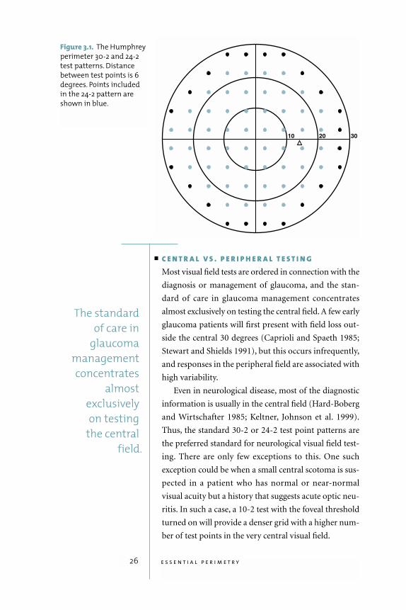
The Humphrey Field Analyzer 30-2 test pattern meas-
ures visual sensitivity at 76 locations within 30 degrees of
fixation—the area commonly referred to as the central
visual field. The 24-2 test pattern consists of the 54 most
central test locations of the 30-2 pattern (fig. 3-1). At one
time many doctors, and many university centers, made
the 24-2 pattern their standard test because there was evi-
dence that little diagnostic information was lost and con-
siderable testing time was saved by testing only 54 points
rather than 76 (Alexander et al. 1995). New testing algo-
rithms, especially SITA, have now reduced test times so
much that there is much less incentive to test fewer points,
and the 30-2 pattern gives more test locations from which
disease progression may be judged. It may also be more
useful in following established field loss.
26 e s s e n t i a l p e r i m e t r y
C E N T R A L V S . P E R I P H E R A L T E S T I N GMost visual field tests are ordered in connection with the
diagnosis or management of glaucoma, and the stan-
dard of care in glaucoma management concentrates
almost exclusively on testing the central field. A few early
glaucoma patients will first present with field loss out-
side the central 30 degrees (Caprioli and Spaeth 1985;
Stewart and Shields 1991), but this occurs infrequently,
and responses in the peripheral field are associated with
high variability.
Even in neurological disease, most of the diagnostic
information is usually in the central field (Hard-Boberg
and Wirtschafter 1985; Keltner, Johnson et al. 1999).
Thus, the standard 30-2 or 24-2 test point patterns are
the preferred standard for neurological visual field test-
ing. There are only few exceptions to this. One such
exception could be when a small central scotoma is sus-
pected in a patient who has normal or near-normal
visual acuity but a history that suggests acute optic neu-
ritis. In such a case, a 10-2 test with the foveal threshold
turned on will provide a denser grid with a higher num-
ber of test points in the very central visual field.
The standard of care in
glaucoma managementconcentrates
almostexclusively on testing
the central field.
Figure 3.1. The Humphrey
perimeter 30-2 and 24-2
test patterns. Distance
between test points is 6
degrees. Points included
in the 24-2 pattern are
shown in blue.
Occasionally, peripheral testing is done to rule out
retinal detachments, or to differentiate between detach-
ment and retinoschisis in eyes that cannot be well visu-
alized ophthalmoscopically, but this is the exception
rather than the rule (see Chapter 7).
Choosing a Stimulus Size
Computerized static perimetry has established the Gold-
mann size III, white stimulus as the standard. It is small
enough at 0.43 degrees in diameter to be used even in
fairly detailed examinations, and large enough to be vis-
ible when the patient’s refractive correction is not quite
perfect. Normative data and statistical analysis packages
for standard perimetry using white stimuli are based
upon the Goldmann size III stimulus.
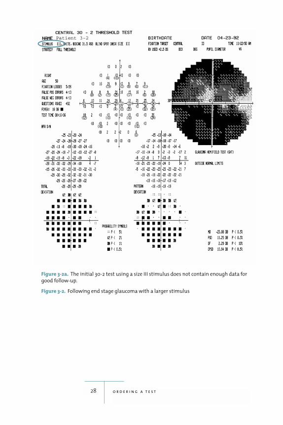
In cases of advanced glaucoma, many or most points
may show absolute defects with size III stimuli, jeopard-
izing perimetric follow-up with a central 24-2 or 30-2
test. One can then switch to the size V stimulus, which is
four times the diameter of size III. Testing with size V
stimuli will result in sensitivity levels that are 5 to 10
decibels higher than those found using size III, often
extending the available sensitivity range and making it
possible to follow such patients (figures 3-2a, 3-2b). It
should be noted that if the size V stimulus is used, one no
longer has access to several of the analytical follow-up
tools available for the standard size III tests.
Choosing a Test Strategy
T H R E S H O L D T E S T I N GIn general, threshold testing provides more diagnostic
information than suprathreshold testing. The aim of a
threshold test is to quantify the patient’s visual sensitiv-
ity at each test point. The result is a set of sensitivity val-
ues representing the minimum brightness the patient
can see at each tested point.
27 o r d e r i n g a t e s t
28 o r d e r i n g a t e s t
Figure 3-2a. The initial 30-2 test using a size III stimulus does not contain enough data for
good follow-up.
Figure 3-2. Following end stage glaucoma with a larger stimulus
Patient 3-2
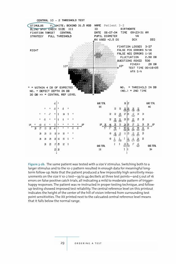
29 o r d e r i n g a t e s t
Figure 3-2b. The same patient was tested with a size V stimulus. Switching both to a
larger stimulus and to the 10-2 pattern resulted in enough data for meaningful long-
term follow-up. Note that the patient produced a few impossibly high sensitivity meas-
urements on the size V 10-2 test—39 to 44 decibels at three test points—and 5 out of 16
errors on false positive catch trials, all indicating a mild to moderate pattern of trigger-
happy responses. The patient was re-instructed in proper testing technique, and follow-
up testing showed improved test reliability. The central reference level on this printout
indicates the height of the center of the hill of vision inferred from surrounding test
point sensitivities. The XX printed next to the calcuated central reference level means
that it falls below the normal range.
Patient 3-2
The patented SITA thresholding strategies available
on recent Humphrey Field Analyzer models are much
faster than the older strategies they replace. SITA Standard
can complete a 30-2 test in about half the time of the
Humphrey Full Threshold strategy with no loss of repro-
ducibility or sensitivity to glaucomatous loss (Inazumi et
al. 1998; Bengtsson and Heijl 1999a; Wild, Pacey, Han-
cock, Cunliffe 1999; Wild, Pacey, O’Neill, Cunliffe 1999;
Remky and Arend 2000; Sharma et al. 2000). SITA Stan-
dard has also been found to shorten testing time without
jeopardizing the clarity of results in children (Donahue
and Porter 2001). SITA Fast takes about half the time of
FastPac and provides the same performance (Bengtsson
and Heijl 1998; Wild, Pacey, Hancock, Cunliffe 1999;
Wild, Pacey, O’Neill, Cunliffe 1999). The SITA strategies
have clear advantages over the older strategies and should
be used whenever available. SITA Standard is more precise
and more able to correct for patient errors, but it is not
quite as quick as SITA Fast (figures 3-3a, 3-3b, 3-3c). SITA
Fast may best be used with younger patients or with those
who have experience with threshold perimetry.
S U P R AT H R E S H O L D T E S T I N GSuprathreshold testing and threshold testing have dif-
ferent goals. Suprathreshold testing, also referred to as
screening, is intended to establish whether or not sensi-
tivity is abnormally low at any location in the visual field.
Because a suprathreshold test presents the patient with
fairly bright stimuli that should be seen if vision is nor-
mal, it is easy to use with patients who have never been
tested before. Before the advent of the current, efficient
threshold testing methods, suprathreshold tests took
considerably less time than threshold tests. Suprathresh-
old tests, however, do not provide quantitative data, and
they are not as sensitive to early glaucomatous field loss
as threshold tests (Mills et al. 1994). As a result, supra-
threshold testing is used less often in glaucoma diagno-
sis now that highly efficient threshold tests can be done
30 e s s e n t i a l p e r i m e t r y
SITA Fast takesabout half the
time of FastPacand provides
the same performance.
31 o r d e r i n g a t e s t
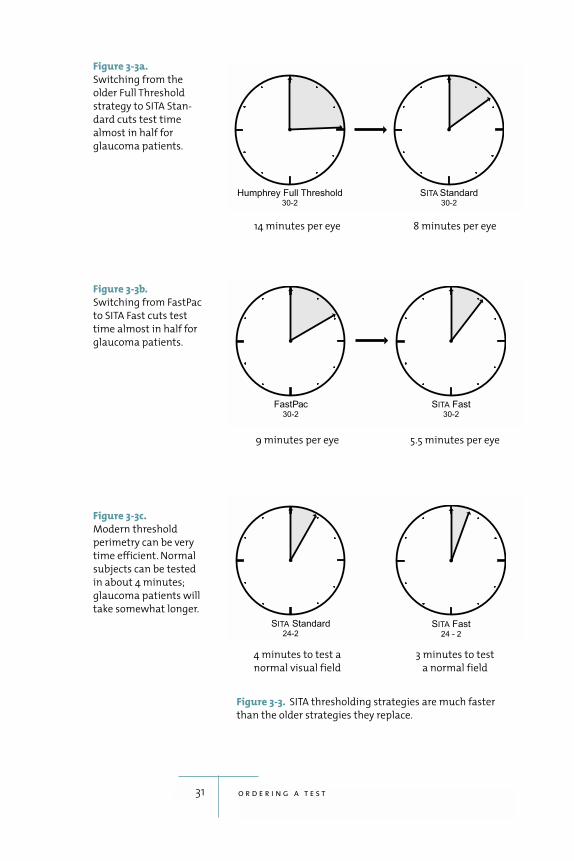
Figure 3-3a.
Switching from the
older Full Threshold
strategy to SITA Stan-
dard cuts test time
almost in half for
glaucoma patients.
Figure 3-3b.
Switching from FastPac
to SITA Fast cuts test
time almost in half for
glaucoma patients.
Figure 3-3c.
Modern threshold
perimetry can be very
time efficient. Normal
subjects can be tested
in about 4 minutes;
glaucoma patients will
take somewhat longer.
14 minutes per eye 8 minutes per eye
9 minutes per eye 5.5 minutes per eye
4 minutes to test a
normal visual field
3 minutes to test
a normal field
Figure 3-3. SITA thresholding strategies are much faster
than the older strategies they replace.
in almost the same time. If suprathreshold screening for
glaucomatous field loss is conducted, the 64-point cen-
tral test pattern using the age-related or threshold-related
strategies is a good choice.
Suprathreshold testing can be sensitive to neurologi-
cally based field loss (Siatkowsky et al. 1996), and the
76-point age-related screening test pattern provides a
useful alternative to the 24-2 or 30-2 threshold tests.
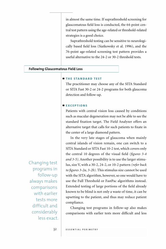
Following Glaucomatous Field Loss
T H E S T A N D A R D T E S TThe practitioner may choose any of the SITA Standard
or SITA Fast 30-2 or 24-2 programs for both glaucoma
detection and follow-up.
E X C E P T I O N SPatients with central vision loss caused by conditions
such as macular degeneration may not be able to see the
standard fixation target. The Field Analyzer offers an
alternative target that calls for such patients to fixate in
the center of a large diamond pattern.
In the very late stages of glaucoma when mainly
central islands of vision remain, one can switch to a
SITA Standard or SITA Fast 10-2 test, which covers only
the central 10 degrees of the visual field (figures 3-4
and 3-5). Another possibility is to use the larger stimu-
lus, size V, with a 30-2, 24-2, or 10-2 pattern (refer back
to figures 3-2a, 3-2b). This stimulus size cannot be used
with the SITA algorithm, however, so one would have to
use the Full Threshold or FastPac algorithms instead.
Extended testing of large portions of the field already
known to be blind is not only a waste of time, it can be
upsetting to the patient, and thus may reduce patient
compliance.
Changing test programs in follow-up also makes
comparisons with earlier tests more difficult and less
32 e s s e n t i a l p e r i m e t r y
Changing testprograms in
follow-upalways makescomparisons
with earliertests more
difficult andconsiderably
less exact.
33 o r d e r i n g a t e s t
exact. When switching from the earlier standard
Humphrey threshold tests, Full Threshold or FastPac, to
the corresponding newer, faster SITA Standard or SITA
Fast, the most relevant comparisons can be made by
focussing on probability plots (see Comparing SITA
Results with Older Strategies in Chapter 4).
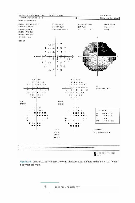
S W A P Short wavelength automated perimetry (SWAP), also
known as blue-yellow perimetry, is a specialized tech-
nique in which blue, Goldmann size V stimuli are pre-
sented on a bright (100 Cd/m2) yellow background
(Wild 2001; Johnson 2002; Solimen et al. 2002) (fig. 3-6).
The yellow background serves to reduce the responsive-
ness of the red and green cone systems so that the blue
stimuli are seen primarily by the blue cone system.
Three prospective clinical trials have found that
SWAP detects glaucomatous visual field loss at an earlier
stage than conventional methods (Johnson et al. 1993a;
Sample et al. 1993; Polo et al. 2002). Similarly, three
prospective studies have found that SWAP detects pro-
gression of field loss in glaucoma patients earlier than
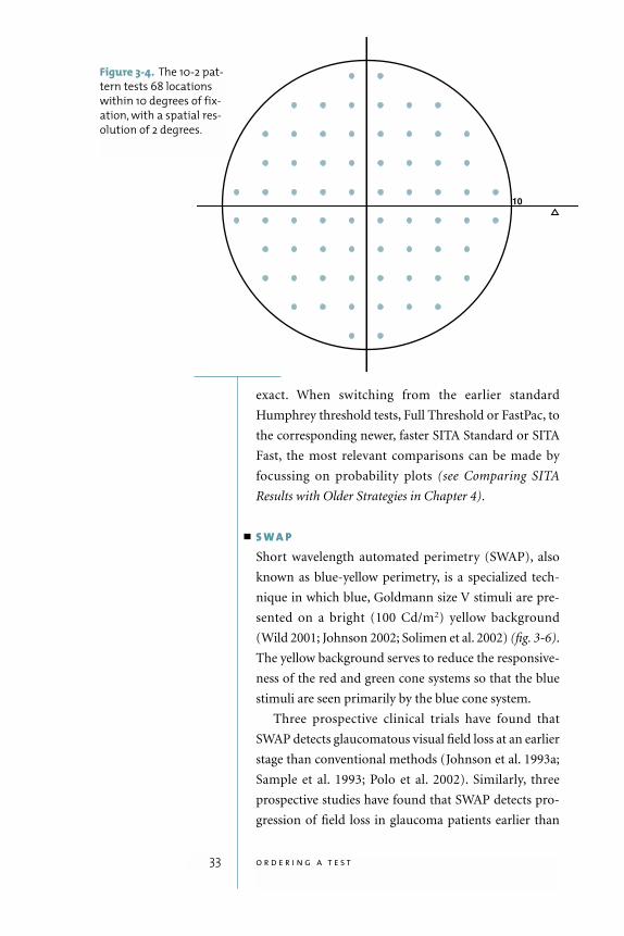
Figure 3-4. The 10-2 pat-
tern tests 68 locations
within 10 degrees of fix-
ation, with a spatial res-
olution of 2 degrees.
34 e s s e n t i a l p e r i m e t r y
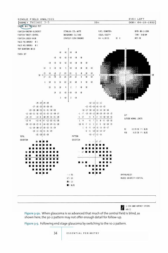
Figure 3-5a. When glaucoma is so advanced that much of the central field is blind, as
shown here, the 30-2 pattern may not offer enough detail for follow-up.
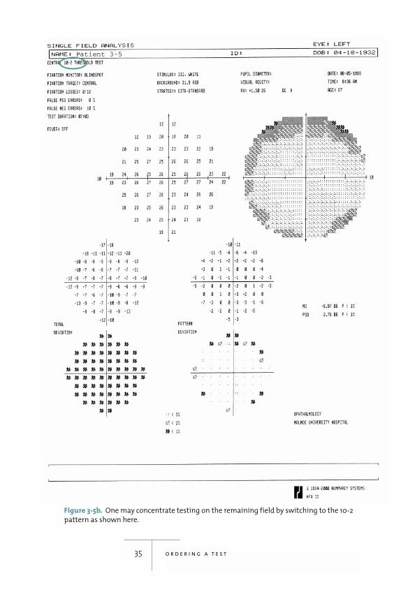
Figure 3-5. Following end stage glaucoma by switching to the 10-2 pattern.
Patient 3-5
35 o r d e r i n g a t e s t
Figure 3-5b. One may concentrate testing on the remaining field by switching to the 10-2
pattern as shown here.
Patient 3-5
36 e s s e n t i a l p e r i m e t r y
Figure 3-6. Central 24-2 SWAP test showing glaucomatous defects in the left visual field of
a 60-year-old man.
Patient 3-6
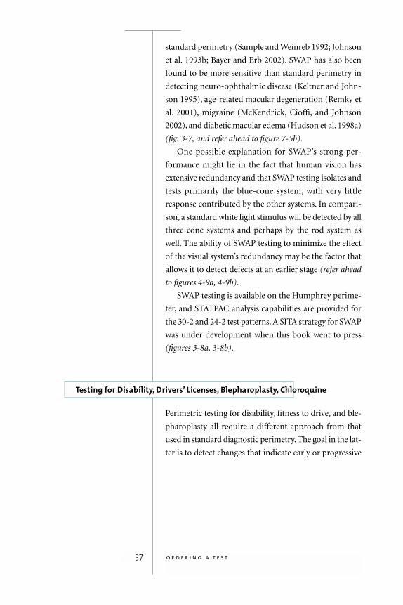
standard perimetry (Sample and Weinreb 1992; Johnson
et al. 1993b; Bayer and Erb 2002). SWAP has also been
found to be more sensitive than standard perimetry in
detecting neuro-ophthalmic disease (Keltner and John-
son 1995), age-related macular degeneration (Remky et
al. 2001), migraine (McKendrick, Cioffi, and Johnson
2002), and diabetic macular edema (Hudson et al. 1998a)
(fig. 3-7, and refer ahead to figure 7-5b).
One possible explanation for SWAP’s strong per-
formance might lie in the fact that human vision has
extensive redundancy and that SWAP testing isolates and
tests primarily the blue-cone system, with very little
response contributed by the other systems. In compari-
son, a standard white light stimulus will be detected by all
three cone systems and perhaps by the rod system as
well. The ability of SWAP testing to minimize the effect
of the visual system’s redundancy may be the factor that
allows it to detect defects at an earlier stage (refer ahead
to figures 4-9a, 4-9b).
SWAP testing is available on the Humphrey perime-
ter, and STATPAC analysis capabilities are provided for
the 30-2 and 24-2 test patterns. A SITA strategy for SWAP
was under development when this book went to press
(figures 3-8a, 3-8b).
Testing for Disability, Drivers’ Licenses, Blepharoplasty, Chloroquine
Perimetric testing for disability, fitness to drive, and ble-
pharoplasty all require a different approach from that
used in standard diagnostic perimetry. The goal in the lat-
ter is to detect changes that indicate early or progressive
37 o r d e r i n g a t e s t
38 e s s e n t i a l p e r i m e t r y
Figure 3-7. Central 10-2 SWAP field for the left eye of a 53-year-old patient with diabetic
macular edema. Hudson and co-workers (1998a) have suggested that SWAP offers
improved sensitivity for detection of clinically significant diabetic macular edema in
comparison to standard white-on-white testing.
Patient 3-7
39 o r d e r i n g a t e s t
disease. Such changes are usually much too subtle to be
noticed by the patient in everyday visual tasks. In the for-
mer, the goal is to rule out profound visual dysfunction;
thus tests for dysfunction are best performed using strong
stimuli that will be missed only if there is clear, well-
defined damage. The stimulus most commonly used for
such tests is the Goldmann III 4e stimulus, which in
Humphrey terms is a 10 dB white, size III stimulus. Such
a stimulus should be used in a single-level, suprathresh-
old testing mode, since threshold testing takes longer and
adds no significant information in these applications.
D I S A B I L I T YStandards for perimetric assessment of visual disability
vary from country to country and, in some countries,
from one government agency to the next. The standards
most commonly used in the US are printed in the Physi-
cians’ Desk Reference for Ophthalmology and are based
upon information published by the American Medical
Association in its Guide to Evaluation of Permanent
Impairment. The Esterman test is one of the methods so
specified, and binocular and monocular versions of this
test are offered as standard testing options on current
Humphrey perimeters. The Esterman test is performed
using the patient’s customary distance spectacle pre-
scription, without making any correction for testing dis-
tance in the perimeter; the goal is to take into account
whatever visual field limitations might be imposed by the
spectacles, and the assumption is that the stimuli used are
strong enough not to be much affected by any refractive
blur caused by the near testing distance (fig. 3-9).
D R I V I N G Automobile drivers’ licensing is sometimes based par-
tially upon visual field assessment. In most jurisdictions
such assessment is the exception rather than the rule,
and there are currently no internationally accepted stan-
dards. Some authors have suggested that the overall
40 e s s e n t i a l p e r i m e t r y
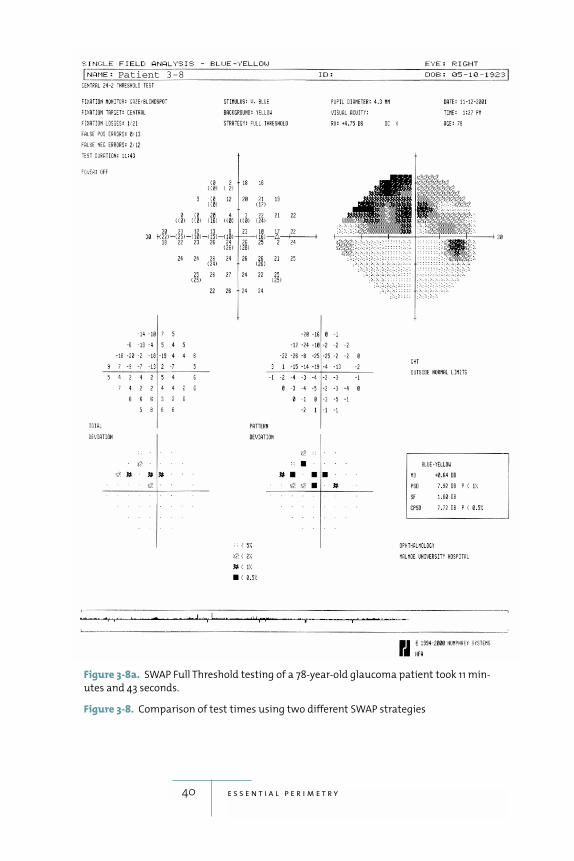
Patient 3-8
Figure 3-8a. SWAP Full Threshold testing of a 78-year-old glaucoma patient took 11 min-
utes and 43 seconds.
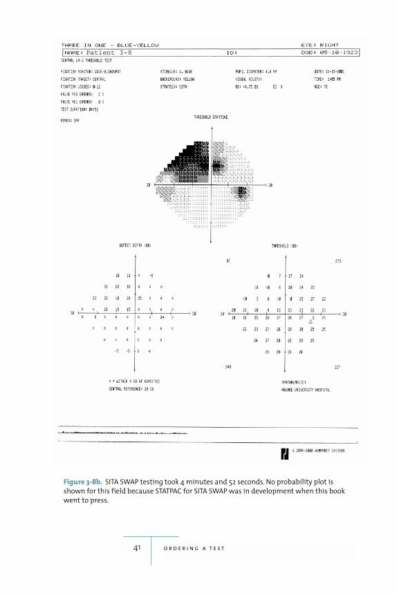
Figure 3-8. Comparison of test times using two different SWAP strategies
41 o r d e r i n g a t e s t
Figure 3-8b. SITA SWAP testing took 4 minutes and 52 seconds. No probability plot is
shown for this field because STATPAC for SITA SWAP was in development when this book
went to press.
Patient 3-8
binocular visual field is most important in driving and
that losses in one eye may well be compensated for if the
other eye’s overlapping field is still functional (Johnson
and Keltner 1983; McKnight et al. 1991; Wood and
Troutbeck 1994).
One text has suggested that, in the absence of more
conservative guidelines from local authorities, drivers
should have binocular visual fields extending at least 50
degrees both to the right and to the left of fixation
(Anderson and Patella 1999). These authors do not pro-
vide any suggestions regarding the superior and inferior
42 e s s e n t i a l p e r i m e t r y
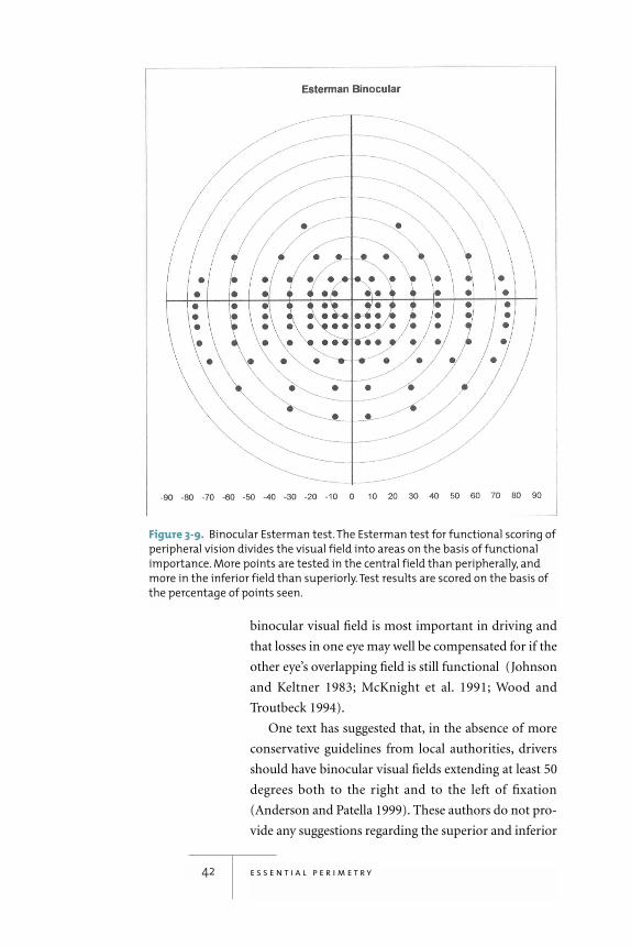
Figure 3-9. Binocular Esterman test. The Esterman test for functional scoring of
peripheral vision divides the visual field into areas on the basis of functional
importance. More points are tested in the central field than peripherally, and
more in the inferior field than superiorly. Test results are scored on the basis of
the percentage of points seen.
fields except to note that overhead objects such as traffic
signals usually do not require an extensive superior visual
field, at least when viewed from a distance.
B L E P H A R O P T O S I SPerimetry is frequently used to document visual
impairment secondary to blepharoptosis, although
non-perimetric methods also may be used (Cahill et
al.1987; Hacker and Hollsten 1992). Such testing is best
done using single-level suprathreshold testing and a
bright stimulus. It is also important to remember that
it is quite normal, especially in elderly patients, to find
asymptomatic restrictions of the upper portion of the
central 30 degree visual field caused by the eyelid. Thus,
it may be best to concentrate on testing the central field
using, for instance, the 76-point screening pattern with
a 10 dB single-level suprathreshold stimulus.
T E S T I N G F O R D R U G - I N D U C E D M A C U L O P AT H I E SPatients undergoing long-term treatment with chloro-
quine or hydroxychloroquine are frequently sent for oph-
thalmic consultation in order to monitor for drug-
associated maculopathy. With the increasing use of
hydroxychloroquine, some have suggested that monitor-
ing with automated perimetry is no longer necessary,
as long as suggested dosing guidelines are followed and as
long as the patient receives routine visual acuity, color
vision, and Amsler grid testing, along with corneal exam-
ination (Easterbrook 1999). Nevertheless, automated
perimetric examination is still part of the standard of
care in many communities and, when requested, proba-
bly is best performed using a standard size III white stim-
ulus, the 10-2 test pattern, and SITA Standard or SITA
Fast. Use of red stimuli has been advocated by some, but
no clear advantages have been established relative to
standard white stimulus testing (Easterbrook and Trope
1988).
43 o r d e r i n g a t e s t
4STATPAC
44
analysis package that
is included in the operating system of all Humphrey
perimeters. STATPAC greatly simplifies visual field inter-
pretation by differentiating between normal and abnor-
mal visual fields, and by identifying significant change in
a series of visual fields.
STATPAC determines if a patient’s visual field results
fall within the range normal for his or her age.A STATPAC
analysis may also involve comparing test results with the
patient’s own baseline from earlier tests in order to deter-
mine if the observed change is larger than that typically
seen when stable patients return for follow-up testing.
Sensitivity ranges vary with testing conditions, the
length of the test, and the testing strategy; databases have
been constructed for many combinations of instrument,
strategy, and test pattern. The normal database for SITA,
for instance, was based upon normal subjects enrolled at
fifteen participating university centers.
Standard threshold test results may be printed out in
any of four formats: Single Field Analysis, Overview,
Glaucoma Change Probability, and Change Analysis.
SWAP test results may be printed out using the first two
of these. The Single Field Analysis is devoted to the analy-
sis of a single test, while the purpose of the other print-
outs is to look for trends in a series of tests. This chapter
describes these basic STATPAC analyses.
The Single Field Analysis
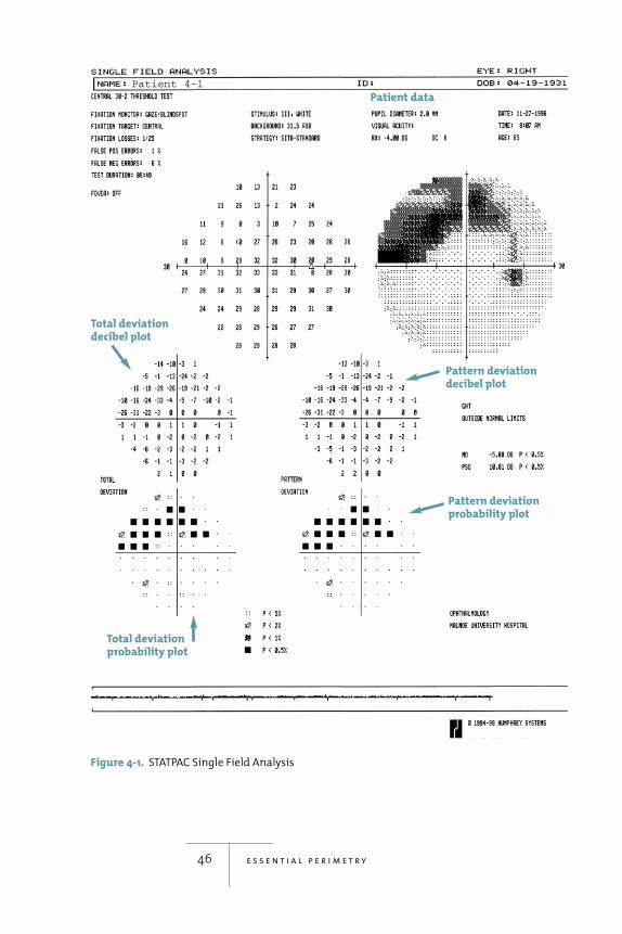
The STATPAC Single Field Analysis (SFA) of threshold
test results is perhaps the most useful and important
printout provided by the Humphrey perimeter (fig. 4-1).
The analysis compares the results of a single threshold
test with age-corrected normative data and highlights
any sensitivity values or patterns that deviate signifi-
cantly from normal. The Single Field Analysis also pres-
ents patient demographic data, indices of test reliability,
and raw test results.
D E V I AT I O N P L O T S Total Deviation Probability Plots: Total deviation prob-
ability plots indicate all test locations that are outside
normal limits, whether because of a general depression of
the whole visual field, or because of localized loss.
Threshold sensitivity is compared with the age-corrected
normal values at each test point to produce the total
deviation (TD) decibel plot. Negative values indicate sen-
sitivities that are below the median age-corrected sensi-
tivity, and positive values indicate higher than normal
sensitivities. The normal range of sensitivity is larger in
the periphery than in the center of the field, and also
larger superiorly than inferiorly. Thus, a depression of 5
decibels from age normal may be quite significant at the
center of the field, but totally within the normal range of
variability in the periphery of the test area.
The significance of these deviations from normal are
indicated in the associated total deviation probability
plot, in which sensitivities that are worse than those
found in 5%, 2%, 1%, and 0.5% of normal subjects of the
45 s t a t p a c
A deviation of 5 decibels
may be quitesignificant atthe center ofthe field, but
totally withinthe normal
range of variability in
the periphery of the test area.
46 e s s e n t i a l p e r i m e t r y
Figure 4-1. STATPAC Single Field Analysis
Pattern deviationdecibel plot
Total deviationdecibel plot
Total deviationprobability plot
Pattern deviationprobability plot
Patient data
Patient 4-1
same age as the patient are highlighted with appropriate
symbols. A 2% symbol, for instance, indicates that fewer
than 2% of normal subjects have a sensitivity that low or
lower. A key showing the meaning of the symbols is given
near the bottom of the printout.
The range of normal threshold values changes from
test point to test point, and does not follow theoretical
Gaussian distributions (Heijl, Lindgren, and Olsson
1987). As a result, attempts to construct probability plots
based upon idealized theoretical models provided poor
diagnostic performance as shown by Heijl and Åsman
(1989). For these reasons, Humphrey’s probability plots
are based on empirically determined normal ranges
found in large groups of subjects, some representing a
random sample of the normal population tested in
multi-center clinical trials.
Pattern Deviation Probability Plots: The single most
useful analysis on an SFA printout is the pattern devia-
tion (PD) probability plot. The pattern deviation analy-
sis shows sensitivity losses after an adjustment has been
made to remove any generalized depression and uses the
same symbols as the total deviation plots to show which
points are significantly worse than normal. Thus, the
pattern deviation decibel and probability plots primarily
highlight only significant localized visual field loss.
The great strength of the probability plots is that they
ignore variations that are within the normal range and
highlight subtle, but significant, variations that might
otherwise escape notice (figures 4-2a, 4-2b). Beginning
field defects regularly show up earlier in the probability
map than in grayscale printouts. Furthermore, STAT-
PAC’s probability plots help de-emphasize common arti-
factual patterns, such as eyelid-induced depressions of
sensitivity in the superior part of the field, that are often
overemphasized on the grayscale. Note that the correc-
tion for homogenous depression used in the PD plot is
based upon the sensitivities at the best points in the TD
47 s t a t p a c
The single most useful
analysis on anSFA printout is
the PatternDeviation (PD)
probability plot.
48 e s s e n t i a l p e r i m e t r y
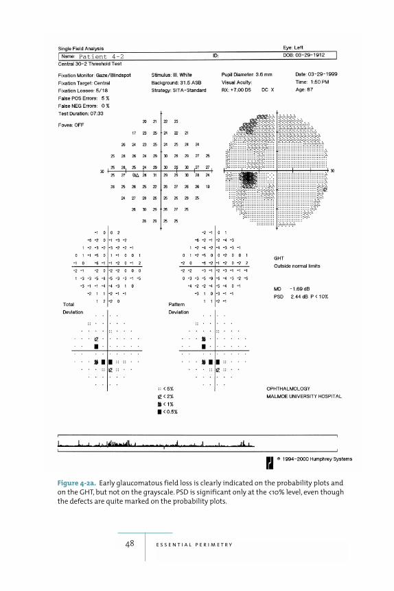
Figure 4-2a. Early glaucomatous field loss is clearly indicated on the probability plots and
on the GHT, but not on the grayscale. PSD is significant only at the <10% level, even though
the defects are quite marked on the probability plots.
Patient 4-2
49 s t a t p a c
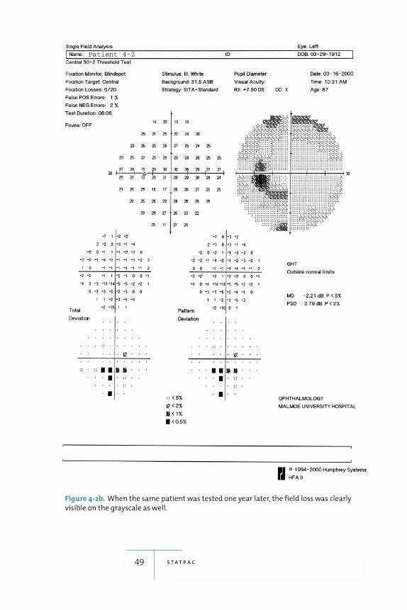
Figure 4-2b. When the same patient was tested one year later, the field loss was clearly
visible on the grayscale as well.
Patient 4-2
plot; thus, if visual field loss is so far advanced that even
the best points are almost blind, then the PD plot will be
unable to highlight localized loss. Such situations are
obvious even when looking at the grayscale, however,
and should not lead to missed diagnoses.
Comparing Total And Pattern Deviation: It is useful to
compare the total deviation and pattern deviation plots.
If the plots look more or less the same, then there is lit-
tle or no generalized loss. A uniformly depressed total
deviation plot combined with a normal-looking pattern
deviation plot probably indicates a cataract (figures 4-3a,
4-3b, 4-3c). The opposite pattern—a normal total devi-
ation plot and an abnormal-looking pattern deviation
plot—often is associated with a trigger-happy patient
who has repeatedly pressed the response button when no
stimulus was seen (see Chapter 8).
G L A U C O M A H E M I F I E L D T E S T The Glaucoma Hemifield Test (GHT) is a plain-language
classification of threshold test results in the following
categories (Åsman and Heijl 1992a; 1992b).
� The “Outside Normal Limits” message is displayed
whenever sensitivities in one or more of the five
zones in the upper half of the field are significantly
different (p<0.01) from the sensitivities measured in
the corresponding zones in the lower half of the field
(fig. 4-4).
� Fields are labeled as “Borderline” whenever zone pairs
differ by an amount greater than is seen in most nor-
mal subjects (p<0.03), but the difference does not
reach the level required for the “Outside Normal Lim-
its” message.
� The GHT will give a “General Depression of Sensi-
tivity” or “Abnormally High Sensitivity” message
whenever even the best test point locations are either
so low or so high as to be at levels seen in only 0.5%
50 e s s e n t i a l p e r i m e t r y
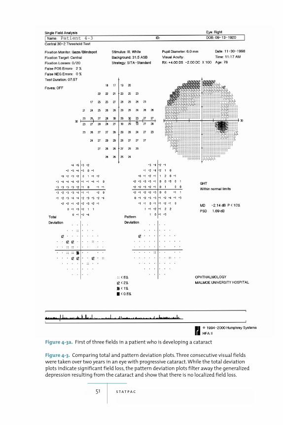
51 s t a t p a c
Figure 4-3a. First of three fields in a patient who is developing a cataract
Figure 4-3. Comparing total and pattern deviation plots. Three consecutive visual fields
were taken over two years in an eye with progressive cataract. While the total deviation
plots indicate significant field loss, the pattern deviation plots filter away the generalized
depression resulting from the cataract and show that there is no localized field loss.
Patient 4-3
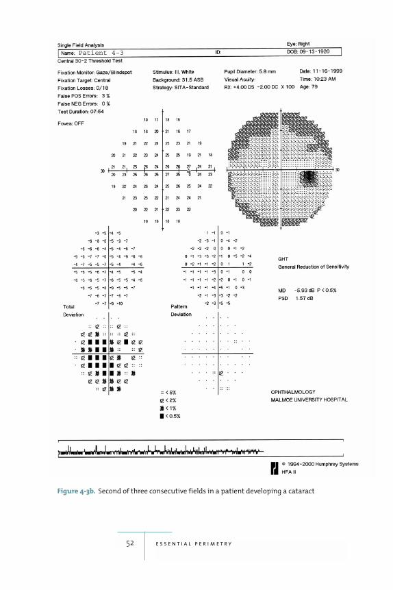
52 e s s e n t i a l p e r i m e t r y
Figure 4-3b. Second of three consecutive fields in a patient developing a cataract
Patient 4-3
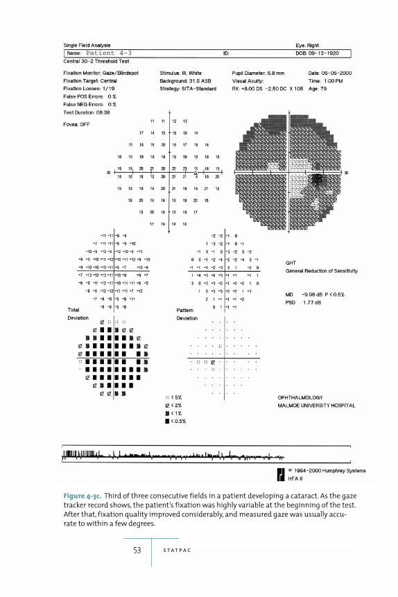
53 s t a t p a c
Figure 4-3c. Third of three consecutive fields in a patient developing a cataract. As the gaze
tracker record shows, the patient’s fixation was highly variable at the beginning of the test.
After that, fixation quality improved considerably, and measured gaze was usually accu-
rate to within a few degrees.
Patient 4-3
of normal subjects. “General Depression of Sensitiv-
ity” will not be displayed, however, when sensitivity
differences between the superior and inferior hemi-
fields are large enough to result in an “Outside Nor-
mal Limits” message.
� The “Within Normal Limits” message is presented
whenever none of the above significance limits are
reached.
Sensitivity differences between the upper and lower
hemifields are a hallmark of glaucomatous field loss. The
GHT analyzes these differences in terms of deviations
from the age-corrected normal reference field and then
translates them into the probability domain, first in indi-
vidual test point locations, and then for the whole central
field. The result is a very powerful interpretation tool.
The GHT has also been reported to be the single most
effective method of visual field analysis and, after over ten
years of use, enjoys wide acceptance worldwide (Katz et
al. 1991).
54 e s s e n t i a l p e r i m e t r y
5Glaucomatous Visual Field Loss
70
of glaucomatous field loss corre-
spond directly to the patterns of optic nerve damage typ-
ical of the disease. Glaucomatous fields show more
variability than normal fields, and variable reductions in
sensitivity frequently precede definite loss. Complete and
quantitative understanding of the amount of variability
typically found in glaucomatous fields greatly aids in
determining whether a patient’s follow-up test results
indicate true disease progression.
Anatomy and Glaucomatous Visual Field Defects
Glaucomatous field loss is the result of axonal damage at
the level of the optic disc, and is therefore the functional
correlate of neural loss or reduced neural function.
R E T I N A L N E R V E F I B E R L AY E R A N D O P T I C D I S C A N AT O M YRetinal ganglion cell axons follow an arcuate path to the
optic nerve (fig. 5-1). Axons extending from the optic disc
toward the temporal retina curve around the macular
area. Neurons from the temporal superior and inferior
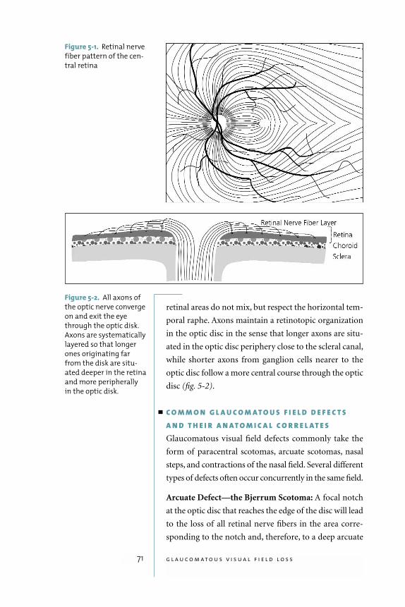
retinal areas do not mix, but respect the horizontal tem-
poral raphe. Axons maintain a retinotopic organization
in the optic disc in the sense that longer axons are situ-
ated in the optic disc periphery close to the scleral canal,
while shorter axons from ganglion cells nearer to the
optic disc follow a more central course through the optic
disc (fig. 5-2).
C O M M O N G L A U C O M AT O U S F I E L D D E F E C T SA N D T H E I R A N AT O M I C A L C O R R E L AT E SGlaucomatous visual field defects commonly take the
form of paracentral scotomas, arcuate scotomas, nasal
steps, and contractions of the nasal field. Several different
types of defects often occur concurrently in the same field.
Arcuate Defect—the Bjerrum Scotoma: A focal notch
at the optic disc that reaches the edge of the disc will lead
to the loss of all retinal nerve fibers in the area corre-
sponding to the notch and, therefore, to a deep arcuate
71 g l a u c o m a t o u s v i s u a l f i e l d l o s s
Figure 5-1. Retinal nerve
fiber pattern of the cen-
tral retina
Figure 5-2. All axons of
the optic nerve converge
on and exit the eye
through the optic disk.
Axons are systematically
layered so that longer
ones originating far
from the disk are situ-
ated deeper in the retina
and more peripherally
in the optic disk.
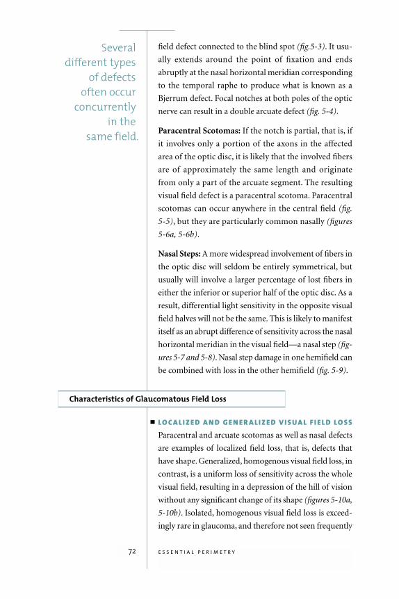
field defect connected to the blind spot (fig.5-3). It usu-
ally extends around the point of fixation and ends
abruptly at the nasal horizontal meridian corresponding
to the temporal raphe to produce what is known as a
Bjerrum defect. Focal notches at both poles of the optic
nerve can result in a double arcuate defect (fig. 5-4).
Paracentral Scotomas: If the notch is partial, that is, if
it involves only a portion of the axons in the affected
area of the optic disc, it is likely that the involved fibers
are of approximately the same length and originate
from only a part of the arcuate segment. The resulting
visual field defect is a paracentral scotoma. Paracentral
scotomas can occur anywhere in the central field (fig.
5-5), but they are particularly common nasally (figures
5-6a, 5-6b).
Nasal Steps: A more widespread involvement of fibers in
the optic disc will seldom be entirely symmetrical, but
usually will involve a larger percentage of lost fibers in
either the inferior or superior half of the optic disc. As a
result, differential light sensitivity in the opposite visual
field halves will not be the same. This is likely to manifest
itself as an abrupt difference of sensitivity across the nasal
horizontal meridian in the visual field—a nasal step (fig-
ures 5-7 and 5-8). Nasal step damage in one hemifield can
be combined with loss in the other hemifield (fig. 5-9).
Characteristics of Glaucomatous Field Loss
LO C A L I Z E D A N D G E N E R A L I Z E D V I S UA L F I E L D LO S SParacentral and arcuate scotomas as well as nasal defects
are examples of localized field loss, that is, defects that
have shape. Generalized, homogenous visual field loss, in
contrast, is a uniform loss of sensitivity across the whole
visual field, resulting in a depression of the hill of vision
without any significant change of its shape (figures 5-10a,
5-10b). Isolated, homogenous visual field loss is exceed-
ingly rare in glaucoma, and therefore not seen frequently
72 e s s e n t i a l p e r i m e t r y
Several different types
of defects often occur
concurrently in the
same field.
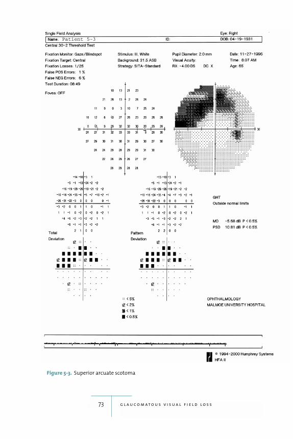
73 g l a u c o m a t o u s v i s u a l f i e l d l o s s
Figure 5-3. Superior arcuate scotoma
Patient 5-3
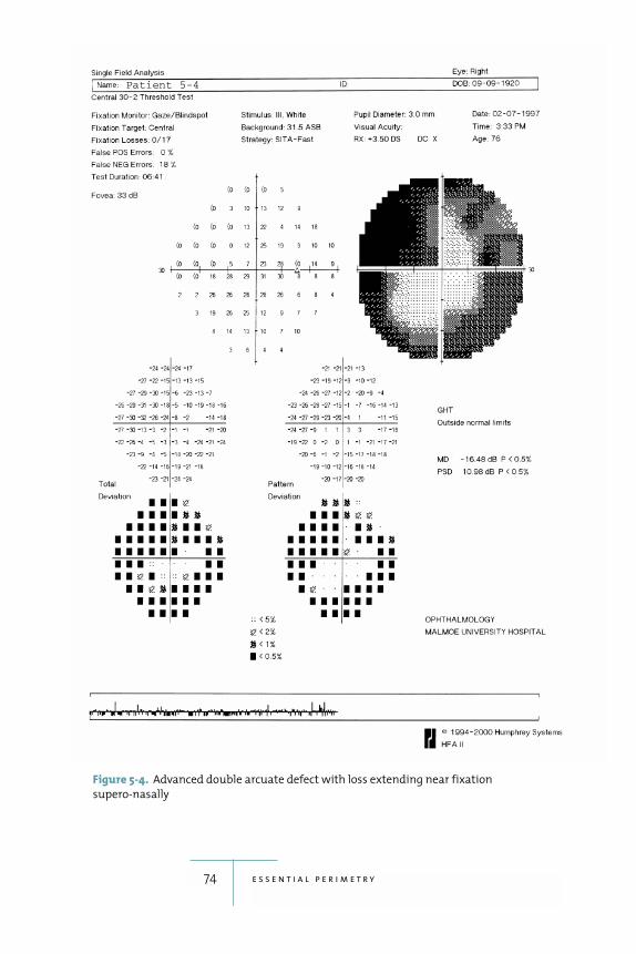
74 e s s e n t i a l p e r i m e t r y
Figure 5-4. Advanced double arcuate defect with loss extending near fixation
supero-nasally
Patient 5-4
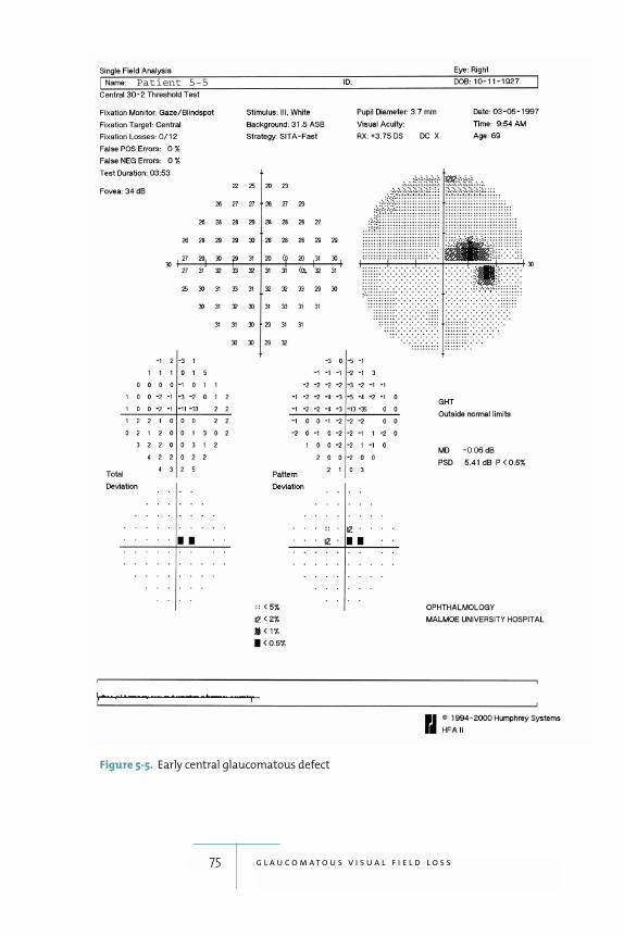
75 g l a u c o m a t o u s v i s u a l f i e l d l o s s
Figure 5-5. Early central glaucomatous defect
Patient 5-5
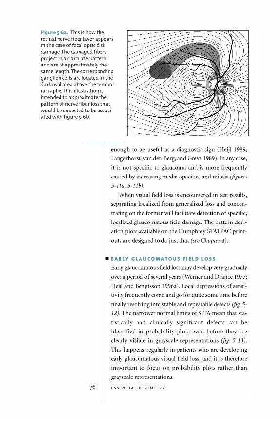
enough to be useful as a diagnostic sign (Heijl 1989;
Langerhorst, van den Berg, and Greve 1989). In any case,
it is not specific to glaucoma and is more frequently
caused by increasing media opacities and miosis (figures
5-11a, 5-11b).
When visual field loss is encountered in test results,
separating localized from generalized loss and concen-
trating on the former will facilitate detection of specific,
localized glaucomatous field damage. The pattern devi-
ation plots available on the Humphrey STATPAC print-
outs are designed to do just that (see Chapter 4).
E A R LY G L A U C O M AT O U S F I E L D L O S SEarly glaucomatous field loss may develop very gradually
over a period of several years (Werner and Drance 1977;
Heijl and Bengtsson 1996a). Local depressions of sensi-
tivity frequently come and go for quite some time before
finally resolving into stable and repeatable defects (fig. 5-
12). The narrower normal limits of SITA mean that sta-
tistically and clinically significant defects can be
identified in probability plots even before they are
clearly visible in grayscale representations (fig. 5-13).
This happens regularly in patients who are developing
early glaucomatous visual field loss, and it is therefore
important to focus on probability plots rather than
grayscale representations.
76 e s s e n t i a l p e r i m e t r y
Figure 5-6a. This is how the
retinal nerve fiber layer appears
in the case of focal optic disk
damage. The damaged fibers
project in an arcuate pattern
and are of approximately the
same length. The corresponding
ganglion cells are located in the
dark oval area above the tempo-
ral raphe. This illustration is
intended to approximate the
pattern of nerve fiber loss that
would be expected to be associ-
ated with figure 5-6b.
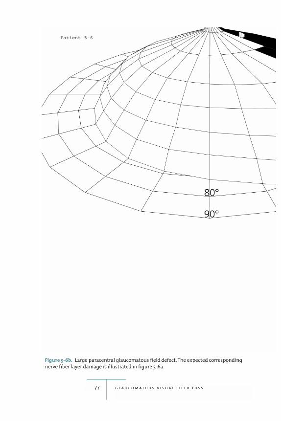
77 g l a u c o m a t o u s v i s u a l f i e l d l o s s
Figure 5-6b. Large paracentral glaucomatous field defect. The expected corresponding
nerve fiber layer damage is illustrated in figure 5-6a.
Patient 5-6
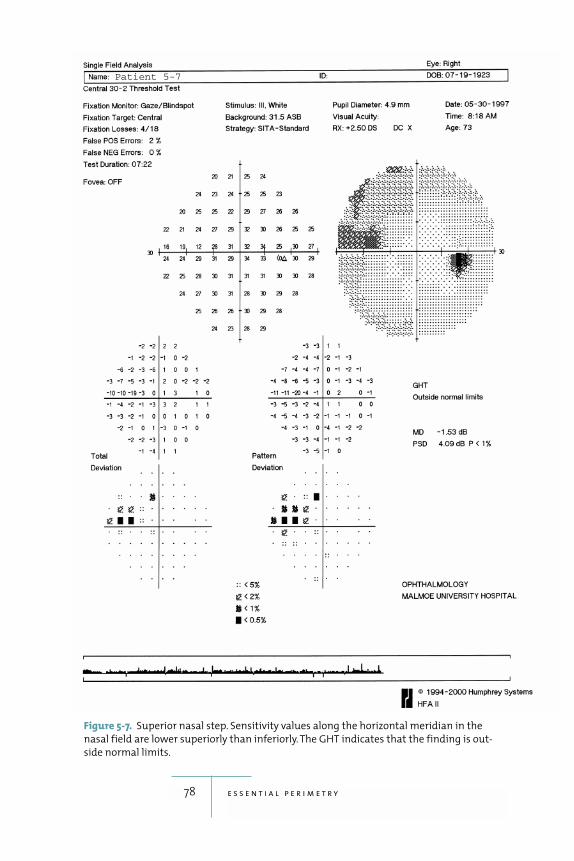
78 e s s e n t i a l p e r i m e t r y
Figure 5-7. Superior nasal step. Sensitivity values along the horizontal meridian in the
nasal field are lower superiorly than inferiorly. The GHT indicates that the finding is out-
side normal limits.
Patient 5-7
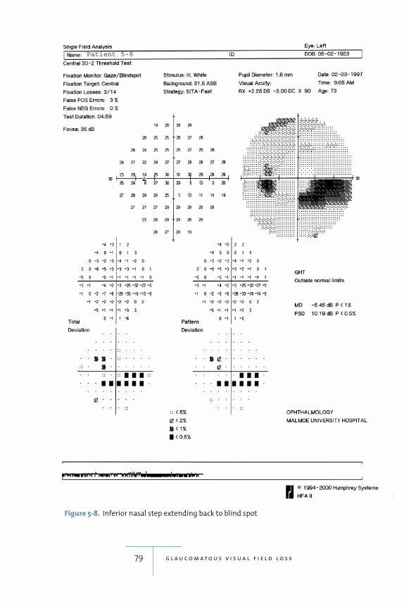
79 g l a u c o m a t o u s v i s u a l f i e l d l o s s
Figure 5-8. Inferior nasal step extending back to blind spot
Patient 5-8
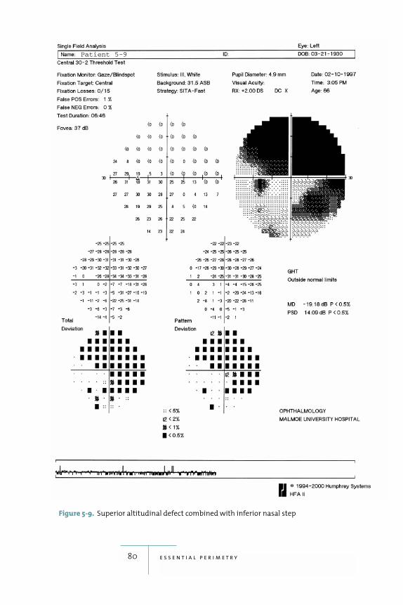
80 e s s e n t i a l p e r i m e t r y
Figure 5-9. Superior altitudinal defect combined with inferior nasal step
Patient 5-9

81 g l a u c o m a t o u s v i s u a l f i e l d l o s s
Figure 5-10b.
Figure 5-10a.
Figure 5-10. Generalized depression of the hill of vision, 5-10a, compared to normal hill of
vision, 5-10b
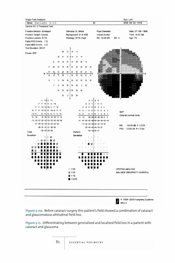
82 e s s e n t i a l p e r i m e t r y
Figure 5-11a. Before cataract surgery this patient’s field showed a combination of cataract
and glaucomatous altitudinal field loss.
Figure 5-11. Differentiating between generalized and localized field loss in a patient with
cataract and glaucoma
Patient 5-11
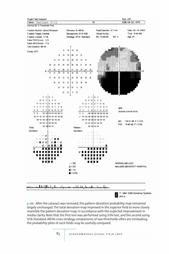
83 g l a u c o m a t o u s v i s u a l f i e l d l o s s
5-11b. After the cataract was removed, the pattern deviation probability map remained
largely unchanged. The total deviation map improved in the superior field to more closely
resemble the pattern deviation map, in accordance with the expected improvement in
media clarity. Note that the first test was performed using SITA Fast, and the second using
SITA Standard. While cross-strategy comparisons of raw thresholds often are misleading,
the probability plots of such fields may be usefully compared.
Patient 5-11
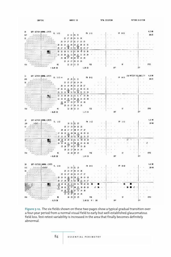
84 e s s e n t i a l p e r i m e t r y
Figure 5-12. The six fields shown on these two pages show a typical gradual transition over
a four-year period from a normal visual field to early but well-established glaucomatous
field loss. Test-retest variability is increased in the area that finally becomes definitely
abnormal.
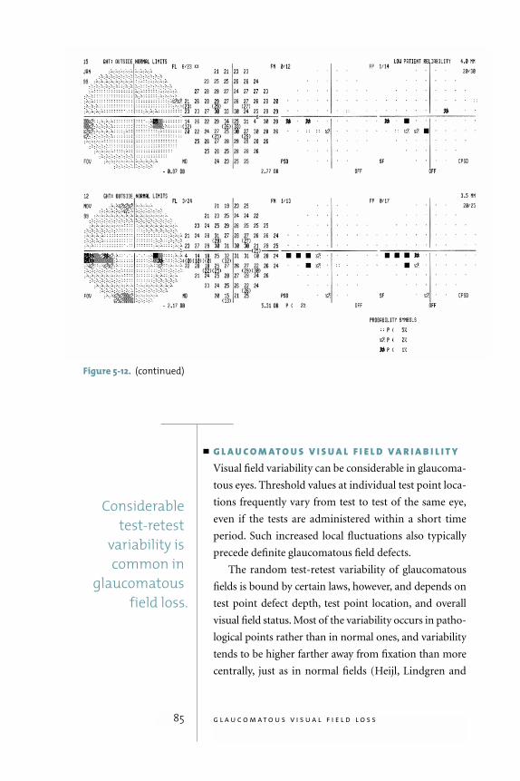
85 g l a u c o m a t o u s v i s u a l f i e l d l o s s
G L A U C O M AT O U S V I S U A L F I E L D V A R I A B I L I T YVisual field variability can be considerable in glaucoma-
tous eyes. Threshold values at individual test point loca-
tions frequently vary from test to test of the same eye,
even if the tests are administered within a short time
period. Such increased local fluctuations also typically
precede definite glaucomatous field defects.
The random test-retest variability of glaucomatous
fields is bound by certain laws, however, and depends on
test point defect depth, test point location, and overall
visual field status. Most of the variability occurs in patho-
logical points rather than in normal ones, and variability
tends to be higher farther away from fixation than more
centrally, just as in normal fields (Heijl, Lindgren and
Considerabletest-retest
variability iscommon in
glaucomatous field loss.
Figure 5-12. (continued)
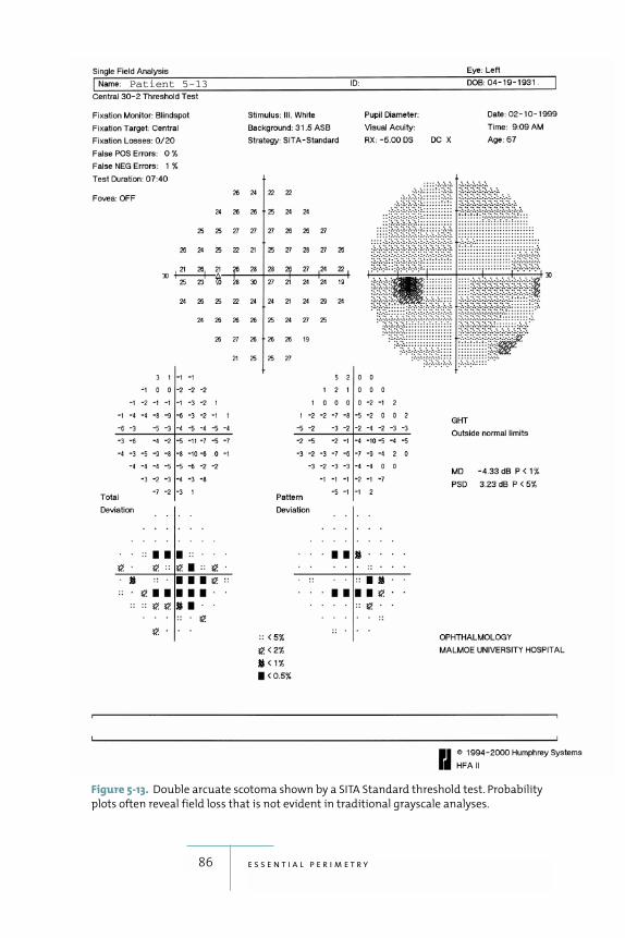
86 e s s e n t i a l p e r i m e t r y
Figure 5-13. Double arcuate scotoma shown by a SITA Standard threshold test. Probability
plots often reveal field loss that is not evident in traditional grayscale analyses.
Patient 5-13
Lindgren 1989; Heijl et al. 1991). Overall field status is
also of importance; fields with widespread areas of dam-
age show higher variability than fields with smaller defects.
Knowledge of the nature of this variability helps interpre-
tation of test results in glaucoma follow-up and is incor-
porated in STATPAC’s glaucoma change probability plots.
Judging whether or not a glaucomatous visual field is
progressing usually requires a series of at least three or four
fields. Basing judgements about disease progression on
only one progressed field is very risky unless the changes
encountered are very large and/or are confirmed by other
clinical findings, such as changes in optic disc configura-
tion. Fortunately, glaucomatous field progression is usu-
ally slow enough that there is time for the patient to take
a confirmatory field test when change is suspected.
P I T F A L L S I N P E R I M E T R I C G L A U C O M A F O L L O W - U PA large percentage of glaucoma patients have coexisting
media opacities, complicating follow-up analysis of their
visual fields. As mentioned previously, these problems
can be largely avoided by using analyses based on pattern
deviation.
Medically induced miosis also results in general
reduction of sensitivity, particularly in eyes that have
some cataract. For this reason it is difficult to compare
consecutive fields when the patient has been treated with
miotics at some, but not all, visits (figures 5-14 a, 5-14b).
Again, a comparison will be facilitated by concentrating
on the pattern deviation plots, which will eliminate most
of the effects of the miotics.
Large, sudden visual field changes are not typical in
glaucoma. Such changes often occur for reasons other
than progression of the glaucomatous disease process, e.g.,
arterial or venous occlusions in the retina or neurological
disease. If a large change is seen and part of the field loss
seems hemianopic or occurs in the other eye as well, neu-
rological causes are generally the rule (see Chapter 6).
87 g l a u c o m a t o u s v i s u a l f i e l d l o s s
Large, suddenvisual field
changes are nottypical in
glaucoma.
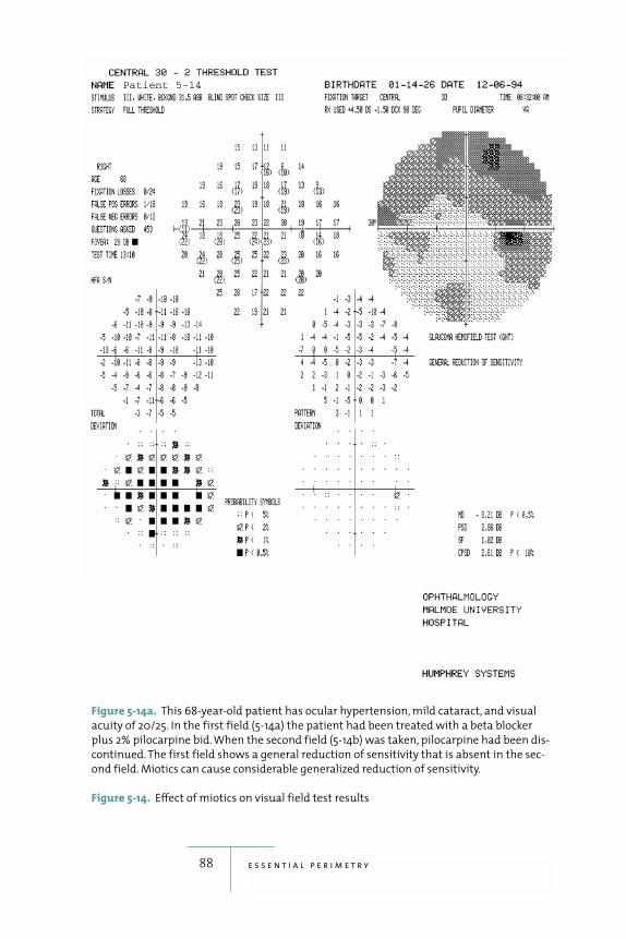
88 e s s e n t i a l p e r i m e t r y
Figure 5-14a. This 68-year-old patient has ocular hypertension, mild cataract, and visual
acuity of 20/25. In the first field (5-14a) the patient had been treated with a beta blocker
plus 2% pilocarpine bid. When the second field (5-14b) was taken, pilocarpine had been dis-
continued. The first field shows a general reduction of sensitivity that is absent in the sec-
ond field. Miotics can cause considerable generalized reduction of sensitivity.
Figure 5-14. Effect of miotics on visual field test results
Patient 5-14
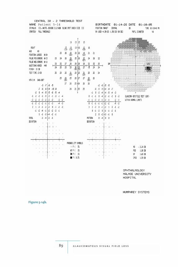
89 g l a u c o m a t o u s v i s u a l f i e l d l o s s
Figure 5-14b.
Patient 5-14
6Neurological Visual Field Loss
90
is an important area for
visual field testing. Before the advent of CT scanning and
MRI, visual fields were often the best indicators of the
location, and sometimes even the nature, of central nerv-
ous system disease. Even today perimetry is often a sim-
ple and cost-effective method of making neurological
diagnoses. This is because the visual system occupies or
passes through so much of the brain, from the optic
nerve and chiasm to the optic radiation and visual cortex.
When there is disease the resulting patterns of visual field
loss are often specific for and vary with disease location.
Modern practice emphasizes testing in the central field in
assessing neurological visual field loss.
Neurological field loss has been shown in some cases
to be more extensive when measured using static meth-
ods than with kinetic perimetry (Riddoch 1917), and
thus static Humphrey perimetry may have some advan-
tages over kinetic methods. Standard Humphrey perime-
try also seems to identify neurological loss more reliably
than perimetry based upon flickering stimuli (Johnson et
al. 1998). SITA Standard has been found to be at least as
Perimetry is often a
simple andcost-effective
method ofmaking
neurologicaldiagnoses
because thevisual system
occupies orpasses through
so much of the brain.
good as the older Full Threshold test in detecting optic
neuropathies and hemianopias (Wall et al. 2001).
Optic Nerve Disease
As its name suggests, unilateral optic nerve disease pro-
duces field defects in the affected eye only. A central sco-
toma is the typical pattern of field loss for several types of
optic nerve disease, e.g., optic neuritis (figures 6-1a, 6-1b),
many toxic reactions, tobacco-alcohol amblyopia, and
mechanical compression of the nerve. The size of the cen-
tral defect varies, and reduced visual acuity is associated
with larger scotomas. If the damage is small enough that
visual acuity is still normal or only slightly depressed, the
scotoma may be so small that sensitivity is only marginally
depressed at some central points in the standard 30-2 or
24-2 test point patterns. Experience with computerized
perimetry has shown, however, that optic neuritis can
cause a large variety of visual field defects, some of which
may even resemble those typical of glaucoma. Residual
visual field defects remaining after an optic neuritis has
resolved were seldom detected with manual perimetry,
but they are frequently seen with computerized threshold
perimetry; these include patterns with variable, mild, and
multifocal depressions.
Anterior ischemic optic neuropathy results in sudden
loss of visual function. The field loss is usually large with
sizeable areas of absolute damage (fig. 6-2). Many differ-
ent patterns are possible, but altitudinal hemianopia is
the most common. Just as with other hemianopias, those
in optic nerve infarction are often not complete, and it is
common to see areas with diminished function in the less
affected hemifield as well.
Early phase optic disc edema produces only an enlarge-
ment of the blind spot, which becomes surrounded by a
zone of relative loss of sensitivity (fig. 6-3). This is of little
diagnostic interest, since the diagnosis is usually made
with ophthalmoscopy and not with perimetry. Patients
91 n e u r o l o g i c a l v i s u a l f i e l d l o s s
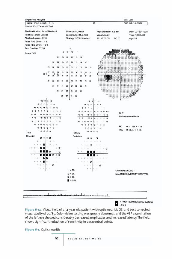
92 e s s e n t i a l p e r i m e t r y
Figure 6-1a. Visual field of a 34-year-old patient with optic neuritis OS, and best corrected
visual acuity of 20/80. Color vision testing was grossly abnormal, and the VEP examination
of the left eye showed considerably decreased amplitudes and increased latency. The field
shows significant reduction of sensitivity in paracentral points.
Figure 6-1. Optic neuritis
Patient 6-1
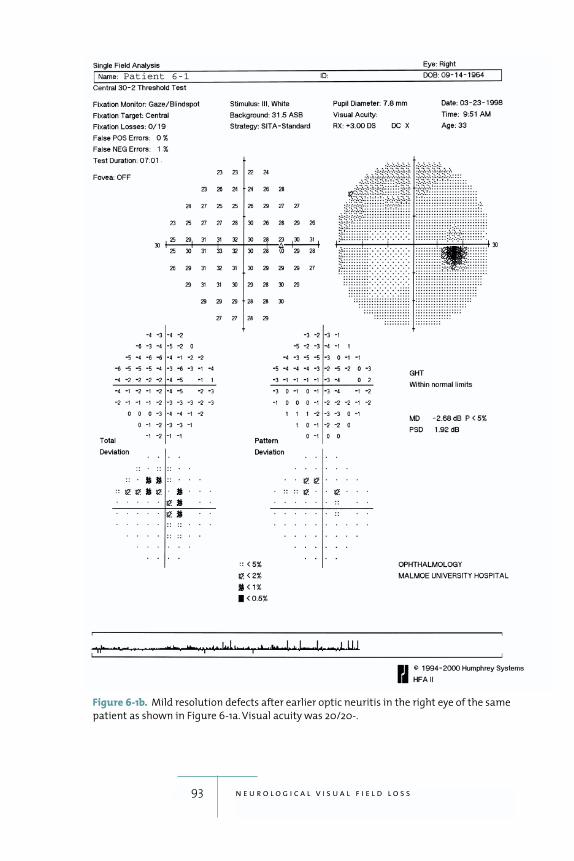
93 n e u r o l o g i c a l v i s u a l f i e l d l o s s
Figure 6-1b. Mild resolution defects after earlier optic neuritis in the right eye of the same
patient as shown in Figure 6-1a. Visual acuity was 20/20-.
Patient 6-1
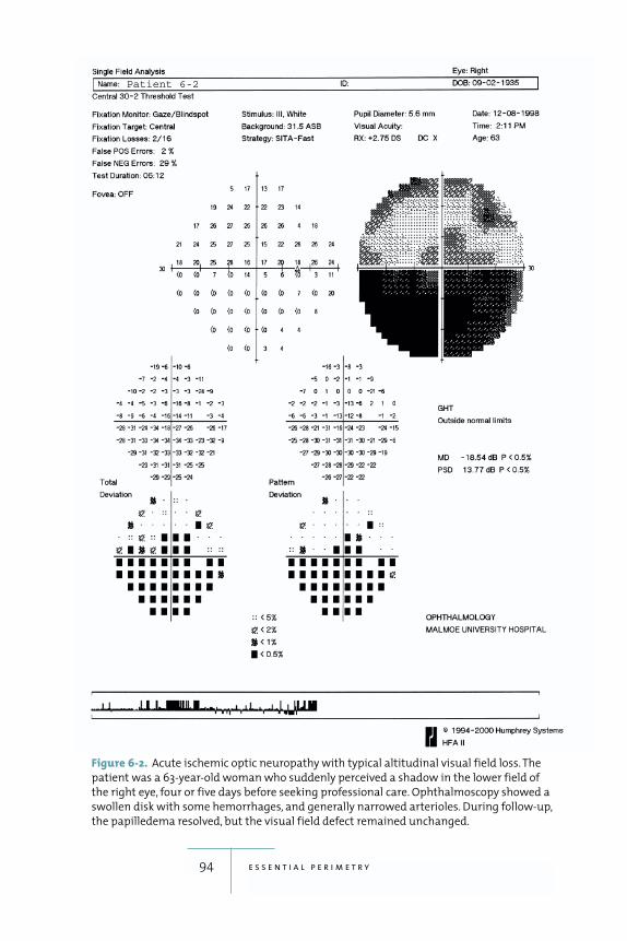
94 e s s e n t i a l p e r i m e t r y
Figure 6-2. Acute ischemic optic neuropathy with typical altitudinal visual field loss. The
patient was a 63-year-old woman who suddenly perceived a shadow in the lower field of
the right eye, four or five days before seeking professional care. Ophthalmoscopy showed a
swollen disk with some hemorrhages, and generally narrowed arterioles. During follow-up,
the papilledema resolved, but the visual field defect remained unchanged.
Patient 6-2
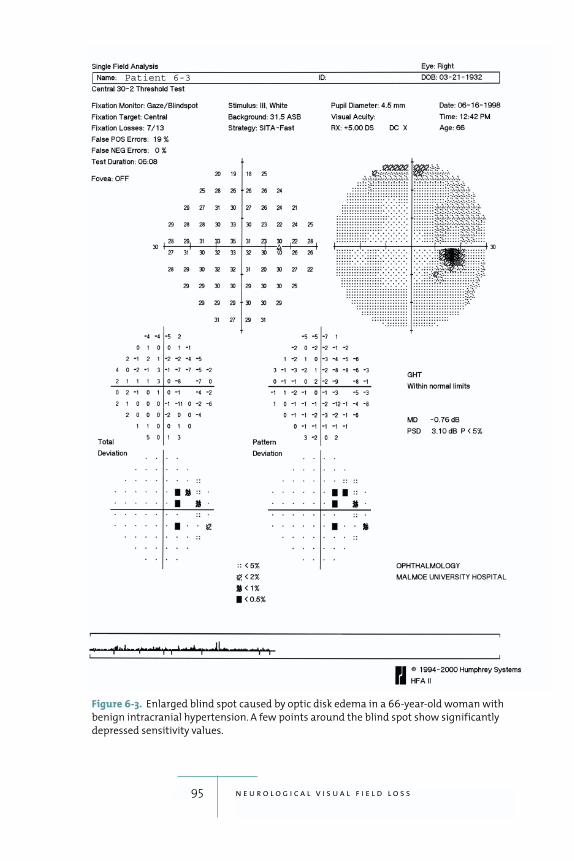
95 n e u r o l o g i c a l v i s u a l f i e l d l o s s
Figure 6-3. Enlarged blind spot caused by optic disk edema in a 66-year-old woman with
benign intracranial hypertension. A few points around the blind spot show significantly
depressed sensitivity values.
Patient 6-3
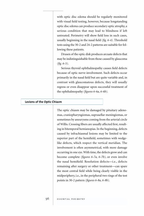
with optic disc edema should be regularly monitored
with visual field testing, however, because longstanding
optic disc edema can produce secondary optic atrophy, a
serious condition that may lead to blindness if left
untreated. Perimetry will show field loss in such cases,
usually beginning in the nasal field (fig. 6-4). Threshold
tests using the 30-2 and 24-2 patterns are suitable for fol-
lowing these patients.
Drusen of the optic disk produces arcuate defects that
may be indistinguishable from those caused by glaucoma
(fig. 6-5).
Serious thyroid ophthalmopathy causes field defects
because of optic nerve involvement. Such defects occur
primarily in the nasal field but are quite variable and, in
contrast with glaucomatous defects, they will usually
regress or even disappear upon successful treatment of
the ophthalmopathy (figures 6-6a, 6-6b).
Lesions of the Optic Chiasm
The optic chiasm may be damaged by pituitary adeno-
mas, craniopharyngiomas, suprasellar meningiomas, or
sometimes by aneurysms coming from the arterial circle
of Willis. Crossing fibers are usually affected first, result-
ing in bitemporal hemianopias. In the beginning, defects
caused by infrachiasmal lesions may be limited to the
superior part of the hemifield, sometimes with wedge-
like defects, which respect the vertical meridian. The
involvement is often asymmetrical, with more damage
occurring in one eye. With time, the defects grow and can
become complete (figures 6-7a, 6-7b), or even involve
the nasal hemifield. Resolution defects—i.e., defects
remaining after surgery or other treatment—can spare
the most central field while being clearly visible in the
midperiphery, i.e., in the peripheral two rings of the test
points in 30-2 pattern (figures 6-8a, 6-8b).
96 e s s e n t i a l p e r i m e t r y
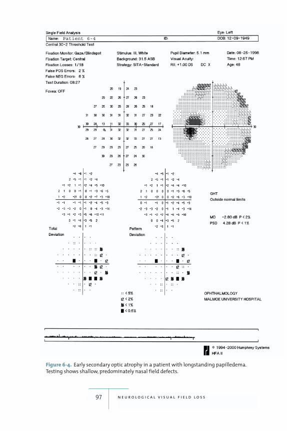
97 n e u r o l o g i c a l v i s u a l f i e l d l o s s
Figure 6-4. Early secondary optic atrophy in a patient with longstanding papilledema.
Testing shows shallow, predominately nasal field defects.
Patient 6-4
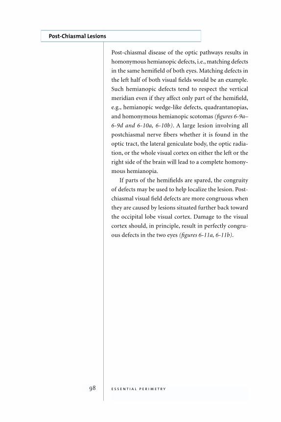
98 e s s e n t i a l p e r i m e t r y
Post-Chiasmal Lesions
Post-chiasmal disease of the optic pathways results in
homonymous hemianopic defects, i.e., matching defects
in the same hemifield of both eyes. Matching defects in
the left half of both visual fields would be an example.
Such hemianopic defects tend to respect the vertical
meridian even if they affect only part of the hemifield,
e.g., hemianopic wedge-like defects, quadrantanopias,
and homonymous hemianopic scotomas (figures 6-9a–
6-9d and 6-10a, 6-10b). A large lesion involving all
postchiasmal nerve fibers whether it is found in the
optic tract, the lateral geniculate body, the optic radia-
tion, or the whole visual cortex on either the left or the
right side of the brain will lead to a complete homony-
mous hemianopia.
If parts of the hemifields are spared, the congruity
of defects may be used to help localize the lesion. Post-
chiasmal visual field defects are more congruous when
they are caused by lesions situated further back toward
the occipital lobe visual cortex. Damage to the visual
cortex should, in principle, result in perfectly congru-
ous defects in the two eyes (figures 6-11a, 6-11b).
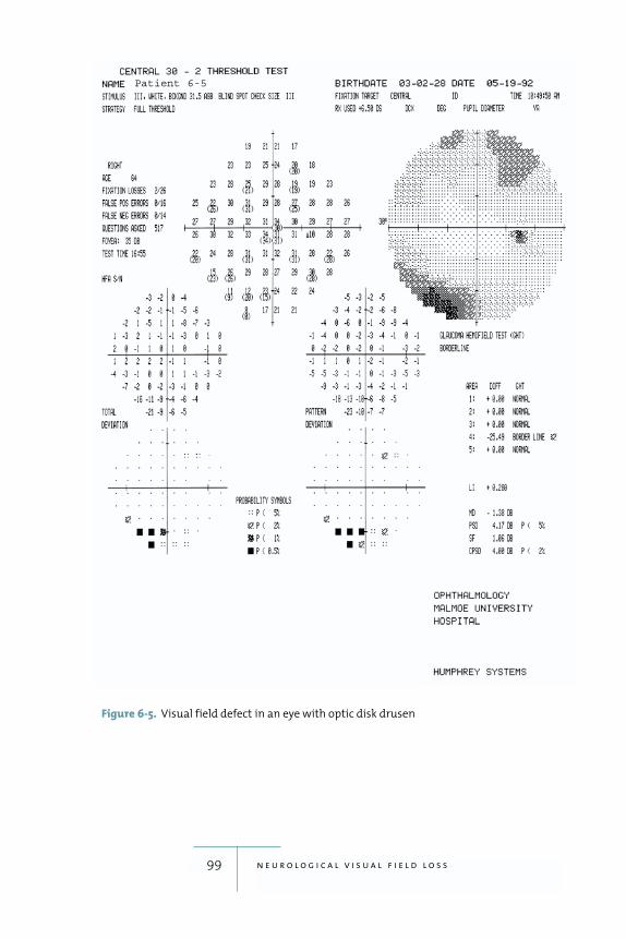
99 n e u r o l o g i c a l v i s u a l f i e l d l o s s
Figure 6-5. Visual field defect in an eye with optic disk drusen
Patient 6-5
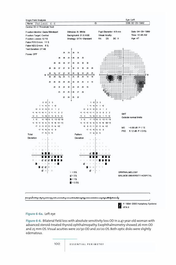
100 e s s e n t i a l p e r i m e t r y
Figure 6-6. Bilateral field loss with absolute sensitivity loss OD in a 47-year-old woman with
advanced steroid-treated thyroid ophthalmopathy. Exophthalmometry showed 26 mm OD
and 25 mm OS. Visual acuities were 20/30 OD and 20/20 OS. Both optic disks were slightly
edematous.
Patient 6-6
Figure 6-6a. Left eye
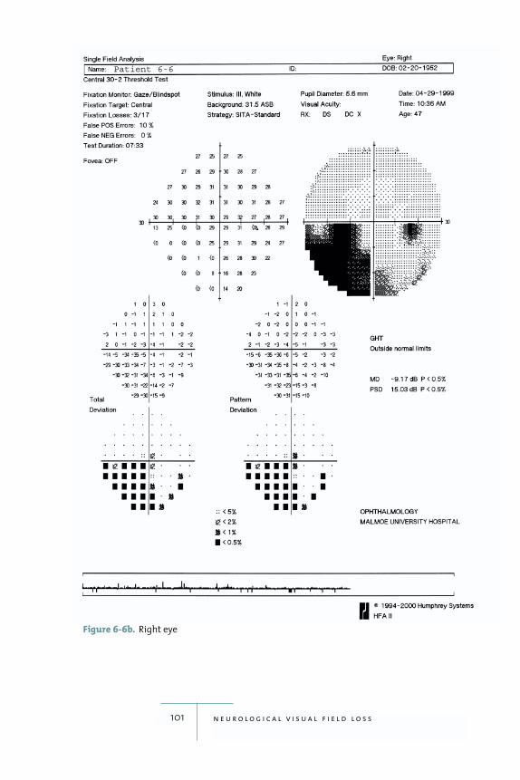
101 n e u r o l o g i c a l v i s u a l f i e l d l o s s
Figure 6-6b. Right eye
Patient 6-6
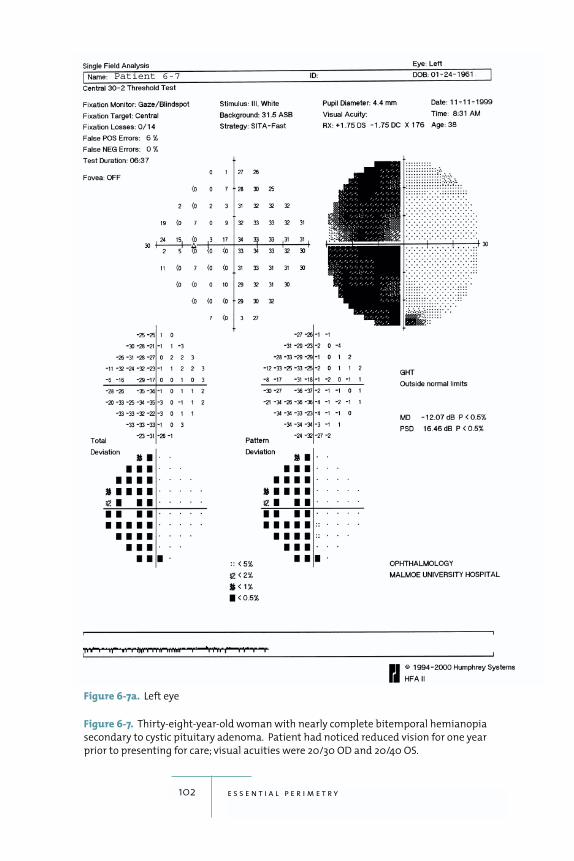
102 e s s e n t i a l p e r i m e t r y
Figure 6-7. Thirty-eight-year-old woman with nearly complete bitemporal hemianopia
secondary to cystic pituitary adenoma. Patient had noticed reduced vision for one year
prior to presenting for care; visual acuities were 20/30 OD and 20/40 OS.
Patient 6-7
Figure 6-7a. Left eye
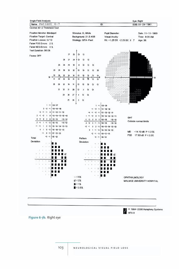
103 n e u r o l o g i c a l v i s u a l f i e l d l o s s
Figure 6-7b. Right eye
Patient 6-7
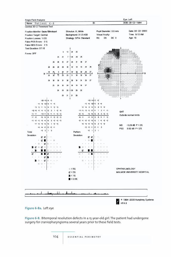
104 e s s e n t i a l p e r i m e t r y
Figure 6-8. Bitemporal resolution defects in a 15-year-old girl. The patient had undergone
surgery for craniopharyngioma several years prior to these field tests.
Patient 6-8
Figure 6-8a. Left eye
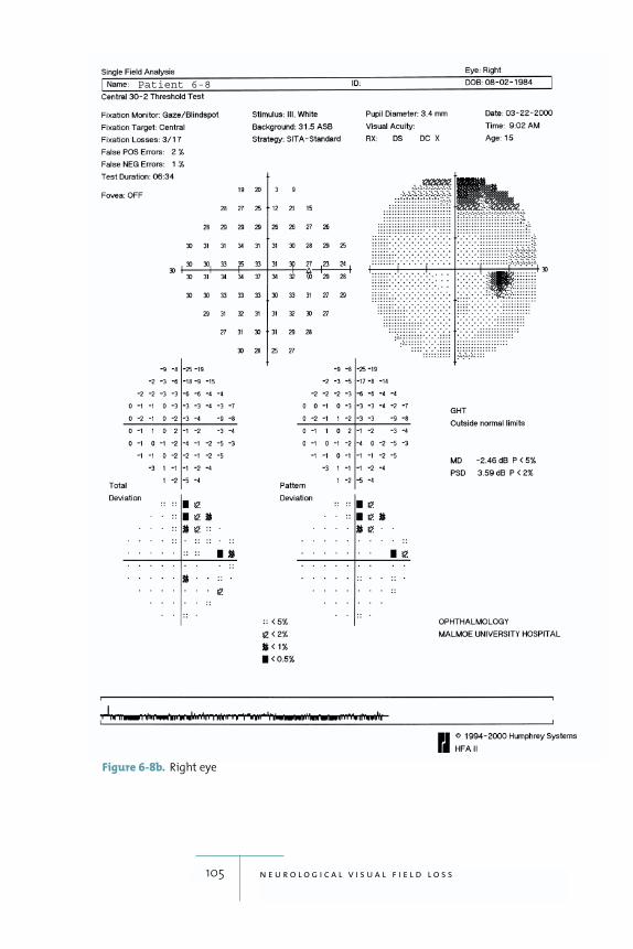
105 n e u r o l o g i c a l v i s u a l f i e l d l o s s
Figure 6-8b. Right eye
Patient 6-8
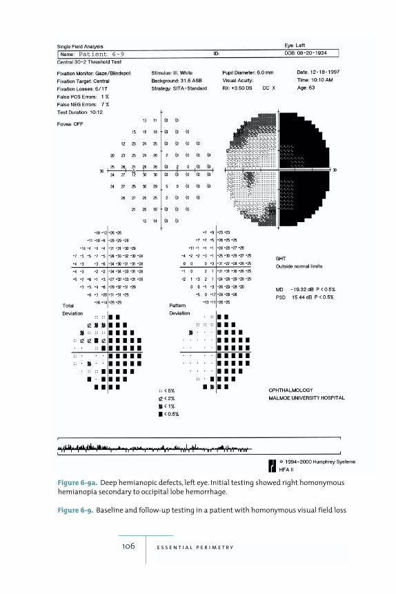
106 e s s e n t i a l p e r i m e t r y
Figure 6-9a. Deep hemianopic defects, left eye. Initial testing showed right homonymous
hemianopia secondary to occipital lobe hemorrhage.
Figure 6-9. Baseline and follow-up testing in a patient with homonymous visual field loss
Patient 6-9
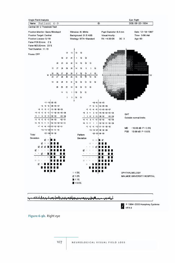
107 n e u r o l o g i c a l v i s u a l f i e l d l o s s
Figure 6-9b. Right eye
Patient 6-9
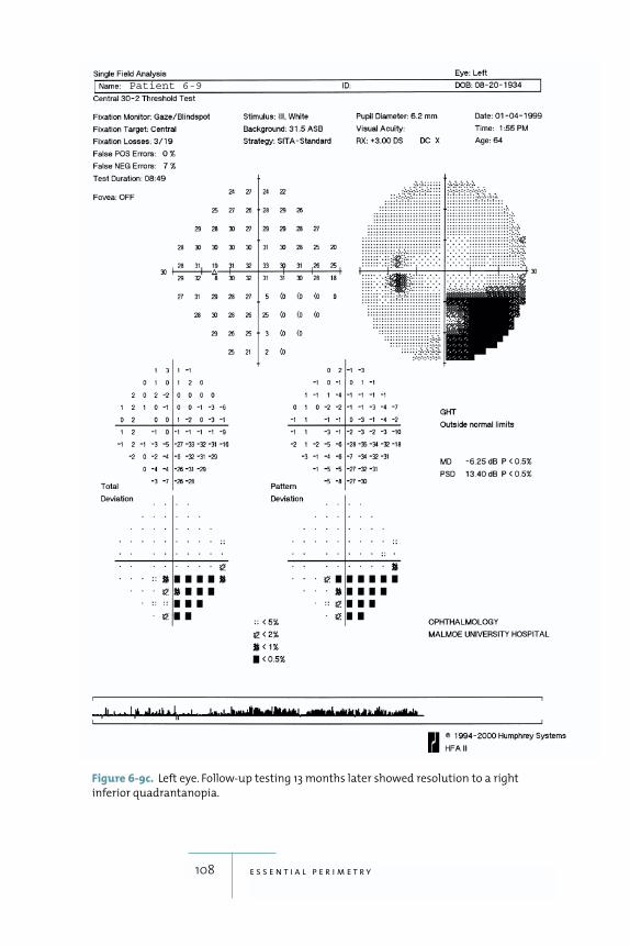
108 e s s e n t i a l p e r i m e t r y
Figure 6-9c. Left eye. Follow-up testing 13 months later showed resolution to a right
inferior quadrantanopia.
Patient 6-9
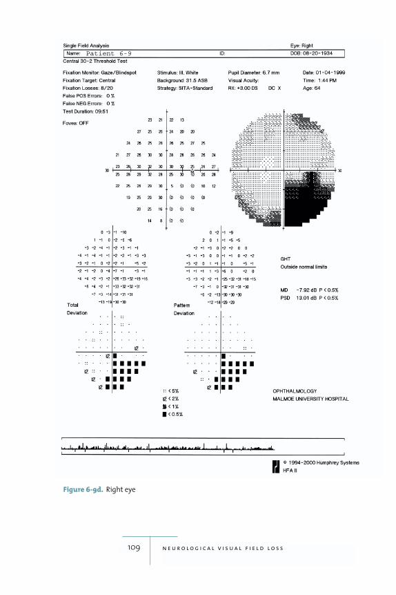
109 n e u r o l o g i c a l v i s u a l f i e l d l o s s
Figure 6-9d. Right eye
Patient 6-9
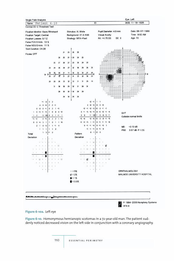
110 e s s e n t i a l p e r i m e t r y
Figure 6-10. Homonymous hemianopic scotomas in a 72-year-old man. The patient sud-
denly noticed decreased vision on the left side in conjunction with a coronary angiography.
Patient 6-10
Figure 6-10a. Left eye
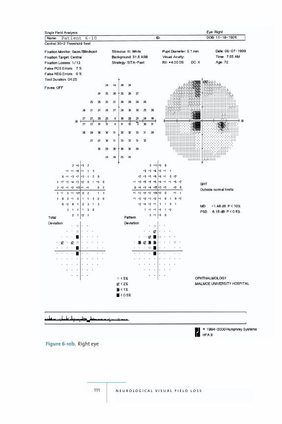
111 n e u r o l o g i c a l v i s u a l f i e l d l o s s
Figure 6-10b. Right eye
Patient 6-10
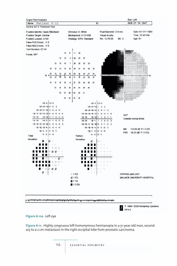
112 e s s e n t i a l p e r i m e t r y
Figure 6-11. Highly congruous left homonymous hemianopia in a 51-year-old man, second-
ary to a 2 cm metastasis in the right occipital lobe from prostatic carcinoma.
Patient 6-11
Figure 6-11a. Left eye
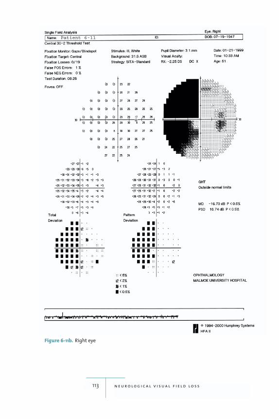
113 n e u r o l o g i c a l v i s u a l f i e l d l o s s
Figure 6-11b. Right eye
Patient 6-11
7Visual Field Loss in Retinal Diseases
114
on ophthalmoscopy in
diagnosing or monitoring retinal disease because most
lesions are visible on ophthalmoscopy. Nevertheless, it is
important to have some knowledge of the visual field
defects caused by retinal lesions. Sometimes retinal dis-
ease can be identified because of field defects found acci-
dentally. Often, several diseases coexist in the same eye,
e.g., glaucoma and retinal disease, and it becomes impor-
tant to determine whether encountered field loss is
caused by one disease or the other.
A common field defect caused by retinal disease is
the central scotoma associated with age-related macular
degeneration. Just a few affected test point locations
may be identified in many cases if a standard grid with
6 degree resolution is used (fig. 7-1). A higher density
10-2 test will show a more detailed picture. Patients with
macular degeneration or central vision loss caused by
other disease should be tested with the large diamond
fixation target if they are having difficulty seeing the
standard fixation LED.
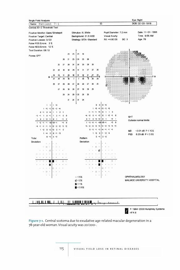
115 v i s u a l f i e l d l o s s i n r e t i n a l d i s e a s e s
Figure 7-1. Central scotoma due to exudative age-related macular degeneration in a
78-year-old woman. Visual acuity was 20/200-.
Patient 7-1
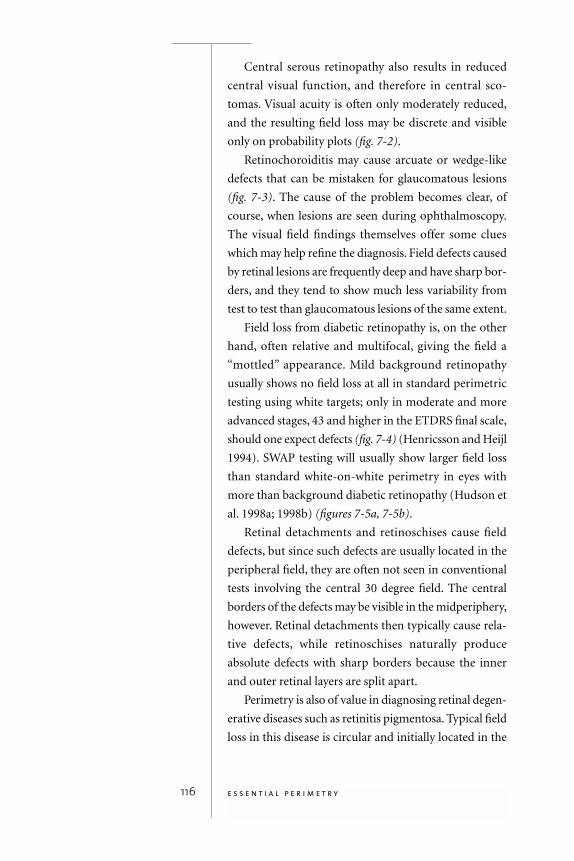
Central serous retinopathy also results in reduced
central visual function, and therefore in central sco-
tomas. Visual acuity is often only moderately reduced,
and the resulting field loss may be discrete and visible
only on probability plots (fig. 7-2).
Retinochoroiditis may cause arcuate or wedge-like
defects that can be mistaken for glaucomatous lesions
(fig. 7-3). The cause of the problem becomes clear, of
course, when lesions are seen during ophthalmoscopy.
The visual field findings themselves offer some clues
which may help refine the diagnosis. Field defects caused
by retinal lesions are frequently deep and have sharp bor-
ders, and they tend to show much less variability from
test to test than glaucomatous lesions of the same extent.
Field loss from diabetic retinopathy is, on the other
hand, often relative and multifocal, giving the field a
“mottled” appearance. Mild background retinopathy
usually shows no field loss at all in standard perimetric
testing using white targets; only in moderate and more
advanced stages, 43 and higher in the ETDRS final scale,
should one expect defects (fig. 7-4) (Henricsson and Heijl
1994). SWAP testing will usually show larger field loss
than standard white-on-white perimetry in eyes with
more than background diabetic retinopathy (Hudson et
al. 1998a; 1998b) (figures 7-5a, 7-5b).
Retinal detachments and retinoschises cause field
defects, but since such defects are usually located in the
peripheral field, they are often not seen in conventional
tests involving the central 30 degree field. The central
borders of the defects may be visible in the midperiphery,
however. Retinal detachments then typically cause rela-
tive defects, while retinoschises naturally produce
absolute defects with sharp borders because the inner
and outer retinal layers are split apart.
Perimetry is also of value in diagnosing retinal degen-
erative diseases such as retinitis pigmentosa. Typical field
loss in this disease is circular and initially located in the
116 e s s e n t i a l p e r i m e t r y
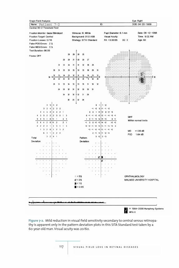
117 v i s u a l f i e l d l o s s i n r e t i n a l d i s e a s e s
Figure 7-2. Mild reduction in visual field sensitivity secondary to central serous retinopa-
thy is apparent only in the pattern deviation plots in this SITA Standard test taken by a
60-year-old man. Visual acuity was 20/60.
Patient 7-2
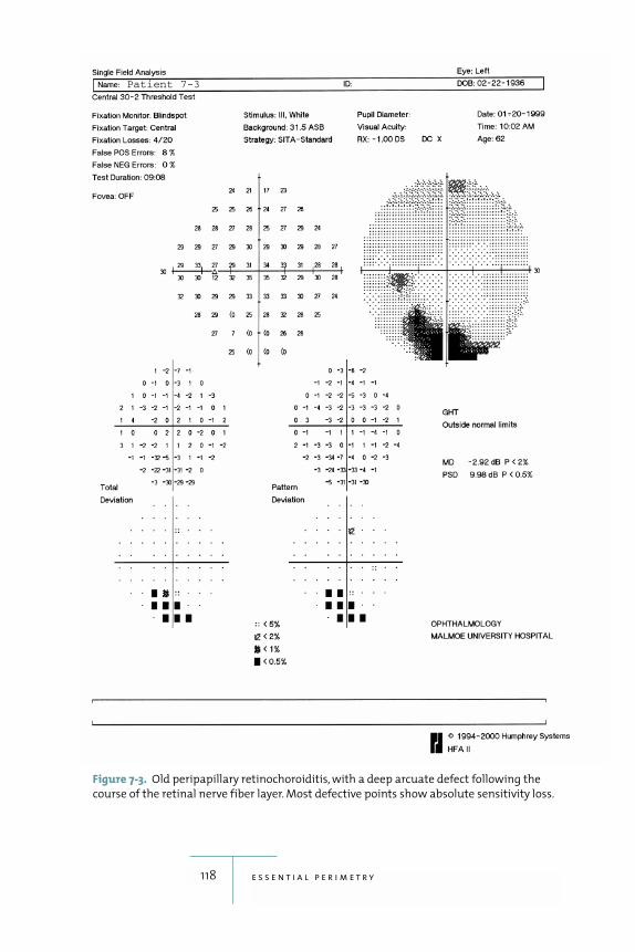
118 e s s e n t i a l p e r i m e t r y
Figure 7-3. Old peripapillary retinochoroiditis, with a deep arcuate defect following the
course of the retinal nerve fiber layer. Most defective points show absolute sensitivity loss.
Patient 7-3
119 v i s u a l f i e l d l o s s i n r e t i n a l d i s e a s e s
midperiphery, but can progress to tunnel vision. There-
fore, searching for visual field loss caused by retinitis pig-
mentosa is one of the few clinical situations where a
standard threshold test using the 30-2 or 24-2 targets
may be a good, but not the best, choice. A suprathresh-
old test that includes the peripheral field could be prefer-
able, particularly because field defects there are often
deep and easily identified.
Of course, retinal vascular occlusions are primarily
diagnosed with ophthalmoscopy, but it is important
when following patients with glaucoma to recognize that
retinal vascular disease can cause field defects (refer
ahead to fig. 8-6b). Arterial occlusions typically result in
absolute field defects, while venous occlusions produce
highly variable field loss. Thus, eyes with small branch
vein occlusions may have entirely normal fields, while
central vein occlusions may sometimes be associated
with profound and widespread field loss.
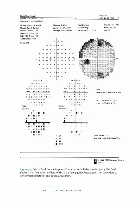
120 e s s e n t i a l p e r i m e t r y
Figure 7-4. Visual field from a 62-year-old woman with diabetic retinopathy. The field
shows a mottled pattern of loss, with an overlying generalized depression secondary to
concomitant posterior sub-capsular cataract.
Patient 7-4
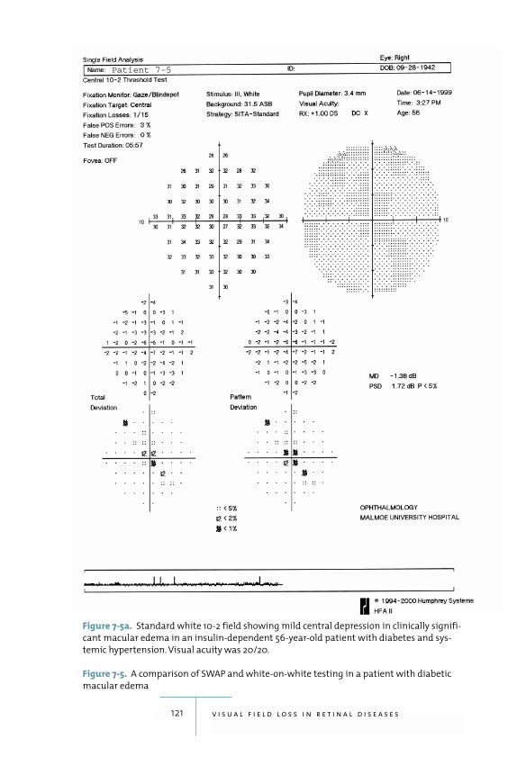
121 v i s u a l f i e l d l o s s i n r e t i n a l d i s e a s e s
Figure 7-5a. Standard white 10-2 field showing mild central depression in clinically signifi-
cant macular edema in an insulin-dependent 56-year-old patient with diabetes and sys-
temic hypertension. Visual acuity was 20/20.
Figure 7-5. A comparison of SWAP and white-on-white testing in a patient with diabetic
macular edema
Patient 7-5
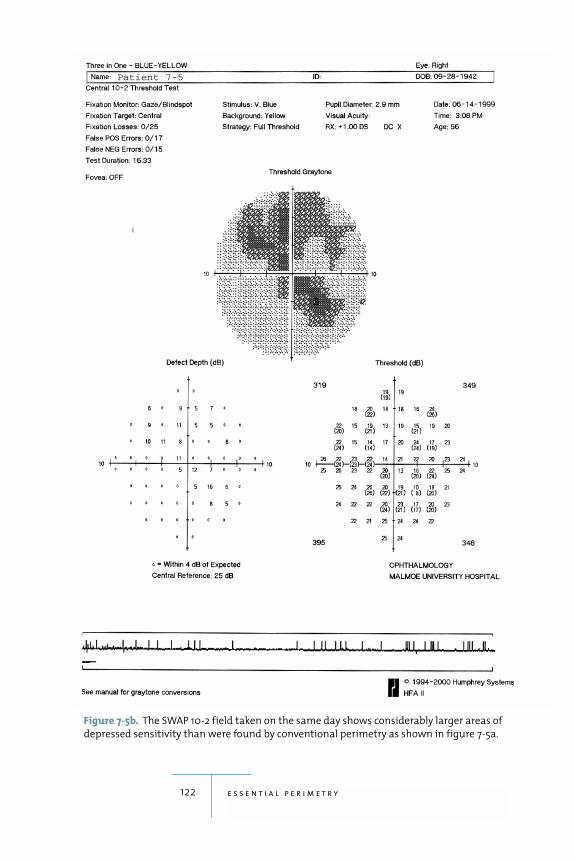
122 e s s e n t i a l p e r i m e t r y
Figure 7-5b. The SWAP 10-2 field taken on the same day shows considerably larger areas of
depressed sensitivity than were found by conventional perimetry as shown in figure 7-5a.
Patient 7-5
8Common Patterns of Artifactual Test Results
123
produce reliable visual
field tests. Fortunately, artifactual results are often easily
recognized. This allows the perimetrist to intercede and
get the patient back on track in order to obtain useful test
results. Common false patterns may be caused by the
patient’s lack of previous perimetric experience, droopy
eyelids or prominent eyebrows, misaligned correction
lenses, lack of proper operator instructions and supervi-
sion, and patient anxiety.
The Untrained Patient and Perimetric Learning
Some patients exhibit perimetric learning, i.e., their field
test results improve after their first test (Heijl, Lindgren,
and Olsson 1989; Wild et al. 1989, 1991; Heijl and Bengts-
son 1996b). Thus, a large minority, probably 10% to 20%,
of patients with a normal visual field do not produce an
entirely normal test result on their first test. Typically,
such fields show depression of sensitivity in the mid-
peripheral area 20 to 30 degrees from fixation, while the
very central field is normal (figures 8-1a–8-1d). If the test
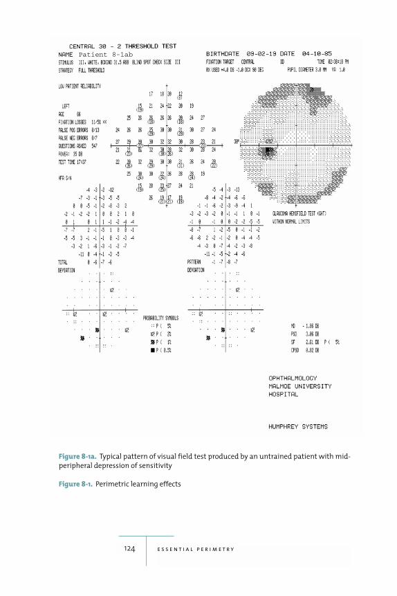
124 e s s e n t i a l p e r i m e t r y
Figure 8-1a. Typical pattern of visual field test produced by an untrained patient with mid-
peripheral depression of sensitivity
Figure 8-1. Perimetric learning effects
Patient 8-1ab
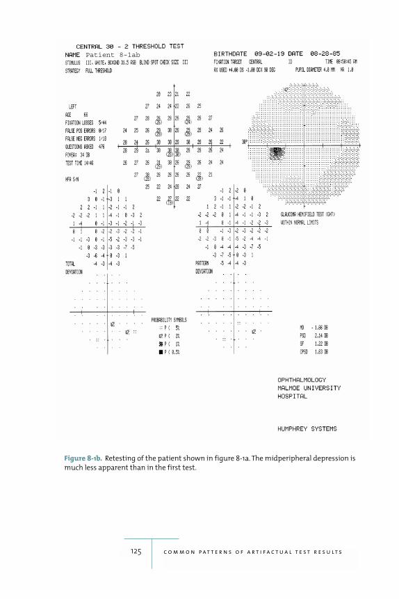
125 c o m m o n p a t t e r n s o f a r t i f a c t u a l t e s t r e s u l t s
Figure 8-1b. Retesting of the patient shown in figure 8-1a. The midperipheral depression is
much less apparent than in the first test.
Patient 8-1ab
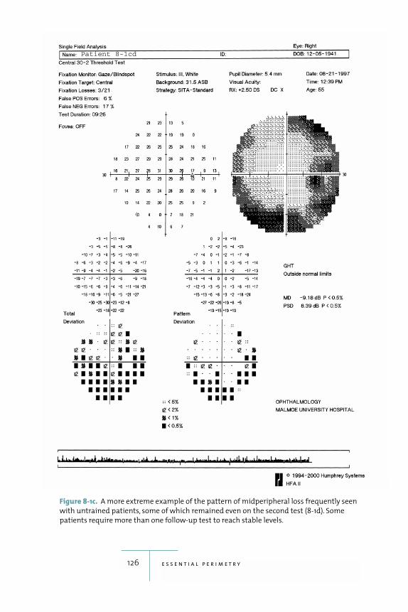
126 e s s e n t i a l p e r i m e t r y
Figure 8-1c. A more extreme example of the pattern of midperipheral loss frequently seen
with untrained patients, some of which remained even on the second test (8-1d). Some
patients require more than one follow-up test to reach stable levels.
Patient 8-1cd
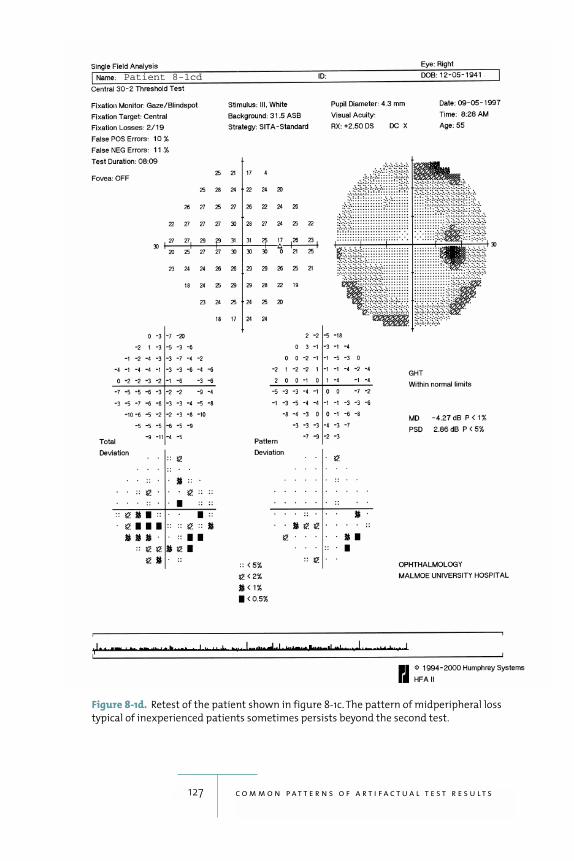
127 c o m m o n p a t t e r n s o f a r t i f a c t u a l t e s t r e s u l t s
Figure 8-1d. Retest of the patient shown in figure 8-1c. The pattern of midperipheral loss
typical of inexperienced patients sometimes persists beyond the second test.
Patient 8-1cd
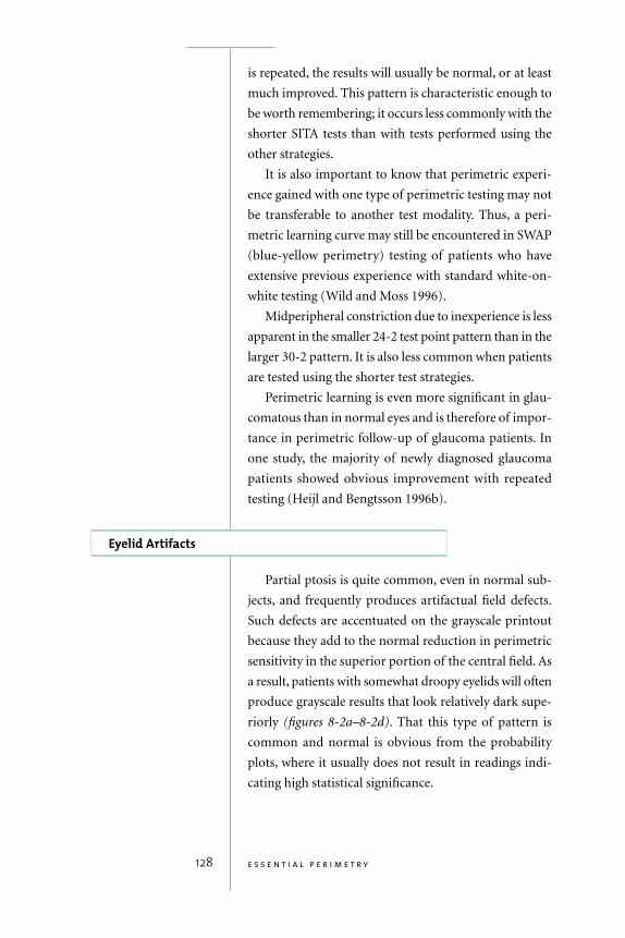
128 e s s e n t i a l p e r i m e t r y
is repeated, the results will usually be normal, or at least
much improved. This pattern is characteristic enough to
be worth remembering; it occurs less commonly with the
shorter SITA tests than with tests performed using the
other strategies.
It is also important to know that perimetric experi-
ence gained with one type of perimetric testing may not
be transferable to another test modality. Thus, a peri-
metric learning curve may still be encountered in SWAP
(blue-yellow perimetry) testing of patients who have
extensive previous experience with standard white-on-
white testing (Wild and Moss 1996).
Midperipheral constriction due to inexperience is less
apparent in the smaller 24-2 test point pattern than in the
larger 30-2 pattern. It is also less common when patients
are tested using the shorter test strategies.
Perimetric learning is even more significant in glau-
comatous than in normal eyes and is therefore of impor-
tance in perimetric follow-up of glaucoma patients. In
one study, the majority of newly diagnosed glaucoma
patients showed obvious improvement with repeated
testing (Heijl and Bengtsson 1996b).
Eyelid Artifacts
Partial ptosis is quite common, even in normal sub-
jects, and frequently produces artifactual field defects.
Such defects are accentuated on the grayscale printout
because they add to the normal reduction in perimetric
sensitivity in the superior portion of the central field. As
a result, patients with somewhat droopy eyelids will often
produce grayscale results that look relatively dark supe-
riorly (figures 8-2a–8-2d). That this type of pattern is
common and normal is obvious from the probability
plots, where it usually does not result in readings indi-
cating high statistical significance.
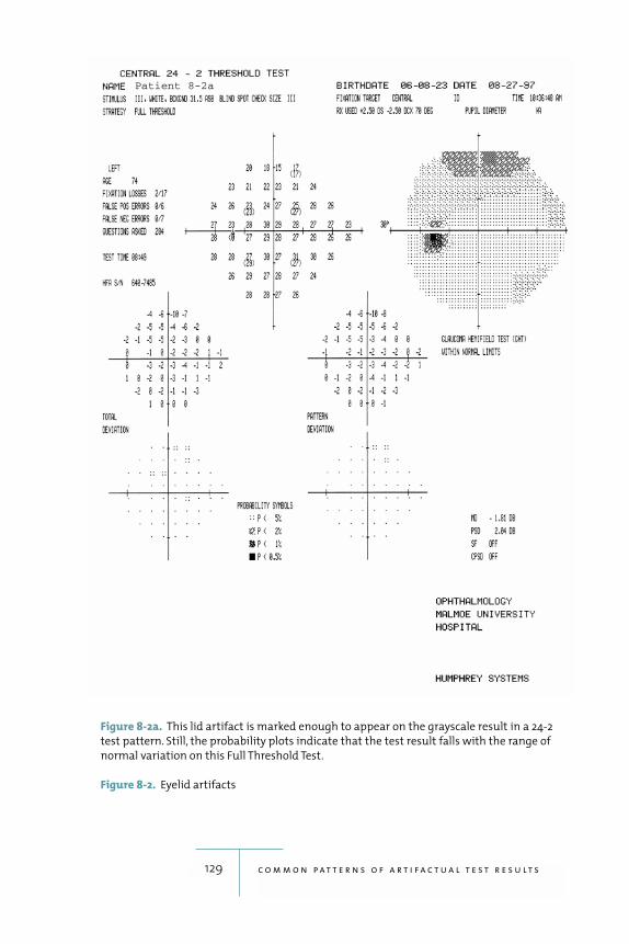
129 c o m m o n p a t t e r n s o f a r t i f a c t u a l t e s t r e s u l t s
Figure 8-2a. This lid artifact is marked enough to appear on the grayscale result in a 24-2
test pattern. Still, the probability plots indicate that the test result falls with the range of
normal variation on this Full Threshold Test.
Figure 8-2. Eyelid artifacts
Patient 8-2a
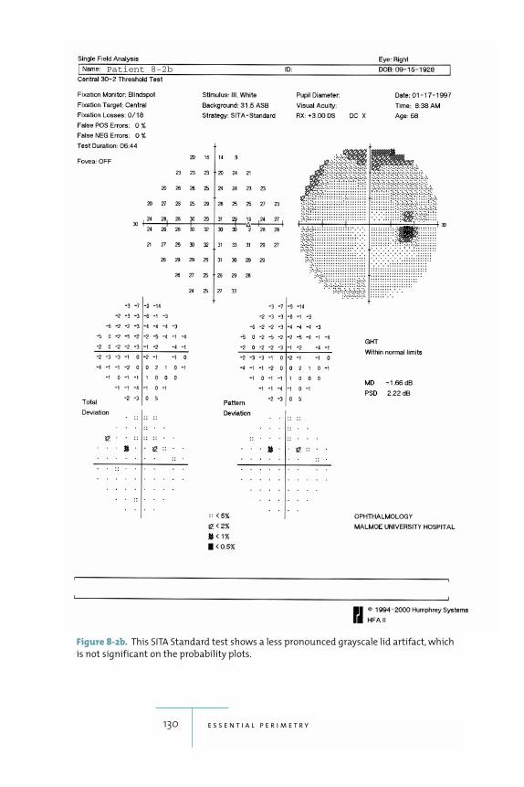
130 e s s e n t i a l p e r i m e t r y
Figure 8-2b. This SITA Standard test shows a less pronounced grayscale lid artifact, which
is not significant on the probability plots.
Patient 8-2b
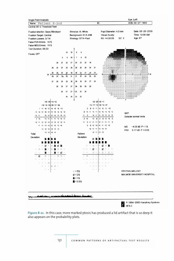
131 c o m m o n p a t t e r n s o f a r t i f a c t u a l t e s t r e s u l t s
Figure 8-2c. In this case, more marked ptosis has produced a lid artifact that is so deep it
also appears on the probability plots.
Patient 8-2cd
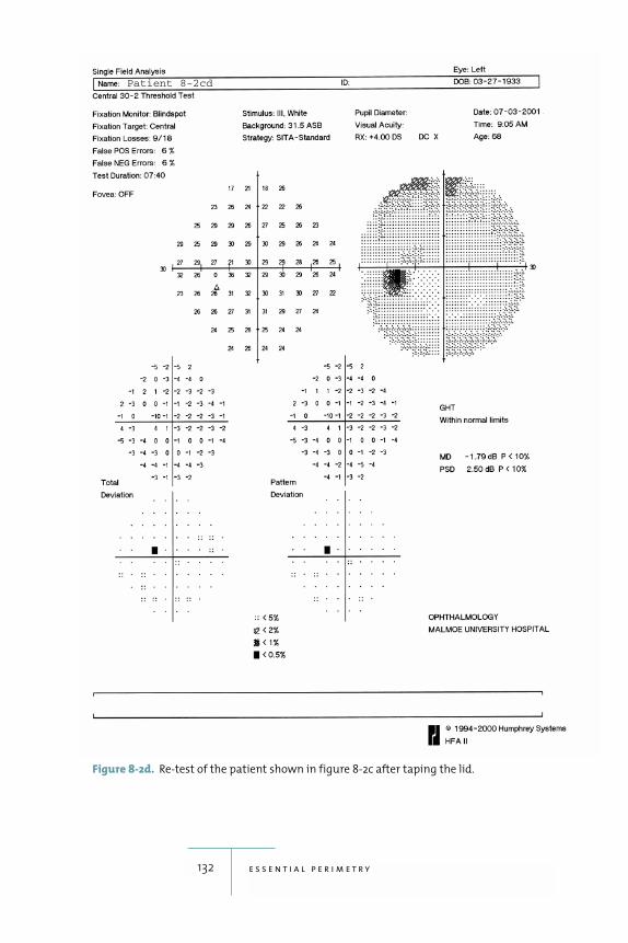
132 e s s e n t i a l p e r i m e t r y
Figure 8-2d. Re-test of the patient shown in figure 8-2c after taping the lid.
Patient 8-2cd
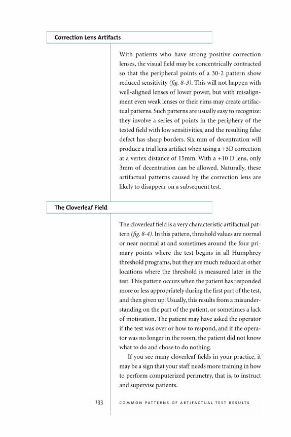
Correction Lens Artifacts
With patients who have strong positive correction
lenses, the visual field may be concentrically contracted
so that the peripheral points of a 30-2 pattern show
reduced sensitivity (fig. 8-3). This will not happen with
well-aligned lenses of lower power, but with misalign-
ment even weak lenses or their rims may create artifac-
tual patterns. Such patterns are usually easy to recognize:
they involve a series of points in the periphery of the
tested field with low sensitivities, and the resulting false
defect has sharp borders. Six mm of decentration will
produce a trial lens artifact when using a +3D correction
at a vertex distance of 15mm. With a +10 D lens, only
3mm of decentration can be allowed. Naturally, these
artifactual patterns caused by the correction lens are
likely to disappear on a subsequent test.
The Cloverleaf Field
The cloverleaf field is a very characteristic artifactual pat-
tern (fig. 8-4). In this pattern, threshold values are normal
or near normal at and sometimes around the four pri-
mary points where the test begins in all Humphrey
threshold programs, but they are much reduced at other
locations where the threshold is measured later in the
test. This pattern occurs when the patient has responded
more or less appropriately during the first part of the test,
and then given up. Usually, this results from a misunder-
standing on the part of the patient, or sometimes a lack
of motivation. The patient may have asked the operator
if the test was over or how to respond, and if the opera-
tor was no longer in the room, the patient did not know
what to do and chose to do nothing.
If you see many cloverleaf fields in your practice, it
may be a sign that your staff needs more training in how
to perform computerized perimetry, that is, to instruct
and supervise patients.
133 c o m m o n p a t t e r n s o f a r t i f a c t u a l t e s t r e s u l t s
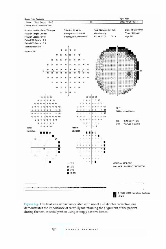
134 e s s e n t i a l p e r i m e t r y
Figure 8-3. This trial lens artifact associated with use of a +8 diopter corrective lens
demonstrates the importance of carefully maintaining the alignment of the patient
during the test, especially when using strongly positive lenses.
Patient 8-3
135 c o m m o n p a t t e r n s o f a r t i f a c t u a l t e s t r e s u l t s
Figure 8-4. The cloverleaf artifact pattern occurred because the patient stopped paying
attention shortly after testing began. Points circled in blue are the primary points, that is,
the first points tested in each quadrant.
Patient 8-4
The “Trigger-Happy” Field
Some patients, particularly if they are anxious, will be
eager to see most or even all stimuli during a test. They
will then press the response button as often as possible,
resulting in large numbers of false responses given when,
in fact, the patient has not seen the stimulus. This will
push up measured threshold values at some points to
levels that no human can see. The result is a classical
“trigger-happy” field, characterized by patches of abnor-
mally light or even entirely white tones in the grayscale
presentation (refer back to fig. 4-5.) Often, the measured
frequency of responses to false-positive catch trials is
high. The Glaucoma Hemifield Test will usually display
the “Abnormally High Sensitivity” message, indicating
the same problem.
The SITA programs calculate the rate of false posi-
tive answers more precisely and are therefore more
likely to identify this type of patient than the older pro-
grams, which had to limit the number of false positive
catch trials in order not to prolong the test time unnec-
essarily. The SITA programs can also partially correct
for false positive answers. Therefore, the full-blown
“trigger-happy” fields with very light grayscale patches
occur less frequently with SITA than with older thresh-
old programs.
Sudden and False Change
Diseases followed over time with repeated visual fields
often have a slow and protracted course. The most com-
mon example is glaucoma, of course, but there are many
other such conditions, e.g., pituitary tumors and retinal
dystrophies. Even if the disease does not really change or
progress, biological variability will result in slightly dif-
ferent fields from test to test. True disease progression is
136 e s s e n t i a l p e r i m e t r y
best identified by analyzing a series of visual fields instead
of only two or three consecutive tests.
If the clinician finds a large difference between two
consecutive fields obtained within a short time period,
the changes are usually not the result of progression of
the chronic disease but of some other new condition. A
sudden and large change in a glaucoma patient is often
due to a stroke, or perhaps retinal vascular occlusion
(figures 8-5a, 8-5b, 8-5c, 8-5d). A stroke can be suspected
when the new field loss respects the vertical meridian, at
least to some extent. This may be difficult to see if there
is also considerable glaucomatous field loss. The diag-
nostic clue in such situations is provided by the fact that
postchiasmal field loss is bilateral and homonymous, and
there will be evidence of sudden and similar worsening in
both of the patient’s visual fields. In contrast, sudden
progression caused by retinal vascular catastrophes will
be unilateral, but the cause will be seen on ophthal-
moscopy (figures 8-6a, 8-6b).
In any case, it is wise to look for other and previously
undiagnosed disease any time that large and sudden
apparent field progression is found when following
patients who have chronic disease.
137 c o m m o n p a t t e r n s o f a r t i f a c t u a l t e s t r e s u l t s
If the clinicianfinds a large
differencebetween two
consecutivefields obtained
within a reasonable
time period,the changes
are usually notthe result ofprogression
of the chronicdisease but of
some other new condition.
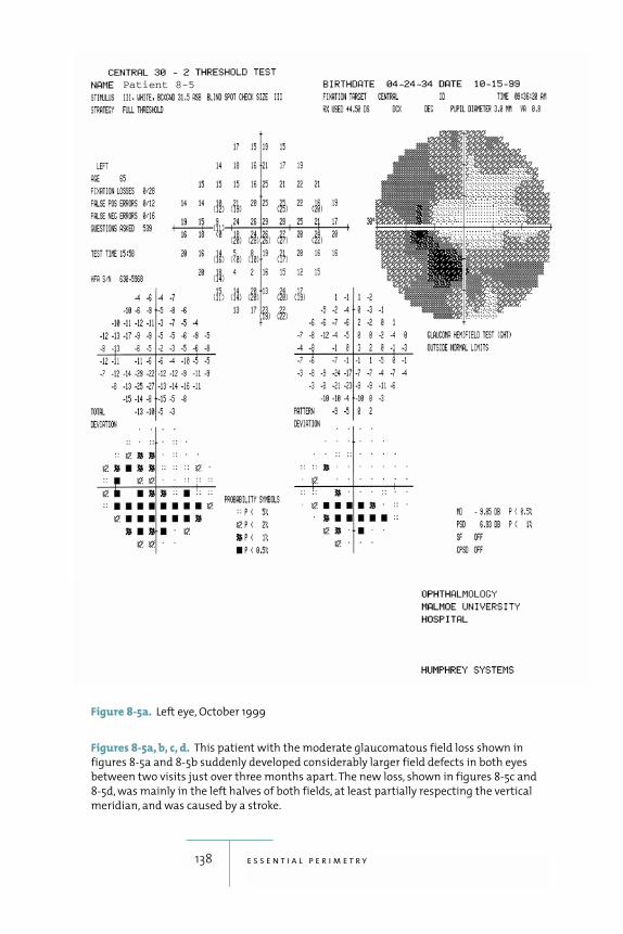
138 e s s e n t i a l p e r i m e t r y
Figures 8-5a, b, c, d. This patient with the moderate glaucomatous field loss shown in
figures 8-5a and 8-5b suddenly developed considerably larger field defects in both eyes
between two visits just over three months apart. The new loss, shown in figures 8-5c and
8-5d, was mainly in the left halves of both fields, at least partially respecting the vertical
meridian, and was caused by a stroke.
Figure 8-5a. Left eye, October 1999
Patient 8-5
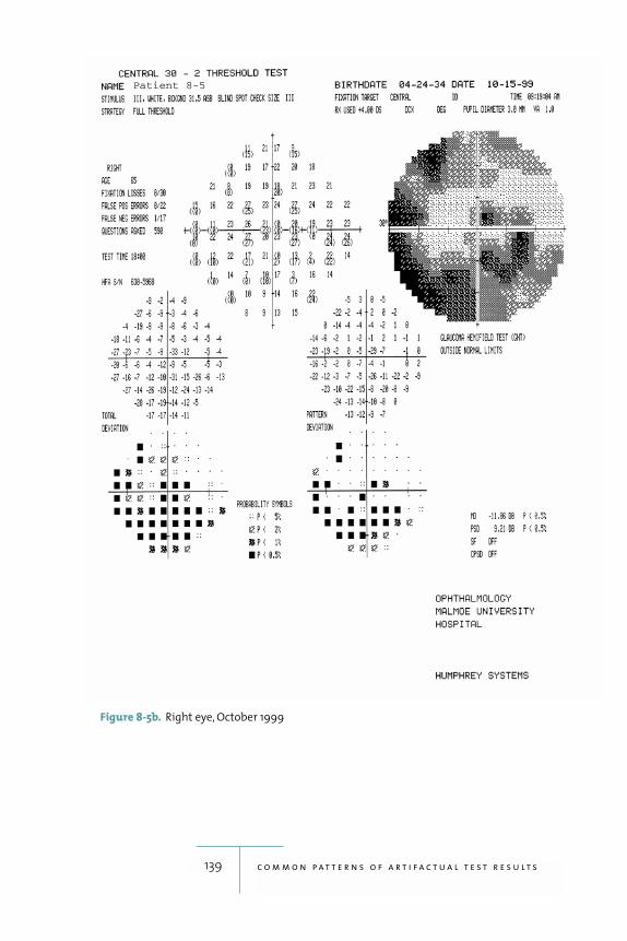
139 c o m m o n p a t t e r n s o f a r t i f a c t u a l t e s t r e s u l t s
Figure 8-5b. Right eye, October 1999
Patient 8-5
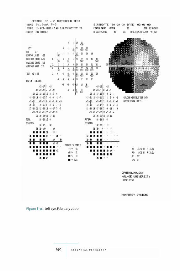
140 e s s e n t i a l p e r i m e t r y
Figure 8-5c. Left eye, February 2000
Patient 8-5
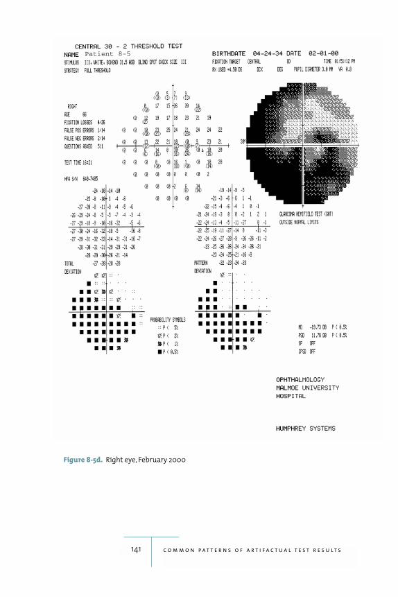
141 c o m m o n p a t t e r n s o f a r t i f a c t u a l t e s t r e s u l t s
Figure 8-5d. Right eye, February 2000
Patient 8-5
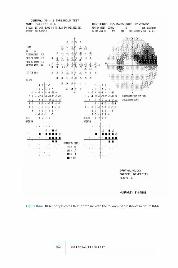
142 e s s e n t i a l p e r i m e t r y
Figure 8-6a. Baseline glaucoma field. Compare with the follow-up test shown in figure 8-6b.
Patient 8-6
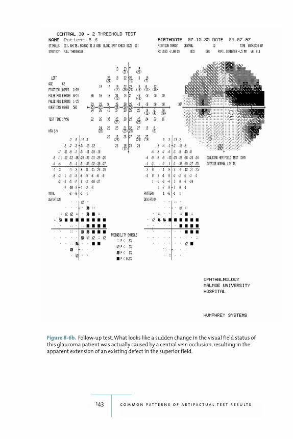
143 c o m m o n p a t t e r n s o f a r t i f a c t u a l t e s t r e s u l t s
Figure 8-6b. Follow-up test. What looks like a sudden change in the visual field status of
this glaucoma patient was actually caused by a central vein occlusion, resulting in the
apparent extension of an existing defect in the superior field.
Patient 8-6
9The Hardware
144
(HFA II) con-
sists of four basic elements: the bowl or projection surface,
the optical system, the central processor, and the patient
interface. The overall design goal was to combine accurate
and consistent perimetric testing with ergonomic features
that provide as much patient comfort as possible.
The Bowl
The bowl of the HFA II is a patented, aspherical, or bullet-
shaped, surface upon which stimuli are projected. This is
a departure from earlier hemispherical designs, such as
the original Goldmann perimeter, and was adopted
because it improves patient ergonomics and reduces
instrument size. The distance from the eye to the center of
the bowl is 30 centimeters—the same as the original
Goldmann perimeter. The amount of asphericity was
chosen such that the surface departs negligibly from the
traditional spherical shape in the central 30 degrees; HFA
II test results are entirely comparable with those of the
original Humphrey perimeter, now known as HFA I
(Johnson et al. 1997). This curvature also assures that the
refractive correction needed for clear vision in the center
of the bowl is proper even at the edge of the central visual
field. Outside the central visual field, the bowl’s aspheric-
ity causes stimuli to be somewhat closer than is the case
in a standard hemispherical bowl. The effect is corrected
for by making small adjustments in stimulus brightness.
The bowl surface is textured to provide an almost per-
fectly matte finish known as a Lambertian surface. Lam-
bertian surfaces provide almost no direct or specular
reflections but instead scatter light diffusely and equally
in all directions. Thus, stimuli projected on this surface
will seem equally bright regardless of viewing angle.
The Optical System
The Humphrey perimeter’s optical system provides stim-
uli of known brightness for a known amount of time in
a known location, and against a background of known
brightness. All five standard Goldmann stimulus sizes (I
through V) are available, although most testing is done
with the size III. Stimuli are presented by aiming a pro-
jection system at the particular location to be tested,
adjusting a set of neutral density filters to obtain the cor-
rect stimulus brightness, and then opening a mechanical
shutter for a fixed time, usually 200 milliseconds. Back-
ground brightness—the brightness of the bowl surface
itself—is checked at the beginning of each test, and con-
stantly during testing. Stimulus brightness is checked
every time the instrument is started up. Stimulus bright-
ness is finely adjusted just before each stimulus is pre-
sented, based upon the local background brightness
measured at each test location. This fine adjustment is
done with the goal of keeping stimulus contrast constant
in spite of any local variations in bowl brightness, such as
those that might be caused by shadows falling on the
bowl from an open door.
145 t h e h a r d w a r e
The Central Processor
The Humphrey perimeter’s central processor not only
fulfills many of the functions commonly seen in a stan-
dard desktop computer, it also must control the optical
system as well as make complex, split-second strategy
adjustments based upon each patient response. The
development of modern, high-speed microprocessors
has made it possible to incorporate the computation-
intensive, maximum-likelihood calculations of the SITA
strategies into everyday clinical practice. The system has
a hard disk for program and data storage, a disk drive,
and a video screen. As with any computer system, all
clinical data must be safeguarded by frequent backing up.
A printer is also available so that visual field test results
may be printed for future reference.
The Patient Interface
The patient interface consists of a chin rest, a forehead
rest, a trial lens holder, the patient response button, and
the instrument table and chair. The chin rest and fore-
head rest are powered by a small electric motor and are
moved horizontally as a unit. A second motor is used to
adjust the chin rest up and down to center the tested eye
behind the lens holder.
The trial lens holder is used to hold standard 37 mm
ophthalmic trial lenses in place in front of the patient’s
eye in order to assure clear vision of the stimuli pre-
sented. Trial lens correction is used only when necessary
for clear vision in central field testing; trial lenses are
never used for testing outside of 30 degrees because the
lens and its holder will produce an area of deep artifac-
tual field loss where they block the patient’s vision of the
periphery. When it is not in use, the trial lens holder can
be folded down and out of the way.
146 e s s e n t i a l p e r i m e t r y
An optional feature on the Humphrey perimeter
automatically adjusts the chin rest and forehead rest in
minute (0.3mm) increments—right-left and up-down—
in order to keep the patient’s eye centered relative to the
trial lens. An automatic vertex distance monitor also
sounds an audible alarm if the patients backs away from
the lens holder. These features are intended as adjuncts to
proper patient instruction and supervision, not as
replacements.
The patient response button is designed for maxi-
mum comfort for elderly patients, especially those whose
hands have been weakened by arthritis, for example.
The instrument table is designed to allow the patient
comfortable and unimpeded access to the perimeter
when sitting in a standard office chair or even a wheel-
chair. The combination of the highly accessible table and
the small-profile aspherical bowl allows the patient to sit
upright comfortably.
147 t h e h a r d w a r e
Literature Cited
148
Alexander, L. J., D. A. Corliss, C. Vinson, J. Williams,L. Casser, M. Fingeret, V. Malinovsky, and J. C.Townsend. 1995. Clinical implications of intra-and inter-reader agreement in four differentautomated visual fields. J Am Optom Assoc 66(11): 681–92.
Anderson, D. R., and V. M. Patella. 1999. AutomatedStatic Perimetry, 2d Ed. St. Louis: Mosby.
Åsman, P., and A. Heijl. 1992a. Glaucoma HemifieldTest: Automated visual field evaluation. ArchOphthalmol 110 (6): 812–19.
———. 1992b. Evaluation of methods for automatedhemifield analysis in perimetry. ArchOphthalmol 110 (6): 820–26.
Aulhorn, E., and H. Harms. 1972. Visual perimetry.In Handbook of Sensory Physiology, ed. Jamesonand Hurvich. vol. 7, no. 4, 102–145. Berlin:Springer-Verlag.
Bayer, A., and C. Erb. 2002. Short-wavelength auto-mated perimetry, frequency-doubling technol-ogy perimetry, and pattern-electroretinographyfor prediction of progressive glaucomatous stan-dard visual field defects. Ophthalmol 109 (5):1009–17.
Bengtsson, B. 2000. Reliability of computerized peri-metric threshold tests as assessed by reliabilityindices and threshold reproducibility in patientswith suspect and manifest glaucoma. ActaOphthalmol 78 (5): 519–22.
Bengtsson, B., and A. Heijl. 1998. SITA Fast, a newrapid perimetric threshold test. Description ofmethods and evaluation in patients with mani-fest and suspect glaucoma. Acta Ophthalmol 76(4): 431–37.
———. 1999a. Comparing significance and magni-tude of glaucomatous visual field defects usingthe SITA and Full Threshold strategies. ActaOphthalmol 77 (2): 143–46.
———. 1999b. Perimetry Update 1998/99. The Hague:Kugler Publications. 3–7.
———. 2000. False-negative responses in glaucomaperimetry: indicators of patient performance ortest reliability? Invest Ophthalmol Vis Sci 41 (8):2201–04.
Bengtsson, B., A. Lindgren, A. Heijl, G. Lindgren, P.Åsman, and V. M. Patella. 1997. Perimetric prob-ability maps to separate change caused by glau-coma from that caused by cataract. ActaOphthalmol 75 (2): 184–88.
Bengtsson, B., J. Olsson, A. Heijl, and H. Rootzen.1997. A new generation of algorithms for computerized threshold perimetry, SITA.Acta Ophthalmol 75 (4): 368–75.
Cahill, K. V., J. A. Burns, and P. A. Weber. 1987. Theeffect of blepharoptosis on the field of vision.Ophthal Plast Reconstr Surg 3 (3): 121–25.
149 l i t e r a t u r e c i t e d
Caprioli, J., and G. L. Spaeth. 1985. Static thresholdexamination of the peripheral nasal visual fieldin glaucoma. Arch Ophthalmol 103 (8): 1150–54.
Donahue, S. P., and A. Porter. 2001. SITA visual fieldtesting in children. J AAPOS 5 (2): 114–17.
Easterbrook, M. 1999. Detection and prevention ofmaculopathy associated with antimalarialagents. Int Ophthalmol Clin 39 (2): 49–57.Review.
Easterbrook, M., and G. Trope. 1989. Value ofHumphrey perimetry in the detection of earlychloroquine retinopathy. Lens Eye Toxic Res 6(1–2): 255–68.
Hacker, H. D., and D. A. Hollsten. 1992. Investigation of automated perimetry in the evaluation ofpatients for upper lid blepharoplasty. OphthalPlast Reconstr Surg 8 (4): 250–55.
Hard-Boberg, A., and J. D. Wirtschafter. 1985. Eval-uating the usefulness in neuro-ophthalmologyof visual field examination peripheral to 30degrees. Doc Ophthal Proceedings Series 42:197–206.
Heijl, A. 1976. Automatic perimetry in glaucoma visualfield screening. A clinical study. Graefes Archiv200: 21–37.
———. 1989. Lack of diffuse loss of differential lightsensitivity in early glaucoma. Acta Ophthalmol67 (4): 353–60.
Heijl, A., and P. Åsman. 1989. A clinical study of peri-metric probability maps. Arch Ophthalmol 107(2): 199–203.
Heijl, A., and B. Bengtsson. 1996a. Early visual fielddefects in glaucoma: a study of eyes developingfield loss. In Glaucoma: Decision Making inTherapy, edited by M. G. Bucci. Milan: Springer-Verlag. 75–78.
150 e s s e n t i a l p e r i m e t r y
———. 1996b. The effect of perimetric experience inpatients with glaucoma. Arch Ophthalmol 114(1): 19–22.
Heijl, A., B. Bengtsson, and V. M. Patella. 2000.Glaucoma follow-up when converting from long to short perimetric threshold tests. ArchOphthalmol 118 (4): 489–93.
Heijl, A., A. Lindgren, and G. Lindgren. 1989. Test-retest variability in glaucomatous visual fields.Am J Ophthalmol 198: 130.
Heijl A., A. Lindgren, G. Lindgren, and V. M. Patella.1991. Inter-test threshold variability in glau-coma, importance of censored observations andgeneral field status. Perimetry Update 1990–91.Edited by R.P. Mills and A. Heijl. Amsterdamand New York: Kugler Publications. 189–192.
Heijl, A., G. Lindgren, and J. Olsson. 1987. Normalvariability of static perimetric threshold valuesacross the central visual field. Arch Ophthalmol105 (11): 1544–49.
———. 1989. The effect of perimetric experience innormal subjects. Arch Ophthalmol 107 (1):81–86.
Heijl, A., G. Lindgren, A. Lindgren, J. Olsson, P. Åsman,S. Myers, and M. Patella. 1991. Extended empiri-cal statistical package for evaluation of singleand multiple fields in glaucoma: Statpac 2.Perimetry Update 1990–91. Edited by R. P. Millsand A. Heijl. Amsterdam and New York: KuglerPublications. 303–315.
Henricsson, M. and A. Heijl. 1994. Visual fields at different stages of diabetic retinopathy. ActaOphthalmol 72 (5): 560–69.
Herse, P. R. 1992. Factors influencing normal perimet-ric thresholds. Invest Ophthalmol Vis Sci 33 (3):611–17.
151 l i t e r a t u r e c i t e d
Heuer, D. K., D. R. Anderson, W. J. Feuer, and M. G.Gressel. 1987. The influence of refraction accu-racy on automated perimetric threshold meas-urements. Ophthalmology 94 (12): 1550–53.
Hudson, C., J. G. Flanagan, G. S. Turner, H. C. Chen,L. B. Young, and D. McLeod. 1998a. Short-wavelength sensitive visual field loss in patientswith clinically significant diabetic macularoedema. Diabetologia 41 (8): 918–28.
———. 1998b. Influence of laser photocoagulationfor clinically significant diabetic macularoedema (DMO) on short-wavelength and con-ventional automated perimetry. Diabetologia 41(11): 1283–92.
Inazumi, K. A., Tsuji, T. Yamamoto, and Y. Kitazawa.1998. [Evaluation of the Swedish interactivethresholding algorithm, a new thesholding algo-rithm, of the Humphrey Field Analyzer in glau-coma patients.] Nippon Ganka Gakkai Zasshi102 (10): 667–72. Japanese.
International Council of Opthalmology. 1979.Perimetric Standards and Perimetric Glossary.The Hague: Dr. W. Junk bv Publishers.
Johnson, C. A. 2002. Recent developments in auto-mated perimetry in glaucoma diagnosis andmanagement. Curr Opin Ophthalmol 13 (2):77–84.
Johnson, C. A., M. Wall, M. Fingeret, and P. Lalle. 1998.A Primer for Frequency Doubling Technology.Skaneateles Falls, NY: Welch Allyn, Inc. 59–60.
Johnson, C. A., G. A. Cioffi, S. M. Drance, D. Gaaster-land, R. P. Mills, F. Ashburn, P. Hnik, and R. E.Van Coevorden. 1997. A multicenter comparisonstudy of the Humphrey Field Analyzer I and theHumphrey Field Analyzer II. Ophthalmology 104(11): 1910–17.
152 e s s e n t i a l p e r i m e t r y
Johnson, C. A., A. J. Adams, E. J. Casson, and J. D.Brandt. 1993a. Blue-on-yellow perimetry canpredict the development of glaucomatous visualfield loss. Arch Ophthalmol 111 (5): 645–50.
———. 1993b. Progression of early glaucomatousvisual field loss as detected by blue-on-yellowand standard white-on-white automatedperimetry. Arch Ophthalmol 111 (5): 651–56.
Johnson, C. A., and J. L. Keltner. 1983. Incidence ofvisual field loss in 20,000 eyes and its relation-ship to driving performance. Arch Ophthalmol101: 371–75.
Katz, J., A. Sommer, D. E. Gaasterland, and D. R.Anderson. 1991. Comparison of analytic algo-rithms for detecting glaucomatous visual fieldloss. Arch Ophthalmol 109 (12): 1684–89.
Katz, J., J. M. Tielsch, H. A. Quigley, and A. Sommer.1995. Automated perimetry detects visual fieldloss before manual Goldmann perimetry.Ophthalmology 102 (1): 21–26.
Keltner, J. L., and C. A. Johnson. 1995. Short-wavelengthautomated perimetry in neuro-ophthalmologicdisorders. Arch Ophthalmol 113 (4): 475–81.
Keltner, J. L., C. A. Johnson, J. O. Spurr, and R. W. Beck.1999. Comparison of central and peripheralvisual field properties in the optic neuritis treat-ment trial. Am J Ophthalmol 128 (5): 543–53.
Langerhorst, C. T., T. J. van den Berg, and E. L. Greve.1989. Is there general reduction of sensitivity inglaucoma? Int Ophthalmol 13 (1–2): 31–35.
Leske, M. C., A. Heijl, L. Hyman, and B. Bengtsson.1999 Early Manifest Glaucoma Trial: design andbaseline data. Ophthalmology 106 (11): 2144–53.
Lynn, J. R. 1969. Examination of the visual field inglaucoma. Invest Ophthalmol 8: 76–84.
153 l i t e r a t u r e c i t e d
McKendrick, A., G. A. Cioffi, C. A. Johnson. 2002.Short-wavelength sensitivity deficits in patientswith migraine. Arch Ophthalmol 120: 154–61.
McKnight, A. J., D. Shinar, and B. Hilburn. 1991.Thevisual and driving performance of monocularand binocular heavy-duty truck drivers. AccidAnal Prev 23: 225–37.
Mills, R. P., H. S. Barnebey, C. V. Migliazzo, and Y. Li.1994. Does saving time using FastPac orsuprathreshold testing reduce quality of visualfields? Ophthalmology 101 (9): 1596–603.
Polo, V., J. M. Larrosa, I. Pinilla, S. Perez, F. Gonzalvo,and F. M. Honrubia. 2002. Predictive value of short-wavelength automated perimetry:A three-year follow-up study. Ophthalmology109 (4): 761–65.
Remky, A., and O. Arend. 2000. [Clinical experienceswith the “Swedish interactive threshold algo-rithm (SITA).”] Klin Monatsbl Augenheilkd 216(3): 143–37. German.
Remky, A., K. Lichtenberg, A. E. Elsner, and O. Arend.2001. Short wavelength automated perimetry inage related maculopathy. Br J Ophthalmol 85:1432–36.
Riddoch, G. 1917. Dissociation of visual perceptionsdue to occipital injuries, with especial referenceto appreciation of movement. Brain 40: 15–57.
Sample, P. A., J. D. Taylor, G. A. Martinez, M. Lusky,and R. N. Weinreb. 1993. Short-wavelengthcolor visual fields in glaucoma suspects at risk.Am J Ophthalmol 115 (2): 225–33.
Sample, P. A., and R. N. Weinreb. 1992. Progressivecolor visual field loss in glaucoma. InvestOphthalmol Vis Sci 33 (6): 2068–71.
Sharma, A. K., I. Goldberg, S. L. Graham, and M.Mohsin. 2000. Comparison of the HumphreySwedish interactive thresholding algorithm(SITA) and full threshold strategies. J Glaucoma9 (1): 20–27.
154 e s s e n t i a l p e r i m e t r y
Siatkowski, R. M., B. Lam, D. R. Anderson, W. J.Feuer, and A. M. Halikman. 1996. Automatedsuprathreshold static perimetery screening inneuro-ophthalmology. Ophthalmology 103:907–17.
Soliman, M. A., L. A. de Jong, A. A. Ismaeil, T. J. vanden Berg, and M. D. de Smet. 2002. Standardachromatic perimetry, short wavelength auto-mated perimetry, and frequently doubling tech-nology for detection of glaucoma damage.Ophthalmology 109 (3): 444–54.
Stewart, W. C., and M. B. Shields. 1991. The peripheralvisual field in glaucoma: re-evaluation in the ageof automated perimetry. Surv Ophthalmol 36(1): 59–69.
Wall, M., S. G. Punke, T. L. Stickney, C. F. Brito,K. R. Withrow, and R. H. Kardon. 2001. SITAStandard in optic neuropathies and hemi-anopias: a comparison with full threshold test-ing. Invest Ophthalmol Vis Sci 42 (2): 528–37.
Weinreb, R. N., and J. P. Perlman. 1986. The effect ofrefractive correction on automated perimetricthresholds. Am J Ophthamol 101 (6): 706–09.
Werner, E.B., and S.M. Drance. 1997. Early visual fielddisturbances in glaucoma. Arch Ophthalmol 95(7): 1173-75.
Wild, J. M. 2001. Short wavelength automated perime-try. Acta Ophthalmol 79: 546–59.
Wild, J. M., M. Dengler-Harles, A. E. Searle, E. C.O’Neill, and S. J. Crews. 1989. The influence ofthe learning effect on automated perimetry inpatients with suspected glaucoma. ActaOphthalmol 67 (5): 537–45.
Wild, J. M., and I. D. Moss. 1996. Baseline alterationsin blue-on-yellow normal perimetric sensitivity.Graefes Arch Clin Exp Ophthalmol 234 (3):141–49.
155 l i t e r a t u r e c i t e d
Wild, J. M., I. E. Pacey, S. A. Hancock, and I. A.Cunliffe. 1999. Between-algorithm, between-individual differences in normal perimetricsensitivity: Full Threshold, FastPac, and SITA.Invest Ophthalmol Vis Sci 40 (6): 1152–61.
Wild, J. M., I. E. Pacey, E. C. O’Neill, and I. A. Cunliffe.1999. The SITA perimetric threshold algorithmsin glaucoma. Invest Ophthalmol Vis Sci 40 (9):1998–2009.
Wild, J. M., A. E. Searle, M. Dengler-Harles, and E. C.O’Neill. 1991. Long-term follow-up of baselinelearning and fatigue effects in the automatedperimetry of glaucoma and ocular hypertensivepatients. Acta Ophthalmol 69 (2): 210–16.
Wood, J. M., and R. Troutbeck. 1994. Effect of visualimpairment on driving. Hum Factors 36:476–87.
156 e s s e n t i a l p e r i m e t r y
Index
157
Aabnormal visual fields,
14–15. See also defects;glaucomatous fielddefects
absolute field defects, 119age-related macular degen-
eration, 38altitudinal field loss before
and after cataract surgery,82–83
amblyopia, 91analysis of tests. See inter-
preting test resultsanatomy, 70–72aneurysms, 96anterior ischemic optic
neuropathy, 91arcuate defects
double, 74, 86in drusen of optic disk,
96patterns of field loss, 76peripapillary
retinochoroiditis, 115,116, 117
scotomas, 13, 71–72, 73,86
arterial circle of Willis, 96arterial occlusions, 119artifacts, 13, 47
caused by untrainedpatient, 123, 128
cloverleaf, 133, 135contractions of field, 133correction lens, 133, 134eyelid, 43, 128, 129–132sudden and false change,
136–137trial lens holder, 24, 146trigger happy fields, 136
asymptomatic visualrestrictions, 43
Bbackground illumination,
18–19baseline tests, 62, 64,
142–143benign intracranial hyper-
tension, 95bilateral field loss in thyroid
ophthalmopathy,100–101
binocular Esterman test, 42
bitemporal hemianopias,96, 102–103
blepharoplasty, 37, 42blepharoptosis, 43blind spot. See also optic
nerve/optic diskenlargement of, 91, 96Heijl-Krakau monitoring
technique, 20–21, 57,59
normal diameter of, 20blue-cone system, 37blue-yellow perimetry, 8,
33, 37branch vein occlusions, 119
Ccase examples
altitudinal field lossbefore and aftercataract surgery,82–83
arcuate defect/peripapil-lary retinochoroiditis,117
baseline glaucoma field,142–143
bilateral field loss in thy-roid ophthalmopathy,100–101
bitemporal resolutiondefects/craniopharyn-gioma, 104–105
central depression/macu-lar edema/diabetes/systemic hypertension,121–122
central scotoma/age-related macular degen-eration, 115
Change Analysis/glauco-matous visual fieldloss, 68
cloverleaf artifact, 135complete bitemporal
hemianopia/cysticpituitary adenoma,102–103
congruous left homo-noumous hemi-anopia/prostatic carci-noma metastasis,112–113
deep hemianopicdefects/occipital lobehemorrhage, 106–108
defect depth, 66–67diabetic macular edema,
38diabetic retinopathy/pos-
terior sub-capsularcataract, 120
double arcuate defect, 74,86
early central glaucoma-tous defect, 75–76
early glaucoma field loss,48–49
end stage glaucoma, 28,29, 34–35
eyelid artifacts, 129–132false positives, 58gaze tracker results, 60generalized depression of
hill of vision, 81glaucoma, 40–42homonymous hemianopic
scotomas/coronaryangiography, 110–111
inferior nasal step, 79ischemic optic neuropa-
thy, 94modern threshold
perimetry, 31normal tension glauco-
ma/progressive fieldloss, 60
ocularhypertension/cataract/normal visual acuity,88–89
optic disk drusen, 99optic disk edema, 95optic neuritis, 92–93paracentral glaucoma-
tous field defect, 77
perimetric learningeffects, 124–127
progressive cataract,51–53
progressive open-angleglaucoma, 63
secondary optic atrophy,97
sensitivity reduction/cen-tral serous retinopathy,117
STATPAC single fieldanalysis, 9
sudden field loss/glauco-matous/stroke,138–141
superior altitudinaldefect/inferior nasalstep, 80
superior arcuate sco-toma, 73
superior nasal step, 78transition from normal
to glaucomatous fieldloss, 84–85
trial lens artifact, 134cataracts. See also media
opacitiesaltitudinal field loss
before and after sur-gery, 82–83
diabetic retinopathy and,120
ocular hypertension and,88–89
posterior subcapsular,120
progressive, 51–53central depression, 121–122central field
central scotomas, 115central vision loss, 32,
11430 degree, 116depression of, 121–122testing, 43
central serous retinopathy,115, 117
158 e s s e n t i a l p e r i m e t r y
central vs. peripheral test-ing, 26–27
Change Analysis format, 44,64, 65, 68
chloroquine-induced mac-ulopathy, 43
circular field loss, 116, 119clinical trials, 33, 37cloverleaf artifact, 12, 133,
135comparisons
cross-strategy, of rawthresholds, 83
follow-up test, 7generalized depression
of/normal hill ofvision, 81
of newer SITA tests toolder standards, 32–33
between old and new teststrategies, 69
total and pattern devia-tion, 50
congruous left homony-mous hemianopia,112–113
consistency, 32contractions of field, 71–72,
133coronary angiography,
110–111craniopharyngioma, 96,
104–105cystic pituitary adenoma,
102–103
Ddecibel values, 10Defect Depth printout, 65defects. See also by name or
type of defect, e.g. arcuatedefectsawareness of, by patients,
15basic definition of, 14–15bitemporal resolution,
104–105Bjerrum, 71–72
caused by retinal disease,114
central field, 5congruity of, 98Defect Depth printout,
65depth of, 66–67describing field, 15early central glaucoma-
tous, 75–76false, 12, 56–57, 58, 133,
136localized, 15, 72, 76matching, in both eyes,
98residual, 91resolution, 96retinal, steepness of
borders in, 6shallow, 59size of, 91wedge-like, 115
demographics, 8diabetes, 38, 116, 120,
121–122diagnostic methods
diagnosing field loss,10–11
glaucoma, 4, 30neurological disease, 4, 26retinal disease, 4
differential diagnosisglaucoma/optic neuritis,
91optic disk drusen/glauco-
ma, 96retinal
detachment/retino-schisis, 27
thyroid ophthalmo-pathy/glaucoma, 96
disabilities, testing for, 37, 39,42. See also driving tests
disc edema, 91distance
from eye to center ofbowl, 144
to stimulus, 24
distance correction for test-ing, 39
double arcuate defects, 74,86
driving tests, 7, 16, 37, 39, 42drug-induced macu-
lopathies, 43drusen of the optic disk, 96
Eedematous disorders
diabetic macular edema,38
macular edema, 121–122optic disc edema, 91, 95,
96papilledema, 94, 97
errors. See also artifactsfalse negative (FN)
results, 57false positive (FP) results,
12, 56–57, 58, 136of interpreting test
results, 12in perimetric glaucoma
follow-up, 87red flags, 12, 13
Esterman test, 39, 42eyelids
artifacts caused by, 43,128, 129–132
asymptomatic visualrestrictions caused by,43
blepharoplasty, 37, 42blepharoptosis, 43
Ffalse defects, 12, 56–57, 58,
133, 136false positives, 58fatigue, 7field defects. See defectsfield of vision,
normal/abnormal, 14–15fixation
fixation loss (FL) rate, 57,59
159 i n d e x
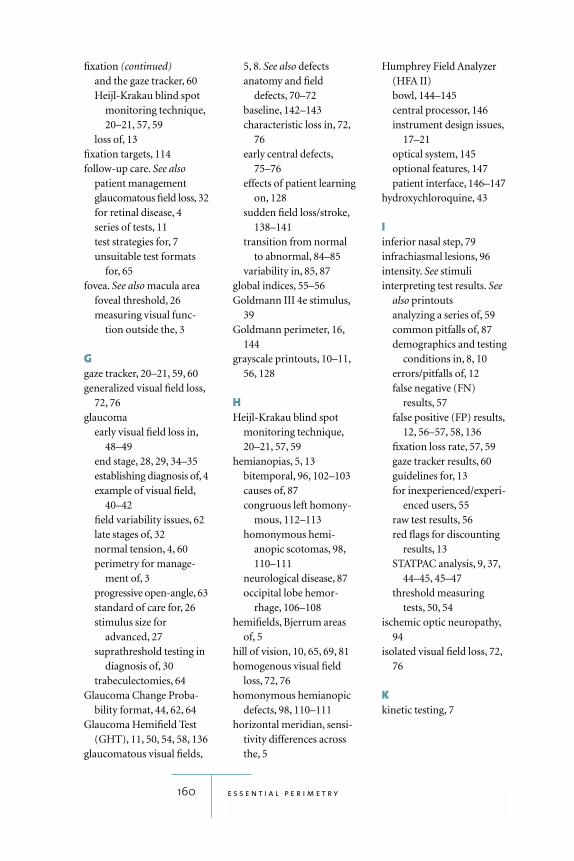
fixation (continued)and the gaze tracker, 60Heijl-Krakau blind spot
monitoring technique,20–21, 57, 59
loss of, 13fixation targets, 114follow-up care. See also
patient managementglaucomatous field loss, 32for retinal disease, 4series of tests, 11test strategies for, 7unsuitable test formats
for, 65fovea. See also macula area
foveal threshold, 26measuring visual func-
tion outside the, 3
Ggaze tracker, 20–21, 59, 60generalized visual field loss,
72, 76glaucoma
early visual field loss in,48–49
end stage, 28, 29, 34–35establishing diagnosis of, 4example of visual field,
40–42field variability issues, 62late stages of, 32normal tension, 4, 60perimetry for manage-
ment of, 3progressive open-angle, 63standard of care for, 26stimulus size for
advanced, 27suprathreshold testing in
diagnosis of, 30trabeculectomies, 64
Glaucoma Change Proba-bility format, 44, 62, 64
Glaucoma Hemifield Test(GHT), 11, 50, 54, 58, 136
glaucomatous visual fields,
5, 8. See also defectsanatomy and field
defects, 70–72baseline, 142–143characteristic loss in, 72,
76early central defects,
75–76effects of patient learning
on, 128sudden field loss/stroke,
138–141transition from normal
to abnormal, 84–85variability in, 85, 87
global indices, 55–56Goldmann III 4e stimulus,
39Goldmann perimeter, 16,
144grayscale printouts, 10–11,
56, 128
HHeijl-Krakau blind spot
monitoring technique,20–21, 57, 59
hemianopias, 5, 13bitemporal, 96, 102–103causes of, 87congruous left homony-
mous, 112–113homonymous hemi-
anopic scotomas, 98,110–111
neurological disease, 87occipital lobe hemor-
rhage, 106–108hemifields, Bjerrum areas
of, 5hill of vision, 10, 65, 69, 81homogenous visual field
loss, 72, 76homonymous hemianopic
defects, 98, 110–111horizontal meridian, sensi-
tivity differences acrossthe, 5
Humphrey Field Analyzer(HFA II)bowl, 144–145central processor, 146instrument design issues,
17–21optical system, 145optional features, 147patient interface, 146–147
hydroxychloroquine, 43
Iinferior nasal step, 79infrachiasmal lesions, 96intensity. See stimuliinterpreting test results. See
also printoutsanalyzing a series of, 59common pitfalls of, 87demographics and testing
conditions in, 8, 10errors/pitfalls of, 12false negative (FN)
results, 57false positive (FP) results,
12, 56–57, 58, 136fixation loss rate, 57, 59gaze tracker results, 60guidelines for, 13for inexperienced/experi-
enced users, 55raw test results, 56red flags for discounting
results, 13STATPAC analysis, 9, 37,
44–45, 45–47threshold measuring
tests, 50, 54ischemic optic neuropathy,
94isolated visual field loss, 72,
76
Kkinetic testing, 7
160 e s s e n t i a l p e r i m e t r y
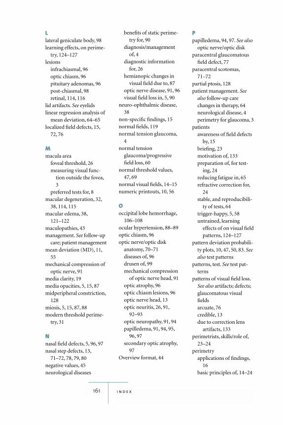
Llateral geniculate body, 98learning effects, on perime-
try, 124–127lesions
infrachiasmal, 96optic chiasm, 96pituitary adenomas, 96post-chiasmal, 98retinal, 114, 116
lid artifacts. See eyelidslinear regression analysis of
mean deviation, 64–65localized field defects, 15,
72, 76
Mmacula area
foveal threshold, 26measuring visual func-
tion outside the fovea,3
preferred tests for, 8macular degeneration, 32,
38, 114, 115macular edema, 38,
121–122maculopathies, 43management. See follow-up
care; patient managementmean deviation (MD), 11,
55mechanical compression of
optic nerve, 91media clarity, 19media opacities, 5, 15, 87midperipheral constriction,
128miosis, 5, 15, 87, 88modern threshold perime-
try, 31
Nnasal field defects, 5, 96, 97nasal step defects, 13,
71–72, 78, 79, 80negative values, 45neurological diseases
benefits of static perime-try for, 90
diagnosis/managementof, 4
diagnostic informationfor, 26
hemianopic changes invisual field due to, 87
optic nerve disease, 91, 96visual field loss in, 5, 90
neuro-ophthalmic disease,38
non-specific findings, 15normal fields, 119normal tension glaucoma,
4normal tension
glaucoma/progressivefield loss, 60
normal threshold values,47, 69
normal visual fields, 14–15numeric printouts, 10, 56
Ooccipital lobe hemorrhage,
106–108ocular hypertension, 88–89optic chiasm, 96optic nerve/optic disk
anatomy, 70–71diseases of, 96drusen of, 99mechanical compression
of optic nerve head, 91optic atrophy, 96optic chiasm lesions, 96optic nerve head, 13optic neuritis, 26, 91,
92–93optic neuropathy, 91, 94papilledema, 91, 94, 95,
96, 97secondary optic atrophy,
97Overview format, 44
Ppapilledema, 94, 97. See also
optic nerve/optic diskparacentral glaucomatous
field defect, 77paracentral scotomas,
71–72partial ptosis, 128patient management. See
also follow-up carechanges in therapy, 64neurological disease, 4perimetry for glaucoma, 3
patientsawareness of field defects
by, 15briefing, 23motivation of, 133preparation of, for test-
ing, 24reducing fatigue in, 65refractive correction for,
24stable, and reproducibili-
ty of tests, 64trigger-happy, 5, 58untrained, learning
effects of on visual fieldpatterns, 124–127
pattern deviation probabili-ty plots, 10, 47, 50, 83. Seealso test patterns
patterns, test. See test pat-terns
patterns of visual field loss.See also artifacts; defects;glaucomatous visualfieldsarcuate, 76credible, 13due to correction lens
artifacts, 133perimetrists, skills/role of,
23–24perimetry
applications of findings,16
basic principles of, 14–24
161 i n d e x
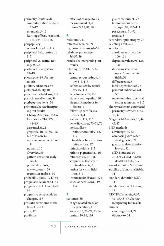
perimetry (continued)computerization of static,
16–17essentials, 3–13learning effects, results of,
123, 124–127, 128peripapillary
retinochoroiditis, 117peripheral field, testing of,
5, 7peripheral vs. central test-
ing, 26–27photopic visual system,
18–19pilocarpine, 88. See also
miosispituitary adenomas, 96plots, probability, 10postchiasmal field loss, 137post-chiasmal lesions, 98presbyopic patients, 24printouts. See also interpret-
ing test resultsChange Analysis (CA), 65formats for STATPAC,
44–45gaze tracker, 21grayscale, 10–11, 56, 128hill of vision, 69information recorded on,
8numeric, 10Overview, 59pattern deviation analy-
sis, 47probability plots, 10raw test results, 56regression analysis, 64
probability plots, 10, 47, 50progressive cataract, 51–53progressive field loss, 11, 60,
86progressive versus sudden
changes, 137prostatic carcinoma metas-
tasis, 112–113ptosis, 128pupil size
effects of changes to, 19measurement of, 8miosis, 5, 15, 87, 88
Rred stimuli, 43refractive blur, 24, 39regression analysis, 64–65reliability parameters,
56–57, 59results. See interpreting test
resultsretesting, 5, 62, 84–85, 87retina
central serous retinopa-thy, 115, 117
defects caused by retinaldisease, 114
detachments, 27, 116diabetic retinopathy, 120diagnostic methods for
disease, 4follow-up care for dis-
eases of, 4lesions of, 114, 116nerve fiber layer, 70–71, 76peripapillary
retinochoroiditis, 115,117
retinal detachment versusretinoschisis, 27
retinchoroiditis, 115retinitis pigmentosa, 116retinoschisis, 27, 116steepness of borders in
retinal defects, 6testing for visual field
loss, 5–6treatment for diseases of, 4vascular occlusions, 119,
137
Sscotomas, 36
in age-related maculardegeneration, 115
arcuate, 13, 71–72, 73, 86central, 26, 91, 114
glaucomatous, 71–72homonymous hemi-
anopic, 98, 110–111paracentral, 71–72relative, 5
secondary optic atrophy, 97selecting a test, 6–7sensitivity
absolute sensitivity loss,100–101
depressed values, 95, 123,128
differences betweenupper/lower hemi-fields, 54
differences in, 5local depressions of, 76printout indications of,
56reductions due to central
serous retinopathy, 117short wavelength automated
perimetry (SWAP), 8, 33,36, 37
Single Field Analysis, 10, 44,45, 47
SITA methodsadvantages of, 22comparing with older
strategies, 65, 69glaucoma detection/fol-
low-up, 32SITA Standard, 3030-2 or 24-2 SITA Stan-
dard/Fast tests, 6–7size of stimulus. See stimulistability of abnormal fields,
11standard deviation (SD),
11standardization of testing,
17STATPAC analysis, 9, 37,
44–45, 45–47. See alsointerpreting test results
stimulichoosing size of, 27distance to, 24
162 e s s e n t i a l p e r i m e t r y
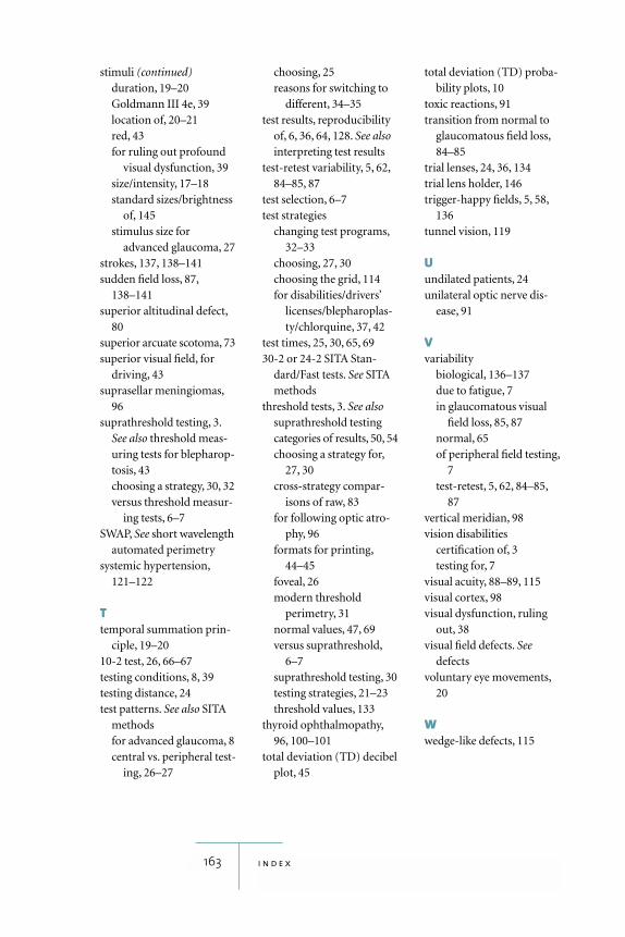
stimuli (continued)duration, 19–20Goldmann III 4e, 39location of, 20–21red, 43for ruling out profound
visual dysfunction, 39size/intensity, 17–18standard sizes/brightness
of, 145stimulus size for
advanced glaucoma, 27strokes, 137, 138–141sudden field loss, 87,
138–141superior altitudinal defect,
80superior arcuate scotoma, 73superior visual field, for
driving, 43suprasellar meningiomas,
96suprathreshold testing, 3.
See also threshold meas-uring tests for blepharop-tosis, 43choosing a strategy, 30, 32versus threshold measur-
ing tests, 6–7SWAP, See short wavelength
automated perimetrysystemic hypertension,
121–122
Ttemporal summation prin-
ciple, 19–2010-2 test, 26, 66–67testing conditions, 8, 39testing distance, 24test patterns. See also SITA
methodsfor advanced glaucoma, 8central vs. peripheral test-
ing, 26–27
choosing, 25reasons for switching to
different, 34–35test results, reproducibility
of, 6, 36, 64, 128. See alsointerpreting test results
test-retest variability, 5, 62,84–85, 87
test selection, 6–7test strategies
changing test programs,32–33
choosing, 27, 30choosing the grid, 114for disabilities/drivers’
licenses/blepharoplas-ty/chlorquine, 37, 42
test times, 25, 30, 65, 6930-2 or 24-2 SITA Stan-
dard/Fast tests. See SITAmethods
threshold tests, 3. See alsosuprathreshold testingcategories of results, 50, 54choosing a strategy for,
27, 30cross-strategy compar-
isons of raw, 83for following optic atro-
phy, 96formats for printing,
44–45foveal, 26modern threshold
perimetry, 31normal values, 47, 69versus suprathreshold,
6–7suprathreshold testing, 30testing strategies, 21–23threshold values, 133
thyroid ophthalmopathy,96, 100–101
total deviation (TD) decibelplot, 45
total deviation (TD) proba-bility plots, 10
toxic reactions, 91transition from normal to
glaucomatous field loss,84–85
trial lenses, 24, 36, 134trial lens holder, 146trigger-happy fields, 5, 58,
136tunnel vision, 119
Uundilated patients, 24unilateral optic nerve dis-
ease, 91
Vvariability
biological, 136–137due to fatigue, 7in glaucomatous visual
field loss, 85, 87normal, 65of peripheral field testing,
7test-retest, 5, 62, 84–85,
87vertical meridian, 98vision disabilities
certification of, 3testing for, 7
visual acuity, 88–89, 115visual cortex, 98visual dysfunction, ruling
out, 38visual field defects. See
defectsvoluntary eye movements,
20
Wwedge-like defects, 115
163 i n d e x
T H E F I E L D A N A L Y Z E R P R I M E R
T H I R D E D I T I O N
Anders HeijlVincent Michael Patella
Anders HeijlVincent Michael Patella
Essential PerimetryEssential Perimetry
HEIJL &
PATELLA
ESSENTIA
L PER
IMETR
Y TH
E FIELD A
NA
LYZ
ER P
RIM
ER
ISBN 0-9721560-0-3
P/N 54000